computational topology lecture notes
TRANSCRIPT
Computational TopologyLecture notes
Francis Lazarus and Arnaud de Mesmay
2016-2018
Contents
1 Panorama 41.0.1 Topology. . . . . . . . . . . . . . . . . . . . . . . . . . . . . . . . . . . . . . . . . . 41.0.2 Computational Topology. . . . . . . . . . . . . . . . . . . . . . . . . . . . . . 6
2 Planar Graphs 82.1 Topology . . . . . . . . . . . . . . . . . . . . . . . . . . . . . . . . . . . . . . . . . . . . . . 9
2.1.1 The Jordan Curve Theorem . . . . . . . . . . . . . . . . . . . . . . . . . . . . 102.1.2 Euler’s Formula . . . . . . . . . . . . . . . . . . . . . . . . . . . . . . . . . . . . 12
2.2 Kuratowski’s Theorem . . . . . . . . . . . . . . . . . . . . . . . . . . . . . . . . . . . . . 152.2.1 The Subdivision Version . . . . . . . . . . . . . . . . . . . . . . . . . . . . . . 152.2.2 The Minor Version . . . . . . . . . . . . . . . . . . . . . . . . . . . . . . . . . . 19
2.3 Other Planarity Characterizations . . . . . . . . . . . . . . . . . . . . . . . . . . . . 192.4 Planarity Test . . . . . . . . . . . . . . . . . . . . . . . . . . . . . . . . . . . . . . . . . . . 222.5 Drawing with Straight Lines . . . . . . . . . . . . . . . . . . . . . . . . . . . . . . . . 27
3 Surfaces and Embedded Graphs 323.1 Surfaces . . . . . . . . . . . . . . . . . . . . . . . . . . . . . . . . . . . . . . . . . . . . . . . 32
3.1.1 Surfaces and cellularly embedded graphs . . . . . . . . . . . . . . . . . 323.1.2 Polygonal schemata . . . . . . . . . . . . . . . . . . . . . . . . . . . . . . . . . 353.1.3 Classification of surfaces . . . . . . . . . . . . . . . . . . . . . . . . . . . . . 36
3.2 Maps . . . . . . . . . . . . . . . . . . . . . . . . . . . . . . . . . . . . . . . . . . . . . . . . . 393.3 The Genus of a Map . . . . . . . . . . . . . . . . . . . . . . . . . . . . . . . . . . . . . . 433.4 Homotopy . . . . . . . . . . . . . . . . . . . . . . . . . . . . . . . . . . . . . . . . . . . . . 45
3.4.1 Groups, generators and relations . . . . . . . . . . . . . . . . . . . . . . . 463.4.2 Fundamental groups, the combinatorial way . . . . . . . . . . . . . . . 463.4.3 Fundamental groups, the topological way . . . . . . . . . . . . . . . . . 503.4.4 Covering spaces . . . . . . . . . . . . . . . . . . . . . . . . . . . . . . . . . . . . 52
4 The Homotopy Test 554.1 Dehn’s Algorithm . . . . . . . . . . . . . . . . . . . . . . . . . . . . . . . . . . . . . . . . 564.2 van Kampen Diagrams . . . . . . . . . . . . . . . . . . . . . . . . . . . . . . . . . . . . 58
4.2.1 Disk Diagrams . . . . . . . . . . . . . . . . . . . . . . . . . . . . . . . . . . . . . 584.2.2 Annular Diagrams . . . . . . . . . . . . . . . . . . . . . . . . . . . . . . . . . . 59
4.3 Gauss-Bonnet Formula . . . . . . . . . . . . . . . . . . . . . . . . . . . . . . . . . . . . 594.4 Quad Systems . . . . . . . . . . . . . . . . . . . . . . . . . . . . . . . . . . . . . . . . . . . 614.5 Canonical Representatives . . . . . . . . . . . . . . . . . . . . . . . . . . . . . . . . . 62
4.5.1 The Four Bracket Lemma . . . . . . . . . . . . . . . . . . . . . . . . . . . . . 62
1
CONTENTS 2
4.5.2 Bracket Flattening . . . . . . . . . . . . . . . . . . . . . . . . . . . . . . . . . . 644.5.3 Canonical Representatives . . . . . . . . . . . . . . . . . . . . . . . . . . . . 65
4.6 The Homotopy Test . . . . . . . . . . . . . . . . . . . . . . . . . . . . . . . . . . . . . . . 67
5 Minimum Weight Bases 685.1 Minimum Basis of the Fundamental Group of a Graph . . . . . . . . . . . . . 695.2 Minimum Basis of the Cycle Space of a Graph . . . . . . . . . . . . . . . . . . . 70
5.2.1 The Greedy Algorithm . . . . . . . . . . . . . . . . . . . . . . . . . . . . . . . 705.3 Uniqueness of Shortest Paths . . . . . . . . . . . . . . . . . . . . . . . . . . . . . . . 735.4 First Homology Group of Surfaces . . . . . . . . . . . . . . . . . . . . . . . . . . . . 74
5.4.1 Back to Graphs . . . . . . . . . . . . . . . . . . . . . . . . . . . . . . . . . . . . . 745.4.2 Homology of Surfaces . . . . . . . . . . . . . . . . . . . . . . . . . . . . . . . . 75
5.5 Minimum Basis of the Fundamental Group of a Surface . . . . . . . . . . . . 775.5.1 Dual Maps and Cutting . . . . . . . . . . . . . . . . . . . . . . . . . . . . . . . 775.5.2 Homotopy Basis Associated with a Tree-Cotree Decomposition . 775.5.3 The Greedy Homotopy Basis . . . . . . . . . . . . . . . . . . . . . . . . . . . 78
5.6 Minimum Basis of the First Homology Group of a Surface . . . . . . . . . . . 805.6.1 Homology Basis Associated with a Tree-Cotree Decomposition . 805.6.2 The Greedy Homology Basis . . . . . . . . . . . . . . . . . . . . . . . . . . . 80
6 Homology 836.1 Complexes . . . . . . . . . . . . . . . . . . . . . . . . . . . . . . . . . . . . . . . . . . . . . 836.2 Homology . . . . . . . . . . . . . . . . . . . . . . . . . . . . . . . . . . . . . . . . . . . . . 85
6.2.1 Chain complexes . . . . . . . . . . . . . . . . . . . . . . . . . . . . . . . . . . . 856.2.2 Simplicial homology . . . . . . . . . . . . . . . . . . . . . . . . . . . . . . . . . 866.2.3 Examples and the question of the coefficient ring . . . . . . . . . . . 876.2.4 Betti numbers and Euler-Poincaré formula . . . . . . . . . . . . . . . . 886.2.5 Homology as a functor . . . . . . . . . . . . . . . . . . . . . . . . . . . . . . . 88
6.3 Homology computations . . . . . . . . . . . . . . . . . . . . . . . . . . . . . . . . . . . 896.3.1 Over a field . . . . . . . . . . . . . . . . . . . . . . . . . . . . . . . . . . . . . . . 896.3.2 Computation of the Betti numbers: the Delfinado-Edelsbrunner
algorithm . . . . . . . . . . . . . . . . . . . . . . . . . . . . . . . . . . . . . . . . . 896.3.3 Over the integers: the Smith-Poincaré reduction algorithm . . . . 90
7 Persistent Homology 937.1 Persistence Modules . . . . . . . . . . . . . . . . . . . . . . . . . . . . . . . . . . . . . . 94
7.1.1 Classification of Persistence Modules . . . . . . . . . . . . . . . . . . . . 957.1.2 Restrictions of Persistence Modules . . . . . . . . . . . . . . . . . . . . . 97
7.2 Application to Topological Inference . . . . . . . . . . . . . . . . . . . . . . . . . . 987.3 Computing the Barcode . . . . . . . . . . . . . . . . . . . . . . . . . . . . . . . . . . . 99
7.3.1 Compatible Boundary Basis . . . . . . . . . . . . . . . . . . . . . . . . . . . 1017.3.2 Algorithm . . . . . . . . . . . . . . . . . . . . . . . . . . . . . . . . . . . . . . . . 102
7.4 Persistence Diagrams . . . . . . . . . . . . . . . . . . . . . . . . . . . . . . . . . . . . . 1037.4.1 Stability of Persistence Diagrams . . . . . . . . . . . . . . . . . . . . . . . 104
CONTENTS 3
8 Knots and 3-Dimensional Computational Topology 1068.1 Knots . . . . . . . . . . . . . . . . . . . . . . . . . . . . . . . . . . . . . . . . . . . . . . . . . 1078.2 Knot diagrams . . . . . . . . . . . . . . . . . . . . . . . . . . . . . . . . . . . . . . . . . . 1088.3 The knot complement . . . . . . . . . . . . . . . . . . . . . . . . . . . . . . . . . . . . . 111
8.3.1 Homotopy . . . . . . . . . . . . . . . . . . . . . . . . . . . . . . . . . . . . . . . . 1128.3.2 Homology . . . . . . . . . . . . . . . . . . . . . . . . . . . . . . . . . . . . . . . . 1148.3.3 Triangulations . . . . . . . . . . . . . . . . . . . . . . . . . . . . . . . . . . . . . 114
8.4 An algorithm for unknot recognition . . . . . . . . . . . . . . . . . . . . . . . . . . 1158.4.1 Normal surface theory . . . . . . . . . . . . . . . . . . . . . . . . . . . . . . . 1168.4.2 Trivial knot and spanning disks . . . . . . . . . . . . . . . . . . . . . . . . . 1188.4.3 Normalization of spanning disks . . . . . . . . . . . . . . . . . . . . . . . . 1208.4.4 Haken sum, fundamental and vertex normal surfaces . . . . . . . . 123
8.5 Knotless graphs . . . . . . . . . . . . . . . . . . . . . . . . . . . . . . . . . . . . . . . . . 126
9 Undecidability in Topology 1289.1 The Halting Problem . . . . . . . . . . . . . . . . . . . . . . . . . . . . . . . . . . . . . . 129
9.1.1 Turing Machines . . . . . . . . . . . . . . . . . . . . . . . . . . . . . . . . . . . 1299.1.2 Undecidability of the Halting Problem . . . . . . . . . . . . . . . . . . . 130
9.2 Decision Problems in Group Theory . . . . . . . . . . . . . . . . . . . . . . . . . . 1319.3 Decision Problems in Topology . . . . . . . . . . . . . . . . . . . . . . . . . . . . . . 134
9.3.1 The Contractibility and Transformation Problems . . . . . . . . . . . 1349.3.2 The Homeomorphism Problem . . . . . . . . . . . . . . . . . . . . . . . . 136
9.4 Proof of the Undecidability of the Group Problems . . . . . . . . . . . . . . . . 1399.4.1 Z2-Machines . . . . . . . . . . . . . . . . . . . . . . . . . . . . . . . . . . . . . . 1399.4.2 Useful Constructs in Combinatorial Group Theory . . . . . . . . . . 1409.4.3 Undecidability of the Generalized Word Problem . . . . . . . . . . . . 141
1
Panorama
Contents1.0.1 Topology. . . . . . . . . . . . . . . . . . . . . . . . . . . . . . . . . . . . . . . . 4
1.0.2 Computational Topology. . . . . . . . . . . . . . . . . . . . . . . . . . . . 6
1.0.1 Topology.
Topology deals with the study of spaces. One of its goals is to answer the followingbroad class of questions:
“Are these two spaces the same?”
This naturally leads to the following subquestions:
• What is a space? General topology typically defines topological spaces via openand closed sets. In order to avoid pathological examples, and with an eye towardsapplications, we will take a more concrete approach1: in this course, topologicalspaces will be obtained in the form of complexes, that is, by gluing togetherfundamental blocks. For example, gluing segments yields a graph, while bygluing together triangles one can obtain a surface (or something more compli-cated). The usual notions of distance on these fundamental blocks naturallyinduce a notion of proximity on such a complex, and therefore a topology whoseproperties are convenient to understand geometrically.
1This is by no means original: see introductory textbooks on algebraic topology, for exampleHatcher [Hat02] or Stillwell [Sti93].
4
1. PANORAMA 5
• What is “the same” ? It very much depends on the context. The most commonequivalence relation is homeomorphism, which is a continuous map with acontinuous inverse function. But in some contexts, when a space is embeddedin another space, one will be interested in distinguishing between differentembeddings. There, a convenient notion is isotopy : two embedded spaces willbe considered the same if one can deform continuously one into the other one.
Let us look at examples.
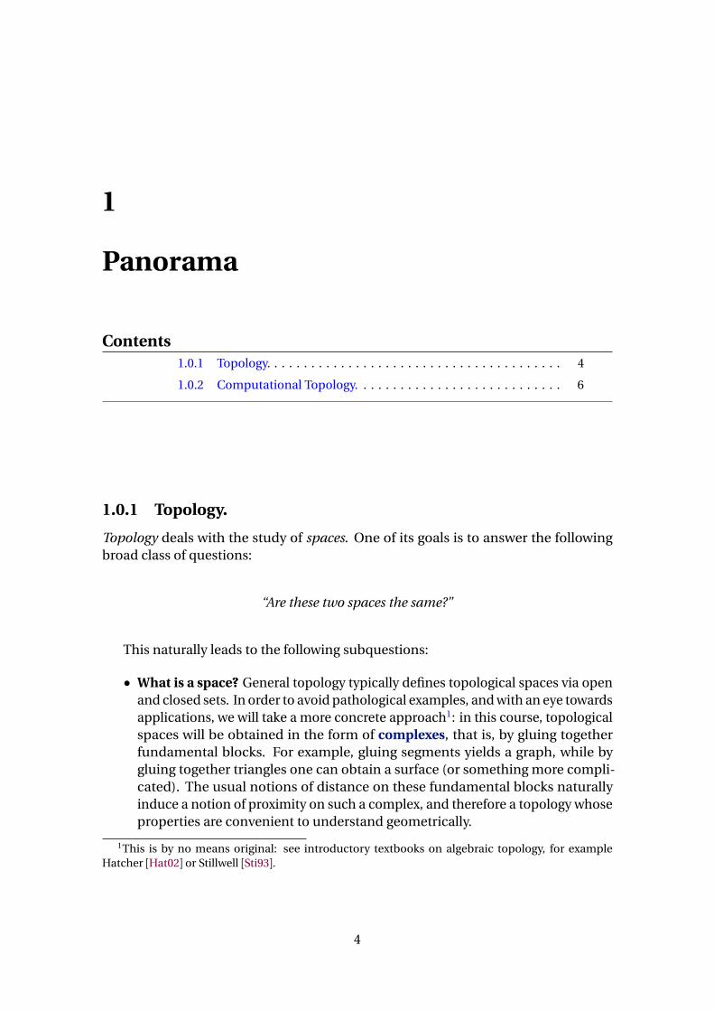
Example 1: By gluing triangles or quadrilaterals, one can easily obtain a sphere (leftfigure), or a torus (right figure).
Are these two spaces homeomorphic? Obviously not: the torus has a hole. Butwhat is a hole? Two naive answers will guide us to the two fundamental constructs ofalgebraic topology:
• Homotopy: On the sphere, every closed curve can be deformed into a singlepoint. While on the torus, a curve going around the hole can not. Such a curveis not homotopic to a point.
• Homology: On the sphere, every closed curve separates the sphere into tworegions. While on the torus, a curve going around the hole is not separating.Such a curve is not trivial in homology.
These intuitions can be formalized into algebraic objects which will constituteinvariants (actually, functors) that one can use to distinguish topological spaces.
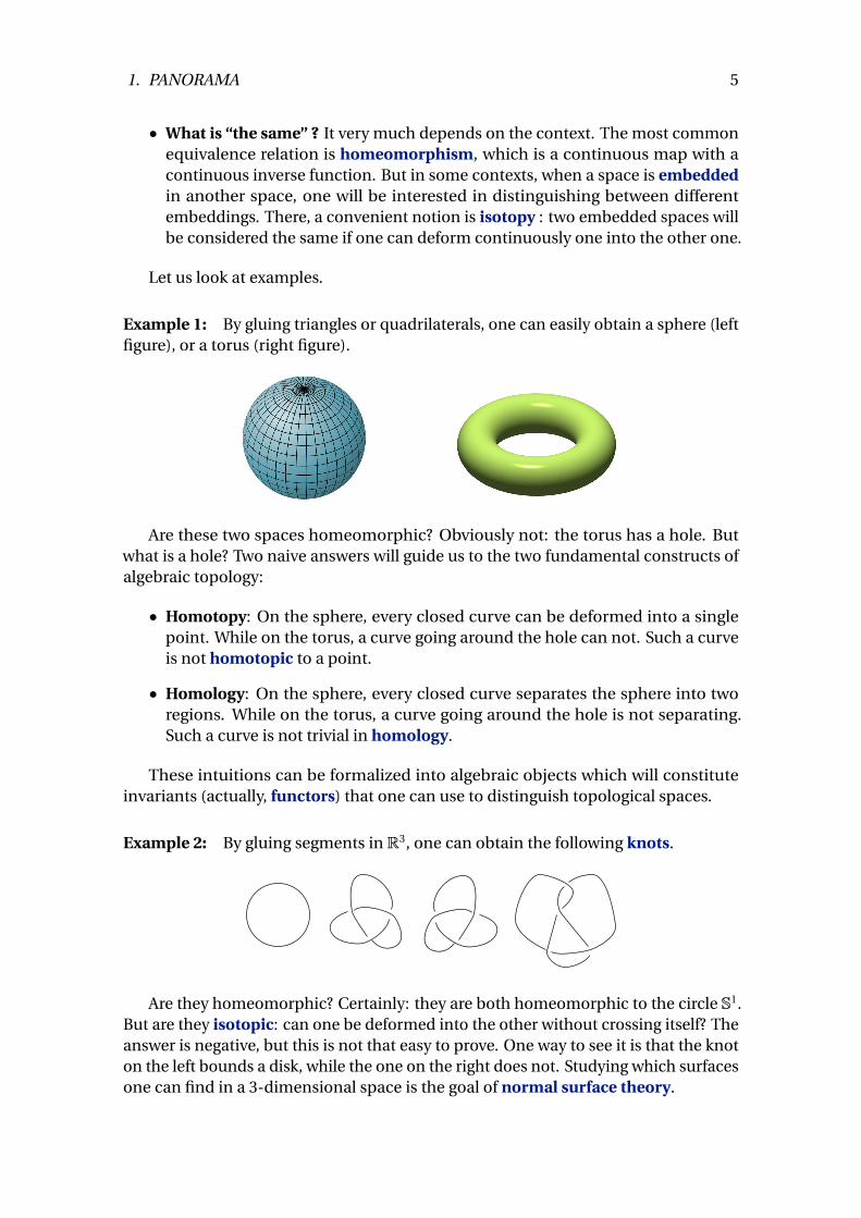
Example 2: By gluing segments in R3, one can obtain the following knots.
Are they homeomorphic? Certainly: they are both homeomorphic to the circle S1.But are they isotopic: can one be deformed into the other without crossing itself? Theanswer is negative, but this is not that easy to prove. One way to see it is that the knoton the left bounds a disk, while the one on the right does not. Studying which surfacesone can find in a 3-dimensional space is the goal of normal surface theory.
1. PANORAMA 6
1.0.2 Computational Topology.
Computational topology deals with effective computations on topological spaces.The main question now becomes:
“How to compute whether these two spaces are the same?”
Note that since we study spaces described by gluings of fundamental blocks, inmost instances this can be made into a well-defined algorithmic problem, with a finiteinput. One can then wonder about the complexity of this problem, and aim to designthe most efficient algorithm, or conversely prove hardness results. Throughout thecourse, we will investigate the complexity of various instances of this question, withpractical algorithms computing homeomorphism, homotopy, homology or isotopyfor example.
Outline. We will work by increasing progressively the dimension, and thus the com-plexity of the objects we consider.
1. We start with one of the simplest topological spaces : the plane R2. Describingit as a union of small blocks amounts to the study of planar graphs. This topo-logical constraint on graphs has a strong impact on their combinatorics, whichwe will study through various angles.
2. Next come surfaces, which look locally like the plane. From a mathematicalpoint of view, these are still fairly simple, as they can be easily classified. Butonce again, there is a very fruitful interplay between the topology of surfaces andthe combinatorics of embedded graphs. Moreover, surfaces are a convenientand easy framework to introduce homotopy and homology and we will presentefficient algorithms for the computation of these invariants.
3. In dimension 3, we will introduce knots and 3-manifolds. Distinguishing vari-ous knots is hard: the whole field of knot theory is dedicated to this. We will seethrough various examples why this is hard, and will introduce normal surfacetheory, one of the main tools used for computational problems in 3 dimensions.As an application, we will use it to provide an algorithm to recognize trivial knotsin NP.
4. As soon as we hit dimension 4, we start to hit the limits of computational topol-ogy: many problems are not only hard, they are undecidable. We will introducesimplicial complexes, which are the main model for high-dimensional topo-logical spaces, and show that deciding homeomorphism of such complexes isalready undecidable in dimension 4, as is testing the homotopy of curves in2-dimensional complexes.
5. Although computing homotopy and homeomorphism quickly becomes intractablein high dimensions, homology does not: its simple algebraic structure allows
1. PANORAMA 7
for efficient computations that scale well with the dimension. This can be lever-aged as a tool for big data: the techniques of topological data analysis aim atrecognizing topological features in point clouds by computing their persistenthomology. As we shall see, this is a surprisingly powerful way to infer informa-tion from a structured point cloud.
Applications. The approach in this course is to focus on the mathematical motiva-tions to study topological objects and their computation. This does not mean that thisis all devoid of applications. Quite the contrary: topological spaces are ubiquitous incomputer science, and the primitives we develop here have practical implications incomputer graphics [LGQ09], mesh processing [GW01], robotics [Far08], combinatorialoptimization (see references in [Eri12]), machine learning [ACC16], and many otherfields. Believe it or not, they even revolutionized basketball [Bec12]!
2
Planar Graphs
Contents2.1 Topology . . . . . . . . . . . . . . . . . . . . . . . . . . . . . . . . . . . . . . . . . . 9
2.1.1 The Jordan Curve Theorem . . . . . . . . . . . . . . . . . . . . . . . . . . 10
2.1.2 Euler’s Formula . . . . . . . . . . . . . . . . . . . . . . . . . . . . . . . . . . 12
2.2 Kuratowski’s Theorem . . . . . . . . . . . . . . . . . . . . . . . . . . . . . . . . . 15
2.2.1 The Subdivision Version . . . . . . . . . . . . . . . . . . . . . . . . . . . . 15
2.2.2 The Minor Version . . . . . . . . . . . . . . . . . . . . . . . . . . . . . . . . 19
2.3 Other Planarity Characterizations . . . . . . . . . . . . . . . . . . . . . . . . 19
2.4 Planarity Test . . . . . . . . . . . . . . . . . . . . . . . . . . . . . . . . . . . . . . . 22
2.5 Drawing with Straight Lines . . . . . . . . . . . . . . . . . . . . . . . . . . . . 27
A graph is planar if it can be drawn on a sheet of paper so that no two edges inter-sect, except at common endpoints. This simple property not only allows to visualizeplanar graphs easily, but implies many nice properties. Planar graphs are sparse: theyhave a linear number of edges with respect to their number of vertices (specifically asimple planar graph with n vertices has at most 3n −6 edges), they are 4-colorable,they can be encoded efficiently, etc. Classical examples of planar graphs include thegraphs formed by the vertices and edges of the five Platonic polyhedra, and in fact ofany convex polyhedron. Although being planar is a topological property, planar graphshave purely combinatorial characterizations. Such characterizations may lead to effi-cient algorithms for planarity testing or, more surprisingly, for geometric embedding(=drawing).
In the first part of this lecture we shall deduce the combinatorial characterizationsof planar graphs from their topological definition. That we can get rid of topologicalconsiderations should not be surprising. It is actually possible to develop a combinato-rial theory of surfaces where a drawing of a graph is defined by a circular ordering of itsedges around each vertex. The collection of these circular orderings is called a rotation
8
2.1. Topology 9
system. A rotation system is thus described combinatorially by a single permutationover the (half-)edges of a graph; the cycle decomposition of the permutation inducesthe circular orderings around each vertex. The topology of the surface correspondingto a rotation system can be deduced from the computation of its Euler characteristic.Being planar then reduces to the existence of a rotation system with the appropriateEuler characteristic.
The following notes are largely inspired by the monographs of Mohar and Thomassen[MT01] and of Diestel [Die05].
2.1 Topology
A graph G = (V , E ) is defined by a set V =V (G ) of vertices and a set E = E (G ) of edgeswhere each edge is associated one or two vertices, called its endpoints. A loop is anedge with a single endpoint. Edges sharing the same endpoints are said parallel anddefine a multiple edge. A graph without loops or multiple edges is said simple orsimplicial. In a simple graph every edge is identified unambiguously with the pair ofits endpoints. Edges should be formally considered as pairs of oppositely oriented arcs.A path is an alternating sequence of vertices and arcs such that every arc is precededby its origin vertex and followed by the origin of its opposite arc. A path may haverepeated vertices (beware that this is not standard, and usually called a walk in graphtheory books). Two or more paths are independent if none contains an inner vertexof another. A circuit is a closed path, i.e. a path whose first and last vertex coincide. Acycle is a simple circuit (without repeated vertices). We will restrict to finite graphs forwhich V and E are finite sets.
The Euclidean distance in the plane R2 induces the usual topology where a subsetX ⊂R2 is open if every of its points is contained in a ball that is itself included in X .
The closure X of X is the set of limit points of sequences of points of X . The interior◦
Xof X is the union of the open balls contained in X . An embedding of a non-loop edgein the plane is just a topological embedding (a homeomorphism onto its image) ofthe segment [0, 1] into R2. Likewise, an embedding of a loop-edge is an embedding ofthe circle S 1 =R/Z. An embedding of a finite graph G = (V , E ) in the plane is definedby a 1-1 map V ,→R2 and, for each edge e ∈ E , by an embedding of e sending {0, 1} toe ’s endpoints such that the relative interior of e (the image of ]0,1[) is disjoint fromother edge embeddings and vertices1.
A graph is planar if it has an embedding into the plane. Thanks to the stereographicprojection, the plane can be equivalently replaced by the sphere. A plane graph is aspecific embedding of a planar graph. A connected plane graph in the plane has asingle unbounded face. In contrast, all the faces play the same role in an embeddinginto the sphere and any face can be sent to the unbounded face of a plane embeddingby a stereographic projection.
As far as planarity is concerned we can restrict to simple graphs. Indeed, it is easilyseen that a graph has an embedding in the plane if and only if this is the case for thegraph obtained by removing loop edges and replacing each multiple edge by a single
1In other words, this is a topological embedding of the quotient space (V t [0,1]×E )/∼, where ∼identifies edge extremities (0, e ) and (1, e )with the corresponding vertices.
2.1. Topology 10
edge. When each edge embedding [0,1]→ R2 is piecewise linear the embedding issaid PL, or polygonal. A straight line embedding corresponds to the case where eachedge is a line segment.
Lemma 2.1.1. A graph is planar if and only if it admits a PL embedding.
The proof is left as an exercise. One can first show that a connected subset of theplane is connected by simple PL arcs.
2.1.1 The Jordan Curve Theorem
Most of the facts about planar graphs ultimately relies on the Jordan curve theorem,one of the most emblematic results in topology. Its statement is intuitively obvious: asimple closed curves cuts the plane into two connected parts. Its proof is nonethe-less far from obvious, unless one appeals to more advanced arguments of algebraictopology. Camille Jordan (1838 – 1922) himself proposed a proof whose validity isstill subject of debates [Hal07b]. A rather accessible proof was proposed by HelgeTverberg [Tve80] (see the course notes [Laz12] for a gentle introduction). Eventually, aformal proof was given by Thomas Hales (and other mathematicians) [Hal07b, Hal07a]and was automatically checked by a computer. Concerning the Jordan-Schoenfliestheorem, the situation is even worse. This stronger version of the Jordan curve the-orem asserts that a simple curve does not only cut a sphere into two pieces but thateach piece is actually a topological disc. A nice proof by elementary means – butfar from simple – and resorting to the fact that K3,3 is not planar is due to CarstenThomassen [Tho92].
The main source of difficulties in the proof of the Jordan curve theorem is that acontinuous curve can be quite wild, e.g. fractal. When dealing with PL curves only,the theorem becomes much easier to prove.
Theorem 2.1.2 (Polygonal Jordan curve — ). Let C be a simple closed PL curve. ItscomplementR2 \C has two connected components, one of which is bounded and eachof which has C as boundary.
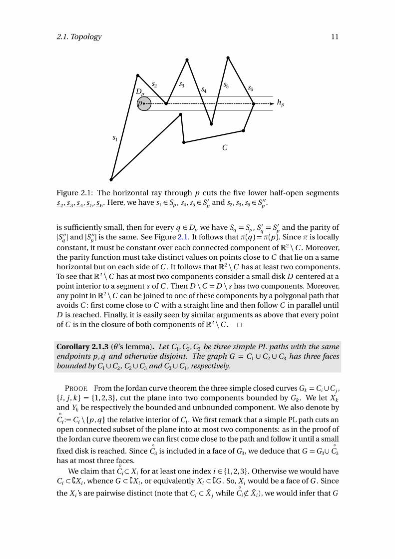
PROOF. Since C is contained in a compact ball, its complement has exactly oneunbounded component. Define the horizontal rightward direction ~h as some fixeddirection transverse to the all the line segments of C . For every segment s of C we lets be the lower half-open segment obtained from s by removing its upper endpoint.We also denote by hp the ray with direction ~h starting at a point p ∈R2. We considerthe parity function π :R2 \C →{ even, odd } that counts the parity of the number oflower half-open segments of C intersected by a ray:
π(p ) := parity of�
�{ segment s of C | hp ∩ s 6= ;}�
�
Every p ∈R2 \C is the center of small disk Dp over which π is constant. Indeed, let Sp
be the set of segments (of C ) that avoid hp , let S ′p be the set of segments whose interiorcrosses hp and let S ′′p be the set of segments whose lower endpoint lies on hp . If Dp
2.1. Topology 11
p
Dp
C
hp
s2 s3 s4s5
s1
s6
Figure 2.1: The horizontal ray through p cuts the five lower half-open segmentss 2, s 3, s 4, s 5, s 6. Here, we have s1 ∈ Sp , s4, s5 ∈ S ′p and s2, s3, s6 ∈ S ′′p .
is sufficiently small, then for every q ∈Dp we have Sq = Sp , S ′q = S ′p and the parity of|S ′′q | and |S ′′p | is the same. See Figure 2.1. It follows that π(q ) =π(p ). Since π is locally
constant, it must be constant over each connected component ofR2 \C . Moreover,the parity function must take distinct values on points close to C that lie on a samehorizontal but on each side of C . It follows that R2 \C has at least two components.To see that R2 \C has at most two components consider a small disk D centered at apoint interior to a segment s of C . Then D \C =D \ s has two components. Moreover,any point inR2 \C can be joined to one of these components by a polygonal path thatavoids C : first come close to C with a straight line and then follow C in parallel untilD is reached. Finally, it is easily seen by similar arguments as above that every pointof C is in the closure of both components of R2 \C .
Corollary 2.1.3 (θ ’s lemma). Let C1, C2, C3 be three simple PL paths with the sameendpoints p , q and otherwise disjoint. The graph G = C1 ∪ C2 ∪ C3 has three facesbounded by C1 ∪C2, C2 ∪C3 and C3 ∪C1, respectively.
PROOF. From the Jordan curve theorem the three simple closed curves Gk =Ci ∪C j ,{i , j , k} = {1,2,3}, cut the plane into two components bounded by Gk . We let Xk
and Yk be respectively the bounded and unbounded component. We also denote by◦
Ci :=Ci \ {p , q } the relative interior of Ci . We first remark that a simple PL path cuts anopen connected subset of the plane into at most two components: as in the proof ofthe Jordan curve theorem we can first come close to the path and follow it until a small
fixed disk is reached. Since◦
C3 is included in a face of G3, we deduce that G =G3∪◦
C3
has at most three faces.We claim that
◦Ci⊂ X i for at least one index i ∈ {1,2,3}. Otherwise we would have
Ci ⊂ ûX i , whence G ⊂ ûX i , or equivalently X i ⊂ ûG . So, X i would be a face of G . Since
the X i ’s are pairwise distinct (note that Ci ⊂ X j while◦
Ci 6⊂ X i ), we would infer that G
2.1. Topology 12
has at least three bounded faces, hence at least four faces. This would contradict the
first part of the proof. Without loss of generality we now assume◦
C3⊂ X3.From G =G1 ∪G2 we get that each face of G is a component of the intersection of
a face of G1 with a face of G2. From G3 ⊂G ⊂ ûY3 we get that Y3 is a face of G . Since Y3
is unbounded we must have Y3 ⊂ Y1 ∩Y2.Now, C1 ⊂ Y3 ⊂ Y1 = ûX1 implies G =G1 ∪C1 ⊂ ûX1. It follows that X1 is a face of G .
Likewise, X2 is a face of G . Moreover, these two faces are distinct (C1 bounds X1 butnot X2). We conclude that Y3, X1 and X2 are the three faces of G .
2.1.2 Euler’s Formula
The famous formula relating the number of vertices, edges and faces of a plane graphis credited to Leonhard Euler (1707-1783) although René Descartes had already de-duced very close relations for the graph of a convex polyhedron. See the histori-cal account of R. J. Wilson in [Jam99, Sec. 17.3] and in J. Erickson’s course noteshttp://jeffe.cs.illinois.edu/teaching/topology17/chapters/02-planar-graphs.pdf
Recall that a graph G is 2-connected if it contains at least three vertices and ifremoving any one of its vertices leaves a connected graph. If G is 2-connected, it canbe constructed by iteratively adding paths to a cycle. In other words, there must be asequence of graphs G0,G1, . . . ,Gk =G such that G0 is a cycle and Gi is deduced fromGi−1 by attaching a simple path between two distinct vertices of Gi−1.
Proposition 2.1.4. Each face of a 2-connected PL plane graph is bounded by a cycle ofthe graph. Moreover, each edge is incident to (= is in the closure of) exactly two faces.
PROOF. Let G be a 2-connected PL plane graph. Consider the sequence G0,G1, . . . ,Gk =G as above. We prove the proposition by induction on k . If k = 0, then G is acycle and the proposition reduces to the Jordan curve theorem 2.1.2. Otherwise, bythe induction hypothesis Gk−1 satisfies the proposition. Let P be the attached pathsuch that G = Gk−1 ∪P . The relative interior of P must be contained in a face f ofGk−1. This face is bounded by a cycle C of Gk−1. We can now apply θ ’s lemma 2.1.3 toC ∪P and conclude that f is cut by G into two faces bounded by the cycles C1∪P andC2 ∪P , where C1, C2 are the subpaths of C cut by the endpoints of P . Moreover all theother faces of Gk−1 are faces of G bounded by the same cycles. It easily follows thatthe edges of G are each incident to exactly two faces.
Lemma 2.1.5. Let G be a PL plane graph. If v is a vertex of degree one in G then G − vand G have the same number of faces.
PROOF. We denote by e the edge incident to v in G . Every face of G is contained ina face of G − v . Moreover, the relative interior of (the embedding of) e is containedin a face f of G − v . Hence, every other face of G − v is also a face of G . It remainsto count the number of faces of G in f . Let p , p ′ be two points in f \ e . There is aPL path in f connecting p and p ′. This path may intersect e , but we may avoid thisintersection by considering a detour in a small neighborhood Ne of e in f (indeed,
2.1. Topology 13
Ne \ e is connected). It follows that p and p ′ belong to a same component of f \ e . Weconclude that G has only one face in f , so that G and G − v have the same number offaces.
Theorem 2.1.6 (Euler’s formula). Let |V |, |E | and |F | be the number of vertices, edgesand faces of a connected plane graph G . Then,
|V | − |E |+ |F |= 2
PROOF. We argue by induction on |E |. If G has no edges then it has a single vertexand the above formula is trivial. Otherwise, suppose that G has a vertex v of degreeone. Then by Lemma 2.1.5, G has the same number of faces as G − v . Note that Ghas one vertex more and one edge more than G − v . By the induction hypothesis wecan apply Euler’s formula to G − v , from which we immediately infer the validity ofEuler’s formula for G . If every vertex of G has degree at least two, then G contains acycle C . Let e be an edge of C . We claim that G has one face more than G − e . Thiswill allow to conclude the theorem by applying Euler’s formula to G − e , noting that Ghas the same number of vertices but one edge less than G − e . By the Jordan curvetheorem 2.1.2, C cuts the plane into two faces (components) bounded by C . SinceG =C ∪ (G − e ), every face of G is included in the intersection of a face of C and a faceof G −e . Let f be the face of G −e containing the relative interior of e . Every other faceof G − e does not meet C , hence is also a face of G . Since f intersects the two facesof C (both bounded by e ), G has at least one face more than G − e . By considering asmall tubular neighborhood of e in f , one shows by an already seen argument thatf \ e has at most two components. It follows that f contains exactly two faces of G ,which concludes the claim.
Application. Two old puzzles that go back at least to the nineteenth century arerelated to planarity and can be solved using Euler’s formula. The first asks whether itis possible to divide a kingdom into five regions so that each region shares a frontierline with each of the four other regions. The second puzzle, sometimes called the gaz-water-electricity problem requires to join three houses to three gaz, water and electricityfacilities using pipes so that no two pipes cross. By duality, the first puzzle translatesto the question of the planarity of the complete graph K5 obtained by connectingfive vertices in all possible ways. The second problem reduces to the planarity ofthe complete bipartite graph K3,3 obtained by connecting each of three independentvertices to each of three other independent vertices. It appears that these two puzzlesare unfeasible.
Theorem 2.1.7. K5 and K3,3 are not planar.
PROOF. We give two proofs. The first one is based on Euler’s formula.
1. Suppose by way of contradiction that K3,3 has a plane embedding. Euler’s formuladirectly implies that the embedding has n = 2−6+9= 5 faces. Since K3,3 is 2-connected, it follows from Proposition 2.1.4 that every edge is incident to two
2.1. Topology 14
distinct faces. By the same proposition, each face is bounded by a cycle, henceby at least 4 edges (cycles in a bipartite graph have even lengths). It follows fromthe handshaking lemma that twice the number of edges is larger than four timesthe number of faces, i.e. 18≥ 20. A contradiction.
An analogous argument for K5 implies that an embedding must have 7 faces.Since every face is incident to at least 3 edges, we infer that 2×10≥ 3×7. Anothercontradiction.
2. Let {1,3,5} and {2,4,6} be the two vertex parts of K3,3. The cycle (1,2,3,4,5,6)separates the plane into two components in any plane embedding of K3,3. By θ ’slemma the edges (1, 4) and (2, 5)must lie in the face that does not contain (3, 6).Then (1,4) and (2,5) intersect, a contradiction. A similar argument applies forthe non-planarity of K5.
Exercise 2.1.8. Every simple planar graph G with n ≥ 3 vertices has at most 3n − 6edges and at most 2n −4 faces.
Exercise 2.1.9. Every simple planar graph with at least six vertices has a vertex withdegree less than 6.
To conclude, we prove a very strong generalization of Exercise 2.1.8, which allowsto quantify how non-planar dense graphs are. Here, a drawing of a graph is justa continuous map f : G → R2, that is, a drawing of the graph on the plane wherecrossings are allowed. The crossing number c r (G ) of a graph is the minimal numberof crossings over all possible drawings of G . For instance, c r (G ) = 0 if and only if Gis planar. The crossing number inequality [ACNS82, Lei84] provides the followinglower bound on the crossing number.
Theorem 2.1.10. c r (G )≥ |E |364|V |2 if |E | ≥ 4|V |.
The proof is a surprising application of (basic) probabilistic tools.
PROOF. Starting with a drawing of G with the minimal number of crossings, definea new graph G ′ obtained by removing one edge for each crossing. This graph is planarsince we removed all the crossings, and it has at least |E |− c r (G ) edges (removing oneedge may remove more than one crossing), so we obtain that |E |− c r (G )≤ 3|V |. (Notethat we removed the -6 to obtain an inequality valid for any number of vertices.) Thisgives in turn
c r (G )≥ |E | −3|V |.
This can be amplified in the following way. Starting from G , define another graphby removing vertices (and the edges adjacent to them) at random with some probability1−p < 1, and denote by G ′′ the obtained graph. Taking the previous inequality withexpectations, we obtain E(c r (G ′′)) ≥ E(|E ′′|)− 3E(|V ′′|). Since vertices are removedwith probability 1−p , we have E(|V ′′|) = p |V |. An edge survives if and only if bothits endpoints survive, and a crossing survives if and only if the four adjacent verticessurvive (there may be less than four adjacent vertices in general, but not in the drawing
2.2. Kuratowski’s Theorem 15
minimizing the crossing number, we leave this as an exercise to check), so we getE(|E ′′|) = p 2|E | and E(c r (G ′′)) = p 4c r (G ). So we obtain
c r (G )≥ p−2|E | −3p−3|V |,
and taking p = 4|V |/|E | – which is less than 1 if |E | ≥ 4|V | – gives the result.
2.2 Kuratowski’s Theorem
2.2.1 The Subdivision Version
We say that H is subdivision of G if H is obtained by replacing the edges of G byindependent simple paths of one or more edges. Obviously, a subdivision of a non-planar graph is also non-planar. It follows from Theorem 2.1.7 that a planar graphcannot have a subdivision of K5 or K3,3 as a subgraph. In 1929, Kazimierz Kuratowski(1896 – 1980) succeeded to prove that this condition is actually sufficient for a graph tobe planar. For this reason K5 and K3,3 are called the Kuratowski graphs, or the forbiddengraphs.
Theorem 2.2.1 (Kuratowski, 1929). A graph is planar if and only if it does not containa subdivision of K5 or K3,3 as a subgraph.
As just noted, we only need to show that a graph without any subdivision of aforbidden graph is planar. We follow the proof of Thomassen [MT01]. Recall thata graph is 3-connected if it contains at least four vertices and if removing any twoof its vertices leaves a connected graph. By Menger’s theorem [Wil96, cor. 28.4], agraph is 3-connected if and only if any two distinct vertices can be connected by atleast three independent paths. If e is an edge of a graph G we denote by G //e thegraph obtained by the contraction of e , i.e. by deleting e , identifying its endpoints,and merging each resulting multiple edge, if any, into a single edge. The proof ofKuratowski’s theorem first restricts to 3-connected graphs. By Lemma 2.2.2 below wecan repeatedly contract edges while maintaining the 3-connectivity until the graph issmall enough so that it can be trivially embedded into the plane. We then undo theedge contractions one by one and construct corresponding embeddings. In the end,the existence of an embedding attests the planarity of the graph. In a second phase weextend the theorem to any graph, not necessarily 3-connected, that does not containany subdivision of K5 or K3,3. This is done by adding as many edges as possible tothe graph without introducing a (subdivision of a) forbidden graph. By Lemma 2.2.5below the resulting graph is 3-connected and we may conclude with the first part ofthe proof.
Lemma 2.2.2. Any 3-connected graph G with at least five vertices contains an edge esuch that G //e is 3-connected.
PROOF. Suppose for the sake of contradiction that for any edge e = x y , the graphG //e is not 3-connected. Denote by ve the vertex of G //e resulting from the identifica-tion of x and y . Then we can find a vertex z ∈V (G //e ) such that {z , ve } disconnects
2.2. Kuratowski’s Theorem 16
x
y
e
u
v
t
HH ′
z
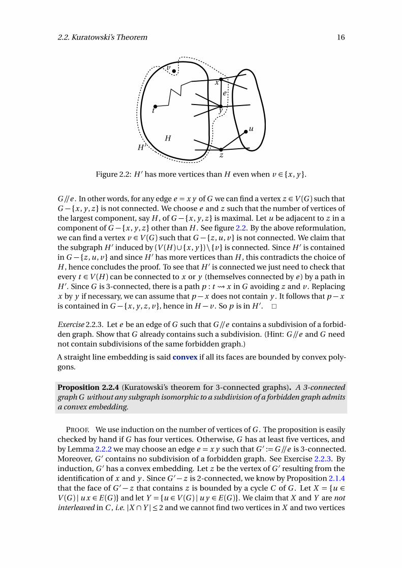
Figure 2.2: H ′ has more vertices than H even when v ∈ {x , y }.
G //e . In other words, for any edge e = x y of G we can find a vertex z ∈V (G ) such thatG −{x , y , z } is not connected. We choose e and z such that the number of vertices ofthe largest component, say H , of G −{x , y , z } is maximal. Let u be adjacent to z in acomponent of G −{x , y , z } other than H . See figure 2.2. By the above reformulation,we can find a vertex v ∈V (G ) such that G −{z , u , v } is not connected. We claim thatthe subgraph H ′ induced by (V (H )∪{x , y }) \ {v } is connected. Since H ′ is containedin G −{z , u , v } and since H ′ has more vertices than H , this contradicts the choice ofH , hence concludes the proof. To see that H ′ is connected we just need to check thatevery t ∈V (H ) can be connected to x or y (themselves connected by e ) by a path inH ′. Since G is 3-connected, there is a path p : t x in G avoiding z and v . Replacingx by y if necessary, we can assume that p − x does not contain y . It follows that p − xis contained in G −{x , y , z , v }, hence in H − v . So p is in H ′.
Exercise 2.2.3. Let e be an edge of G such that G //e contains a subdivision of a forbid-den graph. Show that G already contains such a subdivision. (Hint: G //e and G neednot contain subdivisions of the same forbidden graph.)
A straight line embedding is said convex if all its faces are bounded by convex poly-gons.
Proposition 2.2.4 (Kuratowski’s theorem for 3-connected graphs). A 3-connectedgraph G without any subgraph isomorphic to a subdivision of a forbidden graph admitsa convex embedding.
PROOF. We use induction on the number of vertices of G . The proposition is easilychecked by hand if G has four vertices. Otherwise, G has at least five vertices, andby Lemma 2.2.2 we may choose an edge e = x y such that G ′ :=G //e is 3-connected.Moreover, G ′ contains no subdivision of a forbidden graph. See Exercise 2.2.3. Byinduction, G ′ has a convex embedding. Let z be the vertex of G ′ resulting from theidentification of x and y . Since G ′− z is 2-connected, we know by Proposition 2.1.4that the face of G ′ − z that contains z is bounded by a cycle C of G . Let X = {u ∈V (G ) | u x ∈ E (G )} and let Y = {u ∈V (G ) | u y ∈ E (G )}. We claim that X and Y are notinterleaved in C , i.e. |X ∩Y | ≤ 2 and we cannot find two vertices in X and two vertices
2.2. Kuratowski’s Theorem 17
x1
yz
x2
y1y2
x1
x2
y1y2
x
C
z
C CC
x yee
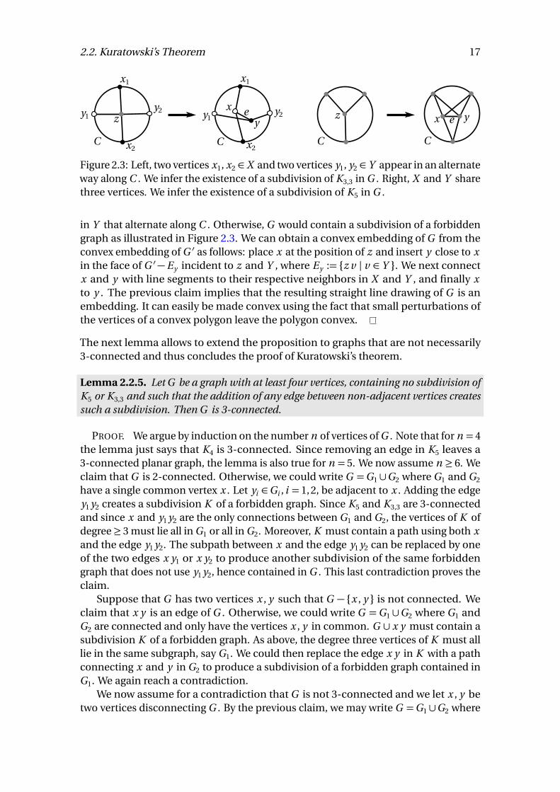
Figure 2.3: Left, two vertices x1, x2 ∈ X and two vertices y1, y2 ∈ Y appear in an alternateway along C . We infer the existence of a subdivision of K3,3 in G . Right, X and Y sharethree vertices. We infer the existence of a subdivision of K5 in G .
in Y that alternate along C . Otherwise, G would contain a subdivision of a forbiddengraph as illustrated in Figure 2.3. We can obtain a convex embedding of G from theconvex embedding of G ′ as follows: place x at the position of z and insert y close to xin the face of G ′−Ey incident to z and Y , where Ey := {z v | v ∈ Y }. We next connectx and y with line segments to their respective neighbors in X and Y , and finally xto y . The previous claim implies that the resulting straight line drawing of G is anembedding. It can easily be made convex using the fact that small perturbations ofthe vertices of a convex polygon leave the polygon convex.
The next lemma allows to extend the proposition to graphs that are not necessarily3-connected and thus concludes the proof of Kuratowski’s theorem.
Lemma 2.2.5. Let G be a graph with at least four vertices, containing no subdivision ofK5 or K3,3 and such that the addition of any edge between non-adjacent vertices createssuch a subdivision. Then G is 3-connected.
PROOF. We argue by induction on the number n of vertices of G . Note that for n = 4the lemma just says that K4 is 3-connected. Since removing an edge in K5 leaves a3-connected planar graph, the lemma is also true for n = 5. We now assume n ≥ 6. Weclaim that G is 2-connected. Otherwise, we could write G =G1 ∪G2 where G1 and G2
have a single common vertex x . Let yi ∈Gi , i = 1, 2, be adjacent to x . Adding the edgey1 y2 creates a subdivision K of a forbidden graph. Since K5 and K3,3 are 3-connectedand since x and y1 y2 are the only connections between G1 and G2, the vertices of K ofdegree≥ 3 must lie all in G1 or all in G2. Moreover, K must contain a path using both xand the edge y1 y2. The subpath between x and the edge y1 y2 can be replaced by oneof the two edges x y1 or x y2 to produce another subdivision of the same forbiddengraph that does not use y1 y2, hence contained in G . This last contradiction proves theclaim.
Suppose that G has two vertices x , y such that G − {x , y } is not connected. Weclaim that x y is an edge of G . Otherwise, we could write G =G1 ∪G2 where G1 andG2 are connected and only have the vertices x , y in common. G ∪ x y must contain asubdivision K of a forbidden graph. As above, the degree three vertices of K must alllie in the same subgraph, say G1. We could then replace the edge x y in K with a pathconnecting x and y in G2 to produce a subdivision of a forbidden graph contained inG1. We again reach a contradiction.
We now assume for a contradiction that G is not 3-connected and we let x , y betwo vertices disconnecting G . By the previous claim, we may write G =G1 ∪G2 where
2.2. Kuratowski’s Theorem 18
G1 ∩G2 reduces to the edge x y . By the same type of arguments used in the aboveclaims we see that adding an edge to Gi (i = 1, 2) creates a subdivision of a forbiddengraph in the same Gi . We can thus apply the induction hypothesis and assume thateach Gi is 3-connected, or has at most three vertices. By Proposition 2.2.4, both graphsare planar and we can choose a convex embedding for each of them. Let zi 6= x , y bea vertex of a face Fi of Gi bounded by x y . Note that Fi must be equal to the trianglezi x y . (Otherwise, we could add an edge to Gi inside Fi to obtain a larger planar graph.)Adding the edge z1z2 to G creates a subdivision K of a forbidden graph. We shall showthat some planar modification of G1 or G2 contains a subdivision of a forbidden graph,leading to a contradiction.
If all the vertices of K of degree ≥ 3 were in G1, we could replace the path of K inG2 + z1z2 that uses z1z2 by one of the two edges z1 x or z1 y . We would get anothersubdivision of the same forbidden graph in G1. Likewise, G2 cannot contain all thevertices of K of degree ≥ 3. Furthermore, V (G1) \ {x , y } and V (G2) \ {x , y } cannotboth contain two vertices of degree ≥ 3 in K since there would be four independentpaths between them, although G1 and G2 are only connected through x , y and z1z2
in G + z1z2. For the same reason, K cannot be a subdivision of K5. Hence, K is asubdivision of K3,3 and five of its degree three vertices are in the same Gi . Adding apoint p inside Fi and drawing the three line segments p x , p y , p zi we would obtain aplanar embedding of Gi + {p x , p y , p zi } that contains a subdivision of K3,3. This lastcontradiction concludes the proof.
Corollary 2.2.6. Every triangulation of the sphere with at least four vertices is 3-connected.
PROOF. By Euler’s formula it is seen that such a triangulation has a maximal numberof edges. By the previous lemma, it must be 3-connected.
We end this section with a simple characterization of the faces of a 3-connectedplanar graph. A cycle of a graph G is induced if it is induced by its vertices, or equiva-lently if it has no chord in G . It is separating if the removal of its vertices disconnectsG . The set of boundary edges of a face of a plane embedding is called a facial cycle.
Proposition 2.2.7. The face boundaries of a 3-connected plane graph are its non-separating induced cycles.
PROOF. Suppose that C is a non-separating induced cycle of a 3-connected planegraph G . By the Jordan curve theorem R2 \C has two components. Since C is non-separating one of the two components contains no vertices of G . This component isnot cut by an edge since C has no chord. It is thus a face of G .
Conversely, consider a face f of G . By Proposition 2.1.4 this face is bounded bya cycle C . If C had a chord e = x y then by the 3-connectivity of G there would be apath p connecting the two components of C −{x , y }. However, p and e being in thesame component ofR2 \C (other than f ), they would cross by an application of θ ’slemma 2.1.3. Finally, consider two vertices x , y of G −C . They are connected by threeindependent paths. By θ ’s lemma f is included in one of the three components cutby these paths and the boundary of this component is included in the correspondingtwo paths. Hence, C avoids the third path. It follows that G −C is connected.
2.3. Other Planarity Characterizations 19
This proposition says that a planar 3-connected graph has essentially a unique planeembedding: if we realize the graph as a net of strings there are only two ways of dressingthe sphere with this net; they correspond to the two orientations of the sphere.
2.2.2 The Minor Version
A minor of a graph G is any graph obtained from a subgraph of G by contracting asubset of its edges. In other words, a minor results from any sequence of contractionof edges, deletion of edges or deletion of vertices (in any order). Equivalently, H is aminor of G if the vertices of H can be put into correspondence with the trees of a forestin G and if every edge of H corresponds to a pair of trees connected by a (non-tree)edge (but all such pairs do not necessarily give rise to edges). Being a minor of anothergraph defines a partial order on the set of graphs. This partial order is the object of thefamous graph minor theory developed by Robertson and Seymour and culminating inthe proof of Wagner’s conjecture that the minor relation is a well-quasi-order, i.e. thatevery infinite sequence of graphs contains two graphs such that the first appearingin the sequence is a minor of the other. As an easy consequence, every minor closedfamily of graphs is characterized by a finite set of excluded minors. In other words, ifa family of graphs contains all the minors of its graphs, then a graph is in the family ifand only if none of its minors belongs to a certain finite set of graphs. The set of allplanar graphs is the archetypal instance of a minor closed family. Its set of excludedminors happens to be precisely the two Kuratowski graphs.
Theorem 2.2.8 (Wagner, 1937). A graph G is planar if and only if none of K5 or K3,3 isa minor of G .
Remark that if G contains a subdivision of H , then H is a minor of G , but the con-verse is not true in general (think of a counter-example). We can nonetheless deduceWagner’s version from Kuratowski’s theorem: the condition in Wagner’s theorem isobviously necessary by noting that a minor of a planar graph is planar and by Theo-rem 2.1.7. The condition is also sufficient by the above remark and by Kuratowski’stheorem. In fact, the equivalence between Wagner and Kuratowski’s theorems can beshown by proving that a graph contains a subdivision of K5 or K3,3 if and only if K5 orK3,3 is a minor of this graph [Die05, Sec. 4.4].
2.3 Other Planarity Characterizations
We give some other planarity criteria demonstrating the fascinating interplay betweenTopology, Combinatorics and Algebra.
An algebraic cycle of a graph G is any subset of its edges that induces an Euleriansubgraph, i.e. a subgraph of G with vertices of even degrees2. It is a simple exercise toprove that any algebraic cycle can be decomposed into a set of (simple) cycles in theusual acception. The set of (algebraic) cycles is given a group structure by defining thesum of two cycles as the symmetric difference of their edge sets. It can be considered
2An Eulerian subgraph in this sense is not necessarily connected.
2.3. Other Planarity Characterizations 20
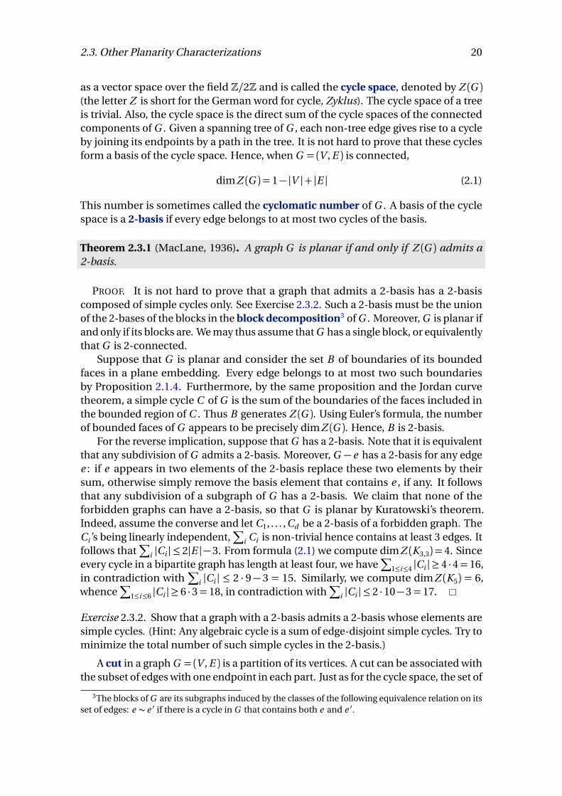
as a vector space over the field Z/2Z and is called the cycle space, denoted by Z (G )(the letter Z is short for the German word for cycle, Zyklus). The cycle space of a treeis trivial. Also, the cycle space is the direct sum of the cycle spaces of the connectedcomponents of G . Given a spanning tree of G , each non-tree edge gives rise to a cycleby joining its endpoints by a path in the tree. It is not hard to prove that these cyclesform a basis of the cycle space. Hence, when G = (V , E ) is connected,
dim Z (G ) = 1− |V |+ |E | (2.1)
This number is sometimes called the cyclomatic number of G . A basis of the cyclespace is a 2-basis if every edge belongs to at most two cycles of the basis.
Theorem 2.3.1 (MacLane, 1936). A graph G is planar if and only if Z (G ) admits a2-basis.
PROOF. It is not hard to prove that a graph that admits a 2-basis has a 2-basiscomposed of simple cycles only. See Exercise 2.3.2. Such a 2-basis must be the unionof the 2-bases of the blocks in the block decomposition3 of G . Moreover, G is planar ifand only if its blocks are. We may thus assume that G has a single block, or equivalentlythat G is 2-connected.
Suppose that G is planar and consider the set B of boundaries of its boundedfaces in a plane embedding. Every edge belongs to at most two such boundariesby Proposition 2.1.4. Furthermore, by the same proposition and the Jordan curvetheorem, a simple cycle C of G is the sum of the boundaries of the faces included inthe bounded region of C . Thus B generates Z (G ). Using Euler’s formula, the numberof bounded faces of G appears to be precisely dim Z (G ). Hence, B is 2-basis.
For the reverse implication, suppose that G has a 2-basis. Note that it is equivalentthat any subdivision of G admits a 2-basis. Moreover, G − e has a 2-basis for any edgee : if e appears in two elements of the 2-basis replace these two elements by theirsum, otherwise simply remove the basis element that contains e , if any. It followsthat any subdivision of a subgraph of G has a 2-basis. We claim that none of theforbidden graphs can have a 2-basis, so that G is planar by Kuratowski’s theorem.Indeed, assume the converse and let C1, . . . , Cd be a 2-basis of a forbidden graph. TheCi ’s being linearly independent,
∑
i Ci is non-trivial hence contains at least 3 edges. Itfollows that
∑
i |Ci | ≤ 2|E | −3. From formula (2.1) we compute dim Z (K3,3) = 4. Sinceevery cycle in a bipartite graph has length at least four, we have
∑
1≤i≤4 |Ci | ≥ 4 ·4= 16,in contradiction with
∑
i |Ci | ≤ 2 · 9− 3 = 15. Similarly, we compute dim Z (K5) = 6,whence
∑
1≤i≤6 |Ci | ≥ 6 ·3= 18, in contradiction with∑
i |Ci | ≤ 2 ·10−3= 17.
Exercise 2.3.2. Show that a graph with a 2-basis admits a 2-basis whose elements aresimple cycles. (Hint: Any algebraic cycle is a sum of edge-disjoint simple cycles. Try tominimize the total number of such simple cycles in the 2-basis.)
A cut in a graph G = (V , E ) is a partition of its vertices. A cut can be associated withthe subset of edges with one endpoint in each part. Just as for the cycle space, the set of
3The blocks of G are its subgraphs induced by the classes of the following equivalence relation on itsset of edges: e ∼ e ′ if there is a cycle in G that contains both e and e ′.

2.3. Other Planarity Characterizations 21
cuts can be given a vector space structure overZ/2Z by defining the sum of two cuts asthe symmetric difference of the associated edge sets. Equivalently, we observe that thesum of two cuts {V1, V2} and {W1, W2} is the cut {(V1∩W1)∪(V2∩W2), (V1∩W2)∪(V2∩W1)}.Remark that the cut space is generated by the elementary cuts of the form {v, V − v },for v ∈V . A cut is minimal if its edge set is not contained in the edge set of anothercut. In a connected graph minimal cuts correspond to partitions both parts of whichinduce a connected subgraph. Such minimal cuts generate the cut space.
Given a plane graph G , we define its geometric dual G ∗ as the graph obtainedby placing a vertex inside each face of G and connecting two such vertices if theirfaces share an edge in G . Note that distinct plane embeddings of a planar graph maygive rise to non-isomorphic duals. When the plane graph G is connected, its vertex,edge and face sets are in 1-1 correspondence with the face, edge and vertex sets ofG ∗ respectively. Note that the geometric dual of a plane tree has a single vertex, sothat G ∗ may not be simple even if G is. It is not hard to prove that the set of edges ofa (simple) cycle of G corresponds to a minimal cut in G ∗. The converse is also truesince the dual of the dual is the original graph.
For non-planar graphs the above construction is meaningless and we define anabstract notion of duality that applies in all cases. A graph G ∗ is an abstract dual ofa graph G if the respective edge sets can be put in 1-1 correspondence so that every(simple) cycle in G corresponds to a minimal cut in G ∗.
Theorem 2.3.3 (Whitney, 1933). A graph is planar if and only if is has an abstract dual.
The theorem can be proved by mimicking the proof of MacLane’s theorem 2.3.1,first showing that if a graph has an abstract dual so does its subgraphs and subdivisions.We provide a shorter proof based on MacLane’s theorem.
PROOF. The theorem can be easily reduced to the case of connected graphs. Bythe above discussion a geometric dual is an abstract dual, so that the condition isnecessary. For the reverse implication, suppose that a graph G has an abstract dual G ∗.The cycle space of G is generated by its simple cycles, hence by the dual edge sets ofthe minimal cuts of G ∗. Those cuts are themselves generated by the elementary cuts.Clearly an edge appears in at most two elementary cuts (loop-edges do not appear inany cuts). It follows that the cycle space of G has a 2-basis, and we may conclude withMacLane’s theorem.
We list below some other well-known characterizations of planarity without proof.A strict partial order on a set S is a transitive, antisymmetric and irreflexive binary
relation, usually denoted by <. Two distinct elements x , y ∈ S such that either x < yor y < x are said comparable. A partial order is a linear, or total, order when all theelements are pairwise comparable. The dimension of a partial order is the minimumnumber of linear orders whose intersection (as binary relations) is the partial order.The order complex of a graph G = (V , E ) is the partial order on the set S =V ∪E wherethe only relations are v < e for v an endpoint of e .
2.4. Planarity Test 22
Theorem 2.3.4 (Schnyder, 1989). A graph is planar if and only if its order complex hasdimension at most 3.
See Mohar and Thomassen [MT01, p. 36] for more details. The contact graph of afamily of interior disjoint disks in the plane is the graph whose vertices are the disks inthe family and whose edges are the pairs of tangent disks.
Theorem 2.3.5 (Koebe-Andreev-Thurston). A graph is planar if and only if it is thecontact graph of a family of disks.
Section 2.8 in [MT01] is devoted to this theorem and its extensions. A 3-polytopeis an intersection of half-spaces in R3 which is bounded and has non-empty interior.Its graph, or 1-skeleton, is the graph defined by its vertices and edges.
Theorem 2.3.6 (Steinitz, 1922). A 3-connected graph is planar if and only if it is thegraph of a 3-polytope.
A proof can be found in the monograph by Ziegler [Zie95, Chap. 4]. We end thissection with a nice and simple planarity criterion relying on a result by Hanani (1934)stating that any drawing of K5 and of K3,3 has a pair of independent edges with anodd number of crossings. (Recall that two edges are independent if they do not shareany endpoint.) In fact, we have the stronger property that the number of pairs ofindependent edges crossing oddly is odd. This can be proved by first observing theproperty on a straight line drawing of K5 (resp. K3,3) and then deforming any otherdrawing to the given one using a sequence of elementary moves that preserve4 theparity of the number of oddly crossing pairs of independent edges. Together withKuratowski’s theorem, this proves the following
Theorem 2.3.7 (Hanani-Tutte). A graph is planar if and only if it has a drawing inwhich every pair of independent edges crosses evenly.
A weaker version of the theorem asks that every pair of edges, not necessarilyindependent, should cross evenly. See Mustafa’s course notes for a geometric proof,not relying on Kuratowski’s theorem.
2.4 Planarity Test
There is a long and fascinating story for the design of planarity tests, culminating withthe first optimal linear time algorithm by Hopcroft and Tarjan [HT74] in 1974. Patrig-nani [Pat13] offers a nice and comprehensive survey on planarity testing. Although
4Those moves are of five types: (i) two edges locally (un)crossing and creating or canceling a bigon,(ii) an edge locally (un)crossing and creating or canceling a monogon, (iii) an edge passing over acrossing, (iv) an edge passing over a vertex, and (v) two consecutive edges around a vertex swappingtheir circular order. The three first moves are analogous to the Reidemeister moves performed on knotdiagrams. (i),(ii), (iii) and (v) clearly preserve the number of oddly crossing pairs of independent edges.For (iv) we use the fact that for every vertex and every edge of K5 or K3,3 the edge is independent withan even number of the edges incident to the vertex.
2.4. Planarity Test 23
most of the linear time algorithms have actual implementations, they are rather com-plex and we only describe a simpler non optimal algorithm based on works of deFraissex and Rosensthiel [dFR85, Bra09]. We first recall that the block decompositiondecomposes a connected graph into 2-connected subgraphs connected by trees in atree structure. Hence, a graph is planar if and only if its blocks are planar. We can thusrestrict the planarity test to 2-connected graphs. Note that the block decompositionof a graph can be computed in linear time using depth-first search. (See West [Wes01,p. 157].)
root
e1
e2
b1
b2
a. b.
v
t1
t2
t3
b3
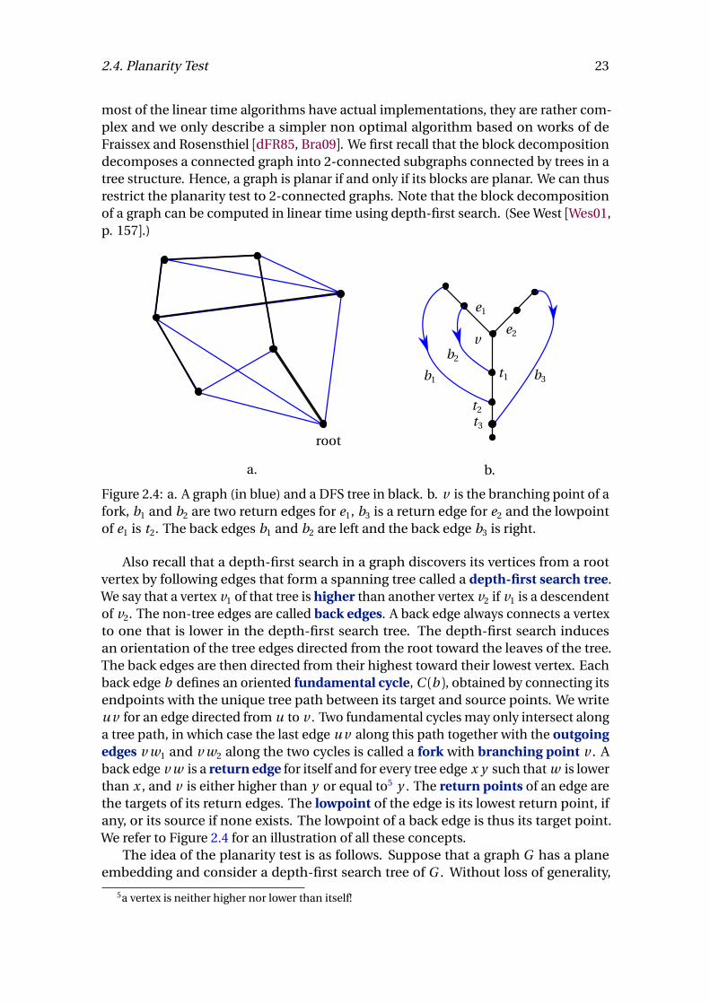
Figure 2.4: a. A graph (in blue) and a DFS tree in black. b. v is the branching point of afork, b1 and b2 are two return edges for e1, b3 is a return edge for e2 and the lowpointof e1 is t2. The back edges b1 and b2 are left and the back edge b3 is right.
Also recall that a depth-first search in a graph discovers its vertices from a rootvertex by following edges that form a spanning tree called a depth-first search tree.We say that a vertex v1 of that tree is higher than another vertex v2 if v1 is a descendentof v2. The non-tree edges are called back edges. A back edge always connects a vertexto one that is lower in the depth-first search tree. The depth-first search inducesan orientation of the tree edges directed from the root toward the leaves of the tree.The back edges are then directed from their highest toward their lowest vertex. Eachback edge b defines an oriented fundamental cycle, C (b ), obtained by connecting itsendpoints with the unique tree path between its target and source points. We writeu v for an edge directed from u to v . Two fundamental cycles may only intersect alonga tree path, in which case the last edge u v along this path together with the outgoingedges v w1 and v w2 along the two cycles is called a fork with branching point v . Aback edge v w is a return edge for itself and for every tree edge x y such that w is lowerthan x , and v is either higher than y or equal to5 y . The return points of an edge arethe targets of its return edges. The lowpoint of the edge is its lowest return point, ifany, or its source if none exists. The lowpoint of a back edge is thus its target point.We refer to Figure 2.4 for an illustration of all these concepts.
The idea of the planarity test is as follows. Suppose that a graph G has a planeembedding and consider a depth-first search tree of G . Without loss of generality,
5a vertex is neither higher nor lower than itself!
2.4. Planarity Test 24
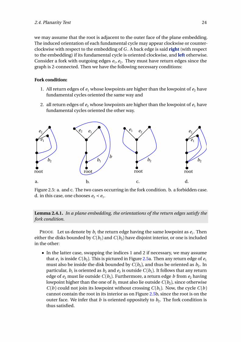
we may assume that the root is adjacent to the outer face of the plane embedding.The induced orientation of each fundamental cycle may appear clockwise or counter-clockwise with respect to the embedding of G . A back edge is said right (with respectto the embedding) if its fundamental cycle is oriented clockwise, and left otherwise.Consider a fork with outgoing edges e1, e2. They must have return edges since thegraph is 2-connected. Then we have the following necessary conditions:
Fork condition:
1. All return edges of e1 whose lowpoints are higher than the lowpoint of e2 havefundamental cycles oriented the same way and
2. all return edges of e2 whose lowpoints are higher than the lowpoint of e1 havefundamental cycles oriented the other way.
e1
e2
b2
root
a.
e2 e1
b1
root
b.
e1
e2
b2
root
d.
e1 e2
b2
root
c.
b
Figure 2.5: a. and c. The two cases occurring in the fork condition. b. a forbidden case.d. in this case, one chooses e2 ≺ e1.
Lemma 2.4.1. In a plane embedding, the orientations of the return edges satisfy thefork condition.
PROOF. Let us denote by bi the return edge having the same lowpoint as ei . Theneither the disks bounded by C (b1) and C (b2) have disjoint interior, or one is includedin the other:
• In the latter case, swapping the indices 1 and 2 if necessary, we may assumethat e1 is inside C (b2). This is pictured in Figure 2.5a. Then any return edge of e1
must also be inside the disk bounded by C (b2), and thus be oriented as b2. Inparticular, b1 is oriented as b2 and e2 is outside C (b1). It follows that any returnedge of e2 must lie outside C (b1). Furthermore, a return edge b from e2 havinglowpoint higher than the one of b1 must also lie outside C (b2), since otherwiseC (b ) could not join its lowpoint without crossing C (b1). Now, the cycle C (b )cannot contain the root in its interior as on Figure 2.5b, since the root is on theouter face. We infer that b is oriented oppositely to b2. The fork condition isthus satisfied.
2.4. Planarity Test 25
• In the former case, any return edge b of e1 must lie outside C (b2). See Figure 2.5c.If the lowpoint of b is higher than that of b2, then b must be oriented oppositelyto b2, since C (b ) cannot contain the root in its interior. The mirror argumentshows that a return edge from e2 whose lowpoint is higher than the lowpoint ofb1 must be oriented oppositely to b1. We again conclude that the fork conditionis satisfied.
An LR partition is a left-right assignment of the back edges such that the inducedorientations of the fundamental cycles satisfy the fork condition for all the possibleforks. The above lemma shows that a planar graph has an LR partition deduced fromany particular plane embedding. As the following theorem shows, the existence of anLR partition happens to be sufficient for attesting planarity!
Theorem 2.4.2 (de Fraysseix and Rosenstiehl, 1985). A connected graph G is planar ifand only if it admits an LR partition with respect to some (and thus any) depth-firstsearch tree.
PROOF (SKETCH). Essentially, the proof starts by constructing a combinatorial em-bedding of G from the LR partition, i.e. a circular ordering of the edges around eachvertex, then checking that this combinatorial embedding can indeed be realized inthe plane without introducing crossings. Note that the fork conditions cannot involveback edges in different blocks in the block decomposition of G , so that we can assumeG to be 2-connected by the above discussion. For each vertex v we define a totalordering ≺ on its outgoing edges as follows. If v is the root, it can have only a singleoutgoing edge by the 2-connectivity of G and there is nothing to do. Otherwise, v hasa unique incoming tree edge e and the total ordering will correspond to the circularclockwise ordering around v broken at e into a linear ordering. Let e1, e2 be two edgesgoing out of v , and for i = 1, 2, let bi be equal to ei if ei is a return edge, or a return edgeof ei with the lowest return point (there might be several ones) among its return edges.We need to decide if e1 ≺ e2 or the opposite. The idea is that in any plane drawing ofthe graph, the ordering of e1 and e2 is enforced by the LR-assigment of b1 and b2.
• If b1 is a left back edge while b2 is a right back edge, then we declare e1 ≺ e2 sinceit must be the case in any plane drawing of G that respects the LR assignment(as in Figure 2.5c).
• If b1 and b2 are both right back edges we let e2 ≺ e1 if either the lowpoint of b2 islower than the lowpoint b1 (as in Figure 2.5a), or if e1 has another right returnedge towards another return point (as in Figure 2.5d). By the fork condition, it isimpossible for both e1 and e2 to have another right return edge towards anotherreturn point, so this is well-defined.
• If b1 and b2 are both left back edges, the previous situation leads to the oppositedecision.
• If none of this applies, we order them arbitrarily.
2.4. Planarity Test 26
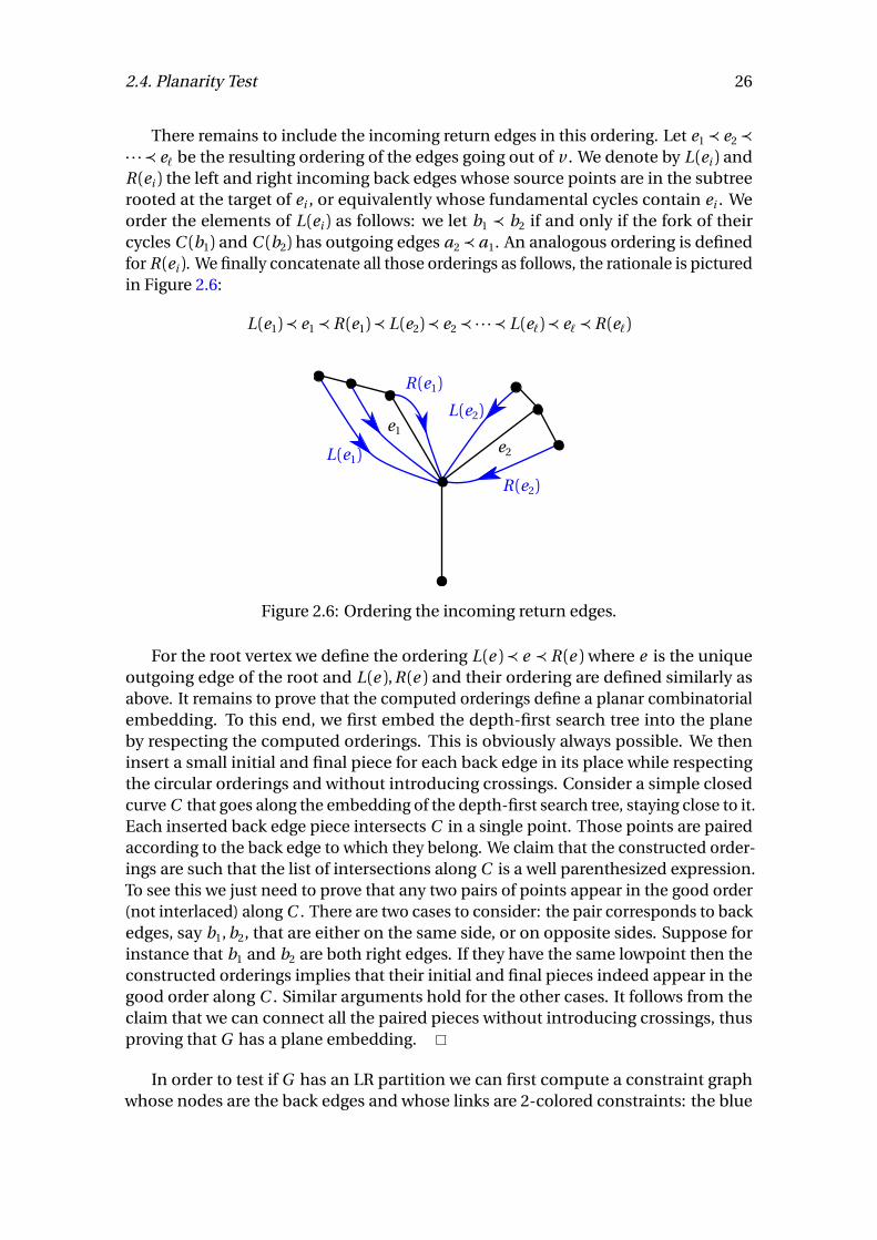
There remains to include the incoming return edges in this ordering. Let e1 ≺ e2 ≺· · · ≺ e` be the resulting ordering of the edges going out of v . We denote by L (ei ) andR (ei ) the left and right incoming back edges whose source points are in the subtreerooted at the target of ei , or equivalently whose fundamental cycles contain ei . Weorder the elements of L (ei ) as follows: we let b1 ≺ b2 if and only if the fork of theircycles C (b1) and C (b2) has outgoing edges a2 ≺ a1. An analogous ordering is definedfor R (ei ). We finally concatenate all those orderings as follows, the rationale is picturedin Figure 2.6:
L (e1)≺ e1 ≺R (e1)≺ L (e2)≺ e2 ≺ · · · ≺ L (e`)≺ e` ≺R (e`)
e1
e2L (e1)
R (e1)
L (e2)
R (e2)
Figure 2.6: Ordering the incoming return edges.
For the root vertex we define the ordering L (e )≺ e ≺ R (e )where e is the uniqueoutgoing edge of the root and L (e ), R (e ) and their ordering are defined similarly asabove. It remains to prove that the computed orderings define a planar combinatorialembedding. To this end, we first embed the depth-first search tree into the planeby respecting the computed orderings. This is obviously always possible. We theninsert a small initial and final piece for each back edge in its place while respectingthe circular orderings and without introducing crossings. Consider a simple closedcurve C that goes along the embedding of the depth-first search tree, staying close to it.Each inserted back edge piece intersects C in a single point. Those points are pairedaccording to the back edge to which they belong. We claim that the constructed order-ings are such that the list of intersections along C is a well parenthesized expression.To see this we just need to prove that any two pairs of points appear in the good order(not interlaced) along C . There are two cases to consider: the pair corresponds to backedges, say b1, b2, that are either on the same side, or on opposite sides. Suppose forinstance that b1 and b2 are both right edges. If they have the same lowpoint then theconstructed orderings implies that their initial and final pieces indeed appear in thegood order along C . Similar arguments hold for the other cases. It follows from theclaim that we can connect all the paired pieces without introducing crossings, thusproving that G has a plane embedding.
In order to test if G has an LR partition we can first compute a constraint graphwhose nodes are the back edges and whose links are 2-colored constraints: the blue
2.5. Drawing with Straight Lines 27
links connect nodes that must be on the same side and the red links connect nodesthat must lie on opposite sides. All the links are obtained from the fork conditions.This graph can easily be constructed in quadratic time with respect to the number ofedges of G . It remains to contract the blue links and check if the resulting constraintgraph is bipartite to decide if G has an LR partition or not. This can clearly be done inquadratic time.
2.5 Drawing with Straight Lines
Proposition 2.2.4 together with Lemma 2.2.5 show that every planar graph has a straightline embedding. One of the oldest proof of existence of straight line embeddings iscredited to Fáry [Fár48] (or Wagner, 1936) and does not rely on Kuratowski’s theorem.By adding edges if necessary we can assume given a maximally planar graph G , sothat adding any other edge yields a non-planar graph. Every embedding of G is thus atriangulation, since otherwise we could add more edges without breaking the planarity.We show by induction on the number of vertices that any (topological) embedding ofG can be realized with straight lines. Choose one embedding. By Euler’s formula, Ghas a vertex v of degree at most 5 that is not a vertex of the unbounded face (triangle)of the embedding. Consider the plane triangulation H obtained from that of G by firstdeleting v and then adding edges (at most two) to triangulate the face of G − v thatcontains v in its interior. By the induction hypothesis, H can be realized with straightlines. We now remove the at most two edges that were added and embed v in theresulting face. Since the face is composed of at most 5 edges, it must be star-shapedand we can put v in its center to join it with line segments to the vertices of the face.We obtain this way a straight line embedding of G .
There is another proof of Proposition 2.2.4 due to Tutte [Tut63] that actually pro-vides an algorithm to explicitly compute a convex embedding of any 3-connectedplanar graph G = (V , E ). The algorithm can be interpreted by a physical spring-masssystem. Consider a facial cycle C of G (recall that those are determined by Proposi-tion 2.2.7) and nail its vertices in some strictly convex positions onto a plane. Connectevery other vertex of G , considered as a punctual mass, to its neighbors by meansof springs. Now, relax the system until it reaches the equilibrium. The final positionprovides a convex embedding! The system equilibrium corresponds to a state withminimal kinetic energy. By differentiating this energy one easily gets a linear system ofequations where each internal vertex in VI :=V \V (C ) is expressed as the barycenterof its neighbors. The barycentric coefficients are the stiffnesses of the springs. Inpractice, we associate with every edge e in E \E (C ) a positive weight (stiffness) λe . Infact, if u and v are neighbor vertices it is not necessary that λu v =λv u . One may use“oriented” stiffness. Formally, we have
Theorem 2.5.1 (Tutte, 1963). Every strictly convex embedding of the vertices of C ex-tends to a unique map τ : V →R2 such that for every internal vertex v , its image τ(v )is the convex combination of the image of its neighbors N (v ) with weights λv w , forw ∈N (v ):
∀v ∈VI ,∑
w∈N (v )
λv w (τ(v )−τ(w )) = 0. (2.2)
2.5. Drawing with Straight Lines 28
Moreover, τ induces a convex embedding of G by connecting the images of every pair ofneighbor vertices with line segments.
For conciseness, we number the vertices in VI from 1 to k and the vertices of Cfrom k +1 to n (hence, k = |VI | and n = |V |). We also write λi j for the weight of edge i jand denote by N (i ) the set of neighbors of vertex i . We finally put λi j = 0 for j 6∈N (i ).We follow the proof from [RG96] and from the course notes of Éric Colin de Verdièrehttp://www.di.ens.fr/~colin/cours/all-algo-embedded-graphs.pdf.
Lemma 2.5.2. If G is connected, the system (2.2) has a unique solution.
PROOF. (2.2) can be written
Λ
τ1...τk
=
∑
j>k λ1 jτ j...
∑
j>k λk jτ j
where τi stands for τ(i ) and
Λ=
∑nj=1λ1 j −λ12 . . . −λ1k
−λ21
∑nj=1λ2 j . . . −λ2k
......
...−λk 1 −λk 2 . . .
∑nj=1λk j
We need to prove that Λ is invertible. Let x ∈Rk such that Λx = 0 and let xi be oneof its components with maximal absolute value. We set xk+1 = xk+2 = . . . = xn = 0.Since (Λx )i =
∑
j∈N (i )λi j (xi − x j ) = 0 and λi j > 0 for j ∈N (i ) we infer that x j = xi forj ∈N (i ). By the connectivity of G , all the x j , j = 1, . . . , n , are null. We conclude that Λis non-singular.
In the sequel, we refer to τ as Tutte’s embedding. We also assume once and for allthat G is 3-connected.
Remark 2.5.3. Since the weights are positive the Tutte embedding of every internalvertex is in the relative interior of the convex hull of its neighbors. In particular, thisremains true for the projection of the vertex and its neighbors on any affine line.
We shall derive a maximal principal from this simple remark. Let K be a cycle ofG . By Proposition 2.2.7, G has a unique embedding on the sphere (up to change oforientation) and its faces can be partitioned into two families corresponding to thetwo connected components of the complement of K . The vertices of G −K incidentto a face in the part that does not contain C are said interior to K .
Lemma 2.5.4 (Maximum principle). Let h be a non-constant affine form overR2 suchthat the Tutte embedding of K is included in the half-plane {h ≤ 0} and such that atmost two vertices of K are on the line {h = 0}. Then each vertex v interior to K satisfiesh (τ(v ))< 0.
2.5. Drawing with Straight Lines 29
PROOF. Consider a vertex v interior to K that maximizes h and suppose for acontradiction that h (τ(v )) ≥ 0. Let H be the subgraph of G induced by the verticesinterior to K and let Hv be the component of v in H . By the above Remark 2.5.3,all the neighbors w ∈ N (v ), which are either interior to K or on K , must satisfyh (τ(w )) = h (τ(v )). Hence, the Tutte embedding of Hv is included in {h ≥ 0}. Since Gis 3-connected, Hv must be attached to K by at least three vertices. These attachmentvertices are embedded in {h ≤ 0} and at least one of them, call it u , is embedded in{h < 0} since at most two are on {h = 0}. Remark 2.5.3 applied to any vertex of Hv
adjacent to u then leads to a contradiction.
Corollary 2.5.5. The Tutte embedding of every internal vertex lies in the interior of theconvex hull of the given strictly convex embedding of C .
PROOF. By the maximum principle, every half-plane that contains C contains theinterior vertices in its interior.
Let h be a nonzero linear form over R2. A vertex of G whose Tutte’s embedding isaligned with the Tutte embedding of its neighbors in the direction of the kernel of h issaid h-passive, and h-active otherwise.
Lemma 2.5.6. Let h be a non-trivial linear form and let v be an h-active interior vertex.G contains two paths U (v, h ) and D (v, h ) such that
1. U (v, h ) := v0, v1, . . . vb joins v = v0 to a vertex vb of C and h is strictly increasingalong U (v, h ), i.e. h (τ(v j+1))> h (τ(v j )) for 1≤ j < b .
2. D (s , h ) joins v to a vertex of C and h is strictly decreasing along D (s , h ).
PROOF. Since v is h-active, Remark 2.5.3 implies the existence of some neighborw with h (τ(w )) > h (τ(v )). If this neighbor is on C then we may set U (v, h ) = v w .Otherwise, w is itself h-active and we can repeat the process until we reach a vertex ofC , thus defining the path U (v, h ). An analogous construction holds for the downwardpath D (s , h ).
Lemma 2.5.7. For every non-trivial linear form h, all the interior vertices are h-active.
PROOF. By way of contradiction, suppose that some interior vertex v is h-passive.By Lemma 2.5.5, some vertex w of C satisfies h (τ(w ))> h (τ(v )). Since G is 3-connected,we can choose three independent paths P1, P2, P3 from v to w . For i = 1,2,3, let Qi
be the initial segment of Pi from v to the first h-active vertex wi along Pi . Remarkthat Qi has at least one edge and that it is contained in the line {h = h (τ(v ))}. ByLemma 2.5.6, we can choose two paths U (wi , h ) and D (wi , h ) from wi to vertices onC . By the preceding remark, the three paths Qi , U (wi , h ) and D (wi , h ) are pairwise dis-joint except at wi . Using that Q1,Q2,Q3 only share their initial vertex v , it is easily seenthat C ∪i=1,2,3 (Qi ∪P (wi , h )∪D (wi , h )) contains a subdivision of K3,3, in contradictionwith Kuratowski’s theorem.
2.5. Drawing with Straight Lines 30
Recall that G is supposed to have a plane embedding with facial cycle C . Using thestereographic projection if necessary, we may assume that C is the facial cycle of theunbounded face. We temporarily assume that all facial cycles of G , except possibly C ,are triangles.
Lemma 2.5.8. Let u v x and u v y be the two facial triangles incident to an edge u v ofG not in C , then τ(x ) and τ(y ) are on either sides of any line through τ(u ) and τ(v ).
PROOF. Note that we do not assumeτ(v ) 6=τ(u ) in the lemma. Let h be a linear formwhose kernel has the direction of a line ` through τ(u ) and τ(v ). By Lemma 2.5.6, thereare two paths U (u , h ) and U (v, h ) embedded strictly above ` connecting respectivelyu and v to C . We can extract from {u v }∪U (u , h )∪U (v, h ) a cycle K above `with onlyu and v on `. By the maximum principle, all the vertices interior to K are embeddedstrictly above `. One of the faces u v x and u v y must be contained in the interior ofK , so that either τ(x ) or τ(y ) is strictly above `. An analogous argument using D (u , h )and D (v, h ) shows that one of τ(x ) or τ(y ) is strictly below `.
Corollary 2.5.9. All facial triangles u v w are non-degenerate, i.e. τ(u ),τ(v ) and τ(w )are pairwise distinct.
PROOF. By Corollary 2.5.5 all the triangles with an edge in C are non-degenerate.By Lemma 2.5.8 all their adjacent triangles are themselves non-degenerate and byconnectivity of the dual graph, all the triangles are non-degenerate.
Corollary 2.5.10. If all the facial triangles other than C are triangles the Tutte embed-ding indeed induces a straight line embedding of G .
PROOF. Since all the facial triangles are non-degenerate, it is enough to prove thattheir embeddings have pairwise disjoint interiors. Let p be a point contained in theinterior of the embedding of some triangle t . Consider a ray r issued from p thatavoids all the embeddings τ(V ) of the vertices of G . This half-line crosses some edgee0 of t0 := t . By Lemma 2.5.9 the other triangle t1 incident to e0 crosses r on the otherside of t0, away from p . In turn, r crosses another edge e1 of t1 and we define t2 as theother incident triangle. This way we define a sequence of interior disjoint trianglest0, t1, . . . , ti and edges e0, e1, . . . , ei all crossed by r , each time further away from p untilwe hit C , i.e. ei belongs to C . Remark that ti only depends on r as it is the uniquetriangle incident to the intersection of r and C . Let t ′ be another triangle that containsp in its interior. It gives rise to another sequence t ′0 = t ′, t ′1, . . . , t ′j of triangles crossedby r . By the preceding remark, ti = t j . Since the preceding triangles are definedunambiguously, we conclude that the two sequences are equal. In particular t = t ′.
PROOF OF TUTTE’S THEOREM. This last corollary concludes the proof of Tutte’s the-orem 2.5.1 when all facial cycles other than C are triangles. When this is not the case,we can triangulate the faces other than C , adding m −3 edges in each face of length
2.5. Drawing with Straight Lines 31
m to obtain a planar graph G ′ with the above property. It is possible to put weights onthe edges of G ′, including those of G , so that the solution for system (2.2) written forG ′ is the same as for the initial system for G . This is a consequence of Remark 2.5.3and of the next exercise. By Corollary 2.5.10, Tutte’s embedding provides a straight lineembedding of G ′. Removing the extra edges, we obtain a straight line embedding of G .It remains to observe that each face of this embedding is convex since by Lemma 2.5.7and Remark 2.5.3, the angle at every vertex of a face is smaller than π.
Exercise 2.5.11. Let p be a point interior to the convex hull of a finite point set P . Showthat p is a convex combination of the points of P with strictly positive coefficientsonly. (Hint: the convex hull of P ∪{p} is star-shaped with respect to p .)
One may wonder whether the barycentric method of Tutte could be extended in threedimensions in order to embed a triangulated 3-ball given a convex embedding ofits boundary. However, É. Colin de Verdiére et al. gave counterexamples to suchan extension showing that expressing each interior vertex as the barycenter of itsneighbors does not always yield an embedding [CdVPV03].
3
Surfaces and Embedded Graphs
Contents3.1 Surfaces . . . . . . . . . . . . . . . . . . . . . . . . . . . . . . . . . . . . . . . . . . . 32
3.1.1 Surfaces and cellularly embedded graphs . . . . . . . . . . . . . . . 32
3.1.2 Polygonal schemata . . . . . . . . . . . . . . . . . . . . . . . . . . . . . . . 35
3.1.3 Classification of surfaces . . . . . . . . . . . . . . . . . . . . . . . . . . . 36
3.2 Maps . . . . . . . . . . . . . . . . . . . . . . . . . . . . . . . . . . . . . . . . . . . . . 39
3.3 The Genus of a Map . . . . . . . . . . . . . . . . . . . . . . . . . . . . . . . . . . . 43
3.4 Homotopy . . . . . . . . . . . . . . . . . . . . . . . . . . . . . . . . . . . . . . . . . 45
3.4.1 Groups, generators and relations . . . . . . . . . . . . . . . . . . . . . 46
3.4.2 Fundamental groups, the combinatorial way . . . . . . . . . . . . . 46
3.4.3 Fundamental groups, the topological way . . . . . . . . . . . . . . . 50
3.4.4 Covering spaces . . . . . . . . . . . . . . . . . . . . . . . . . . . . . . . . . . 52
3.1 Surfaces
3.1.1 Surfaces and cellularly embedded graphs
A surface is a Hausdorff and second countable topological space that is locally homeo-morphic to the plane : that means that every point has a neighborhood homeomorphicto R2. Recall that a space is Hausdorff if every pair of distinct points have disjointneighborhood and is second countable if it admits a countable base of open sets.In this course, we will only deal with compact surfaces, and will generally considersurfaces up to homeomorphism, which is why we say “the sphere” instead of “a sphere”.
32
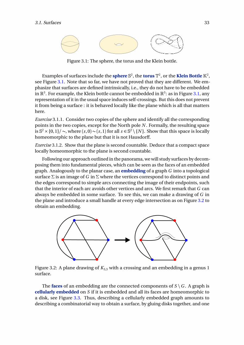
3.1. Surfaces 33
Figure 3.1: The sphere, the torus and the Klein bottle.
Examples of surfaces include the sphere S2, the torus T2, or the Klein BottleK2,see Figure 3.1. Note that so far, we have not proved that they are different. We em-phasize that surfaces are defined intrinsically, i.e., they do not have to be embeddedinR3. For example, the Klein bottle cannot be embedded inR3: as in Figure 3.1, anyrepresentation of it in the usual space induces self-crossings. But this does not preventit from being a surface : it is behaved locally like the plane which is all that mattershere.
Exercise 3.1.1. Consider two copies of the sphere and identify all the correspondingpoints in the two copies, except for the North pole N . Formally, the resulting spaceis S2×{0,1}/∼, where (s ,0)∼ (s ,1) for all s ∈ S2 \ {N }. Show that this space is locallyhomeomorphic to the plane but that it is not Hausdorff.
Exercise 3.1.2. Show that the plane is second countable. Deduce that a compact spacelocally homeomorphic to the plane is second countable.
Following our approach outlined in the panorama, we will study surfaces by decom-posing them into fundamental pieces, which can be seen as the faces of an embeddedgraph. Analogously to the planar case, an embedding of a graph G into a topologicalsurface Σ is an image of G in Σwhere the vertices correspond to distinct points andthe edges correspond to simple arcs connecting the image of their endpoints, suchthat the interior of each arc avoids other vertices and arcs. We first remark that G canalways be embedded in some surface. To see this, we can make a drawing of G inthe plane and introduce a small handle at every edge intersection as on Figure 3.2 toobtain an embedding.
Figure 3.2: A plane drawing of K3,3 with a crossing and an embedding in a genus 1surface.
The faces of an embedding are the connected components of S \G . A graph iscellularly embedded on S if it is embedded and all its faces are homeomorphic toa disk, see Figure 3.3. Thus, describing a cellularly embedded graph amounts todescribing a combinatorial way to obtain a surface, by gluing disks together, and one
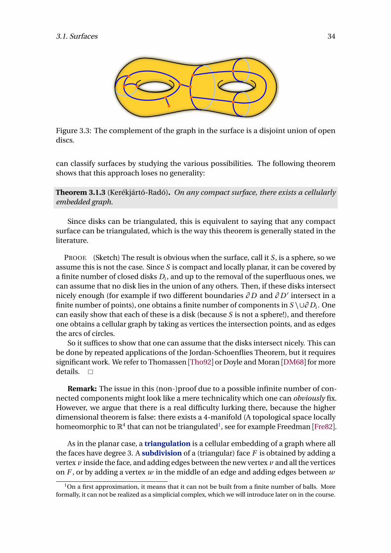
3.1. Surfaces 34
Figure 3.3: The complement of the graph in the surface is a disjoint union of opendiscs.
can classify surfaces by studying the various possibilities. The following theoremshows that this approach loses no generality:
Theorem 3.1.3 (Kerékjártó-Radó). On any compact surface, there exists a cellularlyembedded graph.
Since disks can be triangulated, this is equivalent to saying that any compactsurface can be triangulated, which is the way this theorem is generally stated in theliterature.
PROOF. (Sketch) The result is obvious when the surface, call it S , is a sphere, so weassume this is not the case. Since S is compact and locally planar, it can be covered bya finite number of closed disks Di , and up to the removal of the superfluous ones, wecan assume that no disk lies in the union of any others. Then, if these disks intersectnicely enough (for example if two different boundaries ∂ D and ∂ D ′ intersect in afinite number of points), one obtains a finite number of components in S \∪∂ Di . Onecan easily show that each of these is a disk (because S is not a sphere!), and thereforeone obtains a cellular graph by taking as vertices the intersection points, and as edgesthe arcs of circles.
So it suffices to show that one can assume that the disks intersect nicely. This canbe done by repeated applications of the Jordan-Schoenflies Theorem, but it requiressignificant work. We refer to Thomassen [Tho92] or Doyle and Moran [DM68] for moredetails.
Remark: The issue in this (non-)proof due to a possible infinite number of con-nected components might look like a mere technicality which one can obviously fix.However, we argue that there is a real difficulty lurking there, because the higherdimensional theorem is false: there exists a 4-manifold (A topological space locallyhomeomorphic toR4 that can not be triangulated1, see for example Freedman [Fre82].
As in the planar case, a triangulation is a cellular embedding of a graph where allthe faces have degree 3. A subdivision of a (triangular) face F is obtained by adding avertex v inside the face, and adding edges between the new vertex v and all the verticeson F , or by adding a vertex w in the middle of an edge and adding edges between w
1On a first approximation, it means that it can not be built from a finite number of balls. Moreformally, it can not be realized as a simplicial complex, which we will introduce later on in the course.
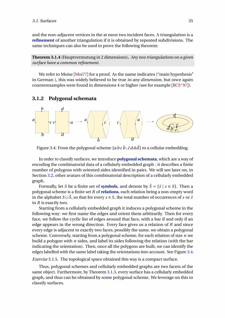
3.1. Surfaces 35
and the non-adjacent vertices in the at most two incident faces. A triangulation is arefinement of another triangulation if it is obtained by repeated subdivisions. Thesame techniques can also be used to prove the following theorem:
Theorem 3.1.4 (Hauptvermutung in 2 dimensions). Any two triangulations on a givensurface have a common refinement.
We refer to Moise [Moi77] for a proof. As the name indicates (“main hypothesis”in German ), this was widely believed to be true in any dimension, but once againcounterexamples were found in dimensions 4 or higher (see for example [RCS+97]).
3.1.2 Polygonal schemata
a
b
b
c c a
d
d
a ac c
b d
d
ba c
Figure 3.4: From the polygonal scheme {a b c b , c d a d } to a cellular embedding.
In order to classify surfaces, we introduce polygonal schemata, which are a way ofencoding the combinatorial data of a cellularly embedded graph : it describes a finitenumber of polygons with oriented sides identified in pairs. We will see later on, inSection 3.2, other avatars of this combinatorial description of a cellularly embeddedgraph.
Formally, let S be a finite set of symbols, and denote by S = {s | s ∈ S}. Then apolygonal scheme is a finite set R of relations, each relation being a non-empty wordin the alphabet S ∪ S , so that for every s ∈ S , the total number of occurences of s or sin R is exactly two.
Starting from a cellularly embedded graph it induces a polygonal scheme in thefollowing way: we first name the edges and orient them arbitrarily. Then for everyface, we follow the cyclic list of edges around that face, with a bar if and only if anedge appears in the wrong direction. Every face gives us a relation of R and sinceevery edge is adjacent to exactly two faces, possibly the same, we obtain a polygonalscheme. Conversely, starting from a polygonal scheme, for each relation of size n webuild a polygon with n sides, and label its sides following the relation (with the barindicating the orientation). Then, once all the polygons are built, we can identify theedges labelled with the same label taking the orientations into account. See Figure 3.4.
Exercise 3.1.5. The topological space obtained this way is a compact surface.
Thus, polygonal schemes and cellularly embedded graphs are two facets of thesame object. Furthermore, by Theorem 3.1.3, every surface has a cellularly embeddedgraph, and thus can be obtained by some polygonal scheme. We leverage on this toclassify surfaces.
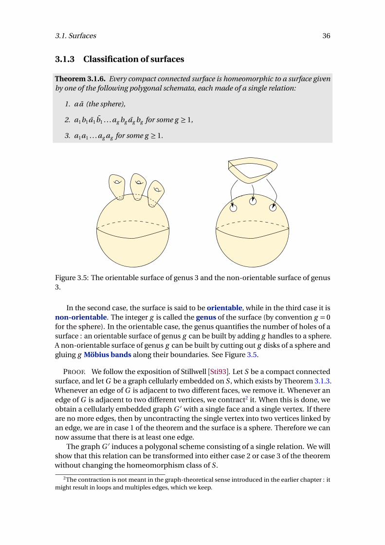
3.1. Surfaces 36
3.1.3 Classification of surfaces
Theorem 3.1.6. Every compact connected surface is homeomorphic to a surface givenby one of the following polygonal schemata, each made of a single relation:
1. a a (the sphere),
2. a1b1a1b1 . . . ag bg ag bg for some g ≥ 1,
3. a1a1 . . . ag ag for some g ≥ 1.
Figure 3.5: The orientable surface of genus 3 and the non-orientable surface of genus3.
In the second case, the surface is said to be orientable, while in the third case it isnon-orientable. The integer g is called the genus of the surface (by convention g = 0for the sphere). In the orientable case, the genus quantifies the number of holes of asurface : an orientable surface of genus g can be built by adding g handles to a sphere.A non-orientable surface of genus g can be built by cutting out g disks of a sphere andgluing g Möbius bands along their boundaries. See Figure 3.5.
PROOF. We follow the exposition of Stillwell [Sti93]. Let S be a compact connectedsurface, and let G be a graph cellularly embedded on S , which exists by Theorem 3.1.3.Whenever an edge of G is adjacent to two different faces, we remove it. Whenever anedge of G is adjacent to two different vertices, we contract2 it. When this is done, weobtain a cellularly embedded graph G ′ with a single face and a single vertex. If thereare no more edges, then by uncontracting the single vertex into two vertices linked byan edge, we are in case 1 of the theorem and the surface is a sphere. Therefore we cannow assume that there is at least one edge.
The graph G ′ induces a polygonal scheme consisting of a single relation. We willshow that this relation can be transformed into either case 2 or case 3 of the theoremwithout changing the homeomorphism class of S .
2The contraction is not meant in the graph-theoretical sense introduced in the earlier chapter : itmight result in loops and multiples edges, which we keep.
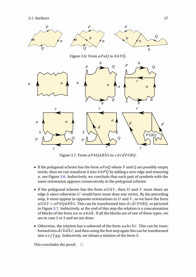
3.1. Surfaces 37
a a
P
Q
a a
P
Q
ba
P
Qb
b
Figure 3.6: From a P aQ to b b PQ .
a a
b
b
aa c
b
b
aa
c
c
a a
c
c
a
dd
c
c
d
P Q
RS
P Q
RS
P
S RQ
S
P
R
QP SRQ
Figure 3.7: From a P bQ a R b S to c d c d P SRQ .
• If the polygonal scheme has the form a P aQ where P and Q are possibly emptywords, then we can transform it into b b PQ by adding a new edge and removinga , see Figure 3.6. Inductively, we conclude that each pair of symbols with thesame orientation appears consecutively in the polygonal scheme.
• If the polygonal scheme has the form aU a V , then U and V must share anedge b since otherwise G ′ would have more than one vertex. By the precedingstep, b must appear in opposite orientations in U and V , so we have the formaU a V = a P bQ a R b S . This can be transformed into d c d c P SRQ , as picturedin Figure 3.7. Inductively, at the end of this step the relation is a concatenationof blocks of the form a a or a b a b . If all the blocks are of one of these types, weare in case 2 or 3 and we are done.
• Otherwise, the relation has a subword of the form a a b c b c . This can be trans-formed into d c b d b c , and then using the first step again this can be transformedinto e e f f g g . Inductively, we obtain a relation of the form 3.
This concludes the proof.
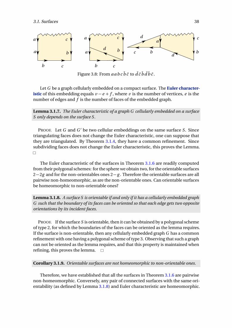
3.1. Surfaces 38
a
a
b c
b
c a
a
b c
d b
c d
c b
a
db
c
Figure 3.8: From a a b c b c to d c b d b c .
Let G be a graph cellularly embedded on a compact surface. The Euler character-istic of this embedding equals v − e + f , where v is the number of vertices, e is thenumber of edges and f is the number of faces of the embedded graph.
Lemma 3.1.7. The Euler characteristic of a graph G cellularly embedded on a surfaceS only depends on the surface S.
PROOF. Let G and G ′ be two cellular embeddings on the same surface S . Sincetriangulating faces does not change the Euler characteristic, one can suppose thatthey are triangulated. By Theorem 3.1.4, they have a common refinement. Sincesubdividing faces does not change the Euler characteristic, this proves the Lemma.
The Euler characteristic of the surfaces in Theorem 3.1.6 are readily computedfrom their polygonal schemes: for the sphere we obtain two, for the orientable surfaces2−2g and for the non-orientables ones 2−g . Therefore the orientable surfaces are allpairwise non-homeomorphic, as are the non-orientable ones. Can orientable surfacesbe homeomorphic to non-orientable ones?
Lemma 3.1.8. A surface S is orientable if and only if it has a cellularly embedded graphG such that the boundary of its faces can be oriented so that each edge gets two oppositeorientations by its incident faces.
PROOF. If the surface S is orientable, then it can be obtained by a polygonal schemeof type 2, for which the boundaries of the faces can be oriented as the lemma requires.If the surface is non-orientable, then any cellularly embedded graph G has a commonrefinement with one having a polygonal scheme of type 3. Observing that such a graphcan not be oriented as the lemma requires, and that this property is maintained whenrefining, this proves the lemma.
Corollary 3.1.9. Orientable surfaces are not homeomorphic to non-orientable ones.
Therefore, we have established that all the surfaces in Theorem 3.1.6 are pairwisenon-homeomorphic. Conversely, any pair of connected surfaces with the same ori-entability (as defined by Lemma 3.1.8) and Euler characteristic are homeomorphic.
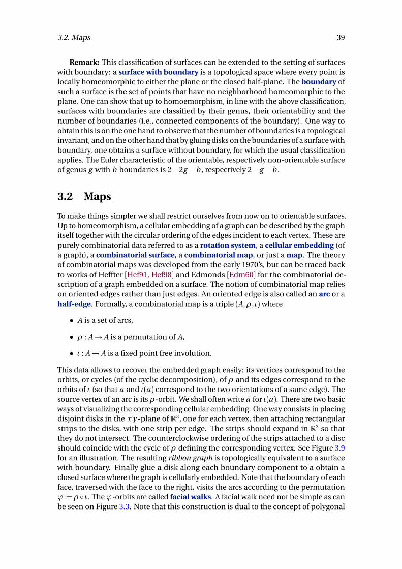
3.2. Maps 39
Remark: This classification of surfaces can be extended to the setting of surfaceswith boundary: a surface with boundary is a topological space where every point islocally homeomorphic to either the plane or the closed half-plane. The boundary ofsuch a surface is the set of points that have no neighborhood homeomorphic to theplane. One can show that up to homoemorphism, in line with the above classification,surfaces with boundaries are classified by their genus, their orientability and thenumber of boundaries (i.e., connected components of the boundary). One way toobtain this is on the one hand to observe that the number of boundaries is a topologicalinvariant, and on the other hand that by gluing disks on the boundaries of a surface withboundary, one obtains a surface without boundary, for which the usual classificationapplies. The Euler characteristic of the orientable, respectively non-orientable surfaceof genus g with b boundaries is 2−2g − b , respectively 2− g − b .
3.2 Maps
To make things simpler we shall restrict ourselves from now on to orientable surfaces.Up to homeomorphism, a cellular embedding of a graph can be described by the graphitself together with the circular ordering of the edges incident to each vertex. These arepurely combinatorial data referred to as a rotation system, a cellular embedding (ofa graph), a combinatorial surface, a combinatorial map, or just a map. The theoryof combinatorial maps was developed from the early 1970’s, but can be traced backto works of Heffter [Hef91, Hef98] and Edmonds [Edm60] for the combinatorial de-scription of a graph embedded on a surface. The notion of combinatorial map relieson oriented edges rather than just edges. An oriented edge is also called an arc or ahalf-edge. Formally, a combinatorial map is a triple (A,ρ, ι)where
• A is a set of arcs,
• ρ : A→ A is a permutation of A,
• ι : A→ A is a fixed point free involution.
This data allows to recover the embedded graph easily: its vertices correspond to theorbits, or cycles (of the cyclic decomposition), of ρ and its edges correspond to theorbits of ι (so that a and ι(a ) correspond to the two orientations of a same edge). Thesource vertex of an arc is itsρ-orbit. We shall often write a for ι(a ). There are two basicways of visualizing the corresponding cellular embedding. One way consists in placingdisjoint disks in the x y -plane of R3, one for each vertex, then attaching rectangularstrips to the disks, with one strip per edge. The strips should expand in R3 so thatthey do not intersect. The counterclockwise ordering of the strips attached to a discshould coincide with the cycle of ρ defining the corresponding vertex. See Figure 3.9for an illustration. The resulting ribbon graph is topologically equivalent to a surfacewith boundary. Finally glue a disk along each boundary component to a obtain aclosed surface where the graph is cellularly embedded. Note that the boundary of eachface, traversed with the face to the right, visits the arcs according to the permutationϕ :=ρ ◦ ι. Theϕ-orbits are called facial walks. A facial walk need not be simple as canbe seen on Figure 3.3. Note that this construction is dual to the concept of polygonal
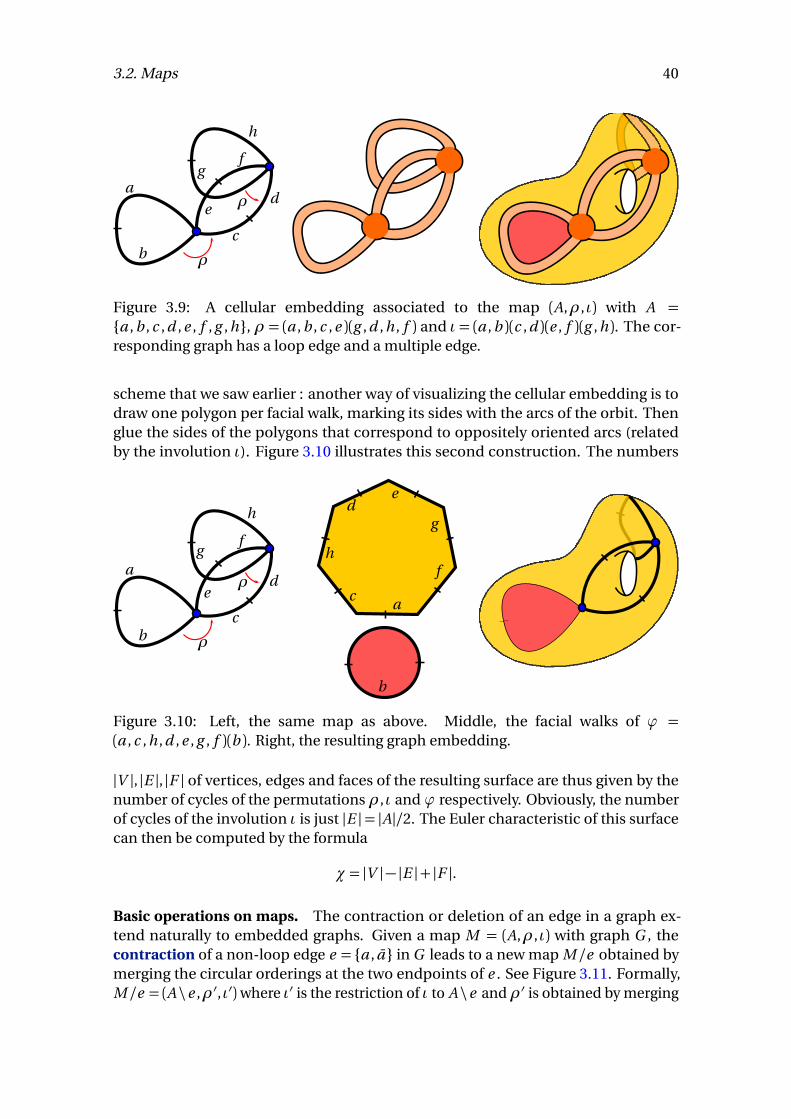
3.2. Maps 40
ρ
ρa
bc
de
fg
h
Figure 3.9: A cellular embedding associated to the map (A,ρ, ι) with A ={a , b , c , d , e , f , g , h}, ρ = (a , b , c , e )(g , d , h , f ) and ι = (a , b )(c , d )(e , f )(g , h ). The cor-responding graph has a loop edge and a multiple edge.
scheme that we saw earlier : another way of visualizing the cellular embedding is todraw one polygon per facial walk, marking its sides with the arcs of the orbit. Thenglue the sides of the polygons that correspond to oppositely oriented arcs (relatedby the involution ι). Figure 3.10 illustrates this second construction. The numbers
ρ
ρa
bc
de
fg
h
ac
h
de
g
f
b
Figure 3.10: Left, the same map as above. Middle, the facial walks of ϕ =(a , c , h , d , e , g , f )(b ). Right, the resulting graph embedding.
|V |, |E |, |F | of vertices, edges and faces of the resulting surface are thus given by thenumber of cycles of the permutations ρ, ι and ϕ respectively. Obviously, the numberof cycles of the involution ι is just |E |= |A|/2. The Euler characteristic of this surfacecan then be computed by the formula
χ = |V | − |E |+ |F |.
Basic operations on maps. The contraction or deletion of an edge in a graph ex-tend naturally to embedded graphs. Given a map M = (A,ρ, ι) with graph G , thecontraction of a non-loop edge e = {a , a } in G leads to a new map M /e obtained bymerging the circular orderings at the two endpoints of e . See Figure 3.11. Formally,M /e = (A \e ,ρ′, ι′)where ι′ is the restriction of ι to A \e andρ′ is obtained by merging
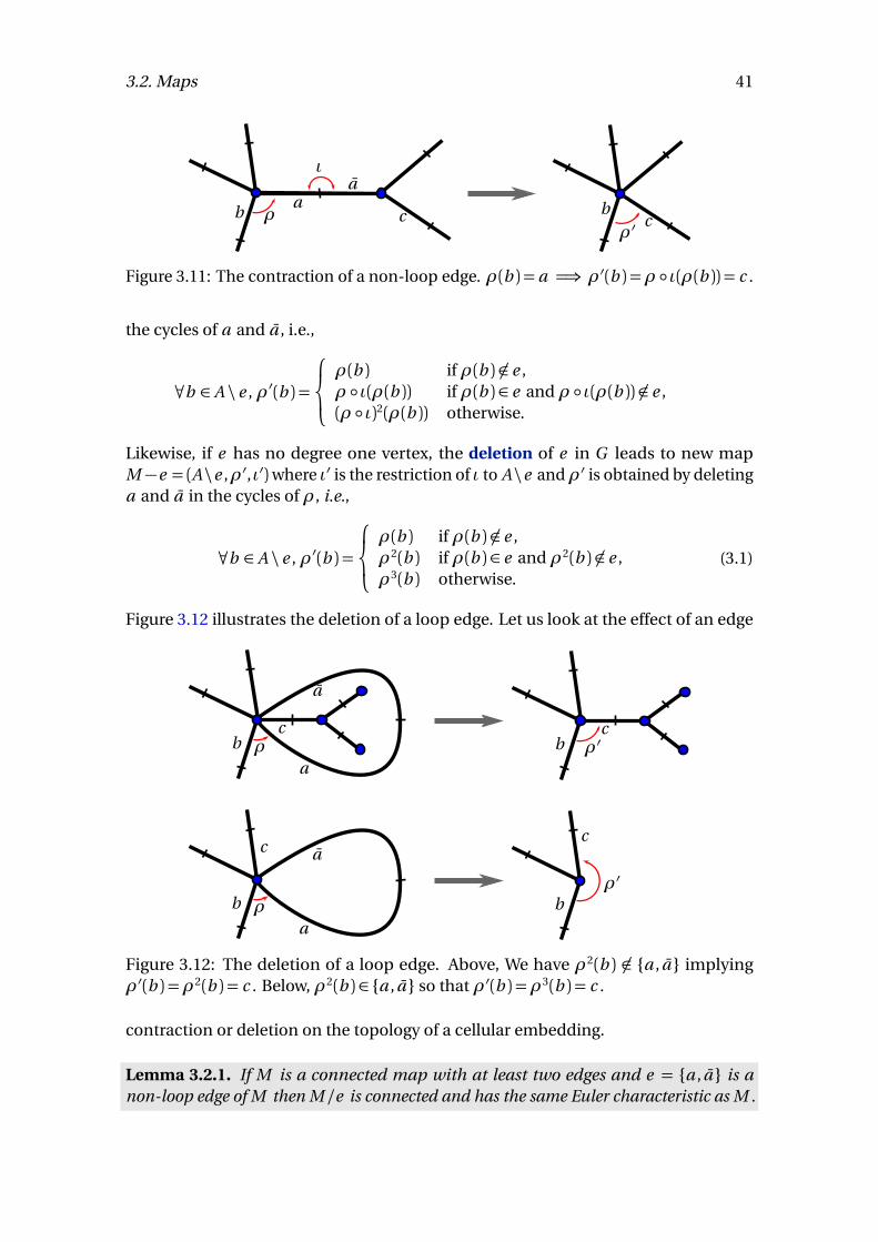
3.2. Maps 41
ba
ρ
ιa
ρ′bc c
Figure 3.11: The contraction of a non-loop edge. ρ(b ) = a =⇒ ρ′(b ) =ρ ◦ ι(ρ(b )) = c .
the cycles of a and a , i.e.,
∀b ∈ A \ e , ρ′(b ) =
ρ(b ) if ρ(b ) 6∈ e ,ρ ◦ ι(ρ(b )) if ρ(b ) ∈ e and ρ ◦ ι(ρ(b )) 6∈ e ,(ρ ◦ ι)2(ρ(b )) otherwise.
Likewise, if e has no degree one vertex, the deletion of e in G leads to new mapM −e = (A\e ,ρ′, ι′)where ι′ is the restriction of ι to A\e andρ′ is obtained by deletinga and a in the cycles of ρ, i.e.,
∀b ∈ A \ e , ρ′(b ) =
ρ(b ) if ρ(b ) 6∈ e ,ρ2(b ) if ρ(b ) ∈ e and ρ2(b ) 6∈ e ,ρ3(b ) otherwise.
(3.1)
Figure 3.12 illustrates the deletion of a loop edge. Let us look at the effect of an edge
b
a
ρa
cb ρ′
c
b
a
ρa
c
bρ′
c
Figure 3.12: The deletion of a loop edge. Above, We have ρ2(b ) 6∈ {a , a } implyingρ′(b ) =ρ2(b ) = c . Below, ρ2(b ) ∈ {a , a } so that ρ′(b ) =ρ3(b ) = c .
contraction or deletion on the topology of a cellular embedding.
Lemma 3.2.1. If M is a connected map with at least two edges and e = {a , a } is anon-loop edge of M then M /e is connected and has the same Euler characteristic as M .
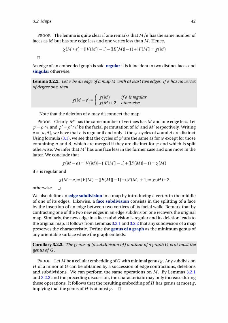
3.2. Maps 42
PROOF. The lemma is quite clear if one remarks that M /e has the same number offaces as M but has one edge less and one vertex less than M . Hence,
χ(M \ e ) = (|V (M )| −1)− (|E (M )| −1) + |F (M )|=χ(M )
An edge of an embedded graph is said regular if is it incident to two distinct faces andsingular otherwise.
Lemma 3.2.2. Let e be an edge of a map M with at least two edges. If e has no vertexof degree one, then
χ(M − e ) =
�
χ(M ) if e is regularχ(M ) +2 otherwise.
Note that the deletion of e may disconnect the map.
PROOF. Clearly, M ′ has the same number of vertices has M and one edge less. Letϕ =ρ ◦ ι and ϕ′ =ρ′ ◦ ι′ be the facial permutation of M and M ′ respectively. Writinge = {a , a }, we have that e is regular if and only if the ϕ-cycles of a and a are distinct.Using formula (3.1), we see that the cycles of ϕ′ are the same as for ϕ except for thosecontaining a and a , which are merged if they are distinct for ϕ and which is splitotherwise. We infer that M ′ has one face less in the former case and one more in thelatter. We conclude that
χ(M − e ) = |V (M )| − (|E (M )| −1) + (|F (M )| −1) =χ(M )
if e is regular and
χ(M − e ) = |V (M )| − (|E (M )| −1) + (|F (M )|+1) =χ(M ) +2
otherwise.
We also define an edge subdivision in a map by introducing a vertex in the middleof one of its edges. Likewise, a face subdivision consists in the splitting of a faceby the insertion of an edge between two vertices of its facial walk. Remark that bycontracting one of the two new edges in an edge subdivision one recovers the originalmap. Similarly, the new edge in a face subdivision is regular and its deletion leads tothe original map. It follows from Lemmas 3.2.1 and 3.2.2 that any subdivision of a mappreserves the characteristic. Define the genus of a graph as the minimum genus ofany orientable surface where the graph embeds.
Corollary 3.2.3. The genus of (a subdivision of) a minor of a graph G is at most thegenus of G .
PROOF. Let M be a cellular embedding of G with minimal genus g . Any subdivisionH of a minor of G can be obtained by a succession of edge contractions, deletionsand subdivisions. We can perform the same operations on M . By Lemmas 3.2.1and 3.2.2 and the preceding discussion, the characteristic may only increase duringthese operations. It follows that the resulting embedding of H has genus at most g ,implying that the genus of H is at most g .
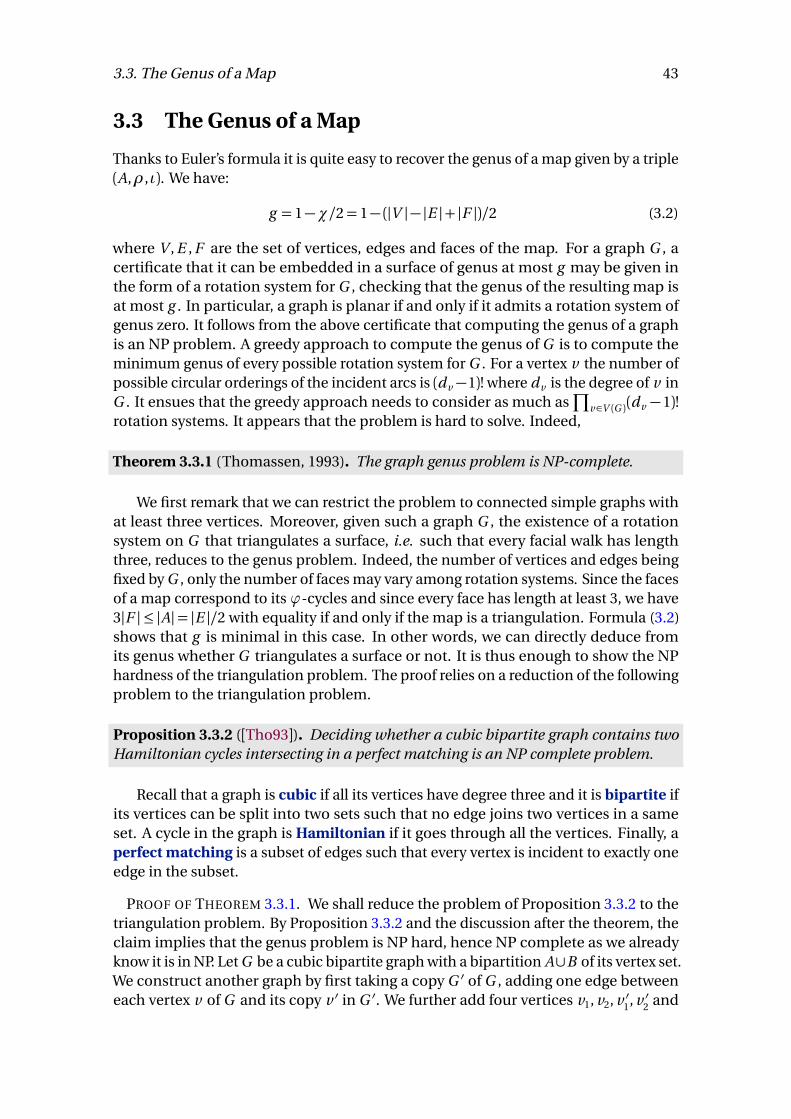
3.3. The Genus of a Map 43
3.3 The Genus of a Map
Thanks to Euler’s formula it is quite easy to recover the genus of a map given by a triple(A,ρ, ι). We have:
g = 1−χ/2= 1− (|V | − |E |+ |F |)/2 (3.2)
where V , E , F are the set of vertices, edges and faces of the map. For a graph G , acertificate that it can be embedded in a surface of genus at most g may be given inthe form of a rotation system for G , checking that the genus of the resulting map isat most g . In particular, a graph is planar if and only if it admits a rotation system ofgenus zero. It follows from the above certificate that computing the genus of a graphis an NP problem. A greedy approach to compute the genus of G is to compute theminimum genus of every possible rotation system for G . For a vertex v the number ofpossible circular orderings of the incident arcs is (dv −1)! where dv is the degree of v inG . It ensues that the greedy approach needs to consider as much as
∏
v∈V (G )(dv −1)!rotation systems. It appears that the problem is hard to solve. Indeed,
Theorem 3.3.1 (Thomassen, 1993). The graph genus problem is NP-complete.
We first remark that we can restrict the problem to connected simple graphs withat least three vertices. Moreover, given such a graph G , the existence of a rotationsystem on G that triangulates a surface, i.e. such that every facial walk has lengththree, reduces to the genus problem. Indeed, the number of vertices and edges beingfixed by G , only the number of faces may vary among rotation systems. Since the facesof a map correspond to its ϕ-cycles and since every face has length at least 3, we have3|F | ≤ |A|= |E |/2 with equality if and only if the map is a triangulation. Formula (3.2)shows that g is minimal in this case. In other words, we can directly deduce fromits genus whether G triangulates a surface or not. It is thus enough to show the NPhardness of the triangulation problem. The proof relies on a reduction of the followingproblem to the triangulation problem.
Proposition 3.3.2 ([Tho93]). Deciding whether a cubic bipartite graph contains twoHamiltonian cycles intersecting in a perfect matching is an NP complete problem.
Recall that a graph is cubic if all its vertices have degree three and it is bipartite ifits vertices can be split into two sets such that no edge joins two vertices in a sameset. A cycle in the graph is Hamiltonian if it goes through all the vertices. Finally, aperfect matching is a subset of edges such that every vertex is incident to exactly oneedge in the subset.
PROOF OF THEOREM 3.3.1. We shall reduce the problem of Proposition 3.3.2 to thetriangulation problem. By Proposition 3.3.2 and the discussion after the theorem, theclaim implies that the genus problem is NP hard, hence NP complete as we alreadyknow it is in NP. Let G be a cubic bipartite graph with a bipartition A∪B of its vertex set.We construct another graph by first taking a copy G ′ of G , adding one edge betweeneach vertex v of G and its copy v ′ in G ′. We further add four vertices v1, v2, v ′1, v ′2 and
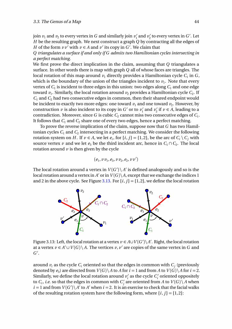
3.3. The Genus of a Map 44
join v1 and v2 to every vertex in G and similarly join v ′1 and v ′2 to every vertex in G ′. LetH be the resulting graph. We next construct a graph Q by contracting all the edges ofH of the form v v ′ with v ∈ A and v ′ its copy in G ′. We claim thatQ triangulates a surface if and only if G admits two Hamiltonian cycles intersecting ina perfect matching.We first prove the direct implication in the claim, assuming that Q triangulates asurface. In other words there is map with graph Q all of whose faces are triangles. Thelocal rotation of this map around v1 directly provides a Hamiltonian cycle C1 in G ,which is the boundary of the union of the triangles incident to v1. Note that everyvertex of C1 is incident to three edges in this union: two edges along C1 and one edgetoward v1. Similarly, the local rotation around v2 provides a Hamiltonian cycle C2. IfC1 and C2 had two consecutive edges in common, then their shared endpoint wouldbe incident to exactly two more edges: one toward v1 and one toward v2. However, byconstruction v is also incident to its copy in G ′ or to v ′1 and v ′2 if v ∈ A, leading to acontradiction. Moreover, since G is cubic C2 cannot miss two consecutive edges of C1.It follows that C1 and C2 share one of every two edges, hence a perfect matching.
To prove the reverse implication of the claim, suppose now that G has two Hamil-tonian cycles C1 and C2 intersecting in a perfect matching. We consider the followingrotation system on H . If v ∈ A, we let ei , for {i , j } = {1,2}, be the arc of Ci \C j withsource vertex v and we let e3 be the third incident arc, hence in C1 ∩C2. The localrotation around v is then given by the cycle
(e1, v v1, e3, v v2, e2, v v ′)
The local rotation around a vertex in V (G ′) \A′ is defined analogously and so is thelocal rotation around a vertex in A′ or in V (G )\A, except that we exchange the indices 1and 2 in the above cycle. See Figure 3.13. For {i , j }= {1, 2}, we define the local rotation
e1v1
v2
e2e3
e1 v1
v2
v ′
e3e2
C2
C1
v vv ′
C2
C1
C1 ∩C2C1 ∩C2
Figure 3.13: Left, the local rotation at a vertex v ∈ A∪V (G ′)\A′. Right, the local rotationat a vertex v ∈ A′ ∪V (G ) \A. The vertices v, v ′ are copies of the same vertex in G andG ′.
around vi as the cycle Ci oriented so that the edges in common with C j (previouslydenoted by e3) are directed from V (G )\A to A for i = 1 and from A to V (G )\A for i = 2.Similarly, we define the local rotation around v ′i as the cycle C ′i oriented oppositelyto Ci , i.e. so that the edges in common with C ′j are oriented from A to V (G ) \A wheni = 1 and from V (G ′)\A′ to A′ when i = 2. It is an exercise to check that the facial walksof the resulting rotation system have the following form, where {i , j }= {1, 2}:
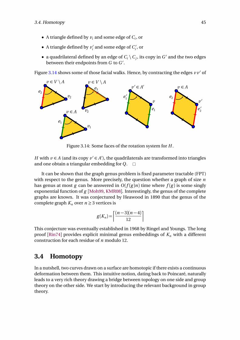
3.4. Homotopy 45
• A triangle defined by vi and some edge of Ci , or
• A triangle defined by v ′i and some edge of C ′i , or
• a quadrilateral defined by an edge of Ci \C j , its copy in G ′ and the two edgesbetween their endpoints from G to G ′.
Figure 3.14 shows some of those facial walks. Hence, by contracting the edges v v ′ of
v2
v ∈V \A
e2
v1
v ∈ A
e1
v
v ′ ∈ A′
e ′1
e1
v ∈V \A
v2
e3
v ′
v ∈ A
e2
e ′2
Figure 3.14: Some faces of the rotation system for H .
H with v ∈ A (and its copy v ′ ∈ A′), the quadrilaterals are transformed into trianglesand one obtain a triangular embedding for Q .
It can be shown that the graph genus problem is fixed parameter tractable (FPT)with respect to the genus. More precisely, the question whether a graph of size nhas genus at most g can be answered in O ( f (g )n ) time where f (g ) is some singlyexponential function of g [Moh99, KMR08]. Interestingly, the genus of the completegraphs are known. It was conjectured by Heawood in 1890 that the genus of thecomplete graph Kn over n ≥ 3 vertices is
g (Kn ) =¡ (n −3)(n −4)
12
¤
This conjecture was eventually established in 1968 by Ringel and Youngs. The longproof [Rin74] provides explicit minimal genus embeddings of Kn with a differentconstruction for each residue of n modulo 12.
3.4 Homotopy
In a nutshell, two curves drawn on a surface are homotopic if there exists a continuousdeformation between them. This intuitive notion, dating back to Poincaré, naturallyleads to a very rich theory drawing a bridge between topology on one side and grouptheory on the other side. We start by introducing the relevant background in grouptheory.
3.4. Homotopy 46
3.4.1 Groups, generators and relations
Although most groups we will be dealing with in this course are infinite, they can oftenbe very succinctly encoded in terms of generators and relations. The attentive readerwill probably notice some similarities between the formalism established here andthe definitions on polygonal schemata : as we will see later on, this is no coincidence.
Let us consider a set G of generators, and denote by G −1 their inverses G −1 = {g −1 |g ∈G }. A word is a string over the alphabet G ∪G −1 , and we denote by ε the emptyword. We consider that two words are equivalent if one can switch from one to theother by adding or removing words of the form g g −1 or g −1g . The set of finite wordsquotiented by this equivalence relation can naturally be endowed with the structureof a group: the law is the concatenation, and the neutral element is ε. Indeed:
• The concatenation is well-defined with respect to the equivalence relation andis associative.
• For any word w , w ε = εw =w .
• Each element has an inverse obtained by reversing the order of the letters andinverting them, e.g., c −1b −1a−1 is the inverse of a b c .
This group is called the free group on the set G , denoted by F (G ).Now, let us also fix a set R of words called the relations, and consider the free
group F (G ), where one also identifies a word with the word obtained by inserting atany place a word taken from R or their inverses. This defines another group, which isformally the quotient of F (G ) by the normal subgroup generated by R 3. This group issaid to admit the presentation <G | R >. So the free group admits the presentation<G | ;>, generally abbreviated by <G >.
Here are a few examples:
• The group Z is the free group on one letter F ({a }).
• The group < a | a a > is the group Z2 (or Z/2Z).
• The group < a , b | a b a−1b −1 > is the two-dimensional lattice Z2: indeed, therelation a b a−1b −1 implies that a b = b a , thus the group is abelian, and theisomorphism with Z2 is the map a 7→ (1, 0), b 7→ (0, 1).
Exercise 3.4.1. Recognize the groups< a , b | a a b , a b −1b −1 >and< a , b | a m , b n , a b a−1b −1 >.
Exercise 3.4.2. Show that any group admits a presentation (with possibly an infinitenumber of generators and relations), and that any finite group admits a finite presen-tation.
3.4.2 Fundamental groups, the combinatorial way
We start by introducing homotopy in a combinatorial setting, which makes computa-tions very convenient. The baby case is the case of graphs, which corresponds directlyto free groups.
3Recall that a subgroup H ⊆G is normal if g H =H g for any g ∈G .
3.4. Homotopy 47
Fundamental groups of graphs
Let G denote a graph (not necessarily embedded) where the edges are oriented. Anarc is an oriented edge or its inverse, it has an origin o (a ) and a target t (a ) = o (a−1).A path in G is a sequence of arcs (e1, . . . , en ) such that the target of ei coincides withthe origin of ei+1. A loop is a path such that the target of en coincides with the originof e1, this point is called the basepoint of the loop. The trivial loop is the empty loop.Two loops with a common basepoint x are homotopic if they can be related to eachother by adding or removing subpaths of the type (e , e −1), and a path is reduced if itdoes not contain such a subpath.
Let x be a vertex of G . The set of homotopy classes of loops in G forms a group,where the law is the concatenation and the neutral element the trivial loop. Indeed:
• The concatenation is well-defined with respect ot the equivalence relation andis associative.
• Concatenating with the trivial loop does not change a loop.
• Every loop (e1, . . . , en ) has an inverse (e −1n , . . . , e −1
1 ).
This group is called the fundamental group of G , denoted by π1(G , x ).
Theorem 3.4.3. Let T be a spanning tree of G containing the vertex x . Then the funda-mental group π1(G , x ) is isomorphic to the free group generated by the edges of G thatare not in T .
PROOF. Let C denote the set of edges not in T . For every arc a , one can associate aloop based at x denoted by γT
a = γTx→o (a ) ·a ·γ
Tt (a )→x , where γT
x→y denotes the uniquereduced path in T between x and y . Then, every loop (e1, . . . , en ) based at x in G ishomotopic to the loop γT
e1, . . . ,γT
en, and for every arc a in T , γT
a is homotopic to theconstant loop. Therefore, π1(G , x ) is generated by the loops γT
a for a and arc not in T ,and since γT
a−1 = (γTa )−1, it is enough to pick one arc for every edge of C . Finally, since
the loop γTa for a not in T is the only one containing a , there is no non-trivial relation
between the loops γTa . This proves the theorem.
An alternative way of seeing this proof is to observe that the fundamental group ofG is the same as the fundamental group of G obtained after contracting a spanningtree of G . The resulting graph is a bouquet of circles, and there is one generator foreach circle.
Fundamental groups of surfaces
Now, let S denote a connected surface and let G be a graph cellularly embedded on S .Similarly as before, a loop and a path in (S ,G ) is a path, respectively a loop in G . Anelementary homotopy between two loops is either a reduction (deletion/addition ofe e −1) or the deletion/addition of a subpath bounding a face of G . This correspondsto the idea that in a continuous deformation between two curves, one can flip a faceof a cellularly embedded graph, see Figure 3.15. Elementary homotopies induce

3.4. Homotopy 48
f f
Figure 3.15: The two red paths are homotopic since they are related by going over theface f .
an equivalence relation, called homotopy between loops based at a common point,denoted by ≡.
As before, the set of homotopy classes of loops based at a vertex x of G forms agroup, where the law is the concatenation. Indeed,
• If γ1 ≡ γ′1 and γ2 ≡ γ′2 are two pairs of homotopic loops, then their concatenationsare homotopic : γ1γ2 ≡ γ′1γ
′2.
• The concatenation law is associative.
• The trivial loop, denoted by 1x or simply 1 is a neutral element for the concate-nation law.
• Every loop (e1, . . . , en ) admits (e −1n , . . . , e −1
1 ) as an inverse.
This group is called the fundamental group of S , denoted by π1(S , x )4.
Exercise 3.4.4. Let x and y be two vertices of G , then show thatπ1(S , x ) andπ1(S , y ) areisomorphic. This justifies the common abuse of notation to just write π1(S )withoutspecifying a base point.
Let T be a spanning tree of G containing a vertex x , and let C denote the set ofedges not in T . The fundamental group of G is the free group on C , and to obtain thefundamental group of S from it, one just needs to add the relations correspondingto the faces of G . Formally, for every face f = (e1, . . . , en ) of G , denote by r f the facialrelation induced by f on C , that is, the word obtained by only keeping the ei that arein C . Then we have the following theorem:
Theorem 3.4.5. Let S be a connected surface, G be a cellularly embedded graph on Swith a vertex x and a set of faces F , and T be a spanning tree of G containing x . Denoteby C the set of edges not in T and by r f the facial relation induced by a face f of G onC . Then π1(S ) is isomorphic to the group π presented by
<C | {r f } f ∈F > .
4To be accurate, we should write π1(S ,G , x ) but as we will shortly see, this actually does not dependon G .
3.4. Homotopy 49
PROOF. As before, every arc a in G corresponds to a loop γTa obtained by adjoining
the reduced paths in T between x and the endpoints of a . Let us consider the mapγ : C →π1(S )mapping every arc a in C to γT
a . This map induces a morphism of groupsγ′ : F (C )→ π1(S ). As for homotopy in graphs, this map is surjective since any loopof S is the image by γ of its arcs in C . We will show that its kernel equals the normalsubgroup N generated by the elements r f for f ∈ F , which proves the theorem.
Let w = e1, . . . en be an element of F (C ) such that γ′(w ) ≡ 1. Then it means thatγ′(w ) can be reduced to the trivial loop by a sequence of elementary homotopies. Thenfor every reduction over edges of C , the same reduction can be applied to w , and forevery face flip over a face f , the corresponding facial relation r f can be used to modifythe word w . Thus w can be reduced to the trivial word using the set of relations r f
and the kernel of γ′ is included in N . Reciprocally, an element of N is mapped to thetrivial loop by γ′ since the facial relations r f dictate the face flips to do to simplify thecorresponding relations. This concludes the proof.
Now, let us observe that the group π(S ) stays the same when one
1. contracts an edge of G between two different endpoints,
2. or one removes an edge of G between two different faces.
For 1, let e be the edge we are contracting, and T be a spanning tree of G containinge . This contraction yields a new tree T ′ with one less edge, but the set C of non-treeedges stays the same, as well as the set of facial relations. So the group stays the same.
For 2, when one removes an edge e of G between two different faces, one mergesthe two adjacent faces f1 and f2 into a single face f . One can pick the spanning treeso that e is not in it, and thus π1(S ) lost one generator g , and the two relations r1 andr2 containing g have been merged into one. Observing that this amounts to deletingevery appearance of g in π1(S ) using r1 (or r2), we see that this operation does notchange the group.
Therefore, by the classification of surfaces (or rather its proof), we see that thegraph G can be transformed into one of the polygonal schemata of Theorem 3.1.6without changing the fundamental group. In particular, π1(S ) only depends on thesurface S and not the graph G , and it is isomorphic to
• the trivial group if S is a sphere,
• the group< a1, b1, . . . ag , bg | a1b1a1b1 . . . ag bg ag bg > if S is the orientable surfaceof genus g ,
• or < a1, . . . , ag | a1a1 . . . ag ag > if S is the non-orientable surface of genus g .
Remark: The operations of contraction and deletion of edges used above can beinterpreted in the light of dual graphs: a graph G embedded on a surface S has adual graph G ∗, defined by placing one vertex in each face of G and edges betweenadjacent faces. Then, contracting an edge in the primal graph amounts to removingan edge in the dual graph, and vice versa. Contracting every edge between different
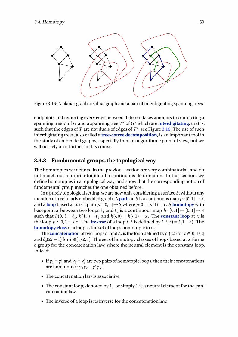
3.4. Homotopy 50
Figure 3.16: A planar graph, its dual graph and a pair of interdigitating spanning trees.
endpoints and removing every edge between different faces amounts to contracting aspanning tree T of G and a spanning tree T ∗ of G ∗ which are interdigitating, that is,such that the edges of T are not duals of edges of T ∗, see Figure 3.16. The use of suchinterdigitating trees, also called a tree-cotree decomposition, is an important tool inthe study of embedded graphs, especially from an algorithmic point of view, but wewill not rely on it further in this course.
3.4.3 Fundamental groups, the topological way
The homotopies we defined in the previous section are very combinatorial, and donot match our a priori intuition of a continuous deformation. In this section, wedefine homotopies in a topological way, and show that the corresponding notion offundamental group matches the one obtained before.
In a purely topological setting, we are now only considering a surface S , without anymention of a cellularly embedded graph. A path on S is a continuous map p : [0, 1]→ S ,and a loop based at x is a path p : [0,1]→ S where p (0) = p (1) = x . A homotopy withbasepoint x between two loops `1 and `2 is a continuous map h : [0,1]→ [0,1]→ Ssuch that h (0, ·) = `1, h (1, ·) = `2 and h (·,0) = h (·,1) = x . The constant loop at x isthe loop p : [0,1] 7→ x . The inverse of a loop `−1 is defined by `−1(t ) = `(1− t ). Thehomotopy class of a loop is the set of loops homotopic to it.
The concatenation of two loops `1 and `2 is the loop defined by `1(2t ) for t ∈ [0, 1/2]and `2(2t −1) for t ∈ [1/2,1]. The set of homotopy classes of loops based at x formsa group for the concatenation law, where the neutral element is the constant loop.Indeed:
• If γ1 ≡ γ′1 and γ2 ≡ γ′2 are two pairs of homotopic loops, then their concatenationsare homotopic : γ1γ2 ≡ γ′1γ
′2.
• The concatenation law is associative.
• The constant loop, denoted by 1x or simply 1 is a neutral element for the con-catenation law.
• The inverse of a loop is its inverse for the concatenation law.
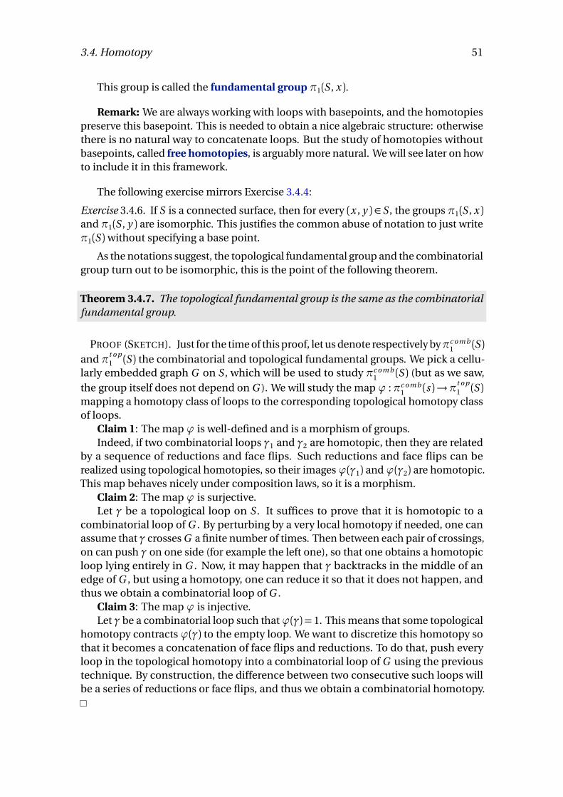
3.4. Homotopy 51
This group is called the fundamental group π1(S , x ).
Remark: We are always working with loops with basepoints, and the homotopiespreserve this basepoint. This is needed to obtain a nice algebraic structure: otherwisethere is no natural way to concatenate loops. But the study of homotopies withoutbasepoints, called free homotopies, is arguably more natural. We will see later on howto include it in this framework.
The following exercise mirrors Exercise 3.4.4:
Exercise 3.4.6. If S is a connected surface, then for every (x , y ) ∈ S , the groups π1(S , x )and π1(S , y ) are isomorphic. This justifies the common abuse of notation to just writeπ1(S )without specifying a base point.
As the notations suggest, the topological fundamental group and the combinatorialgroup turn out to be isomorphic, this is the point of the following theorem.
Theorem 3.4.7. The topological fundamental group is the same as the combinatorialfundamental group.
PROOF (SKETCH). Just for the time of this proof, let us denote respectively byπc o m b1 (S )
and πt o p1 (S ) the combinatorial and topological fundamental groups. We pick a cellu-
larly embedded graph G on S , which will be used to study πc o m b1 (S ) (but as we saw,
the group itself does not depend on G ). We will study the map ϕ :πc o m b1 (s )→πt o p
1 (S )mapping a homotopy class of loops to the corresponding topological homotopy classof loops.
Claim 1: The map ϕ is well-defined and is a morphism of groups.Indeed, if two combinatorial loops γ1 and γ2 are homotopic, then they are related
by a sequence of reductions and face flips. Such reductions and face flips can berealized using topological homotopies, so their imagesϕ(γ1) andϕ(γ2) are homotopic.This map behaves nicely under composition laws, so it is a morphism.
Claim 2: The map ϕ is surjective.Let γ be a topological loop on S . It suffices to prove that it is homotopic to a
combinatorial loop of G . By perturbing by a very local homotopy if needed, one canassume that γ crosses G a finite number of times. Then between each pair of crossings,on can push γ on one side (for example the left one), so that one obtains a homotopicloop lying entirely in G . Now, it may happen that γ backtracks in the middle of anedge of G , but using a homotopy, one can reduce it so that it does not happen, andthus we obtain a combinatorial loop of G .
Claim 3: The map ϕ is injective.Let γ be a combinatorial loop such thatϕ(γ) = 1. This means that some topological
homotopy contracts ϕ(γ) to the empty loop. We want to discretize this homotopy sothat it becomes a concatenation of face flips and reductions. To do that, push everyloop in the topological homotopy into a combinatorial loop of G using the previoustechnique. By construction, the difference between two consecutive such loops willbe a series of reductions or face flips, and thus we obtain a combinatorial homotopy.
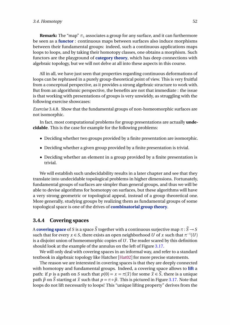
3.4. Homotopy 52
Remark: The “map” π1 associates a group for any surface, and it can furthermorebe seen as a functor : continuous maps between surfaces also induce morphismsbetween their fundamental groups: indeed, such a continuous applications mapsloops to loops, and by taking their homotopy classes, one obtains a morphism. Suchfunctors are the playground of category theory, which has deep connections withalgebraic topology, but we will not delve at all into these aspects in this course.
All in all, we have just seen that properties regarding continuous deformations ofloops can be rephrased in a purely group-theoretical point of view. This is very fruitfulfrom a conceptual perspective, as it provides a strong algebraic structure to work with.But from an algorithmic perspective, the benefits are not that immediate : the issueis that working with presentations of groups is very unwieldy, as struggling with thefollowing exercise showcases:
Exercise 3.4.8. Show that the fundamental groups of non-homeomorphic surfaces arenot isomorphic.
In fact, most computational problems for group presentations are actually unde-cidable. This is the case for example for the following problems:
• Deciding whether two groups provided by a finite presentation are isomorphic.
• Deciding whether a given group provided by a finite presentation is trivial.
• Deciding whether an element in a group provided by a finite presentation istrivial.
We will establish such undecidability results in a later chapter and see that theytranslate into undecidable topological problems in higher dimensions. Fortunately,fundamental groups of surfaces are simpler than general groups, and thus we will beable to devise algorithms for homotopy on surfaces, but these algorithms will havea very strong geometric or topological appeal, instead of a group theoretical one.More generally, studying groups by realizing them as fundamental groups of sometopological space is one of the drives of combinatorial group theory.
3.4.4 Covering spaces
A covering space of S is a space bS together with a continuous surjective map π : bS → Ssuch that for every x ∈ S , there exists an open neighborhood U of x such that π−1(U )is a disjoint union of homeomorphic copies of U . The reader scared by this definitionshould look at the example of the annulus on the left of Figure 3.17.
We will only deal with covering spaces in an informal way, and refer to a standardtextbook in algebraic topology like Hatcher [Hat02] for more precise statements.
The reason we are interested in covering spaces is that they are deeply connectedwith homotopy and fundamental groups. Indeed, a covering space allows to lift apath: if p is a path on S such that p (0) = x = π(bx ) for some bx ∈ bS , there is a uniquepath bp on bS starting at bx such that p =π ◦ bp . This is pictured in Figure 3.17. Note thatloops do not lift necessarily to loops! This “unique lifting property” derives from the
3.4. Homotopy 53
Ux
ππ−1(U )
p
bx
bp
Figure 3.17: A covering of the annulus, and one lift of a path p .
x
p xpbxbp
Figure 3.18: Lifting a loop p on the torus to a path on its universal cover.
definition of covering spaces: when one sits at a point bx of the covering space, thelocal homeomorphism π specifies how to move on bS so that one follows the path p .
Every surface has a unique covering space eS that is simply connected, that is, whereevery loop in eS is homotopic to a trivial loop, it is called the universal cover of S . IfS is a sphere, its universal cover is itself, so let us assume that it is not the case. Oneway to build this cover is as follows: pick a graph G cellularly embedded on S with asingle vertex and a single face (for example one of the graphs used in the classificationtheorem). Cutting S along G gives a polygon and one can tile the plane with thispolygon by putting adjacent copies of this polygon next to each other, so that everyvertex of the tiling is adjacent to the correct number of polygons. This construction ispictured in Figure 8.20 for the torus.
For surfaces of higher genus, the same construction works, but the tiling will notlook as symmetric : indeed it is for example impossible to tile the plane with regularoctagons. This is not an issue for our construction, since any tiling with octagonswill do, even if they do not have the same shape. However, an insightful way to dealwith this issue is to use hyperbolic geometry: it is a non-Euclidean geometry on theopen disk that allows for regular tilings of polygons with an arbitrary number of faces.
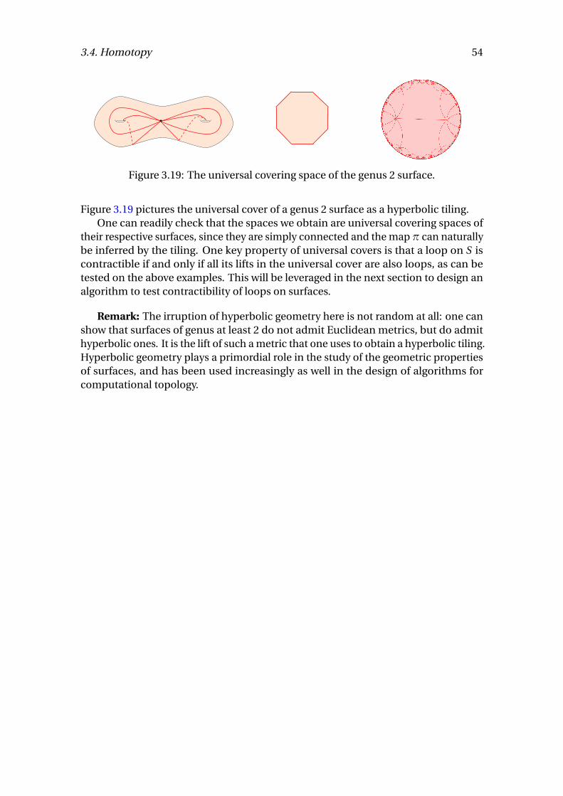
3.4. Homotopy 54
Figure 3.19: The universal covering space of the genus 2 surface.
Figure 3.19 pictures the universal cover of a genus 2 surface as a hyperbolic tiling.One can readily check that the spaces we obtain are universal covering spaces of
their respective surfaces, since they are simply connected and the mapπ can naturallybe inferred by the tiling. One key property of universal covers is that a loop on S iscontractible if and only if all its lifts in the universal cover are also loops, as can betested on the above examples. This will be leveraged in the next section to design analgorithm to test contractibility of loops on surfaces.
Remark: The irruption of hyperbolic geometry here is not random at all: one canshow that surfaces of genus at least 2 do not admit Euclidean metrics, but do admithyperbolic ones. It is the lift of such a metric that one uses to obtain a hyperbolic tiling.Hyperbolic geometry plays a primordial role in the study of the geometric propertiesof surfaces, and has been used increasingly as well in the design of algorithms forcomputational topology.
4
The Homotopy Test
Contents4.1 Dehn’s Algorithm . . . . . . . . . . . . . . . . . . . . . . . . . . . . . . . . . . . . 56
4.2 van Kampen Diagrams . . . . . . . . . . . . . . . . . . . . . . . . . . . . . . . . 58
4.2.1 Disk Diagrams . . . . . . . . . . . . . . . . . . . . . . . . . . . . . . . . . . . 58
4.2.2 Annular Diagrams . . . . . . . . . . . . . . . . . . . . . . . . . . . . . . . . 59
4.3 Gauss-Bonnet Formula . . . . . . . . . . . . . . . . . . . . . . . . . . . . . . . . 59
4.4 Quad Systems . . . . . . . . . . . . . . . . . . . . . . . . . . . . . . . . . . . . . . . 61
4.5 Canonical Representatives . . . . . . . . . . . . . . . . . . . . . . . . . . . . . 62
4.5.1 The Four Bracket Lemma . . . . . . . . . . . . . . . . . . . . . . . . . . . 62
4.5.2 Bracket Flattening . . . . . . . . . . . . . . . . . . . . . . . . . . . . . . . . 64
4.5.3 Canonical Representatives . . . . . . . . . . . . . . . . . . . . . . . . . . 65
4.6 The Homotopy Test . . . . . . . . . . . . . . . . . . . . . . . . . . . . . . . . . . . 67
A fundamental problem when dealing with curves on surfaces is to decide if agiven closed curve can be contracted to a point, or more precisely to a constant curve.This is sometimes referred to as the contractibility problem. More generally, we canask whether two closed curves on a surface are related by a continuous deformation.This question has two variants: we may or may not require the curves to share a givenpoint that remains fixed during the deformation. Note that the problem with fixedpoint has an obvious reduction to the contractibility problem. Indeed, two curves c , dare homotopic with fixed point if and only if the concatenation c ·d −1 is contractible.Without the fixed point requirement, that is when the curves are allowed to movefreely on the surface, the problem is known as the transformation problem and canbe expressed as a conjugacy problem. To see this, choose a point v on a surface S
55
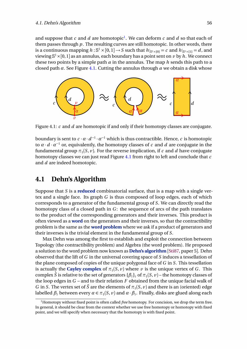
4.1. Dehn’s Algorithm 56
and suppose that c and d are homotopic1. We can deform c and d so that each ofthem passes through p . The resulting curves are still homotopic. In other words, thereis a continuous mapping h : S1× [0,1]→ S such that h S1×{0} = c and h S1×{1} = d , andviewing S1×[0, 1] as an annulus, each boundary has a point sent on v by h . We connectthese two points by a simple path a in the annulus. The map h sends this path to aclosed path α. See Figure 4.1. Cutting the annulus through a we obtain a disk whose
cd
cd
c d
α
α
ααα
v
v
Figure 4.1: c and d are homotopic if and only if their homotopy classes are conjugate.
boundary is sent to c ·α ·d −1 ·α−1 which is thus contractible. Hence, c is homotopicto α · d ·α−1 or, equivalently, the homotopy classes of c and d are conjugate in thefundamental group π1(S , v ). For the reverse implication, if c and d have conjugatehomotopy classes we can just read Figure 4.1 from right to left and conclude that cand d are indeed homotopic.
4.1 Dehn’s Algorithm
Suppose that S is a reduced combinatorial surface, that is a map with a single ver-tex and a single face. Its graph G is thus composed of loop edges, each of whichcorresponds to a generator of the fundamental group of S . We can directly read thehomotopy class of a closed path in G : the sequence of arcs of the path translatesto the product of the corresponding generators and their inverses. This product isoften viewed as a word on the generators and their inverses, so that the contractibilityproblem is the same as the word problem where we ask if a product of generators andtheir inverses is the trivial element in the fundamental group of S .
Max Dehn was among the first to establish and exploit the connection betweenTopology (the contractibility problem) and Algebra (the word problem). He proposeda solution to the word problem now known as Dehn’s algorithm [Sti87, paper 5]. Dehnobserved that the lift of G in the universal covering space of S induces a tessellation ofthe plane composed of copies of the unique polygonal face of G in S . This tessellationis actually the Cayley complex of π1(S , v ) where v is the unique vertex of G . Thiscomplex S is relative to the set of generators {βi }i of π1(S , v ) – the homotopy classes ofthe loop edges in G – and to their relation F obtained from the unique facial walk ofG in S . The vertex set of S are the elements of π1(S , v ) and there is an (oriented) edgelabelled βi between every α ∈ π1(S , v ) and α ·βi . Finally, disks are glued along each
1Homotopy without fixed point is often called free homotopy. For concision, we drop the term free.In general, it should be clear from the context whether we use free homotopy or homotopy with fixedpoint, and we will specify when necessary that the homotopy is with fixed point.
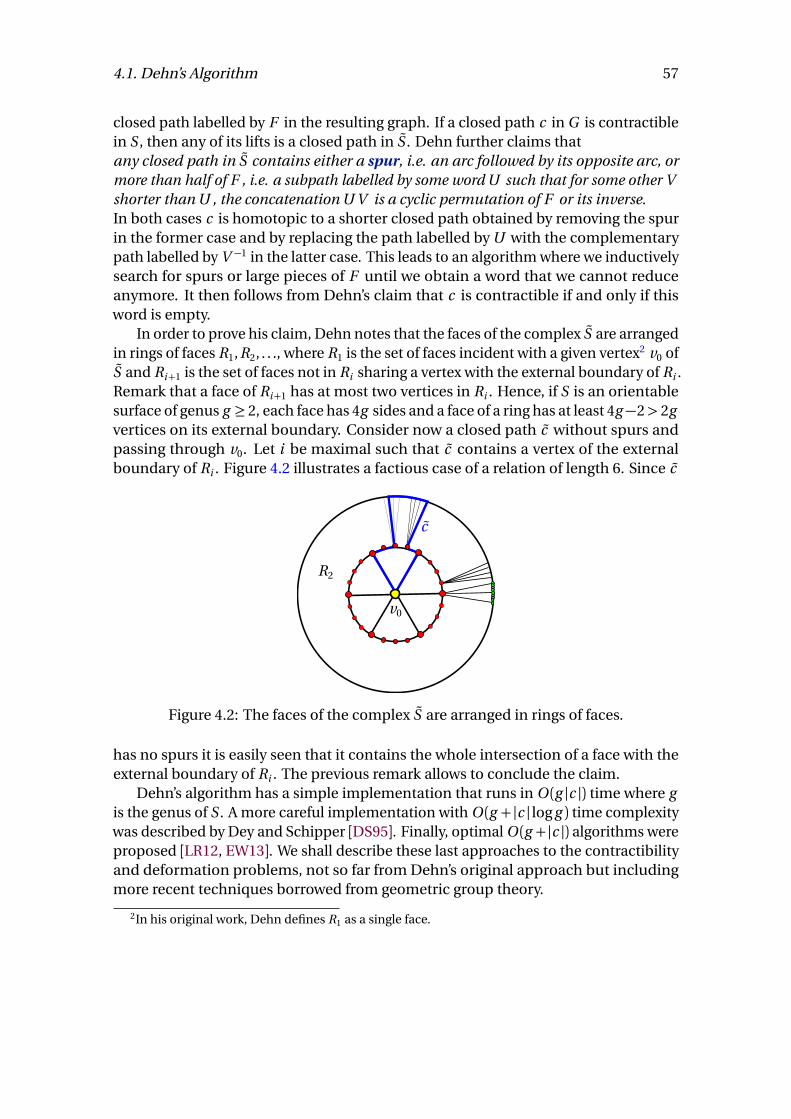
4.1. Dehn’s Algorithm 57
closed path labelled by F in the resulting graph. If a closed path c in G is contractiblein S , then any of its lifts is a closed path in S . Dehn further claims thatany closed path in S contains either a spur, i.e. an arc followed by its opposite arc, ormore than half of F , i.e. a subpath labelled by some word U such that for some other Vshorter than U , the concatenation U V is a cyclic permutation of F or its inverse.In both cases c is homotopic to a shorter closed path obtained by removing the spurin the former case and by replacing the path labelled by U with the complementarypath labelled by V −1 in the latter case. This leads to an algorithm where we inductivelysearch for spurs or large pieces of F until we obtain a word that we cannot reduceanymore. It then follows from Dehn’s claim that c is contractible if and only if thisword is empty.
In order to prove his claim, Dehn notes that the faces of the complex S are arrangedin rings of faces R1, R2, . . ., where R1 is the set of faces incident with a given vertex2 v0 ofS and Ri+1 is the set of faces not in Ri sharing a vertex with the external boundary of Ri .Remark that a face of Ri+1 has at most two vertices in Ri . Hence, if S is an orientablesurface of genus g ≥ 2, each face has 4g sides and a face of a ring has at least 4g −2> 2gvertices on its external boundary. Consider now a closed path c without spurs andpassing through v0. Let i be maximal such that c contains a vertex of the externalboundary of Ri . Figure 4.2 illustrates a factious case of a relation of length 6. Since c
v0
R2
c
Figure 4.2: The faces of the complex S are arranged in rings of faces.
has no spurs it is easily seen that it contains the whole intersection of a face with theexternal boundary of Ri . The previous remark allows to conclude the claim.
Dehn’s algorithm has a simple implementation that runs in O (g |c |) time where gis the genus of S . A more careful implementation with O (g + |c | log g ) time complexitywas described by Dey and Schipper [DS95]. Finally, optimal O (g + |c |) algorithms wereproposed [LR12, EW13]. We shall describe these last approaches to the contractibilityand deformation problems, not so far from Dehn’s original approach but includingmore recent techniques borrowed from geometric group theory.
2In his original work, Dehn defines R1 as a single face.
4.2. van Kampen Diagrams 58
4.2 van Kampen Diagrams
4.2.1 Disk Diagrams
A useful tool concerning contractible curves is provided by the so called van Kampendiagrams. Such diagrams bear different names in the litterature, among which diskdiagrams and Dehn diagrams are the most common. Intuitively, a disk diagramallows to express the combinatorial counterpart of the following characterization ofcontractible loops in a topological space X : a loop S1 = ∂ D2 → X is contractible ifand only if it extends to a continuous map D2→ X , where D2 is the unit disk. Given acombinatorial map M with graph G , a disk diagram over M is a combinatorial sphereD with a marked outer face, and a labelling of the arcs of D by the arcs of M suchthat opposite arcs are labelled by opposite arcs and such that every facial walk of Dthat is not the outer face is labelled by some facial walk of M . In other words, D is agluing of faces and edges of M that is homeomorphic to the complement of an opendisk in a sphere. For instance, this complement could be a tree. In general, it is atree-like arrangement of topological closed disks connected by trees. The facial walkof the outer face of D is denoted by ∂ D . The diagram is reduced if any two of its innerfaces (i.e. not the outer one) sharing a vertex v are labelled by facial walks that are notinverse to each other when starting the facial walks at v .
Lemma 4.2.1 (van Kampen, 1933). A closed path c in M is contractible if and only if itis the label of the outer facial walk of a reduced disk diagram over M .
The proof uses the intuitive fact that homotopic closed paths are combinatoriallyhomotopic, where a combinatorial homotopy is a sequence of elementary homo-topies that consist in either inserting or removing a spur, or replacing a subpath of afacial walk by the complementary subpath. See Theorem 4.7 in the previous lecturenotes.
PROOF OF LEMMA 4.2.1. We first prove the existence of a not necessarily reduceddisk diagram. Let c0 = 1→ c1→ ·· ·→ ck = c be a sequence of k elementary homotopiesattesting the contractibility of c , where 1 denotes a constant path. By induction onk , we may assume the existence of a disk diagram D such that ∂ D is labelled by ck−1.There are three cases to consider.
• If ck−1→ ck consists in inserting a spur a a−1, then we can form a disk diagramfor ck by attaching a pendant edge labelled with a to the boundary of D .
• If ck−1→ ck consists in removing a spur, then either this spur corresponds to twoconsecutive arcs of ∂ D with distinct edge support or it corresponds to the twoarcs of a single pendant edge. In the former case, we form a disk diagram forck by gluing the two arcs along ∂ D . In the latter case, we contract the pendantedge.
• Otherwise, ck−1→ ck consists in the replacement of a subpath p by a subpathq such that p q−1 is a facial walk of M . We then perform a subdivision of theouter face of D , inserting a new edge between the extremities of p . The new
4.3. Gauss-Bonnet Formula 59
outer face is chosen among the two new faces as the one not bounded by p . Wenext subdivide the new edge k −1 times, where k is the number of arcs of q . Wefinally extend the labelling trivially by sending the subdivided edge to the edgesof q . This amounts to glue a face with facial walk p q−1 along p on D .
If the resulting diagram is not reduced, then there are two facial walks sharing a vertexv and labelled by opposite facial walks of M . We “open” D at v and identify the twofacial walks according to the labels of their arcs. This produces a new diagram with twofaces less and does not modify the outer face boundary. We repeat the procedure aslong as the diagram is not reduced. By induction on the number of faces this proceduremust end. Note that the final diagram may have no face, in which case its graph mustbe a tree corresponding to a closed path that can be reduced to a point by removingspurs only.
Exercise 4.2.2. Relates the degree of an inner vertex in a reduced disk diagram over Mwith the degree of the corresponding vertex in M .
4.2.2 Annular Diagrams
There is an analogous notion of annular diagram defined by a combinatorial spherewith two marked outer faces instead of one.
Lemma 4.2.3 (Schupp, 1968). Two closed paths c and d in M are homotopic if andonly if there exists a reduced annular diagram over M such that the facial walks of itsouter faces (oriented consistently) are labelled with c and d respectively.
PROOF. By the introductory discussion there exists a path p such that c ·p ·d −1 ·p−1
is contractible. By Lemma 4.2.1, there exists a disk diagram over M whose boundaryis labelled with c ·p ·d −1 ·p−1. We may identify the subpaths corresponding to p andp−1 respectively and get an annular diagram whose perforated faces are labelled withc and d . If the diagram is not reduced, we proceed as in the proof of Lemma 4.2.1.
4.3 Gauss-Bonnet Formula
Another interesting tool is given by a combinatorial version of the famous Gauss-Bonnet theorem. This theorem relates the curvature of a Riemannian surface S (saya smooth surface embedded into R3) with its Euler characteristic χ , hence a localgeometric quantity with a global topological one. If K is the Gauss curvature of S andkg is the geodesic curvature along its (smooth) boundary ∂ S then:
∫
S
K ds +
∫
∂ S
kg d`= 2πχ (4.1)
We can obtain a combinatorial version of this formula using some kind of angle struc-ture over a combinatorial surface. Given an orientable combinatorial map M = (A,ρ, ι),we consider an angular assignment of its corners, that is a real function θ defined
4.3. Gauss-Bonnet Formula 60
over the set of corners. Here, a corner is any pair (a ,ρ(a )), for a ∈ A, of successive arcsaround a vertex. We require that the sum of the angular assignments of the corners ofany face f satisfies
∑
c∈ f
θ (c ) = d f /2−1, (4.2)
where d f is the degree of the face, i.e. the length of its facial walk. Intuitively, thiscondition amounts to assume that the faces are Euclidean polygons if we view anangular assignment as a normalized angle, measuring angles in terms of parts of acircle instead of radians. Indeed, the total angle of a Euclidean polygon with d f sidesis (d f −2)π, which is d f /2−1 when normalized. We then define the curvature of aninterior vertex v as
κ(v ) = 1−∑
c∈v
θ (c ), (4.3)
where, c ∈ v indicates that the corner c = (a ,ρ(a )) is incident to the source vertex v ofa . We also define the (geodesic) curvature of a boundary vertex3 v as
τ(v ) = 1/2−∑
c∈v
θ (c ) (4.4)
Those curvatures thus measure the angle default with respect to the flat situation(κ= 1 and τ= 1/2). They can be related to the Gauss curvature of the flat conic surfaceSv with one singularity at v obtained by gluing small isocele triangles, one for eachcorner c ∈ v , with angle 2πθ (c ) at v . The boundary of Sv is a broken line so thatFormula (4.1) should be corrected with the term
∑
w (π−αw ), where w runs over theboundary vertices of Sv and αw is the interior angle at w . Since the geodesic curvatureof a line segment is zero, Formula (4.1) becomes
∫
Sv
K ds +∑
w
(π−αw ) = 2πχ = 2π
Noting that with∑
w (π−αw ) is the sum of the angles at the corners of v we obtain∫
SvK = 2πκv .
Theorem 4.3.1 (Combinatorial Gauss-Bonnet —). Let M be a combinatorial mapwhose boundary is composed of disjoint simple cycles in the graph of M . Denote by χthe Euler characteristic of M and by V o ∪V ∂ =V its interior and boundary vertex sets.Then, for any angular assignment, we have
∑
v∈V o
κ(v ) +∑
v∈V ∂
τ(v ) =χ
It is possible to drop the condition on the boundary of M using a slightly differentnotion of curvature, see Erickson and Whittlesey [EW13]. The present presentation isinspired by Gersten and Short [GS90] and makes the parallel with the differentiableversion rather transparent.
3Formally, a combinatorial surface with boundary is defined by marking some faces as perforated,and a boundary vertex is any vertex incident to a perforated face.
4.4. Quad Systems 61
PROOF. By definition, we compute∑
v∈V o
κ(v ) = |V o | −∑
c∈v∈V 0
θ (c ) and∑
v∈V ∂
τ(v ) = |V ∂ |/2−∑
c∈v∈V ∂
θ (c )
It follows that∑
v∈V o κ(v ) +∑
v∈V ∂ τ(v ) = |V | − |V ∂ |/2−∑
c∈v∈V θ (c ). By distributingthe corners according to faces rather than vertices and by the angular assignmentrequirement (4.2), we see that
∑
c∈v∈V
θ (c ) =∑
c∈ f ∈F
θ (c ) =∑
f ∈F
(d f
2−1) =
1
2
∑
f ∈F
d f − |F |
where F is the set of faces of M . Since every arc appears in exactly one facial walk,except for those on the boundary of M , we have:
∑
f ∈F d f = 2|E |−|E ∂ |where E and E ∂
are the set of edges and boundary edges respectively. Since |E ∂ |= |V ∂ |, we concludethat
∑
v∈V o
κ(v ) +∑
v∈V ∂
τ(v ) = |V | − |V ∂ |/2− (|E | − |E ∂ |/2)− |F |)
= |V | − |E |+ |F |
4.4 Quad Systems
From an algorithmic point of view it is more convenient to work with combinatorialsurfaces all of whose faces are quadrilaterals. We call such a surface a quadrangulationor a quad system. Given a combinatorial surface without boundary, we easily get aquadrangulation of the same topological surface as follows. We insert a vertex insideeach face and connect this vertex to all the corners of the face. Hence, if a facialwalk has length k we introduce k new edges in the face. This subdivides each faceinto triangles. We then delete all the edges of the original graph, thus merging allthe triangles by pairs to form quadrilaterals. In practice, we will also require that thevertices have a high degree, say at least 8. For a surface of genus g ≥ 2 this is easilyobtained by first reducing the combinatorial surface to a single vertex and a single facebefore applying the above quadrangulation process. The resulting quadrangulationhas two vertices, 4g edges and 2g quadrilaterals. Figure 4.3 shows a reduced surfaceand its quadrangulation.
Lemma 4.4.1. Let Q be a quadrangulation derived by the previous process from a givenmap M without boundary. We can preprocess M in linear time (proportional to itsnumber of arcs) so that any closed walk c can be transformed in O (|c |) time into ahomotopic closed walk of size at most 2|c | in Q .
To see this, consider a spanning tree T of the graph G of M . Contracting T gives asurface M ′ with graph G /T and with a single vertex. Next consider a spanning tree ofthe dual graph of M ′ and denote by L the corresponding set of primal edges. Deleting
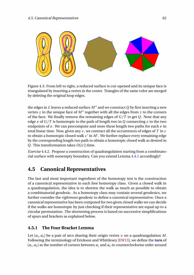
4.5. Canonical Representatives 62
Figure 4.3: From left to right, a reduced surface is cut-opened and its unique face istriangulated by inserting a vertex in the center. Triangles of the same color are mergedby deleting the original loop edges.
the edges in L leaves a reduced surface M ′′ and we construct Q by first inserting a newvertex z in the unique face of M ′′ together with all the edges from z to the cornersof the face. We finally remove the remaining edges of G /T to get Q . Note that anyedge e of G /T is homotopic to the path of length two in Q connecting z to the twoendpoints of e . We can precompute and store these length two paths for each e intotal linear time. Now, given any c , we contract all the occurrences of edges of T in cto obtain a homotopic closed walk c ′ in M ′. We further replace every remaining edgeby the corresponding length two path to obtain a homotopic closed walk as desired inQ . This transformation takes O (|c |) time.
Exercise 4.4.2. Propose a construction of quadrangulation starting from a combinato-rial surface with nonempty boundary. Can you extend Lemma 4.4.1 accordingly?
4.5 Canonical Representatives
The last and most important ingredient of the homotopy test is the constructionof a canonical representative in each free homotopy class. Given a closed walk ina quadrangulation, the idea is to shorten the walk as much as possible to obtaina combinatorial geodesic. As a homotopy class may contain several geodesics, wefurther consider the rightmost geodesic to define a canonical representative. Once acanonical representative has been computed for two given closed walks we can decideif the walks are homotopic by just checking if their representative are equal up to acircular permutation. The shortening process is based on successive simplificationsof spurs and brackets as explained below.
4.5.1 The Four Bracket Lemma
Let (a1, a2) be a pair of arcs sharing their origin vertex v on a quadrangulation M .Following the terminology of Erickson and Whittlesey [EW13], we define the turn of(a1, a2) as the number of corners between a1 and a2 in counterclockwise order around
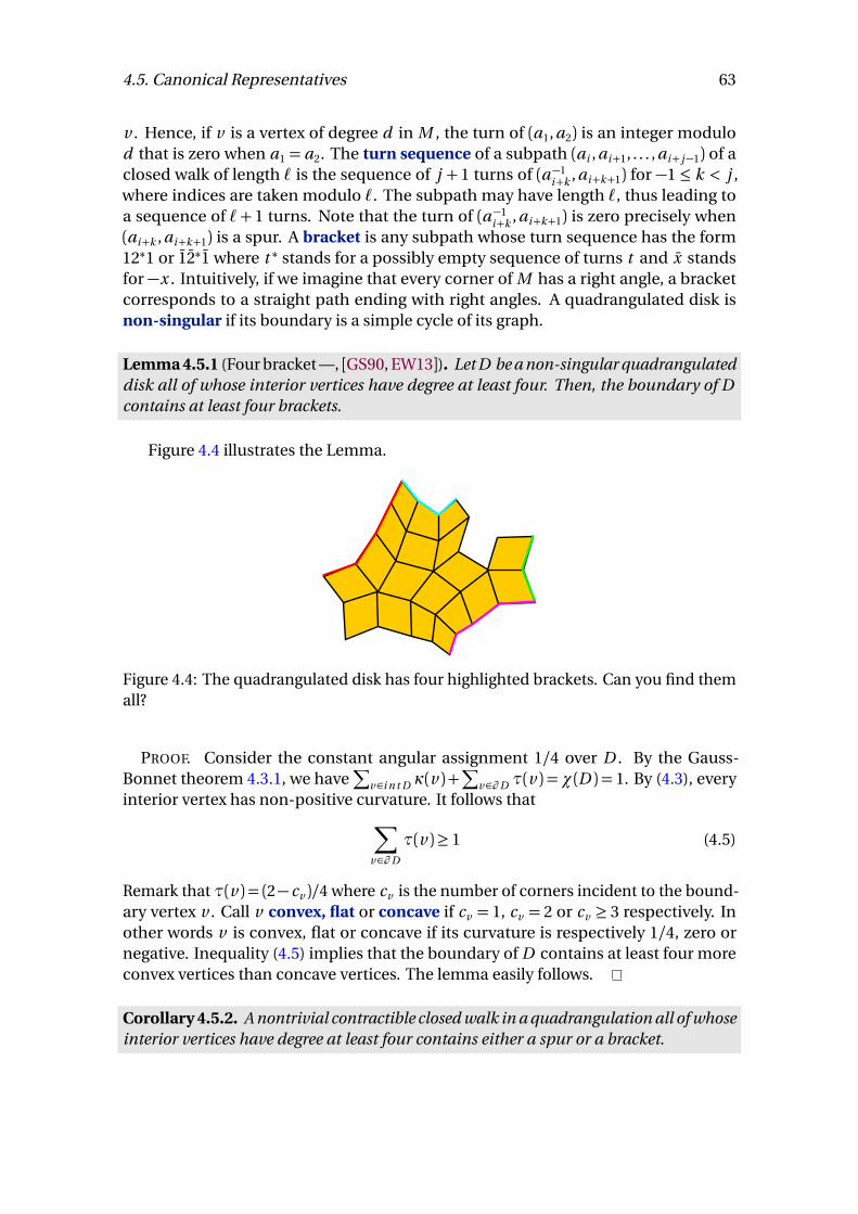
4.5. Canonical Representatives 63
v . Hence, if v is a vertex of degree d in M , the turn of (a1, a2) is an integer modulod that is zero when a1 = a2. The turn sequence of a subpath (ai , ai+1, . . . , ai+ j−1) of aclosed walk of length ` is the sequence of j + 1 turns of (a−1
i+k , ai+k+1) for −1 ≤ k < j ,where indices are taken modulo `. The subpath may have length `, thus leading toa sequence of `+ 1 turns. Note that the turn of (a−1
i+k , ai+k+1) is zero precisely when(ai+k , ai+k+1) is a spur. A bracket is any subpath whose turn sequence has the form12∗1 or 12∗1 where t ∗ stands for a possibly empty sequence of turns t and x standsfor −x . Intuitively, if we imagine that every corner of M has a right angle, a bracketcorresponds to a straight path ending with right angles. A quadrangulated disk isnon-singular if its boundary is a simple cycle of its graph.
Lemma 4.5.1 (Four bracket —, [GS90, EW13]). Let D be a non-singular quadrangulateddisk all of whose interior vertices have degree at least four. Then, the boundary of Dcontains at least four brackets.
Figure 4.4 illustrates the Lemma.
Figure 4.4: The quadrangulated disk has four highlighted brackets. Can you find themall?
PROOF. Consider the constant angular assignment 1/4 over D . By the Gauss-Bonnet theorem 4.3.1, we have
∑
v∈i n t D κ(v )+∑
v∈∂ D τ(v ) =χ(D ) = 1. By (4.3), everyinterior vertex has non-positive curvature. It follows that
∑
v∈∂ D
τ(v )≥ 1 (4.5)
Remark that τ(v ) = (2− cv )/4 where cv is the number of corners incident to the bound-ary vertex v . Call v convex, flat or concave if cv = 1, cv = 2 or cv ≥ 3 respectively. Inother words v is convex, flat or concave if its curvature is respectively 1/4, zero ornegative. Inequality (4.5) implies that the boundary of D contains at least four moreconvex vertices than concave vertices. The lemma easily follows.
Corollary 4.5.2. A nontrivial contractible closed walk in a quadrangulation all of whoseinterior vertices have degree at least four contains either a spur or a bracket.
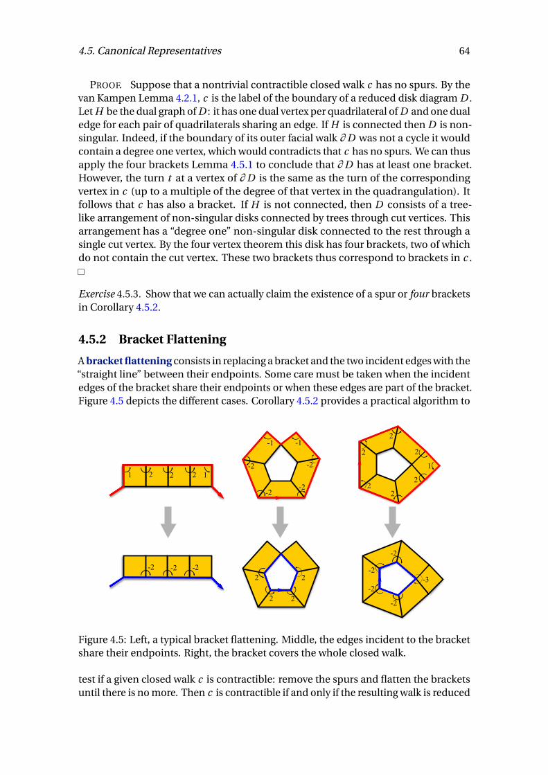
4.5. Canonical Representatives 64
PROOF. Suppose that a nontrivial contractible closed walk c has no spurs. By thevan Kampen Lemma 4.2.1, c is the label of the boundary of a reduced disk diagram D .Let H be the dual graph of D : it has one dual vertex per quadrilateral of D and one dualedge for each pair of quadrilaterals sharing an edge. If H is connected then D is non-singular. Indeed, if the boundary of its outer facial walk ∂ D was not a cycle it wouldcontain a degree one vertex, which would contradicts that c has no spurs. We can thusapply the four brackets Lemma 4.5.1 to conclude that ∂ D has at least one bracket.However, the turn t at a vertex of ∂ D is the same as the turn of the correspondingvertex in c (up to a multiple of the degree of that vertex in the quadrangulation). Itfollows that c has also a bracket. If H is not connected, then D consists of a tree-like arrangement of non-singular disks connected by trees through cut vertices. Thisarrangement has a “degree one” non-singular disk connected to the rest through asingle cut vertex. By the four vertex theorem this disk has four brackets, two of whichdo not contain the cut vertex. These two brackets thus correspond to brackets in c .
Exercise 4.5.3. Show that we can actually claim the existence of a spur or four bracketsin Corollary 4.5.2.
4.5.2 Bracket Flattening
A bracket flattening consists in replacing a bracket and the two incident edges with the“straight line” between their endpoints. Some care must be taken when the incidentedges of the bracket share their endpoints or when these edges are part of the bracket.Figure 4.5 depicts the different cases. Corollary 4.5.2 provides a practical algorithm to
2 12 21
-2 -2 -2
-1 -1
-2
-2-2
-2
2
2 2
2
2
1
2
2
22
2
-2
-2
-2
-2
-3
Figure 4.5: Left, a typical bracket flattening. Middle, the edges incident to the bracketshare their endpoints. Right, the bracket covers the whole closed walk.
test if a given closed walk c is contractible: remove the spurs and flatten the bracketsuntil there is no more. Then c is contractible if and only if the resulting walk is reduced
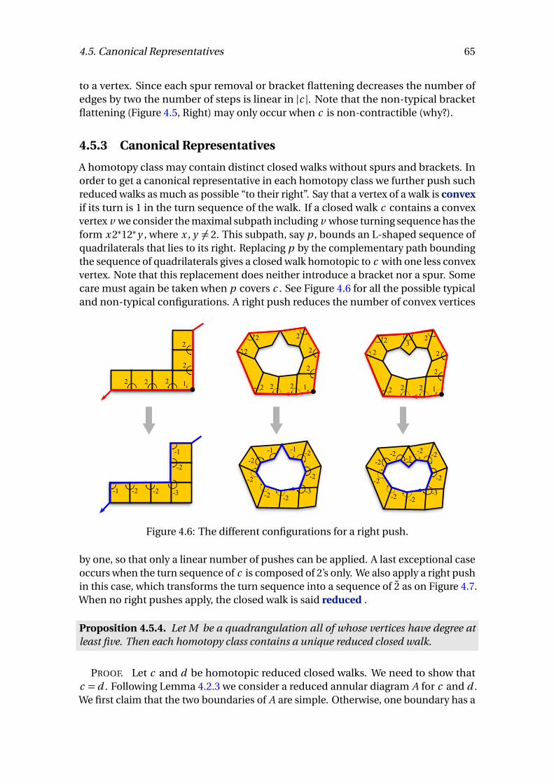
4.5. Canonical Representatives 65
to a vertex. Since each spur removal or bracket flattening decreases the number ofedges by two the number of steps is linear in |c |. Note that the non-typical bracketflattening (Figure 4.5, Right) may only occur when c is non-contractible (why?).
4.5.3 Canonical Representatives
A homotopy class may contain distinct closed walks without spurs and brackets. Inorder to get a canonical representative in each homotopy class we further push suchreduced walks as much as possible “to their right”. Say that a vertex of a walk is convexif its turn is 1 in the turn sequence of the walk. If a closed walk c contains a convexvertex v we consider the maximal subpath including v whose turning sequence has theform x 2∗12∗y , where x , y 6= 2. This subpath, say p , bounds an L-shaped sequence ofquadrilaterals that lies to its right. Replacing p by the complementary path boundingthe sequence of quadrilaterals gives a closed walk homotopic to c with one less convexvertex. Note that this replacement does neither introduce a bracket nor a spur. Somecare must again be taken when p covers c . See Figure 4.6 for all the possible typicaland non-typical configurations. A right push reduces the number of convex vertices
222
2
2
1
2
2
2
2
2 2 2 1
2 32
2
2
2
2 2 2 1
2
-3-1 -2-2
-2
-1
-2
-3
-2
-2
-2 -2
-2
-1-1
-2
-3
-2
-2
-2 -2
-2
-2-1
-2
Figure 4.6: The different configurations for a right push.
by one, so that only a linear number of pushes can be applied. A last exceptional caseoccurs when the turn sequence of c is composed of 2’s only. We also apply a right pushin this case, which transforms the turn sequence into a sequence of 2 as on Figure 4.7.When no right pushes apply, the closed walk is said reduced .
Proposition 4.5.4. Let M be a quadrangulation all of whose vertices have degree atleast five. Then each homotopy class contains a unique reduced closed walk.
PROOF. Let c and d be homotopic reduced closed walks. We need to show thatc = d . Following Lemma 4.2.3 we consider a reduced annular diagram A for c and d .We first claim that the two boundaries of A are simple. Otherwise, one boundary has a
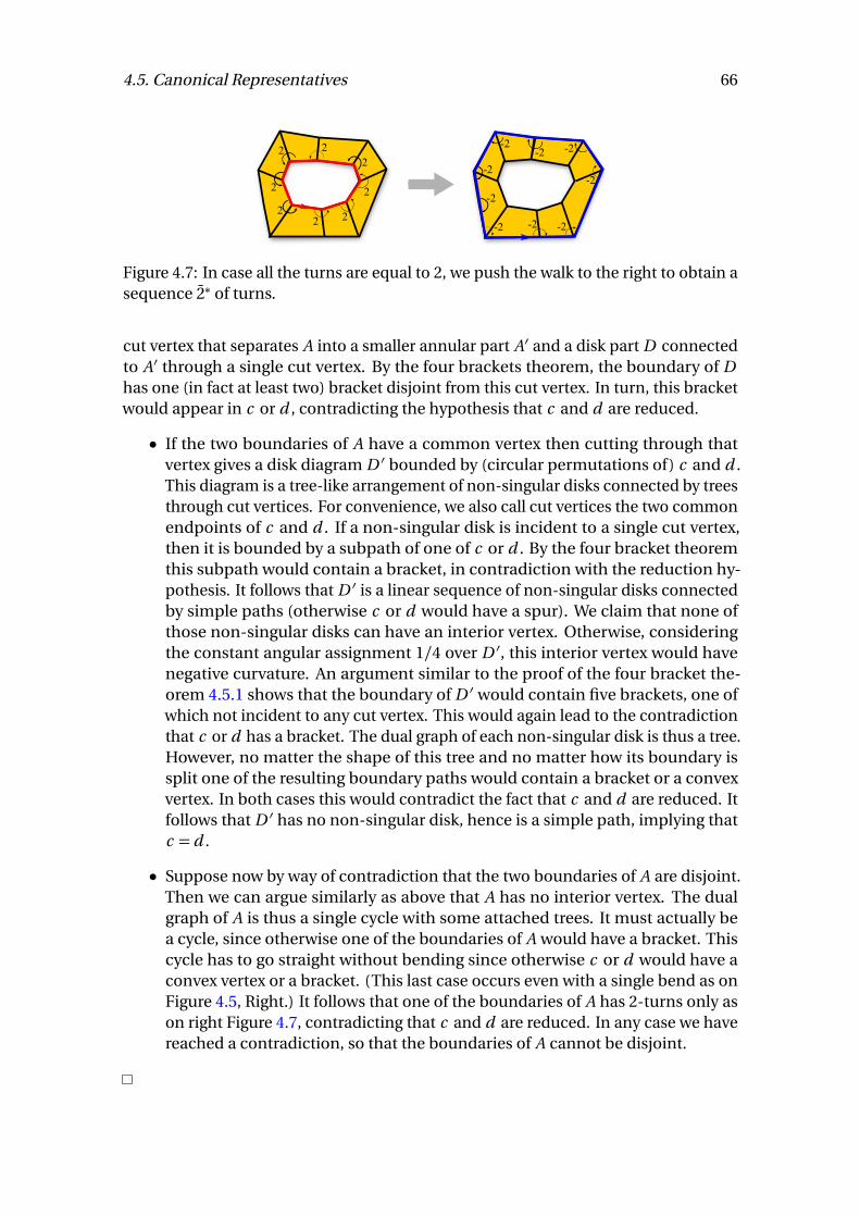
4.5. Canonical Representatives 66
2
2
2
2
22
22
-2
-2
-2
-2
-2-2-2
-2-2
Figure 4.7: In case all the turns are equal to 2, we push the walk to the right to obtain asequence 2∗ of turns.
cut vertex that separates A into a smaller annular part A′ and a disk part D connectedto A′ through a single cut vertex. By the four brackets theorem, the boundary of Dhas one (in fact at least two) bracket disjoint from this cut vertex. In turn, this bracketwould appear in c or d , contradicting the hypothesis that c and d are reduced.
• If the two boundaries of A have a common vertex then cutting through thatvertex gives a disk diagram D ′ bounded by (circular permutations of) c and d .This diagram is a tree-like arrangement of non-singular disks connected by treesthrough cut vertices. For convenience, we also call cut vertices the two commonendpoints of c and d . If a non-singular disk is incident to a single cut vertex,then it is bounded by a subpath of one of c or d . By the four bracket theoremthis subpath would contain a bracket, in contradiction with the reduction hy-pothesis. It follows that D ′ is a linear sequence of non-singular disks connectedby simple paths (otherwise c or d would have a spur). We claim that none ofthose non-singular disks can have an interior vertex. Otherwise, consideringthe constant angular assignment 1/4 over D ′, this interior vertex would havenegative curvature. An argument similar to the proof of the four bracket the-orem 4.5.1 shows that the boundary of D ′ would contain five brackets, one ofwhich not incident to any cut vertex. This would again lead to the contradictionthat c or d has a bracket. The dual graph of each non-singular disk is thus a tree.However, no matter the shape of this tree and no matter how its boundary issplit one of the resulting boundary paths would contain a bracket or a convexvertex. In both cases this would contradict the fact that c and d are reduced. Itfollows that D ′ has no non-singular disk, hence is a simple path, implying thatc = d .
• Suppose now by way of contradiction that the two boundaries of A are disjoint.Then we can argue similarly as above that A has no interior vertex. The dualgraph of A is thus a single cycle with some attached trees. It must actually bea cycle, since otherwise one of the boundaries of A would have a bracket. Thiscycle has to go straight without bending since otherwise c or d would have aconvex vertex or a bracket. (This last case occurs even with a single bend as onFigure 4.5, Right.) It follows that one of the boundaries of A has 2-turns only ason right Figure 4.7, contradicting that c and d are reduced. In any case we havereached a contradiction, so that the boundaries of A cannot be disjoint.

4.6. The Homotopy Test 67
A reduced closed walk can thus play the role of canonical representative for its ho-motopy class.
4.6 The Homotopy Test
We now have all the necessary ingredients to perform a linear time homotopy test.Thanks to Lemma 4.4.1, we can assume given two closed walks in a quadrangulation.We compute the canonical form of each closed walk by first removing spurs andbrackets as described in Sections 4.5.2. We can first remove all the spurs in linear time.The flattening of a bracket may introduce new spurs but their removal can be chargedto the removed edges, so that the total time spent to remove spurs is still linear inthe end. Note that a flattening transforms a bracket into a flat part (a run of 2-turnsor of 2-turns) that may be part of a larger flat part. In order to avoid loosing timefor traversing several times the same flat parts, we add jump pointers between theendpoints of each flat part before we perform any flattening. We also store the turns atthese endpoints and the length of the flat part. Then, after each bracket flattening weupdate the turns at the endpoints and check if the resulting flat part should be mergedwith the at most two surrounding flat parts. This can be done in constant time thanksto the jump pointers. This way each bracket flattening costs a constant time. Sinceeach flattening decreases the number of edges, there can only be a linear number ofthem and the total cost for removing spurs and brackets is thus linear. The sequenceof edges of the resulting closed walk is easily recovered from the jump pointers andthe lengths of the flat parts. We just need to know one edge along the walk, which wecan update easily as spurs and brackets are simplified.
Once spurs and brackets have been removed we obtain a geodesic that needs to bepushed to its right as described in Section 4.5.3. Each right push transforms a subpathof the geodesic into another subpath of the same length without 1-turns or 2-turns. Itfollows that none of the vertices of this subpath will be pushed again. The total timeneeded to obtain a rightmost geodesic is thus linear. This shows that
Theorem 4.6.1. The canonical representative of a closed walk c in a quadrangulation,all of whose vertices have degree at least five, can be computed in O (|c |) time.
Corollary 4.6.2. Given two closed walk of length at most ` in a combinatorial map ofsize n we can decide if they are homotopic in O (n + `) time.
PROOF. According to Lemma 4.4.1, we can reduce the combinatorial map to aquandrangulation in O (n ) time and get closed walks homotopic to the given one inO (`) time. By Theorem 4.6.1 we can compute the canonical form of the walks in O (`)time. Now these canonical forms, say c and d , are homotopic if and only if one isa circular permutation of the other. This can be tested in linear time by checkingwhether c is a substring of d · d thanks to the Knuth-Morris-Pratt string searchingalgorithm [KMP77] [CLRS02, Sec. 32.4].
5
Minimum Weight Bases
Contents5.1 Minimum Basis of the Fundamental Group of a Graph . . . . . . . . . 69
5.2 Minimum Basis of the Cycle Space of a Graph . . . . . . . . . . . . . . . . 70
5.2.1 The Greedy Algorithm . . . . . . . . . . . . . . . . . . . . . . . . . . . . . 70
5.3 Uniqueness of Shortest Paths . . . . . . . . . . . . . . . . . . . . . . . . . . . 73
5.4 First Homology Group of Surfaces . . . . . . . . . . . . . . . . . . . . . . . . 74
5.4.1 Back to Graphs . . . . . . . . . . . . . . . . . . . . . . . . . . . . . . . . . . . 74
5.4.2 Homology of Surfaces . . . . . . . . . . . . . . . . . . . . . . . . . . . . . . 75
5.5 Minimum Basis of the Fundamental Group of a Surface . . . . . . . . 77
5.5.1 Dual Maps and Cutting . . . . . . . . . . . . . . . . . . . . . . . . . . . . . 77
5.5.2 Homotopy Basis Associated with a Tree-Cotree Decomposition 77
5.5.3 The Greedy Homotopy Basis . . . . . . . . . . . . . . . . . . . . . . . . . 78
5.6 Minimum Basis of the First Homology Group of a Surface . . . . . . . 80
5.6.1 Homology Basis Associated with a Tree-Cotree Decomposition 80
5.6.2 The Greedy Homology Basis . . . . . . . . . . . . . . . . . . . . . . . . . 80
In the second lecture we saw that a graph could be associated with a vector space,called the cycle space. We will see that this cycle space can be extended to surfacesgiving birth to the first homology group. We also introduced the fundamental group ofa graph or of a surface in another lecture. Hence, we now have two group structuresthat encode the topology of a space X , where X is either a graph or a surface. Thesestructures are both generated by closed walks in the graph of X and we call a basis anygenerating set with the minimum number of closed walks. In order to derive a moreinformative notion of minimality we assume that the edges of the considered graphhave a positive weight. This allows to define the weight of a closed walk as the sumof its edge weights (counted with multiplicity). A minimum weight basis is then a
68
5.1. Minimum Basis of the Fundamental Group of a Graph 69
basis such that the sum of the weights of its members is minimum. The computationof minimum weight bases has received much attention when X is a graph and wasstudied more recently for combinatorial surfaces. Good references on the subjectinclude a comprehensive survey on cycle bases in graphs by Kavitha et al. [KLM+09]and another survey on optimization of cycles and bases on surfaces by Erickson [Eri12].We shall use the qualifiers minimum and shortest interchangeably to designate a walk,tree or subgraph of minimum weight.
5.1 Minimum Basis of the Fundamental Group of a Graph
Let G be a connected graph with basepoint v and let |.| : E →R+ be a weight function.The fundamental group π1(G , v ) is a free group whose rank is the number of chordsof any spanning tree of G , which is 1−n +m , where n and m are respectively thenumber of vertices and edges of G . Indeed, as we saw, every chord e of a spanningtree T gives rise to a loop γT
v,e obtained by connecting v to each endpoint of the chordusing paths in the tree, and these loops form a basis of π1(G , v ). Not all bases arisethis way but a minimum one may indeed be obtained by this construction. For this,we take for T a shortest path tree with root v : every vertex w of G is linked to v by apath in T whose weight is minimum among all the paths from v to w in G . When allthe weights are equal a shortest path tree can be computed by a breadth-first searchtraversal in time O (m ). In the general case, one may use Dijkstra’s algorithm [CLRS09]to compute a shortest path tree in O (m +n log n ) time. Remark that γT
v,e is a shortestloop through the chord e .
Theorem 5.1.1. The basis of π1(G , v ) associated with a shortest path tree with root v isa minimum weight basis.
The following proof is based on an purely algebraic preliminary lemma. First notethat a free group F over a set (x1, x2, . . . , xr ) gives rise to a free Abelian group (this is thesame a freeZ-module) F a b by making all the generators commute. Hence, if we let R bethe set of relations {xi x j = x j xi }1≤i< j≤r , a presentation for F a b is < {x1, x2, . . . , xr } |R >.We thus have a quotient F � F a b = F / <R > and we denote by [x ] ∈ F a b the image ofany x ∈ F . Note that [x ] can be uniquely written as a linear combination of the [xi ]’s.
Lemma 5.1.2. Let (x1, x2, . . . , xr ) and (y1, y2, . . . , yr ) be two bases of a free group F . De-note by yj (x1, x2, . . . , xr ) the expression of yj in terms of the basis (x1, x2, . . . , xr ). Then,there exists a permutation σ of {1, . . . , r } such that for each i the coefficient of [xi ] in[yσ(i )(x1, x2, . . . , xr )] is nonzero.
PROOF. The automorphism of F defined by xi 7→ yi , 1 ≤ i ≤ r , quotients to anautomorphism of F a b . Let ci j be the coefficient of [x j ] in [yi (x1, x2, . . . , xr )]. ViewingF a b as a free Z-module over the [xi ]’s, the matrix (ci j )1≤i , j≤r of this automorphismhas nonzero determinant. It follows that at least one term
∏
1≤i≤r ciσ(i ) of the usualLeibnitz expansion of the determinant must be nonzero. This implies the lemma.
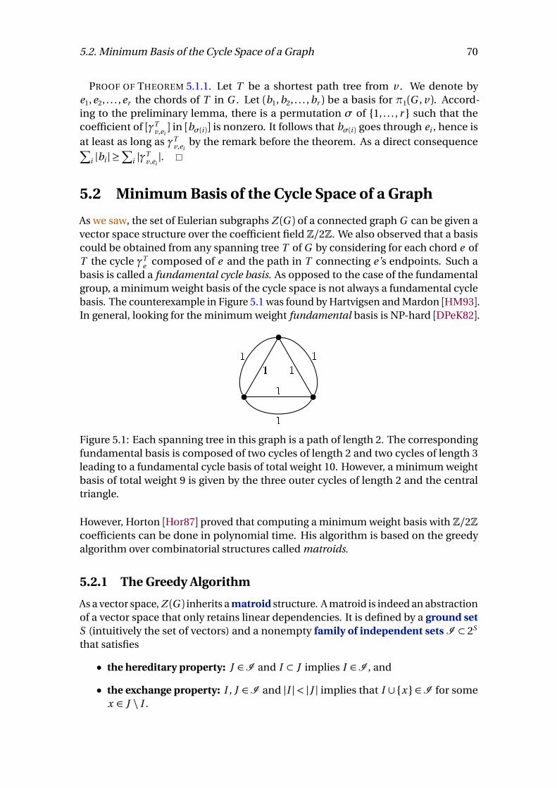
5.2. Minimum Basis of the Cycle Space of a Graph 70
PROOF OF THEOREM 5.1.1. Let T be a shortest path tree from v . We denote bye1, e2, . . . , er the chords of T in G . Let (b1, b2, . . . , br ) be a basis for π1(G , v ). Accord-ing to the preliminary lemma, there is a permutation σ of {1, . . . , r } such that thecoefficient of [γT
v,ei] in [bσ(i )] is nonzero. It follows that bσ(i ) goes through ei , hence is
at least as long as γTv,ei
by the remark before the theorem. As a direct consequence∑
i |bi | ≥∑
i |γTv,ei|.
5.2 Minimum Basis of the Cycle Space of a Graph
As we saw, the set of Eulerian subgraphs Z (G ) of a connected graph G can be given avector space structure over the coefficient field Z/2Z. We also observed that a basiscould be obtained from any spanning tree T of G by considering for each chord e ofT the cycle γT
e composed of e and the path in T connecting e ’s endpoints. Such abasis is called a fundamental cycle basis. As opposed to the case of the fundamentalgroup, a minimum weight basis of the cycle space is not always a fundamental cyclebasis. The counterexample in Figure 5.1 was found by Hartvigsen and Mardon [HM93].In general, looking for the minimum weight fundamental basis is NP-hard [DPeK82].
1
1
1
1
1
1
Figure 5.1: Each spanning tree in this graph is a path of length 2. The correspondingfundamental basis is composed of two cycles of length 2 and two cycles of length 3leading to a fundamental cycle basis of total weight 10. However, a minimum weightbasis of total weight 9 is given by the three outer cycles of length 2 and the centraltriangle.
However, Horton [Hor87] proved that computing a minimum weight basis with Z/2Zcoefficients can be done in polynomial time. His algorithm is based on the greedyalgorithm over combinatorial structures called matroids.
5.2.1 The Greedy Algorithm
As a vector space, Z (G ) inherits a matroid structure. A matroid is indeed an abstractionof a vector space that only retains linear dependencies. It is defined by a ground setS (intuitively the set of vectors) and a nonempty family of independent sets I ⊂ 2S
that satisfies
• the hereditary property: J ∈I and I ⊂ J implies I ∈I , and
• the exchange property: I , J ∈I and |I |< |J | implies that I ∪{x } ∈ I for somex ∈ J \ I .
5.2. Minimum Basis of the Cycle Space of a Graph 71
A basis is just a maximally independent set. By the exchange property, all the baseshave the same cardinality. Matroid theory was introduced by Hassler Whitney (1935)and has many applications including combinatorial optimization, discrete geometry,etc. When the elements of the ground set are weighted, there is a famous greedyalgorithm that determines a minimum weight basis. It works as follows: maintainan independent set starting from the empty set, and iteratively add an element x tothe current set I if I ∪{x } is independent and if x has minimum weight among suchelements. The algorithm stops when no x can be found, i.e. when I is a basis. Inpractice, the elements of S are scanned in increasing order of weights, so that eachtime an x is found such that I ∪{x } is independent it can be added to the current I .The whole set S is thus scanned only once during the algorithm.
Theorem 5.2.1. The greedy algorithm returns a minimum weight basis.
PROOF. Let (x1, x2, . . . , xr ) be the basis returned by the greedy algorithm, where xi isthe i th inserted element. By the choice of each element we have |x1| ≤ |x2| ≤ · · · ≤ |xr |,where |x | is the weight of x . Consider any other basis (y1, y2, . . . , yr ) indexed in non-decreasing order: |y1| ≤ |y2| ≤ · · · ≤ |yr |. Suppose by way of contradiction that there issome index i such that |yi |< |xi | and choose such i as small as possible. Then, by theexchange property we can find y ∈ {y1, . . . , yi } such that {x1, . . . , xi−1, y } is independent.Since |y | ≤ |yi |< |xi | this would contradict the choice of xi . It follows that |yi | ≥ |xi | forall i , implying that (x1, x2, . . . , xr ) has minimum weight.
Since the cycle space contains 2r cycles, the greedy algorithm per se does not seemvery efficient. In order to restrict the search of a new basis element at each step of thealgorithm, Horton [Hor87] gave a characterization of the cycles that may belong to aminimum weight basis.
Lemma 5.2.2. Suppose b = c +d is a cycle of a basis B of Z (G ). Then either B \{b }∪{c }or B \ {b }∪ {d } is a basis.
PROOF. If c and d were both in the linear span of B \ {b }, then so would b .
Corollary 5.2.3. Assuming positive weights, the cycles of a minimum weight basis aresimple.
PROOF. Suppose that b is a non-simple cycle of a minimum weight basis B . Thenb can be written as the sum b = c +d of two edge disjoint cycles. In particular, b islonger than c or d . By the preceding lemma, we can replace b by c or d in B to get ashorter basis, contradicting the minimality of B .
Note: if some of the weights cancel, then basically the same proof shows the existenceof a minimum weight basis with simple cycles only.
5.2. Minimum Basis of the Cycle Space of a Graph 72
Lemma 5.2.4. Let b be a cycle of a minimum weight basis. Let p and q be two edgedisjoint paths such that b = p ·q−1. Then p or q is a shortest path.
PROOF. Let t be a shortest path from the common initial vertex of p and q to theircommon last vertex. With a little abuse of notation, we can write b = p · t −1+ t ·q−1. ByLemma 5.2.2, b must be no longer than p · t −1 or t ·q−1, implying with Corollary 5.2.3that either q or p is a shortest path.
Corollary 5.2.5. Let v be a vertex of a cycle b of a minimum weight basis. Then bdecomposes into p ·a ·q−1 where a is an arc and p , q are two shortest paths with v asinitial vertex.
PROOF. Consider the arc sequence (a1, a2, . . . , ak ) of b with v the origin vertex of a1
and the target of ak . Let i be the maximal index such that (a1, a2, . . . , ai ) is a shortestpath. Then b = (a1, a2, . . . , ai ) ·ai+1 · (ai+2, . . . , ak ) and the previous lemma implies that(ai+2, . . . , ak ) is a (possibly empty) shortest path
When there is a unique shortest path between every pair of vertices, this corollaryallows us to reduce the number of scanned cycles at each addition step of the greedyalgorithm to nm cycles, one for each (vertex, edge) pair. For the rest of this section, weassume uniqueness of shortest paths and discuss the general case in the next section.We denote by γv,e the cycle obtained by connecting the endpoints of e with shortestpaths to v . By the uniqueness of shortest paths, γv,e = γT
v,e where T is the shortest pathtree rooted at v .
Proposition 5.2.6. Let G = (V , E ) be a connected graph with n vertices and m edgesand let r = 1−n +m be the rank of its cycle space. A minimum weight basis of Z (G )can be computed in O (n 2 log n + r 2nm ) =O (nm 3) time.
PROOF. By Corollary 5.2.5, we can restrict the scan step of the greedy algorithm tothe cycles γv,e with (v, e ) ∈V ×E . For each vertex v , we compute a shortest path treeT in O (n log n +m ) time using Dijkstra’s algorithm. There are r nontrivial cycles of theform γT
v,e , each of size O (n ). Their computation and storage for all the vertices v thus
requires O�
n (n log n +m + r n )�
time. They can be sorted according to their length inO (r n log(r n )) time. In order to check if a cycle is independent of the current family ofbasis elements, we view a cycle as a vector in (Z/2Z)E . We use Gauss elimination tomaintain the current family in row echelon form. This family has at most r vectorsand testing a new vector against this family by Gauss elimination needs O (r m ) time.The cumulated time for testing independence is thus O (r 2nm ). The whole greedyalgorithm finally takes time
O�
n (n log n +m + r n ) + r n log(r n ) + r 2nm�
=O (n 2 log n + r 2nm ).
5.3. Uniqueness of Shortest Paths 73
Note that the above scan can be further reduced by discarding the cycles γv,e thatare not simple. We can also decompose a cycle into a linear combination of a fixedfundamental basis associated to a tree. The decomposition of a cycle is just given byits trace over the chords of that tree. This allows to represent the current family of basiselements by a matrix of size r × r instead of r ×m . Further improvements were pro-posed [KMMP04, KMMP08, MM09], often based on randomization. In particular, thealgorithm by Kavitha et al. [KMMP08] runs in O (m 2n +mn 2 log n ) time. Using integercoefficients rather than Z/2Z gives a more general notion of cycle space. However,this space does not form a matroid in general and the greedy algorithm cannot beapplied anymore. The status of the computation of a minimal weight cycle basis withinteger coefficients is still unknown.
5.3 Uniqueness of Shortest Paths
The proof of Proposition 5.2.6 is based on the uniqueness of shortest paths. In fact,the proof can be adapted to show that the same algorithm works even if we do notassume that there is a unique shortest path between every pair of vertices. See [Hor87]or [Laz14, Lem. 1.6.7]. It may happen for other applications that we strongly needuniqueness to ensure correctness of the algorithms. We usually get the uniqueness bya perturbation schema, where the weight of each simple path is replaced by a slightlydifferent one. Let Px y be the set of simple paths with minimal unperturbed weightbetween vertices x and y . The perturbation should be such that Px y contains a uniquepath of minimum perturbed weight. In other words, the aim is to get an order on eachPx y so that we can choose the smallest path as the unique shortest path. This can beachieved by adding an infinitesimal weight of the form (i ) εc (e ) or (i i ) c (e )ε to everyedge e , where ε > 0 is some arbitrarily small number and c (e ) is an appropriatelychosen coefficient.
Using the exponential form (i )we can simply choose pairwise distinct edge coeffi-cients, for example the edge indices, assuming that they are indexed from 1 to m . Thisway, distinct paths are perturbed by distinct polynomials in ε and get distinct weightsfor ε small enough. We can view the polynomials as bit vectors of length m where a 1coordinate at index i indicates the presence of the monomial εi . The ordering in Px y issimply the lexicographic ordering on the bit vectors. This perturbation schema woulda priori require an extra O (m ) time for comparing path lengths. Cabello et al. [CCE13,Sec. 6.2] propose to reduce the comparison time to O (log m ) using some sophisticateddata structure. However, their algorithm assumes that two paths need to be comparedonly when they intersect along a common prefix.
We can avoid this restriction using the linear form (i i ), that is when the weight ofan edge e is perturbed by c (e )ε. The perturbation of a path is now ε times the sumof its edge coefficients. Choosing the edge coefficients such that there is a uniqueminimum weight sum in each Px y is more tricky than for the form (i ). Cabello etal. [CCE13, Sec. 6.1] propose the following random perturbation schema based on theIsolating Lemma of Mulmuley et al. [MVV87, Lem. 1].
5.4. First Homology Group of Surfaces 74
Lemma 5.3.1 (Isolating –). Let I be an arbitrary family of subsets of {1, . . . , m}. For avector c = (c1, c2, . . . , cm ) of m integers and for I ∈I , we put c (I ) =
∑
i∈I ci . Choosing cuniformly at random in {1, . . . , M }m , the probability that c (I ) is minimized by a uniqueI ∈I is at least 1−m/M .
PROOF. We suppose thatI contains at least two subsets, since otherwise the lemmais trivial. For i ∈ {1, . . . , m}we set
I +i = {I ∈I | i ∈ I } and I −i = {I ∈I | i 6∈ I }
Suppose that none of I +i and I −i is empty. Note that the quantities minI∈I +i c (I )− ci
and minI∈I −i c (I ) do not depend on ci . Fixing all the coefficients c j , for j 6= i , theconstant minI∈I −i c (I ) − (minI∈I +i c (I ) − ci ) equals ci with probability at most 1/M .It follows that minI∈I +i c (I ) = minI∈I −i c (I ) holds with unconditional probability atmost 1/M . Hence, with probability at least 1−m/M , minI∈I +i c (I ) 6=minI∈I −i c (I ) forall i such that I +i and I −i are both nonempty. Consider a vector c such that thisoccurs and let I0 ∈I for which c (I0) is minimum. Then, any other J ∈I must differfrom I0 by some index i . If i ∈ I0 and i 6∈ J then c (I0) = minI∈I c (I ) = minI∈I +i c (I )while c (J ) ≥minI∈I −i c (I ). Since minI∈I +i c (I ) 6=minI∈I −i c (I ) we deduce c (J ) > c (I0).Likewise, we again obtain c (J )> c (I0) if i 6∈ I0 and i ∈ J .
Lemma 5.3.2. Choose for each of the m edges of an edge weighted graph G an integralcoefficient in {1, . . . , m 4} uniformly and independently at random. Consider the linearperturbation schema (ii) as described above. With probability at least 1− 1
2m , there is aunique shortest path between any pair of vertices.
PROOF. For each pair {x , y } of vertices, Let Ix y be the family of subsets of edgeindices corresponding to the paths in Px y . Applying Lemma 5.3.1 to Ix y , we deducethat with probability at least 1−1/m 3 there is a unique shortest path between x andy for the perturbed weights. There are n ≤m vertices in G (we may assume that G isnot a tree). Hence, the
�
n2
�
pairs of vertices are each connected by a unique shortest
path with probability at least 1−�
n2
�
/m 3 ≥ 1− 12m .
We shall turn to the computation of minimum bases on surfaces. We first extend thenotion of cycle space to surfaces.
5.4 First Homology Group of Surfaces
5.4.1 Back to Graphs
First recall that the cycle space Z (G ) of a graph G = (V , E ) is the space of its Euleriansubgraphs. One can define such subgraphs thanks to the boundary operator. Thisoperator δ1 sends any edge to the mod 2 sum of its endpoints. In particular, if e isa loop-edge, δ1e = 0. By linear extension, δ1 defines a linear map from the vectorspace (Z/2Z)E of formal mod 2 sum of edges to the space (Z/2Z)V of mod 2 sum of
5.4. First Homology Group of Surfaces 75
vertices. Viewing a subgraph as a mod 2 sum of its edges, it is easily seen that Euleriansubgraphs correspond to the mod 2 sum of edges with empty boundary. In otherwords,
Z (G ) = kerδ1.
We define the mod 2 abelianization of a group A as the quotient A/S (A) by the sub-group S (A) generated by its squares. Note that S (A) is normal and contains the derivedsubgroup [A, A] generated by the commutators [a , b ] = a b a−1b −1. Indeed, one checkthat
[a , b ] = (a b a−1)2a 2(a−1b −1)2 and a s a−1 = s [s−1, a ]
Hence, if s is a product of squares, so is any conjugate a s a−1. We can now relate thecycle space with the fundamental group of a graph thanks to the following mod 2version of the Hurewicz theorem.
Proposition 5.4.1. For any vertex v of a connected graph G the cycle space Z (G ) isisomorphic to the mod 2 abelianization of π1(G , v ).
PROOF. Denote by L the set of loops of G with basepoint v . Consider the mapϕ :L → Z (G ) defined by (a1, a2, . . . , ak ) 7→
∑ki=1 ai , where the coefficient in the sum
are taken modulo 2. Adding or removing a spur in a loop does not change its imageby ϕ. The map ϕ thus quotients to a morphism ϕ : π1(G , v ) → Z (G ). Let T be aspanning tree of G and let C = E (G ) \ E (T ) be its set of chords. We know that Z (G )is generated by the cycles {γT
e }e∈C . Since ϕ(γTv,e ) = γ
Te , the map ϕ is onto. Let γ =
γTv,e1·γT
v,e2· · ·γT
v,ekbe a representative of some element of π1(G , v )written over the basis
{γTv,e }e∈C . Then ϕ(γ) =
∑
e∈C neγTe where ne is the cumulated exponent of γT
v,e in γ.Hence, the homotopy class of γ belongs to kerϕ if and only if all the ne cancel. This isexactly saying that γ belongs to the subgroup S (π1(G , v )) of π1(G , v ). We thus have
Z (G )'π1(G , v )/kerϕ =π1(G , v )/S (π1(G , v ))
Exercise 5.4.2. Given a product w in the generators {x1, x2, . . . , xr } (and their inverses)of a group Γ , show that w = x n1
1 ·xnr2 · · · x
nr1 ·p where each ni is the cumulated exponent
of xi in w and p is a product of commutators. (It might be useful to notice the relationb a = a b [b −1, a−1].) Deduce that S (Γ ) is equal to the set of products whose cumulatedexponents are all even.
5.4.2 Homology of Surfaces
The graph G of a combinatorial surface M has its own cycle space Z (G ). However, atopological surface may have distinct cellularly embedded graphs with non-isomorphiccycle spaces. In order to get a topologically invariant notion of cycle space, we furtherquotient Z (G ) by identifying cycles that bound together a subset of faces of M . Moreformally, let C2(M ) := (Z/2Z)F be the vector space of subsets of the set F of faces of M .The elements of C2(M ) are called 2-chains. The boundary ∂2 f of a face f ∈ F is themod 2 sum of the edges of its facial walk. It is clearly a cycle of Z (G ), meaning that
5.4. First Homology Group of Surfaces 76
∂1∂2 f = 0. This boundary ∂2 extends linearly to a boundary operatorδ2 : C2(M )→ Z (G ).Two cycles c , d ∈ Z (G ) are said homologous, which we write [c ] = [d ], if their mod 2sum is the boundary of some 2-chainσ ∈C2(M ): c −d = ∂2σ. We can now define thefirst homology group of M as the space of homology classes:
H1(M ) := kerδ1/Imδ2.
The fact that this homology group is indeed a topological invariant is an immediateconsequence of the invariance of the fundamental group and of the following mod 2version of the Hurewicz theorem for surfaces.
Proposition 5.4.3. For any vertex v of a connected map M the first homology groupH1(M ) is isomorphic to the mod 2 abelianization of π1(M , v ).
PROOF. Let G be the graph of M . As in the proof of Proposition 5.4.1, denote byL the set of loops of G with basepoint v and by ϕ :L → Z (G ) the mapping definedby ϕ(a1, a2, . . . , ak ) =
∑ki=1 ai . The composition [ϕ] :L → Z (G )→H1(M ) is compatible
with elementary homotopies in M . This is obvious for the addition or removal of aspur. If λ ·p ·µ 7→λ ·q ·µ is an elementary homotopy with p ·q−1 the facial walk of aface f , then ϕ(λ ·p ·µ)−ϕ(λ ·q ·µ) = ∂2 f ∈ Im∂2. Whence [ϕ(λ ·p ·µ)] = [ϕ(λ · q ·µ)]in H1(M ). It follows that [ϕ] descends to the quotient ϕ : π1(M , v ) → H1(M ). Onthe other hand, homotopic loops in G are homotopic in M so that we have an ontomorphism π1(G , v ) � π1(M , v ). We also know from the proof of Proposition 5.4.1that the morphism π1(G , v )� Z (G ) is onto. We thus have two equal compositions
π1(G , v )� Z (G )� H1(M ) andπ1(G , v )� π1(M , v )ϕ→ H1(M ) implying thatϕ is onto.
It remains to prove that kerϕ is the subgroup S (π1(M , v )) generated by the squaresof π1(M , v ) to conclude that H1(M ) ' π1(M , v )/kerϕ is the mod 2 abelianization ofπ1(M , v ). Since multiplication by 2 gives zero in H1(M ), we have S (π1(M , v ))⊂ kerϕ.For the reverse inclusion we consider a loop γwhose homotopy class is in kerϕ, i.e.such that [ϕ(γ)] = 0. Hence, there must be a 2-chain
∑
j f j such thatϕ(γ) =∑
j ∂2 f j . Foreach j , we choose a vertex v j incident to f j and we let pj be the facial walk of f j startingat v j . Using the path γT
v,v jfrom v to v j in T we form the loop γ j := γT
v,v j·pj · (γT
v,v j)−1
with basepoint v . On the one hand, since ϕ(γ j ) = ∂2 f j , we have ϕ(γ) = ϕ(∏
j γ j ) inZ (G ). Equivalently, ϕ(γ)+ϕ(
∏
j γ j ) = 0. By Proposition 5.4.1, the homotopy class ofγ ·∏
j γ j is in S (π1(G , v )). It is thus in S (π1(M , v )) viewed as a loop in M . On the otherhand, since each γ j is contractible in M , the loops γ ·
∏
j γ j and γ are homotopic inM . It follows that the homotopy class of γ is in S (π1(M , v )).
Corollary 5.4.4. Let M be a combinatorial surface of genus g without boundary. Wehave
H1(M )'
¨
(Z/2Z)2g if M is orientable, and
(Z/2Z)g otherwise.
PROOF. If M is orientable, we know that its fundamental group as combinatorialpresentation π1 '< a1, b1, . . . , ag , bg | [a1, b1] · · · [ag , bg ]>. By Proposition 5.4.3, we have
5.5. Minimum Basis of the Fundamental Group of a Surface 77
H1(M )' π1/S (π1). Since [a1, b1] · · · [ag , bg ] ∈ S (π1), we also have π1/S (π1)' F2g /S (F2g )where F2g :=< a1, b1, . . . , ag , bg | −> is the free group over {a1, b1, . . . , ag , bg }. Now, it iseasily seen that the mod 2 abelianization of a free group of rank r is the Z/2Z-vectorspace of dimension r , whence H1(M )' F2g /S (F2g )' (Z/2Z)2g . A similar proof holdswhen M is non-orientable.
5.5 Minimum Basis of the Fundamental Group of a Sur-face
Let M be a combinatorial surface with graph G . As in Section 5.1, we assume that theedges of G are positively weighted. Given a vertex v of M , a minimum weight basis ofπ1(M , v ) is a set of loops with basepoint v whose homotopy classes form a basis ofπ1(M , v ) and whose total weight is minimum. Erickson and Whittlesey [EW05] haveproposed a simple algorithm to compute a minimum weight basis. We first describehow to formally cut M along a subgraph of G .
5.5.1 Dual Maps and Cutting
The dual map M ∗ of M is obtained by inverting the roles of vertices and edges in M .Its graph G ∗ is the dual graph of G . If H is a subgraph of G , we denote by H ∗ thesubgraph of G ∗ induced by the edges dual to the edges of H . We also denote by M \\Hthe map with boundary obtained by cut opening M along H . It boils down to doublethe edges of H , updating the rotation system of M to include these new edges. Equiv-alently, if one views M as a polygonal schema, i.e. as a gluing of polygons by pairwiseidentifications of their sides, cutting along H amounts to forbid the identificationbetween the sides that correspond to edges in H . In the dual map, the effect is todelete the corresponding dual edges. Hence,
Lemma 5.5.1. The adjacency graph of the faces of M \\H is G ∗−E (H ∗). In particular,the connected components of M \\H and of G ∗−E (H ∗) are in 1-1 correspondence.
As usual, E (H ∗) designates the set of edges of H ∗.
5.5.2 Homotopy Basis Associated with a Tree-Cotree Decomposition
Recall that a tree-cotree decomposition (T , D ∗, C ) of M is given by a spanning treeT of G , a spanning tree D ∗ of G ∗− E (T ∗), and the complementary set of edges C =E (G ) \ (E (T )∪E (D )).
Lemma 5.5.2. If (T , D ∗, C ) is a tree-cotree decomposition of M , then C contains 2−χ(M )edges. In particular the cycle spaces of the graphs T ∪C and D ∗ ∪C ∗ have dimension2−χ(M )
5.5. Minimum Basis of the Fundamental Group of a Surface 78
PROOF. The trees T and D ∗ being spanning we have |E (T )| = |V (M )| − 1 and|E (D ∗)|= |F (M )| −1. Thanks to Euler formula, we can write
|V (M )|+ |F (M )| −χ(M ) = |E (M )|= |E (T )|+ |E (D ∗)|+ |C |= |V (M )|+ |F (M )| −2+ |C |,
whence |C |= 2−χ(M ).
In analogy with the basis of the fundamental group of a graph associated with aspanning tree, we can associate a basis of the fundamental group of M with a tree-cotree decomposition.
Lemma 5.5.3. Let v be a vertex of M , and let (T , D ∗, C ) be a tree-cotree decompositionof M . The set of loops {γT
v,c }c∈C is a basis of π1(M , v ).
PROOF. Since D ∗ is a tree, the gluing of faces of M along the edges of D is a disk. Inother words, M \\(T ∪C ) is a disk. Hence, every edge d ∈ E (D ) cuts this disk into twodisks. Choose one of those disks. Its boundary writes (d , e1, . . . , ek )where each ei is anedge of T ∪C . This boundary is obviously contractible. By inserting a round-trip to v inT at each vertex along this boundary, we see that γT
v,d ·γTv,e1· · ·γT
v,ekis contractible. This
shows thatγTv,d is in the span of {γT
v,c }c∈C sinceγTv,ei
is contractible for every ei in T . Now,since {γT
v,e }e∈E (D )∪C is a (fundamental) basis of π1(G , v ), it is also a generating set forπ1(M , v ). In turn this generating set is generated by {γT
v,c }c∈C . Finally, by Lemma 5.5.2we note that C contains the minimum number of elements required for a basis ofπ1(M , v ).
5.5.3 The Greedy Homotopy Basis
For each chord e of T , the loop γTv,e is a shortest loop through e with basepoint v and
we define the weight of the edge e ∗ dual to e as
w (e ∗) = |γTv,e |,
where |.| denotes the given weight function in G . We consider a maximum weightspanning tree K ∗ of G ∗−E (T ∗)with respect to the weight function w , and we let C bethe set of edges primal to the chords of K ∗ in G ∗−E (T ∗). We thus have a tree-cotreedecomposition (T , K ∗, C ) and the set of loops
Γ := {γTv,e }e∈C
is the associated basis of π1(M , v ). Following [EW05], we call Γ a greedy homotopybasis. The name comes from a greedy computation of the maximum spanning tree K ∗
which makes the loops in Γ appear in a greedy fashion. It results from Proposition 5.4.3that the set of homology classes of the loops in Γ is a basis of H1(M ). A greedy factorof a loop `with basepoint v is any loop in Γ which appears with a non-zero coefficientin the decomposition of ` in this homology basis.
5.5. Minimum Basis of the Fundamental Group of a Surface 79
Lemma 5.5.4. The weight w (e ∗) of any chord e of T in G is larger or equal to theweights (with respect to |.|) of the greedy factors of γT
v,e .
PROOF. The set of chords of T is the disjoint union E (K )∪C . If e ∈C , then γTv,e is its
own and unique greedy factor and the result is trivial. We now assume that e ∈ E (K ).We put C1 := {c ∈ C | w (c ∗) ≤ w (e ∗)} and C2 := {c ∈ C | w (c ∗) > w (e ∗)}. We considerthe connected graph K ∗
e :=G ∗− (E (T ∗)∪C ∗1 ) = K ∗+C ∗2 . We claim that K ∗e − e ∗ is not
connected. Otherwise, e ∗ would belong to a cycle of K ∗e . This cycle would contain an
edge c ∗ in C ∗2 and exchanging e ∗ with c ∗ in K ∗ would produce a spanning tree withstrictly larger weight, contradicting the maximality of K ∗. It ensues from Lemma 5.5.1that M \\(T ∪C1) is connected while M \\(T ∪C1∪{e }) is not. Hence, e appears exactlyonce in the boundary of each component of M \\(T ∪C1∪{e }). Considering the formalsum of the faces of one component and its image by the boundary operator, we obtainthat e +κ is 0-homologous for some chain κwith support in T ∪C1. We conclude thatthe greedy factors of γT
v,e are contained in {γTv,c }c∈C1
, as desired.
Lemma 5.5.5. Let ` be a loop with basepoint v in G . Any greedy factor of ` has weightat most |`|.
PROOF. We consider ` as a loop of G and express its homotopy class in the free basisof π1(G , v ) associated with the chords of T in G : `∼ γT
v,e1·γT
v,e2· · ·γT
v,ek. We assume this
expression reduced, so that each ei , 1≤ i ≤ k , occurs at least once in `. In particular,|`| ≥w (e ∗i ). Since any greedy factor of `must occur as a greedy factor of some γT
v,ei, we
can apply Lemma 5.5.4 to ei and conclude.
We denote byγ1, . . .γ|C | the loops in the greedy homology basis Γ . Similarly to Lemma 5.1.2,we can easily show that
Lemma 5.5.6. For any basis {`i }1≤i≤|C | of π1(M , v ), there exists a permutation τ of{1 . . . |C |} such that for each i ∈ {1 . . . |C |}, the loop γi is a greedy factor of `τ(i ).
It directly follows from the two preceding lemmas that
Proposition 5.5.7. Any greedy homotopy basis is a minimum weight basis.
In order to compute a greedy homotopy basis one needs to compute a shortestpath tree and a maximum weight spanning tree. A shortest path tree of a graphwith n vertices and m edges can be computed in O (n log n +m ) time using Dijkstra’salgorithm. Classic maximum (or minimum) weight spanning tree algorithms run1
in O (n log n +m ) time [Tar83]. Since a homotopy basis of a map of genus g has O (g )loops, and since each loop of a greedy basis may have size O (n )we obtain
1A faster O (m ) algorithm exists for embedded graphs. See for instance Sec. 3.1. of Éric Colin deVerdière course notes.
5.6. Minimum Basis of the First Homology Group of a Surface 80
Theorem 5.5.8 ([EW05]). Let M be a finite connected map of genus g without bound-ary with n vertices and m non-negatively weighted edges. Given a vertex v of M , aminimum weight basis of π1(M , v ) can be computed in O (n log n + g n +m ) time.
5.6 Minimum Basis of the First Homology Group of a Sur-face
5.6.1 Homology Basis Associated with a Tree-Cotree Decomposition
In analogy with the fundamental cycle basis of a graph associated with a spanningtree, we can associate a basis of H1(M )with a tree-cotree decomposition.
Lemma 5.6.1. Let (T , D ∗, C ) be a tree-cotree decomposition of M . The set of cycles{γT
c }c∈C is a basis of H1(M ).
PROOF. We can either reproduce the proof of Lemma 5.5.3, replacing contractibleby 0-homologous, or directly apply Proposition 5.4.3.
5.6.2 The Greedy Homology Basis
We again assume that the edges of the graph G of M are positively weighted. We alsoassume uniqueness of shortest path between each pair of vertices in G , see Section 5.3.Analogously to Section 5.2, we look for a basis of H1(M ) such that the sum of theweights of the cycles in the basis is minimal. Since H1(M ) is a vector space, the greedymatroidal algorithm of Section 5.2.1 remains valid as well as the characterization inCorollary 5.2.3 and 5.2.5 of the cycles in a minimum basis. For each vertex v of Mwe let Tv be a shortest path tree rooted at v . By Corollary 5.2.5, we can restrict thecycle scan in the greedy algorithm to simple cycles of the form γv,e := γTv
v,e , one for eachchord e of Tv . In fact, we can further restrict the scan to a subset of O (g ) candidatecycles per vertex.
Lemma 5.6.2. The set of loops Lv = {γv,e | e ∈ E (G ) \ E (Tv )} contains at most 3(1−χ(M )) =O (g ) distinct homology classes. Furthermore, we can select in O (n log n +m )time a subsetSv ⊂Lv of at most 3(1−χ(M )) loops that contains a homologous loop ofminimal weight for each homology class inLv .
PROOF. Following Section 5.5.1 we use a ∗ superscript to denote duality. Put K ∗ :=G ∗−E (T ∗v ). Since Tv is a tree, it can be completed to a tree-cotree decomposition of Mand it results from Lemma 5.5.2 that the cycle space Z (K ∗) has dimension 2−χ(M ). Ife ∗1 , . . . , e ∗k are the edges incident to a vertex dual to a face f of M , then ∂2 f =
∑
i ei =∑
i γv,ei, so that
∑
i γv,eiis null-homologous. This sum can be restricted to ei ∈ E (K )
because γv,eiis null-homologous otherwise. It follows that γv,e is also null-homologous
whenever e ∗ is a pendant edge in K ∗. We can delete recursively all the pendant edgesin K ∗ since their corresponding cycle is null-homologous. We are left with a subgraph
5.6. Minimum Basis of the First Homology Group of a Surface 81
K ∗1 without degree one vertex and with the same cycle space as K ∗ . If two edges e ∗
and e ′∗ share a degree two vertex in K ∗1 we also have that γv,e and γv,e ′ are homologous.
It follows that the number of distinct homology classes is at most the number ofmaximal chains, i.e. of maximal paths with degree two internal vertices in K ∗
1 . This isalso the number of edges of the graphs K ∗
2 obtained by contracting each such maximalchain to a single edge. Because each vertex of K ∗
2 has degree three or more, we have2|E (K ∗
2 )| ≥ 3|V (K ∗2 )| by double counting of the vertex-edge incidences. On the other
hand,
2−χ(M ) = dim Z (K ∗) = dim Z (K ∗1 ) = dim Z (K ∗
2 ) = 1− |V (K ∗2 )|+ |E (K
∗2 )|
It ensues that |E (K ∗2 )| ≤ 3(|E (K ∗
2 )|−|V (K∗
2 )|) = 3(1−χ(M )) as desired. In practice, we firstcompute Tv and the distance of each vertex to the root v in O (n log n +m ) time usingDijkstra’s algorithm. For any edge e of M , the length of γv,e can then be computedin constant time. We recursively remove the pendant edges of K ∗ and traverse eachmaximal chain of the resulting graph K ∗
1 in linear time, only keeping inSv the loopγv,e corresponding to the traversed edge e ∗ if the loop has minimum weight in themaximal chain.
The greedy matroidal algorithm requires to test if a loop is homologically independentof the already selected loops. To this end we consider a fixed homology basisB :={γT
c }c∈C associated with some tree-cotree decomposition (T , D ∗, C ).
Lemma 5.6.3. We can compute the homology coordinates with respect toB of each ofthe loops inSv in O (g m ) total time.
PROOF. We first compute for each edge e of M , the coordinates of γTe with respect
toB . This can be done in O (g m ) time for all the edges in D by a simple traversal ofthe dual tree D ∗. We then traverse the shortest path tree Tv from its root v in order tocompute for each vertex x the homology coordinates with respect toB of the loopγv (x ) := γTv
v,x · γTx ,v composed of the two (x − v )-paths in Tv and T respectively. The
traversal needs O (g n ) time, spending O (g ) time per vertex to compute the coordinatesof [γv (x )] = [γv (y )]+[γT
y x ]using the predecessor y of x in Tv . The coordinates of anyγv,e
inSv can now be decomposed into the sum of the coordinates of γv (x ), γTe and γv (y )
where x , y are the endpoints of e . It thus takes O (g ) time to compute the coordinatesof any loop inSv and the whole computation needs O (g m ) time.
Theorem 5.6.4 ([EW05]). Let M be a finite connected map of genus g with n verticesand m weighted edges. A minimum weight basis of H1(M ) can be computed inO (n 2 log n + g nm + g 3n ) time.
PROOF. We can select O (g n ) loop candidates for the minimal weight basis andcompute their weights in O (n 2 log n + nm ) time according to Lemma 5.6.2. Theirhomology coordinates with respect to B is computed in O (g nm ) time followingLemma 5.6.3. After sorting the O (g n ) candidate loops according to their weight inO (g n log n ) time, the greedy algorithm consists in scanning the candidate loops in
5.6. Minimum Basis of the First Homology Group of a Surface 82
increasing order, keeping the scanned loop in the minimal basis if it is homologicallyindependent of the previously selected loops. This last test can be answered in O (g 2)time using Gauss elimination to maintain the O (g ) selected loops in row echelon form.The whole scan thus takes O (g 3n ) time. Summing up all the steps we may concludethe theorem.
When g = o (n 1/3), a faster O (g 3n log n ) algorithm was obtained by Borradaile etal. [BCFN16]. It combines the approach of Kavitha et al. [KMMP08] for the mini-mum cycle basis with the use of a certain cyclic covering to compute each cycle of theminimum weight basis.
6
Homology
Contents6.1 Complexes . . . . . . . . . . . . . . . . . . . . . . . . . . . . . . . . . . . . . . . . . 83
6.2 Homology . . . . . . . . . . . . . . . . . . . . . . . . . . . . . . . . . . . . . . . . . 85
6.2.1 Chain complexes . . . . . . . . . . . . . . . . . . . . . . . . . . . . . . . . . 85
6.2.2 Simplicial homology . . . . . . . . . . . . . . . . . . . . . . . . . . . . . . . 86
6.2.3 Examples and the question of the coefficient ring . . . . . . . . . 87
6.2.4 Betti numbers and Euler-Poincaré formula . . . . . . . . . . . . . . 88
6.2.5 Homology as a functor . . . . . . . . . . . . . . . . . . . . . . . . . . . . . 88
6.3 Homology computations . . . . . . . . . . . . . . . . . . . . . . . . . . . . . . . 89
6.3.1 Over a field . . . . . . . . . . . . . . . . . . . . . . . . . . . . . . . . . . . . . 89
6.3.2 Computation of the Betti numbers: the Delfinado-Edelsbrunneralgorithm . . . . . . . . . . . . . . . . . . . . . . . . . . . . . . . . . . . . . . . 89
6.3.3 Over the integers: the Smith-Poincaré reduction algorithm . . 90
As we have seen in the previous lecture, as the dimension of the space under studyincreases, most topological problems become very quickly undecidable. In this lecture,we investigate one of the only topological notions that remains computable no matterthe dimension: homology.
6.1 Complexes
In order to talk about algorithms, we first explain how to describe and manipulate topo-logical spaces of arbitrary dimension. Following the path that we used for surfaces, wewill build complicated spaces by gluing together fundamental blocks, called simplices.The resulting object is generally called a complex. However, there are many differentways in which this can be done, each of which having advantages and disadvantages.
83
6.1. Complexes 84
We will focus on two closely related concepts: we first introduce simplicial complexes,which are very simple to define but sometimes cumbersome to use, which is why wegeneralize them slightly to∆-complexes.
An affine simplex in dimension n is the convex hull of n +1 affinely independentpoints in Rp for some big enough p and a simplex is the topological space defined bythis affine simplex. The points are called the vertices of the simplex and a face of asimplexσ is a simplex defined by a subset of the vertices ofσ. A simplicial complexis a collection X of simplices such that every face of a simplex in X is also in X , andany two simplices of X intersect in a common face, possibly empty. The dimensionof a simplicial complex is the maximal dimension of its simplices.
For technical reasons, we will require orientations on simplices. For a simplexσwith vertices s0, . . . , sn , we consider two permutations on the vertices si to be equivalentif they have the same parity, and an orientation is such an equivalence class. We willuse the notation [s0, . . . , sn ] to denote a simplex endowed with the orientation inducedby the permutation (s0, . . . , sn ). For an oriented simplexσ, we denote by −σ the samesimplex with the opposite orientation. In the rest of these notes, we will always considerthat the simplices in a simplicial complex are oriented in an arbitrary fashion.
The notion of simplicial complex is a bit awkward, because it requires some am-bient space, and more restrictive than the notions of triangulations that we saw forsurfaces and 3-manifolds: it allows gluings between different simplices, but not iden-tifications within a single simplex: for example the weird triangulation of Exercise3.6 in the lecture on knots and 3-manifolds is not a simplicial complex. The notionof ∆-complex is a generalization of simplicial complexes that allows us to identifythe faces of a collection of simplices pretty much as we want. An n-simplex is theimage of an affine simplex by a homeomorphism. A∆-complex is the last space inan inductively defined sequence of topological spaces X (0) ⊆ . . . ⊆ X (n ) = X , whereeach space X (k ) is called the k -skeleton of X . For each integer k > 0, we inductivelyconstruct the k -skeleton X (k ) by attaching a set of k -simplices to the (k −1)-skeletonX (k−1). Each k -simplex∆k is attached by a gluing mapσ : ∂∆k → X (k−1) that maps theinterior of each face of∆k homeomorphically to the interior of a simplex in X (k−1) ofthe same dimension. Such maps are called cellular.
For example, a triangulated map is a 2-dimensional∆-complex. If the underlyinggraph is a simple graph this can even be realized as a simplicial complex. Note howeverthat some maps that we used for surfaces (for example the polygonal schemes) arecomplexes which are still not∆-complexes. They fit within a further generalizationwhich is the notion of polyhedral complexes, which allows the building blocks to bearbitrary polyhedra and not just simplices. We will not define it in this course, buteverything homological works the same for them. An even further generalization leadsto the notion of a CW-complex, where the gluing maps are not required to be cellular.We will also not define these, and just say that everything homological works almostthe same, except that some care must be taken when handling attaching maps.
6.2. Homology 85
6.2 Homology
6.2.1 Chain complexes
The homology of a∆-complex is obtained by first defining a chain complex out of a∆-complex, and then taking the homology of this chain complex. This chain complexdepends on the choice of a coefficient ring which we will denote by R in these notes.The correct level of generality to study homology will involves modules over this ringR , but for the reader not very acquainted with commutative algebra, only consideringthe cases where R is the set of integers Z (leading to finitely generated abelian groups)or the p -element field Zp for p prime (leading to vector spaces over Zp ) is enough forintuition and for most practical purposes.
The space of k-chains of a∆-complex X is the set of formal linear combinationsover R of its oriented simplices of dimension k , i.e., a k-chain is a function α : Xk →Rwhere Xk is the set of simplices of dimension k in X . A k -chain is generally written asa formal sum
∑
i αi∆k ,i where∆k ,i is the i th oriented k -simplex in X and αi =α(∆k ,i ).Morally, α describes how many times one picks each simplex in the complex X . Wedenote by Ck (X ) the space of k-chains of a complex X . It is isomorphic (as a module)to R nk where nk denotes the number of k -simplices in X .
The boundary of an oriented simplex is defined by
∂k [s0, . . . , sk ] =n∑
i=0
(−1)i [s0, . . . , si , . . . , sk ]
where si denotes the omission of the vertex si . Thus the boundary of a k -chain is a(k −1)-chain, and by linear extension the boundary operator ∂k can be defined on theset of k -chains Ck (X ) in the following way:
∂k : Ck (X ) → Ck−1(X )∑
i
αi∆k ,i 7→∑
i
αi∂k (∆k ,i ).
The key relation in homology is that the boundary of a boundary is empty:
Lemma 6.2.1. ∂k−1 ◦ ∂k = 0.
PROOF. By linearity, it is enough to prove that the boundary of the boundary of ak -simplex is the empty (k −2)-chain. This is a matter of computation:
∂k−1[s0, . . . , si , . . . , sk ] =∑
j<i
(−1) j [s0, . . . , s j , . . . , si , . . . sk ]−∑
j>i
(−1) j [s0, . . . , si , . . . , s j , . . . sk ]
and thus
6.2. Homology 86
∂k−1 ◦ ∂k [s0, . . . , sn ] =k∑
i=0
∑
j<i
(−1)i+ j [s0, . . . , s j , . . . , si , . . . sk ]−k∑
i=0
∑
j>i
(−1)i+ j [s0, . . . , si , . . . , s j , . . . sk ] = 0
since both sums are equal.
Thus, for an n-dimensional∆-complex X , we have a sequence of boundary mor-phisms linking the chain groups:
0→Cn (X )∂n→Cn−1(X )
∂n−1→ . . .∂2→C1(X )
∂1→C0(X )→ 0,
where ∂k−1 ◦ ∂k = 0 and 0 denotes the trivial group. Such a sequence is called a chaincomplex.
6.2.2 Simplicial homology
The space of k -cycles, denoted by Zk (X ), is the space of simplices without boundary,i.e., the kernel of the morphism ∂k . The space of k -boundaries, denoted by Bk (X ) isthe image of ∂k+1. Since ∂k−1 ◦ ∂k = 0, we have Bk (X ) ⊆ Zk (X ), and this allows us todefine the k th homology group Hk (X ) as the quotient
Hk (X ) = Zk (X )/Bk (X ) = ker∂k/Im∂k+1.
The collection of all the homology groups Hk (X ) is usually denoted by H∗(X ).Obviously, this definition depends heavily on the∆-complex we consider, but it
turns out that the homology groups are invariant under homeomorphism.
Theorem 6.2.2. If X and Y are homeomorphic∆-complexes, then H∗(X ) =H∗(Y ).
One naive way to establish it could be to follow the same line of thought as whenwe proved the invariance of many topological properties for surfaces:
PROOF. (False!) A∆-complex X is a refinement of another∆- complex Y if thereis a homeomorphism from Y to X mapping any simplex of Y to a subcomplex of X .If X is a refinement of Y , one can easily prove that H∗(X ) = H∗(Y ). Thus, if we canprove that any two homeomorphic ∆-complexes have a common refinement, thiswill prove the theorem. This is the (in)famous Hauptvermutung which we alludedto in the lecture notes for surfaces and 3-manifolds, which turns out to be false fordimensions four of higher.
In order to circumvent the difficulty in this false proof, a more general formulationof homology, called singular homology has been introduced, which gives identicalresults for ∆-complexes, but can also be applied to spaces that have no triangula-tions. We will not delve into these technicalities and refer to Hatcher [Hat02] for theappropriate background on singular homology and the equivalence with the simplicialhomology under study here.
6.2. Homology 87
6.2.3 Examples and the question of the coefficient ring
Morally, the homology groups count the number of holes in each dimension. But thesituation is more subtle due to the torsion that may appear in the homology groups.We illustrate this on a few examples.
In order to compute the homology of a surface, the first step is to describe thissurface as a ∆-complex. While, this can be definitely be done, this easily gets a bitunwieldy so we will cheat a bit, and work instead directly with polygonal schemes (i.e.,with a polyhedral complex). The reader can verify that it gives the same result.
Let us start with the orientable surface S of genus g over the coefficient ring Z, wetake a system of loops made of 2g loops so that the resulting complex has 1 face, 1vertex and 2g edges. Then the boundary of the vertex is trivial (as is always the case),but the boundary of the edges as well, since every edge is a loop. And in the boundaryof the face, every edge appears once with each orientation, so they cancel out and theboundary is trivial as well. Thus the computation ends up being trivial and we haveH0(S ) =Z, H1(S ) =Z2g and H2(S ) =Z. We observe that the 1-dimensional homologyis the abelianization of the fundamental group, which we already saw in the lecturenotes on minimum weight bases (Proposition 4.2). It is a general fact, true in anydimension, known as the Hurewicz Theorem (see Hatcher [Hat02, Section 4.2]).
Now, for the non-orientable surface S of genus g , let us pick a system of loopscorresponding to the polygonal scheme a1 . . . ag a1 . . . ¯ag−1ag , which (exercise) is thenon-orientable surface of genus g . The boundary of the vertex and the edges is stilltrivial, but now the boundary of the face f is not, since ag appears twice with thesame orientation. Thus we have ∂ f = 2ag . Thus there are no non-trivial 2-cycles. Thespace of 1-dimensional cycles is generated by a1, . . . ag and the space of 1-dimensionalboundaries is generated by 2ag , thus H1(S ) is isomorphic to Zg−1⊕Z2. Thus there is a1-dimensional “hole” that disappears when taken twice! Once again, one can verifythat H1(S ) is the abelianization of π1(S ).
Exercise 6.2.3. Verify that the homology group is the same when computed with acanonical polygonal scheme a1a1a2a2 . . . ag ag .
This is also a good illustration of the role of the coefficient ring. The reader canverify that for the orientable surface of genus g , taking the ring Z2 instead of Z yieldsH0(S ) = Z2, H1(S ) = Z
2g2 and H2(S ) = Z2, so it makes virtually no difference. But for
the non-orientable surface, we obtain ∂ f = 2ag = 0 since 2= 0 in Z2. Thus there is a2-dimensional cycle, and the homology groups are now H0(S ) = Z2, H1(S ) = Z
g2 and
H2(S ) =Z2. In some sense, the coefficient ring Z2 prevents us from seeing the torsionthat was detected with Z.
Finally, let us try with the ringQ. Now, ∂ f = 2ag is non-trivial, butQg /2Q is iso-morphic toQg−1, so we have yet another result: similarly the ringQ does not see thetorsion. In some sense, the homology overZ is the one that contains the most informa-tion, this can be formalized in the universal coefficient theorem (see Hatcher [Hat02,Section 3.A]), which provides somewhat intricate algebraic constructions to deducethe homology groups over any ring from those over Z.
6.2. Homology 88
6.2.4 Betti numbers and Euler-Poincaré formula
When the homology is taken with the coefficient ring R =Z, the homology groups arefinitely generated abelian groups, which can be decomposed as a product of cyclicgroups:
Hk (X ) =Zβk (X )×∏
i
(Z/diZ)
for some integers βk and 1 ≤ d1 ≤ d2 ≤ . . . ≤ dm where each integer di is a divisorof its successor di+1. Furthermore this decomposition is unique. The rank βk (X )of the free component of Hk (X ) is called the k th Betti number of X . The followingformula is a wide-reaching generalization of the Euler formula we saw for planar andsurface-embedded graphs.
Theorem 6.2.4 (Euler-Poincaré formula). Let X be a finite∆-complex of dimension n,and let ni be the number of simplices in dimension i , then
n∑
i=0
(−1)iβi (K ) =k∑
i=0
(−1)i ni .
PROOF. We have βi (X ) = rank (Hi (X )) = rank (Zi (X ))− rank (Bi (X )), and by the rankformula, rank (Zi (X )) = ni − rank (Im (∂i )), thus
k∑
i=0
(−1)iβi (K ) =k∑
i=0
(−1)i (ni − rank Im (∂i )− rank Im (∂i+1))
=k∑
i=0
(−1)i ni − (−1)k rank Im (∂n+1)− rank Im (∂0)
which concludes the proof since the boundaries ∂0 and ∂n+1 are empty.
The quantity χ(X ) =∑n
i=0(−1)iβi (K ) =∑k
i=0(−1)i ni is called the Euler character-istic of X . Since the homology groups are a topological invariant, so is the Eulercharacteristic. The reader can cross-check with the examples in the previous subsec-tion that for the case of graphs cellularly embedded on surfaces, we recover the Eulerformula.
Remark: One could also define the Betti numbers as the alternate sum of the ranksof the homology groups obtained when taking a field of characteristic zero for thecoefficient ring. By the aforementioned universal coefficient theorem, the two defini-tions coincide, but note that the hypothesis of characteristic zero is necessary here, asthe computation of the Z2 homology groups of non-orientable surfaces illustrate.
6.2.5 Homology as a functor
We saw that the fundamental group of a surface not only associates a group to thesurface, or more generally a topological space, but also associates a group morphismto every continuous maps: it is a functor from the category of topological spaces to the
6.3. Homology computations 89
category of groups. The same can be said for the homology, which maps the categoryof topological spaces to the one of modules, or vector spaces if the coefficient ring isa field. We will see how it works for the restricted case of∆-complexes. A simplicialmap f : K → L between two complexes K and L is a map that sends the verticesof K to the vertices of L and the simplex on the vertices s0, . . . , sk to the simplex onthe vertices f (s0, . . . , sk ). An example of a simplicial map is the inclusion map for a∆-complex K included in another∆-complex L .
One would like to extend by linearity a simplicial map into a map on the chainsof the complex, but the orientations get in the way. Thus we define, for a simplicialmap f , another map f# that maps [s0, . . . , sk ] to [ f (s0), . . . , f (sk )] if the restriction of f to{s0, . . . , sk} is injective, and 0 otherwise. Now this map can be extended by linearity tothe chains of the complexes K and L , and it verifies ∂k ◦ f# = f#◦∂k , thus it is a morphismof chain complexes. This property ensures that the maps f# can be quotiented by theboundary groups: indeed, f#(a + ∂ b ) = f#(a ) + ∂ ( f#(b )), so that the image of a anda + ∂ b is the same when quotiented by the boundary space. This allows to define amap f# : H∗(K )→H∗(L ), which can also be denoted by H∗( f ).
Exercise 6.2.5. Check that H∗(I dK ) = I dH∗(K ) and that if f : K → L and g : L → Mare two simplicial maps, then H∗(g ) ◦H∗( f ) = H∗(g ◦ f ). This property is called thecovariance of the homology functor.
6.3 Homology computations
6.3.1 Over a field
One of the perks of homology is that it is a topological invariant living in the realm ofmodules, vector spaces or finitely generated abelian groups (depending on the choiceof the coefficient rings). Unlike general groups where most problems are undecidable,these algebraic structures are very convenient to exploit in terms of computation. Forinstance, when the coefficient ring is a field like Z2, the spaces of chains, boundaries,cycles, and thus the homology groups are all vector spaces. In particular, computingthe homology groups in this case amounts to computing kernels and images of explicitoperators (the boundaries), and this boils down to linear algebra. For example, usingGaussian elimination, one can easily compute the homology groups in polynomialtime in this case, and faster techniques for matrix multiplication allow us to do thiseven faster.
6.3.2 Computation of the Betti numbers: the Delfinado-Edelsbrunneralgorithm
In order to compute the Betti numbers, there is a conceptually simple algorithmdue to Delfinado and Edelsbrunner [DE95]which allows to bypass the use of linearalgebra in low dimensions. The idea is to add the simplices of a∆-complex one by one,i.e., to consider a∆-complex K as a sequence of inclusions (technically, a filtration)K1 ⊆ K2 . . .⊆ Km = K , and to compute the Betti numbers incrementally.
6.3. Homology computations 90
Proposition 6.3.1. Let K and K ′ be two∆-complexes such that K ′ = K ∪σ whereσ isa k -simplex. If the boundary ofσ in K ′ is a boundary in K , we have
βi (K′) =
�
βi (K ) +1 if i = kβi (K ) otherwise.
Otherwise,
βi (K′) =
�
βi (K )−1 if i = k −1βi (K ) otherwise.
PROOF. Let us denote with a prime the objects related to K ′. The chain complexesof K and K ′ are identical except for the part Ck →∂k Ck−1, thus β ′i =βi for i 6= k , k −1.
If ∂ ′kσ is a boundary in K , i.e., ∂ ′kσ ∈ Im∂k , then Im∂ ′k = Im∂k . Thus β ′k−1 = βk−1,and
rank ker∂ ′k = rank C ′k − rank Im∂ ′k = rank Ck +1− rank Im∂k = rank ker∂k +1.
Thus, β ′k =βk +1.In the other case, we have rank Im∂ ′k = rank Im∂k + 1 and ker∂ ′k = ker∂k , which
gives similarly β ′k−1 =βk−1−1 and β ′k =βk .
This proposition allows to compute the Betti numbers of a∆-complex inductively,provided one can test whether the boundary of each newly added simplex was alreadya boundary. In low dimensions, this is easy: a 0-dimensional complex, i.e., a vertexhas no boundary, and a 1-dimensional complex, i.e., an edge, has two vertices as itsboundary. These were already a boundary if and only if they are in the same connectedcomponent of K , which can be tested easily (or not so easily but very efficiently usinga Union-Find data structure). Some extensions to 2 and 3-dimensional complexesembedded in S3 are discussed in the article of Delfinado and Edelsbrunner [DE95],and for the general case this test can be done using the linear algebraic machineryalluded to above.
6.3.3 Over the integers: the Smith-Poincaré reduction algorithm
When the coefficient ring is not a field, one can still compute the homology groups,but this requires slightly more advanced techniques, which we now introduce in theparadigmatic case of the integers Z. The Smith-Poincaré reduction algorithm is avariant of Gaussian elimination, tailored to deal with the integers instead of the reals.
The Smith normal form of an r × c integer matrix M is the description of M as aproduct M = SM T , where S is an invertible integral r × r matrix, T is an invertibleintegral c × c matrix and M is an integral r × c matrix with only diagonal coefficientsand each coefficient is a multiple of the previous one (some diagonal coefficients canbe zero, but by this condition they have to be the last one). Throughout this paragraph,we will use without mention the well known connections between the multiplicationby invertible matrices and the elementary operations on rows and columns. Notethe similarity with Gaussian elimination, which consists of a similar factorization butwithout the constraint that the matrices are integral.
6.3. Homology computations 91
Let us assume that we put all the boundary operators ∂k in Smith normal form,with diagonal elements dk1
, . . . , dkmk, then the boundary, cycle, and homology groups
are as follows: Zk =Znk−mk , Bk =Zmk+1 and
Hk =Znk−mk−mk+1 ⊕mk+1⊕
i=1
Zdki,
where it is understood that Z1 is trivial and is to omitted from this decomposition.To prove the existence of a Smith normal form, we start with the following prepara-
tory lemma:
Lemma 6.3.2. There exist integral matrices S ′ and T ′ such that M = S ′M T ′ and inM = (m ′
i j ), all the m ′i j are multiple of m ′
11.
PROOF. We can assume that M is non-empty, otherwise the lemma is trivial. Letmi j be the coefficient with the smallest absolute value. The proof is an induction onthis absolute value.
If all the other coefficients are a multiple of mi j (which includes the base case ofthe induction mi j = 1), we can put it in the top-left corner using permutations of therows and the columns, which translate into permutation matrices for S and T .
Otherwise, there is some mk l that is not a multiple of mi j . If k = i or j = l , doing theEuclidean division of mk l =λmi j +α, and subtracting λ times the ith/jth row/columnto the kth/lth row/column, we have α<mi j and we proceed by induction.
Finally, if all the coefficients on the ith row and the kth column are multiples ofmi j , but some mk l persists in not being one, then we have mi l = λmi j for some λ.Subtracting λ−1 times the jth column to the lth column, mi l gets transformed into α,and either |mk l |<α and we proceed by induction, or we are in the previous case.
We can now prove the theorem
Theorem 6.3.3. Every integral matrix can be decomposed in a Smith normal form.
PROOF. By the previous lemma, we can transform the top left element into one thatdivides all the other ones. Then, this element can be used to kill all the non-diagonalelements in the first row and column, and to obtain the matrix
m11 0 . . . 00
. . . M ′
0
where all the elements of M ′ are multiple of m11. Then one can further reduce M ′ byinduction.
Exercise 6.3.4. Show that the Smith normal form of a matrix is unique.
6.3. Homology computations 92
The proof above yields an easily implementable algorithm to compute the Smithnormal form, and thus the integral homology groups of a∆-complex. However, thecomplexity of this algorithm is not so good: the size of the integers involved in thecomputations may easily explode – it is often hidden under the rug, but the sameproblem arises with the usual Gaussian elimination, which can be circumventedusing the Bareiss algorithm (see for example the book of von zur Gathen and Ger-hard [VZGG13]). More careful algorithms can be used to control the size of the integersand compute a Smith normal form in polynomial time, we refer to the survey of Dumaset al. [DHSW03].
7
Persistent Homology
Contents7.1 Persistence Modules . . . . . . . . . . . . . . . . . . . . . . . . . . . . . . . . . . 94
7.1.1 Classification of Persistence Modules . . . . . . . . . . . . . . . . . . 95
7.1.2 Restrictions of Persistence Modules . . . . . . . . . . . . . . . . . . . 97
7.2 Application to Topological Inference . . . . . . . . . . . . . . . . . . . . . . 98
7.3 Computing the Barcode . . . . . . . . . . . . . . . . . . . . . . . . . . . . . . . 99
7.3.1 Compatible Boundary Basis . . . . . . . . . . . . . . . . . . . . . . . . . 101
7.3.2 Algorithm . . . . . . . . . . . . . . . . . . . . . . . . . . . . . . . . . . . . . . 102
7.4 Persistence Diagrams . . . . . . . . . . . . . . . . . . . . . . . . . . . . . . . . . 103
7.4.1 Stability of Persistence Diagrams . . . . . . . . . . . . . . . . . . . . . 104
The theory of persistent homology developed from 2000, motivated by practicalproblems related to approximation and reverse engineering [Rob99, ELZ00]. The mainobjective is to infer the topology of an object given by a finite cloud of points thatapproximates the object. In a typical application one is given a sampling P of thesurface S of a manufactured object captured by some probing device. The questionis to recover topological invariants (e.g., the number of connected components) ofS with the sole knowledge of P . Although S and P may look very different, theirε-neighborhood have a similar topology for an appropriate range of ε. Recall thatthe ε-neighborhood of an object is the union of balls of radius ε centered at everypoint of the object. See Figure 7.1. This crucial observation is the basis of persistenthomology. Since the correct range of ε is unknown and depends on the density of thesampling with respect to S , one is led to study the topology of the whole sequenceof ε-neighborhoods of P for ε ranging from zero to infinity. See Figure 7.2. Note thatε < η implies the inclusion of the ε-neighborhood in the η-neighborhood. Such anested sequence of spaces is called a filtration. By applying the homology functor,each inclusion X ⊂ Y in the filtration induces a linear map H∗(X )→H∗(Y ). The idea
93
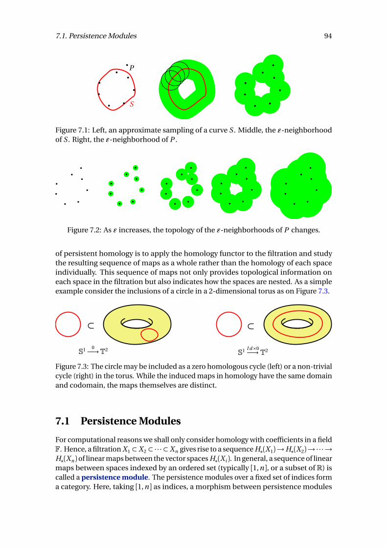
7.1. Persistence Modules 94
S
P
Figure 7.1: Left, an approximate sampling of a curve S . Middle, the ε-neighborhoodof S . Right, the ε-neighborhood of P .
Figure 7.2: As ε increases, the topology of the ε-neighborhoods of P changes.
of persistent homology is to apply the homology functor to the filtration and studythe resulting sequence of maps as a whole rather than the homology of each spaceindividually. This sequence of maps not only provides topological information oneach space in the filtration but also indicates how the spaces are nested. As a simpleexample consider the inclusions of a circle in a 2-dimensional torus as on Figure 7.3.
S1 0−→T2 S1 I d×0−→ T2
⊂ ⊂
Figure 7.3: The circle may be included as a zero homologous cycle (left) or a non-trivialcycle (right) in the torus. While the induced maps in homology have the same domainand codomain, the maps themselves are distinct.
7.1 Persistence Modules
For computational reasons we shall only consider homology with coefficients in a fieldF. Hence, a filtration X1 ⊂ X2 ⊂ · · · ⊂ Xn gives rise to a sequence H∗(X1)→H∗(X2)→ ·· ·→H∗(Xn )of linear maps between the vector spaces H∗(X i ). In general, a sequence of linearmaps between spaces indexed by an ordered set (typically [1, n ], or a subset of R) iscalled a persistence module. The persistence modules over a fixed set of indices forma category. Here, taking [1, n ] as indices, a morphism between persistence modules
7.1. Persistence Modules 95
( fi : Ei → Ei+1)1≤i<n and (g i : Fi → Fi+1)1≤i<n is a sequence of linear maps φi : Ei → Fi
that makes the diagram
( fi ) : E1f1 //
φ1
��
E2f2 //
φ2
��
. . .fn−1 // En
φn
��(g i ) : F1
g1 // F2g2 // . . .
gn−1 // Fn
commute (i.e.,φi+1 ◦ fi = g i ◦φi ). The modules ( fi ) and (g i ) are isomorphic if we canchoose the φi to be isomorphisms. The direct sum of persistence modules ( fi ) and(g i ) is the persistence module
( fi )⊕ (g i ) : E1⊕ F1f1⊕g1−→ E2⊕ F2
f2⊕g2−→ ·· ·fn−1⊕gn−1−→ En ⊕ Fn ,
where, as usual, fi ⊕ g i maps (x , y ) ∈ Ei ⊕ Fi to ( fi (x ), g i (y )).
7.1.1 Classification of Persistence Modules
A persistence module is decomposable if it is isomorphic to the direct sum of twonon-trivial persistence modules. It is otherwise indecomposable. In this section weonly consider finite persistence modules indexed over [1, n ], and for 1≤ a ≤ b ≤ n +1we denote by I[a , b [ the persistence module
10−→ ·· · −→ 0−→
aF
I d−→ ·· · I d−→b−1F −→
b0 · · · −→
n0
whose i th space is the 1-dimensional vector space over F if i ∈ [a , b [ and 0 otherwise.
Exercise 7.1.1. Show that I[a , b [ is indecomposable.
The main result about the classification of persistence modules is the uniquenessof the decomposition into indecomposables.
Theorem 7.1.2. Let ( fi )1≤i<n be a persistence module. There exists a unique multiset Iof subintervals of [1, n +1[ such that
( fi )1≤i<n∼=
⊕
[a ,b [∈I
I[a , b [,
where each interval in this sum occurs with its multiplicity in I .
The multiset I is the barcode of ( fi )1≤i<n . It is composed of persistence intervals.
Corollary 7.1.3. The barcode is a complete invariant for the isomorphism classes ofpersistence modules.
Given a persistence module E1f1−→ E2
f2−→ ·· ·fn−1−→ En , we let fi , j : Ei → E j be the
composition of the fk ’s between ei and e j . Precisely, we set
• ∀i ∈ [1, n ] : fi ,i = I dEi
7.1. Persistence Modules 96
• ∀1≤ i < j ≤ n : fi , j = fi+1, j ◦ fi and f j ,i = 0.
We also denote the rank of fi , j by βi , j . The multiplicity of interval [i , j [ in the barcodeI is denoted by mi , j .
Lemma 7.1.4. mi , j = (βi , j−1−βi−1, j−1)− (βi , j −βi−1, j )
PROOF. Suppose that E1f1−→ E2
f2−→ ·· ·fn−1−→ En
∼=⊕
[a ,b [∈I I[a , b [. We easily compute
βi , j (I[a , b [) =
�
1 if [i , j ]⊂ [a , b [0 else.
Note that for any persistence modules (gk ) and (hk )we haveβi , j ((gk )⊕(hk )) =βi , j ((gk ))+βi , j ((hk )). It follows thatβi , j (( fk )) counts the number of persistence intervals of ( fk ) thatcontain [i , j ]. Hence, δi , j :=βi , j −βi−1, j counts the number of persistence intervals ofthe form [i ,`[, ` > j . We infer that mi , j =δi , j−1−δi , j = (βi , j−1−βi−1, j−1)− (βi , j −βi−1, j ).
Consider a vector x ∈ Ei in the persistence module ( fi )1≤i<n = E1f1−→ E2
f2−→ ·· ·fn−1−→ En .
We put x ( j ) := fi , j (x ). A compatible basis is a family of vectors X ⊂⋃
i Ei , the unionbeing considered as disjoint, so that
X (i ) := {x (i ) | (x ∈ X )∧ (x (i ) 6= 0)}
is a basis of Ei for 1 ≤ i ≤ n . In particular, x , y ∈ X and x (i ) 6= 0 implies y (i ) 6= x (i ).The persistence interval of x ∈ X is defined as Ix = {i | x (i ) 6= 0}. For convenience, weintroduce the activation function a :
⋃
i Ei → [1, n ] such that x ∈ Ea (x ) for all x ∈⋃
i Ei .Hence, the lower bound of Ix is a (x ).
Lemma 7.1.5. If ( fi )1≤i<n admits a compatible basis X , then ( fi )1≤i<n has a decomposi-tion whose barcode is the multiset of persistence intervals {Ix | x ∈ X }.
PROOF.⊕
x∈X I(Ix ) has an obvious compatible basis Y obtained by choosing forevery x ∈ X a generator of F at index a (x ). It remains to check that the persistencemodules ( fi )i and
⊕
x∈X I(Ix ) are isomorphic by constructing an isomorphism sendingthe bases X (i ) to Y (i ).
Proposition 7.1.6. Every persistence module admits a compatible basis.
PROOF. For a persistence module E1f1−→ E2
f2−→ ·· ·fn−1−→ En we build a compatible basis
by induction on n . If n = 1, a compatible basis is provided by any basis of E1. We nextassume to have constructed a compatible basis X for
E1f1−→ E2
f2−→ ·· ·fn−2−→ En−1. (7.1)
Let k = |X | be the number of basis vectors in X . We recursively define compatiblebases X1 = X , X2, . . . , Xk for (7.1). The goal is to get a compatible basis Xk such that
7.1. Persistence Modules 97
{x (n ) | x ∈ Xk ∧ x (n ) 6= 0} is an independent family in En . To this end we first orderthe elements x1, x2, . . . , xk of X in a non-decreasing fashion with respect to activation,i.e. such that 1≤ j < k implies a (x j )≤ a (x j+1). Suppose we have constructed X i−1 ={y1, y2, . . . , yk} for some k ≥ i > 1, such that the yj are indexed in non-decreasing orderfor activation, and such that the nonzero vectors in {y1(n ), y2(n ), . . . , yi−1(n )} form anindependent family in En .
• If yi (n ) = 0 or if {y1(n ), y2(n ), . . . , yi (n )} is independent, we set X i = X i−1,
• otherwise, we may write yi (n ) =∑
j<i λ j yj (n ). We then put y ′i = yi −∑
j<i λ j yj (i ),so that y ′i (n ) = 0, and set X i = X i−1 \ {yi }∪ {y ′i }.
In both cases it is easily seen that X i is a compatible basis for (7.1). By construction thenonzero images in En of the i first vectors in X i form an independent family. By induc-tion, Xk satisfies our goal. It remains to complete Xk with a basis of a complementary
space of fn−1(En−1) in En to obtain a compatible basis for E1f1−→ E2
f2−→ ·· ·fn−1−→ En .
PROOF OF THEOREM 7.1.2. By Proposition 7.1.6, the persistence module ( fi )i has acompatible basis, hence a decomposition into indecomposable modules of the formI[a , b [ by Lemma 7.1.5. This decomposition is determined by its barcode which isuniquely defined according to Lemma 7.1.4.
7.1.2 Restrictions of Persistence Modules
The barcode of a persistence module and of its sub-sequences can be easily related.This relationship will be used in the proof of the stability theorem in Section 7.4.1. Inorder to formalize the relation, consider a strictly increasing mapκ : [1, m ]→ [1, n ]. The
restriction to κ of the persistence module ( fi ) : E1f1−→ E2
f2−→ ·· ·fn−1−→ En is the persistence
module
( fi ) κ : Eκ(1)fκ(1),κ(2)−−−→ Eκ(2) · · ·
fκ(m−1),κ(m )−−−−−→ Eκ(m )
where fi , j was defined below Corollary 7.1.3. Consider the map
µ : [1, n +1] → [1, m +1]i 7→ min{ j ∈ [1, m +1] | κ( j )≥ i }
where by convention κ(m +1) = n +1. It is not difficult to see that
I[a , b [ κ =
�
I[µ(a ),µ(b )[ if µ(a )<µ(b )0 otherwise.
As an immediate consequence:
Lemma 7.1.7. Let I be the barcode of a persistence module. The barcode of its restrictionto κ is the multiset { [µ(a ),µ(b )[}[a ,b [∈I and µ(a )<µ(b ).
Exercise 7.1.8. Prove the above evaluation for I[a , b [ κ.
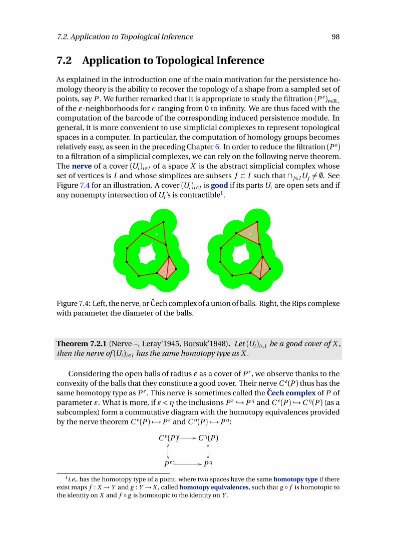
7.2. Application to Topological Inference 98
7.2 Application to Topological Inference
As explained in the introduction one of the main motivation for the persistence ho-mology theory is the ability to recover the topology of a shape from a sampled set ofpoints, say P . We further remarked that it is appropriate to study the filtration (P ε)ε∈R+of the ε-neighborhoods for ε ranging from 0 to infinity. We are thus faced with thecomputation of the barcode of the corresponding induced persistence module. Ingeneral, it is more convenient to use simplicial complexes to represent topologicalspaces in a computer. In particular, the computation of homology groups becomesrelatively easy, as seen in the preceding Chapter 6. In order to reduce the filtration (P ε)to a filtration of a simplicial complexes, we can rely on the following nerve theorem.The nerve of a cover (Ui )i∈I of a space X is the abstract simplicial complex whoseset of vertices is I and whose simplices are subsets J ⊂ I such that ∩ j∈J Uj 6= ;. SeeFigure 7.4 for an illustration. A cover (Ui )i∈I is good if its parts Ui are open sets and ifany nonempty intersection of Ui ’s is contractible1.
Figure 7.4: Left, the nerve, or Cech complex of a union of balls. Right, the Rips complexewith parameter the diameter of the balls.
Theorem 7.2.1 (Nerve –, Leray’1945, Borsuk’1948). Let (Ui )i∈I be a good cover of X ,then the nerve of (Ui )i∈I has the same homotopy type as X .
Considering the open balls of radius ε as a cover of P ε, we observe thanks to theconvexity of the balls that they constitute a good cover. Their nerve C ε(P ) thus has thesame homotopy type as P ε. This nerve is sometimes called the Cech complex of P ofparameter ε. What is more, if ε < η the inclusions P ε ,→ P η and C ε(P ) ,→C η(P ) (as asubcomplex) form a commutative diagram with the homotopy equivalences providedby the nerve theorem C ε(P )↔ P ε and C η(P )↔ P η:
C ε(P ) �� //
OO
��
C η(P )OO
��P ε � � // P η
1i.e., has the homotopy type of a point, where two spaces have the same homotopy type if thereexist maps f : X → Y and g : Y → X , called homotopy equivalences, such that g ◦ f is homotopic tothe identity on X and f ◦ g is homotopic to the identity on Y .
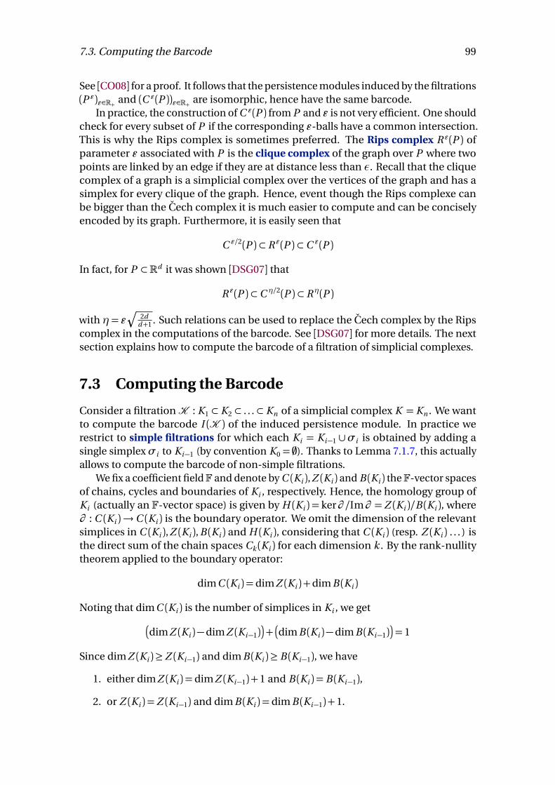
7.3. Computing the Barcode 99
See [CO08] for a proof. It follows that the persistence modules induced by the filtrations(P ε)ε∈R+ and (C ε(P ))ε∈R+ are isomorphic, hence have the same barcode.
In practice, the construction of C ε(P ) from P and ε is not very efficient. One shouldcheck for every subset of P if the corresponding ε-balls have a common intersection.This is why the Rips complex is sometimes preferred. The Rips complex R ε(P ) ofparameter ε associated with P is the clique complex of the graph over P where twopoints are linked by an edge if they are at distance less than ε. Recall that the cliquecomplex of a graph is a simplicial complex over the vertices of the graph and has asimplex for every clique of the graph. Hence, event though the Rips complexe canbe bigger than the Cech complex it is much easier to compute and can be conciselyencoded by its graph. Furthermore, it is easily seen that
C ε/2(P )⊂R ε(P )⊂C ε(P )
In fact, for P ⊂Rd it was shown [DSG07] that
R ε(P )⊂C η/2(P )⊂Rη(P )
with η= εq
2dd+1 . Such relations can be used to replace the Cech complex by the Rips
complex in the computations of the barcode. See [DSG07] for more details. The nextsection explains how to compute the barcode of a filtration of simplicial complexes.
7.3 Computing the Barcode
Consider a filtrationK : K1 ⊂ K2 ⊂ . . .⊂ Kn of a simplicial complex K = Kn . We wantto compute the barcode I (K ) of the induced persistence module. In practice werestrict to simple filtrations for which each Ki = Ki−1 ∪σi is obtained by adding asingle simplexσi to Ki−1 (by convention K0 = ;). Thanks to Lemma 7.1.7, this actuallyallows to compute the barcode of non-simple filtrations.
We fix a coefficient fieldF and denote by C (Ki ), Z (Ki ) and B (Ki ) theF-vector spacesof chains, cycles and boundaries of Ki , respectively. Hence, the homology group ofKi (actually an F-vector space) is given by H (Ki ) = ker∂ /Im∂ = Z (Ki )/B (Ki ), where∂ : C (Ki )→ C (Ki ) is the boundary operator. We omit the dimension of the relevantsimplices in C (Ki ), Z (Ki ), B (Ki ) and H (Ki ), considering that C (Ki ) (resp. Z (Ki ) . . . ) isthe direct sum of the chain spaces Ck (Ki ) for each dimension k . By the rank-nullitytheorem applied to the boundary operator:
dim C (Ki ) = dim Z (Ki ) +dim B (Ki )
Noting that dim C (Ki ) is the number of simplices in Ki , we get
�
dim Z (Ki )−dim Z (Ki−1)�
+�
dim B (Ki )−dim B (Ki−1)�
= 1
Since dim Z (Ki )≥ Z (Ki−1) and dim B (Ki )≥ B (Ki−1), we have
1. either dim Z (Ki ) = dim Z (Ki−1) +1 and B (Ki ) = B (Ki−1),
2. or Z (Ki ) = Z (Ki−1) and dim B (Ki ) = dim B (Ki−1) +1.
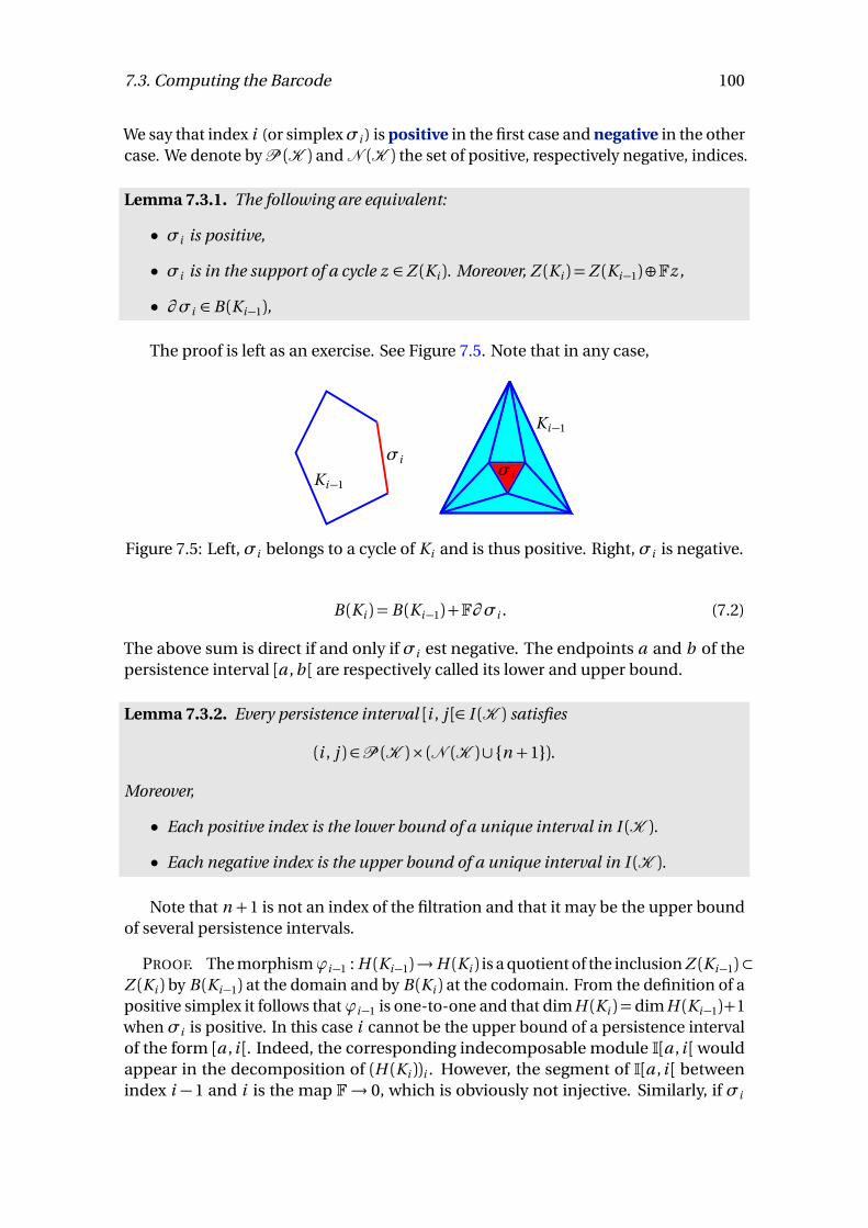
7.3. Computing the Barcode 100
We say that index i (or simplexσi ) is positive in the first case and negative in the othercase. We denote byP (K ) andN (K ) the set of positive, respectively negative, indices.
Lemma 7.3.1. The following are equivalent:
• σi is positive,
• σi is in the support of a cycle z ∈ Z (Ki ). Moreover, Z (Ki ) = Z (Ki−1)⊕Fz ,
• ∂ σi ∈ B (Ki−1),
The proof is left as an exercise. See Figure 7.5. Note that in any case,
σi
Ki−1
Ki−1
σi
Figure 7.5: Left,σi belongs to a cycle of Ki and is thus positive. Right,σi is negative.
B (Ki ) = B (Ki−1) +F∂ σi . (7.2)
The above sum is direct if and only ifσi est negative. The endpoints a and b of thepersistence interval [a , b [ are respectively called its lower and upper bound.
Lemma 7.3.2. Every persistence interval [i , j [∈ I (K ) satisfies
(i , j ) ∈P (K )× (N (K )∪{n +1}).
Moreover,
• Each positive index is the lower bound of a unique interval in I (K ).
• Each negative index is the upper bound of a unique interval in I (K ).
Note that n +1 is not an index of the filtration and that it may be the upper boundof several persistence intervals.
PROOF. The morphismϕi−1 : H (Ki−1)→H (Ki ) is a quotient of the inclusion Z (Ki−1)⊂Z (Ki ) by B (Ki−1) at the domain and by B (Ki ) at the codomain. From the definition of apositive simplex it follows thatϕi−1 is one-to-one and that dim H (Ki ) = dim H (Ki−1)+1whenσi is positive. In this case i cannot be the upper bound of a persistence intervalof the form [a , i [. Indeed, the corresponding indecomposable module I[a , i [wouldappear in the decomposition of (H (Ki ))i . However, the segment of I[a , i [ betweenindex i − 1 and i is the map F→ 0, which is obviously not injective. Similarly, if σi
7.3. Computing the Barcode 101
is negative then ϕi−1 is onto and dim H (Ki ) = dim H (Ki−1)− 1. As a consequence, icannot be the lower bound of any persistence interval. On the other hand, dim H (Ki )is the number of persistence intervals that contain i . It easily follows that exactly oneinterval starts whenσi is positive and one interval ends whenσi is negative.
We can thus define the birth function as the map b :N (K )→P (K ) such that for allj ∈N (K ), [b ( j ), j [∈ I (K ). In particular,
I (K ) = {[b ( j ), j [} j∈N (K ) ∪ {[i , n +1[}i∈P (K )\Im b (7.3)
Hence, we may recover the barcode I (K ) from the knowledge of the signs of thesimplices and of the birth function.
7.3.1 Compatible Boundary Basis
A Compatible boundary basis is a family of cycles B (K ) = {x j } j∈J ⊂ Z (K ), withJ ⊂ [1, n ], such that:
1. ∀i ∈ [1, n ],{x j } j∈J∩[1,i ] is a basis of B (Ki ),
2. the map β : J → [1, n ], j 7→ (maximum index of the simplices in x j ) is injective.
Lemma 7.3.3. Suppose thatK has a compatible boundary basis, then β coincides withthe birth function b .
PROOF. The above Condition 1 and the remark after Equation (7.2) show that J =N (K ). Lemma 7.3.1 also implies that β ( j ) ∈P (K ) for all j ∈ J . For every i ∈P (K ),define zi ∈ Z (Ki ) as follows.
• If i =β ( j ) for some j ∈ J , then zi = x j .
• Else, choose zi such that Z (Ki ) = Z (Ki−1)⊕Fzi (cf. Lemma 7.3.1).
Remark that the simplex with maximum index in the support of zi isσi . Hence, (cf.Lemma 7.3.1) {z j } j∈P (K ), j≤i is a basis of Z (Ki ). Let [z ]i denote the homology classof cycle z in H (Ki ). We need to check that ([z j ] j ) j∈P (K ) is a compatible basis for thehomology sequence ofK and that the persistence interval of each [zβ ( j )]β ( j ) is [β ( j ), j [,while the persistence interval of [z j ] j , j ∈P (K ) \β (J ), is [ j , n +1[. We claim that
Z (i ) := {[zβ ( j )]i }( j∈J )∧(β ( j )≤i )∧( j>i ) ∪{[z j ]i }( j≤i )∧( j∈P (K )\β (J ))
is a basis of H (Ki ). Since [zβ ( j )] j = [x j ] j = 0, we also have [zβ ( j )]i = 0 for i ≥ j and itfollows from the above remark that Z (i ) spans H (Ki ). To see that Z (i ) is an independentset, consider a linear combination
∑
( j∈J )∧(β ( j )≤i )∧( j>i )α j [zβ ( j )]i+∑
( j≤i )∧( j∈P (K )\β (J ))α j [z j ]iof elements in Z (i ). If it is zero, then the combination c :=
∑
( j∈J )∧(β ( j )≤i )∧( j>i )α j zβ ( j )+∑
( j≤i )∧( j∈P (K )\β (J ))α j z j of the corresponding cycles must lie in B (Ki ). By the first condi-tion in the definition of a compatible boundary basis, cycle c must be equal to a linearcombination of {x j | ( j ∈ J )∧ ( j ≤ i )}. Because the maximum index of the simplicesin the support of each zβ ( j ), z j and x j are pairwise distinct, it must be that all thecoefficients α j in c are null, thus concluding the proof of the claim. We finally observethat the persistence interval of [z j ] j is the set of i ’s for which [z j ]i ∈ Z (i ). Whence,for j ∈ J the persistence interval of [zβ ( j )]β ( j ) is [β ( j ), j [, while for j ∈P (K ) \β (J ) thepersistence interval of [z j ] j is [ j , n +1[.
7.3. Computing the Barcode 102
7.3.2 Algorithm
Lemma 7.3.3 and Equation (7.3) show that it is enough to construct a compatibleboundary basis forK to derive the sign of each simplex and the barcode ofK . Wecan construct a compatible boundary basis by induction on the size n of the filtration.The base case n = 1 is trivial because the unique simplex in the filtration must be a(positive) vertex. We thus assume that we have computed a compatible boundarybasisB (K ′) = {x j } j∈J for the sub-filtrationK ′:
K1 ⊂ K2 ⊂ . . .⊂ Kn−1
We denote by b : J →P (K ′) the corresponding birth function. Suppose that we canwrite
∂ σn =∑
j∈J
α j x j + y , (7.4)
where
1. either y = 0,
2. or the maximum index of the simplices in y is not in b (J ).
In case 1, we have B (Kn ) = B (Kn−1) andB (K ′) remains a compatible boundary basisforK . In case 2, n is negative andB (K ′)∪{y } is a compatible boundary basis forK .
By the second condition in its definition, every compatible boundary basis is inechelon form when the cycles are written as combination of simplices. We can thusapply Gaussian elimination as in the following pseudocode to obtain a decompositionas in (7.4).
y := ∂ σn
i :=maximum index of the simplices in yWhile ( (y 6= 0)∧ (i ∈ b (J )) )
j := b −1(i )α := coefficient ofσi in yβ := coefficient ofσi in x j
y := y − (α/β )x j
i :=maximum index of the simplices in y \∗ undefined if y = 0 ∗\End while\∗ y = 0 or y = xn when leaving the while loop ∗\
We can store each x j as a table of coefficients indexed by the n simplices of thefiltration. We represent the birth function as a table of length n ; the j th entry containsb ( j ) if j is negative and 0 otherwise. We also store the inverse map b −1 in a table oflength n . The computation of xn by the above loop takes O (n 2) time. Hence,
Proposition 7.3.4. We can compute a compatible boundary basis and the birth functionof a filtration of length n in O (n 3) time on an F-RAM machine. We can moreovercompute the barcode of the filtration in the same amount of time.
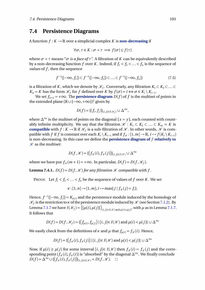
7.4. Persistence Diagrams 103
7.4 Persistence Diagrams
A function f : K →R over a simplicial complex K is non-decreasing if
∀σ,τ ∈ K :σ≺τ =⇒ f (σ)≤ f (τ)
whereσ≺τmeans “σ is a face of τ”. A filtration of K can be equivalently describedby a non-decreasing function f over K . Indeed, if f1 < f2 < . . .< fn is the sequence ofvalues of f , then the sequence
f −1([−∞, f1])⊂ f −1([−∞, f2])⊂ . . .⊂ f −1([−∞, fn ]) (7.5)
is a filtration of K , which we denote byK f . Conversely, any filtration K1 ⊂ K2 ⊂ . . .⊂Kn = K has the formK f for f defined over K by f (σ) = i ⇔σ ∈ Ki \Ki−1.
We set fn+1 =+∞. The persistence diagram D ( f ) of f is the multiset of points inthe extended plane (R∪{−∞,+∞})2 given by
D ( f ) = {( fi , f j )}[i , j [∈I (K f ) ∪ ∆∞,
where∆∞ is the multiset of points on the diagonal {x = y }, each counted with count-ably infinite multiplicity. We say that the filtration K : K1 ⊂ K2 ⊂ . . . ⊂ Km = K iscompatible with f : K →R ifK f is a sub-filtration ofK . In other words,K is com-patible with f if f is constant over each Ki \Ki−1 and if fK : [1, m ]→R, i 7→ f (Ki \Ki−1)is non-decreasing. In this case we define the persistence diagram of f relatively toK as the multiset:
D ( f ,K ) = {�
fK (i ), fK ( j )�
}[i , j [∈I (K ) ∪ ∆∞
where we have put fK (m +1) = +∞. In particular, D ( f ) =D ( f ,K f ).
Lemma 7.4.1. D ( f ) =D ( f ,K ) for any filtrationK compatible with f .
PROOF. Let f1 < f2 < . . .< fn be the sequence of values of f over K . We set
κ : [1, n ]→ [1, m ], i 7→max{ j | fK ( j ) = fi }.
Hence, f −1([−∞, fi ]) = Kκ(i ) and the persistence module induced by the homology ofK f is the restriction toκof the persistence module induced byK (see Section 7.1.2). ByLemma 7.1.7 we have I (K f ) =
�
[µ(i ),µ( j )[
[i , j [∈I (K ) and µ(i )<µ( j ), withµ as in Lemma 7.1.7.
It follows that
D ( f ) =D ( f ,K f ) = {�
fµ(i ), fµ( j )�
| [i , j [∈ I (K ) and µ(i )<µ( j )} ∪ ∆∞
We easily check from the definitions of κ and µ that fµ(i ) = fK (i ). Hence,
D ( f ) = {�
fK (i ), fK ( j )�
| [i , j [∈ I (K ) and µ(i )<µ( j )} ∪ ∆∞
Now, if µ(i ) ≥ µ( j ) for some interval [i , j [∈ I (K ) then fK (i ) = fK ( j ) and the corre-sponding point ( fK (i ), fK (i )) is “absorbed” by the diagonal∆∞. We finally concludeD ( f ) =∆∞ ∪{
�
fK (i ), fK ( j )�
}[i , j [∈I (K ) =D ( f ,K ).
7.4. Persistence Diagrams 104
7.4.1 Stability of Persistence Diagrams
The stability of the persistence diagram D ( f )with respect to f is the main result ofPersistence theory. We first introduce the bottleneck distance dB between persistencediagrams. Note that thanks to the diagonal∆∞ any two diagrams D , D ′ are in bijection.We set
dB (D , D ′) = infφ
supp∈D‖p −φ(p )‖∞
whereφ : D →D ′ runs over the bijections between D and D ′ and ‖p−q‖∞ =max{|xp−xq |, |yp − yq |} (by convention, |+∞−x |= 0 if x =+∞ and |+∞−x |=+∞ otherwise).See Figure 7.6. Note that dB is not a distance properly speaking: it can take infinite
φ
Figure 7.6: The bottleneck distance is computed by minimizing over all bijectionsφthe largest distance in each pairing.
values but otherwise satisfies the triangular inequality.As usual, for any functions f , g : K →R, we denote their L∞ distance by
‖ f − g ‖∞ = supσ∈K| f (σ)− g (σ)|
Theorem 7.4.2 (Stability –, [CSEH07, CSEM06]). dB (D ( f ), D (g ))≤ ‖ f − g ‖∞
PROOF. Put ft = f + t (g − f ). note that if f , g are non-decreasing over K , so is ft .For every two simplicesσ,τ ∈ K , there exists u ∈ [0, 1] such that the sign of ft (σ)− ft (τ)is constant for t ∈ [0, u ] and the same is true for t ∈ [u ,1]. There is thus a finitepartition 0= t0 < t1 < . . .< tr = 1 of2 [0,1] so that the relative order of the ft -values ofthe simplices is independent of t over each interval [ti , ti+1]. It follows that for eachi ∈ [0, r −1]we can exhibit a simple filtrationKi compatible with every function ft fort ∈ [ti , ti+1]. By Lemma 7.4.1, we have
D ( ft ) =D ( ft ,Ki ) =∆∞ ∪{
�
ft (σa ), ft (σb
�
}[a ,b [∈I (Ki )
whereσa is the a th simplex ofKi . Considering the obvious correspondence betweenD ( fti
) and D ( fti+1) that restricts to the identity over ∆∞ and sends
�
fti(σa ), fti
(σb )�
to�
fti+1(σa ), fti+1
(σb )�
, we infer dB (D ( fti), D ( fti+1
)) ≤ (ti+1 − ti )‖ f − g ‖∞. Applying thetriangular inequality we finally conclude
dB (D ( f ), D (g ))≤∑
i
(ti+1− ti )‖ f − g ‖∞ = ‖ f − g ‖∞
2r ≤�m
2
�
+1 where m is the number of simplices of K
7.4. Persistence Diagrams 105
The Stability theorem was refined in a more general context by Chazal et al. andBubenik and Scott [CCSG+09, CDSGO12, BS14]. A first generalization is to consider“continuous” persistence module indexed over R. This is a family of vector spaces(Vx )x∈R and a family of linear maps (vx ,y : Vx → Vy )x≤y satisfying vx ,x = I dVx
andvx ,z = vx ,y ◦ vy ,z for all x ≤ y ≤ z . We denote it by V. Given two persistence modulesV andW over R and a real number d , a degree d morphism ϕ :V→W is a family oflinear maps (ϕx : Vx →Wx+d )x∈R such that the following diagram:
Vx//
ϕx
!!
Vyϕy
!!Wx+ε
//Wy+ε
commutes for all x ∈ R. An ε-interleaving is a pair of morphisms ϕ : V→W andψ :W→V, each of degree ε, such that the following diagrams:
Vx//
ϕx
��
Vx+2ε
Wx+ε
ψx+ε
BBVx+ε
ϕx+ε ��Wx
//
ψxBB
Wx+2ε
commute. The interleaving distance between V,W is
di (V,W) = inf{ε | ∃ε-interleaving between V,W}
When isV is pointwise finite dimensional, i.e., when each space Vx if finite dimensional,it can be shown that the decomposition Theorem 7.1.2 remains valid [CB15]. Thistime each indecomposable module I(ι)may apply to any type of interval ι (half-open,closed, semi-infinite,...) and satisfies I(ι)x = F for x ∈ ι and I(ι)x = 0 otherwise, withidentity or zero maps wherever it applies. The persistence diagram is then definedas the multiset of points (u , v )where u , v runs over the endpoints of the persistenceintervals.
Theorem 7.4.3 (Isometry –, [CCSG+09, CDSGO12]). Let V andW be pointwise finitedimensional persistence modules over R such that rank vx ,y and rank wx ,y is finite forevery x < y . Then,
dB (D (V), D (W)) = di (V,W)
The stability theorem can be deduced from the isometry theorem as follows.Let X be a topological space and f : X → R. Put X f
t := f −1(−∞, t ]. The filtrationX f := (X f
t )t ∈R induces a persistence module H (X f ) by applying the homology func-tor. Now, ‖ f − g ‖∞ ≤ ε implies X f
t ⊂ X gt+ε ⊂ X f
t+2ε. It follows that H (X f ), H (Xg ) areε-interleaved, whence by the isometry Theorem di (H (X f ), H (Xg )) ≤ ε. In turn, thisimplies dB (D ( f ), D (g )) = di (H∗(X f ), H∗(Xg ))≤ ‖ f − g ‖∞.
Exercise 7.4.4. Check that a persistence module over an ordered set (X ,≤), e.g. X =R,is the same as a functor from the category (X ,≤) to the category of F-vector spaces.Here, the objects of (X ,≤) are the elements of X and each pair (x , y ) of objects hasexactly one morphism if x ≤ y (and none otherwise).
8
Knots and 3-DimensionalComputational Topology
Contents8.1 Knots . . . . . . . . . . . . . . . . . . . . . . . . . . . . . . . . . . . . . . . . . . . . . 107
8.2 Knot diagrams . . . . . . . . . . . . . . . . . . . . . . . . . . . . . . . . . . . . . . 108
8.3 The knot complement . . . . . . . . . . . . . . . . . . . . . . . . . . . . . . . . . 111
8.3.1 Homotopy . . . . . . . . . . . . . . . . . . . . . . . . . . . . . . . . . . . . . . 112
8.3.2 Homology . . . . . . . . . . . . . . . . . . . . . . . . . . . . . . . . . . . . . . 114
8.3.3 Triangulations . . . . . . . . . . . . . . . . . . . . . . . . . . . . . . . . . . . 114
8.4 An algorithm for unknot recognition . . . . . . . . . . . . . . . . . . . . . . 115
8.4.1 Normal surface theory . . . . . . . . . . . . . . . . . . . . . . . . . . . . . 116
8.4.2 Trivial knot and spanning disks . . . . . . . . . . . . . . . . . . . . . . . 118
8.4.3 Normalization of spanning disks . . . . . . . . . . . . . . . . . . . . . . 120
8.4.4 Haken sum, fundamental and vertex normal surfaces . . . . . . 123
8.5 Knotless graphs . . . . . . . . . . . . . . . . . . . . . . . . . . . . . . . . . . . . . 126
In the next two courses, we switch our attention from 2-dimensional space (sur-faces) to 3-dimensional space, focusing on knots, and incidentally dealing a bit with3-manifolds. This increase in dimension has a dramatic effect from the point of view ofcomputational topology: while most topological problems on surfaces can be solvedefficiently, their generalizations in dimension 3 are much harder to understand. Asan illustration, while recognizing closed surfaces can be done in linear time by justcomputing the Euler characteristic and orientability, all the algorithms known to de-tect whether two 3-dimensional spaces are homeomorphic [Jac05, Kup15a] are veryinefficient (requiring more than towers of exponentials) and complicated, relying on
106

8.1. Knots 107
Figure 8.1: Example of knots: the trivial knot, the left and right trefoil knots, and thefigure-eight knot. These are not polygonal but can obviously be made so.
Perelman’s recent proof [Per02, Per03] of Thurston’s Geometrization Conjecture. Nev-ertheless, despite being hard, most problems in 3 dimensions are decidable, and thusform an interesting middle ground before higher dimensions where indecidabilityresults start to kick in.
8.1 Knots
A knot is a closed curve in R3, or more formally an embedding S1→R3. In contrastwith the two-dimensional case, allowing arbitrary topological knots might lead topathological objects known as wild knots which, while interesting in their own right,are not very relevant from an algorithmic perspective. So we restrict our attention totame knots, which are polygonal1 embeddings S1→R3. We will omit the word tamethroughout these notes. Two knots are considered equivalent if they can be deformedcontinuously one onto the other one without introducing self-crossings in the process.More formally, the notion of equivalence considered here is through ambient isotopy,that is a continuous family of homeomorphisms ht : R3 × [0,1]→ R3. Two knots K1
and K2 are (ambient) isotopic if there exists an ambient isotopy ht such that h0 = I dR3
and h1(K1) = K2. Figure 8.1 shows some examples of knots.
Remark 1: By the Alexander trick (see for example [BZ85, Proposition 1.9]), anyorientation-preserving homeomorphism of the 3-ball B3→B3 is actually an ambientisotopy, so homeomorphisms could simply be used to define equivalence, but thenotion of ambient isotopies is more intuitive.
Remark 2: On the other hand, our notion of ambient isotopy is a bit unnaturalbecause it breaks the polygonal structure of tame knots. The underlying idea is that werestrict our attention to tame knots to avoid pathologies, but once this restriction hasbeen made, it is much more convenient to allow any kind of continuous deformation.Yet if one insists on only allowing polygonal deformations, one can restrict the allowedisotopies to elementary moves or∆-moves which are illustrated in Figure 8.2. It turnsout that knots are equivalent under ambient isotopies if and only if they are equivalentunder elementary moves, see [BZ85, Proposition 1.10].
Remark 3: Another tempting definition of equivalence could be to use isotopies,i.e., to say that two knots K1 and K2 are isotopic if there is a continuous family ofembeddings it : S1→ S3 such that i0 = K1 and i1 = K2. However, with such a definition
1Considering smooth knots leads to the same theory.
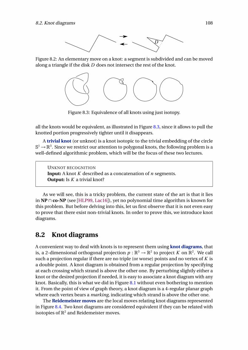
8.2. Knot diagrams 108
D
Figure 8.2: An elementary move on a knot: a segment is subdivided and can be movedalong a triangle if the disk D does not intersect the rest of the knot.
Figure 8.3: Equivalence of all knots using just isotopy.
all the knots would be equivalent, as illustrated in Figure 8.3, since it allows to pull theknotted portion progressively tighter until it disappears.
A trivial knot (or unknot) is a knot isotopic to the trivial embedding of the circleS1→R3. Since we restrict our attention to polygonal knots, the following problem is awell-defined algorithmic problem, which will be the focus of these two lectures.
UNKNOT RECOGNITION
Input: A knot K described as a concatenation of n segments.Output: Is K a trivial knot?
As we will see, this is a tricky problem, the current state of the art is that it liesin NP ∩ co-NP (see [HLP99, Lac16]), yet no polynomial time algorithm is known forthis problem. But before delving into this, let us first observe that it is not even easyto prove that there exist non-trivial knots. In order to prove this, we introduce knotdiagrams.
8.2 Knot diagrams
A convenient way to deal with knots is to represent them using knot diagrams, thatis, a 2-dimensional orthogonal projection p : R3 → R2 to project K on R2. We callsuch a projection regular if there are no triple (or worse) points and no vertex of K isa double point. A knot diagram is obtained from a regular projection by specifyingat each crossing which strand is above the other one. By perturbing slightly either aknot or the desired projection if needed, it is easy to associate a knot diagram with anyknot. Basically, this is what we did in Figure 8.1 without even bothering to mentionit. From the point of view of graph theory, a knot diagram is a 4-regular planar graphwhere each vertex bears a marking, indicating which strand is above the other one.
The Reidemeister moves are the local moves relating knot diagrams representedin Figure 8.4. Two knot diagrams are considered equivalent if they can be related withisotopies of R2 and Reidemeister moves.
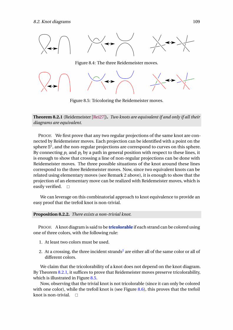
8.2. Knot diagrams 109
Figure 8.4: The three Reidemeister moves.
Figure 8.5: Tricoloring the Reidemeister moves.
Theorem 8.2.1 (Reidemeister [Rei27]). Two knots are equivalent if and only if all theirdiagrams are equivalent.
PROOF. We first prove that any two regular projections of the same knot are con-nected by Reidemeister moves. Each projection can be identified with a point on thesphere S2, and the non-regular projections are correspond to curves on this sphere.By connecting p1 and p2 by a path in general position with respect to these lines, itis enough to show that crossing a line of non-regular projections can be done withReidemeister moves. The three possible situations of the knot around these linescorrespond to the three Reidemeister moves. Now, since two equivalent knots can berelated using elementary moves (see Remark 2 above), it is enough to show that theprojection of an elementary move can be realized with Reidemeister moves, which iseasily verified.
We can leverage on this combinatorial approach to knot equivalence to provide aneasy proof that the trefoil knot is non-trivial.
Proposition 8.2.2. There exists a non-trivial knot.
PROOF. A knot diagram is said to be tricolorable if each strand can be colored usingone of three colors, with the following rule:
1. At least two colors must be used.
2. At a crossing, the three incident strands2 are either all of the same color or all ofdifferent colors.
We claim that the tricolorability of a knot does not depend on the knot diagram.By Theorem 8.2.1, it suffices to prove that Reidemeister moves preserve tricolorability,which is illustrated in Figure 8.5.
Now, observing that the trivial knot is not tricolorable (since it can only be coloredwith one color), while the trefoil knot is (see Figure 8.6), this proves that the trefoilknot is non-trivial.
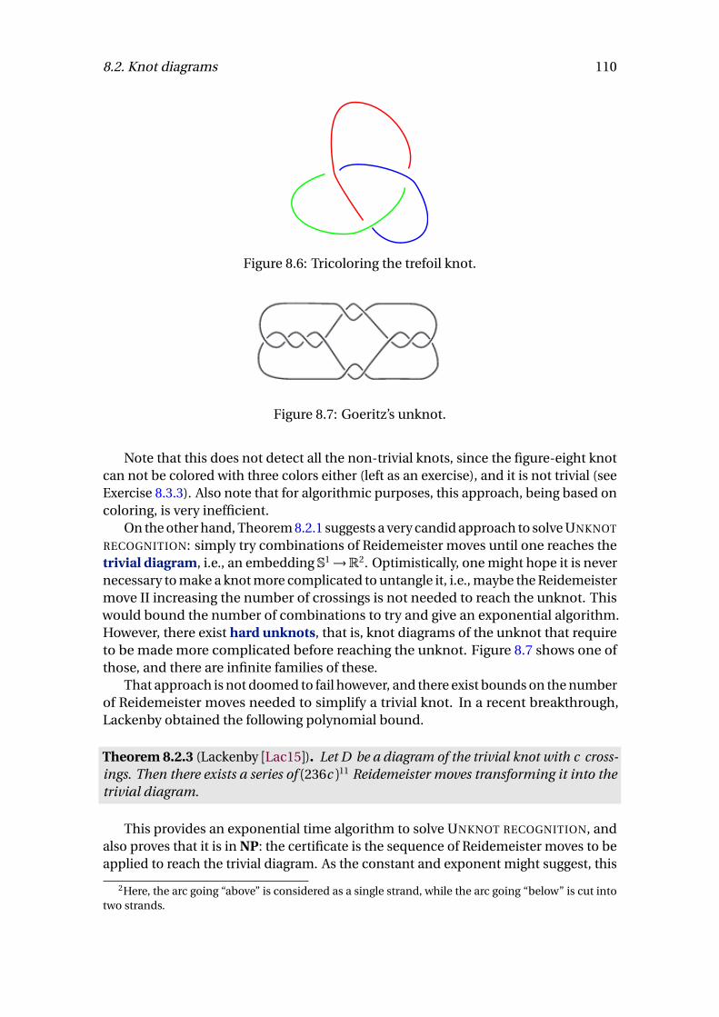
8.2. Knot diagrams 110
Figure 8.6: Tricoloring the trefoil knot.
Figure 8.7: Goeritz’s unknot.
Note that this does not detect all the non-trivial knots, since the figure-eight knotcan not be colored with three colors either (left as an exercise), and it is not trivial (seeExercise 8.3.3). Also note that for algorithmic purposes, this approach, being based oncoloring, is very inefficient.
On the other hand, Theorem 8.2.1 suggests a very candid approach to solve UNKNOT
RECOGNITION: simply try combinations of Reidemeister moves until one reaches thetrivial diagram, i.e., an embedding S1→R2. Optimistically, one might hope it is nevernecessary to make a knot more complicated to untangle it, i.e., maybe the Reidemeistermove II increasing the number of crossings is not needed to reach the unknot. Thiswould bound the number of combinations to try and give an exponential algorithm.However, there exist hard unknots, that is, knot diagrams of the unknot that requireto be made more complicated before reaching the unknot. Figure 8.7 shows one ofthose, and there are infinite families of these.
That approach is not doomed to fail however, and there exist bounds on the numberof Reidemeister moves needed to simplify a trivial knot. In a recent breakthrough,Lackenby obtained the following polynomial bound.
Theorem 8.2.3 (Lackenby [Lac15]). Let D be a diagram of the trivial knot with c cross-ings. Then there exists a series of (236c )11 Reidemeister moves transforming it into thetrivial diagram.
This provides an exponential time algorithm to solve UNKNOT RECOGNITION, andalso proves that it is in NP: the certificate is the sequence of Reidemeister moves to beapplied to reach the trivial diagram. As the constant and exponent might suggest, this
2Here, the arc going “above” is considered as a single strand, while the arc going “below” is cut intotwo strands.
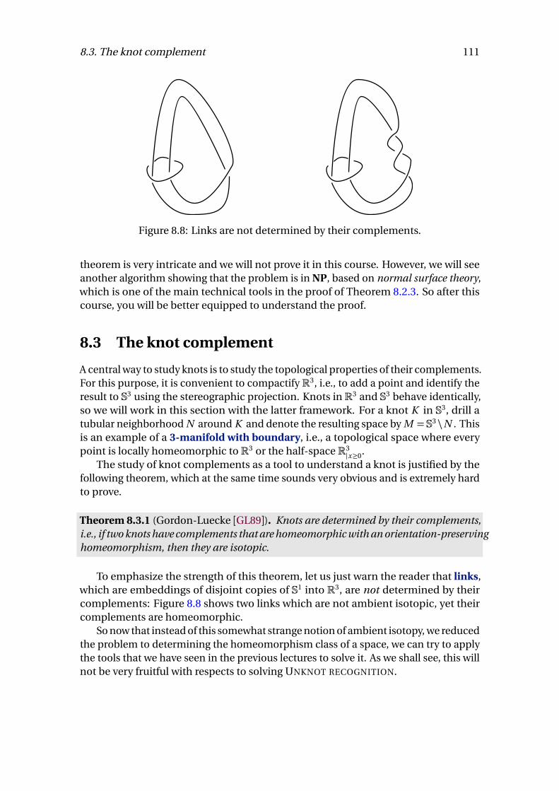
8.3. The knot complement 111
Figure 8.8: Links are not determined by their complements.
theorem is very intricate and we will not prove it in this course. However, we will seeanother algorithm showing that the problem is in NP, based on normal surface theory,which is one of the main technical tools in the proof of Theorem 8.2.3. So after thiscourse, you will be better equipped to understand the proof.
8.3 The knot complement
A central way to study knots is to study the topological properties of their complements.For this purpose, it is convenient to compactifyR3, i.e., to add a point and identify theresult to S3 using the stereographic projection. Knots in R3 and S3 behave identically,so we will work in this section with the latter framework. For a knot K in S3, drill atubular neighborhood N around K and denote the resulting space by M = S3\N . Thisis an example of a 3-manifold with boundary, i.e., a topological space where everypoint is locally homeomorphic to R3 or the half-space R3
|x≥0.The study of knot complements as a tool to understand a knot is justified by the
following theorem, which at the same time sounds very obvious and is extremely hardto prove.
Theorem 8.3.1 (Gordon-Luecke [GL89]). Knots are determined by their complements,i.e., if two knots have complements that are homeomorphic with an orientation-preservinghomeomorphism, then they are isotopic.
To emphasize the strength of this theorem, let us just warn the reader that links,which are embeddings of disjoint copies of S1 into R3, are not determined by theircomplements: Figure 8.8 shows two links which are not ambient isotopic, yet theircomplements are homeomorphic.
So now that instead of this somewhat strange notion of ambient isotopy, we reducedthe problem to determining the homeomorphism class of a space, we can try to applythe tools that we have seen in the previous lectures to solve it. As we shall see, this willnot be very fruitful with respects to solving UNKNOT RECOGNITION.
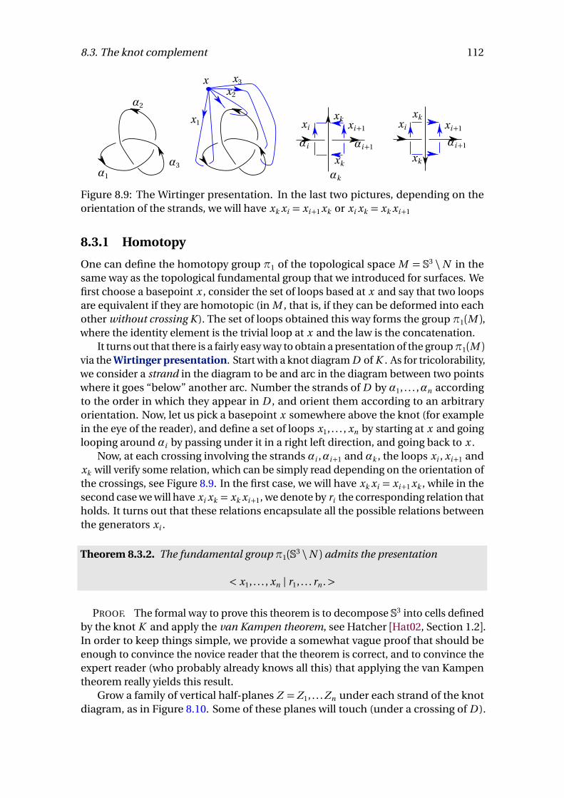
8.3. The knot complement 112
α1
α2
α3
x
x1
x2
x3
αi+1
xi
xkxi+1
xk
αi
αk
xk
xk
αi+1
xi xi+1
Figure 8.9: The Wirtinger presentation. In the last two pictures, depending on theorientation of the strands, we will have xk xi = xi+1 xk or xi xk = xk xi+1
8.3.1 Homotopy
One can define the homotopy group π1 of the topological space M = S3 \N in thesame way as the topological fundamental group that we introduced for surfaces. Wefirst choose a basepoint x , consider the set of loops based at x and say that two loopsare equivalent if they are homotopic (in M , that is, if they can be deformed into eachother without crossing K ). The set of loops obtained this way forms the group π1(M ),where the identity element is the trivial loop at x and the law is the concatenation.
It turns out that there is a fairly easy way to obtain a presentation of the groupπ1(M )via the Wirtinger presentation. Start with a knot diagram D of K . As for tricolorability,we consider a strand in the diagram to be and arc in the diagram between two pointswhere it goes “below” another arc. Number the strands of D by α1, . . . ,αn accordingto the order in which they appear in D , and orient them according to an arbitraryorientation. Now, let us pick a basepoint x somewhere above the knot (for examplein the eye of the reader), and define a set of loops x1, . . . , xn by starting at x and goinglooping around αi by passing under it in a right left direction, and going back to x .
Now, at each crossing involving the strands αi ,αi+1 and αk , the loops xi , xi+1 andxk will verify some relation, which can be simply read depending on the orientation ofthe crossings, see Figure 8.9. In the first case, we will have xk xi = xi+1 xk , while in thesecond case we will have xi xk = xk xi+1, we denote by ri the corresponding relation thatholds. It turns out that these relations encapsulate all the possible relations betweenthe generators xi .
Theorem 8.3.2. The fundamental group π1(S3 \N ) admits the presentation
< x1, . . . , xn | r1, . . . rn .>
PROOF. The formal way to prove this theorem is to decompose S3 into cells definedby the knot K and apply the van Kampen theorem, see Hatcher [Hat02, Section 1.2].In order to keep things simple, we provide a somewhat vague proof that should beenough to convince the novice reader that the theorem is correct, and to convince theexpert reader (who probably already knows all this) that applying the van Kampentheorem really yields this result.
Grow a family of vertical half-planes Z = Z1, . . . Zn under each strand of the knotdiagram, as in Figure 8.10. Some of these planes will touch (under a crossing of D ).
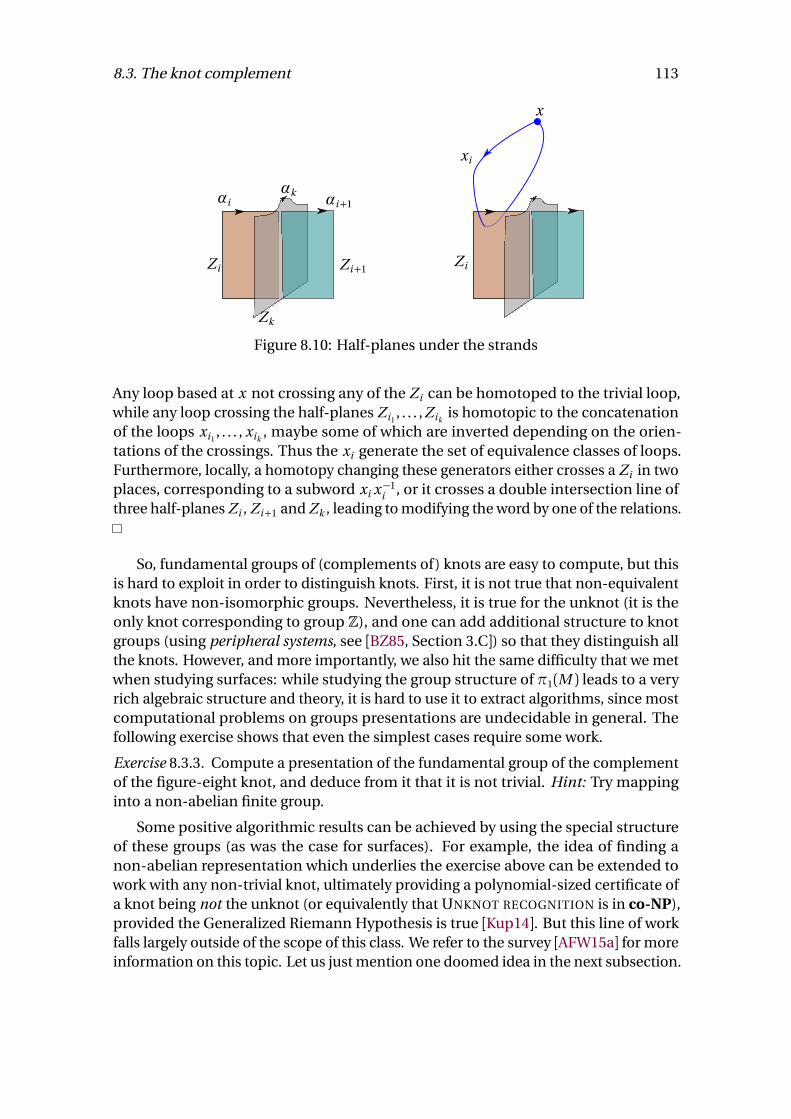
8.3. The knot complement 113
αi αi+1
αk
Zi Zi+1
Zk
x
xi
Zi
Figure 8.10: Half-planes under the strands
Any loop based at x not crossing any of the Zi can be homotoped to the trivial loop,while any loop crossing the half-planes Zi1
, . . . , Zikis homotopic to the concatenation
of the loops xi1, . . . , xik
, maybe some of which are inverted depending on the orien-tations of the crossings. Thus the xi generate the set of equivalence classes of loops.Furthermore, locally, a homotopy changing these generators either crosses a Zi in twoplaces, corresponding to a subword xi x−1
i , or it crosses a double intersection line ofthree half-planes Zi , Zi+1 and Zk , leading to modifying the word by one of the relations.
So, fundamental groups of (complements of) knots are easy to compute, but thisis hard to exploit in order to distinguish knots. First, it is not true that non-equivalentknots have non-isomorphic groups. Nevertheless, it is true for the unknot (it is theonly knot corresponding to group Z), and one can add additional structure to knotgroups (using peripheral systems, see [BZ85, Section 3.C]) so that they distinguish allthe knots. However, and more importantly, we also hit the same difficulty that we metwhen studying surfaces: while studying the group structure of π1(M ) leads to a veryrich algebraic structure and theory, it is hard to use it to extract algorithms, since mostcomputational problems on groups presentations are undecidable in general. Thefollowing exercise shows that even the simplest cases require some work.
Exercise 8.3.3. Compute a presentation of the fundamental group of the complementof the figure-eight knot, and deduce from it that it is not trivial. Hint: Try mappinginto a non-abelian finite group.
Some positive algorithmic results can be achieved by using the special structureof these groups (as was the case for surfaces). For example, the idea of finding anon-abelian representation which underlies the exercise above can be extended towork with any non-trivial knot, ultimately providing a polynomial-sized certificate ofa knot being not the unknot (or equivalently that UNKNOT RECOGNITION is in co-NP),provided the Generalized Riemann Hypothesis is true [Kup14]. But this line of workfalls largely outside of the scope of this class. We refer to the survey [AFW15a] for moreinformation on this topic. Let us just mention one doomed idea in the next subsection.
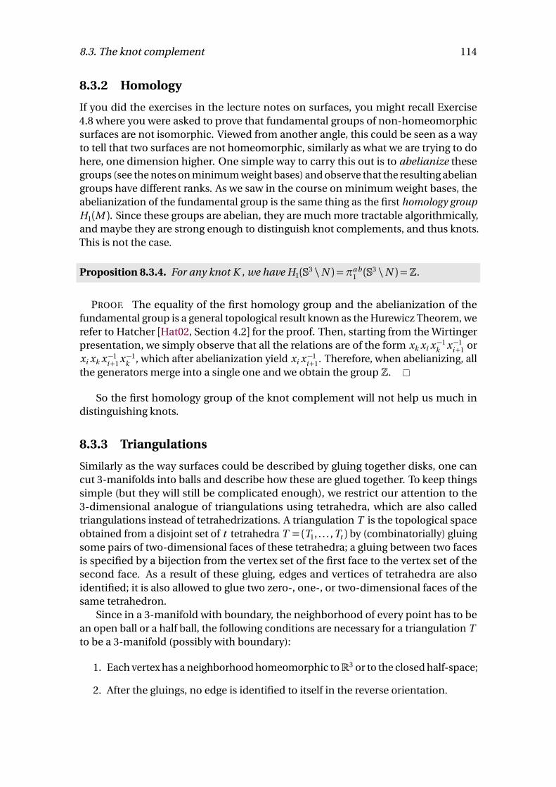
8.3. The knot complement 114
8.3.2 Homology
If you did the exercises in the lecture notes on surfaces, you might recall Exercise4.8 where you were asked to prove that fundamental groups of non-homeomorphicsurfaces are not isomorphic. Viewed from another angle, this could be seen as a wayto tell that two surfaces are not homeomorphic, similarly as what we are trying to dohere, one dimension higher. One simple way to carry this out is to abelianize thesegroups (see the notes on minimum weight bases) and observe that the resulting abeliangroups have different ranks. As we saw in the course on minimum weight bases, theabelianization of the fundamental group is the same thing as the first homology groupH1(M ). Since these groups are abelian, they are much more tractable algorithmically,and maybe they are strong enough to distinguish knot complements, and thus knots.This is not the case.
Proposition 8.3.4. For any knot K , we have H1(S3 \N ) =πa b1 (S
3 \N ) =Z.
PROOF. The equality of the first homology group and the abelianization of thefundamental group is a general topological result known as the Hurewicz Theorem, werefer to Hatcher [Hat02, Section 4.2] for the proof. Then, starting from the Wirtingerpresentation, we simply observe that all the relations are of the form xk xi x−1
k x−1i+1 or
xi xk x−1i+1 x−1
k , which after abelianization yield xi x−1i+1. Therefore, when abelianizing, all
the generators merge into a single one and we obtain the group Z.
So the first homology group of the knot complement will not help us much indistinguishing knots.
8.3.3 Triangulations
Similarly as the way surfaces could be described by gluing together disks, one cancut 3-manifolds into balls and describe how these are glued together. To keep thingssimple (but they will still be complicated enough), we restrict our attention to the3-dimensional analogue of triangulations using tetrahedra, which are also calledtriangulations instead of tetrahedrizations. A triangulation T is the topological spaceobtained from a disjoint set of t tetrahedra T = (T1, . . . , Tt ) by (combinatorially) gluingsome pairs of two-dimensional faces of these tetrahedra; a gluing between two facesis specified by a bijection from the vertex set of the first face to the vertex set of thesecond face. As a result of these gluing, edges and vertices of tetrahedra are alsoidentified; it is also allowed to glue two zero-, one-, or two-dimensional faces of thesame tetrahedron.
Since in a 3-manifold with boundary, the neighborhood of every point has to bean open ball or a half ball, the following conditions are necessary for a triangulation Tto be a 3-manifold (possibly with boundary):
1. Each vertex has a neighborhood homeomorphic toR3 or to the closed half-space;
2. After the gluings, no edge is identified to itself in the reverse orientation.
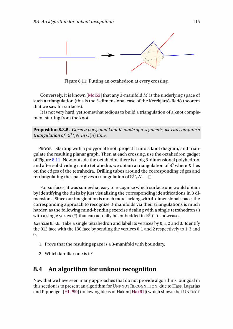
8.4. An algorithm for unknot recognition 115
Figure 8.11: Putting an octahedron at every crossing.
Conversely, it is known [Moi52] that any 3-manifold M is the underlying space ofsuch a triangulation (this is the 3-dimensional case of the Kerékjártó-Radó theoremthat we saw for surfaces).
It is not very hard, yet somewhat tedious to build a triangulation of a knot comple-ment starting from the knot.
Proposition 8.3.5. Given a polygonal knot K made of n segments, we can compute atriangulation of S3 \N in O (n ) time.
PROOF. Starting with a polygonal knot, project it into a knot diagram, and trian-gulate the resulting planar graph. Then at each crossing, use the octahedron gadgetof Figure 8.11. Now, outside the octahedra, there is a big 3-dimensional polyhedron,and after subdividing it into tetrahedra, we obtain a triangulation of S3 where K lieson the edges of the tetrahedra. Drilling tubes around the corresponding edges andretriangulating the space gives a triangulation of S3 \N .
For surfaces, it was somewhat easy to recognize which surface one would obtainby identifying the disks by just visualizing the corresponding identifications in 3 di-mensions. Since our imagination is much more lacking with 4-dimensional space, thecorresponding approach to recognize 3-manifolds via their triangulations is muchharder, as the following mind-bending exercise dealing with a single tetrahedron (!)with a single vertex (!!) that can actually be embedded in R3 (!!!) showcases.
Exercise 8.3.6. Take a single tetrahedron and label its vertices by 0, 1, 2 and 3. Identifythe 012 face with the 130 face by sending the vertices 0, 1 and 2 respectively to 1, 3 and0.
1. Prove that the resulting space is a 3-manifold with boundary.
2. Which familiar one is it?
8.4 An algorithm for unknot recognition
Now that we have seen many approaches that do not provide algorithms, our goal inthis section is to present an algorithm for UNKNOT RECOGNITION, due to Hass, Lagariasand Pippenger [HLP99] (following ideas of Haken [Hak61]) which shows that UNKNOT
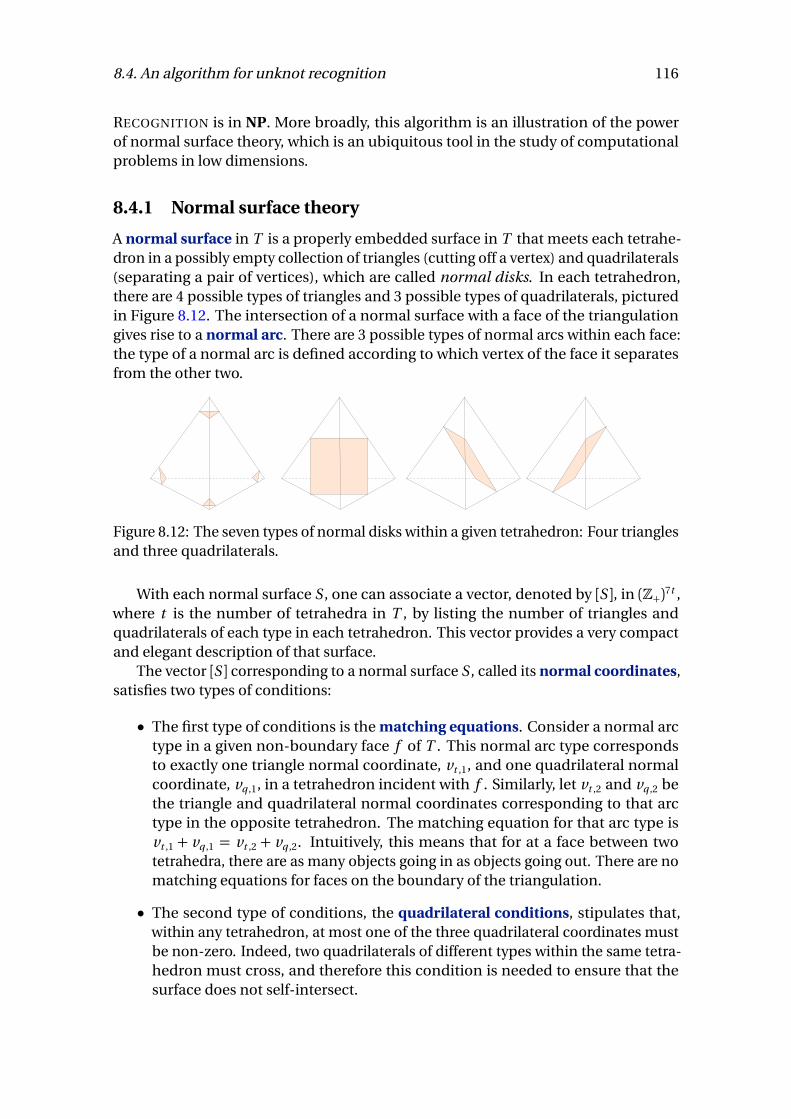
8.4. An algorithm for unknot recognition 116
RECOGNITION is in NP. More broadly, this algorithm is an illustration of the powerof normal surface theory, which is an ubiquitous tool in the study of computationalproblems in low dimensions.
8.4.1 Normal surface theory
A normal surface in T is a properly embedded surface in T that meets each tetrahe-dron in a possibly empty collection of triangles (cutting off a vertex) and quadrilaterals(separating a pair of vertices), which are called normal disks. In each tetrahedron,there are 4 possible types of triangles and 3 possible types of quadrilaterals, picturedin Figure 8.12. The intersection of a normal surface with a face of the triangulationgives rise to a normal arc. There are 3 possible types of normal arcs within each face:the type of a normal arc is defined according to which vertex of the face it separatesfrom the other two.
Figure 8.12: The seven types of normal disks within a given tetrahedron: Four trianglesand three quadrilaterals.
With each normal surface S , one can associate a vector, denoted by [S ], in (Z+)7t ,where t is the number of tetrahedra in T , by listing the number of triangles andquadrilaterals of each type in each tetrahedron. This vector provides a very compactand elegant description of that surface.
The vector [S ] corresponding to a normal surface S , called its normal coordinates,satisfies two types of conditions:
• The first type of conditions is the matching equations. Consider a normal arctype in a given non-boundary face f of T . This normal arc type correspondsto exactly one triangle normal coordinate, vt ,1, and one quadrilateral normalcoordinate, vq ,1, in a tetrahedron incident with f . Similarly, let vt ,2 and vq ,2 bethe triangle and quadrilateral normal coordinates corresponding to that arctype in the opposite tetrahedron. The matching equation for that arc type isvt ,1 + vq ,1 = vt ,2 + vq ,2. Intuitively, this means that for at a face between twotetrahedra, there are as many objects going in as objects going out. There are nomatching equations for faces on the boundary of the triangulation.
• The second type of conditions, the quadrilateral conditions, stipulates that,within any tetrahedron, at most one of the three quadrilateral coordinates mustbe non-zero. Indeed, two quadrilaterals of different types within the same tetra-hedron must cross, and therefore this condition is needed to ensure that thesurface does not self-intersect.
8.4. An algorithm for unknot recognition 117
Conversely, if T is a triangulation of size t and v is a vector in (Z+)7t , then v corre-sponds to a normal surface if and only if the matching equations and the quadrilateralconditions are fulfilled. The reconstruction process can be depicted as follows:
• In each tetrahedron, by the quadrilateral conditions, there is at most one type ofquadrilateral. One places as many parallel copies of this quadrilateral as neededin the tetrahedron, and then place the parallel triangles next to every vertex ofthe tetrahedron. It is straightforward to do so without having any intersectionbetween triangles and quadrilaterals.
• One glues the faces on the triangulation together, and in the process, one needsto glue normal arcs, i.e., triangles or quadrilaterals on the one side to trianglesand quadrilaterals on the other side. By the matching equations, the numbersfit, and the gluing is imposed by the order in which the normal disks are placedin the tetrahedra.
A normal isotopy is an ambient isotopy of M that fixes globally each vertex, edgeand face of T . Therefore, a normal surface is represented up to a normal isotopy by avector in (Z+)7t satisfying the matching equations and the quadrilateral conditions.Moreover, given a triangulation and normal coordinates, checking that the matchingequations or the quadrilateral conditions hold can trivially be done in linear time.
From this construction, one sees moreover that every vector of normal coordinatescorresponds to a unique normal surface, up to a normal isotopy. Therefore, we willoften abuse the notation and call both S and [S ] a normal surface.
Finally, if one is given normal coordinates, how can one recognize which surface itcorresponds to? For usual surfaces it is enough to compute the Euler characteristic andcheck for orientability, but there is an issue of compression here: a vector of complexityn can correspond to a normal surface with 2n normal disks, and thus computing theEuler characteristic “by hand” would take an exponential time. But one can do better:
Lemma 8.4.1. There exists a linear form e onZ7t+ such that if [S ] is the coordinate vector
of a normal surface S, e ([S ]) =χ(S )where χ is the Euler characteristic.
PROOF. A normal coordinate describes the number of normal triangles or quadri-laterals of some type in a tetrahedron. One can estimate how much such a triangle orquadrilateral contributes to the Euler characteristic of the entire surface. Let us pick atriangular normal disk t adjacent to edges e1, e2 and e3 of T , and let us denote by vi
the valence of edge ei , i.e., the number of tetrahedra around it. Then the contributionof t to the Euler characteristic of S is 1/v1+ 1/v2+ 1/v3− 3/2− e∂ /2+ 1, where e∂ isthe number of edges of t on the boundary of the manifold. Indeed, the vertices oft (on the edges e1, e2 and e3) contribute 1 but are “shared” between all the normaldisks adjacent to them. Similarly, the edges contribute −1 but are shared between twonormal disks (except for the boundary ones), and the face contribution is exactly once.For a quadrilateral, we get 1/v1+1/v2+1/v3+1/v4−4/2−e∂ /2+1. Summing all of thesecontributions provides a linear form e which matches with the Euler characteristic.

8.4. An algorithm for unknot recognition 118
8.4.2 Trivial knot and spanning disks
The apparatus of normal surface theory is designed to study the surfaces embeddedin a 3-manifold. In the case of knot complements, this is very relevant to unknotrecognition because of the following easy lemma.
Lemma 8.4.2. A knot K is trivial if and only if it is the boundary of an embedded disk.
PROOF. One direction is immediate: if K is trivial, then it is ambient isotopic tothe usual embedding of S1, which obviously bounds a disk. An ambient isotopy is ahomeomorphism, thus it preserves this disk, so the knot K also bounds a disk.
The other direction is not much harder: if a knot K bounds a disk, then there isan ambient isotopy that contracts K progressively along this disk until it lies in anarbitrarily small neighborhood of a point, where it will be ambient isotopic to a usualembedding of S1.
The starting idea of the algorithm for UNKNOT RECOGNITION is to simply find thisdisk if it exists. But the triangulation we will work with S3 \N (K ) instead of just S3 withK in its 1-skeleton. This is very much needed in order to apply normal surface theory:indeed, we will want to find this disk as a normal surface, and normal surfaces are byconstruction transverse to the 1-skeleton of the triangulation. Therefore, one needs todrill a small tube around K in order to use normal surfaces, we denote this small tubeby TK . The corresponding lemma that we will need is the following one.
Lemma 8.4.3 ([HLP99, Lemma 4.1]). A knot K is trivial if and only if there exists a diskD in S3 \N (K ) such that the boundary of D is non-trivial in ∂ TK .
PROOF. The proof works similarly: If K is trivial, there is an ambient isotopy car-rying it to the standard embedding of S1 intoR3. This ambient isotopy preserves thetrivializing disk and the homotopy class of its boundary on ∂ Tk , which is thereforenon-trivial.
The other direction requires some more work. A meridian of a knot is a simpleclosed curve on TK bounding a disk in TK . A longitude of a knot is a simple closed curveon TK crossing the meridian exactly once, and inducing a null-homologous curve inS3 \N (K ). The existence of these curves follows, for example from the computation ofH1(S3 \N (K )) in Section 8.3.2.
If K is non-trivial, let us assume by contradiction that there exists a disk D havingboundary γ non-trivial on ∂ TK . The homology of γ on ∂ TK is a1[m ] + a2[`] witha1, a2 6= (0,0)where [m ] and [`] denote the homology classes induced on ∂ TK by themeridian and the longitude, respectively. Via the inclusion map ∂ Tk ,→ S3 \N (K ), γhas a homology class in H1(S3\N (K )), which is a1 by definition of the meridian and thelongitude. Since γ bounds a disk, we thus have a1 = 0, and thus a2 =±1 by simplicityof γ. Therefore K cobounds an annulus with γ within TK . Gluing this annulus withthe disk D , we obtain a disk bounded by K and we can apply the previous lemma.
Let us call a disk satisfying the above properties a spanning disk. The key theorembehind the NP algorithm is the following one.
8.4. An algorithm for unknot recognition 119
Theorem 8.4.4. Let K be a trivial knot and T be a triangulation of S3 \N (K ) obtainedby the process of Section 8.3.3. Then there exists a spanning disk of K that is normalwith respect to T and of which normal coordinates are bounded by 2O (t ).
Assuming Theorem 8.4.4 for now, we can (almost) provide the advertised algorithm.Naively, this should be very simple: now that we have established that there exists aspanning disk that is normal and has coordinates of bounded size, one can simply usethis spanning disk (or rather its normal coordinates) as a certificate. The size of thecoordinates might be exponential, but exponential numbers can be encoded usingonly a polynomial number of bits (this trivial observation is what makes everythingwork!), thus the certificate has polynomial size. But there is a hidden issue lurking here:one also needs to verify in polynomial time that the certificate is indeed a spanningdisk. This should be easy in principle, but as we have already mentioned, the certificateis very compressed due to this integer encoding, and it turns out to be non-trivial.
Corollary 8.4.5. UNKNOT RECOGNITION is in NP.
PROOF. Starting with a knot K , described by a diagram with n crossings, one firstbuilds a triangulation of its complement following Section 8.3.3. This triangulationhas O (n ) tetrahedra. The certificate is then the normal spanning disk promised byTheorem 8.4.4. It is a vector in O (n ) dimensions and the size of the coordinates isbounded by 2O (n ), which can be encoded with a number of bits polynomial in n .
Once one is given the certificate, one can verify that is it indeed a spanning disk inthe following way:
1. One first verifies that this is indeed a normal surface S , by checking that thematching and quadrilateral constraints are satisfied.
2. One checks whether S is connected.
3. One checks whether S is a disk.
4. One checks whether the boundary of S is non-contractible.
If all the answers are positive, then we have a spanning disk and K is unknotted.Step 1 can be easily done in polynomial time since the matching equations are linear,and the quadrilateral constraints are easy to verify by looking at each coordinates. Letus assume that Step 2 has been done for now. In order to do step 3, it is enough tocompute the Euler characteristic of S , which can be done in polynomial time usingthe linear form of Lemma 8.4.1. For step 4, from the normal coordinates of S one canobtain normal coordinates3 of ∂ S . Since the fundamental group of the torus is Z2,testing whether ∂ S is contractible can be done in polynomial time from these normalcoordinates.
3More formally, ∂ S is a curve on a torus, and the coordinates we obtain describe this curve withrespect to the triangulation of the torus inherited from T . The underlying theory of normal curves issimilar (but much simpler) than for normal surfaces.
8.4. An algorithm for unknot recognition 120
However, Step 2 is hard. The naive algorithm, which would just follow a startingnormal disk and count the resulting connected components could require exponentialtime, since the size of the normal coordinates could be exponential. A polynomialalgorithm to check connectivity of normal surfaces was designed by Agol, Hass andThurston [AHT06] and can be used here, but we will not delve into this.
The rest of this section is devoted to the proof of Theorem 8.4.4. We first show howto normalize a spanning disk, and then how to prove the existence of one with suitablybounded coordinates.
8.4.3 Normalization of spanning disks
A key observation, initially due to Haken [Hak61], is that there exists a spanning diskthat is a normal surface:
Lemma 8.4.6. Let K be a trivial knot and T be a triangulation of S3 \N (K ) obtainedby the process of Section 8.3.3. Then there exists a spaning disk that is normal withrespect to T .
PROOF. The proof proceeds by starting with a spanning disk D (which exists byLemma 8.4.3) and normalizing it. We can first, by using a small perturbation, putD in general position with respect to the triangulation T : i.e., all the intersectionsbetween D and T can be assumed to be transverse. Now, we look at what can gowrong, i.e., which pieces in D are not normal with respect to T . Let us write c (D ) =(wt1(D ), wt2(D )), where wt1 and wt2 respectively denote the number of connectedcomponents of the intersection of D with the edges of T and the faces of T , and orderthe pairs c (D )with the lexicographic order. There are many different occurences ofnon-normality which we deal with distinct moves, but each time the complexity c (D )will only go down. Since this complexity is finite to begin with, after a finite number ofsteps, the process will finish and we will have a normal surface.
1. If D intersects an inner face F of T in an arc that hits twice the same interioredge e of T , one can push D locally to reduce its number of intersections withe , see Figure 8.13.
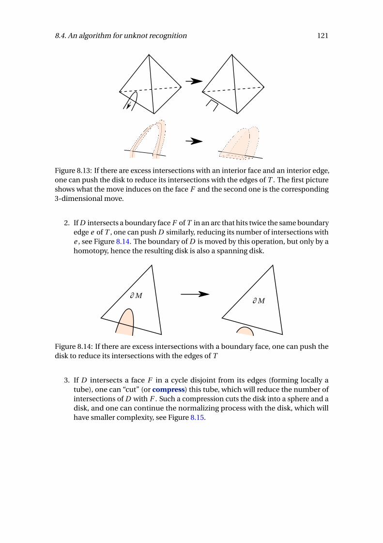
8.4. An algorithm for unknot recognition 121
Figure 8.13: If there are excess intersections with an interior face and an interior edge,one can push the disk to reduce its intersections with the edges of T . The first pictureshows what the move induces on the face F and the second one is the corresponding3-dimensional move.
2. If D intersects a boundary face F of T in an arc that hits twice the same boundaryedge e of T , one can push D similarly, reducing its number of intersections withe , see Figure 8.14. The boundary of D is moved by this operation, but only by ahomotopy, hence the resulting disk is also a spanning disk.
∂M∂M
Figure 8.14: If there are excess intersections with a boundary face, one can push thedisk to reduce its intersections with the edges of T
3. If D intersects a face F in a cycle disjoint from its edges (forming locally atube), one can “cut” (or compress) this tube, which will reduce the number ofintersections of D with F . Such a compression cuts the disk into a sphere and adisk, and one can continue the normalizing process with the disk, which willhave smaller complexity, see Figure 8.15.
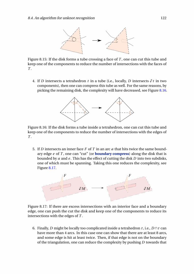
8.4. An algorithm for unknot recognition 122
Figure 8.15: If the disk forms a tube crossing a face of T , one can cut this tube andkeep one of the components to reduce the number of intersections with the faces ofT .
4. If D intersects a tetrahedron t in a tube (i.e., locally, D intersects ∂ t in twocomponents), then one can compress this tube as well. For the same reasons, bypicking the remaining disk, the complexity will have decreased, see Figure 8.16.
Figure 8.16: If the disk forms a tube inside a tetrahedron, one can cut this tube andkeep one of the components to reduce the number of intersections with the edges ofT .
5. If D intersects an inner face F of T in an arc a that hits twice the same bound-ary edge e of T , one can “cut” (or boundary compress) along the disk that isbounded by a and e . This has the effect of cutting the disk D into two subdisks,one of which must be spanning. Taking this one reduces the complexity, seeFigure 8.17.
∂M
F
∂M
F
Figure 8.17: If there are excess intersections with an interior face and a boundaryedge, one can push the cut the disk and keep one of the components to reduce itsintersections with the edges of T .
6. Finally, D might be locally too complicated inside a tetrahedron t , i.e., D ∩ t canhave more than 4 arcs. In this case one can show that there are at least 8 arcs,and some edge is hit at least twice. Then, if that edge is not on the boundaryof the triangulation, one can reduce the complexity by pushing D towards that
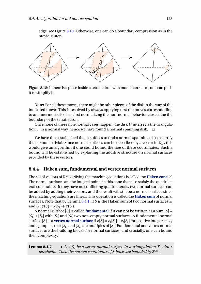
8.4. An algorithm for unknot recognition 123
edge, see Figure 8.18. Otherwise, one can do a boundary compression as in theprevious step.
Figure 8.18: If there is a piece inside a tetrahedron with more than 4 arcs, one can pushit to simplify it.
Note: For all these moves, there might be other pieces of the disk in the way of theindicated move. This is resolved by always applying first the moves correspondingto an innermost disk, i.e., first normalizing the non-normal behavior closest the theboundary of the tetrahedron.
Once none of these non-normal cases happen, the disk D intersects the triangula-tion T in a normal way, hence we have found a normal spanning disk.
We have thus established that it suffices to find a normal spanning disk to certifythat a knot is trivial. Since normal surfaces can be described by a vector in Z7t
+ , thiswould give an algorithm if one could bound the size of these coordinates. Such abound will be established by exploiting the additive structure on normal surfacesprovided by these vectors.
8.4.4 Haken sum, fundamental and vertex normal surfaces
The set of vectors ofR7t+ verifying the matching equations is called the Haken coneC .
The normal surfaces are the integral points in this cone that also satisfy the quadrilat-eral constraints. It they have no conflicting quadrilaterals, two normal surfaces canbe added by adding their vectors, and the result will still be a normal surface sincethe matching equations are linear. This operation is called the Haken sum of normalsurfaces. Note that by Lemma 8.4.1, if S is the Haken sum of two normal surfaces S1
and S2, χ(S ) =χ(S1) +χ(S2).A normal surface [S ] is called fundamental if it can not be written as a sum [S ] =
[S1] + [S2]with [S1] and [S2] two non-empty normal surfaces. A fundamental normalsurface [S ] is a vertex normal surface if c [S ] = c1[S1] + c2[S2] for positive integers c , c1
and c2 implies that [S1] and [S2] are multiples of [S ]. Fundamental and vertex normalsurfaces are the building blocks for normal surfaces, and crucially, one can boundtheir complexity:
Lemma 8.4.7. • Let [S ] be a vertex normal surface in a triangulation T with ttetrahedra. Then the normal coordinates of S have size bounded by 2O (t ).
8.4. An algorithm for unknot recognition 124
• Let [S ] be a fundamental normal surface in a triangulation T with t tetrahedra.Then the normal coordinates of S have size bounded by 2O (t ).
PROOF. • Let us intersect the coneC with the hyperplane H =∑
i xi = 1. Thisforms a polyhedronP and the vertex normal surfaces will be obtained as thefirst integral multiples of some of the vertices ofP . Now, the vertices ofP areobtained as a solution of 7t equations, which either come from the matchingequations, from the hyperplane H or from a hyperplane of the form xi = 0.Thus, such a vertex v verifies M v = (0, . . . , 0, 1)T for some matrix M with entriesin {−1,0,1}. By Cramer’s rule, the coordinates vi are obtained by the quotientdet Mi/det M , where Mi is the matrix M where the i th column has been replacedby (0, . . . 0, 1)T . One can bound these determinants using Hadamard’s inequality(det M )2 ≤
∏
i ||ri ||2 where ri are the rows of M . We obtain |det Mi | = 2O (t ) and|det M |= 2O (t ), and thus vi = 2O (t ). Then, the size of the coordinates of the vertexnormal surfaces is bounded by vi |det M |= 2O (t ) as well.
• Let [S ] be a fundamental normal surface, then multiples of [S ] can be decom-posed on the vertex normal surfaces: c [S ] =
∑
ci [Si ], or equivalently [S ] =∑
ci/c [Si ]. Note that ci/c ≤ 1, otherwise one would have [S ] = ([S ]− [Si ]) + [Si ]which would be a non-trivial integral decomposition of S , a contradiction. Thusany coordinate of [S ] is at most the sum of the coordinates of the vertex normalsurfaces [Si ], of which there are at most 2O (t ) (one can for example bound thenumber of matrices M involved in the previous item). This concludes the proof.
A common principle in normal surface theory is that “interesting” surfaces in a 3-manifold can be found among the fundamental normal surfaces, and even sometimesamong the vertex normal surfaces of the triangulation. This turns out to be true forspanning disks.
Proposition 8.4.8. Let K be a trivial knot and T be a triangulation of S3 \N (K )obtained by the process of Section 8.3.3. Then there exists a spanning disk that is afundamental normal surface with respect to T .
Combining Lemma 8.4.7 and Proposition 8.4.8 directly proves Theorem 8.4.4, andthus the NP algorithm (modulo the connectivity issue already mentioned).
Remark: The main issue in the NP algorithm is to check connectivity in polynomialtime. One way to circumvent it could be to verify that the certificate describes afundamental normal surface, since fundamental normal surfaces are connected. Butthere is no easy way to do that either. On the other hand, one can certify that a normalsurface is a vertex normal surface, by exhibiting the family of 7t equations it satisfies(see the proof of Lemma 8.4.7). And it is also true, but harder to prove, that there existsa spanning disk that is a vertex normal surface: we refer to Jaco and Tollefson [JT95] fora proof. Thus, if one admits this, it gives an alternative way to provide a NP certificate.
There remains to prove Proposition 8.4.8.
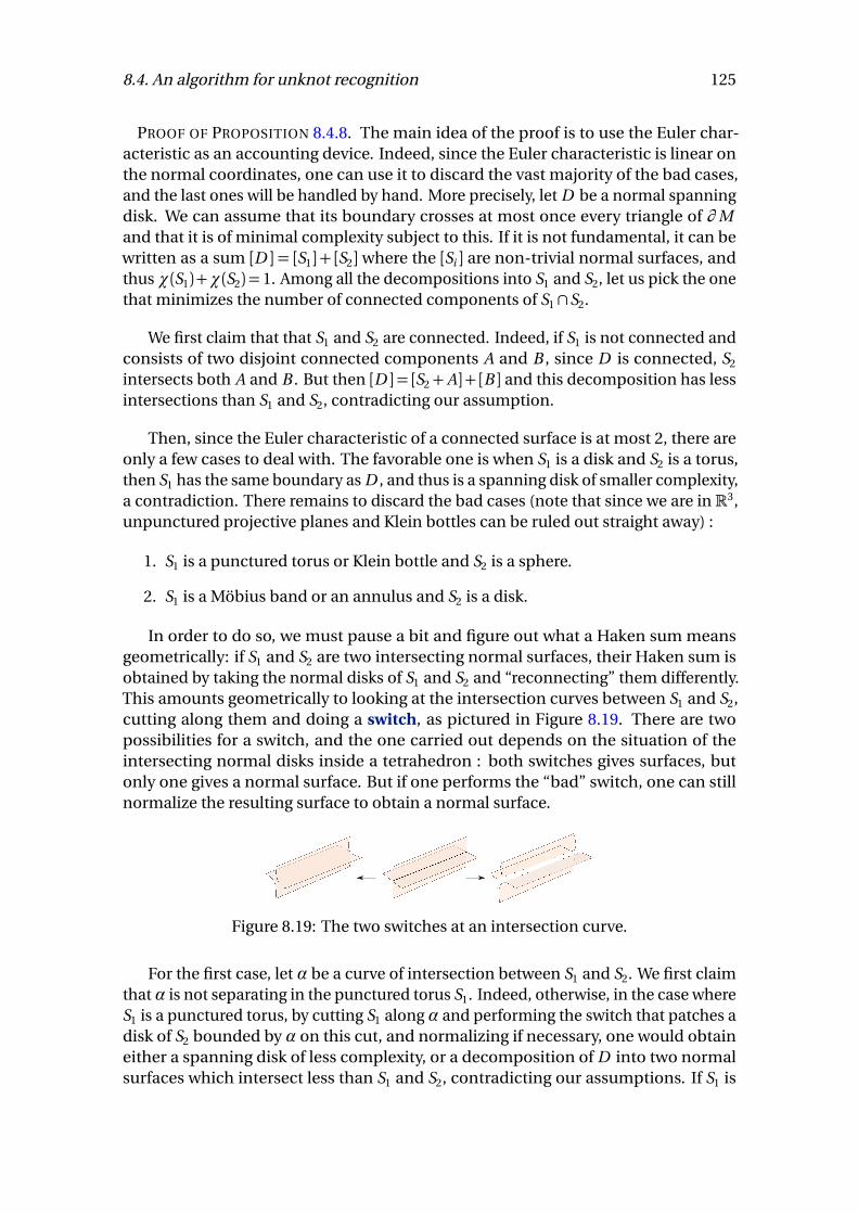
8.4. An algorithm for unknot recognition 125
PROOF OF PROPOSITION 8.4.8. The main idea of the proof is to use the Euler char-acteristic as an accounting device. Indeed, since the Euler characteristic is linear onthe normal coordinates, one can use it to discard the vast majority of the bad cases,and the last ones will be handled by hand. More precisely, let D be a normal spanningdisk. We can assume that its boundary crosses at most once every triangle of ∂Mand that it is of minimal complexity subject to this. If it is not fundamental, it can bewritten as a sum [D ] = [S1] + [S2] where the [Si ] are non-trivial normal surfaces, andthus χ(S1)+χ(S2) = 1. Among all the decompositions into S1 and S2, let us pick the onethat minimizes the number of connected components of S1 ∩S2.
We first claim that that S1 and S2 are connected. Indeed, if S1 is not connected andconsists of two disjoint connected components A and B , since D is connected, S2
intersects both A and B . But then [D ] = [S2+A] + [B ] and this decomposition has lessintersections than S1 and S2, contradicting our assumption.
Then, since the Euler characteristic of a connected surface is at most 2, there areonly a few cases to deal with. The favorable one is when S1 is a disk and S2 is a torus,then S1 has the same boundary as D , and thus is a spanning disk of smaller complexity,a contradiction. There remains to discard the bad cases (note that since we are inR3,unpunctured projective planes and Klein bottles can be ruled out straight away) :
1. S1 is a punctured torus or Klein bottle and S2 is a sphere.
2. S1 is a Möbius band or an annulus and S2 is a disk.
In order to do so, we must pause a bit and figure out what a Haken sum meansgeometrically: if S1 and S2 are two intersecting normal surfaces, their Haken sum isobtained by taking the normal disks of S1 and S2 and “reconnecting” them differently.This amounts geometrically to looking at the intersection curves between S1 and S2,cutting along them and doing a switch, as pictured in Figure 8.19. There are twopossibilities for a switch, and the one carried out depends on the situation of theintersecting normal disks inside a tetrahedron : both switches gives surfaces, butonly one gives a normal surface. But if one performs the “bad” switch, one can stillnormalize the resulting surface to obtain a normal surface.
Figure 8.19: The two switches at an intersection curve.
For the first case, let α be a curve of intersection between S1 and S2. We first claimthat α is not separating in the punctured torus S1. Indeed, otherwise, in the case whereS1 is a punctured torus, by cutting S1 along α and performing the switch that patches adisk of S2 bounded by α on this cut, and normalizing if necessary, one would obtaineither a spanning disk of less complexity, or a decomposition of D into two normalsurfaces which intersect less than S1 and S2, contradicting our assumptions. If S1 is
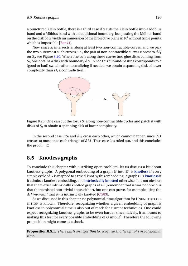
8.5. Knotless graphs 126
a punctured Klein bottle, there is a third case if α cuts the Klein bottle into a Möbiusband and a Möbius band with an additional boundary, but pasting the Möbius bandon the disk of S2 yields an immersion of the projective plane inR3 without triple points,which is impossible [Ban74].
Now, since S1 intersects S2 along at least two non-contractible curves, and we pickthe two outermost such curves, i.e., the pair of non-contractible curves closest to ∂ S1
on S1, see Figure 8.20. When one cuts along these curves and glue disks coming fromS2, one obtains a disk with boundary ∂ S1. Since this cut-and-pasting corresponds to a(good or bad) switch, after normalizing if needed, we obtain a spanning disk of lowercomplexity than D , a contradiction.
Figure 8.20: One can cut the torus S1 along non-contractible cycles and patch it withdisks of S2 to obtain a spanning disk of lower complexity.
In the second case, ∂ S2 and ∂ S1 cross each other, which cannot happen since ∂ Dcrosses at most once each triangle of ∂M . Thus case 2 is ruled out, and this concludesthe proof.
8.5 Knotless graphs
To conclude this chapter with a striking open problem, let us discuss a bit aboutknotless graphs. A polygonal embedding of a graph G into R3 is knotless if everysimple cycle of G is mapped to a trivial knot by this embedding. A graph G is knotless ifit admits a knotless embedding, and intrinsically knotted otherwise. It is not obviousthat there exist intrinsically knotted graphs at all (remember that is was not obviousthat there existed non-trivial knots either), but one can prove, for example using theArf invariant that K7 is intrinsically knotted [CG83].
As we discussed in this chapter, no polynomial-time algorithm for UNKNOT RECOG-NITION is known. Therefore, recognizing whether a given embedding of graph isknotless in polynomial time is also out of reach for current techniques. One couldexpect recognizing knotless graphs to be even harder since naively, it amounts tomaking this test for every possible embedding of G into R3. Therefore the followingproposition might come as a shock.
Proposition 8.5.1. There exists an algorithm to recognize knotless graphs in polynomialtime.

8.5. Knotless graphs 127
PROOF. If H is a minor of G and G is knotless, H is knotless as well: if i is a knotlessembedding of G , every simple cycle of H corresponds to a simple cycle of G and is thusmapped by i to a trivial knot. Thus knotless graphs form a minor-closed family, and itfollows from Robertson-Seymour theory (see for example [Lov05] for an introduction)that they can be recognized in polynomial time.
The proof of this proposition is shockingly unsatisfying: not only is the algorithm,as most algorithms coming from Robertson-Seymour theory, extremely inefficient, butwe actually do not know what it is: what the theory proves is that minor-closed familiesare characterized by a finite family of forbidden minors, and testing for forbiddenminors can be done in polynomial time – but we do not know what these are. It isan open problem to find an explicit polynomial-time algorithm to recognize knotlessgraphs.
9
Undecidability in Topology
Contents9.1 The Halting Problem . . . . . . . . . . . . . . . . . . . . . . . . . . . . . . . . . . 129
9.1.1 Turing Machines . . . . . . . . . . . . . . . . . . . . . . . . . . . . . . . . . 129
9.1.2 Undecidability of the Halting Problem . . . . . . . . . . . . . . . . . 130
9.2 Decision Problems in Group Theory . . . . . . . . . . . . . . . . . . . . . . 131
9.3 Decision Problems in Topology . . . . . . . . . . . . . . . . . . . . . . . . . . 134
9.3.1 The Contractibility and Transformation Problems . . . . . . . . . 134
9.3.2 The Homeomorphism Problem . . . . . . . . . . . . . . . . . . . . . . 136
9.4 Proof of the Undecidability of the Group Problems . . . . . . . . . . . . 139
9.4.1 Z2-Machines . . . . . . . . . . . . . . . . . . . . . . . . . . . . . . . . . . . . 139
9.4.2 Useful Constructs in Combinatorial Group Theory . . . . . . . . 140
9.4.3 Undecidability of the Generalized Word Problem . . . . . . . . . . 141
The purpose of this lecture is to make explicit the limits of computational topologyby showing that some simple and natural questions in topology are undecidable. Inorder to make the statement precise we need to define the notion of decidability andto specify the description of topological spaces we are interested in. Concerning topo-logical spaces we should consider spaces having a combinatorial description suchas finite simplicial complexes1. Note that many interesting spaces have such a de-scription: compact topological manifolds of dimensions 2 or 3, compact differentiablemanifolds, etc. See [Man14] for a survey. Concerning decidability there are essentiallytwo notions. One refers to the independence of a statement with respect to a logicalsystem. In other words, the statement is undecidable if neither its affirmation nor
1Recall that a simplicial complex is a collection of simplices glued in a nice fashion. It is the totalspace of an abstract simplicial complex over a set V , which is a family of subsets of V closed under theoperation of taking non-empty subsets.
128
9.1. The Halting Problem 129
its negation can be proved from the axioms of the system using its logical rules. Theexistence of such undecidable statements relates to the first Gödel’s incompletenesstheorem. The other notion of decidability refers to a family of problems with YES/NOanswers, such as testing a property over a family of objects, and expresses the exis-tence of an algorithm to output the answer of any problem in the family. Note thatany finite family of problems for which the answers is provable is always decidablein this acception. Indeed, an algorithm to solve the problems just needs to store thecorrect answer of each problem. Paradoxically, this is valid even if we do not know yetthe correct answers since the decidability only claims the existence of an algorithmand not the algorithm itself.
Both notions of decidability may be relevant to computational topology. As anillustration, consider the contractibility problem of deciding if a closed path can becontinuously deformed into a point in a simplicial complex. We will prove that thereis no algorithm to decide this problem given the path and the simplicial complex asinput. As a stronger statement there exists a simplicial complex for which there is noalgorithm that decides the contractibility of the closed paths in this simplicial complex.At last, there exists a closed path in some simplicial complex for which it cannot belogically decided if the path is contractible or not.
Most often, undecidability results in topology are shown by first transforming adecision problem into a question concerning combinatorial group theory. In turn,problems about groups are transformed into problems about Turing machines. Ul-timately, the proofs of undecidability rely on a reduction to the halting problem forTuring machines. We recommend the survey by Poonen [Poo14] for many undecidableproblems in mathematics.
9.1 The Halting Problem
9.1.1 Turing Machines
A Turing machine is a mathematical model for the notion of computation. It wasintroduced by Alan Turing in 1936. According to Church-Turing thesis this is a universalmodel for the mechanization of computation. It was proved equivalent to other notionof computation such as recursive functions and λ-calculus.
Formally, a Turing machine is a triple (A ,Q,T ), where A is a finite alphabetincluding a special blank character,Q is a finite set of states, andT ⊂A×Q×A×Q×{R , L} is a transition table specifying how the machine operates on configurations.Those are words of the form uq v ∈A ∗×Q×A ∗. Such a configuration represents themachine in state q together with a linear tape marked with the word u v and whoseread/write head is on the first letter in v (the empty word is interpreted as a blank).Transition a q b p D ∈T applies to any configuration uq v such that a is the first letterin v . It transforms uq v replacing a with b , the state q by p , and moves the head onestep to the left or right according to whether D equals L or R , respectively.
From the computability perspective there is no loss of generality to consider deter-ministic machines for which a q b p D ∈ T and a q b ′p ′D ′ ∈ T implies b ′ = b , p ′ = pand D ′ =D : reading a letter in some state leads to only one new possible configuration.The machine is halting in a given configuration when no transition applies.
9.1. The Halting Problem 130
Standard coding of Turing machines
A Turing Machine M is in standard form if its alphabet is a finite subset ofΣ = {blank,1,1′,1′′,1′′′, . . .} and its set of states is a finite subset of {q , q ′, q ′′, q ′′′, . . .}.One can encode the transition table of M on the six letter alphabet {blank, 1, q ,′ , R , L}by concatenating its transitions (of the form 1′q ′1′′q ′′D ), where the prime symbol isconsidered as a letter. Finally, replacing q ,′ , R , L by the respective letters 1′, 1′′, 1′′′, 1′′′′,we obtain a coding of the transition table over the finite alphabet {blank, 1, 1′, 1′′, 1′′′, 1′′′′}.This coding is the standard code of M and is denoted by dM e.
9.1.2 Undecidability of the Halting Problem
A set of words W ⊂ A ∗ is decidable, or recursive, if there exists a turing machineM = (A ,Q,T ) with three states qi , qa , qr ∈ Q, respectively called initial, acceptingand rejecting, such that for every w ∈A ∗ the machine M starting from configurationqi w reaches a halting configuration in state qa if w ∈W and in state qr otherwise.In particular M always reaches a halting configuration. Note that W is decidableif and only if both W and its complementA ∗ \W are semi-decidable. Recall thatW is semi-decidable if there exists a Turing machine halting in an accepting state ifand only if it is given as input a word of W . Although this definition does not requireany behavior for words not in W , it is equivalent to assume that the machine neverstops given such words. Unfortunately, the same definition was given many namessuch as semi-recursive, recursively enumerable, computably enumerable, listableor Turing recognizable. The plurality of names comes from the fact that it is equivalentto require the existence of a Turing machine that enumerates W , i.e., outputs all itswords one after the other. A decision problem is a set of questions with YES/NOanswers. By extension this problem is decidable, or algorithmically solvable, if thequestions can be encoded as words over a finite alphabet and if the subset of wordscorresponding to questions with positive answers is decidable.
Consider the self-halting problem of deciding if a Turing machine M given asinput its own standard code, i.e. starting with the configuration qi dM e, will eventuallyreach a halting configuration in the accepting state.
Theorem 9.1.1. The self-halting problem is semi-decidable but not decidable.
PROOF. That the self-halting problem is semi-decidable is quite clear. Given thestandard code of a Turing machine, it is enough to simulate the corresponding machineon this same input. The notion of universal Turing machine (see below) provides such asimulation. By way of contradiction, suppose that the self-halting problem is decidable.Hence, there exists a Turing machine, say S , that recognizes the complementarylanguage. In other words, S halts in the accepting case if the input does not correspondto the standard code of a Turing machine that halts in the accepting state on its owninput, and runs forever otherwise. Let us run S with the initial configuration qi dS e. If Shalts in the accepting state, this means that S does not halt in the accepting state onits own input, a contradiction. So S must run forever, meaning that S does halt in theaccepting state on its own input, and we have again reached a contradiction.
9.2. Decision Problems in Group Theory 131
The general halting problem is to decide, given a machine M and a starting con-figuration I if M reaches a halting configuration. Since the self-halting problem is aparticular case of the halting problem, we obtain:
Corollary 9.1.2. The halting problem is unsolvable.
Universal Turing Machine
A Turing machine T is said universal if for any Turing machine M and any initialconfiguration C , starting from configuration qi dM eC the machine T simulates thecomputation of M from C and halts in its accepting state if and only if this computationeventually stops. Though fastidious, one can write a program in his favourite language,say in C++, to simulate a universal Turing machine. This proves a fortiori its existence.The idea is to traverse the initial configuration C to “read” its state and the currentsymbol (the one that should lie under the reading head of M ). Then, T needs totraverse dM e in order to find the transition that applies. This transition transformsC into a configuration C ′ and we obtain the configuration qi dM eC ′ on T . We canproceed this way until some configuration qi dM eC ′′ is reached, where C ′′ is a haltingconfiguration for M . In this case, T should stop in its accepting state. Otherwise, Truns forever.
Theorem 9.1.3. The halting problem for the universal machine T is unsolvable.
In other words, there is no Turing machine that can decide for any configuration ifT eventually stops starting from this configuration. Indeed, such a Turing machinewould solve the general halting problem by considering configurations of the formqi dM eC .
9.2 Decision Problems in Group Theory
Max Dehn (1911) was among the first to work out the connection between topology andcombinatorial group theory. He made explicit that answering to certain topologicalquestions about spaces could be used to solve some general problems about grouppresentations. Recall that a combinatorial presentation ⟨S |R ⟩ of a group G is definedby a set S of generators and a set R of words over2 S , called relations, so that G is thequotient of the free group F (S ) over S by the normal closure of R in F (S ). Hence, theelements of G are classes of words over S where two words are in the same class if onecan be transformed into the other by a sequence of insertions or removals of
1. factors s s−1 with s ∈ S ,
2. or words in R or their inverses.
We shall only consider finitely presented groups for which S and R are both finite. Mostcomputational results nonetheless apply to recursively presented groups whose set ofrelations are recursively enumerable.
2By a word over S we always mean a finite sequence of elements in S ∪S−1, where the elements ofS−1 should be thought of as the inverses of the elements in S .
9.2. Decision Problems in Group Theory 132
Tietze Tranformations
Clearly, a group has (infinitely) many presentations. One can indeed replace a pre-sentation ⟨S |R ⟩ by applying the following Tietze transformations or their inverses toobtain presentations of the same group.
T1: Add a relation which is a consequence of R .
T2: Add a new generator s with a new relation s w , where w is any word over S .
It is quite remarkable that presentations of the same group are always related bysuch transformations.
Theorem 9.2.1. Two finite presentations represent the same group if and only if onecan be obtained from the other by a finite sequence of Tietze transformations and theirinverses.
PROOF. Let ⟨S | R ⟩ and ⟨S ′ | R ′⟩ be two presentations of the same group. In otherwords, there is an isomorphism ⟨S ′ | R ′⟩ ∼= ⟨S | R ⟩. The image of any generator s ′ ∈ S ′
under this isomorphism can be expressed as a word s ′(S ) over S . Remark that therelations in R ′ are consequences of R and the relations {s ′ · (s ′(S ))−1}s ′∈S ′ expressingeach generator s ′ in terms of S (why?). For each generator s ∈ S , we define s (S ′)analogously. We have,
⟨S |R ⟩ ∼= ⟨S ∪S ′ |R ∪{s ′ · (s ′(S ))−1}s ′∈S ′⟩ by repeated applications of T2
∼= ⟨S ∪S ′ |R ∪R ′ ∪{s ′ · (s ′(S ))−1}s ′∈S ′⟩ by repeated applications of T1
∼= ⟨S ∪S ′ |R ∪R ′ ∪{s ′ · (s ′(S ))−1}s ′∈S ′ ,{s · (s (S ′))−1}s∈S ⟩ by repeated applications of T1
This last presentation is symmetric in prime and unprime symbols and could thushave been derived from ⟨S ′ |R ′⟩.
Exercise 9.2.2. By a consequence of R it is meant a word r on S representing an elementof the normal closure of R . Show that r is freely equivalent (i.e., inserting or removings s−1 or s−1s factors) to a word of the form
k∏
j=1
g j rε j
j g −1j ,
where the g j are words over S , r j ∈R , and ε j ∈ {−1, 1}.Exercise 9.2.3. Show that the Tietze transformations T1 and T2 indeed produce isomor-phic groups. In other words, show that:
⟨S |R ⟩ ∼= ⟨S |R ∪{r }⟩ ∼= ⟨S ∪{s } |R ∪{s w }⟩,
where r is a consequence of R .
9.2. Decision Problems in Group Theory 133
Dehn’s Problems
Dehn identified three fundamental algorithmic problems [Sti87]. Let G = ⟨S |R ⟩ be afinitely presented group.
• The word problem: decide if a word over S represents the identity in G .
• The conjugacy problem: decide if two words over S represent conjugate ele-ments in G .
• The isomorphism problem: decide if two combinatorial presentations repre-sent isomorphic groups.
In the late 1940’s Markov and Post independently proved that the word problemin semi-groups is unsolvable. The main idea is to encode the transition of a Turingmachine as relations in a semi-group. In the end the halting problem becomes equiv-alent to the word problem in the constructed semi-group. The unsolvability of theword problem for groups is based on similar ideas but singularly more complex. Itwas eventually shown by P. S. Novikov in 1955 and almost at the same time by Boone.The original article by Novikov was 143 pages long. Thanks to the HNN constructionintroduced by Higman, Neeumann and Neumann in 1949, Boone (1959) and Britton(1963) succeeded to reduce the proof to approximately 10 pages.
Theorem 9.2.4 (Novikov, Boone). There exists a group for which the word problem isunsolvable. In particular, the word problem for groups (given a group and a word asinput) is unsolvable.
The simplest example of a group with unsolvable word problem has 4 generatorsand 12 relations, see Borisov [Bor69]. Since the word problem is a particular case ofthe conjugacy problem, we immediately infer that
Corollary 9.2.5. The conjugacy problem for groups is unsolvable.
The generalized word problem is to decide if a word over the generators S of apresentation P belongs to some subgroup of P specified by a set of generators givenas words over S .
Theorem 9.2.6. The generalized word problem is unsolvable.
Theorem 9.2.7 (Adyan 1957, Rabin 1958). The isomorphism problem for groups isunsolvable.
A Markov property for groups is one that is satisfied by at least one group withfinite presentation and such that there exists a group H with finite presentation suchthat any group including H as a subgroup does not satisfy the property. Being thetrivial group, or being Abelian are Markov properties (why?). Being the fundamentalgroup of a 3-manifold is also a Markov property because there exist finitely presentablegroups which cannot appear as subgroups of 3–manifold groups.
9.3. Decision Problems in Topology 134
Theorem 9.2.8 (Adyan, Rabin). If P is a Markov property, then the problem of decidingif a finite presentation satisfies P is unsolvable.
While those negative results assert that the basic decision problems in group the-ory are unsolvable in general, there are positive results for specific classes of groups.For instance, as we saw in a previous lecture, the word and conjugacy problems aresolvable for surface groups. It results from the classification of surfaces that the isomor-phism problem is also solvable for surface groups. A much stronger result claims thatthose problems are solvable for the class of fundamental groups of closed, orientable3–manifolds. However, none of those groups are algorithmically recognizable. Indeed,the trivial group occurs as the fundamental group of a surface group and of a closed,orientable 3–manifold group. The recognition of such groups would thus allow todecide whether a given finite presentation describes the trivial group, in contradictionwith Theorem 9.2.7. See also the survey on decision problems for 3–manifolds byAschenbrenner, Friedl and Wilton [AFW15b] for more details.
We postpone the proof of the undecidability of the word problem to Section 9.4.In the next section, we shall deduce the undecidability of topological problems fromthe above negative results in group theory.
9.3 Decision Problems in Topology
9.3.1 The Contractibility and Transformation Problems
Given a closed path in a simplicial complex, the contractibility problem is to decideif the path can be deformed continuously to a point in the complex. Likewise, giventwo closed path in a simplicial complex, the transformation problem is to decide ifthe paths can be deformed continuously one into the other in the complex. These areextensions of the corresponding problems we saw in the lecture on the homotopy testfor surfaces.
Proposition 9.3.1. The word and conjugacy problems respectively reduce to the con-tractibility and transformation problems in 2-complexes.
The proof uses a simple construction that associates a two dimensional complexC (⟨S |R ⟩)with every group presentation ⟨S |R ⟩. The complex is built from a bouquet ofcircles, one for each generator in S , and a set of disks, one for each non-trivial3 relationr ∈ R . If r = s ε1
1 · · · sεk
k , the boundary circle of the corresponding disk is subdividedinto k subarcs and glued along the bouquet of circles in such a way that the i tharc is mapped onto the circle corresponding to generator si traversed in the same(εi = 1) or opposite (εi =−1) direction. By a repeated application of the Seifert–vanKampen theorem, the fundamental group of the resulting two dimensional complexis isomorphic to ⟨S |R ⟩:
π1(C (⟨S |R ⟩))∼= ⟨S |R ⟩.3For each trivial relation ”1” we may also attach a sphere to the vertex of the bouquet. See the
construction of Section 9.3.2.
9.3. Decision Problems in Topology 135
Note that the bouquet of circles can be seen as a graph with one vertex and with oneloop edge per generator. This graph is the 1-skeleton ofC (⟨S |R ⟩).
PROOF OF PROPOSITION 9.3.1. Given a word w = s ε11 · · · s
εk
k on the generators of apresentation ⟨S |R ⟩, we consider the closed path `w of length k whose i th edge is theloop edge of the 1-skeleton of C (⟨S | R ⟩) corresponding to si , traversed in the same(εi = 1) or opposite (εi =−1) direction. The homotopy class of `w inC (⟨S |R ⟩) is theclass of w in ⟨S | R ⟩, so that w represents the identity in ⟨S | R ⟩ if and only if `w iscontractible. Namely, the word problem for w in ⟨S |R ⟩ reduces to the contractibilityproblem for `w inC (⟨S |R ⟩). Now, given two words u and v and their correspondingclosed paths `u and `w inC (⟨S |R ⟩)we saw in the lecture on the homotopy test that`u and `w are (freely) homotopic if and only if their homotopy classes are conjugatesin the fundamental group ofC (⟨S | R ⟩). It follows that the conjugacy problem for uand v is equivalent to the transformation problem for `u and `w .
Exercise 9.3.2. A 2-complex can be described as a graph, allowing loop and multipleedges, and a collection of polygons, allowing monogons and bigons, such that theboundary of each polygon is attached to a closed path in the graph. Each side of theboundary should be attached to a single edge, but the closed path need not be simple.
The barycentric subdivision of such a 2-complex is obtained by first insertinga vertex in the middle of each edge in the graph and in the middle of each side ofthe polygons, then triangulating each polygon by inserting a vertex at the centerand joining this vertex to the boundary vertices (including the new ones) with newedges. Show that three barycentric subdivisions ofC (⟨S |R ⟩) always suffice to obtaina simplicial complex.
Corollary 9.3.3. There exists a 2-dimensional complex for which the contractibilityproblem is unsolvable. In particular, the contractibility problem is unsolvable for 2-complexes. The same is true for the transformation problem.
PROOF. This follows directly from Theorem 9.2.4 and the previous Proposition 9.3.1.
In fact, there exists a 2-dimensional complex and a closed path in this complex suchthat the contractibility of the path cannot be decided! The proof relies on the theoryof Diophantine equations. In the famous list of 23 problems published in 1900 byHilbert, the tenth problem asks for an algorithm to decide if a multivariable polynomialequation with integer coefficients has a solution in integers. Such equations are saidDiophantine when one is indeed looking for integral solutions. In 1970, Matiyasevichsucceeded to prove that Hilbert tenth problem is unsolvable by showing that anysemi-decidable set of natural numbers is Diophantine, i.e., has the form
{n ∈N | ∃(n1, . . . , nk ) ∈Zk : p (n , n1, . . . , nk ) = 0}
for some polynomial p with integer coefficients in k + 1 variables. Now, the set ofstatements in any formal system with recursively enumerable description (axioms andinference rules) can be numbered so that the theorems form a semi-decidable subset.
9.3. Decision Problems in Topology 136
By Gödel first incompleteness theorem, such a system, assuming it can express basicfacts about natural numbers, has a statement that can neither be proved or disprovein the system (such as stating its own consistency, which cannot be proved by Gödelsecond incompleteness theorem). If n is the number of an undecidable statementand p is the Diophantine equation for the set of theorems, then it cannot be decidedif p (n , ·) has a solution. (See [Jon82, CM14] for explicit constructions.) More precisely,it cannot be proved that p (n , ·) has no solution (if p (n , ·) had a solution, this solutionwould provide its own proof). Hence, considering a Turing machine M that looks for asolution of p (n , ·), we cannot prove that the machine runs indefinitely given p (n , ·) asinput. In Section 9.4 we shall construct, for every Turing machine and every input, agroup presentation P with a word w in its generators such that the machine eventuallyhalts after being given the input if and only if w represents the identity in P . Thisprovides a 2-complexC (P ) and a closed path corresponding to (an encoding of) p (n , ·)for which we cannot prove that the path is non-contractible.
Remark 9.3.4. The results in this section extend to four dimensional manifolds sinceany finitely presented group can be realized as the fundamental group of a 4-manifoldsthat can effectively be computed (Dehn 1910).
9.3.2 The Homeomorphism Problem
The homeomorphism problem is to decide if two given combinatorial spaces, saysimplicial complexes, are homeomorphic. Since we know that the isomorphism prob-lem is unsolvable (Theorem 9.2.7), it is tempting to use the 2-complexC (P ) associatedto a group presentation P to reduce the isomorphism problem to the homeomorphismproblem and conclude that this last one is also unsolvable. Indeed, if the complexesC (P ) andC (Q ) corresponding to the group presentations P and Q are homeomorphic,then their fundamental groups, hence P and Q , are isomorphic. However, differentpresentations of the same group may lead to non-homeomorphic 2-complexes so thatwe cannot conclude that the group are distinct when the corresponding 2-complexesare not homeomorphic. As a simple example consider the presentations ⟨{s } | {s }⟩,⟨{s } | {s , s }⟩, and ⟨{s } | {s ,1}⟩ of the trivial group. The corresponding 2-complexesare respectively homeomorphic to a disk, a sphere, and a sphere attached to a diskthrough a point. In order to prove the unsolvability of the homeomorphism problemone needs a presentation-invariant construction of a complex whose fundamentalgroup is the given group. This was eventually achieved by Markov, using four dimen-sional manifolds rather than 2-complexes. Markov’s proof is based on a Seifert andThrelfall construction (1934) using manifold surgery. Following Stillwell, we shall relyon a construction of Boone, Haken and Poénaru (1968).
Theorem 9.3.5 (Markov, 1958). The homeomorphism problem is unsolvable for mani-folds of dimension 4 or larger.
PROOF. Given two presentations P and Q we shall construct 4-manifold complexesC ′(P ) andC ′(Q ) such that P ∼=Q if and only ifC ′(P ) andC ′(Q ) are homeomorphic.Since isomorphic presentations are related by Tietze transformations (Theorem 9.2.1)a solution is to provide a construction whose homeomorphism type is invariant by
9.3. Decision Problems in Topology 137
Tietze transformations. The above examples show that this is not the case forC (P ).It turns out that the extra sphere arising from the trivial relation in the examplesis essentially the only obstruction to an invariant construction. To overcome thisproblem Boone et al. introduce three modifications.
1. If P has p generators and m relations and Q has q generators and n relations,first add p +n + 1 trivial relations (1) to P and q +m + 1 trivial relations to Q .Denote by P ? (p +n +1) and Q ? (q +m +1) the resulting presentations.
2. Replace the 2-complexesC (P ) andC (Q ) by their thickening in R5. First notethat any 2-complex C can be triangulated (see Exercise 9.3.2) and that anysuch triangulation has a piecewise linear (PL) embedding in R5. For ε > 0, letC ε be the set of points at distance at most ε from C in R5. When ε is smallenoughC ε deform retracts4 ontoC , hence has the same fundamental group asC . Moreover,C ε can be triangulated and such a triangulation can be computedfromC . We setC ′(P ) to the boundary of the 5-manifoldC ε(P ? (p +n +1)) andC ′(Q ) to the boundary ofC ε(Q ? (q +m +1)).
3. In order to prove the invariance by Tietze transformations, replace the additionof a consequence relation (T1) by four transformations T11, T12, T13 and T14:
T11 : replace a relation r by s s−1r or s−1s r for some generator s ,
T12 : replace a relation u v w by a cyclic permutation v w u ,
T13 : replace a relation r by r −1,
T14 : replace r by r r ′ where r, r ′ are the i th and j th relations, i 6= j .
Hence, transformation T1i replaces a relation rather than adding a new one. Itclearly produces isomorphic presentations (prove it!).
Claim 1. Let P = ⟨S | R ⟩ and P ′ = ⟨S | R ∪ {r }⟩, where r is a consequence of R . ThenP ? 2 may be converted to P ′ ? 1 using transformations T11, . . . , T14 and T2 and theirinverses.
PROOF. By Exercise 9.2.2, we may write r =∏k
j=1 g j rε j
j g −1j . By a combination of
T11, . . . , T14 and their inverses, we can transform the second of the two extra relations inP ?2 into g j r
ε j
j g −1j . We can then use transformation T14 to accumulate such factors in
the first extra relation, resetting each time the second extra relation to 1 by the reversetransformations used to get g j r
ε j
j g −1j . The details are left to the reader.
Claim 2. If P and Q are isomorphic then we can transform P ? (n +m +1) into Q ? (n +m +1) using a sequence of transformations T11, . . . , T14 and T2 and their inverses.
PROOF. Let P = ⟨S | R ⟩ and Q = ⟨S ′ | R ′⟩. Using the notations in the proof ofTheorem 9.2.1 we first transform P ?(p+n+1) into ⟨S∪S ′ |R∪{s ′·(s ′(S ))−1}s ′∈S ′⟩?(p+n+1)by repeated applications of T2. We further mimic the proof of Theorem 9.2.1 using
4A retraction is a continuous map from a topological space onto a subspace whose restriction tothe subspace is the identity map. A deformation retraction is a homotopy between the identity mapand a retraction.
9.3. Decision Problems in Topology 138
combinations of transformations T11, . . . , T14 in place of T1. We obtain this way theisomorphic presentation ⟨S ∪S ′ |R ∪R ′∪{s ′ · (s ′(S ))−1}s ′∈S ′ ,{s · (s (S ′))−1}s∈S ⟩?1 which issymmetric in prime and unprime symbols and could thus have been derived fromQ ? (q +m +1).
Claim 3. If presentation P2 results from presentation P1 by a transformation T11, . . . , T14
or T2, thenC ε(P2) is homeomorphic toC ε(P1).
PROOF. The claim is trivial for transformations T12 and T13 since the 2-complexesC (P1) and C (P2) are the same in those cases. Consider now the transformation T11
applied to P1. It replaces one of its relations r by s s−1r (or s−1s r ). Let P0 be P1 minus therelation r , which is also P2 minus the relation s s−1r . The 2-complexC (P1) is obtainedfrom C (P0) by attaching a disk D to the closed curve corresponding to r in the 1-skeleton ofC (P0). Disk D intersects the thickeningC ε(P0) in a simple closed curve `1
which cuts D into a smaller disk D1 outsideC ε(P0). So,C ε(P1) is the union ofC ε(P0)and the thickening D ε
1 of D1. Likewise,C ε(P2) is the union ofC ε(P0) and the thickeningD ε
2 of a disk D2 that intersectsC ε(P0) in a simple closed curve `2. Now, `1 and `2 differby a thin “tongue” close to the path s s−1. Hence, there is a homeomorphism (in fact anambient isotopy) ofC ε(P0) sending `2 to `1. We can extend this homeomorphism toan homeomorphism betweenC ε(P2) =C ε(P0)∪D ε
2 andC ε(P1) =C ε(P0)∪D ε1 . Similar
constructions hold for the last two transformations T14 and T2. See [Sti93, Sec. 9.4.4]for the details.
We are now ready to prove thatC ′(P ) andC ′(Q ) are homeomorphic if and only if Pand Q are isomorphic. Recall that the fundamental group of C ε(P ? (p + n + 1)) isP ? (p +n+1)∼= P . SinceC ε(P ? (p +n+1)) is a 5-manifold, removing its 2-dimensionalcoreC (P ? (p +n +1)) does not change its fundamental group. Moreover, sinceC ε(P ?(p+n+1))\C (P ?(p+n+1))deform retracts onto the boundary ofC ε(P ?(p+n+1)) theyalso have the same fundamental group. We conclude that π1(C ′(P )) ∼= P . Likewise,π1(C ′(Q ))∼=Q . It follows thatC ′(P ) andC ′(Q ) cannot be homeomorphic if P and Qare not homeomorphic.
Suppose now that P and Q are isomorphic. According to Claim 2, P ? (p +n +1)can be converted to Q ? (q +m +1) using a sequence of transformations T11, . . . , T14 andT2 and their inverses. Following Claim 3,C ε(P ? (p +n +1)) andC ε(Q ? (q +m +1)) arehomeomorphic and so are their boundariesC ′(P ) andC ′(Q ).Exercise 9.3.6. Prove that any finite 2-dimensional simplicial complex has a PL em-bedding in R5.
Exercise 9.3.7. Provide the details in the proof of the above Claim 1.
Quite surprisingly, while there is no algorithm to decide whether two 2-complexeshave isomorphic fundamental groups, the homeomorphism problem for 2-complexesis solvable! This results from the existence of a normal form for 2-complexes dueto Whittlesey [Whi58, Whi60]. This normal form easily leads to an equivalence be-tween the homeomorphism problem for 2-complexes and the graph isomorphismproblem [STP94, DWW00]. The homeomorphism problem is also solvable for closed,oriented, triangulated 3-manifolds as recently proved by Kuperberg [Kup15b]. Theproof relies on the geometrization theorem conjectured by Thurston and provedby Perelman. This geometrization theorem provides a canonical decomposition of3-manifolds into elementary pieces that can be algorithmically recognized.

9.4. Proof of the Undecidability of the Group Problems 139
9.4 Proof of the Undecidability of the Group Problems
In this Section we give a complete proof of Theorems 9.2.4, 9.2.6 and 9.2.7. We followthe proof by Stillwell [Sti82, Sti93]5. A first step is two replace Turing machines by theZ2-machine formalism.
9.4.1 Z2-Machines
We can interpret a Turing machine M = (A ,Q,T ) as a set of transformations overZ2. To this end we associate with every letter and state of M a distinct digit in baseβ between 0 and β −1, where β = |A |+ |Q|. For a word w in (A ∪Q)∗, letB (w ) bethe integer in base β whose digits are associated with the letters and states of w , inthe same order. We encode a configuration uq v of M as a couple (B (uq ),B (v )) ofintegers, where v = v1v2 . . . vk = vk . . . v2v1. Every transition of M may be interpreted asa partial transformation over Z2. Precisely, we associate with every transition a q b p Lthe l -transformations:
(β 2U +B (c q ),βV +B (a )) l→ (βU +B (p ),β 2V +B (b c ))
corresponding to the transitionsB−1(U )c q aB−1(V ) 7→B−1(U )p c bB−1(V ). Thosetransformations can be written as
(β 2U +Al ,βV +Bl )l→ (βU +Cl ,β 2V +Dl )
for some appropriate numbers Al , Bl , Cl , Dl . Those four numbers determine the l -transformation. Note that a single transition gives rise to a number |A |of l -transformations,one for each c ∈A . Similarly, every transition a q b p R is associated the r -transformations:
(βU +B (q ),β 2V +B (c a ))r→ (β 2U +B (b p ),βV +B (c ))
which write(βU +Ar ,β 2V +Br )
r→ (β 2U +Cr ,βV +Dr )
for appropriate Ar , Br , Cr , Dr .For numbers X , Y , X ′, Y ′, we write (X , Y )
s→ (X ′, Y ′) if (X ′, Y ′) is the result of ans -transformation, s ∈ {l , r }, applied to (X , Y ). More generally, we write
(X , Y )∗→ (X ′, Y ′)
if (X ′, Y ′) is obtained from (X , Y ) by applying a finite sequence of transformations.Hence, M changes from a configuration to another one by a sequence of transitions ifand only if (X , Y )
∗→ (X ′, Y ′) for the corresponding Z2-couples. We finally write
(X , Y )∗↔ (X ′, Y ′)
if there exist Z2-couples (X , Y ) = (X0, Y0), (X1, Y1), . . . , (Xn , Yn ) = (X ′, Y ′) such that, for
0≤ i < n , either (X i , Yi )si→ (X i+1, Yi+1) or (X i+1, Yi+1)
si→ (X i , Yi ), where si ∈ {l , r }.5Another interesting but incomplete presentation is proposed by Andrews [And05].
9.4. Proof of the Undecidability of the Group Problems 140
We shall prove that the halting problem for Turing machines is Turing reducible tothe generalized word problem. For this, we consider the Z2-machine Z correspondingto an arbitrary Turing machine. We then construct a group KZ and a 1-1 map p :Z2→KZ so that the statement
Z , starting from some (u , v ) ∈Z2, eventually stopsis equivalent to p (u , v ) belonging to a certain subgroup of KZ . We start recallingfundamental constructions in group theory.
9.4.2 Useful Constructs in Combinatorial Group Theory
Free Groups and Free Products
Recall that a free group over a set S is the group F (S ) = ⟨S | −⟩ of words over S modulothe insertion of trivial relations s s−1 and s−1s , s ∈ S .
A relation between elements of a group is any product of those elements and theirinverses which is the identity in the group. A relation is reduced if it does not containtwo inverse consecutive factors. A subgroup H of a group G is free if H is isomorphicto a free group. A subset S ⊂G is a free basis for the subgroup it generates if there isno non-trivial reduced relations between the elements of S . In this case, the subgroupgenerated by S is a free subgroup isomorphic to F (S ).
The free product of two groups with presentations ⟨S |R ⟩ and ⟨S ′ |R ′⟩ is the group⟨S |R ⟩ ∗ ⟨S ′ |R ′⟩ := ⟨S ∪S ′ |R ∪R ′⟩ (here, S ,S ′ must be considered as disjoint sets evenwhen ⟨S |R ⟩ ∼= ⟨S ′ |R ′⟩). The free product only depends on the group factors and noton the used presentations6. The normal form theorem for free products says thatany non-trivial element of G ∗H may be uniquely written as an alternating productof non-trivial elements of G and non-trivial elements of H . In particular, G and Hembeds as subgroups of G ∗H .
HNN Extension and Britton’s Lemma
Given a group G = ⟨S |R ⟩ and an isomorphismϕ : A→ B between two subgroups A andB of G , Graham Higman, Bernhard Neumann et Hanna Neumann (1949) establishedthe existence of a group G ∗ϕ containing G as a subgroup and such that ϕ : A → Bbecomes an inner automorphism (A and B are conjugate subgroups) in G ∗ϕ. Moreprecisely,
Definition 9.4.1. The HNN extension of G relatively to ϕ is the group
G ∗ϕ := ⟨S ∪{t } |R ∪{ϕ(a ) = t −1a t }a∈A⟩
where t is a new generator qualified as stable.
An essential property of HNN extensions is the existence of some kind of normalforms resulting from the following Britton’s lemma.
6Free products can be defined by a universal property.
9.4. Proof of the Undecidability of the Group Problems 141
Lemma 9.4.2 (Britton, 1963). If a product g0t ε1 g1t ε2 . . . t εn gn represents the identityin G ∗ϕ, where g i ∈G and εi ∈ {−1,1}, ∀i ∈ [0, n ], then either n = 0 and g0 =G 1, or forsome i ∈ [1, n −1]we have
• either εi =−1,εi+1 = 1 and g i ∈ A,
• or εi = 1,εi+1 =−1 and g i ∈ B .
Corollary 9.4.3 (Normal form for HNN extentions). Every element of G ∗ϕ has a uniqueexpression as g0t ε1 g1t ε2 . . . t εn gn , where
• for 0< i < n, g i = 1 implies εi = εi+1,
• εi = 1 implies g i ∈ A,
• εi =−1 implies g i ∈ B .
Here, uniqueness applies to n, the εi , and the right coset representatives of the g i moduloA and B respectively.
9.4.3 Undecidability of the Generalized Word Problem
LetK = ⟨x , y , z | [x , y ]⟩ and p : Z2 −→ K
(u , v ) 7−→ (x u y v )−1z x u y v
Note that K ∼= ⟨x , y | [x , y ]⟩ ∗ ⟨z | −⟩ ∼=Z2 ∗Z
Lemma 9.4.4. The image of Z2 under the map p forms a free basis of a free subgroup ofK . In particular, p is one-to-one.
PROOF. Let w = p (u1, v1) j1 ·p (u2, v2) j2 . . . p (un , vn ) jn be a reduced product of p (u , v )factors, i.e., such that (ui , vi ) 6= (ui+1, vi+1) and ji 6= 0. Substituting the p (ui , vi ) withtheir values and using that x and y commute in K , we get
w =K x−u1 y −v1 z j1 x u1−u2 y v1−v2 z j2 . . . x un−1−un y vn−1−vn z jn x un y vn .
From the normal form theorem of free products, if w is the identity in K , then itcontains a factor x ui−ui+1 y vi−vi+1 which is 1 in ⟨x , y | [x , y ]⟩. However this is in con-tradiction with the hypothesis that (ui , vi ) 6= (ui+1, vi+1). It follows that the p (ui , vi )constitute a free basis.
With every l -transformation, we associate a morphism
φl :< x β2, y β , p (Al , Bl )>→< x β , y β
2, p (Cl , Dl )>
between the two subgroups of K respectively generated by x β2, y β , p (Al , Bl ) and
x β , y β2, p (Cl , Dl ). This morphism is defined by x β
2 7→ x β , y β 7→ y β2
and p (Al , Bl ) 7→
9.4. Proof of the Undecidability of the Group Problems 142
p (Cl , Dl ). That this indeed defines a morphism is not obvious, see the next lemma. Wesimilarly associate with every r -transformation the morphism
φl :< x β , y β2, p (Ar , Br )>→< x β
2, y β , p (Cr , Dr )>
defined by x β 7→ x β2, y β
2 7→ y β , p (Ar , Br ) 7→ p (Cr , Dr ).
Lemma 9.4.5. The mapsφl andφr are well-defined isomorphisms.
PROOF. Let ρl be the (inner) automorphism acting by conjugation by x−Al y −Bl .This morphism sends < x β
2, y β , p (Al , Bl )> isomorphically onto < x β
2, y β , z >. Simi-
larly, we have an inner automorphismθl sending< x β , y β2, p (Cl , Dl )>onto< x β , y β
2, z >.
Now, we just need to show that θl ◦φl ◦ρ−1l exists and is an isomorphism. To see this,
first note that < x β2, y β , z > as a subgroup of K is equal to < x β
2, y β > ∗< z > (show
inclusion in both directions) and similarly< x β , y β2, z >=< x β , y β
2> ∗< z >. Now, the
map x β2 7→ x β , y β 7→ y β
2induces an isomorphism < x β
2, y β >→< x β , y β
2> between
groups isomorphic to Z2. The “free product” of this isomorphism with the identityover < z > is an isomorphism and is precisely θl ◦φl ◦ρ−1
l . The same proof holds forφr , substituting r for l .
We can thus consider the HNN extension K ∗φlof K byφl . Let tl be the stable generator
of this extension.
Lemma 9.4.6. (u , v )l→ (u ′, v ′) if and only if t −1
l p (u , v )tl = p (u ′, v ′) in K ∗φl. Likewise,
(u , v )r→ (u ′, v ′) if and only if t −1
r p (u , v )tr = p (u ′, v ′) in K ∗φr.
PROOF. If (u , v )l→ (u ′, v ′) then for some numbers U , V : u = β 2U + Al , v = βV +
Bl , u ′ = βU +Cl , v ′ = β 2V +Dl . It easily follows that φl (p (u , v )) = p (u ′v ′), whencet −1
l p (u , v )tl = p (u ′, v ′) in K ∗φl. Conversely, suppose that t −1
l p (u , v )tl p (u ′, v ′)−1 = 1.By Britton’s Lemma 9.4.2 applied to K ∗φl
, we have p (u , v ) ∈< x β2, y β , p (Al , Bl ) >.
Hence,
p (u , v ) = x β2 j1 y β j2 p (Al , Bl )
j3 x β2 j4 . . . p (Al , Bl )
jn (9.1)
for some integers j1, j2, . . . , jn . Using trivial relations and the commutation of x and y ,the right-hand side of (9.1) may be written as
p (β 2U1+Al ,βV1+Bl )j3 ·p (β 2U2+Al ,βV2+Bl )
j6 . . . p (β 2Uk +Al ,βVk +Bl )jn x β
2p y βq
for some U1, V1,U2, V2, . . .Uk , Vk , p , q . Making x , y and z commute (by Abelianizing K )in this equality, we deduce that p = q = 0. By Lemma 9.4.4, we then conclude that theright-hand side member of (9.1) reduces to a single factor p (β 2U + Al ,βV +Bl ) forwhich u = β 2U +Al and v = βV +Bl . We thus compute in K ∗φr
that t −1l p (u , v )tl =
φl (p (u , v )) = p (βU +Cl ,β 2V +Dl ). It then follows from the hypothesis p (u ′, v ′) =t −1
l p (u , v )tl and Lemma 9.4.4 that u ′ = βU +Cl et v ′ = β 2V +Cl . In other words,
(u , v )l→ (u ′, v ′). The case of an r -transformation may be treated the same way.
9.4. Proof of the Undecidability of the Group Problems 143
Denote by KZ the group obtained from K by the successive HNN extensions by themorphismsφl andφr associated with all the l and r -transformations of Z . Clearly,the resulting group does not depend on the order of successive extensions. Since agroup embeds in all its extensions, the previous lemma remains valid in KZ . Denoteby {tl } and {tr } the stable generators of all the HNN extensions corresponding to theϕl and ϕr morphisms.
Lemma 9.4.7. (u ′, v ′)∗↔ (u , v ) if and only if p (u ′, v ′) ∈< p (u , v ),{tr },{tl }>⊂ KZ .
PROOF. By repeated applications of Lemma 9.4.6, if (u ′, v ′)∗↔ (u , v ) then there ex-
ists w ∈< {tl },{tr }>⊂ KZ such that p (u ′, v ′) =w −1p (u , v )w . In particular, p (u ′, v ′) ∈<p (u , v ),{tr },{tl } >. Conversely, suppose that p (u ′, v ′) ∈< p (u , v ),{tr },{tl } >. Hence,p (u ′, v ′)may be written
T0p (u , v ) j1 T1p (u , v ) j2 . . . p (u , v ) jk Tk (9.2)
for some integers j1, j2, . . . , jk and words T0, T1, . . . , Tk in < {tr },{tl }>. Since the valuep (u ′, v ′) of this product is in K , it follows by induction on the number of HNN ex-tensions from K to KZ and by Britton’s lemma that this product contains a factorof the form t ±1
s w t ∓1s , where w is in the domain or codomain of φs . We must have
w = p (u , v ) j for some j ∈ { j1, j2, . . . , jk}, so that
t ±1s w t ∓1
s = t ±1s p (u , v ) j t ∓1
s = (t±1s p (u , v )t ∓1
s )j = p (u ′′, v ′′) j
where either (u , v )s→ (u ′′, v ′′) or (u , v )
s← (u ′′, v ′′) depending on the signs in the ts
exponents. In particular, the fact that p (u , v ) j is in the (co)domain ofφs implies thatthe s -transformation (or its inverse) corresponding to ts applies to (u , v ). Substitutingp (u ′′, v ′′) j to t ±1
s p (u , v ) j t ∓1s in (9.2) we get a new expression in terms of the Ti ’s, p (u , v )
and p (u ′′, v ′′). Iterating the process we eventually obtain
p (u ′, v ′) = p (u1, v1)j1 p (u2, v2)
j2 . . . p (uk , vk )jk
where (ui , vi )∗↔ (u , v ) for each i . Lemma 9.4.4 allows to conclude that the right-hand
side reduces to a single p (ui , vi )with (ui , vi ) = (u ′, v ′), so that (u ′, v ′)∗↔ (u , v ).
Lemma 9.4.8. Let (u0, v0) ∈ Z2 corresponds to a halting configuration of Z . Then,(u , v )
∗↔ (u0, v0) if and only if (u , v )∗→ (u0, v0).
PROOF. On the one hand, we cannot have (u , v )s← (u0, v0) since (u0, v0) is halting.
On the other hand, (u , v )s← (u ′, v ′)
s ′→ (u ′′, v ′′) implies (u , v ) = (u ′′, v ′′) since Z isdeterminist. We can thus assume that this pattern does not occur in (u , v )
∗↔ (u0, v0).It follows that (u , v )
∗→ (u0, v0).
PROOF OF THEOREM 9.2.6. let Z be the Z2-machine corresponding to a universalTuring machine T . Up to a simple modification, we can assume that T has a uniquehalting configuration corresponding to some (u0, v0) for Z . It follows from Lem-mas 9.4.7 and 9.4.8 that T eventually halts starting from a configuration with Z2
code (u , v ) if and only if p (u , v ) belongs to the subgroup < p (u0, v0),{tr },{tl }> of KZ .This last generalized word problem is thus unsolvable by Corollary 9.1.2.
9.4. Proof of the Undecidability of the Group Problems 144
PROOF OF THEOREM 9.2.4. Let H =< p (u0, v0),{tr },{tl }>⊂ KZ . Consider the HNNextension L := KZ ∗I dH
and let k be the stable generator of this extension. By Britton’slemma p (u , v )k p (u , v )−1k−1 =L 1 if and only if p (u , v ) ∈ H . Hence, the generalizedword problem reduces to the word problem.
PROOF OF THEOREM 9.2.7. The unsolvability of the isomorphism problem resultsfrom Theorem 9.2.8 since being isomorphic to the trivial group is a Markov property.For completeness we nonetheless provide an independent proof based on the aboveconstruction. First note that all non-trivial elements of KZ have infinite order. Thisis true for K = ⟨x , y , z | [x , y ]⟩ and its embedding in KZ . Moreover, applying Britton’slemma to the powers of the normal form of an element involving a stable generatorshows that such an element has also infinite order.
Let ⟨{s1, s2, . . . , sn} |R ⟩ be the presentation of KZ naturally obtained by the succes-sive extensions. In particular, {s1, s2, . . . , sn}= {x , y , z }∪{tl }∪{tr }. For a word w in thesi ’s, we consider the group with presentation
KZ (w ) := ⟨{s1, s2, . . . , sn}∪ {ki }1≤i≤n |R ∪{k−1i w ki = si }1≤i≤n ⟩
We claim that w represents the identity in KZ if and only if KZ (w ) is isomorphic tothe free group over n elements. Indeed, if w =KZ
1 then the new relations in KZ (w )becomes 1 = si , whence KZ (w ) = ⟨{ki }1≤i≤n | −⟩. Conversely, if w 6= 1 then w , likethe si ’s, has infinite order in KZ . It follows that w 7→ si defines an isomorphism ofcyclic infinite groups. Hence, KZ (w )may be viewed as resulting from a sequence ofHNN extensions with stable generators {ki }1≤i≤n . In particular, KZ embeds in KZ (w ),implying that the word problem for KZ (w ) is unsolvable. On the other hand, if KZ (w )was isomorphic to a free group then the word problem for KZ (w )would be solvable, acontradiction. Hence, KZ (w ) is not isomorphic to a free group, thus proving the claim.It follows that this instance of the isomorphism problem reduces to an unsolvableword problem.
Bibliography
[ACC16] Aaron Adcock, Erik Carlsson, and Gunnar Carlsson. The ring of algebraicfunctions on persistence bar codes. Homology, Homotopy and Applica-tions, 18(1):381–402, 2016.
[ACNS82] Miklós Ajtai, Vašek Chvátal, Monroe M Newborn, and Endre Szemerédi.Crossing-free subgraphs. North-Holland Mathematics Studies, 60:9–12,1982.
[AFW15a] Matthias Aschenbrenner, Stefan Friedl, and Henry Wilton. Decisionproblems for 3–manifolds and their fundamental groups. Geometry &Topology Monographs, 19(1):201–236, 2015.
[AFW15b] Matthias Aschenbrenner, Stefan Friedl, and Henry Wilton. Decisionproblems for 3–manifolds and their fundamental groups. Geometry &Topology Monographs, 19(1):201–236, 2015.
[AHT06] Ian Agol, Joel Hass, and William Thurston. The computational complexityof knot genus and spanning area. Transactions of the American Mathe-matical Society, 358:3821–3850, 2006.
[And05] Uri Andrews. Undecidable problems in topology. https://math.berkeley.edu/~hutching/teach/215b-2005/andrews.ps, May2005.
[Ban74] Thomas Banchoff. Triple points and singularities of projections ofsmoothly immersed surfaces. Proceedings of the American MathematicalSociety, 46(3):402–406, 1974.
[BCFN16] Glencora Borradaile, Erin Wolf Chambers, Kyle Fox, and Amir Nayyeri.Minimum cycle and homology bases of surface embedded graphs. In32nd International Symposium on Computational Geometry (SoCG 2016),volume 51. Schloss Dagstuhl-Leibniz-Zentrum fur Informatik, 2016.
[Bec12] J. Beckham. Analytics reveal 13 new basketball positions. Wired, 2012.
[Bor69] V. V. Borisov. Simple examples of groups with unsolvable word problem.Mathematical Notes, 6(5):768–775, 1969.
[Bra09] Ulrik Brandes. The left-right planarity test. http://www.inf.uni-konstanz.de/algo/publications/b-lrpt-sub.pdf, 2009.
145
BIBLIOGRAPHY 146
[BS14] Peter Bubenik and Jonathan A Scott. Categorification of persistent ho-mology. Discrete & Computational Geometry, 51(3):600–627, 2014.
[BZ85] Gerhard Burde and Heiner Zieschang. Knots. De Gruyter, 1985.
[CB15] William Crawley-Boevey. Decomposition of pointwise finite-dimensionalpersistence modules. Journal of Algebra and Its Applications,14(05):1550066, 2015.
[CCE13] Sergio Cabello, Erin W. Chambers, and Jeff Erickson. Multiple-sourceshortest paths in embedded graphs. SIAM Journal on Computing,42(4):1542–1571, 2013.
[CCSG+09] F. Chazal, D. Cohen-Steiner, M. Glisse, L. Guibas, and S. Oudot. Prox-imity of persistence modules and their diagrams. In Proceedings of thetwenty-fifth annual symposium on Computational geometry, pages 237–246. ACM, 2009.
[CDSGO12] Frédéric Chazal, Vin De Silva, Marc Glisse, and Steve Oudot. The structureand stability of persistence modules. arXiv preprint arXiv:1207.3674, 2012.
[CdVPV03] Éric Colin de Verdière, Michel Pocchiola, and Gert Vegter. Tutte’s barycen-ter method applied to isotopies. Computational Geometry: Theory andApplications, 26(1):81–97, 2003.
[CG83] John H. Conway and Cameron McA. Gordon. Knots and links in spatialgraphs. Journal of Graph Theory, 7(4):445–453, 1983.
[CLRS02] T. Cormen, C. Leiserson, R. Rivest, and C. Stein. Introduction to algorithms.MIT Press, 2nd edition edition, 2002.
[CLRS09] Thomas Cormen, Charles Leiserson, Ronald Rivest, and Clifford Stein.Introduction to Algorithms. MIT Press, third edition, 2009.
[CM14] Merlin Carl and Boris Zelikovich Moroz. On a diophantine representa-tion of the predicate of provability. Journal of Mathematical Sciences,199(1):36–52, 2014.
[CO08] Frédéric Chazal and Steve Yann Oudot. Towards persistence-based recon-struction in euclidean spaces. In Proceedings of the twenty-fourth annualsymposium on Computational geometry, pages 232–241. ACM, 2008.
[CSEH07] David Cohen-Steiner, Herbert Edelsbrunner, and John Harer. Stability ofPersistence Diagrams. Discrete & Computational Ceometry, 37(1):103–120, 2007.
[CSEM06] David Cohen-Steiner, Herbert Edelsbrunner, and Dmitriy Morozov. Vinesand Vineyards by Updating Persistence in Linear Time. In 22nd AnnualACM Symposium on Computational Geometry, pages 119–126, 2006.
BIBLIOGRAPHY 147
[DE95] Cecil Jose A Delfinado and Herbert Edelsbrunner. An incremental algo-rithm for betti numbers of simplicial complexes on the 3-sphere. Com-puter Aided Geometric Design, 12(7):771–784, 1995.
[dFR85] Hubert de Fraysseix and Pierre Rosenstiehl. A characterization of planargraphs by trémaux orders. Combinatorica, 5(2):127–135, 1985.
[DHSW03] Jean-Guillaume Dumas, Frank Heckenbach, David Saunders, and Volk-mar Welker. Computing simplicial homology based on efficient smithnormal form algorithms. In Algebra, Geometry and Software Systems,pages 177–206. Springer, 2003.
[Die05] Reinhard Diestel. Graph theory. Springer Verlag, 2005.
[DM68] P. H. Doyle and D. A. Moran. A short proof that compact 2-manifolds canbe triangulated. Inventiones Mathematicae, 5(2):160–162, 1968.
[DPeK82] Narsingh Deo, Gurpur M. Prabhu, and Mukkai S. et Krishnamoorty. Algo-rithms for generating fundamental cycles in a graph. ACM Trans. Math.Software, 8:26–42, 1982.
[DS95] Tamal K. Dey and Haijo Schipper. A new technique to compute polygonalschema for 2-manifolds with application to null-homotopy detection.Discrete and Computational Geometry, 14:93–110, 1995.
[DSG07] Vin De Silva and Robert Ghrist. Coverage in sensor networks via persistenthomology. Algebraic & Geometric Topology, 7(1):339–358, 2007.
[DWW00] Colm Ó Dúnlaing, Colum Watt, and David Wilkins. Homeomorphism of2-complexes is equivalent to graph isomorphism. International Journalof Computational Geometry & Applications, 10(5):453–476, 2000.
[Edm60] Jack R. Edmonds. A combinatorial representation of polyhedral surfaces.Notices of the American Society, 7:646, 1960.
[ELZ00] Herbert Edelsbrunner, David Letscher, and Afra Zomorodian. TopologicalPersistence and Simplification. In IEEE Symposium on Foundations ofComputer Science, pages 454–463, 2000.
[Eri12] Jeff Erickson. Combinatorial optimization of cycles and bases. In AfraZomorodian, editor, Advances in Applied and Computational Topology.,Proceedings of Symposia in Applied Mathematics, 2012.
[EW05] Jeff Erickson and Kim Whittelsey. Greedy optimal homotopy and homol-ogy generators. In Proceedings of the 16th Annual ACM-SIAM Symposiumon Discrete Algorithms, pages 1038–1046, 2005.
[EW13] Jeff Erickson and Kim Whittelsey. Transforming curves on surfaces redux.In Proc. of the 24rd Annual ACM-SIAM Symposium on Discrete Algorithms,pages 1646–1655, 2013.
BIBLIOGRAPHY 148
[Fár48] István Fáry. On straight line representation of planar graphs. Acta sci.math. (Szeged), 1:229–233, 1948.
[Far08] Michael Farber. Invitation to topological robotics, volume 8. EuropeanMathematical Society, 2008.
[Fre82] Michael Hartley Freedman. The topology of four-dimensional manifolds.J. Differential Geom., 17(3):357–453, 1982.
[GL89] Cameron Gordon and John Luecke. Knots are determined by their com-plements. J. Amer. Math. Soc., 2(2):371–415, 1989.
[GS90] Steve M. Gersten and Hamish B. Short. Small cancellation theory andautomatic groups. Inventiones mathematicae, 102:305–334, 1990.
[GW01] Igor Guskov and Zoë Wood. Topological Noise Removal. In B. Watsonand J. W. Buchanan, editors, Proceedings of Graphics Interface 2001, pages19–26, 2001.
[Hak61] Wolfgang Haken. Theorie der Normalflachen, ein Isotopiekriterium fürden Kreisnoten. Acta Mathematica, 105:245–375, 1961.
[Hal07a] Thomas C. Hales. The Jordan Curve Theorem, Formally and Informally.The American Mathematical Monthly, 114:882–894, dec 2007.
[Hal07b] Thomas C. Hales. Jordan’s Proof of the Jordan Curve Theorem. STUDIESIN LOGIC, GRAMMAR AND RHETORIC, 10(23):45–60, 2007.
[Hat02] Allen Hatcher. Algebraic topology. Cambridge University Press, 2002.Available at http://www.math.cornell.edu/~hatcher/.
[Hef91] Lothar Heffter. Über das Problem der Nachbargebiete. Math. Ann, 38:477–508, 1891.
[Hef98] Lothar Heffter. Über metacyklische Gruppen und Nachbarconfiguratio-nen. Math. Ann, 50:261–268, 1898.
[HLP99] Joel Hass, Jeffrey C. Lagarias, and Nicholas Pippenger. The computationalcomplexity of knot and link problems. Journal of the ACM, 46(2):185–211,1999.
[HM93] David Hartvigsen and Russel Mardon. When Do Short Cycles Generatethe Cycle Space. Journal of Combinatorial Theory, Series B, 57:88–99,1993.
[Hor87] Joseph D. Horton. A Polynomial-Time Algorithm to Find the ShortestCycle Basis of a Graph. SIAM Journal of Computing, 16(2):358–366, 1987.
[HT74] J. Hopcroft and R. Tarjan. Efficient planarity testing. Journal of the ACM,21(4):549–568, 1974.
BIBLIOGRAPHY 149
[Jac05] William Jaco. Peking summer school, 2005. Lecture Notes available athttps://www.math.oakstate.edu/~jaco/pekinglectures.htm.
[Jam99] I. M. James, editor. History of topology. Elsevier, 1999.
[Jon82] James P Jones. Universal diophantine equation. The journal of symboliclogic, 47(03):549–571, 1982.
[JT95] William Jaco and Jeffrey L. Tollefson. Algorithms for the complete de-composition of a closed 3-manifold. Illinois Journal of Mathematics,39(3):358–406, 1995.
[KLM+09] Telikepalli Kavitha, Christian Liebchen, Kurt Mehlhorn, Dimitrios Michail,Romeo Rizzi, Torsten Ueckerdt, and Katharina A Zweig. Cycle bases ingraphs characterization, algorithms, complexity, and applications. Com-puter Science Review, 3(4):199–243, 2009.
[KMMP04] Telikepalli Kavitha, Kurt Mehlhorn, Dimitrios Michail, and KatarzynaPaluch. A Faster Algorithm for Minimum Cycle Basis of Graphs. In ICALP,2004.
[KMMP08] Telikepalli Kavitha, Kurt Mehlhorn, Dimitrios Michail, and Katarzyna E.Paluch. An Õ(m2 n) algorithm for minimum cycle basis of graphs. Algo-rithmica, 52:333–349, 2008.
[KMP77] Donald E. Knuth, James H. Morris, Jr, and Vaughan R. Pratt. Fast patternmatching in strings. SIAM journal on computing, 6(2):323–350, 1977.
[KMR08] Ken-ichi Kawarabayashi, Bojan Mohar, and Bruce Reed. A simpler lineartime algorithm for embedding graphs into an arbitrary surface and thegenus of graphs of bounded tree-width. In 49th Annual IEEE Symposiumon Foundations of Computer Science (FOCS), pages 771–780. IEEE, 2008.
[Kup14] Greg Kuperberg. Knottedness is in NP, modulo GRH. Advances in Mathe-matics, 256:493–506, 2014.
[Kup15a] Greg Kuperberg. Algorithmic homeomorphism of 3-manifolds as a corol-lary of geometrization. arXiv:1508.06720, 2015.
[Kup15b] Greg Kuperberg. Algorithmic homeomorphism of 3-manifolds as acorollary of geometrization. Technical report, arXiV, 2015. https://arxiv.org/abs/1508.06720.
[Lac15] Marc Lackenby. A polynomial upper bound on Reidemeister moves. Ann.Math. (2), 182(2):491–564, 2015.
[Lac16] Marc Lackenby. The efficient certification of knottedness and thurstonnorm. arXiv:1604.00290, 2016.
[Laz12] Francis Lazarus. Géométrie algorithmique. Notes de cours.https://pagesperso.g-scop.grenoble-inp.fr/~lazarusf/Enseignement/geoAlgo.html, 2012.
BIBLIOGRAPHY 150
[Laz14] Francis Lazarus. Combinatorial Graphs and Surfaces from the Computa-tional and Topological Viewpoint Followed by some notes on The IsometricEmbedding of the square Flat Torus. Mémoire d’habilitation à diriger desrecherches, Université Joseph Fourier, September 2014.
[Lei84] Frank Thomson Leighton. New lower bound techniques for vlsi. Mathe-matical Systems Theory, 17(1):47–70, 1984.
[LGQ09] Xin Li, Xianfeng Gu, and Hong Qin. Surface mapping using consistentpants decomposition. IEEE Transactions on Visualization and ComputerGraphics, 15(4):558–571, 2009.
[Lov05] László Lovász. Graph minor theory. Bulletin of the AMS, 43(1):75–86,2005.
[LR12] Francis Lazarus and Julien Rivaud. On the homotopy test on surfaces.In Proceedings of the 53rd Annual IEEE Symposium on Foundations ofComputer Science (FOCS), pages 440–449, 2012.
[Man14] Ciprian Manolescu. Triangulations of manifolds. ICCM Not, 2(2):21–23,2014.
[MM09] Kurt Mehlhorn and Dimitrios Michail. Minimum Cycle Bases: Faster andSimpler. ACM Transactions on Algorithms, 6(1):art. 8, 2009.
[Moh99] Bojan Mohar. A linear time algorithm for embedding graphs in an arbi-trary surface. SIAM J. Discrete Math., 12:6–26, 1999.
[Moi52] Edwin E. Moise. Affine structures in 3-manifolds. V. The triangulationtheorem and Hauptvermutung. Ann. of Math. (2), 56:96–114, 1952.
[Moi77] Edwin E. Moise. Geometric topology in dimensions 2 and 3. Springer-Verlag, 1977.
[MT01] Bojan Mohar and Carsten Thomassen. Graphs on Surfaces. John HopkinsUniversity Press, 2001.
[MVV87] Ketan Mulmuley, Umesh V. Vazirani, and Vijay V. Vazirani. Matching is aseasy as matrix inversion. Combinatorica, 7(1):105–113, 1987.
[Pat13] Maurizio Patrignani. Handbook of graph drawing and visualization,Roberto Tamassia editor, chapter Planarity testing and embedding, pages1–42. CRC press, 2013. https://cs.brown.edu/ rt/gdhandbook/.
[Per02] Grisha Perelman. The entropy formula for the Ricci flow and its geometricapplication. arXiv:math/0211159, 2002.
[Per03] Grisha Perelman. Finite extinction time for the solutions to the Ricci flowon certain three-manifolds. arXiv:math/0307245, 2003.
[Poo14] Bjorn Poonen. Interpreting Gödel: Critical Essays, chapter Undecidableproblems: a sampler, pages 211–241. Cambridge University Press, 2014.
BIBLIOGRAPHY 151
[RCS+97] AA Ranicki, A Casson, D Sullivan, M Armstrong, C Rourke, and G Cooke.The hauptvermutung book. Collection of papers by Casson, Sullivan,Armstrong, Cooke, Rourke and Ranicki, K-Monographs in Mathematics, 1,1997.
[Rei27] Kurt Reidemeister. Elementare begründung der knotentheorie. Ab-handlungen aus dem Mathematischen Seminar der Universität Hamburg,5(1):24–32, 1927.
[RG96] Jürgen Richter-Gebert. Realization spaces of Polytopes, volume 1643 ofLecture Notes in Mathematics. Springer, Berlin, 1996.
[Rin74] Gerhard Ringel. Map Color Theorem. Springer-Verlag, 1974.
[Rob99] Vanessa Robins. Towards computing homology from finite approxima-tions. Topology proceedings, 24, 1999.
[Sti82] John Stillwell. The word problem and the isomorphism problem forgroups. Bull. Amer. Math. Soc., 6(1):33–56, 1982.
[Sti87] John Stillwell. Papers on group theory and topology. Springer-Verlag, NewYork, 1987.
[Sti93] John Stillwell. Classical topology and combinatorial group theory.Springer-Verlag, New York, second edition, 1993.
[STP94] John Shawe-Taylor and Tomaž Pisanski. Homeomorphism of 2-complexes is graph isomorphism complete. SIAM J. Comput., 23(1):120–132, 1994.
[Tar83] Robert E. Tarjan. Data Structures and Network Algorithms. Number 44in CBMS-NFS Regional conference series in applied mathematics. SIAM,1983.
[Tho92] Carsten Thomassen. The Jordan-Schönflies Theorem and the Classifi-cation of Surfaces. American Mathematical Monthly, 99(2):116–130, feb1992.
[Tho93] Carsten Thomassen. Triangulating a surface with a prescribed graph.Journal of Combinatorial Theory, Series B, 57(2):196–206, 1993.
[Tut63] William T. Tutte. How to Draw a Graph. Proc. London MathematicalSociety, 13:743–768, 1963.
[Tve80] Helge Tverberg. A Proof of the Jordan Curve Theorem. Bull. London Math.Soc., 12:34–38, 1980.
[VZGG13] Joachim Von Zur Gathen and Jürgen Gerhard. Modern computer algebra.Cambridge university press, 2013.
[Wes01] Douglas B. West. Introduction to Graph Theory. Prentice Hall, secondedition, 2001.
BIBLIOGRAPHY 152
[Whi58] E. F. Whittelsey. Classification of finite 2-complexes. Proceedings of theAmerican Mathematical Society, 9(6):841–845, 1958.
[Whi60] E. F. Whittlesey. Finite surfaces. a study of finite 2-complexes. part ii. thecanonical form. Mathematics Magazine, 34(2):67–80, 1960.
[Wil96] Robin J. Wilson. Introduction to Graph Theory. Prentice Hall, fourthedition, 1996.
[Zie95] Günter M. Ziegler. Lectures on polytopes. Number 152 in Graduate textsin mathematics. Springer, rev. first ed edition, 1995.