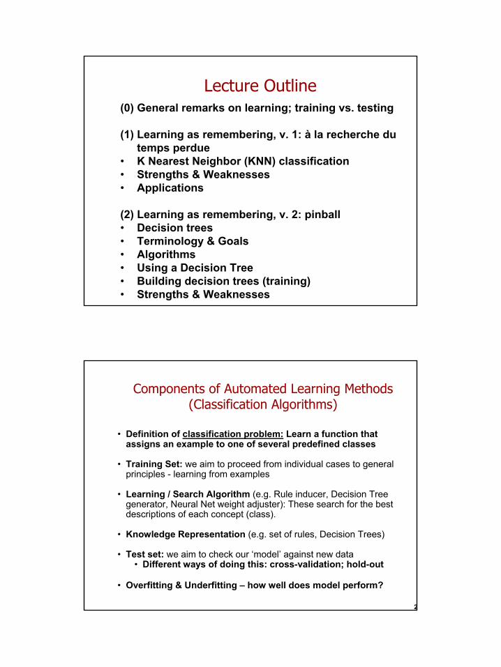
lecture outline
TRANSCRIPT
1
Lecture Outline(0) General remarks on learning; training vs. testing
(1) Learning as remembering, v. 1: à la recherche dutemps perdue
• K Nearest Neighbor (KNN) classification• Strengths & Weaknesses• Applications
(2) Learning as remembering, v. 2: pinball• Decision trees• Terminology & Goals• Algorithms• Using a Decision Tree• Building decision trees (training)• Strengths & Weaknesses
• Definition of classification problem: Learn a function that assigns an example to one of several predefined classes
• Training Set: we aim to proceed from individual cases to general principles - learning from examples
• Learning / Search Algorithm (e.g. Rule inducer, Decision Tree generator, Neural Net weight adjuster): These search for the best descriptions of each concept (class).
• Knowledge Representation (e.g. set of rules, Decision Trees)
• Test set: we aim to check our ‘model’ against new data • Different ways of doing this: cross-validation; hold-out
• Overfitting & Underfitting – how well does model perform?
Components of Automated Learning Methods(Classification Algorithms)
2
2
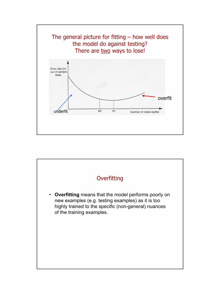
The general picture for fitting – how well does the model do against testing?There are two ways to lose!
underfit
overfit
Overfitting
• Overfitting means that the model performs poorly on new examples (e.g. testing examples) as it is too highly trained to the specific (non-general) nuances of the training examples.
3
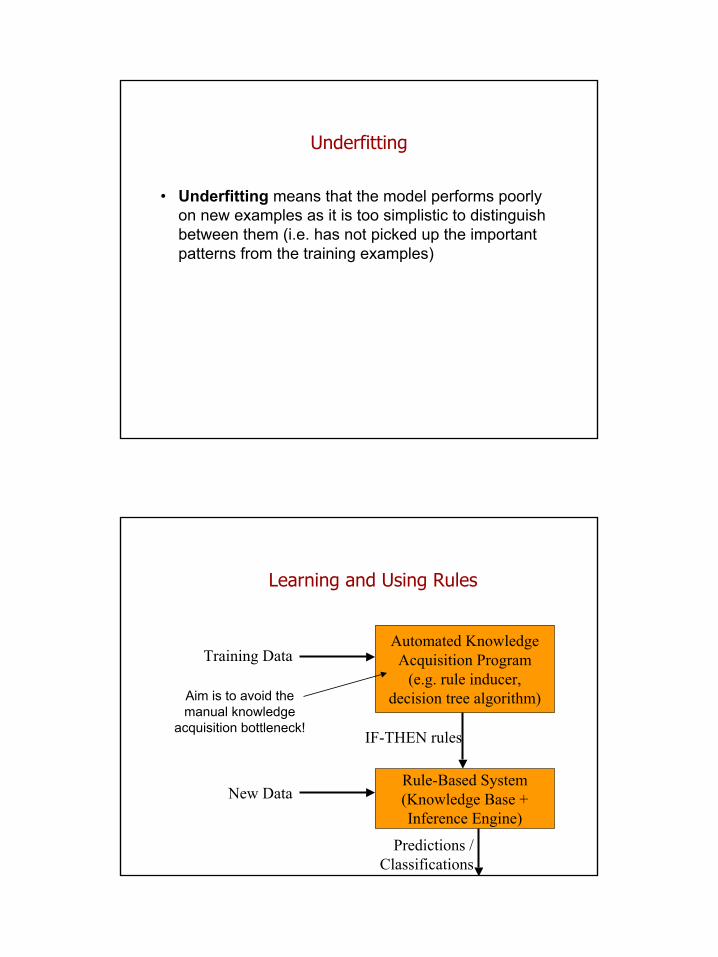
Underfitting
• Underfitting means that the model performs poorly on new examples as it is too simplistic to distinguish between them (i.e. has not picked up the important patterns from the training examples)
Learning and Using Rules
Automated Knowledge Acquisition Program
(e.g. rule inducer, decision tree algorithm)
Training Data
IF-THEN rules
Rule-Based System(Knowledge Base + Inference Engine)
New Data
Predictions /Classifications
Aim is to avoid the manual knowledge
acquisition bottleneck!
4
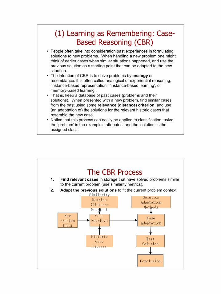
(1) Learning as Remembering: Case-Based Reasoning (CBR)
• People often take into consideration past experiences in formulating solutions to new problems. When handling a new problem one might think of earlier cases when similar situations happened, and use the previous solution as a starting point that can be adapted to the new situation.
• The intention of CBR is to solve problems by analogy or resemblance: it is often called analogical or experiential reasoning, ‘instance-based representation’, ‘instance-based learning’, or ‘memory-based learning’.
• That is, keep a database of past cases (problems and their solutions). When presented with a new problem, find similar cases from the past using some relevance (distance) criterion, and use (an adaptation of) the solutions for the relevant historic cases that resemble the new case.
• Notice that this process can easily be applied to classification tasks: the ‘problem’ is the example’s attributes, and the ‘solution’ is the assigned class.
The CBR Process
New Problem Input
Case Retrieva
l
Similarity Metrics (Distance Metrics)
Historic Case
Library
Case Adaptation
Solution Adaptation Methods
Test Solution
Conclusion
1. Find relevant cases in storage that have solved problems similar to the current problem (use similarity metrics).
2. Adapt the previous solutions to fit the current problem context.
5
Stages in CBR1. Knowledge representation
Decide how to represent cases: attribute selection and transformation
2. Case buildingBuild a repository of cases (a ‘case base’), ideally sampling many regions of the search space
3. Case comparison and retrievalCompare a probe (i.e. new example) with the case base and retrieve the relevant cases
4. AdaptationModify previous solutions to account for the current scenario
5. LearningLearn with new cases, learn the importance of attributes, etc.
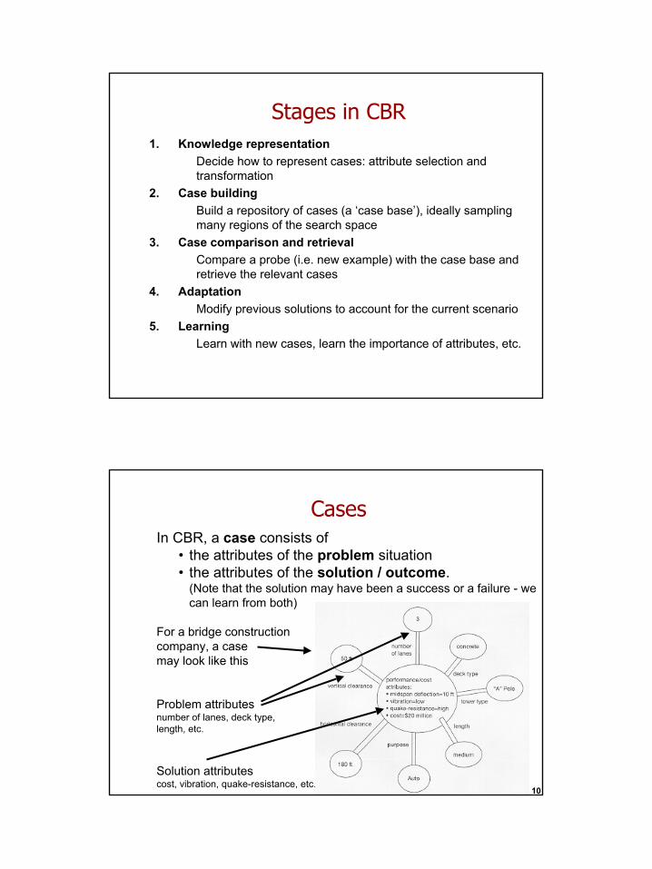
Cases
10
In CBR, a case consists of• the attributes of the problem situation• the attributes of the solution / outcome.
(Note that the solution may have been a success or a failure - we can learn from both)
For a bridge constructioncompany, a case may look like this
Problem attributesnumber of lanes, deck type, length, etc.
Solution attributescost, vibration, quake-resistance, etc.

6
Looking up Similar Cases• We can look up similar cases using a distance metric.• The distance metric can be, for instance, simple Euclidian distance or
weighted Euclidian distance. The Euclidian distance d(X,Y) between two points, X = (x1, x2, ..., xn) and Y = (y1, y2, ..., yn) is:
∑=
−=n
iii yxYXd
1
2)(),(
• We then pull out itemsfrom the database whodistance from our example is belowsome threshold
Difference between Database Querying and CBR
• Regular database queries pull out only items that match certain criteria.
• CBR queries, sometimes called ‘probes’, pull out items that are similar to our criteria, even if they don’t match exactly. CBR queries rank or grade items pulled by similarity.
• Regular queries return historic facts, unaltered.• CBR queries return a proposed solution that has been adapted from
past solutions to fit the current situation

7
Some Issues with Euclidian Distance• Using our bridge example, take a subset of the attributes:
(vertical clearance, number of lanes)• Now, take two cases of bridges in our database:
Bridge 1: (50ft, 3 lanes)Bridge 2: (75ft, 2 lanes)Using simple Euclidian distance:
• Notice that this is a poor distance metric as vertical clearance is having too much influence. We need to scale our numeric attributes so that we have a notion of relative distance (discussed in our lecture on data transformation)!
• Notice that usually not all attributes are equally important, so some weighting of attributes may be appropriate. Taking wi as the weight for attribute i, our distance metric becomes:
• Finally, notice that categorical attributes are trickier to deal with. (See next slide for strategies).
∑=
−=n
iiii yxwYXd
1
2)(),(
626)23()7550()2,1( 22 =−+−=BridgeBridged
Some Issues with Euclidian DistanceTo summarize, some issues with simple Euclidian Distance are:
• Scaling of values• Distances should be relative, not absolute. Since each
numeric attribute may be measured in different units, they should be standardized to have mean of 0 and variance 1.
• Weighting of attributes: • Manual weighting: Weights may be suggested by experts• Automatic weighting: Weights may be computed based on
discriminatory power or other statistics.• Treatment of categorical variables
• Various ways of assigning distance between categories are possible.
8
Adapting Solutions• Because the new problem is seldom exactly the same as the old one,
the old solution usually needs to be adapted a little to fit the new problem
• Adaptation techniques include:• Predefined formulas or processes for adapting the solution• Interpolation: Assuming, you had two old bridges
Bridge 1 = 2 lanes, and cost $1 millionBridge 2 = 4 lanes, and cost $2 millionNow, assuming you wanted a new 3 lane bridge, you might regard it as similar to the 2 lane and the 4 lane bridges, and estimate its cost at:
($2m+$1m)/(4 lanes+2 lanes) x 3 lanes = $0.5m per lane x 3 lanes = $1.5 million
• Extrapolation: This is similar to interpolation, except the new example is outside the bounds of previous cases, and therefore guesses may be less reliable. Assuming a new 6 lane bridge we might guess its cost at:
($0.5m per lane x 6 lanes) + $0.75m contingency = $3.75m
Strengths of CBR
16
• Accuracy improves over time: Incremental learning from past experiences. As new problems arise and are solved, you add them to the case base with their solutions, thereby improving the accuracy of your predictions the next time.
• Low dependence on experts: Unlike rule-based expert systems, you do not need to take the time of experts to capture problem-solving rules, as CBR solves problems based on past experience. (Expert knowledge may of course be helpful for computing distance metrics and deciding on solution adaptation techniques though).
• Some answer may be better than no answer: Whereas rule-based expert systems cannot give a prediction for cases not covered by the rules, CBR can find previous situations that were close and can then guess at something.

9
Weaknesses of kNN-CBR• CBR and KNN are ‘lazy’ approaches: they do not construct a model
in advance, but rather wait till they have to classify a new example.
• Contrast this with ‘eager’ approaches like rule induction and decision trees which construct meaningful symbolic descriptions of classes from the training set and use those models for classification.
• With high-dimensional data, a case may not have any other cases near to it. Selecting a subset of relevant attributes (attribute selection) may help with this.
Applications of CBR• Medicine / 911: Find which diagnosis was made for similar
symptoms in the past, and adapt treatment appropriately• Customer Support (HelpDesk): Find which solution was proposed
for similar problems in the past, and adapt appropriately (e.g. Compaq’s SMART/QUICKSOURCE system)
• Engineering / Construction: Find what costing or design was made for projects with similar requirements in the past, and adapt appropriately
• Law (Legal Advice): Find what judgment was made for similar cases in the past (‘precedents’), and adapt appropriately
• Network Monitoring: Determine whether to cut off a new network session based on bandwidth and network usage attributes, compared to past permitted and prohibited sessions. e.g. David Parish’s CBR system for blocking game-player traffic.
• Web-searching: Search engines track which sites have been useful to people who searched on particular keywords in the past, and rank those highly for new searches.
• Audit and Consulting Engagements: find similar past projects• Insurance Claims Settlement: find similar claims in the past• Real estate: Property price appraisal based on previous sales
10
K Nearest Neighbors (KNN)K-Nearest Neighbor can be used for ‘memory’ based
classification tasks.
• Step 1: Using a chosen distance metric, compute the distance between the new example and all past examples.
• Step 2: Choose the k past examples that are closest to the new example.
• Step 3: Work out the predominant class of those knearest neighbors - the predominant class is your prediction for the new example. i.e. classification is done by majority vote of the k nearest neighbors.
Example – see applet demo
11
K-Nearest Neighbor (KNN)
21
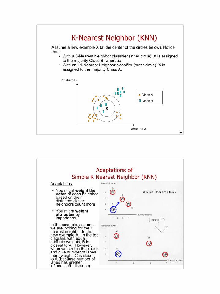
Assume a new example X (at the center of the circles below). Notice that:
• With a 3-Nearest Neighbor classifier (inner circle), X is assigned to the majority Class B, whereas
• With an 11-Nearest Neighbor classifier (outer circle), X is assigned to the majority Class A.
Class A
Attribute B
Class B
Attribute A
XX
Adaptations of Simple K Nearest Neighbor (KNN)
(Source: Dhar and Stein.)
Adaptations:
• You might weight the votes of each neighbor based on their distance: closer neighbors count more.
• You might weight attributes by importance.
In the example, assume we are looking for the 1 nearest neighbor to the new example A. In the top diagram, with equal attribute weights, B is closest to A. However, when we stretch the x-axis and give number of lanes more weight, C is closest to A (because number of lanes has greater influence on distance).
12
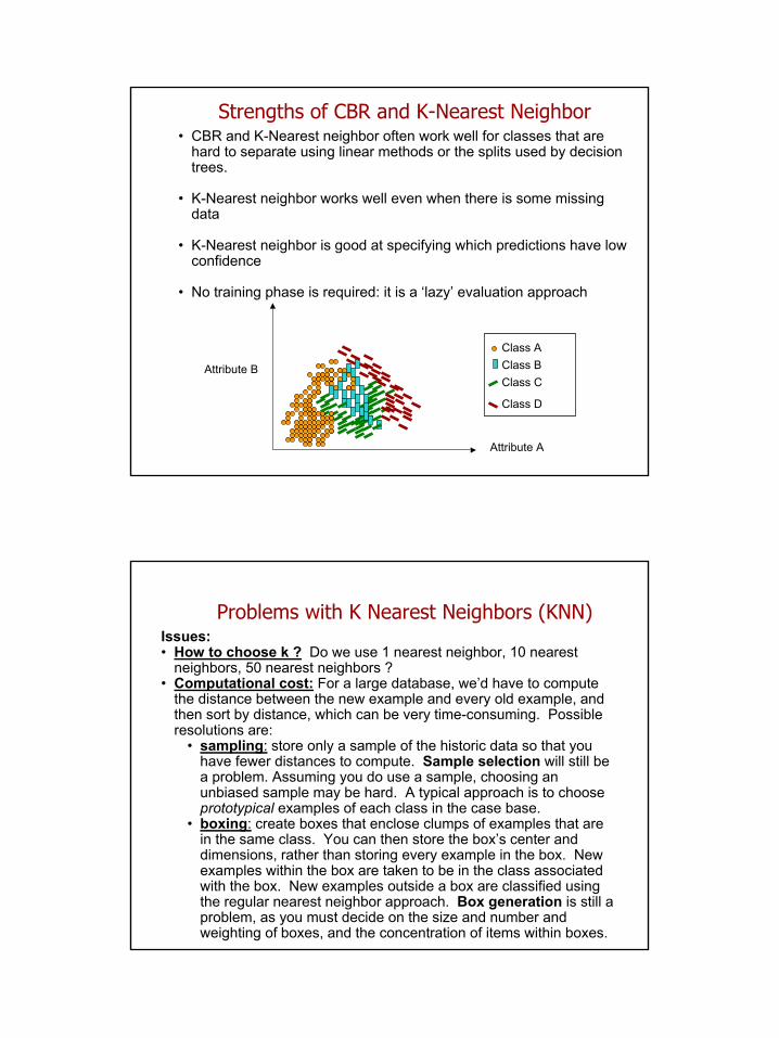
• CBR and K-Nearest neighbor often work well for classes that are hard to separate using linear methods or the splits used by decision trees.
• K-Nearest neighbor works well even when there is some missing data
• K-Nearest neighbor is good at specifying which predictions have low confidence
• No training phase is required: it is a ‘lazy’ evaluation approach
Strengths of CBR and K-Nearest Neighbor
Class A
Attribute A
Attribute B Class BClass C
Class D
Issues:• How to choose k ? Do we use 1 nearest neighbor, 10 nearest
neighbors, 50 nearest neighbors ?• Computational cost: For a large database, we’d have to compute
the distance between the new example and every old example, and then sort by distance, which can be very time-consuming. Possible resolutions are:
• sampling: store only a sample of the historic data so that you have fewer distances to compute. Sample selection will still be a problem. Assuming you do use a sample, choosing an unbiased sample may be hard. A typical approach is to choose prototypical examples of each class in the case base.
• boxing: create boxes that enclose clumps of examples that are in the same class. You can then store the box’s center and dimensions, rather than storing every example in the box. New examples within the box are taken to be in the class associated with the box. New examples outside a box are classified using the regular nearest neighbor approach. Box generation is still a problem, as you must decide on the size and number and weighting of boxes, and the concentration of items within boxes.
Problems with K Nearest Neighbors (KNN)
13
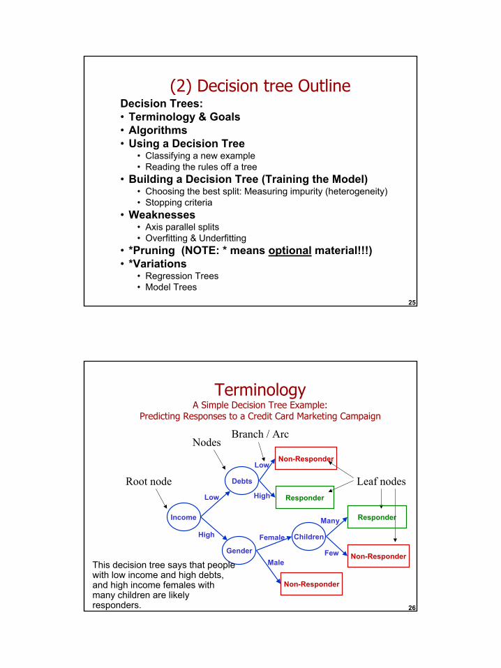
(2) Decision tree Outline
25
Decision Trees:• Terminology & Goals• Algorithms• Using a Decision Tree
• Classifying a new example• Reading the rules off a tree
• Building a Decision Tree (Training the Model)• Choosing the best split: Measuring impurity (heterogeneity)• Stopping criteria
• Weaknesses• Axis parallel splits• Overfitting & Underfitting
• *Pruning (NOTE: * means optional material!!!)• *Variations
• Regression Trees• Model Trees
TerminologyA Simple Decision Tree Example:
Predicting Responses to a Credit Card Marketing Campaign
26
Income
Debts
Gender
Children
Root node
Nodes
Leaf nodes
Branch / Arc
Responder
Non-Responder
Non-Responder
Low
Female
High
Low
High
Male
Many
FewThis decision tree says that people with low income and high debts, and high income females with many children are likely responders.
Non-Responder
Responder
14
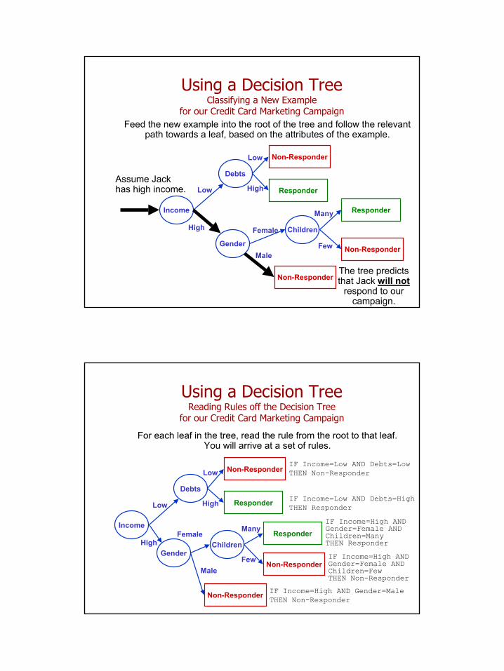
Using a Decision TreeClassifying a New Example
for our Credit Card Marketing Campaign
Income
Debts
Gender
Children
Responder
Non-Responder
Non-Responder
Low
Female
High
Low
High
Male
Many
Few
Assume Jack has high income.
The tree predicts that Jack will not
respond to our campaign.
Feed the new example into the root of the tree and follow the relevant path towards a leaf, based on the attributes of the example.
Non-Responder
Responder
Using a Decision TreeReading Rules off the Decision Tree
for our Credit Card Marketing Campaign
For each leaf in the tree, read the rule from the root to that leaf.You will arrive at a set of rules.
Income
Debts
GenderChildren
Responder
Non-Responder
Non-Responder
Low
Female
High
Low
High
Male
Many
Few
IF Income=Low AND Debts=Low THEN Non-Responder
IF Income=Low AND Debts=High THEN Responder
IF Income=High AND Gender=Female AND Children=Many THEN Responder
IF Income=High AND Gender=Female AND Children=Few THEN Non-Responder
Non-Responder
Responder
IF Income=High AND Gender=Male THEN Non-Responder
15
So, 2 parts:
• Building Decision Trees
• Using Decision Trees
•See demo at: http://www.cs.ubc.ca/labs/lci/CIspace/Version4/dTree/
Users of Decision Trees aim to classify or predict the values of new examples by feeding them into the root of the tree, and determining which leaf the example flows to.
• For categorical outputs (classification): The leaves of the tree assign a class label or a probability of being in a class
• For numeric outputs (prediction): The leaves of the tree assign an average value (‘regression trees’) or specify a function that can be used to compute a value (‘model trees’) for examples that reach that node.
Users of Decision trees may also want to derive a set of rules (descriptions) that describe the general characteristics of each class.
GoalsUsing Decision Trees
16
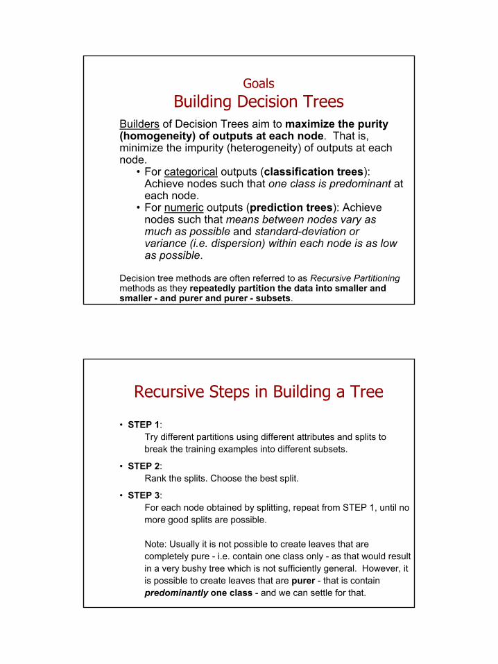
GoalsBuilding Decision Trees
Builders of Decision Trees aim to maximize the purity (homogeneity) of outputs at each node. That is, minimize the impurity (heterogeneity) of outputs at each node.
• For categorical outputs (classification trees): Achieve nodes such that one class is predominant at each node.
• For numeric outputs (prediction trees): Achieve nodes such that means between nodes vary as much as possible and standard-deviation or variance (i.e. dispersion) within each node is as low as possible.
Decision tree methods are often referred to as Recursive Partitioningmethods as they repeatedly partition the data into smaller and smaller - and purer and purer - subsets.
Recursive Steps in Building a Tree
• STEP 1:Try different partitions using different attributes and splits to break the training examples into different subsets.
• STEP 2: Rank the splits. Choose the best split.
• STEP 3: For each node obtained by splitting, repeat from STEP 1, until no more good splits are possible.
Note: Usually it is not possible to create leaves that are completely pure - i.e. contain one class only - as that would result in a very bushy tree which is not sufficiently general. However, it is possible to create leaves that are purer - that is contain predominantly one class - and we can settle for that.

17
Better, as purity of sub-nodes is improving.
Recursive Steps in Building a TreeExample
STEP 1: Split Option A
Not good as sub-nodes are still very heterogenous!
STEP 1: Split Option B
STEP 2: Choose Split Option B as it is the better split.
STEP 3: Try out splits on each of the sub-nodes of Split Option B.Eventually, we arrive at: Notice how examples in a parent
node are split between sub-nodes - i.e. notice how the training examples are partitioned into smaller and smaller subsets. Also, notice that sub-nodes are purer than parent nodes.
Building a TreeChoosing a Split
• The criteria used to choose the best split are called feature selection criteria.
• In C4.5, we choose the split that gives nodes with highest purity. ‘Information Gain’ (used by C4.5) is one possible measure of the purity of nodes in a given split.
• Information gain is just one possible feature selection criterion.
• Most approaches to choosing a split are greedy: That is, they choose the best split first, even if a worse initial split may have resulted in an excellent eventual split. The reason for choosing only the best split at each stage is the possible combinatorial explosion of trying all possible splits. So, most decision trees employ a greedy heuristic search which tries out some good-looking partitions, rather than an costly exhaustive search which tries out all partitions.
18
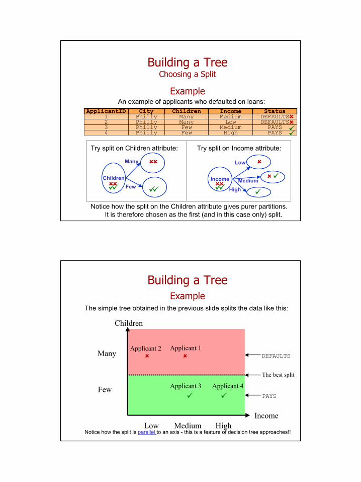
Building a TreeChoosing a Split
ExampleAn example of applicants who defaulted on loans:
Few Medium PAYSFew High PAYS
PhillyPhilly
CityPhillyPhilly
ChildrenManyMany
IncomeMediumLow
StatusDEFAULTSDEFAULTS
34
ApplicantID12
Try split on Children attribute: Try split on Income attribute:
Children
Many
FewIncome
Low
HighMedium
Notice how the split on the Children attribute gives purer partitions.It is therefore chosen as the first (and in this case only) split.
Building a TreeExample
The simple tree obtained in the previous slide splits the data like this:
Applicant 3 Applicant 4
Applicant 1Applicant 2
Children
Many
Few
IncomeLow Medium High
DEFAULTS
PAYS
Notice how the split is parallel to an axis - this is a feature of decision tree approaches!!
The best split
19
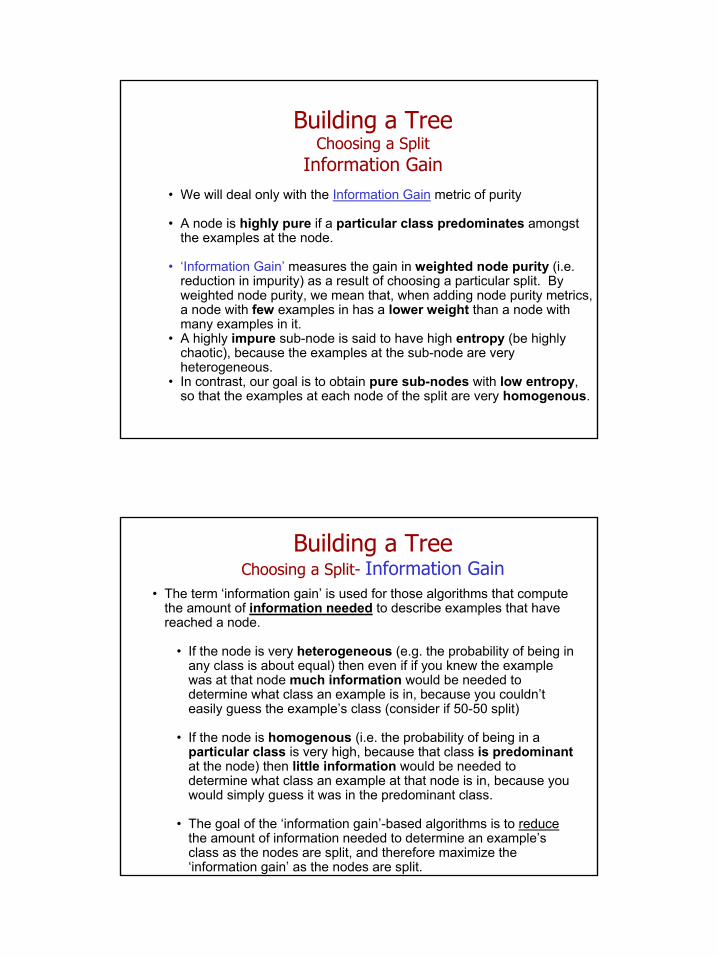
Building a TreeChoosing a Split
Information Gain• We will deal only with the Information Gain metric of purity
• A node is highly pure if a particular class predominates amongst the examples at the node.
• ‘Information Gain’ measures the gain in weighted node purity (i.e. reduction in impurity) as a result of choosing a particular split. By weighted node purity, we mean that, when adding node purity metrics, a node with few examples in has a lower weight than a node with many examples in it.
• A highly impure sub-node is said to have high entropy (be highly chaotic), because the examples at the sub-node are very heterogeneous.
• In contrast, our goal is to obtain pure sub-nodes with low entropy, so that the examples at each node of the split are very homogenous.
Building a TreeChoosing a Split- Information Gain
• The term ‘information gain’ is used for those algorithms that compute the amount of information needed to describe examples that have reached a node.
• If the node is very heterogeneous (e.g. the probability of being in any class is about equal) then even if if you knew the example was at that node much information would be needed to determine what class an example is in, because you couldn’t easily guess the example’s class (consider if 50-50 split)
• If the node is homogenous (i.e. the probability of being in a particular class is very high, because that class is predominantat the node) then little information would be needed to determine what class an example at that node is in, because you would simply guess it was in the predominant class.
• The goal of the ‘information gain’-based algorithms is to reducethe amount of information needed to determine an example’s class as the nodes are split, and therefore maximize the ‘information gain’ as the nodes are split.
20
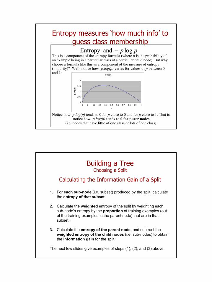
Entropy measures ‘how much info’ to guess class membership
Entropy and logp p−This is a component of the entropy formula (where p is the probability of an example being in a particular class at a particular child node). But why choose a formula like this as a component of the measure of entropy (impurity)? Well, notice how -p.log(p) varies for values of p between 0 and 1:
-p.log(p)
0
0.05
0.1
0.15
0.2
0 0.1 0.2 0.3 0.4 0.5 0.6 0.7 0.8 0.9 1
p
-p.lo
g(p)
Notice how -p.log(p) tends to 0 for p close to 0 and for p close to 1. That is, notice how -p.log(p) tends to 0 for purer nodes
(i.e. nodes that have little of one class or lots of one class).
Building a TreeChoosing a Split
Calculating the Information Gain of a Split
1. For each sub-node (i.e. subset) produced by the split, calculate the entropy of that subset.
2. Calculate the weighted entropy of the split by weighting each sub-node’s entropy by the proportion of training examples (out of the training examples in the parent node) that are in that subset.
3. Calculate the entropy of the parent node, and subtract the weighted entropy of the child nodes (i.e. sub-nodes) to obtain the information gain for the split.
The next few slides give examples of steps (1), (2), and (3) above.
21
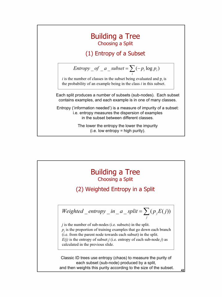
Building a TreeChoosing a Split
(1) Entropy of a Subset
Each split produces a number of subsets (sub-nodes). Each subset contains examples, and each example is in one of many classes.
Entropy (‘information needed’) is a measure of impurity of a subset: i.e. entropy measures the dispersion of examples
in the subset between different classes.
The lower the entropy the lower the impurity (i.e. low entropy = high purity).
)log(___ ii
i ppsubsetaofEntropy ∑ −=
i is the number of classes in the subset being evaluated and pi is the probability of an example being in the class i in this subset.
Building a TreeChoosing a Split
(2) Weighted Entropy in a Split
42
))((____ jEpsplitainentropyWeightedj
j∑=j is the number of sub-nodes (i.e. subsets) in the split.pj is the proportion of training examples that go down each branch (i.e. from the parent node towards each subset) in the split.E(j) is the entropy of subset j (i.e. entropy of each sub-node j) as calculated in the previous slide.
Classic ID trees use entropy (chaos) to measure the purity of each subset (sub-node) produced by a split,
and then weights this purity according to the size of the subset.

22
Building a TreeChoosing a Split: Worked Example
Entropy
Split on Children attribute:
(1) Entropy of each subnode
Children
Many
Few
(2) Weighted entropy of this Split Option:
( ) ( ) 004204
2_____ =×+×=ChildrenonsplitofentropyWeighted
( ) ( ) 022log2
22
0log201___ =−−=subnodeofEntropy
( ) ( ) 020log2
02
2log222___ =−−=subnodeofEntropy
Probability of being in class at this nodeProbability of being in class at this node
Proportion of examples in Sub-node 1Entropy of Sub-node 1
Building a TreeChoosing a Split: Worked Example
Entropy
Split on Income attribute:
(1) Entropy of each subnode
(2) Weighted entropy of this Split Option:
( ) ( ) ( ) 5.004114
2041_____ =×+×+×=IncomeonsplitofentropyWeighted
( ) ( ) 011log1
11
0log101___ =−−=subnodeofEntropy
( ) ( ) 010log1
01
1log113___ =−−=subnodeofEntropy
Income
Low
HighMedium ( ) ( ) 12
1log21
21log2
12___ =−−=subnodeofEntropy
Proportion of examples in Sub-node 2Entropy of Sub-node 2
Probability of being in class at this nodeProbability of being in class at this node
23
Building a TreeChoosing a Split: Worked Example
(3) Information Gain of Split Options
Children
Many
FewIncome
Low
HighMedium
Weighted entropy of this Split Option (Split on Income) =
0.5 (calculated earlier)Information Gain = 1 - 0.5 = 0.5
Notice how the split on Children attribute gives higher information gain (purer partitions), and is therefore the preferred split.
Weighted entropy of this Split Option (Split on Children)
= 0 (calculated earlier)Information Gain = 1 - 0 = 1
( ) ( ) 142log4
24
2log42___ =−−=nodeparentofEntropy
Properties of EntropyFrom a previous slide, you may have been wondering why -p.log(p) on its own doesn’t have a maximum at 0.5 (i.e. where, for 2 classes, there is maximum impurity at a particular node) ? Well, remember that theformula for entropy of a subset is not just -p.log(p), but rather the sum of -pi.log(pi) for all i classes in the subset! Notice that, assuming we had 2 classes in a subset, this would effectively give us:
Entropy = -p.log(p)-((1-p).log(1-p)) where p is the probability of class A in the subset and therefore (1-p) is the probability of class B in the subset. We’ve graphed this below - notice how this does in fact have its maximum at p=0.5 (highest heterogeneity) -that is, while -p.log(p) is not maximized at 0.5 for a particular class in a subset, entropy (which is the sum of -pi.log(pi) for all i classes in the subset) is at a maximum at 0.5.
Note that in general,for the n-class case,entropy has a maximumwhenever the proportionof all n classes in thesubset is equal !
00.10.20.30.40.50.60.70.80.9
1
0 0.1 0.2 0.3 0.4 0.5 0.6 0.7 0.8 0.9 1
p
-p.log(p)-(1-p).log(1-p)(-p.log(p))-((1-p).log(1-p))
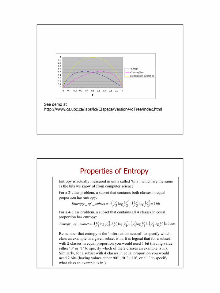
24
00.10.20.30.40.50.60.70.80.9
1
0 0.1 0.2 0.3 0.4 0.5 0.6 0.7 0.8 0.9 1
p
-p.log(p)-(1-p).log(1-p)(-p.log(p))-((1-p).log(1-p))
See demo at http://www.cs.ubc.ca/labs/lci/CIspace/Version4/dTree/index.html
Properties of EntropyEntropy is actually measured in units called ‘bits’, which are the same as the bits we know of from computer science.For a 2-class problem, a subset that contains both classes in equal proportion has entropy:
For a 4-class problem, a subset that contains all 4 classes in equal proportion has entropy:
Remember that entropy is the ‘information needed’ to specify which class an example in a given subset is in. It is logical that for a subset with 2 classes in equal proportion you would need 1 bit (having value either ‘0’ or ‘1’ to specify which of the 2 classes an example is in). Similarly, for a subset with 4 classes in equal proportion you would need 2 bits (having values either ‘00’, ‘01’, ‘10’, or ‘11’ to specify what class an example is in.)
( ) ( ) bitsubsetofEntropy 121log2
12
1log21__ =−−=
( ) ( ) ( ) ( ) bitssubsetofEntropy 241log4
14
1log41
41log4
14
1log41__ =−−−−=
25
Building a TreeChoosing a Split
Information Gain• Note that comparing the entropy between split options and
choosing the lowest entropy is insufficient !
• Why ? Because we also want to make sure that entropy (i.e. impurity) decreases from layer to layer as we move down (from root to leaves) in the decision tree ! If entropy is increasing then the tree is getting worse, so we wouldn’t want to make the split !
• Thus we only choose to split if there is an information gain (i.e. decrease in entropy/chaos) as a result of the split !
Building a TreeStopping Criteria
You can stop building the tree when:
• The impurity of all nodes is zero: Problem is that this tends to lead to bushy, highly-branching trees, often with one example at each node.
• No split achieves a significant gain in purity
• Node size is too small: That is, there are less than a certain number of examples, or proportion of the training set, at each node.
• Note: there is seldom one ‘best’ tree but usually many good trees to choose from.
26
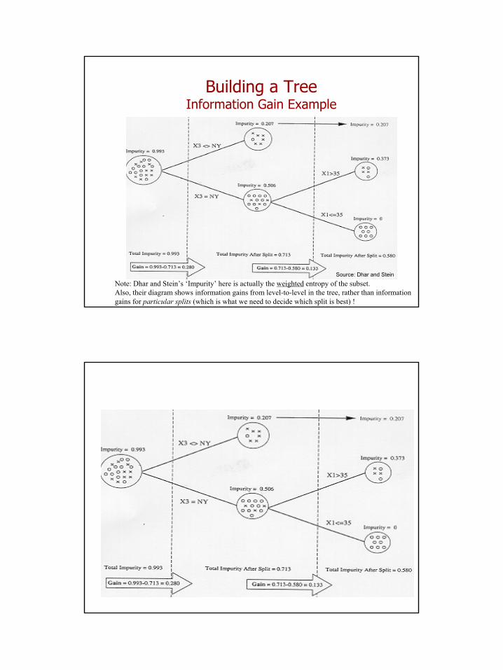
Building a TreeInformation Gain Example
Source: Dhar and Stein
Note: Dhar and Stein’s ‘Impurity’ here is actually the weighted entropy of the subset.Also, their diagram shows information gains from level-to-level in the tree, rather than information gains for particular splits (which is what we need to decide which split is best) !
27
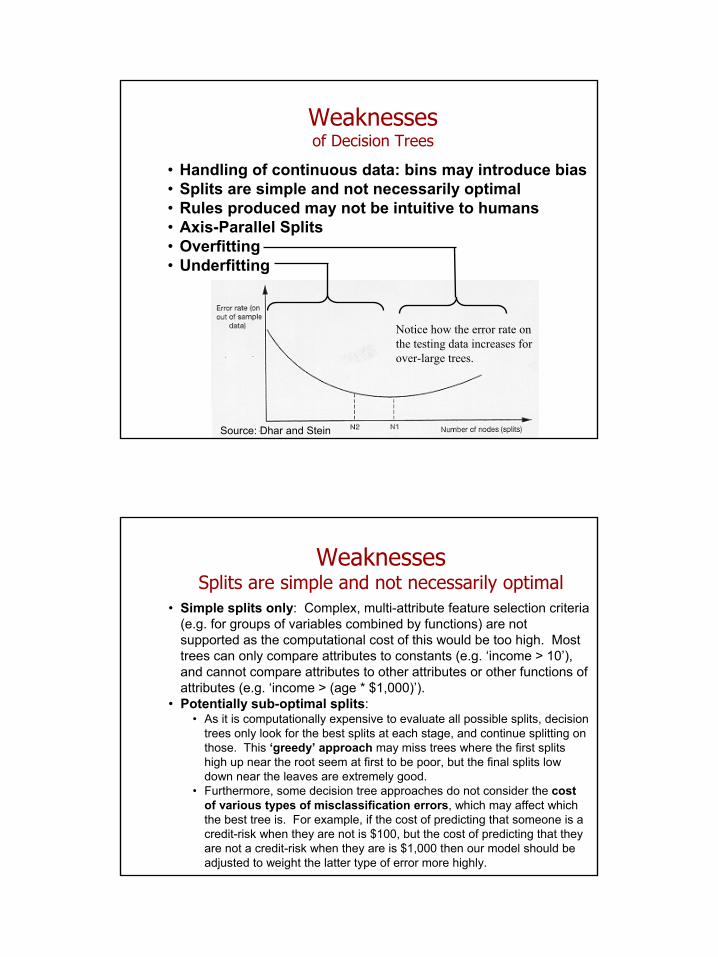
Weaknessesof Decision Trees
• Handling of continuous data: bins may introduce bias• Splits are simple and not necessarily optimal • Rules produced may not be intuitive to humans• Axis-Parallel Splits• Overfitting• Underfitting
Source: Dhar and Stein
Notice how the error rate on the testing data increases for over-large trees.
WeaknessesSplits are simple and not necessarily optimal
• Simple splits only: Complex, multi-attribute feature selection criteria (e.g. for groups of variables combined by functions) are not supported as the computational cost of this would be too high. Most trees can only compare attributes to constants (e.g. ‘income > 10’), and cannot compare attributes to other attributes or other functions of attributes (e.g. ‘income > (age * $1,000)’).
• Potentially sub-optimal splits: • As it is computationally expensive to evaluate all possible splits, decision
trees only look for the best splits at each stage, and continue splitting on those. This ‘greedy’ approach may miss trees where the first splits high up near the root seem at first to be poor, but the final splits low down near the leaves are extremely good.
• Furthermore, some decision tree approaches do not consider the cost of various types of misclassification errors, which may affect which the best tree is. For example, if the cost of predicting that someone is a credit-risk when they are not is $100, but the cost of predicting that they are not a credit-risk when they are is $1,000 then our model should be adjusted to weight the latter type of error more highly.
28
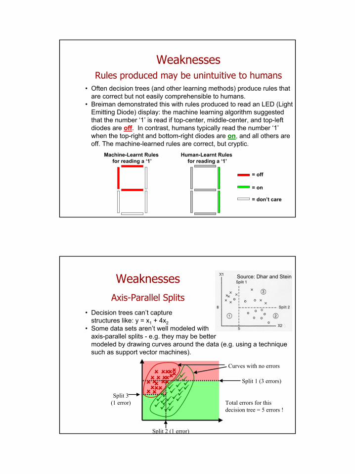
WeaknessesRules produced may be unintuitive to humans
• Often decision trees (and other learning methods) produce rules that are correct but not easily comprehensible to humans.
• Breiman demonstrated this with rules produced to read an LED (Light Emitting Diode) display: the machine learning algorithm suggested that the number ‘1’ is read if top-center, middle-center, and top-left diodes are off. In contrast, humans typically read the number ‘1’ when the top-right and bottom-right diodes are on, and all others are off. The machine-learned rules are correct, but cryptic.
Machine-Learnt Rules for reading a ‘1’
Human-Learnt Rules for reading a ‘1’
= off
= on
= don’t care
WeaknessesAxis-Parallel Splits
• Decision trees can’t capture structures like: y = x1 + 4x2
• Some data sets aren’t well modeled with axis-parallel splits - e.g. they may be better modeled by drawing curves around the data (e.g. using a technique such as support vector machines).
Source: Dhar and Stein
Split 1 (3 errors)
Split 2 (1 error)
Split 3(1 error)
Curves with no errors
Total errors for this decision tree = 5 errors !
29
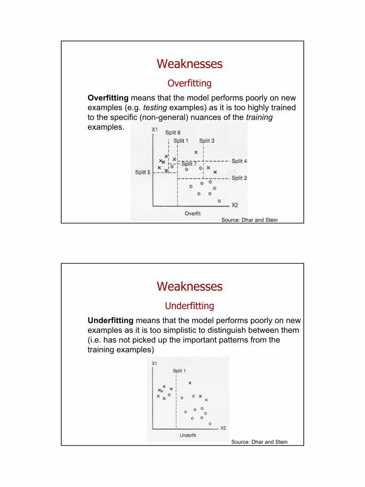
WeaknessesOverfitting
Overfitting means that the model performs poorly on new examples (e.g. testing examples) as it is too highly trained to the specific (non-general) nuances of the trainingexamples.
Source: Dhar and Stein
WeaknessesUnderfitting
Underfitting means that the model performs poorly on new examples as it is too simplistic to distinguish between them (i.e. has not picked up the important patterns from the training examples)
Source: Dhar and Stein
30
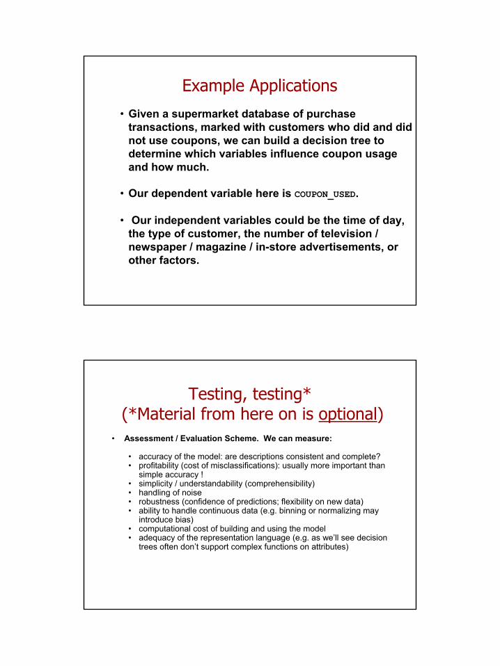
Example Applications
• Given a supermarket database of purchase transactions, marked with customers who did and did not use coupons, we can build a decision tree to determine which variables influence coupon usage and how much.
• Our dependent variable here is COUPON_USED.
• Our independent variables could be the time of day, the type of customer, the number of television / newspaper / magazine / in-store advertisements, or other factors.
Testing, testing*(*Material from here on is optional)
• Assessment / Evaluation Scheme. We can measure:
• accuracy of the model: are descriptions consistent and complete?• profitability (cost of misclassifications): usually more important than
simple accuracy ! • simplicity / understandability (comprehensibility)• handling of noise• robustness (confidence of predictions; flexibility on new data)• ability to handle continuous data (e.g. binning or normalizing may
introduce bias)• computational cost of building and using the model• adequacy of the representation language (e.g. as we’ll see decision
trees often don’t support complex functions on attributes)
31
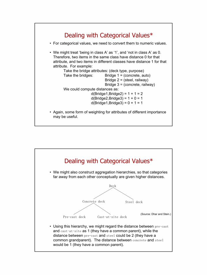
Dealing with Categorical Values*• For categorical values, we need to convert them to numeric values.
• We might treat ‘being in class A’ as ‘1’, and ‘not in class A’ as 0. Therefore, two items in the same class have distance 0 for that attribute, and two items in different classes have distance 1 for that attribute. For example:
Take the bridge attributes: (deck type, purpose)Take the bridges: Bridge 1 = (concrete, auto)
Bridge 2 = (steel, railway)Bridge 3 = (concrete, railway)
We could compute distances as:d(Bridge1,Bridge2) = 1 + 1 = 2d(Bridge2,Bridge3) = 1 + 0 = 1d(Bridge1,Bridge3) = 0 + 1 = 1
• Again, some form of weighting for attributes of different importance may be useful.
Dealing with Categorical Values*
• We might also construct aggregation hierarchies, so that categories far away from each other conceptually are given higher distances.
Concrete deck Steel deck
(Source: Dhar and Stein.)Pre-cast deck Cast-at-site deck
Deck
• Using this hierarchy, we might regard the distance between pre-castand cast-at-site as 1 (they have a common parent), while the distance between pre-cast and steel could be 2 (they have a common grandparent). The distance between concrete and steelwould be 1 (they have a common parent).

32
Dynamically Choosing Attribute Weightings*
(Source: Dhar and Stein)
We could choose attribute weightings dynamically as they apply to the case under consideration. Take the example below where the new bridge we want to cost is X, and previous cases are marked as L, M, or H (for Low, Medium, or High maintenance cost). Looking at the plot, it seems that number of lanes has low discriminatory power because 4 of the 5 historical examples in the gray horizontal bar are H. In contrast, length seems to have high discriminatorypower as the 6 historicexamples in the gray vertical bar are quite varied.We might therefore givelength greater weighting(importance) in our distance metric.
Aside: Possible measures of discriminatory power arechi-squared statistics orentropy, which we haveseen in earlier lectures.
Dealing with Missing Values*
• If there are missing values in the training examples when building the decision tree:
• You can create a separate branch for ‘missing’, or, ...• Provided missing values are few, you can just split on the other
known values, or• Split on other attributes instead.
• If there are missing values in the new examples when using the decision tree:
• You can let them flow down the ‘missing’ branch if you have one, or, if you don’t have a missing branch ...
• You can notionally replicate the new example at the node mentioning the missing attribute, and weight each replica of theexample based on the proportion of training examples that went down each branch during training. Then, once each replica reaches a leaf, calculate the probability of being in a particular class by applying the weighting of each replica to each probability you arrive at.
33
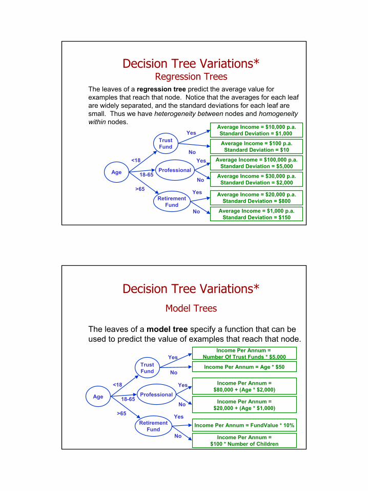
Decision Tree Variations*Regression Trees
The leaves of a regression tree predict the average value for examples that reach that node. Notice that the averages for each leaf are widely separated, and the standard deviations for each leaf are small. Thus we have heterogeneity between nodes and homogeneity within nodes.
Age
TrustFund
RetirementFund
<18No
Yes
>65 Yes
No
Professional18-65
Average Income = $10,000 p.a.Standard Deviation = $1,000
Yes
No
Average Income = $100 p.a.Standard Deviation = $10
Average Income = $100,000 p.a.Standard Deviation = $5,000
Average Income = $30,000 p.a.Standard Deviation = $2,000
Average Income = $20,000 p.a.Standard Deviation = $800
Average Income = $1,000 p.a.Standard Deviation = $150
Decision Tree Variations*Model Trees
The leaves of a model tree specify a function that can be used to predict the value of examples that reach that node.
Age
TrustFund
RetirementFund
<18
No
Yes
>65 Yes
No
Professional18-65
Income Per Annum = Number Of Trust Funds * $5,000
Yes
No
Income Per Annum = Age * $50
Income Per Annum = $80,000 + (Age * $2,000)
Income Per Annum = FundValue * 10%
Income Per Annum = $100 * Number of Children
Income Per Annum = $20,000 + (Age * $1,000)

34
Pruning*A decision trees is typically more accurate on its training data than on its test data. Removing branches from a tree can often improve its accuracy on a test set - so-called ‘reduced error pruning’. The intention of this pruning is to cut off branches from the tree when this improves performance on test data - this reduces overfitting and makes the tree more general.
Some decision trees (e.g. CART) use a cost-complexity metric, that trades of accuracy against simplicity. Error-cost and cost-per-node parameters are set by the user. Higher error-cost favors more accurate trees (as we attempt to minimize the cost of misclassification errors). Higher cost-per-node favors simpler trees (as complex trees have more nodes and are more costly).
Source: Dhar and Stein
Some trees write the following information alongside each node:
• support: the number of training examples that reached that leaf (irrespective of their actual class)
• confidence: the percentage of training examples in the predominant class at that leaf.
Example:
Building a Tree*Support and Confidence
Income(968 cases)
Debts(272 cases)
Gender(696 cases)
Children(153 cases)
Responder57 cases (88%)
Non-Responder96 cases (91%)
Non-Responder543 cases (89%)
Low
Male
High
Low
High
Female
Many
Few
Non-Responder105 cases (90%)
Responder167 cases (97%)
SupportConfidence