UNIVERSITY OF TARTUFACULTY OF MATHEMATICS AND COMPUTER SCIENCE

Institute of Computer Science

Prepared at the Chair of Distributed Systems

Indrek Priks

F2F network topology visualizationMaster’s thesis (20 AP)

Supervisors: Jüri Harju

Ulrich Norbisrath

Author: ……………………………………..…… “…..“ May 2008

Instructor: ………………………………..…. … “…..“ May 2008

Allowed to thesis defense

Professor: ...................... ………………….……. “…..“ May 2008

TARTU 2008

Contents

INTRODUCTION......................................................................................................................4

1. VISUALIZATION TOOL REQUIREMENTS......................................................................6

1.1. Use-case scenario.............................................................................................................6

1.2. Functional requirements...................................................................................................7

1.3. Technical requirements....................................................................................................8

1.4. Summary of the requirements..........................................................................................9

2. TECHNOLOGIES USED IN THE TOOL...........................................................................10

2.1. Graph eXchange Language 1.0......................................................................................10

2.2. Eclipse Rich Client Platform (RCP)..............................................................................12

2.2.1. Why Eclipse RCP....................................................................................................12

2.2.2. The architecture of RCP..........................................................................................13

2.3. Eclipse graphics frameworks.........................................................................................16

2.3.1. Standard Widget Toolkit (SWT).............................................................................16

2.3.2. JFace........................................................................................................................18

2.3.3. Draw2d....................................................................................................................19

2.3.4. Zest – The Eclipse Visualization Toolkit................................................................20

2.4. Java Remote Method Invocation (RMI)........................................................................20

2.5. Summary of the technologies.........................................................................................21

3. GRAPH LAYOUT ALGORITHMS....................................................................................22

3.1. Tree layout algorithm.....................................................................................................22

3.2. Radial tree layout algorithm...........................................................................................23

3.3. Grid layout algorithm.....................................................................................................24

3.4. Spring layout algorithm.................................................................................................25

3.5. Summary of the algorithms............................................................................................26

4. IMPLEMENTED VISUALIZATION TOOL......................................................................27

4.1. Installation......................................................................................................................27

4.2. Usage..............................................................................................................................28

4.2.1. Start the application................................................................................................28

2

4.2.2. Open multiple windows..........................................................................................28

4.2.3. View current network topology..............................................................................28

4.2.4. Save the graph into a file.........................................................................................30

4.2.5. Open a graph from a file.........................................................................................30

4.2.6. Change the graph layout algorithm.........................................................................30

4.2.7. Graph tabs...............................................................................................................31

4.2.8. View detailed node information..............................................................................31

4.2.9. View statistics – the summary of the graph............................................................32

4.2.10. Filter graph elements.............................................................................................32

4.2.11. Informing about errors..........................................................................................34

4.3. The difficulties and the results.......................................................................................35

4.3.1. The difficulties........................................................................................................35

4.3.2. The results...............................................................................................................36

4.4. Summary of the implementation....................................................................................37

SUMMARY AND OUTLOOK................................................................................................38

RESÜMEE................................................................................................................................40

ABSTRACT..............................................................................................................................41

LITERATURE..........................................................................................................................42

APPENDIX...............................................................................................................................44

1. Appendix 1 - Grid layout algorithm and node info view..................................................44

2. Appendix 2 - Radial layout algorithm and statistics view................................................45

3. Appendix 3 – Spring layout algorithm..............................................................................46

4. Appendix 4 - Tree layout and a filter that fades out some graph elements.......................47

5. Appendix 5 - Tree layout and a filter that removes some graph elements........................48

6. Appendix 6 – Sample GXL document..............................................................................49

7. Appendix 7 – The application CD....................................................................................54

3

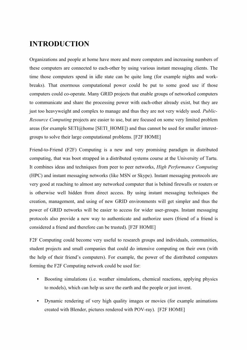
INTRODUCTION

Organizations and people at home have more and more computers and increasing numbers of

these computers are connected to each-other by using various instant messaging clients. The

time those computers spend in idle state can be quite long (for example nights and work-

breaks). That enormous computational power could be put to some good use if those

computers could co-operate. Many GRID projects that enable groups of networked computers

to communicate and share the processing power with each-other already exist, but they are

just too heavyweight and complex to manage and thus they are not very widely used. Public-

Resource Computing projects are easier to use, but are focused on some very limited problem

areas (for example SETI@home [SETI_HOME]) and thus cannot be used for smaller interest-

groups to solve their large computational problems. [F2F HOME]

Friend-to-Friend (F2F) Computing is a new and very promising paradigm in distributed

computing, that was boot strapped in a distributed systems course at the University of Tartu.

It combines ideas and techniques from peer to peer networks, High Performance Computing

(HPC) and instant messaging networks (like MSN or Skype). Instant messaging protocols are

very good at reaching to almost any networked computer that is behind firewalls or routers or

is otherwise well hidden from direct access. By using instant messaging techniques the

creation, management, and using of new GRID environments will get simpler and thus the

power of GRID networks will be easier to access for wider user-groups. Instant messaging

protocols also provide a new way to authenticate and authorize users (friend of a friend is

considered a friend and therefore can be trusted). [F2F HOME]

F2F Computing could become very useful to research groups and individuals, communities,

student projects and small companies that could do intensive computing on their own (with

the help of their friend’s computers). For example, the power of the distributed computers

forming the F2F Computing network could be used for:

• Boosting simulations (i.e. weather simulations, chemical reactions, applying physics

to models), which can help us save the earth and the people or just invent.

• Dynamic rendering of very high quality images or movies (for example animations

created with Blender, pictures rendered with POV-ray). [F2F HOME]

The goal of this work is to help make distributed computing via the F2F network more

popular, usable, and transparent to the users, so the users can easily try out new ideas of

distributed applications. This is achieved by creating an intuitive to use compact tool for

simplified observation of the F2F network. This work must analyze and define the

requirements for the F2F network visualization tool and provide a ready to use open-source

implementation. The technologies that are studied and used for creating the tool are described

in a manner that people who are interested in the tool can continue the development with less

time spent on learning the technologies.

This work is divided into four chapters. The first chapter analyses and defines the

requirements for the visualizing tool that makes understanding the structure of and optimizing

the F2F network a much easier task. The second chapter describes the technologies to be used

in the tool – GXL, Eclipse RCP, Eclipse GEF, Eclipse Zest, and Java RMI. The third chapter

explains with the help of some pictures the main algorithms available for arranging the

network topology graph elements in the display. The fourth chapter is about the

implementation – what exactly are the features and how to use this tool. Also the

implementation difficulties are described briefly. The appendix chapter contains the

developed tool, lots of screenshots of the tool and a sample GXL document.

1. VISUALIZATION TOOL REQUIREMENTS

1.1. Use-case scenario

In order to efficiently use the high computing power of the F2F network a tool for graphically

displaying the topology and properties of the network is extremely useful. With the help of

such a tool, the piece of code that some user wants to send for computing to the computers on

the GRID can be tuned by the user to be more efficient or capable of running on more

computers, because the environmental properties of the computers or connections on the

network can be taken into account. For example, by knowing which kind of hardware

architectures are out there, how good are the computers (i.e. the processor speed or amount of

the memory), which enhanced instruction sets are supported by the processors, what platforms

are used and what libraries or runtimes are installed, a much more efficient code can be

written. Also, by observing the (sum of) properties of the nodes it can easily be seen that

upgrading of some hard- or software on some node would be good.

This kind of information might be quite easy to collect with some other software as well, but

this most probably requires all of the computers to be managed by one administrator. For

example, some company computers that are in the same domain. Collecting such data from

the F2F network which consists of a wide range of home, work, and/or any other kind of

computers and viewing it in one application is quite unique though.

Such a tool could be used to visually detect if creating some other type of instant messaging

connection between some two nodes would make the network perform better. For example, it

would make the path from some node A to some node B shorter in steps or just have higher

throughput and improve the performance. Such tool could easily be used to identify by just

looking at the graph such a node that might be a bottleneck in the sense of being the only

node that connects two sub-networks of the F2F network. Monitoring the network for possible

connection issues between the nodes could be somewhat simplified, because the problematic

connections, if any, could be displayed differently on the graph or on the statistical view. For

an example see the figure 1.

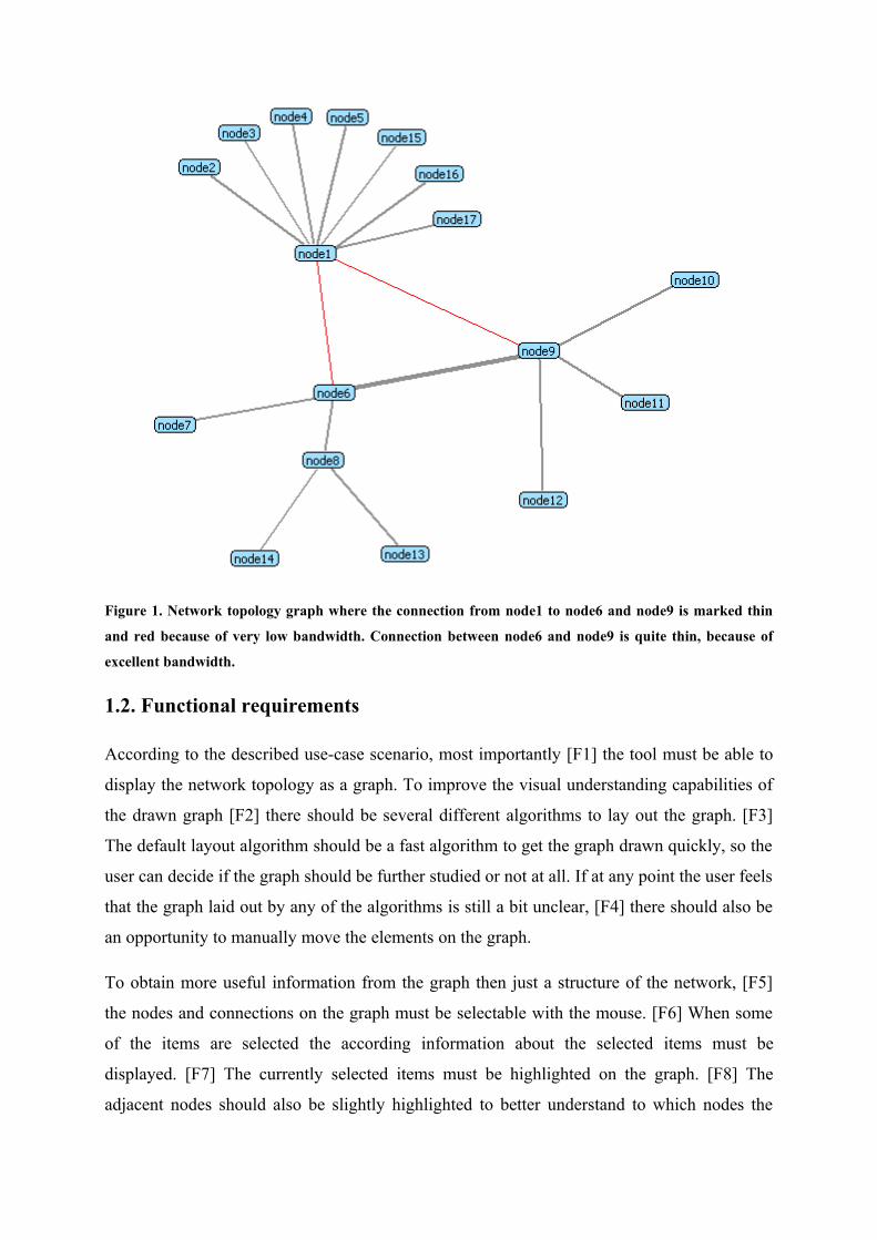
Figure 1. Network topology graph where the connection from node1 to node6 and node9 is marked thin

and red because of very low bandwidth. Connection between node6 and node9 is quite thin, because of

excellent bandwidth.

1.2. Functional requirements

According to the described use-case scenario, most importantly [F1] the tool must be able to

display the network topology as a graph. To improve the visual understanding capabilities of

the drawn graph [F2] there should be several different algorithms to lay out the graph. [F3]

The default layout algorithm should be a fast algorithm to get the graph drawn quickly, so the

user can decide if the graph should be further studied or not at all. If at any point the user feels

that the graph laid out by any of the algorithms is still a bit unclear, [F4] there should also be

an opportunity to manually move the elements on the graph.

To obtain more useful information from the graph then just a structure of the network, [F5]

the nodes and connections on the graph must be selectable with the mouse. [F6] When some

of the items are selected the according information about the selected items must be

displayed. [F7] The currently selected items must be highlighted on the graph. [F8] The

adjacent nodes should also be slightly highlighted to better understand to which nodes the

currently selected node is connected to. Because the networks can grow very large and

complex [F9] a way to narrow the results must be provided. For example, an interface that

enables to filter graph elements by different kind of criteria’s.

[F10] The visualizing tool must be able to obtain the current network topology information

from a F2F network data-gathering tool that is developed separately. [F11] The visualizing

tool must be as generic as possible, allowing to display almost any properties collected by the

data-gathering tool. This imposes that the displayable properties types must be very

dynamical and not coded into the visualizing tool if at all possible. This allows the data-

gathering tool to be continuously developed and improved and still be able to use the tool

with success.

To be able to keep a history of the topology and how it changes it is very important that [F12]

the tool must be able to operate with graph files. This also enables to use the tool while being

offline. Among other things it makes it possible to exchange the topology data to request for

example F2F network related (technical) help from someone who is not part of this F2F

network. [F13] The files must be in some standard format to be able to also exchange the

graph data with other applications when such need may appear (for example, a sophisticated

application that analyzes the history of the topology might be needed some day). [F14] The

application should be able to have multiple tabs open, each one containing a different

topology file or a current network topology, so the current topology can easily be compared to

some older topology file.

For better usability [F15] there must be a standard and neat way to report to the user about the

errors that may have occurred. Different kind of errors might be encountered while interacting

with the data-gathering tool. For example if there is no internet connection, if the tool was

interrupted or failed due to programming error. Errors may also arise when operating with the

files.

1.3. Technical requirements

[T1] The tool for visualizing the F2F network topology must be implemented in Java to be

independent of the platform, as is the F2F framework and the related tools. [T2] The code

must be easy to read and understand, so other people can successfully continue to improve the

product.

Open source applications have proven that open source can be trusted and such applications

evolve fast. F2F is open source and licensed under the GNU General Lesser Public License

(LGPL). To facilitate the great success of the visualization tool, [T3] it should be open source

too and published under the LGPL. So any F2F network user can contribute and help make

this tool more useful, usable and powerful. For that, it is important that [T4] the tool is easy to

develop and extend further. This can be achieved by building the tool on top of some quality

open source framework.

Finally, [T5] the tool should be kept small in size (under 20MB), because it is just a utility

program that should be easy to share over the modern network.

1.4. Summary of the requirements

The tool is needed to make the use of F2F Computing easier and perform better, thus helping

to make distributed computing more popular and widely used. The main criteria’s for the tool

were to be able to display the network topology as a graph and store and load the graph from

a file. The tool must be bound with the F2F network data gathering tool (which is being

developed separately from this work) to collect information about the current network

topology. The tool must have some different algorithms to arrange the topology graph

elements into a more convenient layout. It also has to be able to display the various properties

of the nodes and provide a filtering capability. From the technical side, the tool has to be open

source, developed in Java and kept small in size.

2. TECHNOLOGIES USED IN THE TOOL

This chapter describes all the technologies to be used in the tool. The main features and/or

advantages over other technologies are described.

2.1. Graph eXchange Language 1.0

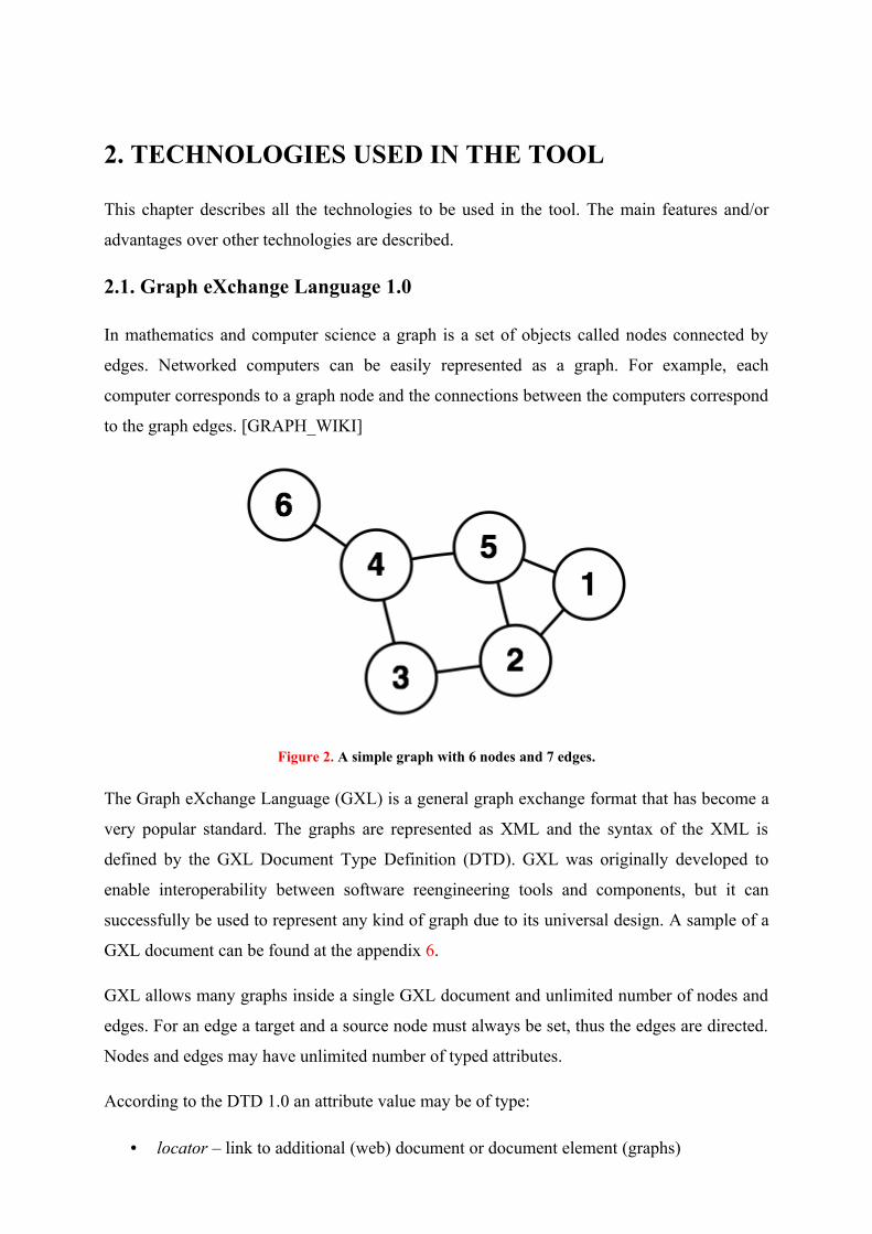
In mathematics and computer science a graph is a set of objects called nodes connected by

edges. Networked computers can be easily represented as a graph. For example, each

computer corresponds to a graph node and the connections between the computers correspond

to the graph edges. [GRAPH_WIKI]

Figure 2. A simple graph with 6 nodes and 7 edges.

The Graph eXchange Language (GXL) is a general graph exchange format that has become a

very popular standard. The graphs are represented as XML and the syntax of the XML is

defined by the GXL Document Type Definition (DTD). GXL was originally developed to

enable interoperability between software reengineering tools and components, but it can

successfully be used to represent any kind of graph due to its universal design. A sample of a

GXL document can be found at the appendix 6.

GXL allows many graphs inside a single GXL document and unlimited number of nodes and

edges. For an edge a target and a source node must always be set, thus the edges are directed.

Nodes and edges may have unlimited number of typed attributes.

According to the DTD 1.0 an attribute value may be of type:

• locator – link to additional (web) document or document element (graphs)

• bool – boolean

• int – an integer

• float – a floating point number

• string – text (may contain characters, numbers etc)

• enum – enumeration is a single value from enumeration of possible values

• seq – a sequence is an ordered sequence of elements (duplicates allowed)

• tup – a tuple is an ordered sequence with fixed number of elements (duplicates

allowed)

• set – a unordered set of non-duplicate elements

• bag – a multi-set of elements

Attribute values like seq, set, bag and tup are composite values which contain more values of

previously mentioned attribute value types. In addition to the attribute values, each attribute

may also contain unlimited number of another attributes as well. For example, this enables to

construct map like structures, where an object contains set of key and value pairs. It is also

possible to extend the value-extension entity to obtain more attribute types, but that is

discouraged because other GXL tools probably can not handle custom types by default.

[GXL_HOME]

Some alternatives to GXL are GRXL (Graph Rewriting Programming Language), GML

(Graph Modeling Language), GraphML (Graph Markup Language), GraphXML (XML based

graph format) or XGMML (eXtensible Graph Markup and Modeling Language). GXL is the

first choice because GXL was influenced by these formats while being designed and thus

improved what other formats were missing. Also GXL is already widely used by many

(already at the GXL homepage about 40 tools are listed) other graph tools like Graphviz,

JGraph, yFiles etc. [GRAPH_DRAWING]

A very nice and small (JAR file size on disk about 50KB) open-source Java library exists for

GXL 1.0. It has a very simple and intuitive API, which easily enables to read/write GXL

documents from/to a file into/from a Java object, random access the document elements from

the Java object, iterate over the document elements or attributes and create and modify each

element or attribute. The API also validates the generated GXL document to be compatible

with the GXL DTD. Because the API can read and write the Java object into a file the data is

easy to serialize for example into a byte array to be sent over the network. [GXL_JAVA]

GXL satisfies all of the requirements, especially the F13, F12 and T5 requirements.

2.2. Eclipse Rich Client Platform (RCP)

2.2.1. Why Eclipse RCP

The Eclipse Rich Client Platform (RCP) is an open source platform for building rich desktop

applications. By rich it is meant that it has rich feature set and rich visual design. At first it

was designed just for the Eclipse IDE, later it was redesigned to be more general, allowing

building just about any application on top of it. The Eclipse platform has been developed and

used since November 1998 [IBM_HISTORY] and thus is quite mature. It is still under very

active development and maintenance, so there is support in case it is needed. That is

something that the users of this platform value highly. The activity of the developer and user

groups of a framework is important, so the bugs and issues get solved fast and do not prevent

the product from evolving.

This platform is based on the Eclipse Equinox framework, which is an implementation of

Open Services Gateway Initiative (OSGI) R4 core framework specification [EQUINOX].

Equinox is one of the first platforms that implemented the OSGI component model.

Developing on the OSGI framework makes the components very modular and independent of

each-other. This enables to develop the products as an Eclipse plug-ins (also known as the

bundles in OSGI), so the looks and features of developed products are available through the

Eclipse IDE or some other Eclipse RCP application. They are also available as a totally

separate Eclipse RCP application, so there is almost no clue that the application was related to

Eclipse. Exporting the plug-in product as a separate application is very easy – only a few

dialogues and wizards at the first time and few clicks the following times.

All the necessary Eclipse Java archive (JAR) files to develop the RCP product take up only

5.8 megabytes. When exporting the product as Eclipse RCP application the result application

will take up only about 15 megabytes (12 megabytes according to the Eclipse RCP frequently

asked questions page). Should the footprint get very important, there is also the option to use

eRCP which is a stripped down version of RCP, which was originally designed for embedded

devices. So it is suitable platform according to the requirements T1 and T5. [RCP_FAQ]

The platform integrates seamlessly with the Eclipse Graphical Editing Framework (GEF)

which is very powerful framework for making graphical components and visuals. This was

preferred by the supervisors for visualization. The RCP architecture facilitates making nice

small distinctive components. It is easy to develop native look-and-feel applications, allowing

concentrating on creating the contents, not the graphics and standard features and routines.

It is proven to be a good and effective framework – Eclipse IDE and many other popular

applications are built on it (over 50 commercial and 20 open source products are listed on the

Eclipse RCP page and definitely even more exist). [RCP_FAQ]

Unfortunately the learning curve to master this platform is quite high. The platform has so

many possible features that need to be learned in order to produce some quality code, that it is

hard to master this platform. There are also many other plug-ins available, so deciding if some

feature has to be implemented from scratch or already exists somewhere is not a simple task.

For a beginner all the possible framework related exceptions and compilation problems (for

example related to faulty configuration or unclean build) that easily arise are quite hard and

time-consuming to resolve. After this struggle and familiarizing with the common problems

the development gets fast and convenient.

The Eclipse platform has low requirements on the Java version – it is built in Java version 1.4,

so newer Java versions are optional but not a must.

2.2.2. The architecture of RCP

An Eclipse RCP application consists of many kind of advisors (WorkbenchAdvisor,

WorkbenchWindowAdvisor, ActionBarAdvisor), perspectives, views and editors (see Figure

3).

The advisor components make the creation of standard layouts and look-and-feel easy.

WorkbenchAdvisor is used to choose the initial perspective, when the application starts.

WorkbenchWindowAdvisor defines the style of the window – the size and placement of the

window; and also which bars (menubar, coolbar, statusbar etc) will be used.

ActionBarAdvisor creates menubar and coolbar and registers actions with the corresponding

buttons and/or menu entries.

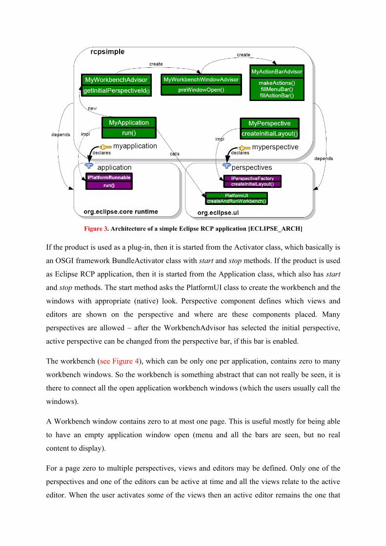
Figure 3. Architecture of a simple Eclipse RCP application [ECLIPSE_ARCH]

If the product is used as a plug-in, then it is started from the Activator class, which basically is

an OSGI framework BundleActivator class with start and stop methods. If the product is used

as Eclipse RCP application, then it is started from the Application class, which also has start

and stop methods. The start method asks the PlatformUI class to create the workbench and the

windows with appropriate (native) look. Perspective component defines which views and

editors are shown on the perspective and where are these components placed. Many

perspectives are allowed – after the WorkbenchAdvisor has selected the initial perspective,

active perspective can be changed from the perspective bar, if this bar is enabled.

The workbench (see Figure 4), which can be only one per application, contains zero to many

workbench windows. So the workbench is something abstract that can not really be seen, it is

there to connect all the open application workbench windows (which the users usually call the

windows).

A Workbench window contains zero to at most one page. This is useful mostly for being able

to have an empty application window open (menu and all the bars are seen, but no real

content to display).

For a page zero to multiple perspectives, views and editors may be defined. Only one of the

perspectives and one of the editors can be active at time and all the views relate to the active

editor. When the user activates some of the views then an active editor remains the one that

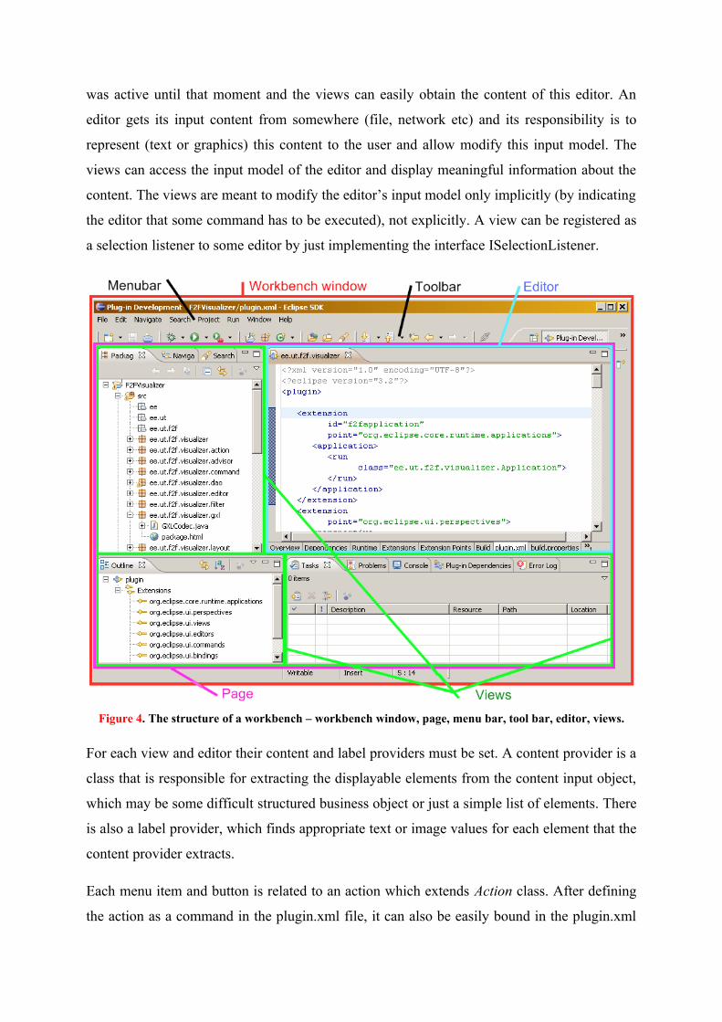
was active until that moment and the views can easily obtain the content of this editor. An

editor gets its input content from somewhere (file, network etc) and its responsibility is to

represent (text or graphics) this content to the user and allow modify this input model. The

views can access the input model of the editor and display meaningful information about the

content. The views are meant to modify the editor’s input model only implicitly (by indicating

the editor that some command has to be executed), not explicitly. A view can be registered as

a selection listener to some editor by just implementing the interface ISelectionListener.

Figure 4. The structure of a workbench – workbench window, page, menu bar, tool bar, editor, views.

For each view and editor their content and label providers must be set. A content provider is a

class that is responsible for extracting the displayable elements from the content input object,

which may be some difficult structured business object or just a simple list of elements. There

is also a label provider, which finds appropriate text or image values for each element that the

content provider extracts.

Each menu item and button is related to an action which extends Action class. After defining

the action as a command in the plugin.xml file, it can also be easily bound in the plugin.xml

file to (the combination of) the keys of the keyboard. Defining an action as a command also

enables to use it as an editor or view action, which becomes visible and executable only if an

editor or view of such type is active. This helps to keep the action bar small and clean by

hiding such buttons from the action bar that cant be used because there is no such view or

editor open to which the action could be applied to. This way the action bar can have only

these buttons displayed that are relevant and usable through out the application.

Eclipse RCP uses SWT and JFace to draw its graphics, which are described in the following

graphics chapter

2.3. Eclipse graphics frameworks

2.3.1. Standard Widget Toolkit (SWT)

Java’s default framework for doing the graphics is the Abstract Windowing Toolkit (AWT).

Sun’s approach when designing the AWT was to only offer the intersection of all the

available widgets of all the platforms that Java had to support. This cuts off a lot of widgets

from lots of platforms. To be able access the features of missing widgets Sun created the

Swing platform, which emulates all the widgets. Because of that, Swing applications do not

look nor feel like native applications and perform poorly compared to native widgets.

To solve the problems that AWT and Swing had, IBM created totally new alternative

framework – Standard Widget Toolkit (SWT). It uses the native widgets of the underlying

operating system through the JNI and if some of the widgets are not available on current

platform, they will be emulated by the SWT. So the standard graphical user interface elements

of an application can have totally native look and feel.

SWT provides the following common GUI elements (widgets) and their events:

• Browser – component that can display HTML content

• Button (check, radio, push, toggle, arrowed) – a selectable object that issues a

notification when it is pressed and released

• Canvas – surface for drawing arbitrary graphics

• Combo – a control that allows user to select an element from a list (or optionally type

in a new element value if not already in the list)

• Composite – a control that can contain multiple control instances

• CoolBar – area that enables the user to dynamically position the items (of type

CoolItem) it contains (it is similar to the toolbars)

• CTabFolder – enables tabbing (similar to tabbed browsing) and next to the tabs are

also some specific buttons

• DateTime – calendar component that allows user to select, enter and modify date or

time value

• ExpandBar – layout of selectable expand bar items

• Group – etched border with optional title around the children items

• Label – non-selectable user interface object for displaying text or image

• Link – selectable user interface object for displaying text with links

• List – selectable list of string values, a notification is issued when a string is selected

(can be single or multi selection list)

• Menu – container for menu items

• ProgressBar – non-selectable object for displaying progress (usually a bar)

• Sash – selectable object that allows to drag a rubber banded outline of the sash within

the parent control horizontally or vertically (an user interface object which’s edges can

be dragged along by the user like it was from rubber)

• ScrolledComposite – provides scrollbars to the composite which may contain multiple

other controls

• Shell – the “window” that the desktop or “window manager” manages

• Slider – sliding user interface object for selecting a value in range of all the possible

discrete numeric values

• Scale – sliding user interface object for selecting a value in range of all the possible

continues numeric values

• Spinner – allows the user to enter numeric value and/or modify the value with arrowed

increment/decrement buttons

• StyledText – editable object for displaying multiple lines of text which can be styled

for example by foreground- and background color, font style, underlining and

strikethrough properties

• TabFolder – enables tabbing (similar to tabbed browsing)

• Table – a table of images and/or strings

• Text (single or multi-line) – selectable object to enter and modify text

• ToolBar – layout for selectable tool bar items (of type ToolItem)

• Tray – a system tray that is part of the task bar area of some operating systems

• Tree – selectable object that displays the hierarchy of items (of type TreeItem), a

notification is issued when some item is selected

[SWT_WIDGETS]

SWT also provides different kind of layouts: Fill, Form, Grid and Row layout. Even OpenGL

graphics can be used quite easily because various libraries are made for the SWT.

Unfortunately the operating systems of today are not written in Java nor do not use much of

the Object Oriented Programming (OOP) that is very common in Java. This non-OOP

approach therefore also transmits into the SWT. Since the drawing is done by the operating

system, the Java Virtual Machine (JVM) does not have much of a control over the images that

are drawn and thus it can not know when they become obsolete and need to be garbage

collected. This requires that the images are explicitly disposed in the Java application after

they become useless. This non-automatic garbage collection is not very appropriate for Java.

2.3.2. JFace

JFace is user interface toolkit based on SWT and offers much simplified and more Java like

usage of the native widgets. It takes care of all the garbage collection that otherwise has to be

done manually in SWT (the components that are drawn by the operating system and which

the JVM can not manage automatically). Also there is less to be worried about the creation of

the windows or complicated components like tables or trees.

JFace viewers are model based adapters for certain SWT widgets, which simplify the

presentation of the application data. The following viewers for common structures are

provided:

• ListViewer – for displaying a single columned list of items

• TreeViewer – for displaying a multi columned tree structured list of items that can be

expanded and collapsed

• TableViewer – for displaying a table of items

• TextViewer – for displaying pure text content (like text editors)

• ContentViewer – for displaying any kind of content (other viewers extend this)

JFace provides an Action class, which represents a command that the user can trigger. It is a

reusable component – instead of writing the method that performs the action for every button,

an instance of the action class can be assigned to the button, menu or toolbar item. Although

the actions are not considered a part of the user interface, the actions have also some user

interface properties like the corresponding tool-tip text, label and image.

Most common dialogues like the info, error or yes/no question and wizards like choose file,

import/export or custom wizards are included. Long-running processes that can run in the

background and display the progress-bar are supported inside both the program window and

in the wizards. Image and Font registries are available for easier handling of these user

interface resources. [JFACE_HOME]

2.3.3. Draw2d

Draw2d enables to draw easily almost any kind of diagram or drawing. It is a lightweight

toolkit of graphical components called figures. Each figure is just a simple Java object and

internally they are drawn by SWT. Most SWT events are forwarded to the EventDispatcher,

which translates them into events on the appropriate figure, which can be listened for example

by some application component. Paint events are forwarded to the draw2d UpdateManager,

which manages the painting and layout. Managing the painting process means the managing

of the order in which the figures and their children must be painted. This is accomplished

because Draw2d keeps track of the Z-order and clipping of the figures. Draw2d also does the

tedious SWT garbage collection. Managing the layout means detecting if some figure in the

drawing becomes invalid and calculating a new position for such figure. All the figures are in

the invalid state when they are constructed.

The figures can be composed via parent-child relationship. Draw2d even has a special type of

a figure – the connection figure. They are used to draw lines between two points. These

figures do not have bounds, only start and end anchors, and usually have to be drawn above

the other figures on the drawing. The connections may have different kind of routers which

route the line from one point to the other (for example, a router which avoids the overlapping

of the line with other non-connection figures). The connections can be decorated, for example

with arrowheads or labels.

Draw2d does the hit testing, which is necessary for example to determine which tool-tip to

display for a figure or to enable the drag (and-drop) functionality. Also absolute and relative

coordinate systems are implemented, which are required by certain optimizations and features

in the draw2d. Among the other things, this makes it possible to easily translate or zoom the

graphics. [DRAW2D_GUIDE]

Draw2d makes the graphical part of the Eclipse Graphical Editing Framework (GEF),

whereas the GEF plug-in itself only provides the sophisticated ways to control and modify

these graphics by connecting the data model to the view

2.3.4. Zest – The Eclipse Visualization Toolkit

Zest is a visualization toolkit for Eclipse, which’s goal is to make programming graphs easier.

Zest components are built entirely in SWT and Draw2d and are modeled after the JFace. The

graphs are considered SWT components which are wrapped in standard JFace viewers, more

precisely into a GrahpViewer viewer. So Zest can be used the same way the tables or trees of

the JFace are used. Zest also contains few standard layout algorithm implementations for

displaying the graphs.

At the time of writing this paper, the Zest project is an independent project in the Eclipse

framework, but in the near future it is to be merged into the GEF. [ZEST]

2.4. Java Remote Method Invocation (RMI)

Java Remote Method Invocation (RMI) is a technology that allows easy invoking of the

methods on remote Java Virtual Machines (JVM), even on another host machine. To marshal

and unmarshal the method input and output parameters, RMI uses automatic object

serialization. RMI enables to exchange the real Java objects with very little effort – only start

the RMI Registry server, make method lookup call and execute the method. For comparison,

in the plain socket connections, the connection has to be manually opened, accepted and read

and each transferred object has to be manually cast each time.

Java RMI is included in the Java Standard Edition (SE), so there is no need for another library

and thus no increase in the visualization tool’s size. It is perfect for exchanging Java objects

and it is proven to be reliable (many remoting frameworks internally use RMI) while being

really straightforward and simple to use. This makes the RMI technology the choice for

communication between the visualizing and data gathering tool. [RMI]

2.5. Summary of the technologies

In this chapter all the technologies (except Java itself) used for implementing the visualization

tool were briefly described. The GXL 1.0 format was selected for exchanging the graph data

because this standard had all the required features, was the newest of the alternative standard

graph file formats and had a nice ready-to-use Java library.

Eclipse graphical frameworks (SWT, JFace, Draw2d, GEF and Zest) and their main features

were described so a clear understanding of which features and benefits needed for the

visualization tool comes with which framework. SWT is the fundamental component for each

of these frameworks. JFace and Draw2d build a solid Java framework on top of the SWT.

JFace is designed for building effective native look graphical user interface (GUI)

applications from common GUI components, whereas the Draw2d (and GEF) is designed for

drawing custom graphics (like diagrams). Zest is designed to draw graphs. Also, the

supervisors preferred the Eclipse graphical framework to an alternative interesting Java graph

editing framework called JGraph, because of some bad experience known before.

Eclipse RCP is a platform for creating native looking applications or Eclipse plug-ins. It was

chosen to be the core framework to the visualizing tool because it integrates seamlessly with

all the Eclipse graphical frameworks and it has good architecture. Eclipse RCP has many well

defined standard components and thus it is easy to add new features and extend the

application. Eclipse platforms support all of the technical requirements defined in this paper.

Java RMI has many advantages over the other possible remoting frameworks, most

importantly being the most compact and easy to use for implementing the communication

between Java applications.

3. GRAPH LAYOUT ALGORITHMS

This chapter gives a brief description about the algorithms available in the visualization tool.

Also the main advantages or disadvantages of the algorithms are mentioned.

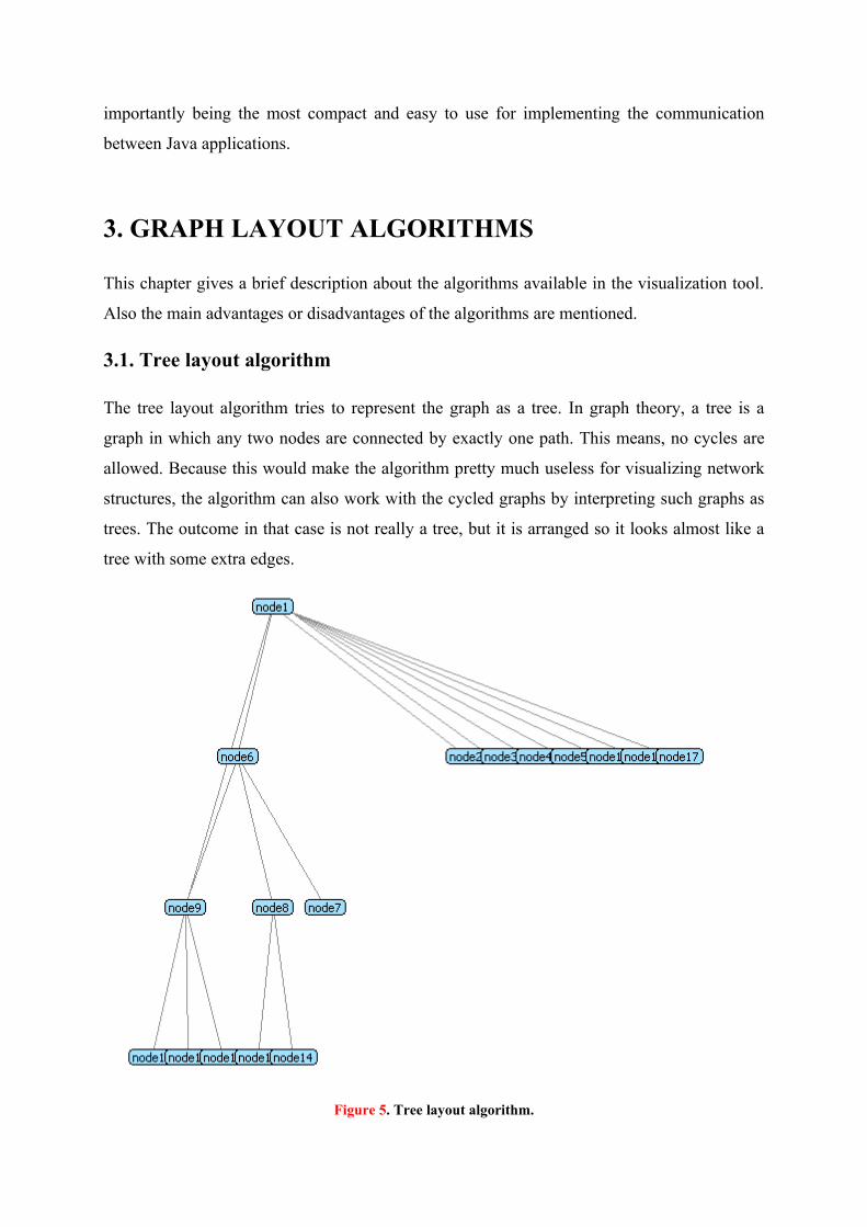
3.1. Tree layout algorithm

The tree layout algorithm tries to represent the graph as a tree. In graph theory, a tree is a

graph in which any two nodes are connected by exactly one path. This means, no cycles are

allowed. Because this would make the algorithm pretty much useless for visualizing network

structures, the algorithm can also work with the cycled graphs by interpreting such graphs as

trees. The outcome in that case is not really a tree, but it is arranged so it looks almost like a

tree with some extra edges.

Figure 5. Tree layout algorithm.

The tree layout algorithm extracts an acyclic graph from the set of nodes by tracing the

relationships of the nodes. Then a layer number is assigned to each of the nodes. The nodes

that are in the same layer are ordered so that the edge crossings between the two consecutive

layers are minimal. After completing the node positioning calculations in the tree, the tree is

drawn with all of its nodes and edges. The edges that were removed (if any) from the graph

for the calculations are also drawn on the graph, thus making even a cyclic graph look similar

to a tree. The results of this algorithm are very good when the structure of the underlying

graph is tree-like. This means, that there should not be many cycles. The major disadvantage

of this algorithm is that it is a bit slow. [TREE_LAYOUT]

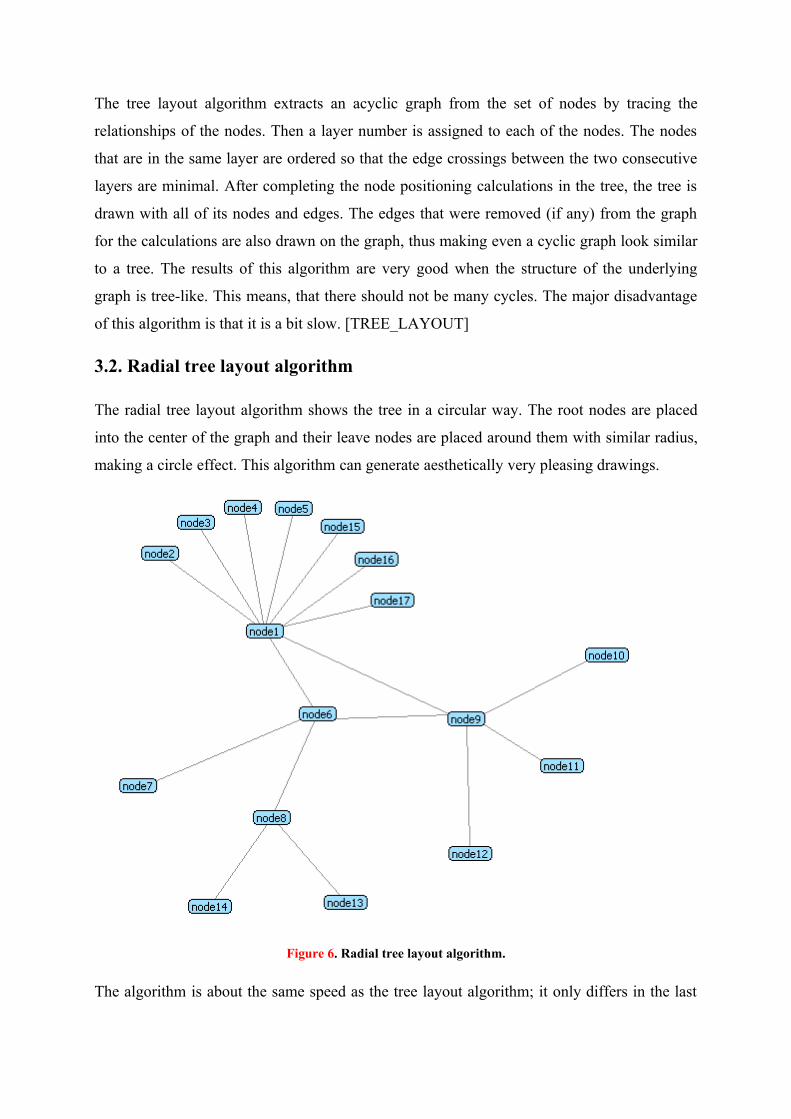
3.2. Radial tree layout algorithm

The radial tree layout algorithm shows the tree in a circular way. The root nodes are placed

into the center of the graph and their leave nodes are placed around them with similar radius,

making a circle effect. This algorithm can generate aesthetically very pleasing drawings.

Figure 6. Radial tree layout algorithm.

The algorithm is about the same speed as the tree layout algorithm; it only differs in the last

step where it calculates the radial positions instead of the vertical or horizontal tree positions.

The algorithm works as good as the tree layout algorithm on the trees. On the non-tree graphs

it yields better results, because it seems to generate less edge crossings and the topologically

more important nodes appear in the center of the picture. So it is very easy to identify the

nodes that matter the most in terms of joining different sub-graphs (sub-networks).

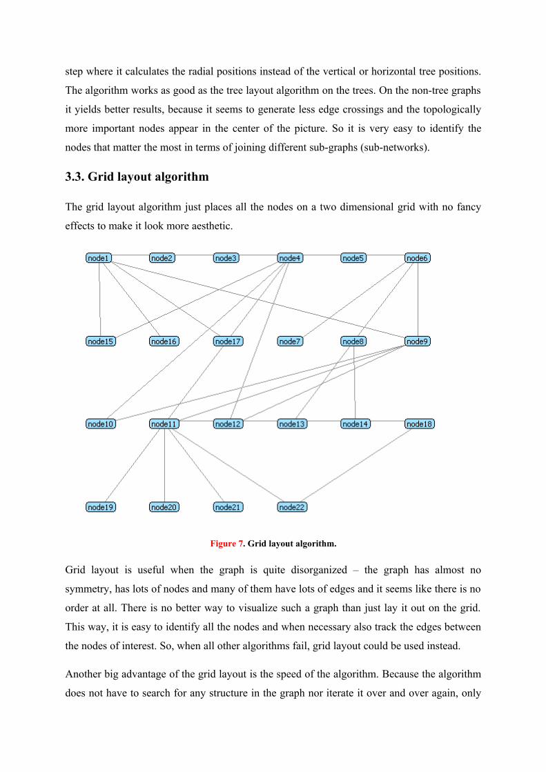
3.3. Grid layout algorithm

The grid layout algorithm just places all the nodes on a two dimensional grid with no fancy

effects to make it look more aesthetic.

Figure 7. Grid layout algorithm.

Grid layout is useful when the graph is quite disorganized – the graph has almost no

symmetry, has lots of nodes and many of them have lots of edges and it seems like there is no

order at all. There is no better way to visualize such a graph than just lay it out on the grid.

This way, it is easy to identify all the nodes and when necessary also track the edges between

the nodes of interest. So, when all other algorithms fail, grid layout could be used instead.

Another big advantage of the grid layout is the speed of the algorithm. Because the algorithm

does not have to search for any structure in the graph nor iterate it over and over again, only

divide the nodes into the grid, it is very fast. This makes this algorithm an ideal candidate for

the initial lay outing of the graph.

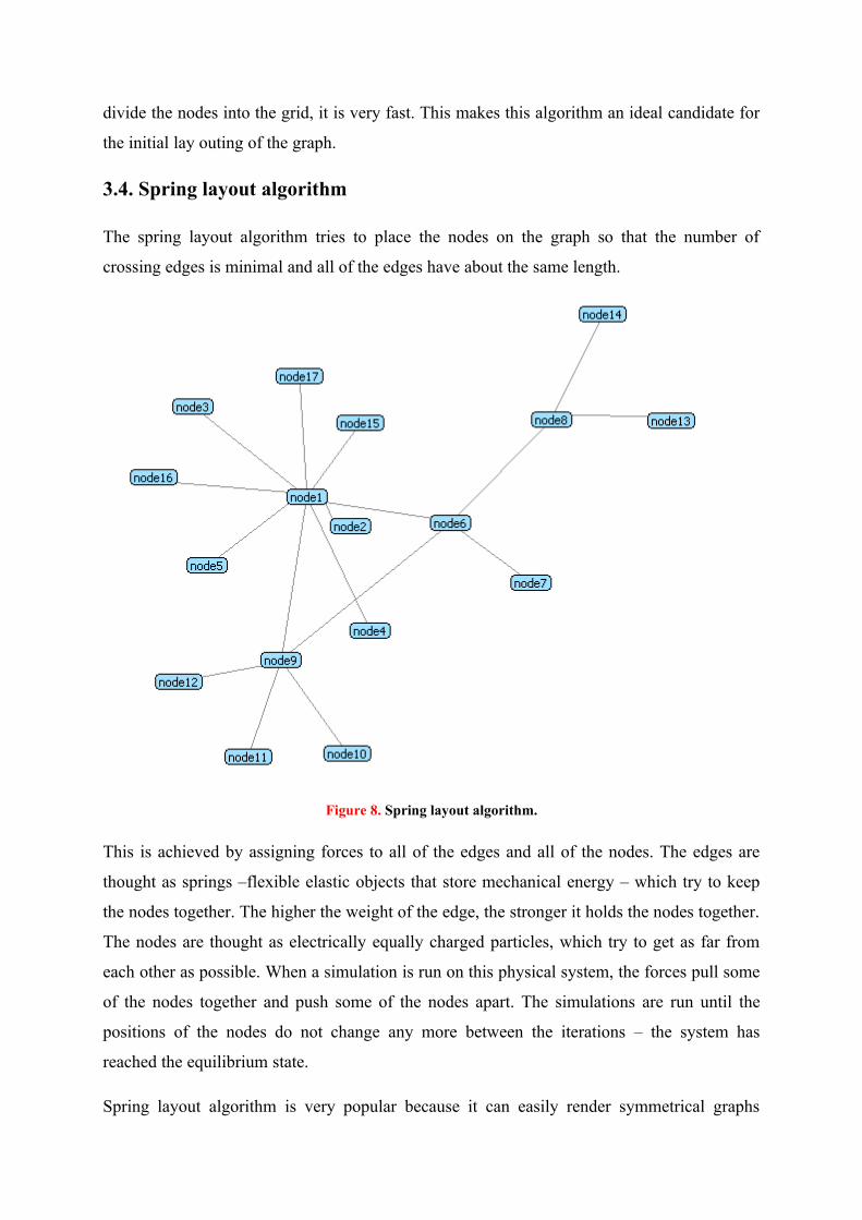
3.4. Spring layout algorithm

The spring layout algorithm tries to place the nodes on the graph so that the number of

crossing edges is minimal and all of the edges have about the same length.

Figure 8. Spring layout algorithm.

This is achieved by assigning forces to all of the edges and all of the nodes. The edges are

thought as springs –flexible elastic objects that store mechanical energy – which try to keep

the nodes together. The higher the weight of the edge, the stronger it holds the nodes together.

The nodes are thought as electrically equally charged particles, which try to get as far from

each other as possible. When a simulation is run on this physical system, the forces pull some

of the nodes together and push some of the nodes apart. The simulations are run until the

positions of the nodes do not change any more between the iterations – the system has

reached the equilibrium state.

Spring layout algorithm is very popular because it can easily render symmetrical graphs

where the nodes are distributed uniformly. It is quite intuitive and easy to predict how the

nodes will position on the graph, because this algorithm is based on the physical analogies of

common objects. Symmetry is very common in the real world. This makes symmetrically laid

out graphs look more natural for a human than randomly laid out graphs and therefore

improve the understanding characteristics of the graph.

The main disadvantage of the spring layout algorithm is the long running time. The algorithm

needs a lot of iterations and in each iteration all of the node pairs must be visited and their

mutual forces be calculated. Another disadvantage is that in case of a very bad initial layout,

where the calculated local minimum energy is a lot worse than the global minimum energy,

the algorithm can produce a poor-looking graph. This could be improved by combining the

algorithm with some better algorithm for the initial layout. [SPRING_LAYOUT]

3.5. Summary of the algorithms

Unfortunately there is no "best" layout — different ways of displaying a graph emphasize

different characteristics. One important measure of the quality of the graph drawing algorithm

is the number of crossing edges it draws. Some graphs cannot be drawn without edge

crossings at all, some graphs can. Generally, the fewer the edge crossings the better the

algorithm is. Another quality measure is the closeness of the nodes to the non-adjacent nodes

and non-adjacent edges. For an aesthetically pleasing drawing there should be sufficient space

between the non-adjacent edges and nodes. A quite important measure is the speed of the

algorithm, when dealing with large graphs.

The spring and radial tree layouts render aesthetically most appealing graphs, where the

adjacent nodes are nicely grouped and non-adjacent nodes appear in some distance. Tree

layout can also look good on some graphs. Unfortunately these can also produce very ugly

graphs when the structure of the graph is messy and they also take the most calculation time

as well. When the graph’s structure is quite disorganized, then the grid layout could be used

instead. The grid layout algorithm is also the best performing algorithm described.

So, for the initial fast preview of the graph the grid layout can be used. Depending on the

structure of the F2F network the user can later choose the algorithm that looks most helpful or

appealing. It would be possible to automatically choose an initial algorithm depending on the

node and edge counts, but before actually implementing it, some user feedback and more real

life examples have to be collected and analyzed first.

4. IMPLEMENTED VISUALIZATION TOOL

This chapter explains how to install and use the product. It will give an answer to the

questions: What were the difficulties in implementing the tool and finally, what are the

results?

4.1. Installation

As a prerequisite a Java version 5 or newer must be installed. Also, to be able to obtain live

network topology data, the SIP-communicator with F2F data gathering bundle must be

installed and running.

No installation is required; the application can be started right away from the executable file.

The executable can be obtained on three ways.

a. Extract the binaries from the compressed archive file which is included on the

Compact Disc in the appendix 7

b. Download the compressed archive file from the project home page at

http://ulno.net/f2f/ and extract the binaries for the target platform (Windows or Linux)

c. Check out the source of the project from the SVN at http://spontaneous-desktop-

grid.googlecode.com/svn/java/F2FVisualizer and open the Java project in the Eclipse

IDE 3.3.2 or newer with the plug-in development plug-in installed. This project must

be viewed in the plug-in development perspective. To run the application one can start

it from the Eclipse or export it to executable. To start the application from Eclipse IDE

one must select the project name on the navigation view. Then click on the “run as”

button or right click on the project name and then select the “Eclipse Application”

menu item from the popped up menu. To export the application into an executable file

a product definition file named “f2fvisualizer.product” must be opened while the plug-

in development perspective is active. This file is located at the project root. The

product definition file reveals a view where is a button/link named the “Eclipse

product export wizard” (under the “Exporting” collapsible section). On the export

wizard the output directory must be selected and after clicking the “Finish” button, the

product is exported.

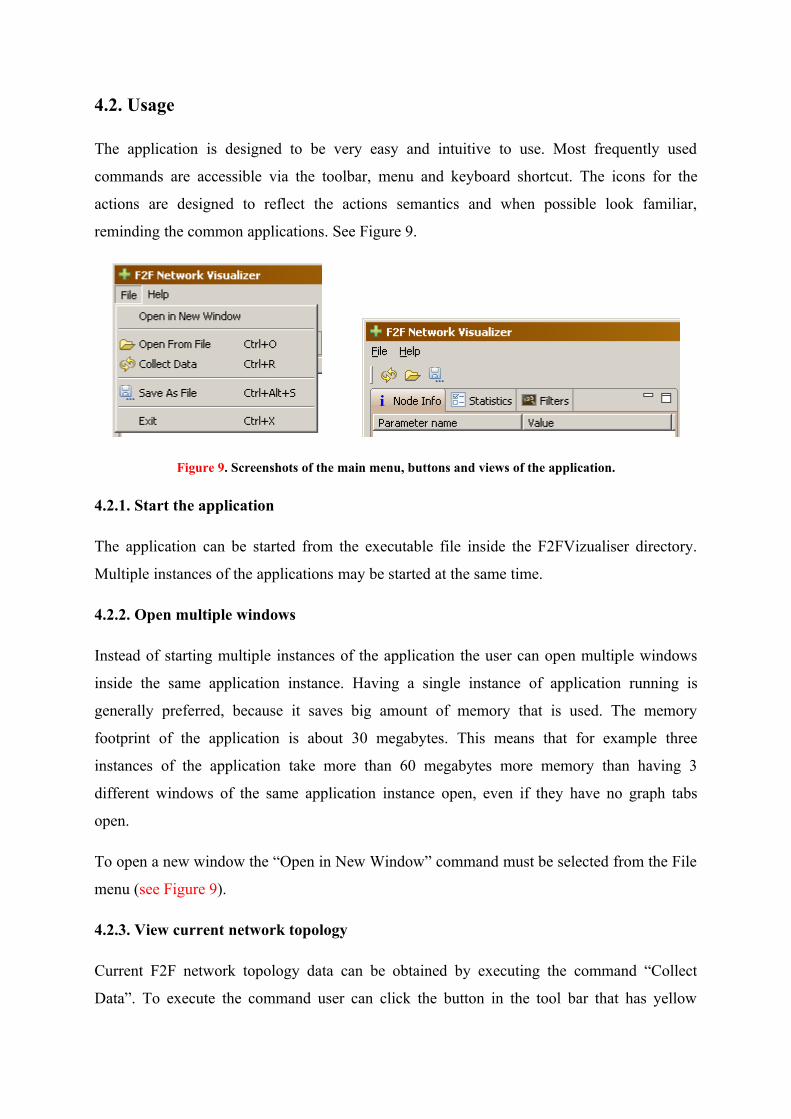
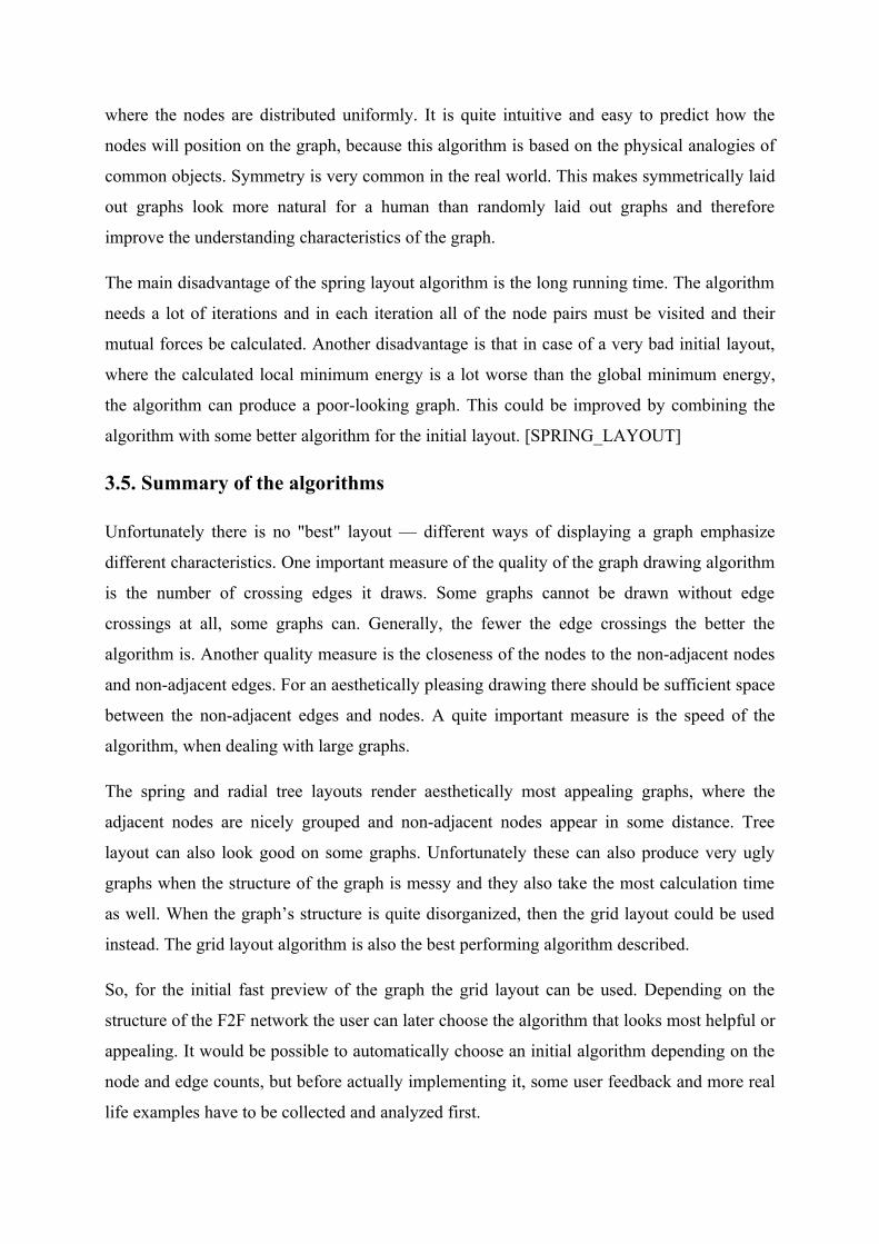
4.2. Usage

The application is designed to be very easy and intuitive to use. Most frequently used

commands are accessible via the toolbar, menu and keyboard shortcut. The icons for the

actions are designed to reflect the actions semantics and when possible look familiar,

reminding the common applications. See Figure 9.

Figure 9. Screenshots of the main menu, buttons and views of the application.

4.2.1. Start the application

The application can be started from the executable file inside the F2FVizualiser directory.

Multiple instances of the applications may be started at the same time.

4.2.2. Open multiple windows

Instead of starting multiple instances of the application the user can open multiple windows

inside the same application instance. Having a single instance of application running is

generally preferred, because it saves big amount of memory that is used. The memory

footprint of the application is about 30 megabytes. This means that for example three

instances of the application take more than 60 megabytes more memory than having 3

different windows of the same application instance open, even if they have no graph tabs

open.

To open a new window the “Open in New Window” command must be selected from the File

menu (see Figure 9).

4.2.3. View current network topology

Current F2F network topology data can be obtained by executing the command “Collect

Data”. To execute the command user can click the button in the tool bar that has yellow

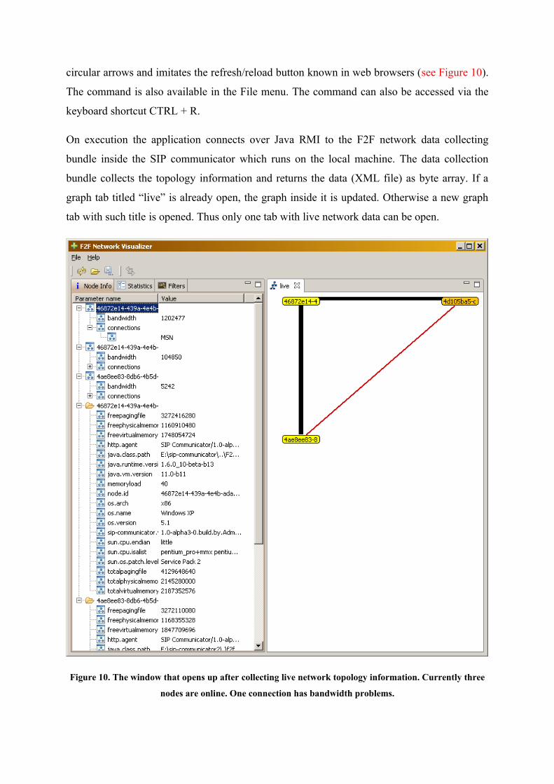
circular arrows and imitates the refresh/reload button known in web browsers (see Figure 10).

The command is also available in the File menu. The command can also be accessed via the

keyboard shortcut CTRL + R.

On execution the application connects over Java RMI to the F2F network data collecting

bundle inside the SIP communicator which runs on the local machine. The data collection

bundle collects the topology information and returns the data (XML file) as byte array. If a

graph tab titled “live” is already open, the graph inside it is updated. Otherwise a new graph

tab with such title is opened. Thus only one tab with live network data can be open.

Figure 10. The window that opens up after collecting live network topology information. Currently three

nodes are online. One connection has bandwidth problems.

4.2.4. Save the graph into a file

At any time the network topology inside the active graph tab can be saved into a file by

executing the “Save As File” command. Only the topology model, not the layout, is saved,

because only the model is necessary for archiving and XML content can grow extremely large

in case of large networks. The command can be executed by clicking the button in the tool bar

that has floppy disc image with three dots on it (see Figure 9). The command is also available

in the File menu and with the keyboard shortcut CTRL + ALT + S.

The file may be saved either with GXL or XML file extension, the content is the same on

both occasions. The GXL extension is preferred by default, to indicate that the content is a

valid GXL 1.0 document. By default the filename in the save file dialogue is set to the name

of graph editor title or when viewing live network data then to the current date.

4.2.5. Open a graph from a file

The application can load a graph from any XML, GXL or any other extension file which is a

valid GXL 1.0 document. The graph can be loaded by executing the “Open From File”

command, which can be accessed through button in the tool bar which depicts a yellow half-

open folder (see Figure 9). The command is also available in the File menu and via the

keyboard shortcut CTRL + O.

The graph is loaded and displayed inside the current window in a new tab which is titled by

the file name. Inside the same window only one tab with the same title/file name can be open.

To open the file multiple times, a new program window must be opened first (see the open

multiple windows section).

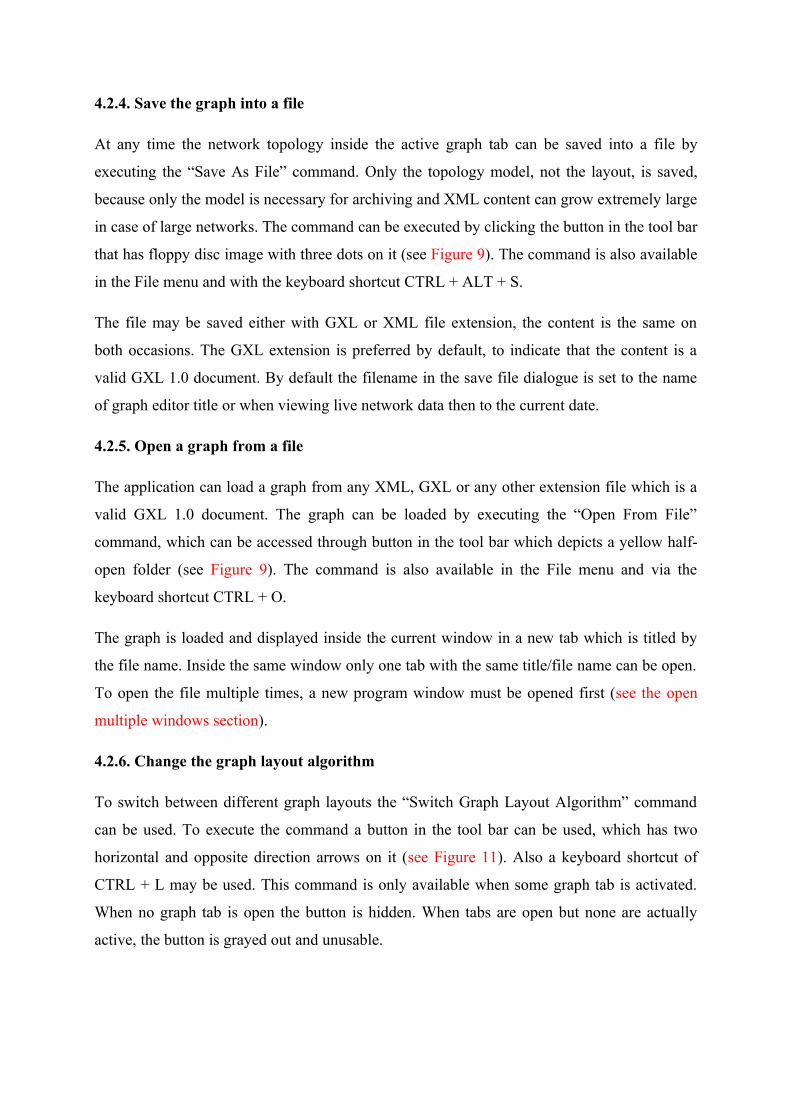
4.2.6. Change the graph layout algorithm

To switch between different graph layouts the “Switch Graph Layout Algorithm” command

can be used. To execute the command a button in the tool bar can be used, which has two

horizontal and opposite direction arrows on it (see Figure 11). Also a keyboard shortcut of

CTRL + L may be used. This command is only available when some graph tab is activated.

When no graph tab is open the button is hidden. When tabs are open but none are actually

active, the button is grayed out and unusable.

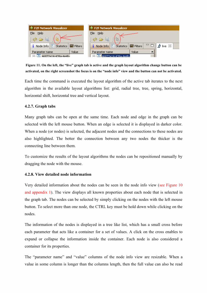
Figure 11. On the left, the “live” graph tab is active and the graph layout algorithm change button can be

activated, on the right screenshot the focus is on the “node info” view and the button can not be activated.

Each time the command is executed the layout algorithm of the active tab iterates to the next

algorithm in the available layout algorithms list: grid, radial tree, tree, spring, horizontal,

horizontal shift, horizontal tree and vertical layout.

4.2.7. Graph tabs

Many graph tabs can be open at the same time. Each node and edge in the graph can be

selected with the left mouse button. When an edge is selected it is displayed in darker color.

When a node (or nodes) is selected, the adjacent nodes and the connections to these nodes are

also highlighted. The better the connection between any two nodes the thicker is the

connecting line between them.

To customize the results of the layout algorithms the nodes can be repositioned manually by

dragging the node with the mouse.

4.2.8. View detailed node information

Very detailed information about the nodes can be seen in the node info view (see Figure 10

and appendix 1). The view displays all known properties about each node that is selected in

the graph tab. The nodes can be selected by simply clicking on the nodes with the left mouse

button. To select more than one node, the CTRL key must be hold down while clicking on the

nodes.

The information of the nodes is displayed in a tree like list, which has a small cross before

each parameter that acts like a container for a set of values. A click on the cross enables to

expand or collapse the information inside the container. Each node is also considered a

container for its properties.

The “parameter name” and “value” columns of the node info view are resizable. When a

value in some column is longer than the columns length, then the full value can also be read

from the tool-tip text, which appears shortly after the cursor has been moved over the value.

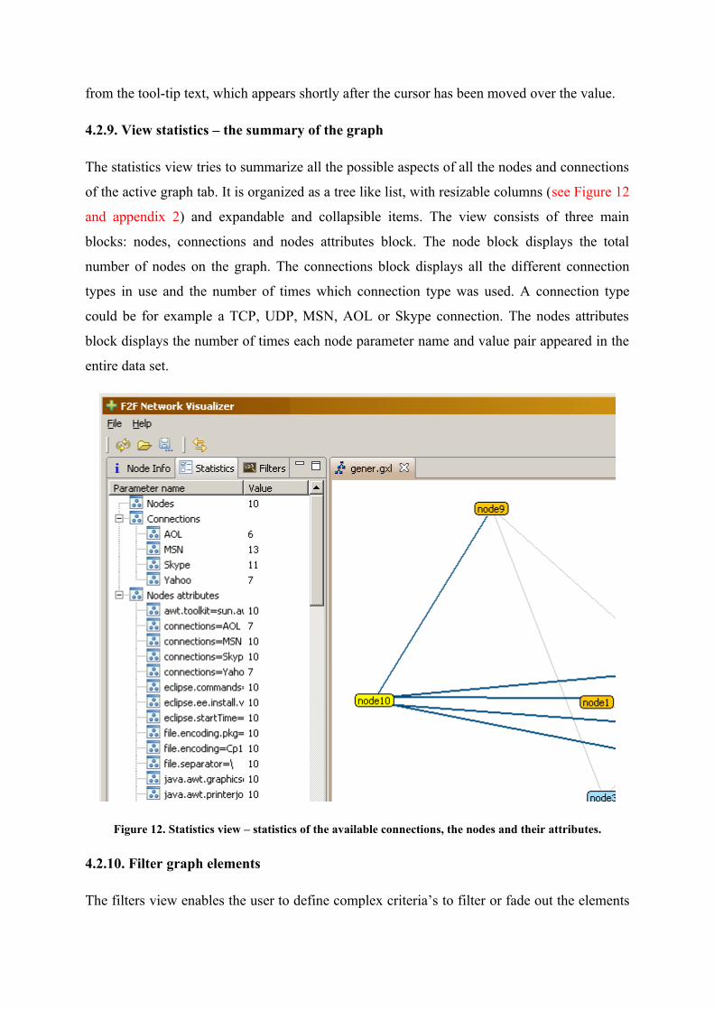
4.2.9. View statistics – the summary of the graph

The statistics view tries to summarize all the possible aspects of all the nodes and connections

of the active graph tab. It is organized as a tree like list, with resizable columns (see Figure 12

and appendix 2) and expandable and collapsible items. The view consists of three main

blocks: nodes, connections and nodes attributes block. The node block displays the total

number of nodes on the graph. The connections block displays all the different connection

types in use and the number of times which connection type was used. A connection type

could be for example a TCP, UDP, MSN, AOL or Skype connection. The nodes attributes

block displays the number of times each node parameter name and value pair appeared in the

entire data set.

Figure 12. Statistics view – statistics of the available connections, the nodes and their attributes.

4.2.10. Filter graph elements

The filters view enables the user to define complex criteria’s to filter or fade out the elements

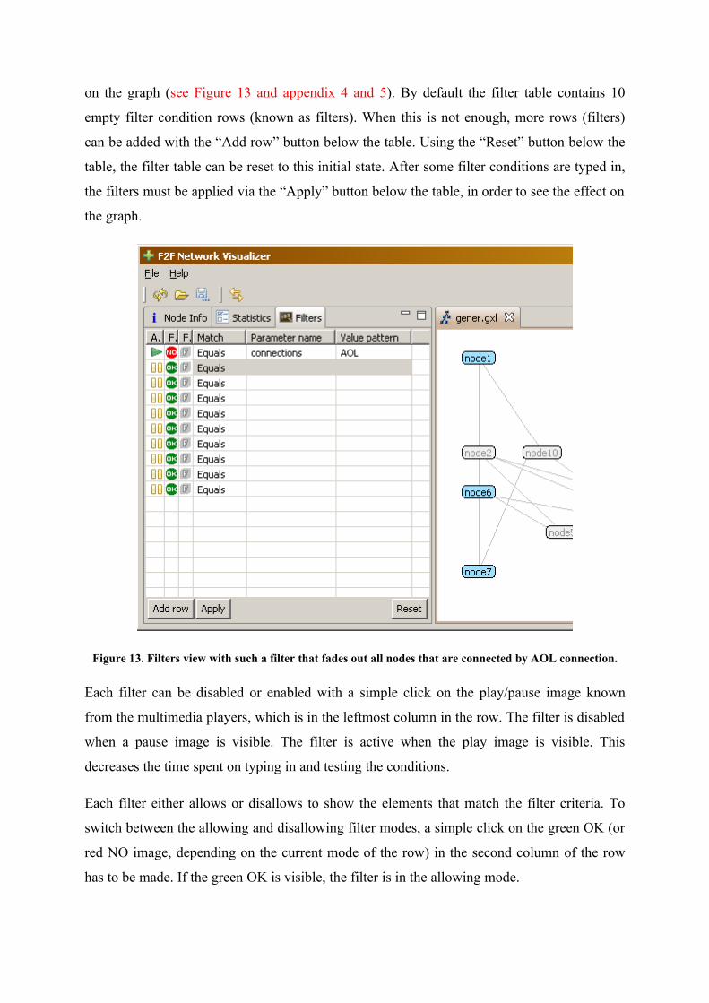
on the graph (see Figure 13 and appendix 4 and 5). By default the filter table contains 10

empty filter condition rows (known as filters). When this is not enough, more rows (filters)

can be added with the “Add row” button below the table. Using the “Reset” button below the

table, the filter table can be reset to this initial state. After some filter conditions are typed in,

the filters must be applied via the “Apply” button below the table, in order to see the effect on

the graph.

Figure 13. Filters view with such a filter that fades out all nodes that are connected by AOL connection.

Each filter can be disabled or enabled with a simple click on the play/pause image known

from the multimedia players, which is in the leftmost column in the row. The filter is disabled

when a pause image is visible. The filter is active when the play image is visible. This

decreases the time spent on typing in and testing the conditions.

Each filter either allows or disallows to show the elements that match the filter criteria. To

switch between the allowing and disallowing filter modes, a simple click on the green OK (or

red NO image, depending on the current mode of the row) in the second column of the row

has to be made. If the green OK is visible, the filter is in the allowing mode.

It might be easier to write the filters when the filters are in the fading mode. In fading mode,

the graph elements that match the criteria are faded out slightly rather than totally removed

from the graph. To switch between the fading and removing filter mode, the gray F or red X

image in the third column of the row must be clicked. The gray F stands for fading out and

red X for deletion of elements. If the gray F is visible, then the filter is in fading mode.

The filters matching conditions can be: equals, contains, starts with or ends with. The

matching is done ignoring the case of the letters. The “equals” mode means that the string

values of the value pattern column and the node attribute value must be equal. The “contains”

mode means that the string value in the value pattern column must also exist inside the value

that it is matched against. The “starts with” mode looks for the values that start with the string

in the value pattern column and the ends with mode looks for the values that end with such

string. These matching modes can be changed by selecting a new mode from the drop-drown

list in the column named “Match”.

After the graph has been simplified by removing most of the unnecessary nodes, another

graph layout could be tried. The less there are nodes on the graph the faster the layout

algorithms work. Also the graphs are potentially a lot easier to read.

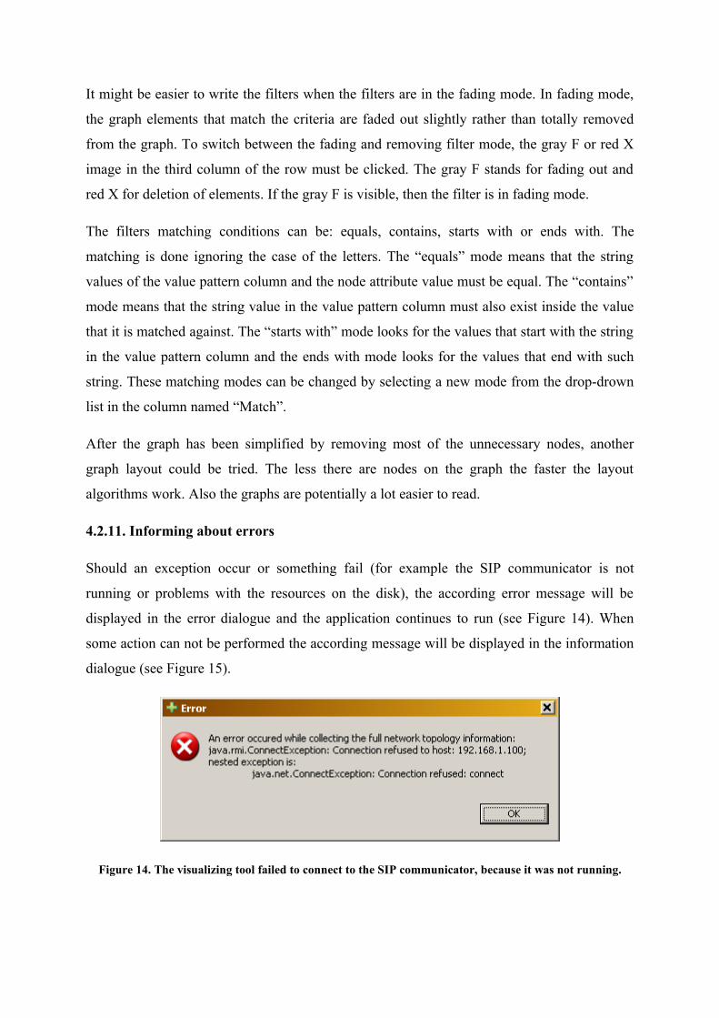
4.2.11. Informing about errors

Should an exception occur or something fail (for example the SIP communicator is not

running or problems with the resources on the disk), the according error message will be

displayed in the error dialogue and the application continues to run (see Figure 14). When

some action can not be performed the according message will be displayed in the information

dialogue (see Figure 15).

Figure 14. The visualizing tool failed to connect to the SIP communicator, because it was not running.

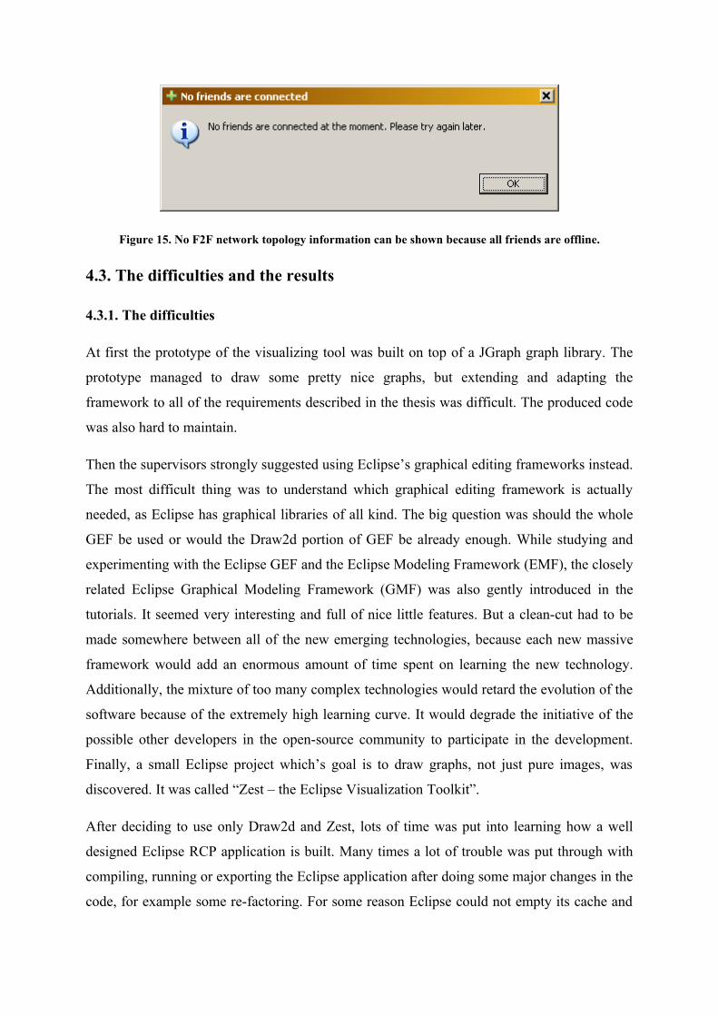
Figure 15. No F2F network topology information can be shown because all friends are offline.

4.3. The difficulties and the results

4.3.1. The difficulties

At first the prototype of the visualizing tool was built on top of a JGraph graph library. The

prototype managed to draw some pretty nice graphs, but extending and adapting the

framework to all of the requirements described in the thesis was difficult. The produced code

was also hard to maintain.

Then the supervisors strongly suggested using Eclipse’s graphical editing frameworks instead.

The most difficult thing was to understand which graphical editing framework is actually

needed, as Eclipse has graphical libraries of all kind. The big question was should the whole

GEF be used or would the Draw2d portion of GEF be already enough. While studying and

experimenting with the Eclipse GEF and the Eclipse Modeling Framework (EMF), the closely

related Eclipse Graphical Modeling Framework (GMF) was also gently introduced in the

tutorials. It seemed very interesting and full of nice little features. But a clean-cut had to be

made somewhere between all of the new emerging technologies, because each new massive

framework would add an enormous amount of time spent on learning the new technology.

Additionally, the mixture of too many complex technologies would retard the evolution of the

software because of the extremely high learning curve. It would degrade the initiative of the

possible other developers in the open-source community to participate in the development.

Finally, a small Eclipse project which’s goal is to draw graphs, not just pure images, was

discovered. It was called “Zest – the Eclipse Visualization Toolkit”.

After deciding to use only Draw2d and Zest, lots of time was put into learning how a well

designed Eclipse RCP application is built. Many times a lot of trouble was put through with

compiling, running or exporting the Eclipse application after doing some major changes in the

code, for example some re-factoring. For some reason Eclipse could not empty its cache and

reload the changes; the development was stuck in a problem that actually should not be a

problem.

According to the initial plan, the data gathering tool and the visualizing tool were supposed to

be integrated simply by including the Java archive file (JAR) of the data gatherer in the

visualizing tool. At some point it was clear that the data gatherer tool should be a part of the

SIP communicator and the F2F project to allow natural access to the F2F network resources.

Therefore it could not reside in the visualizing application.

The Java RMI technology was selected to overcome the integration problems. The RMI set-

up had some issues with the Java Security Manager, which for a long time failed to load the

policy file from the inside of the OSGI bundle.

4.3.2. The results

The application that was created in the thesis meets all of the technical and functional

requirements described in this paper. It can collect the information about the F2F network

topology and display the results as a graph, which can be arranged by many different layout

algorithms. The elements on the graph are multi-selectable and movable by the mouse. The

graph view displays the problematic connections in the eye-catching red color, which helps

the user to detect them quickly. Superior connections are drawn thicker. In case of a large

graph, tracing some path from some node A to some node Z is simplified, because the

adjacent nodes and connections are highlighted. Another mean to simplify the working with

large graphs is to use the filters view which allows to define multiple and different kind of

filters with different passing criteria’s.

The implemented application also features a bonus view where the statistics about the graph

can be seen. This view is basically a two-column table (more accurately a tree) with the

summary of attribute names and values.

The application operates successfully with the GXL graph files. Most of the information that

accompanies the nodes and connections, which are discovered and gathered via the data

gathering tool, is treated very dynamically. Only the connection and bandwidth attributes are

explicitly bound with the application. All other type of attribute data that is or will be

provided in the future by the data gathering tool is displayed automatically, without a certain

need to enhance the visualizing tool. All this information is visible in the node info view,

which is also a two-column table with according attribute names and values.

Currently the data gathering bundle is capable of collecting the information about all of the

properties provided by the Java System API. Also the current memory load, the free and total

sizes of the page file, the physical and virtual memory and the hard drive space. The

bandwidth of the connections is also successfully measured. Therefore, this is also what the

visualization tool currently can display.

At this stage, the F2F network topology visualizing application has reached its first milestone

and can successfully be used by the people in the distributed systems research group. The

value of this application is highly dependent on the success of the data gathering bundle.

The Java code has been carefully documented to endorse the further enhancements. The

source code has been uploaded to the Google SVN repository, so everyone can access and try

to improve it.

4.4. Summary of the implementation

The product has reached its first feature-rich, stable and useful milestone. Due to its native

look and feel it is intuitive and easy to use. It runs on every platform which is supported by

Java and it does not require any installation.

All of the requirements defined previously in the thesis have been fulfilled and in addition a

convenient statistics view has been created. Both, the code and the usage are very well

documented. Many pertinent images are included to demonstrate the various usage aspects.

The main difficulties were to learn many complex frameworks and to choose the appropriate

frameworks amongst them. Great amount of time was spent on tackling the various

framework related barely documented problems. Also, the integration of the visualizing and

the data collecting tool allocated some additional time that was not foreseen.

SUMMARY AND OUTLOOK

The goal of the thesis was to create a solution that could visualize the topology of the F2F

network. This makes observing and using of the powerful F2F Computing framework more

convenient, allowing wider range of users benefiting from it. Most importantly, the

visualizing application had to collect the actual topology data from the data gathering bundle

and display the topology as a graph. Because there is no “best” algorithm to lay out a graph,

many different layout algorithms had to be available. In addition to just displaying a graph

drawing, the detailed info about the topology elements had to be viewable as well. It was very

important that the topology data could be saved to and opened from the standard graph files.

The first chapter of the thesis described the use case scenario and the important technical and

functional requirements of the application. In the second chapter all of the different

technologies learned and used to implement the application were introduced and explained so

that any new developer would have an easier start on developing the application. The third

chapter explained and demonstrated the different layout algorithms available. The fourth

chapter explained how the application can be used, which difficulties were encountered and

what the results are.

During the analysis and implementation, lots of knowledge was obtained about programming

rich desktop applications (especially the Eclipse RCP), graphics and remote applications.

Heavy communication and co-operation with the related thesis project (the F2F network data

gatherer) offered a nice experience in the coordination of the work between the developers.

As a result the thesis provides an application which has reached its first milestone and fulfills

all the defined requirements. The source of the application has been made public via the

“Google Code” public SVN. The application can successfully communicate with the F2F

network data gathering module and handle even more complex structures than the F2F

Computing framework currently supports. This application is already of great value and

suffices the expectations.

After using the application for some time, a few new ideas have emerged that could be

implemented in the future versions. For an outlook, a partial graph information updating

capability would add even more value to the application. This partial update could be

triggered either manually on some nodes or automatically over some short periods. Among

the other things, it would allow monitoring which nodes are currently actively

communicating. Also the ability to search for a specific node and manually delete some of the

nodes on the graph may be needed some day. For example the statistics view could be

enhanced by adding a button for switching between the overall statistics and the statistics

about the selected nodes modes. On selection of some property on the statistics view, the

matching nodes could be highlighted in the graph.

The current work is very valuable and useful for the F2F Computing research group. The

amount of the new fascinating ideas only shows the great potential of the application.

F2F võrgu topoloogia visualiseerimine

Magistritöö

Indrek Priks

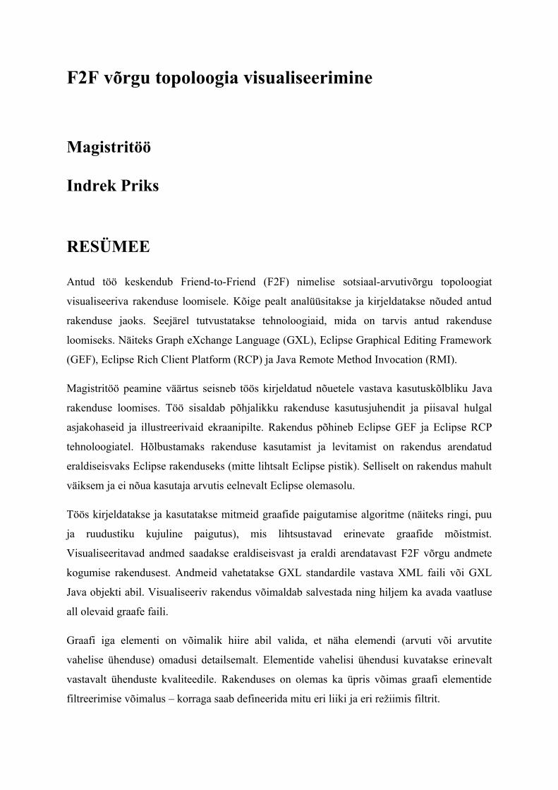
RESÜMEE

Antud töö keskendub Friend-to-Friend (F2F) nimelise sotsiaal-arvutivõrgu topoloogiat

visualiseeriva rakenduse loomisele. Kõige pealt analüüsitakse ja kirjeldatakse nõuded antud

rakenduse jaoks. Seejärel tutvustatakse tehnoloogiaid, mida on tarvis antud rakenduse

loomiseks. Näiteks Graph eXchange Language (GXL), Eclipse Graphical Editing Framework

(GEF), Eclipse Rich Client Platform (RCP) ja Java Remote Method Invocation (RMI).

Magistritöö peamine väärtus seisneb töös kirjeldatud nõuetele vastava kasutuskõlbliku Java

rakenduse loomises. Töö sisaldab põhjalikku rakenduse kasutusjuhendit ja piisaval hulgal

asjakohaseid ja illustreerivaid ekraanipilte. Rakendus põhineb Eclipse GEF ja Eclipse RCP

tehnoloogiatel. Hõlbustamaks rakenduse kasutamist ja levitamist on rakendus arendatud

eraldiseisvaks Eclipse rakenduseks (mitte lihtsalt Eclipse pistik). Selliselt on rakendus mahult

väiksem ja ei nõua kasutaja arvutis eelnevalt Eclipse olemasolu.

Töös kirjeldatakse ja kasutatakse mitmeid graafide paigutamise algoritme (näiteks ringi, puu

ja ruudustiku kujuline paigutus), mis lihtsustavad erinevate graafide mõistmist.

Visualiseeritavad andmed saadakse eraldiseisvast ja eraldi arendatavast F2F võrgu andmete

kogumise rakendusest. Andmeid vahetatakse GXL standardile vastava XML faili või GXL

Java objekti abil. Visualiseeriv rakendus võimaldab salvestada ning hiljem ka avada vaatluse

all olevaid graafe faili.

Graafi iga elementi on võimalik hiire abil valida, et näha elemendi (arvuti või arvutite

vahelise ühenduse) omadusi detailsemalt. Elementide vahelisi ühendusi kuvatakse erinevalt

vastavalt ühenduste kvaliteedile. Rakenduses on olemas ka üpris võimas graafi elementide

filtreerimise võimalus – korraga saab defineerida mitu eri liiki ja eri režiimis filtrit.

F2F network topology visualization

Master Thesis

Indrek Priks

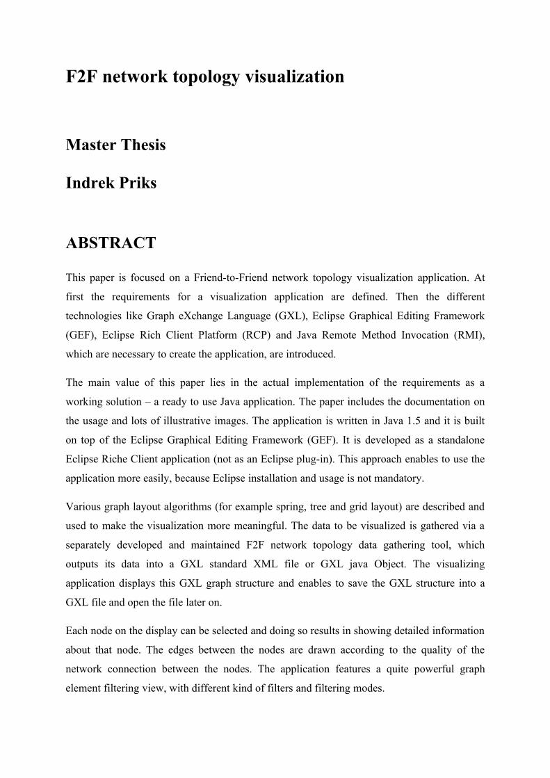
ABSTRACT

This paper is focused on a Friend-to-Friend network topology visualization application. At

first the requirements for a visualization application are defined. Then the different

technologies like Graph eXchange Language (GXL), Eclipse Graphical Editing Framework

(GEF), Eclipse Rich Client Platform (RCP) and Java Remote Method Invocation (RMI),

which are necessary to create the application, are introduced.

The main value of this paper lies in the actual implementation of the requirements as a

working solution – a ready to use Java application. The paper includes the documentation on

the usage and lots of illustrative images. The application is written in Java 1.5 and it is built

on top of the Eclipse Graphical Editing Framework (GEF). It is developed as a standalone

Eclipse Riche Client application (not as an Eclipse plug-in). This approach enables to use the

application more easily, because Eclipse installation and usage is not mandatory.

Various graph layout algorithms (for example spring, tree and grid layout) are described and

used to make the visualization more meaningful. The data to be visualized is gathered via a

separately developed and maintained F2F network topology data gathering tool, which

outputs its data into a GXL standard XML file or GXL java Object. The visualizing

application displays this GXL graph structure and enables to save the GXL structure into a

GXL file and open the file later on.

Each node on the display can be selected and doing so results in showing detailed information

about that node. The edges between the nodes are drawn according to the quality of the

network connection between the nodes. The application features a quite powerful graph

element filtering view, with different kind of filters and filtering modes.

LITERATURE

The literature is ordered by the alphabetic values of the references. All of the internet

addresses have been last checked at May 26, 2008.

[DRAW2D_GUIDE] “Draw2d Programmer's Guide”,

http://help.eclipse.org/help33/index.jsp?

topic=/org.eclipse.draw2d.doc.isv/guide/guide.html

[ECLIPSE_ARCH] Dr. Frank Gerhardt, Michael Scharf, “Developing Eclipse Rich-

Client Applications”, 2007,

http://eclipsezilla.eclipsecon.org/php/attachment.php?

bugid=3667

[EQUINOX] Equinox home page, http://www.eclipse.org/equinox

[F2F HOME] Friend-to-Friend Computing home page, http://ulno.net/f2f

[GRAPH_DRAWING] Graph drawing formats,

http://www.graphdrawing.org/data/format

[GRAPH_WIKI] “Graph (mathematics)”, Wikipedia,

http://en.wikipedia.org/wiki/Graph_(mathematics)

[GXL_HOME] GXL home page,

http://www.gupro.de/GXL/Introduction/background.html

[GXL_JAVA] GXL Java library home page, http://gxl.sourceforge.net

[IBM_HISTORY] “A brief history of Eclipse”, Gary Cernosek, Novemer

15, 2005, http://www.ibm.com/developerworks/rational/library/

nov05/cernosek

[JFACE_HOME] JFace home page, http://wiki.eclipse.org/index.php/JFace

[RCP_FAQ] Eclipse Rich Client Platform FAQ,

http://wiki.eclipse.org/RCP_FAQ

[RMI] Remote Method Invocation Home,

http://java.sun.com/javase/technologies/core/basic/rmi/index.jsp

[SETI_HOME] SETI@home home page, http://setiathome.berkeley.edu

[SPRING_LAYOUT] “Force-based algorithms“, Wikipedia,

http://en.wikipedia.org/wiki/Force-based_algorithms

[SWT_WIDGETS] SWT widgets home page, http://www.eclipse.org/swt/widgets

[TREE_LAYOUT] SHRiMP home page,

http://www.thechiselgroup.org/shrimp_manual_layouts

[ZEST] Zest: The Eclipse Visualization Toolkit, http://www.eclipse.org/

gef/zest

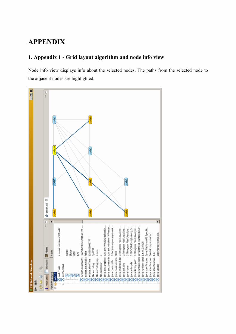
APPENDIX

1. Appendix 1 - Grid layout algorithm and node info view

Node info view displays info about the selected nodes. The paths from the selected node to

the adjacent nodes are highlighted.

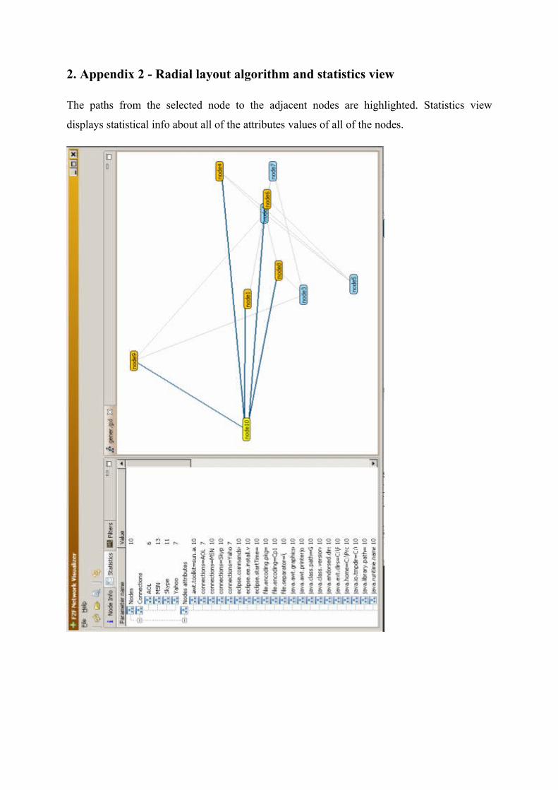
2. Appendix 2 - Radial layout algorithm and statistics view

The paths from the selected node to the adjacent nodes are highlighted. Statistics view

displays statistical info about all of the attributes values of all of the nodes.

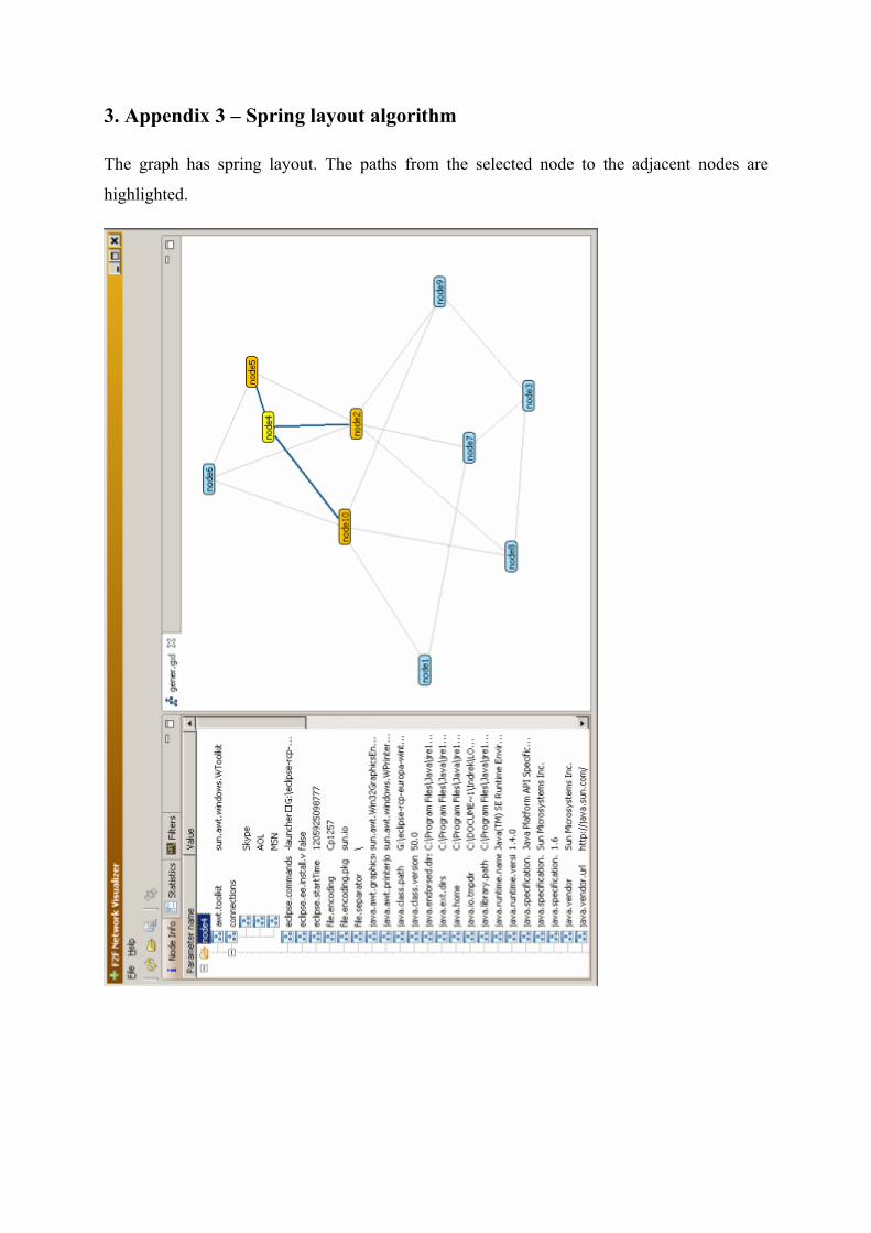
3. Appendix 3 – Spring layout algorithm

The graph has spring layout. The paths from the selected node to the adjacent nodes are

highlighted.

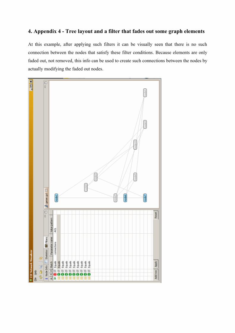
4. Appendix 4 - Tree layout and a filter that fades out some graph elements

At this example, after applying such filters it can be visually seen that there is no such

connection between the nodes that satisfy these filter conditions. Because elements are only

faded out, not removed, this info can be used to create such connections between the nodes by

actually modifying the faded out nodes.

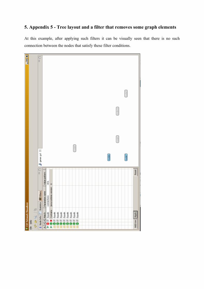
5. Appendix 5 - Tree layout and a filter that removes some graph elements

At this example, after applying such filters it can be visually seen that there is no such

connection between the nodes that satisfy these filter conditions.

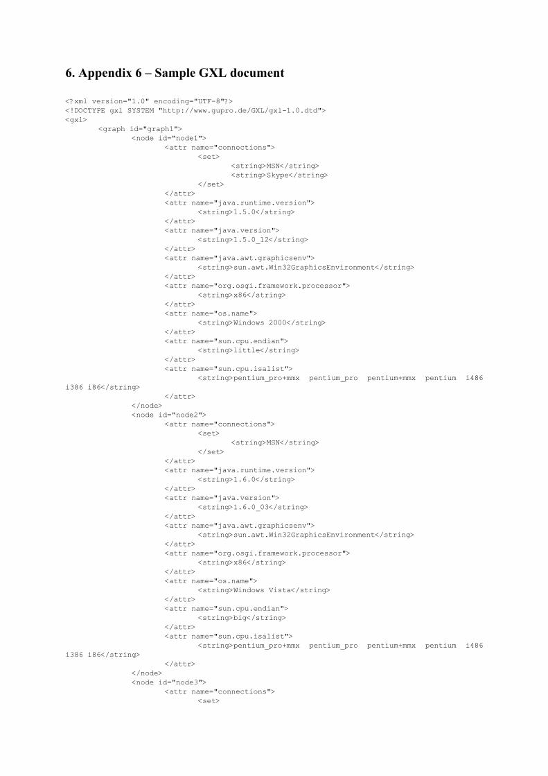
6. Appendix 6 – Sample GXL document

<?xml version="1.0" encoding="UTF-8"?><!DOCTYPE gxl SYSTEM "http://www.gupro.de/GXL/gxl-1.0.dtd"><gxl>

<graph id="graph1"><node id="node1">

<attr name="connections"><set>

<string>MSN</string><string>Skype</string>

</set></attr><attr name="java.runtime.version">

<string>1.5.0</string></attr><attr name="java.version">

<string>1.5.0_12</string></attr><attr name="java.awt.graphicsenv">

<string>sun.awt.Win32GraphicsEnvironment</string></attr><attr name="org.osgi.framework.processor">

<string>x86</string></attr><attr name="os.name">

<string>Windows 2000</string></attr><attr name="sun.cpu.endian">

<string>little</string></attr><attr name="sun.cpu.isalist">

<string>pentium_pro+mmx pentium_pro pentium+mmx pentium i486 i386 i86</string>

</attr></node><node id="node2">

<attr name="connections"><set>

<string>MSN</string></set>

</attr><attr name="java.runtime.version">

<string>1.6.0</string></attr><attr name="java.version">

<string>1.6.0_03</string></attr><attr name="java.awt.graphicsenv">

<string>sun.awt.Win32GraphicsEnvironment</string></attr><attr name="org.osgi.framework.processor">

<string>x86</string></attr><attr name="os.name">

<string>Windows Vista</string></attr><attr name="sun.cpu.endian">

<string>big</string></attr><attr name="sun.cpu.isalist">

<string>pentium_pro+mmx pentium_pro pentium+mmx pentium i486 i386 i86</string>

</attr></node><node id="node3">

<attr name="connections"><set>

<string>Skype</string></set>

</attr><attr name="java.runtime.version">

<string>1.5.0</string></attr><attr name="java.version">

<string>1.6.0_03</string></attr><attr name="java.awt.graphicsenv">

<string>sun.awt.Win32GraphicsEnvironment</string></attr><attr name="org.osgi.framework.processor">

<string>x86</string></attr><attr name="os.name">

<string>Windows XP</string></attr><attr name="sun.cpu.endian">

<string>little</string></attr><attr name="sun.cpu.isalist">

<string>pentium_pro+mmx pentium_pro pentium+mmx pentium i486 i386 i86</string>

</attr></node><node id="node4">

<attr name="connections"><set>

<string>MSN</string></set>

</attr><attr name="java.runtime.version">

<string>1.4.0</string></attr><attr name="java.version">

<string>1.4.0_03</string></attr><attr name="java.awt.graphicsenv">

<string>sun.awt.Win32GraphicsEnvironment</string></attr><attr name="org.osgi.framework.processor">

<string>x86</string></attr><attr name="os.name">

<string>Windows XP</string></attr><attr name="sun.cpu.endian">

<string>little</string></attr><attr name="sun.cpu.isalist">

<string>pentium_pro+mmx pentium_pro pentium+mmx pentium i486 i386 i86</string>

</attr></node><node id="node5">

<attr name="connections"><set>

<string>MSN</string></set>

</attr><attr name="java.runtime.version">

<string>1.5.0</string></attr><attr name="java.version">

<string>1.6.0_03</string></attr><attr name="java.awt.graphicsenv">

<string>sun.awt.Win32GraphicsEnvironment</string></attr>

<attr name="org.osgi.framework.processor"><string>x86</string>

</attr><attr name="os.name">

<string>Windows XP</string></attr><attr name="sun.cpu.endian">

<string>little</string></attr><attr name="sun.cpu.isalist">

<string>pentium_pro+mmx pentium_pro pentium+mmx pentium i486 i386 i86</string>

</attr></node><node id="node6">

<attr name="connections"><set>

<string>MSN</string></set>

</attr><attr name="java.runtime.version">

<string>1.5.0</string></attr><attr name="java.version">

<string>1.6.0_03</string></attr><attr name="java.awt.graphicsenv">

<string>sun.awt.Win32GraphicsEnvironment</string></attr><attr name="org.osgi.framework.processor">

<string>x86</string></attr><attr name="os.name">

<string>Windows XP</string></attr><attr name="sun.cpu.endian">

<string>little</string></attr><attr name="sun.cpu.isalist">

<string>pentium_pro+mmx pentium_pro pentium+mmx pentium i486 i386 i86</string>

</attr></node><node id="node7">

<attr name="connections"><set>

<string>Skype</string></set>

</attr><attr name="java.runtime.version">

<string>1.5.0</string></attr><attr name="java.version">

<string>1.6.0_03</string></attr><attr name="java.awt.graphicsenv">

<string>sun.awt.Win32GraphicsEnvironment</string></attr><attr name="org.osgi.framework.processor">

<string>x86</string></attr><attr name="os.name">

<string>Windows XP</string></attr><attr name="sun.cpu.endian">

<string>little</string></attr><attr name="sun.cpu.isalist">

<string>pentium_pro+mmx pentium_pro pentium+mmx pentium i486 i386 i86</string>

</attr></node><node id="node8">

<attr name="connections"><set>

<string>Skype</string></set>

</attr><attr name="java.runtime.version">

<string>1.5.0</string></attr><attr name="java.version">

<string>1.6.0_03</string></attr><attr name="java.awt.graphicsenv">

<string>sun.awt.Win32GraphicsEnvironment</string></attr><attr name="org.osgi.framework.processor">

<string>x86</string></attr><attr name="os.name">

<string>Windows XP</string></attr><attr name="sun.cpu.endian">

<string>little</string></attr><attr name="sun.cpu.isalist">

<string>pentium_pro+mmx pentium_pro pentium+mmx pentium i486 i386 i86</string>

</attr></node><edge from="node1" to="node2">

<attr name="connections"><set>

<string>MSN</string></set>

</attr></edge><edge from="node1" to="node3">

<attr name="connections"><set>

<string>Skype</string></set>

</attr></edge><edge from="node1" to="node4">

<attr name="connections"><set>

<string>MSN</string></set>

</attr></edge><edge from="node1" to="node5">

<attr name="connections"><set>

<string>MSN</string></set>

</attr></edge><edge from="node1" to="node6">

<attr name="connections"><set>

<string>MSN</string></set>

</attr></edge><edge from="node2" to="node4">

<attr name="connections"><set>

<string>MSN</string>

</set></attr>

</edge><edge from="node5" to="node6">

<attr name="connections"><set>

<string>MSN</string></set>

</attr></edge><edge from="node3" to="node7">

<attr name="connections"><set>

<string>Skype</string></set>

</attr></edge><edge from="node3" to="node8">

<attr name="connections"><set>

<string>Skype</string></set>

</attr></edge><edge from="node7" to="node8">

<attr name="connections"><set>

<string>Skype</string></set>

</attr></edge>

</graph></gxl>

7. Appendix 7 – The application CD