stats50 lecture notes - github pages
TRANSCRIPT

STATS50 Lecture Notes
Zed Chance
Fall 20
1
CONTENTS CONTENTS
Contents
1 What is statistics? 4
2 Combining events 52.1 Mutually exclusive events . . . . . . . . . . . . . . . . . . . . . . . . . . . . . . . . . . . . . . 5
3 Probability 73.1 The axioms of probability . . . . . . . . . . . . . . . . . . . . . . . . . . . . . . . . . . . . . . 73.2 Complementation rule . . . . . . . . . . . . . . . . . . . . . . . . . . . . . . . . . . . . . . . . 7
4 Sample spaces with equally likely outcomes 104.1 General addition rule . . . . . . . . . . . . . . . . . . . . . . . . . . . . . . . . . . . . . . . . . 10
5 Counting methods 145.1 Fundamental principle of counting . . . . . . . . . . . . . . . . . . . . . . . . . . . . . . . . . 155.2 Permutations . . . . . . . . . . . . . . . . . . . . . . . . . . . . . . . . . . . . . . . . . . . . . 17
5.2.1 Factorial Formula for Permutations . . . . . . . . . . . . . . . . . . . . . . . . . . . . . 175.3 Combinations . . . . . . . . . . . . . . . . . . . . . . . . . . . . . . . . . . . . . . . . . . . . . 18
5.3.1 Factorial Formula for Combinations . . . . . . . . . . . . . . . . . . . . . . . . . . . . 18
6 Conditional Probability 206.1 Independent Events . . . . . . . . . . . . . . . . . . . . . . . . . . . . . . . . . . . . . . . . . 216.2 Multiplication Rule . . . . . . . . . . . . . . . . . . . . . . . . . . . . . . . . . . . . . . . . . . 226.3 Law of Total Probability . . . . . . . . . . . . . . . . . . . . . . . . . . . . . . . . . . . . . . . 256.4 Bayes’ Rule . . . . . . . . . . . . . . . . . . . . . . . . . . . . . . . . . . . . . . . . . . . . . . 25
7 Random Variables 287.1 Discrete Random Variables . . . . . . . . . . . . . . . . . . . . . . . . . . . . . . . . . . . . . 28
7.1.1 Mean of a for Discrete Random Variables . . . . . . . . . . . . . . . . . . . . . . . . . 297.1.2 Variance and Standard Deviation of a Discrete Random Variable . . . . . . . . . . . . 30
7.2 Probability Density Functions . . . . . . . . . . . . . . . . . . . . . . . . . . . . . . . . . . . . 327.3 Cumulative Distribution Functions of a Continuous Random Variable . . . . . . . . . . . . . 347.4 Mean and Variance for Continuous Random Variables . . . . . . . . . . . . . . . . . . . . . . 367.5 Median and Percentiles . . . . . . . . . . . . . . . . . . . . . . . . . . . . . . . . . . . . . . . 387.6 Linear Functions of Random Variables . . . . . . . . . . . . . . . . . . . . . . . . . . . . . . . 407.7 Linear Combinations of Random Variables, Means and Variances . . . . . . . . . . . . . . . . 437.8 Simple Random Samples . . . . . . . . . . . . . . . . . . . . . . . . . . . . . . . . . . . . . . . 46
8 Commonly Used Distributions 508.1 Bernoulli Distribution . . . . . . . . . . . . . . . . . . . . . . . . . . . . . . . . . . . . . . . . 508.2 Binomial Distribution . . . . . . . . . . . . . . . . . . . . . . . . . . . . . . . . . . . . . . . . 51
8.2.1 Sample proportion . . . . . . . . . . . . . . . . . . . . . . . . . . . . . . . . . . . . . . 558.2.2 Bias and Uncertainty . . . . . . . . . . . . . . . . . . . . . . . . . . . . . . . . . . . . . 55
8.3 Hypergeometric Distribution . . . . . . . . . . . . . . . . . . . . . . . . . . . . . . . . . . . . 578.4 Geometric Distribution . . . . . . . . . . . . . . . . . . . . . . . . . . . . . . . . . . . . . . . . 588.5 Negative Binomial Distribution . . . . . . . . . . . . . . . . . . . . . . . . . . . . . . . . . . . 608.6 Multinomial Distribution . . . . . . . . . . . . . . . . . . . . . . . . . . . . . . . . . . . . . . 628.7 Poisson Distribution . . . . . . . . . . . . . . . . . . . . . . . . . . . . . . . . . . . . . . . . . 63
8.7.1 Using the Poisson Distribution to estimate rate and uncertainty in the estimated rate 668.8 Exponential Distribution . . . . . . . . . . . . . . . . . . . . . . . . . . . . . . . . . . . . . . . 67
8.8.1 The Exponential Distribution and the Poisson Process . . . . . . . . . . . . . . . . . . 708.9 Normal Distribution . . . . . . . . . . . . . . . . . . . . . . . . . . . . . . . . . . . . . . . . . 72
8.9.1 Standard units and the Standard Normal Distribution . . . . . . . . . . . . . . . . . . 758.9.2 The Distribution of the Sample Mean and the Central Limit Theorem . . . . . . . . . 77
2
CONTENTS CONTENTS
8.9.3 The Central Limit Theorem . . . . . . . . . . . . . . . . . . . . . . . . . . . . . . . . . 78
9 Confidence Intervals 849.1 Confidence intervals for population proportions . . . . . . . . . . . . . . . . . . . . . . . . . . 909.2 t-distributions . . . . . . . . . . . . . . . . . . . . . . . . . . . . . . . . . . . . . . . . . . . . . 93
10 Hypothesis Testing 9710.1 Conclusions for Hypothesis Tests . . . . . . . . . . . . . . . . . . . . . . . . . . . . . . . . . . 10110.2 Small sample tests for a population mean . . . . . . . . . . . . . . . . . . . . . . . . . . . . . 10510.3 Fixed level testing . . . . . . . . . . . . . . . . . . . . . . . . . . . . . . . . . . . . . . . . . . 10710.4 Type I and Type II errors . . . . . . . . . . . . . . . . . . . . . . . . . . . . . . . . . . . . . . 10910.5 Power . . . . . . . . . . . . . . . . . . . . . . . . . . . . . . . . . . . . . . . . . . . . . . . . . 110
11 Jointly Distributed Random Variables 11611.1 Covariance . . . . . . . . . . . . . . . . . . . . . . . . . . . . . . . . . . . . . . . . . . . . . . 12211.2 Correlation . . . . . . . . . . . . . . . . . . . . . . . . . . . . . . . . . . . . . . . . . . . . . . 12411.3 Conditional distribution . . . . . . . . . . . . . . . . . . . . . . . . . . . . . . . . . . . . . . . 12511.4 Independent random variables . . . . . . . . . . . . . . . . . . . . . . . . . . . . . . . . . . . . 12511.5 Relationships . . . . . . . . . . . . . . . . . . . . . . . . . . . . . . . . . . . . . . . . . . . . . 126
12 Review 127
3
1 WHAT IS STATISTICS?
1 What is statistics?
The practice of science of collecting and analyzing numerical data in large quantities, especially for thepurpose of inferring proportions in a whole from those in a representative sample.
Two major types of statistics:
1. Descriptive statistics
(a) Consists of methods for organizing and summarizing information
(b) Graphs, charts, tables, calculating averages, measures of variation, and percentiles
2. Inferential statistics
(a) Consists of methods for drawing and measuring the reliability of conclusions about a populationbased on information from a sample of the population
Probability theory is the science of uncertainty. It enables us evaluate and control the likelihood that astatistical inference is correct. In general, probability theory provides the mathematical basis for inferentialstatistics.
An experiment is a process that results in an outcome that cannot be predicted in advance with certainty.
Example 1. Tossing a coin, weighing the contents of a box of cereal, rolling a die . . .
The set of all possible outcomes of an experiment is called the sample space for the experiment (oftennotated by the capital letter S). For example:
1. Consider the experiment of tossing a fair coin. There are two possible outcomes: heads (H) or tails(T ). The sample space is S = {H,T}, this is a finite sample space.
2. There are six possible outcomes when a six-sided die is rolled: 1, 2, 3, 4, 5, 6, so the sample space isS = {1, 2, 3, 4, 5, 6}, this is a finite sample space.
3. Imagine a punch with a diameter 10mm that punches holes in sheet metal. Because of variations in theangle of the punch and slight movements in the sheet metal, the diameters of the holes vary between10.0mm and 10.2mm. What might be a reasonable sample space for the experiment of punching ahole? (Say we let x represent the diameter, in mm, of a punched out hole.) The sample space wouldbe S = {x | 10.0 < x < 10.2}, this is an infinite sample space.
A subset of a sample space is called an event:
1. Can be represented by a Venn diagram.
2. The sample space when a six-sided die is rolled is S = {1, 2, 3, 4, 5, 6}. The event the die comes upeven is E = {2, 4, 6}.
3. For the previous hole punch example, the event a hole has a diameter less than 10.1mm is the subset{x : 10.1 < x < 10.1}
Note 1. The empty set: ∅, is a set with no outcomes or elements in it. For example ∅ = {}. Theempty set is an event as is the entire sample space. Sometimes referred to as an “impossible event”.The sample space is sometimes referred to as a “certain event”.
We say an event has occurred if the outcome of the experiment is one of the outcomes in the event.
Example 2. Refer to the previous example of rolling a die: If the die comes up 2 when it is rolled,then we can say that the event E = {2, 4, 6}, the event an even number is rolled, has occurred.
4
2 COMBINING EVENTS
2 Combining events
The union of two events, A and B, denoted by A ∪B, is the set of outcomes that belong either to A or B,or to both. In words, A ∪ B means “A or B”. Thus, the event A ∪ B occurs whenever either A or B (orboth) occurs.
The intersection of two events A and B, denoted A ∩B, is the set of outcomes that belong to both A andto B, in words this means “A and B”. Thus the event A ∩B occurs whenever both A and B occur.
The complement of an event A, denoted AC is the set of outcomes that do not belong to A. In words, AC
means “not A”. Thus, the event AC occurs whenever A does *not* occur.
Example 3. When a die is rolled, the sample space is:
S = {1, 2, 3, 4, 5, 6}
Consider the following events:
• A = “the event the die comes up even” = {2, 4, 6}
• B = “the event the die comes up 4 or more” = {4, 5, 6}
• C = “the event the die comes up at most 2” = {1, 2}
• D = “the event the die comes up 3” = {3}
So,
A ∩B = {4, 6}A ∪B = {2, 4, 5, 6}
A ∪B ∪ C = {1, 2, 4, 5, 6}A ∩B ∩ C = ∅
(A ∩B) ∪ C = {4, 6} ∪ {1, 2} = {1, 2, 4, 6}AC = {1, 3, 5}
B ∩AC = {5}BC ∪ CC = {1, 2, 3, 4, 5, 6}BC ∩ CC = {3}
2.1 Mutually exclusive events
The events A and B are mutually exclusive if they have no outcomes in common. More generally, acollection of events A1, A2, . . . , An is said to be mutually exclusive if no two of them have any outcomes incommon.
5
2 COMBINING EVENTS 2.1 Mutually exclusive events
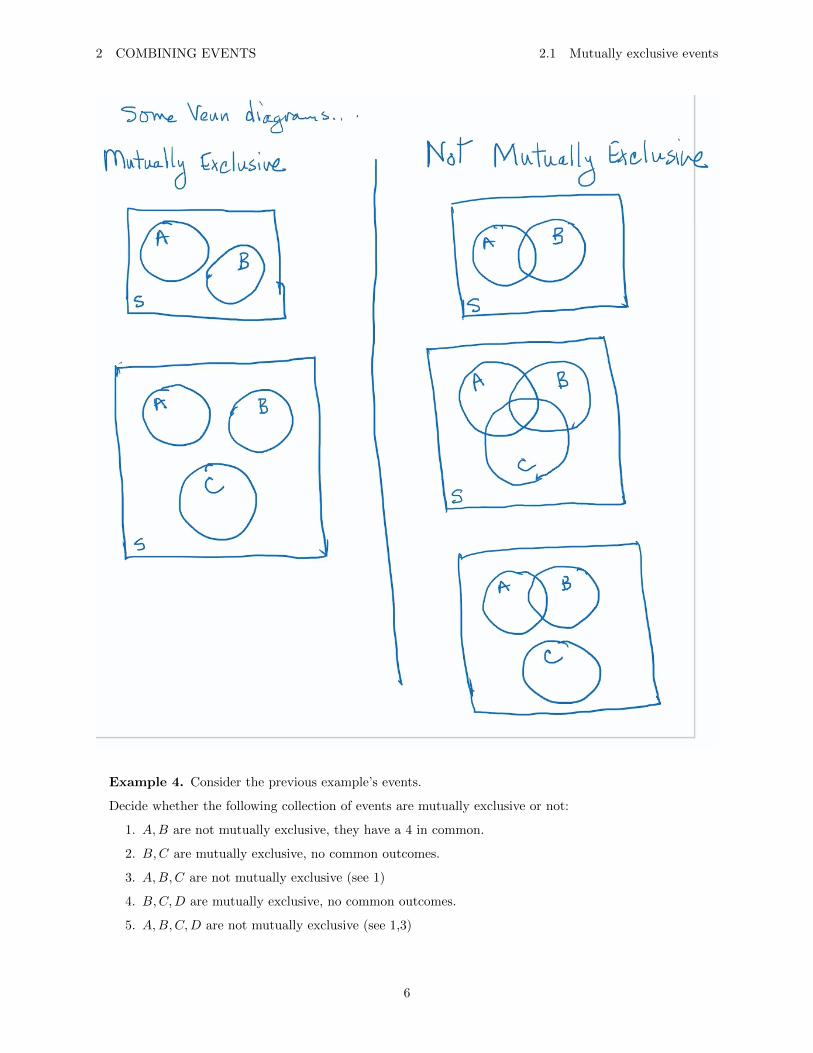
Example 4. Consider the previous example’s events.
Decide whether the following collection of events are mutually exclusive or not:
1. A,B are not mutually exclusive, they have a 4 in common.
2. B,C are mutually exclusive, no common outcomes.
3. A,B,C are not mutually exclusive (see 1)
4. B,C,D are mutually exclusive, no common outcomes.
5. A,B,C,D are not mutually exclusive (see 1,3)
6

3 PROBABILITY
3 Probability
Given any experiment and any event A:
• The expression P (A) denotes the probability that the event A occurs.
• P (A) is the proportion of times that event A would occur in the long run, if the experiment were tobe repeated over and over again.
Example 5. Suppose the probability of a weighted coin comes up heads is 0.75, so:
P (heads) = 0.75
I would expect the weighted coin to come up heads 75% of the time.
3.1 The axioms of probability
Let S be a sample space, then P (S) = 1. For any event A, 0 ≤ P (A) ≤ 1. The long run relative frequencyis always between 0% and 100%. If A and B are mutually exclusive events, then P (A∪B) = P (A) +P (B).
More generally: if A1, A2, · · · are mutually exclusive events, then: P (A1 ∪A2 ∪ · · · ) = P (A1) + P (A2) + · · ·.
3.2 Complementation rule
For any event A, P (AC) = 1− P (A).
Events A and AC are mutually exclusive. So:
P (A ∪AC) = P (A) + P (AC) = P (S) = 1
Remember: P (∅) = 0.
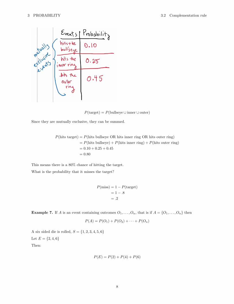
Example 6. A target on a test firing range consists of a bull’s eye with two concentric rings aroundit. A projectile is fired at the target. The probability it hits the bull’s eye is 0.1, the probability that ithits the inner ring is 0.25, and the probability it hits the outer ring is 0.45:
What is the probability that the projectile hits the target?
7
3 PROBABILITY 3.2 Complementation rule
P (target) = P (bullseye ∪ inner ∪ outer)
Since they are mutually exclusive, they can be summed.
P (hits target) = P (hits bullseye OR hits inner ring OR hits outer ring)
= P (hits bullseye) + P (hits inner ring) + P (hits outer ring)
= 0.10 + 0.25 + 0.45
= 0.80
This means there is a 80% chance of hitting the target.
What is the probability that it misses the target?
P (miss) = 1− P (target)
= 1− .8= .2
Example 7. If A is an event containing outcomes O1, . . . , On, that is if A = {O1, . . . , On} then
P (A) = P (O1) + P (O2) + · · ·+ P (On)
A six sided die is rolled, S = {1, 2, 3, 4, 5, 6}
Let E = {2, 4, 6}
Then:
P (E) = P (2) + P (4) + P (6)
8
3 PROBABILITY 3.2 Complementation rule
If the die was known to be fair and that each outcome was equally likely, then each individual outcomewould have the probability of happening 1
6 of the time.
So:
P (E) =1
6+
1
6+
1
6=
1
2
9
4 SAMPLE SPACES WITH EQUALLY LIKELY OUTCOMES
4 Sample spaces with equally likely outcomes
A population from which an item is sampled at random can be thought of as a sample space with equallylikely outcomes.
If a sample space has N has equally likely outcomes, the probability of each outcome is 1N .
Example 8. A card is randomly selected from a deck of 52 cards. Find the probability the selectedcard is:
1. A spade
P (spade) =13
52= .25
2. A face card
P (face card) =12
52= .23
3. A spade or a face card
P (spade or face) =13 + (12− 3)
52(1)
=22
52(2)
= .42 (3)
Can’t simply add the previous probability because they are not mutually exclusive events!
4.1 General addition rule
Let A and B be any events, then:
P (A ∪B) = P (A) + P (B)− P (A ∩B)
10
4 SAMPLE SPACES WITH EQUALLY LIKELY OUTCOMES 4.1 General addition rule
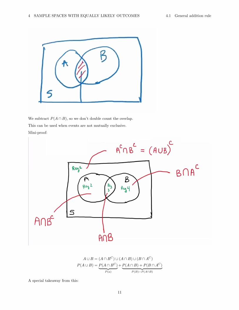
We subtract P (A ∩B), so we don’t double count the overlap.
This can be used when events are not mutually exclusive.
Mini-proof:
A ∪B = (A ∩BC) ∪ (A ∩B) ∪ (B ∩AC)
P (A ∪B) = P (A ∩BC)︸ ︷︷ ︸P (a)
+P (A ∩B) + P (B ∩AC)︸ ︷︷ ︸P (B)−P (A∩B)
A special takeaway from this:
11
4 SAMPLE SPACES WITH EQUALLY LIKELY OUTCOMES 4.1 General addition rule
A = (A ∩B) ∪ (A ∩BC)︸ ︷︷ ︸mutually exclusive
Which means
P (A) = P (A ∩B) + P (A ∩BC)
and this fact is often used.
Example 9. In a process that manufactures aluminum cans, the probability that a can has a flaw onits side is 0.02, the probability that a can has a flaw on the top is 0.03, and the probability that a canhas a flaw on both the top and the side is 0.01
P (flaw on side) = 0.02 P (flaw on top) = 0.03 P (flaw on top AND flaw on side) = 0.01
(a) What is the probability that a randomly chosen can has a flaw?
P (flaw) = P (flaw on top AND flaw on side)
= P (flaw on side) + P (flaw on top)− P (flaw on top AND flaw on side)
= 0.02 + 0.03− 0.01
= 0.04
(b) What is the probability that is has no flaw?
P (no flaw) = 1− P (flaw)
= 1− 0.4
= 0.96
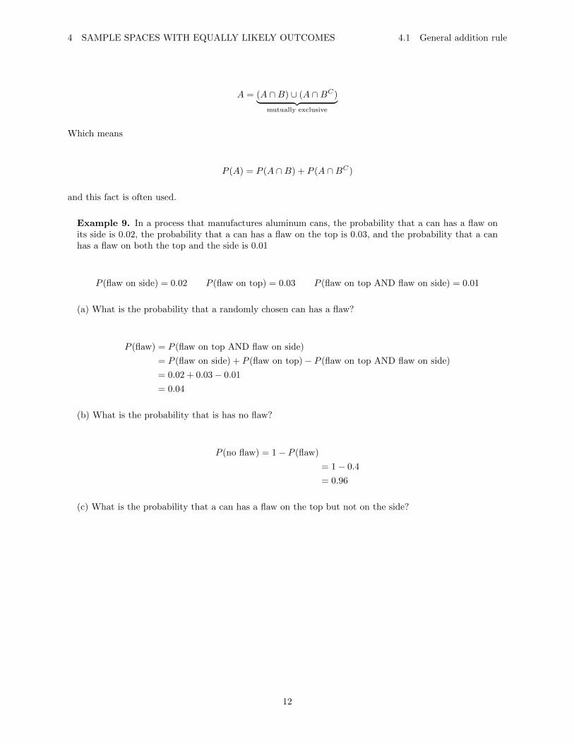
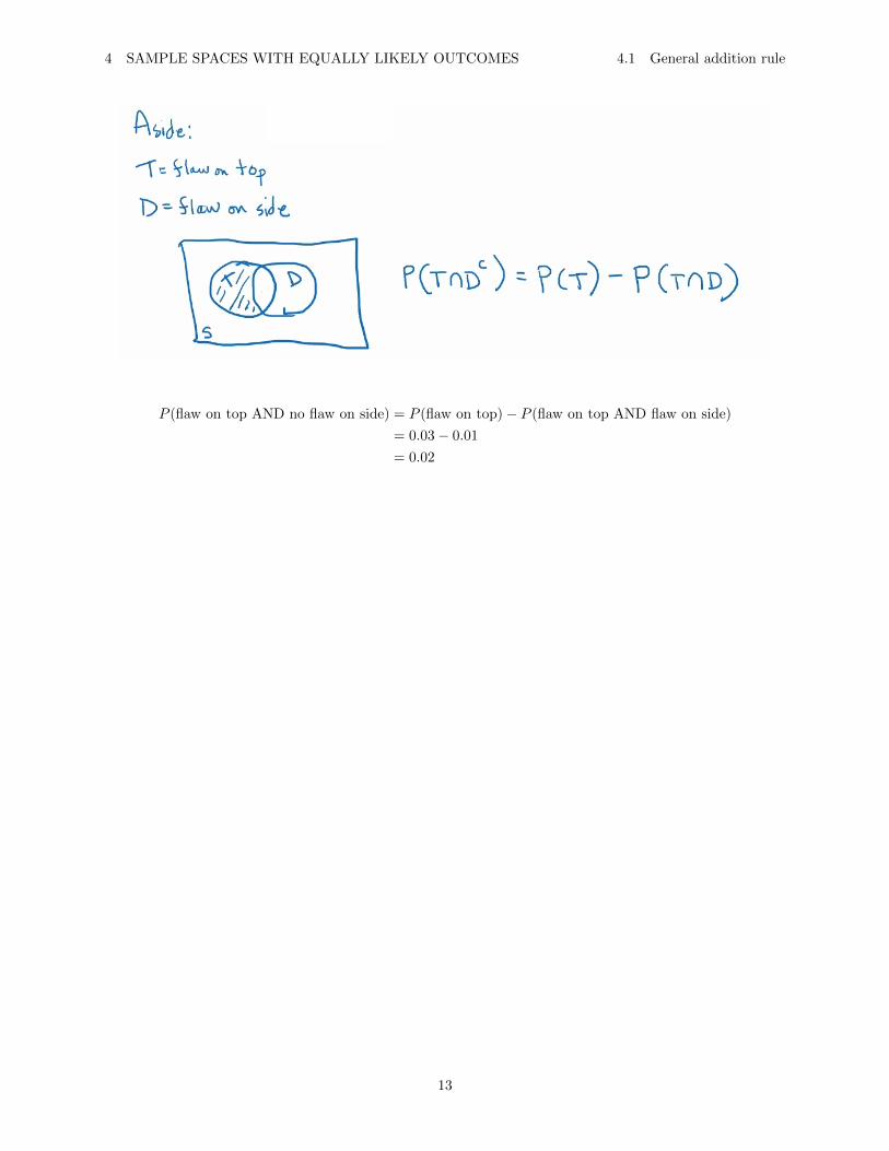
(c) What is the probability that a can has a flaw on the top but not on the side?
12
4 SAMPLE SPACES WITH EQUALLY LIKELY OUTCOMES 4.1 General addition rule
P (flaw on top AND no flaw on side) = P (flaw on top)− P (flaw on top AND flaw on side)
= 0.03− 0.01
= 0.02
13

5 COUNTING METHODS
5 Counting methods
A small local ice cream parlor offers 2 different choices of cones (regular and sugar cone), and 3 differentflavors of ice cream (strawberry, vanilla, and chocolate). How many choices are there for a single (cone andone scoop of ice cream) order?
What if there are also 4 choices of toppings?
2 · 3 · 4 = 24
14
5 COUNTING METHODS 5.1 Fundamental principle of counting
5.1 Fundamental principle of counting
Definition 1. If an operation can be performed in n1 ways, and if for each of these ways a secondoperation can be performed in n2 ways, then the total number of ways to perform the two operationsis n1 · n2.
In general:
Assume that k operations are to be performed. If there are n1 ways to perform the second operation,and if for each of these ways there are n2 ways to perform the second operation, and if for each choiceof ways to perform the first two operations there are n3 ways to perform the third operation, and soon, then the total number of ways to perform the sequence of k operations is:
n1 · n2 · n3 · · · · · nk
Example 10. When ordering a certain type of computer, there are 3 choices of hard drives, 4 choicesof amount of memory, 2 choices of video card, and 3 choices of monitor. How many different computerconfigurations can be ordered?
3 · 4 · 2 · 3 = 72
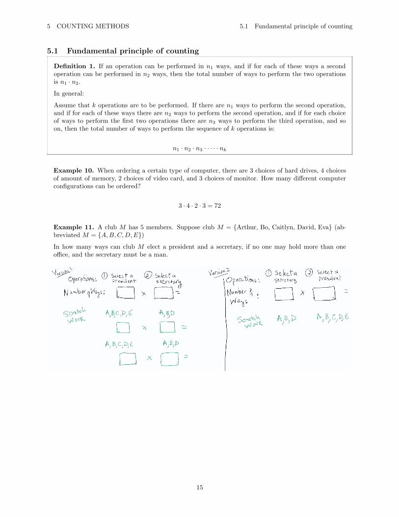
Example 11. A club M has 5 members. Suppose club M = {Arthur, Bo, Caitlyn, David, Eva} (ab-breviated M = {A,B,C,D,E})
In how many ways can club M elect a president and a secretary, if no one may hold more than oneoffice, and the secretary must be a man.
15

5 COUNTING METHODS 5.1 Fundamental principle of counting
As a rule of thumb: count the most restricted parts first. (Start with the subset first).
Example 12. In some states, auto license plates have contained three letters followed by 3 digits.
How many such license plates are possible?
263 · 103 = 17, 576, 000
How many such license plates end in 555?
16
5 COUNTING METHODS 5.2 Permutations
263 · 13 = 17, 576
5.2 Permutations
A permutation is an ordering of a collection of objects.
Example 13. There are six permutations of the letters A, B, C:
ABC, ACB, BAC, BCA, CAB, CBA
The definition of n! “n factorial”: The product of the first n positive integers and is denoted by n!. Thatis for any positive integer n! = n(n− 1)(n− 2) · · · (3)(2)(1) and 0! = 1
Theorem 1. The number of permutations of n objects is n!.
Example 14. Let club M = {A,B,C,D,E}
How many ways can all of the club members arrange themselves in a row for a photo?
5! = 120
How many ways can the club elect a president, a secretary, and a treasurer if no one can hold more thanone office?
5!
2!= 60
5.2.1 Factorial Formula for Permutations
Definition 2. The number of permutations, or ordered selections (arrangements), of r objects chosenfrom a set of n object is given by:
nPr =n!
(n− r)!
Permutations can be used anytime we need to know the number of ordered selections of r objects that canbe selected from a collection of n objects.
We use permutations only in cases that satisfy these conditions:
1. Repetitions are not allowed.
2. Order is important.
5P3 =5!
(5− 3)!=
5!
2!= 60
Example 15. An ATM requires a four digit PIN using the digits 0-9 (the first digit may be 0). Howmany such PINs have no repeated digits?
17
5 COUNTING METHODS 5.3 Combinations
10P4 =10!
6!= 5040
5.3 Combinations
A combination is an unordered selection (subset).
Example 16. Let M = {A,B,C,D,E}
A committee of 3 members would be an unordered selection (a combination), for example: {A,B,C}.Order does not matter!
5.3.1 Factorial Formula for Combinations
Definition 3. The number of combinations, or unordered selections (subsets), of r objects chosenfrom a set of n objects is given by:
nCr =nPrr!
=n!
r!(n− r)!
Another commonly used notation for combinations is:
(n
r
)=
n!
r!(n− r)!
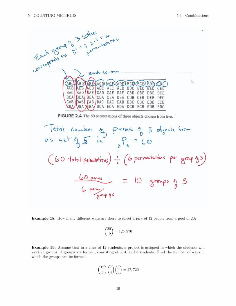
Example 17. Consider club M = Arthur, Bo, Caitlyn, David, Eva = {A,B,C,D,E}. A committeeof three members would be an example of a combination, or unordered selection. For example one suchcomittee might consist of {A,B,C}. Here, order does not matter as it is just a group of 3 people in acomittee.
Use the combinations formula to determine the number of different size 3 committees (subsets) thatcould possibly be made from club M .
(5
3
)=
5!
3!(5− 3)!= 10
18
5 COUNTING METHODS 5.3 Combinations
Example 18. How many different ways are there to select a jury of 12 people from a pool of 20?
(20
12
)= 125, 970
Example 19. Assume that in a class of 12 students, a project is assigned in which the students willwork in groups. 3 groups are formed, consisting of 5, 4, and 3 students. Find the number of ways inwhich the groups can be formed.
(12
5
)(7
4
)(3
3
)= 27, 720
19

6 CONDITIONAL PROBABILITY
6 Conditional Probability
The probability that event B occurs given that event A occurs is called conditional probability. This isdenoted:
P (B | A)
A conditional probability is a probability that is based on a part of the sample space. (An unconditionalprobability would be based on the entire sample space.)
Let A and B be events with P (B) 6= 0. The conditional probability of A given B is:
P (A | B) =P (A ∩B)
P (B)
Example 20. In a genetics experiment, the researcher mated two Drosophila fruit flies and observedthe traits of 300 offspring. The results are shown in the table below.
One of these offspring is randomly selected and observed for the two genetic traits. Determine the followprobabilities. Round your answer to three decimal places.
1. What is the probability that a fly has both normal eye color and normal wing size?
P (normal eye and normal wing) =140
300= .467
2. What is the probability that the fly has vermillion eyes?
P (vermillion eyes) =154
300= .513
20
6 CONDITIONAL PROBABILITY 6.1 Independent Events
3. What is the probability that the fly has normal eye color, given the fly has miniature wings?
P (normal eye — mini wings) =6
157= .038
4. What is the probability that the fly has either vermillion wings or miniature wings (or both)?
P (vermillion eyes or mini wings) =151 + 3 + 6
300= .533
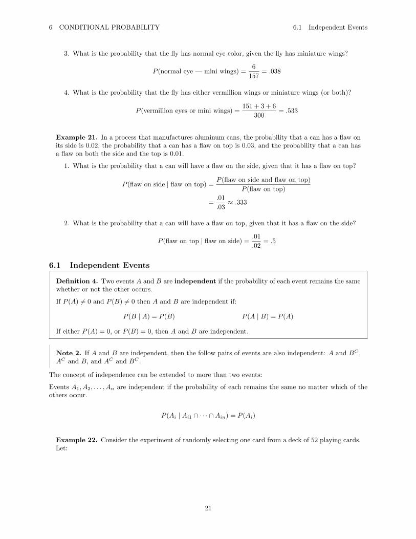
Example 21. In a process that manufactures aluminum cans, the probability that a can has a flaw onits side is 0.02, the probability that a can has a flaw on top is 0.03, and the probability that a can hasa flaw on both the side and the top is 0.01.
1. What is the probability that a can will have a flaw on the side, given that it has a flaw on top?
P (flaw on side | flaw on top) =P (flaw on side and flaw on top)
P (flaw on top)
=.01
.03≈ .333
2. What is the probability that a can will have a flaw on top, given that it has a flaw on the side?
P (flaw on top | flaw on side) =.01
.02= .5
6.1 Independent Events
Definition 4. Two events A and B are independent if the probability of each event remains the samewhether or not the other occurs.
If P (A) 6= 0 and P (B) 6= 0 then A and B are independent if:
P (B | A) = P (B) P (A | B) = P (A)
If either P (A) = 0, or P (B) = 0, then A and B are independent.
Note 2. If A and B are independent, then the follow pairs of events are also independent: A and BC ,AC and B, and AC and BC .
The concept of independence can be extended to more than two events:
Events A1, A2, . . . , An are independent if the probability of each remains the same no matter which of theothers occur.
P (Ai | Ai1 ∩ · · · ∩Ain) = P (Ai)
Example 22. Consider the experiment of randomly selecting one card from a deck of 52 playing cards.Let:
21
6 CONDITIONAL PROBABILITY 6.2 Multiplication Rule
F = event a face card is selected
K = event a king is selected
H = event a heart is selected
P (K) =4
52≈ 0.077
P (K | F ) =4
12≈ 0.333
P (K | F ) 6= P (K)
So, K is not independent of F . The percentage of Kings among face cards (33.3%) is not the same asthe percentage of Kings among all cards (7.7%).
P (K | H) =1
13≈ 0.077
Note 3.P (K | H) = P (K)
So, K is independent of the event H. The percentage of Kings among the hearts is the samepercentage of Kings among all cards.
6.2 Multiplication Rule
Definition 5. If A and B are two events with P (B) 6= 0, then P (A ∩B) = P (B) · P (A | B).
If A and B are two events with P (A) 6= 0, then P (A ∩B) = P (A) · P (B | A).
If P (A) 6= 0 and P (B 6= 0), then both above equations hold.
When two events are independent, then P (A | B) = P (A) and P (B | A) = P (B) and we have thefollowing:
P (A ∩B) = P (A) · P (B)
This result can be extended to any number of events. If A1, A2, . . . , An are independent events, thenfor each collection Ai1, . . . , Ain of events:
P (Ai1 ∩Ai2 ∩ · · · ∩Ain) = P (Ai1)P (Ai2) · · ·P (Ain)
Remember, A ∩B = B ∩A and A ∪B = B ∪A.
22

6 CONDITIONAL PROBABILITY 6.2 Multiplication Rule
P (BC | A) =P (A ∩BC)
P (A)
= 1− P (B | A)
Mutually exclusive events are not usually independent, we are usually working with events that have non-zeroprobabilities.
Example 23. Imagine an urn with 7 balls, 3 yellow and 4 green. 2 balls are selected in succession,without replacement.
Find the probability of selecting a yellow ball first, and a green ball second.
P (Y1 ∩G2) = P (Y1) · P (G2 | Y1)
=3
7· 4
6
=12
42
Find the probability of selecting a yellow ball first, a green ball second, and a green ball third.
23
6 CONDITIONAL PROBABILITY 6.2 Multiplication Rule
P (Y1 ∩G2 ∩G3) = P (Y1) · P (G2 | Y1) · P (G3 | Y1 ∩G2)
=3
7· 4
6· 3
5
=36
210
Now suppose three balls are selected in succession, with replacement. Find the probability of selectinga yellow ball first, a green ball second, and a green ball third.
P (Y1 ∩G2 ∩G3) = P (Y ) · P (G) · P (G)
=3
7· 4
7· 4
7
Example 24. A vehicle contains two engines, a main engine and a backup. The engine component failsonly if both engines fail. The probabilty that the main engine fails is 0.05, and the probability that thebackup engine fails is 0.10. Assume that the main and backup engines function independently. What isthe probability that the engine component fails?
P (failure) = P (main failure) · P (backup failure)
= 0.05 · 0.10
= 0.005
Example 25. A system contains two components, A and B. Both components must function for thesystem to work. The probability that component A fails is 0.08, and the probability that componentB fails is 0.05. Assume the two components function independently. What is the probabilty that thesystem functions?
P (functions) = P (A functions) · P (B functions)
= [1− P (A functionsC)] · [1− P (B functionsC)]
= (1− .08) · (1− .05)
= .874
Example 26. Tests are performed in which structures consisting of concrete columns welded to steelbeams are loaded until failure. 80% of failurs occur in the beam, while 20% occur in the weld. Fivestructures are tested.
What is the probability that all five failures occur in the beam?
0.85 = 0.327
What is the probability that at least one failure occurs in the beam?
24
6 CONDITIONAL PROBABILITY 6.3 Law of Total Probability
1− 0.25 = .99968
6.3 Law of Total Probability
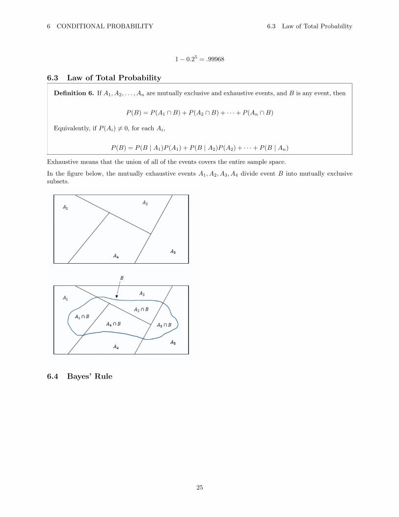
Definition 6. If A1, A2, . . . , An are mutually exclusive and exhaustive events, and B is any event, then
P (B) = P (A1 ∩B) + P (A2 ∩B) + · · ·+ P (An ∩B)
Equivalently, if P (Ai) 6= 0, for each Ai,
P (B) = P (B | A1)P (A1) + P (B | A2)P (A2) + · · ·+ P (B | An)
Exhaustive means that the union of all of the events covers the entire sample space.
In the figure below, the mutually exhaustive events A1, A2, A3, A4 divide event B into mutually exclusivesubsets.
6.4 Bayes’ Rule
25
6 CONDITIONAL PROBABILITY 6.4 Bayes’ Rule
Definition 7. Special case: Let A and B be events with P (A) 6= 0, P (AC) 6= 0, and P (B) 6= 0, then
P (A | B) =P (B | A)P (A)
P (B | A)P (A) + P (B | AC)P (AC)
Bayes’ rule provides a formula that allows us to calculate one of the conditional probabilities, if we knowthe other one.
General case: Let A1, A2, . . . , An be mutually exclusive events and exhaustive events with P (Ai) 6= 0for each Ai. Let B be any event with P (B) 6= 0.
P (Ak | B) =P (B | Ak)P (Ak)
P (B | A1)P (A1) + · · ·+ P (B | An)P (An)
=P (B | Ak)P (Ak)∑ni=1 P (B | Ai)P (Ai)
Note 4. In general,P (A | B) 6= P (B | A)
Example 27. During frequent trips to a certain city, a traveling salesman stays at hotel A 50% of thetime, hotel B 30% of the time, and hotel C 20% of the time. When checking in, there is some problemwith the reservation 3% of the time at hotel A, 6% of the time at hotel B, and 10% of the time at hotelC. Suppose the salesperson travels to this city.
Let
A = stays at hotel A
B = stays at hotel B
C = stays at hotel C
R = problem with res
and
P (A) = 0.5
P (B) = 0.3
P (C) = 0.2
P (R | A) = 0.03
P (R | B) = 0.06
P (R | C) = 0.1
Find the probability that the salesperson stays at hotel A and has a problem.
26
6 CONDITIONAL PROBABILITY 6.4 Bayes’ Rule
P (A ∩R) = P (R | A) · P (A)
= 0.03 · 0.5= 0.015
Find the probability that the salesperson has a problem with the reservation.
P (R) = (0.03 · 0.5) + (0.06 · 0.3) + (0.1 · 0.2)
= 0.053
Suppose the salesperson has a problem with the reservation, what is the probability that the salespersonis staying at hotel A?
We can use the values from the last 2 problems:
P (A | R) =P (A ∩R)
P (R)
=0.015
0.053= 0.283
27
7 RANDOM VARIABLES
7 Random Variables
A random variable assigns a numerical value to each outcome in a sample space (typically denoted bycapital letters, like X,Y, Z). We can think of a random variable X as a function.
Example 28. When a balanced coin is tossed three times, 8 equally likely outcomes are possible: HHHHHT HTH HTT THH THT TTH TTT.
Let X denote the total number of heads obtained in 3 tosses, then X is a random variable where
X = {0, 1, 2, 3}
Two important types of random variables:
• Discrete
– One whose possible values form a discrete set; that is values can be ordered and there are gapsbetween adjacent values.
– Set of integers.
– Set of whole numbers.
– Usually invole a ‘count’ of something.
• Continuous
– Possible values always contain an interval; that is all the points between some two numbers.
– Usually involves a ‘measure’ of something.
7.1 Discrete Random Variables
Definition 8. The probability mass function (pmf) of a discrete random variable X is the function
p(x) = P (X = x)
The probability mass function is sometimes called the probability distribution.
Note 5. If the values of the probability mass function are added over all the possible values of X, thesum equals 1. That is, ∑
x
p(x) =∑x
P (X = x) = 1
where the sum is over all the possible values of X.
Example 29. The number of flaws in a 1-inch length of copper wire manufactured by a certain processvaries from wire to wire. Overall, 48% of the wires produced have no flaws, 39% have 1 flaw, 12% have2 flaws, and 1% have 3 flaws. Let X be the number of flaws in a randomly selected piece of wire.
The possible values of X are:
X = {0, 1, 2, 3}
The pmf is a table showing the possible values of X and their corresponding probabilities.
28
7 RANDOM VARIABLES 7.1 Discrete Random Variables
Definition 9. The cumulative distribution function (cdf) of a random variable X is the function
F (x) = P (X ≤ x)
In general, for any discrete random variable X, the cumulative distribution function F (x) can becomputed by summing the probabilities of all the possible values of X that are less than or equal to x.That is,
F (x) =∑t≤x
p(t) =∑t≤x
p(X = t)
Note 6. F (x) is ddefined for any number x, not just for possible values of X. For a discrete randomyvariable X, the graph of F will be a “step function”.
Example 30. The given values can be turned into a cdf.
F (0) = P (X ≤ 0) = p(0) = .48
F (1) = P (X ≤ 1) = p(0) + p(1) = .87
F (2) = P (X ≤ 2) = .48 + .39 + .12 = .99
F (3) = P (X ≤ 3) = 1
If you want to calculate numbers in between the given:
F (−1.4) = P (X ≤ −1.4) = 0
F (0.5) = P (X ≤ 0.5) = .48
F (.99) = P (X ≤ .99) = .48
F (1.3) = P (X ≤ 1.3) = .87
F (4) = P (X ≤ 4) = 1
There is only a discrete amount of values for X so you must check what the probability X is less thanwhat youre checking.
The cdf is a piecewise defined function:
F (x) =
0 x < 0
0.48 0 ≤ x ≤ 1
0.87 1 < x ≤ 2
0.99 2 < x ≤ 3
1 x ≥ 3
7.1.1 Mean of a for Discrete Random Variables
29
7 RANDOM VARIABLES 7.1 Discrete Random Variables
Definition 10. Let X be a discrete random variable with probability mass function p(x) = P (X = x).
The mean of X is given by
µX =∑X
x · P (X = x)
where the sum is over all possible values of X.
The mean of X is sometimes called the expectation, or expected value, of X and may also be denoted byE(X). Sometimes we leave off the subscript and write the sum as
µ =∑X
xp(x)
Mean: for a small finite data set, the mean would simply be an arithmetic average. The mean of a discreterandom variable is a generalization of this idea and represents a weighted average.
Example 31. Consider a population of 8 students with the following ages in years: 19, 20, 20, 19, 21,27, 20, 21
Say:
X = age of randomly selected student
Arithmetic average would be:
=19 + 20 + 20 + 19 + 21 + 27 + 20 + 21
8= 20.875
But in a weighted average:
=19(2) + 20(3) + 21(2) + 27(1)
8= 19(.25) + 20(.375) + 21(.25) + 27(.125)
=∑x
xp(x) = µ
µ =∑x
xp(x)
= 19(.25) + 20(.375) + 21(.25) + 27(.125)
= 20.875
7.1.2 Variance and Standard Deviation of a Discrete Random Variable
30
7 RANDOM VARIABLES 7.1 Discrete Random Variables
Definition 11. Let X be a discrete random variable with a probability mass function p(x) = P (X = x).
• The variance of X is given by
σ2X =
∑X
(x− µ)2P (X = x)
• An alternate formula for the variance is given by
σ2X =
∑X
x2P (X = x)− µ2X
• The variance of X may also be denoted by V (x) or by σ2.
• The standard deviation is the square root of the variance
σX =√σ2X
The variance can also be written as
σ2 =∑x
[(x− µ)2 · p(x)
]The alternate formula for the variance is known as the computing formula.
The mean is a measure of center. The variance and standard deviation are measures that indicate howfar, on average, an observed value of X is from the mean.
Example 32. Consider a population of 8 students with the following ages in years: 19, 20, 20, 19, 21,27, 20, 21
Say:
X = age of randomly selected student
x− µ is the deviation from mean. (x− µ)2 is the squared deviation.
σ2 =∑x
(x− µ)2 · p(x)
= (−1.875)2(.25) + (−.875)2(.375) + (.125)2(.25) + (6.125)2(.125)
= 5.859375
≈ 5.859 years2
The variance is the “mean of the squared deviations”.
σ =√σ2
=√
5.859375
≈ 2.421 years
31
7 RANDOM VARIABLES 7.2 Probability Density Functions
In words: Observations are on average roughtly 2.421 years from the mean.
Example 33. Using the previous example, lets use the computing formula.
σ2x =
∑x
[x2p(x)
]− µ2
x
Recall
µ = 20.875 years
So using the computing formula:
V (x) = σ2 =∑x
x2p(x)− µ2
σ2 =∑x
x2p(x)− µ2
= 192(.25) + 202(.375) + 212(.25) + 272(.125)− µ2
= 441.625− (20.875)2
= 5.859375
≈ 5.859
σ ≈ 2.421
7.2 Probability Density Functions
Definition 12. A random variable is continuous if its probabilities are given by areas under a curve.This curve is called a probability density function (pmf) for the random variable. The probabilitydensity function is sometimes called the probability distribution.
Let X be a continuous random variable with probability density function f(x). Let a and b be any twonumbers, with a < b.
The proportion of the population whose values of X lie between a and b are given by∫ baf(x) dx, the
area under the probability density function between a and b. This is the probability that the randomvariable X takes on a value between a and b. Note that the area under the curve does not depend onwhether the endpoints a and b are included in the interval. So, probabilities involving X do not dependon whether endpoints are included. That is,
P (a ≤ X ≤ B) = P (a ≤ X < b)
= P (a < X ≤ b)= P (a < X < b)
=
∫ b
a
f(x) dx
In additions,
32

7 RANDOM VARIABLES 7.2 Probability Density Functions
P (X ≤ b) = P (X < b)
=
∫ b
−∞f(x) dx
P (X ≤ a) = P (X > a)
=
∫ ∞a
f(x) dx
Always find the probability that X is in a range, never for a single value.
Note also, for f(x) to be a legitimate pdf, it must satisfy the following conditions:
1. f(x) ≥ 0 for all x.
2.∫∞−∞ f(x) dx = 1. The area under the curve is equal to 1.
Some background: In a probability histogram, areas of rectangles correspond to probabilities. For examplewith a sample of continuous data, data can be organized into categories, or bins.
The areas of these rectangles correspond to probabilities and let us know the proportion of values of x thatfall into a certain category. The sum of the areas of the rectangles must be 1. Note: the vertical axis is notthe probability, the area is.
The probability histogram for a large continuous population could be drawn with extremely narrow rectanglesand might look like this curve:
Example 34. A hole is drilled in a sheet-metal component, and then a shaft is inserted through thehole. The shaft clearance is equal to the different between the radius of the hole and radius of the shaft.Let the random variable X denote the clearance, in millimeters. The probability density function of X
33
7 RANDOM VARIABLES 7.3 Cumulative Distribution Functions of a Continuous Random Variable
is
f(x) =
{1.25(1− x4) 0 < x < 1
0 otherwise
Components with clearances larger than 0.8 mm must be scrapped. What proportion of componentsare scrapped?
P (X > 0.8) =
∫ ∞a
f(x) dx
= limt→∞
∫ t
a
f(x) dx
=
∫ 1
0.8
1.25(1− x4) dx+ limt→∞
∫ t
a
0 dx
= 1.25
∫ 1
0.8
1− x4 dx
= 1.25
[x− 1
5x5
]1
0.8
= 1.25
[(1− 1
5)− (0.8− .85
5)
]≈ 0.0819
7.3 Cumulative Distribution Functions of a Continuous Random Variable
Definition 13. Let X be a continuous randome variable with probability density function f(x). Thecumulative distribution function (cdf) of X is the function
F (x) = P (X ≤ x) =
∫ ∞−∞
f(t) dt
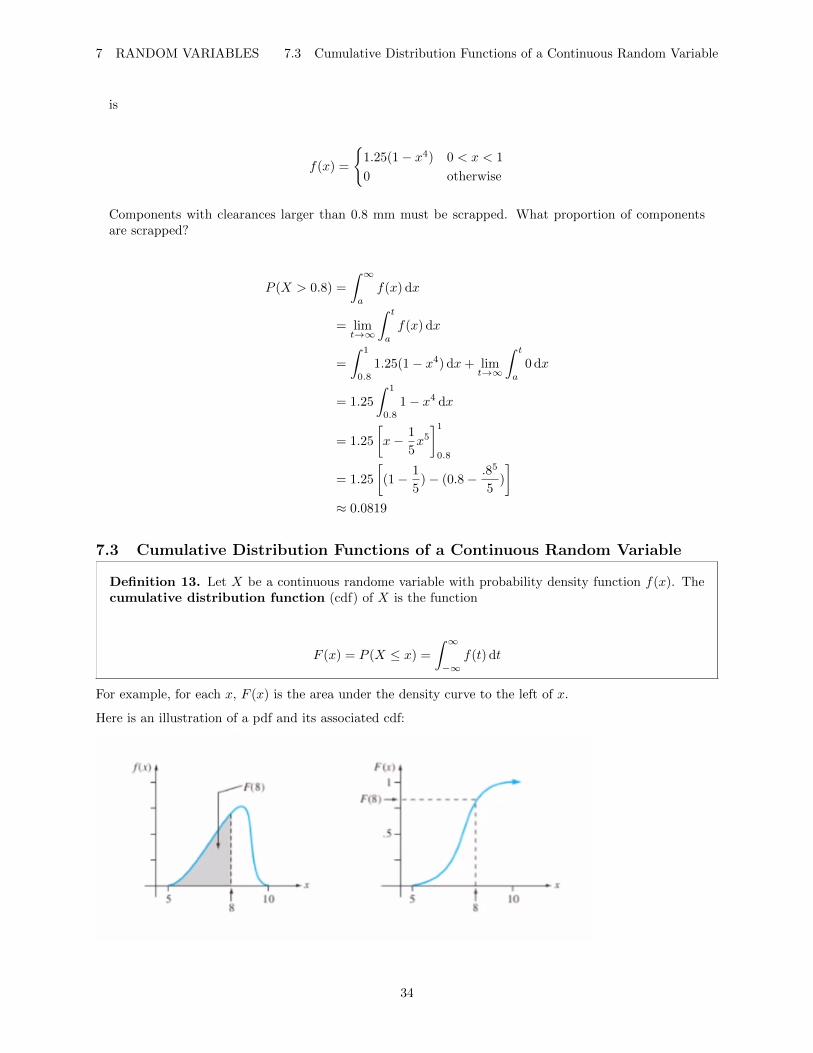
For example, for each x, F (x) is the area under the density curve to the left of x.
Here is an illustration of a pdf and its associated cdf:
34
7 RANDOM VARIABLES 7.3 Cumulative Distribution Functions of a Continuous Random Variable
Example 35. A hole is drilled in a sheet-metal component, and then a shaft is inserted through thehole. The shaft clearance is equal to the different between the radius of the hole and radius of the shaft.Let the random variable X denote the clearance, in millimeters. The probability density function of Xis
f(x) =
{1.25(1− x4) 0 < x < 1
0 otherwise
Find the cumulative distribution function of F (x).
We know:
F (x) = P (X ≤ x) =
∫ x
−∞f(t) dt
Case 1: x ≤ 0
F (x) =
∫ x
−∞0 dt
= 0
Case 2: 0 < x < 1
F (x) =
∫ x
−∞f(t) dt
=
∫ 0
−∞f(t) dt+
∫ x
0
f(t) dt
= 0 +
∫ x
0
1.25(1− t4) dt
= 1.25
∫ x
0
1− t4 dt
= 1.25
[t− 1
5t5]x
0
= 1.25
[(x− 1
5x5)− (0− 0)
]= 1.25
(x− 1
5x5
)
Case 3: x ≥ 1
35
7 RANDOM VARIABLES 7.4 Mean and Variance for Continuous Random Variables
F (x) =
∫ x
−∞f(t) dt
=
∫ 0
−∞f(t) dt+
∫ 1
0
f(t) dt+
∫ x
1
f(t) dt
= 0 +
∫ 1
0
1.25(1− t4) dt+ 0
= 1
The area under the entire cdf should be 1 by definition.
We can define our cdf as:
F (x) =
0 x ≤ 0
1.25(x− 15x
5) 0 < x < 1
1 x ≥ 1
7.4 Mean and Variance for Continuous Random Variables
Definition 14. Let X be a continuous random variable with probability density function f(x). Thenthe mean of X is given by
µx =
∫ ∞−∞
xf(x) dx
The mean of X is sometimes called the expectation, or expected value, of X and may also be denotedby E(X) or µ.
36
7 RANDOM VARIABLES 7.4 Mean and Variance for Continuous Random Variables
Definition 15. Let X be a continuous random variable with probability density function f(x). Then
• The variance of X is given by
σ2x =
∫ ∞−∞
(x0µX)2f(x) dx
• An alternate formula for the variance is given by
σ2X =
∫ ∞−∞
x2f(x) dx− µ2X
• The variance of X may also be denoted by V (x) or by σ2.
• The standard deviation is the square root of the variance
σX =√σ2X
Example 36. A hole is drilled in a sheet-metal component, and then a shaft is inserted through thehole. The shaft clearance is equal to the different between the radius of the hole and radius of the shaft.Let the random variable X denote the clearance, in millimeters. The probability density function of Xis
f(x) =
{1.25(1− x4) 0 < x < 1
0 otherwise
Find the mean clearance and the variance of the clearance.
Recall:
E(X) = µ =
∫ ∞−∞
xf(x) dx
So:
37
7 RANDOM VARIABLES 7.5 Median and Percentiles
µ =
∫ 1
0
xf(x) dx
= 1.25
∫ 1
0
x(1− x4) dx
= 1.25
∫ 1
0
x− x5 dx
= 1.25
[1
2x2 − 1
6x6
]1
0
= 1.25
[1
2− 1
6
]≈ 0.4167
Lets find the variance:
V (x) = σ2 =
∫ ∞−∞
x2f(x) dx− µ2
=
∫ 1
0
x2f(x) dx− (.4167)2
=
∫ 1
0
x2[1.25(1− x4)
]dx− (.4167)2
= 1.25
∫ 1
0
x2 − x6 dx− (.4167)2
= 1.25
[1
3x3 − 1
7x7
]1
0
− (.4167)2
= 1.25
(1
3− 1
7
)− (.4167)2
≈ .0645 mm2
7.5 Median and Percentiles
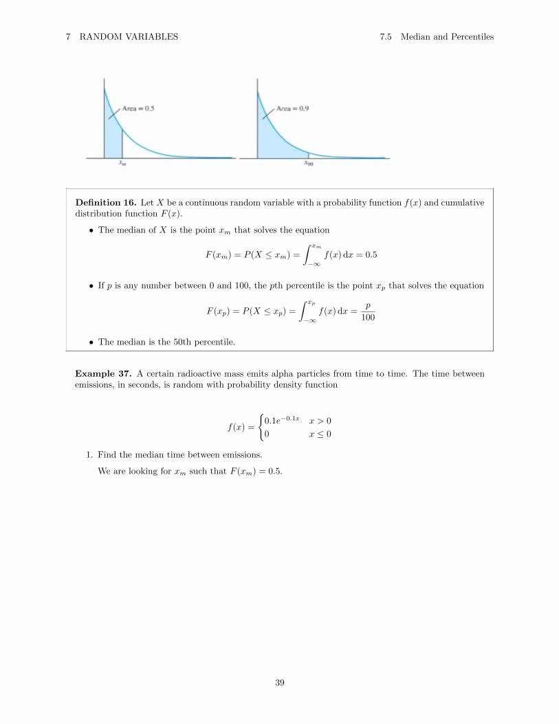
The median of a data set divides the data into two equal parts: the bottom 50% and the top 50%. In termsof probability density function, the median (denoted by xm) is the point at which half the area under thecurve is to the left, and half the area is to the right.
More generall, for p between 0 and 100, the pth percentile (denoted by xp) is the number that dividesthe bottom p% of the data from the top (100 − p)%. For example, the 90th percentile (denoted by x90) isthe number that divides the bottom 90% of the data from the top 10%. In terms of a probability densityfunction, the 90th percentile is the point x90 at which the area under the curve to the left of x90 is 0.9, andthe area under the curve to the right of x90 is 0.1.
38
7 RANDOM VARIABLES 7.5 Median and Percentiles
Definition 16. Let X be a continuous random variable with a probability function f(x) and cumulativedistribution function F (x).
• The median of X is the point xm that solves the equation
F (xm) = P (X ≤ xm) =
∫ xm
−∞f(x) dx = 0.5
• If p is any number between 0 and 100, the pth percentile is the point xp that solves the equation
F (xp) = P (X ≤ xp) =
∫ xp
−∞f(x) dx =
p
100
• The median is the 50th percentile.
Example 37. A certain radioactive mass emits alpha particles from time to time. The time betweenemissions, in seconds, is random with probability density function
f(x) =
{0.1e−0.1x x > 0
0 x ≤ 0
1. Find the median time between emissions.
We are looking for xm such that F (xm) = 0.5.
39

7 RANDOM VARIABLES 7.6 Linear Functions of Random Variables
F (xm) = P (X ≤ xm) =
∫ xm
−∞f(x) dx
=
∫ xm
0
0.1e−0.1x dx
= 0.1
∫ xm
0
e−0.1x dx
= 0.1
[1
−0.1e−0.1x
]xm0
= −e−0.1x |xm0
= −e−0.1xm − (−e0)
= −e−0.1xm + 1
Set it equal to our 0.5 because we are looking for the median:
−e−0.1xm + 1 = 0.5
e−0.1xm = 0.5
ln(e−0.1xm) = ln(0.5)
−0.1xm = ln(0.5)
xm =ln(0.5)
−0.1
xm ≈ 6.931 seconds
Interpretation: half of the times between emissions are less than 6.931 seconds and half are more.
2. Find the 60th percentile of the times.
To find the 60 percentile we can set it equal to 0.6:
F (x60) = −e−0.1x60 + 1 = 0.6
−e−0.1x60 = −0.4
e−0.1x60 = 0.4
−0.1x60 = ln(0.4)
x60 =ln(0.4)
−0.1
x60 ≈ 9.163 seconds
Interpretation: 60% of the times between emissions are less than 9.163 seconds and 40% aregreater.
7.6 Linear Functions of Random Variables
40

7 RANDOM VARIABLES 7.6 Linear Functions of Random Variables
Definition 17. Adding a constant
If X is a random variable and b is a constant, then
µX+b = µX + b σ2X+b = σ2
X
Using the alternate notation
E(X + b) = E(X) + b V (X + b) = V (X)
In general, when a constant is added to a random variable, the mean is shifted by that constant, andthe variance is unchanged.
Example 38. Assume that steel rods produced by a certain machine have a mean length of 5.0 in anda variance of σ2 = 0.003 in2.
1. What is the mean length of the assembly?
Each rod is attached to a base that is 1.0 in long. So the mean length of the assembly will be:
5.0 + 1.0 = 6.0 inches
2. Can you tell what the variance of the length of the assembly might be?
Since each length is increased by the same amount, the spread in the lengths doesn’t change. Sothe variance remains the same:
σ2 = 0.003 in2
3. Let X represent the length of a randomly chosen rod and let Y represent the length of the assembly.Write Y in terms of the variable X.
y = length of rod
x = added length
y = x+ 1
4. Use statistical notation to show how to compute µY .
µy = µx+1
= µx + 1
= 5 + 1
= 6
41
7 RANDOM VARIABLES 7.6 Linear Functions of Random Variables
5. Use statistical notation to show how to compute σ2Y .
σ2y = σ2
x+1
= σ2x
= 0.003 in2
Note that the standard deviation of Y would be:
σy =√
0.003
≈ 0.055 in
Definition 18. Multiplying by a constant
If X is a random variable and a is a constant, then
µaX = aµX σ2aX = a2σ2
X
Using alternative notation
E(aX) = aE(X) V (aX) = a2V (X)
In general, when a random variable is multiplied by a constant, its mean is multiplied by the sameconstant, but its variance is multiplied by the square of the constant.
Example 39. Continuing the last example:
1. If we measure the lengths of the rods described above in centimeters rather than inches, what willthe mean length be? (Use 2.54 cm = 1 in.)
5 · 2.54 = 12.7 cm
2. When the length X of a rod is measured in inches, the variance σ2X must have units of in2. If we
measure the lengths of the rods in centimeters, what must the units of the variance be?
To convert our variance to cm2 we can multiply:
σ2x = 0.003 · 2.542
= 0.019 cm2
3. Let Z represent the length of a rod, in cm. Write Z in terms of the random variable X.
42
7 RANDOM VARIABLES 7.7 Linear Combinations of Random Variables, Means and Variances
Z = 2.54X
4. Use statistical notation to show how to compute µZ .
The mean of the rod length in cm:
µZ = µ2.54X
= 2.54µX
= 2.54(5.0)
= 12.7 cm
5. Use statistical notation to show how to compute σ2Z .
σ2Z = σ2
2.54X
= 2.542 · σ2X
= 2.542(0.003)
≈ 0.019 cm2
Note that the standard deviation of this is:
σZ =√
2.542 · 0.003
≈ 0.139 cm
7.7 Linear Combinations of Random Variables, Means and Variances
Definition 19. If X1, . . . , Xn are random variables, then the mean of the sum X1 + · · ·+Xn is givenby
µX1+···+Xn = µX1+ · · ·+ µXn
“The mean of the sum is the sum of the means.”
The sum X1 + · · ·+Xn is a special case of a linear combination.
Definition 20. If X1, . . . , Xn are random variables and c1, . . . , cn are constants, then the randomvariable
c1X1 + · · ·+ cnXn
is called a linear combination of X1, . . . , Xn.
43
7 RANDOM VARIABLES 7.7 Linear Combinations of Random Variables, Means and Variances
Definition 21. If X1, . . . , Xn are random variables and c1, . . . , cn are constants, then the mean of thelinear combination c1X1 + · · ·+ cnXn is given by
µc1X1+···+cnXn = c1µX1+ · · ·+ cnµXn
Definition 22. If X1, . . . , Xn are independent random variables then the variance of the sum X1 +· · ·+Xn is given by
σ2X1+···+Xn = σ2
X1+ · · ·+ σ2
Xn
“The variance of the sum is the sum of the variances.”
In general, if X1, . . . , Xn are independent random variables, and c1, . . . , cn are constants, then thevariance of the linear combination c1X1 + · · ·+ cnXn is given by
σ2c1X1+···+cnXn = c21σ
2X1
+ · · ·+ c2nσ2Xn
The variance of the sum is the sum of the variances, WHEN the Xi’s are independent.
Note 7. Two frequently encountered linear combinations are the sum and the different of two randomvariables. It is interesting to note that, when the random variables are independent, the variance of thesum is the same as the variance of the different.
For example, if X and Y are independent random variables with variance σ2X and σ2
Y , then the varianceof the sum X + Y is
σ2X+Y = σ2
X + σ2Y
The variance of the different X − Y is
σ2X−Y = σ2
X + σ2Y
Example 40. A piston is placed inside a cylinder. The clearance is the distance between the edgeof the piston and the wall of the cylinder, and is equal to one-half the different between the cylinderdiameter and the piston diameter. Assume the piston diameter has a mean of 80.85 cm with a standarddeviation of 0.02 cm. Assume the cylinder diameter has a mean of 80.95 cm with a standard deviationof 0.03 cm.
1. Find the mean clearance.
Lets define our values
44
7 RANDOM VARIABLES 7.7 Linear Combinations of Random Variables, Means and Variances
C = clearance
X = cylinder diameter
Y = piston diameter
C =1
2(X − Y )
To find the mean clearance:
µC = µ 12X−
12Y
=1
2µX −
1
2µY
=1
2(80.95)− 1
2(80.85)
≈ 0.050 cm
2. Assuming that the piston and cylinder are chosen independently, find the standard deviation ofthe clearance.
We must first find the variance:
σ2C = σ2
12X−
12Y
= σ212X
+ σ2− 1
2Y
= (.5)2σ2Y + (−.5)2σ2
Y
= (.5)2(.03)2 + (−.5)2(.02)2
= 3.25 · 10−4 cm2
The standard deviation of the clearance is the square root of the variance:
σC =√σ2C
=√
(.5)2(.03)2 + (−.5)2(.02)2
≈ 0.018 cm
Example 41. Let X,Y, Z be independent random variables.
45
7 RANDOM VARIABLES 7.8 Simple Random Samples
µX = 30
µY = −18
µZ = 25
σX = 5
σY = 3
σZ = 2.5
1. Find the mean and standard deviation of
(a) 2X + 4Y + 10
µ2X+4Y+10 = µ2X+4Y + 10
= 2µX + 4µY + 10
= 2(30) + 4(−18) + 10
= −2
σ22X+4Y+10 = 22σ2
X + 42σY
= 4(52) + 16(32)
= 244
σ =√
244
≈ 15.6
(b) 3X + 2Y − 4Z
µ3X+2Y−4Z = 3µX + 2µY − 4µZ
= −46
σ23X+2Y−4Z = 32σ2
X + 22σ2Y + (−4)2σ2
Z
= 9(52) + 4(32) + 16(2.52)
= 361
σ =√
361
= 19
7.8 Independent and Simple Random Samples, Mean and Variance of a SampleMean
46
7 RANDOM VARIABLES 7.8 Simple Random Samples
Definition 23. A population is the entire collection of objects or outcomes about which informatinois sought.
A sample is a subset of a population, containing the objects or outcomes that are actually observed.
A simple random sample (SRS) of size n is a sample chosen by a method in which each collection ofn population items is equally likely to make up the sample, just as in a lottery.
When a simple random sample of numerical values is drawn from a population, each item in the samplecan be thought of as a random variable. The items in a simple random sample may be treated asindepent, except when the sample is a large proportion (more than 5%) of a finite population.
For our work from here on, unless explicitly stated to the contrary, we will assume this exception hasnot occured, so that the values in a simple random sample may be treated as independent randomvariables.
In general:
If X1, . . . , Xn is a simple random sample, then X1, . . . , Xn may be treated as independent randomvariables, all with the same distribution.
When X1, . . . , Xn are independent random variables, all with the same distribution, it is sometimessaid that X1, . . . , Xn are independent and identically distributed (i.i.d.).
Items in a sample are independent if knowing the values of some items does not help predict the values ofthe others.
A “pretend” example:
Define a population as: all students at sac state. Define X as the age of a student at sac state.
Consider a simple random sample of size 5. Let:
X1, X2, X3, X4, X5
be a simple random sample. For i = 1, . . . , 5 each Xi is the age of a student at sac state. One particularsample may be:
X1 = 32X2 = 20X3 = 18X4 = 21X5 = 25
47
7 RANDOM VARIABLES 7.8 Simple Random Samples
Definition 24. Sample Mean
If X1, . . . , Xn is a simple random sample from a population with mean µ and variance σ2, then thesample mean is denoted by X and is given by
X =X1 + · · ·+Xn
n
Rewriting the above expression, we see that the sample mean X is a linear combination
X =1
nX1 + · · ·+ 1
nXn
From this fact, we can think about how to derive the mean and variance of X:
Suppose X is the population variable with mean µ and variance σ2. For the simple random sampleX1, . . . , Xn from this population, X1, . . . , Xn all have the same distribution as the population variableX. It follows that
µX = µ 1nX1+···+ 1
nXn=
1
nµX1
+ · · ·+ 1
nµXn
=1
nµ+ · · ·+ 1
nµ︸ ︷︷ ︸
there are n of these
= (n)
(1
n
)µ
= µ
and, since the items in a simple random sample may be treated as indepent random variables
σ2X = σ2
1nX1+···+ 1
nXn=
1
n2σ2X1
+ · · ·+ 1
n2σ2Xn
=1
n2+ · · ·+ 1
n2σ2︸ ︷︷ ︸
there are n of these
= (n)
(1
n2
)σ2
=σ2
n
A sample mean is an arithmetic average.
So considering our last example, with our sample size of 5:
n = 5
So the sample mean can be computed:
48
7 RANDOM VARIABLES 7.8 Simple Random Samples
X =X1 +X2 +X3 +X4 +X5
5
X is a variable. One particular value of a sample mean, using set above would me:
X =32 + 20 + 18 + 21 + 25
5= 23.2 years
The value of X will change depending on which sample we are looking at.
Example 42. A process that fills plastic bottles with a beverage has a mean fill volume of 2.013 L anda standard deviation of 0.005 L. A case contains 24 bottles. Assuming that the bottles in a case area simple random sample of bottles filled by this method, find the mean and standard deviation of theaverage volume per bottle in a case.
Let V1, . . . , V24 be a simple random sample. For i = 1, . . . , 24, each Vi is the volume of a bottle.
Average volume per bottle of a case of 24 bottles is the sample mean:
V =V1 + · · ·+ V24
24
Mean of the average volume per bottle in a case:
µV = µ
= 2.013 L
The standard deviation:
σV =σ√n
=0.005√
24
≈ 0.001 L
49

8 COMMONLY USED DISTRIBUTIONS
8 Commonly Used Distributions
8.1 Bernoulli Distribution
Many applications of probability and statistics concern the repetition of an experiment, where each repetitionis called a trial. A Bernoulli trial is an experiment with exactly two possible outcomes, labaled “success”and “failure”. The probability of success is denoted by p and the probability of failured is denoted as 1− p.
Definition 25. For any Bernoulli trial, we define a random variable X as follows
If the experiment results in success, then X = 1, otherwise X = 0.
It follows that X is a discrete random variable with probabiliity mass function p(x) defined by
p(0) = P (X = 0) = 1− pP (1) = P (X = 1) = p
The random variable X is said to have a Bernoulli distribution with parameter p.
The notation is X ∼ Bernoulli(p).
The mean and variance of a Bernoulli Random Variable is
µX = p σ2X = p(1− p)
Example 43. For example, the tossing of a coin is a simple Bernoulli trial. There are 2 possibleoutcomes, heads or tails. We can define a heads as ”success”. With a fair coin, the probability ofsuccess is p = 0.5.
Let X = 1 if the coin comes up heads. Let X = 0 otherwise. Then X has a Bernoulli distribution withp = 0.5. So:
X Bernoulli(0.5)
Example 44. Ten percent of the components manufactured by a certain process are defective. Acomponent is chosen at random. Let X = 1 if the component is defective and X = 0 otherwise. Whatis the distribution of X?
The success probability is:
p(1) = P (X = 1) = 0.1
X has a Bernoulli distribution with parameter p = 0.1. That is,
X Bernoulli(0.1)
What is the mean and variance?
Recall that the mean is:
50

8 COMMONLY USED DISTRIBUTIONS 8.2 Binomial Distribution
µx =∑x
xp(x)
= 0(1− p) + 1(p)
= p
Recall that the variance is:
σ2x =
∑x
(x− µ)2 · p(x)
= (0− p)2(1− p) + (1− p)2(p)
= p2(1− p) + (1− p)2(p)
= p(1− p) [p+ (1− p)]= p(1− p)
So
µx = 0.1
σ2x = 0.1(0.9)
= .09
8.2 Binomial Distribution
51
8 COMMONLY USED DISTRIBUTIONS 8.2 Binomial Distribution
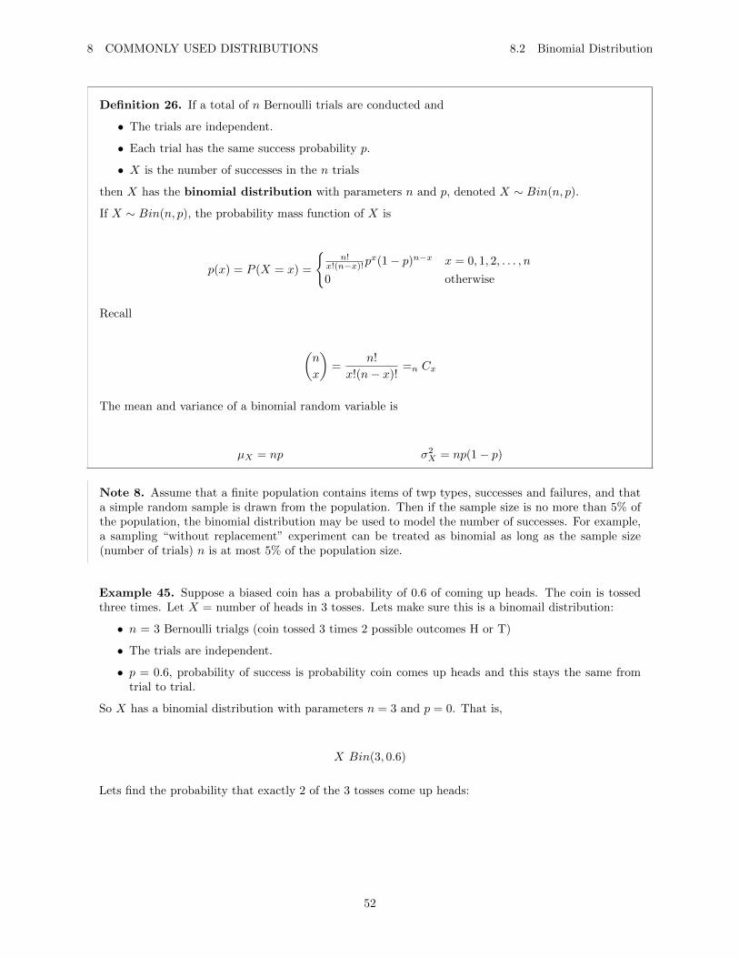
Definition 26. If a total of n Bernoulli trials are conducted and
• The trials are independent.
• Each trial has the same success probability p.
• X is the number of successes in the n trials
then X has the binomial distribution with parameters n and p, denoted X ∼ Bin(n, p).
If X ∼ Bin(n, p), the probability mass function of X is
p(x) = P (X = x) =
{n!
x!(n−x)!px(1− p)n−x x = 0, 1, 2, . . . , n
0 otherwise
Recall
(n
x
)=
n!
x!(n− x)!=n Cx
The mean and variance of a binomial random variable is
µX = np σ2X = np(1− p)
Note 8. Assume that a finite population contains items of twp types, successes and failures, and thata simple random sample is drawn from the population. Then if the sample size is no more than 5% ofthe population, the binomial distribution may be used to model the number of successes. For example,a sampling “without replacement” experiment can be treated as binomial as long as the sample size(number of trials) n is at most 5% of the population size.
Example 45. Suppose a biased coin has a probability of 0.6 of coming up heads. The coin is tossedthree times. Let X = number of heads in 3 tosses. Lets make sure this is a binomail distribution:
• n = 3 Bernoulli trialgs (coin tossed 3 times 2 possible outcomes H or T)
• The trials are independent.
• p = 0.6, probability of success is probability coin comes up heads and this stays the same fromtrial to trial.
So X has a binomial distribution with parameters n = 3 and p = 0. That is,
X Bin(3, 0.6)
Lets find the probability that exactly 2 of the 3 tosses come up heads:
52

8 COMMONLY USED DISTRIBUTIONS 8.2 Binomial Distribution
P (X = x) =
{n!
3!(3−x)! (0.6)x(0.4)3−x x = 0, . . . , n
0 otherwise
So the probability of exactly 2 heads:
P (X = 2) =3!
2!1!(0.6)2(0.4)1
= 0.432
P (X = 2) = 3(0.6)2(0.4)1
=
(3
2
)︸︷︷︸
how many outcomes have exactly 2 heads
·
prob. of an individual outcome with 2 heads︷ ︸︸ ︷(0.6)2(0.4)1
A variation of the Bernoulli random variable.
Mini-proof:
A binomial random variable can be written as a sum of Bernoulli random variables. Assume n independentBernoulli trials are conducted, each with a success probability p. Consider Y1, . . . , Yn defined as follows:
For i = 0, . . . , n:
Yi = 1
If the ith trial results in success, otherwise:
Yi = 0
Let X = number of success among n trials. Then:
X = Y1 + · · ·+ Yn︸ ︷︷ ︸sum gives the number of Yi that equal 1
So the mean of X is the mean of that sum:
µX = µY1 + · · ·+ µYn
= p+ · · ·+ p︸ ︷︷ ︸n of these
= np
The variance:
53
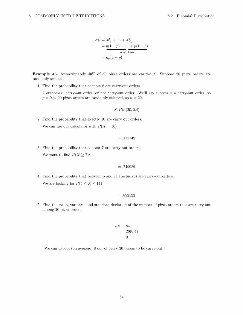
8 COMMONLY USED DISTRIBUTIONS 8.2 Binomial Distribution
σ2X = σ2
Y1+ · · ·+ σ2
Yn
= p(1− p) + · · ·+ p(1− p)︸ ︷︷ ︸n of these
= np(1− p)
Example 46. Approximately 40% of all pizza orders are carry-out. Suppose 20 pizza orders arerandomly selected
1. Find the probability that at most 8 are carry-out orders.
2 outcomes: carry-out order, or not carry-out order. We’ll say success is a carry-out order, sop = 0.4. 20 pizza orders are randomly selected, so n = 20.
X Bin(20, 0.4)
2. Find the probability that exactly 10 are carry out orders.
We can use our calculator with P (X = 10)
= .117142
3. Find the probability that at least 7 are carry out orders.
We want to find P (X ≥ 7):
= .749989
4. Find the probability that between 5 and 11 (inclusive) are carry-out orders.
We are looking for P (5 ≤ X ≤ 11)
= .892522
5. Find the mean, variance, and standard deviation of the number of pizza orders that are carry outamong 20 pizza orders.
µX = np
= 20(0.4)
= 8
“We can expect (on average) 8 out of every 20 pizzas to be carry-out.”
54
8 COMMONLY USED DISTRIBUTIONS 8.2 Binomial Distribution
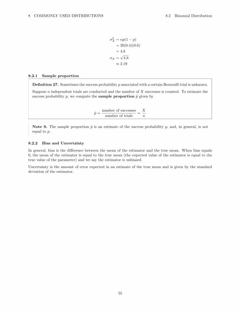
σ2X = np(1− p)
= 20(0.4)(0.6)
= 4.8
σX =√
4.8
≈ 2.19
8.2.1 Sample proportion
Definition 27. Sometimes the success probability p associated with a certain Bernoulli trial is unknown.
Suppose n independent trials are conducted and the number of X successes is counted. To estimate thesuccess probability p, we compute the sample proportion p given by
p =number of successes
number of trials=X
n
Note 9. The sample proportion p is an estimate of the success probability p, and, in general, is notequal to p.
8.2.2 Bias and Uncertainty
In general, bias is the difference between the mean of the estimator and the true mean. When bias equals0, the mean of the estimator is equal to the true mean (the expected value of the estimator is equal to thetrue value of the parameter) and we say the estimator is unbiased.
Uncertainty is the amount of error expected in an estimate of the true mean and is given by the standarddeviation of the estimator.
55
8 COMMONLY USED DISTRIBUTIONS 8.2 Binomial Distribution
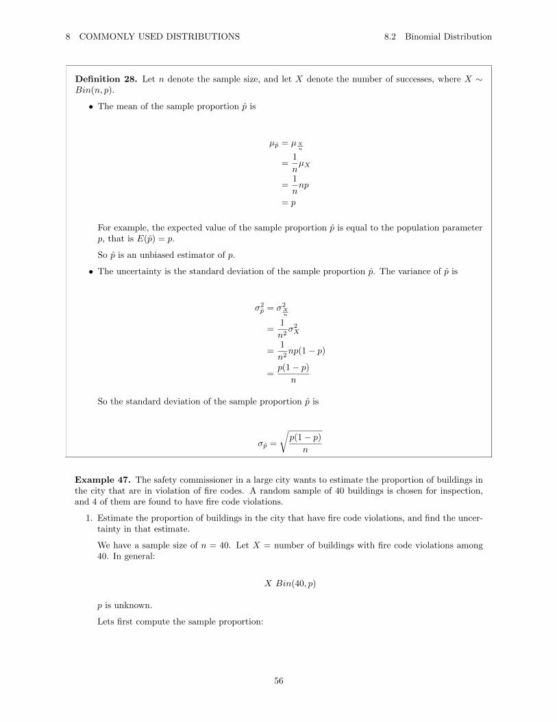
Definition 28. Let n denote the sample size, and let X denote the number of successes, where X ∼Bin(n, p).
• The mean of the sample proportion p is
µp = µXn
=1
nµX
=1
nnp
= p
For example, the expected value of the sample proportion p is equal to the population parameterp, that is E(p) = p.
So p is an unbiased estimator of p.
• The uncertainty is the standard deviation of the sample proportion p. The variance of p is
σ2p = σ2
Xn
=1
n2σ2X
=1
n2np(1− p)
=p(1− p)
n
So the standard deviation of the sample proportion p is
σp =
√p(1− p)
n
Example 47. The safety commissioner in a large city wants to estimate the proportion of buildings inthe city that are in violation of fire codes. A random sample of 40 buildings is chosen for inspection,and 4 of them are found to have fire code violations.
1. Estimate the proportion of buildings in the city that have fire code violations, and find the uncer-tainty in that estimate.
We have a sample size of n = 40. Let X = number of buildings with fire code violations among40. In general:
X Bin(40, p)
p is unknown.
Lets first compute the sample proportion:
56
8 COMMONLY USED DISTRIBUTIONS 8.3 Hypergeometric Distribution
p =X
n
=4
40= 0.1
Next we can calculate the uncertainty:
σp =
√p(1− p)
n
≈√p(1− p)
n
≈√
0.1(1− 0.1)
40
≈ 0.047
2. Approximately how many additional buildings must be inspected so that the uncertainty in thesample proportion of buildings in violation is only 0.02?
Find the sample size n needed so that σp = 0.02. We don’t have p so we must use our value ofp = 0.1.
0.02 =
√p(1− p)
n
=
√0.1(1− 0.1)
n
n =(0.1)(0.9)
(0.002)2
= 225
So we need to subtract the 225 from the 40 already inspected. Therefore:
n = 225− 40
= 185
So we’d need to inspect 185 more buildings to get our uncertainty down to 2%. If our additionalinspections happened to be a decimal, then we round up to the nearest whole number to guaranteewe have the right uncertainty.
8.3 Hypergeometric Distribution
57
8 COMMONLY USED DISTRIBUTIONS 8.4 Geometric Distribution
Definition 29. Assume a finite population contains N items, of which R are classified as successesand N −R are classified as failures. Assume that n items are sampled (without replacement) from thispopulation, let X represent the number of successes in the sample. Then X has the hypergeometricdistribution with parameters N , R, and n, which can be denoted X ∼ H(N,R, n).
The probability mass function of X is
p(x) = P (X = x) =
(Rx)(
N−Rn−x )
(Nn)max(0, R+ n−N) ≤ x ≤ min(n,R)
0 otherwise
The mean and variance of X are
µX =nR
Nσ2X = n
R
N
(1− R
N
)(N −NN − 1
)
8.4 Geometric Distribution
Definition 30. LetX represent the number of trials up to and including the first success in a sequence ofindependent Bernoulli trials with a constant success probability p. ThenX has a geometric distributionwith parameter p, written X ∼ Geom(p).
The probability mass function X is
p(x) = P (X = x) =
{p(1− p)x−1 x = 1, 2, · · ·0 otherwise
The mean and variance of X are
µx =1
pσ2x =
1− pp2
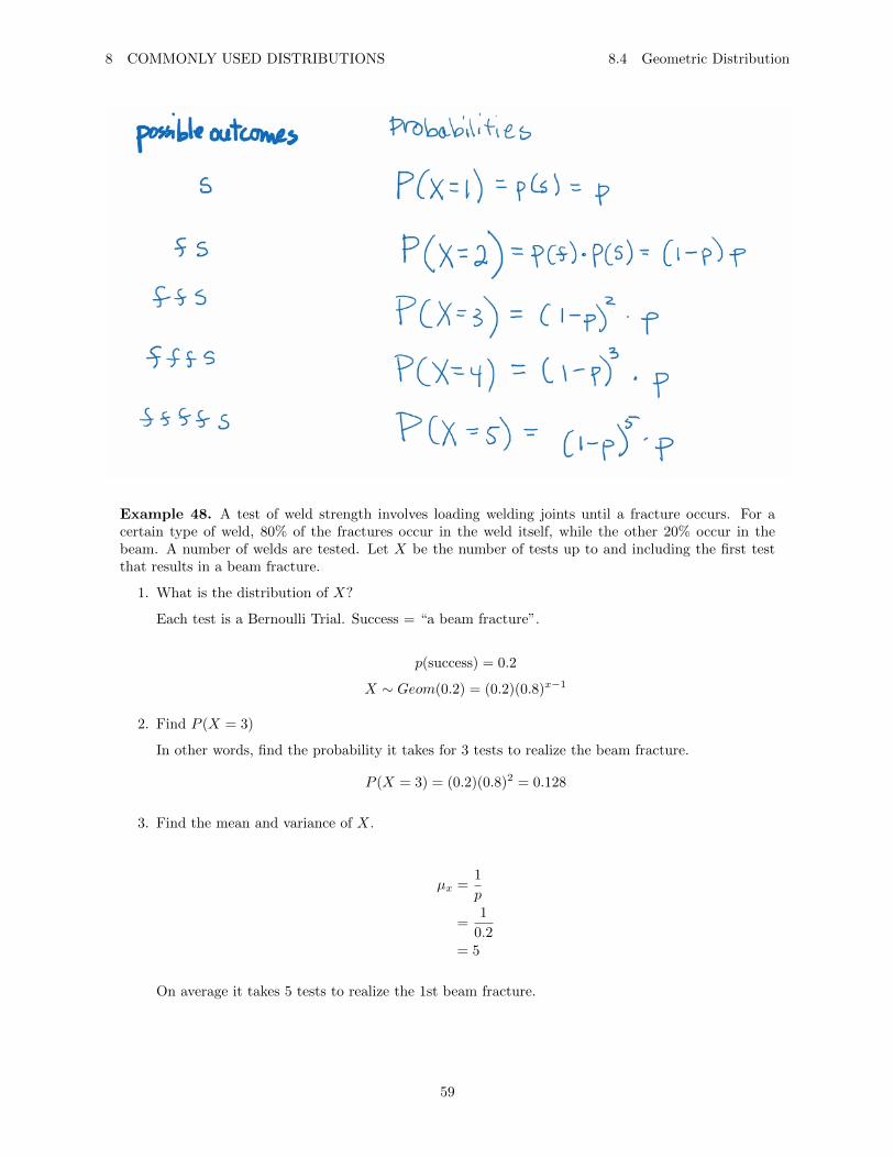
Some background: Think of an experiment like phoning a friend until you get through. The number of callsnecessary until the first success (getting through) is realized is the value of a geometric random variable.
Let X = the number of trials (calls) up to and including the first success (getting through).
Let p = probability of success, and let s = success, f = failure. So,
P (s) = p P (f) = 1− p
58
8 COMMONLY USED DISTRIBUTIONS 8.4 Geometric Distribution
Example 48. A test of weld strength involves loading welding joints until a fracture occurs. For acertain type of weld, 80% of the fractures occur in the weld itself, while the other 20% occur in thebeam. A number of welds are tested. Let X be the number of tests up to and including the first testthat results in a beam fracture.
1. What is the distribution of X?
Each test is a Bernoulli Trial. Success = “a beam fracture”.
p(success) = 0.2
X ∼ Geom(0.2) = (0.2)(0.8)x−1
2. Find P (X = 3)
In other words, find the probability it takes for 3 tests to realize the beam fracture.
P (X = 3) = (0.2)(0.8)2 = 0.128
3. Find the mean and variance of X.
µx =1
p
=1
0.2= 5
On average it takes 5 tests to realize the 1st beam fracture.
59
8 COMMONLY USED DISTRIBUTIONS 8.5 Negative Binomial Distribution
σ2x =
1− pp2
=1− 0.2
0.22
= 20
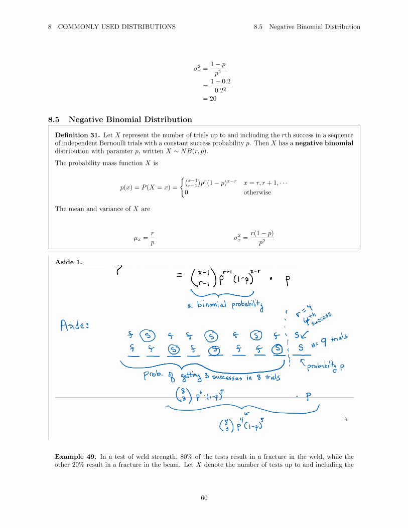
8.5 Negative Binomial Distribution
Definition 31. Let X represent the number of trials up to and incliuding the rth success in a sequenceof independent Bernoulli trials with a constant success probability p. Then X has a negative binomialdistribution with paramter p, written X ∼ NB(r, p).
The probability mass function X is
p(x) = P (X = x) =
{(x−1r−1
)pr(1− p)x−r x = r, r + 1, · · ·
0 otherwise
The mean and variance of X are
µx =r
pσ2x =
r(1− p)p2
Aside 1.
Example 49. In a test of weld strength, 80% of the tests result in a fracture in the weld, while theother 20% result in a fracture in the beam. Let X denote the number of tests up to and including the
60
8 COMMONLY USED DISTRIBUTIONS 8.5 Negative Binomial Distribution
third beam fracture.
1. What is the distribution of X?Success = beam fracture. X has the negative binomial distribution with r = 3 and p = 0.2, thatis
X ∼ NB(3, 0.2)
2. Find P (X = 8)This is the probability it takes exactly 8 tests to realize the 3rd beam fracture.
P (X = 8) =
(8− 2
2
)(0.2)3(0.8)8−3
=
(7
2
)(0.2)3(0.8)5
≈ 0.0551
Another way to compute it with your calculator:(7
2
)(0.2)2(0.8)5 · (0.2)
binompdf(7, .2, 2) · 0.2
3. Find the mean and variance of X.
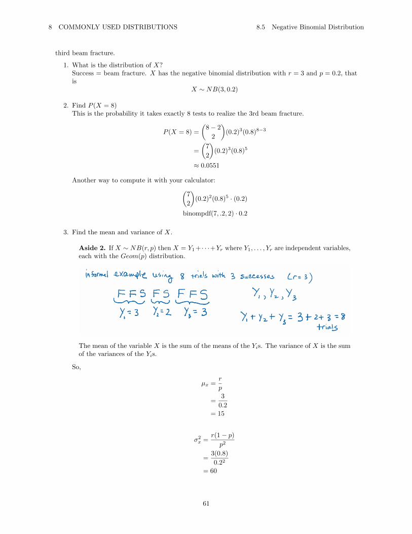
Aside 2. If X ∼ NB(r, p) then X = Y1 + · · ·+Yr where Y1, . . . , Yr are independent variables,each with the Geom(p) distribution.
The mean of the variable X is the sum of the means of the Yis. The variance of X is the sumof the variances of the Yis.
So,
µx =r
p
=3
0.2= 15
σ2x =
r(1− p)p2
=3(0.8)
0.22
= 60
61
8 COMMONLY USED DISTRIBUTIONS 8.6 Multinomial Distribution
8.6 Multinomial Distribution
Recall: A Bernoulli trial is a process that results in one of two possible outcomes. A multinomial trial is ageneralization of the Bernoulli trial and is a process that can result in any of k outcomes, where k ≥ 2.
Definition 32. Assume that n independent multinomial trials are conducted, each with the same kpossible outcomes and with the same probability p1, . . . , pk. Number the outcomes 1, 2, . . . , k. For eachoutcome, let Xi denote the number of trials that result in that outcome. Then X1, . . . , Xk are discreterandom variables.
The collection X1, . . . , Xk is said to have the multinomial distribution with parameters n, p1, . . . , pk.We write X1, . . . , Xk ∼MN(n, p1, . . . , pk).
The probability mass function of X1, . . . , Xk is
p(x1, . . . , xk) = P (X1 = x1, . . . , Xk = xk) =
{n!
x1!x2!...xk!px11 px2
2 . . . pxkk xi = 0, 1, 2, . . . , n and∑xi = n
0 otherwise
Furthermore, if X1, . . . , Xk ∼MN(n, p1, . . . , pk), then for each i:
Xi ∼ Bin(n, pi)
Note 10. The first part of the equation is “the number of ways of dividing a group of n objects intogroups of x1, . . . , xk objects (with x1 + · · · + xk = n)” This gives us the number of outcomes with thedesired quality.
The second part of the equation gives us probability for a particular outcome.
Example 50. Alkaptonuria is a genetic disease that results in the lack of an enzyme necessary to breakdown homogentistic acid. Some people are carriers of alkaptonuria, which means that they do not havethe disease themselves, but they can potentially transmit it to their offspring. According to the laws ofgenetic inheritance, an offspring both of whose parents are carriers of alkaptonuria has a probability of0.25 of being unaffected, 0.5 of being a carrier, and 0.25 of having the disease.
1. In a sample of 10 offspring of carriers of alkaptonuria, what is the probability that 3 are unaffected,5 are carriers, and 2 have the disease?
Sample size of n = 10. Lets define our variables, let X1, X2, X3 denote the numbers among the 10offspring who are unaffected, carriers, and diseased respectively.
So P1 = 0.25 is the probability offspring is unaffected, P2 = 0.5 is probability offspring is carrier,and P3 = 0.25 is the probability offspring is diseased.
We are looking for:
X1, X2, X3 ∼MN(10, 0.25, 0.5, 0.25)
P (X1 = 3, X2 = 5, X3 = 2) =10!
3!5!2!· (0.25)3(0.5)5(0.25)2
≈ 0.07690
62
8 COMMONLY USED DISTRIBUTIONS 8.7 Poisson Distribution
2. Find the probability that exactly 4 of 10 offspring are unaffected.
So our sample size is n = 10. We have a success probability for unaffected of p = 0.25. Let Y =number of offspring unaffected among 10.
Y ∼ Bin(10, 0.25)
P (Y = 4) =
(10
4
)(0.25)4(0.75)6
≈ 0.146
8.7 Poisson Distribution
A Poisson experiment has the following properties:
1. The probability that a single event occurs in a given interval (of time, length, volume, etc.) is the samefor all intervals.
2. The number of events that occur in any interval is independent of the number that occur in any otherinterval.
These properties are often referred to as a “Poisson process” and can be difficult to verify.
63
8 COMMONLY USED DISTRIBUTIONS 8.7 Poisson Distribution
Definition 33. The Poisson random variable X is a count of the number of times the specific eventoccurs during a given interval.
The Poisson distribution is completely determined by the mean, denoted by the Greek latter lambda,λ. (Since the Poisson distribution is often used to count rare events, the mean number of events perinterval is usually small.) If X has a Poisson distribution with parameter λ, we write X ∼ Poisson(λ).
A Poisson distribution can be thought of as an approximation to the binomial distribution with n islarge and p is small. Specifically, if n is very large and p is very small, and we let λ = np, is can beshown by advanced methods that for all x,
n!
x!(n− x)!px(1− p)n−x ≈ e−λλ
x
x!
The approximation above leads to the Poisson probability mass function given below.
If X ∼ Poisson(λ), then
• X is a discrete random variable whose possible values are the non-negative integers.
• The parameter λ is a positive constant.
• The probability mass function of X is
p(x) = P (X = x) =
{e−λ λ
x
x! if x is a non-negative integer
0 otherwise
• The Poisson probability mass function is very close to the binomial probability mass functionwhen n is large, p is small, and λ = np.
• The mean and variance of X are given by
µx = λ σ2x = λ
Example 51. Skydiving is the ultimate thrill for some, and there were over 3.1 million jumps in 2012.Despite an improved safety record, there are approximately 2 skydiving fatalities each month. Supposethis is the mean number of fatalities per month and a random month is selected.
1. Find the probability that exactly three fatalities will occur.
Let X = number of skydiving fatalities that occur in a month. We know that the mean numberof fatalities per month is 2, so λ = 2. So,
X ∼ Poisson(2)
So,
P (X = 3) = e−2 · 23
3!≈ 0.1804
2. Find the probability that at least five fatalities occur.
64
8 COMMONLY USED DISTRIBUTIONS 8.7 Poisson Distribution
P (X ≥ 5) = 1− P (X < 5)
= 1− P (X ≤ 4)
≈ 1− .9473
≈ 0.0527
3. Find the mean and variance of the number of skydiving fatalities per month.
µx = λ = 2
σ2x = λ = 2
Example 52. Particles are suspended in a liquid medium at a concentration of 6 particles per mL.A large volume of suspension is thoroughly agitated, and then 3 mL are withdrawn. What is theprobability that exactly 15 particles are withdrawn?
Let X = number of particles withdrawn in 3 mL. Mean number of particles in 3 mL: 6 · 3 = 18 mL. Soλ = 18.
X ∼ Poisson(18)
P (X = 15) = e−18 1815
15!≈ .07857
Example 53. Assume that the number of hits on a certain website during a fixed time interval followsa Poisson distribution. Assume that the mean rate of hits is 5 per minute.
1. Find the probability that there will be exactly 17 hits in the next three minutes.
Let X = number of hits in 3 minutes. λX = 5 ·3 = 15, 15 hits per minute on average in 3 minutes.
X ∼ Poisson(15)
P (X = 17) = e−15 1517
17!≈ 0.08473
2. Let X be the number of hits in t minutes. Find the probability mass function of X in terms of t.
λX = 5t.X ∼ Poisson(5t)
P (X = x) = e−5t 5tx
x!
65
8 COMMONLY USED DISTRIBUTIONS 8.7 Poisson Distribution
where x = 0, 1, 2, · · ·
8.7.1 Using the Poisson Distribution to estimate rate and uncertainty in the estimated rate
Let λ denote the mean number of events that occur in one unit of time or space. Let X enote the numberof events that are observed to occur in t units of time or space. Then if X ∼ Poisson(λt), λ is estimated
with λ = Xt . In general:
If X ∼ Poisson(λt), we estimate the rate λ with λ = Xt .
• λ is unbiased, (i.e. σλ = λ).
• The uncertainty in λ is σλ =
√λt
In practice, we substitute λ for λ in the equation for σλ above, since λ is unknown.
Example 54. A 5 mL sample of a suspension is withdrawn, and 47 particles are counted. Estimatethe mean number of particles per mL, and find the uncertainty in the estimate.
So our estimated average number of particles per mL is λ ≈ λ = 475 = 9.4. The uncertainty in our
estimate is
σλ =
√λ
t
≈
√λ
t
≈√
9.4
5
≈ 1.371
Example 55. A certain mass of a radioactive substance emits alpha particles at a mean rate of λparticles per second. A physicist counts 1594 emissions in 100 seconds.
1. Estimate λ, and find the uncertainty in the estimate.
The unit rate λ ≈ λ = 1594100 = 15.94 emissions per second. The uncertainty in our estimate is
σλ =
√λ
100
≈
√λ
100
≈√
15.94
100
≈ 0.399
2. For how many seconds should emissions be counted to reduce the uncertainty to 0.3 emissions persecond?
66
8 COMMONLY USED DISTRIBUTIONS 8.8 Exponential Distribution
We want to find time t, so that our uncertainty σλ = 0.3.
0.3 =
√λ
t
≈
√λ
t
=
√15.94
t
t ≈ 177.11 seconds
8.8 Exponential Distribution
The exponential distribution is a continuous distribution that is sometimes used to model the time thatelapses before an event occurs. Such a time is often called a waiting time. For example, the exponentialdistribution is often used to model the time to failure, or lifetime, of an electronic part. The probabilitydensity function of the exponential edistribution involves a parameter, which is a positive constant λ whosevalue determines the density function’s location and shape.
Definition 34. The probability density function of the exponential distribution with paramterλ > 0 is
f(x) =
{λe−λx x > 0
0 x ≤ 0
If X is a random variable whose distribution is the exponential distribution with paramter λ, we writeX ∼ Exp(λ).
The mean and variance of an exponential distribution is
µX =1
λσ2X =
1
λ2
The mean and variance can be calculated by using integration by parts.
Plots of the exponential probability density function for various values of λ:
67
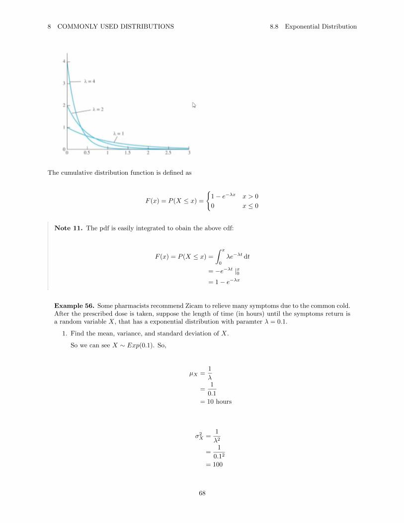
8 COMMONLY USED DISTRIBUTIONS 8.8 Exponential Distribution
The cumulative distribution function is defined as
F (x) = P (X ≤ x) =
{1− e−λx x > 0
0 x ≤ 0
Note 11. The pdf is easily integrated to obain the above cdf:
F (x) = P (X ≤ x) =
∫ x
0
λe−λt dt
= −e−λt |x0= 1− e−λx
Example 56. Some pharmacists recommend Zicam to relieve many symptoms due to the common cold.After the prescribed dose is taken, suppose the length of time (in hours) until the symptoms return isa random variable X, that has a exponential distribution with paramter λ = 0.1.
1. Find the mean, variance, and standard deviation of X.
So we can see X ∼ Exp(0.1). So,
µX =1
λ
=1
0.1= 10 hours
σ2X =
1
λ2
=1
0.12
= 100
68
8 COMMONLY USED DISTRIBUTIONS 8.8 Exponential Distribution
So the standard deviation is
σX =√
100
= 10
2. What is the probability that the length of time until symptoms return is less than the mean?
We are looking for P (X < 10). Since X is a continuous variable we can use the cdf.
P (X < 10) = P (X ≤ 10)
= 1− e−0.1(10)
≈ 1− 0.3679
= 0.6321
3. What is the probability that the length of time until symptoms return is at least 12 hours?
We are looking for P (X ≥ 12). We can use the complementation rule to calculate it.
P (X ≥ 12) = 1− P (X < 12)
= 1− P (X ≤ 12)
= 1−(
1− e−0.1(12))
= e−0.1(12)
≈ 0.3012
4. What is the probability that the length of time until symptoms return is between 8 and 16 hours?
We are looking for P (8 ≤ X ≤ 16).
P (8 ≤ X ≤ 16) = P (X ≤ 16)− P (X ≤ 8)
=(
1− e−0.1(16))−(
1− e−0.1(8))
= e−0.1(8) − e−0.1(16)
≈ 0.2474
5. What is the value of the median length of time until symptoms return?
Recall that the median is the 50th percentile. It is the number that separates the bottom 50%from the top 50%. So we are looking for t such that the P (X ≤ t) = 0.5.
69
8 COMMONLY USED DISTRIBUTIONS 8.8 Exponential Distribution
1− e−0.1t = 0.5
e−0.1t = 0.5
t =ln(0.5)
−0.1
≈ 6.9 hours
8.8.1 The Exponential Distribution and the Poisson Process
The exponential distribution can be used as a model for waiting times whenever the events follow a Poissonprocess. Recall that events follow a Poisson process with rate parameter λ when the number of events indisjoint intervals are independent, and the number of X events that occur on any time interval of lengtht has a Poisson distribution with mean λt, for example, X ∼ Poisson(λt). The connection between theexponential distribution and the Poisson process are as follows:
If any events follow a Poisson process with rate paramter λ, and if T represents the waiting time from anystarting point until the next event, then T ∼ Exp(λ).
Definition 35. The exponential distribution also has a property known as the memorless property:
If T ∼ Exp(λ), and t and s are positive numbers, then
P (T > t+ s | T > s) = P (T > t)
The probability that we must wait an additional t units, given that we have already waited s units, isthe same as the probability that we must wait t units from the start.
Example 57. The probability that a 4 year old circuit lasts 3 additional years is exactly the same asthe probability that a new circuit will last 3 years.
Example 58. A radioactive mass emits particles according to a Poisson process at a mean rate of 15particles per minute (60 seconds). At some point, a clock is started.
1. What is the probability that more than 5 seconds will elapse before the next emission?
Let T = the time in seconds that elapses before the next particle is emitted. The mean rate ofemissions is λ = 15
60 = 0.25. So, T ∼ Exp(0.25).
P (T > 5) = 1− P (T ≤ 5)
= 1−(
1− e−0.25(5))
≈ 0.2865
2. What is the mean waiting time (in seconds) until the next particle is emitted?
The mean waiting time in seconds is
70
8 COMMONLY USED DISTRIBUTIONS 8.8 Exponential Distribution
µT =1
λ
=1
0.25= 4 seconds
Example 59. The lifetime of a an integrated circuit has an exponential distribution with mean 2 years.
1. Find the probability that the circuit lasts longer than three years.
Let T = lifetime of a circuit. The mean of T is µT = 2. We can find λ by solving
µT = 2
1
λ= 2
λ = 0.5
So we have T ∼ Exp(0.5).
P (T > 3) = e−0.5(3)
≈ 0.223
2. Assume the circuit is now four years old and is still functioning. Find the probability that itfunctions for more than three additional years.
We are looking for P (T > 7 | T > 4).
P (T > 7 | T > 4) =P (T > 7)
P (T > 4)
=e−0.5(7)
e−0.5(4)
≈ 0.223
Example 60. The number of hits on a website follows a Poisson process with a rate of 3 per minute.
1. What is the probability that more than a minute goes by without a hit?
So let T = waiting time in minutes until the next hit. Our rate parameter is λ = 3. So,
T ∼ Exp(3)
71
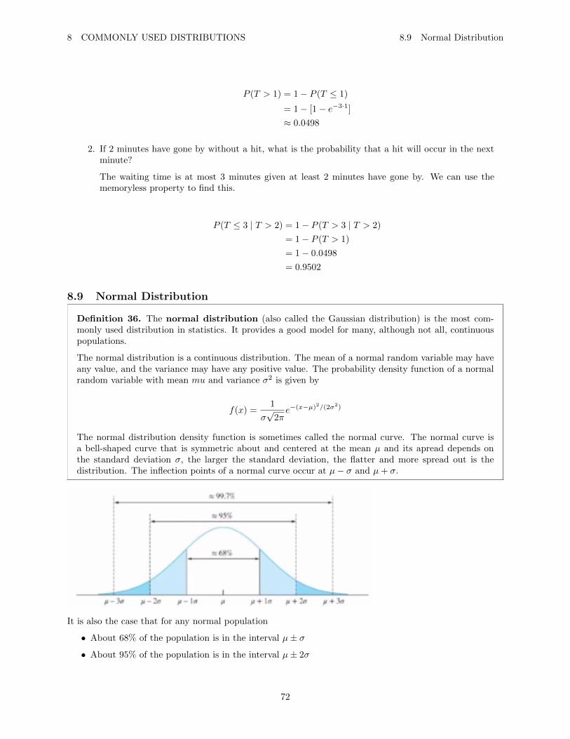
8 COMMONLY USED DISTRIBUTIONS 8.9 Normal Distribution
P (T > 1) = 1− P (T ≤ 1)
= 1− [1− e−3·1]
≈ 0.0498
2. If 2 minutes have gone by without a hit, what is the probability that a hit will occur in the nextminute?
The waiting time is at most 3 minutes given at least 2 minutes have gone by. We can use thememoryless property to find this.
P (T ≤ 3 | T > 2) = 1− P (T > 3 | T > 2)
= 1− P (T > 1)
= 1− 0.0498
= 0.9502
8.9 Normal Distribution
Definition 36. The normal distribution (also called the Gaussian distribution) is the most com-monly used distribution in statistics. It provides a good model for many, although not all, continuouspopulations.
The normal distribution is a continuous distribution. The mean of a normal random variable may haveany value, and the variance may have any positive value. The probability density function of a normalrandom variable with mean mu and variance σ2 is given by
f(x) =1
σ√
2πe−(x−µ)2/(2σ2)
The normal distribution density function is sometimes called the normal curve. The normal curve isa bell-shaped curve that is symmetric about and centered at the mean µ and its apread depends onthe standard deviation σ, the larger the standard deviation, the flatter and more spread out is thedistribution. The inflection points of a normal curve occur at µ− σ and µ+ σ.
It is also the case that for any normal population
• About 68% of the population is in the interval µ± σ
• About 95% of the population is in the interval µ± 2σ
72
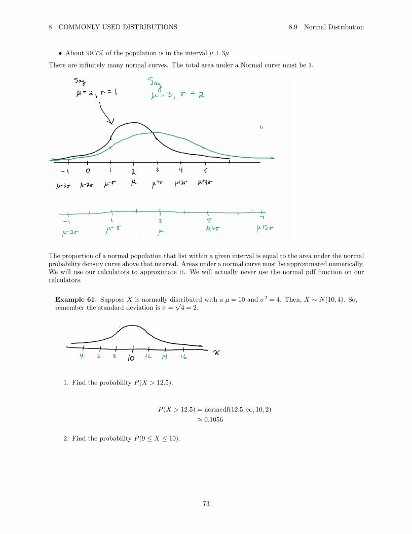
8 COMMONLY USED DISTRIBUTIONS 8.9 Normal Distribution
• About 99.7% of the population is in the interval µ± 3µ
There are infinitely many normal curves. The total area under a Normal curve must be 1.
The proportion of a normal population that list within a given interval is equal to the area under the normalprobability density curve above that interval. Areas under a normal curve must be approximated numerically.We will use our calculators to approximate it. We will actually never use the normal pdf function on ourcalculators.
Example 61. Suppose X is normally distributed with a µ = 10 and σ2 = 4. Then, X ∼ N(10, 4). So,remember the standard deviation is σ =
√4 = 2.
1. Find the probability P (X > 12.5).
P (X > 12.5) = normcdf(12.5,∞, 10, 2)
≈ 0.1056
2. Find the probability P (9 ≤ X ≤ 10).
73
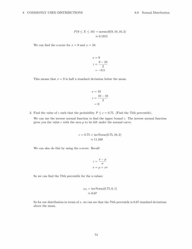
8 COMMONLY USED DISTRIBUTIONS 8.9 Normal Distribution
P (9 ≤ X ≤ 10) = normcdf(9, 10, 10, 2)
≈ 0.1915
We can find the z-score for x = 9 and x = 10.
x = 9
z =9− 10
2= −0.5
This means that x = 9 is half a standard deviation below the mean.
x = 10
z =10− 10
2= 0
3. Find the value of c such that the probability P ≤ c = 0.75. (Find the 75th percentile).
We can use the inverse normal function to find the upper bound c. The inverse normal functiongives you the value c with the area p to its left under the normal curve.
c = 0.75 = invNorm(0.75, 10, 2)
≈ 11.349
We can also do this by using the z-score. Recall:
z =x− µσ
x = µ+ zσ
So we can find the 75th percentile for the z-values:
z75 = invNorm(0.75, 0, 1)
≈ 0.67
So for our distribution in terms of x, we can see that the 75th percentile is 0.67 standard deviationsabove the mean.
74
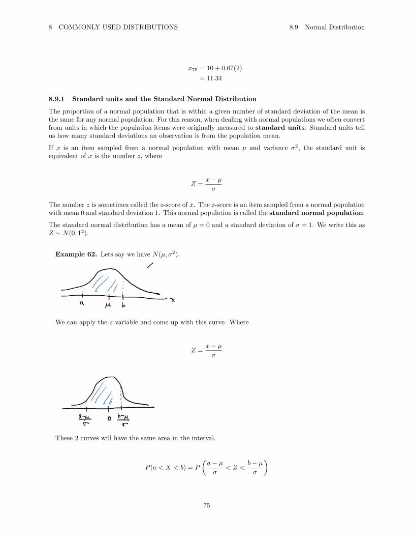
8 COMMONLY USED DISTRIBUTIONS 8.9 Normal Distribution
x75 = 10 + 0.67(2)
= 11.34
8.9.1 Standard units and the Standard Normal Distribution
The proportion of a normal population that is within a given number of standard deviation of the mean isthe same for any normal population. For this reason, when dealing with normal populations we often convertfrom units in which the population items were originally measured to standard units. Standard units tellus how many standard deviations an observation is from the population mean.
If x is an item sampled from a normal population with mean µ and variance σ2, the standard unit isequivalent of x is the number z, where
Z =x− µσ
The number z is sometimes called the z-score of x. The z-score is an item sampled from a normal populationwith mean 0 and standard deviation 1. This normal population is called the standard normal population.
The standard normal distribution has a mean of µ = 0 and a standard deviation of σ = 1. We write this asZ ∼ N(0, 12).
Example 62. Lets say we have N(µ, σ2).
We can apply the z variable and come up with this curve. Where
Z =x− µσ
These 2 curves will have the same area in the interval.
P (a < X < b) = P
(a− µσ
< Z <b− µσ
)
75
8 COMMONLY USED DISTRIBUTIONS 8.9 Normal Distribution
Example 63. Lifetimes of batteries in a certain application are normally distributed with mean 50hours and standard deviation of 5 hours.
1. Find the probability that a randomly chosen batter lasts between 42 and 52 hours.
Let X = lifetime of a randomly chosen battery. Then X ∼ N(50, 52).
So we are looking for
P (42 < X < 52) = normalcdf(42, 52, 50, 5)
≈ 0.6006
2. Find the 40th percentile of battery lifetimes.
X40 = invNorm(0.4, 50, 5)
≈ 48.73
Example 64. A process manufactures ball bearings whose diameters are normally distributed withmean 2.505 cm and a standard deviation of 0.008 cm. Specifications call for the diameter to be in theinterval 2.5± 0.01 cm.
1. What proportion of the ball bearings will meet the specifications?
Let X = the diameter of a randomly chosen ball bearing. So, X ∼ N(2.505, 0.0082).
The ball bearing diameters must be in the range from 2.49 to 2.51.
P (2.49 < X < 2.51) = normalcdf(2.49, 2.51, 2.505, 0.008)
≈ 0.7036
2. The process can be recalibrated so that the mean will equal 2.5 cm, the center of the specificationinterval. The standard deviation of a process remains 0.008 cm. What proportion of the diameterwill meet specifications?
We are looking for P (2.49 < X < 2.51) but our new mean is µX = 2.5 cm.
P (2.49 < X < 2.51) = normalcdf(2.49, 2.51, 2.5, 0.008)
≈ 0.7887
3. Assume that the process has been recalibrated so that the mean diameter is now 2.5 cm. Towhat value must the standard deviation be lowered so that 95% of the diameters will meet thespecifications?
Now we assume X ∼ N(2.5, 0.0082). We are looking for σ so that P (2.49 < X < 2.51) = 0.95.We have to use the standardized version of x:
Z =x− µσ
=x− 2.5
0.008
76
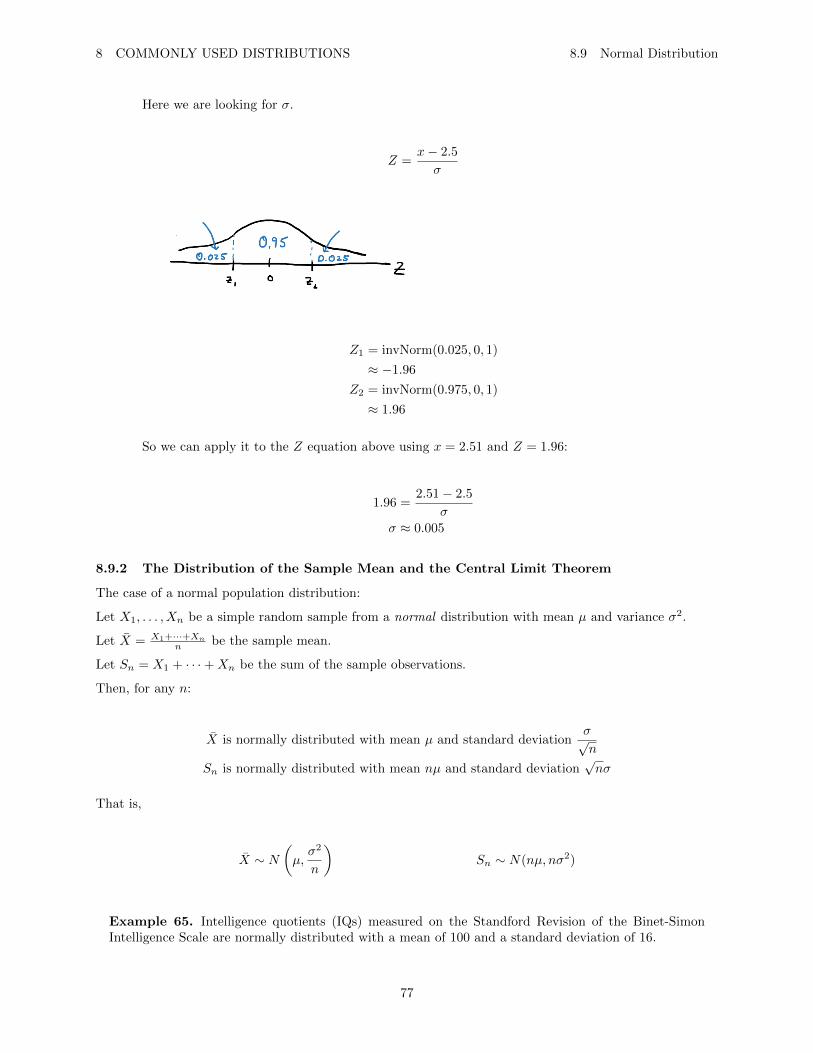
8 COMMONLY USED DISTRIBUTIONS 8.9 Normal Distribution
Here we are looking for σ.
Z =x− 2.5
σ
Z1 = invNorm(0.025, 0, 1)
≈ −1.96
Z2 = invNorm(0.975, 0, 1)
≈ 1.96
So we can apply it to the Z equation above using x = 2.51 and Z = 1.96:
1.96 =2.51− 2.5
σσ ≈ 0.005
8.9.2 The Distribution of the Sample Mean and the Central Limit Theorem
The case of a normal population distribution:
Let X1, . . . , Xn be a simple random sample from a normal distribution with mean µ and variance σ2.
Let X = X1+···+Xnn be the sample mean.
Let Sn = X1 + · · ·+Xn be the sum of the sample observations.
Then, for any n:
X is normally distributed with mean µ and standard deviationσ√n
Sn is normally distributed with mean nµ and standard deviation√nσ
That is,
X ∼ N(µ,σ2
n
)Sn ∼ N(nµ, nσ2)
Example 65. Intelligence quotients (IQs) measured on the Standford Revision of the Binet-SimonIntelligence Scale are normally distributed with a mean of 100 and a standard deviation of 16.
77

8 COMMONLY USED DISTRIBUTIONS 8.9 Normal Distribution
1. Determine the probability that a randomly selected person has an IQ between 90 and 110.
Let X = the IQ of a person. The mean is µ = 100 and the standard devitation σ = 16. So,X ∼ N(100, 162).
P (90 < X < 110) = normalcdf(90, 110, 100, 16)
≈ 0.4680
2. Determine the probability that the mean IQ of 4 randomly selected people will be between 90 and110.
Let X1, . . . , X4 be the IQx of the 4 people in the sample. X = X1+···+X4
4 is the mean IQ of thesample of 4 people. So we are looking P (90 < X < 110). So since X ∼ N(100, 162), we know that
X ∼ N(100, 162
4 ). That is, X ∼ N(100, 64).
P (90 < X < 110) = normalcdf(90, 110, 100, 8)
≈ 0.7887
Standardized version of X:
Z =X − µXσX
=X − µ
σ√n
=X − 100
16√4
=X − 100
8
So when X = 90, Z = −1.25. When X = 110, Z = 1.25.
So if we were doing this problem in standard units it would look like:
P (90 < X < 110) = P (−1.25 < Z < 1.25)
= normalcdf(−1.25, 1.25, 0, 1)
≈ 0.7887
8.9.3 The Central Limit Theorem
78
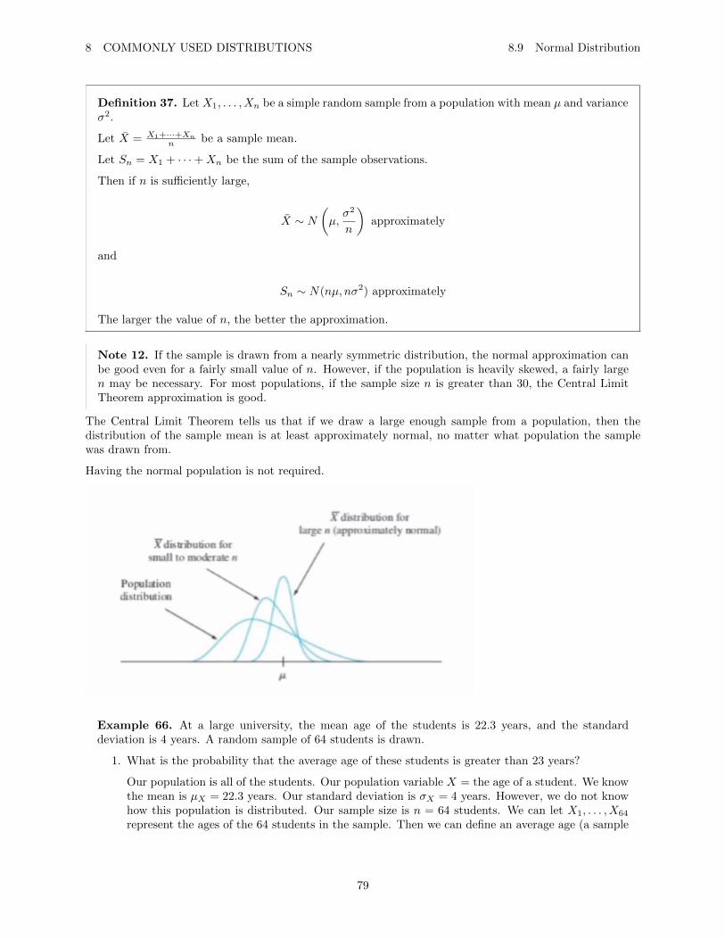
8 COMMONLY USED DISTRIBUTIONS 8.9 Normal Distribution
Definition 37. Let X1, . . . , Xn be a simple random sample from a population with mean µ and varianceσ2.
Let X = X1+···+Xnn be a sample mean.
Let Sn = X1 + · · ·+Xn be the sum of the sample observations.
Then if n is sufficiently large,
X ∼ N(µ,σ2
n
)approximately
and
Sn ∼ N(nµ, nσ2) approximately
The larger the value of n, the better the approximation.
Note 12. If the sample is drawn from a nearly symmetric distribution, the normal approximation canbe good even for a fairly small value of n. However, if the population is heavily skewed, a fairly largen may be necessary. For most populations, if the sample size n is greater than 30, the Central LimitTheorem approximation is good.
The Central Limit Theorem tells us that if we draw a large enough sample from a population, then thedistribution of the sample mean is at least approximately normal, no matter what population the samplewas drawn from.
Having the normal population is not required.
Example 66. At a large university, the mean age of the students is 22.3 years, and the standarddeviation is 4 years. A random sample of 64 students is drawn.
1. What is the probability that the average age of these students is greater than 23 years?
Our population is all of the students. Our population variable X = the age of a student. We knowthe mean is µX = 22.3 years. Our standard deviation is σX = 4 years. However, we do not knowhow this population is distributed. Our sample size is n = 64 students. We can let X1, . . . , X64
represent the ages of the 64 students in the sample. Then we can define an average age (a sample
79
8 COMMONLY USED DISTRIBUTIONS 8.9 Normal Distribution
mean age) as X = X1 + · · · + X64. That is, X = the mean age of a sample of 64 students. By
the central limit theorem, since n = 64 and 64 > 30, we can say that X ∼ N(
22.3, 42
64
), at least
approximately.
P (X > 23) = normalcdf(23,∞, 22.3,√
0.25)
≈ 0.0808
2. How many students must be sampled so that the probability is 0.05 that the sample mean ageexceeds 23?
So we are looking for the sample size n so that P (X > 23) = 0.05. We can use the standardizedvalues to find this (the z-score).
Z = invNorm(0.95, 0, 1)
≈ 1.645
So using Z = 1.645, X = 23, µ = 22.3 and σ = 4
1.645 =23− 22.3
4√n
√n =
1.645(4)
0.7n = 88.36
So to guarantee we have a 0.05 probability of having sample mean age we need to sample 89students.
Example 67. The manufacturer of a certain part requires two different machine operations. The timeon machine 1 has a mean of 0.4 hours and a standard deviation of 0.1 hours. The time on machine 2has a mean of 0.45 hours and a standard deviation of 0.15 hours. The times needed on the machinesare independent. Suppose that 65 parts are manufactured.
1. What is the distribution of the total time on machine 1?
Let X = time on machine 1, so the mean is µX = 0.4 and standard deviation σX = 0.1.
Let X1, . . . , X65 be the times of the 65 parts on machine 1. We can call the sum of the times,the total time on machine 1, SX = X1 + · · · + X65. Remember, our mean µ = 65(0.4) and ourstandard deviation is σ = 65(0.1).
Remember
µSx = µx1+···+x65= µx1
+ · · ·+ µx65
and since there is 65 means, that it why it equals 65(0.4).
By the central limit theorem, since our sample size n = 65 > 30, we can say that SX ∼ N(26, 0.65)approximately.
80
8 COMMONLY USED DISTRIBUTIONS 8.9 Normal Distribution
2. What is the probability that the total time on machine 1 is less than 27 hours?
P (Sx < 27) = normalcdf(−∞, 27, 26,√
0.65)
≈ 0.8926
3. What is the distribution of the total time on machine 2?
Let Y = time on machine 2, so the mean is µY = 0.45 and the standard deviation σY = 0.15.
Let Y1, . . . , Y65 be the times of the 65 parts on machine 2. We can call the sum of the times, thetotal time on machien 2, SY = Y1 + · · ·+ Y65.
So by the central limit theorem, the distribution of the time on machine 2 is SY ∼ N(65(0.45), 65(0.15)2)approximately. This can be cleaned up as SY ∼ N(29.25, 1.4625).
4. What is the probability that the total time, used by both machines together, is between 50 and55 hours?
Let T = total time used by both machines. So
T = SX︸︷︷︸time on machine 1
+
time on machine 2︷︸︸︷SY
The mean of the total time is
µT = µSX + µSY= 26 + 29.25
= 55.25 hours
The variance of the total time is
σ2T = σ2
SX + σ2SY
= 0.65 + 1.4625
= 2.1125
So we can say T ∼ N(55.25, 2.1125) approximately. So we can find the probability that the timeis between 50 and 55 hours
P (50 < T < 55) = normalcdf(50, 55, 55.25,√
2.1125)
≈ 0.4316
5. Find the probability that the total time on machine 2 is greater than the total time on machine 1.
Recall
81
8 COMMONLY USED DISTRIBUTIONS 8.9 Normal Distribution
SX ∼ N(26, 0.65) SY ∼ N(29.25, 1.4625)
We are looking for P (SY > SX). Let D = SY − SX
P (SY > SX) = P (SY − SX > 0)
= P (D > 0)
We can find the difference in means
µD = µSY − µSX= 29.25− 26
= 3.25
and the different in standard deviations
σ2D = σ2
SY − σ2SX
= 2.1125
So we can say that the different has a distribution of D ∼ N(3.25, 2.1125) approximately. So,
P (D > 0) = normalcdf(0,∞, 3.25,√
2.1125)
≈ 0.9873
Example 68. Birth weights of male babies have a standard deviation of 1.33 lb. Determine thepercentage of all samples of 400 male babies that have mean birth weights within 0.125 lb (2 oz.) of thepopulation mean birth weight of all male babies.
Here the population consists of all male babies. Let X = birth weight of a male babie in pounds. Thepopulation mean µX is unknown, however the standard deviation is σX = 1.33 lbs. We have a samplesize of n = 400.
Let X1, . . . , X400 be the birth weights of each of 400 male babies. The mean birth weight of the sampleis X = X1+···+X400
400 . By the central limit theorem, since the sample size is large enough, we can describethe distribution of all possible sample means is at least approximately normal with mean µX = µ andstandard deviation σX = σ√
n= 1.33√
400= 0.0665.
That is, X ∼ N(µ, 0.06652).
82
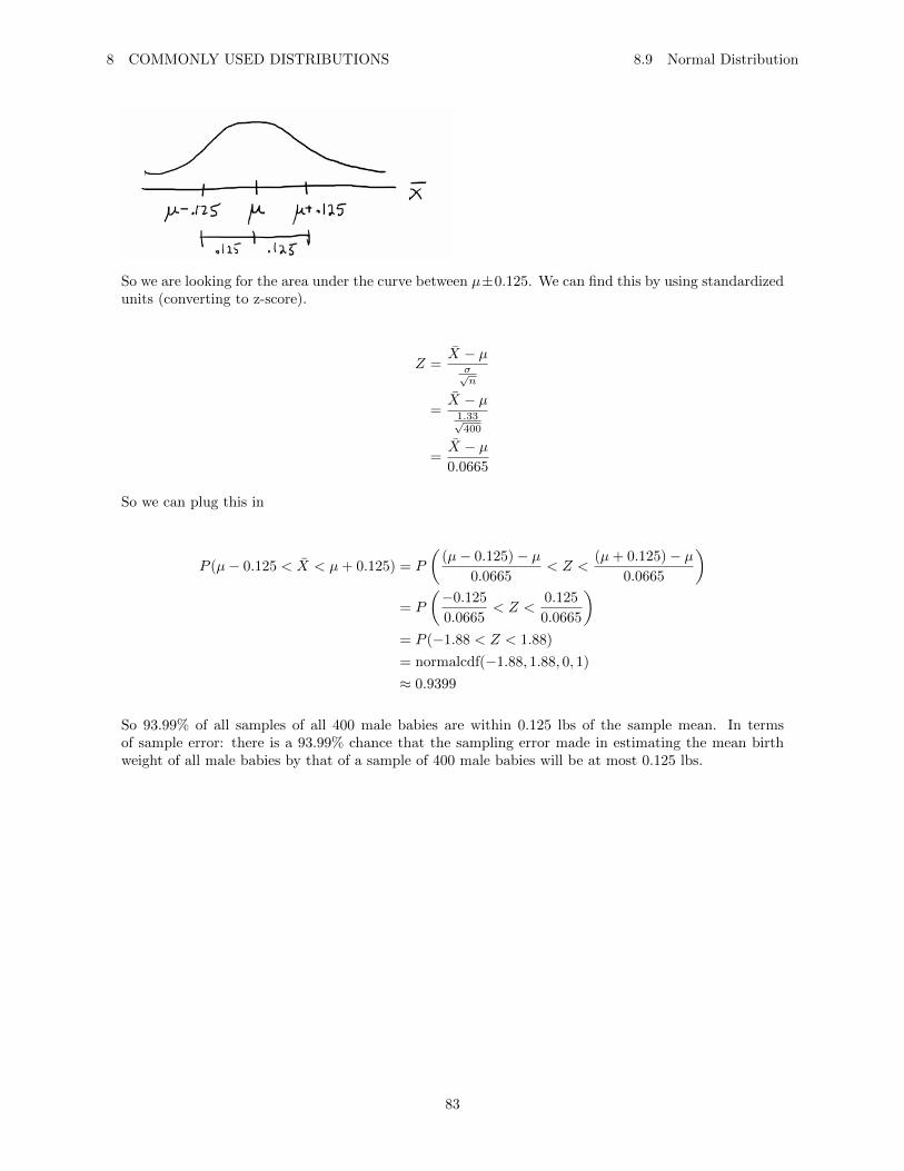
8 COMMONLY USED DISTRIBUTIONS 8.9 Normal Distribution
So we are looking for the area under the curve between µ±0.125. We can find this by using standardizedunits (converting to z-score).
Z =X − µ
σ√n
=X − µ
1.33√400
=X − µ0.0665
So we can plug this in
P (µ− 0.125 < X < µ+ 0.125) = P
((µ− 0.125)− µ
0.0665< Z <
(µ+ 0.125)− µ0.0665
)= P
(−0.125
0.0665< Z <
0.125
0.0665
)= P (−1.88 < Z < 1.88)
= normalcdf(−1.88, 1.88, 0, 1)
≈ 0.9399
So 93.99% of all samples of all 400 male babies are within 0.125 lbs of the sample mean. In termsof sample error: there is a 93.99% chance that the sampling error made in estimating the mean birthweight of all male babies by that of a sample of 400 male babies will be at most 0.125 lbs.
83
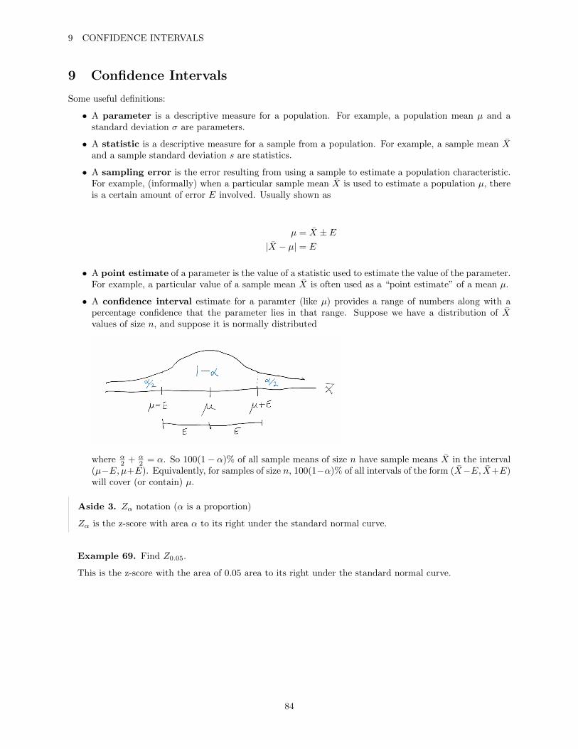
9 CONFIDENCE INTERVALS
9 Confidence Intervals
Some useful definitions:
• A parameter is a descriptive measure for a population. For example, a population mean µ and astandard deviation σ are parameters.
• A statistic is a descriptive measure for a sample from a population. For example, a sample mean Xand a sample standard deviation s are statistics.
• A sampling error is the error resulting from using a sample to estimate a population characteristic.For example, (informally) when a particular sample mean X is used to estimate a population µ, thereis a certain amount of error E involved. Usually shown as
µ = X ± E|X − µ| = E
• A point estimate of a parameter is the value of a statistic used to estimate the value of the parameter.For example, a particular value of a sample mean X is often used as a “point estimate” of a mean µ.
• A confidence interval estimate for a paramter (like µ) provides a range of numbers along with apercentage confidence that the parameter lies in that range. Suppose we have a distribution of Xvalues of size n, and suppose it is normally distributed
where α2 + α
2 = α. So 100(1− α)% of all sample means of size n have sample means X in the interval(µ−E,µ+E). Equivalently, for samples of size n, 100(1−α)% of all intervals of the form (X−E, X+E)will cover (or contain) µ.
Aside 3. Zα notation (α is a proportion)
Zα is the z-score with area α to its right under the standard normal curve.
Example 69. Find Z0.05.
This is the z-score with the area of 0.05 area to its right under the standard normal curve.
84

9 CONFIDENCE INTERVALS
We could either calculate the area to the left of the z-score, 0.95
invNorm(0.95, 0, 1) ≈ 1.645
We could also use symmetry and look for −Z0.05
−Z0.05 = invNorm(0.05, 0, 1)
≈ −1.645
= 1.645
So µ± E can be written as µ± Zα2· σX .
Here E is called the “margin of error” for the confidence interval estimate of µ.
E = Zα2σX
= Zα2
σ√n
85
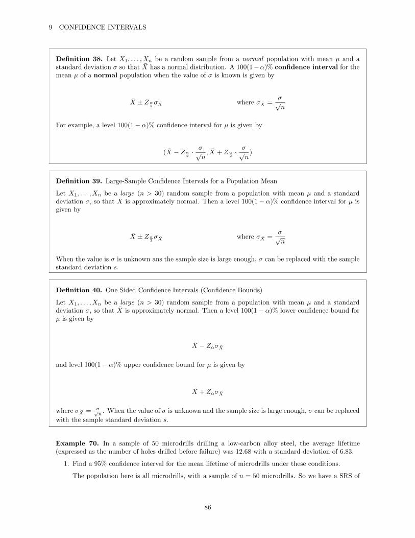
9 CONFIDENCE INTERVALS
Definition 38. Let X1, . . . , Xn be a random sample from a normal population with mean µ and astandard deviation σ so that X has a normal distribution. A 100(1−α)% confidence interval for themean µ of a normal population when the value of σ is known is given by
X ± Zα2σX where σX =
σ√n
For example, a level 100(1− α)% confidence interval for µ is given by
(X − Zα2· σ√
n, X + Zα
2· σ√
n)
Definition 39. Large-Sample Confidence Intervals for a Population Mean
Let X1, . . . , Xn be a large (n > 30) random sample from a population with mean µ and a standarddeviation σ, so that X is approximately normal. Then a level 100(1− α)% confidence interval for µ isgiven by
X ± Zα2σX where σX =
σ√n
When the value is σ is unknown ans the sample size is large enough, σ can be replaced with the samplestandard deviation s.
Definition 40. One Sided Confidence Intervals (Confidence Bounds)
Let X1, . . . , Xn be a large (n > 30) random sample from a population with mean µ and a standarddeviation σ, so that X is approximately normal. Then a level 100(1− α)% lower confidence bound forµ is given by
X − ZασX
and level 100(1− α)% upper confidence bound for µ is given by
X + ZασX
where σX = σ√n
. When the value of σ is unknown and the sample size is large enough, σ can be replaced
with the sample standard deviation s.
Example 70. In a sample of 50 microdrills drilling a low-carbon alloy steel, the average lifetime(expressed as the number of holes drilled before failure) was 12.68 with a standard deviation of 6.83.
1. Find a 95% confidence interval for the mean lifetime of microdrills under these conditions.
The population here is all microdrills, with a sample of n = 50 microdrills. So we have a SRS of
86
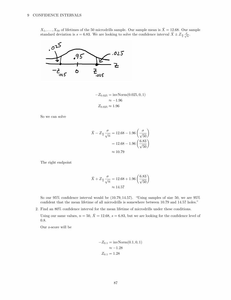
9 CONFIDENCE INTERVALS
X1, . . . , X50 of lifetimes of the 50 microdrills sample. Our sample mean is X = 12.68. Our samplestandard deviation is s = 6.83. We are looking to solve the confidence interval X ± Zα
2
σ√n
.
−Z0.025 = invNorm(0.025, 0, 1)
≈ −1.96
Z0.025 ≈ 1.96
So we can solve
X − Zα2
σ√n
= 12.68− 1.96
(σ√50
)= 12.68− 1.96
(6.83√
50
)≈ 10.79
The right endpoint
X + Zα2
σ√n
= 12.68 + 1.96
(6.83√
50
)≈ 14.57
So our 95% confidence interval would be (10.79, 14.57). “Using samples of size 50, we are 95%confident that the mean lifetime of all microdrills is somewhere between 10.79 and 14.57 holes.”
2. Find an 80% confidence interval for the mean lifetime of microdrills under these conditions.
Using our same values, n = 50, X = 12.68, s = 6.83, but we are looking for the confidence level of0.8.
Our z-score will be
−Z0.1 = invNorm(0.1, 0, 1)
≈ −1.28
Z0.1 = 1.28
87
9 CONFIDENCE INTERVALS
X − Zα2
σ√n≈ 12.68− (1.28)
(6.83√
50
)≈ 11.44
X + Zα2
σ√n≈ 12.68 + (1.28)
(6.83√
50
)≈ 13.92
So our confidence interval for 80% confidence is (11.44, 13.92).
“The wider the confidence interval, the more confident we are that the mean exists in the interval.”The margin of error E = Zα
2σX = Zα
2
σ√n
For the bigger confidence interval
E = 1.96
(6.83√
50
)≈ 1.893
For the smaller confidence interval
E = 1.28
(6.83√
50
)≈ 1.236
Remember that the sample mean X is the midpoint of each confidence interval.
3. How many microdrills must be sampled to obtain a 95% confidence interval that specifies themean to with ±0.5?
Recall, sample mean X = 12.68, sample standard deviation s = 6.83.
We are looking for n so that E = 0.5. Our z-score is Z = 1.96. Since we don’t know σ we can usethe sample standard deviation s and solve for n.
E = Zα2
σ√n
0.5 = 1.96
(6.83√n
)n ≈ 716.8
We will round up to the nearest integer so our sample size n = 717 to have a 95% confidenceinterval.
4. Based on microdrill lifetime data presented above, an engineer reported a confidence interval of(11.09, 14.27) but neglected to specify the level. What is the level of this confidence interval?
Recall, n = 50, X = 12.68, s = 6.83.
88
9 CONFIDENCE INTERVALS
X ± Zα2
σ√n
= 12.68± Zα2
(6.83√
50
)
11.09 = 12.68− Zα2
(6.83√
50
)14.27 = 12.68 + Zα
2
(6.83√
50
)
Lets chose the second one and solve for Zα2
.
14.27 = 12.68 + Zα2
(6.83√
50
)Zα
2=
14.27− 12.686.83√
50
≈ 1.646
We can use a normal cdf to find our confidence interval
normalcdf(−1.646, 1.646, 0, 1) ≈ 0.9002
5. Find both 95% lower confidence bound and a 99% upper confidence bound for the mean lifetimeof the microdrills.
Recall, n = 50, X = 12.68, s = 6.83. For the 95% lower we can solve with a z-score for 95% usingZ = invNorm(0.95, 0, 1) ≈ 1.645.
X − Zασ√n≈ X − Zα
s√n
= 12.68− Zα6.83√
50
= 12.68− 1.645
(6.83√
50
)≈ 11.09
Since this is a lower bound, the interval would be (11.09,∞).
For the 99% upper bound we can solve with a z-score of 99% using Z = invNorm(0.99, 0, 1) ≈ 2.326.
89
9 CONFIDENCE INTERVALS 9.1 Confidence intervals for population proportions
X + Zασ√n≈ X + Zα
s√n
= 12.68 + Zα6.83√
50
= 12.68 + 2.326
(6.83√
50
)≈ 14.93
Since this ia a upper bound, the interval for 99% confidence would be (−∞, 14.93).
Confidence, accuracy (precision) and sample size:
• For a fixed sample size, decreasing the confidence level decreases the margin of error, and, hence,improves the accuracy (precision) of a confidence interval estimate.
• For a fixed confidence level, increasing the sample size decreases the margin of error, and, hence,improves the accuracy (precision) of a confidence interval estimate.
9.1 Confidence intervals for population proportions
Recall that if X ∼ Bin(n, p), then the estimate for p is p = Xn . When the sample size is large enough (n > 30)
it follows that from the Central Limit Theorem that p is at least approximately normally distributed. That
is p ∼ N(p, p(1−p)n
)approximately, where the mean of p is p, and the uncertainty (standard deviation) of p
is σp =√
p(1−p)n .
A traditional 100(1− α)% confidence interval for p would be in the form
p± Zα2σp
Definition 41. Let X be the number of successes in n independent Bernoulli trials with a successprobability p, so that X ∼ Bin(n, p).
Define n = n+ 4 and p = X+2n .
Then, a level 100(1− α)% confidence interval for p is given by
p± Zα/2
√p(1− p)
n
90
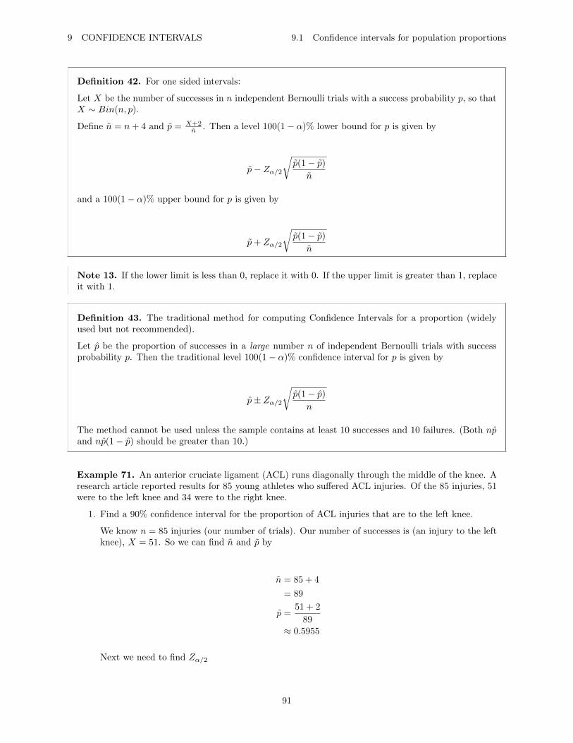
9 CONFIDENCE INTERVALS 9.1 Confidence intervals for population proportions
Definition 42. For one sided intervals:
Let X be the number of successes in n independent Bernoulli trials with a success probability p, so thatX ∼ Bin(n, p).
Define n = n+ 4 and p = X+2n . Then a level 100(1− α)% lower bound for p is given by
p− Zα/2
√p(1− p)
n
and a 100(1− α)% upper bound for p is given by
p+ Zα/2
√p(1− p)
n
Note 13. If the lower limit is less than 0, replace it with 0. If the upper limit is greater than 1, replaceit with 1.
Definition 43. The traditional method for computing Confidence Intervals for a proportion (widelyused but not recommended).
Let p be the proportion of successes in a large number n of independent Bernoulli trials with successprobability p. Then the traditional level 100(1− α)% confidence interval for p is given by
p± Zα/2
√p(1− p)
n
The method cannot be used unless the sample contains at least 10 successes and 10 failures. (Both npand np(1− p) should be greater than 10.)
Example 71. An anterior cruciate ligament (ACL) runs diagonally through the middle of the knee. Aresearch article reported results for 85 young athletes who suffered ACL injuries. Of the 85 injuries, 51were to the left knee and 34 were to the right knee.
1. Find a 90% confidence interval for the proportion of ACL injuries that are to the left knee.
We know n = 85 injuries (our number of trials). Our number of successes is (an injury to the leftknee), X = 51. So we can find n and p by
n = 85 + 4
= 89
p =51 + 2
89≈ 0.5955
Next we need to find Zα/2
91
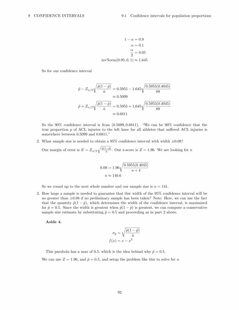
9 CONFIDENCE INTERVALS 9.1 Confidence intervals for population proportions
1− α = 0.9
α = 0.1α
2= 0.05
invNorm(0.95, 0, 1) ≈ 1.645
So for our confidence interval
p− Zα/2
√p(1− p)
n= 0.5955− 1.645
√0.5955(0.4045)
89
≈ 0.5099
p+ Zα/2
√p(1− p)
n= 0.5955 + 1.645
√0.5955(0.4045)
89
≈ 0.6811
So the 90% confidence interval is from (0.5099, 0.6811). “We can be 90% confidence that thetrue proportion p of ACL injuries to the left knee for all athletes that suffered ACL injuries issomewhere between 0.5099 and 0.6811.”
2. What sample size is needed to obtain a 95% confidence interval with width ±0.08?
Our margin of error is E = Zα/2
√p(1−p)n . Our z-score is Z = 1.96. We are looking for n
0.08 = 1.96
√0.5955(0.4045)
n+ 4
n ≈ 140.6
So we round up to the next whole number and our sample size is n = 141.
3. How large a sample is needed to guarantee that thw width of the 95% confidence interval will beno greater than ±0.08 if no preliminary sample has been taken? Note: Here, we can use the factthat the quantity p(1 − p), which determines the width of the confidence interval, is maximizedfor p = 0.5. Since the width is greatest when p(1− p) is greatest, we can compute a conservativesample size estimate by substituting p = 0.5 and proceeding as in part 2 above.
Aside 4.
σp =
√p(1− p)
n
f(x) = x− x2
This parabola has a max of 0.5, which is the idea behind why p = 0.5.
We can use Z = 1.96, and p = 0.5, and setup the problem like this to solve for n
92
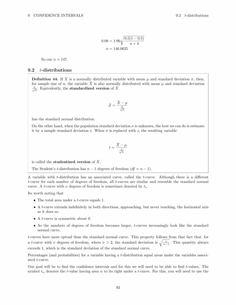
9 CONFIDENCE INTERVALS 9.2 t-distributions
0.08 = 1.96
√0.5(1− 0.5)
n+ 4
n = 146.0625
So our n = 147.
9.2 t-distributions
Definition 44. If X is a normally distributed variable with mean µ and standard deviation σ, then,for sample size of n, the variable X is also normally distributed with mean µ and standard deviationσ√n
. Equivalently, the standardized version of X
Z =X − µ
σ√n
has the standard normal distribution.
On the other hand, when the population standard deviation σ is unknown, the best we can do is estimateit by a sample standard deviation s. When σ is replaced with s, the resulting variable
t =X − µ
s√n
is called the studentized version of X.
The Student’s t-distribution has n− 1 degrees of freedom (df = n− 1).
A variable with t-distribution has an associated curve, called the t-curve. Although there is a differentt-curve for each number of degrees of freedom, all t-curves are similar and resemble the standard normalcurve. A t-curve with ν degrees of freedom is sometimes denoted by tν .
Its worth noting that
• The total area under a t-curve equals 1.
• A t-curve extends indefinitely in both directions, approaching, but never touching, the horizontal axisas it does so.
• A t-curve is symmetric about 0.
• As the numbers of degrees of freedom becomes larger, t-curves increasingly look like the standardnormal curve.
t-curves have more spread than the standard normal curve. This property follows from that fact that, for
a t-curve with ν degrees of freedom, where ν > 2, the standard deviation is√
νν−1 . This quantity always
exceeds 1, which is the standard deviation of the standard normal curve.
Percentages (and probabilities) for a variable having a t-distribution equal areas under the variables associ-ated t-curve.
Our goal will be to find the confidence intervals and for this we will need to be able to find t-values. Thesymbol tα denotes the t-value having area α to its right under a t-curve. For this, you will need to use the
93
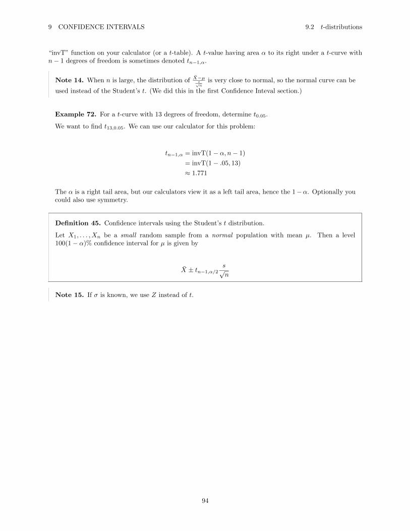
9 CONFIDENCE INTERVALS 9.2 t-distributions
“invT” function on your calculator (or a t-table). A t-value having area α to its right under a t-curve withn− 1 degrees of freedom is sometimes denoted tn−1,α.
Note 14. When n is large, the distribution of X−µs√n
is very close to normal, so the normal curve can be
used instead of the Student’s t. (We did this in the first Confidence Inteval section.)
Example 72. For a t-curve with 13 degrees of freedom, determine t0.05.
We want to find t13,0.05. We can use our calculator for this problem:
tn−1,α = invT(1− α, n− 1)
= invT(1− .05, 13)
≈ 1.771
The α is a right tail area, but our calculators view it as a left tail area, hence the 1−α. Optionally youcould also use symmetry.
Definition 45. Confidence intervals using the Student’s t distribution.
Let X1, . . . , Xn be a small random sample from a normal population with mean µ. Then a level100(1− α)% confidence interval for µ is given by
X ± tn−1,α/2s√n
Note 15. If σ is known, we use Z instead of t.
94
9 CONFIDENCE INTERVALS 9.2 t-distributions
Definition 46. Sample mean variance and standard deviation.
Let X1, . . . , Xn be a sample. The sample mean is
X =1
n
n∑i=1
Xi
The sample variance is the quantity
s2 =1
n− 1
n∑i=1
(Xi − X)2
An equivalent formula, which can be easier to compute, is
s2 =1
n− 1
(n∑i=1
X2i − nX2
)
The sample standard deviation is the quantity
s =
√√√√ 1
n− 1
2∑i=1
(Xi − X)2
An equivalent formula, which can be easier to compute, is
s =
√√√√ 1
n− 1
(n∑i=1
X2i − nX2
)
The sample standard deviation is the square root of the sample variance.
Example 73. A metallurgist is studying a new welding process. He manufactures five welded joinsand measures the yield strength of each. The five values (in ksi) are 56.3, 65.4, 58.7, 70.1, and 63.9.Assume that these values are a random sample from an approximately normal distribution. Find a 95%confidence interval for the mean strength of weld made by this process.
We have a sample size of n = 5. Our X represents the yield strength. The first thing we can do is findthe sum of the X and the sum of the X2.
95
9 CONFIDENCE INTERVALS 9.2 t-distributions
∑X = 56.3 + 65.4 + 58.7 + 70.1 + 63.9
= 314.4∑X2 = 56.32 + 65.42 + 58.72 + 70.12 + 63.92
= 19889.6
Then we can plug those into the formula
X =
∑X
n
=314.4
5≈ 62.88
s2 =
∑X2 − (
∑X)2
n
n− 1
=19889.76− 314.42
5
4≈ 30.072
s =√
30.072
≈ 5.484
Now that we have X and s we just need to find t to find our confidence interval Our degrees of freedomdf = 5− 1 = 4. Confidence level is 1− α = .95, so α
2 = 0.052 = 0.025.
t4,0.025 = invT(0.975, 4)
≈ 2.776
So now to find the left and right endpoint of our interval
X ± tn−1,α/2s√n
= 62.88± 2.776
(5.484√
5
)
So our interval is (56.07, 69.688).
96
10 HYPOTHESIS TESTING
10 Hypothesis Testing
A hypothesis is a statement that something is true. In statistics, a hypothesis is a declaration, or a claim,in the form of mathematical statement, about the value of a specific population parameter (or about thevalues of several population characteristics).
A hypothesis test typically involves two hypotheses:
• A null hypothesis is denoted by H0, is the hypothesis to be tested.
• The Alternative hypothesis, denoted by H1, is the hypothesis to be considered as an alternative tothe null hypothesis. It is the assertion that is contradictory to H0.
A test of hypothesis is a method for using sample data to decide whether the null hypothesis should berejected. The null hypothesis will be rejected in favor of the alternative hypothesis only if sample evidencesuggests that H0 is false. If the sample does not strongly contradict H0, we will continue to believe in thatplausibility of the null hypothesis. The two possible conclusions from a hypothesis-testing analysis are thenwe reject H0, or fail H0.
Note 16. If we fail to reject H0, this just means that H0 is “plausible”. In fact, H0 may or may notactually be true.
In performing a hypothesis test, we essentially put the null hypothesis on trial. We begin by assuming thatH0 is true, just as we begin a trial by assuming a defendant to be innocent. The random sample providesthe evidence. The hypothesis test involves measuring the strength of 0 and 1, called a P -value. The P -valuemeasures the plausibility of H0. The smaller the P -value, the stronger the evidence is against H0. If theP -value is sufficiently small, we may be willing to abandon our assumption that H0 is true and believe thatH1 instead. This is referred to as rejecting the null hypothesis.
In general, a hypothesis test is done by first computing the distribution X under the assumption that H0 istrue. This distribution is called the null distribution of X.
Then the P -value is computed using an observed value of X. The P -value is the probability, under theassumption that H0 is true, of observing a value of X whose disagreement with H0 is as least as great asthat of the observed value of X from the random sample.
Steps in performing a hypothesis test:
1. Define H0 and H1.
2. Assume H0 to be true.
3. Compute a test statistic. A test statistic is a statistic that is used to assess the strength of theevidence against H0.
4. Compute the P -value of the test statistic. The P -value is the probability, assuming H0 to be true,that the test statistic would have a value whose disagreement with H0 is as great or greater than thatactually observed. The P -value is also called the observed significance level.
5. State a conclusion about the strength of evidence against H0.
97
10 HYPOTHESIS TESTING
Definition 47. Procedure used to perform a large-sample hypothesis test for a population mean.
Let X1, . . . , Xn be a large (n > 30) sample from a population with mean µ and standard deviation σ.
To test a null hypothesis of the form
H0 : µ ≤ µ0, or H0 : µ ≥ µ0, or H0 : µ = µ0
• Compute the Z-score
Z =X − µ0
σ√n
If σ is unknown it may be approximated with s.
• Compute the P -value. The P -value is an area under the normal curve, which depends on thealternative hypothesis as follows:
H1 : µ > µ0 Area to the right of ZH1 : µ < µ0 Area to the left of ZH1 : µ 6= µ0 Sum of the areas in the tails cut off by Z and −Z
Example 74. A certain type of automobile engine emits a mean of 100 mg of oxides of nitrogen (NOx)per second at 100 horsepower. A modification to the engine design has been proposed that may reduceNOx emissions. A new design will be put into production if it can be demonstrated that its meanemission rate is less than 100 mg/s. A sample of 50 modified engines are built and tested. The samplemean NOx emissions is 92 mg/s, and the sample standard deviation is 21 mg/s.
Note that the population in this case consists of the emission rates from the engines that would bebuilt if this modified design is put into production. The manufacturers are concerned that the modifiedengines might not reduce emissions at all, that is, that the population mean might be 100 or more. Theywant to know whether this concern is justified. The question, therefore, is this: Is it plausible that thissample, with its mean of 92, could have come from a population whose mean is 100 or more?
For the sample of 92, there are two possible interpretations of this observations:
1. The population mean is actually greater than or equal to 100, that the sample mean is lower thanthis only because of random variation from the population mean. Thus the emissions will not godown if this new design is put into production, and the sample is misleading.
2. The population mean is actually less than 100, and the sample mean reflects this fact. Thus thesample represents a real different, that can be expected if the new design is put into production.
How might a hypothesis test be performed for the above sample?
1. First we define H0 and H1.
H0 : µ ≥ 100 H1 : µ < 100
The manufacturers are hoping to demonstrate H1.
98
10 HYPOTHESIS TESTING
2. Next we assume that H0 is true. Take as the assumed value of µ the value closest to the alternatehypothesis H1. Use µ = 100, (this is the µ0 in the procedure defined above, µ0 = 100). Noteour sample size is n = 50, we have X = 92, and we have s = 21. X = the mean NOx emissionfor a sample of size 50 modified engines. By the Central Limit Theorem, (since n > 30), X isapproximately normally distributed with mean µX = µ = 100 and σx = σ√
n≈ 21√
50≈ 2.97.
X ∼ N(100, 2.972)
That is, the “null distribution” is N(100, 2.972).
3. Compute the test statistic. We can find our Z-score.
Z =X − 100
2.97
=92− 100
2.97≈ −2.69
Our test stat is Z = −2.69. (This corresponds to an X value of 92).
4. Compute the P -value. The P -value is the probability that X takes on a value as extreme as (ormore extreme than) the observed value of 92. We can find this P -value using either the Z-scoreor the X value.
P -value = P (X ≤ 92)
= P (Z ≤ −2.69)
= normalcdf(−∞,−2.69, 0, 1)
≈ 0.0036
Using the X value we get ≈ 0.0035. Most of the time we can do these directly (without convertingto Z-score). So, the probability that X takes on a value as extreme as (or more extreme than)the observed value of 92, is 0.0036.
5. In conclusion, since the probability is so low, we should reject our null hypothesis H0. As a ruleof thumb, we reject H0 if the P -value is ≤ 0.05. Therefore, we have pretty strong evidence thatthe mean NOx emission rate of the modified engines will be less than 100 mg/s.
Example 75. In a certain experiment, 45 steel balls lubricated with purified paraffin were subjected toa 40 kg load at 600 rpm for 60 minutes. The average wear, measured by the reduction in diameter, was673.2 µm and the standard deviation is 14.9 µm. Assume that the specification for a lubricate is thatthe mean wear be less than 675 µm. Find the P -value for testing H0 : µ ≤ 675 versus H1 : µ < 675.
We know n = 45 steel balls, and X = average wear for a sample of 45 steel balls. We have a particularvalue of X = 673.2, and a sample standard deviation of s = 14.9. We can find our mean and standarddeviation for the null distribution:
99
10 HYPOTHESIS TESTING
µX = µ = 675
σX =σ√n≈ 14.9√
45≈ 2.22
So our null distribution is N(675, 2.222). We can find our Z-score:
Z =673.2− 675
2.22≈ −0.81
So our P -value is the area in the left tail.
P (X ≤ 673.2) = normalcdf(−∞, 673.2, 675, 2.22)
≈ 0.2087
We can also find it using the Z-score:
P (Z ≤ −0.81) = normalcdf(−∞,−0.81, 0, 1)
≈ 0.2090
Since our P -value is over 0.05, the evidence is not strong enough to reject H0. That is, we do not rejectH0. This means that H1 is “plausible”. The average wear may, or may not, be greater than or equalto 675 µm. (Note, this also implies that the alternative hypothesis is plausible too. The average wearmay or may not be less than 675 µm.)
Example 76. A scale is to be calibrated by weighing a 1000 g test weight 60 times. The 60 scalereadings have mean 1000.6 g and a standard deviation of 2 g. Find P -value for testing H0 : µ = 1000versus H1 : µ 6= 1000.
Note: µ 6= 1000 means that it is either µ < 1000 or µ > 1000, and the scale is out of calibration.
We know our sample size is n = 60, and X = average weight of 60 scale readings. Our particular valueof X = 1000.6 and a sample standard deviation of s = 2. We can find our mean and standard deviationof X:
µX = µ = 1000
σX =σ√n≈ 2√
60≈ 0.258
So our null distribution is N(1000, 0.2582).
We can find our Z-score
100
10 HYPOTHESIS TESTING 10.1 Conclusions for Hypothesis Tests
Z =1000.6− 1000
0.258≈ 2.33
We are looking at a two tail test, the P -value will be a sum of the area in both tails (0.6 away from thecenter of 1000). Using symmetry we can see that the left hand Z-score will be −2.33.
Using X values:
P (X ≤ 999.4 OR X ≥ 1000.6) = P (X ≤ 999.4) + P (X ≥ 1000.6)
= 2 · P (X ≥ 1000.6)
= 2 · normalcdf(1000.6,∞, 1000, 0.258)
≈ 0.0200
We can multiply one of the tails by 2 because of symmetry. Lets use the Z-score to see if its muchdifferent
P (Z ≤ −2.33 OR Z ≥ 2.33) = P (Z ≤ −2.33) + P (Z ≥ 2.33)
= 2 · P (Z ≥ 2.33)
= 2 · normalcdf(2.33,∞, 0, 1)
≈ 0.0198
This is a very small probability (P ≤ 0.05), so we would reject H0. So, we consider H0 to be false, andwe conclude that H1 is true. There is strong evidence that µ 6= 1000, and the scale is out of calibration.
Example 77. To understand how to calculate right tail tests: use n = 60, X = 1000.6, s = 2, andµ0 = 1000, find the P -value for testing H0 : µ ≤ 1000 and H1 : µ > 1000.
The null distribution is N(1000, 0.2582). The P -value is the area in the right tail. The Z-score is 2.33.
P (X ≥ 1000.6) = P (Z ≥ 2.33)
= normalcdf(2.33,∞, 0, 1)
≈ 0.0099
So rounding to two decimal places P = 0.01.
10.1 Conclusions for Hypothesis Tests
101

10 HYPOTHESIS TESTING 10.1 Conclusions for Hypothesis Tests
Definition 48. Drawing conclusions from the results of hypothesis tests.
The only two conclusions that can be reached in a hypothesis test are that H0 is false or that H0 isplausible.
• The smaller the P -value, the more certain we can be that H0 is false.
• The larger the P -value, the more plausible that H0 becomes, but we can never be certain that H0
is true.
• A rule of thumb suggests to reject H0 whenever P ≤ 0.05. While this rule is convenient, it has noscientific basis.
If we reject H0 : we conclude that H0 is false, and thus, conclude that H1 is true.
If we do not reject H0 : we conclude that H0 is plausible (it may or may not be true.) This implies that H1
is plausible as well.
Definition 49. Statistical significance.
Let α be any value between 0 and 1. Then, if P ≤ α,
• The result of the test is said to be statistically significant at the 100α% level.
• The null hypothesis is rejected at the 100α% level.
• When reporting the result of a hypothesis test, report the P -value, rather than just comparing itto 5% or 1%.
Note 17. Statistical significance is not the same as practical significance, that is, it is possible for astatistically significant result to not have any scientific or practical importance.
Example 78. A hypothesis test is performed of the null hypothesis H0 : µ = 0. The P -value turns outto be 0.03.
1. Is the result statistically significant at the 10% level?
This means that α = 0.1.
The 5% level?
This means that α = 0.05.
The 1% level?
This means that α = 0.01.
Because our P -value is P = 0.03, this means that the value is statistically significant at the 10%and the 5% level, but not at the 1% level.
P ≤ 0.1 and P ≤ 0.05, but P > 0.01.
2. Is the null hypothesis rejected at the 10% level? The 5% level? The 1% level?
With a P = 0.03, our null hypothesis H0 is rejected at the 10% level and the 5% level, but not atthe 1% level.
Choosing H0 to answer the right question:
When performing a hypothesis test, it is important to choose H0 and H1 appropriately so that the result ofthe test can be useful in forming a conclusion.
102
10 HYPOTHESIS TESTING 10.1 Conclusions for Hypothesis Tests
Example 79. Specifications for a water pipe call for a mean breaking strength µ of more than 2000 lbper linear foot. Engineers will perform a hypothesis test to decide whether or not to use a certain kineof pipe. They will select a random sample of 1 ft sections of pipe, measure their breaking strengths, andperform a hypothesis test. The pipe will not be used unless the engineers can conclude that µ > 2000.
1. Assume they test H0 : µ ≤ 2000 versus H1 : µ > 2000. Will the engineers decide to use the pipeif H0 is rejected? What if H0 is not rejected?
If H0 is rejected, the engineers will conclude that µ > 2000, and they will use the pipe. If H0 isnot rejected, it is plausible that µ > 2000, but it is also plausible that µ ≤ 2000, so the engineersdon’t have enough evidence, and will not use the pipe.
2. Assume the engineers test H0 : µ ≥ 2000 versus H1 : µ < 2000. Will the engineers decide to usethe pipe if H0 is rejected? What if H0 is not rejected?
If H0 is rejected, they would conclude that µ < 2000, and therefore would not use the pipe. IfH0 is not rejected, then H0 is plausible, but H1 is also plausible, and so the engineers don’t haveenough evidence, and will not use the pipe.
So we would use the first test, because the second is not a useful test.
Relationship between hypothesis tests and confidence intervals:
In a hypothesis test for a population mean µ, we specify a particular value of µ (the null hypothesis) anddetermine whether that value is plausible. In contrast, a confidence interval for a population mean µ can bethought of as the collection of all values for µ that meet a certain criterion of probability, specified by theconfidence level 100(1− α%.
The values contained within a two-sided level 100(1− α)% confidence interval for a population mean µ areprecisely those values for which the P -value of a two-tailed test will be greater than α. (Similarly, a one-sidedlevel 100(1−α)% confidence interval consists of all the values for which the P -value in a one-tailed test wouldbe greater than α.)
Example 80. In a sample of 50 microdrills drilling a low-carbon alloy steel, the average lifetime(expressed as the number of holes drilled before failure) was 12.68 with a standard deviation of 6.83.Setting α to 0.05, the 95% confidence interval for the population mean life µ is (10.79, 14.57), found by
computing 12.68± 1.96(
6.83√50
).
1. Suppose we tested H0 : µ = 10.79 versus H1 : µ 6= 10.79. What is the P -value?
With X = 12.68, n = 50, and a null distribution of N(10.79, 6.832
50 ). We know σX ≈ 6.83√50≈ 0.9659.
So we can find the Z-score:
Z =12.68− 10.79
0.9659≈ 1.96
So to find our P -value:
P = 2 · P (X ≥ 12.68)
= 2 · P (Z ≥ 1.96)
= 2 · normalcdf(1.96,∞, 0, 1)
≈ 0.0500
103
10 HYPOTHESIS TESTING 10.1 Conclusions for Hypothesis Tests
2. Suppose we tested H0 : µ = 14.57 and H1 : µ 6= 14.57. What is the P -value?
Our null distribution is N(14.57, 0.96592).
Z =12.68− 14.57
0.9659≈ −1.96
So to find our P -value:
P = 2 · P (X ≤ 12.68)
= 2 · P (Z ≤ −1.96)
≈ 0.0500
Both 1 and 2 show that there is a significance level of 5% for hypothesis tests.
3. Suppose we tested H0 : µ = 11.56 versus H1 : µ 6= 11.56. What is the P -value?
Our null distribution is N(11.56, 0.96592).
Our Z-score is
Z =12.68− 11.56
0.9659≈ 1.16
Our P -value is
P = 2 · P (Z ≥ 1.16)
≈ 0.2460
4. Suppose we tested H0 : µ = 14.92 versus H1 : µ 6= 14.92. What is our P -value?
Our null distribution is N(14.92, 0.96592).
Z =12.68− 14.92
0.9659≈ −2.32
So our P -value is
P = 2 · P (Z ≤ −2.32)
≈ 0.0203
104
10 HYPOTHESIS TESTING 10.2 Small sample tests for a population mean
If we choose any value µ0 in the interval (10.79, 14.56) and test H0 : µ = µ0 versus H1 : µ 6= µ0, theP -value will be greater than 0.05. On the other hand, if we choose µ0 < 10.79 or µ0 > 14.57, theP -value will be less than 0.05.
The 95% confidence interval consists of precisely those values of µ whose P -values are greater than 0.05in a hypothesis test. In this sense, the confidence interval contains all the values that are plausible forthe population mean µ.
10.2 Small sample tests for a population mean
Definition 50. Let X1, . . . , Xn be a sample from a normal population with mean µ and standarddeviation σ, where σ is unknown. To test the null hypothesis in the form H0 : µ ≤ µ0, H0 : µ ≥ µ0, orH0 : µ = µ0
• Compute the test statistic
t =X − µ0
s√n
• Compute the P -value. The P -value is an area under the Student’s t curve with n − 1 degrees offreedom, which depends on the alternate hypothesis as follows
H1 : µ > µ0 Area to the right of t
H1 : µ < µ0 Area to the left of t
H1 : µ 6= µ0 Sum of the ares in the tails cut off by t and − t
• If σ is known, the test statistic Z = X−µ0σ√n
, and a Z test should be performed.
Example 81. An article describes a method of measuring precipitation by combining satellite measureswith measurements made on the ground. Errors were recorded monthly for 16 months, and averaged0.393 mm with a standard deviation of 0.368 mm. Can we conclude that the mean error is less than 0.6mm? (Assume error measurements are approximately normally distributed.)
Let µ represent the mean error. The null and alternative hypotheses are
H0 : µ ≥ 0.6
H1 : µ < 0.6
Our n = 16, X = 0.393, and s = 0.368. Since our sample size n = 16 is less than 30, we must use theStudent’s t-distribution. So we can find t:
105
10 HYPOTHESIS TESTING 10.2 Small sample tests for a population mean
t =X − 0.6
s√n
=0.393− 0.6
0.368√16
≈ −2.25
The null distribution here is the Student’s t with 15 degrees of freedom (df = 15). The P -value is theprobability that we find t as as extreme (or more extreme) than that observed. We are looking for thearea in the left tail.
P = P (t ≤ −2.25)
= t cdf(−∞,−2.25, 15)
≈ .01994
Since our P -value is less than 0.05, we can reject H0, therefore H1 is true, and the mean µ < 0.6 mm.(Note also that this result is statistically significant at the 2% level too, since P < 0.02.)
Note 18. Normal probability plots are often used to help decide if a sample might be from a normal(or approximately normal) population. This is usually a graph of normal scores over values in a sample,and if the plots are in a relatively linear fashion then the population is approximately normal.
Example 82. Space collars for a transmission countershaft have a thickness specification of 38.98 to39.02 mm. The process that manufactures the collars is supposed to be calibrated so that the meanthickness is 39.00 mm, which is the center of the specification window. A sample of six collars is drawnand measured for thickness. The six thicknesses are: 39.030, 38.997, 39.012, 39.008, 39.019, and 39.002.
Assume the population of thicknesses of collars is approximately normal. Can we conclude that theprocess needs recalibration?
Lets start by finding our hypotheses:
H0 : µ = 39.00 H1 : µ 6= 39.00
106
10 HYPOTHESIS TESTING 10.3 Fixed level testing
∑X = 234.068∑X2 = 9131.305482
X =234.068
6≈ 39.01133
s =
√∑X2 − (
∑X)2
n
n− 1
≈ 0.011928
Our sample size is n = 6 collars, X = 39.01133, s = 0.011928 We can find t
t =X − µ
s√n
≈ 2.327
Our null distribution is a Student’s t distribution with df = 5.
We are looking for our P -value for the two tails now using our t-value.
P = 2 · P (T ≤ −2.327)
= 2 · tcdf(−∞,−2.327, 5)
≈ 0.0675
Our P -value is greater than 0.05, so we can’t reject H0. The evidence isn’t strong enough to concludethat the process is out of calibration. It is plausible that it is in calibration.
10.3 Fixed level testing
Definition 51 (Fixed level test). When a decision is going to be made on the basis of a hypothesistest, there is no choice but to pick a cutoff point for the P -value. When this is done, the test is referredto as a fixed level test.
To conduct a fixed level test:
• We first choose a number α, where 0 < α < 1. This is called the significance level.
• Compute the P -value in the usual way.
• If P ≤ α, reject H0. If P > α, do not reject H0.
107
10 HYPOTHESIS TESTING 10.3 Fixed level testing
Definition 52 (Critical points and rejection regions). In a fixed level test, a critical point is a valueof the test statistic that produces a P -value exactly equal to α, where α is the significance level of thetest. If the test stat is on one side of the critical point, the P -value will be less than α and H0 will berejected. If the test stat is on the other side of the critical point, the P -value will be greater than α andH0 will not be rejected.
The region on the side of the critical point that leads to rejection of H0 is the rejection region. Note,the critical point itself is also in the rejection region.
Example 83. A new concrete mix is being evaluated. The plan is to sample 100 concrete blocks madewith the new mix, compute the sample mean X, and then test.
H0 : µ ≤ 1350 H1 : µ > 1350
The units are in MPa. It is assumed from previous tests of this sort that the population standarddeviation σ will be close to 70 MPa. Find the critical point and the rejection region if the test will beconducted at a significant level of 5%.
We have a sample size of n = 100 concrete blocks. We can find the standard deviation of X:
σX =σ√n
=70√100
= 7
So our null distribution is N(1350, 72). We have α = 0.05.
We can find the critical point by first finding a Z-score:
Z = invNorm(0.95, 0, 1)
≈ 1.645
We can find the critical point by adding the corresponding number of standard deviations to our samplemean.
X = 1350 + 1.645(7)
= 1361.5
Our rejection region is all of the values beyond the critical point. The rejection region consists of allvalues of X that are greater than or equal to 1361.5. That is, we reject H0 if we get X ≥ 1361.5.
Notice that the rejection region for this one-tailed test consists of the upper 5% of the null distribution.
Also worth trying to get the value directly using X values:
108
10 HYPOTHESIS TESTING 10.4 Type I and Type II errors
invNorm(0.95, 1350, 7) ≈ 1361.5
Example 84. In a hypothesis test to determine whether or not a scale is in calibration, the nullhypothesis is H0 : µ = 1000. The null distribution of X is N(1000, 0.262). Find the rejection region ifthe test will be conducted at a significance level of 5%.
We know that H1 : µ 6= 1000. We know via our significance level that our α = 0.05. Since this is atwo-tailed test, it means that both tails will have an area of 0.05, αx = 0.025. So we can find the Z valuefor those areas:
invNorm(0.025, 0, 1) = −1.96
So our X value for that Z is:
X = 1000± 1.96(0.26)
≈ 999.5, 1000.5
So our area of rejection is X ≤ 999.5 or X ≥ 1000.5. H0 will be rejected if X is in the upper or lower2.5% of the null distribution.
Note that we can also do this directly with X values:
invNorm(0.025, 1000, 0.26) ≈ 999.5
10.4 Type I and Type II errors
There are two types of incorrect decisions that can happen when performing a hypothesis test, called TypeI error and Type II error.
Definition 53 (Type I error). Rejecting the null hypothesis H0 when it is in fact true.
Definition 54 (Type II error). Failing to reject the null hypothesis H0 when it is in fact false.
These can be visualized in table form:
H0 is True H0 is FalseDo not reject H0 Correct Incorrect (II)
Reject H0 Incorrect (I) Correct
Example 85. A snack-food company produces 454 g bags of pretzels. Although the actual net weightsdeviate slightly from 454 g and vary from one bag to another, the company insists that the mean netweight of the bags be 454 g. A hypothesis test is performed:
109
10 HYPOTHESIS TESTING 10.5 Power
H0 : µ = 454 H1 : µ 6= 454
H0 is “the packaging machine is working correctly”. H1 is “the packaging machine is not workingcorrectly.”
Explain what each of the following would be:
1. Type I error: we conclude that the machine isn’t working, when in fact it is working properly.
2. Type II Error: we fail to conclude that the packaging machine is not working properly when infact it is not working properly.
3. Correct decision:
(a) A true null hypothesis is not rejected.
(b) A false null hypothesis is rejected.
A correct decision occurs if either “we fail to conclude the packaging machine is not workingproperly (we conclude it is plausible it is working properly) when it is in fact working properly.”Or, “we conclude that the packaging machine is not working properly when it is in fact not workingproperly.”
4. Now suppose the results of the hypothesis test lead to rejection of the null hypothesis µ = 454, sothat the conclusion is µ 6= 454. Is this a correct conclusion or is there an error?
(a) If the mean net weight µ is in fact 454g: we rejected H0 when in fact it is true, Type I error.
(b) If the mean net weight µ is in fact not 454g: we rejected H0 when in fact it is false, correctdecision.
Definition 55 (Probability of a Type I error). If α is the significance level that has been chosen forthe hypothesis test, then the probability of a Type I error is never greater than α. When µ is on theboundary of H0, for example (µ = µ0), then the probability of a Type I error is equal to α.
When testing
H0 : µ ≤ µ0 H1 : µ > µ0
µ0 is on the boundary of H0, closest to the alternative hypothesis.
P (Type I error) ≤ α
10.5 Power
Definition 56. The power of a hypothesis test is the probability of not making a Type II error. Thatis, it is the probability of rejecting the null hypothesis H0 when it is false.
Let β = P (Type II error). Then, power = 1− β.
The power measures the ability of a hypothesis test to detect a false null hypothesis.
• When power is close to 0, the test is not very good at detecting a false null hypothesis.
110
10 HYPOTHESIS TESTING 10.5 Power
• When power is close to 1, the test is very good at detecting a false null hypothesis.
This will be a conditional probability, where
P (reject H0 | H0 is false)
To compute the power:
1. Compute the rejection region for the test.
2. Compute the probability that the test stat falls in the rejection region if the alternate hypothesis istrue.
For example, let µ1 be a particular value of the mean belonging to the alternative hypothesis. Then,the power = P (rejecting H0 | µ = µ1).
If our tests are
H0 : µ ≤ µ0 H1 : µ > µ0
When we perform our tests for a significance level of α, we can find the critical point that contains thearea of α in the tail. If the mean lands in that area, then we reject H0. If we pick an alternative meanof µ1 that is greater than µ0, we have an alternative distribution, where µX = µ1, and σX = σ√
n. The
area under this alternative curve to the right of the critical point found earlier is the power.
Example 86. Assume that a new chemical process has been developed that may increase a yield overthat of the current process. The current process is known to have a mean yield of 80, and a standarddeviation of 5, where the units are a percentage of a theoretical maximum. If the mean yield of thenew process is shown to be greater than 80, the new process will be put into production. Let µ denotethe mean yield of the new process. It is proposed to run the new process 50 times and then to test thehypothesis
H0 : µ ≤ 80 H1 : µ > 80
at a significance level of 5%. If H0 is rejected, it will be concluded that µ > 80, and the new processwill be put into production.
1. Let us assume that if the new process had a mean yield of 81, then it would be a substantialbenefit to put this process into production. If it is in fact the case that µ = 81, what is the powerof the test, that is, the probability that H0 will be rejected. (Assume the standard deviation forthe new process is σ = 5 and that σX = 5√
50= 0.707.)
We can find power = P (reject H0 | µ = 81). We know our null distribution is N(80, 0.7072). Ourright tail area is 0.05 because that is our significance level. Our critical point is the X value thatsplits the area. We can find that critical point:
critical point = invNorm(0.95, 80, 0.707)
≈ 81.16
111
10 HYPOTHESIS TESTING 10.5 Power
So we can find our alternative distribution, which assumes that our mean µ = 81. Our rejectionregion is all values where X ≥ 81.16. Our alternative distribution is N(81, 0.7072).
We can find our power
Power = P (X ≥ 81.16 | µ = 81)
= normalcdf(81.16,∞, 81, 0.707)
≈ 0.4105
“There is a 41.05% chance of rejecting H0 if µ = 81.” This is considered a relatively low power.So, the test may not be all that good at detecting a false null hypothesis. This means that ifthe mean yield of the new process is actually equal to 81, there is only a 41.05% chance that theproposed experiment will detect the improvement over the old process, and allow the new processto be put into production.
2. Find the power of the 5% level test of H0 : µ ≤ 80 versus H1 : µ > 80 for the mean yield of thenew process under the alternative µ = 82, assuming n = 50 and σ = 5.
Our null distribution is N(80, 0.7072). Our alternative distribution is N(82, 0.7072). We can usethe same critical point as before, X = 81.16. Our rejection region is X ≥ 81.16. We can find thearea under the alternative curve, that is in the rejection region:
Power = P (X ≥ 81.16 | µ = 82)
= normalcdf(81.16,∞, 82, 0.707)
≈ 0.8826
“There is a 88.26% chance of rejecting H0 if µ = 82.”
Lets do this same problem but with Z-scores:
Z = invNorm(0.95, 0, 1)
≈ 1.645
So to find our critical point:
X = 80 + 1.645(0.707)
≈ 81.16
So this X value corresponds to the Z-score of
Z =81.16− 82
0.707≈ −1.19
112
10 HYPOTHESIS TESTING 10.5 Power
So we can find the power, the area under the alternative distribution that lies in the rejectionregion:
Power = P (X ≥ 81.16 | µ = 81)
= P (Z ≥ −1.19)
= normalcdf(−1.19,∞, 0, 1)
≈ 0.8830
Remember, the answers will differ slightly depending on if you use Z-scores or if you calculatedirectly with X.
3. In testing the hypothesis H0 : µ ≤ 80 versus H1 : µ > 80 regarding the mean yield of the newprocess, how many times must the new process be run so that a test conducted at a significancelevel of 5% will have power 0.90 against the alternative µ = 81, if it is assumed that σ = 5?
We are looking for n so that P (Reject H0 | µ1 = 81) = 0.90. We have a null distribution withµX = 80, σX = 5√
n. We have an alternative distribution with µX = 81, σX = σ√
n.
The area to the right of the critical point is the rejection region. We can’t yet find the criticalpoint because we don’t have a σ value for the alternative distribution. We know that the areaunder the curve in the rejection region on the alternative distribution is going to be the power,= 0.9.
We can find the critical point using the null distribution’s X value:
Critical point0 = µ+ ZσX
= 80 + Z
(5√n
)
We can find the Z-score for the null distribution, called Z0 :
Z0 = invNorm(0.95, 0, 1)
≈ 1.645
So our critical point is 1.645 standard deviations above the null distributions mean.
Critical point1 = 80 + 1.645
(5√n
)
We can also find the Z-score for the alternative distribution, that we can call Z1:
Z1 = invNorm(0.10, 0, 1)
≈ −1.28
113
10 HYPOTHESIS TESTING 10.5 Power
So the critical point n the alternative distribution is
Critical point = 81− 1.28
(5√n
)
Since we have 2 expressions that have the variable n, we can now solve for n :
Critical point0 = Critical point1
80 + 1.645
(5√n
)= 81− 1.28
(5√n
)2.925
(5√n
)= 1
√n = 2.925(5)
n = 213.89
We always round sample size up, so n = 214. “The new process must be run 214 times to get a90% power.”
4. Finding the power for a left-tailed and two-tailed tests will be similar to finding the power of aright-tailed test (like we just did), but the picture will be different.
Test H0 : µ = 80 versus H1 : µ 6= 80. n = 50, σ = 5, σX = 5√50≈ 0.707. Use a significance level of
α = 0.05.
Our null distribution has µX = 80, σX = 0.707. Our alternative distribution has µX = 82, σX =0.707.
Since this is a two-tailed test, our tails have the area of α2 = 0.025. Our rejection region is the
area of those tails. We can find the left critical point with:
invNorm(0.025, 80, 0.707) = 78.61
And find our right critical point with symmetry, = 81.39. The power is the area under thealternative distribution curve in the rejection region, which is in in both tails!
Power = P (X ≤ 78.61 OR X ≥ 81.39 | µ = 82)
= normalcdf(−∞, 78.16, 82, 0.707) + normalcdf(81.38,∞, 82, 0.707)
≈ 0.8059
Aside 5.
H0 : µ ≤ 80 H1 : µ > 80
114
10 HYPOTHESIS TESTING 10.5 Power
µ1 Power80.5 0.175381.0 0.410581.5 0.684782.0 0.882682.5 0.971083.0 0.995483.5 0.999584.0 0.99997
When graphed, these values are approaching 1.
Definition 57 (Relationship between Type I and Type II errors). Let α = P (Type I error) and β =P (Type II error). The area in the null hypothesis curve that is not in the rejection region is β. For afixed sample size, the smaller we specify the significance level α, the larger will be the probability β ofnot rejecting a false null hypothesis.
P (Type II error) = P (Not rejecting H0 | H0 is false)
Definition 58 (Relationship between the Power of a Test and Sample Size). For a fixed significancelevel α, the power of a hypothesis increases as the sample size n increases. The area in the alternativecurve that is in the rejection region is the power, so since our standard deviation is σX = σ√
n(often
called standard error). σX gets smaller as n increases.
115
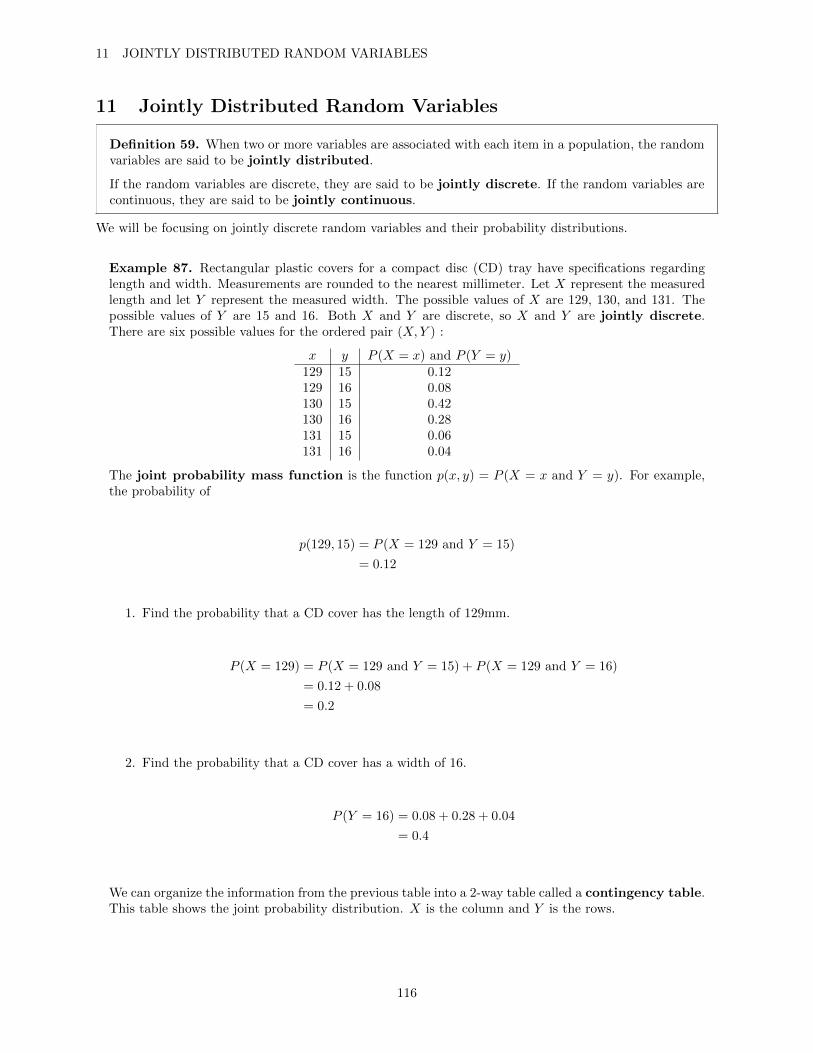
11 JOINTLY DISTRIBUTED RANDOM VARIABLES
11 Jointly Distributed Random Variables
Definition 59. When two or more variables are associated with each item in a population, the randomvariables are said to be jointly distributed.
If the random variables are discrete, they are said to be jointly discrete. If the random variables arecontinuous, they are said to be jointly continuous.
We will be focusing on jointly discrete random variables and their probability distributions.
Example 87. Rectangular plastic covers for a compact disc (CD) tray have specifications regardinglength and width. Measurements are rounded to the nearest millimeter. Let X represent the measuredlength and let Y represent the measured width. The possible values of X are 129, 130, and 131. Thepossible values of Y are 15 and 16. Both X and Y are discrete, so X and Y are jointly discrete.There are six possible values for the ordered pair (X,Y ) :
x y P (X = x) and P (Y = y)129 15 0.12129 16 0.08130 15 0.42130 16 0.28131 15 0.06131 16 0.04
The joint probability mass function is the function p(x, y) = P (X = x and Y = y). For example,the probability of
p(129, 15) = P (X = 129 and Y = 15)
= 0.12
1. Find the probability that a CD cover has the length of 129mm.
P (X = 129) = P (X = 129 and Y = 15) + P (X = 129 and Y = 16)
= 0.12 + 0.08
= 0.2
2. Find the probability that a CD cover has a width of 16.
P (Y = 16) = 0.08 + 0.28 + 0.04
= 0.4
We can organize the information from the previous table into a 2-way table called a contingency table.This table shows the joint probability distribution. X is the column and Y is the rows.
116
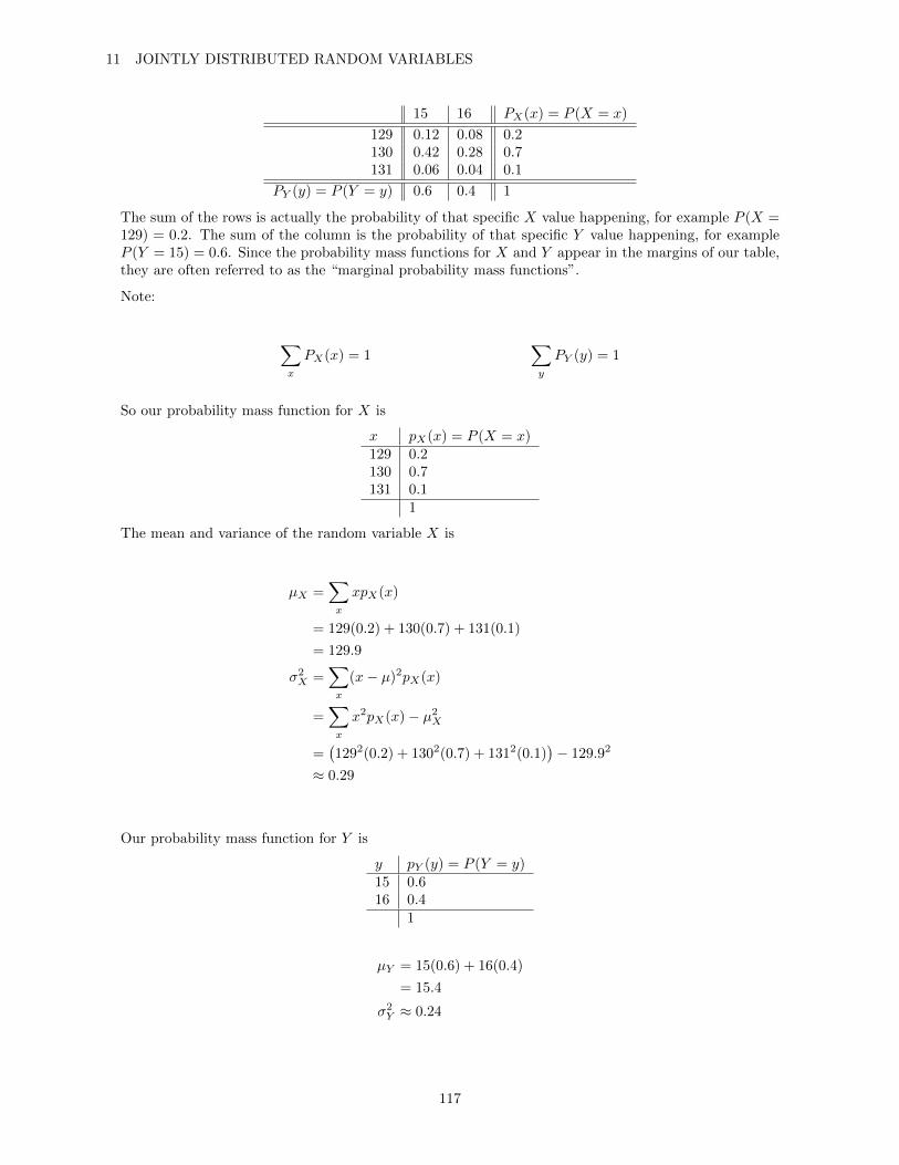
11 JOINTLY DISTRIBUTED RANDOM VARIABLES
15 16 PX(x) = P (X = x)
129 0.12 0.08 0.2130 0.42 0.28 0.7131 0.06 0.04 0.1
PY (y) = P (Y = y) 0.6 0.4 1
The sum of the rows is actually the probability of that specific X value happening, for example P (X =129) = 0.2. The sum of the column is the probability of that specific Y value happening, for exampleP (Y = 15) = 0.6. Since the probability mass functions for X and Y appear in the margins of our table,they are often referred to as the “marginal probability mass functions”.
Note:
∑x
PX(x) = 1∑y
PY (y) = 1
So our probability mass function for X is
x pX(x) = P (X = x)129 0.2130 0.7131 0.1
1
The mean and variance of the random variable X is
µX =∑x
xpX(x)
= 129(0.2) + 130(0.7) + 131(0.1)
= 129.9
σ2X =
∑x
(x− µ)2pX(x)
=∑x
x2pX(x)− µ2X
=(1292(0.2) + 1302(0.7) + 1312(0.1)
)− 129.92
≈ 0.29
Our probability mass function for Y is
y pY (y) = P (Y = y)15 0.616 0.4
1
µY = 15(0.6) + 16(0.4)
= 15.4
σ2Y ≈ 0.24
117

11 JOINTLY DISTRIBUTED RANDOM VARIABLES
Definition 60. If X and Y are jointly discrete random variables:
• The joint probability mass function of X and Y is the function:
p(x, y) = P (X = x and Y = y)
• The marginal probability mass functions of X and of Y can be obtained from the joint probabilitymass function as follows:
pX(x) = P (X = x) =∑y
p(x, y) pY (y) = P (Y = y) =∑x
p(x, y)
where the sums are taken over all possible values of Y and of X, respectively.
• The joint probability mass function has the property
∑x
∑y
p(x, y) = 1
where the sum is taken over all possible values of X and Y .
Note 19. The idea of a joint probability mass function extends easily to more than two variables. Ingeneral, we have the following definition:
If the random variables X1, . . . , Xn are jointly discrete, the joint probability mass function is
p(x1, . . . , xn) = P (X1 = x1, . . . , Xn = xn)
Definition 61 (Mean of a Random Variable). Let X be a random variable, and let h(X) be a functionof X.
• If X is discrete with probability mass function p(x), the mean of h(X) is given by
µh(X) =∑x
h(x)p(x)
This idea can also be used with joint random variables.
If X and Y are jointly distributed random variables, and h(X,Y ) is a function of X and Y , then if Xand Y are jointly discrete with joint probability mass function p(x, y),
µh(X,Y ) =∑x
∑y
h(x, y)p(x, y)
118
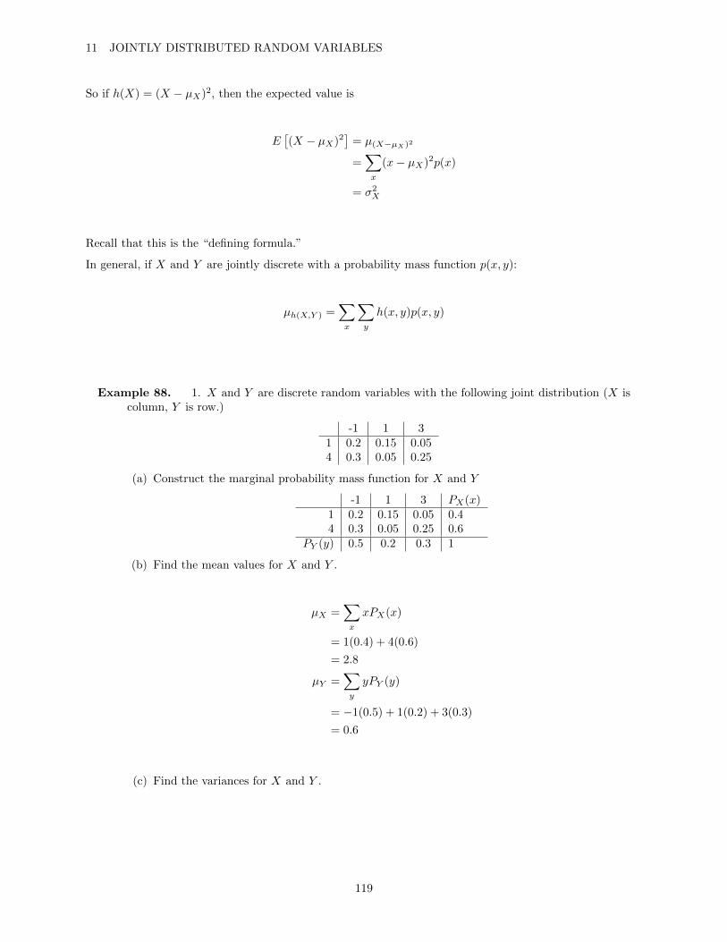
11 JOINTLY DISTRIBUTED RANDOM VARIABLES
So if h(X) = (X − µX)2, then the expected value is
E[(X − µX)2
]= µ(X−µX)2
=∑x
(x− µX)2p(x)
= σ2X
Recall that this is the “defining formula.”
In general, if X and Y are jointly discrete with a probability mass function p(x, y):
µh(X,Y ) =∑x
∑y
h(x, y)p(x, y)
Example 88. 1. X and Y are discrete random variables with the following joint distribution (X iscolumn, Y is row.)
-1 1 31 0.2 0.15 0.054 0.3 0.05 0.25
(a) Construct the marginal probability mass function for X and Y
-1 1 3 PX(x)1 0.2 0.15 0.05 0.44 0.3 0.05 0.25 0.6
PY (y) 0.5 0.2 0.3 1
(b) Find the mean values for X and Y .
µX =∑x
xPX(x)
= 1(0.4) + 4(0.6)
= 2.8
µY =∑y
yPY (y)
= −1(0.5) + 1(0.2) + 3(0.3)
= 0.6
(c) Find the variances for X and Y .
119
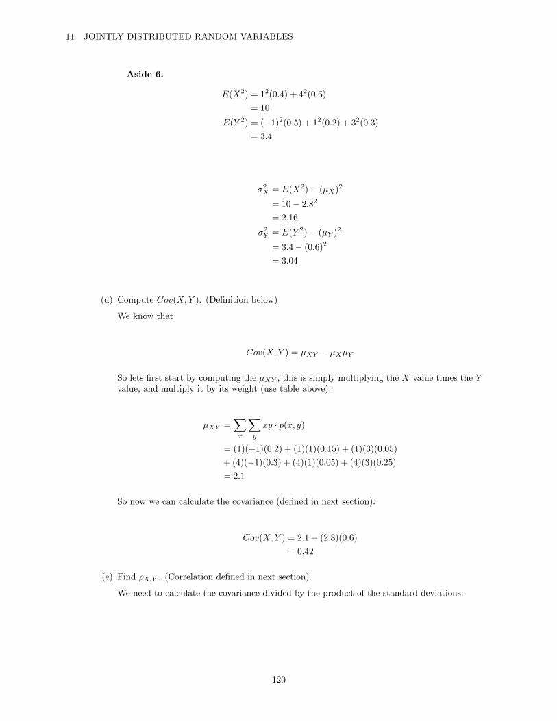
11 JOINTLY DISTRIBUTED RANDOM VARIABLES
Aside 6.
E(X2) = 12(0.4) + 42(0.6)
= 10
E(Y 2) = (−1)2(0.5) + 12(0.2) + 32(0.3)
= 3.4
σ2X = E(X2)− (µX)2
= 10− 2.82
= 2.16
σ2Y = E(Y 2)− (µY )2
= 3.4− (0.6)2
= 3.04
(d) Compute Cov(X,Y ). (Definition below)
We know that
Cov(X,Y ) = µXY − µXµY
So lets first start by computing the µXY , this is simply multiplying the X value times the Yvalue, and multiply it by its weight (use table above):
µXY =∑x
∑y
xy · p(x, y)
= (1)(−1)(0.2) + (1)(1)(0.15) + (1)(3)(0.05)
+ (4)(−1)(0.3) + (4)(1)(0.05) + (4)(3)(0.25)
= 2.1
So now we can calculate the covariance (defined in next section):
Cov(X,Y ) = 2.1− (2.8)(0.6)
= 0.42
(e) Find ρX,Y . (Correlation defined in next section).
We need to calculate the covariance divided by the product of the standard deviations:
120
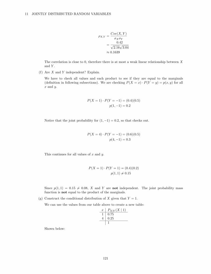
11 JOINTLY DISTRIBUTED RANDOM VARIABLES
ρX,Y =Cov(X,Y )
σXσY
=0.42√
2.16√
3.04
≈ 0.1639
The correlation is close to 0, therefore there is at most a weak linear relationship between Xand Y .
(f) Are X and Y independent? Explain.
We have to check all values and each product to see if they are equal to the marginals(definition in following subsections). We are checking P (X = x) · P (Y = y) = p(x, y) for allx and y.
P (X = 1) · P (Y = −1) = (0.4)(0.5)
p(1,−1) = 0.2
Notice that the joint probability for (1,−1) = 0.2, so that checks out.
P (X = 4) · P (Y = −1) = (0.6)(0.5)
p(4,−1) = 0.3
This continues for all values of x and y.
P (X = 1) · P (Y = 1) = (0.4)(0.2)
p(1, 1) 6= 0.15
Since p(1, 1) = 0.15 6= 0.08, X and Y are not independent. The joint probability massfunction is not equal to the product of the marginals.
(g) Construct the conditional distribution of X given that Y = 1.
We can use the values from our table above to create a new table:
x PX|Y (X | 1)1 0.754 0.25
1
Shown below:
121
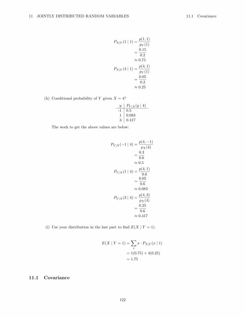
11 JOINTLY DISTRIBUTED RANDOM VARIABLES 11.1 Covariance
PX|Y (1 | 1) =p(1, 1)
pY (1)
=0.15
0.2≈ 0.75
PX|Y (4 | 1) =p(4, 1)
pY (1)
=0.05
0.2≈ 0.25
(h) Conditional probability of Y given X = 4?
y PY |X(y | 4)-1 0.51 0.0833 0.417
The work to get the above values are below:
PY |X(−1 | 4) =p(4,−1)
pX(4)
=0.3
0.6≈ 0.5
PY |X(1 | 4) =p(4, 1)
0.6
=0.05
0.6≈ 0.083
PY |X(3 | 4) =p(4, 3)
pX(4)
=0.25
0.6≈ 0.417
(i) Use your distribution in the last part to find E(X | Y = 1).
E(X | Y = 1) =∑x
x · PX|Y (x | 1)
= 1(0.75) + 4(0.25)
= 1.75
11.1 Covariance
122

11 JOINTLY DISTRIBUTED RANDOM VARIABLES 11.1 Covariance
Definition 62 (Covariance). Let X and Y be random variables with mean µX and µY . The covarianceof X and Y is
Cov(X,Y ) = µ(X−µX)(Y−µY )
= E ((X − µX)(Y − µY ))
An alternate (computing) formula is
Cov(X,Y ) = µXY − µXµY= E(XY )− µXµY
Note 20.
Cov(X,X) = σ2X
In general, the population covariance is a measure of the joint variability between two random variables,a measure of the total variation of two random variables from their expected values. In particular, thecovariance is a measure of a certain type of relationship called a linear relationship. A positive covarianceindicates that the two variables tend to move in the same direction; for example as one variable increasesthe other variable tends to increase as well. A negative covariance indicates that the two variables tend tomove in inverse directions; for example, as one variable increases, the other variable tends to decrease. Thestrength of the linear relationship is also measured but is not easy to interpret since the covariance is not aunitless measure.
To see how the covariance works:
The covariance is the mean of the product of deviations (X−µX)(Y −µY ). If a Cartesian coordinate systemis constructed with the origin at (µX , µY ), this product will be positive in the first and third quadrants, andnegative in the second and fourth quadrants.
It follows that if Cov(X,Y ) is strongly positive, then values of (X,Y ) in the first and third quadrants will beobserved much more often than values in the second and fourth quadrants. In a random sample of points,therefore, larger values of X would tend to be paired with larger values of Y , while smaller values of X wouldtend to be paired with smaller values of Y . (This shows an increase from left to right in the scatter plot.)
Similarly, if Cov(X,Y ) is strongly negative, the points in a random sample would be more likely to lie inthe second and fourth quadrants, so larger values of X would tend to be paired with smaller values of Y .(This shows a decrease from left to right in the scatter plot.)
Finally, if Cov(X,Y ) is near 0, there would be little tendency for larger values of X to be paired with eitherlarger or smaller values of Y . (This shows a random scatter of points in all quadrants in the scatter plot.)
Mini-proof for mean of random variable computing formula:
123

11 JOINTLY DISTRIBUTED RANDOM VARIABLES 11.2 Correlation
E[(X − µ)2] = E(X2)− (µX)2
σ2X = E[(X − µ)2]
= E(X2 − 2µX + µ2)
= E(X2)− 2µE(X) + µ2
= E(X2)− 2µ · µ+ µ2
= E(X2)− µ2
= µX2 − µ2X
Mini-proof for covariance computing formula:
Cov(X,Y ) = E ((X − µX)(Y − µY ))
= E(XY − µYX − µXY + µXµY )
= E(XY )− µY E(X)− µXE(Y ) + µXµY
= E(XY )− µY µX − µXµY + µXµY
= E(XY )− 2µXµY + µXµY
= E(XY )− µXµY= µXY − µXµY
11.2 Correlation
The population correlation is a unitless measure of the strength of a linear relationship between two variables.
Definition 63 (Correlation). Let X and Y be jointly distributed random variables with standarddeviation σX and σY . The correlation between X and Y is denoted ρX,Y and is given by
ρX,Y =Cov(X,Y )
σXσY
For any two random variables X and Y :
−1 ≤ ρX,Y ≤ 1
The closer the correlation value is to either -1 or 1, the stronger the linear relationship is between thevariables. For example, a correlation value close to -1 indicates a strong negative linear relationship betweenX and Y , meaning there is a strong tendency for Y to decrease linearly as X increases. A correlation valueclose to 1 indicates a strong positive linear relationship, meaning there is a strong tendency for Y to increaselinearly as X increases. A correlation value near 0 indicates at most a weak linear relationship between Xand Y .
124
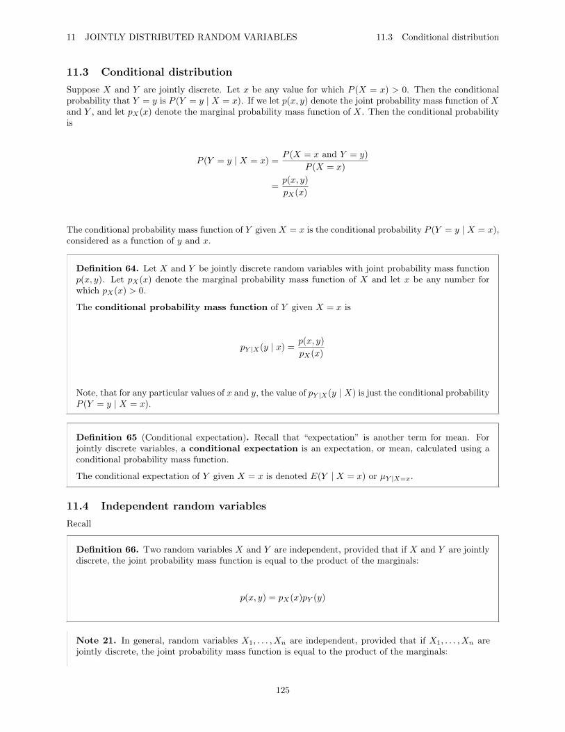
11 JOINTLY DISTRIBUTED RANDOM VARIABLES 11.3 Conditional distribution
11.3 Conditional distribution
Suppose X and Y are jointly discrete. Let x be any value for which P (X = x) > 0. Then the conditionalprobability that Y = y is P (Y = y | X = x). If we let p(x, y) denote the joint probability mass function of Xand Y , and let pX(x) denote the marginal probability mass function of X. Then the conditional probabilityis
P (Y = y | X = x) =P (X = x and Y = y)
P (X = x)
=p(x, y)
pX(x)
The conditional probability mass function of Y given X = x is the conditional probability P (Y = y | X = x),considered as a function of y and x.
Definition 64. Let X and Y be jointly discrete random variables with joint probability mass functionp(x, y). Let pX(x) denote the marginal probability mass function of X and let x be any number forwhich pX(x) > 0.
The conditional probability mass function of Y given X = x is
pY |X(y | x) =p(x, y)
pX(x)
Note, that for any particular values of x and y, the value of pY |X(y | X) is just the conditional probabilityP (Y = y | X = x).
Definition 65 (Conditional expectation). Recall that “expectation” is another term for mean. Forjointly discrete variables, a conditional expectation is an expectation, or mean, calculated using aconditional probability mass function.
The conditional expectation of Y given X = x is denoted E(Y | X = x) or µY |X=x.
11.4 Independent random variables
Recall
Definition 66. Two random variables X and Y are independent, provided that if X and Y are jointlydiscrete, the joint probability mass function is equal to the product of the marginals:
p(x, y) = pX(x)pY (y)
Note 21. In general, random variables X1, . . . , Xn are independent, provided that if X1, . . . , Xn arejointly discrete, the joint probability mass function is equal to the product of the marginals:
125
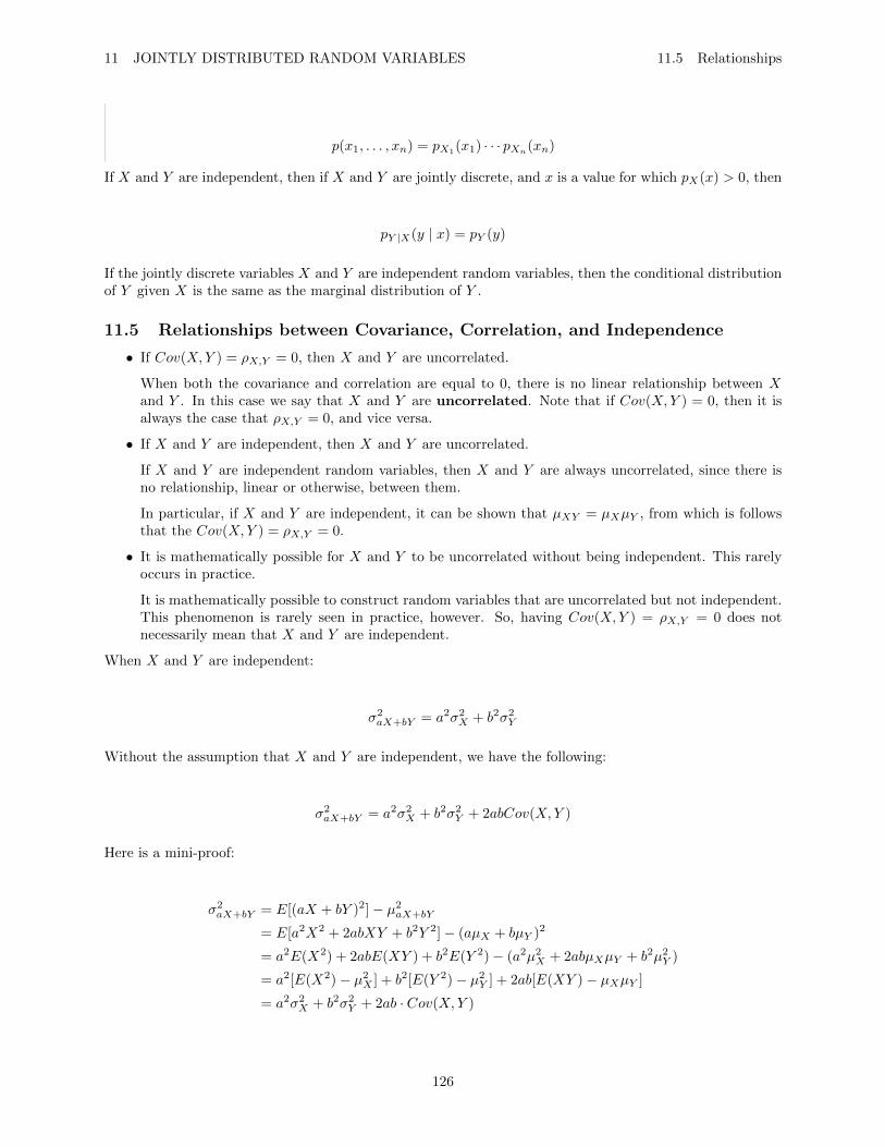
11 JOINTLY DISTRIBUTED RANDOM VARIABLES 11.5 Relationships
p(x1, . . . , xn) = pX1(x1) · · · pXn(xn)
If X and Y are independent, then if X and Y are jointly discrete, and x is a value for which pX(x) > 0, then
pY |X(y | x) = pY (y)
If the jointly discrete variables X and Y are independent random variables, then the conditional distributionof Y given X is the same as the marginal distribution of Y .
11.5 Relationships between Covariance, Correlation, and Independence
• If Cov(X,Y ) = ρX,Y = 0, then X and Y are uncorrelated.
When both the covariance and correlation are equal to 0, there is no linear relationship between Xand Y . In this case we say that X and Y are uncorrelated. Note that if Cov(X,Y ) = 0, then it isalways the case that ρX,Y = 0, and vice versa.
• If X and Y are independent, then X and Y are uncorrelated.
If X and Y are independent random variables, then X and Y are always uncorrelated, since there isno relationship, linear or otherwise, between them.
In particular, if X and Y are independent, it can be shown that µXY = µXµY , from which is followsthat the Cov(X,Y ) = ρX,Y = 0.
• It is mathematically possible for X and Y to be uncorrelated without being independent. This rarelyoccurs in practice.
It is mathematically possible to construct random variables that are uncorrelated but not independent.This phenomenon is rarely seen in practice, however. So, having Cov(X,Y ) = ρX,Y = 0 does notnecessarily mean that X and Y are independent.
When X and Y are independent:
σ2aX+bY = a2σ2
X + b2σ2Y
Without the assumption that X and Y are independent, we have the following:
σ2aX+bY = a2σ2
X + b2σ2Y + 2abCov(X,Y )
Here is a mini-proof:
σ2aX+bY = E[(aX + bY )2]− µ2
aX+bY
= E[a2X2 + 2abXY + b2Y 2]− (aµX + bµY )2
= a2E(X2) + 2abE(XY ) + b2E(Y 2)− (a2µ2X + 2abµXµY + b2µ2
Y )
= a2[E(X2)− µ2X ] + b2[E(Y 2)− µ2
Y ] + 2ab[E(XY )− µXµY ]
= a2σ2X + b2σ2
Y + 2ab · Cov(X,Y )
126
12 REVIEW
12 Review
From the first exam:
P (A) = 0.5
P (B) = 0.3
P (B | A) = 0.4
P (A ∩B) = P (A) · P (B)
Remember, this is only true when A and B are independent. In general,
P (A ∩B) = P (B | A) · P (A)
Remember,
P (A or B) = P (A ∪B)
= P (A) + P (B)− P (A ∩B)
If events A and B are mutually exclusive, then
P (A ∪B) = P (A) + P (B)
Also remember,
P (B | A) =P (A ∩B)
P (A)
Number 5 on the first exam was the problem using Bayes’ rule. If you had 3 events that covered the samplespace, A1, A2, A3:
P (B) = P (A1 ∩B) + P (A2 ∩B) + P (A3 ∩B)
= P (B | A1)P (A1) + P (B | A2)P (A2) + P (B | A3)P (A3)
P (B) = P (B ∩A) + P (B ∩AC)
Recall
127
12 REVIEW
P (A1 | B) =P (A1 ∩B)
P (B)
On this problem, it was stated as “55% of all customers use cash, of these paying with cash 75% usedcoupons.”
P (cash) = 0.55
P (uses coupon | cash) = 0.75
Some counting examples:
Example 89. Seven lifeguards are available for duty on Saturday afternoon. There are four lifeguardstations. How many ways can four lifeguards chosen and ordered among the stations?
7P4
Example 90. Kacey would like to buy ten different paintings but can only afford four of them. Howmany ways can she make her selection?
10C4
Density function examples:
Example 91. Suppose the following is a density function, and X is a random variable:
f(x) =
{12(x2 − x3) 0 < x < 1
0 otherwise
128
12 REVIEW
1. Mean:
µ =
∫ ∞−∞
x · f(x) dx
=
∫ 1
0
x[12(x2 − x3)] dx
=
∫ 1
0
12x(x2 − x3) dx
=
∫ 1
0
(12x3 − 12x4) dx
=
[12
4x4 − 12
5x5
]1
0
2. Variance:
σ2 =
∫ ∞−∞
x2f(x) dx− µ2
=
∫ 1
0
x2(12(x2 − x3)
)dx− µ2
3. P (X < 13 ).
P (X <1
3) =
∫ 13
−∞f(x) dx
=
∫ 13
0
12(x2 − x3) dx
4. The CDF is F (X) = P (X ≤ x). If we are on the interval from (0, 1), there are three cases:
x ≤ 0
0 < x < 1
x ≥ 1
129
12 REVIEW
F (x) =
∫ x
−∞f(x) dx
=
∫ 0
−∞f(t) dt+
∫ x
0
f(t) dt
=
∫ x
0
12(t2 − t3) dt
From the second exam:
Example 92. Let X be a random variable with a mean µ = 14 and a standard deviation σ = 1.2. LetY = 4X and Z = X1 +X2 +X3 +X4 +X5, where each Xi is an independent observation on the variableX.
µY = µ4X
= 4µX
= 4(14)
= 56
µZ = µX1+···+X5
= µX1+ · · ·+ µX5
= 5µX
= 5(14)
= 70
σ2Y = σ2
4X
= 42σ2X
= 16(1.2)2
= 23.04
σ2Z = σ2
X1+···+X5
= σ2X1
+ · · ·+ σ2X5
= 5σ2X
= 5(1.2)2
= 7.2
Example 93. Fuses of a particular type have breaking points that are normally distributed with µ = 7.5amps and σ = 0.5 amps.
1. What is the probability that a fuse has a breaking point greater than 8.0 amps?
130
12 REVIEW
So we know the distribution is N(7.5, 0.52). X = breaking point.
P (X > 8) = normalcdf(8,∞, 7.5, 0.5)
≈ 0.1587
2. Suppose that 10 fuses are randomly selected. What is the probability that exactly two have abreaking point greater than 8.0 amps?
This is a binomial distribution. We have n = 10 trials. We can let Y = number among the 10 thathave breaking point greater than 8 amps. We can define a success as “having a breaking pointgreater than 8 amps.” The probability of that success is p = 0.1587 (found in previous part). Soour distribution is Y ∼ Bin(10, 0.1587).
P (Y = 2) =10!
2!8!(0.1587)2(1− 0.1587)8
P (Y > 2) = 1− P (Y ≤ 2)
= 1− binomcdf(10, 0.1587, 2)
3. Suppose that 25 fuses are randomly selected. What is the probability that their mean breakingpoint is greater than 7.75 amps?
Since breaking points are normally distributed, it doesn’t matter that n < 30, we can use thepopulation mean and use a normal distribution. Let X = mean break point of a sample of 25
fuses. Let X1, . . . , X25 be breaking points of 25 fuses. So, X ∼ N(7.5, 0.52
25 ).
P (X > 7.75) = normalcdf(7.75,∞, 7.5, 0.5√25
)
Example 94. Suppose for a certain computer processor, 75% operate properly at 2.8 GHz, while 20%are capable of operating properly at 3.2 GHz. The remaining 5% are defective.
1. What is the probability that if 20 of the processors are randomly sampled, 15 operate only at 2.8GHz, 4 are capable of operating at 3.2 GHz, and the remaining processor is defective?
This is a multinomial distribution.
P (X1 = 15, X2 = 4, X3 = 1) =20!
15!4!1!(0.75)15(20)4(0.5)1
2. What is the probability that 50 processors must be selected until exactly 10 have been found thatare capable of operating properly at 3.2 GHz?
This is a negative binomial distribution. We are solving for the sample size.
131

12 REVIEW
3. Suppose of 16 processors, 10 operate at 2.8 GHz, 4 operate at 3.2 GHz, and 2 are defective. 6processors are randomly selected (without replacement), what is the probability that exactly 4operate at 2.8 GHz?
This is a hypergeometic distribution.
132