submission of written work - github pages
TRANSCRIPT
IT U
NIV
ERSI
TY O
F CO
PEN
HA
GEN
SUBMISSION OF WRITTEN WORKClass code:
Name of course:
Course manager:
Course e-portfolio:
Thesis or project title:
Supervisor:
Full Name: Birthdate (dd/mm-yyyy): E-mail:
1. @itu.dk
2. @itu.dk
3. @itu.dk
4. @itu.dk
5. @itu.dk
6. @itu.dk
7. @itu.dk
Thesis
Artificial Intelligence for Hero Academy
Tobias Mahlmann and Julian Togelius
13/01-1989Niels Orsleff Justesen noju

Artificial Intelligence for Hero Academy
Master Thesis
Niels Justesen
Advisors: Tobias Mahlmann and Julian TogeliusSubmitted: June 2015

Abstract
In many competitive video games it is possible for players to competeagainst a computer controlled opponent. It is important that such oppo-nents are able to play at a worthy level to keep players engaged. A greatdeal of research has been done on Artificial Intelligence (AI) in gamesto create intelligent computer controlled players, more commonly re-ferred to as AI agents, for a large collection of game genres. In this thesiswe have focused on how to create an intelligent AI agent for the tacti-cal turn-based game Hero Academy, using our own open source gameengine Hero AIcademy. In this game, players can perform five sequen-tial actions resulting in millions of possible outcomes each turn. Wehave implemented and compared several AI methods mainly based onMonte Carlo Tree Search (MCTS) and evolutionary algorithms. A novelprogressive pruning strategy is introduced that significantly improvesMCTS in Hero Academy. Another approach to MCTS is introduced, inwhich the exploration constant is set to zero and greedy rollouts areused, that also gives significant improvement. An online evolutionaryalgorithm that evolves plans during each turn achieved the best results.The fitness function of the evolution is based on depth-limited rolloutsto determine the value of plans. It did, however, not increase the perfor-mance significantly. The online evolution agent was able to play HeroAcademy competitively against human beginners but was easily beatenby intermediate and expert players. Aside from searching for possibleplans it is critical to evaluate the outcome of these intelligently. Weevolved a neural network, using NEAT, that outperforms our own man-ually designed evaluator for small game boards, while more work isneeded to obtain similar results for larger game boards.

iv
Acknowledgements
I would like to thank my supervisors Tobias Mahlmann andJulian Togelius for our many inspiring discussions and their con-tinuous willingness to give me feedback and technical assistance.I also want to thank Sebastian Risi for his lectures in the courseModern AI in Games as they made me interested in the academicworld of game AI.
Contents
Contents v
1 Introduction 11.1 AI in Games . . . . . . . . . . . . . . . . . . . . . . . . . . . . . 21.2 Tactical Turn-based Games . . . . . . . . . . . . . . . . . . . . . . 51.3 Research Question . . . . . . . . . . . . . . . . . . . . . . . . . . 6
2 Hero Academy 72.1 Rules . . . . . . . . . . . . . . . . . . . . . . . . . . . . . . . . 7
2.1.1 Actions . . . . . . . . . . . . . . . . . . . . . . . . . . . 82.1.2 Units . . . . . . . . . . . . . . . . . . . . . . . . . . . . 102.1.3 Items and Spells . . . . . . . . . . . . . . . . . . . . . . . 11
2.2 Game Engine . . . . . . . . . . . . . . . . . . . . . . . . . . . . 122.3 Game Complexity . . . . . . . . . . . . . . . . . . . . . . . . . . . 13
2.3.1 Possible Initial States . . . . . . . . . . . . . . . . . . . . . 142.3.2 Game-tree Complexity . . . . . . . . . . . . . . . . . . . . 142.3.3 State-space Complexity . . . . . . . . . . . . . . . . . . . . 16
3 Related work 193.1 Minimax Search . . . . . . . . . . . . . . . . . . . . . . . . . . . 19
3.1.1 Alpha-beta pruning . . . . . . . . . . . . . . . . . . . . . 203.1.2 Expectiminimax . . . . . . . . . . . . . . . . . . . . . . . 203.1.3 Transposition Table . . . . . . . . . . . . . . . . . . . . . 21
3.2 Monte Carlo Tree Search . . . . . . . . . . . . . . . . . . . . . . . 213.2.1 Pruning . . . . . . . . . . . . . . . . . . . . . . . . . . . 233.2.2 Progressive Strategies . . . . . . . . . . . . . . . . . . . . 243.2.3 Domain Knowledge in Rollouts . . . . . . . . . . . . . . . . 243.2.4 Transpositions . . . . . . . . . . . . . . . . . . . . . . . . 24
vi Contents
3.2.5 Parallelization . . . . . . . . . . . . . . . . . . . . . . . . 253.2.6 Determinization . . . . . . . . . . . . . . . . . . . . . . . 263.2.7 Large Branching Factors . . . . . . . . . . . . . . . . . . . 26
3.3 Artificial Neural Networks . . . . . . . . . . . . . . . . . . . . . . . 283.4 Evolutionary Computation . . . . . . . . . . . . . . . . . . . . . . . 30
3.4.1 Parallelization . . . . . . . . . . . . . . . . . . . . . . . . 303.4.2 Rolling Horizon Evolution . . . . . . . . . . . . . . . . . . . 313.4.3 Neuroevolution . . . . . . . . . . . . . . . . . . . . . . . 32
4 Approach 374.1 Action Pruning & Sorting . . . . . . . . . . . . . . . . . . . . . . . 374.2 State Evaluation . . . . . . . . . . . . . . . . . . . . . . . . . . . 384.3 Game State Hashing . . . . . . . . . . . . . . . . . . . . . . . . . 404.4 Evaluation Function Modularity . . . . . . . . . . . . . . . . . . . . 414.5 Random Search . . . . . . . . . . . . . . . . . . . . . . . . . . . 414.6 Greedy Search . . . . . . . . . . . . . . . . . . . . . . . . . . . . 42
4.6.1 Greedy on Action Level . . . . . . . . . . . . . . . . . . . . 424.6.2 Greedy on Turn Level . . . . . . . . . . . . . . . . . . . . . 42
4.7 Monte Carlo Tree Search . . . . . . . . . . . . . . . . . . . . . . . 434.7.1 Non-explorative MCTS . . . . . . . . . . . . . . . . . . . . 444.7.2 Cutting MCTS . . . . . . . . . . . . . . . . . . . . . . . . 454.7.3 Collapsing MCTS . . . . . . . . . . . . . . . . . . . . . . . 45
4.8 Online Evolution . . . . . . . . . . . . . . . . . . . . . . . . . . . 464.8.1 Crossover & Mutation . . . . . . . . . . . . . . . . . . . . 484.8.2 Parallelization . . . . . . . . . . . . . . . . . . . . . . . . 50
4.9 NEAT . . . . . . . . . . . . . . . . . . . . . . . . . . . . . . . . 504.9.1 Input & Output Layer . . . . . . . . . . . . . . . . . . . . . 51
5 Experimental Results 535.1 Configuration optimization . . . . . . . . . . . . . . . . . . . . . . 54
5.1.1 MCTS . . . . . . . . . . . . . . . . . . . . . . . . . . . . 545.1.2 Online Evolution . . . . . . . . . . . . . . . . . . . . . . . 595.1.3 NEAT . . . . . . . . . . . . . . . . . . . . . . . . . . . . 61
5.2 Comparisons . . . . . . . . . . . . . . . . . . . . . . . . . . . . . 635.2.1 Time budget . . . . . . . . . . . . . . . . . . . . . . . . . 64
5.3 Versus Human Players . . . . . . . . . . . . . . . . . . . . . . . . 65
6 Conclusions 696.1 Discussion . . . . . . . . . . . . . . . . . . . . . . . . . . . . . . 70

Contents vii
6.2 Future Work . . . . . . . . . . . . . . . . . . . . . . . . . . . . . 72
References 75
A JNEAT Parameters 81
B Human Test Results 83

Chapter 1
Introduction
Ever since I was introduced to video games, my mind has been baf-fled by the question: "How can a computer program play games?"The automation and intelligence of game-playing computer programshave kept me fascinated since and have been the primary reason whyI wanted to learn programming. Game-playing programs, or ArtificialIntelligence (AI) agents as they are called, can allow a greater form ofinteraction with the game system e.g. by letting players play against thesystem or as a form of assistance during a game. During my studies atthe IT University of Copenhagen I have had the opportunity to explorethe underlying algorithms of such AI agents providing me with answersto my question. Today I am not only interested in the methods but alsofor which types of games it is possible, using state of the art methods,to produce challenging AI agents. While the current state of research inthis area can be seen as a stepping stone towards something even moreintelligent, it also serves as a collection of methods and results that caninspire game developers in the industry. Exploring the limits and dif-ferent approaches in untested classes of games is something I believe isimportant for both the game industry and the field. My interest in thisquestion has previously led me to explore algorithms for the very com-plex problem of controlling units during combat in the real-time strategygame StarCraft, which turned into a paper for the IEEE Conference onComputational Intelligence and Games in 2014 [1]. This thesis will havea similar focus of exploring AI algorithms for a game with a very highcomplexity, but this time for the Tactical Turn-Based (TTB) game HeroAcademy. Before explaining why TTB games have caught my interest, avery brief overview of Artificial Intelligence (AI) in games is presented.
2 Chapter 1. Introduction
Hereafter I will argue why TTB games including Hero Academy is anunexplored type of game in the game AI literature.
1.1 AI in Games
The fields of Artificial Intelligence and Computational Intelligence in gamesare concerned with research in methods that can produce intelligentbehavior in games. As there is a great overlap between the two fieldsand no real agreement on when to use which term, game AI will be usedthroughout this thesis to describe the two joined fields.
AI methods can be used in many different areas of the game devel-opment process, which have formed several different sub-fields withingame AI. Ten sub-fields were recently identified and described by To-gelius and Yannakakis [2]. One popular sub-field is Procedural contentgeneration, in which AI methods are used to generate content in gamessuch as weapons, storylines, levels and even entire game descriptions.Another is Non-player character (NPC) behavior, which is concerned withmethods used to control characters within a game. In this thesis we willonly be concerned with methods that are used to control an agent toplay a game. This sub-field is also called Games as AI benchmarks. Re-search in this sub-field is relevant for other sub-fields within game AIas they can be used for automatic play-testing and content generationby simulating the behavior of human players. Intelligent AI agents canalso be used as worthy opponents in video games, which is essentialfor some games. Game AI methods can also be applied to many real-world problems related to planning and scheduling, and one could saythat games are merely a sand box in which AI methods can be devel-oped and tested before it is applied to the real world. On the otherhand, games are a huge industry, where AI still has a lot of potentialand unexplored opportunities, especially when it comes to intelligentgame-design assistance tools.
To get a brief overview of the field of game AI, let us take a look atwhich type of games researchers have focused on. This is far from acomplete list of games, but simply an effort to highlight the differentclasses of games that are used.
Programming a computer to play Chess has been of interest sinceShannon introduced the idea in 1950 [3]. In the following decades a
1.1. AI in Games 3
multitude of researchers helped the progress of Chess playing comput-ers, and finally in 1997 the Chess machine Deep Blue beat the worldchess champion Garry Kasparov [4]. Chess playing computer programsimplement variations of the minimax search algorithm that in a bruteforce style makes an exhaustive search of the game tree. One of themost important discoveries in computer Chess has been the Alpha-betapruning algorithm that enables the minimax search to ignore certainbranches in the tree.
In 2007 Schaeffer et al. announced that the game Checkers was solved[5]. The outcome of each possible opening strategy was calculated forwhen no mistakes were made by both players. Since the game tree wasonly partly analyzed, the game is only weakly solved. Another gamethat recently has been weakly solved is Heads-up limit hold’em Poker [6],which requires an immense amount of computation due to the stochasticnature of the game. Most interesting games are, however, not solved, atleast not yet, and may perhaps never be solved due to their complexity.
After Chess programs reached a super-human level, the classic boardgame Go has become the most dominant benchmark game for AI re-search. The number of available actions during a turn in Go is muchlarger than in Chess and creates problems for the Alpha-beta pruningalgorithm. The average number of available actions in a turn is calledthe branching factor and is an important complexity measure for games.Another challenge in Go is that game positions are very difficult to eval-uate, which is essential for a depth-limited search. Monte Carlo TreeSearch (MCTS) has greatly influenced the progress of Go-playing pro-grams. It is a family of search algorithms that uses stochastic simulationsas a heuristic and iteratively expands the tree in the most promising di-rection. These stochastic simulations have turned out to be very effectivewhen it comes to evaluation of game positions in Go. Machine learn-ing techniques in combination with pattern recognition algorithms haveenabled recent Go programs to compete with human experts. The com-puter Go web site keeps track of matches played by expert Go playersagainst the best Go programs1. MCTS has shown to work well in a va-riety of games and has been a popular choice for researchers workingwith AI for modern board games such as Settlers of Catan [7], Carcassonne[8] and Dominion [9].
A lot of game AI research have also been made on methods appliedto real-time video games. While turn-based games are slow and allow
1http://www.computer-go.info/h-c/index.html2013
4 Chapter 1. Introduction
AI agents to think for several seconds before taking an action, real-timegames are fast-paced and often require numerous actions within eachsecond of the game. Among popular real-time benchmark games are:the racing game TORCS, the famous arcade game Ms. PacMan and theplatformer Super Mario Bros. Quality reverse-engineered game clonesexist for these games and several AI competitions have been held usingthese clones to compare different AI methods.
Another very popular game used in this field is the real-time strategy(RTS) game StarCraft. Since this game requires both high-level strategicplanning as well as low-level unit control, it offers a suite of problemsfor AI researchers and has also been subject for several AI competitionsthat are still ongoing. Few open source RTS games such as WarGus (aclone of WarCraft II) and Stratagus have also been used as benchmarkgames.
The general video game playing competition has been popular thelast years, where researchers and students develop AI agents that com-pete in unseen two-dimensional arcade games [10]. A recent approachto general video game playing has been to evolve artificial neural net-works to play a series of Atari games, which even surpassed humanscores in some of the games [11]. Evolutionary computation has beenvery influential to game AI as interesting solutions can be found whenmimicking the evolutionary process seen in nature.
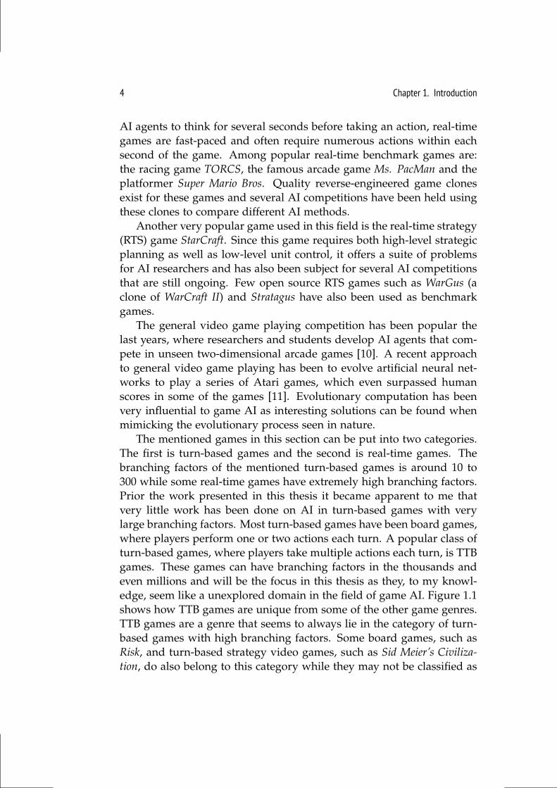
The mentioned games in this section can be put into two categories.The first is turn-based games and the second is real-time games. Thebranching factors of the mentioned turn-based games is around 10 to300 while some real-time games have extremely high branching factors.Prior the work presented in this thesis it became apparent to me thatvery little work has been done on AI in turn-based games with verylarge branching factors. Most turn-based games have been board games,where players perform one or two actions each turn. A popular class ofturn-based games, where players take multiple actions each turn, is TTBgames. These games can have branching factors in the thousands andeven millions and will be the focus in this thesis as they, to my knowl-edge, seem like a unexplored domain in the field of game AI. Figure 1.1shows how TTB games are unique from some of the other game genres.TTB games are a genre that seems to always lie in the category of turn-based games with high branching factors. Some board games, such asRisk, and turn-based strategy video games, such as Sid Meier’s Civiliza-tion, do also belong to this category while they may not be classified as
1.2. Tactical Turn-based Games 5
TTB games. Other dimensions are of course important when categoriz-ing games by their complexity such as hidden information, randomnessand amount of rules. Still, this figure should express the kind of gamesthat I believe needs more attention.
Figure 1.1: A few game genres categorized after their branching factor and whether they are turn-basedor real-time. Tactical Turn-based games, including Hero Academy, is among Turn-based games with veryhigh branching factors.
Next section will explain a bit more about TTB games and give con-crete examples of some published TTB games.
1.2 Tactical Turn-based Games
In strategy games players must make long term plans to defeat theiropponent, and it requires tactic manoeuvres to obtain their objectives.Strategy is extremely important in RTS games as players produce build-ings and upgrades that will have a long term effect on the game. Onesub-genre of strategy games is Tactical Turn-based (TTB) games. In thesegames the continuous execution in each turn is extremely critical. Mov-ing a unit to a wrong position can easily result in a lost game. Thesegames are often concerned with small-scale combats instead of series ofbattles and usually have a very short cycle of rewards. Strategy gamesare mostly implemented as real-time games, while tactical games are
6 Chapter 1. Introduction
more suited as turn-based games. Modern games such as Blood Bowl, X-Com and Battle for Wesnoth are all good examples of TTB games. Thesegames have very large branching factors since players have to make mul-tiple actions each turn. I also refer to such games as multi-action gamesin contrast to single-action games like Chess and Go. It would be igno-rant to say that these games do not require any strategy, but the tacticalexecution is simply much more important. One very interesting digitalTTB game is Hero Academy as its branching factor is in the millions, andit has a very short cycle of rewards. This game was chosen as the bench-mark TTB game for this thesis and a thorough introduction to the gamerules are given in the following chapter.
Among other TTB games that have been studied in game AI researchis Advance Wars. This game has a much larger game world than HeroAcademy and requires more strategic choices such as unit productionand complex terrain analysis. Hero Academy is thus a more focusedtest bed as it is mostly concerned with tactical decisions. Bergsma andSprock [12] designed a two-layered influence map that is merged usingan evolved neural network to control units in Advance Wars. The in-fluence map was used to identify the most promising squares to eithermove to or attack.
1.3 Research Question
In the previous sections I argued why TTB games are an under-exploredtype of game and why I think it is important to focus on these. Thegame Hero Academy was chosen as the benchmark TTB game for thisthesis and the goal will be to explore AI methods for this game andexamine the achieved playing level compared to human players. Onefocused research question was made based on this goal:
Research questionHow can we design an AI agent that is able to challengehuman players in Hero Academy?
In this introduction I have referred to myself as I, but throughoutthis thesis we will be used instead, even though the work presented wassolely made by me, the author.
Chapter 2
Hero Academy
Hero Academy is a two-player Tactical Turn-Based (TTB) video gamedeveloped by Robot Entertainment. It was originally released on iOS in2012 but is now also available on Steam, Android and Mac. The gameis a multi-action game as players have five action points each turn theycan spend to perform actions sequentially. It is played asynchronoustypically over several days but are played in one sitting during tourna-ments. It was generally well received by the critics1 and hit the top 10list of free games in China within just 48 hours2.
2.1 Rules
The rules of Hero Academy will be explained as if it was a board game,as it simply is a digital version of game that could just as well be releasedphysically. This will hopefully make it easier to understand the rules forpeople familiar with board game mechanics.
Hero Academy is played over a number of rounds until one playerhave lost both crystals or all units. The game is played on a game boardof 9x5 squares containing two deploy zones and two crystals for eachplayer. Both players have a deck of 34 cards from which they drawcards onto their secret hand. In the beginning of each round cards aredrawn until the maximum hand size of six is reached or the deck isempty. This is the only element in the game with hidden information
1http://www.metacritic.com/game/pc/hero-academy2http://www.gamasutra.com/view/news/177767/How_Hero_Academy_went_
big_in_China.php
8 Chapter 2. Hero Academy
and randomness. Everything else is deterministic and visible to bothplayers. The graphical user interface in the game does actually not vi-sualize these elements as playing cards but they do work mechanicallyequivalent. Cards can either represent a unit, an item or a spell. The ini-tial game board does not contain any units but will gradually be filledas more rounds are played.
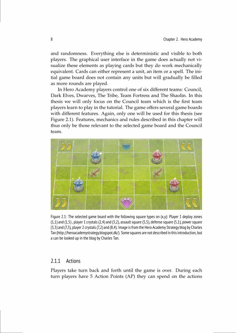
In Hero Academy players control one of six different teams: Council,Dark Elves, Dwarves, The Tribe, Team Fortress and The Shaolin. In thisthesis we will only focus on the Council team which is the first teamplayers learn to play in the tutorial. The game offers several game boardswith different features. Again, only one will be used for this thesis (seeFigure 2.1). Features, mechanics and rules described in this chapter willthus only be those relevant to the selected game board and the Councilteam.
Figure 2.1: The selected game board with the following square types on (x,y): Player 1 deploy zones(1,1) and (1,5) , player 1 crystals (2,4) and (3,2), assault square (5,5), defense square (5,1), power square(3,3) and (7,3), player 2 crystals (7,2) and (8,4). Image is from the Hero Academy Strategy blog by CharlesTan (http://heroacademystrategy.blogspot.dk/). Some squares are not described in this introduction, buta can be looked up in the blog by Charles Tan.
2.1.1 Actions
Players take turn back and forth until the game is over. During eachturn players have 5 Action Points (AP) they can spend on the actions
2.1. Rules 9
described below. Each action costs 1 AP and are allowed to be per-formed in any order and even several times each turn. It is also allowedto perform several actions with the same unit.
DeployA unit can be deployed from a players hand onto an unoccupieddeploy zone they own. Deploying units simply means that a unitcard on the player’s hand is discarded and the unit represented onthe card is placed on the selected deploy zone.
EquipOne unit on the board can be equipped with an item from thehand. Units cannot carry more than one of each item and it isnot possible to equip opponent units. Similar to the deploy action,the item card is discarded and the item represented on the card isgiven to the selected unit.
MoveOne unit can be moved a number of squares equal to or lower thanits Speed attribute. Diagonally moves are not allowed. Units can,however, jump over any number of units along their path as longas the final square is unoccupied.
AttackOne unit can attack an opponent unit within the number of squaresequal to its Attack Range attribute. The amount of damage dealt isbased on numerous factors such as the Power attribute of the at-tacker, which items the attacker and defender holds, which squaresthey stand on and the resistance of the defender. There are twotypes of attacks in the game: Physical Attack and Magical Attack.Likewise, units can have Physical Resistance and Magical Resistancethat protects them against those attacks. The defender will in theend lose health points (HP) equal the calculated damage. If theHP value of the defender reaches zero the defender will becomeKnocked Out. Knocked Out units cannot perform any actions andwill be removed from the game if either a unit moves onto itssquare (called Stomping) or if it is still knocked out by the end ofthe owners following turn.
SpecialSome units have special actions such as healing. These are de-scribed later when each unit type is described.
10 Chapter 2. Hero Academy
Cast SpellEach team have one unique spell that can be cast onto a square onthe board from the hand, where after the spell card is discarded.Spells are very powerful and usually saved until a very good mo-ment in the game.
Swap CardCards on the hand can be shuffled into the deck in hopes of draw-ing better cards in the following round.
2.1.2 Units
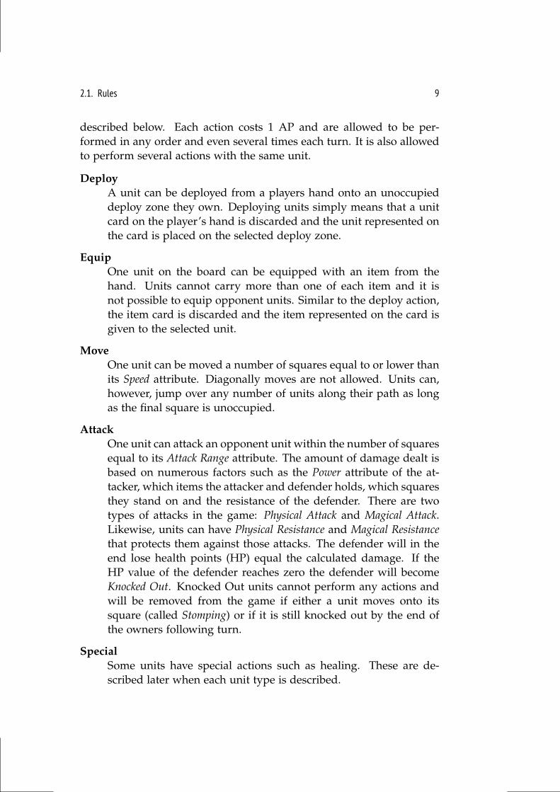
Each team has four different types of basic units and one so called SuperUnit. In this section a short description of each of the five units on theCouncil team is presented. Units normally have Power 200, Speed 2, 800HP and no resistances. Only the specialities of each unit are highlightedbelow.
Figure 2.2: The five different units on the Council team. From left to right: Archer, cleric, knight, ninjaand wizard.
ArcherDeals 300 physical damage within range 3. Archers are very goodat knocking out enemy units in one turn with their long range andpowerful attack.
ClericAs a special action the cleric can heal friendly units within range2. Healed units gain HP equal to three times the power of thecleric. Knocked out units can also be revived using this action butthen only gains two times the power in HP. The cleric deals 200magical damage within range 2 and has 20% Magical Resistance.It is critical to have at least one cleric on the board to be able toheal and revive units.
2.1. Rules 11
KnightWith 1000 HP and 20% Physical Resistance the knight is a verytough unit. It deals 200 physical damage within range 1 andknocks back enemy units one square, if possible, when attacking.The Knight is able to hold and conquer critical positions on theboard as it is very difficult to knock out in one turn.
NinjaThe super unit of the Council team. As a special action the ninjacan swap positions with any other friendly unit that is not knockedout. The ninja deals 200 physical damage within range 2 but dealsdouble damage when attacking at range 1. Additionally, the ninjahas speed 5. This unit is very effective as it is both hard hittingand allows for more mobility on the board.
WizardThe wizard deals 200 magical damage within range 2. Further-more, its attack makes two additional chain attacks if enemy unitsor crystals stand next to the target. The game guide says that thethe chain attacks are random but the actual deterministic behaviorhave been described by Hamlet in his own guide3.
2.1.3 Items and Spells
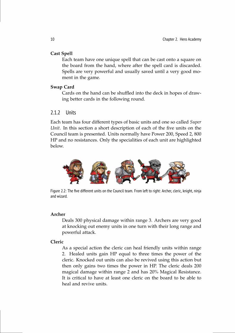
Each team has different items that can be given to units on the boardusing the equip action, and one spell that can be cast onto the boardwith the cast spell action. This section will briefly describe the fivedifferent items and the spell of the Council team.
Figure 2.3: The items and spell of the Council team. From left to right: Dragonscale, healing potion,runemetal, scroll, shining helmet and inferno.
3http://iam.yellingontheinternet.com/2012/08/10/hero-academy-mechanics-guide/#elves
12 Chapter 2. Hero Academy
Dragonscale (item)Gives +20% Physical Resistance and +10% maximum HP.
Healing Potion (item)Heals 1000 HP or revives a knocked out unit to 100 HP. This itemis used instantly and then removed from the game.
Runemetal (item)Boosts the damage dealt by the unit with 50%.
Scroll (item)Boosts the next attack by the unit with 300% where after it is re-moved from the game.
Shining Helmet (item)Gives +20% Physical Resistance and +10% HP.
Inferno (spell)Deals 350 damage to a 3x3 square area. If units in this area arealready knocked out, they are instantly removed from the game.
The council team starts with 3 archers, 3 clerics, 3 knights, 1 ninja,3 wizards, 3 dragonscales, 2 healing potions, 3 runemetals, 2 scrolls, 3shining helmets and 2 infernos in their deck.
2.2 Game Engine
Robot Entertainment have, as most other game companies, not pub-lished the source code for their games and no open source clones existedprior to this thesis to our knowledge. To be able to perform experimentsin the game Hero Academy, we have developed our own clone. The de-velopment of this clone was initiated prior to this thesis, but the qualitywas continuously improved while it was used, and several features havebeen added. This Hero Academy clone have been named Hero AIcademyand is written in Java.
Hero AIcademy only implements the Council team and the squaretypes from the game board on Figure 2.1. Besides that, all rules havebeen implemented. The main focus of Hero AIcademy have been onallowing AI agents to play the game rather than on graphics and ani-mations. In this section a brief overview of how AI agents interact withthe engine is presented. The complete source code of the engine as of
2.3. Game Complexity 13
1st of June 2015 is provided on this GitHub page4 and the continueddevelopment can be followed on the official Hero AIcademy GitHubpage5.
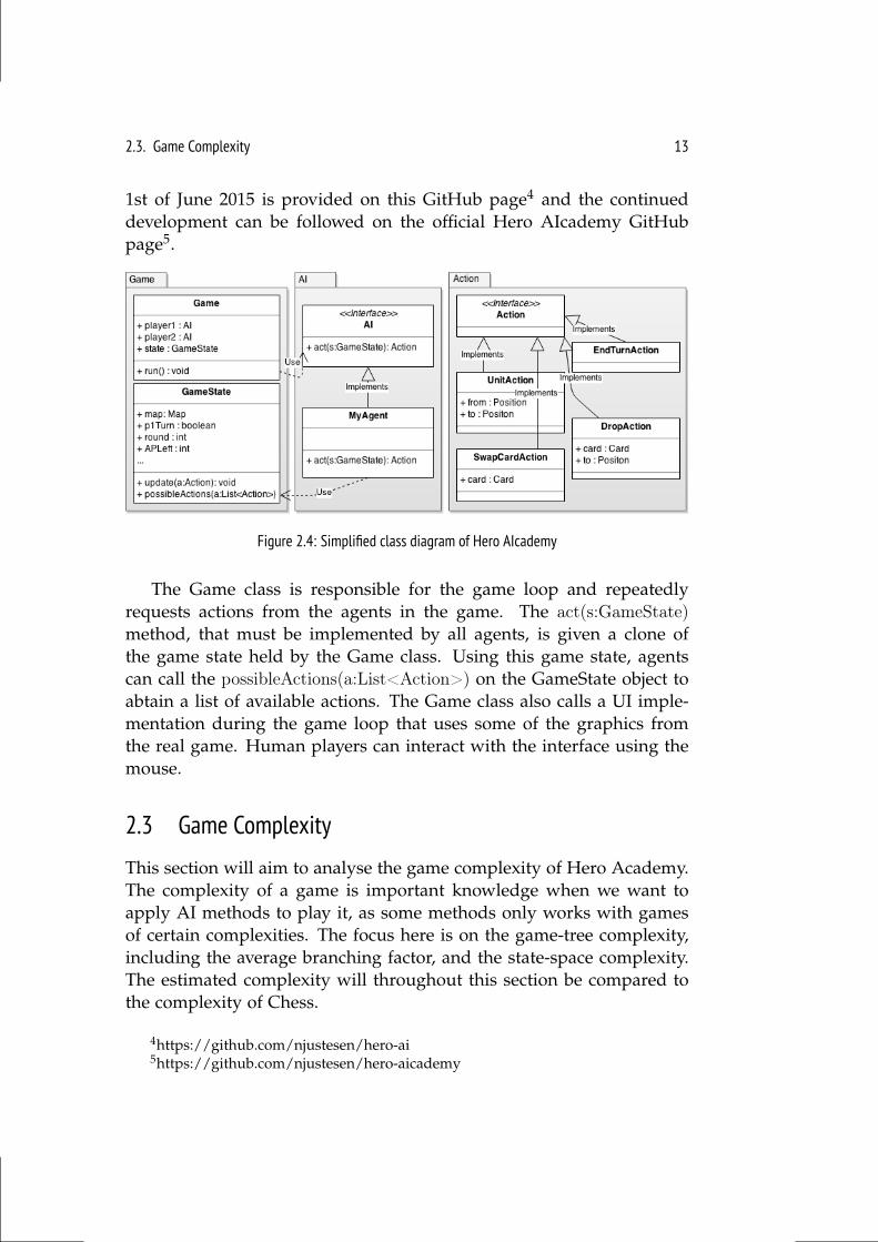
Figure 2.4: Simplified class diagram of Hero AIcademy
The Game class is responsible for the game loop and repeatedlyrequests actions from the agents in the game. The act(s:GameState)method, that must be implemented by all agents, is given a clone ofthe game state held by the Game class. Using this game state, agentscan call the possibleActions(a:List<Action>) on the GameState object toabtain a list of available actions. The Game class also calls a UI imple-mentation during the game loop that uses some of the graphics fromthe real game. Human players can interact with the interface using themouse.
2.3 Game Complexity
This section will aim to analyse the game complexity of Hero Academy.The complexity of a game is important knowledge when we want toapply AI methods to play it, as some methods only works with gamesof certain complexities. The focus here is on the game-tree complexity,including the average branching factor, and the state-space complexity.The estimated complexity will throughout this section be compared tothe complexity of Chess.
4https://github.com/njustesen/hero-ai5https://github.com/njustesen/hero-aicademy
14 Chapter 2. Hero Academy
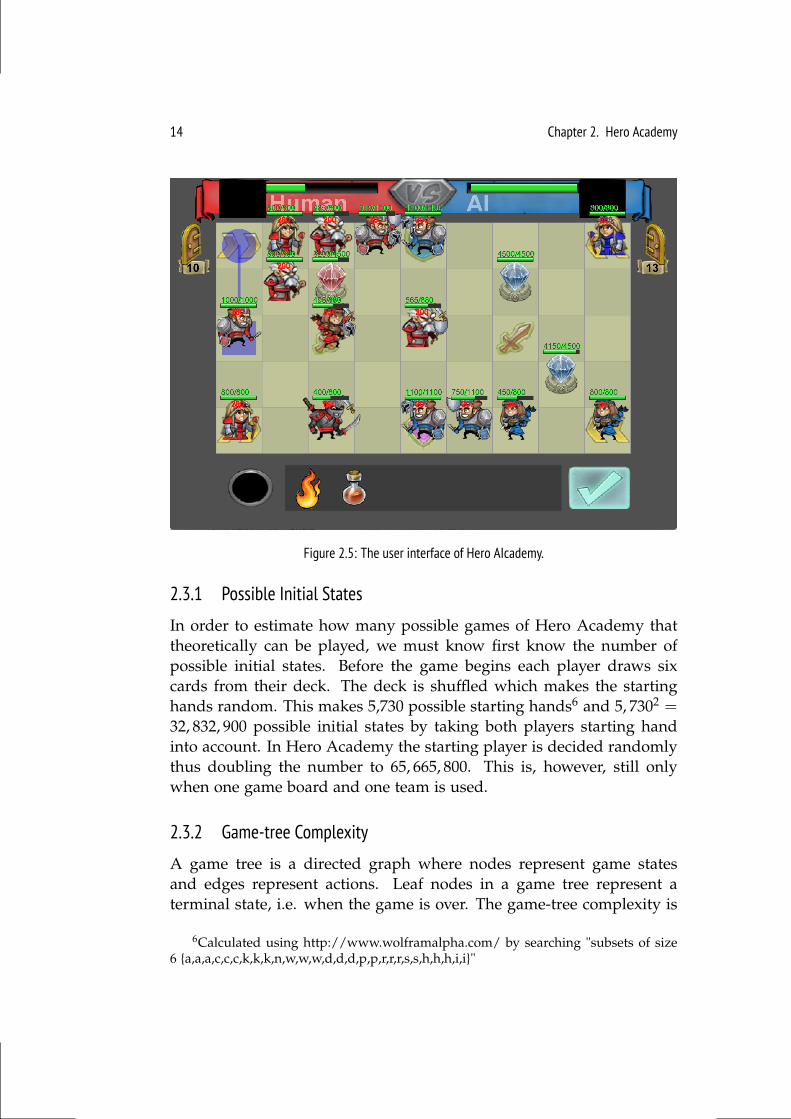
Figure 2.5: The user interface of Hero AIcademy.
2.3.1 Possible Initial States
In order to estimate how many possible games of Hero Academy thattheoretically can be played, we must know first know the number ofpossible initial states. Before the game begins each player draws sixcards from their deck. The deck is shuffled which makes the startinghands random. This makes 5,730 possible starting hands6 and 5, 7302 =32, 832, 900 possible initial states by taking both players starting handinto account. In Hero Academy the starting player is decided randomlythus doubling the number to 65, 665, 800. This is, however, still onlywhen one game board and one team is used.
2.3.2 Game-tree Complexity
A game tree is a directed graph where nodes represent game statesand edges represent actions. Leaf nodes in a game tree represent aterminal state, i.e. when the game is over. The game-tree complexity is
6Calculated using http://www.wolframalpha.com/ by searching "subsets of size6 a,a,a,c,c,c,k,k,k,n,w,w,w,d,d,d,p,p,r,r,r,s,s,h,h,h,i,i"
2.3. Game Complexity 15
determined by the number of leaf nodes in the entire game-tree which isalso the number of possible games. Studying the game-tree complexityof a game is interesting as many AI methods use tree search algorithmsto determine the best action in a given state. Tree search algorithms willobviously be able to search through small game trees very fast, whilesome very large trees will be impractical to search in.
The branching factor of a game tells us the how many children eachnode has in the game tree. In most games this number is not uniformthroughout the tree and we are thus interested in the average. Thebranching factor thus tells us the average number of available movesduring a turn. Since players in Hero Academy are performing actionsin several sequential steps, we will first calculate the branching factor ofa step.
0
10
20
30
40
50
60
70
80
90
5 10 15 20
Po
ssib
le a
ctio
ns
Round
Std. Dev. (12.83)Mean (60.35)
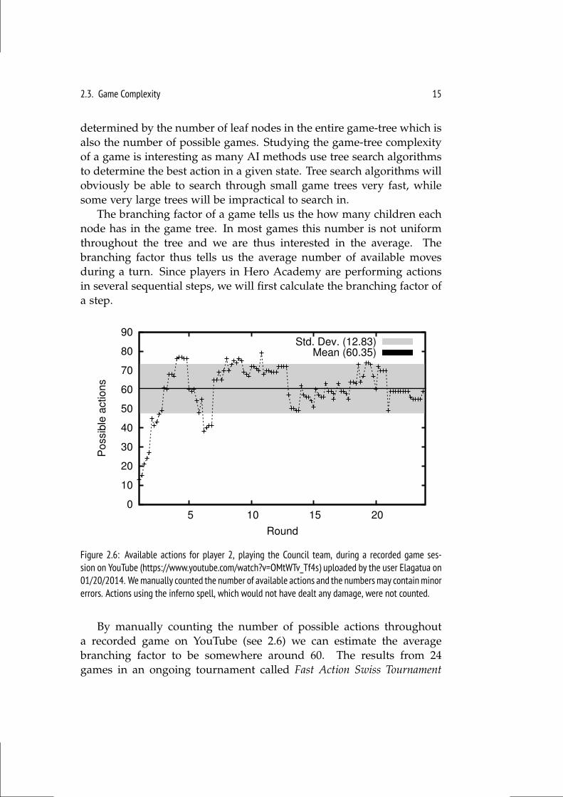
Figure 2.6: Available actions for player 2, playing the Council team, during a recorded game ses-sion on YouTube (https://www.youtube.com/watch?v=OMtWTv_Tf4s) uploaded by the user Elagatua on01/20/2014. Wemanually counted the number of available actions and the numbers may contain minorerrors. Actions using the inferno spell, which would not have dealt any damage, were not counted.
By manually counting the number of possible actions throughouta recorded game on YouTube (see 2.6) we can estimate the averagebranching factor to be somewhere around 60. The results from 24games in an ongoing tournament called Fast Action Swiss Tournament
16 Chapter 2. Hero Academy
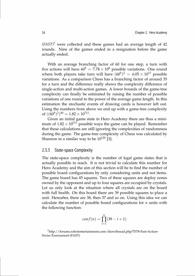
(FAST)7 were collected and these games had an average length of 42rounds. Nine of the games ended in a resignation before the gameactually ended.
With an average branching factor of 60 for one step, a turn withfive actions will have 605 = 7.78× 10⁸ possible variations. One roundwhere both players take turn will have (605)2 = 6.05 × 10¹⁷ possiblevariations. As a comparison Chess has a branching factor of around 35for a turn and the difference really shows the complexity difference ofsingle-action and multi-action games. A lower bounds of the game-treecomplexity can finally be estimated by raising the number of possiblevariations of one round to the power of the average game length. In thisestimation the stochastic events of drawing cards is however left out.Using the numbers from above we end up with a game-tree complexityof ((605)2)40 = 1.82× 10711.
Given an initial game state in Hero Academy there are thus a mini-mum of 1.82× 10711 possible ways the game can be played. Rememberthat these calculations are still ignoring the complexities of randomnessduring the game. The game-tree complexity of Chess was calculated byShannon in a similar way to be 10120 [3].
2.3.3 State-space Complexity
The state-space complexity is the number of legal game states that isactually possible to reach. It is not trivial to calculate this number forHero Academy and the aim of this section will be to find the number ofpossible board configurations by only considering units and not items.The game board has 45 squares. Two of these squares are deploy zonesowned by the opponent and up to four squares are occupied by crystals.Let us only look at the situation where all crystals are on the boardwith full health. On this board there are 39 possible squares to place aunit. Hereafter, there are 38, then 37 and so on. Using this idea we cancalculate the number of possible board configurations for n units withthe following function:
con f (n) =n
∏i=1
(39− i + 1)
7http://forums.robotentertainment.com/showthread.php?5378-Fast-Action-Swiss-Tournament-(FAST)
2.3. Game Complexity 17
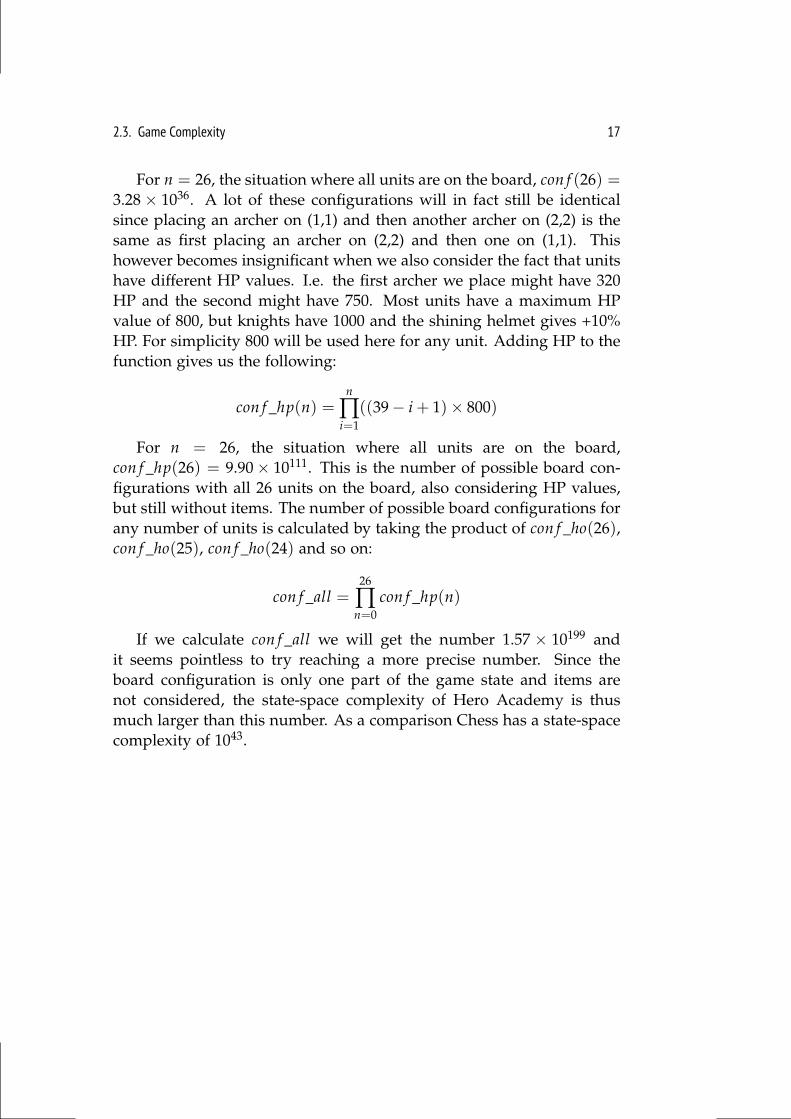
For n = 26, the situation where all units are on the board, con f (26) =3.28× 1036. A lot of these configurations will in fact still be identicalsince placing an archer on (1,1) and then another archer on (2,2) is thesame as first placing an archer on (2,2) and then one on (1,1). Thishowever becomes insignificant when we also consider the fact that unitshave different HP values. I.e. the first archer we place might have 320HP and the second might have 750. Most units have a maximum HPvalue of 800, but knights have 1000 and the shining helmet gives +10%HP. For simplicity 800 will be used here for any unit. Adding HP to thefunction gives us the following:
con f _hp(n) =n
∏i=1
((39− i + 1)× 800)
For n = 26, the situation where all units are on the board,con f _hp(26) = 9.90× 10111. This is the number of possible board con-figurations with all 26 units on the board, also considering HP values,but still without items. The number of possible board configurations forany number of units is calculated by taking the product of con f _ho(26),con f _ho(25), con f _ho(24) and so on:
con f _all =26
∏n=0
con f _hp(n)
If we calculate con f _all we will get the number 1.57 × 10199 andit seems pointless to try reaching a more precise number. Since theboard configuration is only one part of the game state and items arenot considered, the state-space complexity of Hero Academy is thusmuch larger than this number. As a comparison Chess has a state-spacecomplexity of 1043.

Chapter 3
Related work
Games are a very popular domain in the field of AI, as they offer anisolated and fully understood environment that are easy to reproducefor testing. Because of this, thousands of research papers have beenreleased in this field offering numerous algorithms and approaches toAI in games. In this chapter some of the most popular algorithms arepresented that are relevant to the game Hero Academy. Each section willgive an introduction to a new algorithm or method which are followedby a few optimization methods that seem relevant when applied to HeroAcademy.
3.1 Minimax Search
Minimax is a recursive search algorithm that can be used as a decisionrule in two-player zero-sum games. The algorithm considers all possi-ble strategies for both players and selects the strategy that minimizes themaximum loss. In other words, minimax picks the strategy that allowsthe opponent to gain the least advantage in the game. The minimax the-orem that establishes, that there exists such a strategy for both players,was proven by John von Neumann in 1928 [13].
In most interesting games, game trees are so large that the mini-max search must be limited to a certain depth in order to reach a resultwithin a reasonable amount of time. An evaluation function, also calleda heuristic, is then used to evaluate the game state when the depth-limitis reached. E.g. in Chess a simple evaluation function could count thenumber of pieces owned by each player and return the difference.
20 Chapter 3. Related work
In 1997 the Chess Machine called Deep Blue won a six-game matchagainst World Chess Champion Garry Kasparov. Deep Blue was run-ning a parallel version of minimax with a complex evaluation functionand a database of games with grandmasters [4].
3.1.1 Alpha-beta pruning
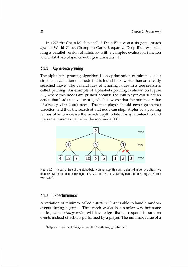
The alpha-beta pruning algorithm is an optimization of minimax, as itstops the evaluation of a node if it is found to be worse than an alreadysearched move. The general idea of ignoring nodes in a tree search iscalled pruning. An example of alpha-beta pruning is shown on Figure3.1, where two nodes are pruned because the min-player can select anaction that leads to a value of 1, which is worse that the minimax-valueof already visited sub-trees. The max-player should never go in thatdirection and thus the search at that node can stop. Alpha-beta pruningis thus able to increase the search depth while it is guaranteed to findthe same minimax value for the root node [14].
Figure 3.1: The search tree of the alpha-beta pruning algorithm with a depth-limit of two plies. Twobranches can be pruned in the right-most side of the tree shown by two red lines. Figure is fromWikipedia1.
3.1.2 Expectiminimax
A variation of minimax called expectiminimax is able to handle randomevents during a game. The search works in a similar way but somenodes, called change nodes, will have edges that correspond to randomevents instead of actions performed by a player. The minimax value of a
1http://fr.wikipedia.org/wiki/%C3%89lagage_alpha-beta
3.2. Monte Carlo Tree Search 21
change node is the sum of all its childrens probilistic values, which arecalulated by multiplying the probability of the event with its minimaxvalue. Expectiminimax can be applied to games such as Backgammon.The search tree is, however, not able to look many turns forward becauseof the many branches in change nodes. This makes Expectiminimax lesseffective for complex games.
3.1.3 Transposition Table
A transposition is a sequence of moves that results in a game state thatcould also have been reached by another sequence of moves. An ex-ample in Hero Academy would be to move a knight to square (2,3)and then a wizard to square (3,3), where the same outcome can be beachieved by first moving the wizard to square (3,3) and then the knightto square (2,3). Transpositions are very common in Chess and resultin a game tree containing a lot of identical sub trees. The idea of in-troducing a transposition table is to ignore entire sub trees during theminimax search. When an already visited game state is reached, it issimply given the value that is stored in the transposition table. Green-blatt et al. was the first to apply this idea to Chess [15], and it has sincebeen an essential optimization in computer Chess. A transposition tableis essentially a hash table with one entry for each unique game state thathas been encountered. Various methods for creating hash codes from agame state in Chess exists with the most popular being Zobrist hashingwhich can be used in other board games as well, e.g. Go and Checkers[16]. Since most interesting games, including Chess and Hero Academy,have a state space complexity much larger than we can express using a64-bit integer, also known as a long, some game states share hash codeseven though they are in fact different. When such a pair of game statesare found, a so-called collision occurs but are usually ignored since theyare very rare.
3.2 Monte Carlo Tree Search
The Alpha-beta algorithm fails to succeed in many complex games orwhen it is difficult to design a good evaluation function. This sectionwill describe another popular tree search method that are useful whenalpha-beta falls short. Monte Carlo Tree Search (MCTS) is a family ofiterative tree search methods that balance randomized exploration of
22 Chapter 3. Related work
the search space with focused search in the most promising direction.Additionally, its heuristic is based on game simulations and thus doesnot need a static evaluation function. MCTS was formalized as a frame-work by Chaslot et al. in 2008 [17] and has since shown to be effectivein many games. Most notably it has revived the interest of computerGo, as the best of these programs today implement MCTS and are ableto compete with Go experts [18]. One advantage of MCTS over alpha-beta is that it merely relies on its random sampling where alpha-betamust use a static evaluation function. Creating evaluation functions forgames such as Go can be extremely difficult and thus makes alpha-betavery unsuitable. Another key feature is that MCTS is able to searchdeep in promising directions while ignoring obvious bad moves early.This makes MCTS more suitable for games with large branching factors.Additionally, MCTS is anytime, meaning that it at any time during thesearch can return the best action found so far.
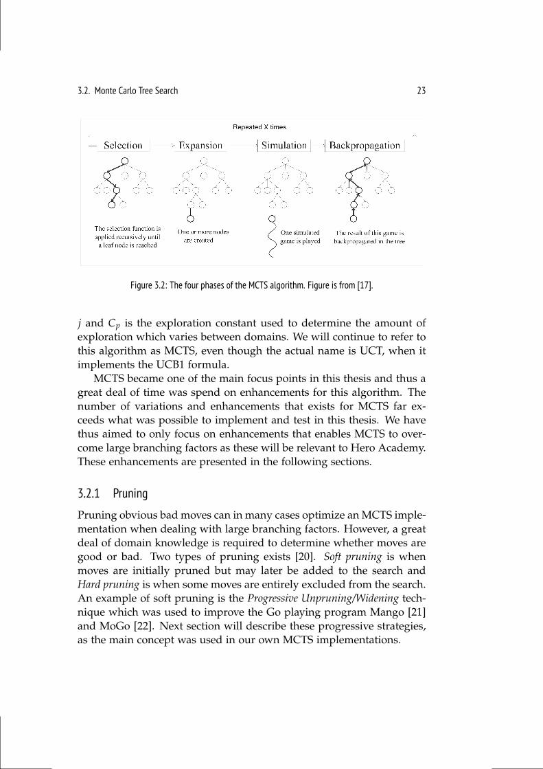
MCTS iteratively expands a search tree in the most urgent direction,where each iteration consists of four phases. These are depicted onFigure 3.2. In the Selection phase The most urgent node is recursivelyselected from the root using a tree policy until a terminal or unexpandednode is found. In the Expansion phase one or more children are addedif the selected node is non-terminal. In the Simulation phase a simulatedgame is played from an expanded node. This is also called a rollout.Simulations are carried out in a so called forward model that implementsthe rules of the environment. In the Backpropagation phase the result ofthe rollout is backpropagated in the tree and the value and visit countof each node are updated.
The tree policy is responsible for balancing exploration over exploita-tion. One solution would be to always expand the search in the direc-tion that gives the best values, but the search would then easily overseemore potent areas of the search space. The Upper Confidence Boundsfor Trees (UCT) algorithm solves this problem with the UCB1 formula[19]. When it has to select the most urgent node amongst the childrenof a node it tries to maximize:
UCB1 = X j + 2Cp
√2 ln n
nj
where X j is the average reward gained by visiting the child, n isthe visit count of the current node, nj is the visit count of the child
3.2. Monte Carlo Tree Search 23
Figure 3.2: The four phases of the MCTS algorithm. Figure is from [17].
j and Cp is the exploration constant used to determine the amount ofexploration which varies between domains. We will continue to refer tothis algorithm as MCTS, even though the actual name is UCT, when itimplements the UCB1 formula.
MCTS became one of the main focus points in this thesis and thus agreat deal of time was spend on enhancements for this algorithm. Thenumber of variations and enhancements that exists for MCTS far ex-ceeds what was possible to implement and test in this thesis. We havethus aimed to only focus on enhancements that enables MCTS to over-come large branching factors as these will be relevant to Hero Academy.These enhancements are presented in the following sections.
3.2.1 Pruning
Pruning obvious bad moves can in many cases optimize an MCTS imple-mentation when dealing with large branching factors. However, a greatdeal of domain knowledge is required to determine whether moves aregood or bad. Two types of pruning exists [20]. Soft pruning is whenmoves are initially pruned but may later be added to the search andHard pruning is when some moves are entirely excluded from the search.An example of soft pruning is the Progressive Unpruning/Widening tech-nique which was used to improve the Go playing program Mango [21]and MoGo [22]. Next section will describe these progressive strategies,as the main concept was used in our own MCTS implementations.
24 Chapter 3. Related work
3.2.2 Progressive Strategies
The concept of progressive strategies for MCTS was introduced by Chaslotet al. [21] as they described two of such strategies called progressivebias and progressive unpruning. With progressive bias the UCT selectionfunction (see the original in Section 3.2) is extended to the following:
UCB1pb = X j + 2Cp
√2 ln n
nj+ f (nj)
where f (nj) adds a heuristic value when nj is low. In this way heuris-tic knowledge is used to guide the search as long as the rollouts producea reliable result. Chaslot et al. chose f (nj) =
Hnj+1 where H is the heuris-
tic value of the game state j.The other progressive strategy is progressive unpruning, where a node’sbranches are first pruned using a heuristic and then later progressivelyunpruned as its visit count increases. A very similar approach intro-duced by Coulom called progressive widening was shown to improve theGo program Crazy Stone [23]. The two progressive strategies both indi-vidually improved the play of the Mango program in the game Go, butcombining both strategies produced the best result.
3.2.3 Domain Knowledge in Rollouts
The basic MCTS algorithm does not include any domain knowledgeother than its use of the forward model. Nijssen showed that usingpseudo random move generation in the rollouts could improve MCTSin Othello [24]. During rollouts moves were not selected uniformly butbetter moves, determined by a heuristic, were preferred and selectedmore often.
Another popular approach is to use ε-greedy rollouts that select thebest action determined by a heuristic with probability ε and otherwiseselect a random action. This heuristic can either be implemented man-ually or learned. ε-greedy rollouts was shown to improve MCTS in thegame Scotland Yard [25].
3.2.4 Transpositions
As for minimax, a transposition table can also improve the performanceof MCTS in some domains. If a game has a high number of transposi-
3.2. Monte Carlo Tree Search 25
tions, it is more likely that introducing a transposition table will increasethe playing strength of MCTS. Méhat et al. tested MCTS in single-playergames from the General Game Playing competition and showed thattransposition tables improved MCTS in some games while no improve-ment was observed in others [26].
Usually, the search tree in MCTS contains nodes which have di-rect references to their children. In order to handle transpositions inMCTS the search tree is often changed to also contain edges, since sev-eral nodes can have multiple parents [27]. This changes the tree into aDirected Acyclic Graph (DAG). During the expansion phase a node isonly created if it represents an unvisited game state. To save memoryand computation, game states are transformed into hash codes. A trans-position table is used where each entry holds the hash code of a gamestate and a reference to its node in the DAG. If the hash code of a newlyexplored game state already exists in the transposition table an edgeis simply created and pointed to the already existing node. In this wayidentical sub trees are ignored. Backpropagation is simple when dealingwith a tree but with a DAG several methods exist [27]. One method is toupdate the descent path only. This method is very simple to implementand is very similar to how back propagation is done in a tree.
3.2.5 Parallelization
Most devices today have multiple processor cores. Since AI techniquesoften require a high amount of computation, utilizing multiple proces-sors efficiently with parallelization can increase the playing strength sig-nificantly. MCTS can be parallelized in three different ways [28]:
Leaf parallelizationThis parallelization method is by far the simplest to implement. Ateach leaf multiple concurrent rollouts are performed. MCTS thusruns single-threaded in the selection, expansion and backpropa-gation phases but multi-threaded in the simulation phase. Thismethod simply improves the precision of evaluations and may beable to identify more promising moves faster.
Root parallelizationThis method builds multiple MCTS trees in parallel, that in the endare merged. Very little communication is needed between threads,which also makes this method simple to implement.
26 Chapter 3. Related work
Tree parallelizationAnother method is to use one shared tree, where several threadssimultaneously traverse and expand it. To enable access to thetree by multiple threads, mutaxes can be used as locks. A simplermethod called virtual loss adds a high number of losses to a nodein use, so no other threads will go in that direction.
Chaslot et al. compared these three methods in 13x13 Go and used astrength-speedup measure to express how much improvement each meth-ods added [28]. All their experiments were performed using 16 proces-sor cores. A strength-speedup measure of 2.0 means that the paral-lelization method plays as well as a non-parellelized method with dou-ble as much computation time. The leaf parallelization method wasthe weakest with a strength-speedup of only 2.4, while root paralleliza-tion gained a strength-speedup of 14.9. Tree parallelization gained astrength-speedup of 8.5 and remains the most complicated of the threemethods to implement.
3.2.6 Determinization
In stochastic games, and games with hidden information, MCTS canuse determinization to transform a game state into a deterministic onewith open information. Another more naive approach would simply beto create a new node for each possible outcome due to randomness orhidden information, but this will often result in extremely large trees.Cazenave used determinization for MCTS in the game Phantom Go [29],which is a version of Go with hidden stones, by guessing the positionsof the opponent stones before each rollout.
3.2.7 Large Branching Factors
MCTS has been successful in many other games than Go. Amazons isa game with a branching factor above 1,000 during the 10 first movesin the game. Using depth-limited rollouts with an evaluation function,among other improvements, Kloetzer was able to show that MCTS out-performs traditional minimax-based programs in this game [30].
Kozelek applied MCTS to the game Arimaa but only achieved a weaklevel of play [31]. Arimaa is a very interesting game as it allows playersto make four consecutive moves in the same way as in Hero Academy.
3.2. Monte Carlo Tree Search 27
The branching factor of Arimaa was calculated to be 17,281 by Haskin2,which is very high compared to single-turn games but still a lot lowerthan the 7.78× 10⁸ in Hero Academy (estimated in Section 2.3.2). Oneimportant difference between Arimaa and Hero Academy is that piecesin Arimaa never get eliminated, which makes it extremely difficult toevaluate positions. Hero Academy is in contrast more like Chess asboth material and positional evaluations can be made. Kozelek showedthat short rollouts with a static evaluation function improved MCTS inArimaa. Transposition tables were also shown to improve the playingstrength significantly, while Rapid Action Value Estimation (RAVE), anenhancement often used in Go, did not.
Kozelek distinguished between a step-based and a move-basedsearch. In a step-based search each ply in the search tree correspondsto moving one piece one time, where one ply in a move-based searchcorresponds to a sequence of steps resulting in one turn. Kozelek pre-ferred the step-based search mainly because of its simplicity and how itwith ease can handle transpositions within turns. Interestingly, a move-based search was used by Churchill et al. [32] and later Justesen et al.[1] in the RTS game StarCraft to overcome the large branching factor.The move-based searches in StarCraft is done by sampling a very lownumber of possible moves and thus ignoring most of the search space.Often heuristic strategies are among the samples of moves together withrandomly generated moves. In Arimaa it is difficult to generate suchheuristic strategies, and thus the move-based approach is likely to beweak in this game. It seems to be a necessity in StarCraft to use themove-based approach, since the search must find a solution within just40 milliseconds, and in this game we do know several heuristic strate-gies. The move-based search would simply ignore very important movesin Arimaa that the step-based search is more likely to find. While nocomparison of these approaches in either of the games exist, it seemsthat the step-based approach is unlikely to succeed in real-time gameswith very large branching factors. The branching factor of combats inStarCraft is around 8n, where n is the number of units under control,which easily surpasses the branching factor of Arimaa.
2http://arimaa.janzert.com/bf_study/
28 Chapter 3. Related work
3.3 Artificial Neural Networks
We have now looked at two methods for searching in the game treeand one more will be introduced when evolutionary computation isintroduced later. It seems clear, that good methods for evaluating gamestates is an important asset to the search algorithms, as dept-limitedsearches are popular in games with large branching factors. Creatingan evaluation function for Hero Academy seems straight forward sincematerial on the board, on the hand and in the deck is easy to count.The positional value of units, and how to balance the pursuit towardsthe two winning conditions in the game (destroying all units or allcrystals), are however two very difficult challenges. Instead of relyingon expert knowledge and a programmers ability to implement this,such evaluation functions can be learned, and one method to store suchlearned knowledge is in artificial neural networks or just neural networks.Before explaining how the such knowledge can be learned, let us look awhat neural networks are.
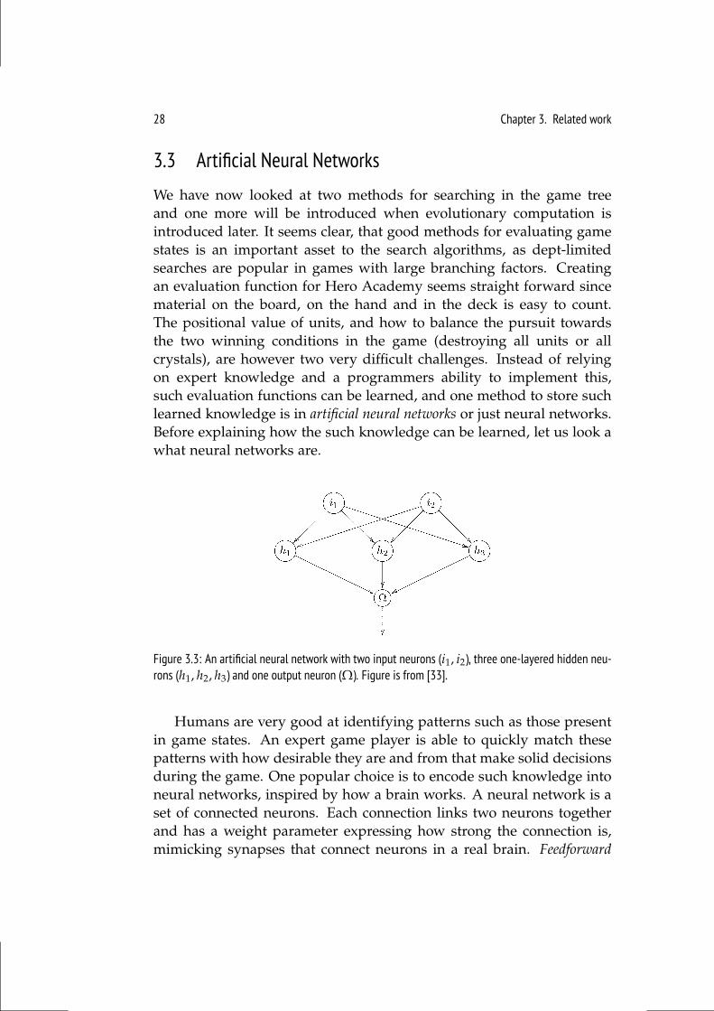
Figure 3.3: An artificial neural network with two input neurons (i1, i2), three one-layered hidden neu-rons (h1, h2, h3) and one output neuron (Ω). Figure is from [33].
Humans are very good at identifying patterns such as those presentin game states. An expert game player is able to quickly match thesepatterns with how desirable they are and from that make solid decisionsduring the game. One popular choice is to encode such knowledge intoneural networks, inspired by how a brain works. A neural network is aset of connected neurons. Each connection links two neurons togetherand has a weight parameter expressing how strong the connection is,mimicking synapses that connect neurons in a real brain. Feedforward
3.3. Artificial Neural Networks 29
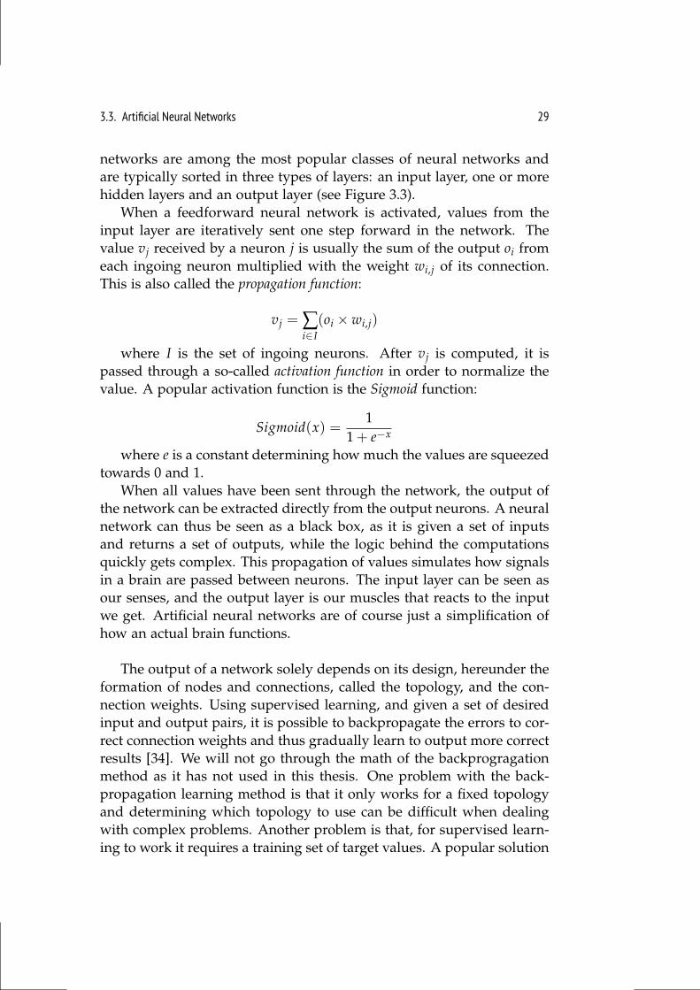
networks are among the most popular classes of neural networks andare typically sorted in three types of layers: an input layer, one or morehidden layers and an output layer (see Figure 3.3).
When a feedforward neural network is activated, values from theinput layer are iteratively sent one step forward in the network. Thevalue vj received by a neuron j is usually the sum of the output oi fromeach ingoing neuron multiplied with the weight wi,j of its connection.This is also called the propagation function:
vj = ∑i∈I
(oi × wi,j)
where I is the set of ingoing neurons. After vj is computed, it ispassed through a so-called activation function in order to normalize thevalue. A popular activation function is the Sigmoid function:
Sigmoid(x) =1
1 + e−x
where e is a constant determining how much the values are squeezedtowards 0 and 1.
When all values have been sent through the network, the output ofthe network can be extracted directly from the output neurons. A neuralnetwork can thus be seen as a black box, as it is given a set of inputsand returns a set of outputs, while the logic behind the computationsquickly gets complex. This propagation of values simulates how signalsin a brain are passed between neurons. The input layer can be seen asour senses, and the output layer is our muscles that reacts to the inputwe get. Artificial neural networks are of course just a simplification ofhow an actual brain functions.
The output of a network solely depends on its design, hereunder theformation of nodes and connections, called the topology, and the con-nection weights. Using supervised learning, and given a set of desiredinput and output pairs, it is possible to backpropagate the errors to cor-rect connection weights and thus gradually learn to output more correctresults [34]. We will not go through the math of the backprogragationmethod as it has not used in this thesis. One problem with the back-propagation learning method is that it only works for a fixed topologyand determining which topology to use can be difficult when dealingwith complex problems. Another problem is that, for supervised learn-ing to work it requires a training set of target values. A popular solution
30 Chapter 3. Related work
is to evolve both the weights and the topology through evolution whichwill be described in the section about neuroevolution (see Section 3.4.3),where examples of successful applications also are presented. To un-derstand neuroevolution, let us first get an overview of the mechanicsand use of evolution in algorithms, as this is a widely used approach ingame AI.
3.4 Evolutionary Computation
Evolutionary computation is concerned with optimization algorithmsinspired by the mechanisms of biological evolution such as geneticcrossover, mutation and the notion survival of the fittest. The most pop-ular of these algorithms are Genetic Algorithms (GA) first described byHolland [35]. In GAs a population of candidate solutions are initiallycreated. Each solution, also called the phenotype, has a correspondingencoding called a genotype. In order to optimize the population of so-lutions it goes through a number of generations, where each individualis tested using a fitness function. The least fit individuals are replacedby offspring of the most fit. Offspring are bred using crossover and/ormutation. In this way promising genes from fit individuals stay in thepopulation, while genes from bad individuals are thrown away. Likeevolution in nature, the goal is to evolve individuals consisting of genesthat make them strong in their environment. Such an environment canbe a game and the the solution can be a strategy or a neural networkfunctioning as a heuristic.
3.4.1 Parallelization
Three different methods for parallelizing GAs were identified byTomassini et al. [36] and are briefly presented in this section. In mostGA implementations, calculating the fitness function is the most timeconsuming part, and thus an obvious solution is to run the fitness func-tion concurrently for multiple individuals. Another simple method isto run several isolated GAs in parallel, either with the same or differentconfigurations. GAs can easily end up in a local optima and by run-ning multiple of these concurrently, there is a higher change of findingeither the global optima or at least several local ones. In the island modelmultiple isolated populations are evolved in parallel, but at a certainfrequency promising individuals will migrate to other populations to
3.4. Evolutionary Computation 31
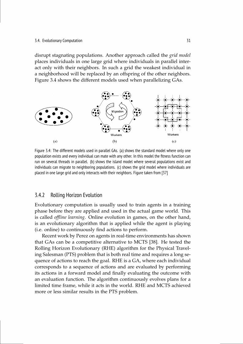
disrupt stagnating populations. Another approach called the grid modelplaces individuals in one large grid where individuals in parallel inter-act only with their neighbors. In such a grid the weakest individual ina neighborhood will be replaced by an offspring of the other neighbors.Figure 3.4 shows the different models used when parallelizing GAs.
Figure 3.4: The different models used in parallel GAs. (a) shows the standard model where only onepopulation exists and every individual can mate with any other. In this model the fitness function canrun on several threads in parallel. (b) shows the island model where several populations exist andindividuals can migrate to neighboring populations. (c) shows the grid model where individuals areplaced in one large grid and only interacts with their neighbors. Figure taken from [37]
3.4.2 Rolling Horizon Evolution
Evolutionary computation is usually used to train agents in a trainingphase before they are applied and used in the actual game world. Thisis called offline learning. Online evolution in games, on the other hand,is an evolutionary algorithm that is applied while the agent is playing(i.e. online) to continuously find actions to perform.
Recent work by Perez on agents in real-time environments has shownthat GAs can be a competitive alternative to MCTS [38]. He tested theRolling Horizon Evolutionary (RHE) algorithm for the Physical Travel-ing Salesman (PTS) problem that is both real time and requires a long se-quence of actions to reach the goal. RHE is a GA, where each individualcorresponds to a sequence of actions and are evaluated by performingits actions in a forward model and finally evaluating the outcome withan evaluation function. The algorithm continuously evolves plans for alimited time frame, while it acts in the world. RHE and MCTS achievedmore or less similar results in the PTS problem.
32 Chapter 3. Related work
This approach is of course interesting since Hero Academy is allabout planning several actions ahead and may be an interesting alter-native to MCTS. There is, however, the difference that Hero Academy isadversarial, i.e. each player takes turn, where the PST problem is a singleplayer environment where every outcome in the future is predictable. InHero Academy we are not able to evolve actions for the opponent, sincewe only have full control in our own turn, and the evolution is thenlimited to plan five actions ahead.
3.4.3 Neuroevolution
Earlier in Section 3.3 we mentioned how neural networks can be used asa heuristic, i.e. a game state evaluation function. One way to train sucha network is to use supervised learning by backpropagating errors, butfor this approach we need a large training set e.g. created from gameslogs with human players. Since Hero Academy is played online thedevelopers should have access to such game logs, while we do not.Several unsupervised learning methods exist where learning happensby interacting with the environment. Temporal Difference (TD) learningis a popular choice when it comes to unsupervised learning and wasused with success in 1959 by Samuel in his Checkers-playing program[39]. Samuel’s program used a database of visited game states usedto store the learned knowledge, while this is impractical for gameswith a high state-space complexity. Tesauro solved this problem inhis famous Backgammon-playing program TD-Gammon that reached asuper-human level [40] by using the TD(λ) algorithm to train a neuralnetwork. TD(λ) backpropagates results of played games through thenetwork for each action taken in the game and gradually corrects theweights. The λ parameter is used to make sure that early moves inthe game are less responsible for the outcome, while later moves aremore. The topology must however still be determined manually whenapplying TD(λ). In the rest of this section the focus will be on methodsthat also evolves the topology.
Neuroevolution is a machine learning method combining neural net-works and evolutionary algorithms and has shown to be effective inmany domains. The conventional neuroevolution method has simplybeen to maintain a fixed topology and evolve only the weights of theconnections. Chellapilla et al. used such an approach to evolve the
3.4. Evolutionary Computation 33
weights of a neural network, that was able to compete with expert play-ers in Checkers [41]. Chellapilla evolved a feedforward network with 32input neurons, 40 neurons in the first hidden layer and 10 neurons inthe second hidden layer.
An early attempt to evolve topologies as well as weights are themarker-based encoding scheme which, inspired by our DNA, has a se-ries of numeric genes representing nodes and connections. The marker-based encoding seems to have been replaced by superior approachesdeveloped later. Moriarty and Miikkulainen was, however, able to dis-cover complex strategies for the game Othello using the marker-basedencoding scheme [42]. Their game playing networks had 64 output neu-rons each expressing how strongly a move to that corresponding squareis considered. Othello is played on a 8x8 game board similar to Chess.
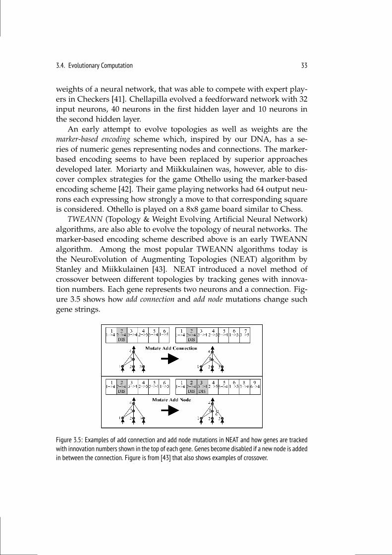
TWEANN (Topology & Weight Evolving Artificial Neural Network)algorithms, are also able to evolve the topology of neural networks. Themarker-based encoding scheme described above is an early TWEANNalgorithm. Among the most popular TWEANN algorithms today isthe NeuroEvolution of Augmenting Topologies (NEAT) algorithm byStanley and Miikkulainen [43]. NEAT introduced a novel method ofcrossover between different topologies by tracking genes with innova-tion numbers. Each gene represents two neurons and a connection. Fig-ure 3.5 shows how add connection and add node mutations change suchgene strings.
Figure 3.5: Examples of add connection and add node mutations in NEAT and how genes are trackedwith innovation numbers shown in the top of each gene. Genes become disabled if a new node is addedin between the connection. Figure is from [43] that also shows examples of crossover.
34 Chapter 3. Related work
The use of innovation numbers also made crossover very simple assingle or multi-point crossover easily can be applied to the genes.When new topologies appear in a population they very rarely achievea high fitness value, as they often need several generations to improvetheir weights and perhaps change their topology further. To protectsuch innovations from being excluded from the population, NEAT in-troduces speciation. Organisms in NEAT primarily compete for survivalwith other organisms of the same specie and not with the entire popula-tion. Another feature of NEAT, called complexification, is that organismsare initialised uniformly without any hidden neurons and then slowlygrow and become more complex. The idea behind this is to only grownetworks if the addition actually provides an improvement. NEAThas been successful in many real-time games such as Pac-Man [44]and The Open Racing Car Simulator (TORCS) [45]. Jacobs comparedseveral neuroevolution algorithms for Othello and was most successfulwith NEAT [46], which also was the only TWEANN algorithms in thecomparison.
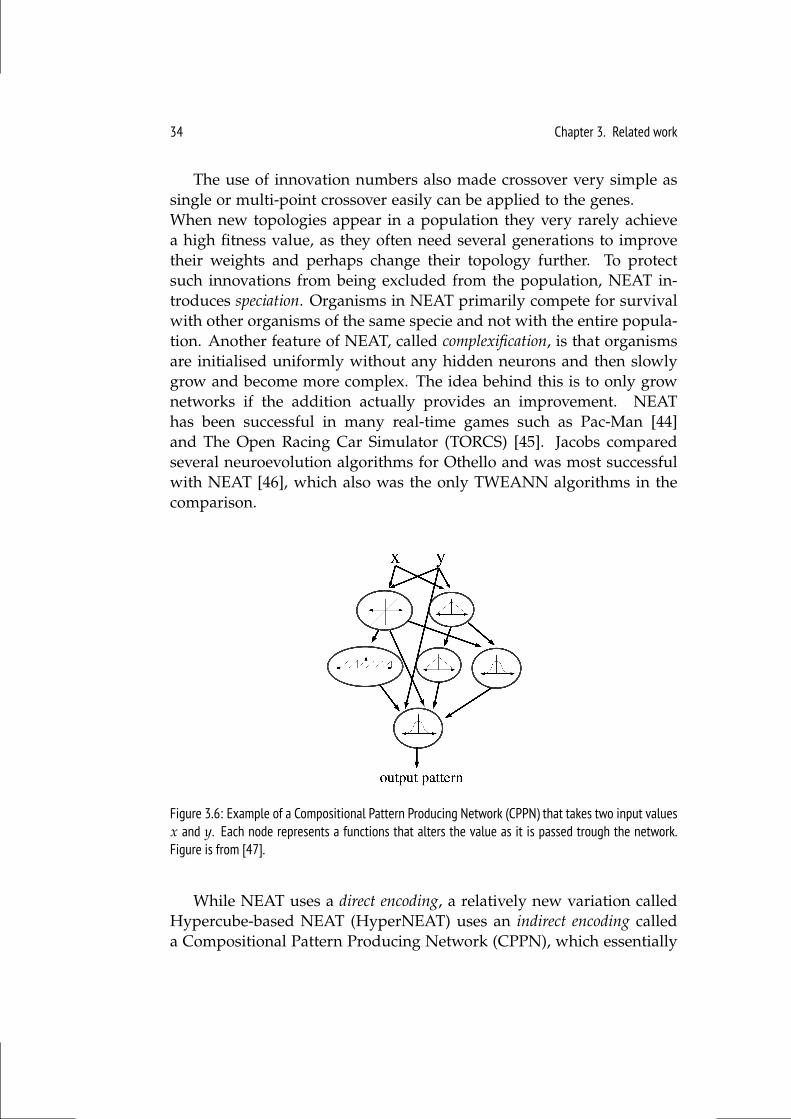
Figure 3.6: Example of a Compositional Pattern Producing Network (CPPN) that takes two input valuesx and y. Each node represents a functions that alters the value as it is passed trough the network.Figure is from [47].
While NEAT uses a direct encoding, a relatively new variation calledHypercube-based NEAT (HyperNEAT) uses an indirect encoding calleda Compositional Pattern Producing Network (CPPN), which essentially
3.4. Evolutionary Computation 35
is a network of connected functions. An example of a CPPN is shownon Figure 3.6. In HyperNEAT it is thus the CPPNs that are evolvedwhich is then used to distribute the weights to a fixed network topology.The input layers forms a two-dimensional plane and thus becomes di-mensionally aware. This feature is advantages when it comes to imagerecognition as neighboring pixels of an image are highly related to eachother. Risi and Togelius argues that this dimensional awareness can beused to learn the symmetries and relationships on a game board [48],but to our knowledge only few attempts have been made and withlimited success.
Recent work on evolving game playing agents with neuroevolutionfor Atari games have shown, that NEAT was the superior of severalcompared methods, and it was even able to beat human scores in threeof the games [11]. The networks were fed with three layers of input.One with the raw pixel data, another with object data and the one withrandom noise. The HyperNEAT method was however shown to be theonly useful method when only the raw pixel layer was used.

Chapter 4
Approach
This chapter will explain our approach of implementing several AIagents for Hero Academy using the theory from the previous chapter.This have resulted in agents with very diverse behaviors. This chapterwill first describe some main functionalities that were used the agentsfollowed by a description of their implementation and enhancements.
4.1 Action Pruning & Sorting
The Hero AIcademy API offers the method possibleActions(a:List<Action>) that fills the given list with all available actions ofthe current game state. This method simply iterates each card on thehand and each unit on the game board and collects all possible actionsfor the given card or unit. Several actions in this set will produce thesame outcome and can thus be pruned. A pruning method were im-plemented that removes some of these actions and thus performs hardpruning.
First, identical swap card actions are pruned, which are seen whenseveral identical cards are on the hand. Next, a cast spell action ispruned if another cast spell action exists that can hit the same units.E.g. a cast spell action that targets the wizard on square (1,1) and thearcher on (2,1) can be pruned, when another cast spell action exists thatcan hit both the wizard, the archer and the knight on (2,2). The targetsof the second action is thus a super set of the targets of the first. It is notguaranteed that the most optimal action survives this pruning, but it isa good estimate as it is based on both the amount of damage it inflictsand which units it can target. If a cast spell action has no targets on the
38 Chapter 4. Approach
game board, it is also pruned.
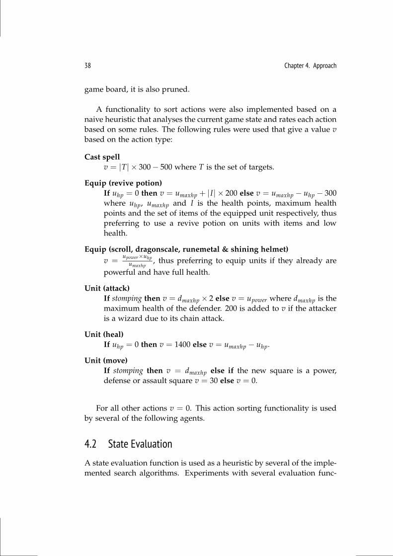
A functionality to sort actions were also implemented based on anaive heuristic that analyses the current game state and rates each actionbased on some rules. The following rules were used that give a value vbased on the action type:
Cast spellv = |T| × 300− 500 where T is the set of targets.
Equip (revive potion)If uhp = 0 then v = umaxhp + |I| × 200 else v = umaxhp − uhp − 300where uhp, umaxhp and I is the health points, maximum healthpoints and the set of items of the equipped unit respectively, thuspreferring to use a revive potion on units with items and lowhealth.
Equip (scroll, dragonscale, runemetal & shining helmet)v =
upower×uhpumaxhp
, thus preferring to equip units if they already arepowerful and have full health.
Unit (attack)If stomping then v = dmaxhp × 2 else v = upower where dmaxhp is themaximum health of the defender. 200 is added to v if the attackeris a wizard due to its chain attack.
Unit (heal)If uhp = 0 then v = 1400 else v = umaxhp − uhp.
Unit (move)If stomping then v = dmaxhp else if the new square is a power,defense or assault square v = 30 else v = 0.
For all other actions v = 0. This action sorting functionality is usedby several of the following agents.
4.2 State Evaluation
A state evaluation function is used as a heuristic by several of the imple-mented search algorithms. Experiments with several evaluation func-
4.2. State Evaluation 39
tions were performed, but one with a great amount of domain knowl-edge showed the best results throughout the experiments. This evalua-tion function named HeuristicEvaluation in the project source code willbe described in this section.
The value of a game state is measured by the difference in healthpoints of remaining units both on the hand, in the deck and on thegame board by each player. The health point value of a unit is howevermultiplied by several factors. The final value v of a unit u on the gameboard is:
v = uhp + umaxhp × up(u)︸ ︷︷ ︸standing bonus
+
equipment bonus︷ ︸︸ ︷eq(u)× up(u) + sq(u)× (up(u)− 1)︸ ︷︷ ︸
square bonuse
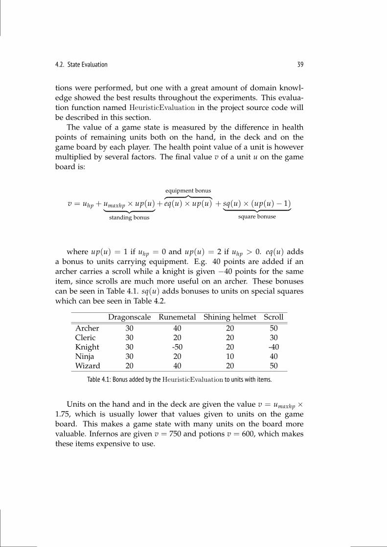
where up(u) = 1 if uhp = 0 and up(u) = 2 if uhp > 0. eq(u) addsa bonus to units carrying equipment. E.g. 40 points are added if anarcher carries a scroll while a knight is given −40 points for the sameitem, since scrolls are much more useful on an archer. These bonusescan be seen in Table 4.1. sq(u) adds bonuses to units on special squareswhich can bee seen in Table 4.2.
Dragonscale Runemetal Shining helmet ScrollArcher 30 40 20 50Cleric 30 20 20 30Knight 30 -50 20 -40Ninja 30 20 10 40Wizard 20 40 20 50
Table 4.1: Bonus added by theHeuristicEvaluation to units with items.
Units on the hand and in the deck are given the value v = umaxhp ×1.75, which is usually lower that values given to units on the gameboard. This makes a game state with many units on the board morevaluable. Infernos are given v = 750 and potions v = 600, which makesthese items expensive to use.
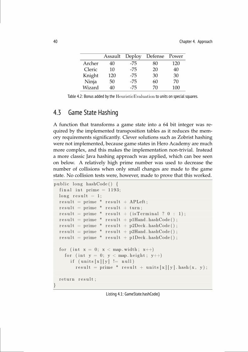
40 Chapter 4. Approach
Assault Deploy Defense PowerArcher 40 -75 80 120Cleric 10 -75 20 40Knight 120 -75 30 30Ninja 50 -75 60 70
Wizard 40 -75 70 100
Table 4.2: Bonus added by theHeuristicEvaluation to units on special squares.
4.3 Game State Hashing
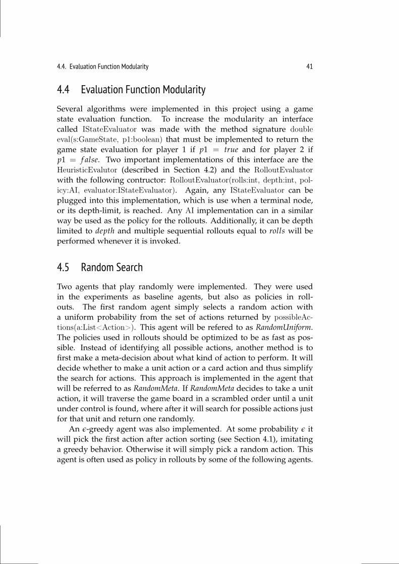
A function that transforms a game state into a 64 bit integer was re-quired by the implemented transposition tables as it reduces the mem-ory requirements significantly. Clever solutions such as Zobrist hashingwere not implemented, because game states in Hero Academy are muchmore complex, and this makes the implementation non-trivial. Insteada more classic Java hashing approach was applied, which can bee seenon below. A relatively high prime number was used to decrease thenumber of collisions when only small changes are made to the gamestate. No collision tests were, however, made to prove that this worked.
pub l i c long hashCode ( ) f i n a l i n t prime = 1193 ;long r e s u l t = 1 ;r e s u l t = prime * r e s u l t + APLeft ;r e s u l t = prime * r e s u l t + turn ;r e s u l t = prime * r e s u l t + ( i sTermina l ? 0 : 1) ;r e s u l t = prime * r e s u l t + p1Hand . hashCode ( ) ;r e s u l t = prime * r e s u l t + p2Deck . hashCode ( ) ;r e s u l t = prime * r e s u l t + p2Hand . hashCode ( ) ;r e s u l t = prime * r e s u l t + p1Deck . hashCode ( ) ;
f o r ( i n t x = 0 ; x < map . width ; x++)f o r ( i n t y = 0 ; y < map . he ight ; y++)
i f ( un i t s [ x ] [ y ] != nu l l )r e s u l t = prime * r e s u l t + un i t s [ x ] [ y ] . hash (x , y ) ;
r e turn r e s u l t ;
Listing 4.1: GameState.hashCode()
4.4. Evaluation Function Modularity 41
4.4 Evaluation Function Modularity
Several algorithms were implemented in this project using a gamestate evaluation function. To increase the modularity an interfacecalled IStateEvaluator was made with the method signature doubleeval(s:GameState, p1:boolean) that must be implemented to return thegame state evaluation for player 1 if p1 = true and for player 2 ifp1 = f alse. Two important implementations of this interface are theHeuristicEvalutor (described in Section 4.2) and the RolloutEvaluatorwith the following contructor: RolloutEvaluator(rolls:int, depth:int, pol-icy:AI, evaluator:IStateEvaluator). Again, any IStateEvaluator can beplugged into this implementation, which is use when a terminal node,or its depth-limit, is reached. Any AI implementation can in a similarway be used as the policy for the rollouts. Additionally, it can be depthlimited to depth and multiple sequential rollouts equal to rolls will beperformed whenever it is invoked.
4.5 Random Search
Two agents that play randomly were implemented. They were usedin the experiments as baseline agents, but also as policies in roll-outs. The first random agent simply selects a random action witha uniform probability from the set of actions returned by possibleAc-tions(a:List<Action>). This agent will be refered to as RandomUniform.The policies used in rollouts should be optimized to be as fast as pos-sible. Instead of identifying all possible actions, another method is tofirst make a meta-decision about what kind of action to perform. It willdecide whether to make a unit action or a card action and thus simplifythe search for actions. This approach is implemented in the agent thatwill be referred to as RandomMeta. If RandomMeta decides to take a unitaction, it will traverse the game board in a scrambled order until a unitunder control is found, where after it will search for possible actions justfor that unit and return one randomly.
An ε-greedy agent was also implemented. At some probability ε itwill pick the first action after action sorting (see Section 4.1), imitatinga greedy behavior. Otherwise it will simply pick a random action. Thisagent is often used as policy in rollouts by some of the following agents.
42 Chapter 4. Approach
4.6 Greedy Search
Greedy algorithms always take the action that gives the best immediateoutcome. Two different greedy algorithms were implemented which aredescribed in this section.
4.6.1 Greedy on Action Level
GreedyAction is a simple greedy agent that makes a one-ply search,where one ply corresponds to one action, and uses the HeuristicEval-utor as a heuristic. It also makes use of action pruning to avoid baduse of the inferno card. The Hero AIcademy engine is used as a for-ward model to obtain the resulting game states. GreedyAction is used asa baseline agent in the experiments and will be compared to the morecomplex implementations.
4.6.2 Greedy on Turn Level
GreedyTurn is a more complex greedy agent that makes a five-ply searchwhich corresponds to one turn of five actions. The search algorithmused is a recursive depth-first search very similar to minimax and willalso produce the exact same results, given the same depth-limit. Duringthis search, the best action sequence is stored together with the heuristicvalue of the resulting game state. The stored action sequence will bereturned when the search is over. This agent will find the most optimalsequence of actions during its turn, assuming the heuristic leads to op-timal play. Since the heuristic used is mostly based on the health pointdifference between the two players, it will most likely lead to a veryaggressive play. It will, however, not be able to search the entire spaceof actions within the six second time budget we have given the agentsin the experiments. In Section 2.3.2 we estimated the average branchingfactor of a turn to be 7.78× 10⁸ which is the average number of movesthis search will have to consider to make an exhaustive search. Threeefforts were made to optimize the performance of the search: actionpruning is applied at every node of the search, a transposition table isused as well as a simple parallelization method.
A transposition table was implemented to reduce the size of thesearch tree. The key of each entry is the hash code of a game state. Thevalue of each entry is actually never used since already visited nodesare simply ignored.
4.7. Monte Carlo Tree Search 43
Parallelization was implemented by first sorting the actions availableat the root level and then assigning them one by one to a number ofthreads equal to the number of processors. Each thread is then respon-sible for calculating the value of the assigned action. The threads use thesame shared transposition table that can only be accessed by one threadat the time.
In order to make this search an anytime algorithm, threads are simplydenied access to more actions when the time budget is used and the bestfound action sequence is finally returned.
4.7 Monte Carlo Tree Search
The MCTS algorithm was implemented with an action based approach,meaning that one ply in the search tree corresponds to one action andnot one turn. The search tree thus has to reach a depth of five to reachthe beginning of the opponents turn. The search tree is constructedusing both node and edge objects to handle parallelization methods.Both nodes and edges have a visit count, while only edges hold values.Action pruning and sorting are applied at every expansion in the tree,and only one child are added in each expansion phase. A child nodewill not be selected until all its siblings are added. The UCB1 formulawere changed to the following to handle nodes and edges:
UCB1edges = X j + 2Cp
√2 ln n
ej
where ej is now the visit count of the edge e, going from node n,instead of the child node. For the backpropagation the descent-pathonly approach was used because of its simplicity. In order to handletwo players with multiple actions, the backpropagation implements anextension of the BackupNegamax method (see Algorithm 1). This back-propagation algorithm is called with a list of edges corresponding tothe traversal during the selection phase, a ∆ value corresponding to theresult of the simulation phase and a boolean p1 which is true if playerone is the max player and false if not.
A transposition table was added to MCTS with game state hashcodes as keys and references to nodes as values. When an already
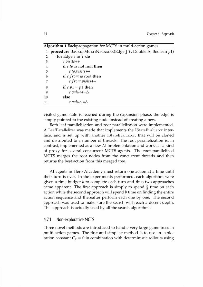
44 Chapter 4. Approach
Algorithm 1 Backpropagation for MCTS in multi-action games1: procedure BackupMultiNegamax(Edge[] T, Double ∆, Boolean p1)2: for Edge e in T do3: e.visits++4: if e.to is not null then5: e.to.visits++6: if e. f rom is root then7: e. f rom.visits++8: if e.p1 = p1 then9: e.value+=∆
10: else11: e.value-=∆
visited game state is reached during the expansion phase, the edge issimply pointed to the existing node instead of creating a new.
Both leaf parallelization and root parallelizaion were implemented.A LeafParallelizer was made that implements the IStateEvaluator inter-face, and is set up with another IStateEvaluator, that will be clonedand distributed to a number of threads. The root parallelization is, incontrast, implemented as a new AI implementation and works as a kindof proxy for several concurrent MCTS agents. The root parallelizedMCTS merges the root nodes from the concurrent threads and thenreturns the best action from this merged tree.
AI agents in Hero AIcademy must return one action at a time untiltheir turn is over. In the experiments performed, each algorithm weregiven a time budget b to complete each turn and thus two approachescame apparent. The first approach is simply to spend b
5 time on eachaction while the second approach will spend b time on finding the entireaction sequence and thereafter perform each one by one. The secondapproach was used to make sure the search will reach a decent depth.This approach is actually used by all the search algorithms.
4.7.1 Non-explorative MCTS
Three novel methods are introduced to handle very large game trees inmulti-action games. The first and simplest method is to use an explo-ration constant Cp = 0 in combination with deterministic rollouts using
4.7. Monte Carlo Tree Search 45
a greedy heuristic as policy. It might seem irrational not to do any explo-ration at all, but since all children are expanded and evaluated at leastonce, a very controlled and limited form of exploration will occur. Addi-tionally, as the search progresses into the opponents turn, counter-movesmay be found that will force the search to explore other directions. Theidea is thus to only explore when promising moves become less promis-ing. A non-explorative MCTS is not guaranteed to converge towardsthe optimal solution, but instead tries to find just one good move thatthe opponent cannot counter. The idea of using deterministic rolloutsguided by a greedy heuristic, might be necessary when no explorationhappens, since most nodes are visited only once. It would have a hugeimpact if an action is given a low value due to one unlucky simulation.
4.7.2 Cutting MCTS
Because of the enormous search space, MCTS will have trouble reachinga depth of ten plies during its search. This is critical since actions willbe selected based on vague knowledge about the possible counter-movesby the opponent, that takes place between ply five and ten. To increasethe depth in the most promising direction, a progressive pruning strategycalled cutting is introduced. The cutting strategy will remove all but themost promising child c from the tree after b
a time has past, where b isthe time budget and a is the number of actions allowed in the turn (fivein Hero Academy). When 2× ( b
a ) time has past all but the most promis-ing child of c are removed from the tree. This is done continuously atimes down the tree. The downside of this cutting strategy is that thereis no going back when actions have been cut. This can lead to an ac-tion sequence in Hero Academy that will make a unit charge towardsan opponent and then retreat back again in the same turn. This shouldhowever be much better than charging forward to leave a unit unpro-tected as a result of insufficient search for counter-moves. An exampleof the cutting approach in three steps is shown on Figure 4.1.
4.7.3 Collapsing MCTS
Another progressive pruning strategy that deals with the enormoussearch space in multi-action games is introduced called the collapsingstrategy. When a satisfying number of nodes K are found at depth d,where d is equal to the number of actions in a turn, the tree is collapsed
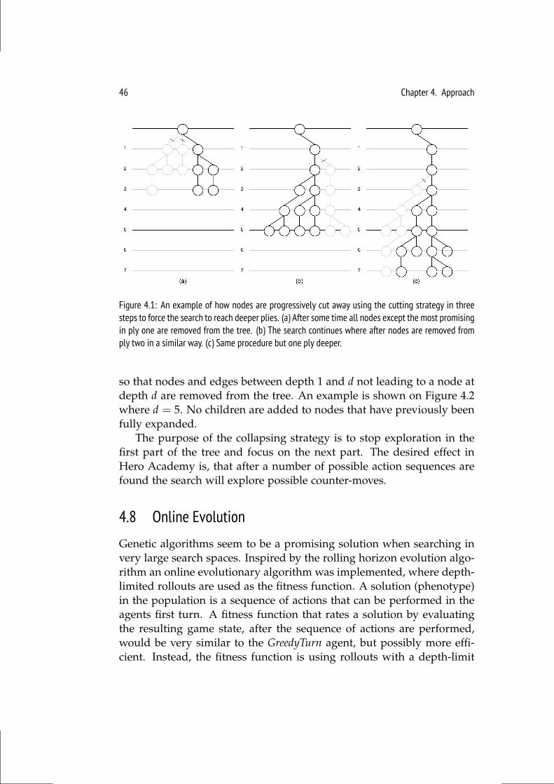
46 Chapter 4. Approach
Figure 4.1: An example of how nodes are progressively cut away using the cutting strategy in threesteps to force the search to reach deeper plies. (a) After some time all nodes except the most promisingin ply one are removed from the tree. (b) The search continues where after nodes are removed fromply two in a similar way. (c) Same procedure but one ply deeper.
so that nodes and edges between depth 1 and d not leading to a node atdepth d are removed from the tree. An example is shown on Figure 4.2where d = 5. No children are added to nodes that have previously beenfully expanded.
The purpose of the collapsing strategy is to stop exploration in thefirst part of the tree and focus on the next part. The desired effect inHero Academy is, that after a number of possible action sequences arefound the search will explore possible counter-moves.
4.8 Online Evolution
Genetic algorithms seem to be a promising solution when searching invery large search spaces. Inspired by the rolling horizon evolution algo-rithm an online evolutionary algorithm was implemented, where depth-limited rollouts are used as the fitness function. A solution (phenotype)in the population is a sequence of actions that can be performed in theagents first turn. A fitness function that rates a solution by evaluatingthe resulting game state, after the sequence of actions are performed,would be very similar to the GreedyTurn agent, but possibly more effi-cient. Instead, the fitness function is using rollouts with a depth-limit
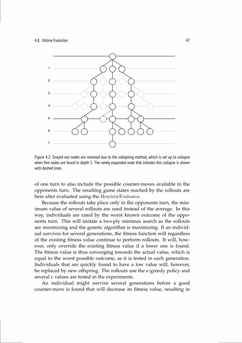
4.8. Online Evolution 47
Figure 4.2: Grayed out nodes are removed due to the collapsing method, which is set up to collapsewhen five nodes are found in depth 5. The newly expanded node that initiates this collapse is shownwith dashed lines.
of one turn to also include the possible counter-moves available in theopponents turn. The resulting game states reached by the rollouts arehere after evaluated using the HeuristicEvaluator.
Because the rollouts take place only in the opponents turn, the min-imum value of several rollouts are used instead of the average. In thisway, individuals are rated by the worst known outcome of the oppo-nents turn. This will imitate a two-ply minimax search as the rolloutsare minimizing and the genetic algorithm is maximizing. If an individ-ual survives for several generations, the fitness function will regardlessof the existing fitness value continue to perform rollouts. It will, how-ever, only override the existing fitness value if a lower one is found.The fitness value is thus converging towards the actual value, which isequal to the worst possible outcome, as it is tested in each generation.Individuals that are quickly found to have a low value will, however,be replaced by new offspring. The rollouts use the ε-greedy policy andseveral ε values are tested in the experiments.
An individual might survive several generations before a goodcounter-move is found that will decrease its fitness value, resulting in
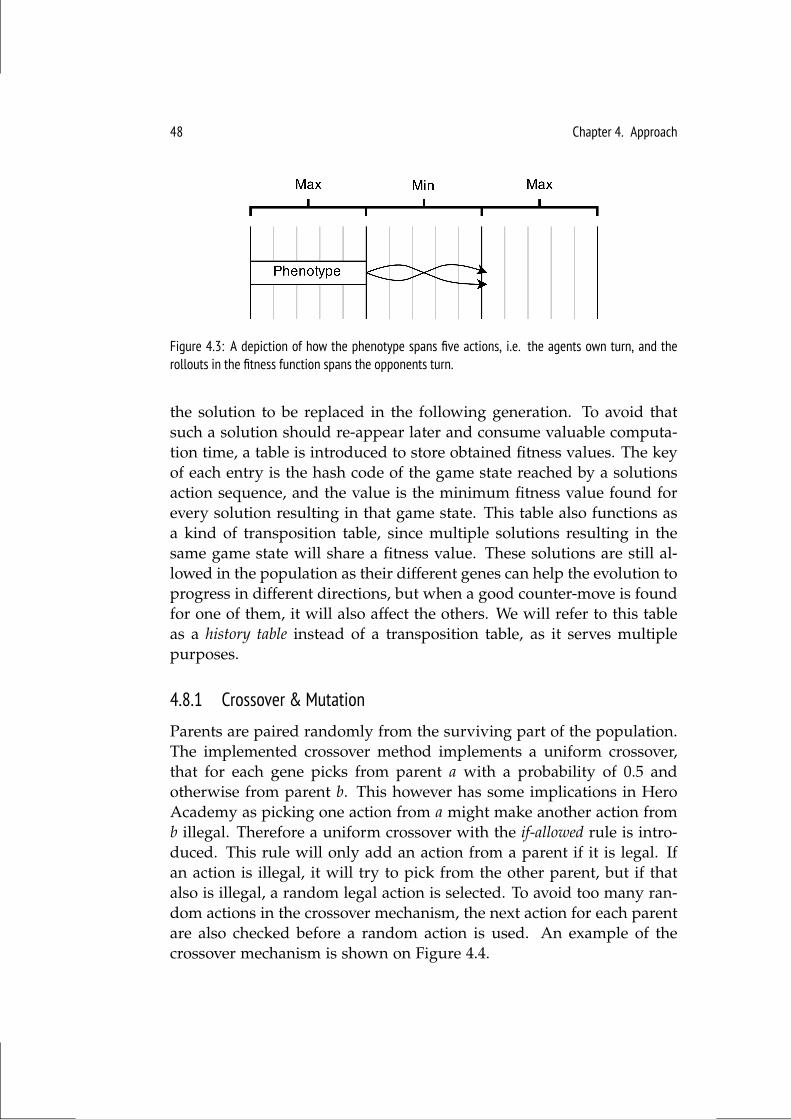
48 Chapter 4. Approach
Figure 4.3: A depiction of how the phenotype spans five actions, i.e. the agents own turn, and therollouts in the fitness function spans the opponents turn.
the solution to be replaced in the following generation. To avoid thatsuch a solution should re-appear later and consume valuable computa-tion time, a table is introduced to store obtained fitness values. The keyof each entry is the hash code of the game state reached by a solutionsaction sequence, and the value is the minimum fitness value found forevery solution resulting in that game state. This table also functions asa kind of transposition table, since multiple solutions resulting in thesame game state will share a fitness value. These solutions are still al-lowed in the population as their different genes can help the evolution toprogress in different directions, but when a good counter-move is foundfor one of them, it will also affect the others. We will refer to this tableas a history table instead of a transposition table, as it serves multiplepurposes.
4.8.1 Crossover & Mutation
Parents are paired randomly from the surviving part of the population.The implemented crossover method implements a uniform crossover,that for each gene picks from parent a with a probability of 0.5 andotherwise from parent b. This however has some implications in HeroAcademy as picking one action from a might make another action fromb illegal. Therefore a uniform crossover with the if-allowed rule is intro-duced. This rule will only add an action from a parent if it is legal. Ifan action is illegal, it will try to pick from the other parent, but if thatalso is illegal, a random legal action is selected. To avoid too many ran-dom actions in the crossover mechanism, the next action for each parentare also checked before a random action is used. An example of thecrossover mechanism is shown on Figure 4.4.
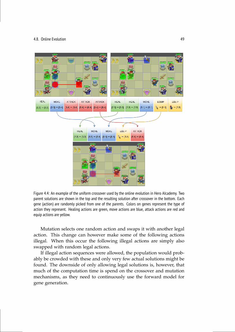
4.8. Online Evolution 49
Figure 4.4: An example of the uniform crossover used by the online evolution in Hero AIcademy. Twoparent solutions are shown in the top and the resulting solution after crossover in the bottom. Eachgene (action) are randomly picked from one of the parents. Colors on genes represent the type ofaction they represent. Healing actions are green, move actions are blue, attack actions are red andequip actions are yellow.
Mutation selects one random action and swaps it with another legalaction. This change can however make some of the following actionsillegal. When this occur the following illegal actions are simply alsoswapped with random legal actions.
If illegal action sequences were allowed, the population would prob-ably be crowded with these and only very few actual solutions might befound. The downside of only allowing legal solutions is, however, thatmuch of the computation time is spend on the crossover and mutationmechanisms, as they need to continuously use the forward model forgene generation.
50 Chapter 4. Approach
4.8.2 Parallelization
Two parallelization methods for the online evolution were implemented.The first is simple, as the LeafParallelizer, also used by the MCTS agent,can be used by the online evolution to run several concurrent rollouts.The online evolution was also implemented with the island paralleliza-tion model, where several evolutions run concurrently each representingan island. In every generation the second best individual is sent to itsneighboring island. Each island uses a queue in which incoming in-dividuals are waiting to enter. Only one individual will enter in eachgeneration unless the queue is empty. In this way genes are spreadacross islands while the most fit individual remains. A simple pausemechanism is added if one thread is running faster than others andends up sending more individuals than it is receiving. In this imple-mentation islands were allowed to be behind with five individuals, butsuch a number should be found experimentally.
4.9 NEAT
This section will describe our preliminary work of evolving neural net-works as game state evaluators for Hero Academy. Some discussionsof other approaches are also presented in the Conclusions chapter later.Designing game state evaluators by hand for Hero Academy turned outto be more challenging than expected. The material evaluation seemsfairly easy, while positional evaluation remains extremely challenging.Positioning units outside range of enemy units should probably be goodto protect them, while being inside range of enemy units can, in somesituations, put pressure on the opponent. Identifying when this is agood idea, and when it is not, is extremely difficult to describe manu-ally, even though human players are good at identifying such patterns.This suggest, that we should try to either evolve or train an evaluationfunction to do this task. In the work presented here, the NeuroEvolutionof Augmenting Topologies (NEAT) algorithm was used to evolve neuralnetworks as game state evaluators. The first experiments were made fora smaller game board of only 5x3 squares (see Figure 4.5). This makesthe size of the input layer smaller, as well as the time spend on eachgeneration in NEAT. The software package JNEAT1 by Stanley was usedin the experiments described.
1http://nn.cs.utexas.edu/?jneat
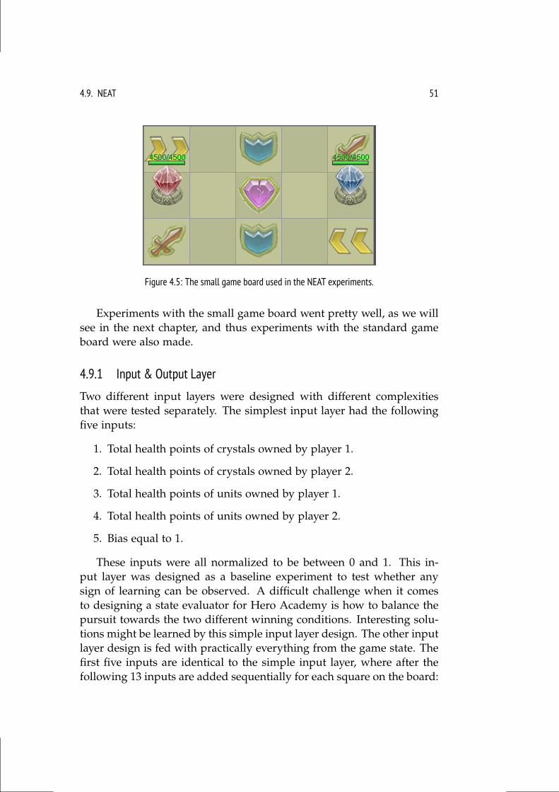
4.9. NEAT 51
Figure 4.5: The small game board used in the NEAT experiments.
Experiments with the small game board went pretty well, as we willsee in the next chapter, and thus experiments with the standard gameboard were also made.
4.9.1 Input & Output Layer
Two different input layers were designed with different complexitiesthat were tested separately. The simplest input layer had the followingfive inputs:
1. Total health points of crystals owned by player 1.
2. Total health points of crystals owned by player 2.
3. Total health points of units owned by player 1.
4. Total health points of units owned by player 2.
5. Bias equal to 1.
These inputs were all normalized to be between 0 and 1. This in-put layer was designed as a baseline experiment to test whether anysign of learning can be observed. A difficult challenge when it comesto designing a state evaluator for Hero Academy is how to balance thepursuit towards the two different winning conditions. Interesting solu-tions might be learned by this simple input layer design. The other inputlayer design is fed with practically everything from the game state. Thefirst five inputs are identical to the simple input layer, where after thefollowing 13 inputs are added sequentially for each square on the board:
52 Chapter 4. Approach
1. If square contains archer then 1 else 0
2. If square contains cleric then 1 else 0
3. If square contains crystal then 1 else 0
4. If square contains dragonscale then 1 else 0
5. If square contains knight then 1 else 0
6. If square contains ninja then 1 else 0
7. If square contains runemetal then 1 else 0
8. If square contains shining helmet then 1 else 0
9. If square contains scroll then 1 else 0
10. If square contains wizard then 1 else 0
11. If square contains a unit then its health points normalized else 0
12. If square contains a unit controlled by player 1 then 1 else 0
13. If square contains a unit controlled by player 2 then 1 else 0
Ten inputs are added after these, describing which cards the currentplayer has on the hand. Again, 1 is added if the player has an archerand 0 if not, and so on for each card type.
The final input layer ends up with 210 neurons for the 5x3 gameboard and for the standard sized game board the size is 600 neurons.Some efforts were made on reducing this number without loosing infor-mation, but no satisfying solution was found. The output layer simplyconsist of just one neuron, and the activation value of this neuron is thenetworks final evaluation of the game state.
Chapter 5
Experimental Results
This chapter will describe the main experiments performed in this thesisand present the results. Experiments were run on a Lenovo Ultrabookwith an Intel Core i7-3517U CPU with 4 x 1.90GHz cores and 8 GB ofram, unless other is specified. The Hero AIcademy engine was used torun the experiments.
Experiments that compare agents consist of 100 games, where eachagent plays as the starting player 50 games each. Winning percentageswere calculated, where draws count as half a win for each player. Agame ends in a draw if no winner is found in 100 turns. A confidenceinterval is presented for all comparative results with a confidence levelof 95%. Agents were given a 6 second time budget for their entire turnunless other is specified. The first part of this chapter will describe theperformance of each implemented algorithm individually, including ex-periments leading to their final configurations. In the second part acomprehensive comparison of all the implemented agents will be pre-sented. The best agent were tested in 111 games against human players,and the results from these experiments are presented in the end.
The Hero AIcademy engine was set to run deterministic games onlywhen two agents were compared. The decks of each player were stillrandomly shuffled in the beginning, but but every card draw were deter-ministic. This was done because no determinization strategy was imple-mented for MCTS. The experiments with human players was howeverrun with random card draws, as it otherwise would be an advantage forthe AI agents, as they can use the forward model to predict the future.
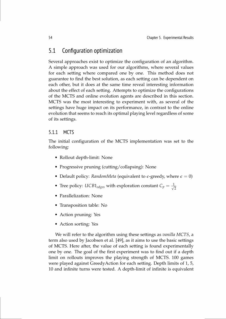
54 Chapter 5. Experimental Results
5.1 Configuration optimization
Several approaches exist to optimize the configuration of an algorithm.A simple approach was used for our algorithms, where several valuesfor each setting where compared one by one. This method does notguarantee to find the best solution, as each setting can be dependent oneach other, but it does at the same time reveal interesting informationabout the effect of each setting. Attempts to optimize the configurationsof the MCTS and online evolution agents are described in this section.MCTS was the most interesting to experiment with, as several of thesettings have huge impact on its performance, in contrast to the onlineevolution that seems to reach its optimal playing level regardless of someof its settings.
5.1.1 MCTS
The initial configuration of the MCTS implementation was set to thefollowing:
• Rollout depth-limit: None
• Progressive pruning (cutting/collapsing): None
• Default policy: RandomMeta (equivalent to ε-greedy, where ε = 0)
• Tree policy: UCB1edges with exploration constant Cp = 1√2
• Parallelization: None
• Transposition table: No
• Action pruning: Yes
• Action sorting: Yes
We will refer to the algorithm using these settings as vanilla MCTS, aterm also used by Jacobsen et al. [49], as it aims to use the basic settingsof MCTS. Here after, the value of each setting is found experimentallyone by one. The goal of the first experiment was to find out if a depthlimit on rollouts improves the playing strength of MCTS. 100 gameswere played against GreedyAction for each setting. Depth limits of 1, 5,10 and infinite turns were tested. A depth-limit of infinite is equivalent
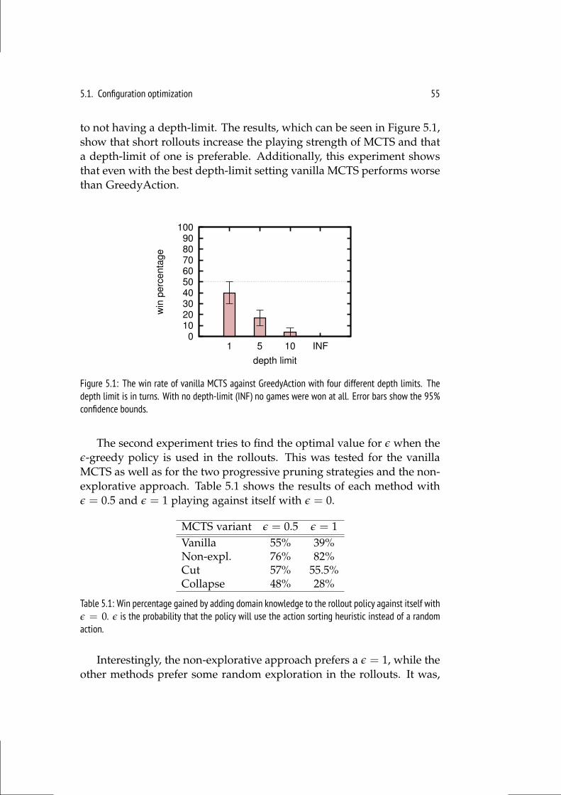
5.1. Configuration optimization 55
to not having a depth-limit. The results, which can be seen in Figure 5.1,show that short rollouts increase the playing strength of MCTS and thata depth-limit of one is preferable. Additionally, this experiment showsthat even with the best depth-limit setting vanilla MCTS performs worsethan GreedyAction.
0 10 20 30 40 50 60 70 80 90
100
1 5 10 INF
win
perc
enta
ge
depth limit
Figure 5.1: The win rate of vanilla MCTS against GreedyAction with four different depth limits. Thedepth limit is in turns. With no depth-limit (INF) no games were won at all. Error bars show the 95%confidence bounds.
The second experiment tries to find the optimal value for ε when theε-greedy policy is used in the rollouts. This was tested for the vanillaMCTS as well as for the two progressive pruning strategies and the non-explorative approach. Table 5.1 shows the results of each method withε = 0.5 and ε = 1 playing against itself with ε = 0.
MCTS variant ε = 0.5 ε = 1Vanilla 55% 39%Non-expl. 76% 82%Cut 57% 55.5%Collapse 48% 28%
Table 5.1: Win percentage gained by adding domain knowledge to the rollout policy against itself withε = 0. ε is the probability that the policy will use the action sorting heuristic instead of a randomaction.
Interestingly, the non-explorative approach prefers a ε = 1, while theother methods prefer some random exploration in the rollouts. It was,
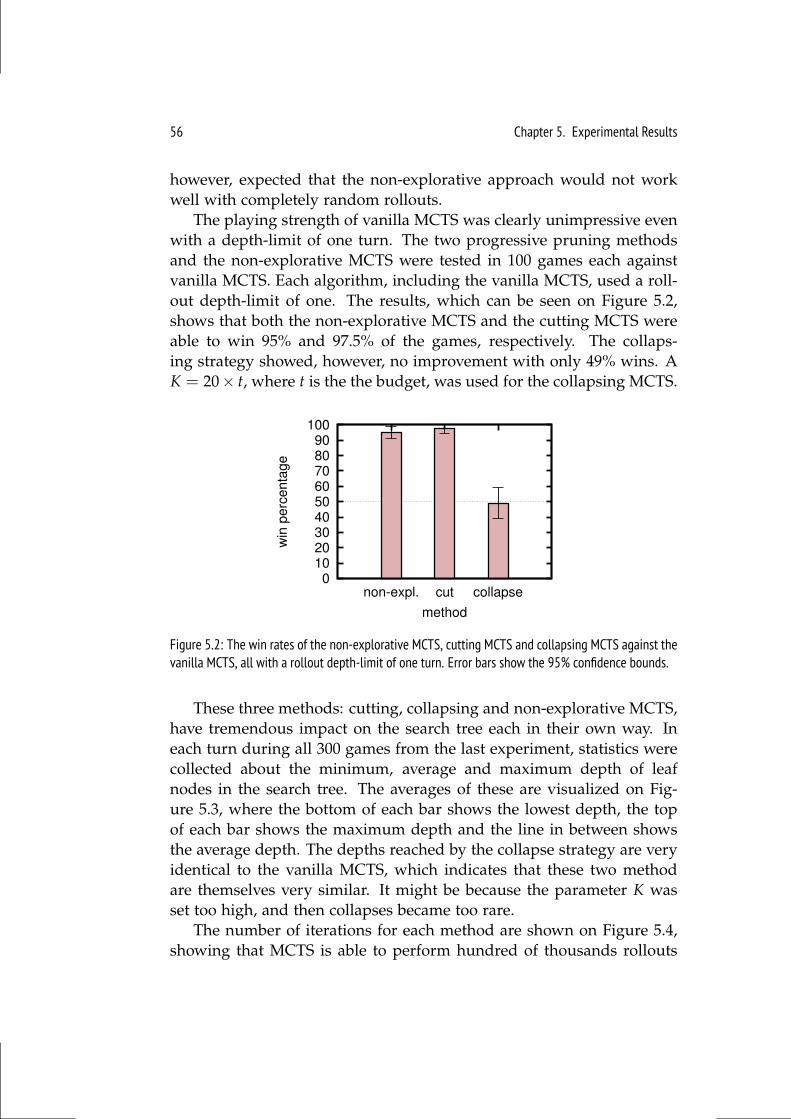
56 Chapter 5. Experimental Results
however, expected that the non-explorative approach would not workwell with completely random rollouts.
The playing strength of vanilla MCTS was clearly unimpressive evenwith a depth-limit of one turn. The two progressive pruning methodsand the non-explorative MCTS were tested in 100 games each againstvanilla MCTS. Each algorithm, including the vanilla MCTS, used a roll-out depth-limit of one. The results, which can be seen on Figure 5.2,shows that both the non-explorative MCTS and the cutting MCTS wereable to win 95% and 97.5% of the games, respectively. The collaps-ing strategy showed, however, no improvement with only 49% wins. AK = 20× t, where t is the the budget, was used for the collapsing MCTS.
0 10 20 30 40 50 60 70 80 90
100
non-expl. cut collapse
win
perc
enta
ge
method
Figure 5.2: The win rates of the non-explorative MCTS, cutting MCTS and collapsing MCTS against thevanilla MCTS, all with a rollout depth-limit of one turn. Error bars show the 95% confidence bounds.
These three methods: cutting, collapsing and non-explorative MCTS,have tremendous impact on the search tree each in their own way. Ineach turn during all 300 games from the last experiment, statistics werecollected about the minimum, average and maximum depth of leafnodes in the search tree. The averages of these are visualized on Fig-ure 5.3, where the bottom of each bar shows the lowest depth, the topof each bar shows the maximum depth and the line in between showsthe average depth. The depths reached by the collapse strategy are veryidentical to the vanilla MCTS, which indicates that these two methodare themselves very similar. It might be because the parameter K wasset too high, and then collapses became too rare.
The number of iterations for each method are shown on Figure 5.4,showing that MCTS is able to perform hundred of thousands rollouts
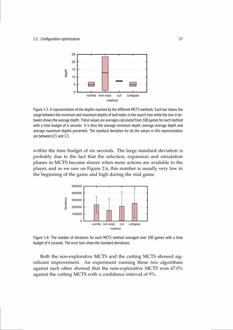
5.1. Configuration optimization 57
0
5
10
15
20
25
vanilla non-expl. cut collapse
depth
method
Figure 5.3: A representation of the depths reached by the different MCTS methods. Each bar shows therange between the minimum and maximum depths of leaf nodes in the search tree while the line in be-tween shows the average depth. These values are averages calculated from 100 games for eachmethodwith a time budget of 6 seconds. It is thus the average minimum depth, average average depth andaverage maximum depths presented. The standard deviation for all the values in this representationare between 0.5 and 1.5.
within the time budget of six seconds. The large standard deviation isprobably due to the fact that the selection, expansion and simulationphases in MCTS become slower when more actions are available to theplayer, and as we saw on Figure 2.6, this number is usually very low inthe beginning of the game and high during the mid game.
0
100000
200000
300000
400000
500000
vanilla non-expl. cut collapse
itera
tions
method
Figure 5.4: The number of iterations for each MCTS method averaged over 100 games with a timebudget of 6 seconds. The error bars show the standard deviations.
Both the non-explorative MCTS and the cutting MCTS showed sig-nificant improvement. An experiment running these two algorithmsagainst each other showed that the non-explorative MCTS won 67.0%against the cutting MCTS with a confidence interval of 9%.
58 Chapter 5. Experimental Results
Since the non-explorative MCTS uses determinstic rollouts, bothleaf and root parallelization does not make sense to apply. With leafparallelization each concurrent rollout would reach the same outcomeand with root parallelization each tree would be identical, except thatsome threads that were given more time by the scheduler would beslightly larger. Tree parallelization were not implemented but wouldmake sense to apply to the non-explorative MCTS, as it would adda new form of exploration while maintaining an exploration constantof zero. The cutting MCTS showed no significant improvement whenleaf parallelization were applied while root parallelization actually de-creased the playing strength, as it only won 2% against the cuttingMCTS without parallelization.
Experiments were performed to explore the effects of the adding atransposition table with the UCB1edges formula to the non-explorativeMCTS. A win percentage of 62.5% was achieved with a transpositiontable against the same algorithm without a transposition table. Theaverage and maximum depths of leaf nodes were increased by aroundone ply. No significant change were however observed when applyingthe transposition table to the cutting MCTS.
The best settings found for MCTS in the experiements described inthis section are the following:
• Rollout depth-limit: 1 turn
• Progressive pruning (cutting/collapsing): None
• Default policy: Greedy (equivalent to ε-greedy, where ε = 1)
• Tree policy: UCB1edges with an exploration constant Cp = 0
• Parallelization: None
• Transposition table: Yes
• Action pruning: Yes
• Action sorting: Yes
5.1. Configuration optimization 59
5.1.2 Online Evolution
Several experiments were performed to optimize the configurationsfor the online evolution agent. These experiments were head to headmatchups between two online evolution agents with a different setting,each given a three second time budget. Most of these experimentsshowed no increase in the playing strength by changing the settings,while some only showed small improvements. The reason might bebecause the agent is able to find a good solution within the three secondtime budget regardless of changes of its configuration.
No significant improvement over the other was found when apply-ing 1, 2, 5 or 10 sequential rollouts to the fitness function. However,when applying 50 rollouts the win percentage decreased to 27% againsta similar online evolution agent with just 1 rollouts.
The online evolution used the ε-greedy policy for its rollouts. Nosignificant improvement was seen when using ε = 0, ε = 0.5 or ε = 1.This was a bit surprising. Additionally, applying rollouts instead ofthe HeuristicEvaluation as heuristic provided only an improvement of54%, which is insignificant with a confidence interval of 10%. Thehistory table gave a small, but also insignificant, improvement with awin percentage of 55.5%.
Applying the island parallelization showed a significant improve-ment of 63%, when a time budget of 2 seconds were used, and a 61%improvement when a time budget of 1 second were used. Figure 5.5shows the progress of four parallel island evolutions, where immigra-tion of the next best individual happens in every generation.
With a time budget of six seconds the evolutions are able to com-plete an average of 1217 (with a standard deviation of 419) generations.The most fit individual found on each island had an average age of60 generations, but with a standard deviation 339. The high deviationmight be due the end game, where the best move is found early, and ahigh number of generations are possible, due to game states with veryfew units.
The best configuration found for the online evolution agent turnedout to be the following:
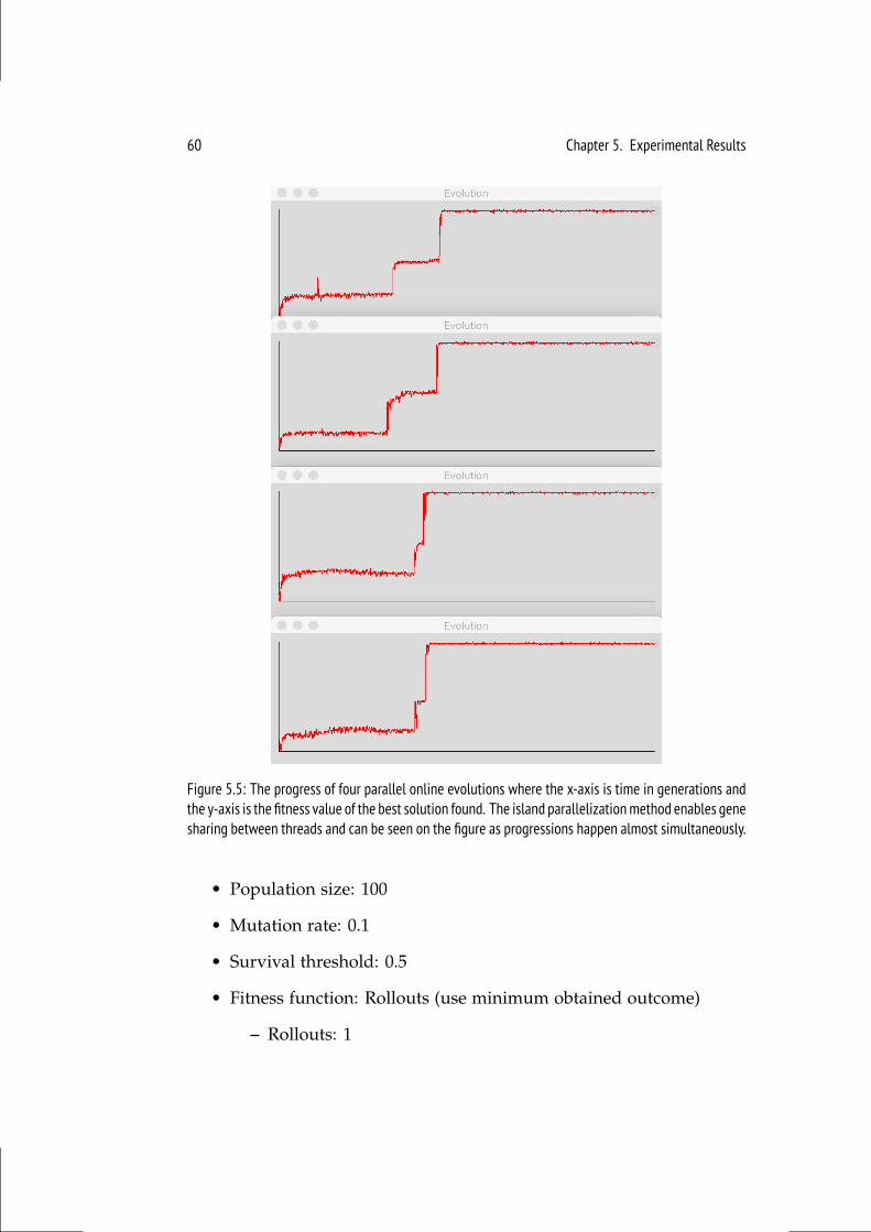
60 Chapter 5. Experimental Results
Figure 5.5: The progress of four parallel online evolutions where the x-axis is time in generations andthe y-axis is the fitness value of the best solution found. The island parallelizationmethod enables genesharing between threads and can be seen on the figure as progressions happen almost simultaneously.
• Population size: 100
• Mutation rate: 0.1
• Survival threshold: 0.5
• Fitness function: Rollouts (use minimum obtained outcome)
– Rollouts: 1
5.1. Configuration optimization 61
– Depth limit: 1 turn
– Policy: ε-greedy where ε = 0.5.
– History table: Yes
• Parallelization: Island parallelization with immigration of secondbest individual each generation.
5.1.3 NEAT
The two input layer designs described in Section 4.9 will be referred toas the simple network, with 5 input neurons, and the complex network with210 input neurons for the small game board and 600 input neurons forthe standard game board. The networks were only evolved to play asthe starting player. The fitness function used in JNEAT simply played 20games using a neural network against the ε-greedy agent and returnedthe win rate. Initially, ε was set to 0 to produce a completely random andthus very easy opponent to train against. As soon as a win rate of 100%was reached, ε would be incremented by 0.05 to give further challengeto the trained networks. This approach was inspired by how Togeliuset al. evolved neural networks to play Super Mario on gradually moredifficult levels [50]. An initial population size of 64 individuals wereused, and a complete list of all the JNEAT parameters can be seen inAppendix A. Figure 5.6 shows how ε grew as the networks evolved. Itis important to stress that e does not express the actual win rate of thebest network against ε-greedy but simply tells that one individual wasable to win 20 games in a row against it.
The experiment for the 5x3 game board ran on the Lenovo laptop,while the experiment on the 9x5 game board ran on a server with eight2.9 GHz processor cores. Each experiment took three to four days beforeit was stopped.
The simple network was able to reach an ε-level of 0.85 in just 38 gen-erations on the 5x3 game board. It is easy to imagine that this networksimply tries to increase the health points of crystals and units undercontrol while decreasing the health points of opponents. The resultsindicate that these features alone are not enough to reach a good play-ing level, as the evolution ran for 3817 generations without reaching anε-level of 1.
The complex network reached the ε-level of 1 in 586 generations onthe 5x3 game board, and the ε-greedy agent with ε = 1 was finally beat
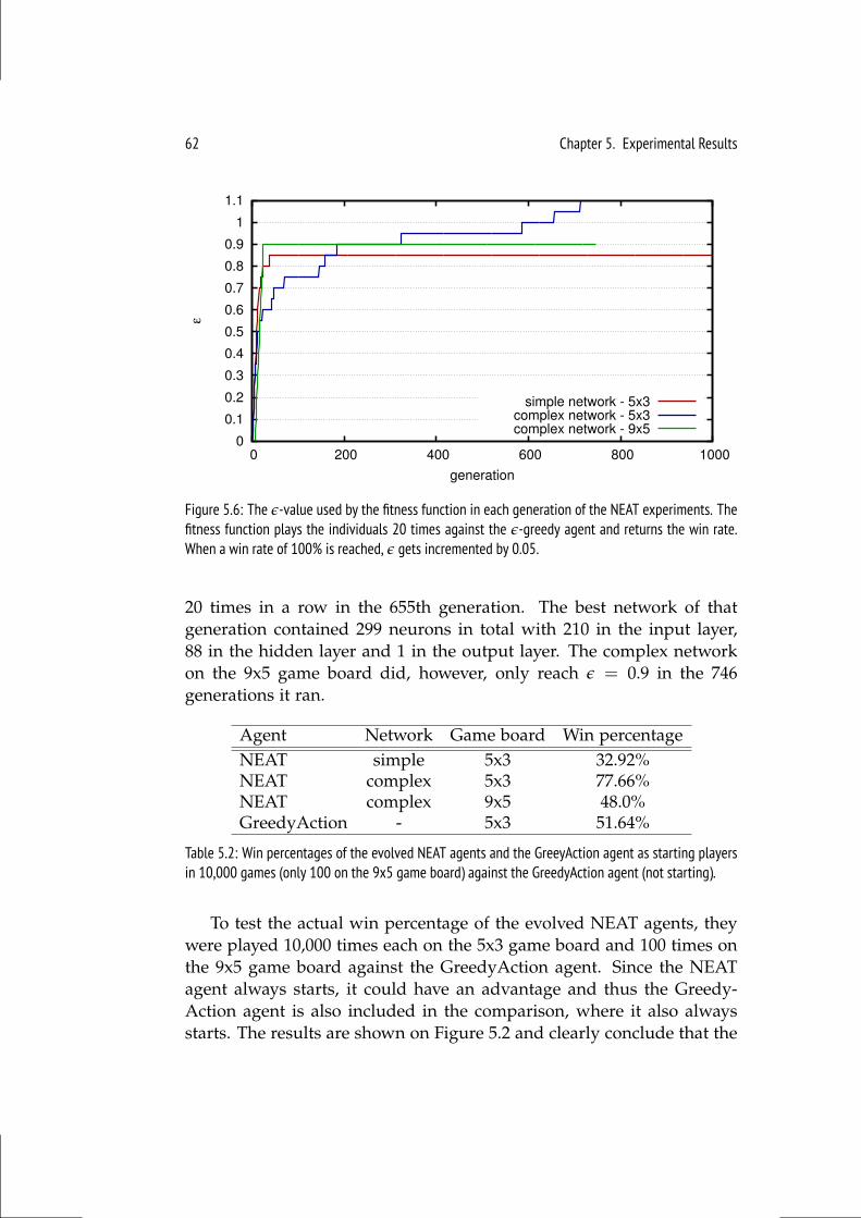
62 Chapter 5. Experimental Results
0
0.1
0.2
0.3
0.4
0.5
0.6
0.7
0.8
0.9
1
1.1
0 200 400 600 800 1000
ε
generation
simple network - 5x3complex network - 5x3complex network - 9x5
Figure 5.6: The ε-value used by the fitness function in each generation of the NEAT experiments. Thefitness function plays the individuals 20 times against the ε-greedy agent and returns the win rate.When a win rate of 100% is reached, ε gets incremented by 0.05.
20 times in a row in the 655th generation. The best network of thatgeneration contained 299 neurons in total with 210 in the input layer,88 in the hidden layer and 1 in the output layer. The complex networkon the 9x5 game board did, however, only reach ε = 0.9 in the 746generations it ran.
Agent Network Game board Win percentageNEAT simple 5x3 32.92%NEAT complex 5x3 77.66%NEAT complex 9x5 48.0%GreedyAction - 5x3 51.64%
Table 5.2: Win percentages of the evolved NEAT agents and the GreeyAction agent as starting playersin 10,000 games (only 100 on the 9x5 game board) against the GreedyAction agent (not starting).
To test the actual win percentage of the evolved NEAT agents, theywere played 10,000 times each on the 5x3 game board and 100 times onthe 9x5 game board against the GreedyAction agent. Since the NEATagent always starts, it could have an advantage and thus the Greedy-Action agent is also included in the comparison, where it also alwaysstarts. The results are shown on Figure 5.2 and clearly conclude that the
5.2. Comparisons 63
NEAT agent using the complex approach have reached a level, whereit is superior to the GreedyAction agent on the 5x3 game board, whilethe simple network approach is much weaker. The same results was notachieved for the 9x5 game board, where the evolved network won 48%of the games. The results with the GreedyAction agents indicate, thatthe advantage of starting is insignificant, at least for the strategy appliedby this agent.
5.2 Comparisons
Each of the implemented agents with their optimized configurationswere tested against each other and against the baseline agents. Theresults are shown in Table 5.3.
Random G-Action G-Turn NE-MCTS OEGreedyAction 100% 46.5% 5% 7.5%GreedyTurn 100% 53.5% 25% 9%NE-MCTS 100% 95% 75% 42.5%OE 100% 92.5% 91% 57.5%
Table 5.3: Win percentages of the agents listed in the left-most column. G are short for greedy, NE fornon-explorative and OE for online evolution.
The results show, that both the online evolution and NE-MCTSagents are significantly superior to the greedy baseline agents. We ex-pected the GreedyTurn agent to be much better than the GreedyActionagent, but it only achieved a win percentage of 53.5%. When observinga game between the two it became apparent why, as GreedyTurn mostlycharges with one unit towards the opponent to make a very effectiveattack. This often leaves the attacking unit defenseless in the opponent’sterritory. The GreedyAction agent cannot make forward planning andsimply attacks if possible and otherwise tries to optimize its immediateposition by deploying units, healing and equipping units with items.The difference in strategies between the GreedyAction agent and theGreedyTurn agent might also be the reason why NE-MCTS is the bestagent against GreeyAction while the online evolution is the best agentagainst GreedyTurn. The results also show that a completely randomagent is useless in Hero Academy with zero wins in all the experiments.This seems to be because it waste actions on useless move actions and
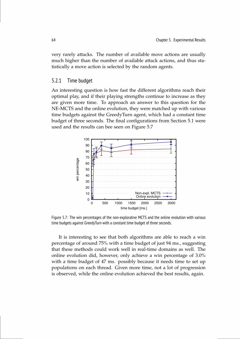
64 Chapter 5. Experimental Results
very rarely attacks. The number of available move actions are usuallymuch higher than the number of available attack actions, and thus sta-tistically a move action is selected by the random agents.
5.2.1 Time budget
An interesting question is how fast the different algorithms reach theiroptimal play, and if their playing strengths continue to increase as theyare given more time. To approach an answer to this question for theNE-MCTS and the online evolution, they were matched up with varioustime budgets against the GreedyTurn agent, which had a constant timebudget of three seconds. The final configurations from Section 5.1 wereused and the results can bee seen on Figure 5.7
0
10
20
30
40
50
60
70
80
90
100
0 500 1000 1500 2000 2500 3000
win
perc
enta
ge
time budget [ms.]
Non-expl. MCTSOnline evolution
Figure 5.7: The win percentages of the non-explorative MCTS and the online evolution with varioustime budgets against GreedyTurn with a constant time budget of three seconds.
It is interesting to see that both algorithms are able to reach a winpercentage of around 75% with a time budget of just 94 ms., suggestingthat these methods could work well in real-time domains as well. Theonline evolution did, however, only achieve a win percentage of 3.0%with a time budget of 47 ms. possibly because it needs time to set uppopulations on each thread. Given more time, not a lot of progressionis observed, while the online evolution achieved the best results, again.
5.3. Versus Human Players 65
5.3 Versus Human Players
One important and often overseen experiment is to test the implementedagents against human players. We were able to test our best agent, theonline evolution agent, against 111 testers. This gives us knowledgeabout the current state of the implemented algorithms, and whetherthey are useful to implement in a real game product. One reason whysuch experiments are often left out, may be because of the time consum-ing task of finding test subjects and manually recording the results. Toovercome this challenge a web server running Node.js on the Herokucloud service was setup and connected to a MongoDB database1. TheHero AIcademy engine was extended to handle such tests by sendinggame results of each turn to the web server. Additionally, test subjectswere asked about their skill level by the program before they enteredthe game, with options of being a beginner, intermediate or expert. Ifplayers had never played the game before they were asked to choose"beginner". Players that did choose "beginner" were supplied with anadditional screen briefly explaining the two winning conditions of thegame and how to undo actions during their turn. The program wasexported as a runnable JAR file and distributed on Facebook amongfriends, colleagues and fellow students, on the Steam community pagefor Hero Academy2 and on the Hero Academy subreddit page3.
After about a month the database contained 111 records with 61beginners, 27 intermediates and 23 experts. All the results can be seenin Appendix B. Among theses records, 55 holds data of games playeduntil a terminal state was reached, with 26 beginners, 13 intermediatesand 16 experts. In the remaining games, players simply left before itwas over. Figure 5.8 shows the heuristic value, found by the HeuristicE-valuation, when they left the game, where 1 equals a win and 0 equals aloss, and the turn in which they left.
It is reasonable to think that some players left early because theysimply did not want to play the game when they saw it, while othersmight leave because they thought it was too easy or too difficult. Resultsoutside of the score range between -0.1 and 0.1 were treated as either a
1https://github.com/njustesen/heroai-testserver2http://steamcommunity.com/app/209270/discussions/3http://www.reddit.com/r/HeroAcademy/
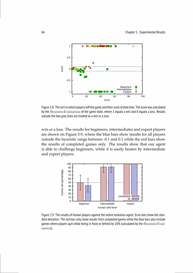
66 Chapter 5. Experimental Results
-1
-0.5
0
0.5
1
0 20 40 60 80 100
sco
re
turns
BeginnersIntermediates
Experts
Figure 5.8: The turn in which players left the game and their score at that time. The score was calculatedby the HeuristicEvaluation of the game state, where 1 equals a win and 0 equals a loss. Resultsoutside the two grey lines are treated as a win or a loss.
win or a loss. The results for beginners, intermediates and expert playersare shown on Figure 5.9, where the blue bars show results for all playersoutside the heuristic range between -0.1 and 0.1 while the red bars showthe results of completed games only. The results show that our agentis able to challenge beginners, while it is easily beaten by intermediateand expert players.
0
10
20
30
40
50
60
70
80
90
100
beginner intermediate expert
hu
ma
n w
in p
erc
en
tag
e
human skill level
completedall
Figure 5.9: The results of human players against the online evolution agent. Error bars show the stan-dard deviation. The red bars only show results from completed games while the blue bars also includegames where players quit while being in front or behind by 10% (calculated by the HeuristicEval-uation).
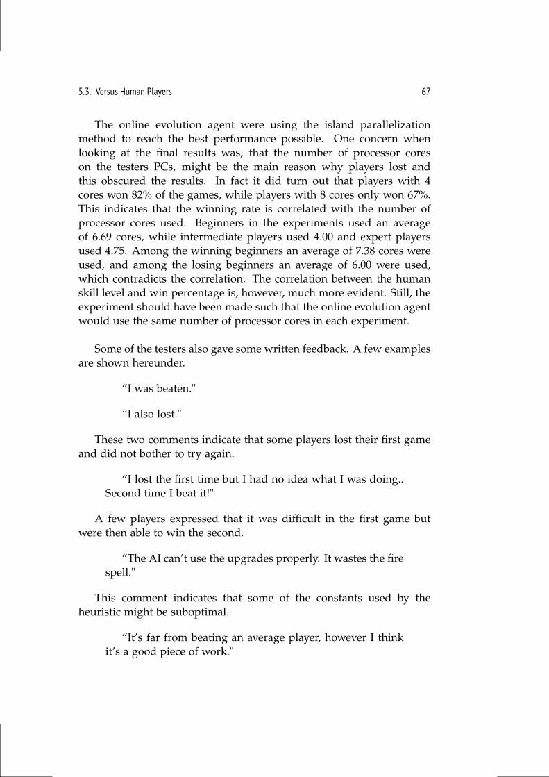
5.3. Versus Human Players 67
The online evolution agent were using the island parallelizationmethod to reach the best performance possible. One concern whenlooking at the final results was, that the number of processor coreson the testers PCs, might be the main reason why players lost andthis obscured the results. In fact it did turn out that players with 4cores won 82% of the games, while players with 8 cores only won 67%.This indicates that the winning rate is correlated with the number ofprocessor cores used. Beginners in the experiments used an averageof 6.69 cores, while intermediate players used 4.00 and expert playersused 4.75. Among the winning beginners an average of 7.38 cores wereused, and among the losing beginners an average of 6.00 were used,which contradicts the correlation. The correlation between the humanskill level and win percentage is, however, much more evident. Still, theexperiment should have been made such that the online evolution agentwould use the same number of processor cores in each experiment.
Some of the testers also gave some written feedback. A few examplesare shown hereunder.
“I was beaten."
“I also lost."
These two comments indicate that some players lost their first gameand did not bother to try again.
“I lost the first time but I had no idea what I was doing..Second time I beat it!"
A few players expressed that it was difficult in the first game butwere then able to win the second.
“The AI can’t use the upgrades properly. It wastes the firespell."
This comment indicates that some of the constants used by theheuristic might be suboptimal.
“It’s far from beating an average player, however I thinkit’s a good piece of work."

68 Chapter 5. Experimental Results
The last comment is from the Steam community page for HeroAcademy and conforms with the results on Figure 5.9, that the AI agentis on level with beginners while intermediate, or average, players areable to beat it. Still, the comment indicates that intelligent behavior isobserved by saying it is a good piece of work.
Chapter 6
Conclusions
This section sums up the results of this thesis. Several algorithms havebeen presented that are able to play Hero Academy and even challengehuman beginners. We have thus been able to answer our research ques-tion partly, while several challenges have been identified, that must besolved to reach a higher playing level. This conclusion can also beseen as our advice to others that want to implement an agent for HeroAcademy or similar TTB games.
Research questionHow can we design an AI agent that is able to challengehuman players in Hero Academy?
A greedy search was implemented, that was barely able to beat ourbaseline agent, despite its use of action sorting, pruning and paralleliza-tion. The vanilla MCTS performed even worse than our baseline, whilewe observed that rollouts with a depth-limit of just one turn followed bya static evaluation function works best. A non-explorative variant thatuses deterministic greedy rollouts and an exploration constant Cp = 0outperformed the vanilla MCTS with a 95% win percentage. Two novelprogressive pruning strategies were also introduced based on cuttingand collapsing the MCTS search tree. The cutting strategy outperformedthe vanilla MCTS with a 97% win percentage, while the collapsing strat-egy showed no improvement. The non-explorative MCTS was shownto be the best of the variants in head to head match-ups. Transposi-tion tables, action sorting, action pruning and ε-greedy rollouts wereused to enhance the performance of the MCTS agents. A parallel online
70 Chapter 6. Conclusions
evolutionary algorithm was implemented that evolves plans each turnand uses a fitness function based on depth-limited rollouts. The mini-mum value found by the fitness function is used and stored in a historytable. This agent reached the best overall performance of all the imple-mented agents. Uniform crossover was applied that, using an if-allowedrule only accepts legal action sequences. The idea of using rollouts incombination with online evolution only showed a small improvement,while it is a unique approach that, to our knowledge, has not been donebefore. It seems that two areas are important when creating an agentin Hero Academy. The first area is concerned with searching for plans,while the second area is concerned with game state evaluation. Theonline evolution agent was able to challenge human beginners, whileintermediate and expert players easily beat it. As we have highlightedseveral methods that are able to search for actions adequate, we believethe greatest challenge now is to produce strong game state evaluators.Preliminary attempts were also made to evolve a game state evaluatorusing NEAT. A network was evolved, that was able to reach a win per-centage of 77.66% against our baseline agent on a small game board,while a win percentage of 48.0% was achieved on the standard sizedgame board. The networks had 13 input neurons for each square on thegame board. This suggests that other solutions should be investigatedwith simple input layers.
6.1 Discussion
The online evolution worked very well in Hero Academy, and it is prob-ably also very effective in other multi-action games with more than fivesequential actions such as Blood Bowl, where players can move up to 11units each turn.
The use of rollouts as a heuristic was quite disappointing. The re-lated work presented in this thesis and our own results suggests, thatdepth-limited rollouts are necessary in games with large branching fac-tors and complex rules. The improvement of using rollouts in the onlineevolution was not significant, while we still think it is a very interestingapproach, as it allows the evolution to take the opponents actions intoaccount.
It was expected that MCTS would have a hard time overcoming thelarge branching factor of Hero Academy and that radical enhancementswere needed. The cutting and non-explorative approaches rigorously
6.1. Discussion 71
and naively ignore most of the game tree, which of course has its down-sides, but enables the search to explore the opponent counter-movesvery well. The collapse approach did, in contrast to our expectations,not improve the performance. Our best guess is that the remainingnodes after the collapse are too uncertain, since MCTS is not able to ex-plore the first five plies very well. Also, the K parameter might be settoo high, so that collapses almost never happen. An investigation of thisshould be performed, but was not possible based on the output of ourexperiments.
Several of our algorithms used some form of transposition table,which performance is depended on the game state hash function.Proper tests should be performed to test the collision probability of thisfunction. We do, however, not believe that this was a problem in ourimplementations for two reasons. First, the MCTS search trees havebeen saved into XML files, where after they were manually studied andthe edge connections looked correct. Second, MCTS would most likelyrun into an infinite loop if collisions were common, as a cycle could beproduced in the tree leading to a stack overflow error. This was notobserved.
The implemented agents were compared by playing the game againsteach other. It is important to note that each agent has its own strategy asa result of their different implementations. E.g. the GreedyTurn agentplays very aggressive and can take out human players very fast, by acrystal kill, if the opponent is unwary. It is, however, very easy to beatit, as it is way too aggressive and thus careless with its units. We believethis agent is able to beat some human beginners as well. It would havebeen optimal if we tested every agent against human players, but itwould also require a lot more testers.
If we were to reproduce the experiments with human players, wewould definitely give the agents the same number of processors in everytest, as not doing so obscured some of the results.
One could argue that our agent only won against human beginners,because most of them did not know the rules. A few rules and the twowinning conditions were presented to the beginners before the gamebegan, so we do not believe, they were unaware of what was going on.Still, the beginner category of course includes players that only knowsome of the rules. We believe the online evolution agent could easily beused, as it is, in the actual game. It could serve as a training opponentfor new players and is fast enough to work on mobile devices. It could
72 Chapter 6. Conclusions
also help the developers with procedural content generation, such asgeneration of game boards and challenges.
Our NEAT approach seems to have more trouble when applied tothe standard sized game board in Hero Academy. It might be a bitnaive that it would actually work, since so many squares create an enor-mous amount of dependencies, that probably requires a network withthousands of neurons. A higher level might have been reached if theevolution was run for more generations, but it may require weeks ofcomputation or a super computer with more than 16 cores. New ap-proaches are probably needed to reach a very solid playing level, andsome ideas are presented when ideas for future work are presented next.
6.2 Future Work
This section offers a list of future work directions representing some ofthe questions that remain unanswered in this thesis. It is made as a listof points that can inspire future projects.
1. Further understanding of the non-explorative MCTS is needed.Will it work better if the exploration constant is very small insteadof zero? Can tree parallelization improve its performance further?In what other games could it be a useful approach?
2. Two progressive strategies were introduced in this thesis, wherethe cutting strategy proved to be effective. Can we design otherprogressive strategies to overcome large branching factors? Canthe cutting and collapsing strategies be improved? How does thecutting strategy work compared to existing progressive strategiessuch as progressive unprunning/widening?
3. MCTS was only tested in the deterministic version of HeroAcademy since no determinization method was implemented.One approach could simply be to assume that players in futuregame positions have all possible cards on their hand. This can vio-late the rules of the game, as it could result in more than six cardson a hand, but this should not be a problem in Hero AIcademy.Another approach would simply be to select the most probablecards for each players and use this fixed sample. It would be in-terested to see how these determinization methods would work inthe stochastic version of the game.
6.2. Future Work 73
4. Online evolution using rollouts as a fitness function with a his-tory table was introduced in this thesis. The enhancement of usingrollouts was however not significant. The idea still seems inter-esting and exploring other methods combining evolution and roll-outs should be interesting. Few attempts were also made on usingcascading fitness functions, but no useful results were achieved. Itwould be ideal to have an algorithm similar to minimax, but wheremoves for each players are evolved. If this vision is even possibleit definitely requires a lot of ingenuity.
5. Applying a genetic algorithm to optimize the parameters used inthe HeuristicEvaluation seems like an obvious way of improvingour results. It would probably solve the issues, also pointed out byone of the testers, that the agents cannot use upgrades and spellsproperly. To be able to improve the positional evaluation as wellthe HeuristicEvaluation must be extended to also take such factorsinto account. This might actually be the most promising direction,to reach a higher playing level fast.
6. Potential fields and influence maps are well known methods ingame AI but have not been used in this thesis. Since positionalevaluation seems to be a very difficult task in Hero Academy, thesemethods might help and should be explored further.
7. While the online evolution agent only achieved a playing levelcompared to human beginners, the same approach might workeven better in other TTB games. Testing this approach in a gamesuch as the previously mentioned Blood Bowl would be very in-teresting.
8. Continuation of our experiments with NEAT to find the limit ofour approach is interesting. Networks reaching an ε-level of 1could probably be further evolved by tournament selection. Agame board of 9x5 squares may be too complex, and new ap-proaches to evolve evaluators for large maps and complex gamestates are very much needed. Perhaps each unit on the map can beevaluated individually with simpler networks? Or maybe Hyper-NEAT can be successfully used somehow.

References
[1] Niels Justesen, Balint Tillman, Julian Togelius, and Sebastian Risi.Script-and Cluster-based UCT for StarCraft, pages 1–8. IEEE Press,2014.
[2] GN Yannakakis and J Togelius. A panorama of artificial and com-putational intelligence in games. 2014.
[3] Claude E Shannon. Xxii. programming a computer for playingchess. The London, Edinburgh, and Dublin Philosophical Magazine andJournal of Science, 41(314):256–275, 1950.
[4] Murray Campbell, A Joseph Hoane, and Feng-hsiung Hsu. Deepblue. Artificial intelligence, 134(1):57–83, 2002.
[5] Jonathan Schaeffer, Neil Burch, Yngvi Björnsson, Akihiro Kishi-moto, Martin Müller, Robert Lake, Paul Lu, and Steve Sutphen.Checkers is solved. science, 317(5844):1518–1522, 2007.
[6] Michael Bowling, Neil Burch, Michael Johanson, and OskariTammelin. Heads-up limit hold’em poker is solved. Science,347(6218):145–149, 2015.
[7] István Szita, Guillaume Chaslot, and Pieter Spronck. Monte-carlotree search in settlers of catan. In Advances in Computer Games, pages21–32. Springer, 2010.
[8] Cathleen Heyden. Implementing a computer player for Carcassonne.PhD thesis, Maastricht University, 2009.
[9] Sondre Glimsdal. Ais for dominion using monte-carlo tree search.In Current Approaches in Applied Artificial Intelligence: 28th Interna-tional Conference on Industrial, Engineering and Other Applications of
76 References
Applied Intelligent Systems, IEA/AIE 2015, Seoul, South Korea, June 10-12, 2015, Proceedings, volume 9101, page 43. Springer, 2015.
[10] Diego Perez, Spyridon Samothrakis, Julian Togelius, Tom Schaul,Simon Lucas, Adrien Couëtoux, Jeyull Lee, Chong-U Lim, andTommy Thompson. The 2014 general video game playing com-petition.
[11] Matthew Hausknecht, Joel Lehman, Risto Miikkulainen, and PeterStone. A neuroevolution approach to general atari game playing.2013.
[12] Maurice HJ Bergsma and Pieter Spronck. Adaptive spatial reason-ing for turn-based strategy games. In AIIDE, 2008.
[13] J v Neumann. Zur theorie der gesellschaftsspiele. MathematischeAnnalen, 100(1):295–320, 1928.
[14] Judea Pearl. The solution for the branching factor of the alpha-betapruning algorithm and its optimality. Communications of the ACM,25(8):559–564, 1982.
[15] Richard D Greenblatt, Donald E Eastlake III, and Stephen DCrocker. The greenblatt chess program. In Proceedings of the Novem-ber 14-16, 1967, fall joint computer conference, pages 801–810. ACM,1967.
[16] Albert L Zobrist. A new hashing method with application for gameplaying. ICCA journal, 13(2):69–73, 1970.
[17] Guillaume Chaslot, Sander Bakkes, Istvan Szita, and PieterSpronck. Monte-carlo tree search: A new framework for game ai.In AIIDE, 2008.
[18] Sylvain Gelly, Levente Kocsis, Marc Schoenauer, Michele Sebag,David Silver, Csaba Szepesvári, and Olivier Teytaud. The grandchallenge of computer go: Monte carlo tree search and extensions.Communications of the ACM, 55(3):106–113, 2012.
[19] Levente Kocsis and Csaba Szepesvári. Bandit based monte-carloplanning. In Machine Learning: ECML 2006, pages 282–293.Springer, 2006.
References 77
[20] Cameron B Browne, Edward Powley, Daniel Whitehouse, Simon MLucas, Peter I Cowling, Philipp Rohlfshagen, Stephen Tavener,Diego Perez, Spyridon Samothrakis, and Simon Colton. A surveyof monte carlo tree search methods. Computational Intelligence andAI in Games, IEEE Transactions on, 4(1):1–43, 2012.
[21] GMJB Chaslot, Mark Winands, JWHM Uiterwijk, H van den Herik,and Bruno Bouzy. Progressive strategies for monte-carlo treesearch. In Proceedings of the 10th Joint Conference on Information Sci-ences (JCIS 2007), pages 655–661. Citeseer, 2007.
[22] Chang-Shing Lee, Mei-Hui Wang, Guillaume Chaslot, J-B Hoock,Arpad Rimmel, F Teytaud, Shang-Rong Tsai, Shun-Chin Hsu, andTzung-Pei Hong. The computational intelligence of mogo revealedin taiwan’s computer go tournaments. Computational Intelligence andAI in Games, IEEE Transactions on, 1(1):73–89, 2009.
[23] Rémi Coulom. Computing elo ratings of move patterns in the gameof go. In Computer games workshop, 2007.
[24] JPAM Nijssen. Playing othello using monte carlo. Strategies, pages1–9, 2007.
[25] JAM Nijssen and Mark HM Winands. Monte-carlo tree search forthe game of scotland yard. In Computational Intelligence and Games(CIG), 2011 IEEE Conference on, pages 158–165. IEEE, 2011.
[26] Jean Méhat and Tristan Cazenave. Combining uct and nested montecarlo search for single-player general game playing. ComputationalIntelligence and AI in Games, IEEE Transactions on, 2(4):271–277, 2010.
[27] Abdallah Saffidine, Tristan Cazenave, and Jean Méhat. Ucd: Upperconfidence bound for rooted directed acyclic graphs. Knowledge-Based Systems, 34:26–33, 2012.
[28] Guillaume MJ-B Chaslot, Mark HM Winands, and H Jaap vanDen Herik. Parallel monte-carlo tree search. In Computers andGames, pages 60–71. Springer, 2008.
[29] Tristan Cazenave. A phantom-go program. In Advances in ComputerGames, pages 120–125. Springer, 2006.
78 References
[30] J Kloetzer. Monte-carlo techniques: Applications to the game of theamazons. Japan Advanced Institute of Science and Technology, pages87–92, 2010.
[31] Tomas Kozelek. Methods of mcts and the game arimaa. CharlesUniversity, Prague, Faculty of Mathematics and Physics, 2009.
[32] David Churchill and Michael Buro. Portfolio greedy search andsimulation for large-scale combat in starcraft. In Computational In-telligence in Games (CIG), 2013 IEEE Conference on, pages 1–8. IEEE,2013.
[33] David Kriesel. A Brief Introduction to Neural Networks. 2007.
[34] David E Rumelhart, Geoffrey E Hinton, and Ronald J Williams.Learning representations by back-propagating errors. Cognitivemodeling, 5, 1988.
[35] John H Holland. Adaptation in natural and artificial systems: an intro-ductory analysis with applications to biology, control, and artificial intel-ligence. U Michigan Press, 1975.
[36] Marco Tomassini. A survey of genetic algorithms. Annual Reviewsof Computational Physics, 3(2):87–118, 1995.
[37] Enrique Alba and Marco Tomassini. Parallelism and evolution-ary algorithms. Evolutionary Computation, IEEE Transactions on,6(5):443–462, 2002.
[38] Diego Perez, Spyridon Samothrakis, Simon Lucas, and PhilippRohlfshagen. Rolling horizon evolution versus tree search for nav-igation in single-player real-time games. In Proceedings of the 15thannual conference on Genetic and evolutionary computation, pages 351–358. ACM, 2013.
[39] Arthur L Samuel. Some studies in machine learning using the gameof checkers. iiâATrecent progress. IBM Journal of research and devel-opment, 11(6):601–617, 1967.
[40] Gerald Tesauro. Temporal difference learning and td-gammon.Communications of the ACM, 38(3):58–68, 1995.
References 79
[41] Kumar Chellapilla and David B. Fogel. Evolving an expert check-ers playing program without using human expertise. EvolutionaryComputation, IEEE Transactions on, 5(4):422–428, 2001.
[42] David E Moriarty and Risto Miikkulainen. Discovering complexothello strategies through evolutionary neural networks. ConnectionScience, 7(3-4):195–210, 1995.
[43] Kenneth O Stanley and Risto Miikkulainen. Evolving neural net-works through augmenting topologies. Evolutionary computation,10(2):99–127, 2002.
[44] Keunhyun Oh and Sung-Bae Cho. A hybrid method of dijkstraalgorithm and evolutionary neural network for optimal ms. pac-man agent. In Nature and Biologically Inspired Computing (NaBIC),2010 Second World Congress on, pages 239–243. IEEE, 2010.
[45] Luigi Cardamone, Daniele Loiacono, and Pier Luca Lanzi. Evolvingcompetitive car controllers for racing games with neuroevolution.In Proceedings of the 11th Annual conference on Genetic and evolutionarycomputation, pages 1179–1186. ACM, 2009.
[46] Bas Jacobs. Learning othello using cooperative and competitiveneuroevolution.
[47] Kenneth O Stanley. Compositional pattern producing networks: Anovel abstraction of development. Genetic programming and evolvablemachines, 8(2):131–162, 2007.
[48] Sebastian Risi and Julian Togelius. Neuroevolution in games: Stateof the art and open challenges. arXiv preprint arXiv:1410.7326, 2014.
[49] Emil Juul Jacobsen, Rasmus Greve, and Julian Togelius. Montemario: platforming with mcts. In Proceedings of the 2014 conferenceon Genetic and evolutionary computation, pages 293–300. ACM, 2014.
[50] Julian Togelius, Sergey Karakovskiy, Jan Koutník, and JürgenSchmidhuber. Super mario evolution. In Computational Intelli-gence and Games, 2009. CIG 2009. IEEE Symposium on, pages 156–161.IEEE, 2009.

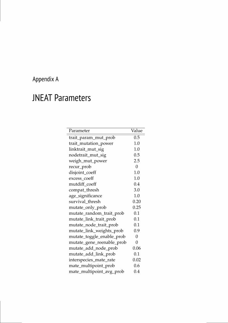
Appendix A
JNEAT Parameters
Parameter Valuetrait_param_mut_prob 0.5trait_mutation_power 1.0linktrait_mut_sig 1.0nodetrait_mut_sig 0.5weigh_mut_power 2.5recur_prob 0disjoint_coeff 1.0excess_coeff 1.0mutdiff_coeff 0.4compat_thresh 3.0age_significance 1.0survival_thresh 0.20mutate_only_prob 0.25mutate_random_trait_prob 0.1mutate_link_trait_prob 0.1mutate_node_trait_prob 0.1mutate_link_weights_prob 0.9mutate_toggle_enable_prob 0mutate_gene_reenable_prob 0mutate_add_node_prob 0.06mutate_add_link_prob 0.1interspecies_mate_rate 0.02mate_multipoint_prob 0.6mate_multipoint_avg_prob 0.4
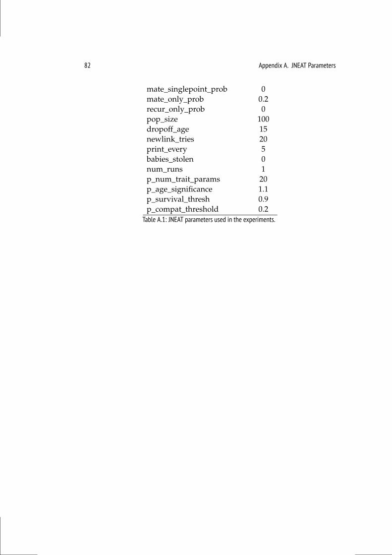
82 Appendix A. JNEAT Parameters
mate_singlepoint_prob 0mate_only_prob 0.2recur_only_prob 0pop_size 100dropoff_age 15newlink_tries 20print_every 5babies_stolen 0num_runs 1p_num_trait_params 20p_age_significance 1.1p_survival_thresh 0.9p_compat_threshold 0.2Table A.1: JNEAT parameters used in the experiments.
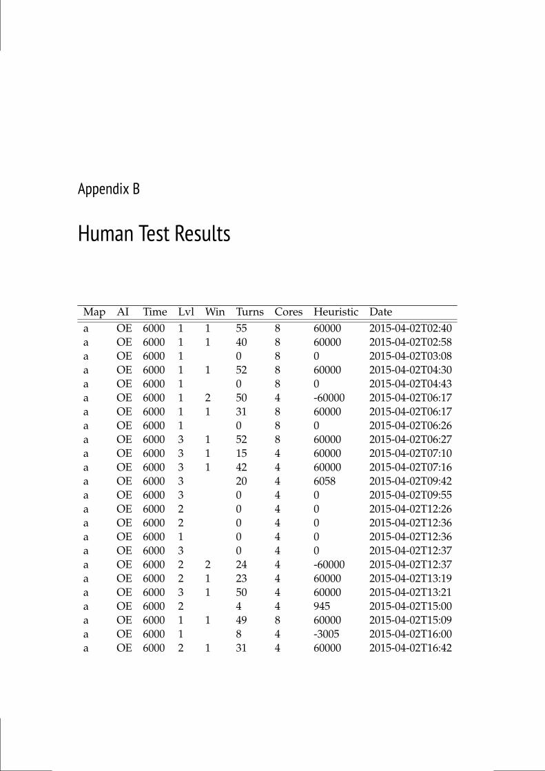
Appendix B
Human Test Results
Map AI Time Lvl Win Turns Cores Heuristic Datea OE 6000 1 1 55 8 60000 2015-04-02T02:40a OE 6000 1 1 40 8 60000 2015-04-02T02:58a OE 6000 1 0 8 0 2015-04-02T03:08a OE 6000 1 1 52 8 60000 2015-04-02T04:30a OE 6000 1 0 8 0 2015-04-02T04:43a OE 6000 1 2 50 4 -60000 2015-04-02T06:17a OE 6000 1 1 31 8 60000 2015-04-02T06:17a OE 6000 1 0 8 0 2015-04-02T06:26a OE 6000 3 1 52 8 60000 2015-04-02T06:27a OE 6000 3 1 15 4 60000 2015-04-02T07:10a OE 6000 3 1 42 4 60000 2015-04-02T07:16a OE 6000 3 20 4 6058 2015-04-02T09:42a OE 6000 3 0 4 0 2015-04-02T09:55a OE 6000 2 0 4 0 2015-04-02T12:26a OE 6000 2 0 4 0 2015-04-02T12:36a OE 6000 1 0 4 0 2015-04-02T12:36a OE 6000 3 0 4 0 2015-04-02T12:37a OE 6000 2 2 24 4 -60000 2015-04-02T12:37a OE 6000 2 1 23 4 60000 2015-04-02T13:19a OE 6000 3 1 50 4 60000 2015-04-02T13:21a OE 6000 2 4 4 945 2015-04-02T15:00a OE 6000 1 1 49 8 60000 2015-04-02T15:09a OE 6000 1 8 4 -3005 2015-04-02T16:00a OE 6000 2 1 31 4 60000 2015-04-02T16:42
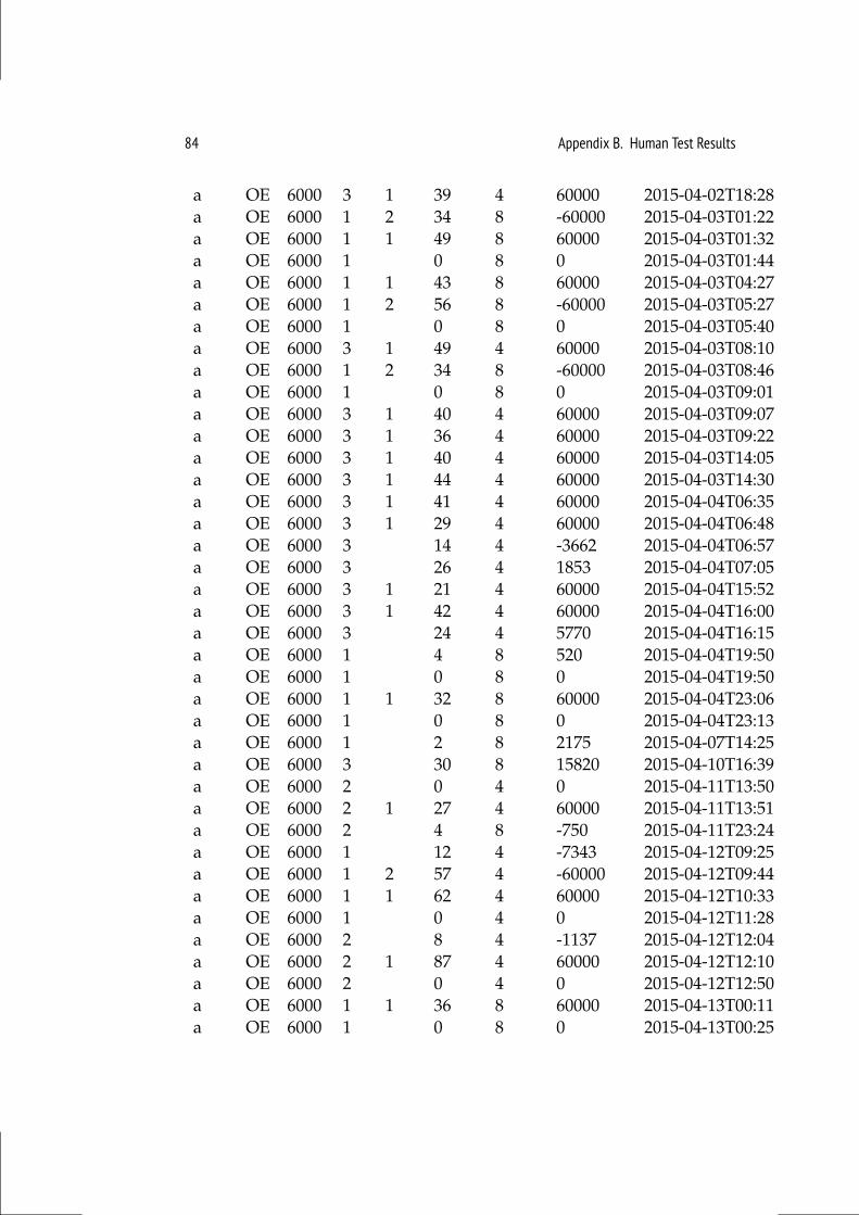
84 Appendix B. Human Test Results
a OE 6000 3 1 39 4 60000 2015-04-02T18:28a OE 6000 1 2 34 8 -60000 2015-04-03T01:22a OE 6000 1 1 49 8 60000 2015-04-03T01:32a OE 6000 1 0 8 0 2015-04-03T01:44a OE 6000 1 1 43 8 60000 2015-04-03T04:27a OE 6000 1 2 56 8 -60000 2015-04-03T05:27a OE 6000 1 0 8 0 2015-04-03T05:40a OE 6000 3 1 49 4 60000 2015-04-03T08:10a OE 6000 1 2 34 8 -60000 2015-04-03T08:46a OE 6000 1 0 8 0 2015-04-03T09:01a OE 6000 3 1 40 4 60000 2015-04-03T09:07a OE 6000 3 1 36 4 60000 2015-04-03T09:22a OE 6000 3 1 40 4 60000 2015-04-03T14:05a OE 6000 3 1 44 4 60000 2015-04-03T14:30a OE 6000 3 1 41 4 60000 2015-04-04T06:35a OE 6000 3 1 29 4 60000 2015-04-04T06:48a OE 6000 3 14 4 -3662 2015-04-04T06:57a OE 6000 3 26 4 1853 2015-04-04T07:05a OE 6000 3 1 21 4 60000 2015-04-04T15:52a OE 6000 3 1 42 4 60000 2015-04-04T16:00a OE 6000 3 24 4 5770 2015-04-04T16:15a OE 6000 1 4 8 520 2015-04-04T19:50a OE 6000 1 0 8 0 2015-04-04T19:50a OE 6000 1 1 32 8 60000 2015-04-04T23:06a OE 6000 1 0 8 0 2015-04-04T23:13a OE 6000 1 2 8 2175 2015-04-07T14:25a OE 6000 3 30 8 15820 2015-04-10T16:39a OE 6000 2 0 4 0 2015-04-11T13:50a OE 6000 2 1 27 4 60000 2015-04-11T13:51a OE 6000 2 4 8 -750 2015-04-11T23:24a OE 6000 1 12 4 -7343 2015-04-12T09:25a OE 6000 1 2 57 4 -60000 2015-04-12T09:44a OE 6000 1 1 62 4 60000 2015-04-12T10:33a OE 6000 1 0 4 0 2015-04-12T11:28a OE 6000 2 8 4 -1137 2015-04-12T12:04a OE 6000 2 1 87 4 60000 2015-04-12T12:10a OE 6000 2 0 4 0 2015-04-12T12:50a OE 6000 1 1 36 8 60000 2015-04-13T00:11a OE 6000 1 0 8 0 2015-04-13T00:25

85
a OE 6000 3 1 46 8 60000 2015-04-13T00:25a OE 6000 1 1 48 8 60000 2015-04-13T18:41a OE 6000 1 2 8 0 2015-04-14T10:00a OE 6000 2 1 53 4 60000 2015-04-16T20:37a OE 6000 1 2 34 4 -60000 2015-04-18T15:58a OE 6000 1 2 38 4 -60000 2015-04-18T16:09a OE 6000 1 6 4 -640 2015-04-18T20:18a OE 6000 2 0 2 0 2015-04-18T22:45a OE 6000 2 6 2 1715 2015-04-18T22:46a OE 6000 2 0 2 0 2015-04-19T23:16a OE 6000 3 1 40 8 60000 2015-04-20T00:27a OE 6000 1 2 46 2 -60000 2015-04-01T10:27a OE 6000 1 4 8 1375 2015-04-01T11:32a OE 6000 1 0 4 0 2015-04-01T12:35a OE 6000 1 16 2 -5027 2015-04-01T12:39a OE 6000 2 1 42 4 60000 2015-04-01T12:45a OE 6000 1 2 8 1970 2015-04-01T12:50a OE 6000 1 2 32 8 -60000 2015-04-01T12:52a OE 6000 1 2 42 4 -60000 2015-04-01T12:58a OE 6000 2 4 4 -410 2015-04-01T13:03a OE 6000 1 2 39 8 -60000 2015-04-01T13:08a OE 6000 1 2 8 0 2015-04-01T13:10a OE 6000 2 1 48 4 60000 2015-04-01T13:28a OE 6000 2 1 41 4 60000 2015-04-01T13:48a OE 6000 1 16 8 -7900 2015-04-01T14:03a OE 6000 1 2 40 8 -60000 2015-04-01T14:45a OE 6000 1 50 8 -750 2015-04-01T14:48a OE 6000 1 1 44 4 60000 2015-04-01T14:49a OE 6000 1 0 4 0 2015-04-01T15:14a OE 6000 1 8 8 -1005 2015-04-01T15:19a OE 6000 1 2 26 8 -60000 2015-04-01T15:30a OE 6000 1 2 8 1925 2015-04-01T15:43a OE 6000 1 10 4 -4280 2015-04-01T16:17a OE 6000 1 20 4 -20205 2015-04-01T17:34a OE 6000 2 0 8 0 2015-04-01T18:42a OE 6000 2 1 49 4 60000 2015-04-01T18:45a OE 6000 2 1 35 4 60000 2015-04-01T19:06a OE 6000 1 12 4 -15795 2015-04-01T19:12a OE 6000 1 12 4 -1110 2015-04-01T19:16

86 Appendix B. Human Test Results
a OE 6000 2 1 40 4 60000 2015-04-01T19:21a OE 6000 2 1 23 4 60000 2015-04-01T19:21a OE 6000 2 0 4 0 2015-04-01T19:29a OE 6000 2 16 6 3390 2015-04-01T19:34a OE 6000 1 8 8 -5300 2015-04-01T20:43a OE 6000 1 18 4 1185 2015-04-01T22:11a OE 6000 1 1 23 8 60000 2015-04-02T00:59a OE 6000 1 0 8 0 2015-04-02T01:05a OE 6000 1 18 8 -21393 2015-04-02T02:35
Human test results against the online evolution agent.