Lecture Notes in Mathematics Edited by A. Dold, Heidelberg and B. Eckmann, ZUrich

368

R. James Miigram Stanford University, Stanford, CA/USA

I I I I

Unstable Homotopy from the Stable Point of View

Springer-Verlag Berl in.Heidelberg • New York 1974

AMS Subject Classifications (1970): 55-02, 55 E 10, 55 E 20, 55 E25, 55 E40, 5 5 E 9 9 , 55 D 20, 55 D35, 55 D40, 5 5 D 9 9

ISBN 3-540-06655-1 Springer-Verlag Berlin • Heidelberg • New York ISBN 0-387-06655-1 Springer-Verlag New York • Heidelberg • Berlin

This work is subject to copyright. All rights are reserved, whether the whole or part of the material is concerned, specifically those of translation, reprinting, re-use of illustrations, broadcasting, reproduction by photo- copying machine or similar means, and storage in data banks. Under § 54 of the German Copyright Law where copies are made for other than private use, a fee is payable to the publisher, the amount of the fee to be determined by agreement with the publisher. © by Springer-Verlag Berlin • Heidelberg 1974. Library of Congress Catalog Card Number 73-21213. Printed in Germany. Offsetdruck: Julius Beltz, Hemsbach/Bergstr.

Pre face

This work had its origins in two projects. The first, undertaken

in 1970 with Elmer Rees, was to construct certain low dimensional embeddings

of real projective spaces. In order to do this we needed methods for

calculating unstable homotopy groups of truncated projective spaces and

associate spaces, as well as their images under various Freudenth~l

suspension homomorphis~s. The second was to understand Mahowald's work on

the metastable homotopy of spheres.

In 1971 and 1972 ~ work in surgery made me enlarge the scope of

the project and consider an apparently unrelated problem - the stable

homo~Dpy of the Eilenberg-MacLane spacesK(Q/Z ,n). By means of

appropriate fiberings these questions are seen to he merely different

faces of the same coin.

Hence, this current work which provides a relatively effective

framework for considering such questions. We generalize Mahowald's

constructions to allow us to apply Ada~' spectral sequence techniques to

calculations, and we give detailed calculations for ma~ examples~ in

particulars, those needed for the work with Rees, and those needed in surgery

with coefficients.

CONTENTS

Introduction . . . . . . . . . . . . . . . . . . . . . . . . . . i

S0. Iterated loop ~paces . . . . . . . . . . . . . . . . . . . . . . ii

§i. The inclusion X ÷ ~n~nx . . . . . . . . . . . . . . . . . . . . 26

§2. The map Fn(X ) + ~Fn_I(ZX) . . . . . . . . . . . . . . . . . . . 3h

§3. The cohomology of the F . . . . . . . . . . . . . . . . . . . 37 n

§h. The structure of iterated loop spaces in the metastable range., hh

PART II.

§6. An unstable Adams spectral sequence ............... 51

§7. The loop space functor for resolutions ............. 56

§8. The metastable exact sequence . . . . . . . . . . . . . . . . . 61

§9. Calculating the groups Exti'Jc~(2)(H*(FL)/A, Z 2) ........ 70

PART III, Applications and Examples

§i0, Calculations of the stable homotopy of the K(w,n)'s ..... 75

§ii. Some calculations of the stable homotopy groups for the K(Z,n), 81

§12. An example for the metastable exact sequence .......... 91

§13. Further calculations for some truncated projective spaces . . • 98

References . . . . . . . . . . . . . . . . . . . . . . . . . . . . . 107

Introduction

In recent years, stable homotopy theory has become a standard tool for

the working topologist. If ~" is a spectrum (YI,Y2, .... Yn,...) , one defines

the stable homotopy groups of X with coefficients in ~ as

Hi(X,Y ) = lira Wn+i(X ^ Yn ) , n~

and these groups, according to G. W. Whitehead, define a generalized

homology theory. (This means that they satisfy all the Eilenberg-Steenrod

axioms except the dimension axiom.) In particular, if ~ is the sphere spec-

trum ~= (SI,s2,...,S n,...} , then

Hi(X, ~) = ~iS(x)

defines the stable homotopy groups of the space X .

Since these groups form a homology theory, it is not surprising that

homological techniques can be applied in calculations. Indeed, a major tool

is the Adams spectral sequence, which has E2-term

Ext~(pl(H*(X ^ Y, Zp), Zp) ,

and converges to H,(X, ~Y® Z ~) . Hered (p) is the rood (p) Steenrod

P algebra, and Zp~ = lim÷ Zpi (see e.g. [2]). Sometimes there are more effi-

cient methods for calculating these groups, but in a range it is quite effi-

cient, and has led to the calculation of the stable homotopy of spheres and

some associated spaces through approximately the first 60 stems. This is a

considerable achievement, since it was not that long ago that there was real

uncertainty as to the order of even the second stem.

These techniques have also yielded spectacular results, such as

Adams' first proof of Hopf-lnvarlant 1 and his later solution of the vector

field problem for spheres. Moreover, the recent work of Mahowald, Quillen

and others on the structure of the stable J-homomorphismpromises further

profound knowledge in stable homotopy theory.

S~rizing, we can regard the stable groups as reasonably well

understood.

For many problems, though, it is unstable groups which are actually

needed. For example, the vector field problem for spheres (or its homotopy

version) was really a question about how far back a certain element (the

Whitehead product [I,IS) in (S 2n-l) desuspends. Its solution was ~ n - 3

o b t a i n e d o n l y a f t e r i t was c o n v e r t e d i n t o a p rob lem abou t t h e s t a b l e homo-

topy groups of truncated projective spaces, and the fact that this unstable

question actually admitted such a reduction is, I suppose, the starting point

of this monograph.

In a range of dimensions, there is an exact sequence, discovered in a

special case by I. M. James and written down in generality by H. Toda, called

the EHP sequence

÷ ~i(S n) ~ ~i+j(S n+j ) ~ ~i_l(S n-1 ^ F~n +j-l) ~ ~i_l(S n) ÷ ,

which relates the unstable homotopy groups of S n , S n+j to the (stable)

groups of a truncated real projective space (Rpmn = Rpm/Rp n-I = *) •

t~2n-i-1) which suspends to The existence of an element 8 ~ ~4n_3_i ~o

the Whitehead product [I,Ij can be interpreted as equivalent to the

- 2n-i-2 ^ ~2n-i , with P(a) = 8 in existence of an element ~ E ~4n_3_i(S ~2n_i_l ) ,

the EHP sequence, and, on pinching S 2n-i-2 ^ p2n-22n_i_l to a point,

e E ~4n_3_i(S 4n-3-i) is a generator, provided i satisfies P(a) is

sufficiently small that the EHP sequence is valid. This can be seen at once

on considering the commutative diagram of EHP sequences

÷ P H W4n_3_i( s2n-i-I 2n-i W4n_3_i(s2n-i-i ) ÷ ~4n_2(S 2n) A P2n_i_l) ÷

~E += ~E'

W4n-2(s2n ) + ~4n-2-i (S2n-i ^ ~2n-i~2n-l)' P ,~2n-i~ E H ÷ ~4n_2_i~o ) ÷

÷

+E += +E'

P is2n_l ) E • ,s2n, W4n 2( s2n'-i .2n-l, ÷ W4n 3 ~4n-2 % J ÷ ^ ~2n-2 ) ÷

since [I,I] generates the kernel of the bottom suspension map.

There are other problems of a similar nature involving, for example,

the number of times a Thorn space is really a suspension, which have implica-

tions for the geometric dimensions of vector bundles and the immersion dimen-

sions for manifolds ( [42] ).

Our main object here is to develop machinery which leads to systematic

methods for attacking such problems in a range of dimensions. Specifically,

we study the problem of passing from the stable to the metastable homotopy

groups of a space. In particular, we develop the following generalization

of the EHP sequence.

Theorem I.ii. There is a S~ace FL(X) = sL-I ~T (X ^ X) , which is

(2n-l)-connected whenever X is (n-l)-connected and an exact sequence valid

in the metastable range (i < 3n-2)

• ... E Wi+L(ZLx ) H wi(FL(X) ) +~ Wi_l(X ) E Wi+L_I(ZLx) .....

So for L sufficiently large, * determines w,(X) in terms of the

stable homotopy of X and FL(X) in this range. If X is a sphere S n ,

then sL-I ~T Sn ^ Sn = ZnRpn+i-I ([22]); however, for more complicated X n

FL(X) becomes considerably more complex. In §§2 and 3, we give H*(FL(X))

as a module over the Steenrod algebra .~(2) or ~g(p) , provided we know the

Steenrod algebra structure of H*(X) . Thus, in principle, we can apply the

Adams spectral sequence to determine w,(FL(X)) through a suitable range.

The idea behind the proof of i.II is contained in two facts: that

wi(Qny) T Wn+i(y ) , where ~ is the n th loop space of Y , and that the

natural map (§I)

j : X~* ~n~nx

gives, on passing to homotopy, the map j, : wi(X) ÷ Wn+i(znx ) , which is the

suspension map E in I.Ii*. Converting j into a fibration and identifying

the fiber with ~(Fn(X)) gives i.II.

In order to make this identification, we need some basic facts about

the structure of the space ~nznx . When n = i , I. M. James showed that

~ZX ~ JI(X) , where JI(X) is the "reduced join,,

(x ~2 x2) x 3 u UF3 ....

Here F 2 is defined on , x X u X x , as the folding map, F 3 is defined

on , x X2 u X x , x X u X 2 x , as the folding map, and so on. There is an

associative product in JI(X) defined by juxtaposition, and * is then the

identity. In fact, JI(X) can be described as the free associative H-space

generated by X with * as unit. This result was generalized in E18] to

give similar constructions for ~n2nx . We review (and explain) this con-

struction in §0.

Specifically, we start almost from first principles and develop the

geometric ideas which lead to an understanding of the basic structure of

~nznx . These lead to constructions JI(X) , J2(X)...Jn(X) , which are, in

a sense, minimal models containing all the basic structures just developed.

It is then a theorem that, for reasonable X , Jn(X) ~ ~nznx . We do not

prove this last result (the proof can be found in [183), but we do explain

the considerations which lead to the constructions, and these should make

the details in [18] almost unnecessary.

In §4, we consider the problem of looking at ~nX when X is no

longer an n-fold suspension. The result is quite intriguing. There is an

evaluation map e : S n ^ ~nx ~ X , and looping e n-times gives

T : ~nzn(fin X) + ~n X .

The fiber of T is shown to be Fn(X) in a range, and we obtain

Theorem 4.4. Suppose X i_~san(n+m-l)-connected CW-complex. Then in dimen-

* Z sions less than 3m-i , H*(~nx, Zp) depends only on H (X, p) for p odd,

and on H*(X,Z 2) as a module over ~az(2) for p = 2 .

To finish Part i, we apply the results of §4 to the desuspension prob-

lem. The result is

Theorem 5. I.

Then

i)

Let X be (n-1)-eonnected and have dimension less than 3n-2 o

2)

if Y is the (2n-L-l)-skeleton of X , there is a unique space Z ,

so zLz = Y ;

X is itself an L-fold suspension if and only if a certain (universally

constructed) map

¢ : X/Y + EL+IsL-1 ~T Z ^ Z

i_~s homotopically trivial (as usual, ¢ is a stable map).

The result would be more satisfactory if we knew more about ¢ or

even the cofiber of ~ . In low dimensions, things can be explicitly worked

out using unstable higher cohomology operations (see e.g. [36]), but at pres-

ent the author has no general results.

In this connection, we would like to point out the worked example at

the end of §4, ~ll(cp128) , where we show that the mod 2 Steenrod algebra

action in H*(~nx) is not determined by its action in X . It is possible

to interpret the work of Ad6m-Gitler on non-immersion theorems ([3]) in

terms of examples of this kind, and such analysis could lead to a sharper

understanding of ¢ .

In Part 2, we develop means for calculating the maps H and P in

i. ii*.

Mahowald showed in [!3] how to use Adams spectral sequence techniques

to study the ordinary EHP sequence. He constructed a map

E2(H) : ExtS'~(2)(Z2,Z2)÷ Ext s-l' t-n-~( 2 (H*(RPn) , Z 2) )

which conmlutes with differentials and, at E ~ , gives a map associated with

H . (Note here that E2(H) changes the s degrees. It is precisely this

change which makes Mahowald's map non-trivial. )

The obvious generalization of E2(H) to the map in I.II* fails, how-

ever, and E2(H) does not exist for any space more complicated than a

sphere (at the prime 2)

Our main object in Part 2 is to provide a satisfactory generalization°

We first review Adams' method for constructing his spectral sequence, and

generalize it slightly so as to define an unstable spectral sequence which

approximates the actual homotopy of a space X . Convergence seems diffi-

cult in general, but the sequence does converge in the metastable range.

There is a natural suspension map E from this spectral sequence to the

stable Adams spectral sequence, which is an isomorphism in the stable range

and, at E ~ , is associated to E . At the E 2 level, E is algebraically

determined through the metastable range. This situation is quite nice

except that the E2-term of our sequence for X is very hard to determine

above the stable range, so we turn to the maps H and P .

In 6.11, we indicate how to define a spectral sequence for a pair

(Y,A) , where A c H*(Y,Z2) is any submodule closed under the action of

~(2 ) . The resulting modified Adams s~ectral sequence has E2-term calcu-

lable in terms of Ex~(2)(A, Z2) , Ex~(2)(H*(Y)/A, Z2) , and a differential

B : Exti'*(H*(Y)/A, Z2)÷ Exti+2'*(A, Z2 ) .

We denote it E~.(Y,A) .

In H (FL(X) , Z2) , there is a natural.~(2)-submodule A , and in

§8 we construct a map

B2 : ExtS,~(2l(H*(X), Z2 ) + E~_I,t_2(FL(X) ' A) ,

which provides the desired generalization of Mahowald's map 6 2 (A is 0

if and only if X is a sphere at 2 , in which case E~,(FL(X), O)

Ext*'*-n-l~(2)~ (H*(FL(X), Z2) . In fact, we are able to prove

Theorem 8.5. Suppose L > 3m , with X (m-l)-connected.

map

j* * , , E. j(FL(X), A)+ E~+l,j+l(X)

and, in the metastable range, the sequence

Then there is a

. . . . ExtS't~(2)(H*(X), Z2)~-~2E2st_ 1 (~*(r{x)), A)

2 z 2) . . . . s+l,t" ) ExtS+l'

is long exact.

This result makes effective calculations feasible in some cases. To

expedite them, we conclude Part 2 with a discussion (§9) of methods for cal-

culating Exti'J 2 (H*(FL(X)/A' Z2) This is highly non-trivial in general, ()

since H*(FL(X)/A) is a very complex~(2)-module; it replaces each Z2-coho-

mology class of X by the cohomology of a truncated projective space. By

an appropriate filtration, we obtain a spectral sequence converging to

Ex~2)(H (FL(X)/A), Z2) , whose El-term contains a copy of

** )(H*(RP n ), * Ext ;~(2 Z 2) for each n-dimensional cohomology class in H (X, Z2) .

A second spectral sequence is also developed, which makes calculations feas-

ible in case Extw(2)(H*(X), Z2) is sufficiently well-known.

In Part 3, we apply the results of Parts i and 2, and give some exam-

ples to show that the theorems there cannot be improved too much.

In §§i0 and ii, we calculate some of the stable homotopy of the

Eilenberg-MacLane spaces K(Z,n) , K(Z2,n) , and K(Q/Z, n) . The results

for K(Q/Z, n) are calculated only so far as we need them in applications

([41])

W2n(K(Q/Z, n)) = 0

s n)) I~/2Z ' n-°dd ~2n+I(K(Q/Z,

, n-even

However, in §ii, we give the first i0 stable groups for K(Z,8k+l) as an

example (Theorem 11.18), and do most of the necessary work to obtain these

groups for other values of n as well. In particular, 11.18 corrects some

errors in [143.

§12 applies the metastable sequence 8.5** to the case X = S n u 2 e n+l ,

and, as an example, we calculate the homotopy groups of S 7 L; 2 e 8 through

the entire metastable range.

Finally, in §13, we give explicit calculations for some truncated

projective spaces. In particular, our final calculation is of the unstable

resolution for P62 to slightly beyond the metastable range, where we see

that wild filtration changes make any reasonable extension of 8.5** impossible.

The remaining calculations in §13 provide the homotopy theoretic results

needed in [42].

These results were originally obtained in 1969 and 1970. Since then,

there has been further work by several authors on some of the questions con-

sidered here. B. Draehman has studied the desuspension problem from another

point of view, and has obtained geometric criteria for deciding when a space

is a suspension. Unfortunately, it seems difficult to iterate his

techniques.

Also, an area which has received only partial attention but clearly

merits more is the extension of the current resul~ to generalized homology

i0

theories, such as unstable MU-theory, which seems ready for serious

development in view of W. Steven Wilson~s thesis (M.I.T., 1972).

In this connection, it would be interesting to explain Donald Davis'

thesis (Stanford, 1971) on the geometric dimensions of bundles over RP n

in terms of obstructions to desuspension of the Thom complexes, since that

would probably give insight into the nature of the map $ (5.1) in b 0 or

b U theory.

PART I

§0. Iterated loop spaces

We begin by describing the category ~ of n-fold loop spaces. We n

can look at ~X as the space of base point-preserving maps S 1 + ~-lx

or the base point-preserving maps S 2 + ~-2X ... , or S n ÷ X . With

respect to the various ways of looking at ~nx , there are evaluation maps

adj,(1) : S k ^ ~(X) ÷ ~-k(X) ,

which fit together to give

n-i .n S n ^ ~(X) Z adOl(!~sn_l ^ ~_I(x)

0. I

zn-2adjn-l(ll ) sn-2 ^ ~ r~oo-2x ~

and the composite

Zn-s , .n-s+l,~ , -i n -i n aaJ I ~±) ... Z n adJl(l ) = Z n adJs(l ) .

The Moore loop space ~(M)(X) is the set of maps f : [0,kf] ÷ X for

variable k -> 0 , which satisfy f(0) = f(k) = * It has an associative

product with unit f * g : [0, kf + kg] ÷ X , defined by setting

f * g(t) = I f(t) t <

kf 2

f(t-kf) , t > kf .

The unit of ~(X) is * : [0] ÷ * Also, there is a natural homotopy

equivalence between ~(X) and ~(X) (as, for example, in J. Adams and

P. Hilton, "On the chain algebra of a loop space," Con~nent. Math. Helv. 30

(1956), 305-330), so in the remainder of this paper, we identify them and

leave it to the reader to make the necessary modifications to go from ~n(x)

to DnM(X) or vice versa.

12

If Z and W are n-fold loop spaces, then a map f : Z ÷ W is

"admissible" if and only if f = ~n(g) for some g : ~-n(z) ÷ ~-n(w) .

Lemma 0.2. Let f : X + ~ny be ~ ma~- Then there is an admissible map

g(f) : ~nznx + ~nT

and a natural inclusion

j : X ÷ ~nznx ,

so g(f)-j : f .

Proof. From the composite

obtaining the map g(f) .

÷ sn (t,x) c ^ X , and 0.2 follows.

znx znf zn~ny adj(l~y , we can loop down n-times,

Now j : X + g2nznx is defined by j(x)(~) =

Remark 0.3. Wn(Y) % w n_k(~kY) , n _> k . Also, if

j : Z + ~kzkz

Y : zkz , then the map

gives j.:~s(Z) + Wk+s(Zkz) , and this is the Freudenthal suspension homo-

morphism. If Z is an (n-l)-connected CW-complex, then the Freudenthal sus-

pension theorem implies j : Z ÷ ~kzkz is a homotopy equivalence in dimen-

sions less than 2n-i , since Milnor has shown that ~kzkz also has the

homotopy type of a CW-con~plex ([25]).

Remark 0.4. The universal example for the situation in 0.2 is g(id) :

~nzn(~ny) + ~ny . Indeed, it has recently been shown by J. P. May that the

existence of an H-map ~nznz + Z , with ~-j = id , is essentially equivalent

to the associative H-space Z being an n-fold loop space.

13

These observations signal the basic role of the spaces ~nzny in

14 n . We study the map j in more detail in §l and T = g(1) in §4. Now

our object is an explicit description of the homotopy type of the space

~nznx .

A model for ~EX was constructed by I. M. James (in "Reduced product

spaces," Ann. of Math. 62 (1955), 170-197). It is easily described. Set

JI(X) = Un= I Xn/R , where R is the relation

0.5 (Xl...x i, *, xi+2...x n) ~ (Xl...x i, xi+2...x n) .

It has an associative product (juxtaposition), a unit * , an obvious topol-

ogy, and James proved that JI(X) -- DZX for X a CW-complex. The equiva-

lence of JI(X) with ~ZX is obtained by mapping JI(X) + ~ZX as the

(unique) multiplicative extension of j : X + ~(Z X) .

Models for ~nznx , n > I , were constructed in [18]. Several

attempts to rework the construction occurred thereafter, culminating with

the construction given by J. P. May(in TheGeometr [ of Iterated Loo~ Spaces,

Lecture Notes in Mathematics 271, Springer-Verlag, 1972). In 1.14, we describe

the basic germ of his models, but in the remainder of this section, we largely

follow [18].

Let us begin by looking at Jl(Z Y) ~ ~Z2Y . Its component building

blocks, the ~ y)n can be written after shuffling the variables in the form

I n x yn ,

where we make the identifications

14

(tl'''£i'''tn'Yl'''Y~ ~ (tl"'tn'~ .... Yi = * .... Yn )

^ ^

~ (tl...ti...tn, yl...yi, ...yn) , n > 1 ,

and (~l,Yl)~ (tl~) ~ * for n = I . Here c i = 0 or I .

Let P(n) he the set of variable length paths starting at (0,0,...,0)

in I n and ending at (i,...,I) . Crossing with yn , we map P(n) x yn

into paths on I n x yn, starting at (0,0 .... ,0) x yn and ending at

(I ..... i) x yn , by defining (f~l...Yn)t = (f(t), yl...yn ) .

In view of our identification 0.6, we see that (0,...,0) x yn

(i ..... I) x yn ~ . in Jl (~ Y) . Thus, in Jl (Z Y) , each point of

P(n) x yn gives rise to a loop; i.e., there is a well-defined and continu-

ous map

¢n : P(n) × r n + ~J1(z Y) ~ ~2Z2y .

As a first approximation of ~2Z2y , we could take the free associative

H-space generated by the disjoint union of the P(n) x yn , and extend the

Cn to a multiplicative map in the evident way. However, to do this would

be to overlook at least one vital bit of additional structure in the @n "

Definition 0.7. There is a pairing

u.. ; P(i) × P(j) + P(i+j) ,

defined by

where [fl

~(f(t), 0 .... 0) , t ~ Ifl

ui,j~f,gjtr ~ = ~(i ..... i, g(t-lf I)) , t ~ Ifl ,

is the length of the path f .

15

Clearly, the u. . are associative in the sense that 1,0

ui+j,k(Ui, j × i) = ui,j+k(l x Uj,k) .

Lemma O. 8. The map

¢n×¢~ (P(n) x yn) x (P(m) x ym) .... ~(jl( Z y)) × ~(jI(Z y))

u + ~(Jl(~ Y))

factors as the composite

(P(n) x yn) × (P(m) x ym) + P(n) x P(m) x (yn x ym)

Um n ×I Cn+~ ~(jl ( z ' ~P(n+m) x yn+m y)) .

(The proof is obvious. )

Thus a better model for ~JI(Z Y) would be obta~ed from the union

of the P(n) × yn by making a further identification

0~.9 (p,y)'(p',y') ~ (Un,m(p,p'), (y,y')) •

The resulting model, although better, is still too big. Recall that,

in 0.6, if Yi * in yn on x by for- = , we collapse i n x yn in-i yn-I

getting the i th coordinates.

Lemma 0.i0. The map ki : In + In-I ' forgetting the _~th coordinate,

induces a map

P(k i) : P(n) -~ P(n-l) ,

and if

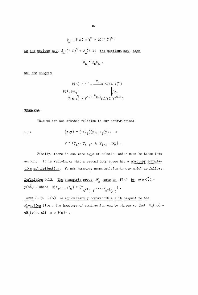
16

@n : P(n) × yn ÷ ~((Z y)n)

is the obvious map, Jn: (Z y)n + jl (Z Y) the Quotient map, the__~n

Cn = Jn@n '

and the diagram

P( n ) vn ~n × ~ ~_, ], f~[(~ y)n]

P(ki)×Xi 1 ~i P(n-1) × yn-I ~n-l~[( z y)n-l]

commutes.

Thus we can add another relation to our construction:

0.Ii (p,y) ~ (P(~i)(p), ~i(y)) if

y = (yl...Yi_l, *, yi+l...yn) .

Finally, there is one more type of relation which must be taken into

account. It is well-known that a second loop space has a homotopy commuta-

tive multiplication. We add homotopy commutativity to our model as follows.

Definition 0.12. The symmetric group ~n acts on P(n) by ~(p)(~) =

p(~) , where ~(t I ..... tn) = (t _i(i) ..... t l(n)) .

Lemma 0.13. P(n) i sequivariantly contractible with respect to the

g-action (i.e., the homotopy of contraction can be chosen so that Ht(~p) = n

~Ht(P) , all p E P(n)) .

17

Pro9f. We start by defining a contraction of I n by Zt(tl...t n) =

(ttl,...,tt n) , and corresponding to Zt ' the contraction H t is given by

Ht(f)(T ) = { ~ , t f ( x / t ) , T s t l f t

( t + T - t I f I . . . . . t ÷ T - t l f t ) otherwise.

( 1 , . . . 1 )

, - ~t(f)

it(In) /

(o,o . . . ,o)

Similarly, we have

Lemma 0.14. The fol.lowing diagram commutes

(P(n) x yn) x (P(m) x ym) tD×¢~ . ~( JIZY ) IT ~( Jl ZY )

)~ (Un,m xl )( shuff

P(n+m) x yn+m ~(JiZy) x ~(JIZY)

Sn,mXl i ~u

P(n+m) x yn+l ......... Cn+m ~ fl/l(~ y)

where Sn, m E "%+m i~s the shuffle of the first

dinates, and T is the interchange.

n with the last

In particular, this implies the additional identification

m-coor-

0.15 (Sn,m(Un,m(p,p')), (y,y')) ~ (Um,n(P',P), Y', Y) •

18

But (Um,n(p' p), y' , , y) is equivalent by 0.9 to the product (p',y')(p,y)

and since P(n) is connected, (Sn,m(Un,m(p,P')),y,y') ishomotopic to

(Un,m(P,P'), (y,y')) ~ (p,y).(p,,y,) •

Theorem O.16. Let K2(Y) = U n P(n) x yn modulo the relations 0.9, 0.ii,

and O.15. Then K2(Y ) is an associative H-space with unit, and the natural

map K2(Y) + ~I(Z Y) is a homotopy equivalence if Y is a connected

CW-complex.

Proof. Consider the type 0.9 and 0.15 relations on P(n) × yn . They

imply that the only t~q~e of (P(n))-relations occur over the points

c~(P(r) x P(n-r)) , where a runs over all (r,n-r) shuffles. We call

these the n-2 "faces" of P(n) . This nomenclature is justified by

Lemma 0.17. Let F = u n-I a(P(r) x P(n-r)) Then a,r=l

i) Hz(P(n),F; Z) = I 0 ' £ / n-I

[z , £=n-I

ii) Let a generator Pn-I of Hn_l(P(n), F) b~e given. Then the

evaluation map

e : (I,$) x (P(n),F) ÷ (I n , DI n )

has degree ±I ; i.e.,

e,(e I ® Pn_l ) = ±e n ,

where e. is the orientation class of (Ii,~) . 1

(The proof is by induction.)

19

In J. F. Adams' paper, "On the cobar construction," Proc. Nat. Acad.

Sci. U.S.A. 42 (1956), 409-412, it is shown that there is a spectral sequence

defined for any space X , and converging to H,(DX, Zp) . Its E2-term has

the form CotorH,(X, Zp)(Zp,Zp) . A similar spectral sequence can be defined

for K2(Y) , and the natural map K2(Y ) + ~(Jl(E Y)) induces a map of spec-

tral sequences. From 0.17, it is then an easy calculation to check that, at

the E2-1evel, the spectral sequence map is actually an isomorphism. Then if

Y is a finite complex, the comparison theorem shows the natural map induces

isomorphisms in homology for all coefficients Zp , and it is known that

G2Z2y has the homotopy type of a locally finite CW-complex. Hence by the

Whitehead theorem (for connected H-spaces), the natural map is a homotopy

equivalence. No~ since Y is the limit of its finite subcomplexes, the

result follows for general Y .

Notice the role of the "complex" of faces a(P(r) x P(k-r)) ,

a((BP(s) x P(r-s)) × P(n-r)) , etc., in the proof of 0.16. Through 0.17,

they are the essential things in making the proof work. The complex for

P(2) is simply that of an interval; that for P(3) has the form of a

hexagon

I

20

As these examples indicate, the comPlexes above are obtained from

cellularly decomposing the boundary of a disc D n-I , and we may simply

replace P(n) by D n-I , and make the type 0.9 and 0.15 identifications

over the corresponding faces to give a much smaller model for ~2~2X .

The explicit construction follows. Recall first that the faces of

the convex hull of a finite point set S in Euclidean space are convex

hulls of certain subsets of S .

Definition 0.18. Let

( 1 , 2 , 3 . . . . . n + l ) ~ R n ~ l

C(n) be the convex hull of the translates of

under the action of /~n+l "

C(n) is easily seen to be the hexagon for n = 2 , the figure

whose faces consist of eight hexagons and six squares C(1) × C(1) for

n = 3 , and in general C(n) has faces of the form ~(C(r) × C(n-r-l)) ,

r = 0 , ... , n-I , as a runs over all (r+l, n-r) shuffles.

let S' c S be the orbit of (l,2,...,n+l) under the action of

Then the convex hull of S' is naturally isomorphic to n-r

C(n-r-l) . Similarly, aC(r) x C(n-r-l) is the convex hull of

(See Lemma 4.2, p. 391 of [18] for details.)

C(n) be the identification above.

Indeed,

~r+l ×

C(r) ×

~ ( S ' ) .

Let I r : C(r) x C(n-r-l) ÷

Note that

faces to faces.

we can define degeneracies

21

C(n) is invariant under the action of "~+i which takes

Also, guided by the need for degeneracies in 0.I0, 0.i!,

D i : C(n)+ C(n-l) , i = I , ... , n+l

(as in Lerm~a 4.5, p. 392 of [18]). Specifically, we have

Lemma 0.19 ([18]). There are maps

D k : C(n) ÷ C(n-l) , i <-k-<n+l ,

so that

i) DII0 is the projection on the second factor;

= ilk-l(oj × id) , j ~ k

ii) Djl k IIk (id × Dj_k) otherwise;

iii) dj(~)D I = Dj8 , 8 ¢ ; B- (j) n-i

iv) DiD j = Dj_ID i ~PF J ~ i .

(Here dj :~n+l ÷~n is the correspondence which makes the diagram

commute.)

Rn+l ~ . Rn+l

8- (j) dj(~) J

Indeed, (i)-(iii) specify Dj on faces, and the map Dj is then

defined by extending linearly along rays to the respective centers. The

reader is advised to check that (i)-(iv) are forced on us by O.10.

22

As the remarks preceding 0.18 indicate, the

replacements for the P(n) , and we have

Corollary 0.20. ~2Z2X ~ U n=0

modulo the relations

C(n) x X n+l

C ( n - 1 ) s e r v e a s

^

i) (C,Xl...xi*,xi+2...Xn+l) ~ (Di+l(c),xl...Xi+l...Xn+l) ;

ii) if c e ~li(C(i) x C(n-i-l)) for ~ an (i+l,n-l) shuffle, then

(c, Xl...Xn+l)~ (~-l(c), x ) ..... x 1 ) ' ~-i(i ~- (n+l)

if X is ~ connected CW-complex with * a vertex. The multiplica-

tion in J2(X) = u 0 C(n) x xn+I/R is given as

{c, Xl...Xn+l}-{c', Xn+l...Xn+m+ 2} = {In(e,c'), Xl...Xn+m+ 2} ,

and with this product, J2(x) is H-equivalent to ~2Z2X .

This provides us with a minimal geometric model for ~2Z2X . Basically,

the model makes it clear that the fundamental data which go into the state-

ment that a space is a 2-fold loop space are an associative unitary multipli-

cation, together with a series of higher homotopies of commutation.

We now indicate how to extend this construction to obtain models for

the higher loop spaces ~nznx , n > 2 .

Consider, for example, the case n = 3 • We have already approxi-

mated ~2Z2(Z X) as J2(Z X) = U C(n) × (Z x)n+I/R = u c(n) x I n+l × xn+I/R ' =

o I n+l x C(n) × xn+i/~ , . Once again we can use the P(n+l) to construct

loops by taking elements of P(n+l) × C(n) × X n+l and defining

23

@(p,c,xl...Xn+ l)t = {p(t),C,Xl...Xn+ I} .

By 0.20(i), these paths become loops. Moreover, the obvious analogues of

0.8, 0.i0, 0.14 continue to hold. Thus we obtain a model for ~3Z3X as

follows.

Definition 0.21. Se_~t J3(X) = u (C(n) × C(n) × X n+l) modulo the relations A

i) (c'c"xl'" "*i .... Xn+l) (Di(c)'Di(c')'Xl'" "xi .... Xn+l) ;

ii) if c' e eIk(c(k) × C(n-k-l)) , then

(c,c',xl...Xn+l) ~ (e-lc,a-lc,,~Xl...Xn+l)) ;

iii if c e ~Ik(C(k) × C(n-k-l)) , then

(C,C',X 1 .... Xn+ I) ~ (~-Ic,o~(c'),~x l...xn+ I)) .

Here Da(c ' ) = [CD~ k+2"~n-k × (Dl)k+l~-l](c ' ) . . . . . . is the obvious degeneracy used

for ~ath$ on (~ X) n+l , which are at * on the first k+l coordinates

half the time, and * on the last n-k coordinates the remainder of the

time.

To complete the definition, we remark that, after using 0.2(i)-(iii),

if the point is equivalent to one of the form

((Cl,C2) , (Cl',C2')Xl...Xn+lXn+2...Xn+m+2) , that is, to a product, then we

asain a~ply (i)-(iii) se~aratel~ to (Cl,Cl'Xl...Xn+ I) , (c2c2'Xn+2...Xn+m+2)

and take the product of the results.

It is now possible to prove an analogue of 0.16 for this model, and

we have

24

Theorem 0.22. If X is a connected CW-complex, then J3(X)

type of ~323X as an associative H-space.

has the homotopy

It is now clear how to generalize the construction. We obtain

co

Definition 0.23. Set Jm(X) = Uo= n (C(n)) m-I x X n+l modulo the relations ^

i) (Cl...Cm_l,X .... *i .... Xn+l) ~ (Di(Cl) ..... Di(cm-i )'x .... xi'"Xn+l) ;

ii) if c. ~ ~Ik(C(k) x C(n-k-l)) , then

(Cl...Cm_l,X!...Xn+l) ~ (~-ic I ..... a-lc. , Da(cj)...Da(Cm_l ), a(x, )) ; J-i "'''Xn+l

iii) the same convention on points equivalent to products as given in 0.21.

Once again we can prove

Theorem 0.24 (Theorem 5.2 o£ El8], p. 395). Let X be a connected CW-com-

plex. Then there is an H-map

j~ - J~(x)÷ ~k~(X) ,

which is a homotopy equivalence.

Remark 0.25. There is a filtration on the points of Jk(X) , given by say-

ing y has filtration m if it is in the equivalence class o£ a point in

(C(m-1) k-1 x X m) under the relations of 0.23. In particular, if * is a

vertex of X , and X is (£-l)-connected, then the set of points having fil-

tration _ < s , Jk(X) (s) , is a subcomplex of Jk(X) and contains all the

cells of Jk(X) of dimension < (s+l)~ (provided X has no cells of

dimension < £ except * , which we can assume). Thus if we wish to con-

sider problems dealing with dimensions ~ (s+l)Z-2 , we can replace Jk(X)

by Jk(x)(S)

25

The reader is advised to work out the explicit structure of Jk(X) (2)

and verify the description given in the proof of 1.11.

26

§i. The Inclusion X ~ ~nznx

Recall from §0 tha~

~ l u s i o n J: X~ ~nznx is defined by sending x ~ X to the map

f : (sn,*) -~ znx , defined as the composition S n -~ (sn,x) ~-~ S n A X = ZnX •

It is clearly natural and continuous, and in homotopy induces the map J, :

-~ ~n+j(znx) , which is just the n-fold iterate of the Freudenthal sus- hi(X)

pension homomorphism. In particular, if X is an m-l-connected locally

finite CW complex, then J is 2m-2-connected.

We convert J into a fibering in the usual way. Thus we first replace

~nznx by the mapping cylinder M(J ) , and J by the inclusion X~ M(J ) •

Then F , the fiber of J , is defined to be the space of paths of unit n

length ExM(J ). starting in X and ending at * , the base point in

~nzn(x) . By the result of Milnor ([25]), if X is a CW complex, then F n

is the homotopy type of one also.

In [18], it was

nzn ~own that H.(~ (X), Zp) is an explicit functor of H.(X, Zp) alone,

and the inclusion J. is injective in homology. Thus, using the Serre spec-

tral sequence of the fibering, it is easily argued that H.(Fn) depends only

o__nn H.(X) and n in dimensions less than 3m-1 if X is m-l-connected.

Here is an alternate description of F Let G , H be associative n

H-spaces with units, and f : G ~ H an inclusion which is also a homomorphism.

f induces an inclusion of classifying spaces ([19], [32])

and we have

Bf : B G -~ B H ,

27

Lemma i.i Let EH~B H be the universal quasi-fiberin~ ([7], [19], [52]).

Then the fiber of Bf is E H restricted to B G ; i.e., p-I(BG) .

The proof is direct.

In particular, if G = ~(X) and H = ~(M(~)) , this provides an

explicit and fairly manageable description of F If X = ZY , the clas- h

sifying space constructions given above can be considerably improved. Indeed,

using the constructions introduced in [18], the inclusion ~ZY~n+Izn+Iy

is H-equivalent to the inclusion

Let X

X ~R +

X : JI(Y) ~Jn+l(Y) .

In §2 of [18], an alternate classifying space construction is given:

be a (free I) associative H-space with unit * and homomorphism h :

so h-l(o) = * ; then E X is defined as X X R + X X mod the relations

(x,t,yz) ~ (xy, t-h(y),z) ,

(x,O,y) ~ (x,t,*) .

B x is then defined as * ×X ~ "

Now, if there is a commutative diagram

(l.2) x-~z ~',~ !+h'

with g a homomorphism~ then there is an induced map Bg : B X ~H Z • More-

over, if g is an inclusion, then Bg is an inclusion and Z X X ~ is the

i This is the geometric analogue of unique factorization in algebra.

28

restriction of E Z to ~ . Thus the fiber in the map Bg

In particular, 395-396 of [18] shows that (1.2) is true for

Y = Jn+l(Z) , using the

we have proved

h I , hn+ I constructed there.

i s x .

X = JI(Y) and

Passing to fiberings,

Le~na 1.3 The fiber F n in the natural map ZY~nzn+Iy is

Jn+l (Y) XJl(y ) EJI(X) "

This space admits a simple description as a CW complex.

Corollary, 1.4 C#(Fn) % C#(Jn+l(Y)) @C#(~Y) and ~(a ® ~(b)) =

(-1) lal aob ® 1 + (-i) lal+l a ®~($b) + ~a ®c(b) .

complex A

applied to

Theorem 1.5

suppose f : A ~A'

phisms i__nnhomology.

i__~nhomology.

There is an algebraic functor ([18], §7) which defines for any chain

an associated chain complex Fnsn(A) • It gives C#(Jn(Y)) when

C#(Y) , and we have ([i~], Theorem 7.2)

Let A , A' be chain complexes over Z (for p a prime), and P

is an augmentation-preserving chain map inducin~ isomor-

Then Fnsn(f) : Fnsn(A) ~Fnsn(A ') also induces isomor-

There are inclusions Yi, j : Fisi(A)~Fi+Jsi+J(A) which, applied to

C#(Y) , are induced from the inclusion Ji(Y)~Ji+j(Y) , and we have

Corollary 1.6 Let X = ZY for Y a connected CW complex. Then H.(Fn, Zp)

depends only on H.(X, Zp) . (Precisely, there are functors ~p(n) for each

p from the category of graded Abelian groups to graded Abelian groups, and

Sp(n)(H.(Z¥)) ~ H.(Fn) .)

29

Proof There is an injection ~ : H.(Y, Zp) ~ C#(Y) @Zp inducing isomorphisms

in homology. Hence we can form the algebraic object corresponding to the com-

plex in 1.3, G = Fn+Isn+l(H.(Y,Zp) @c(H.(Y, Zp)) with boundary as in 1.3.

Z extends to a chain map ~ : G ~ C#(Jn+I(Y)) ® C#(~Y) . Now, filtering both

sides by the dimension in c(Y) , we obtain an algebraic Leray-Serre spectral

sequence with # = H.(Jn+I(Y)) ® H.(ZY) in both cases. Moreover, E2(~) is

evidently an isomorphism of E 2 terms. 1.6 now follows from the comparison

theorem.

Remark 1.7 Suppose we consider the inclusion F ~LzLF , and study its n n

fiber Fn, L If X = ~Y , then the model 1.3 for F n admits a natural

description in terms of spaces CT x (ZY) i where CT is a cell, and identi- ] 1

fioations are made over ~C~ or when a coordinate in (Z Y) i is * . There

is a natural way to construct loops in these sets; namely, by usins the sus-

pension coordinates in (Z Y) i . Thus (ZY) i is an identification space of

I i x yi , and one constructs paths in I i starting at (O---O) and ending

at (i,...,i) . A model for a sufficient number of paths is the Zilchgon o]~ in 0 ~18J

C(i-l) , introduced in §4 of [18 Replacing I i by C(i-l) in each cell above~

performing the appropriate identifications, and forming a universal construction, we

obtain natural, minimal, and canonical models for ~n ' "'" • ~L+IZLFn ' ....

These models also satisfy the property that the inclusions ~LzL-IF n

~L+IzLF ... are homomorphisms. Now we may apply i.} - 1.6 to show that n

H.(Fn,L, Zp) depends only on H.(Y, Zp) . Of course, if X = Z3Y , we can

iterate once more. In general, we have

Theorem 1.8 Define Fnl" . .nk(X ) inductively as the fiber in the ~l~

Fnl...nk_l(X) ~ ~ nk Z~nl.. :nk_l (X) •

30

Then for X = zkY , it fellows that H,(F 1...~K, Zp) depends only on

H.(x,~) .

We will have no further need of 1.7 and 1.8 except incidentally in the

sequel; it is for this reason that the details are so skimpily sketched.

We now turn to the more limited observations which we can make about

F L when X is not a suspension.

Lemma 1.9 (Fiber Le~ua) Let X , Y be n-l-connected and locally finite CW

complexes (n > 2) . Suppos__~e f : X-~ Y satisfies f. : Ht(X~Zp)~ Ht(Y, Zp)

is an isomorphism for t < 2n and a mon~orphism for t < 3n • Convert f

into a fibering with fiber F . Then throu~ h dimensions 3n-2 ~ F is rood p

weakly homotopy equivalent to ~(Y/X) .

Proof F is 2-connected by our hypothesis. Thus, letting C be the class

of finite groups having order prime to p , it is enough to show that there

is a map g : F -~ ~(Y/X) so g. induces a (rood C)-isomorphism H.(F) -~

H.(g~(Y/X)) in dimensions less than 3n-i • But our first description gave

as F = ExY . , and g is defined as the evident projection F

~S* ~ ~.Y/x. = a(Y/X)

Note that F and ~(Y/X) are both 2n-2-connected. Thus the Serre spectral

sequences for the fiberings

F~X~Y ,

D(Y/X) ~ P -~ Y/X

are both exact sequences in dimensions < 3n-2 . Moreover, both sequences

split, and the fact that g. is an isomorphism in this range follows.

51

Remark i.i0 1.9 can obviously be strengthened to give an actual homotopy

equivalence in this range if f. satisfies the h3~othesis of 1.9 with the

integers as coefficients.

In particular~ we can now prove

Theorem I.Ii Let X be a locally finite n-l-connected CW complex (n > I) .

Then through dimension 3n-2 , the fiber F in the inclusion n

X ~ ~nzn(X)

is the spa9 e 2(sn-l~T X A X) (Here sn-1 ~T X A X is given as a quo-

tient space of S n-I x (X A X) where (x,y,z) is identified with (-x,y,z) ,

and (x#*) is set equal to * .)

~ ~ ( I n-I Proof From [18], pp. 394-395/ We know ~nznx ~ X U x X x X)/R through

dimension 3n-i where R is a set of relations defined as follows:

i) (tl...s...tn_l,x,y) ~ (TS(tl)...TS<tj_l) , O...O)TS(x,y)) where

~th position

T(t) = 1-t and T(x,y) = (y~x) if e = 0 or 1 .

2) (tl...tn_l,*~y) ~ (tl...tn_l,yj*) ~ y for * , the base point of

Thus, through dimension 3n-2 , ~nzn(x)/x~ (I n-1 × X A X)/R' where R'

consists of relations of type (1), and (tl...tn_l~*) ~ *

lows from

Now~ l.ll fol-

X .

Lemma 1.12 (I n-I × X A X)/R' ~ S n-I ~T X A X •

Proof Embed IJ~ I j+l as the set of points (~3 tl.-.t j) • This induces

an embedding (I j x X A X)/R'~(I j+l × X A X)/R . (I j+l × X A X)/R' can

be given as the equivalence classes of points of the form (tl...tj+l~x,y)

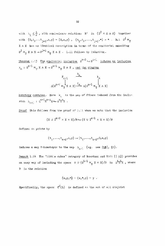
32

i with tl <_~ , with equivalence relations R' in (I j x X A X) together

with (O, t2...tj+l,x,y ) ~ (O,x,y) , (tl,t2,...,tj+l,*) = * But S j ~T

X A X has an identical description in terms of the equitorial embedding

sJ ~T X A X ~S j+l ~T X A X • I.ii follows by induction.

Theorem 1.13

sn-I In : XT

The eguitorial inclusion sn-2~ S n-I induces an inclusion

X A X-~ S n-I ~<T X A X ~ and the diagram

k n F

Fn-I n

~(sn-2 ~<T X A X) " ~(sn'l ~<T X A X)

homotopy commutes. Here k is the map of fibers induced from the inclu- n

~n-iEn-i X sion hn_ I : ~nznx

Proof This follows from the proof of i.ii when we note that the inclusion

(x u I n-2 x X × X ) / R ~ ( X U I n - l × X × X ) / R

defined on points by

(tl,...,tn_2,x,y) ~ (tl,.-.~tn_2,0,x,y)

induces a map H-homotopic to the map hn_ I (eg. see [18], §5).

Remark 1.14 The "little cubes" category of Boardman and Voit ([ 3J) provides

an easy way of including the space X U (S L-I MT X x X)/R in ~L~x , where

R is the relation

(x,y,*~ ~ (x,*,y) ~ y

Specifically~ the space C2(L) is defined as the set of all disjoint

33

embeddings

L

which are linear and take faces into sets parallel to the corresponding

faces in I. 3,~ ) .

acts (freely~) on C2(L) by interchanging I 1 and 12 .

An arbitrary point x of ~Ly can be regarded as a map fx(~,~)

(Y,*) . Given two maps fx ' fy and a point z in C2(L) , there is a map

II~> ~ (Y,*> defined as

This provides a pairing C2(L) M T ~L(y) × ~(y) ~L(y) .

Lemma 1.14 (P. May) C2(L) i_s_sequivariantly homotopig~ to S L-1

antipodal action.

(Indeed, the equivariant inclusion sL-I~c2(L) takes

embedding of a cube of length ~ with center at the point

with the

x to the

x , and the

34

second with center at

i.i4.)

Now~ using the pairing above in ~L~x

desired inclusion of X U (S L-I ~T X × X) in

-x . It is now an easy geometric argument to prove

and restricting to X , the

~L~x is readily obtained.

~2. The Map Fn(X) ~F _z(ZX)

Le~ma2.l ~z(X) =SXVZ(X^X) VZ(X^X^X) V ....

Proof This follows from the well-known ([38]) splittings

ZX n = Z ( X A - - - A X) V ( n ) Z X A . . - A X,,V . . . V(~.) Z X ~ A . . - A X V . - - ,

n n-l' n-j

writing ~JI(X) as an identification space of U Z(X n) .

n

Corollary 2.2 There are H-maps H r : Jl(X) ~ JI(X A ... A X)

r times

(® Hr) . Hj(X)) ~ H.(® QZ(X A .-. A X)) i_£~ injec~ive.

SO

H is called the r th Hopf-invariant map of X • Clearly, if an ele- r

ment ~ in ~.(0ZX) comes from ~.(X), then Hr.(~) = 0 for all r .

Presumably there is a similar splitting for ZnJn(X ) . Thus it seems

reasonable~ in particular, to conjecture a splitting

~J2(x) = ~x v ~2sl ½ x ^ x v z2c(2) ~R (x ̂ x ^ x) v ....

35

Recent results of D. S. Kahn have shown that these splittings exist for

Q(X) = lim ~nznx ; however, at present the splitting theorem for the J n n-+oo

has not been proved.

Thus, we adopt an alternate "Hopf invariant" for the purposes of

this section. The Hopf invariant of a class C~ e ~m(ZX) is defined by

taking -i(~) e ~m_I(~ZX) = ~m_l(Jl(X)) , and projecting onto ~m_I(J(X)/X) .

We denote its image by H(~) , and, in the metastable range, the results of

§i show that H(~) = 0 is both necessary and sufficient in order that

be in the image of o .

In the metastable range, H(~) = H2(~) defined above.

Now we consider the problem of when an element ~ e ~m(ZLx) desus-

pends L-I times but not L times.

Consider the diagram

FL(X ) ~ X ~ 2 L ~ ( x )

I ~t id ~t ~

~tFL_t(ztx ) ~ ~tztx ~ oLzLx .

Clearly~ ~ does not desuspend L times if and only if ~ ~ 0 in

~ . (FL(X) ) . On t h e o t h e r hand, i t desuspends L - t t i m e s i f and o n l y i f

• t . ( ~ ) = 0 . Thus t h e key s t e p ( o u t s i d e o f a n a l y z i n g ~ ~ which we d e f e r

for the moment) is to study the map ~t " We can reduce this to the study

of ~i since ~t can clearly be decomposed as

~I> t-l(

FL(X ) "1> 2FL_I(ZX ) _ _ 22FL_2(Z2X) ~ . . . ~1)> 2 t F L _ t ( z t ( x ) ) .

We have

36

~eorem 2.2

points b_2l

Let f : Z[S n'2 ~<T (X A X)] -~ S n-2 ~<T (ZX A ZX)

f ( t , (x ,y ,z ) ) = (X ( t , y ) , ( t , z ) ) .

Then the diagram

sn-2 ~m (X A X) adj(f)> ~sn-2 ~T (zx ^ zx)

Fn(X) > ~ _ 1 ( ~ )

homotopy commutes in the metastable range.

be given on

Proof The map Q(ZX) ~[Qn-Izn-I(zx)] is given by the inclusion Jl(X) c-~

Jn(X) ([18]). This inclusion satisfies the conditions of 1.9, so the diagram

x * Jn(X)

I JI(X) -~ Jn(X)

induces the inclusion of cofibers in dimensions less than 3n-i ,

sn-i ~<T X A X-~ (S n-I ~<T X A X)/X A X •

In the proof of Theorem 5 of [18], a map (adjoint to the identity) ZJn(X ) -~

Jn_I(ZX) is constructed. Precisely, there is a map (p : I × I ~ ! X I

defined by

(2t,O), t < ½-T

q)(t,T) =1( I -2T, 2(t+T-~)), ½-T < t < I-2T

| [ ( t ~ t ) , I-2~ < 2t

37

for T < ½ , and ~(t, 2A~) = T[~(t,~)] . This then defines a map

r : Z [ (X U I n-1 X ~ ) / R ] ~ (ZX U I n-2 X gX X z x ) t R

by r(t,tl,...,tn_l,x,y ) = [t2,...,tn.l(M(t,tl)x,y ) (identifying 12 X

with ZX X ZX) . In particular, r(t,81,t2,...,tn,X,y ) ~ZX . Thus, fac-

toring X to a point, the induced map factors through

Z[S n-1 ~T (X ^ X)/X A X] •

Finally, note that, for t I = ½ ,

~(t, ½, t2,...,tn_l, x, y) = [t2,...,tn_l(t,x , t,y)} .

Thus 2.2 follows.

Actually, we have proved more than 2.2

Corollary 2.3 Z[S n-I ~T (X A X)/X A X] is_ h~motooy-equivalent t_~o S n-2 ~T

ZX A ZX for X a connected CW c~plex.

Proof Note that, using the cell decomposition of these spaces by the

[I j x X r X Xr] , ~ constructed above is cellular and induces an isomor-

phism of cellular chain complexes.

that

§3. The Cohomology of the

We start by examining the cohomology of the

the structure of H*(Fn(ZX)) we give

There are maps

F n

sn-i ~<T X A X • After

38

J : X A x~sn MT X A X ,

S n K : ~T X A X ~Z~ A X •

K is defined by identifying sn-i MT X A X to a point in sn MT X A X •

Proposition 3.1 (a) J is surjective onto the invariant subalgebra under

(T)* o_ff H*(X A X, Zp) for p an odd prime. Moreover, kernel J = im (K*)

and t h e f o l l o w i n g sequence i_~sexact :

* l+(-1)n(znT)*> H*( ZnX A X, Zp) im (K*) 0 (3.2) ~ (z~x^ x, Zp) ~ ~ .

(b) Mod (2) J i_~s sur.~ective as in (a), 3.2 i_~s again exact, but there are

a d d i t i o n a l e l e m e n t s e i U (0 ® O) fo_._rr 1 < i < n where 0 e H (X, Z2) , and

these completely describe H*(Fn(x), Z2) .

Proof Consider the filtration of fn(x) , X A X~F2(X) ~-~ -..~-~Fn(x) ,

obtained by embedding successive spheres equitorially. The resulting quotient

spaces are the zi[x A X] • Moreover, the d I differential on H*(zix A X, Zp)

is exactly [l+(-l)i(ziT) *]

Lemma 3.3 A chain complex for sn MT X A X is obtained as

W~ C ® C T

where C is any chain complex homotopy equivalent t_oo C#(X) , and W is

any free resolution o_~f Z 2 (e.g. see [18], [27]). (This is immediate from

the geometry.)

Now, to show E 2 = E in ~r special sequence, note, for example,

8e i @ (x @ x) [(i+( i : -1) T)ei_l] @x®x

39

X i s a c y c l e i n ~C • B u t ( T e i _ l ) ® x ® x = "'(-1) d i m X

i f

d u e t o t h e a c t i o n o f T i n S n x X A X • H e n c e

= I0 , i ~ dim (x)(2)

I ® x ® x I t~ei_l ® x ® x , i -= dim x ( 2 )

in W ~ C ® C • Thus cycles in ~ are represented by cycles in

and 3.1 follows.

el_ 1 ® ( x ~ X)

W~C®C ,

It is also fairly easy to verify that cup products (mod 2) are given

by the formulae

(3.4) [e i U (e ® e ) ] U [e j U (T ~ ~) ] = e i + j U (e~ ® e l ) ,

• IO~ i>O, [e t U (8 @ 8 ) ] U (a,b> = (aS,he> , i = 0 .

Here, (a,b) is an appropriate choice of generator, so J (a,b} = a ~ b + b ® a ,

and e ° U 0 ~ 0 i s a n e l e m e n t f o r w h i c h J * ( e ° U 0 ® 0 ) = 0 G O • I n d e e d ,

3.4 follows directly from:

Lemma 3.5 ~ : Fn(x) -~ fn(x) X Fn(x) admits a chain approximation

~: (w®z2 c~c) ............... ½)> w ®W e(z~×%) (c ®c )

- c®c)®(w®z2 c®c) shuf% (w 52

where ~ is a_ (T ~ T, T) equivariant diagonal ~ for W , and ~ i_~s

any chain approximation to the dia~onal in X . (This is again immediate

from the geometry; eg. see [27] .)

40

We turn now to the question of higher Boeksteins. Mod (p) for p

odd, these Bocksteins are determined by 3.1(a); however, their structure

mod 2 is somewhat more involved.

Proposition 3.6 Suppose ~i(a) = b and:

a) dimension a is even] then ~j(a ® a) = 0, j < i and ~i(a ® a) =

<a,b> , while sql(b ® b) : e I U b ® b ;

b) dimension a odd implies that sql(a ® a) : e I U a ® a

+I0, i>l

I (a,b) , i : i ,

while ~i+l((a, b) + 8el U a ® a) : b ® b ;

Sql( e2i+l 2i+2 c) for i e 0 and dm a even, U (a ® a)) = e U a ® a ,

and for dim (a) odd, sql(e 2i U a ® a) = e 2i+I U a @ a .

(The proof is a routine exercise using the explicit chain complex for Fn(x)

in 3.3; e.g., as in [20], [27].)

Finally, it remains to evaluate the action of ~(2) and G(p) in

H*(Fn(x)) . For p odd, this is immediate from 3.1 (modulo an extension

problem, but that is handled in the next section; it turns out that the exten-

sion is trivial). Here is the result for p = 2 .

n . .

Theorem 5.7 Assume e e H--(X, Z2) • Then:

a) Sqi[e k U (0 ® 0)] = E (k) [ n-j ~ek+r-2j • \i-r-2j/ U (SqJo) ® SqJ0 , r,j

b) Sql(e ° U O @ O) = / (sqr8, Sql-re> + Zn-j~ i-2j i_2jle D SqJ(0) (9 SqJ(0) , r<i

i

c) Sqi(a,b> = E (Sq ra, Sqi-rb> ,

r--O

at least modulo terms in i m (K*) .

41

Proof The functor e ~ e ° U e @ e is natural and representable, so it

suffices to establish a , b for ~ @ ~ where ~ is the fundamental class

of a K(Z2,n ) . Moreover, there is the map K : RP ~ X ... x RP~ ~ K(Z2,n ) ,

taking ~ to e I ® ... @ e n which induces a monomorphism in coh~mology for

dimensions ~2n . Reference to ~.i (and the obvious naturality) shows that

£n(K) : Fn(RP ~ x ... x RP ~) ~£n(K(Z2,n)) also introduces a monomorphism in

dimensions ~ 4n . Moreover, Fn(k)*[L ® L] = (e I ® e I ) U ... U (e n ® e n) .

Thus we can apply the Caftan formula (noting by 3.4(b) that sql(e ®e) =

~l(e®e) =e lu(eee) +(e2,e> and Sq2(e®e) :(e~e) 2 = 2® 2)

Now a , b follow directly.

Finally, to prove (c), consider the map

pu~ n S : X K(Z2,m ) × K(Z2,,g ) -~ Fn(K(m) X K(#))

defined by S(x,y,z) = [x(y,z)(y,z)] . It is easy to show that S (tm, Li) = 0 ,

but S*[e i U (SqILm U SqJLI) (2) = e i@ (SqILm U SqJL2)2+W is non-zero. Hence

Sqi(~m,~) can only involve terms (Sql~m , Sqj'r~) and perhaps a term in

im (K*) •

Finally, we will need the evaluation of the suspension map TI (2.1)

in cohomolo~j.

* * i ei+l Theorem 3.8 (~i) (a,b> = 0 • (~i) (e U q(a) ® g(a)) = U (a ® a) .

The proof is direct from 2.3.

now consider the structure of H*(F(ZX)) . By use of the Eilenberg- We

Moore spectral sequence ([26], [30], [31]), there is a spectral sequence

42

converging to H.(Fn(ZX)) having ~ term

* ~ n+l n+l Tor T[H.(X, Zp)](H.(~ Z (X), Zp), Zp) Here T(A) is the tensor alge-

bra on A , and H*(Gn+Izn+I(X) T[H.(X, Zp) Zp) is a module over ] from

the inclusion of H-spaces JI(X)~Jn+I(X) .

Moreover, the arguments of 1.6 show that ~ = E ~ . Thus, to calcu-

late H.(Fn(ZX)) , it suffices to calculate these Tot groups.

Note first that H.(Jn+I(X), Zp) = Pn ®R where P is a polynomial

algebra P( ...7i(x)... ) , with x running over H.(X,Zp) and the 71 over

same basis for the universal loop homology operations# and R is

A(H.(X, Zp)) , the universal commutative algebra generated by H.(X, Zp) . The

action of T on P@R is then obtained by projecting T on I OR •

Also, T is free; hence a resolution of T has the form O~

T ® s(H.(X, Zp)) ~T ~Zp Now, tensoring with P ® R and taking homology,

we see that a basis for Tor~(P ® R, Zp) as a P ® R module is given by

the cycles

(a,b) = as(b)-(-l)laI+Iblbs(a) for a ~ b in H.(X, Zp) .

We have thus calculated

Theorem 3.9 H.(Fn(ZX), Zp) % Pn ® L where L is a module over R with

generators (a,b) o_~f degree lai+Ibl+l , where a , b are non-equal basis

elements in H.(X, Zp) . L i__sscompletely determined as a module b_~the rela-

tions a(b,c)-(-l)lal'Iblb(a,c)+(-l)Ibl'Icl+lal'IClc(b,a> = 0 • *

We now turn to the cohomology structure of F n

fibering ~n+Izn+ix ~ F ~EX ~ ~nzn+Ix . n

This proof was suggested by J. C. Moore.

First note the

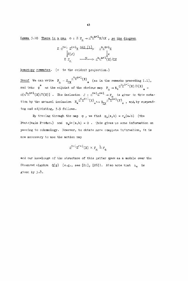
43

Lemma 3.10 There is a map ~ : Z F n ~nzn+ix/zx , so the diagram

Z ~n+l zn+ix ad~) (I)> nzn+l X

E F n cp,, > ~n~n+l(x)/ZX

homotopy commutes. (~ is the evident projection.)

n n+l Proof We can write Fn = EZX~ Z (X). (as in the remarks preceding 1.1),

. ~zn+l(x)/z(x ) and take ~ as the adjoint of the obvious map Fn~E . . =

~n+izn+l ~[anzn+l(x)/E(X)] . The inclusion J : ~ F is given in this nota- n

~nzn+ltx~ EEXg;nzn+l(X) tion by the natural inclusion E. ~ ~.¢-~ . , an~ by suspend-

ing and adjointing, 3.9 follows.

By tracing through the map ~ , we find ~.(a,b) = ~.(aob) (the

Pontrjagin Product) and ~.~o(a,b) = 0 • This gives us some information on

passing to cohomoiogy. However, to obtain more complete information, it is

now necessary to use the action map

~n+izn+l(x) × F ~ F n n

and our knowledge of the structure of this latter syeceas a module over the

Steenrod algebra G(p) (e.g., see [21], [28]). Also note that k. is

given by 3.8.

44

~4. The Structure Of Iterated Loop Spaces In The Metastable Range

We start with the following basic result:

Lemma 4.1 Let X be the n th loop SliCe o~f Y .

G ~ ~nznx ~ X n

has a cross-section. H@nce, u/!to weak homotopy equivalence,

~nznx = G X X • n

Indeed;

the fiber in the inclusion

Then the fiberin5

OG n = F n ,

: X~ ~nznx •

Proof The cross-section of ~ is exactly the inclusion X~ ~nznx • Hence,

since ~nznx is an H-space, there is a map

G × X W ~nzn x , n

and T o W is projection on the first factor. Moreover, if we let G n be

given explicitly as ~n(H) , where H is the fiber in the adjoint map znx -~ Y ,

then the diagram

G × X W > nnz--x n

45

commutes up to reparametrization of paths. Now both maps are fiberings with

fiber G n Thus~ by the five-lemma~ W is a weak equivalence.

n )//H~(Gn,Zp) Corollary 4.2 H.(X,Z) H.(~ znX, Zp a_~sHopf algebras. I__nnpar-

ticular, i_~f X i_~s m-l-connected, then H.( X, Zp) determines H.(Gn, Zp) com-

pletely i~n dimensions < 4m-I , and G is 2m-l-connected. (Indeed, a Hopf n --

algebra basis for H.(Gn, Zp) may be given with generators ~[~.(x)] -

~.[~(x)] , ~.(Xl) ..... ~.(Xn) - ~.(x I ..... Xn) where Xl.-.x n run

over a suitable basis for H.(X, Zp) , and the QI over a basis for the loop

homology operations.)

Corpllary 4.3 Suppose again that X i~sm-l-connected. Then in dimensions

less than 3m-i , G n i__~s homotoDic t__oo sn-I ~T X A X f g~ X, the homotopy

type of a CW complex. Moreover, this equivalence is natural in the same

ranse (from i.Ii and 4.1).

Corollary 4.4 Under the assumptions o__ff4.}, Hi(X, Zp) depends only o n_n

@

H.(Y, Zp) for p odd, and on H (Y, Z2) as a_~n ~(2)-module for i < 3m-I •

Proof Since G = ~nH ~ where H is the fiber in the map znx~Y , n

4.3 implies that H ~ zn(s n'l MT X A X) in dimensions less than n+3m-i .

Also, in this range of dimensions, the Serre spectral sequence of this fibra-

tion becomes a long exact sequence

(4.5)

and, to obtain H (X, Zp) for p a prime, it suffices to evaluate the map

. For example, for p = 2 , to evaluate 5(e i U a ® a) , consider the map

y ~(a)> K(Z2,~ )

46

By 4.3, this then induces a map of exact sequences

• ~i+l. , ~H~(H~,n ) ~n (K(Z2,~)) ~+l(znK(z2,n-~))

l l 1 ~i(H) ~ Hi+l(y) ~ ~i+l(~X) ~ .

Moreover, Fn(~(~))(e i U ~ ® L) = e i U ~®~ , and 5 is determined by its

behavior in the universal model. 4.4 follows.

In considering the proof of 4.4, it becomes clear that we need to know

the map

: Hi(H~, n) ~HI+I(K(Z2,~), Z 2)

in order to determine the explicit form of the functor occurring in 4.4.

Theorem 4.6 5~n[e i U (SqI(L) @ sql(~)] = Sq ~ + deg (I) + i+l(sql(L)) ,

while

n I j*~n(sql(~) U SqJ(~)) = ~ (Sq (~), SqJ(~)) (in 4.5).

Proof The second statement is obvious. To prove the first assertion, it

suffices, by naturality and the known behavior (§§2,3) under suspension, to

check that 5[q(L~® ~)] _ i+l, ~ (~+i)2 in the fibering ZK(Z2,~ ) = ~q ~ + l ) =

K(Z2,~+I ) . Indeed, by the known results ([6]) on H (K(Z2~+I)) , the kernel

of ~* in dimension 2~+2 is exactly (~)2 On the other hand,

~+I(z(K(~,~) A K(~,~)), Z2) = Z 2 , and has generator ~(~ @ ~) .

Remark 4.7 The results 4.4, 4.6 give the structure of H*(~ny, Zp) completely

in the metastable range as a module over In particular, we have

4.6 follows.

Z P

47

Cor011ary 4.8 Suppose Y i__ssm+n-l-connected, and H (Y, Z2) satisfies

SqI(a) = 0 for excess (I) > [dim(a)-n] . Then in dimensions less than

H*(~nY, Z2) = s-nH*(y) @ H*(Gn) .

3m-i ,

However, this splitting need not be valid over C(2) •

12. CP~ 8 certainly satisfies the hypothesis of 4.8 if m = 5 •

secondary operation ¢8 ~ associated with the relation

sqlsq 8 + Sq2Sql(Sq 6) + Sq8Sq I = 0 ,

For example,

However, the

is non-zero when evaluated on the bottom cell of Cp128 . On the other hand,

¢8 is universally zero on any 5 class. Thus, we must have ~II(¢8(e8) )

contained in the indeterminacy of (¢8) . But this indeterminacy is zero in

the part of H*(~IIcpI28) coming from ~!I(H*(CpI28) ) . Thus it must come

from H (Gll, Z2) . In particular, there im~st be an element ~ e H (GII,Z2) ,

so Sq2Sql(~) = ~iI(¢8(e8) ) .

§5- The Obstructions To Desuspension In The Metastable Range

We conclude the first part of this paper by considering a basic exam-

ple. In the metastable range, we reduce the question of desuspension to the

determination of when a certain map ~ of known spaces is homotopy-triviai.

Berstein and Ganea independently have obtained related results ([36]).

Theorem 5.1 Let X be n-l-connected~ and . have dimension less than 3n-2 .

Then:

48

i) if Y is the 2n-L-i skeleton of X , there is a unique space Z ,

s__~o ~Z = Y ;

2) X itself is an L-fold suspension if and only if a certain map

: X/Y ~+IsL-I MT Z A Z

i~shomotopy-trivial;

3) if ~ i__~s trivial, the number of distinct L-fold desuspensions of X

i_~s equivalent to the set of homotopy classes of maps

[X/Y, ~S 2-I ~T Z A Z] .

(To avoid low dimensional complications, we also require L to be less than

n-3 .)

Remark 5.2 In 5.1-9, the equivalence classes comprise: (a) distinct homo-

topy types of desuspensions, and (b) maps

L where Z--W = X , and where

2n-2L-i skeleton of W .

h : W-,W

h is a homotopy equivalence ~i on the

Remark 5.3 By the dimensional restrictions, ~ is actually a stable map

since sL'I MT Z A Z is 2(n-L)-l-connected. Similarly, the set occurring

in 5.1.3 is stable. Thus stable techniques are sufficient to determine them.

Proof g Ly is a CW complex. The dimensional restrictions imply that the

adjoint map zL~LY~ Y induces an isomorphism in homology in dimensions

< 2n-L . Now taking the associated cross-section of ~Ly , we can assume

that Y is actually the 2n-L-i dimensional skeleton of zLoLy ° Thus Y

49

is a suspension ~Z . Moreover, the attaching map of every cell of Z is

stable~ Hence Z is indeed unique. This proves 5.1.1.

From 5.1.1, X/Y = zL+~ for a unique W . Moreover, there is a map

: Z~ ~zLz , so the following is a cofiber sequence:

(5.4) sTm ~ ~z ~ x ~ ~+~w ~ ....

Then X is a suspension ~(M) if and only if • : zLT ' for some z' •

W-~Z .

(5.5)

Consider the diagram

T ~ W ~ Z •

We assert that ~' exists if and only if the composite

(5.6) W a ~ ' ~L. LEL z ~ ~L~z/z

is homotopy trivial. This follows from

Len~ma 5.7 Let ~ be the fiber in the map ~ : ~LzLz~LzLz/z . Then

throug~h dimension 3(n-L)-2 , ~ ~Z , and the inclusion ~ ~LzLz factors

the inclusion Z ~LELz . (This is immediate from the fiber lemma, §i.)

On the other hand~ from the proof of i.ii, it follows that, in the

range of dimensions which concern us, ~LzLz/z ~ S L-I K T Z A Z , and this

concludes the proof of 5.1.2 when we note (as in 5.3) that ~ o ~L o P is

a stable map, hence is homotopic to zero if and only if zL+I(~°~L~oo) =

: X/Y ~EL+Is L'I ~T Z A Z is.

SO

To prove 5-i.)~ note that different suspensions satisfying the

relations imposed by 5.2 are given by different homotopy classes of liftings

in (5.5). But by 5.7, these are given by maps of W into the fiber.

~(~LzLz/z) ~(sL-I ~T Z A Z) in our range. Dimensional considerations

show that these are again stable~ and 5.1.3 follows.

Remark 5.8 Combining 5.1 with 4.6 and the structure of S L-I K T Z A Z , it

is direct to calculate the first few obstructions explicitly in terms of

higher order cohomology operations in X . For the first two obstructions~

see [36] in particular.

Remark 5.9 Recent work of D. Anderson ([)5]) makes it also possible to give

analogues of 4.6 for certain exotic cohomolo~y theories~ eg. K-theory. This

in turn makes it possible to carry through a program analogous to 5.8 in

these theories as well. This remark will be considerably amplified in a

forthcoming paper.

PART I I

§6. An Unstable Adams Spectral Sequence

In this section, we introduce a version of the Adams spectral sequence

which gives information about the unstable homotopy of a Sl~Ce X . It is

invariantly defined from ~ on; however: (1) little is known about its con-

vergence properties~ and (2) in general, ~ is not just a functor of

H*(X, Zp) over Q(p) but actually depends on the space itself.

The construction we use is similar to the one given in [17]. However,

due to the special cohomological properties of the spaces they considered~ it

there turns out that ~ is a functor of H (X, Zp) over G(p) .

In §8~ we will show that, in the metastable range~ ~ is algebrai-

cally determined (explicitly) from H (X, Z2) over G(2) . Thus we reduce

many of the problems involved in metastable calculations to formal algebra

and the determination of differentials in this sequence.

Definition 6.1 An Adams (p,q)-resolution of a space

q a positive integer is a sequence o f_f fiberin~s

P l P2 . P3 X -- E 1 -- E 2 ' E 3

BH1 B~ B~5 BH4

X for p ~prime and

where:

i)

ii)

E i is the fiber in the map ~i ;

~. is a generalized Eilenberg-MacLane s~ace 1

p , and

K(Zp,n~ for the prime

52

iii) ~ = (nl,...,ni) with each nj ! q ;

0 i : Hk(Ei_l,Zp) ~ Hk(Ei,Zp) i s_s 0 for k ~ q . iv)

It is clear that, if X has the homotopy type of a CW complex, then

(p,q)-resolutions of X exist for all (p,q) . They also satisfy the natu-

rality properties:

Lemma 6.2 Let f : X ~Y be a map o__ff CW Complexes, and suppose siren

sequences

a) Y <-- E{ <-- E~ <-- E~ <--

H} H 4

where (a) satisfies (i), (ii) of 6.1, and (iii) with

o_~f q;

b) x <--~l <--E2 <--~3 <-

where (b') satisfies all of 6.1.

Then there are maps fi : Ei -~ E! • I ~ so the diagram

x <--E 1 <--E 2 <--E 3 <--

Y <--El <--E~ <--E% <--

q-i in Dlace

commutes.

Lemma 6.3 Under the assumptions o__ff 6.2, suppose f ~ g : X -~ Y and

[gi : ~i ~ El}

$3

are given. Then there are homotopies

SO

i)

ii)

iii)

K i : I x E i -~Ei_ I ,

Ki(O, Ei) = Pifi ,

Ki(l,Ei) = pigi ,

the diasram

IX P2 IX p} I x X <iXPl I X ~ < i x ~ <

, <-- , <-- y <-- E 1 E 2

I×Es< ..... ...

commutes.

As usual, taking the homotopy exact couple of the (p,q)-resolution in

6 . 1 g i v e s a s p e c t r a l s e q u e n c e . S i n c e E i ~ Ei_ t ~ BH. i s a f i b e r i n g , i t f o l - 1

lows that ~.(Ei_l,Ei) ~ ~.(BH. ) . Moreover, the d I differential is i

obtained b y p a s s i n g t o homot opy i n t h e c G m p o s i t i o n

H i -J-> E i ~ BHi+I

where j : H i ~ E i represents H i as the fiber in the map Pi " By using

6.2, 6.3, we define our desired spectral sequence by passing to inverse limits

over q when we note

Corollary 6.4 ~i,j(X)[(p,q)] depends only on X for i-j < q-i , and is

isomorphic to ~i,j(X) . l__nn particular, h~i,o(X > depend ~ only o__nn X and

not the resolutions used to take the inverse limit.

$4

Note that, when X is a (single) suspension~ the convergence proof

given in [34] carries over without change. (It depends only on 6.2 and the

fact that it is possible to map a suspension onto a space Yx ' which satis-

fies 6.5(i) below for x c ~.(X) , so the image of x in ~.(Yx) is non-

zero.) Thus we have

Corollary 6.5(i) l_~f X satisfies the condition that, for each j , there r.

is an rj < ~ __s° p 3~j(X) ® Z(p)~ = 0 , then the spectral sequence con-

ver~es to ~.(X) @ Z (p)~

(ii) l_~f X is a susDension, then the spectral sequence always con-

ver6es t_~o ~.(X) @ Z

For general X , the difficulty in extending 6.5 is in the elements

of infinite order in ~.(X) . If X is simply connected, has the homotopy

type of a locally finite CW complex, and is also an associative unitary

H-spae% then: (a) the only elements of ~.(X) of infinite order are con-

tained in Z-direct summands, and (b) have non-trivial images under the

Hurewicz map ([43]).

Put another way~ this says that the Postnikov in~riants are all

finite for X • An easy argument now shows:

Corollary 6.6 i__ff X i_ssa simply connected~ locally finite unitary H-sDace ,

then the spectral se ence qu converges to ~.(X) ® Z

6.5 and 6.6 establish convergence insofar as we need it. It is prob-

able that more extensive results in this direction can be obtained from [44].

55

Example 6.7 Let X = K(Zps,n) . Then Bill = K(Zp, n) X K(Zp,n+I) , and the

k-invariants are (~) and ~(~) . It is easily verified that E 1 = K(Zp3,n ) ,

and the map Pl* is multiplication by p . Thus E 2 ..... E n .....

1 K(Z 3,n) , and Pn* is always multiplication by p . In particular, El, j =

P o E+?. . = 0 unless j-i = n,n+l when it is Z The differentials are all m,j p

d 3 's and are all non-trivial.

A map of spectral sequences ~ : Ei,j(X ) -~ Ei, j+I(ZX ) is defined

from 6 . 2 , 6 . 3 , t h e map ~ : X~-~ ~ , and t h e s e q u e n c e

(6.8) nPl JP2 ~SX <i ~EIIZX) ~'t EX) <

associated to a (p,q)-resolution of ZX .

Corollary 6.9

in dimensions

If X i_~s n-l-connected, the sequence oil (6.8) satisfies 6.1(iv)

< 2n-2 . Thus

a : Ei, j(X ) -* Ei,j+I(ZX )

is an isc~orphism in dimensions j-i ~2n-2 .

Corollary 6.10 If X i_~sn-l-connected, then

~i,j(X ) N Exti,ja(p)(H*(X), Zp)

for j-i < 2n-2 .

Remark 6.11 It is possible to generalize somewhat the above construction.

Let Ac-~H (X, Zp) be an unstable sub-~(p)-module. Then we can resolve X

by a sequence of fiberings

56

X P2 <P3 E5 <__ < D-~-l E 1 <-=- E 2

BG(A) BG 2 ~G 3 BG 4

so im (~i)* is exactly A , while the sequence ~*- E2~- E3~- is a

(p,q)-resolution of E 1 . Analogs of 6.2 through 6.6 continue to hold.

Thus we again have an Adams-type spectral sequence with invariantly-defined

Z-term. We denote it #(X,A) . Clearly, in the stable range, there is an

Ex'i+l'* , ," " ~i+l .(X,A) Ext i' G(p)(H (X)/A, Zp) exact sequence t G(p~[A, Zp) ~

Exti+2'~(~u PJ~(A'ZP) ~ ... , though, as we will see in the examples, 8 may

well be non-trivial.

7. The Loop Space Functor For Resolutions

Let X be m-l-connected, and suppose that

(7.1) x jl E1 & J3 < -

is a (2,q)-resolution with q < 3m+n • In this section, we wish to study

the behavior of (7.1) under the operation of taking loop spaces. It will

appear that the sequence

(7.2) ~nznx ~ ~npl --~nE I

is not a (2,q-n)-resolution, as

~n _ _ ~n~ < ~nE3 < ...

(~npl)* is not zero in general. However,

this is the only point at which the sequence fails to satisfy the definition

for a (2,q-n)-resolution. Moreover, we will be able to calculate exactly

im (anpl)*

We begin by proving

57

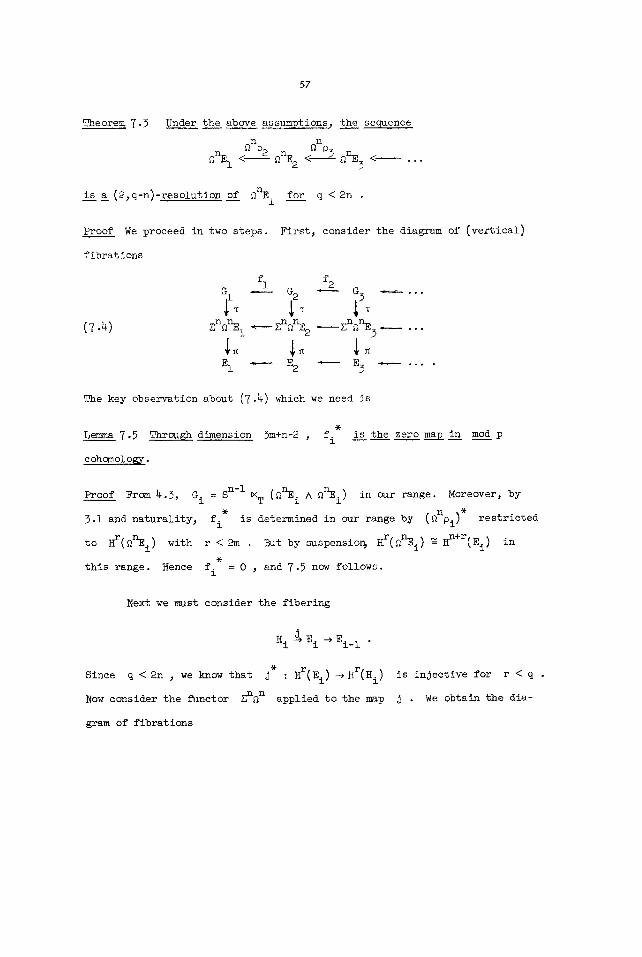
Theorem 7.3 Under the above assumptions, the sequence

eZ_ .%< ...

is a (2,q-n)-resolution of GnE I for q < 2n .

Proof We proceed in two steps. First, consider the diagram of (vertical)

fibrations

(7.4)

fl %

z n a ~ l .~ znanE2 . , z n ~ } . . . .

E 1 ~ ~ " E 5 • ....

The key observation about (7.4) which we need is

Lemma 7.5 Throug~u dimension 3m+n-2 , f. 1

cohomology.

is the zero map in mod p

Proof From4.3, Gi = sn-1 ~T (~nEi A ~nE i) in our range. Moreover, by

* n * 3.1 and naturality, fi is determined in our range by (~ pi ) restricted

to Hr(~nEi ) with r <2m . But by suspensio~ Hr(~nEi ) ~ Hn+r(Ei ) in

this range. Hence fi = 0 , and 7.5 now follows.

Next we must consider the fibering

H i ~ E i ~ El_ 1 •

* HqE~ Since q < 2n , we know that j : ) ~Hr(Hi ) is injective for r < q .

Now consider the functor ~n n applied to the map J . We obtain the dia-

gram of fibrations

58

(7.6)

G: ~ G. 1

zn~nHi~zn~nEi

L I H i ~ E i

From 3.1, it now follows that e. is inJective in our range. In particular,

given x e Hr(Ei ) , we can suppose that J (x) = ~ and ~ ~ 0 ~ then the

class j*(sqdim(~)+k+l'n(x)) : sqdim(~)+k+l-n(~) ~ 0 • Thus sqdimC~)+k+l-n(x) ~ 0 ,

provided, of course, dimension (6) < n+m . From the exact cohomology sequence

for the left-hand fibering in (7.6), we find

5(e k U ~ @ ~) = sqdimC~)+k+l-n(~) •

Hence 5(e k U x @ x) ~ 0 in H (El) • Hence the only possible elements in

H (Gi) which are in the kernel of 5 are the <x,y) with x ~ y in H (El) @

(Of course, x and y must each have dimension less than n+m .) Now note

(as a consequence of 4.6) that

( 7 . 7 ) <x,y}* = T*onc~ncx) U ncy)) ;

hence (x,y> E ker 5 , and these elements give the entire kernel.

n To c~mplete the proof of 7.3, we suppose there is a k e H (Z ~nEi,~)

with (znanpi)*(k) ~ 0 . In the diagram (7.4), It is certainly true that k

is not in the image of

Hence ~*(k) ~ 0 .

Hence ((7.6), (7-7)), it follows that

for some

= ~nc~ncx) u ~ncy)) +

in the image of

5 9

On the other hand, (~npi)*(~n(x) U ncy)) : ( npi)*(nx) U (~npi)*~n(y) : 0

BE -** -

Also, trivi~&ly, (Z ~ pi ) ~ (x) = 0 • But this implies

(zn~npi)*(k) = 0 •

Hence k = 0 , and 7.3 is proved.

We now turn to the first map in (7.2), Gno I : GnE I ~nnz ~X •

the proof of 7.3, we suspend and consider the diagram of (vertical)

fibrations

As in

(7.8)

e G < G 1 < G{

i 1 1 Zncanznx) <znanpl znanE1 < znanH1

z~x < ~ < H a

Note that ~ has a homotopy inverse. Hence, in the metastable range s

(7-9) zn~nznx~znx V G .

Before proceeding further, we need to consider the bottom (horizontal)

fibration in (7.8). For n(~) in H (znx, z2) , let t(~) be any element

@

in H (H1) which s a t i s f i e s

(7.10) 5(t5(~ )) = n(~)

in the Serre exact sequence of the fibration. Note that, for all k ~0 ,

we have

(7.11) sqdi~(~)+k+l(t(~)) ~ im (j) .

60

(In our range, this is due to exactness and the fact that sqdim~aj+l+k(~)f ~ ~ 0

for k ~ 0 ° For general k ~ 0 , it follows from the Borel transgression

theorem.) Hence~ for each k~O , we can choose

satisfying

(7 .m)

Theorem 7.13

correspondin~to

~.CG~ we have "K" "

Proof

%(~) ~ H*(~)

j*(%(~)) : sqdim(~)+k+l(t(~))

Under the splitting (7.9), let qk(~) be the cohomology class

e k U (C®G) i__n_n H*(zn~nznx) . Then for some choice of

(zn~n%)*qk(~) : ~k(~) .

It suffices to verify 7.1~ in the universal situation. The space

which is universal for

the bottom line of (7.8), we consider the fibering

(7.14) K(Z2, n-i + dim (~)) ~ ~znCK(%,

Of course~

n(~) is Zn(K(Z2 , dim (G))) . Thus, in place of

t(°~dim(~)) : ~n÷l÷dim(~) "

Now consider the f i b e r i n g

(y.15)

Clear l y , ~n~

zero element in H*(~) •

dm (a))) .

is 2 dim (~)-l-connected, and e*(L * ~) = > , the first non-

(Here, L * L is the class dual to the Pontrjagin

61

product.) By 4.3, n~ = sn-i ~T K(Z2' dim (G)) A K(Z 2, dim (G)) in the

metastable range 3 and 7.13 follows by naturality under suspension. (Explicitly,

the class corresponding to e k U L ® ~ in H (U, Z2) pulls back under

in (7.14) to sqk+l+dim(G)L .)

Remark 7.15

the space Y

tion is that

Finally 3 it should be noted that 7.3 is valid whether or not

with which we start is znx . Indeed, the only crucial condi-

Y be n+m-l-connected.

8. The Metastable Exact Sequence

In this section, we assume X is m-l-connected, and restrict our

attention to the 3m-2 skeletons of all the spaces under consideration.

Consider the fibering F L ~ X ~ flLzLx ; then 3 as we have observed 3

F L has the homotopy type of

fl(S~-i ~T X ^ X)

w in our range. Consequently 3 H (FL,Z2) has a natural sub-~(2)-module

A = [~ (a3b) ; a3b e H*(X)} .

A plays a fundamental role in the sequel. Before proceeding to our

main result, 8.53 we illustrate why this must be so.

Lemma 8.1 Consider the inclusion

~L+IzL X e : ~F

Then ker (@*) is exactly A . (This follows immediately from the results

of Part I (notably 3.10).)

62

Now suppose we start to construct (2~q)-resolutions. Observe that the

composite

(8.2)

is onto in cohomology.

x ~ ~ L ~ x ~ ~Lz~x ~ ~ Hence the first stage in the resolution of X can

be assumed to be the fiber in the map of (8.2). The following diagram of

(vertical and horizontal) fibrations is thus obtained.

(8.3)

F L = > F L

E{ > X

aL( Pl)> nL~ ~LELx

! (since E 1 can be regarded as the pull-back via

: x * ~Lz~x)

> nLBHI

~L( 01 ) of the fibering

T e=~ 8.4 (a) ~ (7)* = A,

(h) H(~I)~AeB

L * where B = H*(aT(~)l/im a (pl)

Proof In our range~ the Leray-Serre spectral sequence becomes a long exact

sequence. Note that, in the sequence of the left-hand fibering in (8.3),

L * ~L( pl)*(y ) 5(x,y) = x O y and ~L(ol)* x U y = ~ (pl) (x) U = 0 • On the

other hand, 5e i O (x @ x) = (Qi(x))* , and the results of §7 show that

~L(pl)*(Qi(x))* ~ 0 • Indeed, the ~L(D1)*(Qi(x))* span im ~L(pl )*

8.4 follows.

63

We are now ready to state the main result of Part II.

Theorem 8.5 Suppose L > 5m • Then there are maps o_~f spectral sequences

~I." : Ei,j(~X)* ~ Ei, j_L_I(FL,A ) * ,

jl. : Ei,j(FL,A) ~ Ei+I,j+I(X ) ,

and the resulting sequences

J2 L

i,j L i 1,j "'"

are exact fo__~r j-i ~ 3m-2 , and converge to the generalized E.H.P. sequence.

Remark 8.6 The mechanism for determining ~I. will be made clear during

the course of the proof.

Proof We begin by constructing the maps ~. , J..

Consider the first stage of an (FL,A)-resolution of F L :

(FL) 1 ~FLZ B(A )

where im ~ = A . From Lemma 8.!~ there is no obstruction to extending 8

to a map 81 so

aL+Ip I 0

~+lzL x o> F~

commutes. The map 81 may now be continued to a map of resolutions. This

gives ~. on passing to spectral sequences. Moreover~ by 6.3, ~. is

invariantly defined from ~ on.

64

* e i (aL+lO1)*(Qi(x.))* Remark 8.7 From 7.13, it follows that e I ( O x ~ x) =

Thus the map e I is completely determined except on secondary elements asso-

ciated to the resolution of A . We shall discuss this situation more care-

fully later in this section.

Now~ consider the map

F L ~ X •

Since ~* : H*(~LzLx) ~H*(X) is surjective, it follows that j* = 0 . Let

' be the first stage in a resolution of X • It follows that j lifts to E 1

7. FL~ i •

From 8.4(a), ira (7)* = A ; thus if E~ is the next stage in a resolution of

X , it follows that 7 lifts to

al : ( ~ ) l -~ ~'~ •

We then continue Jl to a map of resolutions

(8 .8) .,. -~ (F~) 4 -~ (F~) 3 -~ (FL) ~ (F2)l -, (F L) / / 7/ lJ

... ~ E' E' ' 4 ~ 3 -'~ E2 ~ --* X •

This defines J. • Of course, J. is not,as it stands, well-defined since

it depends on the choice of lifting ~ . However, anticipating the feet that

the sequence 7.5 is exact, it is certain that the image of J2 is invariant

under the different choices of liftings.

In order to demonstrate this exactness, we construct a very special

resolution of X , one which tries to be the direct sum of the resolution

65

for ~LE I and (FL,A) . Only the first two steps, due to the influence of

A , must be handled with special care.

To begin, take E i as given in (8.5). Consider the situation in

(8.5). We have the fibering

and we can i n d u c e a f i b e r t n g o v e r ~ ]L~ f r om t h e f i b e r i n g o v e r f~LE i

the left in (8.3). This gives the diagram of (vertical) fiberings

on

=

F L > F L

(8.9) g2 >

~L P2> $

From 8.4(b), im (~)* = A since the map (~Lp2)* m 0 in our range.

we can kill A in H (g2) • This gives us the diagram

Thus

(8.1o) (F )l

1 =

> F L > F L

Lemma 8.11 l__nn (8.10), the c~posite ma~ p~ has as fiber a ~eneralized

Eilenber~-MacLane space.

Proof Consider the diagram

66

(8.12)

/ BH(A)

E' @ > i ~"-~> BH(A) × 2LBH I

a BHI

Here the 45 ° lines are fiberings~ as well as the horizontal line starting

with ~ Clearly, there are liftings ~i ' P--2 to make the triangles in

(8.12) commute. But E~ is universal for such pairs of maps. Hence there

' making 8.11 commutative in its entirety. Thus we have is a k : @ ~ E 2

a map of fibrations

(8.13)

H(A)×~(H 1)~ ~ ~E i

F , E~ ---> F~

Note ~.(F) % ~.(H(A) × ~LHI) , and reference to (8.13) shows that the iso-

morphism is actually induced by kl.. 8 , E~ have the homotopy type of

CW complexes. Thus, since the five-lemma shows k. : ~.(~) ~.(~) is

an isomorphism, it follows that ~ ~E~ • 8.11 follows.

Again in view of 8.4(b), (O~)* = 0 in our range. Henc% from 8.11,

it follows that p~ is the second stage in our resolution.

To continue the process, consider the diagram

67

(8.z4)

(%)I : > (%)i > %

Here ~3 is the fibering over E~ induced by (~.~) from

(DL03)* = 0 , it follows as in 8.4 that

(8.1~) H*(e3) ~ H*((Fpl) • H*(O~Ep

in our range. We construct E~ by now k i l l i n g H ((%)i)

in the proof of 8.11~ we find that the composite

(DL03) . Since

{-

in H (S3) . As

has as fiber a generalized Eilenberg-MaeLane space.

tion~ the mp is zero in cohomology.

This process evidently continues giving us a resolution of

fiber at each stage the product of a fiber in a resolution of F L

fiber in the resolution of 9LE I o

Passing to El-terms gives

(8.16) E~,j(x) ~ EI,j+6~LX) • E~_l,j+l(%,A) •

Moreover~ by construe-

X , with

with a

Now we need

Lemma 8.17 The ~ operator for the resolution ~iven i__nn (8.15) is the

pair

68

where

from the resolution of ZLX

Thus, algebraically, ~.(X)

exactness of 8.5 follows.

~l is the boundary map constructed in the first ste~ off our proof

tO that of (FL,A) •

is the homology of the mapping cone, and the

Proof We find immediately that the diagram

( 8 . t 8 ) s , ] ~ i + 2 / i + l /L/l

~i (Fn)i L

El+ 1

commutes. The fiber of the map

E' ~ E! i+l I

~L+IB H × ~B , and the map iou embeds ~L+IBH. as is the first i (FL)i-i

I factor in this fiber. On the other hand, El+ 2 is the fiber in the map

' B( and 7 : El+ I -+ FL)~

The differential

composite

~ : ~, ~.B × ~ B ~ , i+l (FL) i i+l

is exactly plo~ , the projection on the first factor.

d I is determined by the map in homotopy in the

69

E' -e ~LB H X B( , (8.19) aL+IB~ i × aB(F~)i_ 1 i+l i+l FL)i

and now 8.17 follows.

This completes the proof of 8.5.

We now turn to the problem of determining the map ~, as explicitly

as possible.

In 6.!l, an exact sequence was exhibited which determines ~(FL,A,Z2)

in terms of an exact sequence. Part of this sequence is a map

(8.20) ~ : ~i,j(FL,A,Z2) -~ Exti-I'j+IG(2)(H*(FL)/A , Z~2) .

In terms of the map, we have

Theorem 8.21 The composite

~°~ 2 : ~bcti'JG(2)(H*(X), Z 2) -~ ~b:ti-l'j+2m-2G(2)(H*(FL)/A , ~)

i__ss algebraically determined, and commutes with the action of ExtG(2)(Z2JZ2)

on each of these modules. (This is an immediate consequence of 8.7 and the

fact that the map (8.20) is determined by the algebraic inclusion of

~i*(Fzl/A in H*((FL)I).)

Remark 8.22 In the special case that X is the sphere S m ~ note that A =

Thus (8.20) is an isomorphism, and we obtain as a corollary the main result

of [13], on the existence of 8.5 for spheres.

Remark 8.23 In particular, this gives us many examples where 82 is non-

trivial. For example, if X = S 7 ther~ in the first non-trivial dimension,

we have

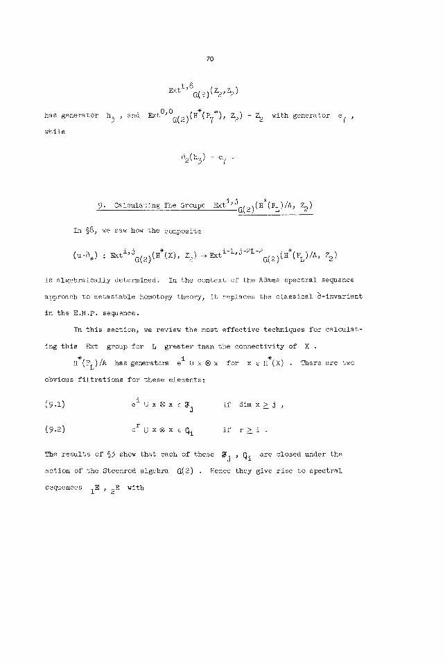
70

Extl' 8~(2) (Z2, Z2 )

has generator h 3 , and ExtO'Oc(2)(H*(P7~), Z2) : Z 2 with generator e 7 ,

while

$2(h3) = e 7 •

9. Calculating The Groups Exti'J~(2)(H*(FL)/A , Z2)

In §8, we saw how the composite

(u.~.) : Exti'Ja(2)(H*(X) , Z2)~Exti-I'j-2L-2c(2)(H*(FL)/A, ~)

is algebraically determined. In the context of the Adams spectral sequence

approach to metastable homotopy theory, it replaces the classical ~-invariant

in the E.H.P. sequence.

In this section, we review the most effective techniques for calculat-

ing this Ext group for L greater than the connectivity of X •

@

H (FL)/A has generators e i U x @ x for x ~ H*(X) . There are two

obvious filtrations for these elements:

(9.1) e i ux®x ~ ~j

(9.2) er U x ® x c ~i

The results of §3 show that each of these

action of the Steenrod algebra

sequences i E , 2 E with

if dim x ~ j ,

if r> i .

~j ' ~i are closed under the

~(2) . Hence they give rise to spectral

7i

(9.3) ~ ~ z 2) , i j Ext,(2) (~j/~j+l'

i (9.4) 2Ej ~ ExtG(2)(~i/~i+l , ~) .

In order to identify these terms further, we note

Theorem 9.5 ~j/~j+l ~ H (P j) ~ HJ(x) •

Proof This is immediate from 3.1, or see [22, §2]. These groups have been

tabulated in a range ([13]), and hence may be regarded as available for

calculations.

Now, turning to the second filtration, let

ant subalgebra of H*(X) ® H*(X) , and let

B(H*(X))

be the quotient of S2(H*(X)) by the sub-G(2)-module

dently have

Theorem 9.6 The

2 is a copy of

S2(H*(X)) be the T-invari-

image (I+T) . We evi-

2El. k-term of the sDectral sequence defined by filtration

Ext G(2)(s~(H*(X)), ~) .

There are eases~ for example: when X has very few cells, when the

first spectral is more convenient. However, when the structure of H*(X) is

very intricate, but Ext~(2)(H (X), Z2) is completely known in a range, then

the second spectral sequence is usually much easier to work with. (For exam-

ple, in §ii we will study the case when X = K(Z,m) .)

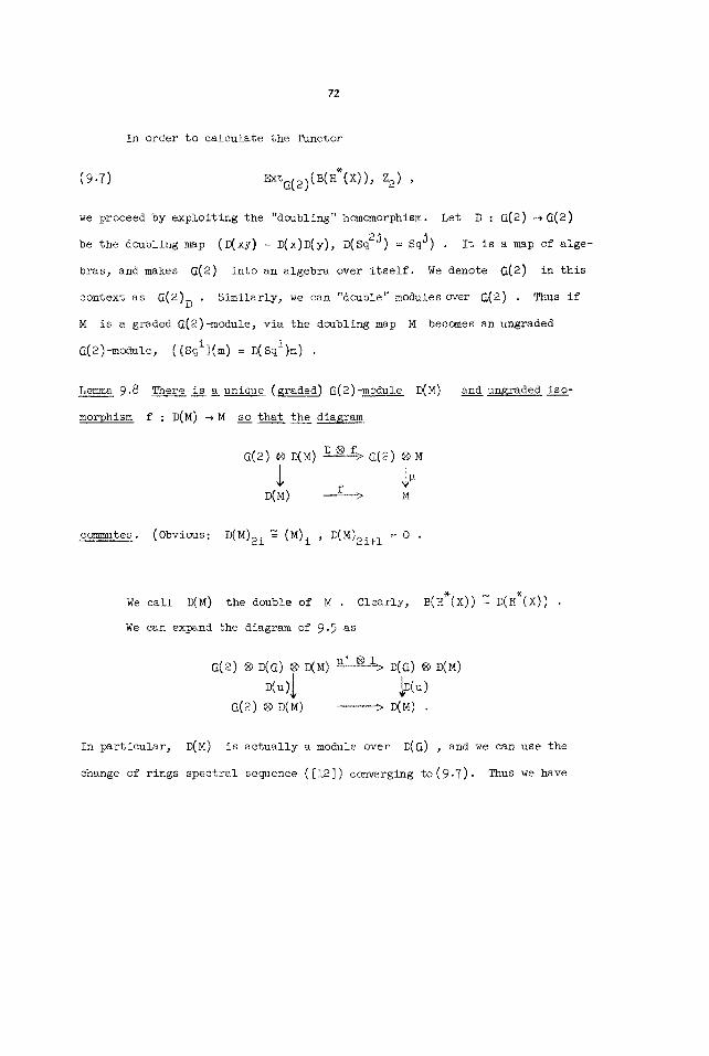
72

In order to calculate the functor

(9-7) ExtG(2)(B(H*(X)), Z 2) ,

we proceed by exploiting the "doubling" homomorphism. Let D : ~(2) ~G(2)

be the doubling map (~xy) = [~x)~y), D(Sq 2j) = Sq j) • It is a map of alge-

bras, and makes ~(2) into an algebra over itself. We denote ~(2) in this

context as C(2)D . Similarly, we can "double" modules over ~(2) . Thus if

M is a graded ~(2)-module, via the doubling map M becomes an ungraded

G(2)-module, ([Sqi](m) = ~Sqi)m) .

Lemma 9.8

morphism

There is a unique (graded) G(2)-module D(M)

f : D(M) ~M so that the diagram

D(M) f > M

and ungraded iso___-

commutes. (Obvious: D(M)2 i ~ (M)i , D(M)2i+ 1 = 0 •

We call I~M) the double of M • Clearly, B(H*(X)) ~ D(H*(X)) .

We can expand the diagram of 9.5 as

D(~)~ ;D(u)

G(2) ® D(M) ........ > D(M) .

In particular, D(M) is actually a module over D(~) , and we can use the

change of rings spectral sequence ([12]) ccnverging to(9.7). Thus we have

73

Lemma 9.10 There is a spectral sequence converging to ExtG(2)(BH (X), ~)

with ~ term

mtG(2)(M, mt~(2)(z~(2), z2)) •

(Here the tilde over the internal Ext denotes the fact that this is a spec-

tral sequence with twisted coefficients.)

However, 9.10 is still very useful since ExtG(2)(IXI(2), ~) has a

very simple form; e.g., see [23, §2]. Specifically, we have

Theorem 9.11 Ext G(2)(D(G), Z2) ~ p ( q o , q l , . . . , q i . " ' )

bidegree (i, 2i+i-I) .

where qi has

To illustrate methods, we outline the proof. The dual

is a polynomial algebra on generators ~i of degree 2m-i .

2 d : ~i ~ ~I extendsto a map of Hopf algebras.

to the sequence of Hopf algebras

(9.z2)

there is the sequence

Clearly~ the map

Its dual is D ~ Thus~ dual

G(2) / /dG(2) ,

(9.13)

Of c@~rs%

becomes an exact sequence of G(2)-modules as

(9.14) 0 ~ ~(2) • Ker (D) ~ G(2) ~ IXI(2) ~ 0 •

(9.14) gives rise to a long exact sequence of ~xt groups, and, since

is G(2)-free, this implies

(Ker D) -cO(2) ~G(2) l lKer (D) m D(e(2))

G(2) t/dO(2) E ( ~ l ' ' ' ~ i ' ' ' ) ~ Ker (D) • Now the sequence (9.13)

74

i "- Ext C(2)(~(2), z2) ~ Ex¢ la(2)(C(2).Ker (D), Z 2)

On the other hand, Exti-ic(2)(G(2).B , Z2) % EXtiB(Z2,~) for any sub-Hopf

algebra of G(2) ([23, §2]). Thus the result follows from the routine cal-

culation of the Ext groups for a graded exterior algebra.

Remark 9.15 The difficulty with using 9.10 and 9.11 for the spectral sequence

(9.4) is that the twisting in 9.10 is almost always non-trivial.

Example 9.16 In case X = K(Z2,m ) , we find the spectral sequence (9.4) by

far the more convenient. Its E 1 term in our range is a copy of r

P(qo... ) ; however, the differentials are very involved. Considerable work

on this case has been done by J. Harper ([i0], [ii]).

PART III

APPLI~TIO~ ~DEXAMPL~

10. Calculations Of The Stable Homotopy Of K(~,n) 's

In [4], [5], and [14], methods were given for studying the stable

homotopy groups ~S.(K(~n)) . These techniques give only fragmentary infor-

mation in actual practice. More recently, work of Browder and Brown ([38], [39])

and Brumflel, Madsen, and the author ([40]) has shown the importance of these

groups for problems relating to the classification of manifolds. Also, and

rather tautologically, these groups give the classification of higher order

one-variable cohomology operations which vanish for dimensional reasons,

[3], [8], [i0], [ll] universally on appropriate cohomology classes.

In this section, we apply the methods of Sections 4 and 9 to the prob-

lem, obtaining somewhat more efficient tools for the calculations. We begin

bY considering the first few groups when ~ = Z 2 or Q/Z , the cases of inte-

rest in [38], [39], [40]. We then continue in the next section by giving more

extensive calculations for the case ~ = Z .

In all cases, we begin by considering the fibering

(lO.l)

Thi~ is of the type considered in ~.l~ hence in our range

GL = ELsL'1 ~T (K(~,n) A K(~,n)) •

Moreover, since ~i(K(~,n+L)) = 0 for i > n+L , it follows from the homo-

s s G topy exact sequence of (10.1) that ~i (K(~,n)) ~ ~i ( L ) in our range.

Thus to compute

76

s ~i K(Z2'n) ' we ~st calculate the homotopy of

sL'I ~T K(Z2'n) A K(Z2,n) •

In the first few dimensions~ this has cells as follows:

e 3 U ~ ® L e I U sqlL ® Sq!L (sql~, Sq2L) (~, Sq2Sql~)

e 2 U L ® ~ Sq I~ ® Sq IL (~, Sq 2~)

(i0.2) e I U ~ ® ~ (~, sqlL)

The action of the Steenrod algebra ~(2) on the elements enumerated above

depends, of course, on n . Thus for n ~ 2(4) ~ we find from 3.7 that

sql(~ ® L) = (~, SqiL) ,

Sq2(~ ® L) = sql~ ® sqlL + (L, Sq2L) + e2 U ~ @ ~

Sq3~ ® ~ = (Sq2~, sql~) + (Sq~L, L) ,

sqlel ® ~ ® ~ = e 2 D ~ ® ~

Sq2el ® ~ @ ~ = e 3 D ~ ® ~ + e I D sql~ ® sqlL ,

SqI(sqlL ® sql~) = e I U sql~ ® sqlL •

In this range, there are at least four non-trivial ~ 's in homotopy; the

first dual to ~ ® ~ ~ the second dual to e I U ~ ® ~ • the third dual to

sql~ ® sql~ , and the fourth dual to (sql~, Sq2L) . Applying 3.7 in the

remaining cases~ we obtain the table

77

n = 0(2) s ~2n+i(K(Z2,n))

generator

n = 1(2) ~n+i(K(~,n))

generator

(4 ® L).

Z2

(4 ® 4).

z 2

(e I U 4 @ ~).

z 4

(e I u 4 @ ~) + <~, sqlL>).

Z 2

(Sql4 @ sgl~).

Z 2

(e 2 U 4 ® L).

Now we consider the group Q/Z . Suprisingly, this involves us in

some algebraic problems. The first is a suitable description of Q/Z . To

this end, let Z = l~m (Z i) for each prime p . P

Lemma 10.4 Q/Z %0(Z ) a_~s p runs over all primes.

Proof Injections 8p : Z(p)~ ~Q/Z are defined as the direct limits of maps

where Pi(n) = n/p i .

Pi : Z i -~ Q/Z P

These in turn induce a morphism

(p)~

given on elements by

To see that

if and only if

8(np'-.nq) : 8p(np) + ... + eq(nq) .

ker (8) = 0 , note that

np/p i + ... + nq/q j 6 Z

np(...q j) + ... + (pi...)nq ~ O(pi...q j) .

np(...q j) + ... + (pi..-)nq ~ O(p i)

O(q j ) ,

In particular,

78

and these congruences imply np ~ O(p i) , ... , nq ~ O(q j) • Thus ker (@) = 0 .

To see the converse, suppose the fraction n is given in Q/Z • Since 2i3J...q k

the ideals (pj) + (qk) = Z in the integers, for p a prime and q rela-

tively prime to p , there are integers m 2 , n 2 so

n22i + m2(3J...qk) = n •

Similarly3 there are integers m 3 , n 3 so

m3(5s...q k) + n35J = n 2 ,

etc. Hence we can write

n/2i...qk = m2/2i + ... + mq/qk ,

and this shows that e is onto. 10.4 follows.

Now note that the inclusion Z i~Z i+l P P

K(Z i,n)~K(Z i+l,n) (e.g., see the models for P P

Clearly~ we have

induces an inclusion

K(~,n) introduced in [19]).

Lemma 10.5 K(Z(p)~,~ l~m (weak) K(Zpi,n) under these inclusions. (Here,

the topology in K(Z(p)~n) is given by specifying its compact sets [which are

the sets X contained in K(Z i,n) for some i , so X D K(Z i,n) is e(~n- P P

pact], and letting Y be open if and only if Y 0 X is open for each com-

pact set X .)

W

Corollary 10.6 K(Q/Z,n) = p p~rime K(Z(p)®~n)

Cartesian products).

(weak limit of the finite

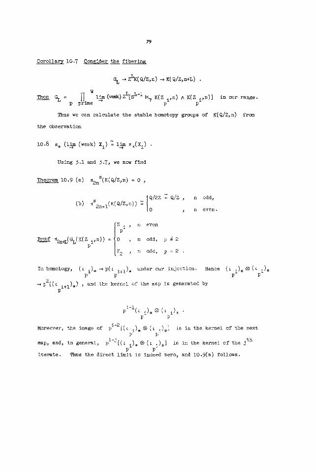
79

Corollary lO.7 Consider the fibering

G L ~ zLK(Q/Z,n) ~ K(Q/Z,n+L) •

Then % = W

M p prnne

lira (weak) zL[s L-I ~<T K(Z i,n) A K(Z i,n)] P P

in our range.

Thus we can calculate the stable homotopy groups of K(Q/Z,n) from

the observation

io.8 ~. (i~ (~eak) Xi) : i~ ~.(X i) •

Using 3.1 and 3.7, we now find

Theorem 10.9 (a) ~2nS(K(Q/Z,n) = 0 ,

~S2n+l(K(Q/Z'n)) ~ IQ/2Z ~ Q/Z , n odd, (b) 0 , n even.

ipi ~ n even

i,n)) = , n odd, p % 2

Z 2 , n odd, ~ = 2 .

In homology, (L i) . ~p(~ i+l) . under our injection. Hence P P

p2((~ i+l).) ' and the kernel of the map is generated by P

(~ i). ® (~ i). P P

Moreover, the image of

map, and, in general,

iterate.

pi-l(L i). ® (L i). • P P

pi-2[(L i) . ® (~ i).] is in the kernel of the next P P

pi-j[(L i). ® (L i).] is in the kernel of the jth P P

Thus the direct limit is indeed zero, and lO.9(a) follows.

80

To prove (b), note that

(10.10) ~2n+I+L(GL(K(Z i,n))) =- P

Z i , n odd, p ~ 2 P

Z2i+l , n odd, p = 2

0 , n even, p ~ 2

Z2 , n even, p = 2 .

Moreover, from examining the action in homology of the Hurewicz images of

the generators 3 we conclude that, in each case, the inclusion of the one in

the next is given by multiplication by p . Hence

l~m (Z 4 C , Z 8 C ...) = Z(2)~

is the two-local component of the limit. Clearly, there is a surjection of

this Z on Z with kernel Z 2 . Thus it is natural to embed the (2 ~) (2 ~)

resulting group in Q/2Z . This completes the proof of (b).

Remark i0.ii Theorem 10.9 is exactly the homotopy theoretic result which is

needed to do simply-connected surgery ([41]), and also plays a key role in

[40]. The results of Section 2 also allow us to know exactly at which sus-

pension the various homotopy elements first appear. For example, the reader

is asked to verify that~ for n odd, a

~2n+I(K(Q/Zsn) A KQ/Z,n) , and hence in

the map

Q/Z appears in

~2n+2(Z(KQ/Z,n)) . However, while

~2n+2(Z(K(Q/Z, n) )) -~ ~2n+lS(K(Q/Z,n))

is an isomorphism, the approximating maps

Z2i -~ Z2i+l

for K(Z i,n) always have cokernel Z 2 . 2

81

ii. Some Calculations Of The Stable Homotopy Groups For The K(Z,n)

s In this section, we apply the techniques of §9 to study ~ .(K(Z,n))

in some special cases. The calcu]ational results illustrate the structure

of the exact sequence 6.11.

(i0.i) shows that we need study only ~.(S L-I N T K(Z,n) A K(Z,n))

for L > n . To do this, we shall calculate the groups

Ext,(2) (H (FLK(Z,n)), Z2) , (il.l)

Exta(2)**(H*(FL) , A, Z2)

in three steps. First, we calculate Ext,(2) (H (GL)/A, %) ; then we cal-

culate Ext,(2) (A,~) ; finally, we put them together to obtain the desired

groups (tl.l)°

We begin with the calculation of Ext,(2) (H*(GL)/A , Z2) , using the

second s p e c t r a l sequence i n §9.

~emma 11.2 E~t a(2)(D[H (K(Z,n))], Z 2)

Ext ~I(Z2,Z2) ® Ext A(Q~Q4...)(Z2,Z2)

in total degrees less than 4n+l . Here ~i is the subal~ebra of ~(2)

generated by Sq I and Sq 2

Proof We imitate the main idea in the proof of 9.11.

H*CKCZ, n))

~(2)sq I

The map u

is onto in dimensions less than or equal to 2n and has kernel

Thus, the kernel of the doubling homomorphism

82

is D-I(G(2)Sq l) : Ker (D) ~ G(2)(Sq 2) , but this is

G(2)(Sq 2) , but this ideal is clearly isomorphic to

~(2 ) . (% ~ s(Q3Q4...)) ,

and 11.2 follows.

G(2)~(sq l, %, Qs")

Now we recall the well-known

Lemma ii.3 Ext ~(Z2,Z2) = P(ho,hlQ, P)/R where R is the set of relations

Q2 h~P,

hoh I = 0 ,

h~ = 0 ,

hlQ = 0 •

Here h 0 has bidegree (1,1) , h I has bide~ree (1,2) , Q s Ext 3'7 and

Ext 4~12 (See e.g. [9, §6.1] for a proof.) P s

We mention in passing that Q has Massey product representation

2 2 (h~,hl,ho) . Also, P has representation (hi,hi,hi,hi) •

ll.2 and ll.3 together determine the E 1 term of our spectral sequence.

We now turn to the evaluation of the differentials. I know of no way to do

this without going to the chain level. First, we need some notation. In

E 1 , we denote an element in the k th copy of EXt~l ®E(Q 3...)(Z2,Z2) with

i I i kt h a (k) on the right. Thus e ® q3 "''qr r in the copy will be written

i I i e @ q3 "''qr r(k) "

The generators of C O are thus the ((k).] , and those in C I are the

ho(k). ~ hl(k). , q3(k). "'" . In principal, we can completely describe the

differentials once we have specified the boundaries of the generators in C (1)

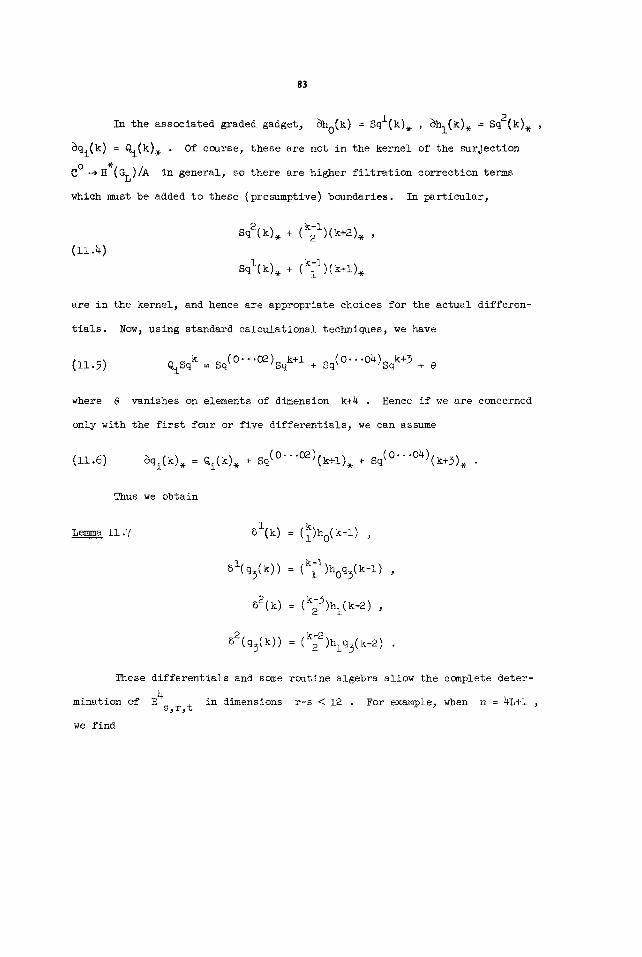
83

In the associated graded gadget, 3ho(k ) = sql(k). , 8hl(k). = Sq2(k). ,

8qi(k ) = Qi(k). • Of course, these are not in the kernel of the surJection

C ° -~ H (GL)/A in general, so there are higher filtration correction terms

which m~st be added to these (presumptive) boundaries. In particular,

sq2(k). + (k~l)(k+2). , (ll.4)

Sql(k). + (k~l)(k+l).

are in the kernel, and hence are appropriate choices for the actual differen-

tials. Now, using standard calculational techniques, we have

(11.5) QiSq k = Sq(0"'0e)Sq k+l + Sq(0"'O4)sqk+} + 0

where e vanishes on elements of dimension k+4 . Hence if we are concerned

only with the first four or five differentials, we can assume

(i1.6) ~qi(k). = Qi(k). + Sq(0'''0~)(k+l). + sq(O'''O4)(k+3)..

Lemma 11.7 51(k) = (k)ho(k-i) ,

81(q3(k)) = (k[1)hoq3(k-l) ,

~2(k) = (~3)hl(k-2) ,

~2(q3(k) ) (~2 = )hlq3( k-2 )

These differentials and some routine algebra allow the complete deter-

mination of E4s,r,t in dimensions r-s < 12 . For example, when n = 4L+l ,

we find

Thus we obtain

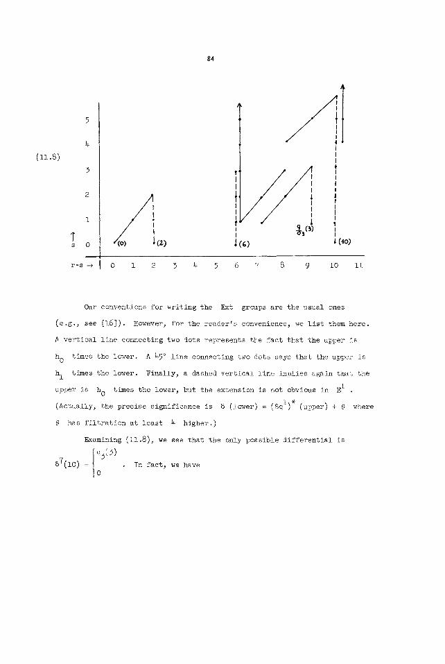
84

(~1.8)

5

4

3

2

i

T s 0

r - s --~

A (z) 0 i 2 3

7

4 5 6 7 8 9 I0 ii

Our conventions for writing the Ext groups are the usual ones

(e.g., see [16]). However, for the reader's convenience, we list them here.

A vertical line connecting two dots represents the fact that the upper is

h 0 times the lower. A 45 ° line connecting two dots says that the upper is

h I times the lower. Finally, a dashed vertical line implies again that the

upper is h 0 times the lower, but the extension is not obvious in E 1 .

(Actually, the precise significance is 5 (lower) = (sql) * (upper) + 8 where

e has filtration at least 4 higher.)

Examining (11.8), we see that the only possible differential is

67(10) = In fact, we have 0

85

q3(3) , n -= l(8)

Lemma 11.9 57(10) = O , n -= 5(8)

(For the proof~ it is necessary

only to expand (11.6) two further stages in these cases.)

Thus, in view of the dashed vertical lines, this determines the remain-

ing differentials, and (11.8) represents Ext~(2)(H (rn)/A , ~) for n ~ 5(8) ,

while

for n ~ 1(8) has the form

Ext~(2)(H*(rn)/A, Z 2)

4

3

2

i

T s O

/ r-s -~ O i 2 3 4 5 6 7 8 9 iO Ii

86

Now, following our program, we turn to the calculation of ExtG(2)(A,Z2)

Unfortunately, I know no indirect way of studying this group, so I found it

necessary to write down an explicit resolution in our range of interest. We

suppress the calculations (in the interest of mercy to all concerned) and

record the result:

5

4

3

2

1

s 0

r-s

/ J • • • •

o 1 2 3 4 5 6 7 8 9 lo ii

withj perhaps, some missing terms in r-s = ll . Combining this with (ll.10),

and calculating some obvious differentials in the exact sequence

(ii.12) ...ExtG(2)(H*(FL) 3 ~) ~ ExtG(2)(A~Z2) ~ Ext~(2)(H*(FL)/A, ~) ~ ... ,

we find that ExtG(2)(H (F8k+l), Z2) has the form

87

2

1

T s 0

r-s -~

l

• "C

7 8

/

I m • • E •

0 l 2 3 4 5 6 9 l0 ll

There are a number of "suprising" facts concealed in (11.13). For

one, note that 5 in (ll.12) is highly non-trivial. For another, note e.g.

that, for hoD , H , there are extensions of the ExtG(2)(Z2,~) module

structure connecting the remaining terms from (ll.lO) and (ll.ll). The orig-

inal interpretation of elements in ExtG(2)(H (Fn)/A , ~) was as "stable"

higher order cohomology operations which vanish universally on integral coho-

mology classes of dimension n (e.g. see [ll]). However, it is clear that

that hypothesis can no longer be supported since the terms from Ext (2)(A, Z2)

play a very definite role in determining the actual Ext groups of F n '

and the differential depends on n . Thus the general defining system for an

operation represented in ExtG(2)(H (Fn)/A , ~) may well have been built on

relations which depend on lower order elements in ExtG(2)(A,~ ) and n .

We now calculate the differentials in (ll.13), and conclude this sec-

tion by evaluating

88

~**(Fn, A, Z 2)

in this range.

We first observe that the Z 4 Bockstein (Proposition 3.6) implies

some 82 differentials. Thus we have

L~mm~ 11.14 I__nn (iI.13)~ we have

~293(o) = nob ,

~2(H) = hoD •

Somewhat less immediately, we have

Lemma II.15 (i) ~2(g3(i)) = 0 ,

(ll) ~2(E) =0 •

Proof (i) Consider the inclusion

S I sn-i u : ~<T K A K~ ~<T K A K .

It is easy to verify that g3(1) is present in im (u.) on Ext groups.

However, ho3D is not in this image. Hence ~2(g3(i)) = u.~2(g3(1)) = 0 ,

and (i) follows. To prove (ii), note that E has representative cycle

(Sq3, Sq4Sq 2 ) . Consider the inclusion

I : K A K-~sn-I ~<T K A K .

K A K is a wedge of K(~,n) 's and K(Z,n) 's in low dimensions. A direct

calculation shows that Sq4Sq2~ ® Sq3L is a generator in H*(K A K) over

89

~(2) . Hence it is dual to an element

@ is detected by E , and (ii) follows.

Remark 11.16 The splitting of K A K

with the cofibrations

(11.17) sr ~T K A K ~ S r+l ~T

b in ~.(K A K) • C l e a r l y , I . ( b )

used in the proof of ll.15(ii), together

K A K-~Er+l K A K-*E sr ~<T K A K-~ ... 3

provide us with a good method for constructing homotopy classes in our range,

while the global calculations of Ext groups provide an effective way to

limit the number of elements whose study is required. It would seem to the

author that this remark provides the reader with effective tools for analyzing

the stable homotopy of Eilenberg-MacLane spaces so far as desired in our

range~

Returning to our calculation3 we easily see that 11.14 and 11.15 give

all the 82 differentials. Moreover, E 3 ~ E ~ , and we have

Theorem 11.18 The first ten stable h~motopy groups of K(Z,8k+I) are given

by the table

1°llr 2 q31 ~16k+j+l Z 2 .... 0 Z 4 0 Z 2 ~ Z 2

6 17j819 Zl6 Z 2 Z 2 @ Z 2

For j = I0 , ~16k+l~(K(Z, Sk+l)) has order at most 8 .

Remark 11.19 The grOups obtained in 11.18 for j = 6 , 7 do not agree with

those obtained by Mahowald and Williams in [14]. They apparently missed the

generator C corresponding to the cycle (Sq 2, Sq 4) .

90

Finally, we apply ll.18 to calculate the differential

i * Z21_ * : Ext ~(2)(H (Fn)/A , Exti+2a(2)(A, Z2) defined in 6.11.

find that

~.(F8k+l , A, ~)

has the form

We easily

/ .8

A•/ P

• "C

0 i 2 3 4 5 6 7 8 9 i0

/

//IH £

Again using 11.18, the reader can easily calculate the higher dif-

ferentials in (ll.20).

91

12. An Example For The,,,Metastable Exact Sequence

In [13], Mahowald used his special case of 8.5 to give extensive

calculations of the metastable homotopy groups of spheres. The most element-

ary spaces after the spheres are the various two-cell complexes; in particu-

lar, the four such non-trlvial ones distinguished by their structure as

G(2)-modules.

In this section, we apply 8.5 to calculate some of the unstable

groups of the space ~ = S 7 U 2 e 8

The stable homotopy of

sequence

(12.1)

as an example of the techniques involved.

is easily studied. We have an exact

ExtG(2)(Z2,Z 2) ~ ExtG(2)(H*(X7), Z 2) ~ ExtG(2)(Z2,Z 2) -~,

and 8 is exactly multiplication by h ° , 8x = hoX (eg., see [2]).

ExtG(2)(H (~)~ Z2) consists of elements of two kinds:

( 12.2) i) elements ~ in the image of I ,

ii) elements ~ for which J(~) ~ 0 and hoJ(~ ) = 0 •

Hence

Elements of this second kind may be written explicitly as Massey products in

ExtG(2)(H (~), Z2) . Exactly, we have

(m.3) ~ = <j(~), h o, ~J

where ~= I(~) is the unique non-zero element in Ext 0'7 * G(2)( H (XT), Z 2) •

Consequently~ we obtain

92

Proposition 12.4 The following extensions occur in

i) ho(7 ,ho~ > : h l I ( 7 ) ~ ;

i i ) I ~ ~ = 0 i~ s~t (2 ) (12 ,12 ) , then

Proof

Ext~(2)(H*(~), Z 2) :

~<7,ho,±,> = <~,~,ho> h •

By the slide formula for Massey products,

~(# ,~ ,~ ) = <a,# ,~)8 ,

we obtain (ii),

from 1 2 . 2 ( i i ) and 1 2 . 4 ( i i ) .

[24]) (a,b,a> = (a U 1 ~)b

and (i) now follows.

To show (i), note that.

~o<7,ho,~> = <~o,~,ho>~

On the other hand~ the "Hirsch" formula ([17]~

implies (ho,7,ho> = h17 since h ° U I h ° = h I ,

Using the tabulated results ([16], [59]) on

Ext~(2)(H*(X~),{ Z2) f o r t - s < 2 0 as

~xtG(2)(Z2,Z2) , we obtain

L =

<h l,

h o,

#>

M=<

~2 2

, h o

, ~.>

p =

<hO3

h3,.

hO,~

>

= (h

0, h2

22 P)

Q :

<~3 2

, ~o

2,

T =

(hof

, ho,

L~>

S

10 9 8 7 6 5 4 3 2 i o

~ 4,

" 1

hi

1,

4~ /

.~ .~

.

~ Q"

JT

//~

* cI

t-s-

, 7

8 9

i0

Ii

12

13

14

15

16

17

18

19

20

21

22

23

24

25

26

27

94

Proposition 12.6

differentials:

In the range o_ff (12.5), there are only two non-zero

82(eo) = hl2do ,

82T = hl2doL •

Moreover, there is a non-trivial extension

2[h4] = Q •

Proof These differentials are non-trivial since the sequence (12.1) is actu-

ally a long exact sequence of Adams spectral sequences, being induced from

the obvious cofiber map of spaces, and the corresponding differentials are

non-zero for spheres.

The next possibility for a non-zero differential is h4L . In fact,

~2(h4L) = (2h32)L = [22]L by naturality~ but 2~2L = 2 2~ = 0 since

2 ~ = 0 • Thus h4L represents the Toda bracket

i n ~ s . ( x T ) , a n d i s i n d e e d a n i n f i n i t e c y c l e .

There remains the possiblity of a differential on f . In the Adams

spectral sequence for the sphere, 82(fo) = 2h2(do) . Hence fo represents

the Toda bracket

{O(do), 2, ~

s in ~ .(~) . This completes the first part of 12.6.

For the second assertion, note that h 4 is a permanent cycle repre-

senting the Toda bracket

95

Hence

(i2.7)

But thls last represents

{ ~ , 2, , j .

(h32,hJ~A) = 0 , and 12.6 follows.

96

Remark 12.8 The reader might wonder why we did not use the slide formula in

(12.7), obtaining 2[~2,2,~) C [2a2,2]~ = ~o2~ = 0 • But these equations are

valid only modulo the total indeterminacy which in this case is 2~s22(~) .

New we turn to the calculation of ~.(S 7 U 2 e 8) in the metastable

range. The fiber in the map

F L ~S 7 U 2 e 8 ~L(sL+7 U 2 e L+8)

is given as ~sL-I MT [$7 U2 e8) A (S 7 U 2 e8)] • The calculation of

Ext ~(2)(H (FL),A, Z2) is routine using the first spectral sequence in §9

s,r * (in this case an exact sequence), and we find Ext ~(2)(H (FL),A,~) has

the form

2

(is .9) I

s=O

r-s-- 0 i 2 3 4 5 6 7 8

In particular, the reader should note that, since ~4(e7,e8) = (e 8 ® e8) ,

it follows that the element 7 , in the space ~(FL,A ) , corresponding to

sql(~o ) satisfies sql(7) = e 8 ® e 8 . This is an example of the type of

twisting referred to in §6, particularly 6.11. It is easy to check that

there are no differentials in this range in the resulting Adams sequence, so

97

We now evaluate the map ~l 2 of 8.5.

Proposition 12.10

for r-s < 8 .

~2(h3~) = I ° , and there are no further non-trivial images

of h3~ is Sq8(~7) , it is evident that Proof Since the k- invariant

~2(h3~) = I ° The only other possibility is ~(h}L) = ~hl(e7,e8) , but

this is part of the tower associated purely to A . Hence ~ = 0 , and 12.10

follows.

COrollary 12.11 The unstable resolution of S 7 U 2 e 8 in the metastable

range has the form

8

6

4

2

s=o

r-S -~

f

O i 2 3 4 5 6 7 8 9 iO i! 12

There are clearly no further differentials, so ~ = ~ in this range.

98

13. Further Calculations For Some Truncated Projective Spaces

(13.1)

In this section• we study the groups

~i+n(Zn(P62 ) )

~i+n ( zn(p6) )

, i!6,

• i~6,n=2.

They are of importance in the joint work of the author and E. Rees on embed-

ding projective spaces ([42]), and provide examples illustrating ranch of the

theory of Part I not already explored in §§9-12.

We being by recording the stable homotopy of the spaces in (13.1) and

in our range.

* 6 Lemma 13.2 Ext~(2)(H (P 2) , Z2) i__ss ~iven by the table

4

3

-~ 2

1

s 0

t-s -~ 2 3 4 5 6 7 8 9 lO

in our range.

99

Lemma 13.3

5

4

3

2

i T s 0

t-s -~

* 6 ExtG(2)(H (P 2) , Z2) i_ss given by the table

1 2 3 4 5 6 7 8 9 lO ll

in our range. (Both 13.2 and 13.3 are evaluated by using the exact sequence

of cofiberings

(13.4) p2 6 A p2 ~ . P7 '

pl 6 ~ PI ~ '

taking the resulting long exact sequences of Ext

tables in [13], pp. 54, 55, and 60 to evaluate

range.)

From 13.2, 13.3, and the fact that, in

groups, and using the

Extc(2)(H (Pi)~ Z2) in our

~8(P2 ) , the class correspond-

ing to 4L(5) is non-zero ([13], p. 55# and the observation j.(L(5)) =

2[e5} ) , it follows that 82h2(5) = 0 in the Adams spectral sequences for

which 13.2 and 13.3 are the ~ terms. On the other hand, by inspection

we see that 82(h2(5)) is the only possible non-zero differential. Thus

= E ~ in both cases, and we have the table (localized at 2)

(13~) j ~Sj(P62)

~Sj(P61)

2

0 Z

z 2 z 2

4

z 4 0

z 8 z 2

6

z 4

Z2

7 z 8

z2 ~z8

8 (Z2)3

9

~6 • (zJ

(z2)5 .

100

Now we consider the unstable homotopy groups (I].I) for Z2p61 ,

Z2p6 2 . Since these are suspensions; the fibers

(i}.6)

%1. z2p6 o~z~+2p6

FL2 ~ Z2p6 2 -~ DLEL+2p 6 . ~ 2

are given explicitly in §I and their homology calculated in §3 (particularly

3.9, 3.10). There is no difficulty in constructing resolutions to evaluate

~.(FLa ) for * < 8 (For the fiber FL I _ . ~ we are one dimension beyond the

point where i.ii is valid] thus the fact that we are dealing with suspensions

is essential for effective calculation.)

Lemma 13.7 n7(FL 2) = Z generator A ,

~8(FL 2) = Z 4 ~ Z 2 generators B , C

with relation NA = 2B .

Proof We are in the range in which i.ii applies.

ogy generators

2 The fiber F_ has homol-

b

7 8 9

o(e 4 * e4) o~(e~) o~(e 4)

~(e 4. e 5) ~(e 5. e 5)

c(e 4 * e6)

Passing to cohomology over C(2) , we apply 3.7 to show that

101

sq~(o%(%) *) : °(%(%))*,

s q l ( d ( % * % ) ) * = Sq2(o (e4 * e4) ) ,

and there are no further non-zero operations in (1}.8). 13.7 now follows on

• 2 taking Ext~(2)(H (F L ), Z2) in this range.

The situation for FLI is similar. However, we must also take into

account the classes Z2el<~el , ~e2) , Z2e2(Pel , Z2e2) (in the notation

of 3.9).

Lemma 13.8 ~5(FL 1) = ~ g e n e r a t o r D = ( ~ e 1 * ~2el)

~6(FL 1) = Z 4 g e n e r a t o r E = % ( Z 2 e l ) + ( Z 2 e l , ~ e 2 )

~(FLI ) = ~ generator F = (Z2el, Z2e3)

[G = Z2el'(Z2el , Z2e2)

~8(Fl ) = Z2(3) ~nerators !~D

I H = (n,4,D)

Also~ in the map

but

: FLI 2 * F~ , we f i n d ~ . ( D ) = ~ . ( E ) = ~ . ( F ) = ~ . ( G ) = 0 ,

~ . (H) = I]A .

~.(F~ l) = ~.s(F~l) sinoe FL1 * 1

H (F L ) has generators

Proof Through dimension 8 ,

We thus take a stable resolution.

is 4-connected.

102

(e 3

(13.9)

5 6 7

* e 3) %Ce 31 %Ce31* <~,%> (e~ * e4)

(es,es)*

8 9

Q3(e3)* Q~(e3)* %(e4)* %(e4)* (e3,e6)* (e 5 * e5)*

(e4,e5)* (e3,e7)*

e3(e3,e4)* e4(e3,e4)*

<e4,e 6)

in dimensions less than or equal to 9 • A basis over G(2) is easily seen

to be (e 3 * e3)*, ~(e3)*, (e 4 * %)*, <e3,eS>*, e3<e~,%>*, Q4(e3)*,

(e 5 * e5)* in this range. Relations are sql(~(e3))* = sql(e4 * e4)* = 0 ,

Sq4(e 3 * e3)* = Sq3(Ql(e3))* , (13.1o)

(Sq4+Sq3sql)(e~ * e3)* = Sq2(e4 * e4)* .

Next, since ~4(e4 * e4) = (e3,e4) + ~(e3) , we see that, in the

Adams spectral sequence for FLI , 82(e4 * e4) = h02(~(e3) ) . Moreover,

there are no further differentials in our range, and E 3 = E ~

Finally, noting the fact that

* I * ! * * (e 4 e 4) = (%* e 4) ,

we see that the filtration 2 class, due to the second relation in (13.10),

maps to qA in ~.(F#) •

Corollary 13.11 Th__~e # term of oar spectral ~equence 6.4 for Z2P2 6 has

the form

103

4

3

2

1

0 T-

4 5 6 7 8

up to extensions (which are marked with dotted lines).

Remark 13.12 By using the techniques of §§i and 8, we note that j.(G) ,

j.(H) generate the unstable part of the homotopy grOup ~8(Z2P 6) . More-

over, a simple argument with Whitehead products shows that J.(G) cannot be

a suspension element. Thus j.(H) is the only candidate for an element in

~2~6(P6 ) in ~8(~P 6) • In particular, the generator of ~6(P 6) is the

attaching map of the cell building p7 :

(13.13) s6hP6-~# ~ S 7 ,

and it must be clear from (13.13) that the top class in

if and only if ~2(k) = O in ~8(~P 6) .

is j.(H) ; and in (~P62) , i.j.(H) ~ 0

result needed in [43]:

Z 2 P is spherical

But the only non-zero candidate

by 13.8. This proves the key

Theorem 13.13 ~p7 ha s top-class sl0herical if and only if ~P72 does.

We now complete the calculations of this paper by calculating

~2+i(ZP62) and ~i+i(P62) in the range of(13.~.

difficultyj we find that the h~motopy of the fiber FL3 Without

the map

in

zp62 -~ ~z~+lp62

104

is given by

(13.~4)

J

~j(FL3)

Generator

5 6

I J

7

Z 2 ~

K, [~,2,1] •

Clearly, 82(D2) = I , and no other non-trivial boundary is possible. A

schematic representation of ~.(ZP62 ) in our range can now be given as

(13.15) 1

T s 0

t - s

4

3

2

3 4 5 6 7

The extensions 20(3) = J.(K) , ~[hoh2(2)] = j.(G,2,I] must be veri-

fied. (Of course, the second extension follows directly from the fact that

~[h2(2)] = I .) To obtain the remaining extension, note that we are outside

the range where 8.5 holds, so the extension is not necessarily surprising-

(The point is~ if 8.5 were true in this dimension, then in the resolution

both K and h2(} ) would occur in filtration I , and the extension 2D(3) =

J.K would clearly be impossible.)

Specifically~ the difficulty with extending 8.5 occurs here because

Sq4(c4 ) = L42 is a Z 4 class, and ~4(L4 )2 = [sqlL4 U c 4 + Sq4Sql~4] in

K(~,4) . Using the fact that we can take an unstable "resolution" of ZP62

with first K-invariants given as

105

(@e2'@e3)> K(Z,9) x K(Z2,4 ) SqI~4+Sq2~Y ~42 (1}.16) ZP6 2 - > ~(Z2,5) x K(Z~,8) ,

we easily justify (13.15)~ and this provides a good example of why the range

of dimensions in which 8.5 holds cat, lot be extended.

Remark 13.17 We note in passing that, in the map ~ : FL3 ~ ~FL I , we have

~.(K) : 0 , ~.{~,2,1] = GA ; and in the map ~ : E P6 2 ~Z2p6 2 ~ we have

~.(hoh2(2)) = j.(A) + 2~(2) .

Now we conclude the discussion by studying briefly the homotopy of

P6 2 itself. It is a routine calculation with the Serre spectral sequence

to give the homology of the f~ber in the map

P26-~LzLp62

in dimensions less than 8 . The fact that there are non-trivial cup prod-

ucts in P6 2 produces some minor unpleasantries such as: (i) the class

which should have transgressed to (e3oe4) is identified with the class

transgressing to (e2oe5) , and (ii) in H7(F) , the class which transgresses

to (e2Oe2oe2Oe2)* is a Z8-Bockstein ,

~8(~-!((e3,e4 )* + e I U e 3 O et)] .

This illustrates the way in which the results of §i fail when X is not a

suspension.

The homotopy of F is given by

(13.18) J

Generator

3 Z

[~2, ~2]

4

2

5

z2 z2

~, [L3,~ 3]

6

z s

M, P

106

Further, we have relations 2 ~ = 2M , 9 [ ~ 2 , ~ 2 ] = 2K, and Z(K) = I ,

Z(M) = [~,2,I] while ZP = K on suspending, i.e., taking the map

3 F ~ L

Clearly, ~(2) =K@ L , c~o(3) = [~3~3] • We may also verify 8(L(5)) =

2P . This is not trivial; it involves the construction of an unstable reso-

lution of P62 , and makes essential use of the fact ([29]) that ~P72 is

reducible. Here is what the resolution looks like through dimension 6 :

t-s 2 3 4 5 6

The k-invariants may be easily calculated. Notice that M has fil-

tration 2 here but aM has filtration 3 in the resolution of ZP62 .

This change of filtration degree would seem to merit further study (e.g., see

I15] for an example of what can happen).

107

References

1. J. F. Adams, "On the non-existence of elements of Hopf invariant one,"

Ann. of Math. 72 (1960), 20-104.

2. , Stable Homotopy Theory, Lecture Notes in Mathematics 3,

Springer-Verlag.

5. J. Adem, S. Gitler, "Secondary characteristic classes and the immersion

problem," Bol. Soc. Mat. Mex~cana 2 (1963), 53-78.

4. W. D. Barcus, "The stable suspension of an Eilenberg-MacLane space,"

Trans. Amer. Math. Soc. 96 (1960), 101-113.

5. W. D. Barcus, J. P. Meyer, "The suspension of a loop space," Amer. J.

Math. 80 (1958), 895-920.

6. H. Cartan, "Sur les groupes d'Eilenberg-MacLane H(~,n) , I, II," Proc.

Nat. Acad. Sci. U.S.A. 40 (1954), 464-471, 704-707.

7. M. Fuchs, '~ modified Dold-Lashof construction that does classify

H-principal fibrations," mimeo, Mich. State Univ., 1969.

8. S. Gitler, R. J. Milgram, "Unstable divisibility properties of the Chern

character," to appear.

9. V. K. A. M. Guger~eim, R. J. Milgram, "On successive approximations in

homological algebra," Trans. Amer. Math. Soc. 150 (1970), 157-182.

I0. J. Harper, thesis, Univ. of Chicago, 1967.

ii. , "Stable secondary cohomology operations," Comment. Math.

Helv. 44 (1969), 341-353.

12. A. Liulevicius, "Multicomplexes and a general change of rings theorem,"

mimeo, Univ. of Chicago, 1967.

15. M. Mahowald, Th__~e Metastable Homotop~ o__ff S n , Mem. Amer. Math. Soc. 72,

1967-

14. , R. Williams, "The stable homotopy of K(Z,n) ," Bol. Soc.

Mat. Mexicana 12 (1967), 22-28.

15. , "On the order of the image of J ," Topology 6 (1967),

371-378.

16. , M. Tangora, "Some differentials in the Adams spectral

sequence," Topology 6 (1967), 349-369.

108

17.

18.

19.

20.

21.

22

23

24

25

26

27

28

29

30.

51.

32.

33.

34.

35.

36.

W. Massey, F. Peterson~ The Mod 2 Cohomology of Certain Fiber Space,

Mem. Amer. Math. Soc. 74, 1967.

R. J. Milgram, "Iterated loop spaces," Ann. of Math. 84 (1966), 386-403.

, The bar construction and abelian H-spaces," Illinois J.

Math. ii (1967), 242-250.

, "The homology of symmetric products," Trans. Amer. Math.

Soc. 138 (1969), 251-265.

, "The mod 2 spherical characteristic classes," Ann. of

Math. 92 (1970), 2~8-261.

, "Group representation and the Adams spectral sequence,"

to appear.

, "The structure over the Steenrod algebra of some 2-stage

~ostnikov systems," Quart. J. Math. 20 (1969), 161-169.

, "Steenrod squares and h~gher Massey products," Bol. Soc.

Mat. Mexicana l~ (1968), ~2-57.

J. Milnor, "On spaces having the homotopy type of a CW-complex," Trans.

Amer. Math. Soc. 90 (1959), 272-280.

J. C. Moore, "Alg@bre homologique et homologie des espaces classifiants,"

S@m. H. Cartan 12 (1959), 701-7~7.

M. Nakaoka, "Decomposition theorems for homology groups of sym~metric

groups," Ann. of Math. 71 (1960), 16-42.

T. Nishida, "Cohomology operations in iterated loop spaces," Proc. Japan

Acad. 44 (1968), 104-109.

E. Rees, "~nbedding theorems for real projective spaces," to appear.

L. Smith, J. C. Moore, "Hopf algebras and multiplicative fiber maps, I,

II," Amer. J. Math. 90 (1968), 752-780, 1113-1150.

J. Stasheff, "Homotopy associativity of H-spaces II," Trans. kmer. Math.

Soc. I08 (1965), 293-310.

N. Steenrod, "Milgram's classifying space for a topological group,"

Topology 7 (1968), 349-368.

M. Tangora, thesis, Northwestern Univ., 1966.

J. F. Adams, "Structure and applications of the Steenrod algebra,"

Comment. Math. Helv. 52 (1958), 180-214.

D. W. Anderson, "The e-invariant and the Hopf invariant," Topology 9

(1970), 49-54.

l. Berstein, T. Ganea, "Iterated suspensions," to appear, Comment. Math. Hel~

109

37- J.M. Boardman, R. M. Voigt, "Homotopy everything H-spaces," Bull. Amer.

Math. Soc. 746 (1968), 1117-1122.

38. W. Browder, "The Kervaire invariant of framed manifolds and its generali-

zations," Ann. of Math. 90 (1969), 157-186.

39- E. H. Brown, "The Kervaire invariant of a manifold," Proc. Amer. Math.

Soc. Symposia in Pare Math. 22 (1971), 65-72.

40. G. Brumfiel, I. Madsen, R. J. Milgram, "PL-characteristic classes and

cobordism," Bull. Amer. Math. Soc. 77 (1971), 1025-1050.

41. R. J. Milgram, "Surgery with coefficients," mimeo, Stanford Univ., 1972.

42. , E. Rees~ "On the normal bundle to an embedding, to appear,

Topology.

47. J. Milnor, J. C. Moore, "On the structure of Hopf algebras," Ann. of

Math. 81 (1965), 211-264.

44. D. Quillen, "Rational homotopy theory," Ann. of Math. 90 (1969), 205-295.