lecture notes on compiler design
TRANSCRIPT
LECTURE NOTES
ON
COMPILER DESIGN
2020 – 2021
III B. Tech I Semester (JNTUK-R16)
P.Naga Deepthi/
Mr J.S.V. Gopala Krishna
Department of Computer Science and
Engineering
SIR CRREDDY COLLEGE OF ENGINEERING,
ELURU
CSE Dept.,Sir CRR COE.
JSVG Krishna, Associate Professor.
UNIT – I
Introduction Language Processing, Structure of a compiler, the Evaluation of Programming language,
The Science of building a Compiler application of Compiler Technology. Programming Language
Basics.
Lexical Analysis-:The role of lexical analysis buffering, specification of tokens. Recognitions of tokens
the lexical analyzer generator lexical
UNIT -1
TRANSLATOR
A translator is a program that takes as input a program written in one language and produces as output a program in another language. Beside program translation, the translator performs another very important role, the error-detection. Any violation of HLL specification would be detected and reported to the programmers. Important role of translator are:
1 Translating the HLL program input into an equivalent machine language program.
2 Providing diagnostic messages wherever the programmer violates specification of
the HLL.
A translator is a program that takes as input a program written in one language and produces as output a program in another language. Beside program translation, the translator performs another very important role, the error-detection. Any violation of HLL specification would be detected and reported to the programmers. Important role of translator are:
1 Translating the hll program input into an equivalent ml program.
2 Providing diagnostic messages wherever the programmer violates specification of
the hll.
TYPE OF TRANSLATORS:-
a. Compiler
b. Interpreter
c. Preprocessor
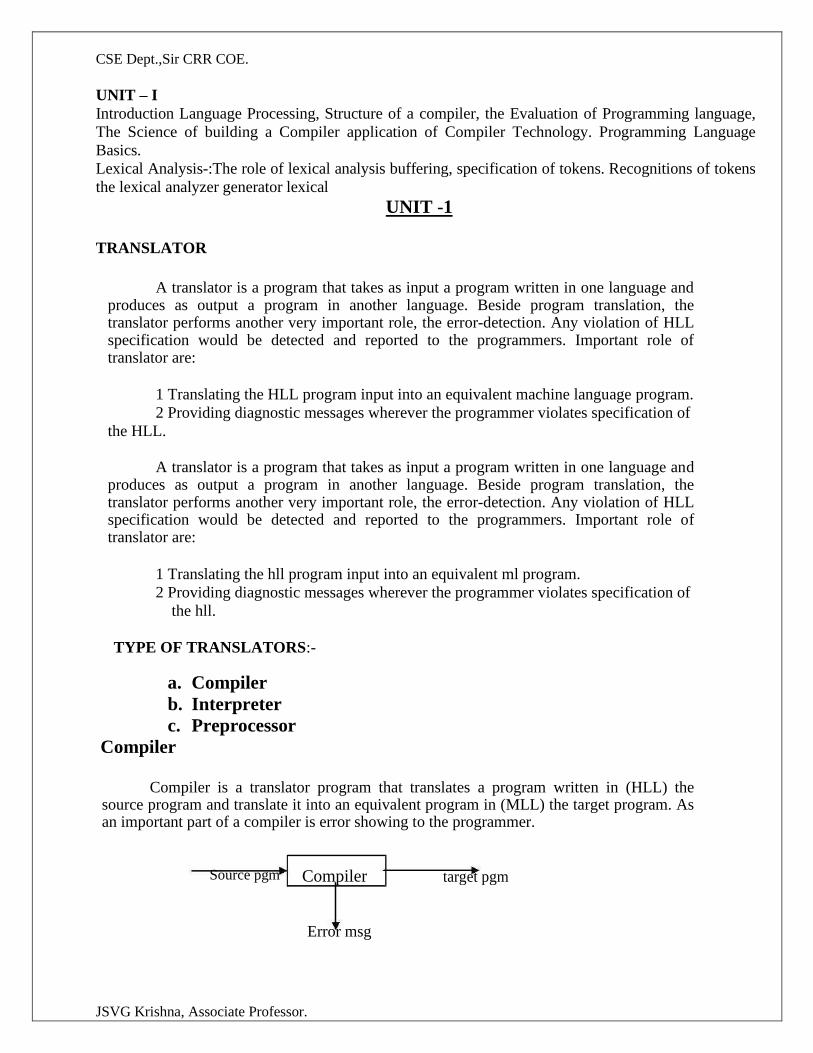
Compiler
Compiler is a translator program that translates a program written in (HLL) the source program and translate it into an equivalent program in (MLL) the target program. As an important part of a compiler is error showing to the programmer.
Source pgm Compiler target pgm
Error msg
CSE Dept.,Sir CRR COE.
JSVG Krishna, Associate Professor.
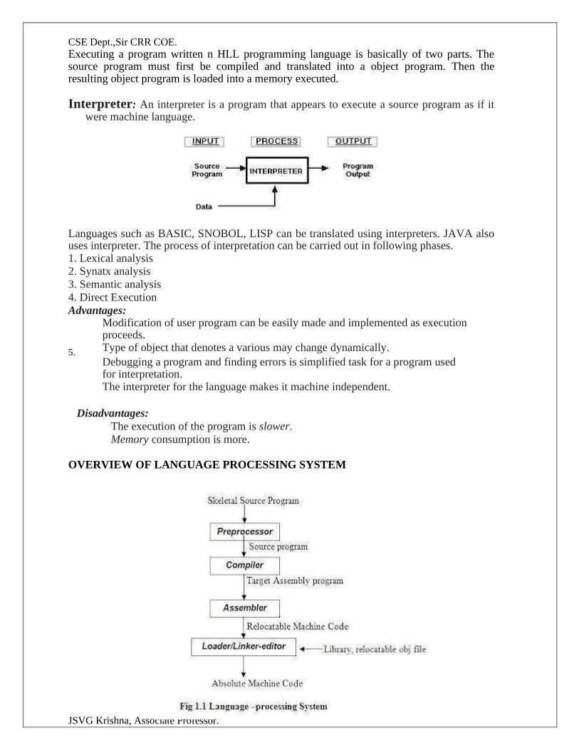
Executing a program written n HLL programming language is basically of two parts. The source program must first be compiled and translated into a object program. Then the resulting object program is loaded into a memory executed.
Interpreter: An interpreter is a program that appears to execute a source program as if it were machine language.
Languages such as BASIC, SNOBOL, LISP can be translated using interpreters. JAVA also uses interpreter. The process of interpretation can be carried out in following phases. 1. Lexical analysis
2. Synatx analysis
3. Semantic analysis
4. Direct Execution
Advantages:
Modification of user program can be easily made and implemented as execution proceeds. Type of object that denotes a various may change dynamically. 5. Debugging a program and finding errors is simplified task for a program used for interpretation. The interpreter for the language makes it machine independent.
Disadvantages:
The execution of the program is slower.
Memory consumption is more. OVERVIEW OF LANGUAGE PROCESSING SYSTEM
CSE Dept.,Sir CRR COE.
JSVG Krishna, Associate Professor.
Preprocessor
A preprocessor produce input to compilers. They may perform the following functions. 1. Macro processing: A preprocessor may allow a user to define macros that are
short hands for longer constructs. 2. File inclusion: A preprocessor may include header files into the program text. 3. Rational preprocessor: these preprocessors augment older languages with more
modern flow-of-control and data structuring facilities. 4. Language Extensions: These preprocessor attempts to add capabilities to the
language by certain amounts to build-in macro
Assembler: programmers found it difficult to write or read programs in machine language. They begin to use a mnemonic (symbols) for each machine instruction, which they would subsequently translate into machine language. Such a mnemonic machine language is now called an assembly language. Programs known as assembler were written to automate the translation of assembly language in to machine language. The input to an assembler program is called source program, the output is a machine language translation (object program).
Loader and Link-editor: Once the assembler procedures an object program, that program must be placed into memory and executed. The assembler could place the object program directly in memory and transfer control to it, thereby causing the machine language program to be execute. This would waste core by leaving the assembler in memory while the user‟s program was being executed. Also the programmer would have to retranslate his program with each execution, thus wasting translation time. To overcome this problems of wasted translation time and memory. System programmers developed another component called loader
“A loader is a program that places programs into memory and prepares them for execution.” It would be more efficient if subroutines could be translated into object form the loader could”relocate” directly behind the user‟s program. The task of adjusting programs othey may be placed in arbitrary core locations is called relocation.
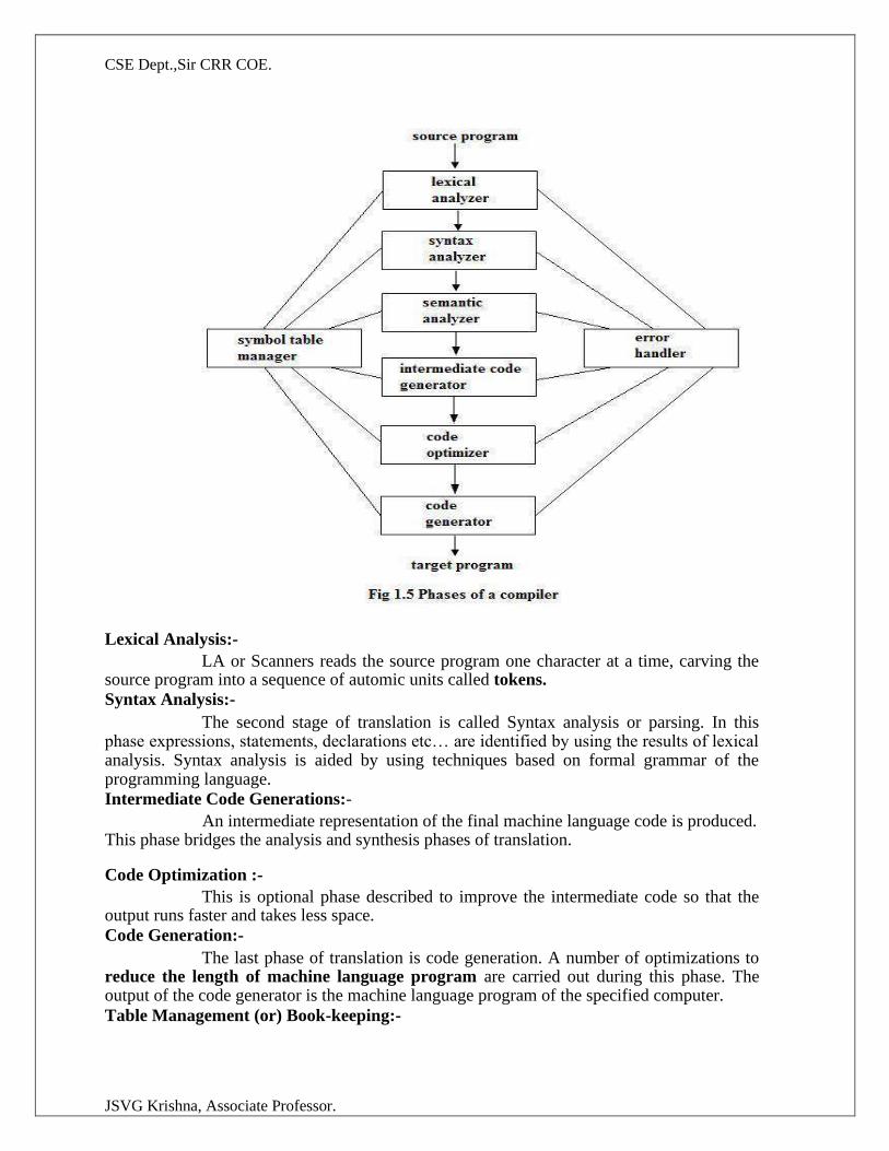
STRUCTURE OF A COMPILER
Phases of a compiler: A compiler operates in phases. A phase is a logically interrelated operation that takes source program in one representation and produces output in another representation. The phases of a compiler are shown in below
There are two phases of compilation. a. Analysis (Machine Independent/Language Dependent) b. Synthesis(Machine Dependent/Language independent)
Compilation process is partitioned into no-of-sub processes called phases’.
CSE Dept.,Sir CRR COE.
JSVG Krishna, Associate Professor.
Lexical Analysis:- LA or Scanners reads the source program one character at a time, carving the
source program into a sequence of automic units called tokens. Syntax Analysis:-
The second stage of translation is called Syntax analysis or parsing. In this phase expressions, statements, declarations etc… are identified by using the results of lexical analysis. Syntax analysis is aided by using techniques based on formal grammar of the programming language. Intermediate Code Generations:-
An intermediate representation of the final machine language code is produced. This phase bridges the analysis and synthesis phases of translation. Code Optimization :-
This is optional phase described to improve the intermediate code so that the output runs faster and takes less space. Code Generation:-
The last phase of translation is code generation. A number of optimizations to reduce the length of machine language program are carried out during this phase. The output of the code generator is the machine language program of the specified computer. Table Management (or) Book-keeping:-
CSE Dept.,Sir CRR COE.
JSVG Krishna, Associate Professor.
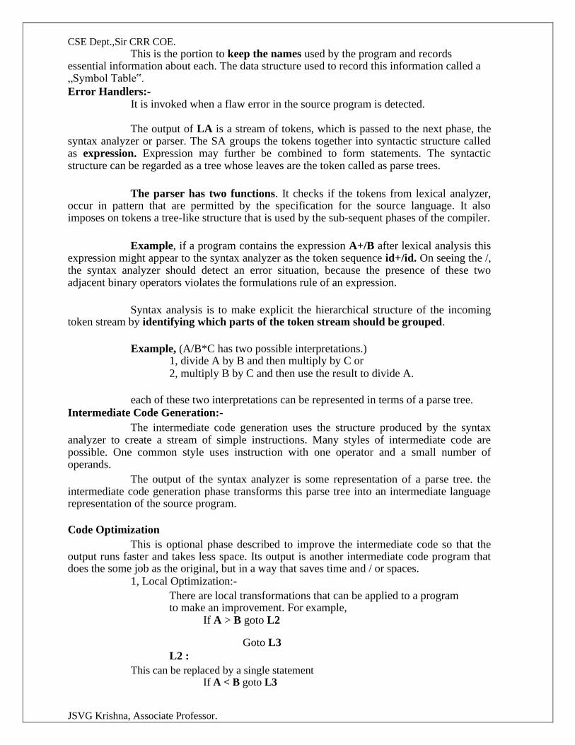
This is the portion to keep the names used by the program and records essential information about each. The data structure used to record this information called a „Symbol Table‟.
Error Handlers:-
It is invoked when a flaw error in the source program is detected. The output of LA is a stream of tokens, which is passed to the next phase, the
syntax analyzer or parser. The SA groups the tokens together into syntactic structure called as expression. Expression may further be combined to form statements. The syntactic structure can be regarded as a tree whose leaves are the token called as parse trees.
The parser has two functions. It checks if the tokens from lexical analyzer, occur in pattern that are permitted by the specification for the source language. It also imposes on tokens a tree-like structure that is used by the sub-sequent phases of the compiler.
Example, if a program contains the expression A+/B after lexical analysis this expression might appear to the syntax analyzer as the token sequence id+/id. On seeing the /, the syntax analyzer should detect an error situation, because the presence of these two adjacent binary operators violates the formulations rule of an expression.
Syntax analysis is to make explicit the hierarchical structure of the incoming token stream by identifying which parts of the token stream should be grouped.
Example, (A/B*C has two possible interpretations.)
1, divide A by B and then multiply by C or
2, multiply B by C and then use the result to divide A.
each of these two interpretations can be represented in terms of a parse tree.
Intermediate Code Generation:-
The intermediate code generation uses the structure produced by the syntax analyzer to create a stream of simple instructions. Many styles of intermediate code are possible. One common style uses instruction with one operator and a small number of operands.
The output of the syntax analyzer is some representation of a parse tree. the intermediate code generation phase transforms this parse tree into an intermediate language representation of the source program.
Code Optimization This is optional phase described to improve the intermediate code so that the
output runs faster and takes less space. Its output is another intermediate code program that does the some job as the original, but in a way that saves time and / or spaces.
1, Local Optimization:- There are local transformations that can be applied to a program to make an improvement. For example,
If A > B goto L2
Goto L3 L2 :
This can be replaced by a single statement If A < B goto L3
CSE Dept.,Sir CRR COE.
JSVG Krishna, Associate Professor.
Another important local optimization is the elimination of common sub-expressions
A := B + C + D
E := B + C + F
Might be evaluated as
T1 := B + C
A := T1 + D
E := T1 + F
Take this advantage of the common sub-expressions B + C.
2, Loop Optimization:-
Another important source of optimization concerns about increasing the speed of loops. A typical loop improvement is to move a computation that produces the same result each time around the loop to a point, in the program just before the loop is entered.
Code Generator :-
Code Generator produces the object code by deciding on the memory locations for data, selecting code to access each datum and selecting the registers in which each computation is to be done. Many computers have only a few high speed registers in which computations can be performed quickly. A good code generator would attempt to utilize registers as efficiently as possible. Table Management OR Book-keeping :-
A compiler needs to collect information about all the data objects that appear in the source program. The information about data objects is collected by the early phases of the compiler-lexical and syntactic analyzers. The data structure used to record this information is called as Symbol Table.
Error Handing :-
One of the most important functions of a compiler is the detection and reporting of errors in the source program. The error message should allow the programmer to determine exactly where the errors have occurred. Errors may occur in all or the phases of a compiler.
Whenever a phase of the compiler discovers an error, it must report the error to the error handler, which issues an appropriate diagnostic msg. Both of the table-management and error-Handling routines interact with all phases of the compiler.
CSE Dept.,Sir CRR COE.
JSVG Krishna, Associate Professor.
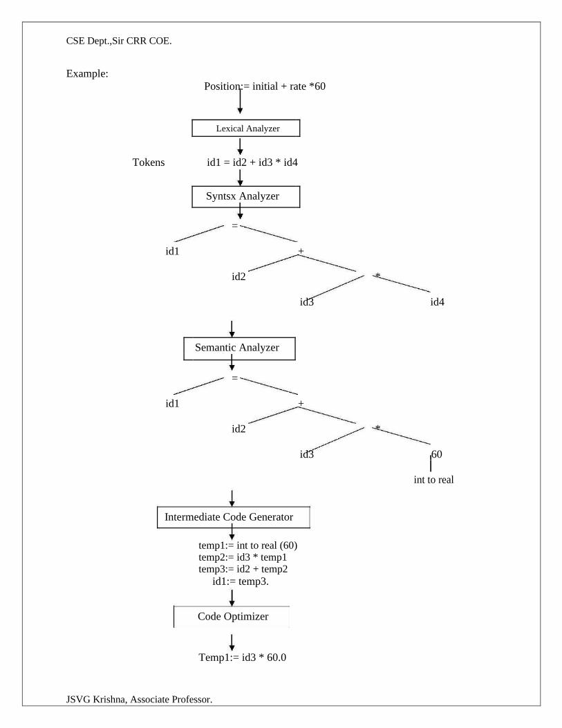
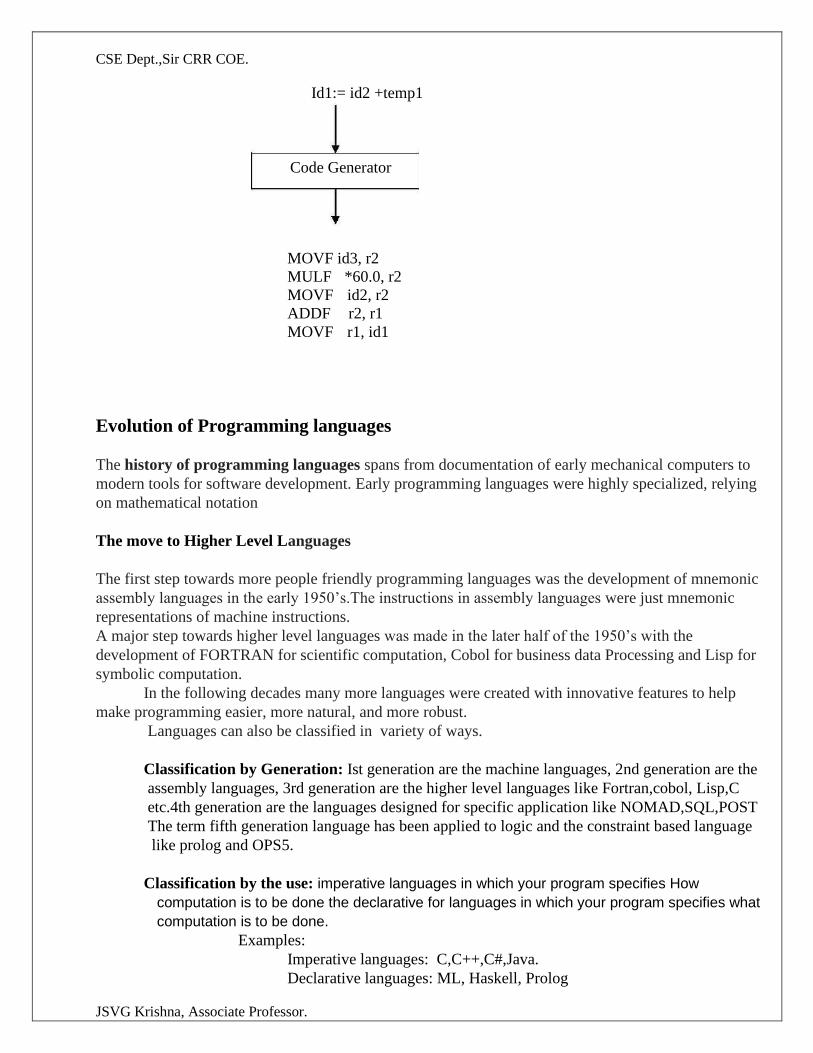
Example:
Position:= initial + rate *60
Lexical Analyzer
Tokens id1 = id2 + id3 * id4
Syntsx Analyzer
=
id1 +
id2 *
id3 id4
Semantic Analyzer
=
id1 +
id2 *
id3 60
int to real
Intermediate Code Generator
temp1:= int to real (60)
temp2:= id3 * temp1
temp3:= id2 + temp2 id1:= temp3.
Code Optimizer
Temp1:= id3 * 60.0
CSE Dept.,Sir CRR COE.
JSVG Krishna, Associate Professor.
Id1:= id2 +temp1
Code Generator
MOVF id3, r2
MULF *60.0, r2
MOVF id2, r2
ADDF r2, r1 MOVF r1, id1
Evolution of Programming languages The history of programming languages spans from documentation of early mechanical computers to
modern tools for software development. Early programming languages were highly specialized, relying
on mathematical notation
The move to Higher Level Languages
The first step towards more people friendly programming languages was the development of mnemonic
assembly languages in the early 1950’s.The instructions in assembly languages were just mnemonic
representations of machine instructions.
A major step towards higher level languages was made in the later half of the 1950’s with the
development of FORTRAN for scientific computation, Cobol for business data Processing and Lisp for
symbolic computation.
In the following decades many more languages were created with innovative features to help
make programming easier, more natural, and more robust.
Languages can also be classified in variety of ways.
Classification by Generation: Ist generation are the machine languages, 2nd generation are the
assembly languages, 3rd generation are the higher level languages like Fortran,cobol, Lisp,C
etc.4th generation are the languages designed for specific application like NOMAD,SQL,POST
The term fifth generation language has been applied to logic and the constraint based language
like prolog and OPS5.
Classification by the use: imperative languages in which your program specifies How
computation is to be done the declarative for languages in which your program specifies what
computation is to be done.
Examples:
Imperative languages: C,C++,C#,Java.
Declarative languages: ML, Haskell, Prolog
CSE Dept.,Sir CRR COE.
JSVG Krishna, Associate Professor.
Object oriented language is one that supports Object oriented programming, a
Programming style in which a program consists of a collection of objects that interact with
one another.
Examples: Simula 67, small talk, C ++, Java,Ruby
Scripting languages are interpreted languages with high level operators designed for
“gluing together” computations These computations originally called Scripts
Example: JavaScript, Perl, PHP, python, Ruby, TCL
The Science of building a Compiler
A compiler must accept all source programs that conform to the specification of the language;
the set of source programs is infinite and any program can be very large, consisting of possibly millions
of lines of code. Any transformation performed by the compiler while translating a source program must
preserve the meaning of the program being compiled. Compiler writers thus have influence over not just
the compilers they create, but all the programs that their compilers compile. This leverage makes
writing compilers particularly rewarding; however, it also makes compiler development challenging.
Modelling in compiler design and implementation: The study of compilers is mainly a study of how
we design the right mathematical models and choose the right algorithms.Some of most fundamental
models are finite-state machines and regular expressions.These models are useful for de-scribing the
lexical units of programs (keywords, identifiers, and such) and for describing the algorithms used by the
compiler to recognize those units. Also among the most fundamental models are context-free grammars,
used to describe the syntactic structure of programming languages such as the nesting of parentheses or
control constructs. Similarly, trees are an important model for representing the structure of programs
and their translation into object code.
The science of code optimization: The term "optimization" in compiler design refers to the attempts
that a com-piler makes to produce code that is more efficient than the obvious code. In modern times,
the optimization of code that a compiler performs has become both more important and more complex.
It is more complex because processor architectures have become more complex, yielding more
opportunities to improve the way code executes. It is more important because massively par-allel
computers require substantial optimization, or their performance suffers by orders of magnitude.
Compiler optimizations must meet the following design objectives:
1. The optimization must be correct, that is, preserve the meaning of the compiled program, 2. The optimization must improve the performance of many programs, 3. The compilation time must be kept reasonable, and 4. The engineering effort required must be manageable.
Thus, in studying compilers, we learn not only how to build a compiler, but also the general
methodology of solving complex and open-ended problems.
Applications of Compiler Technology
Compiler design impacts several other areas of computer science.
Implementation of high-level programming language: A high-level programming language defines a
programming abstraction: the programmer expresses an algorithm using the language, and the compiler
CSE Dept.,Sir CRR COE.
JSVG Krishna, Associate Professor.
must translate that program to the target language. higher-level programming languages are easier to
program in, but are less efficient, that is, the target programs run more slowly. Programmers using a
low-level language have more control over a computation and can, in principle, produce more efficient
code.
Language features that have stimulated significant advances in compiler technology.
Practically all common programming languages, including C, Fortran and Cobol, support user-defined
aggregate data types, such as arrays and structures, and high-level control flow, such as loops and
procedure invocations. If we just take each high-level construct or data-access operation and translate it
directly to machine code, the result would be very inefficient. A body of compiler optimizations, known
as data-flow optimizations, has been developed to analyze the flow of data through the program and
removes redundancies across these constructs. They are effective in generating code that resembles code
written by a skilled programmer at a lower level.
Object orientation was first introduced in Simula in 1967, and has been incorporated in languages such
as Smalltalk, C + + , C # , and Java. The key ideas behind object orientation are
1. Data abstraction and
2. Inheritance of properties,
Java has many features that make programming easier, many of which have been introduced previously
in other languages. Compiler optimizations have been developed to reduce the overhead, for example,
by eliminating unnecessary range checks and by allocating objects that are not accessible beyond a
procedure on the stack instead of the heap. Effective algorithms also have been developed to minimize
the overhead of garbage collection.
In dynamic optimization, it is important to minimize the compilation time as it is part of the execution
overhead. A common technique used is to only compile and optimize those parts of the program that
will be frequently executed.
Optimizations for Computer Architecture: high-performance systems take advantage of the same
two basic techniques: parallelism and memory hierarchies. Parallelism can be found at several levels: at
the instruction level, where multiple operations are executed simultaneously and at
the processor level, where different threads of the same application are run on different processors.
Memory hierarchies are a response to the basic limitation that we can build very fast storage or very
large storage, but not storage that is both fast and large.
Design of New Computer Architectures: in modern computer architecture development, compilers are
developed in the processor-design stage, and compiled code, running on simulators, is used to evaluate
the proposed architectural features. One of the best known examples of how compilers influenced the
design of computer architecture was the invention of the RISC (Reduced Instruction-Set Computer)
architecture.
Compiler optimizations often can reduce these instructions to a small number of simpler operations by
eliminating the redundancies across complex instructions. Thus, it is desirable to build simple
instruction sets; compilers can use them effectively and the hardware is much easier to optimize. Most
general-purpose processor architectures, including PowerPC, SPARC, MIPS, Alpha, and PA-RISC, are
based on the RISC concept.
Specialized Architectures Over the last three decades, many architectural concepts have been
proposed. They include data flow machines, vector machines, VLIW (Very Long Instruction Word)
machines, SIMD (Single Instruction, Multiple Data) arrays of processors, systolic arrays,
multiprocessors with shared memory, and multiprocessors with distributed memory. The development
of each of these architectural concepts was accompanied by the research and development of
corresponding compiler technology.
CSE Dept.,Sir CRR COE.
JSVG Krishna, Associate Professor.
Program Translations: The following are some of the important applications of program-translation
techniques.
Binary Translation: Compiler technology can be used to translate the binary code for one machine to
that of another, allowing a machine to run programs originally compiled for another instruction set.
Binary translation technology has been used by various computer companies to increase the availability
of software for their machines.
Hardware Synthesis: Not only is most software written in high-level languages; even hardware de-
signs are mostly described in high-level hardware description languages like Verilog and VHDL.
Hardware designs are typically described at the register trans-fer level (RTL), where variables represent
registers and expressions represent combinational logic.
Database Query Interpreters: Besides specifying software and hardware, languages are useful in
many other applications. For example, query languages, especially SQL (Structured Query Language),
are used to search databases. Database queries consist of predicates containing relational and boolean
operators. They can be interpreted or com-piled into commands to search a database for records
satisfying that predicate.
Programming Language Basics:
1 The Static/Dynamic Distinction
2 Environments and States
3 Static Scope and Block Structure
4 Explicit Access Control
5 Dynamic Scope
6 Parameter Passing Mechanisms
The Static/Dynamic Distinction: Among the most important issues that we face when designing a
compiler for a language is what decisions can the compiler make about a program. If a language uses a
policy that allows the compiler to decide an issue, then we say that the language uses a static policy or
that the issue can be decided at compile time. On the other hand, a policy that only allows a decision to
be made when we execute the program is said to be a dynamic policy. One issue is the scope of
declarations. The scope of a declaration of x is the region of the program in which uses of x refer to this
declaration. A language uses static scope or lexical scope if it is possible to determine the scope of a
declaration by looking only at the program. Otherwise, the language uses dynamic scope. With dynamic
scope, as the program runs, the same use of x could refer to any of several different declarations of x.
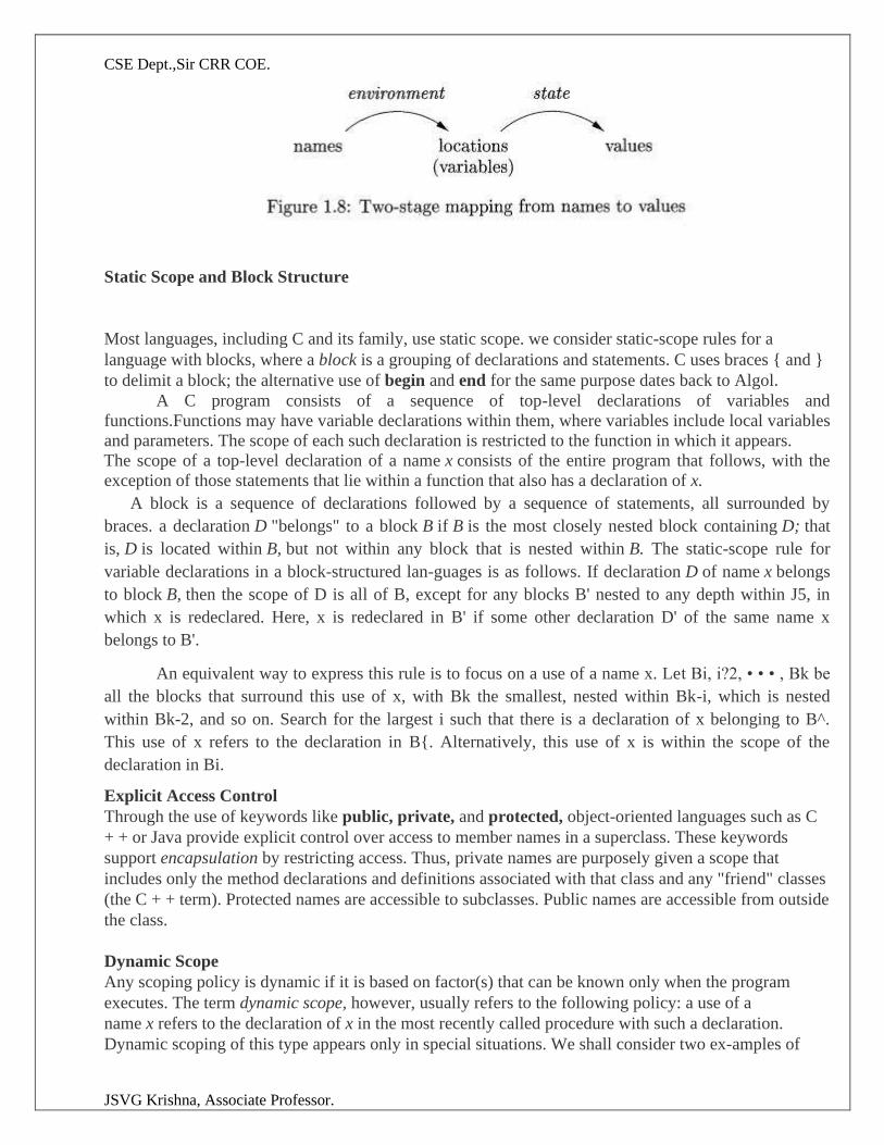
Environments and States:
The environment is a mapping from names to locations in the store. Since variables refer to
locations, we could alternatively define an environment as a mapping from names to variables.
The state is a mapping from locations in store to their values. That is, the state maps 1-values to
their corresponding r-values, in the terminology of C. Environments change according to the scope rules
of a language.
CSE Dept.,Sir CRR COE.
JSVG Krishna, Associate Professor.
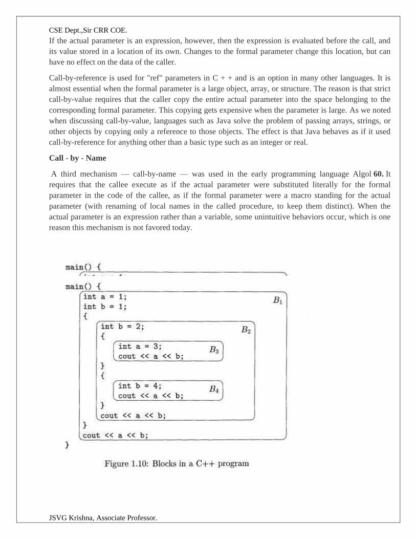
Static Scope and Block Structure
Most languages, including C and its family, use static scope. we consider static-scope rules for a
language with blocks, where a block is a grouping of declarations and statements. C uses braces { and }
to delimit a block; the alternative use of begin and end for the same purpose dates back to Algol.
A C program consists of a sequence of top-level declarations of variables and
functions.Functions may have variable declarations within them, where variables include local variables
and parameters. The scope of each such declaration is restricted to the function in which it appears.
The scope of a top-level declaration of a name x consists of the entire program that follows, with the
exception of those statements that lie within a function that also has a declaration of x.
A block is a sequence of declarations followed by a sequence of statements, all surrounded by
braces. a declaration D "belongs" to a block B if B is the most closely nested block containing D; that
is, D is located within B, but not within any block that is nested within B. The static-scope rule for
variable declarations in a block-structured lan-guages is as follows. If declaration D of name x belongs
to block B, then the scope of D is all of B, except for any blocks B' nested to any depth within J5, in
which x is redeclared. Here, x is redeclared in B' if some other declaration D' of the same name x
belongs to B'.
An equivalent way to express this rule is to focus on a use of a name x. Let Bi, i?2, • • • , Bk be
all the blocks that surround this use of x, with Bk the smallest, nested within Bk-i, which is nested
within Bk-2, and so on. Search for the largest i such that there is a declaration of x belonging to B^.
This use of x refers to the declaration in B{. Alternatively, this use of x is within the scope of the
declaration in Bi.
Explicit Access Control
Through the use of keywords like public, private, and protected, object-oriented languages such as C
+ + or Java provide explicit control over access to member names in a superclass. These keywords
support encapsulation by restricting access. Thus, private names are purposely given a scope that
includes only the method declarations and definitions associated with that class and any "friend" classes
(the C + + term). Protected names are accessible to subclasses. Public names are accessible from outside
the class.
Dynamic Scope
Any scoping policy is dynamic if it is based on factor(s) that can be known only when the program
executes. The term dynamic scope, however, usually refers to the following policy: a use of a
name x refers to the declaration of x in the most recently called procedure with such a declaration.
Dynamic scoping of this type appears only in special situations. We shall consider two ex-amples of
CSE Dept.,Sir CRR COE.
JSVG Krishna, Associate Professor.
dynamic policies: macro expansion in the C preprocessor and method resolution in object-oriented
programming.
Declarations and Definitions
Declarations tell us about the types of things, while definitions tell us about their values. Thus, i n t i is a
declaration of i, while i = 1 is a definition of i.
The difference is more significant when we deal with methods or other procedures. In C + + , a method
is declared in a class definition, by giving the types of the arguments and result of the method (often
called the signature for the method. The method is then defined, i.e., the code for executing the method
is given, in another place. Similarly, it is common to define a C function in one file and declare it in
other files where the function is used.
Parameter Passing Mechanisms
In this section, we shall consider how the actual parameters (the parameters used in the call of a
procedure) are associated with the formal parameters (those used in the procedure definition). Which
mechanism is used determines how the calling-sequence code treats parameters. The great majority of
languages use either "call-by-value," or "call-by-reference," or both.
Call - by - Value
In call-by-value, the actual parameter is evaluated (if it is an expression) or copied (if it is a variable).
The value is placed in the location belonging to the corresponding formal parameter of the called
procedure. This method is used in C and Java, and is a common option in C + + , as well as in most
other languages. Call-by-value has the effect that all computation involving the formal parameters done
by the called procedure is local to that procedure, and the actual parameters themselves cannot be
changed.
Note, however, that in C we can pass a pointer to a variable to allow that variable to be changed by the
callee. Likewise, array names passed as param eters in C, C + + , or Java give the called procedure what
is in effect a pointer or reference to the array itself. Thus, if a is the name of an array of the calling
procedure, and it is passed by value to corresponding formal parameter x, then an assignment such as
x [ i ] = 2 really changes the array element a[2]. The reason is that, although x gets a copy of the value
of a, that value is really a pointer to the beginning of the area of the store where the array named a is
located.
Similarly, in Java, many variables are really references, or pointers, to the things they stand for. This
observation applies to arrays, strings, and objects of all classes. Even though Java uses call-by-value
exclusively, whenever we pass the name of an object to a called procedure, the value received by that
procedure is in effect a pointer to the object. Thus, the called procedure is able to affect the value of the
object itself.
Call - by - Reference
In call-by-reference, the address of the actual parameter is passed to the callee as the value of the
corresponding formal parameter. Uses of the formal parameter in the code of the callee are implemented
by following this pointer to the location indicated by the caller. Changes to the formal parameter thus
appear as changes to the actual parameter.
CSE Dept.,Sir CRR COE.
JSVG Krishna, Associate Professor.
If the actual parameter is an expression, however, then the expression is evaluated before the call, and
its value stored in a location of its own. Changes to the formal parameter change this location, but can
have no effect on the data of the caller.
Call-by-reference is used for "ref" parameters in C + + and is an option in many other languages. It is
almost essential when the formal parameter is a large object, array, or structure. The reason is that strict
call-by-value requires that the caller copy the entire actual parameter into the space belonging to the
corresponding formal parameter. This copying gets expensive when the parameter is large. As we noted
when discussing call-by-value, languages such as Java solve the problem of passing arrays, strings, or
other objects by copying only a reference to those objects. The effect is that Java behaves as if it used
call-by-reference for anything other than a basic type such as an integer or real.
Call - by - Name
A third mechanism — call-by-name — was used in the early programming language Algol 60. It
requires that the callee execute as if the actual parameter were substituted literally for the formal
parameter in the code of the callee, as if the formal parameter were a macro standing for the actual
parameter (with renaming of local names in the called procedure, to keep them distinct). When the
actual parameter is an expression rather than a variable, some unintuitive behaviors occur, which is one
reason this mechanism is not favored today.
CSE Dept.,Sir CRR COE.
JSVG Krishna, Associate Professor.
LEXICAL ANALYSIS
2.1 OVER VIEW OF LEXICAL ANALYSIS
o To identify the tokens we need some method of describing the possible tokens that can appear in the input stream. For this purpose we introduce regular expression, a notation that can be used to describe essentially all the tokens of programming language.
o Secondly , having decided what the tokens are, we need some mechanism to recognize
these in the input stream. This is done by the token recognizers, which are designed using transition diagrams and finite automata.
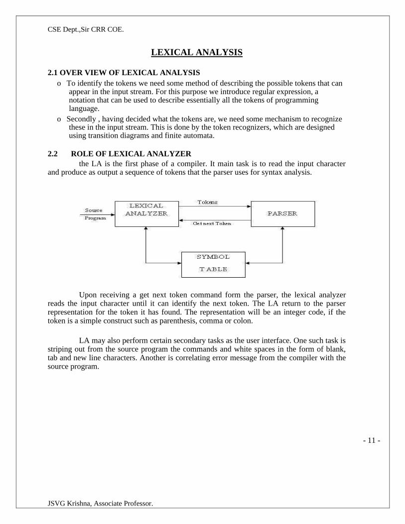
2.2 ROLE OF LEXICAL ANALYZER the LA is the first phase of a compiler. It main task is to read the input character
and produce as output a sequence of tokens that the parser uses for syntax analysis.
Upon receiving a get next token command form the parser, the lexical analyzer reads the input character until it can identify the next token. The LA return to the parser representation for the token it has found. The representation will be an integer code, if the token is a simple construct such as parenthesis, comma or colon.
LA may also perform certain secondary tasks as the user interface. One such task is striping out from the source program the commands and white spaces in the form of blank, tab and new line characters. Another is correlating error message from the compiler with the source program.
- 11 -
CSE Dept.,Sir CRR COE.
JSVG Krishna, Associate Professor.
LEXICAL ANALYSIS VS PARSING:
Lexical analysis Parsing
A Scanner simply turns an input String (say a A parser converts this list of tokens into a
file) into a list of tokens. These tokens Tree-like object to represent how the tokens
represent things like identifiers, parentheses, fit together to form a cohesive whole
operators etc. (sometimes referred to as a sentence).
The lexical analyzer (the "lexer") parses A parser does not give the nodes any
individual symbols from the source code file meaning beyond structural cohesion. The
into tokens. From there, the "parser" proper next thing to do is extract meaning from this
turns those whole tokens into sentences of structure (sometimes called contextual
your grammar analysis).
2.3 INPUT BUFFERING
The LA scans the characters of the source pgm one at a time to discover tokens. Because of large amount of time can be consumed scanning characters, specialized buffering techniques have been developed to reduce the amount of overhead required to process an input character. Buffering techniques:
1. Buffer pairs
2. Sentinels
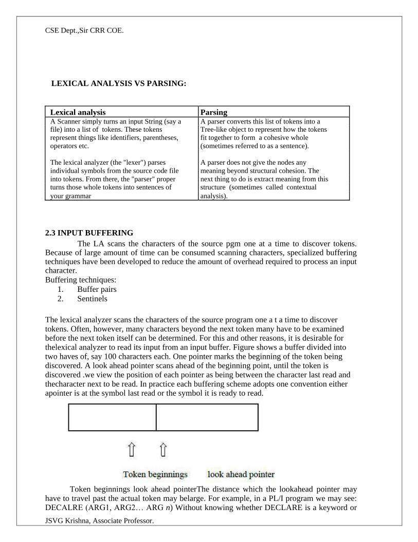
The lexical analyzer scans the characters of the source program one a t a time to discover tokens. Often, however, many characters beyond the next token many have to be examined before the next token itself can be determined. For this and other reasons, it is desirable for thelexical analyzer to read its input from an input buffer. Figure shows a buffer divided into two haves of, say 100 characters each. One pointer marks the beginning of the token being discovered. A look ahead pointer scans ahead of the beginning point, until the token is discovered .we view the position of each pointer as being between the character last read and thecharacter next to be read. In practice each buffering scheme adopts one convention either apointer is at the symbol last read or the symbol it is ready to read.
Token beginnings look ahead pointerThe distance which the lookahead pointer may have to travel past the actual token may belarge. For example, in a PL/I program we may see: DECALRE (ARG1, ARG2… ARG n) Without knowing whether DECLARE is a keyword or
CSE Dept.,Sir CRR COE.
JSVG Krishna, Associate Professor.
an array name until we see the character that follows the right parenthesis. In either case, the token itself ends at the second E. If the look ahead pointer travels beyond the buffer half in which it began, the other half must be loaded with the next characters from the source file. Since the buffer shown in above figure is of limited size there is an implied constraint on how much look ahead can be used before the next token is discovered. In the above example, ifthe look ahead traveled to the left half and all the way through the left half to the middle, we could not reload the right half, because we would lose characters that had not yet been groupedinto tokens. While we can make the buffer larger if we chose or use another buffering scheme,we cannot ignore the fact that overhead is limited.
2.4 TOKEN, LEXEME, PATTERN:
Token: Token is a sequence of characters that can be treated as a single logical entity. Typical tokens are,
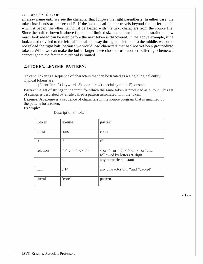
1) Identifiers 2) keywords 3) operators 4) special symbols 5)constants Pattern: A set of strings in the input for which the same token is produced as output. This set of strings is described by a rule called a pattern associated with the token. Lexeme: A lexeme is a sequence of characters in the source program that is matched by the pattern for a token. Example:
Description of token
Token lexeme pattern
const const const
if if If
relation <,<=,= ,< >,>=,> < or <= or = or < > or >= or letter
followed by letters & digit
i pi any numeric constant
nun 3.14 any character b/w “and “except"
literal "core" pattern
- 12 -
CSE Dept.,Sir CRR COE.
JSVG Krishna, Associate Professor.
A pattern is a rule describing the set of lexemes that can represent a particular token in source program.
2.5 LEXICAL ERRORS:
Lexical errors are the errors thrown by your lexer when unable to continue. Which means that there's no way to recognise a lexeme as a valid token for you lexer. Syntax errors, on the other side, will be thrown by your scanner when a given set of already recognised valid tokens don't match any of the right sides of your grammar rules. simple panic-mode error handling system requires that we return to a high-level parsing function when a parsing or lexical error is detected.
Error-recovery actions are: i. Delete one character from the remaining input.
ii. Insert a missing character in to the remaining input.
iii. Replace a character by another character.
iv. Transpose two adjacent characters.
2.6 DIFFERENCE BETWEEN COMPILER AND INTERPRETER
A compiler converts the high level instruction into machine language while an interpreter converts the high level instruction into an intermediate form. Before execution, entire program is executed by the compiler whereas after translating the first line, an interpreter then executes it and so on. List of errors is created by the compiler after the compilation process while an interpreter stops translating after the first error. An independent executable file is created by the compiler whereas interpreter is required by an interpreted program each time.
The compiler produce object code whereas interpreter does not produce object code. In the process of compilation the program is analyzed only once and then the code is generated whereas source program is interpreted every time it is to be executed and every time the source program is analyzed. hence interpreter is less efficient than compiler.
Examples of interpreter: A UPS Debugger is basically a graphical source level debugger but it contains built in C interpreter which can handle multiple source files. Example of compiler: Borland c compiler or Turbo C compiler compiles the programs written in C or C++.
CSE Dept.,Sir CRR COE.
JSVG Krishna, Associate Professor.
2.7 REGULAR EXPRESSIONS
Regular expression is a formula that describes a possible set of string. Component of regular expression..
X the character x
. any character, usually accept a new line
[x y z] any of the characters x, y, z, …..
R? a R or nothing (=optionally as R)
R* zero or more occurrences…..
R+ one or more occurrences ……
R1R2 an R1 followed by an R2
R2R1 either an R1 or an R2. A token is either a single string or one of a collection of strings of a certain type. If we view the set of strings in each token class as an language, we can use the regular-expression notation to describe tokens.
Consider an identifier, which is defined to be a letter followed by zero or more letters or digits. In regular expression notation we would write.
Identifier = letter (letter | digit)*
Here are the rules that define the regular expression over alphabet .
o is a regular expression denoting { € }, that is, the language containing only the empty string.
o For each „a‟ in ∑, is a regular expression denoting { a }, the language with only one string consisting of the single symbol „a‟ .
o If R and S are regular expressions, then
(R) | (S) means LrULs R.S means Lr.Ls R* denotes Lr*
2.8 REGULAR DEFINITIONS
For notational convenience, we may wish to give names to regular expressions and to define regular expressions using these names as if they were symbols.
Identifiers are the set or string of letters and digits beginning with a letter. The following regular definition provides a precise specification for this class of string. Example-1,
Ab*|cd? Is equivalent to (a(b*)) | (c(d?))
Pascal identifier
Letter -
Digits -
A | B | ……| Z | a | b |……| z| 0 | 1 | 2 | …. | 9
letter (letter / digit)* I
CSE Dept.,Sir CRR COE.
JSVG Krishna, Associate Professor.
Recognition of tokens:
We learn how to express pattern using regular expressions. Now, we must study how to take
the patterns for all the needed tokens and build a piece of code that examins the input string and finds a prefix that is a lexeme matching one of the patterns.
Stmt -> if expr then stmt | If expr then else stmt | є
Expr --> term relop term |term
Term -->id
For relop ,we use the comparison operations of languages like Pascal or SQL where = is “equals” and < > is “not equals” because it presents an interesting structure of lexemes. The terminal of grammar, which are if, then , else, relop ,id and numbers are the names of tokens as far as the lexical analyzer is concerned, the patterns for the tokens are described using regular definitions.
digit -->[0,9]
digits -->digit+
number -->digit(.digit)?(e.[+-]?digits)?
letter -->[A-Z,a-z]
id -->letter(letter/digit)*
if --> if
then -->then
else -->else
relop --></>/<=/>=/==/< >
In addition, we assign the lexical analyzer the job stripping out white space, by recognizing the “token” we defined by:
ws --> (blank/tab/newline)+
Here, blank, tab and newline are abstract symbols that we use to express the ASCII characters of the same names. Token ws is different from the other tokens in that ,when we recognize it, we do not return it to parser ,but rather restart the lexical analysis from the character that follows the white space . It is the following token that gets returned to the parser.
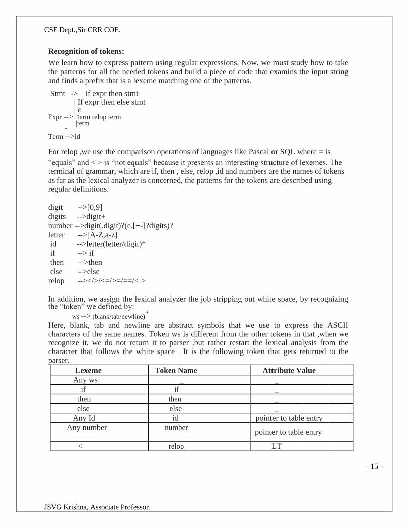
Lexeme Token Name Attribute Value
Any ws _ _
if if _
then then _
else else _
Any Id id pointer to table entry
Any number number pointer to table entry
< relop LT
- 15 -
CSE Dept.,Sir CRR COE.
JSVG Krishna, Associate Professor.
<= relop LE
= relop ET
< > relop NE
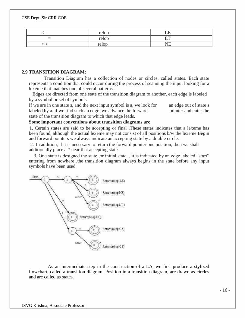
2.9 TRANSITION DIAGRAM: Transition Diagram has a collection of nodes or circles, called states. Each state
represents a condition that could occur during the process of scanning the input looking for a lexeme that matches one of several patterns .
Edges are directed from one state of the transition diagram to another. each edge is labeled by a symbol or set of symbols.
If we are in one state s, and the next input symbol is a, we look for an edge out of state s
labeled by a. if we find such an edge ,we advance the forward pointer and enter the
state of the transition diagram to which that edge leads.
Some important conventions about transition diagrams are 1. Certain states are said to be accepting or final .These states indicates that a lexeme has been found, although the actual lexeme may not consist of all positions b/w the lexeme Begin and forward pointers we always indicate an accepting state by a double circle. 2. In addition, if it is necessary to return the forward pointer one position, then we shall
additionally place a * near that accepting state. 3. One state is designed the state ,or initial state ., it is indicated by an edge labeled “start”
entering from nowhere .the transition diagram always begins in the state before any input symbols have been used.
As an intermediate step in the construction of a LA, we first produce a stylized flowchart, called a transition diagram. Position in a transition diagram, are drawn as circles and are called as states.
- 16 -
CSE Dept.,Sir CRR COE.
JSVG Krishna, Associate Professor.
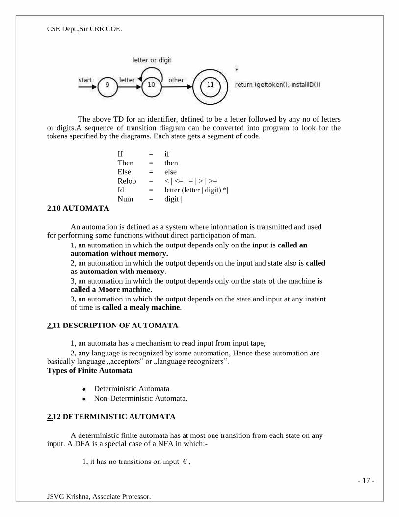
The above TD for an identifier, defined to be a letter followed by any no of letters or digits.A sequence of transition diagram can be converted into program to look for the tokens specified by the diagrams. Each state gets a segment of code.
If = if
Then = then
Else = else
Relop = < | <= | = | > | >=
Id = letter (letter | digit) *|
Num = digit | 2.10 AUTOMATA
An automation is defined as a system where information is transmitted and used for performing some functions without direct participation of man.
1, an automation in which the output depends only on the input is called an automation without memory. 2, an automation in which the output depends on the input and state also is called as automation with memory. 3, an automation in which the output depends only on the state of the machine is called a Moore machine. 3, an automation in which the output depends on the state and input at any instant of time is called a mealy machine.
2.11 DESCRIPTION OF AUTOMATA
1, an automata has a mechanism to read input from input tape,
2, any language is recognized by some automation, Hence these automation are basically language „acceptors‟ or „language recognizers‟. Types of Finite Automata
Deterministic Automata Non-Deterministic Automata.
2.12 DETERMINISTIC AUTOMATA
A deterministic finite automata has at most one transition from each state on any input. A DFA is a special case of a NFA in which:-
1, it has no transitions on input € ,
- 17 -
CSE Dept.,Sir CRR COE.
JSVG Krishna, Associate Professor.
2, each input symbol has at most one transition from any state.
DFA formally defined by 5 tuple notation M = (Q, ∑, δ, qo, F), where Q is a finite „set of states‟, which is non empty. ∑ is „input alphabets‟, indicates input set.
qo is an „initial state‟ and qo is in Q ie, qo, ∑, Q
F is a set of „Final states‟, δ is a „transmission function‟ or mapping function, using this function
the next state can be determined.
The regular expression is converted into minimized DFA by the following procedure:
Regular expression → NFA → DFA → Minimized DFA
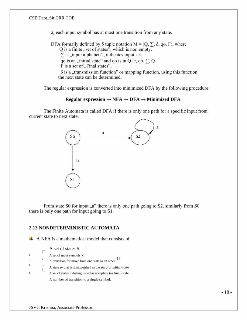
The Finite Automata is called DFA if there is only one path for a specific input from current state to next state.
a
So a
S2
b
S1
From state S0 for input „a‟ there is only one path going to S2. similarly from S0 there is only one path for input going to S1.
2.13 NONDETERMINISTIC AUTOMATA
A NFA is a mathematical model that consists of
A set of states S.
A set of input symbols ∑.
A transition for move from one state to an other.
A state so that is distinguished as the start (or initial) state.
A set of states F distinguished as accepting (or final) state.
A number of transition to a single symbol.
- 18 -
CSE Dept.,Sir CRR COE.
JSVG Krishna, Associate Professor.
A NFA can be diagrammatically represented by a labeled directed graph, called a transition graph, In which the nodes are the states and the labeled edges represent the transition function.
This graph looks like a transition diagram, but the same character can label two or more transitions out of one state and edges can be labeled by the special symbol € as well as by input symbols.
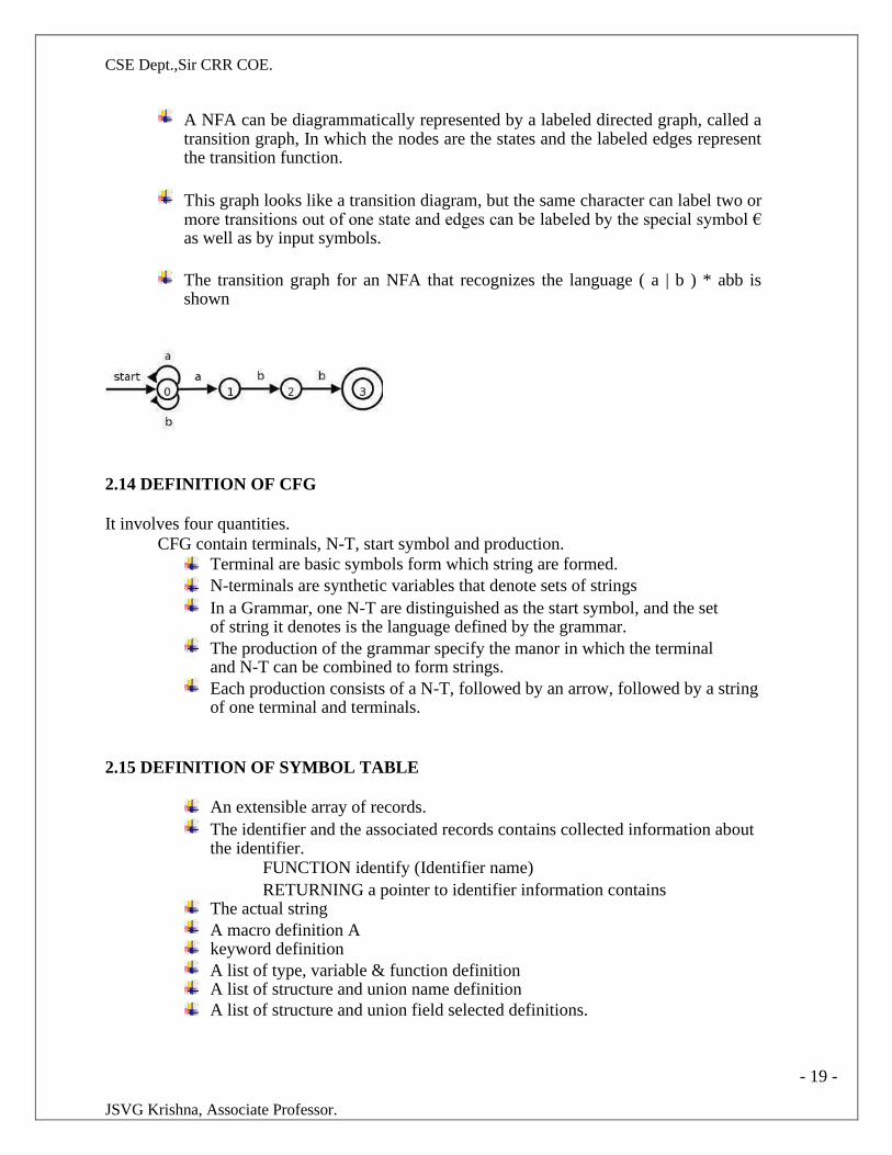
The transition graph for an NFA that recognizes the language ( a | b ) * abb is shown
2.14 DEFINITION OF CFG
It involves four quantities.
CFG contain terminals, N-T, start symbol and production.
Terminal are basic symbols form which string are formed. N-terminals are synthetic variables that denote sets of strings In a Grammar, one N-T are distinguished as the start symbol, and the set of string it denotes is the language defined by the grammar. The production of the grammar specify the manor in which the terminal and N-T can be combined to form strings. Each production consists of a N-T, followed by an arrow, followed by a string of one terminal and terminals.
2.15 DEFINITION OF SYMBOL TABLE
An extensible array of records. The identifier and the associated records contains collected information about the identifier.
FUNCTION identify (Identifier name) RETURNING a pointer to identifier information contains
The actual string A macro definition A
keyword definition A list of type, variable & function definition
A list of structure and union name definition A list of structure and union field selected definitions.
- 19 -
CSE Dept.,Sir CRR COE.
JSVG Krishna, Associate Professor.
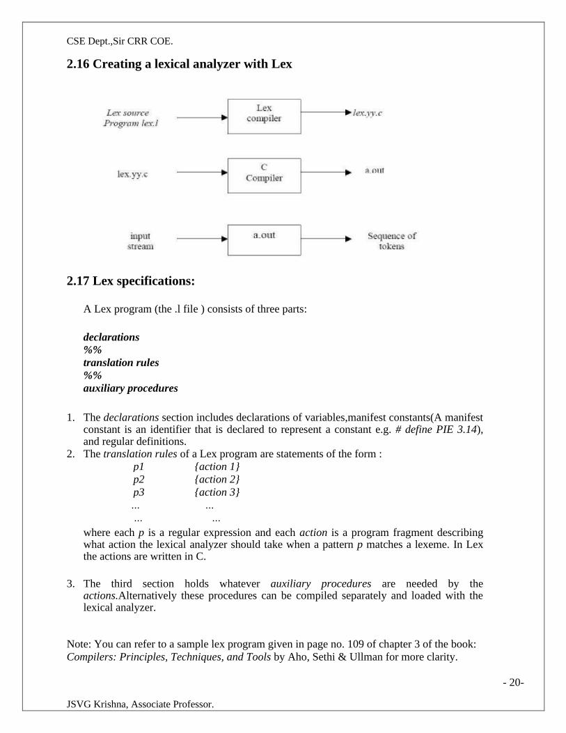
2.16 Creating a lexical analyzer with Lex
2.17 Lex specifications:
A Lex program (the .l file ) consists of three parts:
declarations
%%
translation rules
%%
auxiliary procedures
1. The declarations section includes declarations of variables,manifest constants(A manifest constant is an identifier that is declared to represent a constant e.g. # define PIE 3.14), and regular definitions.
2. The translation rules of a Lex program are statements of the form : p1 {action 1}
p2 {action 2}
p3 {action 3}
… …
… …
where each p is a regular expression and each action is a program fragment describing what action the lexical analyzer should take when a pattern p matches a lexeme. In Lex the actions are written in C.
3. The third section holds whatever auxiliary procedures are needed by the actions.Alternatively these procedures can be compiled separately and loaded with the lexical analyzer.
Note: You can refer to a sample lex program given in page no. 109 of chapter 3 of the book:
Compilers: Principles, Techniques, and Tools by Aho, Sethi & Ullman for more clarity.
- 20-
CSE Dept.,Sir CRR COE.
JSVG Krishna, Associate Professor.
LECTURE NOTES
ON
COMPILER DESIGN
2020 – 2021
III B. Tech I Semester (JNTUK-R16)
P.Naga Deepthi/
Mr J.S.V. Gopala Krishna
Department of Computer Science and Engineering
SIR CRREDDY COLLEGE OF ENGINEERING,
ELURU
- 21 -
CSE Dept.,Sir CRR COE.
JSVG Krishna, Associate Professor.
UNIT –II
Syntax Analysis-:The Role of a parser, Context free Grammars, Writing A grammar, top down parsing
bottom up parsing, Introduction to Lr Parser.
UNIT -2
SYNTAX ANALYSIS
2.1 ROLE OF THE PARSER
Parser obtains a string of tokens from the lexical analyzer and verifies that it can be generated
by the language for the source program. The parser should report any syntax errors in an
intelligible fashion. The two types of parsers employed are:
1.Top down parser: which build parse trees from top(root) to bottom(leaves)
2.Bottom up parser: which build parse trees from leaves and work up the root.
Therefore there are two types of parsing methods– top-down parsing and bottom-up parsing
2.2 Context free Grammars(CFG)
CFG is used to specify the syntax of a language. A grammar naturally describes the
hierarchical structure of most program-ming language constructs.
Formal Definition of Grammars
A context-free grammar has four components:
1. A set of terminal symbols, sometimes referred to as "tokens." The terminals are the elementary
symbols of the language defined by the grammar. 2. A set of nonterminals, sometimes called "syntactic variables." Each non-terminal represents a set of
strings of terminals, in a manner we shall describe. 3. A set of productions, where each production consists of a nonterminal, called the head or left side
of the production, an arrow, and a sequence of terminals and1or nonterminals, called
the body or right side of the production. The intuitive intent of a production is to specify one of the
written forms of a construct; if the head nonterminal represents a construct, then the body
represents a written form of the construct.
CSE Dept.,Sir CRR COE.
JSVG Krishna, Associate Professor.
4. A designation of one of the nonterminals as the start symbol.
Production is for a nonterminal if the nonterminal is the head of the production. A string of
terminals is a sequence of zero or more terminals. The string of zero terminals, written as E , is called
the empty string.
Derivations
A grammar derives strings by beginning with the start symbol and repeatedly replacing a nonterminal
by the body of a production for that nonterminal. The terminal strings that can be derived from the start
symbol form the language defined by the grammar.
Leftmost and Rightmost Derivation of a String
• Leftmost derivation − A leftmost derivation is obtained by applying production to the leftmost
variable in each step.
• Rightmost derivation − A rightmost derivation is obtained by applying production to the
rightmost variable in each step.
• Example
Let any set of production rules in a CFG be
X → X+X | X*X |X| a
over an alphabet {a}.
The leftmost derivation for the string "a+a*a" is
X → X+X → a+X → a + X*X → a+a*X → a+a*a
The rightmost derivation for the above string "a+a*a" is
X → X*X → X*a → X+X*a → X+a*a → a+a*a
Derivation or Yield of a Tree
The derivation or the yield of a parse tree is the final string obtained by concatenating the labels of the
leaves of the tree from left to right, ignoring the Nulls. However, if all the leaves are Null, derivation is
Null.
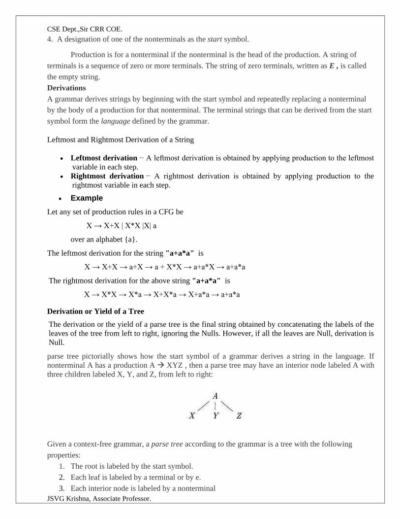
parse tree pictorially shows how the start symbol of a grammar derives a string in the language. If
nonterminal A has a production A → XYZ , then a parse tree may have an interior node labeled A with
three children labeled X, Y, and Z, from left to right:
Given a context-free grammar, a parse tree according to the grammar is a tree with the following
properties:
1. The root is labeled by the start symbol.
2. Each leaf is labeled by a terminal or by e.
3. Each interior node is labeled by a nonterminal
CSE Dept.,Sir CRR COE.
JSVG Krishna, Associate Professor.
If A is the nonterminal labeling some interior node and X I , Xz, . . . ,Xn are the labels of the children
of that node from left to right, then there must be a production A → X1X2 . . Xn . Here, X1,
X2,. . . , Xn, each stand for a symbol that is either a terminal or a nonterminal. As a special case,
if A → c is a production, then a node labeled A may have a single child labeled E
Ambiguity
A grammar can have more than one parse tree generating a given string of terminals. Such a grammar is
said to be ambiguous. To show that a grammar is ambiguous, all we need to do is find a terminal string
that is the yield of more than one parse tree. Since a string with more than one parse tree usually has
more than one meaning, we need to design unambiguous grammars for compiling applications, or to use
ambiguous grammars with additional rules to resolve the ambiguities.
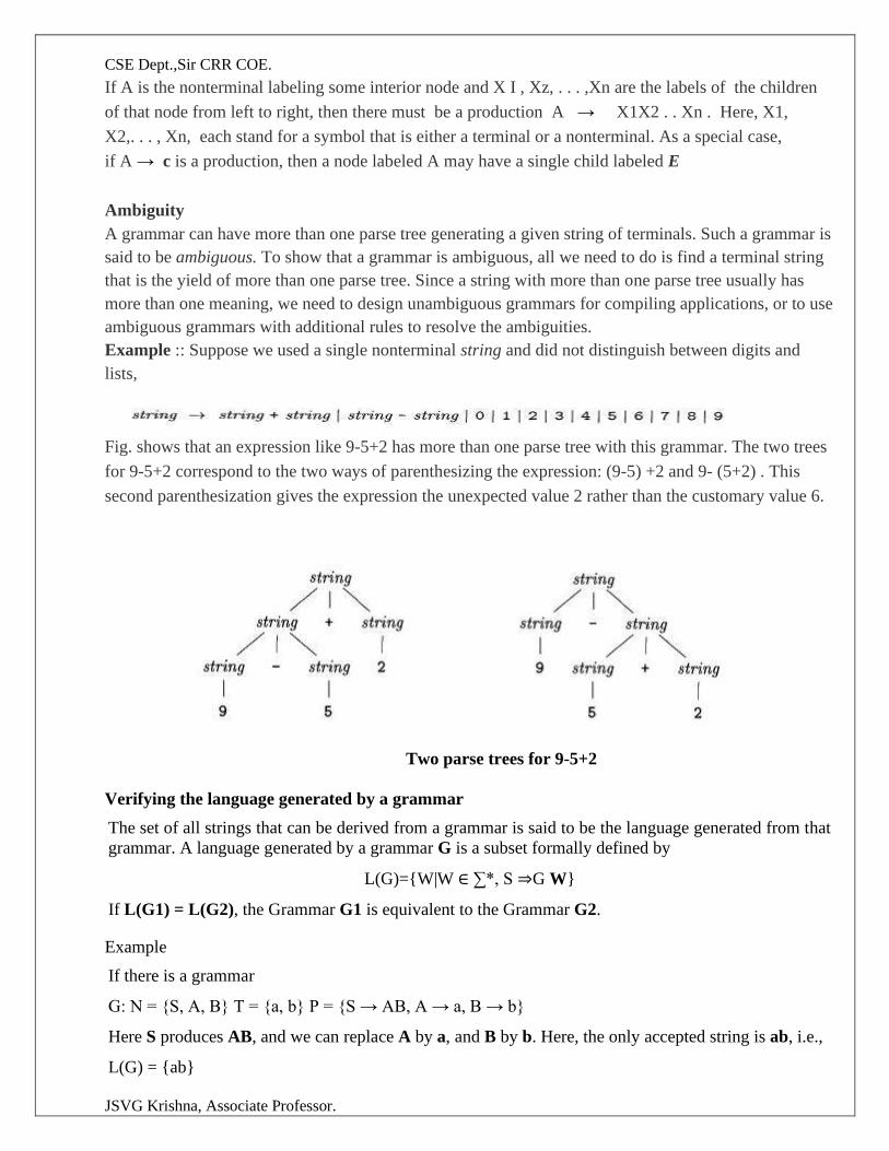
Example :: Suppose we used a single nonterminal string and did not distinguish between digits and
lists,
Fig. shows that an expression like 9-5+2 has more than one parse tree with this grammar. The two trees
for 9-5+2 correspond to the two ways of parenthesizing the expression: (9-5) +2 and 9- (5+2) . This
second parenthesization gives the expression the unexpected value 2 rather than the customary value 6.
Two parse trees for 9-5+2
Verifying the language generated by a grammar
The set of all strings that can be derived from a grammar is said to be the language generated from that
grammar. A language generated by a grammar G is a subset formally defined by
L(G)={W|W ∈ ∑*, S ⇒G W}
If L(G1) = L(G2), the Grammar G1 is equivalent to the Grammar G2.
Example
If there is a grammar
G: N = {S, A, B} T = {a, b} P = {S → AB, A → a, B → b}
Here S produces AB, and we can replace A by a, and B by b. Here, the only accepted string is ab, i.e.,
L(G) = {ab}
CSE Dept.,Sir CRR COE.
JSVG Krishna, Associate Professor.
2.3 Writing a grammar
A grammar consists of a number of productions. Each production has an abstract symbol
called a nonterminal as its left-hand side, and a sequence of one or more nonterminal
and terminal symbols as its right-hand side. For each grammar, the terminal symbols are drawn from a
specified alphabet.
Starting from a sentence consisting of a single distinguished nonterminal, called
the goal symbol, a given context-free grammar specifies a language, namely, the set of
possible sequences of terminal symbols that can result from repeatedly replacing any nonterminal in
the sequence with a right-hand side of a production for which the nonterminal is the left-hand side.
There are four categories in writing a grammar :
1. Lexical Vs Syntax Analysis
2. Eliminating ambiguous grammar.
3. Eliminating left-recursion
4. Left-factoring. Each parsing method can handle grammars only of a certain form hence, the initial grammar may have
to be rewritten to make it parsable
1. Lexical Vs Syntax Analysis
Reasons for using the regular expression to define the lexical syntax of a language
a) Regular expressions provide a more concise and easier to understand notation for tokens than
grammars.
b) The lexical rules of a language are simple and to describe them, we donot need notation as
powerful as grammars.
c) Efficient lexical analyzers can be constructed automatically from RE than from grammars.
d) Separating the syntactic structure of a language into lexical and nonlexical parts provides a
convenient way of modularizing the front end into two manageable-sized components.
2. Eliminating ambiguous grammar.
Ambiguity of the grammar that produces more than one parse tree for leftmost or rightmost
derivation can be eliminated by re-writing the grammar.
Consider this example,
G: stmt→if expr then stmt
|if expr then stmt else stmt
|other
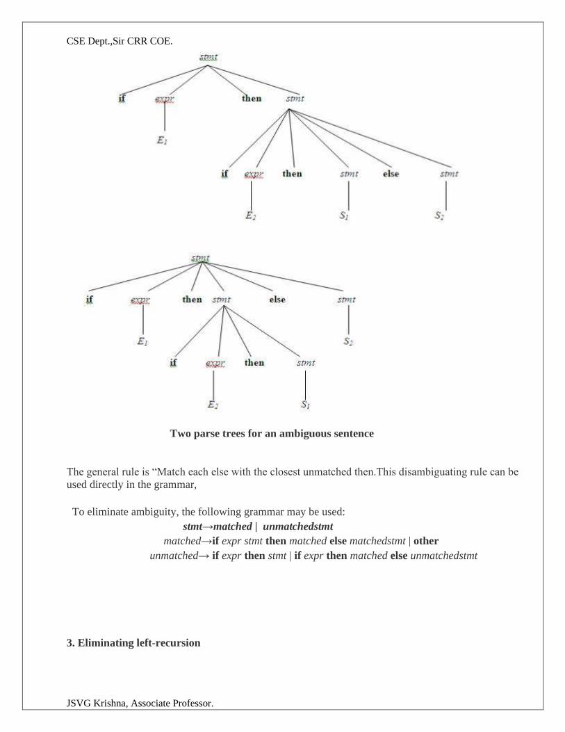
This grammar is ambiguous since the string if E1 then if E2 then S1 else S2 has the following two
parse trees for leftmost derivation
CSE Dept.,Sir CRR COE.
JSVG Krishna, Associate Professor.
Two parse trees for an ambiguous sentence
The general rule is “Match each else with the closest unmatched then.This disambiguating rule can be
used directly in the grammar,
To eliminate ambiguity, the following grammar may be used:
stmt→matched | unmatchedstmt
matched→if expr stmt then matched else matchedstmt | other
unmatched→ if expr then stmt | if expr then matched else unmatchedstmt
3. Eliminating left-recursion
CSE Dept.,Sir CRR COE.
JSVG Krishna, Associate Professor.
Because we try to generate a leftmost derivation by scanning the input from left to right, grammars of the
form A → A x may cause endless recursion.Such grammars are called left-recursive and they must be
transformed if we want to use a top-down parser.
◼ A grammar is left recursive if for a non-terminal A, there is a derivation A+ A
◼ To eliminate direct left recursion replace
1) A → A | with A’ → A’|
2) A → A1 | A2 | ... | Am | 1 | 2 | ... | n
with
A → 1B | 2B | ... | nB
B → 1B | 2B | ... | mB |
4. Left-factoring
Left factoring is a grammar transformation that is useful for producing a grammar suitable for predictive
parsing. When it is not clear which of two alternative productions to use to expand a non-terminal A, we
can rewrite the A-productions to defer the decision until we have seen enough of the input to make the
right choice.
◼ Consider S → if E then S else S | if E then S
◼ Which of the two productions should we use to expand non-terminal S when the next
token is if?
We can solve this problem by factoring out the common part in these rules.
A → 1 | 2 |...| n |
becomes
A → B|
B → 1 | 2 |...| n
Consider the grammar , G : S → iEtS | iEtSeS | a
E → b
Left factored, this grammar becomes
S → iEtSS’ | a
S’ → eS |ε
E → b
2.4 PARSING
It is the process of analyzing a continuous stream of input in order to determine its grammatical
structure with respect to a given formal grammar.
Types of parsing:
1. Top down parsing
2. Bottom up parsing
Top-down parsing : A parser can start with the start symbol and try to transform it to the
input string. Example : LL Parsers.
CSE Dept.,Sir CRR COE.
JSVG Krishna, Associate Professor.
Bottom-up parsing : A parser can start with input and attempt to rewrite it into the start symbol.
Example : LR Parsers.
2.5 TOP-DOWN PARSING
It can be viewed as an attempt to find a left-most derivation for an input string or an
attempt to construct a parse tree for the input starting from the root to the leaves.
Types of TOP-DOWN PARSING
1. Recursive descent parsing
2. Predictive parsing
2.5.1 RECURSIVE DESCENT PARSING
Recursive descent is a top-down parsing technique that constructs the parse tree from the top and the
input is read from left to right. It uses procedures for every non-terminal entity. This parsing technique
recursively parses the input to make a parse tree, which may or may not require back-tracking. But the
grammar associated with it (if not left factored) cannot avoid back-tracking. A form of recursive-
descent parsing that does not require any back-tracking is known as predictive parsing.
This parsing technique is regarded recursive as it uses context-free grammar which is recursive in
nature.
This parsing method may involve backtracking.
Example for :backtracking
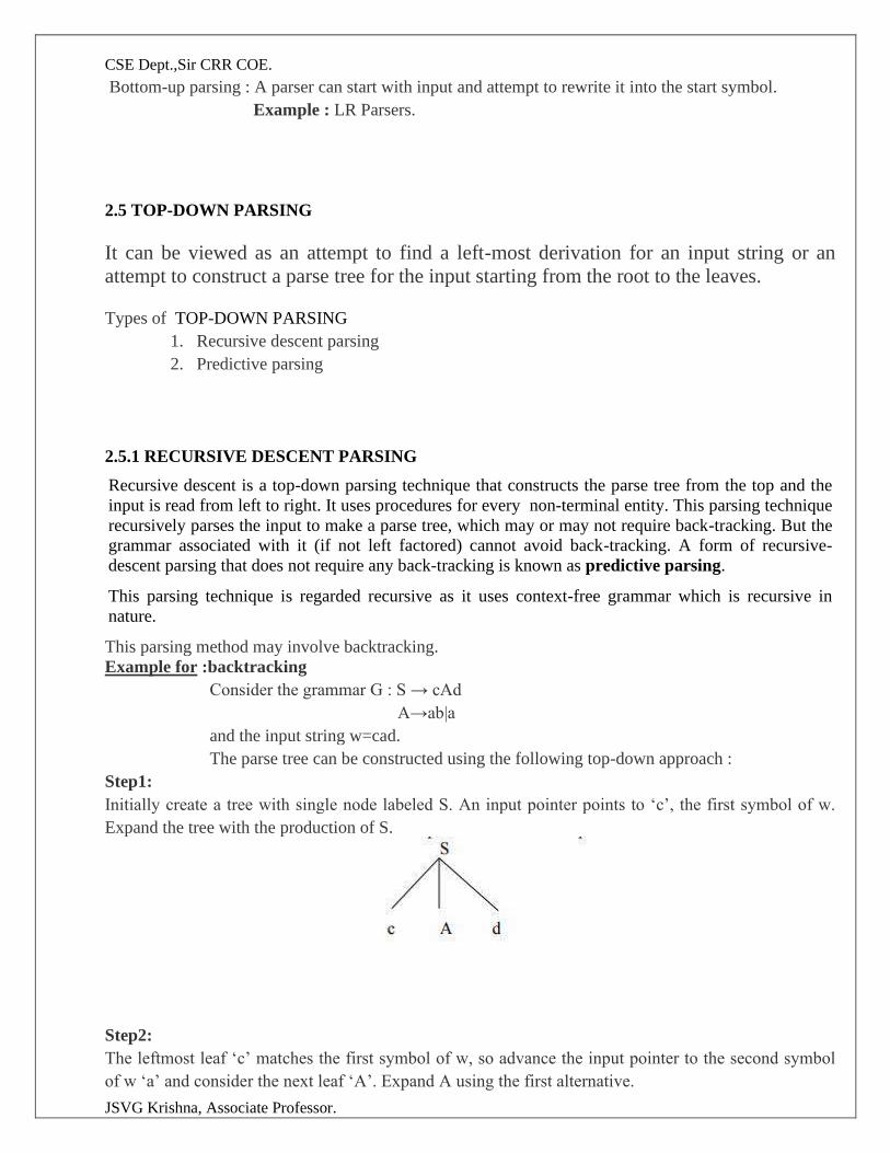
Consider the grammar G : S → cAd
A→ab|a
and the input string w=cad.
The parse tree can be constructed using the following top-down approach :
Step1:
Initially create a tree with single node labeled S. An input pointer points to ‘c’, the first symbol of w.
Expand the tree with the production of S.
Step2:
The leftmost leaf ‘c’ matches the first symbol of w, so advance the input pointer to the second symbol
of w ‘a’ and consider the next leaf ‘A’. Expand A using the first alternative.
CSE Dept.,Sir CRR COE.
JSVG Krishna, Associate Professor.
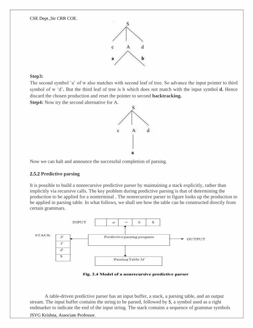
Step3:
The second symbol ‘a’ of w also matches with second leaf of tree. So advance the input pointer to third
symbol of w ‘d’. But the third leaf of tree is b which does not match with the input symbol d. Hence
discard the chosen production and reset the pointer to second backtracking.
Step4: Now try the second alternative for A.
Now we can halt and announce the successful completion of parsing.
2.5.2 Predictive parsing
It is possible to build a nonrecursive predictive parser by maintaining a stack explicitly, rather than
implicitly via recursive calls. The key problem during predictive parsing is that of determining the
production to be applied for a nonterminal . The nonrecursive parser in figure looks up the production to
be applied in parsing table. In what follows, we shall see how the table can be constructed directly from
certain grammars.
A table-driven predictive parser has an input buffer, a stack, a parsing table, and an output
stream. The input buffer contains the string to be parsed, followed by $, a symbol used as a right
endmarker to indicate the end of the input string. The stack contains a sequence of grammar symbols
CSE Dept.,Sir CRR COE.
JSVG Krishna, Associate Professor.
with $ on the bottom, indicating the bottom of the stack. Initially, the stack contains the start symbol of
the grammar on top of $. The parsing table is a two dimensional array M[A,a] where A is a nonterminal,
and a is a terminal or the symbol $. The parser is controlled by a program that behaves as follows. The
program considers X, the symbol on the top of the stack, and a, the current input symbol. These two
symbols determine the action of the parser. There are three possibilities.
1 If X= a=$, the parser halts and announces successful completion of parsing. 2 If X=a!=$, the parser pops X off the stack and advances the input pointer to the next input symbol.
3 If X is a nonterminal, the program consults entry M[X,a] of the parsing table M. This entry will be
either an X-production of the grammar or an error entry. If, for example, M[X,a]={X- >UVW}, the
parser replaces X on top of the stack by WVU( with U on top). As output, we shall assume that the
parser just prints the production used; any other code could be executed here. If M[X,a]=error, the
parser calls an error recovery routine
Implementation of predictive parser:
1. Elimination of left recursion, left factoring and ambiguous grammar.
2. Construct FIRST() and FOLLOW() for all non-terminals.
3. Construct predictive parsing table.
4. Parse the given input string using stack and parsing table
Algorithm for Nonrecursive predictive parsing.
Input. A string w and a parsing table M for grammar G.
Output. If w is in L(G), a leftmost derivation of w; otherwise, an error indication.
Method. Initially, the parser is in a configuration in which it has $S on the stack with S, the start symbol
of G on top, and w$ in the input buffer. The program that utilizes the predictive parsing table M to
produce a parse for the input is shown in Fig.
set ip to point to the first symbol of w$. repeat
let X be the top stack symbol and a the symbol pointed to by ip. if X is a terminal of $ then
if X=a then
pop X from the stack and advance ip else error()
else
if M[X,a]=X->Y1Y2...Yk then begin pop X from the stack;
push Yk,Yk-1...Y1 onto the stack, with Y1 on top; output the production X-> Y1Y2...Yk
end
else error()
until X=$ /* stack is empty */
CSE Dept.,Sir CRR COE.
JSVG Krishna, Associate Professor.
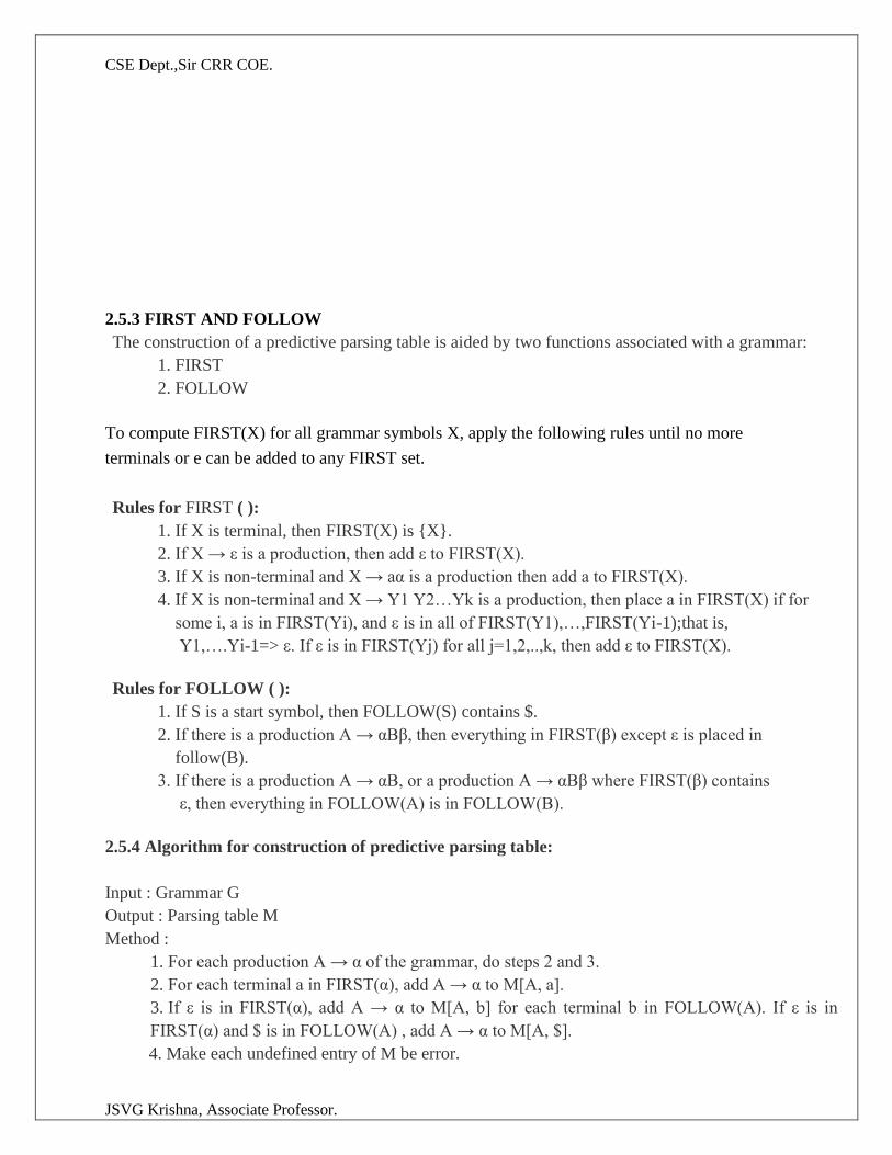
2.5.3 FIRST AND FOLLOW
The construction of a predictive parsing table is aided by two functions associated with a grammar:
1. FIRST
2. FOLLOW
To compute FIRST(X) for all grammar symbols X, apply the following rules until no more
terminals or e can be added to any FIRST set.
Rules for FIRST ( ):
1. If X is terminal, then FIRST(X) is {X}.
2. If X → ε is a production, then add ε to FIRST(X).
3. If X is non-terminal and X → aα is a production then add a to FIRST(X).
4. If X is non-terminal and X → Y1 Y2…Yk is a production, then place a in FIRST(X) if for
some i, a is in FIRST(Yi), and ε is in all of FIRST(Y1),…,FIRST(Yi-1);that is,
Y1,….Yi-1=> ε. If ε is in FIRST(Yj) for all j=1,2,..,k, then add ε to FIRST(X).
Rules for FOLLOW ( ):
1. If S is a start symbol, then FOLLOW(S) contains $.
2. If there is a production A → αBβ, then everything in FIRST(β) except ε is placed in
follow(B).
3. If there is a production A → αB, or a production A → αBβ where FIRST(β) contains
ε, then everything in FOLLOW(A) is in FOLLOW(B).
2.5.4 Algorithm for construction of predictive parsing table:
Input : Grammar G
Output : Parsing table M
Method :
1. For each production A → α of the grammar, do steps 2 and 3.
2. For each terminal a in FIRST(α), add A → α to M[A, a].
3. If ε is in FIRST(α), add A → α to M[A, b] for each terminal b in FOLLOW(A). If ε is in
FIRST(α) and $ is in FOLLOW(A) , add A → α to M[A, $].
4. Make each undefined entry of M be error.
CSE Dept.,Sir CRR COE.
JSVG Krishna, Associate Professor.
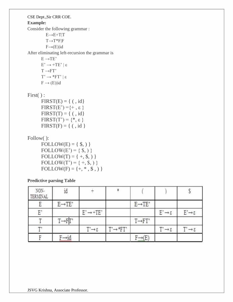
Example:
Consider the following grammar :
E→E+T|T
T→T*F|F
F→(E)|id
After eliminating left-recursion the grammar is
E →TE’
E’ → +TE’ | ε
T →FT’
T’ → *FT’ | ε
F → (E)|id
First( ) :
FIRST(E) = { ( , id}
FIRST(E’) ={+ , ε }
FIRST(T) = { ( , id}
FIRST(T’) = {*, ε }
FIRST(F) = { ( , id }
Follow( ):
FOLLOW(E) = { $, ) }
FOLLOW(E’) = { $, ) }
FOLLOW(T) = { +, $, ) }
FOLLOW(T’) = { +, $, ) }
FOLLOW(F) = {+, * , $ , ) }
Predictive parsing Table
CSE Dept.,Sir CRR COE.
JSVG Krishna, Associate Professor.
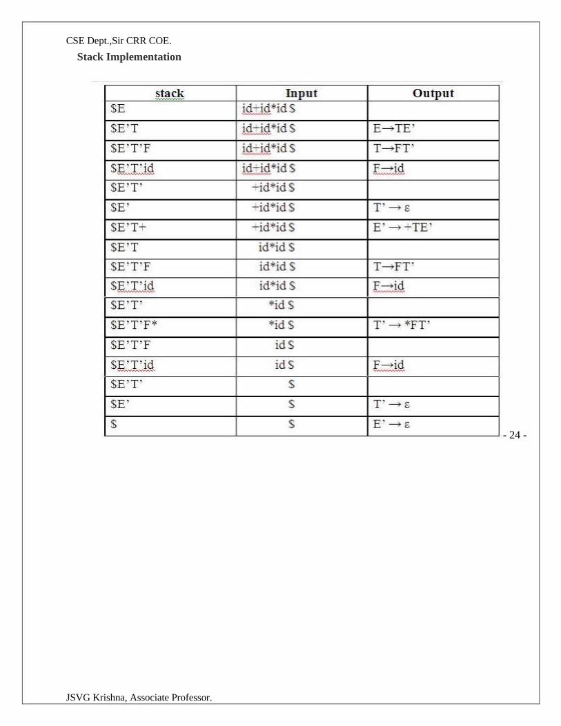
Stack Implementation
- 24 -
CSE Dept.,Sir CRR COE.
JSVG Krishna, Associate Professor.
2.5.5.LL(1) GRAMMAR
The parsing table algorithm can be applied to any grammar G to produce a parsing table M.
For some Grammars, for example if G is left recursive or ambiguous, then M will have at
least one multiply-defined entry. A grammar whose parsing table has no multiply defined
entries is said to be LL(1). It can be shown that the above algorithm can be used to produce
for every LL(1) grammar G, a parsing table M that parses all and only the sentences of G.
LL(1) grammars have several distinctive properties. No ambiguous or left recursive grammar
can be LL(1). There remains a question of what should be done in case of multiply defined
entries. One easy solution is to eliminate all left recursion and left factoring, hoping to
produce a grammar which will produce no multiply defined entries in the parse tables.
Unfortunately there are some grammars which will give an LL(1) grammar after any kind of
alteration. In general, there are no universal rules to convert multiply defined entries into
single valued entries without affecting the language recognized by the parser.
The main difficulty in using predictive parsing is in writing a grammar for the source
language such that a predictive parser can be constructed from the grammar. Although left
recursion elimination and left factoring are easy to do, they make the resulting grammar hard
to read and difficult to use the translation purposes. To alleviate some of this difficulty, a
common organization for a parser in a compiler is to use a predictive parser for control
constructs and to use operator precedence for expressions.however, if an lr parser generator
is available, one can get all the benefits of predictive parsing and operator precedence
automatically.
2.5.6.ERROR RECOVERY IN PREDICTIVE PARSING
The stack of a nonrecursive predictive parser makes explicit the terminals and nonterminals
that the parser hopes to match with the remainder of the input. We shall therefore refer to
symbols on the parser stack in the following discussion. An error is detected during
predictive parsing when the terminal on top of the stack does not match the next input
symbol or when nonterminal A is on top of the stack, a is the next input symbol, and the
parsing table entry M[A,a] is empty.
Consider error recovery predictive parsing using the following two methods
Panic-Mode recovery
Phrase Level recovery
Panic-mode error recovery is based on the idea of skipping symbols on the input until a
token in a selected set of synchronizing tokens appears. Its effectiveness depends on the
choice of synchronizing set. The sets should be chosen so that the parser recovers quickly
from errors that are likely to occur in practice. As a starting point, we can place all symbols in FOLLOW(A) into the synchronizing set for
nonterminal A. If we skip tokens until an element of FOLLOW(A) is seen and pop A from
the stack, it is likely that parsing can continue.
It is not enough to use FOLLOW(A) as the synchronizingset for A. Fo example , if
semicolons terminate statements, as in C, then keywords that begin statements may not
appear in the FOLLOW set of the nonterminal generating expressions. A missing semicolon
after an assignment may therefore result in the keyword beginning the next statement being
skipped. Often, there is a hierarchica structure on constructs in a language; e.g., expressions
appear within statement, which appear within bblocks,and so on. We can add to the
CSE Dept.,Sir CRR COE.
JSVG Krishna, Associate Professor.
synchronizing set of a lower construct the symbols that begin higher constructs. For
example, we might add keywords that begin statements to the synchronizing sets for the
nonterminals generaitn expressions.
If we add symbols in FIRST(A) to the synchronizing set for nonterminal A, then it
may be possible to resume parsing according to A if a symbol in FIRST(A) appears in the
input.
If a nonterminal can generate the empty string, then the production deriving e can be
used as a default. Doing so may postpone some error detection, but cannot cause an error
to be missed. This approach reduces the number of nonterminals that have to be considered
during error recovery.
If a terminal on top of the stack cannot be matched, a simple idea is to pop the
terminal, issue a message saying that the terminal was inserted, and continue parsing. In
effect, this approach takes the synchronizing set of a token to consist of all other tokens.
Phrase Level recovery
This involves, defining the blank entries in the table with pointers to some error routines
which may
Change, delete or insert symbols in the input or
May also pop symbols from the stack
2.6 BOTTOM-UP PARSING Constructing a parse tree for an input string beginning at the leaves and going towards the root is
called bottom-up parsing. A general type of bottom-up parser is a shift-reduce parser.
2.6.1 SHIFT-REDUCE PARSING
Shift-reduce parsing is a type of bottom-up parsing that attempts to construct a parse tree for
an input string beginning at the leaves (the bottom) and working up towards the root (the
top).
Example:
Consider the grammar: S → aABe
A → Abc | b
B → d
The sentence to be recognized is abbcde.
REDUCTION (LEFTMOST) RIGHTMOST DERIVATION
abbcde (A → b) S → aABe
aAbcde(A → Abc) → aAde
aAde (B → d) → aAbcde
aABe (S → aABe) → abbcde
S
The reductions trace out the right-most derivation in reverse.
CSE Dept.,Sir CRR COE.
JSVG Krishna, Associate Professor.
Handles: A handle of a string is a substring that matches the right side of a production, and
whose reduction to the non-terminal on the left side of the production represents one step
along the reverse of a rightmost derivation.
Example:
Consider the grammar:
E→E+E
E→E*E
E→(E)
E→id
And the input string id1+id2*id3
The rightmost derivation is :
E→E+E
→ E+E*E
→ E+E*id3
→ E+id2*id3
→ id1+id2*
In the above derivation the underlined substrings are called handles.
Handle pruning:
A rightmost derivation in reverse can be obtained by “handle pruning”. (i.e.) if w is a sentence
or string of the grammar at hand, then w = γn, where γn is the nth right sentential form of
some rightmost derivation.
Actions in shift-reduce parser:
• shift - The next input symbol is shifted onto the top of the stack.
• reduce - The parser replaces the handle within a stack with a non-terminal.
• accept - The parser announces successful completion of parsing.
• error - The parser discovers that a syntax error has occurred and calls an error recovery routine.
Conflicts in shift-reduce parsing:
There are two conflicts that occur in shift-reduce parsing:
1. Shift-reduce conflict: The parser cannot decide whether to shift or to reduce.
2. Reduce-reduce conflict: The parser cannot decide which of several reductions to make.
CSE Dept.,Sir CRR COE.
JSVG Krishna, Associate Professor.
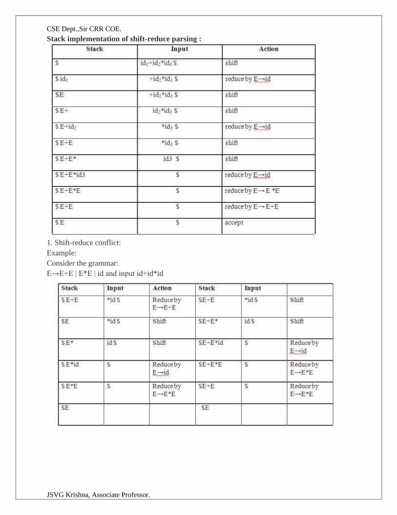
Stack implementation of shift-reduce parsing :
1. Shift-reduce conflict:
Example:
Consider the grammar:
E→E+E | E*E | id and input id+id*id
CSE Dept.,Sir CRR COE.
JSVG Krishna, Associate Professor.
2. Reduce-reduce conflict:
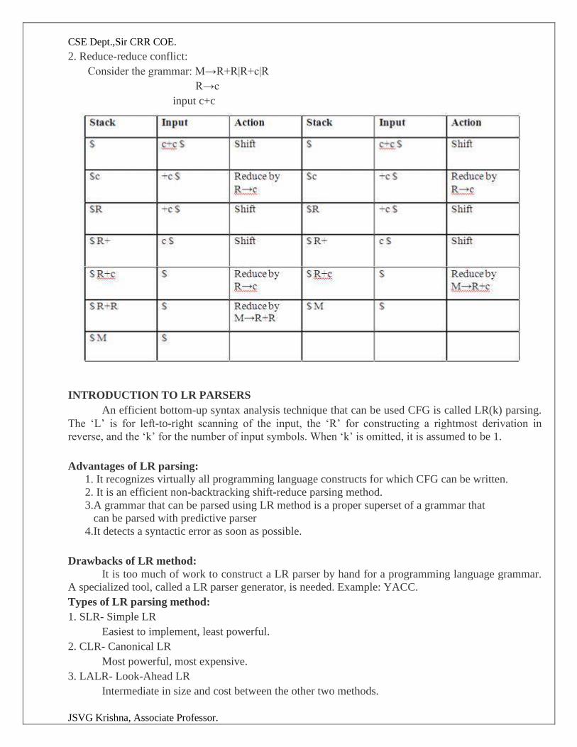
Consider the grammar: M→R+R|R+c|R
R→c
input c+c
INTRODUCTION TO LR PARSERS
An efficient bottom-up syntax analysis technique that can be used CFG is called LR(k) parsing.
The ‘L’ is for left-to-right scanning of the input, the ‘R’ for constructing a rightmost derivation in
reverse, and the ‘k’ for the number of input symbols. When ‘k’ is omitted, it is assumed to be 1.
Advantages of LR parsing:
1. It recognizes virtually all programming language constructs for which CFG can be written.
2. It is an efficient non-backtracking shift-reduce parsing method.
3.A grammar that can be parsed using LR method is a proper superset of a grammar that
can be parsed with predictive parser
4.It detects a syntactic error as soon as possible.
Drawbacks of LR method:
It is too much of work to construct a LR parser by hand for a programming language grammar.
A specialized tool, called a LR parser generator, is needed. Example: YACC.
Types of LR parsing method:
1. SLR- Simple LR
Easiest to implement, least powerful.
2. CLR- Canonical LR
Most powerful, most expensive.
3. LALR- Look-Ahead LR
Intermediate in size and cost between the other two methods.
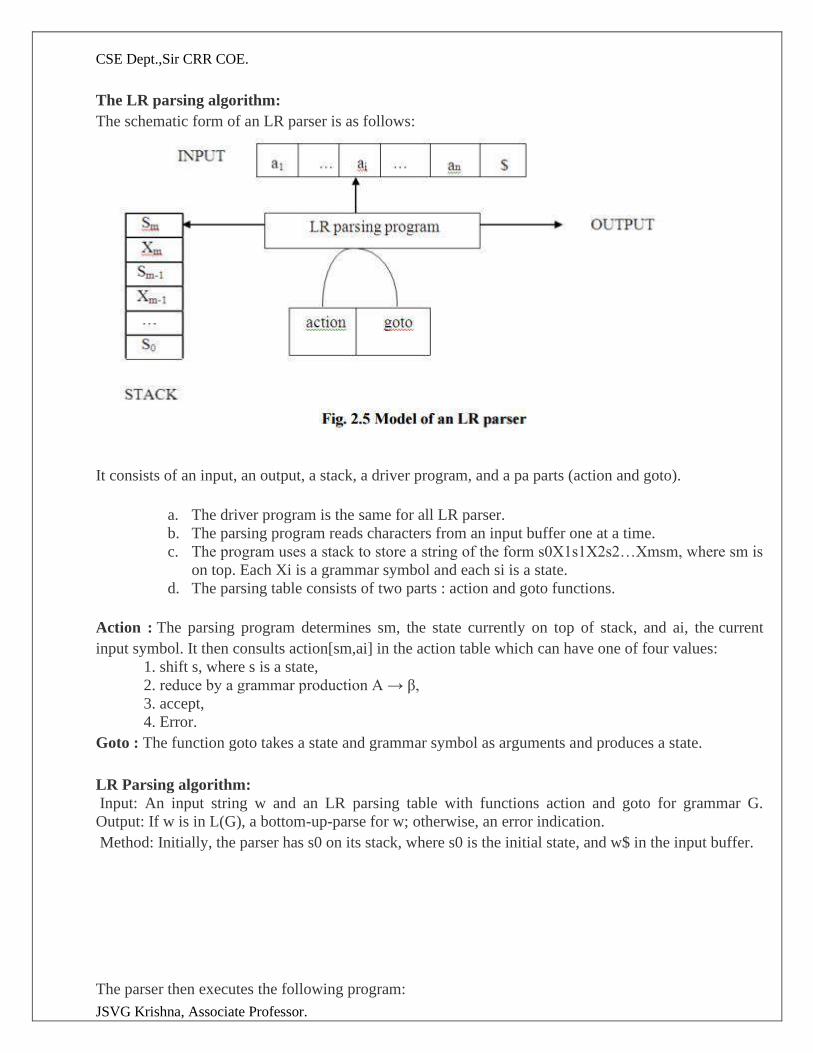
CSE Dept.,Sir CRR COE.
JSVG Krishna, Associate Professor.
The LR parsing algorithm:
The schematic form of an LR parser is as follows:
It consists of an input, an output, a stack, a driver program, and a pa parts (action and goto).
a. The driver program is the same for all LR parser.
b. The parsing program reads characters from an input buffer one at a time.
c. The program uses a stack to store a string of the form s0X1s1X2s2…Xmsm, where sm is
on top. Each Xi is a grammar symbol and each si is a state.
d. The parsing table consists of two parts : action and goto functions.
Action : The parsing program determines sm, the state currently on top of stack, and ai, the current
input symbol. It then consults action[sm,ai] in the action table which can have one of four values:
1. shift s, where s is a state,
2. reduce by a grammar production A → β,
3. accept,
4. Error.
Goto : The function goto takes a state and grammar symbol as arguments and produces a state.
LR Parsing algorithm:
Input: An input string w and an LR parsing table with functions action and goto for grammar G.
Output: If w is in L(G), a bottom-up-parse for w; otherwise, an error indication.
Method: Initially, the parser has s0 on its stack, where s0 is the initial state, and w$ in the input buffer.
The parser then executes the following program:
CSE Dept.,Sir CRR COE.
JSVG Krishna, Associate Professor.
set ip to point to the first input symbol of w$; repeat forever begin
let s be the state on top of the stack and a the symbol pointed to by ip;
if action[s, a] = shift s’ then begin
push a then s’ on top of the stack; advance ip to the next input symbol end
else if action[s, a] = reduce A→β then begin pop 2* | β | symbols off the stack;
let s’ be the state now on top of the stack; push A then goto[s’, A] on top of the stack; output the
production A→ β
end
else if action[s, a] = accept then
return
else error( )
end
CONSTRUCTING SLR(1) PARSING TABLE
To perform SLR parsing, take grammar as input and do the following:
1. Find LR(0) items.
2. Completing the closure.
3. Compute goto(I,X), where, I is set of items and X is grammar symbol.
LR(0) items:
An LR(0) item of a grammar G is a production of G with a dot at some position of the right side. For
example, production A → XYZ yields the four items :
A→.XYZ
A → X . YZ
A → XY . Z
A → XYZ .
Closure operation:
If I is a set of items for a grammar G, then closure(I) is the set of items constructed from I by
the two rules:
1. Initially, every item in I is added to closure(I).
2. If A → α . Bβ is in closure(I) and B → γ is a production, then add the item B → . γ to I , if it
is not already there. We apply this rule until no more new items can be added to closure(I).
Goto operation:
Goto(I, X) is defined to be the closure of the set of all items [A→ αX . β] such that [A→ α . Xβ] is in I.
Steps to construct SLR parsing table for grammar G are:
1. Augment G and produce G’
2. Construct the canonical collection of set of items C for G’
3. Construct the parsing action function action and goto using the following algorithm that requires
FOLLOW(A) for each non-terminal of grammar.
CSE Dept.,Sir CRR COE.
JSVG Krishna, Associate Professor.
Algorithm for construction of SLR parsing table:
Input : An augmented grammar G’
Output : The SLR parsing table functions action and goto for G’
Method :
1. Construct C = {I0, I1, …. In}, the collection of sets of LR(0) items for G’.
2. State i is constructed from Ii.. The parsing functions for state i are determined as
follows:
(a) If [A→α∙aβ] is in Ii and goto(Ii,a) = Ij, then set action[i,a] to “shift j”. Here a must be
terminal.
(b) If [A→α∙] is in Ii , then set action[i,a] to “reduce A→α” for all a in FOLLOW(A).
(c) If [S’→S.] is in Ii, then set action[i,$] to “accept”.
If any conflicting actions are generated by the above rules, we say grammar is not SLR(1).
3. The goto transitions for state i are constructed for all non-term
If goto(Ii,A) = Ij, then goto[i,A] = j.
4. All entries not defined by rules (2) and (3) are made “error”
5. The initial state of the parser is the one constructed from the [S’→.S].
Example on SLR ( 1 ) Grammar
S → E
E → E + T | T
T → T * F | F
F → id
Add Augment Production and insert '•' symbol at the first position for every production in G
S` → •E
E → •E + T
E → •T
T → •T * F
T → •F
F → •id
I0 State:
Add Augment production to the I0 State and Compute the Closure
I0 = Closure (S` → •E)
Add all productions starting with E in to I0 State because "." is followed by the non-terminal. So, the I0
State becomes
I0 = S` → •E
E → •E + T
E → •T
Add all productions starting with T and F in modified I0 State because "." is followed by the non-
terminal. So, the I0 State becomes.
CSE Dept.,Sir CRR COE.
JSVG Krishna, Associate Professor.
I0= S` → •E
E → •E + T
E → •T
T → •T * F
T → •F
F → •id
I1= Go to (I0, E) = closure (S` → E•, E → E• + T)
I2= Go to (I0, T) = closure (E → T•T, T• → * F)
I3= Go to (I0, F) = Closure ( T → F• ) = T → F•
I4= Go to (I0, id) = closure ( F → id•) = F → id•
I5= Go to (I1, +) = Closure (E → E +•T)
Add all productions starting with T and F in I5 State because "." is followed by the non-terminal. So, the
I5 State becomes
I5 = E → E +•T
T → •T * F
T → •F
F → •id
Go to (I5, F) = Closure (T → F•) = (same as I3)
Go to (I5, id) = Closure (F → id•) = (same as I4)
I6= Go to (I2, *) = Closure (T → T * •F)
Add all productions starting with F in I6 State because "." is followed by the non-terminal. So, the I6
State becomes
I6 = T → T * •F
F → •id
Go to (I6, id) = Closure (F → id•) = (same as I4)
I7= Go to (I5, T) = Closure (E → E + T•) = E → E + T•
I8= Go to (I6, F) = Closure (T → T * F•) = T → T * F•
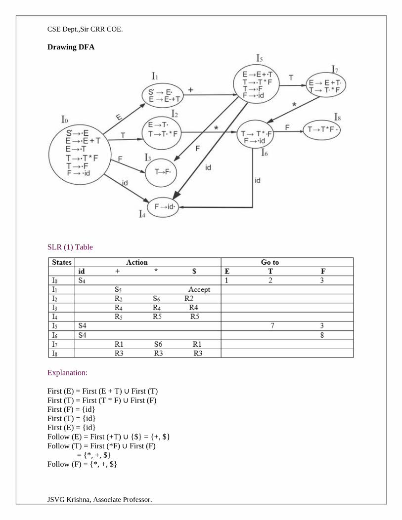
CSE Dept.,Sir CRR COE.
JSVG Krishna, Associate Professor.
Drawing DFA
SLR (1) Table
Explanation:
First (E) = First (E + T) ∪ First (T)
First (T) = First (T * F) ∪ First (F)
First (F) = {id}
First (T) = {id}
First (E) = {id}
Follow (E) = First (+T) ∪ {$} = {+, $}
Follow (T) = First (*F) ∪ First (F)
= {*, +, $}
Follow (F) = {*, +, $}
CSE Dept.,Sir CRR COE.
JSVG Krishna, Associate Professor.
1) I1 contains the final item which drives S → E• and follow (S) = {$}, so action {I1, $} = Accept
2) I2 contains the final item which drives E → T• and follow (E) = {+, $}, so action {I2, +} = R2,
action {I2, $} = R2
3) I3 contains the final item which drives T → F• and follow (T) = {+, *, $}, so action {I3, +} =
R4, action {I3, *} = R4, action {I3, $} = R4
4) I4 contains the final item which drives F → id• and follow (F) = {+, *, $}, so action {I4, +} =
R5, action {I4, *} = R5, action {I4, $} = R5
5) I7 contains the final item which drives E → E + T• and follow (E) = {+, $}, so action {I7, +} =
R1, action {I7, $} = R1
6) I8 contains the final item which drives T → T * F• and follow (T) = {+, *, $}, so action {I8, +}
= R3, action {I8, *} = R3, action {I8, $} = R3.
- 27 -

CSE Dept.,Sir CRR COE.
JSVG Krishna, Associate Professor.
LECTURE NOTES
ON
COMPILER DESIGN
2020 – 2021
III B. Tech I Semester (JNTUK-R16)
P.Naga Deepthi/ Mr J.S.V. Gopala Krishna
Department of Computer Science and Engineering
SIR CRREDDY COLLEGE OF ENGINEERING,
ELURU
- 21 -
CSE Dept.,Sir CRR COE.
JSVG Krishna, Associate Professor.
UNIT –III
More Powerful LR parser (LR1,LALR) Using Armigers Grammars Equal Recovery in Lr parser
Syntax Directed Transactions Definition, Evolution order of SDTS Application of SDTS. Syntax
Directed Translation Schemes.
UNIT -3
3.1 CANONICAL LR PARSING
CLR refers to canonical lookahead. CLR parsing use the canonical collection of LR (1) items to build
the CLR (1) parsing table. CLR (1) parsing table produces the more number of states as compare to the
SLR (1) parsing.
In the CLR (1), we place the reduce node only in the lookahead symbols.
Various steps involved in the CLR (1) Parsing:
1) For the given input string write a context free grammar
2) Check the ambiguity of the grammar
3) Add Augment production in the given grammar
4) Create Canonical collection of LR (0) items
5) Draw a data flow diagram (DFA)
6) Construct a CLR (1) parsing table
In the SLR method we were working with LR(0)) items. In CLR parsing we will be using LR(1)
items. LR(k) item is defined to be an item using lookaheads of length k. So ,the LR(1) item is
comprised of two parts : the LR(0) item and the lookahead associated with the item. The look ahead
is used to determine that where we place the final item. The look ahead always add $ symbol for the
argument production.
LR(1) parsers are more powerful parser.
for LR(1) items we modify the Closure and GOTO function.
Closure Operation
Closure(I)
repeat
for (each item [ A -> ?.B?, a ] in I )
for (each production B -> ? in G’)
for (each terminal b in FIRST(?a))
add [ B -> .? , b ] to set I;
until no more items are added to I;
return I;
CSE Dept.,Sir CRR COE.
JSVG Krishna, Associate Professor.
Goto Operation
Goto(I, X)
Initialise J to be the empty set;
for ( each item A -> ?.X?, a ] in I )
Add item A -> ?X.?, a ] to se J; /* move the dot one step */
return Closure(J); /* apply closure to the set */
LR(1) items
Void items(G’)
Initialise C to { closure ({[S’ -> .S, $]})};
Repeat
For (each set of items I in C)
For (each grammar symbol X)
if( GOTO(I, X) is not empty and not in C)
Add GOTO(I, X) to C;
Until no new set of items are added to C;
3.2 ALGORITHM FOR CONSTRUCTION OF THE CANONICAL LR PARSING
TABLE
Input: grammar G' Output: canonical LR parsing table functions action and goto
1. Construct C = {I0, I1 , ..., In} the collection of sets of LR(1) items for G'.State i is constructed from Ii.
2. if [A -> a.ab, b>] is in Ii and goto(Ii, a) = Ij, then set action[i, a] to "shift j". Here a must be a terminal.
3. if [A -> a., a] is in Ii, then set action[i, a] to "reduce A -> a" for all a in FOLLOW(A). Here A may not be S'.
4. if [S' -> S.] is in Ii, then set action[i, $] to "accept" 5. If any conflicting actions are generated by these rules, the grammar is not
LR(1) and the algorithm fails to produce a parser. 6. The goto transitions for state i are constructed for all nonterminals A using the
rule: If goto(Ii, A)= Ij, then goto[i, A] = j. 7. All entries not defined by rules 2 and 3 are made "error".
8. The inital state of the parser is the one constructed from the set of items
containing [S' -> .S, $].
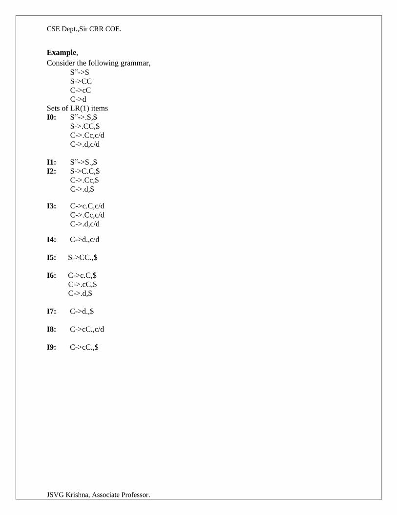
CSE Dept.,Sir CRR COE.
JSVG Krishna, Associate Professor.
Example,
Consider the following grammar,
S‟->S
S->CC
C->cC
C->d
Sets of LR(1) items
I0: S‟->.S,$ S->.CC,$
C->.Cc,c/d
C->.d,c/d
I1: S‟->S.,$
I2: S->C.C,$
C->.Cc,$
C->.d,$
I3: C->c.C,c/d
C->.Cc,c/d
C->.d,c/d
I4: C->d.,c/d
I5: S->CC.,$
I6: C->c.C,$
C->.cC,$
C->.d,$
I7: C->d.,$
I8: C->cC.,c/d
I9: C->cC.,$
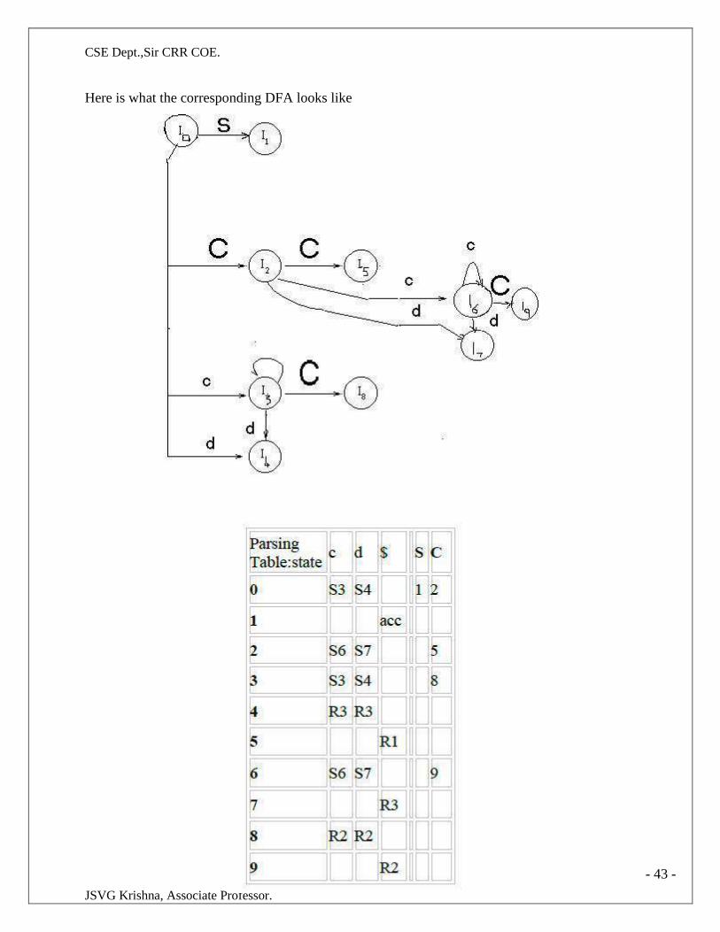
CSE Dept.,Sir CRR COE.
JSVG Krishna, Associate Professor.
Here is what the corresponding DFA looks like
- 43 -
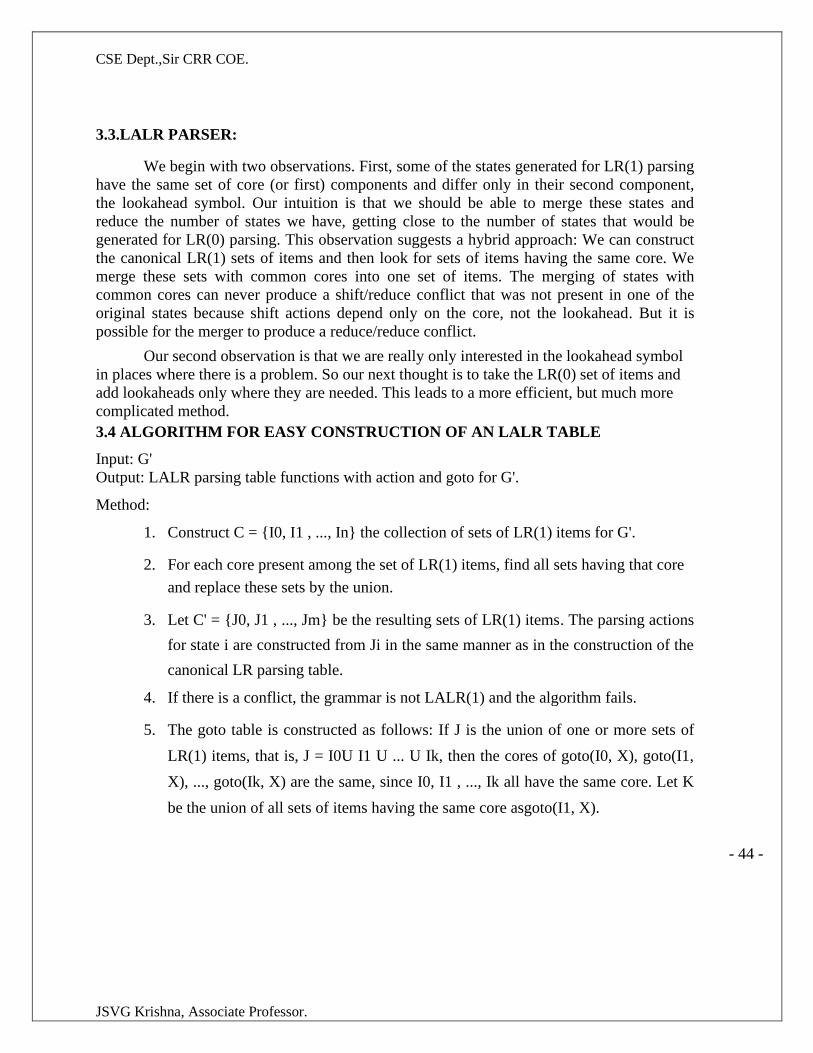
CSE Dept.,Sir CRR COE.
JSVG Krishna, Associate Professor.
3.3.LALR PARSER:
We begin with two observations. First, some of the states generated for LR(1) parsing
have the same set of core (or first) components and differ only in their second component,
the lookahead symbol. Our intuition is that we should be able to merge these states and
reduce the number of states we have, getting close to the number of states that would be
generated for LR(0) parsing. This observation suggests a hybrid approach: We can construct
the canonical LR(1) sets of items and then look for sets of items having the same core. We
merge these sets with common cores into one set of items. The merging of states with
common cores can never produce a shift/reduce conflict that was not present in one of the
original states because shift actions depend only on the core, not the lookahead. But it is
possible for the merger to produce a reduce/reduce conflict.
Our second observation is that we are really only interested in the lookahead symbol
in places where there is a problem. So our next thought is to take the LR(0) set of items and
add lookaheads only where they are needed. This leads to a more efficient, but much more
complicated method.
3.4 ALGORITHM FOR EASY CONSTRUCTION OF AN LALR TABLE
Input: G'
Output: LALR parsing table functions with action and goto for G'.
Method:
1. Construct C = {I0, I1 , ..., In} the collection of sets of LR(1) items for G'.
2. For each core present among the set of LR(1) items, find all sets having that core
and replace these sets by the union.
3. Let C' = {J0, J1 , ..., Jm} be the resulting sets of LR(1) items. The parsing actions
for state i are constructed from Ji in the same manner as in the construction of the
canonical LR parsing table.
4. If there is a conflict, the grammar is not LALR(1) and the algorithm fails.
5. The goto table is constructed as follows: If J is the union of one or more sets of
LR(1) items, that is, J = I0U I1 U ... U Ik, then the cores of goto(I0, X), goto(I1,
X), ..., goto(Ik, X) are the same, since I0, I1 , ..., Ik all have the same core. Let K
be the union of all sets of items having the same core asgoto(I1, X).
- 44 -
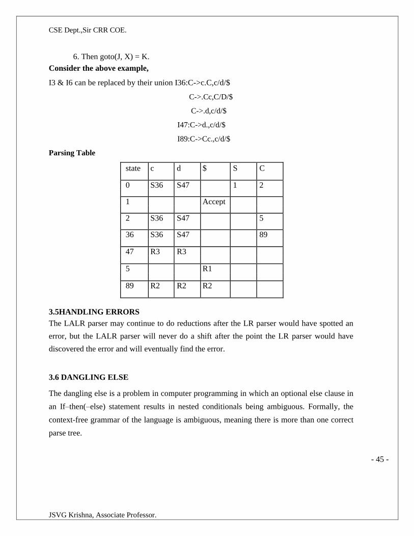
CSE Dept.,Sir CRR COE.
JSVG Krishna, Associate Professor.
6. Then goto(J, X) = K.
Consider the above example, I3 & I6 can be replaced by their union I36:C->c.C,c/d/$ C->.Cc,C/D/$
C->.d,c/d/$
I47:C->d.,c/d/$
I89:C->Cc.,c/d/$
Parsing Table
state c d $ S C
0 S36 S47 1 2
1 Accept
2 S36 S47 5
36 S36 S47 89
47 R3 R3
5 R1
89 R2 R2 R2
3.5HANDLING ERRORS
The LALR parser may continue to do reductions after the LR parser would have spotted an
error, but the LALR parser will never do a shift after the point the LR parser would have
discovered the error and will eventually find the error.
3.6 DANGLING ELSE
The dangling else is a problem in computer programming in which an optional else clause in
an If–then(–else) statement results in nested conditionals being ambiguous. Formally, the
context-free grammar of the language is ambiguous, meaning there is more than one correct
parse tree.
- 45 -
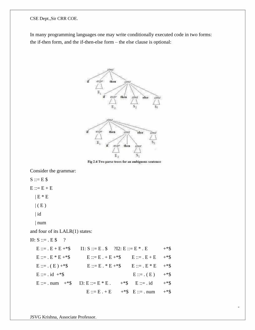
CSE Dept.,Sir CRR COE.
JSVG Krishna, Associate Professor.
In many programming languages one may write conditionally executed code in two forms:
the if-then form, and the if-then-else form – the else clause is optional:
Consider the grammar:
S ::= E $
E ::= E + E
| E * E
| ( E )
| id
| num
and four of its LALR(1) states:
I0: S ::= . E $ ?
E ::= . E + E +*$ I1: S ::= E . $ ?I2: E ::= E * . E +*$
E ::= . E * E +*$ E ::= E . + E +*$ E ::= . E + E +*$
E ::= . ( E ) +*$ E ::= E . * E +*$ E ::= . E * E +*$
E ::= . id +*$ E ::= . ( E ) +*$
E ::= . num +*$ I3: E ::= E * E . +*$ E ::= . id +*$
E ::= E . + E +*$ E ::= . num +*$
-
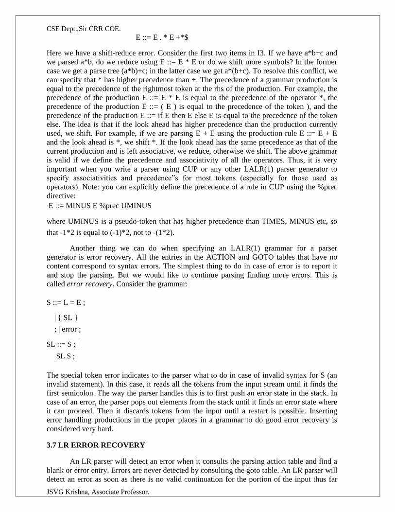
CSE Dept.,Sir CRR COE.
JSVG Krishna, Associate Professor.
E ::= E . * E +*$
Here we have a shift-reduce error. Consider the first two items in I3. If we have a*b+c and
we parsed a*b, do we reduce using E ::= E * E or do we shift more symbols? In the former
case we get a parse tree (a*b)+c; in the latter case we get a*(b+c). To resolve this conflict, we
can specify that * has higher precedence than +. The precedence of a grammar production is
equal to the precedence of the rightmost token at the rhs of the production. For example, the
precedence of the production E ::= E * E is equal to the precedence of the operator *, the
precedence of the production E ::= ( E ) is equal to the precedence of the token ), and the
precedence of the production E ::= if E then E else E is equal to the precedence of the token
else. The idea is that if the look ahead has higher precedence than the production currently
used, we shift. For example, if we are parsing E + E using the production rule E ::= E + E
and the look ahead is *, we shift *. If the look ahead has the same precedence as that of the
current production and is left associative, we reduce, otherwise we shift. The above grammar
is valid if we define the precedence and associativity of all the operators. Thus, it is very
important when you write a parser using CUP or any other LALR(1) parser generator to
specify associativities and precedence‟s for most tokens (especially for those used as
operators). Note: you can explicitly define the precedence of a rule in CUP using the %prec
directive:
E ::= MINUS E %prec UMINUS
where UMINUS is a pseudo-token that has higher precedence than TIMES, MINUS etc, so
that -1*2 is equal to (-1)*2, not to -(1*2).
Another thing we can do when specifying an LALR(1) grammar for a parser
generator is error recovery. All the entries in the ACTION and GOTO tables that have no
content correspond to syntax errors. The simplest thing to do in case of error is to report it
and stop the parsing. But we would like to continue parsing finding more errors. This is
called error recovery. Consider the grammar:
S ::= L = E ;
| { SL }
; | error ;
SL ::= S ; |
SL S ;
The special token error indicates to the parser what to do in case of invalid syntax for S (an
invalid statement). In this case, it reads all the tokens from the input stream until it finds the
first semicolon. The way the parser handles this is to first push an error state in the stack. In
case of an error, the parser pops out elements from the stack until it finds an error state where
it can proceed. Then it discards tokens from the input until a restart is possible. Inserting
error handling productions in the proper places in a grammar to do good error recovery is
considered very hard.
3.7 LR ERROR RECOVERY
An LR parser will detect an error when it consults the parsing action table and find a
blank or error entry. Errors are never detected by consulting the goto table. An LR parser will
detect an error as soon as there is no valid continuation for the portion of the input thus far
CSE Dept.,Sir CRR COE.
JSVG Krishna, Associate Professor.
scanned. A canonical LR parser will not make even a single reduction before announcing the
error. SLR and LALR parsers may make several reductions before detecting an error, but
they will never shift an erroneous input symbol onto the stack.
3.7.1 PANIC-MODE ERROR RECOVERY
We can implement panic-mode error recovery by scanning down the stack until a
state s with a goto on a particular nonterminal A is found. Zero or more input symbols are
then discarded until a symbol a is found that can legitimately follow A. The parser then
stacks the state GOTO(s, A) and resumes normal parsing. The situation might exist where
there is more than one choice for the nonterminal A. Normally these would be nonterminals
representing major program pieces, e.g. an expression, a statement, or a block. For example,
if A is the nonterminal stmt, a might be semicolon or }, which marks the end of a statement
sequence. This method of error recovery attempts to eliminate the phrase containing the
syntactic error. The parser determines that a string derivable from A contains an error. Part of
that string has already been processed, and the result of this processing is a sequence of states
on top of the stack. The remainder of the string is still in the input, and the parser attempts to
skip over the remainder of this string by looking for a symbol on the input that can
legitimately follow A. By removing states from the stack, skipping over the input, and
pushing GOTO(s, A) on the stack, the parser pretends that if has found an instance of A and
resumes normal parsing.
3.7.2 PHRASE-LEVEL RECOVERY
Phrase-level recovery is implemented by examining each error entry in the LR action
table and deciding on the basis of language usage the most likely programmer error that
would give rise to that error. An appropriate recovery procedure can then be constructed;
presumably the top of the stack and/or first input symbol would be modified in a way deemed
appropriate for each error entry. In designing specific error-handling routines for an LR
parser, we can fill in each blank entry in the action field with a pointer to an error routine that
will take the appropriate action selected by the compiler designer.
The actions may include insertion or deletion of symbols from the stack or the input
or both, or alteration and transposition of input symbols. We must make our choices so that
the LR parser will not get into an infinite loop. A safe strategy will assure that at least one
input symbol will be removed or shifted eventually, or that the stack will eventually shrink if
the end of the input has been reached. Popping a stack state that covers a non terminal should
be avoided, because this modification eliminates from the stack a construct that has already
been successfully parsed. Syntax Directed Translations
We associate information with a language construct by attaching attributes to the grammar symbol(s)
representing the construct, A syntax-directed definition specifies the values of attributes by associating
semantic rules with the grammar productions. For example, an infix-to-postfix translator might have a
production and rule
CSE Dept.,Sir CRR COE.
JSVG Krishna, Associate Professor.
This production has two nonterminals, E and T; the subscript in E1 distinguishes the occurrence of E in
the production body from the occurrence of E as the head. Both E and T have a string-valued attribute
code. The semantic rule specifies that the string E.code is formed by concatenating Ei.code, T.code, and
the character '+'. While the rule makes it explicit that the translation of E is built up from the translations
of E1, T, and '+', it may be inefficient to implement the translation directly by manipulating strings.
a syntax-directed translation scheme embeds program fragments called semantic actions within
production bodies
There are two notations for attaching semantic rules:
1. Syntax Directed Definitions. High-level specification hiding many implementation
details (also called Attribute Grammars). 2. Translation Schemes. More implementation oriented: Indicate the order in which
semantic rules are to be evaluated.
Syntax Directed Definitions
Syntax Directed Definitions are a generalization of context-free grammars in which:
1. Grammar symbols have an associated set of Attributes; 2. Productions are associated with Semantic Rules for computing the values of attributes
Such formalism generates Annotated Parse-Trees where each node of the tree is a
record with a field for each attribute (e.g.,X.a indicates the attribute a of the grammar
symbol X).
The value of an attribute of a grammar symbol at a given parse-tree node is defined by a semantic rule associated with the production used at that node.
We distinguish between two kinds of attributes:
1. Synthesized Attributes. They are computed from the values of the attributes of the
children nodes. 2. Inherited Attributes. They are computed from the values of the attributes of both the
siblings and the parent nodes
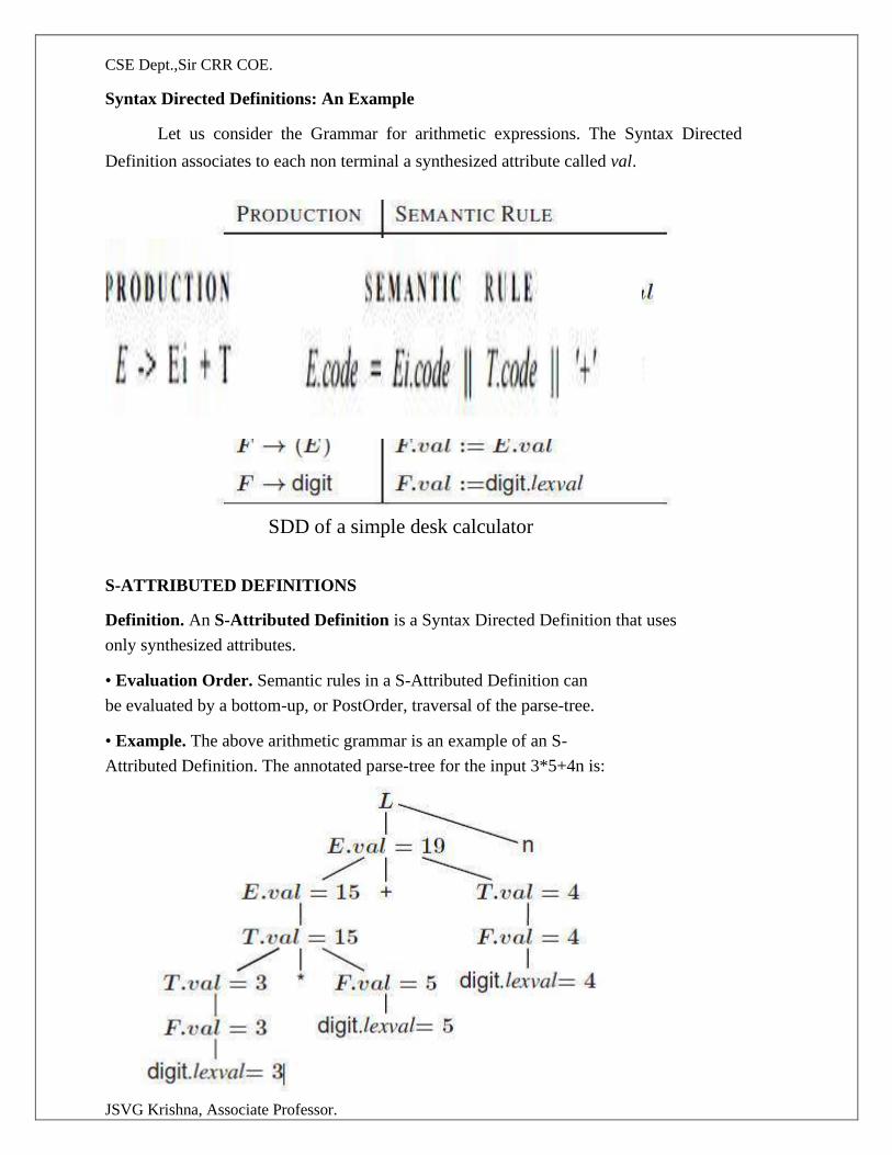
CSE Dept.,Sir CRR COE.
JSVG Krishna, Associate Professor.
Syntax Directed Definitions: An Example
Let us consider the Grammar for arithmetic expressions. The Syntax Directed
Definition associates to each non terminal a synthesized attribute called val.
SDD of a simple desk calculator
S-ATTRIBUTED DEFINITIONS
Definition. An S-Attributed Definition is a Syntax Directed Definition that uses
only synthesized attributes.
• Evaluation Order. Semantic rules in a S-Attributed Definition can
be evaluated by a bottom-up, or PostOrder, traversal of the parse-tree. • Example. The above arithmetic grammar is an example of an S-
Attributed Definition. The annotated parse-tree for the input 3*5+4n is:
CSE Dept.,Sir CRR COE.
JSVG Krishna, Associate Professor.
L-attributed definition Definition: A SDD its L-attributed if each inherited attribute of Xi in the RHS of A ! X1 : :Xn depends only on 1. attributes of X1;X2; : : : ;Xi 1 (symbols to the left of Xi in the RHS)
2. inherited attributes of A. Restrictions for translation schemes:
1. Inherited attribute of Xi must be computed by an action before Xi. 2. An action must not refer to synthesized attribute of any symbol to the right of that action.
3. Synthesized attribute for A can only be computed after all attributes it references have
been completed (usually at end of RHS). Evaluation order of SDTS
1 Dependency Graphs
2 Ordering the Evaluation of Attributes
3 S-Attributed Definitions
4 L-Attributed Definitions
"Dependency graphs" are a useful tool for determining an evaluation order for the attribute
instances in a given parse tree. While an annotated parse tree shows the values of attributes, a dependency graph helps us determine how those values can be computed.
1 Dependency Graphs
A dependency graph depicts the flow of information among the attribute in-stances in a particular parse tree; an edge from one attribute instance to an-other means that the value of the first is needed to compute the second. Edges express constraints implied by the semantic rules. In more detail:
Suppose that a semantic rule associated with a production p defines the value of inherited
attribute B.c in terms of the value of X.a. Then, the dependency graph has an edge from X.a to B.c. For each node N labeled B that corresponds to an occurrence of this B in the body of production p, create an edge to attribute c at N from the attribute a at the node M that corresponds to this occurrence of X. Note that M could be either the parent or a sibling of N.
Since a node N can have several children labeled X, we again assume that subscripts distinguish among uses of the same symbol at different places in the production.
Example: Consider the following production and rule:
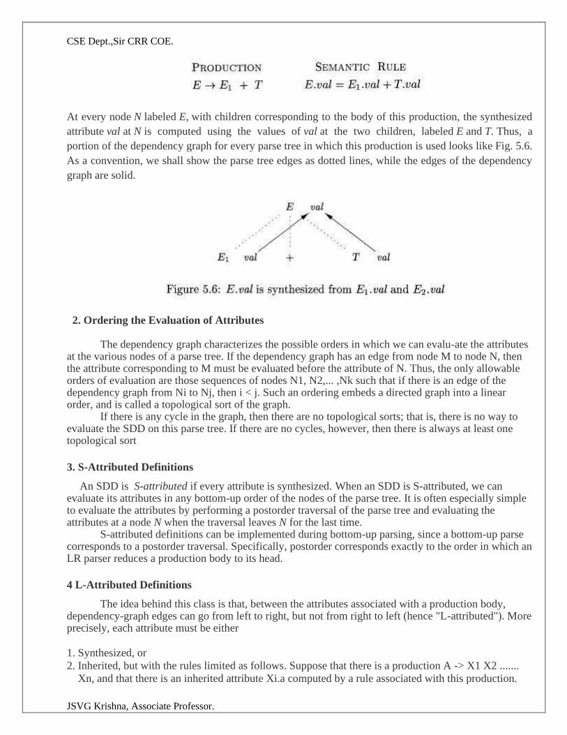
CSE Dept.,Sir CRR COE.
JSVG Krishna, Associate Professor.
At every node N labeled E, with children corresponding to the body of this production, the synthesized
attribute val at N is computed using the values of val at the two children, labeled E and T. Thus, a
portion of the dependency graph for every parse tree in which this production is used looks like Fig. 5.6.
As a convention, we shall show the parse tree edges as dotted lines, while the edges of the dependency
graph are solid.
2. Ordering the Evaluation of Attributes
The dependency graph characterizes the possible orders in which we can evalu-ate the attributes at the various nodes of a parse tree. If the dependency graph has an edge from node M to node N, then the attribute corresponding to M must be evaluated before the attribute of N. Thus, the only allowable orders of evaluation are those sequences of nodes N1, N2,... ,Nk such that if there is an edge of the dependency graph from Ni to Nj, then i < j. Such an ordering embeds a directed graph into a linear order, and is called a topological sort of the graph.
If there is any cycle in the graph, then there are no topological sorts; that is, there is no way to evaluate the SDD on this parse tree. If there are no cycles, however, then there is always at least one topological sort
3. S-Attributed Definitions
An SDD is S-attributed if every attribute is synthesized. When an SDD is S-attributed, we can evaluate its attributes in any bottom-up order of the nodes of the parse tree. It is often especially simple to evaluate the attributes by performing a postorder traversal of the parse tree and evaluating the attributes at a node N when the traversal leaves N for the last time.
S-attributed definitions can be implemented during bottom-up parsing, since a bottom-up parse corresponds to a postorder traversal. Specifically, postorder corresponds exactly to the order in which an LR parser reduces a production body to its head.
4 L-Attributed Definitions
The idea behind this class is that, between the attributes associated with a production body, dependency-graph edges can go from left to right, but not from right to left (hence "L-attributed"). More precisely, each attribute must be either
1. Synthesized, or 2. Inherited, but with the rules limited as follows. Suppose that there is a production A -> X1 X2 .......
Xn, and that there is an inherited attribute Xi.a computed by a rule associated with this production.
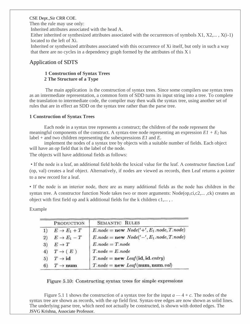
CSE Dept.,Sir CRR COE.
JSVG Krishna, Associate Professor.
Then the rule may use only: Inherited attributes associated with the head A. Either inherited or synthesized attributes associated with the occurrences of symbols X1, X2,... , X(i-1)
located to the left of Xi. Inherited or synthesized attributes associated with this occurrence of Xi itself, but only in such a way
that there are no cycles in a dependency graph formed by the attributes of this X i Application of SDTS 1 Construction of Syntax Trees 2 The Structure of a Type
The main application is the construction of syntax trees. Since some compilers use syntax trees as an intermediate representation, a common form of SDD turns its input string into a tree. To complete the translation to intermediate code, the compiler may then walk the syntax tree, using another set of rules that are in effect an SDD on the syntax tree rather than the parse tree. 1 Construction of Syntax Trees
Each node in a syntax tree represents a construct; the children of the node represent the meaningful components of the construct. A syntax-tree node representing an expression E1 + E2 has label + and two children representing the subexpressions E1 and E2 implement the nodes of a syntax tree by objects with a suitable number of fields. Each object will have an op field that is the label of the node.
The objects will have additional fields as follows:
• If the node is a leaf, an additional field holds the lexical value for the leaf. A constructor function Leaf
(op, val) creates a leaf object. Alternatively, if nodes are viewed as records, then Leaf returns a pointer
to a new record for a leaf.
• If the node is an interior node, there are as many additional fields as the node has children in the
syntax tree. A constructor function Node takes two or more arguments: Node(op,ci,c2,... ,ck) creates an
object with first field op and k additional fields for the k children c1,... , .
Example
Figure 5.1 1 shows the construction of a syntax tree for the input a — 4 + c. The nodes of the syntax tree are shown as records, with the op field first. Syntax-tree edges are now shown as solid lines. The underlying parse tree, which need not actually be constructed, is shown with dotted edges. The
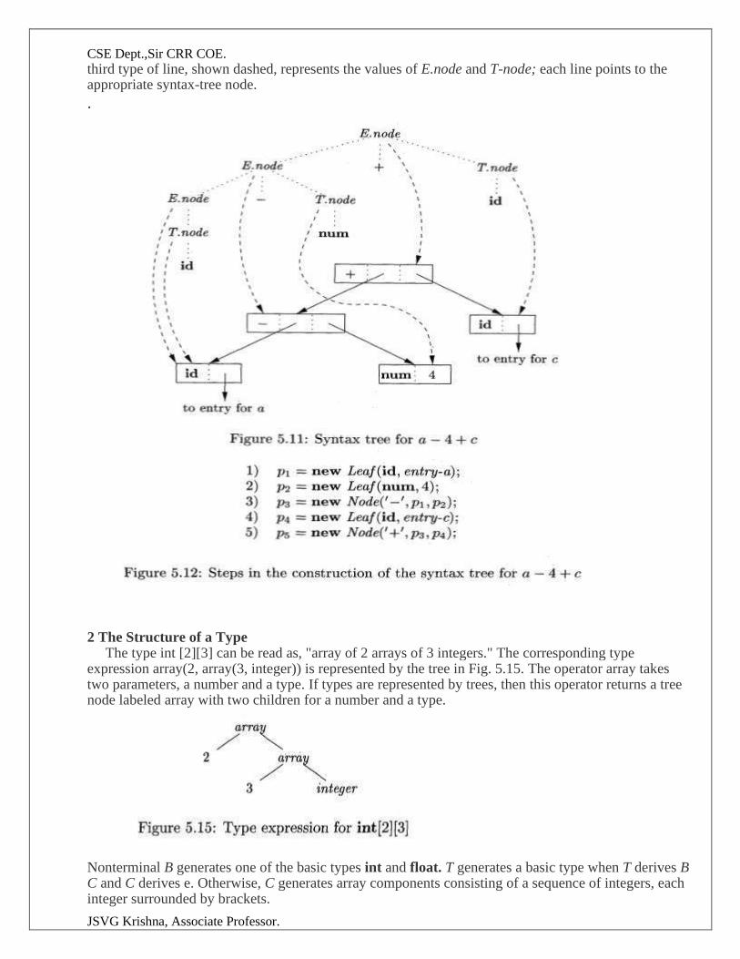
CSE Dept.,Sir CRR COE.
JSVG Krishna, Associate Professor.
third type of line, shown dashed, represents the values of E.node and T-node; each line points to the appropriate syntax-tree node.
.
2 The Structure of a Type The type int [2][3] can be read as, "array of 2 arrays of 3 integers." The corresponding type expression array(2, array(3, integer)) is represented by the tree in Fig. 5.15. The operator array takes two parameters, a number and a type. If types are represented by trees, then this operator returns a tree node labeled array with two children for a number and a type.
Nonterminal B generates one of the basic types int and float. T generates a basic type when T derives B C and C derives e. Otherwise, C generates array components consisting of a sequence of integers, each integer surrounded by brackets.
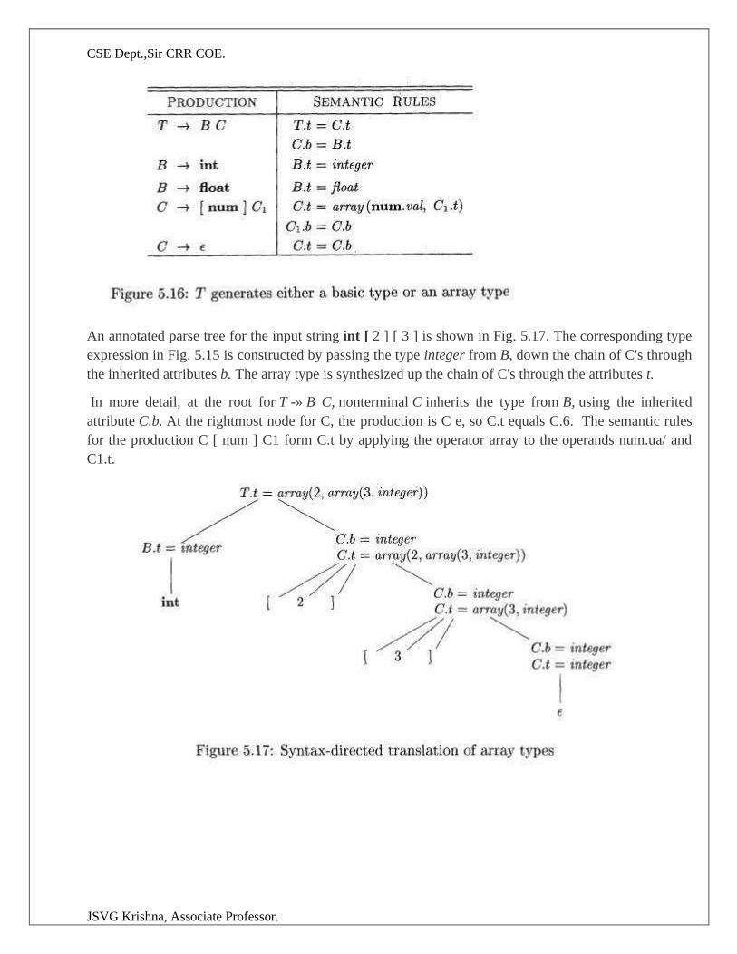
CSE Dept.,Sir CRR COE.
JSVG Krishna, Associate Professor.
An annotated parse tree for the input string int [ 2 ] [ 3 ] is shown in Fig. 5.17. The corresponding type
expression in Fig. 5.15 is constructed by passing the type integer from B, down the chain of C's through
the inherited attributes b. The array type is synthesized up the chain of C's through the attributes t.
In more detail, at the root for T -» B C, nonterminal C inherits the type from B, using the inherited
attribute C.b. At the rightmost node for C, the production is C e, so C.t equals C.6. The semantic rules
for the production C [ num ] C1 form C.t by applying the operator array to the operands num.ua/ and
C1.t.
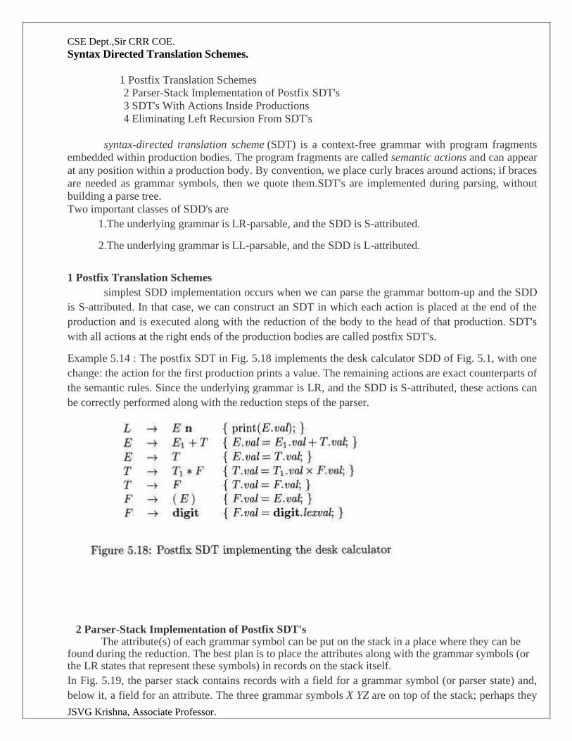
CSE Dept.,Sir CRR COE.
JSVG Krishna, Associate Professor.
Syntax Directed Translation Schemes.
1 Postfix Translation Schemes 2 Parser-Stack Implementation of Postfix SDT's 3 SDT's With Actions Inside Productions 4 Eliminating Left Recursion From SDT's
syntax-directed translation scheme (SDT) is a context-free grammar with program fragments
embedded within production bodies. The program fragments are called semantic actions and can appear
at any position within a production body. By convention, we place curly braces around actions; if braces
are needed as grammar symbols, then we quote them.SDT's are implemented during parsing, without
building a parse tree.
Two important classes of SDD's are
1.The underlying grammar is LR-parsable, and the SDD is S-attributed.
2.The underlying grammar is LL-parsable, and the SDD is L-attributed.
1 Postfix Translation Schemes
simplest SDD implementation occurs when we can parse the grammar bottom-up and the SDD
is S-attributed. In that case, we can construct an SDT in which each action is placed at the end of the
production and is executed along with the reduction of the body to the head of that production. SDT's
with all actions at the right ends of the production bodies are called postfix SDT's.
Example 5.14 : The postfix SDT in Fig. 5.18 implements the desk calculator SDD of Fig. 5.1, with one
change: the action for the first production prints a value. The remaining actions are exact counterparts of
the semantic rules. Since the underlying grammar is LR, and the SDD is S-attributed, these actions can
be correctly performed along with the reduction steps of the parser.
2 Parser-Stack Implementation of Postfix SDT's
The attribute(s) of each grammar symbol can be put on the stack in a place where they can be found during the reduction. The best plan is to place the attributes along with the grammar symbols (or the LR states that represent these symbols) in records on the stack itself.
In Fig. 5.19, the parser stack contains records with a field for a grammar symbol (or parser state) and,
below it, a field for an attribute. The three grammar symbols X YZ are on top of the stack; perhaps they
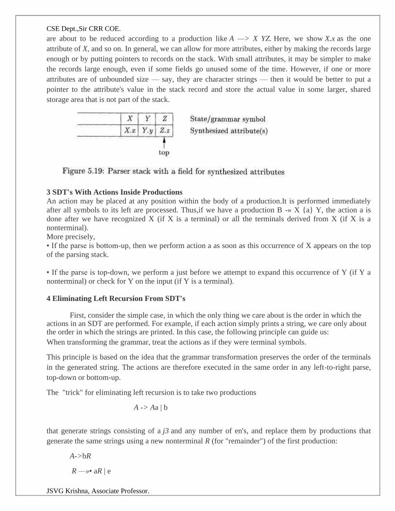
CSE Dept.,Sir CRR COE.
JSVG Krishna, Associate Professor.
are about to be reduced according to a production like A —> X YZ. Here, we show X.x as the one
attribute of X, and so on. In general, we can allow for more attributes, either by making the records large
enough or by putting pointers to records on the stack. With small attributes, it may be simpler to make
the records large enough, even if some fields go unused some of the time. However, if one or more
attributes are of unbounded size — say, they are character strings — then it would be better to put a
pointer to the attribute's value in the stack record and store the actual value in some larger, shared
storage area that is not part of the stack.
3 SDT's With Actions Inside Productions An action may be placed at any position within the body of a production.It is performed immediately
after all symbols to its left are processed. Thus,if we have a production B -» X {a} Y, the action a is
done after we have recognized X (if X is a terminal) or all the terminals derived from X (if X is a
nonterminal).
More precisely, • If the parse is bottom-up, then we perform action a as soon as this occurrence of X appears on the top
of the parsing stack. • If the parse is top-down, we perform a just before we attempt to expand this occurrence of Y (if Y a
nonterminal) or check for Y on the input (if Y is a terminal).
4 Eliminating Left Recursion From SDT's
First, consider the simple case, in which the only thing we care about is the order in which the actions in an SDT are performed. For example, if each action simply prints a string, we care only about the order in which the strings are printed. In this case, the following principle can guide us:
When transforming the grammar, treat the actions as if they were terminal symbols.
This principle is based on the idea that the grammar transformation preserves the order of the terminals
in the generated string. The actions are therefore executed in the same order in any left-to-right parse,
top-down or bottom-up.
The "trick" for eliminating left recursion is to take two productions
A -> Aa | b
that generate strings consisting of a j3 and any number of en's, and replace them by productions that
generate the same strings using a new nonterminal R (for "remainder") of the first production:
A->bR
R —»• aR | e
CSE Dept.,Sir CRR COE.
JSVG Krishna, Associate Professor.
If (3 does not begin with A, then A no longer has a left-recursive production. In regular-definition terms,
with both sets of productions, A is defined by 0(a)*.
Example 5 . 1 7 : Consider the following E-productions from an SDT for translating infix expressions
into postfix notation:
E -> E i + T { print('+'); }
E -> T
If we apply the standard transformation to E, the remainder of the left-recursive production is
a = + T { print('-r'); }
and the body of the other production is T. If we introduce R for the remainder of E, we get the set of
productions:
E --> T R
R --> + T { printC-h'); } R
R -> e
When the actions of an SDD compute attributes rather than merely printing output, we must be more
careful about how we eliminate left recursion from a grammar. However, if the SDD is S-attributed,
then we can always construct an SDT by placing attribute-computing actions at appropriate positions in
the new productions.
CSE Dept.,Sir CRR COE.
JSVG Krishna, Associate Professor.
LECTURE NOTES
ON
COMPILER DESIGN
2020 – 2021
III B. Tech I Semester (JNTUK-R16)
P.Naga Deepthi/ Mr J.S.V. Gopala Krishna
Department of Computer Science and Engineering
SIR CRREDDY COLLEGE OF ENGINEERING,
ELURU
- 21 -
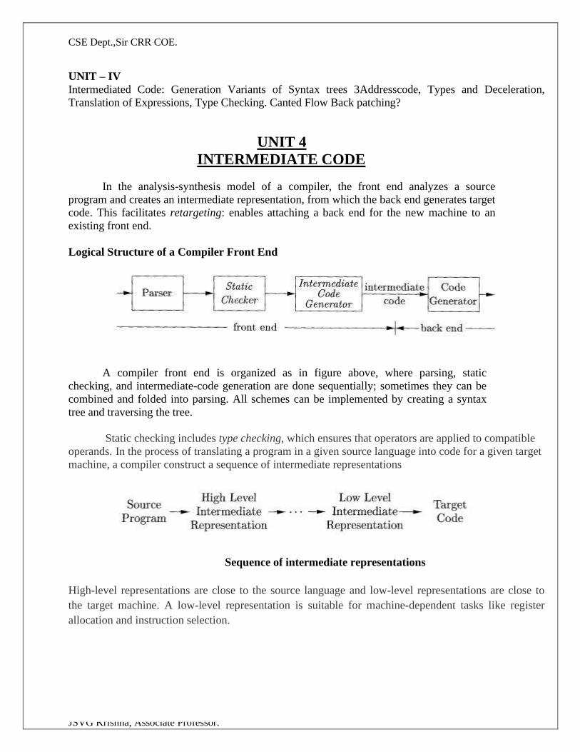
CSE Dept.,Sir CRR COE.
JSVG Krishna, Associate Professor.
UNIT – IV
Intermediated Code: Generation Variants of Syntax trees 3Addresscode, Types and Deceleration,
Translation of Expressions, Type Checking. Canted Flow Back patching?
UNIT 4
INTERMEDIATE CODE
In the analysis-synthesis model of a compiler, the front end analyzes a source
program and creates an intermediate representation, from which the back end generates target
code. This facilitates retargeting: enables attaching a back end for the new machine to an
existing front end.
Logical Structure of a Compiler Front End
A compiler front end is organized as in figure above, where parsing, static
checking, and intermediate-code generation are done sequentially; sometimes they can be
combined and folded into parsing. All schemes can be implemented by creating a syntax
tree and traversing the tree.
Static checking includes type checking, which ensures that operators are applied to compatible
operands. In the process of translating a program in a given source language into code for a given target
machine, a compiler construct a sequence of intermediate representations
Sequence of intermediate representations
High-level representations are close to the source language and low-level representations are close to
the target machine. A low-level representation is suitable for machine-dependent tasks like register
allocation and instruction selection.
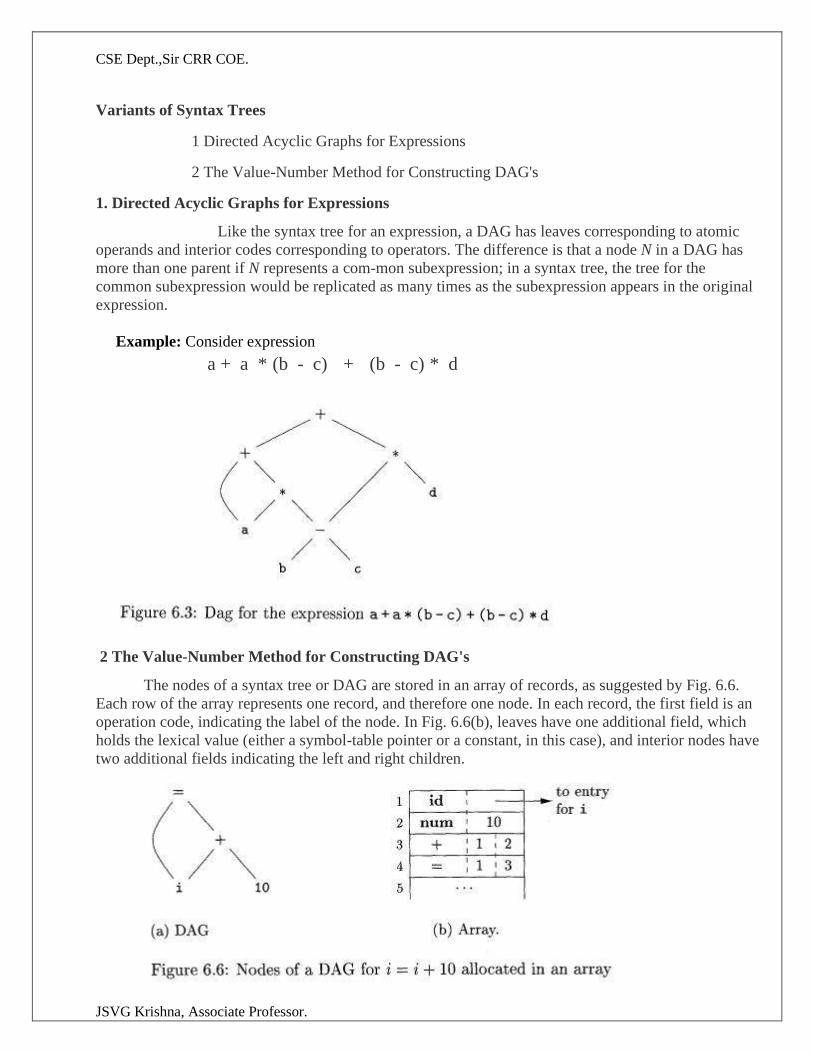
CSE Dept.,Sir CRR COE.
JSVG Krishna, Associate Professor.
Variants of Syntax Trees
1 Directed Acyclic Graphs for Expressions
2 The Value-Number Method for Constructing DAG's
1. Directed Acyclic Graphs for Expressions
Like the syntax tree for an expression, a DAG has leaves corresponding to atomic
operands and interior codes corresponding to operators. The difference is that a node N in a DAG has
more than one parent if N represents a com-mon subexpression; in a syntax tree, the tree for the
common subexpression would be replicated as many times as the subexpression appears in the original
expression.
Example: Consider expression
a + a * (b - c) + (b - c) * d
2 The Value-Number Method for Constructing DAG's
The nodes of a syntax tree or DAG are stored in an array of records, as suggested by Fig. 6.6.
Each row of the array represents one record, and therefore one node. In each record, the first field is an
operation code, indicating the label of the node. In Fig. 6.6(b), leaves have one additional field, which
holds the lexical value (either a symbol-table pointer or a constant, in this case), and interior nodes have
two additional fields indicating the left and right children.
CSE Dept.,Sir CRR COE.
JSVG Krishna, Associate Professor.
In this array, we refer to nodes by giving the integer index of the record for that node within
the array. This integer is called the value number for the node.
Algorithm:The value-number method for constructing the nodes of a DAG.
INPUT : Label op, node /, and node r.
OUTPUT : The value number of a node in the array with signature (op, l,r).
METHOD : Search the array for a node M with label op, left child I, and right child r. If there is such a
node, return the value number of M. If not, create in the array a new node N with label op,
left child I, and right child r, and return its value number.
Three-Address Code
1 Addresses and Instructions
2 Quadruples
3 Triples
In three-address code, there is at most one operator on the right side of an instruction; that is, no
built-up arithmetic expressions are permitted. Thus a source-language expression like x+y*z might be
translated into the sequence of three-address instructions
where ti and t2 are compiler-generated temporary names.
1 Addresses and Instructions
An address can be one of the following:
• A name. Source-program names to appear as addresses in three-address code. In an
implementation, a source name is replaced by a pointer to its symbol-table entry,
where all information about the name is kept. • A constant. A compiler must deal with many different types of constants and variables.
• A compiler-generated temporary. Useful in optimizing com-pilers, to create a distinct name each
time a temporary is needed. These temporaries can be combined, if possible, when registers are
allocated to variables.
common three-address instruction
1. Assignment Statement: x = y op z and x = op y
Here,x, y and z are the operands. op represents the operator.
2. Copy Statement: x = y
3. Conditional Jump: If x relop y goto X
CSE Dept.,Sir CRR COE.
JSVG Krishna, Associate Professor.
If the condition “x relop y” gets satisfied, then-
The control is sent directly to the location specified by label X.
All the statements in between are skipped.
If the condition “x relop y” fails, then-
The control is not sent to the location specified by label X.
The next statement appearing in the usual sequence is executed.
4. Unconditional Jump- goto X
On executing the statement,The control is sent directly to the location specified by label X.
All the statements in between are skipped.
5. Procedure Call- param x call p return y
Here, p is a function which takes x as a parameter and returns y.
For a procedure call p(x1, …, xn)
param x1 … param xn call p, n
6.Indexed copy instructions: x = y[i] and x[i] = y
Left: sets x to the value in the location i memory units beyond y
Right: sets the contents of the location i memory units beyond x to y
7.Address and pointer instructions:
x = &y sets the value of x to be the location (address) of y. x = *y, presumably y is a pointer or temporary whose value is a
location. The value of x is set to the contents of that location.
*x = y sets the value of the object pointed to by x to the value of y.
Data Structure
Three address code is represented as record structure with fields for operator and
operands. These records can be stored as array or linked list. Most common
implementations of three address code are Quadruples, Triples and Indirect triples.
2. Quadruples Quadruples consists of four fields in the record structure. One field to store operator op, two
fields to store operands or arguments arg1and arg2 and one field to store result res.
res = arg1 op arg2
Example: a = b + c
b is represented as arg1, c is represented as arg2, + as op and a as res.
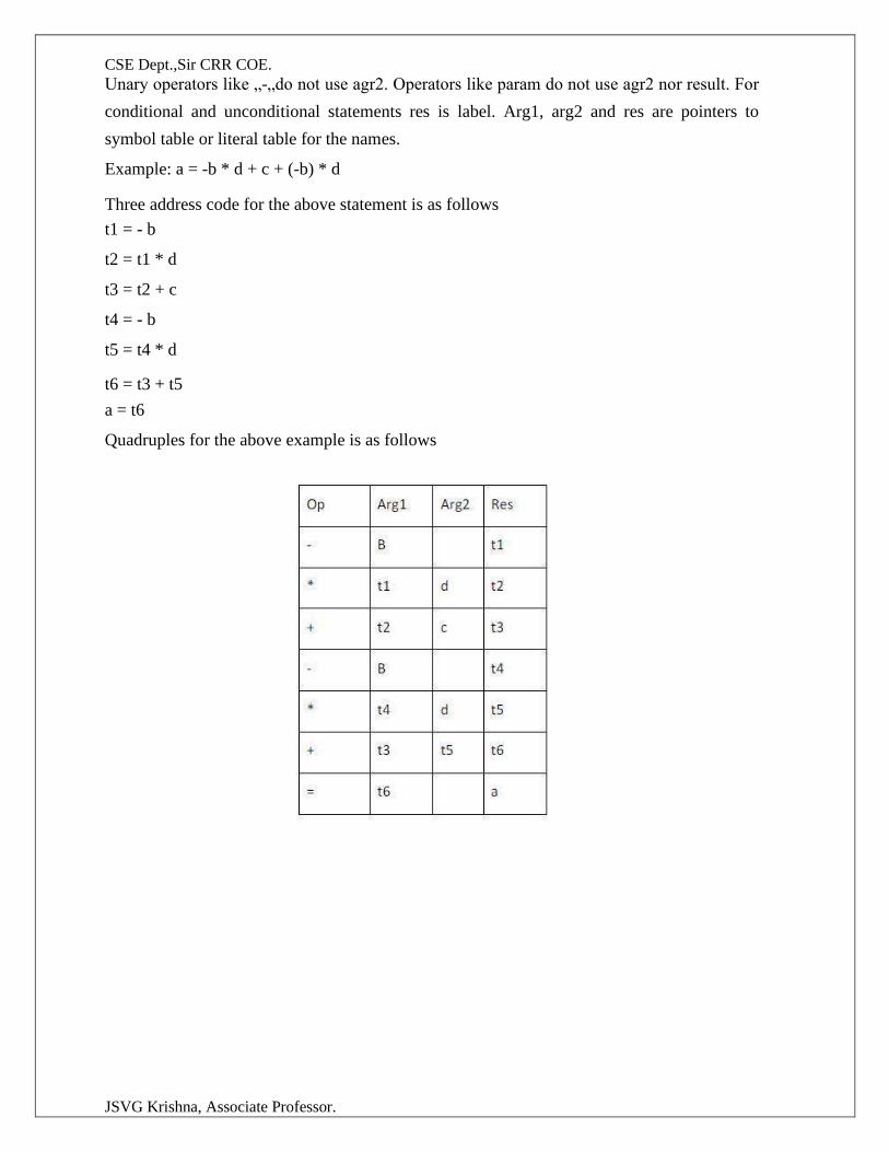
CSE Dept.,Sir CRR COE.
JSVG Krishna, Associate Professor.
Unary operators like „-„do not use agr2. Operators like param do not use agr2 nor result. For
conditional and unconditional statements res is label. Arg1, arg2 and res are pointers to
symbol table or literal table for the names.
Example: a = -b * d + c + (-b) * d
Three address code for the above statement is as follows
t1 = - b
t2 = t1 * d
t3 = t2 + c
t4 = - b
t5 = t4 * d
t6 = t3 + t5
a = t6
Quadruples for the above example is as follows
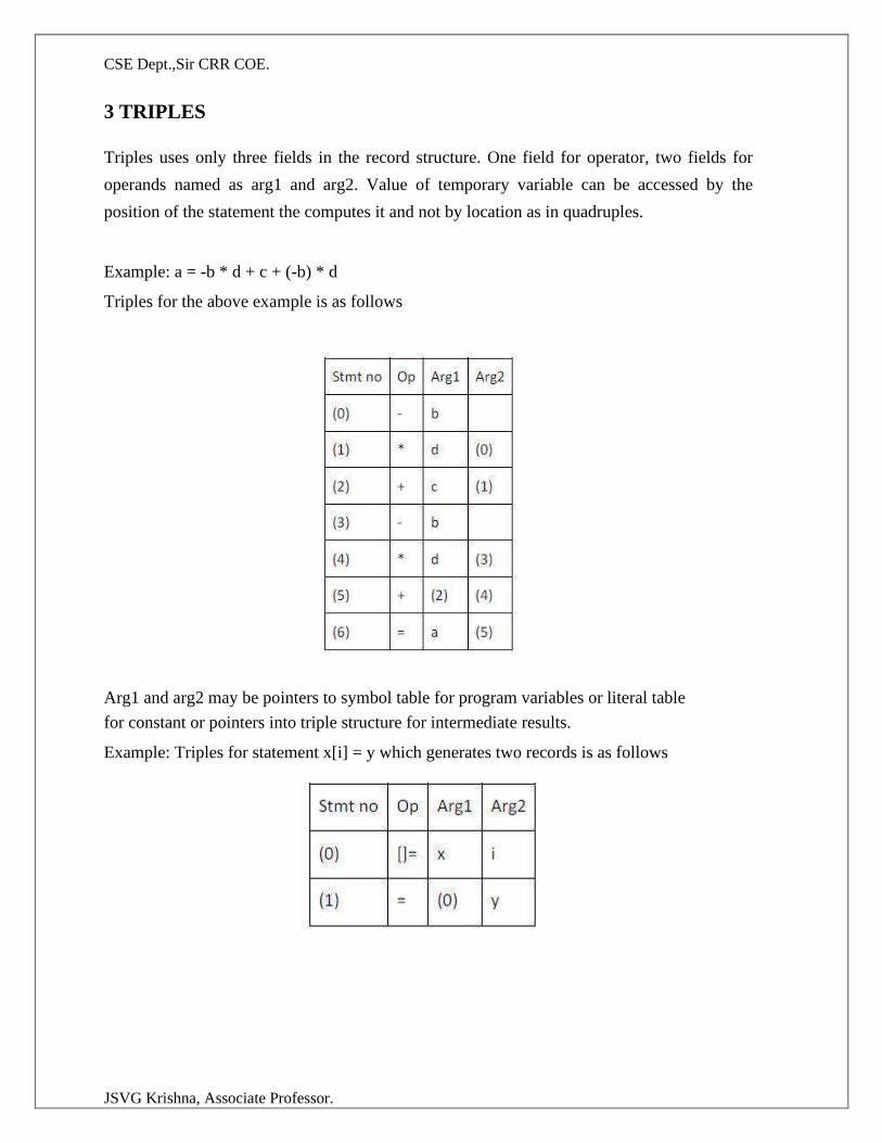
CSE Dept.,Sir CRR COE.
JSVG Krishna, Associate Professor.
3 TRIPLES
Triples uses only three fields in the record structure. One field for operator, two fields for
operands named as arg1 and arg2. Value of temporary variable can be accessed by the
position of the statement the computes it and not by location as in quadruples.
Example: a = -b * d + c + (-b) * d
Triples for the above example is as follows
Arg1 and arg2 may be pointers to symbol table for program variables or literal table
for constant or pointers into triple structure for intermediate results.
Example: Triples for statement x[i] = y which generates two records is as follows
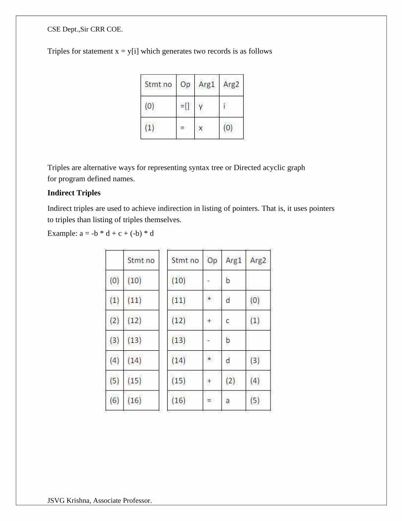
CSE Dept.,Sir CRR COE.
JSVG Krishna, Associate Professor.
Triples for statement x = y[i] which generates two records is as follows
Triples are alternative ways for representing syntax tree or Directed acyclic graph
for program defined names.
Indirect Triples
Indirect triples are used to achieve indirection in listing of pointers. That is, it uses pointers
to triples than listing of triples themselves.
Example: a = -b * d + c + (-b) * d
CSE Dept.,Sir CRR COE.
JSVG Krishna, Associate Professor.
Types and Declarations
1 Type Expressions 2 Type Equivalence
3 Declarations 4 Storage Layout for Local Names 1 Type Expressions
Types have structure, which we shall represent using type expressions: a type expression is either a basic type or is formed by applying an operator called a type constructor to a type expression.
Definition
• A basic type is a type expression. Typical basic types for a language include boolean, char,
integer, float, and void; the latter denotes "the absence of a value."
• A type name is a type expression.
• A type expression can be formed by applying the array type constructor to a number and a type
• expression.
• A record is a data structure with named fields. A type expression can be formed by applying
the record type constructor to the field names and their types.
• If s and t are type expressions, then their Cartesian product s x t is a type expression. Products are introduced for completeness; they can be used to represent a list or tuple of types (e.g., for function parameters).
• Type expressions may contain variables whose values are type expressions
2 Type Equivalence
Many type-checking rules have the form, "if two type expressions are equal then return a certain
type else error." Potential ambiguities arise when names are given to type expressions. The key issue is
whether a name in a type expression stands for itself or whether it is an abbreviation for another type
expression.
Since type names denote type expressions, they can set up implicit cycles; see the box on "Type
Names and Recursive Types." If edges to type names are redirected to the type expressions denoted by
the names, then the resulting graph can have cycles due to recursive types.
When type expressions are represented by graphs, two types are structurally equivalent if and only if
one of the following conditions is true:
They are the same basic type.
They are formed by applying the same constructor to structurally equivalent types.
One is a type name that denotes the other.
If type names are treated as standing for themselves, then the first two conditions in the above
definition lead to name equivalence of type expressions.
Name-equivalent expressions are assigned the same value number,. Structural equivalence can be
tested using the unification algorithm .
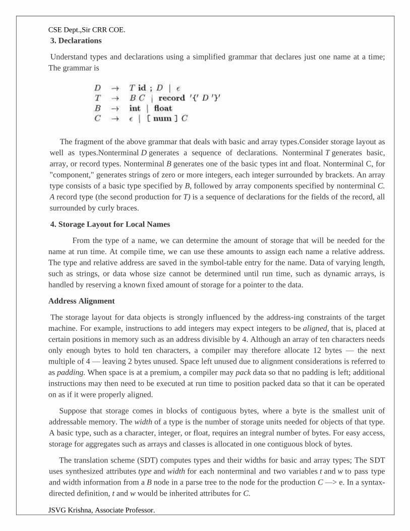
CSE Dept.,Sir CRR COE.
JSVG Krishna, Associate Professor.
3. Declarations
Understand types and declarations using a simplified grammar that declares just one name at a time;
The grammar is
The fragment of the above grammar that deals with basic and array types.Consider storage layout as
well as types.Nonterminal D generates a sequence of declarations. Nonterminal T generates basic,
array, or record types. Nonterminal B generates one of the basic types int and float. Nonterminal C, for
"component," generates strings of zero or more integers, each integer surrounded by brackets. An array
type consists of a basic type specified by B, followed by array components specified by nonterminal C.
A record type (the second production for T) is a sequence of declarations for the fields of the record, all
surrounded by curly braces.
4. Storage Layout for Local Names
From the type of a name, we can determine the amount of storage that will be needed for the
name at run time. At compile time, we can use these amounts to assign each name a relative address.
The type and relative address are saved in the symbol-table entry for the name. Data of varying length,
such as strings, or data whose size cannot be determined until run time, such as dynamic arrays, is
handled by reserving a known fixed amount of storage for a pointer to the data.
Address Alignment
The storage layout for data objects is strongly influenced by the address-ing constraints of the target
machine. For example, instructions to add integers may expect integers to be aligned, that is, placed at
certain positions in memory such as an address divisible by 4. Although an array of ten characters needs
only enough bytes to hold ten characters, a compiler may therefore allocate 12 bytes — the next
multiple of 4 — leaving 2 bytes unused. Space left unused due to alignment considerations is referred to
as padding. When space is at a premium, a compiler may pack data so that no padding is left; additional
instructions may then need to be executed at run time to position packed data so that it can be operated
on as if it were properly aligned.
Suppose that storage comes in blocks of contiguous bytes, where a byte is the smallest unit of
addressable memory. The width of a type is the number of storage units needed for objects of that type.
A basic type, such as a character, integer, or float, requires an integral number of bytes. For easy access,
storage for aggregates such as arrays and classes is allocated in one contiguous block of bytes.
The translation scheme (SDT) computes types and their widths for basic and array types; The SDT
uses synthesized attributes type and width for each nonterminal and two variables t and w to pass type
and width information from a B node in a parse tree to the node for the production C —> e. In a syntax-
directed definition, t and w would be inherited attributes for C.
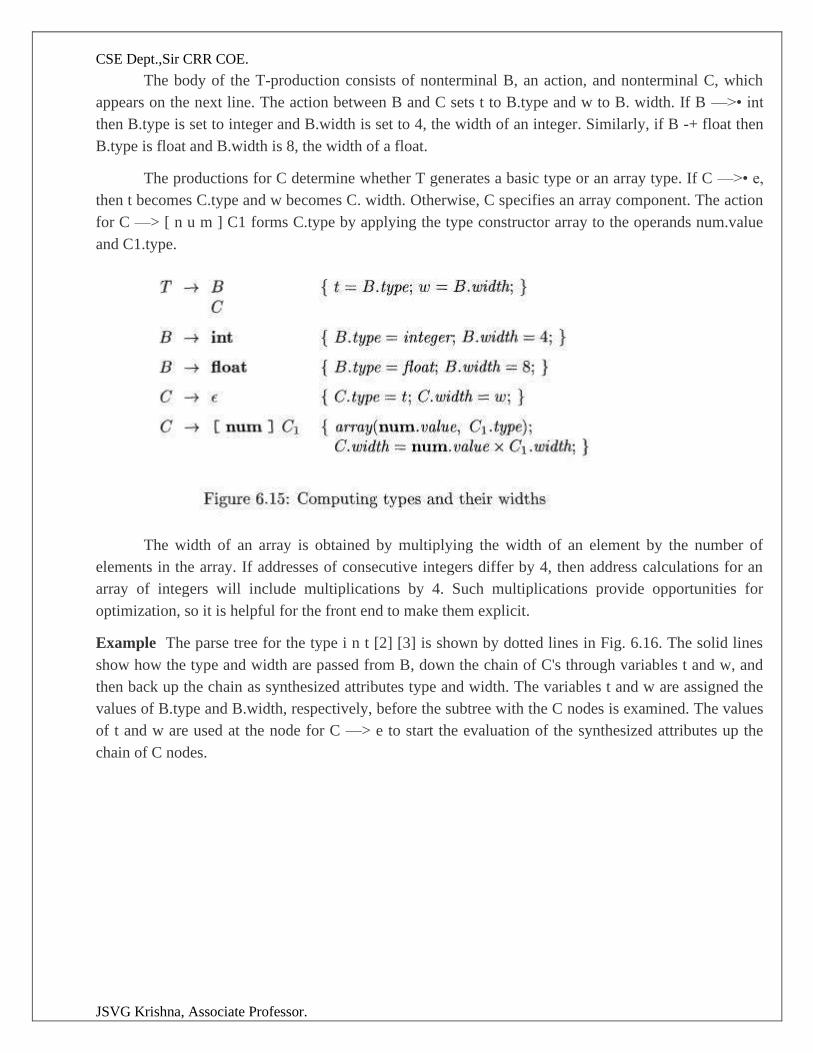
CSE Dept.,Sir CRR COE.
JSVG Krishna, Associate Professor.
The body of the T-production consists of nonterminal B, an action, and nonterminal C, which
appears on the next line. The action between B and C sets t to B.type and w to B. width. If B —>• int
then B.type is set to integer and B.width is set to 4, the width of an integer. Similarly, if B -+ float then
B.type is float and B.width is 8, the width of a float.
The productions for C determine whether T generates a basic type or an array type. If C —>• e,
then t becomes C.type and w becomes C. width. Otherwise, C specifies an array component. The action
for C —> [ n u m ] C1 forms C.type by applying the type constructor array to the operands num.value
and C1.type.
The width of an array is obtained by multiplying the width of an element by the number of
elements in the array. If addresses of consecutive integers differ by 4, then address calculations for an
array of integers will include multiplications by 4. Such multiplications provide opportunities for
optimization, so it is helpful for the front end to make them explicit.
Example The parse tree for the type i n t [2] [3] is shown by dotted lines in Fig. 6.16. The solid lines
show how the type and width are passed from B, down the chain of C's through variables t and w, and
then back up the chain as synthesized attributes type and width. The variables t and w are assigned the
values of B.type and B.width, respectively, before the subtree with the C nodes is examined. The values
of t and w are used at the node for C —> e to start the evaluation of the synthesized attributes up the
chain of C nodes.
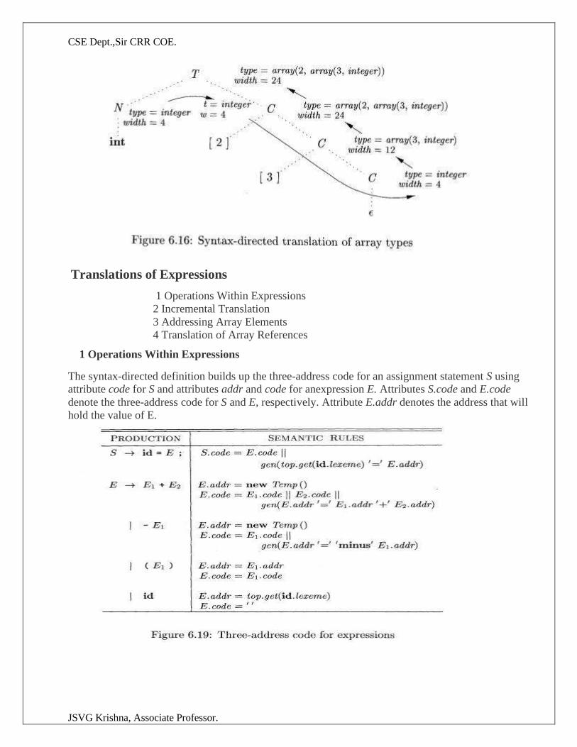
CSE Dept.,Sir CRR COE.
JSVG Krishna, Associate Professor.
Translations of Expressions
1 Operations Within Expressions 2 Incremental Translation 3 Addressing Array Elements 4 Translation of Array References 1 Operations Within Expressions The syntax-directed definition builds up the three-address code for an assignment statement S using
attribute code for S and attributes addr and code for anexpression E. Attributes S.code and E.code
denote the three-address code for S and E, respectively. Attribute E.addr denotes the address that will
hold the value of E.
CSE Dept.,Sir CRR COE.
JSVG Krishna, Associate Professor.
Example The syntax-directed definition in Fig. 6.19 translates the assignment statement
a = b + - c; into the TAC
2 Incremental Translation
Code attributes can be long strings, so they are generated incrementally In the incremental approach, gen not only constructs a three-address instruction, it appends the instruction to the sequence of instructions generated so far. The sequence may either be retained in memory for further processing, or it may be output incrementally.attribute addr represents the address of a node rather than a variable or constant.
3.Addressing Array Elements Elements of arrays can be accessed quickly if the elements are stored in a block of consecutive location. Array can be one dimensional or two dimensional.
For one dimensional array:
A: array[low..high] of the ith elements is at:
base + (i-low)*width = i*width + (base - low*width)
Multi-dimensional arrays:
Row major or column major forms
o Row major: a[1,1], a[1,2], a[1,3], a[2,1], a[2,2], a[2,3]
o Column major: a[1,1], a[2,1], a[1, 2], a[2, 2],a[1, 3],a[2,3]
o In row major form, the address of a[i1, i2] is
o Base+((i1-low1)*(high2-low2+1)+i2-low2)*width
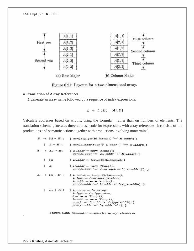
CSE Dept.,Sir CRR COE.
JSVG Krishna, Associate Professor.
4 Translation of Array References
L generate an array name followed by a sequence of index expressions:
Calculate addresses based on widths, using the formula rather than on numbers of elements. The
translation scheme generates three-address code for expressions with array references. It consists of the
productions and semantic actions together with productions involving nonterminal
.
CSE Dept.,Sir CRR COE.
JSVG Krishna, Associate Professor.
Type Checking
1 Rules for Type Checking
2 Type Conversions
3 Overloading of Functions and Operators
4 Type Inference and Polymorphic Functions
5 An Algorithm for Unification
Type checking a compiler needs to assign a type expression to each component of the source program. The compiler must then determine that these type expressions conform to a collection of logical rules that is called the type system for the source language.
1 Rules for Type Checking
Type checking can take on two forms: synthesis and inference. Type synthesis builds up the type
of an expression from the types of its subexpressions. It requires names to be declared before they are
used. The type of E1 + E2 is defined in terms of the types of E1 and E2 • A typical rule for type
synthesis has the form
Type inference determines the type of a language construct from the way it is used.Rule for type
inference has the form
2 Type Conversions
integers are converted to floats when necessary, using a unary operator ( f l o a t ) . For example, the
integer 2 is converted to a float in the code for the expression 2*3.14:
Type conversion rules vary from language to language. The rules for Java in Fig. 6.25 distinguish between widening conversions, which are intended to preserve information, and narrowing conversions, which can lose information. Conversion from one type to another is said to be implicit if it is done automatically by the compiler.
Implicit type conversions, also called coercions,
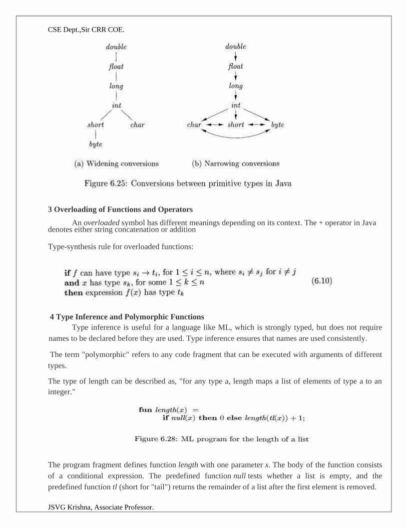
CSE Dept.,Sir CRR COE.
JSVG Krishna, Associate Professor.
3 Overloading of Functions and Operators
An overloaded symbol has different meanings depending on its context. The + operator in Java denotes either string concatenation or addition
Type-synthesis rule for overloaded functions:
4 Type Inference and Polymorphic Functions
Type inference is useful for a language like ML, which is strongly typed, but does not require
names to be declared before they are used. Type inference ensures that names are used consistently.
The term "polymorphic" refers to any code fragment that can be executed with arguments of different
types.
The type of length can be described as, "for any type a, length maps a list of elements of type a to an
integer."
The program fragment defines function length with one parameter x. The body of the function consists
of a conditional expression. The predefined function null tests whether a list is empty, and the
predefined function tl (short for "tail") returns the remainder of a list after the first element is removed.
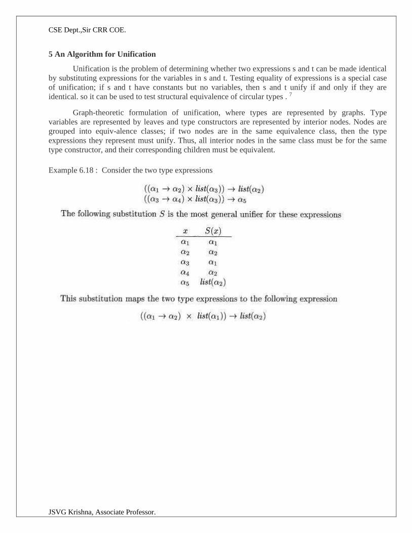
CSE Dept.,Sir CRR COE.
JSVG Krishna, Associate Professor.
5 An Algorithm for Unification
Unification is the problem of determining whether two expressions s and t can be made identical
by substituting expressions for the variables in s and t. Testing equality of expressions is a special case
of unification; if s and t have constants but no variables, then s and t unify if and only if they are
identical. so it can be used to test structural equivalence of circular types . 7
Graph-theoretic formulation of unification, where types are represented by graphs. Type
variables are represented by leaves and type constructors are represented by interior nodes. Nodes are
grouped into equiv-alence classes; if two nodes are in the same equivalence class, then the type
expressions they represent must unify. Thus, all interior nodes in the same class must be for the same
type constructor, and their corresponding children must be equivalent.
Example 6.18 : Consider the two type expressions
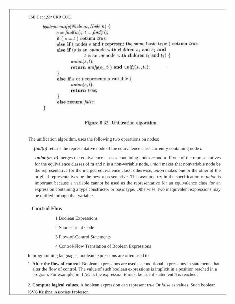
CSE Dept.,Sir CRR COE.
JSVG Krishna, Associate Professor.
The unification algorithm, uses the following two operations on nodes:
find{n) returns the representative node of the equivalence class currently containing node n.
union(m, n) merges the equivalence classes containing nodes m and n. If one of the representatives
for the equivalence classes of m and n is a non-variable node, union makes that nonvariable node be
the representative for the merged equivalence class; otherwise, union makes one or the other of the
original representatives be the new representative. This asymme-try in the specification of union is
important because a variable cannot be used as the representative for an equivalence class for an
expression containing a type constructor or basic type. Otherwise, two inequivalent expressions may
be unified through that variable.
Control Flow
1 Boolean Expressions
2 Short-Circuit Code
3 Flow-of-Control Statements
4 Control-Flow Translation of Boolean Expressions
In programming languages, boolean expressions are often used to
1. Alter the flow of control. Boolean expressions are used as conditional expressions in statements that
alter the flow of control. The value of such boolean expressions is implicit in a position reached in a
program. For example, in if (E) 5, the expression E must be true if statement S is reached.
2. Compute logical values. A boolean expression can represent true Or false as values. Such boolean
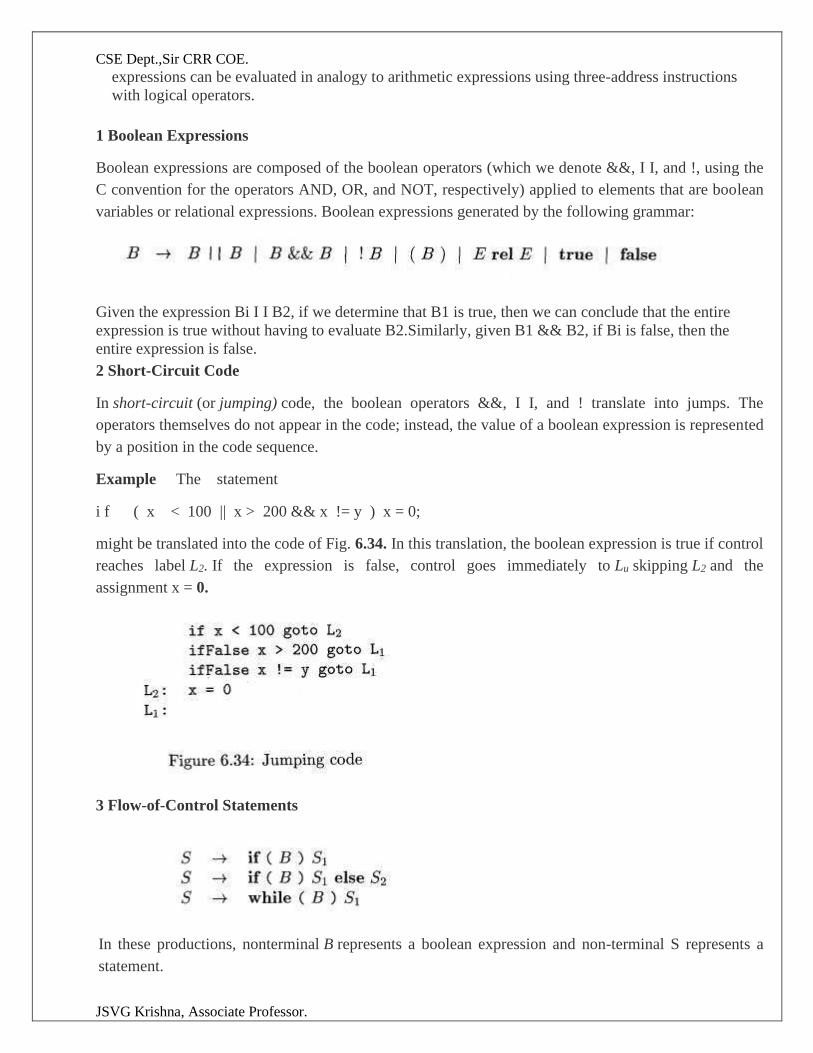
CSE Dept.,Sir CRR COE.
JSVG Krishna, Associate Professor.
expressions can be evaluated in analogy to arithmetic expressions using three-address instructions
with logical operators.
1 Boolean Expressions
Boolean expressions are composed of the boolean operators (which we denote &&, I I, and !, using the
C convention for the operators AND, OR, and NOT, respectively) applied to elements that are boolean
variables or relational expressions. Boolean expressions generated by the following grammar:
Given the expression Bi I I B2, if we determine that B1 is true, then we can conclude that the entire
expression is true without having to evaluate B2.Similarly, given B1 && B2, if Bi is false, then the
entire expression is false.
2 Short-Circuit Code
In short-circuit (or jumping) code, the boolean operators &&, I I, and ! translate into jumps. The
operators themselves do not appear in the code; instead, the value of a boolean expression is represented
by a position in the code sequence.
Example The statement
i f ( x < 100 || x > 200 && x != y ) x = 0;
might be translated into the code of Fig. 6.34. In this translation, the boolean expression is true if control
reaches label L2. If the expression is false, control goes immediately to Lu skipping L2 and the
assignment x = 0.
3 Flow-of-Control Statements
In these productions, nonterminal B represents a boolean expression and non-terminal S represents a
statement.
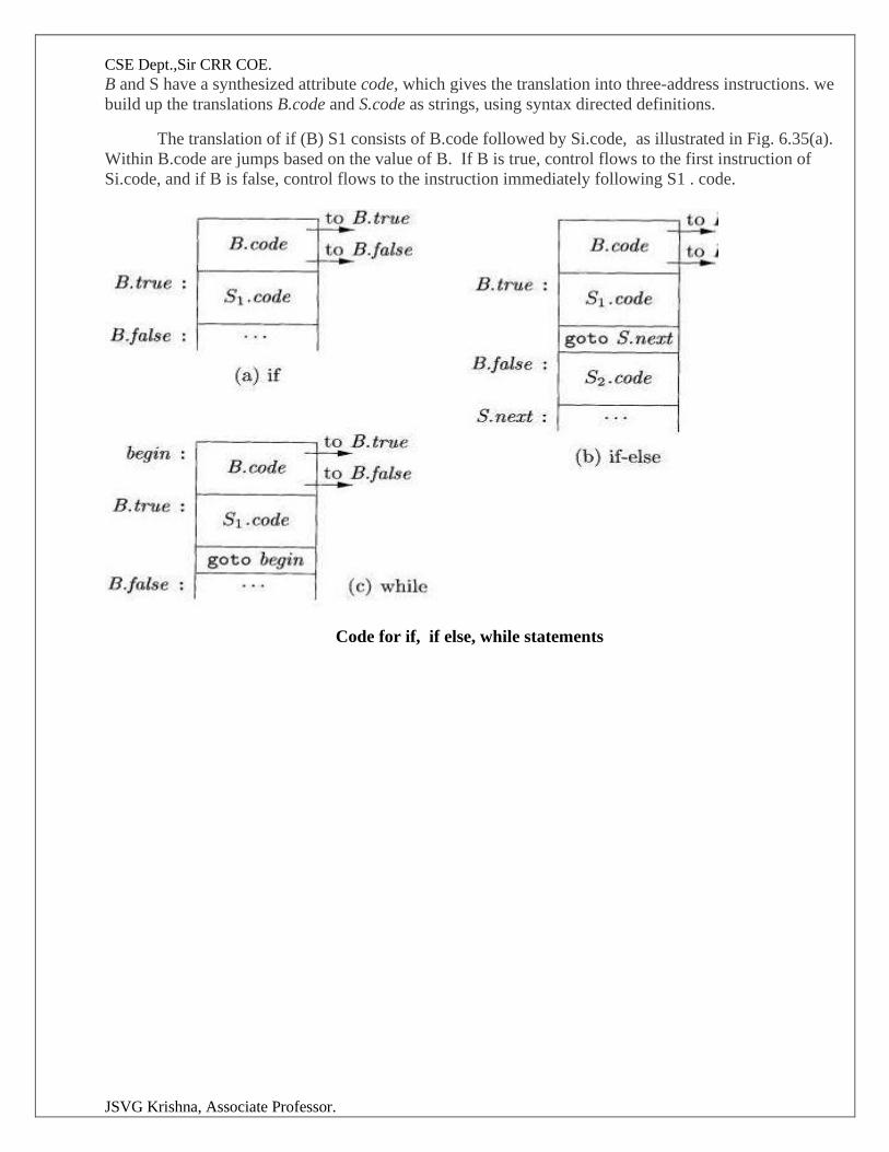
CSE Dept.,Sir CRR COE.
JSVG Krishna, Associate Professor.
B and S have a synthesized attribute code, which gives the translation into three-address instructions. we
build up the translations B.code and S.code as strings, using syntax directed definitions.
The translation of if (B) S1 consists of B.code followed by Si.code, as illustrated in Fig. 6.35(a).
Within B.code are jumps based on the value of B. If B is true, control flows to the first instruction of
Si.code, and if B is false, control flows to the instruction immediately following S1 . code.
Code for if, if else, while statements
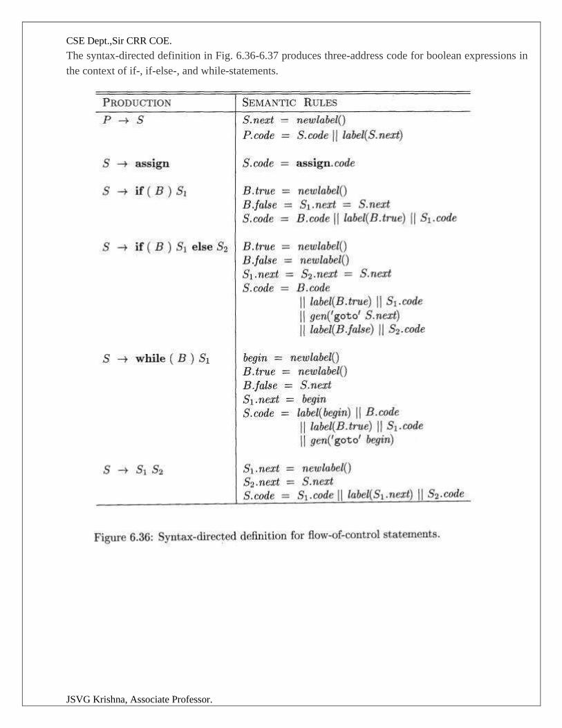
CSE Dept.,Sir CRR COE.
JSVG Krishna, Associate Professor.
The syntax-directed definition in Fig. 6.36-6.37 produces three-address code for boolean expressions in
the context of if-, if-else-, and while-statements.
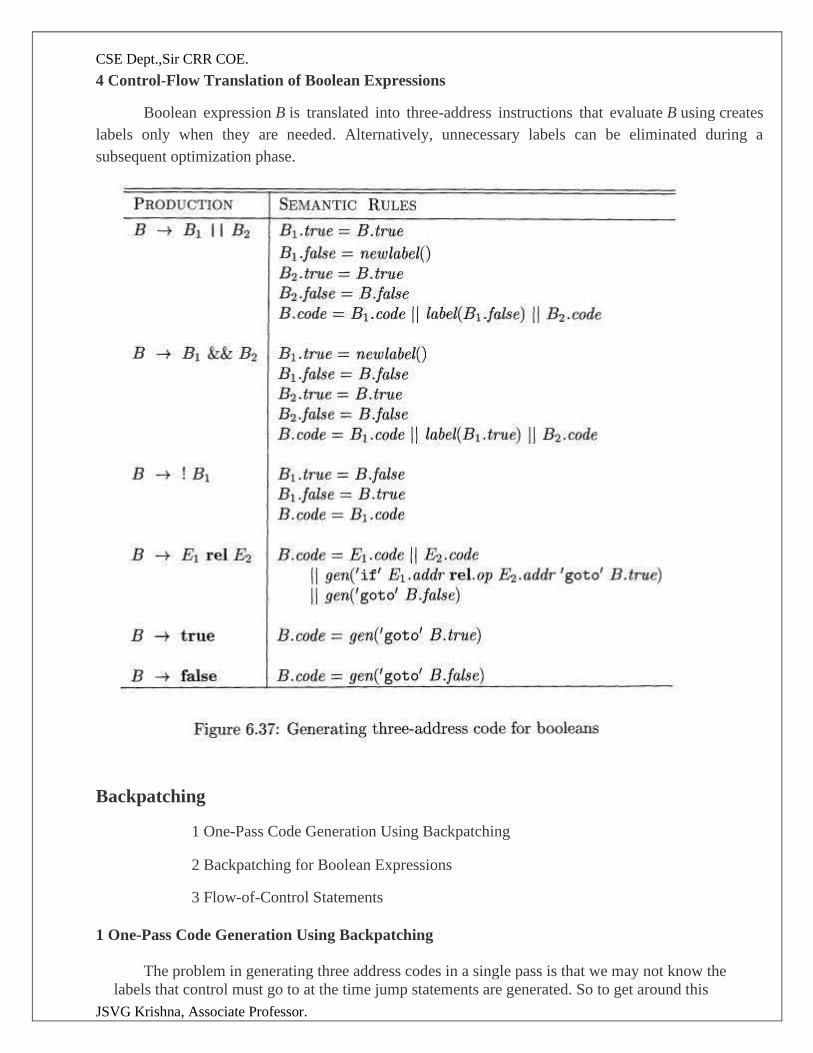
CSE Dept.,Sir CRR COE.
JSVG Krishna, Associate Professor.
4 Control-Flow Translation of Boolean Expressions
Boolean expression B is translated into three-address instructions that evaluate B using creates
labels only when they are needed. Alternatively, unnecessary labels can be eliminated during a
subsequent optimization phase.
Backpatching
1 One-Pass Code Generation Using Backpatching
2 Backpatching for Boolean Expressions
3 Flow-of-Control Statements
1 One-Pass Code Generation Using Backpatching
The problem in generating three address codes in a single pass is that we may not know the
labels that control must go to at the time jump statements are generated. So to get around this
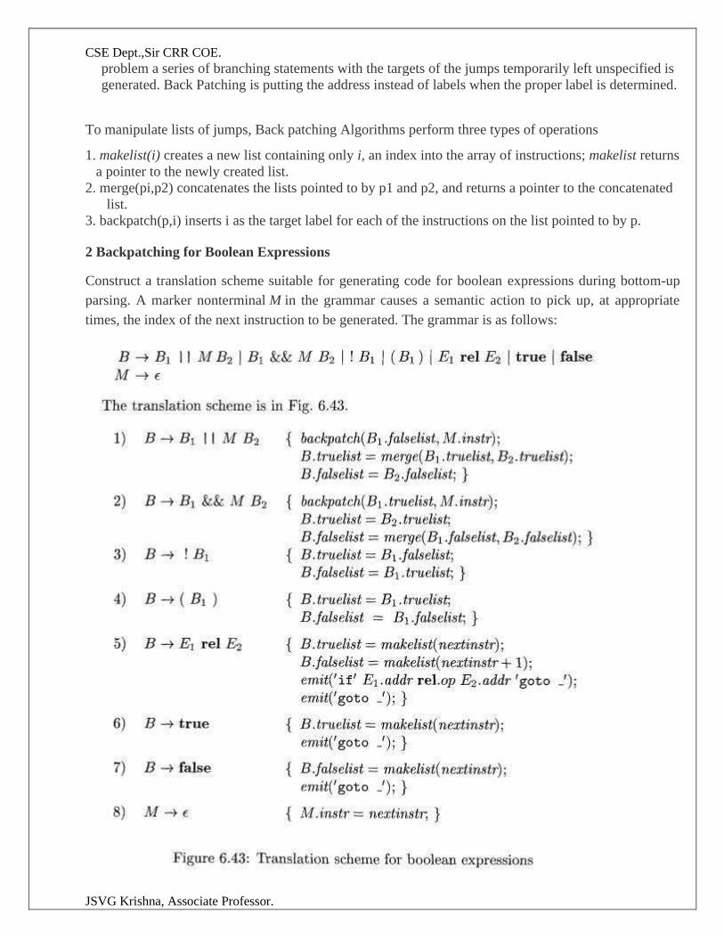
CSE Dept.,Sir CRR COE.
JSVG Krishna, Associate Professor.
problem a series of branching statements with the targets of the jumps temporarily left unspecified is
generated. Back Patching is putting the address instead of labels when the proper label is determined.
To manipulate lists of jumps, Back patching Algorithms perform three types of operations
1. makelist(i) creates a new list containing only i, an index into the array of instructions; makelist returns
a pointer to the newly created list.
2. merge(pi,p2) concatenates the lists pointed to by p1 and p2, and returns a pointer to the concatenated
list.
3. backpatch(p,i) inserts i as the target label for each of the instructions on the list pointed to by p.
2 Backpatching for Boolean Expressions
Construct a translation scheme suitable for generating code for boolean expressions during bottom-up
parsing. A marker nonterminal M in the grammar causes a semantic action to pick up, at appropriate
times, the index of the next instruction to be generated. The grammar is as follows:
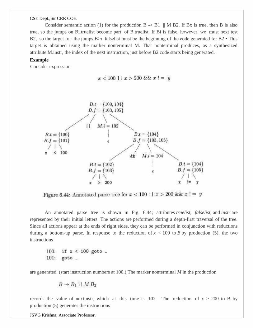
CSE Dept.,Sir CRR COE.
JSVG Krishna, Associate Professor.
Consider semantic action (1) for the production B -> B1 || M B2. If Bx is true, then B is also
true, so the jumps on Bi.truelist become part of B.truelist. If Bi is false, however, we must next test
B2, so the target for the jumps B>i .falselist must be the beginning of the code generated for B2 • This
target is obtained using the marker nonterminal M. That nonterminal produces, as a synthesized
attribute M.instr, the index of the next instruction, just before B2 code starts being generated.
Example
Consider expression
An annotated parse tree is shown in Fig. 6.44; attributes truelist, falselist, and instr are
represented by their initial letters. The actions are performed during a depth-first traversal of the tree.
Since all actions appear at the ends of right sides, they can be performed in conjunction with reductions
during a bottom-up parse. In response to the reduction of x < 100 to B by production (5), the two
instructions
are generated. (start instruction numbers at 100.) The marker nonterminal M in the production
records the value of nextinstr, which at this time is 102. The reduction of x > 200 to B by
production (5) generates the instructions
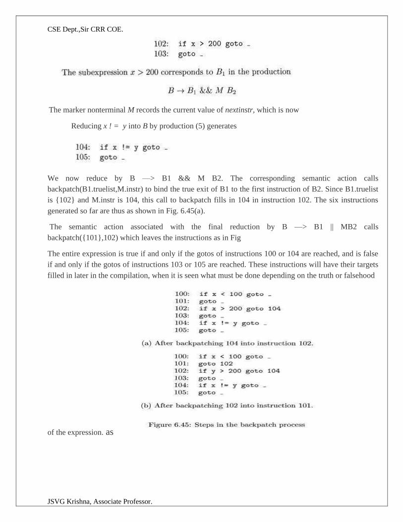
CSE Dept.,Sir CRR COE.
JSVG Krishna, Associate Professor.
The marker nonterminal M records the current value of nextinstr, which is now
Reducing x ! = y into B by production (5) generates
We now reduce by B —> B1 && M B2. The corresponding semantic action calls
backpatch(B1.truelist,M.instr) to bind the true exit of B1 to the first instruction of B2. Since B1.truelist
is {102} and M.instr is 104, this call to backpatch fills in 104 in instruction 102. The six instructions
generated so far are thus as shown in Fig. 6.45(a).
The semantic action associated with the final reduction by B —> B1 || MB2 calls
backpatch({101},102) which leaves the instructions as in Fig
The entire expression is true if and only if the gotos of instructions 100 or 104 are reached, and is false
if and only if the gotos of instructions 103 or 105 are reached. These instructions will have their targets
filled in later in the compilation, when it is seen what must be done depending on the truth or falsehood
of the expression. as
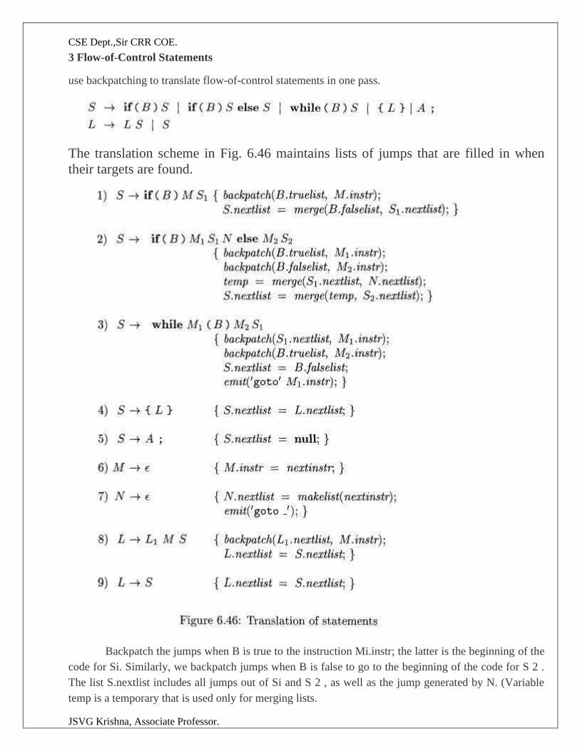
CSE Dept.,Sir CRR COE.
JSVG Krishna, Associate Professor.
3 Flow-of-Control Statements
use backpatching to translate flow-of-control statements in one pass.
The translation scheme in Fig. 6.46 maintains lists of jumps that are filled in when
their targets are found.
Backpatch the jumps when B is true to the instruction Mi.instr; the latter is the beginning of the
code for Si. Similarly, we backpatch jumps when B is false to go to the beginning of the code for S 2 .
The list S.nextlist includes all jumps out of Si and S 2 , as well as the jump generated by N. (Variable
temp is a temporary that is used only for merging lists.
CSE Dept.,Sir CRR COE.
JSVG Krishna, Associate Professor.
Semantic actions (8) and (9) handle sequences of statements. In
the instruction following the code for L± in order of execution is the beginning of S. Thus the
L1.nextlist list is backpatched to the beginning of the code for S, which is given by M.instr. In L —> S,
L.nextlist is the same as S.nextlist.
Note that no new instructions are generated anywhere in these semantic rules, except for rules (3)
and (7). All other code is generated by the semantic actions associated with assignment-statements and
expressions. The flow of control causes the proper backpatching so that the assignments and boolean
expression evaluations will connect properly.

CSE Dept.,Sir CRR COE.
JSVG Krishna, Associate Professor.
LECTURE NOTES
ON
COMPILER DESIGN
2020 – 2021
III B. Tech I Semester (JNTUK-R16)
P.Naga Deepthi/ Mr J.S.V. Gopala Krishna
Department of Computer Science and Engineering
SIR CRREDDY COLLEGE OF ENGINEERING,
ELURU
- 21 -
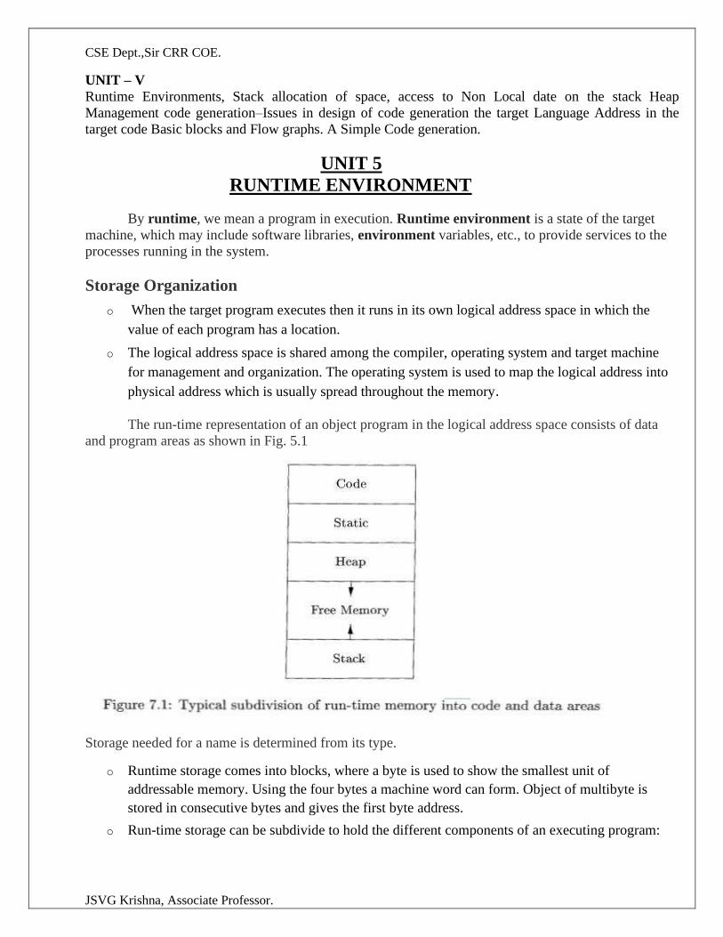
CSE Dept.,Sir CRR COE.
JSVG Krishna, Associate Professor.
UNIT – V
Runtime Environments, Stack allocation of space, access to Non Local date on the stack Heap
Management code generation–Issues in design of code generation the target Language Address in the
target code Basic blocks and Flow graphs. A Simple Code generation.
UNIT 5
RUNTIME ENVIRONMENT
By runtime, we mean a program in execution. Runtime environment is a state of the target
machine, which may include software libraries, environment variables, etc., to provide services to the
processes running in the system.
Storage Organization
o When the target program executes then it runs in its own logical address space in which the
value of each program has a location.
o The logical address space is shared among the compiler, operating system and target machine
for management and organization. The operating system is used to map the logical address into
physical address which is usually spread throughout the memory.
The run-time representation of an object program in the logical address space consists of data
and program areas as shown in Fig. 5.1
Storage needed for a name is determined from its type.
o Runtime storage comes into blocks, where a byte is used to show the smallest unit of
addressable memory. Using the four bytes a machine word can form. Object of multibyte is
stored in consecutive bytes and gives the first byte address.
o Run-time storage can be subdivide to hold the different components of an executing program:
CSE Dept.,Sir CRR COE.
JSVG Krishna, Associate Professor.
1. Generated executable code
2. Static data objects
3. Dynamic data-object- heap
4. Automatic data objects- stack
Two areas, Stack and Heap, are at the opposite ends of the remainder of the address space. These areas
are dynamic; their size can change as the program executes. Stack to support call/return policy for
procedures.Heap to store data that can outlive a call to a procedure. . The heap is used to manage
allocate and deallocate data.
Static Versus Dynamic Storage Allocation
The layout and allocation of data to memory locations in the run-time environment are key issues in
storage management. The two terms static and dynamic distinguish between compile time and run time,
respectively. We say that a storage-allocation decision is
Static:- if it can be made by the compiler looking only at the text of the program, not at what
the program does when it executes.
Dynamic:- if it can be decided only while the program is running.
Compilers use following two strategies for dynamic storage allocation:
Stack storage. Names local to a procedure are allocated space on a stack. stack supports the normal
call/return policy for procedures.
Heap storage. Data that may outlive the call to the procedure that created it is usually allocated on a
"heap" of reusable storage.The heap is an area of virtual memory that allows objects or other data
elements to obtain storage when they are created and to return that storage when they are invalidated.
Stack allocation of space
1 Activation Trees
2 Activation Records
3 Calling Sequences
4 Variable-Length Data on the Stack
Each time a procedure is called, space for its local variables is pushed onto a stack, and when the
procedure terminates, that space is popped off the stack.
1 Activation Trees
Stack allocation is a valid allocation for procedures since procedure calls are nested
Example: quicksort algorithm
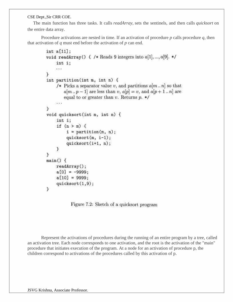
CSE Dept.,Sir CRR COE.
JSVG Krishna, Associate Professor.
The main function has three tasks. It calls readArray, sets the sentinels, and then calls quicksort on
the entire data array.
Procedure activations are nested in time. If an activation of procedure p calls procedure q, then
that activation of q must end before the activation of p can end.
Represent the activations of procedures during the running of an entire program by a tree, called
an activation tree. Each node corresponds to one activation, and the root is the activation of the "main"
procedure that initiates execution of the program. At a node for an activation of procedure p, the
children correspond to activations of the procedures called by this activation of p.
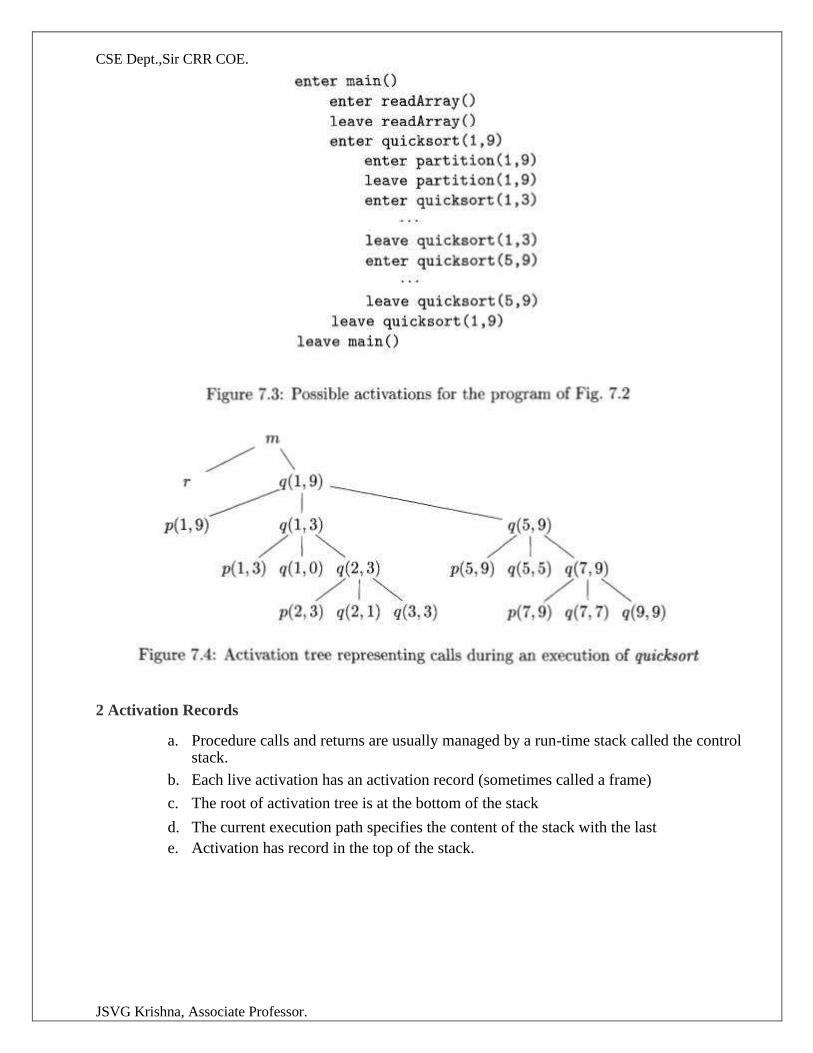
CSE Dept.,Sir CRR COE.
JSVG Krishna, Associate Professor.
2 Activation Records
a. Procedure calls and returns are usually managed by a run-time stack called the control stack.
b. Each live activation has an activation record (sometimes called a frame)
c. The root of activation tree is at the bottom of the stack
d. The current execution path specifies the content of the stack with the last
e. Activation has record in the top of the stack.
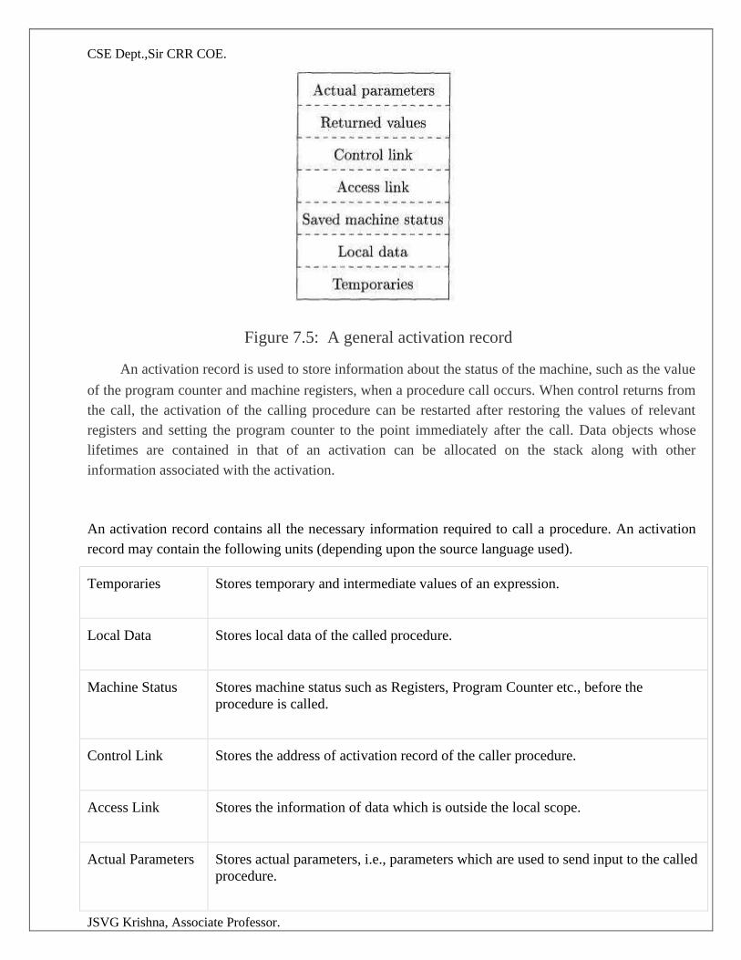
CSE Dept.,Sir CRR COE.
JSVG Krishna, Associate Professor.
Figure 7.5: A general activation record
An activation record is used to store information about the status of the machine, such as the value
of the program counter and machine registers, when a procedure call occurs. When control returns from
the call, the activation of the calling procedure can be restarted after restoring the values of relevant
registers and setting the program counter to the point immediately after the call. Data objects whose
lifetimes are contained in that of an activation can be allocated on the stack along with other
information associated with the activation.
An activation record contains all the necessary information required to call a procedure. An activation
record may contain the following units (depending upon the source language used).
Temporaries Stores temporary and intermediate values of an expression.
Local Data Stores local data of the called procedure.
Machine Status Stores machine status such as Registers, Program Counter etc., before the
procedure is called.
Control Link Stores the address of activation record of the caller procedure.
Access Link Stores the information of data which is outside the local scope.
Actual Parameters Stores actual parameters, i.e., parameters which are used to send input to the called
procedure.
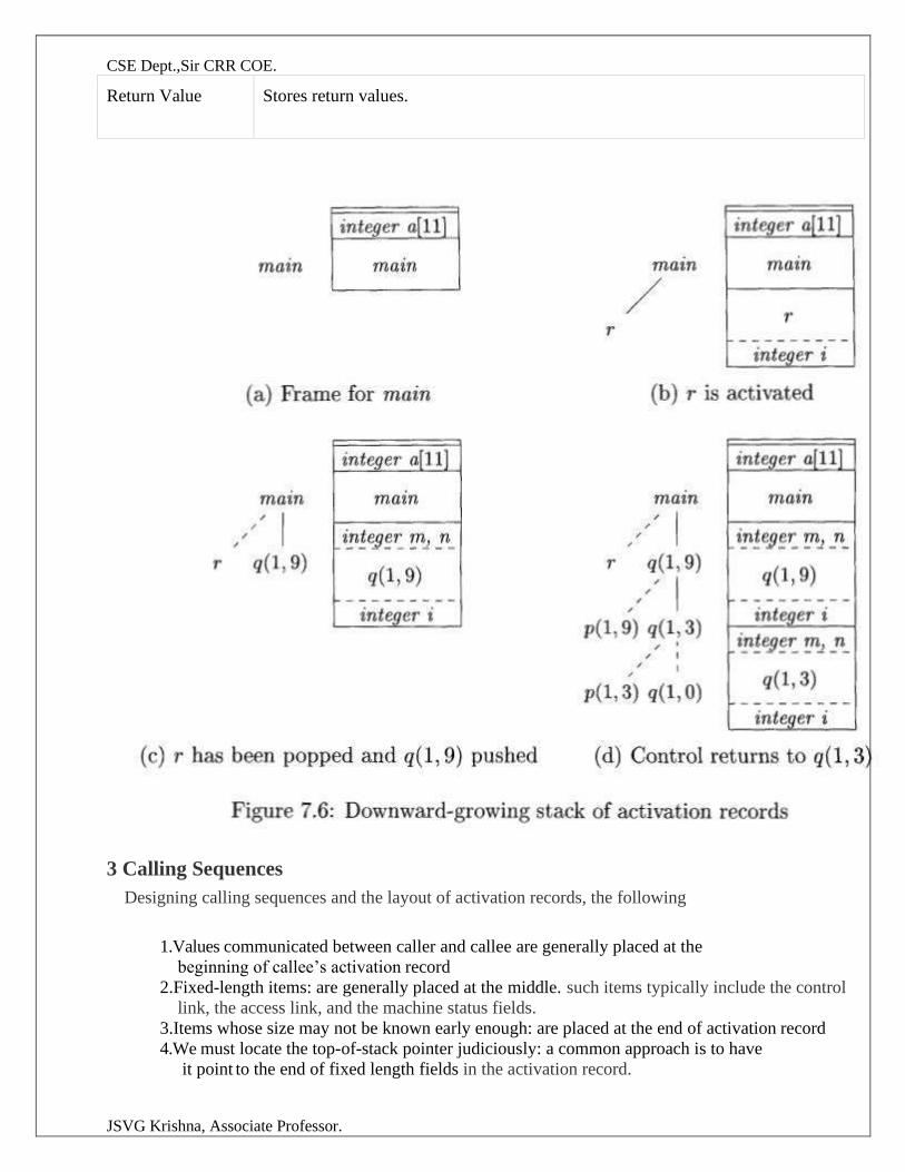
CSE Dept.,Sir CRR COE.
JSVG Krishna, Associate Professor.
Return Value Stores return values.
3 Calling Sequences
Designing calling sequences and the layout of activation records, the following
1.Values communicated between caller and callee are generally placed at the
beginning of callee’s activation record
2.Fixed-length items: are generally placed at the middle. such items typically include the control
link, the access link, and the machine status fields.
3.Items whose size may not be known early enough: are placed at the end of activation record
4.We must locate the top-of-stack pointer judiciously: a common approach is to have
it point to the end of fixed length fields in the activation record.
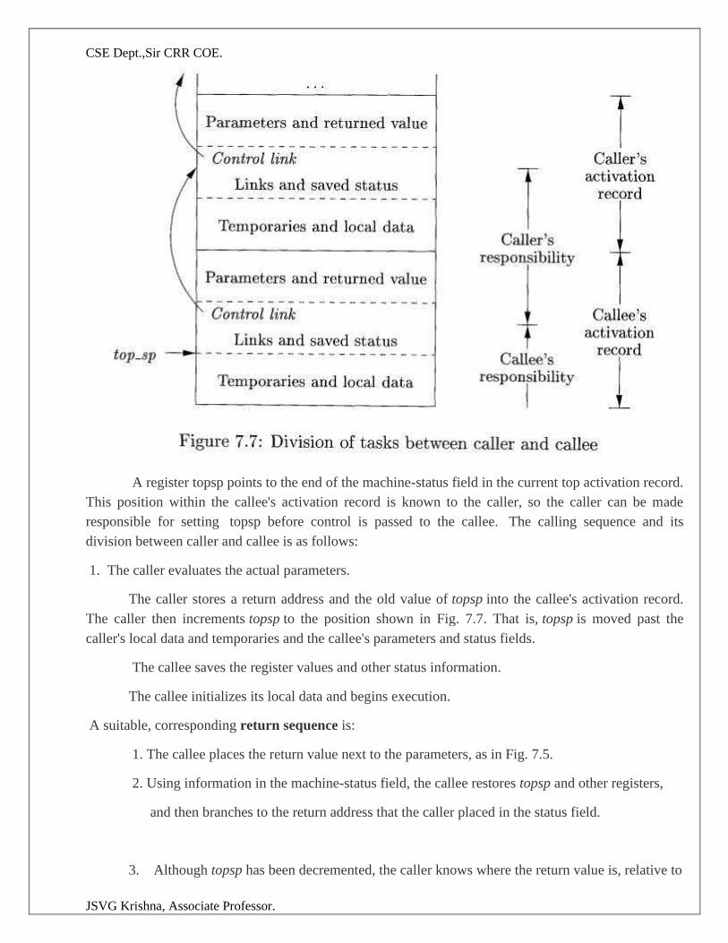
CSE Dept.,Sir CRR COE.
JSVG Krishna, Associate Professor.
A register topsp points to the end of the machine-status field in the current top activation record.
This position within the callee's activation record is known to the caller, so the caller can be made
responsible for setting topsp before control is passed to the callee. The calling sequence and its
division between caller and callee is as follows:
1. The caller evaluates the actual parameters.
The caller stores a return address and the old value of topsp into the callee's activation record.
The caller then increments topsp to the position shown in Fig. 7.7. That is, topsp is moved past the
caller's local data and temporaries and the callee's parameters and status fields.
The callee saves the register values and other status information.
The callee initializes its local data and begins execution.
A suitable, corresponding return sequence is:
1. The callee places the return value next to the parameters, as in Fig. 7.5.
2. Using information in the machine-status field, the callee restores topsp and other registers,
and then branches to the return address that the caller placed in the status field.
3. Although topsp has been decremented, the caller knows where the return value is, relative to
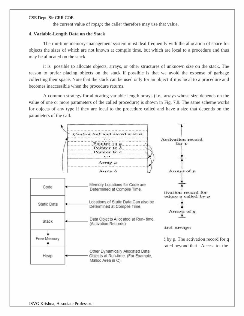
CSE Dept.,Sir CRR COE.
JSVG Krishna, Associate Professor.
the current value of topsp; the caller therefore may use that value.
4. Variable-Length Data on the Stack
The run-time memory-management system must deal frequently with the allocation of space for
objects the sizes of which are not known at compile time, but which are local to a procedure and thus
may be allocated on the stack.
it is possible to allocate objects, arrays, or other structures of unknown size on the stack. The
reason to prefer placing objects on the stack if possible is that we avoid the expense of garbage
collecting their space. Note that the stack can be used only for an object if it is local to a procedure and
becomes inaccessible when the procedure returns.
A common strategy for allocating variable-length arrays (i.e., arrays whose size depends on the
value of one or more parameters of the called procedure) is shown in Fig. 7.8. The same scheme works
for objects of any type if they are local to the procedure called and have a size that depends on the
parameters of the call.
Also shown in Fig. 7.8 is the activation record for a procedure q, called by p. The activation record for q
begins after the arrays of p, and any variable-length arrays of q are located beyond that . Access to the
data on the stack is through two pointers, top and topsp.
CSE Dept.,Sir CRR COE.
JSVG Krishna, Associate Professor.
Access to Non Local data on the stack
1 Data Access Without Nested Procedures
2 Issues With Nested Procedures
3 A Language With Nested Procedure Declarations
4 Nesting Depth
5 Access Links
6 Manipulating Access Links
7 Access Links for Procedure Parameters
8 Displays
Consider how procedures access their data. Especially im-portant is the mechanism for finding
data used within a procedure p but that does not belong to p
1 Data Access Without Nested Procedures
Names are either local to the procedure in question or are declared globally.
1. For global names the address is known statically at compile time providing there is only one
source file. If multiple source files, the linker knows. In either case no reference to the activation
record is needed; the addresses are know prior to execution.
2. For names local to the current procedure, the address needed is in the AR at a known-at-
compile-time constant offset from the sp. In the case of variable size arrays, the constant offset
refers to a pointer to the actual storage.
2 Issues With Nested Procedures
Access becomes far more complicated when a language allows procedure dec-larations to be
nested .The reason is that knowing at compile time that the declaration of p is immediately nested
within q does not tell us the relative positions of their activation records at run time. In fact, since
either p or q or both may be recursive, there may be several activation records of p and/or q on the
stack.
Finding the declaration that applies to a nonlocal name x in a nested pro-cedure p is a static
decision; it can be done by an extension of the static-scope rule for blocks. Suppose x is declared in the
enclosing procedure q. Finding the relevant activation of q from an activation of p is a dynamic
decision; it re-quires additional run-time information about activations. One possible solution is to use
access links.
3. A Language With Nested Procedure Declarations
In various languages with nested procedures, one of the most influential is ML.
CSE Dept.,Sir CRR COE.
JSVG Krishna, Associate Professor.
ML is a functional language, meaning that variables, once declared and initialized, are not
changed. There are only a few exceptions, such as the array, whose elements can be changed by special
function calls.
• Variables are defined, and have their unchangeable values initialized,
v a l (name) = (expression)
• Functions are defined using the syntax:
fun (name) ( (arguments) ) = (body)
• For function bodies, use let-statements of the form:
let (list of definitions) in (statements) end The definitions are normally v a l or fun statements.
The scope of each such definition consists of all following definitions, up to the in, and all the
statements up to the end. Most importantly, function definitions can be nested. For example, the body of
a function p can contain a let-statement that includes the definition of another (nested) function q.
Similarly, q can have function definitions within its own body, leading to arbitrarily deep nesting of
function
4. Nesting Depth
Nesting depth is 1 to procedures that are not nested within any other procedure. For example, all
C functions are at nesting depth 1. However, if a procedure p is defined immediately within a procedure
at nesting depth i, then give p the nesting depth i
+1
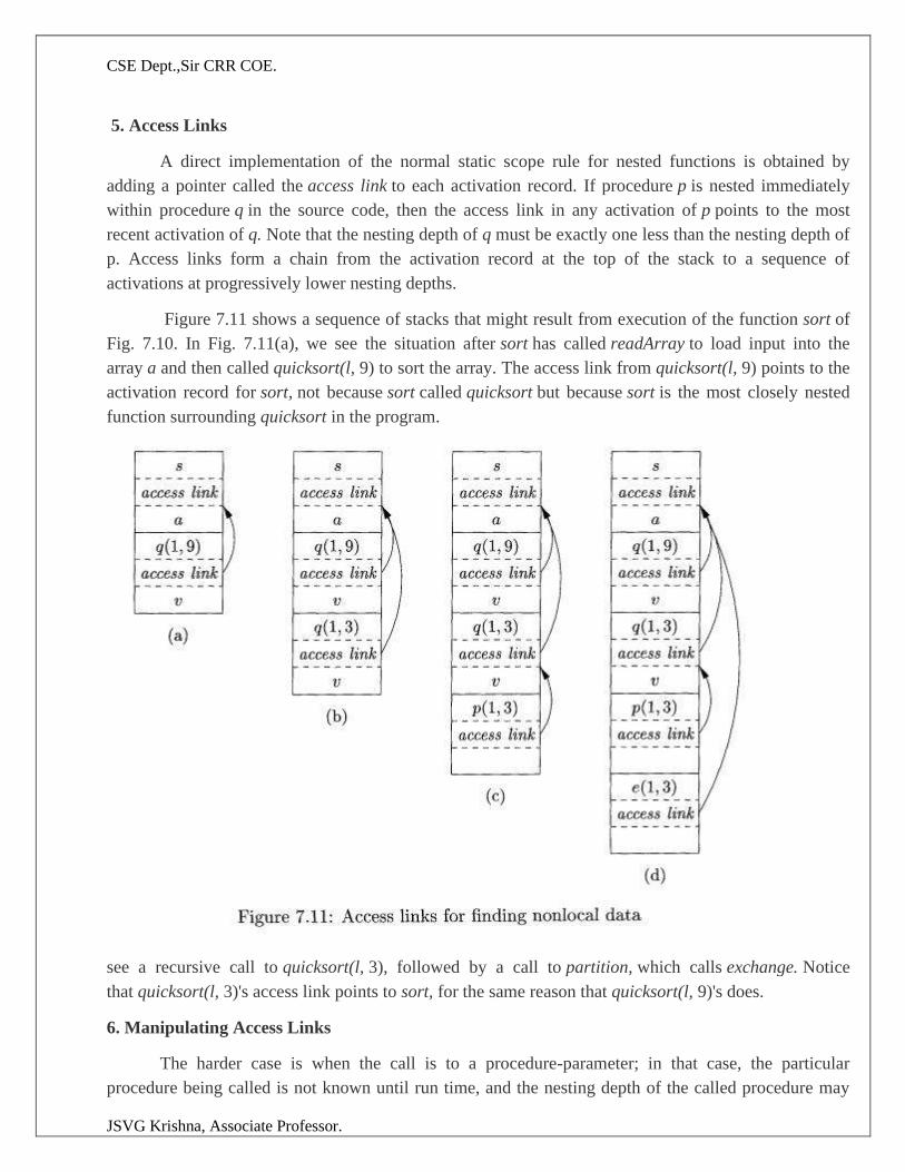
CSE Dept.,Sir CRR COE.
JSVG Krishna, Associate Professor.
5. Access Links
A direct implementation of the normal static scope rule for nested functions is obtained by
adding a pointer called the access link to each activation record. If procedure p is nested immediately
within procedure q in the source code, then the access link in any activation of p points to the most
recent activation of q. Note that the nesting depth of q must be exactly one less than the nesting depth of
p. Access links form a chain from the activation record at the top of the stack to a sequence of
activations at progressively lower nesting depths.
Figure 7.11 shows a sequence of stacks that might result from execution of the function sort of
Fig. 7.10. In Fig. 7.11(a), we see the situation after sort has called readArray to load input into the
array a and then called quicksort(l, 9) to sort the array. The access link from quicksort(l, 9) points to the
activation record for sort, not because sort called quicksort but because sort is the most closely nested
function surrounding quicksort in the program.
see a recursive call to quicksort(l, 3), followed by a call to partition, which calls exchange. Notice
that quicksort(l, 3)'s access link points to sort, for the same reason that quicksort(l, 9)'s does.
6. Manipulating Access Links
The harder case is when the call is to a procedure-parameter; in that case, the particular
procedure being called is not known until run time, and the nesting depth of the called procedure may
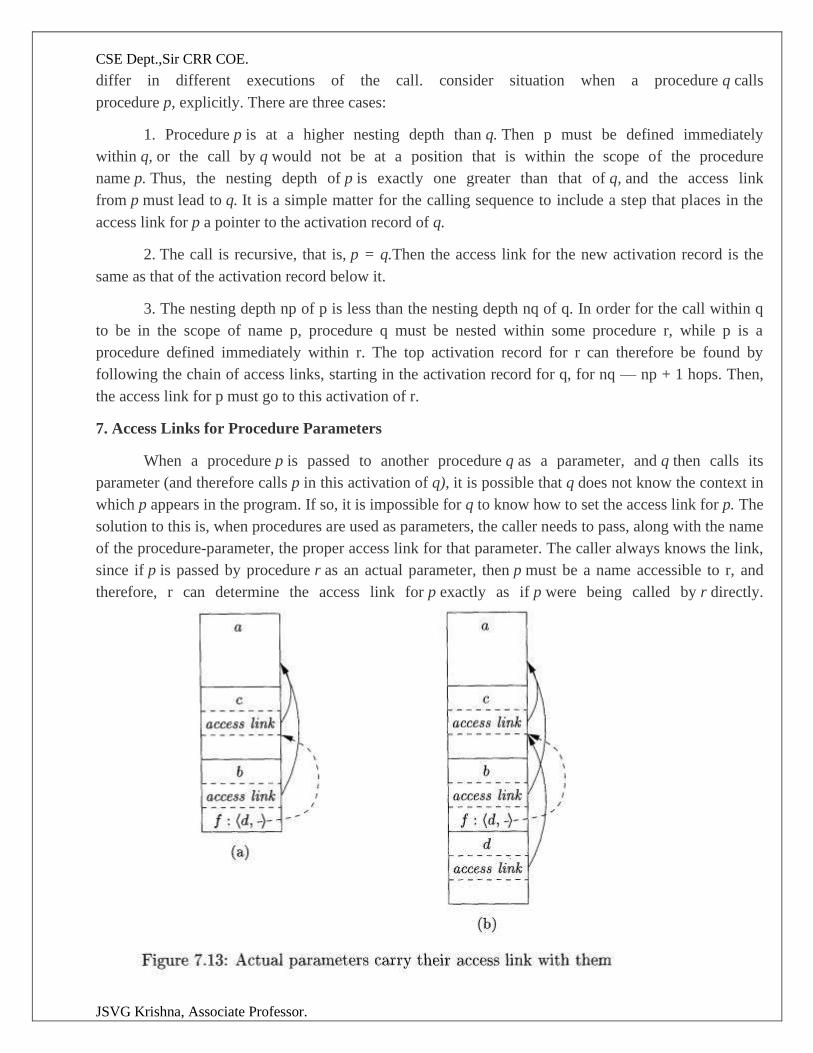
CSE Dept.,Sir CRR COE.
JSVG Krishna, Associate Professor.
differ in different executions of the call. consider situation when a procedure q calls
procedure p, explicitly. There are three cases:
1. Procedure p is at a higher nesting depth than q. Then p must be defined immediately
within q, or the call by q would not be at a position that is within the scope of the procedure
name p. Thus, the nesting depth of p is exactly one greater than that of q, and the access link
from p must lead to q. It is a simple matter for the calling sequence to include a step that places in the
access link for p a pointer to the activation record of q.
2. The call is recursive, that is, p = q.Then the access link for the new activation record is the
same as that of the activation record below it.
3. The nesting depth np of p is less than the nesting depth nq of q. In order for the call within q
to be in the scope of name p, procedure q must be nested within some procedure r, while p is a
procedure defined immediately within r. The top activation record for r can therefore be found by
following the chain of access links, starting in the activation record for q, for nq — np + 1 hops. Then,
the access link for p must go to this activation of r.
7. Access Links for Procedure Parameters
When a procedure p is passed to another procedure q as a parameter, and q then calls its
parameter (and therefore calls p in this activation of q), it is possible that q does not know the context in
which p appears in the program. If so, it is impossible for q to know how to set the access link for p. The
solution to this is, when procedures are used as parameters, the caller needs to pass, along with the name
of the procedure-parameter, the proper access link for that parameter. The caller always knows the link,
since if p is passed by procedure r as an actual parameter, then p must be a name accessible to r, and
therefore, r can determine the access link for p exactly as if p were being called by r directly.
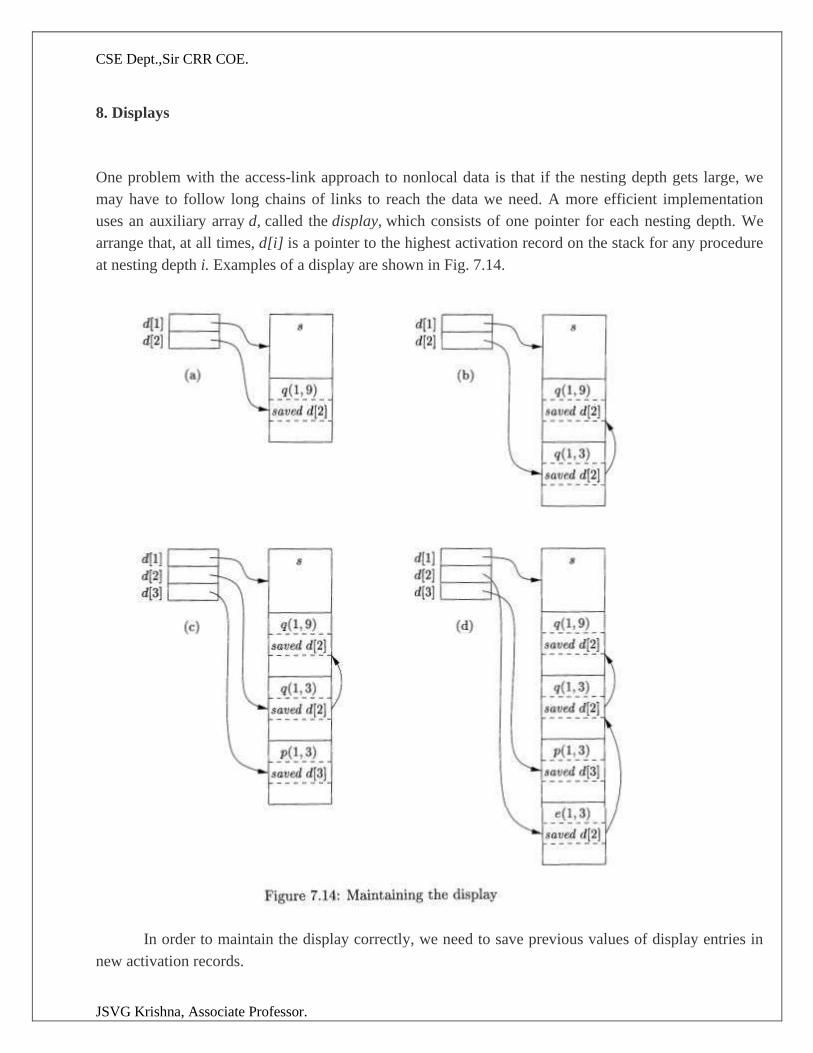
CSE Dept.,Sir CRR COE.
JSVG Krishna, Associate Professor.
8. Displays
One problem with the access-link approach to nonlocal data is that if the nesting depth gets large, we
may have to follow long chains of links to reach the data we need. A more efficient implementation
uses an auxiliary array d, called the display, which consists of one pointer for each nesting depth. We
arrange that, at all times, d[i] is a pointer to the highest activation record on the stack for any procedure
at nesting depth i. Examples of a display are shown in Fig. 7.14.
In order to maintain the display correctly, we need to save previous values of display entries in
new activation records.
CSE Dept.,Sir CRR COE.
JSVG Krishna, Associate Professor.
Heap Management
The heap is the portion of the store that is used for data that lives indefinitely, or until the
program explicitly deletes it.
1 The Memory Manager
2 The Memory Hierarchy of a Computer
3 Locality in Programs
4 Reducing Fragmentation
5 Manual Deallocation Requests
1 The Memory Manager
It performs two basic functions:
• Allocation. When a program requests memory for a variable or object,3 the memory manager
produces a chunk of contiguous heap memory of the requested size. If possible, it satisfies an allocation
request using free space in the heap; if no chunk of the needed size is available, it seeks to increase the
heap storage space by getting consecutive bytes of virtual memory from the operating system. If space
is exhausted, the memory manager passes that information back to the application program.
• Deallocation. The memory manager returns deallocated space to the pool of free space, so it can reuse
the space to satisfy other allocation requests. Memory managers typically do not return memory to the
operating sys-tem, even if the program's heap usage drops.
Thus, the memory manager must be prepared to service, in any order, allo-cation and
deallocation requests of any size, ranging from one byte to as large as the program's entire address
space.
Here are the properties we desire of memory managers:
• Space Efficiency. A memory manager should minimize the total heap space needed by a
program. Larger programs to run in a fixed virtual address space..
• Program Efficiency. A memory manager should make good use of the memory subsystem to allow
programs to run faster.
• Low Overhead. Because memory allocations and deallocations are fre-quent operations in many
programs, it is important that these operations be as efficient as possible. That is, we wish to minimize
the overhead
2. The Memory Hierarchy of a Computer
The efficiency of a program is determined not just by the number of instructions executed, but
also by how long it takes to execute each of these instructions. The time taken to execute an instruction
can vary significantly, since the time taken to access different parts of memory can vary from
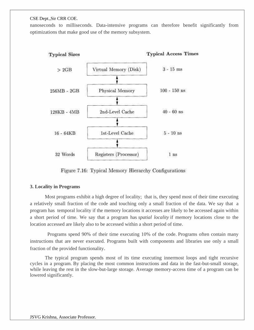
CSE Dept.,Sir CRR COE.
JSVG Krishna, Associate Professor.
nanoseconds to milliseconds. Data-intensive programs can therefore benefit significantly from
optimizations that make good use of the memory subsystem.
3. Locality in Programs
Most programs exhibit a high degree of locality; that is, they spend most of their time executing
a relatively small fraction of the code and touching only a small fraction of the data. We say that a
program has temporal locality if the memory locations it accesses are likely to be accessed again within
a short period of time. We say that a program has spatial locality if memory locations close to the
location accessed are likely also to be accessed within a short period of time.
Programs spend 90% of their time executing 10% of the code. Programs often contain many
instructions that are never executed. Programs built with components and libraries use only a small
fraction of the provided functionality.
The typical program spends most of its time executing innermost loops and tight recursive
cycles in a program. By placing the most common instructions and data in the fast-but-small storage,
while leaving the rest in the slow-but-large storage. Average memory-access time of a program can be
lowered significantly.
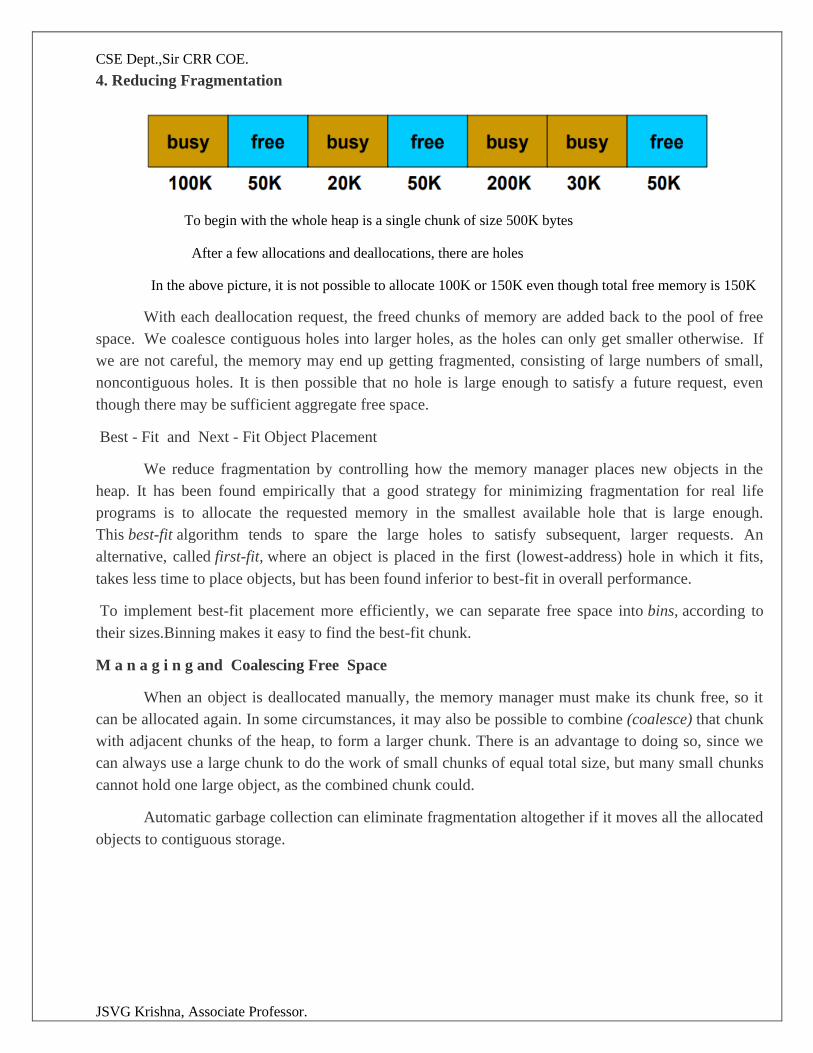
CSE Dept.,Sir CRR COE.
JSVG Krishna, Associate Professor.
4. Reducing Fragmentation
To begin with the whole heap is a single chunk of size 500K bytes
After a few allocations and deallocations, there are holes
In the above picture, it is not possible to allocate 100K or 150K even though total free memory is 150K
With each deallocation request, the freed chunks of memory are added back to the pool of free
space. We coalesce contiguous holes into larger holes, as the holes can only get smaller otherwise. If
we are not careful, the memory may end up getting fragmented, consisting of large numbers of small,
noncontiguous holes. It is then possible that no hole is large enough to satisfy a future request, even
though there may be sufficient aggregate free space.
Best - Fit and Next - Fit Object Placement
We reduce fragmentation by controlling how the memory manager places new objects in the
heap. It has been found empirically that a good strategy for minimizing fragmentation for real life
programs is to allocate the requested memory in the smallest available hole that is large enough.
This best-fit algorithm tends to spare the large holes to satisfy subsequent, larger requests. An
alternative, called first-fit, where an object is placed in the first (lowest-address) hole in which it fits,
takes less time to place objects, but has been found inferior to best-fit in overall performance.
To implement best-fit placement more efficiently, we can separate free space into bins, according to
their sizes.Binning makes it easy to find the best-fit chunk.
M a n a g i n g and Coalescing Free Space
When an object is deallocated manually, the memory manager must make its chunk free, so it
can be allocated again. In some circumstances, it may also be possible to combine (coalesce) that chunk
with adjacent chunks of the heap, to form a larger chunk. There is an advantage to doing so, since we
can always use a large chunk to do the work of small chunks of equal total size, but many small chunks
cannot hold one large object, as the combined chunk could.
Automatic garbage collection can eliminate fragmentation altogether if it moves all the allocated
objects to contiguous storage.
CSE Dept.,Sir CRR COE.
JSVG Krishna, Associate Professor.
5. Manual Deallocation Requests
In manual memory management, where the programmer must explicitly arrange for the
deallocation of data, as in C and C + + . Ideally, any storage that will no longer be accessed should be
deleted.
Problems with Manual Deallocation
1.Memory leaks ‰
Failing to delete data that cannot be referenced ‰
Important in long running or nonstop programs „
2.Dangling pointer dereferencing ‰
Referencing deleted data „
Both are serious and hard to debug
Garbage Collection „
1. Reclamation of chunks of storage holding objects that can no longer be accessed by a program „
2. GC should be able to determine types of objects ‰
Then, size and pointer fields of objects can be determined by the GC ‰
Languages in which types of objects can be determined at compile time or run-time are type
safe „
Java is type safe „
C and C++ are not type safe because they permit type casting, which creates new
pointers
„
Thus, any memory location can be (theoretically) accessed at any time and hence
cannot be considered inaccessible
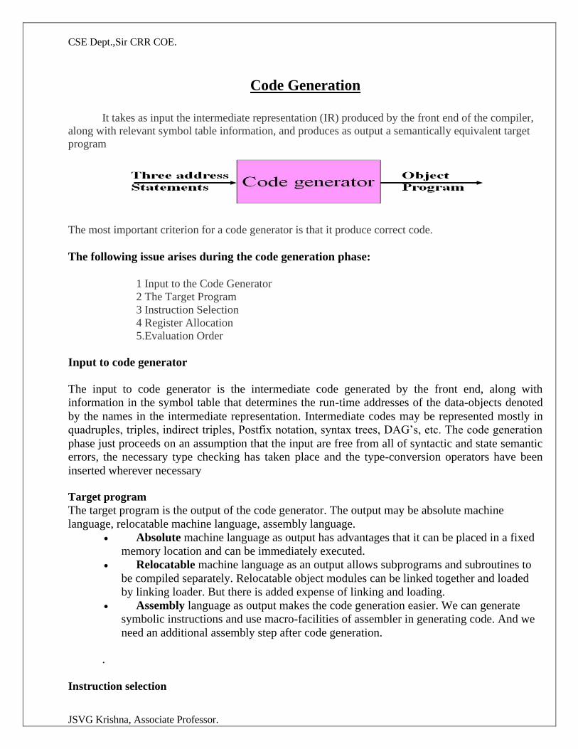
CSE Dept.,Sir CRR COE.
JSVG Krishna, Associate Professor.
Code Generation
It takes as input the intermediate representation (IR) produced by the front end of the compiler,
along with relevant symbol table information, and produces as output a semantically equivalent target
program
The most important criterion for a code generator is that it produce correct code.
The following issue arises during the code generation phase:
1 Input to the Code Generator 2 The Target Program 3 Instruction Selection 4 Register Allocation 5.Evaluation Order
Input to code generator
The input to code generator is the intermediate code generated by the front end, along with
information in the symbol table that determines the run-time addresses of the data-objects denoted
by the names in the intermediate representation. Intermediate codes may be represented mostly in
quadruples, triples, indirect triples, Postfix notation, syntax trees, DAG’s, etc. The code generation
phase just proceeds on an assumption that the input are free from all of syntactic and state semantic
errors, the necessary type checking has taken place and the type-conversion operators have been
inserted wherever necessary
Target program
The target program is the output of the code generator. The output may be absolute machine
language, relocatable machine language, assembly language.
• Absolute machine language as output has advantages that it can be placed in a fixed
memory location and can be immediately executed.
• Relocatable machine language as an output allows subprograms and subroutines to
be compiled separately. Relocatable object modules can be linked together and loaded
by linking loader. But there is added expense of linking and loading.
• Assembly language as output makes the code generation easier. We can generate
symbolic instructions and use macro-facilities of assembler in generating code. And we
need an additional assembly step after code generation.
.
Instruction selection
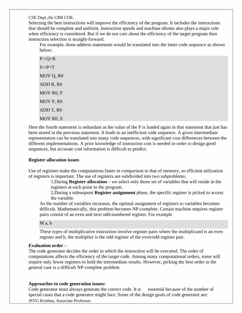
CSE Dept.,Sir CRR COE.
JSVG Krishna, Associate Professor.
Selecting the best instructions will improve the efficiency of the program. It includes the instructions
that should be complete and uniform. Instruction speeds and machine idioms also plays a major role
when efficiency is considered. But if we do not care about the efficiency of the target program then
instruction selection is straight-forward.
For example, three-address statements would be translated into the latter code sequence as shown
below:
P:=Q+R
S:=P+T
MOV Q, R0
ADD R, R0
MOV R0, P
MOV P, R0
ADD T, R0
MOV R0, S
Here the fourth statement is redundant as the value of the P is loaded again in that statement that just has
been stored in the previous statement. It leads to an inefficient code sequence. A given intermediate
representation can be translated into many code sequences, with significant cost differences between the
different implementations. A prior knowledge of instruction cost is needed in order to design good
sequences, but accurate cost information is difficult to predict.
Register allocation issues
Use of registers make the computations faster in comparison to that of memory, so efficient utilization
of registers is important. The use of registers are subdivided into two subproblems:
1.During Register allocation – we select only those set of variables that will reside in the
registers at each point in the program.
2.During a subsequent Register assignment phase, the specific register is picked to access
the variable.
As the number of variables increases, the optimal assignment of registers to variables becomes
difficult. Mathematically, this problem becomes NP-complete. Certain machine requires register
pairs consist of an even and next odd-numbered register. For example
M a, b
These types of multiplicative instruction involve register pairs where the multiplicand is an even
register and b, the multiplier is the odd register of the even/odd register pair.
Evaluation order –
The code generator decides the order in which the instruction will be executed. The order of
computations affects the efficiency of the target code. Among many computational orders, some will
require only fewer registers to hold the intermediate results. However, picking the best order in the
general case is a difficult NP-complete problem.
Approaches to code generation issues:
Code generator must always generate the correct code. It is essential because of the number of
special cases that a code generator might face. Some of the design goals of code generator are:
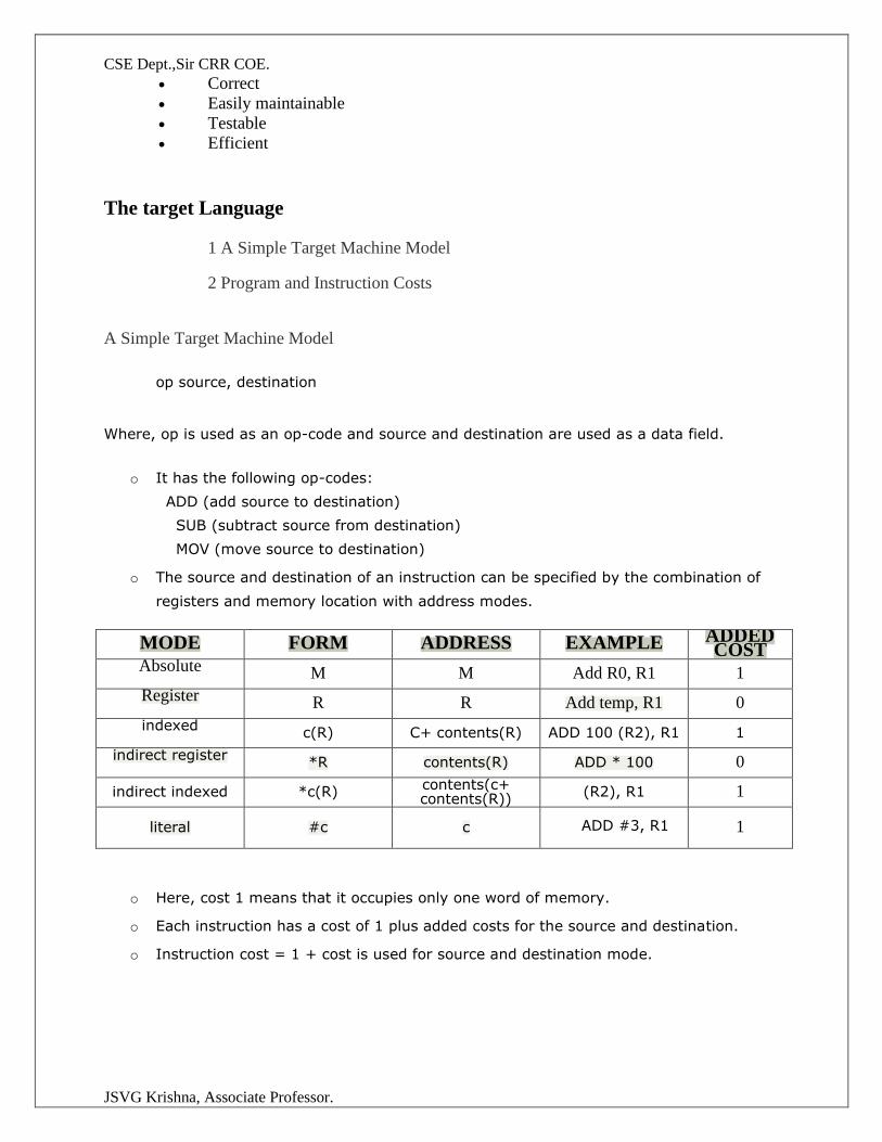
CSE Dept.,Sir CRR COE.
JSVG Krishna, Associate Professor.
• Correct
• Easily maintainable
• Testable
• Efficient
The target Language
1 A Simple Target Machine Model
2 Program and Instruction Costs
A Simple Target Machine Model
op source, destination
Where, op is used as an op-code and source and destination are used as a data field.
o It has the following op-codes:
ADD (add source to destination)
SUB (subtract source from destination)
MOV (move source to destination)
o The source and destination of an instruction can be specified by the combination of
registers and memory location with address modes.
MODE FORM ADDRESS EXAMPLE ADDED COST
Absolute M M Add R0, R1 1
Register R R Add temp, R1 0
indexed c(R) C+ contents(R) ADD 100 (R2), R1 1
indirect register *R contents(R) ADD * 100 0
indirect indexed *c(R) contents(c+ contents(R)) (R2), R1 1
literal #c c ADD #3, R1
1
o Here, cost 1 means that it occupies only one word of memory.
o Each instruction has a cost of 1 plus added costs for the source and destination.
o Instruction cost = 1 + cost is used for source and destination mode.
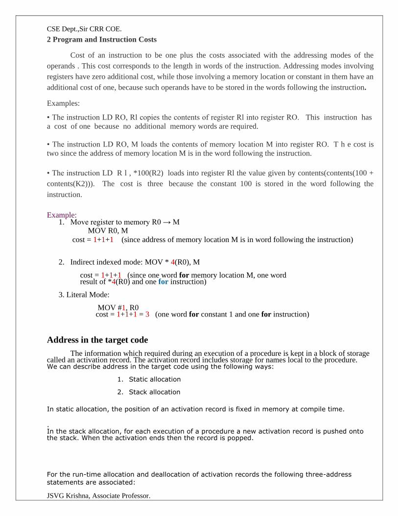
CSE Dept.,Sir CRR COE.
JSVG Krishna, Associate Professor.
2 Program and Instruction Costs
Cost of an instruction to be one plus the costs associated with the addressing modes of the
operands . This cost corresponds to the length in words of the instruction. Addressing modes involving
registers have zero additional cost, while those involving a memory location or constant in them have an
additional cost of one, because such operands have to be stored in the words following the instruction.
Examples:
• The instruction LD RO, Rl copies the contents of register Rl into register RO. This instruction has
a cost of one because no additional memory words are required.
• The instruction LD RO, M loads the contents of memory location M into register RO. T h e cost is
two since the address of memory location M is in the word following the instruction.
• The instruction LD R l , *100(R2) loads into register Rl the value given by contents(contents(100 +
contents(K2))). The cost is three because the constant 100 is stored in the word following the
instruction.
Example:
1. Move register to memory R0 → M MOV R0, M
cost = 1+1+1 (since address of memory location M is in word following the instruction)
2. Indirect indexed mode: MOV * 4(R0), M cost = 1+1+1 (since one word for memory location M, one word
result of *4(R0) and one for instruction) 3. Literal Mode: MOV #1, R0 cost = 1+1+1 = 3 (one word for constant 1 and one for instruction) Address in the target code
The information which required during an execution of a procedure is kept in a block of storage called an activation record. The activation record includes storage for names local to the procedure. We can describe address in the target code using the following ways:
1. Static allocation
2. Stack allocation
In static allocation, the position of an activation record is fixed in memory at compile time.
. In the stack allocation, for each execution of a procedure a new activation record is pushed onto the stack. When the activation ends then the record is popped.
For the run-time allocation and deallocation of activation records the following three-address
statements are associated:
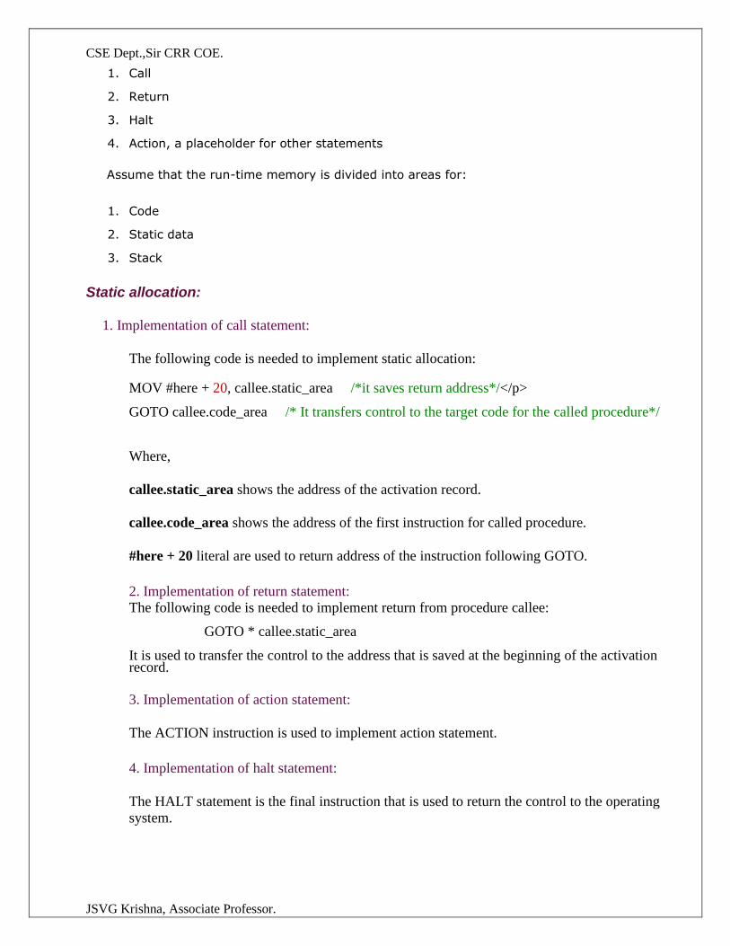
CSE Dept.,Sir CRR COE.
JSVG Krishna, Associate Professor.
1. Call
2. Return
3. Halt
4. Action, a placeholder for other statements
Assume that the run-time memory is divided into areas for:
1. Code
2. Static data
3. Stack
Static allocation:
1. Implementation of call statement:
The following code is needed to implement static allocation:
MOV #here + 20, callee.static_area /*it saves return address*/</p>
GOTO callee.code_area /* It transfers control to the target code for the called procedure*/
Where,
callee.static_area shows the address of the activation record.
callee.code_area shows the address of the first instruction for called procedure.
#here + 20 literal are used to return address of the instruction following GOTO.
2. Implementation of return statement:
The following code is needed to implement return from procedure callee: GOTO * callee.static_area
It is used to transfer the control to the address that is saved at the beginning of the activation record.
3. Implementation of action statement:
The ACTION instruction is used to implement action statement.
4. Implementation of halt statement:
The HALT statement is the final instruction that is used to return the control to the operating
system.
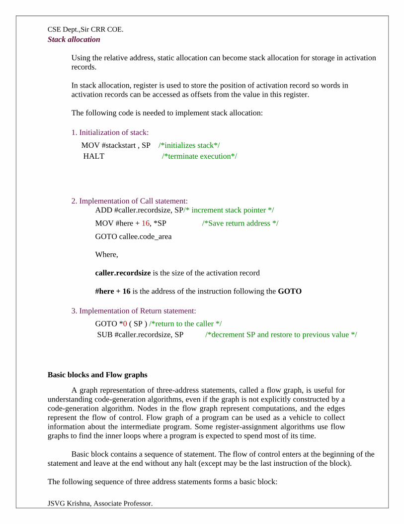
CSE Dept.,Sir CRR COE.
JSVG Krishna, Associate Professor.
Stack allocation
Using the relative address, static allocation can become stack allocation for storage in activation
records.
In stack allocation, register is used to store the position of activation record so words in
activation records can be accessed as offsets from the value in this register.
The following code is needed to implement stack allocation:
1. Initialization of stack:
MOV #stackstart , SP /*initializes stack*/
HALT /*terminate execution*/
2. Implementation of Call statement:
ADD #caller.recordsize, SP/* increment stack pointer */
MOV #here + 16, *SP /*Save return address */
GOTO callee.code_area
Where,
caller.recordsize is the size of the activation record
#here + 16 is the address of the instruction following the GOTO
3. Implementation of Return statement:
GOTO *0 ( SP ) /*return to the caller */
SUB #caller.recordsize, SP /*decrement SP and restore to previous value */ Basic blocks and Flow graphs
A graph representation of three-address statements, called a flow graph, is useful for
understanding code-generation algorithms, even if the graph is not explicitly constructed by a
code-generation algorithm. Nodes in the flow graph represent computations, and the edges
represent the flow of control. Flow graph of a program can be used as a vehicle to collect
information about the intermediate program. Some register-assignment algorithms use flow
graphs to find the inner loops where a program is expected to spend most of its time.
Basic block contains a sequence of statement. The flow of control enters at the beginning of the
statement and leave at the end without any halt (except may be the last instruction of the block).
The following sequence of three address statements forms a basic block:
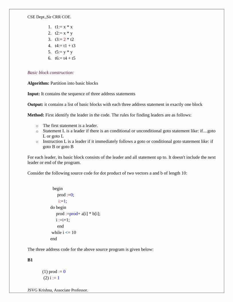
CSE Dept.,Sir CRR COE.
JSVG Krishna, Associate Professor.
1. t1:= x * x
2. t2:= x * y
3. t3:= 2 * t2
4. t4:= t1 + t3
5. t5:= y * y
6. t6:= t4 + t5
Basic block construction:
Algorithm: Partition into basic blocks
Input: It contains the sequence of three address statements
Output: it contains a list of basic blocks with each three address statement in exactly one block
Method: First identify the leader in the code. The rules for finding leaders are as follows:
o The first statement is a leader.
o Statement L is a leader if there is an conditional or unconditional goto statement like: if....goto
L or goto L
o Instruction L is a leader if it immediately follows a goto or conditional goto statement like: if
goto B or goto B
For each leader, its basic block consists of the leader and all statement up to. It doesn't include the next
leader or end of the program.
Consider the following source code for dot product of two vectors a and b of length 10:
begin
prod :=0;
i:=1;
do begin
prod :=prod+ a[i] * b[i];
i :=i+1;
end
while i <= 10
end
The three address code for the above source program is given below:
B1
(1) prod := 0
(2) i := 1
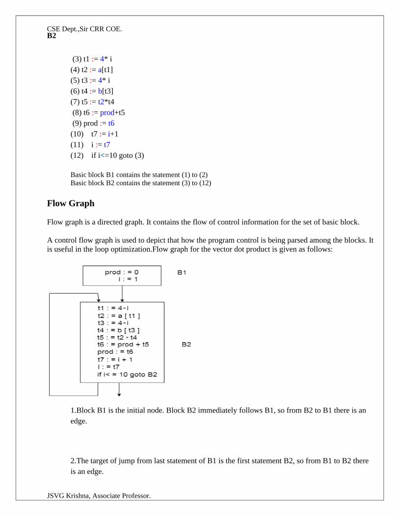
CSE Dept.,Sir CRR COE.
JSVG Krishna, Associate Professor.
B2
(3) t1 := 4* i
(4) t2 := a[t1]
(5) t3 := 4* i
(6) t4 := b[t3]
(7) t5 := t2*t4
(8) t6 := prod+t5
(9) prod := t6
(10) t7 := i+1
(11) i := t7
(12) if i<=10 goto (3)
Basic block B1 contains the statement (1) to (2)
Basic block B2 contains the statement (3) to (12)
Flow Graph
Flow graph is a directed graph. It contains the flow of control information for the set of basic block.
A control flow graph is used to depict that how the program control is being parsed among the blocks. It
is useful in the loop optimization.Flow graph for the vector dot product is given as follows:
1.Block B1 is the initial node. Block B2 immediately follows B1, so from B2 to B1 there is an
edge.
2.The target of jump from last statement of B1 is the first statement B2, so from B1 to B2 there
is an edge.
CSE Dept.,Sir CRR COE.
JSVG Krishna, Associate Professor.
A Simple Code generation.
Code generator is used to produce the target code for three-address statements. It uses registers
to store the operands of the three address statement. Consider the three address statement x:= y + z. It can have the following sequence of codes:
MOV x, R0
ADD y, R0
Register and Address Descriptors:
o A register descriptor contains the track of what is currently in each register. The register
descriptors show that all the registers are initially empty.
o An address descriptor is used to store the location where current value of the name can be found
at run time.
A code-generation algorithm:
The algorithm takes a sequence of three-address statements as input. For each three address statement of
the form a:= b op c perform the various actions. These are as follows:
1. Invoke a function getreg to find out the location L where the result of computation b op c should
be stored.
2. Consult the address description for y to determine y'. If the value of y currently in memory and
register both then prefer the register y' . If the value of y is not already in L then generate the
instruction MOV y' , L to place a copy of y in L.
3. Generate the instruction OP z' , L where z' is used to show the current location of z. if z is in
both then prefer a register to a memory location. Update the address descriptor of x to indicate
that x is in location L. If x is in L then update its descriptor and remove x from all other
descriptor.
4. If the current value of y or z have no next uses or not live on exit from the block or in register
then alter the register descriptor to indicate that after execution of x : = y op z those register will
no longer contain y or z.
Generating Code for Assignment Statements:
The assignment statement d:= (a-b) + (a-c) + (a-c) can be translated into the following sequence of three
address code:
t:= a-b
u:= a-c
v:= t +u
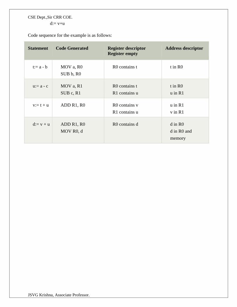
CSE Dept.,Sir CRR COE.
JSVG Krishna, Associate Professor.
d:= v+u Code sequence for the example is as follows:
Statement Code Generated Register descriptor
Register empty
Address descriptor
t:= a - b MOV a, R0
SUB b, R0
R0 contains t t in R0
u:= a - c MOV a, R1
SUB c, R1
R0 contains t
R1 contains u
t in R0
u in R1
v:= t + u ADD R1, R0 R0 contains v
R1 contains u
u in R1
v in R1
d:= v + u ADD R1, R0
MOV R0, d
R0 contains d d in R0
d in R0 and
memory
CSE Dept.,Sir CRR COE.
JSVG Krishna, Associate Professor.
LECTURE NOTES
ON
COMPILER DESIGN
2020 – 2021
III B. Tech I Semester (JNTUK-R16)
P. Naga Deepthi/ Mr J.S.V. Gopala Krishna
Department of Computer Science and
Engineering
SIR CRREDDY COLLEGE OF ENGINEERING,
ELURU
- 21 -
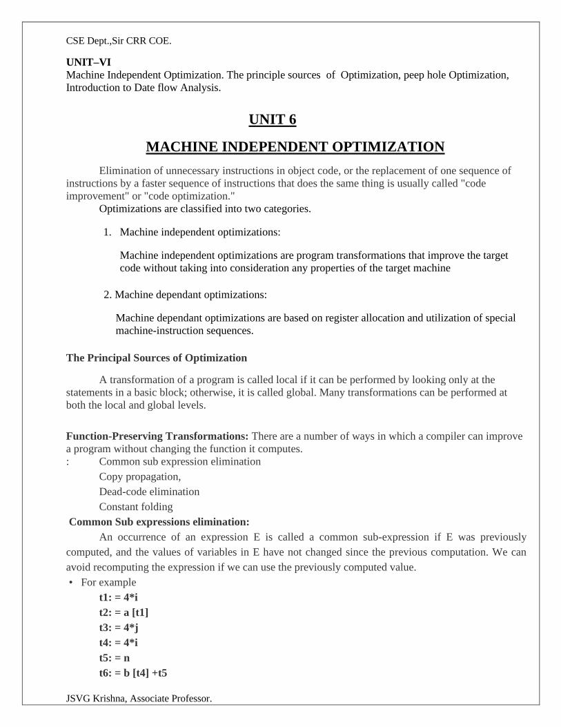
CSE Dept.,Sir CRR COE.
JSVG Krishna, Associate Professor.
UNIT–VI
Machine Independent Optimization. The principle sources of Optimization, peep hole Optimization,
Introduction to Date flow Analysis.
UNIT 6
MACHINE INDEPENDENT OPTIMIZATION
Elimination of unnecessary instructions in object code, or the replacement of one sequence of
instructions by a faster sequence of instructions that does the same thing is usually called "code
improvement" or "code optimization."
Optimizations are classified into two categories.
1. Machine independent optimizations:
Machine independent optimizations are program transformations that improve the target
code without taking into consideration any properties of the target machine
2. Machine dependant optimizations:
Machine dependant optimizations are based on register allocation and utilization of special
machine-instruction sequences.
The Principal Sources of Optimization
A transformation of a program is called local if it can be performed by looking only at the
statements in a basic block; otherwise, it is called global. Many transformations can be performed at
both the local and global levels.
Function-Preserving Transformations: There are a number of ways in which a compiler can improve
a program without changing the function it computes.
: Common sub expression elimination
Copy propagation,
Dead-code elimination
Constant folding
Common Sub expressions elimination:
An occurrence of an expression E is called a common sub-expression if E was previously
computed, and the values of variables in E have not changed since the previous computation. We can
avoid recomputing the expression if we can use the previously computed value.
• For example
t1: = 4*i
t2: = a [t1]
t3: = 4*j
t4: = 4*i
t5: = n
t6: = b [t4] +t5
CSE Dept.,Sir CRR COE.
JSVG Krishna, Associate Professor.
The above code can be optimized using the common sub-expression elimination as
t1: = 4*i
t2: = a [t1]
t3: = 4*j
t5: = n
t6: = b [t1] +t5
The common sub expression t4: =4*i is eliminated as its computation is already in t1 and the value of i
is not been changed from definition to use.
Copy Propagation:
Assignments of the form f : = g called copy statements, or copies for short. The idea behind the
copy-propagation transformation is to use g for f, whenever possible after the copy statement f: = g.
Copy propagation means use of one variable instead of another.
• For example:
x=Pi;
A=x*r*r;
The optimization using copy propagation can be done as follows: A=Pi*r*r;
Here the variable x is eliminated
Dead-Code Eliminations:
A variable is live at a point in a program if its value can be used subsequently; otherwise, it is
dead at that point.
Example:
i=0;
if(i==1)
{
a=b+5;
}
Here, ‘if’ statement is dead code because this condition will never get satisfied.
Constant folding:
Deducing at compile time that the value of an expression is a constant and using the constant
instead is known as constant folding. One advantage of copy propagation is that it often turns the copy
statement into dead code.
For example,
a=3.14157/2 can be replaced by
a=1.570
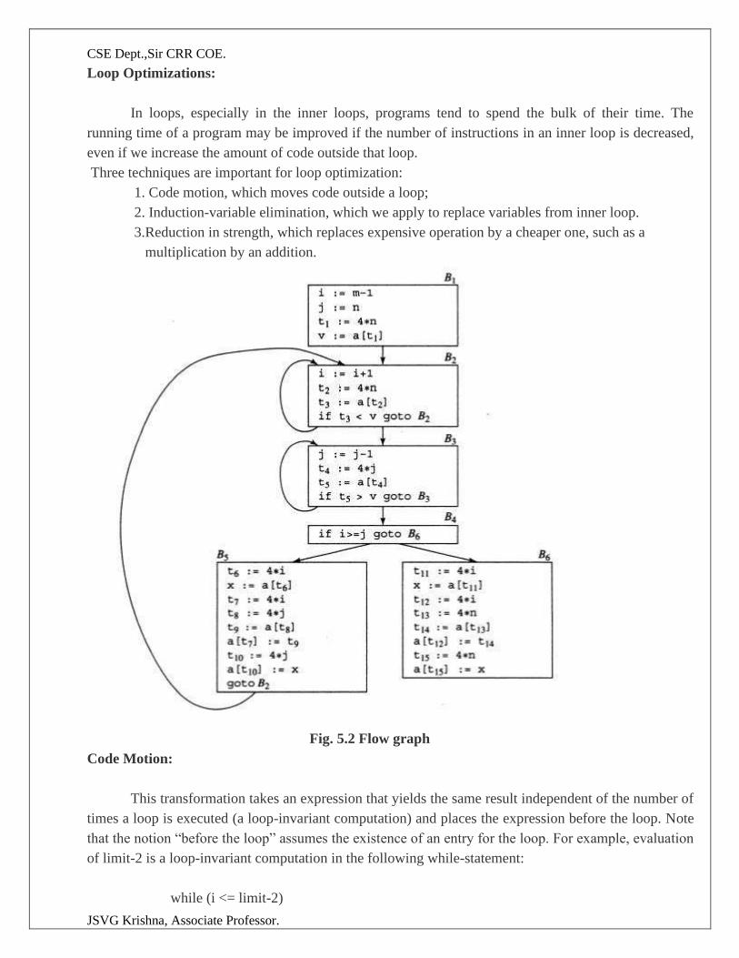
CSE Dept.,Sir CRR COE.
JSVG Krishna, Associate Professor.
Loop Optimizations:
In loops, especially in the inner loops, programs tend to spend the bulk of their time. The
running time of a program may be improved if the number of instructions in an inner loop is decreased,
even if we increase the amount of code outside that loop.
Three techniques are important for loop optimization:
1. Code motion, which moves code outside a loop;
2. Induction-variable elimination, which we apply to replace variables from inner loop.
3.Reduction in strength, which replaces expensive operation by a cheaper one, such as a
multiplication by an addition.
Fig. 5.2 Flow graph
Code Motion:
This transformation takes an expression that yields the same result independent of the number of
times a loop is executed (a loop-invariant computation) and places the expression before the loop. Note
that the notion “before the loop” assumes the existence of an entry for the loop. For example, evaluation
of limit-2 is a loop-invariant computation in the following while-statement:
while (i <= limit-2)
CSE Dept.,Sir CRR COE.
JSVG Krishna, Associate Professor.
Code motion will result in the equivalent of
t= limit-2;
while (i<=t) /* statement does not change limit or t */
Induction Variables :
Loops are usually processed inside out. For example consider the loop around B3. Note that the
values of j and t4 remain in lock-step; every time the value of j decreases by 1, that of t4 decreases by 4
because 4*j is assigned to t4. Such identifiers are called induction variables.
When there are two or more induction variables in a loop, it may be possible to get rid of all but
one, by the process of induction-variable elimination. For the inner loop around B3 in Fig.5.3 we cannot
get rid of either j or t4 completely; t4 is used in B3 and j in B4.
However, we can illustrate reduction in strength and illustrate a part of the process of induction-
variable elimination. Eventually j will be eliminated when the outer loop of B2- B5 is considered.
Example:
As the relationship t4:=4*j surely holds after such an assignment to t4 in Fig. and t4 is not
changed elsewhere in the inner loop around B3, it follows that just after the statement j:=j-1 the
relationship t4:= 4*j-4 must hold. We may therefore replace the assignment t4:= 4*j by t4:= t4-4. The
only problem is that t4 does not have a value when we enter block B3 for the first time. Since we must
maintain the relationship t4=4*j on entry to the block B3, we place an initializations of t4 at the end of
the block where j itself is initialized, shown by the dashed addition to block B1 in Fig.5.3.
The replacement of a multiplication by a subtraction will speed up the object code if
multiplication takes more time than addition or subtraction
Reduction In Strength:
Reduction in strength replaces expensive operations by equivalent cheaper ones on the target
machine. Certain machine instructions are considerably cheaper than others and can often be used as
special cases of more expensive operators. For example, x² is invariably cheaper to implement as x*x
than as a call to an exponentiation routine. Fixed-point multiplication or division by a power of two is
cheaper to implement as a shift. Floating-point division by a constant can be implemented as
multiplication by a constant, which may be cheaper.
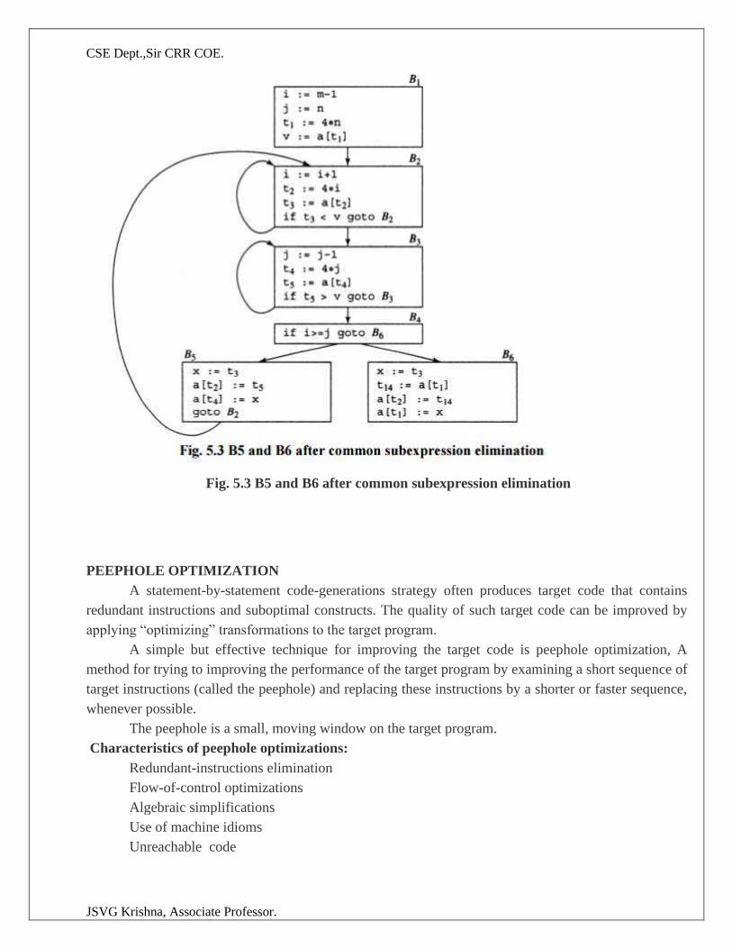
CSE Dept.,Sir CRR COE.
JSVG Krishna, Associate Professor.
Fig. 5.3 B5 and B6 after common subexpression elimination
PEEPHOLE OPTIMIZATION
A statement-by-statement code-generations strategy often produces target code that contains
redundant instructions and suboptimal constructs. The quality of such target code can be improved by
applying “optimizing” transformations to the target program.
A simple but effective technique for improving the target code is peephole optimization, A
method for trying to improving the performance of the target program by examining a short sequence of
target instructions (called the peephole) and replacing these instructions by a shorter or faster sequence,
whenever possible.
The peephole is a small, moving window on the target program.
Characteristics of peephole optimizations:
Redundant-instructions elimination
Flow-of-control optimizations
Algebraic simplifications
Use of machine idioms
Unreachable code
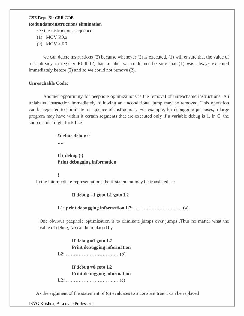
CSE Dept.,Sir CRR COE.
JSVG Krishna, Associate Professor.
Redundant-instructions elimination
see the instructions sequence
(1) MOV R0,a
(2) MOV a,R0
we can delete instructions (2) because whenever (2) is executed. (1) will ensure that the value of
a is already in register R0.If (2) had a label we could not be sure that (1) was always executed
immediately before (2) and so we could not remove (2).
Unreachable Code:
Another opportunity for peephole optimizations is the removal of unreachable instructions. An
unlabeled instruction immediately following an unconditional jump may be removed. This operation
can be repeated to eliminate a sequence of instructions. For example, for debugging purposes, a large
program may have within it certain segments that are executed only if a variable debug is 1. In C, the
source code might look like:
#define debug 0
….
If ( debug ) {
Print debugging information
}
In the intermediate representations the if-statement may be translated as:
If debug =1 goto L1 goto L2
L1: print debugging information L2: ………………………… (a)
One obvious peephole optimization is to eliminate jumps over jumps .Thus no matter what the
value of debug; (a) can be replaced by:
If debug ≠1 goto L2
Print debugging information
L2: …………………………… (b)
If debug ≠0 goto L2
Print debugging information
L2: …………………………… (c)
As the argument of the statement of (c) evaluates to a constant true it can be replaced
CSE Dept.,Sir CRR COE.
JSVG Krishna, Associate Professor.
By goto L2. Then all the statement that print debugging aids are manifestly unreachable and can
be eliminated one at a time.
Flows-Of-Control Optimizations:
The unnecessary jumps can be eliminated in either the intermediate code or the target code by
the following types of peephole optimizations. We can replace the jump sequence
goto L1
….
L1: gotoL2 (d)
by the sequence
goto L2
….
L1: goto L2
If there are now no jumps to L1, then it may be possible to eliminate the statement L1:goto L2
provided it is preceded by an unconditional jump .Similarly, the sequence
if a < b goto L1
….
L1: goto L2 (e)
can be replaced by
If a < b goto L2
….
L1: goto L2
Ø Finally, suppose there is only one jump to L1 and L1 is preceded by an unconditional goto.
Then the sequence
goto L1
L1: if a < b goto L2 (f) L3:
may be replaced by
CSE Dept.,Sir CRR COE.
JSVG Krishna, Associate Professor.
If a < b goto L2
goto L3
…….
L3:
While the number of instructions in(e) and (f) is the same, we sometimes skip the unconditional jump
in (f), but never in (e).Thus (f) is superior to (e) in execution time
Algebraic Simplification:
There is no end to the amount of algebraic simplification that can be attempted through peephole
optimization. Only a few algebraic identities occur frequently enough that it is worth considering
implementing them. For example, statements such as
x := x+0 or
x := x * 1
are often produced by straightforward intermediate code-generation algorithms, and they can be
eliminated easily through peephole optimization.
Reduction in Strength:
Reduction in strength replaces expensive operations by equivalent cheaper ones on the target
machine. Certain machine instructions are considerably cheaper than others and can often be used as
special cases of more expensive operators.
For example, x² is invariably cheaper to implement as x*x than as a call to an exponentiation
routine. Fixed-point multiplication or division by a power of two is cheaper to implement as a shift.
Floating-point division by a constant can be implemented as multiplication by a constant, which may be
cheaper.
X2 → X*X
Use of Machine Idioms:
The target machine may have hardware instructions to implement certain specific operations
efficiently. For example, some machines have auto-increment and auto-decrement addressing modes.
These add or subtract one from an operand before or after using its value. The use of these modes
greatly improves the quality of code when pushing or popping a stack, as in parameter passing. These
modes can also be used in code for statements like i : =i+1.
i:=i+1 → i++
CSE Dept.,Sir CRR COE.
JSVG Krishna, Associate Professor.
i:=i-1 → i- -
Introduction to Date flow Analysis.
1 The Data-Flow Abstraction
2 The Data-Flow Analysis Schema
3 Data-Flow Schemas on Basic Blocks
4 Reaching Definitions
5 Live-Variable Analysis
6 Available Expressions
"Data-flow analysis" refers to a body of techniques that derive information about the flow of data along
program execution paths.
1. The Data-Flow Abstraction
The execution of a program can be viewed as a series of transformations of the program state,
which consists of the values of all the variables in the program. Each execution of an intermediate-code
statement transforms an input state to a new output state. The input state is associated with the program
point before the statement and the output state is associated with the program point after the statement.
When we analyze the behavior of a program, we must consider all the possible sequences of
program points ("paths") through a flow graph that the program execution can take. We then extract,
from the possible program states at each point, the information we need for the particular data-flow
analysis problem we want to solve. In more complex analyses, we must consider paths that jump among
the flow graphs for various procedures, as calls and returns are executed.
Within one basic block, the program point after a statement is the same as the program point
before the next statement.
If there is an edge from block B1 to block B22 , then the program point after the last statement
of B1 may be followed immediately by the program point before the first statement of B2.
Thus, we may define an execution path (or just path) from point pi to point pn to be a sequence of
points pi,p2,... ,pn such that for each i = 1,2, ... ,n - 1, either
1. Pi is the point immediately preceding a statement and pi+i is the point immediately following
that same statement, or
2.pi is the end of some block and pi+1 is the beginning of a successor block.
CSE Dept.,Sir CRR COE.
JSVG Krishna, Associate Professor.
. In data-flow analysis, we do not distinguish among the paths taken to reach a program point.
Moreover, we do not keep track of entire states; rather, we abstract out certain details, keeping only the
data we need for the purpose of the analysis. Two examples will illustrate how the same program states
may lead to different information abstracted at a point.
1. To help users debug their programs, we may wish to find out what are all the values a variable may
have at a program point, and where these values may be defined. For instance, we may summarize all
the program states at point (5) by saying that the value of a is one of {1,243}, and that it may be defined
by one of { ^ 1 , ^ 3 } . The definitions that may reach a program point along some path are known
as reaching definitions.
2. Suppose, instead, we are interested in implementing constant folding. If a use of the variable x is
reached by only one definition, and that definition assigns a constant to x, then we can simply
replace x by the constant. If, on the other hand, several definitions of x may reach a single program
point, then we cannot perform constant folding on x. Thus, for constant folding we wish to find those
definitions that are the unique definition of their variable to reach a given program point, no matter
which execution path is taken. For point (5) of Fig. 9.12, there is no definition that must be the
definition of a at that point, so this set is empty for a at point (5). Even if a variable has a unique
definition at a point, that definition must assign a constant to the variable. Thus, we may simply
describe certain variables as "not a constant," instead of collecting all their possible values or all their
possible definitions.
2. The Data-Flow Analysis Schema
, we associate with every program point a data-flow value that represents an abstraction of the set of all
possible program states that can be observed for that point. The set of possible data-flow values is the
domain for this application. For example, the domain of data-flow values for reaching definitions is the
set of all subsets of definitions in the program.
CSE Dept.,Sir CRR COE.
JSVG Krishna, Associate Professor.
A particular data-flow value is a set of definitions, and we want to associate with each point in the
program the exact set of definitions that can reach that point. As discussed above, the choice of
abstraction depends on the goal of the analysis; to be efficient, we only keep track of information that is
relevant.
Denote the data-flow values before and after each statement s by IN[S ] and OUT[s], respectively.
The data-flow problem is to find a solution to a set of constraints on the IN[S]'S and OUT[s]'s, for all
statements s. There are two sets of constraints: those based on the semantics of the statements ("transfer
functions") and those based on the flow of control.
Transfer Functions
The data-flow values before and after a statement are constrained by the semantics of the statement. For
example, suppose our data-flow analysis involves determining the constant value of variables at points.
If variable a has value v before executing statement b = a, then both a and b will have the value v after
the statement. This relationship between the data-flow values before and after the assignment
statement is known as a transfer function.
Transfer functions come in two flavors: information may propagate forward along execution paths, or it
may flow backwards up the execution paths. In a forward-flow problem, the transfer function of a
statement s, which we shall usually denote f(a), takes the data-flow value before the statement and
produces a new data-flow value after the statement. That is,
Conversely, in a backward-flow problem, the transfer function f(a) for statement 8 converts a data-flow
value after the statement to a new data-flow value before the statement. That is,
Control – Flow Constraints
The second set of constraints on data-flow values is derived from the flow of control. Within a basic
block, control flow is simple. If a block B consists of statements s1, s 2 , • • • ,sn in that order, then the
control-flow value out of Si is the same as the control-flow value into Si+i. That is,
However, control-flow edges between basic blocks create more complex constraints between the last
statement of one basic block and the first statement of the following block. For example, if we are
interested in collecting all the definitions that may reach a program point, then the set of definitions
reaching the leader statement of a basic block is the union of the definitions after the last statements of
each of the predecessor blocks. The next section gives the details of how data flows among the blocks.
CSE Dept.,Sir CRR COE.
JSVG Krishna, Associate Professor.
3. Data-Flow Schemas on Basic Blocks
While a data-flow schema involves data-flow values at each point in the program, we can save time
and space by recognizing that what goes on inside a block is usually quite simple. Control flows from
the beginning to the end of the block, without interruption or branching. Thus, we can restate the
schema in terms of data-flow values entering and leaving the blocks. We denote the data-flow values
immediately before and immediately after each basic block B by m[B] and 0 U T [ S ] , respectively.
The constraints involving m[B] and 0UT[B] can be derived from those involving w[s] and OUT[s] for
the various statements s in B as follows.
Suppose block B consists of statements s 1 , . . . , sn, in that order. If si is the first statement of basic
block B, then m[B] = I N [ S I ] , Similarly, if sn is the last statement of basic block B, then OUT[S] =
OUT[s„] . The transfer function of a basic block B, which we denote fB, can be derived by composing
the transfer functions of the statements in the block. That is, let fa. be the transfer function of
statement st. Then of statement si. Then fB = f,sn, o . . . o f,s2, o fsl. . The relationship between the
beginning and end of the block is
The constraints due to control flow between basic blocks can easily be rewritten by
substituting IN[B] and OUT[B] for IN[SI ] and OUT[sn], respectively. For instance, if data-flow values
are information about the sets of constants that may be assigned to a variable, then we have a forward-
flow problem in which
When the data-flow is backwards as we shall soon see in live-variable analy-sis, the equations are
similar, but with the roles of the IN's and OUT's reversed. That is,
Unlike linear arithmetic equations, the data-flow equations usually do not have a unique solution. Our
goal is to find the most "precise" solution that satisfies the two sets of constraints: control-flow and
transfer constraints. That is, we need a solution that encourages valid code improvements, but does not
justify unsafe transformations — those that change what the program computes.
4. Reaching Definitions
CSE Dept.,Sir CRR COE.
JSVG Krishna, Associate Professor.
"Reaching definitions" is one of the most common and useful data-flow schemas. By knowing where in
a program each variable x may have been defined when control reaches each point p, we can determine
many things about x. For just two examples, a compiler then knows whether x is a constant at
point p, and a debugger can tell whether it is possible for x to be an undefined variable, should x be used
at p.
We say a definition d reaches a point p if there is a path from the point immediately
following d to p, such that d is not "killed" along that path. We kill a definition of a variable x if there is
any other definition of x anywhere along the path . if a definition d of some variable x reaches point p,
then d might be the place at which the value of x used at p was last defined.
A definition of a variable x is a statement that assigns, or may assign, a value to x. Procedure
parameters, array accesses, and indirect references all may have aliases, and it is not easy to tell if a
statement is referring to a particular variable x. Program analysis must be conservative; if we do not
note that the path may have loops, so we could come to another occurrence of d along the path, which
does not "kill" d.
know whether a statement s is assigning a value to x, we must assume that it may assign to it; that is,
variable x after statement s may have either its original value before s or the new value created by s. For
the sake of simplicity, the rest of the chapter assumes that we are dealing only with variables that have
no aliases. This class of variables includes all local scalar variables in most languages; in the case of C
and C++, local variables whose addresses have been computed at some point are excluded.
Transfer Equations for Reaching Definitions
Start by examining the details of a single statement. Consider a definition
Here, and frequently in what follows, + is used as a generic binary operator. This statement "generates"
a definition d of variable u and "kills" all the
other definitions in the program that define variable u, while leaving the re-maining incoming
definitions unaffected. The transfer function of definition d thus can be expressed as
where gend = {d}, the set of definitions generated by the statement, and killd is the set of all other
definitions of u in the program.
The transfer function of a basic block can be found by composing the transfer functions of the
statements contained therein. The composition of functions of the form (9.1), which we shall refer to as
"gen-kill form," is also of that form, as we can see as follows. Suppose there are two functions fi(x) =
gen1 U (x - kill1) and f2(x) = gen2 U (x — kill2). Then
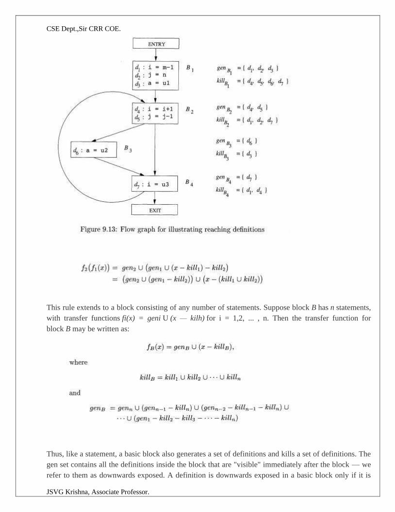
CSE Dept.,Sir CRR COE.
JSVG Krishna, Associate Professor.
This rule extends to a block consisting of any number of statements. Suppose block B has n statements,
with transfer functions fi(x) = geni U (x — kilh) for i = 1,2, ... , n. Then the transfer function for
block B may be written as:
Thus, like a statement, a basic block also generates a set of definitions and kills a set of definitions. The
gen set contains all the definitions inside the block that are "visible" immediately after the block — we
refer to them as downwards exposed. A definition is downwards exposed in a basic block only if it is
CSE Dept.,Sir CRR COE.
JSVG Krishna, Associate Professor.
not "killed" by a subsequent definition to the same variable inside the same basic block. A basic block's
kill set is simply the union of all the definitions killed by the individual statements. Notice that a
definition may appear in both the gen and kill set of a basic block. If so, the fact that it is in gen takes
precedence, because in gen-kill form, the kill set is applied before the gen set.
Example 9 . 1 0 : The gen set for the basic block
is {d2} since d1 is not downwards exposed. The kill set contains both d1 and d2, since d1 kills d2
and vice versa. Nonetheless, since the subtraction of the kill set precedes the union operation with the
gen set, the result of the transfer function for this block always includes definition d2.
Control - Flow Equations
Next, we consider the set of constraints derived from the control flow between basic blocks. Since a
definition reaches a program point as long as there exists at least one path along which the definition
reaches, O U T [ P ] C m[B] whenever there is a control-flow edge from P to B. However, since a
definition cannot reach a point unless there is a path along which it reaches, w[B] needs to be no larger
than the union of the reaching definitions of all the predecessor blocks. That is, it is safe to assume
We refer to union as the meet operator for reaching definitions. In any data-flow schema, the meet
operator is the one we use to create a summary of the contributions from different paths at the
confluence of those paths.
Iterative Algorithm for Reaching Definitions
We assume that every control-flow graph has two empty basic blocks, an ENTRY node, which
represents the starting point of the graph, and an EXIT node to which all exits out of the graph go.
Since no definitions reach the beginning of the graph, the transfer function for the ENTRY block is a
simple constant function that returns 0 as an answer. That is, O U T [ E N T R Y ] = 0.
The reaching definitions problem is defined by the following equations:
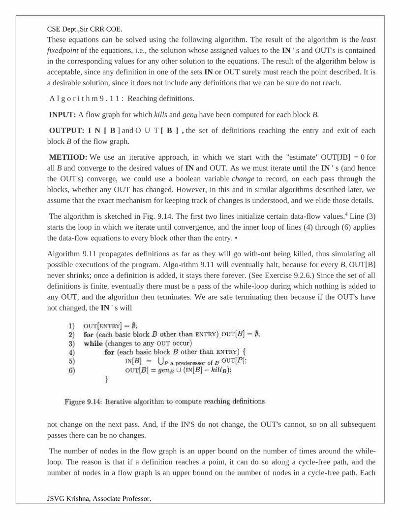
CSE Dept.,Sir CRR COE.
JSVG Krishna, Associate Professor.
These equations can be solved using the following algorithm. The result of the algorithm is the least
fixedpoint of the equations, i.e., the solution whose assigned values to the IN ' s and OUT's is contained
in the corresponding values for any other solution to the equations. The result of the algorithm below is
acceptable, since any definition in one of the sets IN or OUT surely must reach the point described. It is
a desirable solution, since it does not include any definitions that we can be sure do not reach.
A l g o r i t h m 9 . 1 1 : Reaching definitions.
INPUT: A flow graph for which kills and genB have been computed for each block B.
OUTPUT: I N [ B ] and O U T [ B ] , the set of definitions reaching the entry and exit of each
block B of the flow graph.
METHOD: We use an iterative approach, in which we start with the "estimate" OUT[JB] = 0 for
all B and converge to the desired values of IN and OUT. As we must iterate until the IN ' s (and hence
the OUT's) converge, we could use a boolean variable change to record, on each pass through the
blocks, whether any OUT has changed. However, in this and in similar algorithms described later, we
assume that the exact mechanism for keeping track of changes is understood, and we elide those details.
The algorithm is sketched in Fig. 9.14. The first two lines initialize certain data-flow values.4 Line (3)
starts the loop in which we iterate until convergence, and the inner loop of lines (4) through (6) applies
the data-flow equations to every block other than the entry. •
Algorithm 9.11 propagates definitions as far as they will go with-out being killed, thus simulating all
possible executions of the program. Algo-rithm 9.11 will eventually halt, because for every B, OUT[B]
never shrinks; once a definition is added, it stays there forever. (See Exercise 9.2.6.) Since the set of all
definitions is finite, eventually there must be a pass of the while-loop during which nothing is added to
any OUT, and the algorithm then terminates. We are safe terminating then because if the OUT's have
not changed, the IN ' s will
not change on the next pass. And, if the IN'S do not change, the OUT's cannot, so on all subsequent
passes there can be no changes.
The number of nodes in the flow graph is an upper bound on the number of times around the while-
loop. The reason is that if a definition reaches a point, it can do so along a cycle-free path, and the
number of nodes in a flow graph is an upper bound on the number of nodes in a cycle-free path. Each
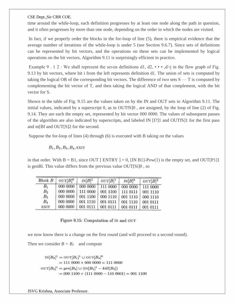
CSE Dept.,Sir CRR COE.
JSVG Krishna, Associate Professor.
time around the while-loop, each definition progresses by at least one node along the path in question,
and it often progresses by more than one node, depending on the order in which the nodes are visited.
In fact, if we properly order the blocks in the for-loop of line (5), there is empirical evidence that the
average number of iterations of the while-loop is under 5 (see Section 9.6.7). Since sets of definitions
can be represented by bit vectors, and the operations on these sets can be implemented by logical
operations on the bit vectors, Algorithm 9.11 is surprisingly efficient in practice.
Example 9 . 1 2 : We shall represent the seven definitions d1, d2, • • • ,d>j in the flow graph of Fig.
9.13 by bit vectors, where bit i from the left represents definition d{. The union of sets is computed by
taking the logical OR of the corresponding bit vectors. The difference of two sets S — T is computed by
complementing the bit vector of T, and then taking the logical AND of that complement, with the bit
vector for S.
Shown in the table of Fig. 9.15 are the values taken on by the IN and OUT sets in Algorithm 9.11. The
initial values, indicated by a superscript 0, as in OUTfS]0 , are assigned, by the loop of line (2) of Fig.
9.14. They are each the empty set, represented by bit vector 000 0000. The values of subsequent passes
of the algorithm are also indicated by superscripts, and labeled IN [I?]1 and OUTfS]1 for the first pass
and m[Bf and OUT[S]2 for the second.
Suppose the for-loop of lines (4) through (6) is executed with B taking on the values
in that order. With B = B1, since OUT [ ENTRY ] = 0, [IN B1]-Pow(1) is the empty set, and OUT[P1]1
is genBl. This value differs from the previous value OUT[Si]0 , so
we now know there is a change on the first round (and will proceed to a second round).
Then we consider B = B2 and compute
CSE Dept.,Sir CRR COE.
JSVG Krishna, Associate Professor.
This computation is summarized in Fig. 9.15. For instance, at the end of the first pass, OUT [ 5 2 ] 1 =
001 1100, reflecting the fact that d4 and d5 are generated in B2, while d3 reaches the beginning of B2
and is not killed in B2.
Notice that after the second round, OUT [ B2 ] has changed to reflect the fact that d& also reaches the
beginning of B2 and is not killed by B2. We did not learn that fact on the first pass, because the path
from d6 to the end of B2, which is B3 -» B4 -> B2, is not traversed in that order by a single pass. That
is, by the time we learn that d$ reaches the end of B4, we have already computed IN[B2 ] and OUT [ B
2 ] on the first pass.
There are no changes in any of the OUT sets after the second pass. Thus, after a third pass, the
algorithm terminates, with the IN's and OUT's as in the final two columns of Fig. 9.15.
5. Live-Variable Analysis
Some code-improving transformations depend on information computed in the direction opposite to the
flow of control in a program; we shall examine one such example now. In live-variable analysis we
wish to know for variable x and point p whether the value of x at p could be used along some path in the
flow graph starting at p. If so, we say x is live at p; otherwise, x is dead at p.
An important use for live-variable information is register allocation for basic blocks. Aspects of this
issue were introduced in Sections 8.6 and 8.8. After a value is computed in a register, and presumably
used within a block, it is not necessary to store that value if it is dead at the end of the block. Also, if all
registers are full and we need another register, we should favor using a register with a dead value, since
that value does not have to be stored.
Here, we define the data-flow equations directly in terms of IN [5] and OUTpB], which represent
the set of variables live at the points immediately before and after block B, respectively. These
equations can also be derived by first defining the transfer functions of individual statements and
composing them to create the transfer function of a basic block. Define
1. defB as the set of variables defined (i.e., definitely assigned values) in B prior to any use of that
variable in B, and useB as the set of variables whose values may be used in B prior to any definition of
the variable.
Example 9 . 1 3 : For instance, block B2 in Fig. 9.13 definitely uses i. It also uses j before any
redefinition of j, unless it is possible that i and j are aliases of one another. Assuming there are no
aliases among the variables in Fig. 9.13, then uses2 = {i,j}- Also, B2 clearly defines i and j.
Assuming there are no aliases, defB2 = as well.
As a consequence of the definitions, any variable in useB must be considered live on entrance to block
B, while definitions of variables in defB definitely are dead at the beginning of B. In effect,
membership in defB "kills" any opportunity for a variable to be live because of paths that begin at B.
Thus, the equations relating def and use to the unknowns IN and OUT are defined as follows:
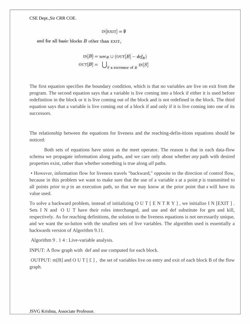
CSE Dept.,Sir CRR COE.
JSVG Krishna, Associate Professor.
The first equation specifies the boundary condition, which is that no variables are live on exit from the
program. The second equation says that a variable is live coming into a block if either it is used before
redefinition in the block or it is live coming out of the block and is not redefined in the block. The third
equation says that a variable is live coming out of a block if and only if it is live coming into one of its
successors.
The relationship between the equations for liveness and the reaching-defin-itions equations should be
noticed:
Both sets of equations have union as the meet operator. The reason is that in each data-flow
schema we propagate information along paths, and we care only about whether any path with desired
properties exist, rather than whether something is true along all paths.
• However, information flow for liveness travels "backward," opposite to the direction of control flow,
because in this problem we want to make sure that the use of a variable x at a point p is transmitted to
all points prior to p in an execution path, so that we may know at the prior point that x will have its
value used.
To solve a backward problem, instead of initializing O U T [ E N T R Y ] , we initialize I N [EXIT ] .
Sets I N and O U T have their roles interchanged, and use and def substitute for gen and kill,
respectively. As for reaching definitions, the solution to the liveness equations is not necessarily unique,
and we want the so-lution with the smallest sets of live variables. The algorithm used is essentially a
backwards version of Algorithm 9.11.
Algorithm 9 . 1 4 : Live-variable analysis.
INPUT: A flow graph with def and use computed for each block.
OUTPUT: m[B] and O U T [ £ ] , the set of variables live on entry and exit of each block B of the flow
graph.
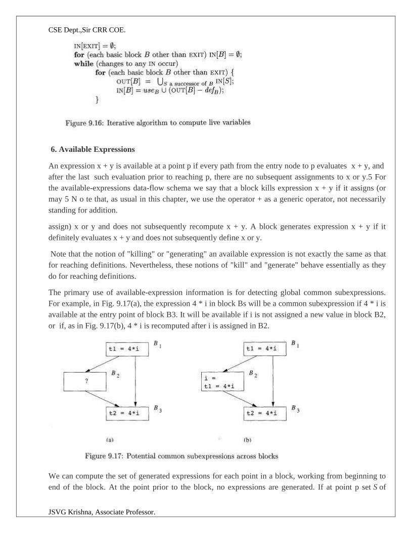
CSE Dept.,Sir CRR COE.
JSVG Krishna, Associate Professor.
6. Available Expressions
An expression x + y is available at a point p if every path from the entry node to p evaluates x + y, and
after the last such evaluation prior to reaching p, there are no subsequent assignments to x or y.5 For
the available-expressions data-flow schema we say that a block kills expression x + y if it assigns (or
may 5 N o te that, as usual in this chapter, we use the operator + as a generic operator, not necessarily
standing for addition.
assign) x or y and does not subsequently recompute x + y. A block generates expression x + y if it
definitely evaluates x + y and does not subsequently define x or y.
Note that the notion of "killing" or "generating" an available expression is not exactly the same as that
for reaching definitions. Nevertheless, these notions of "kill" and "generate" behave essentially as they
do for reaching definitions.
The primary use of available-expression information is for detecting global common subexpressions.
For example, in Fig. 9.17(a), the expression 4 * i in block Bs will be a common subexpression if 4 * i is
available at the entry point of block B3. It will be available if i is not assigned a new value in block B2,
or if, as in Fig. 9.17(b), 4 * i is recomputed after i is assigned in B2.
We can compute the set of generated expressions for each point in a block, working from beginning to
end of the block. At the point prior to the block, no expressions are generated. If at point p set S of
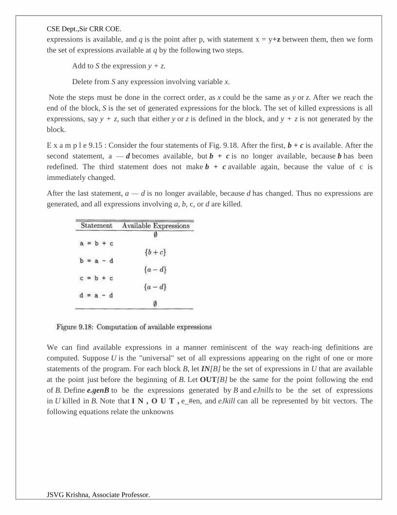
CSE Dept.,Sir CRR COE.
JSVG Krishna, Associate Professor.
expressions is available, and q is the point after p, with statement x = y+z between them, then we form
the set of expressions available at q by the following two steps.
Add to S the expression y + z.
Delete from S any expression involving variable x.
Note the steps must be done in the correct order, as x could be the same as y or z. After we reach the
end of the block, S is the set of generated expressions for the block. The set of killed expressions is all
expressions, say y + z, such that either y or z is defined in the block, and y + z is not generated by the
block.
E x a m p l e 9.15 : Consider the four statements of Fig. 9.18. After the first, b + c is available. After the
second statement, a — d becomes available, but b + c is no longer available, because b has been
redefined. The third statement does not make b + c available again, because the value of c is
immediately changed.
After the last statement, a — d is no longer available, because d has changed. Thus no expressions are
generated, and all expressions involving a, b, c, or d are killed.
We can find available expressions in a manner reminiscent of the way reach-ing definitions are
computed. Suppose U is the "universal" set of all expressions appearing on the right of one or more
statements of the program. For each block B, let IN[B] be the set of expressions in U that are available
at the point just before the beginning of B. Let OUT[B] be the same for the point following the end
of B. Define e.genB to be the expressions generated by B and eJnills to be the set of expressions
in U killed in B. Note that I N , O U T , e_#en, and eJkill can all be represented by bit vectors. The
following equations relate the unknowns
CSE Dept.,Sir CRR COE.
JSVG Krishna, Associate Professor.
T he above equations look almost identical to the equations for reaching definitions. Like reaching
definitions, the boundary condition is OUT [ ENTRY ] = 0, because at the exit of the E N T R Y node,
there are no available expressions.
The most important difference is that the meet operator is intersection rather than union. This operator is
the proper one because an expression is available at the beginning of a block only if it is available at the
end of all its predecessors. In contrast, a definition reaches the beginning of a block whenever it reaches
the end of any one or more of its predecessors.
The use of D rather than U makes the available-expression equations behave differently from those of
reaching definitions. While neither set has a unique solution, for reaching definitions, it is the solution
with the smallest sets that corresponds to the definition of "reaching," and we obtained that solution by
starting with the assumption that nothing reached anywhere, and building up to the solution. In that
way, we never assumed that a definition d could reach a point p unless an actual path
propagating d to p could be found. In contrast, for available expression equations we want the solution
with the largest sets of available expressions, so we start with an approximation that is too large and
work down.
It may not be obvious that by starting with the assumption "everything (i.e., the set U) is available
everywhere except at the end of the entry block" and eliminating only those expressions for which we
can discover a path along which it is not available, we do reach a set of truly available expressions. In
the case of available expressions, it is conservative to produce a subset of the exact set of available
expressions. The argument for subsets being conservative is that our intended use of the information is
to replace the computation of an available expression by a previously computed value. Not knowing an
expres-sion is available only inhibits us from improving the code, while believing an expression is
available when it is not could cause us to change what the program computes.
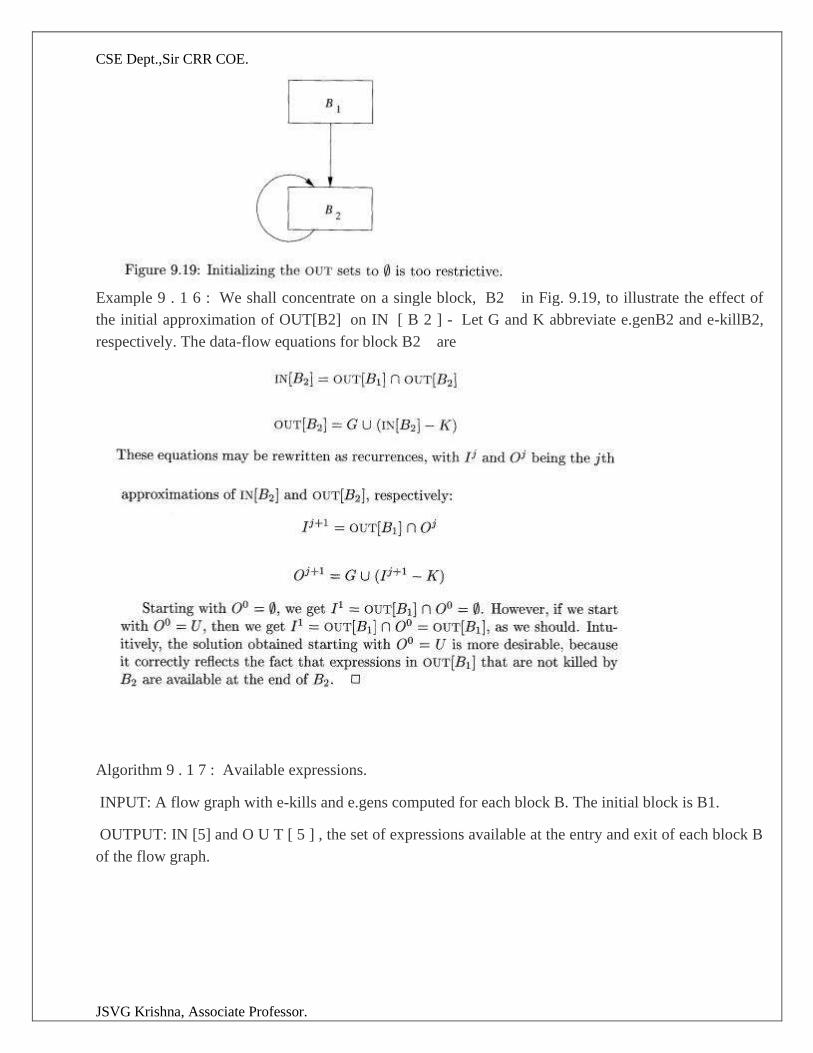
CSE Dept.,Sir CRR COE.
JSVG Krishna, Associate Professor.
Example 9 . 1 6 : We shall concentrate on a single block, B2 in Fig. 9.19, to illustrate the effect of
the initial approximation of OUT[B2] on IN [ B 2 ] - Let G and K abbreviate e.genB2 and e-killB2,
respectively. The data-flow equations for block B2 are
Algorithm 9 . 1 7 : Available expressions.
INPUT: A flow graph with e-kills and e.gens computed for each block B. The initial block is B1.
OUTPUT: IN [5] and O U T [ 5 ] , the set of expressions available at the entry and exit of each block B
of the flow graph.
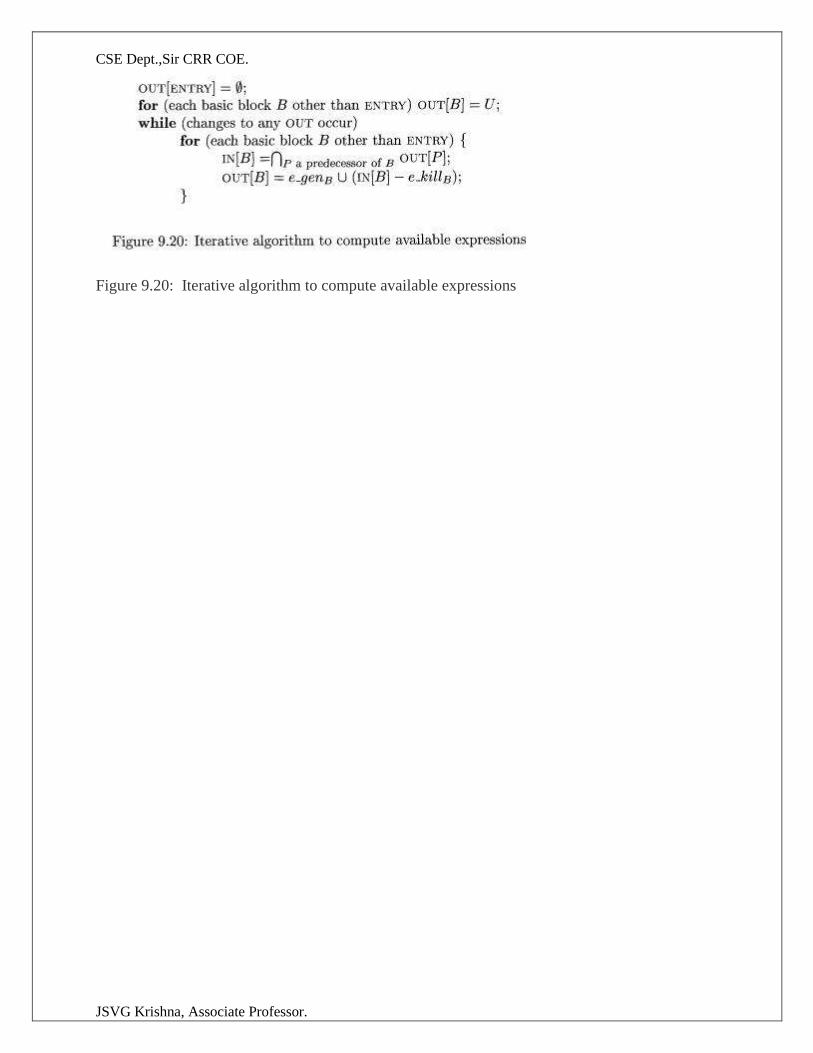
CSE Dept.,Sir CRR COE.
JSVG Krishna, Associate Professor.
Figure 9.20: Iterative algorithm to compute available expressions