ec 202 lecture notes 12

EC 202

Lecture notes 12

George Symeonidis

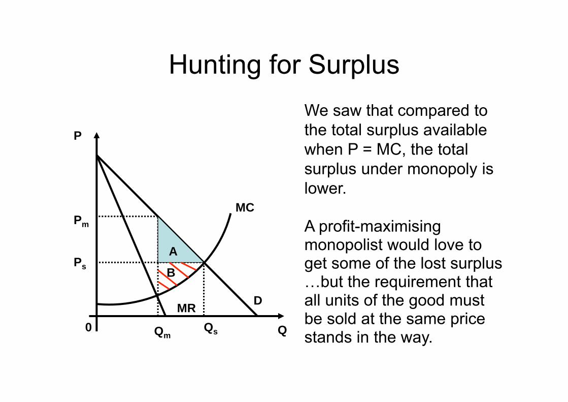
Hunting for Surplus

0 Q

P

D

MC

MRQs

Ps

Qm

Pm

A

B

We saw that compared to the total surplus available when P = MC, the total surplus under monopoly is lower.

A profit-maximising monopolist would love to get some of the lost surplus …but the requirement that all units of the good must be sold at the same price stands in the way.

The Answer: Price Discrimination

• Price discrimination involves setting different prices for different units of the same good.

• Different prices might be set for different customers, for different units bought by the same customer or both.

• But not all price differences for the same good are due to price discrimination.

First Degree (or “Perfect”) Price Discrimination

• Under first degree price discrimination the monopolist sets a different price for every single unit that it sells.

• If each customer wants at most one unit, this requires setting different prices to different customers.

• If each customer is willing to purchase more than one unit of the good, first degree price discrimination also requires the ability to charge different prices for different units sold to the same customer.

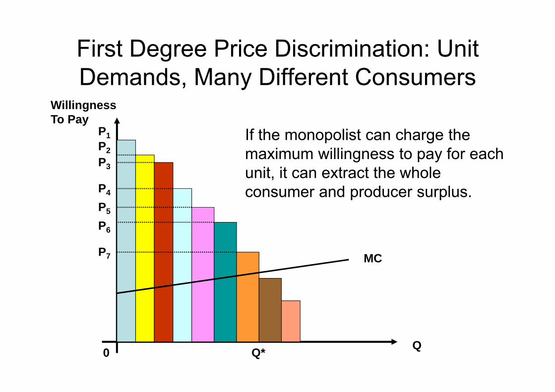
First Degree Price Discrimination: Unit Demands, Many Different Consumers

0 Q

WillingnessTo Pay

If the monopolist can charge themaximum willingness to pay for eachunit, it can extract the wholeconsumer and producer surplus.

MC

Q*

P1P2P3

P4

P5

P6

P7

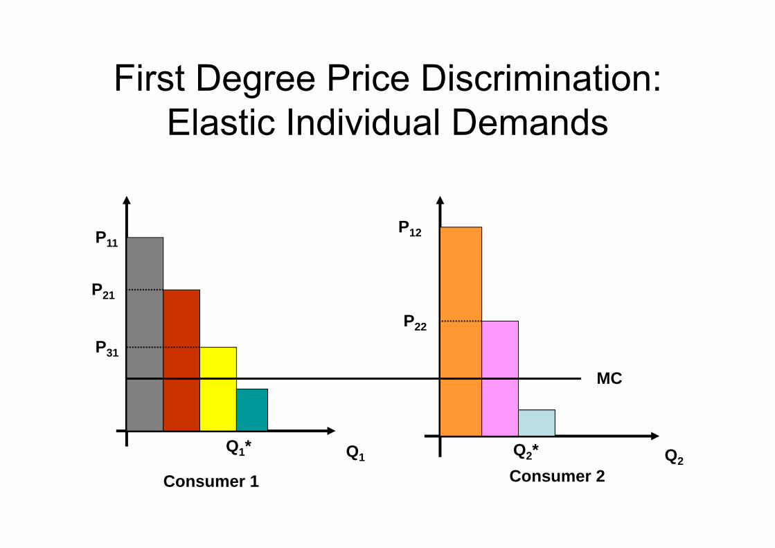
First Degree Price Discrimination: Elastic Individual Demands

Consumer 1 Consumer 2Q1 Q2

MC

Q1* Q2*

P11

P21

P31

P12

P22

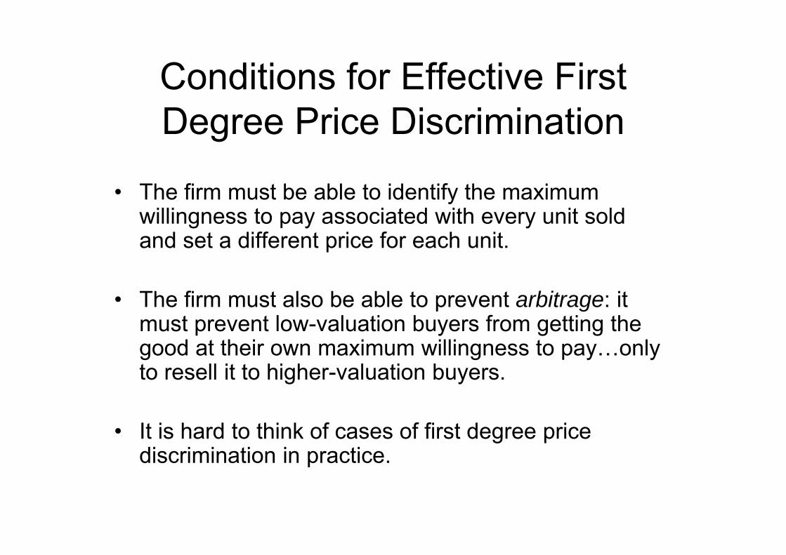
Conditions for Effective First Degree Price Discrimination

• The firm must be able to identify the maximum willingness to pay associated with every unit sold and set a different price for each unit.

• The firm must also be able to prevent arbitrage: it must prevent low-valuation buyers from getting the good at their own maximum willingness to pay…only to resell it to higher-valuation buyers.

• It is hard to think of cases of first degree price discrimination in practice.

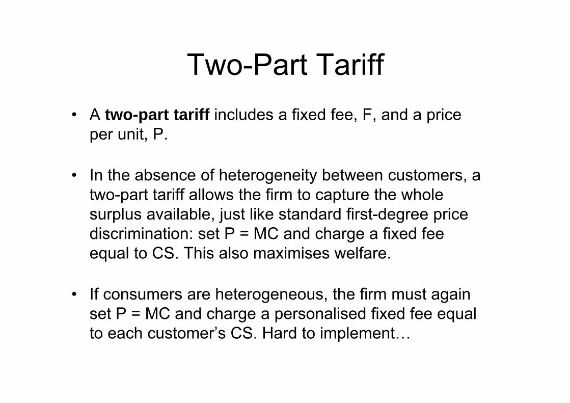
Two-Part Tariff• A two-part tariff includes a fixed fee, F, and a price

per unit, P.

• In the absence of heterogeneity between customers, a two-part tariff allows the firm to capture the whole surplus available, just like standard first-degree price discrimination: set P = MC and charge a fixed fee equal to CS. This also maximises welfare.

• If consumers are heterogeneous, the firm must again set P = MC and charge a personalised fixed fee equal to each customer’s CS. Hard to implement…

Two-Part Tariff

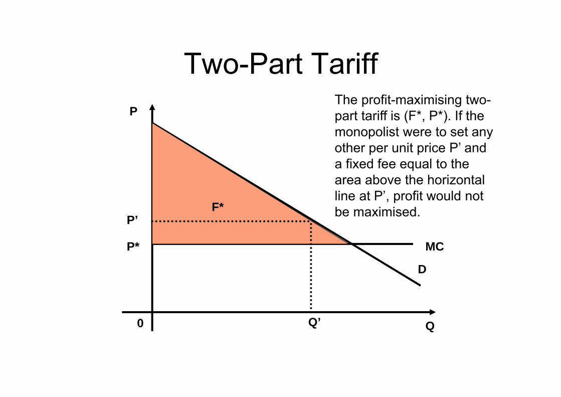
0 Q

P

D

MCP*

F*P’

Q’

The profit-maximising two-part tariff is (F*, P*). If the monopolist were to set any other per unit price P’ and a fixed fee equal to the area above the horizontal line at P’, profit would not be maximised.

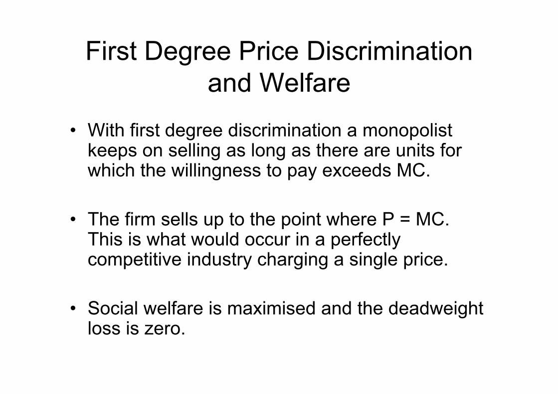
First Degree Price Discrimination and Welfare

• With first degree discrimination a monopolist keeps on selling as long as there are units for which the willingness to pay exceeds MC.

• The firm sells up to the point where P = MC. This is what would occur in a perfectly competitive industry charging a single price.

• Social welfare is maximised and the deadweight loss is zero.

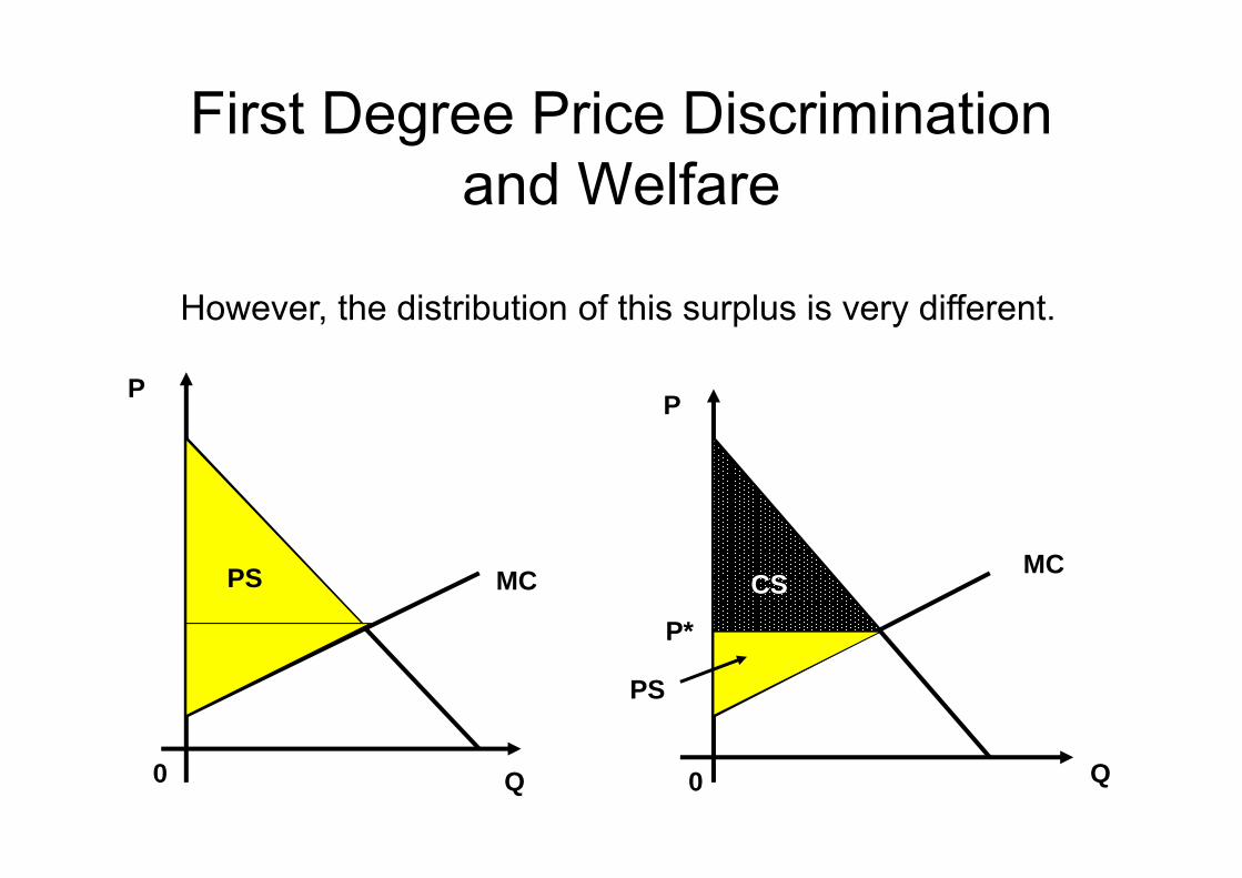
First Degree Price Discrimination and Welfare

However, the distribution of this surplus is very different.

0 Q 0 Q

P P

MC MCPS

P*

CS

PS

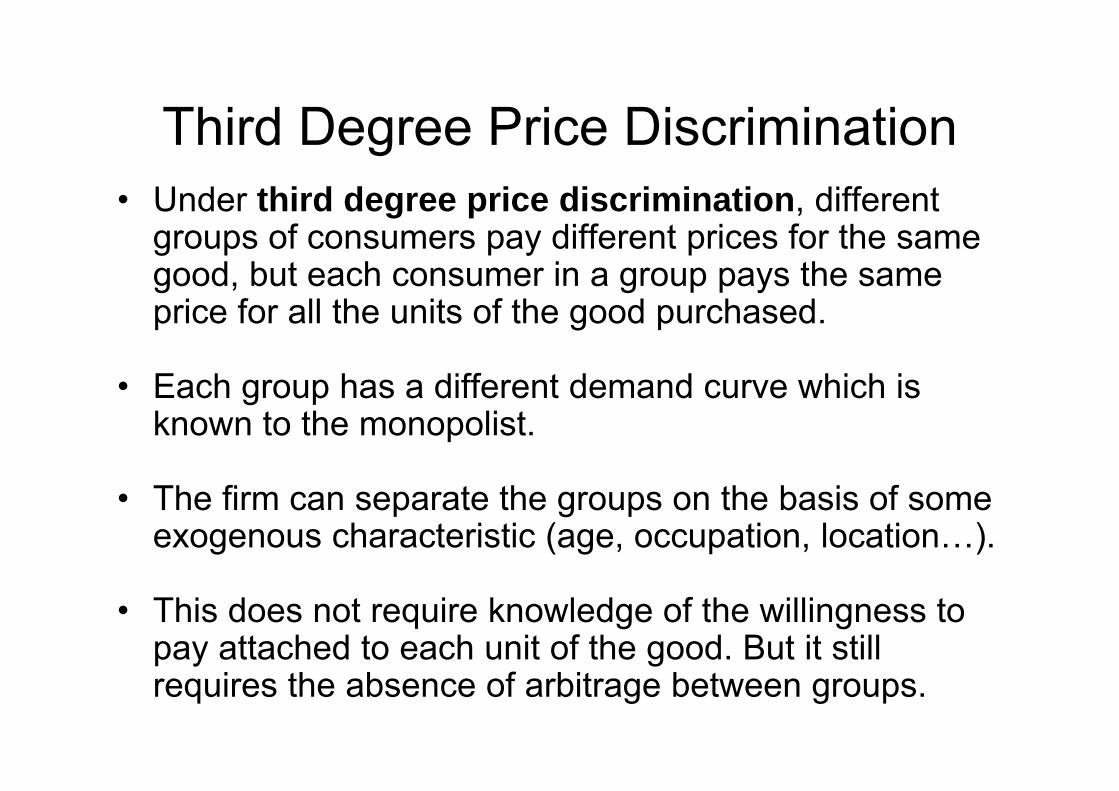
Third Degree Price Discrimination• Under third degree price discrimination, different

groups of consumers pay different prices for the same good, but each consumer in a group pays the same price for all the units of the good purchased.

• Each group has a different demand curve which is known to the monopolist.

• The firm can separate the groups on the basis of some exogenous characteristic (age, occupation, location…).

• This does not require knowledge of the willingness to pay attached to each unit of the good. But it still requires the absence of arbitrage between groups.

Examples

• Special “student” or “senior” prices

• Journal subscription prices for libraries versus prices for individuals

• Pharmaceutical products, cars, DVDs etc. sold at different prices in different countries

Profit Maximisation with Third Degree Price Discrimination

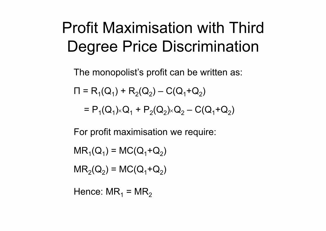
The monopolist’s profit can be written as:

П = R1(Q1) + R2(Q2) – C(Q1+Q2)

= P1(Q1)Q1 + P2(Q2)Q2 – C(Q1+Q2)

For profit maximisation we require:

MR1(Q1) = MC(Q1+Q2)

MR2(Q2) = MC(Q1+Q2)

Hence: MR1 = MR2

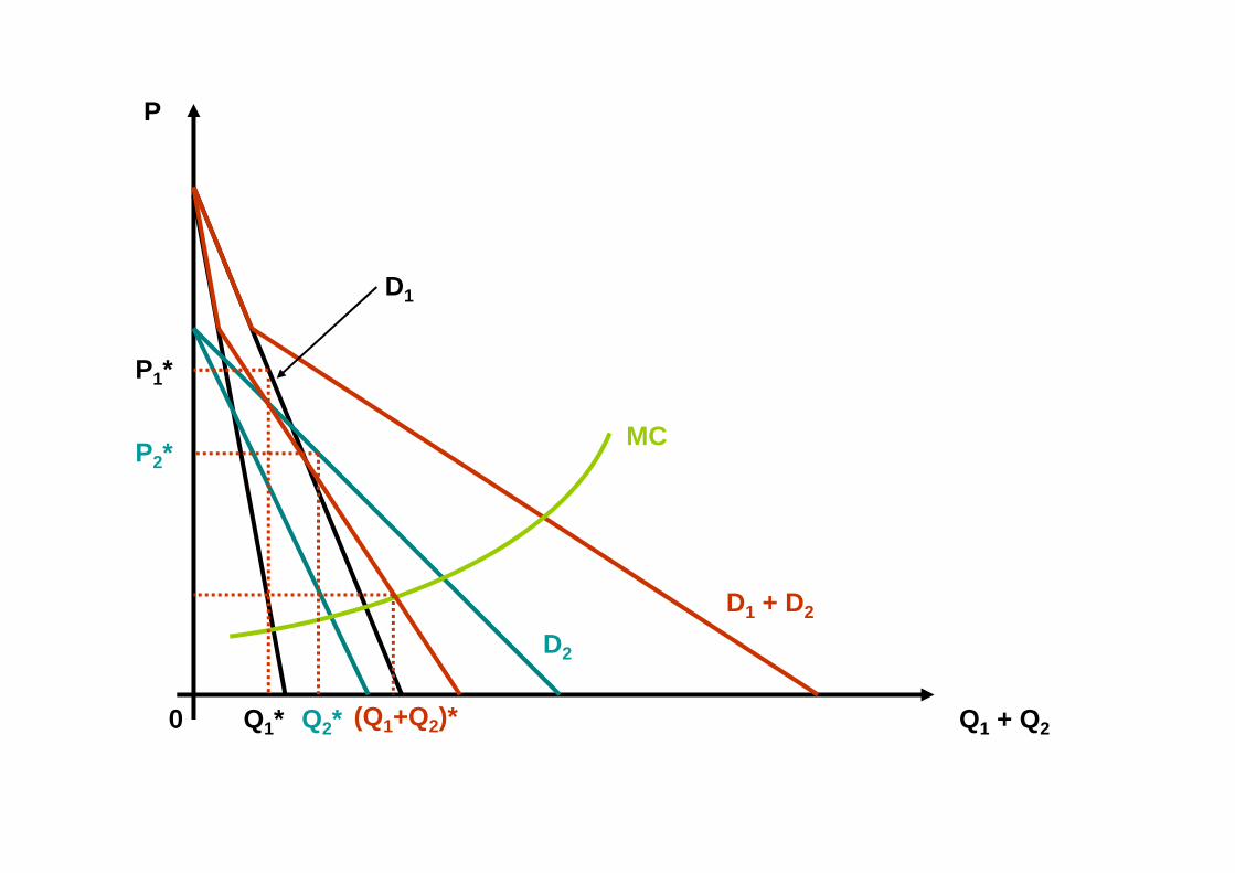
Q1 + Q2

MC

D2

D1

(Q1+Q2)*Q1* Q2*

P1*

P2*

D1 + D2

0

P


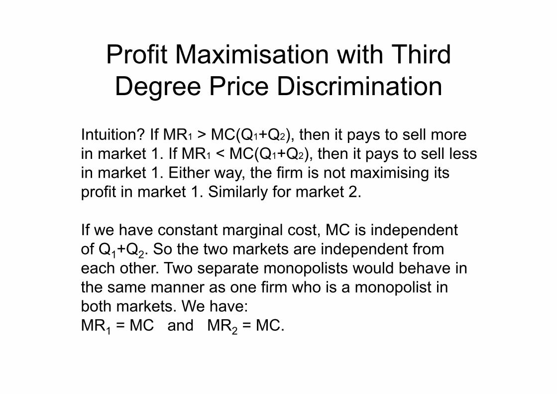
Intuition? If MR1 > MC(Q1+Q2), then it pays to sell more in market 1. If MR1 < MC(Q1+Q2), then it pays to sell less in market 1. Either way, the firm is not maximising its profit in market 1. Similarly for market 2.

If we have constant marginal cost, MC is independentof Q1+Q2. So the two markets are independent from each other. Two separate monopolists would behave in the same manner as one firm who is a monopolist in both markets. We have:MR1 = MC and MR2 = MC.

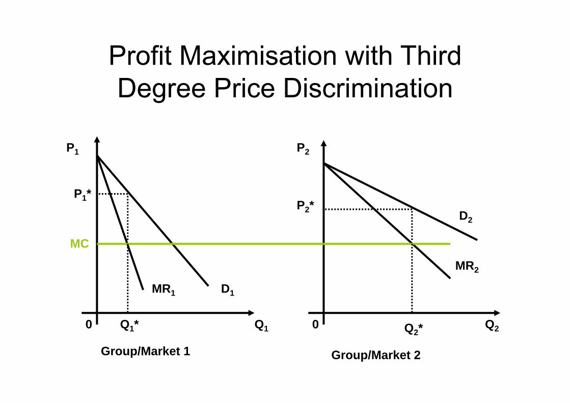
Group/Market 1 Group/Market 2

0 0Q1 Q2

P1 P2

D1

D2

MR1

MR2

MC

P1*

Q1*

P2*

Q2*


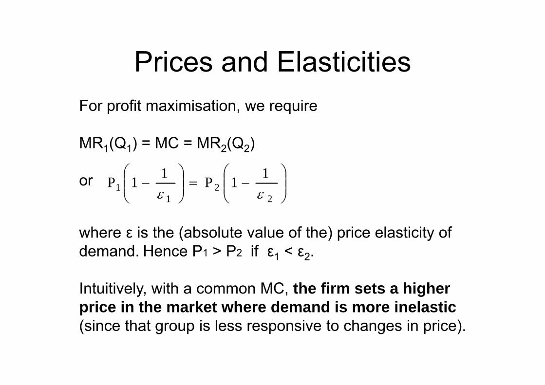
Prices and ElasticitiesFor profit maximisation, we require

MR1(Q1) = MC = MR2(Q2)

or

where ε is the (absolute value of the) price elasticity of demand. Hence P1 > P2 if ε1 < ε2.

Intuitively, with a common MC, the firm sets a higher price in the market where demand is more inelastic(since that group is less responsive to changes in price).

22

11

11P11P

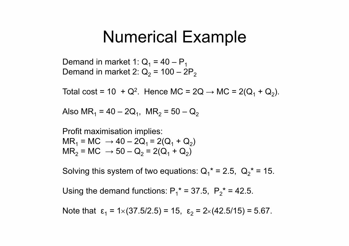
Numerical ExampleDemand in market 1: Q1 = 40 – P1Demand in market 2: Q2 = 100 – 2P2

Total cost = 10 + Q2. Hence MC = 2Q → MC = 2(Q1 + Q2).

Also MR1 = 40 – 2Q1, MR2 = 50 – Q2

Profit maximisation implies:MR1 = MC → 40 – 2Q1 = 2(Q1 + Q2)MR2 = MC → 50 – Q2 = 2(Q1 + Q2)

Solving this system of two equations: Q1* = 2.5, Q2* = 15.

Using the demand functions: P1* = 37.5, P2* = 42.5.

Note that ε1 = 1(37.5/2.5) = 15, ε2 = 2(42.5/15) = 5.67.

Third Degree Price Discrimination and Welfare

• Let’s compare the pricing decisions of a monopolist facing two groups of consumers with different demands under two different scenarios.

• Scenario 1: the monopolist must charge the same price Po to all customers.

• Scenario 2: the monopolist can divide the customers into two groups, A and B, and can charge different prices, PA and PB, to these groups. Suppose that PA < PB.


• Assume further that at price Po sales would be made to both groups of consumers.

• It will be the case that PA < Po < PB. This means that discrimination helps type A customers but hurts type B customers.

• Consumers in the low-elasticity market are hurt by third degree PD, since they pay a higher price, buy a smaller quantity and enjoy less consumer surplus than under uniform pricing.

• The reverse is true for consumers in the high-elasticity market: they gain from third degree PD.


• Moreover, price discrimination increases profit(producer surplus).

• The overall effect of third degree PD on welfare is ambiguous and depends on the specifics of demand functions.

• When demand curves are linear and all customers are served under a uniform monopoly price, it turns out that third degree price discrimination lowers overall welfare.


• Note that these results hold assuming the monopolist serves both markets in the absence of PD.

• If PD is prohibited, then the firm might choose not to serve the high-elasticity market at all, and that would definitely result in lower welfare than under price discrimination.

• In any case, third degree price discrimination has a significant effect on the distribution of the surplus.

Second Degree Price Discrimination

• When the monopolist cannot distinguish between buyers on the basis of an exogenous characteristic, then third degree price discrimination is not feasible.

• However, the seller might still be able to use the consumers’ own actions to learn something about their willingness to pay.

• This is the essence of second degree price discrimination: to get the consumers to sort themselves into various groups.

Self-Selection

• Obviously, self-selection is an issue only if the monopolist faces at least two different types of consumers.

• The idea is to offer different options that are available to all consumers but design the options so that each option is chosen by a different consumer type.

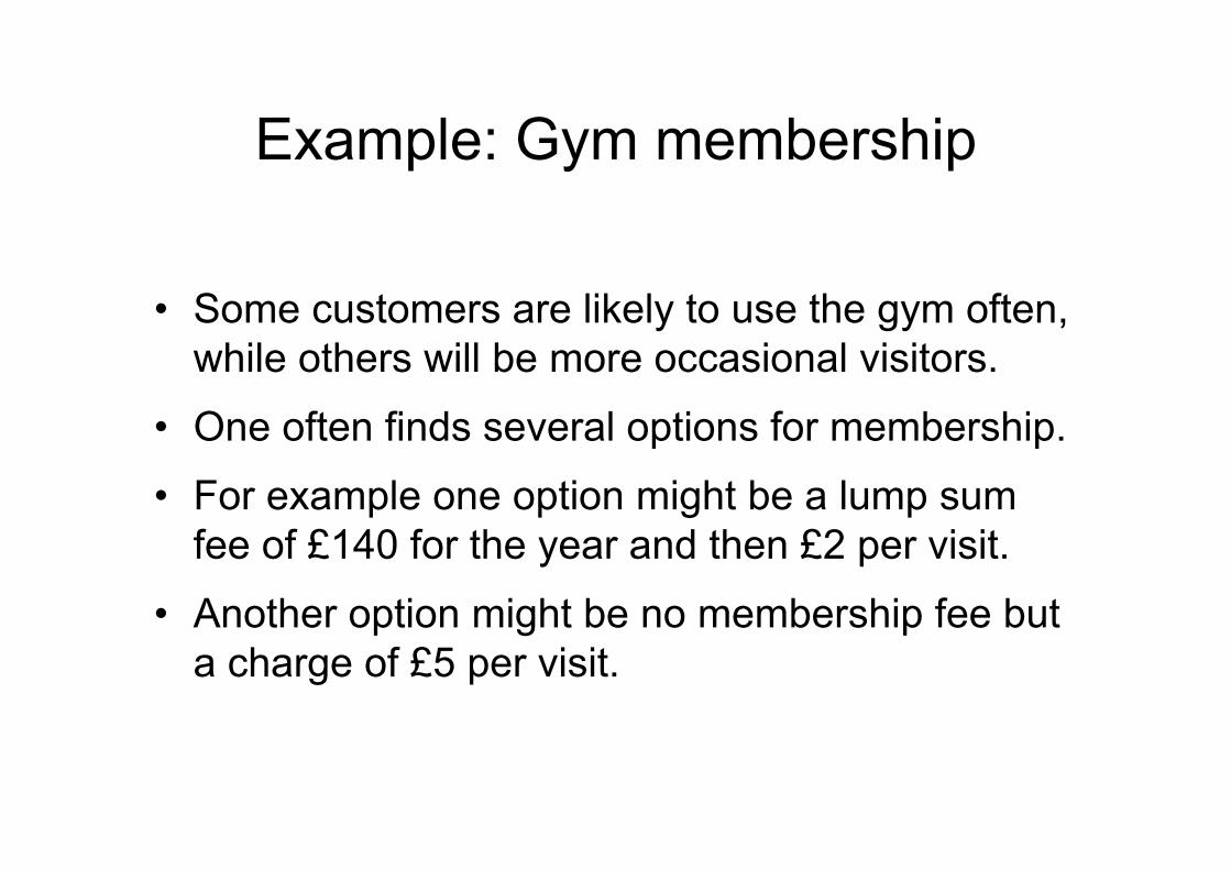
Example: Gym membership

• Some customers are likely to use the gym often, while others will be more occasional visitors.

• One often finds several options for membership.

• For example one option might be a lump sum fee of £140 for the year and then £2 per visit.

• Another option might be no membership fee but a charge of £5 per visit.

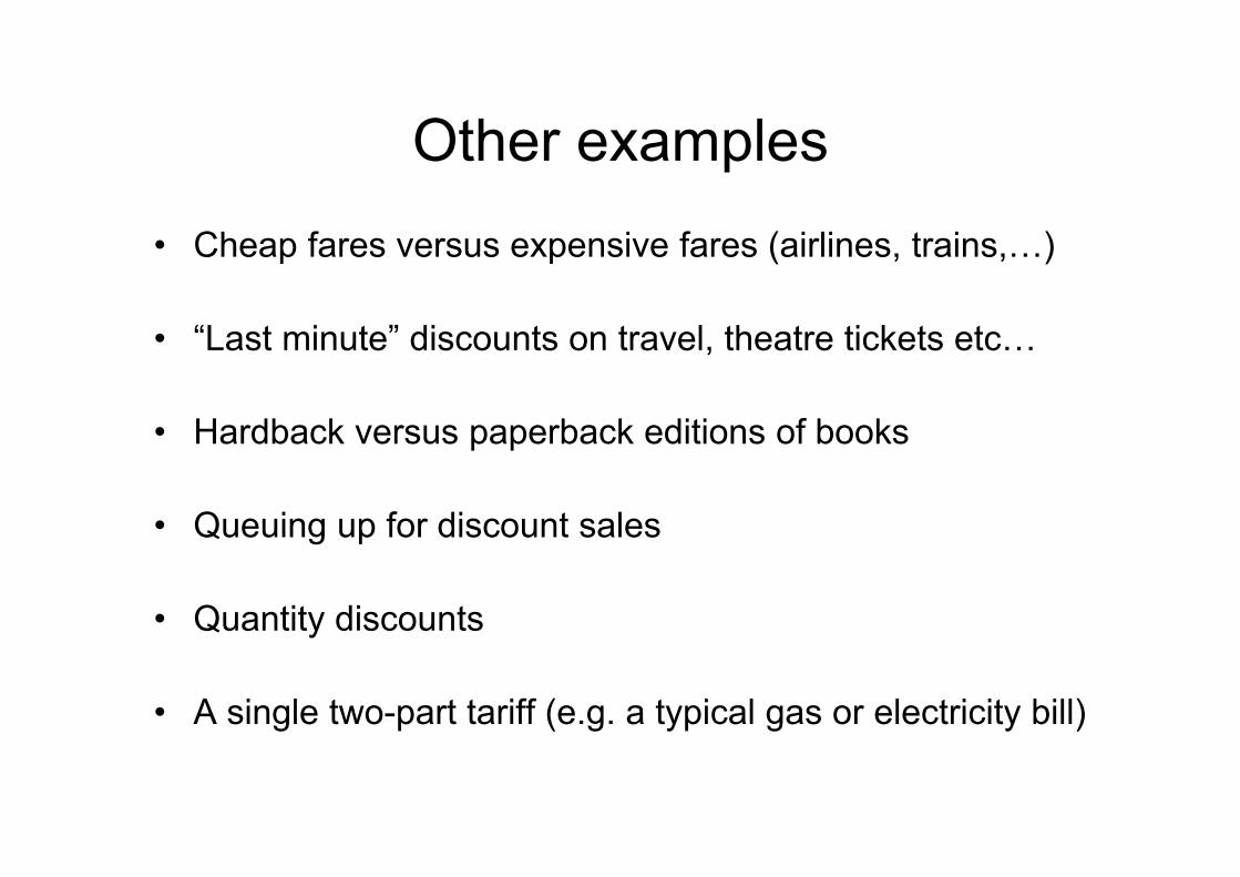
Other examples• Cheap fares versus expensive fares (airlines, trains,…)

• “Last minute” discounts on travel, theatre tickets etc…

• Hardback versus paperback editions of books

• Queuing up for discount sales

• Quantity discounts

• A single two-part tariff (e.g. a typical gas or electricity bill)

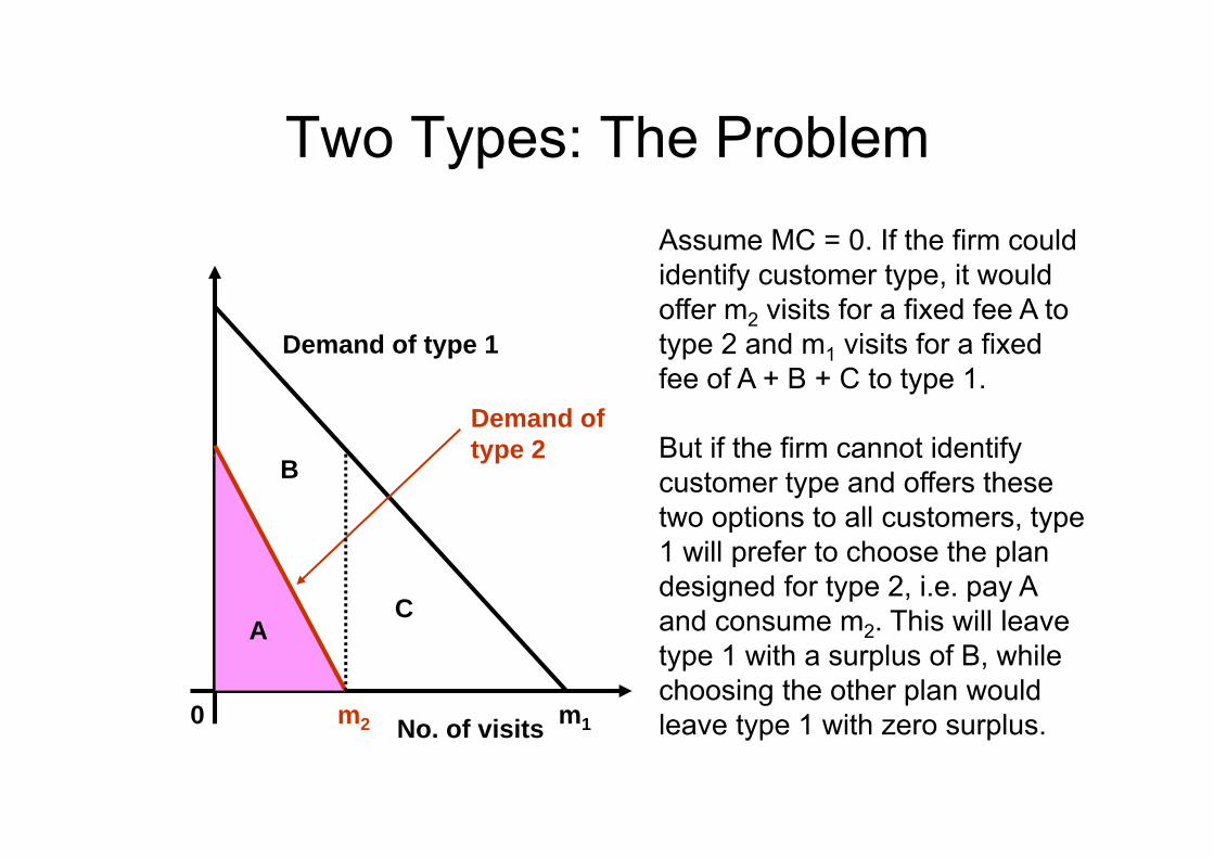
Two Types: The Problem

0 No. of visits

Demand of type 1

Demand oftype 2

m2 m1

A

Assume MC = 0. If the firm could identify customer type, it would offer m2 visits for a fixed fee A to type 2 and m1 visits for a fixed fee of A + B + C to type 1.

But if the firm cannot identify customer type and offers these two options to all customers, type 1 will prefer to choose the plan designed for type 2, i.e. pay A and consume m2. This will leave type 1 with a surplus of B, while choosing the other plan would leave type 1 with zero surplus.

C

B

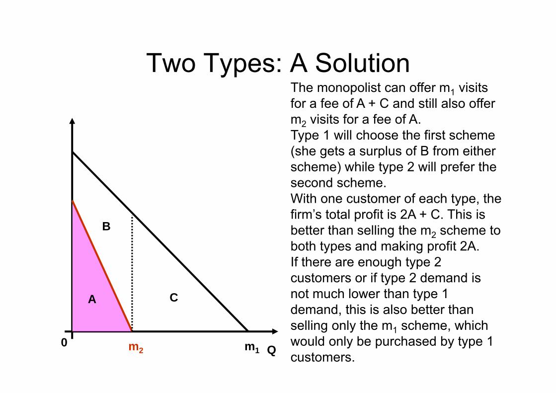
Two Types: A SolutionThe monopolist can offer m1 visits for a fee of A + C and still also offer m2 visits for a fee of A. Type 1 will choose the first scheme (she gets a surplus of B from either scheme) while type 2 will prefer the second scheme.With one customer of each type, the firm’s total profit is 2A + C. This is better than selling the m2 scheme to both types and making profit 2A. If there are enough type 2 customers or if type 2 demand is not much lower than type 1 demand, this is also better than selling only the m1 scheme, which would only be purchased by type 1 customers.

0 Qm1

A

m2

C

B

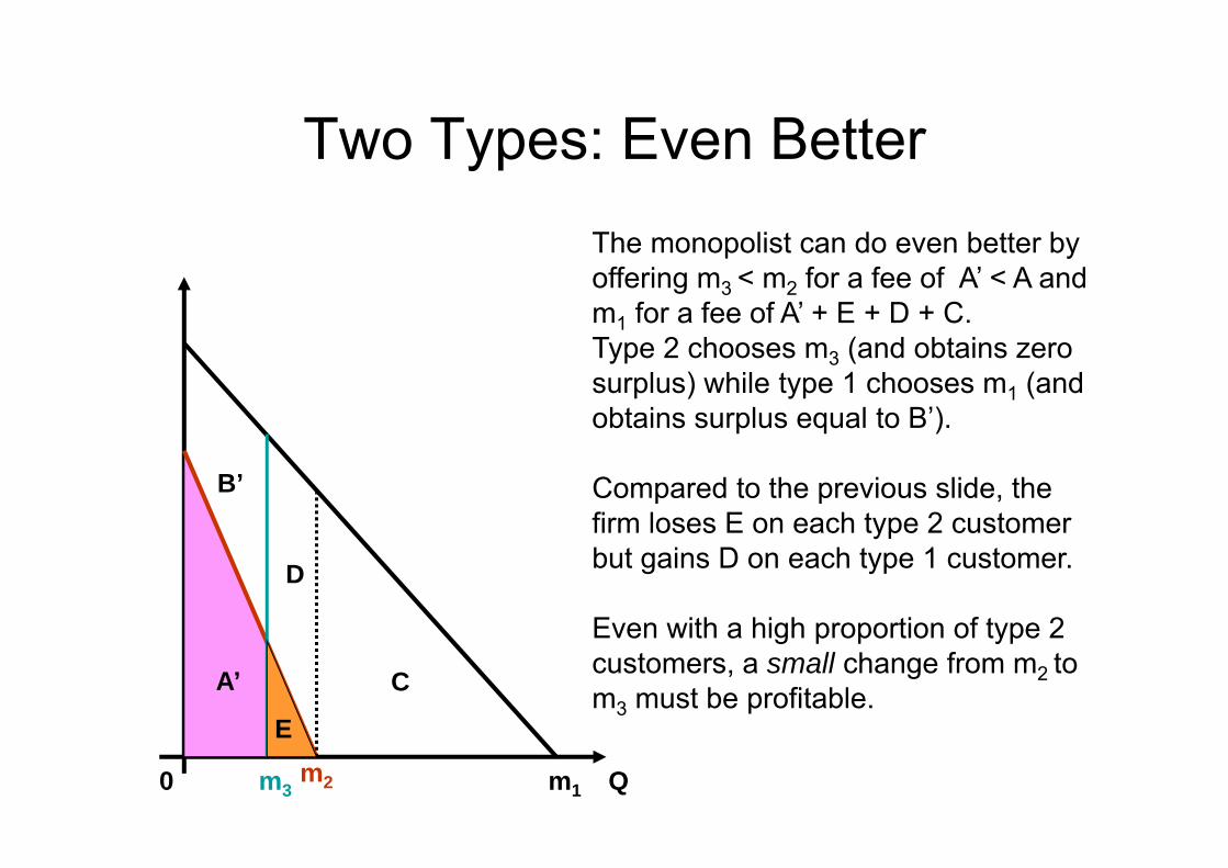
Two Types: Even Better

0 Q

A’

m1m2m3

C

D

B’

E

The monopolist can do even better by offering m3 < m2 for a fee of A’ < A and m1 for a fee of A’ + E + D + C. Type 2 chooses m3 (and obtains zero surplus) while type 1 chooses m1 (and obtains surplus equal to B’).

Compared to the previous slide, the firm loses E on each type 2 customer but gains D on each type 1 customer.

Even with a high proportion of type 2 customers, a small change from m2 to m3 must be profitable.

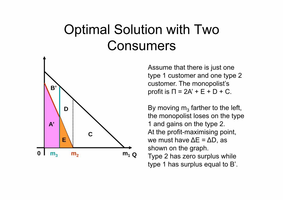
Optimal Solution with Two Consumers

Assume that there is just one type 1 customer and one type 2 customer. The monopolist’s profit is П = 2A’ + E + D + C.

By moving m3 farther to the left, the monopolist loses on the type 1 and gains on the type 2. At the profit-maximising point, we must have ∆E = ∆D, as shown on the graph. Type 2 has zero surplus while type 1 has surplus equal to B’.

0 Qm1m2m3

EC

D

A’

B’

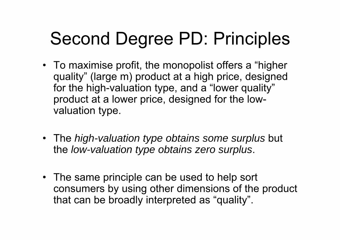
Second Degree PD: Principles• To maximise profit, the monopolist offers a “higher

quality” (large m) product at a high price, designed for the high-valuation type, and a “lower quality” product at a lower price, designed for the low-valuation type.

• The high-valuation type obtains some surplus but the low-valuation type obtains zero surplus.

• The same principle can be used to help sort consumers by using other dimensions of the product that can be broadly interpreted as “quality”.

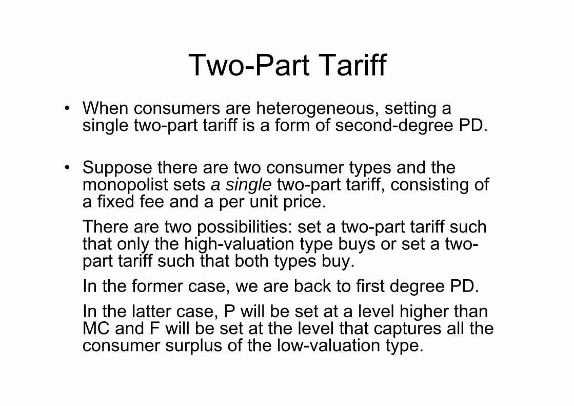
Two-Part Tariff• When consumers are heterogeneous, setting a

single two-part tariff is a form of second-degree PD.

• Suppose there are two consumer types and the monopolist sets a single two-part tariff, consisting of a fixed fee and a per unit price. There are two possibilities: set a two-part tariff such that only the high-valuation type buys or set a two-part tariff such that both types buy. In the former case, we are back to first degree PD.In the latter case, P will be set at a level higher than MC and F will be set at the level that captures all the consumer surplus of the low-valuation type.

Bundling• Selling several goods together can also allow the

firm to extract more surplus from consumers.• Assume that there are two goods, 1 and 2, and two

consumers, A and B.• Each consumer purchases at most one unit of each

good. • Each consumer has a maximum willingness to pay

for each of the good.• A consumer’s willingness to pay for a bundle

consisting of one unit of each good is the sum of her willingness to pay for each good separately.

Pure Bundling

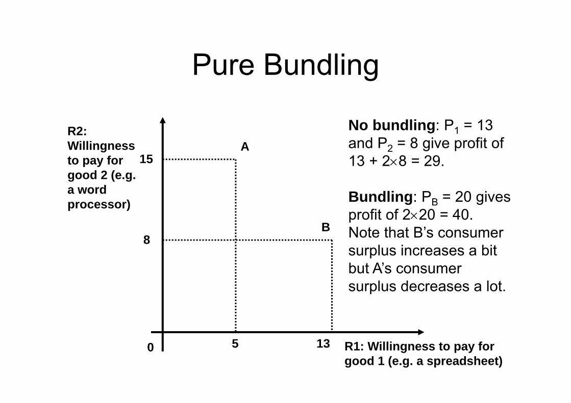
0 R1: Willingness to pay for good 1 (e.g. a spreadsheet)

R2: Willingness to pay for good 2 (e.g. a word processor)

15

5

8

13

No bundling: P1 = 13 and P2 = 8 give profit of 13 + 28 = 29.

Bundling: PB = 20 gives profit of 220 = 40. Note that B’s consumer surplus increases a bit but A’s consumer surplus decreases a lot.

A

B

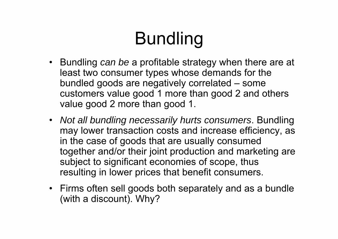
Bundling• Bundling can be a profitable strategy when there are at

least two consumer types whose demands for the bundled goods are negatively correlated – some customers value good 1 more than good 2 and others value good 2 more than good 1.

• Not all bundling necessarily hurts consumers. Bundling may lower transaction costs and increase efficiency, as in the case of goods that are usually consumed together and/or their joint production and marketing are subject to significant economies of scope, thus resulting in lower prices that benefit consumers.

• Firms often sell goods both separately and as a bundle (with a discount). Why?

Mixed Bundling

0 R1

R2

15

8

13

B

D

10

C

2

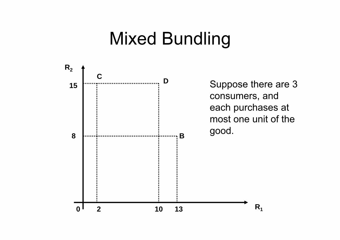
Suppose there are 3 consumers, and each purchases at most one unit of the good.

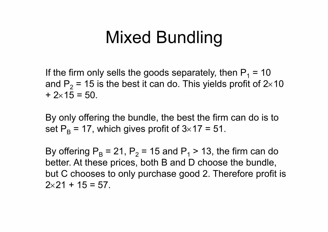
Mixed Bundling

If the firm only sells the goods separately, then P1 = 10 and P2 = 15 is the best it can do. This yields profit of 210 + 215 = 50.

By only offering the bundle, the best the firm can do is to set PB = 17, which gives profit of 317 = 51.

By offering PB = 21, P2 = 15 and P1 > 13, the firm can do better. At these prices, both B and D choose the bundle, but C chooses to only purchase good 2. Therefore profit is 221 + 15 = 57.

ec 202 lecture notes 12

Documents