lecture notes in computer science 2152
TRANSCRIPT
Lecture Notes in Computer Science 2152Edited by G. Goos, J. Hartmanis and J. van Leeuwen

3BerlinHeidelbergNew YorkBarcelonaHong KongLondonMilanParisTokyo

Richard J. Boulton Paul B. Jackson (Eds.)
Theorem Provingin Higher Order Logics
14th International Conference, TPHOLs 2001Edinburgh, Scotland, UK, September 3-6, 2001Proceedings
1 3
Series Editors
Gerhard Goos, Karlsruhe University, GermanyJuris Hartmanis, Cornell University, NY, USAJan van Leeuwen, Utrecht University, The Netherlands
Volume Editors
Richard J. BoultonUniversity of Glasgow, Department of Computing Science17 Lilybank Gardens, Glasgow G12 8QQ, Scotland, UKE-mail: [email protected]
Paul B. JacksonUniversity of Edinburgh, Division of InformaticsJames Clerk Maxwell Building, King’s BuildingsEdinburgh EH9 3JZ, Scotland, UKE-mail: [email protected]
Cataloging-in-Publication Data applied for
Die Deutsche Bibliothek - CIP-Einheitsaufnahme
Theorem proving in higher order logics : 14th international conference ;proceedings / TPHOLs 2001, Edinburgh, Scotland UK, September 3 - 6, 2001.Richard J. Boulton ; Paul B. Jackson (ed.). - Berlin ; Heidelberg ; NewYork ;Barcelona ; Hong Kong ; London ; Milan ; Paris ; Tokyo : Springer, 2001(Lecture notes in computer science ; Vol. 2152)ISBN 3-540-42525-X
CR Subject Classification (1998): F.4.1, I.2.3, F.3.1, D.2.4, B.6.3
ISSN 0302-9743ISBN 3-540-42525-X Springer-Verlag Berlin Heidelberg NewYork
This work is subject to copyright. All rights are reserved, whether the whole or part of the material isconcerned, specifically the rights of translation, reprinting, re-use of illustrations, recitation, broadcasting,reproduction on microfilms or in any other way, and storage in data banks. Duplication of this publicationor parts thereof is permitted only under the provisions of the German Copyright Law of September 9, 1965,in its current version, and permission for use must always be obtained from Springer-Verlag. Violations areliable for prosecution under the German Copyright Law.
Springer-Verlag Berlin Heidelberg NewYorka member of BertelsmannSpringer Science+Business Media GmbH
http://www.springer.de
© Springer-Verlag Berlin Heidelberg 2001Printed in Germany
Typesetting: Camera-ready by author, data conversion by Christian Grosche, HamburgPrinted on acid-free paper SPIN 10845517 06/3142 5 4 3 2 1 0
Preface
This volume constitutes the proceedings of the 14th International Conference onTheorem Proving in Higher Order Logics (TPHOLs 2001) held 3–6 September2001 in Edinburgh, Scotland. TPHOLs covers all aspects of theorem proving inhigher order logics, as well as related topics in theorem proving and verification.
TPHOLs 2001 was collocated with the 11th Advanced Research WorkingConference on Correct Hardware Design and Verification Methods (CHARME2001). This was held 4–7 September 2001 in nearby Livingston, Scotland at theInstitute for System Level Integration, and a joint half-day session of talks wasarranged for the 5th September in Edinburgh. An excursion to Traquair Houseand a banquet in the Playfair Library of Old College, University of Edinburghwere also jointly organized. The proceedings of CHARME 2001 have been pub-lished as volume 2144 of Springer-Verlag’s Lecture Notes in Computer Scienceseries, with Tiziana Margaria and Tom Melham as editors.
Each of the 47 papers submitted in the full research category was refereedby at least 3 reviewers who were selected by the Program Committee. Of thesesubmissions, 23 were accepted for presentation at the conference and publicationin this volume. In keeping with tradition, TPHOLs 2001 also offered a venuefor the presentation of work in progress, where researchers invite discussion bymeans of a brief preliminary talk and then discuss their work at a poster session.A supplementary proceedings containing associated papers for work in progresswas published by the Division of Informatics at the University of Edinburgh.
The organizers are grateful to Bart Jacobs and N. Shankar for agreeing togive invited talks at TPHOLs 2001, and to Steven D. Johnson for agreeing togive an invited talk at the joint session with CHARME 2001. Much of BartJacobs’s research is on formal methods for object-oriented languages, and heis currently coordinator of a multi-site project funded by the European Unionon tool-assisted specification and verification of JavaCard programs. His talkcovered his own research and research of this project. A three page abstracton the background to his talk is included in this volume. N. Shankar is one ofthe principal architects of the popular PVS theorem prover, and has publishedwidely on many theorem-proving related topics. He talked about the kinds ofdecision procedures that can be deployed in a higher-order-logic setting and theopportunities for interaction between them. We are very pleased to include anaccompanying paper in these proceedings. Steven D. Johnson is a prominentfigure in the formal methods community. His talk surveyed formalized systemdesign from the perspective of research in interactive reasoning. He contrastedtwo interactive formalisms: one based on logic and proof, the other based ontransformations and equivalence. The latter has been the subject of Johnson’sresearch since the early 1980s. An abstract for this talk is included in theseproceedings, and a full accompanying paper can be found in the CHARME 2001proceedings.
VI Preface
The TPHOLs conference traditionally changes continent each year in orderto maximize the chances that researchers all over the world can attend. Start-ing in 1993, the proceedings of TPHOLs and its predecessor workshops havebeen published in the following volumes of the Springer-Verlag Lecture Notes inComputer Science series:
1993 (Canada) 780 1997 (USA) 12751994 (Malta) 859 1998 (Australia) 14791995 (USA) 971 1999 (France) 16901996 (Finland) 1125 2000 (USA) 1869
The 2001 conference was organized by a team from the Division of Informaticsat the University of Edinburgh and the Department of Computing Science atthe University of Glasgow.
Financial support came from Intel and Microsoft Research. The Universityof Glasgow funded publicity and the University of Edinburgh loaned computingequipment. This support is gratefully acknowledged.
June 2001 Richard J. Boulton, Paul Jackson
Preface VII
Conference Organization
Richard Boulton (Conference Chair)Paul Jackson (Program Chair)Louise Dennis (Local Arrangements Co-chair)Jacques Fleuriot (Local Arrangements Co-chair)Ken Baird (Local Arrangements & Finances)Deirdre Burke (Local Arrangements)Jennie Douglas (Local Arrangements)Gordon Reid (Computing Support)Simon Gay (Publicity Chair)Tom Melham (TPHOLs/CHARME Coordinating General Chair)
Program Committee
Mark Aagaard (Waterloo) Paul Jackson (Edinburgh)David Basin (Freiburg) Sara Kalvala (Warwick)Richard Boulton (Glasgow) Michael Kohlhase (CMU & Saarbrucken)Albert Camilleri (Netro) J Moore (Texas, Austin)Victor Carreno (NASA Langley) Sam Owre (SRI)Gilles Dowek (INRIA Rocquencourt) Christine Paulin-Mohring (Paris Sud)Harald Ganzinger (MPI Saarbrucken) Lawrence Paulson (Cambridge)Ganesh Gopalakrishnan (Utah) Frank Pfenning (CMU)Jim Grundy (Intel) Klaus Schneider (Karlsruhe)Elsa Gunter (NJIT) Henny Sipma (Stanford)John Harrison (Intel) Konrad Slind (Cambridge)Doug Howe (Carleton) Don Syme (Microsoft)Bart Jacobs (Nijmegen) Sofiene Tahar (Concordia)
Invited Speakers
Bart Jacobs (Nijmegen)Steven D. Johnson (Indiana) (joint with CHARME 2001 )N. Shankar (SRI)
Additional Reviewers
Andrew A. Adams John Gunnels Christine RocklJohn Cowles Martin Hofmann Harald RuessPaul Curzon Matt Kaufmann N. ShankarAbdelkader Dekdouk Robert Krug Jun SawadaLeonardo Demoura John Longley Alan SmaillEwen Denney Helen Lowe Luca ViganoJonathan Mark Ford Tobias Nipkow Burkhart WolffRuben Gamboa Randy Pollack
VIII Preface
CHARME 2001 Organization
Tom Melham (Conference Chair)Tiziana Margaria (Program Chair)Andrew Ireland (Local Arrangements Chair)Steve Beaumont (Local Arrangements)Lorraine Fraser (Local Arrangements)Simon Gay (Publicity Chair)
Table of Contents
Invited Talks
JavaCard Program Verification . . . . . . . . . . . . . . . . . . . . . . . . . . . . . . . . . . . . . . 1Bart Jacobs
View from the Fringe of the Fringe (Joint with CHARME 2001) . . . . . . . . . 4Steven D. Johnson
Using Decision Procedures with a Higher-Order Logic . . . . . . . . . . . . . . . . . . 5Natarajan Shankar
Regular Contributions
Computer Algebra Meets Automated Theorem Proving: IntegratingMaple and PVS . . . . . . . . . . . . . . . . . . . . . . . . . . . . . . . . . . . . . . . . . . . . . . . . . . . . 27Andrew Adams, Martin Dunstan, Hanne Gottliebsen, Tom Kelsey,Ursula Martin, Sam Owre
An Irrational Construction of R from Z . . . . . . . . . . . . . . . . . . . . . . . . . . . . . . . 43Rob D. Arthan
HELM and the Semantic Math-Web . . . . . . . . . . . . . . . . . . . . . . . . . . . . . . . . . . 59Andrea Asperti, Luca Padovani, Claudio Sacerdoti Coen, Irene Schena
Calculational Reasoning Revisited (An Isabelle/Isar Experience) . . . . . . . . . 75Gertrud Bauer, Markus Wenzel
Mechanical Proofs about a Non-repudiation Protocol . . . . . . . . . . . . . . . . . . . 91Giampaolo Bella, Lawrence C. Paulson
Proving Hybrid Protocols Correct . . . . . . . . . . . . . . . . . . . . . . . . . . . . . . . . . . . . 105Mark Bickford, Christoph Kreitz, Robbert van Renesse, Xiaoming Liu
Nested General Recursion and Partiality in Type Theory . . . . . . . . . . . . . . . 121Ana Bove, Venanzio Capretta
A Higher-Order Calculus for Categories . . . . . . . . . . . . . . . . . . . . . . . . . . . . . . . 136Mario Caccamo, Glynn Winskel
Certifying the Fast Fourier Transform with Coq . . . . . . . . . . . . . . . . . . . . . . . . 154Venanzio Capretta
A Generic Library for Floating-Point Numbers and Its Application toExact Computing . . . . . . . . . . . . . . . . . . . . . . . . . . . . . . . . . . . . . . . . . . . . . . . . . . 169Marc Daumas, Laurence Rideau, Laurent Thery
X Table of Contents
Ordinal Arithmetic: A Case Study for Rippling in a Higher Order Domain 185Louise A. Dennis, Alan Smaill
Abstraction and Refinement in Higher Order Logic . . . . . . . . . . . . . . . . . . . . . 201Matt Fairtlough, Michael Mendler, Xiaochun Cheng
A Framework for the Formalisation of Pi Calculus Type Systems inIsabelle/HOL . . . . . . . . . . . . . . . . . . . . . . . . . . . . . . . . . . . . . . . . . . . . . . . . . . . . . . 217Simon J. Gay
Representing Hierarchical Automata in Interactive Theorem Provers . . . . . . 233Steffen Helke, Florian Kammuller
Refinement Calculus for Logic Programming in Isabelle/HOL . . . . . . . . . . . . 249David Hemer, Ian Hayes, Paul Strooper
Predicate Subtyping with Predicate Sets . . . . . . . . . . . . . . . . . . . . . . . . . . . . . . 265Joe Hurd
A Structural Embedding of Ocsid in PVS . . . . . . . . . . . . . . . . . . . . . . . . . . . . . 281Pertti Kellomaki
A Certified Polynomial-Based Decision Procedure for Propositional Logic . 297Inmaculada Medina-Bulo, Francisco Palomo-Lozano,Jose A. Alonso-Jimenez
Finite Set Theory in ACL2 . . . . . . . . . . . . . . . . . . . . . . . . . . . . . . . . . . . . . . . . . . 313J Strother Moore
The HOL/NuPRL Proof Translator(A Practical Approach to Formal Interoperability) . . . . . . . . . . . . . . . . . . . . . 329Pavel Naumov, Mark-Oliver Stehr, Jose Meseguer
Formalizing Convex Hull Algorithms . . . . . . . . . . . . . . . . . . . . . . . . . . . . . . . . . 346David Pichardie, Yves Bertot
Experiments with Finite Tree Automata in Coq . . . . . . . . . . . . . . . . . . . . . . . . 362Xavier Rival, Jean Goubault-Larrecq
Mizar Light for HOL Light . . . . . . . . . . . . . . . . . . . . . . . . . . . . . . . . . . . . . . . . . . 378Freek Wiedijk
Author Index . . . . . . . . . . . . . . . . . . . . . . . . . . . . . . . . . . . . . . . . . . . . . . . . . . . . 395
JavaCard Program Verification
Bart Jacobs
Computing Science Institute, University of NijmegenToernooiveld 1, 6525 ED Nijmegen
http://www.cs.kun.nl/~bart
Abstract. This abstract provides some background information onsmart cards, and explains the challenges these cards represent for for-mal verification of software.
Smart Card Trends
Increasingly, physical keys are being replaced by cryptographic keys, which aretypically a thousand bits in size. Modern smart cards are the ideal carriersfor such keys, because they have enough computing power to do the necessaryen- or de-cryption on-card, so that the secret key never has to leave the card.Smart cards are meant to be tamper-resistant secure tokens, typically bound toindividuals via a PIN, possibly in combination with biometric identification.
Modern smart cards contain a standard interface (API) for a mini-operatingsystem which is capable of executing application programs (called applets) writ-ten in high-level languages. The standard language in this area is JavaCard[Che00], which is a “superset of a subset” of Java: it is a simplified version ofJava (no threads, multi-dimensional arrays, floats or doubles) with some spe-cial features, like persistent objects and a transaction-commit mechanism. Twofurther characteristics of modern smart cards are:
– Multi-application. One card can hold multiple applets for different appli-cations. These are typically centered around the basic cryptographic func-tions, in for example banking, telecommunication (GSM or UMTS SIMs),access to buildings or networks, identification, voting, etc.) Limited com-munication can be allowed between applets, e.g. for automatically addingloyalty points after certain commercial transactions.
– Post-issuance Downloading. In principle, it is possible to add applets toa card after it has been issued. This option gives enormous flexibility, but isdisabled for security reasons in all currently operational cards.
Security evaluation and certification are very important in the smart cardarea, because cards are distributed in large numbers for security critical appli-cations. Correctness should be established both for the card platform, and forapplets.
R.J. Boulton and P.B. Jackson (Eds.): TPHOLs 2001, LNCS 2152, pp. 1–3, 2001.c© Springer-Verlag Berlin Heidelberg 2001
2 Bart Jacobs
Challenges for Formal Methods
The so-called Common Criteria1 form a standard for the evaluation of IT secu-rity. They are much used for smart cards. The Common Criteria involve sevendifferent levels of evaluation, where the two highest levels (6 and 7) require theexplicit use of formal methods. Currently available smart cards are evaluated atlevels 4 and 5, but there is a clear pressure to move to higher levels. Thereforethe smart card industry is open to the use of formal methods. For the formalverification community smart cards form an ideal target since they are withinreach of existing verification tools, because of their limited size.
VerifiCard: Aims
In 2000 a European research consortium called VerifiCard2 was set up, with sup-port from the European Union’s IST programme. Its aim is to apply the existingverification tools (mostly theorem provers, but also model checkers) to establishthe correctness of JavaCard-based smart cards. The approach is pragmatic: nonew development of semantics of Java(Card) from scratch, but application ofavailable expertise and experience in Europe in tool-assisted formal methods, tosee what can be achieved in a concentrated effort in a small, well-defined area.This is a potential killer application for formal methods in software verification,which can cut in two directions: if this succeeds, the success may spread to otherareas. But if this fails there may be a serious setback for formal methods insoftware: it is bad news if these methods cannot deliver for such relatively smallsystems as smart cards.
VerifiCard: Work
The VerifiCard consortium consists of five academic partners, some of which arewell-known in the TPHOLs community: Nijmegen (coordinator; Jacobs, Poll),INRIA (Barthe, Bertot, Jensen, Paulin-Mohring), Munich (Nipkow, Strecker),Hagen (Poetzsch-Heffter), SICS (Dam). Also, the consortium involves two smartcard manufacturers: Gemplus and SchlumbergerSema (formerly Bull CP8). Theplanned work is roughly divided along two lines: source code / byte code, andplatform / applets. The work involves for instance formalization of the JavaCardvirtual machine and byte code verifier, non-interference properties, and specifi-cation and verification of the API and of individual applets. Towards the end ofthe project the industrial partners will carry out a tool-evaluation, to see whichapproaches can contribute most to their evaluation needs.
Scientific Work of Nijmegen
The talk will elaborate on the work done at Nijmegen, as part of VerifiCard. Thisinvolves verification of JavaCard programs, that are part of the API and applets.1 See http://www.commoncriteria.org.2 See http://www.verificard.org.
JavaCard Program Verification 3
The correctness properties are specified using the interface specification languageJML [LBR99], developed by Gary Leavens et al. in Iowa, see e.g. [PBJ01]. AJava(Card) program with JML annotation is translated to PVS using the LOOPtool [BJ01]. Actual verification in PVS proceeds via a tailor-made Hoare logicfor JML [JP01]. See [BJP01] for a small case study, involving the AID class fromthe JavaCard API. Basically, the verification technology for Java is there, butscaling it up to larger programs is still a real challenge.
References
BJ01. J. van den Berg and B. Jacobs. The LOOP compiler for Java and JML. InT. Margaria and W. Yi, editors, Tools and Algorithms for the Constructionand Analysis of Software (TACAS), number 2031 in Lect. Notes Comp. Sci.,pages 299–312. Springer, Berlin, 2001.
BJP01. J. van den Berg, B. Jacobs, and E. Poll. Formal specification and verificationof JavaCard’s Application Identifier Class. In I. Attali and Th. Jensen, editors,Proceedings of the Java Card 2000 Workshop, Lect. Notes Comp. Sci. Springer,Berlin, 2001.
Che00. Z. Chen. Java Card Technology for Smart Cards. The Java Series. Addison-Wesley, 2000.
JP01. B. Jacobs and E. Poll. A logic for the Java Modeling Language JML.In H. Hussmann, editor, Fundamental Approaches to Software Engineering(FASE), number 2029 in Lect. Notes Comp. Sci., pages 284–299. Springer,Berlin, 2001.
LBR99. G.T. Leavens, A.L. Baker, and C. Ruby. JML: A notation for detailed design.In H. Kilov and B. Rumpe, editors, Behavioral Specifications of Business andSystems, pages 175–188. Kluwer, 1999.
PBJ01. E. Poll, J. van den Berg, and B. Jacobs. Formal specification of the JavaCardAPI in JML: The APDU class. Comp. Networks Mag., 2001. To appear.
View from the Fringe of the Fringe
(Joint with CHARME 2001)
Steven D. Johnson
Computer Science DepartmentIndiana University, Lindley Hall, Room 215
150 S. Woodlawn, Bloomington, IN 47405-7104, USA
Abstract. Formal analysis remains outside the mainstream of systemdesign practice. Theorem proving is regarded by many to be on the mar-gin of exploratory and applied research activity in this formalized systemdesign. Although it may seem relatively academic, it is vital that this av-enue continue to be as vigorously explored as approaches favoring highlyautomated reasoning. Design derivation, a term for design formalismsbased on transformations and equivalence, represents just a small twigon the theorem-proving branch of formal system analysis. A perspectiveon current trends in is presented from this remote outpost, including areview of the author’s work since the early 1980s.A full accompanying paper can be found in the CHARME 2001 proceed-ings [1].
References
[1] Steven D. Johnson. View from the fringe of the fringe. In Tiziana Margariaand Tom Melham, editors, Proceedings of 11th Advanced Research Workshop onCorrect Hardware Design and Verification Methods (CHARME 2001), volume 2144of Lecture Notes in Computer Science. Springer Verlag, 2001.
R.J. Boulton and P.B. Jackson (Eds.): TPHOLs 2001, LNCS 2152, pp. 4–4, 2001.c© Springer-Verlag Berlin Heidelberg 2001
Using Decision Procedures
with a Higher-Order Logic�
Natarajan Shankar
Computer Science LaboratorySRI International, Menlo Park CA 94025 USA
http://www.csl.sri.com/~shankar/
Phone: +1 (650) 859-5272 Fax: +1 (650) 859-2844
Abstract. In automated reasoning, there is a perceived trade-off be-tween expressiveness and automation. Higher-order logic is typicallyviewed as expressive but resistant to automation, in contrast with first-order logic and its fragments. We argue that higher-order logic and itsvariants actually achieve a happy medium between expressiveness andautomation, particularly when used as a front-end to a wide range of de-cision procedures and deductive procedures. We illustrate the discussionwith examples from PVS, but some of the observations apply to othervariants of higher-order logic as well.
It does not matter if a cat is black or white so long as it catches mice.
Deng Xiaoping
Expressiveness and automation are the two basic concerns for formalized math-ematics. In theoretical terms, expressiveness is characterized by the range ofconcepts that can be captured within a given logic. For practical applicationof logic, the directness with which concepts can be captured and manipulatedin the logic is also important. The theoretical idea of automation for a givenlogic is usually in terms of the degree of solvability or unsolvability of its deci-sion problem. We argue that such characterizations are theoretically interestingbut irrelevant in practice. A more important quality for a logic is the degree towhich useful fragments of the logic can be supported by means of automation.We have used the higher-order logic of PVS (SRI’s Prototype Verification Sys-tem) [ORS92,ORSvH95] as an interface to various automated procedures. Weassess the effectiveness of the PVS logic, and higher-order logic in general, as alogical front end.
Logics based on higher-order types have a long and distinguished history inthe foundations of mathematics. Paradoxes such as that of Russell (the set of� This work was funded by NSF Grant CCR-0082560, DARPA/AFRL Contract
F33615-00-C-3043, and NASA Contract NAS1-00079.
R.J. Boulton and P.B. Jackson (Eds.): TPHOLs 2001, LNCS 2152, pp. 5–26, 2001.c© Springer-Verlag Berlin Heidelberg 2001
6 Natarajan Shankar
all those sets that do not contain themselves as elements) led to various restric-tions on hitherto unquestioned logical principles such as unrestricted compre-hension. Whitehead and Russell’s system Principia Mathematica (PM) [WR27]introduced a type system consisting of the types of individuals, sets of individ-uals, sets of sets of individuals, and so on. Overlaid on this type hierarchy wasa notion of order so that a term of order k could only contain quantificationover variables of lower order to ensure predicativity. However, as Chwistek (seeHatcher [Hat68]) showed, the axiom of reducibility (comprehension) renders thesystem equivalent to a simple type theory with impredicative comprehension.Ramsey [Ram90] showed that the basic type system was sufficient to avoid thelogical paradoxes (such as Russell’s). Predicativity did not actually address theepistemological paradoxes (such as the Liar’s paradox) since these had to do withthe interpretation of concepts expressed in the logic and not with the means ofdefinition. Church [Chu40] presented a system based on a simple type theorywith types for individuals and propositions, and a type [A→B] for any typesA and B. Church’s system is based on the simply typed lambda-calculus withChurch numerals, an axiom of infinity, and operators for universal quantificationand choice. Church’s system is equivalent in power to Zermelo’s set theory. Mostmodern higher-order logics are based on Church’s system.1
Many automated reasoning systems have been based on higher-order logics.Perhaps the earliest of these is de Bruijn’s Automath proof checker [dB80] whichemploys a dependently typed metalogic to represent judgments and derivations.The TPS system [AINP88] is one of the earliest automated theorem proversbased on a higher-order logic. TPS has been used to automatically find suc-cinct higher-order proofs for several interesting theorems. Many of the sys-tems developed during the 1980s such as HOL [GM93], Veritas [HD92], andEHDM [vHCL+88,RvHO91] are based on higher-order logic. The Nuprl sys-tem [CAB+86] is based on a constructive system of higher types and universesinspired by the type theories of Martin-Lof. The Coq system [CH85,DFH+91]also features a similar constructive type theory with impredicative type quan-tification and abstraction. Isabelle [Pau94] is a metalogical framework that useshigher-order Horn clauses to represent inference rules. λ-Prolog [NM90] is a sim-ilar metalogical framework based on the hereditary-Harrop fragment of higher-order logic.
There is a general impression that higher-order logics are not easily auto-mated. We get a different picture if we view higher-order logic as a frameworkfor embedding small and useful sublogics that are more readily amenable to au-tomation [Gor88]. The convenience of higher-order logic is that other formalismsincluding program logics, modal and temporal logics, can be embedded directlyand elegantly within it. Given such embeddings, it is easy to recognize thosefragments that are well-supported by automation. The decision as to whether a
1 Excellent surveys of the logical aspects of higher-order logic have been givenby Feferman [Fef78], Andrews [And86], van Bentham and Doets [vBD83], andLeivant [Lei94].
Using Decision Procedures with a Higher-Order Logic 7
problem is in a decidable fragment can itself be undecidable. By allowing otherlogics to be embedded within it, higher-order logic makes it easy to recognizewhen an assertion falls within a decidable fragment. The dialogue between theproof designer and the theorem prover is guided by the goal of reducing a givenproblem into a form that has been effectively automated. The sharing of resultsbetween different automated deductive procedures is straightforward because thehigher-order logic serves as a common semantic medium. The term glue logic hasbeen applied to this function, but higher-order logic is not merely an interlingua.It supports both the direct expression and effective manipulation of formalizedmathematics.
Boyer and Moore [BM86] have already argued that the integration of decisionprocedures into an automatic theorem prover can be a delicate matter. This iseven more acutely the case with an interactive prover. Decision procedures mustensure that the interaction is conducted at a reasonably high-level by eliminatingtrivial inferences. At the same time, the internal details of the decision proceduresmust, to the extent possible, be concealed from the human user. On the otherhand, decision procedures can be used with greater resilience in an interactivecontext through the use of contextual knowledge and the “productive use offailure” [Bun83].
Highly automated deduction procedures are crucial for achieving useful re-sults within specific domains. The primary challenge for interactive theoremproving is that of integrating these procedures within a unifying logic so thatthey can be combined into a proof development in a coherent manner. In con-trast, the Automath [dB80] and LCF [GMW79] systems emphasize formality,foundational reductions, and fully expansive formal proof construction over au-tomation. In the LCF approach, ML is used as a metalanguage in which theoremsare an inductively defined datatype, tactics are defined as a way of introducingderived inference rules in a sound manner, and tacticals are used for combiningtactics.
Soundness is an obviously critical property of a deductive procedure, butmanifest soundness as ensured by fully expansive proofs must be balancedagainst the efficiency of the procedure, its transparency, usability, and interoper-ability with other procedures. Fully expansive proof construction [Bou93,Har96]is a powerful organizing principle and an effective technique for achieving sound-ness, but at the algorithmic level, it requires a serious investment of time andeffort that can be justified only after a great deal of experimentation. Eventually,it will be both prudent and feasible to verify the soundness of these deductiveprocedures (as demonstrated by Thery’s verification [The98] of Buchberger’salgorithm), but expanded proofs might still be useful for applications such asproof-carrying code [NL00].
The initial goal in the development of PVS was not dissimilar to that of theLCF family of systems with a fixed set of inference rules and a tactic-like mech-anism for combining useful patterns of inference. More recently, we have cometo view PVS as a semantic framework for integrating powerful deductive pro-
8 Natarajan Shankar
cedures. This viewpoint is similar to that of the PROSPER project [DCN+00]though PVS employs a tighter and more fine-grained coupling of deductive pro-cedures. Other ways of combining PVS with other existing automation have beenstudied by Martin and her colleagues [DKML99] for adding soundness checks tocomputer algebra systems, Buth [But97] for discharging proof obligations gen-erated by PAMELA from VDM-style specifications, and the LOOP system ofJacobs and his colleagues [JvdBH+98] for verifying object-oriented systems de-scribed in Java, among others.
We outline the PVS logic (Section 1) and present a few examples of deductiveprocedures that have been used to automate proof development in its higher-order logic. The deductive procedures include extended typechecking (Section 2),evaluation (Section 3), ground decision procedures for equality (Section 4), andsymbolic model checking (Section 5). Most of these procedures can be employedwithin modest extensions to first-order logic, but the use of higher-order logicextends the range of applicability without compromising the automation. Manyof the methods have been described in detail elsewhere and not all of these areoriginal with PVS. The PVS system is a work in progress toward a vision ofinteractive proof checking based on exploiting the synergy between expressive-ness and automation. The present paper is a progress report on some of theexperiments on this front and an attempt to connect the dots.
1 The PVS Higher-Order Logic
The core of the PVS higher-order logic is described in the formal semantics ofPVS [OS97]. The types consist of the base types bool and real. Compound typesare constructed from these as tuples [T1, . . . , Tn], records [#l1 : T1, . . . , ln : Tn#],or function types [S→T ]. Predicates over a type T are of type [T→bool]. Pred-icate subtypes are a distinctive feature of the PVS higher-order logic. Given apredicate p over T , {x : T | p(x)} is a predicate subtype of T consisting of thoseelements of T satisfying p. Dependent versions of tuple, record, and functiontypes can be constructed by introducing dependencies between different compo-nents of a type through predicates. Let T (x1, . . . , xn) range over a type expres-sion that contains free variables from the set {x1, . . . , xn}. A dependent tuplehas the form [x1 : T1, x2 : T2(x1), . . . , Tn(x1, . . . , xn−1)], a dependent record hasthe form [#x1 : T1, x2 : T2(x1), . . . , xn : Tn(x1, . . . , xn−1)#], and a dependentfunction type has the form [x : S→T (x)].
Predicate subtyping can be used to type partial operations but it can alsobe used to declare more refined type information than is possible with simpletypes [ROS98]. As examples, the division operation is declared to range overnon-zero denominators, and the square-root operation is declared to take a non-negative argument. The range of an operation can also be constrained by subtyp-ing so that the absolute-value function can be asserted to return a non-negativeresult. At the first-order level, types such as the natural numbers, even numbers,
Using Decision Procedures with a Higher-Order Logic 9
prime numbers, subranges, nonempty lists, ordered binary trees, and balancedbinary trees, can be defined through predicate subtyping. An empty subtype ofany given type can be easily defined. At higher types, predicate subtyping can beused to define types such as injective, surjective, bijective, and order-preservingmaps, and monotone predicate transformers. Arrays can be typed as functionswith subranges as domains. Dependent typing at higher types admits, for exam-ple, the definition of a finite sequence (of arbitrary length) as a pair consistingof a length and an array of the given length. Length or size preserving maps canbe captured by dependent types. A sorting operation can be typed to return anordered permutation of its argument. A choice operation that picks an arbitraryelement from a nonempty set (predicate) can be captured by dependent typing.
Predicate subtypes and dependent types are conservative extensions to thesimply typed higher-order logic. Any concept that can be defined with the useof subtypes and dependent types, can be captured within the simple type sys-tem. As examples, division by zero can be defined to return a chosen arbitraryvalue, and finite sequences can be defined from infinite sequences by ignoringthe irrelevant values. However, this embedding has the disadvantage that theequality operation on finite sequences has to be defined to ignore these irrele-vant elements or they have to be coerced to a fixed element. Either option addssome overhead to the formal manipulations involving such types.
In addition to variables x, constants c, applications f(a), and abstractionsλ(x : T ) : a, PVS expressions include conditionals IF a1 THEN a2 ELSE a3ENDIF,and updates e[a := v] where e is of tuple, record, or function type and a isrespectively, a tuple component number, a record field name, or a function argu-ment.2 The update construct is an interesting extension. Although, for a giventype, the update operation can be defined by means of copying, there are someimportant differences. In executing higher-order specifications as programs, it ispossible to identify update operations that can be executed by a destructive orin-place udpate. Such destructive updates yield substantial efficiencies over copy-ing. The update operation has the property of being polymorphic with respectto structural subtyping.3
2 Typechecking in PVS
Typechecking of PVS terms is undecidable in general because it can yield arbi-trary formulas as proof obligations. For example, the singleton subtype of the
2 The actual update construct also admits simultaneous and nested updates.3 Structural subtyping is different from predicate subtyping. For example, a record
type r that has fields l1, l2, and l3, of types T1, T2, and T3, is a structure subtype ofa record s with field l1 and l2 with types T1 and T2. Updates are structural subtypepolymorphic in the sense that any update operation that maps s to s is also a validupdate from r to r. Structural subtyping is not yet part of the PVS logic but itnevertheless illustrates the nontriviality of the update operation.
10 Natarajan Shankar
booleans consisting of the element TRUE is a valid type for any valid sentencein the logic. Other judgments such as equalities between types, the subtypingrelation between types, and the compatibility between types are also similarlyundecidable.
Typechecking of a PVS expression a with respect to a context Γ which isa list of declarations for type names, constants, and variable names, is givenby means of an operation τ(Γ )(a) that either signals an error, or computes thecanonical type of a with respect to Γ and a collection of proof obligations ψ.Typechecking is usually specified by type inference rules, but we have opted for afunctional presentation because it gives a deterministic algorithm that constructsa canonical type for a given term. Proof obligations are generated with respectto this canonical type. The semantic mapping for a well-formed term is alsogiven by a recursion similar to that of τ , and the soundness proofs follow thesame structure. Type correctness of a with respect to Γ holds when all the proofobligations have been discharged.
The typechecking of application expressions is worth examining in some detailsince it captures the key ideas. The context Γ includes formulas correspondingto any governing conditions, in addition to declarations. The corresponding casein the definition of τ is given below.
τ(Γ )(f a) = B′, where µ0(τ(Γ )(f)) = [x : A→B],τ(Γ )(a) = A′,(A a∼ A′)Γ ,B′ is B[a/x],�Γ π(A)(a)
The body of the definition for τ(Γ )(f a) first computes the canonical typeτ(Γ )(f) for f and the canonical type τ(Γ )(a) as A′. The direct maximal su-pertype of τ(Γ )(f) must be a possibly dependent type of the form [x : A→B]for some types A and B, or typechecking fails. The expected type A and actualtype A′ must be compatible, i.e., (A a∼ A′)Γ , and this compatibility test gener-ates proof obligations that must be discharged. The types int of integers, andnat of natural numbers, are compatible since they have a common supertype.The types [nznat→int] and [posnat→nat], where nznat is {x : nat |x �= 0} andposnat is {x : nat |x > 0}, are also compatible since the domain types are equal(modulo the verification of the proof obligation ∀(x : nat) : x �= 0 ⇐⇒ x > 0),and the range types are compatible. Finally, any proof obligations correspondingto constraints on a with respect to the expected type A, namely π(A)(a) mustalso be discharged.
Typical proof obligations involve little more than subranges and interval con-straints. For example, arrays in PVS are just functions on subrange types andarray bounds checking ensures that for any array access a(i), i occurs within thesubrange corresponding to the index type of a. Proof obligations correspondingto subtype constraints in the range are generated, for example, to demonstratethat the absolution-value operation returns a non-negative result. Range sub-
Using Decision Procedures with a Higher-Order Logic 11
type constraints are interesting because they can be used to verify propertiesthat might otherwise require inductive reasoning. For example, a function whichhalves an even integer can be defined as
half (x : even) : {y : int | 2 ∗ y = x}= IF x = 0
THEN 0ELSIF x > 0THEN half (x− 2) + 1ELSE half (x + 2)− 1ENDIF.
The type even is defined as {x : int | even?(x)}. The range type captures theconstraint that 2 ∗ half (x) = x. The subtype proof obligations generated are
1. ∀(x : even) : x = 0 ⊃ 2 ∗ 0 = 0. The return value 0 when x = 0 must satisfythe subtype {y : int | 2 ∗ y = x}.
2. ∀(x : even) : x �= 0 ∧ x > 0 ⊃ even?(x − 2). The argument x − 2 in therecursive call half (x − 2) must satisfy the constraint given by the subtypeeven.
3. ∀(x : even, z : {y : int | 2 ∗ y = x − 2}) : x �= 0 ∧ x > 0 ⊃ 2 ∗ (z + 1) = x.The return value half (x− 2) + 1) satisfies the constraint given by the rangetype {y : int | 2 ∗ y = x}.
4. ∀(x : even) : x �= 0 ∧ ¬x > 0 ⊃ even?(x + 2). The recursive call argumentx + 2 satisfies the constraint given by even.
5. ∀(x : even, z : {y : int | 2 ∗ y = x + 2}) : x �= 0 ∧ ¬x > 0 ⊃ 2 ∗ (z − 1) = x.The return value half (x+ 2)− 1) satisfies the constraint given by the rangetype {y : int | 2 ∗ y = x}.
Proof obligations are also generated to ensure the termination of recursivedefinitions. For example, the above definition of half can be shown to be well-formed with respect to termination by supplying the termination measure λ(x :even) : abs(x) and the well-founded ordering relation < on natural numbers.The termination proof obligations generated are
1. ∀(x : even) : x �= 0 ∧ x > 0 ⊃ abs(x− 2) < abs(x).2. ∀(x : even) : x �= 0 ∧ ¬x > 0 ⊃ abs(x + 2) < abs(x).
All these proof obligations can be trivially discharged using decision proce-dures such as those outlined in Section 4. Conversely, the subtype constraintsare exploited by the ground decision procedures. Since it is possible to buildin arbitrarily complex subtype constraints, some proof obligations might requireinteractive proof. The handling of predicate subtypes requires a fair bit of infras-tructure. Subtyping judgments can be used to cache subtype information. Onekind of subtyping judgment merely introduces more refined typing on an existingconstant. For example, the numeral constant 2 can be introduced as an natural
12 Natarajan Shankar
number, but judgments can be introduced to assert that 2 is also an even numberand a prime number. The subtyping judgments generate proof obligations thatmust be discharged for type correctness. Subtyping judgments are invoked bythe type checker for annotating terms and propagating type information that ismore refined than the canonical type so that the corresponding type correctnessproof obligations are not generated. For the absolute-value operation abs of type[real→real], a judgment can be used to assert that abs(x) has type int if xhas type int. This way, when the term abs(a) is typechecked where a has typeint, the typechecker deduces that abs(a) also has type int.
Another form of judgment is used to record a subtyping relation betweentwo types. For example, a judgment can be used to note that a subrange froma positive natural number up to another natural number is a subtype of thepositive natural numbers. Judgments are similar to the intersection type disci-pline [CDC80] for Curry-style type inference systems. PVS uses a Church-styletype discipline and judgments are used for type propagation rather than infer-ence.
3 Executing PVS Specifications
Evaluation is the simplest of all decision procedures. It has many uses within aproof checker. First, specifications can be validated by executing them on knowntest suites. This is a useful way of ensuring that the specifications capture thespecifier’s intent. Second, evaluation can be used to obtain executable code froma specification so that the program that is executed is essentially identical tothe program that has been verified. Third, evaluation can be used to efficientlysimplify executable expressions. Fourth, evaluation can be used to add a reflec-tive capability so that metatheorems involving deductive procedures for a logiccan be verified in the logic itself, and the resulting procedures can be efficientlyexecuted.4 An evaluation capability was added to PVS in response to a prac-tical need identified by researchers at Rockwell Collins [HWG98] for validatinghardware descriptions used in processor verification.
There are several options in designing an execution capability for PVS. Oneoption is to build an interpreter for the language, but its efficiency would bea serious bottleneck. A second option is to write a compiler for the languageto compile source code down to the machine code, but this would involve re-doing work that has already been done for more widely used programming lan-guages. The option we have taken has been to write code generators from PVS toother high-level languages. The compilers for these language can be used to per-form low-level optimizations while high-level transformations can be carried outwithin the logic. The generated code can also be integrated with other, possiblynon-critical, code.4 Boyer and Moore [BM81] were the first to emphasize executability in the context of
theorem provers.
Using Decision Procedures with a Higher-Order Logic 13
A surprisingly large fraction of higher-order logic turns out to be executable.The executable PVS expressions are those that do not contain any free vari-ables, uninterpreted constants, or equalities between unbounded higher-ordertypes.5 Any high-level language can serve as the target for code generation fromPVS. We have used Common Lisp as the target language since it is also theimplementation language for PVS, but several other languages would be equallysuitable. Since PVS functions are total, both lazy and eager evaluation wouldreturn the same result. Currently, code generation is with respect to an ea-ger order of evaluation. The result of evaluation following code generation fromPVS might contain closures, and hence may not be translatable back into PVS.A PVS expression of non-functional type, i.e., one that does not contain typecomponents that are of function type, can be evaluated to return a value that isa PVS expression. Executable equality comparisons are those between terms ofnon-functional type.
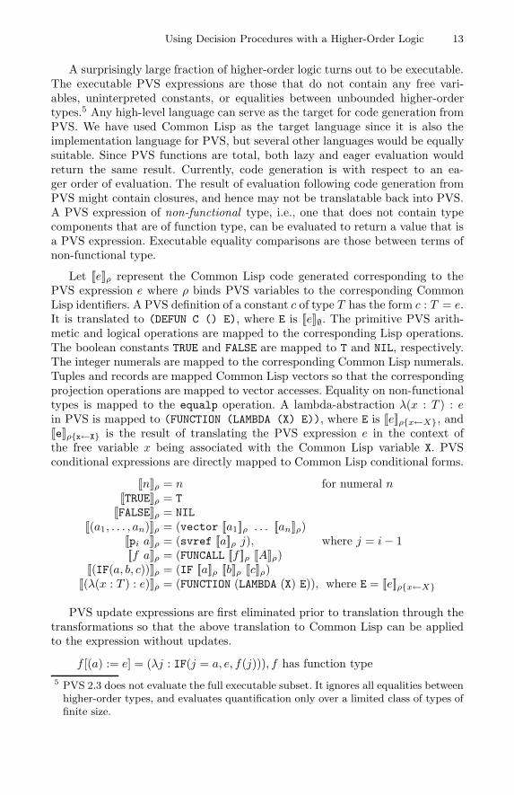
Let [[e]]ρ represent the Common Lisp code generated corresponding to thePVS expression e where ρ binds PVS variables to the corresponding CommonLisp identifiers. A PVS definition of a constant c of type T has the form c : T = e.It is translated to (DEFUN C () E), where E is [[e]]∅. The primitive PVS arith-metic and logical operations are mapped to the corresponding Lisp operations.The boolean constants TRUE and FALSE are mapped to T and NIL, respectively.The integer numerals are mapped to the corresponding Common Lisp numerals.Tuples and records are mapped Common Lisp vectors so that the correspondingprojection operations are mapped to vector accesses. Equality on non-functionaltypes is mapped to the equalp operation. A lambda-abstraction λ(x : T ) : ein PVS is mapped to (FUNCTION (LAMBDA (X) E)), where E is [[e]]ρ{x←X}, and[[e]]ρ{x←X} is the result of translating the PVS expression e in the context ofthe free variable x being associated with the Common Lisp variable X. PVSconditional expressions are directly mapped to Common Lisp conditional forms.
[[n]]ρ = n for numeral n[[TRUE]]ρ = T
[[FALSE]]ρ = NIL[[(a1, . . . , an)]]ρ = (vector [[a1]]ρ . . . [[an]]ρ)
[[pi a]]ρ = (svref [[a]]ρ j), where j = i− 1[[f a]]ρ = (FUNCALL [[f ]]ρ [[A]]ρ)
[[(IF(a, b, c))]]ρ = (IF [[a]]ρ [[b]]ρ [[c]]ρ)[[(λ(x : T ) : e)]]ρ = (FUNCTION (LAMBDA (X) E)), where E = [[e]]ρ{x←X}
PVS update expressions are first eliminated prior to translation through thetransformations so that the above translation to Common Lisp can be appliedto the expression without updates.
f [(a) := e] = (λj : IF(j = a, e, f(j))), f has function type5 PVS 2.3 does not evaluate the full executable subset. It ignores all equalities between
higher-order types, and evaluates quantification only over a limited class of types offinite size.
14 Natarajan Shankar
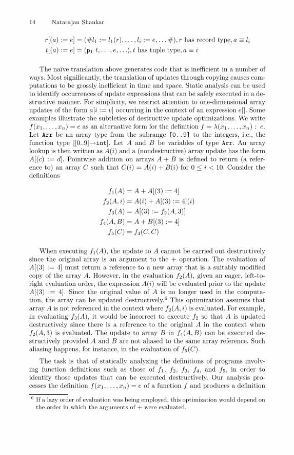
r[(a) := e] = (#l1 := l1(r), . . . , li := e, . . .#), r has record type, a ≡ li
t[(a) := e] = (p1 t, . . . , e, . . .), t has tuple type, a ≡ i
The naıve translation above generates code that is inefficient in a number ofways. Most significantly, the translation of updates through copying causes com-putations to be grossly inefficient in time and space. Static analysis can be usedto identify occurrences of update expressions that can be safely executed in a de-structive manner. For simplicity, we restrict attention to one-dimensional arrayupdates of the form a[i := v] occurring in the context of an expression e[]. Someexamples illustrate the subtleties of destructive update optimizations. We writef(x1, . . . , xn) = e as an alternative form for the definition f = λ(x1, . . . , xn) : e.Let Arr be an array type from the subrange [0..9] to the integers, i.e., thefunction type [[0..9]→int]. Let A and B be variables of type Arr. An arraylookup is then written as A(i) and a (nondestructive) array update has the formA[(c) := d]. Pointwise addition on arrays A + B is defined to return (a refer-ence to) an array C such that C(i) = A(i) + B(i) for 0 ≤ i < 10. Consider thedefinitions
f1(A) = A + A[(3) := 4]f2(A, i) = A(i) + A[(3) := 4](i)f3(A) = A[(3) := f2(A, 3)]
f4(A,B) = A + B[(3) := 4]f5(C) = f4(C,C)
When executing f1(A), the update to A cannot be carried out destructivelysince the original array is an argument to the + operation. The evaluation ofA[(3) := 4] must return a reference to a new array that is a suitably modifiedcopy of the array A. However, in the evaluation f2(A), given an eager, left-to-right evaluation order, the expression A(i) will be evaluated prior to the updateA[(3) := 4]. Since the original value of A is no longer used in the computa-tion, the array can be updated destructively.6 This optimization assumes thatarray A is not referenced in the context where f2(A, i) is evaluated. For example,in evaluating f3(A), it would be incorrect to execute f2 so that A is updateddestructively since there is a reference to the original A in the context whenf2(A, 3) is evaluated. The update to array B in f4(A,B) can be executed de-structively provided A and B are not aliased to the same array reference. Suchaliasing happens, for instance, in the evaluation of f5(C).
The task is that of statically analyzing the definitions of programs involv-ing function definitions such as those of f1, f2, f3, f4, and f5, in order toidentify those updates that can be executed destructively. Our analysis pro-cesses the definition f(x1, . . . , xn) = e of a function f and produces a definition
6 If a lazy order of evaluation was being employed, this optimization would depend onthe order in which the arguments of + were evaluated.
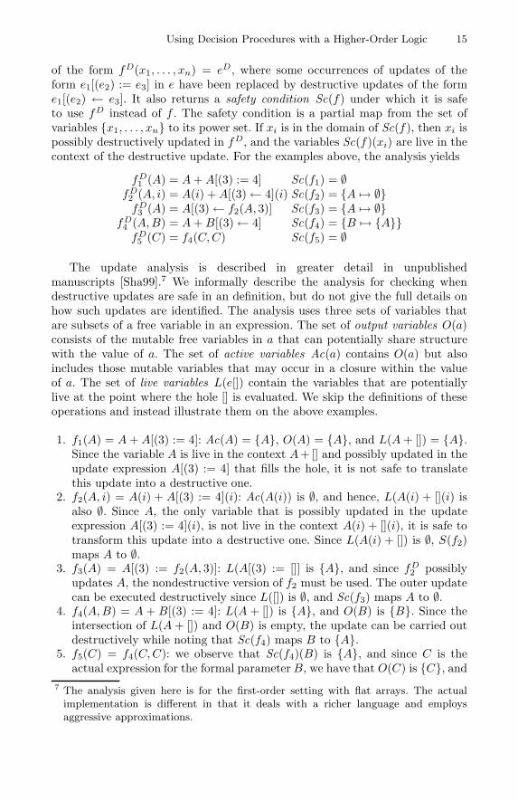
Using Decision Procedures with a Higher-Order Logic 15
of the form fD(x1, . . . , xn) = eD, where some occurrences of updates of theform e1[(e2) := e3] in e have been replaced by destructive updates of the forme1[(e2) ← e3]. It also returns a safety condition Sc(f) under which it is safeto use fD instead of f . The safety condition is a partial map from the set ofvariables {x1, . . . , xn} to its power set. If xi is in the domain of Sc(f), then xi ispossibly destructively updated in fD, and the variables Sc(f)(xi) are live in thecontext of the destructive update. For the examples above, the analysis yields
fD1 (A) = A + A[(3) := 4] Sc(f1) = ∅
fD2 (A, i) = A(i) + A[(3)← 4](i) Sc(f2) = {A �→ ∅}fD3 (A) = A[(3)← f2(A, 3)] Sc(f3) = {A �→ ∅}
fD4 (A,B) = A + B[(3)← 4] Sc(f4) = {B �→ {A}}fD5 (C) = f4(C,C) Sc(f5) = ∅
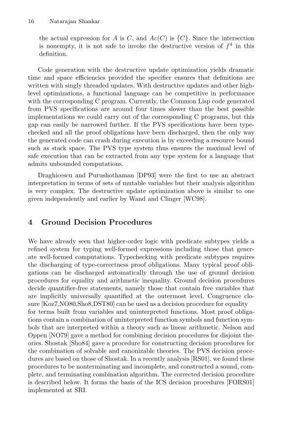
The update analysis is described in greater detail in unpublishedmanuscripts [Sha99].7 We informally describe the analysis for checking whendestructive updates are safe in an definition, but do not give the full details onhow such updates are identified. The analysis uses three sets of variables thatare subsets of a free variable in an expression. The set of output variables O(a)consists of the mutable free variables in a that can potentially share structurewith the value of a. The set of active variables Ac(a) contains O(a) but alsoincludes those mutable variables that may occur in a closure within the valueof a. The set of live variables L(e[]) contain the variables that are potentiallylive at the point where the hole [] is evaluated. We skip the definitions of theseoperations and instead illustrate them on the above examples.
1. f1(A) = A + A[(3) := 4]: Ac(A) = {A}, O(A) = {A}, and L(A + []) = {A}.Since the variable A is live in the context A+ [] and possibly updated in theupdate expression A[(3) := 4] that fills the hole, it is not safe to translatethis update into a destructive one.
2. f2(A, i) = A(i) + A[(3) := 4](i): Ac(A(i)) is ∅, and hence, L(A(i) + [](i) isalso ∅. Since A, the only variable that is possibly updated in the updateexpression A[(3) := 4](i), is not live in the context A(i) + [](i), it is safe totransform this update into a destructive one. Since L(A(i) + []) is ∅, S(f2)maps A to ∅.
3. f3(A) = A[(3) := f2(A, 3)]: L(A[(3) := []] is {A}, and since fD2 possibly
updates A, the nondestructive version of f2 must be used. The outer updatecan be executed destructively since L([]) is ∅, and Sc(f3) maps A to ∅.
4. f4(A,B) = A + B[(3) := 4]: L(A + []) is {A}, and O(B) is {B}. Since theintersection of L(A + []) and O(B) is empty, the update can be carried outdestructively while noting that Sc(f4) maps B to {A}.
5. f5(C) = f4(C,C): we observe that Sc(f4)(B) is {A}, and since C is theactual expression for the formal parameter B, we have that O(C) is {C}, and
7 The analysis given here is for the first-order setting with flat arrays. The actualimplementation is different in that it deals with a richer language and employsaggressive approximations.
16 Natarajan Shankar
the actual expression for A is C, and Ac(C) is {C}. Since the intersectionis nonempty, it is not safe to invoke the destructive version of f4 in thisdefinition.
Code generation with the destructive update optimization yields dramatictime and space efficiencies provided the specifier ensures that definitions arewritten with singly threaded updates. With destructive updates and other high-level optimizations, a functional language can be competitive in performancewith the corresponding C program. Currently, the Common Lisp code generatedfrom PVS specifications are around four times slower than the best possibleimplementations we could carry out of the corresponding C programs, but thisgap can easily be narrowed further. If the PVS specifications have been type-checked and all the proof obligations have been discharged, then the only waythe generated code can crash during execution is by exceeding a resource boundsuch as stack space. The PVS type system thus ensures the maximal level ofsafe execution that can be extracted from any type system for a language thatadmits unbounded computations.
Draghicescu and Purushothaman [DP93] were the first to use an abstractinterpretation in terms of sets of mutable variables but their analysis algorithmis very complex. The destructive update optimization above is similar to onegiven independently and earlier by Wand and Clinger [WC98].
4 Ground Decision Procedures
We have already seen that higher-order logic with predicate subtypes yields arefined system for typing well-formed expressions including those that gener-ate well-formed computations. Typechecking with predicate subtypes requiresthe discharging of type-correctness proof obligations. Many typical proof obli-gations can be discharged automatically through the use of ground decisionprocedures for equality and arithmetic inequality. Ground decision proceduresdecide quantifier-free statements, namely those that contain free variables thatare implicitly universally quantified at the outermost level. Congruence clo-sure [Koz77,NO80,Sho78,DST80] can be used as a decision procedure for equalityfor terms built from variables and uninterpreted functions. Most proof obliga-tions contain a combination of uninterpreted function symbols and function sym-bols that are interpreted within a theory such as linear arithmetic. Nelson andOppen [NO79] gave a method for combining decision procedures for disjoint the-ories. Shostak [Sho84] gave a procedure for constructing decision procedures forthe combination of solvable and canonizable theories. The PVS decision proce-dures are based on those of Shostak. In a recently analysis [RS01], we found theseprocedures to be nonterminating and incomplete, and constructed a sound, com-plete, and terminating combination algorithm. The corrected decision procedureis described below. It forms the basis of the ICS decision procedures [FORS01]implemented at SRI.
Using Decision Procedures with a Higher-Order Logic 17
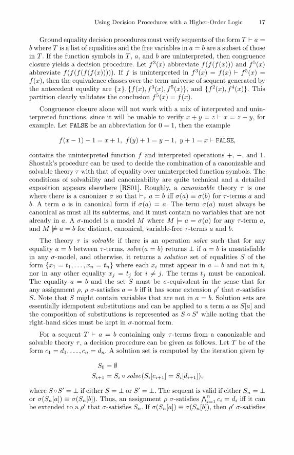
Ground equality decision procedures must verify sequents of the form T � a =b where T is a list of equalities and the free variables in a = b are a subset of thosein T . If the function symbols in T , a, and b are uninterpreted, then congruenceclosure yields a decision procedure. Let f3(x) abbreviate f(f(f(x))) and f5(x)abbreviate f(f(f(f(f(x))))). If f is uninterpreted in f3(x) = f(x) � f5(x) =f(x), then the equivalence classes over the term universe of sequent generated bythe antecedent equality are {x}, {f(x), f3(x), f5(x)}, and {f2(x), f4(x)}. Thispartition clearly validates the conclusion f5(x) = f(x).
Congruence closure alone will not work with a mix of interpreted and unin-terpreted functions, since it will be unable to verify x + y = z � x = z − y, forexample. Let FALSE be an abbreviation for 0 = 1, then the example
f(x− 1)− 1 = x + 1, f(y) + 1 = y − 1, y + 1 = x � FALSE,
contains the uninterpreted function f and interpreted operations +, −, and 1.Shostak’s procedure can be used to decide the combination of a canonizable andsolvable theory τ with that of equality over uninterpreted function symbols. Theconditions of solvability and canonizability are quite technical and a detailedexposition appears elsewhere [RS01]. Roughly, a canonizable theory τ is onewhere there is a canonizer σ so that �τ a = b iff σ(a) ≡ σ(b) for τ -terms a andb. A term a is in canonical form if σ(a) = a. The term σ(a) must always becanonical as must all its subterms, and it must contain no variables that are notalready in a. A σ-model is a model M where M |= a = σ(a) for any τ -term a,and M �|= a = b for distinct, canonical, variable-free τ -terms a and b.
The theory τ is solvable if there is an operation solve such that for anyequality a = b between τ -terms, solve(a = b) returns ⊥ if a = b is unsatisfiablein any σ-model, and otherwise, it returns a solution set of equalities S of theform {x1 = t1, . . . , xn = tn} where each xi must appear in a = b and not in tinor in any other equality xj = tj for i �= j. The terms tj must be canonical.The equality a = b and the set S must be σ-equivalent in the sense that forany assignment ρ, ρ σ-satisfies a = b iff it has some extension ρ′ that σ-satisfiesS. Note that S might contain variables that are not in a = b. Solution sets areessentially idempotent substitutions and can be applied to a term a as S[a] andthe composition of substitutions is represented as S ◦ S′ while noting that theright-hand sides must be kept in σ-normal form.
For a sequent T � a = b containing only τ -terms from a canonizable andsolvable theory τ , a decision procedure can be given as follows. Let T be of theform c1 = d1, . . . , cn = dn. A solution set is computed by the iteration given by
S0 = ∅Si+1 = Si ◦ solve(Si[ci+1] = Si[di+1]),
where S ◦S′ = ⊥ if either S = ⊥ or S′ = ⊥. The sequent is valid if either Sn = ⊥or σ(Sn[a]) ≡ σ(Sn[b]). Thus, an assignment ρ σ-satisfies
∧ni=1 ci = di iff it can
be extended to a ρ′ that σ-satisfies Sn. If σ(Sn[a]) ≡ σ(Sn[b]), then ρ′ σ-satisfies
18 Natarajan Shankar
a = Sn[a] = σ(Sn[a]) = σ(Sn[b]) = Sn[b] = b. Otherwise, ρ σ-satisfies T but nota = b and hence T � a = b is not valid.
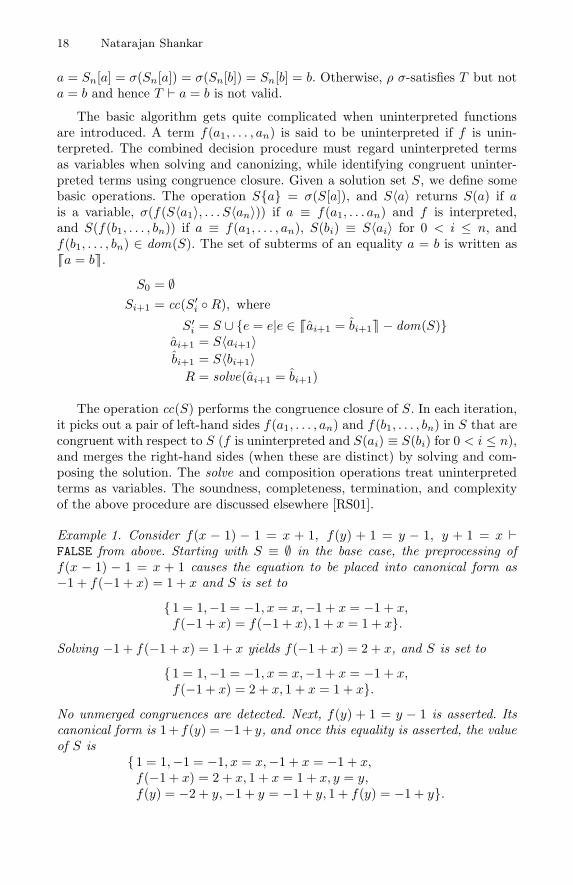
The basic algorithm gets quite complicated when uninterpreted functionsare introduced. A term f(a1, . . . , an) is said to be uninterpreted if f is unin-terpreted. The combined decision procedure must regard uninterpreted termsas variables when solving and canonizing, while identifying congruent uninter-preted terms using congruence closure. Given a solution set S, we define somebasic operations. The operation S{a} = σ(S[a]), and S〈a〉 returns S(a) if ais a variable, σ(f(S〈a1〉, . . . S〈an〉)) if a ≡ f(a1, . . . an) and f is interpreted,and S(f(b1, . . . , bn)) if a ≡ f(a1, . . . , an), S(bi) ≡ S〈ai〉 for 0 < i ≤ n, andf(b1, . . . , bn) ∈ dom(S). The set of subterms of an equality a = b is written as��a = b��.
S0 = ∅Si+1 = cc(S′i ◦R), where
S′i = S ∪ {e = e|e ∈ ��ai+1 = bi+1�� − dom(S)}ai+1 = S〈ai+1〉bi+1 = S〈bi+1〉
R = solve(ai+1 = bi+1)
The operation cc(S) performs the congruence closure of S. In each iteration,it picks out a pair of left-hand sides f(a1, . . . , an) and f(b1, . . . , bn) in S that arecongruent with respect to S (f is uninterpreted and S(ai) ≡ S(bi) for 0 < i ≤ n),and merges the right-hand sides (when these are distinct) by solving and com-posing the solution. The solve and composition operations treat uninterpretedterms as variables. The soundness, completeness, termination, and complexityof the above procedure are discussed elsewhere [RS01].
Example 1. Consider f(x − 1) − 1 = x + 1, f(y) + 1 = y − 1, y + 1 = x �FALSE from above. Starting with S ≡ ∅ in the base case, the preprocessing off(x − 1) − 1 = x + 1 causes the equation to be placed into canonical form as−1 + f(−1 + x) = 1 + x and S is set to
{ 1 = 1,−1 = −1, x = x,−1 + x = −1 + x,f(−1 + x) = f(−1 + x), 1 + x = 1 + x}.
Solving −1 + f(−1 + x) = 1 + x yields f(−1 + x) = 2 + x, and S is set to
{ 1 = 1,−1 = −1, x = x,−1 + x = −1 + x,f(−1 + x) = 2 + x, 1 + x = 1 + x}.
No unmerged congruences are detected. Next, f(y) + 1 = y − 1 is asserted. Itscanonical form is 1+ f(y) = −1+ y, and once this equality is asserted, the valueof S is
{ 1 = 1,−1 = −1, x = x,−1 + x = −1 + x,f(−1 + x) = 2 + x, 1 + x = 1 + x, y = y,f(y) = −2 + y,−1 + y = −1 + y, 1 + f(y) = −1 + y}.
Using Decision Procedures with a Higher-Order Logic 19
Next y + 1 = x is processed. Its canonical form is 1 + y = x and the equality1+ y = 1+ y is added to S. Solving y+1 = x yields x = 1+ y, and S is reset to
{ 1 = 1,−1 = −1, x = 1 + y,−1 + x = y,f(−1 + x) = 3 + y, 1 + x = 2 + y, y = y,f(y) = −2 + y,−1 + y = −1 + y,1 + f(y) = −1 + y, 1 + y = 1 + y}.
The congruence close operation cc detects the congruence f(1 − y) S∼ f(x) andinvokes merge on 3 + y and −2 + y. Solving this equality 3 + y = −2 + y yields⊥ returning the desired contradiction.
The ground decision procedures can be used in an incremental manner. As-sertions can be added to update the context given by the state of the datastructures used by decision procedures. Assertions can be tested for truth orfalsity with respect to a given context. In PVS, ground decision procedures areused to build up a context associated with each sequent in a proof consistingof type information and the atomic formulas in the sequent. Many of the leafnodes of a proof consist of sequents that have been verified by the ground de-cision procedures. These procedures are also used to simplify expressions usingthe contextual information given by the governing conditionals and type infor-mation from bound variables. The simplifier based on the decision procedures isused to automatically discharge proof obligations that arise in rewriting eitherthrough conditions of conditional rewrite rules or through subtype conditions ona matching substitution.
5 Finite-State Methods
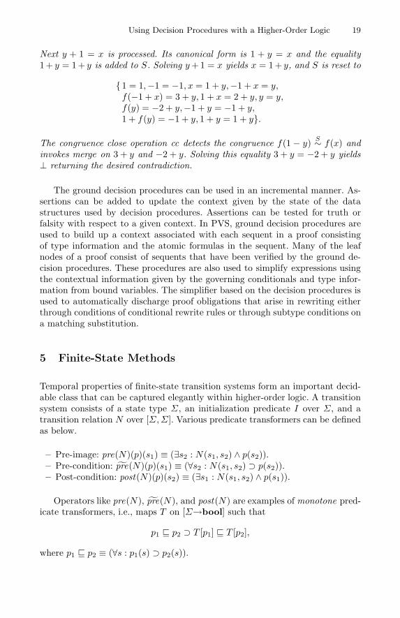
Temporal properties of finite-state transition systems form an important decid-able class that can be captured elegantly within higher-order logic. A transitionsystem consists of a state type Σ, an initialization predicate I over Σ, and atransition relation N over [Σ,Σ]. Various predicate transformers can be definedas below.
– Pre-image: pre(N)(p)(s1) ≡ (∃s2 : N(s1, s2) ∧ p(s2)).– Pre-condition: pre(N)(p)(s1) ≡ (∀s2 : N(s1, s2) ⊃ p(s2)).– Post-condition: post(N)(p)(s2) ≡ (∃s1 : N(s1, s2) ∧ p(s1)).
Operators like pre(N), pre(N), and post(N) are examples of monotone pred-icate transformers, i.e., maps T on [Σ→bool] such that
p1 � p2 ⊃ T [p1] � T [p2],
where p1 � p2 ≡ (∀s : p1(s) ⊃ p2(s)).
20 Natarajan Shankar
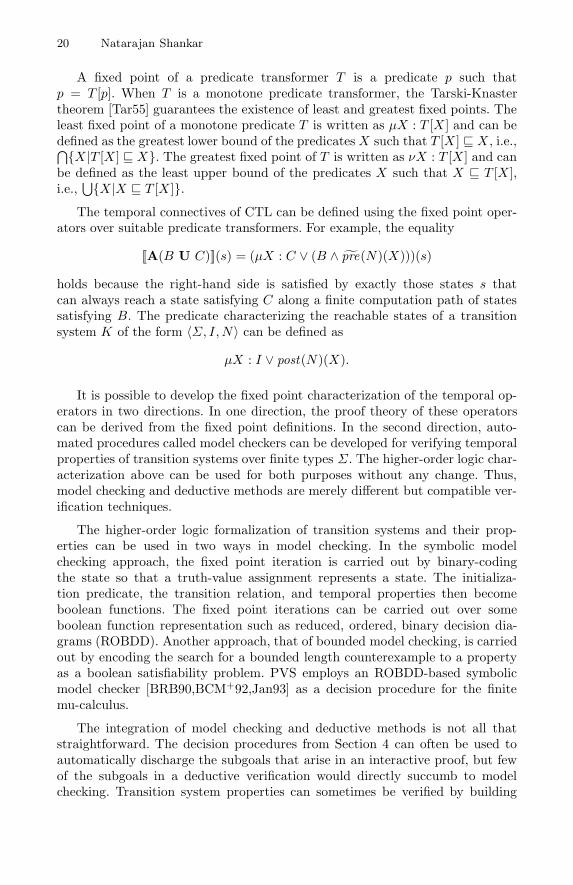
A fixed point of a predicate transformer T is a predicate p such thatp = T [p]. When T is a monotone predicate transformer, the Tarski-Knastertheorem [Tar55] guarantees the existence of least and greatest fixed points. Theleast fixed point of a monotone predicate T is written as µX : T [X ] and can bedefined as the greatest lower bound of the predicates X such that T [X ] � X , i.e.,⋂{X |T [X ] � X}. The greatest fixed point of T is written as νX : T [X ] and canbe defined as the least upper bound of the predicates X such that X � T [X ],i.e.,
⋃{X |X � T [X ]}.The temporal connectives of CTL can be defined using the fixed point oper-
ators over suitable predicate transformers. For example, the equality
[[A(B U C)]](s) = (µX : C ∨ (B ∧ pre(N)(X)))(s)
holds because the right-hand side is satisfied by exactly those states s thatcan always reach a state satisfying C along a finite computation path of statessatisfying B. The predicate characterizing the reachable states of a transitionsystem K of the form 〈Σ, I,N〉 can be defined as
µX : I ∨ post(N)(X).
It is possible to develop the fixed point characterization of the temporal op-erators in two directions. In one direction, the proof theory of these operatorscan be derived from the fixed point definitions. In the second direction, auto-mated procedures called model checkers can be developed for verifying temporalproperties of transition systems over finite types Σ. The higher-order logic char-acterization above can be used for both purposes without any change. Thus,model checking and deductive methods are merely different but compatible ver-ification techniques.
The higher-order logic formalization of transition systems and their prop-erties can be used in two ways in model checking. In the symbolic modelchecking approach, the fixed point iteration is carried out by binary-codingthe state so that a truth-value assignment represents a state. The initializa-tion predicate, the transition relation, and temporal properties then becomeboolean functions. The fixed point iterations can be carried out over someboolean function representation such as reduced, ordered, binary decision dia-grams (ROBDD). Another approach, that of bounded model checking, is carriedout by encoding the search for a bounded length counterexample to a propertyas a boolean satisfiability problem. PVS employs an ROBDD-based symbolicmodel checker [BRB90,BCM+92,Jan93] as a decision procedure for the finitemu-calculus.
The integration of model checking and deductive methods is not all thatstraightforward. The decision procedures from Section 4 can often be used toautomatically discharge the subgoals that arise in an interactive proof, but fewof the subgoals in a deductive verification would directly succumb to modelchecking. Transition system properties can sometimes be verified by building
Using Decision Procedures with a Higher-Order Logic 21
finite-state abstractions that are amenable to model checking. Even when sucha finite-state abstraction is not immediately verified by model checking, it ispossible to extract useful intermediate properties.
Deductive methods have difficulties with control-intensive systems where ab-straction and model checking are quite successful. Invariants are properties oftransition systems that are satisfied in all reachable states. Deduction requiresan inductive invariant that is preserved by each transition. Finding inductive in-variants is not easy. Model checking can restrict its exploration to the reachablestates and thus avoids constructing inductive invariants. Abstraction is a use-ful way of decomposing the verification task between deductive and explorativemethods. An abstraction mapping indicates how the concrete state is mappedto a finite state. In the case of predicate abstraction, the abstract state containsbooleans that capture predicates on the concrete state. An abstract model ap-proximating the behavior of the concrete transition system can be constructedby using a theorem prover to eliminate abstract transitions that have no con-crete counterpart. Then the reachable states of the resulting abstract transitionsystem can be used to construct a valid invariant for the concrete transitionsystem.
Ground decision procedures play a crucial role in the construction of anabstract transition system from a concrete one based on a given abstractionmap. This construction involves a large number of small-sized proof obligationsthat are mostly dischargeable using decision procedures.
Predicate abstraction was first used by Graf and Saıdi [SG97] to construct theabstract reachability graph of a transition system with respect to an abstractionmap. The InVest system [BLO98] uses the elimination method mentioned aboveto construct abstractions of transition systems described in a fragment of PVS.An abstraction capability for the mu-calculus has been added to PVS in order toabstract transition systems along with their temporal properties [SS99,Sha01].
6 Discussion
We have barely scratched the surface of the kinds of problems that can benaturally expressed and effectively automated using higher-order logics. As apragmatic point, we have argued that higher-order logic provides a good bal-ance between expressiveness and automation by embedding useful formalismsfor which there is good automation support. Most of these problems can alreadybe expressed in second-order or third-order logic, but the full range of finite-order types adds very little complexity. The directness with which these logicscan be embedded in higher-order logic allows the decision procedures to be usedwithout having to span the semantic gap between diverse logics.
We have shown a few ways in which decision procedures interact synergisti-cally with higher-order logic. They can be used to add expressivity to the type
22 Natarajan Shankar
system through predicate subtypes and dependent types. Static analysis can beapplied to higher-order programs to infer safe destructive array updates. Theresulting optimized programs can be executed with efficiencies that are com-parable with implementations in low-level imperative programming languages.Fixed point calculi can be embedded in higher-order logic. A number of tempo-ral logics can be defined using the fixed point operators. The finite-state versionof the fixed point calculus can be decided using a BDD-based symbolic modelchecker. Ground decision procedures can be used to construct finite-state ab-stractions from large or infinite-state transition systems. Decidable fragments ofhigher-order logic can be used to verify properties of parametric systems.
The synergy between expressiveness and automation can be further exploredalong a number of lines. We have examined evaluation in a functional sublan-guage of higher-order logic. A number of high-level optimizations can be ex-plored in the context of a theorem proving environment. It is also possible toembed programming vernaculars such as logic programming [Sym98] and im-perative programming. Higher-order logic programming with the use of higher-order syntactic encoding has emerged as an important medium for metaprogram-ming [NM90]. A number of useful decision procedures from computer algebra,operations research, and engineering, can also be usefully incorporated into atheorem proving environment. Drawing inspiration from the work of Boyer andMoore [BM81], a metaprogramming capability can be used to reflectively developa theorem proving system within itself in a bootstrapped manner.
Proof search is an area where PVS is currently inadequate. First-orderproof search methods have been successfully used in Isabelle [Pau98]. Proofsearch methods within the full higher-order logic have had some selective suc-cesses [AINP88,BK98], but quantifier-elimination methods and proof searchmethods for limited fragments are more likely to yield profitable results in theshort run.
The entire enterprise of theorem proving in higher-order logics is poised atan interesting confluence between expressiveness and automation, principle andpragmatism, and theory and practice. Significant breakthroughs can be antici-pated if we see synergies rather than conflict in this confluence.
Acknowledgments
I thank the TPHOLS’01 conference chair Richard Boulton, the programme chairPaul Jackson, and the programme committee, for their kind invitation. I amalso grateful to the TPHOLS community for stimulus and inspiration. MichaelKohlhase was generous with his insights on higher-order proof search. Paul Jack-son gave me detailed and helpful comments on an earlier draft, as did Sam Owreand John Rushby. The ideas and results presented here are the fruits of col-laborations with several people including Sam Owre, John Rushby, Sree Rajan,Harald Rueß, Hassen Saıdi, and Mandayam Srivas.
Using Decision Procedures with a Higher-Order Logic 23
References
AINP88. Peter B. Andrews, Sunil Issar, Daniel Nesmith, and Frank Pfenning. TheTPS theorem proving system. In E. Lusk and R. Overbeek, editors, 9thInternational Conference on Automated Deduction (CADE), volume 310of Lecture Notes in Computer Science, pages 760–761, Argonne, IL, May1988. Springer-Verlag.
And86. Peter B. Andrews. An Introduction to Logic and Type Theory: To Truththrough Proof. Academic Press, New York, NY, 1986.
BCM+92. J. R. Burch, E. M. Clarke, K. L. McMillan, D. L. Dill, and L. J. Hwang.Symbolic model checking: 1020 states and beyond. Information and Com-putation, 98(2):142–170, June 1992.
BK98. Christoph Benzmuller and Michael Kohlhase. Extensional higher-orderresolution. In H. Kirchner and C. Kirchner, editors, Proceedings of CADE-15, number 1421 in Lecture Notes in Artificial Intelligence, pages 56–71,Berlin, Germany, July 1998. Springer-Verlag.
BLO98. Saddek Bensalem, Yassine Lakhnech, and Sam Owre. Computing abstrac-tions of infinite state systems compositionally and automatically. In Huand Vardi [HV98], pages 319–331.
BM81. R. S. Boyer and J S. Moore. Metafunctions: Proving them correct andusing them efficiently as new proof procedures. In R. S. Boyer and J S.Moore, editors, The Correctness Problem in Computer Science. AcademicPress, London, 1981.
BM86. R. S. Boyer and J S. Moore. Integrating decision procedures into heuris-tic theorem provers: A case study with linear arithmetic. In MachineIntelligence, volume 11. Oxford University Press, 1986.
Bou93. R. J. Boulton. Lazy techniques for fully expansive theorem proving. For-mal Methods in System Design, 3(1/2):25–47, August 1993.
BRB90. K. S. Brace, R. L. Rudell, and R. E. Bryant. Efficient implementationof a BDD package. In Proc. of the 27th ACM/IEEE Design AutomationConference, pages 40–45, 1990.
Bun83. Alan Bundy. The Computer Modelling of Mathematical Reasoning. Aca-demic Press, London, UK, 1983.
But97. Bettina Buth. PAMELA + PVS. In Michael Johnson, editor, AlgebraicMethodology and Software Technology, AMAST’97, volume 1349 of LectureNotes in Computer Science, pages 560–562, Sydney, Australia, December1997. Springer-Verlag.
CAB+86. R. L. Constable, S. F. Allen, H. M. Bromley, W. R. Cleaveland, J. F. Cre-mer, R. W. Harper, D. J. Howe, T. B. Knoblock, N. P. Mendler, P. Panan-gaden, J. T. Sasaki, and S. F. Smith. Implementing Mathematics with theNuprl Proof Development System. Prentice Hall, Englewood Cliffs, NJ,1986.
CDC80. Mario Coppo and Mariangiola Dezani-Ciancaglini. An extension of thebasic functionality theory for the lambda-calculus. Notre Dame J. FormalLogic, 21(4):685–693, 1980.
CH85. T. Coquand and G. P. Huet. Constructions: A higher order proof sys-tem for mechanizing mathematics. In Proceedings of EUROCAL 85, Linz(Austria), Berlin, 1985. Springer-Verlag.
Chu40. A. Church. A formulation of the simple theory of types. Journal ofSymbolic Logic, 5:56–68, 1940.
24 Natarajan Shankar
dB80. N. G. de Bruijn. A survey of the project Automath. In To H. B. Curry:Essays on Combinatory Logic, Lambda Calculus and Formalism, pages589–606. Academic Press, 1980.
DCN+00. Louise A. Dennis, Graham Collins, Michael Norrish, Richard Boulton,Konrad Slind, Graham Robinson, Mike Gordon, and Tom Melham. ThePROSPER toolkit. In Susanne Graf and Michael Schwartzbach, edi-tors, Tools and Algorithms for the Construction and Analysis of Systems(TACAS 2000), number 1785 in Lecture Notes in Computer Science, pages78–92, Berlin, Germany, March 2000. Springer-Verlag.
DFH+91. Gilles Dowek, Amy Felty, Hugo Herbelin, Gerard Huet, Christine Paulin-Mohring, and Benjamin Werner. The COQ proof assistant user’s guide:Version 5.6. Rapports Techniques 134, INRIA, Rocquencourt, France,December 1991.
DKML99. Martin Dunstan, Tom Kelsey, Ursula Martin, and Steve Linton. Formalmethods for extensions to CAS. In Jeannette Wing and Jim Woodcock,editors, FM99: The World Congress in Formal Methods, volume 1708 and1709 of Lecture Notes in Computer Science, pages 1758–1777, Toulouse,France, September 1999. Springer-Verlag. Pages 1–938 are in the firstvolume, 939–1872 in the second.
DP93. M. Draghicescu and S. Purushothaman. A uniform treatment of or-der of evaluation and aggregate update. Theoretical Computer Science,118(2):231–262, September 1993.
DST80. P.J. Downey, R. Sethi, and R.E. Tarjan. Variations on the common subex-pressions problem. Journal of the ACM, 27(4):758–771, 1980.
Fef78. Solomon Feferman. Theories of finite type related to mathematical prac-tice. In Jon Barwise, editor, Handbook of Mathematical Logic, volume 90of Studies in Logic and the Foundations of Mathematics, chapter D4, pages913–972. North-Holland, Amsterdam, Holland, 1978.
FORS01. J-C. Filliatre, S. Owre, H. Rueß, and N. Shankar. ICS: Integrated canon-izer and solver. In CAV 01: Computer-Aided Verification. Springer-Verlag,2001. To appear.
GM93. M. J. C. Gordon and T. F. Melham, editors. Introduction to HOL: A The-orem Proving Environment for Higher-Order Logic. Cambridge UniversityPress, Cambridge, UK, 1993.
GMW79. M. Gordon, R. Milner, and C. Wadsworth. Edinburgh LCF: A MechanizedLogic of Computation, volume 78 of Lecture Notes in Computer Science.Springer-Verlag, 1979.
Gor88. M. J. C. Gordon. Mechanizing programming logics in higher order logic.Technical Report CCSRC-006, Cambridge Computer Science ResearchCenter, SRI International, Cambridge, England, September 1988.
Har96. John Harrison. Stalmarck’s algorithm as a HOL derived rule. InJ. von Wright, J. Grundy, and J. Harrison, editors, Proceedings of the9th TPHOLS, number 1125 in Lecture Notes in Computer Science, pages251–266, Berlin, Germany, 1996. Springer-Verlag.
Hat68. William S. Hatcher. Foundations of Mathematics. W. B. Saunders Com-pany, Philadelphia, PA, 1968.
HD92. F. K. Hanna and N. Daeche. Dependent types and formal synthesis. InC. A. R. Hoare and M. J. C. Gordon, editors, Mechanized Reasoning andHardware Design, pages 121–135, Hemel Hempstead, UK, 1992. PrenticeHall International Series in Computer Science.
Using Decision Procedures with a Higher-Order Logic 25
HV98. Alan J. Hu and Moshe Y. Vardi, editors. Computer-Aided Verification,CAV ’98, volume 1427 of Lecture Notes in Computer Science, Vancouver,Canada, June 1998. Springer-Verlag.
HWG98. David Hardin, Matthew Wilding, and David Greve. Transforming thetheorem prover into a digital design tool: From concept car to off-roadvehicle. In Hu and Vardi [HV98], pages 39–44.
Jan93. G. L. J. M. Janssen. ROBDD Software. Department of Electrical Engi-neering, Eindhoven University of Technology, October 1993.
JvdBH+98. Bart Jacobs, Joachim van den Berg, Marieke Huisman, Martijn vanBerkum, Ulrich Hensel, and Hendrick Tews. Reasoning about Java classes.In Proceedings, Object-Oriented Programming Systems, Languages andApplications (OOPSLA’98), pages 329–340, Vancouver, Canada, October1998. Association for Computing Machinery. Proceedings issued as ACMSIGPLAN Notices Vol. 33, No. 10, October 1998.
Koz77. D. Kozen. Complexity of finitely represented algebras. In Proc. 9th ACMSTOC, pages 164–177, 1977.
Lei94. Daniel Leivant. Higher order logic. In D. M. Gabbay, C. J. Hogger, andJ. A. Robinson, editors, Handbook of Logic in Artificial Intelligence andLogic Programming, Volume 2: Deduction Methodologies, pages 229–321.Clarendon Press, Oxford, 1994.
NL00. George C. Necula and Peter Lee. Proof generation in the touchstone the-orem prover. In David McAllester, editor, Automated Deduction—CADE-17, volume 1831 of Lecture Notes in Artificial Intelligence, pages 25–44,Pittsburgh, PA, June 2000. Springer-Verlag.
NM90. G. Nadathur and D. Miller. Higher-order Horn clauses. Journal of theACM, 37(4):777–814, 1990.
NO79. G. Nelson and D. C. Oppen. Simplification by cooperating decision pro-cedures. ACM Transactions on Programming Languages and Systems,1(2):245–257, 1979.
NO80. G. Nelson and D. C. Oppen. Fast decision procedures based on congruenceclosure. Journal of the ACM, 27(2):356–364, 1980.
ORS92. S. Owre, J. M. Rushby, and N. Shankar. PVS: A prototype verificationsystem. In Deepak Kapur, editor, 11th International Conference on Au-tomated Deduction (CADE), volume 607 of Lecture Notes in ArtificialIntelligence, pages 748–752, Saratoga, NY, June 1992. Springer-Verlag.
ORSvH95. Sam Owre, John Rushby, Natarajan Shankar, and Friedrich von Henke.Formal verification for fault-tolerant architectures: Prolegomena to thedesign of PVS. IEEE Transactions on Software Engineering, 21(2):107–125, February 1995.
OS97. Sam Owre and Natarajan Shankar. The formal semantics of PVS. Tech-nical Report SRI-CSL-97-2, Computer Science Laboratory, SRI Interna-tional, Menlo Park, CA, August 1997.
Pau94. Lawrence C. Paulson. Isabelle: A Generic Theorem Prover, volume 828 ofLecture Notes in Computer Science. Springer-Verlag, 1994.
Pau98. L. Paulson. The inductive approach to verifying cryptographic protocols.Journal of Computer Security, 6(1):85–128, 1998.
Ram90. F. P. Ramsey. The foundations of mathematics. In D. H. Mellor, editor,Philosophical Papers of F. P. Ramsey, chapter 8, pages 164–224. Cam-bridge University Press, Cambridge, UK, 1990. Originally published inProceedings of the London Mathematical Society , 25, pp. 338–384, 1925.
26 Natarajan Shankar
ROS98. John Rushby, Sam Owre, and N. Shankar. Subtypes for specifications:Predicate subtyping in PVS. IEEE Transactions on Software Engineering,24(9):709–720, September 1998.
RS01. Harald Rueß and Natarajan Shankar. Deconstructing Shostak. In Pro-ceedings 16th Annual IEEE Symp. on Logic in Computer Science, pages19–28. IEEE Computer Society Press, 2001.
RvHO91. John Rushby, Friedrich von Henke, and Sam Owre. An introduction toformal specification and verification using Ehdm. Technical Report SRI-CSL-91-2, Computer Science Laboratory, SRI International, Menlo Park,CA, February 1991.
SG97. Hassen Saıdi and Susanne Graf. Construction of abstract state graphs withPVS. In Orna Grumberg, editor, Computer-Aided Verification, CAV ’97,volume 1254 of Lecture Notes in Computer Science, pages 72–83, Haifa,Israel, June 1997. Springer-Verlag.
Sha99. N. Shankar. Efficiently executing PVS. Project report, Computer ScienceLaboratory, SRI International, Menlo Park, CA, November 1999. Avail-able at http://www.csl.sri.com/shankar/PVSeval.ps.gz.
Sha01. Natarajan Shankar. Automated verification using deduction, exploration,and abstraction. In Essays on Programming Methodology. Springer-Verlag,2001. To appear.
Sho78. R. Shostak. An algorithm for reasoning about equality. Comm. ACM,21:583–585, July 1978.
Sho84. R. E. Shostak. Deciding combinations of theories. Journal of the ACM,31(1):1–12, 1984.
SS99. Hassen Saıdi and N. Shankar. Abstract and model check while you prove.In Nicolas Halbwachs and Doron Peled, editors, Computer-Aided Verifica-tion, CAV ’99, volume 1633 of Lecture Notes in Computer Science, pages443–454, Trento, Italy, July 1999. Springer-Verlag.
Sym98. D. Syme. Declarative Theorem Proving for Operational Semantics. PhDthesis, University of Cambridge, 1998.
Tar55. A. Tarski. A lattice-theoretical fixpoint theorem and its applications.Pacific J. of Math., 5:285–309, 1955.
The98. Laurent Thery. A certified version of Buchberger’s algorithm. In H. Kirch-ner and C. Kirchner, editors, Proceedings of CADE-15, number 1421 inLecture Notes in Artificial Intelligence, pages 349–364, Berlin, Germany,July 1998. Springer-Verlag.
vBD83. Johan van Benthem and Kees Doets. Higher-order logic. In Dov M.Gabbay and Franz Guenthner, editors, Handbook of Philosophical Logic–Volume I: Elements of Classical Logic, volume 164 of Synthese Library,chapter I.4, pages 275–329. D. Reidel Publishing Company, Dordrecht,Holland, 1983.
vHCL+88. F. W. von Henke, J. S. Crow, R. Lee, J. M. Rushby, and R. A. Whitehurst.The Ehdm verification environment: An overview. In Proceedings 11thNational Computer Security Conference, pages 147–155, Baltimore, MD,October 1988. NBS/NCSC.
WC98. Mitchell Wand and William D. Clinger. Set constraints for destructivearray update optimization. In Proc. IEEE Conf. on Computer Languages’98, pages 184–193. IEEE, April 1998.
WR27. A. N. Whitehead and B. Russell. Principia Mathematica. CambridgeUniversity Press, Cambridge, revised edition, 1925–1927. Three volumes.The first edition was published 1910–1913.
Computer Algebra Meets Automated TheoremProving: Integrating Maple and PVS
Andrew Adams1, Martin Dunstan2, Hanne Gottliebsen3, Tom Kelsey3,Ursula Martin3, and Sam Owre4
1 School of CS, Cyb and EE, University of ReadingReading RG6 6AY, UK
2 NAG LTD, Wilkinson House, Jordan Hill RoadOxford OX2 8DR, UK
3 School of Computer Science, University of St. AndrewsSt Andrews KY16 9SS, UK
4 Computer Science Laboratory, SRI International333 Ravenswood Avenue, Menlo Park CA 94025, USA
Abstract. We describe an interface between version 6 of the Maplecomputer algebra system with the PVS automated theorem prover. Theinterface is designed to allow Maple users access to the robust and check-able proof environment of PVS. We also extend this environment by theprovision of a library of proof strategies for use in real analysis. Wedemonstrate examples using the interface and the real analysis library.These examples provide proofs which are both illustrative and applicableto genuine symbolic computation problems.
1 Introduction
In this paper we describe an interface between version 6 of the Maple com-puter algebra system, henceforth CAS, and the PVS automated theorem prover,ATP. CAS like Maple (which has 1 million users, mostly in the educationalsector) incorporate a wide variety of symbolic techniques, for example for fac-toring polynomials or computing Grobner bases, and increasingly some numeri-cal elements also. They provide a mathematical programming environment andfacilities such as graphics and document generation. They have enjoyed someoutstanding successes: for example ’t Hooft and Veltman received the 1999 No-bel Prize in Physics, Veltman for using computer algebra to verify ’t Hooft’sresults on quantum field theory. The advantages of combining symbolic/numericcomputation with logical reasoning are evident: improved inference capabilityand increased expressivity. A human performing symbolic mathematics by handwill make automatic use of the logical framework upon which the mathematicsis based. A human performing similar calculations using a CAS has to supplythe same logical framework; there is, in general, no sound reasoning system builtin to the CAS. Our objective is to provide the CAS user with an interface to anATP, so that certain side conditions which are implicit in many analytic sym-bolic computations can be highlighted, checked, and either verified or flaggedas an error. The user interacts with the CAS, making calls to the ATP systemwhich acts as a black box for the provision of formal proofs.
R.J. Boulton and P.B. Jackson (Eds.): TPHOLs 2001, LNCS 2152, pp. 27–42, 2001.c© Springer-Verlag Berlin Heidelberg 2001
28 Andrew Adams et al.
While there have been many projects aimed at combining the calculationpower of CAS with the logical power of ATP systems, the basic approach isalways from the point of view of a user interested in completely correct develop-ments. That is, the point of view of a theorem proving user who wishes to havepowerful calculation available to generate existential witnesses or factorisations.Our approach takes the view point of a user of a CAS who simply wishes it tobe more robust. Current users of CAS, while not pleased when incorrect resultsare generated, are nevertheless willing to accept a certain level of deficiency as atrade-off for the utility of the system. We aim to improve the existing support forusers of CAS by adding to the correctness in an incremental way, with a blackbox ATP system supporting better computer algebra calculation. The work de-scribed in this paper is another step toward this goal, though much remains to bedone, both in terms of developing the formalisations needed in ATP systems andin re-engineering the algorithms implemented in CAS to take advantage of theblack box without losing the speed and power of existing CAS implementations.
The aims of this paper are (i) to describe the design and implementationof the interface (Section 3), and (ii) to illustrate its power by describing theautomated verification of properties needed to ensure correctness of routines fordifferential equations in Maple (Section 4). The remainder of this introductionprovides motivating examples, and briefly describe the systems involved and thebackground to the project. In Section 2 we discuss the extension to PVS whichallows automated proofs of side conditions, continuity and convergence for ele-mentary functions with parameters. One use of the interface is the checking ofthe validity of input to certain Maple procedures. For example, when solving adifferential equation, one must ensure that the input function f(x, y) is contin-uous (and thus defined) on the required region. This is not done by Maple, andso Maple might return an answer that looks like a plausible solution even if theinput is not of the right form. However, using the interface one can verify thecontinuity of f(x, y). Although our current PVS implementation of continuitychecking relies on a fairly simple method for verifying continuity, it does handlea large class of functions well.
1.1 Motivating Examples
In this section we show that CAS output can be misleading or incorrect. Atypical CAS will have no general mechanism for checking that results are math-ematically correct. Hence errors can arise in the determination of equality oftwo expressions, or in the definedness of expressions with respect to symbolicparameters. By not formally checking each result, CAS output can propagateerrors throughout a complicated symbolic calculation, and hence produce invalidresults. The following examples illustrate typical problems which can occur.
Simplification. The expression√x2 will not automatically simplify to x in
a CAS, since this is incorrect for negative x. Maple provides a mechanism forassuming that variables (and functions) have properties such as negativity (ordifferentiability), but the system can still fail to simplify expressions containingsquare roots correctly. To see this, consider the expressions a = |x − y| and
Integrating Maple and PVS 29
b = |√x+√y||√x−√y|, where x and y are positive reals. Suppose a Maple user
wishes to verify that a = b. The commands available are> a := abs(x-y);
a := |x− y|> b := abs(sqrt(x)+sqrt(y))*abs(sqrt(x)-sqrt(y));
b :=∣∣√x+
√y∣∣ ∣∣√x−√y
∣∣> assume(x > 0): assume(y > 0):> verify(a,b);
false
> verify(a,b,equal);
FAIL
Note that issuing a command assume (y > 0) binds all future occurrences inthis Maple session of the parameter y to be positive unless a new assumptionabout y is issued. However, not all algorithms will check the assumption databasefor information about the parameters included in their arguments. It is evidentthat there is a problem with the robustness of the Maple verify command:verify(a,b) returns false for this example; the heuristic simplification tech-niques used to reduce a − b to zero are inadequate. verify(a,b,equal) usesa more sophisticated set of heuristic techniques, but still fails to provide theexpected result, namely true. Hence, for this example, the output from Mapleis either an admission of failure or misleading to the user.
Definedness and Parameters. Consider the definite integral∫ b
0
1x− a
dx (1)
where a and b are positive real parameters. Maple returns the solution log(b −a)− log(a)−iπ, which, when a = 1 and b = 2, reduces to −iπ which is a complexnumber, and hence incorrect. Maple does not check that the function is definedeverywhere in the interval of integration; in this case that a is not in (0, b).
Continuity Checking. Maple has an inbuilt procedure for checking propertiesof functions and expressions. This procedure does not always return correctresults:
> is(x -> (1/x)+1-(1/x),continuous);
falseEven the assumption of positive arguments does not solve the problem:
> assume(y > 0):> is(y -> (1/y)+1-(1/y),continuous);
falseThe Maple/PVS interface described in this paper is designed to address the
problem of the lack of verification of CAS results. The Maple user works in the
30 Andrew Adams et al.
usual Maple environment, and has access to a formal, checkable proof mecha-nism which has been extended to deal with properties of real valued expressionsinvolving parameters, such as those given in the above examples. In Section 4.1we use the Maple/PVS interface to prove that
|x− y| = |√x+√y||√x−√y| for x, y > 0 (2)
and thatb > a > 0 =⇒ ∃x ∈ (0, b) such that x /∈ R \ {a} . (3)
These proofs allow the user to correct, modify or disregard the incorrect resultsfrom Maple.
1.2 Background
Previous approaches to the combination of CAS and ATP are discussed and clas-sified in [8]. We mention selected examples which are direct or indirect predeces-sors to this work. All approaches share the common problem of communicatingmathematical information between the CAS and ATP systems. One solutionis to define a standard for mathematical information that can, in principle, beunderstood by any mathematical computation system. Examples of this com-mon knowledge approach include the OpenMath project [1,11], and protocolsfor the exchange of information between generic CAS and ATP systems [5,15].Another solution is the sub-package approach, in which communication issuesare side-stepped by building an ATP within a CAS. Examples include Ana-lytica [4], REDLOG [12], the Theorema project [6,7], and a logical extensionto the type system of the AXIOM CAS [18,25]. The third common approachinvolves the choice of preferred CAS and ATP environments, and the construc-tion of a specific interface for communication between them. Examples includeMaple-HOL [16], Maple-Isabelle [3], and Weyl-NuPrl [17].
The common-knowledge approach depends on wholesale acceptance of theprotocols by both the CAS and ATP communities. Since this has not yet hap-pened, we concentrate on the remaining two approaches. The sub-package ap-proach has the advantage that communication is easy, and the disadvantage thatimplementation of an ATP in a language designed for symbolic/numeric com-putation can be hard. In particular, there may be problems with misleading orincorrect output from CAS routines, which adversely affect the soundness of theproof system. For example, the simplification error described in Section 1.1 couldlead to an undetected division by zero, which could propagate logical errors.
The specific interface approach has the advantage that the target CAS andATP are implemented and developed by experts in the respective technologies,and the disadvantage that communication problems remain. Another issue is therelationship between the systems. In the examples mentioned above, the primarysystem in use was the ATP, and the CAS was used as an oracle to providecalculation steps. By contrast the motivation for our work is to support theusers of computer algebra systems in their work by giving them the opportunityto use the rigour of theorem prover when they wish, completely automaticallyin some cases. This has the advantage that users can use all the facilities of the
Integrating Maple and PVS 31
CAS, but the theorem prover implementation can be restricted. Since Maple isa programming language calls to a prover can be embedded in procedures andmade invisible to the user.
The objective of this project is to develop a specific interface which linksthe major commercial CAS Maple [19] to the widely used ATP PVS [21] in away which minimises the inherent problems of linking two unrelated systems.We also utilise recent extensions to PVS [14,2] which allow reasoning in the the-ory of real analysis, so that properties of symbolic expressions can be describedand checked. The project is in approach similar to the PROSPER toolkit [10],which allows systems designers using CAD and CASE tools access to mecha-nised verification. The PROSPER paradigm involves the CAD/CASE systemas the master, with a slave proof engine running in the background. We havealso adopted the PROSPER architectural format: a core proof engine which isintegrated with a non-formal system via a script interface. Our target, however,is the engineering/scientific/mathematical community of CAS users.
1.3 Maple
Maple [9] is a commercial CAS, consisting of a kernel library of numeric, symbolicand graphics routines, together with packages aimed at specific areas such aslinear algebra and differential equations.
The key feature of version 6 of Maple is that it was designed to run a subsetof the NAG numerics library. We utilise this ability to extend Maple by runningPVS as a subprocess.
1.4 PVS
PVS [23] supports formal specification and verification and consists of a specifica-tion language, various predefined theories and a theorem prover which supportsa high level of automation. The specification language is based on classical, typedhigher-order logic and supports predicate and dependent sub-typing.
PVS is normally run using Gnu or X emacs for its interface, but can alsobe run in batch mode or from a terminal interface. However, running PVS viaemacs provides many useful features such as abbreviations for prover commandsand graphical representations of proofs and library structures. The core of PVSis implemented in Allegro Common Lisp.
1.5 Design Issues
The overall view of our system is one in which the user interacts with the CAS,posing questions and performing computations. Some of these computations mayrequire ATP technology, either to obtain a solution or to validate answers ob-tained by existing computer algebra algorithms. In such cases the CAS willpresent the theorem prover with a number of lemmas and request it to makesome proof attempts. The results of these attempts, whether successful or other-wise, will guide the rest of the computation within the CAS: the theorem proveracts as a slave to the CAS.
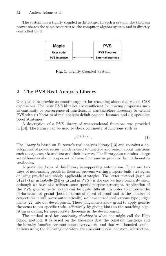
32 Andrew Adams et al.
The system has a tightly coupled architecture. In such a system, the theoremprover shares the same resources as the computer algebra system and is directlycontrolled by it.
MapleUser code
PVS Interface
PVS Theories
External Interface
PVS
Fig. 1. Tightly Coupled System.
2 The PVS Real Analysis Library
Our goal is to provide automatic support for reasoning about real valued CASexpressions. The basic PVS libraries are insufficient for proving properties suchas continuity or convergence of functions. It was therefore necessary to extendPVS with (i) libraries of real analysis definitions and lemmas, and (ii) specialistproof strategies.
A description of a PVS library of transcendental functions was providedin [14]. The library can be used to check continuity of functions such as
ex2+|1−x| . (4)
The library is based on Dutertre’s real analysis library [13] and contains a de-velopment of power series, which is used to describe and reason about functionssuch as exp, cos, sin and tan and their inverses. The library also contains a largeset of lemmas about properties of these functions as provided by mathematicstextbooks.
A particular focus of this library is supporting automation. There are twoways of automating proofs in theorem provers: writing purpose-built strategies;or using pre-defined widely applicable strategies. The latter method (such asblast-tac in Isabelle [24] or grind in PVS ) is the one we have primarily used,although we have also written some special purpose strategies. Application ofthe PVS generic tactic grind can be quite difficult. In order to improve theperformance of grind (both in terms of speed of proof and in the number ofconjectures it will prove automatically) we have introduced various type judge-ments [22] into our development. These judgements allow grind to apply generictheorems to our specific tasks, effectively by giving hints to the matching algo-rithm searching for appropriate theorems in the development.
The method used for continuity checking is what one might call the HighSchool method. It is based on the theorems that the constant functions andthe identity function are continuous everywhere, and that well-founded combi-nations using the following operators are also continuous: addition, subtraction,
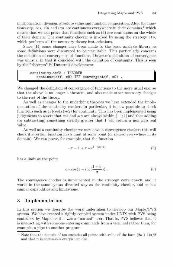
Integrating Maple and PVS 33
multiplication, division, absolute value and function composition. Also, the func-tions exp, cos, sin and tan are continuous everywhere in their domains,1 whichmeans that we can prove that functions such as (4) are continuous on the wholeof their domain. The continuity checker is invoked by using the strategy cts,which performs all the necessary theory instantiations.
Since [14] some changes have been made to the basic analysis library assome definitions were discovered to be unsuitable. This particularly concernsthe definition of convergence of functions. Dutertre’s definition of convergencewas unusual in that it coincided with the definition of continuity. This is seenby the ”theorem” in Dutetre’s development:
continuity def2 : THEOREMcontinuous(f, x0) IFF convergent(f, x0) .
We changed the definition of convergence of functions to the more usual one, sothat the above is no longer a theorem, and also made other necessary changesto the rest of the theory.
As well as changes to the underlying theories we have extended the imple-mentation of the continuity checker. In particular, it is now possible to checkfunctions such as 1/(cos(x)+2) for continuity. This has been implemented usingjudgements to assert that cos and sin are always within [−1; 1] and that adding(or subtracting) something strictly greater that 1 will return a non-zero realvalue.
As well as a continuity checker we now have a convergence checker; this willcheck if a certain function has a limit at some point (or indeed everywhere in itsdomain). We can prove, for example, that the function
−π − 1 + π ∗ e1−cos(x) (5)
has a limit at the point
arccos(1 − log(1 + π
π)) . (6)
The convergence checker is implemented in the strategy conv-check, and itworks in the same syntax directed way as the continuity checker, and so hassimilar capabilities and limitations.
3 Implementation
In this section we describe the work undertaken to develop our Maple/PVSsystem. We have created a tightly coupled system under UNIX with PVS beingcontrolled by Maple as if it was a “normal” user. That is, PVS believes that itis interacting with someone entering commands from a terminal rather than, forexample, a pipe to another program.1 Note that the domain of tan excludes all points with value of the form (2n+ 1)π/2and that it is continuous everywhere else.
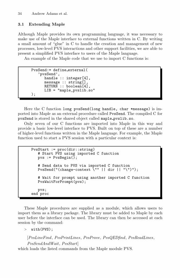
34 Andrew Adams et al.
3.1 Extending Maple
Although Maple provides its own programming language, it was necessary tomake use of the Maple interface to external functions written in C. By writinga small amount of “glue” in C to handle the creation and management of newprocesses, low-level PVS interactions and other support facilities, we are able topresent a simplified PVS interface to users of the Maple language.
An example of the Maple code that we use to import C functions is:
PvsSend:= define external(’pvsSend’,
handle :: integer[4],message :: string[],RETURN :: boolean[4],LIB = "maple_pvslib.so"
);
Here the C function long pvsSend(long handle, char *message) is im-ported into Maple as an external procedure called PvsSend. The compiled C forpvsSend is stored in the shared object called maple pvslib.so.
Only seven of our C functions are imported into Maple in this way andprovide a basic low-level interface to PVS. Built on top of these are a numberof higher-level functions written in the Maple language. For example, the Maplefunction used to start a PVS session with a particular context is:
PvsStart := proc(dir::string)# Start PVS using imported C functionpvs := PvsBegin();
# Send data to PVS via imported C functionPvsSend("(change-context \"" || dir || "\")");
# Wait for prompt using another imported C functionPvsWaitForPrompt(pvs);
pvs;end proc
These Maple procedures are supplied as a module, which allows users toimport them as a library package. The library must be added to Maple by eachuser before the interface can be used. The library can then be accessed at eachsession by the command:
> with(PVS);
[PvsLineFind , PvsPrintLines , PvsProve, PvsQEDfind , PvsReadLines ,PvsSendAndWait , PvsStart ]
which loads the listed commands from the Maple module PVS.
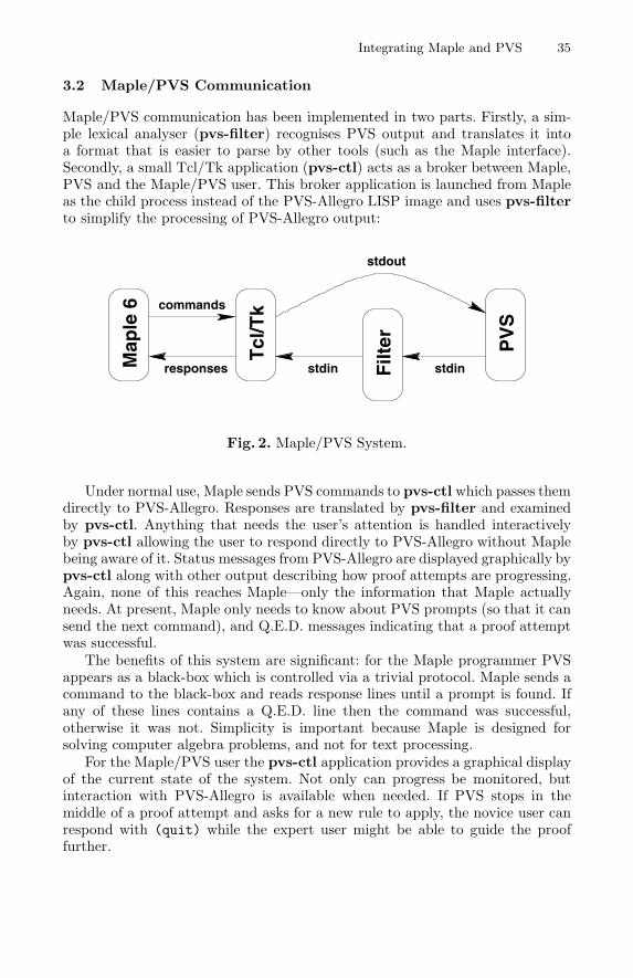
Integrating Maple and PVS 35
3.2 Maple/PVS Communication
Maple/PVS communication has been implemented in two parts. Firstly, a sim-ple lexical analyser (pvs-filter) recognises PVS output and translates it intoa format that is easier to parse by other tools (such as the Maple interface).Secondly, a small Tcl/Tk application (pvs-ctl) acts as a broker between Maple,PVS and the Maple/PVS user. This broker application is launched from Mapleas the child process instead of the PVS-Allegro LISP image and uses pvs-filterto simplify the processing of PVS-Allegro output:
Map
le 6
Tcl
/Tk
PV
S
Filt
erstdin stdinresponses
commands
stdout
Fig. 2. Maple/PVS System.
Under normal use, Maple sends PVS commands to pvs-ctl which passes themdirectly to PVS-Allegro. Responses are translated by pvs-filter and examinedby pvs-ctl. Anything that needs the user’s attention is handled interactivelyby pvs-ctl allowing the user to respond directly to PVS-Allegro without Maplebeing aware of it. Status messages from PVS-Allegro are displayed graphically bypvs-ctl along with other output describing how proof attempts are progressing.Again, none of this reaches Maple—only the information that Maple actuallyneeds. At present, Maple only needs to know about PVS prompts (so that it cansend the next command), and Q.E.D. messages indicating that a proof attemptwas successful.
The benefits of this system are significant: for the Maple programmer PVSappears as a black-box which is controlled via a trivial protocol. Maple sends acommand to the black-box and reads response lines until a prompt is found. Ifany of these lines contains a Q.E.D. line then the command was successful,otherwise it was not. Simplicity is important because Maple is designed forsolving computer algebra problems, and not for text processing.
For the Maple/PVS user the pvs-ctl application provides a graphical displayof the current state of the system. Not only can progress be monitored, butinteraction with PVS-Allegro is available when needed. If PVS stops in themiddle of a proof attempt and asks for a new rule to apply, the novice user canrespond with (quit) while the expert user might be able to guide the prooffurther.
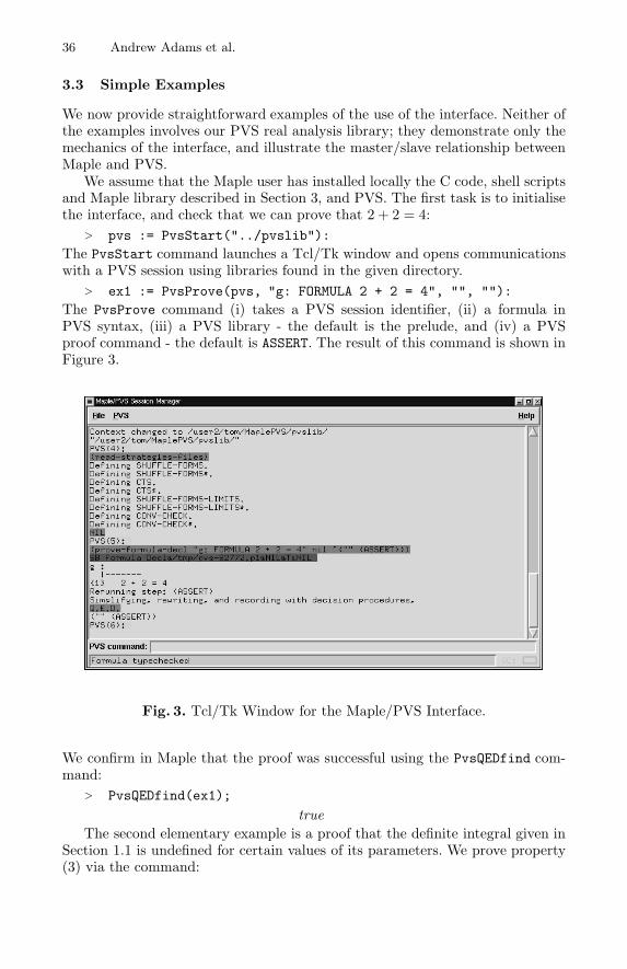
36 Andrew Adams et al.
3.3 Simple Examples
We now provide straightforward examples of the use of the interface. Neither ofthe examples involves our PVS real analysis library; they demonstrate only themechanics of the interface, and illustrate the master/slave relationship betweenMaple and PVS.
We assume that the Maple user has installed locally the C code, shell scriptsand Maple library described in Section 3, and PVS. The first task is to initialisethe interface, and check that we can prove that 2 + 2 = 4:
> pvs := PvsStart("../pvslib"):The PvsStart command launches a Tcl/Tk window and opens communicationswith a PVS session using libraries found in the given directory.
> ex1 := PvsProve(pvs, "g: FORMULA 2 + 2 = 4", "", ""):The PvsProve command (i) takes a PVS session identifier, (ii) a formula inPVS syntax, (iii) a PVS library - the default is the prelude, and (iv) a PVSproof command - the default is ASSERT. The result of this command is shown inFigure 3.
Fig. 3. Tcl/Tk Window for the Maple/PVS Interface.
We confirm in Maple that the proof was successful using the PvsQEDfind com-mand:
> PvsQEDfind(ex1);
trueThe second elementary example is a proof that the definite integral given in
Section 1.1 is undefined for certain values of its parameters. We prove property(3) via the command:
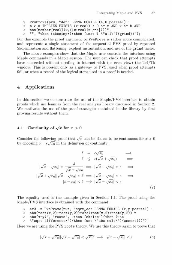
Integrating Maple and PVS 37
> PvsProve(pvs, "def: LEMMA FORALL (a,b:posreal) :> b > a IMPLIES EXISTS (x:real) : 0 <= x AND x <= b AND> not(member[real](x,({z:real|z /=a})))",> "", "then (skosimp*)(then (inst 1 \"a!1\")(grind))");
For this example the proof argument to PvsProve is rather more complicated,and represents a single statement of the sequential PVS proof by repeatedSkolemisation and flattening, explicit instantiation, and use of the grind tactic.
The above examples show that the Maple user controls the interface usingMaple commands in a Maple session. The user can check that proof attemptshave succeeded without needing to interact with (or even view) the Tcl/Tkwindow. This is present only as a gateway to PVS, used when proof attemptsfail, or when a record of the logical steps used in a proof is needed.
4 Applications
In this section we demonstrate the use of the Maple/PVS interface to obtainproofs which use lemmas from the real analysis library discussed in Section 2.We motivate the use of the proof strategies contained in the library by firstproving results without them.
4.1 Continuity of√
x for x > 0
Consider the following proof that√x can be shown to be continuous for x > 0
by choosing δ = ε√x0 in the definition of continuity:
δ = ε√x0 =⇒
δ ≤ ε(√x+√x0) =⇒
|√x−√x0| < δ√x+√x0
=⇒ |√x−√x0| < ε =⇒
|√x+√x0||√x−√x0| < δ =⇒ |√x−√x0| < ε =⇒|x− x0| < δ =⇒ |√x−√x0| < ε
(7)
The equality used is the example given in Section 1.1. The proof using theMaple/PVS interface is obtained with the command:
> ex3 := PvsProve(pvs, "sqrt_eq: LEMMA FORALL (x,y:posreal) :> abs(root(x,2)-root(y,2))*abs(root(x,2)+root(y,2)) => abs(x-y)", "roots", "then (skolem!)(then (use> \"sqrt_difference\")(then (use \"abs_mult\")(assert)))");
Here we are using the PVS roots theory. We use this theory again to prove that
|√x+√x0||√x−√x0| < √x0δ =⇒ |√x−√x0| < ε (8)
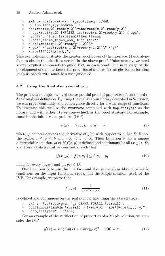
38 Andrew Adams et al.
> ex4 := PvsProve(pvs, "sqroot_ineq: LEMMA> FORALL (eps,x,y:posreal) :> abs(root(x,2)-root(y,2))*abs(root(x,2)+root(y,2))> < eps*root(y,2) IMPLIES abs(root(x,2)-root(y,2)) < eps",> "roots", "then (skosimp)(then (lemma> \"both_sides_times_pos_lt1\" (\"x\"> \"abs(root(x!1,2)-root(y!1,2))\"> \"pz\" \"abs(root(x!1,2)+root(y!1,2))\" \"y\"> \"eps!1\"))(grind))");
This example demonstrates the greater proof power of the interface. Maple alonefails to obtain the identities needed in the above proof. Unfortunately, we needseveral explicit commands to guide PVS in each proof. The next stage of thedevelopment of the interface is the provision of a suite of strategies for performinganalysis proofs with much less user guidance.
4.2 Using the Real Analysis Library
The previous example involved the sequential proof of properties of a standard ε-δ real analysis definition. By using the real analysis library described in Section 2,we can prove continuity and convergence directly for a wide range of functions.To illustrate this we use the PvsProve command with top analysis as thelibrary, and with either cts or conv-check as the proof strategy. For example,consider the initial value problem (IVP)
y′(x) = f(x, y), y(a) = η (9)
where y′ denotes denotes the derivative of y(x) with respect to x. Let D denotethe region a ≤ x ≤ b and −∞ < y < ∞. Then Equation 9 has a uniquedifferentiable solution, y(x), if f(x, y) is defined and continuous for all (x, y) ∈ D,and there exists a positive constant L such that
|f(x, y0)− f(x, y1)| ≤ L|y0 − y1| (10)
holds for every (x, y0) and (x, y1) ∈ D.Our intention is to use the interface and the real analysis library to verify
conditions on the input function,f(x, y), and the Maple solution, y(x), of theIVP. For example, we prove that
f(x, y) =1
eπ−|6cos(x)| (11)
is defined and continuous on the real number line using the cts strategy:> ex5 := PvsProve(pvs, "g: LEMMA FORALL (y:real) :> continuous(lambda (x:real) : 1/exp(pi - abs(6*cos(x))),y)",> "top_analysis", "cts");
For an example of the verification of properties of a Maple solution, we con-sider the IVP
y′(x) = sin(x)y(x) + sin(x)y(x)2, y(0) = π . (12)
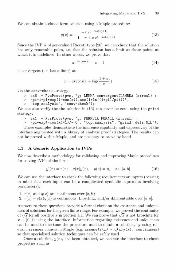
Integrating Maple and PVS 39
We can obtain a closed form solution using a Maple procedure:
y(x) =−π e(−cos(x)+1)
−1− π + π e(−cos(x)+1)(13)
Since the IVP is of generalised Riccati type [20], we can check that the solutionhas only removable poles, i.e. that the solution has a limit at those points atwhich it is undefined. In other words, we prove that
πe1−cos(x) − π − 1 (14)
is convergent (i.e. has a limit) at
x = arccos(1 + log(1 + π
π)) (15)
via the conv-check strategy:> ex6 := PvsProve(pvs, "g: LEMMA convergent(LAMBDA (x:real) :> -pi-1+pi*exp(1-cos(x)),acs(1+ln((1+pi)/pi)))",> "top_analysis", "conv-check");
We can also verify the the solution in (13) can never be zero, using the grindstrategy:
> ex1 := PvsProve(pvs, "g: FORMULA FORALL (x:real) :> -pi*exp(-cos(x)+1)/= 0", "top_analysis", "grind :defs NIL");These examples demonstrate the inference capability and expressivity of the
interface augmented with a library of analytic proof strategies. The results cannot be proved within Maple, and are not easy to prove by hand.
4.3 A Generic Application to IVPs
We now describe a methodology for validating and improving Maple proceduresfor solving IVPs of the form
y′(x) = r(x) − q(x)y(x), y(a) = η, x ∈ [a, b] (16)
We can use the interface to check the following requirements on inputs (bearingin mind that each input can be a complicated symbolic expression involvingparameters):
1. r(x) and q(x) are continuous over [a, b];2. r(x) − q(x)y(x) is continuous, Lipschitz, and/or differentiable over [a, b].
Answers to these questions provide a formal check on the existence and unique-ness of solutions for the given finite range. For example, we proved the continuityof√x for all positive x in Section 4.1. We can prove that
√x is not Lipschitz for
x ∈ (0, 1) using the interface. Information regarding existence and uniquenesscan be used to fine tune the procedure used to obtain a solution, by using rel-evant assumes clauses in Maple (e.g. assume(r(x) - q(x)y(x), continuous)so that specialised solution techniques can be safely used.
Once a solution, y(x), has been obtained, we can use the interface to checkproperties such as
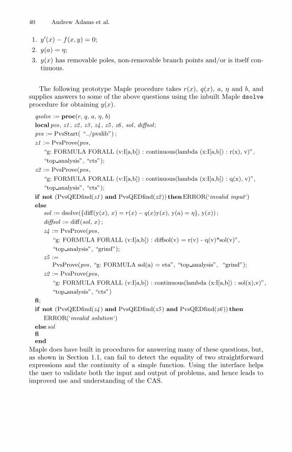
40 Andrew Adams et al.
1. y′(x) − f(x, y) = 0;
2. y(a) = η;
3. y(x) has removable poles, non-removable branch points and/or is itself con-tinuous.
The following prototype Maple procedure takes r(x), q(x), a, η and b, andsupplies answers to some of the above questions using the inbuilt Maple dsolveprocedure for obtaining y(x).
qsolve := proc(r, q, a, η, b)
local pvs , z1 , z2 , z3 , z4 , z5 , z6 , sol , diffsol ;
pvs := PvsStart( “../pvslib”) ;
z1 := PvsProve(pvs ,
“g: FORMULA FORALL (v:I[a,b]) : continuous(lambda (x:I[a,b]) : r(x), v)”,
“top analysis”, “cts”);
z2 := PvsProve(pvs ,
“g: FORMULA FORALL (v:I[a,b]) : continuous(lambda (x:I[a,b]) : q(x), v)”,
“top analysis”, “cts”);
if not (PvsQEDfind(z1 ) and PvsQEDfind(z2 )) thenERROR(‘invalid input ‘)
elsesol := dsolve({diff(y(x), x) = r(x)− q(x)y(x), y(a) = η}, y(x)) ;diffsol := diff(sol , x) ;
z4 := PvsProve(pvs ,
“g: FORMULA FORALL (v:I[a,b]) : diffsol(v) = r(v) - q(v)*sol(v)”,
“top analysis”, “grind”);
z5 :=PvsProve(pvs , “g: FORMULA sol(a) = eta”, “top analysis”, “grind”);
z2 := PvsProve(pvs ,
“g: FORMULA FORALL (v:I[a,b]) : continuous(lambda (x:I[a,b]) : sol(x),v)”,
“top analysis”, “cts”)
fi;
if not (PvsQEDfind(z4 ) and PvsQEDfind(z5 ) and PvsQEDfind(z6 )) then
ERROR(‘invalid solution‘)
else solfiend
Maple does have built in procedures for answering many of these questions, but,as shown in Section 1.1, can fail to detect the equality of two straightforwardexpressions and the continuity of a simple function. Using the interface helpsthe user to validate both the input and output of problems, and hence leads toimproved use and understanding of the CAS.
Integrating Maple and PVS 41
5 Conclusions
We have presented an interface between Maple and PVS. The interface givesMaple users access to the proof capabilities of PVS, thus providing a means togain more formal knowledge of Maple results.
We have created a tightly coupled interface between Maple and PVS, underwhich PVS is controlled by Maple. A small Tcl/Tk application sits betweenMaple and PVS, so that PVS looks like a black box to the Maple user. However,it also allows a more experienced user to interact directly with PVS.
In Section 1.1 we saw that Maple can fail to recognise a seemingly obvi-ous equality, which could lead to an undetected division by zero, and also thatMaple might apply standard procedures without checking validity of the input.In Section 4 we showed how the interface can be used to correct these errors.
Our aim is to extend the applicability of the interface in two ways. Firstlythe extension of the real analysis library discussed in Section 2 by adding newstrategies, and secondly by providing Maple procedures which automate thechecking of validity of input and output, as described in Section 4.3. Theseextensions will require an improvement in the communication between the twosystems, both in terms of syntax of expressions, and in decision procedures basedon failed proof attempts.
References
1. Abbott, J., van Leeuwen, A., and Strotman, A. Objectives of OpenMath.Available from, Jan. 1995,http://www.rrz.uni-koeln.de/themen/Computeralgebra/OpenMath/.
2. Adams, A., Gottliebsen, H., Linton, S., and Martin, U. Automated the-orem proving in support of computer algebra: symbolic definite integration as acase study. In Proceedings of the 1999 International Symposium on Symbolic andAlgebraic Computation, Vancouver, Canada (1999), ACM Press.
3. Ballarin, C., Homann, K., and Calmet, J. Theorems and algorithms: Aninterface between Isabelle and Maple. In Proceedings of the International Sympo-sium on Symbolic and Algebraic Computation (1995), A. Levelt, Ed., ACM Press,pp. 150–157.
4. Bauer, A., Clarke, E., and Zhao, X. Analytica - an experiment in combiningtheorem proving and symbolic computation. Journal of Automated Reasoning 21(1998), 295–325.
5. Bertoli, P., Calmet, J., Guinchiglia, F., and Homann, K. Specificationand integration of theorem provers and computer algebra systems. In Artificialintelligence and symbolic computation (Plattsburgh, NY, 1998), no. 1476 in LectureNotes in Computer Science. Springer-Verlag, 1998.
6. Buchberger, B. Symbolic computation: Computer algebra and logic. In Frontiersof Combining Systems (1996), F. Baader and K. Schultz, Eds., Applied LogicSeries, Kluwer Academic Publishers, pp. 193–220.
7. Buchberger, B., Jebelean, T., Kriftner, F., Marin, M., Tomuta, E., and
Vasaru, D. A survey of the theorema project. In Proceedings of the 1997 Interna-tional Symposium on Symbolic and Algebraic Computation (1997), W. Kuechlin,Ed., ACM Press, pp. 384–391.
42 Andrew Adams et al.
8. Calmet, J., and Homann, K. Classification of communication and cooperationmechanisms for logical and symbolic computation systems. In Frontiers of Com-bining Systems: Proceedings of the 1st International Workshop, Munich (Germany)(1996), F. Baader and K. U. Schulz, Eds., Applied Logic, Kluwer, pp. 221–234.
9. Char, B. W. Maple V language Reference Manual. Springer-Verlag, 1991.10. Dennis, L. A., Collins, G., Norrish, M., Boulton, R., Slind, K., Robinson,
G., Gordon, M., and Melham, T. The PROSPER Toolkit. In Proceedings ofthe 6th International Conference on Tools and Algorithms for the Constructionand Analysis of Systems (2000), vol. 1785 of Lecture Notes in Computer Science,Springer-Verlag.
11. Dewar, M. Special Issue on OPENMATH. ACM SIGSAM Bulletin 34, 2 (June2000).
12. Dolzmann, A., and Sturm, T. REDLOG: Computer algebra meets computerlogic. ACM SIGSAM Bulletin 31, 2 (June 1997), 2–9.
13. Dutertre, B. Elements of mathematical analysis in PVS. In Theorem Proving inHigher Order Logics: 9th International Conference, TPHOLs ’96 (Turku, Finland,Aug. 1996), J. von Wright, J. Grundy, and J. Harrison, Eds., vol. 1125 of LectureNotes in Computer Science, Springer-Verlag, pp. 141–156.
14. Gottliebsen, H. Transcendental Functions and Continuity Checking in PVS. InTheorem Proving in Higher Order Logics: 13th International Conference, TPHOLs2000 (2000), J. Harrison and M. Aagaard, Eds., vol. 1869 of Lecture Notes inComputer Science, Springer-Verlag, pp. 198–215.
15. Gray, S., Kajler, N., and Wang, P. S. MP: A Protocol for Efficient Exchangeof Mathematical Expressions. In Proc. of the International Symposium on Symbolicand Algebraic Computation (ISSAC’94), Oxford, GB (July 1994), M. Giesbrecht,Ed., ACM Press, pp. 330–335.
16. Harrison, J., and Thery, L. Reasoning about the reals: the marriage of HOLand Maple. In Logic Programming and Automated Reasoning (1993), A.Voronkov,Ed., no. 698 in Lecture Notes in Artificial Intelligence, LPAR’93, Springer-Verlag,pp. 351–359.
17. Jackson, P. Enhancing the NUPRL Proof Development System and Applying itto Computational Abstract Algebra. PhD thesis, Department of Computer Science,Cornell University, Ithaca, New York, Apr. 1995.
18. Jenks, R. D., and Sutor, R. S. AXIOM: the scientific computation system.Numerical Algorithms Group Ltd., 1992.
19. Monagan, M., Geddes, K., Heal, K., Labahn, G., Vorkoetter, S., and
McCarron, J. Maple6 Programming Guide. Waterloo Maple Inc., 2000.20. Murphy, G. M. Ordinary differential equations and their solutions. D. van Nos-
trand Company, Inc., 1960.21. Owre, S., Shankar, N., and Rushby, J. M. User Guide for the PVS Specifi-
cation and Verification System. Computer Science Laboratory, SRI International,Menlo Park, CA, February 1993.
22. Owre, S., Shankar, N., Rushby, J. M., and Stringer-Calvert, D. W. J.
PVS Language Reference. Computer Science Laboratory, SRI International, MenloPark, CA, Sept. 1999.
23. Owre, S., Shankar, N., Rushby, J. M., and Stringer-Calvert, D. W. J.
PVS System Guide. Computer Science Laboratory, SRI International, Menlo Park,CA, Sept. 1999.
24. Paulson, L. C. The Isabelle Reference Manual. Computer Laboratory, Universityof Cambridge, February 2001.
25. Poll, E., and Thompson, S. Adding the axioms to AXIOM: Towards a system ofautomated reasoning in Aldor. Tech. Rep. 6-98, Computing Laboratory, Universityof Kent at Canterbury, May 1998.
An Irrational Construction of R from Z
Rob D. Arthan
Lemma 1 Ltd., 2nd Floor, 31A Chain StreetReading RG1 2HX, [email protected]
Abstract. This paper reports on a construction of the real numbers inthe ProofPower implementation of the HOL logic. Since the original con-struction was implemented, some major improvements to the ideas havebeen discovered. The improvements involve some entertaining mathe-matics: it turns out that the Dedekind cuts provide many routes one cantravel to get from the ring of integers, Z, to the field of real numbers, R.The traditional stop-over on the way is the field of rational numbers, Q.This paper shows that going via certain rings of algebraic numbers canprovide a pleasant alternative to the more well-trodden track.
1 Introduction
1.1 Automated Theorem Proving Background
ProofPower is a suite of tools supporting specification and proof in a range offormalisms. At the heart of the tools is the logical kernel for HOL, which is are-engineering of the kernel of the Classic HOL system[7]. This re-engineering[1]was undertaken by ICL between 1988 and 1992 to meet requirements for a toolto reason about security properties expressed in Z[10]. Since 1993 ProofPower hasbeen applied to research and development in methods for specification and veri-fication of safety-critical systems. In 1994, a method for specifying and verifyingAda code called the Compliance Notation[12, 15] was implemented to form theCompliance Tool component of ProofPower. Research and development into thenotation and the tool continues informed by a number of successful applicationsand case studies and the tool is currently being put to work on significant veri-fication problems in the military avionics domain.
Early versions of the Compliance Tool had only vestigial support for the Adadata types that represent real numbers. However, investigation of actual codein the intended applications domain has shown that real programmers do usereals. During 1999 and 2000 it became clear that proper support for Ada realtypes was essential. In 2000, the Defence and Evaluation Research Agency, thedesigners and main users of the Compliance Notation, commissioned Lemma 1Ltd., who now develop and market ProofPower, to provide this support.
Ada real types in the Compliance Tool use a formalisation of the real numbersin Z, which, in turn, is based on a theory of the real numbers in ProofPower-HOL.
R.J. Boulton and P.B. Jackson (Eds.): TPHOLs 2001, LNCS 2152, pp. 43–58, 2001.c© Springer-Verlag Berlin Heidelberg 2001
44 Rob D. Arthan
The ProofPower-HOL theory was developed in November 2000 by the present au-thor using some novel methods intended to make use of the fact that ProofPower-HOL already possessed reasonably well-supported theories for both natural num-ber and integer arithmetic.
As is the norm in the HOL community, the theory of the reals in ProofPower-HOL is developed by conservative extension rather than by axiomatisation. In-deed, just to assert the axioms of the reals, characterised say, as a complete or-dered field, would be a relatively trivial (albeit error-prone) exercise. The meritsof conservative extension over axiomatisation by fiat have been widely discussed,see[8] for a survey.
I should remind the reader that HOL is a typed logic with well-defined prin-ciples of conservative extension for introducing new types and constants. Thedefining property for a new constant c : τ can be an arbitrary satisfiable pred-icate defined on the type τ , e.g., one might introduce a constant Sqrt :N → N,with defining property: ∀m • (Sqrt m)2 ≤ m < (Sqrt m + 1)2. The HOL logicalkernel imposes a proof obligation to ensure that the defining property is indeedsatisfiable so that the introduction of the constant is conservative.
The defining property for a new type has a standard form asserting thatthe new type is in one-to-one correspondence with a non-empty subset of anexisting type. Again a proof obligation is imposed to ensure that the subset isnon-empty. As an example, one can introduce a type with a given finite number ofelements by requiring it to be in one-to-one correspondence with an appropriateinterval of natural numbers. This simple subtyping mechanism, combined withthe power of the primitive type constructors, allows a wide variety of standardtype constructions to be carried out. For example, given an equivalence relationon an existing type τ , the quotient type (with one element for each equivalenceclass) can be formed as a subtype of the power set type (τ)SET.
John Harrison[8] has developed a very elegant refinement of the method offundamental sequences which is well adapted to constructing a theory of realsusing the natural numbers as a starting point. The present author would nothesitate to recommend Harrison’s approach in a context where a good theory ofintegers is not to hand. If the integers are available, the approach of the presentpaper is offered as an alternative which has its attractions. In particular:
– There is no need to work with equivalence classes1
– the only subtype1 that needs to be created is the type, R, of the real numbersthemselves;
– the theories of order, addition and multiplication are dealt with in succession,each one building on what has come before and providing reusable theoryfor use in later work.
1 While automation can make dealing with equivalence classes and subtypes straight-forward, these devices inevitably involve additional proof obligations.
An Irrational Construction of R from Z 45
1.2 Mathematical Background
The textbook journey from Z to R is the composite of two standard means oftransport. First we take the ring Z and form its field of fractions, Q and notethat the order structure on Z carries over to Q. However, Q is incomplete —numbers such as
√2 and π fail to show up at this stage of the trip. To remedy
this, we appeal to something like the Dedekind completion by cuts, or Cantor’smethod of fundamental sequences (a.k.a. Cauchy sequences) to arrive at ourgoal R. Excellent surveys of the terrain are given in [5, 8]. In the sequel, we willconcentrate on the Dedekind cuts construction. In an elementary treatment, thisconstruction is presented along something like the following lines.
i) The rational numbers Q are constructed (e.g., as equivalence classes of pairs(m,n) : Z × N1, with (m,n) representing the fraction m/n). The rationalnumbers are then shown to comprise an ordered field.
ii) A Dedekind cut is now defined to be any non-empty set, C, of rationalnumbers which is, (a), downwards-closed (i.e., if q ∈ C, then any rationalnumber p < q is also in C), (b), unbounded above in itself (i.e., for anyq ∈ C, there is a p ∈ C with q < p), and (c) bounded above in Q (i.e., forsome q ∈ Q, every p ∈ C satisfies p < q). R is defined to be the set of allsuch cuts.The rational numbers Q are identified with a subset of R, the set of rationalcuts, by associating q ∈ Q with the cut compromising all rational numbersless than q.The set of cuts is shown to be linearly ordered by set-theoretic inclusionand this ordering is shown to agree with the usual ordering on Q whenrestricted to rational cuts. This ordering is seen to be complete (i.e., any non-empty subset of R that is bounded above has a supremum in R). Indeed, thesupremum of a bounded set of cuts turns out to be its set-theoretic union.
iii) Addition of cuts is now defined as follows: if C and D are cuts, the sumC+D is defined to be the set of all sums p+ q where p ∈ C and q ∈ D. Thisis shown to be a cut and so defines a binary operation R→ R→ R, which isthen shown to be associative and commutative and to have the rational cutcorresponding to 0 ∈ Q as an identity element.
iv) The additive inverse operator is now defined as follows: if C is a cut, −C isdefined to be the set of all q ∈ Q such that p+ q < 0 for every p ∈ C. Again,this is shown to be a cut and so to define a unary operator R→ R, which isan inverse for the addition.
v) Multiplication and its inverse are defined in a similar fashion to addition andadditive inverse, but with some complications due to signs. The interactionsamong the ordering relation, the additive structure and the multiplicativestructure are investigated and we conclude that R is a complete ordered field.
An analysis of what is being assumed and what the arguments actually provehere reveals a number of useful facts:
– Step (ii) applies to any ordered set. This is the Dedekind-MacNeille comple-tion theorem. For more on this, see, for example, [4]. The algebraic structure
46 Rob D. Arthan
of Q is irrelevant here. Indeed, the completion of any countable, unbounded,densely ordered set is known by a theorem of Cantor to have the same ordertype as R (see, for example, [11]).
– Step (iii) makes no use of the multiplicative structure of Q — only its or-dering and its additive structure are needed. However, it is not the case thatjust any ordered commutative group will do2. In fact, what is required is thatQ contains arbitrarily small positive elements, or equivalently, it is denselyordered: for any x < y, there is a z with x < z < y. Density is requiredin verifying that the rational cut determined by 0 is indeed an identity foraddition.
– Step (iv) also makes no use of the multiplicative structure except for theability (which exists in any group) to “multiply” elements by natural num-bers. However density is not sufficient to make the proof go through3. Itturns out that we require the archimedean property on the additive groupQ: for any positive elements, x and y, there is an n ∈ N such that y < nx.Here nx denotes the n-fold sum x+ x+ . . .+ x.
– Finally, essentially by a theorem of Holder [9], step (v) is an instance of ageneral construction that is independent of the details of the additive struc-ture. Holder’s theorem is usually stated as saying that any archimedeanordered group is isomorphic to a subgroup of the real numbers under addi-tion. Consequently, the completion of any ordered group that is both denseand archimedean must be isomorphic to the real numbers, and so must ad-mit a multiplication. Moreover, the method of the proof of Holder’s theoremcomes close to providing a definition for the multiplication.
1.3 A New Approach
The observations of the previous section suggest new approaches to constructingthe real numbers. The rest of this paper is mainly concerned with presenting onesuch approach and is organised as follows:
Section 2 discusses the Dedekind-MacNeille completion theorem. This is well-known and so the discussion is very brief.
Section 3 discusses how the additive structure of the real numbers may bederived from the Dedekind-MacNeille completion of any dense, archimedean,ordered group. Again this is very brief — the classical proofs go throughwithout change.
Section 4 is concerned with deriving the multiplicative structure of the realnumbers from the additive structure. This seems to be one of those topicsthat is well-known but rarely written down, so we give a complete, albeitrather condensed, discussion.
Section 5 is the main contribution of this paper. It provides a source of dense,archimedean, ordered groups that are algebraically much simpler than the
2 E.g., try using Z in place of Q.3 E.g., try using the product group Z×Q with the lexicographic order in place of Q.
An Irrational Construction of R from Z 47
rational numbers. The groups considered are the additive groups of the ringsZ[α] where α can be any one of a variety of irrational numbers. For definite-ness, we concentrate on the case α =
√2.
Section 6 offers my confession that the construction outlined in the presentpaper is not what was actually done in November 2000 for the ProofPowerproduct. The construction used algebraic structures weaker than orderedgroups as its basis. The derivation of the additive structure of the realsfrom these weaker systems has to be more general than the constructiondescribed in this paper. In comparison, the approach proposed here providessome considerable economies in the proofs.
Section 7 gives some concluding remarks.
The present paper deliberately concentrates on the mathematics rather thanthe details of the particular formalisation in ProofPower. This is because someof the mathematics is not very accessible in the literature and some parts of itare believed to be new, whereas how to formalise the mathematics will dependon the system being used and should be fairly clear to a competent user of anyadequately expressive system.
Demo versions of the ProofPower treatment of the material outlined in thisdocument are available on the World-Wide Web4. The reader is referred to thatmaterial for further details of the formalisation.
The construction described in this document may seem at first sight to berather exotic. However, from several points of view it can be seen as quite natural.One such point of view is this: let us take it as given that we wish to avoid theexpense of constructing the rationals and tools to reason about them prior toconstructing the reals, since Q will appear as a subfield of R in any case. As asubstitute for Q, we look for a dense subgroup of R which is simple enough to bedirectly amenable to existing tools for reasoning about the integers. A subgroupsuch as Z[
√2], which is isomorphic as an additive group to the cartesian product
Z × Z, would do nicely. However we will need an easy way of working with theordering that Z[
√2] receives as a subgroup of R. As we will see in section 5.2 of
this paper, it turns out that there is a very tractable description of this orderingand the properties needed of Z[
√2] are very easy to prove.
2 Dedekind-MacNeille Completion
The Dedekind-MacNeille completion theorem proves to be simplicity itself. In theProofPower treatment, MacNeille’s generalisation of the Dedekind constructionto partially ordered sets was not needed, so the theory was developed for linearlyordered sets only.
The result we have to prove is that any unbounded, dense, linearly orderedmay be embedded as an unbounded dense subset of a complete ordered set.The actual statement of the theorem gives an explicit witness for the complete4 Follow the link from http://www.lemma-one.com/papers/papers.html.
48 Rob D. Arthan
ordered set. This is very simple first-order set theory and the main proofs werefound in the course of one day.
Once one has a suitable densely ordered set, S say, the theory of Dedekind-MacNeille immediately enables one to define the type R. The defining propertyfor the new type is entirely order-theoretic and just states that there R admitsa linear order which is dense and complete and admits an embedding of S asan unbounded, dense subset. On the basis of this type definition, it involves atrivial proof to define the constant <: R→ R→ B that gives the ordering on thereal numbers. One can then define the supremum operator5 Sup : (R)SET→ R.≤, > and ≥ can also conveniently be defined at this stage.
At this point, one can start to develop useful, reusable, theory about theordering and the supremum operator. E.g., one can show that for non-empty,bounded above, sets A and B, a sufficient condition for Sup(A) ≤ Sup(B) is thatA ⊆ B. This theory is useful both in the rest of the construction and in ordinaryuse of the theory of reals once the construction is complete.
3 Defining the Additive Structure
Defining the additive structure of the reals given a dense, archimedean, or-dered group is essentially what is achieved in steps (iii) and (iv) of the classicalDedekind cuts construction as described in section 1.2 above. The reader is re-ferred to any good calculus textbook for the details, e.g., [14]. However, somedescriptions, e.g., that in [5], skate over the role of the archimedean property.
As with the order structure, new constants + : R → R → R, 0R : R and− : R→ R are introduced and their elementary properties derived. Particularlyuseful are theorems about cancellation of like terms on either side of an equalityor inequality.
4 Defining the Multiplicative Structure
The author has been unable to find an accessible modern treatment of the deriva-tion of the multiplicative structure in the literature. This is probably becauseresults like Holder’s theorem are generally given in a context where the realnumbers are already available.
The arguments needed are, in essence, all given in a paper by Behrend[2].However, Behrend’s arguments are set in a context which is rather different fromours. The ProofPower treatment uses a recasting of the core arguments fromBehrend in modern dress. It also delivers theorems which may be of general usein further development of the theory.
So let us assume that R is a non-trivial complete ordered commutative group.We want to show that R can be equipped with a multiplication turning it into5 Sup is conceptually a partial function. It is formalised in ProofPower as a totalfunction whose defining property reveals no information about values of the functionwhich are conceptually undefined.
An Irrational Construction of R from Z 49
an ordered field. To this end, let us fix some positive element 1R : R which wewill make into the multiplicative identity element of the field.
The basic idea is that, if R can be turned into an ordered field, then, for anyx : R, multiplication by x determines an additive group homomorphism R →R. Moreover, if x is positive, multiplication by x is (strictly) order-preserving(i.e., xy < xz whenever y < z). Thus we can hope to derive the multiplicativestructure by investigating the order-preserving additive homomorphismsR→ R.Let us call these OPAHs.
It is not hard to see that OPAHs are necessarily injective functions6. What istrue, but somewhat harder to prove is that OPAHs are also surjective. To provethis we first observe that any subgroup of R containing arbitrarily small positiveelements is dense in R. Now the image of an OPAH, f , is a subgroup of R and itis not hard to see that it contains arbitrarily small positive elements7. Thus theimage of f is a dense subgroup of R. So any OPAH, f , is an order-preservinginjective function from R to a dense subset of itself; but viewed as a subset of Rordered as a subset of R, the image of f must be complete because R is complete,and f is order-preserving. It is now not hard to see that the image must be equalto R and so f is indeed surjective8.
A homomorphism f : R→ R is said to be central if it commutes with everyhomomorphism g : R → R, i.e., if f(g(x)) = g(f(x)) for every x ∈ R. CentralOPAHs (COPAHs) will serve for us as a substitute for the multiplication bynatural numbers used in [2] and other treatments such as [9].
What we now want to show is that COPAHs abound. To see this, let δ ∈ Rbe any positive element. Consider the set A = Aδ of elements, x ∈ R such thateither x = 0 or for some COPAH g, we have g(δ) = x or g(δ) = −x. Then it isnot very hard to see that A is a dense subgroup of R. Density is the only trickypart. For density, one verifies that the function t : R→ R defined by t(x) = x+xis a COPAH. Since COPAHs are OPAHs, and OPAHs are surjective, t has aninverse h : R → R, and h is then itself a COPAH with the property that, forany x ∈ R, we have x = h(x) + h(x). I.e., h is “division by 2”. It follows that Ahas no least positive element9, i.e. A is dense.
In fact, the dense subgroups Aδ defined in the previous paragraph are com-plete and so Aδ = R for every positive δ. I.e., for any x ∈ R with x �= 0, there isa COPAH g, such that either x = g(δ) or x = −g(δ). The proof of this requiresus to show, in effect, that the (pointwise) supremum of a bounded family ofCOPAHs is itself a COPAH. We omit the details, just noting that the key is toshow that if f and g are two OPAHs, then if f(x) < g(x) for some positive x,then f(x) < g(x) for every positive x. This is proved essentially by the argument
6 If f(x) = f(y), then x < y and y < x are both impossible, so we must have x = y.7 It contains some positive elements, e.g., f(1R); if it contained a least positive element,
f(ε), say, then by density of R there would be a δ with 0 < δ < ε, but then f(δ) ispositive and smaller than f(ε).
8 Consider a least positive element that is not in the image.9 If x = f(δ) were such an element, with f the COPAH that testifies to x ∈ A, then
g = h ◦ f is also a COPAH and g(δ) < f(δ).
50 Rob D. Arthan
of the uniqueness half of the main theorem in [2], using COPAHs rather thanmultiplication by natural numbers to show that it is not possible for f(y) ≥ g(y)for any y.
What we have just proved is that for any positive δ ∈ R and any non-zerox ∈ R, there is a COPAH, g, with g(δ) = x or g(δ) = −x, and this may be shownto be unique. Fixing δ = 1R, this says that for every positive x, there is a uniqueg = gx such that g(1R) = x. We now define multiplication by x by xy = gx(y).This definition may be extended to cover the case when x ≤ 0 in the obviousway, and making heavy use of the uniqueness of gx, one shows that this turns Rinto ring with unit 1R. Since COPAHs are bijections, this ring is actually a fieldand all the properties of an ordered field follow. For the details, we refer to [2]yet again — this part of the argument translates easily into the present context.
In ProofPower this part of the construction was not difficult, but was a littletime-consuming. It took perhaps 5 days to discover and formalise the arguments,which provide the consistency proofs for the definitions of the constants ∗ : R→R → R and −1 : R → R giving multiplication and multiplicative inverse for thereal numbers.
5 An Alternative to Q
In this section, we construct a dense, archimedean ordered commutative group.Given the arguments of sections 2, 3 and 4 above, this is all that is needed tocomplete our construction of the reals. The group we use is called Z[
√2]. It is
introduced in section 5.1 below. In fact, since it involves little extra work, wewill show that Z[
√2] is actually an ordered ring.
5.1 Calculating in Z[√
2]
Imagine using a square with 1-inch sides to mark off points along the real numberline starting at the fixed base point 0. Using a side of the square you can mark offany whole number of inches to the left or the right of the base point. However,you can use the diagonal of the square to mark off distances in either directiontoo. Pythagoras’ theorem says that the diagonal is
√2 =√12 + 12 inches long.
So, the points you can mark off are precisely the real numbers a+ b√2 where a
and b are integers. These are the numbers that make up the ring Z[√2].
Addition and additive inverse in Z[√2] is easy to describe purely in terms of
integer arithmetic; describing multiplication is not much harder:
(a+ b√2) + (c+ d
√2) = (a+ c) + (b+ d)
√2
−(a+ b√2) = (−a) + (−b)
√2
(a+ b√2)(c+ d
√2) = (ac+ 2bd) + (ad+ bc)
√2.
In the sequel we will often turn facts about the real numbers into definitions.Here, if we consider pairs (a, b) where a and b are integers, we can define addition,
An Irrational Construction of R from Z 51
negation and multiplication as follows:
(a, b) + (c, d) = (a+ c, b+ d)−(a, b) = (−a,−b)
(a, b)(c, d) = (ac+ 2bd, ad+ bc).
One may then check that the above definitions turn the set, Z×Z, of all pairsof integers into a ring with zero element 0 = (0, 0) and unit element 1 = (1, 0).
The pairs (a, b) ∈ Z×Z thus give a model, defined solely in terms of integerarithmetic, for the arithmetic of all real numbers of the form a + b
√2. From
now on, we shall refer to this model as Z[√2]. It is here that Z[
√2] has its main
advantage over Q: the verifications of the ring laws reduce to equations over theintegers that are easily solved by a linear arithmetic decision procedure. Statingand proving the laws took the author less than half an hour in ProofPower.
5.2 The Ordering of Z[√
2]
Given members y = (c, d) and z = (e, f) of Z[√2], how do we decide the relative
order of the real numbers y = c+ d√2 and z = e+ f
√2 that y and z represent?
To simplify the problem a little, I should explain that it is enough to decide,given any x = (a, b) in Z[
√2], whether or not x = a+b
√2 is positive (i.e., greater
than 0). For, in R, we know that y < z precisely when 0 < z − y. In general, todefine an ordering on a (commutative) group, G, it is enough to identify a subsetP of “positive elements”. This subset must be closed under the group operation(addition), must not contain 0, and must be such that, for any non-zero element,g, of G, either g or −g belongs to P . Given such a subset, P , defining g < h tomean h− g ∈ P gives a linear ordering of the elements of G compatible with theaddition in G, in the sense that whenever g < h, then, also, g + k < h + k forany k in G.
In the case of Z[√2], a first attempt at a rule for deciding whether x = (a, b) is
positive would be to consider four cases as follows: if, (i), a and b are both positivethen x certainly represents a positive real number; if, (ii), neither of a and b ispositive then x certainly does not represent a positive real number; otherwise, toensure that x represents a positive real number, we must have either, (iii), that ais negative and b is positive and a2 < 2b2 or, (iv) that a is positive, b is negativeand a2 > 2b2.
Unfortunately the above rules for identifying the positive numbers is not atall convenient10. It involves four cases, and when we try to verify the propertieswe require of the set of positive elements, the cases multiply and we find our-selves having to do some not very nice algebra in each case. While there are somesymmetries between the cases, to show that the set of positive elements is closed
10 Nonetheless, proving that Z[√2] becomes an ordered group under this definition is set
as an exercise in the well-known textbook on algebra by Birkhoff and MacLane[13].They also set the case Z[
√3] as an asterisked, i.e., hard, exercise.
52 Rob D. Arthan
under addition requires verification of several different kinds of quadratic dio-phantine inequality whose proofs require some ingenuity. An alternative methodis called for.
There is a recipe that has been known since antiquity for producing goodrational approximations to
√2. Consider the following sequence of rational num-
bers:u1/v1 = 1/1u2/v2 = 3/2u3/v3 = 7/5u4/v4 = 17/12
. . .ui+1/vi+1 = (ui + 2vi)/(ui + vi)
. . .
An induction on i shows that u2i −2v2i = (−1)i for all natural numbers i. E.g.,
172 − 2× 122 = 289− 288 = 1 = (−1)4. So, for each i, (ui/vi)2 = 2 + (−1)i/v2i .Using the methods of the calculus, it follows that ui/vi converges to
√2 as i tends
to infinity. Because of this, a+ b√2 will be positive precisely when a+ (ui/vi)b
is positive for all sufficiently large i. However, while we are en route to R, themethods of the calculus are away in the distance. We need a rule for decidingwhen a + (ui/vi)b is positive without appealing to the calculus or even to theexistence of real or rational numbers.
Since the vi are all positive, a + (ui/vi)b will be positive precisely whenwi = via+ uib is positive. Given integers a, and b, let’s look at the sequence ofnumbers wi:
w1 = a+ bw2 = 2a+ 3bw3 = 5a+ 7bw4 = 12a+ 17b. . .
If we set w0 = b to help us get started, the wi follow a very simple rule:
w0 = bw1 = a+ b
wi+2 = 2wi+1 + wi
We have already observed that a+b√2 is positive precisely when wi is positive
for all sufficiently large i. From the above rule for the wi, this will happenprecisely when two consecutive values, wi and wi+1 are positive for some i.
In the light of the above, we can now describe an algorithm, which to the bestof my knowledge is new, for testing the sign of an element, x = (a, b) of Z[
√2]. To
describe the algorithm, we begin by introducing the “sign-test” functions. Theseare a family of functions, STi, one for each natural number i. Each of the sign-test functions maps Z[
√2] to Z. They are defined by the following recurrence
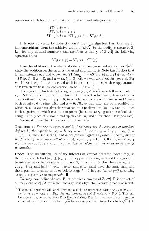
An Irrational Construction of R from Z 53
equations which hold for any natural number i and integers a and b:
ST0(a, b) = bST1(a, b) = a+ b
STi+2(a, b) = 2STi+1(a, b) + STi(a, b)
It is easy to verify by induction on i that the sign-test functions are allhomomorphisms from the additive group of Z[
√2] to the additive group of Z.
I.e., for any natural number i and members x and y of Z[√2] the following
equation holds:STi(x+ y) = STi(x) + STi(y)
Here the addition on the left-hand side is our newly-defined addition in Z[√2],
while the addition on the right is the usual addition in Z. Note this implies thatfor any integers n, a and b, we have STi(na, nb) = nSTi(a, b) and STi(−a,−b) =−STi(a, b). If n ∈ Z, and x = (a, b) ∈ Z[
√2], we will write nx for (na, nb). For
n ∈ N, nx is equal to the iterated addition: x+ x+ . . .+ x, with n appearancesof x (which we take, by convention, to be 0 if n = 0).
The algorithm for testing the sign of x = (a, b) ∈ Z[√2] is as follows: calculate
wi = STi(x) for i = 0, 1, 2, . . . in turn until one of the following three outcomesoccurs: either, (i), wi = wi+1 = 0, in which case, as is easy to see, a and b wereboth equal to 0 to start with and x = 0; (ii), wi and wi+1 are both positive, inwhich case, as we have already remarked, x is positive; or, (iii), wi and wi+1 areboth negative, in which case x is negative (because carrying out the calculationusing −x in place of x would end up in case (ii) and show that −x is positive).
We must prove that this algorithm terminates:
Theorem 1. For any integers a and b, if we construct the sequence of numbersdefined by the equations, w0 = b, w1 = a + b and wi+2 = 2wi+1 + wi, (i =0, 1, 2, . . .), then, for some i, and hence for all sufficiently large i, exactly one ofthe following three cases will obtain: (i), wi = wi+1 = 0, (ii), 0 < wi ∧ 0 < wi+1
or, (iii) wi < 0 ∧ wi+1 < 0. I.e., the sign-test algorithm described above alwaysterminates.
Proof: The absolute values of the integers wi cannot decrease indefinitely, sothere is a k such that |wk| ≤ |wk+1|. If wk+1 = 0, then wk = 0 and the algorithmterminates at or before stage k in case (i). If wk+1 �= 0, then because wk+2 =2wk+1 + wk and |wk| ≤ |wk+1|, wk+2 and wk+1 must have the same sign, andthe algorithm terminates at or before stage k + 1 in case (ii) or (iii) accordingas wk+1 is positive or negative11.
We may now define the set, P, of positive elements of Z[√2]. P is the set of
all members of Z[√2] for which the sign-test algorithm returns a positive result.
11 The same argument will work if we replace the recurrence equation wi+2 = 2wi+1 +wi, by wi+2 = Awi+1 + Bwi, for any integers A and B with A ≥ B > 0. This canbe shown to give routes from Z to R via subrings Z[α] for a variety of real numbersα including all those of the form
√m for m any positive integer for which
√m �∈ Z.
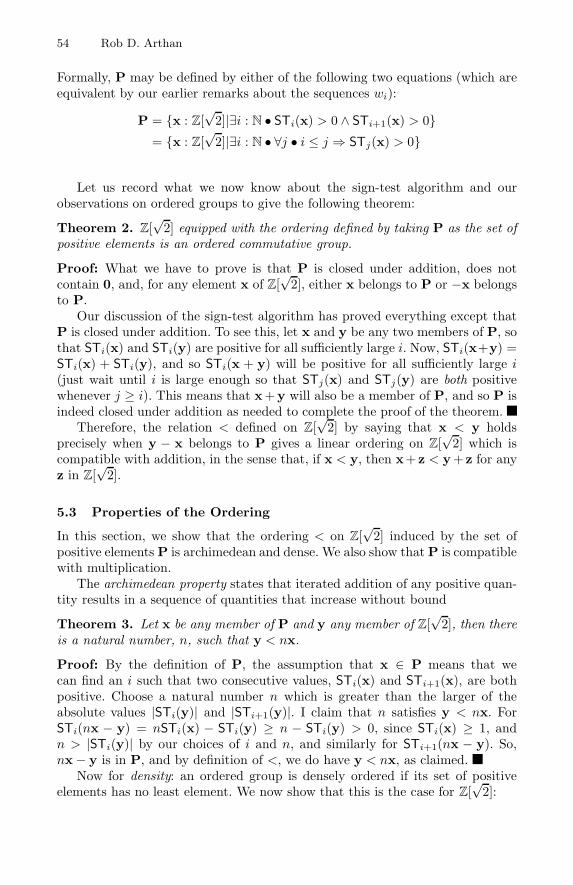
54 Rob D. Arthan
Formally, P may be defined by either of the following two equations (which areequivalent by our earlier remarks about the sequences wi):
P = {x : Z[√2]|∃i : N • STi(x) > 0 ∧ STi+1(x) > 0}
= {x : Z[√2]|∃i : N • ∀j • i ≤ j ⇒ STj(x) > 0}
Let us record what we now know about the sign-test algorithm and ourobservations on ordered groups to give the following theorem:
Theorem 2. Z[√2] equipped with the ordering defined by taking P as the set of
positive elements is an ordered commutative group.
Proof: What we have to prove is that P is closed under addition, does notcontain 0, and, for any element x of Z[
√2], either x belongs to P or −x belongs
to P.Our discussion of the sign-test algorithm has proved everything except that
P is closed under addition. To see this, let x and y be any two members of P, sothat STi(x) and STi(y) are positive for all sufficiently large i. Now, STi(x+y) =STi(x) + STi(y), and so STi(x + y) will be positive for all sufficiently large i(just wait until i is large enough so that STj(x) and STj(y) are both positivewhenever j ≥ i). This means that x+y will also be a member of P, and so P isindeed closed under addition as needed to complete the proof of the theorem.
Therefore, the relation < defined on Z[√2] by saying that x < y holds
precisely when y − x belongs to P gives a linear ordering on Z[√2] which is
compatible with addition, in the sense that, if x < y, then x+ z < y+ z for anyz in Z[
√2].
5.3 Properties of the Ordering
In this section, we show that the ordering < on Z[√2] induced by the set of
positive elements P is archimedean and dense. We also show that P is compatiblewith multiplication.
The archimedean property states that iterated addition of any positive quan-tity results in a sequence of quantities that increase without bound:
Theorem 3. Let x be any member of P and y any member of Z[√2], then there
is a natural number, n, such that y < nx.
Proof: By the definition of P, the assumption that x ∈ P means that wecan find an i such that two consecutive values, STi(x) and STi+1(x), are bothpositive. Choose a natural number n which is greater than the larger of theabsolute values |STi(y)| and |STi+1(y)|. I claim that n satisfies y < nx. ForSTi(nx − y) = nSTi(x) − STi(y) ≥ n − STi(y) > 0, since STi(x) ≥ 1, andn > |STi(y)| by our choices of i and n, and similarly for STi+1(nx − y). So,nx− y is in P, and by definition of <, we do have y < nx, as claimed.
Now for density: an ordered group is densely ordered if its set of positiveelements has no least element. We now show that this is the case for Z[
√2]:
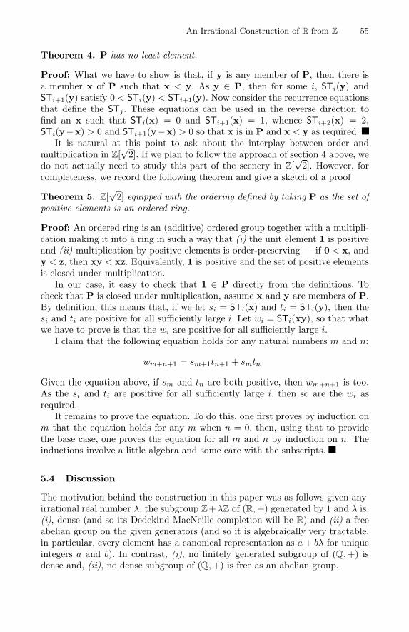
An Irrational Construction of R from Z 55
Theorem 4. P has no least element.
Proof: What we have to show is that, if y is any member of P, then there isa member x of P such that x < y. As y ∈ P, then for some i, STi(y) andSTi+1(y) satisfy 0 < STi(y) < STi+1(y). Now consider the recurrence equationsthat define the STj . These equations can be used in the reverse direction tofind an x such that STi(x) = 0 and STi+1(x) = 1, whence STi+2(x) = 2,STi(y−x) > 0 and STi+1(y−x) > 0 so that x is in P and x < y as required.
It is natural at this point to ask about the interplay between order andmultiplication in Z[
√2]. If we plan to follow the approach of section 4 above, we
do not actually need to study this part of the scenery in Z[√2]. However, for
completeness, we record the following theorem and give a sketch of a proof:
Theorem 5. Z[√2] equipped with the ordering defined by taking P as the set of
positive elements is an ordered ring.
Proof: An ordered ring is an (additive) ordered group together with a multipli-cation making it into a ring in such a way that (i) the unit element 1 is positiveand (ii) multiplication by positive elements is order-preserving — if 0 < x, andy < z, then xy < xz. Equivalently, 1 is positive and the set of positive elementsis closed under multiplication.
In our case, it easy to check that 1 ∈ P directly from the definitions. Tocheck that P is closed under multiplication, assume x and y are members of P.By definition, this means that, if we let si = STi(x) and ti = STi(y), then thesi and ti are positive for all sufficiently large i. Let wi = STi(xy), so that whatwe have to prove is that the wi are positive for all sufficiently large i.
I claim that the following equation holds for any natural numbers m and n:
wm+n+1 = sm+1tn+1 + smtn
Given the equation above, if sm and tn are both positive, then wm+n+1 is too.As the si and ti are positive for all sufficiently large i, then so are the wi asrequired.
It remains to prove the equation. To do this, one first proves by induction onm that the equation holds for any m when n = 0, then, using that to providethe base case, one proves the equation for all m and n by induction on n. Theinductions involve a little algebra and some care with the subscripts.
5.4 Discussion
The motivation behind the construction in this paper was as follows: given anyirrational real number λ, the subgroup Z+λZ of (R,+) generated by 1 and λ is,(i), dense (and so its Dedekind-MacNeille completion will be R) and (ii) a freeabelian group on the given generators (and so it is algebraically very tractable,in particular, every element has a canonical representation as a+ bλ for uniqueintegers a and b). In contrast, (i), no finitely generated subgroup of (Q,+) isdense and, (ii), no dense subgroup of (Q,+) is free as an abelian group.
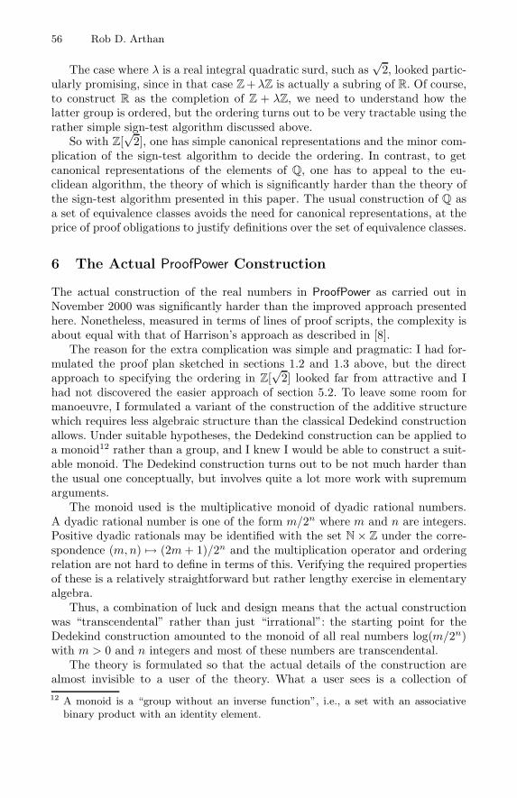
56 Rob D. Arthan
The case where λ is a real integral quadratic surd, such as√2, looked partic-
ularly promising, since in that case Z+λZ is actually a subring of R. Of course,to construct R as the completion of Z + λZ, we need to understand how thelatter group is ordered, but the ordering turns out to be very tractable using therather simple sign-test algorithm discussed above.
So with Z[√2], one has simple canonical representations and the minor com-
plication of the sign-test algorithm to decide the ordering. In contrast, to getcanonical representations of the elements of Q, one has to appeal to the eu-clidean algorithm, the theory of which is significantly harder than the theory ofthe sign-test algorithm presented in this paper. The usual construction of Q asa set of equivalence classes avoids the need for canonical representations, at theprice of proof obligations to justify definitions over the set of equivalence classes.
6 The Actual ProofPower Construction
The actual construction of the real numbers in ProofPower as carried out inNovember 2000 was significantly harder than the improved approach presentedhere. Nonetheless, measured in terms of lines of proof scripts, the complexity isabout equal with that of Harrison’s approach as described in [8].
The reason for the extra complication was simple and pragmatic: I had for-mulated the proof plan sketched in sections 1.2 and 1.3 above, but the directapproach to specifying the ordering in Z[
√2] looked far from attractive and I
had not discovered the easier approach of section 5.2. To leave some room formanoeuvre, I formulated a variant of the construction of the additive structurewhich requires less algebraic structure than the classical Dedekind constructionallows. Under suitable hypotheses, the Dedekind construction can be applied toa monoid12 rather than a group, and I knew I would be able to construct a suit-able monoid. The Dedekind construction turns out to be not much harder thanthe usual one conceptually, but involves quite a lot more work with supremumarguments.
The monoid used is the multiplicative monoid of dyadic rational numbers.A dyadic rational number is one of the form m/2n where m and n are integers.Positive dyadic rationals may be identified with the set N× Z under the corre-spondence (m,n) �→ (2m+ 1)/2n and the multiplication operator and orderingrelation are not hard to define in terms of this. Verifying the required propertiesof these is a relatively straightforward but rather lengthy exercise in elementaryalgebra.
Thus, a combination of luck and design means that the actual constructionwas “transcendental” rather than just “irrational”: the starting point for theDedekind construction amounted to the monoid of all real numbers log(m/2n)with m > 0 and n integers and most of these numbers are transcendental.
The theory is formulated so that the actual details of the construction arealmost invisible to a user of the theory. What a user sees is a collection of12 A monoid is a “group without an inverse function”, i.e., a set with an associative
binary product with an identity element.
An Irrational Construction of R from Z 57
constants giving the field operations and ordering relation on R with definingproperties that give the usual axiomatisation of R as a complete ordered field.
7 Concluding Remarks
The reader is again referred to [5, 8] for comprehensive surveys of constructionsof the real numbers with many additional references. In this paper, there is onlyspace for a few observations about other approaches.
The approach promoted here derives the multiplicative structure of R from itsadditive structure. This lets us exploit the delightfully simple additive structureof groups such as Z[
√2] which turn out to have a very tractable order structure
as well. However, the ring structure is simple too, and it now seems to the authorthat deriving the multiplicative structure of the reals in the traditional way fromthe ring structure of Z[
√2] may well be advantageous.
This paper has concentrated on the Dedekind-MacNeille method of com-pleting a dense ordered algebraic system. However, an approach using Cantor’smethod of fundamental sequences could also take Z[
√2] as a starting point. This
would need multiplicative inverses to be defined by a supremum argument ratherthan by pointwise operations on the fundamental sequences, but the supremumargument is an easy one.
A construction of the real numbers from the integers bypassing the rationalsis given by Faltin et al. in [6]. Their method is to use a binary positional repre-sentation in which the digits are allowed to be arbitrary integers. This results ina presentation of the real numbers as a quotient of a certain subring of a ring offormal Laurent series. This gives considerable insight into the way carries propa-gate in infinite binary arithmetic and can be applied to other constructions (suchas the p-adic completions of the integers). However, the method is considerablymore complicated from an arithmetic point of view than the more traditionalconstructions.
In [3], Conway gives a construction which embraces N, Z, Q and R andmuch more using a uniform representation of numbers as pairs of sets which canbe thought of as two-player games. The uniform representation leads to veryuniform, if rather recondite, methods of proof. Characterising the real numberswithin the Conway numbers is a little tricky but can be done. Unfortunately,in a typed framework such as HOL, identifying a type suitable for carryingout enough of the Conway construction to include R involves a far from trivialexercise in justifying transfinite inductive definitions.
In conclusion, selecting a method of constructing R in a mechanised theorem-proving system involves many trade-offs. The choice will be heavily influenced bywhat theories are already available and what theories are going to be developedin the future. If, for example, you have plans to do a lot of general commutativealgebra, then your best route might be to do the general field-of-fractions con-struction and the standard material on ideals and quotient rings first and usethese big guns to attack the specific problems of constructing Q as a field-of-fractions and then R via fundamental sequences. If you only have N, and want to
58 Rob D. Arthan
get going on analysis quickly, then Harrison’s approach is probably the methodof choice. If you have good working theories for N and Z then the methods ofthe present paper are offered for your consideration as a quick and simple routefrom Z to R.
Acknowledgments
I am grateful to John Harrison for some very helpful correspondence and, inparticular, for drawing the work of Behrend to my attention. I am indebted tothe referees for all their comments and suggestions; these were most stimulatingand have been of great assistance in revising the paper for publication.
References
1. R.D. Arthan. A Report on ICL HOL. In Myla Archer, Jeffrey J. Joyce, Karl N.Levitt, and Philip J. Windley, editors, Proceedings of the 1991 International Work-shop on the HOL Theorem Proving System and its Applications. IEEE ComputerSociety Press, 1992.
2. F.A. Behrend. A Contribution to the Theory of Magnitudes and the Foundationsof Analysis. Mathematische Zeitschrift, 63:345–362, 1956.
3. John H. Conway. On Numbers and Games. A.K. Peters Ltd., Second edition, 2001.4. B.A. Davey and H.A. Priestley. Introduction to Lattices and Order. Cambridge
University Press, 1990.5. H.-D. Ebbinghaus, H. Hermes, F. Hirzebruch, M. Koecher, K. Mainzer, J. Neukirch,
A. Prestel, and R. Remmert. Numbers. Springer-Verlag, 1990.6. F. Faltin, N. Metropolis, B. Ross, and G.-C. Rota. The Real Numbers as a Wreath
Product. Advances in Mathematics, 16, 1975.7. Michael J.C. Gordon and Tom F. Melham, editors. Introduction to HOL. Cam-
bridge University Press, 1993.8. John Harrison. Theorem Proving with the Real Numbers. Technical report, Uni-
versity of Cambridge Computer Laboratory, 1996.9. O. Holder. Die Axiome der Quantitat und die Lehre vom Mass. Ber. Verh. Kon.
Sch. Ges. Wiss., pages 1–64, 1901.10. R.B. Jones. Methods and Tools for the Verification of Critical Properties. In
R.Shaw, editor, 5th Refinement Workshop, Workshops in Computing. Springer-Verlag/BCS-FACS, 1992.
11. E. Kamke. Mengenlehre. Berlin, 1928. Reprinted by Dover in an English translationby F. Bagemihl as Theory of Sets. 1950.
12. D.J. King and R.D. Arthan. Development of Practical Verification Tools. Ingenuity— the ICL Technical Journal, 1996.
13. Saunders MacLane and Garrett Birkhoff. Algebra. AMS Chelsea Publishing, Thirdedition, 1999.
14. Walter Rudin. Principles of Mathematical Analysis. McGraw-Hill Book Company,1974.
15. C. T. Sennett. Demonstrating the Compliance of Ada Programs with Z Specifi-cations. In R.Shaw, editor, 5th Refinement Workshop, Workshops in Computing.Springer-Verlag/BCS-FACS, 1992.
HELM and the Semantic Math-Web
Andrea Asperti, Luca Padovani, Claudio Sacerdoti Coen, and Irene Schena
Department of Computer ScienceVia di Mura Anteo Zamboni 7, 40127 Bologna, Italy
Abstract. The eXtensible Markup Language (XML) opens the possi-bility to start anew, on a solid technological ground, the ambitious goalof developing a suitable technology for the creation and maintenanceof a virtual, distributed, hypertextual library of formal mathematicalknowledge. In particular, XML provides a central technology for stor-ing, retrieving and processing mathematical documents, comprising so-phisticated web-publishing mechanisms (stylesheets) covering notationaland stylistic issues. By the application of XML technology to the largerepositories of structured, content oriented information offered by Logi-cal Frameworks we meet the ultimate goal of the Semantic Web, that isto allow machines the sharing and exploitation of knowledge in the Webway, i.e. without central authority, with few basic rules, in a scalable,adaptable, extensible manner.
1 Introduction
Existing logical systems are not suitable for the creation of large repositoriesof structured mathematical knowledge accessible via Web. In fact, libraries inlogical frameworks are usually saved in two formats: a textual one, in the spe-cific tactical language of the proof assistant, and a compiled (proof checked)one in some internal, concrete representation language. Both representations areclearly unsatisfactory, since they are too oriented to the specific application: theinformation is not directly available, if not by means of the functionalities of-fered by the system itself. This is in clear contrast with the main guidelines ofthe modern Information Society, the recent emphasis on content and the newfrontier of the so called “Semantic Web.1” The goal of the Semantic Web is topass from a “machine readable” to a “machine understandable” encoding of theinformation: establishing a layer of machine understandable data would allowautomated agents, sophisticated search engines and interoperable services andwill enable higher degree of automation and more intelligent applications.In contrast with current encodings of mathematical information (e.g. in digi-
tal libraries), which are “machine-readable” but not “machine-understandable”,Logical Frameworks offer huge repositories of structured, content oriented in-formation, naturally providing a major arena for the Semantic Web and itstechnologies. The point is to allow access to this mathematical knowledge in the
1 Semantic Web Activity, http://www.w3.org/2001/sw.
R.J. Boulton and P.B. Jackson (Eds.): TPHOLs 2001, LNCS 2152, pp. 59–74, 2001.c© Springer-Verlag Berlin Heidelberg 2001
60 Andrea Asperti et al.
“Web way”, i.e. without central authority, with few basic rules, in a scalable,adaptable, extensible manner.The first, mandatory step in this direction is the direct encoding of the li-
braries in XML, which has recently imposed as the main tool for representation,manipulation, linking and exchange of structured information. But of course thebroad goal of the Semantic Web goes far beyond the trivial suggestion to adoptXML as a neutral specification language for the “compiled” versions of the li-braries, or even the observation that in this way we could take advantage of alot of functionalities on XML-documents already offered by standard commercialtools. Here is a short list of the added-value offered by the XML approach:
Standardization. Having a common, application independent, meta-languagefor mathematical proofs, similar software tools could be applied to differentlogical dialects, regardless of their concrete nature. This would be especiallyrelevant for all those operations like searching, retrieving, displaying or au-thoring (just to mention a few of them) that are largely independent of thespecific logical system.
Publishing. XML offers sophisticated web-publishing technologies (Stylesheets,MathML, . . . ) which can be profitably used to solve, in a standard way, theannoying notational problems that traditionally afflict formal mathematics.
Searching and Retrieving. The World Wide Web is currently doing a bigeffort in the Metadata and Semantic Web area. Languages as the ResourceDescription Framework or XML-Query are likely to produce innovative tech-nological solutions in this field.
Interoperability. If having a common representation layer is not the ultimatesolution to all interoperability problems between different applications, it ishowever a first and essential step in this direction.
Modularity. The “XML-ization” process should naturally lead to a substantialsimplification and re-organization of the current, “monolithic” architectureof logical frameworks. All the many different and often loosely connectedfunctionalities of these complex programs (proof checking, proof editing,proof displaying, search and consulting, program extraction, and so on) couldbe clearly split in more or less autonomous tasks, possibly (and hopefully!)developed by different teams, in totally different languages. This is the newcontent-based architecture of future systems.
In this article we present our project on the use of XML technology for thedevelopment and maintenance of distributed repositories of formal mathematicalknowledge: the Hypertextual Electronic Library of Mathematics (HELM2).
2 The eXtensible Markup Language
Perhaps, the best way to introduce XML in few lines is to take a look at a simpleexample. The following XML document is a possible encoding of the definitionof the inductive type of natural numbers in Coq [3].
2 http://www.cs.unibo.it/helm.
HELM and the Semantic Math-Web 61
<?xml version="1.0" encoding="ISO-8859-1"?>
<!DOCTYPE InductiveDefinition
SYSTEM "http://www.cs.unibo.it/helm/dtd/cic.dtd">
<InductiveDefinition noParams="0" params="">
<InductiveType name="nat" inductive="true">
<arity><SORT value="Set"/></arity>
<Constructor name="O"><REL value="1" binder="nat"/></Constructor>
<Constructor name="S">
<PROD>
<source><REL value="1" binder="nat"/></source>
<target><REL value="2" binder="nat"/></target>
</PROD>
</Constructor>
</InductiveType>
</InductiveDefinition>
XML gives a method for structuring data in a text file. Roughly speaking, theXML specification says that a XML document is made of tags (words bracketedby ’<’ and ’>’), attributes (of the form name="value") and text. Tags are used todelimit elements. Elements may appear in one of the following two forms: eitherthey are non-empty elements, as InductiveDefinition or InductiveType (theycan contain other elements or text), or they are empty elements, as SORT or REL.The previous example contains no text: this is a peculiarity of really formalencodings, where every bit of knowledge has a specific intelligence worth to beencapsulated in markup.The XML specification defines a XML document to be well-formed if it meets
some syntactical constraints on the use of tags and attributes. For example, non-empty elements must be perfectly balanced. For this reason, someone can thinkof tags of non-empty elements as labeled brackets for structuring the document.XML lets the user specify his own grammar by means of a Document Type
Definition (DTD), a document which defines the allowed tags, the related at-tributes and which is the legal content for each element. The XML specificationjust defines the validity of a XML document with respect to a given DTD. Thisis why XML is a meta-language that can be instantiated to a potentially infiniteset of languages, each with its own DTD.For example, here is a DTD fragment for the previous XML file:
<?xml version="1.0" encoding="ISO-8859-1"?>
...
<!ENTITY % term ’(LAMBDA|CAST|PROD|REL|SORT|APPLY|VAR|META|IMPLICIT|
CONST|LETIN|MUTIND|MUTCONSTRUCT|MUTCASE|FIX|COFIX)’>
...
<!ELEMENT InductiveDefinition (InductiveType+)>
<!ATTLIST InductiveDefinition
noParams NMTOKEN #REQUIRED
params CDATA #REQUIRED
id ID #REQUIRED>
<!ELEMENT InductiveType (arity,Constructor*)>
<!ATTLIST InductiveType
name CDATA #REQUIRED
62 Andrea Asperti et al.
inductive (true|false) #REQUIRED>
<!ELEMENT Constructor %term;>
<!ATTLIST Constructor name CDATA #REQUIRED>
...
A InductiveDefinition element may contain one or more InductiveTypeelements, each InductiveType contains an arity followed by a possibly emptysequence of Constructors, and a Constructor is an arbitrary term (an ENTITYis a macro declaration). The attributes of InductiveDefinition are noParams,params and id, while name is the only attribute of Constructor. The keywordREQUIRED states that an attribute cannot be omitted when using its related tag.
References to Documents. Documents and resources in general must have a namein order to be accessible over the Web. This is accomplished via the use of URIs(Universal Resource Identifiers) as defined in [6]. A generic URI is made of aformatted (structured) string of characters whose intended meaning is associ-ated by the applications managing it. URLs (Uniform Resource Locators) area particular kind of URIs specifically designed to name resources accessed bymeans of a given standard protocol (for example the HTTP protocol). URLsconsist of a first part identifying the protocol and a host followed by a secondpart to locate the resource on it.URLs can be resolved by standard processing tools and browsers, but suf-
fer from problems of consistency: moving the target document leads to danglingpointers; moreover, being physical names, they cannot be used to identify a wholeset of copies located on different servers for fault-tolerance and load-balancingpurposes. URIs, instead, can be designed as logical names, leaving to applica-tions the burden of resolution to physical names. So, for examples, the URI“cic:/Coq/Reals/Rdefinitions/R.con” could be used as a logical name forthe axiom which defines the existence of the set R of real numbers in the stan-dard library of the Coq Proof Assistant; then, an application is required to mapthe URI to a physical name (an URL) as
http://coq.inria.fr/library/Reals/Rdefinitions/R.con.xml
3 The HELM Project
The overall architecture of our project is depicted in Fig. 1.Once XML has been chosen as the standard encoding format3 for the li-
brary, we must face the problem of recovering the already codified mathematicalknowledge. Hence, we need new modules implementing exporting functionalitiestoward the XML representation for all the available tools for proof reasoning.Currently, we have just written such a module only for the Coq proof assistant[3]. In the near future, we expect that similar exporting functionalities will beprovided by the developers of the other logical systems. We will describe theexporting issues in Sect. 4.
3 A standard format, not a standard language! In other words, the standardization weare pursuing is not at the logical level, but at the technological one.
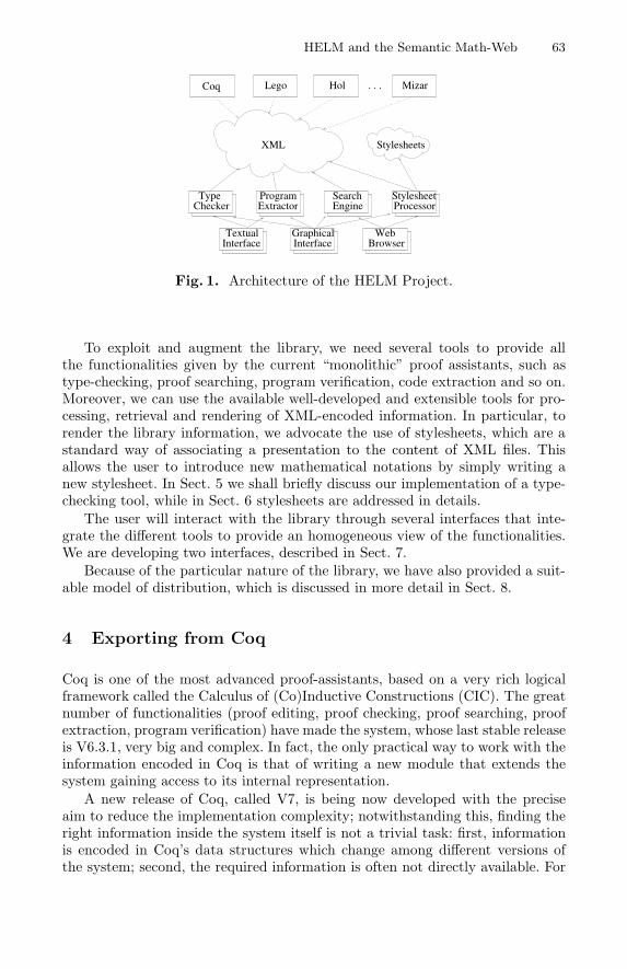
HELM and the Semantic Math-Web 63
Coq
Search
. . .
StylesheetProcessorEngine
ProgramExtractorChecker
Type
Textual WebGraphicalBrowserInterfaceInterface
Lego Hol Mizar
StylesheetsXML
Fig. 1. Architecture of the HELM Project.
To exploit and augment the library, we need several tools to provide allthe functionalities given by the current “monolithic” proof assistants, such astype-checking, proof searching, program verification, code extraction and so on.Moreover, we can use the available well-developed and extensible tools for pro-cessing, retrieval and rendering of XML-encoded information. In particular, torender the library information, we advocate the use of stylesheets, which are astandard way of associating a presentation to the content of XML files. Thisallows the user to introduce new mathematical notations by simply writing anew stylesheet. In Sect. 5 we shall briefly discuss our implementation of a type-checking tool, while in Sect. 6 stylesheets are addressed in details.The user will interact with the library through several interfaces that inte-
grate the different tools to provide an homogeneous view of the functionalities.We are developing two interfaces, described in Sect. 7.Because of the particular nature of the library, we have also provided a suit-
able model of distribution, which is discussed in more detail in Sect. 8.
4 Exporting from Coq
Coq is one of the most advanced proof-assistants, based on a very rich logicalframework called the Calculus of (Co)Inductive Constructions (CIC). The greatnumber of functionalities (proof editing, proof checking, proof searching, proofextraction, program verification) have made the system, whose last stable releaseis V6.3.1, very big and complex. In fact, the only practical way to work with theinformation encoded in Coq is that of writing a new module that extends thesystem gaining access to its internal representation.A new release of Coq, called V7, is being now developed with the precise
aim to reduce the implementation complexity; notwithstanding this, finding theright information inside the system itself is not a trivial task: first, informationis encoded in Coq’s data structures which change among different versions ofthe system; second, the required information is often not directly available. For
64 Andrea Asperti et al.
example, when a file is loaded in V6.3.1, its path is forgotten, while we wouldlike to export files in directories reflecting the logical structure of the library.In the rest of this section we only focus on the implementation of the export-
ing module4 for version 6.3.1 which is a representative example of the difficultiesthat could be faced when exporting from an existing proof-assistant without thecollaboration of its development team.
4.1 Relevant Information to Be Exported
To design the module, the first difficulty has been the identification of whichinformation is worth to be exported. We have chosen not to export:
Parsing and pretty-printing rules. Parsing rules should depend only on theproof engine. To be able to use other proof engines different from Coq wecannot rely on Coq’s own rules. Similarly, pretty-printing rules should de-pend only on the users choice and the type of available browser.
Tactics-related information. These, too, are proof engine dependent. More-over, we do not think that the tactics used to do a proof are really meaningfulto understand the proof itself (surely, they are not the real informative con-tent). In fact, the level of tactics and the level at which a proof should beunderstood are not the same: what some simple tactics do (as “Auto” thatautomatically search a proof) is not at all obvious. Moreover, the sequence oftactics used is clearly reflected in the λ-term of the proof; hence it is possibleto add as an attribute to a sub term the name and parameters of the tacticused to generate it.
Redundant information added by Coq to the terms of CIC. Coq addsin several places a lot of information to CIC terms in order to speed upthe type-checking. For example, during the type-checking of an inductivedefinition, Coq records which are the recursive parameters of its inductiveconstructors; this information is then used during the type-checking of fixfunctions to ensure their termination. This is an example of a clearly redun-dant information, surely useless for browsing purposes or for indexing, butnecessary to every proof-checker implementation. Other times, instead, theadded information is important only for browsing purposes. For example,sometimes the user asks the system to infer a type and probably does notwant to view the inferred type thereafter.So, we have decided to export a first core of information, roughly correspond-ing to the only one available at the logical level, according to a principle ofminimalism: no redundant information should be exported. If the principlewere not followed, in every application loading an XML file we would have toadd checks to verify the consistency of the redundant (and possibly useless!)information. In Sect. 4.2 we will see how this does not prevent us to link ina precise way additional information to the core one.
4 The module is fully working and has been used to export the whole library providedwith the Coq System, yielding about 64 Mb of XML (2 Mb after compression).
HELM and the Semantic Math-Web 65
The remaining, interesting information could be structured into three differentlevels that we have clearly separated in the XML representation. The first one isthe level of terms. Terms (or expressions) can never appear alone, but only as partof an object definition. In Coq, the terms are CIC λ-expressions, i.e. variables(encoded as DeBrujin indexes), λ-abstractions and applications, product typesand sorts, augmented with a system of inductive types in the spirit of the onesof Martin-Lof, comprising (co)inductive types and constructors, case analysisoperators and inductive and co-inductive function definitions. The whole level isextremely dependent on the logical framework.The second level, that uses the previous one to encode both bodies and types,
is the one of objects. Every object is stored into a different file. The files arestructured into directories that corresponds to sections in Coq, i.e. delimiters ofthe scope of a variable. Sections are also used in Coq to structure a large theoryinto sub-theories. In HELM, the former usage is retained, while theories aredescribed in another way (see the third level). In Coq, the objects are constants,representing definitions, theorems and axioms, (the former two have both a typeand a body, while the latter has a type only), variables, (co)inductive definitions(such as nat for the natural numbers) and proofs in progress.The last level is the level of theories which is completely independent of the
particular logical framework. In our idea, a theory is a (structured) mathematicaldocument containing objects taken almost freely from different sections. Writinga new theory should consist in developing new objects and assembling thesenew objects and older ones into the mathematical document. It is during thecreation of a theory that objects must also be assigned the particular, semanticalmeaning used to classify them, for example into lemmas, conjectures, corollaries,etc. Theories, that are described in different XML files, do not include the objectsdirectly, but refers to them via their URIs.The following is an example of theory file with two sections, the first one
delimiting the scope of variables A and B.
<?xml version="1.0" encoding="ISO-8859-1"?>
<!DOCTYPE Theory SYSTEM "http://www.cs.unibo.it/helm/dtd/maththeory.dtd">
<Theory uri="cic:/Coq/Init/Logic">
<!-- Require Export Datatypes -->
<DEFINITION uri="True.ind"/>
<DEFINITION uri="False.ind"/>
<DEFINITION uri="not.con"/>
<SECTION uri="Conjunction">
<DEFINITION uri="and.ind"/>
<VARIABLE uri="A.var"/>
<VARIABLE uri="B.var"/>
<THEOREM id="id1" uri="proj1.con"/>
<THEOREM id="id2" uri="proj2.con"/>
</SECTION>
<SECTION uri="Disjunction">
<DEFINITION uri="or.ind"/>
</SECTION>
</Theory>
66 Andrea Asperti et al.
All the URIs, but that of Theory, are relative URIs; so, the absolute URI ofid1 is “cic:/Coq/Init/Logic/Conjunction/proj1.con”. In the example youcan also see the usage of sections to bound the scope of variables: the scope ofA and B is the section Conjunction.It is important to note that at the theory level, sections are not used to
structure the document into, for instance, chapters, paragraphs and so on; manykind of (XML) markup languages have just been developed to do so. Accordinglyto the spirit of XML, our theory markup will be freely and modularly intermixedwith other kinds of markup, such as XHTML;5 so, our language will play formathematical theories the same role of MathML for mathematical expressionsand SVG6 for vectorial graphics. The added value of using the theory level(instead of directly embedding the object markup) is that, while enriching thesemantics of the objects of the previous level, it could also be used to enforcesome constraints as, for example, on the scope of variables or on the links betweentheorems and lemmas.
4.2 Auxiliary Information and Metadata
In this paragraph we address the problem of the association of additional andpossibly redundant information to the one exported using the Coq module. Thepurpose of this added information is to enable or facilitate specific functionalitiessuch as rendering, searching, indexing and so on.7
A simple observation suggests that such information could be naturally as-sociated either to the whole object definition (e.g. the name of the author of atheorem) or to a particular node of a λ-term (e.g. the tactic used to generateit or an informal description of its meaning). So, we can easily store the addi-tional information in a distinct XML file and use XLink technology to relateit to the appropriate XML element in the corresponding logical-level document.Moreover, in the specific case of metadata, we can benefit from the Resource De-scription Framework (RDF, [11] [12]), which provides a general model for repre-senting metadata as well as a syntax for encoding and exchanging this metadataover the Web. In several cases, this meta-information can be extracted from thedocument, for instance by means of XSL Transformations. It is important tonote that, in this approach, no modification at all is required to the DTDs or tothe source document. As a side effect, an application can consult just the XMLfiles holding the information it really needs, without having to parse, check forconsistency and finally ignore non-interesting information.
5 http://www.w3.org/TR/xhtml1.6 http://www.w3.org/TR/SVG.7 For instance, a major example of such additional information, which is essential forrendering purposes, are the intermediate conclusions inside complex proofs (see [4]),which are typically omitted (as redundant) in a Curry-Howard representation ofproofs as λ-terms.
HELM and the Semantic Math-Web 67
5 Proof-Checker
In order to verify that all the needed core information was exported from Coq,we have developed a stand-alone proof-checker for CIC objects, similar to theCoq one, but fairly simpler and smaller thanks to its independence of the proofengine. It is the first example of a tool working directly on the XML encoding.With respect to other proof-checkers (as the one of Coq), it is fairly standard
but for the peculiar management of the environment: usually, proof-checkers areused to check whole theories, i.e. sequence of definitions or proofs. Each timea definition is checked, it is added to the environment and then it is used insubsequent type-checking. So, every theorem is always checked with the same,statically defined environment. Our proof-checker, instead, builds the environ-ment (a cache, actually) “on-demand”: every time a reference to another objectnot present in the environment is found, the type-checking is interrupted, pro-cessing the new object first. Checks are introduced in order to avoid cycles inthe definitions, corresponding to an inconsistent environment.
6 XSL Transformations and MathML
XSLT [17] is a language for transforming XML documents into other XML doc-uments. In particular, a stylesheet is a set of rules expressed in XSLT to trans-form the tree representing a XML document into a result tree. When a patternis matched against elements in the source tree, the corresponding template isinstantiated to create part of the result tree. In this way the source tree can befiltered and reordered, and arbitrary structure can be added. A pattern is anexpression of XPath [16] language, that allows to match elements according totheir values, structure and position in the source tree.XSLT is primarily aimed to associate a style to a XML document, generating
formatted documents suitable for rendering purposes, thus providing a standardtool for processing and transforming XML mathematical document, accordingto alternative notations and encodings.A natural encoding for mathematics on the Web is MathML [8], an instance of
XML for describing the notation of a mathematical expression, capturing both itsstructure and content. MathML has, roughly, two categories of markup elements:the presentation markup, which describes the layout structure of mathematicalnotation, and the content markup, that provides an explicit encoding of theunderlying mathematical structure of an expression.Although the target of MathML is the encoding of expressions (so it can-
not describe mathematical objects and documents), the MathML PresentationMarkup can be considered as a privileged rendering format, providing a standardon the web already implemented by several applications.The choice of MathML content markup as an intermediate representation
between the logic-dependent representation of the mathematical information andits presentation is justified by several reasons:
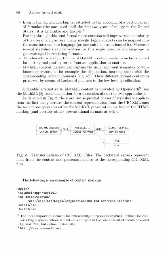
68 Andrea Asperti et al.
– Even if the content markup is restricted to the encoding of a particular setof formulas (the ones used until the first two years of college in the UnitedStates), it is extensible and flexible.8
– Passing through this semi-formal representation will improve the modularityof the overall architecture: many specific logical dialects can be mapped intothe same intermediate language (or into suitable extensions of it). Moreoverseveral stylesheets can be written for this single intermediate language togenerate specific rendering formats.
– The characteristic of portability of MathML content markup can be exploitedfor cutting and pasting terms from an application to another.
– MathML content markup can capture the usual informal semantics of well-known operators, as for example the disjunction, marking them with thecorresponding content elements (e.g. or). Their different formal content ispreserved by means of backward pointers to the low level specification.
A feasible alternative to MathML content is provided by OpenMath9 (seethe MathML [8] recommendation for a discussion about the two approaches).As depicted in Fig. 2, there are two sequential phases of stylesheets applica-
tion: the first one generates the content representation from the CIC XML one;the second one generates either the MathML presentation markup or the HTMLmarkup (and possibly others presentational formats as well).
CIC XML OBJECTS HTML/MATHML PRES.
MATHML PRES.MATHML CONTENT
XML OBJECTS
CIC XML TERMS
XSLTXSLT
HTML
HTML
Fig. 2. Transformations of CIC XML Files: The backward arrows representlinks from the content and presentation files to the corresponding CIC XMLfiles.
The following is an example of content markup
<apply>
<csymbol>app</csymbol>
<ci definitionURL=
"cic:/Coq/Init/Logic/Conjunction/and_ind.con">and_ind</ci>
<ci>A</ci>
<ci>B</ci>
8 The most important element for extensibility purposes is csymbol, defined for con-structing a symbol whose semantics is not part of the core content elements providedby MathML, but defined externally.
9 http://www.openmath.org.
HELM and the Semantic Math-Web 69
<ci>A</ci>
<lambda>
<bvar><ci>H0</ci><type><ci>A</ci></type></bvar>
<lambda>
<bvar><ci>H1</ci><type><ci>B</ci></type></bvar>
<ci>H0</ci>
</lambda>
</lambda>
<ci>H</ci>
</apply>
The main problems related to the definition of content stylesheets are:
– Objects, in general, cannot be considered as terms. Hence, we have addedto the MathML content markup a XML level to describe the level of objects(using different namespaces [9]).
– Operators which are not covered by the MathML content base set are en-coded by means of the csymbol element.
– The standard semantics of MathML content elements is only informally de-fined in the specification. In HELM, formal semantics of content elements isenforced, wherever it is possible, by means of pointers to the XML files oftheir corresponding CIC definitions.
As you can see in Fig. 2, we produce MathML content and presentation intwo distinct steps. The only way to combine and link together content andpresentation in compliance to the MathML specification consists of using thesemantics element. This content element is quite ambiguous, a kind of “bridge”between content and presentation; moreover, it is currently ignored by all thebrowsers supporting MathML. For us, the next natural improvement will consistof having content and the associated presentations in different files, one for thecontent expression and one for each presentation. Then we need to relate apresentation expression and subexpressions to the respective content expressionand subexpressions. This can be achieved in a standard way using the machineryof XLink and XPointer [14,15].The above solution has been also exploited for the implementation of the
links of Fig. 2 for linking the content and presentation markup to the corre-sponding source CIC XML terms. In this way the user can browse the MathMLpresentation and also modify it: the changes will have effect on the correspondingCIC XML file.An example of MathML presentation markup generated after the second
phase is:
<mrow>
<mo stretchy="false">(</mo>
<mi>and_ind</mi><mphantom><mtext>_</mtext></mphantom>
<mi>A</mi><mphantom><mtext>_</mtext></mphantom>
<mi>B</mi><mphantom><mtext>_</mtext></mphantom>
<mi>A</mi><mphantom><mtext>_</mtext></mphantom>
<mrow>
70 Andrea Asperti et al.
<mo color="Red">λ</mo>
<mi>H0</mi> <mo>:</mo> <mi>A</mi> <mo>.</mo>
<mrow>
<mo color="Red">λ</mo>
<mi>H1</mi> <mo>:</mo> <mi>B</mi> <mo>.</mo>
<mi>H0</mi>
</mrow>
</mrow>
<mphantom><mtext>_</mtext></mphantom><mi>H</mi>
<mo stretchy="false">)</mo>
</mrow>
To generate presentation markup from the corresponding content markup, weuse, among others, a stylesheet, compliant with the last specification of MathML,written by Igor Rodionov.10 This stylesheet, written in collaboration with theMathML Working Group, transforms MathML content markup in MathML pre-sentation one.We must solve several problems regarding the presentation output:
– We have had to associate an output to every object and to every csymboldefined in the content phase.
– We have modified the MathML stylesheet to implement the policy of line-breaking and alignment for long terms: our choice consists of using tablesmade of multiple rows. The mtable element is specifically designed to arrangeexpressions in a two-dimensional layout and in particular it provides a setof related elements and attributes to achieve proper alignment and line-breaking.
As we have said above, MathML is not the only format exploited: anotherpresentation format is HTML, due to the wide-spreading of browsers for it andits native hypertextual nature. Thanks to the modular architecture (see Fig. 2),many other formats could be added too.Finally, note that the general architecture gives the possibility of applying
stylesheets of arbitrary complexity. For example, we have developed stylesheetsto render proofs in natural language, in the spirit of [5].We will exploit the same modular architecture of the object level at the
level of theories. At this level we can use the same presentation formats of theprevious levels; on the contrary, there is no standard language for describingtheories at the content level. So we will develop a new (XML) language thatwill be largely independent of the specific foundational dialect and could aspireto play the same role MathML plays for mathematical expressions. An alreadyexistent corresponding proposal for OpenMath is OMDoc [10]. A possibilitycould consist of achieving the integration of our proposal with an extension toMathML of OMDoc, giving a common standard way to represent the structureof a mathematical document.
10 Computer Science Department of the University of Western Ontario, London,Canada.
HELM and the Semantic Math-Web 71
7 Interfaces to HELM
Two of the main goals of HELM are the easiness in augmenting and browsingthe library:
1. Every user with a small amount of HTTP or FTP space should be able topublish a document.
2. Every user with a common browser should be able to browse the library.
To fullfil these aims, we must face the actual state of technology:
1. Currently, almost all of the Internet users have a web space, but usuallywithout being allowed to run any kind of program on the server, even simpleCGIs. So no intelligence can be put on the publisher side.
2. The browser technology is rapidly evolving in such a way that we expectin a few time to have browsers able to understand MathML and, probably,even to apply XSLT stylesheets. At the moment, though, if we require thebrowser to be standard, then we have to put the intelligence on the otherside, i.e. on the server.
Therefore, where can we put the intelligence? A first answer is the creation of pre-sentation sites able to retrieve documents from distribution sites, process them(e.g. applying stylesheets) and return them to the users in the user requestedformat.In a first prototype of presentation site we relied on the capabilities of Co-
coon, a XML server-based web-publishing framework, for the processing of therequested documents. Recently we adopted a more modular and more reusablesolution, consisting in having a completely separate component, a servlet indeed,for the application of stylesheets. This component is designed to receive HTTPrequests of stylesheet application, sending the result of the transformation asthe reply of the request. In this way, ordinary browsing tools can access the pro-cessed documents simply by invoking the servlet with a proper URL containingboth a reference to the source document to be processed, the list of stylesheetsto be applied and possibly a sequence of parameters. In this way the numberand order of the stylesheets can be changed at any invocation and their behaviormay be affected by the value of the parameters passed by the client. Moreover,the documents, the stylesheets and the DTDs are not constrained to reside onthe same host of the processor, thus over-passing the greatest limitation of theCocoon-based framework.Though this solution is perfect for browsing11 and doing simple elaborations,
it gives the user too strict interaction possibilities, which are required for morecomplex tasks (as the creation of new theories, for example). Hence, more ad-vanced interfaces with such capabilities are required. These interfaces must berun on the user’s machine and should, at least, be able to provide all the pro-cessing functionalities of the presentation servers. At the same time, they should11 An on-line library of Coq V7 theories can be found at the address
http://phd.cs.unibo.it/helm/library/. Each document is rendered on-the-flyeither to HTML or to MathML.
72 Andrea Asperti et al.
also overcome the limitations of standard browsers through the addition of newinteraction possibilities.Since our preferential browsing language is MathML, our interface should at
least be able to render its presentation markup. Unfortunately, there are no sat-isfactory implementations available yet. Moreover, we also need to interact withthe MathML rendered files, for example for editing. Not only forms of interactionwith this kind of markup have never been proposed before, but we also need to re-flect the changes on the source files of the XSLT rendering transformations. Thishas led us to the development of a brand new engine with rendering and editingcapabilities for documents embedding MathML presentation markup. The en-gine, which is also able to export rendered MathML documents to Postscript, isdesigned to be stand-alone and it is freely available as a Gtk widget.12
We have integrated our widget, the proof-checker and the external XSLTprocessor into a minimal interface that we are going to extend with editingfunctionalities.
8 The Model of Distribution
Mathematical documents have some peculiar properties. First of all a mathe-matical document should be immutable: the correctness of a document A thatrefers to a document B can be guaranteed only if B does not change. Notwith-standing this, new versions of a mathematical document could be released (forexample if a conjecture is actually proved). Secondly, a user cannot be forcedto retain a copy of his document forever, even if other documents refer to it.So, it should be possible for everyone to make a copy of a document and alsodistribute it. When more than a copy is available, the user should be able todownload it from any suitable server (for example, from the nearest one). Thisimplies that documents could not be referred to via URLs, but only with logicalnames in the form of URIs. A particular naming policy should then be adoptedto prevent users to publish different documents under the same URI.To fulfill these requirements, we have adopted almost the same model of dis-
tribution of the Debian packaging system APT13 which has similar requirements(a package could not be modified, but only updated, it is available on differentservers, could be downloaded from the user preferred server).Every document is identified by an URI. For example, the URI that references
an inductive definition (“.ind”) in the subsection Datatypes of the subsectionInit of the section Coq is “cic:/Coq/Init/Datatypes/nat.ind”. Similarly,the URI “theories:/Coq/Init/Datatypes.theory” refers to the mathematicaltheory named Datatypes located in the subdirectory Init of the directory Coq.In order to translate the URI to a valid URL, a particular tool, named getter,
is needed. It takes in input an ordered list of servers and an URI and returnsthe URL of the document on the first server in the list supplying it. Each server
12 The widget is now a package of the forthcoming Debian distribution.See http://www.cs.unibo.it/helm/mml-widget/ for further details.
13 http://www.debian.org.
HELM and the Semantic Math-Web 73
publishes a list of the URIs of the documents it provides along with their corre-sponding URL.In order to flexibly allow communication between the components of HELM
architecture, the interface provided by the getter is the one of an HTTP dae-mon, pre-dating the ideas of the SOAP working draft [13]: when a document isrequired, its logical name is resolved in an URL, the document is downloaded, itis processed if needed14 and finally it is returned to the client and it is possiblylocally stored for caching purposes. If the machine hosting the getter is also adistribution site, then, once cached, a document could also be added to the listof documents the server exports. In such a way, often referred to or simply in-teresting documents spread rapidly over the net, downloading times are reducedand the author can freely get rid of his copy of the document if he does not needit any more. This architecture imposes no constraints on the naming policy: upto now we have not chosen or implemented one yet. To face the issue, one pos-sibility can be the choice of having a centralized naming authority, even if othermore distributed scenarios will surely be considered.
9 Conclusions and Further Developments
In this paper we have presented the current status of the HELM project, whoseaim is to exploit the potentiality of XML technology for the creation and main-tenance of large repositories of structured, content oriented information offeredby Logical Frameworks, sharing and processing knowledge in compliance withthe main philosophy of Web, i.e. without central authority, with few basic rules,in a scalable, adaptable, extensible manner.Due to our methodology (HELM is independent of Coq), the extension of
the library to other logical frameworks and systems does not look problematic.We are soon going to develop:Tools for indexing and retrieval of mathematical documents, based on meta-
data specified in the Resource Description Framework (RDF, see [11]). RDFprovides a foundation for processing meta-data, complements XML, and im-proves interoperability between applications that exchange information on theWeb.
Tools for the (re)annotation of mathematical objects and terms: the intuitivemeaning of these entities is usually lost in their description in a logical framework.Even their automatically extracted presentations in a natural language are oftenunsatisfactory, being quite different from the typical presentation in a book. Webelieve that a feasible solution is giving the user the possibility of enriching termswith annotations given in an informal, still structured language.
Tools to provide functionalities missing from monolithic proof assistants, suchas proof-extraction of proof-editing.
14 For example, typical processing are deflating compressed files or the resolution ofrelative URIs contained in the document to absolute ones.
74 Andrea Asperti et al.
References
1. Asperti, A., Padovani, L., Sacerdoti Coen, C., Schena, I., “Towards a library of for-mal mathematics”. Panel session of the 13th International Conference on TheoremProving in Higher Order Logics (TPHOLS’2000), Portland, Oregon, USA.
2. Asperti, A., Padovani, L., Sacerdoti Coen, C., Schena, I., “XML, Stylesheets andthe re-mathematization of Formal Content”, Department of Computer Science,Bologna, Italy, May 2000.
3. Barras, B., et al., “The Coq Proof Assistant Reference Manual, version 6.3.1”,http://pauillac.inria.fr/coq/.
4. Coscoy, Y., Kahn, G., Thery, L., Extracting Text from Proofs. Technical ReportRR-2459, INRIA Sophia Antipolis.
5. Coscoy, Y., “Explication textuelle de preuves pour le Calcul des ConstructionsInductives”, Phd. Thesis, Universite de Nice-Sophia Antipolis, 2000.
6. Berners-Lee, T., “Universal Resource Identifiers in WWW”, RFC 1630, CERN,June 1994.
7. Extensible Markup Language (XML) (Second Edition). Version 1.0. W3C Recom-mendation, 6 October 2000. http://www.w3.org/TR/REC-xml.
8. Mathematical Markup Language (MathML). Version 2.0. W3C Recommendation,21 February 2001. http://www.w3.org/TR/MathML2/.
9. Namespaces in XML. W3C Recommendation, 14 January 1999.http://www.w3.org/TR/REC-xml-names/
10. Open Mathematical Documents (OMDoc) 1.0, November 1 2000.http://www.mathweb.org/omdoc/.
11. Resource Description Framework (RDF) Model and Syntax Specification, W3CRecommendation 22 February 1999.http://www.w3.org/TR/1999/REC-rdf-syntax-19990222/ .
12. Resource Description Framework (RDF) Schema Specification 1.0, W3C CandidateRecommendation 27 March 2000. http://www.w3.org/TR/rdf-schema/.
13. Simple Object Access Protocol (SOAP). Version 1.1. W3C Note, 8 May 2000.http://www.w3.org/TR/SOAP/.
14. XML Linking Language (XLink). Version 1.0. W3C Proposed Recommendation,20 December 2000. http://www.w3.org/TR/xlink/.
15. XML Pointer Language (XPointer). Version 1.0. W3C Working Draft (Last Call),8 January 2001. http://www.w3.org/TR/xptr/.
16. XML Path Language (XPath). Version 1.0, W3C Recommendation, 16 November1999. http://www.w3.org/TR/xpath.
17. XSL Transformations (XSLT). Version 1.0, W3C Recommendation, 16 November1999. http://www.w3.org/TR/xslt/.
Calculational Reasoning Revisited
An Isabelle/Isar Experience
Gertrud Bauer and Markus Wenzel
Technische Universitat MunchenInstitut fur Informatik, Arcisstrasse 21, 80290 Munchen, Germany
http://www.in.tum.de/~bauerg/
http://www.in.tum.de/~wenzelm/
Abstract. We discuss the general concept of calculational reasoningwithin Isabelle/Isar, which provides a framework for high-level naturaldeduction proofs that may be written in a human-readable fashion. Set-ting out from a few basic logical concepts of the underlying meta-logicalframework of Isabelle, such as higher-order unification and resolution,calculational commands are added to the basic Isar proof language ina flexible and non-intrusive manner. Thus calculational proof style maybe combined with the remaining natural deduction proof language in aliberal manner, resulting in many useful proof patterns. A case-study onformalizing Computational Tree Logic (CTL) in simply-typed set-theorydemonstrates common calculational idioms in practice.
1 Introduction
A proof by calculational reasoning basically proceeds by forming a chain of inter-mediate results that are meant to be composed by basic principles, such as transi-tivity of =/</≤ (or similar relations). More advanced calculations may even in-volve substitution, which in the case of inequalities usually includes monotonicityconstraints. In informal mathematics, this kind of proof technique is routinelyused in a very casual manner. Whenever mathematicians write down sequencesof mixed equalities or inequalities, underline subexpressions to be replaced etc.then it is likely that they are doing calculational reasoning.In fact, calculational reasoning has been occasionally proposed as simple meansto rephrase mathematical proof into a slightly more formal setting (e.g. [2,1]),which does not necessarily include machine-checking of proofs, of course. Observ-ing that logical equivalence and implication may be just as well used in calcula-tions, some have even set out to do away with traditional natural-deduction stylereasoning altogether [5], although that discipline does not appeal to everyone.Nevertheless, calculational reasoning offers a relatively simple conceptual basisto build tools for logical manipulations. The popular Math
∫pad tool supports
manipulation of algebraic expressions in a systematic way; it has recently evenacquired means for formal proof checking [18], using PVS as the backend.
R.J. Boulton and P.B. Jackson (Eds.): TPHOLs 2001, LNCS 2152, pp. 75–90, 2001.c© Springer-Verlag Berlin Heidelberg 2001
76 Gertrud Bauer and Markus Wenzel
The Mizar system [17,12,22] focuses on formal proof in common mathematicsstyle in the first place. It also offers a mechanism for iterated equality reasoning,which shall serve here as an example for calculations within a formal setting.The following trivial proof is taken from article #185 of the Mizar library [11].
theorem Th1:
for X,Y being set holds union {X,Y,{}} = union {X,Y}
proof
let X,Y be set;
thus union {X,Y,{}} = union ({X,Y} U {{}}) by ENUMSET1:43
.= union {X,Y} U union {{}} by ZFMISC_1:96
.= union {X,Y} U {} by ZFMISC_1:31
.= union {X,Y};
end;
In Mizar “thus” indicates that the subsequent statement is meant to solve apending goal. The continued equality sign “.=” indicates that the actual resultshall emerge from a number of individual equations, each being proven separatelyand the results composed by transitivity behind the scenes.
The present paper discusses quite general concepts of calculational reasoningthat may be expressed within the Isabelle/Isar framework for human-readableproof documents [19,20]. Isar provides a high-level view on natural deduction,but is open to incorporate additional derived language elements such as those forcalculational reasoning. Thus techniques of natural deduction and calculationsmay be conveniently used together in the same proof, enabling the writer toapply the most appropriate one for the particular situation at hand.So the two paradigms may coexist peacefully, and even benefit from each other.There need not be a conflict of natural deduction versus calculational reasoning,as is occasionally raised by followers of Dijkstra’s proof format [5].
Before going into further details, we shall see how the above example works outwithin the Isar proof language.1 First of all, we observe that it could be easilyfinished by a single stroke of an automated proof method of Isabelle [13].
theorem⋃ {X , Y , {}} =
⋃ {X , Y } by auto
In fact, many calculations in the Mizar library are rather trivial from the per-spective of automated proof tools available in Isabelle, HOL, PVS etc., whichindicates that Mizar’s builtin automation does not handle equality too well. Onthe other hand, we would usually be less lucky with automated tools, once thatthe applications get more “realistic”. In contrast, well-defined concepts of struc-tured proof (such as calculations) provide means to arrange formal reasoning ina robust and scalable manner, being oriented towards the human reader (andwriter) of proof texts, rather than the machine. Automated methods would thenfind there proper place in solving local proof obligations only.The subsequent version mimics the original Mizar proof as closely as possible.
1 All formal proofs given in this paper have been processed with Isabelle99-2.
Calculational Reasoning Revisited 77
theorem⋃ {X , Y , {}} =
⋃ {X , Y }proof −have
⋃ {X , Y , {}} =⋃
({X , Y } ∪ {{}}) by auto
also have . . . =⋃ {X , Y } ∪ ⋃ {{}} by auto
also have . . . =⋃ {X , Y } ∪ {} by auto
also have . . . =⋃ {X , Y } by auto
finally show⋃ {X , Y , {}} =
⋃ {X , Y } .
qed
Isar provides an explicit mechanism to finish a calculation (unlike Mizar). In thecanonical style of writing calculations this is used to reiterate the final result,sparing readers to determine it themselves. Calculations are not restricted to afixed scheme, but may be freely composed via a few additional commands (alsoand finally encountered above) and the “. . .” notation for the right-hand sideof the most recent statement (see §2.4). Thus the above text merely turns outas an idiomatic expression within a more general language framework (see §3).We now inspect a bit further how the proof actually proceeds, and recall that theoriginal Mizar proof basically imitates a simplification process. The justificationsof intermediate claims (as indicated by by) are only of marginal interest here.We look more closely at the transformational process of the equations involved,which is represented at the top level as a plain transitive chain, but essentiallyperforms a few substitution steps. Since Isabelle/Isar handles substitution aswell, we may explain these technical details directly within the formal text.
theorem⋃ {X , Y , {}} =
⋃ {X , Y }proof −have {X , Y , {}} = {X , Y } ∪ {{}} by auto
also have⋃
({X , Y } ∪ {{}}) =⋃ {X , Y } ∪ ⋃ {{}} by auto
also have⋃ {{}} = {} by auto
also have⋃ {X , Y } ∪ {} =
⋃ {X , Y } by auto
finally show⋃ {X , Y , {}} =
⋃ {X , Y } .
qed
Apparently, the result of a calculation need not be the first left-hand side beingequal to the last right-hand side, as more general rules get involved.
2 Foundations of Calculational Reasoning
2.1 Logical Preliminaries
We use standard mathematical notation as far as possible; just note that wewrite lists as [x1, . . ., xn] and a @ b for appending lists a and b.Our basic logical foundations are that of the Isabelle/Pure framework [13], aminimal higher-order logic with universal quantification
∧x . P x and implication
A =⇒ B ; the underlying term language is that of simply-typed λ-calculus, withapplication f x and abstraction λx . f. Examples are presented in the object-logic
78 Gertrud Bauer and Markus Wenzel
Isabelle/HOL [13], which extends Pure by common connectives (¬, −→, ∧, ∨,∀ , ∃ etc.), the classical axiom, and Hilbert’s choice operator.By theorem we denote the set of derivable theorems of Pure, we write � ϕ toindicate that proposition ϕ is a theorem; furthermore let facts be the set oflists over theorem. Theorems of Pure actually represent (derived) rules of theembedded object logic. The main (derived) operations of Pure are resolution(back-chaining, generalized modus ponens) and proof by assumption [13] —both are quite powerful primitives as they may involve higher-order unification.We write r · a for the resulting theorem of resolving facts a in parallel into rule r.A goal is represented as a theorem, which is � ϕ =⇒ ϕ initially and gets refinedby resolution to become � ϕ eventually [13]; note that Isabelle/Isar is alreadycontent with a goal state that is finished up to proof-by-assumption.
2.2 The Isabelle/Isar Proof Language
The Isar proof language provides a general framework for human-readable nat-ural deduction proofs [19,20]; its basic concepts are somewhat oriented towardsthe basic Isabelle/Pure framework, which happens to offer a good basis for prim-itive operations of natural deduction (especially resolution r · a).The Isar language consists of 12 primitives [20, Appendix A]: “fix x :: τ” and“assume a: A” augment the context, then indicates forward chaining, “have a:A” and “show a: A” claim local statements (the latter also solves some pendinggoal afterwards), “proof m” performs an initial proof step by applying somemethod, “qed m” concludes a (sub-)proof, { } and next manage block structure,“note a = b” binds reconsidered facts, and “let p = t” abbreviates terms viahigher-order matching (the form “(is p)” may be appended to any statement).Basic proof methods are: “−” to do nothing, this to resolve facts directly (per-forms goal · this), and “(rule r)” to apply a rule resolved with facts (performsgoal · (r · this)). Arbitrary automated proof tools may be used as well, such assimp for Isabelle’s Simplifier, and auto for a combination of several tools [13].Standard abbreviations include ?thesis for the initial claim (head of the proof),and “. . .” for the right-hand side of the latest (finished) statement; this refers theresult from the previous step. Default methods are rule for proof, and “−” forqed. Further derived proof commands are “by m1 m2” for “proof m1 qed m2”,“..” for “by rule”, “.” for “by this”, and “from a” for “note a then”.
Isar’s natural deduction kernel directly corresponds to the underlying logicalframework. A meta-level statement may be established as follows.have
∧x y z . A =⇒ B =⇒ C
proof −fix x y z assume A and B
show C 〈proof 〉qed
In reality, such rule statements would typically emerge from a different claimbeing refined by an initial proof method, used instead of “−” encountered here.
Calculational Reasoning Revisited 79
2.3 Calculational Sequences
From a syntactical point of view, the essence of a calculational proof is whatwe shall call a calculational sequence: let calculation be freely generated by theconstructors start : facts → calculation and continue: calculation → facts →calculation. Apparently, any calculation simply represents a non-empty list offacts. We fine-tune our notation and write canonical calculational sequencescontinue (. . . (continue (start a1) a2) . . . an) concisely as a1 ◦ a2 · · · ◦ an.
An interpreted calculation sequence shall be any result achieved by mapping startand continue in a primitive recursive fashion. We only consider interpretationsof calculation back into facts, i.e. result : calculation → facts; we also fix result(start a) = a. There is only one degree of freedom left to specify result (c ◦ a)in order to give an interpretation of continue steps. The following two kinds ofcalculational steps will be considered within the Isabelle/Isar framework.
(rule-step): specify result (c ◦ a) = r · (result c @ a) where r is a suitable ruletaken from a given set T of transitivity rules. We produce a (single) resultby applying a rule to the current calculational result plus some new facts.
(accumulation-step): specify result (c ◦ a) = result c @ a. We simply collectfurther facts without applying any rule yet.
As a basic example of interpreted calculation sequences, just fix the singleton setT = {� x = y =⇒ y = z =⇒ x = z} of transitivity rules and only perform rulesteps; then we have result (� x1 = x2 ◦ � x2 = x3 ◦ � x3 = x4) = � x1 = x4. Thuswe may represent canonical chains of equations composed by plain transitivity.Alternatively, only perform accumulation steps to achieve result (� ϕ1 ◦ � ϕ2
◦ � ϕ2) = [� ϕ1, � ϕ2, � ϕ2], i.e. simply get a number of facts collected as asingle list. As we shall see later on, even the latter case of seemingly degeneratecalculational sequences turns out to be quite useful in practice.
2.4 Calculational Elements within the Proof Language
In the next stage we investigate how suitable proof development systems mayprovide a language interface for the user to compose calculational sequences.
At first sight, the way taken by Mizar [17] seems to be the obvious one: simplyinvent concrete syntax for the primitive operations of composing calculationalsequences, and make the implementation support this directly — probably withsome link to the basic mechanisms of stating and proving facts. This way of“making a system do something particular” is usually limited to just the specificfeature one had in mind when planning the implementation — no more, no less.In Isabelle/Isar we do not hardwire calculational reasoning, but figure out howthe process of composing calculational sequences may be mapped into the naturalflow of reasoning within the existing Isar framework in a non-intrusive fashion.By adding only a few abbreviations and conventions, we achieve a very generalframework for calculational reasoning with minimal effort. The resulting spaceof possible combined proof patterns shall be explored later on.
80 Gertrud Bauer and Markus Wenzel
First of all, we fix a special facts register called “calculation” to hold the currentstate of the (partially interpreted) sequence the user is currently working on. Thestart of a calculation shall be determined implicitly, as indicated by calculationbeing empty. Whenever a calculation is finished (by an explicit command tobe given below), calculation will be reset to await the next sequence to start.The result of a finished sequence is exhibited to the subsequent goal statementas explicitly highlighted facts (their actual use in the subsequent proof is notcontrolled by the calculational process anymore).We also wish to exploit Isar’s inherent block structure to support nested calcula-tions. So any update operation on calculation needs to track the current nestinglevel, in order to commence a new sequence whenever blocks are opened.
The derived Isar proof commands to maintain the calculation register are definedas follows, leaving the policies of initializing and resetting the state implicit.
also ≡ note calculation = this (initial case)also ≡ note calculation = r · (calculation @ this) (for some r ∈ T )
finally ≡ also from calculationmoreover ≡ note calculation = calculation @ this
ultimately ≡moreover from calculation
Here the two main elements are also and moreover, corresponding to the “rule-steps” and “accumulation-steps” introduced before. The variants of finally andultimately finish the current sequence after performing a final step. Due to theforward chaining involved in the from operation, the next command has to bea goal statement like have or show (cf. the Isar semantics given in [19]).
With one more element we arrive at a viable calculational proof language withinthe Isar framework: the standard term binding “. . .” refers to right-hand side ofthe most recent explicit fact statement. This enables the user to include relevantparts of the previous statement in a succinct manner. The “Mizar mode forHOL” [8] provides a similar element, while Mizar [12] uses the “.=” construct.
We may now write the previous examples of calculational sequences as follows.
have x1 = x2 〈proof 〉also have . . . = x3 〈proof 〉also have . . . = x4 〈proof 〉finally have x1 = x4 .
In the next calculation we use the ultimate list of accumulated facts to prove aresult by a certain rule r = � ϕ1 =⇒ ϕ2 =⇒ ϕ3 =⇒ ϕ4.
have ϕ1 〈proof 〉moreover have ϕ2 〈proof 〉moreover have ϕ3 〈proof 〉ultimately have ϕ4 by (rule r)
Certainly, we may rephrase these calculations as basic natural deduction in back-wards style, while performing exactly the same inferences internally.
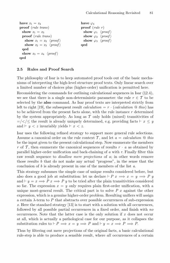
Calculational Reasoning Revisited 81
have x1 = x4
proof (rule trans)show x1 = x3
proof (rule trans)show x1 = x2 〈proof 〉show x2 = x3 〈proof 〉
qedshow x3 = x4 〈proof 〉
qed
have ϕ4
proof (rule r)show ϕ1 〈proof 〉show ϕ2 〈proof 〉show ϕ3 〈proof 〉
qed
2.5 Rules and Proof Search
The philosophy of Isar is to keep automated proof tools out of the basic mecha-nisms of interpreting the high-level structure proof texts. Only linear search overa limited number of choices plus (higher-order) unification is permitted here.Reconsidering the commands for outlining calculational sequences in Isar (§2.4),we see that there is a single non-deterministic parameter: the rule r ∈ T to beselected by the also command. As Isar proof texts are interpreted strictly fromleft to right [19], the subsequent result calculation = r · (calculation @ this) hasto be achieved from the present facts alone, with the rule instance r determinedby the system appropriately. As long as T only holds (mixed) transitivities of=/</≤ the result is already uniquely determined, e.g. providing facts � x ≤ yand � y < z invariably yields � x < z.
Isar uses the following refined strategy to support more general rule selections.Assume a canonical order on the rule context T , and let a = calculation @ thisbe the input given to the present calculational step. Now enumerate the membersr of T , then enumerate the canonical sequences of results r · a as obtained byparallel higher-order unification and back-chaining of a with r. Finally filter thisraw result sequence to disallow mere projections of a; in other words removethose results b that do not make any actual “progress”, in the sense that theconclusion of b is already present in one of the members of the list a.This strategy subsumes the simple case of unique results considered before, butalso does a good job at substitution: let us declare �P x =⇒ x = y =⇒ P yand � y = x =⇒ P x =⇒ P y to be tried after the plain transitivities consideredso far. The expression x = y only requires plain first-order unification, with aunique most-general result. The critical part is to solve P x against the otherexpression, which is a genuine higher-order problem. Resulting unifiers will assigna certain λ-term to P that abstracts over possible occurrences of sub-expressionx. Here the standard strategy [13] is to start with a solution with all occurrences,followed by all possible partial occurrences in a fixed order, and finish with nooccurrences. Note that the latter case is the only solution if x does not occurat all, which is actually a pathological case for our purpose, as it collapses thesubstitution rules to �P =⇒ x = y =⇒ P and � y = x =⇒ P =⇒ P.
Thus by filtering out mere projections of the original facts, a basic calculationalrule-step is able to produce a sensible result, where all occurrences of a certain
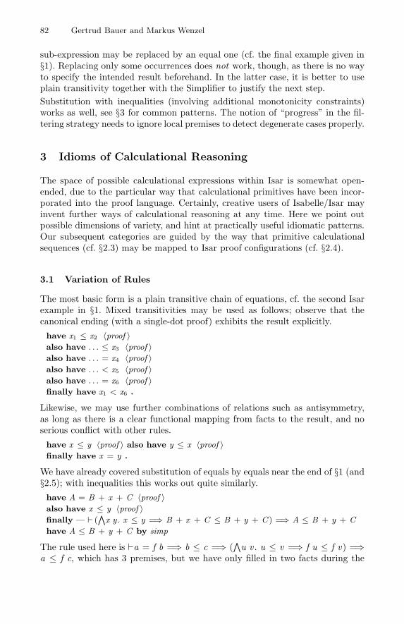
82 Gertrud Bauer and Markus Wenzel
sub-expression may be replaced by an equal one (cf. the final example given in§1). Replacing only some occurrences does not work, though, as there is no wayto specify the intended result beforehand. In the latter case, it is better to useplain transitivity together with the Simplifier to justify the next step.Substitution with inequalities (involving additional monotonicity constraints)works as well, see §3 for common patterns. The notion of “progress” in the fil-tering strategy needs to ignore local premises to detect degenerate cases properly.
3 Idioms of Calculational Reasoning
The space of possible calculational expressions within Isar is somewhat open-ended, due to the particular way that calculational primitives have been incor-porated into the proof language. Certainly, creative users of Isabelle/Isar mayinvent further ways of calculational reasoning at any time. Here we point outpossible dimensions of variety, and hint at practically useful idiomatic patterns.Our subsequent categories are guided by the way that primitive calculationalsequences (cf. §2.3) may be mapped to Isar proof configurations (cf. §2.4).
3.1 Variation of Rules
The most basic form is a plain transitive chain of equations, cf. the second Isarexample in §1. Mixed transitivities may be used as follows; observe that thecanonical ending (with a single-dot proof) exhibits the result explicitly.have x1 ≤ x2 〈proof 〉also have . . . ≤ x3 〈proof 〉also have . . . = x4 〈proof 〉also have . . . < x5 〈proof 〉also have . . . = x6 〈proof 〉finally have x1 < x6 .
Likewise, we may use further combinations of relations such as antisymmetry,as long as there is a clear functional mapping from facts to the result, and noserious conflict with other rules.
have x ≤ y 〈proof 〉 also have y ≤ x 〈proof 〉finally have x = y .
We have already covered substitution of equals by equals near the end of §1 (and§2.5); with inequalities this works out quite similarly.have A = B + x + C 〈proof 〉also have x ≤ y 〈proof 〉finally — (
∧x y . x ≤ y =⇒ B + x + C ≤ B + y + C ) =⇒ A ≤ B + y + C
have A ≤ B + y + C by simp
The rule used here is �a = f b =⇒ b ≤ c =⇒ (∧
u v . u ≤ v =⇒ f u ≤ f v) =⇒a ≤ f c, which has 3 premises, but we have only filled in two facts during the
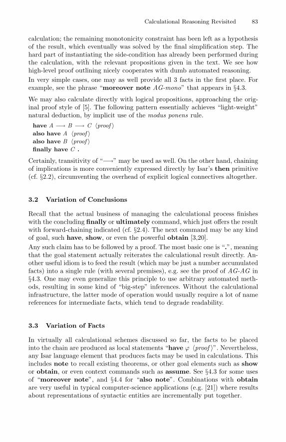
Calculational Reasoning Revisited 83
calculation; the remaining monotonicity constraint has been left as a hypothesisof the result, which eventually was solved by the final simplification step. Thehard part of instantiating the side-condition has already been performed duringthe calculation, with the relevant propositions given in the text. We see howhigh-level proof outlining nicely cooperates with dumb automated reasoning.In very simple cases, one may as well provide all 3 facts in the first place. Forexample, see the phrase “moreover note AG-mono” that appears in §4.3.We may also calculate directly with logical propositions, approaching the orig-inal proof style of [5]. The following pattern essentially achieves “light-weight”natural deduction, by implicit use of the modus ponens rule.
have A −→ B −→ C 〈proof 〉also have A 〈proof 〉also have B 〈proof 〉finally have C .
Certainly, transitivity of “−→” may be used as well. On the other hand, chainingof implications is more conveniently expressed directly by Isar’s then primitive(cf. §2.2), circumventing the overhead of explicit logical connectives altogether.
3.2 Variation of Conclusions
Recall that the actual business of managing the calculational process finisheswith the concluding finally or ultimately command, which just offers the resultwith forward-chaining indicated (cf. §2.4). The next command may be any kindof goal, such have, show, or even the powerful obtain [3,20].Any such claim has to be followed by a proof. The most basic one is “.”, meaningthat the goal statement actually reiterates the calculational result directly. An-other useful idiom is to feed the result (which may be just a number accumulatedfacts) into a single rule (with several premises), e.g. see the proof of AG-AG in§4.3. One may even generalize this principle to use arbitrary automated meth-ods, resulting in some kind of “big-step” inferences. Without the calculationalinfrastructure, the latter mode of operation would usually require a lot of namereferences for intermediate facts, which tend to degrade readability.
3.3 Variation of Facts
In virtually all calculational schemes discussed so far, the facts to be placedinto the chain are produced as local statements “have ϕ 〈proof 〉”. Nevertheless,any Isar language element that produces facts may be used in calculations. Thisincludes note to recall existing theorems, or other goal elements such as showor obtain, or even context commands such as assume. See §4.3 for some usesof “moreover note”, and §4.4 for “also note”. Combinations with obtainare very useful in typical computer-science applications (e.g. [21]) where resultsabout representations of syntactic entities are incrementally put together.
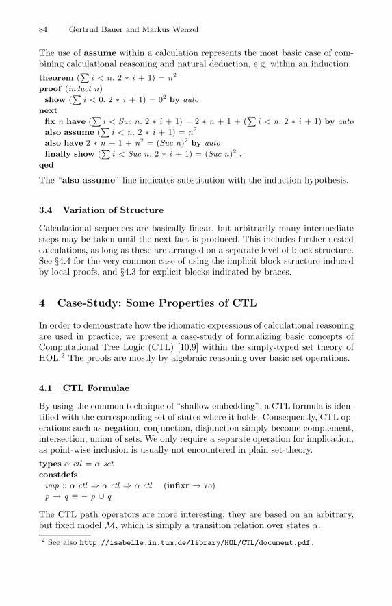
84 Gertrud Bauer and Markus Wenzel
The use of assume within a calculation represents the most basic case of com-bining calculational reasoning and natural deduction, e.g. within an induction.theorem (
∑i < n. 2 ∗ i + 1) = n2
proof (induct n)
show (∑
i < 0. 2 ∗ i + 1) = 02 by auto
next
fix n have (∑
i < Suc n. 2 ∗ i + 1) = 2 ∗ n + 1 + (∑
i < n. 2 ∗ i + 1) by auto
also assume (∑
i < n. 2 ∗ i + 1) = n2
also have 2 ∗ n + 1 + n2 = (Suc n)2 by auto
finally show (∑
i < Suc n. 2 ∗ i + 1) = (Suc n)2 .
qed
The “also assume” line indicates substitution with the induction hypothesis.
3.4 Variation of Structure
Calculational sequences are basically linear, but arbitrarily many intermediatesteps may be taken until the next fact is produced. This includes further nestedcalculations, as long as these are arranged on a separate level of block structure.See §4.4 for the very common case of using the implicit block structure inducedby local proofs, and §4.3 for explicit blocks indicated by braces.
4 Case-Study: Some Properties of CTL
In order to demonstrate how the idiomatic expressions of calculational reasoningare used in practice, we present a case-study of formalizing basic concepts ofComputational Tree Logic (CTL) [10,9] within the simply-typed set theory ofHOL.2 The proofs are mostly by algebraic reasoning over basic set operations.
4.1 CTL Formulae
By using the common technique of “shallow embedding”, a CTL formula is iden-tified with the corresponding set of states where it holds. Consequently, CTL op-erations such as negation, conjunction, disjunction simply become complement,intersection, union of sets. We only require a separate operation for implication,as point-wise inclusion is usually not encountered in plain set-theory.types α ctl = α set
constdefs
imp :: α ctl ⇒ α ctl ⇒ α ctl (infixr → 75)
p → q ≡ − p ∪ q
The CTL path operators are more interesting; they are based on an arbitrary,but fixed modelM, which is simply a transition relation over states α.2 See also http://isabelle.in.tum.de/library/HOL/CTL/document.pdf.
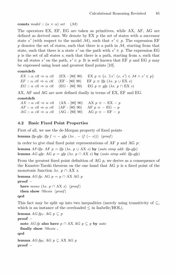
Calculational Reasoning Revisited 85
consts model :: (α × α) set (M)
The operators EX, EF, EG are taken as primitives, while AX, AF, AG aredefined as derived ones. We denote by EX p the set of states with a successorstate s ′ (with respect to the model M), such that s ′ ∈ p. The expression EFp denotes the set of states, such that there is a path in M, starting from thatstate, such that there is a state s ′ on the path with s ′ ∈ p. The expression EGp is the set of all states s, such that there is a path, starting from s, such thatfor all states s ′ on the path, s ′ ∈ p. It is well known that EF p and EG p maybe expressed using least and greatest fixed points [10].constdefs
EX :: α ctl ⇒ α ctl (EX - [80] 90) EX p ≡ {s. ∃ s ′. (s, s ′) ∈ M ∧ s ′ ∈ p}EF :: α ctl ⇒ α ctl (EF - [80] 90) EF p ≡ lfp (λs. p ∪ EX s)
EG :: α ctl ⇒ α ctl (EG - [80] 90) EG p ≡ gfp (λs. p ∩ EX s)
AX, AF and AG are now defined dually in terms of EX, EF and EG.constdefs
AX :: α ctl ⇒ α ctl (AX - [80] 90) AX p ≡ − EX − pAF :: α ctl ⇒ α ctl (AF - [80] 90) AF p ≡ − EG − pAG :: α ctl ⇒ α ctl (AG - [80] 90) AG p ≡ − EF − p
4.2 Basic Fixed Point Properties
First of all, we use the de-Morgan property of fixed pointslemma lfp-gfp: lfp f = − gfp (λs . − (f (− s))) 〈proof 〉in order to give dual fixed point representations of AF p and AG p:lemma AF-lfp: AF p = lfp (λs. p ∪ AX s) by (auto simp add : lfp-gfp)
lemma AG-gfp: AG p = gfp (λs. p ∩ AX s) by (auto simp add : lfp-gfp)
From the greatest fixed point definition of AG p, we derive as a consequence ofthe Knaster-Tarski theorem on the one hand that AG p is a fixed point of themonotonic function λs . p ∩ AX s.lemma AG-fp: AG p = p ∩ AX AG p
proof −have mono (λs. p ∩ AX s) 〈proof 〉then show ?thesis 〈proof 〉
qed
This fact may be split up into two inequalities (merely using transitivity of ⊆,which is an instance of the overloaded ≤ in Isabelle/HOL).lemma AG-fp1: AG p ⊆ p
proof −note AG-fp also have p ∩ AX AG p ⊆ p by auto
finally show ?thesis .
qed
lemma AG-fp2: AG p ⊆ AX AG p
proof −
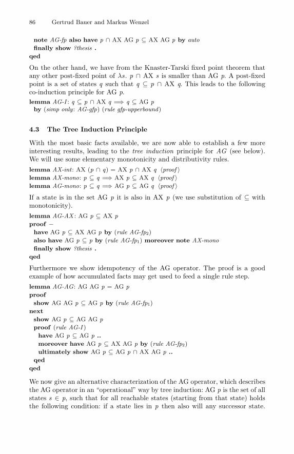
86 Gertrud Bauer and Markus Wenzel
note AG-fp also have p ∩ AX AG p ⊆ AX AG p by auto
finally show ?thesis .
qed
On the other hand, we have from the Knaster-Tarski fixed point theorem thatany other post-fixed point of λs . p ∩ AX s is smaller than AG p. A post-fixedpoint is a set of states q such that q ⊆ p ∩ AX q. This leads to the followingco-induction principle for AG p.lemma AG-I : q ⊆ p ∩ AX q =⇒ q ⊆ AG pby (simp only : AG-gfp) (rule gfp-upperbound)
4.3 The Tree Induction Principle
With the most basic facts available, we are now able to establish a few moreinteresting results, leading to the tree induction principle for AG (see below).We will use some elementary monotonicity and distributivity rules.lemma AX-int : AX (p ∩ q) = AX p ∩ AX q 〈proof 〉lemma AX-mono: p ⊆ q =⇒ AX p ⊆ AX q 〈proof 〉lemma AG-mono: p ⊆ q =⇒ AG p ⊆ AG q 〈proof 〉If a state is in the set AG p it is also in AX p (we use substitution of ⊆ withmonotonicity).lemma AG-AX : AG p ⊆ AX p
proof −have AG p ⊆ AX AG p by (rule AG-fp2)
also have AG p ⊆ p by (rule AG-fp1) moreover note AX-mono
finally show ?thesis .
qed
Furthermore we show idempotency of the AG operator. The proof is a goodexample of how accumulated facts may get used to feed a single rule step.lemma AG-AG: AG AG p = AG p
proof
show AG AG p ⊆ AG p by (rule AG-fp1)
next
show AG p ⊆ AG AG p
proof (rule AG-I )
have AG p ⊆ AG p ..
moreover have AG p ⊆ AX AG p by (rule AG-fp2)
ultimately show AG p ⊆ AG p ∩ AX AG p ..
qed
qed
We now give an alternative characterization of the AG operator, which describesthe AG operator in an “operational” way by tree induction: AG p is the set of allstates s ∈ p, such that for all reachable states (starting from that state) holdsthe following condition: if a state lies in p then also will any successor state.
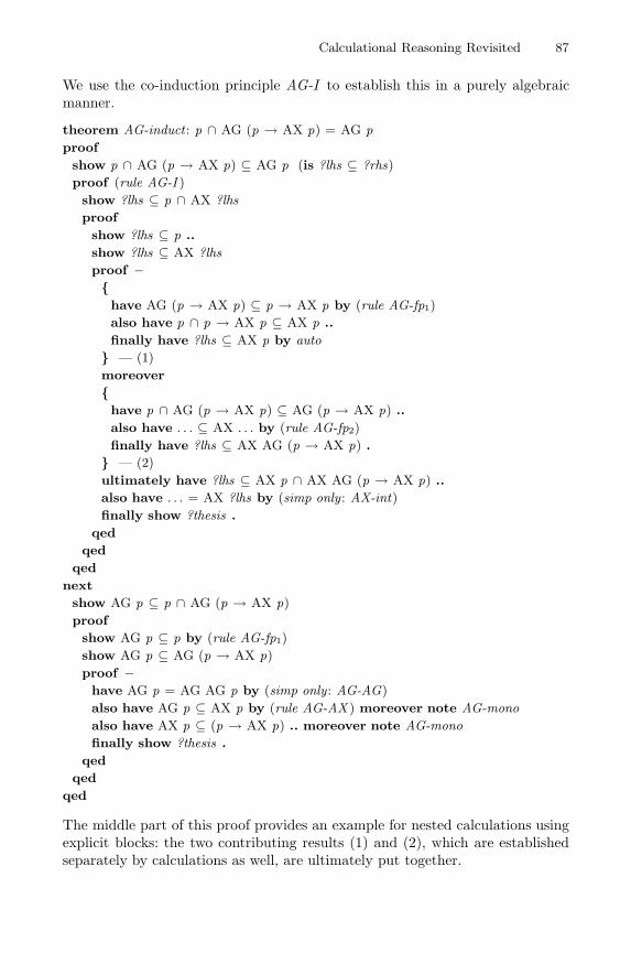
Calculational Reasoning Revisited 87
We use the co-induction principle AG-I to establish this in a purely algebraicmanner.
theorem AG-induct : p ∩ AG (p → AX p) = AG p
proof
show p ∩ AG (p → AX p) ⊆ AG p (is ?lhs ⊆ ?rhs)
proof (rule AG-I )
show ?lhs ⊆ p ∩ AX ?lhs
proof
show ?lhs ⊆ p ..
show ?lhs ⊆ AX ?lhs
proof −{have AG (p → AX p) ⊆ p → AX p by (rule AG-fp1)
also have p ∩ p → AX p ⊆ AX p ..
finally have ?lhs ⊆ AX p by auto
} — (1)
moreover
{have p ∩ AG (p → AX p) ⊆ AG (p → AX p) ..
also have . . . ⊆ AX . . . by (rule AG-fp2)
finally have ?lhs ⊆ AX AG (p → AX p) .
} — (2)
ultimately have ?lhs ⊆ AX p ∩ AX AG (p → AX p) ..
also have . . . = AX ?lhs by (simp only : AX-int)
finally show ?thesis .
qed
qed
qed
next
show AG p ⊆ p ∩ AG (p → AX p)
proof
show AG p ⊆ p by (rule AG-fp1)
show AG p ⊆ AG (p → AX p)
proof −have AG p = AG AG p by (simp only : AG-AG)
also have AG p ⊆ AX p by (rule AG-AX ) moreover note AG-mono
also have AX p ⊆ (p → AX p) .. moreover note AG-mono
finally show ?thesis .
qed
qed
qed
The middle part of this proof provides an example for nested calculations usingexplicit blocks: the two contributing results (1) and (2), which are establishedseparately by calculations as well, are ultimately put together.
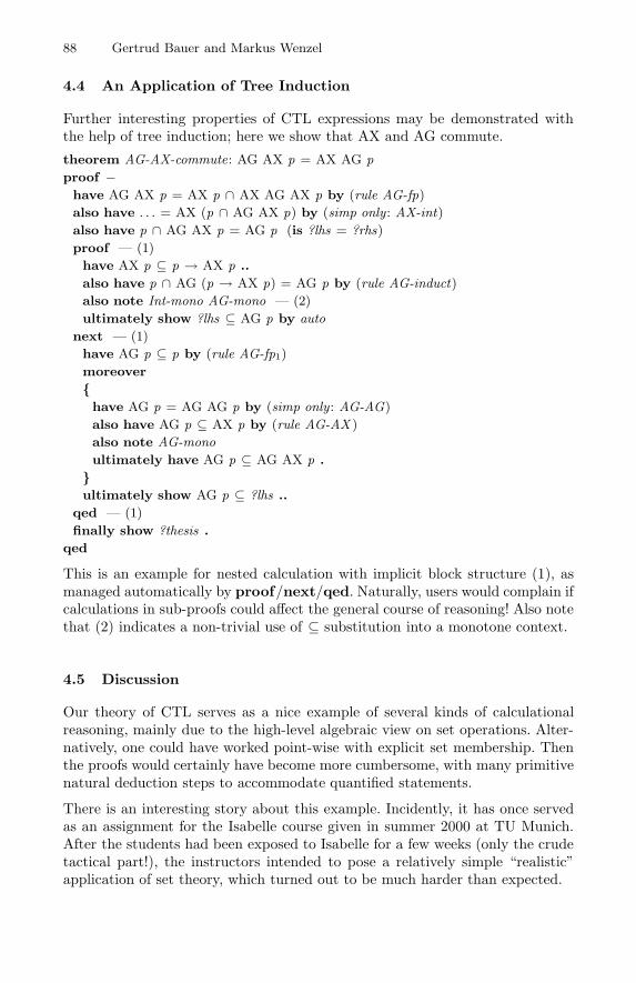
88 Gertrud Bauer and Markus Wenzel
4.4 An Application of Tree Induction
Further interesting properties of CTL expressions may be demonstrated withthe help of tree induction; here we show that AX and AG commute.
theorem AG-AX-commute: AG AX p = AX AG p
proof −have AG AX p = AX p ∩ AX AG AX p by (rule AG-fp)
also have . . . = AX (p ∩ AG AX p) by (simp only : AX-int)
also have p ∩ AG AX p = AG p (is ?lhs = ?rhs)
proof — (1)
have AX p ⊆ p → AX p ..
also have p ∩ AG (p → AX p) = AG p by (rule AG-induct)
also note Int-mono AG-mono — (2)
ultimately show ?lhs ⊆ AG p by auto
next — (1)
have AG p ⊆ p by (rule AG-fp1)
moreover
{have AG p = AG AG p by (simp only : AG-AG)
also have AG p ⊆ AX p by (rule AG-AX )
also note AG-mono
ultimately have AG p ⊆ AG AX p .
}ultimately show AG p ⊆ ?lhs ..
qed — (1)
finally show ?thesis .
qed
This is an example for nested calculation with implicit block structure (1), asmanaged automatically by proof/next/qed. Naturally, users would complain ifcalculations in sub-proofs could affect the general course of reasoning! Also notethat (2) indicates a non-trivial use of ⊆ substitution into a monotone context.
4.5 Discussion
Our theory of CTL serves as a nice example of several kinds of calculationalreasoning, mainly due to the high-level algebraic view on set operations. Alter-natively, one could have worked point-wise with explicit set membership. Thenthe proofs would certainly have become more cumbersome, with many primitivenatural deduction steps to accommodate quantified statements.
There is an interesting story about this example. Incidently, it has once servedas an assignment for the Isabelle course given in summer 2000 at TU Munich.After the students had been exposed to Isabelle for a few weeks (only the crudetactical part!), the instructors intended to pose a relatively simple “realistic”application of set theory, which turned out to be much harder than expected.
Calculational Reasoning Revisited 89
The reason was that on the one hand, the instructors simply started off by de-veloping the theory interactively in Isabelle/Isar, using its proper proof languagebasically to “think aloud formally”. This was a relatively leisurely experience, asit involves only a number of algebraic manipulation, as we have presented here.On the other hand, the students only knew traditional tactic scripts, with thatstrong bias towards hairy natural deduction operations performed in backwardsstyle. This posed a real problem to them; some students would even proclaimthat the assignment was impossible to finish with their present knowledge.In retrospect, it is understandable that rephrasing the kind of algebraic reasoningwe have seen here into tactic scripts is quite cumbersome, even for the expert.
5 Conclusion and Related Work
We have seen that calculational reasoning in Isabelle/Isar provides a viableconcept for arranging a large variety of algebraic proof techniques in a well-structured manner. While requiring only minimal conservative additions to thebasic Isar proof engine, we have been able to achieve a large space of useful pat-terns of calculational reasoning, including mixed transitivity rules, substitutionof equals-by-equals, and even substitution by greater (or equal) sub-expressions.The underlying mechanisms of Isabelle/Isar do not need any advanced proofsearch, apart from plain (higher-order) unification with a simple filtering scheme.
Interestingly, traditional tactic-based interactive proof systems such as (classic)Isabelle, HOL, Coq, PVS etc. lack support for calculational reasoning altogether.This has been addressed several times in the past. Simons proposes tools to sup-port calculational reasoning within tactical proof scripts [14]. Grundy providesan even more general transformational infrastructure for “window inference” [7].Harrison’s “Mizar mode for HOL” simulates a number of concepts of declara-tive theorem proving on top of the tactic-based hol-light system [8], includingcalculational reasoning for mixed transitivity rules.Concerning the class of theorem proving environments for human-readable proofs,its canonical representative Mizar [17,12] supports a fixed format for iterativeequations, with implicit application of both transitivity and general substitutionrules. Syme’s DECLARE system for declarative theorem proving [15,16] doesnot address calculations at all. Zammit outlines a generalized version of Mizar-style calculations for SPL [23], but observes that these have not been requiredfor the examples at hand, so it has not been implemented.
For users of Isabelle/Isar, calculational reasoning has become a useful tool foreveryday applications — not just the typical “mathematical” ones [3], but also(abstract) system verification tasks [21]. Calculations fit indeed very well intothe general high-level natural deduction framework of Isar, so we may say thatcalculational reasoning [5] and natural deduction [6] have been finally reconciled.
90 Gertrud Bauer and Markus Wenzel
References
1. R.J. Back, J. Grundy, and J. von Wright. Structured calculational proof. FormalAspects of Computing, 9, 1997.
2. R.J. Back and J. von Wright. Structured derivations: A method for doing high-school mathematics carefully. Technical report, Turku Centre for C.S., 1999.
3. G. Bauer and M. Wenzel. Computer-assisted mathematics at work — the Hahn-Banach theorem in Isabelle/Isar. In T. Coquand, P. Dybjer, B. Nordstrom, andJ. Smith, editors, Types for Proofs and Programs: TYPES’99, LNCS, 2000.
4. Y. Bertot, G. Dowek, A. Hirschowitz, C. Paulin, and L. Thery, editors. TheoremProving in Higher Order Logics: TPHOLs ’99, LNCS 1690, 1999.
5. E.W. Dijkstra and C.S. Scholten. Predicate Calculus and Program Semantics.Texts and monographs in computer science. Springer, 1990.
6. G. Gentzen. Untersuchungen uber das logische Schließen. MathematischeZeitschrift, 1935.
7. J. Grundy. Window inference in the HOL system. In M. Archer, J. J. Joyce, K. N.Levitt, and P. J. Windley, editors, Proceedings of the International Workshop onHOL. ACM SIGDA, IEEE Computer Society Press, 1991.
8. J. Harrison. A Mizar mode for HOL. In J. Wright, J. Grundy, and J. Harrison,editors, Theorem Proving in Higher Order Logics: TPHOLs ’96, LNCS 1125, 1997.
9. K. McMillan. Lecture notes on verification of digital and hybrid systems. NATOsummer school,http://www-cad.eecs.berkeley.edu/~kenmcmil/tutorial/toc.html.
10. K. McMillan. Symbolic Model Checking: an approach to the state explosion problem.PhD thesis, Carnegie Mellon University, 1992.
11. Mizar mathematical library. http://www.mizar.org/library/ .12. M. Muzalewski. An Outline of PC Mizar. Fondation of Logic, Mathematics and
Informatics — Mizar Users Group, 1993.13. L.C. Paulson. Isabelle: A Generic Theorem Prover. LNCS 828. 1994.14. M. Simons. Proof presentation for Isabelle. In E. L. Gunter and A. Felty, editors,
Theorem Proving in Higher Order Logics: TPHOLs ’97, LNCS 1275, 1997.15. D. Syme. DECLARE: A prototype declarative proof system for higher order logic.
Technical Report 416, University of Cambridge Computer Laboratory, 1997.16. D. Syme. Three tactic theorem proving. In Bertot et al. [4].17. A. Trybulec. Some features of the Mizar language. Presented at a workshop in
Turin, Italy, 1993.18. R. Verhoeven and R. Backhouse. Interfacing program construction and verifica-
tion. In J. Wing and J. Woodcock, editors, FM99: The World Congress in FormalMethods, volume 1708 and 1709 of LNCS, 1999.
19. M. Wenzel. Isar — a generic interpretative approach to readable formal proofdocuments. In Bertot et al. [4].
20. M. Wenzel. The Isabelle/Isar Reference Manual, 2000. Part of the Isabelle distri-bution, http://isabelle.in.tum.de/doc/isar-ref.pdf.
21. M. Wenzel. Some aspects of Unix file-system security. Isabelle/Isar proof docu-ment, http://isabelle.in.tum.de/library/HOL/Unix/document.pdf , 2001.
22. F. Wiedijk. Mizar: An impression. Unpublished paper, 1999.http://www.cs.kun.nl/~freek/mizar/mizarintro.ps.gz.
23. V. Zammit. On the implementation of an extensible declarative proof language.In Bertot et al. [4].
Mechanical Proofs about aNon-repudiation Protocol
Giampaolo Bella1,2 and Lawrence C. Paulson1
1 Computer Laboratory, University of CambridgePembroke Street, Cambridge CB2 3QG (UK)
{gb221,lcp}@cl.cam.ac.uk2 Dipartimento di Matematica e Informatica, Universita di Catania
Viale A. Doria 6, I-95125 Catania (Italy)[email protected]
Abstract. A non-repudiation protocol of Zhou and Gollmann [18] hasbeen mechanically verified. A non-repudiation protocol gives each partyevidence that the other party indeed participated, evidence sufficient topresent to a judge in the event of a dispute. We use the theorem-proverIsabelle [10] and model the security protocol by an inductive definition,as described elsewhere [1,12]. We prove the protocol goals of validity ofevidence and of fairness using simple strategies. A typical theorem statesthat a given piece of evidence can only exist if a specific event took placeinvolving the other party.
1 Introduction
A wide variety of techniques are available for verifying cryptographic proto-cols [3,8,12,14]. Past work has focused largely on two security goals: confidential-ity (who can read the message?) and authenticity (who originated the message?).One direction for further research is to attempt proofs of more esoteric securitygoals. Traditional protocols help a pair of honest agents to communicate in thepresence of an attacker, but in some situations agents may act unfairly andabandon protocol sessions before these terminate. The present work concernsnon-repudiation, which seeks to prevent a party from abandoning an agreement.Non-repudiation would provide us with a reliable means of making contractsover a network.
The primary goal of a non-repudiation protocol is validity of evidence. Itmust provide each peer with convincing evidence of the other’s participation ina protocol session. If one peer falsely denies participating in a session, then theother peer can present his evidence to a judge, who can safely conclude that theother peer did participate. Crucially, the judge does not have to monitor thenetwork traffic, but can make his judgement on the basis of the evidence alone.Some of the evidence is usually referred to as non-repudiation of origin, other asnon-repudiation of receipt. The initiator of a session typically seeks evidence ofthe first form, and the responder typically looks for evidence of the second form.
An additional goal of some non-repudiation protocols is fairness : at no timeshould one peer hold more evidence than the other does. Although fairness is not
R.J. Boulton and P.B. Jackson (Eds.): TPHOLs 2001, LNCS 2152, pp. 91–104, 2001.c© Springer-Verlag Berlin Heidelberg 2001
92 Giampaolo Bella and Lawrence C. Paulson
indispensable in all situations, it may be needed for certain e-commerce transac-tions. For example, if a client C holds evidence that a merchant M received C’srequest for goods, fairness means that C cannot deny sending the request: Mholds the corresponding evidence. Similarly, if M holds evidence that C receivedthe goods, fairness means that C holds evidence that it was M who sent them.In the latter case for example, M could claim the payment for the goods but,should the goods be unsatisfactory, C could demand a refund. Resolving suchdisputes becomes a matter of cyberlaw; the judge referred to above could be areal judge sitting in a traditional courtroom.
A number of protocols have been designed to achieve non-repudiation, butthey are not yet deployed [7,9,18]. Verifying them formally [16,17] might increasetheir credibility. Proving non-repudiation was one of the the first author’s reasonsfor extending the Inductive Approach to verifying cryptographic protocols [12]with message reception [1] and agents’ knowledge [2]. This paper shows that wehave now achieved that purpose through the development of simple strategiesto prove validity of evidence and fairness. We were pleased to observe that thesestrategies differ little from those for proving authentication goals [5,6], and thatthe approach required no extensions. Our proofs were conducted on a popularnon-repudiation protocol due to Zhou and Gollmann [18] using the second au-thor’s original modelling of agents. An unlimited population of agents can onlysend messages of the form that the protocol prescribes but can quit a protocolsession at any time; the spy can send messages of arbitrary form.
This paper is organised as follows. A brief overview of the Inductive Approach(§2) precedes the description of our strategies to proving the non-repudiationgoals (§3). The Zhou-Gollmann protocol is described (§4), modelled (§5) andverified without the spy (§6). Then, the verification is repeated in the presenceof the spy (§7). Finally, the related work is discussed (§8), and some conclusionsare given (§9).
2 The Inductive Approach
The Inductive Approach has been used successfully to analyse Local Area Net-work protocols [5], Internet protocols [13], e-commerce protocols [4] and smartcard protocols [3]. Here, we recall only its main concepts, but a full treatmentmay be found elsewhere [1,12].
The approach draws from the observation that the goals of security protocolsare invariants of the protocol execution, so proving the goals means showing thatthey are preserved by all protocol steps. The inductive model of a protocol is theset of all possible histories (traces) of the network that the protocol executionmay produce. There is no limit to the number of agents who may participate.They may also interleave sessions at will.
A trace is a list of network events of the following form:
– Says AB X , indicating that agent A sends a message X to agent B;– Gets AX , indicating that A receives X ;– NotesAX , indicating that A notes down X for future use.
Mechanical Proofs about a Non-repudiation Protocol 93
The last event can model an agent’s storing a message component or the resultof a computation [13].
There are traces in which some events have not taken place although thenecessary preconditions are met. Therefore, the protocol model does not forceevents to happen; messages may be sent but may not be received, and agentsmay abandon a protocol execution. This captures the unreliability of the com-munications, and a degree of unfairness of agents. However, the only agent whocan build messages other than those prescribed by the protocol is the spy. Also,messages cannot alter during transmission.
Given a trace evs , we model the knowledge that agent A acquires during thenetwork history denoted by evs as knowsA evs [2]. This is the set of messagesthat A sent or received or noted on evs . In particular, knowsSpy evs containsthe private signature keys of a set bad of agents and all messages that were sentor received by anyone or noted by bad agents on evs .
Three operators can be applied to a message set H :
– parts, yielding all components of messages in H , except encryption keys;– analz, yielding those components of messages in H whose encryption key is
recursively available;– synth, yielding all messages constructed by concatenation or encryption from
messages recursively obtained from H .
The special set synth(analz(knows Spy evs)) contains all messages that thespy can synthesise using the components obtained from the analysis of the trafficwith the help of bad agents’ private keys. The spy can send in the traffic anymessage derived from that set (§7).
3 Strategies to Proving Non-repudiation
How can a judge who is off-line evaluate the non-repudiation evidence presentedby a peer? The judge could perhaps make a decision given a full log of thenetwork traffic, but that would not be practical. Our proofs can help the judgeby establishing that a given piece of evidence guarantees that certain criticalevents occurred. Our proofs are subject to human error (for instance, our modelcould be too abstract), but they add credibility to the protocol. The judge weighsup these points in making his decision; a Guilty verdict requires the absence ofa reasonable doubt.
Each trace of the protocol model is in fact a full log of a network history. So,scanning the trace tells what events have occurred. These observations inspireour strategy to proving validity of evidence, which must be applied for each pieceof evidence that an agent presents to the judge. If A presents evidence X , thencertainly A holds X ; formally: X ∈ knowsA evs for some trace evs . Our strategyrests on an assumption of that form, and develops through two main types ofresult:
1. If A holds some evidence X , then A got the evidence from the network,perhaps from the spy.
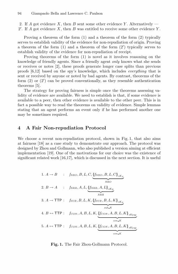
94 Giampaolo Bella and Lawrence C. Paulson
2. If A got evidence X , then B sent some other evidence Y . Alternatively —2′. If A got evidence X , then B was entitled to receive some other evidence Y .
Proving a theorem of the form (1) and a theorem of the form (2) typicallyserves to establish validity of the evidence for non-repudiation of origin. Provinga theorem of the form (1) and a theorem of the form (2′) typically serves toestablish validity of the evidence for non-repudiation of receipt.
Proving theorems of the form (1) is novel as it involves reasoning on theknowledge of friendly agents. Since a friendly agent only knows what she sendsor receives or notes [2], these proofs generate longer case splits than previousproofs [6,12] based on the spy’s knowledge, which includes everything that issent or received by anyone or noted by bad agents. By contrast, theorems of theform (2) or (2′) can be proved conventionally, as they resemble authenticationtheorems [5].
The strategy for proving fairness is simple once the theorems assessing va-lidity of evidence are available. We need to establish is that, if some evidence isavailable to a peer, then other evidence is available to the other peer. This is infact a possible way to read the theorems on validity of evidence. Simple lemmasstating that an agent performs an event only if he has performed another onemay be sometimes required.
4 A Fair Non-repudiation Protocol
We choose a recent non-repudiation protocol, shown in Fig. 1, that also aimsat fairness [18] as a case study to demonstrate our approach. The protocol wasdesigned by Zhou and Gollmann, who also published a version aiming at efficientimplementation [19]. One of the motivations for our choice was the existence ofsignificant related work [16,17], which is discussed in the next section. It is useful
1. A→ B : fNRO , B, L, C, {|fNRO , B, L, C|}sKA︸ ︷︷ ︸NRO
2. B → A : fNRR, A, L, {|fNRR, A, L|}sKB︸ ︷︷ ︸NRR
3. A→ TTP : fSUB , B, L, K, {|fSUB , B, L, K|}sKA︸ ︷︷ ︸sub K
4. B ↔ TTP : fCON , A, B,L, K, {|fCON , A, B, L, K|}sKTTP︸ ︷︷ ︸con K
5. A↔ TTP : fCON , A, B,L, K, {|fCON , A, B, L, K|}sKTTP︸ ︷︷ ︸con K
Fig. 1. The Fair Zhou-Gollmann Protocol.
Mechanical Proofs about a Non-repudiation Protocol 95
to outline the syntax we use:
– A is the initiator of a protocol session with B;– B is the responder of the session initiated by A;– TTP is the trusted third party;– M is the message that A wants to transmit to B;– K is the key that A chooses to transmit M ;– C is M encrypted with K (the C refers to A’s Commitment to B);– L is a unique label identifying the session between A and B;– f� are the non-repudiation flags;– sKX is the private signature key of agent X (no syntax is needed for the
public verification key of X);– {|m|}sKX
is the signature of message m by key sKX .
The protocol intends to transmit a message M from A to B, giving A ev-idence for non-repudiation of receipt, giving B evidence for non-repudiation oforigin, and ensuring fairness. The first protocol step prescribes that A pick acryptographic key K and a random label L. Then, A uses symmetric cryptogra-phy to build C out of M and K, signs {|fNRO , B, L, C|} and sends the result to Balong with the unsigned message, which is in general needed for signature verifi-cation. Note that A sends M encrypted, so B will not be able to obtain M untilhe gets K. Upon reception of the first message, B verifies A’s signature, signs{|fNRR, A, L|} and sends the result to A. Upon reception of the second message,A lodges K with TTP by sending her signature on {|fSUB , B, L, K|}.
Once TTP has successfully verified A’s signature on the received message,TTP signs {|fCON , A, B, L, K|} and makes it available in its public directory.This message confirms that the key K concerns the session between A and Bthat is identified by label L. The last two steps, which are interchangeable, seethe peers ftp get the message available from TTP. The protocol assumes thatnobody can interfere with an ftp get operation, but we will relax this assumptionbelow (§7).
Zhou and Gollmann [18] observe that, even if the peers do not want to playfair, they must complete a session in order to get sufficient evidence to winany disputes with each other. Let us informally analyse how to resolve disputes.From B’s standpoint, it appears that obtaining con K signifies that A submittedK, bound to label L, to TTP; obtaining NRO should signify that A sent Cas a commitment bound to label L. In consequence, message M , obtained bydecrypting C with K, should have originated with A. From A’s standpoint, asimilar reasoning seems feasible. If A holds con K, this should guarantee thatA lodged K and L with TTP, and so B should be able to get it via ftp. IfA also holds NRR, it should be the case that B accepted commitment C. Inconsequence, B would be able to obtain M .
This reasoning might resemble that of a judge who is provided with evidenceNRO, con K, M , C, K, L by agent B, or with a similar evidence (but NRR ratherthan NRO) by agent A. It is not trivial to verify such reasoning for all possiblenetwork histories. The communication means is unreliable, and the protocol isexecuted by an unlimited number of agents, each entitled to interleave or quitsessions at will.
96 Giampaolo Bella and Lawrence C. Paulson
5 Modelling a Fair Non-repudiation Protocol
We build our protocol model on the Isabelle theory Public [11] for cryptographicprotocols based on asymmetric encryption. The theory models three kinds ofnetwork agents: a spy, whom we discuss later (§7), a trusted server, which isrenamed as TTP here, and an unlimited population of legitimate agents. Eachagent X is endowed with a key pair. His private signature key, priKX , he keepssecret; his public verification key, pubKX , is known to all. The theory alsoprovides a primitive for encryption, Crypt, which we use where the protocolrequires a digital signature.
The protocol model is the set of traces zg, whose inductive definition is inFig. 2. A rule for the base of the induction, stating that the empty trace belongsto zg, is omitted from the figure. Rules ZG1, ZG2 and ZG3 respectively modelthe first three steps of the protocol. Note that agent A chooses a fresh noncein rule ZG1 to initiate the protocol with B. Recall that A runs the protocolbecause she wants to transmit some message M to B. All these messages andthe ciphertexts obtained from them by any key constitute the set targetmsgs.We reasonably assume that this set contains none of the other messages (eitheratomic or compound) exchanged by the protocol. Also, A is free to choose anykey to encrypt M , even an old one — we merely assume that she cannot pickprivate signature keys.
We highlight the important certificates by defining them in the premises, us-ing equations; we use the names so defined in the conclusions. When a certificateis defined in the premises of a rule, then the rule only applies for a certificate ofthe specified form: informally, the agent verifies it. For example, B must checkthat NRO in rule ZG2 is signed by A in order to learn the sender of the messagejust received and address NRR to her.
By contrast, A does not need to check that NRR in rule ZG3 is signed by Bbecause NRR is associated to label L, which A knows to be associated with B.Clearly, the check becomes mandatory in the presence of the spy, who can ac-tively intercept and fake the messages that are in the traffic (§7).
Rule TTP prepare ftp models TTP’s preparation of the key confirmationcon K. Note that TTP verifies the signature on sub K to learn the identitiesof the peers of K. All the components needed to verify that signature are avail-able. The installation of con K in TTP’s public directory can be modelled by aNotes event.
Rules A ftp and B ftp model the peers’ retrieval of con K. The two rules arenot forced to fire simultaneously, since each peer decides independently whetherto terminate the protocol. Rather than introducing a new event to express theftp get operation, we again adopt Notes. Using a Gets event instead would violatethe conventions of the message reception model: each Gets event must follow amatching Says event, as established by rule Reception.
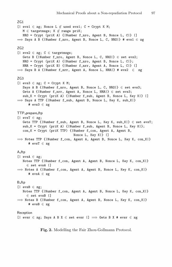
Mechanical Proofs about a Non-repudiation Protocol 97
ZG1
[| evs1 ∈ zg; Nonce L �∈ used evs1; C = Crypt K M;
M ∈ targetmsgs; K �∈ range priK;
NRO = Crypt (priK A) {|Number f_nro, Agent B, Nonce L, C|} |]
=⇒ Says A B {|Number f_nro, Agent B, Nonce L, C, NRO|} # evs1 ∈ zg
ZG2
[| evs2 ∈ zg; C ∈ targetmsgs;
Gets B {|Number f_nro, Agent B, Nonce L, C, NRO|} ∈ set evs2;
NRO = Crypt (priK A) {|Number f_nro, Agent B, Nonce L, C|};
NRR = Crypt (priK B) {|Number f_nrr, Agent A, Nonce L, C|} |]
=⇒ Says B A {|Number f_nrr, Agent A, Nonce L, NRR|} # evs2 ∈ zg
ZG3
[| evs3 ∈ zg; C = Crypt K M;
Says A B {|Number f_nro, Agent B, Nonce L, C, NRO|} ∈ set evs3;
Gets A {|Number f_nrr, Agent A, Nonce L, NRR|} ∈ set evs3;
sub_K = Crypt (priK A) {|Number f_sub, Agent B, Nonce L, Key K|} |]
=⇒ Says A TTP {|Number f_sub, Agent B, Nonce L, Key K, sub_K|}
# evs3 ∈ zg
TTP prepare ftp
[| evsT ∈ zg;
Gets TTP {|Number f_sub, Agent B, Nonce L, Key K, sub_K|} ∈ set evsT;
sub_K = Crypt (priK A) {|Number f_sub, Agent B, Nonce L, Key K|};
con_K = Crypt (priK TTP) {|Number f_con, Agent A, Agent B,
Nonce L, Key K|} |]
=⇒ Notes TTP {|Number f_con, Agent A, Agent B, Nonce L, Key K, con_K|}
# evsT ∈ zg
A ftp
[| evsA ∈ zg;
Notes TTP {|Number f_con, Agent A, Agent B, Nonce L, Key K, con_K|}
∈ set evsA |]
=⇒ Notes A {|Number f_con, Agent A, Agent B, Nonce L, Key K, con_K|}
# evsA ∈ zg
B ftp
[| evsB ∈ zg;
Notes TTP {|Number f_con, Agent A, Agent B, Nonce L, Key K, con_K|}
∈ set evsB |]
=⇒ Notes B {|Number f_con, Agent A, Agent B, Nonce L, Key K, con_K|}
# evsB ∈ zg
Reception
[| evsr ∈ zg; Says A B X ∈ set evsr |] =⇒ Gets B X # evsr ∈ zg
Fig. 2. Modelling the Fair Zhou-Gollmann Protocol.
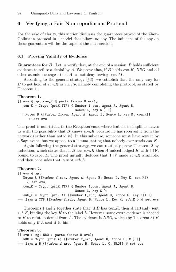
98 Giampaolo Bella and Lawrence C. Paulson
6 Verifying a Fair Non-repudiation Protocol
For the sake of clarity, this section discusses the guarantees proved of the Zhou-Gollmann protocol in a model that allows no spy. The influence of the spy onthese guarantees will be the topic of the next section.
6.1 Proving Validity of Evidence
Guarantees for B. Let us verify that, at the end of a session, B holds sufficientevidence to refute a denial by A. We prove that, if B holds con K, NRO and allother atomic messages, then A cannot deny having sent M .
According to the general strategy (§3), we establish that the only way forB to get hold of con K is via ftp, namely completing the protocol, as stated byTheorem 1.
Theorem 1.[| evs ∈ zg; con_K ∈ parts (knows B evs);
con_K = Crypt (priK TTP) {|Number f_con, Agent A, Agent B,
Nonce L, Key K|} |]
=⇒ Notes B {|Number f_con, Agent A, Agent B, Nonce L, Key K, con_K|}
∈ set evs
The proof is non-trivial in the Reception case, where Isabelle’s simplifier leavesus with the possibility that B knows con K because he has received it from thenetwork (rather than noted it). In this sub-case, someone must have sent it bya Says event, but we appeal to a lemma stating that nobody ever sends con K.
Again following the general strategy, we can routinely prove Theorem 2 byinduction, which states that if B has con K then A indeed lodged K with TTP,bound to label L. The proof initially deduces that TTP made con K available,and then concludes that A sent sub K.
Theorem 2.[| evs ∈ zg;
Notes B {|Number f_con, Agent A, Agent B, Nonce L, Key K, con_K|}
∈ set evs;
con_K = Crypt (priK TTP) {|Number f_con, Agent A, Agent B,
Nonce L, Key K|};
sub_K = Crypt (priK A) {|Number f_sub, Agent B, Nonce L, Key K|} |]
=⇒ Says A TTP {|Number f_sub, Agent B, Nonce L, Key K, sub_K|} ∈ set evs
Theorems 1 and 2 together state that, if B has con K, then A certainly sentsub K, binding the key K to the label L. However, some extra evidence is neededto B to refute a denial from A. The evidence is NRO, which (by Theorem 3) Bholds only if A sent it to him.
Theorem 3.[| evs ∈ zg; NRO ∈ parts (knows B evs);
NRO = Crypt (priK A) {|Number f_nro, Agent B, Nonce L, C|} |]
=⇒ Says A B {|Number f_nro, Agent B, Nonce L, C, NRO|} ∈ set evs

Mechanical Proofs about a Non-repudiation Protocol 99
Proving this theorem requires a lemma concluding that B could only receiveNRO inside the first message of the protocol, namely that the event
Gets B {|Number f nro, Agent B, NonceL, C,NRO|} (1)
occurred. In the Reception case, the simplifier tries to establish whether B mightlearn NRO by receiving a message of any form, but another lemma states thatthis is impossible. Event (1) implies that NRO is in the network traffic, andthen an authenticity theorem derives that it certainly originated with A, thusconcluding the proof. Theorem 3 states that a judge may safely conclude fromB’s presenting NRO that A sent it, binding the ciphertext C to the label L.
These theorems show that C is bound to the key K via the label L. Hence,if B presents NRO, con K, C, L and K to a judge, then the judge can concludethat A sent B the message M that is obtained decrypting C by K.
Guarantees for A. Analogous theorems justify A’s evidence that B receivedthe plaintext, M . In particular, Theorem 1 can be proved analogously for A,stating that, when con K is known to A, then A certainly noted it. On thisassumption, we easily prove that TTP made con K publicly available. Combiningthese two results, we get Theorem 4.
Theorem 4.[| evs ∈ zg; con_K ∈ parts (knows A evs);
con_K = Crypt (priK TTP) {|Number f_con, Agent A, Agent B,
Nonce L, Key K|};
=⇒ Notes TTP {|Number f_con, Agent A, Agent B, Nonce L, Key K, con_K|}
∈ set evs
Following this theorem, when A presents con K to a judge, she also provesthat she has bound the key K to L via TTP. Theorem 5 also states that, ifA has NRR, then B certainly received NRO confirming that A associated theciphertext C to the label L.
Theorem 5.[| evs ∈ zg; NRR ∈ parts (knows A evs);
NRR = Crypt (priK B) {|Number f_nrr, Agent A, Nonce L, C|};
NRO = Crypt (priK A) {|Number f_nro, Agent B, Nonce L, C|} |]
=⇒ Gets B {|Number f_nro, Agent B, Nonce L, C, NRO|} ∈ set evs
The proof resembles that of Theorem 3 to derive that B sent NRR inside aninstance of message 2. This, in turn, requires an appeal to an authenticity theo-rem: once NRR is in the traffic, then it certainly originated with B. A subsidiarylemma stating that B only sends NRR upon reception of NRO concludes.
Theorems 4 and 5 guarantee to a judge that, if A presents NRR, con K, C, Land K, then B can decrypt C using the key K, which was available with con Kvia ftp. It is up to B to get con K, so this may appear a weaker guarantee thanthe corresponding one for B. However, the protocol authors observe that B isinterested in getting con K in order to win a dispute over A, as confirmed byTheorems 1 and 2.
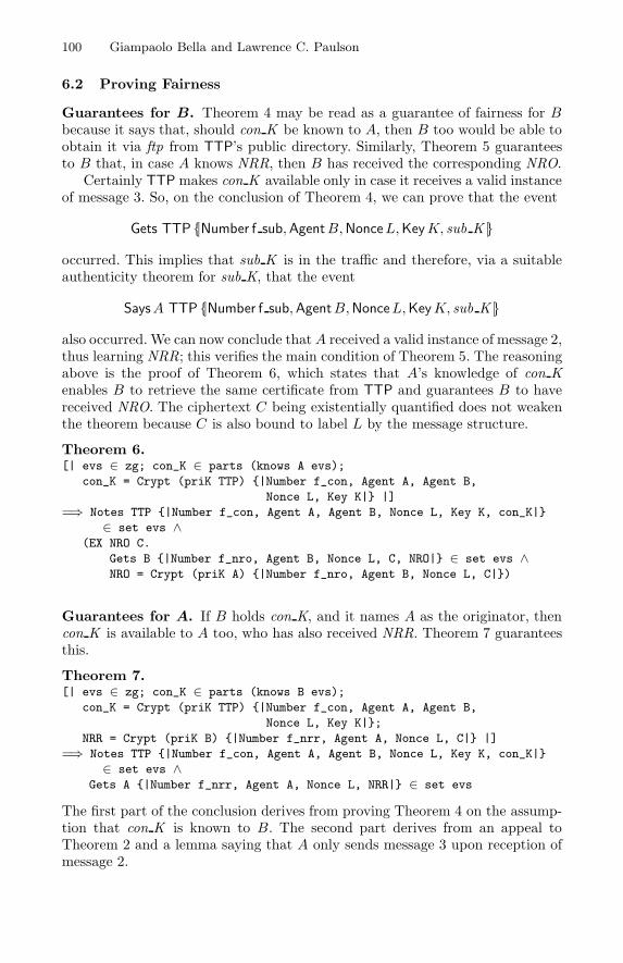
100 Giampaolo Bella and Lawrence C. Paulson
6.2 Proving Fairness
Guarantees for B. Theorem 4 may be read as a guarantee of fairness for Bbecause it says that, should con K be known to A, then B too would be able toobtain it via ftp from TTP’s public directory. Similarly, Theorem 5 guaranteesto B that, in case A knows NRR, then B has received the corresponding NRO.
Certainly TTP makes con K available only in case it receives a valid instanceof message 3. So, on the conclusion of Theorem 4, we can prove that the event
Gets TTP {|Number f sub, AgentB, NonceL, KeyK, sub K |}
occurred. This implies that sub K is in the traffic and therefore, via a suitableauthenticity theorem for sub K, that the event
SaysA TTP {|Number f sub, AgentB, NonceL, KeyK, sub K |}also occurred. We can now conclude that A received a valid instance of message 2,thus learning NRR; this verifies the main condition of Theorem 5. The reasoningabove is the proof of Theorem 6, which states that A’s knowledge of con Kenables B to retrieve the same certificate from TTP and guarantees B to havereceived NRO. The ciphertext C being existentially quantified does not weakenthe theorem because C is also bound to label L by the message structure.
Theorem 6.[| evs ∈ zg; con_K ∈ parts (knows A evs);
con_K = Crypt (priK TTP) {|Number f_con, Agent A, Agent B,
Nonce L, Key K|} |]
=⇒ Notes TTP {|Number f_con, Agent A, Agent B, Nonce L, Key K, con_K|}
∈ set evs ∧(EX NRO C.
Gets B {|Number f_nro, Agent B, Nonce L, C, NRO|} ∈ set evs ∧NRO = Crypt (priK A) {|Number f_nro, Agent B, Nonce L, C|})
Guarantees for A. If B holds con K, and it names A as the originator, thencon K is available to A too, who has also received NRR. Theorem 7 guaranteesthis.
Theorem 7.[| evs ∈ zg; con_K ∈ parts (knows B evs);
con_K = Crypt (priK TTP) {|Number f_con, Agent A, Agent B,
Nonce L, Key K|};
NRR = Crypt (priK B) {|Number f_nrr, Agent A, Nonce L, C|} |]
=⇒ Notes TTP {|Number f_con, Agent A, Agent B, Nonce L, Key K, con_K|}
∈ set evs ∧Gets A {|Number f_nrr, Agent A, Nonce L, NRR|} ∈ set evs
The first part of the conclusion derives from proving Theorem 4 on the assump-tion that con K is known to B. The second part derives from an appeal toTheorem 2 and a lemma saying that A only sends message 3 upon reception ofmessage 2.
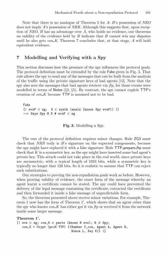
Mechanical Proofs about a Non-repudiation Protocol 101
Note that there is no analogue of Theorem 5 for A: B’s possession of NROdoes not imply A’s possession of NRR. Although this suggests that, upon recep-tion of NRO, B has an advantage over A, who holds no evidence, our theoremson validity of the evidence held by B indicate that B cannot win any disputesuntil he also gets con K. Theorem 7 concludes that, at that stage, A will holdequivalent evidence.
7 Modelling and Verifying with a Spy
This section discusses how the presence of the spy influences the protocol goals.The protocol definition must be extended by the rule Fake given in Fig. 3. Thatrule allows the spy to send any of the messages that can be built from the analysisof the traffic using the private signature keys of bad agents [12]. Note that thespy also sees the messages that bad agents retrieve via ftp, for those events weremodelled in terms of Notes (§2, §5). By contrast, the spy cannot exploit TTP’screation of con K because TTP is assumed not to be bad.
Fake
[| evsF ∈ zg; X ∈ synth (analz (knows Spy evsF)) |]
=⇒ Says Spy B X # evsF ∈ zg
Fig. 3. Modelling a Spy.
The rest of the protocol definition requires minor changes. Rule ZG3 mustcheck that NRR truly is B’s signature on the expected components, becausethe spy might have replaced it with a fake signature. Rule TTP prepare ftp mustcheck that K is a symmetric key, as the spy might have inserted some bad agent’sprivate key. This attack could not take place in the real world, since private keysare asymmetric, with a typical length of 1024 bits, while a symmetric key istypically no longer that 128 bits. So it is realistic to assume that TTP can rejectsuch substitutions.
Our strategies to proving the non-repudiation goals work as before. However,when proving validity of evidence, the exact form of the message whereby anagent learnt a certificate cannot be stated. The spy could have prevented thedelivery of the legal message containing the certificate, extracted the certificateand then forwarded it inside a fake message of unpredictable form.
So, the theorems presented above receive minor variations. For example, The-orem 1 now has the form of Theorem 1′, which shows that an agent other thanthe spy who knows con K has either got it via ftp or received it from the networkinside some larger message.
Theorem 1′.[| evs ∈ zg; con_K ∈ parts (knows B evs); B �= Spy;
con_K = Crypt (priK TTP) {|Number f_con, Agent A, Agent B,
Nonce L, Key K|} |]
102 Giampaolo Bella and Lawrence C. Paulson
=⇒ Notes B {|Number f_con, Agent A, Agent B, Nonce L, Key K, con_K|}
∈ set evs ∨Gets B X ∈ set evs ∧ con_K ∈ parts {X}
What was Theorem 2 can now be proved on the conclusion of Theorem 1′ viathe observation that con K was certainly in the traffic, and therefore originatedwith TTP. In consequence, combining the two new theorems produces the sameguarantee as before, but only for an agent who is not the spy.
Other minor changes concern the authenticity theorems that have been men-tioned along the treatment. For example, NRO is encrypted by A’s private key,so proving that it originated with A requires assuming that A does not belongto the set bad, otherwise the spy would know A’s private signature key priK Aand could forge the certificate. The same extra condition is needed on A whenproving that sub K originated with A, or on B when proving that NRR origi-nated with B. In consequence, for Theorem 3 to continue to hold, B must not bebad. Likewise, Theorem 5 now needs A not to be bad, and can only state thatB gets NRO inside a message of some form. Theorem 4 remains unchanged.
The fairness theorems do not need extra assumptions because they rest onthe message signed by TTP, which cannot be forged. However, their conclu-sions cannot state the exact form of the messages that deliver NRO and NRRrespectively. Those messages are now existentially quantified.
Following these considerations, it seems fair to conclude that the Zhou-Gollmann protocol achieves its goals even in the presence of a spy who is allowedto monitor the traffic and to exploit bad agent’s private signature keys.
8 Related Work
Schneider was the first to analyse the Zhou-Gollmann protocol formally [16].He uses the theory of Communicating Sequential Processes (CSP) to extend anexisting model previously used for authentication protocols with extra channelswhereby the peers present their evidence to a judge. His excellent account onvalidity of evidence and fairness is carried out by pen and paper. The proofstrategies are significantly different from ours. Events are enforced by provingthat they do not belong to a CSP refusal set. He writes,
the verifications of the correctness of evidence properties are carried outwithout reference to the protocol at all, but only with respect to thecapabilities and assumptions concerning the participating agents [15, §5]
Schneider allows any agent to send messages of any form using componentsfrom the agent’s knowledge, but obviously prevents this when proving fairness.By contrast, in our model, all agents must send messages of the form that theprotocol prescribes and can arbitrarily decide to quit the protocol; but we havealso considered the influence of a powerful spy. This difference between the twomodels is superficial: it would be trivial to define a set of unfair agents and alloweach agent A of the set to send messages from synth(analz(knowsA evs)) on anytrace evs .
Mechanical Proofs about a Non-repudiation Protocol 103
Zhou and Gollmann analyse their protocol using a belief logic [17]. The ap-proach allows for simple proofs on validity of evidence that only require fouraxioms and two inference rules. They formalise a judge J and reach the con-clusions that, at the end of a session between agents A and B, the followingpredicates hold:
– J believes (A said M)– J believes (B received M)
These predicates do not highlight what evidence the peers have to present toconvince the judge, but the protocol verifier could understand this from followingthe proofs more closely. Fairness properties are not considered, and the difficultyin tackling them appears to be a limitation of the approach. The philosophicaldifferences between reasoning on beliefs and reasoning on traces of events arewell known. However, it may be interesting to note that also these proofs onvalidity of evidence closely follow the events of the session. The protocol in factrequires each agent to send certain evidence only upon reception of some other,specific evidence.
Both works discussed here model a judge explicitly. We have chosen not tomodel a judge because his functioning as well as the peers’ interaction with himare external to the non-repudiation protocol. A peer’s presenting some evidenceto the judge in fact implies that the peer holds the evidence, which our functionknows concisely expresses. A desirable consequence is that the current InductiveApproach can be used with no extensions to verify non-repudiation goals.
9 Conclusions
A non-repudiation protocol differs from the protocols traditionally studied inthat the protocol participants do not trust each other. Every agent is a potentialenemy. This change affects our models and our theorems slightly, but not drasti-cally. We plan to enrich the model further, to model more precisely an agent whois trying to subvert the protocol. (The spy behaves too arbitrarily; for instance,he might give away his private keys, as no real villain would). To the best of ourknowledge, no one else has proved non-repudiation properties using verificationtools.
Acknowledgements
This work was funded by the epsrc grant GR/R01156/01 Verifying ElectronicCommerce Protocols.
References
1. G. Bella. Message Reception in the Inductive Approach. Research Report 460,University of Cambridge — Computer Laboratory, 1999.
2. G. Bella. Modelling Agents’ Knowledge Inductively. In Proc. of the 7th Interna-tional Workshop on Security Protocols, LNCS 1796. Springer-Verlag, 1999.
104 Giampaolo Bella and Lawrence C. Paulson
3. G. Bella. Mechanising a protocol for smart cards. In Proc. of International Con-ference on Research in Smart Cards (e-Smart’01), LNCS. Springer-Verlag, 2001.In Press.
4. G. Bella, F. Massacci, L.C. Paulson, and P. Tramontano. Formal Verificationof Cardholder Registration in SET. In F. Cuppens, Y. Deswarte, D. Gollmann,and M. Waidner, editors, Proc. of the 6th European Symposium on Research inComputer Security (ESORICS 2000), LNCS 1895, pages 159–174. Springer-Verlag,2000.
5. G. Bella and L.C. Paulson. Kerberos Version IV: Inductive Analysis of the Se-crecy Goals. In J.-J. Quisquater, Y. Deswarte, C. Meadows, and D. Gollmann,editors, Proc. of the 5th European Symposium on Research in Computer Security(ESORICS’98), LNCS 1485, pages 361–375. Springer-Verlag, 1998.
6. G. Bella and L.C. Paulson. Mechanising BAN Kerberos by the Inductive Method.In A. J. Hu and M. Y. Vardi, editors, Proc. of the International Conferenceon Computer-Aided Verification (CAV’98), LNCS 1427, pages 416–427. Springer-Verlag, 1998.
7. M. Ben-Or, O. Goldreich, S. Micali, and R. Rivest. A Fair Protocol for SigningContracts. IEEE Transactions on Information Theory, 36(1):40–46, 1990.
8. C.A. Meadows. The NRL Protocol Analyzer: An Overview. Journal of LogicProgramming, 26(2):113–131, 1996.
9. T. Okamoto and K. Ohta. How to Simultaneously Exchange Secrets by GeneralAssumptions. In Proc. of the 2nd ACM Conference on Computer and Communi-cation Security (CCS’94), pages 184–192, 1994.
10. L.C. Paulson. Isabelle: A Generic Theorem Prover. LNCS 828. Springer-Verlag,1994.
11. L.C. Paulson. Theory for public-key protocols, 1996.http://www4.informatik.tu-muenchen.de/~isabelle/library/
HOL/Auth/Public.html.12. L.C. Paulson. The Inductive Approach to Verifying Cryptographic Protocols. Jour-
nal of Computer Security, 6:85–128, 1998.13. L.C. Paulson. Inductive Analysis of the Internet protocol TLS. ACM Transactions
on Computer and System Security, 1999. In press.14. P.Y.A. Ryan and S.A. Schneider. The Modelling and Analysis of Security Protocols:
the CSP Approach. Addison-Wesley, 2000.15. S. Schneider. Verifying Authentication Protocols with CSP. In Proc. of the 10th
IEEE Computer Security Foundations Workshop, pages 3–17. IEEE Computer So-ciety Press, 1997.
16. S. Schneider. Formal Analysis of a Non-Repudiation Protocol. In Proc. of the 11thIEEE Computer Security Foundations Workshop. IEEE Computer Society Press,1998.
17. G. Zhou and D. Gollmann. Towards Verification of Non-Repudiation Protocols. InProc. of the 1998 International Refinement Workshop and Formal Methods Pacific,pages 370–380. Springer-Verlag, 1998.
18. J. Zhou and D. Gollmann. A Fair Non-Repudiation Protocol. In Proc. of the 15thIEEE Symposium on Security and Privacy, pages 55–61. IEEE Computer SocietyPress, 1996.
19. J. Zhou and D. Gollmann. An Efficient Non-Repudiation Protocol. In Proc. ofthe 10th IEEE Computer Security Foundations Workshop, pages 126–132. IEEEComputer Society Press, 1996.
Proving Hybrid Protocols Correct
Mark Bickford, Christoph Kreitz, Robbert van Renesse, and Xiaoming Liu
Department of Computer Science, Cornell UniversityIthaca, NY, U.S.A.
{markb,kreitz,rvr,xliu}@cs.cornell.edu
Abstract. We describe a generic switching protocol for the construc-tion of hybrid protocols and prove it correct with the Nuprl proof de-velopment system. For this purpose we introduce the concept of meta-properties and use them to formally characterize communication prop-erties that can be preserved by switching. We also identify switching in-variants that an implementation of the switching protocol must satisfyin order to work correctly.
1 Introduction
Formal methods tools have greatly influenced our ability to increase the reliabil-ity of software and hardware systems by revealing errors and clarifying criticalconcepts. Tools such as extended type checkers, model checkers [9] and theoremprovers [2,15,23,25] have been used to detect subtle errors in prototype codeand to clarify critical concepts in the design of hardware and software systems.System falsification is already an established technique for finding errors in theearly stages of the development of hardware circuits and the impact of formalmethods has become larger the earlier they are employed in the design process.
An engagement of formal methods at an early stage of the design depends onthe ability of the formal language to naturally and compactly express the ideasunderlying the system. When it is possible to precisely define the assumptionsand goals that drive the system design, then a theorem prover can be used as adesign assistant that helps the designers explore in detail ideas for overcomingproblems or clarifying goals. This formal design process can proceed at a reason-able pace, if the theorem prover is supported by a sufficient knowledge base ofbasic facts about systems concepts that the design team uses in its discussions.
The Nuprl Logical Programming Environment (LPE) [10,3] is a frameworkfor the development of formalized mathematical knowledge that is well suited tosupport such a formal design of software systems. It provides an expressive formallanguage and a substantial body of formal knowledge that was accumulated inincreasingly large applications, such as verifications of a logic synthesis tool [1]and of the SCI cache coherency protocol [13] as well as the verification andoptimization of communication protocols [17,12,18].
We have used the Nuprl LPE and its database of thousands of definitions,theorems and examples for the formal design of an adaptive network protocolfor the Ensemble group communication system [28,11,19]. The protocol is real-ized as a hybrid protocol that switches between specialized protocols. Its design
R.J. Boulton and P.B. Jackson (Eds.): TPHOLs 2001, LNCS 2152, pp. 105–120, 2001.c© Springer-Verlag Berlin Heidelberg 2001
106 Mark Bickford et al.
was centered around a characterization of communication properties that can bepreserved by switching. This led to a study of meta-properties, i.e. properties ofproperties, as a means for classifying those properties. It also led to the char-acterization of a switch-invariant that an implementation of the switch has tosatisfy to preserve those properties.
In this paper we show how to formally prove such hybrid protocols correct.In Section 2 we describe the basic architecture of hybrid protocols that are basedon protocol switching. We then discuss the concept of meta-properties and useit to characterize switchable properties, i.e. communication properties that canbe preserved by switching (Section 3). In Section 4 we give a formal account ofcommunication properties and meta-properties as a basis for the verification ofhybrid protocols with the Nuprl system. In Section 5 we develop the switch-invariant and formally prove that switchable properties are preserved wheneverthe implementation of a switching protocol satisfies this invariant.
2 Protocol Switching
Networking properties such as total order or recovery from message loss canbe realized by many different protocols. These protocols offer the same func-tionality but are optimized for different environments or applications. Hybridprotocols can be used to combine the advantages of various protocols, but de-signing them correctly is difficult, because they require a distributed migrationbetween different approaches to implementing the desired properties.
The Ensemble system [28,11] provides a mechanism for switching betweendifferent protocols at run-time. So far, however, it was not clear how to guaranteethat the result was actually correct , i.e. under what circumstances a switch wouldactually preserve the properties of the individual protocols.
Our new approach to switching is to design a generic switching protocol (SP )that would serve as a wrapper for a set of protocols with the same functional-ity. This switching protocol shall interact with the application in a transparentfashion, that is, the application cannot tell easily that it is running on the SPrather than on one of the underlying protocols, even as the SP switches betweenprotocols. The kinds of uses we envision include the following:
– Performance. By using the best protocol for a particular network and appli-cation behavior, performance can always be optimal.
– On-line Upgrading. Protocol switching can be used to upgrade network pro-tocols or fix minor bugs at run-time without having to restart applications.
– Security. System managers will be able to increase security at run-time, forexample when an intrusion detection system notices unusual behavior.
In a protocol layering architecture like the one used in Ensemble the switchingprotocol will reside on top of the individual protocols to be switched, coupledby a multiplexer below them, as illustrated in Figure 1.
The basic idea of the switching protocol is to operate in one of two modes.In normal mode it simply forwards messages from the application to the cur-rent protocol and vice versa. When there is a request to switch to a different
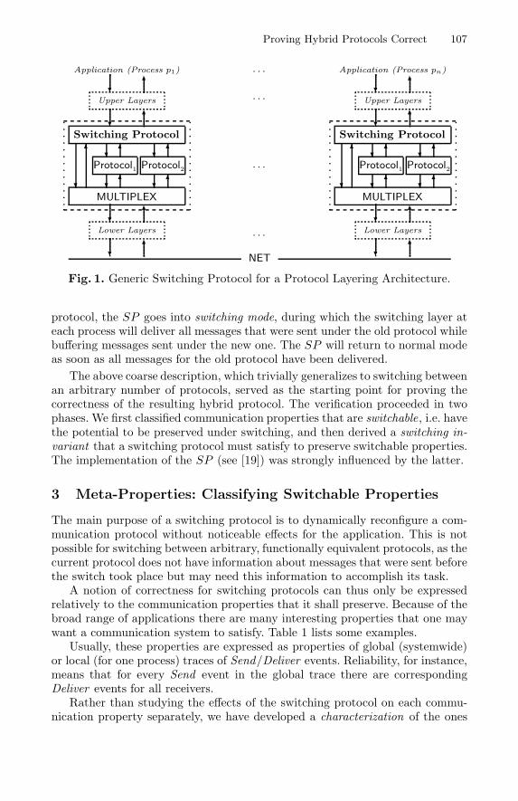
Proving Hybrid Protocols Correct 107
Application (Process p1)
❄ ✻Upper Layers
❄ ✻Switching Protocol
❄
✻ ❄✻ ❄✻Protocol1 Protocol2
❄✻ ❄✻MULTIPLEX
❄ ✻Lower Layers
❄ ✻
. . .
. . .
. . .
. . .
NET
Application (Process pn)
❄ ✻Upper Layers
❄ ✻Switching Protocol
❄
✻ ❄✻ ❄✻Protocol1 Protocol2
❄✻ ❄✻MULTIPLEX
❄ ✻Lower Layers
❄ ✻
Fig. 1. Generic Switching Protocol for a Protocol Layering Architecture.
protocol, the SP goes into switching mode, during which the switching layer ateach process will deliver all messages that were sent under the old protocol whilebuffering messages sent under the new one. The SP will return to normal modeas soon as all messages for the old protocol have been delivered.
The above coarse description, which trivially generalizes to switching betweenan arbitrary number of protocols, served as the starting point for proving thecorrectness of the resulting hybrid protocol. The verification proceeded in twophases. We first classified communication properties that are switchable, i.e. havethe potential to be preserved under switching, and then derived a switching in-variant that a switching protocol must satisfy to preserve switchable properties.The implementation of the SP (see [19]) was strongly influenced by the latter.
3 Meta-Properties: Classifying Switchable Properties
The main purpose of a switching protocol is to dynamically reconfigure a com-munication protocol without noticeable effects for the application. This is notpossible for switching between arbitrary, functionally equivalent protocols, as thecurrent protocol does not have information about messages that were sent beforethe switch took place but may need this information to accomplish its task.
A notion of correctness for switching protocols can thus only be expressedrelatively to the communication properties that it shall preserve. Because of thebroad range of applications there are many interesting properties that one maywant a communication system to satisfy. Table 1 lists some examples.
Usually, these properties are expressed as properties of global (systemwide)or local (for one process) traces of Send/Deliver events. Reliability, for instance,means that for every Send event in the global trace there are correspondingDeliver events for all receivers.
Rather than studying the effects of the switching protocol on each commu-nication property separately, we have developed a characterization of the ones
108 Mark Bickford et al.
Table 1. Examples of Commonly Used Communication Properties.
Reliability: Every message that is sent is delivered to all receiversIntegrity: Messages cannot be forged; they are sent by trusted processesConfidentiality: Non-trusted processes cannot see messages from trusted onesTotal Order: Processes that deliver the same messages deliver them in the
same orderNo Replay: A message body can be delivered at most once to a process
that are preserved by protocol switching. For this purpose, we introduce theconcept of meta-properties, i.e. properties of properties, that classify communi-cation properties into those that are preserved by certain communication proto-col architectures and those that are not. In this section we will give an intuitivedescription of such meta-properties (see [19] for details). Their formalization asused in the verification of the switching protocol will be described in section 4.2.
Our verification efforts showed that four meta-properties are important forcharacterizing the effects of layered communication systems.
Safety. Safety [4] is probably the best-known meta-property. Safety meansthat a property does not depend on how far the communication has progressed:if the property holds for a trace, then it also holds for every prefix of that trace.Total order, for instance, is safe since taking events of the end off a trace cannotreorder message delivery. Reliability, however, is not safe since chopping off asuffix containing a Deliver event can make a reliable trace unreliable.
Asynchrony. Any global ordering that a protocol implements on events canget lost due to delays in the send and deliver streams through the protocollayers above it. Only properties that are asynchronous, i.e. do not depend on therelative order of events of different processes, are preserved under the effects oflayering. Total order is asynchronous as well, as it does not require an absoluteorder of delivery events at different processes.
Delayable. Another effect of layered communication is local: at any process,Send events are delayed on the way down, and Deliver events are delayed onthe way up. A property that survives these delays is called delayable. Totalorder is delayable, since delays do not change the order of Deliver event. Thismeta-property is similar to delay-insensitivity in asynchronous circuits.
Send Enabled. A protocol that implements a property for the layer above typ-ically does not restrict when the layer above sends messages. We call a propertySend Enabled if it is preserved by appending new Send events to traces. Totalorder is obviously send enabled. Send Enabled and Delayable are related, as bothare concerned with being unable to control when the application sends messages.
These four meta-properties are sufficient for properties to survive the effectsof delay in any layered environment. Since the switching protocol is based on alayered architecture, these meta-properties will be important for a property tobe preserved by the switching protocol. However, two additional meta-propertiesare necessary to describe the specific effects of switching.
Proving Hybrid Protocols Correct 109
Memoryless. When we switch between protocols, the current protocol maynot see part of the history of events that were handled by another protocol. Itthus has to be able to work as if these events never happened. A property ismemoryless if we can remove all events pertaining to a particular message froma trace without violating the property. That is, whether such a message was eversent or delivered is no longer of importance. This does not imply, however, that aprotocol that implements the property has to be stateless and must forget aboutthe message. Total order is memoryless, since it only places conditions on eventsthat actually take place, but its implementations are certainly not stateless.
Composable. Protocol switching causes the traces of several protocols to beglued together. Since we expect the resulting trace to satisfy the same propertiesas the individual traces, these properties must be composable in the sense thatif they hold for any two traces that have no messages in common, then theyalso must hold for the concatenation. Total order is composable, because theconcatenation of traces does not change the order of events in either trace.
Using the Nuprl system [3] we have shown that these six meta-propertiesare sufficient for a communication property to be preserved by the switchingprotocol: if such a property holds for the traces of the two protocols below theswitching protocol, then it also holds for the resulting trace above the switch. Inthe following sections we will show how this is formally proven.
4 Formalization
A formal verification of the switching protocol with a formal proof system has tobe based on an appropriate formalization of the underlying concepts in the lan-guage of the proof system. The formal language of the Nuprl proof developmentsystem [10,3], an extension of Martin-Lof’s intuitionistic Type Theory [22], al-ready provides formalizations of the fundamental concepts of mathematics, datatypes, and programming.
Nuprl supports conservative language extensions by user-defined conceptsvia abstractions and display forms . An abstraction of the form
operator-id( parameters) ≡ expression with parameters
defines a new, possibly parameterized term in terms of already existing type-theoretical expressions. Display forms can be used to change the textual repre-sentation of this term on the screen or within formal printed documents almostarbitrarily. In particular they can be used to suppress the presentation of implicitassumptions and thus ease the comprehensibility of formal text.
The Nuprl proof development system supports interactive and tactic-basedreasoning in a sequent-based formalism, decision procedures, an evaluation mech-anism for programs, and an extendable library of verified knowledge from variousdomains. A formal documentation mechanism supports the automated creationof “informal documents” from the formal objects. The technical report [5], con-taining a complete formal account of the work described in the following sections,for instance, was created entirely from within Nuprl.
110 Mark Bickford et al.
4.1 A Formal Model of Communication
To support a formal verification of communication protocols, we have devel-oped a formal model of distributed communication systems and their proper-ties. Our model formalizes notions for the specification of distributed algorithmsintroduced by Lynch [20] and concepts used for the implementation of reliablenetwork systems [6], particularly of Ensemble and its predecessors [7,27,11].
Messages, Events, and Traces. Processes multicast messages that containa body, a sender, and a unique identifier. We will consider two types of events .A Send(m) event models that some process p has multicast a message m. ADeliver(p,m) event models that process p has delivered message m. A trace isan ordered sequence of Send and Deliver events without duplicate Send events.
In order to be able to reason formally about messages, events and traces,we introduce two classes MessageStruct and EventStruct of formal messagestructures and event structures , respectively.
A message structure M ∈MessageStruct provides a carrier |M| and threefunctions, contentM, senderM, and uidM, which compute the body, sender, andidentifier of a message m ∈M . Two messages m1 and m2 are considered equal,denoted by m1=M m2 if they have the same content, sender, and identifier.
Similarly, an event structure E ∈EventStruct provides a carrier type |E|, amessage structure MSE, and three functions, is-sendE, locE, and msgE, whereis-sendE(e) is true when the event e ∈|E| is a Send event (otherwise it isa Deliver event); locE(e), the location of the event e, is the identifier of theprocess that sends or receives e; and msgE(e) is the message m ∈MSE containedin the event e. Using the latter we define a binary relation, e1=
mE
e2, which holds ifthe messages contained in the events e1 and e2 are equal wrt. =M. For example, e1
and e2 might be Deliver events of the same message m at two different locations.
Given an event structure E, a trace is just a list of events of type |E|. Thedata type of traces over E is thus defined as
TraceE ≡ |E| List
All the usual list operations like length |tr|, selecting the i-th element tr[i],concatenation tr1@tr2, prefix relation tr1
�tr2, and filtering elements that satisfya property P , [e ∈ tr|P], apply to traces as well.
For process identifiers we introduce a (recursively defined) type PID thatcontains tokens and integers and is closed under pairing. A similar type, calledLabel, will be later be used to tag events processed by different protocols.
Properties of Traces. A trace property is a predicate on traces that describescertain behaviors of communication. We formalize trace properties as proposi-tions on traces, i.e. as functions from TraceE to the type P of logical propositions.
TracePropertyE ≡ TraceE → P
All traces that we consider must satisfy at least three basic properties.
Proving Hybrid Protocols Correct 111
Every delivered message must have been sent before (causality), no messageis sent twice, and no message is delivered twice (replayed) to the same process.These assumptions are made implicitly in the implementation of communicationsystems but need to be made explicit in a formal account.
CausalE(tr)≡ ∀i<|tr|.∃j<|tr|. j≤i ∧ is-sendE(tr[j]) ∧ tr[j] =mE
tr[i]
No-dup-sendE(tr)≡ ∀i,j<|tr|. (is-sendE(tr[i]) ∧ is-sendE(tr[j]) ∧ tr[j] =mE tr[i])
⇒ i = j
No-replayE(tr)≡ ∀i,j<|tr|. ( ¬is-sendE(tr[i]) ∧ ¬is-sendE(tr[j])∧ tr[j] =m
E tr[i] ∧ locE(tr[i]) = locE(tr[j])) ⇒ i = j
The properties reliability (for multicasting), integrity, confidentiality, and totalorder (c.f. Section 3) can be formalized as follows.
ReliableE(tr)≡ ∀e ∈ tr. is-sendE(e) ⇒∀p:PID. ∃e1∈ tr. ¬is-sendE(e1) ∧ e =m
Ee1 ∧ locE(e1) = p
IntegrityE(tr)≡ ∀e ∈ tr. (¬is-sendE(e) ∧ trusted(locE(e))) ⇒∀e1∈ tr. (is-sendE(e1) ∧ e =m
Ee1) ⇒ trusted(locE(e1))
ConfidentialE(tr)≡ ∀e ∈ tr. (¬is-sendE(e) ∧ ¬trusted(locE(e))) ⇒¬(∃e1∈ tr. is-sendE(e1) ∧ e =m
E e1 ∧ trusted(locE(e1)))
TotalOrderE(tr)≡ ∀p,q:PID. tr↓p �tr↓q = tr↓q �tr↓pwhere trusted(p) characterizes trusted processes, tr↓p is the trace tr deliveredat process p (the projection of all Deliver(p,m) events from trace tr), and tr1 �tr2
denotes the restriction of tr1 to events whose messages also occur in tr2.
tr↓p ≡ [ e ∈ tr |¬is-sendE(e) ∧ locE(e)=p ]
tr1�tr2≡ [ e1
∈ tr1| ∃e2∈ tr2. e1=
mEe2]
In the following investigations we also need a notion of refinement on traceproperties, which is defined as follows.
P � Q ≡ ∀tr:TraceE. P(tr) ⇒ Q(tr)
4.2 Meta-properties
Meta-properties are predicates on properties that are used to classify which prop-erties are preserved by a protocol layer. In principle, any predicate on propertiescould be meta-property. But the meta-properties that we are specifically inter-ested in are the ones that describe how passing events through a protocol layer
112 Mark Bickford et al.
affects the properties of the traces above and below that layer. We say that areflexive and transitive relation R on traces preserves a property P if, whenevertwo traces tr1 and tr2 are related by R, and P holds for trace tr1, then it alsoholds for tr2. A similar definition is also given for ternary relations.
R preserves P≡ ∀tru,trl
:TraceE. (P(trl) ∧ tru R tr
l) ⇒ P(tru)
R preserves3 P≡ ∀tru,tr1,tr2:TraceE. (P(tr1) ∧ P(tr2) ∧ R(tru,tr1,tr2) )
⇒ P(tru)
Preservation by a (binary or ternary) relationR is thus a predicate on proper-ties, i.e. a meta-property. Note that preservation automatically makes the effectsof the relation R transitive, even if R is not. Below, we will formalize six suchrelations that describe the meta-properties discussed in Section 3.
Safety. Safety means that if the property holds for a trace, then it is also sat-isfied for every prefix of that trace. The corresponding relation Rsafety specifiesthat the trace above the protocol (tru) is a prefix of the one below (tr
l).
tru R safetyE trl
≡ tru � trl
Asynchrony. A property is asynchronous if it does not depend on the rela-tive order of events at different processes. The corresponding relation Rasynchspecifies that two traces are related if they can be formed by swapping adjacentevents that belong to different processes. Events belonging to the same processmay not be swapped.
tru R asyncE trl
≡ tru swap-adjacent[locE(e)�=locE(e′)] tr
l
where tr1 swap-adjacent[c(e;e′)] tr2 denotes that tr1 can be transformed into tr2
by swapping adjacent events e and e′ of tr1 that satisfy the condition c(e; e′).
Delayable. A property is delayable if it survives delays of Send events onthe way down and of Deliver events on the way up. The corresponding relationRdelayable specifies that adjacent Send and Deliver events in the lower tracemay be swapped in the upper. Events of the same kind or containing the samemessage may not be swapped.
tru R delayableE trl
≡ tru swap-adjacent[e =m
Ee′ ∧ is−sendE(e) =is−sendE(e′)] tr
l
Send Enabled. A property is Send Enabled if it is preserved by appendingSend events to traces. The corresponding relation Rsend-enabled specifies thatthe upper trace is formed by adding Send events to the end of the lower trace.
tru R send-enabledE trl≡ ∃e:|E|. is-sendE(e) ∧ tru = tr
l@[e]
Memoryless. A property is memoryless if we can remove all events pertain-ing to a particular message from a trace without violating the property. The
Proving Hybrid Protocols Correct 113
corresponding relation Rmemoryless defines that the upper trace can be formedfrom the one below by removing all events related to certain messages.
tru R memorylessE trl≡ ∃e:|E|. tru = [ e1
∈ trl| e =m
E e1]
Composable. A property is composable if it is preserved when two tracesthat have no messages in common are concatenated. The corresponding relationRcomposable is ternary, as it characterizes the upper trace tr as concatenation oftwo lower traces without common messages.
R composableE(tru,tr1,tr2) ≡ tru = tr1@tr2 ∧ ∀e1∈ tr1.∀e2
∈ tr2. e1 =mEe2
Switchable Properties. The above collection of meta-properties and its for-malization is the result of a complex formal analysis of the switching protocol.The formal verification process with the Nuprl proof development system [3] re-quired us to make many assumptions explicit that are usually implicitly presentin an informal analysis of communication protocols. This is reflected in the defini-tion of switchable communication properties. A trace property P is switchable ifit requires the trace to be meaningful and satisfies all of the six meta-properties.
switchableE(P) ≡ P � CausalE∧ P � No-replayE∧ R safetyE preserves P∧ R asyncE preserves P∧ R delayableE preserves P∧ R send-enabledE preserves P∧ R memorylessE preserves P∧ R composableE preserves3 P
In the following section we will show that switchable communcation proper-ties are in fact preserved by the switching protocol.
5 Verification of Hybrid Protocols
In the previous sections we have given an abstract and formal characterizationof communication protocols whose properties can be preserved by switching. Ina similar way we will now develop an abstract characterization of the switch-ing protocol in terms of a switching invariant . We will then prove that everyimplementation of a switching protocol that satisfies the switching invariant isguaranteed to preserve switchable properties. In this paper, we will focus on thehighlights of this proof and the underlying formal theory. A complete accountof this theory, which has been developed entirely within the Nuprl proof devel-opment system [3], can be found in the technical report that has been createdautomatically from the formal theory [5].
In order to prove the switching protocol to work correctly for a switchableproperty P we have to show that if P holds for the traces tr1 and tr2 of the twoprotocols below the switching protocol, then P also holds for the trace tru above
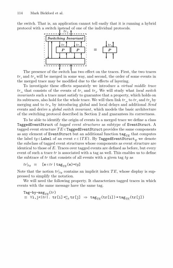
114 Mark Bickford et al.
the switch. That is, an application cannot tell easily that it is running a hybridprotocol with a switch instead of one of the individual protocols.
tr1 tr2
tru
tru
❄ ✻Switching Invariant
❄
✻ ❄ ✻ ❄ ✻P P
❄ ✻ ❄ ✻
❄ ✻
≡❄ ✻P
❄ ✻
The presence of the switch has two effect on the traces. First, the two tracestr1 and tr2 will be merged in some way, and second, the order of some events inthe merged trace may be modified due to the effects of layering.
To investigate these effects separately we introduce a virtual middle tracetr
mthat consists of the events of tr1 and tr2. We will study what local switch
invariants such a trace must satisfy to guarantee that a property, which holds onits subtraces, also hold for the whole trace. We will then link tr
mto tr1 and tr2 by
merging and to tru by introducing global and local delays and additional Sendevents and derive a global switch invariant , which models the basic architectureof the switching protocol described in Section 2 and guarantees its correctness.
To be able to identify the origin of events in a merged trace we define a classTaggedEventStruct of tagged event structures as subtype of EventStruct. Atagged event structure TE ∈TaggedEventStruct provides the same componentsas any element of EventStruct but an additional function tagTE that computesthe label tg ∈Label of an event e ∈|TE|. By TaggedEventStructE we denotethe subclass of tagged event structures whose components as event structure areidentical to those of E. Traces over tagged events are defined as before, but everyevent of such a trace tr is associated with a tag as well. This enables us to definethe subtrace of tr that consists of all events with a given tag tg as
tr|tg ≡ [e ∈ tr | tagTE(e)=tg]
Note that the notion tr|tg contains an implicit index TE, whose display is sup-pressed to simplify the notation.
We will need the following property. It characterizes tagged traces in whichevents with the same message have the same tag.
Tag-by-msgTE(tr)≡ ∀i,j<|tr|. tr[i] =mTE tr[j] ⇒ tagTE(tr[i])= tagTE(tr[j])
Proving Hybrid Protocols Correct 115
5.1 The Local Switching Invariant
A local switch invariant I on a trace tr shall guarantee that a switchable propertyP holds for tr whenever P holds for all subtraces tr|tg. If this is the case we saythat I fuses P :
I fuses P ≡ ∀tr:TraceE. I(tr) ⇒ (∀tg:Label.P(tr|tg)) ⇒ P(tr)
From the description of the switching protocol we know that if two messagesare sent using different protocols, then the second message will be buffered ata location until the first one has been delivered. In other words, if two Sendevents have different tags, then at any location, the first message must havebeen delivered before the second. This requirement is represented by the follow-ing invariant.
switch invTE(tr)≡ ∀i,j,k<|tr|.(i<j ∧ is-sendTE(tr[i]) ∧ is-sendTE(tr[j])∧ tagTE(tr[i]) =tagTE(tr[j]) ∧ tr[j]↓TEtr[k] )
⇒ ∃k’<k. locTE(tr[k’]) = locTE(tr[k]) ∧ tr[i]↓TEtr[k’]
where e↓TEtr[k] denotes that a message related to the event e is delivered attime k in tr:
e↓TEtr[k] ≡ e =mTE tr[k] ∧ ¬is-sendTE(tr[k])
switch invTE is sufficient to fuse switchable properties, provided the trace de-scribes a meaningful communication, i.e. does not contain duplicate send events.
Theorem 1.
� ∀TE:TaggedEventStruct. ∀P:TracePropertyE. switchableTE(P)⇒ (No-dup-sendTE ∧ switch invTE) fuses P
Proof. Theorem 1 is the result of a series of steps that refine the invariants for fusingcertain classes of properties until we arrive at the fusion condition for the class ofswitchable predicates.
1. We begin by proving an invariant for the preservation of all properties P that arememoryless, composable, and safe, denoted by the meta-property MCS
TE(P). A suf-
ficient condition is single-tag-decomposability , meaning that any nonempty trace canbe decomposed into two traces with no messages in common, such that all events ofthe (non-empty) second trace have the same tag.
single-tag-decomposableTE
(tr)≡ tr �=[] ⇒ ∃tr1,tr2:TraceTE
. tr = tr1@tr2 ∧ tr2�=[]∧ ∀e1∈tr1.∀e2∈tr2. e1 �=m
E e2
∧ ∃tg:Label. ∀e2∈tr2. tagTE
(e2) = tg
By induction over the length of a trace we prove that any single-tag-decomposablesafety property is a fusion condition for any MCS property.
∀TE:TaggedEventStruct. ∀P,I:TracePropertyTE
. MCSTE
(P) ⇒R safety
TEpreserves I ∧ I � single-tag-decomposable
TE⇒ I fuses P
116 Mark Bickford et al.
2. In the next step we refine single-tag-decomposability to a more constructive condi-tion that we call switch decomposability . It says that it must be possible to charac-terize timing of some send events in a trace (i.e. their indices) by some decidablepredicate Q that satisfies a number of closure conditions.
switch-decomposableTE
(tr)≡ tr = [] ∨ ∃Q:IN→P. decidable(Q) ∧ ∃i<|tr|. Q(i)
∧ ∀i<|tr|. Q(i) ⇒ is-sendTE
(tr[i])∧ ∀i,j<|tr|. Q(i) ∧ Q(j) ⇒ tag
TE(tr[i]) = tag
TE(tr[j])
∧ ∀i<|tr|. Q(i) ⇒ ∀i≤j<|tr|. ClQ(j)
where ClQ(j), the message closure of Q at time j is defined as
ClQ(i) ≡ ∃k<|tr|. Q(k) ∧ tr[k] =mE tr[i]
By partitioning the trace into those events that satisfy ClQ(i) and those that don’twe can prove that switch-decomposability refines single-tag-decomposability.
∀TE:TaggedEventStruct(switch-decomposable
TE∧ Tag-by-msg
TE∧ Causal
TE∧ No-dup-send
TE)
� single-tag-decomposableTE
3. In the third step we show that a certain strengthening of switch invTE
refinesswitch-decomposability. For this purpose we have to find a predicate Q that satisfiesthe five conditions for switch-decomposability.If the trace satisfies switch inv
TEand causality, then it must contain a Send event.
We define Q to hold on all indices that are related to the index ls of the last Sendevent by the transitive closure of the relation R switchtr , which relates Send eventswhose messages were delivered out of order at some location.
i R switchtr j ≡ is-sendTE
(tr[i]) ∧ is-sendTE
(tr[j])∧ (i<j ∧ tr[j]↓<
TEtr[i] ∨ j<i ∧ tr[i]<
TEtr[j])
where e↓<TE
tr[k] denotes that the event e is delivered at some time before time k.It is fairly easy to prove that Q has the first four of the five required properties. Forthe fifth, however, we need more than just switch inv
TEand Causal
TE. We have
to assume that the trace tr has a certain normal form, in which Send events occuras late as possible and asynchronous Deliver events match the order of their Sendevents. Since the algorithm for generating this normal form can be shown to pre-serve asynchronous and delayable properties, we call this property an asynchronous-delayable normal form or AD-normal .
AD-normalTE
(tr)≡ ∀i<|tr|. (is-send
TE(tr[i]) ∧ ¬is-send
TE(tr[i+1]) ⇒ tr[i] =m
E tr[i+1]∧ (∃j,k<|tr|. j<k ∧ is-send
TE(tr[j]) ∧ tr[j]↓
TEtr[i+1]
∧ is-sendTE
(tr[k]) ∧ tr[k]↓TE
tr[i] )
⇒ locTE
(tr[i]) = locTE
(tr[i+1]))
This property, together with causality and no-duplicate-deliver suffices to prove thefifth property of Q. Thus altogether we have proved the following
∀TE:TaggedEventStruct(switch inv
TE∧ Causal
TE∧ AD-normal
TE∧ No-replay
TE)
� switch-decomposableTE
4. Putting the above results together we can show
∀TE:TaggedEventStruct. ∀P:TracePropertyTE
.
Proving Hybrid Protocols Correct 117
MCSTE
(P) ∧ P � (CausalTE
∧ No-replayTE
)
⇒ (switch invTE
∧ AD-normalTE
∧ No-dup-sendTE
) fuses P
In the last step we prove that the normal form requirement can be removed if weassume the predicate P to be asynchronous and delayable.For this purpose we apply general theorem about the existence of partially sortedlists. It says that, if swapping adjacent elements e and e′ in a list tr for which adecidable predicate GOOD(e, e′) does not hold increases the number of good pairs,then we may reach a list tr′ in which all adjacent pairs satisfy GOOD (proof byinduction over the number of bad pairs).By instantiating GOOD with a localized version of AD-normal
TEwe can show that
a trace can be converted into normal form.
∀TE:TaggedEventStruct. ∀tr:TraceTE
switch invTE
(tr) ∧ No-dup-sendTE
(tr)
⇒ ∃tr’:TraceTE
. switch invTE
(tr’) ∧ AD-normalTE
(tr’)
∧ tr (R delayableTE
∨ R asynchTE
)∗ tr’
Since switchable properties are preserved by R delayableTE
∨ R asynchTE, Theo-
rem 1 follows from the above two results. �
The proof of Theorem 1 was developed completely within the Nuprl proofdevelopment system. Further details can be found in [5].
5.2 Global Correctness of Switching
Theorem 1 states that a switchable property P holds on a tagged event tracetrm whenever P holds for all subtraces trm|tg, provided trm satisfies the localswitch invariant and does not contain duplicate Send events.
The global switch invariant expresses that some virtual inner trace trm, which
is created by merging the traces tr1 and tr2 of the protocols below and is linkedto the upper trace tru by introducing global and local delays and additional Sendevents, must satisfy the local switch invariant and be free of duplicates.
In the formal model, we describe the traces tr1 and tr2 by a single lowertrace tr
lof tagged events. tr
lis related to tr
mby allowing adjacent events with
different tags to be swapped, which accounts for the effects of buffering duringswitch mode. trm is related to tru by allowing (global and local) delays andenabling Send events.
Rtag ≡ (swap-adjacent[tag(e)�=tag(e′)])
∗
R layerTE ≡ (R asyncTE ∨ R delayableTE ∨ R send-enabledTE)∗
where R∗ denotes the transitive closure of a relation R. Note that R layerTE isthe same as R layerE if TE ∈TaggedEventStructE.
The definition of the global switch invariant summarizes all the above insightsinto a single relation between the lower and the upper trace.
full switch invTE(tru;trl) ≡ ∃tr
m:TraceTE. tr
lRtagTE
trm
∧ switch invTE(trm)
∧ trm
R layerTE tru
∧ No-dup-sendE(tru)
118 Mark Bickford et al.
Switching protocols that implement this invariant, support all protocols thatimplement switchable properties. Whenever a switchable property P holds for alltraces tr
l|tg of the individual protocols below a switching protocol that satisfies
the global switching invariant, then it also holds for the trace tru above it. Inthe Nuprl proof development system this theorem, which is an straightforwardconsequence of Theorem 1, is formalized as follows.
Theorem 2 (Correctness of Switching).
� ∀E:EventStruct. ∀P:TracePropertyE. ∀TE:TaggedEventStructE∀tru:TraceE. ∀trl:TraceTE.
( switchableE(P) ∧ full switch invTE(tru;trl) )
⇒ ( ∀tg:Label. P(trl|tg) ) ⇒ P(tru)
5.3 Implementation Aspects
The implementation of a switching protocol was developed in parallel to theformal verification efforts, and took into account that the switch has to satisfy theglobal switch invariant. Together with the fact that switching protocols designedaccording to the description in Section 2 are live, this gives us assurance thatthe resulting hybrid protocol works correctly.
We have evaluated the performance implications of using the switching proto-col by switching between two well-known total order protocols [19], one based ona centralized sequencer [16] and the other using a rotating token with a sequencenumber [8]. These two protocols have an interesting trade-off. The sequencer-based algorithm has low latency, but the sequencer may become a bottleneckwhen there are many active senders. The token-based algorithm does not have abottleneck, but the latency is relatively high under low load. Experiments haveshown that having the switch follow a small hysteresis at the cross-over pointhas the potential of achieving the best of both
6 Conclusion
We have designed a generic switching protocol for the construction of adap-tive network systems and formally proved it correct with the Nuprl LogicalProgramming Environment. In the process we have developed an abstract char-acterization of communication properties that can be preserved by switchingand an abstract characterization of invariants that an implementation of theswitching protocol must satisfy in order to work correctly.
There has been a flurry of research on the verification of software systemsand communication protocols (see e.g. [14,21,24,26]). But most approaches sofar provided only a-posteriori verifications of well-understood algorithms. Toour knowledge this is the first case in which a new communication protocolwas designed, verified, and implemented in parallel. Because of a team thatconsisted of both systems experts and experts in formal methods the protocolconstruction could proceed at the same pace of implementation as designs that
Proving Hybrid Protocols Correct 119
are not formally assisted, and at the same time provide a formal guarantee forthe correctness of the resulting protocol.
The verification efforts revealed a variety of implicit assumptions that areusually made when reasoning about communication systems and uncovered mi-nor design errors that would have otherwise made their way into the imple-mentation (such as to use switching for arbitrary protocols). This demonstratesthat an expressive theorem proving environment with a rich specification lan-guage (such as provided by the Nuprl LPE) can contribute to the design andimplementation of verifiably correct network software.
So far we have limited ourselves to investigating sufficient conditions for aswitching protocol to work correctly. However, some of the conditions on switch-able properties may be stricter than necessary. Reliability, for instance, is not asafety property, but we are confident that it is preserved by protocol layering andthus by our hybrid protocol. We intend to refine our characterization of switch-able predicates and demonstrate that larger class of protocols can be supported.
Also, we would like to apply our proof methodology to the verification of pro-tocol stacks. To prove that a given protocol stack satisfies certain properties, wehave to be able to prove that these properties, once “created” by some protocol,are preserved by the other protocols in the stack. We believe that using meta-properties to characterize the properties preserved by specific communicationprotocols will make these investigations feasible.
Our case study has shown that formal methods are moving into the designand implementation phases of software construction as well as into the testingand debugging phases. The impact of formal methods is larger the more theyare engaged at the earliest stages of design and implementation. We believe thatthe early use can add value to all subsequent stages, including the creation ofinformative documentation need for maintenance and evolution of software.
Acknowledgements
This work was supported by DARPA grants F 30620-98-2-0198 (An Open LogicalProgramming Environment) and F 30602-99-1-0532 (Spinglass).
References
1. M.Aagaard and M. Leeser. Verifying a logic synthesis tool in Nuprl. InG.Bochmann and D.Probst, eds., Workshop on Computer-Aided Verification,LNCS 663, pages 72–83. Springer, 1993.
2. ACL2 home page. http://www.cs.utexas.edu/users/moore/acl2 .3. S.Allen, R.Constable, R.Eaton, C.Kreitz, L. Lorigo. The Nuprl open logical envi-ronment. In D.McAllester, ed., 17th Conference on Automated Deduction, LNAI1831, pages 170–176. Springer, 2000.
4. B.Alpern and F. Schneider. Recognizing safety and liveness. Distributed Comput-ing, 2(3):117–126, 1987.
5. M.Bickford, C.Kreitz, R. van Renesse. Formally verifying hybrid protocols withthe Nuprl logical programming environment. Technical report Cornell CS:2001-1839, Cornell University. Department of Computer Science, 2001.
120 Mark Bickford et al.
6. K.Birman. Building Secure and Reliable Network Applications. Manning Publish-ing Co. and Prentice Hall, 1997.
7. K.Birman and R. van Renesse. Reliable Distributed Computing with the IsisToolkit. IEEE Computer Society Press, 1994.
8. J. Chang and N.Maxemchuk. Reliable broadcast protocols. ACM Transactions onComputer Systems, 2(3):251–273, 1984.
9. E.M. Clarke, O.Grumberg, D.Peled. Model Checking. MIT Press, 1999.10. R.Constable, S.Allen, M.Bromley, R.Cleaveland, J. Cremer, R.Harper, D.Howe,
T.Knoblock, P.Mendler, P. Panangaden, J. Sasaki, S. Smith. Implementing Math-ematics with the Nuprl proof development system. Prentice Hall, 1986.
11. M.Hayden. The Ensemble System. PhD thesis, Cornell University. Department ofComputer Science, 1998.
12. J.Hickey, N. Lynch, R. van Renesse. Specifications and proofs for Ensemble layers.In R.Cleaveland, ed., 5th International Conference on Tools and Algorithms for theConstruction and Analysis of Systems, LNCS 1579, pages 119–133. Springer, 1999.
13. D.Howe. Importing mathematics from HOL into NuPRL. In J. von Wright,J.Grundy, J. Harrison, eds., Theorem Proving in Higher Order Logics, LNCS 1125,pages 267–282. Springer, 1996.
14. D.Hutter, B. Langenstein, C. Sengler, J. H. Siekmann, W. Stephan, and A.Wolpers.Verification support environment (VSE). Journal of High Integrity, 1997.
15. Isabelle home page. http://www.cl.cam.ac.uk/Research/HVG/Isabelle .16. M.Kaashoek, A.Tanenbaum, S. Flynn-Hummel, H. E. Bal. An efficient reliable
broadcast protocol. Operating Systems Review, 23(4):5–19, 1989.17. C.Kreitz, M.Hayden, J. Hickey. A proof environment for the development of group
communication systems. In C. and H.Kirchner, eds., 15th Conference on Auto-mated Deduction, LNAI 1421, pages 317–332. Springer, 1998.
18. X.Liu, C.Kreitz, R. van Renesse, J.Hickey, M.Hayden, K.Birman, R.Constable.Building reliable, high-performance communication systems from components. Op-erating Systems Review 34(5):80–92, 1999.
19. X.Liu, R. van Renesse, M.Bickford, C.Kreitz, R.Constable. Protocol switching:Exploiting meta-properties. In Luis Rodrigues and Michel Raynal, eds., Inter-national Workshop on Applied Reliable Group Communication. IEEE CS Press,2001.
20. N.Lynch. Distributed Algorithms. Morgan Kaufmann, 1996.21. Z.Manna and A.Pnueli. Temporal Verification of Reactive Systems. Springer,
1995.22. P.Martin-Lof. Intuitionistic Type Theory. Bibliopolis, 1984.23. Nuprl home page. http://www.cs.cornell.edu/Info/Projects/NuPrl .24. L. Paulson. The inductive approach to verifying cryptographic protocols. Journal
of Computer Security, 6:85–128, 1998.25. PVS home page. http://pvs.csl.sri.com.26. John Rushby. Systematic formal verification for fault-tolerant time-triggered algo-
rithms. IEEE Transactions on Software Engineering, 25(5):651–660, 1999.27. R. van Renesse, K.Birman, S.Maffeis. Horus: A flexible group communication
system. Communications of the ACM, 39(4):76–83, 1996.28. R. van Renesse, K.Birman, M.Hayden, A.Vaysburd, D.Karr. Building adaptive
systems using Ensemble. Software—Practice and Experience, 1998.
Nested General Recursion and Partiality
in Type Theory
Ana Bove1 and Venanzio Capretta2
1 Department of Computing Science, Chalmers University of Technology412 96 Goteborg, Sweden
e-mail: [email protected]: +46-31-7721020, fax: +46-31-165655
2 Computing Science Institute, University of NijmegenPostbus 9010, 6500 GL Nijmegen, The Netherlands
e-mail: [email protected]: +31+24+3652647, fax: +31+24+3553450
Abstract. We extend Bove’s technique for formalising simple generalrecursive algorithms in constructive type theory to nested recursive al-gorithms. The method consists in defining an inductive special-purposeaccessibility predicate, that characterizes the inputs on which the algo-rithm terminates. As a result, the type-theoretic version of the algorithmcan be defined by structural recursion on the proof that the input val-ues satisfy this predicate. This technique results in definitions in whichthe computational and logical parts are clearly separated; hence, thetype-theoretic version of the algorithm is given by its purely functionalcontent, similarly to the corresponding program in a functional program-ming language. In the case of nested recursion, the special predicate andthe type-theoretic algorithm must be defined simultaneously, becausethey depend on each other. This kind of definitions is not allowed inordinary type theory, but it is provided in type theories extended withDybjer’s schema for simultaneous inductive-recursive definitions. Thetechnique applies also to the formalisation of partial functions as propertype-theoretic functions, rather than relations representing their graphs.
1 Introduction
Constructive type theory (see for example [ML84,CH88]) can be seen as a pro-gramming language where specifications are represented as types and programsas elements of types. Therefore, algorithms are correct by construction or canbe proved correct by using the expressive power of constructive type theory.
Although this paper is intended mainly for those who already have someknowledge of type theory, we recall the basic ideas that we use here. The basicnotion in type theory is that of type. A type is explained by saying what itsobjects are and what it means for two of its objects to be equal. We write a ∈ αfor “a is an object of type α”.
We consider a basic type and two type formers.
R.J. Boulton and P.B. Jackson (Eds.): TPHOLs 2001, LNCS 2152, pp. 121–135, 2001.c© Springer-Verlag Berlin Heidelberg 2001
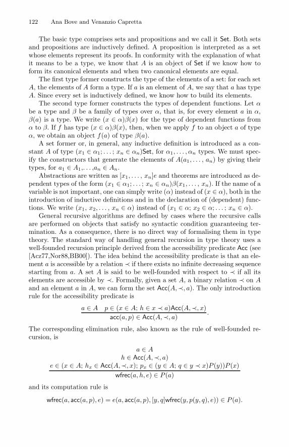
122 Ana Bove and Venanzio Capretta
The basic type comprises sets and propositions and we call it Set. Both setsand propositions are inductively defined. A proposition is interpreted as a setwhose elements represent its proofs. In conformity with the explanation of whatit means to be a type, we know that A is an object of Set if we know how toform its canonical elements and when two canonical elements are equal.
The first type former constructs the type of the elements of a set: for each setA, the elements of A form a type. If a is an element of A, we say that a has typeA. Since every set is inductively defined, we know how to build its elements.
The second type former constructs the types of dependent functions. Let αbe a type and β be a family of types over α, that is, for every element a in α,β(a) is a type. We write (x ∈ α)β(x) for the type of dependent functions fromα to β. If f has type (x ∈ α)β(x), then, when we apply f to an object a of typeα, we obtain an object f(a) of type β(a).
A set former or, in general, any inductive definition is introduced as a con-stant A of type (x1 ∈ α1; . . . ; xn ∈ αn)Set, for α1, . . . , αn types. We must spec-ify the constructors that generate the elements of A(a1, . . . , an) by giving theirtypes, for a1 ∈ A1,. . . ,an ∈ An.
Abstractions are written as [x1, . . . , xn]e and theorems are introduced as de-pendent types of the form (x1 ∈ α1; . . . ; xn ∈ αn)β(x1, . . . , xn). If the name of avariable is not important, one can simply write (α) instead of (x ∈ α), both in theintroduction of inductive definitions and in the declaration of (dependent) func-tions. We write (x1, x2, . . . , xn ∈ α) instead of (x1 ∈ α; x2 ∈ α; . . . ; xn ∈ α).
General recursive algorithms are defined by cases where the recursive callsare performed on objects that satisfy no syntactic condition guaranteeing ter-mination. As a consequence, there is no direct way of formalising them in typetheory. The standard way of handling general recursion in type theory uses awell-founded recursion principle derived from the accessibility predicate Acc (see[Acz77,Nor88,BB00]). The idea behind the accessibility predicate is that an ele-ment a is accessible by a relation ≺ if there exists no infinite decreasing sequencestarting from a. A set A is said to be well-founded with respect to ≺ if all itselements are accessible by ≺. Formally, given a set A, a binary relation ≺ on Aand an element a in A, we can form the set Acc(A,≺, a). The only introductionrule for the accessibility predicate is
a ∈ A p ∈ (x ∈ A; h ∈ x ≺ a)Acc(A,≺, x)acc(a, p) ∈ Acc(A,≺, a) .
The corresponding elimination rule, also known as the rule of well-founded re-cursion, is
a ∈ Ah ∈ Acc(A,≺, a)
e ∈ (x ∈ A; hx ∈ Acc(A,≺, x); px ∈ (y ∈ A; q ∈ y ≺ x)P (y))P (x)wfrec(a, h, e) ∈ P (a)
and its computation rule is
wfrec(a, acc(a, p), e) = e(a, acc(a, p), [y, q]wfrec(y, p(y, q), e)) ∈ P (a).
Nested General Recursion and Partiality in Type Theory 123
Hence, to guarantee that a general recursive algorithm that performs therecursive calls on elements of type A terminates, we have to prove that A iswell-founded and that the arguments supplied to the recursive calls are smallerthan the input.
Since Acc is a general predicate, it gives no information that can help usin the formalisation of a specific recursive algorithm. As a consequence, its usein the formalisation of general recursive algorithms often results in long andcomplicated code. On the other hand, functional programming languages likeHaskell [JHe+99] impose no restrictions on recursive programs; therefore, writinggeneral recursive algorithms in Haskell is straightforward. In addition, functionalprograms are usually short and self-explanatory. However, there is no powerfulframework to reason about the correctness of Haskell-like programs.
Bove [Bov01] introduces a method to formalise simple general recursive al-gorithms in type theory (by simple we mean non-nested and non-mutually re-cursive) in a clear and compact way. We believe that this technique helps toclose the gap between programming in a functional language and programmingin type theory.
This work is similar to that of Paulson in [Pau86]. He defines an orderingassociated with the recursive steps of an algorithm, such that the inputs onwhich the algorithm terminates are the objects accessible by the order. Then hedefines the algorithm by induction on the order. The proof of termination forthe algorithm reduces to a proof that the order is wellfounded. Bove’s idea is atranslation of this in the framework of type theory in a way more convenient thanthe straightforward translation. Given the Haskell version of an algorithm f alg,the method in [Bov01] uses an inductive special-purpose accessibility predicatecalled fAcc. We construct this predicate directly from f alg, and we regard itas a characterization of the collection of inputs on which f alg terminates. Ithas an introduction rule for each case in the algorithm and provides a syntacticcondition that guarantees termination. In this way, we can formalise f alg in typetheory by structural recursion on the proof that the input of f alg satisfies fAcc,obtaining a compact and readable formalisation of the algorithm.
However, the technique in [Bov01] cannot be immediately applied to nestedrecursive algorithms. Here, we present a method for formalising nested recursivealgorithms in type theory in a similar way to the one used in [Bov01]. Thus,we obtain short and clear formalisations of nested recursive algorithms in typetheory. This technique uses the schema for simultaneous inductive-recursive def-initions presented by Dybjer in [Dyb00]; hence, it can be used only in typetheories extended with such schema.
The rest of the paper is organised as follows. In section 2, we illustrate themethod used in [Bov01] on a simple example. In addition, we point out theadvantages of this technique over the standard way of defining general recursivealgorithms in type theory by using the predicate Acc. In section 3, we adaptthe method to nested recursive algorithms, using Dybjer’s schema. In section 4,we show how the method can be put to use also in the formalisation of partialfunctions. Finally, in section 5, we present some conclusions and related work.
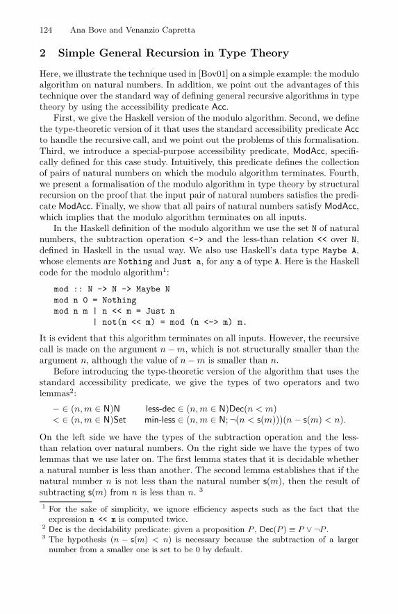
124 Ana Bove and Venanzio Capretta
2 Simple General Recursion in Type Theory
Here, we illustrate the technique used in [Bov01] on a simple example: the moduloalgorithm on natural numbers. In addition, we point out the advantages of thistechnique over the standard way of defining general recursive algorithms in typetheory by using the accessibility predicate Acc.
First, we give the Haskell version of the modulo algorithm. Second, we definethe type-theoretic version of it that uses the standard accessibility predicate Accto handle the recursive call, and we point out the problems of this formalisation.Third, we introduce a special-purpose accessibility predicate, ModAcc, specifi-cally defined for this case study. Intuitively, this predicate defines the collectionof pairs of natural numbers on which the modulo algorithm terminates. Fourth,we present a formalisation of the modulo algorithm in type theory by structuralrecursion on the proof that the input pair of natural numbers satisfies the predi-cate ModAcc. Finally, we show that all pairs of natural numbers satisfy ModAcc,which implies that the modulo algorithm terminates on all inputs.
In the Haskell definition of the modulo algorithm we use the set N of naturalnumbers, the subtraction operation <-> and the less-than relation << over N,defined in Haskell in the usual way. We also use Haskell’s data type Maybe A,whose elements are Nothing and Just a, for any a of type A. Here is the Haskellcode for the modulo algorithm1:
mod :: N -> N -> Maybe Nmod n 0 = Nothingmod n m | n << m = Just n
| not(n << m) = mod (n <-> m) m.
It is evident that this algorithm terminates on all inputs. However, the recursivecall is made on the argument n−m, which is not structurally smaller than theargument n, although the value of n−m is smaller than n.
Before introducing the type-theoretic version of the algorithm that uses thestandard accessibility predicate, we give the types of two operators and twolemmas2:
− ∈ (n,m ∈ N)N less-dec ∈ (n,m ∈ N)Dec(n < m)< ∈ (n,m ∈ N)Set min-less ∈ (n,m ∈ N;¬(n < s(m)))(n− s(m) < n).
On the left side we have the types of the subtraction operation and the less-than relation over natural numbers. On the right side we have the types of twolemmas that we use later on. The first lemma states that it is decidable whethera natural number is less than another. The second lemma establishes that if thenatural number n is not less than the natural number s(m), then the result ofsubtracting s(m) from n is less than n. 3
1 For the sake of simplicity, we ignore efficiency aspects such as the fact that theexpression n << m is computed twice.
2 Dec is the decidability predicate: given a proposition P , Dec(P ) ≡ P ∨ ¬P .3 The hypothesis (n − s(m) < n) is necessary because the subtraction of a largernumber from a smaller one is set to be 0 by default.
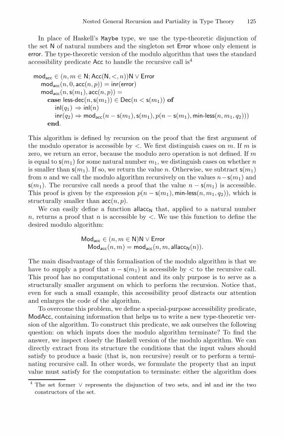
Nested General Recursion and Partiality in Type Theory 125
In place of Haskell’s Maybe type, we use the type-theoretic disjunction ofthe set N of natural numbers and the singleton set Error whose only element iserror. The type-theoretic version of the modulo algorithm that uses the standardaccessibility predicate Acc to handle the recursive call is4
modacc ∈ (n,m ∈ N;Acc(N, <, n))N ∨ Errormodacc(n, 0, acc(n, p)) = inr(error)modacc(n, s(m1), acc(n, p)) =
case less-dec(n, s(m1)) ∈ Dec(n < s(m1)) ofinl(q1) ⇒ inl(n)inr(q2)⇒ modacc(n− s(m1), s(m1), p(n− s(m1),min-less(n,m1, q2)))
end.
This algorithm is defined by recursion on the proof that the first argument ofthe modulo operator is accessible by <. We first distinguish cases on m. If m iszero, we return an error, because the modulo zero operation is not defined. If mis equal to s(m1) for some natural number m1, we distinguish cases on whether nis smaller than s(m1). If so, we return the value n. Otherwise, we subtract s(m1)from n and we call the modulo algorithm recursively on the values n−s(m1) ands(m1). The recursive call needs a proof that the value n − s(m1) is accessible.This proof is given by the expression p(n − s(m1),min-less(n,m1, q2)), which isstructurally smaller than acc(n, p).
We can easily define a function allaccN that, applied to a natural numbern, returns a proof that n is accessible by <. We use this function to define thedesired modulo algorithm:
Modacc ∈ (n,m ∈ N)N ∨ ErrorModacc(n,m) = modacc(n,m, allaccN(n)).
The main disadvantage of this formalisation of the modulo algorithm is that wehave to supply a proof that n − s(m1) is accessible by < to the recursive call.This proof has no computational content and its only purpose is to serve as astructurally smaller argument on which to perform the recursion. Notice that,even for such a small example, this accessibility proof distracts our attentionand enlarges the code of the algorithm.
To overcome this problem, we define a special-purpose accessibility predicate,ModAcc, containing information that helps us to write a new type-theoretic ver-sion of the algorithm. To construct this predicate, we ask ourselves the followingquestion: on which inputs does the modulo algorithm terminate? To find theanswer, we inspect closely the Haskell version of the modulo algorithm. We candirectly extract from its structure the conditions that the input values shouldsatisfy to produce a basic (that is, non recursive) result or to perform a termi-nating recursive call. In other words, we formulate the property that an inputvalue must satisfy for the computation to terminate: either the algorithm does
4 The set former ∨ represents the disjunction of two sets, and inl and inr the twoconstructors of the set.
126 Ana Bove and Venanzio Capretta
not perform any recursive call, or the values on which the recursive calls areperformed have themselves the property. We distinguish three cases:
– if the input numbers are n and zero, then the algorithm terminates;– if the input number n is less than the input number m, then the algorithmterminates;
– if the number n is not less than the number m and m is not zero5, then thealgorithm terminates on the inputs n and m if it terminates on the inputsn−m and m.
Following this description, we define the inductive predicate ModAcc overpairs of natural numbers by the introduction rules (for n andm natural numbers)
ModAcc(n, 0),
n < m
ModAcc(n,m),¬(m = 0) ¬(n < m) ModAcc(n−m,m)
ModAcc(n,m).
This predicate can easily be formalised in type theory:
ModAcc ∈ (n,m ∈ N)Setmodacc0 ∈ (n ∈ N)ModAcc(n, 0)modacc< ∈ (n,m ∈ N;n < m)ModAcc(n,m)modacc≥ ∈ (n,m ∈ N;¬(m = 0);¬(n < m);ModAcc(n−m,m))
ModAcc(n,m).
We now use this predicate to formalise the modulo algorithm in type theory:
mod ∈ (n,m ∈ N;ModAcc(n,m))N ∨ Errormod(n, 0,modacc0(n)) = inr(error)mod(n,m,modacc<(n,m, q)) = inl(n)mod(n,m,modacc≥(n,m, q1, q2, h)) = mod(n−m,m, h).
This algorithm is defined by structural recursion on the proof that the inputpair of numbers satisfies the predicate ModAcc. The first two equations arestraightforward. The last equation considers the case where n is not less thanm; here q1 is a proof that m is different from zero, q2 is a proof that n is not lessthan m and h is a proof that the pair (n−m, m) satisfies the predicateModAcc.In this case, we call the algorithm recursively on the values n−m and m. Wehave to supply a proof that the pair (n−m, m) satisfies the predicate ModAccto the recursive call, which is given by the argument h.
To prove that the modulo algorithm terminates on all inputs, we use theauxiliary lemma modaccaux. Given a natural number m, this lemma provesModAcc(i,m), for i an accessible natural number, from the assumption thatModAcc(j,m) holds for every natural number j smaller than i. The proof pro-ceeds by case analysis on m and, when m is equal to s(m1) for some natural
5 Observe that this condition is not needed in the Haskell version of the algorithm dueto the order in which Haskell processes the equations that define an algorithm.
Nested General Recursion and Partiality in Type Theory 127
number m1, by cases on whether i is smaller than s(m1). The term nots0(m1) isa proof that s(m1) is different from 0.
modaccaux ∈ (m, i ∈ N;Acc(N, <, i); f ∈ (j ∈ N; j < i)ModAcc(j,m))ModAcc(i,m)
modaccaux(0, i, h, f) = modacc0(i)modaccaux(s(m1), i, h, f) =
case less-dec(i, s(m1)) ∈ Dec(i < s(m1)) ofinl(q1) ⇒ modacc<(i, s(m1), q1)inr(q2)⇒ modacc≥(i, s(m1), nots0(m1), q2,
f(i− s(m1),min-less(i,m1, q2)))end
Now, we prove that the modulo algorithm terminates on all inputs, that is, weprove that all pairs of natural numbers satisfy ModAcc6:
allModAcc ∈ (n,m ∈ N)ModAcc(n,m)allModAcc(n,m) = wfrec(n, allaccN(n),modaccaux(m)).
Notice that the skeleton of the proof of the function modaccaux is very similarto the skeleton of the algorithm modacc.
Finally, we can use the previous function to write the final modulo algorithm:
Mod ∈ (n,m ∈ N)N ∨ ErrorMod(n,m) = mod(n,m, allModAcc(n,m)).
Observe that, even for such a small example, the version of the algorithmthat uses our special predicate is slightly shorter and more readable than thetype-theoretic version of the algorithm that is defined by using the predicateAcc. Notice also that we were able to move the non-computational parts fromthe code of modacc into the proof that the predicateModAcc holds for all possibleinputs, thus separating the actual algorithm from the proof of its termination.
We hope that, by now, the reader is quite familiar with our notation. So, inthe following sections, we will not explain the type-theoretic codes in detail.
3 Nested Recursion in Type Theory
The technique we have just described to formalise simple general recursion can-not be applied to nested general recursive algorithms in a straightforward way.We illustrate the problem on a simple nested recursive algorithm over naturalnumbers. Its Haskell definition is
nest :: N -> Nnest 0 = 0nest (S n) = nest(nest n).
6 Here, we use the general recursor wfrec with the elimination predicate P (n) ≡ModAcc(n, m).
128 Ana Bove and Venanzio Capretta
Clearly, this is a total algorithm returning 0 on every input.If we want to use the technique described in the previous section to formalise
this algorithm, we need to define an inductive special-purpose accessibility pred-icate NestAcc over the natural numbers. To construct NestAcc, we ask ourselvesthe following question: on which inputs does the nest algorithm terminate? Byinspecting the Haskell version of the nest algorithm, we distinguish two cases:
– if the input number is 0, then the algorithm terminates;– if the input number is s(n) for some natural number n, then the algorithmterminates if it terminates on the inputs n and nest(n).
Following this description, we define the inductive predicate NestAcc overnatural numbers by the introduction rules (for n natural number)
NestAcc(0),
NestAcc(n) NestAcc(nest(n))NestAcc(s(n))
.
Unfortunately, this definition is not correct since nest is not yet defined. More-over, the purpose of defining the predicate NestAcc is to be able to define thealgorithm nest by structural recursion on the proof that its input value satisfiesNestAcc. Hence, the definitions of NestAcc and nest are locked in a vicious circle.
However, there is an extension of type theory that gives us the means to definethe predicate NestAcc inductively generated by two constructors correspondingto the two introduction rules of the previous paragraph. This extension has beenintroduced by Dybjer in [Dyb00] and it allows the simultaneous definition of aninductive predicate P and a function f , where f has the predicate P as part ofits domain and is defined by recursion on P . In our case, given the input valuen, nest requires an argument of type NestAcc(n). Using Dybjer’s schema, we cansimultaneously define NestAcc and nest:
NestAcc ∈ (n ∈ N)Setnest ∈ (n ∈ N;NestAcc(n))N
nestacc0 ∈ NestAcc(0)nestaccs ∈ (n ∈ N;h1 ∈ NestAcc(n);h2 ∈ NestAcc(nest(n, h1)))
NestAcc(s(n))
nest(0, nestacc0) = 0nest(s(n), nestaccs(n, h1, h2)) = nest(nest(n, h1), h2).
This definition may at first look circular: the type of nest requires that thepredicate NestAcc is defined, while the type of the constructor nestaccs of thepredicate NestAcc requires that nest is defined. However, we can see that it isnot so by analysing how the elements in NestAcc and the values of nest aregenerated. First of all, NestAcc(0) is well defined because it does not depend onany assumption and its only element is nestacc0. Once NestAcc(0) is defined,the result of nest on the inputs 0 and nestacc0 becomes defined and its value is0. Now, we can apply the constructor nestaccs to the arguments n = 0, h1 =
Nested General Recursion and Partiality in Type Theory 129
nestacc0 and h2 = nestacc0. This application is well typed since h2 must bean element in NestAcc(nest(0, nestacc0)), that is, NestAcc(0). At this point, wecan compute the value of nest(s(0), nestaccs(0, nestacc0, nestacc0)) and obtainthe value zero7, and so on. Circularity is avoided because the values of nest canbe computed at the moment a new proof of the predicate NestAcc is generated;in turn, each constructor of NestAcc calls nest only on those arguments thatappear previously in its assumptions, for which we can assume that nest hasalready been computed.
The next step consists in proving that the predicate NestAcc is satisfied byall natural numbers:
allNestAcc ∈ (n ∈ N)NestAcc(n).
This can be done by first proving that, given a natural number n and a proofh of NestAcc(n), nest(n, h) ≤ n (by structural recursion on h), and then usingwell-founded recursion on the set of natural numbers.
Now, we define Nest as a function from natural numbers to natural numbers:
Nest ∈ (n ∈ N)NNest(n) = nest(n, allNestAcc(n)).
Notice that by making the simultaneous definition of NestAcc and nest wecan treat nested recursion similarly to how we treat simple recursion. In thisway, we obtain a short and clear formalisation of the nest algorithm.
To illustrate our technique for nested general recursive algorithms in moreinteresting situations, we present a slightly more complicated example: Paulson’snormalisation function for conditional expressions [Pau86]. Its Haskell definitionis
data CExp = At | If CExp CExp CExp
nm :: CExp -> CExpnm At = Atnm (If At y z) = If At (nm y) (nm z)nm (If (If u v w) y z)= nm (If u (nm (If v y z)) (nm (If w y z))).
To define the special-purpose accessibility predicate, we study the differentequations in the Haskell version of the algorithm, putting the emphasis on theinput expressions and the expressions on which the recursive calls are performed.We obtain the following introduction rules for the inductive predicate nmAcc (fory, z, u, v and w conditional expressions):
nmAcc(At),
nmAcc(y) nmAcc(z)nmAcc(If(At, y, z))
,
nmAcc(If(v, y, z))nmAcc(If(w, y, z))
nmAcc(If(u, nm(If(v, y, z)), nm(If(w, y, z))))nmAcc(If(If(u, v, w), y, z))
.
7 Since nest(s(0), nestaccs(0, nestacc0, nestacc0)) = nest(nest(0, nestacc0), nestacc0) =nest(0, nestacc0) = 0.
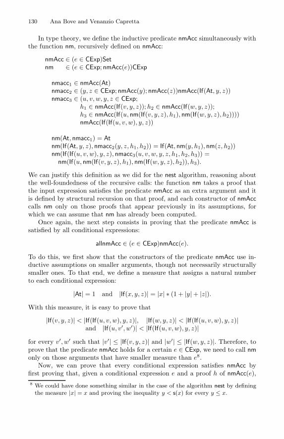
130 Ana Bove and Venanzio Capretta
In type theory, we define the inductive predicate nmAcc simultaneously withthe function nm, recursively defined on nmAcc:
nmAcc ∈ (e ∈ CExp)Setnm ∈ (e ∈ CExp; nmAcc(e))CExp
nmacc1 ∈ nmAcc(At)nmacc2 ∈ (y, z ∈ CExp; nmAcc(y); nmAcc(z))nmAcc(If(At, y, z))nmacc3 ∈ (u, v, w, y, z ∈ CExp;
h1 ∈ nmAcc(If(v, y, z));h2 ∈ nmAcc(If(w, y, z));h3 ∈ nmAcc(If(u, nm(If(v, y, z), h1), nm(If(w, y, z), h2))))nmAcc(If(If(u, v, w), y, z))
nm(At, nmacc1) = Atnm(If(At, y, z), nmacc2(y, z, h1, h2)) = If(At, nm(y, h1), nm(z, h2))nm(If(If(u, v, w), y, z), nmacc3(u, v, w, y, z, h1, h2, h3)) =
nm(If(u, nm(If(v, y, z), h1), nm(If(w, y, z), h2)), h3).
We can justify this definition as we did for the nest algorithm, reasoning aboutthe well-foundedness of the recursive calls: the function nm takes a proof thatthe input expression satisfies the predicate nmAcc as an extra argument and itis defined by structural recursion on that proof, and each constructor of nmAcccalls nm only on those proofs that appear previously in its assumptions, forwhich we can assume that nm has already been computed.
Once again, the next step consists in proving that the predicate nmAcc issatisfied by all conditional expressions:
allnmAcc ∈ (e ∈ CExp)nmAcc(e).
To do this, we first show that the constructors of the predicate nmAcc use in-ductive assumptions on smaller arguments, though not necessarily structurallysmaller ones. To that end, we define a measure that assigns a natural numberto each conditional expression:
|At| = 1 and |If(x, y, z)| = |x| ∗ (1 + |y|+ |z|).With this measure, it is easy to prove that
|If(v, y, z)| < |If(If(u, v, w), y, z)|, |If(w, y, z)| < |If(If(u, v, w), y, z)|and |If(u, v′, w′)| < |If(If(u, v, w), y, z)|
for every v′, w′ such that |v′| ≤ |If(v, y, z)| and |w′| ≤ |If(w, y, z)|. Therefore, toprove that the predicate nmAcc holds for a certain e ∈ CExp, we need to call nmonly on those arguments that have smaller measure than e8.
Now, we can prove that every conditional expression satisfies nmAcc byfirst proving that, given a conditional expression e and a proof h of nmAcc(e),8 We could have done something similar in the case of the algorithm nest by definingthe measure |x| = x and proving the inequality y < s(x) for every y ≤ x.

Nested General Recursion and Partiality in Type Theory 131
|nm(e, h)| ≤ |e| (by structural recursion on h), and then using well-founded re-cursion on the set of natural numbers.
We can then define NM as a function from conditional expressions to condi-tional expressions:
NM ∈ (e ∈ CExp)CExpNM(e) = nm(e, allnmAcc(e)).
4 Partial Functions in Type Theory
Until now we have applied our technique to total functions for which totalitycould not be proven easily by structural recursion. However, it can also be put touse in the formalisation of partial functions. A standard way to formalise partialfunctions in type theory is to define them as relations rather than objects ofa function type. For example, the minimization operator for natural numbers,which takes a function f ∈ (N)N as input and gives the least n ∈ N such thatf(n) = 0 as output, cannot be represented as an object of type ((N)N)N becauseit does not terminate on all inputs. A standard representation of this operatorin type theory is the inductive relation
µ ∈ (f ∈ (N)N;n ∈ N)Setµ0 ∈ (f ∈ (N)N; f(0) = 0)µ(f, 0)µ1 ∈ (f ∈ (N)N; f(0) = 0;n ∈ N;µ([m]f(s(m)), n))µ(f, s(n)).
The relation µ represents the graph of the minimization operator. If we indi-cate the minimization function by min, then µ(f, n) is inhabited if and only ifmin(f) = n. The fact that min may be undefined on some function f is expressedby µ(f, n) being empty for every natural number n.
There are reasons to be unhappy with this approach. First, for a relation toreally define a partial function, we must prove that it is univocal: in our case,that for all n,m ∈ N, if µ(f, n) and µ(f,m) are both nonempty then n = m.Second, there is no computational content in this representation, that is, wecannot actually compute the value of min(f) for any f .
Let us try to apply our technique to this example and start with the Haskelldefinition of min:
min :: (N -> N) -> Nmin f | f 0 == 0 = 0
| f 0 /= 0 = s (min (\m -> f (s m))).
We observe that the computation of min on the input f terminates if f(0) = 0or if f(0) = 0 and min terminates on the input [m]f(s(m)). This leads to theinductive definition of the special predicate minAcc on functions defined by theintroduction rules (for f a function from natural numbers to natural numbersand m a natural number)
f(0) = 0minAcc(f)
,f(0) = 0 minAcc([m]f(s(m)))
minAcc(f).
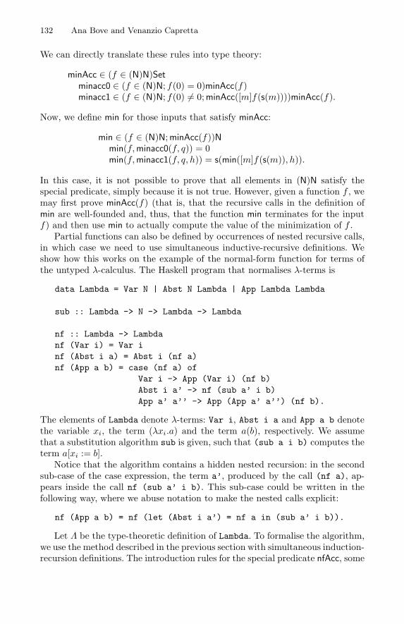
132 Ana Bove and Venanzio Capretta
We can directly translate these rules into type theory:
minAcc ∈ (f ∈ (N)N)Setminacc0 ∈ (f ∈ (N)N; f(0) = 0)minAcc(f)minacc1 ∈ (f ∈ (N)N; f(0) = 0;minAcc([m]f(s(m))))minAcc(f).
Now, we define min for those inputs that satisfy minAcc:
min ∈ (f ∈ (N)N;minAcc(f))Nmin(f,minacc0(f, q)) = 0min(f,minacc1(f, q, h)) = s(min([m]f(s(m)), h)).
In this case, it is not possible to prove that all elements in (N)N satisfy thespecial predicate, simply because it is not true. However, given a function f , wemay first prove minAcc(f) (that is, that the recursive calls in the definition ofmin are well-founded and, thus, that the function min terminates for the inputf) and then use min to actually compute the value of the minimization of f .
Partial functions can also be defined by occurrences of nested recursive calls,in which case we need to use simultaneous inductive-recursive definitions. Weshow how this works on the example of the normal-form function for terms ofthe untyped λ-calculus. The Haskell program that normalises λ-terms is
data Lambda = Var N | Abst N Lambda | App Lambda Lambda
sub :: Lambda -> N -> Lambda -> Lambda
nf :: Lambda -> Lambdanf (Var i) = Var inf (Abst i a) = Abst i (nf a)nf (App a b) = case (nf a) of
Var i -> App (Var i) (nf b)Abst i a’ -> nf (sub a’ i b)App a’ a’’ -> App (App a’ a’’) (nf b).
The elements of Lambda denote λ-terms: Var i, Abst i a and App a b denotethe variable xi, the term (λxi.a) and the term a(b), respectively. We assumethat a substitution algorithm sub is given, such that (sub a i b) computes theterm a[xi := b].
Notice that the algorithm contains a hidden nested recursion: in the secondsub-case of the case expression, the term a’, produced by the call (nf a), ap-pears inside the call nf (sub a’ i b). This sub-case could be written in thefollowing way, where we abuse notation to make the nested calls explicit:
nf (App a b) = nf (let (Abst i a’) = nf a in (sub a’ i b)).
Let Λ be the type-theoretic definition of Lambda. To formalise the algorithm,we use the method described in the previous section with simultaneous induction-recursion definitions. The introduction rules for the special predicate nfAcc, some
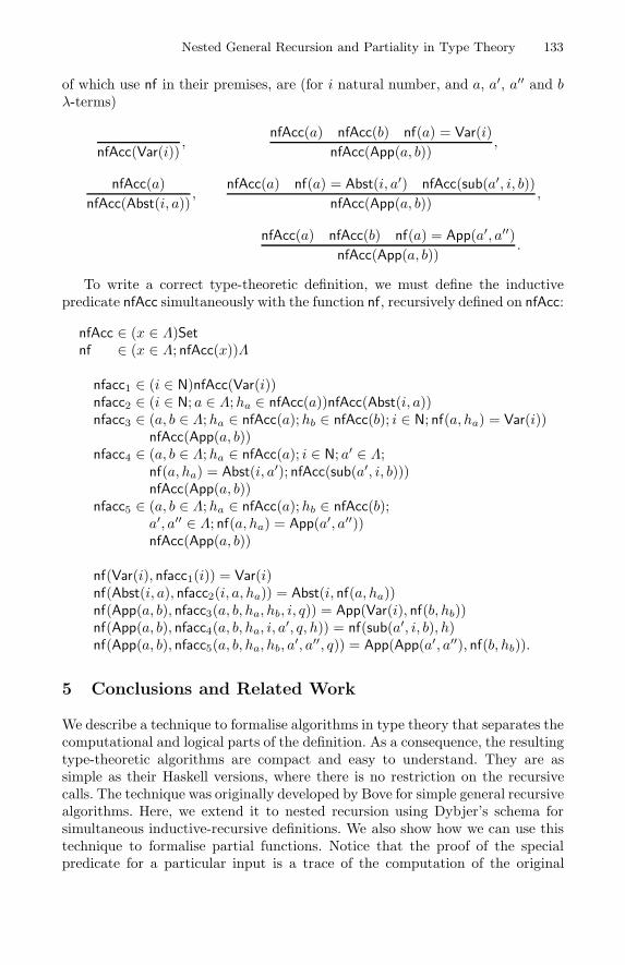
Nested General Recursion and Partiality in Type Theory 133
of which use nf in their premises, are (for i natural number, and a, a′, a′′ and bλ-terms)
nfAcc(Var(i)),
nfAcc(a) nfAcc(b) nf(a) = Var(i)nfAcc(App(a, b))
,
nfAcc(a)nfAcc(Abst(i, a))
,nfAcc(a) nf(a) = Abst(i, a′) nfAcc(sub(a′, i, b))
nfAcc(App(a, b)),
nfAcc(a) nfAcc(b) nf(a) = App(a′, a′′)nfAcc(App(a, b))
.
To write a correct type-theoretic definition, we must define the inductivepredicate nfAcc simultaneously with the function nf, recursively defined on nfAcc:
nfAcc ∈ (x ∈ Λ)Setnf ∈ (x ∈ Λ; nfAcc(x))Λ
nfacc1 ∈ (i ∈ N)nfAcc(Var(i))nfacc2 ∈ (i ∈ N; a ∈ Λ;ha ∈ nfAcc(a))nfAcc(Abst(i, a))nfacc3 ∈ (a, b ∈ Λ;ha ∈ nfAcc(a);hb ∈ nfAcc(b); i ∈ N; nf(a, ha) = Var(i))
nfAcc(App(a, b))nfacc4 ∈ (a, b ∈ Λ;ha ∈ nfAcc(a); i ∈ N; a′ ∈ Λ;
nf(a, ha) = Abst(i, a′); nfAcc(sub(a′, i, b)))nfAcc(App(a, b))
nfacc5 ∈ (a, b ∈ Λ;ha ∈ nfAcc(a);hb ∈ nfAcc(b);a′, a′′ ∈ Λ; nf(a, ha) = App(a′, a′′))nfAcc(App(a, b))
nf(Var(i), nfacc1(i)) = Var(i)nf(Abst(i, a), nfacc2(i, a, ha)) = Abst(i, nf(a, ha))nf(App(a, b), nfacc3(a, b, ha, hb, i, q)) = App(Var(i), nf(b, hb))nf(App(a, b), nfacc4(a, b, ha, i, a
′, q, h)) = nf(sub(a′, i, b), h)nf(App(a, b), nfacc5(a, b, ha, hb, a
′, a′′, q)) = App(App(a′, a′′), nf(b, hb)).
5 Conclusions and Related Work
We describe a technique to formalise algorithms in type theory that separates thecomputational and logical parts of the definition. As a consequence, the resultingtype-theoretic algorithms are compact and easy to understand. They are assimple as their Haskell versions, where there is no restriction on the recursivecalls. The technique was originally developed by Bove for simple general recursivealgorithms. Here, we extend it to nested recursion using Dybjer’s schema forsimultaneous inductive-recursive definitions. We also show how we can use thistechnique to formalise partial functions. Notice that the proof of the specialpredicate for a particular input is a trace of the computation of the original
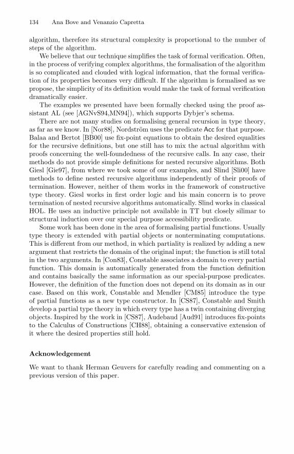
134 Ana Bove and Venanzio Capretta
algorithm, therefore its structural complexity is proportional to the number ofsteps of the algorithm.
We believe that our technique simplifies the task of formal verification. Often,in the process of verifying complex algorithms, the formalisation of the algorithmis so complicated and clouded with logical information, that the formal verifica-tion of its properties becomes very difficult. If the algorithm is formalised as wepropose, the simplicity of its definition would make the task of formal verificationdramatically easier.
The examples we presented have been formally checked using the proof as-sistant ALF (see [AGNvS94,MN94]), which supports Dybjer’s schema.
There are not many studies on formalising general recursion in type theory,as far as we know. In [Nor88], Nordstrom uses the predicate Acc for that purpose.Balaa and Bertot [BB00] use fix-point equations to obtain the desired equalitiesfor the recursive definitions, but one still has to mix the actual algorithm withproofs concerning the well-foundedness of the recursive calls. In any case, theirmethods do not provide simple definitions for nested recursive algorithms. BothGiesl [Gie97], from where we took some of our examples, and Slind [Sli00] havemethods to define nested recursive algorithms independently of their proofs oftermination. However, neither of them works in the framework of constructivetype theory. Giesl works in first order logic and his main concern is to provetermination of nested recursive algorithms automatically. Slind works in classicalHOL. He uses an inductive principle not available in TT but closely silimar tostructural induction over our special purpose accessibility predicate.
Some work has been done in the area of formalising partial functions. Usuallytype theory is extended with partial objects or nonterminating computations.This is different from our method, in which partiality is realized by adding a newargument that restricts the domain of the original input; the function is still totalin the two arguments. In [Con83], Constable associates a domain to every partialfunction. This domain is automatically generated from the function definitionand contains basically the same information as our special-purpose predicates.However, the definition of the function does not depend on its domain as in ourcase. Based on this work, Constable and Mendler [CM85] introduce the typeof partial functions as a new type constructor. In [CS87], Constable and Smithdevelop a partial type theory in which every type has a twin containing divergingobjects. Inspired by the work in [CS87], Audebaud [Aud91] introduces fix-pointsto the Calculus of Constructions [CH88], obtaining a conservative extension ofit where the desired properties still hold.
Acknowledgement
We want to thank Herman Geuvers for carefully reading and commenting on aprevious version of this paper.
Nested General Recursion and Partiality in Type Theory 135
References
[Acz77] P. Aczel. An Introduction to Inductive Definitions. In J. Barwise, editor,Handbook of Mathematical Logic, pages 739–782. North-Holland PublishingCompany, 1977.
[AGNvS94] T. Altenkirch, V. Gaspes, B. Nordstrom, and B. von Sydow. A User’sGuide to ALF. Chalmers University of Technology, Sweden, May 1994.Available on the WWWftp://ftp.cs.chalmers.se/pub/users/alti/alf.ps.Z.
[Aud91] P. Audebaud. Partial Objects in the Calculus of Constructions. In 6thAnnual IEEE Symposium on Logic in Computer Science, Amsterdam, pages86–95, July 1991.
[BB00] Antonia Balaa and Yves Bertot. Fix-point equations for well-founded re-cursion in type theory. In Harrison and Aagaard [HA00], pages 1–16.
[Bov01] A. Bove. Simple general recursion in type theory. Nordic Journal of Com-puting, 8(1):22–42, Spring 2001.
[CH88] Thierry Coquand and Gerard Huet. The Calculus of Constructions. Infor-mation and Computation, 76:95–120, 1988.
[CM85] R. L. Constable and N. P. Mendler. Recursive Definitions in Type Theory.In Logic of Programs, Brooklyn, volume 193 of Lecture Notes in ComputerScience, pages 61–78. Springer-Verlag, June 1985.
[Con83] R. L. Constable. Partial Functions in Constructive Type Theory. In The-oretical Computer Science, 6th GI-Conference, Dortmund, volume 145 ofLecture Notes in Computer Science, pages 1–18. Springer-Verlag, January1983.
[CS87] R. L. Constable and S. F. Smith. Partial Objects in Constructive TypeTheory. In Logic in Computer Science, Ithaca, New York, pages 183–193,June 1987.
[Dyb00] Peter Dybjer. A general formulation of simultaneous inductive-recursivedefinitions in type theory. Journal of Symbolic Logic, 65(2), June 2000.
[Gie97] J. Giesl. Termination of nested and mutually recursive algorithms. Journalof Automated Reasoning, 19:1–29, 1997.
[HA00] J. Harrison and M. Aagaard, editors. Theorem Proving in Higher OrderLogics: 13th International Conference, TPHOLs 2000, volume 1869 of Lec-ture Notes in Computer Science. Springer-Verlag, 2000.
[JHe+99] Simon Peyton Jones, John Hughes, (editors), Lennart Augustsson, DaveBarton, Brian Boutel, Warren Burton, Joseph Fasel, Kevin Hammond, RalfHinze, Paul Hudak, Thomas Johnsson, Mark Jones, John Launchbury, ErikMeijer, John Peterson, Alastair Reid, Colin Runciman, and Philip Wadler.Report on the Programming Language Haskell 98, a Non-strict, PurelyFunctional Language. Available from http://haskell.org, February 1999.
[ML84] P. Martin-Lof. Intuitionistic Type Theory. Bibliopolis, Napoli, 1984.[MN94] L. Magnusson and B. Nordstrom. The ALF proof editor and its proof
engine. In Types for Proofs and Programs, volume 806 of LNCS, pages213–237, Nijmegen, 1994. Springer-Verlag.
[Nor88] B. Nordstrom. Terminating General Recursion. BIT, 28(3):605–619, Oc-tober 1988.
[Pau86] L. C. Paulson. Proving Termination of Normalization Functions for Con-ditional Expressions. Journal of Automated Reasoning, 2:63–74, 1986.
[Sli00] K. Slind. Another look at nested recursion. In Harrison and Aagaard[HA00], pages 498–518.
A Higher-Order Calculus for Categories
Mario Caccamo� and Glynn Winskel
Computer Laboratory, University of Cambridge{Mario.Caccamo,Glynn.Winskel}@cl.cam.ac.uk
Abstract A calculus for a fragment of category theory is presented. Thetypes in the language denote categories and the expressions functors. Thejudgements of the calculus systematise categorical arguments such as: anexpression is functorial in its free variables; two expressions are naturallyisomorphic in their free variables. There are special binders for limits andmore general ends. The rules for limits and ends support an algebraicmanipulation of universal constructions as opposed to a more traditionaldiagrammatic approach. Duality within the calculus and applications inproving continuity are discussed with examples. The calculus gives abasis for mechanising a theory of categories in a generic theorem proverlike Isabelle.
1 Introduction
A language for category theory [11] together with a calculus to derive naturalisomorphisms are presented. We systematise categorical judgements of the kind:an expression is functorial in its free variables; there is an isomorphism betweentwo expressions natural in their free variables. The resulting logic gives the foun-dations for a mechanisation of category theory in a generic theorem prover likeIsabelle [15].
The language is based on the simply typed λ-calculus [2] where types denotecategories and expressions functors between categories. We introduce constants,for hom-sets, for example, and binders for ends and coends. Ends are a generali-sation of limits and play a central role in the calculus in increasing its expressivepower.
The rules of the calculus enable a mechanical manipulation of formulae withends and their dual coends. This gives a more calculational approach to cate-gories than is usual, and less dependence on diagrams. This approach suppliestools for proving preservation of limits and colimits.
One motivation behind this work is the increasing use of the machinery ofcategory theory in denotational semantics. There categories are often seen as gen-eralised domains. An application of special interest to us is the use of presheafcategories as models for concurrency. A central result there is that functions be-tween presheaf categories which preserve colimits, a form of continuity, preserveopen-map bisimulation [9] (see [7] for details).
� PhD student at BRICS, Centre of the Danish National Research Foundation.
R.J. Boulton and P.B. Jackson (Eds.): TPHOLs 2001, LNCS 2152, pp. 136–153, 2001.c© Springer-Verlag Berlin Heidelberg 2001
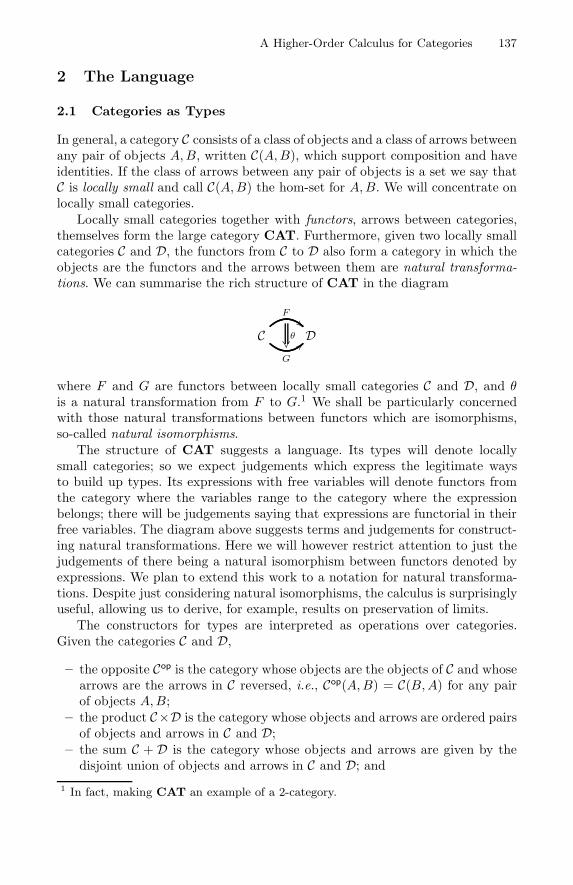
A Higher-Order Calculus for Categories 137
2 The Language
2.1 Categories as Types
In general, a category C consists of a class of objects and a class of arrows betweenany pair of objects A,B, written C(A,B), which support composition and haveidentities. If the class of arrows between any pair of objects is a set we say thatC is locally small and call C(A,B) the hom-set for A,B. We will concentrate onlocally small categories.
Locally small categories together with functors, arrows between categories,themselves form the large category CAT. Furthermore, given two locally smallcategories C and D, the functors from C to D also form a category in which theobjects are the functors and the arrows between them are natural transforma-tions. We can summarise the rich structure of CAT in the diagram
CF
��
G
���D
where F and G are functors between locally small categories C and D, and θis a natural transformation from F to G.1 We shall be particularly concernedwith those natural transformations between functors which are isomorphisms,so-called natural isomorphisms.
The structure of CAT suggests a language. Its types will denote locallysmall categories; so we expect judgements which express the legitimate waysto build up types. Its expressions with free variables will denote functors fromthe category where the variables range to the category where the expressionbelongs; there will be judgements saying that expressions are functorial in theirfree variables. The diagram above suggests terms and judgements for construct-ing natural transformations. Here we will however restrict attention to just thejudgements of there being a natural isomorphism between functors denoted byexpressions. We plan to extend this work to a notation for natural transforma-tions. Despite just considering natural isomorphisms, the calculus is surprisinglyuseful, allowing us to derive, for example, results on preservation of limits.
The constructors for types are interpreted as operations over categories.Given the categories C and D,
– the opposite Cop is the category whose objects are the objects of C and whosearrows are the arrows in C reversed, i.e., Cop(A,B) = C(B,A) for any pairof objects A,B;
– the product C×D is the category whose objects and arrows are ordered pairsof objects and arrows in C and D;
– the sum C + D is the category whose objects and arrows are given by thedisjoint union of objects and arrows in C and D; and
1 In fact, making CAT an example of a 2-category.
138 Mario Caccamo and Glynn Winskel
– the functor category [C,D] is the category of functors from C to D and thenatural transformation between them.
Observe that a functor category built out of locally small categories is not nec-essarily locally small (Crole discusses this point in [8, page 61]). We constrainthe use of functor categories [C,D] to the case where C is small. A locally smallcategory is small when the collection of objects is a set. Simple examples of smallcategories are 0 and 1, the empty and singleton categories respectively. We writeC,D, I, J, · · · for small categories.
The syntax for types as locally small categories is
C ::= Set | 0 | 1 | Cop | C1 × C2 | C1 + C2 | [C, C] .Thus, for the language locally small category and type are synonymous.
2.2 Syntax for Expressions
The expressions E1, E2, · · · are defined by
E ::=X | 1 | λX.E | E1(E2) | C(E1, E2) | (E1, E2) |fst(E) | snd(E) | inl(E) | inr(E) | caseC+D(E1, E2, E3) |E1 × E2 | E1 + E2 |
∫X∈Cop,Y ∈C
E | ∫ X∈Cop,Y ∈C
E
where C, D and C are types, and X is drawn from a countably infinite set ofvariables. The constant 1 stands for the singleton set.
The syntax is that of the typed λ-calculus with products and sums. The“integral” binders denote ends and coends. Ends extend the concept of limit tofunctors of mixed variance with domain of the form C
op × C. The treatmentof ends given in this work supports a mechanical manipulation of these binderswhose properties resemble the properties of the integral in mathematical anal-ysis. Ends are discussed later – they are a central notion of the language forcategories.
2.3 Functoriality
Not all possible expressions in the language give rise to functors. An exampleof a non-functorial expression is C(X,X) for a nontrivial category C; there is noaction over arrows matching the action over objects. Well-typed expressions inthe language represent those expressions functorial in their free variables.
The syntactic judgement X1 : C1, · · · , Xn : Cn � E : C says that the ex-pression E of type C is functorial in the free variables occurring in the contextX1 : C1, · · · , Xn : Cn; i.e. it denotes a functor from C1× . . .×Cn to C. In informalmathematical usage one says E(X1, · · · , Xn) is functorial in X1, · · · , Xn. Thus,an expression-in-context has two possible readings: as an object when the freevariables are interpreted as objects, and as an arrow when the free variables areinterpreted as arrows.
From the typing rules we derive well-typed expressions enforcing functoriality.One example is the rule for hom-expressions:
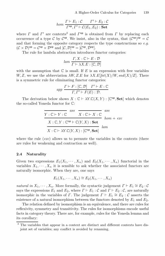
A Higher-Order Calculus for Categories 139
homΓ � E1 : C Γ ′ � E2 : CΓ op, Γ ′ � C(E1, E2) : Set
where Γ and Γ ′ are contexts2 and Γ op is obtained from Γ by replacing eachoccurrence of a type C by Cop. We insist, also in the syntax, that (Cop)op = Cand that forming the opposite category respects the type constructions so e.g.(C × D)op = Cop ×Dop and [C,D]op = [Cop,Dop].
The rule for lambda abstraction introduces functor categories:
lamΓ,X : C � E : DΓ � λX.E : [C,D]
with the assumption that C is small. If E is an expression with free variablesW,Z, we use the abbreviation λW,Z.E for λX.E[fst(X)/W, snd(X)/Z]. Thereis a symmetric rule for eliminating functor categories:
appΓ � F : [C,D] Γ ′ � E : C
Γ, Γ ′ � F (E) : D.The derivation below shows X : C � λY.C(X,Y ) : [Cop,Set] which denotes
the so-called Yoneda functor for C:
Y : C � Y : C
assX : C � X : C
ass
X : C, Y : Cop � C(Y,X) : Set
hom + exc
X : C � λY.C(Y,X) : [Cop,Set]lam
where the rule (exc) allows us to permute the variables in the contexts (thereare rules for weakening and contraction as well).
2.4 Naturality
Given two expressions E1(X1, · · · , Xn) and E2(X1, · · · , Xn) functorial in thevariables X1, · · · , Xn it is sensible to ask whether the associated functors arenaturally isomorphic. When they are, one says
E1(X1, · · · , Xn) ∼= E2(X1, · · · , Xn)
natural in X1, · · · , Xn. More formally, the syntactic judgement Γ � E1∼= E2 : C
says the expressions E1 and E2, where Γ � E1 : C and Γ � E2 : C, are naturallyisomorphic in the variables of Γ . The judgement Γ � E1
∼= E2 : C asserts theexistence of a natural isomorphism between the functors denoted by E1 and E2.
The relation defined by isomorphism is an equivalence, and there are rules forreflexivity, symmetry and transitivity. The rules for isomorphisms encode usefulfacts in category theory. There are, for example, rules for the Yoneda lemma andits corollary:2 The variables that appear in a context are distinct and different contexts have dis-joint set of variables; any conflict is avoided by renaming.
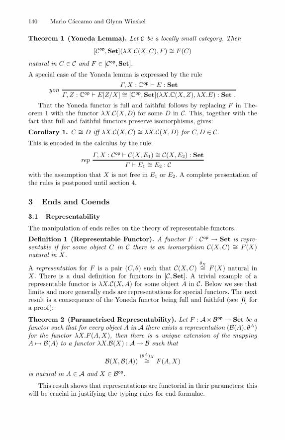
140 Mario Caccamo and Glynn Winskel
Theorem 1 (Yoneda Lemma). Let C be a locally small category. Then[Cop,Set](λX.C(X,C), F ) ∼= F (C)
natural in C ∈ C and F ∈ [Cop,Set].
A special case of the Yoneda lemma is expressed by the rule
yonΓ,X : C
op � E : Set
Γ,Z : Cop � E[Z/X ] ∼= [Cop,Set](λX.C(X,Z), λX.E) : Set .
That the Yoneda functor is full and faithful follows by replacing F in The-orem 1 with the functor λX.C(X,D) for some D in C. This, together with thefact that full and faithful functors preserve isomorphisms, gives:
Corollary 1. C ∼= D iff λX.C(X,C) ∼= λX.C(X,D) for C,D ∈ C.This is encoded in the calculus by the rule:
repΓ,X : Cop � C(X,E1) ∼= C(X,E2) : Set
Γ � E1∼= E2 : C
with the assumption that X is not free in E1 or E2. A complete presentation ofthe rules is postponed until section 4.
3 Ends and Coends
3.1 Representability
The manipulation of ends relies on the theory of representable functors.
Definition 1 (Representable Functor). A functor F : Cop → Set is repre-sentable if for some object C in C there is an isomorphism C(X,C) ∼= F (X)natural in X.
A representation for F is a pair (C, θ) such that C(X,C)θX∼= F (X) natural in
X . There is a dual definition for functors in [C,Set]. A trivial example of arepresentable functor is λX.C(X,A) for some object A in C. Below we see thatlimits and more generally ends are representations for special functors. The nextresult is a consequence of the Yoneda functor being full and faithful (see [6] fora proof):
Theorem 2 (Parametrised Representability). Let F : A×Bop → Set be afunctor such that for every object A in A there exists a representation (B(A), θA)for the functor λX.F (A,X), then there is a unique extension of the mappingA �→ B(A) to a functor λX.B(X) : A → B such that
B(X,B(A))(θA)X∼= F (A,X)
is natural in A ∈ A and X ∈ Bop.
This result shows that representations are functorial in their parameters; thiswill be crucial in justifying the typing rules for end formulae.
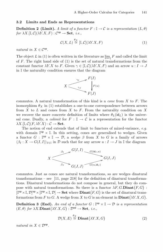
A Higher-Order Calculus for Categories 141
3.2 Limits and Ends as Representations
Definition 2 (Limit). A limit of a functor F : I→ C is a representation (L, θ)for λX.[I, C](λY.X, F ) : Cop → Set, i.e.,
C(X,L)θX∼= [I, C](λY.X, F ) (1)
natural in X ∈ Cop.
The object L in (1) is often written in the literature as lim←−IF and called the limit
of F . The right hand side of (1) is the set of natural transformations from theconstant functor λY.X to F . Given γ ∈ [I, C](λY.X, F ) and an arrow u : I → Jin I the naturality condition ensures that the diagram
F (I)
F (u)
��X
γI�������������
γJ
������������
F (J)
commutes. A natural transformation of this kind is a cone from X to F . Theisomorphism θX in (1) establishes a one-to-one correspondence between arrowsfrom X to L and cones from X to F . From the naturality condition on Xwe recover the more concrete definition of limits where θL(idL) is the univer-sal cone. Dually, a colimit for F : I → C is a representation for the functorλX.[I, C](F, λY.X) : C → Set.
The notion of end extends that of limit to functors of mixed-variance, e.g.with domain I
op × I. In this setting, cones are generalised to wedges. Givena functor G : I
op × I → D, a wedge β from X to G is a family of arrows〈βI : X → G(I, I)〉I∈I in D such that for any arrow u : I → J in I the diagram
G(I, I)G(idI ,u)
�������������
X
βI �������������
βJ������������ G(I, J)
G(J, J) G(u,idJ )
������������
commutes. Just as cones are natural transformations, so are wedges dinaturaltransformations – see [11, page 218] for the definition of dinatural transforma-tions. Dinatural transformations do not compose in general, but they do com-pose with natural transformations. So there is a functor λF,G.Dinat
(F,G
):
[Iop×I,D]op× [Iop×I,D]→ Set where Dinat(F,G
)is the set of dinatural trans-
formations from F to G. A wedge from X to G is an element in Dinat(λY.X,G
).
Definition 3 (End). An end of a functor G : Iop × I → D is a representation
(E, θ) for λX.Dinat(λY.X,G
): Dop → Set, i.e.,
D(X,E)θX∼= Dinat
(λY.X,G
)(2)
natural in X ∈ Dop.
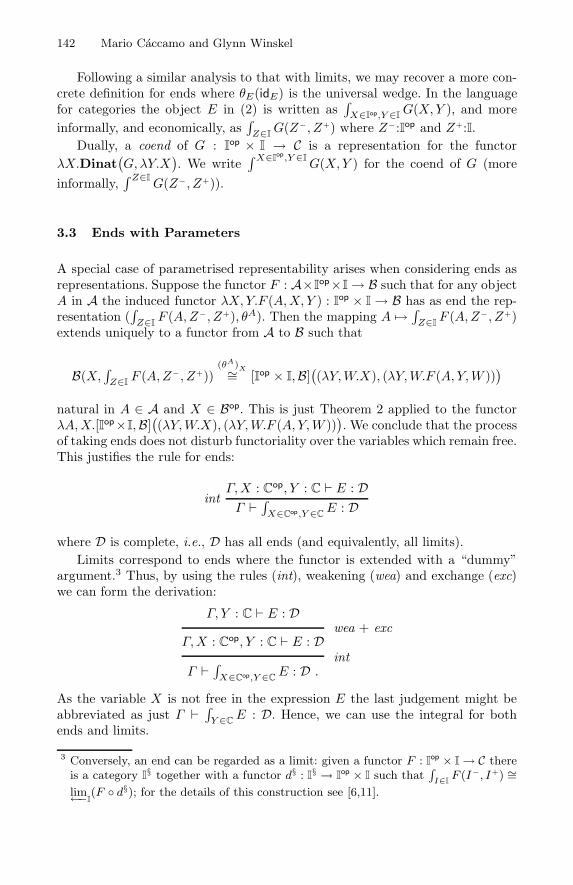
142 Mario Caccamo and Glynn Winskel
Following a similar analysis to that with limits, we may recover a more con-crete definition for ends where θE(idE) is the universal wedge. In the languagefor categories the object E in (2) is written as
∫X∈Iop,Y ∈I
G(X,Y ), and moreinformally, and economically, as
∫Z∈I
G(Z−, Z+) where Z−:Iop and Z+:I.Dually, a coend of G : I
op × I → C is a representation for the functorλX.Dinat
(G, λY.X
). We write
∫ X∈Iop,Y ∈I
G(X,Y ) for the coend of G (moreinformally,
∫ Z∈IG(Z−, Z+)).
3.3 Ends with Parameters
A special case of parametrised representability arises when considering ends asrepresentations. Suppose the functor F : A×I
op×I→ B such that for any objectA in A the induced functor λX, Y.F (A,X, Y ) : I
op × I→ B has as end the rep-resentation (
∫Z∈I
F (A,Z−, Z+), θA). Then the mapping A �→ ∫Z∈I
F (A,Z−, Z+)extends uniquely to a functor from A to B such that
B(X,∫Z∈I
F (A,Z−, Z+))(θA)X∼= [Iop × I,B]
((λY,W.X), (λY,W.F (A, Y,W ))
)
natural in A ∈ A and X ∈ Bop. This is just Theorem 2 applied to the functorλA,X.[Iop×I,B]
((λY,W.X), (λY,W.F (A, Y,W ))
). We conclude that the process
of taking ends does not disturb functoriality over the variables which remain free.This justifies the rule for ends:
intΓ,X : C
op, Y : C � E : DΓ � ∫
X∈Cop,Y ∈CE : D
where D is complete, i.e., D has all ends (and equivalently, all limits).Limits correspond to ends where the functor is extended with a “dummy”
argument.3 Thus, by using the rules (int), weakening (wea) and exchange (exc)we can form the derivation:
Γ, Y : C � E : DΓ,X : C
op, Y : C � E : Dwea + exc
Γ � ∫X∈Cop,Y ∈C
E : D .int
As the variable X is not free in the expression E the last judgement might beabbreviated as just Γ � ∫
Y ∈CE : D. Hence, we can use the integral for both
ends and limits.
3 Conversely, an end can be regarded as a limit: given a functor F : Iop × I→ C there
is a category I§ together with a functor d§ : I
§ → Iop × I such that
∫I∈I
F (I−, I+) ∼=lim←−I
(F ◦ d§); for the details of this construction see [6,11].
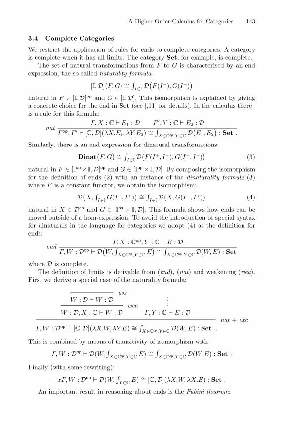
A Higher-Order Calculus for Categories 143
3.4 Complete Categories
We restrict the application of rules for ends to complete categories. A categoryis complete when it has all limits. The category Set, for example, is complete.
The set of natural transformations from F to G is characterised by an endexpression, the so-called naturality formula:
[I,D](F,G) ∼= ∫I∈ID(F (I−), G(I+)
)
natural in F ∈ [I,D]op and G ∈ [I,D]. This isomorphism is explained by givinga concrete choice for the end in Set (see [6,11] for details). In the calculus thereis a rule for this formula:
natΓ,X : C � E1 : D Γ ′, Y : C � E2 : D
Γ op, Γ ′ � [C,D](λX.E1, λY.E2) ∼=∫
X∈Cop,Y ∈CD(E1, E2
): Set .
Similarly, there is an end expression for dinatural transformations:
Dinat(F,G
) ∼= ∫I∈ID(F (I+, I−), G(I−, I+)
)(3)
natural in F ∈ [Iop× I,D]op and G ∈ [Iop× I,D]. By composing the isomorphismfor the definition of ends (2) with an instance of the dinaturality formula (3)where F is a constant functor, we obtain the isomorphism:
D(X,
∫I∈I
G(I−, I+)) ∼= ∫
I∈ID(X,G(I−, I+)
)(4)
natural in X ∈ Dop and G ∈ [Iop × I,D]. This formula shows how ends can bemoved outside of a hom-expression. To avoid the introduction of special syntaxfor dinaturals in the language for categories we adopt (4) as the definition forends:
endΓ,X : C
op, Y : C � E : DΓ,W : Dop � D(
W,∫
X∈Cop,Y ∈CE
) ∼= ∫X∈Cop,Y ∈C
D(W,E) : Set
where D is complete.The definition of limits is derivable from (end), (nat) and weakening (wea).
First we derive a special case of the naturality formula:
W : D �W : Dass
W : D, X : C �W : Dwea
....Γ, Y : C � E : D
Γ,W : Dop � [C,D](λX.W, λY.E) ∼= ∫X∈Cop,Y ∈C
D(W,E) : Set .nat + exc
This is combined by means of transitivity of isomorphism with
Γ,W : Dop � D(W,∫
X∈Cop,Y ∈CE) ∼= ∫
X∈Cop,Y ∈CD(W,E) : Set .
Finally (with some rewriting):
xΓ,W : Dop � D(W,∫
Y ∈CE) ∼= [C,D](λX.W, λX.E) : Set .
An important result in reasoning about ends is the Fubini theorem:
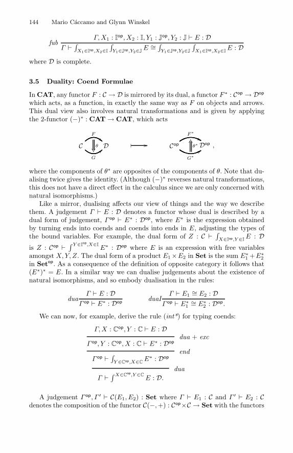
144 Mario Caccamo and Glynn Winskel
fubΓ,X1 : I
op, X2 : I, Y1 : Jop, Y2 : J � E : D
Γ � ∫X1∈Iop,X2∈I
∫Y1∈Jop,Y2∈J
E ∼= ∫Y1∈Jop,Y2∈J
∫X1∈Iop,X2∈I
E : Dwhere D is complete.
3.5 Duality: Coend Formulae
In CAT, any functor F : C → D is mirrored by its dual, a functor F ∗ : Cop → Dop
which acts, as a function, in exactly the same way as F on objects and arrows.This dual view also involves natural transformations and is given by applyingthe 2-functor (−)∗ : CAT→ CAT, which acts
CF
��
G
���D � Cop
F∗
G∗��θ∗
��Dop ,
where the components of θ∗ are opposites of the components of θ. Note that du-alising twice gives the identity. (Although (−)∗ reverses natural transformations,this does not have a direct effect in the calculus since we are only concerned withnatural isomorphisms.)
Like a mirror, dualising affects our view of things and the way we describethem. A judgement Γ � E : D denotes a functor whose dual is described by adual form of judgement, Γ op � E∗ : Dop, where E∗ is the expression obtainedby turning ends into coends and coends into ends in E, adjusting the types ofthe bound variables. For example, the dual form of Z : C � ∫
X∈Iop,Y ∈IE : D
is Z : Cop � ∫ Y ∈Iop,X∈I
E∗ : Dop where E is an expression with free variablesamongst X,Y, Z. The dual form of a product E1×E2 in Set is the sum E∗1 +E∗2in Setop. As a consequence of the definition of opposite category it follows that(E∗)∗ = E. In a similar way we can dualise judgements about the existence ofnatural isomorphisms, and so embody dualisation in the rules:
duaΓ � E : D
Γ op � E∗ : DopduaI
Γ � E1∼= E2 : D
Γ op � E∗1 ∼= E∗2 : Dop.
We can now, for example, derive the rule (int*) for typing coends:
Γ,X : Cop, Y : C � E : D
Γ op, Y : Cop, X : C � E∗ : Dop
dua + exc
Γ op � ∫Y ∈Cop,X∈C
E∗ : Dopend
Γ � ∫ X∈Cop,Y ∈C
E : D.dua
A judgement Γ op, Γ ′ � C(E1, E2) : Set where Γ � E1 : C and Γ ′ � E2 : Cdenotes the composition of the functor C(−,+) : Cop×C → Set with the functors
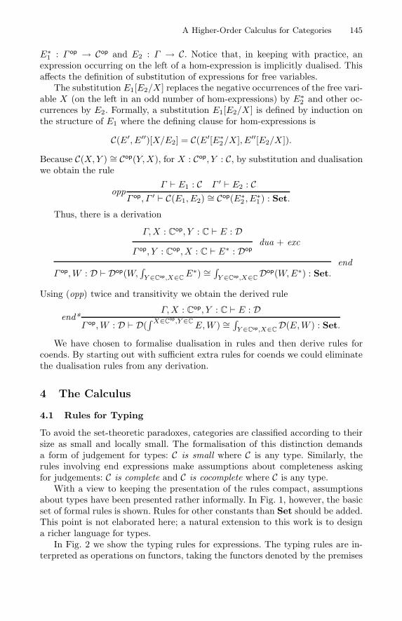
A Higher-Order Calculus for Categories 145
E∗1 : Γ op → Cop and E2 : Γ → C. Notice that, in keeping with practice, anexpression occurring on the left of a hom-expression is implicitly dualised. Thisaffects the definition of substitution of expressions for free variables.
The substitution E1[E2/X ] replaces the negative occurrences of the free vari-able X (on the left in an odd number of hom-expressions) by E∗2 and other oc-currences by E2. Formally, a substitution E1[E2/X ] is defined by induction onthe structure of E1 where the defining clause for hom-expressions is
C(E′, E′′)[X/E2] = C(E′[E∗2/X ], E′′[E2/X ]).
Because C(X,Y ) ∼= Cop(Y,X), for X : Cop, Y : C, by substitution and dualisationwe obtain the rule
oppΓ � E1 : C Γ ′ � E2 : C
Γ op, Γ ′ � C(E1, E2) ∼= Cop(E∗2 , E∗1 ) : Set.
Thus, there is a derivation
Γ,X : Cop, Y : C � E : D
Γ op, Y : Cop, X : C � E∗ : Dop
dua + exc
Γ op,W : D � Dop(W,∫
Y ∈Cop,X∈CE∗) ∼= ∫
Y ∈Cop,X∈CDop(W,E∗) : Set.
end
Using (opp) twice and transitivity we obtain the derived rule
end*Γ,X : C
op, Y : C � E : DΓ op,W : D � D(
∫ X∈Cop,Y ∈C
E,W ) ∼= ∫Y ∈Cop,X∈C
D(E,W ) : Set.
We have chosen to formalise dualisation in rules and then derive rules forcoends. By starting out with sufficient extra rules for coends we could eliminatethe dualisation rules from any derivation.
4 The Calculus
4.1 Rules for Typing
To avoid the set-theoretic paradoxes, categories are classified according to theirsize as small and locally small. The formalisation of this distinction demandsa form of judgement for types: C is small where C is any type. Similarly, therules involving end expressions make assumptions about completeness askingfor judgements: C is complete and C is cocomplete where C is any type.
With a view to keeping the presentation of the rules compact, assumptionsabout types have been presented rather informally. In Fig. 1, however, the basicset of formal rules is shown. Rules for other constants than Set should be added.This point is not elaborated here; a natural extension to this work is to designa richer language for types.
In Fig. 2 we show the typing rules for expressions. The typing rules are in-terpreted as operations on functors, taking the functors denoted by the premises
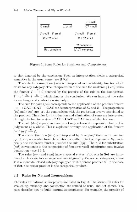
146 Mario Caccamo and Glynn Winskel
0 small 1 small
C small
Cop small
C small D small
C × D small
C small D small
C +D small
Set complete
D complete
[C,D] complete
Figure 1. Some Rules for Smallness and Completeness.
to that denoted by the conclusion. Such an interpretation yields a categoricalsemantics in the usual sense (see [1,5,8]).
The rule for assumption (ass) is interpreted as the identity functor whichexists for any category. The interpretation of the rule for weakening (wea) takesthe functor Γ E−→ C denoted by the premise of the rule to the compositionΓ × Γ ′ πΓ−→ Γ
E−→ C which denotes the conclusion. We can interpret the rulesfor exchange and contraction similarly.
The rule for pairs (pai) corresponds to the application of the product functor−×− : CAT×CAT→ CAT to the interpretation ofE1 and E2. The projections(fst) and (snd) are just the composition with the projection arrows associated tothe product. The rules for introduction and elimination of sums are interpretedthrough the functor −+− : CAT×CAT→ CAT in a similar fashion.
The rule (dua) is peculiar since it not only acts on the expressions but on thejudgement as a whole. This is explained through the application of the functor(−)∗ to Γ E−→ C.
The abstraction rule (lam) is interpreted by “currying” the functor denotedby E, i.e., a variable from the context is shifted into the expression. Symmet-rically the evaluation functor justifies the rule (app). The rule for substitution(sub) corresponds to the composition of functors; recall substitution may involvedualisation – see § 3.5.
The rules (ten) and (uni) have a special status. Products in Set are intro-duced with a view to a more general model given by V-enriched categories, whereV is a monoidal closed category equipped with a tensor product ⊗. In the caseof Set, the tensor product is the categorical product.
4.2 Rules for Natural Isomorphisms
The rules for natural isomorphisms are listed in Fig. 3. The structural rules forweakening, exchange and contraction are defined as usual and not shown. Therules describe how to build natural isomorphisms. For example, the premise of
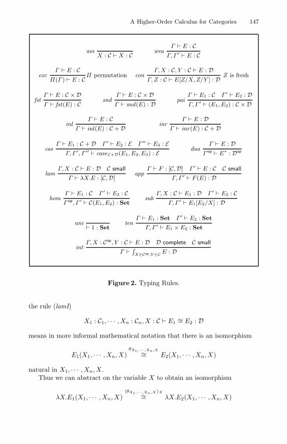
A Higher-Order Calculus for Categories 147
assX : C � X : C wea
Γ � E : CΓ, Γ ′ � E : C
excΓ � E : C
Π(Γ ) � E : CΠ permutation conΓ, X : C, Y : C � E : D
Γ, Z : C � E[Z/X, Z/Y ] : D Z is fresh
fstΓ � E : C × DΓ � fst(E) : C snd
Γ � E : C ×DΓ � snd(E) : D pai
Γ � E1 : C Γ ′ � E2 : DΓ,Γ ′ � (E1, E2) : C ×D
inlΓ � E : C
Γ � inl(E) : C +D inrΓ � E : D
Γ � inr(E) : C +D
casΓ � E1 : C +D Γ ′ � E2 : E Γ ′′ � E3 : E
Γ, Γ ′, Γ ′′ � caseC+D(E1, E2, E3) : E duaΓ � E : D
Γ op � E∗ : Dop
lamΓ, X : C � E : D C small
Γ � λX.E : [C,D] appΓ � F : [C,D] Γ ′ � E : C C small
Γ, Γ ′ � F (E) : D
homΓ � E1 : C Γ ′ � E2 : CΓ op, Γ ′ � C(E1, E2) : Set
subΓ, X : C � E1 : D Γ ′ � E2 : C
Γ, Γ ′ � E1[E2/X] : D
uni � 1 : Setten
Γ � E1 : Set Γ ′ � E2 : Set
Γ, Γ ′ � E1 × E2 : Set
intΓ, X : Cop, Y : C � E : D D complete C small
Γ � ∫X∈Cop,Y ∈C E : D
Figure 2. Typing Rules.
the rule (lamI)
X1 : C1, · · · , Xn : Cn, X : C � E1∼= E2 : D
means in more informal mathematical notation that there is an isomorphism
E1(X1, · · · , Xn, X)θX1,··· ,Xn,X∼= E2(X1, · · · , Xn, X)
natural in X1, · · · , Xn, X .Thus we can abstract on the variable X to obtain an isomorphism
λX.E1(X1, · · · , Xn, X)〈θX1,··· ,Xn,X〉X∼= λX.E2(X1, · · · , Xn, X)
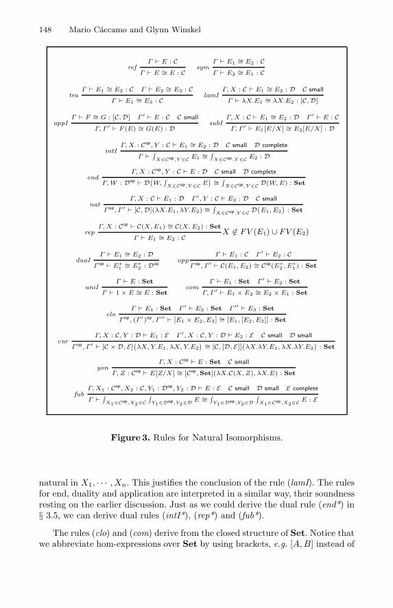
148 Mario Caccamo and Glynn Winskel
refΓ E : C
Γ E ∼= E : Csym
Γ E1 ∼= E2 : CΓ E2 ∼= E1 : C
traΓ E1 ∼= E2 : C Γ E2 ∼= E3 : C
Γ E1 ∼= E3 : C lamIΓ, X : C E1 ∼= E2 : D C small
Γ λX.E1 ∼= λX.E2 : [C,D]
appIΓ F ∼= G : [C,D] Γ ′ E : C C small
Γ, Γ ′ F (E) ∼= G(E) : DsubI
Γ, X : C E1 ∼= E2 : D Γ ′ E : CΓ, Γ ′ E1[E/X] ∼= E2[E/X] : D
intIΓ, X : Cop, Y : C E1 ∼= E2 : D C small D complete
Γ ∫X∈Cop,Y ∈C E1 ∼=
∫X∈Cop,Y ∈C E2 : D
endΓ, X : Cop, Y : C E : D C small D complete
Γ, W : Dop D(W,
∫X∈Cop,Y ∈C E
) ∼=∫
X∈Cop,Y ∈C D(W, E) : Set
natΓ, X : C E1 : D Γ ′, Y : C E2 : D C small
Γ op, Γ ′ [C,D](λX.E1, λY.E2) ∼=∫
X∈Cop,Y ∈C D(E1, E2
): Set
repΓ, X : Cop C(X, E1) ∼= C(X, E2) : Set
Γ E1 ∼= E2 : CX ∈ FV (E1) ∪ FV (E2)
duaIΓ E1 ∼= E2 : D
Γ op E∗1∼= E∗
2 : Dopopp
Γ E1 : C Γ ′ E2 : CΓ op, Γ ′ C(E1, E2) ∼= Cop(E∗
2 , E∗1 ) : Set
uniIΓ E : Set
Γ 1× E ∼= E : Setcom
Γ E1 : Set Γ ′ E2 : Set
Γ, Γ ′ E1 × E2 ∼= E2 × E1 : Set
cloΓ E1 : Set Γ ′ E2 : Set Γ ′′ E3 : Set
Γ op, (Γ ′)op, Γ ′′ [E1 × E2, E3] ∼= [E1, [E2, E3]] : Set
curΓ, X : C, Y : D E1 : E Γ ′, X : C, Y : D E2 : E C small D small
Γ op, Γ ′ [C × D, E](λX, Y.E1, λX, Y.E2) ∼= [C, [D,E]](λX.λY.E1, λX.λY.E2
): Set
yonΓ, X : Cop E : Set C small
Γ, Z : Cop E[Z/X] ∼= [Cop, Set](λX.C(X, Z), λX.E) : Set
fubΓ, X1 : Cop, X2 : C, Y1 : Dop, Y2 : D E : E C small D small E complete
Γ ∫X1∈Cop,X2∈C
∫Y1∈Dop,Y2∈D E ∼=
∫Y1∈Dop,Y2∈D
∫X1∈Cop,X2∈C E : E
Figure 3. Rules for Natural Isomorphisms.
natural in X1, · · · , Xn. This justifies the conclusion of the rule (lamI). The rulesfor end, duality and application are interpreted in a similar way, their soundnessresting on the earlier discussion. Just as we could derive the dual rule (end*) in§ 3.5, we can derive dual rules (intI*), (rep*) and (fub*).
The rules (clo) and (com) derive from the closed structure of Set. Notice thatwe abbreviate hom-expressions over Set by using brackets, e.g. [A,B] instead of
A Higher-Order Calculus for Categories 149
Set(A,B). The “closed” structure of CAT gives the rule (cur) for currying. Arule for swapping arguments in functors is derivable from (cur), (nat) and (fub).
5 Examples
5.1 Continuity
The two driving notions in the previous sections have been functoriality andnatural isomorphism. The example below shows that the calculus is rich enoughto prove continuity.
Definition 4 (Preservation of Limits). Let F : I → C be a functor withlimiting cone 〈kI : lim←−I
F → F (I)〉I∈I, a functor G : C → D preserves the limitof F iff 〈G(kI) : G(lim←−I
F )→ G(F (I))〉I∈I is a limiting cone in D. Preservationof colimits is defined dually.
We say that G preserves I-index limits if G preserves the limits of all functorsin [I, C]. A functor which preserves all limits is called continuous.
One might expect to prove that a given functor preserves limits by showingan isomorphism of objects. This gives, however, a necessary but not sufficientcondition.4 The situation improves when the isomorphism is sufficiently naturalhowever:
Theorem 3. Assume that the categories C and D have limits for all functorswith domain I. The functor G : C → D preserves I-indexed limits iff
lim←−I
(G ◦ F ) ∼= G(lim←−I
F ),
natural in F ∈ [I, C] (see [6] for a proof.).This theorem supplies the key to proving continuity within the calculus. Forexample, that C(C,X) preserves limits in X is a direct consequence of the nat-urality formula.
Another result we can prove in the calculus is that right adjoints preservelimits. Given the judgements X : C � E1 : D and Y : D � E2 : C respectivelydenoting functors E1 : C → D and E2 : D → C, an adjunction where, as functors,E1 is the left adjoint and E2 is the right adjoint consists of an isomorphism
X : Cop, Y : D � D(E1, Y
) ∼= C(X,E2) : Set.
By Theorem 3 is enough to prove E2[∫
I∈IH/Y ] ∼= ∫
I∈IE2[H(I)/Y ] : C where
H : [I,D]. The proof proceeds backwards, using (rep) to obtain the goal:
X : Cop, H : [I,D] � C(X,E2[∫
I∈IH(I)/Y ]
) ∼= C(X, ∫I∈IE2[H(I)/Y ]
): Set.
4 There are examples of functors which preserve limiting objects but don’t preservethe limiting cones, see [3, ex. 5.3.16(4)].
150 Mario Caccamo and Glynn Winskel
The derivation of this goal is sketched in the chain of isomorphisms:
C(X,E2[∫
I∈IH(I)/Y ]
) ∼= D(E1,
∫I∈I
H(I))
by the adjunction,∼= ∫
I∈ID(E1, H(I)
)by (end),
∼= ∫I∈IC(X,E2[H(I)/Y ]
)by the adjunction,
∼= C(X, ∫I∈IE2[H(I)/Y ]
)by (end).
We conclude that the functor denoted by Y : C � E2 : D preserves limits.The dual result, i.e. left adjoints preserve colimits, follows from the rules opp
and duaI. From the definition of adjunction and by applying the rule opp twicetogether with transitivity we get
X : Cop, Y : D � Cop(E∗2 , X) ∼= Dop(Y,E∗1
): Set
i.e. an adjunction where the functor denoted by E∗1 is the right adjoint. Fromthe derivation above we can conclude
H : [Iop, Cop] � E∗1 [∫
I∈Iop H(I)/X ] ∼= ∫I∈Iop E
∗1 [H(I)/X ] : Dop
and by applying the rule duaI
H : [I, C] � E1[∫ I∈I
H(I)/X ] ∼= ∫ I∈IE1[H(I)/X ] : D.
5.2 The Density Formula
Functor categories of the form [Cop,Set] have a number of important propertiesthat give them a special rank in the calculus.5 From the rules (yon) and (nat),a functor X : [Cop,Set] is expressible as the end formula:
X : [Cop,Set],W : Cop � X(W ) ∼= ∫
Y ∈Cop
[C(Y −,W ), X(Y +)
]: Set . (5)
There is also a coend formula for X , the so-called density formula:
X : [Cop,Set],W : Cop � X(W ) ∼= ∫ Y ∈C
C(W,Y +)×X(Y −) : Set . (6)
The chain of isomorphisms below sketches a derivation for this formula:
[Cop,Set](λW.
∫ Y ∈CC(W,Y +)×X(Y −), Z
)
∼= ∫W∈Cop [(
∫ Y ∈CC(W−, Y +)×X(Y −), Z(W+)] by (nat),
∼= ∫W∈Cop
∫Y ∈Cop [C(W−, Y +)×X(Y −), Z(W+)] by (end*) and (intI),
∼= ∫Y ∈Cop
∫W∈Cop [C(W−, Y +)×X(Y −), Z(W+)] by (fub),
∼= ∫Y ∈Cop
∫W∈Cop
[X(Y −), [C(W−, Y +), Z(W+)]
]by (com) and (clo)
∼= ∫Y ∈Cop
[X(Y −),
∫W∈Cop [C(W−, Y +), Z(W+)]
]by (end) and (intI),
∼= ∫Y ∈Cop [X(Y −), Z(Y +)] by (5) and (intI),
∼= [Cop,Set](X,Z
)by (nat).
The next step applies the rule (rep*) to yield the isomorphism (6).5 Such categories are called presheaf categories.
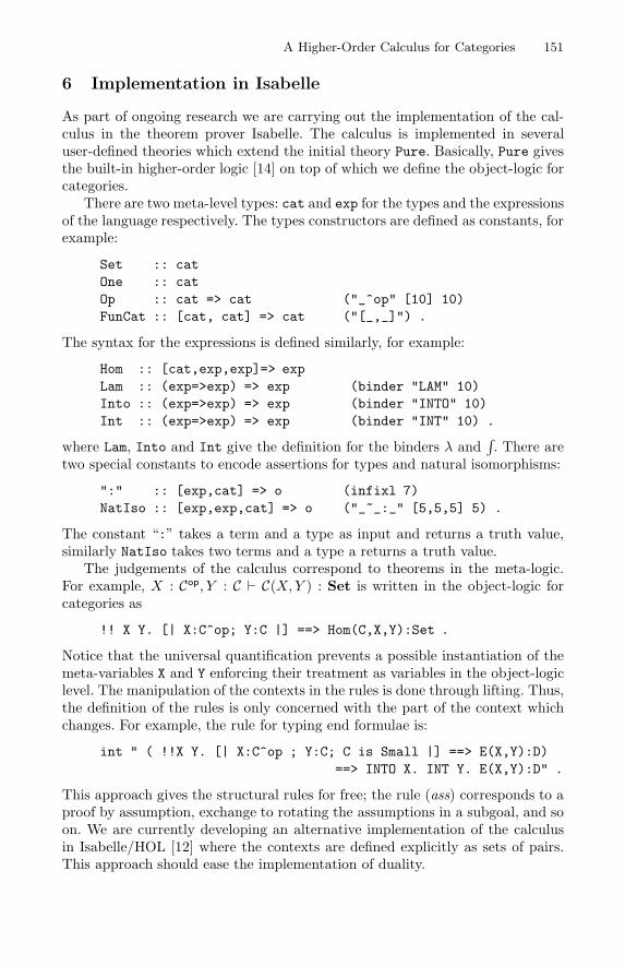
A Higher-Order Calculus for Categories 151
6 Implementation in Isabelle
As part of ongoing research we are carrying out the implementation of the cal-culus in the theorem prover Isabelle. The calculus is implemented in severaluser-defined theories which extend the initial theory Pure. Basically, Pure givesthe built-in higher-order logic [14] on top of which we define the object-logic forcategories.
There are two meta-level types: cat and exp for the types and the expressionsof the language respectively. The types constructors are defined as constants, forexample:
Set :: catOne :: catOp :: cat => cat ("_^op" [10] 10)FunCat :: [cat, cat] => cat ("[_,_]") .
The syntax for the expressions is defined similarly, for example:
Hom :: [cat,exp,exp]=> expLam :: (exp=>exp) => exp (binder "LAM" 10)Into :: (exp=>exp) => exp (binder "INTO" 10)Int :: (exp=>exp) => exp (binder "INT" 10) .
where Lam, Into and Int give the definition for the binders λ and∫. There are
two special constants to encode assertions for types and natural isomorphisms:
":" :: [exp,cat] => o (infixl 7)NatIso :: [exp,exp,cat] => o ("_~_:_" [5,5,5] 5) .
The constant “:” takes a term and a type as input and returns a truth value,similarly NatIso takes two terms and a type a returns a truth value.
The judgements of the calculus correspond to theorems in the meta-logic.For example, X : Cop, Y : C � C(X,Y ) : Set is written in the object-logic forcategories as
!! X Y. [| X:C^op; Y:C |] ==> Hom(C,X,Y):Set .
Notice that the universal quantification prevents a possible instantiation of themeta-variables X and Y enforcing their treatment as variables in the object-logiclevel. The manipulation of the contexts in the rules is done through lifting. Thus,the definition of the rules is only concerned with the part of the context whichchanges. For example, the rule for typing end formulae is:
int " ( !!X Y. [| X:C^op ; Y:C; C is Small |] ==> E(X,Y):D)==> INTO X. INT Y. E(X,Y):D" .
This approach gives the structural rules for free; the rule (ass) corresponds to aproof by assumption, exchange to rotating the assumptions in a subgoal, and soon. We are currently developing an alternative implementation of the calculusin Isabelle/HOL [12] where the contexts are defined explicitly as sets of pairs.This approach should ease the implementation of duality.
152 Mario Caccamo and Glynn Winskel
7 Conclusions, Related Work, and Future Directions
A calculus which formalises an expressive fragment of category theory has beenpresented. The rules of the calculus support a calculational approach to uni-versality where the manipulation of ends and coends plays a central role. Wehave shown how to formalise judgements about functoriality and how to verifyisomorphisms. In this setting, we have explored duality and studied applicationsto encode and prove results on continuous functors. An implementation of thecalculus in the theorem prover Isabelle has been outlined briefly.
Previous work in the automation of category theory has followed a some-what different tack. Takeyama [18] presents a computer checked language withthe goal of supplying a categorical framework for type theory and includes animplementation in the theorem prover Lego [16]. This follows in spirit the workof Rydeheard and Burstall [17] on formalising universal constructions in ML.Beylin and Dybjer [4] formalise monoidal categories and present a proof of theMac Lane’s coherence theorem in Martin Lof’s type theory [13].
The interpretation of the rules suggests a language for natural isomorphisms.Observe that in theorem provers like Isabelle where a goal may contain un-knowns, a witness for a natural isomorphism may be given as output of theproof search. More generally, a further extension to the calculus is to introduceexpressions for natural transformations.
A richer language for types may be considered by adding new constructorslike recursion and lifting. For recursive definition of categories we need to extendthe language for types to allow expressions with variables. The lifted type C⊥would be interpreted as the category C with an initial object ⊥ freely adjoined.
The utility of end and coend notation was demonstrated in the pioneeringwork of Kelly and others in enriched category theory [10]. In emphasising acalculus for categories, a goal has been to make working with functor categoriesroutine. The formalisation here should lend itself to enriched category theory.
Acknowledgments
This work was inspired by Martin Hyland’s Cambridge part III lecture courseon category theory and its emphasis on end and coend manipulation.
References
1. A. Asperti and G. Longo. Categories, Types and Structures : An introduction tocategory theory for the working computer scientist. Foundations of ComputingSeries. MIT Press, 1991.
2. H. Barendregt. Lambda calculi with types. In S. Abramsky, D. M. Gabbay, andT. S. E. Maibaum, editors, Handbook of Logic in Computer Science, volume 2:Computational Structures. Oxford University Press, 1991.
3. M. Barr and C. Wells. Category Theory for Computing Science. C.A.R. HoareSeries Editor. Prentice Hall, second edition, 1996.
A Higher-Order Calculus for Categories 153
4. I. Beylin and P. Dybjer. Extracting a proof of coherence for monoidal categoriesfrom a proof of normalization for monoids. Lecture Notes in Computer Science,1158, 1996.
5. T. Brauner. An Axiomatic Approach to Adequacy. PhD thesis, BRICS PhD School,1996.
6. M. Caccamo, J. M. E. Hyland, and G. Winskel. Lecture notes in category theory.Available from: http://www.brics.dk/~mcaccamo.
7. G. L. Cattani. Presheaf Models for Concurrency. PhD thesis, BRICS PhD School,1999.
8. R. L. Crole. Categories for Types. Cambridge Mathematical Textbooks. CambridgeUniversity Press, 1993.
9. A. Joyal, M. Nielsen, and G. Winskel. Bisimulation and open maps. In R. L.Constable, editor, Proceedings of the 8th Annual IEEE Symposium on Logic inComputer Science, Montreal, Canada, June 1993. IEEE Computer Society Press.
10. G. M. Kelly. Basic Concepts of Enriched Category Theory, volume 64 of LondonMathematical Society Lecture Note Series. Cambridge University Press, 1982.
11. S. Mac Lane. Categories for the Working Mathematician, volume 5 of GraduateTexts in Mathematics. Springer-Verlag, second edition, 1998.
12. T. Nipkow and L. Paulson. Isabelle HOL: The tutorial. Documentation includedin the official distribution of Isabelle, Feb. 2001.
13. B. Nordstrom, K. Petterson, and J. Smith. Programming in Martin-Lof ’s TypeTheory. An Introduction. Oxford University Press, 1990.
14. L. Paulson. The foundation of a generic theorem prover. Journal of AutomatedReasoning, 5(3):363–397, 1988.
15. L. C. Paulson. Isabelle: A Generic Theorem Prover, volume 828 of Lecture Notesin Computer Science. Springer-Verlag, 1994.
16. R. Pollack. The Theory of LEGO: A Proof Checker for the Extended Calculus ofConstructions. PhD thesis, The University of Edinburgh, 1994.
17. D. Rydeheard and R. Burstall. Computational Category Theory. InternationalSeries in Computer Science. Prentice Hall, 1988.
18. M. Takeyama. Universal Structure and a Categorical Framework for Type Theory.PhD thesis, The University of Edinburgh, 1995.
Certifying the Fast Fourier Transform with Coq
Venanzio Capretta�
Computing Science Institute, University of NijmegenPostbus 9010, 6500 GL Nijmegen, The Netherlands
telephone: +31+24+3652647, fax: +31+24+3553450
Abstract. We program the Fast Fourier Transform in type theory, usingthe tool Coq. We prove its correctness and the correctness of the InverseFourier Transform. A type of trees representing vectors with interleavedelements is defined to facilitate the definition of the transform by struc-tural recursion. We define several operations and proof tools for this datastructure, leading to a simple proof of correctness of the algorithm. Theinverse transform, on the other hand, is implemented on a different rep-resentation of the data, that makes reasoning about summations easier.The link between the two data types is given by an isomorphism. Thiswork is an illustration of the two-level approach to proof developmentand of the principle of adapting the data representation to the specificalgorithm under study. CtCoq, a graphical user interface of Coq, helpedin the development. We discuss the characteristics and usefulness of thistool.
1 Introduction
An important field of research in formalized mathematics tackles the verificationof classical algorithms widely used in computer science. It is important for atheorem prover to have a good library of proof-checked functions, that can beused both to extract a formally certified program and to quickly verify softwarethat uses the algorithm. The Fast Fourier Transform [8] is one of the most widelyused algorithms, so I chose it as a case study in formalization using the type-theory proof tool Coq [2]. Here I present the formalization and discuss in detailthe parts of it that are more interesting in the general topic of formal verificationin type theory.
Previous work on the computer formalization of FFT was done by RubenGamboa [10] in ACL2 using the data structure of powerlists introduced byJayadev Misra [11], which is similar to the structure of polynomial trees that weuse here.� I worked on the formalization of FFT during a two-month stay at the INRIA researchcenter in Sophia Antipolis, made possible by a grant from the Dutch Organization forScientific Research (NWO, Dossiernummer F 62-556). I am indebted to the people ofthe Lemme group for their support and collaboration. In particular, I want to thankYves Bertot for his general support and for teaching me how to use CtCoq, and LoıcPottier for his help in formulating the Fast Fourier Transform in type theory.
R.J. Boulton and P.B. Jackson (Eds.): TPHOLs 2001, LNCS 2152, pp. 154–168, 2001.c© Springer-Verlag Berlin Heidelberg 2001
Certifying the Fast Fourier Transform with Coq 155
The Discrete Fourier Transform is a function commuting between two rep-resentations of polynomials over a commutative ring, usually the algebraic fieldC. One representation is in the coefficient domain, where a polynomial is givenby the list of its coefficients. The second representation is in the value domain,where a polynomial of degree n − 1 is given by its values on n distinct points.The function from the coefficient domain to the value domain is called evalua-tion, the inverse function is called interpolation. The Discrete Fourier Transform(DFT) and the Inverse Discrete Fourier Transform (iDFT) are the evaluation andinterpolation functions in the case in which the points of evaluation are distinctn-roots of the unit element of the ring. The reason to consider such particularevaluation points is that, in this case, an efficient recursive algorithm exists toperform evaluation, the Fast Fourier Transform (FFT), and interpolation, theInverse Fourier Transform (iFT). Let
f(x) = a0 + a1x+ a2x2 + . . .+ an−1x
n−1 =n−1∑i=0
aixi
be a polynomial of degree n − 1 and ω be a primitive n-root of unity, that is,ωn = 1 but ωj �= 1 for 0 < j < n. We must compute f(ωj) for j = 0, 1, . . . , n−1.First of all we write f(x) as the sum of two components, the first comprisingthe monomials of even power and the second the monomials of odd power, forwhich we can collect a factor x:
f(x) = fe(x2) + xfo(x2). (1)
The polynomials fe and fo have degree n/2− 1 (assuming that n is even). Wecould apply our algorithm recursively to them and to ω2, which is an n/2-rootof unity. We obtain the values
fe((ω2)0), fe((ω2)1), . . . , fe((ω2)n/2−1);fo((ω2)0), fo((ω2)1), . . . , fo((ω2)n/2−1).
We have, therefore, fe((ω2)i) = fe((ωi)2) for i = 0, . . . , n/2−1 which we can feedinto Formula 1. The only problem is that Formula 1 must be evaluated for x = ωi
when i = 0, . . . , n−1. We are still missing the values for i = n/2, . . . , n−1. Hereis where the fact that ω is a primitive n-root of unity comes useful: ωn/2 = −1,so for j = 0, . . . , n/2− 1 we have that
ωn/2+j = ωn/2ωj = −ωj
and therefore fe((ωn/2+j)2) = fe((ωj)2). So the values of the first term of For-mula 1 for i = n/2, . . . , n−1 are equal to the values for i = 0, . . . , n/2−1 and wedon’t need to compute them. A similar argument holds for fo. If we measure thealgorithmic complexity by the number of multiplications of scalars that need tobe performed, we see that the algorithm calls itself twice on inputs of half sizeand then must still perform n multiplications (multiply x by fo(x) in Formula1). This gives an algorithm of complexity O(n log n), much better than the naivequadratic algorithm.
156 Venanzio Capretta
Vice versa if we are given the values of the polynomial f on the n-roots ofunity, y0 = f(ω0), . . . , yn−1 = f(ωn−1), we can compute the vector of coefficientsof f by applying DFT to the vector 〈y0, . . . , yn−1〉 with ω−1 in place of ω and thendivide by n. The proof of this fact is well-known. We will give a type-theoreticversion of it in section 5.
One useful application of FFT is the computation the product of two poly-nomials. If f(x) =
∑n−1i=0 aix
i and g(x) =∑n−1
i=0 bixi, we want to compute their
product f(x)g(x) =∑n−1
i=0 cixi. A direct computation of the coefficients would
require the evaluation the formula ci =∑
j+k=i ajbk for i = 0, . . . , 2n− 2, for atotal of n2 scalar products. A faster way to compute it is, first, to find the rep-resentations of the polynomials in the value domain with FFT: f(ωi) and g(ωi)for i = 0, . . . , 2n − 1; second, to multiply the corresponding values to obtainthe representation of the product in the value domain: f(ωi)g(ωi); and third, toreturn to the coefficient domain iFT. In this way we need to perform only 2nmultiplications plus the O(n log n) multiplications needed for the conversions.The overall complexity of the multiplication algorithm is then also O(n log n),instead of quadratic.
The rest of the article describes the formalization of these ideas in type theory,using the proof tool Coq. In Section 2 we discuss the different representationsfor the data types involved. We choose a tree representation that is specificallydesigned for FFT. We prove that it is equivalent to a more natural one. In Section3 we apply the two-level approach (see [3] and [6]) to the tree representation toprove some basic facts about it. Section 4 contains the definition and proof ofcorrectness of FFT. Section 5 introduces iFT and proves its correctness. Finally,Section 6 discusses the tools used in the formalization and some implementationissues.
2 Data Representation
Let us fix the domain of coefficients and values. We need to work in a commuta-tive ring with unity, and in the case of the inverse transform we will need a field.Usually it is required that the domain is an algebraically closed field, becausethe transform is applied to a polynomial and a root of unity. We will not do that,but just require that, when the algorithm is applied, a proof that its argumentis a root of unity is supplied. This covers the useful case in which we want toapply the algorithm to finite fields (that can never be algebraically closed) orfinite rings. In type theory an algebraic structure like that of ring is representedby an underlying setoid , which is a type with an equivalence relation, plus someoperations on the setoid and proofs of the defining properties of the structure.In our case we will have the following data:
K : SetK eq : K → K → PropK eq refl : (reflexive K eq)K eq symm : (symmetric K eq)K eq trans : (transitive K eq).
Certifying the Fast Fourier Transform with Coq 157
K eq is thus an equivalence relation that expresses the equality of the objectsrepresented by terms of the type K. We will write x ≡ y for (K eq a b). Thebasic ring constants and operations are
0, 1: Ksm,ml : K → K → Ksm inv : K → K.
We will use the notations x+y, x·y and −x for (sm x y), (ml x y) and (sm inv x),respectively. We need to require that they are well behaved with respect to ≡,or, equivalently, that ≡ is a congruence relation with respect to these operations:
sm congr : ∀x1, x2, y1, y2 : K.x1 ≡ x2 → y1 ≡ y2 → x1 + y1 ≡ x2 + y2
ml congr : ∀x1, x2, y1, y2 : K.x1 ≡ x2 → y1 ≡ y2 → x1 · y1 ≡ x2 · y2
sm congr : ∀x1, x2 : K.x1 ≡ x2 → (−x1) ≡ (−x2)
The axioms of commutative rings can now be formulated for these operationsand for the equality ≡.
We will often require that a certain element ω : K is a primitive n-root ofunity. This means that ωn ≡ 1 (ω is a root) and n is the smallest non-zeroelement for which this happens (primitivity). At some point we will also needthat, if n is even, ωn/2 ≡ −1. Note that this fact does not generally follow fromω being a primitive n-root of unity. Indeed, if K is an integral domain, we canprove this from the fact that ωn/2 is a solution of the equation x2 ≡ 1, butcannot be 1 by primitivity of ω. In an integral domain 1 and −1 are the onlysolutions of the equation. But in a commutative ring this is not always true.For example, take the finite commutative ring Z15 and the value ω = 4, whichis a primitive 2-root of unity (42 ≡ 16 ≡ 1). Nevertheless 41 ≡ 4 ≡/ −1. So therequirement ωn/2 ≡ −1 will have to be stated explicitly when needed.
Polynomials in one variable are usually represented as the vectors of theircoefficients. So the polynomial a0 + a1x+ · · ·+ an−1x
n−1 is represented by thevector 〈a0, a1, . . . , an−1〉. We can choose to implement such a vector in threestandard ways: as a list (in which case there is no restriction on the length), asan element of a type with fixed length, or as a function from the finite type withn elements, Nn, to K. This last representation is the most elastic for a certainnumber of purposes, specifically for reasoning about summations. It will be usefulwhen prove the correctness of iFT. So we adopt it as our basic implementationof polynomials. The type of polynomials of degree n− 1 will then be Nn → K.
However, in the proof of correctness of FFT, a different representation resultsmore useful. A fundamental step of the computation consists in breaking thepolynomial f in two parts fe and fo, consisting of the even and odd terms,respectively. We apply the algorithm recursively on these two polynomials. Therecursion is wellfounded because fe and fo have smaller degree than f . Thisrequires the use of course-of-value recursion on the degree of the polynomial,which can be realized in type theory using a general method for wellfoundedrecursion (see [1]). The formalization of the algorithm that we obtain is morecomplex than necessary, because it contains the proofs of the fact that the degrees
158 Venanzio Capretta
decrease. Simpler algorithms are obtained by using structural recursion in placeof wellfounded recursion. To use structural recursion we need that the algorithmcalls itself recursively only on structurally smaller arguments.
So we are led to look for a different implementation of polynomials whosestructure reflects the steps of the algorithm. A general method to obtain a datatype whose structure is derived from the recursive definition of a function ispresented in [7]. In our case we obtain the result by representing polynomials astree structures in which the left subtree contains the even coefficients and theright subtree contains the odd coefficients. This results in the recursive definition
Tree : N→ Set :=Tree(0) := KTree(k + 1) := Tree(k)× Tree(k).
An element of Tree(k) is a binary tree of depth k whose leaves are elements ofthe coefficient domain K. We will use the notation leaf(a) to denote an elementa : K when it is intended as a tree of depth 0, that is, an element of Tree(0) = K.We will use the notation node(t1, t2) to denote the element 〈t1, t2〉 : Tree(k+1) =Tree(k) × Tree(k), if t1 and t2 are elements of Tree(k). The number of leaves ofsuch a tree is 2k. This is not a problem since, for the application of FFT, wealways assume that the degree of the input polynomial is one less than a powerof 2. Otherwise we adjust it to the closest power of 2 by adding terms with zerocoefficients.
The equality ≡ on K is extended to the equality ∼= on trees. We say thattwo elements t1, t2 : Tree(k) are equal, and write t1 ∼= t2, when the relation ≡holds between corresponding leaves. The relation ∼= can be formally defined byrecursion on k.
A polynomial is represented by putting the coefficients of the even powers ofx in the left subtree and the coefficients of the odd powers of x in the right one,and this procedure is repeated recursively on the two subtrees. If we have, forexample, a polynomial of degree 7 (= 23 − 1),
f(x) = a0 + a1x+ a2x2 + a3x
3 + a4x4 + a5x
5 + a6x6 + a7x
7,
we break it into two parts
fe(y) := a0 + a2y + a4y2 + a6y
3, fo(y) := a1 + a3y + a5y2 + a7y
3
so that f(x) = fe(x2)+xfo(x2). Recursively fe(y) and fo(y) can be broken intoeven and odd terms
fee(z) := a0 + a4z, feo(z) := a2 + a6z,foe(z) := a1 + a5z, foo(z) := a3 + a7z
so that fe(y) = fee(y2)+ yfeo(y2) and fo(y) = foe(y2)+ yfoo(y2). With anotherstep we reach single coefficients:
feee(u) := a0, feeo(u) := a4, feoe(u) := a2, feoo(u) := a6,foee(u) := a1, foeo(u) := a5, fooe(u) := a3, fooo(u) := a7
Certifying the Fast Fourier Transform with Coq 159
with fee(z) = feee(z2) + zfeeo(z2), feo(z) = feoe(z2) + zfeoo(z2), foe(z) =foee(z2) + zfoeo(z2), foo(z) = fooe(z2) + zfooo(z2). Now we transform each ofthese polynomials in trees, starting with the single-coefficient ones. We simplyobtain
teee := leaf(a0) = a0, teeo := leaf(a4) = a4,teoe := leaf(a2) = a2, teoo := leaf(a6) = a6,toee := leaf(a1) = a1, toeo := leaf(a5) = a5,tooe := leaf(a3) = a3, tooo := leaf(a7) = a7.
The polynomials of degree one are then represented by the trees
tee := node(teee, teeo) = 〈a0, a4〉, teo := node(teoe, teoo) = 〈a2, a6〉,toe := node(toee, toeo) = 〈a1, a5〉, too := node(tooe, tooo) = 〈a3, a7〉.
The polynomials of degree three are represented by
te := node(tee, teo) = 〈〈a0, a4〉, 〈a2, a6〉〉,to := node(toe, too) = 〈〈a1, a5〉, 〈a3, a7〉〉.
Finally, the original polynomial is represented by
t := node(te, to) = 〈〈〈a0, a4〉, 〈a2, a6〉〉, 〈〈a1, a5〉, 〈a3, a7〉〉〉.It is clear that the two representations are equivalent, in the sense that the typesTree(k) and N2k → K are isomorphic, with the isomorphism outlined above.
The type Tree(k) is similar to the structure of powerlists by Misra [11], usedby Gamboa in the verification of FFT in ACL2 [10]. The difference consists inthe fact that powerlists are presented as an abstract data type that can beconstructed and read in two different ways: by concatenation or by interleaving.It is not specified how powerlists are actually represented. One could implementthem as simple lists or as a structure like Tree(k). The important fact is thatthere are functions doing and undoing the two different construction methods,and that we have corresponding recursion and induction principles. Here wemade the choice of committing to the particular representation Tree(k) and keepit both for polynomials and for argument lists, avoiding costly representationtransformations. Instead of using the normal list operations we have then todefine equivalent ones for the tree types.
We go on to the definition of DFT. It is defined simply as the vector ofevaluations of a polynomial on the powers of an argument, that is, if f is a poly-nomial of degree 2k − 1 and w is an element of K, we want that DFT(f, w) =〈f(w0), f(w1), f(w2), . . . , f(ω2k−1)〉. For consistency we also want that this re-sult vector is represented in the same form as the polynomials, that is, as anelement of N2k → K in the first representation and as an element of Tree(k)in the second representation with the values interleaved in the same way as thecoefficient. For example if k = 3 we want that
DFT(f, w)=〈〈〈f(w0), f(w4)〉, 〈f(w2), f(w6)〉〉, 〈〈f(w1), f(w5)〉, 〈f(w3), f(w7)〉〉〉.The proof that the two definitions of DFT for the two representations are
equivalent via the isomorphism of the types Tree(k) and N2k → K is straight-forward.
160 Venanzio Capretta
3 The Two-Level Approach for Trees
We need some operations on the type of trees and tools that facilitate reasoningabout them. First of all, we define the mapping of the operations of the domainK on the trees: When we write t1 ◦ t2 with t1, t2 : Tree(k) and ◦ one of the binaryoperations of K (·,+,−), we mean that the operation must be applied to pairsof corresponding leaves on the two trees, to obtain a new tree of the same type.Similarly, the unary operation of additive inversion (−) will be applied to eachleaf of the argument tree. Multiplication by a scalar, also indicated by ·, is theoperation that takes an element a of K and a tree t and multiplies a for each ofthe leaves of t.
We denote the evaluation of a polynomial with (t e→w), meaning “the valuegiven by the evaluation of the polynomial represented by the tree t in the pointw”:
( e→ ) : Tree(k)×K → K
(leaf(a) e→ w) := a
(node(t1, t2)e→ w) := (t1
e→ w2) + w · (t2 e→ w2).
The evaluation operation can be extended to evaluate a polynomial in all theleaves of a tree. This extension is achieved by mapping e→ to the trees in a waysimilar to the basic ring operations,
(e� ) : Tree(k)→ Tree(h)→ Tree(h).
Two other operations that we need are the duplication of the leaves of atree, in which every leaf is replaced by a tree containing two copies of it, and aduplication with change of the sign of the second copy:
� : Tree(k)→ Tree(k + 1)� leaf(a) := node(a, a)� node(t1, t2) := node(� t1,� t2),
± : Tree(k)→ Tree(k + 1)± leaf(a) := node(a,−a)± node(t1, t2) := node(± t1,± t2).
We use ± also as a binary operator: We write t1 ± t2 for � t1 + (± t2).Given any scalar x : K, we want to generate the tree containing the powers
of x in the interleaved order. So, for example for k = 3, we want to obtain
〈〈〈x0, x4〉, 〈x2, x6〉〉, 〈〈x1, x5〉, 〈x3, x7〉〉〉.This is achieved by the function
( ⇑ ) : K × N→ Tree(k)(x⇑0) := leaf(1)(x⇑k+1) := node(t, x · t) with t := (x2⇑k).
To facilitate reasoning about trees, we use the method known as the two-levelapproach (see, for example, [3] and [6]). It is a general technique to automatethe proof of a class of goals by internalizing it as an inductive type. Supposewe want to implement a decision procedure for a class of goals G ⊆ Prop. First
Certifying the Fast Fourier Transform with Coq 161
of all we define a type of codes for the goals, goal : Set, and an interpretationfunction [[ ]] : goal→ Prop, such that the image of the whole type goal is G. Thenwe define a decision procedure as a function dec : goal→ bool and we prove thatit is correct, that is, correctness : ∀g : goal.dec(g) = true→ [[g]]. As a consequence,whenever we want to prove a goal P ∈ G, we can do it with just one command,correctness(g)(eq refl(true)), where g is the code corresponding to P . In the caseof equational reasoning the method can be further refined. We have a certaintype of objects T : Set, and a certain number of operations over it. We want tobe able to prove the equality of two expressions of type T build from constantsand variables using the operations. We define a type codeT : Set of codes forsuch expressions. It is defined as an inductive type having as basis names for theconstants and variables, and as constructors names for the operations. Then wedefine an interpretation function that associate an object of T to a code under acertain assignment of values to the variables, that is, if α is an assignment thatassociates an element of T to every variable, and c : codeT is a code, we obtainan element [[c]]α : T . We can now use the syntactic level codeT to implementdifferent tactics to decide equality of terms. For example, we may have a simpli-fying function simplify : codeT → codeT . If we prove that the simplification doesnot change the interpretation of the term, ∀c : codeT .∀α.[[c]]α = [[simplify(c)]]α,then we can easily prove the equality of two terms by simply checking if thesimplifications of their codes are equal.
A very helpful use of the two-level approach consists in proving equalitiesobtained by substitution of equal elements in a context. Suppose that we needto prove C[· · · a · · · ] = C[· · · b · · · ] for a certain context C[· · · ] and two objects aand b of which we know that they are equal. If the equality considered is Leibnizequality, then the goal can be proved by rewriting. But if we are using a definedequality (a generic equivalence relation), this method will not work and we willhave to decompose the context C[· · · ] and apply various times the proofs thatthe operations preserve equality. If the context is complex, this may result invery long and tedious proofs. We want to be able to solve such goals in onestep. This can be done by simply encoding the context as an element of codeT
containing a variable corresponding to the position of the objects a and b. If wehave a proof that the interpretation of a code does not change when we assignequal values to a variable, we are done.
We apply this general method to trees. The objects that we are considering,trees, do not form a single type but a family of types indexed on the naturalnumbers according to their depth. This means that also the type of tree codesneeds to be parameterized on the depth. Also the variables appearing inside atree expression can have different depths, not necessarily equal to the depth of thewhole expression. Having expressions in which several variables of different depthmay appear would create complications that we do not need or desire. Insteadwe implement expressions in which only one variable appears, in other words,we formalize the notion of a context with a hole that can be filled with differenttrees. Be careful not to confuse this kind of variable, a hole in the context, froma regular variable of type Tree(k), that at the syntactic level is treated as a
162 Venanzio Capretta
constant. We could call the hole variables metavariables, but contrary to usualmetavariables, there can be occurrences of at most one hole variable in a term.Here is the definition of tree expressions, it has two natural-number parameters,the first for the depth of the metavariable, the second for the depth of the wholetree:
Inductive Tree exp : N→ N→ Set :=trex var(k) : (Tree exp k k) for k : N
trex const(h, k, t) : (Tree exp h k) for h, k : N; t : Tree(k)trex leaf(h, x) : (Tree exp h 0) for h : N;x : Ktrex node(h, k, e1, e2) : (Tree exp h k + 1) for h, k : N; e1, e2 : (Tree exp h k)trex sm(h, k, e1, e2) : (Tree exp h k) for h, k : N; e1, e2 : (Tree exp h k)trex ml(h, k, e1, e2) : (Tree exp h k) for h, k : N; e1, e2 : (Tree exp h k)trex mn(h, k, e1, e2) : (Tree exp h k) for h, k : N; e1, e2 : (Tree exp h k)trex sc ml(h, k, x, e) : (Tree exp h k) for h, k : N;x : K; e : (Tree exp k h)trex pow(h, k, x, e) : (Tree exp h k) for h : N;x : K; k : N
trex dupl(h, k, e) : (Tree exp h k + 1) for h, k : N; e : (Tree exp h k)trex id inv(h, k, e) : (Tree exp h k + 1) for h, k : N; e : (Tree exp h k)trex sm mn(h, k, e1, e2) : (Tree exp h k + 1) for h, k : N; e1, e2 : (Tree exp h k)trex eval(h, k1, k2, e1, e2) : (Tree exp h k2) for h, k1, k2 : N; e1 : (Tree exp h k1);
e2 : (Tree exp h k2).
Each of the constructors of Tree exp corresponds to an operation on trees, excepttrex var, that introduces a metavariable, and trex const that quotes an actual treeinside an expression. We now define the interpretation function that takes a treeexpression, a tree in which the metavariable must be interpreted, of depth equalto the first argument of the tree expression type, and gives a tree as a result. Weomit the first two arguments of the function, the natural-number parameters hand k, because they can be inferred from the types of the other arguments.
[[ ]] : (h, k : N)(Tree exp h k)→ Tree(h)→ Tree(k)[[trex var(k)]]s := s[[trex const(h, k, t)]]s := t[[trex leaf(h, x)]]s := leaf(x) = x[[trex node(h, k, e1, e2)]]s := node([[e1]]s, [[e2]]s) = 〈[[e1]]s, [[e2]]s〉[[trex sm(h, k, e1, e2)]]s := [[e1]]s + [[e2]]s[[trex ml(h, k, e1, e2)]]s := [[e1]]s · [[e2]]s[[trex mn(h, k, e1, e2)]]s := [[e1]]s − [[e2]]s[[trex sc ml(h, k, x, e2)]]s := x · [[e2]]s[[trex pow(h, x, k)]]s := x⇑k
[[trex dupl(h, k, e)]]s := �[[e]]s[[trex id inv(h, k, e)]]s := ±[[e]]s[[trex sm mn(h, k, e1, e2)]]s := [[e1]]s ± [[e2]]s[[trex eval(h, k1, k2, e1, e2)]]s := ([[e1]]s
e� [[e2]]s)
The most important use of this setup is in proving equality of substitutionsinside a context.
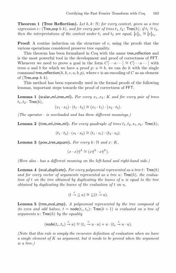
Certifying the Fast Fourier Transform with Coq 163
Theorem 1 (Tree Reflection). Let h, k : N; for every context, given as a treeexpression e : (Tree exp h k), and for every pair of trees t1, t2 : Tree(h); if t1 ∼= t2,then the interpretations of the context under t1 and t2 are equal, [[e]]t1 ∼= [[e]]t2 .
Proof: A routine induction on the structure of e, using the proofs that thevarious operations considered preserve tree equality.
This theorem has been formalized in Coq with the name tree reflection andis the most powerful tool in the development and proof of correctness of FFT.Whenever we need to prove a goal in the form C[· · · a · · · ] ∼= C[· · · a · · · ] withtrees a and b for which we have a proof p : a ∼= b, we can do it with the singlecommand tree reflection(h, k, e, a, b, p), where e is an encoding of C as an elementof (Tree exp h k).
This method has been repeatedly used in the formal proofs of the followinglemmas, important steps towards the proof of correctness of FFT.
Lemma 1 (scalar ml tree ml). For every x1, x2 : K and for every pair of treest1, t2 : Tree(k),
(x1 · x2) · (t1 · t2) ∼= (x1 · t1) · (x2 · t2).(The operator · is overloaded and has three different meanings.)
Lemma 2 (tree ml tree ml). For every quadruple of trees t1, t2, s1, s2 : Tree(k),
(t1 · t2) · (s1 · s2) ∼= (t1 · s1) · (t2 · s2).
Lemma 3 (pow tree square). For every k : N and x : K,
(x · x)⇑k ∼= (x⇑k · x⇑k).
(Here also · has a different meaning on the left-hand and right-hand side.)
Lemma 4 (eval duplicate). For every polynomial represented as a tree t : Tree(k)and for every vector of arguments represented as a tree u : Tree(h), the evalua-tion of t on the tree obtained by duplicating the leaves of u is equal to the treeobtained by duplicating the leaves of the evaluation of t on u,
(te� �u) ∼= �(t
e� u).
Lemma 5 (tree eval step). A polynomial represented by the tree composed ofits even and odd halves, t = node(te, to) : Tree(k + 1) is evaluated on a tree ofarguments u : Tree(h) by the equality
(node(te, to)e� u) ∼= (te
e� u · u) + u · (to e� u · u).
(Note that this rule is simply the recursive definition of evaluation when we havea single element of K as argument, but it needs to be proved when the argumentis a tree.)
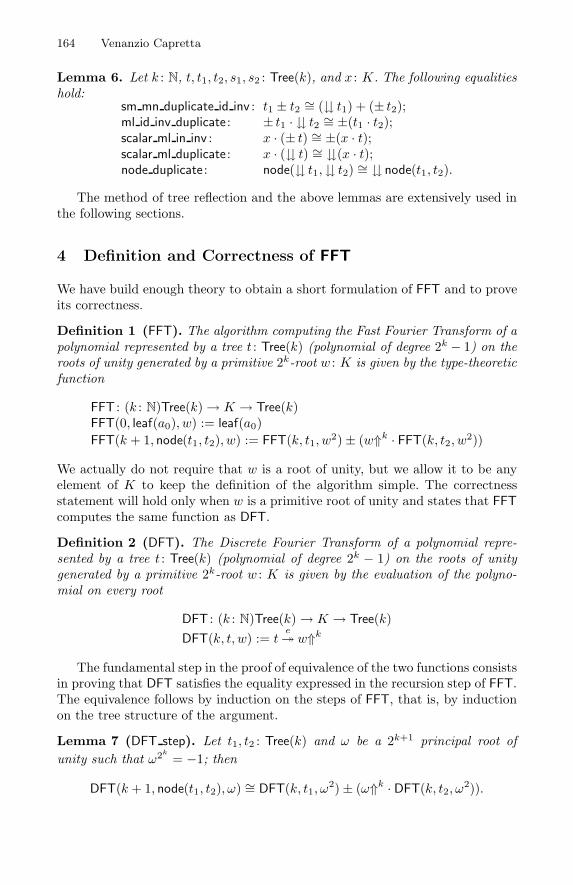
164 Venanzio Capretta
Lemma 6. Let k : N, t, t1, t2, s1, s2 : Tree(k), and x : K. The following equalitieshold:
sm mn duplicate id inv : t1 ± t2 ∼= (� t1) + (± t2);ml id inv duplicate : ± t1 ·� t2 ∼= ±(t1 · t2);scalar ml in inv : x · (± t) ∼= ±(x · t);scalar ml duplicate : x · (� t) ∼= �(x · t);node duplicate : node(� t1,� t2) ∼= � node(t1, t2).
The method of tree reflection and the above lemmas are extensively used inthe following sections.
4 Definition and Correctness of FFT
We have build enough theory to obtain a short formulation of FFT and to proveits correctness.
Definition 1 (FFT). The algorithm computing the Fast Fourier Transform of apolynomial represented by a tree t : Tree(k) (polynomial of degree 2k − 1) on theroots of unity generated by a primitive 2k-root w : K is given by the type-theoreticfunction
FFT : (k : N)Tree(k)→ K → Tree(k)FFT(0, leaf(a0), w) := leaf(a0)FFT(k + 1, node(t1, t2), w) := FFT(k, t1, w2)± (w⇑k · FFT(k, t2, w2))
We actually do not require that w is a root of unity, but we allow it to be anyelement of K to keep the definition of the algorithm simple. The correctnessstatement will hold only when w is a primitive root of unity and states that FFTcomputes the same function as DFT.
Definition 2 (DFT). The Discrete Fourier Transform of a polynomial repre-sented by a tree t : Tree(k) (polynomial of degree 2k − 1) on the roots of unitygenerated by a primitive 2k-root w : K is given by the evaluation of the polyno-mial on every root
DFT : (k : N)Tree(k)→ K → Tree(k)DFT(k, t, w) := t
e� w⇑k
The fundamental step in the proof of equivalence of the two functions consistsin proving that DFT satisfies the equality expressed in the recursion step of FFT.The equivalence follows by induction on the steps of FFT, that is, by inductionon the tree structure of the argument.
Lemma 7 (DFT step). Let t1, t2 : Tree(k) and ω be a 2k+1 principal root ofunity such that ω2k
= −1; then
DFT(k + 1, node(t1, t2), ω) ∼= DFT(k, t1, ω2)± (ω⇑k · DFT(k, t2, ω2)).
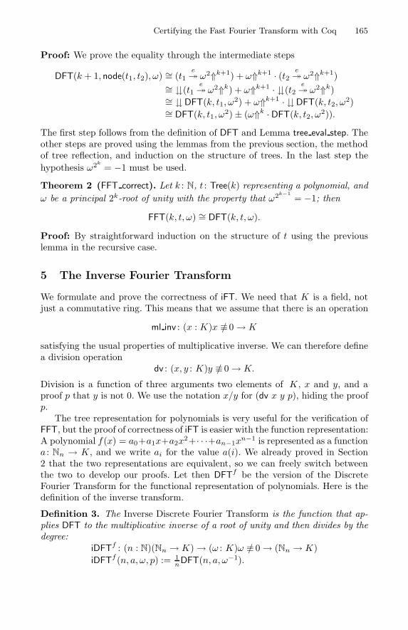
Certifying the Fast Fourier Transform with Coq 165
Proof: We prove the equality through the intermediate steps
DFT(k + 1, node(t1, t2), ω) ∼= (t1e� ω2⇑k+1) + ω⇑k+1 · (t2 e� ω2⇑k+1)
∼= �(t1e� ω2⇑k) + ω⇑k+1 ·�(t2
e� ω2⇑k)∼= � DFT(k, t1, ω2) + ω⇑k+1 ·� DFT(k, t2, ω2)∼= DFT(k, t1, ω2)± (ω⇑k ·DFT(k, t2, ω2)).
The first step follows from the definition of DFT and Lemma tree eval step. Theother steps are proved using the lemmas from the previous section, the methodof tree reflection, and induction on the structure of trees. In the last step thehypothesis ω2k
= −1 must be used.
Theorem 2 (FFT correct). Let k : N, t : Tree(k) representing a polynomial, andω be a principal 2k-root of unity with the property that ω2k−1
= −1; thenFFT(k, t, ω) ∼= DFT(k, t, ω).
Proof: By straightforward induction on the structure of t using the previouslemma in the recursive case.
5 The Inverse Fourier Transform
We formulate and prove the correctness of iFT. We need that K is a field, notjust a commutative ring. This means that we assume that there is an operation
ml inv : (x : K)x ≡/ 0→ K
satisfying the usual properties of multiplicative inverse. We can therefore definea division operation
dv : (x, y : K)y ≡/ 0→ K.
Division is a function of three arguments: two elements of K, x and y, and aproof p that y is not 0. We use the notation x/y for (dv x y p), hiding the proofp.
The tree representation for polynomials is very useful for the verification ofFFT, but the proof of correctness of iFT is easier with the function representation:A polynomial f(x) = a0+a1x+a2x
2+· · ·+an−1xn−1 is represented as a function
a : Nn → K, and we write ai for the value a(i). We already proved in Section2 that the two representations are equivalent, so we can freely switch betweenthe two to develop our proofs. Let then DFTf be the version of the DiscreteFourier Transform for the functional representation of polynomials. Here is thedefinition of the inverse transform.
Definition 3. The Inverse Discrete Fourier Transform is the function that ap-plies DFT to the multiplicative inverse of a root of unity and then divides by thedegree:
iDFTf : (n : N)(Nn → K)→ (ω : K)ω ≡/ 0→ (Nn → K)iDFTf (n, a, ω, p) := 1
nDFT(n, a, ω−1).
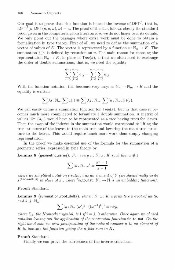
166 Venanzio Capretta
Our goal is to prove that this function is indeed the inverse of DFTf , that is,iDFTf (n,DFT(n, a, ω), ω) = a. The proof of this fact follows closely the standardproof given in the computer algebra literature, so we do not linger over its details.We only point out the passages where extra work must be done to obtain aformalization in type theory. First of all, we need to define the summation of avector of values of K. The vector is represented by a function v : Nn → K. Thesummation
∑v is defined by recursion on n. The main reason for choosing the
representation Nn → K, in place of Tree(k), is that we often need to exchangethe order of double summations, that is, we need the equality
n−1∑i=0
m−1∑j=0
aij =m−1∑j=0
n−1∑i=0
aij .
With the function notation, this becomes very easy: a : Nn → Nm → K and theequality is written
∑λi : Nn.
∑a(i) ≡
∑λj : Nm.
∑λi : Nna(i)(j).
We can easily define a summation function for Tree(k), but in that case it be-comes much more complicated to formulate a double summation. A matrix ofvalues like {aij} would have to be represented as a tree having trees for leaves.Then the swap of the indexes in the summation would correspond to lifting thetree structure of the leaves to the main tree and lowering the main tree struc-ture to the leaves. This would require much more work than simply changingrepresentation.
In the proof we make essential use of the formula for the summation of ageometric series, expressed in type theory by
Lemma 8 (geometric series). For every n : N, x : K such that x ≡/ 1,∑
λi : Nn.xi ≡ xn − 1
x− 1
where we simplified notation treating i as an element of N (we should really writex(fin to nat(i)) in place of xi, where fin to nat : Nn → N is an embedding function).
Proof: Standard.
Lemma 9 (summation root delta). For n : N, ω : K a primitive n-root of unity,and k, j : Nn, ∑
λi : Nn.(ωi)j · ((ω−1)k)i ≡ nδjk
where δij, the Kronecker symbol, is 1 if i = j, 0 otherwise. Once again we abusednotation leaving out the application of the conversion function fin to nat. On theright-hand side we used juxtaposition of the natural number n to an element ofK to indicate the function giving the n-fold sum in K.
Proof: Standard.Finally we can prove the correctness of the inverse transform.
Certifying the Fast Fourier Transform with Coq 167
Theorem 3 (inverse DFT). Let n : N, a : Nn → K, ω : K a primitive n-root ofunity; then for every k : Nn,
DFTf (n,DFTf (n, a, ω), ω−1)k ≡ n · ak.
Proof: Standard using the previous lemmas.Once iDFT has been defined and proved correct for the functional represen-
tation of polynomials, we can use the equivalence of the two representations toobtain a proof of correctness of the version of the inverse transform for treesusing the fast algorithm:
iFT(n, t, ω) :=1n
FFT(n, t, ω−1).
6 Conclusion
The definition and the proof of correctness for FFT and iFT have been com-pletely formalized using the proof tool Coq. I have used the graphical interfaceCtCoq [4] to develop the formalization. CtCoq was extremely useful for severalreasons. It affords extendable notation which allows the printing of terms in nicemathematical formalism, hiding parts that have no mathematical content (forexample the applications of the commutation function fin to nat or the presenceof a proof that the denominator is not zero in a division). The technique of proof-by-pointing [5] allows the user to construct complicated tactics with a few clicksof the mouse. It is easy to search for theorems and lemmas previously provedand apply them by just pressing a key. I found that the use of CtCoq increasedthe efficiency and speed of work, and I could complete the whole developmentin just a couple of months.
The proof uses two main techniques. First, instead of using the most naturaldata type to represent the objects on which the algorithm operates, we chose analternative data type that makes it easier to reason about the computations bystructural recursion. Second, we used the two-level approach to automate partof the generation of proofs of equality for tree expressions.
Future work will concentrate in controlling more carefully how the algorithmexploits time and space resources. It is known that FFT runs in O(n log n) time,but we didn’t prove it formally in Coq. The problem here is that there is noformal study of algorithmic complexity in type theory. In general it is difficultto reason about the running time of functional programs, since the reductionstrategy is not fixed. A solution could be achieved by translating FFT into a de-velopment of imperative programming and then reasoning about its complexityin that framework. Another point is the use of memory. One important featureof FFT is that it can be computed in place, that means that the memory oc-cupied by the input data can be reused during the computation, without theneed of extra memory. Also memory management is a sore point in functionalprogramming. I think it is possible to use the uniqueness types of the program-ming language Clean [9] to force the algorithm to reuse the space occupied bythe data.
168 Venanzio Capretta
References
1. Antonia Balaa and Yves Bertot. Fix-point equations for well-founded recursion intype theory. In J. Harrison and M. Aagaard, editors, Theorem Proving in HigherOrder Logics: 13th International Conference, TPHOLs 2000, volume 1869 of Lec-ture Notes in Computer Science, pages 1–16. Springer-Verlag, 2000.
2. Bruno Barras, Samuel Boutin, Cristina Cornes, Judicael Courant, Yann Coscoy,David Delahaye, Daniel de Rauglaudre, Jean-Christophe Filliatre, EduardoGimenez, Hugo Herbelin, Gerard Huet, Henri Laulhere, Cesar Munoz, ChetanMurthy, Catherine Parent-Vigouroux, Patrick Loiseleur, Christine Paulin-Mohring,Amokrane Saıbi, and Benjanin Werner. The Coq Proof Assistant Reference Man-ual. Version 6.3. INRIA, 1999.
3. G. Barthe, M. Ruys, and H. P. Barendregt. A two-level approach towards leanproof-checking. In S. Berardi andM. Coppo, editors, Types for Proofs and Programs(TYPES’95), volume 1158 of LNCS, pages 16–35. Springer, 1995.
4. Yves Bertot. The CtCoq system: Design and architecture. Formal aspects ofComputing, 11:225–243, 1999.
5. Yves Bertot, Gilles Kahn, and Laurent Thery. Proof by pointing. In Symposiumon Theoretical Aspects Computer Software (STACS), Sendai (Japan), volume 789of LNCS. Springer, April 1994.
6. Samuel Boutin. Using reflection to build efficient and certified decision proce-dures. In Martın Abadi and Takayasu Ito, editors, Theoretical Aspects of ComputerSoftware. Third International Symposium, TACS’97, volume 1281 of LNCS, pages515–529. Springer, 1997.
7. Ana Bove and Venanzio Capretta. Nested general recursion and partiality in typetheory. http://www.cs.kun.nl/ venanzio/publications/nested.ps.gz, 2001.
8. James W. Cooley and John W. Tukey. An algorithm for the machine calculation ofcomplex Fourier series. Mathematics of Computation, 19(90):297–301, April 1965.
9. Paul de Mast, Jan-Marten Jansen, Dick Bruin, Jeroen Fokker, Pieter Koopman,Sjaak Smetsers, Marko van Eekelen, and Rinus Plasmeijer. Functional Program-ming in Clean. Computing Science Institute, University of Nijmegen.
10. Ruben A. Gamboa. The correctness of the Fast Fourier Transform: a structuredproof in ACL2. Formal Methods in System Design, Special Issue on UNITY, 2001.in print.
11. Jayadev Misra. Powerlist: a structure for parallel recursion. TOPLAS, 16(6):1737–1767, November 1994.
A Generic Library for Floating-Point Numbers
and Its Application to Exact Computing
Marc Daumas1, Laurence Rideau2, and Laurent Thery2
1 CNRS, Laboratoire de l’Informatique du ParallelismeUMR 5668 - ENS de Lyon - INRIA
[email protected] INRIA, 2004 route des Lucioles, 06902 Sophia Antipolis France
{Laurence.Rideau,Laurent.Thery}@sophia.inria.fr
Abstract. In this paper we present a general library to reason aboutfloating-point numbers within the Coq system. Most of the results of thelibrary are proved for an arbitrary floating-point format and an arbitrarybase. A special emphasis has been put on proving properties for exactcomputing, i.e. computing without rounding errors.
1 Introduction
Building a reusable library for a prover is not an easy task. The library should becarefully designed in order to give direct access to all key properties. This work isusually underestimated. Often libraries are developed for a given application, sothey tend to be incomplete and too specific. This makes their reuse problematic.Still we believe that the situation of proving is similar to the one of programming.The fact that the programming language Java was distributed with a quitecomplete set of libraries has been an important factor to its success.This paper presents a library for reasoning about floating-point numbers
within the Coq system [18]. There has already been several attempts to formalizefloating-point numbers in other provers. Barrett [2] proposed a formalization offloating-point numbers using the specification language Z [33]. Miner [25] wasthe first to provide a proving environment for reasoning about floating-pointnumbers. It was done for PVS [30]. More recently Harrison [16] and Russinoff [31]have developed libraries for HOL [14] and ACL2 [21] respectively and appliedthem successfully to prove the correctness of some algorithms and hardwaredesigns. When developing our library we have tried to take a generic approach.The base of the representation and the actual format of the mantissa and of theexponent are parameterized. We still use the key property of correct roundingand the clean ideas of the IEEE 754 and 854 standards [35,7,13].The paper is organized as follows. We first present some basic notions and
their representation in Coq. Then we spend some time to explain how we havedefined the central notion of rounding. In Section 4, we give examples of the kindof properties that are in the library and how they have been proved. Section5 details the proof of correctness of a program that is capable to detect the
R.J. Boulton and P.B. Jackson (Eds.): TPHOLs 2001, LNCS 2152, pp. 169–184, 2001.c© Springer-Verlag Berlin Heidelberg 2001
170 Marc Daumas, Laurence Rideau, and Laurent Thery
base of an arbitrary arithmetic. Finally we show an application of this libraryto floating-point expansions. These expansions were presented in [11] first andmore formally in [28,32]. The technique can be specialized for the predicates ofcomputational geometry [5,19] or to small-width multiple precision arithmetic[1,9], among other applications.
2 Floating-Point Format and Basic Notions
2.1 Definitions
Our floating-point numbers are defined as a new type composed by records:Record. float: Set := Float {Fnum:Z; Fexp:Z}This command creates a new type float, a constructor function Float of typeZ→ Z→ float and two destructor functions Fnum and Fexp of type float → Z.The fact that float is of type Set indicates that float is a datatype. The compo-nent Fnum represents the mantissa and Fexp the exponent. In the following wewrite (Float x y) simply as 〈x, y〉 and (Fnum p) and (Fexp p) as n[p] and e[p]respectively.In order to give a semantics to this new type, we have to relate our float
to their value as a real. The reals in Coq are defined axiomatically [24] as thesmallest complete archimedian field. We define the function FtoR of type float →R as:Definition. FtoR := λp: float . n[p] ∗ βe[p].
This definition is parameterized over an arbitrary base β. We suppose that thebase is an integer strictly greater than one. Our notation differs from the IEEEstandard notation [35] and even from the pre-standard notation [6]. The mantissais an integer and βe[x] is one unit in the last place of the float x or the weight ofits least significant bit.Having the type float as a separate type instead of a subtype of the real
numbers as in [16] implies that we have to manipulate two notions of equality.The usual Leibniz equality p = q means that p and q have the same componentsas a record. The equality over R (FtoR p) = (FtoR q) means that they representthe same real. In the following this last equality will be denoted p == q andthe function FtoR is used implicitly as a coercion between our floating-pointnumbers and the reals, so 0 < p should be understood as 0 < (FtoR p). The twonotions of equality are related. For example we have the following theorems:Theorem. FtoREqInv1 :∀p, q: float .¬p == 0⇒ p == q ⇒ n[p] = n[q]⇒ p = q.
Theorem. FtoREqInv2 :∀p, q: float . p == q ⇒ e[p] = e[q]⇒ p = q.
On the type float, we can define the usual operations that return an element oftype float such as:Definition. Fplus := λp, q: float .
〈n[p] ∗ (βe[p]−min(e[p],e[q])) + n[q] ∗ (βe[q]−min(e[p],e[q])),min(e[p], e[q])〉
A Generic Library for Floating-Point Numbers 171
Definition. Fop := λp: float . 〈−n[p], e[p]〉.Definition. Fabs := λp: float . 〈|n[p]|, e[p]〉.Definition. Fminus := λp, q: float . (Fplus p (Fop q)).
Definition. Fmult := λp, q: float . 〈n[p] ∗ n[q], e[p] + e[q]〉.For each of these functions we have proved a theorem of correctness. For additionthis theorem looks like:Theorem. Fplus correct :∀p, q: float . (Fplus p q) == p+ q.
where the rightmost addition is the usual addition on real numbers. Note thatsince we do not have uniqueness of representation, these functions just pick apossible representant of the result. In the following we write +,−,| |, −,∗ forFplus, Fop, Fabs, Fminus, Fmult respectively.
2.2 Bounded Floating-Point Numbers
As it is defined, the type float contains too many elements. In order to representmachine floating-point numbers we need to define the notion of bound:Record. Fbound: Set := Bound {vNum:N; dExp:N}We use this notion of bound to parameterize our development over an arbitrarybound b. In the following, we write (vNum b) and (dExp b) as N [b] and E[b].With this arbitrary bound we can define a predicate Fbounded to characterizebounded floating-point numbers:Definition. Fbounded := λp: float . −N [b] ≤ n[p] ≤ N [b] ∧ −E[b] ≤ e[p].
In the following we write (Fbounded p) as B[p]. A real that has a boundedfloating-point number equivalent is said to be representable. Note that we donot impose any upper bound on the exponent. This allows us to have a moreuniform definition of rounding since any real is always between two boundedfloating-point numbers.In existing systems, overflows generate combinatorial quantities like infinities,
errors (NaN) and so on. Having the upper bound would force us to treat thesenon-numerical quantities at each theorem. The bound should rather be addedonly to the final data type. Only the high level theorems will be proved both fornumerical and for combinatorial values.Removing the lower bound is not admissible as it will hide the difficult ques-
tion of the subnormal numbers. As can be seen for example in [10], the lowerbound is used to prove properties through the full set of floating-point numbersand not uniquely on small numbers.
2.3 Canonical Numbers
So far the bound on the mantissa is arbitrary. In practice, it is set so that anynumber is represented with a fixed width field. The width of the field is calledthe precision. We define an arbitrary integer variable precision that is supposed
172 Marc Daumas, Laurence Rideau, and Laurent Thery
not null and we add the following hypothesis:
Hypothesis. pGivesBound:N [b] = βprecision − 1.This insures that the number of digits of the mantissa is at most precision inbase β. We can also define a notion of canonical representant.
We first define the property of a floating-point number to be normal if it isbounded and the number of digits of its mantissa is exactly the precision:Definition. Fnormal := λp: float .B[p] ∧ digit(p) = precision .
where digit is a function that returns the number of radix-β digits in the integern[p] (no leading zeros). All bounded numbers do not have a normal equivalent,take for example 〈0, 0〉. For numbers near zero, we define the property of beingsubnormal by relaxing the constraint on the number of digits:Definition. Fsubnormal := λp: float .B[p] ∧ e[p] = −E[b] ∧ digit(p) < precision.
We can now define what it is for a number to be canonic as:Definition. Fcanonic := λp: float . (Fnormal p) ∨ (Fsubnormal p).
In the following the properties (Fnormal p), (Fsubnormal p), (Fcanonic p) willbe denoted as N [p], S[p], and C[p] respectively. It is easy to show that normal,subnormal and canonic representations are unique:Theorem. FnormalUnique :∀p, q: float .N [p]⇒ N [q]⇒ p == q ⇒ p = q.
Theorem. FsubnormalUnique : ∀p, q: float .S [p]⇒ S [q]⇒ p == q ⇒ p = q.
Theorem. FcanonicUnique :∀p, q: float . C[p]⇒ C[q]⇒ p == q ⇒ p = q.
In order to compute the canonical representant of a bounded number, we buildthe following function:Definition. Fnormalize := λp: float .if n[p] = 0 then 〈0,−E[b]〉else let z = min(precision − digit(p), |E[b] + e[p]|) in 〈n[p] ∗ βz, e[p]− z〉.
The following two theorems insure that what we get is the expected function:Theorem. FnormalizeCorrect :∀p: float . (Fnormalize p) == p.
Theorem. FnormalizeCanonic:∀p: float .B[p]⇒ C[(Fnormalize p)].
With the function Fnormalize, it is possible to capture the usual notion of unitin the last place with the following definition:
Definition. Fulp := λp: float . βe[(Fnormalize p)].
Working with canonical representations not only do we get that equality is thesyntactic one but also the comparison between two numbers can be interpreteddirectly on their components with lexicographic order on positive numbers:Theorem. FcanonicLtPos : ∀p, q: float . C[p]⇒ C[q]⇒0 ≤ p < q ⇒ (e[p] < e[q]) ∨ (e[p] = e[q] ∧ n[p] < n[q]).
We have a similar theorem for negative floating-point numbers. These two the-
A Generic Library for Floating-Point Numbers 173
orems give us a direct way to construct the successor of a canonical number:Definition. FSucc := λp: float .if n[p] = N [b] then 〈βprecision−1 , e[p] + 1〉else if n[p] = −βprecision−1 then
if e[p] = −E[b] then 〈n[p] + 1, e[p]〉 else 〈−N [b], e[p]− 1〉else 〈n[p] + 1, e[p]〉
To be sure that this function is the expected one, we have proved the three fol-lowing theorems:Theorem. FSuccCanonic:∀p: float . C[p]⇒ C[(FSucc p)].
Theorem. FSuccLt :∀p: float . p < (FSucc p).
Theorem. FSuccProp :∀p, q: float . C[p]⇒ C[q]⇒ p < q ⇒ (FSucc p) ≤ q.
The function FPred that computes the preceeding canonical number can also bedefined in a similar way.
3 Rounding Mode
Rounding plays a central role in any implementation of floating-point numbers.Following the philosophy of the IEEE standard, all operations on floating-pointnumbers should return the rounded value of the result of the exact operation.The logic of Coq is constructive: every function definition has to be explicit. Insuch a context defining a rounding function is problematic. We overcome thisproblem by defining rounding as a relation between a real number and a floating-point number. Rounding is defined abstractly. The first property a rounding mustverify is to be total:Definition. TotalP := λP: R→ float → Prop.∀r: R.∃p: float . (P r p).
In Coq, propositions are of type Prop, so an object P of type R→ float → Propis a relation between a real and a floating-point number. Another property thatis needed is the compatibility:Definition. CompatibleP := λP: R→ float → Prop.∀r1 , r2: R.∀p, q: float .(P r1 p)⇒ r1 = r2 ⇒ p == q ⇒ B[q]⇒ (P r2 q).
Although we defined a canonical representation of floating-point numbers, wewill not specify that the rounded value of a floating-point number should becanonical. This is definitively not needed at this point and we will see later thatbeing more general allows us to build easier proofs. We specify that the roundingmust be monotone:Definition. MonotoneP := λP: R→ float → Prop.∀r1 , r2: R.∀p, q: float .
r1 < r2 ⇒ (P r1 p)⇒ (P r2 q)⇒ p ≤ q.
Finally looking for a projection, we set that the rounded value of a real mustbe one of the two floats that are around it. When the real to be rounded can berepresented by a bounded floating-point number, the two floating-point numbersaround it are purposely equal. We define the ceil (isMin) and the floor (isMax)
174 Marc Daumas, Laurence Rideau, and Laurent Thery
relations and the property for a rounded value to be either a ceil or a floor:Definition. isMin := λr: R. λmin: float .B[min] ∧min ≤ r ∧ ∀p: float .B[p]⇒ p ≤ r ⇒ p ≤ min.
Definition. isMax := λr: R. λmax: float .B[max] ∧ r ≤ max ∧ ∀p: float .B[p]⇒ r ≤ p⇒ max ≤ p.
Definition. MinOrMaxP := λP: R→ float → Prop.∀r: R.∀p: float . (P r p)⇒ (isMin r p) ∨ (isMax r p).
Using the previous definitions, we can define what is a rounding mode:Definition. RoundedModeP := λP: R→ float → Prop.(TotalP P ) ∧ (CompatibleP P ) ∧ (MinOrMaxP P ) ∧ (Monotone P ).
Having defined the rounding abstractly gives us for free the possibility of provinggeneral properties of rounding. An example is the property that the rounding ofa bounded floating-point number is the number itself. It can be stated as:Definition. ProjectorP := λP: R→ float → Prop.∀p, q: float .B[p]⇒ (P p q)⇒ p == q.
Theorem. RoundedProjector :∀P: R→ float → Prop.(RoundedModeP P )⇒ (ProjectorP P ).
As a matter of fact we could have replaced in the definition of RoundModeP theproperty MinOrMax by ProjectorP.
We can now define the usual rounding modes. First of all, the two relationsisMin and isMax are rounding:Theorem. MinRoundedModeP : (RoundedModeP isMin).
Theorem. MaxRoundedModeP : (RoundedModeP isMax ).
The rounding to zero is defined as follows:Definition. ToZeroP := λr: R. λp: float .(0 ≤ r ∧ (isMin r p)) ∨ (r ≤ 0 ∧ (isMax r p)).
Theorem. ToZeroRoundedModeP : (RoundedModeP ToZeroP).
Similarly we define the rounding to infinity:Definition. ToInfinityP := λr: R. λp: float .(r ≤ 0 ∧ (isMin r p)) ∨ (0 ≤ r ∧ (isMax r p)).
Theorem. ToInfinityRoundedModeP : (RoundedModeP ToInfinityP).
While the preceeding roundings are really functions, we take advantage of havinga relation to define rounding to the closest:Definition. Closest := λr: R. λp: float .B[p] ∧ ∀f : float .B[f ]⇒ |p− r| ≤ |f − r|.Theorem. ClosestRoundedModeP : (RoundedModeP Closest).
For the real in the middle of two successive bounded floating-point numbers thereare two possible closest. So a tie-break rule is usually invoked. In our presenta-tion, we simply accept these two points as a rounding value since uniqueness is
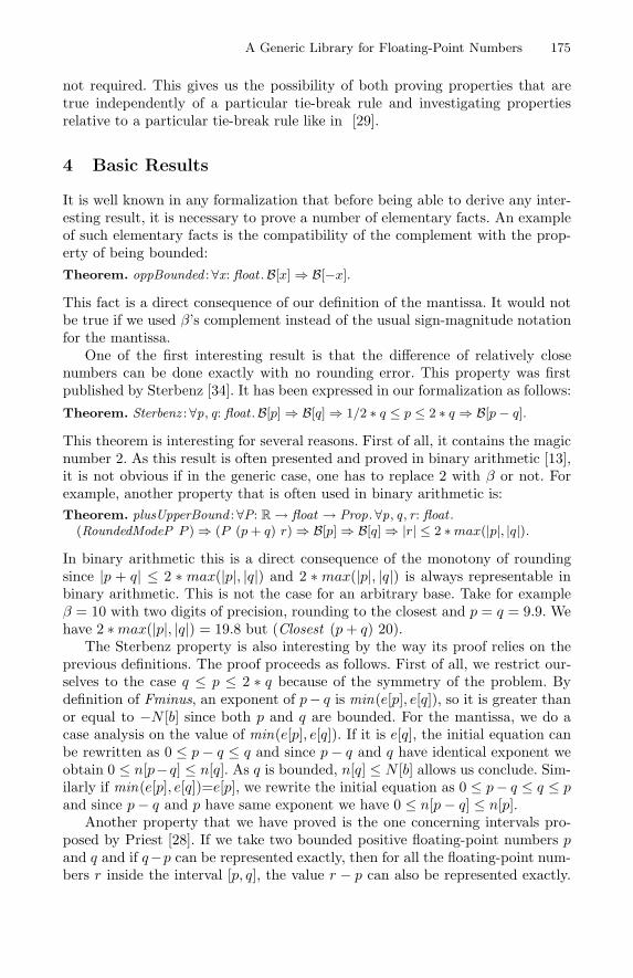
A Generic Library for Floating-Point Numbers 175
not required. This gives us the possibility of both proving properties that aretrue independently of a particular tie-break rule and investigating propertiesrelative to a particular tie-break rule like in [29].
4 Basic Results
It is well known in any formalization that before being able to derive any inter-esting result, it is necessary to prove a number of elementary facts. An exampleof such elementary facts is the compatibility of the complement with the prop-erty of being bounded:Theorem. oppBounded :∀x: float .B[x]⇒ B[−x].This fact is a direct consequence of our definition of the mantissa. It would notbe true if we used β’s complement instead of the usual sign-magnitude notationfor the mantissa.One of the first interesting result is that the difference of relatively close
numbers can be done exactly with no rounding error. This property was firstpublished by Sterbenz [34]. It has been expressed in our formalization as follows:Theorem. Sterbenz :∀p, q: float .B[p]⇒ B[q]⇒ 1/2 ∗ q ≤ p ≤ 2 ∗ q ⇒ B[p− q].
This theorem is interesting for several reasons. First of all, it contains the magicnumber 2. As this result is often presented and proved in binary arithmetic [13],it is not obvious if in the generic case, one has to replace 2 with β or not. Forexample, another property that is often used in binary arithmetic is:Theorem. plusUpperBound :∀P: R→ float → Prop.∀p, q , r: float .(RoundedModeP P )⇒ (P (p+ q) r)⇒ B[p]⇒ B[q]⇒ |r| ≤ 2 ∗max(|p|, |q|).
In binary arithmetic this is a direct consequence of the monotony of roundingsince |p + q| ≤ 2 ∗ max(|p|, |q|) and 2 ∗max(|p|, |q|) is always representable inbinary arithmetic. This is not the case for an arbitrary base. Take for exampleβ = 10 with two digits of precision, rounding to the closest and p = q = 9.9. Wehave 2 ∗max(|p|, |q|) = 19.8 but (Closest (p+ q) 20).The Sterbenz property is also interesting by the way its proof relies on the
previous definitions. The proof proceeds as follows. First of all, we restrict our-selves to the case q ≤ p ≤ 2 ∗ q because of the symmetry of the problem. Bydefinition of Fminus, an exponent of p− q is min(e[p], e[q]), so it is greater thanor equal to −N [b] since both p and q are bounded. For the mantissa, we do acase analysis on the value of min(e[p], e[q]). If it is e[q], the initial equation canbe rewritten as 0 ≤ p− q ≤ q and since p− q and q have identical exponent weobtain 0 ≤ n[p−q] ≤ n[q]. As q is bounded, n[q] ≤ N [b] allows us conclude. Sim-ilarly if min(e[p], e[q])=e[p], we rewrite the initial equation as 0 ≤ p− q ≤ q ≤ pand since p− q and p have same exponent we have 0 ≤ n[p− q] ≤ n[p].Another property that we have proved is the one concerning intervals pro-
posed by Priest [28]. If we take two bounded positive floating-point numbers pand q and if q−p can be represented exactly, then for all the floating-point num-bers r inside the interval [p, q], the value r − p can also be represented exactly.
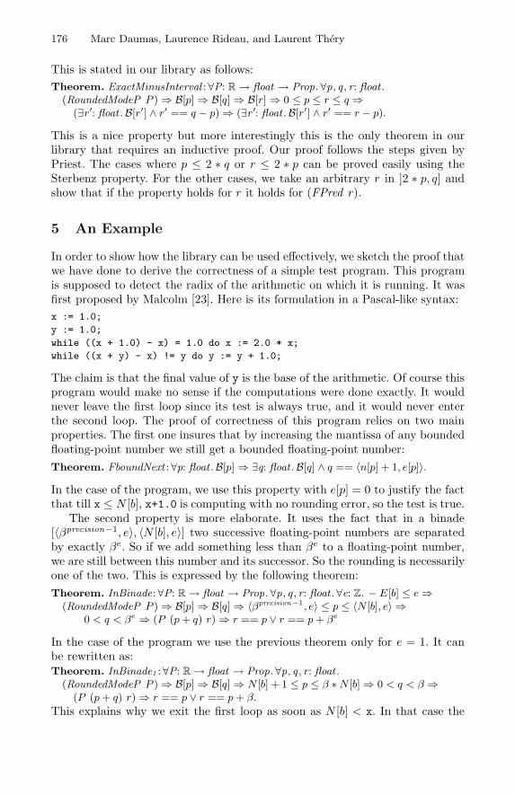
176 Marc Daumas, Laurence Rideau, and Laurent Thery
This is stated in our library as follows:Theorem. ExactMinusInterval :∀P: R→ float → Prop.∀p, q , r: float .(RoundedModeP P )⇒ B[p]⇒ B[q]⇒ B[r]⇒ 0 ≤ p ≤ r ≤ q ⇒(∃r ′: float .B[r′] ∧ r′ == q − p)⇒ (∃r ′: float .B[r′] ∧ r′ == r − p).
This is a nice property but more interestingly this is the only theorem in ourlibrary that requires an inductive proof. Our proof follows the steps given byPriest. The cases where p ≤ 2 ∗ q or r ≤ 2 ∗ p can be proved easily using theSterbenz property. For the other cases, we take an arbitrary r in ]2 ∗ p, q] andshow that if the property holds for r it holds for (FPred r).
5 An Example
In order to show how the library can be used effectively, we sketch the proof thatwe have done to derive the correctness of a simple test program. This programis supposed to detect the radix of the arithmetic on which it is running. It wasfirst proposed by Malcolm [23]. Here is its formulation in a Pascal-like syntax:x := 1.0;
y := 1.0;
while ((x + 1.0) - x) = 1.0 do x := 2.0 * x;
while ((x + y) - x) != y do y := y + 1.0;
The claim is that the final value of y is the base of the arithmetic. Of course thisprogram would make no sense if the computations were done exactly. It wouldnever leave the first loop since its test is always true, and it would never enterthe second loop. The proof of correctness of this program relies on two mainproperties. The first one insures that by increasing the mantissa of any boundedfloating-point number we still get a bounded floating-point number:Theorem. FboundNext :∀p: float .B[p]⇒ ∃q: float .B[q] ∧ q == 〈n[p] + 1, e[p]〉.In the case of the program, we use this property with e[p] = 0 to justify the factthat till x ≤ N [b], x+1.0 is computing with no rounding error, so the test is true.The second property is more elaborate. It uses the fact that in a binade
[〈βprecision−1, e〉, 〈N [b], e〉] two successive floating-point numbers are separatedby exactly βe. So if we add something less than βe to a floating-point number,we are still between this number and its successor. So the rounding is necessarilyone of the two. This is expressed by the following theorem:Theorem. InBinade:∀P: R→ float → Prop. ∀p, q , r: float .∀e: Z. − E[b] ≤ e⇒(RoundedModeP P )⇒ B[p]⇒ B[q]⇒ 〈βprecision−1, e〉 ≤ p ≤ 〈N [b], e〉 ⇒
0 < q < βe ⇒ (P (p+ q) r)⇒ r == p ∨ r == p+ βe
In the case of the program we use the previous theorem only for e = 1. It canbe rewritten as:Theorem. InBinade1 :∀P: R→ float → Prop.∀p, q , r: float .(RoundedModeP P )⇒ B[p]⇒ B[q]⇒ N [b] + 1 ≤ p ≤ β ∗N [b]⇒ 0 < q < β ⇒(P (p+ q) r)⇒ r == p ∨ r == p+ β.
This explains why we exit the first loop as soon as N [b] < x. In that case the
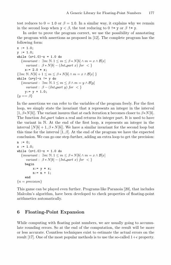
A Generic Library for Floating-Point Numbers 177
test reduces to 0 = 1.0 or β = 1.0. In a similar way, it explains why we remainin the second loop when y < β, the test reducing to 0 != y or β != y.In order to prove the program correct, we use the possibility of annotating
the program with assertions as proposed in [12]. The complete program has thefollowing form:x := 1.0;
y := 1.0;
while (x+1.0)-x = 1.0 do
{invariant : ∃m: N. 1 ≤ m ≤ β ∗N [b] ∧m = x ∧ B[x]variant : β ∗N [b]− (Int part x) for < }x:= 2.0 * x;
{∃m: N. N [b] + 1 ≤ m ≤ β ∗N [b] ∧m = x ∧ B[x] }while (x+y)-x != y do
{invariant : ∃m: N. 1 ≤ m ≤ β ∧m = y ∧ B[y]variant : β − (Int part y) for < }y:= y + 1.0;
{y == β}In the assertions we can refer to the variables of the program freely. For the firstloop, we simply state the invariant that x represents an integer in the interval[1, β∗N [b]]. The variant insures that at each iteration x becomes closer to β∗N [b].The function Int part takes a real and returns its integer part. It is used to havethe variant in N. At the end of the first loop, x represents an integer in theinterval [N [b] + 1, β ∗N [b]]. We have a similar invariant for the second loop butthis time for the interval [1, β]. At the end of the program we have the expectedconclusion. We can go one step further, adding an extra loop to get the precision:n := 0;
x := 1.0;
while (x+1.0)-x = 1.0 do
{invariant : ∃m: N. 1 ≤ m ≤ β ∗N [b] ∧m = x ∧ B[x]variant : β ∗N [b]− (Int part x) for < }begin
x:= y * x;
n:= n + 1;
end
{n = precision}This game can be played even further. Programs like Paranoia [20], that includesMalcolm’s algorithm, have been developed to check properties of floating-pointarithmetics automatically.
6 Floating-Point Expansion
While computing with floating point numbers, we are usually going to accumu-late rounding errors. So at the end of the computation, the result will be moreor less accurate. Countless techniques exist to estimate the actual errors on theresult [17]. One of the most popular methods is to use the so-called 1+ε property.
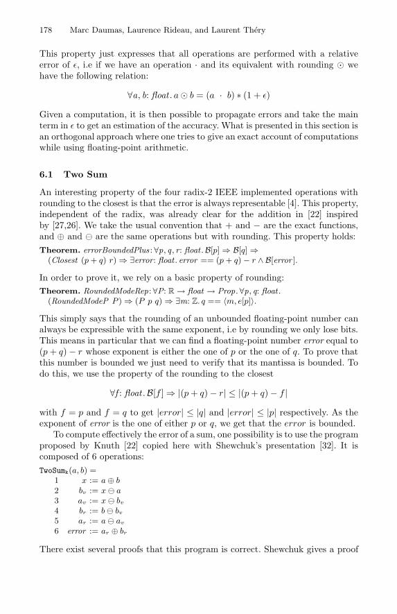
178 Marc Daumas, Laurence Rideau, and Laurent Thery
This property just expresses that all operations are performed with a relativeerror of ε, i.e if we have an operation · and its equivalent with rounding wehave the following relation:
∀a, b: float . a b = (a · b) ∗ (1 + ε)Given a computation, it is then possible to propagate errors and take the mainterm in ε to get an estimation of the accuracy. What is presented in this section isan orthogonal approach where one tries to give an exact account of computationswhile using floating-point arithmetic.
6.1 Two Sum
An interesting property of the four radix-2 IEEE implemented operations withrounding to the closest is that the error is always representable [4]. This property,independent of the radix, was already clear for the addition in [22] inspiredby [27,26]. We take the usual convention that + and − are the exact functions,and ⊕ and � are the same operations but with rounding. This property holds:Theorem. errorBoundedPlus : ∀p, q , r: float .B[p]⇒ B[q]⇒(Closest (p+ q) r)⇒ ∃error: float . error == (p+ q)− r ∧ B[error ].
In order to prove it, we rely on a basic property of rounding:Theorem. RoundedModeRep : ∀P: R→ float → Prop.∀p, q: float .(RoundedModeP P )⇒ (P p q)⇒ ∃m: Z. q == 〈m, e[p]〉.
This simply says that the rounding of an unbounded floating-point number canalways be expressible with the same exponent, i.e by rounding we only lose bits.This means in particular that we can find a floating-point number error equal to(p+ q)− r whose exponent is either the one of p or the one of q. To prove thatthis number is bounded we just need to verify that its mantissa is bounded. Todo this, we use the property of the rounding to the closest
∀f : float .B[f ]⇒ |(p+ q)− r| ≤ |(p+ q)− f |with f = p and f = q to get |error| ≤ |q| and |error| ≤ |p| respectively. As theexponent of error is the one of either p or q, we get that the error is bounded.To compute effectively the error of a sum, one possibility is to use the program
proposed by Knuth [22] copied here with Shewchuk’s presentation [32]. It iscomposed of 6 operations:TwoSumk(a, b) =
1 x := a⊕ b2 bv := x� a3 av := x� bv
4 br := b� bv
5 ar := a� av
6 error := ar ⊕ br
There exist several proofs that this program is correct. Shewchuk gives a proof
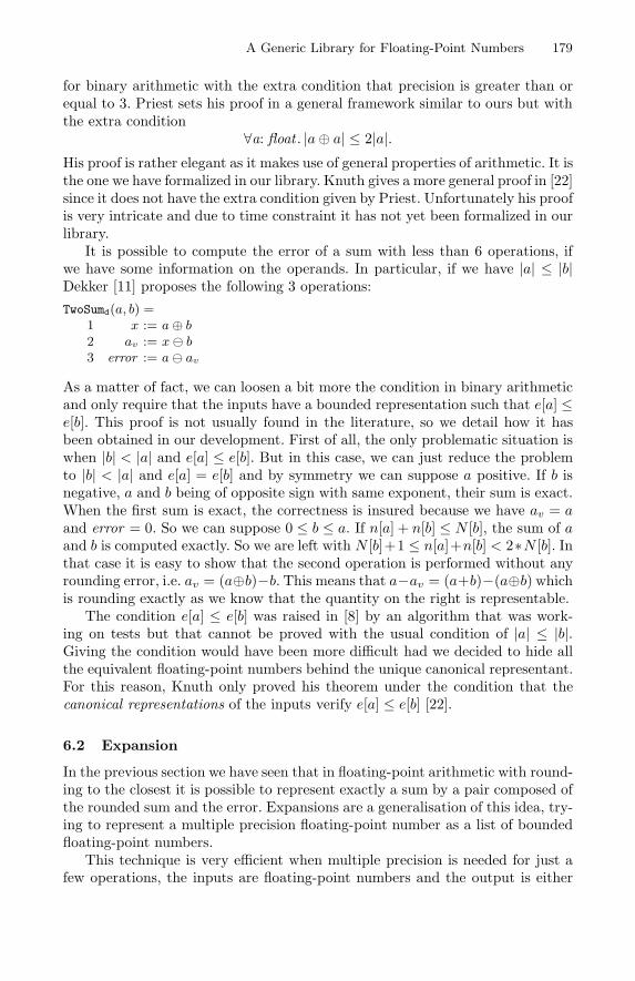
A Generic Library for Floating-Point Numbers 179
for binary arithmetic with the extra condition that precision is greater than orequal to 3. Priest sets his proof in a general framework similar to ours but withthe extra condition
∀a: float . |a⊕ a| ≤ 2|a|.His proof is rather elegant as it makes use of general properties of arithmetic. It isthe one we have formalized in our library. Knuth gives a more general proof in [22]since it does not have the extra condition given by Priest. Unfortunately his proofis very intricate and due to time constraint it has not yet been formalized in ourlibrary.It is possible to compute the error of a sum with less than 6 operations, if
we have some information on the operands. In particular, if we have |a| ≤ |b|Dekker [11] proposes the following 3 operations:TwoSumd(a, b) =
1 x := a⊕ b2 av := x� b3 error := a� av
As a matter of fact, we can loosen a bit more the condition in binary arithmeticand only require that the inputs have a bounded representation such that e[a] ≤e[b]. This proof is not usually found in the literature, so we detail how it hasbeen obtained in our development. First of all, the only problematic situation iswhen |b| < |a| and e[a] ≤ e[b]. But in this case, we can just reduce the problemto |b| < |a| and e[a] = e[b] and by symmetry we can suppose a positive. If b isnegative, a and b being of opposite sign with same exponent, their sum is exact.When the first sum is exact, the correctness is insured because we have av = aand error = 0. So we can suppose 0 ≤ b ≤ a. If n[a] + n[b] ≤ N [b], the sum of aand b is computed exactly. So we are left with N [b]+1 ≤ n[a]+n[b] < 2∗N [b]. Inthat case it is easy to show that the second operation is performed without anyrounding error, i.e. av = (a⊕b)−b. This means that a−av = (a+b)−(a⊕b) whichis rounding exactly as we know that the quantity on the right is representable.The condition e[a] ≤ e[b] was raised in [8] by an algorithm that was work-
ing on tests but that cannot be proved with the usual condition of |a| ≤ |b|.Giving the condition would have been more difficult had we decided to hide allthe equivalent floating-point numbers behind the unique canonical representant.For this reason, Knuth only proved his theorem under the condition that thecanonical representations of the inputs verify e[a] ≤ e[b] [22].
6.2 Expansion
In the previous section we have seen that in floating-point arithmetic with round-ing to the closest it is possible to represent exactly a sum by a pair composed ofthe rounded sum and the error. Expansions are a generalisation of this idea, try-ing to represent a multiple precision floating-point number as a list of boundedfloating-point numbers.This technique is very efficient when multiple precision is needed for just a
few operations, the inputs are floating-point numbers and the output is either
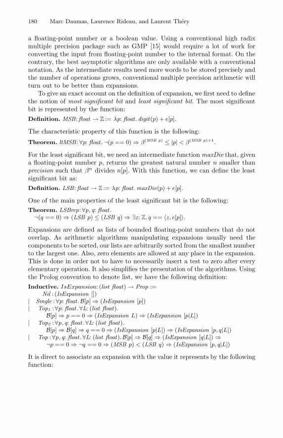
180 Marc Daumas, Laurence Rideau, and Laurent Thery
a floating-point number or a boolean value. Using a conventional high radixmultiple precision package such as GMP [15] would require a lot of work forconverting the input from floating-point number to the internal format. On thecontrary, the best asymptotic algorithms are only available with a conventionalnotation. As the intermediate results need more words to be stored precisely andthe number of operations grows, conventional multiple precision arithmetic willturn out to be better than expansions.To give an exact account on the definition of expansion, we first need to define
the notion of most significant bit and least significant bit. The most significantbit is represented by the function:Definition. MSB :float → Z := λp: float . digit(p) + e[p].
The characteristic property of this function is the following:
Theorem. ltMSB :∀p: float .¬(p == 0)⇒ β(MSB p) ≤ |p| < β(MSB p)+1.
For the least significant bit, we need an intermediate function maxDiv that, givena floating-point number p, returns the greatest natural number n smaller thanprecision such that βn divides n[p]. With this function, we can define the leastsignificant bit as:Definition. LSB : float → Z := λp: float .maxDiv(p) + e[p].
One of the main properties of the least significant bit is the following:Theorem. LSBrep:∀p, q: float .¬(q == 0)⇒ (LSB p) ≤ (LSB q)⇒ ∃z: Z. q == 〈z, e[p]〉.
Expansions are defined as lists of bounded floating-point numbers that do notoverlap. As arithmetic algorithms manipulating expansions usually need thecomponents to be sorted, our lists are arbitrarily sorted from the smallest numberto the largest one. Also, zero elements are allowed at any place in the expansion.This is done in order not to have to necessarily insert a test to zero after everyelementary operation. It also simplifies the presentation of the algorithms. Usingthe Prolog convention to denote list, we have the following definition:Inductive. IsExpansion: (list float)→ Prop :=
Nil : (IsExpansion [])| Single :∀p: float .B[p]⇒ (IsExpansion [p])| Top1 :∀p: float .∀L: (list float).
B[p]⇒ p == 0⇒ (IsExpansion L)⇒ (IsExpansion [p|L])| Top2 :∀p, q: float .∀L: (list float).
B[p]⇒ B[q]⇒ q == 0⇒ (IsExpansion [p|L])⇒ (IsExpansion [p, q|L])| Top :∀p, q: float .∀L: (list float).B[p]⇒ B[q]⇒ (IsExpansion [q|L]) ⇒
¬p == 0⇒ ¬q == 0⇒ (MSB p) < (LSB q)⇒ (IsExpansion [p, q|L])It is direct to associate an expansion with the value it represents by the followingfunction:
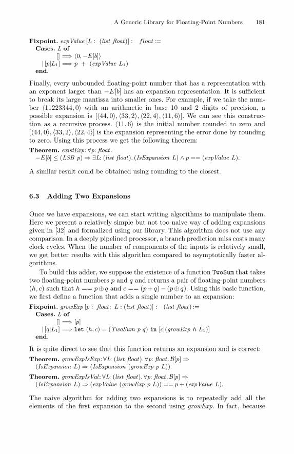
A Generic Library for Floating-Point Numbers 181
Fixpoint. expValue [L : (list float)] : float :=Cases. L of
[] =⇒ 〈0,−E[b]〉| [p|L1] =⇒ p + (expValue L1)
end.
Finally, every unbounded floating-point number that has a representation withan exponent larger than −E[b] has an expansion representation. It is sufficientto break its large mantissa into smaller ones. For example, if we take the num-ber 〈11223344, 0〉 with an arithmetic in base 10 and 2 digits of precision, apossible expansion is [〈44, 0〉, 〈33, 2〉, 〈22, 4〉, 〈11, 6〉]. We can see this construc-tion as a recursive process. 〈11, 6〉 is the initial number rounded to zero and[〈44, 0〉, 〈33, 2〉, 〈22, 4〉] is the expansion representing the error done by roundingto zero. Using this process we get the following theorem:Theorem. existExp :∀p: float .−E[b] ≤ (LSB p)⇒ ∃L: (list float). (IsExpansion L) ∧ p == (expValue L).
A similar result could be obtained using rounding to the closest.
6.3 Adding Two Expansions
Once we have expansions, we can start writing algorithms to manipulate them.Here we present a relatively simple but not too naive way of adding expansionsgiven in [32] and formalized using our library. This algorithm does not use anycomparison. In a deeply pipelined processor, a branch prediction miss costs manyclock cycles. When the number of components of the inputs is relatively small,we get better results with this algorithm compared to asymptotically faster al-gorithms.To build this adder, we suppose the existence of a function TwoSum that takes
two floating-point numbers p and q and returns a pair of floating-point numbers(h, c) such that h == p⊕ q and c == (p+ q)− (p⊕ q). Using this basic function,we first define a function that adds a single number to an expansion:Fixpoint. growExp [p : float ; L : (list float)] : (list float) :=
Cases. L of[] =⇒ [p]
| [q|L1] =⇒ let (h, c) = (TwoSum p q) in [c|(growExp h L1)]end.
It is quite direct to see that this function returns an expansion and is correct:Theorem. growExpIsExp :∀L: (list float).∀p: float .B[p]⇒(IsExpansion L)⇒ (IsExpansion (growExp p L)).
Theorem. growExpIsVal : ∀L: (list float).∀p: float .B[p]⇒(IsExpansion L)⇒ (expValue (growExp p L)) == p+ (expValue L).
The naive algorithm for adding two expansions is to repeatedly add all theelements of the first expansion to the second using growExp. In fact, because
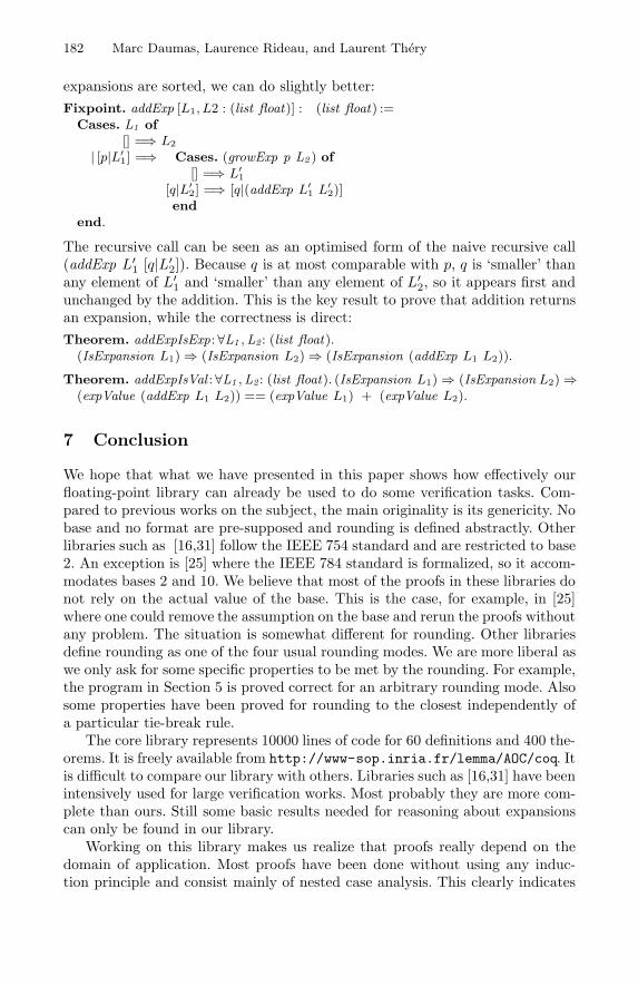
182 Marc Daumas, Laurence Rideau, and Laurent Thery
expansions are sorted, we can do slightly better:Fixpoint. addExp [L1, L2 : (list float)] : (list float) :=
Cases. L1 of[] =⇒ L2
| [p|L′1] =⇒ Cases. (growExp p L2 ) of
[] =⇒ L′1
[q|L′2] =⇒ [q|(addExp L′
1 L′2)]
endend.
The recursive call can be seen as an optimised form of the naive recursive call(addExp L′1 [q|L′2]). Because q is at most comparable with p, q is ‘smaller’ thanany element of L′1 and ‘smaller’ than any element of L
′2, so it appears first and
unchanged by the addition. This is the key result to prove that addition returnsan expansion, while the correctness is direct:Theorem. addExpIsExp :∀L1 ,L2: (list float).(IsExpansion L1)⇒ (IsExpansion L2)⇒ (IsExpansion (addExp L1 L2)).
Theorem. addExpIsVal :∀L1 ,L2 : (list float). (IsExpansion L1)⇒ (IsExpansion L2)⇒(expValue (addExp L1 L2)) == (expValue L1) + (expValue L2).
7 Conclusion
We hope that what we have presented in this paper shows how effectively ourfloating-point library can already be used to do some verification tasks. Com-pared to previous works on the subject, the main originality is its genericity. Nobase and no format are pre-supposed and rounding is defined abstractly. Otherlibraries such as [16,31] follow the IEEE 754 standard and are restricted to base2. An exception is [25] where the IEEE 784 standard is formalized, so it accom-modates bases 2 and 10. We believe that most of the proofs in these libraries donot rely on the actual value of the base. This is the case, for example, in [25]where one could remove the assumption on the base and rerun the proofs withoutany problem. The situation is somewhat different for rounding. Other librariesdefine rounding as one of the four usual rounding modes. We are more liberal aswe only ask for some specific properties to be met by the rounding. For example,the program in Section 5 is proved correct for an arbitrary rounding mode. Alsosome properties have been proved for rounding to the closest independently ofa particular tie-break rule.The core library represents 10000 lines of code for 60 definitions and 400 the-
orems. It is freely available from http://www-sop.inria.fr/lemma/AOC/coq. Itis difficult to compare our library with others. Libraries such as [16,31] have beenintensively used for large verification works. Most probably they are more com-plete than ours. Still some basic results needed for reasoning about expansionscan only be found in our library.Working on this library makes us realize that proofs really depend on the
domain of application. Most proofs have been done without using any induc-tion principle and consist mainly of nested case analysis. This clearly indicates
A Generic Library for Floating-Point Numbers 183
a limit to the generic approach of provers like Coq and the need for the devel-opment of specific tools. This is especially true for the presentation of proofs.Tactic-based theorem proving is not adequate to represent proof scripts. A moredeclarative approach a la Isar [36] would be more than needed in order to beable to communicate our proofs to non-specialists of Coq.Finally, we are aware that building a library is a never-ending process. New
applications could give rise to new elementary results and a need for some globalreorganization of the library. In order to get a more stable and complete corelibrary, we plan to work further on expansions. Recent works such as [32,9] haveproposed elaborated algorithms to manipulate expansions. Getting a computer-checked version of these algorithms is a challenging task.
References
1. David H. Bailey, Robert Krasny, and Richard Pelz. Multiple precision, multipleprocessor vortex sheet roll-up computation. In Proceedings of the Sixth SIAM Con-ference on Parallel Processing for Scientific Computing, pages 52–56, Philadelphia,Pennsylvania, 1993.
2. Geoff Barrett. Formal Methods Applied to a Floating-Point Number System. IEEETransactions on Software Engineering, 15(5):611–621, 1989.
3. Yves Bertot, Gilles Dowek, Andre Hirschowitz, Christine Paulin, and LaurentThery, editors. Theorem Proving in Higher Order Logics: 12th InternationalConference, TPHOLs’99, number 1690 in LNCS, Nice, France, September 1999.Springer-Verlag.
4. Gerd Bohlender, Wolfgang Walter, Peter Kornerup, and David W. Matula. Seman-tics for exact floating point operations. In Peter Kornerup and David W. Matula,editors, Proceedings of the 10th Symposium on Computer Arithmetic, pages 22–26,Grenoble, France, 1991. IEEE Computer Society Press.
5. C. Burnikel, R. Fleischer, K. Mehlhorn, and S. Schirra. Efficient exact geometriccomputation made easy. In Proceedings of the 15th Annual ACM Symposium onComputational Geometry, pages 341–350, Miami, Florida, 1999.
6. William J. Cody. Static and dynamic numerical characteristics of floating pointarithmetic. IEEE Transactions on Computers, 22(6):598–601, 1973.
7. William J. Cody, Richard Karpinski, et al. A proposed radix and word-lengthindependent standard for floating point arithmetic. IEEE Micro, 4(4):86–100,1984.
8. Marc Daumas. Multiplications of floating point expansions. In Israel Koren andPeter Kornerup, editors, Proceedings of the 14th Symposium on Computer Arith-metic, pages 250–257, Adelaide, Australia, 1999.
9. Marc Daumas and Claire Finot. Division of Floating-Point Expansions with anapplication to the computation of a determinant. Journal of Universal ComputerScience, 5(6):323–338, 1999.
10. Marc Daumas and Philippe Langlois. Additive symmetric: the non-negative case.Theoretical Computer Science, 2002.
11. T. J. Dekker. A Floating-Point Technique for Extending the Available Precision.Numerische Mathematik, 18(03):224–242, 1971.
12. Jean-Christophe Filliatre. Proof of Imperative Programs in Type Theory. InInternational Workshop, TYPES ’98, Kloster Irsee, Germany, number 1657 inLNCS. Springer-Verlag, March 1998.
184 Marc Daumas, Laurence Rideau, and Laurent Thery
13. David Goldberg. What every computer scientist should know about floating pointarithmetic. ACM Computing Surveys, 23(1):5–47, 1991.
14. Michael J. C. Gordon and Thomas F. Melham. Introduction to HOL : a theoremproving environment for higher-order logic. Cambridge University Press, 1993.
15. Tobjorn Granlund. The GNU multiple precision arithmetic library, 2000. Version3.1.
16. John Harrison. A Machine-Checked Theory of Floating Point Arithmetic. In Bertotet al. [3], pages 113–130.
17. Nicholas J. Higham. Accuracy and stability of numerical algorithms. SIAM, 1996.18. Gerard Huet, Gilles Kahn, and Christine Paulin-Mohring. The Coq Proof Assis-
tant: A Tutorial: Version 6.1. Technical Report 204, INRIA, 1997.19. V. Karamcheti, C. Li, I. Pechtchanski, and Chee Yap. A core library for robust
numeric and geometric computation. In Proceedings of the 15th Annual ACMSymposium on Computational Geometry, pages 351–359, Miami, Florida, 1999.
20. Richard Karpinski. PARANOIA: a floating-point benchmark. Byte, 10(2):223–235,1985.
21. Matt Kaufmann, Panagiotis Manolios, and J Strother Moore. Computer-AidedReasoning: An Approach. advances in formal methods. Kluwer Academic Publish-ers, 2000.
22. Donald E. Knuth. The art of computer programming: Seminumerical Algorithms.Addison Wesley, 1973. Second edition.
23. Michael A. Malcolm. Algorithms to reveal properties of floating-Point Arithmetic.Communications of the ACM, 15(11):949–951, 1972.
24. Micaela Mayero. The Three Gap Theorem: Specification and Proof in Coq. Tech-nical Report 3848, INRIA, 1999.
25. Paul S. Miner. Defining the IEEE-854 floating-point standard in pvs. TechnicalMemorandum 110167, NASA, Langley Research Center, 1995.
26. Ole Møller. Note on quasi double-precision. BIT, 5(4):251–255, 1965.27. Ole Møller. Quasi double-precision in floating point addition. BIT, 5(1):37–50,
1965.28. Douglas M. Priest. On Properties of Floating Point Arithmetics: Numerical Sta-
bility and the Cost of Accurate. Phd, U.C. Berkeley, 1993.29. John F. Reiser and Donald E. Knuth. Evading the drift in floating point addition.
Information Processing Letter, 3(3):84–87, 1975.30. John M. Rushby, Natajaran Shankar, and Mandayam Srivas. PVS: Combining
specification, proof checking, and model checking. In CAV ’96, volume 1102 ofLNCS. Springer-Verlag, July 1996.
31. David M. Russinoff. A Mechanically Checked Proof of IEEE Compliance of theAMD K5 Floating-Point Square Root Microcode. Formal Methods in System De-sign, 14(1):75–125, January 1999.
32. Jonathan Richard Shewchuk. Adaptive Precision Floating-Point Arithmeticand Fast Robust Geometric Predicates. Discrete & Computational Geometry,18(03):305–363, 1997.
33. Mike J. Spivey. Understanding Z: A Specification Language and its Formal Seman-tics. Cambridge Tracts in Theoretical Computer Science. Cambridge UniversityPress, 1988.
34. Pat H. Sterbenz. Floating point computation. Prentice Hall, 1974.35. David Stevenson et al. An american national standard: IEEE standard for binary
floating point arithmetic. ACM SIGPLAN Notices, 22(2):9–25, 1987.36. Markus Wenzel. A Generic Interpretative Approach to Readable Formal Proof
Documents. In Bertot et al. [3], pages 167–184.
Ordinal Arithmetic: A Case Study for Rippling
in a Higher Order Domain
Louise A. Dennis and Alan Smaill
Division of Informatics, University of Edinburgh80 South Bridge, Edinburgh, EH1 1HN, [email protected], [email protected]
Abstract. This paper reports a case study in the use of proof planningin the context of higher order syntax. Rippling is a heuristic for guid-ing rewriting steps in induction that has been used successfully in proofplanning inductive proofs using first order representations. Ordinal arith-metic provides a natural set of higher order examples on which transfi-nite induction may be attempted using rippling. Previously Boyer-Moorestyle automation could not be applied to such domains. We demonstratethat a higher-order extension of the rippling heuristic is sufficient to plansuch proofs automatically. Accordingly, ordinal arithmetic has been im-plemented in λClam, a higher order proof planning system for induction,and standard undergraduate text book problems have been successfullyplanned. We show the synthesis of a fixpoint for normal ordinal functionswhich demonstrates how our automation could be extended to producemore interesting results than the textbook examples tried so far.
1 Introduction
This paper reports on using λClam to plan proofs about ordinal arithmetic,making use of higher order features. Ordinal arithmetic is of interest, amongother things, for its use in aiding termination proofs (see [7]), and in classifyingproof-theoretic complexity.
The system was used to attempt to plan proofs of examples appearing in anumber of text books [21,9,14] with encouraging results. We were also able tosynthesize a fixpoint for a normal function. The emphasis is on the automatedcontrol of proof search, and we aim for both a declarative account of this control,and the construction of mathematically natural proofs. As far as we know thisis the first time that automation of such proofs has been attempted in a fullyhigher-order fashion.
It was found that no modifications of the existing proof plan for inductionand theory of rippling were needed to plan these higher order proofs. This resultsupports the generality of the rippling approach, and its ability to generatemathematically natural proofs.
This paper begins with an overview of ordinal arithmetic (§2) and proofplanning focusing on the proof plan for induction using the ripple heuristic asimplemented in λClam (§3). We then discuss the modifications we had to make
R.J. Boulton and P.B. Jackson (Eds.): TPHOLs 2001, LNCS 2152, pp. 185–200, 2001.c© Springer-Verlag Berlin Heidelberg 2001
186 Louise A. Dennis and Alan Smaill
to this in order to handle ordinal arithmetic (§4) and evaluate our results (§5).Finally we consider some options for further work (§6).
2 Ordinal Arithmetic: A Higher Order Family ofProblems
First we present the background to the problem area. Traditionally the theory ofordinals is presented within set theory; a machine-checked presentation followingthis route is given in [17]. We instead present a computationally more directtheory of ordinals in which to reason.
Ordinals can be thought of as (equivalence classes of) well-ordered linearorders, i.e. orders where each non-empty set has a least element. As such theyare a generalisation of the usual natural numbers. We work with so-called ordinalnotations, as in [15]. These notations give us a language that allows us to speakabout some (but not all) of the ordinals. The underlying formal language here isa constructive type theory with a general mechanism for introducing inductivelydefined types1. An inductively defined type for ordinal notations is given byCoquand in [8] as follows:
datatype ordinal = 0 | s of ordinal | lim of (nat -> ordinal)
where we understand s as a successor operation, and lim to refer to the leastupper bound of the ordinals in the range of its argument. This definition yieldscorresponding induction and recursion schemes as follows.
Theorem 1 (Induction for Ordinal Notations). Suppose that
1. φ(0);2. for every α, if φ(α) then φ(s(α));3. for every function f : nat→ordinal, if for every n : nat, φ(f(n)) then
φ(lim(f)).
Then for every ordinal notation α, φ(α).
This makes ordinals a credible test case for inductive theorem provers. Proofsusing this principle are naturally higher-order, as we will see.
A corresponding iteration principle is then available to us, allowing us todefine operations involving ordinal notations. Suppose that for some type T wehave a : T , G : T → T and H : (nat → T ) → T . Then the iteration principleyields a function F : ordinal → T such that:
F (0) = a, (1)F (s(x)) = G(F (x)), (2)
F (lim(f)) = H(f). (3)
1 Specifically, the extended calculus of constructions as formulated in the Lego proofsystem [12].
Ordinal Arithmetic: A Case Study for Rippling in a Higher Order Domain 187
Note that equality here is between ordinal notations – this is a finer equalitythan that between ordinals where isomorphic orders are identified. However, itis sufficient for present purposes.
To take a particular example, addition for ordinals is defined as follows:
x+ 0 = x, (4)x+ s(y) = s(x+ y), (5)
x+ lim(f) = lim(λn. x+ f(n)). (6)
We can embed the natural numbers in the ordinals in the obvious way viaa function embed; the ordinal ω, the first infinite ordinal, is then denoted bylim(embed).
Since for an infinite order, tacking an extra element at the beginning or atthe end can give different results, in the sense of having different properties asorders, not all the arithmetic identities for natural numbers still hold for ordinals(commutativity of addition fails for example), and we have to be more carefulabout the arguments used for recursive definitions. Halmos [13] gives a goodaccount of the ideas involved.
In brief, ordinal arithmetic presents itself as an area where induction ap-plies but one which contains higher order aspects. Not all theorems in standardarithmetic hold for ordinal numbers making it genuinely distinct from the finitecase.
3 Proof Planning
Proof planning was first suggested by Bundy [4]. A proof plan is a proof of a the-orem, at some level of abstraction, presented as a tree. A proof plan is generatedusing AI-style planning techniques. The planning operators used by a proof plan-ner are the proof methods. These are defined by their pre- and post-conditionswhich are used by the planner to form the proof plan. The defining feature of aproof method is this presentation in terms of pre- and post- conditions. Methodsthemselves need not contain any guarantee of soundness and generally refer toa tactic in an LCF-style theorem prover which can be run to create a soundproof. In principle a method could directly include a justification function etc.in which case it would be both a method and a tactic. There is, in our opinion,no reason why methods and tactics must necessarily be distinct. On the otherhand proof methods are a general framework for coordinating proof steps andso are not specifically tied to the LCF paradigm.
The first and most famous proof plan is that for induction with the asso-ciated rippling heuristic (a form of rewriting constrained to be terminating bymeta-logical annotations). This was implemented in the Clam proof planner.λClam [19] is a higher order descendant of Clam and was the chosen system forthis case study.
188 Louise A. Dennis and Alan Smaill
3.1 Proof Planning in λClam
Proof planning in λClam works as follows: A goal is presented to the system.This goal is a sequent and several of the methods embody standard sequent cal-culus inference rules. There are two sorts of method; compound and atomic. Acompound method is a methodical expression built from methods and methodi-cals. Methodicals are analogous to tacticals in an LCF setting. They specify that,for instance, one method should be applied then another, or a method shouldbe repeated as many times as possible. Each compound method thus imposesa structure on its submethods. In this way the step case method for inductionattempts to ripple (rewrite) the induction conclusion at least once and does notattempt any other theorem proving method (thus reducing the search space atthis point) and then tries to fertilise (exploit the induction hypothesis) once itis no longer possible to rewrite the conclusion. Atomic methods have the nor-mal preconditions and effects (postconditions)2 presentation. If all of an atomicmethod’s preconditions are satisfied then it is applied and the effects are usedto determine the new goal on which planning should be attempted.
λclam3 is implemented in λProlog, a higher order, strongly typed, modularlogic programming language. λProlog is used to provide a declarative languagefor method precondition descriptions.
3.2 The Proof Strategy for Induction and Rippling
The proof strategy for induction can be seen in figure 1. This is implemented asa selection of atomic and compound methods. The diagram shows a top level re-peat which attempts a disjunction of methods. These include basic propositionallogic, generalisation of common subterms and also symbolic evaluation and theinduction strategy (ind strat). Within the induction strategy, the inductionmethod performs ripple analysis [6] to choose an induction scheme (from a se-lection specified in λClam ’s theories) and produces subgoals for base and stepcases. The base cases are passed out to the repeat of the top level strategy. Thestep cases are annotated with skeletons and embeddings (described below) andthen the wave method is repeatedly applied to them followed by fertilisation(exploitation of the induction hypothesis). Annotations are then removed. Themethods (set up ripple and post ripple) which place and remove annotationsare omitted from the diagram. The results are then passed out to the top levelstrategy again. The process terminates when all subgoals have been reduced totrue (or false in the case of failure).
We will discuss the wave method in more detail since it was a new formula-tion of this method we wished to investigate. The wave method embodies the
2 In λClam method postconditions are entirely concerned with generating the nextsubgoal (the output) – hence they are frequently called effects to illustrate theirmore restricted role.
3 Details of λClam are at http://dream.dai.ed.ac.uk/systems/lambda-clam/ . Thecurrent implementation can be obtained by emailing [email protected].
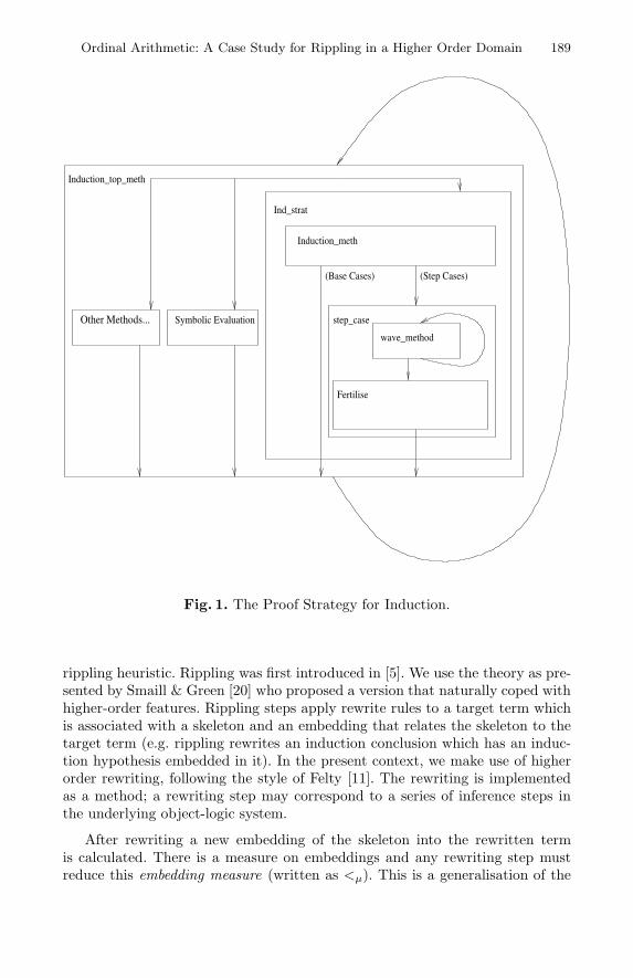
Ordinal Arithmetic: A Case Study for Rippling in a Higher Order Domain 189
Symbolic EvaluationOther Methods...
Induction_top_meth
(Base Cases) (Step Cases)
Ind_strat
Induction_meth
step_case
Fertilise
wave_method
Fig. 1. The Proof Strategy for Induction.
rippling heuristic. Rippling was first introduced in [5]. We use the theory as pre-sented by Smaill & Green [20] who proposed a version that naturally coped withhigher-order features. Rippling steps apply rewrite rules to a target term whichis associated with a skeleton and an embedding that relates the skeleton to thetarget term (e.g. rippling rewrites an induction conclusion which has an induc-tion hypothesis embedded in it). In the present context, we make use of higherorder rewriting, following the style of Felty [11]. The rewriting is implementedas a method; a rewriting step may correspond to a series of inference steps inthe underlying object-logic system.
After rewriting a new embedding of the skeleton into the rewritten termis calculated. There is a measure on embeddings and any rewriting step mustreduce this embedding measure (written as <µ). This is a generalisation of the
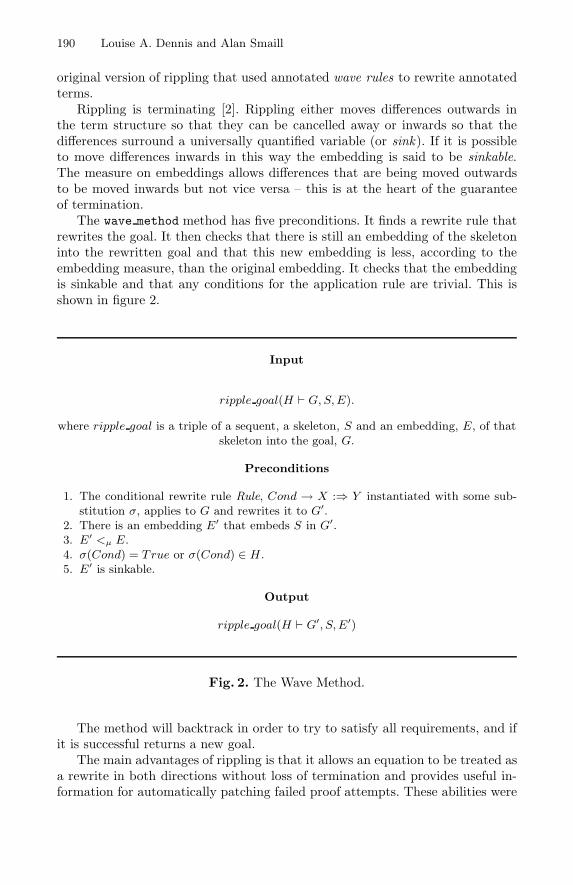
190 Louise A. Dennis and Alan Smaill
original version of rippling that used annotated wave rules to rewrite annotatedterms.
Rippling is terminating [2]. Rippling either moves differences outwards inthe term structure so that they can be cancelled away or inwards so that thedifferences surround a universally quantified variable (or sink). If it is possibleto move differences inwards in this way the embedding is said to be sinkable.The measure on embeddings allows differences that are being moved outwardsto be moved inwards but not vice versa – this is at the heart of the guaranteeof termination.
The wave method method has five preconditions. It finds a rewrite rule thatrewrites the goal. It then checks that there is still an embedding of the skeletoninto the rewritten goal and that this new embedding is less, according to theembedding measure, than the original embedding. It checks that the embeddingis sinkable and that any conditions for the application rule are trivial. This isshown in figure 2.
Input
ripple goal(H � G, S, E).
where ripple goal is a triple of a sequent, a skeleton, S and an embedding, E, of thatskeleton into the goal, G.
Preconditions
1. The conditional rewrite rule Rule, Cond → X :⇒ Y instantiated with some sub-stitution σ, applies to G and rewrites it to G′.
2. There is an embedding E′ that embeds S in G′.3. E′ <µ E.4. σ(Cond) = True or σ(Cond) ∈ H .5. E′ is sinkable.
Output
ripple goal(H � G′, S, E′)
Fig. 2. The Wave Method.
The method will backtrack in order to try to satisfy all requirements, and ifit is successful returns a new goal.
The main advantages of rippling is that it allows an equation to be treated asa rewrite in both directions without loss of termination and provides useful in-formation for automatically patching failed proof attempts. These abilities were
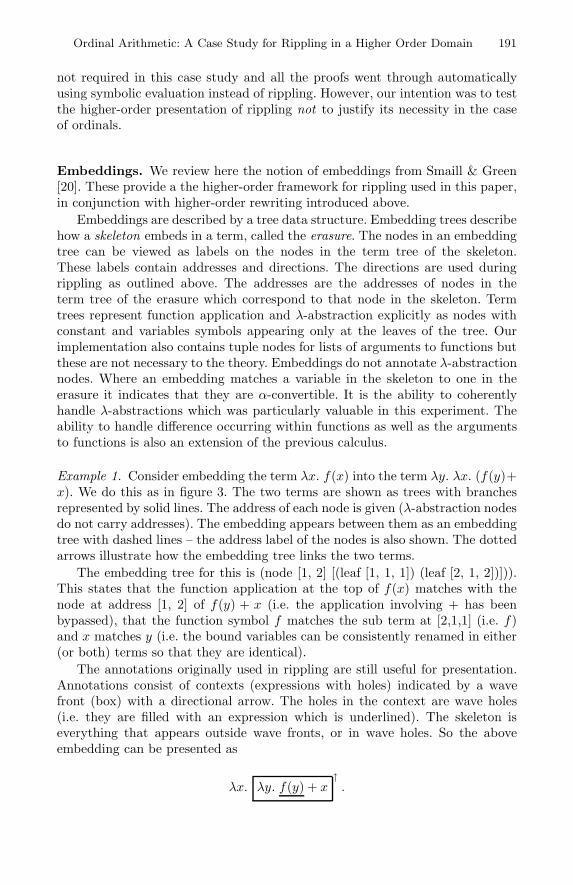
Ordinal Arithmetic: A Case Study for Rippling in a Higher Order Domain 191
not required in this case study and all the proofs went through automaticallyusing symbolic evaluation instead of rippling. However, our intention was to testthe higher-order presentation of rippling not to justify its necessity in the caseof ordinals.
Embeddings. We review here the notion of embeddings from Smaill & Green[20]. These provide a the higher-order framework for rippling used in this paper,in conjunction with higher-order rewriting introduced above.
Embeddings are described by a tree data structure. Embedding trees describehow a skeleton embeds in a term, called the erasure. The nodes in an embeddingtree can be viewed as labels on the nodes in the term tree of the skeleton.These labels contain addresses and directions. The directions are used duringrippling as outlined above. The addresses are the addresses of nodes in theterm tree of the erasure which correspond to that node in the skeleton. Termtrees represent function application and λ-abstraction explicitly as nodes withconstant and variables symbols appearing only at the leaves of the tree. Ourimplementation also contains tuple nodes for lists of arguments to functions butthese are not necessary to the theory. Embeddings do not annotate λ-abstractionnodes. Where an embedding matches a variable in the skeleton to one in theerasure it indicates that they are α-convertible. It is the ability to coherentlyhandle λ-abstractions which was particularly valuable in this experiment. Theability to handle difference occurring within functions as well as the argumentsto functions is also an extension of the previous calculus.
Example 1. Consider embedding the term λx. f(x) into the term λy. λx. (f(y)+x). We do this as in figure 3. The two terms are shown as trees with branchesrepresented by solid lines. The address of each node is given (λ-abstraction nodesdo not carry addresses). The embedding appears between them as an embeddingtree with dashed lines – the address label of the nodes is also shown. The dottedarrows illustrate how the embedding tree links the two terms.
The embedding tree for this is (node [1, 2] [(leaf [1, 1, 1]) (leaf [2, 1, 2])])).This states that the function application at the top of f(x) matches with thenode at address [1, 2] of f(y) + x (i.e. the application involving + has beenbypassed), that the function symbol f matches the sub term at [2,1,1] (i.e. f)and x matches y (i.e. the bound variables can be consistently renamed in either(or both) terms so that they are identical).
The annotations originally used in rippling are still useful for presentation.Annotations consist of contexts (expressions with holes) indicated by a wavefront (box) with a directional arrow. The holes in the context are wave holes(i.e. they are filled with an expression which is underlined). The skeleton iseverything that appears outside wave fronts, or in wave holes. So the aboveembedding can be presented as
λx. λy. f(y) + x↑.
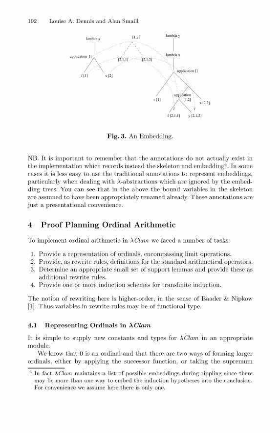
192 Louise A. Dennis and Alan Smaill
lambda x
x [2]
+ [1]
f [1]
f [2,1,1] y [2,1,2]
x [2,2]
lambda x
lambda y
[1,2]application
application []
application []
[1,2]
[2,1,1] [2,1,2]
Fig. 3. An Embedding.
NB. It is important to remember that the annotations do not actually exist inthe implementation which records instead the skeleton and embedding4. In somecases it is less easy to use the traditional annotations to represent embeddings,particularly when dealing with λ-abstractions which are ignored by the embed-ding trees. You can see that in the above the bound variables in the skeletonare assumed to have been appropriately renamed already. These annotations arejust a presentational convenience.
4 Proof Planning Ordinal Arithmetic
To implement ordinal arithmetic in λClam we faced a number of tasks.
1. Provide a representation of ordinals, encompassing limit operations.2. Provide, as rewrite rules, definitions for the standard arithmetical operators.3. Determine an appropriate small set of support lemmas and provide these as
additional rewrite rules.4. Provide one or more induction schemes for transfinite induction.
The notion of rewriting here is higher-order, in the sense of Baader & Nipkow[1]. Thus variables in rewrite rules may be of functional type.
4.1 Representing Ordinals in λClam
It is simple to supply new constants and types for λClam in an appropriatemodule.
We know that 0 is an ordinal and that there are two ways of forming largerordinals, either by applying the successor function, or taking the supremum4 In fact λClam maintains a list of possible embeddings during rippling since theremay be more than one way to embed the induction hypotheses into the conclusion.For convenience we assume here there is only one.
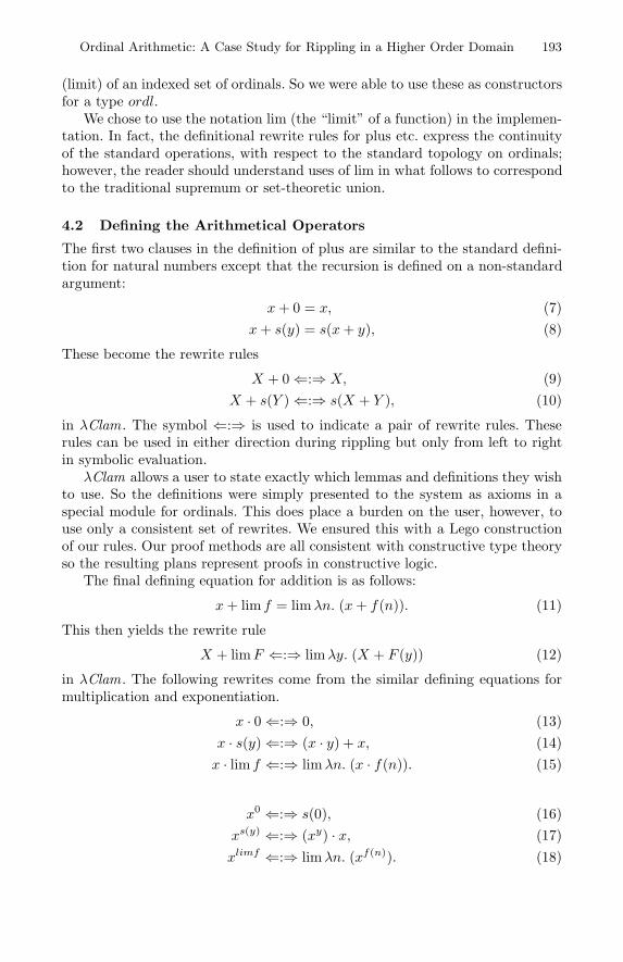
Ordinal Arithmetic: A Case Study for Rippling in a Higher Order Domain 193
(limit) of an indexed set of ordinals. So we were able to use these as constructorsfor a type ordl.
We chose to use the notation lim (the “limit” of a function) in the implemen-tation. In fact, the definitional rewrite rules for plus etc. express the continuityof the standard operations, with respect to the standard topology on ordinals;however, the reader should understand uses of lim in what follows to correspondto the traditional supremum or set-theoretic union.
4.2 Defining the Arithmetical Operators
The first two clauses in the definition of plus are similar to the standard defini-tion for natural numbers except that the recursion is defined on a non-standardargument:
x+ 0 = x, (7)x+ s(y) = s(x+ y), (8)
These become the rewrite rules
X + 0⇐:⇒ X, (9)X + s(Y )⇐:⇒ s(X + Y ), (10)
in λClam . The symbol ⇐:⇒ is used to indicate a pair of rewrite rules. Theserules can be used in either direction during rippling but only from left to rightin symbolic evaluation.
λClam allows a user to state exactly which lemmas and definitions they wishto use. So the definitions were simply presented to the system as axioms in aspecial module for ordinals. This does place a burden on the user, however, touse only a consistent set of rewrites. We ensured this with a Lego constructionof our rules. Our proof methods are all consistent with constructive type theoryso the resulting plans represent proofs in constructive logic.
The final defining equation for addition is as follows:
x+ lim f = limλn. (x+ f(n)). (11)
This then yields the rewrite rule
X + limF ⇐:⇒ limλy. (X + F (y)) (12)
in λClam . The following rewrites come from the similar defining equations formultiplication and exponentiation.
x · 0⇐:⇒ 0, (13)x · s(y)⇐:⇒ (x · y) + x, (14)x · lim f ⇐:⇒ limλn. (x · f(n)). (15)
x0 ⇐:⇒ s(0), (16)xs(y) ⇐:⇒ (xy) · x, (17)xlimf ⇐:⇒ limλn. (xf(n)). (18)
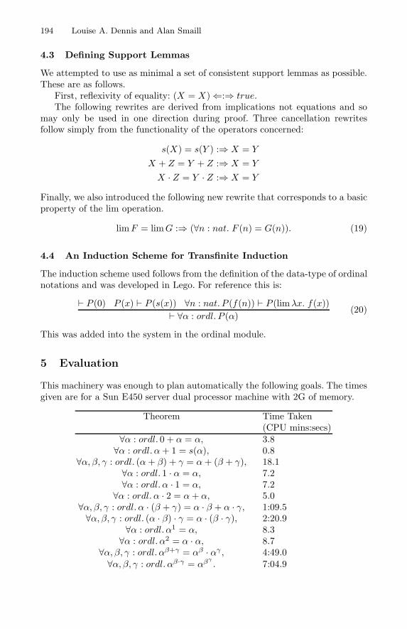
194 Louise A. Dennis and Alan Smaill
4.3 Defining Support Lemmas
We attempted to use as minimal a set of consistent support lemmas as possible.These are as follows.
First, reflexivity of equality: (X = X)⇐:⇒ true.The following rewrites are derived from implications not equations and so
may only be used in one direction during proof. Three cancellation rewritesfollow simply from the functionality of the operators concerned:
s(X) = s(Y ) :⇒ X = Y
X + Z = Y + Z :⇒ X = Y
X · Z = Y · Z :⇒ X = Y
Finally, we also introduced the following new rewrite that corresponds to a basicproperty of the lim operation.
limF = limG :⇒ (∀n : nat. F (n) = G(n)). (19)
4.4 An Induction Scheme for Transfinite Induction
The induction scheme used follows from the definition of the data-type of ordinalnotations and was developed in Lego. For reference this is:
� P (0) P (x) � P (s(x)) ∀n : nat. P (f(n)) � P (limλx. f(x))� ∀α : ordl. P (α)
(20)
This was added into the system in the ordinal module.
5 Evaluation
This machinery was enough to plan automatically the following goals. The timesgiven are for a Sun E450 server dual processor machine with 2G of memory.
Theorem Time Taken(CPU mins:secs)
∀α : ordl. 0 + α = α, 3.8∀α : ordl. α+ 1 = s(α), 0.8
∀α, β, γ : ordl. (α+ β) + γ = α+ (β + γ), 18.1∀α : ordl. 1 · α = α, 7.2∀α : ordl. α · 1 = α, 7.2∀α : ordl. α · 2 = α+ α, 5.0
∀α, β, γ : ordl. α · (β + γ) = α · β + α · γ, 1:09.5∀α, β, γ : ordl. (α · β) · γ = α · (β · γ), 2:20.9
∀α : ordl. α1 = α, 8.3∀α : ordl. α2 = α · α, 8.7
∀α, β, γ : ordl. αβ+γ = αβ · αγ , 4:49.0∀α, β, γ : ordl. αβ·γ = αβγ
. 7:04.9
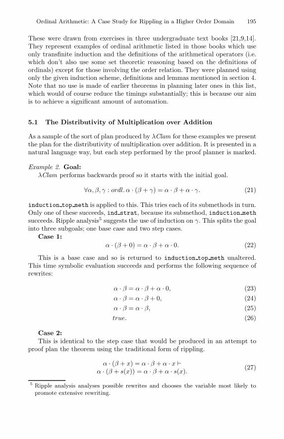
Ordinal Arithmetic: A Case Study for Rippling in a Higher Order Domain 195
These were drawn from exercises in three undergraduate text books [21,9,14].They represent examples of ordinal arithmetic listed in those books which useonly transfinite induction and the definitions of the arithmetical operators (i.e.which don’t also use some set theoretic reasoning based on the definitions ofordinals) except for those involving the order relation. They were planned usingonly the given induction scheme, definitions and lemmas mentioned in section 4.Note that no use is made of earlier theorems in planning later ones in this list,which would of course reduce the timings substantially; this is because our aimis to achieve a significant amount of automation.
5.1 The Distributivity of Multiplication over Addition
As a sample of the sort of plan produced by λClam for these examples we presentthe plan for the distributivity of multiplication over addition. It is presented in anatural language way, but each step performed by the proof planner is marked.
Example 2. Goal:λClam performs backwards proof so it starts with the initial goal.
∀α, β, γ : ordl. α · (β + γ) = α · β + α · γ. (21)
induction top meth is applied to this. This tries each of its submethods in turn.Only one of these succeeds, ind strat, because its submethod, induction methsucceeds. Ripple analysis5 suggests the use of induction on γ. This splits the goalinto three subgoals; one base case and two step cases.
Case 1:α · (β + 0) = α · β + α · 0. (22)
This is a base case and so is returned to induction top meth unaltered.This time symbolic evaluation succeeds and performs the following sequence ofrewrites:
α · β = α · β + α · 0, (23)α · β = α · β + 0, (24)α · β = α · β, (25)true. (26)
Case 2:This is identical to the step case that would be produced in an attempt to
proof plan the theorem using the traditional form of rippling.
α · (β + x) = α · β + α · x �α · (β + s(x)) = α · β + α · s(x). (27)
5 Ripple analysis analyses possible rewrites and chooses the variable most likely topromote extensive rewriting.
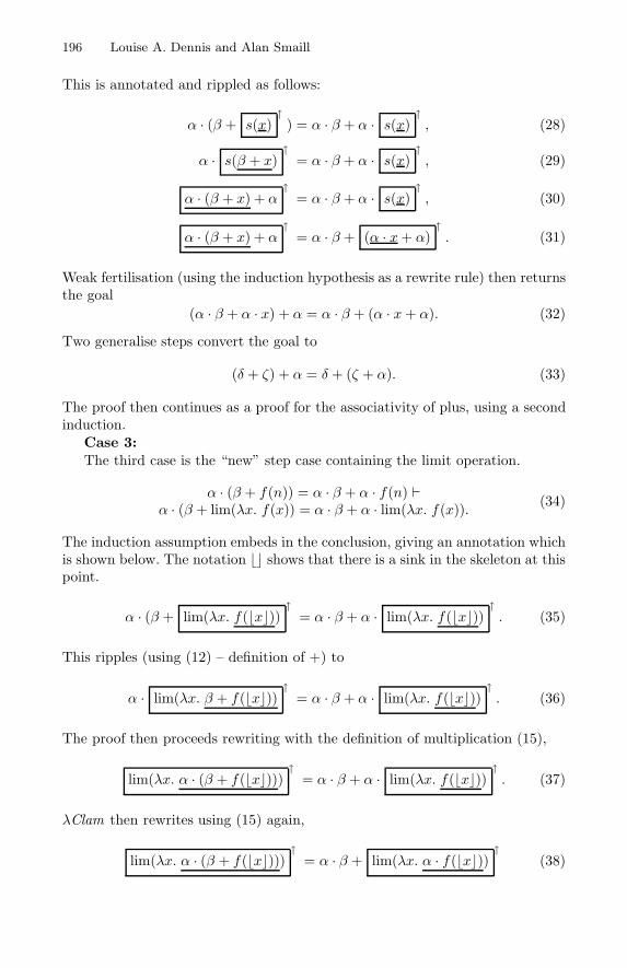
196 Louise A. Dennis and Alan Smaill
This is annotated and rippled as follows:
α · (β + s(x)↑) = α · β + α · s(x) ↑ , (28)
α · s(β + x)↑
= α · β + α · s(x) ↑ , (29)
α · (β + x) + α↑
= α · β + α · s(x) ↑ , (30)
α · (β + x) + α↑
= α · β + (α · x+ α)↑. (31)
Weak fertilisation (using the induction hypothesis as a rewrite rule) then returnsthe goal
(α · β + α · x) + α = α · β + (α · x+ α). (32)
Two generalise steps convert the goal to
(δ + ζ) + α = δ + (ζ + α). (33)
The proof then continues as a proof for the associativity of plus, using a secondinduction.
Case 3:The third case is the “new” step case containing the limit operation.
α · (β + f(n)) = α · β + α · f(n) �α · (β + lim(λx. f(x)) = α · β + α · lim(λx. f(x)). (34)
The induction assumption embeds in the conclusion, giving an annotation whichis shown below. The notation � shows that there is a sink in the skeleton at thispoint.
α · (β + lim(λx. f(�x)) ↑ = α · β + α · lim(λx. f(�x)) ↑ . (35)
This ripples (using (12) – definition of +) to
α · lim(λx. β + f(�x)) ↑ = α · β + α · lim(λx. f(�x)) ↑ . (36)
The proof then proceeds rewriting with the definition of multiplication (15),
lim(λx. α · (β + f(�x))) ↑ = α · β + α · lim(λx. f(�x)) ↑ . (37)
λClam then rewrites using (15) again,
lim(λx. α · (β + f(�x))) ↑ = α · β + lim(λx. α · f(�x)) ↑ (38)
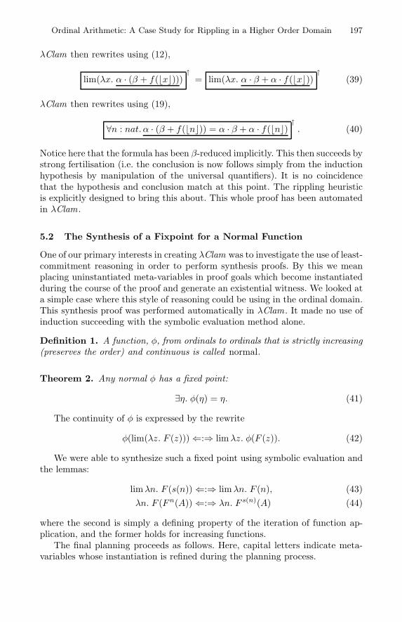
Ordinal Arithmetic: A Case Study for Rippling in a Higher Order Domain 197
λClam then rewrites using (12),
lim(λx. α · (β + f(�x))) ↑ = lim(λx. α · β + α · f(�x)) ↑ (39)
λClam then rewrites using (19),
∀n : nat. α · (β + f(�n)) = α · β + α · f(�n) ↑ . (40)
Notice here that the formula has been β-reduced implicitly. This then succeeds bystrong fertilisation (i.e. the conclusion is now follows simply from the inductionhypothesis by manipulation of the universal quantifiers). It is no coincidencethat the hypothesis and conclusion match at this point. The rippling heuristicis explicitly designed to bring this about. This whole proof has been automatedin λClam .
5.2 The Synthesis of a Fixpoint for a Normal Function
One of our primary interests in creating λClam was to investigate the use of least-commitment reasoning in order to perform synthesis proofs. By this we meanplacing uninstantiated meta-variables in proof goals which become instantiatedduring the course of the proof and generate an existential witness. We looked ata simple case where this style of reasoning could be using in the ordinal domain.This synthesis proof was performed automatically in λClam . It made no use ofinduction succeeding with the symbolic evaluation method alone.
Definition 1. A function, φ, from ordinals to ordinals that is strictly increasing(preserves the order) and continuous is called normal.
Theorem 2. Any normal φ has a fixed point:
∃η. φ(η) = η. (41)
The continuity of φ is expressed by the rewrite
φ(lim(λz. F (z)))⇐:⇒ lim λz. φ(F (z)). (42)
We were able to synthesize such a fixed point using symbolic evaluation andthe lemmas:
limλn. F (s(n))⇐:⇒ limλn. F (n), (43)λn. F (Fn(A))⇐:⇒ λn. F s(n)(A) (44)
where the second is simply a defining property of the iteration of function ap-plication, and the former holds for increasing functions.
The final planning proceeds as follows. Here, capital letters indicate meta-variables whose instantiation is refined during the planning process.
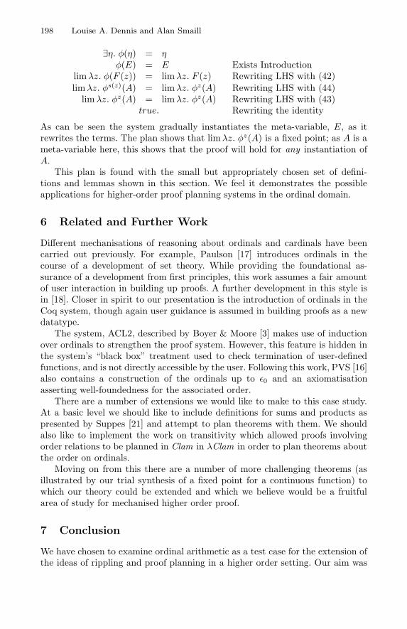
198 Louise A. Dennis and Alan Smaill
∃η. φ(η) = ηφ(E) = E Exists Introduction
limλz. φ(F (z)) = limλz. F (z) Rewriting LHS with (42)limλz. φs(z)(A) = limλz. φz(A) Rewriting LHS with (44)
limλz. φz(A) = limλz. φz(A) Rewriting LHS with (43)true. Rewriting the identity
As can be seen the system gradually instantiates the meta-variable, E, as itrewrites the terms. The plan shows that limλz. φz(A) is a fixed point; as A is ameta-variable here, this shows that the proof will hold for any instantiation ofA.
This plan is found with the small but appropriately chosen set of defini-tions and lemmas shown in this section. We feel it demonstrates the possibleapplications for higher-order proof planning systems in the ordinal domain.
6 Related and Further Work
Different mechanisations of reasoning about ordinals and cardinals have beencarried out previously. For example, Paulson [17] introduces ordinals in thecourse of a development of set theory. While providing the foundational as-surance of a development from first principles, this work assumes a fair amountof user interaction in building up proofs. A further development in this style isin [18]. Closer in spirit to our presentation is the introduction of ordinals in theCoq system, though again user guidance is assumed in building proofs as a newdatatype.
The system, ACL2, described by Boyer & Moore [3] makes use of inductionover ordinals to strengthen the proof system. However, this feature is hidden inthe system’s “black box” treatment used to check termination of user-definedfunctions, and is not directly accessible by the user. Following this work, PVS [16]also contains a construction of the ordinals up to ε0 and an axiomatisationasserting well-foundedness for the associated order.
There are a number of extensions we would like to make to this case study.At a basic level we should like to include definitions for sums and products aspresented by Suppes [21] and attempt to plan theorems with them. We shouldalso like to implement the work on transitivity which allowed proofs involvingorder relations to be planned in Clam in λClam in order to plan theorems aboutthe order on ordinals.
Moving on from this there are a number of more challenging theorems (asillustrated by our trial synthesis of a fixed point for a continuous function) towhich our theory could be extended and which we believe would be a fruitfularea of study for mechanised higher order proof.
7 Conclusion
We have chosen to examine ordinal arithmetic as a test case for the extension ofthe ideas of rippling and proof planning in a higher order setting. Our aim was
Ordinal Arithmetic: A Case Study for Rippling in a Higher Order Domain 199
to maintain the natural higher-order presentation of the ordinals while retainingfull automation of the proof generation process.
We were greatly helped in our case study by the higher order features builtinto λProlog which removed the need for explicitly stating β-reduction as arewrite rule and allowed side-conditions preventing variable capture to be left tothe underlying language to handle.
With a small amount of theory building we were able to successfully planstandard undergraduate textbook examples and exercises. We were also able todemonstrate how proof planning, in particular least commitment devices suchas the use of meta-variables, could have a part to play in the mechanisation ofproof theoretic results in the ordinal domain. These results were confirmationthat λClam can naturally handle higher order examples and that λProlog is asuitable language in which to express such mathematical concepts.
Thus, we claim to have identified common patterns of proof search thatextend automated inductive theorem proving to the mathematically interestinghigher order domain of ordinals and ordinal functions.
Acknowledgements
This research was funded by EPSRC grant Gr/m45030. We thank members ofthe Mathematical Reasoning Group, and especially Alan Bundy for input tothis work. The presentation has benefited from the comments of the anonymousreferees.
References
1. F. Baader and T. Nipkow. Term Rewriting and All That. Cambridge UniversityPress, 1998.
2. David Basin and Toby Walsh. A calculus for and termination of rippling. Journalof Automated Reasoning, 16(1–2):147–180, 1996.
3. R. S. Boyer and J S. Moore. A Computational Logic Handbook. Academic Press,1988. Perspectives in Computing, Vol 23.
4. A. Bundy. The use of explicit plans to guide inductive proofs. In R. Lusk andR. Overbeek, editors, 9th International Conference on Automated Deduction, pages111–120. Springer-Verlag, 1988. Longer version available from Edinburgh as DAIResearch Paper No. 349.
5. A. Bundy, A. Stevens, F. van Harmelen, A. Ireland, and A. Smaill. Rippling:A heuristic for guiding inductive proofs. Artificial Intelligence, 62:185–253, 1993.Also available from Edinburgh as DAI Research Paper No. 567.
6. Alan Bundy. The automation of proof by mathematical induction. In A. Robin-son and A. Voronkov, editors, Handbook of Automated Reasoning. Elsevier., 1998.Forthcoming.
7. A. Cichon and H. Touzet. An ordinal calculus for proving termination in termrewriting. In Proceedings of CAAP’96, Coll. on Trees in Algebra and Programming,number 1059 in Lecture Notes in Computer Science. Springer, 1996.
8. Th. Coquand. Une Theorie des Constructions. PhD thesis, University of ParisVII, 1985.
200 Louise A. Dennis and Alan Smaill
9. Herbert B. Enderton. Elements of Set Theory. Academic Press, 1977.10. W. M. Farmer, J. D. Guttman, and F. J. Thayer. IMPS : an interactive mathe-
matical proof system. Journal of Automated Reasoning, 9(11):213–248, 1993.11. A. Felty. A logic programming approach to implementing higher-order term rewrit-
ing. In L-H Eriksson et al., editors, Second International Workshop on Extensionsto Logic Programming, volume 596 of Lecture Notes in Artificial Intelligence, pages135–61. Springer-Verlag, 1992.
12. Lego group. Lego home page. http://www.dcs.ed.ac.uk/home/lego/.13. P. Halmos. Naive Set Theory. Van Nostrand, Princeton, NJ, 1960.14. A. G. Hamilton. Numbers, sets and axioms: the apparatus of mathematics. Cam-
bridge University Press, 1982.15. Jean-Pierre Jouannaud and Mitsuhiro Okada. Satisfiability of systems of ordinal
notations with the subterm property is decidable. In Proceedings of the EighteenthEATCS Colloquium on Automata, Languages and Programming, Madrid, Spain,1991.
16. S. Owre, J. M. Rushby, and N. Shankar. PVS : An integrated approach to speci-fication and verification. Tech report, SRI International, 1992.
17. L.C. Paulson. Set theory for verification: II. induction and recursion. Journal ofAutomated Reasoning, 15:353–389, 1995.
18. L.C. Paulson and K. Grabczewski. Mechanizing set theory: cardinal arithmeticand the axiom of choice. Journal of Automated Reasoning, pages 291–323, 1996.
19. J.D.C Richardson, A. Smaill, and Ian Green. System description: proof planningin higher-order logic with LambdaCLAM. In Claude Kirchner and Helene Kirch-ner, editors, 15th International Conference on Automated Deduction, volume 1421of Lecture Notes in Artificial Intelligence, pages 129–133, Lindau, Germany, July1998.
20. Alan Smaill and Ian Green. Higher-order annotated terms for proof search. InJoakim von Wright, Jim Grundy, and John Harrison, editors, Theorem Proving inHigher Order Logics: 9th International Conference, TPHOLs’96, volume 1275 ofLecture Notes in Computer Science, pages 399–414, Turku, Finland, 1996. Springer-Verlag. Also available as DAI Research Paper 799.
21. P. Suppes. Axiomatic Set Theory. Van Nostrand, Princeton, NJ, 1960.
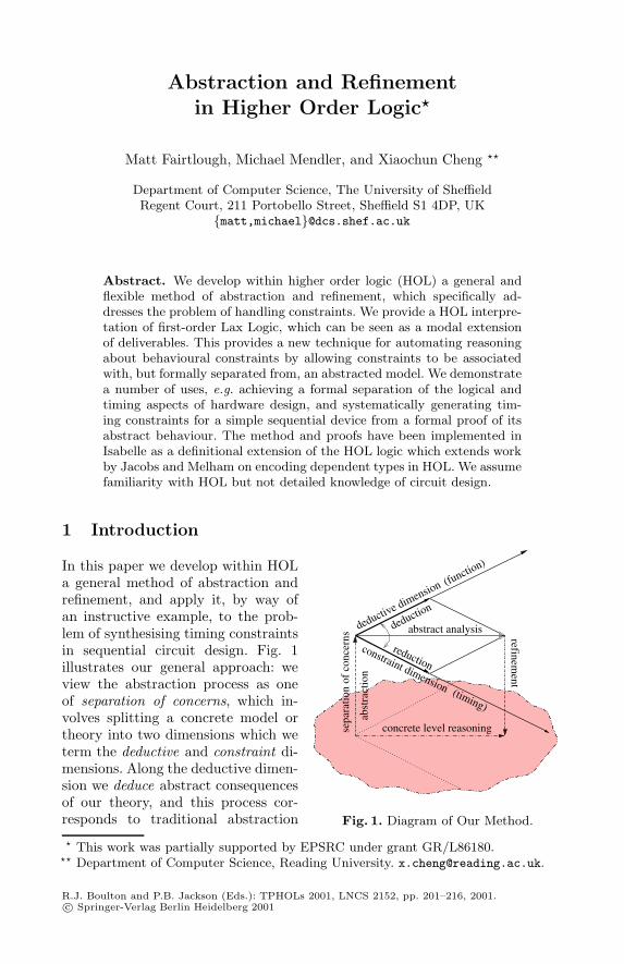
Abstraction and Refinementin Higher Order Logic�
Matt Fairtlough, Michael Mendler, and Xiaochun Cheng ��
Department of Computer Science, The University of SheffieldRegent Court, 211 Portobello Street, Sheffield S1 4DP, UK
{matt,michael}@dcs.shef.ac.uk
Abstract. We develop within higher order logic (HOL) a general andflexible method of abstraction and refinement, which specifically ad-dresses the problem of handling constraints. We provide a HOL interpre-tation of first-order Lax Logic, which can be seen as a modal extensionof deliverables. This provides a new technique for automating reasoningabout behavioural constraints by allowing constraints to be associatedwith, but formally separated from, an abstracted model. We demonstratea number of uses, e.g. achieving a formal separation of the logical andtiming aspects of hardware design, and systematically generating tim-ing constraints for a simple sequential device from a formal proof of itsabstract behaviour. The method and proofs have been implemented inIsabelle as a definitional extension of the HOL logic which extends workby Jacobs and Melham on encoding dependent types in HOL. We assumefamiliarity with HOL but not detailed knowledge of circuit design.
1 Introduction
abst
ract
ion
(timing)
reduction
deduction
abstract analysis
sepa
ratio
n of
con
cern
s
concrete level reasoning
refinement
deductive dimension (function)
constraint dimension
Fig. 1. Diagram of Our Method.
In this paper we develop within HOLa general method of abstraction andrefinement, and apply it, by way ofan instructive example, to the prob-lem of synthesising timing constraintsin sequential circuit design. Fig. 1illustrates our general approach: weview the abstraction process as oneof separation of concerns, which in-volves splitting a concrete model ortheory into two dimensions which weterm the deductive and constraint di-mensions. Along the deductive dimen-sion we deduce abstract consequencesof our theory, and this process cor-responds to traditional abstraction
� This work was partially supported by EPSRC under grant GR/L86180.�� Department of Computer Science, Reading University. [email protected].
R.J. Boulton and P.B. Jackson (Eds.): TPHOLs 2001, LNCS 2152, pp. 201–216, 2001.c© Springer-Verlag Berlin Heidelberg 2001
202 Matt Fairtlough et al.
methods in Artificial Intelligence as presented, for example, in [16]. Along theconstraint dimension we track the discrepancies between the abstract and con-crete models by computing and reducing the constraints under which the ab-straction is valid: our method is of practical use insofar as this process can beautomated for the constraint domain involved. A key ingredient in our method isan algorithm for recombining the two dimensions at any point, a process implicitin [10] and strongly related to realizability [17] which we term refinement. It isthis constraint dimension and the associated concept of refinement that appearsto be missing in the AI literature. If we perform an abstraction on a concretemodel, develop an abstract analysis and then refine the result, we obtain a con-crete consequence which could have been obtained by concrete level reasoningalone; however we argue that the abstraction mechanism will often make it easierto obtain the desired result. In our main example we apply the method to thegeneration of timing constraints for an RS latch, addressing an open problemraised in [8] and by [9]: a formal proof of circuit behaviour is produced (deduc-tion) at an abstract level at which timing details are elided; an interpretationof the proof as a constraint λ-term then yields a concrete proof of correctnessincorporating the necessary timing constraints (reduction). The key differenceto the previous works is that the constraints are systematically synthesised anddo not need to be anticipated at the outset.
Abstraction in Artificial Intelligence. Abstraction techniques have been exten-sively applied and studied in Artificial Intelligence. See for example [16, 7]. In[7] Walsh and Guinchiglia present a very general method to analyse the uses ofabstraction in a number of different fields such as theorem proving, planning,problem solving and approximate reasoning. They give an informal definition ofabstraction as a process which “allows people to consider what is relevant andforget a lot of irrelevant details which would get in the way of what they aretrying to do”; they go on to note that
. . . the process of abstraction is related to the process of separating, ex-tracting from a representation an “abstract” representation . . .
It is however important to realize that separation does not just involve extrac-tion; after separating eggs we may wish to use the white as well as the yolk,perhaps by transforming both and then recombining them. In the context offormal design or verification it is misleading to think of abstraction as extract-ing the relevant details and discarding the rest as irrelevant; rather we view theprocess as one of separation of concerns: for example, a system can be split intoa deductive part, relating to the broad functionality of the system, and an al-gorithmic part, representing non-functional aspects such as timing properties.The algorithmic information represents the offset between the abstract systemmodel and the concrete one, i.e. it represents the constraints under which theabstraction is valid [13]. Complementing the abstraction process there shouldtherefore be a dual process of refinement, in which the areas of concern are re-combined and constraints are (re-)generated. In the examples we present in thispaper, the result of refinement is a concrete-level statement that the system hasthe required functionality provided the constraints are satisfied.
Abstraction and Refinement in Higher Order Logic 203
Abstraction and Constraints in Hardware Verification. There is a substantialamount of work on the use of abstraction techniques in formal hardware verifi-cation. We cite [5, 6, 1] and [12] as early publications. A fundamental obstacleto the sound use of abstraction techniques is that the associated constraintsaccumulate in the opposite direction to the proof effort, whether forward orgoal-directed proof methods are used. Thus a situation typically arises where itis not known at the outset what exactly needs to be proved. A knock-on effectof the presence of constraints is a loss of compositionality or modularity withrespect to refinement.
Although pervasive, this problem of non-compositionality has not often beenclearly delineated in the literature. A notable exception is [1]. In his discussionof hierarchical design methods, Eveking presents an example which “. . . showsthat, in the general case, one has to make a complete reanalysis of a switch-levelnetwork even if the correctness of the fragments was proven”. Our research showshow such a painful reanalysis may be mitigated, since a lack of attention to lowerlevel constraints is a major stumbling block to the successful decomposition ofsystems at an abstract level.
In [12] Melham takes two approaches to the problem of handling the con-straints involved in the abstraction process. The first process he calls “abstrac-tion within models”, and involves theorems of the form � C ⊃M sat
FS whereM
represents the implementation, S the specification and C the constraints underwhich the implementation satisfies the specification. F is an abstraction func-tion that serves to relate e.g. concrete information to its abstract counterpart.Constraints are handled using explicit rules. In our approach, the abstraction isexplicit and the associated constraint rules are implicit, being generated fromthe abstraction itself. This may prove to be more convenient and flexible inapplications.
Melham’s second abstraction process is called “abstraction between models”and involves a formal proof of a relationship between hardware models whichmay be seen as saying “provided certain design rules are followed, the abstractmodel is a valid description of concrete behaviour”. The relevant constraintsare automatically satisfied for any correct combination of basic components. [5]takes essentially the same approach. The approach has two limitations: firstlythe concrete model at least must be represented by a deep embedding in theobject logic, and secondly an adequate set of design rules must be discoveredand formalised. While this approach can be highly effective, in general it is notpossible to find such a set of design rules, or they are deliberately broken tooptimise designs. In contrast, our approach does not require a deep embeddingof the concrete model or a formalised set of design rules.
Our Contribution. Our approach involves maintaining a close connection be-tween abstraction (the deductive dimension) and constraints (the algorithmicdimension). The algorithmic aspect corresponds to the calculation of constraints,and in accordance with this principle we record the “irrelevant” information assets of constraint λ-terms. Let us consider a small example to explain our ap-
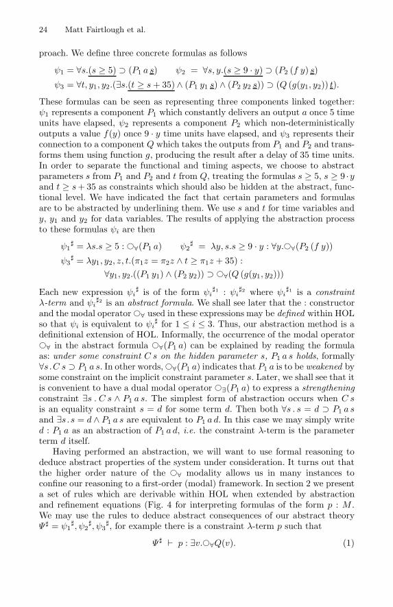
204 Matt Fairtlough et al.
proach. We define three concrete formulas as follows
ψ1 = ∀s.(s ≥ 5) ⊃ (P1 a s) ψ2 = ∀s, y.(s ≥ 9 · y) ⊃ (P2 (f y) s)
ψ3 = ∀t, y1, y2.(∃s.(t ≥ s+ 35) ∧ (P1 y1 s) ∧ (P2 y2 s)) ⊃ (Q (g(y1, y2)) t).
These formulas can be seen as representing three components linked together:ψ1 represents a component P1 which constantly delivers an output a once 5 timeunits have elapsed, ψ2 represents a component P2 which non-deterministicallyoutputs a value f(y) once 9 · y time units have elapsed, and ψ3 represents theirconnection to a component Q which takes the outputs from P1 and P2 and trans-forms them using function g, producing the result after a delay of 35 time units.In order to separate the functional and timing aspects, we choose to abstractparameters s from P1 and P2 and t from Q, treating the formulas s ≥ 5, s ≥ 9 ·yand t ≥ s+ 35 as constraints which should also be hidden at the abstract, func-tional level. We have indicated the fact that certain parameters and formulasare to be abstracted by underlining them. We use s and t for time variables andy, y1 and y2 for data variables. The results of applying the abstraction processto these formulas ψi are then
ψ1� = λs.s ≥ 5 : ©∀(P1 a) ψ2
� = λy, s.s ≥ 9 · y : ∀y.©∀(P2 (f y))
ψ3� = λy1, y2, z, t.(π1z = π2z ∧ t ≥ π1z + 35) :
∀y1, y2.((P1 y1) ∧ (P2 y2)) ⊃ ©∀(Q (g(y1, y2)))
Each new expression ψi� is of the form ψi
�1 : ψi�2 where ψi
�1 is a constraintλ-term and ψi
�2 is an abstract formula. We shall see later that the : constructorand the modal operator©∀ used in these expressions may be defined within HOLso that ψi is equivalent to ψi
� for 1 ≤ i ≤ 3. Thus, our abstraction method is adefinitional extension of HOL. Informally, the occurrence of the modal operator©∀ in the abstract formula ©∀(P1 a) can be explained by reading the formulaas: under some constraint C s on the hidden parameter s, P1 a s holds, formally∀s.C s ⊃ P1 a s. In other words,©∀(P1 a) indicates that P1 a is to be weakened bysome constraint on the implicit constraint parameter s. Later, we shall see that itis convenient to have a dual modal operator ©∃(P1 a) to express a strengtheningconstraint ∃s . C s ∧ P1 a s. The simplest form of abstraction occurs when C sis an equality constraint s = d for some term d. Then both ∀s . s = d ⊃ P1 a sand ∃s.s = d ∧ P1 a s are equivalent to P1 a d. In this case we may simply writed : P1 a as an abstraction of P1 a d, i.e. the constraint λ-term is the parameterterm d itself.
Having performed an abstraction, we will want to use formal reasoning todeduce abstract properties of the system under consideration. It turns out thatthe higher order nature of the ©∀ modality allows us in many instances toconfine our reasoning to a first-order (modal) framework. In section 2 we presenta set of rules which are derivable within HOL when extended by abstractionand refinement equations (Fig. 4 for interpreting formulas of the form p : M .We may use the rules to deduce abstract consequences of our abstract theoryΨ � = ψ1
�, ψ2�, ψ3
�, for example there is a constraint λ-term p such that
Ψ � � p : ∃v.©∀Q(v). (1)
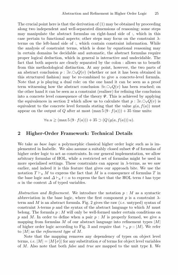
Abstraction and Refinement in Higher Order Logic 205
The crucial point here is that the derivation of (1) may be obtained by proceedingalong two independent and well-separated dimensions of reasoning: some stepsmay manipulate the abstract formulas on right-hand side of :, which in thiscase pertain to functional aspects; other steps may focus on the constraint λ-terms on the left-hand side of :, which contain constraint information. Whilethe analysis of constraint terms, which is done by equational reasoning mayin certain domains be decidable and automatic, the abstract formulas requireproper logical deduction, which in general is interactive and undecidable. Thefact that both aspects are clearly separated by the colon : allows us to benefitfrom this methodological distinction. At any point, however, the two parts ofan abstract conclusion p : ∃v.©∀Q(v) (whether or not it has been obtained inthis structured fashion) may be re-combined to give a concrete-level formula.Note that p is playing a dual role: on the one hand it can be seen as a proofterm witnessing how the abstract conclusion ∃v.©∀Q(v) has been reached; onthe other hand it can be seen as a constraint (realiser) for refining the conclusioninto a concrete level consequence of the theory Ψ . This is achieved by applyingthe equivalences in section 2 which allow us to calculate that p : ∃v.©∀Q(v) isequivalent to the concrete level formula stating that the value g(a, f(a)) mustappear on the output of Q after at most (max 5 (9 · f(a))) + 35 time units:
∀u.u ≥ (max 5 (9 · f(a))) + 35 ⊃ (Q (g(a, f(a)))u).
2 Higher-Order Framework: Technical Details
We take as base logic a polymorphic classical higher order logic such as is im-plemented in Isabelle. We also assume a suitably closed subset Φ of formulas ofhigher order logic to act as constraints. In our general implementation, we allowarbitrary formulas of HOL, while a restricted set of formulas might be used inmore specialised settings. These constraints can appear in λ-terms, as we sawearlier, and indeed it is this feature that gives our approach bite. We use thenotation T �B M to express the fact that M is a consequence of formulas T inthe base logic and ∆ �B t :: α to express the fact that the HOL term t has typeα in the context ∆ of typed variables.
Abstraction and Refinement. We introduce the notation p : M as a syntacticabbreviation in the base logic, where the first component p is a constraint λ-term and M is an abstract formula. Fig. 2 gives the raw (i.e. untyped) syntax ofconstraint λ-terms p and the syntax of the abstract language to which M mustbelong. The formula p : M will only be well-formed under certain conditions onp and M . In order to define when a pair p : M is properly formed, we give amapping from formulas M of our abstract language into refinement types |M |of higher order logic according to Fig. 3 and require that �B p :: |M |. We referto |M | as the refinement type of M .
Note that the mapping removes any dependency of types on object levelterms, i.e. |M | = |M{σ}| for any substitution σ of terms for object level variablesof M . Also note that both false and true are mapped to the unit type 1. We
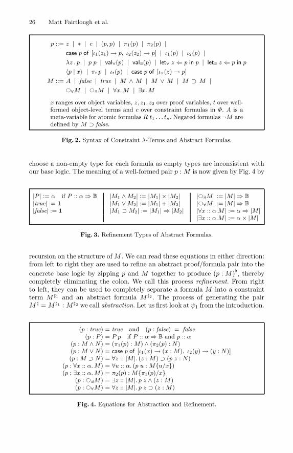
206 Matt Fairtlough et al.
p ::= z | ∗ | c | (p, p) | π1(p) | π2(p) |case p of [ι1(z1)→ p, ι2(z2)→ p] | ι1(p) | ι2(p) |λz . p | p p | val∀(p) | val∃(p) | let∀ z ⇐ p in p | let∃ z ⇐ p in p
〈p | x〉 | πt p | ιt(p) | case p of [ιx(z)→ p]
M ::= A | false | true | M ∧ M | M ∨ M | M ⊃ M |©∀M | ©∃M | ∀x.M | ∃x. M
x ranges over object variables, z, z1, z2 over proof variables, t over well-formed object-level terms and c over constraint formulas in Φ. A is ameta-variable for atomic formulas R t1 . . . tn. Negated formulas ¬M aredefined by M ⊃ false.
Fig. 2. Syntax of Constraint λ-Terms and Abstract Formulas.
choose a non-empty type for each formula as empty types are inconsistent withour base logic. The meaning of a well-formed pair p : M is now given by Fig. 4 by
|P | := α if P :: α⇒ B |M1 ∧M2| := |M1| × |M2| |©∃M | := |M | ⇒ B
|true| := 1 |M1 ∨M2| := |M1|+ |M2| |©∀M | := |M | ⇒ B
|false| := 1 |M1 ⊃M2| := |M1| ⇒ |M2| |∀x :: α.M | := α⇒ |M ||∃x :: α.M | := α× |M |
Fig. 3. Refinement Types of Abstract Formulas.
recursion on the structure of M . We can read these equations in either direction:from left to right they are used to refine an abstract proof/formula pair into theconcrete base logic by zipping p and M together to produce (p : M)�, therebycompletely eliminating the colon. We call this process refinement. From rightto left, they can be used to completely separate a formula M into a constraintterm M �1 and an abstract formula M �2 . The process of generating the pairM � = M �1 : M �2 we call abstraction. Let us first look at ψ1 from the introduction.
(p : true) = true and (p : false) = false(p : P ) = P p if P :: α⇒ B and p :: α
(p : M ∧N) = (π1(p) : M) ∧ (π2(p) : N)(p : M ∨N) = case p of [ι1(x)→ (x : M), ι2(y)→ (y : N)](p : M ⊃ N) = ∀z :: |M |. (z : M) ⊃ (p z : N)
(p : ∀x :: α. M) = ∀u :: α. (p u : M{u/x})(p : ∃x :: α. M) = π2(p) : M{π1(p)/x}
(p : ©∃M) = ∃z :: |M |. p z ∧ (z : M)(p : ©∀M) = ∀z :: |M |. p z ⊃ (z : M)
Fig. 4. Equations for Abstraction and Refinement.
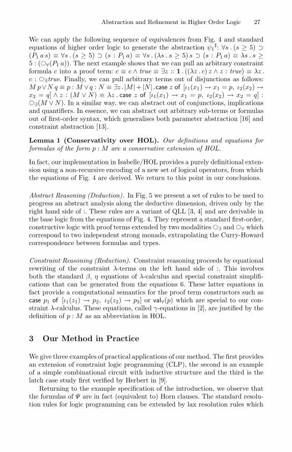
Abstraction and Refinement in Higher Order Logic 207
We can apply the following sequence of equivalences from Fig. 4 and standardequations of higher order logic to generate the abstraction ψ1
�: ∀s . (s ≥ 5) ⊃(P1 a s) ≡ ∀s . (s ≥ 5) ⊃ (s : P1 a) ≡ ∀s . (λs . s ≥ 5) s ⊃ (s : P1 a) ≡ λs . s ≥5 : (©∀(P1 a)). The next example shows that we can pull an arbitrary constraintformula c into a proof term: c ≡ c ∧ true ≡ ∃z :: 1 . ((λz . c) z ∧ z : true) ≡ λz .c : ©∃true. Finally, we can pull arbitrary terms out of disjunctions as follows:M p∨N q ≡ p : M ∨ q : N ≡ ∃z . |M |+ |N | .case z of [ι1(x1)→ x1 = p, ι2(x2)→x2 = q] ∧ z : (M ∨ N) ≡ λz . case z of [ι1(x1) → x1 = p, ι2(x2) → x2 = q] :©∃(M ∨N). In a similar way, we can abstract out of conjunctions, implicationsand quantifiers. In essence, we can abstract out arbitrary sub-terms or formulasout of first-order syntax, which generalises both parameter abstraction [16] andconstraint abstraction [13].
Lemma 1 (Conservativity over HOL). Our definitions and equations forformulas of the form p : M are a conservative extension of HOL.
In fact, our implementation in Isabelle/HOL provides a purely definitional exten-sion using a non-recursive encoding of a new set of logical operators, from whichthe equations of Fig. 4 are derived. We return to this point in our conclusions.
Abstract Reasoning (Deduction). In Fig. 5 we present a set of rules to be used toprogress an abstract analysis along the deductive dimension, driven only by theright hand side of :. These rules are a variant of QLL [3, 4] and are derivable inthe base logic from the equations of Fig. 4. They represent a standard first-order,constructive logic with proof terms extended by two modalities ©∃ and©∀ whichcorrespond to two independent strong monads, extrapolating the Curry-Howardcorrespondence between formulas and types.
Constraint Reasoning (Reduction). Constraint reasoning proceeds by equationalrewriting of the constraint λ-terms on the left hand side of :. This involvesboth the standard β, η equations of λ-calculus and special constraint simplifi-cations that can be generated from the equations 6. These latter equations infact provide a computational semantics for the proof term constructors such ascase p1 of [ι1(z1) → p2, ι2(z2) → p3] or val∀(p) which are special to our con-straint λ-calculus. These equations, called γ-equations in [2], are justified by thedefinition of p : M as an abbreviation in HOL.
3 Our Method in Practice
We give three examples of practical applications of our method. The first providesan extension of constraint logic programming (CLP), the second is an exampleof a simple combinational circuit with inductive structure and the third is thelatch case study first verified by Herbert in [9].
Returning to the example specification of the introduction, we observe thatthe formulas of Ψ are in fact (equivalent to) Horn clauses. The standard resolu-tion rules for logic programming can be extended by lax resolution rules which
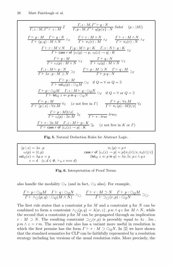
208 Matt Fairtlough et al.
IΓ, z : M, Γ ′ � z : M
Γ, z : M, Γ ′ � q : NSubst (p :: |M |)
Γ, p : M, Γ ′ � q{p/x} : N
Γ � p : M Γ � q : N ∧IΓ � (p, q) : M ∧N
Γ � r : M ∧N ∧EΓ � π1(r) : M
Γ � r : M ∧N ∧EΓ � π2(r) : N
Γ � r : M ∨N Γ, y : M � p : K Γ, z : N � q : K ∨EΓ � case r of [ι1(y)→ p, ι2(z)→ q] : K
Γ � p : M ∨IΓ � ι1(p) : M ∨N
Γ � q : N ∨IΓ � ι2(q) : M ∨N
Γ, z : M � p : N ⊃IΓ � λz . p : M ⊃ N
Γ � p : M ⊃ N Γ � q : M ⊃EΓ � p q : N
Γ � p : M ©I if Q = ∀ or Q = ∃Γ � valQ(p) : ©QM
Γ � p : ©QM Γ, z : M � q : ©QN ©E if Q = ∀ or Q = ∃Γ � letQ z ⇐ p in q : ©QN
Γ � p : M ∀I (x not free in Γ )Γ � 〈p | x〉 : ∀x.M
Γ � p : ∀x.M ∀EΓ � πt (p) : M [t/x]
Γ � p : M [t/x] ∃IΓ � ιt(p) : ∃x.M
trueIΓ � ∗ : true
Γ � r : ∃x.M Γ, z : M � p : K ∃E (x not free in K or Γ )Γ � case r of [ιx(z)→ p] : K
Fig. 5. Natural Deduction Rules for Abstract Logic.
〈p | x〉 = λx . p πt (p) = p tιt(p) = (t, p) case r of [ιx(z)→ p] = p{π1(r)/x, π2(r)/z}
valQ(x) = λy.x = y (letQ z ⇐ p in q) = λx.∃z. p z ∧ q xc = d (c, d ∈ Φ, �B c⇐⇒ d)
Fig. 6. Interpretation of Proof Terms.
also handle the modality ©∀ (and in fact, ©∃ also). For example,
Γ � p : ©QM Γ � q : ©QN ∧©Γ � ∧©(p, q) : ©Q(M ∧N)Γ � r : M ⊃ N Γ � p : ©QM ⊃©.Γ � ⊃©(r, p) : ©QN
The first rule states that a constraint p for M and a constraint q for N can becombined to form a constraint ∧©(p, q) = λ(w, z) . p w ∧ q z for M ∧ N , whilethe second that a constraint p for M can be propagated through an implicationr : M ⊃ N . The resulting constraint ⊃©(r, p) is provably equal to λz . ∃m .pm ∧ z = rm. The second rule also has a variant more useful in resolution inwhich the first premise has the form Γ � r : M ⊃ ©QN . In [2] we have shownthat the standard semantics for CLP can be faithfully represented by a resolutionstrategy including lax versions of the usual resolution rules. More precisely, the

Abstraction and Refinement in Higher Order Logic 209
execution of a CLP program corresponds to a lax resolution strategy for proofsand the CLP constraint analysis corresponds to the reduction of proof terms inour framework. This means that we can use our abstraction method to separatethe constraints from any CLP program, producing an abstract lax logic programand a separate constraint table. The abstract program may be run using a laxform of SLD resolution and the corresponding constraints generated from thetable. We conjecture that our results can be extended to higher order hereditaryHarrop formulas.
The second example is taken from [13] where Mendler sets himself the taskof realising the abstract successor function at the concrete level of bit vectors.He defines Incw :: B
w ⇒ Bw as a cascade of w half-adders which implements
the successor function provided the result can be encoded as a word of at mostw bits. This overflow constraint is constructed by a recursion mirroring therecursive construction of the incrementor itself. The abstract goal to prove is
∀w, n.©∀((αw ◦ Incw ◦ ρw)n = n+ 1)
where αw :: Bw ⇒ N and ρw :: N⇒ B
w are the abstraction and realisation map-pings that translate from bit vectors to numbers and conversely. The constraintgenerated by the lax proof of the goal is λw, n . f w n true where f is definedrecursively by f 0 n c = (n = 0 ∧ ¬c) and f (k + 1) n c = f k (n ÷ 2) (n = 1(mod 2) ∧ c). This constraint has computational behaviour, but it can also beshown to be equivalent to a flattened version n + 1 < 2w. The key differencelies in the fact that in certain contexts the recursive version may evaluate to thetrivial constraint, while the flattened version would have to be proved trivial.Note that the inductive basis of the constraint f w n true when w = 0, which is(n = 0∧¬true), is not only unsatisfiable, but in fact inconsistent. In other words,the abstract proof started from an inconsistent base case. Nevertheless, the laxproof returns a satisfiable constraint, since there are solutions to the constraintn+ 1 < 2w for any fixed w > 0.
qoutsin
rinqout
Fig. 7. RS Latch.
Finally we apply our method to the RS latch,which is illustrated in Fig. 7. The latch is the sim-plest of three memory devices verified by Herbertin [9]. He verifies the device in the HOL systemat a detailed timing level, using a discrete modelof time and a transport model of basic componentbehaviour. For example, he defines a NOR gate asNOR2(in0, in1, out, del) := ∀t. out(t+ del) =¬(in0 t ∨ in1 t) and the latch as NOR2(rin, qout, d1, qout) ∧NOR2(sin, qout, d2, qout) . It is clear that the proofs he presents are the resultof several iterations which were needed to discover the exact timing constraintsnecessary to prove them. Similar problems were reported in the work by Hannaand Daeche [8]. The main improvement yielded by our approach is that we donot need to make repeated attempts to prove the memory properties, becausethe timing constraints are synthesised in the course of the abstract analysis.
Our previous work e.g. [15, 14] in this area was focussed on combinational de-vices. The analysis of the system represented by Ψ in the introduction illustrates
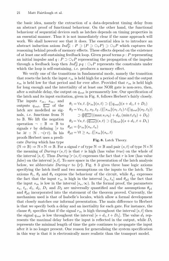
210 Matt Fairtlough et al.
the basic idea, namely the extraction of a data-dependent timing delay froman abstract proof of functional behaviour. On the other hand, the functionalbehaviour of sequential devices such as latches depends on timing properties inan essential manner. Thus it is not immediately clear if the same approach willwork. We shall however see that it does. The essential idea is to introduce anabstract induction axiom Ind �1
P : P ⊃ (P ⊃ ©∀P ) ⊃ ©∀P which captures thereasoning behind proofs of memory effects. These effects depend on the existenceof at least one self-sustaining feedback loop. Given proof terms p : P representingan initial impulse and q : P ⊃ ©∀P representing the propagation of the impulsethrough a feedback loop then Ind �1
P p q : ©∀P represents the constraints underwhich the loop is self-sustaining, i.e. produces a memory effect.
We verify one of the transitions in fundamental mode, namely the transitionthat resets the latch: the input rin is held high for a period of time and the outputsin is held low for that period and for ever after. Provided that rin is held highfor long enough and the intertiality of at least one NOR gate is non-zero, then,after a suitable delay, the output on qout is permanently low. Our specification ofthe latch and its input excitation, given in Fig. 8, follows Herbert’s fairly closely.
θ1 = ∀s, t .(|rin |)(s, t) ⊃ (|�qout |)(s+ d1, t+D1)θ2 = ∀s1, t1, s2, t2 . ((|�sin |)(s1, t1)∧(|�qout |)(s2, t2))
⊃ (||)qout ((max s1s2) + d2, (min t1t2) +D2)θ3= ∀s, t .(|qout |)(s, t) ⊃ (|�qout |)(s+ d1, t+D1)θp1 = (|rin |)(sa, ta)θp2 = ∀t ≥ sa .(|�sin |)(sa, t)
Fig. 8. Latch Theory.
The inputs rin , sin , andoutputs qout , qout of thelatch are modelled as sig-nals, i.e. functions from N
to B. We lift the negationoperation ¬ :: B ⇒ B tosignals r by defining �r tobe λt :: N . ¬(r t). In hisproofs Herbert uses a predi-cate During which has type(N⇒ B)⇒ N×N⇒ B. For a signal r of type N⇒ B and pair (s, t) of type N×N
the meaning of During r (s, t) is that r is high (has value true) on the whole ofthe interval [s, t]. Thus During �r (s, t) expresses the fact that r is low (has valuefalse) on the interval [s, t]. To save space in the presentation of the latch analysisbelow, we abbreviate During r to (|r|). Fig. 8 3 gives three base logic axiomsspecifying the latch itself and two assumptions on the inputs to the latch. Theaxioms θ1, θ2 and θ3 express the behaviour of the circuit, while θp1 expressesthe fact that the input rin is high in the interval [sa, ta] and θp2 the fact thatthe input sin is low in the interval [sa,∞). In the formal proof, the parameterssa, ta, d1, d2, D1 and D2 are universally quantified and the assumptions θp1
and θp2 incorporated into the statement of the theorem proved. Currently, themechanism used is that of Isabelle’s locales, which allow a formal developmentthat closely matches our informal presentation. The main difference to Herbertis that we specify both a delay and an inertiality for each gate. For instance, theclause θ1 specifies that if the signal rin is high throughout the interval [s, t] thenthe signal qout is low throughout the interval [s+ d1, t+D1]. The value d1 rep-resents the maximal delay before the input is reflected in the output, while D1
represents the minimal length of time the gate continues to propagate the inputafter it is no longer present. One reason for generalising the system specificationin this way is that it is electronically more realistic than the transport model.
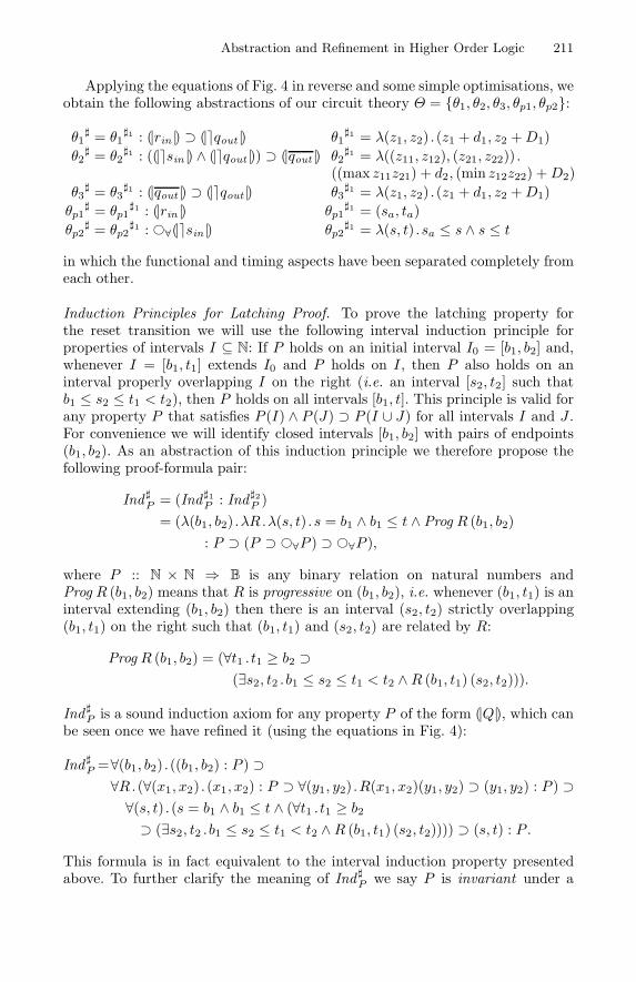
Abstraction and Refinement in Higher Order Logic 211
Applying the equations of Fig. 4 in reverse and some simple optimisations, weobtain the following abstractions of our circuit theory Θ = {θ1, θ2, θ3, θp1, θp2}:
θ1� = θ1
�1 : (|rin |) ⊃ (|�qout |) θ1�1 = λ(z1, z2) . (z1 + d1, z2 +D1)
θ2� = θ2
�1 : ((|�sin |) ∧ (|�qout |)) ⊃ (|qout |) θ2�1 = λ((z11, z12), (z21, z22)) .
((max z11z21) + d2, (min z12z22) +D2)θ3
� = θ3�1 : (|qout |) ⊃ (|�qout |) θ3
�1 = λ(z1, z2) . (z1 + d1, z2 +D1)θp1
� = θp1�1 : (|rin |) θp1
�1 = (sa, ta)θp2
� = θp2�1 : ©∀(|�sin |) θp2
�1 = λ(s, t) . sa ≤ s ∧ s ≤ t
in which the functional and timing aspects have been separated completely fromeach other.
Induction Principles for Latching Proof. To prove the latching property forthe reset transition we will use the following interval induction principle forproperties of intervals I ⊆ N: If P holds on an initial interval I0 = [b1, b2] and,whenever I = [b1, t1] extends I0 and P holds on I, then P also holds on aninterval properly overlapping I on the right (i.e. an interval [s2, t2] such thatb1 ≤ s2 ≤ t1 < t2), then P holds on all intervals [b1, t]. This principle is valid forany property P that satisfies P (I) ∧ P (J) ⊃ P (I ∪ J) for all intervals I and J .For convenience we will identify closed intervals [b1, b2] with pairs of endpoints(b1, b2). As an abstraction of this induction principle we therefore propose thefollowing proof-formula pair:
Ind �P = (Ind �1
P : Ind �2P )
= (λ(b1, b2) .λR.λ(s, t) . s = b1 ∧ b1 ≤ t ∧ Prog R (b1, b2): P ⊃ (P ⊃ ©∀P ) ⊃ ©∀P ),
where P :: N × N ⇒ B is any binary relation on natural numbers andProg R (b1, b2) means that R is progressive on (b1, b2), i.e. whenever (b1, t1) is aninterval extending (b1, b2) then there is an interval (s2, t2) strictly overlapping(b1, t1) on the right such that (b1, t1) and (s2, t2) are related by R:
Prog R (b1, b2) = (∀t1 . t1 ≥ b2 ⊃(∃s2, t2 . b1 ≤ s2 ≤ t1 < t2 ∧R (b1, t1) (s2, t2))).
Ind �P is a sound induction axiom for any property P of the form (|Q|), which can
be seen once we have refined it (using the equations in Fig. 4):
Ind �P =∀(b1, b2) .((b1, b2) : P ) ⊃∀R. (∀(x1, x2) . (x1, x2) : P ⊃ ∀(y1, y2) .R(x1, x2)(y1, y2) ⊃ (y1, y2) : P ) ⊃∀(s, t) . (s = b1 ∧ b1 ≤ t ∧ (∀t1 . t1 ≥ b2
⊃ (∃s2, t2 . b1 ≤ s2 ≤ t1 < t2 ∧R (b1, t1) (s2, t2)))) ⊃ (s, t) : P .
This formula is in fact equivalent to the interval induction property presentedabove. To further clarify the meaning of Ind �
P we say P is invariant under a
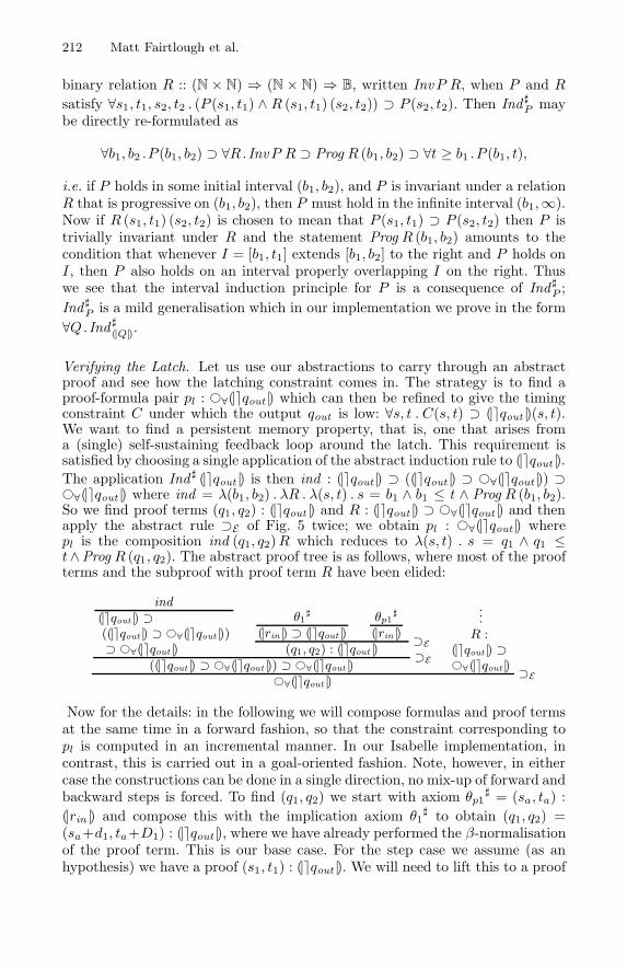
212 Matt Fairtlough et al.
binary relation R :: (N × N) ⇒ (N × N) ⇒ B, written InvP R, when P and R
satisfy ∀s1, t1, s2, t2 . (P (s1, t1) ∧ R (s1, t1) (s2, t2)) ⊃ P (s2, t2). Then Ind �P may
be directly re-formulated as
∀b1, b2 .P (b1, b2) ⊃ ∀R. InvP R ⊃ Prog R (b1, b2) ⊃ ∀t ≥ b1 .P (b1, t),
i.e. if P holds in some initial interval (b1, b2), and P is invariant under a relationR that is progressive on (b1, b2), then P must hold in the infinite interval (b1,∞).Now if R (s1, t1) (s2, t2) is chosen to mean that P (s1, t1) ⊃ P (s2, t2) then P istrivially invariant under R and the statement Prog R (b1, b2) amounts to thecondition that whenever I = [b1, t1] extends [b1, b2] to the right and P holds onI, then P also holds on an interval properly overlapping I on the right. Thuswe see that the interval induction principle for P is a consequence of Ind �
P ;Ind �
P is a mild generalisation which in our implementation we prove in the form∀Q.Ind �
(|Q|).
Verifying the Latch. Let us use our abstractions to carry through an abstractproof and see how the latching constraint comes in. The strategy is to find aproof-formula pair pl : ©∀(|�qout |) which can then be refined to give the timingconstraint C under which the output qout is low: ∀s, t . C(s, t) ⊃ (|�qout |)(s, t).We want to find a persistent memory property, that is, one that arises froma (single) self-sustaining feedback loop around the latch. This requirement issatisfied by choosing a single application of the abstract induction rule to (|�qout |).The application Ind � (|�qout |) is then ind : (|�qout |) ⊃ ((|�qout |) ⊃ ©∀(|�qout |)) ⊃©∀(|�qout |) where ind = λ(b1, b2) . λR . λ(s, t) . s = b1 ∧ b1 ≤ t ∧ Prog R (b1, b2).So we find proof terms (q1, q2) : (|�qout |) and R : (|�qout |) ⊃ ©∀(|�qout |) and thenapply the abstract rule ⊃E of Fig. 5 twice; we obtain pl : ©∀(|�qout |) wherepl is the composition ind (q1, q2)R which reduces to λ(s, t) . s = q1 ∧ q1 ≤t∧Prog R (q1, q2). The abstract proof tree is as follows, where most of the proofterms and the subproof with proof term R have been elided:
ind(|�qout |) ⊃((|�qout |) ⊃ ©∀(|�qout |))⊃ ©∀(|�qout |)
θ1�
(|rin |) ⊃ (|�qout |)θp1
�
(|rin |) ⊃E(q1, q2) : (|�qout |) ⊃E
((|�qout |) ⊃ ©∀(|�qout |)) ⊃ ©∀(|�qout |)
...R :
(|�qout |) ⊃©∀(|�qout |) ⊃E©∀(|�qout |)
Now for the details: in the following we will compose formulas and proof termsat the same time in a forward fashion, so that the constraint corresponding topl is computed in an incremental manner. In our Isabelle implementation, incontrast, this is carried out in a goal-oriented fashion. Note, however, in eithercase the constructions can be done in a single direction, no mix-up of forward andbackward steps is forced. To find (q1, q2) we start with axiom θp1
� = (sa, ta) :(|rin |) and compose this with the implication axiom θ1
� to obtain (q1, q2) =(sa+d1, ta+D1) : (|�qout |), where we have already performed the β-normalisationof the proof term. This is our base case. For the step case we assume (as anhypothesis) we have a proof (s1, t1) : (|�qout |). We will need to lift this to a proof
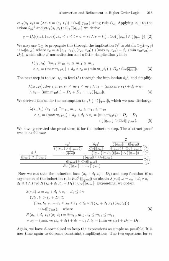
Abstraction and Refinement in Higher Order Logic 213
val∀(s1, t1) = (λz . z = (s1, t1)) : ©∀(|�qout |) using rule ©I . Applying ∧© to theaxiom θp2
� and val∀(s1, t1) : ©∀(|�qout |) we derive
q = (λ((s, t), (u, v)) . sa ≤ s ≤ t ∧ u = s1 ∧ v = t1) : ©∀((|�sin |) ∧ (|�qout |)). (2)
We may use⊃© to propagate this through the implication θ2� to obtain⊃©(r2, q)
: ©∀(|qout |) where r2 = λ((z11, z12), (z21, z22)) . ((max z11z21) + d2, (min z12z22) +D2), which after β-normalisation and a little simplication yields:
λ(z1, z2) .∃m11,m12 .sa ≤ m11 ≤ m12
∧ z1 = (maxm11s1) + d2 ∧ z2 = (minm12t1) +D2 : ©∀(|qout |). (3)
The next step is to use ⊃© to feed (3) through the implication θ3�, and simplify:
λ(z1, z2) .∃m11,m12 .sa ≤ m11 ≤ m12 ∧ z1 = (maxm11s1) + d2 + d1
∧ z2 = (minm12t1) +D2 +D1 : ©∀(|�qout |). (4)
We derived this under the assumption (s1, t1) : (|�qout |), which we now discharge:
λ(s1, t1), (z1, z2) .∃m11,m12 .sa ≤ m11 ≤ m12
∧ z1 = (maxm11s1) + d2 + d1 ∧ z2 = (minm12t1) +D2 +D1
: (|�qout |) ⊃ ©∀(|�qout |). (5)
We have generated the proof term R for the induction step. The abstract prooftree is as follows:
θ3�
(|qout |) ⊃ (|�qout |)
θ2�
((|�sin |) ∧ (|�qout |))⊃ (|qout |)
θp2�
©∀(|�sin |)
I(|�qout |) � (|�qout |) ©I
(|�qout |) � ©∀(|�qout |) ∧©(|�qout |) � ©∀((|�sin |) ∧ (|�qout |)) ⊃©(|�qout |) � ©∀(|qout |) ⊃©(|�qout |) � ©∀(|�qout |) ⊃I
R : (|�qout |) ⊃ ©∀(|�qout |)
Now we can take the induction base (sa + d1, ta +D1) and step function R asarguments of the induction rule Ind � (|�qout |) to obtain λ(s, t) . s = sa + d1 ∧ sa +d1 ≤ t ∧ Prog R (sa + d1, ta +D1) : ©∀(|�qout |). Expanding, we obtain
λ(s, t) . s = sa + d1 ∧ sa + d1 ≤ t ∧(∀t1 . t1 ≥ ta +D1 ⊃(∃s2, t2 .sa + d1 ≤ s2 ≤ t1 < t2 ∧R (sa + d1, t1) (s2, t2))): ©∀(|�qout |), where (6)
R (sa + d1, t1) (s2, t2) = ∃m11,m12 .sa ≤ m11 ≤ m12
∧ s2 = (maxm11sa + d1) + d2 + d1 ∧ t2 = (minm12t1) +D2 +D1.
Again, we have β-normalised to keep the expressions as simple as possible. It isnow time again to do some constraint simplifications. The two equations for s2
214 Matt Fairtlough et al.
and t2 allow us to eliminate the ∃s2, t2 quantifiers, a computation that wouldbe part of simple constraint analysis, i.e. incorporated into constraint simplifi-cations.
λ(s, t) . s = sa + d1 ∧ sa + d1 ≤ t ∧(∀t1 . t1 ≥ ta +D1 ⊃ (∃m11,m12 .sa ≤ m11 ≤ m12
sa + d1 ≤ (maxm11sa) + d1 + d2 + d1 ≤ t1 < (minm12t1) +D2 +D1)): ©∀(|�qout |). (7)
The constraint computation will detect that t1 < (minm12t1) + D2 + D1 isequivalent to D2 + D1 > 0; that maxm11sa is the same as m11 and hence(maxm11sa) + d1 + d2 + d1 ≤ t1 is equivalent to m11 +2 · d1 + d2 ≤ t1; and thatsa + d1 ≤ (maxm11sa) + d1 + d2 + d1 is always trivially satisfied. Thus, we endup with
λ(s, t) . s = sa + d1 ∧ sa + d1 ≤ t ∧(∀t1 ≥ ta +D1 .∃m11 ≥ sa .m11 + 2d1 + d2 ≤ t1 ∧D2 +D1 > 0)
: ©∀(|�qout |). (8)
At this point, now, it appears we need one slightly more sophisticated argumentto deal with the ∀t1 and ∃m11 quantifiers: the condition ∀t1 ≥ ta +D1 .∃m11 ≥sa . m11 + 2d1 + d2 ≤ t1 is logically equivalent to ta + D1 ≥ sa + 2d1 + d2.Given such reasoning is built into constraint simplifications, we are looking atthe solution form:
λ(s, t) . s = sa + d1 ∧ sa + d1 ≤ t ∧ta +D1 ≥ sa + 2d1 + d2 ∧D2 +D1 > 0 : ©∀(|�qout |). (9)
When (9) is refined back into the base logic we have the desired result:
(ta +D1 ≥ sa + 2d1 + d2 ∧D2 +D1 > 0) ⊃ ∀t ≥ sa + d1. (|�qout |) (sa + d1, t).
The predicate ta +D1 ≥ sa + 2d1 + d2 is the external hold constraint: input rinmust remain high for a period of length at least 2d1 + d2−D1 for the latch fullyto reset; the second part D2 +D1 > 0 is the internal memory constraint that atleast one of the gates must have non-zero inertia; finally, the third componentt ≥ sa + d1 of the overall constraint states that the propagation delay is d1.
4 Conclusions
We have presented a conservative extension to higher order logic reasoning thatallows for general shallow abstractions and an inverse refinement operation. Ourmethod subsumes some abstraction techniques used in AI, for instance proposi-tional abstraction [16], and can be used for data and structural abstractions aswell as for the timing abstractions on which we have concentrated.
The extension uses a computational lambda calculus to represent constraintinformation that is factored out by the abstraction. The combination between
Abstraction and Refinement in Higher Order Logic 215
these constraint terms and abstract formulas (syntactically separated by thecolon : operator) is a realisability interpretation of constructive logic which for-mally extends the “deliverables” approach of [11], and is implemented much asdescribed in [10], although the motivation of these papers and the theory of [11]is rather different from ours. It is important to stress that the method does notdepend on a constructive (intuitionistic) version of higher-order logic. However,the abstraction process applies constructive principles, within HOL.
Our approach to organising proofs in HOL allows for the clean and yet soundseparation of algorithmic (constraint λ-calculus) and non-algorithmic reasoning(abstract formulas). Abstraction by realisability separation should also openup new avenues for developing heuristic techniques for proof search in HOL,borrowing ideas from AI and constraint programming (CLP). The method yieldsa natural embedding and generalisation of CLP within HOL. To support ourclaims we have applied the technique here to the verification of a memory deviceand demonstrated how abstract functional verification can be combined withconstraint synthesis, in one and the same derivation. This solves a methodologicalproblem in the verification of memory devices as highlighted in the work ofHanna and Daeche [8] or Herbert [9]. We are not proposing our approach as areplacement for the many other effective approaches to verifying hardware inHOL, but we do suggest that it is compatible with them and is especially usefulwhere the handling of differing levels of abstraction is involved.
We have implemented our method in the Isabelle theorem prover and syn-thesised and analysed the timing constraints for the latch and the incrementorexample. Our priority is now to develop a set of tactics to automate constraintsimplification. Space permits discussion of only one point of detail: the readermay have noticed that the connectives in the abstract formulas of Fig. 4 donot have their expected types. For example, if P :: α ⇒ B, Q :: β ⇒ B,p :: α and q :: β then P p ∧ Qq = ((p, q) : P ∧ Q) which forces the secondoccurrence of ∧ to have type (α ⇒ B) ⇒ (β ⇒ B) ⇒ (α × β) ⇒ B insteadof the usual B ⇒ B ⇒ B. In our implementation we have defined a new setof logical connectives �,�,�, . . . to connect abstract formulas and used thisdefinition to derive the rules of Fig. 4. This is very straightforward to do fol-lowing the example of [10], e.g. we define the abstract version of conjunction byP �Q := λ(p, q) . p : P ∧ q : Q, where p : P can now be simply defined as P p.
Acknowledgements
We are grateful to Tom Melham for his encouragement and advice and to theanonymous referees for their comments and suggestions.
216 Matt Fairtlough et al.
References
[1] H. Eveking. Behavioural consistency between register-transfer- and switch-leveldescriptions. In D. A. Edwards, editor, Design Methodologies for VLSI and Com-puter Architecture. Elsevier Science, B. V., 1989.
[2] M. Fairtlough, M. Mendler, and M. Walton. First-order Lax Logic as a Frame-work for CLP. Technical Report MIPS-9714, Passau University, Department ofMathematics and Computer Science, 1997.
[3] M. Fairtlough and M. V. Mendler. Propositional Lax Logic. Information andComputation, 137(1):1–33, August 1997.
[4] M. Fairtlough and M. Walton. Quantified Lax Logic. Technical Report CS-97-11,Sheffield University, Department of Computer Science, 1997.
[5] M.P. Fourman. Proof and design. Technical Report ECS-LFCS-95-319, EdinburghUniversity, Department of Computer Science, 1995.
[6] M.P. Fourman and R.A. Hexsel. Formal synthesis. In G. Birtwistle, editor, Pro-ceedings of the IV Higher Order Workshop, Banff, 1990, 1991.
[7] F. Giunchiglia and T. Walsh. A theory of abstraction. Artificial Intelligence,57:323–389, 1992.
[8] F.K. Hanna and N. Daeche. Specification and verification using higher orderlogic: A case study. In G. M. Milne and P. A. Subrahmanyam, editors, FormalAspects of VLSI design, Proc. of the 1985 Edinburgh conf. on VLSI, pages 179–213. North-Holland, 1986.
[9] J. Herbert. Formal reasoning about timing and function of basic memory devices.In Dr. Luc Claesen, editor, IMEC-IFIP International Workshop on Applied For-mal Methods for Correct VLSI Design, Volume 2, pages 668–687. Elsevier SciencePublishers, B.V., 1989.
[10] B. Jacobs and T. Melham. Translating dependent type theory into higher or-der logic. In Typed Lambda Calculi and Applications, TLCA’93, pages 209–229.Springer LNCS 664, 1993.
[11] J.H. McKinna. Deliverables: A Categorical Approach to Program Developmentin Type Theory. PhD thesis, Edinburgh University, Department of ComputerScience, 1992.
[12] T.F. Melham. Higher Order Logic and Hardware Verification. Cambridge Uni-versity Press, 1993.
[13] M. Mendler. A Modal Logic for Handling Behavioural Constraints in Formal Hard-ware Verification. PhD thesis, Edinburgh University, Department of ComputerScience, ECS-LFCS-93-255, 1993.
[14] M. Mendler. Timing refinement of intuitionistic proofs and its application to thetiming analysis of combinational circuits. In P. Miglioli, U. Moscato, D. Mundici,and M. Ornaghi, editors, Proc. 5th Int. Workshop on Theorem Proving with An-alytic Tableaux and Related Methods, pages 261–277. Springer, 1996.
[15] M. Mendler and M. Fairtlough. Ternary simulation: A refinement of binary func-tions or an abstraction of real-time behaviour? In M. Sheeran and S. Singh,editors, Proc. 3rd Workshop on Designing Correct Circuits (DCC’96). SpringerElectronic Workshops in Computing, 1996.
[16] D.A. Plaisted. Theorem proving with abstraction. Artificial Intelligence, 16:47–108, 1981.
[17] A.S. Troelstra. Realizability. In S. Buss, editor, Handbook of Proof Theory. Else-vier Science B.V., 1998.
A Framework for the Formalisation of PiCalculus Type Systems in Isabelle/HOL
Simon J. Gay�
Department of Computing Science, University of GlasgowGlasgow, G12 8QQ, [email protected]
Abstract. We present a formalisation, in the theorem proving systemIsabelle/HOL, of a linear type system for the pi calculus, including aproof of runtime safety of typed processes. The use of a uniform encodingof pi calculus syntax in a meta language, the development of a generaltheory of type environments, and the structured formalisation of themain proofs, facilitate the adaptation of the Isabelle theories and proofscripts to variations on the language and other type systems.Keywords: Types; pi calculus; automatic theorem proving; semantics.
1 Introduction
Static type systems are an established feature of programming languages, andthe range of type systems is growing. The general principle is that a programwhich has been typechecked (at compile time) is guaranteed to satisfy a partic-ular runtime property: for example (traditionally) that all functions are calledwith the correct number and type of arguments, or (more exotically) that somesecurity property, such as secrecy, holds. In order for typechecking to give aproper guarantee of some form of program correctness, it is essential to prove,with respect to a well-defined semantics, that execution of typed programs iswell-behaved.
Proofs of type soundness have traditionally been carried out by hand, whichis feasible for small theoretical languages but much more difficult for real pro-gramming languages such as Java. The proofs are characterised by large induc-tions over the syntax of the language, the definition of the typing rules, and thedefinition of the operational semantics; many cases must be considered, whichoften differ in subtle ways and are very sensitive to the precise formulation ofthe syntax and the typing rules. Modifications of the language require proofs tobe redone, often with only minor variations but it is dangerous to assume thatpreviously-established properties will survive.
For these reasons, the idea of formalising proofs of type soundness (and otheraspects of programming language theory, such as program equivalence, but thisis not the concern of the present paper) within an automatic theorem provingsystem is very attractive. As part of a research project investigating type systems
� Partially supported by EPSRC grants GR/L75177 and GR/N39494.
R.J. Boulton and P.B. Jackson (Eds.): TPHOLs 2001, LNCS 2152, pp. 217–232, 2001.c© Springer-Verlag Berlin Heidelberg 2001
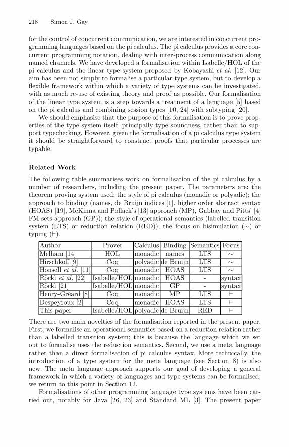
218 Simon J. Gay
for the control of concurrent communication, we are interested in concurrent pro-gramming languages based on the pi calculus. The pi calculus provides a core con-current programming notation, dealing with inter-process communication alongnamed channels. We have developed a formalisation within Isabelle/HOL of thepi calculus and the linear type system proposed by Kobayashi et al. [12]. Ouraim has been not simply to formalise a particular type system, but to develop aflexible framework within which a variety of type systems can be investigated,with as much re-use of existing theory and proof as possible. Our formalisationof the linear type system is a step towards a treatment of a language [5] basedon the pi calculus and combining session types [10, 24] with subtyping [20].
We should emphasise that the purpose of this formalisation is to prove prop-erties of the type system itself, principally type soundness, rather than to sup-port typechecking. However, given the formalisation of a pi calculus type systemit should be straightforward to construct proofs that particular processes aretypable.
Related Work
The following table summarises work on formalisation of the pi calculus by anumber of researchers, including the present paper. The parameters are: thetheorem proving system used; the style of pi calculus (monadic or polyadic); theapproach to binding (names, de Bruijn indices [1], higher order abstract syntax(HOAS) [19], McKinna and Pollack’s [13] approach (MP), Gabbay and Pitts’ [4]FM-sets approach (GP)); the style of operational semantics (labelled transitionsystem (LTS) or reduction relation (RED)); the focus on bisimulation (∼) ortyping (�).
Author Prover Calculus Binding Semantics FocusMelham [14] HOL monadic names LTS ∼Hirschkoff [9] Coq polyadic de Bruijn LTS ∼Honsell et al. [11] Coq monadic HOAS LTS ∼Rockl et al. [22] Isabelle/HOL monadic HOAS - syntaxRockl [21] Isabelle/HOL monadic GP - syntaxHenry-Greard [8] Coq monadic MP LTS �Despeyroux [2] Coq monadic HOAS LTS �This paper Isabelle/HOL polyadic de Bruijn RED �
There are two main novelties of the formalisation reported in the present paper.First, we formalise an operational semantics based on a reduction relation ratherthan a labelled transition system; this is because the language which we setout to formalise uses the reduction semantics. Second, we use a meta languagerather than a direct formalisation of pi calculus syntax. More technically, theintroduction of a type system for the meta language (see Section 8) is alsonew. The meta language approach supports our goal of developing a generalframework in which a variety of languages and type systems can be formalised;we return to this point in Section 12.
Formalisations of other programming language type systems have been car-ried out, notably for Java [26, 23] and Standard ML [3]. The present paper
A Framework for the Formalisation of Pi Calculus Type Systems 219
concentrates on concurrent languages in the style of the pi calculus; the ambi-tious goal of applying our meta language approach to a wider range of languageparadigms is left for future work.
2 Pi Calculus
We assue some familiarity with the pi calculus [16, 17] but summarise its syntaxand semantics in this section.
The following grammar defines processes P ; variables x stand for channelnames; x is a list of variables. There are two binding operators: the variables xare bound in (νx)P and in x?[x] . P . All other variable occurrences are free.
P ::= 0 (nil) | (νx)P (restriction)| P | P (parallel) | x?[x] . P (input)| !P (replication) | x![x] . P (output)| P + P (choice)
The operational semantics of the pi calculus is defined in two stages. The struc-tural congruence relation axiomatises some basic process equivalences, and thereduction relation axiomatises inter-process communication.
The structural congruence relation, denoted by ≡, is defined inductively asthe smallest equivalence relation which is additionally a congruence (i.e. is pre-served by the process constructors) and is closed under a number of rules. Theserules include α-equivalence, basic properties of parallel composition and choice(commutativity, associativity, the fact that 0 is a unit), and some less trivialequivalences. Chief among these are a rule which captures the meaning of repli-cation:
!P ≡ P |!Pand the scope extrusion rule:
P | (νx)Q ≡ (νx)(P |Q) if none of the x are free in P .
The reduction relation is also defined inductively, by the following rules.The first rule uses substitution to express transmission of channel names duringcommunication; only substitution of variables for variables is required.
length(y) = length(z)
x?[y] . P | x![z] . Q −→ P{z/y} |QP −→ P ′
(νx)P −→ (νx)P ′
P ′ ≡ P P −→ Q Q ≡ Q′P ′ −→ Q′
P −→ P ′
P |Q −→ P ′ |QP −→ P ′
P +Q −→ P ′
Communication between an input and an output of different arities is notdefined, and the appearance of such a miscommunication during the execution ofa process can be interpreted as a runtime error, analogous to calling a functionwith the wrong number of arguments. The simple type system [15, 25] for the pi
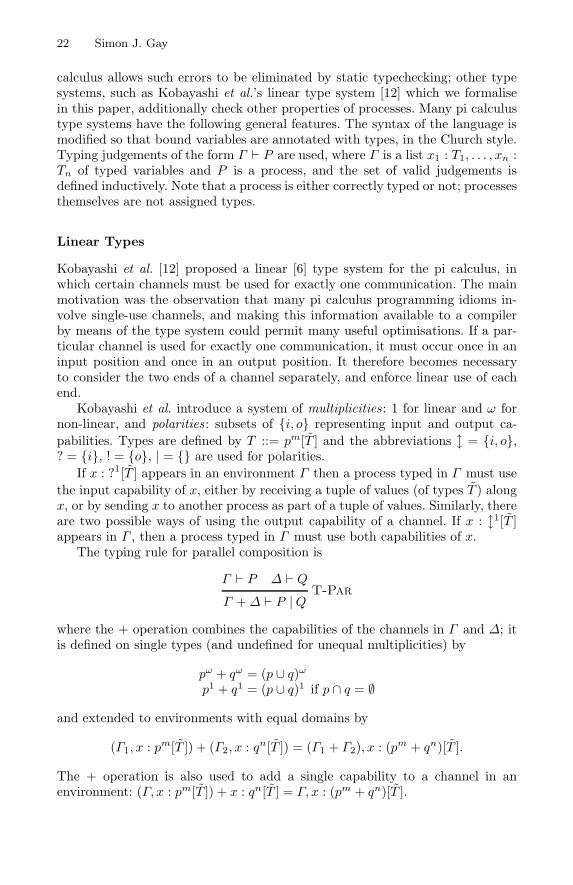
220 Simon J. Gay
calculus allows such errors to be eliminated by static typechecking; other typesystems, such as Kobayashi et al.’s linear type system [12] which we formalisein this paper, additionally check other properties of processes. Many pi calculustype systems have the following general features. The syntax of the language ismodified so that bound variables are annotated with types, in the Church style.Typing judgements of the form Γ � P are used, where Γ is a list x1 : T1, . . . , xn :Tn of typed variables and P is a process, and the set of valid judgements isdefined inductively. Note that a process is either correctly typed or not; processesthemselves are not assigned types.
Linear Types
Kobayashi et al. [12] proposed a linear [6] type system for the pi calculus, inwhich certain channels must be used for exactly one communication. The mainmotivation was the observation that many pi calculus programming idioms in-volve single-use channels, and making this information available to a compilerby means of the type system could permit many useful optimisations. If a par-ticular channel is used for exactly one communication, it must occur once in aninput position and once in an output position. It therefore becomes necessaryto consider the two ends of a channel separately, and enforce linear use of eachend.
Kobayashi et al. introduce a system of multiplicities: 1 for linear and ω fornon-linear, and polarities : subsets of {i, o} representing input and output ca-pabilities. Types are defined by T ::= pm[T ] and the abbreviations = {i, o},? = {i}, ! = {o}, | = {} are used for polarities.
If x : ?1[T ] appears in an environment Γ then a process typed in Γ must usethe input capability of x, either by receiving a tuple of values (of types T ) alongx, or by sending x to another process as part of a tuple of values. Similarly, thereare two possible ways of using the output capability of a channel. If x : 1[T ]appears in Γ , then a process typed in Γ must use both capabilities of x.
The typing rule for parallel composition is
Γ � P ∆ � QT-Par
Γ +∆ � P |Qwhere the + operation combines the capabilities of the channels in Γ and ∆; itis defined on single types (and undefined for unequal multiplicities) by
pω + qω = (p ∪ q)ωp1 + q1 = (p ∪ q)1 if p ∩ q = ∅
and extended to environments with equal domains by
(Γ1, x : pm[T ]) + (Γ2, x : qn[T ]) = (Γ1 + Γ2), x : (pm + qn)[T ].
The + operation is also used to add a single capability to a channel in anenvironment: (Γ, x : pm[T ]) + x : qn[T ] = Γ, x : (pm + qn)[T ].
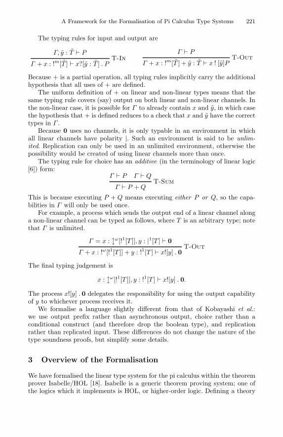
A Framework for the Formalisation of Pi Calculus Type Systems 221
The typing rules for input and output are
Γ, y : T � PT-In
Γ + x : !m[T ] � x?[y : T ] . PΓ � P
T-OutΓ + x : !m[T ] + y : T � x ! [y]P
Because + is a partial operation, all typing rules implicitly carry the additionalhypothesis that all uses of + are defined.
The uniform definition of + on linear and non-linear types means that thesame typing rule covers (say) output on both linear and non-linear channels. Inthe non-linear case, it is possible for Γ to already contain x and y, in which casethe hypothesis that + is defined reduces to a check that x and y have the correcttypes in Γ .
Because 0 uses no channels, it is only typable in an environment in whichall linear channels have polarity |. Such an environment is said to be unlim-ited. Replication can only be used in an unlimited environment, otherwise thepossibility would be created of using linear channels more than once.
The typing rule for choice has an additive (in the terminology of linear logic[6]) form:
Γ � P Γ � QT-Sum
Γ � P +Q
This is because executing P + Q means executing either P or Q, so the capa-bilities in Γ will only be used once.
For example, a process which sends the output end of a linear channel alonga non-linear channel can be typed as follows, where T is an arbitrary type; notethat Γ is unlimited.
Γ = x : ω[!1[T ]], y : |1[T ] � 0T-Out
Γ + x : !ω[!1[T ]] + y : !1[T ] � x![y] . 0The final typing judgement is
x : ω[!1[T ]], y : !1[T ] � x![y] . 0.The process x![y] . 0 delegates the responsibility for using the output capabilityof y to whichever process receives it.
We formalise a language slightly different from that of Kobayashi et al.:we use output prefix rather than asynchronous output, choice rather than aconditional construct (and therefore drop the boolean type), and replicationrather than replicated input. These differences do not change the nature of thetype soundness proofs, but simplify some details.
3 Overview of the Formalisation
We have formalised the linear type system for the pi calculus within the theoremprover Isabelle/HOL [18]. Isabelle is a generic theorem proving system; one ofthe logics which it implements is HOL, or higher-order logic. Defining a theory
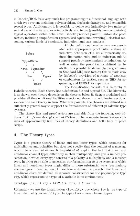
222 Simon J. Gay
in Isabelle/HOL feels very much like programming in a functional language witha rich type system including polymorphism, algebraic datatypes, and extensiblerecord types. Additionally, it is possible to define sets inductively (we make es-sential use of this feature) or coinductively, and to use (possibly non-computable)logical operators within definitions. Isabelle provides powerful automatic prooftactics, including simplification (generalised equational rewriting), classical rea-soning, various kinds of resolution, induction, and case-analysis.
All the definitional mechanisms are associ-Pi|
Subst|
TypedMeta/ \
Meta TypedEnv\ / \Env Types
\ /Main
ated with appropriate proof rules: making aninductive definition of a set automatically de-fines elimination rules and an induction rule tosupport proofs by case-analysis or induction. Aswell as using the proof tactics defined by Is-abelle, it is possible to define (by programmingin Standard ML) new tactics; this is made easyby Isabelle’s provision of a range of tacticals,or combinators for tactics, such as THEN for se-quencing and REPEAT for repetition.
The formalisation consists of a hierarchy ofIsabelle theories. Each theory has a definition file and a proof file. The hierarchyis as shown; each theory depends on the theories below it. Main is predefined andprovides all the definitional facilities mentioned above. In the following sections,we describe each theory in turn. Wherever possible, the theories are defined in asufficiently general way to support the formalisation of different pi calculus typesystems.
The theory files and proof scripts are available from the following web ad-dress: http://www.dcs.gla.ac.uk/~simon. The complete formalisation con-sists of approximately 650 lines of theory definitions and 6500 lines of proofscript.
4 The Theory Types
Types is a generic theory of linear and non-linear types, which accounts formultiplicities and polarities but does not specify that the content of a messageis a tuple of channel names. Kobayashi et al. exploit the fact that linear andnon-linear channel types differ only in their multiplicity, and give a unified pre-sentation in which every type consists of a polarity, a multiplicity and a messagetype. In order to be able to generalise our formalisation to type systems in whichlinear and non-linear types might differ in more substantial ways (particularlysession types — see Section 11), we take a different approach. The linear andnon-linear cases are defined as separate constructors for the polymorphic typevty, which represents the type of a variable in an environment.
datatype (’a,’b) vty = LinV (’a linv) | NLinV ’b
Ultimately we use the instantiation (lty,nlty) vty where lty is the type oflinear channel types and nlty is the type of non-linear channel types.
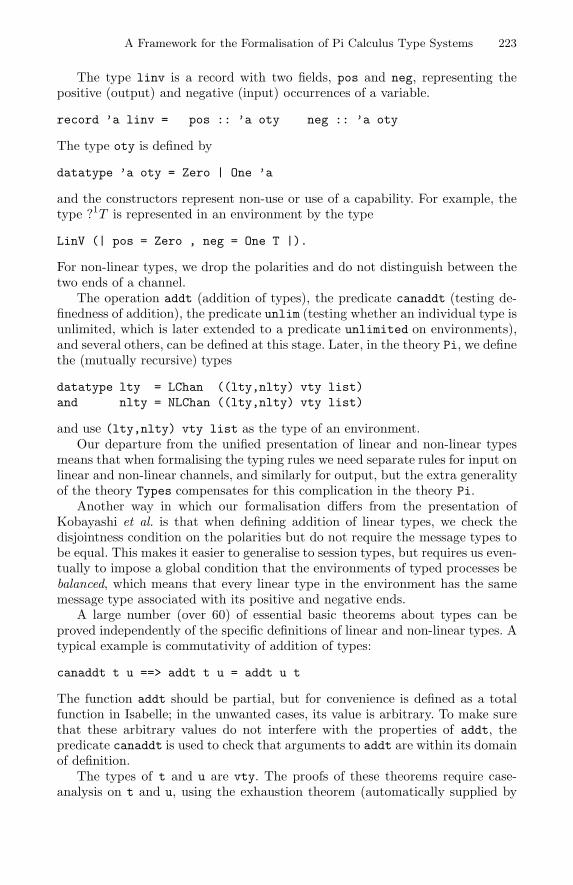
A Framework for the Formalisation of Pi Calculus Type Systems 223
The type linv is a record with two fields, pos and neg, representing thepositive (output) and negative (input) occurrences of a variable.
record ’a linv = pos :: ’a oty neg :: ’a oty
The type oty is defined by
datatype ’a oty = Zero | One ’a
and the constructors represent non-use or use of a capability. For example, thetype ?1T is represented in an environment by the type
LinV (| pos = Zero , neg = One T |).
For non-linear types, we drop the polarities and do not distinguish between thetwo ends of a channel.
The operation addt (addition of types), the predicate canaddt (testing de-finedness of addition), the predicate unlim (testing whether an individual type isunlimited, which is later extended to a predicate unlimited on environments),and several others, can be defined at this stage. Later, in the theory Pi, we definethe (mutually recursive) types
datatype lty = LChan ((lty,nlty) vty list)and nlty = NLChan ((lty,nlty) vty list)
and use (lty,nlty) vty list as the type of an environment.Our departure from the unified presentation of linear and non-linear types
means that when formalising the typing rules we need separate rules for input onlinear and non-linear channels, and similarly for output, but the extra generalityof the theory Types compensates for this complication in the theory Pi.
Another way in which our formalisation differs from the presentation ofKobayashi et al. is that when defining addition of linear types, we check thedisjointness condition on the polarities but do not require the message types tobe equal. This makes it easier to generalise to session types, but requires us even-tually to impose a global condition that the environments of typed processes bebalanced, which means that every linear type in the environment has the samemessage type associated with its positive and negative ends.
A large number (over 60) of essential basic theorems about types can beproved independently of the specific definitions of linear and non-linear types. Atypical example is commutativity of addition of types:
canaddt t u ==> addt t u = addt u t
The function addt should be partial, but for convenience is defined as a totalfunction in Isabelle; in the unwanted cases, its value is arbitrary. To make surethat these arbitrary values do not interfere with the properties of addt, thepredicate canaddt is used to check that arguments to addt are within its domainof definition.
The types of t and u are vty. The proofs of these theorems require case-analysis on t and u, using the exhaustion theorem (automatically supplied by
224 Simon J. Gay
Isabelle) for the datatype vty; use of Isabelle’s tactic record split tac to de-compose goals involving variables of type linv; and further case-analysis usingthe exhaustion theorem for the datatype oty. Simplification is also used at eachstage.
All of these theorems are proved in essentially the same way, and we have im-plemented a specialised tactic, Types tac, for this purpose. Unfortunately, whenapplying case-analysis it is necessary to provide the name of the variable involved.This means that Types tac only works if the theorems are stated in terms of thevariables t, u, v, w or a subset of these; none of the theorems involve more than 4variables. Furthermore, the second round of case-analysis depends on the exactnames of variables which are introduced by Isabelle during the first round. Thebehaviour of Types tac, in terms of the number of subgoals generated and thetime taken by simplification, depends on the order in which variables are con-sidered in the second round of case-analysis. In practice, Types tac works welland proves all but two of the theorems in Types. The remaining theorems areproved by a variation of Types tac which considers variables in a different order.The dependence on particular variable names, particularly internally-generatednames, means that Types tac is not robust and this is somewhat unsatisfactory.We are still trying to find a better way of expressing the proofs in this theory.
5 Environments
The theories Env and TypedEnv define operations on environments. An environ-ment is a list of types, and variable indices refer to positions within an environ-ment. Env defines all operations which can be expressed independently of Types,for example the function typeof which returns the type at a particular posi-tion in an environment. The operations defined by Env are either polymorphicoperations on lists, which will later be applied to environments, or operationsmanipulating positions within environments, which are therefore functions onintegers or lists of integers.
TypedEnv defines, in terms of addt, operations associated with addition oftypes and environments: addtypetoenv, which adds a capability to the type at agiven position within an environment; addtoenv, which adds a list of capabilitiesto the types at a list of positions; and addenv, which adds environments. All ofthese operations are partial, because addt is partial. Each operation therefore hasan associated predicate, for example canaddenv, which is used in the hypothesesof theorems about the partial operations. For example, the theorem that additionof environments is commutative is
canaddenv G H ==> addenv G H = addenv H G.
This theorem is proved by induction on G and case-analysis on H, using thecorresponding theorem about addt (mentioned in Section 4).
A Framework for the Formalisation of Pi Calculus Type Systems 225
6 The Meta Language
Rather than define a representation of pi terms directly, we use a meta lan-guage, which is a lambda calculus with constants. This approach has a numberof advantages.
– Once basic properties of the meta language (e.g. injectivity of constructors)have been proved, the corresponding properties of the pi calculus are easilyproved by Isabelle’s automatic tactics, and it is trivial to transfer the proofsto extensions or variations of the calculus.
– The meta language is simpler (has fewer constructors) than the pi calculus.This means that some key theorems, whose proofs are complex, are easierto prove for the meta language and lift to the pi calculus than to prove forthe pi calculus directly; see Section 8.
– Both of the n-ary binding operators of the pi calculus are represented interms of a single unary binding operator in the meta language; issues todo with variable binding are therefore concentrated into a single, relativelysimple, area.
We represent variables by de Bruijn indices [1], to avoid the complications ofreasoning about α-conversion and freshness of variable names in substitutions[7]. Theory Meta defines the following datatype, parameterised by a type ofconstants.
datatype ’a meta =mCon ’a (* constant *)
| mVar var (* variable *)| mAbs (’a meta) (* abstraction *)| mApp (’a meta) (’a meta) (* application *)| mAdd (’a meta) (’a meta) (* additive application *)
The type var is a record type with fields index, of type nat, and tag, whosetype is an enumeration with possible values Pos, Neg or Both. The index fieldis the de Bruijn index of the variable occurrence. The tag field distinguishesbetween positive and negative occurrences of linear variables and occurrencesof non-linear variables (which have tag Both). This explicit tagging of variableoccurrences simplifies some proofs by making it easier to determine which endof a linear channel is being transmitted by an output. In a practical languagethis information could probably be obtained by type inference, and it might bepossible to eliminate it from our formalisation in the future. More generally, weanticipate other uses of the tag field when adapting our formalisation to othertype systems; for example, Pierce and Sangiorgi’s proof of type soundness forthe pi calculus with subtyping [20] uses an auxiliary syntax in which variableoccurrences are tagged with runtime types.
The de Bruijn index of a variable occurrence counts the number of abstrac-tions between the occurrence and the abstraction which binds it. Indices so largethat they point outside all abstractions refer to positions in a notional list of free
226 Simon J. Gay
variables; this list is, in effect, an untyped environment for the term. For exam-ple, if the environment of free variables is taken to be u, v (the order is arbitrary),and if we pretend that var = nat and omit the mVar constructors, then the term
λx.u(λy.u(x(yv)))
is represented by mAbs (mApp 1 (mAbs (mApp 2 (mApp 1 (mApp 0 3))))).It is slightly misleading to think of the meta language as a lambda calculus.
Because we never apply β-reduction to meta language terms, mAbs and mAppare unrelated; in particular, the order of the arguments of mApp is unimportant.Note the inclusion of a second “application”, called mAdd, which will be usedwhen representing additive linear operators; it is convenient for multiplicativeand additive operators to use different meta language constructors.
In order to support the n-ary binding operators of the pi calculus, and torepresent output (which involves a list of variables), we define mABS for iteratedabstraction and mAPP which applies mApp repeatedly to the elements of a list.
7 Substitution
Substitution is defined for the meta language in theory Meta and lifted to the picalculus in theory Pi. In order to define substitution appropriately, we considerthe key case in the proof of the subject reduction theorem. The derivation
Γ � PΓ + x : !1[T ] + y : T � x![y] . P
∆, z : T � Q∆+ x : ?1[T ] � x?[z : T ] . Q
Γ +∆+ x : 1[T ] + y : T � x![y] . P | x?[z : T ] . Qtypes the process
x![y] . P | x?[z : T ] . Qwhich reduces to
P |Q{y/z}and we must therefore derive a typing for the latter process. If we have
∆+ y : T � Q{y/z}
then we can deriveΓ +∆+ y : T � P |Q{y/z}
which is sufficient; note that the linear input and output capabilities of x wereused by the communication and are not needed in order to type P | Q{y/z}.This example shows that the variables z do not appear in the environment ofQ{y/z}, but that the types of z must be added to the environment as extracapabilities for y. Theory Subst defines a function substenv which calculatesthe typed environment for a substituted term, and a predicate oksubst whichtests definedness of this environment.
A Framework for the Formalisation of Pi Calculus Type Systems 227
We have already noted that it is sufficient to define substitution of variables(not arbitrary terms) for variables. Furthermore, because it is only necessaryto substitute for input-bound variables, we can assume that the variables beingreplaced are distinct from each other and from the variables replacing them;it is therefore possible to define the simultaneous substitution of a list of vari-ables as a sequence of substitutions of single variables. This is different fromother pi calculus formalisations (for example, Melham’s [14]) which define si-multaneous substitution directly, but given that we are using de Bruijn indicesit represents a very significant simplification. Because substitution in a typedprocess requires a change in the environment, the variable indices throughoutthe process must be adjusted. This adjustment would be rather complex to de-fine for simultaneous substitutions, but is much more straightforward for a singlesubstitution. Similarly, proofs about simultaneous substitution use induction toextend results about single substitution to lists, and this is simpler than reason-ing directly about simultaneous substitution. Reasoning about the adjustmentof indices in single substitutions is facilitated by Isabelle’s recently-introducedtactic arith tac, which is based on a decision procedure for linear arithmetic.
8 The Typed Meta Language
Another novel feature of our formalisation is that we define a type system forthe meta language, which keeps track of linear variable use. The rules (omittingtags, and presented informally) are shown in Figure 1.
Γ unlimited
Γ + v : LinV (| pos = One T , neg = Zero |) �m mVar v
Γ unlimited
Γ �m mCon c
Γ unlimited
Γ + v : LinV (| pos = Zero , neg = One T |) �m mVar v
Γ, x : T �m t
Γ �m mAbs t
Γ unlimited
Γ + v : NLinV T �m mVar v
Γ �m t ∆ �m u
Γ + ∆ �m mApp t u
Γ �m t Γ �m u
Γ �m mAdd t u
Fig. 1. Typing Rules for the Meta Language.
A few technical theorems are proved at this stage, for example:
If Γ �m p and ∆ �m p and Γ +∆ is defined and Γ is unlimited then∆ is unlimited.
The proof of this theorem is simpler for the typed meta language than itwould be for the typed pi calculus, because the meta language has fewer con-structors. In the theory Pi we prove that every typing rule for the pi calculus is aderived rule for the meta language type system. Hence this theorem, and others
228 Simon J. Gay
like it, can be lifted very easily to the pi calculus level, and extended easily tovariations of the pi calculus. This particular theorem is used in the proof thatstructural congruence preserves typability (Section 10).
This technique only applies to theorems whose conclusions do not mentionthe typing relation. Correct typing of (the representation of) a pi calculus termas a meta language term does not imply corect typing of the pi calculus term— the pi calculus typing rules have extra hypotheses which are not captured bythe meta language typing rules. Nevertheless, we have found the introduction ofthe meta language type system to be a useful structuring technique which verysignificantly simplifies the proofs of the theorems to which it is applicable.
9 Formalising the Pi Calculus
The theory Pi defines specific linear and non-linear channel types and a spe-cialised type of environments, as mentioned in Section 4. A specific type con ofconstants for the meta language is defined, and representations of pi calculusterms are defined as meta language terms of type pi = con meta. For example,
OUT x n xs p == mAPP (mApp (mCon (Out n)) p) (map mVar (x # xs))
represents x![xs ] . p where length(xs) = n.The structural congruence relation, the reduction relation and the typing
relation are all defined inductively. The de Bruijn representation affects somerules: for example, the scope extrusion rule for structural congruence (Section 2)becomes (SCONG is an inductively-defined subset of pi * pi, formalising thestructural congruence relation, so that (p,q):SCONG means p ≡ q)
(PAR p (NEW n ts q) , NEW n ts (PAR (lift 0 n p) q)) : SCONG
where lift 0 n p adjusts the indices of the free variables of p to take accountof the insertion of n variables at position 0 in the environment. The definitionof lift guarantees that the first n variables in the environment, correspondingto x, do not occur in lift 0 n p, so the condition on free variables disappears.
As indicated in Section 7, if Γ � P and P −→ Q by a communication on alinear channel, then Q is typed in an environment in which the polarity of thatchannel has been reduced to |. It is therefore necessary to label a reduction withthe name of the channel involved (or τ if the channel is hidden by an enclosingν), represented by type redch. The reduction P x−→ Q is formalised by (P , x, Q) : RED where RED is an inductively defined subset of pi * redch * pi.
Defining pi terms via a meta language rather than directly as a datatypemeans that distinctness and injectivity theorems need to be proved explicitlyfor the pi calculus constructors. The number of such theorems is fairly large(the square of the number of constructors), but they are all proved by Isabelle’sautomatic tactics.
Theorems about substitution on pi terms are also proved automatically, forexample (note the addition of n due to changing environments):
(NEW n ts p)[x//i] = NEW n ts p[x+n // i+n].
A Framework for the Formalisation of Pi Calculus Type Systems 229
Similarly, theorems about lift on pi terms are proved automatically.Theorems stating that the pi typing rules are derived rules for the typed
meta language are proved, as mentioned in Section 8. Each theorem is simply api typing rule with the pi typing relation replaced by the meta typing relation.The proofs are short, the only complexity being some explicit use of theoremsabout environments.
10 Type Soundness
The key to proving soundness of the type system is the subject reduction theorem,which states that reduction of a typed process yields a typed process. We prove
[| G |- p ; (p, x, q) : RED ; balanced G |] ==> usechan x G |- q
by induction on the reduction relation, RED. As discussed in Section 7, q is typednot in G but in an environment in which the capability of the channel x has beenused, if its type is linear.
As we also saw in Section 7, we need to prove a substitution lemma:
[| G |- p ; oksubst x i G |] ==> substenv x i G |- p[x//i]
for substitutions of single variables and extend it by induction to substitutions oflists of variables. Here we use the induction principle derived from the inductivedefinition of the typing relation. The proof breaks down into a number of cases,one for each pi calculus constructor. In order to make it easier to extend thelanguage later, we prove a lemma for each case and then combine them with a“driver” proof which simply applies the induction rule to generate the cases andthen applies the appropriate lemma to each case. Once the proof is structuredin this way, it is easy to see how to extend it if new constructors are added. Allof our proofs about the typing relation are similarly modularised.
Because structural congruence can be used when deriving reductions, weprove that structural congruence preserves typability:
[| G |- p ; (p , q) : SCONG |] ==> G |- q.
The proof is by induction on the definition of SCONG, and as with the induc-tive proofs about |-, we structure the proof by extracting the cases as separatelemmas. The congruence cases are almost trivial and are all proved by a simplespecialised tactic, SCONG tac, which uses Isabelle’s classical reasoner to search fora proof involving the introduction and elimination rules arising from the induc-tive definition of the typing relation. Most of the other cases are straightforward,involving application of the typing rules and some reasoning about addition ofenvironments. Some of the cases dealing with replication and restriction aremore complex, requiring (for replication) the fact about unlimited environmentsmentioned in Section 8 and (for restriction) the following weakening lemma:
[| G |- p ; length ts = n ; unlimited ts ; m <= length G |] ==>ins ts m G |- lift m n p
230 Simon J. Gay
in which ins ts m G is the environment obtained by inserting the types ts intoG at position m. Another form of weakening adds capabilities to types which arealready in the environment. We prove
[| G |- p ; unlimited H ; canaddenv G H |] ==> addenv G H |- p
by induction on the typing relation, again structuring the proof into a lemmafor each case.
The subject reduction theorem states that reductions of typed processes yieldtyped processes, but because reduction is not defined for communications withan arity mismatch, we need to prove that these incorrect communications cannotoccur in typed processes. Following Kobayashi et al. we prove that if a typedprocess contains a term x![z] . P |x?[y : T ] .Q then length(y) = length(z) and thetype of x (in the environment or in an enclosing restriction) has polarity . Wealso prove their theorems about correct use of linear and non-linear channels,for example that if a typed process contains a term x![z] . P | x![z] . Q then thetype of x is non-linear.
11 Extension to Session Types
Honda et al. [10, 24] have proposed session types, which allow successive commu-nications on a channel to carry different message types. Branching is also allowed,so that the transmission of a particular value (from a finite range) can deter-mine the type of the subsequent interaction. Consider, for example, a server formathematical operations, which initially offers a choice between equality testingand negation. A client must choose an operation and then send the appropriatenumber of arguments to the server, which responds by sending back the result.All communications take place on a single session channel called x; the type ofthe server side of this channel is
S = &〈eq :?[int] . ?[int] . ![bool] . end, neg :?[int] . ![int] . end〉.The author and Malcolm Hole [5] have defined a notion of subtyping for ses-sion types, proposing a language whose type system allows the description ofbackward-compatible upgrades to client-server systems. Ultimately we aim toformalise the type system of this language.
To avoid runtime type errors, a session channel must be shared by exactlytwo processes, one at each end. Within each process, however, the channel mustbe used for as many communications as are specified by its type. Session typestherefore require an interesting mixture of linear and non-linear (but bounded)control and this will require a generalisation of our present theory Types. Addi-tion of a capability to a session type should mean prefixing a new communicationto the existing type, for example extending ![bool] . end to ?[int] . ![bool] . end.
Using Pierce and Sangiorgi’s [20] technique, proving type soundness for thesystem with subtyping requires the definition of an auxiliary language in whichvariable occurrences are tagged with runtime types. Our formalisation will haveto define two different, although related, languages, and our structured approachshould make it easy to achieve this, especially as we have already included sup-port for tagging of variable occurrences.
A Framework for the Formalisation of Pi Calculus Type Systems 231
12 Conclusions
We have formalised a linear type system for the pi calculus, and a proof of itssoundness, as a step towards a formalisation of a more complex type systemincorporating session types and subtyping.
Our work differs from other formalisations of the pi calculus in several signif-icant ways. One is that we concentrate on reasoning about the reduction relationand type systems, including systems with linear features, rather than labelledtransition systems and bisimulation. More importantly, mindful of our desireto extend this work to a more complex language, we have aimed to develop amethodology and general framework for the formalisation of type systems forlanguages based on the pi calculus, rather than simply to formalise a partic-ular type system. The use of a typed meta language (Sections 6 and 8), thedevelopment of a generic theory of linear and non-linear types (Section 4) andenvironments (Section 5), and the modular structure of the proofs about the picalculus typing relation (Section 10), are all intended to facilitate the transfer ofour techniques to other languages.
Acknowledgements
The author is grateful to Tom Melham and the anonymous referees for manyvaluable comments, to Malcolm Hole for discussions of pi calculus type soundnessproofs, and to Simon Ambler for discussions of formalisations of operationalsemantics.
References
[1] N. G. deBruijn. Lambda calculus notation with nameless dummies. IndagationesMathematicae, 34:381–392, 1972.
[2] J. Despeyroux. A higher-order specification of the pi-calculus. In Proceedings ofthe IFIP International Conference on Theoretical Computer Science, 2000.
[3] C. Dubois. Proving ML type soundness within Coq. In M. Aagaard and J. Harri-son, editors, Proceedings of TPHOLs2000, the 13th International Conference onTheorem Proving in Higher Order Logics, LNCS, pages 126–144. Springer, 2000.
[4] M. J. Gabbay and A. M. Pitts. A new approach to abstract syntax with variablebinding. Formal Aspects of Computing, 2001.
[5] S. J. Gay and M. J. Hole. Types and subtypes for client-server interactions.In S. D. Swierstra, editor, ESOP’99: Proceedings of the European Symposium onProgramming Languages and Systems, number 1576 in Lecture Notes in ComputerScience, pages 74–90. Springer-Verlag, 1999.
[6] J.-Y. Girard. Linear Logic. Theoretical Computer Science, 50(1):1–102, 1987.[7] A. D. Gordon and T. Melham. Five axioms of alpha conversion. In J. von Wright,
J. Grundy, and J. Harrison, editors, Theorem Proving in Higher Order Logics: 9thInternational Conference, TPHOLs’96, volume 1125 of Lecture Notes in ComputerScience, pages 173–190. Springer-Verlag, 1996.
[8] L. Henry-Greard. Proof of the subject reduction property for a π-calculus inCOQ. Technical Report 3698, INRIA Sophia-Antipolis, May 1999.
232 Simon J. Gay
[9] D. Hirschkoff. A full formalisation of π-calculus theory in the calculus of construc-tions. In Proceedings of the Tenth International Conference on Theorem Provingin Higher Order Logics, volume 1275 of Lecture Notes in Computer Science, pages153–169. Springer-Verlag, 1997.
[10] K. Honda, V. Vasconcelos, and M. Kubo. Language primitives and type disciplinefor structured communication-based programming. In Proceedings of the Euro-pean Symposium on Programming, Lecture Notes in Computer Science. Springer-Verlag, 1998.
[11] F. Honsell, M. Miculan, and I. Scagnetto. π-calculus in (co)inductive type theory.Theoretical Computer Science, 253(2):239–285, 2001.
[12] N. Kobayashi, B. C. Pierce, and D. N. Turner. Linearity and the Pi-Calculus. ACMTransactions on Programming Languages and Systems, 21(5):914–947, September1999.
[13] J. McKinna and R. Pollack. Some lambda calculus and type theory formalized.Journal of Automated Reasoning, 23(3), 1999.
[14] T. F. Melham. A mechanized theory of the π-calculus in HOL. Nordic Journalof Computing, 1(1):50–76, 1994.
[15] R. Milner. The polyadic π-calculus: A tutorial. Technical Report 91-180, Labo-ratory for Foundations of Computer Science, Department of Computer Science,University of Edinburgh, 1991.
[16] R. Milner. Communicating and Mobile Systems: the π-calculus. Cambridge Uni-versity Press, 1999.
[17] R. Milner, J. Parrow, and D. Walker. A calculus of mobile processes, I and II.Information and Computation, 100(1):1–77, September 1992.
[18] L. C. Paulson. Isabelle — A Generic Theorem Prover, volume 828 of LectureNotes in Computer Science. Springer-Verlag, 1994.
[19] F. Pfenning and C. Elliott. Higher-order abstract syntax. In Proceedings of theACM SIGPLAN ’88 Symposium on Programming Language Design and Imple-mentation. ACM Press, 1988.
[20] B. C. Pierce and D. Sangiorgi. Types and subtypes for mobile processes. In Pro-ceedings, Eighth Annual IEEE Symposium on Logic in Computer Science. IEEEComputer Society Press, 1993.
[21] C. Rockl. A first-order syntax for the pi-calculus in Isabelle/HOL using per-
mutations. Technical report, Departement d’Informatique, Ecole PolytechniqueFederale de Lausanne, 2001.
[22] C. Rockl, D. Hirschkoff, and S. Berghofer. Higher-order abstract syntax with in-duction in Isabelle/HOL: Formalizing the pi-calculus and mechanizing the theoryof contexts. In F. Honsell and M. Miculan, editors, Proceedings of FOSSACS’01,number 2030 in Lecture Notes in Computer Science, pages 364–378. Springer-Verlag, 2001.
[23] D. Syme. Proving Java type soundness. In J. Alves-Foss, editor, Formal Syntaxand Semantics of Java, volume 1523 of LNCS. Springer, 1999.
[24] K. Takeuchi, K. Honda, and M. Kubo. An interaction-based language and itstyping system. In Proceedings of the 6th European Conference on Parallel Lan-guages and Architectures, number 817 in Lecture Notes in Computer Science.Springer-Verlag, 1994.
[25] D. N. Turner. The Polymorphic Pi-Calculus: Theory and Implementation. PhDthesis, University of Edinburgh, 1996.
[26] D. von Oheimb and T. Nipkow. Machine-checking the Java specification: Provingtype-safety. In J. Alves-Foss, editor, Formal Syntax and Semantics of Java, volume1523 of LNCS, pages 119–156. Springer, 1999.
Representing Hierarchical Automata inInteractive Theorem Provers
Steffen Helke and Florian Kammuller
Technische Universitat BerlinInstitut fur Softwaretechnik und Theoretische Informatik
Abstract. Hierarchical Automata represent a structured model of stat-echarts. They are formalized in Isabelle/HOL. The formalization is ontwo levels. The first level is the set-based semantics; the second levelexploits the tree-like structure of the hierarchical automata to repre-sent them using Isabelle’s datatypes and primitive recursive functions.Thereby the proofs about hierarchical automata are simplified. In orderto ensure soundness of this twofold approach we define a mapping fromthe latter to the former representation and prove that it preserves thedefining properties of hierarchical automata.
1 Introduction
Statecharts [HN96] are a popular formalism for describing dynamic systems.Most recently they have even been incorporated as a separate view into the uni-fied modelling language (UML). In this paper we want to report on an approachto formalizing statecharts in the theorem prover Isabelle/HOL [Pau94].
One of our interests is to find abstraction concepts for the simplificationof the data contained in statecharts. Abstraction is a means to enable modelchecking [CGP99] of infinite state systems. Another interest is the integration ofstatic and dynamic views of a system. Current trends in Software engineering –like UML — lack a clean semantical foundation for such combinations [KH00].
For both goals we need to be able to transfer properties proved for a state-chart to an aggregation or to related statecharts at other levels of abstraction. Inother words, we need to be able to compose and abstract properties and proofs.That is, we have to find a model that supports compositionality of propertiesand modular reasoning.
To that end, we use a structured model for representing statecharts: hier-archical automata (HA). This representation is used by Mikk [Mik00] as anintermediate language for connecting STATEMATE to the modelchecking toolsSPIN and SMV. Hence, as a by-product of formalizing HA instead of the classicalstatecharts semantics [HN96] we can exploit the results of [Mik00] by feeding ourformalization in a one-to-one manner into model checkers — once they becomesufficiently small by abstraction and decomposition.
One major drawback of most model checking approaches is the restriction tofinite state spaces. Therefore, to use model checkers one has to first simplify thesystem that has to be verified. This hand-made abstraction process is naturally
R.J. Boulton and P.B. Jackson (Eds.): TPHOLs 2001, LNCS 2152, pp. 233–248, 2001.c© Springer-Verlag Berlin Heidelberg 2001
234 Steffen Helke and Florian Kammuller
error-prone: unless this is done on paper there is no rigorous proof that thesimplified model used in the model checker does actually correspond to the realsystem. This problem may be overcome by embedding a formalism in a theoremprover and combine it with a model checker. Our formalization of HA in higherorder logic offers rigorous mechanical support for this first simplification step.
Another motivation for our work is to further the semantical foundation ofstatecharts — statecharts semantics are known to contain a lot of subtleties[vdB94]. Other work on formalizing statecharts in higher order logic has beenperformed by Day [DJ93]. The emphasis of this formalization is on building afront-end to the HOL/VOSS model checker rather than on building a basis forabstract reasoning about the structure.
Although there are formalizations from the designers of statecharts [HN96]these are often not satisfactory as they are not suited for precise semanticaldescriptions crucial for rigorous analysis. Other approaches to formalize dia-grammatic models for dynamic systems and combine them with model checkersincludes the work by Muller and Nipkow on I/O-Automata [MN95] – based onsome earlier mechanizations by Nipkow and Slind [NS95].
The combination of model checking and theorem proving using abstractionhas been studied, e.g. [SS99]. It uses, as many other approaches, theoreticalconcepts based on Galois connections for abstract interpretation [CC77] whichwe studied in the context of this work discovering a foundational error [BKS01].
The expressive strength of higher order logic enables an adequate formaliza-tion of HA. In Section 2 the formalization of a set based semantics similar tothe one given in [Mik00] is described in Isabelle/HOL. This formalization of thesemantics in higher order logic gives rise to a more efficient representation of theautomata that uses a recursive tree-like datatype definition for the compositionfunction; this approach is described in Section 3. We illustrate how the latterrepresentation is mapped onto the former validating the efficient representation;the two representations are related via a function that is proved to preservethe defining properties of the HA. In Section 4 we describe the behaviour ofstatecharts by configurations and statuses.
2 Hierarchical Automata
As a first step to defining statecharts we formalize sequential automata (SA).Those will then be assembled in a structured way to build HA. Section 2.2presents this representation of SA and HA. To provide an intuitive understandingof statecharts, we start this section with an example statechart modelling a car-audio-system that served at our university as an exercise for students. Thisexample will accompany us throughout the paper.
2.1 Example Specification: Car-Audio-System
First we introduce the problem domain. The following picture illustrates the userinterface of the car-audio-system.
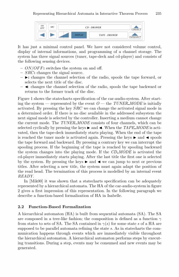
Representing Hierarchical Automata in Interactive Theorem Provers 235
DISPLAY
SRCONOFF CDEJECT
TAPEEJECTTAPE - DRAWER
CD - DRAWER
It has just a minimal control panel. We have not considered volume control,display of internal informations, and programming of a channel storage. Thesystem has three signal sources (tuner, tape-deck and cd-player) and consists ofthe following sensing devices.
– ON/OFF : switches the system on and off.– SRC: changes the signal source.– �: changes the channel selection of the radio, spools the tape forward, or
selects the next title of the disc.– �: changes the channel selection of the radio, spools the tape backward or
returns to the former track of the disc.
Figure 1 shows the statecharts specification of the car-audio-system. After start-ing the system — represented by the event O — the TUNER MODE is initiallyactivated. By pressing the key SRC we can change the activated signal mode ina determined order. If there is no disc available in the addressed subsystem thenext signal mode is selected by the controller. Inserting a medium cannot changethe current mode. The TUNER MODE consists of four channels, which can beselected cyclically by pressing the keys � and �. When the TAPE MODE is acti-vated, then the tape-deck immediately starts playing. When the end of the tapeis reached the tuner mode is activated again. Pressing the keys � and � spoolsthe tape forward and backward. By pressing a contrary key we can interrupt thespooling process. If the beginning of the tape is reached by spooling backwardthe system changes into the playing mode. If the CD MODE is activated thecd-player immediately starts playing. After the last title the first one is selectedby the system. By pressing the keys � and � we can jump to next or previoustitles. After selecting a new title, the system must again adapt the position ofthe read head. The termination of this process is modelled by an internal eventREADY.
In [Mik00] it was shown that a statecharts specification can be adequatelyrepresented by a hierarchical automata. The HA of the car-audio-system in figure2 gives a first impression of this representation. In the following paragraph wedescribe a function-based formalization of HA in Isabelle.
2.2 Function-Based Formalization
A hierarchical automaton (HA) is built from sequential automata (SA). The SAare composed in a tree-like fashion; the composition is defined as a function γfrom states to sets of SA. The SA contained in γ(s) for some state s of a HA aresupposed to be parallel automata refining the state s. As in statecharts the com-munication happens through events which are immediately visible throughoutthe hierarchical automaton. A hierarchical automaton performs steps by execut-ing transitions. During a step, events may be consumed and new events may begenerated.
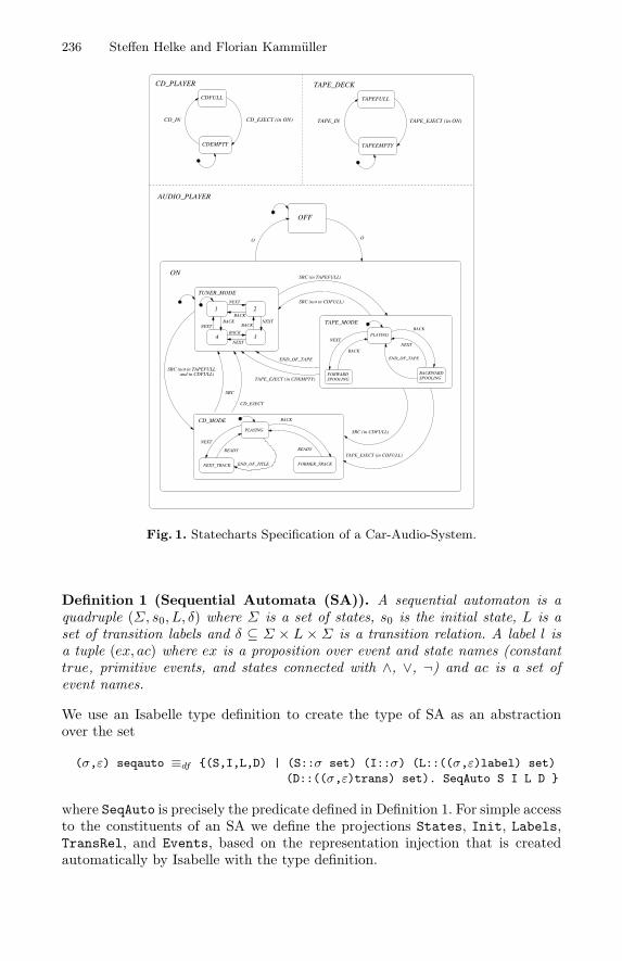
236 Steffen Helke and Florian Kammuller
BACKWARDSPOOLING
FORWARDSPOOLING
PLAYING
PLAYING
NEXT_TRACK FORMER_TRACK
SRC (not in CDFULL)
SRC (in TAPEFULL)
TAPE_EJECT (in CDEMPTY)
END_OF_TAPE
SRC (in CDFULL)
TAPE_EJECT (in CDFULL)
SRC (not in TAPEFULL and in CDFULL)
CD_EJECT
SRC
OO
CD_PLAYER TAPE_DECK
ON
OFF
1 2
4 3BACK
BACKBACK
NEXT
NEXT
NEXT
NEXT
END_OF_TAPE
READY
END_OF_TITLE
READY
BACK
BACK
NEXTNEXT
BACK
NEXT
BACK
TUNER_MODE
TAPE_MODE
CD_MODE
TAPEFULL
TAPEEMPTY
TAPE_IN TAPE_EJECT (in ON)
CDEMPTY
CD_IN
CDFULL
CD_EJECT (in ON)
AUDIO_PLAYER
Fig. 1. Statecharts Specification of a Car-Audio-System.
Definition 1 (Sequential Automata (SA)). A sequential automaton is aquadruple (Σ, s0, L, δ) where Σ is a set of states, s0 is the initial state, L is aset of transition labels and δ ⊆ Σ × L × Σ is a transition relation. A label l isa tuple (ex, ac) where ex is a proposition over event and state names (constanttrue, primitive events, and states connected with ∧, ∨, ¬) and ac is a set ofevent names.
We use an Isabelle type definition to create the type of SA as an abstractionover the set
(σ,ε) seqauto ≡df {(S,I,L,D) | (S::σ set) (I::σ) (L::((σ,ε)label) set)
(D::((σ,ε)trans) set). SeqAuto S I L D }
where SeqAuto is precisely the predicate defined in Definition 1. For simple accessto the constituents of an SA we define the projections States, Init, Labels,TransRel, and Events, based on the representation injection that is createdautomatically by Isabelle with the type definition.
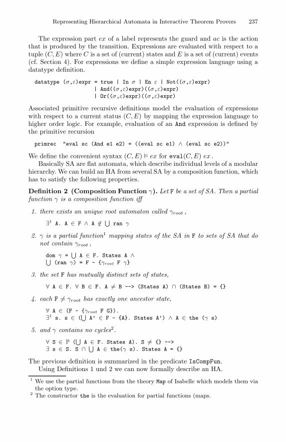
Representing Hierarchical Automata in Interactive Theorem Provers 237
The expression part ex of a label represents the guard and ac is the actionthat is produced by the transition. Expressions are evaluated with respect to atuple (C,E) where C is a set of (current) states and E is a set of (current) events(cf. Section 4). For expressions we define a simple expression language using adatatype definition.
datatype (σ,ε)expr = true | In σ | En ε | Not((σ,ε)expr)| And((σ,ε)expr)((σ,ε)expr)| Or((σ,ε)expr)((σ,ε)expr)
Associated primitive recursive definitions model the evaluation of expressionswith respect to a current status (C,E) by mapping the expression language tohigher order logic. For example, evaluation of an And expression is defined bythe primitive recursion
primrec "eval sc (And e1 e2) = ((eval sc e1) ∧ (eval sc e2))"
We define the convenient syntax (C,E) � ex for eval(C,E) ex .Basically SA are flat automata, which describe individual levels of a modular
hierarchy. We can build an HA from several SA by a composition function, whichhas to satisfy the following properties.
Definition 2 (Composition Function γ). Let F be a set of SA. Then a partialfunction γ is a composition function iff
1. there exists an unique root automaton called γroot ,
∃1 A. A ∈ F ∧ A /∈ ⋃ran γ
2. γ is a partial function1 mapping states of the SA in F to sets of SA that donot contain γroot ,
dom γ =⋃
A ∈ F. States A ∧⋃(ran γ) = F - {γroot F γ}
3. the set F has mutually distinct sets of states,
∀ A ∈ F. ∀ B ∈ F. A �= B --> (States A) ∩ (States B) = {}
4. each F �= γroot has exactly one ancestor state,
∀ A ∈ (F - {γroot F G}).
∃1 s. s ∈ (⋃
A’ ∈ F - {A}. States A’) ∧ A ∈ the (γ s)
5. and γ contains no cycles2.
∀ S ∈ P (⋃
A ∈ F. States A). S �= {} -->
∃ s ∈ S. S ∩ ⋃A ∈ the(γ s). States A = {}
The previous definition is summarized in the predicate IsCompFun.Using Definitions 1 und 2 we can now formally describe an HA.
1 We use the partial functions from the theory Map of Isabelle which models them viathe option type.
2 The constructor the is the evaluation for partial functions (maps).
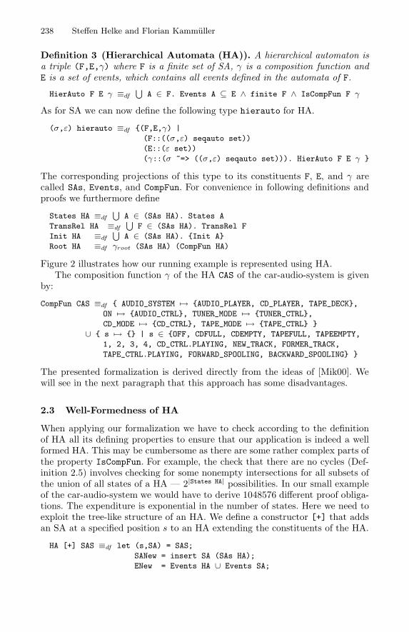
238 Steffen Helke and Florian Kammuller
Definition 3 (Hierarchical Automata (HA)). A hierarchical automaton isa triple (F,E,γ) where F is a finite set of SA, γ is a composition function andE is a set of events, which contains all events defined in the automata of F.
HierAuto F E γ ≡df
⋃A ∈ F. Events A ⊆ E ∧ finite F ∧ IsCompFun F γ
As for SA we can now define the following type hierauto for HA.
(σ,ε) hierauto ≡df {(F,E,γ) |
(F::((σ,ε) seqauto set))
(E::(ε set))
(γ::(σ ~=> ((σ,ε) seqauto set))). HierAuto F E γ }
The corresponding projections of this type to its constituents F, E, and γ arecalled SAs, Events, and CompFun. For convenience in following definitions andproofs we furthermore define
States HA ≡df
⋃A ∈ (SAs HA). States A
TransRel HA ≡df
⋃F ∈ (SAs HA). TransRel F
Init HA ≡df
⋃A ∈ (SAs HA). {Init A}
Root HA ≡df γroot (SAs HA) (CompFun HA)
Figure 2 illustrates how our running example is represented using HA.The composition function γ of the HA CAS of the car-audio-system is given
by:
CompFun CAS ≡df { AUDIO_SYSTEM → {AUDIO_PLAYER, CD_PLAYER, TAPE_DECK},
ON → {AUDIO_CTRL}, TUNER_MODE → {TUNER_CTRL},
CD_MODE → {CD_CTRL}, TAPE_MODE → {TAPE_CTRL} }
∪ { s → {} | s ∈ {OFF, CDFULL, CDEMPTY, TAPEFULL, TAPEEMPTY,
1, 2, 3, 4, CD_CTRL.PLAYING, NEW_TRACK, FORMER_TRACK,
TAPE_CTRL.PLAYING, FORWARD_SPOOLING, BACKWARD_SPOOLING} }
The presented formalization is derived directly from the ideas of [Mik00]. Wewill see in the next paragraph that this approach has some disadvantages.
2.3 Well-Formedness of HA
When applying our formalization we have to check according to the definitionof HA all its defining properties to ensure that our application is indeed a wellformed HA. This may be cumbersome as there are some rather complex parts ofthe property IsCompFun. For example, the check that there are no cycles (Def-inition 2.5) involves checking for some nonempty intersections for all subsets ofthe union of all states of a HA — 2|States HA| possibilities. In our small exampleof the car-audio-system we would have to derive 1048576 different proof obliga-tions. The expenditure is exponential in the number of states. Here we need toexploit the tree-like structure of an HA. We define a constructor [+] that addsan SA at a specified position s to an HA extending the constituents of the HA.
HA [+] SAS ≡df let (s,SA) = SAS;
SANew = insert SA (SAs HA);
ENew = Events HA ∪ Events SA;
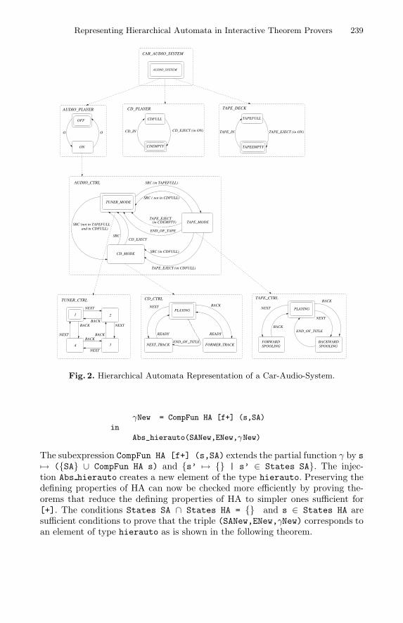
Representing Hierarchical Automata in Interactive Theorem Provers 239
(in CDEMPTY)TAPE_EJECT
and in CDFULL)SRC (not in TAPEFULL
AUDIO_SYSTEM
CD_PLAYER
CAR_AUDIO_SYSTEM
TAPE_DECK
TUNER_CTRL CD_CTRL TAPE_CTRL
OFF
ON
OO CD_IN
CDFULL
CD_EJECT (in ON) TAPE_EJECT (in ON)
TAPEFULL
TAPEEMPTY
TAPE_IN
END_OF_TAPE
SRC ( not in CDFULL)
SRC (in TAPEFULL)
CD_EJECTSRC
TAPE_EJECT (in CDFULL)
SRC (in CDFULL)
1
34
NEXT
BACKBACK
BACKBACK
NEXT
NEXT
NEXT
NEXT_TRACK FORMER_TRACK
PLAYING
END_OF_TITLE
READY READYEND_OF_TITLE
BACKWARDSPOOLING
FORWARDSPOOLING
PLAYINGNEXT BACK
BACK
NEXT
BACK
NEXT2
TUNER_MODE
TAPE_MODE
CD_MODE
CDEMPTY
AUDIO_PLAYER
AUDIO_CTRL
Fig. 2. Hierarchical Automata Representation of a Car-Audio-System.
γNew = CompFun HA [f+] (s,SA)
in
Abs_hierauto(SANew,ENew,γNew)
The subexpression CompFun HA [f+] (s,SA) extends the partial function γ by s�→ ({SA} ∪ CompFun HA s) and {s’ �→ {} | s’ ∈ States SA}. The injec-tion Abs hierauto creates a new element of the type hierauto. Preserving thedefining properties of HA can now be checked more efficiently by proving the-orems that reduce the defining properties of HA to simpler ones sufficient for[+]. The conditions States SA ∩ States HA = {} and s ∈ States HA aresufficient conditions to prove that the triple (SANew,ENew,γNew) corresponds toan element of type hierauto as is shown in the following theorem.
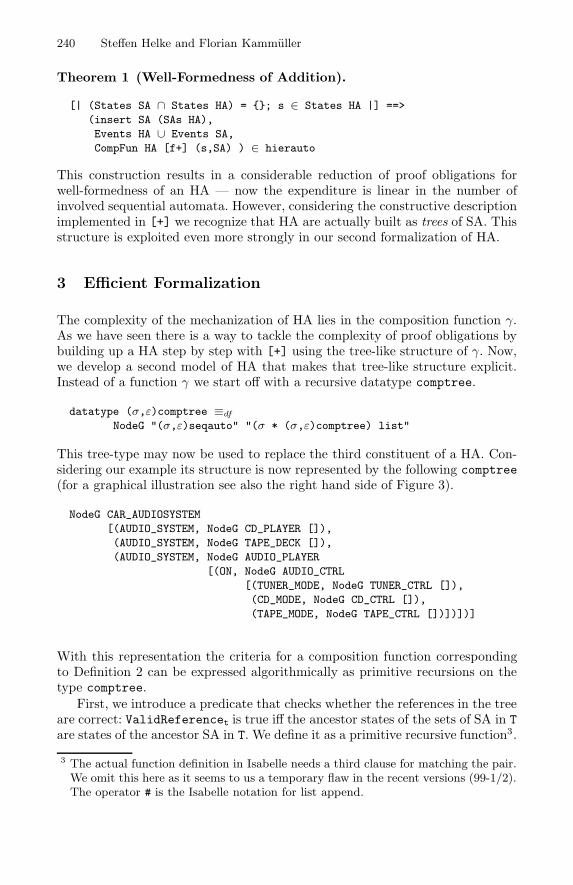
240 Steffen Helke and Florian Kammuller
Theorem 1 (Well-Formedness of Addition).
[| (States SA ∩ States HA) = {}; s ∈ States HA |] ==>
(insert SA (SAs HA),
Events HA ∪ Events SA,
CompFun HA [f+] (s,SA) ) ∈ hierauto
This construction results in a considerable reduction of proof obligations forwell-formedness of an HA — now the expenditure is linear in the number ofinvolved sequential automata. However, considering the constructive descriptionimplemented in [+] we recognize that HA are actually built as trees of SA. Thisstructure is exploited even more strongly in our second formalization of HA.
3 Efficient Formalization
The complexity of the mechanization of HA lies in the composition function γ.As we have seen there is a way to tackle the complexity of proof obligations bybuilding up a HA step by step with [+] using the tree-like structure of γ. Now,we develop a second model of HA that makes that tree-like structure explicit.Instead of a function γ we start off with a recursive datatype comptree.
datatype (σ,ε)comptree ≡df
NodeG "(σ,ε)seqauto" "(σ * (σ,ε)comptree) list"
This tree-type may now be used to replace the third constituent of a HA. Con-sidering our example its structure is now represented by the following comptree(for a graphical illustration see also the right hand side of Figure 3).
NodeG CAR_AUDIOSYSTEM
[(AUDIO_SYSTEM, NodeG CD_PLAYER []),
(AUDIO_SYSTEM, NodeG TAPE_DECK []),
(AUDIO_SYSTEM, NodeG AUDIO_PLAYER
[(ON, NodeG AUDIO_CTRL
[(TUNER_MODE, NodeG TUNER_CTRL []),
(CD_MODE, NodeG CD_CTRL []),
(TAPE_MODE, NodeG TAPE_CTRL [])])])]
With this representation the criteria for a composition function correspondingto Definition 2 can be expressed algorithmically as primitive recursions on thetype comptree.
First, we introduce a predicate that checks whether the references in the treeare correct: ValidReferencet is true iff the ancestor states of the sets of SA in Tare states of the ancestor SA in T. We define it as a primitive recursive function3.
3 The actual function definition in Isabelle needs a third clause for matching the pair.We omit this here as it seems to us a temporary flaw in the recent versions (99-1/2).The operator # is the Isabelle notation for list append.
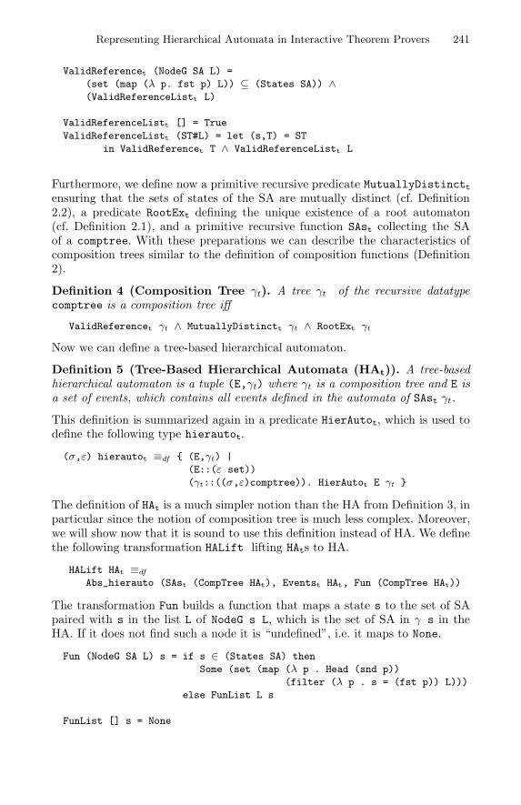
Representing Hierarchical Automata in Interactive Theorem Provers 241
ValidReferencet (NodeG SA L) =
(set (map (λ p. fst p) L)) ⊆ (States SA)) ∧(ValidReferenceListt L)
ValidReferenceListt [] = True
ValidReferenceListt (ST#L) = let (s,T) = ST
in ValidReferencet T ∧ ValidReferenceListt L
Furthermore, we define now a primitive recursive predicate MutuallyDistincttensuring that the sets of states of the SA are mutually distinct (cf. Definition2.2), a predicate RootExt defining the unique existence of a root automaton(cf. Definition 2.1), and a primitive recursive function SAst collecting the SAof a comptree. With these preparations we can describe the characteristics ofcomposition trees similar to the definition of composition functions (Definition2).
Definition 4 (Composition Tree γt). A tree γt of the recursive datatypecomptree is a composition tree iff
ValidReferencet γt ∧ MutuallyDistinctt γt ∧ RootExt γt
Now we can define a tree-based hierarchical automaton.
Definition 5 (Tree-Based Hierarchical Automata (HAt)). A tree-basedhierarchical automaton is a tuple (E,γt) where γt is a composition tree and E isa set of events, which contains all events defined in the automata of SAst γt.
This definition is summarized again in a predicate HierAutot, which is used todefine the following type hierautot.
(σ,ε) hierautot ≡df { (E,γt) |
(E::(ε set))
(γt::((σ,ε)comptree)). HierAutot E γt }
The definition of HAt is a much simpler notion than the HA from Definition 3, inparticular since the notion of composition tree is much less complex. Moreover,we will show now that it is sound to use this definition instead of HA. We definethe following transformation HALift lifting HAts to HA.
HALift HAt ≡df
Abs_hierauto (SAst (CompTree HAt), Eventst HAt, Fun (CompTree HAt))
The transformation Fun builds a function that maps a state s to the set of SApaired with s in the list L of NodeG s L, which is the set of SA in γ s in theHA. If it does not find such a node it is “undefined”, i.e. it maps to None.
Fun (NodeG SA L) s = if s ∈ (States SA) then
Some (set (map (λ p . Head (snd p))
(filter (λ p . s = (fst p)) L)))
else FunList L s
FunList [] s = None
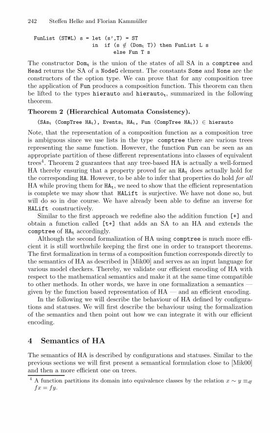
242 Steffen Helke and Florian Kammuller
FunList (ST#L) s = let (s’,T) = ST
in if (s /∈ (Domt T)) then FunList L s
else Fun T s
The constructor Domt is the union of the states of all SA in a comptree andHead returns the SA of a NodeG element. The constants Some and None are theconstructors of the option type. We can prove that for any composition treethe application of Fun produces a composition function. This theorem can thenbe lifted to the types hierauto and hierautot, summarized in the followingtheorem.
Theorem 2 (Hierarchical Automata Consistency).
(SAst (CompTree HAt), Eventst HAt, Fun (CompTree HAt)) ∈ hierauto
Note, that the representation of a composition function as a composition treeis ambiguous: since we use lists in the type comptree there are various treesrepresenting the same function. However, the function Fun can be seen as anappropriate partition of these different representations into classes of equivalenttrees4. Theorem 2 guarantees that any tree-based HA is actually a well-formedHA thereby ensuring that a property proved for an HAt does actually hold forthe corresponding HA. However, to be able to infer that properties do hold for allHA while proving them for HAt, we need to show that the efficient representationis complete: we may show that HALift is surjective. We have not done so, butwill do so in due course. We have already been able to define an inverse forHALift constructively.
Similar to the first approach we redefine also the addition function [+] andobtain a function called [t+] that adds an SA to an HA and extends thecomptree of HAt accordingly.
Although the second formalization of HA using comptree is much more effi-cient it is still worthwhile keeping the first one in order to transport theorems.The first formalization in terms of a composition function corresponds directly tothe semantics of HA as described in [Mik00] and serves as an input language forvarious model checkers. Thereby, we validate our efficient encoding of HA withrespect to the mathematical semantics and make it at the same time compatibleto other methods. In other words, we have in one formalization a semantics —given by the function based representation of HA — and an efficient encoding.
In the following we will describe the behaviour of HA defined by configura-tions and statuses. We will first describe the behaviour using the formalizationof the semantics and then point out how we can integrate it with our efficientencoding.
4 Semantics of HA
The semantics of HA is described by configurations and statuses. Similar to theprevious sections we will first present a semantical formulation close to [Mik00]and then a more efficient one on trees.4 A function partitions its domain into equivalence classes by the relation x ∼ y ≡df
fx = fy.
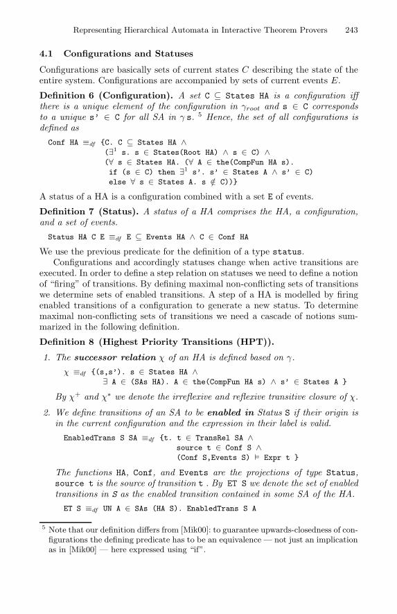
Representing Hierarchical Automata in Interactive Theorem Provers 243
4.1 Configurations and Statuses
Configurations are basically sets of current states C describing the state of theentire system. Configurations are accompanied by sets of current events E.
Definition 6 (Configuration). A set C ⊆ States HA is a configuration iffthere is a unique element of the configuration in γroot and s ∈ C correspondsto a unique s’ ∈ C for all SA in γ s. 5 Hence, the set of all configurations isdefined as
Conf HA ≡df {C. C ⊆ States HA ∧(∃1 s. s ∈ States(Root HA) ∧ s ∈ C) ∧(∀ s ∈ States HA. (∀ A ∈ the(CompFun HA s).
if (s ∈ C) then ∃1 s’. s’ ∈ States A ∧ s’ ∈ C)
else ∀ s ∈ States A. s /∈ C))}
A status of a HA is a configuration combined with a set E of events.
Definition 7 (Status). A status of a HA comprises the HA, a configuration,and a set of events.
Status HA C E ≡df E ⊆ Events HA ∧ C ∈ Conf HA
We use the previous predicate for the definition of a type status.Configurations and accordingly statuses change when active transitions are
executed. In order to define a step relation on statuses we need to define a notionof “firing” of transitions. By defining maximal non-conflicting sets of transitionswe determine sets of enabled transitions. A step of a HA is modelled by firingenabled transitions of a configuration to generate a new status. To determinemaximal non-conflicting sets of transitions we need a cascade of notions sum-marized in the following definition.
Definition 8 (Highest Priority Transitions (HPT)).
1. The successor relation χ of an HA is defined based on γ.
χ ≡df {(s,s’). s ∈ States HA ∧∃ A ∈ (SAs HA). A ∈ the(CompFun HA s) ∧ s’ ∈ States A }
By χ+ and χ∗ we denote the irreflexive and reflexive transitive closure of χ.
2. We define transitions of an SA to be enabled in Status S if their origin isin the current configuration and the expression in their label is valid.
EnabledTrans S SA ≡df {t. t ∈ TransRel SA ∧source t ∈ Conf S ∧(Conf S,Events S) � Expr t }
The functions HA, Conf, and Events are the projections of type Status,source t is the source of transition t . By ET S we denote the set of enabledtransitions in S as the enabled transition contained in some SA of the HA.
ET S ≡df UN A ∈ SAs (HA S). EnabledTrans S A
5 Note that our definition differs from [Mik00]: to guarantee upwards-closedness of con-figurations the defining predicate has to be an equivalence — not just an implicationas in [Mik00] — here expressed using “if”.
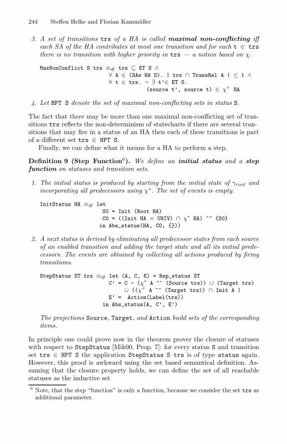
244 Steffen Helke and Florian Kammuller
3. A set of transitions trs of a HA is called maximal non-conflicting iffeach SA of the HA contributes at most one transition and for each t ∈ trsthere is no transition with higher priority in trs — a notion based on χ.
MaxNonConflict S trs ≡df trs ⊆ ET S ∧∀ A ∈ (SAs HA S). | trs ∩ TransRel A | ≤ 1 ∧∀ t ∈ trs. ¬ ∃ t’∈ ET S.
(source t’, source t) ∈ χ+ HA
4. Let HPT S denote the set of maximal non-conflicting sets in status S.
The fact that there may be more than one maximal non-conflicting set of tran-sitions trs reflects the non-determinism of statecharts: if there are several tran-sitions that may fire in a status of an HA then each of these transitions is partof a different set trs ∈ HPT S.
Finally, we can define what it means for a HA to perform a step.
Definition 9 (Step Function6). We define an initial status and a stepfunction on statuses and transition sets.
1. The initial status is produced by starting from the initial state of γroot andincorporating all predecessors using χ∗. The set of events is empty.
InitStatus HA ≡df let
S0 = Init (Root HA)
C0 = ((Init HA × UNIV) ∩ χ∗ HA) ^^ {S0}
in Abs_status(HA, C0, {}))
2. A next status is derived by eliminating all predecessor states from each sourceof an enabled transition and adding the target state and all its initial prede-cessors. The events are obtained by collecting all actions produced by firingtransitions.
StepStatus ST trs ≡df let (A, C, E) = Rep_status ST
C’ = C - (χ∗ A ^^ (Source trs)) ∪ (Target trs)
∪ ((χ+ A ^^ (Target trs)) ∩ Init A )
E’ = Action(Label(trs))
in Abs_status(A, C’, E’)
The projections Source, Target, and Action build sets of the correspondingitems.
In principle one could prove now in the theorem prover the closure of statuseswith respect to StepStatus [Mik00, Prop. 7]: for every status S and transitionset trs ∈ HPT S the application StepStatus S trs is of type status again.However, this proof is awkward using the set based semantical definition. As-suming that the closure property holds, we can define the set of all reachablestatuses as the inductive set6 Note, that the step “function” is only a function, because we consider the set trs asadditional parameter.
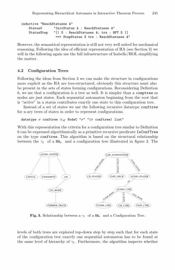
Representing Hierarchical Automata in Interactive Theorem Provers 245
inductive "ReachStatuses A"
Status0 "InitStatus A : ReachStatuses A"
StatusStep "[| S : ReachStatuses A; trs : HPT S |]
==> StepStatus S trs : ReachStatuses A"
However, the semantical representation is still not very well suited for mechanicalreasoning. Following the idea of efficient representation of HA (see Section 3) wewill in the following again use the full infrastructure of Isabelle/HOL simplifyingthe matter.
4.2 Configuration Trees
Following the ideas from Section 3 we can make the structure in configurationsmore explicit: as the HA are tree-structured, obviously this structure must alsobe present in the sets of states forming configurations. Reconsidering Definition6, we see that a configuration is a tree as well. It is simpler than a comptree asnodes are just states. Each sequential automaton beginning from the root thatis “active” in a status contributes exactly one state to this configuration tree.
Instead of a set of states we use the following recursive datatype conftreefor n-ary trees of states in order to represent configurations.
datatype σ conftree ≡df NodeC "σ" "(σ conftree) list"
With this representation the criteria for a configuration tree similar to Definition6 can be expressed algorithmically as a primitive recursive predicate IsConfTreeon the type conftree. This algorithm is based on the structural relationshipbetween the γt of a HAt and a configuration tree illustrated in figure 3. The
AUDIO_SYSTEM CAR_AUDIOSYSTEM
TAPE_DECK AUDIO_PLAYERCD_PLAYERTAPEEMPTY
AUDIO_CTRL
CD_CTRLTUNER_CTRL TAPE_CTRL
ONCDFULL
CD_MODE
FORMER_TRACK
AU
DIO
_SYST
EMAU
DIO
_SYS
TEM AU
DIO
_SYSTEM
ON
TAPE_MODETUNER_MODE CD
_MO
DE
Fig. 3. Relationship between a γt of a HAt and a Configuration Tree.
levels of both trees are explored top-down step by step such that for each stateof the configuration tree exactly one sequential automaton has to be found atthe same level of hierarchy of γt . Furthermore, the algorithm inspects whether
246 Steffen Helke and Florian Kammuller
the successor relation for states in the configuration tree respects the successorrelation for automata in γt . Based on the introduced configuration trees weobtain now an alternative definition for statuses (cf. Definition 7).
Definition 10 (Tree-Based Status). A status of a HAt comprises the HAt, aconfiguration tree, and a set of events.
Statust HAt Ct E ≡df E ⊆ Eventst HAt ∧ IsConfTree (CompTree HAt) Ct
We use this predicate to define a type statust. Similar to the described proce-dure in Section 3, a tree-based status can be transformed into a “flat” status, i.e.the previously defined status with configurations as sets with no information onhierarchical structure. The definition of the semantical relationship between thetwo status types is on the one hand relevant for the validation of our encoding,on the other hand it is helpful for defining constitutive theories, as for examplefor classical temporal logics, which are usually defined on flat models. One canprove the following proof obligation similarly to Theorem 2 where the functionSet maps a configuration tree to a flat set of states.
Theorem 3 (Status Consistency).
(HALift (HAt St), Eventst St, Set (Conft St)) ∈ status
In order to obtain a notion of “firing” of transitions for tree-based statuses wehave defined a predicate MaxNonConflictt algorithmically by primitive recur-sions on the type conftree. Based on this predicate we have derived the tran-sition set HPTt, which reflects the non-determinism of “tree-based” statecharts.Definition 9 can be expressed by primitive recursions on the type conftree aswell. However, these recursive functions are quite technical and will not be pre-sented fully in this paper. To give at least an impression of these definitions wepresent the function InitConft here. It is used to calculate the initial configu-ration tree for a given γt.
InitConft (NodeG SA L) = NodeC (Init SA) (InitConfListt L (Init SA))
InitConfListt [] s = []
InitConfListt (ST#L) s = let (s’,T) = ST
in if (s = s’) then
(InitConft T)#(InitConfListt L s)
else InitConfListt L s
Starting with the initial state of the root automaton we can determine the initialconfiguration tree constructively by gradual investigation of γt . The definitionof StepConft — omitted here — is based on a similar recursive procedure calcu-lating a new configuration tree for a given set of transitions trs. This algorithmdetermines first all subtrees of the current configuration tree, in which root statescoincide with source states of individual transitions from trs. Afterwards thesesubtrees are replaced by initial configuration trees, which are derived from thetarget states of the transitions. Finally we obtain an inductive definition of setsfor reachable statuses, which are derived directly from a HAt. The correspondingclosure theorem (cf. Section 4.1) can now be proved much more efficiently.
Representing Hierarchical Automata in Interactive Theorem Provers 247
In general we believe that this efficient representation of the semantics of stat-echarts — in addition to their efficient structural representation — is a furtherimportant ingredient in order to derive theorems for compositional reasoningeffectively.
5 Conclusion
We have formalized a hierarchical semantics of statecharts in Isabelle/HOL. Asa first step we followed the mathematical description as it is given in [Mik00].
The logic proved to be strong enough to capture all the structural conceptsand enabled the formulation of the dynamic behaviour of these automata ex-pressed as configurations. It was feasible to encode the simple expression lan-guage of a guard language. Here, mightier languages may be plugged in later.As usual the process of formalization revealed some minor inconsistencies in theoriginal definitions.
However, as became apparent during the process of formalizing the tree-structured hierarchical automata we could employ much more powerful construc-tion mechanisms of HOL: datatypes and primitive recursion. Since Isabelle/HOLis a mature proof environment we were able to deviate from the classical way ofencoding an object language using merely the basic mathematical toolset of sets,relations, and closures. The obvious representation of the composition functionas a recursive tree is an intuitive, efficient, and — since it is based on the rigorousconstruction methods of HOL — a sound formalization of HA.
Nevertheless, to validate our efficient encoding of tree-based hierarchical au-tomata as the type hierautot, we preserved the set-based formalization andmapped the HAt to this mathematical semantics. This shows the well-formednessof elements of HAt. Rather than just being an academic challenge this has theeffect that we may now use the set-based semantics to interface our formaliza-tion to model checkers as this semantics was defined for that purpose. Althoughnot yet fully accomplished it is clear that we will be able to prove surjectivity ofthe translation function HALift . If we show in addition that HALift respectsthe step function we will be able to lift general proof obligation for HA to ourefficient representation and solve them there.
In comparison to other formalizations of statecharts (e.g. [DJ93]) the ap-proach we have chosen has some advantages. Since it is structured it is verynatural to decompose automata — as has already been illustrated in this pa-per. Furthermore, the modular fashion of the automata promises to supportdecomposition of properties along with the automata — a feature particularlyrelevant for reducing properties to make them accessible to model checking. An-other advantage of our formalization is that through the explicit modelling ofhierarchy we can express multi-level transitions (cf. [Mik00]). Also, we have al-ready developed — though not yet integrated in the formalization — ideas toexpress history connectors. This is particularly simple in our formalization as itformalizes configurations as trees and those can be stored as histories even overmultiple layers.
248 Steffen Helke and Florian Kammuller
It is an interesting experience to discover that paradigms of programming,i.e. datatypes and recursive function, do actually apply to mathematics, i.e. se-mantics, and cause a considerable simplification of representation and proof.
Acknowledgements
We would like to thank Andre Nordwig for providing us with the car-audio-system example, Thomas Santen for very valuable discussions, and the anony-mous referees for their suggestions.
References
[BKS01] J. Burghardt, F. Kammuller, J. Sanders. On the Antisymmetry of GaloisEmbeddings. Information Processing Letters, 79:2, Elsevier, June 2001.
[CC77] P. Cousot and R. Cousot. Abstract Interpretation. In Principles of Program-ming Languages, ACM Press, 1977.
[CGP99] Edmund M. Clarke, Orna Grumberg, and Doron A. Peled. Model Checking.The MIT Press, Cambridge, Massachusetts, 1999.
[DJ93] Nancy Day and Jeffrey Joyce. The Semantics of Statecharts in HOL. InInternational Meeting on Higher-Order Logic Theorem Proving and its Ap-plications. Springer LNCS, 780:338-351, 1993.
[HN96] D. Harel and D. Naamad. A STATEMATE semantics for statecharts. ACMTrans. on Software Engineering and Methodology, 5(4):293–333, Oct 1996.
[KH00] F. Kammuller and S. Helke. Mechanical Analysis of UML State Machines andClass Diagrams. In Defining Precise Semantics for UML, Sophia Antipolis,France, June 2000. Satellite Workshop, ECOOP 2000.
[Mik00] E. Mikk. Semantics and Verification of Statecharts. PhD thesis, Christian-Albrechts-Universitat, Kiel. Bericht Nr. 2001, October 2000.
[MN95] Olaf Muller and Tobias Nipkow. Combining Model Checking and Deductionfor I/O Automata. In TACAS’95, Tools and Algorithms for the Constructionand Analysis of Systems, Springer LNCS, 1019:1–16, 1995.
[NS95] T. Nipkow and K. Slind. I/O Automata in Isabelle/HOL. In Types for Proofsand Programs, Springer LNCS, 996:101–119, 1995.
[Pau94] L. C. Paulson. Isabelle: A Generic Theorem Prover, Springer LNCS, 828,1994.
[SS99] Hassen Saıdi and Natarajan Shankar. Abstract and Model Check While YouProve. In N. Halbwachs and D. Peled, editors, 11th International Conferenceon Computer Aided Verification, CAV’99, Springer LNCS, 1633, 1999.
[vdB94] M. von der Beeck. A Comparison of Statechart Variants. In Formal Tech-niques in Real-Time and Fault-Tolerant Systems. Springer LNCS, 863: 128–148, 1994.
Refinement Calculus for Logic Programming in
Isabelle/HOL
David Hemer1, Ian Hayes2, and Paul Strooper2
1 Software Verification Research CentreThe University of Queensland, Australia
[email protected] School of Computer Science and Electrical Engineering
The University of Queensland, Australia
Abstract. This paper describes a deep embedding of a refinement cal-culus for logic programs in Isabelle/HOL. It extends a previous tool withsupport for procedures and recursion. The tool supports refinement incontext, and a number of window-inference tactics that ease the burdenon the user. In this paper, we also discuss the insights gained into thesuitability of different logics for embedding refinement calculii (appli-cable to both declarative and imperative paradigms). In particular, wediscuss the richness of the language, choice between typed and untypedlogics, automated proof support, support for user-defined tactics, andrepresentation of program states.
1 Introduction
In this paper we present a deep embedding of a refinement calculus for logicprograms [8] based on the Isabelle/HOL logic [13,1]; this embedding forms partof the Marvin tool. The refinement calculus includes a wide-spectrum language,a declarative semantics for the language, and a collection of refinement laws. Thewide-spectrum language includes executable constructs such as sequential con-junction, disjunction, existential quantification, procedures and recursion; thelanguage also includes a number of specification constructs, including assump-tions, specifications, parallel conjunction and universal quantification. The se-mantics of the language is described in terms of executions, which are mappingsbetween initial and final states. Refinement laws have been proven in terms of thesemantic framework, including: algebraic properties of the language; monotonic-ity rules; rules for lifting predicate connectives to the command level; rules forintroducing commands; and rules for manipulating specifications and assump-tions. These laws are applied by the user to refine programs to implementablecode. Marvin lets the user write procedures, that can be called within otherprocedures or recursively. When introducing recursive calls, Marvin ensures therecursion terminates by insisting that the arguments to the recursive procedureare strictly decreasing with respect to a well-founded relation.
In embedding the refinement calculus we have two main choices : a shallowor a deep embedding. A shallow embedding avoids explicitly defining a separate
R.J. Boulton and P.B. Jackson (Eds.): TPHOLs 2001, LNCS 2152, pp. 249–264, 2001.c© Springer-Verlag Berlin Heidelberg 2001
250 David Hemer, Ian Hayes, and Paul Strooper
syntax for the language. Rather it embeds the language directly in the host syn-tax and expresses the semantics of the language in terms of this representation.A deep embedding, on the other hand, explicitly represents an abstract syntaxof the language and provides an explicit function to map the syntax to the se-mantics as defined in the host language. Thus it decouples issues of syntacticequality from semantic equality. In this paper we describe a deep embedding ofa refinement calculus.
Marvin supports refinement in context, where information about the programenvironment and local assumptions are automatically passed down to subcom-mands. This context information can then be used in the refinement of thesesubcommands. The approach used in Marvin is similar to program window in-ference, developed by Nickson and Hayes [12]. This approach allows context in-formation to be handled separately from the rest of the command. Marvin alsoincludes several window-inference-like tactics that support step-wise refinementof programs, thereby greatly reducing the number and complexity of individualrefinement steps.
In providing tool support for the refinement calculus we were initially facedwith the question of what logic/proof tool to embed the calculus in. Prototypetools had been developed in several different logics prior to the version describedin this paper. An earlier prototype [5] — based on a different semantic framework[7] — includes a shallow embedding of the calculus in the Ergo 4 theorem prover[19], a prover based on the window-inference paradigm. Two more embeddings(also based on the earlier semantics) were done in Ergo 5 [20] (a generic theoremprover based on sequent calculus) and Isabelle/ZF as part of a comparativestudy [9]. Finally, before settling on the current version, an embedding, basedon the current semantics, was investigated in HOL-Z [11] (an embedding of theZ specification language in Isabelle/HOL).
At first, the choice of logic seemed rather arbitrary, but after experimentingwith the different logics, we found several features of refinement calculi thathave a fundamental effect on the choice of logics. Before choosing a logic, severalquestions need to be answered:
1. Can the constructs that model the syntax and semantics of the wide-spectrumlanguage be easily represented in the logic?
2. Do the semantics include types?3. To what extent does the proof tool automate proof of properties of the
semantics and refinement laws, as well as the proof obligations that ariseduring refinement?
4. Can tactics be implemented to assist the user during the refinement process?5. How readily can program states be represented in the logic?
In this paper, we discuss how the answers to these questions affect the choiceof logic, using the embedding of the logic program refinement calculus as anexample. Section 2 gives details of an embedding of the calculus in Isabelle/HOL.In Section 3 we illustrate the tool by showing the refinement of a simple program.We then show how this appears in the tool for the first couple of steps. InSection 4 we discuss how the questions raised above affect the choice of logic.
Refinement Calculus for Logic Programming in Isabelle/HOL 251
2 Refinement Calculus for Logic Programs inIsabelle/HOL
2.1 Preliminary Definitions
The semantics of our wide-spectrum language are defined in terms of a relation-ship between the initial and final states of a program. A state consists of a setof bindings, where a binding is a function that maps each variable to a value.The type Val represents the values that program variables can take; we wish toassociate these with Isabelle types in some manner. To do this we represent Valas a type sum (using a datatype declaration):
Bnds == Var → Val
State == P Bnds
datatype Val ==
natV nat | listV (nat list) | setV (nat set) | pairV Val Val
The building blocks of our language are terms and predicates. A term isdefined as either a variable or a function application to a list of terms. Thefunctions evallist and eval evaluate a list of terms and a term respectively fora particular binding. Terms are evaluated to an element of Val. Predicates aremodelled using a datatype; they are evaluated, with respect to a binding, by thefunction evalp, a boolean-valued result is returned.
datatype rterm == varT Var | funT (rterm list)
evallist : rterm list × Bnds → Val list
eval : rterm × Bnds → Val
datatype pred == pred ∧ pred | pred ∨ pred | pred ⇒ pred
| pred ⇔ pred | rterm = rterm | rterm < rterm
| ¬ pred | ∃ Var pred | ∀ Var pred | true | false
| isNat Var | isList Var | isSet Var | isPair Var
evalp :: pred × Bnds → bool
2.2 Wide-Spectrum Language
The wide spectrum language includes both logic programming language andspecification constructs. It allows constructs that may not be executable, al-lowing gradual refinement without the need for notational changes during therefinement process. The syntax of the commands in the wide-spectrum languageis defined by the datatype Cmd.
datatype Cmd == 〈 pred 〉 -- specification
| { pred } -- assumption
| Cmd ∧ Cmd -- parallel conjunction
| Cmd ∨ Cmd -- parallel disjunction
| Cmd , Cmd -- sequential conjunction
| ∃ Var • Cmd -- existential quantification
| ∀ Var • Cmd -- universal quantification
| PIdent(rterm) -- procedure call
252 David Hemer, Ian Hayes, and Paul Strooper
A specification 〈P〉 represents a set of instantiations of free variables of P thatsatisfy P . An assumption {A} formally states the context in which a program iscalled. If an assumption does not hold, the program fragment in which it appearsmay abort. Aborting includes program behaviour such as nontermination andabnormal termination due to exceptions like division by zero (the latter beingdistinct from a procedure that fails if the divisor is zero), as well as terminationwith arbitrary results.
Sequential conjunction (S ,T ) evaluates S before T . The parallel conjunction(S ∧ T ) evaluates S and T independently and forms the intersection of theirrespective results on completion. The disjunction of two programs (S ∨ T )computes the union of the results of the two programs. Disjunction is generalisedto an existential quantifier (∃X • S ), which computes the union of the resultsof S for all possible values of X . Similarly, the universal quantifier (∀X • S )computes the intersection of the results of S for all possible values of X . Aprocedure can be called by referring to the procedure identifier and applying itto a term, e.g., pid(T ) applies the procedure named pid to the term T .
Parameterised commands are defined as a separate datatype PCmd consistingof two entries: non-recursive commands and recursive commands.
datatype PCmd == Var :- Cmd | re PIdent • PCmd er
A command can be parameterised over a variable; it has the form v:-S , wherev is a variable and S is a wide-spectrum program. A parameterised command isinstantiated by applying it to a term — the result is a command.
Recursive calls are introduced within a recursion block. A recursion blockhas the form re id • pc er, where id names the block and pc is a parameterisedcommand. Within recursion blocks, recursive calls of the form id(T ) can be used,provided certain termination conditions are met. We associate a well-foundedrelation with the arguments of the recursive call, and prove that the argumentsare strictly decreasing with respect to the relation.
Procedures are defined by associating a procedure identifier, pid , with a pa-rameterised command, e.g., pid = v:-S .
2.3 Execution Semantics
The semantics of the wide-spectrum language is defined in terms of the functionexec, which maps each command to a partial mapping between initial and finalstates (so-called executions). The mapping is partial because programs may notdefined for all initial states.
We begin by defining the type StateMap, representing the set of partialmappings between initial and final states. Partial mappings are defined in Is-abelle/HOL in terms of total functions. The labels Some and None are used todistinguish defined and undefined values. More precisely, for a partial mappingf and element x , if x is in the domain of f then there exists a y such that f(x)
= Some y, otherwise f(x) = None.
StateMap == State �→ State
Refinement Calculus for Logic Programming in Isabelle/HOL 253
We define the type Exec, as a subtype of StateMap, using Isabelle’s typedef
facility. The three conditions in the set comprehension correspond to the threehealthiness conditions for executions [8].
Exec == {e: StateMap | dom(e) = P {b. {b} ∈ dom(e)}∧ ∀ s ∈ dom(e). the e(s) ⊆ s
∧ ∀ s ∈ dom(e). e(s) = Some {b. b ∈ s & (e({b}) = Some {b})}}
These conditions characterise useful properties of our wide-spectrum languagethat allow us to consider the effect of language constructs on a single bindingrather than having to look at the effect on an entire state. The first conditionstates that the domain of an execution is equivalent to those states formed bymerging states consisting of a single binding in the domain of the execution.Effectively the domain of an execution is closed under union and intersection (ofstates in the domain). The second condition states that executions are restrictedto those mappings for which the output state is a subset of the input state. Thethird condition states that for an input state, the output state can be determinedby considering the effect of the execution on each singleton binding in the inputstate, and then forming the union of the results.
The typedef facility defines Exec as a meta-level type, as well as an objectlevel set. In defining a type in Isabelle/HOL, we must exhibit that the set isnon-empty which is easily established by showing that the element {∅ �→ ∅} isin the set.
The definition of Exec illustrates the overhead that is involved in representingpartial functions in Isabelle/HOL. The second line of the definition requires thefunction “the”, used in this case to strip away the label Some associated withe(s). Conversely, in the third line we must include the label Some.
Programs are refined in the context of a program environment, describingany predefined procedures. The type Env is a mapping from procedure identifiersto their corresponding parameterised executions. Parameterised executions aredefined as mappings from terms to executions, and provide the semantics ofparameterised commands. Note that in this case Exec is used as a meta-leveltype.
PExec == rterm → Exec
Env == PIdent �→ PExec
The function exec, used to define the semantics of the wide-spectrum lan-guage, is declared as a function mapping an environment and a command to astate mapping.
exec : Env × Cmd → StateMap
The translation of the exec into Isabelle/HOL was straightforward, with twoexceptions. Firstly, to define exec for sequential conjunction, we needed to definecomposition of partial functions. Secondly, in defining exec for procedure callswe needed to perform a type coercion between the type StateMap (the expectedtype) and the type Exec (the actual type). This was done by introducing a call
254 David Hemer, Ian Hayes, and Paul Strooper
to the auxiliary function Rep Exec (created by the typedef facility), that mapsan abstract type to its representative type.
Having defined the exec function, we prove that for any environment ρ andcommand c, (exec ρ c) is of type Exec, and thus satisfies the three healthinessproperties above. This is proved by structural induction on the command c.Notice in this case we are using Exec as an object level set. Defining types usingIsabelle/HOL’s typedef facility allows this dual usage.
The number of proof steps for this theorem was significantly less than thesame proof in an earlier embedding in HOL-Z. This can be attributed to thefact that the HOL-Z proof involved large amounts of type checking (the types inHOL-Z are modelled as sets at the object level, and therefore do not make useof Isabelle/HOL’s built-in type checker), as well as the fact that the automatedproof tactics were more effective in Isabelle/HOL.
2.4 Refinement
We define the refinement relations� and �� for state mappings (and consequentlyfor executions).
e1 � e2 == dom(e1) ⊆ dom(e2) ∧ (∀ s: dom(e1). e1(s) = e2(s))
e1 �� e2 == (e1 = e2)
The above definition states that an execution can be refined by extending the setof initial states for which it is defined. Next we define the notion of refinementfor commands, including the context in which the commands are refined. Thecontext includes the environment, env, under which the commands are refined.
env ρ � c1 �� c2 == (exec ρ c1) �� (exec ρ c2)
env ρ � c1 � c2 == (exec ρ c1) � (exec ρ c2)
Refinement of a command is defined in terms of its underlying execution. Acommand is refined by extending the set of initial states for which we can asso-ciate a final state, effectively removing undefinedness. “�” is a preorder and “��”is an equivalence relation. These properties are exploited to perform step-wiserefinement.
Refinement laws for the wide-spectrum language have been proven in termsof the underlying execution semantics. When performing program refinement,these refinement laws are used to prove the correctness of individual refinementsteps, rather than apply the definition of refinement directly.
The collection of rules include: algebraic properties for the propositional con-structs; monotonicity rules for the language constructs; rules for lifting predicateconnectives appearing in specifications to corresponding program constructs;rules for introducing and eliminating program constructs; and rules for manip-ulating specifications and assumptions.
Monotonicity. The wide-spectrum language is monotonic with respect to re-finement in that a command can be refined by refining one or more of its sub-commands. Consider, for example the law sand-right-mono given as:
Refinement Calculus for Logic Programming in Isabelle/HOL 255
env ρ � c1 � c2
env ρ � c3 , c1 � c3 , c2
This law states that the command “c3 , c1” can be refined by refining the secondcommand c1.
Predicate Lifting. Predicate lifting laws are used to lift predicate connectivescontained in specifications to their program construct counterparts. For examplethe rule lift-exists lifts an existential quantifier within a specification to acommand-level existential quantifier:
env ρ � 〈∃V • P〉 �� ∃ V • 〈P〉
Note that the existential quantifier symbol ∃ is overloaded in the above law.The first occurence is the predicate quantifier, while the second occurence is thecommand quantifier.
Table 1 gives a comparison of the number of steps required to prove variousrefinement laws in Isabelle/HOL and HOL-Z. The table shows the reduction inproof steps in Isabelle/HOL, which can be attributed to the built-in type checkerand improved automated proof support.
Table 1. Comparison of Proof Steps to Prove Refinement Laws.
Law Isabelle/HOL HOL-Z
lift-exists 4 75por-mono 26 37distribute-pand-over-por 4 8left-distribute-sand-over-por 3 122weaken-assume 5 54
2.5 Assumption Context
We have already seen that commands are refined in the context of a programenvironment ρ. In this section we describe a second kind of context, the so-called assumption context (based on the “pre” context used in the programwindow inference of Nickson and Hayes [12]), assumptions are introduced withthe keyword “assume”. Consider the command “{A} , S”. In refining S and itssubcommands we may use the assumption A. Rather than having to propagatethe assumption throughout S and its subcommands, we add the assumption A
to the context of the refinement. Refinement of commands in the context ofassumptions extends the definition of command refinement given in Section 2.4.
env ρ assume A � c1 � c2 == env ρ � {A} , c1 � {A} , c2
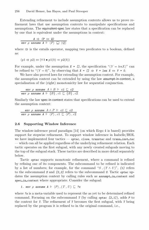
256 David Hemer, Ian Hayes, and Paul Strooper
Extending refinement to include assumption contexts allows us to prove re-finement laws that use assumption contexts to manipulate specifications andassumptions. The equivalent-spec law states that a specification can be replacedby one that is equivalent under the assumptions in context:
A � (P ⇔ Q)
env ρ assume A � 〈P〉 �� 〈Q〉where � is the entails operator, mapping two predicates to a boolean, definedas:
(p1 � p2)⇔ (∀ b • p1(b)⇒ p2(b))
For example, under the assumption X = [], the specification “〈Y = lenX 〉” canbe refined to “〈Y = 0〉”, by observing that X = [] � Y = len X ⇔ Y = 0.
We have also proved laws for extending the assumption context. For example,the assumption context can be extended by using the law assumpt-in-context, aspecialisation of the (right) monotonicity law for sequential conjunction.
env ρ assume A ∧ B � c1 � c2
env ρ assume A � {B} , c1 � {B} , c2
Similarly the law spec-in-context states that specifications can be used to extendthe assumption context:
env ρ assume A ∧ P � c1 � c2
env ρ assume A � 〈P〉 , c1 � 〈P〉 , c2
2.6 Supporting Window Inference
The window-inference proof paradigm [14] (on which Ergo 4 is based) providessupport for stepwise refinement. To support window inference in Isabelle/HOLwe have implemented four tactics — optac, close, transtac and trans inst tac
—which can all be applied regardless of the underlying refinement relation. Eachtactic operates on the first subgoal, with any newly created subgoals moving tothe top of the subgoal stack. These tactics are described in more detail separatelybelow.
Tactic optac supports monotonic refinement, where a command is refinedby refining one of its components. The subcommand to be refined is indicatedby a list of numbers; for example, for the command “S , (T ∧ U )”, [1] refersto the subcommand S and [2,2] refers to the subcommand U. Tactic optac up-dates the assumption context by calling rules such as assumpt in context andspec in context where appropriate. Consider the subgoal:
1. env ρ assume A � 〈P〉 , (T , U ) � ?x
where ?x is a meta-variable used to represent the as yet to be determined refinedcommand. Focusing on the subcommand T (by calling optac [2,1]), adds P tothe context for T. The refinement of T becomes the first subgoal, with T beingreplaced by the program it is refined to in the original command, i.e.,
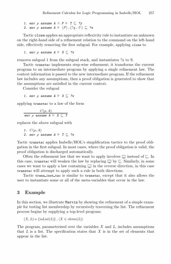
Refinement Calculus for Logic Programming in Isabelle/HOL 257
1. env ρ assume A ∧ P � T � ?y
2. env ρ assume A � 〈P〉 , (?y , U ) � ?x
Tactic close applies an appropriate reflexivity rule to instantiate an unknownon the right-hand side of a refinement relation to the command on the left-handside, effectively removing the first subgoal. For example, applying close to
1. env ρ assume A � S � ?x
removes subgoal 1 from the subgoal stack, and instantiates ?x to S.Tactic transtac implements step-wise refinement; it transforms the current
program to an intermediate program by applying a single refinement law. Thecontext information is passed to the new intermediate program. If the refinementlaw includes any assumptions, then a proof obligation is generated to show thatthe assumptions are satisfied in the current context.
Consider the subgoal
1. env ρ assume A � S � ?x
applying transtac to a law of the form
C (ρ,A)
env ρ assume A � S � T
replaces the above subgoal with
1. C (ρ,A)2. env ρ assume A � T � ?x
Tactic transtac applies Isabelle/HOL’s simplification tactics to the proof obli-gation in the first subgoal. In most cases, where the proof obligation is valid, theproof obligation is discharged automatically.
Often the refinement law that we want to apply involves � instead of �. Inthis case, transtac will weaken the law by replacing � by �. Similarly, in somecases we want to apply a law containing � in the reverse direction, in this casetranstac will attempt to apply such a rule in both directions.
Tactic trans inst tac is similar to transtac, except that it also allows theuser to instantiate some or all of the meta-variables that occur in the law.
3 Example
In this section, we illustrate Marvin by showing the refinement of a simple exam-ple for testing list membership by recursively traversing the list. The refinementprocess begins by supplying a top-level program:
(X ,L) :- {isList(L)} , 〈X ∈ elems(L)〉
The program, parameterised over the variables X and L, includes assumptionsthat L is a list. The specification states that X is in the set of elements thatappear in the list.
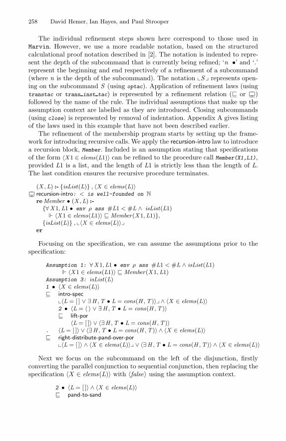
258 David Hemer, Ian Hayes, and Paul Strooper
The individual refinement steps shown here correspond to those used inMarvin. However, we use a more readable notation, based on the structuredcalculational proof notation described in [2]. The notation is indented to repre-sent the depth of the subcommand that is currently being refined; ‘n •’ and ‘.’represent the beginning and end respectively of a refinement of a subcommand(where n is the depth of the subcommand). The notation �S� represents open-ing on the subcommand S (using optac). Application of refinement laws (usingtranstac or trans inst tac) is represented by a refinement relation (� or �)followed by the name of the rule. The individual assumptions that make up theassumption context are labelled as they are introduced. Closing subcommands(using close) is represented by removal of indentation. Appendix A gives listingof the laws used in this example that have not been described earlier.
The refinement of the membership program starts by setting up the frame-work for introducing recursive calls. We apply the recursion-intro law to introducea recursion block, Member. Included is an assumption stating that specificationsof the form 〈X 1 ∈ elems(L1)〉 can be refined to the procedure call Member(X1,L1),provided L1 is a list, and the length of L1 is strictly less than the length of L.The last condition ensures the recursive procedure terminates.
(X ,L) :- {isList(L)} , 〈X ∈ elems(L)〉�� recursion-intro: < is well-founded on N
reMember • (X ,L) :-{∀X 1, L1 • env ρ ass #L1 < #L ∧ isList(L1)
� 〈X 1 ∈ elems(L1)〉 � Member(X 1, L1)},{isList(L)} , �〈X ∈ elems(L)〉�
er
Focusing on the specification, we can assume the assumptions prior to thespecification:
Assumption 1: ∀X 1,L1 • env ρ ass #L1 < #L ∧ isList(L1)� 〈X 1 ∈ elems(L1)〉 � Member(X 1, L1)
Assumption 3: isList(L)1 • 〈X ∈ elems(L)〉� intro-spec
�〈L = [ ] ∨ ∃H ,T • L = cons(H , T )〉� ∧ 〈X ∈ elems(L)〉2 • 〈L = 〈 〉 ∨ ∃H ,T • L = cons(H , T )〉� lift-por
〈L = [ ]〉 ∨ 〈∃H ,T • L = cons(H , T )〉. 〈L = [ ]〉 ∨ 〈∃H ,T • L = cons(H , T )〉 ∧ 〈X ∈ elems(L)〉� right-distribute-pand-over-por
�〈L = [ ]〉 ∧ 〈X ∈ elems(L)〉� ∨ 〈∃H ,T • L = cons(H , T )〉 ∧ 〈X ∈ elems(L)〉
Next we focus on the subcommand on the left of the disjunction, firstlyconverting the parallel conjunction to sequential conjunction, then replacing thespecification 〈X ∈ elems(L)〉 with 〈false〉 using the assumption context.
2 • 〈L = [ ]〉 ∧ 〈X ∈ elems(L)〉� pand-to-sand
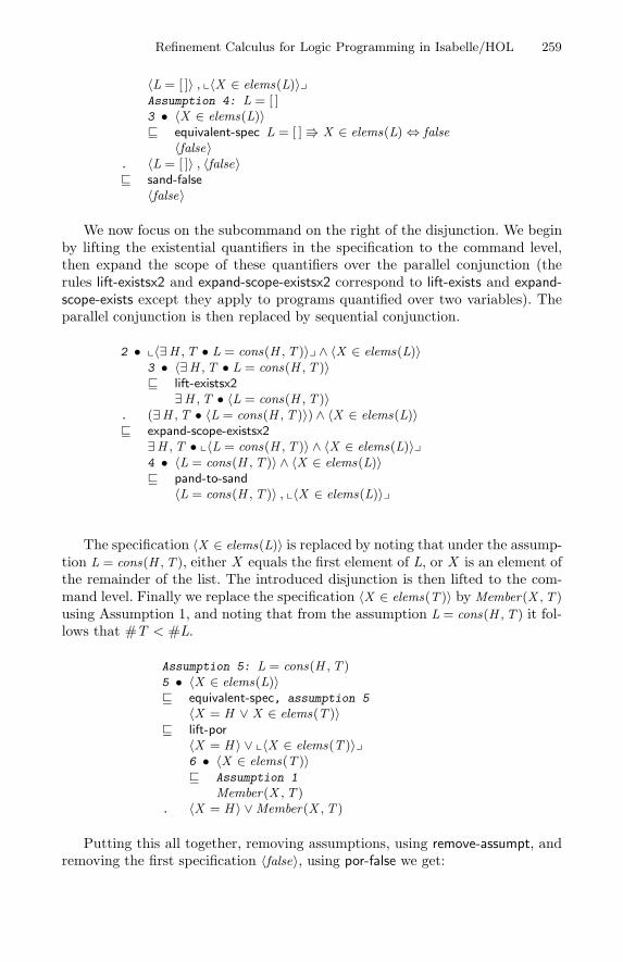
Refinement Calculus for Logic Programming in Isabelle/HOL 259
〈L = [ ]〉 , �〈X ∈ elems(L)〉�Assumption 4: L = [ ]3 • 〈X ∈ elems(L)〉� equivalent-spec L = [ ] � X ∈ elems(L)⇔ false
〈false〉. 〈L = [ ]〉 , 〈false〉� sand-false
〈false〉
We now focus on the subcommand on the right of the disjunction. We beginby lifting the existential quantifiers in the specification to the command level,then expand the scope of these quantifiers over the parallel conjunction (therules lift-existsx2 and expand-scope-existsx2 correspond to lift-exists and expand-scope-exists except they apply to programs quantified over two variables). Theparallel conjunction is then replaced by sequential conjunction.
2 • �〈∃H ,T • L = cons(H , T )〉� ∧ 〈X ∈ elems(L)〉3 • 〈∃H ,T • L = cons(H , T )〉� lift-existsx2
∃H ,T • 〈L = cons(H , T )〉. (∃H ,T • 〈L = cons(H , T )〉) ∧ 〈X ∈ elems(L)〉� expand-scope-existsx2
∃H , T • �〈L = cons(H , T )〉 ∧ 〈X ∈ elems(L)〉�4 • 〈L = cons(H , T )〉 ∧ 〈X ∈ elems(L)〉� pand-to-sand
〈L = cons(H , T )〉 , �〈X ∈ elems(L)〉�
The specification 〈X ∈ elems(L)〉 is replaced by noting that under the assump-tion L = cons(H , T ), either X equals the first element of L, or X is an element ofthe remainder of the list. The introduced disjunction is then lifted to the com-mand level. Finally we replace the specification 〈X ∈ elems(T )〉 by Member(X ,T )
using Assumption 1, and noting that from the assumption L = cons(H , T ) it fol-lows that #T < #L.
Assumption 5: L = cons(H , T )5 • 〈X ∈ elems(L)〉� equivalent-spec, assumption 5
〈X = H ∨ X ∈ elems(T )〉� lift-por
〈X = H 〉 ∨ �〈X ∈ elems(T )〉�6 • 〈X ∈ elems(T )〉� Assumption 1
Member(X , T ). 〈X = H 〉 ∨Member(X , T )
Putting this all together, removing assumptions, using remove-assumpt, andremoving the first specification 〈false〉, using por-false we get:
260 David Hemer, Ian Hayes, and Paul Strooper
reMember • (X ,L) :-(∃H ,T • 〈L = cons(H , T )〉 , (〈X = H 〉 ∨Member(X , T )))
er
The resulting program is now at a sufficiently concrete level to be readilytranslated into code in a language such as Prolog or Mercury.
4 Discussion
There are a number of different embeddings of refinement calculi in theoremprovers [3]. While these embeddings differ in many ways, there are a number offundamental issues for each. In this section we present these issues, comparingthe solutions presented in this paper to solutions presented elsewhere.
4.1 Richness of Language
The first issue relates to the richness of the syntax of the logic. Can the syntaxand semantics of the refinement language be conveniently expressed in the logic?In particular, when the language has already been specified using some formallanguage (such as Z), can this specification be readily translated (by hand orindeed automatically) into the notation used by the logic?
The semantics of our language [8] are formally specified using the Z specifica-tion language [15]; this in turn is based on Zermelo Frankel set theory. Thereforeit was relatively straightforward to translate the semantics into HOL-Z and Is-abelle/ZF notation. However, while the translation to Isabelle/HOL notationrequired a little more effort, we found that in reference to the other issues raisedbelow, the extra effort up front was more than rewarded later on. We concludehere that we need to be wary of selecting a logic primarily because of its richnesswithout considering the other factors. Also note that while in this case ZF andHOL-Z were closer to the specification language than HOL, this is not necessar-ily always the case. For example users of higher-order logics might specify theircalculus using a language that is closer to HOL.
4.2 Typed versus Untyped Logics
The second issue involves the choice of an untyped or typed logic. Embeddingrefinement calculi in logics such as HOL-Z or Isabelle/ZF requires that any typesin the semantics be expressed at the object level (as sets). The result of this isthat large parts of proofs involve discharging type constraints. These same typeconstraints are handled automatically by a built-in type checker in the typedIsabelle/HOL logic.
Isabelle/HOL is a typed logic, meaning that types used in our semantics canbe modelled at the meta-level. Isabelle/HOL employs a built-in type checker thatautomatically checks type constraints, therefore simplifying proofs. New typesare introduced using either type synonyms or type definitions. The type system
Refinement Calculus for Logic Programming in Isabelle/HOL 261
available in Isabelle/HOL is not as rich as those used in the untyped logics (wheretypes are modelled as sets). However it does include the basic types required tomodel our semantics; including natural numbers, lists, sets and functions.
4.3 Automated Proof Support
The third issue relates to the fact that embeddings of refinement calculi in-volve a large amount of proof. An embedding will typically involve establishingsome general properties of the language and proving refinement laws. Automatedproof support to take care of the mundane proof steps is useful here. Howeverit is worth noting that embedding the calculus is a one-off process usually per-formed by somebody with expertise in theorem proving; of more importance isautomatically discharging proof obligations that arise during refinement of pro-grams. The extra importance here is twofold: firstly refinement of programs isan ongoing process, and secondly the user of the tool is not necessarily an expertin theorem proving.
We found that Isabelle/HOL gave us a better level of automation (and con-sequently fewer proof steps) than the other logics, in both setting up and usingthe tool. This is despite the fact that Isabelle/ZF and HOL-Z both employ thesame tactics as Isabelle/HOL. The decreased performance for these two logicscan be partly explained by the fact that the tactics struggled to discharge typeconstraints1. For HOL-Z, we also note that the tactics have been set up forthe HOL logic, but have not been extended to provide support for the HOL-Ztheories.
An earlier report [9] shows that the tactics employed by Ergo 4 and Ergo 5were in turn significantly less effective than those used in Isabelle/ZF.
4.4 User-Defined Tactics
In relation to tactics, we observe that significant reductions in both the numberand complexity of refinement steps can be achieved by using a window-inferenceparadigm. Some theorem provers, most notably Ergo 4 [19], provide native sup-port for window inference. The majority, however, are based on other proofparadigms, in which case it is important to be able to emulate the window-inference paradigm through the use of tactics [6,16]. Only those provers thatoffer user-extensionality, usually in the form of tactics, are suitable in this case.
As we have seen earlier in the paper, it was a straightforward task to definetactics in Isabelle/HOL that emulate the window inference paradigm. Indeedwe were able to write (or adapt) tactics that emulate window inference in all ofthe logics that we have trialed. The approach used here is similar to that usedby [16] in Isabelle/ZF, except we provide better support for context, based onprogram window inference [12].
1 We used an earlier version of Isabelle/ZF. The most recent version includes tacticsfor discharging type constraints and we have not evaluated the effectiveness of thesetactics.
262 David Hemer, Ian Hayes, and Paul Strooper
4.5 Representing Program State
Finally, we need to consider how we can model the state of programs within aparticular logic. More precisely, given that a state associates program variableswith values, we need to consider what range of values can be modelled, i.e., howdo we model the type of values? Earlier embeddings tended to ignore the issueby only allowing the set of natural numbers as values. However, this severelyrestricts the application of the tool.
States are represented in our embedding as sets of bindings, which are in turnmappings from variables to values. The type of values is represented as a sumof Isabelle types (including lists, sets, naturals and pairs). This sum of types isstatic, therefore introducing a new value type can only be done by reworking thesemantics. This would be of no use if we wanted to introduce data abstraction,where users can introduce new value types on the fly.
Von Wright [21] represents states as a tuple of values, with each state com-ponent (program variable) corresponding to a value in the tuple. Each state isassigned a product of types, with one type for each variable. Staples [17] notessome limitations of this approach, in particular the fact that variables are notexplicitly named.
Staples’s [17,18] solution to these problems is to represent states as depen-dently typed functions from variable names to under-specified families of types.This function is dynamically extendible, meaning that arbitrary abstract typesfor local program variables can be introduced during the refinement.
5 Conclusions
Using an embedding of a refinement calculus in a theorem prover leads to greaterassurance that any proof obligations for individual refinement steps have beensatisfied. The more mundane proof obligations can often be discharged automat-ically by the prover. In this paper we presented a deep embedding of a refine-ment calculus for logic programs in the Isabelle/HOL logic, including supportfor parameterised procedures and recursion. The embedding includes support forrefinement in context, based on program window inference [12]. In comparisonto other embeddings of (imperative) refinement calculi [6,18,4,21], the embed-ding presented here makes use of Isabelle/HOL’s datatypes, primitive recursivedefinitions and type definitions to provide a deep embedding.
In developing Marvin, we formulated a number of criteria that are funda-mental in choosing a logic for embedding refinement calculi (or other similarsemantic models [10]). These criteria were gathered by tracing the problems en-countered during the embedding back to deficiencies in the logics. Against thesecriteria, Isabelle/HOL scored well. In particular, we found:
– Isabelle/HOL notation was rich enough to represent our Z specified semanticswith only minimal adaptations required.
– The type system significantly reduced the amount of proof in comparison tothe untyped logics (cf. Table 1).
Refinement Calculus for Logic Programming in Isabelle/HOL 263
– Automated proof support performed better than for the other provers.– Window-inference-like tactics could be easily written using Isabelle’s tactic
language.
One remaining concern is with representing program state. Our solution onlyallows state variables to range over a fixed product of types.
Acknowledgements
We would like to thank Robert Colvin for his comments on earlier drafts of thispaper. The work reported in this paper is supported by Australian ResearchCouncil grant number A49937007 : Refinement Calculus for Logic Programming.
References
1. Isabelle home page.http://www.cl.cam.ac.uk/Research/HVG/Isabelle/index.html.
2. Ralph Back, Jim Grundy, and Joakim von Wright. Structured calculational proof.Formal Aspects of Computing, 9(5–6):469–483, 1997.
3. D. Carrington, I. Hayes, R. Nickson, G. Watson, and J. Welsh. A review of existingrefinement tools. Technical report 94-08, Software Verification Research Centre,The University of Queensland, Brisbane 4072. Australia, June 1994.
4. D. Carrington, I. Hayes, R. Nickson, G. Watson, and J. Welsh. A program refine-ment tool. Formal Aspects of Computing, 10:97–124, 1998.
5. R. Colvin, I. Hayes, R. Nickson, and P. Strooper. A tool for logic program refine-ment. In D. J. Duke and A. S. Evans, editors, Second BCS-FACS Northern FormalMethods Workshop, Electronic Workshops in Computing. Springer Verlag, 1997.
6. J. Grundy. A window inference tool for refinement. In C.B. Jones, R.C. Shaw, andT. Denvir, editors, Fifth Refinement Workshop, Workshops in Computing, pages230–254. BCS FACS, Springer-Verlag, 1992.
7. I. Hayes, R. Nickson, and P. Strooper. Refining specifications to logic programs.In J. Gallagher, editor, Logic Program Synthesis and Transformation. Proceedingsof the 6th International Workshop, LOPSTR’96, Stockholm, Sweden, August 1996,volume 1207 of Lecture Notes in Computer Science, pages 1–19. Springer Verlag,1997.
8. I. Hayes, R. Nickson, P. Strooper, and R. Colvin. A declarative semantics forlogic program refinement. Technical Report 00-30, Software Verification ResearchCentre, The University of Queensland, October 2000.
9. D. Hemer. Building tool support for a refinement calculus for logic programming:A comparison of interactive theorem provers. Technical Report 00-06, SoftwareVerification Research Centre, The University of Queensland, March 2000.
10. P. Homeier and D. Martin. Mechanical verification of mutually recursive proce-dures. In M.A. McRobbie and J.K. Slaney, editors, Proceedings of the 13th Inter-national Conference on Artificial Deduction (CADE-13), number 1104 in LectureNotes in Artificial Intelligence, pages 201–215. Springer-Verlag, 1996.
11. Kolyang, T. Santen, and B. Wolff. A structure preserving encoding of Z in Is-abelle/HOL. In J. von Wright, J. Grundy, and J. Harrison, editors, Theorem Prov-ing in Higher Order Logics — 9th International Conference, LNCS 1125, pages283–298. Springer Verlag, 1996.
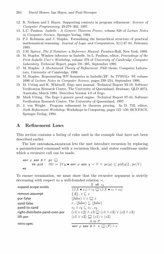
264 David Hemer, Ian Hayes, and Paul Strooper
12. R. Nickson and I. Hayes. Supporting contexts in program refinement. Science ofComputer Programming, 29:279–302, 1997.
13. L.C. Paulson. Isabelle - A Generic Theorem Prover, volume 828 of Lecture Notesin Computer Science. Springer-Verlag, 1994.
14. P.J. Robinson and J. Staples. Formalising the hierarchical structure of practicalmathematical reasoning. Journal of Logic and Computation, 3(1):47–61, February1993.
15. J.M. Spivey. The Z Notation: a Reference Manual. Prentice-Hall, New York, 1989.16. M. Staples. Window inference in Isabelle. In L. Paulson, editor, Proceedings of the
First Isabelle User’s Workshop, volume 379 of University of Cambridge ComputerLaboratory Technical Report, pages 191–205, September 1995.
17. M. Staples. A Mechanised Theory of Refinement. PhD thesis, Computer Labora-tory, University of Cambridge, 1998.
18. M. Staples. Representing WP Semantics in Isabelle/ZF. In TPHOLs ’99, volume1690 of Lecture Notes in Computer Science, pages 239–254, September 1999.
19. M. Utting and K. Whitwell. Ergo user manual. Technical Report 93-19, SoftwareVerification Research Centre, The University of Queensland, Brisbane, QLD 4072,Australia, March 1994. Describes Version 4.0 of Ergo.
20. Mark Utting. The Ergo 5 generic proof engine. Technical Report 97-44, SoftwareVerification Research Centre, The University of Queensland, 1997.
21. J. von Wright. Program refinement by theorem proving. In D. Till, editor,Sixth Refinement Workshop, Workshops in Computing, pages 121–150. BCS FACS,Springer-Verlag, 1994.
A Refinement Laws
This section contains a listing of rules used in the example that have not beendescribed earlier.
The law introduce recursion lets the user introduce recursion by replacinga parameterised command with a recursion block, and states conditions underwhich a recursive call can be made.
env ρ ass A � pc ��re pid . (V) :- {∀ y • env ρ ass y ≺ V � pc(y) � pid(y)} , pc(V )
er
To ensure termination, we must show that the recursive argument is strictlydecreasing with respect to a well-founded relation ≺.expand-scope-exists
X nfi c2
(∃X • c1) ∧ c2 �� (∃X • c1 ∧ c2)
remove-assumpt {A} , c � cpor-false 〈false〉 ∨ c � csand-false c , 〈false〉 � 〈false〉pand-to-sand c1 ∧ c2 � c1 , c2
right-distribute-pand-over-por (c1 ∨ c2) ∧ c3 � (c1 ∧ c3) ∨ (c2 ∧ c3)lift-por 〈c1 ∨ c2〉 � 〈c1〉 ∨ 〈c2〉intro-spec
A � P
env ρ ass A � c �� 〈P〉 ∧ c
Predicate Subtyping with Predicate Sets
Joe Hurd�
Computer LaboratoryUniversity of [email protected]
Abstract. We show how PVS-style predicate subtyping can be simu-lated in HOL using predicate sets, and explain how to perform subtypechecking using this model. We illustrate some applications of this to spec-ification and verification in HOL, and also demonstrate some limits ofthe approach. Finally we report on the effectiveness of a subtype checkerused as a condition prover in a contextual rewriter.
1 Introduction
HOL [4] and PVS [13] are both interactive theorem-provers extending Church’ssimple type theory [1]: in HOL with Hindley-Milner polymorphism [11]; and inPVS with parametric theories1 and predicate subtyping [14]. In this paper wewill focus on PVS predicate subtyping, and show how it can be simulated inHOL.
Predicate subtyping allows the creation of a new subtype corresponding toan arbitrary predicate, where elements of the new type are also elements of thecontaining type. As a simple illustration of this, the type of real division (/) inHOL is R→ R → R, and in PVS is R → R
�=0 → R, where R is the type of realnumbers and R
�=0 is the predicate subtype of non-zero real numbers, expressedby the predicate λx. x �= 0.
This extension of the type system allows more information to be encoded intypes, leading to benefits for specification and verification such as:
– The ability to express dependent types, for example a type for natural num-ber subtraction that prevents the second argument from being larger thanthe first argument, or a type representing lists of a fixed length in order tomodel arrays.
– Greater use of types to express side-conditions of theorems, for example thePVS rewrite rule
�PVS ∀x : R �=0. x/x = 1 (1)
In HOL this would have to be expressed
� ∀x : R. (x �= 0)⇒ (x/x = 1) (2)� Supported by an EPSRC studentship.1 Parametric theories allow polymorphism at the granularity of the theory (think C++
templates), whereas Hindley-Milner polymorphism operates at the granularity of thedeclaration (think ML functions).
R.J. Boulton and P.B. Jackson (Eds.): TPHOLs 2001, LNCS 2152, pp. 265–280, 2001.c© Springer-Verlag Berlin Heidelberg 2001
266 Joe Hurd
and the extra condition must be proved each time the rule is applied.2– More errors can be found in specifications during type-checking, giving great-er confidence that the goal is correct before a verification is embarked upon.Mokkedem [12] has observed this to be very effective in a large networkprotocol verification performed in PVS. Many specifications are not verifiedat all, and in that case the extra confidence is especially valuable.
However, there are also some costs:
– Type-checking becomes undecidable, so (potentially human) effort must beexpended to allow terms to be accepted into the system.
– Type-correctness depends on the current logical context, imposing an extraburden on term operations to keep careful track of what can be assumed ateach subterm. In the case of users wishing to program their own tactics thismerely steepens the learning curve; for term operations in the logical kernelfaulty implementations have produced a string of soundness bugs.3
In the literature there are papers arguing for and against predicate subtyping.Shankar [17] gives many examples of their utility, while Lamport [9] gives anexample where the costs must be paid without much benefit, in his case becausepredicate subtypes cannot naturally encode the desired invariant.
In this paper we describe our efforts to gain the functionality of predicatesubtypes in HOL, without altering the logic in any way. Instead of creating a first-class type associated with a particular predicate P , we reason with the subsetof elements that satisfy P . With this substitution, it is possible to simulate theextra reasoning power needed to automatically prove HOL side-conditions thatwould be expressed in PVS using predicate subtypes (such as the condition ofTheorem 2 above). Using the same technology, we can also perform an analogueof predicate subtype-checking for terms, although as we shall see the HOL logicimposes certain limitations on this.
The structure of the paper is as follows: in Section 2 we lay out the details ofour formalism and explain how to perform subtype-checking; Section 3 describessome tools that have been built using this technology, and reports on theireffectiveness in a case study; in Section 4 we consider some fundamental logicallimits of this approach; and finally in Sections 5, 6 and 7 we conclude, examinefuture prospects, and look at related work.
1.1 Notation
We use sans serif font to notate HOL constants, such as the function power op-erator funpow, the real number function inv (multiplicative inverse or reciprocal)2 Analogously, typed logics such as HOL and PVS enjoy this advantage over an un-
typed logic such as ZF set theory, in which the theorem � ∀n : N. n + 0 = n mustbe expressed � ∀n. n ∈ N⇒ (n + 0 = n).
3 Shankar [17] writes “these bugs stem largely from minor coding errors rather thanfoundational issues or complexities”. However, the extra complexity generated bypredicate subtyping does play a part in this: there have been very few soundnessbugs found in HOL over the years.
Predicate Subtyping with Predicate Sets 267
and the list functions length and mem. This font is also used for predicate setssuch as nzreal and posreal, in contrast to types (either HOL simple types or PVSpredicate subtypes) which are written in mathematical font. Examples of simpletypes are α, β (type variables), α×β (pairs), α∗ (lists), B (booleans) and R (thereal numbers); whereas R
�=0 and R≥0 are predicate subtypes.
2 The Formalism
2.1 Subtypes
A predicate set is a function P : α → B which represents the set of elementsx : α for which P x = �. Note that P is parameterized by the type α, andwe shall use the terminology ‘α predicate set’ (or just ‘α set’) when we wishto make this dependency explicit. Predicate sets are a standard modelling ofsets in higher-order logic, and we can define polymorphic higher-order constantsrepresenting all the usual set operations such as ∈, ∪ and image. In addition, foreach α there exists a universe set Uα = (λx : α. �) that contains every elementof type α.4
As examples, consider the following definitions of predicate sets that we willmake use of:
nzreal = λx : R. x �= 0 (3)posreal = λx : R. 0 < x (4)
nnegreal = λx : R. 0 ≤ x (5)∀n : N. lenum n = λm : N. m ≤ n (6)∀n : N. nlist n = λ l : α∗. length l = n (7)
∀ p : α→ B. list p = λ l : α∗. ∀x : α. mem x l ⇒ x ∈ p (8)∀ p : α→ B. ∀ q : β → B.
pair p q = λx : α× β. fst x ∈ p ∧ snd x ∈ q (9)
Definitions 3–5 are straightforward, each representing the set of real numbersthat are mapped to � by the predicate on the right hand side of the definition.Definitions 6–9 are all parameterized by various terms: in the case of lenum n bya natural number n so that lenum n = {0, 1, . . . , n}. Definitions 7–9 are polymor-phic too, which of course is just another way of saying they are parameterizedby types as well as terms. The set nlist n contains all α-lists having length n;the set list p contains all α-lists satisfying the condition that each member mustlie in the parameter set p; and finally the set pair p q contains all (α × β)-pairs(x, y) where x lies in the first parameter set p and y lies in the second parameterset q.
4 Since the HOL logic specifies that all types are disjoint, so must be these universesets.
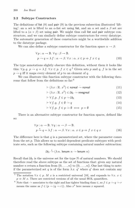
268 Joe Hurd
2.2 Subtype Constructors
The definitions of list (8) and pair (9) in the previous subsection illustrated ‘lift-ing’: an α set is lifted to an α-list set using list, and an α set and a β set arelifted to a (α × β) set using pair. We might thus call list and pair subtype con-structors, and we can similarly define subtype constructors for every datatype.The automatic generation of these constuctors might be a worthwhile additionto the datatype package.
We can also define a subtype constructor for the function space α→ β:
∀ p : α→ B. ∀ q : β → B.
p·→ q = λ f : α→ β. ∀x : α. x ∈ p⇒ f x ∈ q (10)
The type annotations slightly obscure this definition, without them it looks likethis: ∀ p, q. p ·→ q = λ f. ∀x ∈ p. f x ∈ q.5 Given sets p and q, f is in the setp·→ q iff it maps every element of p to an element of q.We can illustrate this function subtype constructor with the following theo-
rems that follow from the definitions so far:6
� (λx : R. x2) ∈ nzreal·→ nzreal (11)
� (λx : R. x2) ∈ UR
·→ nnegreal (12)
� ∀ f, p. f ∈ p ·→ UR (13)
� ∀ f, q. f ∈ ∅ ·→ q (14)
� ∀ f, p. f ∈ p ·→ ∅ ⇐⇒ p = ∅ (15)
There is an alternative subtype constructor for function spaces, defined likeso:
∀ p : α→ B. ∀ q : α→ β → B.
p�→ q = λ f : α→ β. ∀x : α. x ∈ p⇒ f x ∈ q x (16)
The difference here is that q is a parameterized set, where the parameter comesfrom the set p. This allows us to model dependent predicate subtypes with pred-icate sets, such as the following subtype containing natural number subtraction:
UN
�→ (λn. lenum n·→ lenum n)
Recall that UN is the universe set for the type N of natural numbers. We shouldtherefore read the above subtype as the set of functions that: given any naturalnumber n return a function from {0, . . . , n} to {0, . . . , n}. One last thing to note:if the parameterized set q is of the form λx. q′ where q′ does not contain any
5 The notation ∀x ∈ p. M x is a restricted universal [18], and expands to ∀x. x ∈p⇒M x. There are restricted versions of all the usual HOL quantifiers.
6 Note that·→ associates to the right and has tighter binding than ∈, so f ∈ p
·→ q·→ r
means the same as f ∈ (p·→ (q
·→ r)). Also x2 here means x squared.
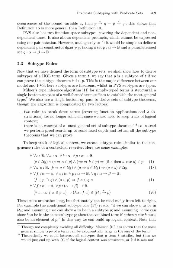
Predicate Subtyping with Predicate Sets 269
occurrences of the bound variable x, then p �→ q = p·→ q′: this shows that
Definition 16 is more general than Definition 10.PVS also has two function space subtypes, covering the dependent and non-
dependent cases. It also allows dependent products, which cannot be expressedusing our pair notation. However, analogously to �→ it would be simple to define adependent pair constructor dpair p q, taking a set p : α→ B and a parameterizedset q : α→ β → B.
2.3 Subtype Rules
Now that we have defined the form of subtype sets, we shall show how to derivesubtypes of a HOL term. Given a term t, we say that p is a subtype of t if wecan prove the subtype theorem � t ∈ p. This is the major difference between ourmodel and PVS: here subtypes are theorems, whilst in PVS subtypes are types.
Milner’s type inference algorithm [11] for simply-typed terms is structural: asingle bottom-up pass of a well-formed term suffices to establish the most generaltype.7 We also use a single bottom-up pass to derive sets of subtype theorems,though the algorithm is complicated by two factors:
– two rules to break down terms (covering function applications and λ-ab-stractions) are no longer sufficient since we also need to keep track of logicalcontext;
– there is no concept of a ‘most general set of subtype theorems’,8 so insteadwe perform proof search up to some fixed depth and return all the subtypetheorems that we can prove.
To keep track of logical context, we create subtype rules similar to the con-gruence rules of a contextual rewriter. Here are some examples:
� ∀ c : B. ∀ a : α. ∀ b : α. ∀ p : α→ B.
(c ∈ UB) ∧ (c⇒ a ∈ p) ∧ (¬c⇒ b ∈ p)⇒ (if c then a else b) ∈ p (17)� ∀ a, b : B. (b⇒ a ∈ UB) ∧ (a⇒ b ∈ UB)⇒ (a ∧ b) ∈ UB (18)� ∀ f : α→ β. ∀ a : α. ∀ p : α→ B. ∀ q : α→ β → B.
(f ∈ p �→ q) ∧ (a ∈ p)⇒ f a ∈ q a (19)� ∀ f : α→ β. ∀ p : (α→ β)→ B.
(∀x : α. f x ∈ p x)⇒ (λx. f x) ∈ (Uα�→ p) (20)
These rules are rather long, but fortunately can be read easily from left to right.For example the conditional subtype rule (17) reads: “if we can show c to be inUB; and assuming c we can show a to be in a subtype p; and assuming ¬c we canshow b to be in the same subtype p; then the combined term if c then a else bmustalso be an element of p.” In this way we can build up logical context. Note that7 Though not completely avoiding all difficulty: Mairson [10] has shown that the most
general simple type of a term can be exponentially large in the size of the term.8 Theoretically we could intersect all subtypes that a term t satisfies, but then we
would just end up with {t} if the logical context was consistent, or ∅ if it was not!
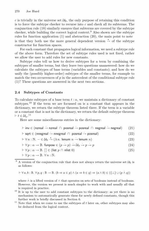
270 Joe Hurd
c is trivially in the universe set UB, the only purpose of retaining this conditionis to force the subtype checker to recurse into c and check all its subterms. Theconjunction rule (18) similarly ensures that subterms are covered by the subtypechecker, while building the correct logical context.9 Also shown are the subtyperules for function application (19) and abstraction (20), the main point to noteis that they both use the more general dependent version �→ of the subtypeconstructor for function spaces.
For each constant that propagates logical information, we need a subtype ruleof the above form. Therefore the set of subtype rules used is not fixed, ratherwe allow the user to add rules for new constants.
Subtype rules tell us how to derive subtypes for a term by combining thesubtypes of smaller terms, but they leave two questions unanswered: how do wecalculate the subtypes of base terms (variables and constants); and how do weunify the (possibly higher-order) subtypes of the smaller terms, for example tomatch the two occurrences of p in the antecedent of the conditional subtype rule(17)? These questions are answered in the next two sections.
2.4 Subtypes of Constants
To calculate subtypes of a base term t : α, we maintain a dictionary of constantsubtypes.10 If the term we are focussed on is a constant that appears in thedictionary, we return the subtype theorem listed there. If the term is a variableor a constant that is not in the dictionary, we return the default subtype theorem� t ∈ Uα.11
Here are some miscellaneous entries in the dictionary:
� inv ∈ (nzreal·→ nzreal ∩ posreal
·→ posreal ∩ negreal·→ negreal) (21)
� sqrt ∈ (nnegreal·→ nnegreal ∩ posreal
·→ posreal) (22)
� ∀n : N. − ∈ UN
�→ (λn. lenum n·→ lenum n) (23)
� ∀ p : α→ B. funpow ∈ (p ·→ p) ·→ UN
·→ p·→ p (24)
� ∀ p : α→ B. [ ] ∈ (list p ∩ nlist 0) (25)� ∀ p : α→ B. ∀n : N.
9 A version of the conjunction rule that does not always return the universe set UB isas follows:
� ∀ a, b : B. ∀ p, q : B→ B. (b⇒ a ∈ p) ∧ (a⇒ b ∈ q)⇒ (a ∧ b) ∈ ({⊥} ∪ (p·∧ q))
where·∧ is a lifted version of ∧ that operates on sets of booleans instead of booleans.
However, the version we present is much simpler to work with and usually all thatis required in practice.
10 It is up to the user to add constant subtypes to the dictionary: as yet there is nomechanism to automatically generate these for newly defined constants, though thisfurther work is briefly discussed in Section 6.
11 Note that when we come to use the subtypes of t later on, other subtypes may alsobe deduced from the logical context.
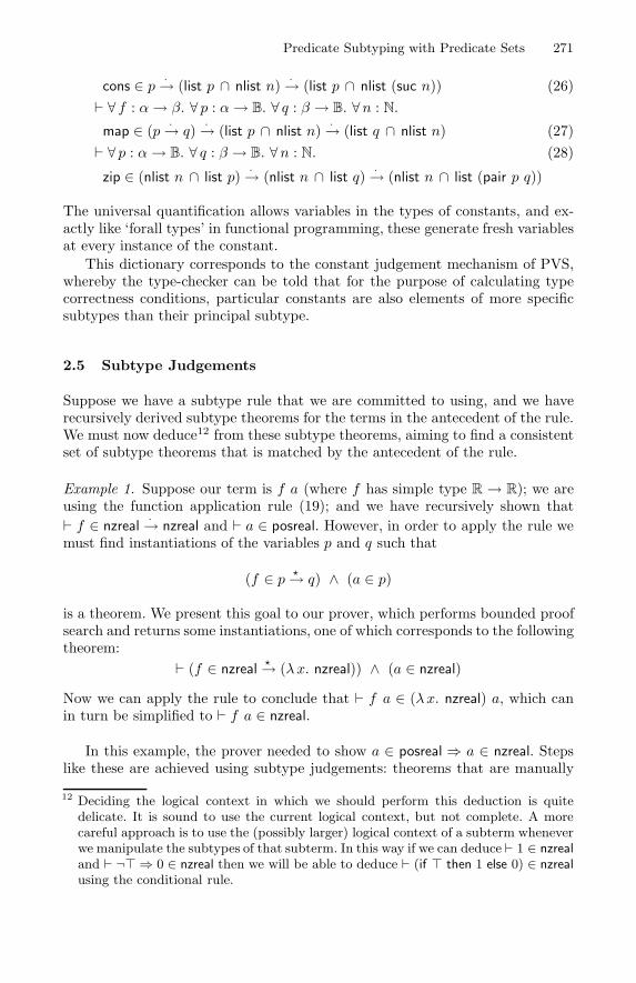
Predicate Subtyping with Predicate Sets 271
cons ∈ p ·→ (list p ∩ nlist n) ·→ (list p ∩ nlist (suc n)) (26)� ∀ f : α→ β. ∀ p : α→ B. ∀ q : β → B. ∀n : N.map ∈ (p ·→ q) ·→ (list p ∩ nlist n) ·→ (list q ∩ nlist n) (27)� ∀ p : α→ B. ∀ q : β → B. ∀n : N. (28)
zip ∈ (nlist n ∩ list p) ·→ (nlist n ∩ list q) ·→ (nlist n ∩ list (pair p q))
The universal quantification allows variables in the types of constants, and ex-actly like ‘forall types’ in functional programming, these generate fresh variablesat every instance of the constant.
This dictionary corresponds to the constant judgement mechanism of PVS,whereby the type-checker can be told that for the purpose of calculating typecorrectness conditions, particular constants are also elements of more specificsubtypes than their principal subtype.
2.5 Subtype Judgements
Suppose we have a subtype rule that we are committed to using, and we haverecursively derived subtype theorems for the terms in the antecedent of the rule.We must now deduce12 from these subtype theorems, aiming to find a consistentset of subtype theorems that is matched by the antecedent of the rule.
Example 1. Suppose our term is f a (where f has simple type R → R); we areusing the function application rule (19); and we have recursively shown that� f ∈ nzreal
·→ nzreal and � a ∈ posreal. However, in order to apply the rule wemust find instantiations of the variables p and q such that
(f ∈ p �→ q) ∧ (a ∈ p)
is a theorem. We present this goal to our prover, which performs bounded proofsearch and returns some instantiations, one of which corresponds to the followingtheorem:
� (f ∈ nzreal�→ (λx. nzreal)) ∧ (a ∈ nzreal)
Now we can apply the rule to conclude that � f a ∈ (λx. nzreal) a, which canin turn be simplified to � f a ∈ nzreal.
In this example, the prover needed to show a ∈ posreal ⇒ a ∈ nzreal. Stepslike these are achieved using subtype judgements: theorems that are manually
12 Deciding the logical context in which we should perform this deduction is quitedelicate. It is sound to use the current logical context, but not complete. A morecareful approach is to use the (possibly larger) logical context of a subterm wheneverwe manipulate the subtypes of that subterm. In this way if we can deduce � 1 ∈ nzrealand � ¬� ⇒ 0 ∈ nzreal then we will be able to deduce � (if � then 1 else 0) ∈ nzrealusing the conditional rule.
272 Joe Hurd
added to the top-level logical context, and are available for use in deriving sub-types.13 These will be theory specific, and can be extended by the user at anytime. Examples are:
� posreal ⊂ nzreal (29)� ∀ p, q : α→ B. p ⊂ q ⇒ list p ⊂ list q (30)
From the example we can see that a suitable prover must be: higher-orderto deal with parameterized types; able to find multiple instantiations of a goal(‘prolog-style’); and able to perform bounded proof search. Any prover thatsatisfies these criteria will be able to plug in at this point and enable subtypederivation.
However, since there are not many provers available that can satisfy all theserequirements, we have implemented one to test our subtype derivation algo-rithm. Robinson [15] presents an approach to higher-order proving by convert-ing all terms to combinatory form.14 Together with translation to CNF thisconversion leaves terms in a normal form that simplifies the writing of auto-matic proof search tools. For our application we implement a version of modelelimination (mostly following Harrison’s presentation [5], with some higher-orderextensions), since that is able to return multiple instantiations of goals and wecan use a simple depth-bound to limit the search. More powerful normalizationmeans that it can compete with the HOL first-order prover MESON_TAC on somefirst-order problems, and results on higher-order problems are basic but promis-ing. It is under active development, and a paper will soon be available describingits operation in more detail.
2.6 Subtype Derivation Algorithm
To summarize this section, we present the complete algorithm to derive subtypesof a term.
Inputs: A term t having simple type α; a logical context C initialized witha set of assumptions and the current subtype judgements; a set R of subtyperules; and a dictionary D of constant subtypes.
Outputs: A set P of subtype theorems.
1. If t is a variable, return [� t ∈ Uα].2. If t is a constant, look in the dictionary D to see if there is an entry (t, p).If so, return [� t ∈ p], otherwise return [� t ∈ Uα].
3. Otherwise find a subtype rule in R matching t.15 The rule will have the form
� ∀v.
∧
1≤i≤n
∀vi. ai[vi]⇒ ti[vi] ∈ pi[vi,v]
⇒ t ∈ p[v] (31)
13 The name ‘subtype judgements’ was borrowed from PVS, which contains resultsused for exactly the same purpose.
14 Many thanks to John Harrison for drawing my attention to this paper.15 If there is more than one rule that matches, return the rule that was most recently
added to R: this is almost always the most specific rule too.
Predicate Subtyping with Predicate Sets 273
4. For each 1 ≤ i ≤ n, create the logical context Ci by adding the assumptionai[vi] to C and recursively apply the algorithm using Ci to ti to find a setof subtypes
Pi = {� ti[vi] ∈ pi0[vi], . . . , � ti[vi] ∈ pini [vi]}
5. Find consistent sets of subtypes by calling the following search function withcounter i← 1 and instantiation σ ← id.(a) If i > n then return σ.(b) Using the subtype theorems in Pi and the logical context Ci, use the
higher-order prover to find theorems of the form � ti[vi] ∈ σ(pi[vi,v]).(c) For each theorem returned, let σi be the returned instantiation. Recur-
sively call the depth-first search function with counter i ← i + 1 andinstantiation σ ← (σi ◦ σ).
6. Each instantiation σ returned by depth-first search corresponds to a special-ization of the subtype rule (31) for which we have proven the antecedent.We may thus deduce the consequent by modus ponens, and we add this tothe result set P of subtype theorems.
3 Applications
3.1 Predicate Set Prover
An obvious application for the subtype derivation algorithm is to prove set mem-bership goals. Supposing the current goal is t ∈ p, we can derive a set P ofsubtype theorems for t, and then invoke the higher-order prover once again withthe top-level context and the set P to tackle the goal directly.
Example 2. To illustrate the two steps, consider the goal 3 ∈ nzreal.16 Subtypesare derived for the term 3 (of type R), and the following list of subtype theoremsare returned:
[� 3 ∈ K posreal 3, � 3 ∈ K nnegreal 3]
(where K = λx. λ y. x). Next these two theorems are passed to the higher-orderprover along with the top-level logical context containing type-judgements, andit quickly proves the goal � 3 ∈ nzreal.
We package up the predicate set prover into a HOL tactic, which calls theprover with the current subgoal as argument: if successful the resulting theoremwill match the subgoal and can be dispatched. We can prove some interestinggoals with this tactic:
� map inv (cons (−1) (map sqrt [3, 1])) ∈ list nzreal
� (λx ∈ negreal. funpow inv n x) ∈ negreal·→ negreal
16 This is not quite as trivial as it looks, since the real number ‘3’ in HOL is really thecomplex term real of num (numeral (bit1 (bit1 0))).
274 Joe Hurd
One optimization that is effective even with this basic tactic is to maintain acache of the subtypes that have already been derived for HOL constants.17 Forexample, the innocuous-looking term ‘3’ used in the above example is actuallycomposed of 4 nested function applications! Rederiving subtypes for constantsis unnecessary and inefficient.
Another optimization arises naturally from certain subtype rules, such as theconjunction rule (18), repeated here:
∀ a, b : B. (b⇒ a ∈ UB) ∧ (a⇒ b ∈ UB)⇒ (a ∧ b) ∈ UB
The set UB is the universe set UB of booleans, so we can immediately prove� b ⇒ a ∈ UB and � a ⇒ b ∈ UB without recursing into the structure of thesubterms a and b. Note that if we were deriving subtypes in order to check theterm for subtype correctness then we would be obliged to carry out this recursionstep to check a and b, but if our goal is proving set membership then we cansafely skip this.
3.2 Proving Conditions During Rewriting
We can use the predicate set prover as a condition prover in a contextual rewriter,and there are several reasons why it is useful to integrate these tools:
– There is a trend to incorporate tools into contextual rewriters because of theautomatic subterm traversal and context accumulation. The logical contextbuilt up by the contextual rewriter is easily transferred to the predicateset prover, and the subterm traversal allows us to attempt a proof of alloccurrences of t ∈ p in the goal term.18
– Many rewrites have side conditions that can be expressed very naturallyusing restricted quantifiers, and these generate goals for the predicate setprover when the rewrite is applied.
– Subtype judgements, rules and constants can be stored with the simplifi-cation set of a theory, thus reducing the administration burden of theory-specific rules.
Here are some miscellaneous rewrite rules that make use of subtype condi-tions:
� ∀x ∈ nzreal. x/x = 1 (32)� ∀n. ∀m ∈ lenum n. m+ (n−m) = n (33)� ∀n ∈ nznum. n mod n = 0 (34)� ∀ s ∈ finite. ∀ f ∈ injection s. |image f s| = |s| (35)� ∀G ∈ group. ∀ g ∈ set G. idG ∗G g = g (36)� ∀G ∈ group. ∀ g, h ∈ set G. (g ∗G h = h) = (g = idG) (37)
17 Here ‘constant’ means any term having no free variables.18 When subtype derivation is applied to a subterm it accumulates context in much the
same way as a contextual rewriter. However, despite this similarity, the two toolsare orthogonal and are best implemented separately: we tried both approaches.
Predicate Subtyping with Predicate Sets 275
Using rule 32, a term like 5/5 = 3/3 is straightforwardly rewritten to �.An effective optimization for this tool is to make adding assumptions into the
subtype logical context a lazy operation. This delays their conversion to combi-natory form and CNF normalization until the predicate set prover is invoked ona goal, which might not happen at all.
The last two examples above come from a body of computational numbertheory that we have recently formalized [6], which provided a test of the utilityof our predicate set prover as a condition prover in a contextual rewriter. Theproperties that were targeted in the development were group membership (e.g.,g ∗G h ∈ set G), simple natural number inequalities (e.g., 0 < n or 1 < mn) andnonemptiness properties of lists and sets (e.g., s �= ∅).
In theory, the architecture laid out in the previous section can establish muchmore exotic properties than these, but the predicate subtype prover was foundto be most useful and robust on these relatively simple properties that come upagain and again during conditional rewriting. These properties naturally propa-gate upwards through a term, being preserved by most of the basic operations,and in such situations the predicate set prover can be relied upon to show thedesired condition (albeit sometimes rather slowly). This tool lent itself to more ef-ficient development of the required theories, particularly the group theory wherealmost every theorem has one or more group membership side-conditions.
If the predicate set prover had not been available, it would have been possibleto use a first-order prover to show most of the side-conditions, but there are threereasons why this is a less attractive proposition: firstly it would have requiredeffort to find the right ‘property propagation’ theorems needed for the each goal;secondly the explicit invocations would have led to more complicated tactics; andthirdly some of the goals that can be proved using our specialized tool wouldsimply have been out of range of a more general first-order prover.
3.3 Debugging Specifications
How can we use our algorithm for deriving subtypes to find errors in a specifica-tion? We do this by invoking the algorithm on the specification, and generatingan exception whenever the algorithm would return an empty set of subtypes fora subterm.
Consider the following family of specifications:
(inv x) ∗ x = 1 (38)x ∈ nzreal⇒ (inv x) ∗ x = 1 (39)
inv x ∈ nzreal⇒ (inv x) ∗ x = 1 (40)
inv ∈ UR
·→ nzreal⇒ (inv x) ∗ x = 1 (41)
inv ∈ UR
·→ UR ⇒ (inv x) ∗ x = 1 (42)
The subtype checker will generate an exception for specification 38, complainingthat it could not derive a type for the subterm inv x. Why does it say this?The exception is raised because the algorithm could not find a consistent setof subtypes for the subterms inv and x, when using the subtype rule (19) for
276 Joe Hurd
function application. And this we see to be true, because without any additionalknowledge of x we cannot show it to be in any of the sets nzreal, posreal ornegreal that the subtype (21) of the constant inv demands.
Specification 39 shows the right solution: add a guard to stop x from takingthe illegal value of 0. And this solves the problem, the subtype checker can nowderive a subtype of nzreal for the subterm inv x (and a subtype of UB for thewhole term).
This is how we would expect the subtype checker to be used in practice. Aspecification is entered and subtype checked, the errors are corrected by addingthe necessary guards, and only then is verification started. This could potentiallysave much wasted effort and act as a valuable teaching tool.
Specifications 40–42 represent various attempts to subvert the subtypechecker. Specification 40 is a silly attempt: now the inv x in the antecedentfails to subtype check! However, even if the antecedent were added uncheckedto the logical context, the consequent would still not subtype check: an extrasubtype for inv x does not help at all in the search to find consistent subtypes forinv and x using the rule for function application. Specification 41 steps up a levelin the arms race by assuming a subtype for inv, and now this term does subtypecheck since the higher-order prover just needs to show that x ∈ UR: a triviality.However, we may take consolation in the fact that this antecedent is unprovable.Finally Specification 42 is the most worrying attack: the term subtype checks,and we can use Theorem 13 to prove the condition.
4 Logical Limits
The final example of the previous section showed how to subvert the subtypechecker that we implement. Unfortunately, this is not just an inadequacy ofthe subtype checker, but rather an inescapable consequence of reasoning withpredicate sets in the HOL logic. Since HOL is a logic of total functions, givenany function f : α→ β we can prove the theorem
� f ∈ Uα·→ Uβ (43)
since this just expands to � ∀x. x ∈ Uα ⇒ f x ∈ Uβ , which is true by thedefinition of the universal set Uβ .
This means that enforceable predicate subtyping using predicate sets cannotexist as a layer on top of the existing HOL kernel, since Theorem 43 is true evenfor restricted constants (such as inv), and can be used by the subtype checker toallow the application of such constants to any argument.
Example 3. Even if the user is not trying to subvert the system, it might happenaccidentally. If we are subtype checking the following specification
P ⇒ Q (inv 0)
then when we subtype check the consequent Q (inv 0) we add the antecedentP to the logical context, and it might transpire that P somehow causes the
Predicate Subtyping with Predicate Sets 277
higher-order prover to deduce inv ∈ UR
·→ UR,19 which then allows Q (inv 0) tobe successfully subtype checked.
PVS is also a logic of total functions, but the ability to make a first-class typeof non-zero reals means that if inv is declared to have type R
�=0 → R then thetype-system can stop the function from being ‘lifted’ to a larger type. Essentiallythe PVS logic implements a logic of partial functions, but by insisting that a typeis available for every function’s domain can avoid all questions of definedness.
5 Conclusion
We have shown how predicate subtyping can be modelled in HOL using predi-cate sets, explained how to perform subtype checking using our framework, andillustrated some applications of this to specification and verification in HOL.
It is helpful to divide the benefits of predicate subtyping into two categories:negative features, which consist of spotting and disallowing type-incorrect terms;and positive features, which consist of allowing properties to be (more quickly)deduced that help prove theorems.
In this paper we have shown that we can gain many of the positive benefitsof predicate subtyping,20 and in some ways we can even do better: our systemdoes not only calculate with principal subtypes but rather with any subtype thatthe term can be shown to satisfy using the rules. This was shown to provide aneffective proof procedure on a body of formalized mathematics.
In our experience the model is also quite robust when used for the negativefeatures of predicate subtyping, and finds most typical errors that predicatesubtyping is designed to prevent. Unfortunately, we have shown that in certainsituations it can be subverted, and so we cannot claim to match the PVS level oftype safety. However, it is worth remarking that specifications that are provablemust possess this level of type safety,21 so a guarantee is most valuable if thespecification will never be verified. If verification is our goal, then any debuggingthat can be performed in advance will speed up the process, but an absoluteguarantee is not necessary. In conclusion, predicate subtyping using predicatesets should be seen as an extra box of tools to aid verification.
6 Further Work
On the basis of our case study, we can seek to improve the predicate set proverby making it faster and more robust on simple and ubiquitous subtypes. Oneobvious approach to this would be to improve the underlying higher-order prover.19 After all, it is a theorem!20 Although almost certainly the performance using our model is worse than genuine
predicate subtyping: keeping subtypes with the terms so they never have to bederived must provide a boost. We also experimented with this kind of architecture,but dropped it in favour of the system presented in the current paper to simplifythe design and increase interoperability with existing tools.
21 That is, if restricted constants are underspecified outside their domain.
278 Joe Hurd
In particular the handling of equality and reasoning with total orders could bemuch more effective; perhaps we could interface to a linear decision procedureto speed up the latter.
Another, more speculative, line of research would be to use subtype checkingto perform subtype inference of new constants. If it could be made to work thiswould be extremely useful: currently for each constant which we would like toadd to the constant subtype dictionary, we must specify and prove a result ofthe form of Theorems 21–28. The idea is to initially enter the type of the newconstant c as c ∈ p where p is a variable; during subtype checking we collectconstraints on p; and finally at the top-level we try to solve these constraints:the solutions being subtypes for c.
7 Related Work
The model of predicate subtyping using predicate sets builds upon Wong’s [18]restricted quantifier library in HOL88, and the exact details of the predicate sub-typing in our model attempts to follow the PVS architecture. For the full detailsof the semantics and implementation of subtyping in PVS, refer to Owre [14].
Previous work in this area has been done by Jones [7], who built a tool inHOL to specify the subtype of constants and subtype check terms with respectto the subtypes. Given a term t, the tool sets up HOL goals that, if proved, wouldcorrespond to the term being subtype-correct. The user is then free to use theseextra theorems during verification. Our model extends Jones’ by the introduc-tion of subtype rules for generating type-correctness conditions, the higher-orderprover to automatically prove conditions, and the integration of the tool into arewriter to aid interactive proof.
A comparison of HOL and PVS was made by Gordon [3], from the perspec-tives of logic, automatic proof and usability. Our work is only relevant to partof this comparison, and enthusiastically takes up some of the suggestions formodelling PVS-style constructs in HOL.
ACL2 uses guards [8] to stop functions from being applied outside theirdomain; these generate proof obligations when new functions are defined in termsof guarded functions. When the proof obligations have been satisfied the newfunction is given a ‘gold’ status, and can be safely executed without causing run-time type errors. This is very similar to the way PVS type-checks terms beforeadmitting them into the system.
Saaltink [16] has also implemented a system of guard formulas in Z/EVES,which both aids formal Z proofs and has found some errors in Z specifications.The Z logic allows terms to be ‘undefined’, but the system of guard formulasimposed will flag the situations that can result in undefinedness, allowing clas-sical reasoning on the partial logic. Since Z is based on set theory, this use ofguards does not suffer from the logical limitations we outlined in Section 4, andcan provide strong guarantees about a checked specification. However, whereasour subtype rules propagate all available logical information around the term,Saaltink chooses a “left-to-right system of interpretation” that is not complete,but works well in most practical situations and simplifies guard conditions.
Predicate Subtyping with Predicate Sets 279
Finally, there has been a huge amount of work on subtyping and polymor-phism in various λ-calculi, used to model object-orientated programming lan-guages. Some concepts from this field are related to our work, in particular thenotion of intersection types corresponds to finding multiple subtypes of a term.Campognoni’s thesis [2] provides a good introduction to this area.
Acknowledgements
My Ph.D. supervisor, Mike Gordon, got me started on this topic and helpedbring the project to a successful conclusion. I had many valuable conversationsabout predicate subtyping with Judita Preiss, Konrad Slind and Michael Nor-rish, and their comments on this paper (particularly Konrad’s keen eye) helpedremove many potential misunderstandings. John Harrison gave me help withimplementing the higher-order prover, and Ken Larsen should be credited as thelocal ML guru. Finally, the comments of the TPHOLs referees improved thispaper tremendously.
References
1. Alonzo Church. A formulation of the simple theory of types. Journal of SymbolicLogic, 5:56–68, 1940.
2. Adriana B. Compagnoni. Higher-Order Subtyping with Intersection Types. PhDthesis, Catholic University, Nigmegen, January 1995.
3. M. J. C. Gordon. Notes on PVS from a HOL perspective. Available from theUniversity of Cambridge Computer Laboratory web server.
4. M. J. C. Gordon and T. F. Melham. Introduction to HOL (A theorem-provingenvironment for higher order logic). Cambridge University Press, 1993.
5. John Harrison. Optimizing proof search in model elimination. In M. A. McRobbieand J. K. Slaney, editors, 13th International Conference on Automated Deduction,volume 1104 of Lecture Notes in Computer Science, pages 313–327, New Brunswick,NJ, 1996. Springer-Verlag.
6. Joe Hurd. Verification of the Miller-Rabin probabilistic primality test. Submittedas a Category B paper to TPHOLs 2001, May 2001.
7. Michael D. Jones. Restricted types for HOL. In TPHOLs 1997 Category B papers,1997.
8. Matt Kaufmann and J. S. Moore. Industrial strength theorem prover for a logicbased on Common Lisp. IEEE Transactions on Software Engineering, 23(4):203–213, April 1997.
9. Leslie Lamport and Lawrence C. Paulson. Should your specification language betyped? ACM Transactions on Programming Languages and Systems, 21(3):502–526, May 1999.
10. Harry G. Mairson. Deciding ML typability is complete for deterministic exponen-tial time. In Conference Record of the Seventeenth Annual ACM Symposium onPrinciples of Programming Languages, pages 382–401. ACM SIGACT and SIG-PLAN, ACM Press, 1990.
11. R. Milner. A theory of type polymorphism in programming. Journal of Computerand System Sciences, 17:348–375, December 1978.
280 Joe Hurd
12. Abdel Mokkedem and Tim Leonard. Formal verification of the Alpha 21364 net-work protocol. In Mark Aagaard and John Harrison, editors, Theorem Proving inHigher Order Logics: 13th International Conference, TPHOLs 2000, volume 1869of Lecture Notes in Computer Science, pages 443–461, Portland, OR, August 2000.Springer-Verlag.
13. S. Owre, N. Shankar, J. M. Rushby, and D. W. J. Stringer-Calvert. PVS Sys-tem Guide. Computer Science Laboratory, SRI International, Menlo Park, CA,September 1999.
14. Sam Owre and Natarajan Shankar. The formal semantics of PVS. Technical ReportSRI-CSL-97-2, Computer Science Laboratory, SRI International, Menlo Park, CA,August 1997.
15. J. A. Robinson. A note on mechanizing higher order logic. Machine Intelligence,5:121–135, 1970.
16. Mark Saaltink. Domain checking Z specifications. In C. Michael Holloway andKelly J. Hayhurst, editors, LFM’ 97: Fourth NASA Langley Formal Methods Work-shop, pages 185–192, Hampton, VA, September 1997.
17. Natarajan Shankar and Sam Owre. Principles and pragmatics of subtyping inPVS. In D. Bert, C. Choppy, and P. D. Mosses, editors, Recent Trends in AlgebraicDevelopment Techniques, WADT ’99, volume 1827 of Lecture Notes in ComputerScience, pages 37–52, Toulouse, France, September 1999. Springer-Verlag.
18. Wai Wong. The HOL res quan library. HOL88 documentation.
A Structural Embedding of Ocsid in PVS
Pertti Kellomaki
Tampere University of Technology, Tampere, [email protected]
http://www.cs.tut.fi/~pk
Abstract. We describe a structural embedding of the Ocsid specificationlanguage into the logic of the PVS theorem prover. A front end tool isused to manipulate the structural elements of the language, while theexpression language is directly borrowed from the theorem prover.The structural embedding allows us to express and verify invariant prop-erties of distributed systems in an abstract form. An invariant can beverified once, and reused multiple times by discharging a set of relativelysimple proof obligations.
1 Introduction
In [25], Munoz and Rushby advocate structural embeddings, where a formalmethod (e.g. B [2] or VDM [12]) provides the outer level structural elementsand means to manipulate them, while a general purpose verification system(e.g. PVS [26] or HOL [14]) provides the semantics for expressions within thestructural elements, as well as mechanized means of reasoning about them. Wedescribe an application of this approach, namely an embedding of the Ocsidspecification language using the PVS theorem prover.
The Ocsid specification language is an experimental variant of the DisCo [18,21]language, essentially a proof of concept for a new way of structuring superpo-sition. Since we did not want to spend too much effort on uninteresting imple-mentation work in the exploratory phase, we decided to implement the Ocsidcompiler as a front end that delegates as much of the work as possible to existingtools. To this end, we use the existing DisCo tool set [1] for visualization andanimation of Ocsid specifications, and the PVS theorem prover for type checkingand verification. The focus of this paper is on how Ocsid utilizes PVS.
The main motivation behind this work has been independent verificationof superposition steps. In our earlier work [19,20] on mechanical verificationof DisCo specifications it became painfully obvious that many proofs in theverification of distributed systems are really instances of more abstract proofs,but the DisCo language lacks the expressive power required for expressing theseabstractions. The Ocsid language provides mechanisms for expressing behaviorin a more abstract fashion, and PVS parametric theories provide the requiredmechanism for instantiating proofs.
Defining the semantics of a specification language by giving a tool that mapsit to the input language of another tool may not be very elegant, but from a
R.J. Boulton and P.B. Jackson (Eds.): TPHOLs 2001, LNCS 2152, pp. 281–296, 2001.c© Springer-Verlag Berlin Heidelberg 2001
282 Pertti Kellomaki
pragmatic point of view it has proved to be a good design decision. The frontend compiler (about 3000 lines of Haskell) provides features explicitly targetedat the specific problem domain, in our case reactive distributed systems. Sharingthe expression language with PVS makes mapping from Ocsid to PVS straight-forward, and removes the possibility of subtle errors caused by small differencesbetween the logics of the specification language and the verification system.
The type system of PVS is rich enough to allow a fairly straightforwardmapping from Ocsid to the PVS logic. It handles the issue of undefined values, itis used for modeling inheritance hierarchies, and it is also used to express scopingrules for variables embedded within states of hierarchical state machines.
The rest of the paper is structured as follows. Section 2 describes the Ocsidspecification language, and Sections 3 and 4 describe the structural embedding.Related work is discussed Section 5, and conclusions are presented in Section 6.
2 The Ocsid Language
Ocsid is based on superposition, originally used as a design technique for dis-tributed algorithms without any specific syntactic support (e.g. [13,11,9]). As asyntactic construct, superposition has been used at least in the DisCo [18,21] andUnity [10] languages. In superposition, the underlying program or specificationis augmented with new statements or other elements in such a way that someproperties of interest of the original are retained.
Ocsid also allows for composition of independent branches of specification.This part of the language is still under development and it is not addressed here.
The semantics of Ocsid is based on the joint action [6,7] formalism of Backand Kurki-Suonio, which can further be mapped to Lamport’s Temporal Logicof Actions [22]. The world consists of a set of objects, which are containers ofstate variables. State variables can only be changed in joint actions in whichsome combinations of objects, the participants of the action, synchronize andmodify their state variables. An action execution may also involve parameters,which are similar to participants but denote values instead of mutable objects. Abehavior is a sequence of states resulting from atomic executions of joint actions.
Like DisCo, Ocsid is targeted at formal specification of reactive distributedsystems. Early focus on collective behavior and atomicity addresses concernsthat are especially relevant for systems with a large degree of concurrency andasynchrony.
In Ocsid, the unit of modularity is a layer. A layer describes a syntactictransformation that can be applied to a specification, provided that the spec-ification satisfies the assumptions of the layer. The requires section of a layerspecifies what entities (types, classes, actions) are assumed to be present in aspecification to which the layer is applied. The provides section introduces newentities and extends the existing ones.
Superposition in Ocsid preserves safety properties by construction. When alayer introduces a new state variable, all assignments to it must be given. Newassignments cannot be given in later superposition steps.
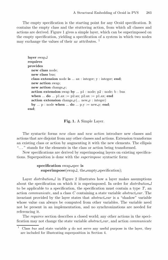
A Structural Embedding of Ocsid in PVS 283
The empty specification is the starting point for any Ocsid specification. Itcontains the empty class and the stuttering action, from which all classes andactions are derived. Figure 1 gives a simple layer, which can be superimposed onthe empty specification, yielding a specification of a system in which two nodesmay exchange the values of their ax attributes. 1
layer swap lrequiresprovides
new class node;new class bus;class extension node is ... ax : integer; y : integer; end;new action swap;new action change y;action extension swap by ... p1 : node; p2 : node; b : buswhen ... do ... p1.ax := p2.ax; p2.ax := p1.ax; endaction extension change y(... new y : integer)by ... p : node when ... do ... p.y := new y; end;
end;
Fig. 1. A Simple Layer.
The syntactic forms new class and new action introduce new classes andactions that are disjoint from any other classes and actions. Extension transformsan existing class or action by augmenting it with the new elements. The ellipsis“. . . ” stands for the elements in the class or action being transformed.
New specifications are derived by superimposing layers on existing specifica-tions. Superposition is done with the superimpose syntactic form:
specification swap spec issuperimpose(swap l, the empty specification);
Layer distribution l in Figure 2 illustrates how a layer makes assumptionsabout the specification on which it is superimposed. In order for distribution lto be applicable to a specification, the specification must contain a type T , anaction communicate, and a class C containing a state variable abstract var . Theinvariant provided by the layer states that abstract var is a “shadow” variablewhose value can always be computed from other variables. The variable neednot be present in an implementation, and no synchronizations are needed forreferencing it.
The requires section describes a closed world; any other actions in the speci-fication may not change the state variable abstract var , and action communicate1 Class bus and state variable y do not serve any useful purpose in the layer, theyare included for illustrating superposition in Section 4.
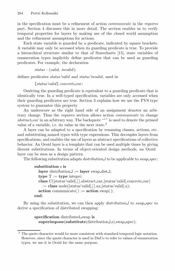
284 Pertti Kellomaki
in the specification must be a refinement of action communicate in the requirespart. Section 4 discusses this in more detail. The section enables us to verifytemporal properties for layers by making use of the closed world assumptionand the refinement assumptions for actions.
Each state variable is guarded by a predicate, indicated by square brackets.A variable may only be accessed when its guarding predicate is true. To providea hierarchical structure similar to that of Statecharts [15], state variables ofenumeration types implicitly define predicates that can be used as guardingpredicates. For example, the declaration
status : (valid, invalid);
defines predicates status’valid and status’invalid , used in
[status’valid].concrete var ;
Omitting the guarding predicate is equivalent to a guarding predicate that isidentically true. In a well-typed specification, variables are only accessed whentheir guarding predicates are true. Section 3 explains how we use the PVS typesystem to guarantee this property.
An underscore as the right hand side of an assignment denotes an arbi-trary change. Thus the requires section allows action communicate to changeabstract var in an arbitrary way. The backquote “‘” is used to denote the primedvalue of a variable, i.e. its value in the next state.2
A layer can be adapted to a specification by renaming classes, actions, etc.and substituting named types with type expressions. This decouples layers fromspecifications, and enables the use of layers as abstract specifications of collectivebehavior. An Ocsid layer is a template that can be used multiple times by givingdifferent substitutions. In terms of object-oriented design methods, an Ocsidlayer can be seen as a design pattern.
The following substitution adapts distribution l to be applicable to swap spec:
substitution s islayer distribution l := layer swap dist l;type T := type integer;class C([status’valid],[ ].abstract var,[status’valid].concrete var):= class node([status’valid],[ ].ax,[status’valid].x);
action communicate( ) := action swap( );end;
By using the substitution, we can then apply distribution l to swap spec toderive a specification of distributed swapping:
specification distributed swap issuperimpose(substitute(distribution l,s),swap spec);
2 The quote character would be more consistent with standard temporal logic notation.However, since the quote character is used in DisCo to refer to values of enumerationtypes, we use it in Ocsid for the same purpose.
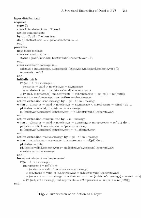
A Structural Embedding of Ocsid in PVS 285
layer distribution lrequires
type T;class C is abstract var : T; end;action communicateby p1 : C; p2 : C when truedo p1.abstract var := ; p2.abstract var := ;end;
providesnew class message;class extension C is ...status : (valid, invalid); [status’valid].concrete var : T;
end;class extension message is ...exists as : (no message, a message); [exists as’a message].concrete var : T;represents : ref C;
end;initially init is(∀ (cc : C, m : message) :cc.status = valid ∧ m.exists as = no message∧ cc.abstract var = cc.[status’valid].concrete var))∧ (∀ (m1, m2:message): m1.represents = m2.represents ⇒ ref(m1) = ref(m2)));
new action send message; new action receive message;action extension send message by ... p1 : C; m : messagewhen ... p1.status = valid ∧ m.exists as = no message ∧ m.represents = ref(p1) do ...p1.status := invalid; m.exists as := a message;m.[exists as’a message].concrete var := p1.[status’valid].concrete var;
end;action extension communicate by ... m : messagewhen ... p2.status = valid ∧ m.exists as = a message ∧ m.represents = ref(p1) do ...p2.[status’valid].concrete var := ‘p2.abstract var;m.[exists as’a message].concrete var := ‘p1.abstract var;
end;action extension receive message by ... p1 : C; m : messagewhen ... m.exists as = a message ∧ m.represents = ref(p1) do ...p1.status := valid;p1.[status’valid].concrete var := m.[exists as’a message].concrete var;m.exists as := no message;
end;invariant abstract var implemented(∀(n : C, m : message) :(m.represents = ref(n)) ⇒¬ (n.status = valid ∧ m.exists as = a message)∧ ((n.status = valid ⇒ n.abstract var = n.[status’valid].concrete var)∧ (m.exists as = a message ⇒ n.abstract var = m.[exists as’a message].concrete var))))
∧ (∀ (m1, m2 : message): m1.represents = m2.represents ⇒ ref(m1) = ref(m2)));end;
Fig. 2. Distribution of an Action as a Layer.
286 Pertti Kellomaki
3 Base Ocsid in PVS
In this section we describe the small amount of infrastructure needed for em-bedding Ocsid in PVS. We also describe how the basic building blocks of Ocsidare mapped to PVS.
3.1 Infrastructure
A small number of PVS definitions are needed to support the structural embed-ding. They define the empty specification and some temporal logic.
All Ocsid specifications are derived from the empty specification, which de-fines the empty class and the stuttering action. Figure 3 gives the PVS theorycorresponding to the empty specification. Axiom Object unique ref models theassumption that each Ocsid object has a unique reference accessed with thefunction ref.
PVS theory temporal operators in Figure 4 specifies some linear time temporallogic for reasoning about invariants. The predefined function suffix is the expectedoperation on infinite sequences.
3.2 Actions in PVS
An Ocsid action is mapped to a PVS function whose arguments are the currentstate, the next state, and the parameters and participants of the action. Thefunction is composed of the guard of the action, the assignments in the actionbody, and universally quantified formulas specifying that no other changes takeplace. We refer to such functions as action functions in the following. Section 4explains how action functions are used for superposition and temporal reasoning.
In temporal logic, an action is a boolean function of two states. An actionfunction is converted to an action by existentially quantifying over the parame-ters and participants of the action.
3.3 Ocsid Classes in PVS
Ocsid classes are represented as subtypes of Ocsid object. Ocsid classes form asubclass hierarchy, which is mirrored in PVS as a subtype hierarchy, where eachOcsid class C gives rise to a PVS predicate C. An Ocsid declaration cc: C mapsto PVS as cc: (C), where (C) denotes a subtype of Ocsid object whose valuessatisfy predicate C.
Subtypes offer a convenient way to encode the class hierarchy. A subclassinherits the ability to participate in a role declared to be of the base type. InPVS, participation corresponds to existential quantification, and quantificationover a base type also includes the values of any of its subtypes.
In a logic without subtypes we would either need to simulate them axiomati-cally, or to make explicit all the possible combinations of classes of participants.The latter approach is not practical, since the number of combinations grows fast.
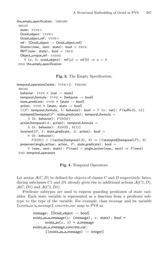
A Structural Embedding of Ocsid in PVS 287
the empty specification: theory
begin
state: type+
Ocsid object: type+
Ocsid object ref: type+
ref: [Ocsid object → Ocsid object ref]Stutter(now, next: state): bool = true
INIT(now: state): bool = true
Object unique ref: axiom
∀ (a, b: ocsid object): ref(a) = ref(b) ⇒ a = bend the empty specification
Fig. 3. The Empty Specification.
temporal operators[state: type+]: theory
begin
behavior: type = [nat → state]temporal formula: type = [behavior → bool]state predicate: type = [state → bool]action: type = [state, state → bool]✷(F: temporal formula, b: behavior): bool = ∀ (n: nat): F(suffix(b, n))statepred2temporal(P: state predicate): temporal formula =
λ (b: behavior): P(b(0))action2temporal(A: action): temporal formula =
λ (b: behavior): A(b(0), b(1))invariant(P, I: state predicate, A: action): bool =
∀ (b: behavior):I(b(0)) ∧ ✷(action2temporal(A), b) ⇒ ✷(statepred2temporal(P), b)
preserves(single action: action, P: state predicate): bool =
∀ (now, next: state): P(now) ∧ single action(now, next) ⇒ P(next)end temporal operators
Fig. 4. Temporal Operators.
Let action A(C,D) be defined for objects of classes C and D respectively. Intro-ducing subclasses C1 and D1 already gives rise to additional actions A(C1, D),A(C,D1) and A(C1, D1).
Predicate subtypes are used to express guarding predicates of state vari-ables. Each state variable is represented as a function from a predicate sub-type to the type of the variable. For example, class message and its variable[exists as’a message].concrete var map to PVS as
message: [Ocsid object → bool]exists as a message(x: (message), s: state): bool =
exists as(x, s) = a messageexists as a message concrete var:
[(exists as a message) → integer]
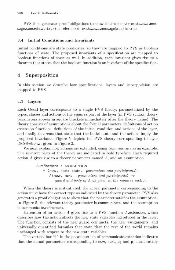
288 Pertti Kellomaki
PVS then generates proof obligations to show that whenever exists as a mes-sage concrete var(x, s) is referenced, exists as a message(x, s) is true.
3.4 Initial Conditions and Invariants
Initial conditions are state predicates, so they are mapped to PVS as booleanfunctions of state. The proposed invariants of a specification are mapped toboolean functions of state as well. In addition, each invariant gives rise to atheorem that states that the boolean function is an invariant of the specification.
4 Superposition
In this section we describe how specifications, layers and superposition aremapped to PVS.
4.1 Layers
Each Ocsid layer corresponds to a single PVS theory, parameterized by thetypes, classes and actions of the requires part of the layer (in PVS syntax, theoryparameters appear in square brackets immediately after the theory name). Thetheory consists of assumptions about the formal parameters, definitions of actionextension functions, definitions of the initial condition and actions of the layer,and finally theorems that state that the initial state and the actions imply theproposed invariants. Figure 5 depicts the PVS theory corresponding to layerdistribution l , given in Figure 2.
We next explain how actions are extended, using communicate as an example.The relevant parts of the theory are indicated in bold typeface. Each requiredaction A gives rise to a theory parameter named A, and an assumption
A refinement : assumption
∀ (now, next: state, parameters and participants):A(now, next, parameters and participants) ⇒
guard and body of A as given in the requires section
When the theory is instantiated, the actual parameter corresponding to theaction must have the correct type as indicated by the theory parameter. PVS alsogenerates a proof obligation to show that the parameter satisfies the assumption.In Figure 5, the relevant theory parameter is communicate, and the assumptionis communicate refinement.
Extension of an action A gives rise to a PVS function A extension, whichdescribes how the action affects the new state variables introduced in the layer.The function consists of the new guard conjuncts, the new assignments, anduniversally quantified formulas that state that the rest of the world remainsunchanged with respect to the new state variables.
The vertical bar “|” in the parameter list of communicate extension indicatesthat the actual parameters corresponding to now, next, p2 and p1 must satisfy
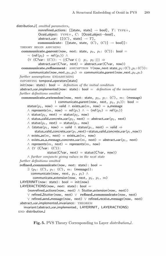
A Structural Embedding of Ocsid in PVS 289
distribution l[ omitted parameters,nonrefined actions: [[state, state] → bool], T: type+,
Ocsid object: type+, C: [Ocsid object→bool],abstract var: [[(C), state] → T],
communicate: [[state, state, (C), (C)] → bool]]:theory begin assuming
communicate parent(now, next: state, p2, p1: (C)): bool =
¬ (ref(p2) = ref(p1)) ∧(∀ (C?var: (C)): ¬ ((C?var ∈ (: p1, p2 :))) ⇒
abstract var(C?var, next) = abstract var(C?var, now))communicate refinement: assumption ∀(now,next:state,p2:(C),p1:(C)):
communicate(now,next,p2,p1) ⇒ communicate parent(now,next,p2,p1)
further assumptions endassuming
importing temporal operators[state]init(now: state): bool = definition of the initial conditionabstract var implemented(now: state): bool = definition of the invariantfurther definitions omittedcommunicate extension(now, next: state, p2, p1: (C), m: (message)
| communicate parent(now, next, p2, p1)): bool =
status(p2, now) = valid ∧ exists as(m, now) = a message∧ represents(m, now) = ref(p1) ∧ ¬ (ref(p2) = ref(p1))
∧ status(p2, next) = status(p2, now)∧ status valid concrete var(p2, next) = abstract var(p2, next)∧ status(p1, next) = status(p1, now)∧ (status(p1, now) = valid ∧ status(p1, next) = valid ⇒
status valid concrete var(p1,next)=status valid concrete var(p1,now))∧ exists as(m, next) = exists as(m, now)∧ exists as a message concrete var(m, next) = abstract var(p1, next)∧ represents(m, next) = represents(m, now)∧ (∀ (C?var: (C)):
status(C?var, next) = status(C?var, now))∧ further conjuncts giving values in the next state
further definitions omittedrefined communicate(now, next: state): bool =
∃ (p2: (C), p1: (C), m: (message)):communicate(now, next, p2, p1) ∧communicate extension(now, next, p2, p1, m)
LAYERINIT(now: state): bool = init(now)LAYERACTIONS(now, next: state): bool =
(nonrefined actions(now, next) ∧ Stutter extension(now, next))∨ refined Stutter(now, next) ∨ refined communicate(now, next)∨ refined send message(now, next) ∨ refined receive message(now, next)
abstract var implemented invariance: theorem
invariant(abstract var implemented, LAYERINIT, LAYERACTIONS)end distribution l
Fig. 5. PVS Theory Corresponding to Layer distribution l .
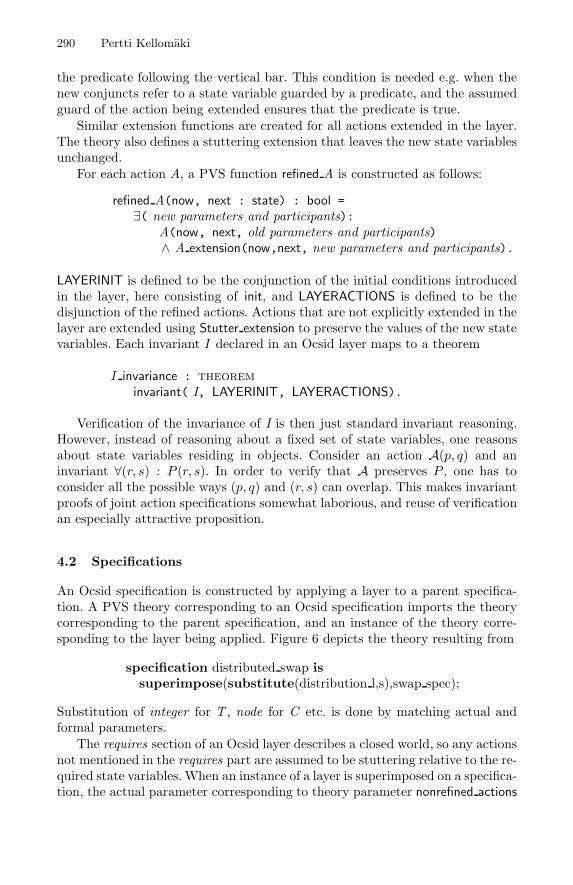
290 Pertti Kellomaki
the predicate following the vertical bar. This condition is needed e.g. when thenew conjuncts refer to a state variable guarded by a predicate, and the assumedguard of the action being extended ensures that the predicate is true.
Similar extension functions are created for all actions extended in the layer.The theory also defines a stuttering extension that leaves the new state variablesunchanged.
For each action A, a PVS function refined A is constructed as follows:
refined A(now, next : state) : bool =∃( new parameters and participants):
A(now, next, old parameters and participants)∧ A extension(now,next, new parameters and participants).
LAYERINIT is defined to be the conjunction of the initial conditions introducedin the layer, here consisting of init, and LAYERACTIONS is defined to be thedisjunction of the refined actions. Actions that are not explicitly extended in thelayer are extended using Stutter extension to preserve the values of the new statevariables. Each invariant I declared in an Ocsid layer maps to a theorem
I invariance : theorem
invariant( I, LAYERINIT, LAYERACTIONS).
Verification of the invariance of I is then just standard invariant reasoning.However, instead of reasoning about a fixed set of state variables, one reasonsabout state variables residing in objects. Consider an action A(p, q) and aninvariant ∀(r, s) : P (r, s). In order to verify that A preserves P , one has toconsider all the possible ways (p, q) and (r, s) can overlap. This makes invariantproofs of joint action specifications somewhat laborious, and reuse of verificationan especially attractive proposition.
4.2 Specifications
An Ocsid specification is constructed by applying a layer to a parent specifica-tion. A PVS theory corresponding to an Ocsid specification imports the theorycorresponding to the parent specification, and an instance of the theory corre-sponding to the layer being applied. Figure 6 depicts the theory resulting from
specification distributed swap issuperimpose(substitute(distribution l,s),swap spec);
Substitution of integer for T , node for C etc. is done by matching actual andformal parameters.
The requires section of an Ocsid layer describes a closed world, so any actionsnot mentioned in the requires part are assumed to be stuttering relative to the re-quired state variables.When an instance of a layer is superimposed on a specifica-tion, the actual parameter corresponding to theory parameter nonrefined actions
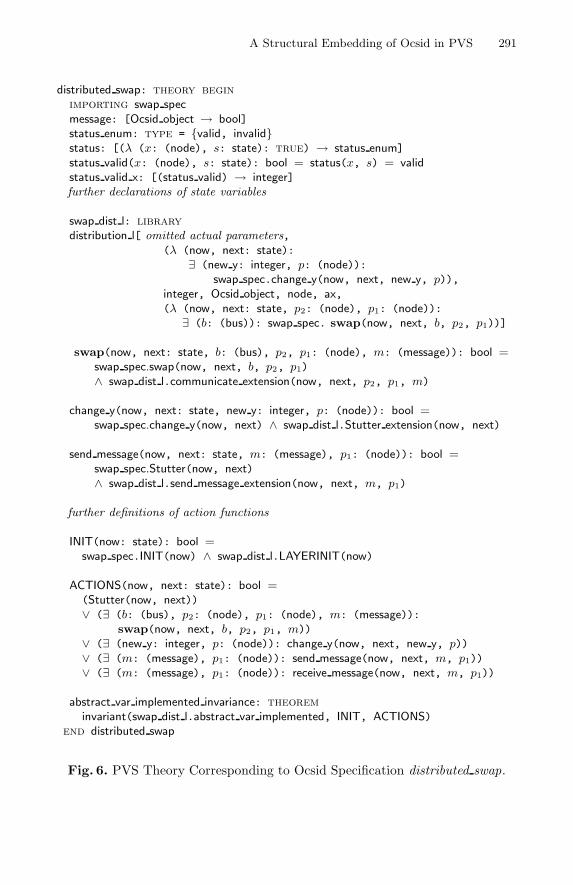
A Structural Embedding of Ocsid in PVS 291
distributed swap: theory begin
importing swap specmessage: [Ocsid object → bool]status enum: type = {valid, invalid}status: [(λ (x: (node), s: state): true) → status enum]
status valid(x: (node), s: state): bool = status(x, s) = validstatus valid x: [(status valid) → integer]further declarations of state variables
swap dist l: library
distribution l[ omitted actual parameters,(λ (now, next: state):
∃ (new y: integer, p: (node)):swap spec.change y(now, next, new y, p)),
integer, Ocsid object, node, ax,(λ (now, next: state, p2: (node), p1: (node)):∃ (b: (bus)): swap spec. swap(now, next, b, p2, p1))]
swap(now, next: state, b: (bus), p2, p1: (node), m: (message)): bool =
swap spec.swap(now, next, b, p2, p1)
∧ swap dist l.communicate extension(now, next, p2, p1, m)
change y(now, next: state, new y: integer, p: (node)): bool =
swap spec.change y(now, next) ∧ swap dist l.Stutter extension(now, next)
send message(now, next: state, m: (message), p1: (node)): bool =
swap spec.Stutter(now, next)∧ swap dist l.send message extension(now, next, m, p1)
further definitions of action functions
INIT(now: state): bool =
swap spec.INIT(now) ∧ swap dist l.LAYERINIT(now)
ACTIONS(now, next: state): bool =
(Stutter(now, next))∨ (∃ (b: (bus), p2: (node), p1: (node), m: (message)):
swap(now, next, b, p2, p1, m))
∨ (∃ (new y: integer, p: (node)): change y(now, next, new y, p))∨ (∃ (m: (message), p1: (node)): send message(now, next, m, p1))
∨ (∃ (m: (message), p1: (node)): receive message(now, next, m, p1))
abstract var implemented invariance: theorem
invariant(swap dist l.abstract var implemented, INIT, ACTIONS)end distributed swap
Fig. 6. PVS Theory Corresponding to Ocsid Specification distributed swap.
292 Pertti Kellomaki
is a disjunct of all actions that do not match any action in the requires sec-tion. The assuming part contains an assumption that nonrefined actions doesnot change any of the variables mentioned in the requires section.
In the case of distributed swap, action swap is matched with communicate, soonly change y is not matched with any of the required actions. The expressionprovided as the actual parameter for nonrefined actions is thus
λ (now, next: state):∃ (new y: integer, p: (node)):
swap spec.change y(now, next, new y, p).
The required action communicate has two participants, while action swap hasthree. To make swap compatible with communicate, it is wrapped in a lambdaform, and the extra participant b is existentially quantified:
λ (now, next: state, p2: (node), p1: (node)):∃ (b: (bus)): swap spec.swap(now, next, b, p2, p1).
When constructing the action functions for the new specification, an actionfunction from the parent specification is conjoined with an extension functionfrom the instantiated theory. For the actions extended in the layer, the corre-sponding extension is used, and for all other actions the stuttering extension isused.
ACTIONS is defined to be the disjunct of actions so constructed, and theinitial condition INIT is the conjunction of the initial condition of the parentspecification and the initial condition of the layer. In terms of temporal logic,the specification is
INIT ∧✷ACTIONS.
Let I be an invariant property provided by a layer. The theorem verified forthe corresponding theory is
invariant(I, LAYERINIT, LAYERACTIONS) (1)
while the theorem we are interested in is
invariant(I, INIT,ACTIONS). (2)
From the way INIT is constructed, we know that it implies LAYERINIT, asthe latter is a conjunct in the former. ACTIONS also implies LAYERACTIONSby construction. These are meta-level theorems as far as our embedding is con-cerned, so we have to resort to using (1) as a lemma when proving (2).
The structure of the formulas makes the proof straightforward. An action AS
in a specification is the conjunct of a base action AB in the parent specification,and an extension E from the layer being superimposed. The corresponding actionAL in the layer is the conjunct of the formal parameter AF and the extension E.When the layer is instantiated, AB is matched with AF , possibly by existentiallyquantifying some parameters and participants. The action implication AS ⇒ AL
A Structural Embedding of Ocsid in PVS 293
is then verified by skolemizing the existentially quantified variables in AS andinstantiating the corresponding existentially quantified variables in AL with theskolem constants, and rewriting the definitions of action functions.
5 Discussion
There is a plethora of work on the theme “X in Y ” where X is a specificationlanguage and Y is a verification system [4,3,16,5,29,8,23,20]. Most of this work(including our own) suffers from the problem pointed out in [25]: a mismatchbetween the logic of X and the logic of Y, which unnecessarily complicates thetranslation and hinders efficient mechanization. By defining the logic of Ocsidto be the logic of PVS, we avoid the mismatch. Ease of mapping to the logic ofPVS has been an explicit goal when designing the Ocsid language.
Compared to embeddings of Unity such as [5,28], our goals are much moremodest and pragmatic. We are only interested in safety properties, invariantsin particular. The reason for this is that superposition as used in DisCo andOcsid may invalidate liveness properties in refinement. We have opted for givingthe translation from Ocsid to PVS as an auxiliary tool instead of defining thesemantics of the specification language using the logic of PVS. The justificationis that we are interested in verifying properties of Ocsid specifications instead ofreasoning about the language itself. In our experience, verification is much morestraightforward with a shallow embedding than with a deep embedding.
Our work is related with the structural embeddings of a tabular notation [27]and the B-method [24] in PVS. The latter is especially close to our work, as itis implemented as a front end tool for PVS.
We originally started to develop a deep embedding, in which one could verifythe theorem that links an invariance property of a layer with an invarianceproperty in its application. However, it turns out that the shallow structuralembedding gives most of the benefits we would get from a deep embedding. Theshallow embedding also makes it easier to utilize the PVS type system as thetype system of the specification language, and is less cumbersome when verifyingactual specifications.
The drawback of using a shallow embedding is that even though we can usethe verification system for proving that the translation of the Ocsid specificationimplies the translation of the invariants, the question remains whether these areequivalent to the Ocsid specification and its invariants. We plan to utilize a deepembedding for checking this. Let sem be the semantic function that maps asyntactic construct to its meaning, S an Ocsid specification expressed as a set oflayers, superpositions and compositions, and St the translation of S from Ocsidto PVS. Establishing
sem(S)⇔ St (3)
would then suffice for showing that the invariants verified for St are in factinvariants of S. We speculate that proving (3) may not be too difficult, becauseif the translation is correct, then the structure of S is identical to that of St. The
294 Pertti Kellomaki
verification would be laborious but completely mechanical, consisting mostly ofrewriting sem and the definitions of action functions.
The main thrust of our work has been the recognition of common abstractionsin distributed systems. With Ocsid layers, we are able to specify and verify theseabstractions, and to reuse both design and verification effort. An Ocsid layer canbe utilized in a specification by verifying a set of action refinements, which inour experience are easily handled by the heuristics of PVS.
Many relevant invariant properties are not inductive, i.e. strong enough to beverified using deductive methods. Successful verification needs additional invari-ants, which easily leads to large invariants that are extremely tedious to verify.When an invariant property has been packaged in a reusable layer, this reasoningcan be done once and for all.
The Ocsid compiler is still under development, so we have not applied it tomore sizeable problems. However, we have experimented with the ideas using theDisCo specification language. For example, specifying the Recoverable Distribu-tor pattern [17] in DisCo reveals many opportunities for extracting and reusingabstract collective behavior.
6 Conclusions
We have described a structural embedding of the Ocsid specification languagein the logic of the PVS theorem prover. The specification language consists ofa structuring mechanism peculiar to Ocsid, and an expression language that isdefined to be the expression language of PVS.
The structuring mechanism allows us to specify and verify collective behaviorof distributed objects in an abstract way. The syntactic unit of specification is alayer, which describes a superposition step (transformation) that derives a moreconcrete specification from a more abstract specification. The implementationeffort for Ocsid has been relatively small, only a few thousand lines of Haskellcode. We feel that this implementation work has paid off rather well.
Invariant properties can be expressed and verified for layers, and reused bydischarging a set of proof obligations related to action refinement. Potentiallyexpensive temporal reasoning is then reused by verifying relatively simple proofobligations. In the example given in the paper, temporal reasoning took approx-imately 160 seconds, while the proof obligations were proved in 9 seconds.
Our future plan is to investigate whether one could define a pattern languagefor distributed systems based on archived superposition steps.
Acknowledgments
Part of this work was carried out when the author was visiting University ofDortmund on a grant from the Academy of Finland. Financial support has alsocome from Academy of Finland project 757473. Comments from the anonymousreviewers were helpful in improving the presentation.
A Structural Embedding of Ocsid in PVS 295
References
1. Timo Aaltonen, Mika Katara, and Risto Pitkanen. DisCo toolset – thenew generation. Journal of Universal Computer Science, 7(1):3–18, 2001.http://www.jucs.org.
2. Jean-Raymond Abrial. The B Book - Assigning Programs to Meanings. CambridgeUniversity Press, August 1996.
3. S. Agerholm and J. Frost. An isabelle-based theorem prover for VDM-SL. In Proc.10th International Theorem Proving in Higher Order Logics Conference, pages 1–16, 1997.
4. Sten Agerholm, Juan Bicarregui, and Savi Maharaj. On the verification of VDMspecification and refinement with PVS. In Juan Bicarregui, editor, Proof in VDM:Case Studies, FACIT (Formal Approaches to Computing and Information Tech-nology), chapter 6, pages 157–190. Springer-Verlag, London, UK, 1997.
5. F. Andersen, K. D. Petersen, and J. S. Petterson. Program verification usingHOL-UNITY. In J. J. Joyce and C.-J.H Seger, editors, International Workshop onHigher Order Logic and its Applications, volume 780 of Lecture Notes in ComputerScience, pages 1–16, 1994.
6. R. J. R. Back and R. Kurki-Suonio. Distributed cooperation with action systems.ACM Transactions on Programming Languages and Systems, 10(4):513–554, Oc-tober 1988.
7. R. J. R. Back and R. Kurki-Suonio. Decentralization of process nets with a cen-tralized control. Distributed Computing, (3):73–87, 1989.
8. J. Bowen and M. J. C. Gordon. Z and HOL. In J. Bowen and A. Hall, editors, ZUser Workshop, Workshops in Computing, pages 141–167. Springer-Verlag, Cam-bridge, 1994.
9. K. M. Chandy and L. Lamport. Distributed snapshots: determining the globalstate of distributed systems. ACM Transactions on Computer Systems, 3(1):63–75, 1985.
10. K. M. Chandy and J. Misra. Parallel Program Design: A Foundation. Addison-Wesley, 1988.
11. K. Mani Chandy, Jayadev Misra, and Laura M. Haas. Distributed deadlock detec-tion. ACM Transactions on Computer Systems, 1(2):144–156, May 1983.
12. John Dawes. The VDM-SL Reference Guide. Pitman, 1991. ISBN 0-273-03151-1.13. Edsger W. Dijkstra and C. S. Scholten. Termination detection for diffusing com-
putations. Information Processing Letters, 11(1):1–4, August 1980.14. Michael J. C. Gordon. HOL: A proof generating system for higher-order logic. In
Graham Birtwistle and P. A. Subrahmanyam, editors, VLSI Specification, Verifi-cation and Synthesis, pages 73–128. Boston Kluwer Academic Publishers, 1988.
15. David Harel. Statecharts: A visual formalism for complex systems. Science ofComputer Programming, 8(3):231–274, June 1987.
16. Barbara Heyd and Pierre Cregut. A modular coding of UNITY in COQ. In J. vonWright, T. Grundy, and J. Harrison, editors, Proceedings of the 9th InternationalConference on Theorem Proving in Higher Order Logics, volume 1125 of LectureNotes in Computer Science, pages 251–266, 1996.
17. Nayeem Islam and Murthy Devarakonda. An essential design pattern for fault-tolerant distributed state sharing. Communications of the ACM (CACM),39(10):65–74, October 1996.
18. H.-M. Jarvinen, R. Kurki-Suonio, M. Sakkinen, and K. Systa. Object-orientedspecification of reactive systems. In Proceedings of the 12th International Confer-ence on Software Engineering, pages 63–71. IEEE Computer Society Press, 1990.
296 Pertti Kellomaki
19. Pertti Kellomaki. Mechanical Verification of Invariant Properties of DisCo Speci-fications. PhD thesis, Tampere University of Technology, 1997.
20. Pertti Kellomaki. Verification of reactive systems using DisCo and PVS. In JohnFitzgerald, Cliff B. Jones, and Peter Lucas, editors, FME’97: Industrial Applica-tions and Strengthened Foundations of Formal Methods, number 1313 in LectureNotes in Computer Science, pages 589–604. Springer–Verlag, 1997.
21. Reino Kurki-Suonio. Fundamentals of object-oriented specification and model-ing of collective behaviors. In H. Kilov and W. Harvey, editors, Object-OrientedBehavioral Specifications, pages 101–120. Kluwer Academic Publishers, 1996.
22. Leslie Lamport. The temporal logic of actions. ACM Transactions on ProgrammingLanguages and Systems, 16(3):872–923, May 1994.
23. Thomas Langbacka. A HOL formalization of the temporal logic of actions. InT. F. Melham and J. Camilleri, editors, Higher Order Logic Theorem Proving andIts Applications, volume 859 of Lecture Notes in Computer Science, Valetta, Malta,1994. Springer Verlag.
24. Cesar Munoz. PBS: Support for the B-method in PVS. Technical Report SRI-CSL-99-1, Computer Science Laboratory, SRI International, Menlo Park, CA, February1999.
25. Cesar Munoz and John Rushby. Structural embeddings: Mechanization withmethod. In Jeannette Wing and Jim Woodcock, editors, FM99: The WorldCongress in Formal Methods, volume 1708 of Lecture Notes in Computer Science,pages 452–471, Toulouse, France, September 1999. Springer-Verlag.
26. S. Owre, J. M. Rushby, and N. Shankar. PVS: A prototype verification system.In Deepak Kapur, editor, 11th International Conference on Automated Deduction,volume 607 of Lecture Notes in Artificial Intelligence, pages 748–752. SpringerVerlag, 1992.
27. Sam Owre, John Rushby, and N. Shankar. Integration in PVS: Tables, types, andmodel checking. In Ed Brinksma, editor, Tools and Algorithms for the Constructionand Analysis of Systems TACAS ’97, number 1217 in Lecture Notes in ComputerScience, pages 366–383, Enschede, The Netherlands, April 1997. Springer-Verlag.
28. Paulson. Mechanizing UNITY in isabelle. ACM Transactions on ComputationalLogic, 1(1), 2000.
29. S. Kalvala. A Formulation of TLA in Isabelle. In E.T. Schubert, P.J. Windley, andJ. Alves-Foss, editors, 8th International Workshop on Higher Order Logic TheoremProving and its Applications, volume 971 of Lecture Notes in Computer Science,pages 214–228, Aspen Grove, Utah, USA, September 1995. Springer-Verlag.
A Certi�ed Polynomial-Based Decision Procedure
for Propositional Logic
Inmaculada Medina-Bulo1, Francisco Palomo-Lozano1,and José A. Alonso-Jiménez2
1 Department of Computer Languages and Systems. University of CádizEsc. Superior de Ingeniería de Cádiz. C/ Chile, s/n. 11003 Cádiz. Spain
{francisco.palomo,inmaculada.medina}@uca.es2 Department of Comp. Sciences and Arti�cial Intelligence, University of SevillaFac. de Informática y Estadística. Avda. Reina Mercedes, s/n. 41012 Sevilla, Spain
Abstract. In this paper we present the formalization of a decision pro-cedure for Propositional Logic based on polynomial normalization. Thisformalization is suitable for its automatic veri�cation in an applicativelogic like Acl2. This application of polynomials has been developed byreusing a previous work on polynomial rings [19], showing that a properformalization leads to a high level of reusability. Two checkers are de-�ned: the �rst for contradiction formulas and the second for tautologyformulas. The main theorems state that both checkers are sound andcomplete. Moreover, functions for generating models and counterexam-ples of formulas are provided. This facility plays also an important rolein the main proofs. Finally, it is shown that this allows for a highlyautomated proof development.
1 Introduction
In this paper we present the main results obtained through the development of anautomated proof of the correctness of a polynomial-based decision procedure forPropositional Logic in Acl2 [14,15,16]. Acl2 1 is the successor of Nqthm [3,5],the Boyer-Moore theorem prover. A concise description of Acl2 can be foundin [14]. In order to understand Acl2, it is necessary to consider it under threedi�erent perspectives:
1. From a logic viewpoint, Acl2 is a untyped quanti�er-free �rst-order logic oftotal recursive functions with equality. However, its encapsulation principleallows for some kind of higher-order reasoning.
2. From a programming language viewpoint, Acl2 is an applicative program-ming language in which the result of the application of a function is uniquelydetermined by its arguments. Every Acl2 function admitted under the def-initional principle is a Lisp function, so you can obtain both veri�ed andexecutable software.
1 A Computational Logic for Applicative Common Lisp.
R.J. Boulton and P.B. Jackson (Eds.): TPHOLs 2001, LNCS 2152, pp. 297�312, 2001.c© Springer-Verlag Berlin Heidelberg 2001
298 Inmaculada Medina-Bulo et al.
3. From a reasoning system viewpoint, Acl2 is an automated reasoning systemand it behaves as a heuristic theorem prover.
Representation issues play a major role in this work. We have representedPropositional Logic formulas in terms of just one Boolean function symbol: thethree-place conditional construct present in most programming languages. Thisis discussed in Sect. 2.1. De�nitions related with Boolean polynomials are pre-sented in Sect. 2.2.
Surprisingly, polynomial-based theorem proving has a long history. Accordingto H. Zhang [28], Boole himself [2] was the �rst to use Boolean polynomials torepresent logical formulas and Herbrand described a polynomial-based decisionprocedure in his thesis. Later, in 1936, M. Stone [23] stated the strong relationexisting between Boolean algebras and Boolean rings. Analogous results hadbeen discovered, independently, in 1927 by I. I. Zhegalkin [29].
This relation is at the basis of the modern �algebraic methods� of logicaldeduction. The algebraic approach began with the development by J. Hsiangof a canonical term-rewriting system for Boolean algebras with applications to�rst-order theorem proving [11,12]. Concurrently, D. Kapur and P. Narendranused Gröbner bases and Buchberger's algorithm for the same purpose [17].2 Thislast method has been extended to many-valued propositional logics [7,26] and ithas been recently applied to knowledge based systems veri�cation [18].
Several decision procedures for propositional logic that produce a veri�ableproof log have been implemented. For example, [9,10] report the development ofBDDs and Stªmarck's algorithm as HOL derived rules. On the other hand, actualformal veri�cations of decision procedures are less common. The classical workfrom [3] contains a veri�ed decision procedure in Nqthm using IF-expressions. Asimilar procedure has been extracted from a Coq proof in [22]. Another decisionprocedure obtained via proof extraction in Nuprl is described in [6]. However,none of them is based on polynomial normalization.
We have not considered the possibility of integrating the decision procedureinto the theorem prover via re�ection, though this is feasible in Acl2 thanksto its metatheoretical extensibility capabilities [4]. A re�ected decision proce-dure has been developed in [1] with Nuprl. See also [8] for a critical survey ofre�ection in theorem proving from a theoretical and practical viewpoint.
Section 2.3 presents a translation algorithm from formulas into polynomials.Once that suitable evaluation functions have been de�ned, this translation isshown to be interpretation-preserving. In Sect. 3, we review Hsiang's canonicalterm-rewriting system (TRS) for Boolean algebras. A normalization algorithmthat is not based in term-rewriting is also presented. In Sect. 4, we prove thecorrectness of the decision procedure for Propositional Logic. As the involvedalgorithms are written in an applicative subset of Common Lisp, they are in-trinsically executable. Some examples of execution are shown in Sect. 5.
Finally, we will discuss the degree of automation achieved and we will alsoanalyze some possible extensions of this work.
2 See also [13,28,27].
A Certi�ed Polynomial-Based Decision Procedure for Propositional Logic 299
2 IF-Formulas and Boolean Polynomials
In [20] an Acl2 formalization of IF-Formulas and Boolean polynomials is pro-posed. Next, the notion of Stone polynomial of an IF-formula is easily de�ned.We review here the main results obtained with some improvements.
As the conditional construct IF is functionally complete, we can regard ourPropositional Logic formulas as IF-formulas without loss of generality. In fact,the Nqthm Boyer-Moore logic and its descendant Acl2 de�ne the usual propo-sitional connectives after axiomatizing IF. IF-formulas are also related with theOBDD algorithm as can be seen in [21]. A BDD manager has been recentlyformalized in Acl2 [24].
2.1 IF-Formulas
The underlying representation of IF-formulas is based on the notion of IF-cons.IF-conses are weaker than IF-formulas in the sense that they may not repre-sent well-formed formulas. We use record structures to represent IF-conses. Thisprovides us with a weak recognizer predicate that we strengthen to develop arecognizer for well-formed formulas.
Boolean constants, nil and t, are recognized by the Acl2 booleanp predi-cate. The set of propositional variables could be then represented by the set ofatoms not including the Boolean constants. However, if we represent variablesusing natural numbers then it is easier to share the same notion of variable informulas and polynomials. Thus, we de�ne our variable recognizer, variablep,to recognize just natural numbers.
Our notion of IF-cons is captured by an Acl2 structure. An IF-cons is justa collection of three objects (the test, and the then and else branches). Thepredicate if-consp will recognize terms constructed with if-cons, while thefunctions test, then and else act as destructors. Well-formed IF-formulas canbe recognized by the following total recursive Acl2 predicate:
(defun formulap (f)
(or (booleanp f) (variablep f)
(and (if-consp f)
(formulap (test f))
(formulap (then f))
(formulap (else f)))))
An assignment of values to variables can be represented as a list of Booleans.3
Thus, the value of a variable with respect to an assignment is given by theelement which occupies its corresponding position.
(defun truth-value (v a)
(nth v a))
3 Remember each Boolean variable is represented as a natural number.
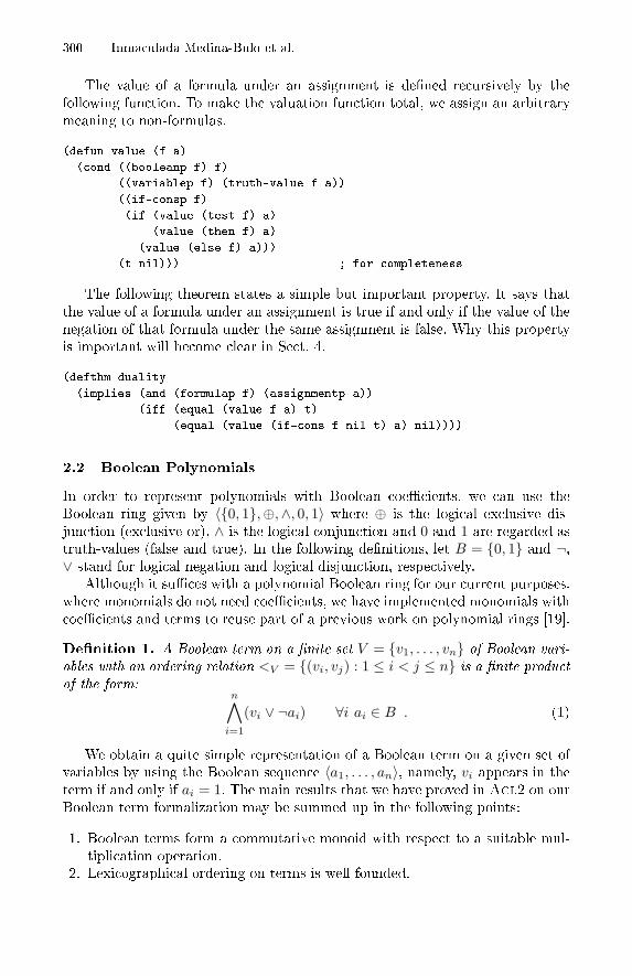
300 Inmaculada Medina-Bulo et al.
The value of a formula under an assignment is de�ned recursively by thefollowing function. To make the valuation function total, we assign an arbitrarymeaning to non-formulas.
(defun value (f a)
(cond ((booleanp f) f)
((variablep f) (truth-value f a))
((if-consp f)
(if (value (test f) a)
(value (then f) a)
(value (else f) a)))
(t nil))) ; for completeness
The following theorem states a simple but important property. It says thatthe value of a formula under an assignment is true if and only if the value of thenegation of that formula under the same assignment is false. Why this propertyis important will become clear in Sect. 4.
(defthm duality
(implies (and (formulap f) (assignmentp a))
(iff (equal (value f a) t)
(equal (value (if-cons f nil t) a) nil))))
2.2 Boolean Polynomials
In order to represent polynomials with Boolean coe�cients, we can use theBoolean ring given by 〈{0, 1},⊕,∧, 0, 1〉 where ⊕ is the logical exclusive dis-junction (exclusive-or), ∧ is the logical conjunction and 0 and 1 are regarded astruth-values (false and true). In the following de�nitions, let B = {0, 1} and ¬,∨ stand for logical negation and logical disjunction, respectively.
Although it su�ces with a polynomial Boolean ring for our current purposes,where monomials do not need coe�cients, we have implemented monomials withcoe�cients and terms to reuse part of a previous work on polynomial rings [19].
De�nition 1. A Boolean term on a �nite set V = {v1, . . . , vn} of Boolean vari-
ables with an ordering relation <V = {(vi, vj) : 1 ≤ i < j ≤ n} is a �nite product
of the form:n∧
i=1
(vi ∨ ¬ai) ∀i ai ∈ B . (1)
We obtain a quite simple representation of a Boolean term on a given set ofvariables by using the Boolean sequence 〈a1, . . . , an〉, namely, vi appears in theterm if and only if ai = 1. The main results that we have proved in Acl2 on ourBoolean term formalization may be summed up in the following points:
1. Boolean terms form a commutative monoid with respect to a suitable mul-tiplication operation.
2. Lexicographical ordering on terms is well-founded.
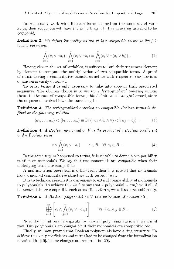
A Certi�ed Polynomial-Based Decision Procedure for Propositional Logic 301
As we usually work with Boolean terms de�ned on the same set of vari-ables, their sequences will have the same length. In this case they are said to becompatible.
De�nition 2. We de�ne the multiplication of two compatible terms as the fol-
lowing operation:
n∧i=1
(vi ∨ ¬ai) ·n∧
i=1
(vi ∨ ¬bi) =n∧
i=1
(vi ∨ ¬(ai ∨ bi)) . (2)
Having chosen the set of variables, it su�ces to �or� their sequences elementby element to compute the multiplication of two compatible terms. A proofof terms having a commutative monoid structure with respect to the previousoperation is easily obtained.
To order terms it is only necessary to take into account their associatedsequences. The obvious choice is to set up a lexicographical ordering amongthem. In the case of compatible terms, this de�nition is straightforward, sincethe sequences involved have the same length.
De�nition 3. The lexicographical ordering on compatible Boolean terms is de-
�ned as the following relation:
〈a1, . . . , an〉 < 〈b1, . . . , bn〉 ≡ ∃i (¬ai ∧ bi ∧ ∀j < i aj = bj) . (3)
De�nition 4. A Boolean monomial on V is the product of a Boolean coe�cient
and a Boolean term.
c ∧n∧
i=1
(vi ∨ ¬ai) c ∈ B ∀i ai ∈ B . (4)
In the same way as happened to terms, it is suitable to de�ne a compatibilityrelation on monomials. We say that two monomials are compatible when theirunderlying terms are compatible.
A multiplication operation is de�ned and then it is proved that monomialshave a monoid commutative structure with respect to it.
Due to technical reasons it is convenient to extend compatibility of monomialsto polynomials. To achieve this we �rst say that a polynomial is uniform if all ofits monomials are compatible each other. Henceforth, we will assume uniformity.
De�nition 5. A Boolean polynomial on V is a �nite sum of monomials.
m⊕i=1
ci ∧
n∧j=1
(vj ∨ ¬aij)
∀i, j ci, aij ∈ B . (5)
Now, the de�nition of compatibility between polynomials arises in a naturalway. Two polynomials are compatible if their monomials are compatible too.
Finally, we have proved that Boolean polynomials have a ring structure. Toachieve this, only coe�cients and terms had to be changed from the formalizationdescribed in [19]. These changes are reported in [20].
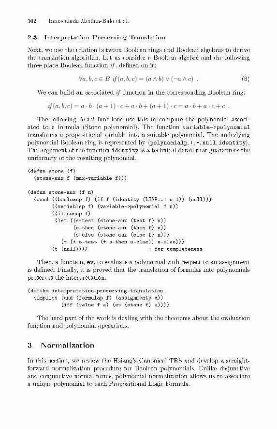
302 Inmaculada Medina-Bulo et al.
2.3 Interpretation Preserving Translation
Next, we use the relation between Boolean rings and Boolean algebras to derivethe translation algorithm. Let us consider a Boolean algebra and the followingthree place Boolean function if , de�ned on it:
∀a, b, c ∈ B if (a, b, c) = (a ∧ b) ∨ (¬a ∧ c) . (6)
We can build an associated if function in the corresponding Boolean ring:
if (a, b, c) = a · b · (a + 1) · c + a · b + (a + 1) · c = a · b + a · c + c .
The following Acl2 functions use this to compute the polynomial associ-ated to a formula (Stone polynomial). The function variable->polynomial
transforms a propositional variable into a suitable polynomial. The underlyingpolynomial Boolean ring is represented by 〈polynomialp, +, *, null, identity〉.The argument of the function identity is a technical detail that guarantees theuniformity of the resulting polynomial.
(defun stone (f)
(stone-aux f (max-variable f)))
(defun stone-aux (f n)
(cond ((booleanp f) (if f (identity (LISP::+ n 1)) (null)))
((variablep f) (variable->polynomial f n))
((if-consp f)
(let ((s-test (stone-aux (test f) n))
(s-then (stone-aux (then f) n))
(s-else (stone-aux (else f) n)))
(+ (* s-test (+ s-then s-else)) s-else)))
(t (null)))) ; for completeness
Then, a function, ev, to evaluate a polynomial with respect to an assignmentis de�ned. Finally, it is proved that the translation of formulas into polynomialspreserves the interpretation:
(defthm interpretation-preserving-translation
(implies (and (formulap f) (assignmentp a))
(iff (value f a) (ev (stone f) a))))
The hard part of the work is dealing with the theorems about the evaluationfunction and polynomial operations.
3 Normalization
In this section, we review the Hsiang's Canonical TRS and develop a straight-forward normalization procedure for Boolean polynomials. Unlike disjunctiveand conjunctive normal forms, polynomial normalization allows us to associatea unique polynomial to each Propositional Logic Formula.
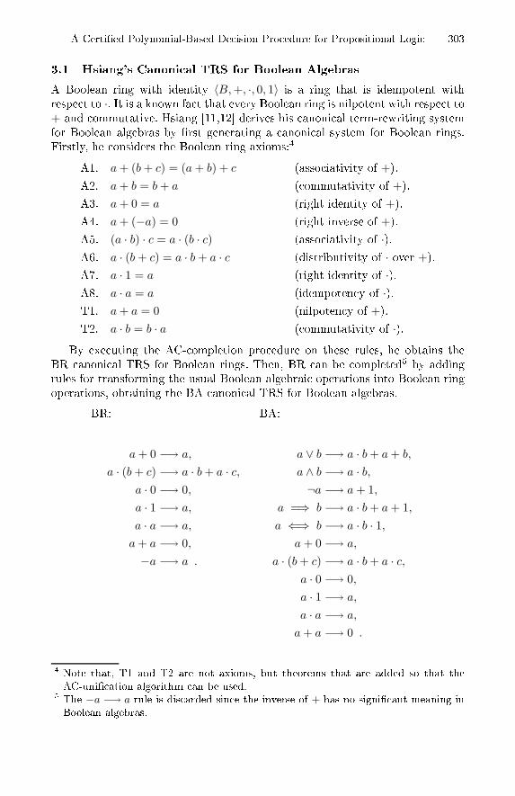
A Certi�ed Polynomial-Based Decision Procedure for Propositional Logic 303
3.1 Hsiang's Canonical TRS for Boolean Algebras
A Boolean ring with identity 〈B, +, ·, 0, 1〉 is a ring that is idempotent withrespect to ·. It is a known fact that every Boolean ring is nilpotent with respect to+ and commutative. Hsiang [11,12] derives his canonical term-rewriting systemfor Boolean algebras by �rst generating a canonical system for Boolean rings.Firstly, he considers the Boolean ring axioms:4
A1. a + (b + c) = (a + b) + c (associativity of +).
A2. a + b = b + a (commutativity of +).
A3. a + 0 = a (right identity of +).
A4. a + (−a) = 0 (right inverse of +).
A5. (a · b) · c = a · (b · c) (associativity of ·).A6. a · (b + c) = a · b + a · c (distributivity of · over +).
A7. a · 1 = a (right identity of ·).A8. a · a = a (idempotency of ·).T1. a + a = 0 (nilpotency of +).
T2. a · b = b · a (commutativity of ·).By executing the AC-completion procedure on these rules, he obtains the
BR canonical TRS for Boolean rings. Then, BR can be completed5 by addingrules for transforming the usual Boolean algebraic operations into Boolean ringoperations, obtaining the BA canonical TRS for Boolean algebras.
BR: BA:
a + 0 −→ a,
a · (b + c) −→ a · b + a · c,a · 0 −→ 0,
a · 1 −→ a,
a · a −→ a,
a + a −→ 0,
−a −→ a .
a ∨ b −→ a · b + a + b,
a ∧ b −→ a · b,¬a −→ a + 1,
a =⇒ b −→ a · b + a + 1,
a ⇐⇒ b −→ a · b · 1,
a + 0 −→ a,
a · (b + c) −→ a · b + a · c,a · 0 −→ 0,
a · 1 −→ a,
a · a −→ a,
a + a −→ 0 .
4 Note that, T1 and T2 are not axioms, but theorems that are added so that theAC-uni�cation algorithm can be used.
5 The −a −→ a rule is discarded since the inverse of + has no signi�cant meaning inBoolean algebras.
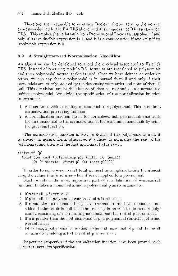
304 Inmaculada Medina-Bulo et al.
Therefore, the irreducible form of any Boolean algebra term is the normalexpression de�ned by the BA TRS above, and it is unique (since BA is a canonicalTRS). This implies that a formula from Propositional Logic is a tautology if andonly if its irreducible expression is 1, and it is a contradiction if and only if itsirreducible expression is 0.
3.2 A Straightforward Normalization Algorithm
An algorithm can be developed to avoid the overhead associated to Hsiang'sTRS. Instead of rewriting modulo BA, formulas are translated to polynomialsand then polynomial normalization is used. Once we have de�ned an order onterms, we can say that a polynomial is in normal form if and only if theirmonomials are strictly ordered by the decreasing term order and none of them isnull. This de�nition implies the absence of identical monomials in a normalizeduniform polynomial. We divide the speci�cation of the normalization functionin two steps:
1. A function capable of adding a monomial to a polynomial. This must be anormalization-preserving function.
2. A normalization function stable for normalized null polynomials that addsthe �rst monomial to the normalization of the remaining monomials by usingthe previous function.
The normalization function is easy to de�ne: if the polynomial is null, itis already in normal form, otherwise, it su�ces to normalize the rest of thepolynomial and then add the �rst monomial to the result.
(defun nf (p)
(cond ((or (not (polynomialp p)) (nullp p)) (null))
(t (+-monomial (first p) (nf (rest p))))))
In order to make +-monomial total we need to complete, taking the utmostcare, the values that it returns when it is not applied to a polynomial.
Next, we show the most important part of the de�nition of +-monomialfunction. It takes a monomial m and a polynomial p as its arguments.
1. If m is null, p is returned.2. If p is null, the polynomial composed of m is returned.3. If m and the �rst monomial of p have the same term, both monomials are
added. If the result is null then the rest of p is returned, otherwise a poly-nomial consisting of the resulting monomial and the rest of p is returned.
4. If m is greater than the �rst monomial of p, a polynomial consisting of m andp is returned.
5. Otherwise, a polynomial consisting of the �rst monomial of p and the resultof recursively adding m to the rest of p is returned.
Important properties of the normalization function have been proved, suchas that it meets its speci�cation,
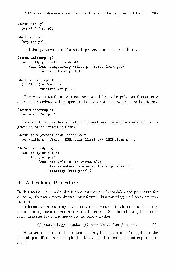
A Certi�ed Polynomial-Based Decision Procedure for Propositional Logic 305
(defun nfp (p)
(equal (nf p) p))
(defthm nfp-nf
(nfp (nf p)))
and that polynomial uniformity is preserved under normalization.
(defun uniformp (p)
(or (nullp p) (nullp (rest p))
(and (MON::compatiblep (first p) (first (rest p)))
(uniformp (rest p)))))
(defthm uniformp-nf
(implies (uniformp p)
(uniformp (nf p))))
One relevant result states that the normal form of a polynomial is strictlydecreasingly ordered with respect to the lexicographical order de�ned on terms.
(defthm orderedp-nf
(orderedp (nf p)))
In order to obtain this, we de�ne the function orderedp by using the lexico-graphical order de�ned on terms.
(defun term-greater-than-leader (m p)
(or (nullp p) (TER::< (MON::term (first p)) (MON::term m))))
(defun orderedp (p)
(and (polynomialp p)
(or (nullp p)
(and (not (MON::nullp (first p)))
(term-greater-than-leader (first p) (rest p))
(orderedp (rest p))))))
4 A Decision Procedure
In this section, our main aim is to construct a polynomial-based procedure fordeciding whether a propositional logic formula is a tautology and prove its cor-rectness.
A formula is a tautology if and only if the value of the formula under everypossible assignment of values to variables is true. So, the following �rst-orderformula states the correctness of a tautology-checker:
∀f [(tautology-checker f) ⇐⇒ ∀a (value f a) = t] (7)
However, it is not possible to write directly this theorem in Acl2, due to thelack of quanti�ers. For example, the following �theorem� does not capture ouridea:
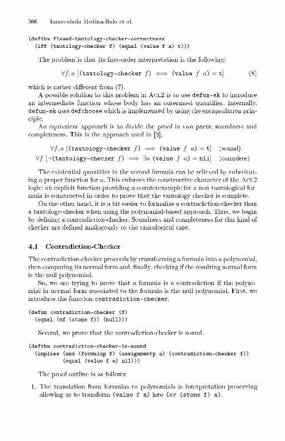
306 Inmaculada Medina-Bulo et al.
(defthm flawed-tautology-checker-correctness
(iff (tautology-checker f) (equal (value f a) t)))
The problem is that its �rst-order interpretation is the following:
∀f, a [(tautology-checker f) ⇐⇒ (value f a) = t] (8)
which is rather di�erent from (7).A possible solution to this problem in Acl2 is to use defun-sk to introduce
an intermediate function whose body has an outermost quanti�er. Internally,defun-sk uses defchoosewhich is implemented by using the encapsulation prin-ciple.
An equivalent approach is to divide the proof in two parts: soundness andcompleteness. This is the approach used in [3].
∀f, a [(tautology-checker f) =⇒ (value f a) = t] (sound)
∀f [¬(tautology-checker f) =⇒ ∃a (value f a) = nil] (complete)
The existential quanti�er in the second formula can be relieved by substitut-ing a proper function for a. This enforces the constructive character of the Acl2logic: an explicit function providing a counterexample for a non-tautological for-mula is constructed in order to prove that the tautology-checker is complete.
On the other hand, it is a bit easier to formalize a contradiction-checker thana tautology-checker when using the polynomial-based approach. Thus, we beginby de�ning a contradiction-checker. Soundness and completeness for this kind ofchecker are de�ned analogously to the tautological case.
4.1 Contradiction-Checker
The contradiction-checker proceeds by transforming a formula into a polynomial,then computing its normal form and, �nally, checking if the resulting normal formis the null polynomial.
So, we are trying to prove that a formula is a contradiction if the polyno-mial in normal form associated to the formula is the null polynomial. First, weintroduce the function contradiction-checker.
(defun contradiction-checker (f)
(equal (nf (stone f)) (null)))
Second, we prove that the contradiction-checker is sound.
(defthm contradiction-checker-is-sound
(implies (and (formulap f) (assignmentp a) (contradiction-checker f))
(equal (value f a) nil)))
The proof outline is as follows:
1. The translation from formulas to polynomials is interpretation-preservingallowing us to transform (value f a) into (ev (stone f) a).
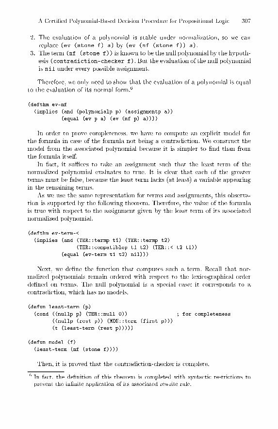
A Certi�ed Polynomial-Based Decision Procedure for Propositional Logic 307
2. The evaluation of a polynomial is stable under normalization, so we canreplace (ev (stone f) a) by (ev (nf (stone f)) a).
3. The term (nf (stone f)) is known to be the null polynomial by the hypoth-esis (contradiction-checker f). But the evaluation of the null polynomialis nil under every possible assignment.
Therefore, we only need to show that the evaluation of a polynomial is equalto the evaluation of its normal form.6
(defthm ev-nf
(implies (and (polynomialp p) (assignmentp a))
(equal (ev p a) (ev (nf p) a))))
In order to prove completeness, we have to compute an explicit model forthe formula in case of the formula not being a contradiction. We construct themodel from the associated polynomial because it is simpler to �nd than fromthe formula itself.
In fact, it su�ces to take an assignment such that the least term of thenormalized polynomial evaluates to true. It is clear that each of the greaterterms must be false, because the least term lacks (at least) a variable appearingin the remaining terms.
As we use the same representation for terms and assignments, this observa-tion is supported by the following theorem. Therefore, the value of the formulais true with respect to the assignment given by the least term of its associatednormalized polynomial.
(defthm ev-term-<
(implies (and (TER::termp t1) (TER::termp t2)
(TER::compatiblep t1 t2) (TER::< t2 t1))
(equal (ev-term t1 t2) nil)))
Next, we de�ne the function that computes such a term. Recall that nor-malized polynomials remain ordered with respect to the lexicographical orderde�ned on terms. The null polynomial is a special case: it corresponds to acontradiction, which has no models.
(defun least-term (p)
(cond ((nullp p) (TER::null 0)) ; for completeness
((nullp (rest p)) (MON::term (first p)))
(t (least-term (rest p)))))
(defun model (f)
(least-term (nf (stone f))))
Then, it is proved that the contradiction-checker is complete.
6 In fact, the de�nition of this theorem is completed with syntactic restrictions toprevent the in�nite application of its associated rewrite rule.
308 Inmaculada Medina-Bulo et al.
(defthm contradiction-checker-is-complete
(implies (and (formulap f) (not (contradiction-checker f)))
(equal (value f (model f)) t)))
The proof outline is as follows:
1. Let m be (model f).2. The translation from formulas to polynomials is interpretation-preserving
allowing us to transform (value f m) into (ev (stone f) m).3. The evaluation of a polynomial is stable under normalization, so we can
replace (ev (stone f) m) by (ev (nf (stone f)) m).4. But the evaluation of (nf (stone f)) is t under m, by induction on the
structure of (nf (stone f)), which is known to be an ordered polynomial.
Some lemmas are needed for the last step. The main lemma asserts thatwhenever least-term is applied to a non-null ordered uniform polynomial, itcomputes an assignment that makes its evaluation t.
(defthm ev-least-term
(implies (and (polynomialp p) (uniformp p) (orderedp p)
(not (equal p (null))))
(equal (ev p (least-term p)) t)))
4.2 Tautology-Checker
Once we have certi�ed the contradiction-checker, the de�nition and certi�cationof a tautology-checker is considerably easier. We proceed by constructing theIF-formula corresponding to the negation of the input formula, then it is onlynecessary to check whether the resulting IF-formula is a contradiction.
(defun tautology-checker (f)
(equal (nf (stone (if-cons f nil t))) (null)))
Let us consider the duality property stated in Sect. 2.1. This importantresult reduces the problem of determining whether a formula is a tautologyto the dual problem of determining whether the negation of this formula is acontradiction. Using this result, we can easily show that the tautology-checkeris sound.
(defthm tautology-checker-is-sound
(implies (and (formulap f) (assignmentp a) (tautology-checker f))
(equal (value f a) t)))
But counterexamples of a formula are just models of its negation. Therefore,we can state the completeness of the tautology-checker in the following way:
(defun counterexample (f)
(model (if-cons f nil t)))
(defthm tautology-checker-is-complete
(implies (and (formulap f) (not (tautology-checker f)))
(equal (value f (counterexample f)) nil)))
A Certi�ed Polynomial-Based Decision Procedure for Propositional Logic 309
Consequently, the proof of this theorem is simply reduced to the completenessof the contradiction-checker, which we have proven before.
5 Execution Examples
For the sake of simplicity, we are assuming in this section the following macrode�nitions. In order to prevent name con�icts, we do this in a new package, EX.
(defmacro not (a) `(if-cons ,a nil t))
(defmacro and (a b) `(if-cons ,a (if-cons ,b t nil) nil))
(defmacro or (a b) `(if-cons ,a t (if-cons ,b t nil)))
(defmacro imp (a b) `(if-cons ,a (if-cons ,b t nil) t))
(defmacro iff (a b) `(if-cons ,a (if-cons ,b t nil) (if-cons ,b nil t)))
This is just a bit of syntactic sugar to avoid cumbersome IF-notation whenwriting formulas from Classical Propositional Logic. In fact, these macros areproved to do the correct thing, though we omit the details here. Basically, theproof consist of stating that the interpretation of the formula built by each macroagree with its corresponding truth-table.
Next, we are going to enumerate some formulas as we discuss their charactersby means of the execution of the corresponding functions in an Acl2 session.Let us recall that �false� and �true� are represented by 0 and 1, but they areimplemented with nil and t. Variables are represented by natural numbers sothat, for example, we can think of p0, p1 and p2 as 0, 1 and 2, respectively.
Although we have not discussed it, we have speci�ed and veri�ed suitableguards for every presented function. Thanks to guard veri�cation we can be surethat execution will not abort7 if functions are applied to data in their intended(guarded) domain.
� The formula ¬((p0 =⇒ p1) ⇐⇒ (¬p1 =⇒ ¬p0)) is a contradiction.
EX !> (contradiction-checker (not (iff (imp 0 1) (imp (not 1) (not 0)))))
T
� The formula ¬(p0 =⇒ p1) ∨ (p1 =⇒ p0) is not a tautology (p0 = 0,p1 = 1 is a counterexample), nor a contradiction (p0 = p1 = 0 is a model). Itscorresponding Boolean polynomial in normal form is (p0 ∧ p1)⊕ p1 ⊕ 1.
EX !> (tautology-checker (or (not (imp 0 1)) (imp 1 0)))
NIL
EX !> (counterexample (or (not (imp 0 1)) (imp 1 0)))
(NIL T)
EX !> (contradiction-checker (or (not (imp 0 1)) (imp 1 0)))
NIL
EX !> (model (or (not (imp 0 1)) (imp 1 0)))
(NIL NIL)
EX !> (nf (stone (or (not (imp 0 1)) (imp 1 0))))
((T (T T)) (T (NIL T)) (T (NIL NIL)))
7 As long as there are enough resources to do the computation.
310 Inmaculada Medina-Bulo et al.
� The formula ((p0∨p1) =⇒ (p0∨p2)) ⇐⇒ (p0∨(p1 =⇒ p2)) is a tautology.
EX !> (tautology-checker (iff (imp (or 0 1) (or 0 2)) (or 0 (imp 1 2))))
T
� The formula (p0 ∨ (p1 ∧ p2)) ∧ ((p0 ∨ p1) ∧ (p0 ∨ p2)) is not a tautology(p0 = p1 = p2 = 0 is a counterexample), nor a contradiction (p0 = 0, p1 =p2 = 1 is a model). Its corresponding Boolean polynomial in normal form is(p0 ∧ p1 ∧ p2)⊕ p0 ⊕ (p1 ∧ p2).
EX !> (tautology-checker (and (or 0 (and 1 2)) (and (or 0 1) (or 0 2))))
NIL
EX !> (counterexample (and (or 0 (and 1 2)) (and (or 0 1) (or 0 2))))
(NIL NIL NIL)
EX !> (contradiction-checker (and (or 0 (and 1 2)) (and (or 0 1) (or 0 2))))
NIL
EX !> (model (and (or 0 (and 1 2)) (and (or 0 1) (or 0 2))))
(NIL T T)
EX !> (nf (stone (and (or 0 (and 1 2)) (and (or 0 1) (or 0 2)))))
((T (T T T)) (T (T NIL NIL)) (T (NIL T T)))
� The formula ((p0 ⇐⇒ p1) ⇐⇒ p2) ⇐⇒ (p0 ⇐⇒ (p1 ⇐⇒ p2)) is atautology.
EX !> (tautology-checker (iff (iff (iff 0 1) 2) (iff 0 (iff 1 2))))
T
6 Conclusions and Further Work
A decision procedure for Propositional Logic in Acl2 has been presented. Thisincludes a contradiction-checker and a tautology-checker together with theirproofs of soundness and completeness. Functions for �nding counterexamplesand models for formulas are also provided. They are useful not only to computebut also to prove the main theorems stating the correctness of the checkers.These results are by no means trivial and we think that this work is testimonialto the high level of automation that can be reached in Acl2 when a properformalization is used.
All the functions and theorems presented here have been collected in Acl2
books to increase their reusability. Moreover, we have speci�ed and veri�ed suit-able guards for every presented function. So, we can be sure that execution willnot abort if functions are applied to data in their intended (guarded) domain.
This decision procedure is based in Boolean polynomial normalization, butinstead of applying Hsiang's canonical term-rewriting system for Boolean al-gebras, a straightforward normalization algorithm is used. This application ofpolynomials has been developed by reusing a previous work on polynomial rings[19]. The formalization presented there is modi�ed to accommodate polynomi-als with rational coe�cients to Boolean polynomials. These modi�cations arepresented in [20].
A Certi�ed Polynomial-Based Decision Procedure for Propositional Logic 311
Previously, formulas are translated into polynomials by using the relationbetween Boolean algebras and Boolean rings. This translation is interpretation-preserving with respect to a suitable valuation function for formulas and a suit-able evaluation function for polynomials. This and other properties were formal-ized in [20].
The whole formalization consists of (roughly) 40 pages of Acl2 source code.23 pages are devoted to the formalization of Boolean polynomials and 17 to theformalization of the decision procedures. The automation degree that we haveobtained is high, though some technical lemmas and hints were required.
As polynomial formalization has been the most time-consuming task, some ofour future work will be devoted to the study of better formalization techniquesfor generic polynomials.
One important method of logical deduction is the �algebraic method� whichalso uses the idea of translating formulas into polynomials. This technique trans-forms the logical problem into an algebraic problem, polynomial ideal member-ship, what reduces the problem to the computation of Gröbner bases.
The �rst step to achieve this would consist of certifying Buchberger's al-gorithm for Gröbner bases computation in Acl2. A work from L. Théry [25],achieves this goal in Coq. Nevertheless, Acl2 and Coq logics di�er in manyaspects. Automated certi�cation of Buchberger's algorithm in Acl2 remains achallenging project.
The reduction relation de�ned for Buchberger's algorithm is a subset of theordering on polynomials. Once we have stated an ordering between terms, it canbe extended to polynomials. Therefore, de�ning a term order is required priorto the de�nition of the concepts associated with Buchberger's algorithm and,particularly, to its termination. We have already formalized a suitable lexico-graphical order on terms and proved its well-foundedness in Acl2.
References
1. Aitken, W. E., Constable, R. L., Underwood, J. L.: Metalogical Frameworks II:Developing a Re�ected Decision Procedure. J. Automated Reasoning 22(2) (1999)
2. Boole, G. The Mathematical Analysis of Logic. Macmillan (1847)3. Boyer, R. S., Moore, J S.: A Computational Logic. Academic Press (1978)4. Boyer, R. S., Moore, J S.: Metafunctions: Proving Them Correct and Using Them
E�ciently as New Proof Procedures. In: Boyer, R. S., Moore, J S. (eds.): TheCorrectness Problem in Computer Science. Academic Press (1981)
5. Boyer, R. S., Moore, J S.: A Computational Logic Handbook. Academic Press.2nd edn. (1998)
6. Caldwell, J. L.: Classical Propositional Decidability via Nuprl Proof Extraction.11th International Conference on Theorem Proving in Higher Order Logics. LNCS1479 (1998)
7. Chazarain, J., Riscos, A., Alonso, J. A., Briales, E.: Multi-Valued Logic and Gröb-ner Bases with Applications to Modal Logic. J. Symbolic Computation 11 (1991)
8. Harrison, J.: Metatheory and Re�ection in Theorem Proving: A Survey and Cri-tique. SRI International Cambridge Computer Science Research Centre. TechnicalReport CRC�053 (1995)
312 Inmaculada Medina-Bulo et al.
9. Harrison, J.: Binary Decision Diagrams as a HOL Derived Rule. The ComputerJournal 38 (1995)
10. Harrison, J.: Stªmarck's Algorithm as a HOL Derived Rule. 9th InternationalConference on Theorem Proving in Higher Order Logics. LNCS 1125 (1996)
11. Hsiang, J.: Refutational Theorem Proving using Term-Rewriting Systems. Arti�-cial Intelligence 25 (1985)
12. Hsiang, J.: Rewrite Method for Theorem Proving in First-Order Theory withEquality. J. Symbolic Computation 3 (1987)
13. Hsiang, J., Huang, G. S.: Some Fundamental Properties of Boolean Ring NormalForms. DIMACS series on Discrete Mathematics and Computer Science: TheSatis�ability Problem. AMS (1996)
14. Kaufmann, M., Moore, J S.: An Industrial Strength Theorem Prover for a LogicBased on Common Lisp. IEEE Trans. on Software Engineering 23(4) (1997)
15. Kaufmann, M., Manolios, P., Moore, J S.: Computer-Aided Reasoning: An Ap-proach. Kluwer Academic Publishers (2000)
16. Kaufmann, M., Manolios, P., Moore, J S.: Computer-Aided Reasoning: ACL2 CaseStudies. Kluwer Academic Publishers (2000)
17. Kapur, D., Narendran, P.: An Equational Approach to Theorem Proving in First-Order Predicate Calculus. 9th International Conference on Arti�cial Intelligence(1985)
18. Laita, L. M., Roanes-Lozano, E., Ledesma, L., Alonso, J. A.: A Computer AlgebraApproach to Veri�cation and Deduction in Many-Valued Knowledge Systems. SoftComputing 3(1) (1999)
19. Medina-Bulo, I., Alonso-Jiménez, J. A., Palomo-Lozano, F.: Automatic Veri�cationof Polynomial Rings Fundamental Properties in ACL2. ACL2 Workshop 2000Proceedings, Part A. The University of Texas at Austin, Department of ComputerSciences. Technical Report TR�00�29 (2000)
20. Medina-Bulo, I., Palomo-Lozano, F., Alonso-Jiménez, J. A.: A Certi�ed Algorithmfor Translating Formulas into Polynomials. An ACL2 Approach. InternationalJoint Conference on Automated Reasoning (2001)
21. Moore, J S.: Introduction to the OBDD Algorithm for the ATP Community.Computational Logic, Inc. Technical Report 84 (1992)
22. Paulin-Mohring, C., Werner, B.: Synthesis of ML Programs in the System Coq.J. Symbolic Computation 15(5�6) (1993)
23. Stone, M.: The Theory of Representation for Boolean Algebra. Trans. AMS 40
(1936)24. Sumners, R.: Correctness Proof of a BDD Manager in the Context of Satis�ability
Checking. ACL2 Workshop 2000 Proceedings, Part A. The University of Texas atAustin, Department of Computer Sciences. Technical Report TR�00�29 (2000)
25. Théry, L. A Machine-Checked Implementation of Buchberger's Algorithm. J. Au-tomated Reasoning 26 (2001)
26. Wu, J., Tan, H.: An Algebraic Method to Decide the Deduction Problem in Propo-sitional Many-Valued Logics. International Symposium on Multiple-Valued Logics.IEEE Computer Society Press (1994)
27. Wu, J.: First-Order Polynomial Based Theorem Proving. In: Gao, X., Wang, D.(eds.): Mathematics Mechanization and Applications. Academic Press (1999)
28. Zhang, H.: A New Strategy for the Boolean Ring Based Approach to First OrderTheorem Proving. Department of Computer Science. University of Iowa. TechnicalReport (1991)
29. Zhegalkin, I. I.: On a Technique of Evaluation of Propositions in Symbolic Logic.Mat. Sb. 34 (1927)
Finite Set Theory in ACL2
J Strother Moore�
Department of Computer Sciences, University of Texas at AustinTaylor Hall 2.124, Austin, Texas 78712
[email protected] telephone: 512 471 9568http://www.cs.utexas.edu/users/moore
Abstract. ACL2 is a first-order, essentially quantifier free logic of com-putable recursive functions based on an applicative subset of CommonLisp. It supports lists as a primitive data structure. We describe howwe have formalized a practical finite set theory for ACL2. Our finite settheory “book” includes set equality, set membership, the subset relation,set manipulation functions such as union, intersection, etc., a choicefunction, a representation of finite functions as sets of ordered pairs and acollection of useful functions for manipulating them (e.g., domain, range,apply) and others. The book provides many lemmas about these prim-itives, as well as macros for dealing with set comprehension and someother “higher order” features of set theory, and various strategies or tac-tics for proving theorems in set theory. The goal of this work is not toprovide “heavy duty set theory” – a task more suited to other logics –but to allow the ACL2 user to use sets in a “light weight” fashion in spec-ifications, while continuing to exploit ACL2’s efficient executability, builtin proof techniques for certain domains, and extensive lemma libraries.
1 Introduction
Doesn’t ACL2 [4,3] already provide sets? It contains such standard Lisp functionsas member, subsetp, union and intersection. These operate on lists, ignoringduplication and order. For example, consider the two lists (1 2) and (2 1). Bothlists can be used to represent the set {1, 2}. Member can be used to determinethat 1 and 2 are elements of both lists and that 3 is an element of neither.Subsetp can be used to determine that each list is a subset of the other and sowe can say they are “set equal.”
But these primitives are like their set theory counterparts only on sets ofatoms. For example, (2 1) is not a member of ((1 2)) even though {2, 1} isa member of {{1, 2}}. That is because member compares elements with Lisp’sequal, not “set equality.” We wish to define finite sets in such a way that setscan be elements of other sets.
Extensive set theory work has been done in both the Isabelle and the Mizarcommunities. For example, Paulson [9,10] describes a formalization of Zermelo-
� This work was supported in part by Compaq Systems Research Center, PaloAlto, CA.
R.J. Boulton and P.B. Jackson (Eds.): TPHOLs 2001, LNCS 2152, pp. 313–328, 2001.c© Springer-Verlag Berlin Heidelberg 2001
314 J Strother Moore
Fraenkel set theory and proves Cantor’s Theorem and Ramsey’s Theorem. Paul-son and Grabczewski develop ZF to the point of proving equivalent twenty dif-ferent formulations of the Axiom of Choice. The Mizar system is essentiallybased on Tarski Grothendieck set theory and virtually all of the extensive resultsproved by the Mizar community and published in their Journal of FormalizedMathematics (http://www.mizar.org/JFM) may be thought of as set theoreticin nature. See especially [1] and the other articles in Volume 1 of the Journal.There is a little set theory work in HOL [2]. If one’s goal is to check the resultsof set theory, we would recommend Isabelle or Mizar.
But our goal is not “heavy duty set theory.” Our goal is to provide sets tothe ACL2 user. A typical use of ACL2 is to build an executable model of somesystem. Execution speed is essential. The ACL2 model of the microprocessordescribed by Greve andWilding in [3] executes at 3 million simulated instructionsper second (on a 733 MHz machine). Lisp’s data structures are excellent for this.But now imagine that in formalizing some property, the ACL2 user wishes tospeak of the set of all the states visited during some execution or the powersetof the set of all scheduled threads. A little “light weight” set theory is clearlyuseful here, whether efficiently executable or not.
We could, of course, adopt a system like Isabelle or Mizar and formalizeall of ACL2’s objects as sets. For example, we could adopt the von Neumanncoding and represent the number 1 as the set containing the empty set, say. Thennatural number addition has a straightforward set theoretic definition. But theelementary arithmetic functions are already defined in ACL2 and they do nottreat {{}} as the multiplicative identity. So, without some kind of reflectionprinciple, we are forced by this embedding to abandon ACL2’s native objectsand the functions for manipulating them, in favor of a set theoretic treatmentof everything. That also means abandoning ACL2’s execution efficiency, built indecision procedures, and existing lemma libraries.
But we want to preserve those things. So we want sets of native ACL2 objects– integers, rationals, strings, symbols and lists representing all manner of othercomputational objects such as bit vectors, frames, stacks, class tables, superclasshierarchies, etc. We want to be able to load libraries defining various computa-tional objects and functions for manipulating them and theorems relating thosefunctions, and we want to collect those objects together into sets. (Our approachalso allows ACL2 objects to contain (objects to be treated as) sets. Since ACL2is untyped, the functions manipulating those objects must “know” when a com-ponent is to be treated as a set and use the set theory functions to manipulateit.)
Having established the need to do something to provide first-class finite setsin ACL2 while preserving ACL2’s native objects, here is a quick sketch of whatwe will do.
We are going to develop what might be called the “hereditarily finite setsbuilt from the ACL2 universe of objects.” That is, the base elements, or “ur-elements,” of our sets will be the ACL2 objects and the elements of all sets willbe these ur-elements or other such sets.
Finite Set Theory in ACL2 315
ACL2 does not support the introduction of new data types. So we will rep-resent the set theory individuals (e.g., ur-elements and all the sets we can build)as ACL2 objects. We define an equivalence relation, =, on these ACL2 objectsso that two objects are equivalent precisely if they represent the same set theoryindividual.1 We define “set theory functions and predicates” that treat objects asthough they were the set theory individuals they represent. These functions andpredicates enjoy the expected algebraic properties of their set theory counter-parts. Throughout this paper we use “ = ” to mean this new equivalence relation,not the normal Leibniz identity, which we denote as “=”. Once we get going,the distinction is not germane to this paper.
So that we do not redefine existing Lisp functions, we do all of our work in anew symbol package named "S" (for “sets”). Common Lisp provides packages sousers can have disjoint name spaces. We “import” into our "S" package all of thestandard ACL2 symbols except for union, intersection, subsetp, add-to-set,functionp, =, and apply, and use "S" as the selected (implicit) package in thispaper. This means that when we use a familiar Lisp symbol, such as car, weare referring to its standard Lisp meaning. That is, car is just shorthand for thesymbol whose full name is lisp::car. But when we use one of the importedsymbols above we are referring to the symbol of that name in our "S" package,e.g., by union we mean s::union.
The primitive set theory predicates and functions, such as member and union,are defined so that = is a congruence relation for each argument position. Aunary function f admits = as a congruence relation if u = v → f(u) = f(v). Thisnotion is extended to functions and predicates of arbitrary arity and to differentequivalence relations in the hypothesis and conclusion. Thus, u = v → (p(x, u)↔p(x, v)) is a congruence rule. It tells us that p(x, u) is equivalent (in “↔” senseof propositional equivalence) to p(x, v) when u is equivalent (in the “ = ” sense)to v.
The ACL2 theorem prover contains special provisions for dealing with user-defined equivalence relations and congruence rules. When ACL2 rewrites a term,it maintains a given sense of equivalence, specified by an equivalence relation.That goal equivalence relation and the known congruence rules determine theequivalences that may be used as rewrite rules. For example, suppose the systemis rewriting p(γ, union(α, β)), maintaining the goal equivalence “↔”. Then theabove congruence rule allows the system to shift from “↔” to “ = ” while rewrit-ing the second argument of p. That, in turn, allows it to use theorems concludingwith “ = ” as rewrite rules. For example, union(x, y) = union(y, x) is such a rule.Using it, the rewriter may replace the union(α, β) here by union(β, α), eventhough the two terms are not necessarily equal (in the “=” sense of Leibnizidentity native to the logic).
1 In ACL2, true and false are denoted by the objects T and NIL. “Relations” and“predicates” are defined as Boolean valued functions, i.e., functions that return eitherT or NIL. By proving that a relation is an equivalence relation the user may causethe ACL2 theorem prover to manipulate it with special techniques described below.
316 J Strother Moore
In ACL2, a collection of definitions and theorems is called a “book.” Booksmay be included into an ACL2 session to configure the theorem prover. Our settheory book is available athttp://www.cs.utexas.edu/users/moore/publications/finite-set-theory. In thispaper we present our formulas in an abstract syntax rather than ACL2’s concretesyntax.
Why might this work be of interest outside the ACL2 user community? First,it highlights the importance of certain general theorem proving techniques sup-ported by ACL2 (especially congruence based rewriting). Second, we explore avariety of issues that arise in any attempt to embed one mathematical formalismin another, e.g., identity versus equivalence, mutual recursion versus canonical-ization, useful definitional schemes, transparency with respect to existing prooftechniques, etc. Third, if one takes the view that all we have done is implementfinite set theory in a programming language and prove that the implementationsatisfies the standard algebraic laws, then the paper represents an interestingchallenge to any software verification system. Fourth, if your theorem proverprovides set theory, define the powerset function recursively and see if yoursystem can do the proofs required in Section 9 with less guidance than ACL2requires.
2 Basics
Definitions. The ACL2 universe consists of all ACL2 numbers (rationals andcomplex rationals), characters, strings, symbols, and conses of objects in theACL2 universe. These notions are made clear in [4]; informally, these are theobjects the ACL2 programmer can construct and manipulate. The elements ofthe ACL2 universe are called ACL2 objects.Definition. An ur-element is an ACL2 object other than the keyword symbol:UR-CONS.
To motivate what follows, now imagine some construction of finite sets al-lowing us to distinguish non-empty sets from ACL2 objects and identifying theempty set with the ACL2 object NIL. We are interested in all the finite setscontaining ur-elements and/or other such finite sets.Definition. The hereditarily finite ACL2 sets is the smallest set S with theproperty that a set s is an element of S precisely if s is finite and every elementof s is either an ur-element or is some element of S.Definition. The ACL2 set theory universe consists of all the ur-elements and allthe hereditarily finite ACL2 sets. An element of the ACL2 set theory universe iscalled an ACL2 set theory individual. Note that not every set theory individualis a set, e.g., some are numbers, strings, etc.
We are interested in representing the ACL2 set theory individuals. In par-ticular, each such individual can be represented by an ACL2 object, often inmultiple ways.Definition. Let x be an ACL2 set theory individual. We define a representativeof x recursively as follows. If x is an atomic ur-element (a number, character,
Finite Set Theory in ACL2 317
string or symbol), then a (in fact, the) representative of x is x itself. If x is acons, then a (the) representative of x is (:UR-CONS x). If x is the empty set, arepresentative is NIL. Otherwise, x is a non-empty set containing some elemente. In this case, a representative of x is the cons whose car is a representative ofe and whose cdr is a representative of the set x \ {e}.
In our set theory book we define an equivalence relation = with the followingproperty: two ACL2 objects are equivalent under = precisely if they representthe same ACL2 set theory individual. We do not show the definition here. Ourequivalence relation is insensitive to the order in which elements of sets are pre-sented and in fact allows duplications of elements. Our elimination of the symbol:UR-CONS as an ur-element makes our representation of sets non-ambiguous. The= relation can distinguish ur-elements from each other and from sets. Two setsare = precisely when they are subsets of one another.
Henceforth, we speak of ACL2 objects as though they were the ACL2 settheory individuals they represent. For example, here are three example sets.
– The set containing the symbolic names of the first three days of the week,which ordinarily might be written {SUNDAY, MONDAY, TUESDAY}, may be writ-ten (SUNDAY MONDAY TUESDAY). Equivalently (in the “=” sense), it may bewritten (MONDAY SUNDAY TUESDAY SUNDAY).
– The set of digits, as integers, may be written (0 1 2 3 4 5 6 7 8 9).– The set consisting of the set of even digits and the set of odd digits may bewritten ((0 2 4 6 8) (1 3 5 7 9)).
When an ACL2 list, e.g., a machine state, thread, stack, etc., is used as anur-element, it must be embedded in the :UR-CONS form so it is not treated asa set. Here is a set that contains the set of even digits, the set of odd digits,the list of even digits in ascending order and the list of odd digits in ascendingorder.
((0 2 4 6 8)(1 3 5 7 9)(:UR-CONS (0 2 4 6 8))(:UR-CONS (1 3 5 7 9)))
Because ACL2’s is a syntactically untyped language it is possible to use ur-elements where sets are expected. We deal with this with a sweeping convention.The Non-Set Convention. If a non-NIL ur-element is used where a set isexpected, all set theory functions shall behave as though the empty set hadbeen used instead.
For example, our answer to the question “does 3 occur as an element in theset 5?” is “no,” because 5 is not a set and hence the question is treated as thoughit had been “does 3 occur as an element in the set {}?” This should not concernthe reader since such “ill-formed” questions are never asked. We tend to ignoresuch issues in this paper.
Following the normal rules of Lisp, it is necessary to quote values when theyare used as literal constants in terms. For example, cardinality(’(1 2 3))
318 J Strother Moore
denotes the application of the function cardinality to (a constant representing)the set {1, 2, 3}.
3 Set Theoretic Functions and Theorems Proved
In Figure 1 we name some of the functions and macros defined in the "S" package.We discuss below how other operations can be defined.
Since numbers in ACL2 set theory are just ACL2’s numbers and all theACL2 arithmetic functions and predicates (except =) are imported into the "S"package, the arithmetic functions of ACL2 set theory are exactly the arithmeticfunctions of ACL2.
In Figure 2 we list some of the theorems available in the set theory book.These theorems have some subtle attractive properties that one can appreciateonly by considering alternative formulations of set theory in ACL2. One is thatmost are not burdened by hypotheses restricting them to sets or individuals.Another is the use of = as the only sense of equivalence. Any theorem concludingwith an = could be used as a rewrite rule (under certain restrictions imposedby ACL2’s rewriter). Still another is that the proofs of most of these theoremsare extraordinarily simple. We omit many of our theorems (especially duals) forbrevity.
4 The Choice Function
In order to allow us to define certain functions on sets, such as extracting thecomponents of an ordered pair represented by {x, {x, y}}, we must be able toobtain an element of a non-empty set. We therefore defined choose.
Key properties of choose(s) are that it admits = as a congruence, i.e., thechoice is independent of the representation or presentation of s, and choose(s)is a member of s if s is non-empty. Ideally, perhaps, nothing else need be saidabout choose. But it is in fact quite specifically defined. We simply opt seldomto expose its other properties. But logically speaking those properties are presentand important.
Choose is computable. For example, choose(’(1 2 3 4)) is 4. Our definitionof choose chooses the largest element of the set, where the ordering is a certain(arbitrarily defined but unspecified here) total ordering on our objects.
Our definition of choose allows us to prove the following property.
Weak Choose-Scons Property:choose(scons(e, a)) = e ∨ choose(scons(e, a)) = choose(a).That is, choose on scons(e, a) is either e or the choice from a. Of course, it ispossible to say exactly which of these cases obtains: choose(scons(e, a)) is e, ife dominates choose(a), and is choose(a) otherwise. We call this stronger state-ment the Strong Choose-Scons Property. The strong property requires mentionof the total order while the weak property does not. Since this can complicateproofs, we avoid the use of the strong property when possible.
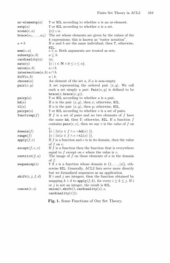
Finite Set Theory in ACL2 319
ur-elementp(a) T or NIL according to whether a is an ur-element.setp(a) T or NIL according to whether a is a set.scons(e, a) {e} ∪ a.brace(α1, . . . , αk) The set whose elements are given by the values of the
k expressions; this is known as “roster notation”.a = b If a and b are the same individual, then T, otherwise,
NIL.mem(e, a) e ∈ a. Both arguments are treated as sets.subsetp(a, b) a ⊆ b.cardinality(a) |a|.nats(n) {i | i ∈ N ∧ 0 ≤ i ≤ n}.union(a, b) a ∪ b.intersection(a, b) a ∩ b.diff(a, b) a \ b.choose(a) An element of the set a, if a is non-empty.pair(x, y) A set representing the ordered pair 〈x, y〉. We call
such a set simply a pair. Pair(x, y) is defined to bebrace(x, brace(x, y)).
pairp(a) T or NIL according to whether a is a pair.hd(a) If a is the pair 〈x, y〉, then x; otherwise, NIL.tl(a) If a is the pair 〈x, y〉, then y; otherwise, NIL.pairps(s) T or NIL according to whether s is a set of pairs.functionp(f) If f is a set of pairs and no two elements of f have
the same hd, then T; otherwise, NIL. If a function fcontains pair(e, v), then we say v is the value of f one.
domain(f) {e | ∃x(x ∈ f ∧ e =hd(x) )}.range(f) {e | ∃x(x ∈ f ∧ e =tl(x) )}.apply(f, e) If f is a function and e is in its domain, then the value
of f on e.except(f, e, v) If f is a function then the function that is everywhere
equal to f except on e where the value is v.restrict(f, a) The image of f on those elements of a in the domain
of f .sequencep(s) T if s is a function whose domain is {1, . . . , |s|}, oth-
erwise NIL. Generally, ACL2 lists serve more directlybut we formalized sequences as an application.
shift(i, j, f, d) If i and j are integers, then the function obtained bymapping k + d to apply(f, k), for every i ≤ k ≤ j. If ior j is not an integer, the result is NIL.
concat(r, s) union(r, shift(1, cardinality(s), s,cardinality(r))).
Fig. 1. Some Functions of Our Set Theory.
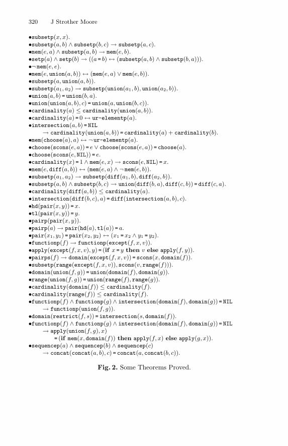
320 J Strother Moore
•subsetp(x, x).•subsetp(a, b) ∧ subsetp(b, c)→ subsetp(a, c).•mem(e, a) ∧ subsetp(a, b)→ mem(e, b).•setp(a) ∧ setp(b)→ ((a = b)↔ (subsetp(a, b) ∧ subsetp(b, a))).•¬ mem(e, e).•mem(e, union(a, b))↔ (mem(e, a) ∨ mem(e, b)).•subsetp(a, union(a, b)).•subsetp(a1, a2)→ subsetp(union(a1, b), union(a2, b)).•union(a, b) = union(b, a).•union(union(a, b), c) = union(a, union(b, c)).•cardinality(a) ≤ cardinality(union(a, b)).•cardinality(a) = 0↔ ur-elementp(a).•intersection(a, b) = NIL
→ cardinality(union(a, b)) = cardinality(a) + cardinality(b).•mem(choose(a), a)↔ ¬ ur-elementp(a).•choose(scons(e, a)) = e ∨ choose(scons(e, a)) = choose(a).•choose(scons(e, NIL)) = e.•cardinality(x) = 1 ∧ mem(e, x)→ scons(e, NIL) =x.•mem(e, diff(a, b))↔ (mem(e, a) ∧ ¬ mem(e, b)).•subsetp(a1, a2)→ subsetp(diff(a1, b),diff(a2, b)).•subsetp(a, b) ∧ subsetp(b, c)→ union(diff(b, a),diff(c, b)) = diff(c, a).•cardinality(diff(a, b)) ≤ cardinality(a).•intersection(diff(b, c), a) = diff(intersection(a, b), c).•hd(pair(x, y)) =x.•tl(pair(x, y)) = y.•pairp(pair(x, y)).•pairp(a)→ pair(hd(a),tl(a)) = a.•pair(x1, y1) = pair(x2, y2)↔ (x1 =x2 ∧ y1 = y2).•functionp(f)→ functionp(except(f, x, v)).•apply(except(f, x, v), y) = (if x = y then v else apply(f, y)).•pairps(f)→ domain(except(f, x, v)) = scons(x, domain(f)).•subsetp(range(except(f, x, v)), scons(v, range(f))).•domain(union(f, g)) = union(domain(f), domain(g)).•range(union(f, g)) = union(range(f), range(g)).•cardinality(domain(f)) ≤ cardinality(f).•cardinality(range(f)) ≤ cardinality(f).•functionp(f) ∧ functionp(g) ∧ intersection(domain(f), domain(g)) = NIL
→ functionp(union(f, g)).•domain(restrict(f, s)) = intersection(s,domain(f)).•functionp(f) ∧ functionp(g) ∧ intersection(domain(f), domain(g)) = NIL
→ apply(union(f, g), x)= (if mem(x, domain(f)) then apply(f, x) else apply(g, x)).
•sequencep(a) ∧ sequencep(b) ∧ sequencep(c)→ concat(concat(a, b), c) = concat(a,concat(b, c)).
Fig. 2. Some Theorems Proved.
Finite Set Theory in ACL2 321
ACL2 allows the user to constrain undefined functions to satisfy arbitraryproperties, provided some function (a “witness”) can be shown to have thoseproperties. Using this feature of ACL2, it is possible to introduce an undefinedchoice function, ch, which admits = as a congruence and which selects a memberof a non-empty set, without otherwise constraining the choice made. Our choosecan be used as a witness to introduce ch.
It should be noted that ch does not enjoy the analogue of the Weak Choose-Scons Property. That is, it is impossible to prove from the properties of ch abovethat ch(scons(e, s)) is either e or ch(s). For example, chmight choose the largestelement of the set if the cardinality of the set is odd and the smallest elementif the cardinality is even. Such a ch would have the required properties andfurthermore ch(scons(1, ’(2 3))) would be 3, which is neither 1 nor ch(’(2 3)),which is 2.
Therefore, even when using only the weak property, we assume more aboutchoose than we could about an arbitrary choice function. Most importantly, ourchoose is executable, which means that functions defined in terms of it are alsoexecutable. Such functions include pair, hd, tl and apply.
5 Behind the Scenes
Two sets are equal if and only if they are subsets of one another. If we define setequality this way, then equality, membership and subset are mutually recursive:set equality is defined in terms of subset, membership is iterated set equality,and subset is iterated membership. ACL2 supports mutual recursion. But mutualrecursion can be awkward when dealing with induction. To prove an inductivetheorem about one function in a clique of mutually recursive functions, onemust often prove a conjunction of related theorems about the other functions ofthe clique. While ACL2 can often manage the proofs, the user must state theconjunction of theorems in order for the conjecture to be strong enough to beprovable. We found this often inconvenient, especially in the early going whennothing but the definitions of the functions are available.
We considered many ways around this obstacle. The eventual solution, whichwas supported by some work done concurrently by Pete Manolios, was to intro-duce the notion of canonical forms. Without engaging in mutual recursion it ispossible to
– define a total order on our objects,– canonicalize lists so that their elements are presented in this order and with-out duplicates,
– define set equality to compare sets in canonical form,– define membership as iterated set equality,– define subset as iterated membership, and– prove that two sets are set equal iff they are subsets of one another.
This program actually has at least two interpretations and we explored both. Theinterpretation initially favored was to keep lists representing sets in canonical
322 J Strother Moore
form all the time. That is, the basic set constructor, e.g., scons(e, x), inserts e(if it is not already there) at the position in x at which it belongs. This has thepowerful attraction that set equality, =, is Leibniz identity, =.
But we found this approach to complicate set construction to a degree out ofproportion to its merits. In particular, functions like union and intersection,which are quite easy to reason about in the list world (where order and dupli-cation matter but are simply ignored), become quite difficult to reason about inthe set world, where most of the attention is paid to the sorting of the outputwith respect to the total ordering. In the end we abandoned this approach andadopted a second interpretation of the program above: lists representing setsare created and manipulated in non-canonical form and are canonicalized onlyfor determining whether two sets are equal. This was quite effective. Scons iscons (with appropriate treatment of :UR-CONS), union is essentially append,etc. ACL2 is designed to prove theorems about these kinds of functions.
Another question that drew our attention was: what are the “ur-elements”of our set theory? The first attack was to formalize hereditarily finite sets: finitesets built entirely from the empty set. Initially we felt that the details of the settheory were irrelevant to the user, since the high level individuals with which theuser would deal — numbers, sequences, functions, etc., — would be abstractlyrepresented. According to this thinking, proofs about these high level individualswould be conducted more or less algebraically, using theorems provided by theset theory book.
However, we found the use of hereditarily finite sets to be too cumbersome.
– Concrete examples of sets representing naturals, pairs, etc., were practicallyimpossible to read and comprehend. Here is 3 in the von Neumann repre-sentation of the naturals {{{{}}{}}{{}}{}}. It was hard to test definitionsand conjectures.
– The need to embed everything as sets forced ACL2 to spend its resourcesunraveling the embedding rather than dealing with the gist of the user’sproblem. This was particularly evident when dealing with arithmetic.
In the final view of this project, we saw the objective as to produce a settheory that was “natural” to ACL2’s mode of reasoning, so that its power wouldbe spent at the core of the user’s problem, not on getting down there. Arithmeticin our set theory is just ACL2’s arithmetic. Arbitrary ACL2 objects can be col-lected into sets. The set primitives are simple and their definitions are usuallyeasily manipulated to derive clean versions of the algebraic laws of set theory.Because of support for congruences, these laws can then be used in the normalway to manipulate set expressions without regard for how sets are actually rep-resented, provided certain basic conventions are followed. The main conventionsare that = be used to compare sets and that every time a new set generatingfunction is introduced the appropriate congruence rules are proved establishingthat the function admits set equality as a congruence relation.
Finite Set Theory in ACL2 323
6 Codified Proof Strategies
The set theory book includes several proof strategies particular to set theory.Such strategies are convenient because they overcome ACL2’s lack of quantifi-cation.
To prove α = β, where α and β are two set theory expressions that producesets (as opposed to ur-elements), it is sometimes convenient to prove that (e ∈α) ↔ (e ∈ β). That is, a set is entirely determined by its elements. This factmay be formalized in set theory as (∀e : e ∈ a↔ e ∈ b)→ a = b.
But ACL2 does not have the quantificational power to express this fact di-rectly.2 We have defined an ACL2 macro (named defx) that allows the userto direct the theorem prover to prove a theorem using a specified strategy.When defx is used to prove γ → α = β with the “set equivalence” strategyit generates two subgoals, γ ∧ mem(e, α) → mem(e, β) and its symmetric coun-terpart, and then proves the main theorem by “functional instantiation” [5]of a general theorem. (The general theorem can be described as follows. Sup-pose that alpha and beta are two 0-ary functions satisfying the constraintmem(e, alpha())→ mem(e, beta()). Then subsetp(alpha(), beta()) is a theorem.)
Another special strategy, called “functional equivalence,” is useful when αand β are functions: prove that applying them produces identical results. Foursubgoals are produced, (a) functionp(α), (b) functionp(β), (c) domain(α) =domain(β), and (d) mem(e, domain(α)) → apply(α, e) = apply(β, e). Proof obli-gation (d) could be simplified by dropping the hypothesis; we included it simplybecause it weakens the proof obligation. The previously mentioned theorem•sequencep(a) ∧ sequencep(b) ∧ sequencep(c)→ concat(concat(a, b), c) = concat(a, concat(b, c))
is proved with the functional equivalence strategy. (Sequences in this set theoryare functions. We would expect the ACL2 user to prefer to use the native lists,but we formalized sequences-as-functions to test the library.) The two concatexpressions are equivalent because they yeild the same results when applied toarbitrary indices.
Defx is defined in a general way that allows the user to add new strategies.(Hint to ACL2 cognoscenti: define each strategy as a macro. Defx forms expandto calls of the strategy.) The defx form provides a uniform appearance in com-mand files (“books”) and allows the continued use of Emacs’ tag feature forindexing names. This use of macros is novel to most ACL2 users.
7 Recursive Functions on Sets
The first order nature of ACL2, combined with the absence of quantification,prevents the formalization of set comprehension in its general form. That is, itis impossible in ACL2 to formalize with complete generality such notation as“{x | φ(x)}.” We have implemented some macros to mitigate the problem.2 Actually, ACL2 does provide full first-order quantification via defun-sk, but that isno more convenient that what we are about to describe.
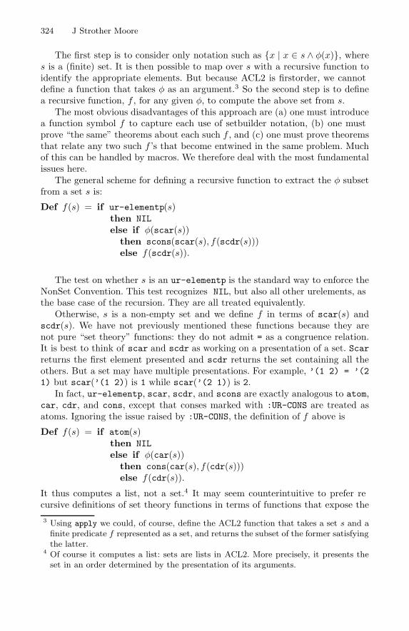
324 J Strother Moore
The first step is to consider only notation such as {x | x ∈ s ∧ φ(x)}, wheres is a (finite) set. It is then possible to map over s with a recursive function toidentify the appropriate elements. But because ACL2 is first-order, we cannotdefine a function that takes φ as an argument.3 So the second step is to definea recursive function, f , for any given φ, to compute the above set from s.
The most obvious disadvantages of this approach are (a) one must introducea function symbol f to capture each use of set-builder notation, (b) one mustprove “the same” theorems about each such f , and (c) one must prove theoremsthat relate any two such f ’s that become entwined in the same problem. Muchof this can be handled by macros. We therefore deal with the most fundamentalissues here.
The general scheme for defining a recursive function to extract the φ subsetfrom a set s is:
Def f(s) = if ur-elementp(s)then NILelse if φ(scar(s))
then scons(scar(s), f(scdr(s)))else f(scdr(s)).
The test on whether s is an ur-elementp is the standard way to enforce theNon-Set Convention. This test recognizes NIL, but also all other ur-elements, asthe base case of the recursion. They are all treated equivalently.
Otherwise, s is a non-empty set and we define f in terms of scar(s) andscdr(s). We have not previously mentioned these functions because they arenot pure “set theory” functions: they do not admit = as a congruence relation.It is best to think of scar and scdr as working on a presentation of a set. Scarreturns the first element presented and scdr returns the set containing all theothers. But a set may have multiple presentations. For example, ’(1 2) = ’(21) but scar(’(1 2)) is 1 while scar(’(2 1)) is 2.
In fact, ur-elementp, scar, scdr, and scons are exactly analogous to atom,car, cdr, and cons, except that conses marked with :UR-CONS are treated asatoms. Ignoring the issue raised by :UR-CONS, the definition of f above is
Def f(s) = if atom(s)then NILelse if φ(car(s))
then cons(car(s), f(cdr(s)))else f(cdr(s)).
It thus computes a list, not a set.4 It may seem counterintuitive to prefer re-cursive definitions of set theory functions in terms of functions that expose the
3 Using apply we could, of course, define the ACL2 function that takes a set s and afinite predicate f represented as a set, and returns the subset of the former satisfyingthe latter.
4 Of course it computes a list: sets are lists in ACL2. More precisely, it presents theset in an order determined by the presentation of its arguments.
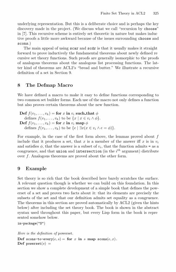
Finite Set Theory in ACL2 325
underlying representation. But this is a deliberate choice and is perhaps the keydiscovery made in the project. (We discuss what we call “recursion by choose”in [7]. This recursive scheme is entirely set theoretic in nature but makes induc-tive proofs a little more awkward because of the issues surrounding choose andscons.)
The main appeal of using scar and scdr is that it usually makes it straight-forward to prove inductively the fundamental theorems about newly defined re-cursive set theory functions. Such proofs are generally isomorphic to the proofsof analogous theorems about the analogous list processing functions. The lat-ter kind of theorems are ACL2’s “bread and butter.” We illustrate a recursivedefinition of a set in Section 9.
8 The Defmap Macro
We have defined a macro to make it easy to define functions corresponding totwo common set builder forms. Each use of the macro not only defines a functionbut also proves certain theorems about the new function.
Def f(v1, . . . , vk) = for x in vi such that φdefines f(v1, . . . , vk) to be {x | x ∈ vi ∧ φ}.
Def f(v1, . . . , vk) = for x in vi map φdefines f(v1, . . . , vk) to be {e | ∃x(x ∈ vi ∧ e = φ)}.
For example, in the case of the first form above, the lemmas proved about finclude that it produces a set, that x is a member of the answer iff x is in vi
and satisfies φ, that the answer is a subset of vi, that the function admits = as acongruence, and that union and intersection (in the ith argument) distributeover f . Analogous theorems are proved about the other form.
9 Example
Set theory is so rich that the book described here barely scratches the surface.A relevant question though is whether we can build on this foundation. In thissection we show a complete development of a simple book that defines the pow-erset of a set and proves two facts about it: that its elements are precisely thesubsets of the set and that our definition admits set equality as a congruence.The theorems in this section are proved automatically by ACL2 (given the hintsbelow) after including the set theory book. The book is shown in the abstractsyntax used throughout this paper, but every Lisp form in the book is repre-sented somehow below.in-package("S")
Here is the definition of powerset.
Def scons-to-every(e, s) = for x in s map scons(e, x).Def powerset(s) =
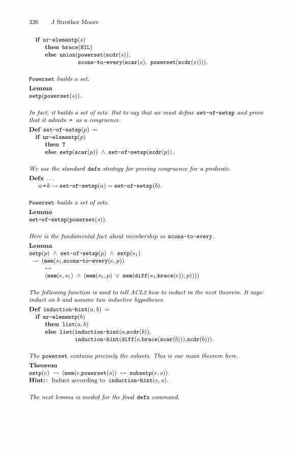
326 J Strother Moore
if ur-elementp(s)then brace(NIL)else union(powerset(scdr(s)),
scons-to-every(scar(s), powerset(scdr(s)))).
Powerset builds a set.
Lemmasetp(powerset(s)).
In fact, it builds a set of sets. But to say that we must define set-of-setsp and provethat it admits = as a congruence.
Def set-of-setsp(p) =if ur-elementp(p)
then T
else setp(scar(p)) ∧ set-of-setsp(scdr(p)).
We use the standard defx strategy for proving congruence for a predicate.
Defx . . .a = b→ set-of-setsp(a) = set-of-setsp(b).
Powerset builds a set of sets.
Lemmaset-of-setsp(powerset(s)).
Here is the fundamental fact about membership in scons-to-every.
Lemmasetp(p) ∧ set-of-setsp(p) ∧ setp(s1)→ (mem(s1,scons-to-every(e, p))
↔(mem(e, s1) ∧ (mem(s1, p) ∨ mem(diff(s1,brace(e)), p))))
The following function is used to tell ACL2 how to induct in the next theorem. It says:induct on b and assume two inductive hypotheses.
Def induction-hint(a, b) =if ur-elementp(b)
then list(a, b)else list(induction-hint(a,scdr(b)),
induction-hint(diff(a,brace(scar(b))),scdr(b))).
The powerset contains precisely the subsets. This is our main theorem here.
Theoremsetp(e) → (mem(e,powerset(s)) ↔ subsetp(e, s)).Hint:: Induct according to induction-hint(e, s).
The next lemma is needed for the final defx command.
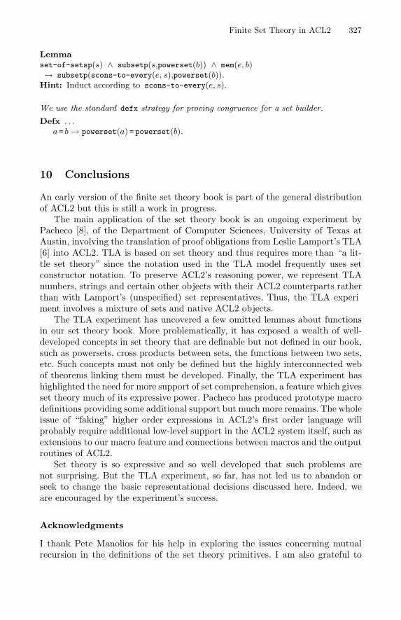
Finite Set Theory in ACL2 327
Lemmaset-of-setsp(s) ∧ subsetp(s,powerset(b)) ∧ mem(e, b)→ subsetp(scons-to-every(e, s),powerset(b)).
Hint: Induct according to scons-to-every(e, s).
We use the standard defx strategy for proving congruence for a set builder.
Defx . . .a = b→ powerset(a) = powerset(b).
10 Conclusions
An early version of the finite set theory book is part of the general distributionof ACL2 but this is still a work in progress.
The main application of the set theory book is an ongoing experiment byPacheco [8], of the Department of Computer Sciences, University of Texas atAustin, involving the translation of proof obligations from Leslie Lamport’s TLA[6] into ACL2. TLA is based on set theory and thus requires more than “a lit-tle set theory” since the notation used in the TLA model frequently uses setconstructor notation. To preserve ACL2’s reasoning power, we represent TLAnumbers, strings and certain other objects with their ACL2 counterparts ratherthan with Lamport’s (unspecified) set representatives. Thus, the TLA experi-ment involves a mixture of sets and native ACL2 objects.
The TLA experiment has uncovered a few omitted lemmas about functionsin our set theory book. More problematically, it has exposed a wealth of well-developed concepts in set theory that are definable but not defined in our book,such as powersets, cross products between sets, the functions between two sets,etc. Such concepts must not only be defined but the highly interconnected webof theorems linking them must be developed. Finally, the TLA experiment hashighlighted the need for more support of set comprehension, a feature which givesset theory much of its expressive power. Pacheco has produced prototype macrodefinitions providing some additional support but much more remains. The wholeissue of “faking” higher order expressions in ACL2’s first order language willprobably require additional low-level support in the ACL2 system itself, such asextensions to our macro feature and connections between macros and the outputroutines of ACL2.
Set theory is so expressive and so well developed that such problems arenot surprising. But the TLA experiment, so far, has not led us to abandon orseek to change the basic representational decisions discussed here. Indeed, weare encouraged by the experiment’s success.
Acknowledgments
I thank Pete Manolios for his help in exploring the issues concerning mutualrecursion in the definitions of the set theory primitives. I am also grateful to
328 J Strother Moore
Carlos Pacheco for his willingness to dive into the undocumented set theorybook and begin to use it. Finally, I am grateful to Yuan Yu and Leslie Lamportfor helping clarify the goals of the set theory work.
References
1. Grzegorz Bancerek. A model of ZF set theory language. Journal of FormalizedMathematics, 1, 1989. http://mizar.org/JFM/Vol1/zf_lang.html.
2. M. J. C. Gordon. Higher order logic, set theory or both? Inhttp://www.cl.cam.ac.uk/~mjcg/papers/holst/index.html. Invited talk,TPHOLs 96, Turku, Finland, August 1996.
3. M. Kaufmann, P. Manolios, and J S. Moore, editors. Computer-Aided Reasoning:ACL2 Case Studies. Kluwer Academic Press, 2000.
4. M. Kaufmann, P. Manolios, and J S. Moore. Computer-Aided Reasoning: AnApproach. Kluwer Academic Press, 2000.
5. M. Kaufmann and J S. Moore. Structured theory development for a mechanizedlogic. Journal of Automated Reasoning, 26(2):161–203, 2001.
6. L. Lamport. The temporal logic of actions. ACM Trans. on Programming Lan-guages and Systems, 16(3):872–923, May 1994.
7. J S. Moore. Recursion by choose. Inhttp://www.cs.utexas.edu/users/moore/publications/finite-set-theory/
recursion-by-choose.lisp. Department of Computer Sciences, University ofTexas at Austin, 2000.
8. Carlos Pacheco. Reasoning about TLA actions. Technical Report CS-TR-01-16, Computer Sciences, University of Texas at Austin, May 2001.http://www.cs.utexas.edu/ftp/pub/techreports/tr01-16.ps.Z.
9. L. C. Paulson. Set theory for verification: I. from foundations to functions. Journalof Automated Reasoning, 11:353–389, 1993.
10. L. C. Paulson. Set theory for verification: Ii. induction and recursion. Journal ofAutomated Reasoning, 15:167–215, 1995.
The HOL/NuPRL Proof TranslatorA Practical Approach to Formal Interoperability�
Pavel Naumov1, Mark-Oliver Stehr2, and Jose Meseguer2
1 Pennsylvania State University, Middletown, PA 17057, [email protected]
2 SRI International, Menlo Park, CA 94025, USA{stehr,meseguer}@csl.sri.com
Abstract. We have developed a proof translator from HOL into a clas-sical extension of NuPRL which is based on two lines of previous work.First, it draws on earlier work by Doug Howe, who developed a transla-tor of theorems from HOL into a classical extension of NuPRL which isjustified by a hybrid set-theoretic/computational semantics. Second, werely on our own previous work, which investigates this mapping from aproof-theoretic viewpoint and gives a constructive meta-logical proof ofits soundness. In this paper the logical foundations of the embedding ofHOL into this classical extension of NuPRL as well as technical aspectsof the proof translator implementation are discussed.
1 Introduction
During the last couple of decades we have witnessed an appearance of severaldominant theorem proving systems that have attracted considerable attentionand have gradually found their way into applications. Simultaneously, the sameprocess has fragmented the research community and has made work and resultsof any one group almost useless for the rest. The main reason for this fragmen-tation is the fact that a majority of modern theorem provers have been designedas stand-alone products that can not share formal results with other systems.Partially this can be explained by the fact that different systems are based onquite different logical foundations, which makes any translation a non-trivialmathematical problem. But probably even more importantly, the designers haveseldom seen the need for such compatibility. Their goal was to explore new ap-proaches, not to form standards. The need for compatibility appeared when theleading systems accumulated substantial libraries of formal theories producedby joint work of many users. Reproducing such theories in systems where theyare not available would be a very tedious and time-consuming task. At the sametime, those other systems have unique and interesting features that make them� The first author was supported by DARPA grant F30602-98-2-0198 on the initialstage of this work that was done at Cornell University, Ithaca, NY. We furthermoregratefully acknowledge support for the work conducted at SRI by DARPA and NASA(Contract NAS2-98073), by Office of Naval Research (Contract N00014-96-C-0114),by NSF Grant (CCR-9633363), and by a DAAD grant in the scope of HSP-III.
R.J. Boulton and P.B. Jackson (Eds.): TPHOLs 2001, LNCS 2152, pp. 329–345, 2001.c© Springer-Verlag Berlin Heidelberg 2001
330 Pavel Naumov, Mark-Oliver Stehr, and Jose Meseguer
attractive for some users. As a result, the need for proof translation tools hasbecome apparent.
1.1 Two Kinds of Translators
A translation of formal results from one system into another can be carried outat two different levels. First, one can translate statements of proven theoremsfrom a source system into a target system. Secondly, one can translate the proofsthemselves.
The first approach is obviously easier to implement, but it forces the targetsystem to trust the correctness of the source system. In addition, since systemsare usually based on different logical foundations, the user has to rely completelyon an (informal) meta-logical proof of the fact that the translator is based on alogically sound mapping. Besides, one can raise doubts about the validity of thecode of the translator that can have bugs or, for technical reasons, may slightlydeviate from the mapping used in the soundness proof. All these problems canbe avoided with the second approach, but the need to translate proofs makesthe implementation much harder.
Ideally, there is a close connection between the soundness of the mappingbetween the two formal systems and proof translation: If L and L′ are thesource and target logics, respectively, and α is the mapping of L into L′ thensoundness1 is the property that Γ �L P implies α(Γ ) �L′ α(P ) for any set Γ ofaxioms and any formula P . Hence, a proof of soundness would demonstrate thatfor each proof of P from Γ in L there is a corresponding proof of α(P ) from α(Γ )in L′. Furthermore, if the soundness proof is conducted in a constructive way,it implicitly contains a description of the translation algorithm that we need. Infact, in our case the proof translator from HOL into NuPRL is an algorithm,which is essentially extracted from a mathematical proof of soundness.
Obviously, soundness of the underlying mapping is the main theoretical re-quirement for the correctness of the proof translator. Notice, however, thatsoundness can always be achieved by extending the target system by additionalaxioms and inference rules, as it is often necessary in practice. Of course, suchan extension could make the target system inconsistent, which is why the sound-ness proof is meaningful only in the presence of a consistency proof of the targetsystem. Typically, such a consistency proof is done using an abstraction of thetarget system, e.g. by construction of a semantic model. In a more general setting,where we work relative to arbitrary theories, a suitably general model preserva-tion property2 property is that each modelM of L can be obtained from a modelM ′ of L′ by a mapping β such that β(M ′) |=L P iff M ′ |=L′ α(P ). Although aproof of model preservation is generally important for the translation mappingto be semantically meaningful, it is of little use for the implementation of theproof translator itself which typically relies on proof-theoretic constructions.
1 Soundness is the central property of a map of entailments systems, which representthe notion of derivability in general logics [14].
2 This property is usually expressed in the context of a map of institutions [8], whichconstitute the model-theoretic component of general logics [14].
The HOL/NuPRL Proof Translator 331
1.2 Previous Results
Some early work on translating formal results between theorem provers was con-ducted by Doug Howe and Amy Felty. In [12] Howe defined a mapping from HOL[9] into a classical extension of NuPRL [3] and gave a semantic justification forthe admissibility of this translation, essentially by constructing a hybrid set-theoretic/computational semantics for the classical extension of NuPRL3, whereHOL models appear as submodels of somewhat richer NuPRL models [10]. Later,Howe developed a translator [11] based on this mapping, which translates state-ments of HOL theorems. Since Howe gave only a semantic justification, extendingit to a proof translation is a non-trivial task. The practical usefulness of Howe’sHOL/NuPRL connection has been demonstrated in [7], where his translator isused to produce HOL/NuPRL hybrid proofs. In [17] the first author applied asimilar approach to built a translator from Isabelle’s higher-order logic [19] intoNuPRL. This work also sketched a soundness proof, which was so straightfor-ward that in [18] he has been able to formalize it in NuPRL. A correspondingsoundness proof can also be given for Howe’s original mapping from HOL intoNuPRL. In fact, we gave a detailed constructive proof in [22] using general log-ics terminology [14]. In this paper we present a proof translator from HOL to aclassical extension of NuPRL which is based on this proof. Comparison to otherclosely related works is done in the end of the paper.
1.3 Why Translating from HOL to NuPRL?
There are at least three factors to consider when selecting the source and thetarget systems for a proof translator to be useful in practice: (1) The sourcelogic should be supported by a well-established theorem proving system thathas accumulated a substantial amount of non-trivial results. (2) The target logicshould be sufficiently expressive to serve as a target for the translation, so thatthe translation is natural in the sense that, say, results about standard datatypes in the source logic can be interpreted as results about the correspondingdata types in the target logic. (3) The target logic should be equipped with asemantics that allows us to establish a close relationship to the semantics of thesource logic. Taking into account the previous results we think that the pairHOL/NuPRL is a good choice for the source and the target systems from theviewpoint of these three requirements.
1.4 Challenges
There are two major obstacles that we faced in the context of this work: Onthe theoretical level, the main challenge was to supplement Howe’s semanticjustification by a proof of soundness on which the translator could be potentiallybased. The primary concern here is that HOL inference rules, taken literally, are
3 We always use “NuPRL” to refer to Howe’s variant of NuPRL which enjoys thishybrid set-theretic/computational semantics. Howe’s classical extension of NuPRLis then obtained by adding type-theoretic version of the law of the excluded middle.
332 Pavel Naumov, Mark-Oliver Stehr, and Jose Meseguer
not sound in NuPRL. On the implementation level, a technical difficulty hasbeen the lack of proof objects in HOL. Hence, it was necessary to equip theHOL system with an explicit notion of proof objects and support for exportingsuch objects.
1.5 Paper Outline
We begin in Section 2 by giving a brief introduction to the logical foundationsof HOL and NuPRL and their implementations. Section 3 discusses the classicalextension of NuPRL that we are using and sketches the translation of formulasand proofs. Section 4 gives a high-level description of the translator and com-plements it with a discussion of some implementation details and some practicalexperience that we have found to be interesting. We compare our work with re-cent work by Ewen Denney [6] on translating proofs from HOL to Coq in Section5. Finally, we present some conclusions in Section 6.
2 Overview of the Theorem Provers
This section gives a brief introduction to the HOL and NuPRL proof develop-ment systems and their underlying formal logics and type theories.
2.1 The HOL System
Logic. HOL [9] is an interactive theorem prover based on a Gentzen-style for-malization of higher-order logic over a simply typed lambda calculus extended byHindley-Milner polymorphism, which admits types with (implicitly quantified)type variables.
Syntactically, HOL clearly distinguishes two kinds of entities: types andterms. Types are built from type variables and type constants, which includetype operators and regular type constants:
Type := TypeV ar | TypeConst(Type1, . . . , T ypen)
HOL terms are constructed from free and bound variables as well as constantsusing application and typed λ-abstraction:
Term := FV arType | BV ar | ConstType | Term Term | λ Type . T erm
Notice that HOL terms carry explicit type information embedded into them. Thisis done by specifying free variables and constants together with their types. Sincebound variables are implemented using de Bruijn indices [5], bound variables arejust natural numbers, but their types can be extracted from the type of the λ-term they refer to. In HOL all terms used in theories and rules are well-typed,and, as a result, the unique type of any HOL term can be recursively computed.In spite of the use of de Bruijn indices in the HOL system we prefer to use namesin the following for better readability.
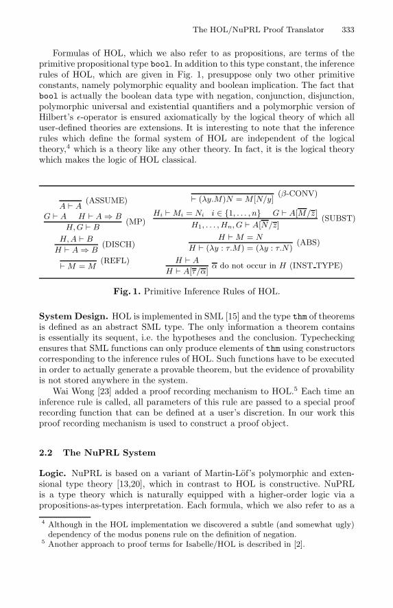
The HOL/NuPRL Proof Translator 333
Formulas of HOL, which we also refer to as propositions, are terms of theprimitive propositional type bool. In addition to this type constant, the inferencerules of HOL, which are given in Fig. 1, presuppose only two other primitiveconstants, namely polymorphic equality and boolean implication. The fact thatbool is actually the boolean data type with negation, conjunction, disjunction,polymorphic universal and existential quantifiers and a polymorphic version ofHilbert’s ε-operator is ensured axiomatically by the logical theory of which alluser-defined theories are extensions. It is interesting to note that the inferencerules which define the formal system of HOL are independent of the logicaltheory,4 which is a theory like any other theory. In fact, it is the logical theorywhich makes the logic of HOL classical.
A � A(ASSUME)
G � A H � A⇒ B
H,G � B(MP)
H,A � B
H � A⇒ B(DISCH)
�M = M(REFL)
� (λy.M)N = M [N/y](β-CONV)
Hi �Mi = Ni i ∈ {1, . . . , n} G � A[M/z]
H1, . . . , Hn, G � A[N/z](SUBST)
H �M = N
H � (λy : τ.M) = (λy : τ.N)(ABS)
H � A
H � A[τ/α]α do not occur in H (INST TYPE)
Fig. 1. Primitive Inference Rules of HOL.
System Design. HOL is implemented in SML [15] and the type thm of theoremsis defined as an abstract SML type. The only information a theorem containsis essentially its sequent, i.e. the hypotheses and the conclusion. Typecheckingensures that SML functions can only produce elements of thm using constructorscorresponding to the inference rules of HOL. Such functions have to be executedin order to actually generate a provable theorem, but the evidence of provabilityis not stored anywhere in the system.
Wai Wong [23] added a proof recording mechanism to HOL.5 Each time aninference rule is called, all parameters of this rule are passed to a special proofrecording function that can be defined at a user’s discretion. In our work thisproof recording mechanism is used to construct a proof object.
2.2 The NuPRL System
Logic. NuPRL is based on a variant of Martin-Lof’s polymorphic and exten-sional type theory [13,20], which in contrast to HOL is constructive. NuPRLis a type theory which is naturally equipped with a higher-order logic via apropositions-as-types interpretation. Each formula, which we also refer to as a
4 Although in the HOL implementation we discovered a subtle (and somewhat ugly)dependency of the modus ponens rule on the definition of negation.
5 Another approach to proof terms for Isabelle/HOL is described in [2].
334 Pavel Naumov, Mark-Oliver Stehr, and Jose Meseguer
proposition, can be interpreted as a type, and provability of this formula corre-sponds to the fact this type is inhabited. Unlike some other type theories such asthe Calculus of Constructions [4] the elements of such propositional types shouldnot be interpreted as proofs, since type checking in NuPRL is not decidable, butmerely represents the computational contents of the associated proposition.
Both types and their elements are represented in NuPRL by terms. Theseterms are untyped in the sense that there is in general no effective procedureto reconstruct types of NuPRL terms, which is why NuPRL is sometimes calledan “untyped type theory”. Syntactically, a NuPRL term is build from so-calledabstractions, where each abstraction has an identifier, a list of parameters, anda list of subterms with binders. A subterm with binder is a term with an at-tached list of variables bound by it. The abstraction identifier (such as var, int,add, lambda, etc.) is the main descriptor, but sometimes an abstraction requiresextra parameters to be specified. For example, each variable is represented asan abstraction var together with its name as a parameter. As one can see, thetype information is not a fixed part of the NuPRL term structure, and reflectingthe polymorphic nature of NuPRL, some terms, such as the λ-abstraction λx.x,represent elements of many different types. The NuPRL abstraction mechanismis a powerful tool, which in connection with NuPRL’s user-definable displayforms, provides syntactic flexibility and readability. In most cases abstractionsare introduced by specifying them through existing ones, but it is also possibleto introduce an abstraction that is not associated with a definition, in whichcase we refer to it as a primitive abstraction. A special case of abstractions areconstants, which do not have any associated subterms.
The flexibility of NuPRL’s polymorphism and the fact that NuPRL does notimpose computability of types in any sense enables NuPRL to use a rich andopen-ended type theory, which has a predicative cumulative hierarchy of typeuniverses, dependent function types, subset types, parametrized inductive types,quotient types, and other features not present in HOL. As one would expect,most features of NuPRL are not essential for representing HOL theories. In fact,only a few abstractions and inference rules of NuPRL will be used by our prooftranslator. A detailed description of a fragment of NuPRL sufficient for our workcan be found in [21].
System Design. NuPRL is implemented in a hybrid programming frameworkof Common Lisp and Classic ML. Core parts of the system are written in Lisp,and ML is mostly used as the language to express theorem proving tactics. Datastructures for NuPRL terms and proofs are defined in Lisp but are accessiblevia an ML interface. As a result, dealing with the Lisp part of NuPRL is rarelynecessary. In fact, we have implemented the main part of the proof translatorentirely in Classic ML on the top of NuPRL.
Unlike HOL, NuPRL uses an explicit representation of proofs as trees. Aproof of a theorem consists of the theorem itself, a justification which allowsus to infer this theorem, and a list of subproofs, containing one proof for eachpremise needed by the justification. The justification can either be an instanceof a NuPRL inference rule, or, more generally, a NuPRL tactic. To emphasize

The HOL/NuPRL Proof Translator 335
the style of backward-reasoning employed in NuPRL, we refer to the theoremsof the proof and its subproofs also as the goal and its subgoals, respectively.
3 Logical Foundations of the Translator
In [21] we have shown that the mapping from HOL to the classical extensionof NuPRL can be understood in the framework of general logics [14] as a com-position of two stages: The first stage is a translation of an axiomatic theory ofHOL into an axiomatic theory of the classical extension of NuPRL. The use ofthe term “axiomatic” emphasizes the fact that the theories are not necessarilyonly definitional extensions of the base logic. The second stage is the interpreta-tion of an axiomatic theory inside the classical extension of NuPRL.6 Whereasthe translation stage is of meta-logical nature, the interpretation stage can takeplace inside the logic of NuPRL in a formally rigorous way. However, since thereare many possible choices for the interpretation of translated HOL theories inNuPRL theories, and certain proofs, namely of the NuPRL axioms resultingfrom the translation of HOL axioms, to be carried out, the user might need tointervene before each separate HOL theory is translated.
3.1 A Classical Extension of NuPRL
Unlike HOL, NuPRL is based on a constructive type theory. Hence, valid HOLtheorems like the law of the excluded middle ∀P.P∨¬P and logical extensionality∀P.(P ⇔ Q) ⇔ (P = Q) are not provable in NuPRL. There are at least threepotential ways to set up the translation:
– First, one can look for a translation that maps HOL into the constructivetype theory of NuPRL. For instance, Godel’s double-negation translation(see, for example, [16], p.98) is known to do just that. Unfortunately, doublenegation or any similar translation would not be very useful for connectingtheorem proving systems. The results translated under a non-trivial mappingare difficult to use as lemmas in the target system. Notice also that thistranslation would still require logical extensionality as an axiom.
– Second, one can consider a stronger non-conservative extension of the con-structive type theory of NuPRL by the axiom of the excluded middle, andconsider the most straightforward mapping of HOL in this classical exten-sion of NuPRL. Under such a mapping, HOL propositions are translated intoNuPRL propositions and logical HOL operators into their NuPRL counter-parts. Unfortunately, this approach does not lead to a general solution. Thedifficulty is that HOL is an impredicative higher-order logic, but NuPRL hasa predicative higher-order logic, which is inherited from its predicative typetheory via the Curry-Howard isomorphism. As a consequence, the proposi-tional type bool of HOL is closed under universal quantification, whereas
6 By means of an interpretation we can often obtain a computationally meaningful the-ory which makes only use of the constructive sublanguage of the classical extensionof NuPRL that we consider in this paper.
336 Pavel Naumov, Mark-Oliver Stehr, and Jose Meseguer
in NuPRL the use of universal quantification over a proposition in Pi canresult in a proposition from a higher propositional universe Pi+1. Hence,there is no single propositional universe in NuPRL that is a suitable imageof HOL’s propositional type bool under this translation. Still, this partialsolution could be useful to translate certain predicative developments fromHOL into NuPRL.7 On the other hand, such an approach provides a simpleand general solution for the embedding of HOL into an impredicative typetheory such as the Calculus of Inductive Constructions (cf. Section 5).
– Third, following Howe [12] one can translate HOL’s propositional type boolinto the boolean type B of NuPRL. The type B is not one of the NuPRLprimitive types, but is defined as a disjoint union of two single-element types,and all the operators of boolean logic and their (classical) properties are de-rived, including the law of the excluded middle and logical extensionality.Clearly, B is a model of classical boolean logic inside NuPRL’s constructivetype theory, and therefore an obvious candidate for the image of the HOLtype bool. The only problem is that it lacks some of the features neededfor the translation, namely a polymorphic boolean-valued equality, a poly-morphic boolean-valued universal quantifier, and a polymorphic version ofHilbert’s ε-operator which uses boolean-valued predicates.
In our work we have followed the third approach, since it seems to be the bestsolution in terms of usability and generality. To fill the remaining gap betweenthe propositional type bool of HOL and the boolean type B of NuPRL weextended NuPRL by new primitive abstractions and axioms as follows.
– HOL equality is a boolean predicate, unlike the standard NuPRL equalityx =T y which is a type living in some propositional univese Pi. In order totranslate HOL equality statements into NuPRL terms of type B, we definein NuPRL a new primitive abstraction x =b
T y which stands for boolean-valued equality of elements of a type T . The following two axioms, that wehave added to NuPRL, state that we have a boolean-valued equality thatprecisely mirrors NuPRL’s propositional equality:
∀T : Ui. ∀x, y : T. x =bT y ∈ B
∀T : Ui. ∀x, y : T. (↑ (x =bT y))⇔ x =T y
(where ↑ b stands for the proposition b =B true)– We dealt similarly with the universal quantifier which has type Pi in NuPRL,i.e. we introduced a boolean counterpart ∀b with the following axioms:
∀T : Ui. ∀b : T → B. (∀bx : T. b(x)) ∈ B
∀T : Ui. ∀b : T → B. (↑ ∀bx : T. b(x))⇐⇒ (∀x : T ↑ b(x))7 Notice, however that we cannot assume logical extensionality in NuPRL, since thiswould be inconsistent with NuPRL’s nontrivial data types, which cannot be distin-guished from propositional types.
The HOL/NuPRL Proof Translator 337
– Finally, we added a non-constructive ε-operator in order to interpret thecorresponding HOL operator. The axiom for this operator is:
∀T : U. ∀b : T → B. T ⇒ (εx : T. b(x)) ∈ T
For the understanding of the last axiom recall that NuPRL is based onpropositions-as-types paradigm and, as a result, any type T is simultaneouslya proposition which asserts non-emptiness of this type.
In [12] it is shown that the operators and axioms given above can all bederived from a simple extension of NuPRL by the axiom of the excluded middle∀P.P ∨¬P (more precisely, its type-theoretic version). Assumption of this axiomin NuPRL means, according to the propositions-as-types interpretation, that thecorresponding dependent type is inhabited by a function which “decides” for eachtype P if P is inhabited and returns one of its elements if this is the case. Infact, Howe uses this axiom to define a function ↓b that casts propositions intobooleans, and then defines boolean equality and the boolean universal quantifierby lifting their NuPRL counterparts using ↓b. Another function, that can beobviously derived from the axiom of the law of the excluded middle, selects anelement from a given non-empty type. Howe uses such a function to define theε-operator.
3.2 Translation of Formulas
The translation of formulas of HOL into propositions of NuPRL is a straightfor-ward recursive procedure once HOL constants are mapped into correspondingNuPRL constants. The mapping of constants, which we call a dictionary, has tobe provided by the user. The translation is then a natural extension of this map-ping to a mapping from the types and terms of HOL into the terms of NuPRL:Type operators of HOL are mapped to functions operating on type universes.Typed λ-abstractions of HOL are translated to λ-abstractions in NuPRL (al-though the latter are untyped, we decided to keep the type information for bet-ter readability). Furthermore, implicitly polymorphic functions (and their types)in HOL are translated to explicitly polymorphic functions (and correspondingtypes) in NuPRL, and suitable explicit type arguments are generated on theNuPRL side when such functions are applied.
The proof translator requires that the dictionary is an injective mapping ofHOL constants into NuPRL constants.8 For example, the HOL type bool ismapped to the NuPRL type B by an entry
α(bool) = B .
In some cases we would like to map an HOL constant to a more complicatedNuPRL term. For instance, the HOL conjunction ∧ is a function of type bool→8 In the theoretical treatment [21] we have abstracted from renaming issues by usingnames of HOL constants directly for NuPRL constants.
338 Pavel Naumov, Mark-Oliver Stehr, and Jose Meseguer
bool → bool, whereas in NuPRL conjunction ∧ is an abstraction with twosubterms but not a constant. Hence, we would like to have a translation:
α(∧) = λp, q.p ∧ qTo this end we exploit the flexibility provided by the interpretation stage men-tioned before, that is we introduce an explicit NuPRL counterpart for each HOLconstant, which in this case would be a new NuPRL constant ∧h and we in-terpret this constant by adding a definition ∧h := λp, q.p ∧ q. That makes thecorresponding dictionary entry a simple renaming, namely α(∧) = ∧h, and en-hances readability of the result of the translation. In a similar way we deal withother HOL constants such as ∨h, →h, =h, etc.
After an HOL formula is translated into a NuPRL formula it becomes a termof type B. In order to treat this term as a NuPRL theorem, we have to cast itinto a propositional type. To this end, we use the standard NuPRL functionassert ↑, which is defined as ↑ b := (b =B true). In addition, since, unlike HOL,NuPRL does not allow free variables in theorem statements, we bind all suchvariables by an appropriate universal quantifier. For instance, the HOL theoremxσ = xσ (provable in one step using the REFL rule), is translated into theNuPRL statement
∀α(σ) : S. ∀x : α(σ) ↑ (=h x x)
where S is a type of all representations of HOL types.9 Note that in most casestranslated HOL theorems can be lifted to NuPRL propositions by propagating ↑through boolean quantifiers, connectives, and equalities. This transforms theseboolean operations into their regular NuPRL (propositional) counterparts. Wehave developed a NuPRL tactic to perform this transformation.
3.3 Translation of Inference Rules
HOL inference rules, taken literally, are not valid in the classical extension ofNuPRL, because they are missing explicit well-formedness conditions. These con-ditions are implicit in HOL because a built-in type checking mechanism guaran-tees that each HOL term is well-formed. Because of its open-ended type system,NuPRL imposes much weaker a priori conditions on its terms. In fact, any syn-tactically valid expression is a term in NuPRL. In the inference rules of NuPRLwell-formedness is usually enforced through extra premises which give rise toso-called well-formedness subgoals during a proof. For the standard types ofNuPRL these subgoals can be proven automatically by NuPRL’s Auto tactic inthe majority of cases.
To translate inference rules from HOL into NuPRL we have to come up withderived rules in NuPRL that match HOL rules as closely as possible and have9 In order to interpret the HOL axiom for the ε-operator in NuPRL, all translationsof HOL types have to be nonempty. In the present version of the proof translatorwe ignore nonemptiness condition and just use Ui for S (instead of the subtype ofnon-empty types described in [12,21]), since most HOL proofs do not depend onthis condition. We think that in the future the proof translator should support bothpossibilities.
The HOL/NuPRL Proof Translator 339
suitable well-formedness subgoals to reflect the fact that only well-typed termsoccur in the rule. Our proof translator redirects well-formedness subgoals to theAuto tactic. Although in general these extra subgoals might not be provable byAuto tactic (or even false), in the case when the derived rules are applied to thetranslation of HOL formulas, well-formedness subgoals are provable by a slightlymodified version of the Auto tactic.
4 Implementation of the Proof Translator
4.1 Adding Proof Objects to HOL
The generation of new HOL theorems from existing ones is done in ML by HOLinference rules which are ML functions with an arbitrary number of arguments oftype thm and a result of the same type. Many actual proofs are written in termsof tactics which are, essentially, ML programs combining several applications ofinference rules.
Once an ML term of type thm is parsed by the system, verified by the typechecker, and executed successfully, the value of the term (representing the the-orem) becomes available and can be used as a lemma in other proofs, but thereis no way to reconstruct the proof from the resulting theorem.
Clearly, in order to translate HOL proofs into NuPRL we first have to recoverthose proofs. Our initial idea was to extract the proofs from the files containingthe ML code that generated them. Unfortunately, this is not an easy task. SinceHOL tactics could potentially make use of the full power of Standard ML, whichis the tactic-language of HOL, the proof translator would need to include ageneral compiler or interpreter from Standard ML into Classic ML, which isused in NuPRL as the tactic language.
A simpler approach, that we have eventually adopted, is to modify the HOLabstract data type thm in such a way that every element of this type storesadditional information about how it has been constructed. To achieve this, wehave changed the HOL definition of the thm type from
datatype thm = THM of Term.term list * Term.term
todatatype thm = THM of Term.term list * Term.term
* (string * just_arg list)
where an element of type string represents the name of the inference rule thatcreated this theorem and the list over just arg stores additional arguments thatdetermine the instance of the inference rule which was actually used. For exam-ple, if a theorem H � (λy.M) = (λy.N) was proven using the HOL abstractionrule
H �M = N
H � (λy.M) = (λy.N)(ABS)
then it will have ABS as the name of the inference rule and the variable y andtheorem H � M = N as its arguments10. We have modified all HOL theorem10 We are using Wong’s [23] just arg type to store inference rule arguments.
340 Pavel Naumov, Mark-Oliver Stehr, and Jose Meseguer
constructors that operate on the type thm to work correspondingly. Of course,once each theorem keep track of its parents theorems, the entire proof tree canbe reconstructed recursively.
After these modifications to HOL, we have recompiled the system to makeevery theorem in every HOL theory aware of its proof. Although, this modi-fication drastically increases the size of thm objects, we have not observed anoticeable degradation in the system performance.
4.2 Translating Rules as Tactics
Since HOL and NuPRL have different sets of primitive inference rules, typicallyseveral NuPRL rules have to be used to imitate one HOL rule. In the previoussection we have expressed this idea by saying that there are derived NuPRLrules that closely match HOL rules. Technically, since NuPRL does not have anexplicit concept of derived rules, we have written special NuPRL tactics thatcombine several primitive inference rule to mimic one derived rule application.
In most cases it was possible to define such tactics using existing NuPRLtactics such as the backchaining tactic BLemma together with a suitable theoremto model HOL inference rules. For example, the HOL inference rule
H,A � BH � A⇒ B
(DISCH)
is imitated by our translator essentially via backchaining through the lemma
∀p, q : B. (↑ p⇒↑ q)⇒↑ (⇒h p q)
followed by a decomposition of implication using the tactic D 0 and a call toNuPRL’s Auto tactic to eliminate potential well-formedness subgoals as dis-cussed earlier:
let DISCH = BLemma ’DISCH_lemma’ THENM D 0 THENW Auto;;
4.3 Dealing with Derived Rules of HOL
Our work was substantially complicated by the status of HOL derived rules.In spite of Gordon’s original intention [9] that all the HOL derived rules arereduced to primitive inference rules, in the version 90.10 of HOL that we haveused the majority of originally derived rules are represented in the HOL systemas new constructors for the thm type.11 Hence, the majority of derived rules areessentially proclaimed to be new primitive rules. Our understanding is that thischange has been done at some point in the past for efficiency reasons.
To face the reality of the HOL implementation we decided to constructNuPRL equivalents for these derived rules the same way as we have done it
11 Although the HOL system contains deactivated ML code that is supposed to definederived rules via primitive rules, an inspection of this code indicated that it is nolonger compatible with the current version of HOL.
The HOL/NuPRL Proof Translator 341
for primitive rules. On the positive side, the higher level of abstraction providedby the derived rules allows us to avoid reducing logical operators (in particularconjunction and the existential quantifier) to terms involving the ε-operator. Thisdoes not only lead to more readable proofs, but more importantly the ε-operatoris only needed in cases where it is explicitly used in a theory.12
4.4 Implementation Details
The proof translator is implemented as a pair of functions (export, import) intwo different dialects of ML. The function export is written in Standard MLand is integrated into the HOL system. When this function is called in theHOL environment on any theorem named theorem, a separate file theorem.mlis created and a description of the theorem’s proof is stored in the file in whatwe call portable theorem format. Essentially, this file contains a theorem togetherwith its associated proof tree written in Classic ML. When the theorem.ml fileis loaded into the NuPRL environment this tree is re-created as a Classic MLdata structure. The second function import, written in Classic ML, takes thisstructure as an argument, translates the theorem into a NuPRL proposition,proves it by invoking the NuPRL tactics corresponding to the HOL inferencerules given by the proof, and adds the new result to the NuPRL library.
Although the translation process itself does not require user intervention, itrelies on the user-defined dictionary in order to translate HOL constants intotheir NuPRL counterparts. The dictionary not only allows the user to choosemeaningful names for the translation of HOL constants, but it is also needed toavoid name clashes which can occur, since in the current version (4.2) NuPRLhas a flat name space, and the names for the translated constants could havebeen already used in one of the theories the user is working with.
4.5 Efficiency Issues
Although the translated proofs that the proof translator produced in a numberof small examples of logical nature are valid NuPRL proofs, we were surprisedby their sizes. In many cases, a few lines of HOL proofs, invoking just a fewtactic calls, turned out to hide thousands of HOL inference rule applications(see Figure 2). Since every HOL inference rule call is translated into a NuPRLtactic call, which itself normally requires several inference rule applications, theresulting NuPRL proofs even for basic propositional theorems are unexpectedlylong. From our experience, it takes NuPRL several minutes just to check thevalidity of the produced proof.
5 Related Work
The translation of proofs between higher-order logic theorem provers is a rel-atively new field which has both practical potential and interesting theoretical12 The current version of our proof translator can deal with nearly all basic inference
rules and most of the derived rules mentioned above. In this point we are extendingthe theoretical treatment [21] which uses the HOL logic as presented in [9].
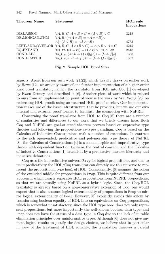
342 Pavel Naumov, Mark-Oliver Stehr, and Jose Meseguer
Theorem Name Statement HOL ruleinvocations
DISJ ASSOC ∀A,B, C. A ∨B ∨ C = (A ∨B) ∨ C 3218DE MORGAN THM ∀A,B. (¬(A ∧ B) = ¬A ∨ ¬B)∧
∧(¬(A ∨B) = ¬A ∧ ¬B) 4733LEFT AND OVER OR ∀A,B, C. A ∧ (B ∨ C) = A ∧B ∨A ∧ C 4215EQ EXPAND ∀t1, t2. (t1 = t2) = t1 ∧ t2 ∨ ¬t1 ∧ ¬t2 2618COND ABS ∀b, f, g. (λx.b⇒ (fx)|(gx)) = (b⇒ f |g) 1368COND RATOR ∀b, f, g, x. (b⇒ f |g)x = (b⇒ (fx)|(gx)) 1357
Fig. 2. Sample HOL Proof Sizes.
aspects. Apart from our own work [21,22], which heavily draws on earlier workby Howe [12], we are only aware of one further implementation of a higher-orderlogic proof translator, namely the translator from HOL into Coq [1] developedby Ewen Denney and described in [6]. Another piece of work which is relatedto ours from an implementation point of view is the work by Wai Wong [23] onrechecking HOL proofs using an external HOL proof checker. Our implementa-tion makes use of the basic infrastructure that he provides, but we use our owninternal and external proof format to facilitate the connection with NuPRL.
Concerning the proof translator from HOL to Coq [6] there are a numberof similarities and differences to our work that we briefly discuss here. BothCoq and NuPRL are goal-oriented theorem provers based on expressive typetheories and following the propositions-as-types paradigm. Coq is based on theCalculus of Inductive Constructions with a number of extensions. In contrastto the rich open-ended, predicative and polymorphic type theory of NuPRL[3], the Calculus of Constructions [4] is a monomorphic and impredicative typetheory with dependent function types as the central concept, and the Calculusof Inductive Constructions [1] extends it by a predicative universe hierarchy andinductive definitions.
Coq uses the impredicative universe Prop for logical propositions, and due toits impredicativity the HOL/Coq translator can directly use this universe to rep-resent the propositional type bool of HOL. Consequently, [6] assumes the axiomof the excluded middle for propositions in Prop. This is quite different from ourapproach, which clearly separates HOL propositions from NuPRL propositions,so that we are actually using NuPRL as a hybrid logic. Since, the Coq/HOLtranslator is already based on a non-conservative extension of Coq, one wouldexpect that it also assumes logical extensionality of propositions in Prop to mir-ror logical extensionality of bool. However, [6] explicitly avoids this axiom bytransforming boolean equality of HOL into an equivalence on Coq propositions,which is somewhat unsatisfactory, since the HOL type bool does not only repre-sent propositions, but more importantly the well-known boolean data type, andProp does not have the status of a data type in Coq due to the lack of suitableelimination principles over uninformative types. Although [6] does not give anymeta-logical results to justify the design choices, we believe that in particularin view of the treatment of HOL equality, the translation deserves a careful
The HOL/NuPRL Proof Translator 343
study, since functions in HOL clearly respect equality, but the correspondingequivalence in Coq does not in general enjoy the Leibnitz property.13
In spite of these foundational differences, we found many similarities on thepractical side, namely that both translators make use of an intermediate portableproof format for exchanging proofs between the two provers, and they both usemostly backchaining via suitable lemmas to model applications of HOL primitiveinference rules. A unique feature of the HOL/Coq translator is the use of theDAG representation of the proof in the intermediate format and an automated“factoring out” of lemmas in the final proof. We think that this is an interestingidea worth considering also for the HOL/NuPRL translator which could partiallysolve the inefficiency issues we have discussed before.
Apart from the differences in the choice of the theorem provers and themapping, there is a more important methodological difference between these twolines of research. Our starting point was the semantic justification that Howe gavefor the mapping from HOL into NuPRL [12] together with our proof-theoreticsoundness proof for this mapping [21] from which we essentially derived theproof translator. The work [6], however, neither gives a corresponding soundnessproof for the mapping from HOL to Coq nor a semantic justification. We thinkthat in general such meta-logical justifications are important to obtain a betterunderstanding of the translation mapping. On the other hand, since Coq isbased on a monomorphic and impredicative type theory in contrast to NuPRLwhich is polymorphic and predicative, the intuitive distance between HOL andCoq is smaller than the distance between HOL and NuPRL, both from a type-theoretic and from a semantic point of view, which makes such meta-theoreticaljustifications probably more critical for the HOL/NuPRL translator.
6 Conclusions
We have discussed the design principles and the implementation of a proof trans-lator from HOL to NuPRL. The design of the translator is based on our math-ematical proof of soundness for a mapping of HOL theories to NuPRL theories[21]. The mapping at the level of theories agrees with Howe’s translation [12],but our justification is proof-theoretic whereas Howe’s is semantic. Both ap-proaches complement each other. Furthermore, the proof-theoretic nature of ourresult provides a method for the translation of HOL proofs into NuPRL proofs.In summary, we have designed and implemented a translator based on strongmeta-logical justifications, both semantic (thanks to Howe) and proof-theoretic(our own) which in addition generates proofs as internal justifications in the tar-get logic. Further work is required to cover some additional inference rules andto reduce the size of proofs, so that translation of large developments becomesfeasible.
13 An issue that remains unclear in [6] is how non-emptiness of HOL types is reflected.In practice, we found that most HOL proofs do not need this assumption, althoughit is needed for the interpretation of the logical theory of HOL.
344 Pavel Naumov, Mark-Oliver Stehr, and Jose Meseguer
Acknowledgements
We would like to thank Robert Constable and Stuart Allen for several discussionson the particularities of NuPRL and the issue of logic translation. We also wouldlike to thank Doug Howe, since this project draws on his earlier work and wouldnot have been possible without his support. He made not only the source code ofthe HOL/NuPRL connection available to us, but he also gave us the opportunityto discuss with him our initial ideas on a proof-theoretic soundness result.
References
1. B. Barras et al. The Coq Proof Assistant Reference Manual: Version 6.1. TechnicalReport RT-0203, INRIA, May 1997.
2. S. Berghofer and T. Nipkow. Proof terms for simply typed higher order logic. InM. Aagaard and J. Harrison, editors, 13th International Conference on TheoremProving in Higher Order Logics, volume 1869 of Lecture Notes in Computer Science,pages 38–52, Portland, Oregon, August 2000. Springer.
3. R.L. Constable et al. Implementing Mathematics with Nuprl Proof DevelopmentSystem. Prentice Hall, 1986.
4. T. Coquand and G. Huet. The calculus of constructions. Information and Com-putation, 76(2/3):95–120, 1988.
5. N.G. de Bruijn. Lambda calculus notation with nameless dummies, a tool forautomatic formula manipulation, with application to the Church-Rosser theorem.Indag. Math., 34:381–392, 1972.
6. E. Denney. A Prototype Proof Translator from HOL to Coq. In M. Aagaard andJ. Harrison, editors, The 13th International Conference on Theorem Proving inHigher Order Logics, volume 1869 of Lecture Notes in Computer Science, pages108–125, Portland, Oregon, August 2000. Springer-Verlag.
7. A.P. Felty and D.J. Howe. Hybrid interactive theorem proving using Nuprl andHOL. In W. McCune, editor, Automated Deduction – CADE-14, volume 1249of Lecture Notes in Artificial Intelligence, pages 351–365, Berlin, 1997. Springer-Verlag.
8. J. Goguen and R. Burstall. Institutions: Abstract model theory for specificationand programming. Journal of the ACM, 39(1):95–146, 1992.
9. M.J.C. Gordon and T.F. Melham. Introduction to HOL – A Theorem ProvingEnvironment for Higher Order Logic. Cambridge University Press, 1993.
10. D. J. Howe. A classical set-theoretic model of polymorphic extensional type theory.Manuscript.
11. D.J. Howe. Importing mathematics from HOL into Nuprl. In J. von Wright,J. Grundy, and J. Harrison, editors, Theorem Proving in Higher Order Logics,volume 1125 of Lecture Notes in Computer Science, pages 267–282, Berlin, 1996.Springer-Verlag.
12. D.J Howe. Semantics foundation for embedding HOL in Nuprl. In M. Wirsing andA. Nivat, editors, Algebraic Methodology and Software Technology, volume 1101 ofLecture Notes in Computer Science, pages 85–101, Berlin, 1996. Springer-Verlag.
13. P. Martin-Lof. Intuitionistic Type Theory. Bibliopolis, Napoli, 1984.14. J. Meseguer. General logics. In H.-D. Ebbinghaus et al., editor, Logical Colloquium,
1987, pages 275–329. North-Holland, 1989.15. R. Milner, M. Tofte, R.M. Harper, and D.B. MacQueen. The Definition of Standard
ML (Revised). MIT Press, Cambridge, 1997.
The HOL/NuPRL Proof Translator 345
16. G. Mints. A Short Introduction to Intuitionistic Logic. Kluwer Academic/PlenumPublishers, 2000.
17. P. Naumov. Importing Isabelle Formal Mathematics into NuPRL. In Supplementalproceedings of the 12th International Conference on Theorem Proving in HigherOrder Logics, Nice, France, September 1999.
18. P. Naumov. Formalization of Isabelle Meta Logic in NuPRL. In Supplementalproceedings of the 13th International Conference on Theorem Proving in HigherOrder Logics, pages 141–156, Portland, OR, August 2000.
19. L.C. Paulson. Isabelle – A Generic Theorem Prover, volume 828 of Lecture Notesin Computer Science. Springer-Verlag, Berlin, 1994.
20. K. Petersson, J. Smith, and B. Nordstroem. Programming in Martin-Lof ’s TypeTheory. An Introduction. International Series of Monographs on Computer Science.Oxford: Clarendon Press, 1990.
21. M.-O. Stehr, P. Naumov, and J. Meseguer. A proof-theoretic approach toHOL-Nuprl connection with applications to proof translation (full version).http://cs.hbg.psu.edu/~naumov/Papers/holnuprl.ps , March 2000.
22. M.-O. Stehr, P. Naumov, and J. Meseguer. A proof-theoretic approach to HOL-Nuprl connection with applications to proof translation. In 15th InternationalWorkshop on Algebraic Development Techniques, Genova, Italy, April 2001. Toappear. See [21] for the full version.
23. W. Wong. Validation of HOL proofs by proof checking. Formal Methods in SystemDesign: An International Journal, 14(2):193–212, 1999.
Formalizing Convex Hull Algorithms
David Pichardie1 and Yves Bertot2
1 ENS [email protected]
2 INRIA Sophia [email protected]
Abstract. We study the development of formally proved algorithms forcomputational geometry. The result of this work is a formal descrip-tion of the basic principles that make convex hull algorithms work andtwo programs that implement convex hull computation and have beenautomatically obtained from formally verified mathematical proofs. Aspecial attention has been given to handling degenerate cases that areoften overlooked by conventional algorithm presentations.
1 Introduction
Algorithms to compute the convex hull of a collection of points in two or three di-mensions abound. The complexity of this problem is known to be approximatelythe same as for a sorting algorithm in the worst case, but the average complexitydepends very much on the distribution of data: some algorithms actually havea complexity of the form n × h, where n is the total number of points and h isthe number of points on the convex hull. These algorithms will be more efficientthan nlog(n) when few points are on the convex hull. This makes it useful tohave several algorithms around.
We have studied two algorithms. The first is an incremental algorithm, wherenew points are progressively added to the input data. If the new point is outsidethe convex hull, then it is necessary to add two new edges to the convex hull andremove some others. The second algorithm is known as the package-wrappingalgorithm: it follows the intuition of tying a band around the collection of points.At the nth step, the band is already in contact with a few points and the al-gorithm proceeds by computing what the next point is going to be: if with theband turning clockwise around the points, the next point in the hull is going tobe the leftmost remaining point.
All these algorithms rely on an orientation predicate that expresses whetherthe points of a triangle are enumerated clockwise or counter-clockwise. Thisorientation predicate is easily computed using the coordinates of the points, butit is meaningless when the points are aligned. Usual presentation of convex hullsalgorithms assume that three points in the input data are never aligned.
The structure of convex hull algorithms rely on the fact that the orienta-tion predicate satisfies some properties: for instance the triangles built with four
R.J. Boulton and P.B. Jackson (Eds.): TPHOLs 2001, LNCS 2152, pp. 346–361, 2001.c© Springer-Verlag Berlin Heidelberg 2001
Formalizing Convex Hull Algorithms 347
points have to be oriented in a consistent manner. Knuth [8] describes the min-imal properties of the orientation predicates and calls them axioms.
Knuth’s approach of axioms for convex hulls has the nice property of sepa-rating concerns about the properties of arithmetic expressions containing pointcoordinates and the control structure of algorithms. It has proved a good orga-nization principle for our description and proof development.
Thus, our work contains distinct parts. The first part is about the axioms, andshowing that they hold for an implementation predicate. This part involves somenumerical computation. The second part describes the main structure of thealgorithms based on the axioms, with numeric computation completely avoided.In the last part, we revisit the algorithms to make them robust with respect todegenerate data.
All our proofs have been mechanically checked using the Coq system [2].
1.1 Related Work
Automatic theorem proving and geometry have been in contact for some time.The work in this domain that we are better aware of is that of Chou [5]. In thisdevelopment, theorems about basic geometric figures like straight lines, trianglesand circles are proved automatically, but there is no result about computationalgeometry per se, since algorithms are not the object of the study, but there areother similarities. This work introduces a clever reasoning methods based onsurfaces of triangles and ratios of lengths to establish many results (more than400 theorems, whose proofs are done automatically, are described in the book).This approach using triangle areas is related to the one in this paper, becausethe determinant we compute actually correspond to the “oriented area” of thetriangle being observed. For instance, Axiom 4 can simply be interpreted as thesize of triangle being the sum of sub-triangles that compose it. Thus, Chou’swork shows before ours the benefit there is to find a different level of abstractionto reason on geometry.
Puitg and Dufourd [9], used the Coq proof system to describe notions ofplanarity. Work on finding minimal axioms to describe geometric concepts hasalso been done in constructive proof theory by Jan von Plato [11] and formal-ized in Coq by Gilles Kahn [7]. Last, we should refer to all the work done oncomputational geometry, but this domain is far too large to be cited entirely, wecan only refer to the books we have used as reference, [6], [3], and [10].
2 Knuth’s “Axioms” for Convex Hulls
In what follows, we assume that points are taken from a set P and we describethe orientation predicate as a predicate over three points p, q, r in P , which wedenote pqr.
Knuth’s axioms describe the various ways in which triangles can be lookedat and arranged on the plane. The first axiom expresses that when enumeratingthe points of a triangle, one may start with any of them:
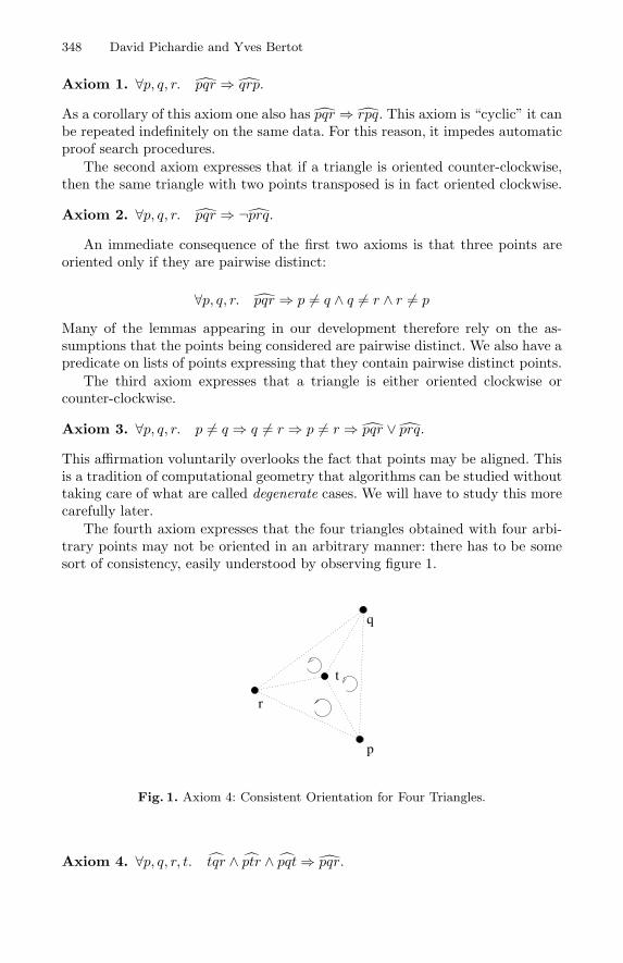
348 David Pichardie and Yves Bertot
Axiom 1. ∀p, q, r. pqr⇒ qrp.
As a corollary of this axiom one also has pqr⇒ rpq. This axiom is “cyclic” it canbe repeated indefinitely on the same data. For this reason, it impedes automaticproof search procedures.
The second axiom expresses that if a triangle is oriented counter-clockwise,then the same triangle with two points transposed is in fact oriented clockwise.
Axiom 2. ∀p, q, r. pqr⇒ ¬prq.An immediate consequence of the first two axioms is that three points are
oriented only if they are pairwise distinct:
∀p, q, r. pqr ⇒ p �= q ∧ q �= r ∧ r �= p
Many of the lemmas appearing in our development therefore rely on the as-sumptions that the points being considered are pairwise distinct. We also have apredicate on lists of points expressing that they contain pairwise distinct points.
The third axiom expresses that a triangle is either oriented clockwise orcounter-clockwise.
Axiom 3. ∀p, q, r. p �= q ⇒ q �= r ⇒ p �= r⇒ pqr ∨ prq.This affirmation voluntarily overlooks the fact that points may be aligned. Thisis a tradition of computational geometry that algorithms can be studied withouttaking care of what are called degenerate cases. We will have to study this morecarefully later.
The fourth axiom expresses that the four triangles obtained with four arbi-trary points may not be oriented in an arbitrary manner: there has to be somesort of consistency, easily understood by observing figure 1.
p
q
r
t
Fig. 1. Axiom 4: Consistent Orientation for Four Triangles.
Axiom 4. ∀p, q, r, t. tqr ∧ ptr ∧ pqt⇒ pqr.
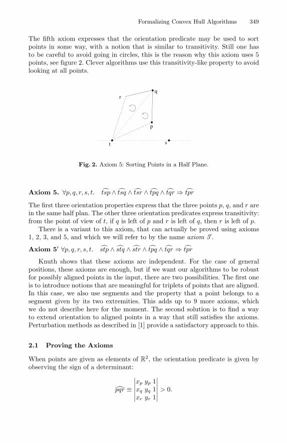
Formalizing Convex Hull Algorithms 349
The fifth axiom expresses that the orientation predicate may be used to sortpoints in some way, with a notion that is similar to transitivity. Still one hasto be careful to avoid going in circles, this is the reason why this axiom uses 5points, see figure 2. Clever algorithms use this transitivity-like property to avoidlooking at all points.
t s
p
qr
Fig. 2. Axiom 5: Sorting Points in a Half Plane.
Axiom 5. ∀p, q, r, s, t. tsp ∧ tsq ∧ tsr ∧ tpq ∧ tqr⇒ tpr
The first three orientation properties express that the three points p, q, and r arein the same half plan. The other three orientation predicates express transitivity:from the point of view of t, if q is left of p and r is left of q, then r is left of p.
There is a variant to this axiom, that can actually be proved using axioms1, 2, 3, and 5, and which we will refer to by the name axiom 5′.
Axiom 5′ ∀p, q, r, s, t. stp ∧ stq ∧ str ∧ tpq ∧ tqr ⇒ tpr
Knuth shows that these axioms are independent. For the case of generalpositions, these axioms are enough, but if we want our algorithms to be robustfor possibly aligned points in the input, there are two possibilities. The first oneis to introduce notions that are meaningful for triplets of points that are aligned.In this case, we also use segments and the property that a point belongs to asegment given by its two extremities. This adds up to 9 more axioms, whichwe do not describe here for the moment. The second solution is to find a wayto extend orientation to aligned points in a way that still satisfies the axioms.Perturbation methods as described in [1] provide a satisfactory approach to this.
2.1 Proving the Axioms
When points are given as elements of R2, the orientation predicate is given by
observing the sign of a determinant:
pqr ≡∣∣∣∣∣∣xp yp 1xq yq 1xr yr 1
∣∣∣∣∣∣> 0.
350 David Pichardie and Yves Bertot
In the following we will write |pqr| for this determinant. Knuth’s axioms are notproper axioms anymore, they become simple consequences of the properties ofaddition and multiplication of real numbers.
The proof of Axioms 1 and 2 is given by two equations:
|pqr| = |qrp|, |pqr| = −|prq|.
From a mechanical proof point of view, the proofs of these equalities is donepainlessly by the usual confluent rewriting system for ring structures, as imple-mented by the Ring tactic in Coq. Axiom 3 simply does not hold in general.When points are aligned, the determinant is null. A common solution to thisproblem is to consider only data that are in general position, that is, assumethat no three points given in the problem are ever aligned. We will first followthis practice to get a better idea of the algorithms. In a later section, we will seedifferent solutions to the problem of considering degenerate cases.
In man-made proofs, Axiom 4 relies on an equality obtained from a 4-by-4determinant that is obviously null, since it has 2 identical columns.
∣∣∣∣∣∣∣∣
xp yp 1 1xq yq 1 1xr yr 1 1xt yt 1 1
∣∣∣∣∣∣∣∣= |pqr| − |tqr| − |ptr| − |pqt| = 0.
Proving the right-hand side equality is also a simple matter of equality in a ringstructure. Now, if |tqr|, |ptr|, |pqt| are all strictly positive, then |pqr| is.
Verifying Axiom 5 also relies on an equation, known as Cramer’s equation,which has the following form:
|stq||tpr| = |tqr||stp|+ |tpq||str|
Here again, automatically proving this equation is a simple matter of ring basedcomputations.
The conclusion of this section on the orientation predicate is twofold. Firstnumeric computation can be done in a ring rather than in a complete field. Thisis important as one of the reasons for problems in geometric algorithms is theloss of precision in floating point arithmetic. For convex hulls, floating points arenot required. The points may be given by integer coordinates in a small grid. Iffloating points are used, one may notice that, since the determinant basically is apolynomial of degree two in the coordinates of the three points being considered,it is only necessary to compute the orientation predicate with a precision thatis double the precision of the input data.
2.2 The Specification
What is the convex hull of a set of points S? One definition is to describe it asa minimal subset S′ ⊂ S, such that all points in S can be described as positivelinear combinations of points in S′.
Formalizing Convex Hull Algorithms 351
An alternative description of the convex hull uses oriented edges. A possiblyopen line (i.i. a list of points) S′ encompasses a set of points S if for any point pin S and any two consecutive points ti, ti+1 in S′, titi+1p or p ∈ {titi+1} holds.We consider that a list l is a convex hull of S if l is included in S, l is non-emptyif S is not, l contains no duplicates, and if t is the last element of l, then t · l,formed by adding t at the head of l, encompasses S. In other terms, the convexhull is defined as a minimal intersection of half-planes.
When a data set is the empty set, a singleton, or a pair, then the convex hullis simply the list enumerating the set’s elements.
Knuth chooses the second definition in his monograph. We will also, forseveral reasons. First, lists are a natural data-structure in the functional pro-gramming language we use in our proofs. Second, this definition also relies onthe orientation predicate, thus making it possible to forget everything about nu-merical computation in the main structure of algorithm. Third, most algorithmsto compute convex hulls naturally rely on the fact that the intermediary datathey construct already is a list of points included in S.
The three parts of the specification are given using inductive definitions onlists (actually we also consider that the input data is given as a list of points).
Still, we have made an effort to establish a bridge between the two definitions.We have mechanically verified a proof that if S′ is a convex hull of S and p is anarbitrary point in S, then there exists three points ti, tj , and tk ∈ S′ such thatp is inside the triangle formed by ti, tj and tk. This is expressed by the followingthree orientation predicates:
titjp tjtkp tktip
The proof by induction on the length of a convex polygon S′ encompassing pworks as follows. First, S′ cannot be empty, since it encompasses p. If S′ is asingleton or a pair, the degenerate p, p, p will do. If the convex polygon containsat least three points, first check whether p is equal to t1, t2, or t3, then computet1t3p. If any of these conditions holds, then take t1t2t3. If none of these conditionsholds, then p is actually inside the convex polygon defined by t1t3 . . . You canuse an induction hypothesis on this smaller convex polygon to reach the result.
Once you have the three points encompassing p it is possible to show that thecoordinates of p are a positive linear combination of the coordinates of the threepoints. This is simply because the coordinates of p verify the following equation:
p× |titjtk| = ti × |tjtkp|+ tj × |tktip|+ tk × |titjp|
This equation is easily verified using the ring decision procedure.If titjp, tjtkp, and tktip hold, then the three determinants on the right-hand
side are positive and by Axiom 4 the determinant on the left-hand side also is.Dividing by this determinant is legitimate and p really is obtained by a positivelinear combination of the t’s. The cases where the convex hull contains less thanthree points are also easy to prove. Notice that this proof requires that we workin a field.
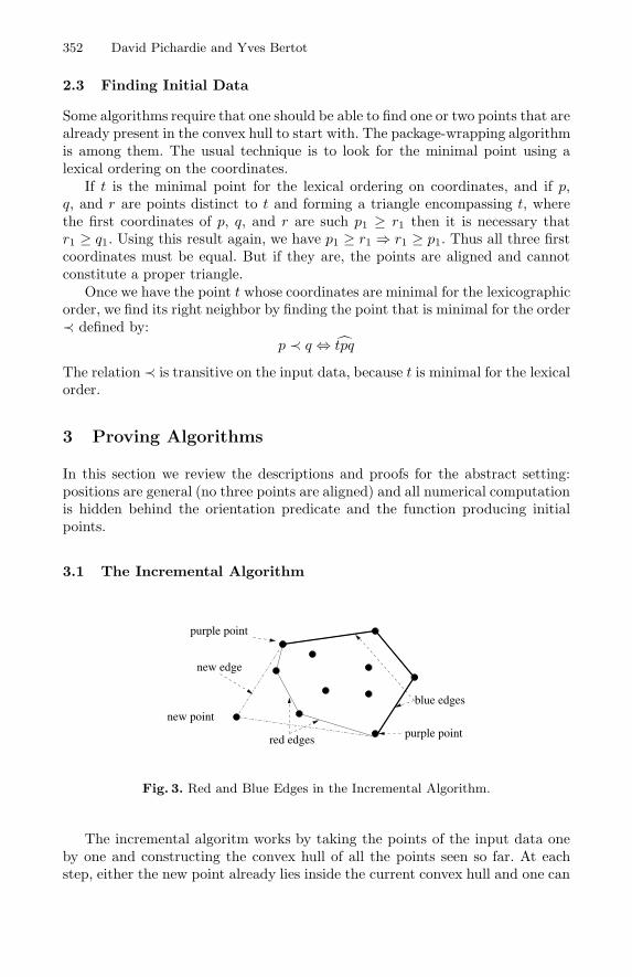
352 David Pichardie and Yves Bertot
2.3 Finding Initial Data
Some algorithms require that one should be able to find one or two points that arealready present in the convex hull to start with. The package-wrapping algorithmis among them. The usual technique is to look for the minimal point using alexical ordering on the coordinates.
If t is the minimal point for the lexical ordering on coordinates, and if p,q, and r are points distinct to t and forming a triangle encompassing t, wherethe first coordinates of p, q, and r are such p1 ≥ r1 then it is necessary thatr1 ≥ q1. Using this result again, we have p1 ≥ r1 ⇒ r1 ≥ p1. Thus all three firstcoordinates must be equal. But if they are, the points are aligned and cannotconstitute a proper triangle.
Once we have the point t whose coordinates are minimal for the lexicographicorder, we find its right neighbor by finding the point that is minimal for the order≺ defined by:
p ≺ q ⇔ tpq
The relation ≺ is transitive on the input data, because t is minimal for the lexicalorder.
3 Proving Algorithms
In this section we review the descriptions and proofs for the abstract setting:positions are general (no three points are aligned) and all numerical computationis hidden behind the orientation predicate and the function producing initialpoints.
3.1 The Incremental Algorithm
new point
red edges
blue edges
purple point
new edge
purple point
Fig. 3. Red and Blue Edges in the Incremental Algorithm.
The incremental algoritm works by taking the points of the input data oneby one and constructing the convex hull of all the points seen so far. At eachstep, either the new point already lies inside the current convex hull and one can
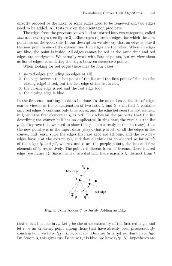
Formalizing Convex Hull Algorithms 353
directly proceed to the next, or some edges need to be removed and two edgesneed to be added. All tests rely on the orientation predicate.
The edges from the previous convex hull are sorted into two categories, calledblue and red edges (see figure 3). Blue edges represent edges, for which the newpoint lies on the good side. In our description we also say that an edge is blue ifthe new point is one of the extremities. Red edges are the other. When all edgesare blue, the point is inside. All edges cannot be red at the same time and rededges are contiguous. We actually work with lists of points, but we view themas list of edges, considering the edges between successive points.
When looking for red edges there may be four cases:
1. no red edges (including no edges at all),2. the edge between the last point of the list and the first point of the list (the
closing edge) is red, but the last edge of the list is not,3. the closing edge is red and the last edge too,4. the closing edge is blue.
In the first case, nothing needs to be done. In the second case, the list of edgescan be viewed as the concatenation of two lists, lr and lb, such that lr containsonly red edges lb contains only blue edges, and the edge between the last elementin lr and the first element in lb is red. This relies on the property that the listdescribing the convex hull has no duplicates. In this case, the result is the listp · lb. To prove this, we need to show that p is not already in the list (easy), thatthe new point p is in the input data (easy), that p is left of all the edges in theconvex hull (easy, since the edges that are kept are all blue, and the two newedges have p at the extremity), and that all the data considered so far is leftof the edges tp and pt′, where t and t′ are the purple points, the last and firstelements of lb, respectively. The point t is different from t′ because there is a rededge (see figure 4). Since t and t′ are distinct, there exists a tk distinct from t
tk
red edge
blue edge
p q
rt
Fig. 4. Using Axiom 5′ to Justify Adding an Edge.
that is last-but-one in lb. Let q be the other extremity of the first red edge, andlet r be an arbitrary point among those that have already been processed. Byconstruction, we have tktr, tktq, and tqr. Because tq is red we don’t have tqp.By Axiom 3, this gives tpq. Because tkt is blue, we have tktp. All hypotheses are
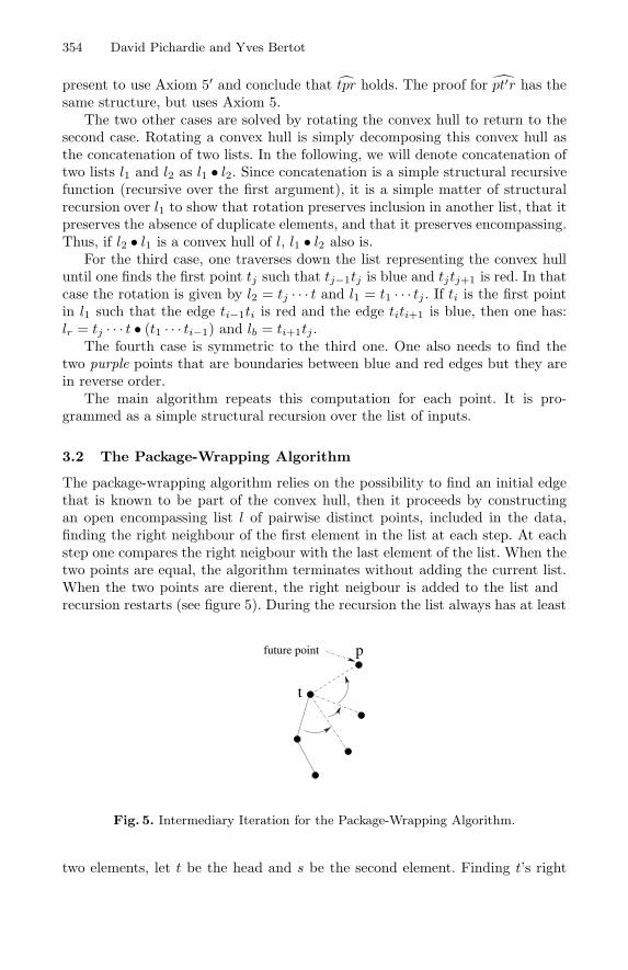
354 David Pichardie and Yves Bertot
present to use Axiom 5′ and conclude that tpr holds. The proof for pt′r has thesame structure, but uses Axiom 5.
The two other cases are solved by rotating the convex hull to return to thesecond case. Rotating a convex hull is simply decomposing this convex hull asthe concatenation of two lists. In the following, we will denote concatenation oftwo lists l1 and l2 as l1 • l2. Since concatenation is a simple structural recursivefunction (recursive over the first argument), it is a simple matter of structuralrecursion over l1 to show that rotation preserves inclusion in another list, that itpreserves the absence of duplicate elements, and that it preserves encompassing.Thus, if l2 • l1 is a convex hull of l, l1 • l2 also is.
For the third case, one traverses down the list representing the convex hulluntil one finds the first point tj such that tj−1tj is blue and tjtj+1 is red. In thatcase the rotation is given by l2 = tj · · · t and l1 = t1 · · · tj . If ti is the first pointin l1 such that the edge ti−1ti is red and the edge titi+1 is blue, then one has:lr = tj · · · t • (t1 · · · ti−1) and lb = ti+1tj .
The fourth case is symmetric to the third one. One also needs to find thetwo purple points that are boundaries between blue and red edges but they arein reverse order.
The main algorithm repeats this computation for each point. It is pro-grammed as a simple structural recursion over the list of inputs.
3.2 The Package-Wrapping Algorithm
The package-wrapping algorithm relies on the possibility to find an initial edgethat is known to be part of the convex hull, then it proceeds by constructingan open encompassing list l of pairwise distinct points, included in the data,finding the right neighbour of the first element in the list at each step. At eachstep one compares the right neigbour with the last element of the list. When thetwo points are equal, the algorithm terminates without adding the current list.When the two points are different, the right neigbour is added to the list andrecursion restarts (see figure 5). During the recursion the list always has at least
future point
t
p
Fig. 5. Intermediary Iteration for the Package-Wrapping Algorithm.
two elements, let t be the head and s be the second element. Finding t’s right
Formalizing Convex Hull Algorithms 355
neighbour is done by finding the greatest element for the relation ≺ defined by
p ≺ q ⇔ tpq.
This relation is not reflexive, but its reflexive closure is a total order, thanks toAxioms 2, 3, and 5. Finding the least element of a list for an arbitrary order isan easy piece of functional programming, and it is also easily proved correct. Ifp is this greatest element, tqp holds for every point in the input data, and byAxiom 1 ptq also holds. Thus the input data is left of the edge pt and the listp · l also encompasses the input data.
A key ingredient to proving the termination of the algorithm is to ensure thatthe list being constructed never contains duplicate elements and is included inthe input data. The hardest part is to show that checking that p is distinct fromthe last element of l is enough to ensure that p does not belong to l. In fact, if tis the head of the list, t′ is the last element and q is another element of the list,one needs to show that tqt′ holds. This is done by recursion over the length oflist l but there are many intricacies with base cases, because the proof relies onAxiom 5, which needs 5 distinct points. Let us have a look at this proof.
First assume q is the second element of the list, tqt′ comes easily from thefact that the list encompasses the input data and t′ is in the input data. Then ifq is not the second element of the list, let t1 be this second element. We do theproof by structural recursion over the list q · · · t′. If this list is reduced to 0 or 1element, this is contradictory with our hypotheses, if this list has two elements,then qt′ is an edge from the list, and qt′t holds because t is in the input data. Theresult then comes from Axiom 1. If the list q · · · t′ has more than two elements, letq′ be the second element, one has tq′t′ by induction hypothesis, tqq′ because qq′
encompasses the input data and thanks to Axiom 1. Moreover, the propertiestt1q, tt1q′, and tt1t′ hold, because q, q′, and t′ are in the input data. This isenough to use axiom 5 and conclude.
Now, the package-wrapping algorithm is not structural recursive. The termi-nation argument is that the size of the list l is bounded by the size of the inputdata, because all its elements are pairwise distinct, and that this size increases ateach step. For this reason, the function is defined using Coq’s solution for defin-ing well-founded recursive functions. This means that we have to exhibit a setcontaining the principal argument of the recursive function and a well-foundedorder on this set and show that recursive calls are done only on smaller terms.
The set LS we exhibit is the set of lists that are included in the input data Sand contain no duplicates. In Coq’s type theory, this set is described as a typeusing dependently typed inductive types. We show that the length of a list inin this set is always smaller than the size N of the input data S. We define theorder <S to be :
l <S l′ ⇔ N − length(l) < N − length(l′).
Proving that this order is well-founded is a simple application of theorems aboutcomposing well-founded orders with functions provided in Coq’s libraries. Inother theorem provers where the termination of recursive functions is ensured
356 David Pichardie and Yves Bertot
by exhibiting measure functions, the measure function to exhibit is the followingone:
f : l �→ N − length(l).
At each recursive step, the main argument is l and the argument for thenext recursive call is p · l such that p · l ∈ LS , therefore one has length(p) <length(p · l) ≤ N and f(p · l) < f(l).
4 Degenerate Cases
If we want to allow for aligned points in the input data, we need to review ourtechnique. One solution is to change Axiom 3, since it is the one that assumesthat a triple of points can always be viewed as a triangle. If we do that, anydecision taken with respect to orientation in the algorithms must be reviewedand replaced by a new decision taking extra cases into account. The structureof the algorithm remains, but all the details of its control-flow are deformed bythis constraint.
A second solution is to change the orientation predicate so that it satisfiesall five axioms even in the presence of aligned triples. This solution somehowimposes that one changes the definition of convex hulls, since our definitionrelies on the orientation predicate. We shall see that both solutions actuallyrequire that we relax our definition of a convex hull.
4.1 Segments
When three distinct points are aligned, one of them lies between the two other.We introduce a new predicate, written �pqr� to express that q occurs inside thesegment pr. Axiom 3 is changed to obtain the following formulation:
Axiom 3 ∀p, q, r. p = q ∨ q = r ∨ p = r ∨ pqr ∨ prq∨�pqr�∨�qrp�∨�rpq�.In Knuth’s work, Axioms 1-5 express a form of internal consistency for the
orientation predicate. We need to have the same kind of internal consistency forthe segment predicate and between segments and oriented triangles. The firsttwo axioms describe internal consistency for three aligned points.
Axiom 6. ∀p, q, r. �pqr�⇒�rqp�.Axiom 7. ∀p, q, r. �pqr�⇒ ¬�qpr�.The next five axioms describe consistency between segments and triangles.
Axiom 8. ∀p, q, r. �pqr�⇒ ¬pqr.Axiom 9. ∀p, q, r, t. pqr∧�ptq�⇒ ptr.
Axiom 10. ∀p, q, r, t. pqr∧�pqt�⇒ ptr.
Axiom 11. ∀p, q, r, t. pqr∧�ptq�⇒ tqr.
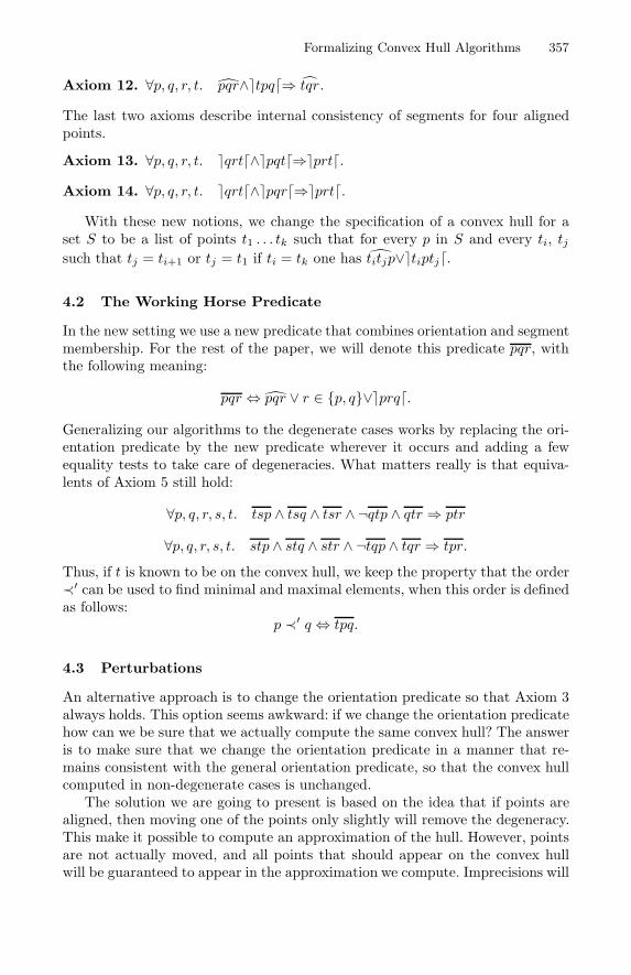
Formalizing Convex Hull Algorithms 357
Axiom 12. ∀p, q, r, t. pqr∧�tpq�⇒ tqr.
The last two axioms describe internal consistency of segments for four alignedpoints.
Axiom 13. ∀p, q, r, t. �qrt�∧�pqt�⇒�prt�.Axiom 14. ∀p, q, r, t. �qrt�∧�pqr�⇒�prt�.
With these new notions, we change the specification of a convex hull for aset S to be a list of points t1 . . . tk such that for every p in S and every ti, tjsuch that tj = ti+1 or tj = t1 if ti = tk one has titjp∨�tiptj�.
4.2 The Working Horse Predicate
In the new setting we use a new predicate that combines orientation and segmentmembership. For the rest of the paper, we will denote this predicate pqr, withthe following meaning:
pqr ⇔ pqr ∨ r ∈ {p, q}∨�prq�.
Generalizing our algorithms to the degenerate cases works by replacing the ori-entation predicate by the new predicate wherever it occurs and adding a fewequality tests to take care of degeneracies. What matters really is that equiva-lents of Axiom 5 still hold:
∀p, q, r, s, t. tsp ∧ tsq ∧ tsr ∧ ¬qtp ∧ qtr ⇒ ptr
∀p, q, r, s, t. stp ∧ stq ∧ str ∧ ¬tqp ∧ tqr ⇒ tpr.
Thus, if t is known to be on the convex hull, we keep the property that the order≺′ can be used to find minimal and maximal elements, when this order is definedas follows:
p ≺′ q ⇔ tpq.
4.3 Perturbations
An alternative approach is to change the orientation predicate so that Axiom 3always holds. This option seems awkward: if we change the orientation predicatehow can we be sure that we actually compute the same convex hull? The answeris to make sure that we change the orientation predicate in a manner that re-mains consistent with the general orientation predicate, so that the convex hullcomputed in non-degenerate cases is unchanged.
The solution we are going to present is based on the idea that if points arealigned, then moving one of the points only slightly will remove the degeneracy.This make it possible to compute an approximation of the hull. However, pointsare not actually moved, and all points that should appear on the convex hullwill be guaranteed to appear in the approximation we compute. Imprecisions will
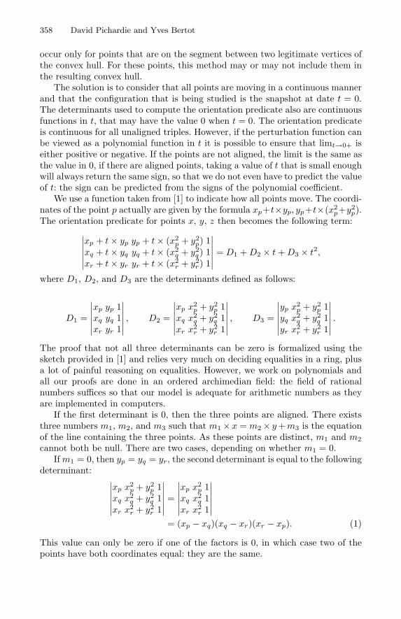
358 David Pichardie and Yves Bertot
occur only for points that are on the segment between two legitimate vertices ofthe convex hull. For these points, this method may or may not include them inthe resulting convex hull.
The solution is to consider that all points are moving in a continuous mannerand that the configuration that is being studied is the snapshot at date t = 0.The determinants used to compute the orientation predicate also are continuousfunctions in t, that may have the value 0 when t = 0. The orientation predicateis continuous for all unaligned triples. However, if the perturbation function canbe viewed as a polynomial function in t it is possible to ensure that limt→0+ iseither positive or negative. If the points are not aligned, the limit is the same asthe value in 0, if there are aligned points, taking a value of t that is small enoughwill always return the same sign, so that we do not even have to predict the valueof t: the sign can be predicted from the signs of the polynomial coefficient.
We use a function taken from [1] to indicate how all points move. The coordi-nates of the point p actually are given by the formula xp+t×yp, yp+t×(x2
p+y2p).
The orientation predicate for points x, y, z then becomes the following term:∣∣∣∣∣∣
xp + t× yp yp + t× (x2p + y2
p) 1xq + t× yq yq + t× (x2
q + y2q) 1
xr + t× yr yr + t× (x2r + y2
r) 1
∣∣∣∣∣∣= D1 +D2 × t+D3 × t2,
where D1, D2, and D3 are the determinants defined as follows:
D1 =
∣∣∣∣∣∣xp yp 1xq yq 1xr yr 1
∣∣∣∣∣∣, D2 =
∣∣∣∣∣∣xp x
2p + y2
p 1xq x
2q + y2
q 1xr x
2r + y2
r 1
∣∣∣∣∣∣, D3 =
∣∣∣∣∣∣yp x
2p + y2
p 1yq x
2q + y2
q 1yr x
2r + y2
r 1
∣∣∣∣∣∣.
The proof that not all three determinants can be zero is formalized using thesketch provided in [1] and relies very much on deciding equalities in a ring, plusa lot of painful reasoning on equalities. However, we work on polynomials andall our proofs are done in an ordered archimedian field: the field of rationalnumbers suffices so that our model is adequate for arithmetic numbers as theyare implemented in computers.
If the first determinant is 0, then the three points are aligned. There existsthree numbers m1, m2, and m3 such that m1× x = m2× y+m3 is the equationof the line containing the three points. As these points are distinct, m1 and m2
cannot both be null. There are two cases, depending on whether m1 = 0.If m1 = 0, then yp = yq = yr, the second determinant is equal to the following
determinant:∣∣∣∣∣∣xp x
2p + y2
p 1xq x
2q + y2
q 1xr x
2r + y2
r 1
∣∣∣∣∣∣=
∣∣∣∣∣∣xp x
2p 1
xq x2q 1
xr x2r 1
∣∣∣∣∣∣= (xp − xq)(xq − xr)(xr − xp). (1)
This value can only be zero if one of the factors is 0, in which case two of thepoints have both coordinates equal: they are the same.
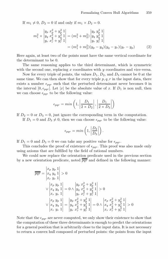
Formalizing Convex Hull Algorithms 359
If m1 �= 0, D2 = 0 if and only if m1 ×D2 = 0.
m21 ×
∣∣∣∣∣∣
yp x2p + y2
p 1yq x
2q + y2
q 1yr x
2r + y2
r 1
∣∣∣∣∣∣= (m2
1 +m22)
∣∣∣∣∣∣
yp y2p 1
yq y2q 1
yr y2r 1
∣∣∣∣∣∣= (m2
1 +m22)(yp − yq)(yq − yr)(yr − yp) (2)
Here again, at least two of the points must have the same vertical coordinate forthe determinant to be 0.
The same reasoning applies to the third determinant, which is symmetricwith the second one, replacing x coordinates with y coordinates and vice-versa.
Now for every triple of points, the values D1, D2, and D3 cannot be 0 at thesame time. We can then show that for every triple p, q, r in the input data, thereexists a number εpqr such that the perturbed determinant never becomes 0 inthe interval ]0, εpqr[. Let |x| be the absolute value of x. If D1 is non null, thenwe can choose εpqr to be the following value:
εpqr = min
(1,
∣∣∣∣D1
2×D2
∣∣∣∣ ,∣∣∣∣
D1
2×D3
∣∣∣∣)
If D2 = 0 or D3 = 0, just ignore the corresponding term in the computation.If D1 = 0 and D3 �= 0, then we can choose εpqr to be the following value:
εpqr = min
(1,
∣∣∣∣D2
D3
∣∣∣∣).
If D1 = 0 and D3 = 0 we can take any positive value for εpqr.This concludes the proof of existence of εpqr. This proof was also made only
using axioms that are fulfilled by the field of rational numbers.We could now replace the orientation predicate used in the previous section
by a new orientation predicate, noted pqr and defined in the following manner:
pqr =
∣∣∣∣∣∣xp yp 1xq yq 1xr yr 1
∣∣∣∣∣∣> 0
∨∣∣∣∣∣∣xp yp 1xq yq 1xr yr 1
∣∣∣∣∣∣= 0 ∧
∣∣∣∣∣∣yp x
2p + y2
p 1yq x
2q + y2
q 1yr x
2r + y2
r 1
∣∣∣∣∣∣> 0
∨∣∣∣∣∣∣xp yp 1xq yq 1xr yr 1
∣∣∣∣∣∣=
∣∣∣∣∣∣yp x
2p + y2
p 1yq x
2q + y2
q 1yr x
2r + y2
r 1
∣∣∣∣∣∣= 0 ∧
∣∣∣∣∣∣xp x
2p + y2
p 1xq x
2q + y2
q 1xr x
2r + y2
r 1
∣∣∣∣∣∣> 0
Note that the εpqr are never computed, we only show their existence to show thatthe computation of these three determinants is enough to predict the orientationsfor a general position that is arbitrarily close to the input data. It is not necessaryto return a convex hull composed of perturbed points: the points from the input
360 David Pichardie and Yves Bertot
data are correct, since they can be shown to be arbitrarily closed to a legitimateconvex hull (we have not done this proof yet).
It is also interesting that the convex hull computation done in this mannerreturns exactly the same result as the computation described in previous sectionif the input data is not degenerate. If the input data is degenerate and the convexhulls are required to contain no aligned points, a trivial traversal of the list ofpoints may be needed to remove the useless points. The cost of this traversalshould be proportional to the total cost.
It is remarkable that testing the sign of the D2 can be done by simply com-bining the signs of the terms (yp−yq), (yq−yr), (yr−yp), according to equations(1) and (2). In fact, D2 is strictly positive if and only if the line carrying the threepoints is not horizontal, the point r is outside the segment pq, and the points pand q are ordered in their first coordinate, similarly for D3. As a result, testingthe sign of D2 and D3 is equivalent to testing whether r is outside the segmentpq and whether p and q are ordered lexicographically. Thus, we have a programthat computes (pqr) without computing the larger determinants above. This al-gebraic reasoning brings an elegant justification to the use of segment predicatesand lexical ordering in combination with traditional orientation.
5 Conclusion
The development of certified algorithms is well suited to domains where it is easyto have a mathematical formulation of the data and the specifications. Compu-tational geometry is one of these domains. Euclidean geometry makes it easyto connect the various notions encountered in computational geometry to realanalysis and algebra. In our experiment, the presence of a decision procedure forring equalities has been instrumental, although it has also been quite annoyingthat this decision procedure was not complete, at least for the version we used.This decision procedure Ring, a tactic based on a reflective approach [4].
The problem of numeric computation also deserves some thoughts. We haveperformed our proofs with an “axiomatized” set of numbers for the coordinates.The axioms we have taken were carefully chosen to make them accurate as arepresentation of computer numbers used in exact computation. These numberslive in an archimedian field. The model for the field that is needed to expressthe correction of the algorithm is the field of rational numbers. However, thealgorithm does not actually use numbers in the whole field. It only computesa polynomial expression of degree two, so that if the numbers describing inputdata are bounded, the set of numbers needed for the algorithm to work is muchsmaller. It could be useful to express the difference between the “concrete” arith-metic used in the algorithm, and the “abstract” arithmetic used in the proof.This is actually the spirit of the work of Laurent Thery and his colleagues in aproject to study computer arithmetics.
Perturbation methods are used in other parts of computational geometry,for instance for Delaunay triangulation, where degenerate positions occur whenfour points are cocyclic. They seem very well adapted as a method to make
Formalizing Convex Hull Algorithms 361
algorithms robust to degeneracy without changing their structure. Still, one hasto be aware that we changed the specification of the problem when we changedthe orientation predicate, since the specification is expressed using this predicate.
We actually heard about the perturbation method after having done most ofthe proofs for the algorithm based on the extended axioms combining the tradi-tional orientation and segment predicates. Still both developments are useful intheir own right, since the first development can be tuned to include or excludecolinear points from the convex hull at will, while the second is not as flexible.
We would like to acknowledge the help of several researchers from the com-putational geometry group at INRIA Sophia Antipolis. In particular, MarietteYvinec pointed us to Knuth’s work on axioms and Olivier Devillers described usthe perturbation method.
References
1. Pierre Alliez, Olivier Devillers, and Jack Snoeyink. Removing degeneracies byperturbing the problem or the world. Reliable Computing, 6:61–79, 2000. SpecialIssue on Computational Geometry.
2. Bruno Barras, Samuel Boutin, Cristina Cornes, Judicael Courant, Yann Coscoy,David Delahaye, Jean-Christophe Filliatre Daniel de Rauglaudre, EduardoGimenez, Hugo Herbelin, Gerard Huet, Cesar Munoz, Chetan Murthy, CatherineParent, Christine Paulin-Mohring, Amokrane Saibi, and Benjamin Werner. TheCoq Proof Assistant User’s Guide. Version 6.3.1. INRIA, December 1999.
3. Jean-Daniel Boissonnat and Mariette Yvinec. Algorithmic geometry. CambridgeUniversity Press, 1995.
4. Samuel Boutin. Using reflection to build efficient and certified decision procedures.In Theoretical Aspects of Computer Science, number 1281 in Lecture Notes inComputer Science. Springer-Verlag, 1997.
5. S.C. Chou, X.S. Gao, and J.Z. Zhang. Machine Proofs in Geometry. World Scien-tific, Singapore, 1994.
6. Thomas H. Cormen, Charles E. Leiserson, and Ronald L. Rivest. Introduction toalgorithms. MIT-Press, 1990.
7. Gilles Kahn. Elements of constructive geometry group theory and domain theory,1995. Available as a Coq contribution athttp://coq.inria.fr/contribs-eng.html.
8. Donald Knuth. Axioms and Hulls. Number 606 in Lecture Notes in ComputerScience. Springer-Verlag, 1991.
9. Francois Puitg and Jean-Francois Dufourd. Formal specification and theoremproving breakthroughs in geometric modeling. In Theorem Proving in Higher-Order Logics, volume 1479 of Lecture Notes in Computer Science, pages 410–422.Springer-Verlag, 1998.
10. Robert Sedgewick. Algorithms. Addison-Wesley, 1988.11. Jan von Plato. A constructive theory of ordered affine geometry. Indagationes
Mathematicae, 9:549–562, 1998.
Experiments with Finite Tree Automata in Coq�
Xavier Rival1,2 and Jean Goubault-Larrecq1,3
1 GIE Dyade, INRIA RocquencourtDomaine de Voluceau B.P. 105, 78153 Le Chesnay Cedex, France
2 Ecole Normale Superieure45, rue d’Ulm, 75005 Paris, France
3 LSV, ENS Cachan61, av. du president-Wilson, 94235 Cachan Cedex, France
Abstract. Tree automata are a fundamental tool in computer science. We reporton experiments to integrate tree automata in Coq using shallow and deep reflec-tion techniques. While shallow reflection seems more natural in this context, itturns out to give disappointing results. Deep reflection is more difficult to apply,but is more promising.
1 Introduction
Finite-state automata, and more generally tree automata [7], are of fundamental impor-tance in computer science, and in particular in hardware or software verification (seee.g. [12]). One particular domain of interest to the authors is cryptographic protocolverification, where tree automata [13] and slight extensions of them [9] have been usedwith success. In this domain in particular—but this is already true to some extent inverification in general—it is important to document the process by which verification isdeemed to be complete, as well as to be able to convince any third party that the resultof verification is correct. Both goals can be achieved by producing a formal proof insome trusted proof assistant. Our aim in this paper is to report on experience we gainedin producing formal proofs of correctness of computations on tree automata in Coq [ 1].As we shall see, there are many possible approaches to this apparently simple problem,and several unexpected pitfalls to each.
We survey related work in Section 2, recall the features of Coq that we shall usein Section 3, and give a short introduction to finite tree automata in Section 4. Westudy the most promising technique to check tree automata computations done by anexternal tool in Coq, namely shallow reflection, in Section 5. Rather surprisingly, thisyields disastrous performance. We discuss reasons for this failure at the end of thissection. This prompts us to investigate deep reflection in Section 6: in deep reflection,the algorithms themselves are coded, proved, and run in the target proof assistant. Whilethis is a complex task to engage in, and seems to provide little return on investments,it is worthwhile to investigate, considering the results of Section 5. We shall see inSection 6 that this actually yields encouraging results. We conclude in Section 7.
� This work was done as part of Dyade, a common venture between Bull S.A. and INRIA.
R.J. Boulton and P.B. Jackson (Eds.): TPHOLs 2001, LNCS 2152, pp. 362–377, 2001.c© Springer-Verlag Berlin Heidelberg 2001
Experiments with Finite Tree Automata in Coq 363
2 Related Work
There does not seem to have been any work yet on integrating automata-theoretic tech-niques with proof assistants. Works like [14] are notable exceptions, and deal with ex-tended automata that really are concurrent programs which a proof assistant is called toreason about. We rather wish to use automata as a means of augmenting the capabilitesof proof assistants, using external tools. This is shallow reflection, where the externaltool constructs a trace of its verification, which can then be checked by the given proofassistant. For instance, this is how Harrison [10,11] integrates computations done byan external binary decision diagram package, resp. an implementation of Stalmarck’salgorithm into HOL. Similarly, the model-checker of Yu and Luo [ 18] outputs a proofthat can be checked by Lego.
Shallow reflection has many advantages. First, it is a safe way to extend the capabil-ities of proof assistants in practice, as the core of the proof assistant is not modified orenriched in any way: the proof assistant still only trusts arguments it (re)checks. Second,the external tool can be swapped for another, provided the new one is instrumented tooutput traces that the proof assistant can still check. This is important for maintenance,where tools can be optimized or upgraded easily enough, with only an instrumentationeffort. Third, it is much easier to check a series of computations done by an externalalgorithm A that to prove that A itself is correct.
However, some applications seem to require the latter, where algorithm A itself iscoded, proved and run inside the proof assistant. This approach is called deep reflection,and was pioneered in [17,3]. In Coq, one first application is Boutin’s Ring tactic [2]deciding equalities in the theory of rings, mixing shallow and deep reflection. One ofthe largest deep reflection endeavours is certainly the work by Verma et al. [ 16], wherebinary decision diagrams are integrated in Coq through total reflection. In the last twocases, total reflection was called for, as traces produced by external tools would havegrown far too much to be usable in practice: this is the case for binary decision diagrams,as Harrison shows [10]. Total reflection can roughly be thought as “replacing proofs inthe logic by computations”, and will be described in more detail in Section 3.
3 A Short Tour of Coq
Coq is a proof assistant based on the Calculus of Inductive Constructions (CIC), a typetheory that is powerful enough to formalize most of mathematics. It properly includeshigher-order intuitionistic logic, augmented with definitional mechanisms for induc-tively defined types, sets, propositions and relations. CIC is also a typed λ-calculus,and can therefore also be used as a programming language. We describe here the mainfeatures of Coq that we shall need later.
Among the sorts of CIC are Prop, the sort of all propositions, and Set, the sort ofall specifications, programs and data types. What it means for Prop to be the sort ofpropositions is that any object F : Prop (read: F of type Prop) denotes a proposition,i.e., a formula. In turn, any object π : F is a proof π of F . A formula is consideredproved in Coq whenever we have succeeded to find a proof of it. Proofs are written, atleast internally, as λ-terms, but we shall be content to know that we can produce themwith the help of tactics, allowing one to write proofs by reducing the goal to subgoals,and eventually to immediate, basic inferences.
364 Xavier Rival and Jean Goubault-Larrecq
Similarly, any object t : Set denotes a data type, like the data type N of naturalnumbers, or the type N → N of all functions from naturals to naturals. Data types can,and will usually be, defined inductively: e.g., the standard definition of N in Coq is bygiving its two constructors 0 : N and S : N → N; that is, as the smallest set containingO : N and such that S(n) : N for any n : N. In particular, every natural number must beof the form S(. . . S(0) . . .), which is expressed by Peano’s induction principle.
If t : Set, and p : t, we say that p is a program of type t. Programs in Coq arepurely functional: the language of programs is based on a λ-calculus with variables,application pq of p to q, abstraction [x : T ]p (the function mapping each x of type T top), case splits (e.g., Cases n of O⇒ v | S(m)⇒ fm end either returns v if n = 0, orfm if n is of the form S(m)), and functions defined by structural recursion on their lastargument. For soundness reasons, Coq refuses to accept any non-terminating function.In fact, Coq refuses to acknowledge any definition of a recursive function that is notprimitive recursive, even though its termination might be obvious.
In general, propositions and programs can be mixed. We shall exploit this in a verylimited form: when π and π ′ are programs (a.k.a., descriptions of data), then π = π ′
is a proposition, expressing that π and π ′ have the same value. Deep reflection canthen be implemented as follows: given a property P : T → Prop, write a programπ : T → bool deciding P (where bool is the inductive type of Booleans). Then provethe correctness lemma ∀x : T · π(x) = true → P (x). To show P (a), apply thecorrectness lemma: it remains to prove that π(a) = true. If this is indeed so, one callto the Reflexivity tactic will verify that the left-hand side indeed reduces to true,by computing with program π. At this point, the proof of P (a) will be complete.
Not only data structures, but also predicates can be defined by induction. This cor-responds to the mathematical practice of defining the smallest set or relation suchthat a number of conditions are satisfied. For instance, we may define the binary re-lation ≤ on natural numbers as having constructors le n : ∀n : N · n ≤ n andle S : ∀n,m : N · n ≤ m → n ≤ S(m). This defines it as the smallest binary re-lation such that n ≤ n for all n ∈ N (the le n clause) and such that whenever n ≤ m,then n ≤ m + 1 (the le S clause). Note that the constructors le n and le S play therole of clause names, whose types are Horn clauses. (In Prolog notation, they would ben ≤ n and n ≤ S(m) ← n ≤ m.) It is in fact useful to think of inductively definedpredicates as sets of Horn clauses, a.k.a. pure Prolog programs.
4 Tree Automata
A signature Σ is a collection of so-called function symbols f , together with naturalnumbers n called arities. We shall always assume that Σ is finite. The set T (Σ,X)of first-order terms, a.k.a. trees, over Σ with variables in X is defined inductively by:x ∈ T (Σ,X) for every x ∈ X , and f(t1, . . . , tn) for every n-ary function symbol fand every t1, . . . , tn ∈ T (Σ,X). Elements of T (Σ, ∅) are called ground terms over Σ.Note that there is a ground term over Σ if and only if Σ contains at least one constant,i.e., one 0-ary function symbol. In the sequel, we shall assume Σ fixed.
Tree automata are finite data structures that represent possibly infinite sets of terms,the so-called regular tree languages. (As in [7], we only consider languages of finiteterms. For more information on regular infinite term languages, see [ 15].) Tree au-tomata generalize ordinary (word) finite-state automata, where the word a 1a2 . . . an is
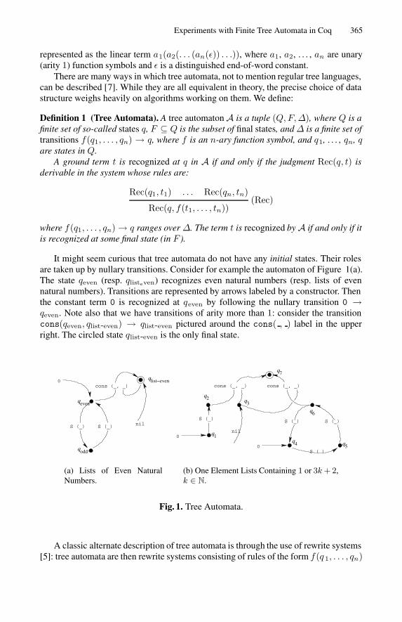
Experiments with Finite Tree Automata in Coq 365
represented as the linear term a1(a2(. . . (an(ε)) . . .)), where a1, a2, . . . , an are unary(arity 1) function symbols and ε is a distinguished end-of-word constant.
There are many ways in which tree automata, not to mention regular tree languages,can be described [7]. While they are all equivalent in theory, the precise choice of datastructure weighs heavily on algorithms working on them. We define:
Definition 1 (Tree Automata). A tree automatonA is a tuple (Q,F,∆), where Q is afinite set of so-called states q, F ⊆ Q is the subset of final states, and ∆ is a finite set oftransitions f(q1, . . . , qn) → q, where f is an n-ary function symbol, and q1, . . . , qn, qare states in Q.
A ground term t is recognized at q in A if and only if the judgment Rec(q, t) isderivable in the system whose rules are:
Rec(q1, t1) . . . Rec(qn, tn)(Rec)
Rec(q, f(t1, . . . , tn))
where f(q1, . . . , qn)→ q ranges over ∆. The term t is recognized by A if and only if itis recognized at some final state (in F ).
It might seem curious that tree automata do not have any initial states. Their rolesare taken up by nullary transitions. Consider for example the automaton of Figure 1(a).The state qeven (resp. qlisteven) recognizes even natural numbers (resp. lists of evennatural numbers). Transitions are represented by arrows labeled by a constructor. Thenthe constant term 0 is recognized at qeven by following the nullary transition 0 →qeven. Note also that we have transitions of arity more than 1: consider the transitioncons(qeven, qlist-even) → qlist-even pictured around the cons( , ) label in the upperright. The circled state qlist-even is the only final state.
qeven
qodd
qlist−even
S (_)
0cons (_, _)
nilS (_)
(a) Lists of Even NaturalNumbers.
0
S (_) S (_)
S ( )
q10
cons (_, _) cons (_, _)
nil
q2 q3
q4 q5
q6
q7
S (_)
(b) One Element Lists Containing 1 or 3k + 2,k ∈ N.
Fig. 1. Tree Automata.
A classic alternate description of tree automata is through the use of rewrite systems[5]: tree automata are then rewrite systems consisting of rules of the form f(q 1, . . . , qn)
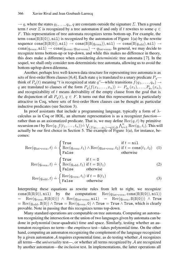
366 Xavier Rival and Jean Goubault-Larrecq
→ q, where the states q1, . . . , qn, q are constants outside the signatureΣ. Then a groundterm t over Σ is recognized by a tree automaton if and only if t rewrites to some q ∈F . This representation of tree automata recognizes terms bottom-up. For example, theterm cons(S(S(0)), nil) is recognized by the automaton of Figure 1(a) by the rewritesequence cons(S(S(0)), nil) → cons(S(S(qeven)), nil) → cons(S(qodd), nil) →cons(qeven, nil) → cons(qeven, qlist-even) → qlist-even. In general, we may decide torecognize terms bottom-up or top-down, and while this makes no difference in theory,this does make a difference when considering deterministic tree automata [ 7]. In thesequel, we shall only consider non-deterministic tree automata, allowing us to avoid thebottom-up/top-down dilemma.
Another, perhaps less well-known data structure for representing tree automata is assets of first-order Horn clauses [6,4]. Each state q is translated to a unary predicatePq—think of Pq(t) meaning “t is recognized at state q”—while transitions f(q1, . . . , qn)→q are translated to clauses of the form Pq(f(x1, . . . , xn)) ← Pq1 (x1), . . . , Pqn(xn),and recognizability of t means derivability of the empty clause from the goal that isthe disjunction of all Pq(t), q ∈ F . It turns out that this representation is particularlyattractive in Coq, where sets of first-order Horn clauses can be thought as particularinductive predicates (see Section 3).
In proof assistants that include a programming language, typically a form of λ-calculus as in Coq or HOL, an alternate representation is as a recognizer function—rather than as an axiomatized predicate. That is, we may define Rec(q, t) by primitiverecursion on t by Rec(q, f(t1, . . . , tn))=
∨(f(q1,...,qn)→q)∈∆
∧ni=1 Rec(qi, ti). This will
actually be our first choice in Section 5. The example of Figure 1(a), for instance, be-comes:
Rec(qlist-even, t) =
True if t = nilRec(qeven, t1) ∧ Rec(qlist-even, t2) if t = cons(t1, t2)False otherwise
(1)
Rec(qeven, t) =
True if t = ORec(qodd, t1) if t = S(t1)False otherwise
(2)
Rec(qodd, t) ={
Rec(qeven, t1) if t = S(t1)False otherwise
(3)
Interpreting these equations as rewrite rules from left to right, we recognizecons(S(S(0)), nil) by the computation: Rec(qlist-even, cons(S(S(0)), nil))= Rec(qeven, S(S(0))) ∧ Rec(qlist-even, nil) = Rec(qeven, S(S(0))) ∧ True= Rec(qodd, S(0)) ∧ True = Rec(qeven, 0) ∧ True = True ∧ True, which is clearlyprovable. Note in passing that this recognizes terms top-down.
Many standard operations are computable on tree automata. Computing an automa-ton recognizing the intersection or the union of two languages given by automata can bedone in polynomial (near-quadratic) time and space. Similarly, testing whether an au-tomaton recognizes no term—the emptiness test—takes polynomial time. On the otherhand, computing an automaton recognizing the complement of the language recognizedby a given automatonA requires exponential time, as do testing whether A recognizesall terms—the universality test—, or whether all terms recognized byA are recognizedby another automaton—the inclusion test. In implementations, the latter operations all
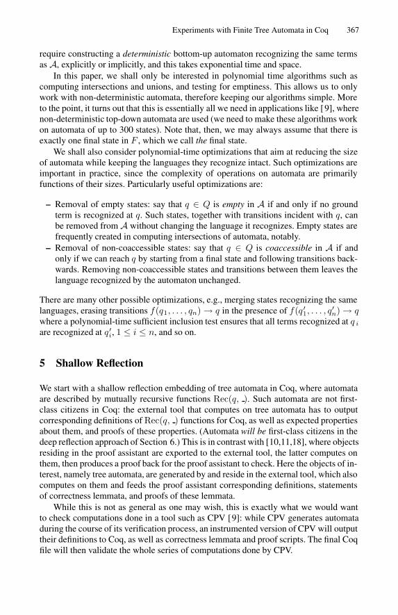
Experiments with Finite Tree Automata in Coq 367
require constructing a deterministic bottom-up automaton recognizing the same termsas A, explicitly or implicitly, and this takes exponential time and space.
In this paper, we shall only be interested in polynomial time algorithms such ascomputing intersections and unions, and testing for emptiness. This allows us to onlywork with non-deterministic automata, therefore keeping our algorithms simple. Moreto the point, it turns out that this is essentially all we need in applications like [9], wherenon-deterministic top-down automata are used (we need to make these algorithms workon automata of up to 300 states). Note that, then, we may always assume that there isexactly one final state in F , which we call the final state.
We shall also consider polynomial-time optimizations that aim at reducing the sizeof automata while keeping the languages they recognize intact. Such optimizations areimportant in practice, since the complexity of operations on automata are primarilyfunctions of their sizes. Particularly useful optimizations are:
– Removal of empty states: say that q ∈ Q is empty in A if and only if no groundterm is recognized at q. Such states, together with transitions incident with q, canbe removed from A without changing the language it recognizes. Empty states arefrequently created in computing intersections of automata, notably.
– Removal of non-coaccessible states: say that q ∈ Q is coaccessible in A if andonly if we can reach q by starting from a final state and following transitions back-wards. Removing non-coaccessible states and transitions between them leaves thelanguage recognized by the automaton unchanged.
There are many other possible optimizations, e.g., merging states recognizing the samelanguages, erasing transitions f(q1, . . . , qn)→ q in the presence of f(q ′1, . . . , q
′n)→ q
where a polynomial-time sufficient inclusion test ensures that all terms recognized at q i
are recognized at q ′i, 1 ≤ i ≤ n, and so on.
5 Shallow Reflection
We start with a shallow reflection embedding of tree automata in Coq, where automataare described by mutually recursive functions Rec(q, ). Such automata are not first-class citizens in Coq: the external tool that computes on tree automata has to outputcorresponding definitions of Rec(q, ) functions for Coq, as well as expected propertiesabout them, and proofs of these properties. (Automata will be first-class citizens in thedeep reflection approach of Section 6.) This is in contrast with [10,11,18], where objectsresiding in the proof assistant are exported to the external tool, the latter computes onthem, then produces a proof back for the proof assistant to check. Here the objects of in-terest, namely tree automata, are generated by and reside in the external tool, which alsocomputes on them and feeds the proof assistant corresponding definitions, statementsof correctness lemmata, and proofs of these lemmata.
While this is not as general as one may wish, this is exactly what we would wantto check computations done in a tool such as CPV [9]: while CPV generates automataduring the course of its verification process, an instrumented version of CPV will outputtheir definitions to Coq, as well as correctness lemmata and proof scripts. The final Coqfile will then validate the whole series of computations done by CPV.
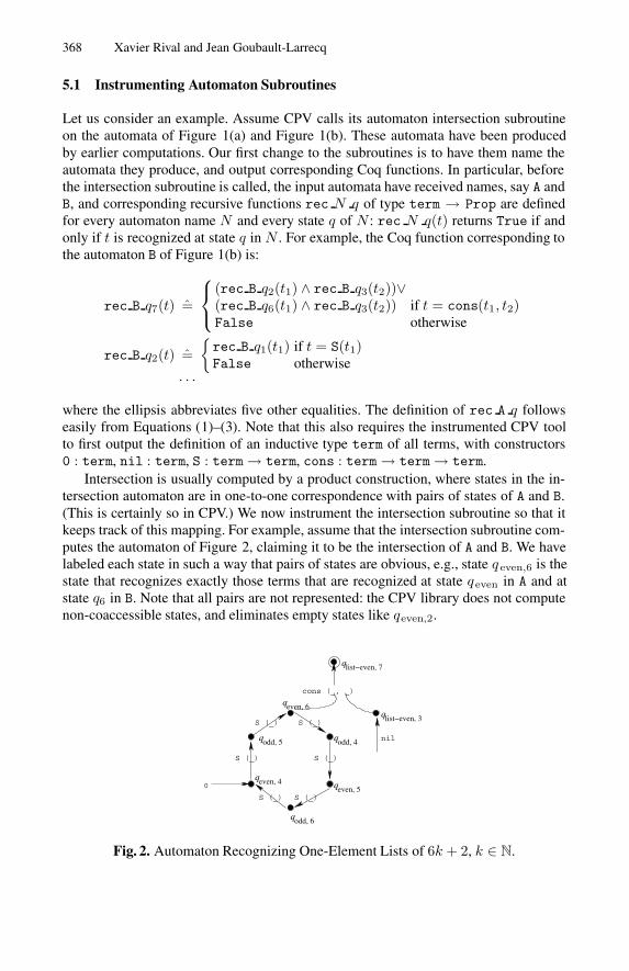
368 Xavier Rival and Jean Goubault-Larrecq
5.1 Instrumenting Automaton Subroutines
Let us consider an example. Assume CPV calls its automaton intersection subroutineon the automata of Figure 1(a) and Figure 1(b). These automata have been producedby earlier computations. Our first change to the subroutines is to have them name theautomata they produce, and output corresponding Coq functions. In particular, beforethe intersection subroutine is called, the input automata have received names, say A andB, and corresponding recursive functions rec N q of type term → Prop are definedfor every automaton name N and every state q of N : rec N q(t) returns True if andonly if t is recognized at state q in N . For example, the Coq function corresponding tothe automaton B of Figure 1(b) is:
rec B q7(t) =
(rec B q2(t1) ∧ rec B q3(t2))∨(rec B q6(t1) ∧ rec B q3(t2)) if t = cons(t1, t2)False otherwise
rec B q2(t) ={rec B q1(t1) if t = S(t1)False otherwise
. . .
where the ellipsis abbreviates five other equalities. The definition of rec A q followseasily from Equations (1)–(3). Note that this also requires the instrumented CPV toolto first output the definition of an inductive type term of all terms, with constructors0 : term, nil : term, S : term→ term, cons : term→ term→ term.
Intersection is usually computed by a product construction, where states in the in-tersection automaton are in one-to-one correspondence with pairs of states of A and B.(This is certainly so in CPV.) We now instrument the intersection subroutine so that itkeeps track of this mapping. For example, assume that the intersection subroutine com-putes the automaton of Figure 2, claiming it to be the intersection of A and B. We havelabeled each state in such a way that pairs of states are obvious, e.g., state q even,6 is thestate that recognizes exactly those terms that are recognized at state qeven in A and atstate q6 in B. Note that all pairs are not represented: the CPV library does not computenon-coaccessible states, and eliminates empty states like qeven,2.
0
S (_)
cons (_, _)
qlist−even, 7
qeven, 4
qodd, 5
qeven, 6
q
qeven, 5
qodd, 6
qlist−even, 3S (_)
S (_)S (_)
S (_) S (_)
odd, 4 nil
Fig. 2. Automaton Recognizing One-Element Lists of 6k + 2, k ∈ N.
Experiments with Finite Tree Automata in Coq 369
Next, we instrument the intersection subroutine so that it generates the correctnesslemma:
∀t : term · rec C qfinal(t)⇐⇒ rec A qfinal(t) ∧ rec B qfinal(t) (4)
where qfinal is the name of the final state in each automaton: q list-even,7 for C, qlist-evenfor A, q7 for B.
Finally, we let the intersection subroutine output a proof of the correctness lemma(4). It is interesting to examine how we might prove it in the case of the example C =A∩ B. This can only be proved by structural induction on the term t. However, we needto generalize the lemma first. Indeed, if t = cons(t1, t2), then the body of (4) simpli-fies (by reduction in the λ-calculus) to (rec C qeven,6(t1)∧rec C qlist-even,3(t2))⇐⇒(rec A qeven(t1) ∧ rec A qlist-even(t2)) ∧ ((rec B q2(t1) ∧ rec B q3(t2))∨(rec B q6(t1) ∧ rec B q3(t2))). This in turn obtains from the equivalences:
rec C qeven,6(t1)⇐⇒ rec A qeven(t1) ∧ rec B q6(t1)rec C qlist-even,3(t2)⇐⇒ rec A qlist-even(t2) ∧ rec B q3(t2)
False⇐⇒ rec A qeven(t1) ∧ rec B q2(t1)
where the latter expresses that there is no term recognized both at state q even in A andat state q2 in B—note that there is no state qeven,2 in C: it was empty, so was deleted.However, proving (4) by induction does not generate these equivalences, and we haveto prove the conjunction of (4) and the above equivalences (at least) simultaneously.
In general it is necessary to generalize (4) to the conjunction of mn statements,where m is the number of states in A and n is the number of states in B: for each stateqi in A and each state qj in B, either there is a corresponding state qij in C and wegenerate Cij , the conjunct rec C qij(t) ⇐⇒ rec A qi(t) ∧ rec B qj(t), or there isnone and, if the intersection subroutine is correct, no term is recognized both at q i andat qj , so we generate Cij , the conjunct False⇐⇒ rec A qi(t) ∧ rec B qj(t). We letthe instrumented intersection subroutine generate the generalized correctness lemma∀t : term ·∧i,j Cij .
The proof script of the generalized correctness lemma is actually obvious, and isthe same for all possible automata: do an induction on t; on all generated subgoals,compute, i.e., simplify as much as possible (use the Simpl tactic of Coq). All gener-ated subgoals, if valid, are then provable using only rules of propositional logic (evenintuitionistic): so use the Tauto tactic, which finds precisely such proofs. The proof of(4) is generated from the generalized correctness lemma using Tauto again.
Instrumenting the union subroutine is either similar (in tools that work on deter-ministic bottom-up automata, where union is computed by a similar product construc-tion), or simpler. In the case of CPV, which works on non-deterministic top-down au-tomata, this is definitely simpler: computing the union of two automata with disjointsets of states amounts to generating a new final state q ′, and generating new transitionsf(q1, . . . , qn) → q′ for each transition f(q1, . . . , qn) → q in either input automatonsuch that q was final. It follows that the correctness lemma for unions only requires acase analysis, and no induction, and that it needs no prior generalization.
Instrumenting the emptiness test is also easy. Given an automaton C, either it isempty, and because CPV eliminates empty states, its corresponding function in Coq isthe constant function False, so there is nothing to prove (in general, a polynomial-time
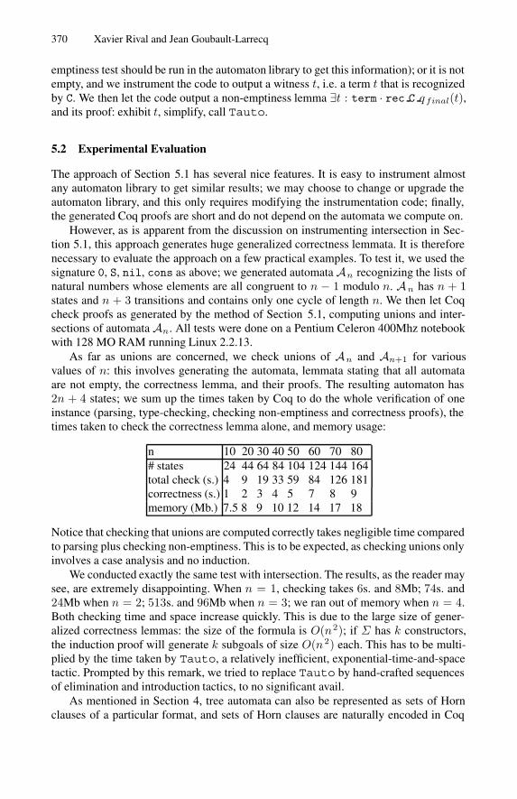
370 Xavier Rival and Jean Goubault-Larrecq
emptiness test should be run in the automaton library to get this information); or it is notempty, and we instrument the code to output a witness t, i.e. a term t that is recognizedby C. We then let the code output a non-emptiness lemma ∃t : term · rec C qfinal(t),and its proof: exhibit t, simplify, call Tauto.
5.2 Experimental Evaluation
The approach of Section 5.1 has several nice features. It is easy to instrument almostany automaton library to get similar results; we may choose to change or upgrade theautomaton library, and this only requires modifying the instrumentation code; finally,the generated Coq proofs are short and do not depend on the automata we compute on.
However, as is apparent from the discussion on instrumenting intersection in Sec-tion 5.1, this approach generates huge generalized correctness lemmata. It is thereforenecessary to evaluate the approach on a few practical examples. To test it, we used thesignature 0, S, nil, cons as above; we generated automata An recognizing the lists ofnatural numbers whose elements are all congruent to n − 1 modulo n. An has n + 1states and n + 3 transitions and contains only one cycle of length n. We then let Coqcheck proofs as generated by the method of Section 5.1, computing unions and inter-sections of automata An. All tests were done on a Pentium Celeron 400Mhz notebookwith 128 MO RAM running Linux 2.2.13.
As far as unions are concerned, we check unions of An and An+1 for variousvalues of n: this involves generating the automata, lemmata stating that all automataare not empty, the correctness lemma, and their proofs. The resulting automaton has2n + 4 states; we sum up the times taken by Coq to do the whole verification of oneinstance (parsing, type-checking, checking non-emptiness and correctness proofs), thetimes taken to check the correctness lemma alone, and memory usage:
n 10 20 30 40 50 60 70 80# states 24 44 64 84 104 124 144 164total check (s.) 4 9 19 33 59 84 126 181correctness (s.) 1 2 3 4 5 7 8 9memory (Mb.) 7.5 8 9 10 12 14 17 18
Notice that checking that unions are computed correctly takes negligible time comparedto parsing plus checking non-emptiness. This is to be expected, as checking unions onlyinvolves a case analysis and no induction.
We conducted exactly the same test with intersection. The results, as the reader maysee, are extremely disappointing. When n = 1, checking takes 6s. and 8Mb; 74s. and24Mb when n = 2; 513s. and 96Mb when n = 3; we ran out of memory when n = 4.Both checking time and space increase quickly. This is due to the large size of gener-alized correctness lemmas: the size of the formula is O(n2); if Σ has k constructors,the induction proof will generate k subgoals of size O(n2) each. This has to be multi-plied by the time taken by Tauto, a relatively inefficient, exponential-time-and-spacetactic. Prompted by this remark, we tried to replace Tauto by hand-crafted sequencesof elimination and introduction tactics, to no significant avail.
As mentioned in Section 4, tree automata can also be represented as sets of Hornclauses of a particular format, and sets of Horn clauses are naturally encoded in Coq
Experiments with Finite Tree Automata in Coq 371
as inductive predicates. It was suggested by C. Paulin-Mohring and B. Werner that thisformat usually has distinctive advantages over recursive functions as in Section 5.1:the main one is that induction and case analysis proofs only consider cases that actu-ally happen. For example, if a state has two incoming transitions, the correspondinginductive predicate will have two clauses, even though terms might be built on moreconstructors (4 in our examples). In the encoding using recursive functions, any switchon the shape of terms actually always compiles to a k-way switch, where k is the num-ber of constructors.
However, this alternate implementation of tree automata also turned out to be disap-pointing, as experience with hand-generated examples demonstrated. Compared to thetechnique of Section 5.1, proof scripts are harder to generate. In principle, it is enoughto use the Auto resolution tactic instead of Tauto; however the use of conjunctions∧ and disjunctions ∨ foils this strategy: in Coq, conjunctions and disjunctions are notprimitive and need to be decomposed by some other mechanism. The crucial point how-ever is that checking proofs, in particular for intersection, in this new scheme is onlyroughly twice as fast as with the scheme of Section 5.1, and uses as much memory.
6 Deep Reflection
As said in Section 3, deep reflection means implementing tree automata and operationson them in Coq’s λ-calculus, and proving the correctness of the latter in Coq. However,tree automata may be represented in several different ways, so one first contribution hereis the choice of a workable data structure for tree automata in Coq (Section 6.1). Weshall opt for a compromise between efficiency of algorithms and simplicity of proofs,and describe the computation of unions, intersections, and removal of empty and non-coaccessible states in Sections 6.2, 6.3 and 6.4 respectively. This will be rather cursory,and we shall only stress salient features.
6.1 Data Structures
We have chosen to represent tree automata as top-down non-deterministic tree au-tomata. Previous experience with CPV [9] indicates that this is probably one of thesimplest possible implementations. Such automata are described as a table mappingeach state q to the set of possible transitions reaching q. This set is itself organized asa table mapping each function symbol f labeling such a transition to the set of lists[q1, . . . , qn] of states such that f(q1, . . . , qn) → q is a transition. Note that all lists in agiven set have the same length n.
To represent tables, we use the map library of [8]. This provides a data type ad ofaddresses, a.k.a. keys, and a type constructor Map, such that Map(τ) is the type of mapsover τ , i.e., tables mapping keys to objects of type τ . The implementation of maps overτ is an efficient binary trie representation, where addresses are essentially finite listsof bits, or alternatively natural numbers in binary. The map library provides functionssuch as MapGet to fetch the object associated with a given key—or return the constantNONE if there is none—, and MapPut to produce a new map obtained from a given mapm by adding a binding from a given key a to a given object x, erasing any possible
372 Xavier Rival and Jean Goubault-Larrecq
preexisting binding to a. We shall simply write f(a) to denote MapGet(f, a) when it isdefined, i.e., does not return NONE.
This is used to define pre-automata as objects of type Map(st) mapping states q toelements of st; the latter map function symbols of arity n to sets of lists of states oflength n, as indicated above. Since maps only take addresses, i.e., elements of ad asindices, this requires us to encode states as addresses, as well as function symbols.
In particular, we define terms, of inductive type term with one constructor app :ad → term list → term list, where term list is defined simultaneously as thetype of finite lists of terms. For example, f(t1, . . . , tn) is coded as app(f, [t1, . . . , tn]).Each function symbol f : ad has an arity; this is summed up in a signature Σ, i.e., amap from function symbols f to their arities, of type Map(N).
Returning to pre-automata, the only remaining difficulty is to represent sets of listsof states of length n. The standard way to represent finite sets with maps is to encodethem as elements of Map(∗), where ∗ is a one-element type. However, this only al-lows us to encode sets of addresses, and while states are addresses, lists of states arenot. Since addresses are natural numbers, it is in principle feasible to encode lists ofaddresses as natural numbers, solving this conundrum. However, this solution is com-plex, not particularly efficient in practice, and hard to reason about formally. Instead,we create a new data structure to represent sets of lists of states of length n as binarytrees whose nodes are labeled with states: each branch in the tree is taken to denote thelist of all states labeling nodes to the left of which the branch goes, provided it is oflength n. Formally, the type prec list of sets of lists of states is the inductive typewith two constructors prec cons : ad → prec list → prec list → prec listand prec empty : prec list. The formal semantics [[pl]]n of pl : prec list asa set of lists of length n is defined by: [[prec empty]]0={[]}; [[prec empty]]n+1=∅;[[prec cons q � r]]0=∅; [[prec cons q � r]]n+1={q :: pl | pl ∈ [[�]]n} ∪ [[r]]n+1, whereq :: l is the list obtained from l by adding q in front.
Recall that, then, st=Map(prec list) and the type of pre-automata is predta=Map(st). Tree automata, of type dta, are pairs of a pre-automatonA and a state, takento be the final state. They are well-formed w.r.t. a signature Σ provided the followingconditions hold:
1. each state q is mapped to a map A(q) from function symbols f to sets of lists oflength n, where n = Σ(f) is the arity of f ;
2. for every state q, every function symbol f , every list [q 1, . . . , qn] ∈ A(q)(f), qi isin the domain of A for every i, 1 ≤ i ≤ n (no dangling pointers);
3. Similarly, the final state is in the domain of A.
Conditions 1–3 are necessary to establish the correctness of operations in the following.In particular, Condition 1 is crucial to be able to give a semantics to prec lists.
The semantics of tree automata is defined by mutually inductive predicatesrec predta : predta → ad → term → Prop (recognizing a term at a given state),rec st : predta→ st→ term→ Prop (recognizing a term at a state given by its setof incoming transitions), rec prec list : predta → prec list → term list →Prop (recognizing a list of terms at a list of states in some set of lists of states),where rec predta(A, q, t) provided A(q) is defined and rec st(A,A(q), t); whererec st(A, tr, t) provided t = app(f, [t1, . . . , tn]), tr(f) is defined andrec prec list(A, tr(f), [t1, . . . , tn]); finally, rec prec list(A, prec empty, []),
Experiments with Finite Tree Automata in Coq 373
rec prec list(A, prec cons(q, �, r), t :: tl) provided either rec predta(A, q, t)and rec prec list(A, �, tl), or rec prec list(A, r, t :: tl).
6.2 Implementing Union
Computing unions is done by the algorithm used in CPV, described in Section 5.1: gen-erate a new final state q′, and generate new transitions f(q1, . . . , qn) → q′ for eachtransition f(q1, . . . , qn) → q in any of the input automata A or B where q was final.However, this is only correct provided A and B have disjoint sets of states. In imple-mentations like CPV, states are memory locations pointing to maps of type st, and dis-jointness is not required for correctness, as any state common to both automata points tothe same sub-automaton. The latter condition is hard to ensure (we might have modeleda full store as in [16], but this looked like overkill), while the disjointness condition issimpler to implement in the representation of Section 6.1: therefore, in Coq, we firstcopy each input automaton by adding a 0 bit in front of any address inA (i.e., changingq into 2q) and a 1 bit in front of any address in B (i.e., changing q into 2q+1), then adda new final state and all relevant incoming transitions.
We prove that this algorithm is correct: the term t is recognized by the union of twowell-formed automata if and only if t is recognized by one or the other, by structuralinduction on t. That the input automata are well-formed (Conditions 1–3) is neededin the proof. Condition 1 is needed to give a meaning [[pl]]n to prec lists A(q)(f),where n is the arity of f . Conditions 2 and 3 are needed to give meaning to the setof all transitions f(q1, . . . , qn) → q where q is given. We also prove that the union oftwo well-formed automata is again well-formed, one condition at a time. Notice that wenever had to impose any well-formedness condition on terms, only on automata.
6.3 Implementing Intersection
Intersection of two automata A and B is trickier. The standard product constructionconsists in generating new states 〈q, q ′〉 that are in one-to-one correspondence withpairs of states q of A and q ′ of B. There is a transition f(〈q1, q
′1〉, . . . , 〈qn, q
′n〉) →
〈q, q′〉 in the computed intersection automaton C if and only if f(q 1, . . . , qn) → q isa transition in A and f(q ′1, . . . , q′n) → q′ is a transition in B, and the final state of Cis 〈qfinal, q
′final〉, where qfinal is final in A and q′final is final in B. Our first problem
here is that states 〈q, q′〉 should be of type ad, so we need a one-to-one mapping frompairs of addresses to addresses. There are several solutions to this. The one we chooseis one of the simplest, and also of the most efficient to compute: looking at q and q ′ assequences of bits, we interleave them to get 〈q, q ′〉. For example, if q is 10010 in binaryand q′ is 01011, then 〈q, q′〉 is 1001001101.
Linking in such an explicit way the states 〈q, q ′〉 to q and q′, i.e., making sure thatwe can get back q and q ′ easily from 〈q, q′〉 without the help of any outside machineryis a great help in proofs of correctness. The construction of the intersection automatonC is then direct: generate all states 〈q, q ′〉, and add transitions as specified above. Thisinvolves quite many nested structural inductions, though: we have to induct on the triesthat encode the pre-automata A and B, then on the tries that encode transitions withsymbol function f , for each f in each of the two input automata, then induct on two
374 Xavier Rival and Jean Goubault-Larrecq
prec lists. It then turns out that the intersection construction applied to two automataindeed computes the intersection, provided Condition 1 is satisfied; this is proved bystructural induction on the terms fed to each automaton. Finally, we prove that theintersection construction preserves well-formedness, as expected.
Nonetheless, this intersection construction is naive: it generates many empty or non-coaccessible states. To correct this, it is common practice to only generate states 〈q, q ′〉by need. Intuitively, generate 〈qfinal, q
′final〉; then, for each f , for each pair of transi-
tions f(q1, . . . , qn)→ qfinal inA and f(q′1, . . . , q′n)→ q′final in B, generate the states〈q1, q′1〉, . . . , 〈qn, q
′n〉 (observe that they may fail to be new), and recurse. Note that this
is not well-founded induction, and a loop-checking mechanism has to be implemented:when some state 〈q, q′〉 is required that has already been generated, stop recursing. Cod-ing such an algorithm in Coq, and above all proving it, is daunting—recall that the naivealgorithm already requires 6 nested inductions. Thus, we have refrained from doing so.
6.4 Removing Empty and Non-coaccessible States
Instead, we have implemented algorithms to delete empty and non-coaccessible statesas separate functions. This is already rather involved, as this involves some form ofloop-checking. First, we observe that, from the logical point of view, recursing withloop checks is just an implementation of a least fixpoint computation. For example,define the set NV of non-void states of A as the smallest such that for every tran-sition f(q1, . . . , qn) → q such that q1, . . . , qn ∈ NV , then q ∈ NV . While this isnaturally coded in Coq as an inductive predicate, such a predicate does not lend it-self to computation. To compute NV , we must instead compute the least fixpoint ofthe function NV mapping any set S of states to NV (S)=S ∪ {q | f(q1, . . . , qn) →q transition in A, q1 ∈ S, . . . , qn ∈ S}. We then prove that both definitions are equiv-alent, by well-founded induction on the definition of the non-vacuity predicate in onedirection, and by Tarskian fixpoint induction in the other direction.
This however requires that we develop a Tarskian theory of fixpoints of mono-tonic functions over complete lattices—at least over complete Boolean lattices of fi-nite height. Indeed, subsets of a given set of states Q of cardinality n form a Booleanlattice of height n. In Coq, we represent subsets of Q as objects of type Map(bool),constrained to haveQ as domain. We show in Coq that this can be given the structure ofa complete Boolean lattice of cardinality 2n and height n, taking as ordering m ≤∗ m′if and only if m(q) ≤ m′(q) for every q ∈ Q , where ≤ is the ordering false ≤ truein bool. Independently, we show in Coq that, for every complete lattice L of height n,with bottom element ⊥, for every monotonic f : L→ L, f n(⊥) is the least fixpoint off . This is especially convenient for computation, as f n(⊥) can be defined by structuralrecursion on n in Coq, while general fixpoints cannot be defined as recursive functions.
Summing up, we obtain a function that computes the set of non-void states of agiven automaton, together with a proof of its correctness. Observing now that a stateq is non-void if and only if it is non-empty, where a state q of A is non-empty if andonly if there is a term t recognized at q in A, we deduce that the automaton B obtainedfrom A by only keeping non-void (a.k.a, non-empty) states has the same semantics asA. Therefore, composing empty states removal with the naive intersection algorithmyields another correct intersection algorithm. (The empty state removal algorithm isactually slightly trickier, in that it also removes transitions f(q1, . . . , qn) → q where
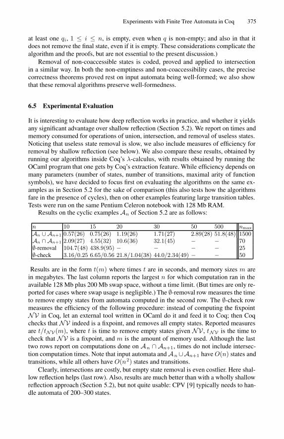
Experiments with Finite Tree Automata in Coq 375
at least one qi, 1 ≤ i ≤ n, is empty, even when q is non-empty; and also in that itdoes not remove the final state, even if it is empty. These considerations complicate thealgorithm and the proofs, but are not essential to the present discussion.)
Removal of non-coaccessible states is coded, proved and applied to intersectionin a similar way. In both the non-emptiness and non-coaccessibility cases, the precisecorrectness theorems proved rest on input automata being well-formed; we also showthat these removal algorithms preserve well-formedness.
6.5 Experimental Evaluation
It is interesting to evaluate how deep reflection works in practice, and whether it yieldsany significant advantage over shallow reflection (Section 5.2). We report on times andmemory consumed for operations of union, intersection, and removal of useless states.Noticing that useless state removal is slow, we also include measures of efficiency forremoval by shallow reflection (see below). We also compare these results, obtained byrunning our algorithms inside Coq’s λ-calculus, with results obtained by running theOCaml program that one gets by Coq’s extraction feature. While efficiency depends onmany parameters (number of states, number of transitions, maximal arity of functionsymbols), we have decided to focus first on evaluating the algorithms on the same ex-amples as in Section 5.2 for the sake of comparison (this also tests how the algorithmsfare in the presence of cycles), then on other examples featuring large transition tables.Tests were run on the same Pentium Celeron notebook with 128 Mb RAM.
Results on the cyclic examplesAn of Section 5.2 are as follows:
n 10 15 20 30 50 500 nmax
An ∪ An+1 0.57(26) 0.75(26) 1.19(26) 1.71(27) 2.89(28) 51.8(48) 1500An ∩ An+1 2.09(27) 4.55(32) 10.6(36) 32.1(45) − − 70∅-removal 104.7(48) 438.9(95) − − − − 25∅-check 3.16/0.25 6.65/0.56 21.8/1.04(38) 44.0/2.34(49) − − 50
Results are in the form t(m) where times t are in seconds, and memory sizes m arein megabytes. The last column reports the largest n for which computation ran in theavailable 128 Mb plus 200 Mb swap space, without a time limit. (But times are only re-ported for cases where swap usage is negligible.) The ∅-removal row measures the timeto remove empty states from automata computed in the second row. The ∅-check rowmeasures the efficiency of the following procedure: instead of computing the fixpointNV in Coq, let an external tool written in OCaml do it and feed it to Coq; then Coqchecks that NV indeed is a fixpoint, and removes all empty states. Reported measuresare t/tNV(m), where t is time to remove empty states given NV , tNV is the time tocheck that NV is a fixpoint, and m is the amount of memory used. Although the lasttwo rows report on computations done on An ∩ An+1, times do not include intersec-tion computation times. Note that input automata andAn ∪An+1 have O(n) states andtransitions, while all others have O(n2) states and transitions.
Clearly, intersections are costly, but empty state removal is even costlier. Here shal-low reflection helps (last row). Also, results are much better than with a wholly shallowreflection approach (Section 5.2), but not quite usable: CPV [9] typically needs to han-dle automata of 200–300 states.
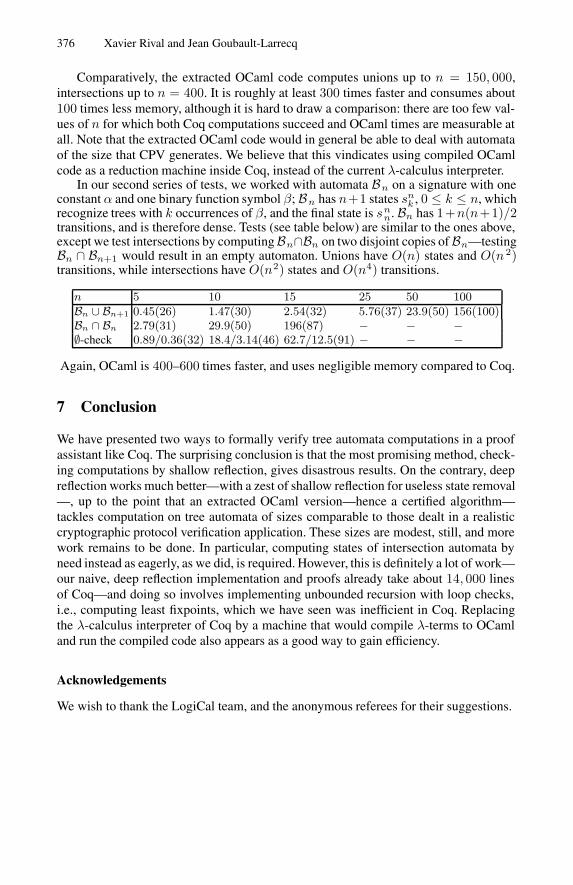
376 Xavier Rival and Jean Goubault-Larrecq
Comparatively, the extracted OCaml code computes unions up to n = 150, 000,intersections up to n = 400. It is roughly at least 300 times faster and consumes about100 times less memory, although it is hard to draw a comparison: there are too few val-ues of n for which both Coq computations succeed and OCaml times are measurable atall. Note that the extracted OCaml code would in general be able to deal with automataof the size that CPV generates. We believe that this vindicates using compiled OCamlcode as a reduction machine inside Coq, instead of the current λ-calculus interpreter.
In our second series of tests, we worked with automata Bn on a signature with oneconstant α and one binary function symbol β; Bn has n+1 states sn
k , 0 ≤ k ≤ n, whichrecognize trees with k occurrences of β, and the final state is sn
n. Bn has 1+n(n+1)/2transitions, and is therefore dense. Tests (see table below) are similar to the ones above,except we test intersections by computingBn∩Bn on two disjoint copies ofBn—testingBn ∩ Bn+1 would result in an empty automaton. Unions have O(n) states and O(n 2)transitions, while intersections have O(n2) states and O(n4) transitions.
n 5 10 15 25 50 100Bn ∪ Bn+1 0.45(26) 1.47(30) 2.54(32) 5.76(37) 23.9(50) 156(100)Bn ∩ Bn 2.79(31) 29.9(50) 196(87) − − −∅-check 0.89/0.36(32) 18.4/3.14(46) 62.7/12.5(91) − − −
Again, OCaml is 400–600 times faster, and uses negligible memory compared to Coq.
7 Conclusion
We have presented two ways to formally verify tree automata computations in a proofassistant like Coq. The surprising conclusion is that the most promising method, check-ing computations by shallow reflection, gives disastrous results. On the contrary, deepreflection works much better—with a zest of shallow reflection for useless state removal—, up to the point that an extracted OCaml version—hence a certified algorithm—tackles computation on tree automata of sizes comparable to those dealt in a realisticcryptographic protocol verification application. These sizes are modest, still, and morework remains to be done. In particular, computing states of intersection automata byneed instead as eagerly, as we did, is required. However, this is definitely a lot of work—our naive, deep reflection implementation and proofs already take about 14, 000 linesof Coq—and doing so involves implementing unbounded recursion with loop checks,i.e., computing least fixpoints, which we have seen was inefficient in Coq. Replacingthe λ-calculus interpreter of Coq by a machine that would compile λ-terms to OCamland run the compiled code also appears as a good way to gain efficiency.
Acknowledgements
We wish to thank the LogiCal team, and the anonymous referees for their suggestions.
Experiments with Finite Tree Automata in Coq 377
References
1. B. Barras, S. Boutin, C. Cornes, J. Courant, J.-C. Filliatre, E. Gimenez, H. Herbelin, G. Huet,C. Munoz, C. Murthy, C. Parent, C. Paulin-Mohring, A. Saibi, and B. Werner. The Coq proofassistant reference manual: Version 6.3.1. Technical report, INRIA, France, 1999.
2. S. Boutin. Using reflection to build efficient and certified decision procedures. In M. Abadiand T. Ito, editors, TACS’97. Springer-Verlag LNCS 1281, 1997.
3. R. Boyer and J. S. Moore. Metafunctions: Proving them correct and using them efficientlyas new proof procedures. In The Correctness Problem in Computer Science. Acad. Press,1981.
4. W. Charatonik and A. Podelski. Set-based analysis of reactive infinite-state systems. InB. Steffen, editor, TACAS’98, pages 358–375. Springer Verlag LNCS 1384, 1998.
5. H. Comon, M. Dauchet, R. Gilleron, F. Jacquemard, D. Lugiez, T. Sophie,and M. Tommasi. Tree automata techniques and applications. Available athttp://www.grappa.univ-lille3.fr/tata, 1997.
6. L. Fribourg and M. Veloso Peixoto. Automates concurrents a contraintes. Technique etScience Informatique, 13(6):837–866, 1994.
7. F. Gecseg and M. Steinby. Tree languages. In G. Rozenberg and A. Salomaa, editors,Handbook of Formal Languages, volume 3, pages 1–68. Springer Verlag, 1997.
8. J. Goubault-Larrecq. Satisfiability of inequality constraints and detection of cycleswith negative weight in graphs. Part of the Coq contribs, available at http://pauillac.inria.fr/coq/contribs/graphs.html, 1998.
9. J. Goubault-Larrecq. A method for automatic cryptographic protocol verification. InFMPPTA’2000, pages 977–984. Springer Verlag LNCS 1800, 2000.
10. J. Harrison. Binary decision diagrams as a HOL derived rule. The Computer Journal,38:162–170, 1995.
11. J. Harrison. Stalmarck’s algorithm as a HOL derived rule. In J. von Wright, J. Grundy, andJ. Harrison, editors, TPHOL’96, pages 221–234. Springer Verlag LNCS 1125, 1996.
12. J.-P. Jouannaud. Rewrite proofs and computations. In H. Schwichtenberg, editor, Proofand Computation, volume 139 of NATO series F: Computer and Systems Sciences, pages173–218. Springer Verlag, 1995.
13. D. Monniaux. Abstracting cryptographic protocols with tree automata. In SAS’99, pages149–163. Springer-Verlag LNCS 1694, 1999.
14. O. Muller. A verification environment for I/O automata based on formalized meta-theory.Master’s thesis, Technische Universitat Munchen, 1998.
15. W. Thomas. Automata on infinite objects. In J. van Leeuwen, editor, Handbook of Theoreti-cal Computer Science, chapter 4, pages 133–191. Elsevier Science Publishers B. V., 1990.
16. K. N. Verma, J. Goubault-Larrecq, S. Prasad, and S. Arun-Kumar. Reflecting BDDs in Coq.In ASIAN’2000, pages 162–181. Springer Verlag LNCS 1961, 2000.
17. R. W. Weyhrauch. Prolegomena to a theory of mechanized formal reasoning. ArtificalIntelligence, 13(1, 2):133–170, 1980.
18. S. Yu and Z. Luo. Implementing a model checker for LEGO. In J. Fitzgerald, C. B. Jones,and P. Lucas, editors, FME’97, pages 442–458. Springer-Verlag LNCS 1313, 1997.
Mizar Light for HOL Light
Freek Wiedijk
Department of Computer ScienceUniversity of Nijmegen, The Netherlands
Abstract. There are two different approaches to formalizing proofs in acomputer: the procedural approach (which is the one of the HOL system)and the declarative approach (which is the one of the Mizar system).Most provers are procedural. However declarative proofs are much closerin style to informal mathematical reasoning than procedural ones.There have been attempts to put declarative interfaces on top of proce-dural proof assistants, like John Harrison’s Mizar mode for HOL andMarkus Wenzel’s Isar mode for Isabelle. However in those cases thedeclarative assistant is a layer on top of the procedural basis, havinga separate syntax and a different ‘feel’ from the underlying system.This paper shows that the procedural and the declarative ways of provingare related and can be integrated seamlessly. It presents an implementa-tion of the Mizar proof language on top of HOL that consists of only 41lines of ML. This shows how close the procedural and declarative stylesof proving really are.
1 Introduction
We describe a programming experiment with the HOL system. To be able toread this paper one has to have some familiarity with both the HOL [10] andMizar [12,17] systems. The software described here is not meant to be used forserious work (and it certainly doesn’t emulate the full Mizar language). Ratherit’s a kind of ‘thought experiment’ to clarify the relation between the proceduraland declarative styles of proving.
This paper uses HOL for the procedural prover. However the way the paperintegrates Mizar-style proofs with it also applies to other procedural systemslike Coq [2] and Isabelle [14]. For each of these systems a set of ‘Mizar tactics’could be written as described in this paper, giving them ‘Mizar style’ declarativeproofs without a separate syntactic layer.
The plan of this paper is as follows. It first presents the procedural anddeclarative styles of proving and the HOL and Mizar systems. Then Section 6presents the main idea of the paper which is implementing Mizar steps as HOLtactics. For each of these ‘Mizar tactics’ this section gives an ML type in theframework of the HOL system. After that the paper discusses various variationson this Mizar mode for HOL. The paper concludes with a bigger example andan outlook. The source code of the Mizar mode is an appendix.
R.J. Boulton and P.B. Jackson (Eds.): TPHOLs 2001, LNCS 2152, pp. 378–393, 2001.c© Springer-Verlag Berlin Heidelberg 2001
Mizar Light for HOL Light 379
2 Procedural versus Declarative Proving
The idea of formalizing mathematical proofs in such a way that a computercan check the correctness is not new but only recently it has become practicaland popular. Most of the proofs that are currently checked are proofs of thecorrectness of computer software or hardware but some people have also beenformalizing other kinds of proofs (for instance of mathematical theorems [3,6]).
There are two main styles of proof checking programs (the so-called proofcheckers or proof assistants): the procedural style and the declarative style.
The procedural proof checkers descend from a system from the seventiescalled LCF [8]. Such a system has a proof state which consists of a set of ‘proofobligations’. This state is transformed by means of so-called tactics which take aproof obligation and reduce it to several simpler ones (possibly none). The proofprocess starts with the statement to be proved as the sole proof obligation; onceno proof obligations remain, the proof is complete. Procedural proofs consistingof a sequence of tactics cannot be understood without interactively running themon a computer because they only contain the transitions between the proof statesand not the proof states themselves.1 Also since the initial proof obligation isthe final statement to be proved, procedural proofs tend to run backwards , fromthe conclusion back to the assumptions.
The other two proof checkers from the seventies, Automath [13] and Mizar[12,17], both are of the declarative kind. (Another system that is declarative isthe Ontic system by David McAllester [11].) In a declarative system, a proofdoesn’t consist of instructions to transform statements but of those statementsthemselves. Furthermore, the statements are present in deductive order: theassumptions are at the start and the conclusion is at the end.2
The procedural and declarative styles differ in several ways:
– Declarative proofs are closer to informal mathematical reasoning and there-fore are more readable than procedural proofs because in a declarative proofthe statements are present themselves and in the proper order.
– Most current proof assistants are procedural (perhaps because LCF styleprovers are programmable by their users, while declarative systems can gen-erally only be extended by its developers).
– Declarative proofs can be written without the proof assistant running andthen checked with a batch oriented system. Procedural proofs can only bedeveloped interactively because the computer has to keep track of the proofobligations. Indeed, some declarative provers only have a batch mode whileprocedural provers always also have an interactive mode.
1 Procedural proofs are therefore sometimes presented using runs of proof scripts (or,even better, proof trees) showing intermediate goals.
2 The relation between backward and forward reasoning as related to procedural anddeclarative proofs is more subtle than is suggested here. Declarative proofs (and in-formal mathematical reasoning as well) also take backward steps. And many proce-dural provers also can do forward reasoning. However the particular tactic collectionsfound in procedural provers tend to be biased towards backward reasoning.
380 Freek Wiedijk
– Since a declarative proof contains a chain of statements, it is fairly robustwith respect to errors. If one step in the proof is erroneous, a declarativesystem can recover from the error and check the rest of the proof file reason-ably well. In contrast, a procedural prover stops checking at the first error itencounters. So after the point in the file where an error occurs, a proceduralsystem can’t say much about correctness.
It seems natural to look for a way to integrate the procedural and declarativeapproaches to proving. Two attempts to put a declarative interface on a pro-cedural prover are the Mizar mode for HOL by John Harrison [9] and the Isarmode for Isabelle by Markus Wenzel [16].
The Mizar mode for HOL by John Harrison is a true integration, in thesense that the Mizar commands behave like ordinary HOL tactics. Howeverthis doesn’t become clear from the way this mode is presented. For instance,the Mizar sub-language has a separate parser from the (ML based) HOL prooflanguage. Also once the Mizar mode is active, the normal parser of the HOLterms is no longer easily available. This seems to suggest that once the Mizarmode has been activated, the ‘normal’ style of procedural HOL proving is notmeant to be used anymore.
The Mizar mode for HOL in this paper is a variation on the Mizar mode ofJohn Harrison. Its main difference with Harrison’s Mizar mode is that the Mizarprimitives are HOL tactics (so are not just compiled to them) and therefore theintegration is very tight. Also the implementation of our Mizar mode takes only41 lines of ML, which is smaller than Harrison’s implementation which consistsof about 650 lines of ML.
The Isar mode for Isabelle differs from the Mizar mode for HOL in thatit has outgrown the experimental stage and has been used for serious proofs[3,5,4]. However it really is a second layer on top of the Isabelle layer (althoughit is possible to ‘embed’ tactic scripts in Isar proofs), so in this case there is nomixture between the two approaches. In fact, both layers have their own proofstate (called ‘the static proof context’ and ‘the dynamic goal state’) which areto be synchronized at certain checkpoints. This is presented as a benefit becauseit makes it possible to give a different order to the proof steps from the orderimposed by the underlying procedural basis but it shows that there is no tightintegration.
Two other declarative systems that integrate declarative proofs with higherorder logic are the SPL system by Vincent Zammit [18] and the Declare systemby Don Syme [15]. These two systems are not meant as a declarative interfaceto a procedural prover. Instead they are autonomous declarative systems. (TheSPL system is implemented on top of the HOL system but it is not an interfaceto HOL.)
Procedural and declarative proof checkers both might or might not satisfywhat Henk Barendregt calls the de Bruijn principle and the Poincare principle[1]. This paper is about the relation between procedural and declarative proofstyles. This is unrelated to the issue of whether a system should satisfy either ofthese principles or how to make it do so.
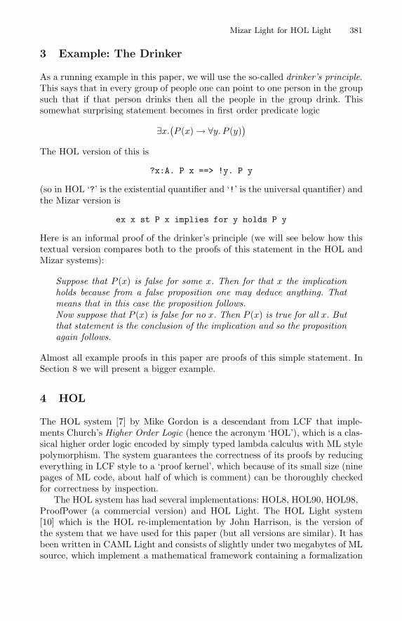
Mizar Light for HOL Light 381
3 Example: The Drinker
As a running example in this paper, we will use the so-called drinker’s principle.This says that in every group of people one can point to one person in the groupsuch that if that person drinks then all the people in the group drink. Thissomewhat surprising statement becomes in first order predicate logic:
∃x.(P (x)→ ∀y. P (y)
)
The HOL version of this is:
?x:A. P x ==> !y. P y
(so in HOL ‘?’ is the existential quantifier and ‘!’ is the universal quantifier) andthe Mizar version is:
ex x st P x implies for y holds P y
Here is an informal proof of the drinker’s principle (we will see below how thistextual version compares both to the proofs of this statement in the HOL andMizar systems):
Suppose that P (x) is false for some x. Then for that x the implicationholds because from a false proposition one may deduce anything. Thatmeans that in this case the proposition follows.Now suppose that P (x) is false for no x. Then P (x) is true for all x. Butthat statement is the conclusion of the implication and so the propositionagain follows.
Almost all example proofs in this paper are proofs of this simple statement. InSection 8 we will present a bigger example.
4 HOL
The HOL system [7] by Mike Gordon is a descendant from LCF that imple-ments Church’s Higher Order Logic (hence the acronym ‘HOL’), which is a clas-sical higher order logic encoded by simply typed lambda calculus with ML stylepolymorphism. The system guarantees the correctness of its proofs by reducingeverything in LCF style to a ‘proof kernel’, which because of its small size (ninepages of ML code, about half of which is comment) can be thoroughly checkedfor correctness by inspection.
The HOL system has had several implementations: HOL88, HOL90, HOL98,ProofPower (a commercial version) and HOL Light. The HOL Light system[10] which is the HOL re-implementation by John Harrison, is the version ofthe system that we have used for this paper (but all versions are similar). It hasbeen written in CAML Light and consists of slightly under two megabytes of MLsource, which implement a mathematical framework containing a formalization
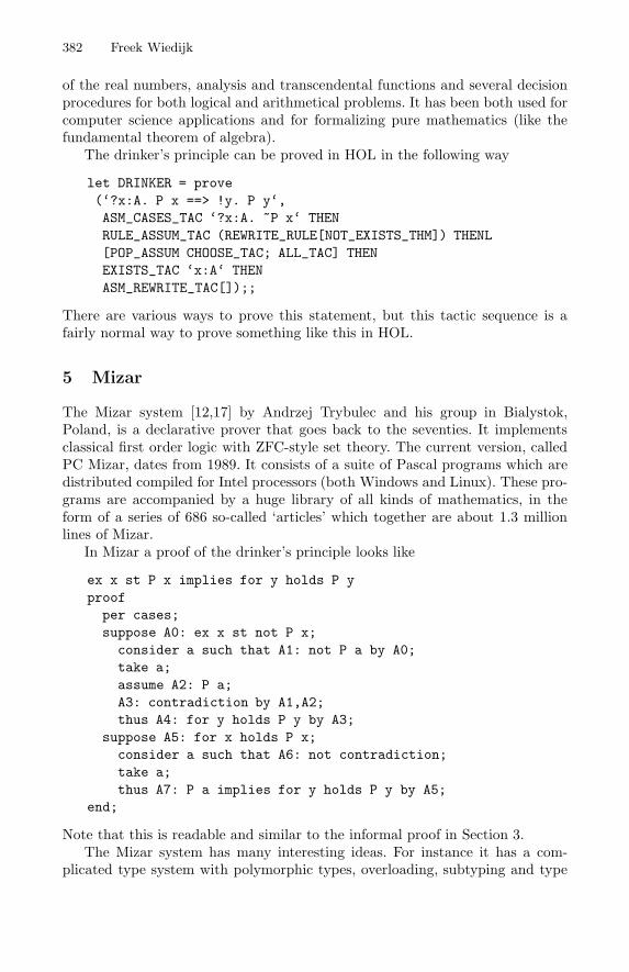
382 Freek Wiedijk
of the real numbers, analysis and transcendental functions and several decisionprocedures for both logical and arithmetical problems. It has been both used forcomputer science applications and for formalizing pure mathematics (like thefundamental theorem of algebra).
The drinker’s principle can be proved in HOL in the following way:
let DRINKER = prove(‘?x:A. P x ==> !y. P y‘,ASM_CASES_TAC ‘?x:A. ~P x‘ THENRULE_ASSUM_TAC (REWRITE_RULE[NOT_EXISTS_THM]) THENL[POP_ASSUM CHOOSE_TAC; ALL_TAC] THENEXISTS_TAC ‘x:A‘ THENASM_REWRITE_TAC[]);;
There are various ways to prove this statement, but this tactic sequence is afairly normal way to prove something like this in HOL.
5 Mizar
The Mizar system [12,17] by Andrzej Trybulec and his group in Bialystok,Poland, is a declarative prover that goes back to the seventies. It implementsclassical first order logic with ZFC-style set theory. The current version, calledPC Mizar, dates from 1989. It consists of a suite of Pascal programs which aredistributed compiled for Intel processors (both Windows and Linux). These pro-grams are accompanied by a huge library of all kinds of mathematics, in theform of a series of 686 so-called ‘articles’ which together are about 1.3 millionlines of Mizar.
In Mizar a proof of the drinker’s principle looks like:
ex x st P x implies for y holds P yproofper cases;suppose A0: ex x st not P x;
consider a such that A1: not P a by A0;take a;assume A2: P a;A3: contradiction by A1,A2;thus A4: for y holds P y by A3;
suppose A5: for x holds P x;consider a such that A6: not contradiction;take a;thus A7: P a implies for y holds P y by A5;
end;
Note that this is readable and similar to the informal proof in Section 3.The Mizar system has many interesting ideas. For instance it has a com-
plicated type system with polymorphic types, overloading, subtyping and type
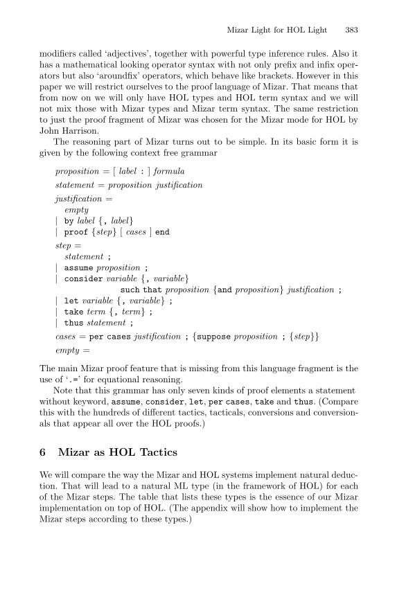
Mizar Light for HOL Light 383
modifiers called ‘adjectives’, together with powerful type inference rules. Also ithas a mathematical looking operator syntax with not only prefix and infix oper-ators but also ‘aroundfix’ operators, which behave like brackets. However in thispaper we will restrict ourselves to the proof language of Mizar. That means thatfrom now on we will only have HOL types and HOL term syntax and we willnot mix those with Mizar types and Mizar term syntax. The same restrictionto just the proof fragment of Mizar was chosen for the Mizar mode for HOL byJohn Harrison.
The reasoning part of Mizar turns out to be simple. In its basic form it isgiven by the following context free grammar:
proposition = [ label : ] formulastatement = proposition justificationjustification =
empty| by label {, label}| proof {step} [ cases ] endstep =
statement ;| assume proposition ;| consider variable {, variable}
such that proposition {and proposition} justification ;| let variable {, variable} ;| take term {, term} ;| thus statement ;
cases = per cases justification ; {suppose proposition ; {step}}empty =
The main Mizar proof feature that is missing from this language fragment is theuse of ‘.=’ for equational reasoning.
Note that this grammar has only seven kinds of proof elements: a statementwithout keyword, assume, consider, let, per cases, take and thus. (Comparethis with the hundreds of different tactics, tacticals, conversions and conversion-als that appear all over the HOL proofs.)
6 Mizar as HOL Tactics
We will compare the way the Mizar and HOL systems implement natural deduc-tion. That will lead to a natural ML type (in the framework of HOL) for eachof the Mizar steps. The table that lists these types is the essence of our Mizarimplementation on top of HOL. (The appendix will show how to implement theMizar steps according to these types.)
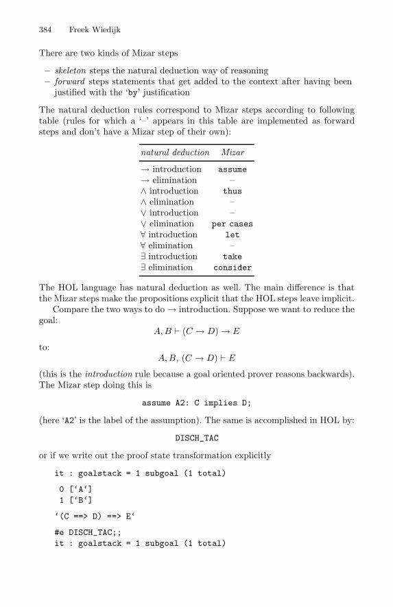
384 Freek Wiedijk
There are two kinds of Mizar steps:
– skeleton steps: the natural deduction way of reasoning– forward steps: statements that get added to the context after having been
justified with the ‘by’ justification
The natural deduction rules correspond to Mizar steps according to followingtable (rules for which a ‘–’ appears in this table are implemented as forwardsteps and don’t have a Mizar step of their own):
natural deduction Mizar
→ introduction assume→ elimination –∧ introduction thus∧ elimination –∨ introduction –∨ elimination per cases∀ introduction let∀ elimination –∃ introduction take∃ elimination consider
The HOL language has natural deduction as well. The main difference is thatthe Mizar steps make the propositions explicit that the HOL steps leave implicit.
Compare the two ways to do→ introduction. Suppose we want to reduce thegoal:
A, B (C → D)→ E
to:A, B, (C → D) E
(this is the introduction rule because a goal oriented prover reasons backwards).The Mizar step doing this is:
assume A2: C implies D;
(here ‘A2’ is the label of the assumption). The same is accomplished in HOL by:
DISCH_TAC
or if we write out the proof state transformation explicitly:
it : goalstack = 1 subgoal (1 total)
0 [‘A‘]1 [‘B‘]
‘(C ==> D) ==> E‘
#e DISCH_TAC;;it : goalstack = 1 subgoal (1 total)
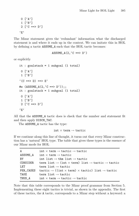
Mizar Light for HOL Light 385
0 [‘A‘]1 [‘B‘]2 [‘C ==> D‘]
‘E‘
The Mizar statement gives the ‘redundant’ information what the dischargedstatement is and where it ends up in the context. We can imitate this in HOLby defining a tactic ASSUME_A such that the HOL tactic becomes:
ASSUME_A(2,‘C ==> D‘)
or explicitly:
it : goalstack = 1 subgoal (1 total)
0 [‘A‘]1 [‘B‘]
‘(C ==> D) ==> E‘
#e (ASSUME_A(2,‘C ==> D‘));;it : goalstack = 1 subgoal (1 total)
0 [‘A‘]1 [‘B‘]2 [‘C ==> D‘]
‘E‘
All that the ASSUME_A tactic does is check that the number and statement fitand then apply DISCH_TAC.
The ASSUME_A tactic has the type:
int × term → tactic
If we continue along this line of thought, it turns out that every Mizar construc-tion has a ‘natural’ HOL type. The table that gives these types is the essence ofour Mizar mode for HOL:
A int × term → tactic → tacticASSUME_A int × term → tacticBY int list → thm list → tacticCONSIDER term list → (int × term) list → tactic → tacticLET term list → tacticPER_CASES tactic → ((int × term) × tactic) list → tacticTAKE term list → tacticTHUS_A int × term → tactic → tactic
Note that this table corresponds to the Mizar proof grammar from Section 5.Implementing these eight tactics is trivial, as shown in the appendix. The firstof these tactics, the A tactic, corresponds to a Mizar step without a keyword: a
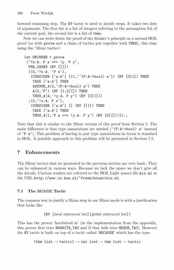
386 Freek Wiedijk
forward reasoning step. The BY tactic is used to justify steps. It takes two listsof arguments. The first list is a list of integers referring to the assumption list ofthe current goal, the second list is a list of thms.
Now we can write down the proof of the drinker’s principle as a normal HOLproof (so with prove and a chain of tactics put together with THEN), this timeusing the ‘Mizar tactics’:
let DRINKER = prove(‘?x:A. P x ==> !y. P y‘,PER_CASES (BY [][])[(0,‘?x:A. ~P x‘),(CONSIDER [‘a:A‘] [(1,‘~(P:A->bool) a‘)] (BY [0][]) THENTAKE [‘a:A‘] THENASSUME_A(2,‘(P:A->bool) a‘) THENA(3,‘F‘) (BY [1;2][]) THENTHUS_A(4,‘!y:A. P y‘) (BY [3][]))
;(0,‘!x:A. P x‘),(CONSIDER [‘a:A‘] [] (BY [][]) THENTAKE [‘a:A‘] THENTHUS_A(1,‘P a ==> !y:A. P y‘) (BY [0][]))]);;
Note that this is similar to the Mizar version of this proof from Section 5. Themain difference is that type annotations are needed (‘(P:A->bool) a‘ insteadof ‘P a‘). This problem of having to put type annotations in terms is standardin HOL. A possible approach to this problem will be presented in Section 7.5.
7 Enhancements
The Mizar tactics that we presented in the previous section are very basic. Theycan be enhanced in various ways. Because we lack the space we don’t give allthe details. Curious readers are referred to the HOL Light source file miz.ml atthe URL http://www.cs.kun.nl/~freek/mizar/miz.ml.
7.1 The BECAUSE Tactic
The common way to justify a Mizar step in our Mizar mode is with a justificationthat looks like:
(BY [local statement list][global statement list])
This has the prover ‘hardwired in’ (in the implementation from the appendix,this prover first tries REWRITE_TAC and if that fails tries MESON_TAC). Howeverthe BY tactic is built on top of a tactic called ‘BECAUSE’ which has the type:
(thm list → tactic) → int list → thm list → tactic
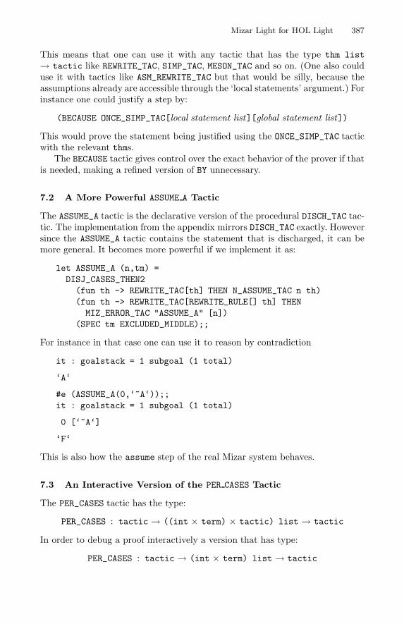
Mizar Light for HOL Light 387
This means that one can use it with any tactic that has the type thm list→ tactic like REWRITE_TAC, SIMP_TAC, MESON_TAC and so on. (One also coulduse it with tactics like ASM_REWRITE_TAC but that would be silly, because theassumptions already are accessible through the ‘local statements’ argument.) Forinstance one could justify a step by:
(BECAUSE ONCE_SIMP_TAC[local statement list][global statement list])
This would prove the statement being justified using the ONCE_SIMP_TAC tacticwith the relevant thms.
The BECAUSE tactic gives control over the exact behavior of the prover if thatis needed, making a refined version of BY unnecessary.
7.2 A More Powerful ASSUME A Tactic
The ASSUME_A tactic is the declarative version of the procedural DISCH_TAC tac-tic. The implementation from the appendix mirrors DISCH_TAC exactly. Howeversince the ASSUME_A tactic contains the statement that is discharged, it can bemore general. It becomes more powerful if we implement it as:
let ASSUME_A (n,tm) =DISJ_CASES_THEN2
(fun th -> REWRITE_TAC[th] THEN N_ASSUME_TAC n th)(fun th -> REWRITE_TAC[REWRITE_RULE[] th] THENMIZ_ERROR_TAC "ASSUME_A" [n])
(SPEC tm EXCLUDED_MIDDLE);;
For instance in that case one can use it to reason by contradiction:
it : goalstack = 1 subgoal (1 total)
‘A‘
#e (ASSUME_A(0,‘~A‘));;it : goalstack = 1 subgoal (1 total)
0 [‘~A‘]
‘F‘
This is also how the assume step of the real Mizar system behaves.
7.3 An Interactive Version of the PER CASES Tactic
The PER_CASES tactic has the type:
PER_CASES : tactic → ((int × term) × tactic) list → tactic
In order to debug a proof interactively a version that has type:
PER_CASES : tactic → (int × term) list → tactic
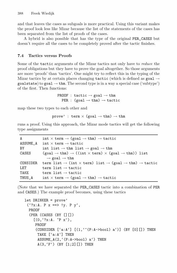
388 Freek Wiedijk
and that leaves the cases as subgoals is more practical. Using this variant makesthe proof look less like Mizar because the list of the statements of the cases hasbeen separated from the list of proofs of the cases.
A hybrid is also possible that has the type of the original PER_CASES butdoesn’t require all the cases to be completely proved after the tactic finishes.
7.4 Tactics versus Proofs
Some of the tactic arguments of the Mizar tactics not only have to reduce theproof obligations but they have to prove the goal altogether. So those argumentsare more ‘proofs’ than ‘tactics’. One might try to reflect this in the typing of theMizar tactics by at certain places changing tactic (which is defined as goal→goalstate) to goal→ thm. The second type is in a way a special case (‘subtype’)of the first. Then functions:
PROOF : tactic → goal → thmPER : (goal → thm) → tactic
map these two types to each other and:
prove’ : term × (goal → thm) → thm
runs a proof. Using this approach, the Mizar mode tactics will get the followingtype assignments:
A int × term → (goal → thm) → tacticASSUME_A int × term → tacticBY int list → thm list → goal → thmCASES (goal → thm) → ((int × term) × (goal → thm)) list
→ goal → thmCONSIDER term list → (int × term) list → (goal → thm) → tacticLET term list → tacticTAKE term list → tacticTHUS_A int × term → (goal → thm) → tactic
(Note that we have separated the PER_CASES tactic into a combination of PERand CASES.) The example proof becomes, using these tactics:
let DRINKER = prove’(‘?x:A. P x ==> !y. P y‘,PROOF(PER (CASES (BY [][])
[(0,‘?x:A. ~P x‘),PROOF(CONSIDER [‘a:A‘] [(1,‘~(P:A->bool) a‘)] (BY [0][]) THENTAKE [‘a:A‘] THENASSUME_A(2,‘(P:A->bool) a‘) THENA(3,‘F‘) (BY [1;2][]) THEN
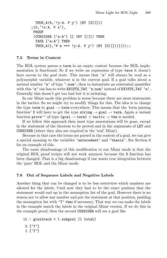
Mizar Light for HOL Light 389
THUS_A(4,‘!y:A. P y‘) (BY [3][]));(0,‘!x:A. P x‘),PROOF(CONSIDER [‘a:A‘] [] (BY [][]) THENTAKE [‘a:A‘] THENTHUS_A(1,‘P a ==> !y:A. P y‘) (BY [0][]))])));;
7.5 Terms in Context
The HOL system parses a term in an empty context because the HOL imple-mentation is functional. So if we write an expression of type term it doesn’thave access to the goal state. This means that ‘n‘ will always be read as apolymorphic variable, whatever is in the current goal. If a goal talks about anatural number ‘n‘ of type ‘:num‘, then to instantiate an existential quantifierwith this ‘n‘ one has to write EXISTS_TAC ‘n:num‘ instead of EXISTS_TAC ‘n‘.Generally this doesn’t get too bad but it is irritating.
In our Mizar mode this problem is worse because there are more statementsin the tactics. So we might try to modify things for this. The idea is to changethe type term to goal → term everywhere. This means that the ‘term parsingfunction’ X will have to get the type string → goal → term. Again a variantfunction prove’’ of type (goal → term) × tactic → thm is needed.
If we follow this approach then most type annotations will be gone, exceptin the statement of the theorem to be proved and in the arguments of LET andCONSIDER (where they also are required in the ‘real’ Mizar).
Because in that case the terms are parsed in the context of a goal, we can givea special meaning to the variables ‘antecedent‘ and ‘thesis‘. See Section 8for an example of this.
The main disadvantage of this modification to our Mizar mode is that theoriginal HOL proof scripts will not work anymore because the X function hasbeen changed. That is a big disadvantage if one wants true integration betweenthe ‘pure’ HOL and the Mizar mode.
7.6 Out of Sequence Labels and Negative Labels
Another thing that can be changed is to be less restrictive which numbers areallowed for the labels. Until now they had to be the exact position that thestatement would end up in the assumption list of the goal. However there is noreason not to allow any number and put the statement at that position, paddingthe assumption list with ‘T‘ thms if necessary. That way we can make the labelsin the example match the labels in the original Mizar version. If we do this inthe example proof, then the second CONSIDER will see a goal like:
it : goalstack = 1 subgoal (1 total)
0 [‘T‘]1 [‘T‘]
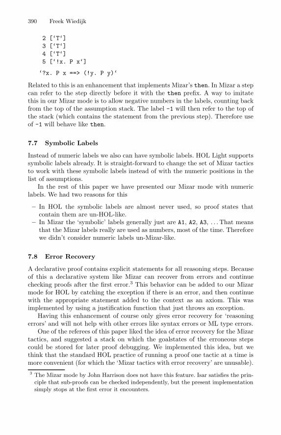
390 Freek Wiedijk
2 [‘T‘]3 [‘T‘]4 [‘T‘]5 [‘!x. P x‘]
‘?x. P x ==> (!y. P y)‘
Related to this is an enhancement that implements Mizar’s then. In Mizar a stepcan refer to the step directly before it with the then prefix. A way to imitatethis in our Mizar mode is to allow negative numbers in the labels, counting backfrom the top of the assumption stack. The label -1 will then refer to the top ofthe stack (which contains the statement from the previous step). Therefore useof -1 will behave like then.
7.7 Symbolic Labels
Instead of numeric labels we also can have symbolic labels. HOL Light supportssymbolic labels already. It is straight-forward to change the set of Mizar tacticsto work with these symbolic labels instead of with the numeric positions in thelist of assumptions.
In the rest of this paper we have presented our Mizar mode with numericlabels. We had two reasons for this:
– In HOL the symbolic labels are almost never used, so proof states thatcontain them are un-HOL-like.
– In Mizar the ‘symbolic’ labels generally just are A1, A2, A3, . . . That meansthat the Mizar labels really are used as numbers, most of the time. Thereforewe didn’t consider numeric labels un-Mizar-like.
7.8 Error Recovery
A declarative proof contains explicit statements for all reasoning steps. Becauseof this a declarative system like Mizar can recover from errors and continuechecking proofs after the first error.3 This behavior can be added to our Mizarmode for HOL by catching the exception if there is an error, and then continuewith the appropriate statement added to the context as an axiom. This wasimplemented by using a justification function that just throws an exception.
Having this enhancement of course only gives error recovery for ‘reasoningerrors’ and will not help with other errors like syntax errors or ML type errors.
One of the referees of this paper liked the idea of error recovery for the Mizartactics, and suggested a stack on which the goalstates of the erroneous stepscould be stored for later proof debugging. We implemented this idea, but wethink that the standard HOL practice of running a proof one tactic at a time ismore convenient (for which the ‘Mizar tactics with error recovery’ are unusable).3 The Mizar mode by John Harrison does not have this feature. Isar satisfies the prin-
ciple that sub-proofs can be checked independently, but the present implementationsimply stops at the first error it encounters.
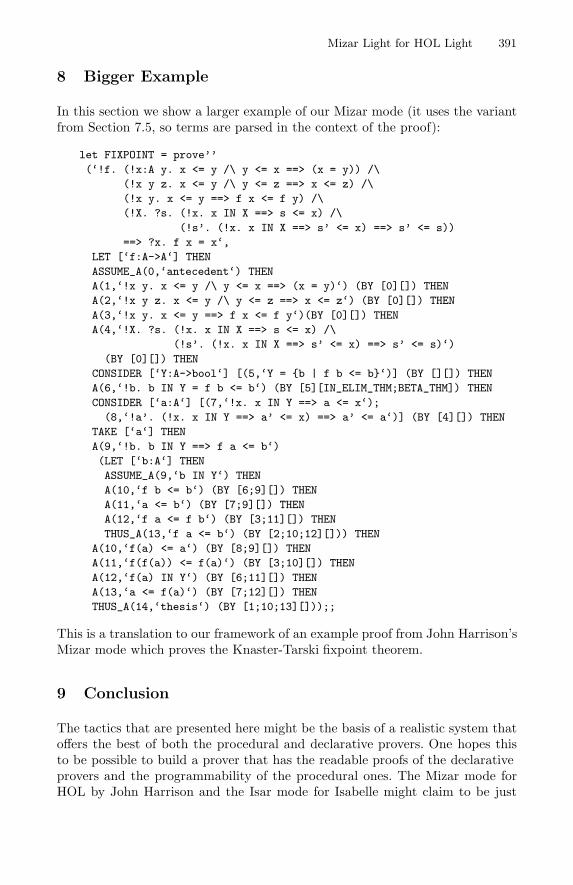
Mizar Light for HOL Light 391
8 Bigger Example
In this section we show a larger example of our Mizar mode (it uses the variantfrom Section 7.5, so terms are parsed in the context of the proof):
let FIXPOINT = prove’’
(‘!f. (!x:A y. x <= y /\ y <= x ==> (x = y)) /\
(!x y z. x <= y /\ y <= z ==> x <= z) /\
(!x y. x <= y ==> f x <= f y) /\
(!X. ?s. (!x. x IN X ==> s <= x) /\
(!s’. (!x. x IN X ==> s’ <= x) ==> s’ <= s))
==> ?x. f x = x‘,
LET [‘f:A->A‘] THEN
ASSUME_A(0,‘antecedent‘) THEN
A(1,‘!x y. x <= y /\ y <= x ==> (x = y)‘) (BY [0][]) THEN
A(2,‘!x y z. x <= y /\ y <= z ==> x <= z‘) (BY [0][]) THEN
A(3,‘!x y. x <= y ==> f x <= f y‘)(BY [0][]) THEN
A(4,‘!X. ?s. (!x. x IN X ==> s <= x) /\
(!s’. (!x. x IN X ==> s’ <= x) ==> s’ <= s)‘)
(BY [0][]) THEN
CONSIDER [‘Y:A->bool‘] [(5,‘Y = {b | f b <= b}‘)] (BY [][]) THEN
A(6,‘!b. b IN Y = f b <= b‘) (BY [5][IN_ELIM_THM;BETA_THM]) THEN
CONSIDER [‘a:A‘] [(7,‘!x. x IN Y ==> a <= x‘);
(8,‘!a’. (!x. x IN Y ==> a’ <= x) ==> a’ <= a‘)] (BY [4][]) THEN
TAKE [‘a‘] THEN
A(9,‘!b. b IN Y ==> f a <= b‘)
(LET [‘b:A‘] THEN
ASSUME_A(9,‘b IN Y‘) THEN
A(10,‘f b <= b‘) (BY [6;9][]) THEN
A(11,‘a <= b‘) (BY [7;9][]) THEN
A(12,‘f a <= f b‘) (BY [3;11][]) THEN
THUS_A(13,‘f a <= b‘) (BY [2;10;12][])) THEN
A(10,‘f(a) <= a‘) (BY [8;9][]) THEN
A(11,‘f(f(a)) <= f(a)‘) (BY [3;10][]) THEN
A(12,‘f(a) IN Y‘) (BY [6;11][]) THEN
A(13,‘a <= f(a)‘) (BY [7;12][]) THEN
THUS_A(14,‘thesis‘) (BY [1;10;13][]));;
This is a translation to our framework of an example proof from John Harrison’sMizar mode which proves the Knaster-Tarski fixpoint theorem.
9 Conclusion
The tactics that are presented here might be the basis of a realistic system thatoffers the best of both the procedural and declarative provers. One hopes thisto be possible: to build a prover that has the readable proofs of the declarativeprovers and the programmability of the procedural ones. The Mizar mode forHOL by John Harrison and the Isar mode for Isabelle might claim to be just
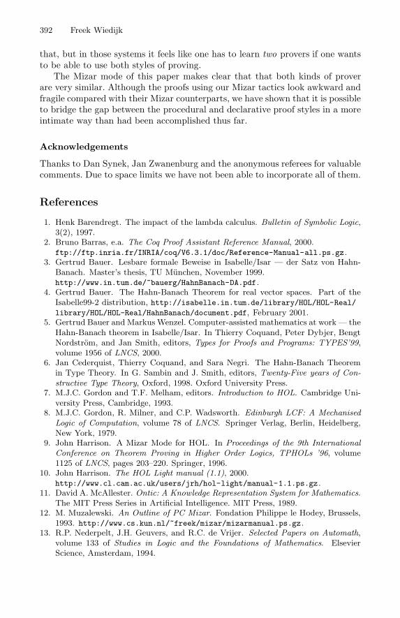
392 Freek Wiedijk
that, but in those systems it feels like one has to learn two provers if one wantsto be able to use both styles of proving.
The Mizar mode of this paper makes clear that that both kinds of proverare very similar. Although the proofs using our Mizar tactics look awkward andfragile compared with their Mizar counterparts, we have shown that it is possibleto bridge the gap between the procedural and declarative proof styles in a moreintimate way than had been accomplished thus far.
Acknowledgements
Thanks to Dan Synek, Jan Zwanenburg and the anonymous referees for valuablecomments. Due to space limits we have not been able to incorporate all of them.
References
1. Henk Barendregt. The impact of the lambda calculus. Bulletin of Symbolic Logic,3(2), 1997.
2. Bruno Barras, e.a. The Coq Proof Assistant Reference Manual, 2000.ftp://ftp.inria.fr/INRIA/coq/V6.3.1/doc/Reference-Manual-all.ps.gz.
3. Gertrud Bauer. Lesbare formale Beweise in Isabelle/Isar — der Satz von Hahn-Banach. Master’s thesis, TU Munchen, November 1999.http://www.in.tum.de/~bauerg/HahnBanach-DA.pdf.
4. Gertrud Bauer. The Hahn-Banach Theorem for real vector spaces. Part of theIsabelle99-2 distribution, http://isabelle.in.tum.de/library/HOL/HOL-Real/library/HOL/HOL-Real/HahnBanach/document.pdf, February 2001.
5. Gertrud Bauer and Markus Wenzel. Computer-assisted mathematics at work — theHahn-Banach theorem in Isabelle/Isar. In Thierry Coquand, Peter Dybjer, BengtNordstrom, and Jan Smith, editors, Types for Proofs and Programs: TYPES’99,volume 1956 of LNCS, 2000.
6. Jan Cederquist, Thierry Coquand, and Sara Negri. The Hahn-Banach Theoremin Type Theory. In G. Sambin and J. Smith, editors, Twenty-Five years of Con-structive Type Theory, Oxford, 1998. Oxford University Press.
7. M.J.C. Gordon and T.F. Melham, editors. Introduction to HOL. Cambridge Uni-versity Press, Cambridge, 1993.
8. M.J.C. Gordon, R. Milner, and C.P. Wadsworth. Edinburgh LCF: A MechanisedLogic of Computation, volume 78 of LNCS. Springer Verlag, Berlin, Heidelberg,New York, 1979.
9. John Harrison. A Mizar Mode for HOL. In Proceedings of the 9th InternationalConference on Theorem Proving in Higher Order Logics, TPHOLs ’96, volume1125 of LNCS, pages 203–220. Springer, 1996.
10. John Harrison. The HOL Light manual (1.1), 2000.http://www.cl.cam.ac.uk/users/jrh/hol-light/manual-1.1.ps.gz .
11. David A. McAllester. Ontic: A Knowledge Representation System for Mathematics.The MIT Press Series in Artificial Intelligence. MIT Press, 1989.
12. M. Muzalewski. An Outline of PC Mizar. Fondation Philippe le Hodey, Brussels,1993. http://www.cs.kun.nl/~freek/mizar/mizarmanual.ps.gz.
13. R.P. Nederpelt, J.H. Geuvers, and R.C. de Vrijer. Selected Papers on Automath,volume 133 of Studies in Logic and the Foundations of Mathematics. ElsevierScience, Amsterdam, 1994.
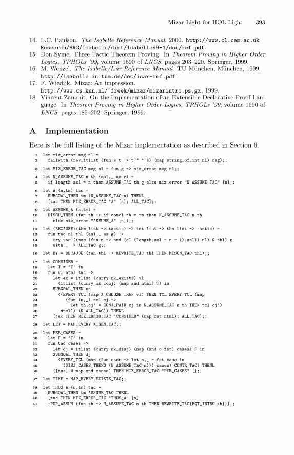
Mizar Light for HOL Light 393
14. L.C. Paulson. The Isabelle Reference Manual, 2000. http://www.cl.cam.ac.uk
Research/HVG/Isabelle/dist/Isabelle99-1/doc/ref.pdf.15. Don Syme. Three Tactic Theorem Proving. In Theorem Proving in Higher Order
Logics, TPHOLs ’99, volume 1690 of LNCS, pages 203–220. Springer, 1999.16. M. Wenzel. The Isabelle/Isar Reference Manual. TU Munchen, Munchen, 1999.
http://isabelle.in.tum.de/doc/isar-ref.pdf.17. F. Wiedijk. Mizar: An impression.
http://www.cs.kun.nl/~freek/mizar/mizarintro.ps.gz, 1999.18. Vincent Zammit. On the Implementation of an Extensible Declarative Proof Lan-
guage. In Theorem Proving in Higher Order Logics, TPHOLs ’99, volume 1690 ofLNCS, pages 185–202. Springer, 1999.
A Implementation
Here is the full listing of the Mizar implementation as described in Section 6.1 let miz_error msg nl =2 failwith (rev_itlist (fun s t -> t^" "^s) (map string_of_int nl) msg);;
3 let MIZ_ERROR_TAC msg nl = fun g -> miz_error msg nl;;
4 let N_ASSUME_TAC n th (asl,_ as g) =5 if length asl = n then ASSUME_TAC th g else miz_error "N_ASSUME_TAC" [n];;
6 let A (n,tm) tac =7 SUBGOAL_THEN tm (N_ASSUME_TAC n) THENL8 [tac THEN MIZ_ERROR_TAC "A" [n]; ALL_TAC];;
9 let ASSUME_A (n,tm) =10 DISCH_THEN (fun th -> if concl th = tm then N_ASSUME_TAC n th11 else miz_error "ASSUME_A" [n]);;
12 let (BECAUSE:(thm list -> tactic) -> int list -> thm list -> tactic) =13 fun tac nl thl (asl,_ as g) ->14 try tac ((map (fun n -> snd (el (length asl - n - 1) asl)) nl) @ thl) g15 with _ -> ALL_TAC g;;
16 let BY = BECAUSE (fun thl -> REWRITE_TAC thl THEN MESON_TAC thl);;
17 let CONSIDER =18 let T = ‘T‘ in19 fun vl ntml tac ->20 let ex = itlist (curry mk_exists) vl21 (itlist (curry mk_conj) (map snd ntml) T) in22 SUBGOAL_THEN ex23 ((EVERY_TCL (map X_CHOOSE_THEN vl) THEN_TCL EVERY_TCL (map24 (fun (n,_) tcl cj ->25 let th,cj’ = CONJ_PAIR cj in N_ASSUME_TAC n th THEN tcl cj’)26 ntml)) (K ALL_TAC)) THENL27 [tac THEN MIZ_ERROR_TAC "CONSIDER" (map fst ntml); ALL_TAC];;
28 let LET = MAP_EVERY X_GEN_TAC;;
29 let PER_CASES =30 let F = ‘F‘ in31 fun tac cases ->32 let dj = itlist (curry mk_disj) (map (snd o fst) cases) F in33 SUBGOAL_THEN dj34 (EVERY_TCL (map (fun case -> let n,_ = fst case in35 (DISJ_CASES_THEN2 (N_ASSUME_TAC n))) cases) CONTR_TAC) THENL36 ([tac] @ map snd cases) THEN MIZ_ERROR_TAC "PER_CASES" [];;
37 let TAKE = MAP_EVERY EXISTS_TAC;;
38 let THUS_A (n,tm) tac =39 SUBGOAL_THEN tm ASSUME_TAC THENL40 [tac THEN MIZ_ERROR_TAC "THUS_A" [n]41 ;POP_ASSUM (fun th -> N_ASSUME_TAC n th THEN REWRITE_TAC[EQT_INTRO th])];;
Author Index
Adams, Andrew 27Alonso-Jimenez, Jose A. 297Arthan, Rob D. 43Asperti, Andrea 59
Bauer, Gertrud 75Bella, Giampaolo 91Bertot, Yves 346Bickford, Mark 105Bove, Ana 121
Caccamo, Mario 136Capretta, Venanzio 121, 154Cheng, Xiaochun 201
Daumas, Marc 169Dennis, Louise A. 185Dunstan, Martin 27
Fairtlough, Matt 201
Gay, Simon J. 217Gottliebsen, Hanne 27Goubault-Larrecq, Jean 362
Hayes, Ian 249Helke, Steffen 233Hemer, David 249Hurd, Joe 265
Jacobs, Bart 1Johnson, Steven D. 4
Kammuller, Florian 233Kellomaki, Pertti 281Kelsey, Tom 27
Kreitz, Christoph 105
Liu, Xiaoming 105
Martin, Ursula 27Medina-Bulo, Inmaculada 297Mendler, Michael 201Meseguer, Jose 329Moore, J Strother 313
Naumov, Pavel 329
Owre, Sam 27
Padovani, Luca 59Palomo-Lozano, Francisco 297Paulson, Lawrence C. 91Pichardie, David 346
Renesse, Robbert van 105Rideau, Laurence 169Rival, Xavier 362
Sacerdoti Coen, Claudio 59Schena, Irene 59Shankar, Natarajan 5Smaill, Alan 185Stehr, Mark-Oliver 329Strooper, Paul 249
Thery, Laurent 169
Wenzel, Markus 75Wiedijk, Freek 378Winskel, Glynn 136