LANDUSE MAPPING BY GIS

BY

ANU.M.BABU RAMYA.P

SMITHA.K.E

Department of

Land and Water Resources and Conservation Engineering KELAPPAJI COLLEGE OF AGRICULTURAL ENGINEERING AND TECHNOLOGY

Tavanur-679 573, Malappuram Kerala, India

2005

LAND USE MAPPING BY GIS

BY

ANU.M.BABU. RAMYA.P.

SMITHA.K.E.

PROJECT REPORT Submitted in partial fulfilment of the requirement for the degree

BACHELOR OF TECHNOLOGY IN

AGRICULTURAL ENGINEERING

Faculty of Agricultural Engineering Kerala Agricultural University

Department of Land and Water Resources and Conservation Engineering

KELAPPAJI COLLEGE OF AGRICULTURAL ENGINEERING AND TECHNOLOGY Tavanur-679 573, Malappuram

Kerala, India 2005

DECLARATION

We hereby declare that this project entitled "Land Use Mapping by

GIS” is a bonafide record of project work done by us during the course of project and that the

report has not previously formed the basis for the award to us of any degree, diploma,

associateship, fellowship or other similar title of any other university or society.

Place: Tavanur

Date:

Anu.M.Babu

Ramya.P

Smitha.K.E

CERTIFICATE

Certified that this project report entitled "Land Use Mapping by GIS" is a record

of project work done jointly by Anu. M. Babu, Ramya. P and Smitha, K.E under my

guidance and supervision and that it has not previously formed the basis for the award of

any degree, diploma, fellowship or associateship to them.

Er. Vishnu, B,

Project guide

Assistant Professor

Dept. of LWRCE

K.C.A.E.T, Tavanur

Place : Tavanur

Date :

ACKNOWLEDGEMENT

We express our respect and gratitude to our guide Er. Vishnu. B, Assistant Professor,

Department of Land and Water Resources and Conservation Engineering, K.C.A.E.T,

Tavanur for all the help and encouragement and guidance during the course of this work and

preparation of this project report.

We are immensely thankful to Prof. C.P Muhammad, Dean, K.C.A.E.T, Tavanur for

the co-operation extended towards us for the completion of this work.

We express our sincere thanks to Er. Sathian. K.K, Er. Renukakumari and Er. Shyla

Joseph, Assistant Professors, Department of Land and Water Resources and Conservation

Engineering, K.C.A.E.T, Tavanur for the valuable advice and help rendered us during the

project.

We acknowledge with gratitude to Dr.Habeeburrahman, Associate Professor and

Head, KVK, Tavanur for the help offered during the study.

We express our sincere thanks to Mrs. Meagle, Assistant professor, PFDC for the help

provided to us during this project.

We are indebted to Mr. Alikutty, Farm assistant, K.C.A.E.T for all the services

rendered to us.

We express our special thanks to all of our friends for all the help they had provided

us for the completion of this work.

At this moment we also do remember our parents whose help on this project we

thankfully acknowledge.

Above all, we extend our sincere gratitude and praise to God almighty in enabling us

to complete this work.

Anu.M.Babu

Ramya.P

Smitha.K.E

Dedicated

To

Our Loving Parents

CONTENTS

Chapter Title Page

LIST OF TABLES

LIST OF FIGURES

SYMBOLS AND ABBREVIATIONS

I INTRODUCTION 1

II REVIEW OF LITERATURE 4

III MATERIALS AND METHODS 9

IV RESULTS AND DISCUSSIONS 25

V SUMMARY AND CONCLUSION 38

REFERENCES 39

ABSTRACT

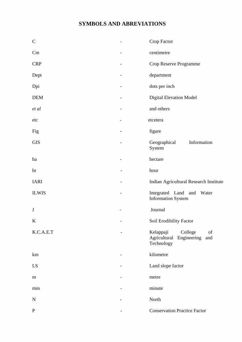
SYMBOLS AND ABREVIATIONS

C - Crop Factor

Cm - centimetre

CRP - Crop Reserve Programme

Dept - department

Dpi - dots per inch

DEM - Digital Elevation Model

et al - and others

etc - etcetera

Fig - figure

GIS - Geographical Information System

ha - hectare

hr - hour

IARI - Indian Agricultural Research Institute

ILWIS - Integrated Land and Water Information System

J - Journal

K - Soil Erodibility Factor

K.C.A.E.T - Kelappaji College of Agricultural Engineering and Technology

km - kilometre

LS - Land slope factor

m - metre

min - minute

N - North

P - Conservation Practice Factor

R - Rainfall erosivity Factor

RUSLE - Revised Universal Soil Loss Equation

SCS - Soil Conservation Service

SYI - Sediment Yield Index

USLE - Universal Soil Loss Equation

yr - year

% - percentage

/ - per

LIST OF TABLES

Table no: Title Page no:

1 Land use pattern of K.C.A.E.T campus 28

2 Percentage area distribution under different landuses 29

3. Buildings in K.C.A.E.T campus 36

4 Area code for different land uses 37

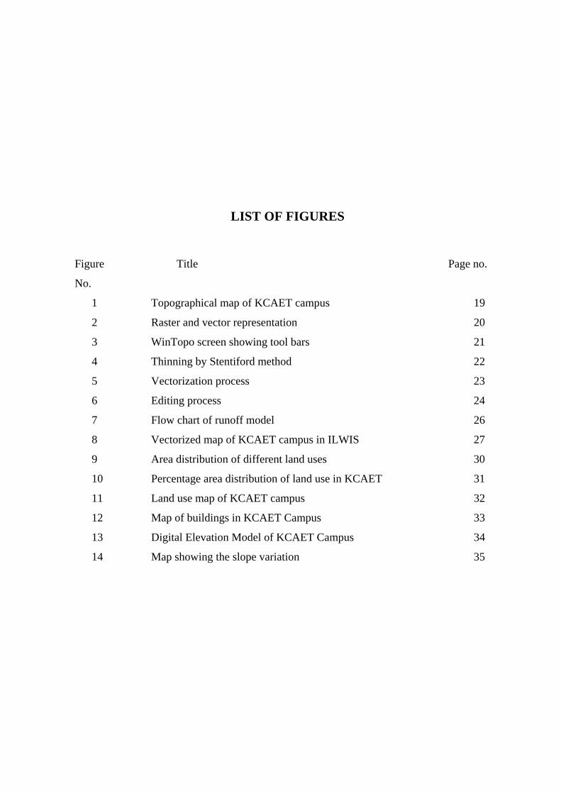
LIST OF FIGURES Figure Title Page no.

No.

1 Topographical map of KCAET campus 19

2 Raster and vector representation 20

3 WinTopo screen showing tool bars 21

4 Thinning by Stentiford method 22

5 Vectorization process 23

6 Editing process 24

7 Flow chart of runoff model 26

8 Vectorized map of KCAET campus in ILWIS 27

9 Area distribution of different land uses 30

10 Percentage area distribution of land use in KCAET 31

11 Land use map of KCAET campus 32

12 Map of buildings in KCAET Campus 33

13 Digital Elevation Model of KCAET Campus 34

14 Map showing the slope variation 35

Introduction

1

INTRODUCTION

Land resources are of paramount importance for the survival and

welfare of people. The type of land varies from place to place because of differences in the

interaction of various factors, geological, topographical and hydrological, under the influence

of climate and people’s activities over centuries. Agricultural land use, one of the primary

uses of land has been of prime importance since the beginning of civilization. Agricultural

development has been the foundation of the industrial superstructure in the developing

countries.

Land use change is the temporal shift in human exploitation of

biospheric resources in terrestrial ecosystems. In view of the rapidly increasing need for more

food production and the claims of different types of users for a share in land resources, it is

necessary to accord high priority to the promotion of optimum land use and it’s conservation.

Land use management is the process by which human land use is controlled to attain a

specific goal, such as the maximization of resource extraction, minimization of

environmental impact, or some combination of both.

1.1 Land Use

Land use is the result of a continuous field of tension created between

available resources and human needs and acted upon by human efforts .Land cover refers to

different features covering the earth's surface including vegetation cover, water bodies, rock

outcrops etc. The land use term refers to man's use of the land and its cover. Although land

use and land cover are conceptually different, they are used synonymously in many instances.

Land use can change over the years. The causes of the land use change

are different. Land use / land cover changes with time because of many factors like land-

ownership, population pressure etc. The major procedure in achieving the temporal figure of

land use is through the application of remote sensing data, which provide an aid in the rapid

assessment of the land use in a GIS environment.

2

1.1 Land Use Mapping Land use mapping encompasses a wide range of procedures and data

sources that are employed to measure the spatial arrangement of human activities in

terrestrial ecosystems. Land use mapping techniques are widely employed to monitor and

predict the environmental and human health impacts of different land uses.

Land use and land cover change has become a central component in current

strategies for managing natural resources and monitoring environmental change. Since the

late 1960’s, the rapid development of the concept of vegetation mapping has lead to increased

studies of land use and land cover change worldwide.

1.2 GIS

A GIS has been variously defined in literature as follows:

A special case of information systems where the data consists of

observation on spatially distributed features, activities or an automated spatial information

system designed for data management, mapping and analysis .GIS is a system of hardware,

software and procedures designed to support the capture, management, manipulation,

analysis, modelling and display of spatially referenced data for solving complex planning and

management problems.

GIS can be applied towards answering questions regarding parcel location,

condition, trends, patterns and modelling for analysis and problem solving. This powerful

planning tool can aid decision makers for finding and classifying the most sensitive and

critical open space areas in order to prioritize future acquisition strategies.

3

1.2.1 History of GIS

The initial developments originated in North America in 1960’s with the

organization such as US Bureau of Censes, the US Geological Survey and the Harvard

Laboratory for Computer Graphics and Environmental System Research Institute (ESRI) etc.

Later, commercial agencies started to develop and offer GIS software. Among them, today’s

market leaders are ESRI, Intergraph, Lasers Scan and Auto Desk etc. A sound and stable

data structure to store and analysis map data became dominant in the early 1970’s.

Potentiality of GIS is realised in the recent past and now it has popular among many users for

variety of uses. Recently commercial organizations in India have realized the importance of

GIS for many applications like natural resource management, infrastructure development,

facility management, business / market application etc and many GIS based projects

according to the user organization requirements.

1.2.2 GIS objectives

• Maximise the efficiency of planning and decision making

• Provide the efficient means for data distribution and handling

• Capacity to integrate information from many sources.

• Routing of roads, transmission lines, pipelines, sewer lines and network

analysis through these transportation routes.

• Mapping and managing urban infrastructure included base map, tax, water

supply, drainage, electricity, telephone and gas.

The objective of the study is

• To prepare the landuse map of K.C.A.E.T Campus using GIS.

Review of Literature

4

REVIEW OF LITERATURE

2.1 GIS

GIS is a computer system which can hold and use data describing on earth

surface. GIS has the powerful capability of spatially representing the complex interactions

such as land use, climate, vegetation, slope, soils, population density, topography, wildlife

distribution and migration pattern.

2.1.1 GIS in Landuse

Lin Xinhong et al (1992) conducted study on evaluation of land use in a

selected area in south of Guilin by using GIS. The system includes four functions: input,

storage, analysis and output. While the map of land use is overlaid on the map of slope

classification, the analysis of land potentialities can be made.

Desmet et al (1996) conducted a GIS procedure for automatically

calculating the USLE LS factor on topography complex landscapes units. A computer

algorithm to calculate the USLE and RUSLE LS factors over a two dimensional

landscape is presented. The computer procedure has the obvious advantage that it can

easily be linked to GIS software. If data on land use and soils were available, specific K,

C and P values can be assigned to each land unit so that predicted soil losses can then be

calculated using a simple overlay procedure.

Richard et al (1997) made few studies on comparison of GIS verses

manual techniques for land cover analysis in a Riparian restoration project. In this case

study land cover maps created as a part of Riparian restoration research projects were

used to compare the cost involve in calculating land cover areas with a GIS and manually

with a planimeter and dot grid. While estimates of land cover areas were similar for two

methods, GIS cost were much higher than manual technical cost.

Wu et al (1997) studied about evaluating soil properties of CRP land.

Remote sensing and GIS Techniques are used to evaluate the present CRP in terms of its

main goal and to give recommendations for the future of the program in Finney country,

5

Kansas. With GIS technology, calculation of erosion index was more efficient and value

was more accurate than that calculated by hand.

Van Liehout et al (1998) calculated the total water requirement for

a common area with different crops and soils. The table and map calculation features of

ILWIS for Windows are used to combine different map layers and table attributes.

Van Westen et al (1998) conducted a study on methods of

combining multiple maps for empirical modelling in a GIS. Several approaches to

annualize multiple maps (Boolean logic models, Binary evidence maps, Index overlay

with multi class maps and Fussy logic method) are introduced by means of basic

exercises.

Hoobler et al (2003) conducted a study using the GIS combined

with land evaluation and site assessment (LESA) which enhances land use planning by

delivering a versatile and dynamic model to assist state policy and decision makers,

county and local officials, landowners and interested citizens in making wasteland

management decisions. Objective of this study is to integrate LESA methods and GIS to

assess their use for land use planning in East Park County, Wyoming. Study results were

fairly consistent with a park county land use plan, suggesting the combination of LESA

and GIS is a rapid, versatile and up to date approach to assist in land management

decisions.

Bathgate et al (2003) studied about GIS based landscape

classification model to enhance soil survey. The objective of the research was to develop

a quantitative tool to model landscape elements using GIS and digital elevation model for

application in soil survey. The model was tested at a case study site in a quarter section of

Massac County, Illinois. Potential productive capabilities of the model are great and

should be extended to heterogeneous landscape through further testing model for

communities that contend with landslide risk.

2.1.2 GIS in Watershed Management

GIS has wide range of application in watershed management

including prioritization of watershed, determination of erosion status of watershed etc.

6

Hamlett et al (1992) studied about the state-wide GIS based

ranking of watersheds for agricultural pollution prevention. GIS combined with a

pollutant generation and transport model can be used to identify and rank critical

pollutant source areas on a region basis. This model was used to rank the agricultural

pollution potential of 104 watersheds in Pennsylvania. The ranking allowed identification

of critical non-point source pollutant contributing watersheds in Pennsylvania and is

useful for targeting further investigations and control Programs.

Kwong Fai et al (1995) conducted a study on erosion assessment

of a large watershed in Taiwan. The objective of this study was to integrate the

Agricultural Non-point source pollution model and the technology of GIS to quantify

erosion problems at the Bajun river basin and Tswengwen reservoir watershed in Taiwan.

They found that the annual sedimentation depth for the Tswengwen reservoir is

approximately 5.9 mm, which is not significantly different from the observed rate.

Sidhu et al (1998) prioritized the upper Machukund watershed

covering an area of 16111 ha by Remote Sensing and GIS Techniques. Based on

secondary and tertiary drainage pattern, watershed areas were subdivided into 8 sub

watersheds. By using GIS, land use, land cover and slope maps were combined to

generate erosion intensity and composite maps. Watershed was prioritized by following

sediment delivery index approach

De Roo et al (1998) conducted a study on modelling runoff and

sediment transport in catchments using GIS. Existing erosion models can be loosely

coupled to a GIS, such as the ANSWERS model. More models can be fully integrated by

embedded coupling, such as the LISEM model.

Tripathi et al (2001) conducted a study using a calibrated Soil and

Water Assessment Tool (SWAT). The model was verified for a small watershed

(Nagvan) and used for identification and prioritization of critical sub-watersheds to

develop an effective management plan. The study revealed that the SWAT model could

successfully be used for identifying and prioritizing critical sub-watersheds for

management purposes.

7

Fernandez et al (2003) studied about estimating water erosion and

sediment yield with GIS and RUSLE. The method was applied to a typical agricultural

watershed in the state of Idaho, which is subjected to increasing soil erosion and flooding

problems. The spatial pattern of annual soil erosion and sediment yield was obtained by

integrating RUSLE and raster GIS. Required GIS data layers included precipitation, soil

characteristics, elevation and landuse. Thus it provides a useful and efficient tool for

predicting long term water erosion impacts of various cropping systems and conservation

support practices.

2.1.3 GIS in General Purposes

GIS can be applied in various fields such as siting farm ponds, rural planning

etc.

Cheryl et al (1990) conducted a study about GIS as a tool for siting farm

ponds. GIS was developed for identifying potential sites for a farm pond to serve as a

permanent livestock. Watering system amenable to rotational grazing and independent of

ephemeral streams. Using water balance calculations for 10 years of simulated climate data,

the potential amount of water harvested at each site was determined using water harvesting

potential. Location and negative impacts of a pond at a specific site as criteria, nine sites were

ranked as most desirable.

Novelize et al (1992) conducted a study on wasteland development

using GIS techniques. Soil pH, soil texture, soil drainage and permeability conditions, rainfall,

altitude, slope, water availability, water quality forms the layers which were analyzed for land

suitability. Favourable sites for conducting percolation ponds have been selected by adopting

GIS techniques to augment the ground water potential. The same methodology can be

extended to develop the cultivable wastelands elsewhere.

Joseph (1992) conducted a study on the highway route production

line using a GIS-based approach for economic road planning. It can be used to predict

probable road construction and maintenance costs. The generalized, probabilistic analysis

methods are based on GIS concepts and applied to a test area in Nigeria. GIS concepts allow

the creation of predictive cost models that can support road way planning. This numerical

model defines road way cost factors by assessing database from Remote Sensing Image

Interpretation.

8

Srivastava et al (1992) conducted a study on RS and GIS for natural

resource study. The effectiveness of this technique increases manifolds when it is integrated

with other kind of data sets. GIS permits integration of different sets specially referenced data

of interrelated parameters or periodic data sets about a resource type for its better utilization

and management.

Norberto Fernandez (1993) conducted a study on the design and

implementation of a soil geographic database for rural planning and management. The

physical design of a database involves the evaluation of implementation alternatives using the

data model of the Data Base Management System. This database, which is part of a GIS, will

provide information for soil erosion and soil management studies, and land appraisal for tax

assessment. The results of the conceptual design of a soil database were mapped to the

relational data model.

Pascal Storck and Laura Bowling (1997) made a GIS based distributed

hydrology model for prediction of forest harvest effects on peak stream flow in the Pacefic

Northwest. The model, known as Distributed Hydrology Soil Vegetation Model provides a

dynamic representation of the spatial distribution of soil moisture, snow cover,

evapotranspiration and runoff prediction, at the scale of digital topographic data.

Zaitchik et al (2003) studied about applying a GIS slope stability model to

site specific and landslide prevention in Honduras. This model was applied to an agricultural

region of Honduras that suffered extensive landslide damage during Hurricane milth. Zones

of predicted instability were subsequently categorized according to local slope gradient and

relative wetness (w) based on steady hydrology for Hurricane conditions. Knowledge about,

w in potentially unstable zones allows for informed stability, management practices,

improving the utility of hazard.

5

Materials and Methods

9

MATERIALS AND METHODS

3.1 Location

The experiment was conducted in K.C.A.E.T. campus at Tavanur in

Malappuram district. It is situated at 100 52’ 30” North latitude and 76 0 East longitude. The

total geographical area of the region is about 40.25 ha.

3.2 List of Maps and Data Used

3.2.1 Contour Map of KCAET Campus

The contour map of K.C.A.E.T campus prepared in 1986 was used by

giving modifications to it to incorporate the changes taken place over the last 19 years.

3.2.2 Land Use Data

Field observation of the 40.25 ha area of the campus was made and

change in land use was recorded. Elevation difference of the ground was found out by

theodelite survey.

3.3 Digitizing

Data input is the operation of encoding the data and writing them to the

database. The creation of a clean, digital database is a most important and complex task upon

which the usefulness of the GIS depends. Two aspects of the data need to be considered for

GIS, these are first the positional or geographical data necessary to define where the

geographic or cartographic features occur, and second the associated attributes that record

what the cartographic features represent.

In the raster form, the object space is divided into a group of regularly

spaced grids (some times called pixels) to which the attributes are assigned. The raster form

is basically identical to the data format of remote sensing data.

Most objects on a map can be represented as a combination of a point

(or node), edge (or arc) and area (or polygon). The vector form is provided by the above

geometric factors. The attributes are assigned to points, edges and areas. A point is

represented by geographic coordinates. An edge is represented by a series of line segments

10

with a start point and an end point. A polygon is defined as the sequential edges of a

boundary.

The most common method of entering the spatial data is digitizing. The

features on the existing maps can be digitized with a scanner or tablet digitizer. Raster data

are obtained from a scanner while vector data are measured by a digitizer. Raster scanner of

flat bed design was used for scanning the land use map of K.C.A.E.T. The scanned data were

retained in the form of pixels.

3.3.1 Creation of Raster Image by Scanning Tracing

• Topographic map was traced on a tracing paper.

Scanning

• The flatbed scanner available had only A4 size. Hence the traced map was cut into

10 pieces of size 21 cm x 29.7 cm.

• Each of the pieces was scanned at a resolution of 300 dpi.

Image Editing

• Each of the pieces of the image was imported into different layers.

• The images in different layers were carefully aligned to form the final picture.

• Finally all the layers were merged to obtain the topographic map.

Image Manipulation

• The background of the image had many contrasting pixels, which could interfere

with the automatic digitization process. So the background of the image,

excluding the lines was selected using the “magic wand” tool and removed.

• The scanned image contained lot of speckles, so “despeckling filter” was applied

to the image.

• Finally a clean image devoid of any orphan pixels is obtained.

Contrast stretching:

• In order that the foreground black lines are clearly visible compared to the

background, the “levels” of the image has been adjusted.

3.3.2 Vectorization:

In this study, WinTopo was used for vectorization

11

WinTopo

WinTopo is a high quality tool for converting raster images to vector data. The

following options are available on the view menu:

-Toolbar

This option selects whether or not to show the Tool Bar buttons. The Tool Bar

contains buttons for the most popular options from the menu.

-Status Bar

This option selects whether or not to show the Status Bar at the bottom of the

WinTopo main window. The Status Bar displays information pertinent to options and

progress.

-Zoom In

WinTopo can magnify the raster image and vectors up to 32 times. Selecting the

Zoom In option increases the magnification by 1. Pressing Control-D on the keyboard also

performs a Zoom-In operation.

-Zoom Out

WinTopo can reduce the raster image and vectors up to 32 times. Selecting the

Zoom Out option decreases the magnification by 1. Pressing Control-A on the keyboard also

performs a Zoom Out operation.

-Pan Real time

We can pan the image by selecting this menu option, or clicking the toolbar

button. The button will stay depressed until it is clicked again to release the option. When in

Pan mode the cursor shows as a hand symbol and when click the image and drag the mouse

(keeping the mouse button held down) the image will get dragged, so that the same part of the

image stays under the cursor. We can use the pan mode when working with other functions -

for instance, digitizing polylines.

-Zoom All

This option zooms the image so that it is all visible within the view window.

This is useful if we want to quickly return from high magnification to see the whole image.

12

-Show Raster Image

This option selects whether or not the raster image is displayed. You may wish

to turn off the raster image to see the vectors more easily.

-Show Vector Lines

This option selects whether or not the vector lines are displayed. Turn off the

vector lines to see the raster image more easily.

-Show Line Colour

When a raster is vectorized the vectors are normally displayed in green, so that

they show up against the raster background. If we select the Show Line Colour option the

vectors will be displayed in their actual Colour

3.3.2.1 Stages of Vectorization

WinTopo employs a two stage vectorization process:

1. Thinning of the raster image to single pixel width lines.

2. Extraction of vectors from the pixel lines.

Thinning

In order for WinTopo to extract vectors from a raster image it needs to

determine which parts of the image constitute lines, and where those lines start and end. For

example, the lines may be fairly obvious to a human observer, until the image is magnified, at

which point it may be seen that the lines are several pixels wide, uneven along the edges and

fade out into the background. The approach used by WinTopo is to reduce thick or blobby

regions down to single pixel width items, so that the image is transformed into lines of pixels.

This process is called thinning.

Thinning of the image can be done by three methods: Stentiford, Zhang

Suen and Best combination. It was found that the Stentiford method gave a better digitization

for the map we have used.

13

Vector Extraction

Once a raster has been thinned down to lines of single width pixels, the

vectorize button can be used to extract real vectors. This also occurs as the last stage of the

One Touch Vectorization option. During vectorization a progress meter window shows the

stage of vectorization, and the number of pixels processed when complete, the vectors will be

displayed over the top of the raster image.

Automatic vectorization was used in this study to trace the lines. The

automatically vectorizied image had lot of anomalies like overhanging lines, breakage in

continuous lines, dotted lines represented as different polylines etc.

3.3.4 Editing: Error Detection and Correction

All digital map data can be assumed to include errors of some sort. They

arise from a combination of inaccuracies in source data and from limitations of the digitizer

operator and computer system in use. Certain type of errors, such as that due to inaccuracy of

the original surveyed data, is implicit in the map source and cannot be rectified without

obtaining another source of data. Other errors arise due to the operator failing to position the

curser accurately over the graphic object to be digitized or, missing objects from the map or

wrongly entering the identity of an object. As a general rule, if an error can be detected at the

time of data acquisition, it will be easier to correct it than if it is not detected later.

The errors in automatically vectorized vector image were corrected by

the editing tools available in WinTopo. The editing tools used for editing were: insert node,

move node, delete line, join polylines etc. The vector obtained was having screen coordinates

which were different from the actual spatial values. Hence the vector image was

‘georeferenced’.

Georeferencing was done by entering ‘control points’. Four points on

the vector map which were easily distinguishable was selected and the distance between them

were actually measured in the field. The (x,y) coordinates of these points were determined by

fixing the left most and bottom most point as (0,0). The (x,y) coordinates of these control

points were entered to georeference the vector image. Now, the points in the vector map

represented the actual ground co-ordinates. The vectors can be saved in different file formats

from WinTopo.

14

3.4 Database creation using ILWIS

ILWIS is commonly used GIS software with image processing

capabilities. It is a synonym of Integrated Land Water Information System. ILWIS allows

inputting, managing, analyzing and presenting geographical data. From the data we can

generate information on the spatial and temporal patterns and processes on the earth

surface.

To start ILWIS, double click the ILWIS icon on the desktop. After

opening we can see the ILWIS main window. From this, we can start all operations.

3.4.1 Creation of a Polygon Map Already digitized map was checked for errors and polygonized here.

3.4.1.1 Checking Segments

• In the Catalog, click the segment map with the right mouse button and select Edit from the

context-sensitive menu. Before a map could be polygonized, it should be checked whether

the segments had been digitized and snapped in a proper way. This check was done using the

option Check Segments from the File menu of the Segment editor map window. Mouse

pointer could be used to make corrections.

• From the File menu of the editor window, select Check Segment and Self Overlap to open

the Check Segments dialog box . Accept the defaults and click OK.

• Click Yes to automatically zoom in on the part where the error occurs.

The next check that would be made was on dead ends in segments.

• From the File menu in the Segment editor, select Check Segments and Dead Ends to Open

Check Segments dialog box.

• Click OK. The map was checked for segments that were not connected to others (dead

ends).

• Click Yes to zoom in on the area. The situation is shown in the Figure

• Use the mouse pointer to move the nodes of the segments until they connect. Return to

Select Mode and click the Entire map button when finished.

• From the File menu of the Segment editor, select Check Segments, Dead Ends to Open

Check Segments dialog box.

• Continue checking dead ends until no more error messages appear.

The last check that will be made is on intersections without nodes

• Display the entire map.

15

• From the File menu of the Segment editor, select Check Segments and Intersections. The

Check Segments dialog box was opened.

• Click OK. The map was now checked for segments that were intersecting without a node.

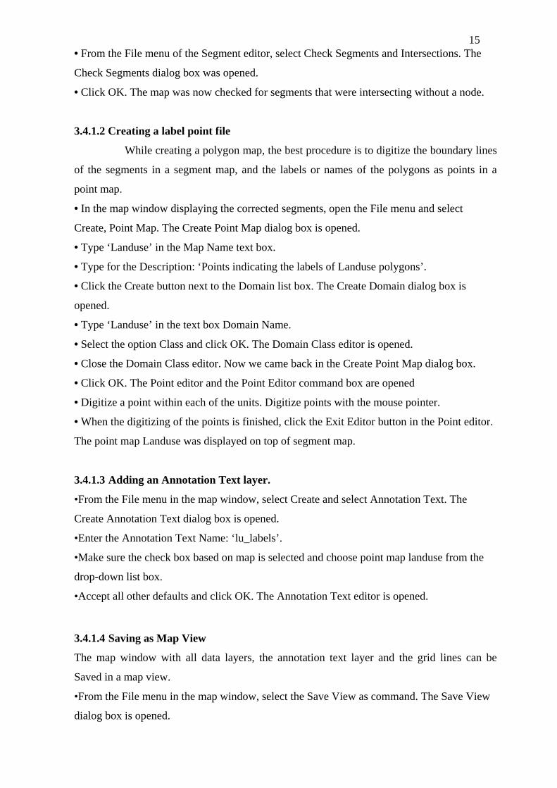
3.4.1.2 Creating a label point file

While creating a polygon map, the best procedure is to digitize the boundary lines

of the segments in a segment map, and the labels or names of the polygons as points in a

point map.

• In the map window displaying the corrected segments, open the File menu and select

Create, Point Map. The Create Point Map dialog box is opened.

• Type ‘Landuse’ in the Map Name text box.

• Type for the Description: ‘Points indicating the labels of Landuse polygons’.

• Click the Create button next to the Domain list box. The Create Domain dialog box is

opened.

• Type ‘Landuse’ in the text box Domain Name.

• Select the option Class and click OK. The Domain Class editor is opened.

• Close the Domain Class editor. Now we came back in the Create Point Map dialog box.

• Click OK. The Point editor and the Point Editor command box are opened

• Digitize a point within each of the units. Digitize points with the mouse pointer.

• When the digitizing of the points is finished, click the Exit Editor button in the Point editor.

The point map Landuse was displayed on top of segment map.

3.4.1.3 Adding an Annotation Text layer. •From the File menu in the map window, select Create and select Annotation Text. The

Create Annotation Text dialog box is opened.

•Enter the Annotation Text Name: ‘lu_labels’.

•Make sure the check box based on map is selected and choose point map landuse from the

drop-down list box.

•Accept all other defaults and click OK. The Annotation Text editor is opened.

3.4.1.4 Saving as Map View The map window with all data layers, the annotation text layer and the grid lines can be

Saved in a map view.

•From the File menu in the map window, select the Save View as command. The Save View

dialog box is opened.

16

•Enter the MapView Name: ‘Landview’.

•Enter the Title: ‘Landuse map of KCAET’.

•Click OK. The view is now saved.

•Close the map window.

•Open the map view Landview. All layers that combined earlier are now appearing in the

same way as displayed them before.

3.4.1.5 Layout and Annotation

Creating a Layout

•From the File menu of the Main window, select Create, Layout. The Layout editor is

opened.

•From the File menu of the Layout editor, select Page Setup. The Page Setup dialog box is

opened.

•Make sure the paper size is A4, change the orientation to landscape and click OK. The

orientation of the layout is now changed into landscape.

Digitizing contour lines

• From the File menu of the Main window, select Map Reference. The Map Reference dialog

box is opened.

• Expand the create item in the operation-tree and double-click New Segment Map. The

Create Segment Map dialog box is opened.

• Type ‘Isolines’ for the name of the map.

• Select landuse from the list box Coordinate System.

• Click the Create Domain button. The Create Domain dialog box appears.

• Type ‘Isolines’ for the Domain Name and select domain Type Value.

• Type 0 and 50 in the Min, Max text boxes, and type 0.1 in the text box Precision.

• Close the Create Domain dialog box by clicking OK. You are now back in the Create

Segment Map dialog box. Click OK.

• From the Edit menu of the segment editor, select Insert Code.

• The Edit dialog box is opened.

• Type the value: 8. This will be the default value for all segments that will digitize from now

on. Click OK.

• Digitize the contour lines with the altitude 8. After you finished digitizing each line, click

OK in the Edit dialog box.

17

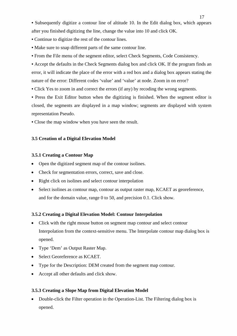
• Subsequently digitize a contour line of altitude 10. In the Edit dialog box, which appears

after you finished digitizing the line, change the value into 10 and click OK.

• Continue to digitize the rest of the contour lines.

• Make sure to snap different parts of the same contour line.

• From the File menu of the segment editor, select Check Segments, Code Consistency.

• Accept the defaults in the Check Segments dialog box and click OK. If the program finds an

error, it will indicate the place of the error with a red box and a dialog box appears stating the

nature of the error: Different codes ‘value’ and ‘value’ at node. Zoom in on error?

• Click Yes to zoom in and correct the errors (if any) by recoding the wrong segments.

• Press the Exit Editor button when the digitizing is finished. When the segment editor is

closed, the segments are displayed in a map window; segments are displayed with system

representation Pseudo.

• Close the map window when you have seen the result.

3.5 Creation of a Digital Elevation Model

3.5.1 Creating a Contour Map

• Open the digitized segment map of the contour isolines.

• Check for segmentation errors, correct, save and close.

• Right click on isolines and select contour interpolation

• Select isolines as contour map, contour as output raster map, KCAET as georeference,

and for the domain value, range 0 to 50, and precision 0.1. Click show.

3.5.2 Creating a Digital Elevation Model: Contour Interpolation

• Click with the right mouse button on segment map contour and select contour

Interpolation from the context-sensitive menu. The Interpolate contour map dialog box is

opened.

• Type ‘Dem’ as Output Raster Map.

• Select Georeference as KCAET.

• Type for the Description: DEM created from the segment map contour.

• Accept all other defaults and click show.

3.5.3 Creating a Slope Map from Digital Elevation Model

• Double-click the Filter operation in the Operation-List. The Filtering dialog box is

opened.

18

• Select Raster Map ‘Dem’ and Filter Name DFDX.

• Type for Output Raster Map: ‘Dx’.

• Accept all other defaults and click Show. The map is calculated, after which the Display

Options – Raster Map dialog box is opened.

• Click OK in the Display Options – Raster Map dialog box. The map is now displayed.

• Repeat the procedure to create a gradient map in the y-direction, but select the Filter

Name DFDY and type ‘Dy’ for the Output Raster Map name.

• Close the map windows.

• Type ‘Slope=HYP(Dx,Dy)/pixsize(Dem)*100’ on the command line to obtain a slope

map ‘slope’ with the percentage slope values.

19

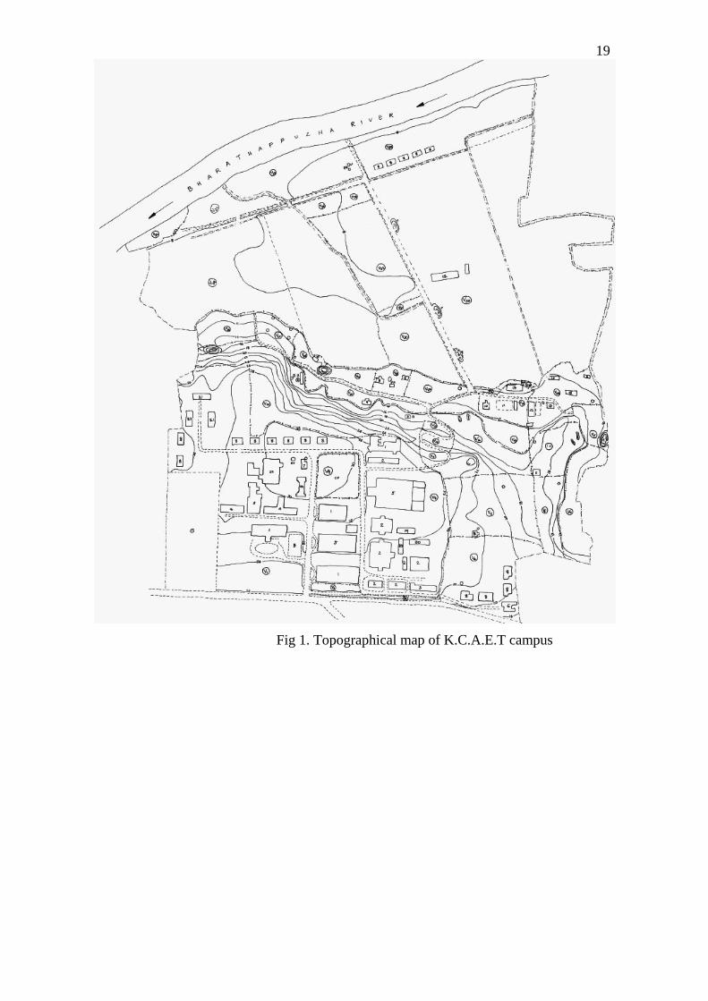
Fig 1. Topographical map of K.C.A.E.T campus

20

Fig.2 Raster and Vector Representation

21

Fig 3. Wintopo screen showing tool bars

22

Fig 4 Thinning by Stentiford method Fig 4 Thinning by Stentiford method

23

Fig 5. Vectorization process

24

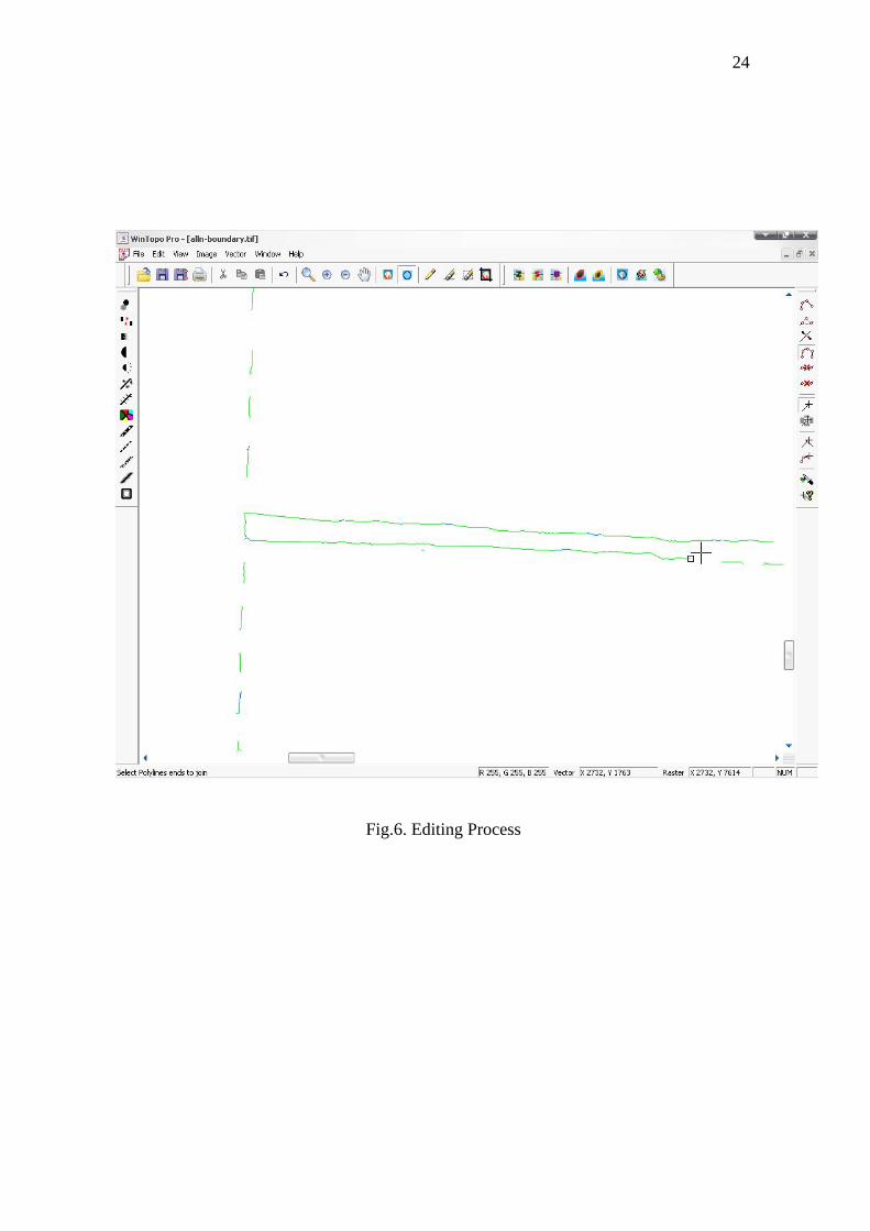
Fig.6. Editing Process

25

Results and Discussion

25

RESULTS AND DISCUSSION

This chapter describes the results of the study conducted for mapping

the land use pattern of K.C.A.E.T Campus using GIS. This can be used as a basis for further

planning and management purposes.

4.1 Landuse

The land use term refers to man's use of the land and its cover. Although

land use and land cover are conceptually different, they are used synonymously in many

instances.

The present change in landuse was noted by field observations. The change

in ground slope was found out by theodolite survey and it was estimated to be 0.67 %.

4.2 Land Use Mapping

The Land use map of K.C.A.E.T was prepared using WinTopo and ILWIS

software. The topographic map of K.C.A.E.T is given in chapter 3. (Fig.1) and the present

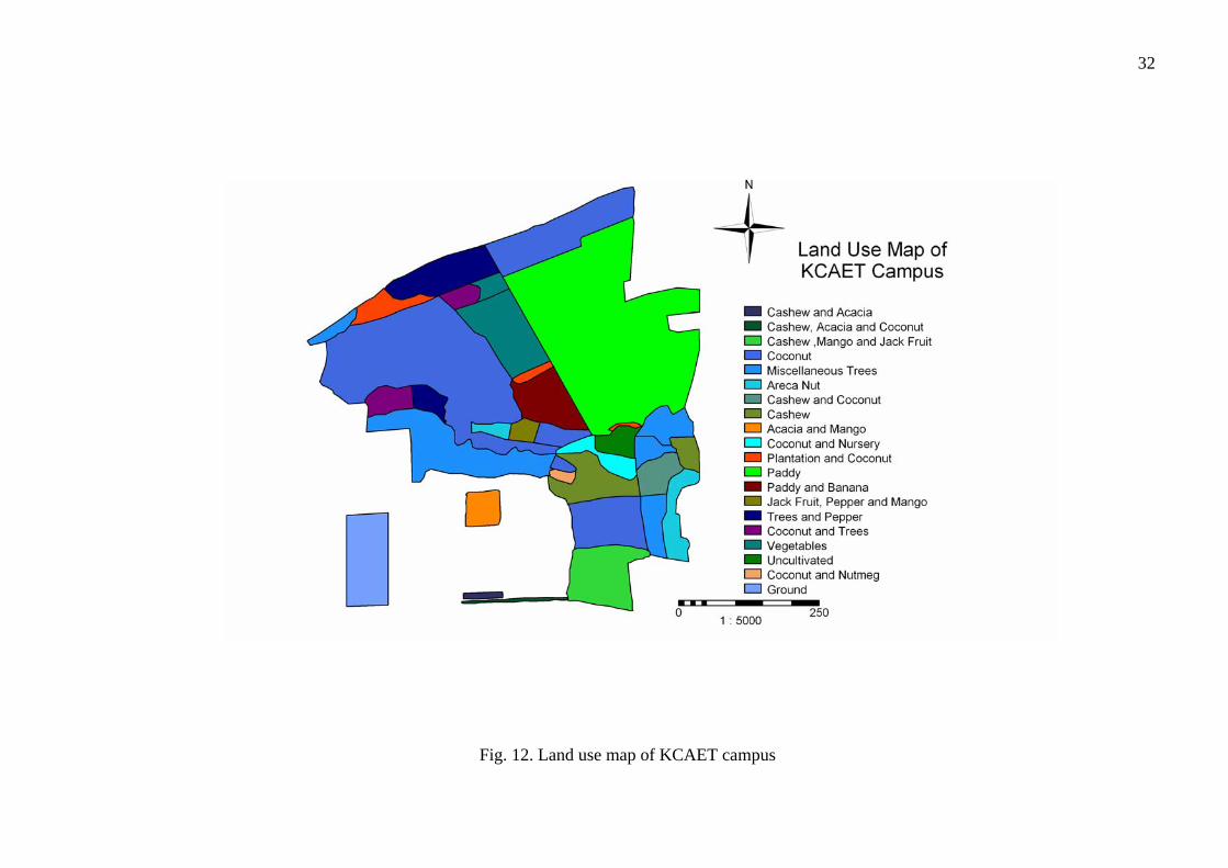
land use distribution are represented in Fig. 12.

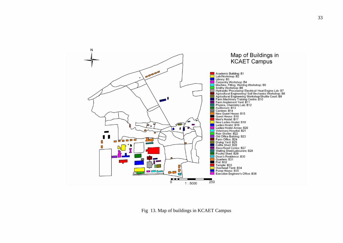
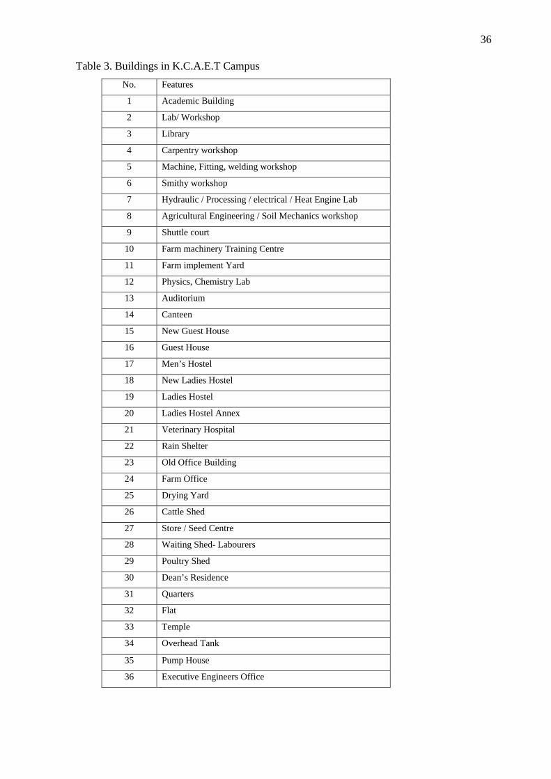
The map of buildings in K.C.A.E.T campus is shown in Fig. 13. The digital elevation

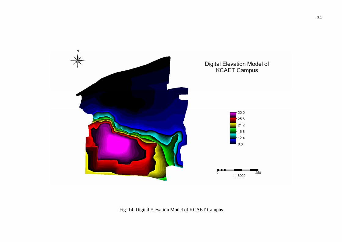
model (DEM) of K.C.A.E.T campus (Fig. 14) was obtained using the contour map. From the

DEM many useful information like hill shading map, slope aspect, 3D terrain view etc. can

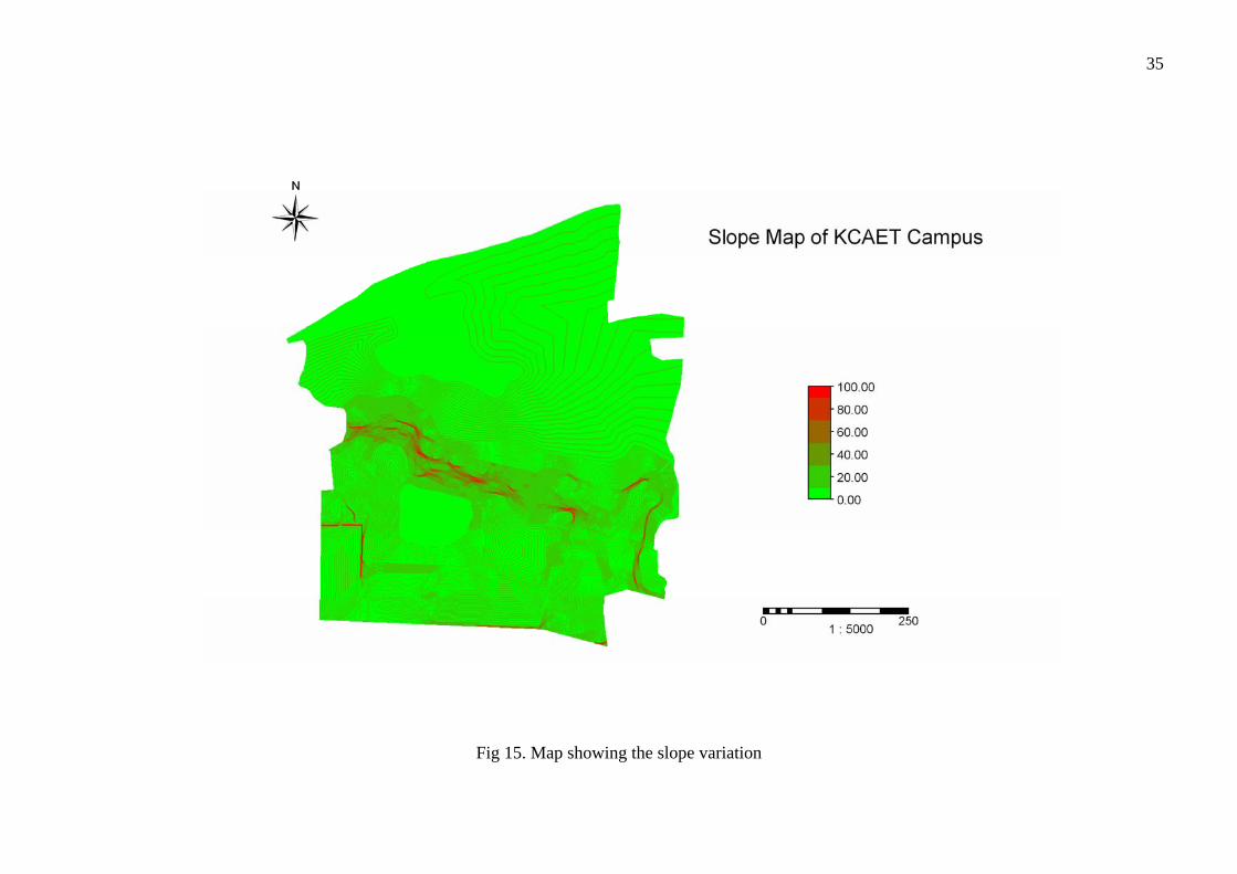
be easily obtained, if required. The slope map of the K.C.A.E.T campus is obtained from the

DEM and is shown in Fig. 15. This slope map can help in making decisions regarding the

type of crop to be grown, soil conservation practice to be followed, siting of water

conservation structures etc.

As the land use map is already prepared in ILWIS, further analysis like

estimating the irrigation water requirement, finding soil erosion rate, yield from each land

parcels etc. can be very easily done by adding appropriate layers with parameters for

estimating the different factors. This database can act as a basic planning tool for agricultural

as well as other land management functions. An example use of GIS for finding the runoff is

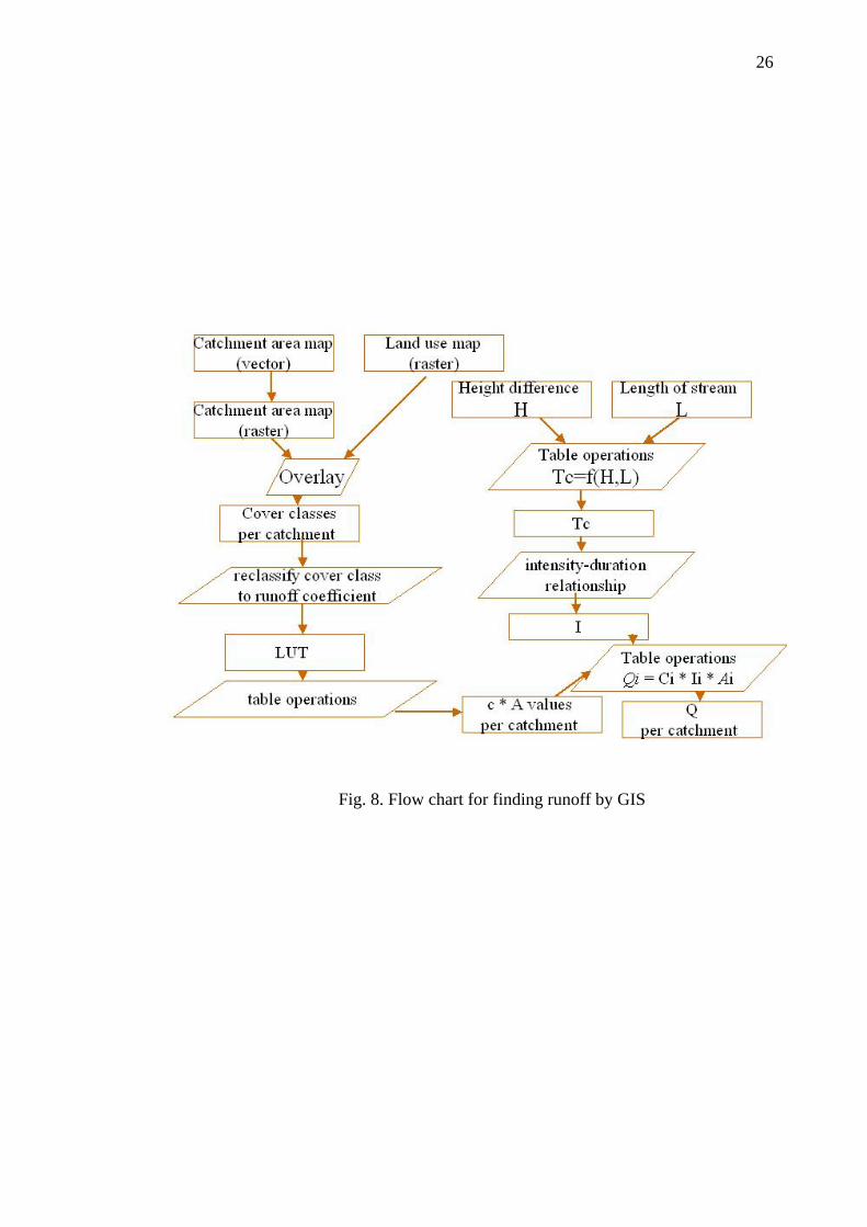
shown in the flowchart (Fig. 8).

26

Fig. 8. Flow chart for finding runoff by GIS

27

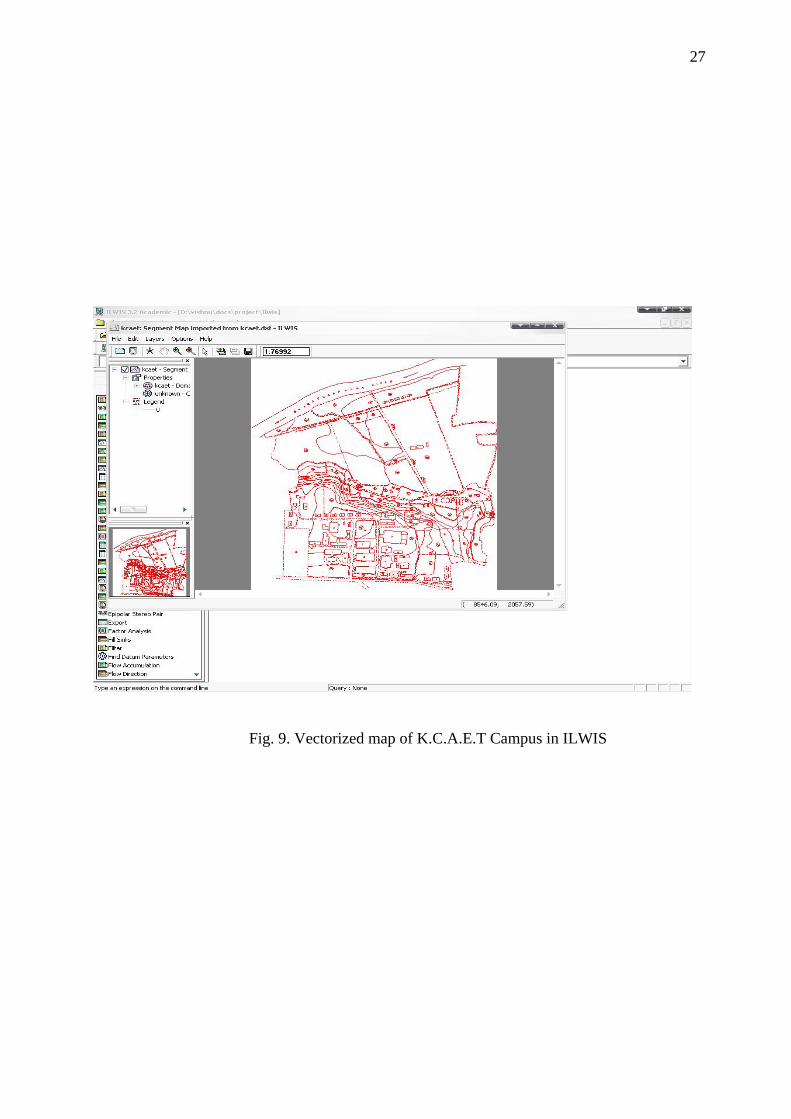
ig. 9. Vectorized map of K.C.A.E.T Campus in ILWIS

F

28

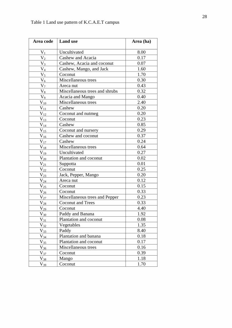
Table 1 Land use pattern of K.C.A.E.T campus

Area code Land use Area (ha)

V1 Uncultivated 8.00 V2 Cashew and Acacia 0.17 V3 Cashew, Acacia and coconut 0.07 V4 Cashew, Mango, and Jack 1.60 V5 Coconut 1.70 V6 Miscellaneous trees 0.30 V7 Areca nut 0.43 V8 Miscellaneous trees and shrubs 0.32 V9 Acacia and Mango 0.40 V10 Miscellaneous trees 2.40 V11 Cashew 0.20 V12 Coconut and nutmeg 0.20 V13 Coconut 0.23 V14 Cashew 0.85 V15 Coconut and nursery 0.29 V16 Cashew and coconut 0.37 V17 Cashew 0.24 V18 Miscellaneous trees 0.64 V19 Uncultivated 0.27 V20 Plantation and coconut 0.02 V21 Suppotta 0.01 V22 Coconut 0.25 V23 Jack, Pepper, Mango 0.20 V24 Areca nut 0.12 V25 Coconut 0.15 V26 Coconut 0.33 V27 Miscellaneous trees and Pepper 0.23 V28 Coconut and Trees 0.33 V29 Coconut 4.40 V30 Paddy and Banana 1.92 V31 Plantation and coconut 0.08 V32 Vegetables 1.35 V33 Paddy 8.40 V34 Plantation and banana 0.18 V35 Plantation and coconut 0.17 V36 Miscellaneous trees 0.16 V37 Coconut 0.39 V38 Mango 1.18 V39 Coconut 1.70

29

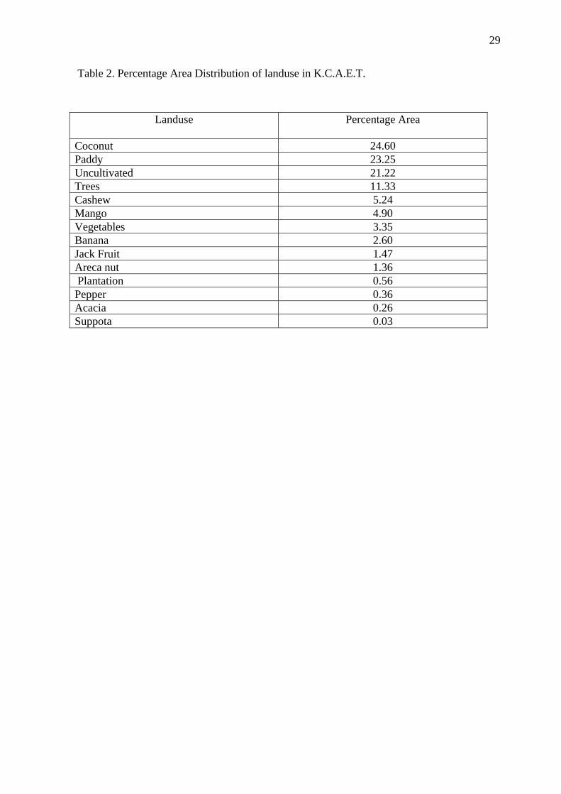
Table 2. Percentage Area Distribution of landuse in K.C.A.E.T.

Landuse

Percentage Area

Coconut 24.60 Paddy 23.25 Uncultivated 21.22 Trees 11.33 Cashew 5.24 Mango 4.90 Vegetables 3.35 Banana 2.60 Jack Fruit 1.47 Areca nut 1.36 Plantation 0.56 Pepper 0.36 Acacia 0.26 Suppota 0.03

30

0.010.10

8

0.14

3

0.22

5

0.55

0.59

5

1.051.

351.97

6

2.11

3

4.59

7

8.27

9.369.

903

012345678910

Are

a (h

a)

Cocon

ut

Paddy

Uncult

ivatedTree

s

Cashe

w

Mango

Vegeta

bles

Banan

a

Jack

fruit

Areca n

ut

Plantat

ion

Peppe

r

Acacia

Suppo

ta

Landuse Pattern

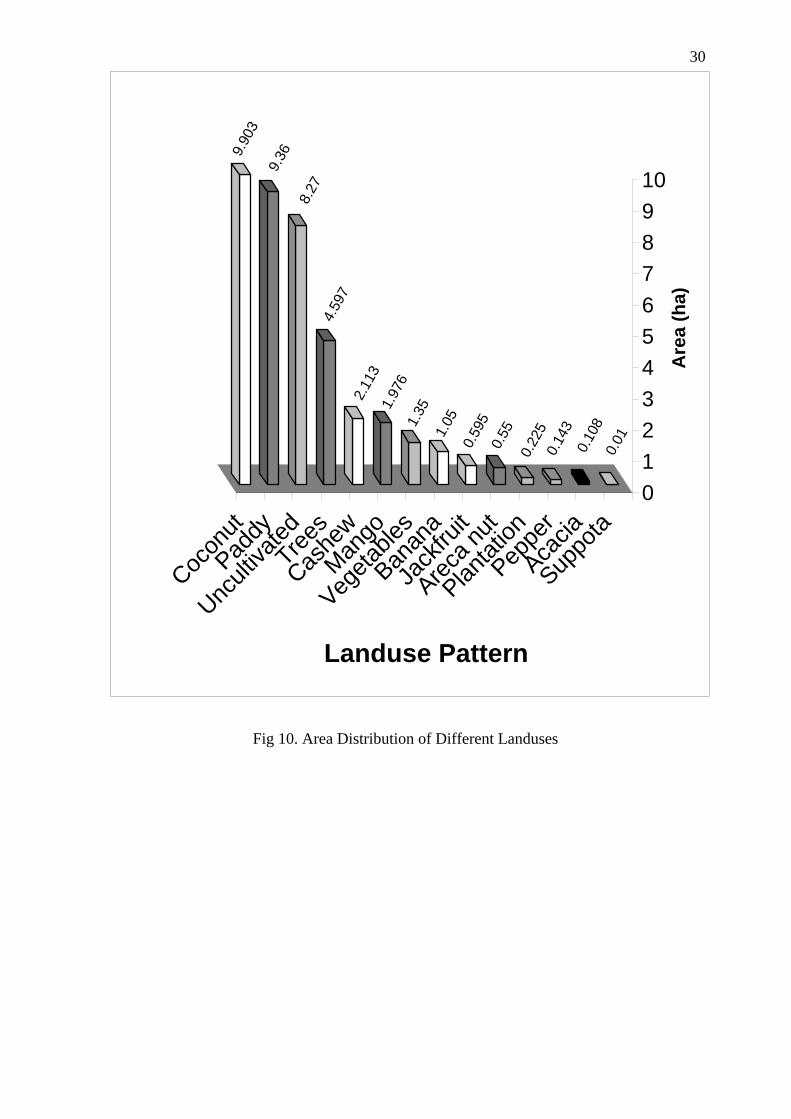
Fig 10. Area Distribution of Different Landuses

31

Landuse Pattern

1.

5 1.4

0.4

0.3

0.02

23.320.5

0.6

11.4

24.6

CoconutPaddyUncultivatedTreesCashew MangoVegetablesBananaJackfruitAreca nutPlantationPepperAcaciaSupp tao

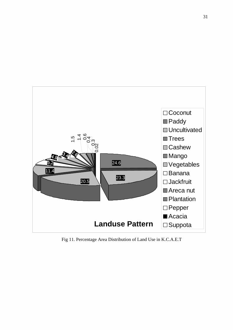
Fig 11. Percentage Area Distribution of Land Use in K.C.A.E.T

32

Fig. 12. Land use map of KCAET campus

33

Fig 13. Map of buildings in KCAET Campus

34

Fig 14. Digital Elevation Model of KCAET Campus

35

Fig 15. Map showing the slope variation

36

Table 3. Buildings in K.C.A.E.T CampusNo. Features

1 Academic Building

2 Lab/ Workshop

3 Library

4 Carpentry workshop

5 Machine, Fitting, welding workshop

6 Smithy workshop

7 Hydraulic / Processing / electrical / Heat Engine Lab

8 Agricultural Engineering / Soil Mechanics workshop

9 Shuttle court

10 Farm machinery Training Centre

11 Farm implement Yard

12 Physics, Chemistry Lab

13 Auditorium

14 Canteen

15 New Guest House

16 Guest House

17 Men’s Hostel

18 New Ladies Hostel

19 Ladies Hostel

20 Ladies Hostel Annex

21 Veterinary Hospital

22 Rain Shelter

23 Old Office Building

24 Farm Office

25 Drying Yard

26 Cattle Shed

27 Store / Seed Centre

28 Waiting Shed- Labourers

29 Poultry Shed

30 Dean’s Residence

31 Quarters

32 Flat

33 Temple

34 Overhead Tank

35 Pump House

36 Executive Engineers Office

37

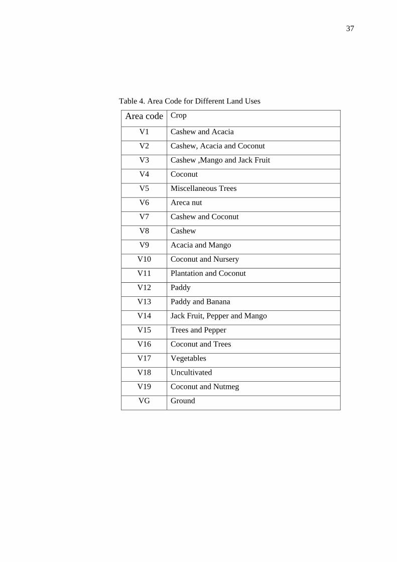
Table 4. Area Code for Different Land Uses

Area code Crop

V1 Cashew and Acacia

V2 Cashew, Acacia and Coconut

V3 Cashew ,Mango and Jack Fruit

V4 Coconut

V5 Miscellaneous Trees

V6 Areca nut

V7 Cashew and Coconut

V8 Cashew

V9 Acacia and Mango

V10 Coconut and Nursery

V11 Plantation and Coconut

V12 Paddy

V13 Paddy and Banana

V14 Jack Fruit, Pepper and Mango

V15 Trees and Pepper

V16 Coconut and Trees

V17 Vegetables

V18 Uncultivated

V19 Coconut and Nutmeg

VG Ground

Summary and Conclusion

38

SUMMARY AND CONCLUSION

Land cover refers to different features covering the earth's

surface including vegetation Land cover, water bodies, rock outcrops etc. The land use refers

to man's use of land and its cover. Land use can change over the years. Land use change is

the temporal shift in human exploitation of biospherical resources in terrestrial ecosystems.

Land use mapping encompasses a wide range of procedures

and data sources that are employed to measure the spatial arrangement of human activities in

terrestrial ecosystems. GIS enables the effective and efficient manipulation of the spatial and

nonspatial data for land use mapping. ILWIS which is the most common software of GIS is

used in this study for land use mapping.

Field observations of the entire study area were done and

change in land use was recorded. The traced topographical map was cut into 10 pieces of size

21cm x 29.7cm. Each of the pieces was scanned with A4 size flat bed scanner. Finally all the

layers were merged to obtain the topographical map.

The software WinTopo was used for vectorization of the

scanned topographical map. After vectorization, editing was done to correct the errors. Data

input and editing were very important procedures and it occupied 80 % of the total

expenditure in GIS. This database can act as a basic planning tool for different fields like

agricultural development, Land evaluation analysis, Change detection of vegetated areas,

analysis of deforestation and associated environmental hazards, monitoring vegetation health,

soil resources mapping, ground water potential mapping, monitoring forest fire, monitoring

ocean productivity etc.

References

39

REFERENCES

Bathgate, J.D and Duram, L.A. (2003). GIS based landscape classification model to enhance

the soil survey. A southern Illinois case study. J. soil and water conservation 58(3): 119-127

Cheryl, F.V. and James, M.H. (1996). GIS - a tool for siting farm pond units J. soil and water

conservation. 51(5): 434-439

Dermet, B.G., Xon, K. and Paul, A.M. (1996) GIS procedure for automatically calculating

the USLE, LS factor on topographic complex landscape units J. soil and water conservation.

50(3): 134-143

De Roo, Paul, A.N and Zein, K (1998) Modelling runoff and sediment transport in

catchments using GIS J. soil and water conservation 50(6): 158-164

Fernadez, C., Win J.Q. and Stockle, C.O. (2003). Estimating water erosion and sediment

yield with GIS, RUSLE and SEDD. J. Soil and Water Conservation 58(1): 128-137

Hamlett, J.M., Miller, D.A., Day, R., Peerse, G.W., Baumer, G.M and Russo, J. (1992) State

wide GIS based ranking of watersheds for agricultural pollution prevention. J. soil and water

conservation 47(5): 399-405

Hoobler, B.M., Vans, H and James, D (2003) Application of land evaluation and site

assessment (LESA) and GIS in East Park County, Wyoming. J. soil and water conservation

58(2): 105-113

Joseph, O.A. (1992) .Highway route production line: a GIS based approach for economic

road planning. RS application and GIS. Tata Mc Graw-hill publishing company ltd, New

Delhi. 406-410

Kwong, A.C. (1998). Erosion assessment of large watershed in Taiwan J. soil and water

conservation 50(2): 180-184

Lin, X., Joseph, P.M and Perce, J.M . (1992). Evaluation of land use in selected areas in

south of Guilin by using GIS J. soil and water conservation 46(5): 280-292

40

Michael, F. and William, M.D (1997) Use of GIS in hydrology and water management J. Soil

and Water Conservation 52(4): 250-259

Noveline, R.A. and Sundaram, A. (1992). Wasteland development using GIS technique. Tata

Mc Graw-hill publishing company ltd, New Delhi.388-394

Pascal, S and Laura, B.C. (1997). GIS based distributed hydrology model for forest harvest

effect on peak flow in the Pacific North West. J. soil and water conservation 52(4): 148-155

Richard, R.H., Hopkinson, P., Caffery, S. and Huntsinger, L. (1997) .Comparison of GIS

verses manual techniques for land cover analysis in a Riparian restoration project. J. soil and

water conservation 52(2):112-118

Sarangi, A. and Bhattacharya, A.K. (2001). Use of GIS in assessing the erosion status of

watersheds, Indian J. soil conservation.29 (3): 190-195

Sidhu, G.S., Singh, R.S., Sharma, R.K and Ravisankar, R.(1998). Remote sensing and GIS

techniques for prioritization of watersheds, Indian J. soil conservation.26 (2): 71-75

Sooraj Kannan, P.V., Saritha, S.S and Anish, J.E. (2003) Estimation of erosion and runoff.

Unpublished B-Tech Report, K.C.A.E.T, Tavanur.

Srivasthava, D., Singh, R.S and Ravishankar, R. (1992) Remote Sensing and GIS for natural

resource study. J. soil and water conservation 52(5): 150-158

Tripathi, M.P., Pandya, R.K. and Raghuvamshi, N.S. (2001). Identification and prioritization

of critical sub-watersheds for soil conservation management using the SWAT model,

Biosystems engg. 85(5):365-379

Van, L., Thomas, K.M and Fred, O.M. (1998). Calculation of water requirement using GIS.

J. soil and water conservation. 51(4): 214-218

Van, W., Caffery, Sand Xoneg, S,G. (1998) Methods of combining multiple maps for

empirical modelling in GIS. J. soil and water conservation. 52(5): 150-175

41

Wu, J., Nellis, M.D., Ranson, M.D. and Price, K. (1997). Evaluating CRP land soil properties

by using GIS and Remote Sensing. J. soil and water conservation 52(5): 358-363

Zaitchik, B,F and Van, H,M. (2003). Applying a GIS slope stability model to site specific

land slide prevention in Honduras. J. soil and water conservation 58(1): 45-53

LAND USE MAPPING BY GIS

BY

ANU.M.BABU. RAMYA.P.

SMITHA.K.E.

ABSTRACT OF THE PROJECT REPORT

Submitted in partial fulfilment of the requirement for the degree

BACHELOR OF TECHNOLOGY IN

AGRICULTURAL ENGINEERING

Faculty of Agricultural Engineering Kerala Agricultural University

Department of Land and water resources and conservation engineering

KELAPPAJI COLLEGE OF AGRICULTURAL ENGINEERING AND TECHNOLOGY Tavanur-679 573, Malappuram

Kerala, India 2005

ABSTRACT Land use is the fundamental to sustainability. Agricultural land use, one of the

primary uses of land has been of prime importance since the beginning of civilization. Agricultural

development has been the foundation of the industrial superstructure in the developing countries.

GIS enables the effective and efficient utilisation of spatial and nonspatial data for land use

mapping.

The preparation of land use map of KCAET campus was done in this study

using WinTopo and ILWIS. The raster scanner of flat bed design scanned the traced topographical

map. The raster image was converted to vector form by using a high quality tool called WinTopo.

This database can act as a basic planning tool for different fields like agricultural development,

land evaluation analysis, change detection of vegetated areas, irrigation water requirement etc.