interaction between vertical and horizontal tax competition: theory and evidence
TRANSCRIPT
MPRAMunich Personal RePEc Archive
Interaction between Vertical andHorizontal tax Competition: Theory andEvidence
Leonzio Rizzo
Universita degli studi di Ferrara
January 2005
Online at http://mpra.ub.uni-muenchen.de/5334/MPRA Paper No. 5334, posted 16. October 2007

UNIVERSITÀ DEGLI STUDI DI FERRARADIPARTIMENTO DI ECONOMIA ISTITUZIONI TERRITORIO
Corso Ercole I d’Este, 44 – 44100 Ferrara
Quaderno n. 5/2005
January 2005
Interaction between Vertical and Horizontal TaxCompetition: Theory and Evidence
Leonzio Rizzo
Quadeni deit
Editor: Giovanni Ponti ([email protected])Managing Editor: Marisa Sciutti ([email protected])Editorial Board: Giovanni Masino
Simonetta Rengahttp://newdeit.economia.unife.it/quaderno.phtml

Interaction between Vertical and Horizontal Tax Competition: Theory and Evidence*
Leonzio Rizzo**
Abstract
We develop a model with two provinces, producing two goods: one mobile and the other not. The mobile good is taxed according to the destination principle by the local government; it is also federally taxed. People decide to buy the good at the most advantageous price. Namely they can buy bootlegged cigarettes and, if the price is very high in both provinces, they can decide to buy smuggled cigarettes, on which no tax is levied. The two provinces engage in tax competition. The province tax-reaction function are non linear because of scale economies in the cost of bootlegging. An increase in federal tax offsets the non linearity, because it decreases the magnitude of the horizontal externality. We test the theoretical results by using Canada-US data set from 1984-1994. Keywords: horizontal externality, vertical externality, tax competition, tax rate. JEL classification: H21.
________________________ *I wish to thank Tim Besley, Umberto Galmarini, Jim Hines, Valentino Larcinese for discussions and comments. I also thank participants to seminars at Catholic University of Milan in February 2003, EEA at Stockholm University in August 2003, UK Public Economic Weekend at Leicester in December 2003. **University of Ferrara, Department of Economics, Corso Ercole d’Este 44 – 44100 Ferrara. E_mail: [email protected]

1 IntroductionVertical and horizontal fiscal relations must be explored if European nationswant to increase the size of EU budget, by giving more fiscal power to theEuropean Parliament. Italy is also nowadays, facing a similar problem afterthe recent approval by the Parliament of the Constitutional reform about therelationship between central state and regions. The new Constitution calls formore fiscal power to the regions which can be obtained only by letting some taxbases overlap.There are federal provinces like US and Canada, where many tax bases over-
lap without apparently big problems. This seems to contrast with traditionalfiscal federalism literature (Musgrave (1959); Oates (1972)) which prescribesa fiscal imbalance between federal and local government. Decentralization offiscal expenditure does not correspond to the same level of decentralization forthe taxes necessary to finace it: many taxes cannot be decentralized becauseof the tax-base mobility threat, which could arise tax-competition phenomena,unabling the local authority to raise the revenue it need. Moreover, a pro-gressive income tax should be centralized to preserve horizontal equity betweenindividuals living in different states of the federation. These problems seemnot to worry Canada, where the main provincial tax bases (like corporate andpersonal income or sales) are shared with the federal government. What drivesthe public finance Canadian system to work, given so big a tax decentralizationon mobile tax bases? One simple explanation may be that the mobility effectis very small. Another, more appealing, is that the particular relation betweenvertical and horizontal externality mitigate the effect of the tax-base mobilitythreat.We explore this issue by using a model with two provinces choosing taxes
on a mobile tax base, which is also taxed by a federal state. People decide tobuy the good at the better price. Important differences in province’s taxes cancause relevant bootlegging phenomena. These, in the cigarette market, involve(Thursby and Thursby, 2000) the purchase of goods in low tax jurisdictions. Thegoods are then transported into high tax provinces, where counterfeit stampsare used to allow their sale along. In general bootlegging involves transportingcigarettes over relatively short distances. In this context a change in tax byone province affects the other province’s tax base (horizontal externality), thatresponds by changing its tax. On the other end the so-called "wholesale smug-gling" is a very big threat on the revenue of all provinces (Joossens et al., 1992) ina federal country, which does not depend on the relationship between provinces’taxes. In this case, in fact, smugglers do not pay taxes either in the selling, orin the purchasing province. This type of smuggling is a big problem for thosegoods with high federal taxes. A change in tax by the federal government affectsall provinces’ tax base (vertical externality), inducing an appropriate reply byevery province. In our model the greater the total tax (federal + state tax), thebigger the quota of total consumers in the province who decide to buy the goodin the "wholesale-smuggling" market, causing a decrease in the provinces’s taxbase. Notice that, since this does not correspond to an increase in the other
1

provinces’s tax base as in the bootlegging case, it causes an increase in eachstate tax in the attempt to recover the lost tax revenue. On the contrary thetax-competition process, due to bootlegging and cross-border shopping drivestax rates to the bottom: tax rates, for a given federal tax, are lower than theywould be without tax-base mobility. We use a data set 1984-1994 for Canadaand US and test the effect of an increase in federal tax on cigarettes on the hor-izontal tax-competition on cigarettes. We find that the federal tax rate affectsthe neighboring average tax rate in explaining the variance of the own tax rate.In fact it offsets the non linearity of the tax-reaction functions.The remainder of the paper is organized as follows: in the next section we
examine the related literature, in the third and forth section we develop thetheoretical model. Section 5 tests the model and section 6 concludes.
2 Related literatureJohnson (1988) first, highlighted that state residents would prefer redistributionto be undertaken by state rather than federal government. This is because partof the increase in the use of redistributive income taxation is born indirectlyby residents of other states by virtue of their being federal tax payers. Thefederal government would be in fact obliged to increase its federal tax if itwants to respect its public budget constraint, giving the depressing effect onthe tax base of the state deciding to increase the use of redistributive incometaxation. On the line of this work Boadway, Marchand, Vigneault (1998) studiedthe implication of this externality phenomenon for the optimality of resourcesallocation in a federation. They explored the externalities in the bottom-up andtop-down direction: both types of exernalities are present if we assume that thefederal and state government play a Nash game; only the bottom-up (stateversus federal government) holds if we assume a Stackelberg game. Moreoverif the federal state can implement contingent transfers, vertical and horizontalexternalities will be nullified. Keen and Kotsogiannis (2002) study the verticaland horizontal externalities in a model with capital taxation, where capital ismobile. They also examine the welfare properties of a Nash and Stackelbergequilibrium, highlighting the case when the vertical externality prevails on thehorizontal and vice-versa.There are some empirical works on vertical externalities. Besley, Rosen
(1998) estimate the existence of vertical fiscal externalities for cigarettes andgasoline in US, by relating the own state tax rate to the federal governmenttax rate. They find a positive link between state and federal tax rate on ciga-rette and gasoline with a US data set for the year 1975 to 1989. Esteller-Moré,Solé-Ollé (2001) find a positive sign for vertical externality by using US data forincome tax during the period 1987-96. This sign is not very robust to compara-tive statics. In fact in Boadway and Keen (1996) an increase in the federal publicexpenditure due to a higher federal tax rate can induce the local governmentto react by lowering local public expenditure and indeed local income tax rate(public expenditure effect). Andersson et al.(2004) find a negative sign, explor-
2
ing the relation between counties and municipal income tax rates for Swedenwith a panel data 1981-1990.Other empirical literature concentrates on estimating vertical and horizontal
fiscal competition togheter. Goodspeed (2000) uses a data set with 13 OECDprovinces for the period 1975-1984. A poverty index is used as a measure ofintra-province mobility: the poorer the less mobile people are, the smaller thehorizontal externality. He uses local income tax as dependent variable and findsnegative sign for the federal tax rate and for the mobility index. Boadway andHayashi (2001), using Canadian annual data 1963-1996, test horizontal and ver-tical tax competition by looking at corporate taxes on businesses. They find anegative sign for the vertical externality and positive for the horizontal external-ity. Each estimate is for a single province or an average province. Revelli (2003)studies the non-metropolitan two-tier system of local government in England -comprising 34 counties and 238 districts - using per capita current expenditurefor the financial year 2000/2001, disaggregated in various functions of inter-est. He finds that horizontal externality disappears when a vertical externalitycoefficient is introduced, arguing that the relevant externality is just the lastone. Interestingly, with tax variables Devereux, Lockwood and Redoano (2004)find the opposite for US by using a panel data 1977-1997: vertical external-ity for cigarettes and gasoline is not significant if they also test for horizontalexternality, which is significant.Goodspeed (2002), extending some results of Goodspeed (2000), finds that
the vertical externality affects the horizontal externality (measured as in Good-speed (2000)) in an income tax enviroment, by offsetting it. However, the paperdoes not present structural explanations of the result.
3 The modelConsider a federation with two provinces with equal populations. Consumersin the two provinces differ in their utility function for preference for the localpublic good. Two goods are produced: a mobile taxed good and an immobilegood, whose price we take as numeraire. The two goods are produced, by usingone input with constant returns to scale. Each resident can decide where tobuy the consumption good, according to the post-tax price and the cost ofbootlegging the good. Each province decides upon a local public good and atax on the mobile good according to the destination principle. The good can betransported not for personal consumption, but to be resold, from the low taxprovince to the high tax province (bootlegging) and in this case a combinationof transport cost and storage cost is incurred to buy the good (Scharf, 1999).This is the relevant empirical situation we focus on, for cigarette tax in Canada.Let us index the two provinces as 1 and 2. Both have the same number of
residents, normalized to 1 and uniformly distributed over n ∈ [0, 1]. We assumethat the extremum 0 is the border of the province. Since the residents areuniformly distributed, the distance of each resident from the border is d ∈ [0, 1] ,coinciding with the distribution of the residents. Assume that each consumer
3
in province 1 has the following utility function:
U(x, y) = u(x) + y + γs ln g +Ψ lnG with s = 1, 2,
where x ∈ 0, 1 is the taxed good; y is the numeraire no-mobile good, g is thelocal public good, G is the federal public good, γ1 6= γ2 > 0 is a parameter whichdetermines the preference for the local public good respectively in province 1and 2, Ψ is a parameter, determining the preference for the federal public good,which we is assumed identical in each province and u(0) = 0. The source ofheterogeneity between the residents in the two provinces is the propensity toconsume the local public good.1A symmetric equilibrium would make no sensein a federation, whose nature implicitly recognizes the existence of structuraland tastes heterogeneity.The ln function let us have a clear-cut FOC for the public good, but this
does not affect the final results, which is affected by the quasilinear formulationof the utility function. This says that there is no link between public and privategood. It seems reasonable that there is not any public good, which increasesthe utility due to one more cigarette.It is more difficult to justify the perfect substitutability with the untaxed
good. There is no reason why this should not be linked to the taxed good,but on the other side this assumption allows to get a constant marginal utilityof income, since we have only two private goods. This let us underline thedeadweightloss effect, due to the tax on the x-good (Besley, Rosen, 1998): themore the tax rate increases, the greater the loss in utility, because the more itcosts to consume 1 unit of the x-good. Since y enters linearly in the primitiveutility function, this last result does not depend on the level of income.The mobile good is dichotomous following the Kanbur and Keen (1993)
formulation. This is of great help in obtaining tractable reaction functions.In the cigarette case it is, moreover, reasonable to think of the demand forthese goods, as to be very rigid. Finally it helps to isolate the role of mobility indetermining the change in tax-base elesticity after a change in its own neighbor’stax rate: if the demand is rigid the only determinant of the change of the tax-base elesticity is mobility.
3.1 The third stage
The following assumptions are useful (Rizzo, 2002):Assumption 1: u(1) − p > 0, where r = u(1) − p is the reservation price
for the mobile good, net of production cost, of a consumer living either in 1 or2.The meaning of this assumption is that it is always worth it for the consumer
to buy the good x when it is not taxed.
1This will later allow us to skip out symmetric equilibria, for which static comparativeresults are note definite.
4

Assumption 2: The cost of bootlegging per consumption unit is given by:
φ(d) =ln(1 + d)
A(1)
where d is the distance of the consumer from the border and A ≥ 1 is a fixedparameter.Think of the cigarette bootlegger, that, for a given quantity to be provided,
minimizes its cost during a certain time period. This implies that, the furtherfrom the border the market place, the lower the optimal number of trips and thegreater the amount of good purchased in every trip.2 This decreases the fixedtransaction cost per unit of consumption, which, with a non increasing per unitstorage cost, insures concavity of the unit cost of bootlegging in the distancefrom the border (Scharf, 1999). In a stylized model, such as the one presentedhere, this reasoning can be summarized by a cost of bootlegging concave in thedistance from the border.Notice that (1) is an increasing and concave function of d and φ(0) = 0.
When A → ∞, we are in the perfect mobility case, in fact φ(d) = 0 ∀d, andA = 1 implies the minimum mobility case and therefore the maximum possibleunit cost of bootlegging. Notice that the intensity of the scale economies inthe bootlegging technology is captured by A: the higher A, the lower the unitcost of bootlegging per unit of distance from the border. Finally, 0 ≤ d ≤ 1implies 0 ≤ φ(d) ≤ ln 2
A .We use a logaritmic function, because it let us get someinteresting explicit results, which would have not been possible with a moregeneral form, because of the ambiguous sign of the third order derivatives. Weare indeed assuming that the magnitude of the third order derivatives is not sobig to overcome the effects due to the second and first order ones.
3.1.1 The shopping technology
Let us define t2 as the specific unit tax on the mobile good in province 2. Assumethat t1 > t2, if assumption 1 holds and t1+T ∈ [0, r], the consumer in 1 decideswhere to buy the good by comparing its indirect utility derived from buyingthe legal or the bootlegged good. If it shops bootlegged goods from 2, it paysφ (k)+ t2+T. Therefore the consumer will shop bootlegged goods from 2 until:
φ (k) = t1 − t2.
If we use (1):k = [φ(t1 − t2)]
−1 = eA(t1−t2) − 1 (2)
Notice that the level of T does not enter in determining k, because the federaltax is identical in both provinces.3 The variable k is the distance from the border
2Fitz Gerald et al. (1995) show evidence of this. They analyzed two case-studies: Germany-Denmark and Ireland-Northern Ireland. In both cases the greater the distance from the border,the greater the amount of goods purchased and the fewer the trips in any given period.
3This has also been highlighted in Devereux, Lockwood, Redoano (2004). It is the reasonwhy, in a model with zero demand-elasticity of the taxed good (Kanbur and Keen, 2003), theydo not get any vertical externality, even if mobility is allowed.
5
of the consumer in province 1, who is indifferent between shopping legally in1 or a bootlegged good from 2. Moreover, since consumers in 1 are uniformlydistributed on [0, 1], k is also the number of residents in 1, buying bootleggedgoods, for a given t1 − t2. Note that k is convex in t1. The higher t1, thebigger the increase in the number of people buying from 2, for a given increasein t1 (
∂k∂t1
> 0 and ∂2k∂t21
> 0). This is because the higher t1, the further fromthe border the indifferent consumer is, the lower the increase in the bootleggingcost is (∂
2φ∂d2 < 0).
If t1 ≤ t2, we obtain an expression symmetric to (13), with opposite prop-erties for the second order derivative of the bootlegging cost function: l =eA(t2−t1) − 1.
3.2 The second stage
If assumption 1 holds, t1 ∈ [0, r] and t2 ∈ [0, r], it will always be economicfor consumers in 1 to buy good x. In this case, taking account of the initialassumption that the number of people is normalized to 1 and using the resultsfrom the third stage, we have that if t1 > t2, B1 = 1− k(t1, t2) and if t1 ≤ t2,B1 = 1+ l(t1, t2), where B1 is the tax base faced by province 1. We can simplifythe notation by defining:
n(t1, t2) =
½ −k(t1, t2) if t1 > t2l(t1, t2) if t1 ≤ t2.
(3)
It follows that:B1 = 1 + n(t1, t2)
where n is the mobile tax-base quota coming in or going out depending on whichtax regime we are dealing with.The same reasoning applies to province 2.
g −B1(t1 + T ) ≤ 0. (4)
3.2.1 Tax evasion
Price differentials among provinces create incentive for bootlegging, while hightaxes create incentive for wholesale smuggling, from now on simply smuggling.As already discussed in the introduction smuggling occurs when cigarettes aresold without payment of tax or duties even in the province of origin and, moreimportant, this is a long distance phenomenon. Therefore it affects the tax basein all the federation, without regards to the distance from the border of theprovided consumer. We model the tax base loss due to smuggling as:
E1 = αB1 (t1 + T ) (5)
6

where E1 is tax evasion in province 1 and α is a constant, which reflects thelevel of controls and corruption in the province. Tax evasion in province 1is a characteristic positively linked to the number of individuals (B1), legallyshopping in their province, if t1 > t2, plus those living in 2 and shoppingbootlegged goods from 1, if .t1 ≤ t2.It is reasonable to think that tax evasion, which is driven by the quota of B1,
shopping in the smuggling market, increases when the total tax rate (t1 + T )increases. Moreover since tax evasion is increasing in B1 and (t1 + T ), taxevasion is also increasing in B1 (t1 + T ) for a given α. In (5) we assume that taxevasion is linked to this last expression by a linear function. Notice that if bothprovinces increase their tax, t1 and t2, of the same amount, B1 does not change,but E1 increases via t1: if the level of state taxes increases of the same level, aquota of people in both states switches to smuggled products. The same thinghappens if T increases.
3.2.2 The local government problem
If t1+T ∈ [0, r] and t2+T ∈ [0, r], in the second stage, province 1 maximizes theindirect utility function of a representative resident shopping at home, subjectto a budget constraint, by solving the following problem:
Maxt1,g,µ
u(1) +m− (p+ t1 + T ) + γ1 ln g1 +Ψ lnG (6)
−µ g − (B1t1 −E1)The following assumptions are useful:
Assumption 3: r < 1A .
The meaning of assumption 3 is that, the bigger the scale economies (thegreater A) in the bootlegging technology, the smaller the unit net reservationprice can be. The greater A is, the less costly to buy the bootlegged good.
Assumption 4: 0 < α < 3−√52 .
We assume that the quota of revenue lost, because people go to the smug-gling market is no more than 0.38 of the total revenue (provincial + federal),collected in the province. This assumption defines the α − set which, togetherwith assumptions 1-3, allows us to prove the existence of a subgame perfectequilibrium in federal and local tax rates and public goods.
3.3 The first stage: the federal government problem
The federal government maximizes a function which is the sum of the welfarefunctions of the two provinces (Boadway, Marchand, Vigneault, 1998; Keen,Kotsogiannis, 2002). The federal government moves first, by choosing G and
7

T , that maximize its objective function. After that, at the second stage, localgovernments choose their local tax rates and public goods and therefore:
Proposition 1: If assumptions 1-4 hold then the Stackelberg game where acentral authority chooses a federal tax rate and a federal public good, by maximiz-ing a its welfare function, subject to a budget constraint and the two provinceschoose their tax rates and public goods by maximizing their welfare function,subject to a budget constraint, has a subgame perfect Nash equilibrium.Proof: see appendix.
The existence of a federal tax induces each province belonging to the fed-eration to modify its tax-rate decision, taking into account the effect on theresident’s tax base of the federal tax.
4 The federal tax and the slope of the provincereaction functions
An increase in T (section 3.2.1), decreases the revenue in both provinces, becausesmuggling increases, making the provincial tax base decrease. In our setting thetax reply to a neighboring tax increase is linked to the amount of tax base comingin from the increasing tax province, which decreases because of the federal taxincrease. Therefore the magnitude of the horizontal fiscal externality decreases.It is useful to look at the anlytical formula of the impact on the horizontal fis-
cal externality of an increase in the federal tax: ∂L1∂t2∂T
= −µhα ∂n∂t2− ∂2n
∂t2∂t2∂T (t1 − α (t1 + T ))
i.
A quota of the tax base "going to province 1", because of the increase in taxin the other province, ∂n
∂t2, is offset by the increase in tax evasion, due to the
increase in T ,−α ∂n∂t2.4 An increase in the vertical externality, offsets part of the
horizontal externality effect.Since we can test this, by using the slopes of the tax rate reaction function,
we start by totally differentiating the FOC of (11), to derive the slope of tax-ratereaction function of province 1, for a given marginal cost of public funds:
dt1dt2
= −∂2n
∂t1∂t2(t1 − α (t1 + T )) + ∂n
∂t2(1− α)
∂2n∂t21(t1 − α (t1 + T )) + 2 ∂n∂t1 (1− α)
(7)
(22) catches only the so called deadweight loss effect (Besley, Rosen 1998).According to this, a tax increase in province 2 leads to an increase of the taxrate in province 1: the deadweight loss, for a given marginal cost of publicfunds, is minimized by increasing its own tax and therefore its own revenue.Another effect is not considered: the revenue effect (Smart, 1998). This leads
4Moreover this effect is stronger if t1 > t2, because in this case ∂2n∂t2
< 0, due to theconcavity of the bootlegging cost function. Conversely the effect is milder if t1 < t2. In this
case in fact ∂2n∂t2
> 0.
8

to a decrease in tax rate after an increase in the neighbor’s rate, because thegovernment need a lower tax rate to raise the same level of revenue, after theincrease in t2: the marginal cost of public funds decreases. The final effect onthe tax rate is therefore ambiguous. If this last effect is not very high, as it seemsto be from the flypaper literature5 (Inman, 1971; Case, Hines and Rosen, 1993),(22) can be considered a good proxy of the reaction function slope, obtained byendogenizing the marginal cost of public funds.We describe the reaction function’s slope, for given marginal cost of public
funds and derive all the propositions, which will follow, for a given marginal costof public funds, because we assumed welfare maximizing provinces and thereforeface a six-sumultaneous equation system with six unknowns (t1, g1, µ1, t2, g2, µ2).It is theoretically possible to partially solve the six-equation system and get areaction function linking t1 to t2, where µ1 is endogenized. Unfortunately thisfunction is not properly estimable, because it would be a structural equationestimate of the six-equation system with a missing variable, namely the endog-enized µ1. We estimate, in fact, a linear approximation of :
1− µ
·(1 + n (t1, t2))(1− α) + [t1 − α(t1 + T )]
∂n (t1, t2)
∂t1
¸= 0,
which is the first order condition with respect to t1 from the maximization ofthe welfare function of province 1.From (22) we get:
Proposition 2: If assumption 1-4 hold then, for a given marginal cost ofpublic funds and a fixed t2,
dt1dt2
> 0.Proof: see appendix.This is because an increase in t2, decreases the migrating tax-base quota, for
a given t1, if t1 > t2, or increases the migrating tax-base quota, for a given t1,if t1 < t2. Therefore if t2 increases, province 1 is induced to increase t1, withrespect to the situation before the increase in t2, in the process of providing gby minimizing its deadweight loss, for a given marginal cost of public funds.
Proposition 3: If assumptions 1-4 hold, then the slope of the tax-ratereaction function when t1 > t2 is greater than the slope of the tax-rate reactionfunction when t1 < t2, for a given marginal cost of public funds and a given t2.Proof: see appendix.This proposition comes from the the concavity assumption of the cost of
bootlegging in the distance from the border, which implies that the furtherpeople are from the border, the less the bootlegging cost increases when thatdistance from the border increases. In fact if t1 > t2, for a given increase in t2(which means a decrease in the distance from the border of the consumer in 1,who is indifferent to buy legally in 1 or bootlegged goods from 2), the increasein the number of people willing to buy legally in 1 decreases with t2, for a
5We can think of the tax base flow, due to the increase in t2, as money transfer to province1.
9

given t1. If t1 < t2, for a given increase in t2 (which means an increase of thedistance from the border of the consumer in 2, who is indifferent to buy legally2 or bootlegged good from 1), the increase in the number of people illegallyshopping increases with t2, for a given t1 (see fig. 1). Therefore province 1, fora given increase in t2, is induced to increase more t1 in the former case than inthe latter one. In the former case an increase in t1 causes a loss in the benefitfrom the increase in t2, lower than in the latter case.
Proposition 4: If assumption 1-4 hold then (a) a unit increase in thefederal tax decreases the tax-rate reaction function slope if t1 > t2, moreover (b)it increases the tax-rate reaction function slope if t1 < t2, for a given marginalcost of public funds and a given fixed t2.Proof: see appendix.As we have just seen, if t1 > t2, for a given increase in t2, the increase in the
number of people illegally shopping goods bootlegged from 2 decreases with t2,for a given t1. The decrease is smaller when the federal tax increases, becausetax evasion increases and a quota of tax base disappears. Therefore the loss inbenefit due to an increase in t1 after the increase in t2 is higher than before theincrease in the federal tax. That is why the reaction of 1 to an increase in t2 issmother when T increases.If t1 < t2, for a given increase in t2, the increase in the number of people
illegally shopping goods bootlegged from 1, increases with t2, for a given t1. Aquota of this increase will disappear if we introduce the federal tax and so taxevasion increases. Hence, the loss in benefit due to an increase in t1, after theincrease in t2 is lower than before the increase in the federal tax. That is whythe reaction of 1 to an increase in t2 is stronger after an increase in T .
4.1 Testable theory
In the paper we focus on assumption 2, which we think is the most reasonablefor cigarette bootlegging and test the following hypotheses:1) ∂t1
∂t2> 0
2) dt1dt2
¯t1>t2
> dt1dt2
¯t1<t2
3)·dt1dt2
¯T>0− dt1
dt2
¯T=0
¸t1>t2
< 0 and·dt1dt2
¯T>0− dt1
dt2
¯T=0
¸t1<t2
> 0
Assumption 2 is indirectly tested, by veryfing its effect on the reaction func-tion slope (inequality 2). After doing that, we test wheather the difference inslopes is affected by the existence of the federal tax (inequality 3).
5 The empirical testOur main goal is to estimate if there is any significant strategic link betweenfederal and provincial taxation, when tax is levied on the same tax base. Inthe literature this has been done by regressing local tax rate on federal tax rate
10

(Besley, Rosen, 1998). The method normally prevents from checking for yeareffects, because the federal tax rate in a panel-data set does not have the statedimension and the insertion of the year effects results into an insignificant coef-ficient for the federal tax rate. The typical objection in these works is that thefederal tax-coefficient is significant because it picks up yearly macroeconomicsshocks. A way out of this problem could be to estimate the effect of a change infederal tax on the tax-competition behaviour, which shows off when the tax baseis mobile. If an increase in federal tax affects the tax-rate choice of a province,given the tax rate on the same mobile tax base of a neighboring province, itmeans that there is a link between the tax rate, chosen at federal and locallevel on the same tax base. This is also, what our theory shows: if a federalauthority intervenes by introducing a central tax, it modifies the local tax baseand increases the deadweight loss each local authority would bear with only itslocal tax; this implies that a local authority modifies the choice of its tax andso the tax-rate answer to an increase in tax rate from a neighboring state. Wetest this idea by using a Canada-US data set from 1984-1994.In our case we argue that tax competition is due to bootlegging. This is likely
to happen between border provinces: the further a province from the other, themore costly (in transport terms) is to bootleg. At a first glance bootleggingcould not appear a relevant threat for the provincial tax base in the Canadianreality, where provinces are very big and densities very low. But at a furtherinspection, almost all the Canadian population lives near the US border. Noticethat eight, out of the ten considered provinces,6 border the US. This means thatpopulation in each of these provinces is concentrated along a line, which makesthe bootlegging threat between provinces or the US a relevant problem. This isreinforced by the fact that in two, out of the eight provinces bordering the US(Nova Scotia, New Brunswick), bootlegging is a relevant issue, just because theyare very small. The two provinces not bordering the US are P.E.I, which is verysmall and Newfoundland which is basically extended along the Quebec border:both characteristics play an important role for the relevance of bootlegging.7
In order to isolate the independent impact of the neighboring tax rates on theCanadian province tax, one must take into account other variables, that mightaffect the provinces tax rate. First of all we control for the US neighboringtax rates. Moreover the province’s tax rate on commodities depends on severalother types of variables. Province taxation can be influenced by economic and
6We excluded the three Territories Nunavut, Northwest Territories and Yukon becausethey represent a very small part of Canada in terms of population, income and tax base.
7How Canadian provinces relate their tax decisions on cigarettes seems to be an importantissue, according to the provisional agenda on tobacco control of the World Health Organizationmeeting in 1999: “differentials in the price of tobacco....lead to both casual cross-bordershopping and illegal bootlegging. Cross-border sales may occur within countries, such asCanada and United States, given the intracountry price differences among Canadian provincesand states within the United States”. Moreover, this issue seems to worry also the nationalprint: "Cigarettes are smuggled interprovincially by road, through mail-order operators, bycommercial couriers ....The smugglers have little fear of the law." (Moon, The Globe and Mail,28 June 1997)
11

demographic environment. We controlled for it by using many socio-economicvariables (see data appendix). For all of them we computed the correspondingmean variables of the neighboring Canadian provinces and neighboring US statesto each Canadian province. The political colour of the provincial governmentcan also affect the tax-rate level: we divided the Canadian party system in threemain groups: the conservative-progressive, which is right wing, the liberals,which is center, and left wing group, composed by the Democratic-Progressive,the Quebec party and the Social Credit party. We have then built dummies forthe case when the premier belongs to one of the three groups. Finally we havedichotomous variables to control for province and year effects. We estimate thefollowing equations:
tst = ςs + δ1hst + δ2vt + δ4EXPEst + δ5mst + ϑxst + st (8)
tst = αs + βt + λ1hst + λ2vt ∗ hst + λ3EXPEst + λ4mst + θxst + st, (9)
where: tst is the tax rate for province s and year t; αs are province fixed effects;βt are dummies variables that pick up for macro-shock and common change infiscal policies; xst is a vector of province specific time varying shocks; hst is thetax-rate average of the neighboring provinces of province s in year t; vt is thefederal tax rate in year t; EXPEst is the ratio of the total expenditure on GDPfor province s in year t; mst is the tax-rate average of the neighboring US statesof province s in year t; st is the error term.Equation (8) estimates the effect of an increase in federal tax, by omitting
year effects and using some invariant year controls (federal GDP and federalunemployment). Equation (9) estimates the effect of an increase in federal taxthrough the tax-competition coefficient, controlling for year and province effects.
5.1 Hypotheses
Equation (8) estimates two parameters: δ1, which is the tax-rate reaction coef-ficient to an increase in the tax-rate average of the neighboring provinces andδ2, which is the tax-rate reaction coefficient to an increase in federal tax-rate.Here, we take the traditional approach, estimating the link between a federaltax and a local tax, levied on the same tax base.Equation (9) does not include the federal tax, but the interaction term vt∗hst
and controls for year effects. The interaction accounts for the change in tax-rate reaction to an increase in the tax-rate average of the neighboring provinces,after a change in federal tax. From our theory, δ3 could be both positive, ornegative, depending on the prevailing tax regime (tst > hst or tst < hst).We estimate λ1 = γ1 + γ2ψ and λ2 = γ3ψ, where ψ is a dummy which
equals 1 for provinces where tst > hst. Therefore γ1 is the slope of the tax-ratereaction function in the case tst < hst and γ1 + γ2 + γ3vt is the slope of thetax-rate reaction function in the case tst > hst, for a given federal tax rate vt.Proposition 3 predicts γ2+γ3vt > 0: the slope of the tax-rate reaction functionin the case tst > hst is higher than in the case tst < hst. Moreover proposition4 predicts γ3 < 0: when tst > hst, an increase in the federal tax rate decreases
12
the coefficient of the rate reaction function, due to an increase in the tax-rateaverage of the neighboring provinces.We then estimate λ1 = ϕ1+ϕ2 (1− ψ) and λ2 = ϕ3 (1− ψ) , where ϕ1 is the
slope of the tax-rate reaction function in the case tst > hst and ϕ1 + ϕ2 + ϕ3vtis the slope of the tax-rate reaction function in the case tst < hst, for a givenfederal tax rate vt. Proposition 3 predicts ϕ2 + ϕ3vt < 0: the slope of the tax-rate reaction function in the case tst < hst is lower than in the case tst > hst.Proposition 4 says that ϕ3 > 0: when tst < hst, an increase in the federal taxrate increases the coefficient of the tax-rate reaction function, after an increasein the average rate of the neighboring provinces.
5.2 Estimation Strategy
In theoretical section we describe a two stage game a la Stackelberg. We areempirically interested in the second stage where we face a system of six simulta-neous equations: three from the solution of the optimal tax problem of province1, which determines t1, g1 and µ1, for a given t2; and three from the symmetrictax problem solved by province 2, which determines t2, g2 and µ2, for a givent1. In the empirical specification we can think of t1 as the Canadian provincetax rate (tst) and t2 as the mean of the neighboring province tax rates (hst).By using not all the neighboring variables but just the mean, we reduce the em-pirical situation to a two-province problem: each province competes with onefictitious (average) neighboring province. This is quite a usual procedure in theliterature (Hines et al. 1993; Besley, Rosen 1998; Brueckner, Saavedra 2001;Esteller-Moré, Sollé-Ollé, 2001), especially when the spatial dimension must beemphasized.Like all studies of social interactions, this economic framework suffers from
an identification problem of the model’s structural equations and a simultaneitybias of the standard errors of the equation estimated. The issues arise becausetax-rate interactions are symmetric, in the sense that each province’s behavioraffects that of its neighbors in the same way, the neighboring provinces behavioraffects the province’s own behavior, which feeds back again on the neighbors.We tackle these two problems firstly by identifying one of these six equations,
the first order condition with respect to the tax choice of province 1; and sec-ondly, by instrumenting the endogenous variables to cope with the endogeneitybias. We have two endogenous variables, if we assume a Stackelberg model: theaverage neighboring tax rate, t2, and the marginal cost of public funds, µ1. Ina model of simultaneous equations, the federal tax rate is also endogenous. Ifwe want to correctly identify the estimated equation, we need variables whichare correlated with t2, µ1and T (if we use a simultaneous decision model), butnot to t1.Equation (9) can be written as follows:
tst = αs+βt+γ1hst+γ2ψhst+γ3ψvthst+γ4EXPEst+γ5mst+θxst+ st (10)
The vector x is composed by 23 variables: INCst and its square, GRANTst,UNEMPst, GDPst (per-capita GDP), POPst, AGEDst, CHILDst andDENSst;
13
the neighboring Canadian variables for INCst and its square, GRANTst, UNEMPst,GDPst, DENSst and symmetric variables for the neighboring US provinces,two dummies for the political colour of the premier. Moreover macroeconomicshocks and province fixed effects are controlled through 10 dummies for yeareffects and 9 dummies for province effects.
5.2.1 Instrumentation
The mean Canadian neighboring tax rate and its interactions are endogenous,because they can also be influenced by the Canadian province. The marginalcost of public funds (endogenous from the theoretical model) is proxied withtotal government expenditure over GDP (EXPEst), using the first order condi-tion of the theoretical model relative to the optimal choice of the public good.8
The mean neighboring US tax rate, mst could clearly be endogenous: the USrate mean can also be influenced by the Canadian province.If this is the structural model, a simple OLS estimate of (10) would suffer
from endogeneity and measurement error bias: the error term st would be cor-related with the error terms of the other simultaneous equations of the system.The endogeneity bias comes from the fact that we are dealing with simultaneousequations; the measurement error bias is because we have no exact measure ofthe marginal cost of public funds, µ, that we have had to proxy. We use thetwo-stage least squares method: first we estimate the reduced forms of the sixendogenous variables and then we substitute their fitted values into (10). Theresiduals of this last equation are corrected by using the actual values of theendogenous variables.9
We define a vector of instruments, composed by 10 variables: GRANT, INCTAX,andthe mean Canadian and US neighboring variables for POP,AGED,CHILDand INCTAX. We argue that these variables, not appearing in (10), affecthst, ψhst, ψvthst, EXPEst and mst, but are uncorrelated with tst. The vectorallows us to identify equation (10), which has five endogenous variables.We instrumented the mean Canadian neighboring tax rate hst, γψhst, ψvthst
with the neighboring Canadian variables for POPst, AGEDst, CHILDst INCTAXst.The level of taxation, and in a reduced form equation also the tax rate
on cigarettes, is in fact normally linked to the size of population: these vari-able influence the available tax base and the cost of public goods. Moreover agestructure influences taxation, according to the relative preference for social poli-cies. It is reasonable to think of these neighboring variables not affectinng the
8The first order condition with respect to g is:
∂L
∂g=
γ1g− µ = 0.
For more analytical details see appendix.9The two-stage least square strategy would deliver residuals using the fitted values of the
endogenous variables. Since we are estimating the structural model, we are interested in theresiduals using the actual values of the endogenous variables.We execute the procedure, by using the ivreg command of STATA, which already gives the
corrected residuals with the actual values of the endogenous variables.
14
province’ s tax rate on cigarettes. The inclusion of INCTAXst is explained bythe fact that the federal income tax can influence the provincial tax and there-fore provincial taxes on cigarettes in a reduced form equation (Besley, Rosen,1998).We instrumented the mean US neighboring state tax rate with the same
corresponding variables.Spatial error dependence can arise when the error includes some omitted
variables not captured in the covariates, which are themselves spatially de-pendent. If the spatial dependence is ignored, estimation may be bayesed(Brueckner, 2001; Brueckner and Saavedra, 2001). We sort out this problemby controlling for more than one variable, giving reason of the neighboring eco-nomic enviroment: the neighboring Canadian variables for INCst and its square,GRANTst,UNEMPst, GDPst and symmetric variables for the neighboring USprovinces. These variables, if omitted, can generate a spurious correlation be-tween its own tax and the neighboring tax or other exogenous covariates.Finally, we instrumented also EXPEst with GRANTst and INCTAXst .
These two variables are all important in determining the tax rate on cigarettenot directly, but indirectly trough the level of public expenditure. The moregrant a province receives, the higher its public expenditure for a given level oftaxation. The inclusion of INCTAXst is explained by the fact that the federalincome tax, can influence the provincial income tax and therefore the provincialtotal revenue. (Besley, Rosen, 1998)It is important to notice that GRANTst and INCTAXst can also proxy
time-varying provincial shocks (business cycle) and so result in missing variablesin the second stage equation. We control for this in the second stage equation,using UNEMPst, INCst and its square, and GDPst.Moreover, in the second stage equation we also control for POPst and its
square, CHILDst, AGEDst and DENSst. We control finally for the effectof politics on the tax-rate choice, by using two dummies accounting for thegovernor progressive-conservative and liberal. We also control for year andprovince effects. We reply the same estimate for the complementary tax regimetst < hst.After performing the two-stage least square regressions we test the validity
of the instruments, regressing the residuals from the second stage equation onthe instruments and all the exogenous variables, running an F-test on the jointsignificance of the instruments.We also estimate (9), where the federal tax-rate is in, instrumenting it with
the federal deficit (therefore the instruments variables become 11), when wetest for the simultaeous decision model: it is reasonable that the federal deficitinfluences the choice of the federal tax, but not the choice of the local tax. Inthis case, since we do not have fixed year effects, we control for cyclical macro-economics shocks with federal GDP and federal unemployment. The estimatedequation is identified because the endogenous variables are four (hst, vt, mst,µst) and the instruments eleven.
15

5.3 Results
We start, by testing for vertical externality only (table 2, column 1), controllingfor socio-eonomic characteristics, province effects and yearly macroeconomicshocks. The coefficient of the federal tax turns out to be 0.82 and significantat 1%. In the second column we add the neighboring tax variables for Canadaand US: the coefficient decreases of more than 100% (0.39) and it becomessignificant at 5%. If then we control for the neighboring economic enviroment,by adding some neighboring socio-economic variables, the mean of the Canadianneighboring tax rates remain almost the same, whereas the federal tax ratecoefficient decreases of almost 50% and is no more significant.In table 3 column 1 we run a two stage least square regression, where, ac-
cording to our theory (Stackelberg model), we instrument the mean Canadianneighboring tax rate. We get a significant horizontal tax-competition coefficient,and again not significant vertical tax competition coefficient, but with a muchlower t-statistics than before.10 This regression performs a very bad overiden-tification test (p-value=0.04). It means that the instruments are not good, orthat the specification is not correct because some variable, correlated with theinstuments is missing.11
In column 2 we try a specification, where the federal tax is instrumented(simultaneous tax decision between different government levels). The federaltax coefficient becomes bigger, but still not significant. The overidentificationtest is better (0.19), but still not satisfactory at all. We, therefore, estimate(column 3) a new regression, where we add an interaction of the neighboringtax with a dummy accounting for the case when tst < hst, and do not instrumentthe federal tax: we get a coefficient for the federal tax very similar to that ofcolumn 2 and the neighboring tax coefficient a bit bigger, but interestingly theoveridentification test jumps to 0.45. This is still not satisfactory, but it givesa hint that the previous specification (column 1, table 3) was not correct andthat the problem was not the endogeneity of the federal tax, but the missinginteraction.However in the regression of column 3, we do not obtain significant t-
statistics for both the interaction term and the federal tax-rate coefficient.In this regression, even if we do not use year effects, we control for macro-economic shocks, by using federal GDP and federal unemployment, which arevery collinear to the federal tax, a province invariant variable. This, with theinclusion of the mean neighboring rate, which, if a vertical tax externality holds(Besley and Rosen, 1998 for US cigarette and gasoline tax), could cause the low
10Note the interesting difference with the opposite result in Revelli (2003), where the decisionvariable is public expenditure: the introduction of a control for expenditure from a highergovernment layer makes the horizontal externality disappear. On the converse this result isconfirmed by Devereux, Lockwood and Redoano (2004) findings.11The residuals could include this variable, which, if related with the instruments, will also
be reflected in the coefficients of the instruments, when we regress the residuals on all thecovariates plus the instruments to test the null hypothesis that the instruments are jointlydifferent from 0. It follows that the test is weakened by the correlation between the instrumentsand the missing variable which is included in the residuals.
16

t-statistic for the federal tax coefficient and the interaction term. A way outfrom this puzzle is to estimate a fixed-effect model, dropping the federal taxcoefficient. We also adopt a more accurate specification of the interaction term,according to the tax regime, which follows our theoretical model.Specifically, we look at the interaction of the federal tax with the tax-
competition coefficient. We (column 1, table 4) estimate the horizontal tax-competition coefficient for a given vt, when tst < hst, ϕ1 + (ϕ2 + ϕ3vt), andthe effect on this coefficient of an increase in the federal tax: ϕ3. In a secondregression (table 4, column 2), we repeat the same test for the case tst > hst,estimating the coefficient γ1 + (γ2 + γ3vt) and the effect on the coefficient ofan increase in the federal tax: γ3. The direct federal tax effect is accountedfor in the year effects. We used the same instruments as before. In the firstregression (column 1) ϕ2 = −2.994 with not very high t-statistics (this can bedue to correlation with the other tax-rate terms) and ϕ3 = 1.547 and more than5% significant. It means that if tst < hst then the tax-rate slope decreases withrespect to the other complementary tax regime (proposition 3). This trend iscounteracted by ϕ3, which is positive (proposition 4): the greater the increase inthe federal tax, the bigger the tax-rate slope. Notice that the overidentificationtest (F>0.8) increases considerably with respect to the previous regression incolumn 3, table 3: the added variables, related to the tax regime were reallymissing in the previous regression. When we estimate the second regression(column 2) we get γ2 = 3.061 and γ3 = −1.61; both coefficients are more than5% significant: if tst > hst, then the tax-rate slope increases with respect tothe other complementary tax-regime (proposition 3). This trend is contrastedby γ3, which is negative (proposition 4): the bigger the increase in the federaltax-rate, the smaller the tax-rate slope. Also in this case the overidentification(F >0.86) btest is much higher than in that of column 4, table 2.The reason why we use two regressions to estimate the effect of an increase
in federal tax on tax competition in the two different tax regimes, is that thetax rates in the two tax regimes are quite correlated (correlation index:-0.54).In fact, if we put them together (column 3, table 3), the t-statistics become verylow, but interestingly the coefficients do not change a lot. The coefficients of theneighboring tax (computed as function of the federal tax, when it is set equal to1) for the case tst > hst is downward biased (3.061-1.610-0.162= 1. 289 insteadof 3.014-0.119-1.381= 1. 514). This is because the interaction in column 3 ispositive ( 1.442) and the correlation between the interactions relative to the tworegimes is negative. There is a very slightly positive bayes in the coefficient ofthe neighboring tax (computed as function of the federal tax, when it is set equalto 1) for the case tst < hst (-2.994+1.547+1.529= 0.082 instead of 1.442-1.381=0.061 ). Analogously the reason for the bias is that the interaction in column 3is negative (-0.119) and the correlation between the interactions relative to thetwo regimes is negative.Notice that in both regimes the coefficients of the neighboring taxes inter-
acted with the federal taxes in column 1 and 2 of table 4 mantain the signs theyhave in column 3 of table 4, which are those predicted by the theoretical model:-0.119 ( column 3), -1.610 (column 2) and 1.442 (column 3), 1.547 (column 1).
17

6 ConclusionsWe theoretically assess the effect of federal and local tax base overlapping,when the tax base is mobile and rection functions are non linear, because thecost of moving the tax base from one province to another is non linear in thedistance from the border. The introduction of a federal tax decreases the fiscalexternality due to tax base mobility. In our model, this means partial offsettingof the non linearity of the reaction functions.We test whether the provincial governments of Canada are aware of this
mechanism, by looking at provinces changes of tax rates if neighboring provinceschange theirs and so the federal government. We derive the reaction functionslopes according to two different complementary tax-rate regimes, which arealso function of the federal tax.The paper develops a test of the theoretical result by using a data set for
Canada and US running from 1984 to 1994, with sales taxes and specific cigarettetaxes.We show evidence that an increase in the federal tax decreases tax compe-
tition due to tax-base mobility, by offsetting the non-linearity of the reactionfunctions. This result has a fiscal policy relevance: tax-base overlapping couldalso have some beneficial effect, when tax bases are mobile. Namely if a federaltax is implemented on a mobile tax base, there would be less need for inter-stateor provincial compensating transfers. Notice that the vertical externality hasalways been seen as source of inefficiency in tax decisions; Keen, Kotsogiannis(2002); Boadway, Marchand, Vigneault (1998); Goodspeed (2002)).Several extensions of this work are possible. On the empirical side, it would
be useful to collect data on border densities and border lengths. It is reason-able to think that each state fixes its tax rate, being aware of the neighboringrates, where population density near the border and the length of the border aregreater. On the theoretical side it would be interesting to explore the politicaleconomy reasons, which could determine the ambiguous sign of the vertical ex-ternality found in previous literature: friendly provinces could decide to sustainthe federal authority willing to increase the federal tax, by decreasing theirs,others, not friendly, could do the opposite.
References[1] Andersson, L., Aronsson, T., Wikström M. (2004), Testing for Vertical
Fiscal Externalities, International Tax and Public Finance, 11, 243-263.
[2] Besley, T. and H. S. Rosen (1998), Vertical externalities in tax setting:evidence from gasoline and cigarettes, Journal of Public Economics 70,383-398.
[3] Boadway, R. and M. Hayashi (2002), An Empirical Analysis of Intergov-ernmental Tax Interaction: the Case of Business Income Taxes in Canada,Canadian Journal of Economics, 34, 481-503.
18

[4] Boadway, R., Marchand M., Vigneault M. (1998), The Consequences ofOverlapping Tax Bases for Redistribution and Public Spending in a Feder-ation, Journal of Public Economics, 68, 453-478.
[5] Boadway, R.and M. Keen (1996), Efficiency and the Optimal Direction ofFederal-State Transfers, International Tax and Public Finance, 3, 137-155.
[6] Brueckner, J. (2001), Strategic Interactions among Governments: anoverview of empirical studies, mimeo.
[7] Brueckner, J. and L. Saavedra (2001), Do Local Governments engage inStrategic Property Tax Competition?, National Tax Journal 54, 203-229.
[8] Devereux, M.,Lockwood, B, Redoano M. (2004) Horizontal and VerticalIndirect Tax Competition: Theory and some Evidence from the USA, War-wick Economic Research Papers n.704, Department of Economics, Univer-sity of Warwick.
[9] Esteller-Moré A. and A. Solé-Ollé (2001), Vertical Income Tax Externalitiesand Fiscal Interdependence: Evidence from the US, Regional Science andUrban Economics, 31, 247-272.
[10] Fitz Gerald J., Johnston J., Williams J. (1995), Indirect Tax Distortion ina Europe of Shopkeepers, ESRI working paper n.56, Dublin.
[11] Kanbur, R. and M. Keen, (1993), Jeux sans Frontiers: Tax Competitionand Tax Coordination when provinces Differ in Size, American EconomicReview, 83, 887-892.
[12] Goodspeed, T J. (2000), Tax Structure in a Federation, Journal of PublicEconomics 75, 493-506.
[13] Goodspeed, T J. (2002), Tax competition and tax structure in open fed-eral economies: Evidence from OECD provinces with implications for theEuropean Union, European Economic Review 46, 375-374.
[14] Keen, M. and C. Kotsogiannis (2002), Does federalism lead to excessivelyhigh taxes?, American Economic Review, 92, 363-369.
[15] Joossens et al (2000), Issues in the smuggling of tobacco products, in To-bacco Control in Developing provinces, edited by P. Jha and F. Chaloupka,World Bank, available at http://www1.worldbank.org/tobacco/tcdc.asp.
[16] Moon, P. (1997), Smugglers go interprovincial - Profits high,chances of getting caught low in the business of contra-band cigarettes, The Globe and Mail, Monday, July 28,http://www.healthwatcher.net/Smuggling/gm970728USMUGN.html.
[17] Revelli, F.(2003), Reaction or Interaction? Spatial Process Identificationin Multi-tiered Government Structures, Journal of Urban Economics, 53,29-53.
19
[18] Rizzo, L. (2002), “Equalization and Tax Competition: Theory and Ev-idence”, in Proceedings of the 2002 North American Summer Meet-ings of the Econometric Society: Urban and Public Economics, editedby D. K. Levine, W. Zame, R. Gordon, T. McGuire, J. Rust,http://www.dklevine.com/proceedings/urban-and-public.html.
[19] Smart, M. (1998) Taxation and deadweight loss in a system of intergovern-mental transfers, Canadian, Journal of Economics, XXXI, n.1.
[20] Scharf, K. A. (1999) Scale Economies in Cross-Border Shopping and Com-modity Taxation, International Tax and Public Finance 6, 89-99.
[21] Thursby, J.G. and M. C. Thursby (2000), Interstate Cigarette Bootlegging:Extent, Revenue Losses, and Effects of Federal Intervention,
National Tax Journal 53, 59-78.
7 Data Appendixtst is the Canadian cigarette tax rate, inclusive of general sales tax, for provinces in year t, divided by the CPI and PPP index. These rates are from theNational Clearinghouse on Tobacco and Health for Canada: the tax rates arealready provided as the sum of the unit tax-equivalent of the general sales taxplus the unit tax rate. They are expressed in Canadian dollars per pack of 20.
7.1 Endogenous variables
vt federal Canadian cigarette tax rate, inclusive of general sales tax. This is alsofrom the National Clearinghouse on Tobacco and Health for Canada.
hst is the mean of the tax rates in year t of the Canadian provinces neigh-boring on province s, divided by the CPI and PPP index.
mst is the mean of the tax rates of the US states neighboring province sin year t. The tax rates on cigarettes for the United States are taken fromwww.library. unt.edu/gpo/acir/acir.html: they are expressed in US dollars perpack of 20 cigarettes. Tax rates on sales are also taken from www.library.unt.edu/gpo/acir/acir.html: they are expressed in percentage of the price. The final taxrate is calculated by taking the unit-tax equivalent of the general sales tax(which is obtained multiplying the general sales tax-rate by the price), addingthis to the unit tax-rate.
EXPEst is the total province expenditure divided by the GDP for provinces in year t. Total province expenditure comes from www.statcan.ca for Canada.
20

7.2 Demographic and economic variables
POPst is the number of persons in province s in year t. It comes from www.statcan.cafor Canada and www.census.gov for the United States.
DENSst is calculated as the total population (POPst) divided by the areafor province s in year t. Areas are expressed in square miles: for Canadafrom www.statcan.ca/english/Pgdb/Land/Geography/phys01.htm and for theUS from http://quickfacts.census.gov/qfd/index.html.
CHILD ratio of individuals who between 5-17 to the total population ofprovince s in year t. The number of individuals who are between 5-17 comesfrom www.statcan.ca for Canada and www.census.gov for the United States.
AGEDst ratio of individuals who are over 65 to the total population ofprovince s in year t. The number of individuals who are over 65 comes fromwww.statcan.ca for Canada and www.census.gov for the United States.
UNEMPst unemployment rate for province s in year t. From www.statcan.cafor Canada and from www.stats.bls.gov for the US.
INCst per-capita income for province s in year t divided by the CPI and PPPindex. Income comes from www.statcan.ca for Canada and from www.bea.doc.govfor the US.
GRANTst federal grant-in-aid over GDP for province s in year t. Federalgrant-in-aid comes for the US from “Federal Expenditures by State” whichis part of the Consolidated Federal Funds Reports program from US CensusBureau and for Canada from www.statcan.ca.
GDPst per-capita GDP for province s in year t. GDP comes from www.statcan.cafor Canada and www.bea.doc.gov for the US.
INCTAXst federal tax revenue over GDP for province s in year t. Federaltax-revenue comes from www.statcan.ca for Canada and from www.bea.doc.govfor the US.We computed two dichotomous variables to account for the party of the
premier (Progressive Conservative and Liberal).From http://www.swishweb.com/Politics/Canada.The PPP (Parity Purchasing Power) index for Canada-US was downloaded
by the OECD web site.US cigarettes price per pack comes from The Federal Tax Burden on Ciga-
rettes, Vol. 27, 1996.The CPI comes from the Statistical Abstracts of the United States (2000).
8 AppendixRecall that the provincial government solves the following problem:
Maxt1,g,µ
u(1) +m− (p+ t1 + T ) + γ1 ln g1 +Ψ lnG. (11)
The federal government, given the second stage equilibrium tax rates of the
21
local governments, solves the following problem:
MaxT,G,Ω
2u(1) + 2m− 2p− 2T − t1 − t2 + 2Ψ lnG+ γ1 ln g1 + γ2 ln g2 (12)
−Ω [G− (2T −E1 −E2)]
where Ω is the marginal cost of federal public funds, E1 = α (t1 + T )B1 isprovince 1’s government estimate of the revenue loss due to tax evasion linkedto the sum of local and federal revenue raised from the same tax base, B1 =1+n (t1(T ), t2(T )) , and E2 = α (t2(T ) + T )B2 is province 2’s government esti-mate of the revenue loss due to tax evasion linked to the sum of local and federalrevenue raised from the same tax base, B2 = 1−n (t1(T ), t2(T )); n (t1(T ), t2(T ))represents mobile people, affecting local tax bases: this depens on T throught1(T ) and t2(T ),which are the second stage Nash-equilibrium tax-rates. There-fore the federal budget constraint can be written as: G− 2T+
α [t1 (T ) + T ] [1 + n (t1(T ), t2(T ))] + α [t2 (T ) + T ] [1− n (t1(T ), t2(T ))] ≥ 0.
8.1 Some results from the paper
If t1 > t2:
k = [φ(t1 − t2)]−1= eA(t1−t2) − 1 (13)
where k is the distance from the border of the consumer in province 1, who isindifferent between shopping legally in 1 or a bootlegged good from 2. Moreover,since consumers in 1 are uniformly distributed on [0, 1], k is also the number ofresidents in 1, buying bootlegged goods, for a given t1 − t2.If t1 ≤ t2:
l = [φ(t2 − t1)]−1 = eA(t2−t1) − 1 (14)
where l is the distance from the border of the consumer in province 2 who isindifferent between shopping legally in 2 or bootlegged goods from 1. l is also thenumber of residents in 2, buying bootlegged goods, for a given t2 − t1. Finally:
n(t1, t2) =
½ −k(t1, t2) if t1 > t2l(t1, t2) if t1 ≤ t2.
(15)
8.2 Proofs
Lemma 1: If assumptions 1-2 hold, the second stage subgame tax-rate equi-librium strategies must necessarily belong to t1 ∈
hα1−αT, r − T
iand t2 ∈h
α1−αT, r − T
i.
Proof: Assume that at the second stage t∗1 ∈h0, α
1−αTh]r − T,+∞[ is a
feasible strategy for some t2, then W (t∗1, t2, T ) > W (t∗∗1 , t2, T ), where t∗∗1 ∈hα1−αT, r − T
i.
22

This is a contradiction because t∗1 ∈h0, α
1−αThimplies g < 0, which cannot
hold, because one of the constraints of the local government problem is g ≥ 0.Moreover if t1 + T > r, then g = −k(t1, t2) [t1 − α (t1 + T )] < 0, when t1 >t2 and g = 0 [t1 − α (t1 + T )], when t1 < t2. The former case cannot hold forthe reason just discussed and the latter case would imply W = −∞ and so,if we use assumption 2, W (t∗1, t2, T,G) = m + γ1 ln(0) ≤ W (t∗∗1 , t2, T,G) =u(1)−p− t∗∗1 −T +m+γ1 ln (1 + n) [t∗∗1 − α (t∗∗1 + T )] +Ψ1 lnG This provesthe lemma.
Lemma 2: If assumptions 1-3 , 4 and T > α1−αr holds, then the the
subgame-perfect-equilibrium federal tax rate must necessarily belong to T ∈hα1−αr, (1− α)r
i.
Proof: Remember W (T,G) = 2u(1) + 2m − 2p − 2T − t1(T ) − t2(T ) +γ1 ln g1(T ) + γ2 ln g2(T ) + Ψ1 lnG + Ψ2 lnG. Note that from the second stageg1 = [1 + n (t1 (T ) , t2 (T ))] t1 − α [t1 (T ) + T ] [1 + n (t1 (T ) , t2 (T ))] and g2 =[1− n (t1 (T ) , t2 (T ))] t2−α [t2 (T ) + T ] [1− n (t1 (T ) , t2 (T ))] and thatG = 2T−α [t1 (T ) + T ] [1 + n (t1 (T ) , t2 (T ))]− α [t2 (T ) + T ] [1− n (t1 (T ) , t2 (T ))] .If T ≥ α
1−αr, which implies T (1− α) ≥ αr, we can write:
2T (1− α) ≥ 2αr ≥ 2αmax [t1, t2] ≥ α [t1 (1 + n) + t2 (1− n)]
which is:2T (1− α)− α [t1 (1 + n) + t2 (1− n)] ≥ 0,
This says that the budget constraint is non negative.We have seen that at the second stage, if assumption 2 holds the provinces
always choose t1 ∈h
α1−αT, r − T
iand t2 ∈
hα1−αT, r − T
i. This let us state
that the condition which guarantees a subgame perfect equilibrium is: T ≤(1 − α)r. Only in this case the previous two sets are not empty. Suppose thecondition does not hold and let us assume that the federal government chooses a
T > (1−α)r, it means ts ∈ [0, r − T ]h
α1−αT,+∞
h. This would imply a negative
revenue for province s when ts ∈ [0, r − T ] , but this choice cannot belong tothe strategy set because the provinces maximize their welfare function undera non-negative revenue constraint. So the strategy choice of province s (s=1,2)
restricts to ts ∈i
α1−αT,+∞
h, which means that the tax base is always 0 in
both provinces. This implies that the federal revenue is also 0, which meansW (T,G(T )) = −∞. Since lemma 1 ( ts ≤ r − T, with s = 1, 2) insures that2u(1)+2m−2p−2T−t1−t2 > 0, we can stateW (T ∗, G(T ∗)) ≥W (T ∗∗, G(T ∗∗))where T ∗ ∈
hα1−αr, (1− α)r
iand T ∗∗ ∈
h0, α
1−αri[(1− α)r, r]
Note that, since 0 < α < 3−√52 , the set T ∗ ∈
hα1−αr, (1− α)r
i, is not empty.
Proposition 1: If assumptions 1-4 hold then the Stackelberg game where acentral authority chooses a federal tax rate and a federal public good, by maxi-mizing its welfare function, subject to a budget constraint and the two provinces
23
choose their tax rates and public goods by maximizing their welfare function,subject to a budget constraint, has a subgame perfect Nash equilibrium.Proof: Since assumption 2 holds, we can apply lemma 1 and define the
following strategy sets for each province of the federation at the second stage ofthe game:
α
1− αT ≤ t1 ≤ r − T
α
1− αT ≤ t2 ≤ r − T
These two sets are compact, non-empty and convex.The pay-off function of province 1 is:
W (t1, t2) = u(1)+m1− (p+ t1+T )+γ1 ln (1 + n) (t1 − α (t1 + T ))+Ψ1 lnG(16)
(16) is the welfare function of province 1 with the budget constraint fitted in.
This function is continuous in ∀t1 ∈h
α1−αT, r − T
i. It is easy to verify the
continuity in t1 > t2 and t1 < t2. Moreover the limit of the function whent1 → t2 coincides in the two regimes (t1 > t2 and t1 ≤ t2): lim
t1→t+2
W (t1, t2) =
limt1→t−2
W (t1, t2) = u(1) +m− (p+ t1 + T )− f + γ1 ln (t1 − α (t1 + T )) +Ψ lnG.
This proves the continuity also when t1 = t2. Taking the derivative of (16):
∂W
∂t1= −1 + γ1
g
·∂n
∂t1(t1 − α (t1 + T )) + (1 + n) (1− α)
¸. (17)
The first order derivative of the pay-off function is a continuous function int1 = t2. In fact its limit when t1 → t2 coincides in the two regimes: lim
t1→t+2
∂W∂t1
=
limt1→t−2
∂W∂t1
= −1 + γ1−A[t1−α(t1+T )]+1−α
t1−α(t1+T ).
Take the derivative of (17):
∂2W (t1, t2)
∂t21=
γ1g2
"µ(t1 − α (t1 + T ))
∂2n
∂t21+ 2
∂n
∂t1(1− α)
¶g −
µ∂g
∂t1
¶2#(18)
if we use (15) and (13), when t1 > t2:
∂2W (t1, t2)
∂t21=
γ1g2
"−AeA(t1−t2) [A (t1 − α (t1 + T )) + 2 (1− α)] g −
µ∂g
∂t1
¶2#.
(19)Notice that assumption 5 and lemma 1 imply:
∂2W (t1, t2)
∂t21< 0.
24
If we use (15) and (14), when t1 < t2:
∂2W (t1, t2)
∂t21=
γ
g2
"AeA(t1−t2) [A (t1 − α (t1 + T ))− 2 (1− α)] g −
µ∂g
∂t1
¶2#.
(20)Assumption 3 and 4 imply:
t1 ≤ r ≤ 1
A<1
A+
α
1− αT
which means that:∂2W (t1, t2)
∂t21< 0.
The first-order derivative of the pay-off function has a kink in t1 = t2. Infact if we take the limit of the second-order derivative when t1 → t2 in the tworegimes: lim
t1→t+2
∂2W∂t21
6= limt1→t−2
∂2W∂t21
. But since the pay-off function is continuous
and differentiable in t1 = t2 and concave in t1 < t2 and t1 > t2, it must be
concave ∀t1 ∈h
α1−αT, r − T
i, whatever t2 ∈
hα1−αT, r − T
i.
Notice that the set of maximizers t1(t2) is non-empty and compact sincethe pay-off function is continuous and the strategy set, where t1 is chosen,( α1−αT ≤ t1 ≤ r) is non-empty and compact. The set of maximizers t1(t2)is also convex since the pay-off function is concave in t1 and the strategy setis convex. The above properties ensures that the reaction function t1(t2) iscontinuous and convex-valued. The same reasoning applies to province 2. Wecan therefore apply Kakutani fixed point theorem and say that the game, wherethe two provinces choose their own tax-rate and local public good by maximizingtheir welfare function, has a Nash equilibrium.We have proved the existence and uniqueness of the second stage sub-game
equilibrium.The first-stage federal welfare functionW (T,G(T )) = 2u(1)+2m−2p−2T−
t1(T )− t2(T )+γ1 ln g1(T )+γ2 ln g2(T )+Ψ lnG(T )+Ψ lnG(T ). Note that fromthe second stage g1 = [1 + n (t1 (T ) , t2 (T ))] t1−α [1 + n (t1 (T ) , t2 (T ))] (t1 + T )and g2 = [1 + n (t1 (T ) , t2 (T ))] t2 − α [1 + n (t1 (T ) , t2 (T ))] (t2 + T ) and thatG = 2T−α [t1 (T ) + T ] [1 + n (t1 (T ) , t2 (T ))]−α [t2 (T ) + T ] [1− n (t1 (T ) , t2 (T ))].
Since (17) is a continuous function in t1 and T , ∂t1∂T exists for ∀T ∈h
α1−αr, (1− α)r
iand therefore t1(T ) is continuous for ∀
hα1−αr, (1− α) r
i. Of course the same
holds for t2(T ). Moreover since n(t1, t2) =n−[eA(t1−t2)−1]if t1>t2
eA(t2−t1)−1 if t1≤t2. is also con-
tinuous for ∀t1 ∈h
α1−αT, r − T
i, we can say that W (T,G(T )) is continuous in
T .Finally, since, at the first stage, the federal state maximize W (T,G(T )), by
choosing T , which by lemma 2 belongs to the compact set T ∈h
α1−αr, (1− α) r
i,we
can apply the Weierstrass Theorem and establish that a subgame-perfect equi-librium exists.
25

Proposition 1a: If assumptions 1-4 hold, an increase in the federal tax,for given marginal cost of public funds, µ, implies for each province a higher taxrate, given the tax rate of the other province fixed.Proof: Sove problem (11), for a given µ and g:
∂L
∂t1= −1− µ
·− ∂n
∂t1[t1 − α (t1 + T )]− (1 + n) (1− α)
¸= 0 (21)
by totally differentiating (21) with respect to t1 and T :
dt1dT
=α ∂n∂t1
2 ∂n∂t1 +∂2n∂t21
(t1 − α (t1 + T ))
when t1 > t2, by using (13) and (15): dt1dT = α
2+A[t1−α(t1+T )] , which, by lemma1, is positive. When t1 < t2, by using (14) and (15): dt1
dT = α2−A[t1−α(t1+T )] .
Notice that this last expression is always positive because by assumptions 3 and4 t1 ≤ r < 1
A < 2A(1−α) +
α1−αT.
We can rule out the case t1 = t2, in fact since γ1 6= γ2, t1 = t2 cannot be anequilibrium.
Notice that if we differentiate with respect to t1 and t2, we obtain:
dt1dt2
= −∂2n
∂t1∂t2(t1 − α (t1 + T )) + ∂n
∂t2(1− α)
∂2n∂t21(t1 − α (t1 + T )) + 2 ∂n∂t1 (1− α)
(22)
Proposition 2: If assumption 1-4 hold then, for a given marginal cost ofpublic funds and a fixed t2,
dt1dt2
> 0.
Proof: When t1 > t2, by using (13) and (15): dt1dt2
= (1−α)+A(t1−α(t1+T ))2(1−α)+A(t1−α(t1+T )) .
Notice that (1− α)+A (t1 − α (t1 + T )) ≥ 0 . In fact 1−α > 0, by assumption4 and A (t1 − α (t1 + T )) ≥ 0, by lemma 1. This implies that the denominatoris positive.When t1 ≤ t2,by using (14) and (15): dt1
dt2= (1−α)−A(t1−α(t1+T ))
2(1−α)−A(t1−α(t1+T )) . Sincethe numerator is positive if t1 ≤ r < 1
A < α1−αT +
2A which is always true
by assumptions 3 and 4. If the numerator is positive, the denominator is alsopositive.We can rule out the case t1 = t2, in fact since γ1 6= γ2, t1 = t2 cannot be an
equilibrium.
Proposition 2a: If assumptions 1-4 hold, an increase in the federal tax T,decreases the horizontal fiscal externality, for a given t1 and marginal cost ofpublic funds.Proof: Notice that the analytical expression for the horizontal externality is:
∂L∂t2
= µ ∂n∂t2(t1 − α (t1 + T )) . Taking the derivative of this last expression with
26

respect to T, for a given t1and given 2’s optimal choice, t2(T ), at the secondstage:
∂L
∂t2∂T= −µ
·α∂n
∂t2− ∂2n
∂t2
∂t2∂T
(t1 − α (t1 + T ))
¸When t1 > t2, if we use (13) and (15), we get ∂L
∂t2∂T= −µαAeA(t1−t2)
h2+A(1−α)(t2−t1)2+A(t2−α(t2+T ))
i.
The denominator is positive by lemma 1. Moreover 2 + A (1− α) (t2 − t1) >2 + A (1− α) (min t2 − max t1) = 2 − A (1− α) r; notice that assumption 3(r < 1
A ) implies 2 − A (1− α) r > 2 − (1 − α), which by using assumption 4
(0 < α < 3−√52 ) and the previous inequality leads to 2+A (1− α) (t2 − t1) > 0.
This shows that the numerator of the fraction in square barackets is positive.All this implies ∂L
∂t2∂T< 0.
When t1 < t2, if we use (14) and (15), we get ∂W∂t2∂T
= −µαAeA(t2−t1)h2−A(1−α)(t2+t1)+2αAT
2−A(t1−α(t1+T ))i.
The denominator is positive by assumptions 3 and 4: t1 ≤ r < 1A < α
1−αT +2A ; the numerator is positive, in fact 2 − A (1− α) (t2 + t1) + 2αAT > 2 −A (1− α) 2r+2αAT , morever assumption 3 (r < 1
A ) implies 2−A (1− α) 2r+2αAT > 2− (1− α) 2 + 2αAT , which, by using the previous inequality and as-sumption 4, (0 < α < 3−√5
2 ), gives 2−A (1− α) (t2 + t1) + 2αAT > 0, namely∂L
∂t2∂T< 0. The symmetric case t1 = t2 is ruled out by assumption 1: γ1 6= γ2.
Proposition 3: If assumptions 1-4 hold, then the slope of the tax-ratereaction function when t1 > t2 is greater than the slope of the tax-rate reactionfunction when t1 < t2, for a given marginal cost of public funds and a givenfixed tax rate.Proof : When t1 > t2, by using (13) and (15): dt1
dt2= (1−α)+A(t1−α(t1+T ))
2(1−α)+A(t1−α(t1+T )) .
Notice that assumptions 1, 3, 4 and lemma 1 insures that dt1dt2= (1−α)+A(t1−α(t1+T ))
2(1−α)+A(t1−α(t1+T )) >12 . When t1 < t2, by using (14) and (15): dt1
dt2= (1−α)−A(t1−α(t1+T ))
2(1−α)−A(t1−α(t1+T )) . Assump-
tions 1, 3, 4 and lemma 1 insures that dt1dt2
= (1−α)−A(t1−α(t1+T ))2(1−α)−A(t1−α(t1+T )) ≤ 1
2 . Notice
that the case dt1dt2
= 12 can happen only in the t1 < t2 regime, in fact dt1
dt2= 1
2if and only if t1 = α
1−αT , which is not feasible in the regime t1 > t2. In fact inthis last case we should have t2 < α
1−αT , which contradicts lemma 1.
This shows that dt1dt2
¯t1>t2
> dt1dt2
¯t1<t2
We can rule out the case t1 = t2, in fact since γ1 6= γ2, t1 = t2 cannot be anequilibrium.
Proposition 4: If assumption 1-4 hold then (a) a unit increase in thefederal tax decreases the tax-rate reaction function slope if t1 > t2, moreover (b)it increases the tax-rate reaction function slope if t1 < t2, for a given marginalcost of public funds and a given fixed t2.Proof: Take t1 > t2, use (13) and (15) and take the derivative of (22) with
27

respect to T :
∂t1∂t2∂T
= −A (1− α)
2³
α1−α − ∂t1
∂T
´[2 (1− α) +A (t1 − α (t1 + T ))]
2 (23)
Suppose that ∂t1∂t2∂T
> 0. This would imply: ∂t1∂T = α
2+A[t1−α(t1+T )] > α1−α .
This last inequality would imply (1 + α)+A (t1 − α (t1 + T )) < 0, which, givenlemma 2 and assumption 4, is impossible. Therefore if t1 > t2, then: ∂t1
∂t2∂T< 0.
Take t1 < t2, use (14) and (15) and take the derivative of (22) with respectto T :
∂t1∂t2∂T
=A (1− α)2
³α1−α − ∂t1
∂T
´[2 (1− α) +A (t1 − α (t1 + T ))]2
(24)
Suppose that ∂t1∂t2∂T
< 0 which impliesdt1dT = α2−A[t1−α(t1+T )] >
α1−α . This also
implies (1 + α)−A (t1 − α (t1 + T )) < 0, which means t1 > 1+α1−α +
α1−αT , which
contradicts assumption 4 (t1 ≤ r < 1A ), given assumption 3 (A ≥ 1). Therefore
if t1 < t2, then ∂t1∂t2∂T
> 0. Finally γ1 6= γ2 rules out the t1 = t2 case.
28

Variable TAX (province unit cigarette tax, inclusive of general sales tax, 1989 US$) 0.9311 (0.3705)C NEIGH TAX (neighboring Canadian province average unit cigarette tax, inclusive of general sales tax, 1989 US$) 0.8882 (0.3138)Federal tax 0.8601 (0.3254)US NEIGH TAX (neighboring US state unit cigarette tax, inclusive of general sales tax, 1989 US$)
0.2485 (0.1452)EXPE (total province public expenditure divided by provincial gdp)
0.6184 (0.1510)POP *10-7 (province population) 0.2718 (0.3110)DENS*10-3 (population density: population divided by area) 12.7921 (11.2883)UNEMP (unemployment rate)
11.4873 (3.7240)AGED (proportion of population over 65) 0.1147 (0.0163)CHILD (proportion of population between 5-17) 0.1920 (0.0171)INC*10-3 (province income per capita in 1989 US$) 13.2187 (1.9920)GRANT (federal grants divided by provincial population) 0.0011 (0.0005)GDP (province gdp per-capita in 1989 US million $) 0.1385 0.0309INCTAX (federal income tax divided by provincial gdp) 0.0825 (0.0131)C NEIGH DENS*10-3 (neighboring Canadian province average population density) 12.5121 (8.2137)US NEIGH DENS*10-3 (neighboring US state average population density) 52.9159 (71.4226)C NEIGH UNEMP (neighboring Canadian province average unemployment rate) 10.9308 (2.4546)US NEIGH UNEMP (neighboring US state average unemployment rate) 4.8178 (2.6718)C NEIGH INC*10-3 (neighboring Canadian province average population per-capita income in 1989 13.4088 (1.3908)US NEIGH INC*10-3 (neighboring US state average per-capita income in 1989 US$) 12.7175 (6.5527)C NEIGH GRANT (neighboring Canadian province average federal grant on provincial pop.) 0.0010 (0.0003)US NEIGH GRANT (neighboring US state average federal grant on state pop.) 0.0005 (0.0003)US NEIGH INCTAX (neighboring US state average federal income tax on state gdp)
0.0806 (0.0104)C NEIGH INCTAX (neighboring Canadian province average federal income tax on provincial gdp)
0.0710 (0.0361)C NEIGH GDP (neighboring Canadian province average gdp per-capita in 1989 US million $) 0.0143 (0.0028)US NEIGH GDP (neighboring US state average gdp per-capita in 1989 US million $) 0.0146 (0.0075)C NEIGH POP (neighboring Canadian province average population) 3060374 (1942044)US NEIGH POP (neighboring US state average population) 2474501 (3165001)C NEIGH AGED (neighboring Canadian province average proportion of population over 65) 0.1133 (0.0131)US NEIGH AGED (neighboring US state average proportion of population over 65) 0.1034 (0.0522)C NEIGH CHILD (neighboring Canadian province average proportion of population between 5-17)
0.1899 (0.009)
US NEIGH CHILD (neighboring US state average proportion of population beteween 5-17) 0.1540 (0.0779)Federal GDP (Federal GDP in 1989 million $) 476244.3 (30030.71)
Federal unemployment rate 9.7272 (1.3761)
Deficit (federal deficit over federal gdp) -0.0496 (0.0093)
Notes: Figures are means, with standard deviations in parenthesis, based on annual data for the years 1984-1994, inclusive, forthe following ten Canadian provinces: Alberta, Ontario, British Columbia Saskatchewan, Newfoundland, Prince Edward Island,Nova Scotia, New Brunsweek, Quebec, Manitoba (110 observations).
Table 1: Summary Statistics

Dependent Variable
TAX: province cig.tax rate(sales tax +specific unittax)
TAX: province cig. tax rate(sales tax +specific unittax)
TAX: province cig.tax rate(sales tax +specific unittax)
0.822 0.390 0.226(3.54)** (2.08)* (1.55)
0.615 0.567(3.49)** (2.85)*0.328 0.583(0.50) (0.63)
-0.105 -0.356 0.568(0.08) (0.23) (0.25)0.159 0.123 0.193(1.10) (1.02) (1.14)0.131 0.172 0.165(2.26)* (2.83)* (2.85)*0.040 -0.141 0.067(0.22) (0.87) (0.21)-6.203 -10.654 -10.345(0.63) (1.13) (1.37)-12.152 -23.510 -17.430(0.48) (0.99) (0.82)-3.732 -0.893 -5.229(0.82) (0.19) (0.66)0.008 0.016 0.056(0.16) (0.34) (2.34)*-0.741 -0.647 -0.789(1.10) (0.89) (1.56)2.690 2.479 3.236(1.02) (0.86) (1.56)-14.272 -30.363 2.763(0.45) (0.86) (0.08)0.020 -0.011 0.005(0.25) (0.14) (0.03)
-0.049 -0.084 -0.068(0.90) (1.56) (0.39)
-0.007(0.17)0.094(1.72)
UNEMP
INC*103
INC2 *108
C NEIGH UNEMP
US NEIGH UNEMP
POP *107
Dummy=1 if the premier of theGovernment belongs to theProgressive Conserv.
Dummy=1 if the premier of the Government belongs to the Liberals
dummy when TAX higher than C
NEIGH TAX
DENS
CHILD
GDP
AGED
Table 2: The impact of federal tax on provincial tax
Federal tax-rate on cigarettes+federal sale tax
C NEIGH TAX
dummy when equalization holds
EXPE
US NEIGH TAX
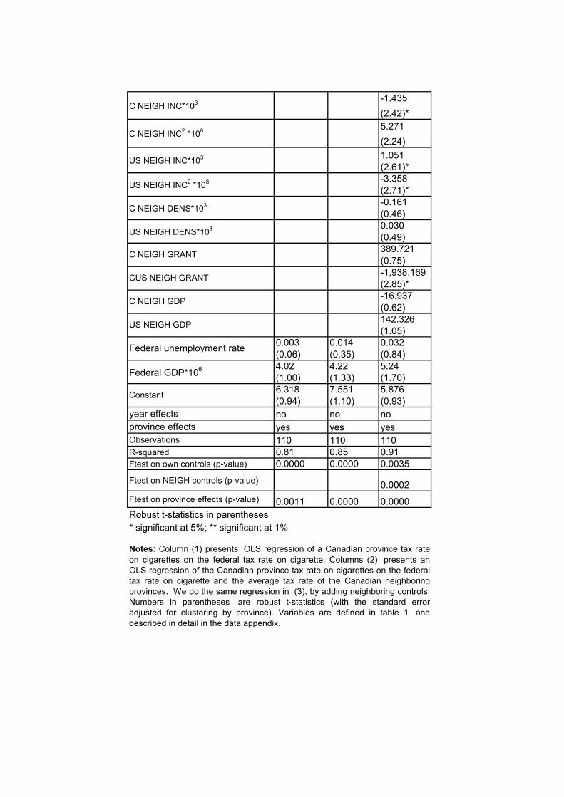
-1.435(2.42)*5.271(2.24)1.051(2.61)*-3.358(2.71)*-0.161(0.46)0.030(0.49)389.721(0.75)-1,938.169(2.85)*-16.937(0.62)142.326(1.05)
0.003 0.014 0.032(0.06) (0.35) (0.84)4.02 4.22 5.24(1.00) (1.33) (1.70)6.318 7.551 5.876(0.94) (1.10) (0.93)
year effects no no noprovince effects yes yes yesObservations 110 110 110R-squared 0.81 0.85 0.91Ftest on own controls (p-value) 0.0000 0.0000 0.0035
Ftest on NEIGH controls (p-value) 0.0002Ftest on province effects (p-value) 0.0011 0.0000 0.0000Robust t-statistics in parentheses* significant at 5%; ** significant at 1%
Constant
Federal unemployment rate
Federal GDP*106
Notes: Column (1) presents OLS regression of a Canadian province tax rateon cigarettes on the federal tax rate on cigarette. Columns (2) presents anOLS regression of the Canadian province tax rate on cigarettes on the federaltax rate on cigarette and the average tax rate of the Canadian neighboringprovinces. We do the same regression in (3), by adding neighboring controls.Numbers in parentheses are robust t-statistics (with the standard erroradjusted for clustering by province). Variables are defined in table 1 anddescribed in detail in the data appendix.
US NEIGH INC*103
C NEIGH INC2 *108
C NEIGH INC*103
US NEIGH GDP
US NEIGH INC2 *108
C NEIGH GRANT
CUS NEIGH GRANT
C NEIGH DENS*103
US NEIGH DENS*103
C NEIGH GDP
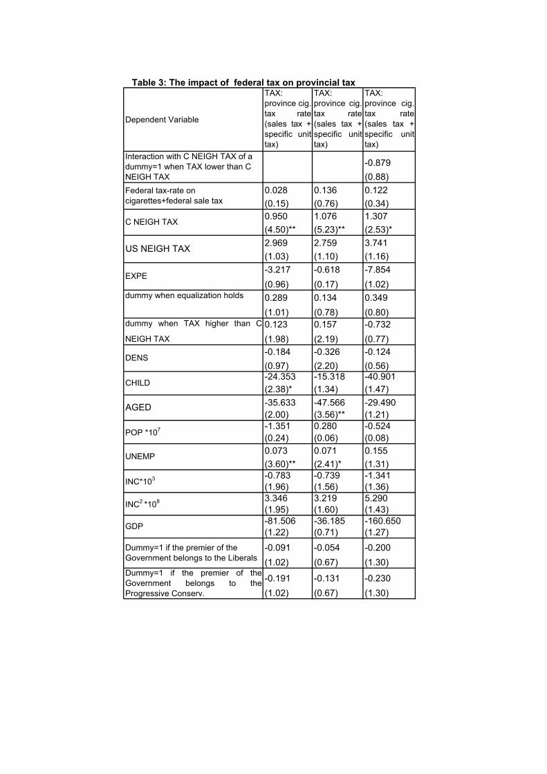
Dependent Variable
TAX: province cig. tax rate(sales tax +specific unittax)
TAX: province cig.tax rate(sales tax +specific unittax)
TAX: province cig.tax rate(sales tax +specific unittax)
-0.879(0.88)
0.028 0.136 0.122(0.15) (0.76) (0.34)0.950 1.076 1.307(4.50)** (5.23)** (2.53)*2.969 2.759 3.741(1.03) (1.10) (1.16)-3.217 -0.618 -7.854(0.96) (0.17) (1.02)0.289 0.134 0.349(1.01) (0.78) (0.80)0.123 0.157 -0.732(1.98) (2.19) (0.77)-0.184 -0.326 -0.124(0.97) (2.20) (0.56)-24.353 -15.318 -40.901(2.38)* (1.34) (1.47)-35.633 -47.566 -29.490(2.00) (3.56)** (1.21)-1.351 0.280 -0.524(0.24) (0.06) (0.08)0.073 0.071 0.155(3.60)** (2.41)* (1.31)-0.783 -0.739 -1.341(1.96) (1.56) (1.36)3.346 3.219 5.290(1.95) (1.60) (1.43)-81.506 -36.185 -160.650(1.22) (0.71) (1.27)-0.091 -0.054 -0.200(1.02) (0.67) (1.30)
-0.191 -0.131 -0.230(1.02) (0.67) (1.30)
UNEMP
INC*103
INC2 *108
POP *107
Dummy=1 if the premier of theGovernment belongs to theProgressive Conserv.
Dummy=1 if the premier of the Government belongs to the Liberals
DENS
CHILD
GDP
AGED
dummy when equalization holds
EXPE
US NEIGH TAX
dummy when TAX higher than C
NEIGH TAX
Interaction with C NEIGH TAX of a dummy=1 when TAX lower than C NEIGH TAX
Table 3: The impact of federal tax on provincial tax
Federal tax-rate on cigarettes+federal sale tax
C NEIGH TAX

-0.022 -0.022 -0.139(0.35) (0.42) (0.83)0.118 0.157 0.190(2.12) (2.65)* (1.45)-1.618 -1.357 -2.035(3.59)** (2.84)* (2.57)*6.431 5.384 7.999(3.45)** (2.79)* (2.62)*0.523 0.498 0.672(1.13) (1.18) (1.03)-1.819 -1.661 -2.322(1.33) (1.18) (1.01)-0.074 -0.425 0.327(0.21) (0.95) (0.55)-0.006 -0.033 -0.043(0.10) (0.50) (0.42)1,030.884 803.276 1,421.467(1.26) (1.27) (1.15)-1,981.173 -2,155.575 -1,425.931(2.42)* (2.39)* (0.98)-55.140 -45.224 -35.135(2.60)* (1.84) (0.99)186.768 226.650 212.553(1.00) (1.24) (0.82)0.064 0.064 0.058(1.18) (1.08) (0.79)4.02 9.35 12.2(1.00) (3.01)* (0.02)17.180 11.184 27.553(2.33)* (1.28) (1.66)
year effects no no noprovince effects yes yes yesObservations 110 110 110R-squared 0.87 0.87 0.80Overidentification test 0.04 0.19 0.45Ftest on own controls (p-value) 0.0000 0.0000 0.0000Ftest on NEIGH controls (p-value) 0.0000 0.0000 0.0000Ftest on province effects (p-value) 0.0000 0.0000 0.0000Robust t-statistics in parentheses* significant at 5%; ** significant at 1%
Constant
Federal unemployment rate
Federal GDP*106
Notes: Column (1) presents a 2 stages least squares estimate of a regressionof the Canadian province tax rate on cigarettes on the federal tax rate oncigarette and the average tax rate of the Canadian neighboring provinces: wedo not instrument the federal tax. We do the same regression in (2), butinstrumenting the federal tax. In column (3) we add the interaction of CNEIGH TAX with a dummy equal to 1 when TAX is lower than C NEIGH TAX.Numbers in parentheses are robust t-statistics (with the standard erroradjusted for clustering by province). Variables are defined in table 1 anddescribed in detail in the data appendix.
US NEIGH INC*103
C NEIGH INC2 *108
US NEIGH UNEMP
C NEIGH INC*103
C NEIGH UNEMP
US NEIGH GDP
US NEIGH INC2 *108
C NEIGH GRANT
CUS NEIGH GRANT
C NEIGH DENS*103
US NEIGH DENS*103
C NEIGH GDP

Dependent Variable
TAX: provincecig. tax rate(sales tax +specific unittax)
TAX: provincecig. tax rate(sales tax +specific unittax)
TAX: provincecig. tax rate(sales tax +specific unittax)
3.061 3.014(2.83)* (2.24)
-1.610 -0.119
(3.36)** (0.04)-2.994
(1.83)
1.547 1.442
(2.99)* (0.56)1.529 -0.162 -1.381(2.18) (0.16) (0.50)-0.204 1.424 -0.085(0.03) (0.30) (0.01)0.730 -4.434 0.329(0.04) (0.38) (0.02)-1.299 -1.306 -1.305(0.86) (1.12) (0.92)-0.078 0.293 -0.049(0.07) (0.53) (0.05)0.139 0.194 0.145(0.26) (0.47) (0.34)-22.874 -35.846 -23.927(0.34) (0.84) (0.41)-29.777 -12.644 -28.472(0.40) (0.24) (0.50)-11.854 -8.727 -11.661(1.08) (1.08) (0.97)0.064 0.072 0.064(0.49) (0.58) (0.49)-1.320 -1.355 -1.322(1.36) (1.46) (1.40)5.558 5.516 5.554(1.76) (1.74) (1.71)13.670 -89.590 5.699(0.03) (0.40) (0.02)
interaction with C NEIGH TAX of adummy =1 when TAX higher than CNEIGH TAXInteraction of the federal tax rate with the
interaction with C NEIGH TAX of a dummy
=1 when TAX higher than C NEIGH TAX
C NEIGH TAX
dummy when equalization holds
EXPE
GDP
Table 4: The effect of the the federal tax on tax competition
POP *107
UNEMP
INC*103
INC2 *108
dummy when TAX higher than C NEIGH
TAX
interaction with C NEIGH TAX of adummy =1 when TAX lower than CNEIGH TAX
AGED
Interaction of the federal tax rate with the
interaction with C NEIGH TAX of a dummy
=1 when TAX lower than C NEIGH TAX
DENS
CHILD
US NEIGH TAX
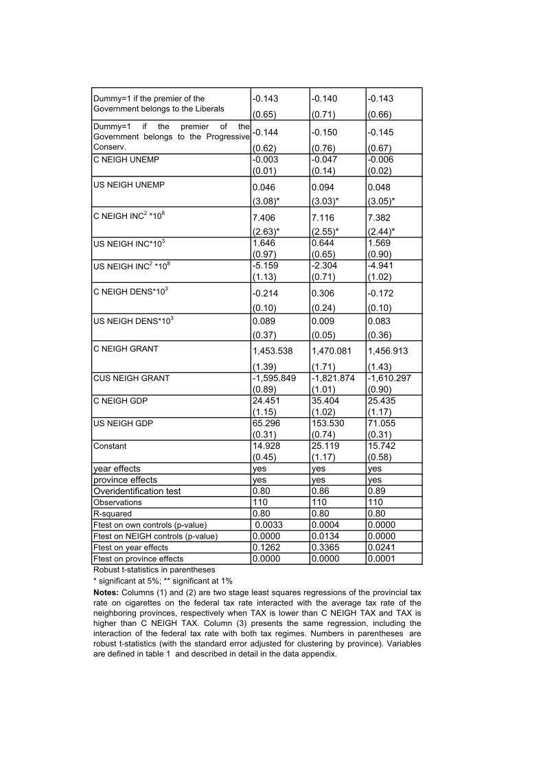
-0.143 -0.140 -0.143
(0.65) (0.71) (0.66)
-0.144 -0.150 -0.145
(0.62) (0.76) (0.67)C NEIGH UNEMP -0.003 -0.047 -0.006
(0.01) (0.14) (0.02)US NEIGH UNEMP 0.046 0.094 0.048
(3.08)* (3.03)* (3.05)*C NEIGH INC2 *108 7.406 7.116 7.382
(2.63)* (2.55)* (2.44)*US NEIGH INC*103 1.646 0.644 1.569
(0.97) (0.65) (0.90)US NEIGH INC2 *108 -5.159 -2.304 -4.941
(1.13) (0.71) (1.02)C NEIGH DENS*103 -0.214 0.306 -0.172
(0.10) (0.24) (0.10)US NEIGH DENS*103 0.089 0.009 0.083
(0.37) (0.05) (0.36)C NEIGH GRANT 1,453.538 1,470.081 1,456.913
(1.39) (1.71) (1.43)CUS NEIGH GRANT -1,595.849 -1,821.874 -1,610.297
(0.89) (1.01) (0.90)C NEIGH GDP 24.451 35.404 25.435
(1.15) (1.02) (1.17)US NEIGH GDP 65.296 153.530 71.055
(0.31) (0.74) (0.31)Constant 14.928 25.119 15.742
(0.45) (1.17) (0.58)year effects yes yes yesprovince effects yes yes yesOveridentification test 0.80 0.86 0.89Observations 110 110 110R-squared 0.80 0.80 0.80Ftest on own controls (p-value) 0.0033 0.0004 0.0000Ftest on NEIGH controls (p-value) 0.0000 0.0134 0.0000Ftest on year effects 0.1262 0.3365 0.0241Ftest on province effects 0.0000 0.0000 0.0001
Notes: Columns (1) and (2) are two stage least squares regressions of the provincial taxrate on cigarettes on the federal tax rate interacted with the average tax rate of theneighboring provinces, respectively when TAX is lower than C NEIGH TAX and TAX ishigher than C NEIGH TAX. Column (3) presents the same regression, including theinteraction of the federal tax rate with both tax regimes. Numbers in parentheses arerobust t-statistics (with the standard error adjusted for clustering by province). Variablesare defined in table 1 and described in detail in the data appendix.
* significant at 5%; ** significant at 1%
Dummy=1 if the premier of theGovernment belongs to the ProgressiveConserv.
Robust t-statistics in parentheses
Dummy=1 if the premier of the Government belongs to the Liberals