1

Crossover-Net: Leveraging the Vertical-HorizontalCrossover Relation for Robust Segmentation

Qian Yu, Yinghuan Shi, Yefeng Zheng, Yang Gao, Jianbing Zhu, Yakang Dai

Abstract—Robust segmentation for non-elongated tissues inmedical images is hard to realize due to the large variationof the shape, size, and appearance of these tissues in differentpatients. In this paper, we present an end-to-end trainable deepsegmentation model termed Crossover-Net for robust segmenta-tion in medical images. Our proposed model is inspired by aninsightful observation: during segmentation, the representationfrom the horizontal and vertical directions can provide differentlocal appearance and orthogonality context information, whichhelps enhance the discrimination between different tissues bysimultaneously learning from these two directions. Specifically, byconverting the segmentation task to a pixel/voxel-wise predictionproblem, firstly, we originally propose a cross-shaped patch,namely crossover-patch, which consists of a pair of (orthogonaland overlapped) vertical and horizontal patches, to capture theorthogonal vertical and horizontal relation. Then, we develop theCrossover-Net to learn the vertical-horizontal crossover relationcaptured by our crossover-patches. To achieve this goal, forlearning the representation on a typical crossover-patch, wedesign a novel loss function to (1) impose the consistency onthe overlap region of the vertical and horizontal patches and (2)preserve the diversity on their non-overlap regions. We haveextensively evaluated our method on CT kidney tumor, MRcardiac, and X-ray breast mass segmentation tasks. Promisingresults are achieved according to our extensive evaluation andcomparison with the state-of-the-art segmentation models.

Index Terms—Deep Convolutional Neural Network; Non-elongated Tissue; Crossover-Net; Segmentation

I. INTRODUCTION

IN medical images, e.g., computed tomography (CT), mag-netic resonance imaging (MRI), and X-ray images, segmen-

tation of non-elongated tissues is a significant yet challengingtask. Basically, the representative non-elongated tissues con-tain the liver, heart, kidney, and brain, etc. The purpose ofsegmenting these tissues is to provide the position, size, andintensity information to physicians for the subsequent diagno-sis of liver cancer, cardiac disease, etc. Unfortunately, due tothe subjective (e.g., inaccurate delineation) and objective (e.g.,massive images) factors, manual delineation is not desirable inclinical practice. Therefore, automatic segmentation methodsfor non-elongated tissues are in a great demand accordingto the aforementioned issues. However, it is known that the

Qian Yu, Yinghuan Shi and Yang Gao are with the State Key Laboratoryfor Novel Software Technology, Nanjing University, China. Qian Yu is alsowith School of Data and Computer Science, Shandong Women’s University,China (e-mail: yuqian@sdwu.edu.cn; syh@nju.edu.cn; gaoy@nju.edu.cn).

Yefeng Zheng is with Youtu Lab, Tencent, China (e-mail:yefengzheng@tencent.com).

Jianbing Zhu is with the Suzhou Science and Technology Town Hospital,China. (e-mail: zeno1839@126.com)

Yakang Dai is with the Suzhou Institute of Biomedical Engineeringand Technology, Chinese Academy of Sciences, China. (e-mail:daiyk@sibet.ac.cn)

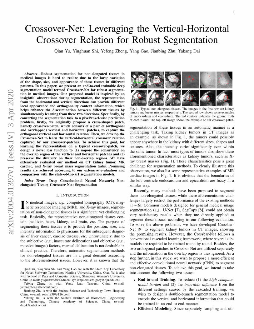
Fig. 1. Typical non-elongated tissues. The images in the first row are kidneytumors and breast masses, respectively. The second row shows some examplesof endocardium and epicardium. The red contour indicates the ground truthof each tissue. The top-left image shows the example of our crossover-patch.

segmentation of these tissues in an automatic manner is achallenging task. Taking kidney tumors in CT images asan example, as shown in Fig. 1, the tumors could possiblyappear anywhere in the kidney with different sizes, shapes andtextures. Also, the intensity varies significantly even withinthe same tumor. In fact, most types of tumors also show theseaforementioned characteristics as kidney tumors, such as X-ray breast masses (Fig. 1). These characteristics pose a greatchallenge for segmentation methods. To clearly illustrate thisobservation, we also list some representative examples of MRcardiac images in Fig. 1. It is obvious that the boundaries ofthe left ventricle endocardium and epicardium are fuzzy in asimilar way.

Recently, many methods have been proposed to segmentthese non-elongated tissues, while these aforementioned chal-lenges largely restrict the performance of the existing methods[1]–[6]. Common models designed for general medical imagesegmentation (e.g., U-Net [7], SegCaps [8]) could not obtainvery satisfactory results when they are directly applied tosegment these tissues according to our following evaluation.To solve the above problems, we have developed Crossbar-Net [9] to segment kidney tumors in CT images, showingthe promising results. However, the Crossbar-Net follows aconventional cascaded learning framework, where several sub-models are required to be trained round by round. Besides, thetwo orthogonal patches in Crossbar-Net are utilized separatelyand the information in the overlap region is thus ignored. As astep further, in this study, we wish to propose a more efficientand effective convolutional neural network (CNN) to segmentnon-elongated tissues. To achieve this goal, we intend to takeinto account the following two issues:

• End-to-end Training. To reduce (1) the high computa-tional burden and (2) the invertible influence from thedifferent settings caused by the cascaded training, wewish to design a double-branch segmentation model toencode the vertical and horizontal information that couldbe trained in an end-to-end manner.

• Efficient Modeling. Since separately sampling and uti-

arX

iv:2

004.

0139

7v1

[ee

ss.I

V]

3 A

pr 2

020

2

lizing the vertical and horizontal patches might wastethe overlap region and bring in a large quantity ofredundant patches, we try to learn a consistent represen-tation between the vertical and horizontal patches if theyhave an overlap region, which could largely improve theutilization of information.

According to the above analysis, we propose an orthogonalpatch pair in this paper, namely crossover-patch (see Fig. 1).Basically, a crossover-patch consists of a vertical patch anda horizontal patch, with each patch fully covering the wholetissue along one direction (i.e., vertical or horizontal) fromside-to-side. Based on the crossover-patch, we construct anend-to-end deep segmentation model, termed as Crossover-Net, to convert the segmentation task to a pixel/voxel-wiseclassification problem. Specifically, our Crossover-Net intendsto classify the central pixel of a crossover-patch belonging tothe target tissue or not. For a given pixel, the vertical andhorizontal patches of its corresponding crossover-patch areutilized as a whole in Crossover-Net. Overall, the technicalcontributions of this work can be summarized into the follow-ing four folds:• For a given location (i.e., pixel or voxel) in the medical

image, our proposed crossover-patch can not only capturethe vertical and horizontal information separately but alsoprovide the crossover relation information to Crossover-Net for the efficient and discriminative learning.

• Our Crossover-Net is a dual-branch end-to-end segmen-tation model. Our model can learn the feature represen-tation of the cross-shaped patches from two directionssimultaneously. We also notice that if the feature repre-sentation in one direction is not discriminative enough,the other direction could benefit the current one from acomplement perspective.

• We design a novel loss function with the goal of makingthe feature representations learned from (1) the overlapregion of each crossover-patch as consistent as possible,while (2) the non-overlap regions of the patch as differentas possible. Thus, the target-guided information could beeffectively highlighted.

• Our model is easy to implement. According to our evalu-ation, our model can achieve the promising performanceon various non-elongated tissue segmentation tasks.

II. RELATED WORK

Previous CNN-based segmentation methods can be roughlyclassified into two categories: the image-based models andthe patch-based models. For the image-based models, thefully convolutional network (FCN) proposed in [10] and itsvariants are widely used in various image segmentation tasks.Among all the FCN-style structure, for medical image seg-mentation, the U-Net [7] is a representative model. Currently,many state-of-the-art segmentation models are inspired by themerits of U-Net. For example, Lalonde et al. [8] designeda common model based on U-Net with capsules, SegCaps,which achieved promising results in many segmentation tasks.Similarly, the H-DenseUNet [11] is a hybrid U-Net modelto fuse 2D and 3D features for liver tumor segmentationin CT images. For the patch-based model, Ciresan et al.[12] employed multiple deep networks to segment biological

neuron membranes by extracting the square patches in multi-scales using sliding-window. Wang et al. [13] devised a multi-branch CNN model to segment the lung nodules. Shi et al.[14] proposed a cascaded deep domain adaptation model tosegment the prostate in CT images.

Recently, training deep models in a multi-scale or multi-branch manner to extract comprehensive features has arousedconsiderable interests. For example, Havaei et al. [15] andRazzak et al. [16] segmented the brain tumors with a two-pathway CNN architecture. Similarly, Moeskops et al. [17]presented a multi-scale approach to segmenting MR brainimages. Also, Kamnitsas et al. [18] proposed a multi-scale3D-CNN with two parallel pathways to segment brain lesions.In [19], a multi-channel multi-scale CNN model was designedto reconstruct the plane-wave ultrasound images. Bien et al.[20] also developed a multi-branch model, namely MRNet,to detect the general abnormalities and specific diagnoseson knee MR images. All these methods utilize the multi-scale input data to obtain high accuracy, and some othermethods aggregate multi-scale features from a single inputdata to achieve good performance. For instance, Lin et al.[21] designed a multi-scale context intertwining strategy to ag-gregate features from different scales for pixel level semanticsegmentation. Huang et al. [22] cropped multi-level featuresfor colorectal tumor segmentation task. Also, methods in [23]–[27] propagated and fused multi-scale features to constructdifferent scale context for accurate segmentation.

From the perspective of the loss function, beyond traditionalloss functions (e.g., the cross-entropy loss, the logistic loss,and the mean squared error loss), it is a new trend to designspecial loss functions to improve the performance of a deepsegmentation model by using the prior knowledge of thesegmentation task. For instance, in V-Net [28] (a typical 3Dmedical image segmentation model), a Dice similarity lossfunction was utilized to segment the MR prostate. Also, in 3DRU-Net [22], a hybrid Dice-based loss function was designedto help the model to locate the region of interesting (ROI)and segment the colorectal tumor simultaneously. In addition,a linear combination loss was introduced to train the CNNmodel for cardiac segmentation in [29]. Cholakkal et al. [30]also proposed two special terms in their loss function to getdesirable result in instance segmentation. Thus, leveragingthese specific information could help improve the performanceof the model. Our loss function is designed based on ourproposed crossover-patch.

Our proposed method has a large difference with previoussegmentation methods. Specifically, compared with the previ-ous methods, the major distinctions of Crossover-Net are (1)our sampled patch is cross-shaped, (2) our model learns therepresentation from two directions simultaneously in an end-to-end manner, and (3) our loss function is able to make fulluse of the proposed crossover-patches.

III. OUR METHOD

A. The Architecture of Crossover-NetAs aforementioned, our Crossover-Net includes two

branches, i.e., vertical branch and horizontal branch, trainedby crossover-patches (see Fig. 2). Here, for CT kidney tumorsegmentation, we set the size of the orthogonal patch pair to

3

Feature maps Height width

120 100

1618 96

3616 92

641 19

641 13

1281 7× × × × × ×

643 21×

1696 18

6419 1

6413 1

1287 1

×

× × ×6421 3×36

92 16×

10001 1

21 1

Linear regression

×

×

1100 20×

conv1 5 3×

conv2 5 3×

pooling1 2 2×

conv3 5 3×

pooling2 2 2×

conv4 3 3×

conv5 7 1×

conv6 7 1×

conv7 7 1×

Original images

×Convolution or pooling

Size of filterCrossover-patch

Crossover-loss layer

Prediction-loss layer

6442 6×

6446 8×

646 42×

648 46×

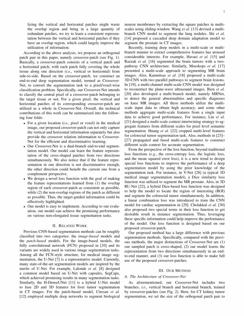
Fig. 2. Illustration of the architecture of our proposed Crossover-Net.

100 × 20 and 20 × 100, respectively. Both the numbers ofkernels and feature maps are experimentally determined bythe rough inner cross-validation.

In particular, each branch consists of seven convolutionallayers, two max pooling layers, and one linear regression layer.Also, each convolutional layer is followed by the dropout [31]operation, the rectified linear unit (ReLU) [32] activation andperformed with stride of one and without any padding. Con-sidering the size of our sampled patch is non-square, we set theconvolutional kernels of each convolutional layer to be non-square for the consistency. The pooling operation is performedwith stride of two and without any padding. The number andsize of feature maps and the size of kernels in each layer areindicated in Fig. 2. After the last convolutional operation (Fig.2, conv7), the last layer in each branch becomes a patch-to-pixel mapping with 500 units being included. We concatenatethe last layer of each branch directly, namely the prediction-loss layer, to combine the two branches (i.e., vertical branchand horizontal branch) together. The prediction-loss layer isrequired to be involved in the loss calculation. The purposeof this design is to capture high-level context informationefficiently since features extracted by deep layers are moreabstracted. Meanwhile, we also insert two crossover-loss lay-ers (the green and blue layers in Fig. 2) at the shallow ormiddle layers to capture the local information to contribute tothe loss calculation. Thus, based on the prediction-loss layerand the crossover-loss layer, the last layer of the model outputsthe probability of the central pixel of current crossover-patchbelonging to tumor.

It is worth noting that the structure of each branch could beeasily modified according to different scenarios. As for whichlayer can be taken as the crossover-loss layer, we introduce itin Section III-B and discuss this issue in Section IV.

B. Loss FunctionFormally, our loss function integrates two terms:• The first one is the prediction loss term to measure if the

prediction of Crossover-Net is correct according to the givenground truth in the training process. This term focuses on theglobal context, thus its corresponding prediction-loss layer iscalculated on the last convolutional layer.

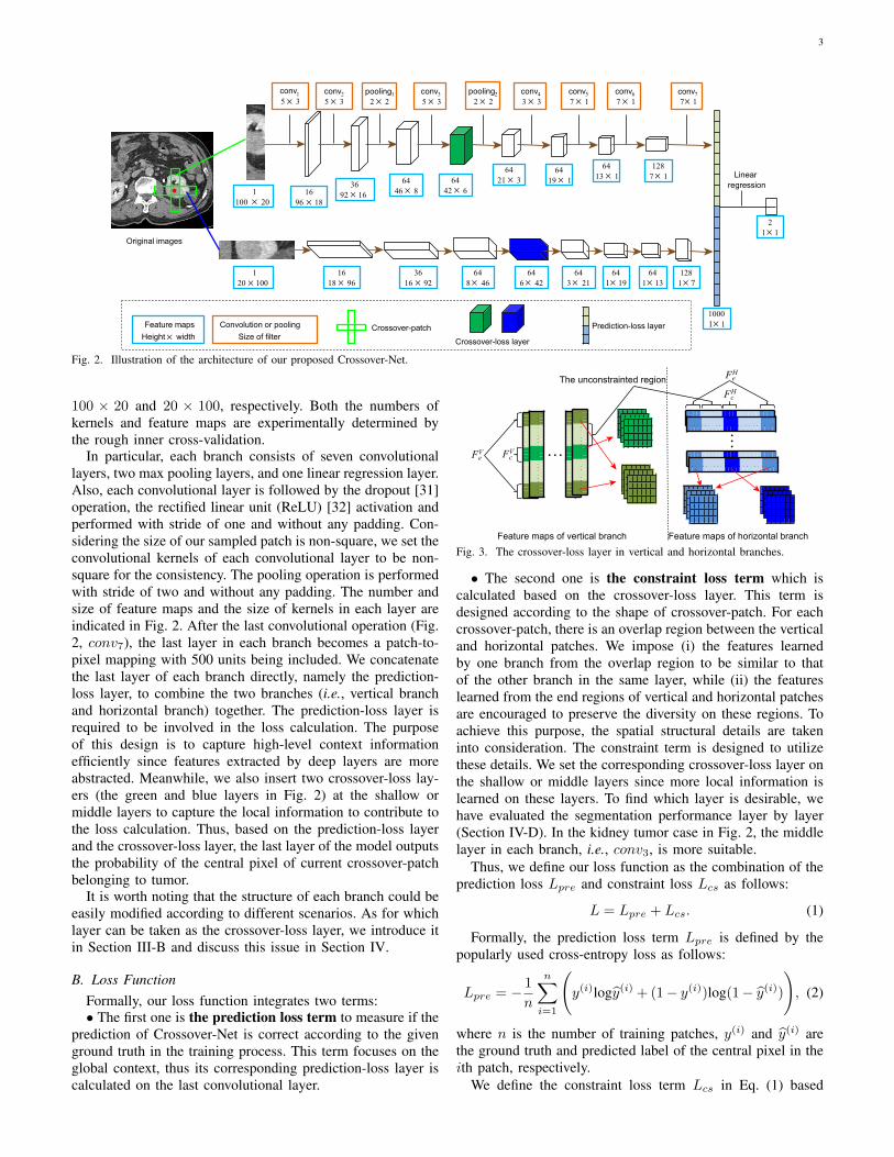
Feature maps of vertical branch Feature maps of horizontal branch

The unconstrainted region

FeV Fc

V

FeH

FcH

Fig. 3. The crossover-loss layer in vertical and horizontal branches.

• The second one is the constraint loss term which iscalculated based on the crossover-loss layer. This term isdesigned according to the shape of crossover-patch. For eachcrossover-patch, there is an overlap region between the verticaland horizontal patches. We impose (i) the features learnedby one branch from the overlap region to be similar to thatof the other branch in the same layer, while (ii) the featureslearned from the end regions of vertical and horizontal patchesare encouraged to preserve the diversity on these regions. Toachieve this purpose, the spatial structural details are takeninto consideration. The constraint term is designed to utilizethese details. We set the corresponding crossover-loss layer onthe shallow or middle layers since more local information islearned on these layers. To find which layer is desirable, wehave evaluated the segmentation performance layer by layer(Section IV-D). In the kidney tumor case in Fig. 2, the middlelayer in each branch, i.e., conv3, is more suitable.

Thus, we define our loss function as the combination of theprediction loss Lpre and constraint loss Lcs as follows:

L = Lpre + Lcs. (1)

Formally, the prediction loss term Lpre is defined by thepopularly used cross-entropy loss as follows:

Lpre = −1

n

n∑i=1

(y(i)logy(i) + (1− y(i))log(1− y(i))

), (2)

where n is the number of training patches, y(i) and y(i) arethe ground truth and predicted label of the central pixel in theith patch, respectively.

We define the constraint loss term Lcs in Eq. (1) based

42 2T T

F FFig. 4. A diagrammatic map of constraint loss term based on Fig. 3. The Tis the transpose operator, and the ‖·‖2F is the squared Frobenius norm.

covn1covn2

pooling1

r1r2

Crossover-patchOne feature map

in crossover-loss layer

Overlap region

Input layer

R1Rc1

R2Rc2

FcV

Fig. 5. Illustration of receptive region of FVc .

on the crossover-loss layer. As shown in Fig. 3, we illustrateeach crossover-loss layer of the two branches in detail. Inthe crossover-loss layer of the vertical branch, two ends ofeach feature map correspond to the two ends of the verticalpatch in the first layer, which are denoted as FV

e . Mean-while, there is also a part which is mapped from the overlapregion of crossover-patch, namely FV

c . The counterparts inhorizontal branch of FV

e and FVc are denoted as FH

e and FHc ,

respectively. Then, we make a diagrammatic drawing for theconstraint loss term in Fig. 4. Specifically, for the ith trainingcrossover-patch, let M

(i)Vc

, M(i)Hc

, M(i)Ve

and M(i)He

denote thematrix of FV

c , FHc , FV

e and FHe , respectively. We can define

the Lcs as

Lcs =1

n

n∑i=1

(∥∥∥M(i)Vc− (M

(i)Hc

)>∥∥∥2F−∥∥∥M(i)

Ve− (M

(i)He

)>∥∥∥2F

).

(3)Now, we describe how to determine the size of the four

matrices in Eq. (3). Taking the crossover-loss layer of verticalbranch as an example here, the FV

c in Fig. 5 is the regionthat is influenced significantly by the overlap region of thecrossover-patch (the cyan region). That is to say, in one featuremap, we need to search the region whose receptive region onthe input layer is closest to the overlap region. As shown inFig. 5, r1 and r2 denote the start and end row of FV

c withR1 and R2 being the row numbers of its receptive region, andRc1, Rc2 being row numbers of the overlap region. Beforesearching the target FV

c , let we reiterate the configuration ofour model: stride with 1 and no padding in the convolutionalprocess, and stride with 2, filter size being 2×2 and no paddingin the pooling process. Under this circumstance, assuming r1and r2 are known, R1 and R2 can be calculated by Algorithm1. The r1 and r2 are our targets which make the R1 and R2

closest to Rc1, Rc2 in Fig. 5. Then, the size of FVe is set the

same as that of FVc . The FH

c and FHe are obtained in the

same way. Thus, in the architecture shown in Fig. 2, the sizeof M(i)

Vc, M(i)

Hc, M(i)

Veand M

(i)He

are 64×4×6, 64×8×6 (thetwo FV

e in each feature map are concatenated), 64 × 6 × 4and 64 × 6 × 8 (the two FH

e are concatenated), respectively.Please note that, these values could be changed according thestructure of the model.

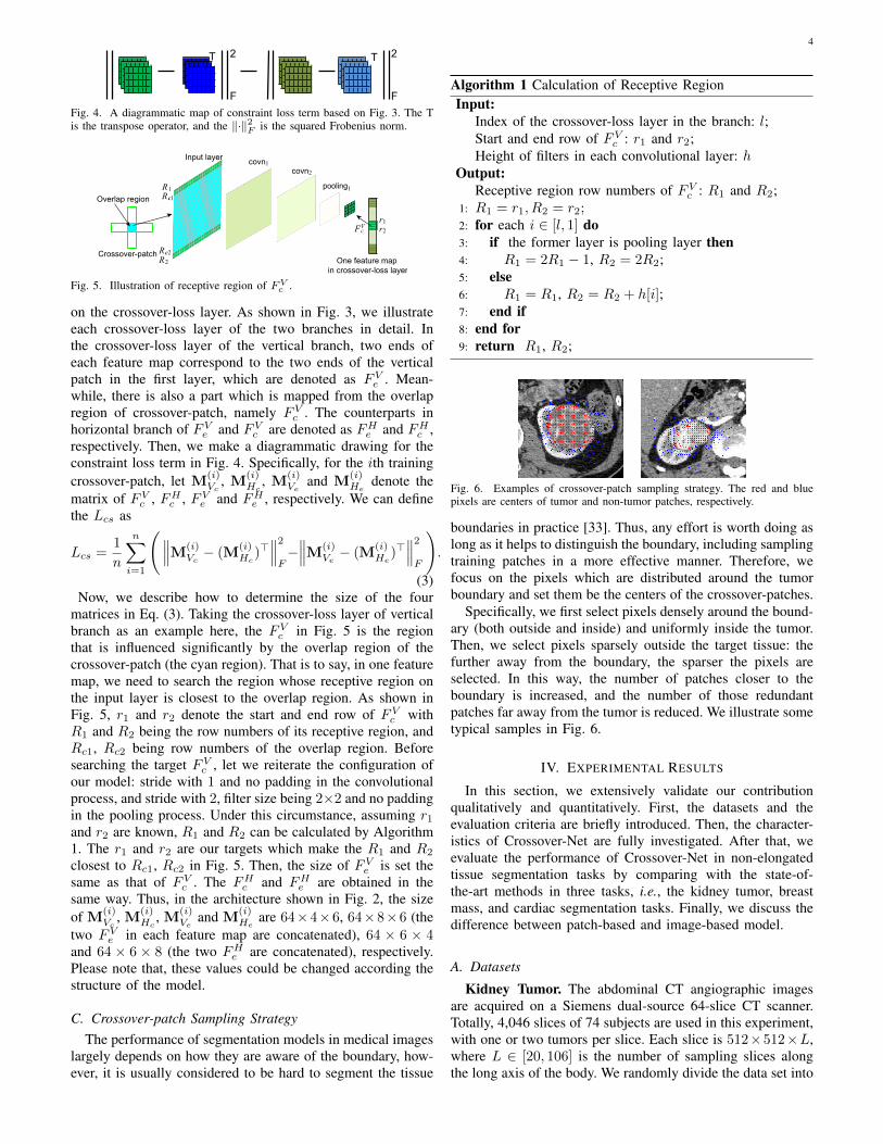
C. Crossover-patch Sampling StrategyThe performance of segmentation models in medical images

largely depends on how they are aware of the boundary, how-ever, it is usually considered to be hard to segment the tissue

Algorithm 1 Calculation of Receptive RegionInput:

Index of the crossover-loss layer in the branch: l;Start and end row of FV

c : r1 and r2;Height of filters in each convolutional layer: h

Output:Receptive region row numbers of FV

c : R1 and R2;1: R1 = r1, R2 = r2;2: for each i ∈ [l, 1] do3: if the former layer is pooling layer then4: R1 = 2R1 − 1, R2 = 2R2;5: else6: R1 = R1, R2 = R2 + h[i];7: end if8: end for9: return R1, R2;

Fig. 6. Examples of crossover-patch sampling strategy. The red and bluepixels are centers of tumor and non-tumor patches, respectively.

boundaries in practice [33]. Thus, any effort is worth doing aslong as it helps to distinguish the boundary, including samplingtraining patches in a more effective manner. Therefore, wefocus on the pixels which are distributed around the tumorboundary and set them be the centers of the crossover-patches.

Specifically, we first select pixels densely around the bound-ary (both outside and inside) and uniformly inside the tumor.Then, we select pixels sparsely outside the target tissue: thefurther away from the boundary, the sparser the pixels areselected. In this way, the number of patches closer to theboundary is increased, and the number of those redundantpatches far away from the tumor is reduced. We illustrate sometypical samples in Fig. 6.

IV. EXPERIMENTAL RESULTS

In this section, we extensively validate our contributionqualitatively and quantitatively. First, the datasets and theevaluation criteria are briefly introduced. Then, the character-istics of Crossover-Net are fully investigated. After that, weevaluate the performance of Crossover-Net in non-elongatedtissue segmentation tasks by comparing with the state-of-the-art methods in three tasks, i.e., the kidney tumor, breastmass, and cardiac segmentation tasks. Finally, we discuss thedifference between patch-based and image-based model.

A. Datasets

Kidney Tumor. The abdominal CT angiographic imagesare acquired on a Siemens dual-source 64-slice CT scanner.Totally, 4,046 slices of 74 subjects are used in this experiment,with one or two tumors per slice. Each slice is 512×512×L,where L ∈ [20, 106] is the number of sampling slices alongthe long axis of the body. We randomly divide the data set into

5

Bounding box Ground truth

Central pixel of crossover-patch

Vertical patch

Horizontal patch

Fig. 7. Example of the cropped image in INBreast. The left one is the croppedimage and the right one shows the crossover-patch extracted outside the image.

three parts for training, validation, and testing. Since the dataset contains many types of tumors and each type has certaincharacteristics, although the data sets are randomly extracted,it should be ensured that at least one case in the training set isof the same type with the test set. In addition, because kidneytumors are growing on both sides of the spine and below thefront and back mid-line of the abdominal cavity, we sampledonly in the second half of the abdominal cavity during the testprocedure, with the left tumor being sampled on the right sideof the spine and vice versa.

Breast Mass. Two publicly available mammogram datasets,INbreast [34], [35] and DDSM [36]–[38] are used here.

The images in INBreast are annotated with high quality.This dataset provides 116 images with one or two massesper image and the size of each image is 3, 328 × 4, 084 or2, 560 × 3, 328. We generate a bounding box for each massaccording to their annotations. The whole dataset is dividedinto two mutually exclusive equal subsets for training and test.For the DDSM, there are 1,923 malignant and benign cases,and each case includes two images of each breast. ROIs aregiven in images containing suspicious areas. Since the ROIis not the accurate boundary of a tumor, the boundary ofeach tumor is annotated again as the ground truth by theexperienced radiologists.

In most of the deep methods which segment INBreast andDDSM, each image is cropped to the bounding box [2], [39]or 1.2 times of the bounding box [35]. We crop the imagesin the same manner with [35]. If there are some crossover-patches being extracted outside the image, the outside partsare filled with black. An example is shown in Fig. 7.

Cardiac. We also evaluate our Crossover-Net on a publicbenchmark dataset of cardiac MR sequences [40]. This datasetconsists of 7,980 MR images for 33 individuals, with eachimage being 256 × 256. In the cardiac image, the boundaryof the left ventricle (LV) cave (i.e., endocardium) and the my-ocardium (MYO, enclosed by endocardium and epicardium)are targets of segmentation. In each image, endocardial andepicardial contours are provided as the ground truth.

B. Implementation Details

For the scale of crossover-patch on these three datasets, weset the size of patch pair to 20×100 and 100×20 on kidney andcardiac datasets. The structure of the model has been shownin Fig. 2. As for the INBreast and DDSM, according to theobservation about the size of masses, the crossover-patch isset to 68 × 340 and 340 × 68. For the large patches of themammography, the depth of the model is also large. There areeleven convolutional layers, three max pooling layers, and one

linear layer in each branch. The learning rate of all models isset to 0.0001. Each sub-model reaches its convergence within16, 18, and 15 epochs on kidney, cardiac, and breast data,respectively. The training and test procedure is repeated threetimes in all experiments for the credibility of the segmentation.In each time, the training, validation and test sets are selectedrandomly in kidney and cardiac data and DDSM. Due to thelimited number, there is no validation set on INBreast. Wereport the final average performance. All deep models areimplemented on a GPU server with NVIDIA GTX 1080 Ti.

We train the Crossover-Net with the standard back prop-agation. The model weights are first initialized with theXavier algorithm [41] which can determine the initializationscale according to the number of input and output neuronsautomatically [42]. In order to minimize the loss function, theparameters are updated by employing the stochastic gradientdescent algorithm during the training procedure.

C. Evaluation Criteria

We employ four popular criteria to evaluate the performanceof different methods, i.e., the Dice ratio score (DSC), the Haus-dorff distance (HD), the over-segmentation ratio (OR) and theunder-segmentation ratio (UR). The DSC is used to measurethe overlap between final prediction and manual segmentation.The HD indicates the max min Euclidean distance betweeneach pixel of the segmentation result and the manual result.A smaller HD indicates a higher proximity between groundtruth and the segmentation result. Please refer to [22], [43]for more details of these four criteria.

D. Characteristics of Crossover-Net

We conduct the extensive experiment on the kidney tumordataset to fully investigate our proposed model which includethe aspects of crossover-patch, loss function and crossover-losslayer.• Advantages of Crossover-patch. The advantage of

crossover-patches is relative to the square patches and thevertical or horizontal patches (a crossbar patch in [9] isessentially a separate vertical or horizontal patch since they areused separately). Similarly, one comparison object of learningfrom two directions is the performance of learning from singledirection. Both the learning based on square patches andvertical (horizontal) patches are the manner of learning from asingle direction. Therefore, we carry out the experiment withsquare patches, vertical and horizontal patches, and crossover-patches, respectively. In addition, simply combining the resultsof the vertical and horizontal patch-based networks is also away to learn from two directions.

Specifically, the two branches of Crossover-Net are takenout to form two separate networks with the vertical andhorizontal patches being their input data, respectively. Then,we set the size of square patches to 28 × 28, 56 × 56 and100 × 100. The size of filters in the corresponding networksare set to 3 × 3, and other parameters are set the same asCrossover-Net. Here, the cross-entropy loss function is used inall networks. Also, for fair comparison, we run Crossover-Neton crossover-patches only with cross-entropy loss function.

6

28×28 56×56 100×100 Ver Hor V-H MSE Entropy Cross

CNNs

0.7

0.75

0.8

0.85

0.9

0.95

DSC

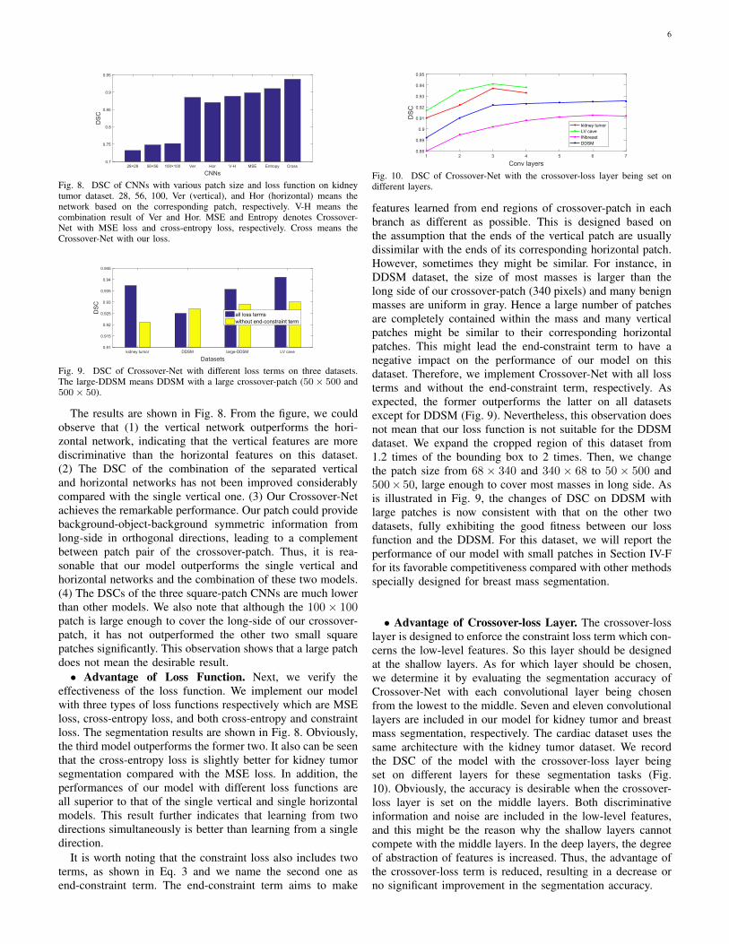
Fig. 8. DSC of CNNs with various patch size and loss function on kidneytumor dataset. 28, 56, 100, Ver (vertical), and Hor (horizontal) means thenetwork based on the corresponding patch, respectively. V-H means thecombination result of Ver and Hor. MSE and Entropy denotes Crossover-Net with MSE loss and cross-entropy loss, respectively. Cross means theCrossover-Net with our loss.

kidney tumor DDSM large-DDSM LV cave

Datasets

0.91

0.915

0.92

0.925

0.93

0.935

0.94

0.945

DSC

all loss termswithout end-constraint term

Fig. 9. DSC of Crossover-Net with different loss terms on three datasets.The large-DDSM means DDSM with a large crossover-patch (50× 500 and500× 50).

The results are shown in Fig. 8. From the figure, we couldobserve that (1) the vertical network outperforms the hori-zontal network, indicating that the vertical features are morediscriminative than the horizontal features on this dataset.(2) The DSC of the combination of the separated verticaland horizontal networks has not been improved considerablycompared with the single vertical one. (3) Our Crossover-Netachieves the remarkable performance. Our patch could providebackground-object-background symmetric information fromlong-side in orthogonal directions, leading to a complementbetween patch pair of the crossover-patch. Thus, it is rea-sonable that our model outperforms the single vertical andhorizontal networks and the combination of these two models.(4) The DSCs of the three square-patch CNNs are much lowerthan other models. We also note that although the 100× 100patch is large enough to cover the long-side of our crossover-patch, it has not outperformed the other two small squarepatches significantly. This observation shows that a large patchdoes not mean the desirable result.• Advantage of Loss Function. Next, we verify the

effectiveness of the loss function. We implement our modelwith three types of loss functions respectively which are MSEloss, cross-entropy loss, and both cross-entropy and constraintloss. The segmentation results are shown in Fig. 8. Obviously,the third model outperforms the former two. It also can be seenthat the cross-entropy loss is slightly better for kidney tumorsegmentation compared with the MSE loss. In addition, theperformances of our model with different loss functions areall superior to that of the single vertical and single horizontalmodels. This result further indicates that learning from twodirections simultaneously is better than learning from a singledirection.

It is worth noting that the constraint loss also includes twoterms, as shown in Eq. 3 and we name the second one asend-constraint term. The end-constraint term aims to make

1 2 3 4 5 6 7

Conv layers

0.88

0.89

0.9

0.91

0.92

0.93

0.94

0.95

DSC

kidney tumorLV caveINbreastDDSM

Fig. 10. DSC of Crossover-Net with the crossover-loss layer being set ondifferent layers.

features learned from end regions of crossover-patch in eachbranch as different as possible. This is designed based onthe assumption that the ends of the vertical patch are usuallydissimilar with the ends of its corresponding horizontal patch.However, sometimes they might be similar. For instance, inDDSM dataset, the size of most masses is larger than thelong side of our crossover-patch (340 pixels) and many benignmasses are uniform in gray. Hence a large number of patchesare completely contained within the mass and many verticalpatches might be similar to their corresponding horizontalpatches. This might lead the end-constraint term to have anegative impact on the performance of our model on thisdataset. Therefore, we implement Crossover-Net with all lossterms and without the end-constraint term, respectively. Asexpected, the former outperforms the latter on all datasetsexcept for DDSM (Fig. 9). Nevertheless, this observation doesnot mean that our loss function is not suitable for the DDSMdataset. We expand the cropped region of this dataset from1.2 times of the bounding box to 2 times. Then, we changethe patch size from 68 × 340 and 340 × 68 to 50 × 500 and500× 50, large enough to cover most masses in long side. Asis illustrated in Fig. 9, the changes of DSC on DDSM withlarge patches is now consistent with that on the other twodatasets, fully exhibiting the good fitness between our lossfunction and the DDSM. For this dataset, we will report theperformance of our model with small patches in Section IV-Ffor its favorable competitiveness compared with other methodsspecially designed for breast mass segmentation.

• Advantage of Crossover-loss Layer. The crossover-losslayer is designed to enforce the constraint loss term which con-cerns the low-level features. So this layer should be designedat the shallow layers. As for which layer should be chosen,we determine it by evaluating the segmentation accuracy ofCrossover-Net with each convolutional layer being chosenfrom the lowest to the middle. Seven and eleven convolutionallayers are included in our model for kidney tumor and breastmass segmentation, respectively. The cardiac dataset uses thesame architecture with the kidney tumor dataset. We recordthe DSC of the model with the crossover-loss layer beingset on different layers for these segmentation tasks (Fig.10). Obviously, the accuracy is desirable when the crossover-loss layer is set on the middle layers. Both discriminativeinformation and noise are included in the low-level features,and this might be the reason why the shallow layers cannotcompete with the middle layers. In the deep layers, the degreeof abstraction of features is increased. Thus, the advantage ofthe crossover-loss term is reduced, resulting in a decrease orno significant improvement in the segmentation accuracy.

7

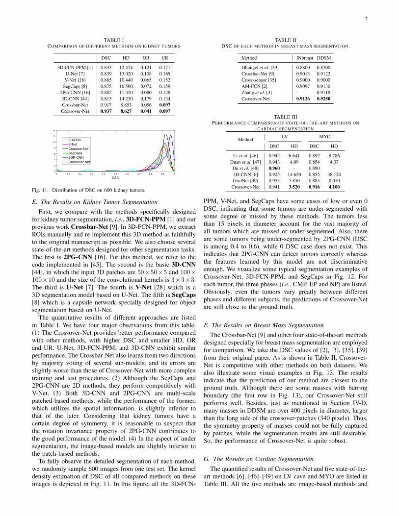
TABLE ICOMPARISON OF DIFFERENT METHODS ON KIDNEY TUMORS

DSC HD OR UR

3D-FCN-PPM [1] 0.833 12.474 0.121 0.171U-Net [7] 0.839 13.020 0.108 0.169V-Net [28] 0.885 10.440 0.065 0.152

SegCaps [8] 0.875 10.500 0.072 0.1592PG-CNN [16] 0.882 11.320 0.080 0.1283D-CNN [44] 0.813 14.230 0.179 0.134Crossbar-Net 0.917 8.853 0.056 0.097Crossover-Net 0.937 8.627 0.041 0.097

0 0.1 0.2 0.3 0.4 0.5 0.6 0.7 0.8 0.9 1

DSC

0

2

4

6

8

10

12

14

3D-FCNV-NetCrossbar-NetSegCaps2GP-CNNCrossover-Net

Fig. 11. Distribution of DSC on 600 kidney tumors.

E. The Results on Kidney Tumor Segmentation

First, we compare with the methods specifically designedfor kidney tumor segmentation, i.e., 3D-FCN-PPM [1] and ourprevious work Crossbar-Net [9]. In 3D-FCN-PPM, we extractROIs manually and re-implement this 3D method as faithfullyto the original manuscript as possible. We also choose severalstate-of-the-art methods designed for other segmentation tasks.The first is 2PG-CNN [16]. For this method, we refer to thecode implemented in [45]. The second is the basic 3D-CNN[44], in which the input 3D patches are 50×50×5 and 100×100×10 and the size of the convolutional kernels is 3×3×3.The third is U-Net [7]. The fourth is V-Net [28] which is a3D segmentation model based on U-Net. The fifth is SegCaps[8] which is a capsule network specially designed for objectsegmentation based on U-Net.

The quantitative results of different approaches are listedin Table I. We have four major observations from this table.(1) The Crossover-Net provides better performance comparedwith other methods, with higher DSC and smaller HD, ORand UR. U-Net, 3D-FCN-PPM, and 3D-CNN exhibit similarperformance. The Crossbar-Net also learns from two directionsby majority voting of several sub-models, and its errors areslightly worse than those of Crossover-Net with more complextraining and test procedures. (2) Although the SegCaps and2PG-CNN are 2D methods, they perform competitively withV-Net. (3) Both 3D-CNN and 2PG-CNN are multi-scalepatched-based methods, while the performance of the former,which utilizes the spatial information, is slightly inferior tothat of the later. Considering that kidney tumors have acertain degree of symmetry, it is reasonable to suspect thatthe rotation invariance property of 2PG-CNN contributes tothe good performance of the model. (4) In the aspect of undersegmentation, the image-based models are slightly inferior tothe patch-based methods.

To fully observe the detailed segmentation of each method,we randomly sample 600 images from one test set. The kerneldensity estimation of DSC of all compared methods on theseimages is depicted in Fig. 11. In this figure, all the 3D-FCN-

TABLE IIDSC OF EACH METHOD IN BREAST MASS SEGMENTATION.

Method INbreast DDSM

Dhungel et al. [39] 0.8800 0.8700Crossbar-Net [9] 0.9013 0.9122Cross-sensor [35] 0.9000 0.9000AM-FCN [2] 0.9097 0.9130Zhang et al. [3] - 0.9118Crossover-Net 0.9126 0.9250

TABLE IIIPERFORMANCE COMPARISON OF STATE-OF-THE-ART METHODS ON

CARDIAC SEGMENTATION

Method LV MYO

DSC HD DSC HD

Li et al. [46] 0.942 6.641 0.892 8.786Duan et al. [47] 0.943 4.09 0.854 4.37Du et al. [48] 0.960 - 0.890 -3D-CNN [6] 0.925 14.650 0.855 38.120GridNet [49] 0.955 5.850 0.885 8.010

Crossover-Net 0.941 3.520 0.916 4.100

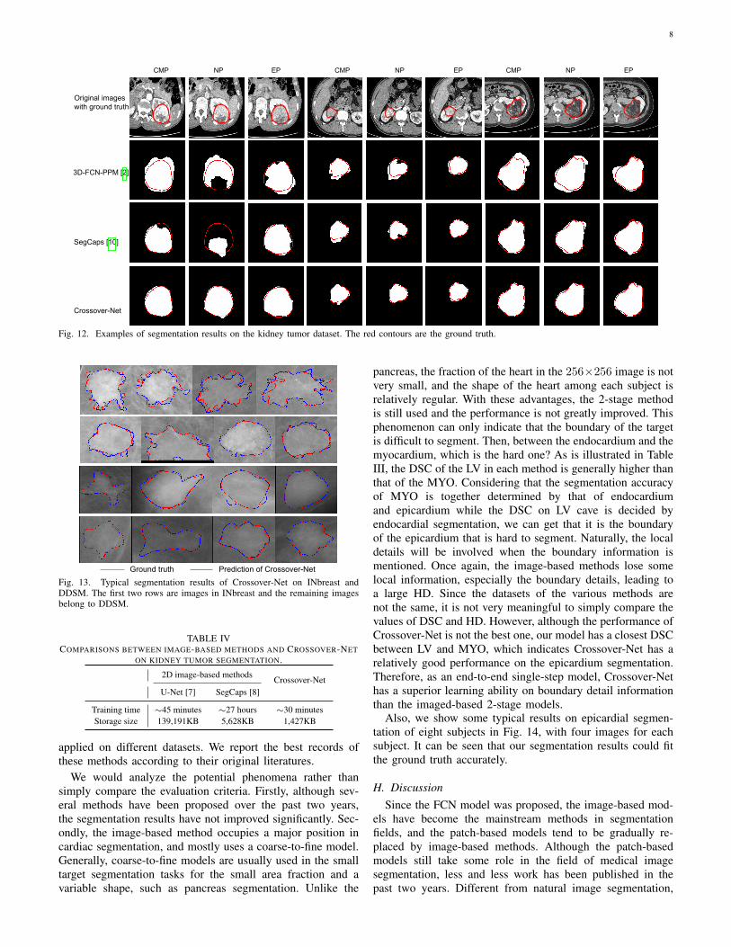
PPM, V-Net, and SegCaps have some cases of low or even 0DSC, indicating that some tumors are under-segmented withsome degree or missed by these methods. The tumors lessthan 15 pixels in diameter account for the vast majority ofall tumors which are missed or under-segmented. Also, thereare some tumors being under-segmented by 2PG-CNN (DSCis among 0.4 to 0.6), while 0 DSC case does not exist. Thisindicates that 2PG-CNN can detect tumors correctly whereasthe features learned by this model are not discriminativeenough. We visualize some typical segmentation examples ofCrossover-Net, 3D-FCN-PPM, and SegCaps in Fig. 12. Foreach tumor, the three phases (i.e., CMP, EP and NP) are listed.Obviously, even the tumors vary greatly between differentphases and different subjects, the predictions of Crossover-Netare still close to the ground truth.

F. The Results on Breast Mass Segmentation

The Crossbar-Net [9] and other four state-of-the-art methodsdesigned especially for breast mass segmentation are employedfor comparison. We take the DSC values of [2], [3], [35], [39]from their original paper. As is shown in Table II, Crossover-Net is competitive with other methods on both datasets. Wealso illustrate some visual examples in Fig. 13. The resultsindicate that the prediction of our method are closest to theground truth. Although there are some masses with burringboundary (the first row in Fig. 13), our Crossover-Net stillperforms well. Besides, just as mentioned in Section IV-D,many masses in DDSM are over 400 pixels in diameter, largerthan the long side of the crossover-patches (340 pixels). Thus,the symmetry property of masses could not be fully capturedby patches, while the segmentation results are still desirable.So, the performance of Crossover-Net is quite robust.

G. The Results on Cardiac Segmentation

The quantified results of Crossover-Net and five state-of-the-art methods [6], [46]–[49] on LV cave and MYO are listed inTable III. All the five methods are image-based methods and

8

CMP NP EP CMP NP EP

Original imageswith ground truth

3D-FCN-PPM [2]

SegCaps [10]

Crossover-Net

CMP NP EP

Fig. 12. Examples of segmentation results on the kidney tumor dataset. The red contours are the ground truth.

Ground truth Prediction of Crossover-Net

Fig. 13. Typical segmentation results of Crossover-Net on INbreast andDDSM. The first two rows are images in INbreast and the remaining imagesbelong to DDSM.

TABLE IVCOMPARISONS BETWEEN IMAGE-BASED METHODS AND CROSSOVER-NET

ON KIDNEY TUMOR SEGMENTATION.

2D image-based methods Crossover-NetU-Net [7] SegCaps [8]

Training time ∼45 minutes ∼27 hours ∼30 minutesStorage size 139,191KB 5,628KB 1,427KB

applied on different datasets. We report the best records ofthese methods according to their original literatures.

We would analyze the potential phenomena rather thansimply compare the evaluation criteria. Firstly, although sev-eral methods have been proposed over the past two years,the segmentation results have not improved significantly. Sec-ondly, the image-based method occupies a major position incardiac segmentation, and mostly uses a coarse-to-fine model.Generally, coarse-to-fine models are usually used in the smalltarget segmentation tasks for the small area fraction and avariable shape, such as pancreas segmentation. Unlike the

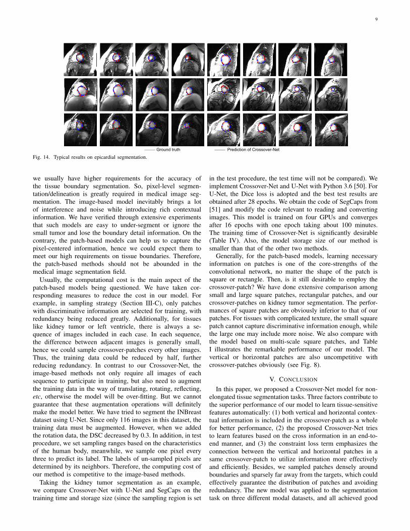
pancreas, the fraction of the heart in the 256×256 image is notvery small, and the shape of the heart among each subject isrelatively regular. With these advantages, the 2-stage methodis still used and the performance is not greatly improved. Thisphenomenon can only indicate that the boundary of the targetis difficult to segment. Then, between the endocardium and themyocardium, which is the hard one? As is illustrated in TableIII, the DSC of the LV in each method is generally higher thanthat of the MYO. Considering that the segmentation accuracyof MYO is together determined by that of endocardiumand epicardium while the DSC on LV cave is decided byendocardial segmentation, we can get that it is the boundaryof the epicardium that is hard to segment. Naturally, the localdetails will be involved when the boundary information ismentioned. Once again, the image-based methods lose somelocal information, especially the boundary details, leading toa large HD. Since the datasets of the various methods arenot the same, it is not very meaningful to simply compare thevalues of DSC and HD. However, although the performance ofCrossover-Net is not the best one, our model has a closest DSCbetween LV and MYO, which indicates Crossover-Net has arelatively good performance on the epicardium segmentation.Therefore, as an end-to-end single-step model, Crossover-Nethas a superior learning ability on boundary detail informationthan the imaged-based 2-stage models.

Also, we show some typical results on epicardial segmen-tation of eight subjects in Fig. 14, with four images for eachsubject. It can be seen that our segmentation results could fitthe ground truth accurately.

H. DiscussionSince the FCN model was proposed, the image-based mod-

els have become the mainstream methods in segmentationfields, and the patch-based models tend to be gradually re-placed by image-based methods. Although the patch-basedmodels still take some role in the field of medical imagesegmentation, less and less work has been published in thepast two years. Different from natural image segmentation,

9

Ground truth Prediction of Crossover-Net

Fig. 14. Typical results on epicardial segmentation.

we usually have higher requirements for the accuracy ofthe tissue boundary segmentation. So, pixel-level segmen-tation/delineation is greatly required in medical image seg-mentation. The image-based model inevitably brings a lotof interference and noise while introducing rich contextualinformation. We have verified through extensive experimentsthat such models are easy to under-segment or ignore thesmall tumor and lose the boundary detail information. On thecontrary, the patch-based models can help us to capture thepixel-centered information, hence we could expect them tomeet our high requirements on tissue boundaries. Therefore,the patch-based methods should not be abounded in themedical image segmentation field.

Usually, the computational cost is the main aspect of thepatch-based models being questioned. We have taken cor-responding measures to reduce the cost in our model. Forexample, in sampling strategy (Section III-C), only patcheswith discriminative information are selected for training, withredundancy being reduced greatly. Additionally, for tissueslike kidney tumor or left ventricle, there is always a se-quence of images included in each case. In each sequence,the difference between adjacent images is generally small,hence we could sample crossover-patches every other images.Thus, the training data could be reduced by half, furtherreducing redundancy. In contrast to our Crossover-Net, theimage-based methods not only require all images of eachsequence to participate in training, but also need to augmentthe training data in the way of translating, rotating, reflecting,etc, otherwise the model will be over-fitting. But we cannotguarantee that these augmentation operations will definitelymake the model better. We have tried to segment the INBreastdataset using U-Net. Since only 116 images in this dataset, thetraining data must be augmented. However, when we addedthe rotation data, the DSC decreased by 0.3. In addition, in testprocedure, we set sampling ranges based on the characteristicsof the human body, meanwhile, we sample one pixel everythree to predict its label. The labels of un-sampled pixels aredetermined by its neighbors. Therefore, the computing cost ofour method is competitive to the image-based methods.

Taking the kidney tumor segmentation as an example,we compare Crossover-Net with U-Net and SegCaps on thetraining time and storage size (since the sampling region is set

in the test procedure, the test time will not be compared). Weimplement Crossover-Net and U-Net with Python 3.6 [50]. ForU-Net, the Dice loss is adopted and the best test results areobtained after 28 epochs. We obtain the code of SegCaps from[51] and modify the code relevant to reading and convertingimages. This model is trained on four GPUs and convergesafter 16 epochs with one epoch taking about 100 minutes.The training time of Crossover-Net is significantly desirable(Table IV). Also, the model storage size of our method issmaller than that of the other two methods.

Generally, for the patch-based models, learning necessaryinformation on patches is one of the core-strengths of theconvolutional network, no matter the shape of the patch issquare or rectangle. Then, is it still desirable to employ thecrossover-patch? We have done extensive comparison amongsmall and large square patches, rectangular patches, and ourcrossover-patches on kidney tumor segmentation. The perfor-mances of square patches are obviously inferior to that of ourpatches. For tissues with complicated texture, the small squarepatch cannot capture discriminative information enough, whilethe large one may include more noise. We also compare withthe model based on multi-scale square patches, and TableI illustrates the remarkable performance of our model. Thevertical or horizontal patches are also uncompetitive withcrossover-patches obviously (see Fig. 8).

V. CONCLUSION

In this paper, we proposed a Crossover-Net model for non-elongated tissue segmentation tasks. Three factors contribute tothe superior performance of our model to learn tissue-sensitivefeatures automatically: (1) both vertical and horizontal contex-tual information is included in the crossover-patch as a wholefor better performance, (2) the proposed Crossover-Net triesto learn features based on the cross information in an end-to-end manner, and (3) the constraint loss term emphasizes theconnection between the vertical and horizontal patches in asame crossover-patch to utilize information more effectivelyand efficiently. Besides, we sampled patches densely aroundboundaries and sparsely far away from the targets, which couldeffectively guarantee the distribution of patches and avoidingredundancy. The new model was applied to the segmentationtask on three different modal datasets, and all achieved good

10

segmentation results. In the experiments, we not only fullyverified the good and robust performance of Crossover-Net,but also highlighted the ability of the patch-based methodto capture boundary detail information by using pixel-centriclocal information, which is what the image-based model lacks.Finally, we also conducted in-depth discussions on the trainingtime and storage size of the two types of models, verifying thecompetitiveness of our model in these two aspects comparedto the image-based model.

The problem with the new model is that when the seg-mentation target is too large, it is necessary to sample largerpatches and design a deeper network. This will lead to anincrease in training time, so the next work is to design a moreefficient model. How to use cross information more effectivelyis the key point of future work. Furthermore, extending ourmodel to elongated tissue segmentation tasks, such as vesselsegmentation, is also an appealing topic.

REFERENCES

[1] G. Yang, G. Li, T. Pan, Y. Kong, J. Wu, H. Shu et al., “Automaticsegmentation of kidney and renal tumor in CT images based on 3Dfully convolutional neural network with pyramid pooling module,” inInternational Conference on Pattern Recognition, 2018, pp. 3790–3795.

[2] W. Zhu, X. Xiang, T. D Tran, G. Hager, and X. Xie, “Adversarialdeep structured nets for mass segmentation from mammograms,” IEEEInternational Symposium on Biomedical Imaging, pp. 847–850, 2018.

[3] J. Zhang, B. Chen, M. Zhou, H. Lan, and F. Gao, “Photoacoustic imageclassification and segmentation of breast cancer: a feasibility study,”IEEE Access, vol. 7, pp. 5457–5466, 2019.

[4] J. Jiang, Y. Hu, C. Liu, D. Halpenny, M. D. Hellmann, J. O. Deasy et al.,“Multiple resolution residually connected feature streams for automaticlung tumor segmentation from CT images,” IEEE Transactions onMedical Imaging, vol. 38, no. 1, pp. 134–144, 2019.

[5] M. Khened, V. Alex, and G. Krishnamurthi, “Densely connected fullyconvolutional network for short-axis cardiac cine MR image segmenta-tion and heart diagnosis using random forest,” International Workshopon Statistical Atlases and Computational Models of the Heart, pp. 140–151, 2018.

[6] J. Patravali, S. Jain, and S. Chilamkurthy, “2D-3D fully convolutionalneural networks for cardiac MR segmentation,” International Workshopon Statistical Atlases and Computational Models of the Heart, pp. 130–139, 2018.

[7] O. Ronneberger, P. Fischer, and T. Brox, “U-Net: Convolutional net-works for biomedical image segmentation,” in Medical Image Comput-ing and Computer Assisted Intervention, 2015, pp. 234–241.

[8] R. LaLonde and U. Bagci, “Capsules for object segmentation,” arXivpreprint arXiv:1804.04241, 2018.

[9] Q. Yu, Y. Shi, J. Sun, Y. Gao, J. Zhu, and Y. Dai, “Crossbar-Net: Anovel convolutional neural network for kidney tumor segmentation inCT images,” IEEE Transactions on Image Processing, vol. 28, no. 8,pp. 4060–4074, 2019.

[10] J. Long, E. Shelhamer, and T. Darrell, “Fully convolutional networksfor semantic segmentation,” pp. 3431–3440, 2015.

[11] X. Li, H. Chen, X. Qi, Q. Dou, C. Fu, and P. Heng, “H-DenseUNet:Hybrid densely connected UNet for liver and tumor segmentation fromCT volumes,” IEEE Transactions on Medical Imaging, vol. 37, no. 12,pp. 2663–2674, 2018.

[12] D. C. Ciresan, A. Giusti, L. M. Gambardella, and J. Schmidhuber, “Deepneural networks segment neuronal membranes in electron microscopyimages,” International Conference on Neural Information ProcessingSystems, vol. 2, pp. 2843–2851, 2012.

[13] S. Wang, M. Zhou, Z. Liu, Z. Liu, D. Gu, Y. Zang et al., “Centralfocused convolutional neural networks: Developing a data-driven modelfor lung nodule segmentation,” Medical Image Analysis, vol. 40, pp.172–183, 2017.

[14] Y. Shi, W. Yang, Y. Gao, and D. Shen, “Does manual delineation onlyprovide the side information in CT prostate segmentation?” pp. 692–700,2017.

[15] M. Havaei, A. Davy, D. Warde-Farley, A. Biard, A. Courville, Y. Bengioet al., “Brain tumor segmentation with deep neural networks,” MedicalImage Analysis, vol. 35, pp. 18–31, 2017.

[16] I. Razzak, M. Imran, and G. Xu, “Efficient brain tumor segmentationwith multiscale two-pathway-group conventional neural networks,” IEEEJournal of Biomedical and Health Informatics, vol. 23, no. 5, pp. 1911–1919, 2019.

[17] P. Moeskops, M. A. Viergever, A. M. Mendrik, L. S. de Vries, M. J.Benders, and I. Isgum, “Automatic segmentation of MR brain imageswith a convolutional neural network,” IEEE Transactions on MedicalImaging, vol. 35, no. 5, pp. 1252–1261, 2016.

[18] K. Kamnitsas, C. Ledig, V. F. Newcombe, J. P. Simpson, A. D. Kane,D. K. Menon et al., “Efficient multi-scale 3D CNN with fully connectedCRF for accurate brain lesion segmentation,” Medical Image Analysis,vol. 36, pp. 61–78, 2017.

[19] Z. Zhou, Y. Wang, J. Yu, Y. Guo, W. Guo, and Y. Qi, “High spa-tialtemporal resolution reconstruction of plane-wave ultrasound imageswith a multichannel multiscale convolutional neural network,” IEEETransactions on Ultrasonics Ferroelectrics and Frequency Control,vol. 65, no. 11, pp. 1983–1996, 2018.

[20] N. Bien, P. Rajpurkar, R. L. Ball, J. Irvin, A. Park, E. Jones et al.,“Deep-learning-assisted diagnosis for knee magnetic resonance imaging:Development and retrospective validation of MRNet,” PLOS Medicine,vol. 15, no. 11, pp. 1–19, 2018.

[21] D. Lin, Y. Ji, D. Lischinski, D. Cohenor, and H. Huang, “Multi-scalecontext intertwining for semantic segmentation.” European Conferenceon Computer Vision, pp. 622–638, 2018.

[22] Y. Huang, Q. Dou, Z. Wang, L. Liu, Y. Jin, C. Li et al., “3D ROI-awareU-Net for accurate and efficient colorectal tumor segmentation,” arXivpreprint arXiv:1806.10342v5, 2019.

[23] D. Lin, D. Shen, S. Shen, Y. Ji, D. Lischinski, D. Cohenor et al.,“ZigZagNet: Fusing top-down and bottom-up context for object segmen-tation,” IEEE Conference on Computer Vision and Pattern Recognition,pp. 7490–7499, 2019.

[24] M. Orsic, I. Kreso, P. Bevandic, and S. Segvic, “In defense of pre-trained ImageNet architectures for real-time semantic segmentation ofroad-driving images,” IEEE Conference on Computer Vision and PatternRecognition, pp. 12 606–12 616, 2019.

[25] H. Li, P. Xiong, H. Fan, and J. Sun, “DFANet: Deep feature aggregationfor real-time semantic segmentation,” IEEE Conference on ComputerVision and Pattern Recognition, pp. 9522–9531, 2019.

[26] T. Xiao, Y. Liu, B. Zhou, Y. Jiang, and J. Sun, “Unified perceptualparsing for scene understanding,” European Conference on ComputerVision, pp. 432–448, 2018.

[27] Z. Tian, T. He, C. Shen, and Y. Yan, “Decoders matter for semanticsegmentation: Data-dependent decoding enables flexible feature aggre-gation,” IEEE Conference on Computer Vision and Pattern Recognition,pp. 3126–3135, 2019.

[28] F. Milletari, N. Navab, and S. Ahmadi, “V-Net: Fully convolutionalneural networks for volumetric medical image segmentation,” in Inter-national Conference on 3D Vision, 2016, pp. 565–571.

[29] O. Oktay, E. Ferrante, K. Kamnitsas, M. P. Heinrich, W. Bai, J. Caballeroet al., “Anatomically constrained neural networks (ACNNs): Applicationto cardiac image enhancement and segmentation,” IEEE Transactions onMedical Imaging, vol. 37, no. 2, pp. 384–395, 2018.

[30] H. Cholakkal, G. Sun, F. S. Khan, and L. Shao, “Object counting andinstance segmentation with image-level supervision.” IEEE Conferenceon Computer Vision and Pattern Recognition, pp. 12 397–12 405, 2019.

[31] G. E. Hinton, N. Srivastava, A. Krizhevsky, I. Sutskever, and R. R.Salakhutdinov, “Improving neural networks by preventing co-adaptationof feature detectors,” arXiv preprint arXiv:1207.0580, 2012.

[32] V. Nair and G. E. Hinton, “Rectified linear units improve restrictedBoltzmann machines,” in International Conference on Machine Learn-ing, 2010, pp. 807–814.

[33] Y. Shi, Y. Gao, S. Liao, D. Zhang, Y. Gao, and D. Shen, “Semi-automaticsegmentation of prostate in CT images via coupled feature representationand spatial-constrained transductive Lasso,” IEEE Transactions on Pat-tern Analysis and Machine Intelligence, vol. 37, no. 11, pp. 2286–2303,2015.

[34] I. Moreira, I. Amaral, I. Domingues, A. Cardoso, M. J. Cardoso, and J. S.Cardoso, “INBreast: toward a full-field digital mammographic database,”Academic Radiology, vol. 19, no. 2, pp. 236–248, 2012.

[35] J. S. Cardoso, N. Marques, N. Dhungel, G. Carneiro, and A. P. Bradley,“Mass segmentation in mammograms: A cross-sensor comparison ofdeep and tailored features,” IEEE International Conference on ImageProcessing, pp. 1737–1741, 2017.

[36] M. Heath, K. Bowyer, D. Kopans, R. Moore, and W. P. Kegelmeyer,“The digital database for screening mammography,” pp. 212–218, 2000.

[37] M. Heath, K. Bowyer, D. Kopans, W. P. Kegelmeyer, R. Moore,K. Chang, and K. MunishKumaran, “Current status of the digitaldatabase for screening mammography,” pp. 457–460, 1998.

11

[38] A. Sharma, “DDSM utility,” GitHub repository, 2015. [Online].Available: https://github.com/trane293/DDSMUtility

[39] N. Dhungel, G. Carneiro, and A. P. Bradley, “Deep structured learningfor mass segmentation from mammograms,” International Conferenceon Image Processing, pp. 2950–2954, 2015.

[40] A. Andreopoulos and J. K. Tsotsos, “Efficient and generalizable sta-tistical models of shape and appearance for analysis of cardiac MRI,”Medical Image Analysis, vol. 12, no. 3, pp. 335–357, 2008.

[41] X. Glorot and Y. Bengio, “Understanding the difficulty of training deepfeedforward neural networks,” International Conference on ArtificialIntelligence and Statistics, pp. 249–256, 2010.

[42] C. Wachinger, M. Reuter, and T. Klein, “DeepNAT: Deep convolutionalneural network for segmenting neuroanatomy,” NeuroImage, vol. 170,pp. 434–445, 2017.

[43] Y. Shi, Y. Gao, S. Liao, D. Zhang, Y. Gao, and D. Shen, “A learning-based CT prostate segmentation method via joint transductive featureselection and regression,” Neurocomputing, vol. 173, pp. 317–331, 2016.

[44] R. Dey, Z. Lu, and Y. Hong, “Diagnostic classification of lung nodulesusing 3D neural networks,” IEEE International Symposium on Biomed-ical Imaging, pp. 774–778, 2018.

[45] “Group equivariant CNN.” [Online]. Available: https://github.com/

adambielski/pytorch-gconv-experiments[46] Z. Li, Y. Lou, Z. Yan, S. Alraref, J. K. Min, L. Axel, and D. N. Metaxas,

“Fully automatic segmentation of short-axis cardiac mri using modifieddeep layer aggregation,” in International Symposium on BiomedicalImaging, 2019, pp. 793–797.

[47] J. Duan, J. Schlemper, W. Bai, and T. J. W. Dawes, “Automatic 3Dbi-ventricular segmentation of cardiac images by a shape-refined multi-task deep learning approach,” IEEE Transactions on Medical Imaging,vol. 38, no. 9, pp. 2151–2164, 2019.

[48] X. Du, S. Yin, R. Tang, Y. Zhang, and S. Li, “Cardiac-deepied:Automatic pixel-level deep segmentation for cardiac bi-ventricle usingimproved end-to-end encoder-decoder network,” IEEE Journal of Trans-lational Engineering in Health and Medicine, vol. 7, pp. 1–10, 2019.

[49] C. Zotti, Z. Luo, O. Humbert, A. Lalande, and P. Jodoin, “GridNet withautomatic shape prior registration for automatic MRI cardiac segmenta-tion,” International Workshop on Statistical Atlases and ComputationalModels of the Heart, pp. 73–81, 2018.

[50] R. G. Van and F. Drake, “Python 3 reference manual,” Paramount (CA):CreateSpace, 2009.

[51] “SegCaps,” GitHub, 2018. [Online]. Available: https://github.com/lalonderodney/SegCaps