discovering and leveraging deep multimodal structure for
TRANSCRIPT
Discovering and Leveraging DeepMultimodal Structure for ReliableRobot Perception and Localization
Abhinav Valada
Technische FakultätAlbert-Ludwigs-Universität Freiburg
Dissertation zur Erlangung des akademischen GradesDoktor der Naturwissenschaften
Betreuer: Prof. Dr. Wolfram Burgard


Discovering and Leveraging DeepMultimodal Structure for ReliableRobot Perception and Localization
Abhinav Valada
Dissertation zur Erlangung des akademischen Grades Doktor der NaturwissenschaftenTechnische Fakultät, Albert-Ludwigs-Universität Freiburg
Dekanin Prof. Dr. Hannah BastErstgutachter Prof. Dr. Wolfram Burgard
Albert-Ludwigs-Universität FreiburgZweitgutachter Prof. Dr. Dieter Fox
University of WashingtonTag der Disputation 7. Februar 2019

Zusammenfassung
Fortschritte in der Robotik und im maschinellen Lernen führen zurzeit zu beispiellosenVeränderungen in verschiedenen gesellschaftlichen Bereichen, einschließlich der Dienst-leistungsbranche, des Bergbaus, der Hausarbeit und des Transportwesens. Während wir unstiefer in das Zeitalter intelligenter Roboter, die nicht mehr nur auf Szenarien in vereinfach-ten, kontrollierten Umgebungen beschränkt sind, begeben, stehen wir vor der kritischenHerausforderung, sie mit der Fähigkeit auszustatten, unsere sich ständig weiterentwickeln-de komplexe Welt wahrzunehmen und zu verstehen. Dies beinhaltet unter anderem, siemit der Möglichkeit auszustatten, Objekte aus einer Vielzahl von Variationen zu erkennen,hochdynamische Umgebungen zu modellieren, Informationen aus unterschiedlichen Sen-sormodalitäten zu gewinnen und Entscheidungen daraus abzuleiten und sich an Umständeanzupassen, die das Erscheinungsbild von Orten verändern, wie z. B. unterschiedlicheWetterbedingungen, Tageszeiten, Lichtverhältnisse und strukturelle Veränderungen. DieseFaktoren führen dazu, dass aktuelle Methoden, die von Hand für bestimmte Szenarienentwickelt wurden, fehlschlagen wenn sie mit der Komplexität und dem Reichtums unseresriesigen Wahrnehmungsraums konfrontiert werden.
In dieser Arbeit stellen wir Techniken vor, die es einem Roboter ermöglichen, die Struk-tur der Umgebung aus früheren Erfahrungen zu lernen, indem robuste Repräsentationenvon Modalitäten genutzt werden, die über einfache Bilder hinausgehen, und indem gemein-same Strukturen zwischen unterschiedlichen Aufgaben entdeckt und ausgenutzt werden.Wenn wir uns davon inspirieren lassen, wie Menschen in einem Gelände ohne visuelleWahrnehmung spüren und navigieren, schlagen wir zuerst eine Netzwerkarchitektur vor,die Fahrzeug-Boden-Interaktionsgeräusche als eine propriozeptive Modalität nutzt, umein breites Spektrum von Innen- und Außengeländen zu klassifizieren. Dieses Modellermöglicht es Robotern, Bodenverhältnisse ohne visuelle Information und auch unter un-günstigen akustischen Bedingungen unter Verwendung kostengünstiger Mikrofone genauzu klassifizieren. Als Zweites stellen wir kompakte Netzwerkarchitekturen für das Sze-nenverständnis vor, die kontextabhängige Multiskaleninformationen zusammenfassen undneuartige Techniken für die semantische Segmentierung mit hoher Auflösung integrieren.Unsere Modelle können effizient auf Robotern mit begrenzten Rechenressourcen eingesetztwerden, und die daraus resultierende semantische Klassifizierung auf Pixelebene lässt sicheffektiv auf Objekte anwenden, die in natürlichen Umgebungen häufig in unterschiedlichenGrößenordnungen vorkommen, von Szenarien des autonomen Fahrens im Stadtverkehr bishin zu Szenarien in Gebäuden und unstrukturierten Waldgebieten. Als Schritt in Richtung
vi
neuronaler Modelle, die sich entsprechend der jeweiligen Situation neu konfigurieren,schlagen wir drittens eine selbstüberwachte multimodale Architektur vor, die Informatio-nen aus komplementären Modalitäten wie visuellen Bildern, Tiefe und Infrarot dynamischverschmilzt, um Objekteigenschaften wie Aussehen, Geometrie und Reflexionsgrad für einganzheitliches semantisches Szenenverständnis zu nutzen. Diese Techniken ermöglichenes Robotern, lokale Unklarheiten in der Klassifizierung aufzulösen und die verschiedenenElemente der Szenerie unter schwierigen Wahrnehmungsbedingungen, die auf wechseln-de Wetter- und Jahreszeiten zurückzuführen sind, zuverlässig zu identifizieren. Viertensschlagen wir das erste Ende-zu-Ende-Lernnetzwerk für eine gemeinsame semantischeBewegungssegmentierung vor, welches sowohl Bewegungshinweise zur Verbesserungdes Semantiklernens als auch entsprechend semantische Hinweise zur Verbesserung derBewegungsschätzung nutzt. Mit unseren Modellen können Roboter die Dynamik der Um-gebung verstehen und gleichzeitig die Semantik der Szene zeitlich kohärent erkennen. ZumSchluss stellen wir eine Multitask-Lernstrategie vor, mit der automatisch Synergien genutztwerden können, um sich visuell zu lokalisieren, die Szenensemantik vorherzusagen und dieEigenbewegung des Roboters abzuschätzen. Unser Beitrag geht über die bestehenden Pa-radigmen hinaus, indem er das kooperative Lernen dieser wichtigen Schlüsseltechnologiender Roboterautonomie erleichtert und die geometrischen und strukturellen Bedingungender Umgebung effektiv kodiert.
Wir werten die in dieser Dissertation vorgestellten Ansätze mit Hilfe von standardisiertenBenchmarks umfassend aus und legen umfangreiche empirische Nachweise dafür vor, dassunsere Modelle auf dem neuesten Stand der Technik sind. Darüber hinaus präsentieren wirpraxisnahe Versuche aller vorgeschlagenen Methoden mit einer Reihe von verschiedenenRobotern, und demonstrieren damit die Generalisierbarkeit auf eine Vielzahl von Umge-bungen und Wahrnehmungsbedingungen. Wir glauben, dass wir Roboter mit Hilfe unsererMethoden einen Schritt näher daran gebracht haben, zuverlässig in komplexen realenUmgebungen eingesetzt zu werden, womit sie unsere Gesellschaft für immer grundlegendverändern werden.
Abstract
Advances in robotics and machine learning are creating unprecedented seismic shifts inseveral domains including the service industry, mining, domestic chores and transporta-tion. As we move deeper into the age of intelligent robots that are no longer confined tooperational scenarios in simplistic controlled environments, we are faced with the criticalchallenge of equipping them with the capability of perceiving and understanding our con-tinuously evolving complex world. Amongst others, this entails enabling them to recognizeobjects that have a multitude of variations, model highly dynamic environments, synthesizeand make decisions from disparate streams of modalities and adapt to circumstances thatchange the visual appearance of places such as different weather conditions, times of theday, illumination and structural changes. Such factors render current methods that arehand-tuned for specialized situations to break down when presented with the complexityand richness of our vast perceptual space.
In this thesis, we introduce techniques that enable a robot to learn the semantic struc-ture of the environment from prior experiences by leveraging robust representations frommodalities beyond just visual images as well as by discovering shared structure betweenmultiple diverse tasks. Firstly, taking inspiration from how humans sense and navigate onterrains in the absence of visual perception, we propose novel network architectures thatexploit vehicle-terrain interaction sounds as a proprioceptive modality to classify a widerange of indoor and outdoor terrains. These include recurrent models that enable robotsto accurately classify terrains without visual information and even in adverse real-worldacoustic conditions using inexpensive microphones. Secondly, we present compact fully-convolutional architectures for scene understanding that aggregate multiscale contextualinformation and incorporate novel techniques for high-resolution semantic segmentation.Our models are efficiently deployable on robots with limited computational resources andthe resulting pixel-level semantic classification effectively generalizes to objects that oftenappear at multiple scales in natural images of different environments ranging from urbanautonomous driving scenarios to indoor scenes and unstructured forested environments.Thirdly, as a step towards neural models that reconfigure themselves according to the en-countered situation, we propose self-supervised multimodal architectures that dynamicallyfuse information from complementary modalities such as visual images, depth and infraredto correspondingly exploit object properties such as appearance, geometry and reflectancefor a more holistic semantic scene understanding. These techniques enable robots equippedwith our models to resolve local ambiguities in their classification and robustly identify the
viii
various elements of the scene in challenging perceptual conditions attributed to changingweather and seasons. Fourthly, we propose the first end-to-end learning network for jointsemantic motion segmentation that simultaneously exploits motion cues to improve learn-ing of semantics and correspondingly exploits semantic cues to improve motion estimation.Our proposed models enable robots to understand the dynamics of the environment whileconcurrently being able to discern the semantics of the scene in a temporally coherentmanner. Finally, we present a multitask learning strategy to automatically exploit synergieswhile learning to visually localize, predict the scene semantics and estimate the ego-motionof the robot. Our contributions goes beyond existing paradigms by facilitating cooperativelearning of these key robot autonomy enablers as well as by effectively encoding geometricand structural constraints from the environment.
We comprehensively evaluate the approaches introduced in this thesis on standardbenchmarks and present extensive empirical evidence that demonstrates that our modelsachieve state-of-the-art performance. Additionally, we present real-world evaluations ofeach of our proposed methods using a number of different robots that demonstrate thegeneralizability to a variety of environments and perceptual conditions. We believe thatthese techniques have brought robots a step closer towards being reliably deployed incomplex real-world environments where they will fundamentally transform our societyforever.

Acknowledgments
This thesis would not have been possible without the support, encouragement, and guidanceof many people, to whom I owe my profound gratitude.
First and foremost, I thank my advisor, Wolfram Burgard for giving me the opportunityto pursue my PhD under his guidance. I thank him for providing me the ideal researchenvironment at the AIS lab, for the freedom to pursue my own ideas, for his constantencouragement to not only solve hard problems but to make them work on real robots, foralways having his doors open for discussions, for providing every resource that I couldever ask for, and for the opportunity to attend the many conferences. I am immensely andsincerely grateful.
I would like to thank Dieter Fox for all the insightful discussions during the conferencesover these years and for agreeing to be the second examiner of this thesis. I thank JoschkaBoedecker and Matthias Teschner for taking the time to be on my thesis committee. Iwould like to thank Luciano Spinello for initially inspiring me to work on deep learning atthe beginning of my doctoral studies. I would like to thank Daniel Büscher for readingevery page of this thesis in such a short time and for his valuable feedback. I would alsolike to thank Christian Dornhege for the constructive feedback and precious insights. Ithank Noha Radwan for wading through the original unedited manuscript and for ironingout the typos.
I had the privilege of collaborating with and learning from many exceptional researchersthroughout my doctoral studies. Special thanks to Johan Vertens for our fruitful collabo-rations, both before and during the PhD. It was a lot of fun building the AIS perceptioncar. I would like to thank Noha Radwan for tirelessly working towards the shared goal ofbeating the state-of-the-art localization network and the subsequent collaborations. I thankGabriel Oliveira for all the collaborations that we did during the first year of our PhD. Iwould like to thank Federico Boniardi for the inputs on how to better formulate problemsmathematically. I thank Andreas Wachaja for the numerous discussions on solving robothardware related issues. I would like to thank Andreas Eitel for setting up and managingthe high-performance computing cluster with me all these years. If we had not organizedand maintained the cluster, none of this research would have been practically possible. Iwould like to thank Nichola Abdo for the valuable comments on my research papers duringmy doctoral studies.
I thank all the students who I have had the opportunity to supervise and collaborate with.Thank you for your hard work and dedication. Special thanks to Rohit Mohan and Ankit

x
Dhall, for working endless days and not giving up until we had the results.This work would not have been possible without the tremendous support and friendship
of everyone in the Autonomous Intelligent Systems lab all these years. Be it the discussionsduring coffee breaks, presentations or the numerous barbeques. You all always inspired meand made the time that I spent during my doctoral studies a lot of fun. Special thanks tothe senior PhD students and postdocs who gave their valuable advice when I just joined thelab. I thank Gian Diego Tipaldi, Bastian Steder, Barbara Frank, Michael Ruhnke, TobiasSchubert, Christoph Sprunk, Mladen Mazuran, and Pratik Agarwal, for all the adviceand valuable feedback. I would like to thank all of my colleagues Tim Caselitz, AyushDewan, Tayyab Naseer, Tim Welschehold, Wera Winterhalter, Freya Fleckenstein, StefanoDi Lucia, Henrich Kolkhorst, Marina Kollmitz, Alexander Schiotka, Camilo Gordillo,Felix Burget, Philipp Ruchti, Alexander Schaefer, Lukas Luft, Chau Do, Daniel Kuhner,Andreas Kuhner, Oier Mees, Michael Krawez, Niklas Wetzel, and Martina Deturres, foralways being supportive and encouraging. I thank Jan Wülfing, Manuel Watter and MariaHuegle for always readily helping me translate German when ever I was clueless whatthose letters meant.
Lots of thanks to Susanne Bourjaillat, Evelyn Rusdea, Bettina Schug and Michael Keserfor handling all the administrative and technical issues during this entire time. Thank youfor being so kind and going out of your way to help.
Special thanks to all my officemates over the years: Federico Boniardi, Gabriel Oliveira,Barbara Frank, Stefano Di Lucia, and Maria Huegle, for putting up with my occasionalranting and everything from talking about work to life. I am grateful to all my friendsin Freiburg and beyond, with whom I have had great times and who have kept me sanethrough my entire doctoral studies. Special thanks to Diego Saul, Sebastian Castaño,Julia Berger, Christoph Scho, Eteri Sokhoyan, Aaron Klein, Carolin Kleber, Anna Doga,Valentina Doga, Branka Mirchevska, Georg Theil, and Eva-Maria Hanke. I thank ShrutiSadani and Rashmi Kumar for being the greatest friends ever since high school. I wouldlike to thank Noha Radwan for constantly motivating me, putting up with my grumpinessduring all the crazy deadlines, and always being there through thick and thin.
Finally, I thank my family and my extended family for always supporting me in ev-ery decision that I made. I thank my parents, my grandparents and my sister for theirunconditional love and support.

Contents
Contents xi
1 Introduction 11.1 Scientific Contributions . . . . . . . . . . . . . . . . . . . . . . . . . . . 71.2 Live Demos . . . . . . . . . . . . . . . . . . . . . . . . . . . . . . . . . 121.3 Dataset Contributions . . . . . . . . . . . . . . . . . . . . . . . . . . . . 121.4 Experimental Robot Platforms . . . . . . . . . . . . . . . . . . . . . . . 131.5 Publications . . . . . . . . . . . . . . . . . . . . . . . . . . . . . . . . . 151.6 Collaborations . . . . . . . . . . . . . . . . . . . . . . . . . . . . . . . . 171.7 Outline . . . . . . . . . . . . . . . . . . . . . . . . . . . . . . . . . . . 18
2 Background Theory 192.1 Camera Model . . . . . . . . . . . . . . . . . . . . . . . . . . . . . . . 192.2 Feed-Forward Neural Networks . . . . . . . . . . . . . . . . . . . . . . 212.3 Convolutional Neural Networks . . . . . . . . . . . . . . . . . . . . . . 24
2.3.1 Architecture Overview . . . . . . . . . . . . . . . . . . . . . . . 242.3.2 Layers . . . . . . . . . . . . . . . . . . . . . . . . . . . . . . . . 252.3.3 Architectural Network Design . . . . . . . . . . . . . . . . . . . 282.3.4 Loss Functions . . . . . . . . . . . . . . . . . . . . . . . . . . . 31
3 Proprioceptive Terrain Classification 333.1 Introduction . . . . . . . . . . . . . . . . . . . . . . . . . . . . . . . . . 333.2 Technical Approach . . . . . . . . . . . . . . . . . . . . . . . . . . . . . 37
3.2.1 Spectrogram Transformation and Augmentation . . . . . . . . . . 383.2.2 TerrainNet Architecture . . . . . . . . . . . . . . . . . . . . . . 393.2.3 TerrainNet++ Architecture . . . . . . . . . . . . . . . . . . . . . 413.2.4 Noise-Aware Training . . . . . . . . . . . . . . . . . . . . . . . 443.2.5 Baseline Feature Extraction . . . . . . . . . . . . . . . . . . . . 45
3.3 Data Collection and Labelling . . . . . . . . . . . . . . . . . . . . . . . 483.4 Experimental Evaluation . . . . . . . . . . . . . . . . . . . . . . . . . . 49
3.4.1 Training Protocol . . . . . . . . . . . . . . . . . . . . . . . . . . 503.4.2 Comparison with the State-of-the-Art . . . . . . . . . . . . . . . 513.4.3 Ablation Study . . . . . . . . . . . . . . . . . . . . . . . . . . . 52
xii Contents
3.4.4 Performance Evaluation . . . . . . . . . . . . . . . . . . . . . . 583.4.5 Evaluation of Noise Tolerance . . . . . . . . . . . . . . . . . . . 603.4.6 Evaluation of Noise-Aware Training . . . . . . . . . . . . . . . . 643.4.7 Evaluation of Hardware Independence . . . . . . . . . . . . . . . 67
3.5 Related Work . . . . . . . . . . . . . . . . . . . . . . . . . . . . . . . . 703.6 Conclusions . . . . . . . . . . . . . . . . . . . . . . . . . . . . . . . . . 72
4 Semantic Scene Segmentation 754.1 Introduction . . . . . . . . . . . . . . . . . . . . . . . . . . . . . . . . . 754.2 Technical Approach . . . . . . . . . . . . . . . . . . . . . . . . . . . . . 80
4.2.1 AdapNet Architecture . . . . . . . . . . . . . . . . . . . . . . . 814.2.2 AdapNet++ Architecture . . . . . . . . . . . . . . . . . . . . . . 844.2.3 Network Compression . . . . . . . . . . . . . . . . . . . . . . . 92
4.3 Freiburg Forest Dataset . . . . . . . . . . . . . . . . . . . . . . . . . . . 944.4 Experimental Evaluation . . . . . . . . . . . . . . . . . . . . . . . . . . 97
4.4.1 Benchmark Datasets . . . . . . . . . . . . . . . . . . . . . . . . 974.4.2 Data Augmentation . . . . . . . . . . . . . . . . . . . . . . . . . 1024.4.3 Network Training . . . . . . . . . . . . . . . . . . . . . . . . . . 1024.4.4 Comparison with the State-of-the-Art . . . . . . . . . . . . . . . 1034.4.5 Evaluation of Model Compression . . . . . . . . . . . . . . . . . 1104.4.6 Ablation Study . . . . . . . . . . . . . . . . . . . . . . . . . . . 1124.4.7 Qualitative Comparison . . . . . . . . . . . . . . . . . . . . . . 1214.4.8 Generalization Analysis . . . . . . . . . . . . . . . . . . . . . . 127
4.5 Related Work . . . . . . . . . . . . . . . . . . . . . . . . . . . . . . . . 1294.6 Conclusions . . . . . . . . . . . . . . . . . . . . . . . . . . . . . . . . . 131
5 Multimodal Semantic Segmentation 1335.1 Introduction . . . . . . . . . . . . . . . . . . . . . . . . . . . . . . . . . 1335.2 Technical Approach . . . . . . . . . . . . . . . . . . . . . . . . . . . . . 138
5.2.1 Convoluted Mixture of Deep Experts . . . . . . . . . . . . . . . 1395.2.2 Self-Supervised Modal Adaptation . . . . . . . . . . . . . . . . . 1415.2.3 Baseline Fusion Architectures . . . . . . . . . . . . . . . . . . . 146
5.3 Experimental Evaluation . . . . . . . . . . . . . . . . . . . . . . . . . . 1485.3.1 Network Training . . . . . . . . . . . . . . . . . . . . . . . . . . 1495.3.2 Comparison with the State-of-the-Art . . . . . . . . . . . . . . . 1505.3.3 Multimodal Fusion Discussion . . . . . . . . . . . . . . . . . . . 1575.3.4 Ablation Study . . . . . . . . . . . . . . . . . . . . . . . . . . . 1585.3.5 Qualitative Comparison . . . . . . . . . . . . . . . . . . . . . . 1665.3.6 Visualizations Across Seasons and Weather Conditions . . . . . . 1705.3.7 Real-World Navigation Experiment . . . . . . . . . . . . . . . . 174
Contents xiii
5.4 Related Work . . . . . . . . . . . . . . . . . . . . . . . . . . . . . . . . 1755.5 Conclusions . . . . . . . . . . . . . . . . . . . . . . . . . . . . . . . . . 178
6 Joint Semantic Motion Segmentation 1816.1 Introduction . . . . . . . . . . . . . . . . . . . . . . . . . . . . . . . . . 1816.2 Technical Approach . . . . . . . . . . . . . . . . . . . . . . . . . . . . . 186
6.2.1 SMSnet Architecture . . . . . . . . . . . . . . . . . . . . . . . . 1876.2.2 SMSnet++ Architecture . . . . . . . . . . . . . . . . . . . . . . 1906.2.3 Ego-Flow Suppression . . . . . . . . . . . . . . . . . . . . . . . 196
6.3 Dataset and Augmentation . . . . . . . . . . . . . . . . . . . . . . . . . 1966.4 Experimental Evaluation . . . . . . . . . . . . . . . . . . . . . . . . . . 200
6.4.1 Network Training . . . . . . . . . . . . . . . . . . . . . . . . . . 2016.4.2 Comparison with the State-of-the-Art . . . . . . . . . . . . . . . 2016.4.3 Influence of the Motion Parallax Effect . . . . . . . . . . . . . . 2096.4.4 Ablation Study . . . . . . . . . . . . . . . . . . . . . . . . . . . 2116.4.5 Qualitative Evaluations . . . . . . . . . . . . . . . . . . . . . . . 2216.4.6 Generalization Evaluations . . . . . . . . . . . . . . . . . . . . . 229
6.5 Related Work . . . . . . . . . . . . . . . . . . . . . . . . . . . . . . . . 2326.6 Conclusions . . . . . . . . . . . . . . . . . . . . . . . . . . . . . . . . . 235
7 Geometrically Consistent Semantic Visual Localization 2377.1 Introduction . . . . . . . . . . . . . . . . . . . . . . . . . . . . . . . . . 2377.2 Technical Approach . . . . . . . . . . . . . . . . . . . . . . . . . . . . . 242
7.2.1 The Geometric Consistency Loss Function . . . . . . . . . . . . 2427.2.2 VLocNet Architecture . . . . . . . . . . . . . . . . . . . . . . . 2447.2.3 VLocNet++ Architecture . . . . . . . . . . . . . . . . . . . . . . 248
7.3 DeepLoc Dataset . . . . . . . . . . . . . . . . . . . . . . . . . . . . . . 2537.4 Experimental Evaluation . . . . . . . . . . . . . . . . . . . . . . . . . . 254
7.4.1 Benchmark Datasets . . . . . . . . . . . . . . . . . . . . . . . . 2557.4.2 Network Training . . . . . . . . . . . . . . . . . . . . . . . . . . 2577.4.3 Comparison with the State-of-the-Art . . . . . . . . . . . . . . . 2587.4.4 Evaluation of Multitask Learning in VLocNet++ . . . . . . . . . 2617.4.5 Ablation Study . . . . . . . . . . . . . . . . . . . . . . . . . . . 2687.4.6 Visualization of the Level of Feature Similarity . . . . . . . . . . 2787.4.7 Visualization of the Regression Activation Maps . . . . . . . . . 2807.4.8 Qualitative Evaluations . . . . . . . . . . . . . . . . . . . . . . . 281
7.5 Related Work . . . . . . . . . . . . . . . . . . . . . . . . . . . . . . . . 2877.6 Conclusions . . . . . . . . . . . . . . . . . . . . . . . . . . . . . . . . . 291
8 Conclusions and Discussion 293

xiv Contents
Appendices 301
A Detailed Multimodal Semantic Segmentation Results 303A.1 Evaluation on the Cityscapes Dataset . . . . . . . . . . . . . . . . . . . . 303A.2 Evaluation on the Synthia Dataset . . . . . . . . . . . . . . . . . . . . . 305A.3 Evaluation on the SUN RGB-D Dataset . . . . . . . . . . . . . . . . . . 305A.4 Evaluation on the ScanNet Dataset . . . . . . . . . . . . . . . . . . . . . 311A.5 Evaluation on the Freiburg Forest Dataset . . . . . . . . . . . . . . . . . 311
Bibliography 321
Chapter 1
Introduction
The Dartmouth Conference of 1956, where the term Artificial Intelligence was coined [1],fueled an era of discovery in several domains including cognition, language understanding,and visual perception. This soon led to some of the foundations of artificial intelligencefor which the four Turing Awards were awarded successively to Marvin Minsky in 1969,John McCarthy in 1971, Herbert Simon and Allen Newell in 1975. These founders of thediscipline of artificial intelligence, explored how to make machines capable of human-likeperception and intelligence. Each of them predicted that completely intelligent machinescapable of doing any work a man can do would be achieved within twenty years [2, 3].However, immense obstacles lead to repeated failures to meet the set expectations and tothe subsequent "AI winters" [4]. Towards the end of the twentieth century Marvin Minskyhimself was quoted describing the progress over the years as
"In the fifties, it was predicted that in 5 years robots would be everywhere.In the sixties, it was predicted that in 10 years robots would be everywhere.In the seventies, it was predicted that in 20 years robots would be everywhere.In the eighties, it was predicted that in 40 years robots would be everywhere.”
– Marvin Minsky, 1987
These unanticipated setbacks were primarily due to the underestimation of the com-plexities of deploying robots in our vast extraordinary world and the oversimplificationof the ability to artificially emulate the capabilities of the human brain [3]. Nevertheless,due to the tremendous progress in robotics, computer vision and machine learning overthe years [5, 6, 7, 8], we have more robots now than ever today in our factories andhomes. The majority of robots perform the most laborious, repetitious and mundane tasks.Development of advanced dextrous manipulators have transformed various industries fromautomotive manufacturing to electronics assembly. Most cars today are welded, paintedand assembled by a robot, as well as most mobile phones today are assembled and quality-inspected largely by robots [9]. The sale of industrial robots reached 16.2 billion USDin 2018 [9]. Robots deployed in these industries have substantially increased production,reduced defects and as a result boosted our economies.
2 Chapter 1. Introduction
Robots have also made their way into critical sectors such as space exploration [10] andhealthcare [11]. All the exploration missions to the moon and mars in the last four decadeshave been carried out using autonomous rovers. Robots have enabled the exploration ofthe deepest depths of our oceans where the pressure is over 1,000 times the atmosphericpressure on the surface of the earth [12]. In healthcare, robots are currently being usedto perform complicated surgeries such as coronary artery bypasses which is extremelyintricate to be performed by surgeons [11]. Consumer home robots for vacuuming, lawnmowing and pool cleaning have been extensively adopted [13]. The worldwide sales ofthese robots reached USD 6.6 billion in 2018 [14]. Robots are also being deployed formaterial handling and logistics where they are used for picking and sorting in e-commercefulfillment warehouses [15]. Telepresence robots [16] are also becoming popular dueto their relatively low price and wide range of application domains such as for remotebusiness meetings, tour guides, distance education and security patrolling. Education andtherapeutic robots such as the Nao [17] and Paro [18] have gained considerable interest.Moreover, it is projected that the next few years will see a more significant growth in theaforementioned areas [14]. However, this raises a question: Are we any closer to havingrobots deployed for tasks that were envisioned in the Dartmouth Conference of 1956?
Most of these robots today are constrained to operate in fairly controlled environments.Industrial robots that are used for manufacturing are enclosed in safety cages and arefixed to the ground at certain locations in the factory. They are pre-programmed to onlyhandle specific parts and for a particular task. Robots that are used for space explorationoperate at a very slow pace in static environments and are mostly programmed in advanceby scientists analyzing various forms of imagery. For example the Curiosity rover has atop speed of 0.14 km h–1 and it has traveled a total distance of 19.75 km in 7 years [19].Although, domestic robots operate around humans, they only perform very limited sim-plistic tasks in a highly structured environment where do they do not require a completeunderstanding of their surroundings or complex predictions on the various elements of thescene. Similarly, telepresence robots have basic obstacle avoidance functionalities but theyare mostly teleoperated. The robots used for surgery have highly restricted motions andare teleoperated by the surgeon. Education and therapeutic robots have a lot of interactioncapabilities but they do not autonomously navigate or perform complex tasks where theenvironment is constantly changing.
However, the recent advent of Convolutional Neural Networks (CNNs) [20] algorithmsand parallel computing technology has revolutionized the field of machine learning, com-puter vision and cognitive robotics, opening doors to a wide range of new domains thatcan now be effectively addressed. Interestingly, the first publication titled "Neural Netsand the Brain Model Problem" [21] which describes theories about learning in neuralnetworks was introduced by Marvin Minksy in his Ph.D. dissertation. However, one ofthe biggest milestones was achieved when Krizhevsky et al. [22] introduced a neuralnetwork architecture in 2010 with eight layers that reduced the classification error rate on
3
the ImageNet challenge [23] by half. Subsequent successes in other areas such as semanticscene understanding [24], object detection [25] and speech recognition [26], demonstratedthat classical methods that employ handcrafted feature descriptors could be significantlyoutperformed by employing this feature learning approach that is completely data-driven.Therefore, CNNs also demonstrate better generalization to different real-world scenariosthat encompass our vast visual space. Moreover, several tasks that were tackled using longmulti-stage pipelines were reduced to an end-to-end approach that substantially decreasedthe computation time [20]. In one of the distinguished talks of the early 21st century titled"It’s 2001: Where is HAL", Minsky was quoted saying
"No program today can distinguish a dog from a cat, or recognize objects intypical rooms, or answer questions that 4-year-olds can!”
– Marvin Minsky, 2001
Today, these tasks can be solved with a high degree of accuracy using CNNs [27, 28],in fact surpassing human-level performance in several benchmarks [23, 29]. However,designing these networks is not remotely trivial as there is no clear analytical solution toarchitecting the right topology. There are several layers, configurations, pre-processing,channels and nonlinearities to choose from. Moreover, there are hundreds of hyperparame-ters that have to be optimized in addition to the various energy minimization techniques thatcan be used to train the network. In the context of the robot cognition domain, obtainingsufficient amount of real-world training data for every foreseeable scenario and for everytask is an extremely arduous, if not infeasible. As these models have to be deployed foronline operation in robots, they have to be highly efficient in their construction in order tomeet the real-time performance requirements, while maintaining their accuracy, robustnessand generalization ability. Additionally, as robots often have strict computational resourceconstrains and several cognition functions that have to be modeled, employing dozensof specialized task-specific networks on small embedded GPUs is highly impractical.Multitask learning learning can prove to be an efficient solution by sharing the resourcesand exploiting the training signals from complementary tasks to alleviate the need ofrequiring a large amount of domain-specific training data. This increases the complexity ofdesigning suitable architectures as the topology should be structured to facilitate sharingof cross-domain information and enabling inter-task learning. In this thesis, we introduceseveral architectures to solve fundamental robot perception and localization problemsby discovering and leveraging the inherent structure from the sensor data as well as byexploiting the structure across different tasks and modalities, with the overall goal ofenabling these models to be deployed effectively on real robot systems.
Since the last demi-decade, robots are being developed for the next generation ofapplications for which they not only require complete understanding of our complexdynamic world but they are also required to acquire knowledge, reason about the space,

4 Chapter 1. Introduction
be able to accurately localize in every scenario, learn from experience and be resilient tounexpected situations throughout their deployment. For example, autonomous vehiclessuch as self-driving cars [30], trucks [31] and shuttles [32], are being developed to providea more safe mode of transportation and to conserve time that humans spend everyday whiledriving to their destination. This technology would reduce driver error which accountsfor deaths of about 1.2 million people each year and also improve the overall drivingefficiency, thereby reducing traffic jams and the fuel consumed [33]. The first step in anysafe navigation is to be able to accurately perceive and identify the various objects in theenvironment surrounding the autonomous vehicle, therefore scene understanding is anessential prerequisite. One of the major challenges is that objects in natural images ofoutdoor environments often appear in multiple scales, which makes learning features thatcapture all the different scales of objects extremely challenging. Different semantic objectsin the environment also have similar local appearances. In order to accurately recognizethese objects, the receptive field of the filters in the network should encapsulate entireobjects that are visible in the images. Additionally, as there are often many objects inthe scene, it is essential to accurately capture the boundaries of these objects in order toeffectively reason about their behavior so that the robot can plan its trajectory to avoid themin a safe manner. More importantly, all of the aforementioned factors should be addressedby the model while being able to perform online in real-time, as it is impractical if theautonomous car navigating amongst human drivers, stops at regular intervals to process itssensor data. This semantic information from scene understanding can then also be usedin various other autonomy modules such as localization [34], navigation [35], trajectoryplanning [36] and human-robot interaction [37].
Another closely related application is focused on last mile logistics [38], where au-tonomous ground delivery vehicles and aerial delivery vehicles are being developed toprovide a more efficient and cost-effective solution for the transportation of goods fromretailers, distribution centers, postal services or restaurants to the consumers directly attheir doorstep. It is estimated that this would save about 28% of a shipments total cost andthis industry is valued at more than 83 billion, while it is further expected to double invalue in roughly 10 years [39]. While the technology for these last mile logistics robots issimilar to self-driving cars in the context of autonomously navigating in dense dynamicurban environments amongst pedestrians, cyclists and human drivers, it differs in a fewdistinct ways. Self-driving cars have to adhere more on road traffic regulations and societaldriving norms, whereas the last mile delivery robots have to be more agile and be able tonavigate around crowds as most of them traverse on sidewalks.
As opposed to the domains where robots are deployed currently such as industrialenvironments and domestic homes, perception in outdoor environments is exceedinglyunpredictable. These environments undergo a wide range of lighting changes that causeshadows on the objects or over and under exposure of the cameras mounted on the robots.Changing weather conditions including fog, mist, haze and rain can drastically reduce the
5
visibility. Seasonal variations such as shedding of leaves or snow can completely changethe appearance of a place. It would be of little use if these aforementioned autonomousvehicles are only operable in ideal perceptual conditions which would entail less than 6out of the 12 months of a year in most part of the world. As the primarily adopted visualRGB images are extremely susceptible to these disturbances, leveraging complementaryinformation from other modalities such as infrared and depth can significantly improve therobustness to such perceptual changes. Additionally, as these changes vary with severalfactors such as location, time of the day and type of modality being used, the modelsemployed should adaptively fuse features from the different modalities to effectivelyexploit the complementary information according to the scene condition at that moment.
Moreover, in both the aforementioned application domains, the robots will encountera wide range of different terrains while navigating in the environment. For example, theself-driving car will come across terrains such as asphalt, offroad rocky surfaces and sand,while the last mile delivery robot will have to traverse a wider range of terrains includingcobblestones, paving, asphalt and sand. Additionally, there are factors that transform theappearance of these terrains such as changing weather conditions, icy or wet roads andcamouflaging due to leaves. These robots have to adapt their traversability strategy bysensing the terrain in order to avoid potentially dangerous situations. For example, if theself-driving car employs the same speed that it uses to traverse on asphalt to traverse onsand or icy roads, it can correspondingly lead to entrenchment of the wheels or slippage.Similarly, if it traverses with a high velocity on cobblestones with passengers in the car,it would result in a uncomfortable ride while leading to damage of the car suspensions.Often different terrain classes also have similar visual appearances such as sand andgranite, therefore entirely relying on camera images makes the system vulnerable to failure.Alternate extroceptive and proprioceptive modalities can be leveraged for a more robustclassification.
In the context of indoor environments, robot butlers [40] are a similar class of au-tonomous vehicles that are being developed to deliver room service orders in hotels, escortpeople to their destination and deliver packages inside office buildings. On the one hand,indoor environments pose a different set of challenges where robots have to navigate intighter spaces, accurately localize themselves in the absence of GPS and recognize objectsthat are often severely occluded. On the other hand, tasks such as localization, motionestimation and scene understanding are similar to the techniques employed outdoors. Inaddition to understanding the semantics of the scene, in both indoor and outdoor environ-ments it is critical to also estimate if the objects are static or moving. For example, inoutdoor environments, the robot needs to first identify if the object is a pedestrian, car orcyclist and then estimate if its static or moving in order for it to plan its trajectory in sucha way to avoid potential collision. Similarly, in indoor environments, robots often haveto navigate in narrow corridors alongside humans, where they need to first semanticallyclassify the object as a person and then estimate the motion status. Detecting the motion
6 Chapter 1. Introduction
of objects using images is an extremely difficult task as both the motion parallax effectand the ego-motion of the robot critically influence the accuracy of the predictions. Themotion parallax effect is often observed for distant moving objects, where the visiblepixel displacement caused by the moving object between two successive frames decreaseswith increasing distance from the camera. Secondly, as the robot is itself moving in mostsituations, it needs to compensate for its ego-motion in order to accurately estimate themotion of other objects in the environment from consecutive camera images. Additionally,in outdoor environments, large objects such as cars and trucks can be partially occludeddue to a tree or a pole causing it to appear as two separate objects. In such situations, themodel needs to robustly estimate if both parts of the object are moving or static. Semanticinformation can also be used to enhance learning of motion features as it can provide themodel with the prior on the semantic object classes that are potentially movable. Moreover,in the context of autonomous navigation, the robot simultaneously requires the informationabout both the semantics as well as the motion of the objects in order to effectively reasonabout the environment.
In all the applications that we discussed thus far, localizing the robot in the environmentis one of the fundamental capabilities that is essential for autonomous navigation. Reliablelocalization in large-scale environments is an exceedingly challenging problem. Localiza-tion can be performed using active sensors such as LiDARs [41], passive sensors such ascameras [42] as well as stereo cameras that provide RGB-D data [43]. LiDAR based local-ization is often accurate due its ability to capture the geometry of the environment, howeverthe cost of such sensors is prohibitively expensive, whereas vision-based approaches arepreferred due to the relative low cost of cameras and reasonable performance in idealconditions. Vision-based localization is most difficult when the environment containshomogeneously textured regions, reflective surface, repeated structures, motion blur andchallenging perceptual conditions. In order to accurately localize using camera images,learning-based approaches can be employed as they have demonstrated substantial robust-ness in learning features that are resilient to challenging perceptual conditions. However,the network needs to be trained in a way that effectively encodes the geometry of the envi-ronment or the sequential trajectory information. Semantics about the environment can alsobe exploited to improve the robustness in scenes that contain reflective surfaces or repeatingstructures. The major challenge lies in how to incorporate the semantic information, asdirectly concatenating the semantic features into the localization network would not yieldmuch benefit as the network needs to be supervised to attend to only the most informativesemantic regions while discarding less informative or ambiguous features. Pre-definingstable structures that do not undergo seasonal changes such as buildings is one option [44].However, this restricts the network from being able to focus on different semantic objectclasses in different scenes based on the scene context. Therefore, this fusion of semanticfeatures into the localization network has to be learned in a self-supervised manner in orderto most effectively utilize the semantic information.
1.1. Scientific Contributions 7
Considering the aforementioned critical challenges that autonomous robots face invarious application domains, we pose the following research questions that we address inthis thesis.
• How can we enable a robot to use sound from vehicle-terrain interactions to reliablyclassify terrains using an end-to-end recurrent CNN architecture?
• How do we design a CNN topology for semantic segmentation that accuratelysegments scenes in indoor, outdoor as well as unstructured forested environmentsand can be effectively employed on a robot with limited computational resources?
• How do we design a self-supervised multimodal CNN fusion framework that im-proves the robustness of semantic segmentation both in regular perceptual conditionsas well as in adverse conditions?
• How do we design a joint CNN architecture that can enable a robot to simultaneouslypredict the semantics and the motion status of various objects in the scene? Addi-tionally, how do we improve learning of both tasks by exploiting complementarycues from the other task?
• How do we enable a robot to accurately localize, predict the semantics and estimateits ego-motion using a multitask CNN architecture? Accordingly, how do we enableinter-task learning and improve the performance of the mulitask model over theindividual task models?
In the scope of this thesis, we tackle the problems raised by these questions and providethe corresponding solutions that exceed the performance of current state-of-the-art methodsboth in benchmarking metrics as well as computational efficiency, in addition to beingpractical for deployment in robots. Although the application scenarios that we describedare in the context of autonomous navigation in indoor and outdoor environments, theprinciple behind these methods is generally applicable to any environment in which arobot needs to perceive and understand its surroundings. These fundamental methods alsoextend to other robotic domains such as the perception of objects in domestic homes orindustrial settings. These solutions are a step towards enabling robots to reliably operate inour complex dynamic world which will pave the way for a new intelligent machine age.
1.1 Scientific Contributions
In this thesis, we make several contributions to the fields of robotics, computer visionand deep learning, and more specifically in area of robot perception and localization. Ourcontributions address the challenges that we highlighted in the previous section that enable
8 Chapter 1. Introduction
robots to robustly perceive and understand our continuously evolving complex world. Thus,bringing us closer to the age of intelligent autonomous robots where these machines are nolonger confined to controlled environments. We briefly describe each of these contributionsin the rest of this section and we also list them concisely at the end of the introductionsection of each chapter.
Terrain Classification from Vehicle-Terrain Interaction Sounds: In Chapter 3, weaddress the problem of proprioceptive terrain classification from vehicle-terrain interactionsounds by presenting two novel CNN architectures, TerrainNet and the recurrent Terrain-Net++. We first transform the raw audio signals into its spectrogram representation andsubsequently employ them as inputs to our network for learning highly discriminative deeprepresentations. Our TerrainNet model only considers a single time window for classifica-tion, whereas our TerrainNet++ model incorporates recurrent units to additionally learnthe temporal dynamics of the signal. We propose a Global Statistical Pooling strategy thatemployes three different pooling methods to aggregate statistics of the temporal features. Inorder to improve the robustness of our models to various forms of ambient environmentalnoises, we propose a noise-aware training scheme that randomly injects ambient noise sam-ples of different signal-to-noise ratios while training the network. Our proposed networksare the first end-to-end learning techniques that classify terrains from proprioceptive sensordata. Extensive evaluations on our dataset consisting of over six hours of vehicle-terraininteraction sounds of nine different indoor as well as outdoor terrains demonstrate thatour networks achieve state-of-the-art performance and significantly faster inference timesthan existing techniques. Additionally, we also present generalization experiments withdifferent hardware setups that demonstrate the efficacy of our approach for deployment inenvironments with different ambient noises.
Efficient Semantic Scene Understanding: In Chapter 4, we address the problem ofaccurate and efficient semantic scene segmentation using visual images. A key challengein this context is to enable the network to effectively learn features representing objectsof multiple scales and ensuring that the network has a large effective receptive field toentirely encapsulate objects such as buses or furniture that occupy a substantial portion ofthe image in urban and indoor scenes correspondingly. Current techniques that achievethis consume a substantial amount of parameters that makes these models not employablein robotic applications that require fast inference times. We address these problems byintroducing two novel fully-convolutional encoder-decoder architectures, AdapNet andAdapNet++. Both our architectures incorporate our proposed multiscale residual unitsfor learning multiscale features throughout the network without increasing the number ofnetwork parameters. Additionally, the AdapNet++ architecture incorporates our proposedefficient Atrous Spatial Pyramid Pooling (eASPP) module that has a topology consisting ofboth parallel and cascaded atrous convolutions with different dilation rates for aggregating
1.1. Scientific Contributions 9
multiscale features and capturing long-range context. We employ a bottleneck structurein each of the branches of our eASPP module to conserve the amount of parametersconsumed. As urban scenes consist of many thin pole-like structures that are often lostin the segmentation due to the inherent downsampling in the network, we propose a newstrong decoder with multistage refinement and a multiresolution supervision strategy torecover the details as well as to also improve the segmentation along object boundaries.In order to efficiently deploy our models on embedded GPUs that are often employed inrobots, we propose a network-wide holistic prunning approach that is invariant to shortcutconnections in the network. Comprehensive emprical evaluations on multiple benchmarkdatasets that contain indoor, outdoor as well as unstructured forested scenes demonstratethat our networks achieve state-of-the-art performance, while being compact and havinga fast inference time. Furthermore, we present experimental evaluations using our AISperception car that demonstrate the generalization ability of our models to previouslyunseen cities.
Robust Multimodal Semantic Segmentation: Our AdapNet and AdapNet++ archi-tectures that we introduce in Chapter 4 perform exceedingly well in normal perceptualconditions, however, robots should be able to operate even in adverse perceptual conditionssuch as rain, snow and fog. In order to achieve this, we propose to leverage featuresfrom complementary modalities such as depth and infrared to improve the resilience ofthe model in such challenging conditions. Moreover, there are several situations whereunimodal semantic segmentation networks demonstrate missclassifications, especially dueto inconspicuous object classes. For example, often networks classify pictures of peopleon decals or billboards as a real person. This could lead to unpredictable situations if aself-driving car encounters this scenario. The major challenge in this problem is to enablethe network to effectively exploit the complementary features as several factors influencethis decision including the spatial location of the objects in the world, the semantic categoryof the objects and the scene context. Due to the diversity of our world and the numerousweather as well as seasonal changes that alter it, the fusion of the modalities will not bebeneficial by directly concatenating the features.
In order to address this problem, we propose two novel adaptive multimodal fusionmechanisms in Chapter 5. We employ a late fusion architecture, where in the first CMoDEapproach, we fuse the features at the end of the decoder, while in the SSMA approach, wefuse the features at the end of the encoder. Our proposed CMoDE fusion module is trainedin a fully supervised fashion and learns to probabilistically weight features of individualmodality streams class-wise. Therefore, during deployment, the model adaptively fuses thefeatures depending on the semantic objects in the scene as well as the information containedin the individual modalities. Our second fusion architecture termed SSMA dynamicallyfuses the features from individual modality streams according to the object classes, theirspatial locations in the scene, the scene context as well as the information contained in the
10 Chapter 1. Introduction
modalities. In order to effectively leverage complementary features in our SSMA model,we employ a self-supervised training strategy. Through extensive experiments on multipleindoor, outdoor and unstructured forest benchmarks, we show that both our networks setthe new state-of-the-art while demonstrating substantial robustness in adverse perceptualconditions. In order to further evaluate the robustness and generalization of our network,we present evaluations from real world experiments using our Viona robot that employs themultimodal semantic segmentation as the only perception module during autonomouslynavigating in a forested environment.
End-to-End Joint Semantic Motion Segmentation: As autonomous robots requireknowledge about the semantics of the scene as well as the motion of objects such aspedestrians and cars, we propose two end-to-end architectures to address the problem ofjoint semantic motion segmentation in Chapter 6. Existing approaches that learn to segmentsemantic objects do not utilize the valuable motion cues and existing motion segmentationtechniques do not utilize the semantic cues. Learning both semantics as well as the motionof semantic objects can substantially improve the performance of both tasks. For example,incorporating semantics can enable the motion segmentation network to attend only toregions in the image that contain movable objects. Similarly, incorporating motion cueswhile learning semantics will enforce temporal consistency in the model. However, themajor challenge lies in how to effectively exploit this complementary information fromboth tasks and how to alleviate the problem of the induced flow magnitudes due to theego-motion of the robot. In our proposed SMSnet architecture, our main goal is to improvemotion segmentation by incorporating semantic cues into the network. Therefore, weintroduce a two stream architecture, where one stream learns coarse optical flow fieldfeatures and the parallel stream learns semantic features. We propose a novel ego-flowsuppression technique to remove the flow induced due to the ego-motion of the robotfrom the predicted full optical flow maps. We then fuse semantic features into the motionsegmentation stream and subsequently upsample the feature maps to yield the pixel-wisesemantic motion labels.
In our proposed SMSnet++ architecture, we additionally aim to improve the perfor-mance of semantic segmentation by exploiting motion cues. In order to achieve this, wepropose to transform the learned optical flow maps into an edge-enhanced representationwhich is then used to warp and fuse intermediate network features from the previousframe into current frame. Furthermore, we employ our SSMA fusion module to adaptivelyincorporate semantic features into the motion segmentation stream. We present compre-hensive experimental evaluations on three benchmark datasets containing scenes in urbanautonomous driving scenarios and show that the performance of both our networks sub-stantially exceed the state-of-the-art, as well as the performance of networks that addressthese two tasks separately. Furthermore, we present evaluations using our AIS perceptioncar that demonstrate the efficacy of our approach to generalize to different challenging
1.1. Scientific Contributions 11
scenarios. The networks that we propose are the first end-to-end learning techniques toaddress the problem of joint semantic motion segmentation.
Multitask Learning for Semantic Visual Localization and Odometry Estimation:The problems that we address thus far, primarily focus on scene understanding. However,the robot requires the fundamental knowledge about where it is in the environment in orderto navigate. Existing end-to-end networks that regress the 6-DoF camera pose are sub-stantially outperformed by the state-of-the-art local-feature based approaches that utilizestructure from motion information for accurate localization. However, these techniquesoften fail to localize in textureless regions due to the inadequate number of correspon-dences that are found, whereas CNN-based approaches are more robust to this factor. Thekey challenge in regressing the 6-DoF poses using CNNs is that the commonly employedEuclidean loss function does not enable the network to learn geometrical constraints aboutthe environment. In order to address this problem, in Chapter 7, we adopt a mulitasklearning strategy and propose two architectures complemented with a new loss functionthat effectively encodes motion-specific information. Our proposed Geometric Consistencyloss function incorporates the relative motion information during training to enforce thepredicted poses to be geometrically consistent with respect to the true motion model. Inorder to effectively employ this loss function, we propose the VLocNet architecture thatconsists of a global pose regression stream a Siamese-type double stream for odometryestimation that both partly share parameters. The network takes consecutive monocularimages are input and regresses the relative odometry estimate which is then used in ourproposed Geometric Consistency loss function to regress the global pose.
Inspired by how humans describe their location with respect to specific landmarks in thescene and to further improve the localization performance, we propose a new strategy inour VLocNet++ architecture to simultaneously encode geometric and structural constraintsby temporally aggregating learned motion-specific information and effectively fusingsemantically meaningful representations. We introduce a weighted fusion layer that learnsto optimally fuse semantic features into the localization stream based on region activationsin a self-supervised manner. Additionally, we utilize the relative motion from the odometrystream for warping and fusing semantic features temporally to improve the performanceof semantic segmentation. We further fuse feature maps from the localization streaminto the semantic stream using our weighted fusion layer to provide weak supervisionsignals for training and to enable inter-task learning. Extensive experimental evaluationson benchmark datasets show that our networks are the first deep learning approach tooutperform local-feature based techniques, thereby setting the new state-of-the-art, whilesimultaneously performing multiple tasks with a fast inference time. Furthermore, wepresent experimental results using our Obelix robot in urban scenarios that are challengingfor both perception and localization tasks to demonstrate the exceptional robustness of ourmodels.
12 Chapter 1. Introduction
1.2 Live Demos
A live demo and several videos of the methods introduced in this thesis are publiclyavailable in the websites listed below.
• Audio Terrain Classification: http://deepterrain.cs.uni-freiburg.de.
• Semantic Scene Segmentaion: http://deepscene.cs.uni-freiburg.de.
• Multimodal Semantic Segmentation: http://deepscene.cs.uni-freiburg.de.
• Semantic Motion Segmentation: http://deepmotion.cs.uni-freiburg.de.
• Semantic Visual Localization: http://deeploc.cs.uni-freiburg.de.
1.3 Dataset Contributions
Generally, research on CNN-based techniques for various robotic tasks is facilitated by theavailability of datasets. In the context of this thesis, we published the following annotateddatasets that have thereafter been adopted for standardized benchmarking in many works.They are publicly available at http://aisdatasets.cs.uni-freiburg.de.
• DeepTerrain Dataset: Audio recordings of over 15 hours of vehicle-terrain interac-tion sounds on nine different indoor and outdoor terrains with manually annotatedclassification labels.
• Freiburg Forest Dataset: Multimodal and multispectral images of unstructuredforested environments with manually annotated pixel-level semantic labels.
• Cityscapes-Motion Dataset: Manually annotated pixel-level motion labels for mov-ing objects in images from the Cityscapes semantic segmentation benchmark dataset.
• KITTI-Motion Dataset: Manually annotated pixel-level motion labels for movingobjects in images from the KITTI semantic segmentation benchmark dataset.
• ApolloScape-Motion Dataset: Manually annotated pixel-level motion labels formoving objects in images from the ApolloScape semantic segmentation benchmarkdataset.
• DeepLoc Dataset: Ten image sequences of a large urban environment, with manuallyannotated pixel-level semantic labels and localization groundtruth labels for each ofthe images.
1.4. Experimental Robot Platforms 13
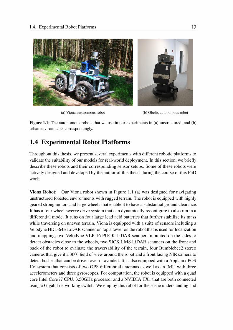
(a) Viona autonomous robot (b) Obelix autonomous robot
Figure 1.1: The autonomous robots that we use in our experiments in (a) unstructured, and (b)urban environments correspondingly.
1.4 Experimental Robot Platforms
Throughout this thesis, we present several experiments with different robotic platforms tovalidate the suitability of our models for real-world deployment. In this section, we brieflydescribe these robots and their corresponding sensor setups. Some of these robots wereactively designed and developed by the author of this thesis during the course of this PhDwork.
Viona Robot: Our Viona robot shown in Figure 1.1 (a) was designed for navigatingunstructured forested environments with rugged terrain. The robot is equipped with highlygeared strong motors and large wheels that enable it to have a substantial ground clearance.It has a four wheel swerve drive system that can dynamically reconfigure to also run in adifferential mode. It runs on four large lead acid batteries that further stabilize its masswhile traversing on uneven terrain. Viona is equipped with a suite of sensors including aVelodyne HDL-64E LiDAR scanner on top a tower on the robot that is used for localizationand mapping, two Velodyne VLP-16 PUCK LiDAR scanners mounted on the sides todetect obstacles close to the wheels, two SICK LMS LiDAR scanners on the front andback of the robot to evaluate the traversability of the terrain, four Bumblebee2 stereocameras that give it a 360 field of view around the robot and a front facing NIR camera todetect bushes that can be driven over or avoided. It is also equipped with a Applanix POSLV system that consists of two GPS differential antennas as well as an IMU with threeaccelerometers and three gyroscopes. For computation, the robot is equipped with a quadcore Intel Core i7 CPU, 3.50GHz processor and a NVIDIA TX1 that are both connectedusing a Gigabit networking switch. We employ this robot for the scene understanding and

14 Chapter 1. Introduction
Figure 1.2: The AIS perception car that we use in our experiments in urban driving scenarios.
autonomous navigation experiments presented in Chapter 5 and Chapter 4.
Obelix Robot: Our Obelix robot [45] shown in Figure 1.1 (b) was designed for au-tonomous navigation in pedestrian environments. The robot runs on four lead acid batteriesand has two unidirectional wheels as well as two castor wheels in the front and back of therobot that enables it to take tight turns in a differential configuration. The sensor systemof the robot consists of a Velodyne HDL-32E LiDAR scanner on the top of the robot thatis used for localization and mapping, two SICK LMS-151 scanners in the front and backof the robot for traversability analysis, a tilting Hokuyo UTM-30LX in the front of therobot for obstacle avoidance, two Delphi ESR radar sensors which are mounted to the leftand right of the robot for tracking moving objects, a Bumblebee2 and ZED stereo camerasfacing the front of the robot. It is also equipped with a Trimble GPS Pathfinder Pro and andXSens IMU. We use a laptop with an Intel Core i7 and an NVIDIA GTX 980M GPU forall the computations. We primarily use our Obelix robot for all the experiments presentedin Chapter 7 for the evaluation of visual localization, temporal semantic segmentation andodometry estimation.
AIS Car: We built the AIS perception car shown in Figure 1.2 for evaluating ourperception and localization algorithms in self-driving car scenarios. The sensor systemmounted on the roof of an Audi A3 car consists of a Velodyne HDL-64E LiDAR scanner,two Velodyne VLP-16 PUCK scanners mounted an angle of 30 to the horizontal plane,six ZED stereo cameras that are mounted in a hexagonal configuration to give a 360 fieldof view and Point Grey Blackfly cameras that are mounted facing the front of the robot toacquire wide baseline stereo images. It is also equipped with an Applanix POS LV systemconsisting of two GPS differential antennas and an IMU. For acquiring all the sensor data
1.5. Publications 15
and computing, we use two custom built computers, each consisting of an Intel Core i77700K, 4.20GHz processor and an NVIDIA GTX 1070 GPU. In order to record all thesensor data simultaneously, we equip the computing systems with 7 hard disks. We usedthe Kalibr Toolbox [46] for the camera-camera calibrations to estimate the intrinsic andextrinsic parameters. We present results of our scene understanding models using our AISperception car in Chapter 4 and Chapter 6.
1.5 Publications
Major parts of the research presented in this thesis have been published in journal articles,book chapters, conference and workshop proceedings. A chronological overview of thecorresponding publications is presented in the following list:
• A. Valada, L. Spinello, and W. Burgard. Deep Feature Learning for Acoustics-basedTerrain Classification. In Proc. of the International Symposium on Robotics Research(ISRR), Robotics Research, Vol. 2, Springer Proceedings in Advanced Robotics,ISBN: 978-3-319-60916-4, 2015. Selected in Top 10 papers.
• A. Valada, G. Oliveira, T. Brox, and W. Burgard. Towards Robust Semantic Segmen-tation using Deep Fusion. In Proc. of the RSS Workshop on Limits and Potentials ofDeep Learning in Robotics, 2016.
• A. Valada, G. Oliveira, T. Brox, and W. Burgard. Deep Multispectral Semantic SceneUnderstanding of Forested Environments. In Proc. of the International Symposiumon Experimental Robotics (ISER), Springer Proceedings in Advanced Robotics bookseries (SPAR, volume 1), ISBN: 978-3-319-50115-4, 2016.
• A. Valada, A. Dhall, and W. Burgard. Convoluted Mixture of Deep Experts forRobust Semantic Segmentation. In Proc. of the IROS Workshop on State Estimationand Terrain Perception for All Terrain Mobile Robots, 2016.
• A. Valada, and W. Burgard. Deep Spatiotemporal Models for Robust ProprioceptiveTerrain Classification. The International Journal of Robotics Research (IJRR),36(13-14):1521-1539, pp. 1521-1539, 2017, doi: 10.1177/0278364917727062.ISRR Invited Journal
• A. Valada, J. Vertens, A. Dhall, and W. Burgard. AdapNet: Adaptive Semantic Seg-mentation in Adverse Environmental Conditions. In Proc. of the IEEE InternationalConference on Robotics and Automation (ICRA), 2017.

16 Chapter 1. Introduction
• J. Vertens∗, A. Valada∗, and W. Burgard. SMSnet: Semantic Motion Segmentationusing Deep Convolutional Neural Networks. In Proc. of the IEEE/RSJ InternationalConference on Intelligent Robots and Systems (IROS), 2017.
• W. Burgard, A. Valada, N. Radwan, T. Naseer, J. Zhang, J. Vertens, O. Mees, A.Eitel and G. Oliveira. Perspectives on Deep Multimodel Robot Learning. In Proc. ofthe International Symposium on Robotics Research (ISRR), 2017.
• A. Valada∗, N. Radwan∗, and W. Burgard. Deep Auxiliary Learning for VisualLocalization and Odometry. In Proc. of the IEEE International Conference onRobotics and Automation (ICRA), 2018.
• A. Valada, and W. Burgard. Learning Reliable and Scalable Representations UsingMultimodal Multitask Deep Learning. In Proc. of the RSS Pioneers Workshop atRobotics: Science and Systems (RSS), 2018.
• A. Valada∗, N. Radwan∗, and W. Burgard. Incorporating Semantic and GeometricPriors in Deep Pose Regression. In Proc. of the Workshop on Learning and Inferencein Robotics: Integrating Structure, Priors and Models at Robotics: Science andSystems (RSS), 2018.
• N. Radwan∗, A. Valada∗, and W. Burgard. VLocNet++: Deep Multitask Learningfor Semantic Visual Localization and Odometry. IEEE Robotics and AutomationLetters (RA-L), 2018, doi: 10.1109/LRA.2018.2869640.
• A. Valada, R. Mohan, and W. Burgard. Self-Supervised Model Adaptation forMultimodal Semantic Segmentation. arXiv preprint arXiv:1808.03833, InternationalJournal of Computer Vision (Under Review), 2018.
Moreover, the following publications of the author of this thesis present work related toperception and localization. However, they are outside the main focus of this thesis andtherefore are not covered.
• F. Boniardi, A. Valada, W. Burgard, and G. D. Tipaldi. Autonomous Indoor RobotNavigation Using Sketched Maps and Routes. In Proc. of the Workshop on ModelLearning for Human-Robot Communicationat Robotics: Science and Systems (RSS),2015.
• G. Oliveira, A. Valada, W. Burgard, and T. Brox. Deep Learning for Human PartDiscovery in Images. In Proc. of the IEEE International Conference on Roboticsand Automation (ICRA), 2016.
∗Denotes equal contribution
1.6. Collaborations 17
• F. Boniardi, A. Valada, W. Burgard, and G. D. Tipaldi. Autonomous Indoor RobotNavigation Using a Sketch Interface for Drawing Maps and Routes. In Proc. of theIEEE International Conference on Robotics and Automation (ICRA), 2016.
• N. Radwan, A. Valada, and W. Burgard. Multimodal Interaction-aware MotionPrediction for Autonomous Street Crossing. arXiv preprint arXiv:1808.06887,International Journal of Robotics Research (Under Review), 2018.
• M. Mittal∗, A. Valada∗, and W. Burgard. Vision-based Autonomous Landing inCatastrophe-Struck Environments. Proc. of the IROS Workshop on Vision-basedDrones: What’s Next?, 2018.
1.6 Collaborations
This thesis covers work that involved collaborations with other researchers. Prof. WolframBurgard was the supervisor of this thesis and therefore, contributed through scientificdiscussions. The collaborations beyond this supervision are outlined below.
• Chapter 6: The initial work on the SMSnet architecture for semantic motion segmen-tation was formulated in collaboration with Johan Vertens for his Master’s thesis,which the author of this thesis supervised. The insights gained during the aforemen-tioned thesis supervision influenced the subsequent improved implementations ofSMSnet that the author of this thesis carried out. No parts of the experiments onSMSnet reported in this thesis intersects with the work carried out in collaborationwith Johan Vertens. The results on SMSnet reported in this thesis outperforms theinitial work [54]. Furthermore, the subsequent work on the SMSnet++ architectureintroduced in the second part of this chapter was entirely carried out by the author ofthis thesis.
• Chapter 7: The VLocNet and the VLocNet++ architectures are a result of collab-oration with Noha Radwan. Noha Radwan contributed to the derivation of theGeometric Consistency Loss function and the formulation of the self-supervisedwarping layer in the VLocNet++ architecture. The topologies of the VLocNet andVLocNet++ architectures consisting of the global localization stream, the visualodometry stream and the semantic segmentation stream as well as the weightedfusion layer, were developed by the author of this thesis. The related publicationsare Valada et al. [56] and Radwan et al. [34].
∗Denotes equal contribution
18 Chapter 1. Introduction
1.7 Outline
This thesis is organized as follows. In Chapter 2, we introduce the main theoretical conceptsand principles that are foundation for our proposed techniques. Chapter 3 presents ourarchitectures for proprioceptive terrain classification using sound from vehicle-terraininteractions. In Chapter 4, we present our novel architectures for efficient semanticsegmentation and subsequently in Chapter 5, we present our proposed self-supervisedadaptive multimodal fusion frameworks for semantic segmentation. Chapter 6 presents ourproposed architectures for joint semantic motion segmentation. In Chapter 7, we introduceour novel architectures for multitask learning of visual localization, semantic segmentationand odometry estimation. We review the relevant related research work at the end of eachchapter in this thesis. Moreover, for each of the problems, we benchmark our proposedmodels on standard datasets and also provide generalization evaluations on data collectedby our robots in Freiburg. Additionally, each chapter lists the corresponding qualitativeresults as videos that are published online. Finally, we conclude the thesis and discussdirections for future research in Chapter 8.
Chapter 2
Background Theory
In this chapter, we briefly discuss the theoretical concepts and principles that are thefoundation of the approaches presented in this thesis. We first describe the camera modelthat maps points in the three-dimensional world to the two-dimensional image created bythe camera. We then give an overview of feed-forward neural networks, followed by adescription of the basic components of a convolutional neural network and loss functionsthat can be employed for training the networks.
2.1 Camera Model
The pinhole camera model describes the geometric relationship between the coordinatesof a point in a three-dimensional space and its two-dimensional corresponding projection
v
u
Cxc
yc
zc
x
y
v
u
P= X,Y,Z
u,v( )T
( )T
principal axis
principalpoint
fImage plane
optical center
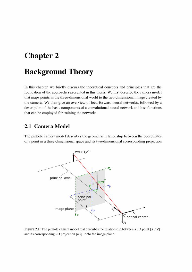
Figure 2.1: The pinhole camera model that describes the relationship between a 3D point [X Y Z]ᵀ
and its corresponding 2D projection [u v]ᵀ onto the image plane.
20 Chapter 2. Background Theory
onto the image plane. This geometric mapping from 3D→ 2D is referred to as perspectiveprojection. A point P in the three-dimensional world can be mapped into a two-dimensionalpoint on the image P′ using the projective transformation π defined as
π : R3 → R2 (2.1)
The geometry related to the mapping of a pinhole camera is illustrated in Figure 2.1.The pinhole camera allows only a single ray from each point on the object to pass throughan infinitely small aperture. The center of the perspective projection where all the raysintersect is called as the optical center C and the line perpendicular to the image planepassing through the optical center is called the principal axis or the optical axis. In addition,the intersection point of the image plane with the optical axis is called the principal point,while the distance from the optical center to the principal point is the focal length f ofthe camera. For convenience, we put the image plane behind the optical center as thisavoids the need to flip the image coordinates about the origin. The standard coordinatesystem of the camera has its origin at the center of the projection and its Z axis along theoptical axis, perpendicular to the image plane. The image plane is located at Z = f in thecamera coordinate system. A point P ∈ R3 on an object with coordinates [X Y Z]ᵀ will beprojected at a pixel position [u v]ᵀ in the image plane. The relationship between these twocoordinate systems is given by
π[X Y Z]ᵀ → [u v]ᵀ (2.2)
u =X fZ
+ cx (2.3)
v =Y fZ
+ cy (2.4)
As the origin of the pixel coordinate system is defined at the top-left corner of the image,the 2D points are offset by a translation vector (cx, cy) to account for the misalignmentbetween the optical center and the origin of the image coordinates. In Eq. (2.3) andEq. (2.4), it was implicitly assumed that the pixels of the image sensor are square. In thecase when the pixels on the sensor chip of the camera are rectangular of size 1/sx and 1/sy,different scaled focal lengths fx = sx f and fy = sy f are employed, where, sx and sy are inunits of horizontal and vertical pixels per meter respectively. The 2D point can also beback-projected to the 3D space, given the depth Z and the camera parameters. We canexpress this transformation as
π–1[u v Z]ᵀ → [X Y Z]ᵀ (2.5)
X =u – cx
fxZ (2.6)
Y =v – cy
fyZ (2.7)
2.2. Feed-Forward Neural Networks 21
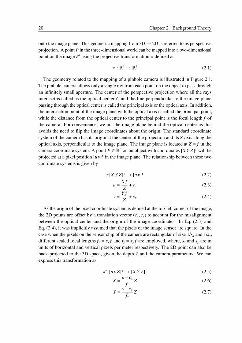
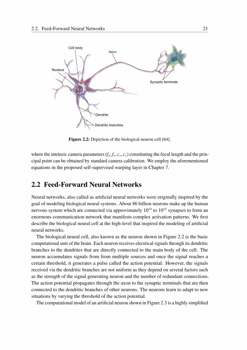
Figure 2.2: Depiction of the biological neuron cell [64].
where the intrinsic camera parameters (fx, fy, cx, cy) constituting the focal length and the prin-cipal point can be obtained by standard camera calibration. We employ the aforementionedequations in the proposed self-supervised warping layer in Chapter 7.
2.2 Feed-Forward Neural Networks
Neural networks, also called as artificial neural networks were originally inspired by thegoal of modeling biological neural systems. About 86 billion neurons make up the humannervous system which are connected via approvimately 1014 to 1015 synapses to form anenormous communication network that manifests complex activation patterns. We firstdescribe the biological neural cell at the high-level that inspired the modeling of artificialneural networks.
The biological neural cell, also known as the neuron shown in Figure 2.2 is the basiccomputational unit of the brain. Each neuron receives electrical signals through its dendriticbranches to the dendrites that are directly connected to the main body of the cell. Theneuron accumulates signals from from multiple sources and once the signal reaches acertain threshold, it generates a pulse called the action potential. However, the signalsreceived via the dendritic branches are not uniform as they depend on several factors suchas the strength of the signal generating neuron and the number of redundant connections.The action potential propagates through the axon to the synaptic terminals that are thenconnected to the dendritic branches of other neurons. The neurons learn to adapt to newsituations by varying the threshold of the action potential.
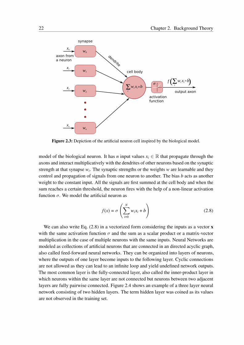
The computational model of an artificial neuron shown in Figure 2.3 is a highly simplified
22 Chapter 2. Background Theory
w0
w1
w2
wn
x0
x1
x2
xn
Σwi xi+bi
(Σwi xi+bi
)fσ
synapse
dendrite
axon froma neuron
activationfunction
output axon
cell body
Figure 2.3: Depiction of the artificial neuron cell inspired by the biological model.
model of the biological neuron. It has n input values xi ∈ R that propagate through theaxons and interact multiplicatively with the dendrites of other neurons based on the synapticstrength at that synapse wi. The synaptic strengths or the weights w are learnable and theycontrol and propagation of signals from one neuron to another. The bias b acts as anotherweight to the constant input. All the signals are first summed at the cell body and when thesum reaches a certain threshold, the neuron fires with the help of a non-linear activationfunction σ. We model the artificial neuron as
f (x) = σ
(N∑
i=0
wixi + b
)(2.8)
We can also write Eq. (2.8) in a vectorized form considering the inputs as a vector xwith the same activation function σ and the sum as a scalar product or a matrix-vectormultiplication in the case of multiple neurons with the same inputs. Neural Networks aremodeled as collections of artificial neurons that are connected in an directed acyclic graph,also called feed-forward neural networks. They can be organized into layers of neurons,where the outputs of one layer become inputs to the following layer. Cyclic connectionsare not allowed as they can lead to an infinite loop and yield undefined network outputs.The most common layer is the fully-connected layer, also called the inner-product layer inwhich neurons within the same layer are not connected but neurons between two adjacentlayers are fully pairwise connected. Figure 2.4 shows an example of a three layer neuralnetwork consisting of two hidden layers. The term hidden layer was coined as its valuesare not observed in the training set.
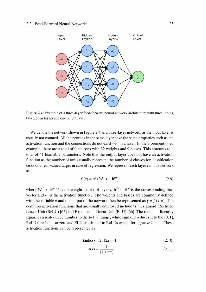
2.2. Feed-Forward Neural Networks 23
InputLayer
HiddenLayer h1
HiddenLayer h2
OutputLayer
x1
x2
x3
h11
h21
h31
h41
h12
h22
h32
h42
y
Figure 2.4: Example of a three-layer feed-forward neural network architecture with three inputs,two hidden layers and one output layer.
We denote the network shown in Figure 2.4 as a three-layer network, as the input layer isusually not counted. All the neurons in the same layer have the same properties such as theactivation function and the connections do not exist within a layer. In the aforementionedexample, there are a total of 9 neurons with 32 weights and 9 biases. This amounts to atotal of 41 learnable parameters. Note that the output layer does not have an activationfunction as the number of units usually represent the number of classes for classificationtasks or a real-valued target in case of regression. We represent each layer l in this networkas
f l(x) = σl (W(l)x + b(l)) (2.9)
where W(l) ∈ Rm×n is the weight matrix of layer l, b(l) ∈ Rm is the corresponding biasvector and σl is the activation function. The weights and biases are commonly definedwith the variable θ and the output of the network then be represented as y = f (x; θ). Thecommon activation functions that are usually employed include tanh, sigmoid, RectifiedLinear Unit (ReLU) [65] and Exponential Linear Unit (ELU) [66]. The tanh non-linearitysquashes a real-valued number to the [–1, 1] range, while sigmoid reduces it to the [0, 1],ReLU thresholds at zero and ELU are similar to ReLUs except for negative inputs. Theseactivation functions can be represented as
tanh(x) = 2σ(2x) – 1 (2.10)
σ(x) =1
(1 + e–x)(2.11)
24 Chapter 2. Background Theory
relu(x) = max(0, x) (2.12)
elu(x) =
x if x > 0
α(ex – a) if x ≤ 0(2.13)
We primarily use ReLUs in the architectures presented in this thesis. However, we alsoemploy the sigmoid activation function and ELUs in the networks that we introduce inChapter 6 and Chapter 7 respectively. We further detail the loss functions that can be usedfor training the networks in the following sections.
2.3 Convolutional Neural Networks
In the previous section, we briefly introduced neural networks in which adjacent layersare fully connected to one another and every neuron in the network is connected to everyneuron in the adjacent layers. However, it can be observed that the number of connectionsgrows quadratically with the size of each layer and the number of trainable weightsincreases correspondingly. Moreover, such networks do not model the spatial relationshipin the input data due to the feed-forward interconnection and as a consequence there is notranslation invariance, which is a critical factor to model, especially while learning visualconcepts from images. As a solution to these problems, Convolutional Neural Networks(CNNs) that consist of several convolutional layers with local connections, followed bypooling layers that provide translational invariance and one or more fully-connected layerscan be employed. CNNs are easier to train and have fewer parameters than standard neuralnetworks with the same number of hidden units. In the following sections, we discuss thebasic constituting components of a CNN architecture and the loss functions that can beemployed for training the models.
2.3.1 Architecture Overview
A convolutional neural network consists of several convolutional and pooling layers,optionally followed by fully-connected layers or deconvolutional layers. The input to aconvolutional layer is an image x of dimensions H×W ×C such that x ∈ RH ×RW ×RC,where H is the height, W is the width and C is the number of channels. Each convolutionallayer has k filters or kernels of size F × F × Q, where F is smaller than the dimensions ofthe input image and Q varies for each kernel. This restricts the connections to a local spatialneighborhood of the input where each filter is convolved with the image to yield K featuremaps of height = H – F + 1 and width = W – F + 1. Restricting the connections enablesa reduction of the number of neuron inputs and weights substantially. Subsequently, anadditive bias and a nonlinearity is applied to each feature map. The feature maps are thendownsampled using different pooling layers along the spatial dimensions. Depending
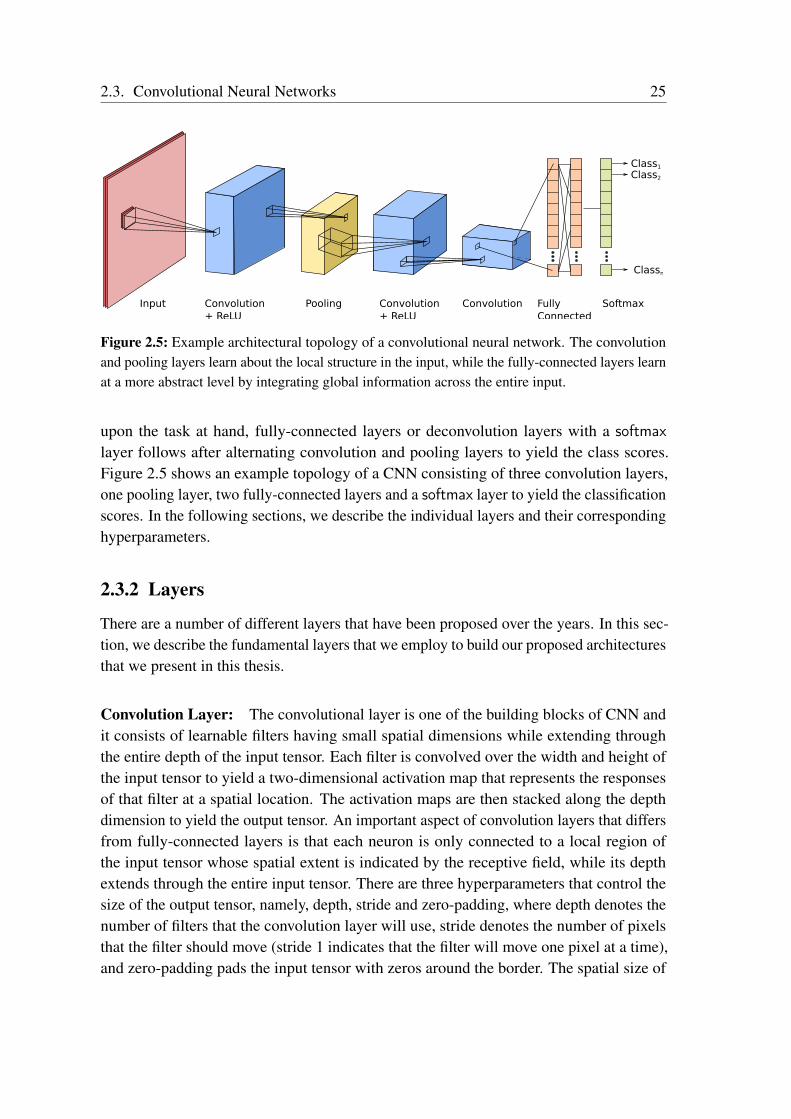
2.3. Convolutional Neural Networks 25
Input Convolution+ ReLU
Pooling Convolution+ ReLU
FullyConnected
Convolution Softmax
Class1
Class2
Classn
Figure 2.5: Example architectural topology of a convolutional neural network. The convolutionand pooling layers learn about the local structure in the input, while the fully-connected layers learnat a more abstract level by integrating global information across the entire input.
upon the task at hand, fully-connected layers or deconvolution layers with a softmaxlayer follows after alternating convolution and pooling layers to yield the class scores.Figure 2.5 shows an example topology of a CNN consisting of three convolution layers,one pooling layer, two fully-connected layers and a softmax layer to yield the classificationscores. In the following sections, we describe the individual layers and their correspondinghyperparameters.
2.3.2 Layers
There are a number of different layers that have been proposed over the years. In this sec-tion, we describe the fundamental layers that we employ to build our proposed architecturesthat we present in this thesis.
Convolution Layer: The convolutional layer is one of the building blocks of CNN andit consists of learnable filters having small spatial dimensions while extending throughthe entire depth of the input tensor. Each filter is convolved over the width and height ofthe input tensor to yield a two-dimensional activation map that represents the responsesof that filter at a spatial location. The activation maps are then stacked along the depthdimension to yield the output tensor. An important aspect of convolution layers that differsfrom fully-connected layers is that each neuron is only connected to a local region ofthe input tensor whose spatial extent is indicated by the receptive field, while its depthextends through the entire input tensor. There are three hyperparameters that control thesize of the output tensor, namely, depth, stride and zero-padding, where depth denotes thenumber of filters that the convolution layer will use, stride denotes the number of pixelsthat the filter should move (stride 1 indicates that the filter will move one pixel at a time),and zero-padding pads the input tensor with zeros around the border. The spatial size of
26 Chapter 2. Background Theory
the output tensor can be computed as a function of the input tensor size (W), size of thereceptive field (Fw, Fh), stride (S) and the zero-padding (P) as
OCw =W – Fw + 2P
Sw+ 1, (2.14)
OCh =W – Fh + 2P
Sh+ 1, (2.15)
where OCw is the output width and OCh is the output height.A convolution layer conserves parameters by sharing the same weight vector and bias
with all the neurons in the same two-dimensional slice of the depth. Therefore, in theforward-pass, each depth slice is computed as a convolution of the weights of the neuronswith the input tensor and during backpropagation, the gradient of every neuron in the tensoris added across each depth slice and only a single set of weights are updated for each slice.
Atrous Convolution Layer: Pooling and striding that is commonly employed in CNNs,decreases the spatial resolution of the feature maps. For tasks such as semantic seg-mentation, this decimates the details which cannot be completely recovered even usingdeconvolution or transpose convolution layers. To alleviate this problem, atrous convolu-tions also known as dilated convolutions [67] can be used to enlarge the field of the filterthereby effectively capturing larger context. Moreover, by using atrous convolutions of dif-ferent dilation rates, we can aggregate multiscale context. While the standard convolutionfilters are contiguous, atrous convolution is equivalent to convolving with a filter whichhas zeros inserted between two consecutive filter values across the spatial dimensions. LetF : Z2 → R be a discrete function, Ω = [–r, r]2 ∩ Z2, k : Ωr → R be a discrete filter ofsize (2r + 1)2 and r be a dilation rate. The atrous convolution ∗r can be defined as
(F ∗r k)(p) =∑
(s+rt=p)
F(s) k(t), (2.16)
where the dilation rate r denotes the stride with which we sample the input signal. Thereforea larger dilation rate indicates a larger receptive field. The standard convolution can beconsidered as a special case by setting r = 1.
Pooling Layer: The pooling layer is employed after the convolution layer to downsampleeach depth slice of the input tensor independently using different operations depending onthe type of pooling. As convolution layers restrict the neuron inputs to a local neighborhood,employing only a series of convolution layers makes the network loose the global context.Pooling provides translation invariance to the information in the input tensors to a certainextent by aggregating information globally. It reduces the the number of parameters andcomputational operations in the network. The two hyperparameters, the filter size (F) andthe stride (S) control the size of the output tensor. The different types of pooling operations
2.3. Convolutional Neural Networks 27
include max, average, L2-norm and stochastic. In practice, max pooling is most commonlyemployed compared to the other methods. The spatial size of the output tensor can becomputed as function of the input tensor size (W), size of the receptive field (F) and thestride stride (S) as
OPw =W – F
S+ 1, (2.17)
OPh =W – F
S+ 1, (2.18)
where OPw is the output width and OPh is the output height.During the forward-pass, it is common to keep track of the index of the resulting
activation so that during the backpropagation, the gradients can be routed through it. Archi-tectures that are designed for certain tasks such as semantic segmentation and adversariallearning do not incorporate pooling layers as they cause the network to loose the exactposition information of the features. Instead, they use a larger stride in the convolutionlayer to perform the downsampling.
Fully-connected Layer: Neurons in fully-connected layers have connections to everyneuron in the previous later. This is similar to the standard neural network, also called themulti-layer perceptron that we described in Section 2.2. The activations of fully-connectedlayers are computed with matrix multiplication, followed by a bias offset. The onlydifference between a fully-connected layer and a convolution layer is that the convolutionlayers have local connectivity and parameters are shared for the neurons in the same depthslice, however their functional form is identical. Fully-connected layers are often usedtowards the end of CNN architectures to aggregate information from all the feature mapsand output a vector that corresponds to the number of objects to classify. We only usefully-connected layers in the architectures that we present in Chapter 3 and Chapter 7 inwhich we propose a network for classification and regression respectively.
Deconvolution Layer: Deconvolution layers, also called transposed convolutions orfractionally strided convolutions, transform the input tensor in the opposite direction ofstandard convolutions such as mapping the feature maps from low-dimensional space to ahigher-dimensional space while maintaining the connection patterns of the convolution. Inpractice, the deconvolution operation is implemented as taking the gradient of the convolu-tion with respect to its inputs. In other words, the only difference between the standardconvolution and the deconvolution is how the forward and backward passes are computed.Deconvolution layers are often employed to obtain a mapping from the convolved valuesto the original inputs. Similar to convolution layers, three hyperparameters control the sizeof the output tensor including depth, stride and zero-padding. The spatial size of the outputtensor can be computed as a function of the input tensor size (W), size of the receptive field
28 Chapter 2. Background Theory
(Fw, Fh), stride stride used (S) and the zero-padding. Deconvolution layers are extensivelyused in architectures that are designed for semantic segmentation, depth estimation andoptical flow estimation. As opposed to naively resizing the outputs to a larger dimension,employing a deconvolution layer with learnable parameters yields an upsampled outputwith finer details.
Dropout Layer: CNNs are plagued by the overfitting problem where the weights of thenetwork are excessively tuned for the training data which causes the network to performpoorly on new examples that have not been seen before. In order to alleviate this problemthe dropout layer can be employed as a regularization technique to randomly drop a setof activations by setting them to zero while training the network. This forces the networkto learn redundant connections and therefore improves the generalization of the network.Dropout layers are often used towards the end of the network on the convolution or fully-connected layers but certain architectures also employ them on max pooling layers tocreate image noise that acts as data augmentation. More recently [68], dropout has alsobeen employed during test-time to obtain the predictive mean and predictive uncertaintyby Monte Carlo averaging of stochastic forward passes through the model.
Network-in-Network Layer: A 1 × 1 convolution layer was initially called as thenetwork-in-network layer by Lin et al. [69]. Unlike in standard applications of the con-volution layer where the receptive fields are large, it employs a convolution layer withthe filter size of 1× 1. As convolutions operate on three-dimensional tensor that span theentire depth of the input, a 1× 1 convolution layer performs a N-dimensional element-wisemultiplication, where N is the depth of the input tensor into the layer. We extensivelyemploy the 1× 1 convolution layer in the architectures proposed in this thesis.
2.3.3 Architectural Network Design
Thus far, in the previous sections, we introduced the basic building blocks a CNN. In thissection, we discuss how these layers are often stacked together to form entire architectures.Classical CNNs usually stack convolution layers with ReLU, followed by a pooling layerand then repeat this pattern until learned features are highly discriminative and spatiallysmall in size. Multiple convolution layers can also be stacked before employing a poolinglayer to learn more complex features before loosing the location information. As opposedto employing one convolution layer with a large receptive field, a stack of convolutionlayers with smaller filters are more beneficial as a stack of convolutions with non-linearitymakes the learned features more discriminative and consumes lesser number of parameters.For example, a stack of three 3 × 3 convolution layers makes the effective receptivefield at the third convolution layer 7× 7 with 27C2 parameters with C as the number ofchannels in the convolution layers, while in comparison, a single 7× 7 convolution layer
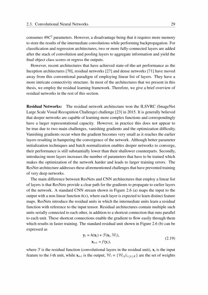
2.3. Convolutional Neural Networks 29
consumes 49C2 parameters. However, a disadvantage being that it requires more memoryto store the results of the intermediate convolutions while performing backpropagation. Forclassification and regression architectures, two or more fully-connected layers are addedafter the stack of convolution and pooling layers to aggregate information and yield thefinal object class scores or regress the outputs.
However, recent architectures that have achieved state-of-the-art performance as theInception architectures [70], residual networks [27] and dense networks [71] have movedaway from this conventional paradigm of employing linear list of layers. They have amore intricate connectivity structure. In most of the architectures that we present in thisthesis, we employ the residual learning framework. Therefore, we give a brief overview ofresidual networks in the rest of this section.
Residual Networks: The residual network architecture won the ILSVRC (ImageNetLarge Scale Visual Recognition Challenge) challenge [23] in 2015. It is generally believedthat deeper networks are capable of learning more complex functions and correspondinglyhave a larger representational capacity. However, in practice this does not appear tobe true due to two main challenges, vanishing gradients and the optimization difficulty.Vanishing gradients occur when the gradient becomes very small as it reaches the earlierlayers resulting in hampering the convergence of the network. Although better parameterinitialization techniques and batch normalization enables deeper networks to converge,their performance is still substantially lower than their shallower counterparts. Secondly,introducing more layers increases the number of parameters that have to be trained whichmakes the optimization of the network harder and leads to larger training errors. TheResNet architecture addresses these aforementioned challenges that have prevented trainingof very deep networks.
The main difference between ResNets and CNN architectures that employ a linear listof layers is that ResNets provide a clear path for the gradients to propagate to earlier layersof the network. A standard CNN stream shown in Figure 2.6 (a) maps the input to theoutput with a non-linear function h(x), where each layer is expected to learn distinct featuremaps. ResNets introduce the residual units in which the intermediate units learn a residualfunction with reference to the input tensor. Residual architectures contain multiple suchunits serially connected to each other, in addition to a shortcut connection that runs parallelto each unit. These shortcut connections enable the gradient to flow easily through themwhich results in faster training. The standard residual unit shown in Figure 2.6 (b) can beexpressed as
yl = h(xl) + F(xl,Wl),
xl+1 = f (yl),(2.19)
where F is the residual function (convolutional layers in the residual unit), xl is the inputfeature to the l-th unit, while xl+1 is the output, Wl = Wl,k|1≤k≤K are the set of weights
30 Chapter 2. Background Theory
xl
3x3 conv
ReLU
3x3 conv
ReLU
h(x)
3x3 conv
ReLU
xl
3x3 conv
BN
ReLU
1x1 conv
BN
ReLU
xl+1
1x1 conv
BN
ReLU
xl
BN
ReLU
3x3 conv
BN
ReLU
xl+1
BN
ReLU
1x1 conv
1x1 conv
(a) Standard CNNstream
(b) Standard residualunit
(c) Full Pre-activationresidual unit
Figure 2.6: Topology of the standard CNN stream in comparison to the original residual unit [27]and the improved full pre-activation residual unit [72].
and biases of the l-th residual unit and K is the number of layers in the unit. The functionf is a non-linearity such as a ReLU and the function h is set to the identity mappingh(xl) = xl. Note that we described the bottleneck structure of the residual unit that enablestraining of deeper networks, as opposed to the two layer design that contains consecutive3× 3 convolution layers. Instead, the bottleneck structure consists of three layers 1× 1convolution, 3 × 3 convolution and a 1 × 1 convolution. The first 1 × 1 convolutionlayer reduces the number of feature maps, making the 3× 3 convolution have a smallerinput/output dimension, while the last 1× 1 convolution restores the dimensions to that ofthe input. There are two types of residual units, identity shortcuts and projection shortcuts.Identity shortcuts are used when the input and outputs are of the same dimensions andthe projection shortcut is used when the dimensionality of the output is different from theinput so a 1× 1 convolution layer to used on the input tensor to match the dimensions ofthe output tensor.
The activation f in the original residual unit described above affects both paths in thenext unit. Therefore, He et al. [72] proposed an improved residual unit where the activationf only affects the path F, which can be defined as
xl+1 = xl + F(f (xl),Wl), (2.20)
This pre-activation residual unit shown in Figure 2.6 (c) enables the gradient to flow
2.3. Convolutional Neural Networks 31
through the shortcut connection to any unit l without any obstruction. Batch normalizationis extensively used in residual networks that help in regularizing the network. However, inthe standard residual unit, the batch normalization is applied before the addition whichcauses the output of the residual unit be un-normalized and consequently, the input to thenext residual unit is also not normalized. In the full pre-activation residual units structure,the input is normalized at the beginning of the identity unit which makes the convolutionsalways receive the normalized inputs. These full pre-activation residual units have beendemonstrated to reduce overfitting, improve the convergence and also yield improvedperformance. The initial architectures that we propose in this thesis employ the standardresidual unit, while the improved architectures employ the full pre-activation residual units.
2.3.4 Loss Functions
Loss functions are used to supervise the training process of a neural network. In this thesis,we primarily use two different loss functions according to the task at hand. In Chapter 3,4, 5, and 6, we employ the softmax function that uses the cross-entropy loss for trainingour proposed architectures that perform classification and pixel-wise classification. Letf (xi) be the activations of the output layer for the CNN, yi be the groundtruth label, C isthe number of object classes to classify, and N is the number of training examples. Let theweights and biases of the last layer of the CNN be W and b. The softmax classifier thatuses the cross-entropy loss can be defined as
Ls = –1N
N∑i=1
yi logexp
(W
ᵀyi f (xi) + byi
)∑Cj=1 exp
(W
ᵀj f (xi) + bj
) (2.21)
While, for regressing the 6-DoF poses in the architectures that we propose in Chapter 7,we use the L2-norm loss function. It minimizes the sum of the square of the differencesbetween the target and the estimated value as
Ll2 =N∑
i=1
(yi – f (xi))2 (2.22)
where yi is the groundtruth and f (xi) is the estimated output of the model. The protocolthat we employ for training our architectures is described in the respective chapters.

Chapter 3
Proprioceptive Terrain Classification
In this chapter, we address the problem of terrain classification us-ing sound from vehicle-terrain interactions. Terrain classificationis a critical component of any autonomous mobile robot system op-erating in environments with unknown spatially-varying terrains.Most existing techniques are predominantly based on using visualfeatures which makes them extremely susceptible to appearancechanges and occlusions. Therefore, relying solely on them inhibitsthe robot from functioning robustly in all conditions. As a solutionto this problem, we propose an approach that uses vehicle-terraininteraction sounds as a proprioceptive modality to classify a widevariety of terrains. We present a novel convolutional neural net-work architecture to learn deep features from spectrograms of au-dio signals. As audio signals are inherently sequential and temporal,we also present a recurrent variant of the model that incorporatesLong Short-Term Memory units to learn the complex temporal dy-namics. Experiments on two extensive datasets collected with dif-ferent microphones on various indoor and outdoor terrains demon-strate that our networks achieve state-of-the-art performance com-pared to existing techniques. In addition, we present experimen-tal results in adverse acoustic conditions with high ambient noiseand propose a noise-aware training scheme that enables learning ofmore generalizable models which are essential for robust real-worlddeployments.
3.1 Introduction
As robots are increasingly being employed for tackling complex tasks in unknown envi-ronments such as in mining, forestry, space exploration as well as search and rescue, theyface an immense amount of perceptual challenges. Mobile robots in particular should have
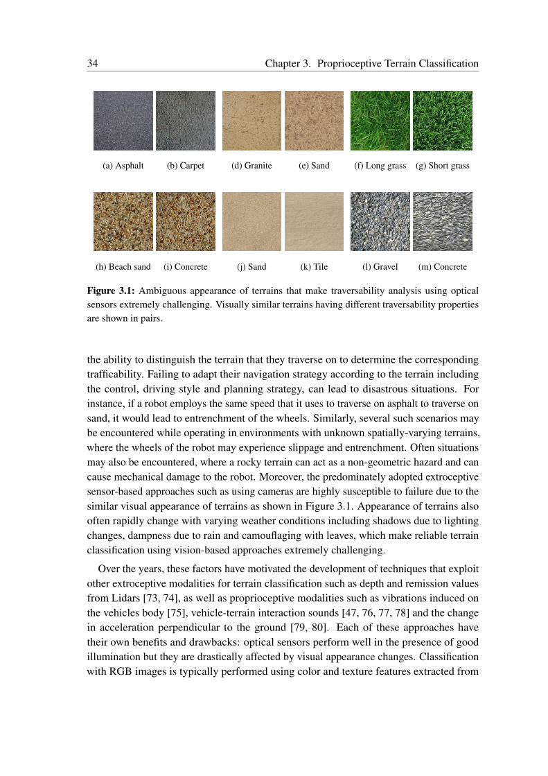
34 Chapter 3. Proprioceptive Terrain Classification
(a) Asphalt (b) Carpet (d) Granite (e) Sand (f) Long grass (g) Short grass
(h) Beach sand (i) Concrete (j) Sand (k) Tile (l) Gravel (m) Concrete
Figure 3.1: Ambiguous appearance of terrains that make traversability analysis using opticalsensors extremely challenging. Visually similar terrains having different traversability propertiesare shown in pairs.
the ability to distinguish the terrain that they traverse on to determine the correspondingtrafficability. Failing to adapt their navigation strategy according to the terrain includingthe control, driving style and planning strategy, can lead to disastrous situations. Forinstance, if a robot employs the same speed that it uses to traverse on asphalt to traverse onsand, it would lead to entrenchment of the wheels. Similarly, several such scenarios maybe encountered while operating in environments with unknown spatially-varying terrains,where the wheels of the robot may experience slippage and entrenchment. Often situationsmay also be encountered, where a rocky terrain can act as a non-geometric hazard and cancause mechanical damage to the robot. Moreover, the predominately adopted extroceptivesensor-based approaches such as using cameras are highly susceptible to failure due to thesimilar visual appearance of terrains as shown in Figure 3.1. Appearance of terrains alsooften rapidly change with varying weather conditions including shadows due to lightingchanges, dampness due to rain and camouflaging with leaves, which make reliable terrainclassification using vision-based approaches extremely challenging.
Over the years, these factors have motivated the development of techniques that exploitother extroceptive modalities for terrain classification such as depth and remission valuesfrom Lidars [73, 74], as well as proprioceptive modalities such as vibrations induced onthe vehicles body [75], vehicle-terrain interaction sounds [47, 76, 77, 78] and the changein acceleration perpendicular to the ground [79, 80]. Each of these approaches havetheir own benefits and drawbacks: optical sensors perform well in the presence of goodillumination but they are drastically affected by visual appearance changes. Classificationwith RGB images is typically performed using color and texture features extracted from
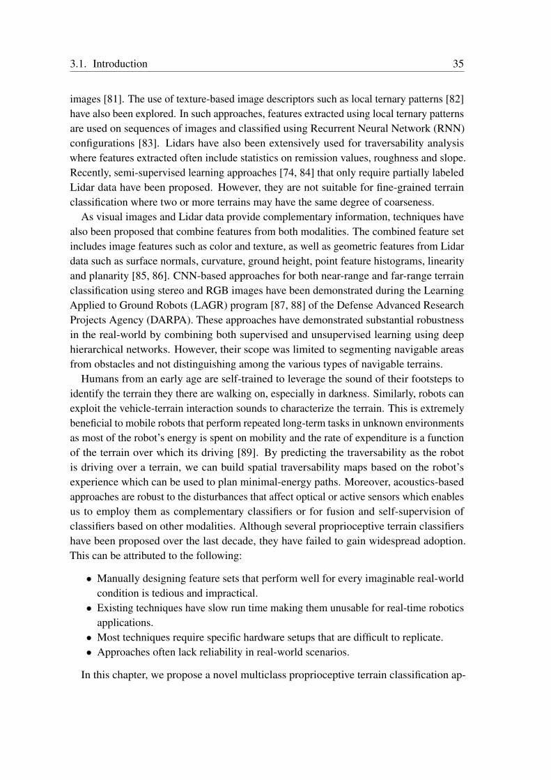
3.1. Introduction 35
images [81]. The use of texture-based image descriptors such as local ternary patterns [82]have also been explored. In such approaches, features extracted using local ternary patternsare used on sequences of images and classified using Recurrent Neural Network (RNN)configurations [83]. Lidars have also been extensively used for traversability analysiswhere features extracted often include statistics on remission values, roughness and slope.Recently, semi-supervised learning approaches [74, 84] that only require partially labeledLidar data have been proposed. However, they are not suitable for fine-grained terrainclassification where two or more terrains may have the same degree of coarseness.
As visual images and Lidar data provide complementary information, techniques havealso been proposed that combine features from both modalities. The combined feature setincludes image features such as color and texture, as well as geometric features from Lidardata such as surface normals, curvature, ground height, point feature histograms, linearityand planarity [85, 86]. CNN-based approaches for both near-range and far-range terrainclassification using stereo and RGB images have been demonstrated during the LearningApplied to Ground Robots (LAGR) program [87, 88] of the Defense Advanced ResearchProjects Agency (DARPA). These approaches have demonstrated substantial robustnessin the real-world by combining both supervised and unsupervised learning using deephierarchical networks. However, their scope was limited to segmenting navigable areasfrom obstacles and not distinguishing among the various types of navigable terrains.
Humans from an early age are self-trained to leverage the sound of their footsteps toidentify the terrain they there are walking on, especially in darkness. Similarly, robots canexploit the vehicle-terrain interaction sounds to characterize the terrain. This is extremelybeneficial to mobile robots that perform repeated long-term tasks in unknown environmentsas most of the robot’s energy is spent on mobility and the rate of expenditure is a functionof the terrain over which its driving [89]. By predicting the traversability as the robotis driving over a terrain, we can build spatial traversability maps based on the robot’sexperience which can be used to plan minimal-energy paths. Moreover, acoustics-basedapproaches are robust to the disturbances that affect optical or active sensors which enablesus to employ them as complementary classifiers or for fusion and self-supervision ofclassifiers based on other modalities. Although several proprioceptive terrain classifiershave been proposed over the last decade, they have failed to gain widespread adoption.This can be attributed to the following:
• Manually designing feature sets that perform well for every imaginable real-worldcondition is tedious and impractical.• Existing techniques have slow run time making them unusable for real-time robotics
applications.• Most techniques require specific hardware setups that are difficult to replicate.• Approaches often lack reliability in real-world scenarios.
In this chapter, we propose a novel multiclass proprioceptive terrain classification ap-
36 Chapter 3. Proprioceptive Terrain Classification
Figure 3.2: The Pioneer P3-DX platform equipped with a shotgun microphone with an integratedshock mount that we use in our experiments. The microphone is mounted close to the wheel withthe supercardioid pointing towards the tire-terrain interface.
proach that overcomes these impediments by using sound from vehicle-terrain interactionsto classify both indoor and outdoor terrains. We propose two DCNN architectures: one thatconsiders a single time window for classification and a recurrent variant that incorporatesLong Short-Term Memory (LSTM) units to capture the temporal dynamics of the signal.Both our architectures incorporate our proposed Global Statistical Pooling (GSP) strategyin which three temporal pooling methods are combined to achieve the time-series represen-tation learning. In addition, our recurrent model forms compositional representations inthe time domain, similar to convolutional models that form compositional representationsin the spatial domain. The structure of our proposed network exploits the temporal infor-mation in each clip as well as in the transitioning clips. In order to evaluate the efficacyof our approach, we gathered two extensive vehicle-terrain interaction datasets consistingof data from nine different indoor and outdoor terrains. The first dataset was collectedusing a mobile robot equipped with a shotgun microphone as shown in Figure 3.2 and thesecond dataset was collected using a mobile phone microphone. The rationale behind usingtwo different microphones was to evaluate the generalizability of the model to differenthardware setups and to demonstrate that even inexpensive microphone can be effectivelyutilized with our proposed system.
Although DCNN-based approaches are more robust to environmental noise than classicalapproaches that employ handcrafted features, their performance still degrades in highambient noise environments. Noise sensitivity is strongly correlated to the capability tooperate in different real-world environments. Moreover, there are two different typesof noise sources in our application; ambient noise and the noise from the drive motorsof the robot. As the motor noise is captured in the training data, the model learns toaccount for this noise corruption. In order to make our model tolerant to ambient noiseand generalize effectively to different real-world environments, we present a noise-awaretraining scheme. Our training scheme randomly injects ambient noise signals from the
3.2. Technical Approach 37
Diverse Environments Multichannel Acoustic Noise Database (DEMAND) [90] at differentSignal-to-Noise (SNR) ratios. We demonstrate that our network trained using our noise-aware scheme shows substantial improvement in the robustness of the model to adverseambient noises. The approach presented in this thesis is the first proprioceptive terrainclassification technique to be able to robustly classify nine different indoor and outdoorterrains with a classification rate of over 80 Hz.
Concretely, we make the following contributions in this chapter:• A novel convolutional neural network architecture for terrain classification from
vehicle-terrain interaction sounds that operates on a single audio clip of fixed length.• A recurrent convolutional neural network architecture for terrain classification from
vehicle-terrain interaction sounds.• A new Global Statistical Pooling (GSP) scheme for aggregating statistics of learned
temporal features.• A noise aware training scheme that substantially increases the generalizability of the
model to real-world environments with different ambient noises.• Thorough empirical evaluations of our proposed system on over 6 h of audio data
using two different audio acquisition systems and in seven different environmentshaving adverse acoustic conditions.
The remainder of this chapter is organized as follows. In Section 3.2, we detail ourproposed network architectures and the noise-aware training strategy. We then describe ourdata collection methodology in Section 3.3, followed by extensive experimental evaluationsthat demonstrate the efficacy of our approach in Section 3.4. Finally, we discuss the relatedwork that has been previously done using acoustics and other proprioceptive sensors inSection 3.5, before concluding the chapter in Section 3.6.
3.2 Technical Approach
In this section, we describe our approach to terrain classification using vehicle-terraininteraction sounds. Recent work has shown that learning audio features from simpletransformations such as spectrograms are more effective than directly leaning from rawaudio waveforms [26, 91]. Therefore, we first transform the vehicle terrain interactionsignals into their spectrogram representation, and then use them as inputs to our network forfeature learning and classification. Figure 3.3 depicts the preprocessing that we perform onthe training set. In the following sections, we first describe the spectrogram transformationtechnique that we apply on the raw audio waveforms. We then detail our proposedTerrainNet architecture that operates on spectrograms of independent audio frames ofvehicle-terrain interactions, followed by our recurrent TerrainNet++ architecture whichincorporates LSTM units to model the sequential nature of the signal and more effectivelyexploit the temporal dynamics.
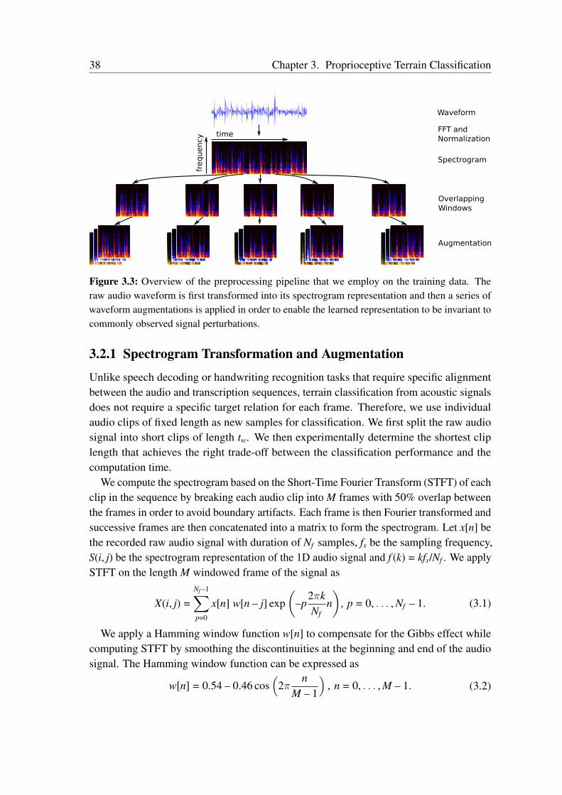
38 Chapter 3. Proprioceptive Terrain Classification
Augmentation
OverlappingWindows
Spectrogram
FFT and Normalization
Waveform
frequency
time
Figure 3.3: Overview of the preprocessing pipeline that we employ on the training data. Theraw audio waveform is first transformed into its spectrogram representation and then a series ofwaveform augmentations is applied in order to enable the learned representation to be invariant tocommonly observed signal perturbations.
3.2.1 Spectrogram Transformation and Augmentation
Unlike speech decoding or handwriting recognition tasks that require specific alignmentbetween the audio and transcription sequences, terrain classification from acoustic signalsdoes not require a specific target relation for each frame. Therefore, we use individualaudio clips of fixed length as new samples for classification. We first split the raw audiosignal into short clips of length tw. We then experimentally determine the shortest cliplength that achieves the right trade-off between the classification performance and thecomputation time.
We compute the spectrogram based on the Short-Time Fourier Transform (STFT) of eachclip in the sequence by breaking each audio clip into M frames with 50% overlap betweenthe frames in order to avoid boundary artifacts. Each frame is then Fourier transformed andsuccessive frames are then concatenated into a matrix to form the spectrogram. Let x[n] bethe recorded raw audio signal with duration of Nf samples, fs be the sampling frequency,S(i, j) be the spectrogram representation of the 1D audio signal and f (k) = kfs/Nf . We applySTFT on the length M windowed frame of the signal as
X(i, j) =Nf –1∑p=0
x[n] w[n – j] exp(
–p2πkNf
n)
, p = 0, . . . , Nf – 1. (3.1)
We apply a Hamming window function w[n] to compensate for the Gibbs effect whilecomputing STFT by smoothing the discontinuities at the beginning and end of the audiosignal. The Hamming window function can be expressed as
w[n] = 0.54 – 0.46 cos(
2πn
M – 1
), n = 0, . . . , M – 1. (3.2)
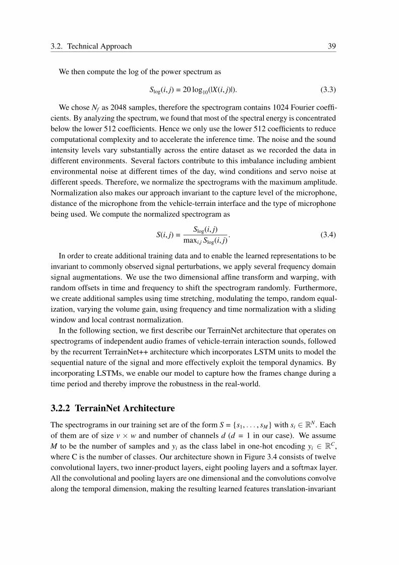
3.2. Technical Approach 39
We then compute the log of the power spectrum as
Slog(i, j) = 20 log10(|X(i, j)|). (3.3)
We chose Nf as 2048 samples, therefore the spectrogram contains 1024 Fourier coeffi-cients. By analyzing the spectrum, we found that most of the spectral energy is concentratedbelow the lower 512 coefficients. Hence we only use the lower 512 coefficients to reducecomputational complexity and to accelerate the inference time. The noise and the soundintensity levels vary substantially across the entire dataset as we recorded the data indifferent environments. Several factors contribute to this imbalance including ambientenvironmental noise at different times of the day, wind conditions and servo noise atdifferent speeds. Therefore, we normalize the spectrograms with the maximum amplitude.Normalization also makes our approach invariant to the capture level of the microphone,distance of the microphone from the vehicle-terrain interface and the type of microphonebeing used. We compute the normalized spectrogram as
S(i, j) =Slog(i, j)
maxi,j Slog(i, j). (3.4)
In order to create additional training data and to enable the learned representations to beinvariant to commonly observed signal perturbations, we apply several frequency domainsignal augmentations. We use the two dimensional affine transform and warping, withrandom offsets in time and frequency to shift the spectrogram randomly. Furthermore,we create additional samples using time stretching, modulating the tempo, random equal-ization, varying the volume gain, using frequency and time normalization with a slidingwindow and local contrast normalization.
In the following section, we first describe our TerrainNet architecture that operates onspectrograms of independent audio frames of vehicle-terrain interaction sounds, followedby the recurrent TerrainNet++ architecture which incorporates LSTM units to model thesequential nature of the signal and more effectively exploit the temporal dynamics. Byincorporating LSTMs, we enable our model to capture how the frames change during atime period and thereby improve the robustness in the real-world.
3.2.2 TerrainNet Architecture
The spectrograms in our training set are of the form S = s1, . . . , sM with si ∈ RN . Eachof them are of size v × w and number of channels d (d = 1 in our case). We assumeM to be the number of samples and yi as the class label in one-hot encoding yi ∈ RC,where C is the number of classes. Our architecture shown in Figure 3.4 consists of twelveconvolutional layers, two inner-product layers, eight pooling layers and a softmax layer.All the convolutional and pooling layers are one dimensional and the convolutions convolvealong the temporal dimension, making the resulting learned features translation-invariant
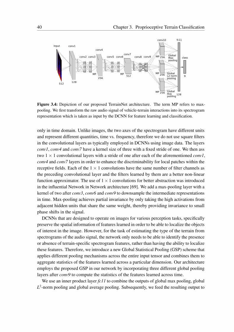
40 Chapter 3. Proprioceptive Terrain Classification
128
9
class
fc11
conv4
conv7
512
GlobalMax pooling
conv2
GlobalAvg pooling
GlobalL2 normpooling
MP
MP
MP
conv3 conv6conv5 conv8 conv9
MP
MP
256
256
256
conv10
Input conv1
128512
256
Figure 3.4: Depiction of our proposed TerrainNet architecture. The term MP refers to max-pooling. We first transform the raw audio signal of vehicle-terrain interactions into its spectrogramrepresentation which is taken as input by the DCNN for feature learning and classification.
only in time domain. Unlike images, the two axes of the spectrogram have different unitsand represent different quantities, time vs. frequency, therefore we do not use square filtersin the convolutional layers as typically employed in DCNNs using image data. The layersconv1, conv4 and conv7 have a kernel size of three with a fixed stride of one. We then asstwo 1× 1 convolutional layers with a stride of one after each of the aforementioned conv1,conv4 and conv7 layers in order to enhance the discriminability for local patches within thereceptive fields. Each of the 1× 1 convolutions have the same number of filter channels asthe preceding convolutional layer and the filters learned by them are a better non-linearfunction approximator. The use of 1× 1 convolutions for better abstraction was introducedin the influential Network in Network architecture [69]. We add a max-pooling layer with akernel of two after conv3, conv6 and conv9 to downsample the intermediate representationsin time. Max-pooling achieves partial invariance by only taking the high activations fromadjacent hidden units that share the same weight, thereby providing invariance to smallphase shifts in the signal.
DCNNs that are designed to operate on images for various perception tasks, specificallypreserve the spatial information of features learned in order to be able to localize the objectsof interest in the image. However, for the task of estimating the type of the terrain fromspectrograms of the audio signal, the network only needs to be able to identify the presenceor absence of terrain-specific spectrogram features, rather than having the ability to localizethese features. Therefore, we introduce a new Global Statistical Pooling (GSP) scheme thatapplies different pooling mechanisms across the entire input tensor and combines them toaggregate statistics of the features learned across a particular dimension. Our architectureemploys the proposed GSP in our network by incorporating three different global poolinglayers after conv9 to compute the statistics of the features learned across time.
We use an inner product layer fc11 to combine the outputs of global max pooling, globalL2-norm pooling and global average pooling. Subsequently, we feed the resulting output to
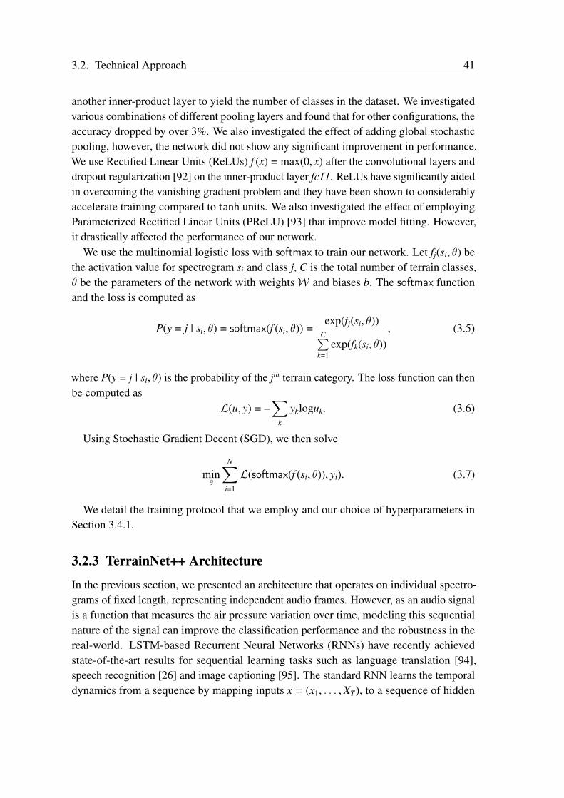
3.2. Technical Approach 41
another inner-product layer to yield the number of classes in the dataset. We investigatedvarious combinations of different pooling layers and found that for other configurations, theaccuracy dropped by over 3%. We also investigated the effect of adding global stochasticpooling, however, the network did not show any significant improvement in performance.We use Rectified Linear Units (ReLUs) f (x) = max(0, x) after the convolutional layers anddropout regularization [92] on the inner-product layer fc11. ReLUs have significantly aidedin overcoming the vanishing gradient problem and they have been shown to considerablyaccelerate training compared to tanh units. We also investigated the effect of employingParameterized Rectified Linear Units (PReLU) [93] that improve model fitting. However,it drastically affected the performance of our network.
We use the multinomial logistic loss with softmax to train our network. Let fj(si, θ) bethe activation value for spectrogram si and class j, C is the total number of terrain classes,θ be the parameters of the network with weightsW and biases b. The softmax functionand the loss is computed as
P(y = j | si, θ) = softmax(f (si, θ)) =exp(fj(si, θ))
C∑k=1
exp(fk(si, θ)), (3.5)
where P(y = j | si, θ) is the probability of the jth terrain category. The loss function can thenbe computed as
L(u, y) = –∑
k
ykloguk. (3.6)
Using Stochastic Gradient Decent (SGD), we then solve
minθ
N∑i=1
L(softmax(f (si, θ)), yi). (3.7)
We detail the training protocol that we employ and our choice of hyperparameters inSection 3.4.1.
3.2.3 TerrainNet++ Architecture
In the previous section, we presented an architecture that operates on individual spectro-grams of fixed length, representing independent audio frames. However, as an audio signalis a function that measures the air pressure variation over time, modeling this sequentialnature of the signal can improve the classification performance and the robustness in thereal-world. LSTM-based Recurrent Neural Networks (RNNs) have recently achievedstate-of-the-art results for sequential learning tasks such as language translation [94],speech recognition [26] and image captioning [95]. The standard RNN learns the temporaldynamics from a sequence by mapping inputs x = (x1, . . . , XT), to a sequence of hidden
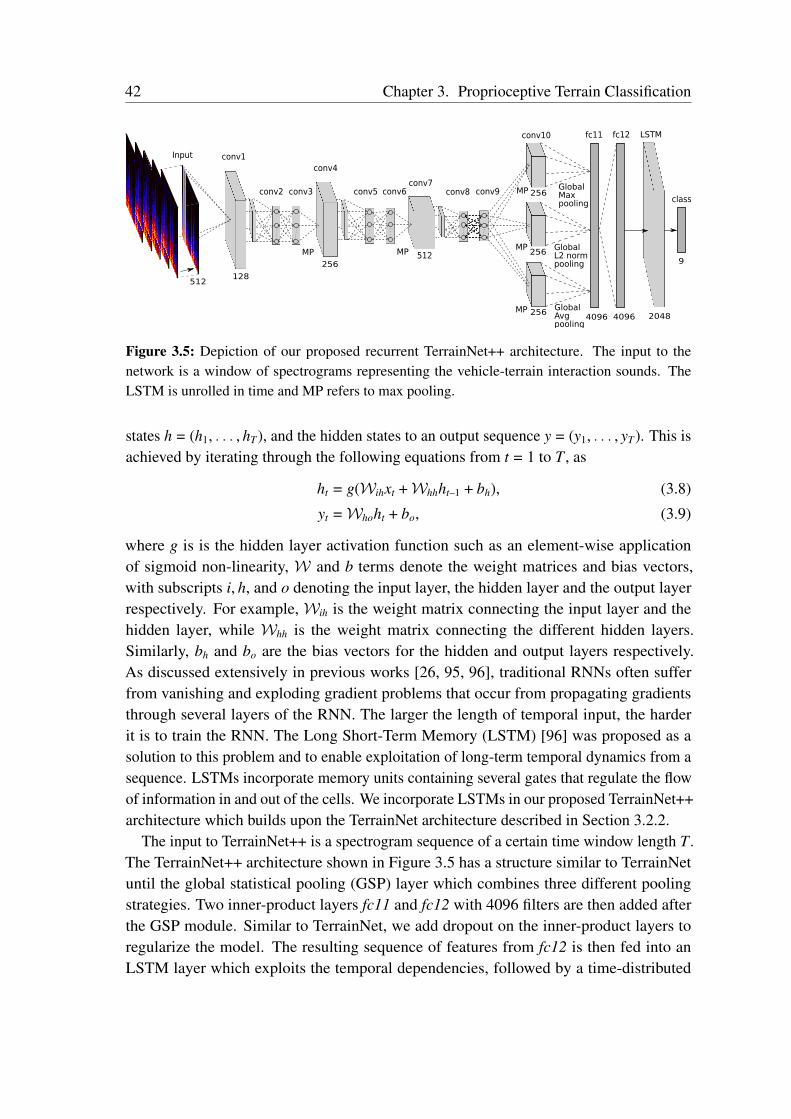
42 Chapter 3. Proprioceptive Terrain Classification
4096
9
class
fc11
conv4
conv7
512
GlobalMax pooling
conv2
GlobalAvg pooling
GlobalL2 normpooling
MP
MP
MP
conv3 conv6conv5 conv8 conv9
MP
MP
256
256
256
conv10 LSTMfc12
4096 2048
256
Input conv1
128512
Figure 3.5: Depiction of our proposed recurrent TerrainNet++ architecture. The input to thenetwork is a window of spectrograms representing the vehicle-terrain interaction sounds. TheLSTM is unrolled in time and MP refers to max pooling.
states h = (h1, . . . , hT), and the hidden states to an output sequence y = (y1, . . . , yT). This isachieved by iterating through the following equations from t = 1 to T , as
ht = g(Wihxt +Whhht–1 + bh), (3.8)
yt =Whoht + bo, (3.9)
where g is is the hidden layer activation function such as an element-wise applicationof sigmoid non-linearity, W and b terms denote the weight matrices and bias vectors,with subscripts i, h, and o denoting the input layer, the hidden layer and the output layerrespectively. For example, Wih is the weight matrix connecting the input layer and thehidden layer, while Whh is the weight matrix connecting the different hidden layers.Similarly, bh and bo are the bias vectors for the hidden and output layers respectively.As discussed extensively in previous works [26, 95, 96], traditional RNNs often sufferfrom vanishing and exploding gradient problems that occur from propagating gradientsthrough several layers of the RNN. The larger the length of temporal input, the harderit is to train the RNN. The Long Short-Term Memory (LSTM) [96] was proposed as asolution to this problem and to enable exploitation of long-term temporal dynamics from asequence. LSTMs incorporate memory units containing several gates that regulate the flowof information in and out of the cells. We incorporate LSTMs in our proposed TerrainNet++architecture which builds upon the TerrainNet architecture described in Section 3.2.2.
The input to TerrainNet++ is a spectrogram sequence of a certain time window length T .The TerrainNet++ architecture shown in Figure 3.5 has a structure similar to TerrainNetuntil the global statistical pooling (GSP) layer which combines three different poolingstrategies. Two inner-product layers fc11 and fc12 with 4096 filters are then added afterthe GSP module. Similar to TerrainNet, we add dropout on the inner-product layers toregularize the model. The resulting sequence of features from fc12 is then fed into anLSTM layer which exploits the temporal dependencies, followed by a time-distributed
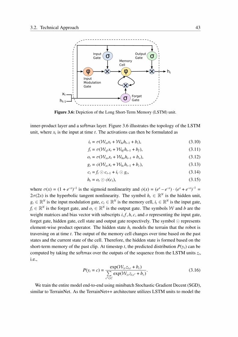
3.2. Technical Approach 43
σ
φ
σ
σ
××
×ForgetGate
MemoryCell
InputGate
InputModulationGate
OutputGate
ht
ht-1
xt
φ
Figure 3.6: Depiction of the Long Short-Term Memory (LSTM) unit.
inner-product layer and a softmax layer. Figure 3.6 illustrates the topology of the LSTMunit, where xt is the input at time t. The activations can then be formulated as
it = σ(Wxixt +Whiht–1 + bi), (3.10)
ft = σ(Wxf xt +Whf ht–1 + bf ), (3.11)
ot = σ(Wxoxt +Whoht–1 + bo), (3.12)
gt = φ(Wxcxt +Whcht–1 + bc), (3.13)
ct = ft ct–1 + it gt, (3.14)
ht = ot φ(ct), (3.15)
where σ(x) = (1 + e–x)–1 is the sigmoid nonlinearity and φ(x) = (ex – e–x) · (ex + e–x)–1 =2σ(2x) is the hyperbolic tangent nonlinearity. The symbol ht ∈ RN is the hidden unit,gt ∈ RN is the input modulation gate, ct ∈ RN is the memory cell, it ∈ RN is the input gate,ft ∈ RN is the forget gate, and ot ∈ RN is the output gate. The symbolsW and b are theweight matrices and bias vector with subscripts i, f , h, c, and o representing the input gate,forget gate, hidden gate, cell state and output gate respectively. The symbol representselement-wise product operator. The hidden state ht models the terrain that the robot istraversing on at time t. The output of the memory cell changes over time based on the paststates and the current state of the cell. Therefore, the hidden state is formed based on theshort-term memory of the past clip. At timestep t, the predicted distribution P(yt) can becomputed by taking the softmax over the outputs of the sequence from the LSTM units zt,i.e.,
P(yt = c) =exp(Wzczt,c + bc)∑
c′∈Cexp(Wzczt,c′ + bc)
. (3.16)
We train the entire model end-to-end using minibatch Stochastic Gradient Decent (SGD),similar to TerrainNet. As the TerrainNet++ architecture utilizes LSTM units to model the
44 Chapter 3. Proprioceptive Terrain Classification
temporal relationships in addition to the proposed GSP module, we evaluate its utility inthe architectural analysis presented in Section 3.4.3.1.
3.2.4 Noise-Aware Training
Noise robustness is a critical factor that substantially influences the performance of themodel in real-world environments. The performance especially degrades when the vehicle-terrain interaction signal has a significantly lower Signal-to-Noise Ratio (SNR) makingthe model more susceptible to additive noise and reverberations. Conventional techniquesemployed in the speech recognition domain are loosely based on known mechanisms ofauditory frequency encoding [97], therefore they are not directly employable while classi-fying vehicle-terrain interaction sounds. Moreover, as vehicle-terrain interaction soundshave very similar spectral properties as noise sources modeled for speech recognition tasks,existing front-end signal processing techniques are not applicable.
As a solution to this problem, we propose a noise-aware training scheme that substan-tially improves the robustness and the generalizability of our model without any additionalpreprocessing or computational burden. The basic principle of our noise-aware trainingscheme is to randomly inject common ambient environmental noises into the training dataso that the model learns to distinguish between noise corruption patterns and the relevantvehicle-terrain interaction features. As our model learns hierarchical representations, thelower layers learn both pure vehicle-terrain interaction features as well as ambient noisefeatures, whereas the higher layers learn compositional representations by distinguishingbetween them. Furthermore, the temporal component of our network enables the model tolearn the evolution of both signals. Due to the temporal depth, the network is able learnheterogeneous signal patterns and at what stage to de-emphasize the noise while makingdecisions. Noise-conditioned decision boundaries are learned as we train the network withsignals corrupted with noise at different SNRs. Additionally, the perturbation introducedby the injected noise regularizes the network and improves the generalization ability ofthe model. It helps improve the classification of pure signals as the easily degraded partsof the signal are blurred by noise which forces the network to learn the more dominantfeatures, hence avoiding over-fitting. In summary, the goal of our noise-aware training is toenable the model to learn the common discriminative noise patterns and better regularizethe network to improve the generalization performance to real-world environments withdifferent ambient noises.
We randomly select a noise following a multinomial distribution Mult(µ1,µ2, . . . ,µn)while training, where n is the types of noises and µi is sampled from a Dirichlet distributionas (µ1,µ2, . . . ,µn) ∼ Dir(α1,α2, . . . ,αn), where αi is set to control the base distribu-tion of the noise types. The SNR of the noised sample follows a Gaussian distributionN (µSNR,σSNR), where µSNR and σSNR are the mean and variance. Following a uniformdistribution, we randomly select a start time s on the noise signal and scale it according

3.2. Technical Approach 45
to the desired SNR before adding it with the pure vehicle-terrain interaction signal. Weuse the Praat framework [98] for all the signal processing computations and the ambientnoise recordings from the Diverse Environments Multichannel Acoustic Noise Database(DEMAND). The recordings in the DEMAND database were captured using 16 omnidi-rectional electret condenser microphones in over 18 different environments. We categorizethe ambient noise environments into seven classes for in-depth experiments as follows:
• White: White noise has a very wide band and it is one of the most common noisesources. It has a very similar effect to that of various physical and environmentaldisturbances including wind and water sources.• Domestic: This category includes ambient noises from living rooms, kitchens and
washing rooms. As our terrain categories also contain indoor terrains, it is crucial totrain the model with common indoor ambient noises.• Nature: The nature category contains outdoor noise samples from a sports field, a
river creek with flowing water and a city park.• Office: This category contains recordings from an office with people working on
computers, a hallway where people pass by occasionally and from interior publicspaces.• Public: The public category contains recordings from interior public spaces such a
bus station, a cafeteria with people and from a university restaurant.• Street: The street category contains noise recordings from outdoor inner-city public
roads and pedestrian traffic. It contains a busy traffic intersection, a town squarewith tourists and a cafe at a public space.• Transportation: This category contains recordings of vehicle noises such as cars,
subways and buses.
As vehicle-terrain interaction sounds are unstructured in nature, corrupting it withvarious heterogeneous noises might quash the most relevant discriminative features leadingto poor performance in the real-world. Therefore, we first investigate the effect of thesenoise disturbances by evaluating the model trained on the pure uncorrupted training setwith the noise corrupted test set. We then perform noise-aware training with differentSNRs. The training procedure that we employ is further detailed in Section 3.4.1.
3.2.5 Baseline Feature Extraction
There is a wide range of audio features that have been proposed for various speechand sound recognition tasks. Recent work has explored the utilization of these featuresfor audio-based terrain classification [76, 77, 78]. We evaluate the performance of ourproposed architectures against the following set of classical baseline audio features thatinclude both time and frequency domain features:
46 Chapter 3. Proprioceptive Terrain Classification
• Ginna features [99]• Spectral features [76]• Ginna & Shape features [99, 100]• MFCC & Chroma features [101]• Trimbral features [102]• Cepstral features [103]
Recently, Ginna and Shape features have demonstrated the best results for terrainclassification using wheeled mobile robots [76]. Ginna features [99] is a six dimensionalfeature vector consisting of three features extracted from the time domain and threefeatures extracted from the frequency domain. The time domain features are Zero CrossingRate (ZCR), Short Time Energy (STE) and entropy (U), while the frequency domainfeatures include Spectral Centroid (SC), Spectral Flux (SF) and Spectral Rolloff (SR).Zero Crossing Rate (ZCR) can be defined as the rate at which the signal changes frompositive to negative and it is a measure of the noisiness of the signal. ZCR is one of themost traditional audio feature used for speech and music classification. STE is the energyin a short segment of the signal which can be computed as the square of the amplitude ofthe signal. Entropy characterizes the abrupt energy changes in the signal. ZCR, STE andentropy can be computed as
ZCR =1
2N
N–1∑m=0
| sgn[y(m)] – sgn[y(i – 1)]|, (3.17)
where, sgn[x(m)] =
1, x(n) ≥ 0
–1, x(n) < 0,
STE =N–1∑m=0
X((m).w(n – m))2, (3.18)
U = –N–1∑i=0
σ2 · log2(σ2), (3.19)
where X(n) is a sample of the power spectrum at bin n, f (n) is the center frequency ofthe bin n, w(n) is the windowing function, N is the size of the window and σ denotes thenormalized energy.
The most commonly used frequency domain feature is the Spectral Centroid (SC), whichis also referred to as the median of the power spectrum. It indicates where the center ofmass of the spectrum lies and it provides a measure of the spectral shape. Spectral Flux(SF) indicates the change in the power spectrum between successive windows and it is ameasure of the amount of local spectral change. Spectral Rolloff (SR) is the frequencybelow the 95th percentile of the power in the spectrum and it is a measure of the skewness
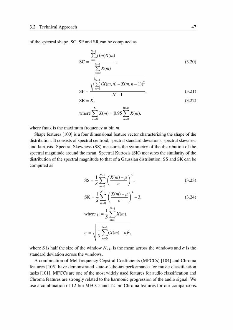
3.2. Technical Approach 47
of the spectral shape. SC, SF and SR can be computed as
SC =
N–1∑m=0
f (m)X(m)
N–1∑m=0
X(m), (3.20)
SF =
√N–1∑m=1
(X(m, n) – X(m, n – 1))2
N – 1, (3.21)
SR = K, (3.22)
whereK∑
m=0
X(m) = 0.95fmax∑m=0
X(m),
where fmax is the maximum frequency at bin m.Shape features [100] is a four dimensional feature vector characterizing the shape of the
distribution. It consists of spectral centroid, spectral standard deviations, spectral skewnessand kurtosis. Spectral Skewness (SS) measures the symmetry of the distribution of thespectral magnitude around the mean. Spectral Kurtosis (SK) measures the similarity of thedistribution of the spectral magnitude to that of a Gaussian distribution. SS and SK can becomputed as
SS =1S
N–1∑m=0
(X(m) – µ
σ
)3
, (3.23)
SK =1S
N–1∑m=0
(X(m) – µ
σ
)4
– 3, (3.24)
where µ =1S
N–1∑m=0
X(m),
σ =
√√√√1S
N–1∑m=0
(X(m) – µ)2,
where S is half the size of the window N, µ is the mean across the windows and σ is thestandard deviation across the windows.
A combination of Mel-frequency Cepstral Coefficients (MFCCs) [104] and Chromafeatures [105] have demonstrated state-of-the-art performance for music classificationtasks [101]. MFCCs are one of the most widely used features for audio classification andChroma features are strongly related to the harmonic progression of the audio signal. Weuse a combination of 12-bin MFCCs and 12-bin Chroma features for our comparisons.
48 Chapter 3. Proprioceptive Terrain Classification
Timbral features have shown impressive results for music genre classification [102]. Theycontain means and variances of spectral centroid, spectral rolloff, spectral flux, zerocrossing rate, low energy, and first 5 MFCCs. We also use this 19 dimensional featurevector for our baseline comparison. For our final baseline, we use a combination ofcepstral features containing 13-bin MFCCs, Line Spectral Pair (LSP) and Linear PredictionCepstral Coefficients (LPCCs) [103].
3.3 Data Collection and Labelling
To the best of our knowledge, there is no publicly available audio-based terrain clas-sification dataset till date. Therefore, in order to facilitate this work, we collected anextensive dataset of vehicle-terrain interactions that we made publicly available. We usedthe Pioneer P3-DX platform which has a small footprint and feeble motor noise. Weequipped the P3-DX with rugged wheels that enabled us to collect data both indoors aswell as in unstructured outdoors environments. Interference from nearby sound sourcesin the environment can drastically influence the classification. It can even augment thevehicle-terrain interaction data by adding its own attributes from each environment. Inorder to prevent such biases in the training data, we use a shotgun microphone that has asupercardioid polar pattern which helps in rejecting off-axis ambient sounds. We chosethe Rode VideoMic Pro and mounted it near the right wheel of the robot as shown inFigure 3.2. The microphone has an integrated shock mount that prevents the pickup of anyunwanted vibrations caused during the traversal. Note that our approach presented in thischapter is platform independent, as the network learns features from the given trainingdata.
Thus far, audio-based terrain classification using mobile robots has only been focusedon outdoor terrains that have a large variation in geometric properties and thereforeproduce very distinct audio signatures. Recently, audio-based terrain classification hasbeen demonstrated for both indoor and outdoor terrains using legged robots. However,legged robots have significantly lesser drive motor noise and they produce very isolatedsounds from their leg-terrain interaction which are substantially easier to detect and classify.In this chapter, our objective is to classify a wide variety of both indoor and outdoor terrainsusing vehicle-terrain interaction signals. Therefore, we collected over 15 h of audio datafrom a total of 9 different indoor and outdoor terrains. We particularly choose our terraincategories such that some of them have similar visual features (Figures 3.7 (a), (h), and (i))and hence pose a big challenge for classification using vision-based approaches.
We collected the data in several different locations to have enough variability in theterrains and to enable our model to generalize effectively to a wide range of environments.Therefore, even the audio signals in the same terrain category have varying spectral andtemporal characteristics. Furthermore, we varied the speed of the robot from 0.1 m s–1 to
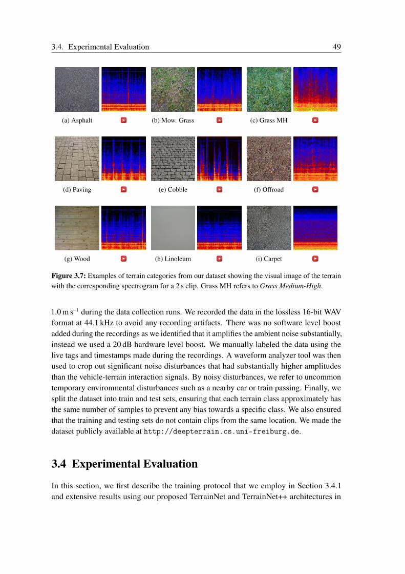
3.4. Experimental Evaluation 49
(a) Asphalt (b) Mow. Grass (c) Grass MH
(d) Paving (e) Cobble (f) Offroad
(g) Wood (h) Linoleum (i) Carpet
Figure 3.7: Examples of terrain categories from our dataset showing the visual image of the terrainwith the corresponding spectrogram for a 2 s clip. Grass MH refers to Grass Medium-High.
1.0 m s–1 during the data collection runs. We recorded the data in the lossless 16-bit WAVformat at 44.1 kHz to avoid any recording artifacts. There was no software level boostadded during the recordings as we identified that it amplifies the ambient noise substantially,instead we used a 20 dB hardware level boost. We manually labeled the data using thelive tags and timestamps made during the recordings. A waveform analyzer tool was thenused to crop out significant noise disturbances that had substantially higher amplitudesthan the vehicle-terrain interaction signals. By noisy disturbances, we refer to uncommontemporary environmental disturbances such as a nearby car or train passing. Finally, wesplit the dataset into train and test sets, ensuring that each terrain class approximately hasthe same number of samples to prevent any bias towards a specific class. We also ensuredthat the training and testing sets do not contain clips from the same location. We made thedataset publicly available at http://deepterrain.cs.uni-freiburg.de.
3.4 Experimental Evaluation
In this section, we first describe the training protocol that we employ in Section 3.4.1and extensive results using our proposed TerrainNet and TerrainNet++ architectures in
50 Chapter 3. Proprioceptive Terrain Classification
comparison to approaches that employ state-of-the-art audio features in Section 3.4.2. Wealso present comprehensive ablation studies on the various architectural configurations andparameter choices in Section 3.4.3, followed by detailed class-wise analysis in Section 3.4.4and performance analysis in the presence of substantial amount of ambient noise inSection 3.4.5. In Section 3.4.6, we then present experiments that demonstrate the efficacyof our noise-aware training scheme in improving the robustness of our models in adverseambient noise conditions. Finally, in Section 3.4.7, we present experiments using a low-costmobile phone microphone that demonstrates the hardware independence of our approach.Note that we do not retrain the network on data using the inexpensive microphone, weonly test our previously trained model.
We use the Caffe [106] deep learning library for all the experiments presented inthis chapter and the LSTM described in [107]. We employ a more efficient LSTMimplementation that is faster than the default Caffe LSTM [95] by computing gradientwith respect to recurrent weights with a single matrix computation. All our models weretrained end-to-end and the experiments were run on a system with an Intel Xeon E5,2.4GHz and an NVIDIA TITAN X GPU with cuDNN acceleration. We primarily reportthe classification accuracy metric to quantify the performance of our models but we alsoreport the precision, recall, confusion matrices, classification error and the inference timefor in the detailed comparisons. The results from our experiments are described in thefollowing sections.
3.4.1 Training Protocol
As the input to our network is the spectrogram of the audio clip, we performed experimentstraining our network with spectrograms of audio clips of varying lengths from 200 msto 2000 ms and identified the shortest clip length that yields a good trade-off betweenperformance and computation time. Results from this experiment is shown in the ablationstudy presented in Section 3.4.3.2. We initialize the convolution and inner-product layerswith Xavier weight initialization [108]. The Xavier weight filler initializes weights bydrawing from a zero mean uniform distribution from [–a, a] and the variance as a functionof the number of input neurons, where a =
√3 / nin and nin is the number of input neurons.
This enables us to move away from the traditional layer by layer generative pre-training.Furthermore, we use a dropout probability of 0.5 on the inner-product layers in order toregularize the network.
We found the network to be extremely sensitive to the hyperparameters employed,especially the hyperparameters in the recurrent TerrainNet++ architecture. Therefore, weuse the Spearmint Bayesian optimization library [109] to tune the hyperparameters. We firstoptimized the learning policy and the initial learning rate over fixed, inverse, step and polylearning rate policies. We obtained the best performance using an initial learning rate ofλ0 = 0.01 and the poly learning rate policy which can be defined as λn = λ0× (1 – N/Nmax)c,
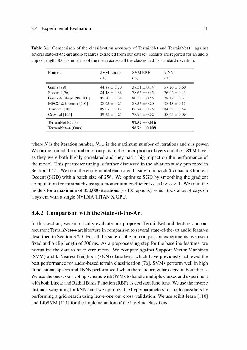
3.4. Experimental Evaluation 51
Table 3.1: Comparison of the classification accuracy of TerrainNet and TerrainNet++ againstseveral state-of-the-art audio features extracted from our dataset. Results are reported for an audioclip of length 300 ms in terms of the mean across all the classes and its standard deviation.
Features SVM Linear SVM RBF k-NN(%) (%) (%)
Ginna [99] 44.87± 0.70 37.51± 0.74 57.26± 0.60Spectral [76] 84.48± 0.36 78.65± 0.45 76.02± 0.43Ginna & Shape [99, 100] 85.50± 0.34 80.37± 0.55 78.17± 0.37MFCC & Chroma [101] 88.95± 0.21 88.55± 0.20 88.43± 0.15Trimbral [102] 89.07± 0.12 86.74± 0.25 84.82± 0.54Cepstral [103] 89.93± 0.21 78.93± 0.62 88.63± 0.06
TerrainNet (Ours) 97.52± 0.016TerrainNet++ (Ours) 98.76± 0.009
where N is the iteration number, Nmax is the maximum number of iterations and c is power.We further tuned the number of outputs in the inner-product layers and the LSTM layeras they were both highly correlated and they had a big impact on the performance ofthe model. This parameter tuning is further discussed in the ablation study presented inSection 3.4.3. We train the entire model end-to-end using minibatch Stochastic GradientDecent (SGD) with a batch size of 256. We optimize SGD by smoothing the gradientcomputation for minibatchs using a momentum coefficient α as 0 < α < 1. We train themodels for a maximum of 350,000 iterations (∼ 135 epochs), which took about 4 days ona system with a single NVIDIA TITAN X GPU.
3.4.2 Comparison with the State-of-the-Art
In this section, we empirically evaluate our proposed TerrainNet architecture and ourrecurrent TerrainNet++ architecture in comparison to several state-of-the-art audio featuresdescribed in Section 3.2.5. For all the state-of-the-art comparison experiments, we use afixed audio clip length of 300 ms. As a preprocessing step for the baseline features, wenormalize the data to have zero mean. We compare against Support Vector Machines(SVM) and k-Nearest Neighbor (kNN) classifiers, which have previously achieved thebest performance for audio-based terrain classification [76]. SVMs perform well in highdimensional spaces and kNNs perform well when there are irregular decision boundaries.We use the one-vs-all voting scheme with SVMs to handle multiple classes and experimentwith both Linear and Radial Basis Function (RBF) as decision functions. We use the inversedistance weighting for kNNs and we optimize the hyperparameters for both classifiers byperforming a grid-search using leave-one-out-cross-validation. We use scikit-learn [110]and LibSVM [111] for the implementation of the baseline classifiers.
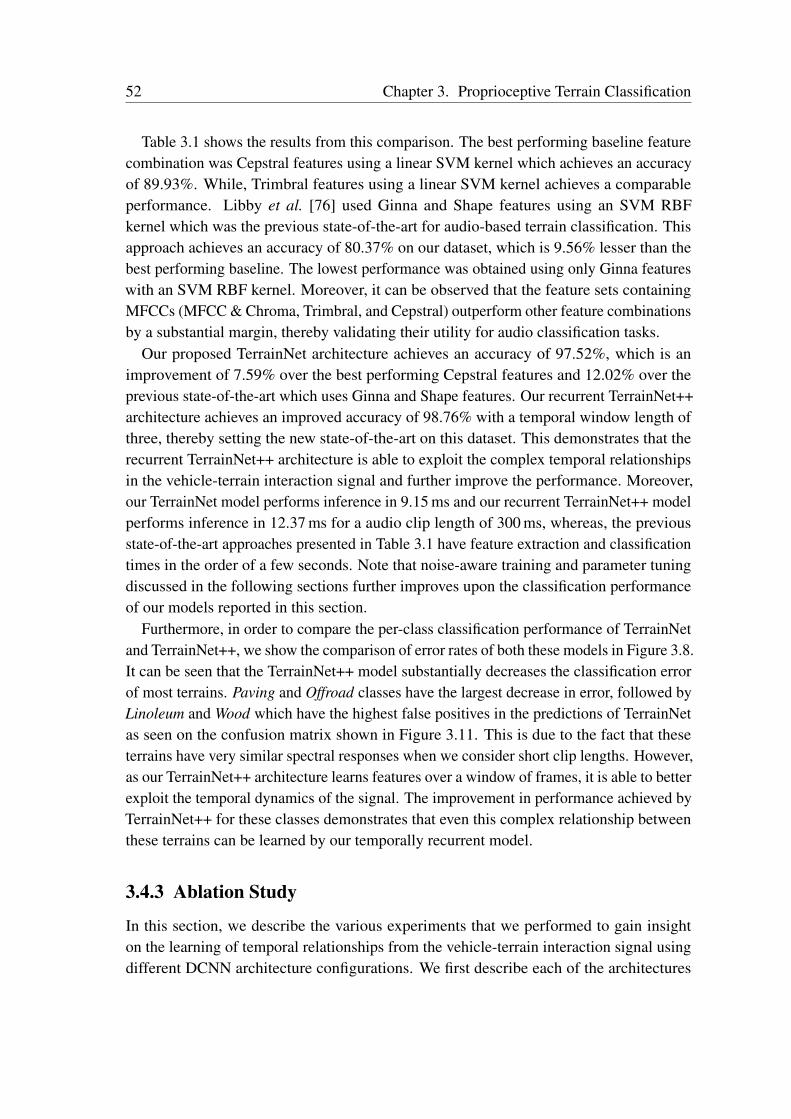
52 Chapter 3. Proprioceptive Terrain Classification
Table 3.1 shows the results from this comparison. The best performing baseline featurecombination was Cepstral features using a linear SVM kernel which achieves an accuracyof 89.93%. While, Trimbral features using a linear SVM kernel achieves a comparableperformance. Libby et al. [76] used Ginna and Shape features using an SVM RBFkernel which was the previous state-of-the-art for audio-based terrain classification. Thisapproach achieves an accuracy of 80.37% on our dataset, which is 9.56% lesser than thebest performing baseline. The lowest performance was obtained using only Ginna featureswith an SVM RBF kernel. Moreover, it can be observed that the feature sets containingMFCCs (MFCC & Chroma, Trimbral, and Cepstral) outperform other feature combinationsby a substantial margin, thereby validating their utility for audio classification tasks.
Our proposed TerrainNet architecture achieves an accuracy of 97.52%, which is animprovement of 7.59% over the best performing Cepstral features and 12.02% over theprevious state-of-the-art which uses Ginna and Shape features. Our recurrent TerrainNet++architecture achieves an improved accuracy of 98.76% with a temporal window length ofthree, thereby setting the new state-of-the-art on this dataset. This demonstrates that therecurrent TerrainNet++ architecture is able to exploit the complex temporal relationshipsin the vehicle-terrain interaction signal and further improve the performance. Moreover,our TerrainNet model performs inference in 9.15 ms and our recurrent TerrainNet++ modelperforms inference in 12.37 ms for a audio clip length of 300 ms, whereas, the previousstate-of-the-art approaches presented in Table 3.1 have feature extraction and classificationtimes in the order of a few seconds. Note that noise-aware training and parameter tuningdiscussed in the following sections further improves upon the classification performanceof our models reported in this section.
Furthermore, in order to compare the per-class classification performance of TerrainNetand TerrainNet++, we show the comparison of error rates of both these models in Figure 3.8.It can be seen that the TerrainNet++ model substantially decreases the classification errorof most terrains. Paving and Offroad classes have the largest decrease in error, followed byLinoleum and Wood which have the highest false positives in the predictions of TerrainNetas seen on the confusion matrix shown in Figure 3.11. This is due to the fact that theseterrains have very similar spectral responses when we consider short clip lengths. However,as our TerrainNet++ architecture learns features over a window of frames, it is able to betterexploit the temporal dynamics of the signal. The improvement in performance achieved byTerrainNet++ for these classes demonstrates that even this complex relationship betweenthese terrains can be learned by our temporally recurrent model.
3.4.3 Ablation Study
In this section, we describe the various experiments that we performed to gain insighton the learning of temporal relationships from the vehicle-terrain interaction signal usingdifferent DCNN architecture configurations. We first describe each of the architectures
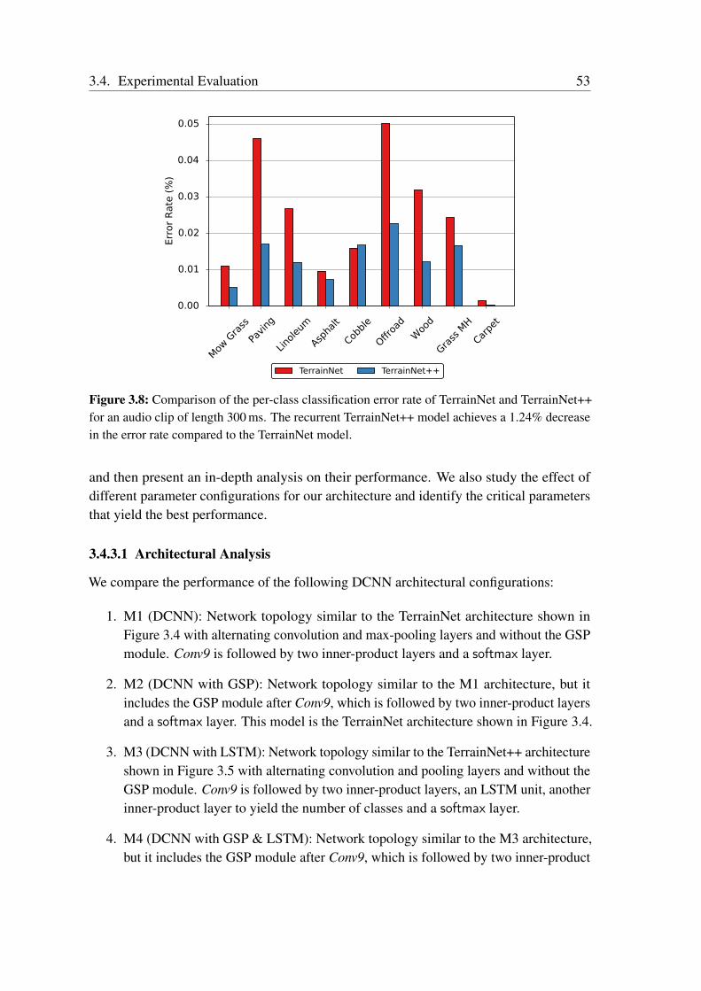
3.4. Experimental Evaluation 53
Mow
Gra
ss
Paving
Lino
leum
Aspha
lt
Cobbl
e
Offroa
d
Woo
d
Grass
MH
Carpe
t
0.00
0.01
0.02
0.03
0.04
0.05
Err
or
Rate
(%
)
TerrainNet TerrainNet++
Figure 3.8: Comparison of the per-class classification error rate of TerrainNet and TerrainNet++for an audio clip of length 300 ms. The recurrent TerrainNet++ model achieves a 1.24% decreasein the error rate compared to the TerrainNet model.
and then present an in-depth analysis on their performance. We also study the effect ofdifferent parameter configurations for our architecture and identify the critical parametersthat yield the best performance.
3.4.3.1 Architectural Analysis
We compare the performance of the following DCNN architectural configurations:
1. M1 (DCNN): Network topology similar to the TerrainNet architecture shown inFigure 3.4 with alternating convolution and max-pooling layers and without the GSPmodule. Conv9 is followed by two inner-product layers and a softmax layer.
2. M2 (DCNN with GSP): Network topology similar to the M1 architecture, but itincludes the GSP module after Conv9, which is followed by two inner-product layersand a softmax layer. This model is the TerrainNet architecture shown in Figure 3.4.
3. M3 (DCNN with LSTM): Network topology similar to the TerrainNet++ architectureshown in Figure 3.5 with alternating convolution and pooling layers and without theGSP module. Conv9 is followed by two inner-product layers, an LSTM unit, anotherinner-product layer to yield the number of classes and a softmax layer.
4. M4 (DCNN with GSP & LSTM): Network topology similar to the M3 architecture,but it includes the GSP module after Conv9, which is followed by two inner-product
54 Chapter 3. Proprioceptive Terrain Classification
Table 3.2: Performance comparison of various architecture configurations using an audio cliplength of 300 ms. Our temporally recurrent DCNN architecture with our proposed GSP and LSTM(M4), achieves a 7.47% improvement in accuracy over the architecture without any temporallearning component.
Model Acc.(%)
Prec.(%)
Rec.(%)
M1 (DCNN) 91.29 91.88 91.56M2 (DCNN + GSP) 97.52 97.56 97.61M3 (DCNN + LSTM) 95.73 95.93 95.88M4 (DCNN + GSP & LSTM) 98.76 98.75 98.82
layers, an LSTM unit, another inner-product layer to yield the number of classes anda softmax layer. This model is the TerrainNet++ architecture shown in Figure 3.5.
For the experiments described in this section, we use an audio clip of length 300 msand for the LSTM models, we use a window size of three. Results from the comparisonof the aforementioned architectural configurations is shown in Table 3.2. The M1 modelwhich does not include any temporal representational learning component achieves anaverage accuracy 91.29%, which outperforms the previous state-of-the-art. This shows theability of our proposed DCNN architecture to learn features that are more discriminativethan classical audio features. The M2 model (TerrainNet) which includes our proposedGSP module that aggregates the statistics of temporal features, achieves an improvementof 6.23% over the M1 model demonstrating the utility of the GSP for temporal featurelearning tasks. Interestingly, the M3 model which incorporates an LSTM unit and doesnot include the GSP module, achieves a lower accuracy than the M2 model. This can beattributed to the fact that the LSTM model does not benefit substantially from learningusing a large audio clip length and a short temporal window. In the following section, weinvestigate the influence of the audio clip length and the temporal window length on theclassification performance. Finally, our M4 model (TerrainNet++) which includes bothour proposed GSP module that aggregates the statistics of pooled features across time andthe LSTM unit that learns the temporal dynamics across several clips, outperforms all theother models by achieving an accuracy of 98.76%, which is a 7.47% improvement over theperformance of the M1 model. Similar improvement can also be seen in the precision andrecall values of the models. This illustrates that our proposed GSP module is critical forlearning effective temporal relations from the vehicle-terrain interaction signals.
Figure 3.9 shows the per-class recall of the various TerrainNet architecture configurationsdiscussed above. The DCNN model without the temporal feature learning components(M1) perform substantially worse than the other configurations for almost all the classes.While, the performance of the DCNN with GSP and LSTM model (M4) surpasses all
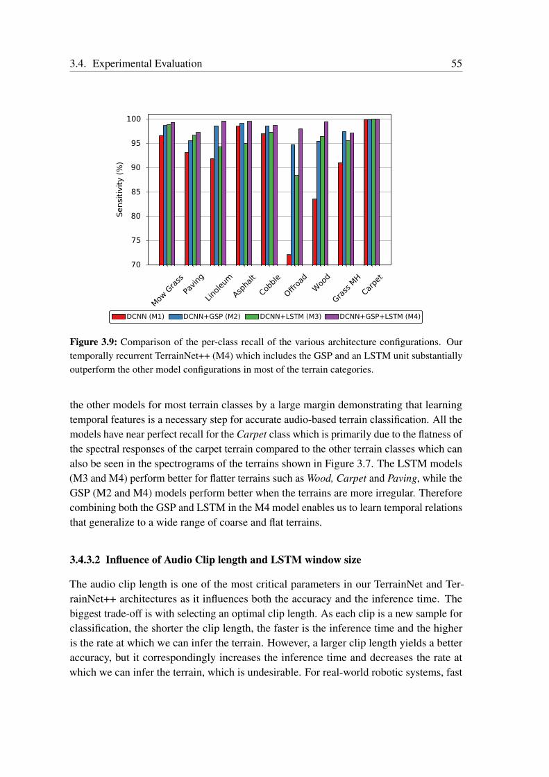
3.4. Experimental Evaluation 55
Mow
Gra
ss
Paving
Lino
leum
Aspha
lt
Cobbl
e
Offroa
d
Woo
d
Grass
MH
Carpe
t
70
75
80
85
90
95
100Sensi
tivit
y (
%)
DCNN (M1) DCNN+GSP (M2) DCNN+LSTM (M3) DCNN+GSP+LSTM (M4)
Figure 3.9: Comparison of the per-class recall of the various architecture configurations. Ourtemporally recurrent TerrainNet++ (M4) which includes the GSP and an LSTM unit substantiallyoutperform the other model configurations in most of the terrain categories.
the other models for most terrain classes by a large margin demonstrating that learningtemporal features is a necessary step for accurate audio-based terrain classification. All themodels have near perfect recall for the Carpet class which is primarily due to the flatness ofthe spectral responses of the carpet terrain compared to the other terrain classes which canalso be seen in the spectrograms of the terrains shown in Figure 3.7. The LSTM models(M3 and M4) perform better for flatter terrains such as Wood, Carpet and Paving, while theGSP (M2 and M4) models perform better when the terrains are more irregular. Thereforecombining both the GSP and LSTM in the M4 model enables us to learn temporal relationsthat generalize to a wide range of coarse and flat terrains.
3.4.3.2 Influence of Audio Clip length and LSTM window size
The audio clip length is one of the most critical parameters in our TerrainNet and Ter-rainNet++ architectures as it influences both the accuracy and the inference time. Thebiggest trade-off is with selecting an optimal clip length. As each clip is a new sample forclassification, the shorter the clip length, the faster is the inference time and the higheris the rate at which we can infer the terrain. However, a larger clip length yields a betteraccuracy, but it correspondingly increases the inference time and decreases the rate atwhich we can infer the terrain, which is undesirable. For real-world robotic systems, fast
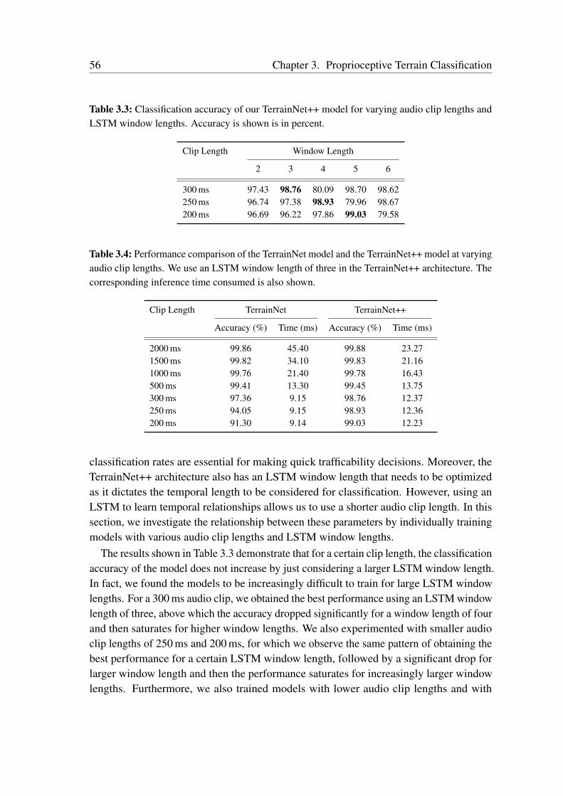
56 Chapter 3. Proprioceptive Terrain Classification
Table 3.3: Classification accuracy of our TerrainNet++ model for varying audio clip lengths andLSTM window lengths. Accuracy is shown is in percent.
Clip Length Window Length
2 3 4 5 6
300 ms 97.43 98.76 80.09 98.70 98.62250 ms 96.74 97.38 98.93 79.96 98.67200 ms 96.69 96.22 97.86 99.03 79.58
Table 3.4: Performance comparison of the TerrainNet model and the TerrainNet++ model at varyingaudio clip lengths. We use an LSTM window length of three in the TerrainNet++ architecture. Thecorresponding inference time consumed is also shown.
Clip Length TerrainNet TerrainNet++
Accuracy (%) Time (ms) Accuracy (%) Time (ms)
2000 ms 99.86 45.40 99.88 23.271500 ms 99.82 34.10 99.83 21.161000 ms 99.76 21.40 99.78 16.43500 ms 99.41 13.30 99.45 13.75300 ms 97.36 9.15 98.76 12.37250 ms 94.05 9.15 98.93 12.36200 ms 91.30 9.14 99.03 12.23
classification rates are essential for making quick trafficability decisions. Moreover, theTerrainNet++ architecture also has an LSTM window length that needs to be optimizedas it dictates the temporal length to be considered for classification. However, using anLSTM to learn temporal relationships allows us to use a shorter audio clip length. In thissection, we investigate the relationship between these parameters by individually trainingmodels with various audio clip lengths and LSTM window lengths.
The results shown in Table 3.3 demonstrate that for a certain clip length, the classificationaccuracy of the model does not increase by just considering a larger LSTM window length.In fact, we found the models to be increasingly difficult to train for large LSTM windowlengths. For a 300 ms audio clip, we obtained the best performance using an LSTM windowlength of three, above which the accuracy dropped significantly for a window length of fourand then saturates for higher window lengths. We also experimented with smaller audioclip lengths of 250 ms and 200 ms, for which we observe the same pattern of obtaining thebest performance for a certain LSTM window length, followed by a significant drop forlarger window length and then the performance saturates for increasingly larger windowlengths. Furthermore, we also trained models with lower audio clip lengths and with
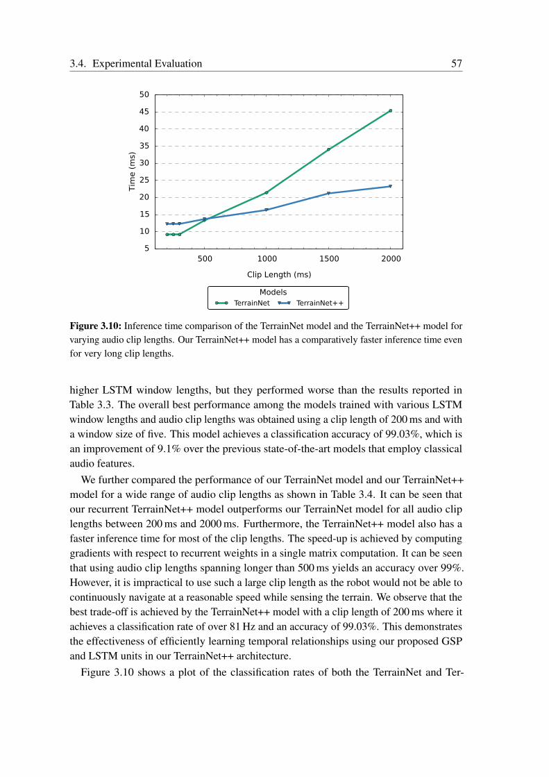
3.4. Experimental Evaluation 57
500 1000 1500 2000
Clip Length (ms)
5
10
15
20
25
30
35
40
45
50
Tim
e (
ms)
ModelsTerrainNet TerrainNet++
Figure 3.10: Inference time comparison of the TerrainNet model and the TerrainNet++ model forvarying audio clip lengths. Our TerrainNet++ model has a comparatively faster inference time evenfor very long clip lengths.
higher LSTM window lengths, but they performed worse than the results reported inTable 3.3. The overall best performance among the models trained with various LSTMwindow lengths and audio clip lengths was obtained using a clip length of 200 ms and witha window size of five. This model achieves a classification accuracy of 99.03%, which isan improvement of 9.1% over the previous state-of-the-art models that employ classicalaudio features.
We further compared the performance of our TerrainNet model and our TerrainNet++model for a wide range of audio clip lengths as shown in Table 3.4. It can be seen thatour recurrent TerrainNet++ model outperforms our TerrainNet model for all audio cliplengths between 200 ms and 2000 ms. Furthermore, the TerrainNet++ model also has afaster inference time for most of the clip lengths. The speed-up is achieved by computinggradients with respect to recurrent weights in a single matrix computation. It can be seenthat using audio clip lengths spanning longer than 500 ms yields an accuracy over 99%.However, it is impractical to use such a large clip length as the robot would not be able tocontinuously navigate at a reasonable speed while sensing the terrain. We observe that thebest trade-off is achieved by the TerrainNet++ model with a clip length of 200 ms where itachieves a classification rate of over 81 Hz and an accuracy of 99.03%. This demonstratesthe effectiveness of efficiently learning temporal relationships using our proposed GSPand LSTM units in our TerrainNet++ architecture.
Figure 3.10 shows a plot of the classification rates of both the TerrainNet and Ter-

58 Chapter 3. Proprioceptive Terrain Classification
rainNet++ models at varying audio clip lengths from 200 ms to 2000 ms. Although theTerrainNet model has a faster inference time for a clip length of 200 ms, it achieves anaccuracy which is 7.73% lower than that of the TerrainNet++ model. Considering the trade-off between the audio clip length which influences the inference time and the classificationaccuracy, we choose the TerrainNet++ model which takes a 200 ms audio clip as input forthe in-depth performance evaluation experiments described in the following sections.
3.4.4 Performance Evaluation
In order to further investigate the performance of our TerrainNet and TerrainNet++ ar-chitectures, we present the confusion matrix in Figure 3.11, which gives us insights onthe misclassifications between the terrain classes. Figure 3.11 (a) shows the confusionmatrix of the TerrainNet model in which we can see that the best performing classes wereCarpet and Asphalt, while the most misclassified classes were Offroad and Paving. TheOffroad and Paving classes have similar spectral responses when the audio clip length issmaller than 500 ms. Wood and Linoleum also have a fair amount of misclassifications asboth these terrains are almost flat and have similar spectral responses when the robot isnavigating at low speeds.
Figure 3.11 (b) shows the confusion matrix of our best performing recurrent Terrain-Net++ model for a clip length of 200 ms and an LSTM window length of five. We cansee that there is a substantial reduction in the number of false positives compared to ourTerrainNet model. Paving and Offroad classes have a reduction of about 3.15% in thenumber of false predictions. While Wood and Linoleum have a reduction of 1.66% in thenumber of false predictions. Another notable reduction of 0.88% can be observed in themisclassification between Offroad and Grass Medium-High. The best performing classeswere Carpet and Linoleum. In fact, the Carpet class demonstrated no false positives.Moreover, most of the classes demonstrate an accuracy of over 99%. The TerrainNet++model outperforms TerrainNet by 1.51% in accuracy and with a shorter audio clip as input,thereby increasing the classification rate.
Furthermore, we also compare the per-class recall of the TerrainNet and TerrainNet++models in Figure 3.12 as it gives us insights on the ratio of the correctly classified instances.For the TerrainNet model, the lowest recall was obtained for Offroad, Wood and Pavingterrains, whereas the highest recall was obtained for the Carpet terrain. A substantialimprovement in the recall of these terrains can be observed in the recall plot of the recurrentTerrainNet++ model shown in Figure 3.12 (b). The overall recall achieved by TerrainNetwas 97.61%, while the TerrainNet++ model demonstrates an improvement of 1.44% andachieves an overall recall of 99.05%.
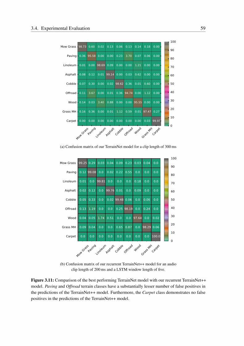
3.4. Experimental Evaluation 59
Mow Gras
sPa
ving
Linole
um
Aspha
lt
Cobble
Offroad
Wood
Grass M
HCarp
et
Mow Grass
Paving
Linoleum
Asphalt
Cobble
Offroad
Wood
Grass MH
Carpet
98.73 0.60 0.02 0.13 0.06 0.13 0.14 0.18 0.00
0.36 95.58 0.00 0.00 0.23 3.70 0.07 0.06 0.00
0.01 0.00 98.69 0.09 0.00 0.00 1.21 0.00 0.00
0.08 0.12 0.01 99.14 0.00 0.03 0.62 0.00 0.00
0.07 0.30 0.00 0.02 98.62 0.36 0.01 0.60 0.00
0.11 3.67 0.00 0.01 0.36 94.74 0.00 1.12 0.00
0.14 0.03 3.40 0.88 0.00 0.00 95.55 0.00 0.00
0.16 0.36 0.00 0.01 1.12 0.59 0.01 97.47 0.27
0.00 0.00 0.00 0.00 0.00 0.00 0.00 0.03 99.970
10
20
30
40
50
60
70
80
90
100
(a) Confusion matrix of our TerrainNet model for a clip length of 300 ms
Mow
Gra
ss
Paving
Lino
leum
Aspha
lt
Cobbl
e
Offroa
d
Woo
d
Grass
MH
Carpe
t
Mow Grass
Paving
Linoleum
Asphalt
Cobble
Offroad
Wood
Grass MH
Carpet
99.25 0.29 0.03 0.04 0.09 0.23 0.03 0.04 0.0
0.12 99.08 0.0 0.02 0.22 0.55 0.0 0.0 0.0
0.01 0.0 99.81 0.0 0.0 0.0 0.18 0.0 0.0
0.02 0.12 0.0 99.76 0.01 0.0 0.09 0.0 0.0
0.05 0.33 0.0 0.02 99.48 0.06 0.0 0.06 0.0
0.13 1.19 0.0 0.0 0.25 98.19 0.0 0.24 0.0
0.04 0.05 1.74 0.51 0.0 0.0 97.64 0.0 0.02
0.09 0.04 0.0 0.0 0.65 0.87 0.0 98.29 0.06
0.0 0.0 0.0 0.0 0.0 0.0 0.0 0.0 100.0
0
10
20
30
40
50
60
70
80
90
100
(b) Confusion matrix of our recurrent TerrainNet++ model for an audioclip length of 200 ms and a LSTM window length of five.
Figure 3.11: Comparison of the best performing TerrainNet model with our recurrent TerrainNet++model. Paving and Offroad terrain classes have a substantially lesser number of false positives inthe predictions of the TerrainNet++ model. Furthermore, the Carpet class demonstrates no falsepositives in the predictions of the TerrainNet++ model.
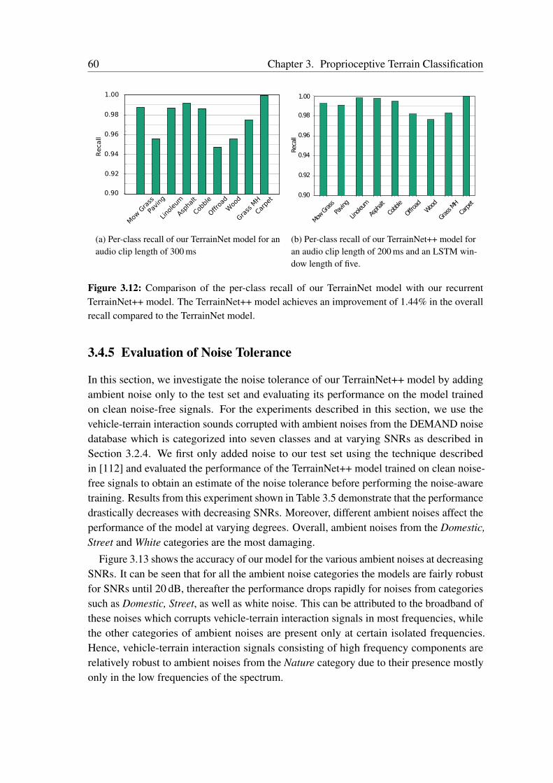
60 Chapter 3. Proprioceptive Terrain Classification
Mow
Gra
ss
Paving
Lino
leum
Aspha
lt
Cobbl
e
Offroa
d
Woo
d
Grass
MH
Carpe
t0.90
0.92
0.94
0.96
0.98
1.00R
eca
ll
Mow Grass
Pavin
g
Linole
um
Asph
alt
Cobb
le
Offro
adWoo
d
Gras
s MH
Carpet
0.90
0.92
0.94
0.96
0.98
1.00
Reca
ll
(a) Per-class recall of our TerrainNet model for anaudio clip length of 300 ms
(b) Per-class recall of our TerrainNet++ model foran audio clip length of 200 ms and an LSTM win-dow length of five.
Figure 3.12: Comparison of the per-class recall of our TerrainNet model with our recurrentTerrainNet++ model. The TerrainNet++ model achieves an improvement of 1.44% in the overallrecall compared to the TerrainNet model.
3.4.5 Evaluation of Noise Tolerance
In this section, we investigate the noise tolerance of our TerrainNet++ model by addingambient noise only to the test set and evaluating its performance on the model trainedon clean noise-free signals. For the experiments described in this section, we use thevehicle-terrain interaction sounds corrupted with ambient noises from the DEMAND noisedatabase which is categorized into seven classes and at varying SNRs as described inSection 3.2.4. We first only added noise to our test set using the technique describedin [112] and evaluated the performance of the TerrainNet++ model trained on clean noise-free signals to obtain an estimate of the noise tolerance before performing the noise-awaretraining. Results from this experiment shown in Table 3.5 demonstrate that the performancedrastically decreases with decreasing SNRs. Moreover, different ambient noises affect theperformance of the model at varying degrees. Overall, ambient noises from the Domestic,Street and White categories are the most damaging.
Figure 3.13 shows the accuracy of our model for the various ambient noises at decreasingSNRs. It can be seen that for all the ambient noise categories the models are fairly robustfor SNRs until 20 dB, thereafter the performance drops rapidly for noises from categoriessuch as Domestic, Street, as well as white noise. This can be attributed to the broadband ofthese noises which corrupts vehicle-terrain interaction signals in most frequencies, whilethe other categories of ambient noises are present only at certain isolated frequencies.Hence, vehicle-terrain interaction signals consisting of high frequency components arerelatively robust to ambient noises from the Nature category due to their presence mostlyonly in the low frequencies of the spectrum.
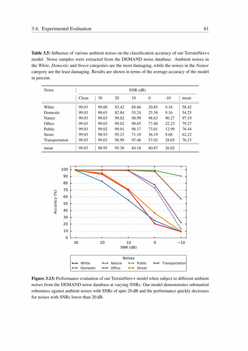
3.4. Experimental Evaluation 61
Table 3.5: Influence of various ambient noises on the classification accuracy of our TerrainNet++model. Noise samples were extracted from the DEMAND noise database. Ambient noises inthe White, Domestic and Street categories are the most damaging, while the noises in the Naturecategory are the least damaging. Results are shown in terms of the average accuracy of the modelin percent.
Noise SNR (dB)
Clean 30 20 10 0 -10 mean
White 99.03 99.00 93.42 69.66 20.85 9.16 58.42Domestic 99.03 98.63 82.84 55.24 25.38 9.16 54.25Nature 99.03 99.03 99.02 98.99 98.63 90.27 97.19Office 99.03 99.03 99.02 98.65 77.40 22.23 79.27Public 99.03 99.02 99.01 98.17 73.01 12.99 76.44Street 99.03 98.93 95.23 71.10 36.19 9.68 62.22Transportation 99.03 99.03 98.99 97.48 57.02 28.65 76.23
mean 99.03 98.95 95.36 84.18 60.87 26.02
30 20 10 0 10SNR (dB)
0102030405060708090
100
Accu
racy
(%)
NoisesWhiteDomestic
NatureOffice
PublicStreet
Transportation
Figure 3.13: Performance evaluation of our TerrainNet++ model when subject to different ambientnoises from the DEMAND noise database at varying SNRs. Our model demonstrates substantialrobustness against ambient noises with SNRs of upto 20 dB and the performance quickly decreasesfor noises with SNRs lower than 20 dB.
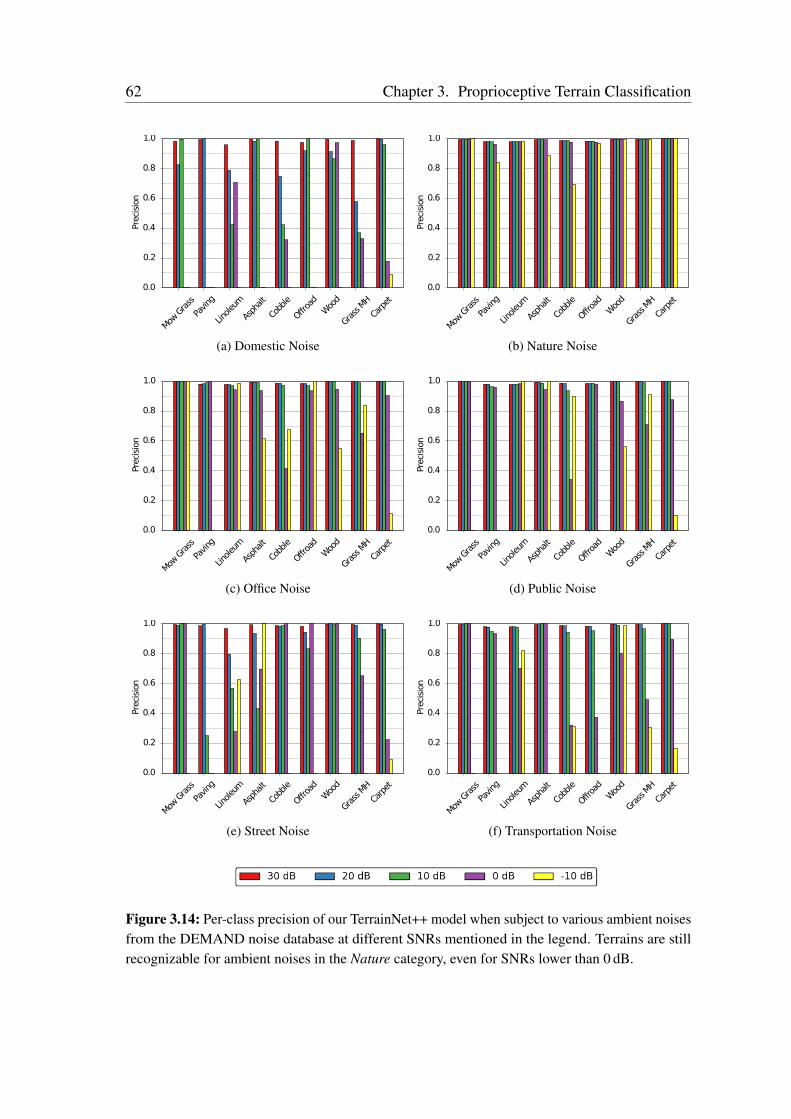
62 Chapter 3. Proprioceptive Terrain Classification
Mow G
rass
Pavin
g
Linole
um
Asph
alt
Cobb
le
Offroa
dWoo
d
Grass
MH
Carp
et0.0
0.2
0.4
0.6
0.8
1.0Pr
ecis
ion
Mow G
rass
Pavin
g
Linole
um
Asph
alt
Cobb
le
Offroa
dWoo
d
Grass
MH
Carp
et0.0
0.2
0.4
0.6
0.8
1.0
Prec
isio
n
(a) Domestic Noise (b) Nature Noise
Mow G
rass
Pavin
g
Linole
um
Asph
alt
Cobb
le
Offroa
dWoo
d
Grass
MH
Carp
et0.0
0.2
0.4
0.6
0.8
1.0
Prec
isio
n
Mow G
rass
Pavin
g
Linole
um
Asph
alt
Cobb
le
Offroa
dWoo
d
Grass
MH
Carp
et0.0
0.2
0.4
0.6
0.8
1.0
Prec
isio
n
(c) Office Noise (d) Public Noise
Mow G
rass
Pavin
g
Linole
um
Asph
alt
Cobb
le
Offroa
dWoo
d
Grass
MH
Carp
et0.0
0.2
0.4
0.6
0.8
1.0
Prec
isio
n
Mow G
rass
Pavin
g
Linole
um
Asph
alt
Cobb
le
Offroa
dWoo
d
Grass
MH
Carp
et0.0
0.2
0.4
0.6
0.8
1.0
Prec
isio
n
(e) Street Noise (f) Transportation Noise
Figure 3.14: Per-class precision of our TerrainNet++ model when subject to various ambient noisesfrom the DEMAND noise database at different SNRs mentioned in the legend. Terrains are stillrecognizable for ambient noises in the Nature category, even for SNRs lower than 0 dB.

3.4. Experimental Evaluation 63
Mow
Gra
ss
Paving
Lino
leum
Aspha
lt
Cobbl
e
Offroa
d
Woo
d
Grass
MH
Carpe
t
0.0
0.2
0.4
0.6
0.8
1.0
Pre
cisi
on
30 dB 20 dB 10 dB 0 dB -10 dB
Figure 3.15: Per-class precision of our TerrainNet++ model when subject to different levels ofwhite Gaussian noise. The levels mentioned in the legend are SNRs. White Gaussian noise is onlydamaging at very low SNRs.
Ambient noises in the Domestic category have the most damaging effect, where themean accuracy at SNRs from 30 dB to –10 dB was 61.71%. From the results shown inFigure 3.13, we can see that the performance of the model drops linearly for decreasingSNRs for noises from the Domestic category. The second most damaging noises were fromthe Street category for which our model achieved a mean accuracy of 68.36%. Nevertheless,we observe remarkable robustness to ambient noises from the Nature category for whichour model yields an average accuracy of 97.49% and even for extremely low SNRs.This is primarily due to the fact that the noises in the Nature category have very distinctspectral patterns that have prominent structures throughout the signal unlike vehicle-terraininteraction signals. Therefore, the model is inherently robust to these corruption patterns.
Often, it is also of interest to know how each of these ambient noises influence theclassification of a specific terrain. Therefore, we computed the per-class precision of theTerrainNet++ model for each of the ambient noise categories. Results from this experimentis shown in Figure 3.14 for ambient noises from the DEMAND noise database and inFigure 3.15 for white noise. The Carpet terrain is recognizable for all the ambient noisesand at all SNRs. While, the Paving terrain is the most affected by noise corruption,followed by Offroad and Asphalt terrains. Interestingly, classification of indoor terrainssuch as Linoleum, Wood and Carpet are less affected by indoor noises than outdoor terrains.However, the converse does not appear to be true, where the outdoor terrains are lessaffected by outdoor noises. This is due to the fact that, generally, outdoor ambient noiseshave continuous noise corruption patterns that span long periods, whereas, indoor ambient
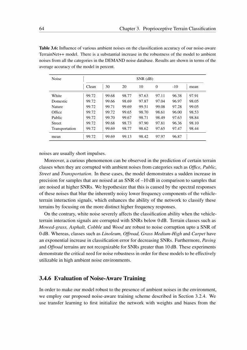
64 Chapter 3. Proprioceptive Terrain Classification
Table 3.6: Influence of various ambient noises on the classification accuracy of our noise-awareTerrainNet++ model. There is a substantial increase in the robustness of the model to ambientnoises from all the categories in the DEMAND noise database. Results are shown in terms of theaverage accuracy of the model in percent.
Noise SNR (dB)
Clean 30 20 10 0 -10 mean
White 99.72 99.68 98.77 97.63 97.11 96.38 97.91Domestic 99.72 99.66 98.69 97.87 97.04 96.97 98.05Nature 99.72 99.71 99.69 99.51 99.08 97.28 99.05Office 99.72 99.72 99.65 98.70 98.61 96.00 98.53Public 99.72 99.70 99.67 98.71 98.49 97.63 98.84Street 99.72 99.68 98.73 97.90 97.81 96.36 98.10Transportation 99.72 99.69 98.77 98.62 97.65 97.47 98.44
mean 99.72 99.69 99.13 98.42 97.97 96.87
noises are usually short impulses.Moreover, a curious phenomenon can be observed in the prediction of certain terrain
classes when they are corrupted with ambient noises from categories such as Office, Public,Street and Transportation. In these cases, the model demonstrates a sudden increase inprecision for samples that are noised at an SNR of –10 dB in comparison to samples thatare noised at higher SNRs. We hypothesize that this is caused by the spectral responsesof these noises that blur the inherently noisy lower frequency components of the vehicle-terrain interaction signals, which enhances the ability of the network to classify theseterrains by focusing on the more distinct higher frequency responses.
On the contrary, white noise severely affects the classification ability when the vehicle-terrain interaction signals are corrupted with SNRs below 0 dB. Terrain classes such asMowed-grass, Asphalt, Cobble and Wood are robust to noise corruption upto a SNR of0 dB. Whereas, classes such as Linoleum, Offroad, Grass Medium-High and Carpet havean exponential increase in classification error for decreasing SNRs. Furthermore, Pavingand Offroad terrains are not recognizable for SNRs greater than 10 dB. These experimentsdemonstrate the critical need for noise robustness in order for these models to be effectivelyutilizable in high ambient noise environments.
3.4.6 Evaluation of Noise-Aware Training
In order to make our model robust to the presence of ambient noises in the environment,we employ our proposed noise-aware training scheme described in Section 3.2.4. Weuse transfer learning to first initialize the network with weights and biases from the
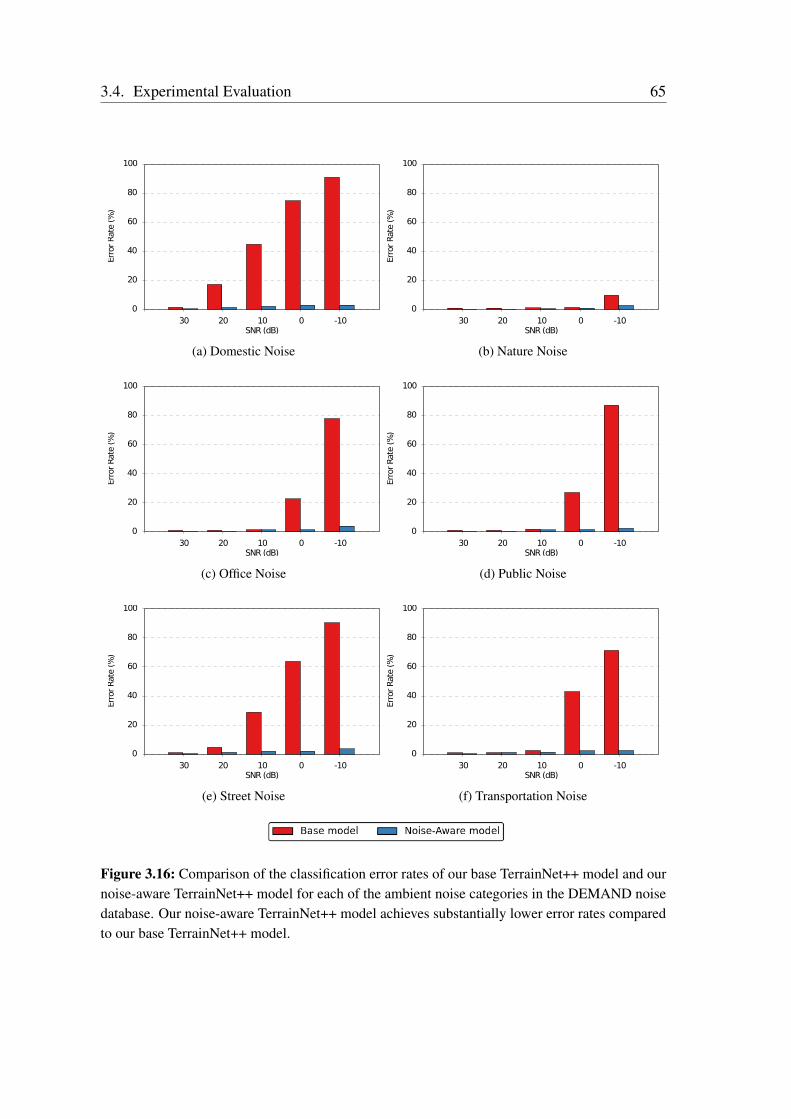
3.4. Experimental Evaluation 65
30 20 10 0 -10SNR (dB)
0
20
40
60
80
100
Erro
r Rat
e (%
)
30 20 10 0 -10SNR (dB)
0
20
40
60
80
100
Erro
r Rat
e (%
)
(a) Domestic Noise (b) Nature Noise
30 20 10 0 -10SNR (dB)
0
20
40
60
80
100
Erro
r Rat
e (%
)
30 20 10 0 -10SNR (dB)
0
20
40
60
80
100Er
ror
Rat
e (%
)
(c) Office Noise (d) Public Noise
30 20 10 0 -10SNR (dB)
0
20
40
60
80
100
Erro
r Rat
e (%
)
30 20 10 0 -10SNR (dB)
0
20
40
60
80
100
Erro
r Rat
e (%
)
(e) Street Noise (f) Transportation Noise
Figure 3.16: Comparison of the classification error rates of our base TerrainNet++ model and ournoise-aware TerrainNet++ model for each of the ambient noise categories in the DEMAND noisedatabase. Our noise-aware TerrainNet++ model achieves substantially lower error rates comparedto our base TerrainNet++ model.
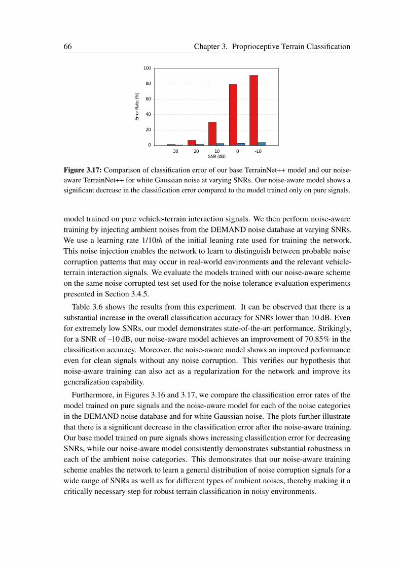
66 Chapter 3. Proprioceptive Terrain Classification
30 20 10 0 -10SNR (dB)
0
20
40
60
80
100
Erro
r Rat
e (%
)
Figure 3.17: Comparison of classification error of our base TerrainNet++ model and our noise-aware TerrainNet++ for white Gaussian noise at varying SNRs. Our noise-aware model shows asignificant decrease in the classification error compared to the model trained only on pure signals.
model trained on pure vehicle-terrain interaction signals. We then perform noise-awaretraining by injecting ambient noises from the DEMAND noise database at varying SNRs.We use a learning rate 1/10th of the initial leaning rate used for training the network.This noise injection enables the network to learn to distinguish between probable noisecorruption patterns that may occur in real-world environments and the relevant vehicle-terrain interaction signals. We evaluate the models trained with our noise-aware schemeon the same noise corrupted test set used for the noise tolerance evaluation experimentspresented in Section 3.4.5.
Table 3.6 shows the results from this experiment. It can be observed that there is asubstantial increase in the overall classification accuracy for SNRs lower than 10 dB. Evenfor extremely low SNRs, our model demonstrates state-of-the-art performance. Strikingly,for a SNR of –10 dB, our noise-aware model achieves an improvement of 70.85% in theclassification accuracy. Moreover, the noise-aware model shows an improved performanceeven for clean signals without any noise corruption. This verifies our hypothesis thatnoise-aware training can also act as a regularization for the network and improve itsgeneralization capability.
Furthermore, in Figures 3.16 and 3.17, we compare the classification error rates of themodel trained on pure signals and the noise-aware model for each of the noise categoriesin the DEMAND noise database and for white Gaussian noise. The plots further illustratethat there is a significant decrease in the classification error after the noise-aware training.Our base model trained on pure signals shows increasing classification error for decreasingSNRs, while our noise-aware model consistently demonstrates substantial robustness ineach of the ambient noise categories. This demonstrates that our noise-aware trainingscheme enables the network to learn a general distribution of noise corruption signals for awide range of SNRs as well as for different types of ambient noises, thereby making it acritically necessary step for robust terrain classification in noisy environments.
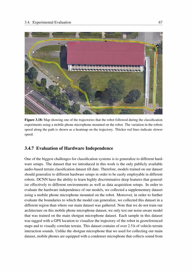
3.4. Experimental Evaluation 67
Figure 3.18: Map showing one of the trajectories that the robot followed during the classificationexperiments using a mobile phone microphone mounted on the robot. The variation in the robotsspeed along the path is shown as a heatmap on the trajectory. Thicker red lines indicate slowerspeed.
3.4.7 Evaluation of Hardware Independence
One of the biggest challenges for classification systems is to generalize to different hard-ware setups. The dataset that we introduced in this work is the only publicly availableaudio-based terrain classification dataset till date. Therefore, models trained on our datasetshould generalize to different hardware setups in order to be easily employable in differentrobots. DCNN have the ability to learn highly discriminative deep features that general-ize effectively to different environments as well as data acquisition setups. In order toevaluate the hardware independence of our models, we collected a supplementary datasetusing a mobile phone microphone mounted on the robot. Moreover, in order to furtherevaluate the boundaries to which the model can generalize, we collected this dataset in adifferent region than where our main dataset was gathered. Note that we do not train ourarchitecture on this mobile phone microphone dataset, we only test our noise-aware modelthat was trained on the main shotgun microphone dataset. Each sample in this datasetwas tagged with a GPS location to visualize the trajectory of the robot in georeferencedmaps and to visually correlate terrain. This dataset contains of over 2.5 h of vehicle-terraininteraction sounds. Unlike the shotgun microphone that we used for collecting our maindataset, mobile phones are equipped with a condenser microphone that collects sound from
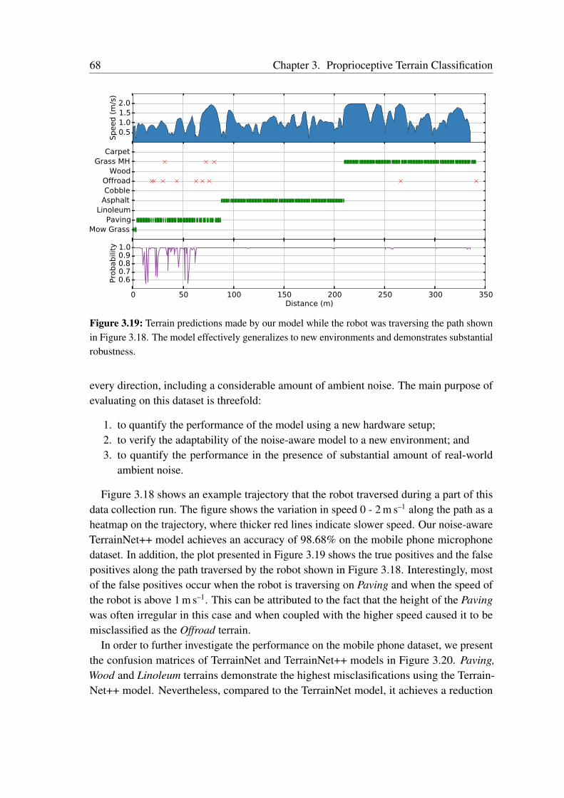
68 Chapter 3. Proprioceptive Terrain Classification
0.51.01.52.0
Speed (
m/s
)
Mow GrassPaving
LinoleumAsphaltCobbleOffroad
WoodGrass MH
Carpet
0 50 100 150 200 250 300 350Distance (m)
0.60.70.80.91.0
Pro
babili
ty
Figure 3.19: Terrain predictions made by our model while the robot was traversing the path shownin Figure 3.18. The model effectively generalizes to new environments and demonstrates substantialrobustness.
every direction, including a considerable amount of ambient noise. The main purpose ofevaluating on this dataset is threefold:
1. to quantify the performance of the model using a new hardware setup;2. to verify the adaptability of the noise-aware model to a new environment; and3. to quantify the performance in the presence of substantial amount of real-world
ambient noise.
Figure 3.18 shows an example trajectory that the robot traversed during a part of thisdata collection run. The figure shows the variation in speed 0 - 2 m s–1 along the path as aheatmap on the trajectory, where thicker red lines indicate slower speed. Our noise-awareTerrainNet++ model achieves an accuracy of 98.68% on the mobile phone microphonedataset. In addition, the plot presented in Figure 3.19 shows the true positives and the falsepositives along the path traversed by the robot shown in Figure 3.18. Interestingly, mostof the false positives occur when the robot is traversing on Paving and when the speed ofthe robot is above 1 m s–1. This can be attributed to the fact that the height of the Pavingwas often irregular in this case and when coupled with the higher speed caused it to bemisclassified as the Offroad terrain.
In order to further investigate the performance on the mobile phone dataset, we presentthe confusion matrices of TerrainNet and TerrainNet++ models in Figure 3.20. Paving,Wood and Linoleum terrains demonstrate the highest misclasifications using the Terrain-Net++ model. Nevertheless, compared to the TerrainNet model, it achieves a reduction

3.4. Experimental Evaluation 69
Mow Gras
sPa
ving
Linole
um
Aspha
lt
Cobble
Offroad
Wood
Grass M
HCarp
et
Mow Grass
Paving
Linoleum
Asphalt
Cobble
Offroad
Wood
Grass MH
Carpet
99.44 0.15 0.00 0.03 0.00 0.16 0.01 0.20 0.00
0.03 92.73 0.00 0.01 0.25 6.60 0.03 0.35 0.00
0.00 0.00 99.95 0.00 0.00 0.00 0.05 0.00 0.00
0.00 0.04 0.00 99.90 0.01 0.00 0.06 0.00 0.00
0.00 0.04 0.00 0.01 97.36 0.30 0.00 2.26 0.02
0.01 0.48 0.00 0.00 0.03 98.43 0.00 1.04 0.00
0.00 0.01 0.09 0.05 0.01 0.00 99.57 0.04 0.23
0.00 0.00 0.00 0.00 0.10 0.27 0.00 99.59 0.04
0.00 0.00 0.00 0.00 0.00 0.00 0.00 0.00 100.000
10
20
30
40
50
60
70
80
90
100
(a) Confusion matrix of our noise-aware TerrainNet model for a cliplength of 300 ms
Mow
Gra
ss
Paving
Lino
leum
Aspha
lt
Cobbl
e
Offroa
d
Woo
d
Grass
MH
Carpe
t
Mow Grass
Paving
Linoleum
Asphalt
Cobble
Offroad
Wood
Grass MH
Carpet
99.13 0.04 0.04 0.08 0.08 0.46 0.04 0.13 0.0
0.43 95.49 0.0 0.06 0.31 3.69 0.01 0.02 0.0
0.01 0.0 99.75 0.0 0.0 0.0 0.24 0.0 0.0
0.02 0.08 0.01 99.81 0.01 0.01 0.06 0.0 0.0
0.02 0.16 0.0 0.02 99.1 0.38 0.0 0.31 0.0
0.05 0.2 0.0 0.0 0.17 99.2 0.0 0.38 0.0
0.04 0.02 2.5 0.44 0.0 0.0 96.98 0.0 0.02
0.09 0.01 0.0 0.0 0.43 0.72 0.0 98.65 0.09
0.0 0.0 0.0 0.0 0.0 0.0 0.0 0.0 100.0
0
10
20
30
40
50
60
70
80
90
100
(b) Confusion matrix of our noise-aware TerrainNet++ model for a cliplength of 200 ms and a LSTM window length of five.
Figure 3.20: Performance comparison on the audio data collected using a mobile phone microphone.There is a significant decrease in misclassifications between the Paving and Ofroad terrains, as wellas Cobble and Grass Medium-High terrains.
70 Chapter 3. Proprioceptive Terrain Classification
of 3% in the misclassifications between the Paving and Offroad terrains, as well as asimilar reduction of misclassifications between the Cobble and Offroad terrains. Theseexperiments demonstrate that our models trained using our noise-aware training schemenot only generalize effectively to different environments but also to different hardwaresetups used for acquiring the data, thereby making our model effectively employable forrobust audio-based terrain classification in different real-world environments.
3.5 Related Work
In this chapter, we addressed the problem of audio-based terrain classification using vehicle-terrain interaction sounds. Terrain classification is a critical and essential component of arobot’s autonomy system that enables safe and efficient navigation on unknown terrains.Unlike conventional approaches that employ cameras or Lidars for terrain classification,using vehicle-terrain interaction sounds as a proprioceptive modality enables our system tobe robust to visual appearance changes and allows us to perform classification of terrainsat finer level. The techniques that we presented in this chapter enables a robot to utilize alow-cost microphone to robustly classify a wide range of indoor and outdoor terrains. Tothe best of our knowledge, our contribution is the first successful proprioceptive terrainclassification system to not require any manual feature engineering. In this section, wediscuss prior work in the literature on terrain classification using proprioceptive modalities.
Terrain classification using proprioceptive modalities has not been explored in the samedepth as vision based approaches, yet there is a sizable amount of work in this area. Themost researched proprioceptive terrain classification technique is using accelerometerdata [80, 113, 114]. Classification of terrains is performed by extracting features suchas power spectral density, discrete fourier transform and other statistical measures fromthe vibrations induced on the vehicles body. Such approaches demonstrate a substantialamount of false positives for finer terrain classes such as asphalt and carpet. However,accuracies as high as 91.8% has been reported for a seven class problem using SVMs [80].Subsequently, accelerometer data from a mobile sensor network system was used to detectpotholes and other road anomalies [79]. Hand-engineered features were used and thesystem achieves an average accuracy of 90% in real-world experiments.
There is a body of work in terrain classification tailored to legged robots. Unlikein wheeled mobile robots, proprioceptive terrain classification can enable safe footholdplacement which is critical to ensure the stability of such legged systems. In one of theinitial works [115], Hoepflinger et al. extracted features from ground contact forces andjoint motor current measurements to train a multiclass AdaBoost classifier. Although theydid not test the efficacy of their approach on real-world terrains, they demonstrated thecapability of the classifier to identify different coarseness and curvatures of surfaces as afirst step towards real-world proprioceptive terrain classification. In another approach [116],
3.5. Related Work 71
Best et al. demonstrate the ability to classify four different outdoor terrains using positionmeasurements from leg servos of a hexapod robot. They extract a 600-dimensional featurevector consisting of gait-phase domain as well as frequency domain features. Theirapproach utilizes a 2.7 s window of data and a SVM is trained to classify the terrains.
Vibration data from contact microphones has also been successfully used for terrainclassification. The vibrations captured from contact microphones are similar to accelerom-eter data than that of air microphones that we use in this work. Contact microphones pickup only structure-borne sound and minimal environmental noise. Brooks et al. equip thewheel of an analog rover with a contact microphone to capture the vibrations induced onthe vehicles body and classify the terrain [75]. The approach extracts log-scale powerspectral density features and uses a pairwise classifier. Their approach was evaluated onthree terrain classes and achieves an average accuracy of 74% on a wheel-terrain testbedand 85.3% in the real-world experiments using a rover. In a subsequent work, they presenta self-supervised classification approach where a visual classifier is trained using labelsprovided by a vibration-based terrain classifier [117].
The use of vehicle-terrain interaction sounds for terrain classification has been themost sparsely explored among all the proprioceptive modalities. In one of the earlyworks, Durst et al. [118] proposed an approach for classifying terrain surfaces from singleimpact sounds that were produced when the surfaces were struck by an aluminum cane.The approach extracts the most significant spikes in the frequency domain as featuresand employs a decision-tree classifier to identify the surface type. In the works thatfollowed, typically, combinations of state-of-the-art classical audio features are usedwith traditional machine learning algorithms. Recently, a multiclass audio-based terrainclassification system [76] for mobile robots was proposed in which several audio featureswere incorporated including spectral coefficients, spectral moments and various otherspectral and temporal statistics. The approach employs a SVM-based classifier thatachieves an average accuracy of 78% over three terrain classes and three hazardousvehicle-terrain interaction classes. Furthermore, they also show that smoothing over largertemporal window of about 2 s yields an improved accuracy of 92%. Ojeda et al. propose anapproach [113] in which a suite of sensors including microphones, accelerometers, motorcurrent and voltage sensors, infrared, ultrasonics and encoders were used along with afeedforward neural network classifier. However, their audio-based classifier only achievesan average accuracy of 60.3% for five terrain classes. They concluded that the overallperformance was poor and such an approach was promising only for terrains such as grass.
Microphones have also been used for terrain classification with legged robots. Ozkul etal. [78] propose an approach in which the terrain is classified from the steps taken bya hexapod robot. They use a feature set that includes zero-crossing rate, frequencyband coefficients and delta-features along with a functional trees classifier. They alsoexperiment with different noise elimination techniques to remove motor/gear-head noise,but concluded that the performance was worse after the noise elimination. Their seven class
72 Chapter 3. Proprioceptive Terrain Classification
terrain classifier achieves an average accuracy of 90%. More recently, Christe et al. [77]introduced an approach that employs an SVM-based classifier using statistics of spectraland band features to classify terrains from the sounds produced during the locomotion ofhexapod robot. Their classifier was trained on a dataset that contains 5 min audio clipsfrom each terrain and uses 1 s windows for classification while operating at 1 Hz. Theirapproach achieves an average accuracy of 89.08% for seven terrain classes. They alsoinvestigated the use of spectral subtraction to eliminate the servo noise and report animprovement of 2.2% in the recall of the classifier.
In all of the previous works, manually handcrafted features were extracted after spe-cialized preprocessing steps. The approaches were evaluated on comparatively limiteddata and only in one environment. Most importantly, these approaches do not model thetemporally discriminative information in proprioceptive data. As we demonstrated inthis chapter, modeling the temporal information substantially improves the classificationperformance, increases robustness and reduces false detections. Furthermore, they do notaddress the robustness of their models to ambient noise, which is one of the most criticalrequirements for real-world deployment. Whereas, in this chapter, we presented twoDCNN architectures that learn to classify terrains from vehicle-terrain interaction soundswithout the need for manually designing the features. Our recurrent DCNN architectureexploits the complex temporal dynamics in the vehicle-terrain interaction signal and has aclassification rate of 81 Hz. We also introduced a noise-aware training scheme to improvethe robustness of our model to different ambient noises, better regularize the network andto enable our model to effectively generalize to different real-world environments.
3.6 Conclusions
In this chapter, we presented a robust proprioceptive terrain classification approach thatuses sound from vehicle terrain-interactions to classify a wide range of indoor and outdoorterrains. We proposed two novel deep convolutional neural network architectures that learnfeatures from spectrograms of vehicle-terrain interaction signals. Both our architecturesemploy one dimensional convolution and pooling layers to learn spectrogram featuresacross the temporal dimension. Additionally, our networks incorporate our proposedGSP module that aggregates the statistics of pooled features across time. In order tofurther learn the complex temporal dynamics in the vehicle-terrain interaction signal, ourrecurrent TerrainNet++ architecture incorporates long short-term memory units that exploittemporal relationships in the sequence of input audio frames. Furthermore, we introduceda noise-aware training scheme that injects ambient environmental noise from the diverseenvironments multichannel acoustic noise database into the pure vehicle-terrain interactionsignals while training to improve the robustness of the model and to regularize the network.In order to facilitate this work, we collected an extensive vehicle-terrain interaction dataset
3.6. Conclusions 73
consisting of over 15 h of audio data using two different hardware setups. Our dataset wascollected on a total of nine different indoor as well as outdoor terrains and we made thedataset publicly available to foster future progress in proprioceptive terrain classification.
We presented extensive empirical evaluations that demonstrate that both our TerrainNetand recurrent TerrainNet++ architectures outperform existing approaches that employclassical audio features and achieve state-of-the-art results for proprioceptive terrainclassification. In depth analysis of our TerrainNet++ architecture shows that exploitingthe temporal dynamics by incorporating both our proposed GSP module and the LSTMunit substantially improves the classification performance while simultaneously increasingthe classification rate. We presented thorough ablation studies on the influence of varioushyperparameters on the classification performance of our network. Our best performingTerrainNet++ model achieves an overall accuracy of 99.03% with a classification rate of81.7 Hz. Additionally, we presented extensive robustness evaluations of our models thatdemonstrate high ambient noise tolerance in various real-world environments. Furthermore,we presented thorough evaluations of our proposed noise-aware training scheme thatenables our model to further improve its performance and achieve an accuracy of 99.72%while demonstrating exceptional robustness to a variety of ambient noises, even for verylow signal-to-noise ratios. We also presented experiments using an inexpensive low-qualitymicrophone in an unknown environment and demonstrated the generalization capabilityas well as the hardware independence of our approach. To the best of our knowledge, theapproach presented in this chapter is the first proprioceptive terrain classification techniquethat does not require manual hand-engineering of features and achieves an accuracy ofover 98% on a wide range of indoor as well as outdoor terrains while being over twice asfast as real-time.

Chapter 4
Semantic Scene Segmentation
Semantic segmentation is an essential task for autonomous robots,as accurate understanding of the surroundings is a precursor fornavigation and action planning. Recently, deep learning-based ap-proaches have achieved unprecedented performance for various se-mantic segmentation problems, yet they face an immense challengesin terms of encoding multiscale information, incorporating globalcontext, accurately capturing object boundaries and in achievingcomputational efficiency. In this chapter, we propose two CNN ar-chitectures that address the aforementioned challenges. Our firstarchitecture termed AdapNet incorporates our multiscale residualunits with atrous convolutions that effectively enlarges the recep-tive field of filters to incorporate a larger context. In addition, weemploy modules with parallel atrous convolutions with different di-lation rates to learn multiscale features without increasing the pa-rameters. We also propose the AdapNet++ architecture that buildsupon AdapNet and integrates our efficient atrous spatial pyramidpooling for aggregating multiscale information as well as captur-ing long range context, complemented with a novel decoder with amulti-resolution supervision scheme that recovers high-resolutiondetails. Furthermore, we propose a network-wide holistic pruningapproach invariant to shortcut connections. Extensive experimentson multiple indoor and outdoor benchmarks demonstrate that ourarchitectures achieve state-of-the-art performance while being effi-cient in terms of parameters and inference time.
4.1 Introduction
In the previous chapter, we proposed an approach to robustly classify different indoorand outdoor terrains in order to enable the robot to adapt its navigation policy so that it
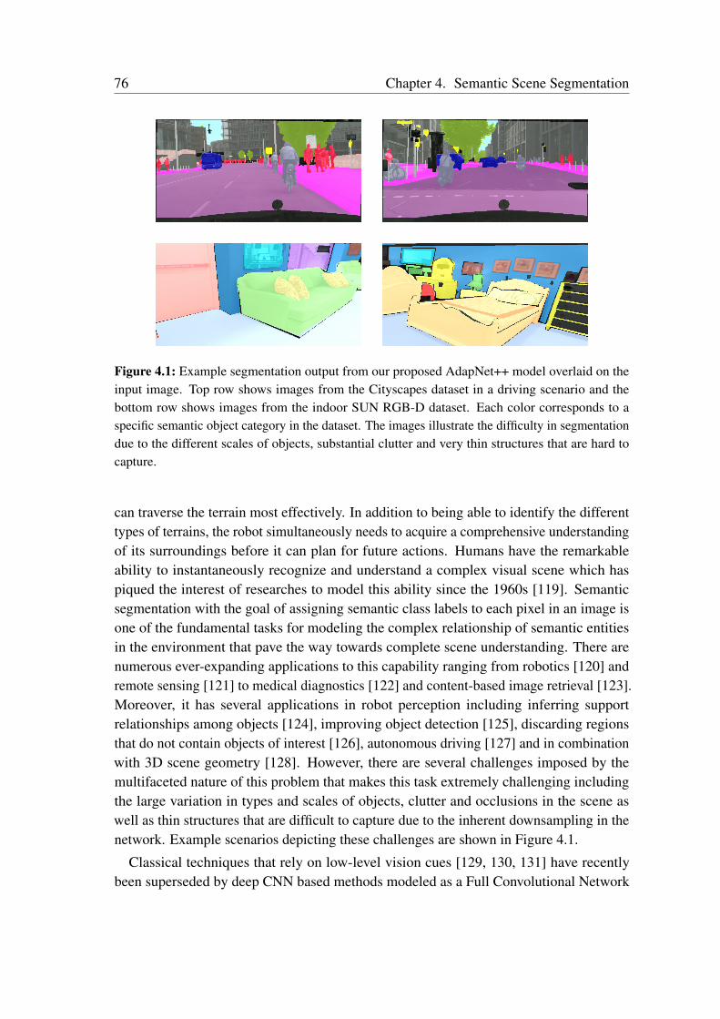
76 Chapter 4. Semantic Scene Segmentation
Figure 4.1: Example segmentation output from our proposed AdapNet++ model overlaid on theinput image. Top row shows images from the Cityscapes dataset in a driving scenario and thebottom row shows images from the indoor SUN RGB-D dataset. Each color corresponds to aspecific semantic object category in the dataset. The images illustrate the difficulty in segmentationdue to the different scales of objects, substantial clutter and very thin structures that are hard tocapture.
can traverse the terrain most effectively. In addition to being able to identify the differenttypes of terrains, the robot simultaneously needs to acquire a comprehensive understandingof its surroundings before it can plan for future actions. Humans have the remarkableability to instantaneously recognize and understand a complex visual scene which haspiqued the interest of researches to model this ability since the 1960s [119]. Semanticsegmentation with the goal of assigning semantic class labels to each pixel in an image isone of the fundamental tasks for modeling the complex relationship of semantic entitiesin the environment that pave the way towards complete scene understanding. There arenumerous ever-expanding applications to this capability ranging from robotics [120] andremote sensing [121] to medical diagnostics [122] and content-based image retrieval [123].Moreover, it has several applications in robot perception including inferring supportrelationships among objects [124], improving object detection [125], discarding regionsthat do not contain objects of interest [126], autonomous driving [127] and in combinationwith 3D scene geometry [128]. However, there are several challenges imposed by themultifaceted nature of this problem that makes this task extremely challenging includingthe large variation in types and scales of objects, clutter and occlusions in the scene aswell as thin structures that are difficult to capture due to the inherent downsampling in thenetwork. Example scenarios depicting these challenges are shown in Figure 4.1.
Classical techniques that rely on low-level vision cues [129, 130, 131] have recentlybeen superseded by deep CNN based methods modeled as a Full Convolutional Network
4.1. Introduction 77
(FCN) [24, 53, 132] that are trained in an end-to-end manner. This success can be attributedto the ability of CNNs to learn highly discriminative hierarchical deep features. The generalstructure of a FCN follows an encoder-decoder design principle, in which the encoderresembles the topology of a classification network and the decoder semantically projectsthe low-resolution discriminative features learned by the encoder onto the high-resolutionpixel space to obtain a dense classification. However, unlike in pure classification networkswhere the built-in invariance of CNNs to local image transformations is beneficial, it ishighly undesirable in dense prediction tasks where abstraction of spatial information affectsthe performance. Concretely, the following are the major challenges for employing CNNsfor semantic segmentation:
• Decrease in feature resolution caused by pooling and striding.• Existence of objects at multiple scales.• Reduced localization accuracy due to invariance.• Large model size and runtime.
In the rest of this section, we discuss each of the aforementioned challenges and describethe techniques that we employ to overcome them in our proposed architectures. CNNsdesigned for classification tasks that are often employed as the encoder in FCNs havemultiple pooling or convolution layers with striding operations to learn increasingly abstractfeature representations that are invariant to local image transformation. However, thissignificantly reduces the spatial resolution of feature maps at the output of the encoder,which have rich semantic information. Due to this factor, details on the object boundariesand thin structures are lost and cannot be recovered even using deconvolutional layersthat learn the up-sampling [24]. In order to alleviate this problem, we reduce the numberof downsampling operations in the encoder section of our network and incorporate ourproposed multiscale residual units that introduce atrous convolutions [67] in parallel to thestandard convolutions to extract denser feature maps. This enables our multiscale residualunits to enlarge the receptive field of the filters thereby encoding higher level semanticswithout increasing the number of parameters or the computational operations.
The second challenge arises due to the presence of objects in different scales in thereal-world. Over the years, several techniques have been proposed to address this problemincluding using multiple rescaled versions of the same image as input to the network [133,134], using spatial pyramid pooling [135], exploiting features from each downsamplingstage in the encoder-decoder topology [136] and employing multiple encoder branches witheach taking a different resolution of the image as input [137]. Though these approacheshave been reasonably effective, they substantially increase the computational overhead andmemory requirement. Alternatively, as we employ atrous convolutions in our proposedmultiscale residual units, incorporating multiple such units into the architecture withdifferent dilation rates can enable effective multiscale feature learning throughout thenetwork. DeepLab [138] proposed a similar module called Atrous Spatial Pyramid Pooling

78 Chapter 4. Semantic Scene Segmentation
(ASPP) that concatenates feature maps from atrous convolutions with different dilationrates to encode multiscale information. However, input images of large resolutions cannotbe employed in order for it be effective, as it requires correspondingly increasing thedilation rate which causes atrous convolutions to become more ineffective due to imageboundary effects [132]. Moreover, ASPP consumes 15.53 M parameters and 34.58 Bfloating point operations per second (FLOPS) which is prohibitively expensive to employin architectures that are used in robotics applications for which computational efficiencyis paramount. In addition, as ASPP uses a large number of high-dimensional and high-resolution feature maps, it requires an enormous amount of GPU memory while trainingwhich also restricts the incorporation of modules to address the other major challenges. Asa solution to this problem we propose an efficient variant of the ASPP termed eASPP thatemploys both parallel and cascaded atrous convolutions in a bottleneck fashion to increasethe resolution of the effective receptive field while significantly reducing the number ofparameters it consumes.
Another challenge lies in the inherent invariance to spatial transformations in CNNsthat limits the spatial localization accuracy of the features. Moreover, atrous convolutionscoarsely sub-sample the features which leads to the loss of important details along objectboundaries. In order to generate high-resolution predictions in the decoder, networks oftenutilize skip connections to leverage features from multiple intermediate network stagesthat retain spatial information and describe mid-level representations of objects [24, 139].These features are complementary to the high-level semantic information at the end ofthe decoder that lack strong spatial information as well as to low-level features from earlynetwork layers that represent edges and corners but also maintain the spatial information.In our proposed architectures we employ such skip connections to leverage both low-leveland mid-level features to improve the resolution of the segmentation output to generatesharp boundaries along the edges of objects. In addition, we also propose a multi-resolutionsupervision strategy that introduces weighted auxiliary losses after each upsampling stagein the decoder to deeply supervise the training and to further help in generating a high-resolution segmentation output. This also enables faster convergence, in addition toimproving the performance of the model along the object boundaries.
State-of-the-art semantic segmentation architectures such as DeepLab v3 [132] andPSPnet [135] employ the ResNet-101 [27] architecture which consumes 42.39 M parame-ters and 113.96 B FLOPS, as the encoder backbone. Training such architectures requiresa large amount of memory and synchronized training across multiple GPUs. Moreover,they have a slow runtime rendering them impractical for resource constrained applicationssuch as robotics and augmented reality. With the goal of achieving the right trade-offbetween performance and computational complexity, we propose the AdapNet and Adap-Net++ architectures for semantic segmentation. Our AdapNet architecture employs theResNet-50 [27] architecture that consumes 25.61 M parameters for the encoder backboneand incorporates our proposed multiscale residual units to aggregate multiscale features
4.1. Introduction 79
throughout the network without increasing the number of parameters. The proposed unitsare more effective in learning multiscale features than the commonly employed multigridapproach introduced in DeepLab v3 [132]. AdapNet uses deconvolution layers and asingle stage skip refinement to yield a segmentation output with the same resolution asthe input image. In order to further improve the performance, we propose the AdapNet++architecture that builds upon AdapNet but uses the full pre-activation ResNet-50 [72] archi-tecture for the encoder backbone in order to reduce overfitting and improve convergence.In addition, we incorporate our proposed eASPP at the end of the encoder to capture longrange context with a larger effective receptive field, while simultaneously reducing thenumber of parameters by 87% in comparison to the originally proposed ASPP. We alsoemploy a new decoder that integrates low and mid-level features from the encoder usingmultiple skip refinement stages and employs a multi-resolution supervision strategy forhigh-resolution segmentation. Both our proposed architectures are compact and end-to-endtrainable with a large mini-batch size on a single consumer grade GPU.
Motivated by the recent success of compressing DCNNs by pruning unimportant neu-rons [140, 141, 142], we explore pruning entire convolutional feature maps of our modelto further reduce the number of parameters. Network pruning approaches utilize a costfunction to first rank the importance of neurons, followed by removing the least importantneurons and fine-tuning the network to recover any loss in accuracy. Thus far, theseapproaches have only been employed for pruning convolutional layers that do not havean identity or a projection shortcut connection. Pruning residual feature maps (third con-volutional layer of a residual unit) also necessitates pruning the projected feature mapsin the same configuration in order to maintain the shortcut connection. This leads to asignificant drop in accuracy, therefore current approaches omit pruning convolutionalfilters with shortcut connections. As a solution to this problem, we propose a network-wideholistic pruning approach that employs a simple and yet effective strategy for pruningconvolutional filters invariant to the presence of shortcut connections. This enables ournetwork to further reduce the number of parameters and computing operations, makingour model efficiently deployable even in resource constrained applications.
Most work in semantic segmentation thus far has been focused on indoor and outdoor ur-ban environments where the scene is highly structured. However, there exists an increasingnumber of applications where mobile robots are tasked to operate in unstructured outdoorenvironments that have significantly more variation in semantic object classes and a sub-stantial amount of perceptual disturbances due to changes in weather conditions. In orderto also evaluate the performance our proposed architectures in such scenarios, we introducea first-of-a-kind dataset collected in unstructured forested environments that we madepublicly available. We present extensive experimental evaluations of our architectures onbenchmark scene understanding datasets including Cityscapes [143], Synthia [144], SUNRGB-D [145] and ScanNet [146] as well as on our Freiburg Forest [50] dataset. The resultsdemonstrate that our architectures set the new state-of-the-art on all these benchmarks
80 Chapter 4. Semantic Scene Segmentation
while being computationally more efficient and with a faster inference time.
In summary, the following are the main contributions that we make in this chapter:
• The novel AdapNet architecture for semantic segmentation that incorporates ourmultiscale residual units to effectively learn multiscale features throughout thenetwork and a decoder with skip refinement for high-resolution segmentation.• The AdapNet++ architecture that further improves the performance by integrating
a new efficient ASPP (eASPP) to aggregate multiscale information, a new decoderwith multiple skip refinement stages and a multi-resolution supervision strategy forfiner segmentation along the object boundaries.• The eASPP for efficiently aggregating multiscale features and capturing long range
context, while having a larger effective receptive field and over 10 times reduction inparameters compared to the standard ASPP.• A holistic network-wide pruning approach that enables pruning of convolutional
filters invariant to the presence of identity or projection shortcuts.• A novel semantic segmentation dataset of unstructured forested environments con-
sisting of multiple modalities and spectra with semantically annotated pixel-levelgroundtruth labels.• Extensive benchmarking of existing approaches with the same input image size and
evaluation setting along with quantitative and qualitative evaluations of our proposedarchitectures on five different benchmark datasets consisting of indoor environments,outdoor driving scenarios and unstructured forested environments.• Implementations of our proposed models are made publicly available at http://deepscene.cs.uni-freiburg.de.
The remainder of this chapter is organized as follows. In Section 4.2, we describeour semantic segmentation architectures and our technique for pruning convolutionalfilters. We then describe the methodology that we employed for collecting the FreiburgForest dataset in Section 4.3. In Section 4.4, we present extensive empirical evaluations,detailed ablation studies on the design choices and model variants, followed by qualitativeevaluations on each of the datasets that we benchmark on. Finally, we discuss recentrelated work on semantic segmentation in Section 4.5 and conclude with a discussion inSection 4.6.
4.2 Technical Approach
In this section, we first describe the topology of our proposed AdapNet architectureand then detail the structure of our AdapNet++ architecture as well as its constitutingcomponents. Subsequently, we present our pruning strategy for network compression thatis invariant to the presence of identity or projection shortcuts in the residual units.
4.2. Technical Approach 81
4.2.1 AdapNet Architecture
Our architecture shown in Figure 4.2 follows the general fully convolutional encoder-decoder design principle. The encoder has a topology similar to classification networksand downsamples the input image, while the decoder upsamples the feature maps back tothe input image resolution. In the following sections, we describe the components of ourproposed AdapNet architecture.
4.2.1.1 AdapNet Encoder
Encoders are the foundation of FCN architectures. Therefore, it is essential to build upon agood baseline that has a high representational ability conforming with the computationalbudget. Our critical requirement is to achieve the right trade-off between the accuracy ofsegmentation and inference time on a consumer grade GPU, while keeping the numberof parameters low. Therefore, in contrast to the previous approaches, we build uponthe ResNet-50 [27] architecture as it offers a good trade-off between learning highlydiscriminative deep features and the computational complexity required. It includes batchnormalization and convolution layers with skip connections. This allows the design ofmuch deeper networks without facing degradation of the gradient and therefore leads tovery large receptive fields. The ResNet architecture has four computational blocks withvarying number of residual units. We use the bottleneck residual units in our encoder asthey are computationally more efficient than the baseline residual units and they enable usto build more complex models that are easily trainable.
In the ResNet architecture, the resolution of the feature maps drops down to a fourth ofthe input resolution after passing through the first 3 layers. On the one hand, this allowsfor context aggregation and speed-up due to smaller feature maps, but on the other hand,this restricts the learning of high-resolution features, which could potentially be useful inthe later stages. In our AdapNet architecture, we introduced an additional convolution witha kernel size of 3× 3 before the first convolution layer in the ResNet-50 architecture. Thisenables the network to learn more high-resolution features without significantly increasingthe inference time. The output of the last residual block of the ResNet-50 architecture is32-times downsampled with respect to the input image resolution. In order to increasethe spatial density of the feature responses and to prevent signal decimation, we set thestride of the convolution layer in the last block (Res4a) from two to one which makes theresolution of the output feature maps 1/16-times the input image resolution. This enablesthe network to retain the higher resolution details while aggregating the same amount ofcontext as before. We then replace the residual blocks that follow this last downsamplingstage with our proposed multiscale residual units.
Multiscale Residual Units: A naive approach to compute the feature responses at thefull image resolution would be to remove the downsampling and replace all the convolution
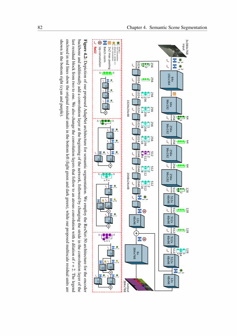
82 Chapter 4. Semantic Scene Segmentation
11
11
12
x4
8x9
6
1113
11
d1
d2
d1
d2
d1
d2
1111
311
3x3
84
x7
68
inp
ut
outp
ut
38
4x7
68
s113
11s1
64
x1
92
x3
84
1327
64
x9
6x1
92
64
25
6
64
25
6
64
25
6
12
8
51
2
12
8
51
22
56
x9
6x1
92
25
6x
96
x1
92
51
2x
48
x9
65
12
x4
8x9
65
12
x4
8x9
62
56
x9
6x1
92
12
8
51
25
12
x4
8x9
6
12
8 1
64
51
2
25
6
10
24
10
24
x2
4x4
8
25
6
10
24
25
6 1
2
56
10
24
25
6 1
25
6
10
24
25
6 1
25
6
10
24
25
6 1
25
6
10
24
51
2 2
51
2
20
48
51
2 2
51
2
20
48
51
2 2
51
2
20
48
20
48
x2
4x4
8
6x
38
4x7
68
12
x4
8x9
6
1111
3
nxn co
nvolu
tion
2x2
max p
oolin
g
Batch
norm
Up
-convolu
tion
ReLU
d1
d2
d3
d3
d1
d1
d2
d1
d1
d2d2
d1
d2
d3d3
d1
d2
d3d3
d2
stride s
n s
nxn co
nvolu
tion
dila
tion d
, stride =
1n d
dd
dd
2
24
81
64
81
6
s
12
2
3 p3 p
pp
22
22
Figure4.2:D
epictionofourproposed
AdapN
etarchitectureforsem
anticsegm
entation.We
employ
theR
esNet-50
architectureforthe
encoderbackbone
andadditionally
adda
convolutionlayeratthe
beginningofthe
network,follow
edby
changingthe
stridein
theconvolution
layerofthelastresidualblock
fromtw
oto
one.We
alsochange
theconvolution
layersthatfollow
toan
atrousconvolution
with
adilation
ofr=
2.The
legendenclosed
inred
linesshow
theoriginalresidualunits
inthe
bottomleft(lightgreen
anddark
green),while
ourproposedm
ultiscaleresidualunits
areshow
nin
thebottom
right(cyanand
purple).
4.2. Technical Approach 83
layers with atrous convolutions having a dilation rate r ≥ 2 but this would be bothcomputationally and memory intensive. Therefore, we propose the novel multiscaleresidual unit to efficiently enlarge the receptive field and aggregate multiscale featureswithout increasing the number of parameters and the computational burden. Specifically,we replace the 3× 3 convolution in the standard residual unit with two parallel 3× 3 atrousconvolutions with different dilation rates and half the number of feature maps each. Wethen concatenate their outputs before the following 1× 1 convolution. By concatenatingtheir outputs, the network additionally learns to combine the feature maps of differentscales. Now, by setting the dilation rate in one of the 3× 3 convolutional layers to r = 1and another to a rate r ≥ 2, we can preserve the original scale of the features within theblock and simultaneously add larger context. While, by varying the dilation rates in eachof the parallel 3×3 convolutions, we can enable the network to effectively learn multiscalerepresentations at different stages of the network. The topology of the proposed multiscaleresidual units and the corresponding original residual units are shown in the legend inFigure 4.2. The lower left two units show the original configuration, while the lower righttwo units show the proposed configuration.
We incorporate the first multiscale residual unit with r1 = 1 and r2 = 2 before the thirdblock at Res3d (unit before the block where we remove the downsampling as mentionedearlier). Subsequently, we replace the units Res4c, Res4d, Res4e, and Res4f with ourproposed multiscale units with rates r1 = 1 in all the units and r2 = 2, 4, 8, 16 corre-spondingly. In addition, we replace the last three units of block four Res5a, Res5b, andRes5c with the multiscale units with increasing rates in both the 3 × 3 convolutions, as(r1 = 2, r2 = 4), (r1 = 2, r2 = 8), and (r1 = 2, r2 = 16) correspondingly. We evaluate ourproposed configuration in comparison to the multigrid method of DeepLab v3 [132] in theablation study presented in Section 4.4.6.1.
4.2.1.2 AdapNet Decoder
The output of the encoder is 16-times downsampled with respect to the input image and itcontains 2, 048 feature channels. In order to obtain the segmented image, we first employ a1× 1 convolution layer to reduce the number of feature channels to the number of semanticobject categories in the dataset. We then upsample feature maps by two times using adeconvolution layer and perform refinement by fusing mid-level features from Res3d ofthe encoder. Subsequently, we employ a second deconvolution layer to upsample thepredictions by eight times to yield an output with the same dimensions as the input image.In comparison to the initial FCN architecture [24], our proposed AdapNet architecture hasa significantly lesser number of parameters and a substantially faster inference time, whichare both critical requirements for models to be employed in real-world robotic perceptionapplications. Moreover, the network converges in 12 hours while training on an NVIDIATitan X GPU, whereas FCNs take about three days for the model to converge.
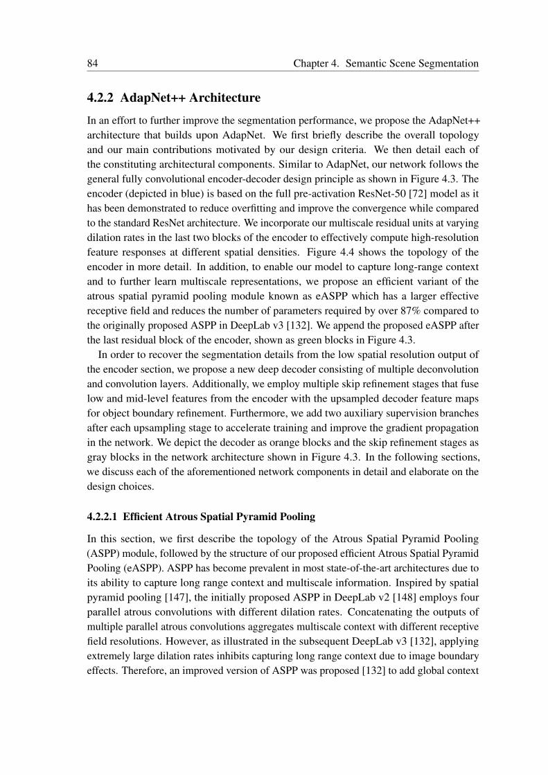
84 Chapter 4. Semantic Scene Segmentation
4.2.2 AdapNet++ Architecture
In an effort to further improve the segmentation performance, we propose the AdapNet++architecture that builds upon AdapNet. We first briefly describe the overall topologyand our main contributions motivated by our design criteria. We then detail each ofthe constituting architectural components. Similar to AdapNet, our network follows thegeneral fully convolutional encoder-decoder design principle as shown in Figure 4.3. Theencoder (depicted in blue) is based on the full pre-activation ResNet-50 [72] model as ithas been demonstrated to reduce overfitting and improve the convergence while comparedto the standard ResNet architecture. We incorporate our multiscale residual units at varyingdilation rates in the last two blocks of the encoder to effectively compute high-resolutionfeature responses at different spatial densities. Figure 4.4 shows the topology of theencoder in more detail. In addition, to enable our model to capture long-range contextand to further learn multiscale representations, we propose an efficient variant of theatrous spatial pyramid pooling module known as eASPP which has a larger effectivereceptive field and reduces the number of parameters required by over 87% compared tothe originally proposed ASPP in DeepLab v3 [132]. We append the proposed eASPP afterthe last residual block of the encoder, shown as green blocks in Figure 4.3.
In order to recover the segmentation details from the low spatial resolution output ofthe encoder section, we propose a new deep decoder consisting of multiple deconvolutionand convolution layers. Additionally, we employ multiple skip refinement stages that fuselow and mid-level features from the encoder with the upsampled decoder feature mapsfor object boundary refinement. Furthermore, we add two auxiliary supervision branchesafter each upsampling stage to accelerate training and improve the gradient propagationin the network. We depict the decoder as orange blocks and the skip refinement stages asgray blocks in the network architecture shown in Figure 4.3. In the following sections,we discuss each of the aforementioned network components in detail and elaborate on thedesign choices.
4.2.2.1 Efficient Atrous Spatial Pyramid Pooling
In this section, we first describe the topology of the Atrous Spatial Pyramid Pooling(ASPP) module, followed by the structure of our proposed efficient Atrous Spatial PyramidPooling (eASPP). ASPP has become prevalent in most state-of-the-art architectures due toits ability to capture long range context and multiscale information. Inspired by spatialpyramid pooling [147], the initially proposed ASPP in DeepLab v2 [148] employs fourparallel atrous convolutions with different dilation rates. Concatenating the outputs ofmultiple parallel atrous convolutions aggregates multiscale context with different receptivefield resolutions. However, as illustrated in the subsequent DeepLab v3 [132], applyingextremely large dilation rates inhibits capturing long range context due to image boundaryeffects. Therefore, an improved version of ASPP was proposed [132] to add global context
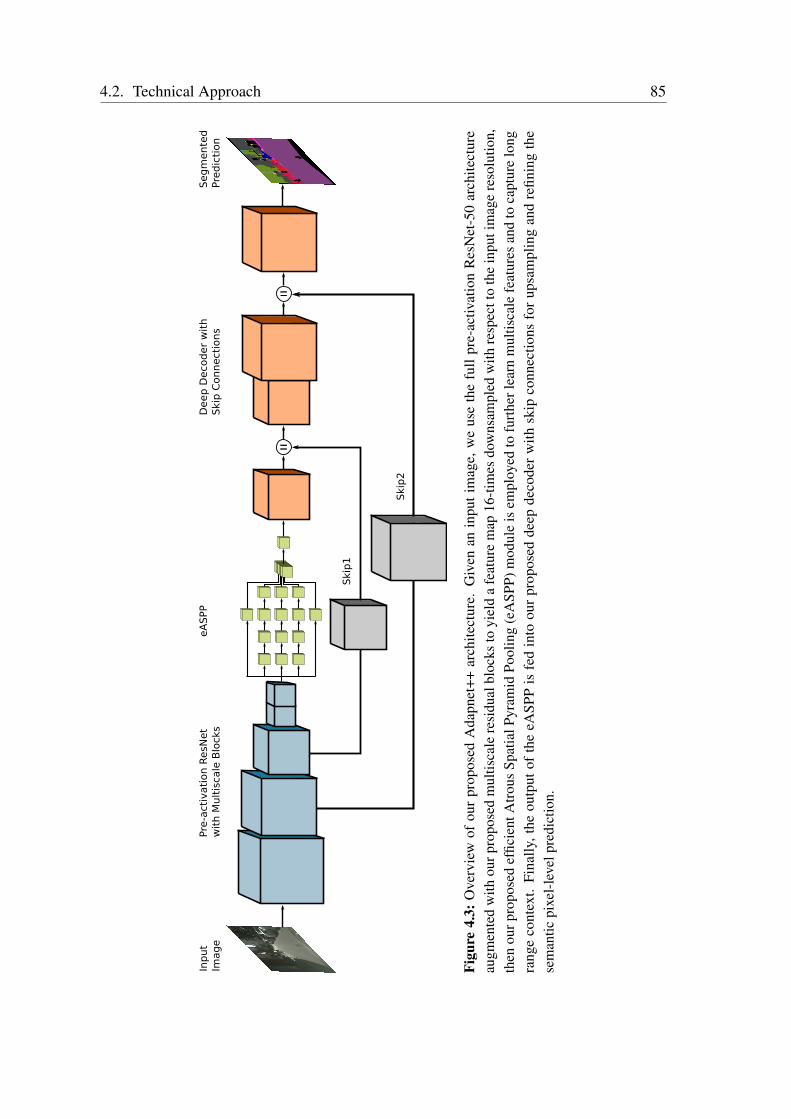
4.2. Technical Approach 85
25
6x
24
x48
25
6x
24
x48
25
6x
24
x48
25
6x
24
x48
Pre
-act
ivati
on R
esN
et
wit
h M
ult
isca
le B
lock
seA
SPP
Deep
Deco
der
wit
h
Ski
p C
onn
ect
ions
Inp
ut
Imag
eS
eg
mente
dPre
dic
tion
Ski
p1
Ski
p2
Figu
re4.
3:O
verv
iew
ofou
rpr
opos
edA
dapn
et++
arch
itect
ure.
Giv
enan
inpu
tim
age,
we
use
the
full
pre-
activ
atio
nR
esN
et-5
0ar
chite
ctur
eau
gmen
ted
with
ourp
ropo
sed
mul
tisca
lere
sidu
albl
ocks
toyi
eld
afe
atur
em
ap16
-tim
esdo
wns
ampl
edw
ithre
spec
tto
the
inpu
tim
age
reso
lutio
n,th
enou
rpro
pose
def
ficie
ntA
trou
sSp
atia
lPyr
amid
Pool
ing
(eA
SPP)
mod
ule
isem
ploy
edto
furt
herl
earn
mul
tisca
lefe
atur
esan
dto
capt
ure
long
rang
eco
ntex
t.Fi
nally
,the
outp
utof
the
eASP
Pis
fed
into
our
prop
osed
deep
deco
der
with
skip
conn
ectio
nsfo
rup
sam
plin
gan
dre
finin
gth
ese
man
ticpi
xel-
leve
lpre
dict
ion.
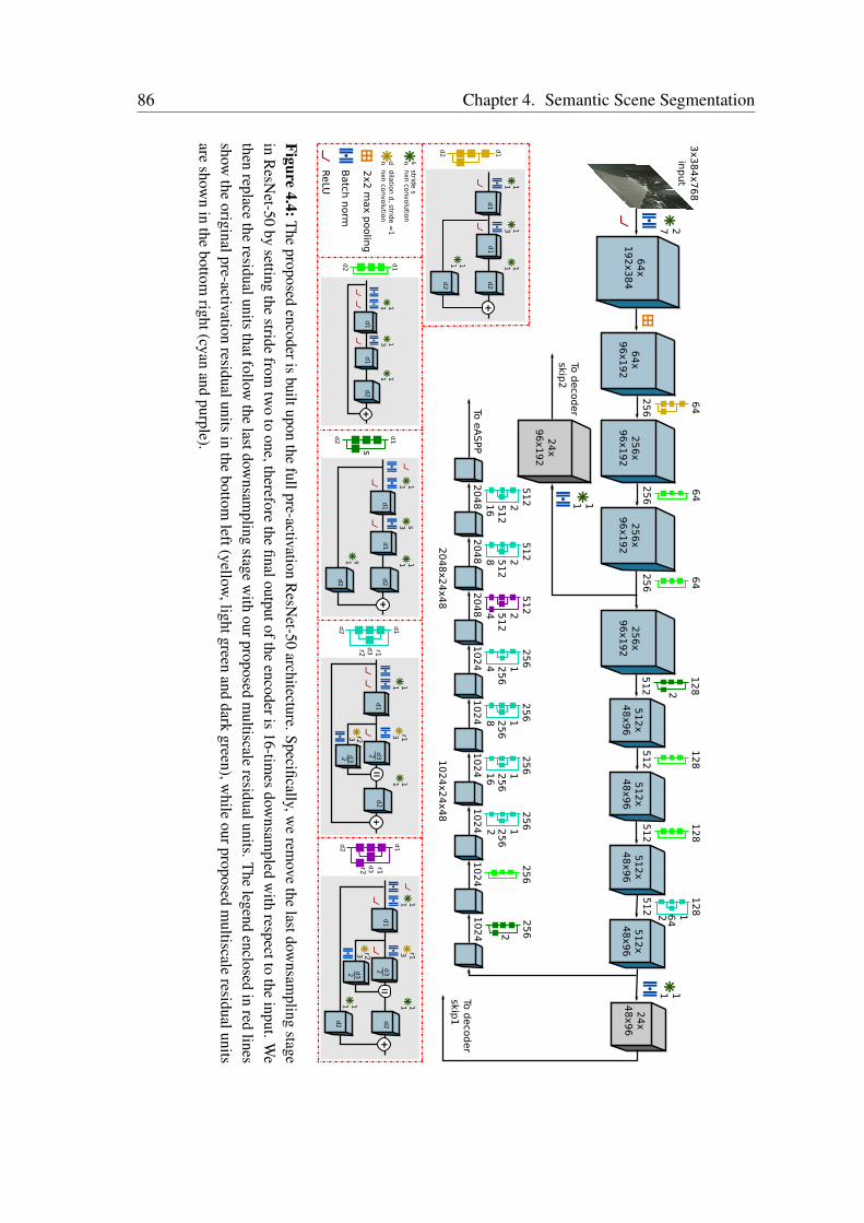
86 Chapter 4. Semantic Scene Segmentation
1113
11
d1
d2
d1
d2
d1
d2
1111
311
3x3
84
x7
68
input
11s3
11s1
64
x1
92
x3
84
27
64
x9
6x1
92
64
25
6
64
25
6
64
25
6
12
8
51
2
12
8
51
22
56
x9
6x1
92
25
6x
96
x1
92
51
2x
48
x9
65
12
x4
8x9
65
12
x4
8x9
62
56
x9
6x1
92
12
8
51
25
12
x4
8x9
6
12
8 1
64
51
2
25
6
10
24
10
24
x2
4x4
8
25
6
10
24
25
6 1
25
6
10
24
25
6 1
25
6
10
24
25
6 1
25
6
10
24
20
48
x2
4x4
8
1111
3
nxn co
nvolu
tion
2x2
max p
oolin
g
Batch
norm
d1
d2
d3
d3
d1
d1
d2
d1
d1
d2d2
d1
d2
d3d3
d1
d2
d3d3
d2
stride s
n s
nxn co
nvolu
tion
dila
tion d
, stride =
1n d
r2r2
r2r2
2
25
6 1
2
56
10
24 2
48
16
s
2
2
3 r13 r1
r1r1
22
22
11
24
x4
8x9
6
51
2 2
51
2
20
48 1
6
51
2 2
51
2
20
48 8
51
2 2
51
2
20
48 4
24
x9
6x1
92
11
To e
ASPP
To d
eco
der
skip2
To d
eco
der
skip1
d1
d2
1113
1111
d1
d1
d2d2
ReLU
Figure4.4:The
proposedencoderis
builtuponthe
fullpre-activationR
esNet-50
architecture.Specifically,we
remove
thelastdow
nsampling
stagein
ResN
et-50by
settingthe
stridefrom
two
toone,therefore
thefinaloutputofthe
encoderis16-tim
esdow
nsampled
with
respecttothe
input.We
thenreplace
theresidualunits
thatfollowthe
lastdownsam
plingstage
with
ourproposedm
ultiscaleresidualunits.The
legendenclosed
inred
linesshow
theoriginalpre-activation
residualunitsin
thebottom
left(yellow,lightgreen
anddark
green),while
ourproposedm
ultiscaleresidualunits
areshow
nin
thebottom
right(cyanand
purple).
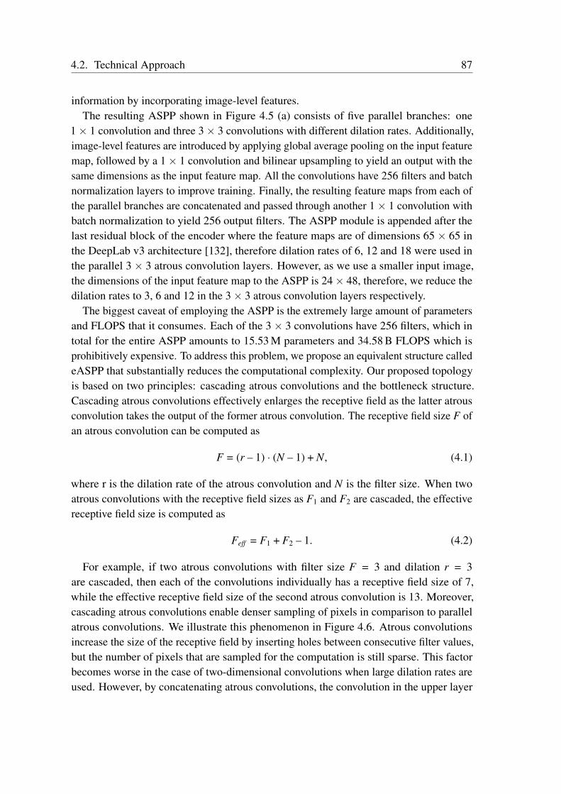
4.2. Technical Approach 87
information by incorporating image-level features.The resulting ASPP shown in Figure 4.5 (a) consists of five parallel branches: one
1× 1 convolution and three 3× 3 convolutions with different dilation rates. Additionally,image-level features are introduced by applying global average pooling on the input featuremap, followed by a 1× 1 convolution and bilinear upsampling to yield an output with thesame dimensions as the input feature map. All the convolutions have 256 filters and batchnormalization layers to improve training. Finally, the resulting feature maps from each ofthe parallel branches are concatenated and passed through another 1× 1 convolution withbatch normalization to yield 256 output filters. The ASPP module is appended after thelast residual block of the encoder where the feature maps are of dimensions 65 × 65 inthe DeepLab v3 architecture [132], therefore dilation rates of 6, 12 and 18 were used inthe parallel 3 × 3 atrous convolution layers. However, as we use a smaller input image,the dimensions of the input feature map to the ASPP is 24× 48, therefore, we reduce thedilation rates to 3, 6 and 12 in the 3× 3 atrous convolution layers respectively.
The biggest caveat of employing the ASPP is the extremely large amount of parametersand FLOPS that it consumes. Each of the 3× 3 convolutions have 256 filters, which intotal for the entire ASPP amounts to 15.53 M parameters and 34.58 B FLOPS which isprohibitively expensive. To address this problem, we propose an equivalent structure calledeASPP that substantially reduces the computational complexity. Our proposed topologyis based on two principles: cascading atrous convolutions and the bottleneck structure.Cascading atrous convolutions effectively enlarges the receptive field as the latter atrousconvolution takes the output of the former atrous convolution. The receptive field size F ofan atrous convolution can be computed as
F = (r – 1) · (N – 1) + N, (4.1)
where r is the dilation rate of the atrous convolution and N is the filter size. When twoatrous convolutions with the receptive field sizes as F1 and F2 are cascaded, the effectivereceptive field size is computed as
Feff = F1 + F2 – 1. (4.2)
For example, if two atrous convolutions with filter size F = 3 and dilation r = 3are cascaded, then each of the convolutions individually has a receptive field size of 7,while the effective receptive field size of the second atrous convolution is 13. Moreover,cascading atrous convolutions enable denser sampling of pixels in comparison to parallelatrous convolutions. We illustrate this phenomenon in Figure 4.6. Atrous convolutionsincrease the size of the receptive field by inserting holes between consecutive filter values,but the number of pixels that are sampled for the computation is still sparse. This factorbecomes worse in the case of two-dimensional convolutions when large dilation rates areused. However, by concatenating atrous convolutions, the convolution in the upper layer
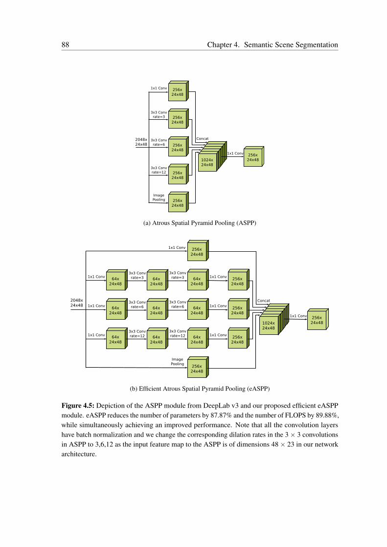
88 Chapter 4. Semantic Scene Segmentation
256x24x48256x
24x48256x24x48256x
24x481024x24x48
2048x24x48
3x3 Convrate=3
3x3 Convrate=12
3x3 Convrate=6
1x1 Conv
ImagePooling
Concat
256x24x48
256x24x48
256x24x48
256x24x48
256x24x48
1x1 Conv 256x24x48
(a) Atrous Spatial Pyramid Pooling (ASPP)
64x24x48
1x1 Conv
1x1 Conv
1x1 Conv
64x24x48
64x24x48
64x24x48
64x24x48
64x24x48
64x24x48
64x24x48
64x24x48
256x24x48
256x24x48
256x24x48
256x24x48
256x24x48
256x24x48256x
24x48256x24x48256x
24x481024x24x48
Concat
1x1 Conv
ImagePooling
1x1 Conv
1x1 Conv
1x1 Conv
3x3 Convrate=3
3x3 Convrate=12
3x3 Convrate=6
3x3 Convrate=3
3x3 Convrate=12
3x3 Convrate=6
1x1 Conv 256x24x48
2048x24x48
(b) Efficient Atrous Spatial Pyramid Pooling (eASPP)
Figure 4.5: Depiction of the ASPP module from DeepLab v3 and our proposed efficient eASPPmodule. eASPP reduces the number of parameters by 87.87% and the number of FLOPS by 89.88%,while simultaneously achieving an improved performance. Note that all the convolution layershave batch normalization and we change the corresponding dilation rates in the 3× 3 convolutionsin ASPP to 3,6,12 as the input feature map to the ASPP is of dimensions 48× 23 in our networkarchitecture.
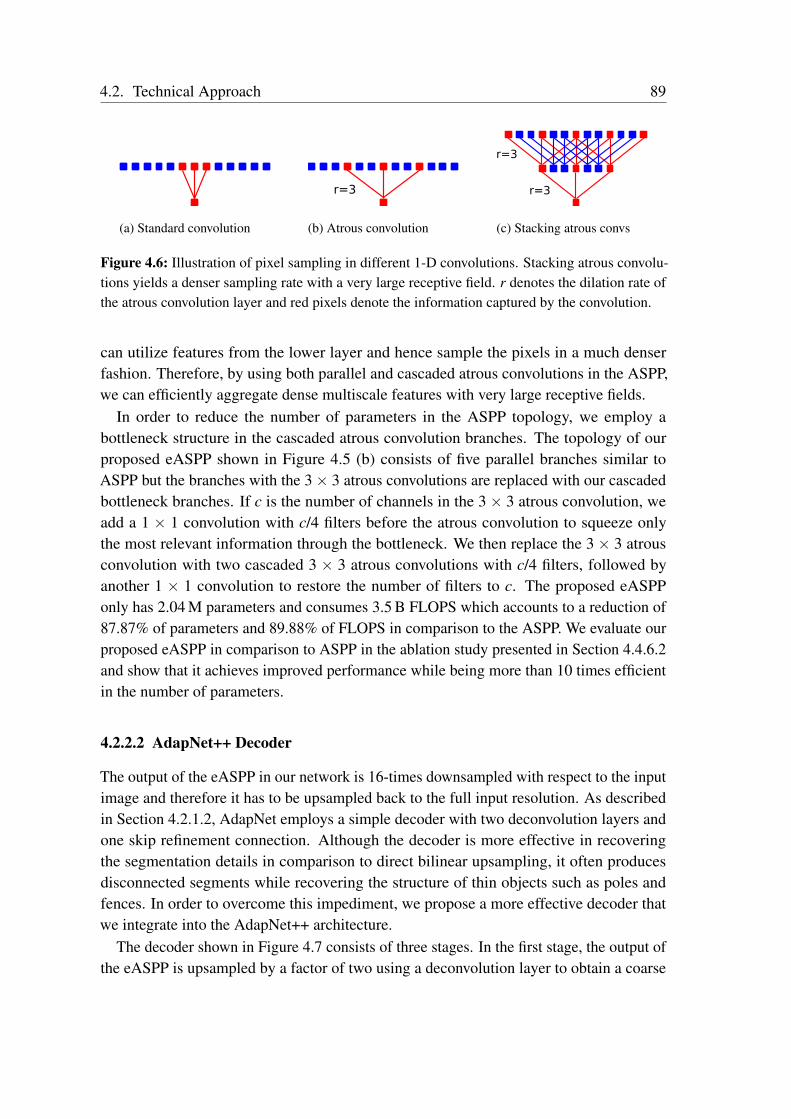
4.2. Technical Approach 89
r=3
r=3
r=3
(a) Standard convolution (b) Atrous convolution (c) Stacking atrous convs
Figure 4.6: Illustration of pixel sampling in different 1-D convolutions. Stacking atrous convolu-tions yields a denser sampling rate with a very large receptive field. r denotes the dilation rate ofthe atrous convolution layer and red pixels denote the information captured by the convolution.
can utilize features from the lower layer and hence sample the pixels in a much denserfashion. Therefore, by using both parallel and cascaded atrous convolutions in the ASPP,we can efficiently aggregate dense multiscale features with very large receptive fields.
In order to reduce the number of parameters in the ASPP topology, we employ abottleneck structure in the cascaded atrous convolution branches. The topology of ourproposed eASPP shown in Figure 4.5 (b) consists of five parallel branches similar toASPP but the branches with the 3× 3 atrous convolutions are replaced with our cascadedbottleneck branches. If c is the number of channels in the 3× 3 atrous convolution, weadd a 1 × 1 convolution with c/4 filters before the atrous convolution to squeeze onlythe most relevant information through the bottleneck. We then replace the 3 × 3 atrousconvolution with two cascaded 3 × 3 atrous convolutions with c/4 filters, followed byanother 1 × 1 convolution to restore the number of filters to c. The proposed eASPPonly has 2.04 M parameters and consumes 3.5 B FLOPS which accounts to a reduction of87.87% of parameters and 89.88% of FLOPS in comparison to the ASPP. We evaluate ourproposed eASPP in comparison to ASPP in the ablation study presented in Section 4.4.6.2and show that it achieves improved performance while being more than 10 times efficientin the number of parameters.
4.2.2.2 AdapNet++ Decoder
The output of the eASPP in our network is 16-times downsampled with respect to the inputimage and therefore it has to be upsampled back to the full input resolution. As describedin Section 4.2.1.2, AdapNet employs a simple decoder with two deconvolution layers andone skip refinement connection. Although the decoder is more effective in recoveringthe segmentation details in comparison to direct bilinear upsampling, it often producesdisconnected segments while recovering the structure of thin objects such as poles andfences. In order to overcome this impediment, we propose a more effective decoder thatwe integrate into the AdapNet++ architecture.
The decoder shown in Figure 4.7 consists of three stages. In the first stage, the output ofthe eASPP is upsampled by a factor of two using a deconvolution layer to obtain a coarse
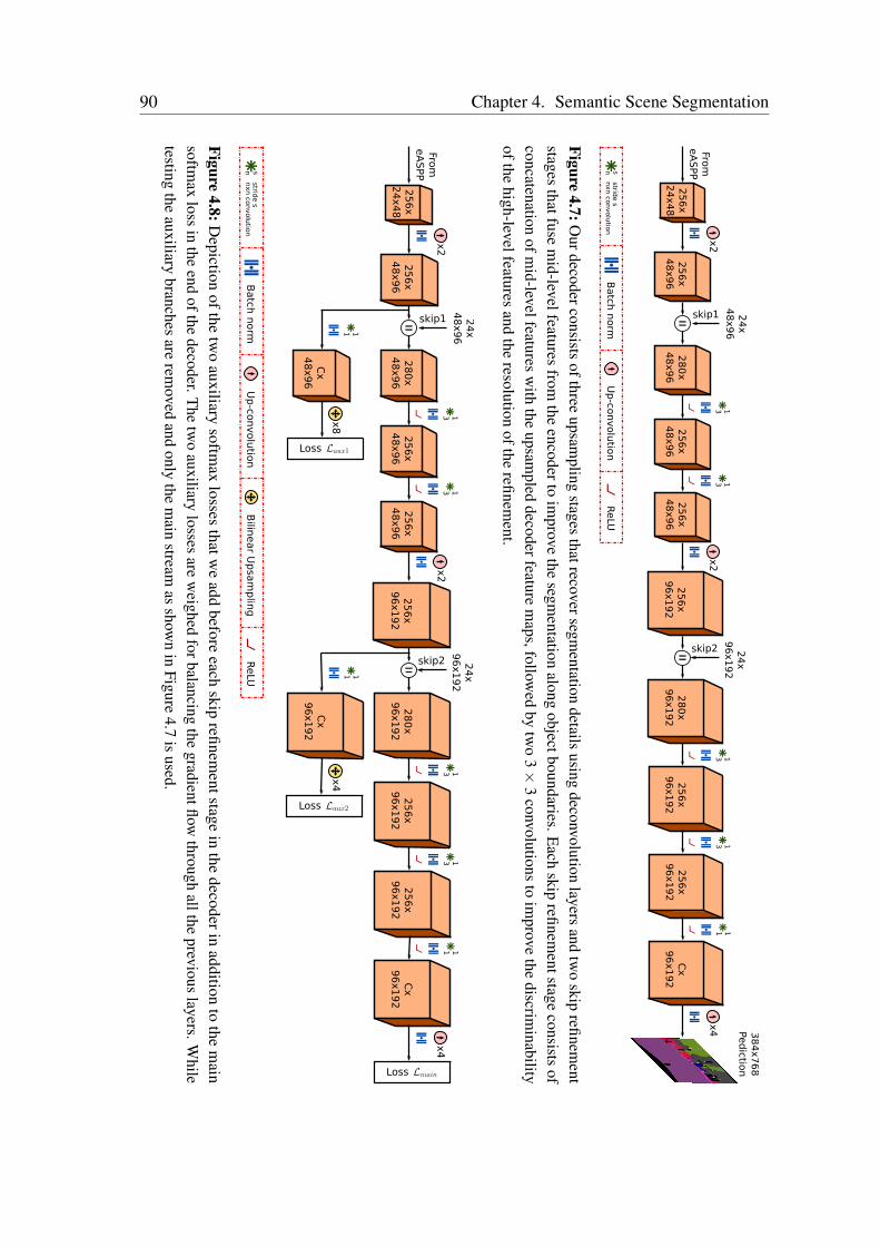
90 Chapter 4. Semantic Scene Segmentation
Batch
norm
Up
-convolu
tion
nxn co
nvolu
tion
stride s
n sR
eLU
x4
Cx
96
x1
92
25
6x
96
x1
92
11
25
6x
96
x1
92
13
28
0x
96
x1
92
13
25
6x
96
x1
92
x2
25
6x
48
x9
62
56
x4
8x9
62
80
x4
8x9
6
1313
24
x4
8x9
6
25
6x
48
x9
6
x2
25
6x
24
x4
8
38
4x7
68
Ped
iction
skip1
24
x9
6x1
92
skip2
From
eA
SPP
Figure4.7:O
urdecoderconsistsofthree
upsampling
stagesthatrecoversegm
entationdetails
usingdeconvolution
layersand
two
skiprefinem
entstages
thatfusem
id-levelfeaturesfrom
theencoderto
improve
thesegm
entationalong
objectboundaries.Each
skiprefinem
entstageconsists
ofconcatenation
ofmid-levelfeatures
with
theupsam
pleddecoderfeature
maps,follow
edby
two
3×
3convolutions
toim
provethe
discriminability
ofthehigh-levelfeatures
andthe
resolutionofthe
refinement.
Cx
96
x1
92
25
6x
96
x1
92
25
6x
96
x1
92
28
0x
96
x1
92
25
6x
96
x1
92
25
6x
48
x9
62
56
x4
8x9
62
80
x4
8x9
6
24
x4
8x9
6
25
6x
48
x9
62
56
x2
4x4
8
skip1
24
x9
6x1
92
skip2
From
eA
SPP
Loss
Loss
Loss
x2
x2
1313
x4
1113
13
Cx
96
x1
92
11
Cx
48
x9
6
11
x8
x4
Batch
norm
Up
-convolu
tion
nxn co
nvolu
tion
stride s
n sR
eLU
Bilin
ear U
psa
mp
ling
Figure4.8:D
epictionof
thetw
oauxiliary
softmax
lossesthatw
eadd
beforeeach
skiprefinem
entstagein
thedecoder
inaddition
tothe
main
softmax
lossin
theend
ofthedecoder.T
hetw
oauxiliary
lossesare
weighed
forbalancingthe
gradientflowthrough
alltheprevious
layers.While
testingthe
auxiliarybranches
arerem
ovedand
onlythe
main
streamas
shown
inFigure
4.7is
used.

4.2. Technical Approach 91
segmentation mask. The upsampled coarse mask is then passed through the second stage,where the feature maps are concatenated with the first skip refinement from Res3d. Theskip refinement consists of a 1× 1 convolution layer to reduce the feature depth in order tonot outweigh the encoder features. We experiment with varying number of feature channelsin the skip refinement in the ablation study presented in Section 4.4.6.3. The concatenatedfeature maps are then passed through two 3× 3 convolutions to improve the resolution ofthe refinement, followed by a deconvolution layer that again upsamples the feature mapsby a factor of two. This upsampled output is fed to the last decoder stage which resemblesthe previous stage consisting of concatenation with the feature maps from the second skiprefinement from Res2c, followed by two 3× 3 convolution layers. All the convolutionaland deconvolutional layers until this stage have 256 feature channels, therefore the outputfrom the two 3 × 3 convolutions in the last stage is fed to a 1 × 1 convolution layer toreduce the number of feature channels to the number of object categories C. This output isfinally fed to the last deconvolution layer which upsamples the feature maps by a factor offour to recover the original input resolution.
4.2.2.3 Multiresolution Supervision
Deep networks often have difficulty in training due to the intrinsic instability associatedwith learning using gradient descent which leads to exploding or vanishing gradientproblems. As our encoder is based on the residual learning framework, shortcut connectionsin each unit help propagating the gradient more effectively. Another technique that can beused to mitigate this problem to a certain extent is by initializing the layers with pretrainedweights, however our proposed eASPP and decoder layers still have to be trained fromscratch which could lead to optimization difficulties. Recent deep architectures haveproposed employing an auxiliary loss in the middle of encoder network [135, 149], inaddition to the main loss towards the end of the network. However, as shown in the ablationstudy presented in Section 4.4.6.1 this does not improve the performance of our networkalthough it helps the optimization to converge faster.
Unlike previous approaches, we propose a multi-resolution supervision strategy to bothaccelerate the training and improve the resolution of the segmentation. As described in theprevious section, our decoder consists of three upsampling stages. We add two auxiliaryloss branches at the end of the first and second stage after the deconvolution layer inaddition to the main softmax loss Lmain at the end of the decoder as shown in Figure 4.8.Each auxiliary loss branch decreases the feature channels to the number of category labelsC using a 1×1 convolution with batch normalization and upsamples the feature maps to theinput resolution using bilinear upsampling. We only use simple bilinear upsampling whichdoes not contain any weights instead of a deconvolution layer in the auxiliary loss branchesas our aim is to force the main decoder stream to improve its discriminativeness at eachupsampling resolution so that it embeds multi-resolution information while learning to
92 Chapter 4. Semantic Scene Segmentation
upsample. We weigh the two auxiliary losses Laux1 and Laux2 to balance the gradient flowthrough all the previous layers. While testing, the auxiliary loss branches are discardedand only the main decoder stream is used. We experiment with different loss weightings inthe ablation study presented in Section 4.4.6.3, and we show that each of the auxiliary lossbranches improves the segmentation performance in addition to speeding-up the trainingin Section 4.4.6.1.
4.2.3 Network Compression
As we strive to design an efficient and compact semantic segmentation architecture that canbe employed in resource constrained applications, we must ensure that the utilization ofconvolutional filters in our network is thoroughly optimized. Often, even the most compactnetworks have abundant neurons in deeper layers that do not significantly contribute tothe overall performance of the model. Excessive convolutional filters not only increasethe model size but also the inference time and the number of computing operations.These factors critically hinder the deployment of models in resource constrained real-world applications. Pruning of neural networks can be traced back to the 80s whenLeCun et al. [150] introduced a technique called Optimal Brain Damage for selectivelypruning weights with a theoretically justified measure. Recently, several new techniqueshave been proposed for pruning weight matrices [141, 142, 151, 152] of convolutionallayers as most of the computation during inference is consumed by them.
These approaches rank neurons based on their contribution and remove the low rankingneurons from the network, followed by fine-tuning of the pruned network. While thesimplest neuron ranking method computes the `1-norm of each convolutional filter [152],more sophisticated techniques have recently been proposed [140, 141, 142]. Some of theseapproaches are based on sparsity based regularization of network parameters which addi-tionally increases the computational overhead during training [141, 151]. Techniques [142]have also been proposed for structured pruning of entire kernels with strided sparsity thatdemonstrate impressive results for pruning small networks. However, their applicability tocomplex networks that are to be evaluated on large validation sets has not been exploreddue its heavy computational processing. Moreover, until a year ago these techniques wereonly applied to simpler architectures such as VGG [153] and AlexNet [22], as pruningcomplex deep architectures such as ResNets requires a holistic approach. Thus far, pruningof residual units has only been performed on convolutional layers that do not have anidentity or shortcut connection as pruning them additionally requires pruning the addedresidual maps in the exact same configuration. Attempts to prune them in the same config-uration have resulted in a significant drop in performance [152]. Therefore, often only thefirst and the second convolutional layers of a residual unit are pruned.
Our proposed architectures have shortcut and skip connections both in the encoder aswell the decoder. Therefore, in order to efficiently maximize the pruning of our network,
4.2. Technical Approach 93
we propose a holistic network-wide pruning technique that is invariant to the presenceof skip or shortcut connections. Our proposed technique first involves pruning all theconvolutional layers of a residual unit, followed by masking out the pruned indices of thelast convolutional layer of a residual unit with zeros before the addition of the residual mapsfrom the shortcut connection. As masking is performed after the pruning, we efficientlyreduce the parameters and computing operations in a holistic fashion, while optimallypruning all the convolutional layers and preserving the shortcut or skip connections. Aftereach pruning iteration, we fine-tune the network to recover any loss in accuracy. Weillustrate this strategy adopting a recently proposed greedy criteria-based oracle pruningtechnique that incorporates a novel ranking method based on a first order Taylor expansionof the network cost function [140]. The pruning problem is framed as a combinatorialoptimization problem such that when the weights B of the network are pruned, the changein cost value will be minimal.
minW ′|C(T |W ′) – C(T |W)| s.t. ‖W ′‖0 ≤ B, (4.3)
where T is the training set, W is the network parameters and C(·) is the negative log-likelihood function. Based on Taylor expansion, the change in the loss function fromremoving a specific parameter can be approximated. Let hi be the output feature mapsproduced by parameter i and hi = z1
0, z20, · · · , zCl
L . The output hi can be pruned by settingit to zero and the ranking can be given by
|∆C(hi)| = |C(T , hi = 0) – C(T , hi)|, (4.4)
Approximating with Taylor expansion, we can write
ΘTE(hi) = |∆C(hi)| = |C(T , hi) –δCδhi
hi – C(T , hi)|
=∣∣∣∣ δCδhi
hi
∣∣∣∣ , (4.5)
ΘTE(z(k)l ) =
∣∣∣∣∣ 1M
∑m
δCδz(k)
l,m
z(k)l,m
∣∣∣∣∣ , (4.6)
where M is the length of the vectorized feature map. This ranking can be easily computedusing the standard back-propagation computation as it requires the gradient of the costfunction with respect to the activation and the product of the activation. Furthermore, inorder to achieve adequate rescaling across layers, a layer-wise `2-norm of the rankings iscomputed as
Θ(z(k)l ) =
Θ(z(k)l )√∑
j Θ2(z(j)l )
. (4.7)
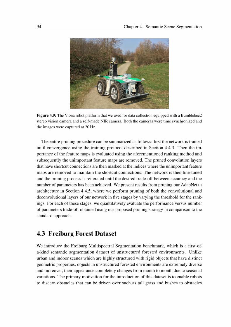
94 Chapter 4. Semantic Scene Segmentation
Figure 4.9: The Viona robot platform that we used for data collection equipped with a Bumblebee2stereo vision camera and a self-made NIR camera. Both the cameras were time synchronized andthe images were captured at 20 Hz.
The entire pruning procedure can be summarized as follows: first the network is traineduntil convergence using the training protocol described in Section 4.4.3. Then the im-portance of the feature maps is evaluated using the aforementioned ranking method andsubsequently the unimportant feature maps are removed. The pruned convolution layersthat have shortcut connections are then masked at the indices where the unimportant featuremaps are removed to maintain the shortcut connections. The network is then fine-tunedand the pruning process is reiterated until the desired trade-off between accuracy and thenumber of parameters has been achieved. We present results from pruning our AdapNet++architecture in Section 4.4.5, where we perform pruning of both the convolutional anddeconvolutional layers of our network in five stages by varying the threshold for the rank-ings. For each of these stages, we quantitatively evaluate the performance versus numberof parameters trade-off obtained using our proposed pruning strategy in comparison to thestandard approach.
4.3 Freiburg Forest Dataset
We introduce the Freiburg Multispectral Segmentation benchmark, which is a first-of-a-kind semantic segmentation dataset of unstructured forested environments. Unlikeurban and indoor scenes which are highly structured with rigid objects that have distinctgeometric properties, objects in unstructured forested environments are extremely diverseand moreover, their appearance completely changes from month to month due to seasonalvariations. The primary motivation for the introduction of this dataset is to enable robotsto discern obstacles that can be driven over such as tall grass and bushes to obstacles
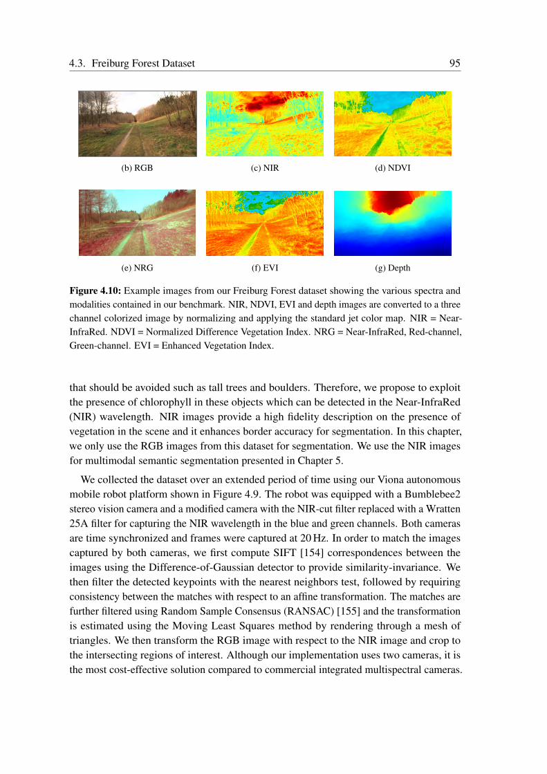
4.3. Freiburg Forest Dataset 95
(b) RGB (c) NIR (d) NDVI
(e) NRG (f) EVI (g) Depth
Figure 4.10: Example images from our Freiburg Forest dataset showing the various spectra andmodalities contained in our benchmark. NIR, NDVI, EVI and depth images are converted to a threechannel colorized image by normalizing and applying the standard jet color map. NIR = Near-InfraRed. NDVI = Normalized Difference Vegetation Index. NRG = Near-InfraRed, Red-channel,Green-channel. EVI = Enhanced Vegetation Index.
that should be avoided such as tall trees and boulders. Therefore, we propose to exploitthe presence of chlorophyll in these objects which can be detected in the Near-InfraRed(NIR) wavelength. NIR images provide a high fidelity description on the presence ofvegetation in the scene and it enhances border accuracy for segmentation. In this chapter,we only use the RGB images from this dataset for segmentation. We use the NIR imagesfor multimodal semantic segmentation presented in Chapter 5.
We collected the dataset over an extended period of time using our Viona autonomousmobile robot platform shown in Figure 4.9. The robot was equipped with a Bumblebee2stereo vision camera and a modified camera with the NIR-cut filter replaced with a Wratten25A filter for capturing the NIR wavelength in the blue and green channels. Both camerasare time synchronized and frames were captured at 20 Hz. In order to match the imagescaptured by both cameras, we first compute SIFT [154] correspondences between theimages using the Difference-of-Gaussian detector to provide similarity-invariance. Wethen filter the detected keypoints with the nearest neighbors test, followed by requiringconsistency between the matches with respect to an affine transformation. The matches arefurther filtered using Random Sample Consensus (RANSAC) [155] and the transformationis estimated using the Moving Least Squares method by rendering through a mesh oftriangles. We then transform the RGB image with respect to the NIR image and crop tothe intersecting regions of interest. Although our implementation uses two cameras, it isthe most cost-effective solution compared to commercial integrated multispectral cameras.

96 Chapter 4. Semantic Scene Segmentation
Figure 4.10 shows examples of each of the spectra and modalities that we captured.
We collected data on three different days to have enough variability in lighting conditionsas shadows and sun angles play a crucial role in the quality of acquired images. Our rawdataset contains over 15, 000 images that were sub-sampled at 1 Hz, corresponding totraversing over 4.7 km each day. Our benchmark contains 366 images with pixel-levelgroundtruth annotations which were hand-annotated for six classes: sky, trail, grass,vegetation, obstacle and void. As there is an abundant presence of vegetation in ourenvironment, we compute global-based vegetation indices such as Normalized DifferenceVegetation Index (NDVI) and Enhanced Vegetation Index (EVI) to extract consistent spatialand global vegetation information. NDVI is resistant to noise caused due to changing sunangles, topography and shadows, but is susceptible to error due to variable atmosphericand canopy background conditions [156]. EVI was proposed to compensate for thesedefects with improved sensitivity to high biomass regions and improved detection thoughdecoupling of canopy background signal and reduction in atmospheric influences. For allthe images in our dataset, we calculate NDVI and EVI using the following equations.
NDVI =ρnir – ρred
ρnir + ρred, (4.8)
where ρnir is the reflectance at the NIR wavelength (0.7 – 1.1µm) and ρred is the reflectanceat the red wavelength (0.6 – 0.7µm).
EVI = G× ρnir – ρred
ρnir + (C1 × ρred – C2 × ρblue) + L, (4.9)
where ρblue is the reflectance at the blue wavelength (0.45 – 0.52µm), G is the gain factor, Lis a soil adjustment factor, C1 and C2 are coefficients used to correct for aerosol scatteringin the red band by the use of the blue band.
Although our dataset contains images from the Bumblebee stereo camera, the processeddisparity images were substantially noisy due to several factors including rectificationartifacts and motion blur. We compared the results from semi-global matching [157] withthe depth map obtained from a CNN-based depth prediction network and found that for anunstructured forested environment, the CNN-based approach provides denser and morereliable estimates. In this work, we use the approach from Liu et al. [158] that employsa deep convolutional neural field model for depth estimation by constructing unary andpairwise potentials of conditional random fields. We convert the depth, NIR, NDVI andEVI images to a three-channel colorized image by normalizing and applying the standardjet color map. We made the raw dataset and the semantic annotations publicly available athttp://deepscene.cs.uni-freiburg.de/#datasets.
4.4. Experimental Evaluation 97
4.4 Experimental Evaluation
In this section, we first describe the datasets that we benchmark on, followed by compre-hensive quantitative results for semantic segmentation using our proposed architecturesin Section 4.4.1 and the results for model compression in Section 4.4.5. We then presentdetailed ablation studies that describe our architectural decisions in Section 4.4.6, followedby the qualitative segmentation results in Section 4.4.7.
All our models were implemented using the TensorFlow [159] deep learning libraryand the experiments were carried out on a system with an Intel Xeon E5, 2.4 GHz and anNVIDIA TITAN X GPU. We primarily use the standard Jaccard Index, also known asthe intersection-over-union (IoU) metric to quantify the performance. It can be computedfor each object class as IoU = TP/(TP + FP + FN), where TP, FP and FN correspond totrue positives, false positives and false negatives respectively. We also report the meanintersection-over-union (mIoU) metric for all the models and also the pixel-wise accuracy(Acc), average precision (AP), global intersection-over-union (gIoU) metric, false positiverate (FPR), false negative rate (FNR) in the detailed analysis.
4.4.1 Benchmark Datasets
We evaluate our proposed AdapNet and AdapNet++ architectures on five publicly availablediverse scene understanding benchmarks ranging from urban driving scenarios to unstruc-tured forested scenes and cluttered indoor environments. The datasets were particularlychosen based on the criteria of containing scenes with challenging perceptual conditionsincluding rain, snow, fog, night-time, glare, motion blur and other seasonal appearancechanges. Each of the datasets contain multiple modalities. For the experiments presented inthis chapter, we only use the visual RGB images from these datasets. The other modalitiesand spectra are used for benchmarking the multimodal semantic segmentation presentedin Chapter 5. In addition to our Freiburg Forest dataset, we benchmark on the followingstandard semantic scene segmentation datasets described in this section.
Cityscapes: The Cityscapes dataset [143] is one of the largest labeled RGB-D dataset forurban scene understanding. Being one of the standard benchmarks, it is highly challengingas it contains images of complex urban scenes, collected from over 50 cities during varyingseasons, lighting and weather conditions. The images were captured using a automotive-grade 22 cm baseline stereo camera at a resolution of 2048 × 1024 pixels. The datasetcontains 5,000 finely annotated images with 30 categories, of which 2,875 are provided fortraining, 500 are provided for validation and 1,525 are used for testing. Additionally 20,000coarse annotations are provided. The testing images are not publicly released, they areused by the evaluation server for benchmarking, excluding the rarely appearing categories.In order to facilitate comparison with previous approaches, we benchmark on the label set
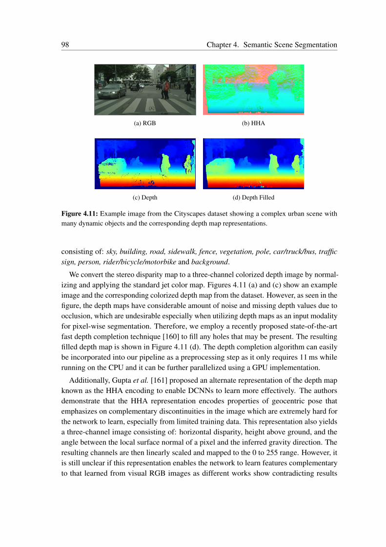
98 Chapter 4. Semantic Scene Segmentation
(a) RGB (b) HHA
(c) Depth (d) Depth Filled
Figure 4.11: Example image from the Cityscapes dataset showing a complex urban scene withmany dynamic objects and the corresponding depth map representations.
consisting of: sky, building, road, sidewalk, fence, vegetation, pole, car/truck/bus, trafficsign, person, rider/bicycle/motorbike and background.
We convert the stereo disparity map to a three-channel colorized depth image by normal-izing and applying the standard jet color map. Figures 4.11 (a) and (c) show an exampleimage and the corresponding colorized depth map from the dataset. However, as seen in thefigure, the depth maps have considerable amount of noise and missing depth values due toocclusion, which are undesirable especially when utilizing depth maps as an input modalityfor pixel-wise segmentation. Therefore, we employ a recently proposed state-of-the-artfast depth completion technique [160] to fill any holes that may be present. The resultingfilled depth map is shown in Figure 4.11 (d). The depth completion algorithm can easilybe incorporated into our pipeline as a preprocessing step as it only requires 11 ms whilerunning on the CPU and it can be further parallelized using a GPU implementation.
Additionally, Gupta et al. [161] proposed an alternate representation of the depth mapknown as the HHA encoding to enable DCNNs to learn more effectively. The authorsdemonstrate that the HHA representation encodes properties of geocentric pose thatemphasizes on complementary discontinuities in the image which are extremely hard forthe network to learn, especially from limited training data. This representation also yieldsa three-channel image consisting of: horizontal disparity, height above ground, and theangle between the local surface normal of a pixel and the inferred gravity direction. Theresulting channels are then linearly scaled and mapped to the 0 to 255 range. However, itis still unclear if this representation enables the network to learn features complementaryto that learned from visual RGB images as different works show contradicting results
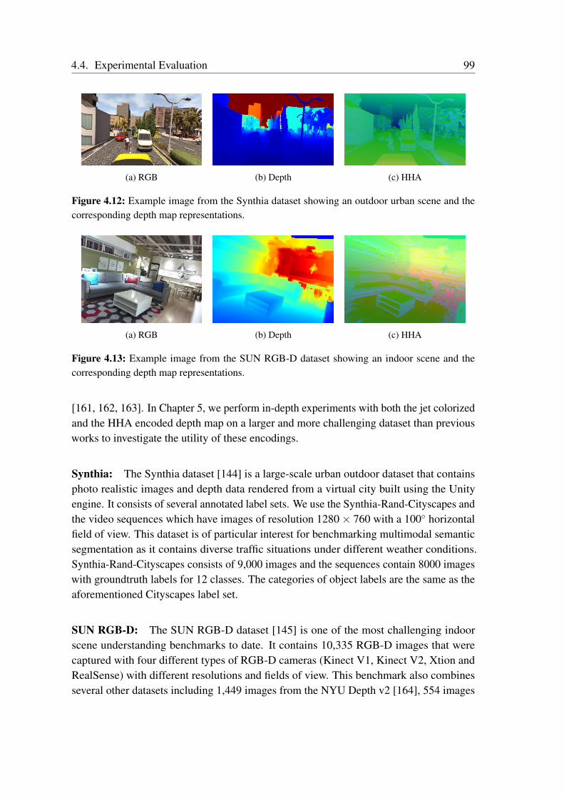
4.4. Experimental Evaluation 99
(a) RGB (b) Depth (c) HHA
Figure 4.12: Example image from the Synthia dataset showing an outdoor urban scene and thecorresponding depth map representations.
(a) RGB (b) Depth (c) HHA
Figure 4.13: Example image from the SUN RGB-D dataset showing an indoor scene and thecorresponding depth map representations.
[161, 162, 163]. In Chapter 5, we perform in-depth experiments with both the jet colorizedand the HHA encoded depth map on a larger and more challenging dataset than previousworks to investigate the utility of these encodings.
Synthia: The Synthia dataset [144] is a large-scale urban outdoor dataset that containsphoto realistic images and depth data rendered from a virtual city built using the Unityengine. It consists of several annotated label sets. We use the Synthia-Rand-Cityscapes andthe video sequences which have images of resolution 1280× 760 with a 100 horizontalfield of view. This dataset is of particular interest for benchmarking multimodal semanticsegmentation as it contains diverse traffic situations under different weather conditions.Synthia-Rand-Cityscapes consists of 9,000 images and the sequences contain 8000 imageswith groundtruth labels for 12 classes. The categories of object labels are the same as theaforementioned Cityscapes label set.
SUN RGB-D: The SUN RGB-D dataset [145] is one of the most challenging indoorscene understanding benchmarks to date. It contains 10,335 RGB-D images that werecaptured with four different types of RGB-D cameras (Kinect V1, Kinect V2, Xtion andRealSense) with different resolutions and fields of view. This benchmark also combinesseveral other datasets including 1,449 images from the NYU Depth v2 [164], 554 images
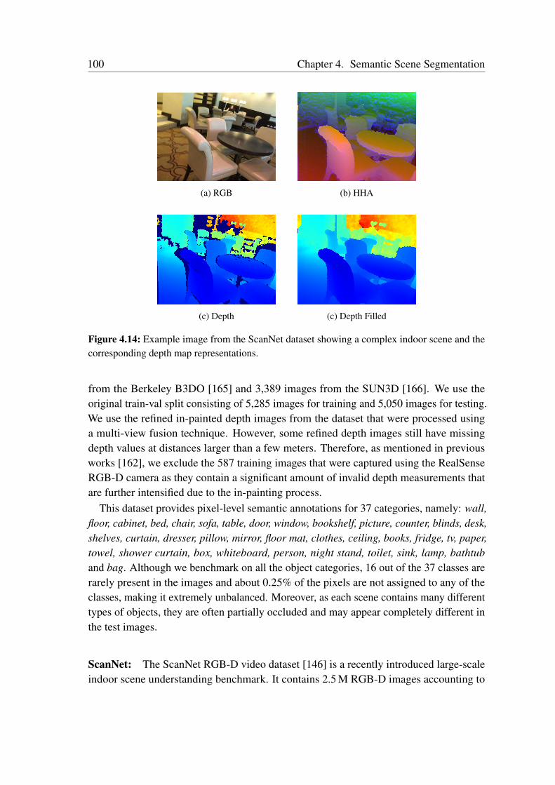
100 Chapter 4. Semantic Scene Segmentation
(a) RGB (b) HHA
(c) Depth (c) Depth Filled
Figure 4.14: Example image from the ScanNet dataset showing a complex indoor scene and thecorresponding depth map representations.
from the Berkeley B3DO [165] and 3,389 images from the SUN3D [166]. We use theoriginal train-val split consisting of 5,285 images for training and 5,050 images for testing.We use the refined in-painted depth images from the dataset that were processed usinga multi-view fusion technique. However, some refined depth images still have missingdepth values at distances larger than a few meters. Therefore, as mentioned in previousworks [162], we exclude the 587 training images that were captured using the RealSenseRGB-D camera as they contain a significant amount of invalid depth measurements thatare further intensified due to the in-painting process.
This dataset provides pixel-level semantic annotations for 37 categories, namely: wall,floor, cabinet, bed, chair, sofa, table, door, window, bookshelf, picture, counter, blinds, desk,shelves, curtain, dresser, pillow, mirror, floor mat, clothes, ceiling, books, fridge, tv, paper,towel, shower curtain, box, whiteboard, person, night stand, toilet, sink, lamp, bathtuband bag. Although we benchmark on all the object categories, 16 out of the 37 classes arerarely present in the images and about 0.25% of the pixels are not assigned to any of theclasses, making it extremely unbalanced. Moreover, as each scene contains many differenttypes of objects, they are often partially occluded and may appear completely different inthe test images.
ScanNet: The ScanNet RGB-D video dataset [146] is a recently introduced large-scaleindoor scene understanding benchmark. It contains 2.5 M RGB-D images accounting to
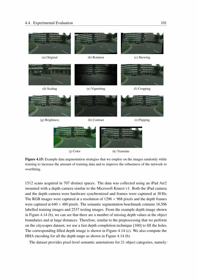
4.4. Experimental Evaluation 101
(a) Original (b) Rotation (c) Skewing
(d) Scaling (e) Vignetting (f) Cropping
(g) Brightness (h) Contrast (i) Flipping
(j) Color (k) Translate
Figure 4.15: Example data augmentation strategies that we employ on the images randomly whiletraining to increase the amount of training data and to improve the robustness of the network tooverfitting.
1512 scans acquired in 707 distinct spaces. The data was collected using an iPad Air2mounted with a depth camera similar to the Microsoft Kinect v1. Both the iPad cameraand the depth camera were hardware synchronized and frames were captured at 30 Hz.The RGB images were captured at a resolution of 1296× 968 pixels and the depth frameswere captured at 640× 480 pixels. The semantic segmentation benchmark contains 16,506labelled training images and 2537 testing images. From the example depth image shownin Figure 4.14 (b), we can see that there are a number of missing depth values at the objectboundaries and at large distances. Therefore, similar to the preprocessing that we performon the cityscapes dataset, we use a fast depth completion technique [160] to fill the holes.The corresponding filled depth image is shown in Figure 4.14 (c). We also compute theHHA encoding for all the depth maps as shown in Figure 4.14 (b).
The dataset provides pixel-level semantic annotations for 21 object categories, namely:
102 Chapter 4. Semantic Scene Segmentation
wall, floor, chair, table, desk, bed, bookshelf, sofa, sink, bathtub, toilet, curtain, counter,door, window, shower curtain, refrigerator, picture, cabinet, other furniture and void.Similar to the SUN RGB-D dataset, many object classes are rarely present making thedataset unbalanced. Moreover, the annotations at the object boundaries are often irregularand parts of objects at large distances are unlabelled. These factors make the task evenmore challenging on this dataset.
4.4.2 Data Augmentation
Training of deep networks can be significantly improved by expanding the dataset tointroduce more variability in the captured scene. The core idea is to apply a set of dataaugmentations on the training data, where the applied transformations define the invarianceproperties that are to be learned by the network. This enables the network to substantiallyimprove its robustness to overfitting and also its generalization ability to different real-world scenarios. In order to achieve this, we apply a series of augmentation strategiesrandomly on the input data while training. The augmentations [6] that we apply includerotation (–13 to 13), skewing (0.05 to 0.10), scaling (0.5 to 2.0), vignetting (210 to 300),cropping (0.8 to 0.9), brightness modulation (–40 to 40), contrast modulation (0.5 to 1.5)and left-right flipping.
4.4.3 Network Training
We represent the training set for semantic segmentation as T = (In, Mn) | n = 1, . . . , N,where In = ur | r = 1, . . . , ρ denotes the input image and the corresponding groundtruth label mask Mn = mn
r | r = 1, . . . , ρ, where mnr ∈ 1, . . . , C is the set of semantic
classes. We define θ as the network parameters consisting of weights and biases, andsj(ur, θ) as the score assigned for labeling pixel ur with label j. We obtain the probabilitiesP = (p1, . . . , pC) for all the semantic classes using the softmax function σ(.) as
pj(ur, θ | In) = σ(sj (ur, θ)
)=
exp(sj (ur, θ)
)∑Ck exp (sk (ur, θ))
. (4.10)
The optimal network parameters are then estimated by minimizing the cross-entropyloss function as
Lseg(T , θ) = –N∑
n=1
ρ∑r=1
C∑j=1
δmnr ,j log pj(ur, θ | In), (4.11)
for (In, Mn) ∈ T , where δmnr ,j is the Kronecker delta.
We train our network with an input image of resolution 768× 384 pixels, therefore, weuse bilinear interpolation for resizing the RGB images and the nearest-neighbor interpo-lation for resizing the groundtruth labels. We initialize the encoder of the network with
4.4. Experimental Evaluation 103
weights pre-trained on the ImageNet dataset [167], while we use the He initialization [93]scheme for the other convolutional and deconvolutional layers. We use the Adam solver foroptimization with β1 = 0.9, β2 = 0.999 and ε = 10–10. We train our model for a maximumof 150,000 iterations using an initial learning rate of λ0 = 10–3 with a mini-batch size of 8and a dropout probability of 0.5. We set the weights λ1 = 0.6 and λ2 = 0.5 to balance theauxiliary losses. The final loss function is computed as L = Lmain + λ1Laux1 + λ2Laux2.
4.4.4 Comparison with the State-of-the-Art
In this section, we report results comparing the performance of our proposed AdapNetand AdapNet++ architectures for a input image of resolution 768× 384 pixels. We bench-mark against several well adopted state-of-the-art models including DeepLab v3 [132],ParseNet [168], FCN-8s [24], SegNet [136], FastNet [48], DeepLab v2 [138] and Decon-vNet [169]. For each of the datasets, we report the mIoU score, as well as the per-classIoU score. Note that we report the performance of each model for the same input imageresolution of 768 × 384 pixels and using the same evaluation setting in order to have afair comparison. We do not apply multiscale inputs or left-right flips during testing asthese techniques require each crop of each image to be evaluated several times whichsignificantly increases the computational complexity and runtime (Note: We do not usecrops for testing, we evaluate on the full image in a single forward-pass). Moreover,these techniques do not improve the performance of the model in real-time applications.However, we show the potential gains that can be obtained in the evaluation metric utilizingthese techniques and with a higher resolution input image in the ablation study presentedin Section 4.4.6.5.
Table 4.1 shows the comparison on the 11 class Cityscapes validation set. Both AdapNetand AdapNet++ outperform all the baselines in each individual object category as well inthe mIoU score. AdapNet and AdapNet++ outperform the highest baseline by a marginof 2.35% and 5.59% respectively. Analyzing the individual class IoU scores, we can seethat AdapNet++ yields the highest improvement over AdapNet in object categories thatcontain thin structures such as poles for which it gives a large improvement of 5.42%, asimilar improvement of 5.05% for fences and the highest improvement for 7.29% for signs.Most architectures struggle to recover the structure of thin objects due to downsamplingby pooling and striding in the network which causes such information to be lost. However,these results show that AdapNet++ efficiently recovers the structure of such objects bylearning multiscale features at several stages of the encoder using the proposed multiscaleresidual units and the eASPP. We further show the improvement in performance due to theincorporation of the multiscale residual units and the eASPP in the ablation study presentedin Section 4.4.6.1. In driving scenarios, information of objects such as pedestrians andcyclists can also be lost when they appear at far away distances. A large improvement canalso be seen in categories such as person in which AdapNet++ achieves an improvement
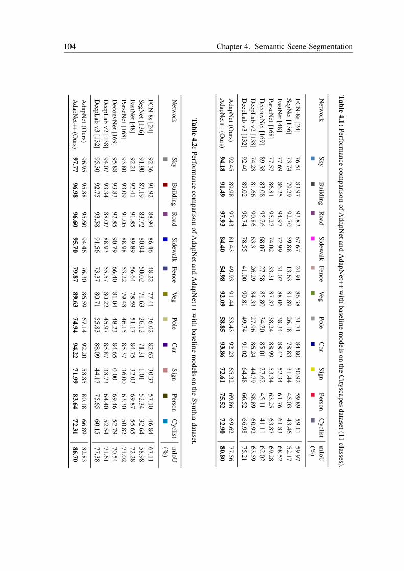
104 Chapter 4. Semantic Scene Segmentation
Table4.1:Perform
ancecom
parisonofA
dapNetand
AdapN
et++w
ithbaseline
models
onthe
Cityscapes
dataset(11classes).
Netw
orkSky
Building
Road
Sidewalk
FenceV
egPole
Car
SignPerson
Cyclist
mIoU
(%)
FCN
-8s[24]
76.5183.97
93.8267.67
24.9186.38
31.7184.80
50.9259.89
59.1159.97
SegNet[136]
73.7479.29
92.7059.88
13.6381.89
26.1878.83
31.4445.03
43.4652.17
FastNet[48]
77.6986.25
94.9772.99
31.0288.06
38.3488.42
52.3461.76
61.8368.52
ParseNet[168]
77.5786.81
95.2774.02
33.3187.37
38.2488.99
53.3463.25
63.8769.28
DeconvN
et[169]89.38
83.0895.26
68.0727.58
85.8034.20
85.0127.62
45.1141.11
62.02D
eepLab
v2[138]
74.2881.66
90.8663.3
26.2984.33
27.9686.24
44.7958.89
60.9263.59
DeepL
abv3
[132]92.40
89.0296.74
78.5541.00
90.8149.74
91.0264.48
66.5266.98
75.21
AdapN
et(Ours)
92.4589.98
97.4381.43
49.9391.44
53.4392.23
65.3269.86
69.6277.56
AdapN
et++(O
urs)94.18
91.4997.93
84.4054.98
92.0958.85
93.8672.61
75.5272.90
80.80
Table4.2:Perform
ancecom
parisonofA
dapNetand
AdapN
et++w
ithbaseline
models
onthe
Synthiadataset.
Netw
orkSky
Building
Road
Sidewalk
FenceV
egPole
Car
SignPerson
Cyclist
mIoU
(%)
FCN
-8s[24]
92.3691.92
88.9486.46
48.2277.41
36.0282.63
30.3757.10
46.8467.11
SegNet[136]
91.9087.19
83.7280.94
50.0271.63
26.1271.31
1.0152.34
32.6458.98
FastNet[48]
92.2192.41
91.8589.89
56.6478.59
51.1784.75
32.0369.87
55.6572.28
ParseNet[168]
93.8093.09
91.0588.98
53.2279.48
46.1585.37
36.0063.30
50.8271.02
DeconvN
et[169]95.88
93.8392.85
90.7966.40
81.0448.23
84.650.00
69.4652.79
70.54D
eepLab
v2[138]
94.0793.34
88.0788.93
55.5780.22
45.9785.87
38.7364.40
52.5471.61
DeepL
abv3
[132]95.30
92.7593.58
91.5673.37
80.7155.83
88.0944.17
75.6560.15
77.38
AdapN
et(Ours)
96.9595.88
95.6094.46
76.3086.59
67.1492.20
58.8580.18
66.8982.83
AdapN
et++(O
urs)97.77
96.9896.60
95.7079.87
89.6374.94
94.2271.99
83.6472.31
86.70

4.4. Experimental Evaluation 105
Table 4.3: Benchmarking results on the Cityscapes dataset with full resolution evaluation on 19semantic class labels. Only the eight top performing published models in the leaderboard are listedin this table. The inference time is reported for an input image resolution of 768× 384 pixels and itwas computed on an NVIDIA TITAN X (PASCAL) GPU using the official implementation of eachmethod. SSMA refers to our multimodal segmentation architecture that builds upon AdapNet++and is detailed in Chapter 5.
Network Backbone mIoU (%) Parms. Timeval test (M) (ms)
PSPNet [135] ResNet-101 80.91 81.19 56.27 172.42DeepLab v3 [132] ResNet-101 79.30 81.34 58.16 79.90Mapillary [170] WideResNet-38 78.31 82.03 135.86 214.46DeepLab v3+ [171] Modified Xception 79.55 82.14 43.48 127.97DPC [172] Modified Xception 80.85 82.66 41.82 144.41DRN [173] WideResNet-38 79.69 82.82 129.16 1259.67
AdapNet++ (Ours) ResNet50 81.24 81.34 30.20 72.92SSMA (Ours) ResNet50 82.19 82.31 56.44 101.95
of 5.66%. The improvement in larger object categories such as cars and vegetation can beattributed to the new decoder which improves the segmentation performance near objectboundaries. This is more evident in the qualitative results presented in Section 4.4.7. Notethat the colors shown below the object category names serve as a legend for the qualitativeresults.
We also report results on the full 19 class Cityscapes validation and test sets in Table 4.3.We compare against the top six published models on the leaderboard, namely, PSPNet [135],DeepLab v3 [132], Mapilary [170], DeepLab v3+ [171], DPC [172], and DRN [173].The results of the competing methods reported in this table are directly taken from thebenchmark leaderboard for the test set and from the corresponding manuscripts of themethods for the validation set. We trained our models on 768× 768 crops from the fullimage resolution for benchmarking on the leaderboard. Our AdapNet++ model with a muchsmaller network backbone achieves a comparable performance as other top performingmodels on the leaderboard. Moreover, our network is the most efficient architecture interms of both the number of parameters that it consumes as well as the inference timecompared to other networks on the entire first page of the Cityscapes leaderboard.
We benchmark on the Synthia dataset largely due to the variety of seasons and adverseperceptual conditions which make the task of semantic segmentation extremely challenging.From the results shown in Table 4.2, it can be seen that both AdapNet and AdapNet++outperform all the baselines in the overall mIoU score as well as in the score of theindividual object categories. AdapNet and AdapNet++ achieve an overall substantialimprovement of 5.45% and 9.32% respectively. A similar observation can be made in the
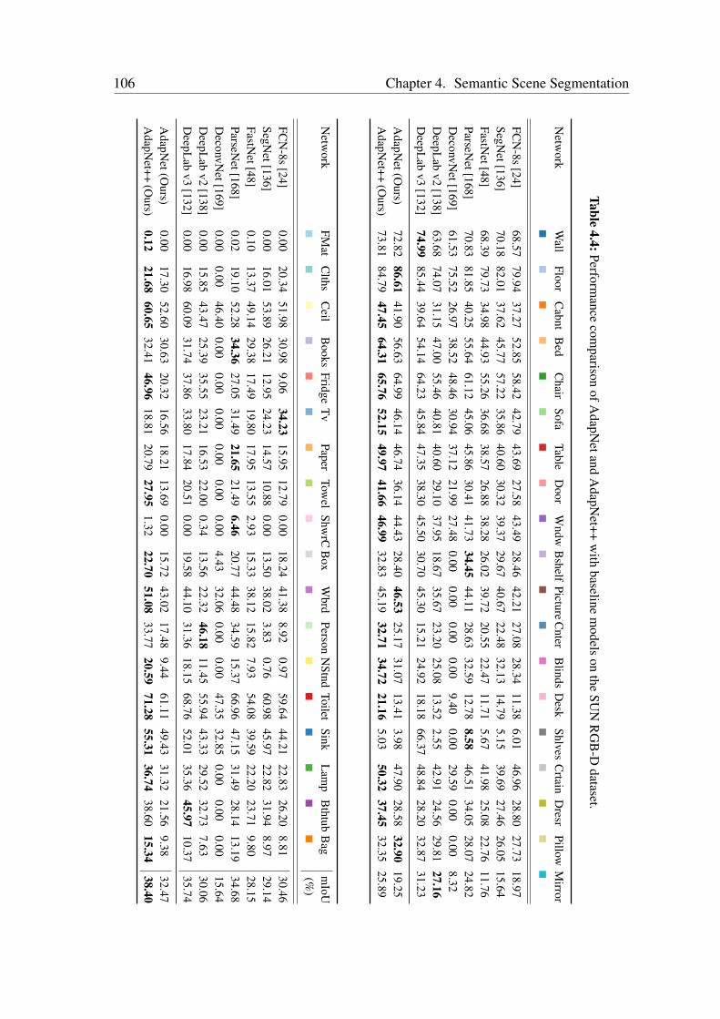
106 Chapter 4. Semantic Scene Segmentation
Table4.4:Perform
ancecom
parisonofA
dapNetand
AdapN
et++w
ithbaseline
models
onthe
SUN
RG
B-D
dataset.
Netw
orkW
allFloor
Cabnt
Bed
Chair
SofaTable
Door
Wndw
Bshelf
PictureC
nterB
lindsD
eskShlves
Crtain
Dresr
PillowM
irror
FCN
-8s[24]
68.5779.94
37.2752.85
58.4242.79
43.6927.58
43.4928.46
42.2127.08
28.3411.38
6.0146.96
28.8027.73
18.97SegN
et[136]70.18
82.0137.62
45.7757.22
35.8640.60
30.3239.37
29.6740.67
22.4832.13
14.795.15
39.6927.46
26.0515.64
FastNet[48]
68.3979.73
34.9844.93
55.2636.68
38.5726.88
38.2826.02
39.7220.55
22.4711.71
5.6741.98
25.0822.76
11.76ParseN
et[168]70.83
81.8540.25
55.6461.12
45.0645.86
30.4141.73
34.4544.11
28.6332.59
12.788.58
46.5134.05
28.0724.82
DeconvN
et[169]61.53
75.5226.97
38.5248.46
30.9437.12
21.9927.48
0.000.00
0.000.00
9.400.00
29.590.00
0.008.32
DeepL
abv2
[138]63.68
74.0731.15
47.0055.46
40.8140.60
29.1037.95
18.6735.67
23.2025.08
13.522.55
42.9124.56
29.8127.16
DeepL
abv3
[132]74.99
85.4439.64
54.1464.23
45.8447.35
38.3045.50
30.7045.30
15.2124.92
18.1866.37
48.8428.20
32.8731.23
AdapN
et(Ours)
72.8286.61
41.9056.63
64.9946.14
46.7436.14
44.4328.40
46.5325.17
31.0713.41
3.9847.90
28.5832.90
19.25A
dapNet++
(Ours)
73.8184.79
47.4564.31
65.7652.15
49.9741.66
46.9932.83
45.1932.71
34.7221.16
5.0350.32
37.4532.35
25.89
Netw
orkFM
atC
lthsC
eilB
ooksFridge
Tv
PaperTow
elShw
rCB
oxW
brdPerson
NStnd
ToiletSink
Lamp
Bthtub
Bag
mIoU
(%)
FCN
-8s[24]
0.0020.34
51.9830.98
9.0634.23
15.9512.79
0.0018.24
41.388.92
0.9759.64
44.2122.83
26.208.81
30.46SegN
et[136]0.00
16.0153.89
26.2112.95
24.2314.57
10.880.00
13.5038.02
3.830.76
60.9845.97
22.8231.94
8.9729.14
FastNet[48]
0.1013.37
49.1429.38
17.4919.80
17.9513.55
2.9315.33
38.1215.82
7.9354.08
39.5922.20
23.719.80
28.15ParseN
et[168]0.02
19.1052.28
34.3627.05
31.4921.65
21.496.46
20.7744.48
34.5915.37
66.9647.15
31.4928.14
13.1934.68
DeconvN
et[169]0.00
0.0046.40
0.000.00
0.000.00
0.000.00
4.4332.06
0.000.00
47.3532.85
0.000.00
0.0015.64
DeepL
abv2
[138]0.00
15.8543.47
25.3935.55
23.2116.53
22.000.34
13.5622.32
46.1811.45
55.9443.33
29.5232.73
7.6330.06
DeepL
abv3
[132]0.00
16.9860.09
31.7437.86
33.8017.84
20.510.00
19.5844.10
31.3618.15
68.7652.01
35.3645.97
10.3735.74
AdapN
et(Ours)
0.0017.30
52.6030.63
20.3216.56
18.2113.69
0.0015.72
43.0217.48
9.4461.11
49.4331.32
21.569.38
32.47A
dapNet++
(Ours)
0.1221.68
60.6532.41
46.9618.81
20.7927.95
1.3222.70
51.0833.77
20.5971.28
55.3136.74
38.6015.34
38.40
4.4. Experimental Evaluation 107
improvement of scores for thin structures, reinforcing the utility of our proposed multiscalefeature learning configuration. AdapNet++ improves over AdapNet by 13.14% for the signclass, followed by an improvement of 7.8% for the pole class. In addition a significantimprovement of 5.42% can also be seen for the cyclist class.
Compared to outdoor driving datasets, indoor benchmarks such as SUN RGB-D andScanNet pose a different challenge. Indoor datasets have vast amounts of object categoriesin various different configurations and images captured from many different view pointscompared to driving scenarios where the camera is always parallel to the ground withsimilar viewpoints from the perspective of the vehicle driving on the road. Moreover,indoor scenes are often extremely cluttered which causes occlusions, in addition to theirregular frequency distribution of the object classes that make the problem even harder.Due to these factors SUN RGB-D is considered one of the hardest datasets to benchmarkon. Despite these factors, as shown in Table 4.4, AdapNet++ outperforms all the baselinenetworks overall by a margin of 2.66% compared to the highest performing DeepLab v3baseline which took 30,000 iterations more to reach this score. Unlike the performancein the Cityscapes and Synthia datasets where our AdapNet architecture yields the secondhighest performance, AdapNet is outperformed by DeepLab v3 in the SUN RGB-Ddataset. AdapNet++ on the other hand, outperforms the baselines in most categoriesby a large margin, while it is outperformed in 13 of the 37 classes by small margin.It can also be observed that the classes in which AdapNet++ get outperformed are themost infrequent classes. This can be alleviated by adding supplementary training imagescontaining the low-frequency classes from other datasets or by employing class balancingtechniques. However, our initial experiments employing techniques such as medianfrequency class balancing, inverse median frequency class balancing, normalized inversefrequency balancing, severely affected the performance of our model.
We also show results on the validation set of the recently introduced ScanNet dataset inTable 4.5, which is currently the largest labeled indoor RGB-D dataset till date. AdapNet++outperforms the state-of-the-art overall by a margin of 2.61%. The large improvement canbe attributed to the proposed eASPP which efficiently captures long range context. Contextaggregation plays an important role in such cluttered indoor datasets as different partsof an object are occluded from different viewpoints and across scenes. As objects suchas the legs of a chair have thin structures, multiscale learning contributes to recoveringsuch structures. We see a similar trend in the performance as in the SUN RGB-D dataset,where our network outperforms the baselines in most of the object categories (11 of the 20classes) significantly, while yielding a comparable performance for the other categories.The largest improvement of 11.62% is obtained for the counter class, followed by animprovement of 8.69% for the curtain class which appears as many different variations inthe dataset. An interesting observation that can be made is that the highest parametrizednetwork DeconvNet which has 252 M parameters has the lowest performance in both SUNRGB-D and ScanNet datasets, while AdapNet++ which has about 1/9th of the parameters,
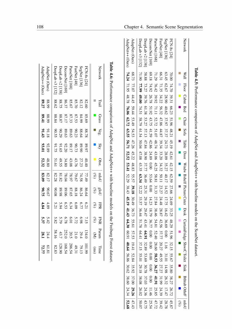
108 Chapter 4. Semantic Scene Segmentation
Table4.5:Perform
ancecom
parisonofA
dapNetand
AdapN
et++w
ithbaseline
models
onthe
ScanNetdataset.
Netw
orkW
allFloor
Cabnt
Bed
Chair
SofaTable
Door
Wndw
Bshelf
PictureCnter
Desk
CurtainFridge
ShwrC
ToiletSink
Bthtub
OthrF
mIoU
(%)
FCN
-8s[24]
70.0074.70
39.3166.23
51.9648.21
45.1942.61
42.1562.59
27.6624.69
33.2548.29
51.9632.15
55.6735.80
38.2726.72
45.87SegN
et[136]63.45
62.6728.90
40.6237.97
37.3724.73
28.0935.27
40.1714.52
17.7516.42
36.690.00
1.1631.01
14.9826.32
17.4728.78
FastNet[48]
66.3171.35
34.2256.32
47.8644.87
39.3433.20
34.3250.11
23.2724.48
28.8742.56
37.7720.27
49.5527.27
31.9924.39
39.42ParseN
et[168]71.29
76.4239.92
71.1152.72
51.0748.74
43.0645.25
58.8131.33
27.8438.46
54.8152.40
28.6058.53
36.2741.91
25.8547.72
DeconvN
et[169]69.18
74.9226.78
51.9243.75
41.5942.86
24.890.00
53.640.00
14.2318.79
36.770.00
0.000.00
0.000.00
11.4625.54
DeepL
abv2
[138]58.88
73.2739.76
61.3853.27
57.1347.84
38.9037.77
36.4925.31
29.1929.47
43.4164.91
32.8953.69
30.7837.03
24.3643.75
DeepL
abv3
[132]71.90
77.9949.00
74.5158.79
61.5450.04
47.0843.35
63.3432.22
33.5736.44
51.7864.41
37.1555.01
29.1838.08
26.0250.07
AdapN
et(Ours)
68.7377.07
44.4559.44
53.4954.53
47.2645.22
48.8355.57
39.1830.49
36.7355.61
57.5319.41
52.8435.92
37.0029.26
47.43A
dapNet++
(Ours)
74.2471.95
48.7876.06
62.7263.55
56.7152.52
53.4152.29
38.4345.19
41.4364.30
60.9140.64
56.8630.62
38.6024.34
52.68
Table4.6:Perform
ancecom
parisonofA
dapNetand
AdapN
et++w
ithbaseline
models
onthe
FreiburgForestdataset.
Netw
orkTrail
Grass
Veg.
SkyO
bst.m
IoUgIoU
FPRFN
RParam
Time
(%)
(%)
(%)
(%)
(M)
(ms)
FCN
-8s[24]
82.6085.69
88.7889.97
40.4077.49
86.646.21
7.15134.0
101.99SegN
et[136]82.12
84.9988.64
89.9027.23
74.5886.24
6.776.98
29.479.13
FastNet[48]
85.7087.53
90.2390.73
43.7679.67
88.186.09
5.7221.0
49.31ParseN
et[168]85.67
87.3389.63
89.1743.08
78.9787.65
6.346.01
20.5286.54
DeconvN
et[169]86.37
87.1789.63
92.2034.80
78.0489.06
6.536.78
252.0168.54
DeepL
abv2
[138]88.75
88.8790.29
91.6549.55
81.8289.98
5.945.79
43.7128.90
DeepL
abv3
[132]88.62
88.8490.55
91.7551.61
82.2890.08
5.215.82
58.1682.83
AdapN
et(Ours)
88.9988.99
91.1892.89
48.8082.17
90.674.89
5.4224.4
61.81A
dapNet++
(Ours)
89.2789.41
91.4393.01
52.3283.09
90.754.84
5.3728.1
72.77
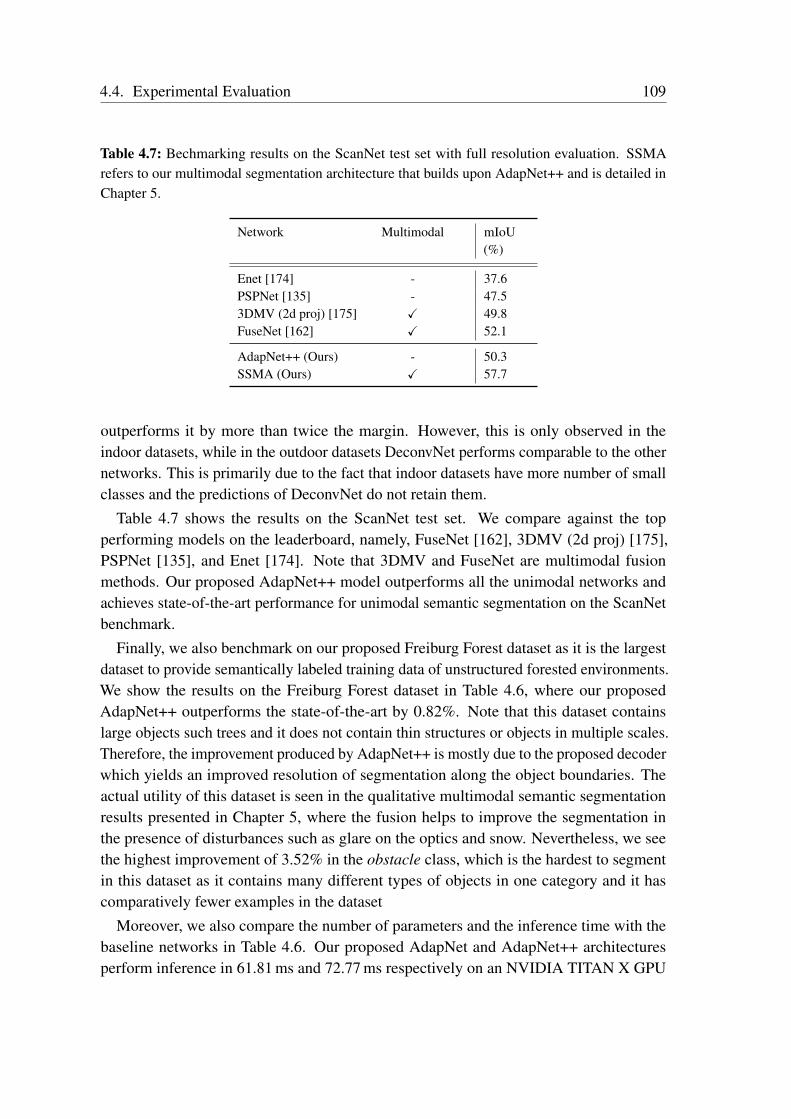
4.4. Experimental Evaluation 109
Table 4.7: Bechmarking results on the ScanNet test set with full resolution evaluation. SSMArefers to our multimodal segmentation architecture that builds upon AdapNet++ and is detailed inChapter 5.
Network Multimodal mIoU(%)
Enet [174] - 37.6PSPNet [135] - 47.53DMV (2d proj) [175] X 49.8FuseNet [162] X 52.1
AdapNet++ (Ours) - 50.3SSMA (Ours) X 57.7
outperforms it by more than twice the margin. However, this is only observed in theindoor datasets, while in the outdoor datasets DeconvNet performs comparable to the othernetworks. This is primarily due to the fact that indoor datasets have more number of smallclasses and the predictions of DeconvNet do not retain them.
Table 4.7 shows the results on the ScanNet test set. We compare against the topperforming models on the leaderboard, namely, FuseNet [162], 3DMV (2d proj) [175],PSPNet [135], and Enet [174]. Note that 3DMV and FuseNet are multimodal fusionmethods. Our proposed AdapNet++ model outperforms all the unimodal networks andachieves state-of-the-art performance for unimodal semantic segmentation on the ScanNetbenchmark.
Finally, we also benchmark on our proposed Freiburg Forest dataset as it is the largestdataset to provide semantically labeled training data of unstructured forested environments.We show the results on the Freiburg Forest dataset in Table 4.6, where our proposedAdapNet++ outperforms the state-of-the-art by 0.82%. Note that this dataset containslarge objects such trees and it does not contain thin structures or objects in multiple scales.Therefore, the improvement produced by AdapNet++ is mostly due to the proposed decoderwhich yields an improved resolution of segmentation along the object boundaries. Theactual utility of this dataset is seen in the qualitative multimodal semantic segmentationresults presented in Chapter 5, where the fusion helps to improve the segmentation inthe presence of disturbances such as glare on the optics and snow. Nevertheless, we seethe highest improvement of 3.52% in the obstacle class, which is the hardest to segmentin this dataset as it contains many different types of objects in one category and it hascomparatively fewer examples in the dataset
Moreover, we also compare the number of parameters and the inference time with thebaseline networks in Table 4.6. Our proposed AdapNet and AdapNet++ architecturesperform inference in 61.81 ms and 72.77 ms respectively on an NVIDIA TITAN X GPU
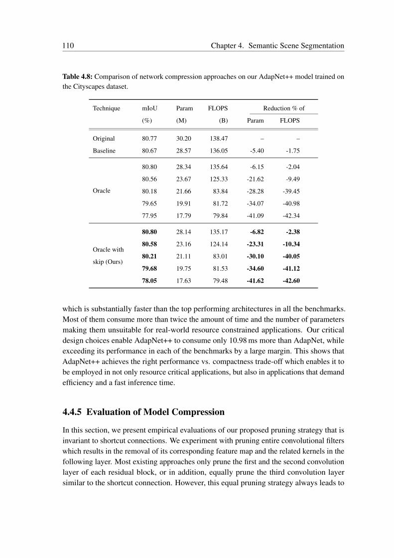
110 Chapter 4. Semantic Scene Segmentation
Table 4.8: Comparison of network compression approaches on our AdapNet++ model trained onthe Cityscapes dataset.
Technique mIoU Param FLOPS Reduction % of
(%) (M) (B) Param FLOPS
Original 80.77 30.20 138.47 – –
Baseline 80.67 28.57 136.05 -5.40 -1.75
Oracle
80.80 28.34 135.64 -6.15 -2.04
80.56 23.67 125.33 -21.62 -9.49
80.18 21.66 83.84 -28.28 -39.45
79.65 19.91 81.72 -34.07 -40.98
77.95 17.79 79.84 -41.09 -42.34
80.80 28.14 135.17 -6.82 -2.38
Oracle with80.58 23.16 124.14 -23.31 -10.34
skip (Ours)80.21 21.11 83.01 -30.10 -40.05
79.68 19.75 81.53 -34.60 -41.12
78.05 17.63 79.48 -41.62 -42.60
which is substantially faster than the top performing architectures in all the benchmarks.Most of them consume more than twice the amount of time and the number of parametersmaking them unsuitable for real-world resource constrained applications. Our criticaldesign choices enable AdapNet++ to consume only 10.98 ms more than AdapNet, whileexceeding its performance in each of the benchmarks by a large margin. This shows thatAdapNet++ achieves the right performance vs. compactness trade-off which enables it tobe employed in not only resource critical applications, but also in applications that demandefficiency and a fast inference time.
4.4.5 Evaluation of Model Compression
In this section, we present empirical evaluations of our proposed pruning strategy that isinvariant to shortcut connections. We experiment with pruning entire convolutional filterswhich results in the removal of its corresponding feature map and the related kernels in thefollowing layer. Most existing approaches only prune the first and the second convolutionlayer of each residual block, or in addition, equally prune the third convolution layersimilar to the shortcut connection. However, this equal pruning strategy always leads to
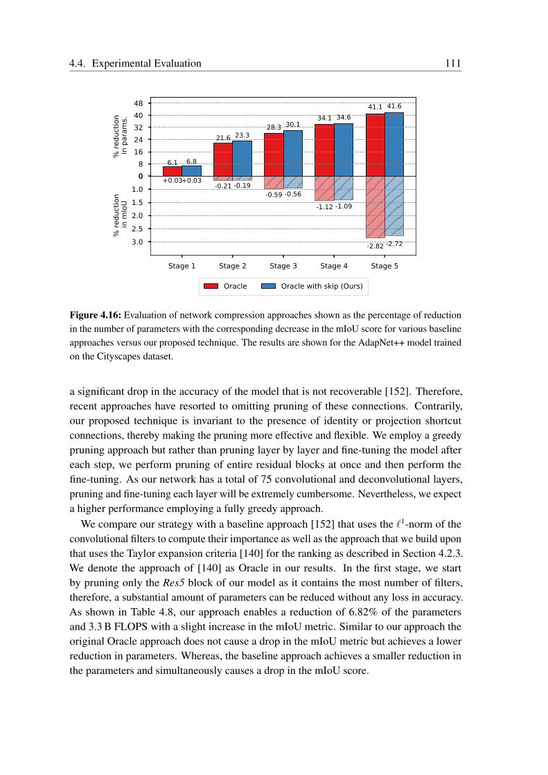
4.4. Experimental Evaluation 111
08
1624324048
% re
duct
ion
in p
aram
s.
6.1
21.628.3
34.141.1
6.8
23.330.1
34.641.6
Stage 1 Stage 2 Stage 3 Stage 4 Stage 5
3.02.52.01.51.0
0
% re
duct
ion
in m
IoU
+0.03 -0.21-0.59
-1.12
-2.82
+0.03 -0.19-0.56
-1.09
-2.72
Oracle Oracle with skip (Ours)
Figure 4.16: Evaluation of network compression approaches shown as the percentage of reductionin the number of parameters with the corresponding decrease in the mIoU score for various baselineapproaches versus our proposed technique. The results are shown for the AdapNet++ model trainedon the Cityscapes dataset.
a significant drop in the accuracy of the model that is not recoverable [152]. Therefore,recent approaches have resorted to omitting pruning of these connections. Contrarily,our proposed technique is invariant to the presence of identity or projection shortcutconnections, thereby making the pruning more effective and flexible. We employ a greedypruning approach but rather than pruning layer by layer and fine-tuning the model aftereach step, we perform pruning of entire residual blocks at once and then perform thefine-tuning. As our network has a total of 75 convolutional and deconvolutional layers,pruning and fine-tuning each layer will be extremely cumbersome. Nevertheless, we expecta higher performance employing a fully greedy approach.
We compare our strategy with a baseline approach [152] that uses the `1-norm of theconvolutional filters to compute their importance as well as the approach that we build uponthat uses the Taylor expansion criteria [140] for the ranking as described in Section 4.2.3.We denote the approach of [140] as Oracle in our results. In the first stage, we startby pruning only the Res5 block of our model as it contains the most number of filters,therefore, a substantial amount of parameters can be reduced without any loss in accuracy.As shown in Table 4.8, our approach enables a reduction of 6.82% of the parametersand 3.3 B FLOPS with a slight increase in the mIoU metric. Similar to our approach theoriginal Oracle approach does not cause a drop in the mIoU metric but achieves a lowerreduction in parameters. Whereas, the baseline approach achieves a smaller reduction inthe parameters and simultaneously causes a drop in the mIoU score.
112 Chapter 4. Semantic Scene Segmentation
Our aim for pruning in the first stage was to compress the model without causing a dropin the segmentation performance, while in the following stages, we aggressively prune themodel to achieve the best parameter to performance ratio. Results from this experimentare shown as the percentage in reduction of parameters in comparison to the change inmIoU in Figure 4.16. In the second stage, we prune the convolutional feature maps ofRes2, Res3, Res4 and Res5 layers. Using our proposed method, we achieve a reduction of23.31% of parameters with minor drop of 0.19% in the mIoU score. Whereas, the Oracleapproach yields a lower reduction in parameters as well as a larger drop in performance. Asimilar trend can also be seen for the other pruning stages where our proposed approachyields a higher reduction in parameters and FLOPS with a minor reduction in the mIoUscore. This shows that pruning convolutional feature maps with regularity leads to a bettercompression ratio than selectively pruning layers at different stages of the network. In thethird stage, we perform pruning of the deconvolutional feature maps, while in the fourthand fifth stages we further prune all the layers of the network by varying the threshold forthe rankings. In the final stage we obtain a reduction of 41.62% of the parameters and42.60% of FLOPS with a drop of 2.72% in the mIoU score. Considering the compressionthat can be achieved, this minor drop in the mIoU score is acceptable to enable efficientdeployment in resource constrained applications.
4.4.6 Ablation Study
In order to evaluate the various components of our AdapNet and AdapNet++ architectures,we performed several experiments in different settings. In this section, we study theimprovement obtained due to the proposed encoder with the multiscale residual units, adetailed analysis of the proposed eASPP, comparisons with different base encoder networktopologies, the improvement that can be obtained by using higher resolution images asinput and using multiscale testing. For each of these components, we also study the effectof different parameter configurations. All the ablation studies presented in this sectionwere performed using models trained on the Cityscapes dataset.
4.4.6.1 Detailed Study on the Architectural Components
We first study the major contributions made to the encoder as well as the decoder in ourproposed architectures. Table 4.9 shows results from this experiment and subsequentimprovement due to each of the configurations. The simple base model M1 consisting ofthe standard ResNet-50 architecture for the encoder and a single deconvolution layer forupsampling achieves a mIoU of 75.22%. The model M2 that incorporates our multiscaleresidual units achieves an improvement of 1.7% without any increase in the memoryconsumption. Whereas, the multigrid approach from DeepLab v3 [132] in the sameconfiguration achieves only 0.38% of improvement in the mIoU score. This shows the

4.4. Experimental Evaluation 113
Tabl
e4.
9:E
ffec
toft
heva
riou
sco
ntri
butio
nspr
opos
edin
the
Ada
pNet
and
Ada
pNet
++ar
chite
ctur
es.T
hepe
rfor
man
ceis
show
nfo
rthe
mod
els
trai
ned
onth
eC
itysc
apes
data
set.
The
sym
bol↑
k fde
note
sa
deco
nvol
utio
nla
yera
ndck f
deno
tes
aco
nvol
utio
nla
yerw
ithf
num
bero
ffilte
rs,k×
kke
rnel
size
and
nis
the
num
bero
fcla
sses
.PA
Res
Net
-50
refe
rsto
the
full
pre-
activ
atio
nR
esN
et-5
0ar
chite
ctur
e.T
hew
eigh
tsfo
rthe
two
auxi
lary
loss
esw
ere
sett
oL
1=
0.5
andL
2=
0.6
fort
his
expe
rim
ent.
Mod
elE
ncod
erM
SD
ecod
erSk
ipA
SPP
Aux
Los
sH
em
IoU
Res
idua
ldi
l3,6
,12
2xIn
it(%
)
M1
Res
Net
-50
-c1 n↑1
6 n-
--
-75
.22
M2
Res
Net
-50
Xc1 n↑1
6 n-
--
-76
.92
M3
Res
Net
-50
Xc1 n↑2 2n⊕↑8 n
3d-
--
77.7
8
M4
PAR
esN
et-5
0X
c1 n↑2 2n⊕↑8 n
3d-
--
78.4
4
M5
PAR
esN
et-5
0X
c1 n↑2 2n⊕↑8 n
3dX
--
78.9
3
M6
PAR
esN
et-5
0X
c1 n↑2 2n⊕↑2 2n⊕↑8 n
3d,2
cX
--
79.1
9
M7
PAR
esN
et-5
0X
↑2‖
c3c3↑2‖
c3c3
c1 n↑8 n
3d,2
cX
--
79.8
2
M8
PAR
esN
et-5
0X
↑2‖
c3c3↑2‖
c3c3
c1 n↑8 n
3d,2
cX
X-
80.3
4
M9
PAR
esN
et-5
0X
↑2‖
c3c3↑2‖
c3c3
c1 n↑8 n
3d,2
cX
XX
80.6
7
114 Chapter 4. Semantic Scene Segmentation
novelty in employing our multiscale residual units for efficiently learning multiscalefeatures throughout the network. In the M3 model, we study the effect of incorporatingskip connections for refinement. Skip connections that were initially introduced in theFCN architecture are still widely used for improving the resolution of the segmentation byincorporating low or mid-level features from the encoder into the decoder while upsampling.The ResNet-50 architecture contains the most discriminative features in the middle of thenetwork. In our M3 model, we first upsample the encoder output by a factor two, followedby fusing the features from Res3d block of the encoder to refinement and subsequentlyusing another deconvolutional layer to upsample back to input resolution. This modelwhich resembles the topology of the AdapNet architecture achieves a further improvementof 0.86%.
In the M4 model, we replace the standard residual units with the full pre-activationresidual units which yields an improvement of 0.66%. As mentioned in the work byHe et al. [72], the results corroborate that pre-activation residual units yields a lowererror than standard residual units due to the ease of training and improved generalizationcapability. Aggregating multiscale context using ASPP has become standard practicein most classification and segmentation networks. In the M5 model, we add the ASPPmodule to the end of the encoder segment. This model demonstrates an improved mIoU of78.93% due to the ability of the ASPP to capture long range context. In the subsequentM6 model, we study if adding another skip refinement connection from the encoder yieldsa better performance. This was challenging as most combinations along with the Res3dskip connection did not demonstrate any improvement. However, adding a skip connectionfrom Res2c showed a slight improvement.
In all the models upto this stage, we fused the low and mid-level encoder features into thedecoder using element-wise addition. In order to make the decoder stronger, we experimentwith improving the learned decoder representations with additional convolutions afterconcatenation of the mid-level features. Specifically, the M7 model has three upsamplingstages, the first two stages consist of a deconvolution layer that upsamples by a factor of two,followed by concatenation of the mid-level features and two following 3× 3 convolutionsthat learn highly discriminative fused features. This model shows an improvement of0.63% which is primarily due to the improved segmentation along the object boundariesas demonstrated in the qualitative results in Section 4.4.7. Our M7 model contains atotal of 75 convolutional and deconvolutional layers, making the optimization challenging.In order to accelerate the training and to further improve the segmentation along objectboundaries, we propose a multi-resolution supervision scheme in which we add a weightedauxiliary loss to each of the first two upsampling stages. This model denoted as M8achieves an improved mIoU of 80.34%. In comparison to aforementioned scheme, we alsoexperimented with adding a weighted auxiliary loss at the end of the encoder of the M7model, however it did not improve the performance, although it accelerated the training.Finally we also experimented with initializing the layers with the He initialization [93]
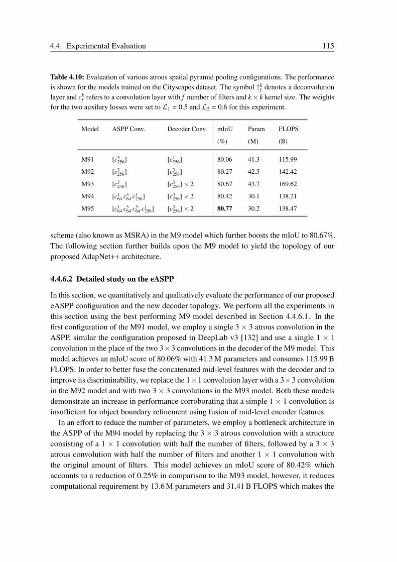
4.4. Experimental Evaluation 115
Table 4.10: Evaluation of various atrous spatial pyramid pooling configurations. The performanceis shown for the models trained on the Cityscapes dataset. The symbol ↑k
f denotes a deconvolutionlayer and ck
f refers to a convolution layer with f number of filters and k× k kernel size. The weightsfor the two auxilary losses were set to L1 = 0.5 and L2 = 0.6 for this experiment.
Model ASPP Conv. Decoder Conv. mIoU Param FLOPS
(%) (M) (B)
M91 [c3256] [c1
256] 80.06 41.3 115.99
M92 [c3256] [c3
256] 80.27 42.5 142.42
M93 [c3256] [c3
256]× 2 80.67 43.7 169.62
M94 [c164 c3
64 c1256] [c3
256]× 2 80.42 30.1 138.21
M95 [c164 c3
64 c364 c1
256] [c3256]× 2 80.77 30.2 138.47
scheme (also known as MSRA) in the M9 model which further boosts the mIoU to 80.67%.The following section further builds upon the M9 model to yield the topology of ourproposed AdapNet++ architecture.
4.4.6.2 Detailed study on the eASPP
In this section, we quantitatively and qualitatively evaluate the performance of our proposedeASPP configuration and the new decoder topology. We perform all the experiments inthis section using the best performing M9 model described in Section 4.4.6.1. In thefirst configuration of the M91 model, we employ a single 3× 3 atrous convolution in theASPP, similar the configuration proposed in DeepLab v3 [132] and use a single 1 × 1convolution in the place of the two 3×3 convolutions in the decoder of the M9 model. Thismodel achieves an mIoU score of 80.06% with 41.3 M parameters and consumes 115.99 BFLOPS. In order to better fuse the concatenated mid-level features with the decoder and toimprove its discriminability, we replace the 1×1 convolution layer with a 3×3 convolutionin the M92 model and with two 3× 3 convolutions in the M93 model. Both these modelsdemonstrate an increase in performance corroborating that a simple 1× 1 convolution isinsufficient for object boundary refinement using fusion of mid-level encoder features.
In an effort to reduce the number of parameters, we employ a bottleneck architecture inthe ASPP of the M94 model by replacing the 3 × 3 atrous convolution with a structureconsisting of a 1 × 1 convolution with half the number of filters, followed by a 3 × 3atrous convolution with half the number of filters and another 1 × 1 convolution withthe original amount of filters. This model achieves an mIoU score of 80.42% whichaccounts to a reduction of 0.25% in comparison to the M93 model, however, it reducescomputational requirement by 13.6 M parameters and 31.41 B FLOPS which makes the
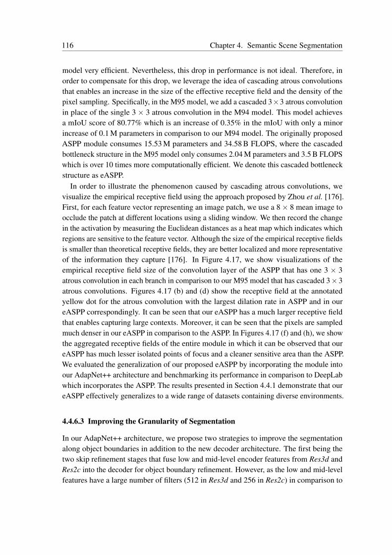
116 Chapter 4. Semantic Scene Segmentation
model very efficient. Nevertheless, this drop in performance is not ideal. Therefore, inorder to compensate for this drop, we leverage the idea of cascading atrous convolutionsthat enables an increase in the size of the effective receptive field and the density of thepixel sampling. Specifically, in the M95 model, we add a cascaded 3×3 atrous convolutionin place of the single 3 × 3 atrous convolution in the M94 model. This model achievesa mIoU score of 80.77% which is an increase of 0.35% in the mIoU with only a minorincrease of 0.1 M parameters in comparison to our M94 model. The originally proposedASPP module consumes 15.53 M parameters and 34.58 B FLOPS, where the cascadedbottleneck structure in the M95 model only consumes 2.04 M parameters and 3.5 B FLOPSwhich is over 10 times more computationally efficient. We denote this cascaded bottleneckstructure as eASPP.
In order to illustrate the phenomenon caused by cascading atrous convolutions, wevisualize the empirical receptive field using the approach proposed by Zhou et al. [176].First, for each feature vector representing an image patch, we use a 8× 8 mean image toocclude the patch at different locations using a sliding window. We then record the changein the activation by measuring the Euclidean distances as a heat map which indicates whichregions are sensitive to the feature vector. Although the size of the empirical receptive fieldsis smaller than theoretical receptive fields, they are better localized and more representativeof the information they capture [176]. In Figure 4.17, we show visualizations of theempirical receptive field size of the convolution layer of the ASPP that has one 3 × 3atrous convolution in each branch in comparison to our M95 model that has cascaded 3× 3atrous convolutions. Figures 4.17 (b) and (d) show the receptive field at the annotatedyellow dot for the atrous convolution with the largest dilation rate in ASPP and in oureASPP correspondingly. It can be seen that our eASPP has a much larger receptive fieldthat enables capturing large contexts. Moreover, it can be seen that the pixels are sampledmuch denser in our eASPP in comparison to the ASPP. In Figures 4.17 (f) and (h), we showthe aggregated receptive fields of the entire module in which it can be observed that oureASPP has much lesser isolated points of focus and a cleaner sensitive area than the ASPP.We evaluated the generalization of our proposed eASPP by incorporating the module intoour AdapNet++ architecture and benchmarking its performance in comparison to DeepLabwhich incorporates the ASPP. The results presented in Section 4.4.1 demonstrate that oureASPP effectively generalizes to a wide range of datasets containing diverse environments.
4.4.6.3 Improving the Granularity of Segmentation
In our AdapNet++ architecture, we propose two strategies to improve the segmentationalong object boundaries in addition to the new decoder architecture. The first being thetwo skip refinement stages that fuse low and mid-level encoder features from Res3d andRes2c into the decoder for object boundary refinement. However, as the low and mid-levelfeatures have a large number of filters (512 in Res3d and 256 in Res2c) in comparison to
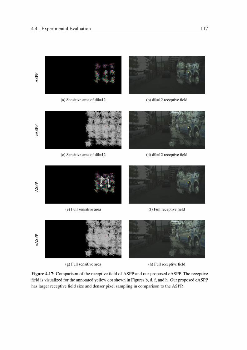
4.4. Experimental Evaluation 117A
SPP
(a) Sensitive area of dil=12 (b) dil=12 receptive field
eASP
P
(c) Sensitive area of dil=12 (d) dil=12 receptive field
ASP
P
(e) Full sensitive area (f) Full receptive field
eASP
P
(g) Full sensitive area (h) Full receptive field
Figure 4.17: Comparison of the receptive field of ASPP and our proposed eASPP. The receptivefield is visualized for the annotated yellow dot shown in Figures b, d, f, and h. Our proposed eASPPhas larger receptive field size and denser pixel sampling in comparison to the ASPP.
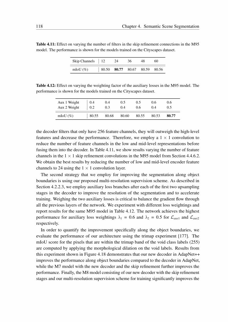
118 Chapter 4. Semantic Scene Segmentation
Table 4.11: Effect on varying the number of filters in the skip refinement connections in the M95model. The performance is shown for the models trained on the Cityscapes dataset.
Skip Channels 12 24 36 48 60
mIoU (%) 80.50 80.77 80.67 80.59 80.56
Table 4.12: Effect on varying the weighting factor of the auxiliary losses in the M95 model. Theperformance is shown for the models trained on the Cityscapes dataset.
Aux 1 Weight 0.4 0.4 0.5 0.5 0.6 0.6Aux 2 Weight 0.2 0.3 0.4 0.6 0.4 0.5
mIoU (%) 80.55 80.68 80.60 80.55 80.53 80.77
the decoder filters that only have 256 feature channels, they will outweigh the high-levelfeatures and decrease the performance. Therefore, we employ a 1 × 1 convolution toreduce the number of feature channels in the low and mid-level representations beforefusing them into the decoder. In Table 4.11, we show results varying the number of featurechannels in the 1× 1 skip refinement convolutions in the M95 model from Section 4.4.6.2.We obtain the best results by reducing the number of low and mid-level encoder featurechannels to 24 using the 1× 1 convolution layer.
The second strategy that we employ for improving the segmentation along objectboundaries is using our proposed multi-resolution supervision scheme. As described inSection 4.2.2.3, we employ auxiliary loss branches after each of the first two upsamplingstages in the decoder to improve the resolution of the segmentation and to acceleratetraining. Weighing the two auxiliary losses is critical to balance the gradient flow throughall the previous layers of the network. We experiment with different loss weightings andreport results for the same M95 model in Table 4.12. The network achieves the highestperformance for auxiliary loss weightings λ1 = 0.6 and λ2 = 0.5 for Laux1 and Laux2
respectively.In order to quantify the improvement specifically along the object boundaries, we
evaluate the performance of our architecture using the trimap experiment [177]. ThemIoU score for the pixels that are within the trimap band of the void class labels (255)are computed by applying the morphological dilation on the void labels. Results fromthis experiment shown in Figure 4.18 demonstrates that our new decoder in AdapNet++improves the performance along object boundaries compared to the decoder in AdapNet,while the M7 model with the new decoder and the skip refinement further improves theperformance. Finally, the M8 model consisting of our new decoder with the skip refinementstages and our multi-resolution supervision scheme for training significantly improves the
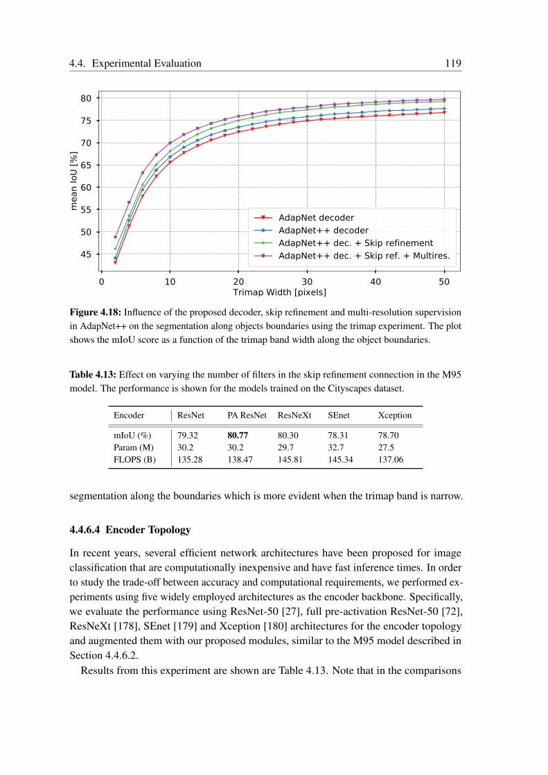
4.4. Experimental Evaluation 119
0 10 20 30 40 50Trimap Width [pixels]
45
50
55
60
65
70
75
80
mea
n Io
U [%
]
AdapNet decoderAdapNet++ decoderAdapNet++ dec. + Skip refinementAdapNet++ dec. + Skip ref. + Multires.
Figure 4.18: Influence of the proposed decoder, skip refinement and multi-resolution supervisionin AdapNet++ on the segmentation along objects boundaries using the trimap experiment. The plotshows the mIoU score as a function of the trimap band width along the object boundaries.
Table 4.13: Effect on varying the number of filters in the skip refinement connection in the M95model. The performance is shown for the models trained on the Cityscapes dataset.
Encoder ResNet PA ResNet ResNeXt SEnet Xception
mIoU (%) 79.32 80.77 80.30 78.31 78.70Param (M) 30.2 30.2 29.7 32.7 27.5FLOPS (B) 135.28 138.47 145.81 145.34 137.06
segmentation along the boundaries which is more evident when the trimap band is narrow.
4.4.6.4 Encoder Topology
In recent years, several efficient network architectures have been proposed for imageclassification that are computationally inexpensive and have fast inference times. In orderto study the trade-off between accuracy and computational requirements, we performed ex-periments using five widely employed architectures as the encoder backbone. Specifically,we evaluate the performance using ResNet-50 [27], full pre-activation ResNet-50 [72],ResNeXt [178], SEnet [179] and Xception [180] architectures for the encoder topologyand augmented them with our proposed modules, similar to the M95 model described inSection 4.4.6.2.
Results from this experiment are shown are Table 4.13. Note that in the comparisons
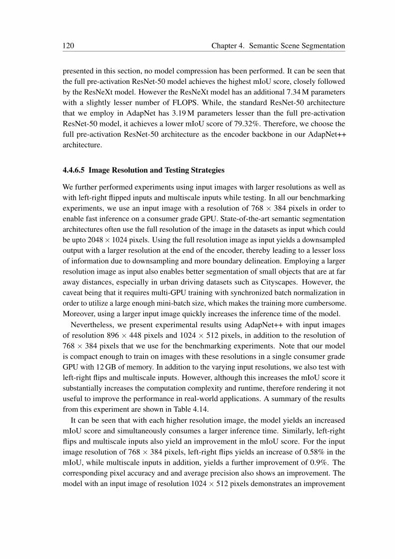
120 Chapter 4. Semantic Scene Segmentation
presented in this section, no model compression has been performed. It can be seen thatthe full pre-activation ResNet-50 model achieves the highest mIoU score, closely followedby the ResNeXt model. However the ResNeXt model has an additional 7.34 M parameterswith a slightly lesser number of FLOPS. While, the standard ResNet-50 architecturethat we employ in AdapNet has 3.19 M parameters lesser than the full pre-activationResNet-50 model, it achieves a lower mIoU score of 79.32%. Therefore, we choose thefull pre-activation ResNet-50 architecture as the encoder backbone in our AdapNet++architecture.
4.4.6.5 Image Resolution and Testing Strategies
We further performed experiments using input images with larger resolutions as well aswith left-right flipped inputs and multiscale inputs while testing. In all our benchmarkingexperiments, we use an input image with a resolution of 768 × 384 pixels in order toenable fast inference on a consumer grade GPU. State-of-the-art semantic segmentationarchitectures often use the full resolution of the image in the datasets as input which couldbe upto 2048× 1024 pixels. Using the full resolution image as input yields a downsampledoutput with a larger resolution at the end of the encoder, thereby leading to a lesser lossof information due to downsampling and more boundary delineation. Employing a largerresolution image as input also enables better segmentation of small objects that are at faraway distances, especially in urban driving datasets such as Cityscapes. However, thecaveat being that it requires multi-GPU training with synchronized batch normalization inorder to utilize a large enough mini-batch size, which makes the training more cumbersome.Moreover, using a larger input image quickly increases the inference time of the model.
Nevertheless, we present experimental results using AdapNet++ with input imagesof resolution 896 × 448 pixels and 1024 × 512 pixels, in addition to the resolution of768 × 384 pixels that we use for the benchmarking experiments. Note that our modelis compact enough to train on images with these resolutions in a single consumer gradeGPU with 12 GB of memory. In addition to the varying input resolutions, we also test withleft-right flips and multiscale inputs. However, although this increases the mIoU score itsubstantially increases the computation complexity and runtime, therefore rendering it notuseful to improve the performance in real-world applications. A summary of the resultsfrom this experiment are shown in Table 4.14.
It can be seen that with each higher resolution image, the model yields an increasedmIoU score and simultaneously consumes a larger inference time. Similarly, left-rightflips and multiscale inputs also yield an improvement in the mIoU score. For the inputimage resolution of 768 × 384 pixels, left-right flips yields an increase of 0.58% in themIoU, while multiscale inputs in addition, yields a further improvement of 0.9%. Thecorresponding pixel accuracy and and average precision also shows an improvement. Themodel with an input image of resolution 1024× 512 pixels demonstrates an improvement
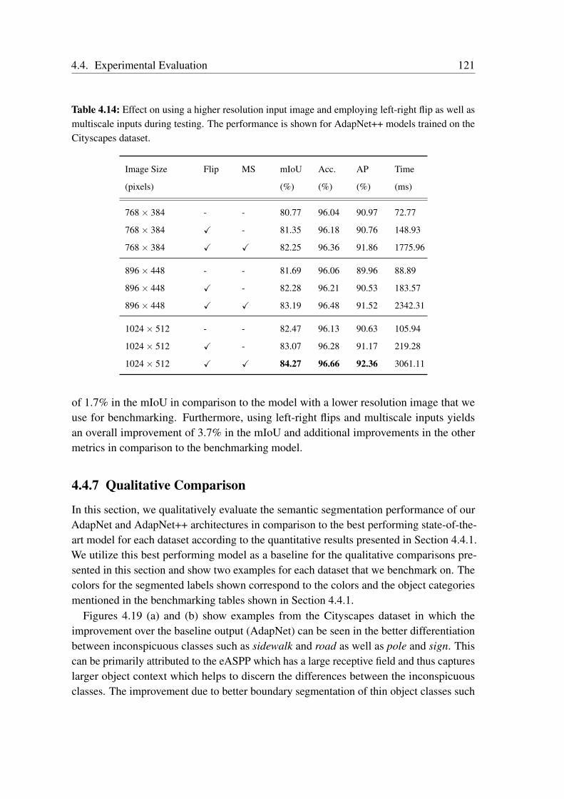
4.4. Experimental Evaluation 121
Table 4.14: Effect on using a higher resolution input image and employing left-right flip as well asmultiscale inputs during testing. The performance is shown for AdapNet++ models trained on theCityscapes dataset.
Image Size Flip MS mIoU Acc. AP Time
(pixels) (%) (%) (%) (ms)
768× 384 - - 80.77 96.04 90.97 72.77
768× 384 X - 81.35 96.18 90.76 148.93
768× 384 X X 82.25 96.36 91.86 1775.96
896× 448 - - 81.69 96.06 89.96 88.89
896× 448 X - 82.28 96.21 90.53 183.57
896× 448 X X 83.19 96.48 91.52 2342.31
1024× 512 - - 82.47 96.13 90.63 105.94
1024× 512 X - 83.07 96.28 91.17 219.28
1024× 512 X X 84.27 96.66 92.36 3061.11
of 1.7% in the mIoU in comparison to the model with a lower resolution image that weuse for benchmarking. Furthermore, using left-right flips and multiscale inputs yieldsan overall improvement of 3.7% in the mIoU and additional improvements in the othermetrics in comparison to the benchmarking model.
4.4.7 Qualitative Comparison
In this section, we qualitatively evaluate the semantic segmentation performance of ourAdapNet and AdapNet++ architectures in comparison to the best performing state-of-the-art model for each dataset according to the quantitative results presented in Section 4.4.1.We utilize this best performing model as a baseline for the qualitative comparisons pre-sented in this section and show two examples for each dataset that we benchmark on. Thecolors for the segmented labels shown correspond to the colors and the object categoriesmentioned in the benchmarking tables shown in Section 4.4.1.
Figures 4.19 (a) and (b) show examples from the Cityscapes dataset in which theimprovement over the baseline output (AdapNet) can be seen in the better differentiationbetween inconspicuous classes such as sidewalk and road as well as pole and sign. Thiscan be primarily attributed to the eASPP which has a large receptive field and thus captureslarger object context which helps to discern the differences between the inconspicuousclasses. The improvement due to better boundary segmentation of thin object classes such
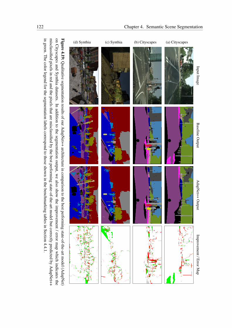
122 Chapter 4. Semantic Scene SegmentationInputIm
ageB
aselineO
utputA
dapNet++
Output
Improvem
ent/ErrorM
ap
(a) Cityscapes(b) Cityscapes(c) Synthia(d) Synthia
Figure4.19:Q
ualitativesegm
entationresults
ofourAdapN
et++architecture
incom
parisonto
thebestperform
ingstate-of-the-artm
odel(AdapN
et)on
Cityscapes
andSynthia
datasets.In
additionto
thesegm
entationoutput,w
ealso
showthe
improvem
ent/
errorm
apw
hichindicates
them
isclassifiedpixels
inred
andthe
pixelsthatare
misclassified
bythe
bestperforming
state-of-the-artmodelbutcorrectly
predictedby
AdapN
et++in
green.The
colorlegendforthe
segmentation
labelscorrespond
tothose
shown
inthe
benchmarking
tablesin
Section4.4.1.
4.4. Experimental Evaluation 123
as poles can be seen in the images.Figures 4.19 (c) and (d) show examples from the Synthia dataset, where objects such
as bicycles, cars and people are better segmented. The baseline output (AdapNet) showsseveral missing cars, people and bicycles, whereas the AdapNet++ output accuratelycaptures these objects. Moreover, it can also be seen that the pole-like structures and treesare often discontinuous in the baseline output, while they are more well defined in theAdapNet++ output. In Figure 4.19 (d), an interesting observation is made where an entirefence is segmented in the baseline output but is absent in the scene. This is due to the factthat the intersection of the sidewalk and the road gives an appearance of a fence which isthen misclassified. In the same image, it can also be observed that a small building-likestructure on the right is not captured, whereas our AdapNet++ model accurately segmentsthe structure.
Figures 4.20 (a) and (b) show examples from the indoor SUN RGB-D dataset. Examplesfrom this dataset show significant misclassification due to inconspicuous objects. Oftenscenes in indoor datasets have large objects that require the network to have very largereceptive fields to be able to accurately distinguish between them. Figure 4.20 (a) shows ascene in which parts of the chair and the table are incorrectly classified as a desk in theoutput of the baseline model (DeepLab v3). These two classes have very similar structureand appearance which makes distinguishing between them extremely challenging. InFigure 4.20 (b), we can see parts of the sofa incorrectly classified in the baseline modeloutput, whereas the entire object is accurately predicted in the AdapNet++ output. In thebaseline output, misclassification can also be seen for the picture on the wall which isprecisely segmented in the AdapNet++ output.
In Figures 4.20 (c) and (d), we show examples from the indoor ScanNet dataset. Fig-ure 4.20 (c) shows misclassification in the output of the baseline model (DeepLab v3) inthe boundary where the wall meets the floor and for parts of the desk that is misclassifiedas other furniture. Figure 4.20 (d) shows a significant improvement in the segmentationof AdapNet++ in comparison to the baseline model. The cabinet and counter are entirelymisclassified as a desk and other furniture correspondingly in the output of the baselinemodel, whereas they are accurately predicted by our AdapNet++ mode.
Figures 4.21 (a) and (b) show examples from the unstructured Freiburg Forest datasetwhere the improvement can largely be seen in discerning the object boundaries of classessuch as grass and vegetation, as well as trail and grass. By observing these images, wecan see that even for us humans it is difficult to estimate the boundaries between theseclasses. Our AdapNet++ architecture predicts the boundaries comparatively better than thebaseline model (DeepLab v3). The improvement in the segmentation can also been seen inthe finer segmentation of the vegetation and the trail path in the AdapNet++ output.
Furthermore, Figure 4.21 (c) shows a failure mode where the image is underexposed dueto direct sunlight on the optics which causes the obstacle in the left of the image indicated inblack to be not fully captured in the segmentation. This could lead to unforeseen situations
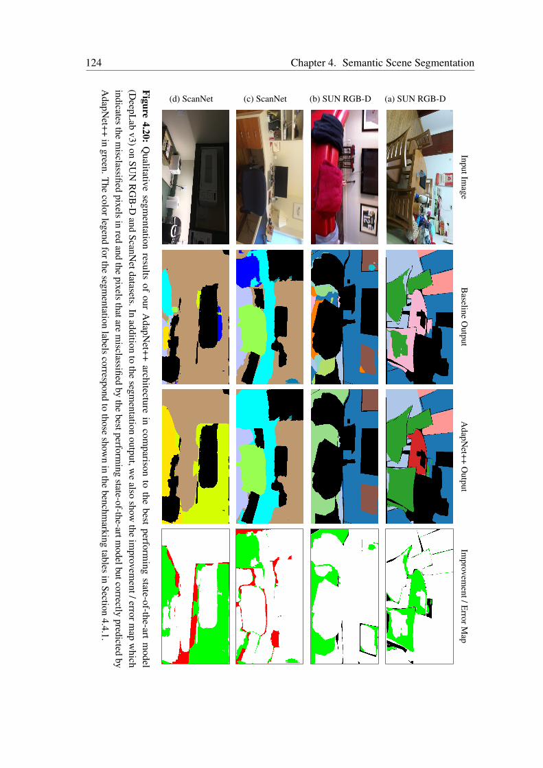
124 Chapter 4. Semantic Scene SegmentationInputIm
ageB
aselineO
utputA
dapNet++
Output
Improvem
ent/ErrorM
ap
(a) SUN RGB-D(b) SUN RGB-D(c) ScanNet(d) ScanNet
Figure4.20:
Qualitative
segmentation
resultsof
ourA
dapNet++
architecturein
comparison
tothe
bestperform
ingstate-of-the-art
model
(DeepL
abv3)on
SUN
RG
B-D
andScanN
etdatasets.Inaddition
tothe
segmentation
output,we
alsoshow
theim
provement/errorm
apw
hichindicates
them
isclassifiedpixels
inred
andthe
pixelsthatare
misclassified
bythe
bestperforming
state-of-the-artmodelbutcorrectly
predictedby
AdapN
et++in
green.The
colorlegendforthe
segmentation
labelscorrespond
tothose
shown
inthe
benchmarking
tablesin
Section4.4.1.
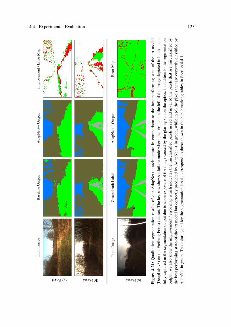
4.4. Experimental Evaluation 125
Inpu
tIm
age
Bas
elin
eO
utpu
tA
dapN
et++
Out
put
Impr
ovem
ent/
Err
orM
ap
(a)Forest (b)Forest
Inpu
tIm
age
Gro
undt
ruth
Lab
elA
dapN
et++
Out
put
Err
orM
ap
(c)Forest
Figu
re4.
21:
Qua
litat
ive
segm
enta
tion
resu
ltsof
our
Ada
pNet
++ar
chite
ctur
ein
com
pari
son
toth
ebe
stpe
rfor
min
gst
ate-
of-t
he-a
rtm
odel
(Dee
pLab
v3)o
nth
eFr
eibu
rgFo
rest
data
set.
The
last
row
show
sa
failu
rem
ode
whe
reth
eob
stac
lein
the
left
ofth
eim
age
depi
cted
inbl
ack
isno
tfu
llyca
ptur
edin
the
segm
enta
tion
outp
utdu
eto
unde
rexp
osur
eof
the
imag
eca
used
byth
egl
arin
gsu
non
the
optic
s.In
addi
tion
toth
ese
gmen
tatio
nou
tput
,we
also
show
the
impr
ovem
ent/
erro
rmap
whi
chin
dica
tes
the
mis
clas
sifie
dpi
xels
inre
dan
din
(a,b
)the
pixe
lsth
atar
em
iscl
assi
fied
byth
ebe
stpe
rfor
min
gst
ate-
of-t
he-a
rtm
odel
butc
orre
ctly
pred
icte
dby
Ada
pNet
++in
gree
n,w
hile
in(c
)the
pixe
lsth
atar
eco
rrec
tlycl
assi
fied
byA
dapN
etin
gree
n.T
heco
lorl
egen
dfo
rthe
segm
enta
tion
labe
lsco
rres
pond
toth
ose
show
nin
the
benc
hmar
king
tabl
esin
Sect
ion
4.4.
1.
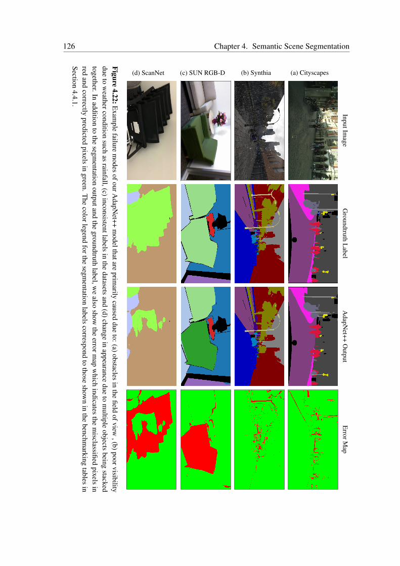
126 Chapter 4. Semantic Scene SegmentationInputIm
ageG
roundtruthL
abelA
dapNet++
Output
ErrorM
ap
(a) Cityscapes(b) Synthia(c) SUN RGB-D(d) ScanNet
Figure4.22:Exam
plefailure
modes
ofourAdapN
et++m
odelthatareprim
arilycaused
dueto:(a)obstacles
inthe
fieldofview
,(b)poorvisibilitydue
tow
eatherconditionsuch
asrainfall,(c)inconsistentlabels
inthe
datasetsand
(d)changein
appearancedue
tom
ultipleobjects
beingstacked
together.Inaddition
tothe
segmentation
outputandthe
groundtruthlabel,w
ealso
showthe
errormap
which
indicatesthe
misclassified
pixelsin
redand
correctlypredicted
pixelsin
green.The
colorlegendforthe
segmentation
labelscorrespond
tothose
shown
inthe
benchmarking
tablesin
Section4.4.1.
4.4. Experimental Evaluation 127
if the robot drives over the area and misses detecting the obstacle. Figure 4.22 shows morefailure modes from the other datasets that we benchmark on. In Figure 4.22 (a), the cyclistbehind the two people in the center of the image is misclassified as a person as most of thebicycle is covered by the two people in front of the cyclist. Figure 4.22 (b) shows a darkscene with rainfall which causes a significant amount of poles and persons that are at faraway distances to be not captured in the segmentation due to bad visibility. Figure 4.22 (c)shows an example from the SUN RGB-D dataset where a sofa is misclassified as a chair.This is caused by the inconsistency in the labels in this dataset. As the SUN RGB-D datasetis a mixture of three different datasets, some instances have the single-person sofa labeledas a chair, while the others have it labeled as the sofa class which causes confusion amongthese object classes. In another example, Figure 4.22 (d) shows a scene where the chairsare folded and stacked with each other which gives a completely different appearance thanthe examples of the chair class in the training set. In the next chapter, we demonstrate howleveraging complementary modalities such as depth and near-infrared can enable robustsemantic segmentation in most of these situations.
4.4.8 Generalization Analysis
In this section, we qualitatively evaluate the generalization performance of our AdapNetand AdapNet++ architectures on data collected by our autonomous car setup in Freiburg.The data was collected over three days in different driving scenarios including both in theinner-city and highways. We use our models trained on the Cityscapes dataset and only teston the images captured in Freiburg. Figure 4.23 shows four examples from this experimentin which we can observe that the structure of these scenes are substantially different thanthe images in the Cityscapes dataset and a significant amount of illumination changes canbe seen. The colors for the segmented labels shown correspond to the colors and the objectcategories mentioned in the Cityscapes benchmarking results shown in Table 4.1.
The AdapNet++ model in general, demonstrates more accurate semantic segmentationthan the AdapNet model in these environments. In Figure 4.23 (a), we see that theAdapNet++ model precisely captures the fences in the scene along the right side of thesidewalk as well as traffic signs that are at far away distances. While in Figure 4.23 (b),we observe that the AdapNet++ model shows a greater granularity in the segmentation ofvegetation and it more accurately captures the dividers in the middle of the road as well assidewalks. This can be attributed to the new decoder in AdapNet++ which enables accuratesegmentation of thin structures and improves the granularity of the segmentation alongthe object boundaries. Figure 4.23 (c) shows a hard example where the middle island onthe road is at the same level as the road, as opposed to being raised similar to sidewalks.Even in this scenario, the AdapNet++ model reasonable segments the middle island dueto its eASPP which enables it to capture long-range context with a large receptive fieldresolution, whereas AdapNet produces misclassifications in this region. It can also be
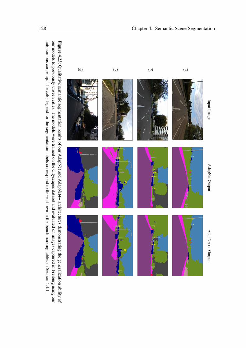
128 Chapter 4. Semantic Scene Segmentation
InputImage
AdapN
etOutput
AdapN
et++O
utput
(a)(b)(c)(d)
Figure4.23:Q
ualitativesem
anticsegm
entationresults
ofourAdapN
etandA
dapNet++
architecturesdem
onstratingthe
generalizationability
ofourm
odelsto
previouslyunseen
cities.The
models
were
trainedon
theC
ityscapesdatasetand
evaluatedon
images
capturedin
Freiburgusing
ourautonom
ouscarsetup.T
hecolorlegend
forthesegm
entationlabels
correspondto
thoseshow
nin
thebenchm
arkingtables
inSection
4.4.1.
4.5. Related Work 129
observed that in some instances, AdapNet segments the shadows made by cars as the carclass and does not capture all the traffic sings in the scene, while the AdapNet++ outputaccurately captures these objects due to the multiscale context aggregation in the encoder.Finally, in Figure 4.23 (d), we can see a more precise segmentation in the AdapNet++output compared to AdapNet for object classes such as sidewalks, person, vegetation,fences and cars. Nevertheless, these results demonstrate that our models reliably segmentsthe scene and generalizes effectively to scenes from previously unseen cities that were notpresent in the training data.
4.5 Related Work
In this chapter, we addressed the problem of efficient semantic segmentation using convo-lutional neural networks. There is a significant amount of prior work in this fundamentalperception problem. However, in the last decade, there has been a sharp transition fromemploying hand engineered features with flat classifiers such as Support Vector Ma-chines [181], Boosting [182] or Random Forests [183, 184], to end-to-end DCNN-basedapproaches [24, 136]. In order to highlight our contributions, we present a through reviewin this section by first briefly discussing some of the classical methods before delving intothe state-of-the-art techniques.
Semantic segmentation is one of the fundamental problems in computer vision. Someof the earlier approaches for semantic segmentation use small patches to classify thecenter pixel using flat classifiers [182, 183] followed by smoothing the predictions usingConditional Random Fields (CRFs) [182]. Rather than only relying on appearance basedfeatures, structure from motion features have also been used with randomized decisionforests [182, 184]. View independent 3D features from dense depth maps have beenshown to outperform appearance based features, that also enabled classification of all thepixels in an image, as opposed to only the center pixel of a patch [185]. Plath et al. [186]propose an approach to combine local and global features using a CRF and an imageclassification method. However, the performance of these approaches is largely boundedby the expressiveness of handcrafted features which is highly scenario-specific.
The remarkable performance achieved by CNNs in classification tasks led to theirapplication for dense prediction problems such as semantic segmentation, depth estimationand optical flow prediction. Initial approaches that employed neural networks for semanticsegmentation still relied on patch-wise training [187, 188, 189]. Pinheiro et al. [189]use a recurrent CNN to aggregate several low-resolution predictions for scene labeling.Clement et al. [188] transforms the input image through a Laplacian pyramid followed byfeeding each scale to a CNN for hierarchical feature extraction and classification. Althoughthese approaches demonstrated improved performance over handcrafted features, theyoften yield a grid-like output that does not capture the true object boundaries. One of the
130 Chapter 4. Semantic Scene Segmentation
first end-to-end approaches that learns to directly map the low-resolution representationsfrom a classification network to a dense prediction output was the Fully ConvolutionalNetwork (FCN) model [24]. FCN proposed an encoder-decoder architecture in which theencoder is built upon the VGG-16 [153] architecture with the inner-product layers replacedwith convolutional layers. While, the decoder consists of successive deconvolution andconvolution layers that upsample and refine the low-resolution feature maps by combiningthem with the encoder feature maps. The last decoder then yields a segmented output withthe same resolution as the input image.
DeconvNet [169] propose an improved architecture containing stacked deconvolutionand unpooling layers that perform non-linear upsampling and outperforms FCNs but atthe cost of a more complex training procedure. The SegNet [136] architecture eliminatesthe need for learning to upsample by reusing pooling indices from the encoder layers toperform upsampling. U-Net [122] adds skip connections from the encoder to each corre-sponding decoder section for biomedical image segmentation. Similarly, RefineNet [190]proposed a network to exploit features along the down-sampling process to enable high-resolution segmentation. Oliveira et al. [48] propose an architecture that builds upon FCNsand introduces more refinement stages and incorporates spatial dropout to prevent overfitting. The ParseNet [168] architecture models global context directly instead of onlyrelying on the largest receptive field of the network. Several recent approaches employConditional Random Fields (CRFs) in cascade with CNNs to encode long-range contextand to improve object boundary segmentation [138, 191]. Some approaches jointly trainCNN and CRF components [192, 193], while others employ several convolutional layerson top of the belief maps to capture context information [194]. Vemulapalli et al. [195]propose an approach that combines Gaussian Conditional Random Fields with CNNs andoutperforms other approaches that combine CNNs with discrete CRF models. However,these techniques are not feed-forward in test time as they require MAP inference over aCRF or other aids such as region proposals.
Recently, there has been more focus on learning multiscale features, which was initiallyachieved by providing the network with multiple rescaled versions of the image [188] or byfusing features from multiple parallel branches that take different image resolutions [24].The general goal of these approaches is to provide the network with both local and globalcontext [196] by using features extracted at multiple scales and incorporating feature mapsfrom early network layers for improving prediction along object boundaries as they retainmore high frequency details. Most of these networks are difficult to train due to the numberof parameters they consume [197], therefore, multi-stage training procedures are oftenemployed. In addition, they have slow runtimes due to multiple convolutional pathwaysfor feature extraction.
In order to alleviate this problem, Yu et al. [67] propose dilated convolutions that allowsfor exponential increase in the receptive field without decrease in resolution or increase inparameters. Since then several approaches have explored the use of dilated convolutions
4.6. Conclusions 131
for semantic segmentation. Wu et al. [198] study the effect of atrous convolutions withdifferent dilation rates for capturing long-range information. Wang et al. [199] employhybrid atrous rates in a residual network architecture. Dai et al. [200] proposes deformableconvolutions that generalize dilated convolutions by sampling the input features with alearned offset. DeepLab [132, 138] build upon the aforementioned idea and uses dilatedconvolutions of different atrous rates to aggregate multiscale global context. Subsequently,Zhao et al. introduce the PSPNet [135] architecture that employs spatial pooling at differentgrid scales to capture multiscale information. However, a major drawback in employingthese approaches is the computational complexity and the substantially large inference timeeven using modern GPUs that hinder them from being deployed in robots that often havelimited resources. Conversely, in this chapter we presented several new contributions forlearning multiscale features, capturing long range context and improving the upsamplingin the decoder, while simultaneously reducing the number of parameters and maintaining afast inference time. Our proposed architectures that incorporate these techniques achievea good trade-off between performance and computational complexity of the model forenabling efficient deployment in real-world robotic perception applications.
4.6 Conclusions
In this chapter, we presented the novel AdapNet and AdapNet++ architectures for efficientsemantic scene segmentation. Our AdapNet architecture follows the encoder-decodertopology and incorporates our multiscale residual units with atrous convolutions thathave gradually increasing dilation rates to encode multiscale information throughout thenetwork without increasing the number of parameters. The proposed multiscale residualunits are more effective at learning multiscale features and outperform the commonlyemployed multigrid method. Furthermore, our proposed AdapNet++ architecture buildsupon AdapNet and additionally incorporates several new network modules for improvingthe performance, including the Efficient Atrous Spatial Pyramid Pooling (eASPP), a newstrong decoder and the multi-resolution supervision strategy. Our eASPP employs bothparallel and cascaded atrous convolutions with different dilation rates in a bottleneckfashion to efficiently capture long range context and probe the features with filters atmultiple sampling rates and field of views. The eASPP has a larger effective receptive fieldand achieves 10 times reduction in the number of parameters with a simultaneous increasein performance compared to the standard ASPP. Our new decoder with skip refinementstages fuses low and mid-level features from the encoder for object boundary refinement.Finally, the proposed multi-resolution supervision scheme accelerates the training andfurther improves the performance along object boundaries. Additionally, we presenteda holistic network-wide pruning approach that is invariant to shortcut connections, tocompress our model and to enable efficient deployment.
132 Chapter 4. Semantic Scene Segmentation
We introduced a first-of-its-kind Freiburg Forest dataset that contains images of multiplemodalities and spectra with pixel-wise ground truth annotations of unstructured forestedenvironments. We presented an exhaustive theoretical analysis, visualizations, quantitativeand qualitative results on the Cityscapes, Synthia, SUN RGB-D, ScanNet and FreiburgForest datasets. The results demonstrate that our architectures achieve state-of-the-artperformance with a significantly lesser number of parameters and a substantially fasterinference time in comparison to several strong state-of-the-art models. Furthermore, wepresented qualitative evaluations on data collected by our autonomous car setup in Freiburgthat demonstrates the generalization ability of our model to previously unseen scenarios.
Chapter 5
Multimodal Semantic Segmentation
Learning to reliably perceive and understand the scene is an inte-gral enabler for robots to operate in the real-world. This prob-lem is inherently challenging due to the multitude of object typesas well as appearance changes caused by varying illumination andweather conditions. Leveraging complementary modalities can en-able learning of semantically richer representations that are re-silient to such perturbations. Despite the tremendous progress inrecent years, most CNNs directly concatenate different modalitiesfrom the outset, or concatenate learned features from modality-specific streams, rendering the model incapable of focusing only onthe relevant complementary information. To address this limitation,we propose two mutimodal semantic segmentation frameworks thatdynamically adapt the fusion of modality-specific features basedon the scene condition. Our first fusion scheme termed CMoDElearns to probabilistically fuse features from modality-specific net-work streams to exploit the most discriminative complementaryclass-specific features. While our subsequently proposed SSMA fu-sion scheme dynamically fuses intermediate representations frommodality-specific encoder streams into a single decoder, while beingsensitive to the object category, spatial location and scene context ina self-supervised manner. Comprehensive empirical evaluations onseveral benchmarks show that both our fusion techniques achievestate-of-the-art performance, while demonstrating substantial ro-bustness in adverse perceptual conditions.
5.1 Introduction
Robust scene understanding is a critical and essential task for autonomous navigation.This problem is heavily characterized by changing environmental conditions that take
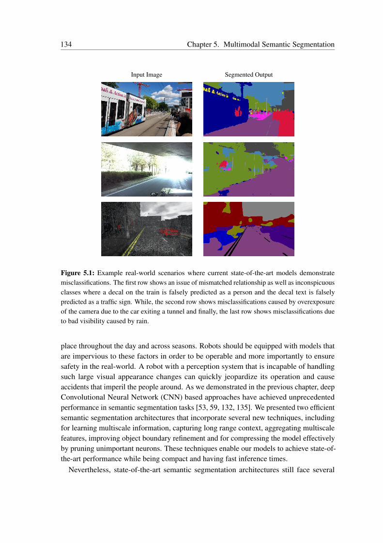
134 Chapter 5. Multimodal Semantic Segmentation
Input Image Segmented Output
Figure 5.1: Example real-world scenarios where current state-of-the-art models demonstratemisclassifications. The first row shows an issue of mismatched relationship as well as inconspicuousclasses where a decal on the train is falsely predicted as a person and the decal text is falselypredicted as a traffic sign. While, the second row shows misclassifications caused by overexposureof the camera due to the car exiting a tunnel and finally, the last row shows misclassifications dueto bad visibility caused by rain.
place throughout the day and across seasons. Robots should be equipped with models thatare impervious to these factors in order to be operable and more importantly to ensuresafety in the real-world. A robot with a perception system that is incapable of handlingsuch large visual appearance changes can quickly jeopardize its operation and causeaccidents that imperil the people around. As we demonstrated in the previous chapter, deepConvolutional Neural Network (CNN) based approaches have achieved unprecedentedperformance in semantic segmentation tasks [53, 59, 132, 135]. We presented two efficientsemantic segmentation architectures that incorporate several new techniques, includingfor learning multiscale information, capturing long range context, aggregating multiscalefeatures, improving object boundary refinement and for compressing the model effectivelyby pruning unimportant neurons. These techniques enable our models to achieve state-of-the-art performance while being compact and having fast inference times.
Nevertheless, state-of-the-art semantic segmentation architectures still face several
5.1. Introduction 135
challenges while being employed in the real-world due to frequent visual appearancechanges caused by transitioning weather, illumination and seasons, in addition to thediversity of complex scenes that cause mismatched relationship as well as inconspicuousobject classes. Figure 5.1 shows example scenes from real-world scenarios in whichmisclassifications are produced due to the decal on the train which is falsely predicted asa person and a traffic sign (first row), overexposure of the camera caused by the vehicleexiting a tunnel (second row), and bad visibility conditions caused by rain and cloudyweather (third row). In order to accurately predict the elements of the scene in thesesituations, features from complementary modalities such as depth and infrared can beleveraged to correspondingly exploit object properties such as geometry and reflectance.Moreover, the network can exploit complex intra-modal dependencies more effectively bydirectly learning to fuse visual appearance information from RGB images with learnedfeatures from complementary modalities in an end-to-end fashion. This not only enablesthe network to resolve inherent ambiguities and improve the reliability but also obtain amore holistic scene segmentation.
While most existing work focuses on where to fuse modality-specific streams topolog-ically [50, 162, 201] and what transformations can be applied on the depth modality toenable better fusion with visual RGB features [161, 163], it still remains an open questionas to how to enable the network to dynamically adapt its fusion strategy based on thenature of the scene such as the types of objects, their spatial location in the world andthe present scene context. This is a crucial requirement in applications such as roboticsand autonomous driving where these systems run in continually changing environmentalcontexts. For example, an autonomous car navigating in ideal weather conditions can pri-marily rely on visual information but when it enters a dark tunnel or exits an underpassage,the cameras might experience under/over exposure, whereas the depth modality will bemore informative. Furthermore, the strategy to be employed for fusion also varies withthe types of objects in the scene, for instance, infrared might be more useful to detectcategories such as people, vehicles, vegetation and boundaries of structures but it does notprovide much information on object categories such as the sky. Additionally, the spatiallocation of objects in the scene also has an influence, for example, the depth modalityprovides rich information on objects that are at nearby distances but degrades very quicklyfor objects that are several meters away. More importantly, the approach employed shouldbe robust to sensor failure and noise as constraining the network to always depend onboth modalities and use noisy information can worsen the actual performance and lead todisastrous situations.
Due to these complex interdependencies, naively treating modalities as multi-channelinput data or concatenating independently learned modality-specific features does notallow the network to adapt to the aforementioned situations dynamically. Moreover, due tothe nature of this dynamicity, the fusion mechanism has to be trained in a self-supervisedmanner in order to make the adaptivity emergent and to generalize effectively to different

136 Chapter 5. Multimodal Semantic Segmentation
real-world scenarios. As a solution to this problem, we present two novel multimodalfusion mechanisms: the Convoluted Mixture of Deep Experts (CMoDE) and the Self-Supervised Model Adaptation (SSMA) scheme. We build upon our AdapNet++ semanticsegmentation architecture presented in Chapter 4, and propose two multimodal variantsincorporating the CMoDE and SSMA fusion mechanisms respectively. The CMoDEacts as a multiplexer and adaptively weighs class-specific features of individual modality-specific network streams using learned probability distributions. The CMoDE moduleconsists of multiple Adaptive Gating Networks (AGN) that each take a two-dimensionalencoder feature channel corresponding to particular object class from each modality-specific stream as input and uses them to map the decoder features to a probabilisticallyfused representation. We employ the CMoDE to fuse the high-level semantically maturefeatures at the end of the modality-specific encoder-decoder streams and feed the outputto an additional convolution layer to further learn discriminative complementary fusedkernels. Although our CMoDE fusion mechanism exploits complementary features frommodality-specific network streams according to the different object classes in the scene,it does not address the fact that the spatial location of the object in the environment alsoinfluences the selection of modality-specific features. For example, modalities such asdepth are accurate at nearby distances but degrades quickly for objects that are at far awaydistances, therefore, the alternate visual RGB features should be leveraged for segmentingdistant objects in this case.
In order to address this limitation, we present the SSMA fusion mechanism that adap-tively recalibrates and fuses modality-specific feature maps based on the object class, itsspatial location and the scene context. The SSMA module takes intermediate encoderrepresentations of modality-specific streams as input and fuses them probabilistically basedon the activations of individual modality streams. As we model the SSMA module in afully convolutional fashion, it yields a probability for each activation in the feature maps(as opposed to only a probability for each object class in the CMoDE approach) whichrepresents the optimal combination to exploit complementary properties. These probabil-ities are then used to amplify or suppress the representations of the individual modalitystreams, followed by the fusion. As we base the fusion on modality-specific activations, itis intrinsically tolerant to sensor failure and noise such as missing depth values. We employthe SSMA module to fuse representations at the end of the modality-specific encoderstreams as well as to fuse the mid-level encoder representations. The fused representationsfrom the SSMA modules are input to the decoder at different stages for upsampling andrefining the predictions.
We employ a combination of mid-level fusion and late-fusion as several experimentshave demonstrated that fusing semantically meaningful representations yields better perfor-mance in comparison to early-fusion [50, 120, 162, 163]. Moreover, studies of the neuraldynamics of the human brain has also shown evidence of late-fusion of modalities forrecognition tasks [202]. However, intermediate network representations are not aligned
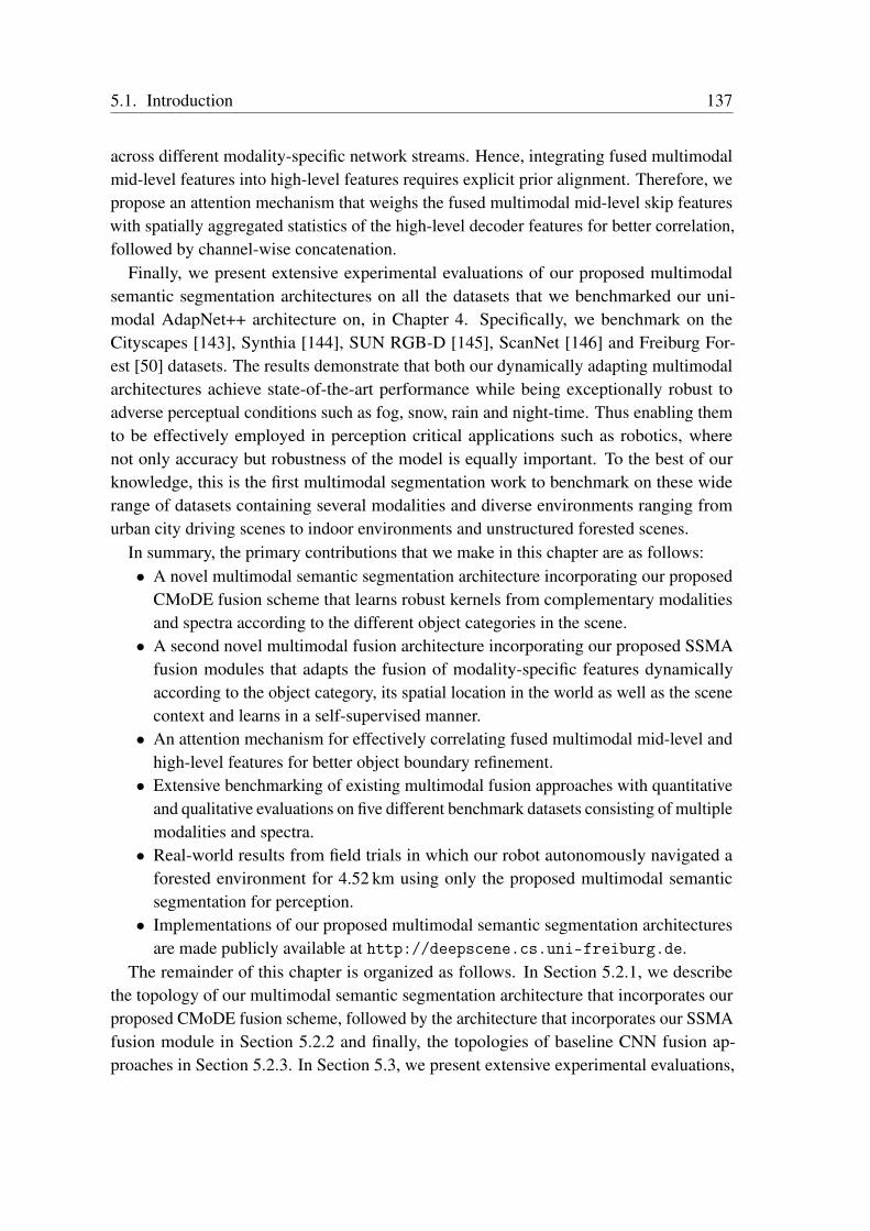
5.1. Introduction 137
across different modality-specific network streams. Hence, integrating fused multimodalmid-level features into high-level features requires explicit prior alignment. Therefore, wepropose an attention mechanism that weighs the fused multimodal mid-level skip featureswith spatially aggregated statistics of the high-level decoder features for better correlation,followed by channel-wise concatenation.
Finally, we present extensive experimental evaluations of our proposed multimodalsemantic segmentation architectures on all the datasets that we benchmarked our uni-modal AdapNet++ architecture on, in Chapter 4. Specifically, we benchmark on theCityscapes [143], Synthia [144], SUN RGB-D [145], ScanNet [146] and Freiburg For-est [50] datasets. The results demonstrate that both our dynamically adapting multimodalarchitectures achieve state-of-the-art performance while being exceptionally robust toadverse perceptual conditions such as fog, snow, rain and night-time. Thus enabling themto be effectively employed in perception critical applications such as robotics, wherenot only accuracy but robustness of the model is equally important. To the best of ourknowledge, this is the first multimodal segmentation work to benchmark on these widerange of datasets containing several modalities and diverse environments ranging fromurban city driving scenes to indoor environments and unstructured forested scenes.
In summary, the primary contributions that we make in this chapter are as follows:• A novel multimodal semantic segmentation architecture incorporating our proposed
CMoDE fusion scheme that learns robust kernels from complementary modalitiesand spectra according to the different object categories in the scene.• A second novel multimodal fusion architecture incorporating our proposed SSMA
fusion modules that adapts the fusion of modality-specific features dynamicallyaccording to the object category, its spatial location in the world as well as the scenecontext and learns in a self-supervised manner.• An attention mechanism for effectively correlating fused multimodal mid-level and
high-level features for better object boundary refinement.• Extensive benchmarking of existing multimodal fusion approaches with quantitative
and qualitative evaluations on five different benchmark datasets consisting of multiplemodalities and spectra.• Real-world results from field trials in which our robot autonomously navigated a
forested environment for 4.52 km using only the proposed multimodal semanticsegmentation for perception.• Implementations of our proposed multimodal semantic segmentation architectures
are made publicly available at http://deepscene.cs.uni-freiburg.de.The remainder of this chapter is organized as follows. In Section 5.2.1, we describe
the topology of our multimodal semantic segmentation architecture that incorporates ourproposed CMoDE fusion scheme, followed by the architecture that incorporates our SSMAfusion module in Section 5.2.2 and finally, the topologies of baseline CNN fusion ap-proaches in Section 5.2.3. In Section 5.3, we present extensive experimental evaluations,
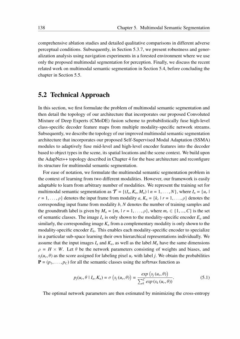
138 Chapter 5. Multimodal Semantic Segmentation
comprehensive ablation studies and detailed qualitative comparisons in different adverseperceptual conditions. Subsequently, in Section 5.3.7, we present robustness and gener-alization analysis using navigation experiments in a forested environment where we useonly the proposed multimodal segmentation for perception. Finally, we discuss the recentrelated work on multimodal semantic segmentation in Section 5.4, before concluding thechapter in Section 5.5.
5.2 Technical Approach
In this section, we first formulate the problem of multimodal semantic segmentation andthen detail the topology of our architecture that incorporates our proposed ConvolutedMixture of Deep Experts (CMoDE) fusion scheme to probabilistically fuse high-levelclass-specific decoder feature maps from multiple modality-specific network streams.Subsequently, we describe the topology of our improved multimodal semantic segmentationarchitecture that incorporates our proposed Self-Supervised Modal Adaptation (SSMA)modules to adaptively fuse mid-level and high-level encoder features into the decoderbased to object types in the scene, its spatial locations and the scene context. We build uponthe AdapNet++ topology described in Chapter 4 for the base architecture and reconfigureits structure for multimodal semantic segmentation.
For ease of notation, we formulate the multimodal semantic segmentation problem inthe context of learning from two different modalities. However, our framework is easilyadaptable to learn from arbitrary number of modalities. We represent the training set formultimodal semantic segmentation as T = (In, Kn, Mn) | n = 1, . . . , N, where In = ur |r = 1, . . . , ρ denotes the input frame from modality a, Kn = kr | r = 1, . . . , ρ denotes thecorresponding input frame from modality b, N denotes the number of training samples andthe groundtruth label is given by Mn = mr | r = 1, . . . , ρ, where mr ∈ 1, ..., C is the setof semantic classes. The image In is only shown to the modality-specific encoder Ea andsimilarly, the corresponding image Kn from a complementary modality is only shown to themodality-specific encoder Eb. This enables each modality-specific encoder to specializein a particular sub-space learning their own hierarchical representations individually. Weassume that the input images In and Kn, as well as the label Mn have the same dimensionsρ = H × W. Let θ be the network parameters consisting of weights and biases, andsj(ur, θ) as the score assigned for labeling pixel ur with label j. We obtain the probabilitiesP = (p1, . . . , pC) for all the semantic classes using the softmax function as
pj(ur, θ | In, Kn) = σ(sj (ur, θ)
)=
exp(sj (ur, θ)
)∑Ck exp (sk (ur, θ))
. (5.1)
The optimal network parameters are then estimated by minimizing the cross-entropy
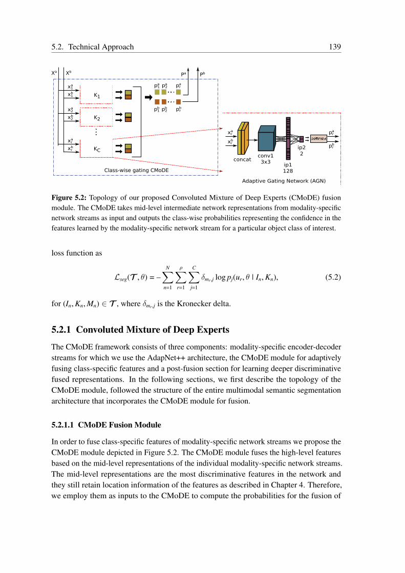
5.2. Technical Approach 139
K1
K2
KC
Xa XbPa
p1a
Pb
softmax
ip22
ip1128
conv13x3concat
Adaptive Gating Network (AGN)
xra
xrb
x1a
x2a
xra
x1b
x2b
xrb
p1b
p2a
p2b pr
b
pra
pra
prb
Class-wise gating CMoDE
Figure 5.2: Topology of our proposed Convoluted Mixture of Deep Experts (CMoDE) fusionmodule. The CMoDE takes mid-level intermediate network representations from modality-specificnetwork streams as input and outputs the class-wise probabilities representing the confidence in thefeatures learned by the modality-specific network stream for a particular object class of interest.
loss function as
Lseg(T , θ) = –N∑
n=1
ρ∑r=1
C∑j=1
δmr ,j log pj(ur, θ | In, Kn), (5.2)
for (In, Kn, Mn) ∈ T , where δmr ,j is the Kronecker delta.
5.2.1 Convoluted Mixture of Deep Experts
The CMoDE framework consists of three components: modality-specific encoder-decoderstreams for which we use the AdapNet++ architecture, the CMoDE module for adaptivelyfusing class-specific features and a post-fusion section for learning deeper discriminativefused representations. In the following sections, we first describe the topology of theCMoDE module, followed the structure of the entire multimodal semantic segmentationarchitecture that incorporates the CMoDE module for fusion.
5.2.1.1 CMoDE Fusion Module
In order to fuse class-specific features of modality-specific network streams we propose theCMoDE module depicted in Figure 5.2. The CMoDE module fuses the high-level featuresbased on the mid-level representations of the individual modality-specific network streams.The mid-level representations are the most discriminative features in the network andthey still retain location information of the features as described in Chapter 4. Therefore,we employ them as inputs to the CMoDE to compute the probabilities for the fusion of

140 Chapter 5. Multimodal Semantic Segmentation
high-level decoder features. Let Xa = xar | r = 1, . . . , C and Xb = xb
r | r = 1, . . . , Cdenote the mid-level modality-specific encoder feature maps from modality a and modalityb network streams respectively, where C is the number of object classes in the dataset andxr has a spatial dimension of H ×W. The class-wise gating network takes Xa and Xb asinput and outputs the respective probabilities Pa and Pb for the fusion.
The class-wise gating CMoDE network consists of C number of adaptive gating sub-networks (AGN). Each AGN takes the class-specific features xa
r and xbr representing the
object class r and from the modality-specific network streams a and b as inputs. Thefeatures are first concatenated to obtain xab
r , followed by applying a 3 × 3 convolutionconv1 with weightsW1 ∈ RC×H×W and a non-linearity function δ(·). We use ReLUs forthe non-linearity and add dropout on the convolution layer to prevent overfitting. Theconvolved features are then passed through an inner-product layer ip1 having weightsW2 ∈ Rγ1×H×W to learn non-linear combinations of features, where γ1 is number of outputfeature channels in ip1. We use γ1 = 128 as identified in the ablation study presented inSection 5.3.4.1. Finally, the resulting feature maps are passed into another inner-productlayer ip2 with weightsW3 ∈ Rγ2×H×W , where γ2 = 2 in this case as we fuse features fromtwo modality-specific network streams. The feature maps from the last inner-product layerip2 can then be represented as
sabr = Fcmode(xab
r ;W) =W3(W2δ
(W1xab
r
)). (5.3)
The feature maps sabr are then passed through a softmax layer σ(·) and using the fusion
scores f , we obtain the probabilities pr for the fusion as
pr(sabr , θ | In, Kn) = σ
(f(sab
r , θ))
=exp(f(sab
r , θ))∑E
k exp(fk(sab
r , θ)) , (5.4)
where θ are the parameters of the AGN and E is the number of modality-specific networkstreams. The resulting probabilities pr denote how much the gating network trusts the class-specific kernels learned the modality-specific streams. This procedure is then employed inC number of AGNs to compute the probabilities for fusion corresponding to each class inthe dataset. The resulting class-specific probabilities for the individual modality streams aand b are then concatenated to yield Pa and Pb respectively. This class-specific probabilitydistribution learned by the gating network gives the model the ability to choose differentmodalitites or spectra according to the object classes present in the scene.
5.2.1.2 CMoDE Fusion Architecture
We incorporate our CMoDE module in a late-fusion framework shown in Figure 5.3. Theframework is adaptable to fuse arbitrary number of modalities, for simplicity we considerfusing two different modalities in our descriptions. Individual modality-specific networkstreams specializing in a particular subspace, first map the representation of the input
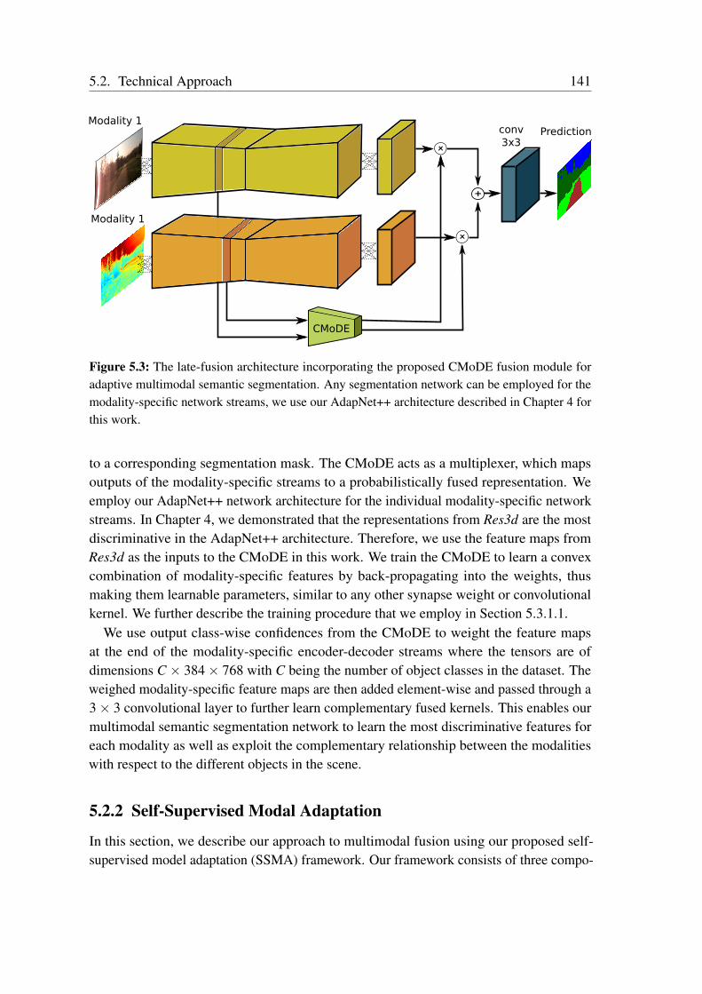
5.2. Technical Approach 141
Modality 1Predictionconv
3x3
CMoDE
Modality 1
Figure 5.3: The late-fusion architecture incorporating the proposed CMoDE fusion module foradaptive multimodal semantic segmentation. Any segmentation network can be employed for themodality-specific network streams, we use our AdapNet++ architecture described in Chapter 4 forthis work.
to a corresponding segmentation mask. The CMoDE acts as a multiplexer, which mapsoutputs of the modality-specific streams to a probabilistically fused representation. Weemploy our AdapNet++ network architecture for the individual modality-specific networkstreams. In Chapter 4, we demonstrated that the representations from Res3d are the mostdiscriminative in the AdapNet++ architecture. Therefore, we use the feature maps fromRes3d as the inputs to the CMoDE in this work. We train the CMoDE to learn a convexcombination of modality-specific features by back-propagating into the weights, thusmaking them learnable parameters, similar to any other synapse weight or convolutionalkernel. We further describe the training procedure that we employ in Section 5.3.1.1.
We use output class-wise confidences from the CMoDE to weight the feature mapsat the end of the modality-specific encoder-decoder streams where the tensors are ofdimensions C × 384× 768 with C being the number of object classes in the dataset. Theweighed modality-specific feature maps are then added element-wise and passed through a3× 3 convolutional layer to further learn complementary fused kernels. This enables ourmultimodal semantic segmentation network to learn the most discriminative features foreach modality as well as exploit the complementary relationship between the modalitieswith respect to the different objects in the scene.
5.2.2 Self-Supervised Modal Adaptation
In this section, we describe our approach to multimodal fusion using our proposed self-supervised model adaptation (SSMA) framework. Our framework consists of three compo-
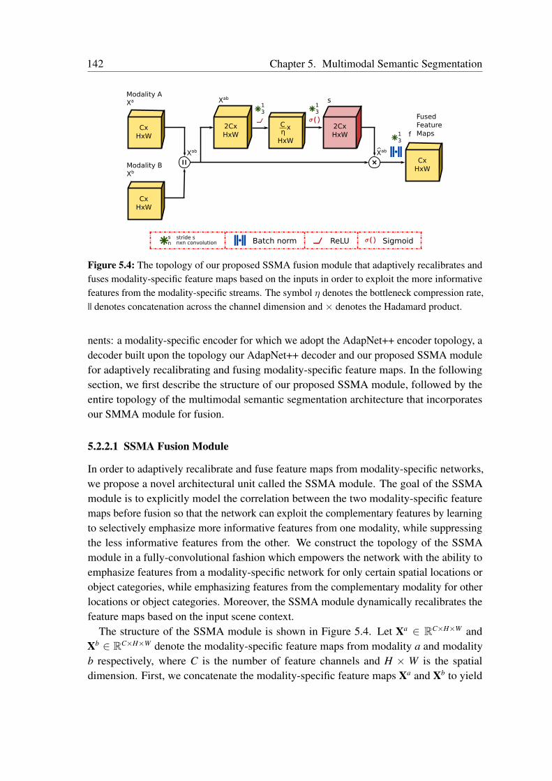
142 Chapter 5. Multimodal Semantic Segmentation
Batch normnxn convolutionstride s
ns
ReLU
CxHxW
CxHxW
2CxHxW
13
C/2xHxW
13
2CxHxW 1
3
CxHxW
Sigmoid
CxHxW
CxHxW
HxW
Cη
x
Modality AXa
Modality BXb
FusedFeatureMaps
Xab s
f
XabXab
Figure 5.4: The topology of our proposed SSMA fusion module that adaptively recalibrates andfuses modality-specific feature maps based on the inputs in order to exploit the more informativefeatures from the modality-specific streams. The symbol η denotes the bottleneck compression rate,|| denotes concatenation across the channel dimension and × denotes the Hadamard product.
nents: a modality-specific encoder for which we adopt the AdapNet++ encoder topology, adecoder built upon the topology our AdapNet++ decoder and our proposed SSMA modulefor adaptively recalibrating and fusing modality-specific feature maps. In the followingsection, we first describe the structure of our proposed SSMA module, followed by theentire topology of the multimodal semantic segmentation architecture that incorporatesour SMMA module for fusion.
5.2.2.1 SSMA Fusion Module
In order to adaptively recalibrate and fuse feature maps from modality-specific networks,we propose a novel architectural unit called the SSMA module. The goal of the SSMAmodule is to explicitly model the correlation between the two modality-specific featuremaps before fusion so that the network can exploit the complementary features by learningto selectively emphasize more informative features from one modality, while suppressingthe less informative features from the other. We construct the topology of the SSMAmodule in a fully-convolutional fashion which empowers the network with the ability toemphasize features from a modality-specific network for only certain spatial locations orobject categories, while emphasizing features from the complementary modality for otherlocations or object categories. Moreover, the SSMA module dynamically recalibrates thefeature maps based on the input scene context.
The structure of the SSMA module is shown in Figure 5.4. Let Xa ∈ RC×H×W andXb ∈ RC×H×W denote the modality-specific feature maps from modality a and modalityb respectively, where C is the number of feature channels and H × W is the spatialdimension. First, we concatenate the modality-specific feature maps Xa and Xb to yield
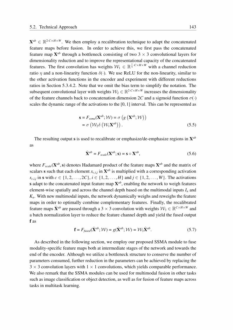
5.2. Technical Approach 143
Xab ∈ R2·C×H×W . We then employ a recalibration technique to adapt the concatenatedfeature maps before fusion. In order to achieve this, we first pass the concatenatedfeature map Xab through a bottleneck consisting of two 3 × 3 convolutional layers fordimensionality reduction and to improve the representational capacity of the concatenatedfeatures. The first convolution has weights W1 ∈ R
1η·C×H×W with a channel reduction
ratio η and a non-linearity function δ(·). We use ReLU for the non-linearity, similar tothe other activation functions in the encoder and experiment with different reductionsratios in Section 5.3.4.2. Note that we omit the bias term to simplify the notation. Thesubsequent convolutional layer with weightsW2 ∈ R2·C×H×W increases the dimensionalityof the feature channels back to concatenation dimension 2C and a sigmoid function σ(·)scales the dynamic range of the activations to the [0, 1] interval. This can be represented as
s = Fssma(Xab;W) = σ(g(Xab;W
))= σ
(W2δ
(W1Xab)) . (5.5)
The resulting output s is used to recalibrate or emphasize/de-emphasize regions in Xab
as
Xab = Fscale(Xab; s) = s Xab, (5.6)
where Fscale(Xab, s) denotes Hadamard product of the feature maps Xab and the matrix ofscalars s such that each element xc,i,j in Xab is multiplied with a corresponding activationsc,i,j in s with c ∈ 1, 2, . . . , 2C, i ∈ 1, 2, . . . , H and j ∈ 1, 2, . . . , W. The activationss adapt to the concatenated input feature map Xab, enabling the network to weigh featureselement-wise spatially and across the channel depth based on the multimodal inputs In andKn. With new multimodal inputs, the network dynamically weighs and reweighs the featuremaps in order to optimally combine complementary features. Finally, the recalibratedfeature maps Xab are passed through a 3× 3 convolution with weightsW3 ∈ RC×H×W anda batch normalization layer to reduce the feature channel depth and yield the fused outputf as
f = Ffused(Xab;W) = g(Xab;W) =W3Xab. (5.7)
As described in the following section, we employ our proposed SSMA module to fusemodality-specific feature maps both at intermediate stages of the network and towards theend of the encoder. Although we utilize a bottleneck structure to conserve the number ofparameters consumed, further reduction in the parameters can be achieved by replacing the3× 3 convolution layers with 1× 1 convolutions, which yields comparable performance.We also remark that the SSMA modules can be used for multimodal fusion in other taskssuch as image classification or object detection, as well as for fusion of feature maps acrosstasks in multitask learning.
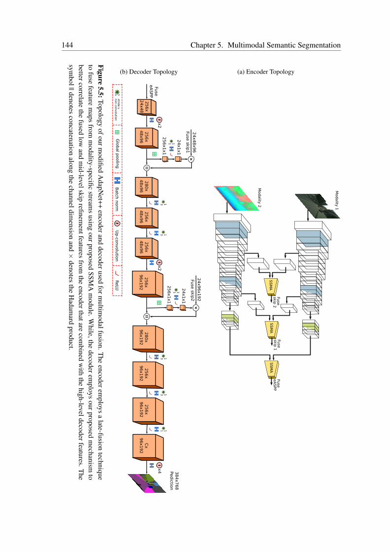
144 Chapter 5. Multimodal Semantic Segmentation
(a) Encoder Topology
Fuse
eA
SPP
Fuse
skip 1
Fuse
skip 2
Mod
ality
1
Mod
ality
2
SS
MA
SS
MA
SS
MA
(b) Decoder Topology
Batch
norm
Glo
bal p
oolin
gU
p-co
nvolu
tion
nxn co
nvolu
tion
stride s
n sR
eLU
x4
Cx
96
x1
92
25
6x
96
x1
92
11
25
6x
96
x1
92
13
28
0x
96
x1
92
13
25
6x
96
x1
92
x2
25
6x
48
x9
62
56
x4
8x9
62
80
x4
8x9
6
1313
24
x4
8x9
6
25
6x
48
x9
6
x2
25
6x
24
x4
8
38
4x7
68
Ped
iction
Fuse
skip1
Fuse
eA
SPP
25
6x1
x1
24
x1
x1
11
24
x9
6x1
92
Fuse
skip2
25
6x1
x1
24
x1
x1
11
Figure5.5:Topology
ofourmodified
AdapN
et++encoderand
decoderusedform
ultimodalfusion.T
heencoderem
ploysa
late-fusiontechnique
tofuse
featurem
apsfrom
modality-specific
streams
usingourproposed
SSMA
module.W
hile,thedecoderem
ploysourproposed
mechanism
tobettercorrelate
thefused
lowand
mid-levelskip
refinementfeatures
fromthe
encoderthatarecom
binedw
iththe
high-leveldecoderfeatures.The
symbol||denotes
concatenationalong
thechanneldim
ensionand×
denotesthe
Hadam
ardproduct.
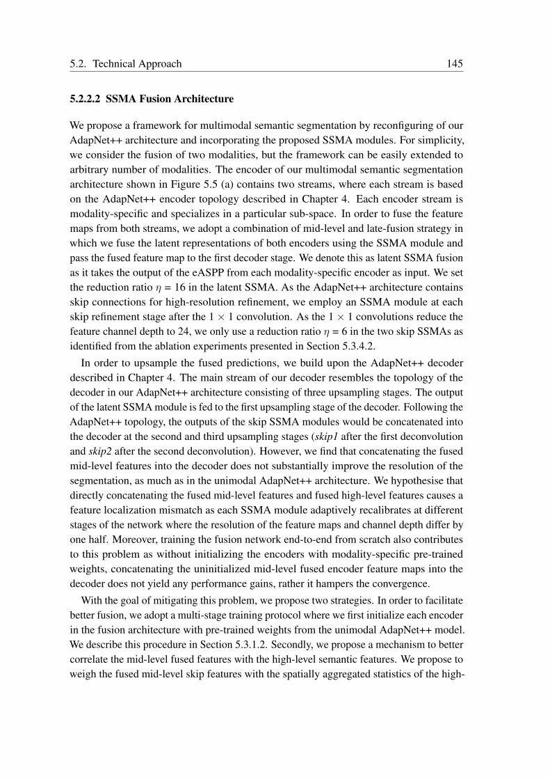
5.2. Technical Approach 145
5.2.2.2 SSMA Fusion Architecture
We propose a framework for multimodal semantic segmentation by reconfiguring of ourAdapNet++ architecture and incorporating the proposed SSMA modules. For simplicity,we consider the fusion of two modalities, but the framework can be easily extended toarbitrary number of modalities. The encoder of our multimodal semantic segmentationarchitecture shown in Figure 5.5 (a) contains two streams, where each stream is basedon the AdapNet++ encoder topology described in Chapter 4. Each encoder stream ismodality-specific and specializes in a particular sub-space. In order to fuse the featuremaps from both streams, we adopt a combination of mid-level and late-fusion strategy inwhich we fuse the latent representations of both encoders using the SSMA module andpass the fused feature map to the first decoder stage. We denote this as latent SSMA fusionas it takes the output of the eASPP from each modality-specific encoder as input. We setthe reduction ratio η = 16 in the latent SSMA. As the AdapNet++ architecture containsskip connections for high-resolution refinement, we employ an SSMA module at eachskip refinement stage after the 1× 1 convolution. As the 1× 1 convolutions reduce thefeature channel depth to 24, we only use a reduction ratio η = 6 in the two skip SSMAs asidentified from the ablation experiments presented in Section 5.3.4.2.
In order to upsample the fused predictions, we build upon the AdapNet++ decoderdescribed in Chapter 4. The main stream of our decoder resembles the topology of thedecoder in our AdapNet++ architecture consisting of three upsampling stages. The outputof the latent SSMA module is fed to the first upsampling stage of the decoder. Following theAdapNet++ topology, the outputs of the skip SSMA modules would be concatenated intothe decoder at the second and third upsampling stages (skip1 after the first deconvolutionand skip2 after the second deconvolution). However, we find that concatenating the fusedmid-level features into the decoder does not substantially improve the resolution of thesegmentation, as much as in the unimodal AdapNet++ architecture. We hypothesise thatdirectly concatenating the fused mid-level features and fused high-level features causes afeature localization mismatch as each SSMA module adaptively recalibrates at differentstages of the network where the resolution of the feature maps and channel depth differ byone half. Moreover, training the fusion network end-to-end from scratch also contributesto this problem as without initializing the encoders with modality-specific pre-trainedweights, concatenating the uninitialized mid-level fused encoder feature maps into thedecoder does not yield any performance gains, rather it hampers the convergence.
With the goal of mitigating this problem, we propose two strategies. In order to facilitatebetter fusion, we adopt a multi-stage training protocol where we first initialize each encoderin the fusion architecture with pre-trained weights from the unimodal AdapNet++ model.We describe this procedure in Section 5.3.1.2. Secondly, we propose a mechanism to bettercorrelate the mid-level fused features with the high-level semantic features. We propose toweigh the fused mid-level skip features with the spatially aggregated statistics of the high-
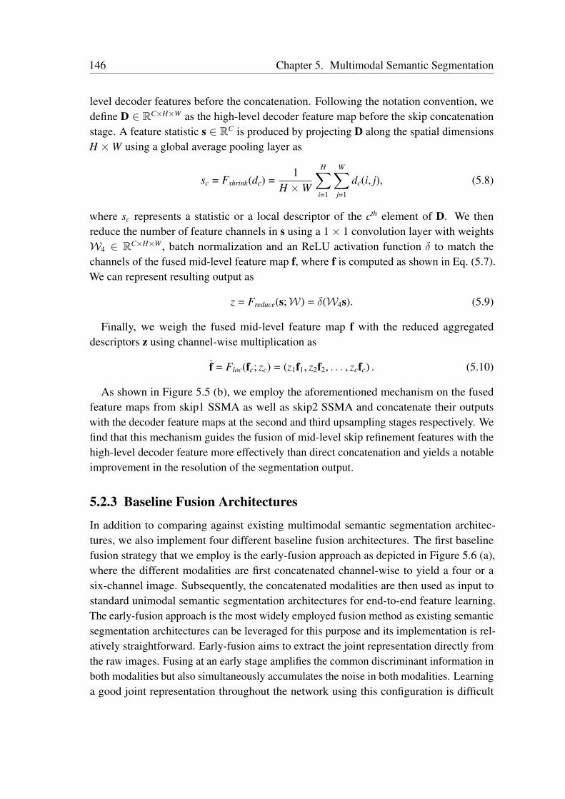
146 Chapter 5. Multimodal Semantic Segmentation
level decoder features before the concatenation. Following the notation convention, wedefine D ∈ RC×H×W as the high-level decoder feature map before the skip concatenationstage. A feature statistic s ∈ RC is produced by projecting D along the spatial dimensionsH ×W using a global average pooling layer as
sc = Fshrink(dc) =1
H ×W
H∑i=1
W∑j=1
dc(i, j), (5.8)
where sc represents a statistic or a local descriptor of the cth element of D. We thenreduce the number of feature channels in s using a 1× 1 convolution layer with weightsW4 ∈ RC×H×W , batch normalization and an ReLU activation function δ to match thechannels of the fused mid-level feature map f, where f is computed as shown in Eq. (5.7).We can represent resulting output as
z = Freduce(s;W) = δ(W4s). (5.9)
Finally, we weigh the fused mid-level feature map f with the reduced aggregateddescriptors z using channel-wise multiplication as
f = Floc(fc; zc) = (z1f1, z2f2, . . . , zcfc) . (5.10)
As shown in Figure 5.5 (b), we employ the aforementioned mechanism on the fusedfeature maps from skip1 SSMA as well as skip2 SSMA and concatenate their outputswith the decoder feature maps at the second and third upsampling stages respectively. Wefind that this mechanism guides the fusion of mid-level skip refinement features with thehigh-level decoder feature more effectively than direct concatenation and yields a notableimprovement in the resolution of the segmentation output.
5.2.3 Baseline Fusion Architectures
In addition to comparing against existing multimodal semantic segmentation architec-tures, we also implement four different baseline fusion architectures. The first baselinefusion strategy that we employ is the early-fusion approach as depicted in Figure 5.6 (a),where the different modalities are first concatenated channel-wise to yield a four or asix-channel image. Subsequently, the concatenated modalities are then used as input tostandard unimodal semantic segmentation architectures for end-to-end feature learning.The early-fusion approach is the most widely employed fusion method as existing semanticsegmentation architectures can be leveraged for this purpose and its implementation is rel-atively straightforward. Early-fusion aims to extract the joint representation directly fromthe raw images. Fusing at an early stage amplifies the common discriminant information inboth modalities but also simultaneously accumulates the noise in both modalities. Learninga good joint representation throughout the network using this configuration is difficult
5.2. Technical Approach 147
ModalitiesConcatenated
Prediction
(a) Early fusion
Modality 1Prediction
Modality 1
Conv1x1
Conv1x1
(b) Late fusion
Figure 5.6: Depiction of the early and late-fusion approaches for multimodal semantic segmentation.In early-fusion, the modalities are concatenated to obtain a four or a six-channel image and then fedto the network as input for end-to-end semantic segmentation. While, in the late-fusion approach,individual network streams that take different modalities as input are employed, followed bycombining the features towards the end of the network using a 1× 1 convolution and element-wiseaddition.
due to significantly different data formats and distinct distributions between modalities.Another disadvantage of this method is that pre-trained weights from networks trainedon large image segmentation datasets cannot be leveraged for initialization using transferlearning.
We employ the late-fusion approach for the second baseline. The topology of the late-fusion shown in Figure 5.6 (b) consists of individual modality-specific network streams thatare first trained end-to-end using their respective modalities. Followed by initializing thejoint model with pre-trained weights from the previous step and adding a 1× 1 convolutionlayer at the end of the streams before the element-wise addition of feature maps fromboth modality-specific streams for the fusion. While training the joint model, the weightsof the individual streams before the 1 × 1 convolution layer are often kept fixed. Thisenables them to retain their modality-specific low and mid-level features while focusingonly on learning the fusion of the high-level semantically mature features. The 1 × 1convolution layer is added so that the networks learn to adapt their individual high-levelrepresentations before the fusion. The late-fusion approach is a popular fusion baseline asit builds upon existing semantic segmentation architectures and therefore the model can be
148 Chapter 5. Multimodal Semantic Segmentation
initialized with pre-trained weights from networks trained on large semantic segmentationdatasets. More importantly, this configuration enables the network to exploit the high-levelsemantically rich information for the fusion, therefore complementary information can beleveraged based on the features describing the semantic object classes in the dataset. Theperformance of late-fusion approaches is largely dependent on the correlation mechanismthat is employed at the end of the individual modality-specific network streams for thefusion.
For the third baseline, we employ the averaging technique in which individual semanticsegmentation architectures are first trained on a specific modality and then the predictionprobabilities of each of the networks are class-wise averaged before computing the argmax.Averaging the class-wise probabilities gives us a measure of the consensus and certaintyamong the modality-specific networks. For instance, if both networks are highly confidentin their predictions for a specific object class, then the consensus value is highest for thisparticular class leading to its subsequent section by the argmax. On the other hand, if oneor both of the networks produce a low score for a particular object class, taking the averageof their probabilities smoothens the score to reflect the joint confidence. Similarly, forthe last fusion baseline, as opposed to computing the average of the class-wise predictionprobabilities, we compute the maximum of the class-wise prediction probabilities acrossthe different modality-specific networks before computing the argmax. This enables us toselect the most certain predictions across the modality-specific networks for a particularobject class.
5.3 Experimental Evaluation
In this section, we first describe the procedure that we employ for training our multimodalsemantic segmentation architectures that incorporate our proposed CMoDE and SSMAfusion modules in Section 5.3.1, followed by detailed benchmarking results using thevarious modalities and spectra contained in the datasets in Section 5.3.2 and comprehensiveablation studies that describe the various architectural decisions that we made whiledesigning the fusion module topologies in Section 5.3.4. In Section 5.3.5, we presentextensive qualitative evaluations on all the datasets that we benchmark on and finally inSection 5.3.7, we present the results from our autonomous navigation experiments usingonly the multimodal semantic segmentation for perception.
For the experiments presented in this chapter, we benchmark on the five multimodal in-door and outdoor datasets described in Chapter 4. Namely, Cityscapes [143], Synthia [144],SUN RGB-D [145], ScanNet [146] and Freiburg Forest [50] datasets. We use the Tensor-Flow [159] deep learning library for the implementations and all the experiments werecarried out on a system with an Intel Xeon E5, 2.4 GHz and an NVIDIA TITAN X GPU.We primarily use the standard Jaccard Index, also known as the intersection-over-union
5.3. Experimental Evaluation 149
(IoU) metric to quantify the performance. It can be computed for each object class asIoU = TP/(TP + FP + FN), where TP, FP and FN correspond to true positives, falsepositives and false negatives respectively. We also report the mean intersection-over-union(mIoU) metric, pixel-wise accuracy (Acc) and average precision (AP) for all the models.We made our models publicly available at http://deepscene.cs.uni-freiburg.de.
5.3.1 Network Training
We train our networks with an input image resolution of 768× 384 pixels, therefore we usebilinear interpolation for resizing the RGB images and the nearest-neighbour interpolationfor resizing the other modalities as well as the groundtruth labels. We employ a multi-stagetraining protocol to effectively train our multimodal semantic segmentation architectures.We first train each modality-specific Adapnet++ model individually using the trainingprotocol described in Section 4.4.3 of Chapter 4. Subsequently, in the second stage, weleverage transfer learning to train the joint fusion model in either the CMoDE or theSSMA framework. We describe the procedure that we employ in the second stage and theparameter settings for training the multimodal fusion in the following sections.
5.3.1.1 CMoDE Training
In the second stage, we initialize the modality-specific encoders and decoders usingweights from the previous stage, while we initialize the class-specific CMoDE and thefused convolution layer using the He initialization [93] scheme. We keep the weights ofthe modality-specific encoders and decoders fixed, which forces the CMoDE to use therepresentations learned by the individual streams from the first stage, while exploitingdiscriminative complementary features from different modalities at the high-level in thesecond stage. We use the Adam solver for optimization with β1 = 0.9, β2 = 0.999 andε = 10–10. We train the second stage of the CMoDE model for a maximum of 50,000iterations using an initial learning rate of λ0 = 10–5 with a mini-batch size of 8 and adropout probability of 0.5.
5.3.1.2 SSMA Training
In order to train the SSMA fusion model, we initialize only the modality-specific encodersusing weights from the previous stage and similar to the CMoDE, we use He initializa-tion [93] scheme for the other layers. We then set the learning rate of the encoder layers toλ0 = 10–4 and the decoder layers to λ0 = 10–3, and train the fusion model with a mini-batchof 7 for a maximum of 100,000 iterations using the Adam solver with β1 = 0.9, β2 = 0.999and ε = 10–10. This enables the SSMA modules to learn the optimal combination ofmultimodal feature maps from the well trained encoders, while slowly adapting the en-coder weights to improve the fusion. In the final stage, we fix the weights of the encoder
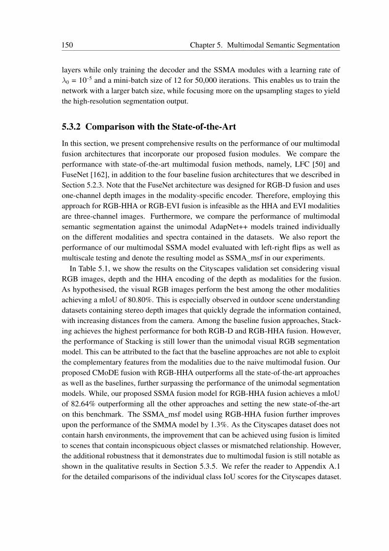
150 Chapter 5. Multimodal Semantic Segmentation
layers while only training the decoder and the SSMA modules with a learning rate ofλ0 = 10–5 and a mini-batch size of 12 for 50,000 iterations. This enables us to train thenetwork with a larger batch size, while focusing more on the upsampling stages to yieldthe high-resolution segmentation output.
5.3.2 Comparison with the State-of-the-Art
In this section, we present comprehensive results on the performance of our multimodalfusion architectures that incorporate our proposed fusion modules. We compare theperformance with state-of-the-art multimodal fusion methods, namely, LFC [50] andFuseNet [162], in addition to the four baseline fusion architectures that we described inSection 5.2.3. Note that the FuseNet architecture was designed for RGB-D fusion and usesone-channel depth images in the modality-specific encoder. Therefore, employing thisapproach for RGB-HHA or RGB-EVI fusion is infeasible as the HHA and EVI modalitiesare three-channel images. Furthermore, we compare the performance of multimodalsemantic segmentation against the unimodal AdapNet++ models trained individuallyon the different modalities and spectra contained in the datasets. We also report theperformance of our multimodal SSMA model evaluated with left-right flips as well asmultiscale testing and denote the resulting model as SSMA_msf in our experiments.
In Table 5.1, we show the results on the Cityscapes validation set considering visualRGB images, depth and the HHA encoding of the depth as modalities for the fusion.As hypothesised, the visual RGB images perform the best among the other modalitiesachieving a mIoU of 80.80%. This is especially observed in outdoor scene understandingdatasets containing stereo depth images that quickly degrade the information contained,with increasing distances from the camera. Among the baseline fusion approaches, Stack-ing achieves the highest performance for both RGB-D and RGB-HHA fusion. However,the performance of Stacking is still lower than the unimodal visual RGB segmentationmodel. This can be attributed to the fact that the baseline approaches are not able to exploitthe complementary features from the modalities due to the naive multimodal fusion. Ourproposed CMoDE fusion with RGB-HHA outperforms all the state-of-the-art approachesas well as the baselines, further surpassing the performance of the unimodal segmentationmodels. While, our proposed SSMA fusion model for RGB-HHA fusion achieves a mIoUof 82.64% outperforming all the other approaches and setting the new state-of-the-arton this benchmark. The SSMA_msf model using RGB-HHA fusion further improvesupon the performance of the SMMA model by 1.3%. As the Cityscapes dataset does notcontain harsh environments, the improvement that can be achieved using fusion is limitedto scenes that contain inconspicuous object classes or mismatched relationship. However,the additional robustness that it demonstrates due to multimodal fusion is still notable asshown in the qualitative results in Section 5.3.5. We refer the reader to Appendix A.1for the detailed comparisons of the individual class IoU scores for the Cityscapes dataset.
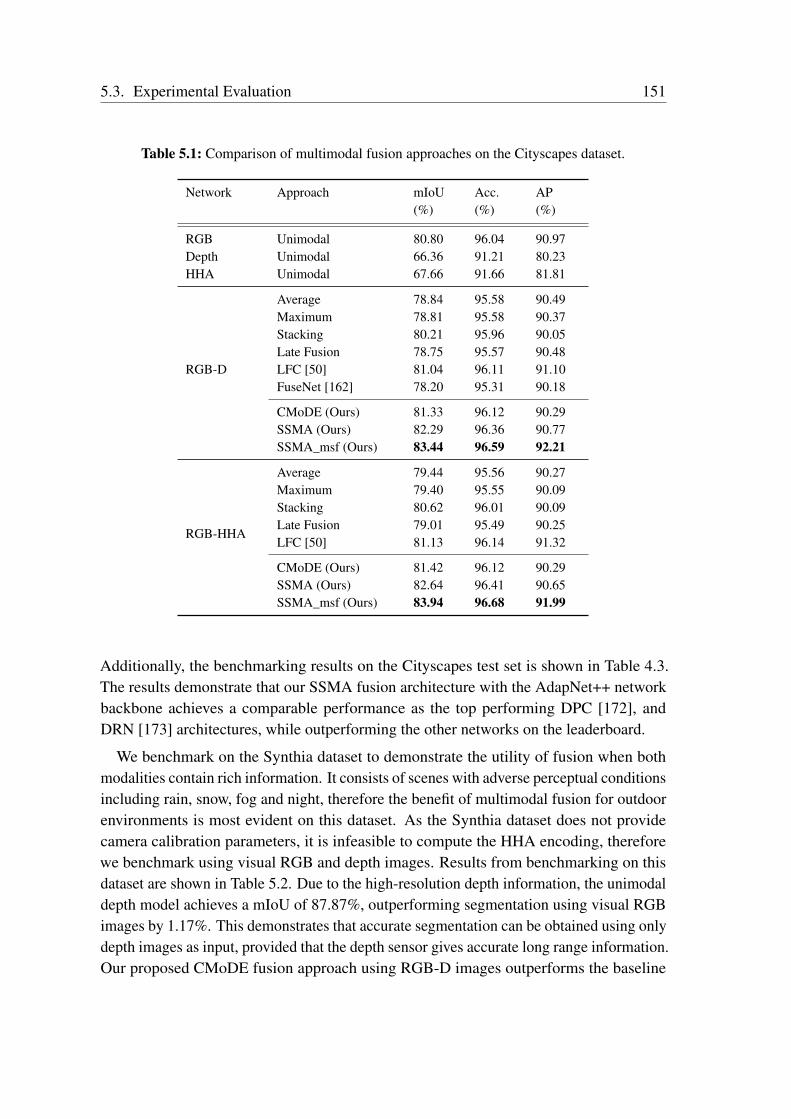
5.3. Experimental Evaluation 151
Table 5.1: Comparison of multimodal fusion approaches on the Cityscapes dataset.
Network Approach mIoU Acc. AP(%) (%) (%)
RGB Unimodal 80.80 96.04 90.97Depth Unimodal 66.36 91.21 80.23HHA Unimodal 67.66 91.66 81.81
RGB-D
Average 78.84 95.58 90.49Maximum 78.81 95.58 90.37Stacking 80.21 95.96 90.05Late Fusion 78.75 95.57 90.48LFC [50] 81.04 96.11 91.10FuseNet [162] 78.20 95.31 90.18
CMoDE (Ours) 81.33 96.12 90.29SSMA (Ours) 82.29 96.36 90.77SSMA_msf (Ours) 83.44 96.59 92.21
RGB-HHA
Average 79.44 95.56 90.27Maximum 79.40 95.55 90.09Stacking 80.62 96.01 90.09Late Fusion 79.01 95.49 90.25LFC [50] 81.13 96.14 91.32
CMoDE (Ours) 81.42 96.12 90.29SSMA (Ours) 82.64 96.41 90.65SSMA_msf (Ours) 83.94 96.68 91.99
Additionally, the benchmarking results on the Cityscapes test set is shown in Table 4.3.The results demonstrate that our SSMA fusion architecture with the AdapNet++ networkbackbone achieves a comparable performance as the top performing DPC [172], andDRN [173] architectures, while outperforming the other networks on the leaderboard.
We benchmark on the Synthia dataset to demonstrate the utility of fusion when bothmodalities contain rich information. It consists of scenes with adverse perceptual conditionsincluding rain, snow, fog and night, therefore the benefit of multimodal fusion for outdoorenvironments is most evident on this dataset. As the Synthia dataset does not providecamera calibration parameters, it is infeasible to compute the HHA encoding, thereforewe benchmark using visual RGB and depth images. Results from benchmarking on thisdataset are shown in Table 5.2. Due to the high-resolution depth information, the unimodaldepth model achieves a mIoU of 87.87%, outperforming segmentation using visual RGBimages by 1.17%. This demonstrates that accurate segmentation can be obtained using onlydepth images as input, provided that the depth sensor gives accurate long range information.Our proposed CMoDE fusion approach using RGB-D images outperforms the baseline
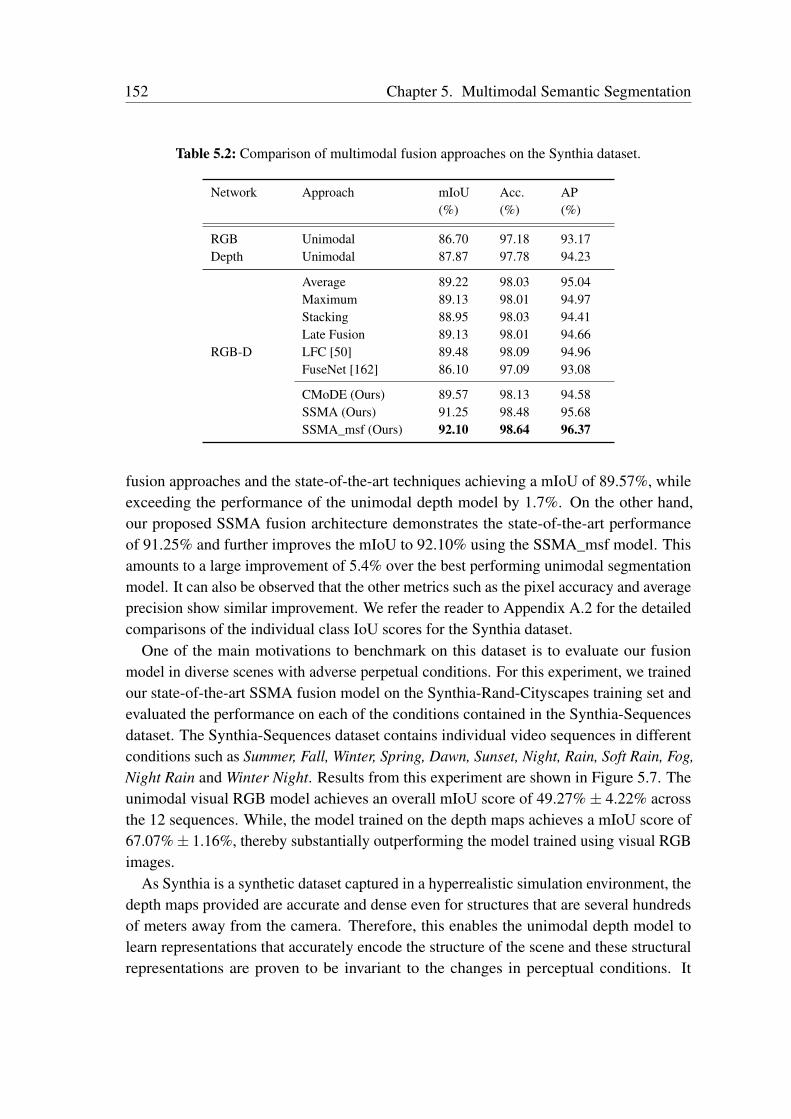
152 Chapter 5. Multimodal Semantic Segmentation
Table 5.2: Comparison of multimodal fusion approaches on the Synthia dataset.
Network Approach mIoU Acc. AP(%) (%) (%)
RGB Unimodal 86.70 97.18 93.17Depth Unimodal 87.87 97.78 94.23
RGB-D
Average 89.22 98.03 95.04Maximum 89.13 98.01 94.97Stacking 88.95 98.03 94.41Late Fusion 89.13 98.01 94.66LFC [50] 89.48 98.09 94.96FuseNet [162] 86.10 97.09 93.08
CMoDE (Ours) 89.57 98.13 94.58SSMA (Ours) 91.25 98.48 95.68SSMA_msf (Ours) 92.10 98.64 96.37
fusion approaches and the state-of-the-art techniques achieving a mIoU of 89.57%, whileexceeding the performance of the unimodal depth model by 1.7%. On the other hand,our proposed SSMA fusion architecture demonstrates the state-of-the-art performanceof 91.25% and further improves the mIoU to 92.10% using the SSMA_msf model. Thisamounts to a large improvement of 5.4% over the best performing unimodal segmentationmodel. It can also be observed that the other metrics such as the pixel accuracy and averageprecision show similar improvement. We refer the reader to Appendix A.2 for the detailedcomparisons of the individual class IoU scores for the Synthia dataset.
One of the main motivations to benchmark on this dataset is to evaluate our fusionmodel in diverse scenes with adverse perpetual conditions. For this experiment, we trainedour state-of-the-art SSMA fusion model on the Synthia-Rand-Cityscapes training set andevaluated the performance on each of the conditions contained in the Synthia-Sequencesdataset. The Synthia-Sequences dataset contains individual video sequences in differentconditions such as Summer, Fall, Winter, Spring, Dawn, Sunset, Night, Rain, Soft Rain, Fog,Night Rain and Winter Night. Results from this experiment are shown in Figure 5.7. Theunimodal visual RGB model achieves an overall mIoU score of 49.27%± 4.22% acrossthe 12 sequences. While, the model trained on the depth maps achieves a mIoU score of67.07%± 1.16%, thereby substantially outperforming the model trained using visual RGBimages.
As Synthia is a synthetic dataset captured in a hyperrealistic simulation environment, thedepth maps provided are accurate and dense even for structures that are several hundredsof meters away from the camera. Therefore, this enables the unimodal depth model tolearn representations that accurately encode the structure of the scene and these structuralrepresentations are proven to be invariant to the changes in perceptual conditions. It

5.3. Experimental Evaluation 153
Summer Fall Winter Spring Dawn Sunset Night Rain SoftRain
Fog NightRain
WinterNight
30
40
50
60
70
80
Inte
rsec
tion
over
Uni
on (%
)
RGB Depth SSMA RGB-D Fusion
Figure 5.7: Evaluation of our proposed SMMA fusion technique on the Synthia-Sequences datasetcontaining a variety of seasons and weather conditions. We use the models trained on the Synthia-Rand-Cityscapes dataset and only test on the individual conditions in the Synthia-Sequences datasetto quantify its robustness. Our model that performs RGB-D fusion consistently outperforms theunimodal models which can be more prominently seen qualitatively in Figure 5.14.
can also be observed that the unimodal depth model performs consistently well in allthe conditions with a variance of 1.36%, demonstrating its generalization to differentweather and seasonal changes. However, the visual RGB model with a variance of 17.79%performs inconsistently across different conditions. Nevertheless, we observe that ourRGB-D SSMA fusion model outperforms the unimodal visual RGB model by achievinga mIoU score of 76.51% ± 0.53% across the 12 conditions, accounting to a significantimprovement of 27.24%. Moreover, the SSMA fusion model has a variance of 0.28%,demonstrating better generalization abilities across varying adverse perceptual conditions.
We benchmark on the indoor SUN RGB-D dataset which demonstrates a different setof challenges than the outdoor datasets. The improvement due to the multimodal fusionis more evident in indoor scenes as the images are often captured in smaller confinedspaces with several cluttered objects and the depth modality provides valuable structuralinformation that can be exploited. Results from multimodal RGB-D and RGB-HHA fusionis shown in Table 5.3. Among the unimodal models, semantic segmentation using visualRGB images yields the highest mIoU of 38.40%. The model trained on depth imagesperforms 4.13% lower than the visual RGB model. This can be attributed to the fact that thedepth images are extremely noisy with numerous missing depth values in the SUN RGB-Ddataset. Nevertheless, our CMoDE approach outperforms the state-of-the-art fusion modelsas well the unimodal segmentation models. The CMoDE model using RGB-HHA fusionachieves a mIoU of 42.55% which is an improvement of 4.15% over the unimodal visual
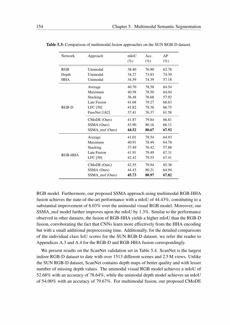
154 Chapter 5. Multimodal Semantic Segmentation
Table 5.3: Comparison of multimodal fusion approaches on the SUN RGB-D dataset.
Network Approach mIoU Acc. AP(%) (%) (%)
RGB Unimodal 38.40 76.90 62.78Depth Unimodal 34.27 73.83 74.39HHA Unimodal 34.59 74.39 57.18
RGB-D
Average 40.70 78.58 64.54Maximum 40.58 78.50 64.04Stacking 36.48 76.68 57.92Late Fusion 41.68 79.27 66.63LFC [50] 41.82 79.36 66.75FuseNet [162] 37.41 76.37 61.58
CMoDE (Ours) 41.87 79.84 66.81SSMA (Ours) 43.90 80.16 66.11SSMA_msf (Ours) 44.52 80.67 67.92
RGB-HHA
Average 41.01 78.54 64.93Maximum 40.91 78.49 64.78Stacking 37.49 76.42 57.88Late Fusion 41.91 79.49 67.31LFC [50] 42.42 79.55 67.41
CMoDE (Ours) 42.55 79.94 65.38SSMA (Ours) 44.43 80.21 64.94SSMA_msf (Ours) 45.73 80.97 67.82
RGB model. Furthermore, our proposed SSMA approach using multimodal RGB-HHAfusion achieves the state-of-the-art performance with a mIoU of 44.43%, constituting to asubstantial improvement of 6.03% over the unimodal visual RGB model. Moreover, ourSSMA_msf model further improves upon the mIoU by 1.3%. Similar to the performanceobserved in other datasets, the fusion of RGB-HHA yields a higher mIoU than the RGB-Dfusion, corroborating the fact that CNNs learn more effectively from the HHA encodingbut with a small additional preprocessing time. Additionally, for the detailed comparisonsof the individual class IoU scores for the SUN RGB-D dataset, we refer the reader toAppendices A.3 and A.4 for the RGB-D and RGB-HHA fusion correspondingly.
We present results on the ScanNet validation set in Table 5.4. ScanNet is the largestindoor RGB-D dataset to date with over 1513 different scenes and 2.5 M views. Unlikethe SUN RGB-D dataset, ScanNet contains depth maps of better quality and with lessernumber of missing depth values. The unimodal visual RGB model achieves a mIoU of52.68% with an accuracy of 78.64%, while the unimodal depth model achieves an mIoUof 54.00% with an accuracy of 79.67%. For multimodal fusion, our proposed CMoDE
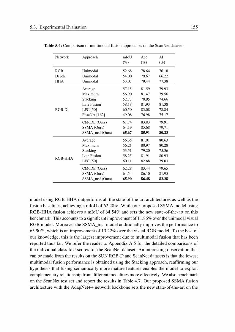
5.3. Experimental Evaluation 155
Table 5.4: Comparison of multimodal fusion approaches on the ScanNet dataset.
Network Approach mIoU Acc. AP(%) (%) (%)
RGB Unimodal 52.68 78.64 76.18Depth Unimodal 54.00 79.67 66.22HHA Unimodal 53.07 79.44 77.38
RGB-D
Average 57.15 81.59 79.93Maximum 56.90 81.47 79.56Stacking 52.77 78.95 74.66Late Fusion 58.18 81.93 81.38LFC [50] 60.50 83.08 78.84FuseNet [162] 49.08 76.98 75.17
CMoDE (Ours) 61.74 83.83 79.91SSMA (Ours) 64.19 85.68 79.71SSMA_msf (Ours) 65.67 85.91 80.23
RGB-HHA
Average 56.35 81.01 80.63Maximum 56.21 80.97 80.28Stacking 53.51 79.20 75.36Late Fusion 58.25 81.91 80.93LFC [50] 60.11 82.88 79.03
CMoDE (Ours) 62.28 83.44 79.65SSMA (Ours) 64.54 86.10 81.95SSMA_msf (Ours) 65.90 86.48 82.28
model using RGB-HHA outperforms all the state-of-the-art architectures as well as thefusion baselines, achieving a mIoU of 62.28%. While our proposed SSMA model usingRGB-HHA fusion achieves a mIoU of 64.54% and sets the new state-of-the-art on thisbenchmark. This accounts to a significant improvement of 11.86% over the unimodal visualRGB model. Moreover the SSMA_msf model additionally improves the performance to65.90%, which is an improvement of 13.22% over the visual RGB model. To the best ofour knowledge, this is the largest improvement due to multimodal fusion that has beenreported thus far. We refer the reader to Appendix A.5 for the detailed comparisons ofthe individual class IoU scores for the ScanNet dataset. An interesting observation thatcan be made from the results on the SUN RGB-D and ScanNet datasets is that the lowestmultimodal fusion performance is obtained using the Stacking approach, reaffirming ourhypothesis that fusing semantically more mature features enables the model to exploitcomplementary relationship from different modalities more effectively. We also benchmarkon the ScanNet test set and report the results in Table 4.7. Our proposed SSMA fusionarchitecture with the AdapNet++ network backbone sets the new state-of-the-art on the
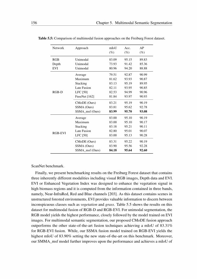
156 Chapter 5. Multimodal Semantic Segmentation
Table 5.5: Comparison of multimodal fusion approaches on the Freiburg Forest dataset.
Network Approach mIoU Acc. AP(%) (%) (%)
RGB Unimodal 83.09 95.15 89.83Depth Unimodal 73.93 91.42 85.36EVI Unimodal 80.96 94.20 88.88
RGB-D
Average 79.51 92.87 90.99Maximum 81.62 93.93 90.87Stacking 83.13 95.19 89.95Late Fusion 82.11 93.95 90.85LFC [50] 82.53 94.99 90.96FuseNet [162] 81.84 93.97 90.93
CMoDE (Ours) 83.21 95.19 90.19SSMA (Ours) 83.81 95.62 92.78SSMA_msf (Ours) 83.99 95.70 93.08
RGB-EVI
Average 83.00 95.10 90.19Maximum 83.00 95.10 90.17Stacking 83.18 95.21 90.11Late Fusion 82.80 95.01 90.07LFC [50] 83.00 95.13 90.28
CMoDE (Ours) 83.31 95.22 90.19SSMA (Ours) 83.90 95.56 92.28SSMA_msf (Ours) 84.18 95.64 92.60
ScanNet benchmark.
Finally, we present benchmarking results on the Freiburg Forest dataset that containsthree inherently different modalities including visual RGB images, Depth data and EVI.EVI or Enhanced Vegetation Index was designed to enhance the vegetation signal inhigh biomass regions and it is computed from the information contained in three bands,namely, Near-InfraRed, Red and Blue channels [203]. As this dataset contains scenes inunstructured forested environments, EVI provides valuable information to discern betweeninconspicuous classes such as vegetation and grass. Table 5.5 shows the results on thisdataset for multimodal fusion of RGB-D and RGB-EVI. For unimodal segmentation, theRGB model yields the highest performance, closely followed by the model trained on EVIimages. For multimodal semantic segmentation, our proposed CMoDE fusion approachoutperforms the other state-of-the-art fusion techniques achieving a mIoU of 83.31%for RGB-EVI fusion. While, our SSMA fusion model trained on RGB-EVI yields thehighest mIoU of 83.90% setting the new state-of-the-art on this benchmark. Moreover,our SMMA_msf model further improves upon the performance and achieves a mIoU of
5.3. Experimental Evaluation 157
84.18%. Additionally, we refer the reader to Appendix A.6 for the detailed comparisons ofthe individual class IoU scores for the Freiburg Forest dataset..
5.3.3 Multimodal Fusion Discussion
To summarize, the models trained on visual RGB images perform the best in comparisonto unimodal segmentation with other modalities and spectra. However, when the depthdata is less noisy and the environment is confined to an indoor space, the model trained ondepth or HHA-encoded depth outperforms visual RGB models. Among the multimodalfusion baselines, Late Fusion and Stacking, each perform well in different environments.Stacking performs better in outdoor environments in the absence of challenging perceptualconditions, while late-fusion performs better in indoor environments and outdoors whenthe noise in the modalities is uncorrelated. This can be attributed to the fact that thelate-fusion method fuses semantically mature representations and effectively exploitscomplementary features. Therefore, in indoor environments, modalities such as depthmaps from stereo cameras are less noisy than in outdoors and as the environment is confined,all the objects in the scene are well represented with dense depth values. This enables thelate-fusion architecture to leverage semantically rich complementary representations forfusion. However in outdoor environments, depth values are very noisy and no informationis present for objects at far away distances. Therefore, the semantic representations fromthe depth stream are considerably less informative for certain parts of the scene whichdoes not allow the late-fusion network to fully exploit the complementary features andhence it does not provide significant gains. On the other hand, in indoor environments orin synthetic scenes outdoors where the depth modality is dense and rich with information,late-fusion significantly outperforms the stacking approach.
Our proposed CMoDE fusion approach outperforms existing state-of-the-art multimodalsemantic segmentation networks in each of the diverse environments. To recapitulate,CMoDE employs a class-wise probabilistic late-fusion technique that adaptively weighs themodality-specific decoder features based on the scene condition. Moreover, our proposedSSMA fusion technique further outperforms CMoDE in all the datasets and sets the newstate-of-the-art in multimodal semantic segmentation. This demonstrates that fusion ofmodalities is an inherently complex problem that depends on several factors such asthe object class, the spatial location of the object and the environmental scene context.Our proposed SSMA fusion approach dynamically adapts the fusion of both mid-leveland high-level semantically mature representations based on the aforementioned factors,thereby enabling our model to effectively exploit the complementary relationship betweenthe modalities. Moreover, as the dynamicity is learned in a self-supervised fashion, itefficiently generalizes to different diverse environments, perceptual conditions and typesof modalities employed for fusion.
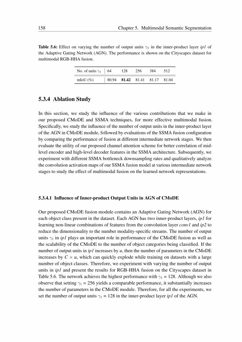
158 Chapter 5. Multimodal Semantic Segmentation
Table 5.6: Effect on varying the number of output units γ1 in the inner-product layer ip1 ofthe Adaptive Gating Network (AGN). The performance is shown on the Cityscapes dataset formultimodal RGB-HHA fusion.
No. of units γ1 64 128 256 384 512
mIoU (%) 80.94 81.42 81.41 81.17 81.04
5.3.4 Ablation Study
In this section, we study the influence of the various contributions that we make inour proposed CMoDE and SSMA techniques, for more effective multimodal fusion.Specifically, we study the influence of the number of output units in the inner-product layerof the AGN in CMoDE module, followed by evaluations of the SSMA fusion configurationby comparing the performance of fusion at different intermediate network stages. We thenevaluate the utility of our proposed channel attention scheme for better correlation of mid-level encoder and high-level decoder features in the SSMA architecture. Subsequently, weexperiment with different SSMA bottleneck downsampling rates and qualitatively analyzethe convolution activation maps of our SSMA fusion model at various intermediate networkstages to study the effect of multimodal fusion on the learned network representations.
5.3.4.1 Influence of Inner-product Output Units in AGN of CMoDE
Our proposed CMoDE fusion module contains an Adaptive Gating Network (AGN) foreach object class present in the dataset. Each AGN has two inner-product layers, ip1 forlearning non-linear combinations of features from the convolution layer conv1 and ip2 toreduce the dimensionality to the number modality-specific streams. The number of outputunits γ1 in ip1 plays an important role in performance of the CMoDE fusion as well asthe scalability of the CMoDE to the number of object categories being classified. If thenumber of output units in ip1 increases by u, then the number of parameters in the CMoDEincreases by C × u, which can quickly explode while training on datasets with a largenumber of object classes. Therefore, we experiment with varying the number of outputunits in ip1 and present the results for RGB-HHA fusion on the Cityscapes dataset inTable 5.6. The network achieves the highest performance with γ1 = 128. Although we alsoobserve that setting γ1 = 256 yields a comparable performance, it substantially increasesthe number of parameters in the CMoDE module. Therefore, for all the experiments, weset the number of output units γ1 = 128 in the inner-product layer ip1 of the AGN.
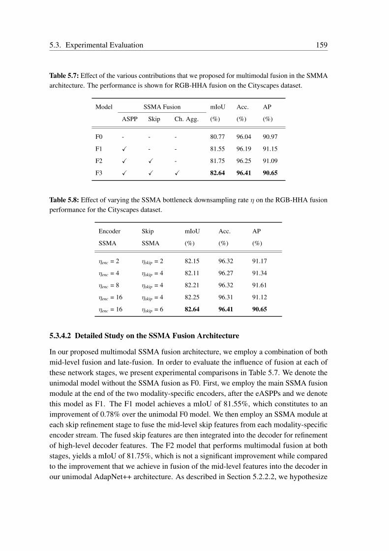
5.3. Experimental Evaluation 159
Table 5.7: Effect of the various contributions that we proposed for multimodal fusion in the SMMAarchitecture. The performance is shown for RGB-HHA fusion on the Cityscapes dataset.
Model SSMA Fusion mIoU Acc. AP
ASPP Skip Ch. Agg. (%) (%) (%)
F0 - - - 80.77 96.04 90.97
F1 X - - 81.55 96.19 91.15
F2 X X - 81.75 96.25 91.09
F3 X X X 82.64 96.41 90.65
Table 5.8: Effect of varying the SSMA bottleneck downsampling rate η on the RGB-HHA fusionperformance for the Cityscapes dataset.
Encoder Skip mIoU Acc. AP
SSMA SSMA (%) (%) (%)
ηenc = 2 ηskip = 2 82.15 96.32 91.17
ηenc = 4 ηskip = 4 82.11 96.27 91.34
ηenc = 8 ηskip = 4 82.21 96.32 91.61
ηenc = 16 ηskip = 4 82.25 96.31 91.12
ηenc = 16 ηskip = 6 82.64 96.41 90.65
5.3.4.2 Detailed Study on the SSMA Fusion Architecture
In our proposed multimodal SSMA fusion architecture, we employ a combination of bothmid-level fusion and late-fusion. In order to evaluate the influence of fusion at each ofthese network stages, we present experimental comparisons in Table 5.7. We denote theunimodal model without the SSMA fusion as F0. First, we employ the main SSMA fusionmodule at the end of the two modality-specific encoders, after the eASPPs and we denotethis model as F1. The F1 model achieves a mIoU of 81.55%, which constitutes to animprovement of 0.78% over the unimodal F0 model. We then employ an SSMA module ateach skip refinement stage to fuse the mid-level skip features from each modality-specificencoder stream. The fused skip features are then integrated into the decoder for refinementof high-level decoder features. The F2 model that performs multimodal fusion at bothstages, yields a mIoU of 81.75%, which is not a significant improvement while comparedto the improvement that we achieve in fusion of the mid-level features into the decoder inour unimodal AdapNet++ architecture. As described in Section 5.2.2.2, we hypothesize
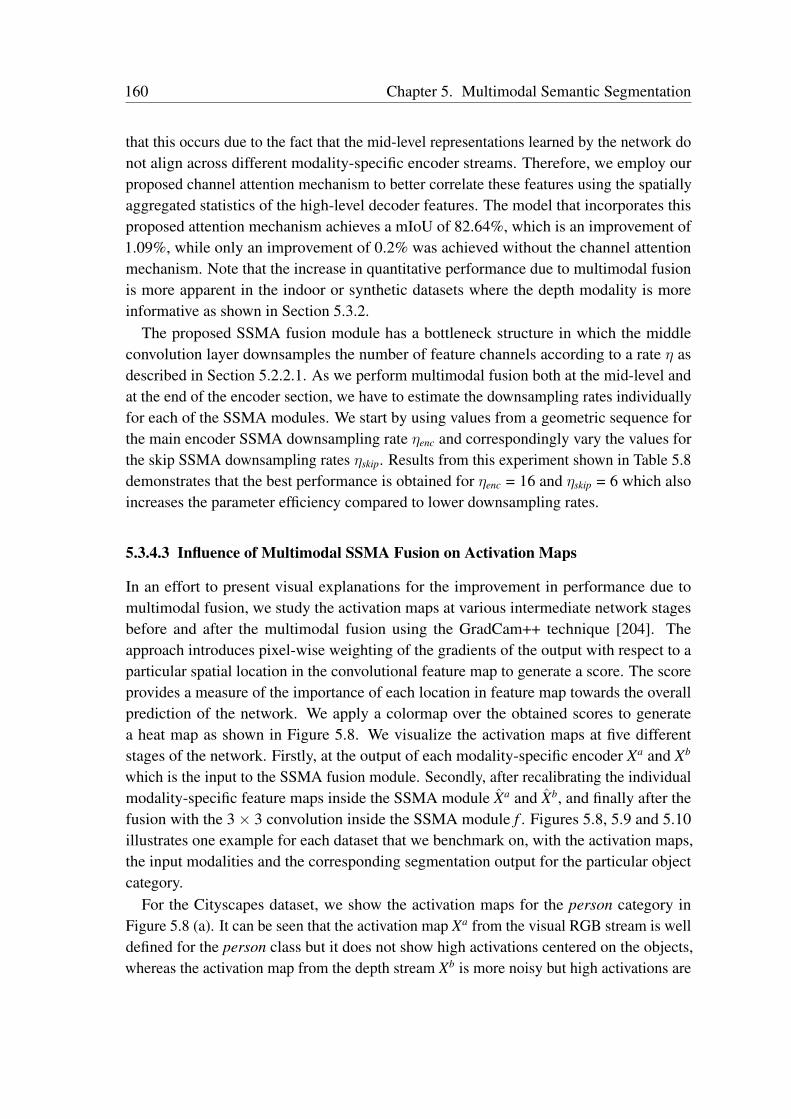
160 Chapter 5. Multimodal Semantic Segmentation
that this occurs due to the fact that the mid-level representations learned by the network donot align across different modality-specific encoder streams. Therefore, we employ ourproposed channel attention mechanism to better correlate these features using the spatiallyaggregated statistics of the high-level decoder features. The model that incorporates thisproposed attention mechanism achieves a mIoU of 82.64%, which is an improvement of1.09%, while only an improvement of 0.2% was achieved without the channel attentionmechanism. Note that the increase in quantitative performance due to multimodal fusionis more apparent in the indoor or synthetic datasets where the depth modality is moreinformative as shown in Section 5.3.2.
The proposed SSMA fusion module has a bottleneck structure in which the middleconvolution layer downsamples the number of feature channels according to a rate η asdescribed in Section 5.2.2.1. As we perform multimodal fusion both at the mid-level andat the end of the encoder section, we have to estimate the downsampling rates individuallyfor each of the SSMA modules. We start by using values from a geometric sequence forthe main encoder SSMA downsampling rate ηenc and correspondingly vary the values forthe skip SSMA downsampling rates ηskip. Results from this experiment shown in Table 5.8demonstrates that the best performance is obtained for ηenc = 16 and ηskip = 6 which alsoincreases the parameter efficiency compared to lower downsampling rates.
5.3.4.3 Influence of Multimodal SSMA Fusion on Activation Maps
In an effort to present visual explanations for the improvement in performance due tomultimodal fusion, we study the activation maps at various intermediate network stagesbefore and after the multimodal fusion using the GradCam++ technique [204]. Theapproach introduces pixel-wise weighting of the gradients of the output with respect to aparticular spatial location in the convolutional feature map to generate a score. The scoreprovides a measure of the importance of each location in feature map towards the overallprediction of the network. We apply a colormap over the obtained scores to generatea heat map as shown in Figure 5.8. We visualize the activation maps at five differentstages of the network. Firstly, at the output of each modality-specific encoder Xa and Xb
which is the input to the SSMA fusion module. Secondly, after recalibrating the individualmodality-specific feature maps inside the SSMA module Xa and Xb, and finally after thefusion with the 3× 3 convolution inside the SSMA module f . Figures 5.8, 5.9 and 5.10illustrates one example for each dataset that we benchmark on, with the activation maps,the input modalities and the corresponding segmentation output for the particular objectcategory.
For the Cityscapes dataset, we show the activation maps for the person category inFigure 5.8 (a). It can be seen that the activation map Xa from the visual RGB stream is welldefined for the person class but it does not show high activations centered on the objects,whereas the activation map from the depth stream Xb is more noisy but high activations are
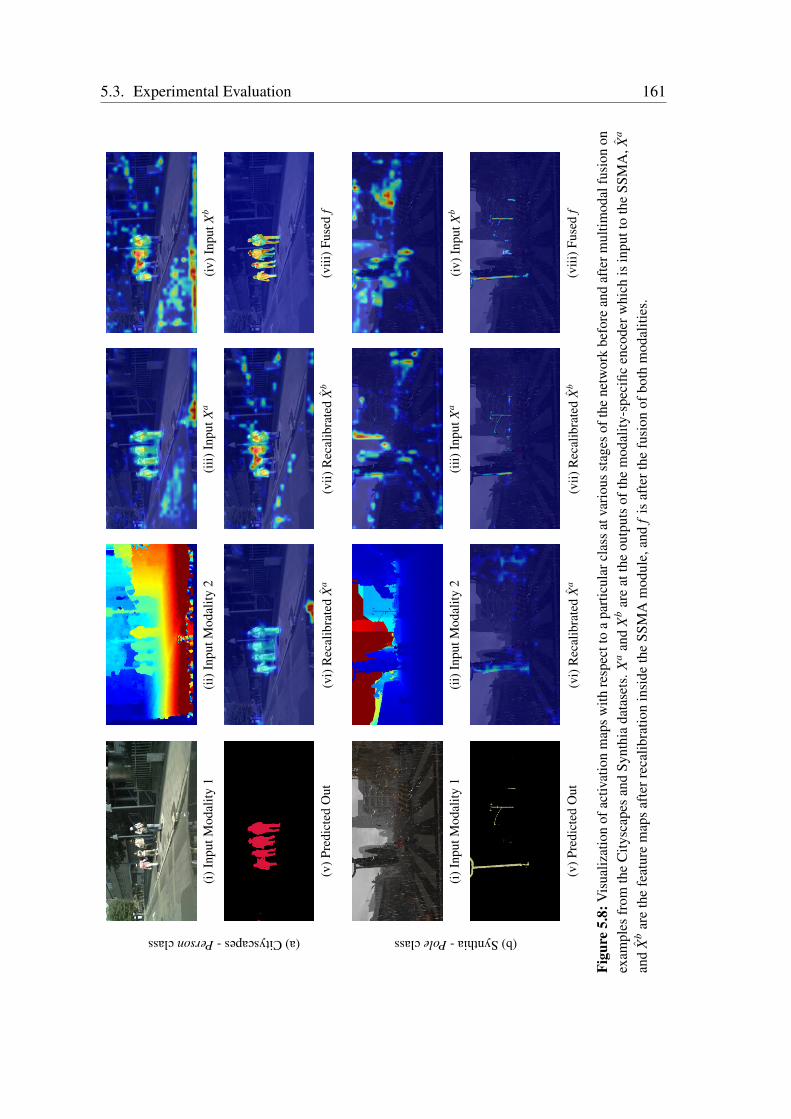
5.3. Experimental Evaluation 161
(a)Cityscapes-Personclass
(i)I
nput
Mod
ality
1(i
i)In
putM
odal
ity2
(iii)
Inpu
tXa
(iv)I
nput
Xb
(v)P
redi
cted
Out
(vi)
Rec
alib
rate
dX
a(v
ii)R
ecal
ibra
ted
Xb
(viii
)Fus
edf
(b)Synthia-Poleclass
(i)I
nput
Mod
ality
1(i
i)In
putM
odal
ity2
(iii)
Inpu
tXa
(iv)I
nput
Xb
(v)P
redi
cted
Out
(vi)
Rec
alib
rate
dX
a(v
ii)R
ecal
ibra
ted
Xb
(viii
)Fus
edf
Figu
re5.
8:V
isua
lizat
ion
ofac
tivat
ion
map
sw
ithre
spec
tto
apa
rticu
larc
lass
atva
rious
stag
esof
the
netw
ork
befo
rean
daf
term
ultim
odal
fusi
onon
exam
ples
from
the
City
scap
esan
dSy
nthi
ada
tase
ts.X
aan
dX
bar
eat
the
outp
uts
ofth
em
odal
ity-s
peci
ficen
code
rwhi
chis
inpu
tto
the
SSM
A,X
a
and
Xb
are
the
feat
ure
map
saf
terr
ecal
ibra
tion
insi
deth
eSS
MA
mod
ule,
and
fis
afte
rthe
fusi
onof
both
mod
aliti
es.
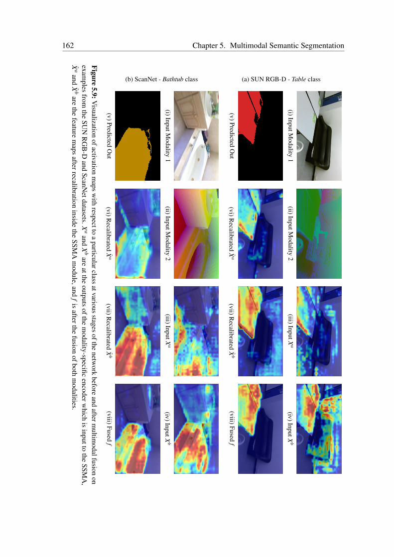
162 Chapter 5. Multimodal Semantic Segmentation
(a) SUN RGB-D - Table class
(i)InputModality
1(ii)InputM
odality2
(iii)InputXa
(iv)InputXb
(v)PredictedO
ut(vi)R
ecalibratedX
a(vii)R
ecalibratedX
b(viii)Fused
f
(b) ScanNet - Bathtub class
(i)InputModality
1(ii)InputM
odality2
(iii)InputXa
(iv)InputXb
(v)PredictedO
ut(vi)R
ecalibratedX
a(vii)R
ecalibratedX
b(viii)Fused
f
Figure5.9:V
isualizationofactivation
maps
with
respecttoa
particularclassatvarious
stagesofthe
network
beforeand
aftermultim
odalfusionon
examples
fromthe
SUN
RG
B-D
andScanN
etdatasets.Xa
andX
bare
attheoutputs
ofthem
odality-specificencoderw
hichis
inputtothe
SSMA
,X
aand
Xb
arethe
featurem
apsafterrecalibration
insidethe
SSMA
module,and
fis
afterthefusion
ofbothm
odalities.
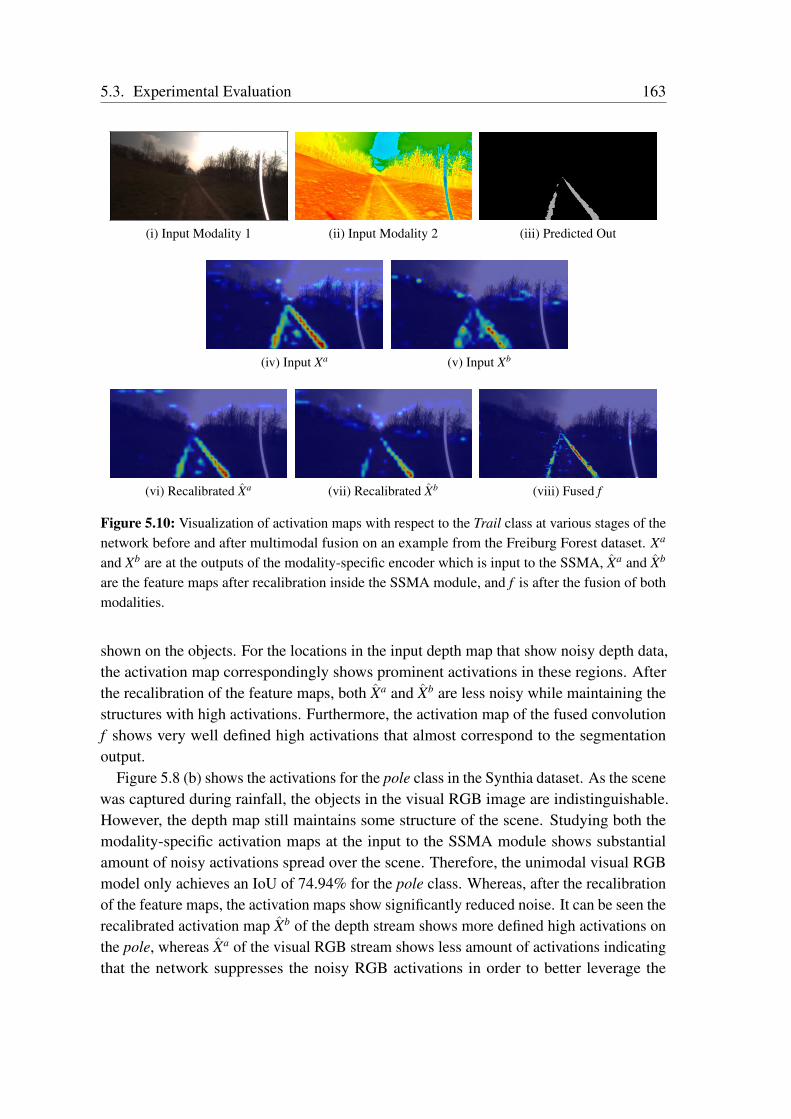
5.3. Experimental Evaluation 163
(i) Input Modality 1 (ii) Input Modality 2 (iii) Predicted Out
(iv) Input Xa (v) Input Xb
(vi) Recalibrated Xa (vii) Recalibrated Xb (viii) Fused f
Figure 5.10: Visualization of activation maps with respect to the Trail class at various stages of thenetwork before and after multimodal fusion on an example from the Freiburg Forest dataset. Xa
and Xb are at the outputs of the modality-specific encoder which is input to the SSMA, Xa and Xb
are the feature maps after recalibration inside the SSMA module, and f is after the fusion of bothmodalities.
shown on the objects. For the locations in the input depth map that show noisy depth data,the activation map correspondingly shows prominent activations in these regions. Afterthe recalibration of the feature maps, both Xa and Xb are less noisy while maintaining thestructures with high activations. Furthermore, the activation map of the fused convolutionf shows very well defined high activations that almost correspond to the segmentationoutput.
Figure 5.8 (b) shows the activations for the pole class in the Synthia dataset. As the scenewas captured during rainfall, the objects in the visual RGB image are indistinguishable.However, the depth map still maintains some structure of the scene. Studying both themodality-specific activation maps at the input to the SSMA module shows substantialamount of noisy activations spread over the scene. Therefore, the unimodal visual RGBmodel only achieves an IoU of 74.94% for the pole class. Whereas, after the recalibrationof the feature maps, the activation maps show significantly reduced noise. It can be seen therecalibrated activation map Xb of the depth stream shows more defined high activations onthe pole, whereas Xa of the visual RGB stream shows less amount of activations indicatingthat the network suppresses the noisy RGB activations in order to better leverage the
164 Chapter 5. Multimodal Semantic Segmentation
well defined features from the depth stream. Activations of the final fused convolutionlayer show higher activations on the pole than either of the recalibrated activation mapsdemonstrating the utility of multimodal fusion. This enables the fusion model to achievean improvement of 8.4% for the pole class.
While, for the indoor SUN RGB-D dataset, Figure 5.9 (a) shows the activation maps forthe table class. Interestingly, both the modality-specific activation maps at the input showhigh activations at different locations indicating the complementary nature of the featuresin this particular scene. However, the activation map Xb from the HHA stream also showshigh activations on the couch in the background which would cause misclassifications.After the recalibration of the HHA feature maps, the activation map Xb no longer hashigh activations on the couch but it retains the high activations on the table. While,the recalibrated activation map Xa of the visual RGB stream shows significantly lessernoisy activations. The activation map of the fused convolution f shows well defined highactivations on the table, more than the modality-specific input activation maps. Thisenables the SSMA fusion model to achieve an improvement of 4.32% in the IoU for thetable category.
For the ScanNet dataset, we show the activation maps for the bathtub category inFigure 5.9 (b). It can be seen that the modality specific activation maps at the input ofthe SSMA module shows high activations at complementary locations, corroborating theutility of exploiting features from both modalities. Moreover, the activation map Xb fromthe HHA stream shows significantly higher activations on the object of interest than theRGB stream. This also aligns with the quantitative results, where the unimodal HHAmodel outperforms the model trained on visual RGB images. After the recalibration of thefeature maps inside the SSMA module, the activation maps show considerably lesser noisewhile maintaining the high activations at complementary locations. The activation mapof the fused convolution f shows only high activations on the bathtub and resembles theactual structure of the segmented output.
Finally, Figure 5.10 (a) shows the activation maps for the trail category in the FreiburgForest dataset. Here we show the fusion with visual RGB and EVI modalities. The EVImodality does not provide substantial complementary information for the trail class incomparison to the RGB images. This is also evident in the visualization of the activationsat the input of the SSMA module. The activation maps of the EVI modality after therecalibration show significantly lesser noise but also smaller number of regions with highactivation than the recalibrated activation maps of the visual RGB stream. Nevertheless,the activation map after the fusion f shows more defined structure of the trail than eitherof the modality-specific activation maps at the input to the SSMA module prior to therecalibration.
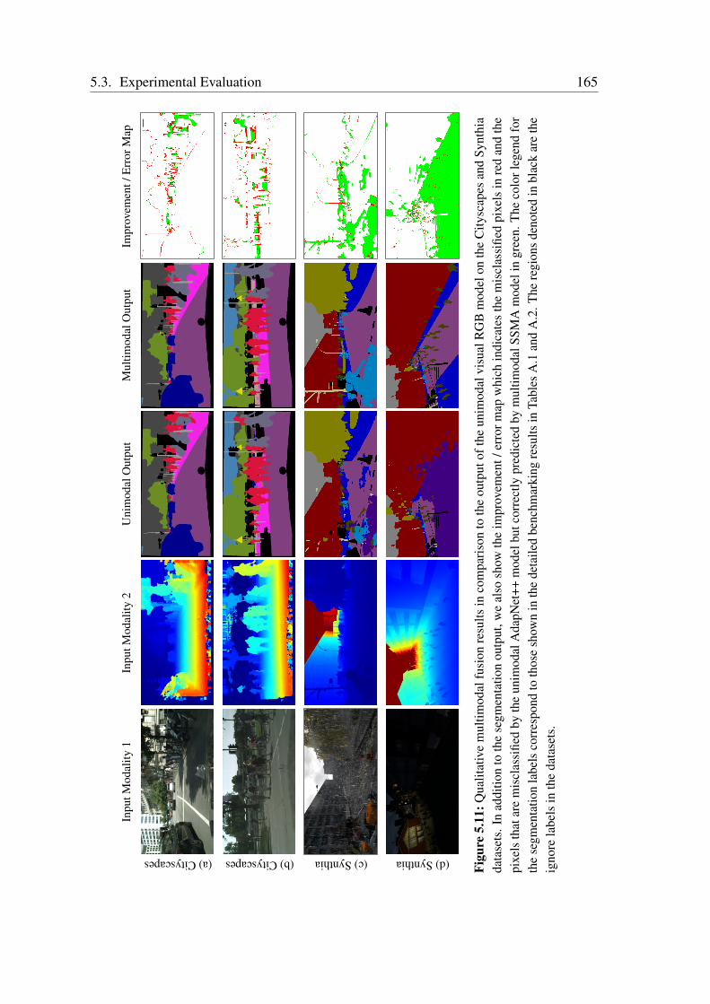
5.3. Experimental Evaluation 165
Inpu
tMod
ality
1In
putM
odal
ity2
Uni
mod
alO
utpu
tM
ultim
odal
Out
put
Impr
ovem
ent/
Err
orM
ap(a)Cityscapes (b)Cityscapes (c)Synthia (d)Synthia
Figu
re5.
11:Q
ualit
ativ
em
ultim
odal
fusi
onre
sults
inco
mpa
riso
nto
the
outp
utof
the
unim
odal
visu
alR
GB
mod
elon
the
City
scap
esan
dSy
nthi
ada
tase
ts.I
nad
ditio
nto
the
segm
enta
tion
outp
ut,w
eal
sosh
owth
eim
prov
emen
t/er
rorm
apw
hich
indi
cate
sth
em
iscl
assi
fied
pixe
lsin
red
and
the
pixe
lsth
atar
em
iscl
assi
fied
byth
eun
imod
alA
dapN
et++
mod
elbu
tcor
rect
lypr
edic
ted
bym
ultim
odal
SSM
Am
odel
ingr
een.
The
colo
rleg
end
for
the
segm
enta
tion
labe
lsco
rres
pond
toth
ose
show
nin
the
deta
iled
benc
hmar
king
resu
ltsin
Tabl
esA
.1an
dA
.2.T
here
gion
sde
note
din
blac
kar
eth
eig
nore
labe
lsin
the
data
sets
.
166 Chapter 5. Multimodal Semantic Segmentation
5.3.5 Qualitative Comparison
In this section, we present qualitative comparisons of multimodal semantic segmentationusing our SSMA fusion approach on each of the five benchmark datasets. We compare withthe output of unimodal AdapNet++ architecture and show the improvement / error mapwhich indicates the improvement over the unimodal AdapNet++ output in green and themisclassifications by the multimodal model in red. Figures 5.11 (a) and (b) show interestingexamples from the Cityscapes dataset. In both these examples, we can see a significantimprovement in the segmentation of cyclists. As cyclists constitute to a person riding abike, often models assign a part of the pixels on the person riding a bike as the personclass, instead of the cyclist class.
Another common scenario is when there is a person standing a few meters behind aparked bike, the model misclassifies the person as a cyclist but since he is not on the bike,the right classification would be the person category. In these examples, we can see that byleveraging the features from the depth modality our network makes accurate predictionsin these situations. In Figure 5.11 (a), we can also see that parts of the car that is severalmeters away is not completely segmented in the unimodal segmentation output but it isaccurately captured in the multimodal segmentation output. Furthermore, in the unimodaloutput of Figure 5.11 (b), we see parts of the sidewalk behind the people is misclassifiedas road and parts of the fence that is several meters away is misclassified as a sidewalk. Asthe distinction between these object categories can clearly be seen in the depth images, ourfusion model accurately identifies these boundaries.
Figures 5.11 (c) and (d) illustrate examples from the Synthia dataset. Here we show thefirst scene during rainfall and the second scene during night-time. In the unimodal outputof first scene, we can see significant misclassifications in all the object classes, exceptbuilding and vegetation that are substantially large in size. Whereas, the multimodal SSMAfusion model leverages the depth features to reliably identify the objects in the scene. InFigure 5.11 (d), even for us humans it is impossible to detect the people on the road due tothe darkness in the scene. As predicted, the unimodal visual RGB model misclassifies theentire road with people as a car, which could lead to disastrous situations if it occurredin the real-world. Whereas, the multimodal SSMA fusion model accurately predicts thescene even in such poor illumination conditions.
In Figures 5.12 (a) and (b), we show examples on the indoor SUN RGB-D dataset. Dueto the large number of object categories in this dataset, several inconspicuous classes oftenexist in the scene. Leveraging structural properties of objects from the HHA-encodeddepth can enable better discrimination between them. Figure 5.12 (a) shows a scene wherethe unimodal model misclassifies parts of the wooden bed as a chair and parts of the pillowas the bed. We can see that the multimodal SSMA output significantly improves uponthe unimodal counterpart. Figure 5.12 (b) shows a complex indoor scene with substantialclutter. The unimodal AdapNet++ model misclassifies the table as a desk and a hatch in the

5.3. Experimental Evaluation 167
Inpu
tMod
ality
1In
putM
odal
ity2
Uni
mod
alO
utpu
tM
ultim
odal
Out
put
Impr
ovem
ent/
Err
orM
ap(a)SUN (b)SUN (c)ScanNet (d)ScanNet
Figu
re5.
12:Q
ualit
ativ
em
ultim
odal
fusi
onre
sults
inco
mpa
rison
toth
eou
tput
ofth
eun
imod
alvi
sual
RG
Bm
odel
onth
eSU
NR
GB
-Dan
dSc
anN
etda
tase
ts.I
nad
ditio
nto
the
segm
enta
tion
outp
ut,w
eal
sosh
owth
eim
prov
emen
t/er
rorm
apw
hich
indi
cate
sth
em
iscl
assi
fied
pixe
lsin
red
and
the
pixe
lsth
atar
em
iscl
assi
fied
byth
eun
imod
alA
dapN
et++
mod
elbu
tcor
rect
lypr
edic
ted
bym
ultim
odal
SSM
Am
odel
ingr
een.
The
colo
rleg
end
for
the
segm
enta
tion
labe
lsco
rres
pond
toth
ose
show
nin
the
deta
iled
benc
hmar
king
resu
ltsin
Tabl
esA
.3an
dA
.5.T
here
gion
sde
note
din
blac
kar
eth
eig
nore
labe
lsin
the
data
sets
.
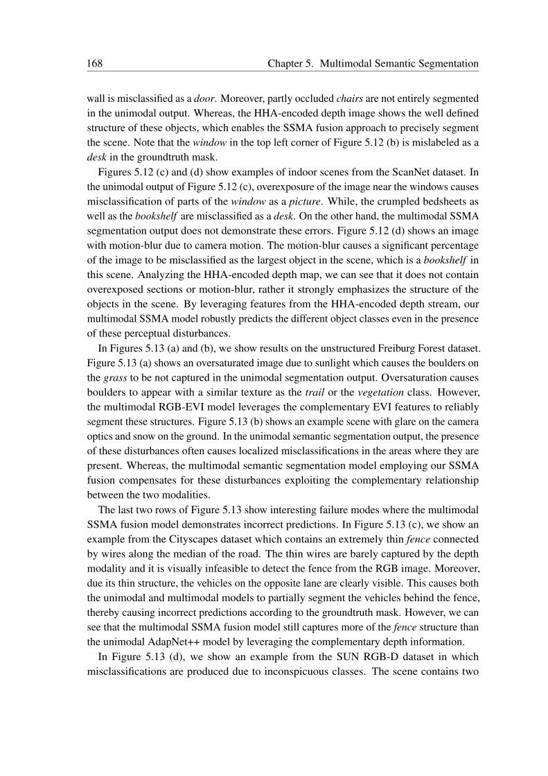
168 Chapter 5. Multimodal Semantic Segmentation
wall is misclassified as a door. Moreover, partly occluded chairs are not entirely segmentedin the unimodal output. Whereas, the HHA-encoded depth image shows the well definedstructure of these objects, which enables the SSMA fusion approach to precisely segmentthe scene. Note that the window in the top left corner of Figure 5.12 (b) is mislabeled as adesk in the groundtruth mask.
Figures 5.12 (c) and (d) show examples of indoor scenes from the ScanNet dataset. Inthe unimodal output of Figure 5.12 (c), overexposure of the image near the windows causesmisclassification of parts of the window as a picture. While, the crumpled bedsheets aswell as the bookshelf are misclassified as a desk. On the other hand, the multimodal SSMAsegmentation output does not demonstrate these errors. Figure 5.12 (d) shows an imagewith motion-blur due to camera motion. The motion-blur causes a significant percentageof the image to be misclassified as the largest object in the scene, which is a bookshelf inthis scene. Analyzing the HHA-encoded depth map, we can see that it does not containoverexposed sections or motion-blur, rather it strongly emphasizes the structure of theobjects in the scene. By leveraging features from the HHA-encoded depth stream, ourmultimodal SSMA model robustly predicts the different object classes even in the presenceof these perceptual disturbances.
In Figures 5.13 (a) and (b), we show results on the unstructured Freiburg Forest dataset.Figure 5.13 (a) shows an oversaturated image due to sunlight which causes the boulders onthe grass to be not captured in the unimodal segmentation output. Oversaturation causesboulders to appear with a similar texture as the trail or the vegetation class. However,the multimodal RGB-EVI model leverages the complementary EVI features to reliablysegment these structures. Figure 5.13 (b) shows an example scene with glare on the cameraoptics and snow on the ground. In the unimodal semantic segmentation output, the presenceof these disturbances often causes localized misclassifications in the areas where they arepresent. Whereas, the multimodal semantic segmentation model employing our SSMAfusion compensates for these disturbances exploiting the complementary relationshipbetween the two modalities.
The last two rows of Figure 5.13 show interesting failure modes where the multimodalSSMA fusion model demonstrates incorrect predictions. In Figure 5.13 (c), we show anexample from the Cityscapes dataset which contains an extremely thin fence connectedby wires along the median of the road. The thin wires are barely captured by the depthmodality and it is visually infeasible to detect the fence from the RGB image. Moreover,due its thin structure, the vehicles on the opposite lane are clearly visible. This causes boththe unimodal and multimodal models to partially segment the vehicles behind the fence,thereby causing incorrect predictions according to the groundtruth mask. However, we cansee that the multimodal SSMA fusion model still captures more of the fence structure thanthe unimodal AdapNet++ model by leveraging the complementary depth information.
In Figure 5.13 (d), we show an example from the SUN RGB-D dataset in whichmisclassifications are produced due to inconspicuous classes. The scene contains two

5.3. Experimental Evaluation 169
Inpu
tMod
ality
1In
putM
odal
ity2
Uni
mod
alO
utpu
tM
ultim
odal
Out
put
Impr
ovem
ent/
Err
orM
ap
(a)Forest (b)Forest (c)Cityscapes (d)SUN
Figu
re5.
13:Q
ualit
ativ
em
ultim
odal
fusi
onre
sults
inco
mpa
riso
nto
the
outp
utof
the
unim
odal
visu
alR
GB
mod
elon
the
Frei
burg
Fore
stda
tase
t.T
hela
sttw
oro
ws
show
failu
rem
odes
onth
eC
itysc
apes
and
SUN
RG
B-D
data
sets
.In
addi
tion
toth
ese
gmen
tatio
nou
tput
,we
also
show
the
impr
ovem
ent/
erro
rmap
whi
chin
dica
tes
the
mis
clas
sifie
dpi
xels
inre
dan
dth
epi
xels
that
are
mis
clas
sifie
dby
the
unim
odal
Ada
pNet
++m
odel
but
corr
ectly
pred
icte
dby
mul
timod
alSS
MA
mod
elin
gree
n.T
heco
lorl
egen
dfo
rthe
segm
enta
tion
labe
lsco
rres
pond
toth
ose
show
nin
the
deta
iled
benc
hmar
king
resu
ltsin
App
endi
xA
.The
regi
ons
deno
ted
inbl
ack
are
the
igno
rela
bels
inth
eda
tase
ts.
170 Chapter 5. Multimodal Semantic Segmentation
object categories that have very similar appearance in some scenes, namely, chair andsofa. The chair class is denoted in dark green, while the sofa class is denoted in lightgreen. As we see in this scene, a single-person sofa is considered to be a chair and onlythe longer sofa in the middle of the image is considered to be in the sofa class accordingto the groundtruth mask. In this scene, the single person sofa is adjacent to the longersofa which causes the both the unimodal AdapNet++ model and the multimodal SSMAfusion model to predict the pixels on both these objects as the sofa class. However, westill observe more pixels that are correctly classified as the chair class in the multimodalSSMA output than in the unimodal AdapNet++ output.
5.3.6 Visualizations Across Seasons and Weather Conditions
In this section, we present qualitative results on the Synthia-Sequences dataset that containsvideo sequences of 12 different seasons and weather conditions. We visualize the segmen-tation output of the multimodal RGB-D SSMA fusion model and unimodal AdapNet++model for which the quantitative results are shown in Figure 5.7. For this experiment,the models were trained on the Synthia-Rand-Cityscapes dataset and only evaluated onthe Synthia-Sequences dataset. The Synthia-Sequences dataset contains a diverse set ofconditions such as summer, fall, winter, spring, dawn, sunset, night, rain, soft-rain, fog,night-rain and winter-night. We show qualitative evaluations on each of these conditionsby comparing the multimodal segmentation performance using the SSMA fusion with theoutput obtained from the unimodal visual RGB model. This aim of this experiment istwofold: to study the robustness of the model to adverse perceptual conditions such as rain,snow, fog and nightime; Secondly, to evaluate the generalization of the model to unseenscenarios.
From the examples shown in Figures 5.14, 5.15 and 5.16, we can see the diverse nature ofthese scenes containing environments such as highway driving, inner-city with skyscrapersand small-sized cities. The RGB images show the visual appearance variations caused bychanging seasons and weather conditions. These appearance changes can be observed inthe color of the vegetation in Figure 5.14 (b), snow on the ground and leaf-less trees inFigure 5.14 (c), glaring light due to sunrise in Figure 5.15 (a), orange hue due to sunset inFigure 5.15 (b), dark scene with isolated lights in Figure 5.15 (c), adverse visibility dueto rain in Figure 5.15 (d) and blurred visibility due to fog in Figure 5.16 (b). Even for ushumans it is extremely hard to identify the different objects in some of these environments.The third column shows the output obtained from the unimodal AdapNet++ model trainedon visual RGB images. The output shows significant misclassifications in scenes thatcontain rain, fog, snow or nighttime. Whereas, the multimodal SSMA model using RGB-Dfusion precisely segments the scene by leveraging the more stable depth features.
From the improvement / error map shown in the last column, we can see a substantialimprovement (green pixels) over unimodal semantic segmentation and minimal error (red
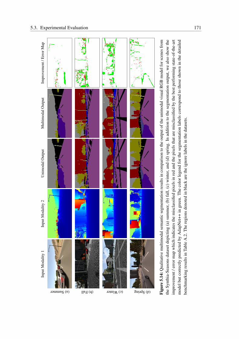
5.3. Experimental Evaluation 171
Inpu
tMod
ality
1In
putM
odal
ity2
Uni
mod
alO
utpu
tM
ultim
odal
Out
put
Impr
ovem
ent/
Err
orM
ap(a)Summer (b)Fall (c)Winter (d)Spring
Figu
re5.
14:Q
ualit
ativ
em
ultim
odal
sem
antic
segm
enta
tion
resu
ltsin
com
paris
onto
the
outp
utof
the
unim
odal
visu
alR
GB
mod
elfo
rsce
nes
from
the
Synt
hia-
Seas
ons
data
setd
epic
ting
(a)s
umm
er,(
b)fa
ll,(c
)win
ter,
and
(d)s
prin
g.In
addi
tion
toth
ese
gmen
tatio
nou
tput
,we
also
show
the
impr
ovem
ent/
erro
rmap
whi
chin
dica
tes
the
mis
clas
sifie
dpi
xels
inre
dan
dth
epi
xels
that
are
mis
clas
sifie
dby
the
best
perf
orm
ing
stat
e-of
-the
-art
mod
elbu
tcor
rect
lypr
edic
ted
byA
dapN
et++
ingr
een.
The
colo
rle
gend
for
the
segm
enta
tion
labe
lsco
rres
pond
toth
ose
show
nin
the
deta
iled
benc
hmar
king
resu
ltsin
Tabl
eA
.2.T
here
gion
sde
note
din
blac
kar
eth
eig
nore
labe
lsin
the
data
sets
.

172 Chapter 5. Multimodal Semantic Segmentation
InputModality
1InputM
odality2
Unim
odalOutput
Multim
odalOutput
Improvem
ent/ErrorM
ap(a) Dawn(b) Sunset(c) Night(d) Rain
Figure5.15:
Qualitative
multim
odalsemantic
segmentation
resultsin
comparison
tothe
outputofthe
unimodalvisualR
GB
modelfor
scenesfrom
theSynthia-Seasons
datasetdepicting(a)daw
n,(b)sunset,(c)night,and(d)rain.In
additionto
thesegm
entationoutput,w
ealso
showthe
improvem
ent/errormap
which
indicatesthe
misclassified
pixelsin
redand
thepixels
thatarem
isclassifiedby
thebestperform
ingstate-of-the-art
modelbutcorrectly
predictedby
AdapN
et++in
green.T
hecolor
legendfor
thesegm
entationlabels
correspondto
thoseshow
nin
thedetailed
benchmarking
resultsin
TableA
.2.The
regionsdenoted
inblack
arethe
ignorelabels
inthe
datasets.
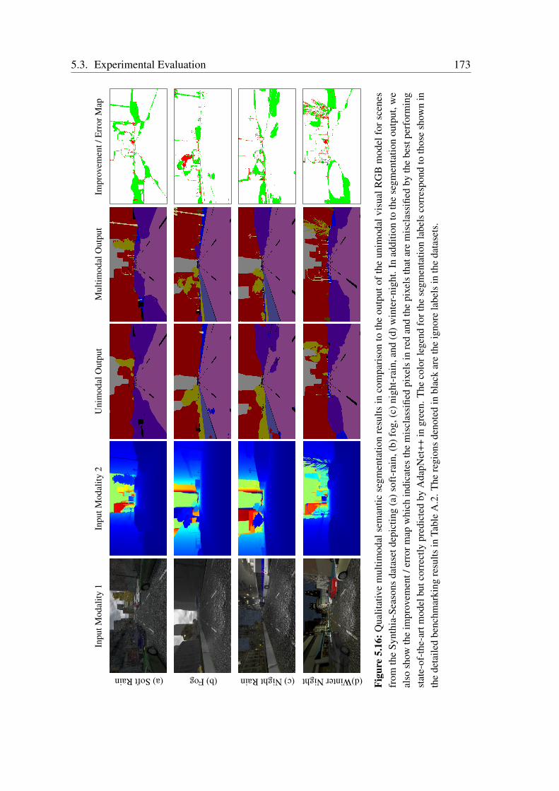
5.3. Experimental Evaluation 173
Inpu
tMod
ality
1In
putM
odal
ity2
Uni
mod
alO
utpu
tM
ultim
odal
Out
put
Impr
ovem
ent/
Err
orM
ap(a)SoftRain (b)Fog (c)NightRain (d)WinterNight
Figu
re5.
16:Q
ualit
ativ
em
ultim
odal
sem
antic
segm
enta
tion
resu
ltsin
com
pari
son
toth
eou
tput
ofth
eun
imod
alvi
sual
RG
Bm
odel
for
scen
esfr
omth
eSy
nthi
a-Se
ason
sda
tase
tdep
ictin
g(a
)sof
t-ra
in,(
b)fo
g,(c
)nig
ht-r
ain,
and
(d)w
inte
r-ni
ght.
Inad
ditio
nto
the
segm
enta
tion
outp
ut,w
eal
sosh
owth
eim
prov
emen
t/er
rorm
apw
hich
indi
cate
sth
em
iscl
assi
fied
pixe
lsin
red
and
the
pixe
lsth
atar
em
iscl
assi
fied
byth
ebe
stpe
rfor
min
gst
ate-
of-t
he-a
rtm
odel
butc
orre
ctly
pred
icte
dby
Ada
pNet
++in
gree
n.T
heco
lorl
egen
dfo
rthe
segm
enta
tion
labe
lsco
rres
pond
toth
ose
show
nin
the
deta
iled
benc
hmar
king
resu
ltsin
Tabl
eA
.2.T
here
gion
sde
note
din
blac
kar
eth
eig
nore
labe
lsin
the
data
sets
.
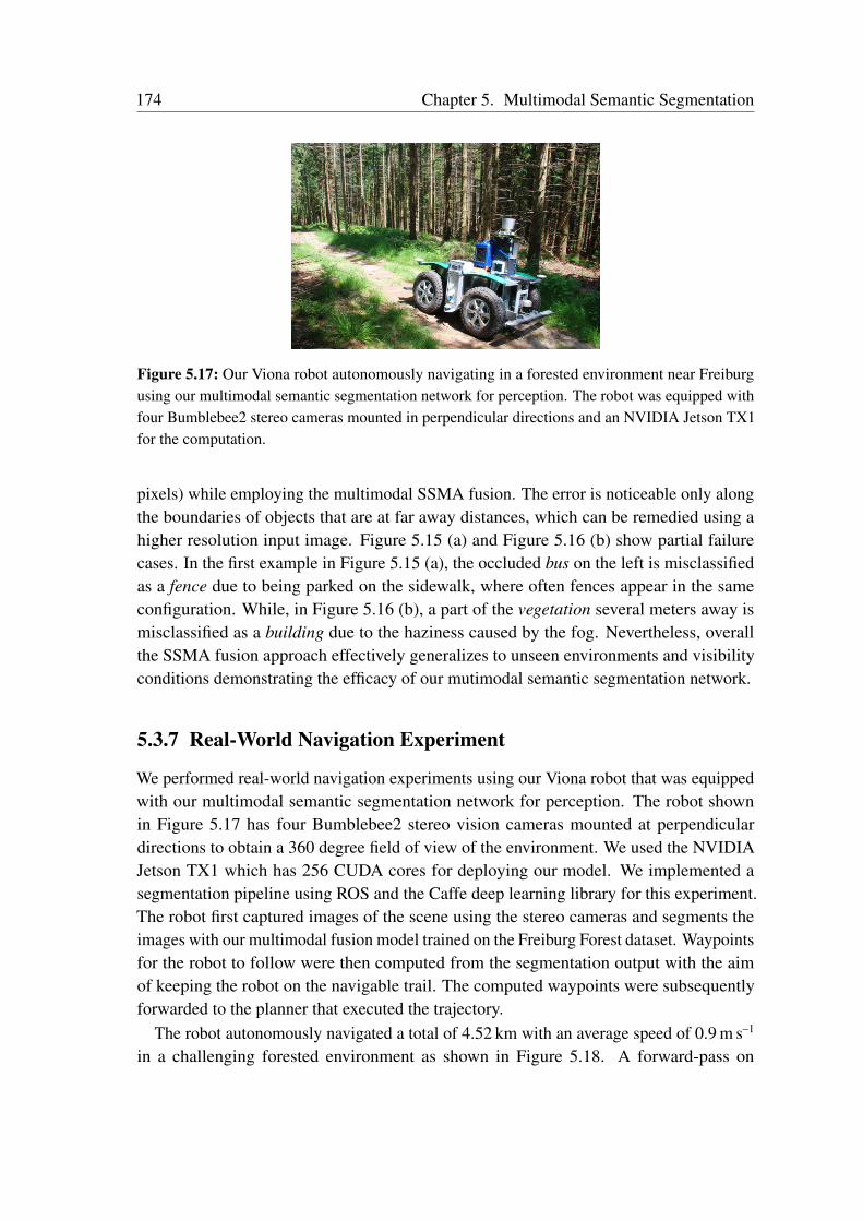
174 Chapter 5. Multimodal Semantic Segmentation
Figure 5.17: Our Viona robot autonomously navigating in a forested environment near Freiburgusing our multimodal semantic segmentation network for perception. The robot was equipped withfour Bumblebee2 stereo cameras mounted in perpendicular directions and an NVIDIA Jetson TX1for the computation.
pixels) while employing the multimodal SSMA fusion. The error is noticeable only alongthe boundaries of objects that are at far away distances, which can be remedied using ahigher resolution input image. Figure 5.15 (a) and Figure 5.16 (b) show partial failurecases. In the first example in Figure 5.15 (a), the occluded bus on the left is misclassifiedas a fence due to being parked on the sidewalk, where often fences appear in the sameconfiguration. While, in Figure 5.16 (b), a part of the vegetation several meters away ismisclassified as a building due to the haziness caused by the fog. Nevertheless, overallthe SSMA fusion approach effectively generalizes to unseen environments and visibilityconditions demonstrating the efficacy of our mutimodal semantic segmentation network.
5.3.7 Real-World Navigation Experiment
We performed real-world navigation experiments using our Viona robot that was equippedwith our multimodal semantic segmentation network for perception. The robot shownin Figure 5.17 has four Bumblebee2 stereo vision cameras mounted at perpendiculardirections to obtain a 360 degree field of view of the environment. We used the NVIDIAJetson TX1 which has 256 CUDA cores for deploying our model. We implemented asegmentation pipeline using ROS and the Caffe deep learning library for this experiment.The robot first captured images of the scene using the stereo cameras and segments theimages with our multimodal fusion model trained on the Freiburg Forest dataset. Waypointsfor the robot to follow were then computed from the segmentation output with the aimof keeping the robot on the navigable trail. The computed waypoints were subsequentlyforwarded to the planner that executed the trajectory.
The robot autonomously navigated a total of 4.52 km with an average speed of 0.9 m s–1
in a challenging forested environment as shown in Figure 5.18. A forward-pass on
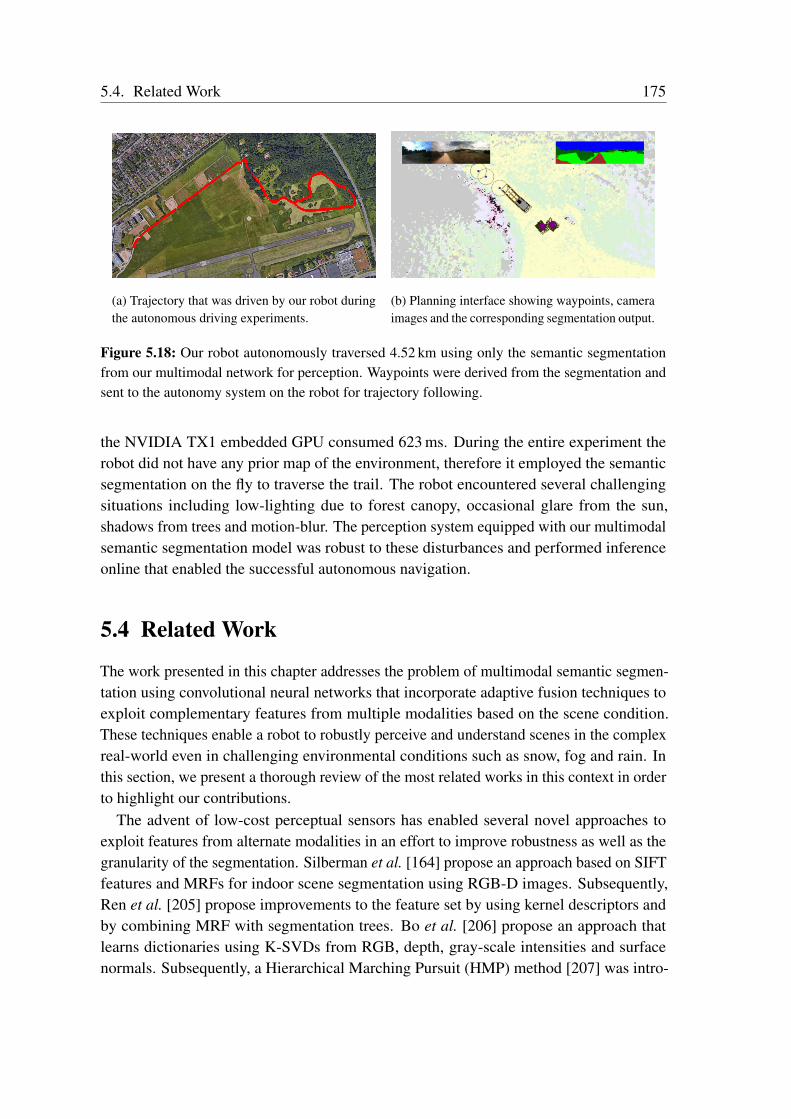
5.4. Related Work 175
(a) Trajectory that was driven by our robot duringthe autonomous driving experiments.
(b) Planning interface showing waypoints, cameraimages and the corresponding segmentation output.
Figure 5.18: Our robot autonomously traversed 4.52 km using only the semantic segmentationfrom our multimodal network for perception. Waypoints were derived from the segmentation andsent to the autonomy system on the robot for trajectory following.
the NVIDIA TX1 embedded GPU consumed 623 ms. During the entire experiment therobot did not have any prior map of the environment, therefore it employed the semanticsegmentation on the fly to traverse the trail. The robot encountered several challengingsituations including low-lighting due to forest canopy, occasional glare from the sun,shadows from trees and motion-blur. The perception system equipped with our multimodalsemantic segmentation model was robust to these disturbances and performed inferenceonline that enabled the successful autonomous navigation.
5.4 Related Work
The work presented in this chapter addresses the problem of multimodal semantic segmen-tation using convolutional neural networks that incorporate adaptive fusion techniques toexploit complementary features from multiple modalities based on the scene condition.These techniques enable a robot to robustly perceive and understand scenes in the complexreal-world even in challenging environmental conditions such as snow, fog and rain. Inthis section, we present a thorough review of the most related works in this context in orderto highlight our contributions.
The advent of low-cost perceptual sensors has enabled several novel approaches toexploit features from alternate modalities in an effort to improve robustness as well as thegranularity of the segmentation. Silberman et al. [164] propose an approach based on SIFTfeatures and MRFs for indoor scene segmentation using RGB-D images. Subsequently,Ren et al. [205] propose improvements to the feature set by using kernel descriptors andby combining MRF with segmentation trees. Bo et al. [206] propose an approach thatlearns dictionaries using K-SVDs from RGB, depth, gray-scale intensities and surfacenormals. Subsequently, a Hierarchical Marching Pursuit (HMP) method [207] was intro-
176 Chapter 5. Multimodal Semantic Segmentation
duced to generate high-level representations from learned spare codes of local patches.Munoz et al. [208] employ modality-specific classifier cascades that hierarchically propa-gate information and do not require one-to-one correspondence between data across modal-ities. In addition to incorporating features based on depth images, Hermans et al. [209]propose an approach that performs joint 3D mapping and semantic segmentation usingRandomized Decision Forests. In most of these approaches, hand engineered or learnedfeatures are extracted from individual modalities and combined together in a joint featureset which is then used for classification. These features do not readily extend to differentmodalities and datasets as they are tuned for specific scenarios. Moreover, these featuresonly capture a subset of cues that are useful for multimodal perception.
More recently, there has been a series of CNN-based techniques [163, 210, 211] that havebeen proposed for end-to-end learning of fused representations from multiple modalities.As opposed to visual RGB images which are three-channel images, alternate modalitiessuch as depth and infrared are one-channel images. Although, approaches have beenproposed that directly learn from one-channel depth images [197], encoding the depthmap into the HHA representation [24, 161] or converting it into a three-channel imageby applying a jet colormap [163] has been demonstrated to be more effective for featurelearning using CNNs. Techniques have also been proposed to augment the standardconvolution with a depth similarity term to force pixels with similar depths at the centerof the filter to contribute more to the output [212]. CNN-based multimodal learningapproaches can be categorized into early, hierarchical and late-fusion methods. An intuitiveearly-fusion technique is to stack data from multiple modalities channel-wise and feed it tothe network as a four or six-channel input. Couprie et al. [213] propose a multiscale CNNfor scene labeling that takes a four-channel RGB-D image as input. However, experimentshave shown that this often does not enable the network to learn complementary featuresand cross-modal interdependencies as they do not exploit the different characteristics ofthe modalities [50, 162].
Hierarchical fusion approaches combine feature maps from multiple modality-specificencoders at various levels (often at each downsampling stage) and upsample the fusedfeatures using a single decoder [162, 210]. Jiang et al. [214] employ an hierarchicalfusion approach with individual RGB and depth streams that fuse features at differentencoder stages while additionally having skip connections to the decoder at the samestages. Alternatively, Schneider et al. [201] propose a mid-level fusion approach in whichNiN layers [69] with depth as input are used to fuse feature maps into the RGB encoderin the middle of the network. Eigen et al. [197] employ a global-to-local strategy thatextracts features using a CNN and combines different levels of predictions. Li et al. [211]propose a Long-Short Term Memory (LSTM) context fusion model that captures and fusescontextual information from multiple modalities accounting for the complex interdepen-dencies between them. Lin et al. [215] employ an FCN-based approach that uses multiplebranches for different discrete depth values in order to provide a better control on the con-

5.4. Related Work 177
textual information of learned features. Qi et al. [216] propose an interesting approach thatemploys 3D graph neural networks for RGB-D semantic segmentation that accounts forboth 2D appearance and 3D geometric relations, while capturing long range dependencieswithin images. A major shortcoming of these approaches is that the complementary natureof different modalities are not fully exploited due to the direct element-wise addition orconcatenation that is performed to fuse the features.
In the late-fusion approach, identical network streams are first trained individually ona specific modality and the feature maps are fused towards the end of network usingconcatenation [163] or element-wise summation [50], followed by learning deeper fusedrepresentations. Lin et al. [217] propose an approach in which individual CNNs areemployed to extract features from RGB images and HHA-encoded maps individually,followed by concatenating the resulting features and employing them as input to anSVM for classification. Socher et al. [218] employ a single layer CNN to learn low-level features which are then input to a Recurrent Neural Network (RNN) for high-levelfeature learning. Features from RGB and depth modalities are learned separately andthen concatenated before the softmax layer. Although these techniques have demonstratedimproved performance over models that solely employ visual RGB images, they do notenable the network to adapt the fusion to changing scene context, which is one of the mainfocus of the approaches presented in this chapter.
Another approach to fusing multimodal features from multiple specialized networksis related to the Mixture of Experts (MoE) technique. Hinton et al. [219] presented theclassical MoE model consisting of experts and a supporting gating network, where eachexpert maps their respective inputs to a corresponding output and the gating networkproduces a probability distribution over the experts. Eigen et al. [220] extend the conceptof MoEs by employing CNNs as experts to classify MNIST [221] and monophone speechdata. This paper highlights the fact that using a mixture with deep networks increasesthe number of trainable parameters without significantly increasing the computationalburden. Cheng et al. [222] introduce a locality-sensitive CNN that performs gated fusionby building a feature affinity matrix that enables weighted average pooling and unpooling.Subsequently, Mees et al. [223] propose a MoE technique that uses inner-product layers tolearn modality-specific weightings which are then used to adaptively compute a weightedaverage over the outputs of CNN streams that take different modalities as input. Theaforementioned techniques provide a framework for adaptively weighing the features ofdifferent CNN streams. However, it is insufficient to solely adapt the features according todifferent modalities as several other factors such the type of objects and its location in thescene also influence the selection of modality-specific features.
In order to address this problem, in this chapter, we presented the CMoDE fusionapproach for learning the most discriminative features from each modality and probabilisti-cally fusing the semantically high-level features according to the different object categoriesin the scene which enables more flexibility in learning the optimal multimodal feature
178 Chapter 5. Multimodal Semantic Segmentation
combination. Nevertheless, there are several real-world scenarios in which class-wisefusion is insufficient, especially in outdoor scenes where different modalities perform wellin different conditions. Moreover, the CMoDE module employs multiple softmax losslayers for each class to compute the probabilities for fusion which does not scale efficientlywhen the number of object categories to be classified significantly increases. Motivatedby this observation, we also proposed a multimodal semantic segmentation architectureincorporating our SSMA fusion module that dynamically adapts the fusion of intermediatenetwork representations from multiple modality-specific network streams according tothe object class, its spatial location and the scene context while learning the fusion in aself-supervised fashion.
5.5 Conclusions
In this chapter, we presented two multimodal semantic segmentation architectures thatadaptively fuse features from multiple modalities and spectra, in order to exploit comple-mentary information based on the scene condition. The first architecture incorporates ourproposed CMoDE fusion mechanism that probabilistically fuses high-level semantic fea-tures from multiple modality-specific network streams to exploit complementary featuresaccording to the different types of objects in the scene and further learns discriminativefused representations. Our second architecture incorporates our proposed SSMA modulesdynamically adapt the fusion of features from modality-specific streams at various inter-mediate network stages in order to optimally exploit complementary features. Our SSMAfusion mechanism is simultaneously sensitive to critical factors that influence multimodalfusion including the object category, its spatial location and the environmental scenecontext, in order to fuse only the relevant complementary information. We also introduceda channel attention mechanism for better correlating the fused mid-level modality-specificencoder features with the high-level decoder features for object boundary refinement.Moreover, as the fusion mechanism is self-supervised, we demonstrated that it effectivelygeneralizes to the fusion of different modalities, beyond the commonly employed RGB-Ddata and across different environments ranging from urban driving scenarios to indoorscenes and unstructured forested environments. Unlike most existing multimodal fusiontechniques, our proposed fusion mechanisms are independent of the base semantic seg-mentation architecture and they can be easily employed in other segmentation frameworks,as well for other multimodal perception tasks.
We presented comprehensive benchmarking results on five standard scene understandingdatasets including Cityscapes, Synthia, SUN RGB-D, ScanNet and Freiburg Forest. Bothour proposed multimodal fusion approaches outperform existing techniques and set the newstate-of-the-art on all the aforementioned benchmarks. We also presented thorough ablationstudies that give insight on our architectural decisions and provided distinctly interpretable
5.5. Conclusions 179
visual explanations that demonstrate the internal functioning of our multimodal fusionscheme. Furthermore, we presented extensive qualitative evaluations on each of thebenchmarked datasets and more importantly, results in adverse perceptual conditions thatdemonstrate the exceptional robustness of our model to a variety of seasonal changes andweather conditions.

Chapter 6
Joint Semantic Motion Segmentation
Understanding the dynamic characteristics of objects in the sceneis an essential prerequisite for autonomous robots that enable themto reason and operate in complex real-world environments. Typ-ically, motion segmentation of objects is achieved using dense op-tical flow methods that make homogenous assumptions about thespatial structure of the flow. However, different semantic objectsin the scene such as pedestrians and cars inherently move differ-ently. Moreover, the problem becomes even more challenging inthe presence of fast and unstable ego-motion induced by the mov-ing robot. In this chapter, we propose two novel convolutional neu-ral network architectures that learn to predict both the semanticobject label and motion status of each pixel in an image. Our pro-posed SMSnet architecture takes a pair of consecutive images as in-put and first learns a coarse representation of the optical flow fieldfeatures, which are then augmented with learned semantic featuresand subsequently refined to yield pixel-wise semantic motion labelsat the original high-resolution. We also propose the SMSnet++ ar-chitecture, in which we strengthen the joint modeling of both se-mantic and motion cues, while concurrently improving the tempo-ral consistency of semantic segmentation using an edge-enhancedflow transformation to warp intermediate network representationsacross time. Extensive experiments demonstrate that our proposedarchitectures achieve state-of-the-art performance on the challeng-ing Cityscapes, KITTI and ApolloScape benchmark datasets.
6.1 Introduction
Recent advancement in robotic technology and machine learning has led to the successfuldeployment of robots to accomplish tasks in various structured and semi-structured en-
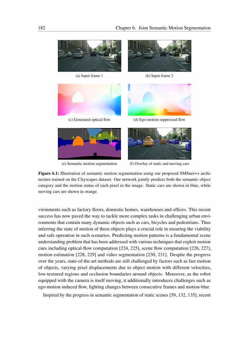
182 Chapter 6. Joint Semantic Motion Segmentation
(a) Input frame 1 (b) Input frame 2
(c) Generated optical flow (d) Ego-motion suppressed flow
(e) Semantic motion segmentation (f) Overlay of static and moving cars
Figure 6.1: Illustration of semantic motion segmentation using our proposed SMSnet++ archi-tecture trained on the Cityscapes dataset. Our network jointly predicts both the semantic objectcategory and the motion status of each pixel in the image. Static cars are shown in blue, whilemoving cars are shown in orange.
vironments such as factory floors, domestic homes, warehouses and offices. This recentsuccess has now paved the way to tackle more complex tasks in challenging urban envi-ronments that contain many dynamic objects such as cars, bicycles and pedestrians. Thusinferring the state of motion of these objects plays a crucial role in ensuring the viabilityand safe operation in such scenarios. Predicting motion patterns is a fundamental sceneunderstanding problem that has been addressed with various techniques that exploit motioncues including optical-flow computation [224, 225], scene flow computation [226, 227],motion estimation [228, 229] and video segmentation [230, 231]. Despite the progressover the years, state-of-the-art methods are still challenged by factors such as fast motionof objects, varying pixel displacements due to object motion with different velocities,low-textured regions and occlusion boundaries around objects. Moreover, as the robotequipped with the camera is itself moving, it additionally introduces challenges such asego-motion induced flow, lighting changes between consecutive frames and motion-blur.
Inspired by the progress in semantic segmentation of static scenes [59, 132, 135], recent
6.1. Introduction 183
work [232, 233] has explored the benefit of learning semantic cues and motion cues jointlyas both provide complementary information about the scene where features learned forsemantic labeling can help infer motion labels and vice versa. On one hand, the transitionin motion is most likely to occur at the dynamic object class boundaries, while on the otherhand, the semantic class of the object itself provides important cues for predicting motionpatterns. For example, in dynamic scenes, the probability of a car or person moving isgreater than the probability of a building or pole. Moreover, as different objects movedifferently, it provides cues on the expectation of motion that varies between regions withdifferent object class labels. Finally, semantic cues also encourage temporal consistency ofthe motion segmentation as the identities of the objects remain constant over time. Fromthe task perspective, the joint knowledge about the semantics and motion of objects givesus a more holistic understanding of the scene that allows robotic systems to increase theirawareness, reason about behaviors and plan autonomous actions more effectively.
In Chapter 4, we introduced architectures for efficient semantic segmentation andsubsequently in Chapter 5, we presented methods that substantially improve the robustnessby exploiting complementary multimodal features. These networks enable a robot toaccurately segment the scene into different semantic object categories, even in challengingperceptual conditions that robots encounter in the complex real-world. While in thischapter, we build upon the techniques that we introduced thus far and propose a jointlearning framework to generate richer semantic descriptions by prefixing motion labelsto potentially dynamic semantic object classes such as a static car and a moving car toenable a more comprehensive understanding of the scene. Deep Convolutional NeuralNetwork (CNN) based approaches have significantly improved the state-of-art in bothsemantic segmentation [24] and motion estimation [225]. There are numerous approachesthat model the motion of objects separately [228, 230, 234, 235, 236] and the semantics ofthe scene separately [53, 67, 135, 136, 138]. However, currently there are only a handfulof methods [232, 233, 237] that aim to capture both semantic and motion cues jointlyconsidering that they are both interrelated.
Reddy et al. [232] propose an approach that integrates semantic, geometric and opticalflow based constraints into a dense fully connected CRF model. They report improvedresults in motion segmentation using the joint formulation compared to geometry-basedmotion segmentation, and joint optimization with superpixel-based clique and motionestimate. Fan et al. [233] propose an approach which combines semantic segmentationobtained from a fully convolutional neural network (FCN) with stereo-vision based motionsegmentation using dense CRFs. Their semantic motion segmentation model outperformsthe approach of Reddy et al. [232] by incorporating better semantic feature learning.Subsequently, Haque et al. [237] propose a three stage pipeline that integrates optical flowas a constraint with semantic features into a dilated CNN for semantic motion segmentation.Their approach achieves state-of-the-art results outperforming the other methods on theKITTI dataset. However, the aforementioned techniques have long multistage pipelines
184 Chapter 6. Joint Semantic Motion Segmentation
that have slow run-times deeming them impractical for real-world applications. Moreover,these approaches only exploit semantic features to improve motion segmentation, whereasthey do not consider the fact that the learned motion features can also be leveraged to enablemore accurate semantic segmentation. Another major hindrance is the lack of a largeenough dataset with groundtruth semantic motion annotations that enable training of CNNswithout overfitting and allow for credible quantitative evaluations as these approaches haveonly been benchmarked on 200 images.
In order to address these problems, in this chapter, we propose two convolutional neuralnetwork architectures that learn to predict both the semantic category and motion statusof each pixel from a pair of consecutive images. Our first architecture termed SMSnetis composed of three components: a stream that learns coarse representations of theoptical flow field features, a parallel stream that generates discriminative semantic features,and a fusion section that combines both motion and semantic features while refining thepredictions to generate a high-resolution pixel-wise semantic motion segmentation output.We build the different streams of the SMSnet architecture based on the AdapNet topologythat we introduced in Chapter 4 and we embed the FlowNet2 [225] architecture to generatethe optical flow maps. Often, the movement of the robot in the scene causes discontinuitiesin the optical flow magnitude. Nearby static objects may appear to have a larger opticalflow magnitudes although they are not moving. In order to alleviate this problem, weemploy a ego-flow suppression technique in which we compute the optical flow purelycaused by the ego-motion using IMU and odometry readings, and subtract it from the flowmagnitudes predicted by the embedded flow generation network.
Our proposed SMSnet model jointly learns to accurately predict both the semantic labeland motion status of each pixel in the image. Although it uses the semantic cues to improvethe motion segmentation performance, it does not exploit the learned motion cues toimprove the semantics learning. In order to address this factor as well as to further improvethe performance of both semantic and motion segmentation, we propose the SMSnet++architecture. The topology of the architecture follows the similar three stream principleas SMSnet. However, we build each of the streams based on our improved AdapNet++architecture that includes our efficient atrous spatial pyramid pooling for multi-scalecontext aggregation and a strong a decoder that significantly improves the performancealong the object boundaries. For generating optical flow maps in SMSnet++, we embedthe new FlowNet3 architecture [227] that introduces a technique to estimate occlusionareas jointly along with the optical flow. We then employ our ego-flow suppressiontechnique to remove any flow magnitudes caused by the movement of the robot equippedwith the camera. Subsequently, we fuse the optical flow field features with the semanticfeatures using our proposed SSMA fusion scheme that we introduced in Chapter 5, ratherthan the simple concatenation that we employ in SMSnet. The SSMA module learnsto adaptively fuse the motion and semantic features by enhancing the optical flow fieldfeatures at areas containing moving objects, while suppressing the activations due to
6.1. Introduction 185
noise at the static regions. Furthermore, in order to simultaneously improve the semanticsegmentation performance, we first transform the ego-flow suppressed optical flow to anedge-enhanced representation using the NetWarp module [238] and subsequently utilize itto warp intermediate semantic representations of the previous frame into the correspondingrepresentations of the current frame. We then fuse the warped feature maps and the featuremaps of the current frame using our SSMA module that we introduced in Chapter 5. Thisrepresentation warping method enables our network to achieve temporal consistency acrossframes resulting in improved prediction accuracy.
Training our proposed networks requires datasets with consecutive image pairs andpixel-level groundtruth labels with both semantic and motion annotations for the currentframe. Thus far, the only publicly available semantic motion segmentation dataset con-tains 200 labeled images from the KITTI [239] benchmark, which is highly insufficientfor training deep networks. Therefore, in order to facilitate this work, we manually la-beled the 3375 training and validation images of the Cityscapes semantic segmentationdataset [143], with motion annotations. As existing techniques are benchmarked on theKITTI dataset, we labeled 255 images with semantic and motion annotations that we em-ploy for training, while using the existing 200 labeled images from Reddy et al. [239] fortesting. Additionally, we also labeled 40,960 training images and 8327 testing images fromthe recently introduced ApolloScape semantic segmentation dataset [240], with motionannotations. We benchmark our proposed architectures as well as existing semantic motionsegmentation techniques on our publicly released Cityscapes-Motion, KITTI-Motion andApolloScape-Motion datasets. Extensive empirical evaluations demonstrate that both ourarchitectures set the new state-of-the-art on these benchmarks, while being several timesfaster than existing techniques. To the best of our knowledge our networks are the firstend-to-end learning techniques to address the problem of semantic motion segmentation,in addition to being the first to simultaneously improve the performance of both these tasksin a joint formulation.
Concretely, we make the following contributions in this chapter:• A novel end-to-end convolutional neural network architecture that takes consecutive
images as input and jointly learns to predict both the semantic object category andmotion status of each pixel in an image.• An refined architecture that adaptively fuses optical flow field features with semantic
features, while simultaneously exploiting the optical flow for learning temporallyconsistent semantics.• A representational warping scheme that improves the temporal consistency of se-
mantic segmentation using our ego-flow suppressed optical flow with the NetWarpmodule [238] and subsequently fusing warped temporal features dynamically usingour adaptive SSMA fusion technique.• We demonstrate how incorporating semantic cues into the motion segmentation net-
work and motion cues into the semantic segmentation network is mutually beneficial
186 Chapter 6. Joint Semantic Motion Segmentation
to both tasks.• We extend the Cityscapes, KITTI and ApolloScape semantic segmentation datasets
with pixel-level motion annotations and make them publicly available. This amountsto a total of 44,090 training images and 9027 testing images with both pixel-levelsemantic and motion annotations.• Extensive benchmarking of existing semantic motion segmentation techniques on all
the three aforementioned datasets with both quantitative and qualitative comparisons.• Implementations of our proposed semantic motion segmentation architectures are
made publicly available at http://deepmotion.cs.uni-freiburg.de.
The remainder of this chapter is organized as follows. In Section 6.2.1, we detail thetopology of our SMSnet architecture for joint semantic motion segmentation, followed bythe architecture of our SMSnet++ model that aims to improve both tasks simultaneouslyin Section 6.2.2. Subsequently, we describe the ego-flow suppression technique in Sec-tion 6.2.3 and we describe the datasets that we introduce in Section 6.3. In Section 6.4,we present comprehensive experimental evaluations, detailed ablation studies and quali-tative comparisons on each of the datasets, followed by detailed generalization analysisof our models in Chapter 6.4.6. Finally, we discuss the extensive related work on motionsegmentation and joint semantic motion segmentation in Section 6.5, before concludingthe chapter in Section 6.6.
6.2 Technical Approach
In this section, we first formulate the problem of semantic motion segmentation. Wethen describe our proposed SMSnet architecture that jointly predicts both the semanticobject class and motion status of each pixel in the image. Subsequently, we detail ourimproved SMSnet++ architecture that uses semantic cues to generate a more precise motionsegmentation and correspondingly uses motion cues to generate a more precise semanticsegmentation. Finally, we detail our ego-flow suppression technique that compensates forthe flow magnitudes induced due to the ego-motion of the robot.
We represent the training set for semantic motion segmentation as T = (In–1, In, Mn) |n = 1, . . . , N, where In = ur | r = 1, . . . , ρ denotes the input frame, In–1 denotes thepreceding frame and the corresponding groundtruth label is given by Mn = mr | r =1, . . . , ρ, where mr ∈ C ×M, where C = 1, ..., C is the set of C semantic object classesand each class can also take the label of static or movingM = m1, m2 with m1 denotinga static pixel and m2 denoting a moving pixel. We assume that the input images (In–1, In)and the labels Mn have the same dimensions ρ = H ×W. Let θ be the network parametersconsisting of weights and biases, and sj(ur, θ) as the score assigned for labeling pixel ur
with label j. We obtain probabilities P = (p1, . . . , p2C) for all the semantic classes using the

6.2. Technical Approach 187
softmax function as
pj (ur, θ | In–1, In) = σ(sj (ur, θ)
)=
exp(sj (ur, θ)
)∑2Ck exp (sk (ur, θ))
. (6.1)
The optimal network parameters are then estimated by minimizing the cross-entropyloss function as
Lseg(T , θ) = –N∑
n=1
ρ∑r=1
2C∑j=1
δmr ,j log pj (ur, θ | In–1, In) , (6.2)
for (In–1, In, Mn) ∈ T , where δmr ,j is the Kronecker delta.
6.2.1 SMSnet Architecture
Our proposed SMSnet architecture shown in Figure 6.2 consists of three streams: MotionFeature Learning, Semantic Feature Learning, and Semantic-Motion Feature Fusion. TheMotion Feature Learning stream shown as green blocks learns optical flow field features,while the Semantic Feature Learning stream shown as gray blocks learns to segment thescene into distinct semantic object categories at the pixel-level. The feature maps fromboth streams are then concatenated in the Semantic-Motion Feature fusion stream indicatedas orange blocks and further discriminative motion representations are learned to generatethe pixel-wise semantic motion segmentation output. In the rest of this section, we describethe topologies of each of these streams in detail.
Motion Feature Learning: This stream learns optical flow field features that representmotion-specific information. Two consecutive input images are first passed through asection of this stream that learns to generate high quality optical flow maps. We embedthe recently proposed FlowNet2 [225] architecture for end-to-end learning of opticalflow, however, any network that performs optical flow estimation can be employed inplace. FlowNet2 consists of multiple stacked subnetworks, where the subsequent networkstake the first image, the second image warped with the intermediate optical flow and theintermediate optical flow itself as input, along with the brightness error. The brightnesserror is the difference between the first and second image warped with the intermediateflow. Moreover, it also includes a subnetwork that focuses on small subpixel motions. Thefinal optical flow is obtained using a small fusion network that combines both the smalland large displacement flows. We use the optical flow generated by this network in the xand y direction, and in addition we also compute the magnitude of the flow. This yields athree-channel image with the same dimensions as the input RGB images. Figure 6.1 (c)shows an example of the generated optical flow image, while the consecutive input framesare shown in Figures 6.1 (a) and (b).
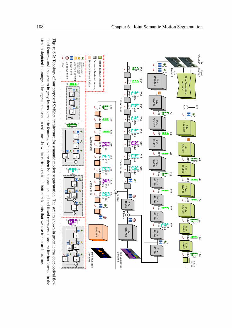
188 Chapter 6. Joint Semantic Motion Segmentation
1113
11
d1
d2
d1
d2
d1
d2
1111
311
s113
11s1
1111
3
nxn co
nvolu
tion
2x2
max p
oolin
g
Batch
norm
Up
-convolu
tion
d1
d2
d3
d3
d1
d1
d2
d1
d1
d2d2
d1
d2
d3d3
d1
d2
d3d3
d2
stride s
n s
nxn co
nvolu
tion
dila
tion d
, stride =
1n d
dd
dd
s
11
11
12
x4
8x9
6Full S
em
an
tics3
84
x7
68
64
x1
92
x3
84
1327
64
x9
6x1
92
64
25
6
64
25
6
64
25
6
12
8
51
2
12
8
51
22
56
x9
6x1
92
25
6x
96
x1
92
51
2x
48
x9
65
12
x4
8x9
65
12
x4
8x9
62
56
x9
6x1
92
12
8
51
25
12
x4
8x9
6
12
8 1
64
51
2
25
6
10
24
10
24
x2
4x4
8
25
6
10
24
25
6 1
2
56
10
24
25
6 1
25
6
10
24
25
6 1
25
6
10
24
25
6 1
25
6
10
24
51
2 2
51
2
20
48
51
2 2
51
2
20
48
51
2 2
51
2
20
48
20
48
x2
4x4
8
6x
38
4x7
68
12
x4
8x9
6
2
24
81
64
81
6
12
2
11
12
8
51
2
10
24
x2
4x4
8
12
8
51
2
12
8
51
2
25
6
12
8
10
24
25
6
12
8
10
24
25
6
25
6
10
24
51
2
25
6
20
48
51
2
25
6
20
48
20
48
x2
4x4
8
3x
38
4x7
68
24
81
61
6
21
11
44
1
Movin
g/S
tatic
38
4x7
68
3 p3 p
pp
22
22
64
x1
92
x3
84
27
64
x9
6x1
92
64
25
6
64
25
6
64
25
6
12
8
51
2
12
8
51
22
56
x9
6x1
92
25
6x
96
x1
92
51
2x
48
x9
65
12
x4
8x9
62
56
x9
6x1
92
12
8
51
2 21
25
12
x2
4x4
8
11
1
Flow
Genera
tion
Netw
ork
3x
38
4x7
68
Inp
ut
Fram
e 1
Inp
ut
Fram
e 2
Conca
t
Eltsu
m
Motio
n Fe
atu
re Le
arn
ing
Sem
antic Fe
atu
re Le
arn
ing
Sem
antic M
otio
n Fu
sion
ReLU
EFS
Figure6.2:Topology
ofourproposedSM
Snetarchitectureforsem
anticm
otionsegm
entation.The
streamshow
nin
greenlearns
deepopticalflow
fieldfeatures
andthe
streamin
graylearns
semantic
features,which
arethen
bothconcatenated
andfused
representationsare
furtherlearnedin
thestream
depictedin
orange.The
legendenclosed
inred
linesshow
thevarious
residualbottleneckunits
thatwe
usein
ourarchitecture.
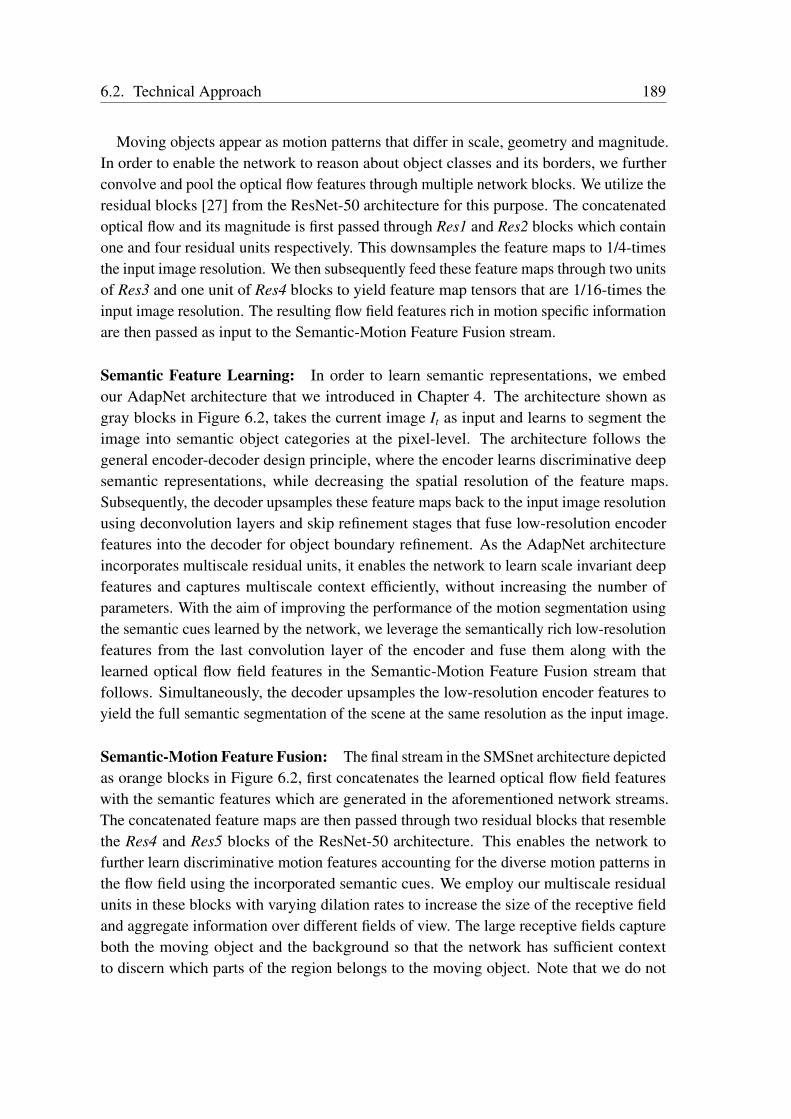
6.2. Technical Approach 189
Moving objects appear as motion patterns that differ in scale, geometry and magnitude.In order to enable the network to reason about object classes and its borders, we furtherconvolve and pool the optical flow features through multiple network blocks. We utilize theresidual blocks [27] from the ResNet-50 architecture for this purpose. The concatenatedoptical flow and its magnitude is first passed through Res1 and Res2 blocks which containone and four residual units respectively. This downsamples the feature maps to 1/4-timesthe input image resolution. We then subsequently feed these feature maps through two unitsof Res3 and one unit of Res4 blocks to yield feature map tensors that are 1/16-times theinput image resolution. The resulting flow field features rich in motion specific informationare then passed as input to the Semantic-Motion Feature Fusion stream.
Semantic Feature Learning: In order to learn semantic representations, we embedour AdapNet architecture that we introduced in Chapter 4. The architecture shown asgray blocks in Figure 6.2, takes the current image It as input and learns to segment theimage into semantic object categories at the pixel-level. The architecture follows thegeneral encoder-decoder design principle, where the encoder learns discriminative deepsemantic representations, while decreasing the spatial resolution of the feature maps.Subsequently, the decoder upsamples these feature maps back to the input image resolutionusing deconvolution layers and skip refinement stages that fuse low-resolution encoderfeatures into the decoder for object boundary refinement. As the AdapNet architectureincorporates multiscale residual units, it enables the network to learn scale invariant deepfeatures and captures multiscale context efficiently, without increasing the number ofparameters. With the aim of improving the performance of the motion segmentation usingthe semantic cues learned by the network, we leverage the semantically rich low-resolutionfeatures from the last convolution layer of the encoder and fuse them along with thelearned optical flow field features in the Semantic-Motion Feature Fusion stream thatfollows. Simultaneously, the decoder upsamples the low-resolution encoder features toyield the full semantic segmentation of the scene at the same resolution as the input image.
Semantic-Motion Feature Fusion: The final stream in the SMSnet architecture depictedas orange blocks in Figure 6.2, first concatenates the learned optical flow field featureswith the semantic features which are generated in the aforementioned network streams.The concatenated feature maps are then passed through two residual blocks that resemblethe Res4 and Res5 blocks of the ResNet-50 architecture. This enables the network tofurther learn discriminative motion features accounting for the diverse motion patterns inthe flow field using the incorporated semantic cues. We employ our multiscale residualunits in these blocks with varying dilation rates to increase the size of the receptive fieldand aggregate information over different fields of view. The large receptive fields captureboth the moving object and the background so that the network has sufficient contextto discern which parts of the region belongs to the moving object. Note that we do not

190 Chapter 6. Joint Semantic Motion Segmentation
downsample the features further at this stage, therefore the feature maps are 1/16-times theinput image resolution. Finally, towards the end of this stream, we use a 1× 1 convolutionlayer to reduce the number of feature channels to two in order to represent the static andmoving object classes. Subsequently, we upsample the coarse representations back to theinput image resolution using a deconvolution layer. The pixels in this upsampled outputdenote the motion status of the semantic object class predicted by the complementarysemantic stream. Figure 6.1 (e) shows the final output of the SMSnet which contains boththe predicted semantic labels and the corresponding motion labels.
6.2.2 SMSnet++ Architecture
In this section, we describe our SMSnet++ architecture that aims to improve motionestimation using learned semantic cues and simultaneously improve semantic segmentationusing learned motion cues. The architecture follows the similar three stream principle asSMSnet consisting of Motion Feature Learning, Semantic Feature Learning, and Semantic-Motion Feature Fusion. Unlike SMSnet, SMSnet++ exploits the temporal coherence acrossconsecutive input images to improve the semantic segmentation performance. This isachieved by warping intermediate network representations of the previous frame into thecorresponding representation of the current frame using an edge-enhanced optical flowrepresentation computed using our ego-flow suppressed optical flow with the NetWarpmodule [238] and dynamically fusing them with the representations of the current frameusing our adaptive SSMA fusion technique. Simultaneously, we improve the performanceof the motion segmentation using our SSMA module to combine the motion and semanticfeatures, in addition to improving the granularity of segmentation using a multi-stagerefinement strategy. In the rest of this section, we detail each of these network components.
Motion Feature Learning: In order to learn optical flow field features from consecutiveimages, we employ the FlowNet3 architecture as shown in Figure 6.3. The FlowNet3architecture improves optical flow prediction by building upon FlowNet2 and incorporatingocclusion estimation as it often negatively influences correspondence estimation tasks.FlowNet3 consists of multiple stacked encoder-decoder networks, where the first networktakes consecutive monocular images as input and the subsequent networks take the firstimage, the second image warped with the intermediate optical flow, the intermediate opticalflow and the occlusions as input. Unlike in FlowNet2, the brightness error is omitted fromthe inputs. In SMSnet, we rescaled the output optical flow to the 0-255 range and roundedit to the nearest integer before extracting motion features. However, in SMSnet++, wemaintain the pixel displacements as floating point numbers and rescale them to the 0-255 range in order to improve the quality of the subsequently learned motion features.We present experiments that demonstrate the improvement due to this transformation inthe ablation study presented in Section 6.5. We obtain the optical flow maps from the
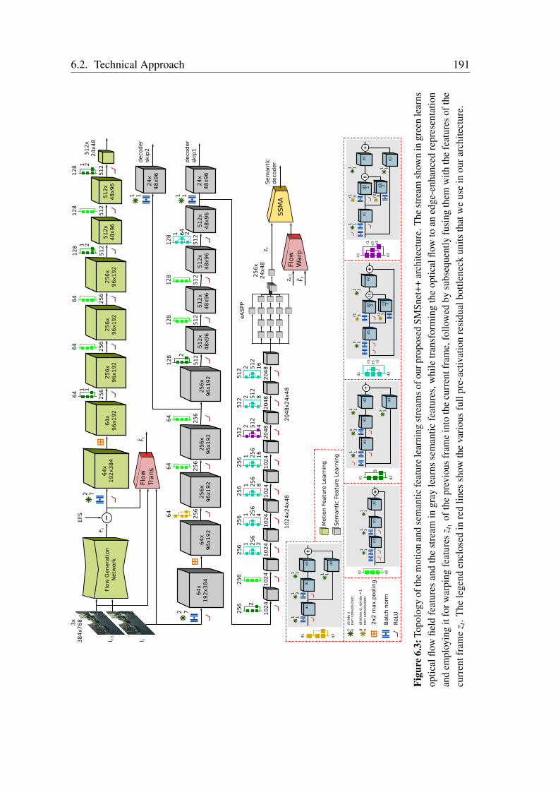
6.2. Technical Approach 191
nxn c
onvolu
tion
2x2
max p
oolin
g
Batc
h n
orm
stri
de s
ns
nxn c
onvolu
tion
dila
tion d
, st
ride =
1nd
1 1
24
x4
8x9
66
4x
19
2x3
84
2 7
64
x9
6x1
92
64
25
6
64
25
6
12
8
51
2
12
8
51
22
56
x9
6x1
92
25
6x
96
x1
92
51
2x
48
x9
65
12
x4
8x9
65
12
x4
8x9
62
56
x9
6x1
92
12
8
51
25
12
x4
8x9
6
12
8
1
6
4
51
2
25
6
10
24
10
24
x2
4x4
8
25
6
10
24
25
6
1
2
56
10
24
25
6
1
2
56
10
24
25
6
1
2
56
10
24
25
6
1
2
56
10
24
51
2
2
5
12
20
48
51
2
2
5
12
20
48
51
2
2
5
12
20
48
20
48
x2
4x4
8
2
24
81
64
81
6
2
2
64
x1
92
x3
84
2 7
64
x9
6x1
92
64
25
6
64
25
6
64
25
6
12
8
51
2
12
8
51
22
56
x9
6x1
92
25
6x
96
x1
92
51
2x
48
x9
65
12
x4
8x9
62
56
x9
6x1
92
12
8
51
221
25
12
x2
4x4
8
11
1
Flow
Genera
tion
Netw
ork
3x
38
4x7
68
I t-1
I t
Moti
on F
eatu
re L
earn
ing
Sem
anti
c Fe
atu
re L
earn
ing
ReLU
EFS
1 11 3
1 1
d1
d2
d1
d2
d1
d2
1 11 1
31 1
1 1s 3
1 1 s 1
1 11 1
3
d1
d2
d3
d3
d1
d1
d2
d1
d1
d2 d2
d1
d2
d3 d3
d1
d2
d3 d3
d2
r2r2
r2r2
s
3r13r1
r1r1
2 2
2 2
d1
d2
1 11 3
1 1 1 1
d1
d1
d2 d2
64
25
6
25
6x
24
x48
25
6x
24
x48
25
6x
24
x48
25
6x
24
x48
eA
SPP
25
6x
24
x4
8
deco
der
skip
1
Sem
anti
cdeco
der
SSM
A
Flow
Warp
1 1
24
x4
8x9
6
deco
der
skip
2Fl
ow
Trans
z t-1
F t
F t
z t
F t
Figu
re6.
3:To
polo
gyof
the
mot
ion
and
sem
antic
feat
ure
lear
ning
stre
amso
four
prop
osed
SMSn
et++
arch
itect
ure.
The
stre
amsh
own
ingr
een
lear
nsop
tical
flow
field
feat
ures
and
the
stre
amin
gray
lear
nsse
man
ticfe
atur
es,w
hile
tran
sfor
min
gth
eop
tical
flow
toan
edge
-enh
ance
dre
pres
enta
tion
and
empl
oyin
git
forw
arpi
ngfe
atur
esz t 1
ofth
epr
evio
usfr
ame
into
the
curr
entf
ram
e,fo
llow
edby
subs
eque
ntly
fusi
ngth
emw
ithth
efe
atur
esof
the
curr
entf
ram
ez t
.The
lege
nden
clos
edin
red
lines
show
the
vari
ous
full
pre-
activ
atio
nre
sidu
albo
ttlen
eck
units
that
we
use
inou
rarc
hite
ctur
e.
192 Chapter 6. Joint Semantic Motion Segmentation
embedded FlowNet3 network and pass the features through a series of convolution andpooling layers, similar to the SMSnet architecture, but we employ the residual units fromthe full pre-activation ResNet-50 architecture [72] as opposed to the standard ResNet-50 [27]. The full pre-activation residual units are shown in the legend enclosed in a red boxin Figure 6.3, while the original residual units are shown in the legend in Figure 6.2. Thefeature maps at the output of this Motion Feature Learning stream which are 1/16-timesdownsampled with respect to the input image resolution are then used for fusion in theSemantic-Motion Feature Fusion stream.
Semantic Feature Learning: We employ our recently proposed AdapNet++ architecturethat we presented in Chapter 4 for learning the semantics in the SMSnet++ architecture. Thearchitecture builds upon AdapNet and incorporates our efficient Atrous Spatial PyramidPooling (eASPP) module that captures long-range context with a large effective receptivefield by cascading multiple atrous convolutions. The size of the receptive field is a criticalfactor for motion segmentation tasks. If a filter with a small receptive field falls entirelywithin an object with non-zero flow values, it is impossible to identify if the flow is due tothe moving object or due to the motion of the robot equipped with the camera. Whereas,if the receptive field includes a portion of the background then the network can easilyidentify the moving regions from the change in flow across the dynamic object boundaries.As objects in driving scenarios have multiple scales, our eASPP effectively aggregatesmultiscale features using atrous convolutions with different dilation rates in parallel. Wealso reconfigure our multiscale residual units that we incorporate in the encoder accordingto the full pre-activation configuration. The two multiscale residual units are shown in thebottom right of the legend enclosed in a red box in Figure 6.3.
Additionally, to further improve the semantic segmentation performance, we propose atechnique to first enhance the optical flow generated by the complementary Motion FeatureLearning stream using the NetWarp module [238] to a more discriminative representationwith sharper object boundaries. We then utilize this edge-enhanced flow to warp interme-diate semantic network representations from the previous frame into the current frame,followed by fusing them with the representations of the current frame. We show examplesof the edge-enhanced flow and evaluate its utility for the temporal warping in comparisonto directly using the optical flow in Section 6.4.4.3. This principle of combining temporallyclose representations learned by the network to improve the semantic consistency acrossframes has previously been explored in different ways [238, 241, 242]. However, in thiswork, we propose to exploit the pixel correspondences learned by our Motion FeatureLearning stream to dynamically fuse intermediate network representations to improve thetemporal consistency.
The NetWarp module [238] that computes the edge-enhanced flow shown in Figure 6.4takes the consecutive images It–1, It and the predicted optical flow Ft as input, and outputsan edge-enhanced flow Ft. Let zk
t–1 and zkt be the representations of the kth layer of the
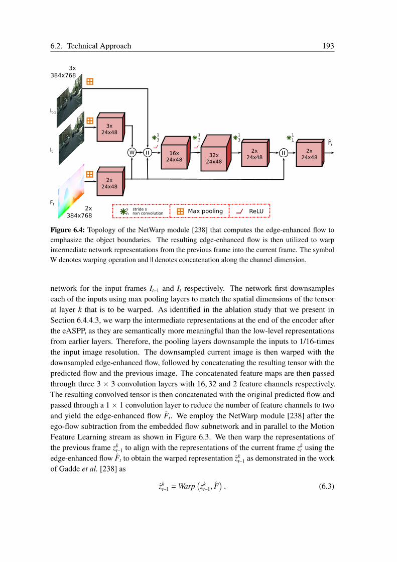
6.2. Technical Approach 193
nxn convolutionstride s
ns ReLU
2x24x48
CxHxW
16x24x48
13
11
C/2xHxW
2x24x48
13
3x24x48
C/2xHxW
2x24x48
Ft
W 32x24x48
13
It-1
It
Ft
Max pooling2x384x768
3x384x768
Figure 6.4: Topology of the NetWarp module [238] that computes the edge-enhanced flow toemphasize the object boundaries. The resulting edge-enhanced flow is then utilized to warpintermediate network representations from the previous frame into the current frame. The symbolW denotes warping operation and || denotes concatenation along the channel dimension.
network for the input frames It–1 and It respectively. The network first downsampleseach of the inputs using max pooling layers to match the spatial dimensions of the tensorat layer k that is to be warped. As identified in the ablation study that we present inSection 6.4.4.3, we warp the intermediate representations at the end of the encoder afterthe eASPP, as they are semantically more meaningful than the low-level representationsfrom earlier layers. Therefore, the pooling layers downsample the inputs to 1/16-timesthe input image resolution. The downsampled current image is then warped with thedownsampled edge-enhanced flow, followed by concatenating the resulting tensor with thepredicted flow and the previous image. The concatenated feature maps are then passedthrough three 3 × 3 convolution layers with 16, 32 and 2 feature channels respectively.The resulting convolved tensor is then concatenated with the original predicted flow andpassed through a 1× 1 convolution layer to reduce the number of feature channels to twoand yield the edge-enhanced flow Ft. We employ the NetWarp module [238] after theego-flow subtraction from the embedded flow subnetwork and in parallel to the MotionFeature Learning stream as shown in Figure 6.3. We then warp the representations ofthe previous frame zk
t–1 to align with the representations of the current frame zkt using the
edge-enhanced flow Ft to obtain the warped representation zkt–1 as demonstrated in the work
of Gadde et al. [238] as
zkt–1 = Warp
(zk
t–1, F)
. (6.3)
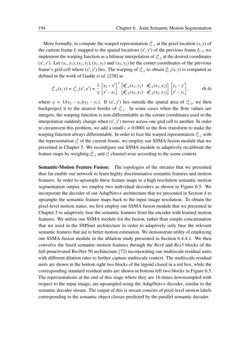
194 Chapter 6. Joint Semantic Motion Segmentation
More formally, to compute the warped representation zkt–1 at the pixel location (x, y) of
the current frame It mapped to the spatial locations (x′, y′) of the previous frame It–1, weimplement the warping function as a bilinear interpolation of zk
t–1 at the desired coordinates(x′, y′). Let (x1, y1), (x1, y2), (x2, y1) and (x2, y2) be the corner coordinates of the previousframe’s grid cell where (x′, y′) lies. The warping of zk
t–1 to obtain zkt–1(x, y) is computed as
defined in the work of Gadde et al. [238] as
zkt–1(x, y) = zk
t–1(x′, y′) =1η
[x2 – x′
x′ – x1
]ᵀ [zk
t–1(x1, y1) zkt–1(x1, y2)
zkt–1(x2, y1) zk
t–1(x2, y2)
] [y2 – y′
y′ – y1
], (6.4)
where η = 1/(x2 – x1)(y2 – y1). If (x′, y′) lies outside the spatial area of zkt–1, we then
backproject it to the nearest border of zkt–1. In some cases when the flow values are
integers, the warping function is non-differentiable as the corner coordinates used in theinterpolation suddenly change when (x′, y′) moves across one grid cell to another. In orderto circumvent this problem, we add a small ε = 0.0001 to the flow transform to make thewarping function always differentiable. In order to fuse the warped representation zk
t–1 withthe representation zk
t of the current frame, we employ our SSMA fusion module that wepresented in Chapter 5. We reconfigure our SSMA module to adaptively recalibrate thefeature maps by weighing zk
t–1 and zkt channel-wise according to the scene context.
Semantic-Motion Feature Fusion: The topologies of the streams that we presentedthus far enable our network to learn highly discriminative semantic features and motionfeatures. In order to upsample these feature maps to a high resolution semantic motionsegmentation output, we employ two individual decoders as shown in Figure 6.5. Weincorporate the decoder of our AdapNet++ architecture that we presented in Section 4 toupsample the semantic feature maps back to the input image resolution. To obtain thepixel-level motion status, we first employ our SSMA fusion module that we presented inChapter 5 to adaptively fuse the semantic features from the encoder with learned motionfeatures. We utilize our SSMA module for the fusion, rather than simple concatenationthat we used in the SMSnet architecture in order to adaptively only fuse the relevantsemantic features that aid in better motion estimation. We demonstrate utility of employingour SSMA fusion module in the ablation study presented in Section 6.4.4.1. We thenconvolve the fused semantic-motion features through the Res4 and Res5 blocks of thefull preactivated ResNet-50 architecture [72] incorporating our multiscale residual unitswith different dilation rates to further capture multiscale context. The multiscale residualunits are shown in the bottom right two blocks of the legend closed in a red box, while thecorresponding standard residual units are shown in bottom left two blocks in Figure 6.5.The representations at the end of this stage where they are 16-times downsampled withrespect to the input image, are upsampled using the AdapNet++ decoder, similar to thesemantic decoder stream. The output of this is stream consists of pixel-level motion labelscorresponding to the semantic object classes predicted by the parallel semantic decoder.
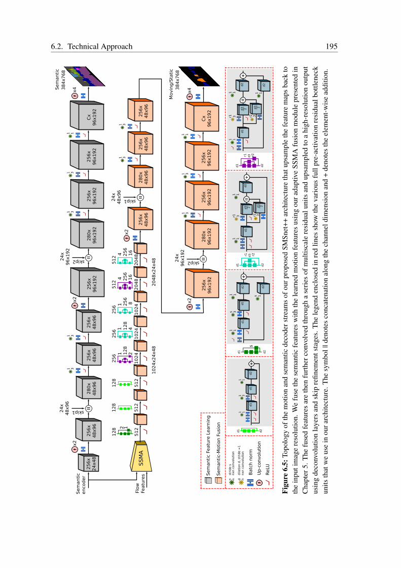
6.2. Technical Approach 195
nxn c
onvolu
tion
Batc
h n
orm
Up
-convolu
tion
stri
de s
ns
nxn c
onvolu
tion
dila
tion d
, st
rid
e =
1nd
12
8
51
2
10
24
x2
4x4
8
12
8
51
2
12
8
51
2
25
6
1
28
10
24
25
6
1
28
10
24
25
6
2
56
10
24
51
2
2
56
20
48
51
2
2
56
20
48
20
48
x2
4x4
8
24
81
61
6
21
11
44
1
Movin
g/S
tati
c3
84
x7
68
Sem
anti
c Fe
atu
re L
earn
ing
Sem
anti
c-M
oti
on F
usi
on
ReLU
1 11 3
1 1
d1
d2
d1
d2
d1
d2
1 11 1
31 1
1 1s 3
1 1 s 1
1 11 1
3
d1
d2
d3
d3
d1
d1
d2
d1
d1
d2 d2
d1
d2
d3 d3
d1
d2
d3 d3
d2
r2r2
r2r2
s
3r13r1
r1r1
2 2
2 2
x4
Cx
96
x1
92
25
6x
96
x1
92
1 1
25
6x
96
x1
92
1 3
28
0x
96
x1
92
1 3
25
6x
96
x1
92
x2
25
6x
48
x9
62
56
x4
8x9
62
80
x4
8x9
6
1 31 3
24
x4
8x9
6
25
6x
48
x9
6
x2
25
6x
24
x4
8
skip1
24
x9
6x1
92
skip2
Sem
anti
cenco
der
SS
MA
Flow
Featu
res
x4
Cx
96
x1
92
25
6x
96
x1
92
1 1
25
6x
96
x1
92
1 3
28
0x
96
x1
92
1 3
25
6x
96
x1
92
x2
25
6x
48
x9
62
56
x4
8x9
62
80
x4
8x9
6
1 31 3
24
x4
8x9
6
25
6x
48
x9
6
x2
skip1
24
x9
6x1
92
skip2
Sem
anti
c3
84
x7
68
Figu
re6.
5:To
polo
gyof
the
mot
ion
and
sem
antic
deco
ders
trea
ms
ofou
rpro
pose
dSM
Snet
++ar
chite
ctur
eth
atup
sam
ple
the
feat
ure
map
sba
ckto
the
inpu
tim
age
reso
lutio
n.W
efu
seth
ese
man
ticfe
atur
esw
ithth
ele
arne
dm
otio
nfe
atur
esus
ing
oura
dapt
ive
SSM
Afu
sion
mod
ule
pres
ente
din
Cha
pter
5.T
hefu
sed
feat
ures
are
then
furt
herc
onvo
lved
thro
ugh
ase
ries
ofm
ultis
cale
resi
dual
units
and
upsa
mpl
edto
ahi
gh-r
esol
utio
nou
tput
usin
gde
conv
olut
ion
laye
rsan
dsk
ipre
finem
ents
tage
s.T
hele
gend
encl
osed
inre
dlin
essh
owth
eva
riou
sfu
llpr
e-ac
tivat
ion
resi
dual
bottl
enec
kun
itsth
atw
eus
ein
oura
rchi
tect
ure.
The
sym
bol|
|den
otes
conc
aten
atio
nal
ong
the
chan
neld
imen
sion
and
+de
note
sth
eel
emen
t-w
ise
addi
tion.

196 Chapter 6. Joint Semantic Motion Segmentation
6.2.3 Ego-Flow Suppression
As the robot equipped with the camera is itself in motion during navigation, the resultingego-motion introduces additional optical flow magnitudes that are not induced by movingobjects in the scene. This hampers the network from distinguishing the real motion ofobjects from the camera motion. The flow induced from ego-motion can cause ambiguitiessince objects in the scene can appear with high optical flow magnitudes although they arenot moving in reality. In order to circumvent this problem, we predict the optical flow mapX′ purely caused by the ego-motion and subtract it from the predicted optical flow. We firstestimate the backward camera translation T and the rotation matrix R from the position ofthe current frame It to the previous frame It–1. Using the IMU and odometry data, we canthen estimate X′ as
X′ = KRK–1X + KTz
, (6.5)
where K is the intrinsic camera matrix, X = (u, v, 1)T is the homogenous coordinate ofthe pixel in the image coordinates and z is the depth of the corresponding pixel in meters.By computing the flow vector for every pixel coordinate using Eq. (6.5), we obtain the2-dimensional optical flow that purely represents the ego-motion, which we denote asthe ego-flow. As Eq. (6.5) requires the depth map of the corresponding input images, weestimate the depth z using the recently proposed DispNet [243] architecture that has a fastinference time. We then subtract the ego-flow X′ from the predicted optical flow X rightafter the flow generation network in our proposed SMSnet and SMSnet++ architecturesas shown in Figure 6.2. We denote this step as Ego-Flow Suppression (EFS) in thiswork. This enables the network to account for the induced ego-flow while maintainingthe flow magnitudes that are caused by the other moving objects. We demonstrate theutility of introducing EFS in the ablation study presented in Section 6.4.4.2. An exampleof the optical flow with ego-flow suppression EFS is shown in Figure 6.1 (d). We presentextensive ablation studies with and without the EFS in Section 6.4.4.
6.3 Dataset and Augmentation
Training our proposed networks require a large amount of labeled semantic and motionannotations. Although there are a handful of approaches that have tackled the problemof semantic motion segmentation, all of them have only utilized the 200 labeled imagesfrom the KITTI dataset that were hand-annotated by Reddy et al. [239]. Employing dataaugmentation strategies can alleviate this problem to a certain extent. However, for crediblequantitative evaluations, several hundreds of training images with groundtruth labels arerequired, apart from the separate set of images and groundtruth labels for testing. Standardmotion segmentation datasets such as DAVIS [244], Sintel [245] and FBMS [246] donot have semantic groundtruth annotations, while standard semantic scene segmentation

6.3. Dataset and Augmentation 197
(a) Image It–1 (b) Image It with motion label overlay
(c) Generated optical flow (d) Ego-motion suppressed flow
Figure 6.6: An example scene from the Cityscapes dataset showing a pair of consecutive imageswith the correspondingly generated optical flow field and the ego-motion compensated flow field.The image from the current timestep It also shows the groundtruth static (blue) and moving (orange)object labels as an overlay.
datasets such as Cityscapes[143], SUN RGB-D [145] and ScanNet [146] do not havemotion annotations.
Training our network for joint semantic motion segmentation requires semantic andmotion annotations for the same scenes. Obtaining pixel-level groundtruth of objectmotion is particularly hard as visible pixel displacement quickly decreases with increasingdistance from the camera due to the motion parallax effect. In addition, ego-motion of thevehicle makes labeling an arduous task. In order to facilitate this work and to allow forcredible quantitative evaluation, we extend three benchmark scene understanding datasetswith manually annotated motion labels. We made these annotations publicly available athttp://deepmotion.cs.uni-freiburg.de to enable further progress in learning thisjoint task. In the rest of this section, we briefly describe these datasets with example scenescontained in them and the annotation procedure that we employ.
Cityscapes-Motion: The Cityscapes dataset [143] is one of the standard benchmarksfor scene understanding, that we also employed for semantic segmentation and multimodalfusion in Chapters 4 and 5 correspondingly. As we already presented an extensive descrip-tion of this dataset in the previous chapters, we only give a brief overview of the motionannotations that we generated. We manually labeled the dynamic objects with motionstatus by observing consecutive images from the video sequences and by assigning thesemantic instance annotations of the objects provided in the dataset with static or movingmotion tags. We labeled a total of 2975 training images and 500 validation images. The
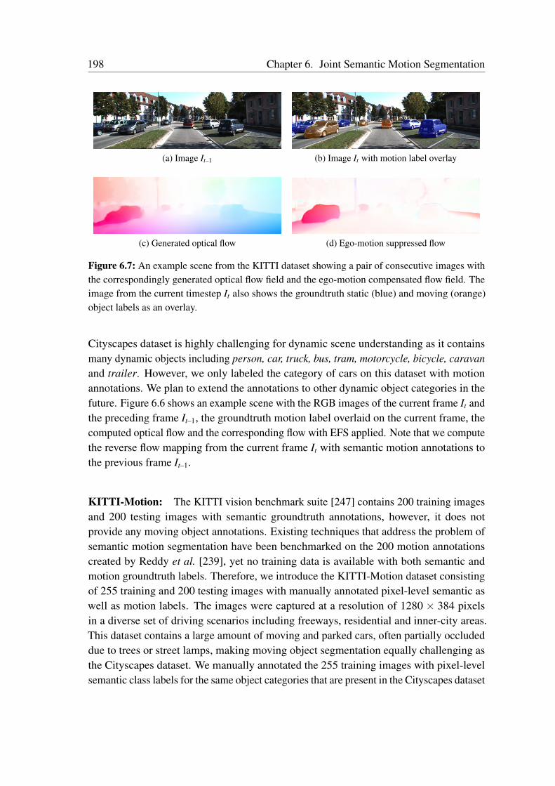
198 Chapter 6. Joint Semantic Motion Segmentation
(a) Image It–1 (b) Image It with motion label overlay
(c) Generated optical flow (d) Ego-motion suppressed flow
Figure 6.7: An example scene from the KITTI dataset showing a pair of consecutive images withthe correspondingly generated optical flow field and the ego-motion compensated flow field. Theimage from the current timestep It also shows the groundtruth static (blue) and moving (orange)object labels as an overlay.
Cityscapes dataset is highly challenging for dynamic scene understanding as it containsmany dynamic objects including person, car, truck, bus, tram, motorcycle, bicycle, caravanand trailer. However, we only labeled the category of cars on this dataset with motionannotations. We plan to extend the annotations to other dynamic object categories in thefuture. Figure 6.6 shows an example scene with the RGB images of the current frame It andthe preceding frame It–1, the groundtruth motion label overlaid on the current frame, thecomputed optical flow and the corresponding flow with EFS applied. Note that we computethe reverse flow mapping from the current frame It with semantic motion annotations tothe previous frame It–1.
KITTI-Motion: The KITTI vision benchmark suite [247] contains 200 training imagesand 200 testing images with semantic groundtruth annotations, however, it does notprovide any moving object annotations. Existing techniques that address the problem ofsemantic motion segmentation have been benchmarked on the 200 motion annotationscreated by Reddy et al. [239], yet no training data is available with both semantic andmotion groundtruth labels. Therefore, we introduce the KITTI-Motion dataset consistingof 255 training and 200 testing images with manually annotated pixel-level semantic aswell as motion labels. The images were captured at a resolution of 1280 × 384 pixelsin a diverse set of driving scenarios including freeways, residential and inner-city areas.This dataset contains a large amount of moving and parked cars, often partially occludeddue to trees or street lamps, making moving object segmentation equally challenging asthe Cityscapes dataset. We manually annotated the 255 training images with pixel-levelsemantic class labels for the same object categories that are present in the Cityscapes dataset
6.3. Dataset and Augmentation 199
(a) Image It–1 (b) Image It with motion label
(c) Generated optical flow (d) Ego-motion suppressed flow
Figure 6.8: An example scene from the ApolloScape dataset showing a pair of consecutive imageswith the correspondingly generated optical flow field and the ego-motion compensated flow field.The image from the current timestep It also shows the groundtruth static (blue) and moving (orange)object labels as an overlay.
and additionally with moving object annotations for cars. The 200 testing images aretaken from the dataset provided by Reddy et al.. In addition, we combine two communityannotated KITTI semantic segmentation datasets [248, 249] consisting of 253 images forpretraining the semantic stream of our network. These images also do not overlap withthe training or testing images in the KITTI-Motion dataset that we introduced. Figure 6.7shows an example scene from this dataset with the preceding frame It–1, the groundtruthmotion label overlaid on the current frame It, the optical flow map that was generated andthe corresponding flow with EFS.
ApolloScape-Motion: ApolloScape [240] is one of the most recent and largest sceneunderstanding datasets till date. The images were captured using two VMX-CS6 cam-eras at a resolution 3384 × 2710 pixels and the depth maps were generated from lasermeasurements acquired using a Riegl VMX-1HA scanner. All the images were taggedwith IMU/GNSS measurements and were time synchronized. A total of 143,906 videoframes and corresponding pixel-level semantic annotations were released, including 89,430instance-level semantic object annotations. The dataset was collected in easy, moderate,and heavy scene complexities, where the complexity is computed from the amount of
200 Chapter 6. Joint Semantic Motion Segmentation
movable objects such as person and vehicles in the scene. This dataset is substantiallymore challenging than Cityscapes and KITTI datasets, as it contains extreme lightingconditions caused by driving under overpasses, glare on the camera optics and reflectionsof multiple nearby vehicles that are visible on other vehicles. Semantic annotations areprovide for 21 object classes including car, motorcycle, bicycle, person, rider, truck, bus,tricycle, road, sidewalk, traffic cone, bollard, fence, traffic light, pole, traffic sign, wall,trash can, billboard, building, bridge, tunnel, overpass and vegetation.
Depth maps have only been released for a subset of the labeled images. Therefore, wechose the images for which the depth maps are available for our ApolloScape-Motiondataset, which corresponds to 40,960 training images and 8327 testing images. Similarto the Cityscapes and KITTI datasets, we manually annotated each of these images withpixel-level motion labels. Unlike the other datasets where only cars, trucks and buseswere annotated with motion labels, in this dataset, we annotated all the different types ofdynamic objects, thereby individually classifying static/moving car, static/moving personand static/moving cyclist. We use the same semantic object classes as the Cityscapes andKITTI datasets for consistency and in order to be able to combine the datasets. Figure 6.8shows an example scene from the ApolloScape dataset with the previous image It–1,the current image It, the current image with the groundtruth motion labels overlaid, thegenerated optical flow image and the corresponding optical flow with EFS.
Despite the reasonable amount of training data, we perform a series of data augmen-tations to introduce more diversity into the training set. Data augmentation is critical toprevent overfitting and to enhance the generalization ability of the network. We applyspatial transformations such as rotation (–13 to 13), scaling (0.5 to 2.0), flipping, trans-lation (–20% to +20%) and cropping (0.8 to 0.9), as well as chromatic transformationssuch as color (0.5 to 2), contrast (0.5 to 1.5) and brightness (–40 to 40) modulation. As ournetworks take two consecutive images as input, we augment the pair and the correspondinggroundtruth label jointly with the same parameters.
6.4 Experimental Evaluation
In this section, we first describe the training protocol that we employ in Section 6.4.1,followed by comprehensive quantitative results for semantic motion segmentation using ourproposed architectures in Section 6.4.2 and an analysis on the influence of motion parallaxin Section 6.4.3. We then present detailed ablation studies that describe our architecturaldecisions in Section 6.4.4 and extensive qualitative semantic motion segmentation resultson each of the datasets in Section 6.4.5. Finally, we present evaluations of the generalizationability of our models to new environments in Section 6.4.6.
We use the TensorFlow [159] deep learning library for the implementations and all theexperiments were carried out on a system with an Intel Xeon E5, 2.4 GHz and an NVIDIA
6.4. Experimental Evaluation 201
TITAN X GPU. We quantify the performance using the standard Jaccard Index which iscommonly known as average intersection-over-union (IoU) metric. It can be computedfor each object class as IoU = TP/(TP + FP + FN), where TP, FP and FN correspond totrue positives, false positives and false negatives respectively. We also report the meanintersection-over-union (mIoU), pixel-wise accuracy (Acc) and average precision (AP) forthe empirical analysis.
6.4.1 Network Training
We train our networks with an input image resolution of 768× 384 pixels. We use bilinearinterpolation for resizing the RGB images and the nearest-neighbour interpolation forresizing the groundtruth labels. We employ the same multi-stage training protocol toeffectively train both our SMSnet and SMSnet++ architectures. We first train the SemanticFeature Learning stream of SMSnet and SMSnet++ that encompass the AdapNet andAdapNet++ architectures respectively for learning the semantic features corresponding tothe C number of object classes in the datasets. We use the training scheme described inSection 4.4.3 of Chapter 4 for this purpose. Subsequently, in the second stage, we leveragetransfer learning to train the joint model in either the SMSnet or the SMSnet++ frameworkby initializing the Semantic Feature Learning stream with weights from the previous stageand the embedded optical flow generation network in the Motion Feature Learning streamwith weights pre-trained on the KITTI Flow dataset [247]. While, we initialize the otherlayers using the He initialization [93] scheme.
We train the entire joint architecture while keeping the weights of the Semantic FeatureLearning stream and the flow generation network fixed. This enables our joint architectureto exploit the stable optical flow field features and semantic features, while learning deeperdiscriminative motion representations at the high-level in the second stage. We use theAdam solver for optimization with β1 = 0.9, β2 = 0.999 and ε = 10–10. We train the jointmodel for a maximum of 100,000 iterations using an initial learning rate of λ0 = 10–4
with a mini-batch size of 8 and a dropout probability of 0.5. In the final stage, we fix theweights of the Semantic Feature Learning stream, the Motion Feature Learning stream andthe layers in the Semantic-Motion Feature Fusion until the first deconvolution layer, whileonly training the decoder for the motion segmentation with a learning rate of λ0 = 10–5 anda mini-batch size of 12 for 50,000 iterations. This enables us to train the network with alarger batch size, while focusing more on the upsampling stages to yield the high-resolutionmotion segmentation output.
6.4.2 Comparison with the State-of-the-Art
In this section, we present comprehensive benchmarking results of our proposed SMSnetand SMSnet++ architectures on the Cityscapes-Motion, KITTI-Motion and Apolloscape-

202 Chapter 6. Joint Semantic Motion Segmentation
Motion datasets. We compare the performance of our models with the state-of-the-artsemantic motion segmentation architectures including CRF-M [232] and CNN-MCA [237],as well as architectures that only perform end-to-end motion segmentation, namely, MP-net [235], MODNet [250], AHCRF-Motion [234] and GEO-M [251]. Additionally, wealso compare against a baseline technique that we term SMSnet++FLO, for which we usethe same topology as our proposed SMSnet++ architecture, but we remove the SemanticFeature Learning stream. Therefore, this baseline performs motion segmentation onlybased on the optical flow and in comparison with the SMSnet++ architecture, it highlightsthe improvement that our model achieves by encoding semantic features into the motionsegmentation stream. Furthermore, we report results of two model variants for each of ourproposed networks; one that is trained on a label set consisting of all the semantic objectclasses in the dataset for motion segmentation, regardless of whether the specific objectclass is movable, and secondly, the model that is trained on the label set consisting of onlythe movable semantic objects classes in the dataset for motion segmentation. Intuitively,providing the network with this prior about the movable objects will help the networklearn the diverse motion patters more accurately, as instead of considering objects suchas building and fence that would never move in reality, it can focus more on learning themotion patters of movable objects such as car and person. We denote the model that istrained on the label set containing all the semantic objects as movable with the suffix FULLand the model that is trained on the label set consisting of only the movable semanticobjects for motion segmentation with the suffix MOV. In the ablation study presented inSection 6.4.4.5, we demonstrate performance comparison of models trained on both theselabel sets for different moving object distances. As our proposed networks jointly predictboth motion segmentation labels as well as semantic segmentation labels, we first presentthe results for motion segmentation using class-wise IoU scores for the static and movingclasses for each of the datasets in Section 6.4.2.1, and subsequently present the class-wiseresults for semantic segmentation in Section 6.4.2.2.
6.4.2.1 Motion Segmentation
Table 6.1 shows the benchmarking results on the Cityscapes-Motion dataset. Among theexisting approaches, the CNN-MCA model achieves the highest mIoU score of 82.23%,followed by MODNet which trails by 1.90%. It should be noted that CNN-MCA jointlypredicts both the semantic object class and motion labels, whereas MODnet is purely amotion segmentation network. Our proposed SMSnet model outperforms the state-of-the-art achieving an mIoU score of 85.78%, which constitutes a moving object IoU scoreof 78.69% and an IoU score of 92.87% for the static class. Furthermore, our SMSnet++architecture sets the new state-of-the-art on this dataset by achieving a mIoU score of89.92%, thereby amounting to a large improvement of 7.69% over the previous state-of-the-art CNN-MCA model. Analyzing the individual class IoU scores in comparison to
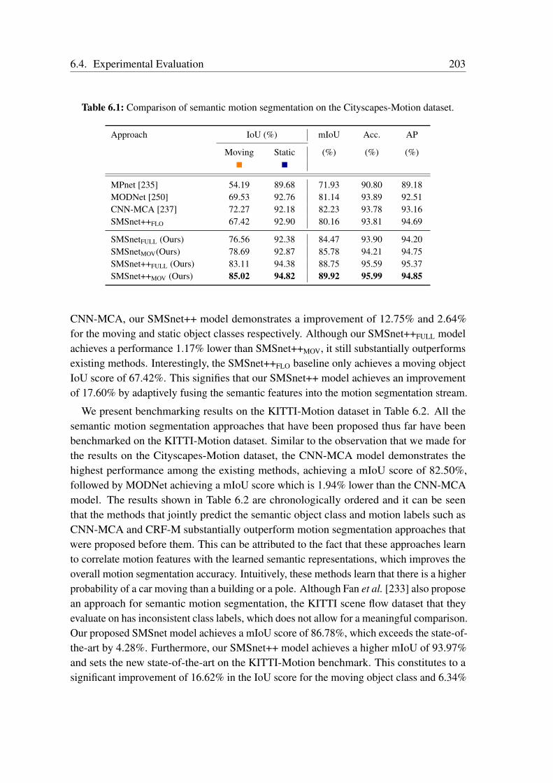
6.4. Experimental Evaluation 203
Table 6.1: Comparison of semantic motion segmentation on the Cityscapes-Motion dataset.
Approach IoU (%) mIoU Acc. AP
Moving Static (%) (%) (%)
MPnet [235] 54.19 89.68 71.93 90.80 89.18MODNet [250] 69.53 92.76 81.14 93.89 92.51CNN-MCA [237] 72.27 92.18 82.23 93.78 93.16SMSnet++FLO 67.42 92.90 80.16 93.81 94.69
SMSnetFULL (Ours) 76.56 92.38 84.47 93.90 94.20SMSnetMOV(Ours) 78.69 92.87 85.78 94.21 94.75SMSnet++FULL (Ours) 83.11 94.38 88.75 95.59 95.37SMSnet++MOV (Ours) 85.02 94.82 89.92 95.99 94.85
CNN-MCA, our SMSnet++ model demonstrates a improvement of 12.75% and 2.64%for the moving and static object classes respectively. Although our SMSnet++FULL modelachieves a performance 1.17% lower than SMSnet++MOV, it still substantially outperformsexisting methods. Interestingly, the SMSnet++FLO baseline only achieves a moving objectIoU score of 67.42%. This signifies that our SMSnet++ model achieves an improvementof 17.60% by adaptively fusing the semantic features into the motion segmentation stream.
We present benchmarking results on the KITTI-Motion dataset in Table 6.2. All thesemantic motion segmentation approaches that have been proposed thus far have beenbenchmarked on the KITTI-Motion dataset. Similar to the observation that we made forthe results on the Cityscapes-Motion dataset, the CNN-MCA model demonstrates thehighest performance among the existing methods, achieving a mIoU score of 82.50%,followed by MODNet achieving a mIoU score which is 1.94% lower than the CNN-MCAmodel. The results shown in Table 6.2 are chronologically ordered and it can be seenthat the methods that jointly predict the semantic object class and motion labels such asCNN-MCA and CRF-M substantially outperform motion segmentation approaches thatwere proposed before them. This can be attributed to the fact that these approaches learnto correlate motion features with the learned semantic representations, which improves theoverall motion segmentation accuracy. Intuitively, these methods learn that there is a higherprobability of a car moving than a building or a pole. Although Fan et al. [233] also proposean approach for semantic motion segmentation, the KITTI scene flow dataset that theyevaluate on has inconsistent class labels, which does not allow for a meaningful comparison.Our proposed SMSnet model achieves a mIoU score of 86.78%, which exceeds the state-of-the-art by 4.28%. Furthermore, our SMSnet++ model achieves a higher mIoU of 93.97%and sets the new state-of-the-art on the KITTI-Motion benchmark. This constitutes to asignificant improvement of 16.62% in the IoU score for the moving object class and 6.34%
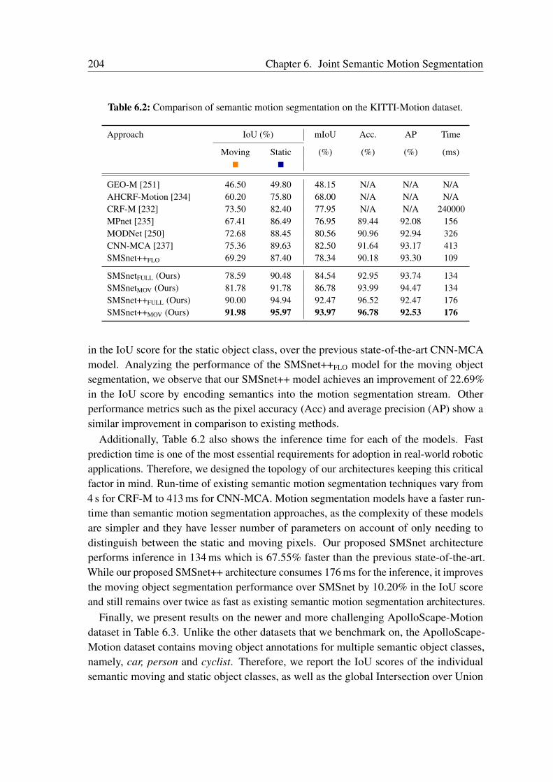
204 Chapter 6. Joint Semantic Motion Segmentation
Table 6.2: Comparison of semantic motion segmentation on the KITTI-Motion dataset.
Approach IoU (%) mIoU Acc. AP Time
Moving Static (%) (%) (%) (ms)
GEO-M [251] 46.50 49.80 48.15 N/A N/A N/AAHCRF-Motion [234] 60.20 75.80 68.00 N/A N/A N/ACRF-M [232] 73.50 82.40 77.95 N/A N/A 240000MPnet [235] 67.41 86.49 76.95 89.44 92.08 156MODNet [250] 72.68 88.45 80.56 90.96 92.94 326CNN-MCA [237] 75.36 89.63 82.50 91.64 93.17 413SMSnet++FLO 69.29 87.40 78.34 90.18 93.30 109
SMSnetFULL (Ours) 78.59 90.48 84.54 92.95 93.74 134SMSnetMOV (Ours) 81.78 91.78 86.78 93.99 94.47 134SMSnet++FULL (Ours) 90.00 94.94 92.47 96.52 92.47 176SMSnet++MOV (Ours) 91.98 95.97 93.97 96.78 92.53 176
in the IoU score for the static object class, over the previous state-of-the-art CNN-MCAmodel. Analyzing the performance of the SMSnet++FLO model for the moving objectsegmentation, we observe that our SMSnet++ model achieves an improvement of 22.69%in the IoU score by encoding semantics into the motion segmentation stream. Otherperformance metrics such as the pixel accuracy (Acc) and average precision (AP) show asimilar improvement in comparison to existing methods.
Additionally, Table 6.2 also shows the inference time for each of the models. Fastprediction time is one of the most essential requirements for adoption in real-world roboticapplications. Therefore, we designed the topology of our architectures keeping this criticalfactor in mind. Run-time of existing semantic motion segmentation techniques vary from4 s for CRF-M to 413 ms for CNN-MCA. Motion segmentation models have a faster run-time than semantic motion segmentation approaches, as the complexity of these modelsare simpler and they have lesser number of parameters on account of only needing todistinguish between the static and moving pixels. Our proposed SMSnet architectureperforms inference in 134 ms which is 67.55% faster than the previous state-of-the-art.While our proposed SMSnet++ architecture consumes 176 ms for the inference, it improvesthe moving object segmentation performance over SMSnet by 10.20% in the IoU scoreand still remains over twice as fast as existing semantic motion segmentation architectures.
Finally, we present results on the newer and more challenging ApolloScape-Motiondataset in Table 6.3. Unlike the other datasets that we benchmark on, the ApolloScape-Motion dataset contains moving object annotations for multiple semantic object classes,namely, car, person and cyclist. Therefore, we report the IoU scores of the individualsemantic moving and static object classes, as well as the global Intersection over Union
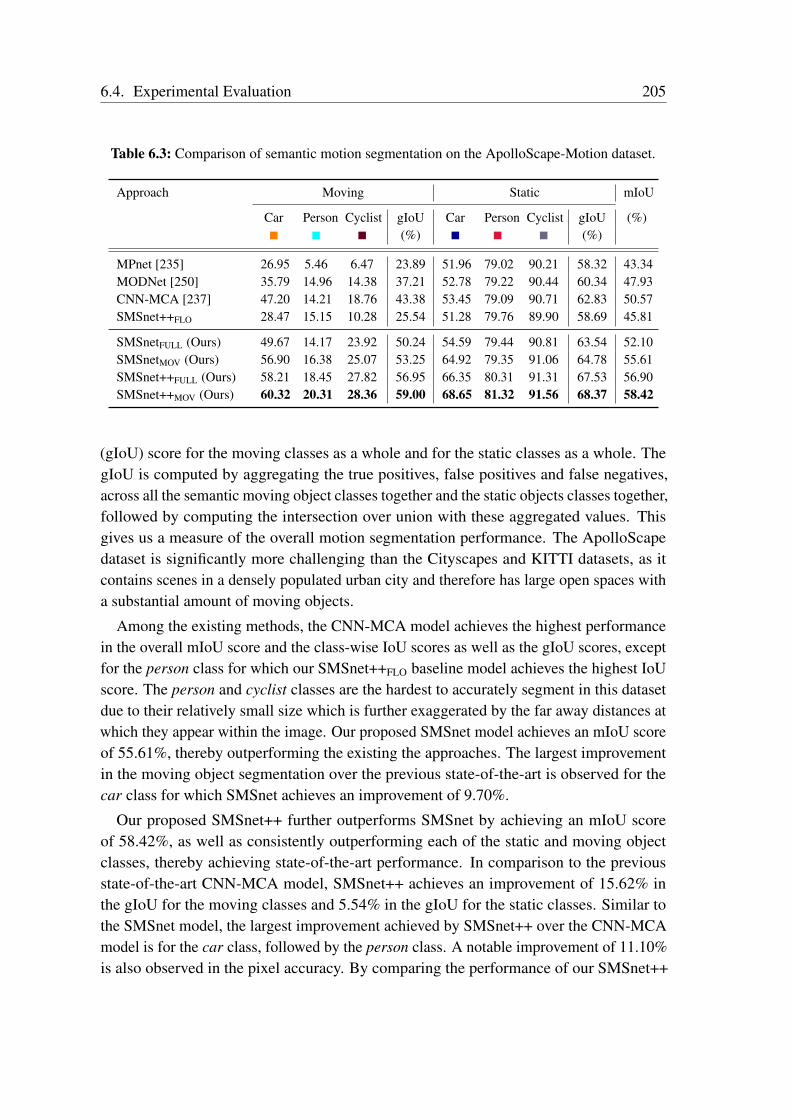
6.4. Experimental Evaluation 205
Table 6.3: Comparison of semantic motion segmentation on the ApolloScape-Motion dataset.
Approach Moving Static mIoU
Car Person Cyclist gIoU Car Person Cyclist gIoU (%)(%) (%)
MPnet [235] 26.95 5.46 6.47 23.89 51.96 79.02 90.21 58.32 43.34MODNet [250] 35.79 14.96 14.38 37.21 52.78 79.22 90.44 60.34 47.93CNN-MCA [237] 47.20 14.21 18.76 43.38 53.45 79.09 90.71 62.83 50.57SMSnet++FLO 28.47 15.15 10.28 25.54 51.28 79.76 89.90 58.69 45.81
SMSnetFULL (Ours) 49.67 14.17 23.92 50.24 54.59 79.44 90.81 63.54 52.10SMSnetMOV (Ours) 56.90 16.38 25.07 53.25 64.92 79.35 91.06 64.78 55.61SMSnet++FULL (Ours) 58.21 18.45 27.82 56.95 66.35 80.31 91.31 67.53 56.90SMSnet++MOV (Ours) 60.32 20.31 28.36 59.00 68.65 81.32 91.56 68.37 58.42
(gIoU) score for the moving classes as a whole and for the static classes as a whole. ThegIoU is computed by aggregating the true positives, false positives and false negatives,across all the semantic moving object classes together and the static objects classes together,followed by computing the intersection over union with these aggregated values. Thisgives us a measure of the overall motion segmentation performance. The ApolloScapedataset is significantly more challenging than the Cityscapes and KITTI datasets, as itcontains scenes in a densely populated urban city and therefore has large open spaces witha substantial amount of moving objects.
Among the existing methods, the CNN-MCA model achieves the highest performancein the overall mIoU score and the class-wise IoU scores as well as the gIoU scores, exceptfor the person class for which our SMSnet++FLO baseline model achieves the highest IoUscore. The person and cyclist classes are the hardest to accurately segment in this datasetdue to their relatively small size which is further exaggerated by the far away distances atwhich they appear within the image. Our proposed SMSnet model achieves an mIoU scoreof 55.61%, thereby outperforming the existing the approaches. The largest improvementin the moving object segmentation over the previous state-of-the-art is observed for thecar class for which SMSnet achieves an improvement of 9.70%.
Our proposed SMSnet++ further outperforms SMSnet by achieving an mIoU scoreof 58.42%, as well as consistently outperforming each of the static and moving objectclasses, thereby achieving state-of-the-art performance. In comparison to the previousstate-of-the-art CNN-MCA model, SMSnet++ achieves an improvement of 15.62% inthe gIoU for the moving classes and 5.54% in the gIoU for the static classes. Similar tothe SMSnet model, the largest improvement achieved by SMSnet++ over the CNN-MCAmodel is for the car class, followed by the person class. A notable improvement of 11.10%is also observed in the pixel accuracy. By comparing the performance of our SMSnet++
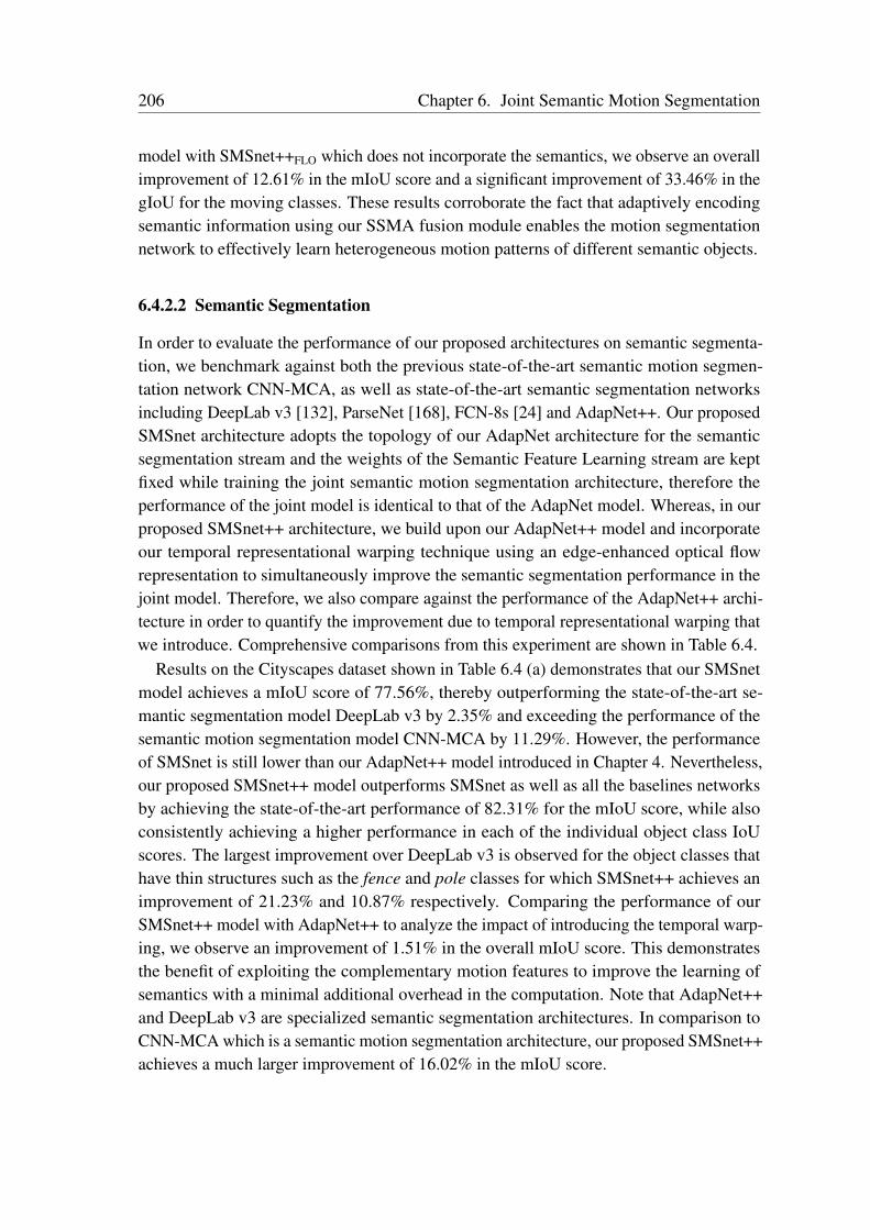
206 Chapter 6. Joint Semantic Motion Segmentation
model with SMSnet++FLO which does not incorporate the semantics, we observe an overallimprovement of 12.61% in the mIoU score and a significant improvement of 33.46% in thegIoU for the moving classes. These results corroborate the fact that adaptively encodingsemantic information using our SSMA fusion module enables the motion segmentationnetwork to effectively learn heterogeneous motion patterns of different semantic objects.
6.4.2.2 Semantic Segmentation
In order to evaluate the performance of our proposed architectures on semantic segmenta-tion, we benchmark against both the previous state-of-the-art semantic motion segmen-tation network CNN-MCA, as well as state-of-the-art semantic segmentation networksincluding DeepLab v3 [132], ParseNet [168], FCN-8s [24] and AdapNet++. Our proposedSMSnet architecture adopts the topology of our AdapNet architecture for the semanticsegmentation stream and the weights of the Semantic Feature Learning stream are keptfixed while training the joint semantic motion segmentation architecture, therefore theperformance of the joint model is identical to that of the AdapNet model. Whereas, in ourproposed SMSnet++ architecture, we build upon our AdapNet++ model and incorporateour temporal representational warping technique using an edge-enhanced optical flowrepresentation to simultaneously improve the semantic segmentation performance in thejoint model. Therefore, we also compare against the performance of the AdapNet++ archi-tecture in order to quantify the improvement due to temporal representational warping thatwe introduce. Comprehensive comparisons from this experiment are shown in Table 6.4.
Results on the Cityscapes dataset shown in Table 6.4 (a) demonstrates that our SMSnetmodel achieves a mIoU score of 77.56%, thereby outperforming the state-of-the-art se-mantic segmentation model DeepLab v3 by 2.35% and exceeding the performance of thesemantic motion segmentation model CNN-MCA by 11.29%. However, the performanceof SMSnet is still lower than our AdapNet++ model introduced in Chapter 4. Nevertheless,our proposed SMSnet++ model outperforms SMSnet as well as all the baselines networksby achieving the state-of-the-art performance of 82.31% for the mIoU score, while alsoconsistently achieving a higher performance in each of the individual object class IoUscores. The largest improvement over DeepLab v3 is observed for the object classes thathave thin structures such as the fence and pole classes for which SMSnet++ achieves animprovement of 21.23% and 10.87% respectively. Comparing the performance of ourSMSnet++ model with AdapNet++ to analyze the impact of introducing the temporal warp-ing, we observe an improvement of 1.51% in the overall mIoU score. This demonstratesthe benefit of exploiting the complementary motion features to improve the learning ofsemantics with a minimal additional overhead in the computation. Note that AdapNet++and DeepLab v3 are specialized semantic segmentation architectures. In comparison toCNN-MCA which is a semantic motion segmentation architecture, our proposed SMSnet++achieves a much larger improvement of 16.02% in the mIoU score.
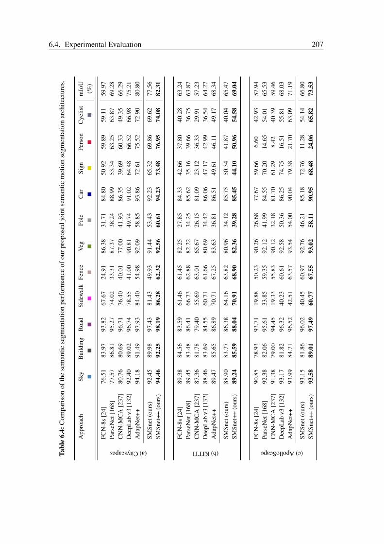
6.4. Experimental Evaluation 207
Tabl
e6.
4:C
ompa
riso
nof
the
sem
antic
segm
enta
tion
perf
orm
ance
ofou
rpro
pose
djo
ints
eman
ticm
otio
nse
gmen
tatio
nar
chite
ctur
es.
App
roac
hSk
yB
uild
ing
Roa
dSi
dew
alk
Fenc
eV
egPo
leC
arSi
gnPe
rson
Cyc
list
mIo
U(%
)(a)Cityscapes
FCN
-8s
[24]
76.5
183
.97
93.8
267
.67
24.9
186
.38
31.7
184
.80
50.9
259
.89
59.1
159
.97
Pars
eNet
[168
]77
.57
86.8
195
.27
74.0
233
.31
87.3
738
.24
88.9
953
.34
63.2
563
.87
69.2
8C
NN
-MC
A[2
37]
80.7
680
.69
96.7
176
.40
40.0
177
.00
41.9
386
.35
39.6
960
.33
49.3
566
.29
Dee
pLab
v3[1
32]
92.4
089
.02
96.7
478
.55
41.0
090
.81
49.7
491
.02
64.4
866
.52
66.9
875
.21
Ada
pNet
++94
.18
91.4
997
.93
84.4
054
.98
92.0
958
.85
93.8
672
.61
75.5
272
.90
80.8
0
SMSn
et(o
urs)
92.4
589
.98
97.4
381
.43
49.9
391
.44
53.4
392
.23
65.3
269
.86
69.6
277
.56
SMSn
et++
(our
s)94
.46
92.2
598
.19
86.2
862
.32
92.5
660
.61
94.2
373
.48
76.9
574
.08
82.3
1
(b)KITTI
FCN
-8s
[24]
89.3
884
.56
83.5
961
.46
61.4
582
.25
27.8
584
.33
42.6
637
.80
40.2
863
.24
Pars
eNet
[168
]89
.45
83.4
886
.41
66.7
362
.88
82.2
234
.25
85.6
235
.16
39.6
636
.75
63.8
7C
NN
-MC
A[2
37]
87.3
681
.78
79.4
055
.69
63.0
165
.67
26.1
581
.09
23.1
236
.33
29.9
157
.23
Dee
pLab
v3[1
32]
88.4
683
.69
84.5
560
.71
61.6
680
.69
34.4
286
.06
47.1
742
.99
36.5
464
.27
Ada
pNet
++89
.47
85.6
586
.89
70.7
167
.25
83.6
336
.81
86.5
149
.61
46.1
149
.17
68.3
4
SMSn
et(o
urs)
88.9
083
.77
86.3
864
.16
63.8
280
.96
34.1
285
.75
50.3
441
.87
40.0
465
.47
SMSn
et++
(our
s)89
.24
85.5
988
.04
70.9
168
.90
82.3
639
.28
85.4
544
.10
50.9
654
.58
69.0
4
(c)ApolloScape
FCN
-8s
[24]
90.8
578
.93
93.7
119
.88
50.2
390
.26
26.6
877
.67
59.6
66.
6042
.93
57.9
4Pa
rseN
et[1
68]
92.3
882
.06
95.6
133
.85
59.3
592
.12
41.9
984
.55
70.2
014
.65
54.0
165
.53
CN
N-M
CA
[237
]91
.38
79.0
094
.45
19.3
355
.83
90.1
232
.18
81.7
061
.29
8.42
40.3
959
.46
Dee
pLab
v3[1
32]
93.1
781
.82
96.3
240
.23
60.6
192
.58
50.3
686
.25
74.7
516
.51
55.8
168
.03
Ada
pNet
++93
.99
84.7
196
.52
42.5
163
.57
93.5
454
.00
90.0
479
.38
21.7
063
.09
71.1
9
SMSn
et(o
urs)
93.1
581
.86
96.0
240
.45
60.9
792
.76
46.2
185
.18
72.7
611
.28
54.1
466
.80
SMSn
et++
(our
s)93
.58
89.0
197
.49
60.7
767
.55
93.0
258
.11
90.9
568
.48
24.0
665
.82
73.5
3
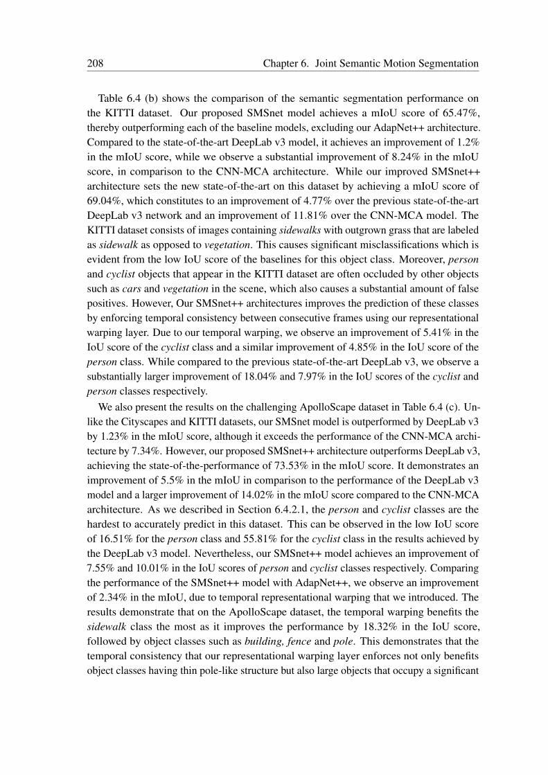
208 Chapter 6. Joint Semantic Motion Segmentation
Table 6.4 (b) shows the comparison of the semantic segmentation performance onthe KITTI dataset. Our proposed SMSnet model achieves a mIoU score of 65.47%,thereby outperforming each of the baseline models, excluding our AdapNet++ architecture.Compared to the state-of-the-art DeepLab v3 model, it achieves an improvement of 1.2%in the mIoU score, while we observe a substantial improvement of 8.24% in the mIoUscore, in comparison to the CNN-MCA architecture. While our improved SMSnet++architecture sets the new state-of-the-art on this dataset by achieving a mIoU score of69.04%, which constitutes to an improvement of 4.77% over the previous state-of-the-artDeepLab v3 network and an improvement of 11.81% over the CNN-MCA model. TheKITTI dataset consists of images containing sidewalks with outgrown grass that are labeledas sidewalk as opposed to vegetation. This causes significant misclassifications which isevident from the low IoU score of the baselines for this object class. Moreover, personand cyclist objects that appear in the KITTI dataset are often occluded by other objectssuch as cars and vegetation in the scene, which also causes a substantial amount of falsepositives. However, Our SMSnet++ architectures improves the prediction of these classesby enforcing temporal consistency between consecutive frames using our representationalwarping layer. Due to our temporal warping, we observe an improvement of 5.41% in theIoU score of the cyclist class and a similar improvement of 4.85% in the IoU score of theperson class. While compared to the previous state-of-the-art DeepLab v3, we observe asubstantially larger improvement of 18.04% and 7.97% in the IoU scores of the cyclist andperson classes respectively.
We also present the results on the challenging ApolloScape dataset in Table 6.4 (c). Un-like the Cityscapes and KITTI datasets, our SMSnet model is outperformed by DeepLab v3by 1.23% in the mIoU score, although it exceeds the performance of the CNN-MCA archi-tecture by 7.34%. However, our proposed SMSnet++ architecture outperforms DeepLab v3,achieving the state-of-the-performance of 73.53% in the mIoU score. It demonstrates animprovement of 5.5% in the mIoU in comparison to the performance of the DeepLab v3model and a larger improvement of 14.02% in the mIoU score compared to the CNN-MCAarchitecture. As we described in Section 6.4.2.1, the person and cyclist classes are thehardest to accurately predict in this dataset. This can be observed in the low IoU scoreof 16.51% for the person class and 55.81% for the cyclist class in the results achieved bythe DeepLab v3 model. Nevertheless, our SMSnet++ model achieves an improvement of7.55% and 10.01% in the IoU scores of person and cyclist classes respectively. Comparingthe performance of the SMSnet++ model with AdapNet++, we observe an improvementof 2.34% in the mIoU, due to temporal representational warping that we introduced. Theresults demonstrate that on the ApolloScape dataset, the temporal warping benefits thesidewalk class the most as it improves the performance by 18.32% in the IoU score,followed by object classes such as building, fence and pole. This demonstrates that thetemporal consistency that our representational warping layer enforces not only benefitsobject classes having thin pole-like structure but also large objects that occupy a significant

6.4. Experimental Evaluation 209
portion of the image.
6.4.3 Influence of the Motion Parallax Effect
In this section, we investigate the performance of motion segmentation using our proposedSMSnet++ architecture considering different maximum ranges within which the movingobjects might lie. One of the primary challenges of motion segmentation is to predict themotion of moving objects that are at far away distances from the camera. As the distanceof moving objects from the camera increases, the pixel displacements of those objects inconsecutive frames decreases due to the motion parallax effect. Therefore, segmentingdistant moving objects from camera images is extremely challenging. On the one hand,including training examples that contain distant moving objects might enable learning ofmore multiscale features that can cover a wide variety of motion appearances. While, onthe other hand, these highly difficult training examples can also restrict the network fromtraining effectively, if it is unable to learn features that can distinguish the state of distantmoving objects. In order to quantify this influence on the performance of our modelsfor motion segmentation, we trained individual models on the entire training data butonly considering moving objects within a certain maximum distance from the camera inthe label set and objects that lie beyond this distance are ignored for training. We thenevaluated these models on the different test sets, each containing moving objects withincertain maximum distances. For this experiment, we considered moving objects withinfour discrete set of maximum distances. Specifically, for 20 m, 40 m, 60 m and over 60 mthat denote as∞.
Figure 6.9 shows results from this experiment on the Cityscapes-Motion and KITTI-Motion datasets. As we hypothesized, our models achieve the best performance whiletraining on the label set containing moving objects within 20 m and testing with the cor-responding label set with same configuration. On the Cityscapes-Motion dataset, ourSMSnet++ model achieves a IoU of 85.02% for the moving object class, whereas onthe KITTI-Motion dataset, it achieves a mIoU of 91.98% for the moving object class.The models demonstrate the best trade-off considering moving objects within a maxi-mum distance of 40 m and subsequently for larger distances, the performance drops byapproximately 3% in the IoU score. However, this score is still over 12% higher than thebest performance achieved by the previous state-of-the-art networks that we presentedin Table 6.1. Furthermore, we observe that there is a larger performance drop when themodel is trained with labels consisting of moving objects within 20 m and tested on thelabel set with moving objects at increasingly larger distances. This is to be expected, as thenetwork has not learned features that represent distant moving objects. Nevertheless, weobserve that training the model on the label sets with moving objects at increasingly largerdistances makes the model perform well across each of the four discrete label sets withdifferent maximum distances. The model trained with the maximum distance at infinity
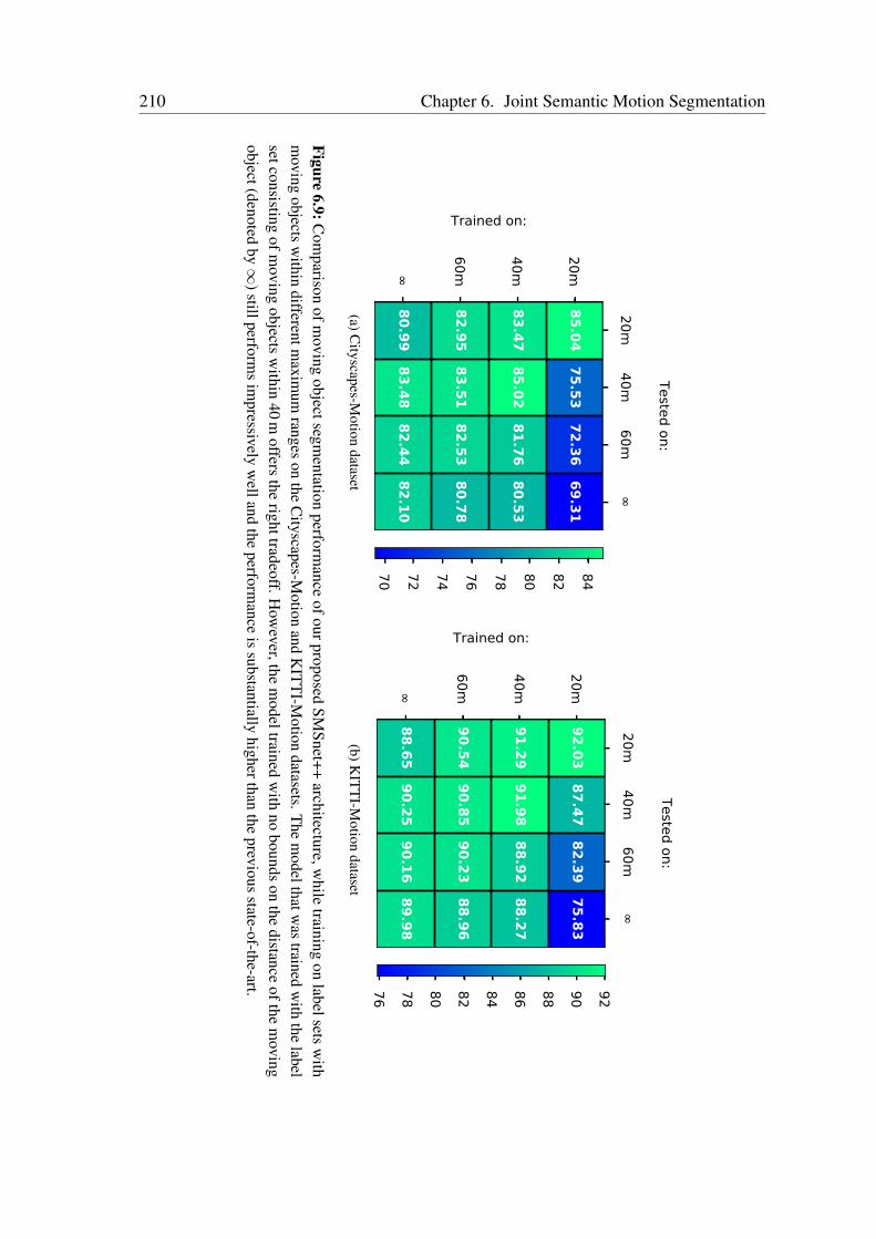
210 Chapter 6. Joint Semantic Motion Segmentation
20m40m
60m∞
Tested on:
20m
40m
60m∞
Trained on:
85.0475.53
72.3669.31
83.4785.02
81.7680.53
82.9583.51
82.5380.78
80.9983.48
82.4482.10
70 72 74 76 78 80 82 84
20m40m
60m∞
Tested on:
20m
40m
60m∞
Trained on:
92.0387.47
82.3975.83
91.2991.98
88.9288.27
90.5490.85
90.2388.96
88.6590.25
90.1689.98
76 78 80 82 84 86 88 90 92
(a)Cityscapes-M
otiondataset
(b)KIT
TI-M
otiondataset
Figure6.9:C
omparison
ofmoving
objectsegmentation
performance
ofourproposedSM
Snet++architecture,w
hiletraining
onlabelsets
with
moving
objectsw
ithindifferentm
aximum
rangeson
theC
ityscapes-Motion
andK
ITT
I-Motion
datasets.The
modelthatw
astrained
with
thelabel
setconsistingofm
ovingobjects
within
40m
offersthe
righttradeoff.How
ever,them
odeltrainedw
ithno
boundson
thedistance
ofthem
ovingobject(denoted
by∞
)stillperforms
impressively
welland
theperform
anceis
substantiallyhigherthan
theprevious
state-of-the-art.
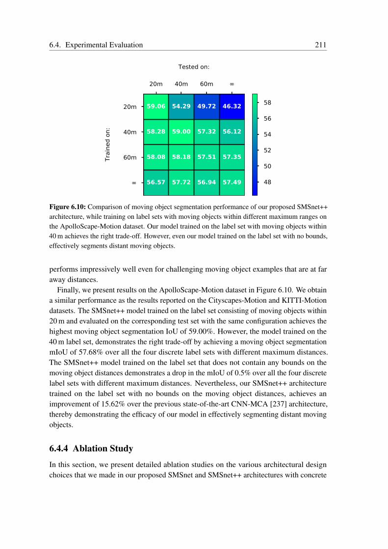
6.4. Experimental Evaluation 211
20m 40m 60m ∞
Tested on:
20m
40m
60m
∞
Trai
ned
on:
59.06 54.29 49.72 46.32
58.28 59.00 57.32 56.12
58.08 58.18 57.51 57.35
56.57 57.72 56.94 57.49 48
50
52
54
56
58
Figure 6.10: Comparison of moving object segmentation performance of our proposed SMSnet++architecture, while training on label sets with moving objects within different maximum ranges onthe ApolloScape-Motion dataset. Our model trained on the label set with moving objects within40 m achieves the right trade-off. However, even our model trained on the label set with no bounds,effectively segments distant moving objects.
performs impressively well even for challenging moving object examples that are at faraway distances.
Finally, we present results on the ApolloScape-Motion dataset in Figure 6.10. We obtaina similar performance as the results reported on the Cityscapes-Motion and KITTI-Motiondatasets. The SMSnet++ model trained on the label set consisting of moving objects within20 m and evaluated on the corresponding test set with the same configuration achieves thehighest moving object segmentation IoU of 59.00%. However, the model trained on the40 m label set, demonstrates the right trade-off by achieving a moving object segmentationmIoU of 57.68% over all the four discrete label sets with different maximum distances.The SMSnet++ model trained on the label set that does not contain any bounds on themoving object distances demonstrates a drop in the mIoU of 0.5% over all the four discretelabel sets with different maximum distances. Nevertheless, our SMSnet++ architecturetrained on the label set with no bounds on the moving object distances, achieves animprovement of 15.62% over the previous state-of-the-art CNN-MCA [237] architecture,thereby demonstrating the efficacy of our model in effectively segmenting distant movingobjects.
6.4.4 Ablation Study
In this section, we present detailed ablation studies on the various architectural designchoices that we made in our proposed SMSnet and SMSnet++ architectures with concrete
212 Chapter 6. Joint Semantic Motion Segmentation
empirical evaluations on each of the related model configurations. We first present resultson the major components of our SMSnet++ architecture in Section 6.4.4.1, followed byan analysis on the introduction of ego-flow suppression in Section 6.4.4.2 and the utilityof temporal representational warping in Section 6.4.4.3. We then present evaluations ofdifferent topologies of the Motion Feature Learning stream in Section 6.4.4.4 and finally,in Section 6.4.4.5, we present an analysis on the performance of motion segmentationwith the label set that contains all the semantic objects in the dataset and the label set thatcontains only the movable semantic object classes.
6.4.4.1 Detailed Study on the Architectural Components
Table 6.5 shows various configurations of the major components of our proposed archi-tectures using models trained on the Cityscapes-Motion dataset. For this experiment, weconsider all the labels in the Cityscapes-Motion dataset for learning the moving objectsegmentation, regardless of whether the object class is movable, therefore this correspondsto the models with the suffix FULL in the benchmarking results that we presented. Themodel M1 has a topology similar to our proposed SMSnet architecture, but we removethe Semantic Feature Learning stream, therefore the model only learns motion featuresfrom the learned optical flow maps. We employ the residual units from the ResNet-50architecture in the various network blocks and we embed the FlowNet2 architecture inthe Motion Feature Learning stream to generate the optical flow maps from which ournetwork learns the motion features. The resulting optical flow maps are scaled to the 0to 255 range and the flow vectors are represented as integers, which is indicated by (i)in the Flow Arch column of Table 6.5. This M1 model demonstrates an IoU of 67.42%and 92.90%, for the moving and static classes respectively. In the subsequent M2 model,we build upon the M1 model and add the Semantic Feature Learning stream, which hasthe topology of our AdapNet architecture that we introduced in Chapter 4. Feature mapsfrom the Semantic Feature Learning stream are then fused with the learned flow fieldfeatures in the Semantic-Motion Fusion stream using simple concatenation. This modelexactly resembles the topology of our proposed SMSnet architecture and hence, learnsjoint semantic motion segmentation. It achieves a semantic segmentation performance of77.58% in the mIoU score and demonstrates an improvement of 9.14% and 0.52%, for themoving and static classes respectively. This improvement can be attributed to the benefitof encoding semantic representations in the motion segmentation stream.
In the M3 model, we replace the standard residual units that are in the M2 model,with full pre-activation residual units and we also replace the AdapNet architecture inthe Semantic Feature Learning stream, with our improved AdapNet++ architecture. Thismodel achieves an improvement of 3.78% for the moving class and 1.01% for the staticclass, in addition to an improvement of 3.22% in the mIoU score for semantic segmentation.This increase in the scores is primarily due to the multiscale feature learning and long-range

6.4. Experimental Evaluation 213
Tabl
e6.
5:In
fluen
ceof
the
vari
ous
arch
itect
ural
cont
ribu
tions
prop
osed
inth
eSM
Snet
and
SMSn
et++
arch
itect
ures
.The
perf
orm
ance
issh
own
for
the
mod
els
trai
ned
onth
eC
itysc
apes
-Mot
ion
data
set.
Bas
eA
rch
deno
tes
that
the
vari
ous
resi
dual
units
follo
wei
ther
the
stan
dard
stan
dard
Res
Net
-50
orth
efu
llpr
e-ac
tivat
ion
Res
Net
-50
arch
itect
ure.
Flo
wA
rch
deno
tes
the
arch
itect
ure
embe
dded
forl
earn
ing
optic
alflo
wfie
ldfe
atur
esan
dth
esy
mbo
ls(i
)or(
f)de
note
ifth
eflo
wdi
spla
cem
ents
are
inte
gers
orflo
atin
gpo
intv
alue
s.T
hesy
mbo
ls⊕
Fw
deno
tew
arpi
ngof
inte
rmed
iate
enco
derr
epre
sent
atio
nsfr
omth
epr
evio
ustim
este
pth
atar
edy
nam
ical
lyfu
sed
usin
gou
rSSM
Am
odul
e,w
ithre
pres
enta
tions
ofth
ecu
rren
ttim
este
p.T
heF
usio
nco
lum
nde
note
sif
the
mot
ion
and
sem
antic
feat
ure
are
conc
aten
ated
(||)o
rada
ptiv
ely
fuse
dus
ing
ourS
SMA
mod
ule.
The
subs
eque
ntco
lum
nsde
note
ifcl
ass
bala
ncin
gis
appl
ied,
ifou
rpr
opos
edne
wde
code
ris
empl
oyed
and
ifth
esk
ipre
finem
enti
spr
efor
med
inth
em
otio
nse
gmen
tatio
nst
ream
.The
final
mod
elM
10is
ourp
ropo
sed
SMSn
et++
arch
itect
ure
trai
ned
onth
efu
llla
bels
et.
Mod
elB
ase
Arc
hFl
owA
rch
Sem
antic
Arc
hFu
sion
Cla
ssN
ewSk
ipM
ovin
gSt
atic
Sem
antic
Bal
Dec
IoU
(%)
IoU
(%)
mIo
U(%
)
M1
Res
Net
-50
Flow
Net
2(i
)-
--
--
67.4
292
.90
-
M2
Res
Net
-50
Flow
Net
2(i
)A
dapN
et||
--
-76
.56
92.3
877
.58
M3
PAR
esN
et-5
0Fl
owN
et2
(i)
Ada
pNet
++||
--
-80
.34
93.3
980
.80
M4
PAR
esN
et-5
0Fl
owN
et3
(i)
Ada
pNet
++||
--
-80
.87
93.4
280
.80
M5
PAR
esN
et-5
0Fl
owN
et3
(f)
Ada
pNet
++||
--
-81
.05
93.5
180
.80
M6
PAR
esN
et-5
0Fl
owN
et3
(f)
Ada
pnet
++⊕
Fw
||-
--
81.0
893
.49
82.3
1
M7
PAR
esN
et-5
0Fl
owN
et3
(f)
Ada
pNet
++⊕
Fw
SSM
A-
--
80.5
594
.78
82.3
1
M8
PAR
esN
et-5
0Fl
owN
et3
(f)
Ada
pNet
++⊕
Fw
SSM
AX
--
81.9
594
.08
82.3
1
M9
PAR
esN
et-5
0Fl
owN
et3
(f)
Ada
pNet
++⊕
Fw
SSM
AX
X-
82.4
994
.05
82.3
1
M10
PAR
esN
et-5
0Fl
owN
et3
(f)
Ada
pNet
++⊕
Fw
SSM
AX
XX
83.1
194
.38
82.3
1
214 Chapter 6. Joint Semantic Motion Segmentation
context aggregation in the semantic segmentation stream. In the subsequent M4 model,we replace the FlowNet2 architecture in the beginning of the Motion Feature Learningstream, with the FlowNet3 architecture with the aim of improving the learning of opticalflow field features. This model achieves a IoU of 80.87% for the moving class and 93.42%for the static class. However, as the improvement in performance is not significant, wefurther removed the rounding-off to the nearest decimal that was being applied on theoptical flow maps and maintained the optical flow vectors are floating point numbers inthe M5 architecture. We indicate the floating point flow maps with the suffix (f) in theFlow Arch column of Table 6.5. This model in comparison to the M3 model, achieves animprovement of 0.71% in the IoU for the moving class and 0.12% in the IoU of the staticclass.
In an effort to simultaneously improve the semantic segmentation performance, weemploy our temporal representational warping layer that also transforms the optical flow tothe edge enhanced flow for improving the warping in the Semantic Feature Learning streamof the M6 model. This improves the semantic segmentation performance by 1.51% in themIoU score. Furthermore, a comparison of warping directly using the optical flow maps,instead of using the edge-enhanced flow is presented in Section 6.4.4.3. In the modelsthat we presented thus far, we concatenate the learned semantic features with the motionfeatures in the Semantic-Motion Fusion stream. This direct concatenation may not be idealas the motion boundaries learned from the optical flow maps do not exactly correspondto the object boundaries in the semantic feature maps. Moreover, the motion features donot contain much information about distant moving objects. Therefore, in order to exploitcomplementary information from both semantic and motion features, we employ ourSSMA fusion module that we introduced in Chapter 5 to fuse the semantic representationswith the motion features in the M7 model. However, this model demonstrates a reductionin the IoU score of the moving object class with a concurrent increase in the IoU scoreof the static object class. Upon closer inspection of the performance of this model, weobserved that static and moving object classes are highly imbalanced. The images oftencontain a substantial amount of pixels that belong to static objects while only a few numberof pixels representing the moving objects. In order to account for this imbalance, in theM8 model, we employ the normalized inverse class frequency weighting to balance theloss. Most networks employ the inverse class frequency weighting, however, as the movingobject class is not present in each training example, it leads to large weight updates andcauses the gradients to explode. In order to alleviate this problem, we re-normalize thefrequency weightings by a factor to make the sum of the weights for each training exampleas one. This model achieves an improved performance of 81.95% and 94.05%, for IoU ofthe moving and static classes respectively.
Finally, in order to improve the granularity of the motion segmentation along objectboundaries, we employ our new multistage decoder that we introduced in Chapter 5 inthe Semantic-Motion Feature Fusion stream of the M9 model and we subsequently add

6.4. Experimental Evaluation 215
two skip refinement stages from the encoder of the Semantic Feature Learning stream tothe decoder of the Semantic-Motion Feature Fusion stream in the M10 model. This leadsto an IoU improvement of 0.54% in the M9 model and an additional 0.62% in the M10model for the moving object class. We denote this final model M10, which achieves a IoUof 83.11% for the moving class, 94.38% for the static class and a mIoU of 82.31% for thesemantic segmentation as our proposed SMSnet++ architecture.
6.4.4.2 Influence of Ego-Flow Suppression
As the main goal of this work is to enable a robot to detect moving objects in dynamicenvironments, the movement of the robot itself causes discontinuities in the optical flowmagnitude, where nearby static objects can appear to have a larger optical flow magnitudeseven though they are static in the environment. In order to alleviate this problem, wecompute the ego-motion of the robot and subtract the resulting ego-flow from the generatedoptical flow maps. In this section, we compare the performance of the SMSnet++ modelwith and without Ego-Flow Suppression (EFS) on the Cityscapes-Motion dataset withonly the movable object labels in the motion segmentation network. Results from thisexperiment shown in Table 6.6 demonstrate that the E1 model that directly uses the opticalflow maps in floating point precision from the embedded FlowNet3 network to learn motionfeatures, achieves a mIoU of 79.44% for the motion segmentation. In the subsequent E2model, we scale the optical flow maps to the 0-255 range and maintain the floating pointprecision. This model achieves an improvement of 3.68% and 2.24% in the IoU score ofthe moving and static classes. Although our Motion Feature Learning stream containsconvolution layers with batch normalization that normalizes the output of the previousactivation layer, we find that explicitly normalizing the optical flow maps to the 0-255range yields a notable performance improvement. In our final E3 model, we employ ourEFS technique to compensate for the flow induced due to the ego-motion of the robot. TheE3 model achieves a mIoU score of 89.92%, which accounts for a large improvement inthe IoU score of 11.53% for the moving class and 3.5% for the static class, in comparisonto the E2 model. The improvement is more apparent when compared with the E1 modelwhich directly uses the optical flow maps from the embedded flow generation network.More specifically, this amounts to an improvement of 15.23% in the moving object classand 5.74% for the static object class.
Furthermore, we show a comparison of the motion segmentation performance usingour SMSnet++ model trained on each of the aforementioned optical flow transformationson all the datasets that we benchmark on in Figure 6.11. The results demonstrate thatour E3 model, which scales the optical flow maps to the 0-255 range in floating pointprecision and employs our EFS technique, consistently achieves the highest performanceon the Cityscapes-Motion, KITTI-Motion and ApolloScape-Motion datasets. The largestimprovement of 15.23% in the IoU score for the moving object class is observed on the
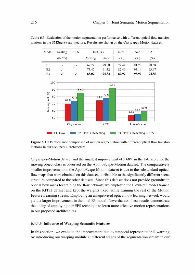
216 Chapter 6. Joint Semantic Motion Segmentation
Table 6.6: Evaluation of the motion segmentation performance with different optical flow transfor-mations in the SMSnet++ architecture. Results are shown on the Cityscapes-Motion dataset.
Model Scaling EFS IoU (%) mIoU Acc. AP
(0-255) Moving Static (%) (%) (%)
E1 - - 69.79 89.08 79.44 91.28 88.68E2 X - 73.47 91.32 82.40 93.14 93.47E3 X X 85.02 94.82 89.92 95.99 94.85
Cityscapes KITTI ApolloScape
50
60
70
80
90
100
Mov
ing
IoU
(%)
69.874.4
53.3
73.577.6
55.2
85.092.0
59.0
E1. Flow E2. Flow + Rescaling E3. Flow + Rescaling + EFS
Figure 6.11: Performance comparison of motion segmentation with different optical flow transfor-mations in our SMSnet++ architecture.
Cityscapes-Motion dataset and the smallest improvement of 5.68% in the IoU score for themoving object class is observed on the ApolloScape-Motion dataset. The comparativelysmaller improvement on the ApolloScape-Motion dataset is due to the substandard opticalflow maps that were obtained on this dataset, attributable to the significantly different scenestructure compared to the other datasets. Since this dataset does not provide groundtruthoptical flow maps for training the flow network, we employed the FlowNet3 model trainedon the KITTI dataset and kept the weights fixed, while training the rest of the MotionFeature Learning stream. Employing an unsupervised optical flow learning network wouldyield a larger improvement in the final E3 model. Nevertheless, these results demonstratethe utility of employing our EFS technique to learn more effective motion representationsin our proposed architectures.
6.4.4.3 Influence of Warping Semantic Features
In this section, we evaluate the improvement due to temporal representational warpingby introducing our warping module at different stages of the segmentation stream in our
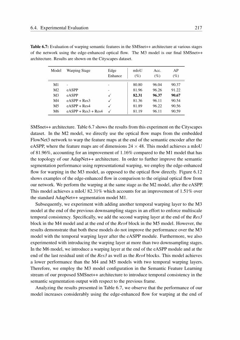
6.4. Experimental Evaluation 217
Table 6.7: Evaluation of warping semantic features in the SMSnet++ architecture at various stagesof the network using the edge-enhanced optical flow. The M3 model is our final SMSnet++architecture. Results are shown on the Cityscapes dataset.
Model Warping Stage Edge mIoU Acc. APEnhance (%) (%) (%)
M1 - - 80.80 96.04 90.37M2 eASPP - 81.96 96.26 91.22M3 eASPP X 82.31 96.37 90.67M4 eASPP + Res3 X 81.36 96.11 90.54M5 eASPP + Res4 X 81.89 96.22 90.56M6 eASPP + Res3 + Res4 X 81.19 96.11 90.59
SMSnet++ architecture. Table 6.7 shows the results from this experiment on the Cityscapesdataset. In the M2 model, we directly use the optical flow maps from the embeddedFlowNet3 network to warp the feature maps at the end of the semantic encoder after theeASPP, where the feature maps are of dimensions 24× 48. This model achieves a mIoUof 81.96%, accounting for an improvement of 1.16% compared to the M1 model that hasthe topology of our AdapNet++ architecture. In order to further improve the semanticsegmentation performance using representational warping, we employ the edge-enhancedflow for warping in the M3 model, as opposed to the optical flow directly. Figure 6.12shows examples of the edge-enhanced flow in comparison to the original optical flow fromour network. We perform the warping at the same stage as the M2 model, after the eASPP.This model achieves a mIoU 82.31% which accounts for an improvement of 1.51% overthe standard AdapNet++ segmentation model M1.
Subsequently, we experiment with adding another temporal warping layer to the M3model at the end of the previous downsampling stages in an effort to enforce multiscaletemporal consistency. Specifically, we add the second warping layer at the end of the Res3block in the M4 model and at the end of the Res4 block in the M5 model. However, theresults demonstrate that both these models do not improve the performance over the M3model with the temporal warping layer after the eASPP module. Furthermore, we alsoexperimented with introducing the warping layer at more than two downsampling stages.In the M6 model, we introduce a warping layer at the end of the eASPP module and at theend of the last residual unit of the Res3 as well as the Res4 blocks. This model achievesa lower performance than the M4 and M5 models with two temporal warping layers.Therefore, we employ the M3 model configuration in the Semantic Feature Learningstream of our proposed SMSnet++ architecture to introduce temporal consistency in thesemantic segmentation output with respect to the previous frame.
Analyzing the results presented in Table 6.7, we observe that the performance of ourmodel increases considerably using the edge-enhanced flow for warping at the end of

218 Chapter 6. Joint Semantic Motion Segmentation
Input frame It Optical Flow Edge-Enhanced Flow
Figure 6.12: Examples from the Cityscapes dataset showing the input image It, the originaloptical flow and the corresponding edge-enhanced flow from our SMSnet++ architecture. Theedge-enhanced flow clearly shows more emphasis on the structure of objects in the scene.
the eASPP but thereafter, the increase in performance is lower than that obtained fromintroducing only one temporal warping layer. This can be attributed to the max poolinglayer that we employ to downsample the optical flow map to the desired warping resolution.Pooling the optical flow maps at multiple scales causes the downsampled flow maps tonot align with the corresponding semantic feature maps and therefore, when the semanticfeature maps from the previous timestep are warped with the unaligned optical flow maps, itnegatively affects the performance of the model. Hence, computing the optical flow maps atmultiple scales or employing a scaling technique that maintains the point correspondencescould potentially alleviate this problem.
6.4.4.4 Evaluation of Motion Feature Learning Configuration
In order to learn optical flow field features in the Motion Feature Learning stream ofour proposed architectures, we experiment with adding different number of residualblocks after the embedded optical flow network. Table 6.8 presents the results from thisexperiment on the Cityscapes-Motion dataset with the full label set. The optical flow
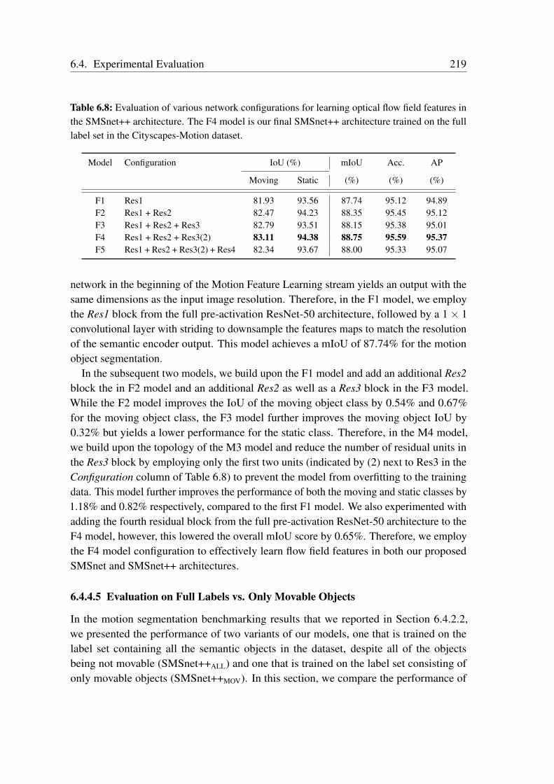
6.4. Experimental Evaluation 219
Table 6.8: Evaluation of various network configurations for learning optical flow field features inthe SMSnet++ architecture. The F4 model is our final SMSnet++ architecture trained on the fulllabel set in the Cityscapes-Motion dataset.
Model Configuration IoU (%) mIoU Acc. AP
Moving Static (%) (%) (%)
F1 Res1 81.93 93.56 87.74 95.12 94.89F2 Res1 + Res2 82.47 94.23 88.35 95.45 95.12F3 Res1 + Res2 + Res3 82.79 93.51 88.15 95.38 95.01F4 Res1 + Res2 + Res3(2) 83.11 94.38 88.75 95.59 95.37F5 Res1 + Res2 + Res3(2) + Res4 82.34 93.67 88.00 95.33 95.07
network in the beginning of the Motion Feature Learning stream yields an output with thesame dimensions as the input image resolution. Therefore, in the F1 model, we employthe Res1 block from the full pre-activation ResNet-50 architecture, followed by a 1× 1convolutional layer with striding to downsample the features maps to match the resolutionof the semantic encoder output. This model achieves a mIoU of 87.74% for the motionobject segmentation.
In the subsequent two models, we build upon the F1 model and add an additional Res2block the in F2 model and an additional Res2 as well as a Res3 block in the F3 model.While the F2 model improves the IoU of the moving object class by 0.54% and 0.67%for the moving object class, the F3 model further improves the moving object IoU by0.32% but yields a lower performance for the static class. Therefore, in the M4 model,we build upon the topology of the M3 model and reduce the number of residual units inthe Res3 block by employing only the first two units (indicated by (2) next to Res3 in theConfiguration column of Table 6.8) to prevent the model from overfitting to the trainingdata. This model further improves the performance of both the moving and static classes by1.18% and 0.82% respectively, compared to the first F1 model. We also experimented withadding the fourth residual block from the full pre-activation ResNet-50 architecture to theF4 model, however, this lowered the overall mIoU score by 0.65%. Therefore, we employthe F4 model configuration to effectively learn flow field features in both our proposedSMSnet and SMSnet++ architectures.
6.4.4.5 Evaluation on Full Labels vs. Only Movable Objects
In the motion segmentation benchmarking results that we reported in Section 6.4.2.2,we presented the performance of two variants of our models, one that is trained on thelabel set containing all the semantic objects in the dataset, despite all of the objectsbeing not movable (SMSnet++ALL) and one that is trained on the label set consisting ofonly movable objects (SMSnet++MOV). In this section, we compare the performance of
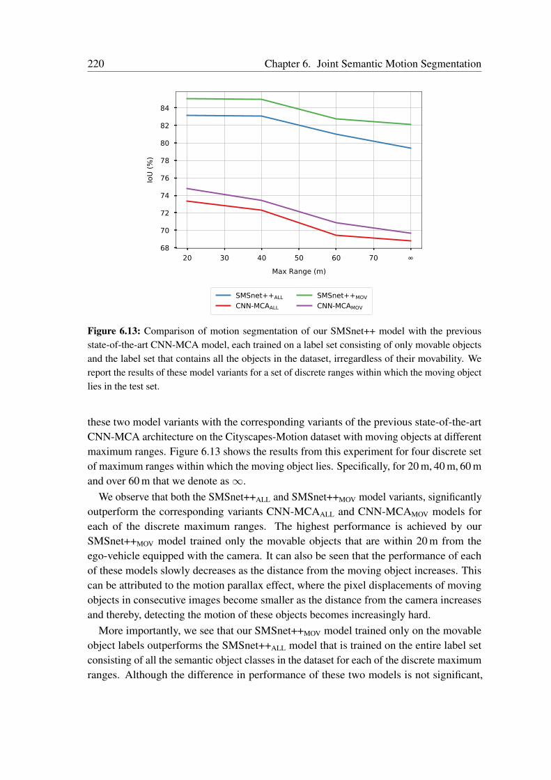
220 Chapter 6. Joint Semantic Motion Segmentation
20 30 40 50 60 70 ∞Max Range (m)
68
70
72
74
76
78
80
82
84
IoU
(%)
SMSnet++ALLCNN-MCAALL
SMSnet++MOVCNN-MCAMOV
Figure 6.13: Comparison of motion segmentation of our SMSnet++ model with the previousstate-of-the-art CNN-MCA model, each trained on a label set consisting of only movable objectsand the label set that contains all the objects in the dataset, irregardless of their movability. Wereport the results of these model variants for a set of discrete ranges within which the moving objectlies in the test set.
these two model variants with the corresponding variants of the previous state-of-the-artCNN-MCA architecture on the Cityscapes-Motion dataset with moving objects at differentmaximum ranges. Figure 6.13 shows the results from this experiment for four discrete setof maximum ranges within which the moving object lies. Specifically, for 20 m, 40 m, 60 mand over 60 m that we denote as∞.
We observe that both the SMSnet++ALL and SMSnet++MOV model variants, significantlyoutperform the corresponding variants CNN-MCAALL and CNN-MCAMOV models foreach of the discrete maximum ranges. The highest performance is achieved by ourSMSnet++MOV model trained only the movable objects that are within 20 m from theego-vehicle equipped with the camera. It can also be seen that the performance of eachof these models slowly decreases as the distance from the moving object increases. Thiscan be attributed to the motion parallax effect, where the pixel displacements of movingobjects in consecutive images become smaller as the distance from the camera increasesand thereby, detecting the motion of these objects becomes increasingly hard.
More importantly, we see that our SMSnet++MOV model trained only on the movableobject labels outperforms the SMSnet++ALL model that is trained on the entire label setconsisting of all the semantic object classes in the dataset for each of the discrete maximumranges. Although the difference in performance of these two models is not significant,
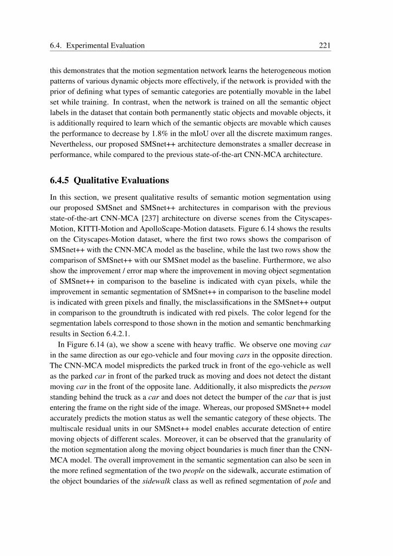
6.4. Experimental Evaluation 221
this demonstrates that the motion segmentation network learns the heterogeneous motionpatterns of various dynamic objects more effectively, if the network is provided with theprior of defining what types of semantic categories are potentially movable in the labelset while training. In contrast, when the network is trained on all the semantic objectlabels in the dataset that contain both permanently static objects and movable objects, itis additionally required to learn which of the semantic objects are movable which causesthe performance to decrease by 1.8% in the mIoU over all the discrete maximum ranges.Nevertheless, our proposed SMSnet++ architecture demonstrates a smaller decrease inperformance, while compared to the previous state-of-the-art CNN-MCA architecture.
6.4.5 Qualitative Evaluations
In this section, we present qualitative results of semantic motion segmentation usingour proposed SMSnet and SMSnet++ architectures in comparison with the previousstate-of-the-art CNN-MCA [237] architecture on diverse scenes from the Cityscapes-Motion, KITTI-Motion and ApolloScape-Motion datasets. Figure 6.14 shows the resultson the Cityscapes-Motion dataset, where the first two rows shows the comparison ofSMSnet++ with the CNN-MCA model as the baseline, while the last two rows show thecomparison of SMSnet++ with our SMSnet model as the baseline. Furthermore, we alsoshow the improvement / error map where the improvement in moving object segmentationof SMSnet++ in comparison to the baseline is indicated with cyan pixels, while theimprovement in semantic segmentation of SMSnet++ in comparison to the baseline modelis indicated with green pixels and finally, the misclassifications in the SMSnet++ outputin comparison to the groundtruth is indicated with red pixels. The color legend for thesegmentation labels correspond to those shown in the motion and semantic benchmarkingresults in Section 6.4.2.1.
In Figure 6.14 (a), we show a scene with heavy traffic. We observe one moving carin the same direction as our ego-vehicle and four moving cars in the opposite direction.The CNN-MCA model mispredicts the parked truck in front of the ego-vehicle as wellas the parked car in front of the parked truck as moving and does not detect the distantmoving car in the front of the opposite lane. Additionally, it also mispredicts the personstanding behind the truck as a car and does not detect the bumper of the car that is justentering the frame on the right side of the image. Whereas, our proposed SMSnet++ modelaccurately predicts the motion status as well the semantic category of these objects. Themultiscale residual units in our SMSnet++ model enables accurate detection of entiremoving objects of different scales. Moreover, it can be observed that the granularity ofthe motion segmentation along the moving object boundaries is much finer than the CNN-MCA model. The overall improvement in the semantic segmentation can also be seen inthe more refined segmentation of the two people on the sidewalk, accurate estimation ofthe object boundaries of the sidewalk class as well as refined segmentation of pole and
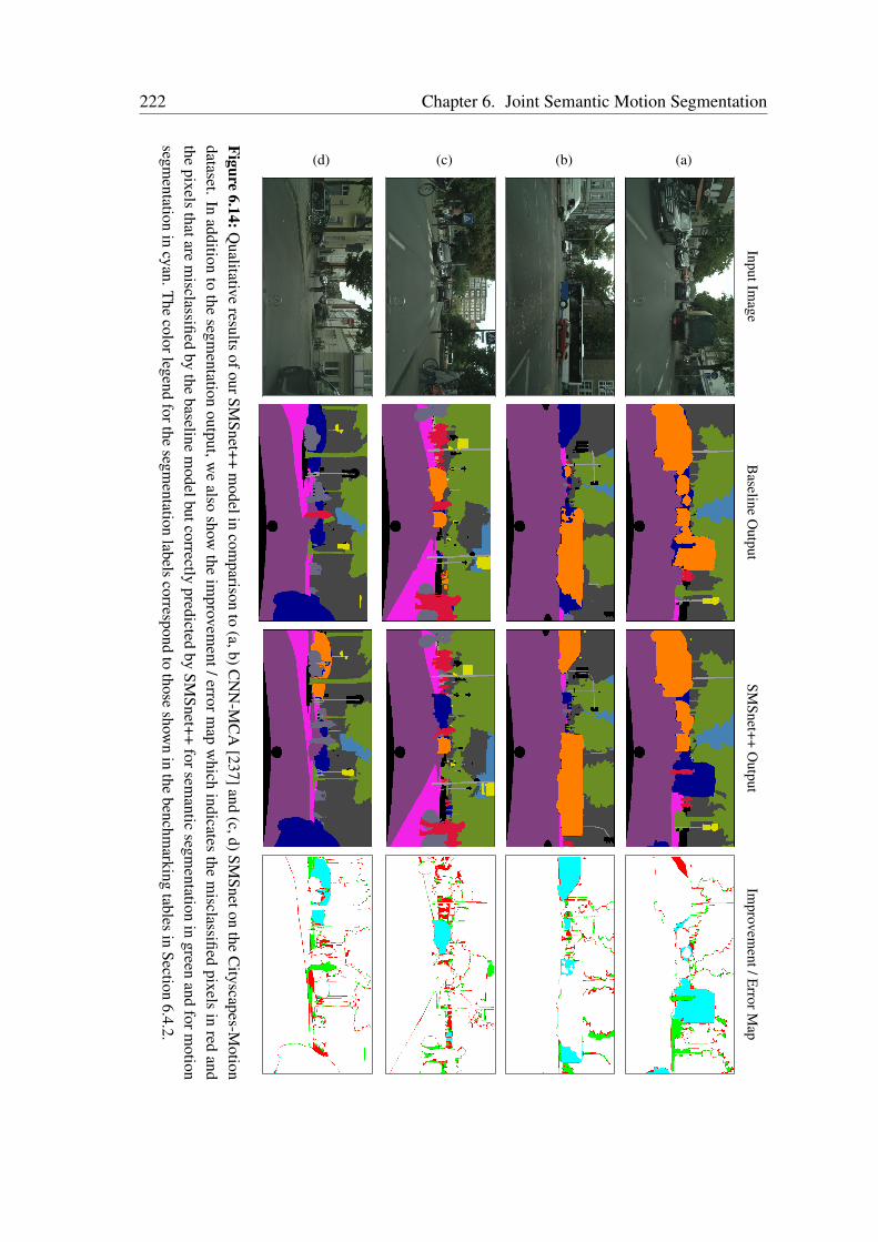
222 Chapter 6. Joint Semantic Motion SegmentationInputIm
ageB
aselineO
utputSM
Snet++O
utputIm
provement/E
rrorMap
(a)(b)(c)(d)
Figure6.14:Q
ualitativeresults
ofourSMSnet++
modelin
comparison
to(a,b)C
NN
-MC
A[237]and
(c,d)SMSneton
theC
ityscapes-Motion
dataset.In
additionto
thesegm
entationoutput,w
ealso
showthe
improvem
ent/errorm
apw
hichindicates
them
isclassifiedpixels
inred
andthe
pixelsthatare
misclassified
bythe
baselinem
odelbutcorrectlypredicted
bySM
Snet++forsem
anticsegm
entationin
greenand
formotion
segmentation
incyan.T
hecolorlegend
forthesegm
entationlabels
correspondto
thoseshow
nin
thebenchm
arkingtables
inSection
6.4.2.
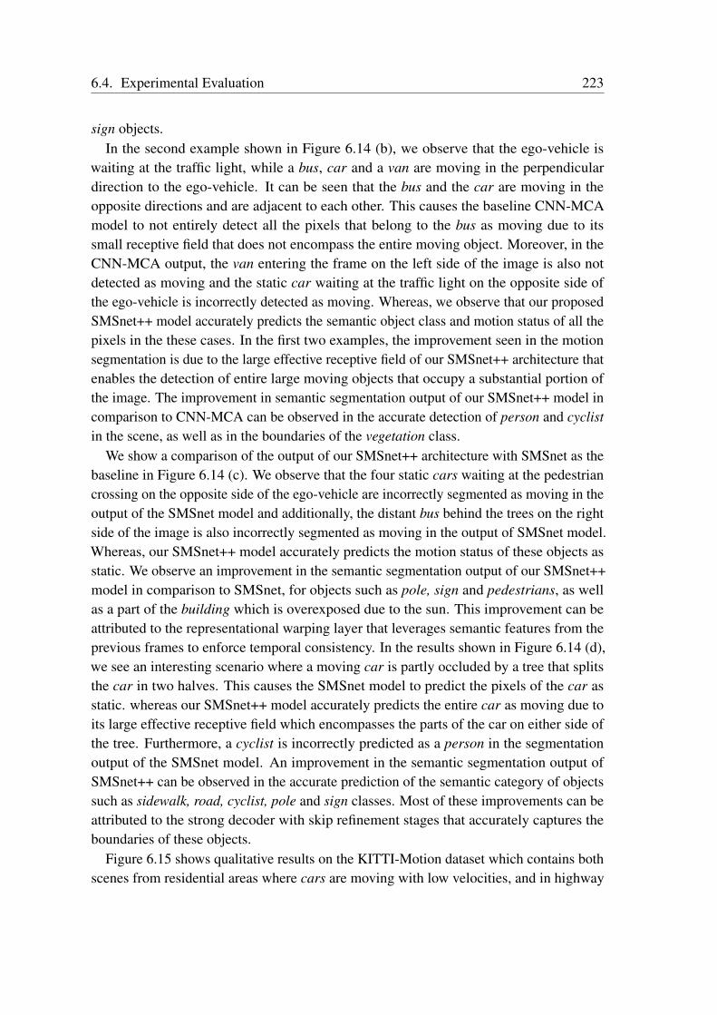
6.4. Experimental Evaluation 223
sign objects.In the second example shown in Figure 6.14 (b), we observe that the ego-vehicle is
waiting at the traffic light, while a bus, car and a van are moving in the perpendiculardirection to the ego-vehicle. It can be seen that the bus and the car are moving in theopposite directions and are adjacent to each other. This causes the baseline CNN-MCAmodel to not entirely detect all the pixels that belong to the bus as moving due to itssmall receptive field that does not encompass the entire moving object. Moreover, in theCNN-MCA output, the van entering the frame on the left side of the image is also notdetected as moving and the static car waiting at the traffic light on the opposite side ofthe ego-vehicle is incorrectly detected as moving. Whereas, we observe that our proposedSMSnet++ model accurately predicts the semantic object class and motion status of all thepixels in the these cases. In the first two examples, the improvement seen in the motionsegmentation is due to the large effective receptive field of our SMSnet++ architecture thatenables the detection of entire large moving objects that occupy a substantial portion ofthe image. The improvement in semantic segmentation output of our SMSnet++ model incomparison to CNN-MCA can be observed in the accurate detection of person and cyclistin the scene, as well as in the boundaries of the vegetation class.
We show a comparison of the output of our SMSnet++ architecture with SMSnet as thebaseline in Figure 6.14 (c). We observe that the four static cars waiting at the pedestriancrossing on the opposite side of the ego-vehicle are incorrectly segmented as moving in theoutput of the SMSnet model and additionally, the distant bus behind the trees on the rightside of the image is also incorrectly segmented as moving in the output of SMSnet model.Whereas, our SMSnet++ model accurately predicts the motion status of these objects asstatic. We observe an improvement in the semantic segmentation output of our SMSnet++model in comparison to SMSnet, for objects such as pole, sign and pedestrians, as wellas a part of the building which is overexposed due to the sun. This improvement can beattributed to the representational warping layer that leverages semantic features from theprevious frames to enforce temporal consistency. In the results shown in Figure 6.14 (d),we see an interesting scenario where a moving car is partly occluded by a tree that splitsthe car in two halves. This causes the SMSnet model to predict the pixels of the car asstatic. whereas our SMSnet++ model accurately predicts the entire car as moving due toits large effective receptive field which encompasses the parts of the car on either side ofthe tree. Furthermore, a cyclist is incorrectly predicted as a person in the segmentationoutput of the SMSnet model. An improvement in the semantic segmentation output ofSMSnet++ can be observed in the accurate prediction of the semantic category of objectssuch as sidewalk, road, cyclist, pole and sign classes. Most of these improvements can beattributed to the strong decoder with skip refinement stages that accurately captures theboundaries of these objects.
Figure 6.15 shows qualitative results on the KITTI-Motion dataset which contains bothscenes from residential areas where cars are moving with low velocities, and in highway
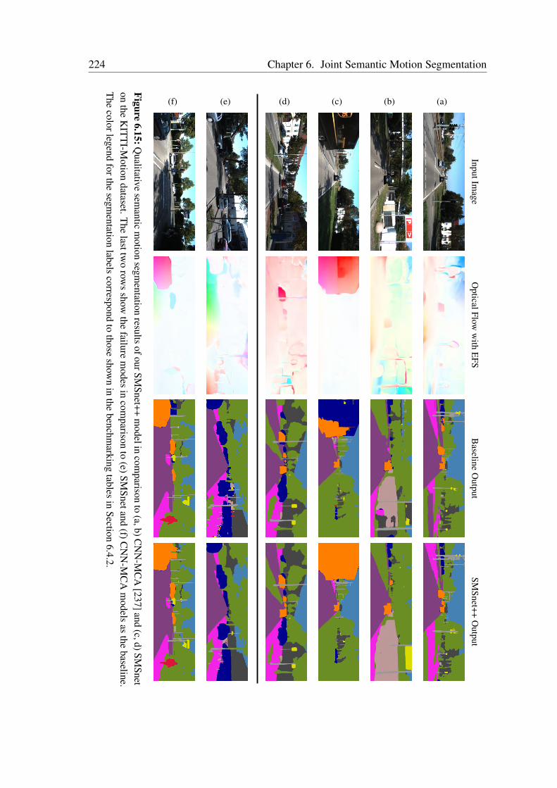
224 Chapter 6. Joint Semantic Motion SegmentationInputIm
ageO
pticalFloww
ithE
FSB
aselineO
utputSM
Snet++O
utput
(a)(b)(c)(d)(e)(f)
Figure6.15:Q
ualitativesem
anticm
otionsegm
entationresults
ofourSMSnet++
modelin
comparison
to(a,b)C
NN
-MC
A[237]and
(c,d)SMSnet
onthe
KIT
TI-M
otiondataset.T
helasttw
orow
sshow
thefailure
modes
incom
parisonto
(e)SMSnetand
(f)CN
N-M
CA
models
asthe
baseline.T
hecolorlegend
forthesegm
entationlabels
correspondto
thoseshow
nin
thebenchm
arkingtables
inSection
6.4.2.
6.4. Experimental Evaluation 225
driving scenarios where cars are moving at high velocities, therefore causing a substantialamount of motion blur in the captured images. These scenes also have moving objectsof different scales and lighting conditions that cause significant shadows on the ground.The first two rows show the comparison of SMSnet++ with the previous state-of-the-artCNN-MCA model as the baseline, while the next two rows show the comparison ofSMSnet++ with the SMSnet model as the baseline model. In addition to the semanticmotion segmentation outputs, we also show the optical flow maps with EFS for each of theexamples. In Figure 6.15 (a), we observe that the CNN-MCA model incorrectly segmentsthe static cars on the opposite lane from the ego-vehicle as moving and also segments theshadow of the first moving car in the opposite direction as belonging to the moving car.Whereas, our SMSnet++ architecture accurately predicts the semantic category and motionstatus of each of these objects. Moreover, the improvement in the semantic segmentationoutput of SMSnet++ can be observed in the accurate segmentation of sidewalk, pole andsign classes. In the second example shown in Figure 6.15 (b), we see that the CNN-MCAmodel incorrectly predicts the moving car on the opposite side of the lane as static anda distant moving car turning on the same side of the lane as the ego-vehicle as static,while our SMSnet++ model accurately predicts these cars as moving. It can also be seenthat the CNN-MCA model misclassifies a large portion of objects such as sign, fence andvegetation. The accurate prediction of object classes such as the sidewalk and the fence inthe above examples can be attributed to the representational warping and the improvementin segmenting thin pole-like structures is enabled by our new decoder that fuses mid-levelencoder features to yield a high-resolution segmentation output.
In the example shown in Figure 6.15 (c), we observe that the SMSnet output shown asthe baseline does not segment the entire van as moving and it also incorrectly segments aparked car on the opposite side of the road adjacent to the van as moving. This primarilyoccurs in the segmentation output of SMSnet, when there is a moving vehicle that is partlyvisible due to it entering or leaving the frame. Note that both our SMSnet and SMSnet++models employ the same optical flow map with EFS to learn the motion features and itcan be observed that even though there are high flow gradients in the optical flow maps,SMSnet does not entirely segment the moving van. In the subsequent example shown inFigure 6.15 (d), we observe a residential scene, in which a moving car on the oppositeside of the lane is only partly segmented as moving in the output of the SMSnet modeldue to an occluding light pole dividing the moving car into two parts. Moreover, it canbe seen that as the distance to the moving objects increases, the region of segmentationon the moving cars decreases. In the output of the SMSnet model, we observe that mostpart of the second moving car is accurately segmented as moving, but only a small partof the third moving car is segmented as moving and the fourth moving car is entirelysegmented incorrectly as static. However, we observe that the multiscale receptive fields ofthe SMSnet++ architecture enable it to efficiently distinguish between static backgroundand moving objects of different scales, thus achieving accurate motion segmentation.
226 Chapter 6. Joint Semantic Motion Segmentation
The last two rows of Figure 6.15 shows failure cases in comparison to SMSnet in (e)and in comparison to the CNN-MCA model in (f). In Figure 6.15 (e), we observe a distantmoving car on the road among static cars being parked on both sides of the street. Boththe SMSnet output shown as the baseline and the SMSnet++ output incorrectly segmentthe moving car as static. As the scene is not well lit near the distant moving car, thenetwork is unable to detect the change in the pixel displacements. While in the secondfailure case shown in Figure 6.15 (f), we observe a scene in which a moving car is merelyvisible due to the occlusion caused by another moving car, in addition to a traffic lightpole and a sign covering most of the vehicle. This causes both the networks to detect thepixels of the moving car as static. However, it can be seen that a moving van on the leftside of the image is accurately segmented as moving in the output of the SMSnet++ model,even though a large portion of the object is occluded by a tree trunk, while the CNN-MCAmodel incorrectly predicts the van as being static. Nevertheless, we remark that thesecorner cases can be overcome by aggregating temporal features of moving objects from asequence of frames, while our network currently only learns the motion patterns from apair of subsequent images.
Finally, Figure 6.16 shows the qualitative semantic motion segmentation results onthe recently introduced ApolloScape-Motion dataset. As this dataset consists of imagesin high resolution, they contain objects such as cars and pedestrians that are capturedat extremely far away distances, which makes motion segmentation highly challenging.Moreover, it contains multiple types of moving objects such as cars, person and cyclistThe first two rows show the comparison of our proposed SMSnet++ architecture with theprevious state-of-the-art CNN-MCA baseline and the last two rows show a comparison ofpartial failure modes of our SMSnet++ model with SMSnet as the baseline. For each ofthe examples, we show the input image, the corresponding optical flow maps with EFS,the segmentation outputs and the improvement / error map.
In the first example shown in Figure 6.16 (a), we see a scene with multiple distantmoving cars in several directions. Out of the six cars that are moving in the same directionas the ego-vehicle, the CNN-MCA model segments two of them as moving and does notcapture the last two cars in the segmentation output. In addition, the CNN-MCA modelmisclassifies the moving motorcycle as static and it does not capture the truck that is movingadjacently in the opposite direction of the ego-vehicle. Whereas, our SMSnet++ model thatincorporates our multiscale residual units and the eASPP, accurately predicts the semanticcategory and motion status of pixels belonging to the aforementioned objects of differentscales. It can also be observed that the CNN-MCA model falsely predicts vegetation onthe bottom left of the road due to motion blur in the image and it does not entirely detectthe two static cars on the left lane. Comparing the quality of the segmentation, we can seethat our SMSnet++ model has a more refined segmentation output due to the multistagerefinement strategy that it incorporates, while the segmentation of the CNN-MCA modelis coarse and has several discontinuities or missing structures of pole-like objects. In
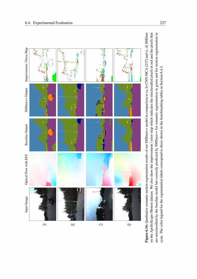
6.4. Experimental Evaluation 227In
putI
mag
eO
ptic
alFl
oww
ithE
FSB
asel
ine
Out
put
SMSn
et++
Out
put
Impr
ovem
ent/
Err
orM
ap
(a) (b) (c) (d)
Figu
re6.
16:Q
ualit
ativ
ese
man
ticm
otio
nse
gmen
tatio
nre
sults
ofou
rSM
Snet
++m
odel
inco
mpa
rison
to(a
,b)C
NN
-MC
A[2
37]a
nd(c
,d)S
MSn
eton
the
Apo
lloSc
ape-
Mot
ion
data
set.
We
also
show
the
impr
ovem
ent/
erro
rmap
whi
chin
dica
tes
the
mis
clas
sifie
dpi
xels
inre
dan
dth
epi
xels
that
are
mis
clas
sifie
dby
the
base
line
mod
elbu
tcor
rect
lypr
edic
ted
bySM
Snet
++fo
rsem
antic
segm
enta
tion
ingr
een
and
form
otio
nse
gmen
tatio
nin
cyan
.The
colo
rleg
end
fort
hese
gmen
tatio
nla
bels
corr
espo
ndto
thos
esh
own
inth
ebe
nchm
arki
ngta
bles
inSe
ctio
n6.
4.2.
228 Chapter 6. Joint Semantic Motion Segmentation
the second example shown in Figure 6.16 (b), there are eight moving cars on the samelane and a moving person on the right side of the image. The CNN-MCA model onlysegments three of the eight cars as moving and misclassifies the moving person as static.Additionally, it does not detect a static person on the right side of the image and againmisclassifies parts of the road on the bottom right of the image as vegetation due to motionblur. Analyzing the segmentation output of our SMSnet++ model, we see that it accuratelypredicts the motion status and the semantic object category of the pixels in this image.
In the next example shown in Figure 6.16 (c), we observe five moving cars on the samedirection as the ego-vehicle, one moving car on the opposite direction of the ego-vehicle,one moving person and one moving motorcycle. The output of the SMSnet model shownas the baseline only partially segments two of the moving cars out of the total six present inthe scene, and does not detect both the moving person and the motorcycle. Moreover, thenumerous parked static cars along the road in front of the ego-vehicle are all left undetectedin the segmentation output and most parts of the buildings are misclassified as vegetation.In addition static pedestrians and poles that are at far away distances are not captured inthe segmentation output of the SMSnet model. Once again, we also observe parts of theroad on the bottom corners of the image are segmented incorrectly, as vegetation due tomotion blur in the images. Whereas, our proposed SMSnet++ model does not demonstratethe misclassifications due to motion blur as it effectively leverages semantic informationfrom the previous frames using our representational warping to yield temporally smootherpredictions. Although SMSnet++ accurately segments the scene, it can be seen that certainpixels of the moving car are incorrectly classified as static. This is primarily due tothe optical flow maps that do not capture the accurate boundaries of the moving objectson this dataset, in addition to artifacts such as trails of ghost regions that are observedbehind moving objects. As there are no groundtruth optical flow labels to train the flowgeneration network in a supervised fashion on this dataset, we employ the network trainedon the KITTI flow dataset and keep the weights fixed while training the rest of the motionsegmentation stream. Therefore, employing an unsupervised optical flow network willalleviate the aforementioned problem.
In the last example shown in Figure 6.16 (d), we observe seven moving cars on thesame lane as the ego-vehicle and a moving bus as well as a moving car on the oppositelane. It can be seen that the SMSnet model only partially segments four out of the eightmoving cars in the same lane, while also partially segmenting the moving bus and thecar on the opposite lane. However, our SMSnet++ model segments all the cars butmisclassifies three out of the seven distantly moving cars on the same lane as static. Whileit accurately segments the bus on the opposite lane as moving, it only partially classifiesthe pixels on the car behind the bus as moving. Observing the optical flow map, we seethat the distant objects are not captured in the scene which causes the motion segmentationnetwork to misclassify distant moving cars as static. Comparing the semantic segmentationoutput of the SMSnet++ model with SMSnet, we observe a significant improvement in
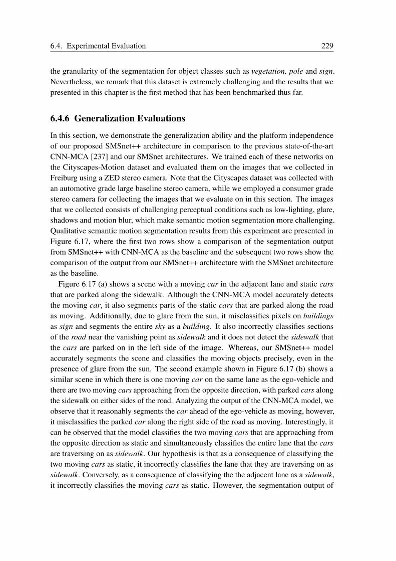
6.4. Experimental Evaluation 229
the granularity of the segmentation for object classes such as vegetation, pole and sign.Nevertheless, we remark that this dataset is extremely challenging and the results that wepresented in this chapter is the first method that has been benchmarked thus far.
6.4.6 Generalization Evaluations
In this section, we demonstrate the generalization ability and the platform independenceof our proposed SMSnet++ architecture in comparison to the previous state-of-the-artCNN-MCA [237] and our SMSnet architectures. We trained each of these networks onthe Cityscapes-Motion dataset and evaluated them on the images that we collected inFreiburg using a ZED stereo camera. Note that the Cityscapes dataset was collected withan automotive grade large baseline stereo camera, while we employed a consumer gradestereo camera for collecting the images that we evaluate on in this section. The imagesthat we collected consists of challenging perceptual conditions such as low-lighting, glare,shadows and motion blur, which make semantic motion segmentation more challenging.Qualitative semantic motion segmentation results from this experiment are presented inFigure 6.17, where the first two rows show a comparison of the segmentation outputfrom SMSnet++ with CNN-MCA as the baseline and the subsequent two rows show thecomparison of the output from our SMSnet++ architecture with the SMSnet architectureas the baseline.
Figure 6.17 (a) shows a scene with a moving car in the adjacent lane and static carsthat are parked along the sidewalk. Although the CNN-MCA model accurately detectsthe moving car, it also segments parts of the static cars that are parked along the roadas moving. Additionally, due to glare from the sun, it misclassifies pixels on buildingsas sign and segments the entire sky as a building. It also incorrectly classifies sectionsof the road near the vanishing point as sidewalk and it does not detect the sidewalk thatthe cars are parked on in the left side of the image. Whereas, our SMSnet++ modelaccurately segments the scene and classifies the moving objects precisely, even in thepresence of glare from the sun. The second example shown in Figure 6.17 (b) shows asimilar scene in which there is one moving car on the same lane as the ego-vehicle andthere are two moving cars approaching from the opposite direction, with parked cars alongthe sidewalk on either sides of the road. Analyzing the output of the CNN-MCA model, weobserve that it reasonably segments the car ahead of the ego-vehicle as moving, however,it misclassifies the parked car along the right side of the road as moving. Interestingly, itcan be observed that the model classifies the two moving cars that are approaching fromthe opposite direction as static and simultaneously classifies the entire lane that the carsare traversing on as sidewalk. Our hypothesis is that as a consequence of classifying thetwo moving cars as static, it incorrectly classifies the lane that they are traversing on assidewalk. Conversely, as a consequence of classifying the the adjacent lane as a sidewalk,it incorrectly classifies the moving cars as static. However, the segmentation output of
230 Chapter 6. Joint Semantic Motion Segmentation
InputImage
OpticalFlow
Baseline
Output
SMSnet++
Output
(a)(b)(c)(d)
Figure6.17:Q
ualitativesem
anticm
otionsegm
entationresults
ofvariousarchitectures
trainedon
theC
ityscapes-Motion
datasetandevaluated
onim
agescollected
inFreiburg.T
heresults
ofourSMSnet++
modelare
shown
incom
parisonto
(a,b)CN
N-M
CA
[237]and(c,d)SM
Snet.The
colorlegendforthe
segmentation
labelscorrespond
tothose
shown
inthe
benchmarking
tablesin
Section6.4.2.
6.4. Experimental Evaluation 231
our SMSnet++ model does not show these incorrect classifications, rather it accuratelydistinguishes between the static and moving objects in the scene.
In Figure 6.17 (c), we observe a scene with a moving car ahead of the ego-vehicle onthe same lane and another moving car approaching on the adjacent lane. The output ofthe SMSnet model shown as the baseline, segments most of the car on the adjacent laneas moving, however, it misclassifies pixels along the edge of the image where the caris exiting the frame as static. Additionally, it incorrectly classifies the car ahead of theego-vehicle as static. Whereas, our SMSnet++ model accurately assigns the pixels to thestatic and moving object categories. Comparing the semantic segmentation output of bothmodels, we observe that due to the glare from the sun, the SMSnet model misclassifiesmost of the pixels near the vanishing point of the road and also misclassifies objects onthe section of the sidewalk on the right side of the image that is brightly lit by sunlight.However, our SMSnet++ model leverages semantic information from the previous viewusing our temporal warping layer to more accurately segment these areas that are overexposed due to the sunlight. The improvement in the semantic segmentation output ofSMSnet++ can be observed in precise segmentation of the object boundaries as well as inthe segmentation of thin pole-like structures.
The final example shown in Figure 6.17 (d) depicts a scene where there is a moving caras well as a motorbike ahead of the ego-vehicle and another moving car is approachingon the opposite side in the adjacent lane. The output of the SMSnet model demonstratesaccurate segmentation of the car and most pixels belonging to the motorbike ahead of theego-vehicle as moving. However, as the car approaching on the opposite side is partlyoccluded due to a bollard on the traffic island, the section of the car on one side of thebollard is incorrectly classified as static, while the other section is incorrectly classified asmotorbike. Observing the output of our SMSnet++ model, we see that both the cars and themotorbike are accurately predicted as moving and more interestingly, both sections of caron the either side of the bollard as predicted as moving. This can be attributed to the largeeffective receptive field of the SMSnet++ architecture that effectively enables the networkto incorporate more context information into the final prediction. The improvement in thesemantic segmentation of the SMSnet++ model is more evident in the area on the left sideof the image, where the distinction between fence and sidewalk is accurately predicted.In addition, we can see that our SMSnet++ model accurately segments the bollard as asign and a pole. However, the SMSnet model misclassifies the bollard as a person anda motorbike. Overall, we observe that our SMSnet++ model trained on the Cityscapes-Motion dataset performs substantially better in newer environments than the previousstate-of-the-art CNN-MCA model and the SMSnet architecture. Our SMSnet++ modelaccurately segments moving objects according to their semantic classes and demonstratesnegligible false positives as well as exceptional generalization of the learned kernels.
232 Chapter 6. Joint Semantic Motion Segmentation
6.5 Related Work
In this chapter, we addressed the problem of joint semantic motion segmentation usingconvolutional neural network architectures. The networks that we introduced enables arobot to simultaneously predict both the semantic object category and motion status ofeach pixel in an image, more accurately than employing individual specialized models foreach task. Moreover, as robots require information from both tasks simultaneously in orderto plan future actions, a single coherent model is more efficient for deployment. Semanticsegmentation and motion segmentation are two fundamental problems in scene understand-ing that each have substantial amount of prior work in their areas. However, there are onlya handful of techniques that have focused on tackling them in a joint framework with theaim of exploiting semantic representations to improve motion segmentation. In Section 4.5of Chapter 4, we presented a thorough review of the related work in semantic scene seg-mentation. In this section, we first describe the most relevant work in motion segmentationas well as the closely related task of video segmentation, followed by methods that addressthe problem of semantic motion segmentation jointly.
There are numerous approaches that have been proposed for segmenting moving objectsfrom stationary camera images [252, 253, 254]. Vidal et al. [252] propose a classicalapproach that minimizes the reprojection error subject to all multibody epipolar con-straints for segmenting dynamic scenes containing multiple rigidly moving objects. Sapag-nolo et al. [253] introduce an approach for foreground moving object segmentation thatcombines background subtraction with temporal image analysis. While, Gao et al. [254]propose a method that combines the Kirsch operator with optical flow for moving objectdetection. However, these approaches fail in degenerate cases and they cannot be directlyapplied to moving camera images as the movement causes a dual motion appearance whichconsists of the background motion and the object motion.
In general, methods that detect motion from freely moving cameras partition the imageinto coherent regions with homogenous motion. This process splits the image into back-ground and moving clusters. These methods can be categorized into optical flow basedand tracking based approaches. Optical flow based techniques [255, 256] check if themotion speed as well as direction of a region is consistent with its radially surroundingpattern and then classifies it as a moving object if the motion of the region deviates fromthis pattern. Namdev et al. [257] propose an approach that combines optical flow andgeometric cues to generate dense segmentation using a graph-based clustering algorithm.The approach further demonstrates how both these cues complement each other to segmentmoving objects that have difficult degenerate motions. In a similar work, Lenz et al. [258]introduce a class independent method for object detection that uses stereo images aswell as optical flow information and demonstrate superior performance in the presenceof unknown objects in traffic scenarios where appearance-based object detectors oftenfail. Wedel et al. [259] propose an energy minimization approach to detect and segment
6.5. Related Work 233
independently moving objects using scene flow and stereo images. Experiments thatwere performed in challenging scenarios show that their approach accurately localizesindependently moving objects where traditional background subtraction techniques fail.Kao et al. [260] derive a geometric model that relates 2D motion to a 3D motion fieldrelative to the camera, based on estimated depth and motion of vanishing points in thescene. Spectral clustering is then applied on the recovered 3D motion field to obtain themoving object segmentation. Although qualitative evaluations have been shown on theKITTI benchmark, no quantitative comparisons were reported. The major disadvantage ofthese methods is that they are prone to occlusion, noise in the optical flow map and edgeeffects due to optical flow misalignments with true object boundaries.
Tracking based techniques [234, 251, 261, 262] on the other hand, aim to detect andlocalize target objects in successive frames. Tracking of objects yields movement trajec-tories and by estimating the ego-motion of the camera, objects can be segmented fromthe background motion. Romero-Cano et al. [263] propose a technique that estimates thelikelihood of pixel motion from the fusion of dense optical flow with depth information andtemporal consistency is incorporated by tracking the moving objects across consecutiveimages. Lin et al. [264] propose a motion segmentation framework that combines 3Dgeometric constrains with high-level spatio-temporal features learned from consecutivestereo images. Tourani et al. [265] propose an approach in which first motion models aregenerated and merged using trajectory clustering into different motion affine subspaces.Moving object proposals generated from the prior model then yield a sparse collection ofpoints on the dynamic object. Drayer et al. [262] introduce a weakly supervised motionsegmentation technique that first extracts temporally consistent object tubes based on anoff-the-shelf detector, followed by building a spatio-temporal graph by connecting thedetections to segment objects. Ochs et al. [230] cluster long term point trajectories fortemporally consistent moving object segmentation. A disadvantage of these approaches isthat they typically have long processing pipelines resulting in high computation times andcoarse segmentations.
Several approaches have extensively explored the use of convolutional neural networksfor motion segmentation [235, 236]. Fragkiadaki et al. [236] propose an approach thatfirst generates region proposals using multiple segmentations on optical flow and staticboundaries, following which a moving objectness detector rejects proposals on staticbackgrounds and then ranks spatio-temporal segments by mapping clustered trajectories topixel tubes. Tokmakov et al. [235] introduce an encoder-decoder architecture that takesthe optical flow as input to first learn a coarse representation of the motion features whichare then iteratively upsampled and refined to yield the full resolution motion segmentation.Perazzi et al. [266] formulates the motion segmentation as a guided instance segmentationproblem, while combining offline and online training on static images to perform videoobject segmentation. Similarly, Caelles et al. [267] propose a video object segmentationnetwork that is first pre-trained on generic datasets for the task of foreground object
234 Chapter 6. Joint Semantic Motion Segmentation
segmentation and then fine-tuned on the first frame of the test sequence while processingeach frame independently. Cheng et al. [268] propose a unified architecture consisting ofan optical flow learning stream and a semantic segmentation stream. Features from boththese streams are propagated bidirectionally at the high-level to improve both segmentationand optical flow generation. Jain et al. [269] propose a similar two-stream architecturethat fuses motion and appearance features for video object segmentation. Subsequently,Siam et al. [250] propose another similar architecture that performs object detection inaddition to motion segmentation in a joint model. Most of these approaches are obliviousto object categories and generate coarse object boundary segmentations. Moreover, theyhave been solely benchmarked on video segmentation datasets that only have one movingobject in each frame. Whereas, our proposed networks are capable of segmenting multiplemoving and static objects while accounting for their semantic object category.
Recent methods have also explored estimating semantic object labels and motion labelsjointly [232, 233, 237, 270]. Reddy et al. [232] propose an approach that generates motionlikelihoods based on depth and optical flow estimations, while combining them withsemantic and geometric constraints within a dense conditional random field. However, theapproach has limited generalization ability as it primarily relies on handcrafted features.Chen et al. [270] introduce a method that detects object-level motion from a movingcamera using two consecutive image frames and provides 2D bounding boxes as theoutput. They design a robust context-aware motion descriptor that considers movingspeed, as well as the direction of objects and combines them with an object classifier. Thedescriptor measures the inconsistency between local optical flow histograms of objects andtheir surroundings, giving a measure of the state of motion. More recently, a multi-stepframework was proposed [233], in which sparse image features from two consecutive stereoimage pairs are first extracted and matched, followed by classifying the matched featurepoints using RANSAC into inliers caused by the camera and outliers caused by movingobjects. Subsequently, the outliers are then clustered in a U-disparity map which providesthe motion information of objects and a dense CRF is then used to merge the motioninformation with the semantic segmentation provided by a FCN. Another closely relatedwork was proposed by Haque et al. [237] in which a three stage pipeline is employed.Their approach integrates optical flow as a constraint with semantic features into a dilatedconvolutional neural network and achieves state-of-the-art performance for joint semanticmotion segmentation on the KITTI dataset.
One of the major drawbacks of these approaches is the substantially large interferencetime, which ranges from a few seconds to even minutes, thereby making them unusablefor robotic applications that require near real-time performance such as autonomous driv-ing. More importantly, these approaches only focus on jointly learning both semanticsegmentation and motion segmentation in single framework but they do not simultaneouslyexploit the semantic cues to improve motion segmentation and vice versa. In contrastto these techniques, in this chapter, we presented the novel SMSnet architecture that
6.6. Conclusions 235
combines learned multiscale semantic representations with optical flow field features forjoint semantic motion segmentation. Our model compensates for the flow induced bythe ego-motion of the camera and is several orders faster than existing techniques. Addi-tionally, our improved SMSnet++ architecture also improves the semantic segmentationperformance using a representational warping technique and further improves the motionsegmentation by incorporating adaptive fusion as well as a multistage refinement strategyfor high-resolution motion segmentation.
6.6 Conclusions
In this chapter, we addressed the problem of semantic motion segmentation using con-volutional neural network architectures that take two consecutive images as input andlearns to predict both the semantic object class label and motion status of each pixel inan image. Our proposed SMSnet architecture first learns coarse representations of opticalflow field features while compensating for the flow induced due to the ego-motion of thecamera and simultaneously learns multiscale semantic representations in a parallel stream.Subsequently, the network combines the learned semantic features with the flow fieldfeatures and further learns discriminative deep representations while refining the predic-tions to yield the pixel-wise semantic motion labels. The fusion of semantic features withlearned optical flow field features boosts the performance of segmenting moving objects,especially in cluttered and challenging scenes with multiple moving objects of differentsemantic categories in the scene. Furthermore, we presented the SMSnet++ architecturethat achieves deeper synergy between semantics, motion and appearance by incorporatinga representational warping technique to improve the temporal consistency of semanticsegmentation, while adaptively fusing semantic information with flow field features toimprove motion segmentation. Rather than using the learned optical flow directly to warpsemantic feature maps, the temporal warping layer transforms the ego-flow suppressedoptical flow to an edge-enhanced representation, which further improves the semanticsegmentation performance. Concurrently, the adaptive fusion of semantic and optical flowfield features discards over-segmentation or parts of semantic objects that are static inthe resulting motion segmentation. The proposed SMSnet++ architecture additionallyintegrates our multistage refinement strategy in both the semantic stream and the motionstream to yield a high resolution segmentation output that accurately captures the objectboundaries. Our proposed semantic motion segmentation frameworks are modular andcan be easily be adapted with other semantic segmentation or optical flow generationarchitectures.
We extended three standard semantic segmentation benchmark datasets with motionannotations and made them publicly available to encourage future research in this domain.These large datasets are the first-of-its-kind and enable training of deep convolutional
236 Chapter 6. Joint Semantic Motion Segmentation
neural networks for joint semantic motion segmentation. We validated the effectiveness ofour joint model through extensive experiments on both semantic segmentation as well asmotion segmentation tasks and showed that it outperforms individual specialized models.We presented exhaustive quantitative results on the Cityscapes-Motion, KITTI-Motion andApolloScape-Motion datasets that demonstrate that both our architectures set the new state-of-the-art on these benchmarks and run in an online fashion. We presented comprehensiveablation studies that detail our architectural design choices and also presented extensivequalitative results in autonomous driving scenarios. Furthermore, we presented qualitativeevaluations on real-world driving data from Freiburg that contain challenging perceptualconditions and demonstrated that our models generalize effectively to new environments.
Chapter 7
Geometrically Consistent SemanticVisual Localization
Semantic understanding and localization are fundamental key en-ablers of robot autonomy that have for the most part been tackledas disjoint problems. While deep learning has enabled recent break-throughs across a wide spectrum of scene understanding tasks, itsapplicability to state estimation tasks has been limited due to the di-rect formulation that renders it incapable of encoding scene-specificconstrains. In this chapter, we propose two multitask convolutionalneural network architectures coupled with a novel Geometric Con-sistency loss function that utilizes auxiliary learning to leverage rel-ative pose information during training, thereby constraining thesearch space to obtain consistent pose estimates. We introduce theVLocNet architecture that incorporates hard parameter sharing toenable inter-task learning while regressing the 6-DoF global poseand the relative odometry estimate from consecutive monocular im-ages. We also propose the novel VLocNet++ architecture that ex-ploits complex interdependencies between learning semantics, re-gressing 6-DoF global pose and odometry, for the mutual benefit ofeach of these tasks. Our network aggregates motion-specific tem-poral information and fuses semantic features into the localizationstream based on region activations. Extensive experiments on theMicrosoft 7-Scenes and DeepLoc datasets demonstrate that our net-works set the new state-of-the-art.
7.1 Introduction
Thus far in this thesis, we have addressed several critical scene understanding challengesin the context of robot perception. The techniques that we have introduced enable a
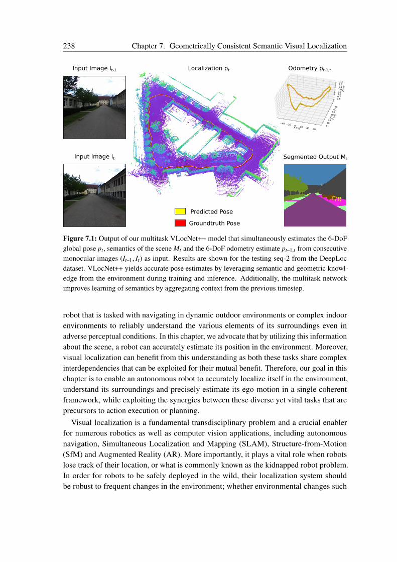
238 Chapter 7. Geometrically Consistent Semantic Visual Localization
Input Image It Segmented Output Mt
Predicted Pose
Groundtruth Pose
Localization pt
X [m]
−40 −20 0 20 40 60
Y [m
]
010203040506070
Z [
m]
0.60.70.80.91.01.11.21.3
Odometry pt-1,tInput Image It-1
Figure 7.1: Output of our multitask VLocNet++ model that simultaneously estimates the 6-DoFglobal pose pt, semantics of the scene Mt and the 6-DoF odometry estimate pt–1,t from consecutivemonocular images (It–1, It) as input. Results are shown for the testing seq-2 from the DeepLocdataset. VLocNet++ yields accurate pose estimates by leveraging semantic and geometric knowl-edge from the environment during training and inference. Additionally, the multitask networkimproves learning of semantics by aggregating context from the previous timestep.
robot that is tasked with navigating in dynamic outdoor environments or complex indoorenvironments to reliably understand the various elements of its surroundings even inadverse perceptual conditions. In this chapter, we advocate that by utilizing this informationabout the scene, a robot can accurately estimate its position in the environment. Moreover,visual localization can benefit from this understanding as both these tasks share complexinterdependencies that can be exploited for their mutual benefit. Therefore, our goal in thischapter is to enable an autonomous robot to accurately localize itself in the environment,understand its surroundings and precisely estimate its ego-motion in a single coherentframework, while exploiting the synergies between these diverse yet vital tasks that areprecursors to action execution or planning.
Visual localization is a fundamental transdisciplinary problem and a crucial enablerfor numerous robotics as well as computer vision applications, including autonomousnavigation, Simultaneous Localization and Mapping (SLAM), Structure-from-Motion(SfM) and Augmented Reality (AR). More importantly, it plays a vital role when robotslose track of their location, or what is commonly known as the kidnapped robot problem.In order for robots to be safely deployed in the wild, their localization system shouldbe robust to frequent changes in the environment; whether environmental changes such
7.1. Introduction 239
as illumination and seasonal appearance, dynamic changes such as moving vehiclesand pedestrians, or structural changes such as renovated buildings. Visual localizationtechniques can be broadly classified into two categories: topological and metric methods.Topological localization provides coarse estimates of the position, usually by dividing themap into a discretized set of locations and employing image retrieval techniques [271, 272,273]. While this approach is well suited for large environments, the resulting locationaccuracy is bounded by the granularity of the discrete set. Metric localization approacheson the other hand, provide a 6-DoF metric estimate of the pose within the environment.Currently, local feature-based approaches that utilize SfM information achieve state-of-the-art performance [274, 275]. However, a critical drawback of these methods is the decreasein speed and increase in complexity of finding feature correspondences as the size of theenvironment grows. Moreover, most approaches require a minimum number of matches tobe able to produce a pose estimate. This in turn causes pose estimation failures when thereis large viewpoint changes, motion blur, occlusions or textureless environments.
Inspired by the outstanding performance of Convolutional Neural Networks (CNNs) ina variety of tasks in various domains and with the goal of eliminating manual engineeringof algorithms for feature selection, CNN architectures that directly regress the 6-DoFmetric pose have recently been explored [276, 277, 278]. However, despite their abilityto handle challenging perceptual conditions and effectively manage large environments,they are still unable to match the performance of state-of-the-art local feature-basedlocalization methods [274, 275]. This can be attributed to their inability to internallymodel the 3D structural constraints of the environment while learning from a singlemonocular image. As a solution to this problem, we propose a principled approach toembed geometric knowledge into the pose regression model by simultaneously learningto estimate visual odometry as an auxiliary task. We then leverage the complementaryrelative motion information from odometry to constrict the search space while trainingthe global localization model using our Geometric Consistency loss function which isa result of joint work with Noha Radwan [56]. However, this problem is non-trivial aswe need to first determine how to structure the architecture to ensure the learning ofthis inter-task correlation and secondly, how to jointly optimize the unified model sincedifferent task-specific networks have different attributes and different convergence rates.
We address the aforementioned challenges and propose our VLocNet architectureconsisting of a global pose regression stream and a Siamese-type relative pose estimationstream. Our network based on the residual learning framework, takes two consecutivemonocular images as input and jointly regresses the 6-DoF global pose as well as the6-DoF relative pose between the images. We incorporate a hard parameter sharing schemeto learn inter-task correlations within the network and present a multitask joint optimizationstrategy for learning shared features across the different task streams. More importantly, wedevise the new Geometric Consistency loss [56] for global pose regression that incorporatesthe relative motion information during training and enforces the predicted poses to be
240 Chapter 7. Geometrically Consistent Semantic Visual Localization
geometrically consistent with respect to the true motion model. By jointly learning bothtasks, our approach is robust to environmental aliasing by utilizing previous pose andrelative motion information, thereby combining the advantages of both local feature anddeep learning-based localization methods.
Inspired by how humans often describe their location to one another with respect toreference landmarks in the scene and giving their position relative to it, we further exploreencoding semantic knowledge into the pose regression model in our proposed VLocNet++architecture. We now formulate this problem from a multitask learning (MTL) perspectivewith the goal of learning more accurate localization and semantic segmentation models byleveraging the predicted ego-motion. This problem is even more challenging as it involvessimultaneously learning cross-domain tasks that perform pixel-wise classification andregression with different units and scales. However, this joint formulation enables inter-task learning which improves both generalization capabilities and alleviates the problemof requiring vast amounts of labeled training data, which is especially hard to obtain in therobotics domain. Moreover, as robots are equipped with limited resources, a joint model ismore efficient for deployment and enables online inference on a consumer grade GPU.
Our motivation for jointly estimating semantics is based on the premise that it can instillstructural cues about the environment into the pose regression network and implicitly pullthe attention towards more informative regions in the scene. Correspondingly, location-specific information from the localization task can help improve learning of semantics.A popular paradigm employed for semantics-aware localization is to extract predefinedfeatures, emphasize on stable features [279] or combine them with local features [280].Although these handcrafted solutions have demonstrated considerable reliability, theirperformance suffers substantially when the predefined structures are occluded or not visiblein the scene. Therefore, in order to alleviate this problem, we propose a weighted fusionlayer to integrate relevant semantic features into the global pose regression stream not onlybased on the semantic object category, but also the activations in the region.
Predicting consistent semantics is a critical prerequisite for semantic visual localization.Inspired by early cognitive studies in humans showing the importance of learning self-motion for acquiring basic perceptual skills [281], we utilize a novel self-supervisedsemantic context aggregation technique (joint work with Noha Radwan [34]) leveragingthe predicted relative motion from the odometry stream of our network. Using pixel-wise depth predictions from a CNN [243] and differential warping, we fuse intermediatenetwork representations from the previous timestep into the current frame using ourproposed weighted fusion layer. This enables our semantic segmentation network toaggregate more scene-level context, thereby improving the performance and leading tofaster convergence. Additionally, in order to efficiently utilize the learned motion-specificfeatures in the global pose regression stream from the previous timestep, we also employthe weighting technique to aggregate motion-specific temporal information.
To the best of our knowledge, there is no publicly available localization or pose estima-

7.1. Introduction 241
tion dataset with pixel-level semantic groundtruth labels tagged with 6-DoF camera posesand containing multiple loops. Therefore, in order to facilitate training of multitask deeplearning models for semantic visual localization and odometry estimation, we introduce thenew DeepLoc dataset [34] that was gathered using our Obelix robot platform and consistsof ten loops amounting a total of 3910 RGB-D images with pixel-level semantic and 6-DoFpose groundtruth labels. The dataset contains repetitive, translucent and reflective surfaces,weakly textured regions and low-lighted scenes with shadows, thereby making it extremelychallenging for benchmarking a variety of tasks. We evaluate our proposed VlocNet andVLocNet++ architectures on the challenging indoor Microsoft 7-Scenes benchmark andour outdoor DeepLoc dataset on each of the diverse tasks. Extensive empirical evaluationsdemonstrate our VLocNet architecture is the first deep learning-based localization methodto perform on par with local feature-based techniques while outperforming existing deeplearning-based approaches. Furthermore, our proposed VLocNet++ architecture sets thenew state-of-the-art outperforming both local feature-based and CNN-based techniqueswhile simultaneously performing multiple tasks and exhibiting substantial robustness inchallenging scenarios. The work that we present in this chapter is the first attempt to showthat a joint multitask model can precisely and efficiently outperform its task-specific coun-terparts for global pose regression, semantic segmentation and visual odometry estimation.
In summary, the primary contributions that we make in this chapter are as follows:• A new residual convolutional neural network architecture for 6-DoF global pose
regression.• A new residual Siamese-type convolutional neural network architecture for 6-DoF
odometry estimation.• The novel VLocNet architecture with a joint optimization strategy for simultaneously
regressing the global pose and visual odometry. Our approach presents an efficient,and scalable alternative to learning task specific models.• The novel VLocNet++ architecture for jointly learning semantics, visual localization
and odometry from consecutive monocular images.• A novel weighted fusion layer for element-wise fusion of feature maps based on
region activations to exploit inter/intra-task dependencies.• A first-of-a-kind urban outdoor localization dataset [34] consisting of multiple loops
with pixel-level semantic labels and 6-DoF camera poses.• Comprehensive quantitative and qualitative comparisons of our task specific net-
works as well as our joint multitask network against various CNN-based approachesas well as state-of-the-art local feature-based techniques on benchmark datasets.
Additionally, we also detail the following contributions which are an outcome of jointwork with Noha Radwan [34, 56]:• The Geometric Consistency loss function [56] that incorporates the relative motion
information during training, thus enabling the network to predict pose estimates thatare consistent with the true motion model.
242 Chapter 7. Geometrically Consistent Semantic Visual Localization
• A self-supervised context aggregation technique [34] based on differential warpingthat improves the semantic segmentation performance and reduces the training time.
The remainder of this chapter is organized as follows. In Section 7.2, we first detail ourGeometric Consistency loss function, followed by the topologies of our proposed VLocNetand VLocNet++ architectures. We then describe the methodology that we employed forcollecting and annotating our DeepLoc dataset in Section 7.3. In Section 7.4, we presentextensive experimental evaluations, detailed ablation studies and insightful qualitativeresults. Subsequently, we discuss the related work in Section 7.5 and conclude the chapterin Section 7.6.
7.2 Technical Approach
In this section, we first introduce our Geometric Consistency loss function [56] for globalpose regression that constricts the search space while training by leveraging the relativemotion between two consecutive frames. We then describe our VLocNet architecture forregressing global poses and simultaneously learning to regress relative motion betweentwo camera frames using only pairs of RGB images. Subsequently, we detail our multitaskVLocNet++ architecture for jointly estimating the global pose, odometry and semanticsegmentation from consecutive monocular images. While the multitask networks presentedin this chapter focus on joint learning of the aforementioned tasks, each of the task-specificmodels can be deployed independently during test-time.
7.2.1 The Geometric Consistency Loss Function
Learning both translational and rotational pose components with the same loss function isinherently challenging due to the difference in scale and units between both the quantities.Equations 7.1 and 7.2 describe the loss function for regressing the translational androtational components in the Euclidean space in which we assume that the quaternionoutput of the network has been normalized a priori for ease of notation.
Lx (f (θ | It)) := ‖xt – xt‖γ (7.1)
Lq (f (θ | It)) := ‖qt – qt‖γ , (7.2)
where θ is the parameters of the network, f (θ | It) denotes the predicted output of thenetwork for image It, xt ∈ R3 and qt ∈ R4 denote the groundtruth translation and rotationcomponents of the pose, xt and qt denote their predicted counterparts and γ refers to theLγ-norm. In this chapter, we use the L2 Euclidean norm. Recent work [282] has shownthat the performance of a model trained to jointly regress the position and orientationcomponents of the pose, outperforms two separate models trained for regressing eachquantity. Therefore, as the loss function is required to learn both the position and orientation

7.2. Technical Approach 243
components simultaneously, a weight regularizer β is used to balance each of the lossterms. We represent this loss function as
Leucβ (f (θ | It)) := Lx(f (θ | It)) + βLq(f (θ | It)). (7.3)
Although initial work [276, 277, 283] has shown that by minimizing this function, thenetwork is able to learn a valid pose regression model, it suffers from the drawback ofhaving to manually tune the hyperparameter β for each new scene in order to achievereasonable results. To counteract this problem, we use two learnable weightings toreplace the β term. As these weightings are learned, their values get updated during theoptimization process and consequently do not require manual tuning. The resulting lossfunction is represented as
Leuc(f (θ | It)) := Lx(f (θ | It)) exp(–sx) + sx (7.4)
+ Lq(f (θ | It)) exp(–sq) + sq,
where sx and sq are the two learnable weighting variables for the translation and rotationalcomponents. Although this formulation overcomes the problem of having to manuallyselect a β value for each scene, it does not ensure that the estimated poses are consistentwith the previous motion.
As a solution to this problem, we utilize our novel Geometric Consistency loss func-tion [56] that incorporates previous motion information, thereby yielding globally consis-tent pose estimates. We introduce an additional geometric pose constraint between pairs ofobservations that bootstraps the loss function by penalizing pose predictions that contradictthe relative motion. More precisely, in addition to the loss function shown in Eq. (7.4), weadd another loss term to constrain the current pose prediction by minimizing the relativemotion error between the groundtruth and the estimated motion from the auxiliary odome-try stream. We useRx(f (θ | It)) andRq(f (θ | It)) to denote the relative motion between theprevious predicted pose pt–1 and the pose of the current image It as
Rx(f (θ | It)) := xt – xt–1 (7.5)
Rq(f (θ | It)) := q–1t–1qt. (7.6)
The components from Equations 7.5 and 7.6 compute the relative motion in terms ofthe network’s predictions. By utilizing the predictions of the network from the previoustimestep along with the current timestep, the relative motion relative motion loss termLrel (f (θ | It)) can be computed as a weighted summation of the translational and rotationalerrors which minimizes the variance between the predicted poses. The corresponding loss
244 Chapter 7. Geometrically Consistent Semantic Visual Localization
function is formulated as
Lxrel(f (θ | It)) := ‖xt–1,t –Rx(f (θ | It))‖γ (7.7)
Lqrel(f (θ | It)) := ‖qt–1,t –Rq(f (θ | It))‖γ (7.8)
Lrel (f (θ | It)) = Lxrel (f (θ | It)) exp(–sxrel) + sxrel (7.9)
+ Lqrel (f (θ | It)) exp(–sqrel) + sqrel
where Lxrel computes the difference between the ground-truth relative translational motionand its predicted counterpart, while Lqrel computes a similar difference for the rotationalcomponent of the pose. We combine both the relative motion loss term with the loss func-tion from Eq. (7.4) to yield the proposed Geometric Consistency loss, thereby minimizing
Lgeo(f (θ | It)) :=(Lx(f (θ | It)) + Lxrel(f (θ | It))
)exp(–sx) + sx (7.10)
+(Lq(f (θ | It)) + Lqrel(f (θ | It))
)exp(–sq) + sq.
By minimizing the aforementioned Geometric Consistency loss function [56], ournetwork learns a model that is geometrically consistent with respect to the motion. Wehypothesize that the resulting trained model is more robust to perceptual aliasing withinthe environment by utilizing this relative motion in the loss function.
7.2.2 VLocNet Architecture
Our proposed VLocNet architecture consists of three network streams; a global poseregression stream and a Siamese-type double-stream for odometry estimation. An overviewof the topology is shown in Figure 7.2. Given a pair of consecutive monocular images(It–1, It), our network predicts both the global pose pt = (xt, qt) and the relative posept–1,t =
(xt–1,t, qt–1,t
)between the input frames, where x ∈ R3 denotes the translation and
q ∈ R4 denotes the rotation in quaternion representation. For ease of notation, we assumethat the quaternion outputs of the network have been normalized a priori. The input tothe Siamese streams are the images (It–1, It), while the input to the global pose regressionstream is It.
Unlike conventional Siamese architectures, we do not share features across the twotemporal streams, instead we share features across the global pose regression stream andthe Siamese stream that takes the image It as input, upto a certain network depth. As ourimages do not encompass any spatially centered structure, sharing features across thesestreams is a viable solution to facilitate auxiliary learning and joint optimization of thetask specific network streams. We employ our Geometric Consistency loss function [56]that enforces global consistency among the predicted poses by utilizing the relative poseestimates while training. In the remainder of this section, we detail the constitutingcomponents of our VLocNet architecture.
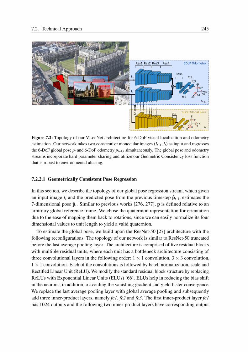
7.2. Technical Approach 245
6DoF Global Pose
6DoF Odometry
Δϕ Δθ
ΔΨ
Δx
Δy
Δz
ϕ θ
Ψ
x
y
z
It
It-1
pt-1Share
d
Res1 Res2 Res3 Res4
Res5
fc2
fc3
fc1
pt
pt-1,t
Figure 7.2: Topology of our VLocNet architecture for 6-DoF visual localization and odometryestimation. Our network takes two consecutive monocular images (It–1, It) as input and regressesthe 6-DoF global pose pt and 6-DoF odometry pt–1,t simultaneously. The global pose and odometrystreams incorporate hard parameter sharing and utilize our Geometric Consistency loss functionthat is robust to environmental aliasing.
7.2.2.1 Geometrically Consistent Pose Regression
In this section, we describe the topology of our global pose regression stream, which givenan input image It and the predicted pose from the previous timestep pt–1, estimates the7-dimensional pose pt. Similar to previous works [276, 277], p is defined relative to anarbitrary global reference frame. We chose the quaternion representation for orientationdue to the ease of mapping them back to rotations, since we can easily normalize its fourdimensional values to unit length to yield a valid quaternion.
To estimate the global pose, we build upon the ResNet-50 [27] architecture with thefollowing reconfigurations. The topology of our network is similar to ResNet-50 truncatedbefore the last average pooling layer. The architecture is comprised of five residual blockswith multiple residual units, where each unit has a bottleneck architecture consisting ofthree convolutional layers in the following order: 1× 1 convolution, 3× 3 convolution,1× 1 convolution. Each of the convolutions is followed by batch normalization, scale andRectified Linear Unit (ReLU). We modify the standard residual block structure by replacingReLUs with Exponential Linear Units (ELUs) [66]. ELUs help in reducing the bias shiftin the neurons, in addition to avoiding the vanishing gradient and yield faster convergence.We replace the last average pooling layer with global average pooling and subsequentlyadd three inner-product layers, namely fc1, fc2 and fc3. The first inner-product layer fc1has 1024 outputs and the following two inner-product layers have corresponding output
246 Chapter 7. Geometrically Consistent Semantic Visual Localization
dimensions of 3 and 4 for regressing the translation x and rotation q respectively. OurGeometric Consistency loss [56], detailed in Section 7.2.1 ensures that the predictedpose is geometrically consistent with respect to the true motion. Therefore, we feed thepredicted pose from the previous timestep to the network so that it can better learn aboutspatial relations of the environment. In order to effectively train the network, we use thegroundtruth pose from the previous timestep during training and the predicted pose fromthe model during evaluation. We do not incorporate recurrent units into our network as ouraim in this work is to localize only using consecutive monocular images and not rely onlong-term temporal features. We first feed the previous predicted pose to an inner-productlayer fc4 of dimension D and reshape the outputs to H × W × C, which correspondsin shape to the output of the last residual unit before the downsampling stage. Both thetensors are then concatenated and fed to the subsequent residual unit. In total, there are fourdownsampling stages in our network and we experiment with fusing at each of these stagesin Section 7.4.5.2. Note that we denote the aforementioned architecture as VLocNetSTL inour experiments.
7.2.2.2 Learning Visual Odometry
Our proposed architecture for relative pose estimation takes a pair of consecutive monocularimages (It–1, It) as input and yields an estimate of ego-motion pt–1,t =
(xt–1,t, qt–1,t
). We
employ a dual-stream architecture in which each of the streams is identically similar instructure and is based on the ResNet-50 model. We concatenate the feature maps of theindividual streams before the last downsampling stage at the end of Res4 and convolvethem through the last residual block, followed by an inner-product layer and two regressorsfor estimating the pose components. During training, we optimize the following lossfunction by minimizing the Euclidean loss between the groundtruth and the predictedrelative poses during training as
Lvo (f (θ | It–1, It)) := Lx (f (θ | It–1, It)) exp(–sxvo) + sxvo (7.11)
+ Lq (f (θ | It–1, It)) exp(–sqvo) + sqvo
Lx (f (θ | It–1, It)) := ‖xt–1,t – xt–1,t‖2
Lq (f (θ | It–1, It)) := ‖qt–1,t – qt–1,t‖2 ,
where Lx and Lq refers to the translational and rotational components respectively. Wealso employ learnable weighting parameters to balance the scale between the translationaland rotational components in the loss term. As shown in Figure 7.2, the dual odometrystreams have an architecture similar to the global pose regression network. In order toenable the inductive transfer of information between both networks, we share parametersbetween the odometry stream taking the current image It and the global pose regressionnetwork as detailed in Section 7.2.2.3.
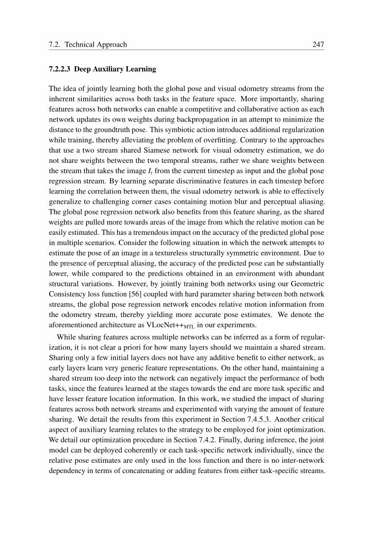
7.2. Technical Approach 247
7.2.2.3 Deep Auxiliary Learning
The idea of jointly learning both the global pose and visual odometry streams from theinherent similarities across both tasks in the feature space. More importantly, sharingfeatures across both networks can enable a competitive and collaborative action as eachnetwork updates its own weights during backpropagation in an attempt to minimize thedistance to the groundtruth pose. This symbiotic action introduces additional regularizationwhile training, thereby alleviating the problem of overfitting. Contrary to the approachesthat use a two stream shared Siamese network for visual odometry estimation, we donot share weights between the two temporal streams, rather we share weights betweenthe stream that takes the image It from the current timestep as input and the global poseregression stream. By learning separate discriminative features in each timestep beforelearning the correlation between them, the visual odometry network is able to effectivelygeneralize to challenging corner cases containing motion blur and perceptual aliasing.The global pose regression network also benefits from this feature sharing, as the sharedweights are pulled more towards areas of the image from which the relative motion can beeasily estimated. This has a tremendous impact on the accuracy of the predicted global posein multiple scenarios. Consider the following situation in which the network attempts toestimate the pose of an image in a textureless structurally symmetric environment. Due tothe presence of perceptual aliasing, the accuracy of the predicted pose can be substantiallylower, while compared to the predictions obtained in an environment with abundantstructural variations. However, by jointly training both networks using our GeometricConsistency loss function [56] coupled with hard parameter sharing between both networkstreams, the global pose regression network encodes relative motion information fromthe odometry stream, thereby yielding more accurate pose estimates. We denote theaforementioned architecture as VLocNet++MTL in our experiments.
While sharing features across multiple networks can be inferred as a form of regular-ization, it is not clear a priori for how many layers should we maintain a shared stream.Sharing only a few initial layers does not have any additive benefit to either network, asearly layers learn very generic feature representations. On the other hand, maintaining ashared stream too deep into the network can negatively impact the performance of bothtasks, since the features learned at the stages towards the end are more task specific andhave lesser feature location information. In this work, we studied the impact of sharingfeatures across both network streams and experimented with varying the amount of featuresharing. We detail the results from this experiment in Section 7.4.5.3. Another criticalaspect of auxiliary learning relates to the strategy to be employed for joint optimization.We detail our optimization procedure in Section 7.4.2. Finally, during inference, the jointmodel can be deployed coherently or each task-specific network individually, since therelative pose estimates are only used in the loss function and there is no inter-networkdependency in terms of concatenating or adding features from either task-specific streams.
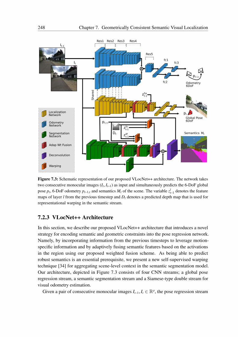
248 Chapter 7. Geometrically Consistent Semantic Visual Localization
pt,t-1
pt-1,t
It
It-1
Share
d
Res1 Res2 Res3 Res4
Res5
fc2
fc3fc1
Adap Wt Fusion
LocalizationNetwork
Odometry Network
Deconvolution
Segmentation Network
Global Pose6DoF
Semantics
Odometry6DoF
Dt
Warping
pt
z5at-1
Mt
z5ct-1
z4ft-1
Figure 7.3: Schematic representation of our proposed VLocNet++ architecture. The network takestwo consecutive monocular images (It, It–1) as input and simultaneously predicts the 6-DoF globalpose pt, 6-DoF odometry pt–1,t and semantics Mt of the scene. The variable zl
t–1 denotes the featuremaps of layer l from the previous timestep and Dt denotes a predicted depth map that is used forrepresentational warping in the semantic stream.
7.2.3 VLocNet++ Architecture
In this section, we describe our proposed VLocNet++ architecture that introduces a novelstrategy for encoding semantic and geometric constraints into the pose regression network.Namely, by incorporating information from the previous timesteps to leverage motion-specific information and by adaptively fusing semantic features based on the activationsin the region using our proposed weighted fusion scheme. As being able to predictrobust semantics is an essential prerequisite, we present a new self-supervised warpingtechnique [34] for aggregating scene-level context in the semantic segmentation model.Our architecture, depicted in Figure 7.3 consists of four CNN streams; a global poseregression stream, a semantic segmentation stream and a Siamese-type double stream forvisual odometry estimation.
Given a pair of consecutive monocular images It–1, It ∈ Rρ, the pose regression stream
7.2. Technical Approach 249
predicts the global pose pt = (xt, qt) for image It, where x ∈ R3 denotes the translationand q ∈ R4 denotes the rotation in quaternion representation, while the semantic streampredicts a pixel-wise segmentation mask Mt mapping each pixel u to one of the C semanticclasses, and the odometry stream predicts the relative motion pt–1,t =
(xt–1,t, qt–1,t
)between
consecutive input frames. While, zl denotes the feature maps from layer l of a particularstream. In order to estimate the odometry in VLocNet++, we employ our proposed Siamese-type double stream architecture that we described in Section 7.2.2.2. However, we use thefull pre-activation residual units [72] as opposed to the standard residual units [27] thatwe used in VLocNet. In the remainder of this section, we describe rest of the constitutingcomponents of our network architecture and our multitask learning scheme.
7.2.3.1 Geometrically Consistent Pose Regression
Our model for regressing the global pose is built upon our VLocNet architecture describedin Section 7.2.2.1. It has five residual blocks that downsample the feature maps by half ateach block, similar to the full pre-activation ResNet-50 architecture [72], as opposed tothe standard ResNet-50 architecture that we used in VLocNet. VLocNet++ also employsExponential Linear Units (ELUs) for the activation function and a global average poolinglayer is added after the fifth residual block. Subsequently, we add three inner-productlayers fc1, fc2 and fc3 with the number of output units as 1024, 3 and 4 respectively, wherefc2 and fc3 regress the translational x and rotational q components of the pose. UnlikeVLocNet which fuses the previous predicted pose directly using inner-product layers, weadopt a more methodological approach in VLocNet++ to provide the network with thisprior. Fusing the previous prediction directly, inhibits the network from being able tocorrelate the critical motion-specific spatial relations with that of the previous timestepas the network does not retain these features thereafter. In this work, we leverage thenetwork’s intermediate representation z5a
t–1 from the last downsampling stage (Res5a) of theprevious timestep using our proposed weighted fusion layer that we detail in Section 7.2.3.3.Our fusion scheme learns the optimal element-wise weighting for this fusion, and when itis trained end-to-end with the Geometric Consistency loss function, it enables aggregationof motion-specific features across the temporal dimension. We denote the aforementionedarchitecture as VLocNet++STL in our experiments.
As opposed to naively minimizing the Euclidean loss between the predicted poses andthe groundtruth, we employ our Geometric Consistency loss function [56] described inSection 7.2.1, which in addition to minimizing the Euclidean loss, adds another loss term toconstrain the current pose prediction by minimizing the relative motion error between thegroundtruth and the estimated motion from the odometry stream. This enables our networkto learn a model that is geometrically consistent with respect to the motion. Moreover, byemploying a mechanism to aggregate motion-specific features temporally, we enable theGeometric Consistency loss function to efficiently leverage this information.
250 Chapter 7. Geometrically Consistent Semantic Visual Localization
7.2.3.2 Incorporating Semantics
Our model for learning consistent semantics is comprised of three components: a basesegmentation architecture (green and purple blocks in Figure 7.3), our proposed self-supervised warping layer (orange blocks) and weighted fusion layer (red blocks). Inthe remainder of this section, we first describe the single-task semantic segmentationarchitecture and then detail our proposed self-supervised warping scheme [34]. Theweighted fusion layer is described in the section that follows.
Network Architecture: For the single-task base model, we employ two variants basedon our AdapNet and AdapNet++ architectures that we presented in Chapter 4. We denotethese two variants as VLocNet++(base) and VLocNet++MTL respectively. The networksfollow the general encoder-decoder design principle where the encoder learns highlydiscriminative semantic features and yields an output 16-times downsampled with respectto the input dimensions. While the decoder upsamples the output of the encoder back tothe input image resolution using deconvolution layers and skip refinement stages. Similarto the global pose regression stream, the encoder in the VLocNet++(base) model is builtupon the ResNet-50 [27] architecture and the encoder in the VLocNet++MTL is built uponthe full pre-activation ResNet-50 model [72]. Both architectures include skip connectionsand batch normalization layers that enable training of deep architectures by alleviatingthe vanishing gradient problem. We also incorporate our multiscale residual units thathave dilated convolutions parallel to the 3× 3 convolutions for aggregating features fromdifferent spatial scales, while concurrently maintaining fast inference times. In addition,the encoder of VLocNet++MTL includes our efficient atrous spatial pyramid pooling thatcaptures long-range context and has a large effective receptive field. We refer the reader toChapter 4 for more details regarding the encoder-decoder topologies.
We represent the training set for semantic segmentation as T = (In, Mn) | n = 1, . . . , N,where In = ur | r = 1, . . . , ρ denotes the input frame and the corresponding groundtruthmask Mn = mn
r | r = 1, . . . , ρ, where mnr ∈ 1, . . . , C is the set of semantic classes. Let
θ be the network parameters consisting of weights and biases, and sj(ur, θ) as the scoreassigned for labeling pixel ur with label j. We obtain the probabilities P = (p1, . . . , pC) forall the semantic classes using the softmax function σ(.) as
pj(ur, θ | In) = σ(sj (ur, θ)
)=
exp(sj (ur, θ)
)∑Ck exp (sk (ur, θ))
. (7.12)
The optimal network parameters are then estimated by minimizing the cross-entropyloss function as
Lseg(T , θ) = –N∑
n=1
ρ∑r=1
C∑j=1
δmnr ,j log pj(ur, θ | In), (7.13)
for (In, Mn) ∈ T , where δmnr ,j is the Kronecker delta.
7.2. Technical Approach 251
Self-Supervised Warping: We employ a temporal warping technique [34] to aggregatescene-level context in order to enable our segmentation network to learn consistent se-mantics. In this method, we first leverage the estimated relative pose from the odometrystream to warp semantic feature maps from the previous timestep into the current viewusing a depth map obtained from the DispNet [243] network and the warping conceptfrom multi-view geometry. We then fuse the warped feature maps with the correspondingsemantic representations from the current timestep using our proposed weighted fusionlayer described in the following Section 7.2.3.3. We introduce the warping and fusionlayers (red and orange blocks in Figure 7.3) at Res4f and Res5c to warp the correspondingfeature maps z4f
t–1 and z5ct–1 from the previous timestep into the current view and fuse them
with the representations z4ft and z5c
t of the current frame respectively. We experimentallyidentify these intermediate network stages to perform the semantic warping and report theresults from these experiments in Section 7.4.5.4.
We employ bilinear interpolation as a sampling mechanism for warping to facilitatecomputation of gradients that are necessary for back-propagation. This sampling mech-anism is fully differentiable and it does not require any pre-computation for training. Inorder to enable our self-supervised warping technique to be computationally more efficient,we only compute the warping grid once at the input image resolution and we then useaverage pooling to downsample the grid to the required scales.
We formulate warping of a pixel ur into its warped representation ur as mentioned inthe work of Radwan et al. [34] using the relative pose pt–1,t obtained from the odometrystream, the estimated depth map Dt of the current image It, and the projection function πas
ur := π(T(pt–1,t
)π–1 (ur, Dt (ur))
). (7.14)
The function T(pt–1,t
)denotes the homogenous transformation matrix of pt–1,t, π denotes
the projection function transforming from camera to image coordinates as π : R3 7→ R2
and π–1 denotes the transformation from image to camera coordinates using the depthDt (ur) at the pixel ur. Our proposed temporal warping scheme enables our network tofuse feature maps from multiple views and resolutions thereby making our semanticsegmentation model invariant to camera angle deviations, object scale and frame-leveldistortions. Moreover, it also implicitly introduces feature augmentation during trainingwhich facilitates the faster convergence of our network.
7.2.3.3 Deep Multitask Learning
Our main motivation for jointly learning the semantics, regressing the 6-DoF global poseand odometry is twofold: to enable inductive transfer by leveraging domain specificinformation and to enable the global pose regression network to encode geometric andsemantic knowledge of the environment while training. In order to achieve this goal, westructure our multitask learning network to be interdependent on the outputs as well as
252 Chapter 7. Geometrically Consistent Semantic Visual Localization
the intermediate representations of the task-specific network streams. More concretely,as shown in Figure 7.3, we employ hard parameter sharing until the end of the Res3block between the global pose regression stream and the odometry stream that bothreceive the image It from the current timestep. This enables the network to exploitsimilarities among these pose regression tasks and influences the shared weights of globalpose regression network to integrate motion-specific features due to inductive bias fromodometry estimation, in addition to effectuating implicit attention on regions that are moreinformative for relative motion estimation. We quantify the influence of sharing featuresbetween the global pose regression stream and the odometry stream for different networkdepths in Section 7.4.5.3.
A common practice employed for combining features from multiple layers or multiplenetworks is to perform concatenation of the tensors or element-wise addition/multiplication.Although this might be effective when both tensors contain sufficient relevant information,it often accumulates irrelevant features and its effectiveness highly depends upon the inter-mediate stages of the network where the fusion is performed. One of the key components ofour multitask learning network is the proposed weighted fusion layer which learns optimalelement-wise weightings for the fusion based on the activations in the region, followedby a non-linear feature pooling over the weighted tensors. As opposed to spatial pooling,pooling in the feature space is a form of coordinate-dependent transformation which yieldsthe same number of filters as the input tensor. While, suppressing or enhancing the featuresusing learned weightings according to the region activations enables our fusion approachto discard irrelevant information.
For ease of notation, we formulate the mathematical representation of the weightedfusion layer with respect to two activation maps za and zb from layers a and b, whileextending the notation to multiple activation maps is straightforward. The activation mapscan be obtained from different layers in the same network or from layers of differenttask-specific networks. The output of the weighted fusion layer can be formulated as
zfuse = max(W ∗
((wa za)⊕
(wb zb)) + b, 0
), (7.15)
where wa and wb are learned weightings having the same dimensions as za and zb; Wand b are the parameters of the non-linear feature pooling; with and ⊕ representingper-channel scalar multiplication and concatenation across the channels; and ∗ representingthe convolution operation. In other words, each channel of the activation map za isfirst weighted and linearly combined with the corresponding weighted channels of theactivation map zb. Non-linear feature pooling is then applied which can be easily realizedwith existing layers in the form of a 1× 1 convolution with a non-linearity such as ReLUs.As shown in Figure 7.3, we incorporate the weighted fusion layers (red blocks) at Res4cto fuse semantic features into the global pose regression stream. In addition, we alsoemploy the proposed weighted fusion layer to fuse warped semantic feature maps fromthe previous timestep into the segmentation stream at the end of Res3 and Res4 blocks. In
7.3. DeepLoc Dataset 253
Section 7.4.4, we demonstrate that over simple concatenation, our weighted fusion layerlearns what features are relevant for both inter-task and intra-task fusion.
In order to jointly learn all the tasks in our network, we minimize the following combinedloss function.
Lmtl := Lloc exp(–sloc) + sloc + Lvo exp(–svo) + svo (7.16)
+ Lseg exp(–sseg) + sseg,
where Lloc is the global pose regression loss for which we use our Geometric Consis-tency loss function [56] defined in Eq. (7.10); Lvo is the visual odometry loss functionfrom Eq. (7.11), and Lseg is the cross-entropy loss function for semantic segmentationdefined in Eq. (7.13). Due to the inherent nature of the diverse tasks at hand, each of theassociated task-specific loss terms has a different scale. If the task-specific losses were tobe naively combined, the task-specific network with the highest scale would dominate thetraining and there would be little if no gain for any of the other tasks. To counteract thisproblem, we use learnable scalar weights sloc, svo, sseg to balance the scale of the loss terms.
7.3 DeepLoc Dataset
We introduce a large-scale urban outdoor localization dataset collected around the universitycampus in Freiburg. The dataset was collected using our Obelix robot equipped with aZED stereo camera, an XSens IMU, a Trimble GPS Pathfinder Pro and several LiDARs.Stereo image pairs and depth images were captured at a resolution of 1280× 720 pixels,at a frame rate of 20 Hz. The dataset was collected in an area spanning 110 × 130 mand contains multiple loops amounting to a total of ten sequences. Each sequence wascollected with a different driving pattern to increase the diversity of the captured data andto have non-overlapping trajectories. The dataset was captured at different times of theday, therefore the images contain varying lighting conditions, reflective glare from the sun,orange dawn-sky and shadows, in addition to the motion-blur caused by the moving robotplatform. Moreover, the environment that the dataset was collected in, contains structuressuch as buildings with similar facades, repetitive structures and translucent as well asreflective buildings made of glass. This renders the dataset challenging for a numberof perception and localization tasks such as global localization, camera relocalization,semantic segmentation, visual odometry and loop closure detection. Additionally, manyobjects in the scene cause partial occlusion from different viewpoints which increases thedifficulty of the semantic segmentation task. Example images from the dataset are shownin Figure 7.4.
In order to tag the images with 6-DoF camera poses, we used the sub-centimeteraccurate LiDAR-based SLAM system from Kümmerle et al. [45]. The resulting poselabels are used as the groundtruth for training our deep networks. Furthermore, we
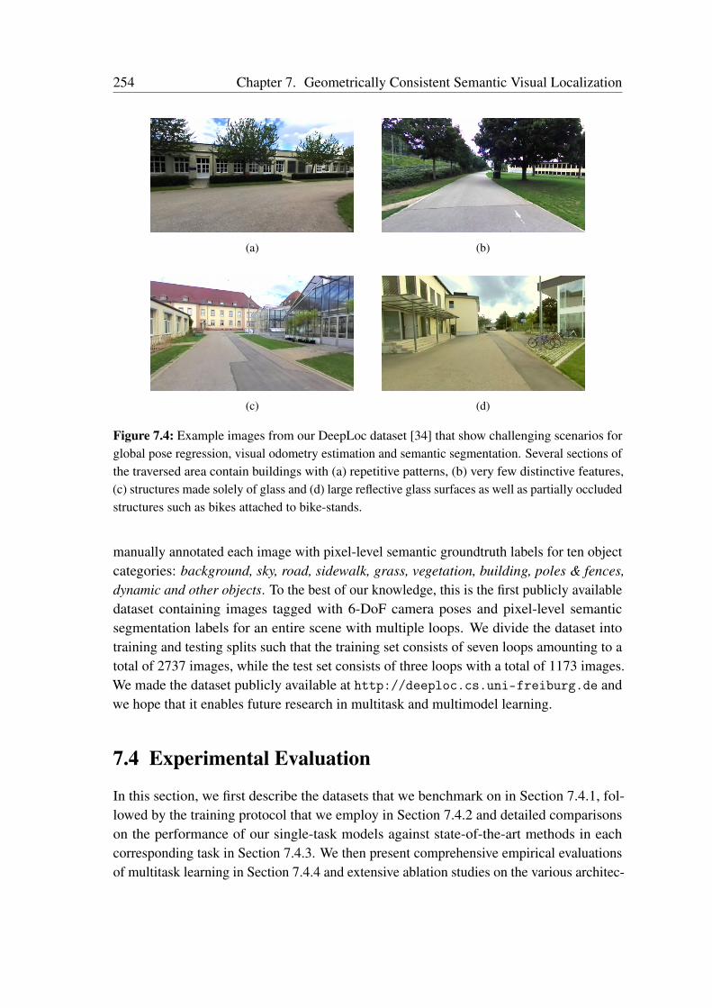
254 Chapter 7. Geometrically Consistent Semantic Visual Localization
(a) (b)
(c) (d)
Figure 7.4: Example images from our DeepLoc dataset [34] that show challenging scenarios forglobal pose regression, visual odometry estimation and semantic segmentation. Several sections ofthe traversed area contain buildings with (a) repetitive patterns, (b) very few distinctive features,(c) structures made solely of glass and (d) large reflective glass surfaces as well as partially occludedstructures such as bikes attached to bike-stands.
manually annotated each image with pixel-level semantic groundtruth labels for ten objectcategories: background, sky, road, sidewalk, grass, vegetation, building, poles & fences,dynamic and other objects. To the best of our knowledge, this is the first publicly availabledataset containing images tagged with 6-DoF camera poses and pixel-level semanticsegmentation labels for an entire scene with multiple loops. We divide the dataset intotraining and testing splits such that the training set consists of seven loops amounting to atotal of 2737 images, while the test set consists of three loops with a total of 1173 images.We made the dataset publicly available at http://deeploc.cs.uni-freiburg.de andwe hope that it enables future research in multitask and multimodel learning.
7.4 Experimental Evaluation
In this section, we first describe the datasets that we benchmark on in Section 7.4.1, fol-lowed by the training protocol that we employ in Section 7.4.2 and detailed comparisonson the performance of our single-task models against state-of-the-art methods in eachcorresponding task in Section 7.4.3. We then present comprehensive empirical evaluationsof multitask learning in Section 7.4.4 and extensive ablation studies on the various architec-
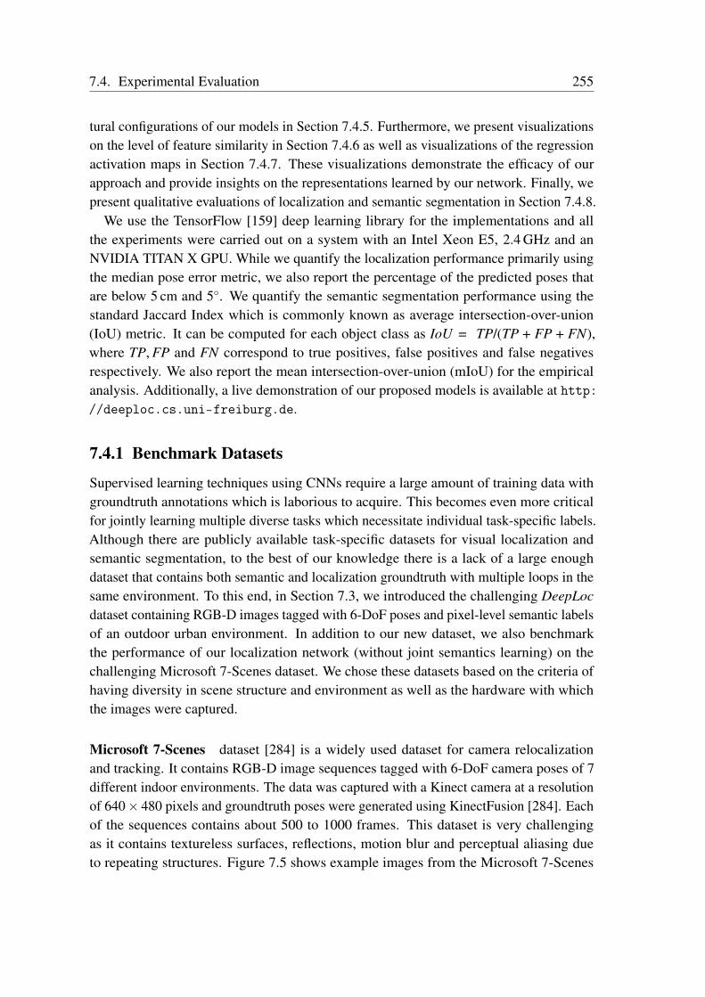
7.4. Experimental Evaluation 255
tural configurations of our models in Section 7.4.5. Furthermore, we present visualizationson the level of feature similarity in Section 7.4.6 as well as visualizations of the regressionactivation maps in Section 7.4.7. These visualizations demonstrate the efficacy of ourapproach and provide insights on the representations learned by our network. Finally, wepresent qualitative evaluations of localization and semantic segmentation in Section 7.4.8.
We use the TensorFlow [159] deep learning library for the implementations and allthe experiments were carried out on a system with an Intel Xeon E5, 2.4 GHz and anNVIDIA TITAN X GPU. While we quantify the localization performance primarily usingthe median pose error metric, we also report the percentage of the predicted poses thatare below 5 cm and 5. We quantify the semantic segmentation performance using thestandard Jaccard Index which is commonly known as average intersection-over-union(IoU) metric. It can be computed for each object class as IoU = TP/(TP + FP + FN),where TP, FP and FN correspond to true positives, false positives and false negativesrespectively. We also report the mean intersection-over-union (mIoU) for the empiricalanalysis. Additionally, a live demonstration of our proposed models is available at http://deeploc.cs.uni-freiburg.de.
7.4.1 Benchmark Datasets
Supervised learning techniques using CNNs require a large amount of training data withgroundtruth annotations which is laborious to acquire. This becomes even more criticalfor jointly learning multiple diverse tasks which necessitate individual task-specific labels.Although there are publicly available task-specific datasets for visual localization andsemantic segmentation, to the best of our knowledge there is a lack of a large enoughdataset that contains both semantic and localization groundtruth with multiple loops in thesame environment. To this end, in Section 7.3, we introduced the challenging DeepLocdataset containing RGB-D images tagged with 6-DoF poses and pixel-level semantic labelsof an outdoor urban environment. In addition to our new dataset, we also benchmarkthe performance of our localization network (without joint semantics learning) on thechallenging Microsoft 7-Scenes dataset. We chose these datasets based on the criteria ofhaving diversity in scene structure and environment as well as the hardware with whichthe images were captured.
Microsoft 7-Scenes dataset [284] is a widely used dataset for camera relocalizationand tracking. It contains RGB-D image sequences tagged with 6-DoF camera poses of 7different indoor environments. The data was captured with a Kinect camera at a resolutionof 640× 480 pixels and groundtruth poses were generated using KinectFusion [284]. Eachof the sequences contains about 500 to 1000 frames. This dataset is very challengingas it contains textureless surfaces, reflections, motion blur and perceptual aliasing dueto repeating structures. Figure 7.5 shows example images from the Microsoft 7-Scenes
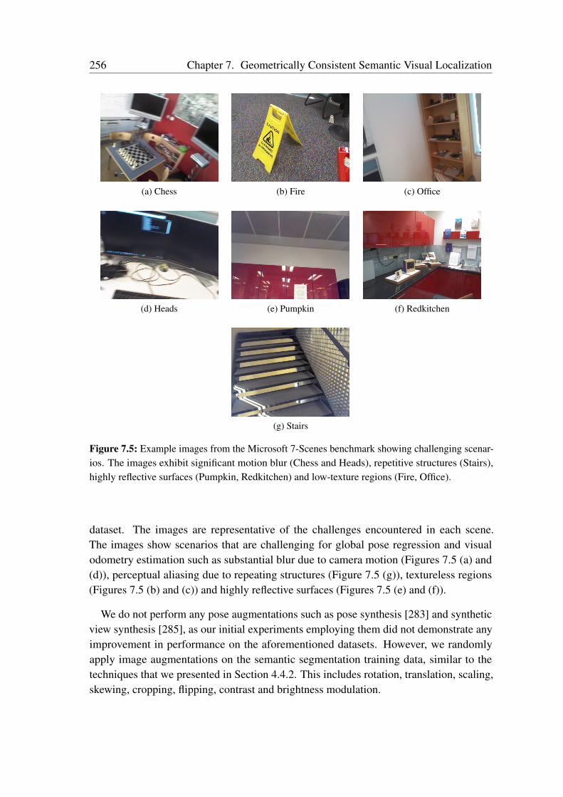
256 Chapter 7. Geometrically Consistent Semantic Visual Localization
(a) Chess (b) Fire (c) Office
(d) Heads (e) Pumpkin (f) Redkitchen
(g) Stairs
Figure 7.5: Example images from the Microsoft 7-Scenes benchmark showing challenging scenar-ios. The images exhibit significant motion blur (Chess and Heads), repetitive structures (Stairs),highly reflective surfaces (Pumpkin, Redkitchen) and low-texture regions (Fire, Office).
dataset. The images are representative of the challenges encountered in each scene.The images show scenarios that are challenging for global pose regression and visualodometry estimation such as substantial blur due to camera motion (Figures 7.5 (a) and(d)), perceptual aliasing due to repeating structures (Figure 7.5 (g)), textureless regions(Figures 7.5 (b) and (c)) and highly reflective surfaces (Figures 7.5 (e) and (f)).
We do not perform any pose augmentations such as pose synthesis [283] and syntheticview synthesis [285], as our initial experiments employing them did not demonstrate anyimprovement in performance on the aforementioned datasets. However, we randomlyapply image augmentations on the semantic segmentation training data, similar to thetechniques that we presented in Section 4.4.2. This includes rotation, translation, scaling,skewing, cropping, flipping, contrast and brightness modulation.

7.4. Experimental Evaluation 257
7.4.2 Network Training
In order to train our network on different datasets, we rescale the images maintainingthe aspect ratio such that the shorter side is of length 256 pixels. We calculate the pixel-level mean for each of the scenes in the datasets and subtract them with the input imageswhile training. We train our models from random crops of the image as it acts as agood regularizer helping the network generalize better in comparison to the syntheticaugmentation techniques and while testing, we take the center crop of the images. We usethe Adam solver for optimization with β1 = 0.9, β2 = 0.999 and ε = 10–10. We employ amulti-stage training procedure and first train task-specific models individually using aninitial learning rate of λ0 = 10–3 with a mini-batch size of 32 and a dropout probabilityof 0.2. Subsequently, we initialize the five residual blocks of our tasks-specific networkswith weights from the ResNet-50 model pre-trained on the ImageNet dataset and the otherlayers with Xavier initialization [108]. We then initialize the joint MTL architecture withweights from the best performing single-task models and train with a lower learning rateof λ0 = 10–4.
Training deep networks in an end-to-end fashion is still a challenging problem, especiallyfor tasks with limited amounts of training data. One approach to overcome this challengeis to leverage transfer learning and initialize the network with pretrained weights from thenetwork trained on a larger dataset. However, the multitask network that we propose inthis chapter is the first approach to address such wide range of tasks, therefore existingpretrained models cannot be leveraged to accelerate the training. In order to alleviate thisproblem, we investigate different weight initializations as bootstrapping methods for ourtraining architecture. Results from this experiment are presented in Section 7.4.5.7.
In order to learn a unified model and to facilitate auxiliary learning, we employ differentoptimization strategies that allow for efficient learning of shared features as well as task-specific features, namely alternate training and joint training. In alternate training we usea separate optimizer for each task and alternatively execute each task optimizer on thetask-specific loss function, thereby allowing synchronized transfer of information fromone task to the other. This instills a form of hierarchy into the tasks, as the odometry sub-network improves the estimate of its relative poses, the global pose network in turn usesthis estimate to improve its prediction. It is often theorized that this enforces commonalitybetween the tasks. The disadvantage of this approach is that a bias in the parameters isintroduced by the task that is optimized the last. In joint training on the other hand, we addeach of the task-specific loss functions and use a single optimizer to train the sub-networksat the same time. The advantage of this approach is that the tasks are trained in a way thatthey maintain the individuality of their functions, but as each of our tasks is of differentunits and scale, the task with the larger scale often dominates the training. We evaluatethe performance of our MTL model trained with different optimization strategies anddiscussed the results in Section 7.4.5.8. We train the models for a maximum of 120,000
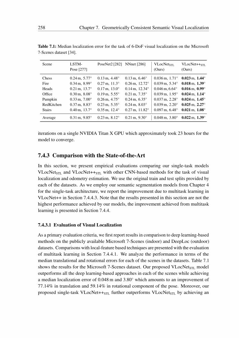
258 Chapter 7. Geometrically Consistent Semantic Visual Localization
Table 7.1: Median localization error for the task of 6-DoF visual localization on the Microsoft7-Scenes dataset [34].
Scene LSTM-Pose [277]
PoseNet2 [282] NNnet [286] VLocNetSTL
(Ours)VLocNet++STL
(Ours)
Chess 0.24 m, 5.77 0.13 m, 4.48 0.13 m, 6.46 0.036 m, 1.71 0.023 m, 1.44
Fire 0.34 m, 8.99 0.27 m, 11.3 0.26 m, 12.72 0.039 m, 5.34 0.018 m, 1.39
Heads 0.21 m, 13.7 0.17 m, 13.0 0.14 m, 12.34 0.046 m, 6.64 0.016 m, 0.99
Office 0.30 m, 8.08 0.19 m, 5.55 0.21 m, 7.35 0.039 m, 1.95 0.024 m, 1.14
Pumpkin 0.33 m, 7.00 0.26 m, 4.75 0.24 m, 6.35 0.037 m, 2.28 0.024 m, 1.45
RedKitchen 0.37 m, 8.83 0.23 m, 5.35 0.24 m, 8.03 0.039 m, 2.20 0.025 m, 2.27
Stairs 0.40 m, 13.7 0.35 m, 12.4 0.27 m, 11.82 0.097 m, 6.48 0.021 m, 1.08
Average 0.31 m, 9.85 0.23 m, 8.12 0.21 m, 9.30 0.048 m, 3.80 0.022 m, 1.39
iterations on a single NVIDIA Titan X GPU which approximately took 23 hours for themodel to converge.
7.4.3 Comparison with the State-of-the-Art
In this section, we present empirical evaluations comparing our single-task modelsVLocNetSTL and VLocNet++STL with other CNN-based methods for the task of visuallocalization and odometry estimation. We use the original train and test splits provided byeach of the datasets. As we employ our semantic segmentation models from Chapter 4for the single-task architecture, we report the improvement due to multitask learning inVLocNet++ in Section 7.4.4.3. Note that the results presented in this section are not thehighest performance achieved by our models, the improvement achieved from multitasklearning is presented in Section 7.4.4.
7.4.3.1 Evaluation of Visual Localization
As a primary evaluation criteria, we first report results in comparison to deep learning-basedmethods on the publicly available Microsoft 7-Scenes (indoor) and DeepLoc (outdoor)datasets. Comparisons with local-feature based techniques are presented with the evaluationof multitask learning in Section 7.4.4.1. We analyze the performance in terms of themedian translational and rotational errors for each of the scenes in the datasets. Table 7.1shows the results for the Microsoft 7-Scenes dataset. Our proposed VLocNetSTL modeloutperforms all the deep learning-based approaches in each of the scenes while achievinga median localization error of 0.048 m and 3.80 which amounts to an improvement of77.14% in translation and 59.14% in rotational component of the pose. Moreover, ourproposed single-task VLocNet++STL further outperforms VLocNetSTL by achieving an
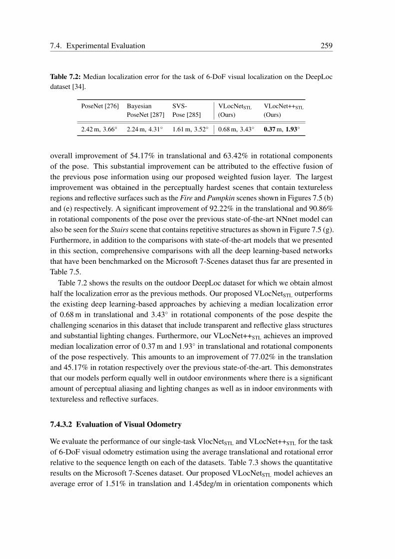
7.4. Experimental Evaluation 259
Table 7.2: Median localization error for the task of 6-DoF visual localization on the DeepLocdataset [34].
PoseNet [276] BayesianPoseNet [287]
SVS-Pose [285]
VLocNetSTL
(Ours)VLocNet++STL
(Ours)
2.42 m, 3.66 2.24 m, 4.31 1.61 m, 3.52 0.68 m, 3.43 0.37 m, 1.93
overall improvement of 54.17% in translational and 63.42% in rotational componentsof the pose. This substantial improvement can be attributed to the effective fusion ofthe previous pose information using our proposed weighted fusion layer. The largestimprovement was obtained in the perceptually hardest scenes that contain texturelessregions and reflective surfaces such as the Fire and Pumpkin scenes shown in Figures 7.5 (b)and (e) respectively. A significant improvement of 92.22% in the translational and 90.86%in rotational components of the pose over the previous state-of-the-art NNnet model canalso be seen for the Stairs scene that contains repetitive structures as shown in Figure 7.5 (g).Furthermore, in addition to the comparisons with state-of-the-art models that we presentedin this section, comprehensive comparisons with all the deep learning-based networksthat have been benchmarked on the Microsoft 7-Scenes dataset thus far are presented inTable 7.5.
Table 7.2 shows the results on the outdoor DeepLoc dataset for which we obtain almosthalf the localization error as the previous methods. Our proposed VLocNetSTL outperformsthe existing deep learning-based approaches by achieving a median localization errorof 0.68 m in translational and 3.43 in rotational components of the pose despite thechallenging scenarios in this dataset that include transparent and reflective glass structuresand substantial lighting changes. Furthermore, our VLocNet++STL achieves an improvedmedian localization error of 0.37 m and 1.93 in translational and rotational componentsof the pose respectively. This amounts to an improvement of 77.02% in the translationand 45.17% in rotation respectively over the previous state-of-the-art. This demonstratesthat our models perform equally well in outdoor environments where there is a significantamount of perceptual aliasing and lighting changes as well as in indoor environments withtextureless and reflective surfaces.
7.4.3.2 Evaluation of Visual Odometry
We evaluate the performance of our single-task VlocNetSTL and VLocNet++STL for the taskof 6-DoF visual odometry estimation using the average translational and rotational errorrelative to the sequence length on each of the datasets. Table 7.3 shows the quantitativeresults on the Microsoft 7-Scenes dataset. Our proposed VLocNetSTL model achieves anaverage error of 1.51% in translation and 1.45deg/m in orientation components which
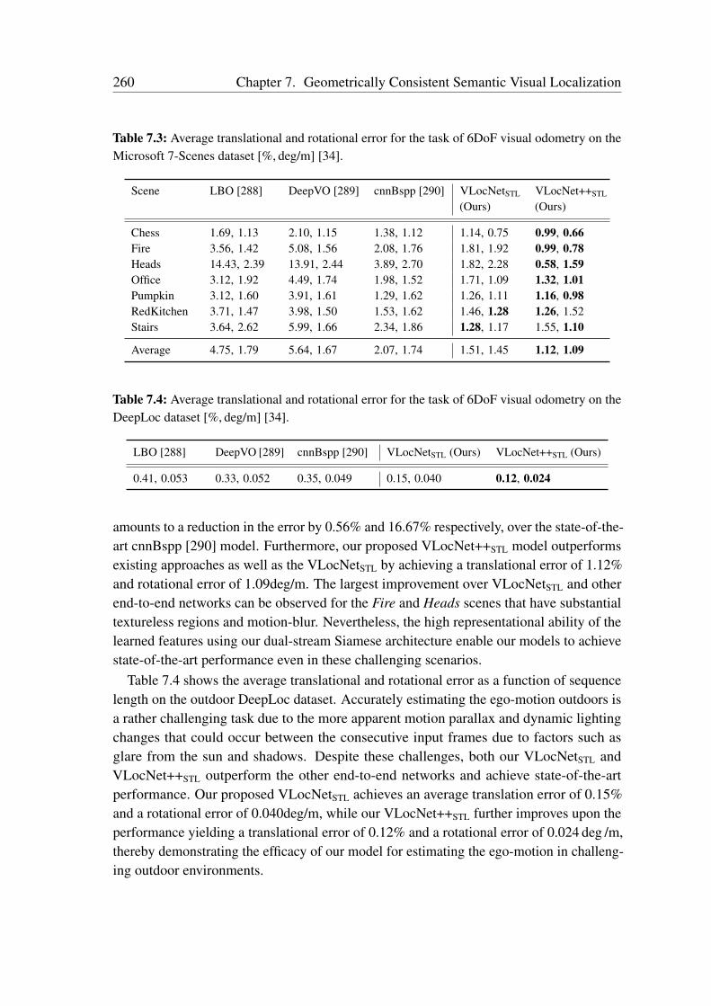
260 Chapter 7. Geometrically Consistent Semantic Visual Localization
Table 7.3: Average translational and rotational error for the task of 6DoF visual odometry on theMicrosoft 7-Scenes dataset [%, deg/m] [34].
Scene LBO [288] DeepVO [289] cnnBspp [290] VLocNetSTL
(Ours)VLocNet++STL
(Ours)
Chess 1.69, 1.13 2.10, 1.15 1.38, 1.12 1.14, 0.75 0.99, 0.66Fire 3.56, 1.42 5.08, 1.56 2.08, 1.76 1.81, 1.92 0.99, 0.78Heads 14.43, 2.39 13.91, 2.44 3.89, 2.70 1.82, 2.28 0.58, 1.59Office 3.12, 1.92 4.49, 1.74 1.98, 1.52 1.71, 1.09 1.32, 1.01Pumpkin 3.12, 1.60 3.91, 1.61 1.29, 1.62 1.26, 1.11 1.16, 0.98RedKitchen 3.71, 1.47 3.98, 1.50 1.53, 1.62 1.46, 1.28 1.26, 1.52Stairs 3.64, 2.62 5.99, 1.66 2.34, 1.86 1.28, 1.17 1.55, 1.10
Average 4.75, 1.79 5.64, 1.67 2.07, 1.74 1.51, 1.45 1.12, 1.09
Table 7.4: Average translational and rotational error for the task of 6DoF visual odometry on theDeepLoc dataset [%, deg/m] [34].
LBO [288] DeepVO [289] cnnBspp [290] VLocNetSTL (Ours) VLocNet++STL (Ours)
0.41, 0.053 0.33, 0.052 0.35, 0.049 0.15, 0.040 0.12, 0.024
amounts to a reduction in the error by 0.56% and 16.67% respectively, over the state-of-the-art cnnBspp [290] model. Furthermore, our proposed VLocNet++STL model outperformsexisting approaches as well as the VLocNetSTL by achieving a translational error of 1.12%and rotational error of 1.09deg/m. The largest improvement over VLocNetSTL and otherend-to-end networks can be observed for the Fire and Heads scenes that have substantialtextureless regions and motion-blur. Nevertheless, the high representational ability of thelearned features using our dual-stream Siamese architecture enable our models to achievestate-of-the-art performance even in these challenging scenarios.
Table 7.4 shows the average translational and rotational error as a function of sequencelength on the outdoor DeepLoc dataset. Accurately estimating the ego-motion outdoors isa rather challenging task due to the more apparent motion parallax and dynamic lightingchanges that could occur between the consecutive input frames due to factors such asglare from the sun and shadows. Despite these challenges, both our VLocNetSTL andVLocNet++STL outperform the other end-to-end networks and achieve state-of-the-artperformance. Our proposed VLocNetSTL achieves an average translation error of 0.15%and a rotational error of 0.040deg/m, while our VLocNet++STL further improves upon theperformance yielding a translational error of 0.12% and a rotational error of 0.024 deg /m,thereby demonstrating the efficacy of our model for estimating the ego-motion in challeng-ing outdoor environments.
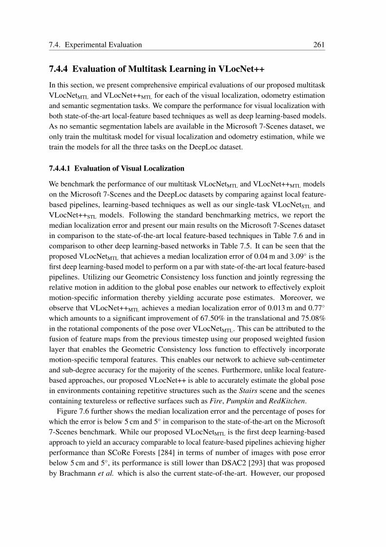
7.4. Experimental Evaluation 261
7.4.4 Evaluation of Multitask Learning in VLocNet++
In this section, we present comprehensive empirical evaluations of our proposed multitaskVLocNetMTL and VLocNet++MTL for each of the visual localization, odometry estimationand semantic segmentation tasks. We compare the performance for visual localization withboth state-of-the-art local-feature based techniques as well as deep learning-based models.As no semantic segmentation labels are available in the Microsoft 7-Scenes dataset, weonly train the multitask model for visual localization and odometry estimation, while wetrain the models for all the three tasks on the DeepLoc dataset.
7.4.4.1 Evaluation of Visual Localization
We benchmark the performance of our multitask VLocNetMTL and VLocNet++MTL modelson the Microsoft 7-Scenes and the DeepLoc datasets by comparing against local feature-based pipelines, learning-based techniques as well as our single-task VLocNetSTL andVLocNet++STL models. Following the standard benchmarking metrics, we report themedian localization error and present our main results on the Microsoft 7-Scenes datasetin comparison to the state-of-the-art local feature-based techniques in Table 7.6 and incomparison to other deep learning-based networks in Table 7.5. It can be seen that theproposed VLocNetMTL that achieves a median localization error of 0.04 m and 3.09 is thefirst deep learning-based model to perform on a par with state-of-the-art local feature-basedpipelines. Utilizing our Geometric Consistency loss function and jointly regressing therelative motion in addition to the global pose enables our network to effectively exploitmotion-specific information thereby yielding accurate pose estimates. Moreover, weobserve that VLocNet++MTL achieves a median localization error of 0.013 m and 0.77
which amounts to a significant improvement of 67.50% in the translational and 75.08%in the rotational components of the pose over VLocNetMTL. This can be attributed to thefusion of feature maps from the previous timestep using our proposed weighted fusionlayer that enables the Geometric Consistency loss function to effectively incorporatemotion-specific temporal features. This enables our network to achieve sub-centimeterand sub-degree accuracy for the majority of the scenes. Furthermore, unlike local feature-based approaches, our proposed VLocNet++ is able to accurately estimate the global posein environments containing repetitive structures such as the Stairs scene and the scenescontaining textureless or reflective surfaces such as Fire, Pumpkin and RedKitchen.
Figure 7.6 further shows the median localization error and the percentage of poses forwhich the error is below 5 cm and 5 in comparison to the state-of-the-art on the Microsoft7-Scenes benchmark. While our proposed VLocNetMTL is the first deep learning-basedapproach to yield an accuracy comparable to local feature-based pipelines achieving higherperformance than SCoRe Forests [284] in terms of number of images with pose errorbelow 5 cm and 5, its performance is still lower than DSAC2 [293] that was proposedby Brachmann et al. which is also the current state-of-the-art. However, our proposed
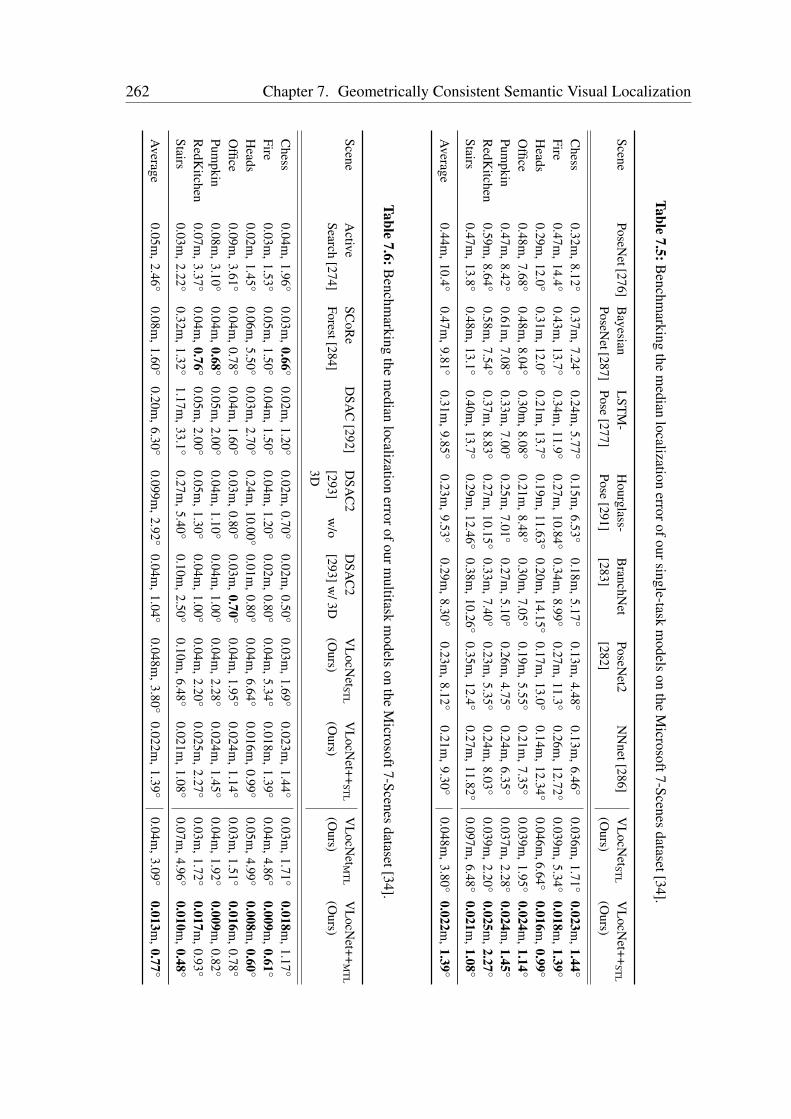
262 Chapter 7. Geometrically Consistent Semantic Visual Localization
Table7.5:B
enchmarking
them
edianlocalization
errorofoursingle-taskm
odelson
theM
icrosoft7-Scenesdataset[34].
ScenePoseN
et[276]B
ayesianL
STM
-H
ourglass-B
ranchNet
PoseNet2
NN
net[286]V
LocN
etSTL
VL
ocNet++
STL
PoseNet[287]
Pose[277]
Pose[291]
[283][282]
(Ours)
(Ours)
Chess
0.32m,8.12
0.37m
,7.24
0.24m,5.77
0.15m
,6.53
0.18m,5.17
0.13m
,4.48
0.13m,6.46
0.036m
,1.71
0.023m,1.44
Fire0.47m
,14.4
0.43m,13.7
0.34m
,11.9
0.27m,10.84
0.34m
,8.99
0.27m,11.3
0.26m
,12.72
0.039m,5.34
0.018m
,1.39
Heads
0.29m,12.0
0.31m
,12.0
0.21m,13.7
0.19m
,11.63
0.20m,14.15
0.17m
,13.0
0.14m,12.34
0.046m
,6.64
0.016m,0.99
Office
0.48m,7.68
0.48m
,8.04
0.30m,8.08
0.21m
,8.48
0.30m,7.05
0.19m
,5.55
0.21m,7.35
0.039m
,1.95
0.024m,1.14
Pumpkin
0.47m,8.42
0.61m
,7.08
0.33m,7.00
0.25m
,7.01
0.27m,5.10
0.26m
,4.75
0.24m,6.35
0.037m
,2.28
0.024m,1.45
RedK
itchen0.59m
,8.64
0.58m,7.54
0.37m
,8.83
0.27m,10.15
0.33m
,7.40
0.23m,5.35
0.24m
,8.03
0.039m,2.20
0.025m
,2.27
Stairs0.47m
,13.8
0.48m,13.1
0.40m
,13.7
0.29m,12.46
0.38m
,10.26
0.35m,12.4
0.27m
,11.82
0.097m,6.48
0.021m
,1.08
Average
0.44m,10.4
0.47m
,9.81
0.31m,9.85
0.23m
,9.53
0.29m,8.30
0.23m
,8.12
0.21m,9.30
0.048m
,3.80
0.022m,1.39
Table7.6:B
enchmarking
them
edianlocalization
errorofourmultitask
models
onthe
Microsoft7-Scenes
dataset[34].
SceneA
ctiveSC
oRe
DSA
C[292]
DSA
C2
DSA
C2
VL
ocNetST
LV
LocNet++
STL
VLocN
etMT
LV
LocNet++
MT
L
Search[274]
Forest[284][293]
w/o
3D[293]w
/3D(O
urs)(O
urs)(O
urs)(O
urs)
Chess
0.04m,1.96
0.03m
,0.66
0.02m,1.20
0.02m
,0.70
0.02m,0.50
0.03m
,1.69
0.023m,1.44
0.03m
,1.71
0.018m,1.17
Fire0.03m
,1.53
0.05m,1.50
0.04m
,1.50
0.04m,1.20
0.02m
,0.80
0.04m,5.34
0.018m
,1.39
0.04m,4.86
0.009m
,0.61
Heads
0.02m,1.45
0.06m
,5.50
0.03m,2.70
0.24m
,10.00
0.01m,0.80
0.04m
,6.64
0.016m,0.99
0.05m
,4.99
0.008m,0.60
Office
0.09m,3.61
0.04m
,0.78
0.04m,1.60
0.03m
,0.80
0.03m,0.70
0.04m
,1.95
0.024m,1.14
0.03m
,1.51
0.016m,0.78
Pumpkin
0.08m,3.10
0.04m
,0.68
0.05m,2.00
0.04m
,1.10
0.04m,1.00
0.04m
,2.28
0.024m,1.45
0.04m
,1.92
0.009m,0.82
RedK
itchen0.07m
,3.37
0.04m,0.76
0.05m
,2.00
0.05m,1.30
0.04m
,1.00
0.04m,2.20
0.025m
,2.27
0.03m,1.72
0.017m
,0.93
Stairs0.03m
,2.22
0.32m,1.32
1.17m
,33.1
0.27m,5.40
0.10m
,2.50
0.10m,6.48
0.021m
,1.08
0.07m,4.96
0.010m
,0.48
Average
0.05m,2.46
0.08m
,1.60
0.20m,6.30
0.099m
,2.92
0.04m,1.04
0.048m
,3.80
0.022m,1.39
0.04m
,3.09
0.013m,0.77
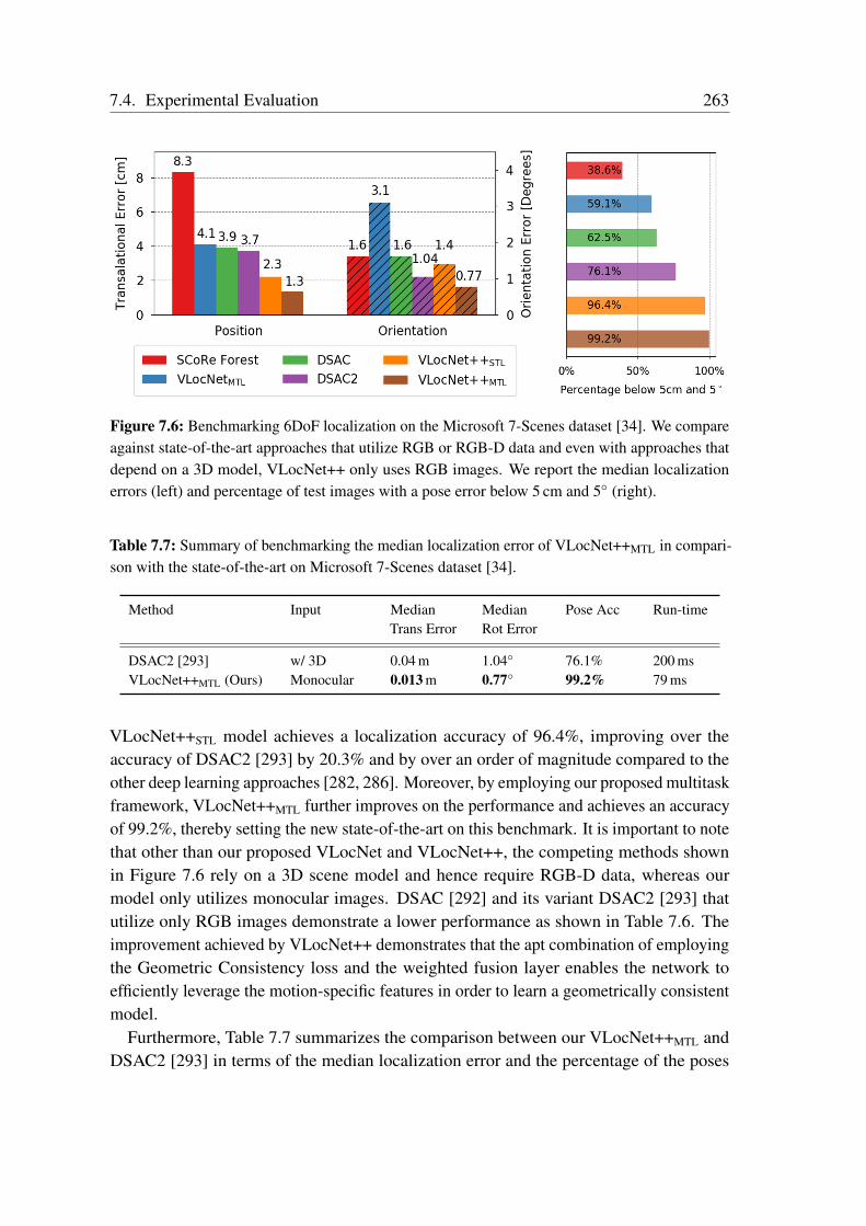
7.4. Experimental Evaluation 263
Figure 7.6: Benchmarking 6DoF localization on the Microsoft 7-Scenes dataset [34]. We compareagainst state-of-the-art approaches that utilize RGB or RGB-D data and even with approaches thatdepend on a 3D model, VLocNet++ only uses RGB images. We report the median localizationerrors (left) and percentage of test images with a pose error below 5 cm and 5 (right).
Table 7.7: Summary of benchmarking the median localization error of VLocNet++MTL in compari-son with the state-of-the-art on Microsoft 7-Scenes dataset [34].
Method Input MedianTrans Error
MedianRot Error
Pose Acc Run-time
DSAC2 [293] w/ 3D 0.04 m 1.04 76.1% 200 msVLocNet++MTL (Ours) Monocular 0.013 m 0.77 99.2% 79 ms
VLocNet++STL model achieves a localization accuracy of 96.4%, improving over theaccuracy of DSAC2 [293] by 20.3% and by over an order of magnitude compared to theother deep learning approaches [282, 286]. Moreover, by employing our proposed multitaskframework, VLocNet++MTL further improves on the performance and achieves an accuracyof 99.2%, thereby setting the new state-of-the-art on this benchmark. It is important to notethat other than our proposed VLocNet and VLocNet++, the competing methods shownin Figure 7.6 rely on a 3D scene model and hence require RGB-D data, whereas ourmodel only utilizes monocular images. DSAC [292] and its variant DSAC2 [293] thatutilize only RGB images demonstrate a lower performance as shown in Table 7.6. Theimprovement achieved by VLocNet++ demonstrates that the apt combination of employingthe Geometric Consistency loss and the weighted fusion layer enables the network toefficiently leverage the motion-specific features in order to learn a geometrically consistentmodel.
Furthermore, Table 7.7 summarizes the comparison between our VLocNet++MTL andDSAC2 [293] in terms of the median localization error and the percentage of the poses

264 Chapter 7. Geometrically Consistent Semantic Visual Localization
Table 7.8: Benchmarking the median localization error of our multitask models on the DeepLocdataset [34].
PoseNet[276]
Bay. PoseNet[287]
SVS-Pose[285]
VLocNetSTL
(Ours)VLocNet++STL
(Ours)VLocNetMTL
(Ours)VLocNet++MTL
(Ours)
2.42m, 3.66 2.24m, 4.31 1.61m, 3.52 0.68m, 3.43 0.37m, 1.93 0.47m, 2.38 0.32m, 1.48
with localization error below 5 cm and 5 denoted by pose accuracy. It can be seen thatour proposed model exceeds the state-of-the-art by 67.5% in the translational and 25.9%in the rotational components of the pose. Unlike DSAC2, our proposed approach doesnot require a 3D model of the scene which facilitates ease of deployment, in additionto occupying less storage space for the model. While achieving accurate pose estimatesis crucial for any localization approach, the run-time requirements and complexity ofdeploying the models play an important role in its ease of deployment in the real-world onvarious robotic systems. Our proposed VLocNet++MTL model only requires 79 ms for aforward-pass on a single consumer grade GPU versus the 200 ms consumed by DSAC2which makes VLocNet++ 60.5% faster. This renders our method well suited for real-timedeployment in an online manner, as well as in resource constrained platforms.
Table 7.8 shows the performance of our multitask VLocNetMTL and VLocNet++MTL onthe DeepLoc dataset. Although our proposed single-task models outperform the the otherdeep learning networks by a large margin, our multitask VLocNetMTL further improvesupon the performance and achieves a median localization error of 0.47 m and 2.38 whichamounts to an improvement of 70.81% in translational and 32.39% in rotational compo-nents of the pose while compared to the best performing SVS-Pose [285] network. Eventhough perceptual aliasing is more apparent outdoors than indoors, this large improvementdemonstrates that our Geometric Consistency loss function is as effective at aggregatingmotion-specific information outdoors as indoors. Furthermore, our VLocNet++MTL modelthat simultaneously encodes geometric and semantic knowledge of the environment intothe pose regression network achieves a median localization error of 0.32 m and 1.48
thereby setting the new state-of-the-art on this benchmark. This amounts to an improve-ment of 31.91% and 37.81% in translation and rotation respectively, over VLocNetMTL
which signifies that our proposed weighted fusion layer enables our network to aggregatemotion-specific temporal information as well as effectively encode semantic constraints tolearn a geometric and structure-aware pose regression model.
7.4.4.2 Evaluation of Visual Odometry
In this section, we evaluate the performance of our multitask models for the task of visualodometry estimation and report the average translation and orientation error as a function
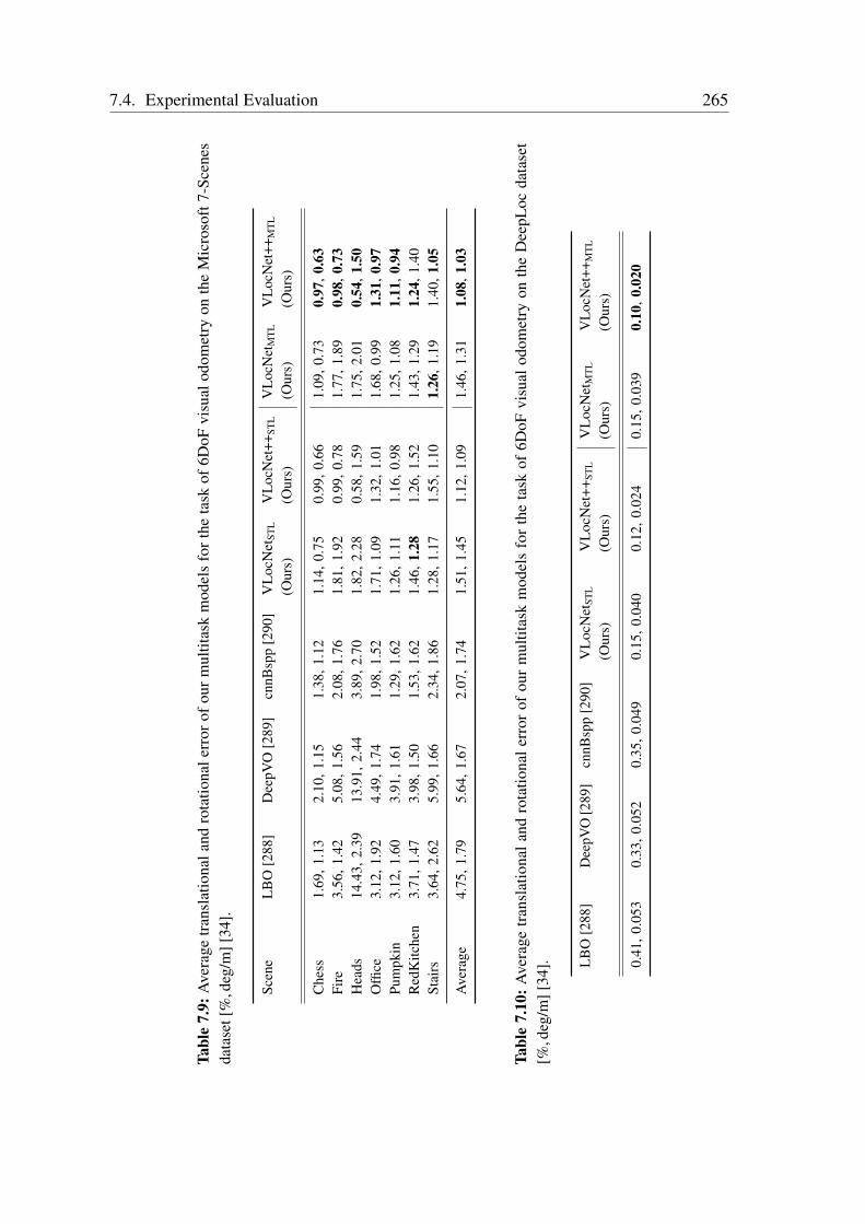
7.4. Experimental Evaluation 265
Tabl
e7.
9:A
vera
getr
ansl
atio
nala
ndro
tatio
nale
rror
ofou
rm
ultit
ask
mod
els
for
the
task
of6D
oFvi
sual
odom
etry
onth
eM
icro
soft
7-Sc
enes
data
set[
%,d
eg/m
][34
].
Scen
eL
BO
[288
]D
eepV
O[2
89]
cnnB
spp
[290
]V
Loc
Net
STL
(Our
s)V
LocN
et++
STL
(Our
s)V
LocN
etM
TL
(Our
s)V
LocN
et++
MT
L
(Our
s)
Che
ss1.
69,1
.13
2.10
,1.1
51.
38,1
.12
1.14
,0.7
50.
99,0
.66
1.09
,0.7
30.
97,0
.63
Fire
3.56
,1.4
25.
08,1
.56
2.08
,1.7
61.
81,1
.92
0.99
,0.7
81.
77,1
.89
0.98
,0.7
3H
eads
14.4
3,2.
3913
.91,
2.44
3.89
,2.7
01.
82,2
.28
0.58
,1.5
91.
75,2
.01
0.54
,1.5
0O
ffice
3.12
,1.9
24.
49,1
.74
1.98
,1.5
21.
71,1
.09
1.32
,1.0
11.
68,0
.99
1.31
,0.9
7Pu
mpk
in3.
12,1
.60
3.91
,1.6
11.
29,1
.62
1.26
,1.1
11.
16,0
.98
1.25
,1.0
81.
11,0
.94
Red
Kitc
hen
3.71
,1.4
73.
98,1
.50
1.53
,1.6
21.
46,1
.28
1.26
,1.5
21.
43,1
.29
1.24
,1.4
0St
airs
3.64
,2.6
25.
99,1
.66
2.34
,1.8
61.
28,1
.17
1.55
,1.1
01.
26,1
.19
1.40
,1.0
5
Ave
rage
4.75
,1.7
95.
64,1
.67
2.07
,1.7
41.
51,1
.45
1.12
,1.0
91.
46,1
.31
1.08
,1.0
3
Tabl
e7.
10:A
vera
getr
ansl
atio
nala
ndro
tatio
nale
rror
ofou
rm
ultit
ask
mod
els
for
the
task
of6D
oFvi
sual
odom
etry
onth
eD
eepL
ocda
tase
t[%
,deg
/m][
34]. L
BO
[288
]D
eepV
O[2
89]
cnnB
spp
[290
]V
Loc
Net
STL
(Our
s)V
Loc
Net
++ST
L
(Our
s)V
Loc
Net
MT
L
(Our
s)V
LocN
et++
MT
L
(Our
s)
0.41
,0.0
530.
33,0
.052
0.35
,0.0
490.
15,0
.040
0.12
,0.0
240.
15,0
.039
0.10
,0.0
20
266 Chapter 7. Geometrically Consistent Semantic Visual Localization
of the trajectory length for each of the scenes in the datasets. Table 7.9 shows the resultson the Microsoft 7-Scenes benchmark where our proposed VLocNetMTL outperforms allthe other deep learning-based approaches and achieves an average error of 1.46% and1.31deg/m in translation and orientation components respectively. This demonstrates thatby jointly learning to regress the relative motion along with the global pose benefits bothtasks and enables the joint model to outperform their single-task counterparts. Additionally,our VLocNet++MTL further improves upon the performance and achieves an average errorof 1.08% in translation and 1.03deg/m in orientation, thereby outperforming each of thesingle-task models and the other deep learning-based methods, while setting the state-of-the-art on this dataset. Our model is able to better estimate the relative motion by sharingrepresentations with the global pose regression stream which enables it to learn temporallyinvariant features which can be used to accurately estimate the relative motion betweenthe input frames, while being robust to motion blur, textureless regions and repetitivestructures in the scene.
We observe a similar trend from the experimental comparisons on the outdoor DeepLocdataset shown in Table 7.10, where both our multitask models outperform their single-task counterparts as well the other deep learning-based networks. Our VLocNet++MTL
achieves state-of-the-art performance with an average error of 0.10% and 0.020deg/m forthe translation and orientation components, which is an improvement of 0.25% and 59.18%respectively, over the best performing cnnBspp [290] network. An improvement of thisscale is especially hard to obtain in outdoor environments due to several factors such asareas with very similar appearance as shown in Figure 7.4 (a), glass structures that causereflections as shown in Figure 7.4 (c) and variable lighting conditions between the consec-utive input images. Despite these factors our proposed models yield reliable performancein challenging outdoor environments demonstrating the efficacy of our multitask leaningscheme.
7.4.4.3 Evaluation of Semantic Segmentation
We present comprehensive empirical evaluations for the task of semantic segmentationusing our proposed VLocNet++MTL model that is built upon the topology of our AdapNet++architecture as well as the VLocNet++(base) variant that is built upon the topology of ourAdapNet architecture. We present results on the DeepLoc dataset and report the Intersectionover Union (IoU) score for each of the individual object categories as well as the meanIoU. We benchmark the performance of our model against several state-of-the-art networksincluding FCN-8s [24], SegNet [136], UpNet [48], ParseNet [168], DeepLab v2 [138] andDeepLab v3 [132]. We also compare with the performance of AdapNet and AdapNet++that we presented in Chapter 4. Results from this experiment are shown in Table 7.11.
Our proposed VLocNet++(base) model achieves a mIoU score of 80.44%, therebyoutperforming the other baseline models in the overall mIoU score as well as consistently
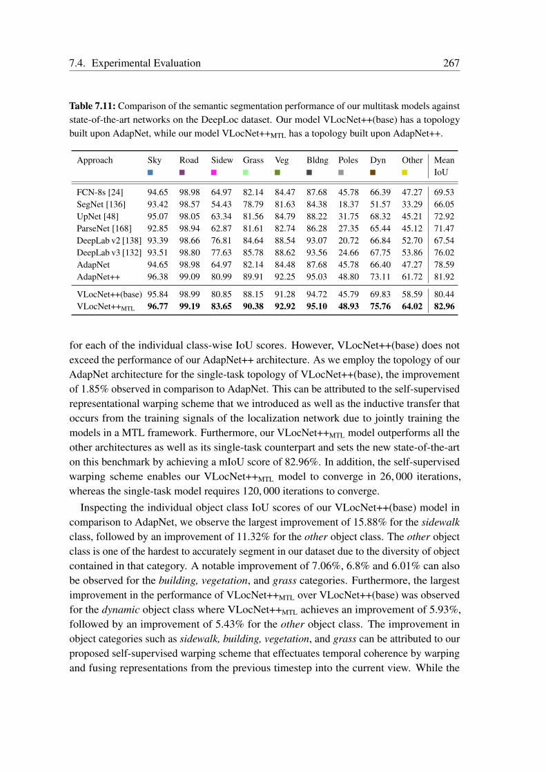
7.4. Experimental Evaluation 267
Table 7.11: Comparison of the semantic segmentation performance of our multitask models againststate-of-the-art networks on the DeepLoc dataset. Our model VLocNet++(base) has a topologybuilt upon AdapNet, while our model VLocNet++MTL has a topology built upon AdapNet++.
Approach Sky Road Sidew Grass Veg Bldng Poles Dyn Other MeanIoU
FCN-8s [24] 94.65 98.98 64.97 82.14 84.47 87.68 45.78 66.39 47.27 69.53SegNet [136] 93.42 98.57 54.43 78.79 81.63 84.38 18.37 51.57 33.29 66.05UpNet [48] 95.07 98.05 63.34 81.56 84.79 88.22 31.75 68.32 45.21 72.92ParseNet [168] 92.85 98.94 62.87 81.61 82.74 86.28 27.35 65.44 45.12 71.47DeepLab v2 [138] 93.39 98.66 76.81 84.64 88.54 93.07 20.72 66.84 52.70 67.54DeepLab v3 [132] 93.51 98.80 77.63 85.78 88.62 93.56 24.66 67.75 53.86 76.02AdapNet 94.65 98.98 64.97 82.14 84.48 87.68 45.78 66.40 47.27 78.59AdapNet++ 96.38 99.09 80.99 89.91 92.25 95.03 48.80 73.11 61.72 81.92
VLocNet++(base) 95.84 98.99 80.85 88.15 91.28 94.72 45.79 69.83 58.59 80.44VLocNet++MTL 96.77 99.19 83.65 90.38 92.92 95.10 48.93 75.76 64.02 82.96
for each of the individual class-wise IoU scores. However, VLocNet++(base) does notexceed the performance of our AdapNet++ architecture. As we employ the topology of ourAdapNet architecture for the single-task topology of VLocNet++(base), the improvementof 1.85% observed in comparison to AdapNet. This can be attributed to the self-supervisedrepresentational warping scheme that we introduced as well as the inductive transfer thatoccurs from the training signals of the localization network due to jointly training themodels in a MTL framework. Furthermore, our VLocNet++MTL model outperforms all theother architectures as well as its single-task counterpart and sets the new state-of-the-arton this benchmark by achieving a mIoU score of 82.96%. In addition, the self-supervisedwarping scheme enables our VLocNet++MTL model to converge in 26, 000 iterations,whereas the single-task model requires 120, 000 iterations to converge.
Inspecting the individual object class IoU scores of our VLocNet++(base) model incomparison to AdapNet, we observe the largest improvement of 15.88% for the sidewalkclass, followed by an improvement of 11.32% for the other object class. The other objectclass is one of the hardest to accurately segment in our dataset due to the diversity of objectcontained in that category. A notable improvement of 7.06%, 6.8% and 6.01% can alsobe observed for the building, vegetation, and grass categories. Furthermore, the largestimprovement in the performance of VLocNet++MTL over VLocNet++(base) was observedfor the dynamic object class where VLocNet++MTL achieves an improvement of 5.93%,followed by an improvement of 5.43% for the other object class. The improvement inobject categories such as sidewalk, building, vegetation, and grass can be attributed to ourproposed self-supervised warping scheme that effectuates temporal coherence by warpingand fusing representations from the previous timestep into the current view. While the
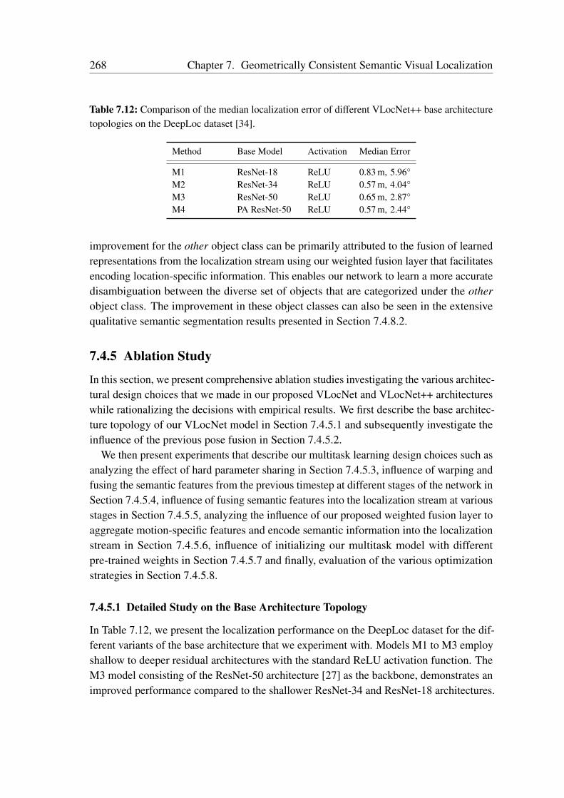
268 Chapter 7. Geometrically Consistent Semantic Visual Localization
Table 7.12: Comparison of the median localization error of different VLocNet++ base architecturetopologies on the DeepLoc dataset [34].
Method Base Model Activation Median Error
M1 ResNet-18 ReLU 0.83 m, 5.96
M2 ResNet-34 ReLU 0.57 m, 4.04
M3 ResNet-50 ReLU 0.65 m, 2.87
M4 PA ResNet-50 ReLU 0.57 m, 2.44
improvement for the other object class can be primarily attributed to the fusion of learnedrepresentations from the localization stream using our weighted fusion layer that facilitatesencoding location-specific information. This enables our network to learn a more accuratedisambiguation between the diverse set of objects that are categorized under the otherobject class. The improvement in these object classes can also be seen in the extensivequalitative semantic segmentation results presented in Section 7.4.8.2.
7.4.5 Ablation Study
In this section, we present comprehensive ablation studies investigating the various architec-tural design choices that we made in our proposed VLocNet and VLocNet++ architectureswhile rationalizing the decisions with empirical results. We first describe the base architec-ture topology of our VLocNet model in Section 7.4.5.1 and subsequently investigate theinfluence of the previous pose fusion in Section 7.4.5.2.
We then present experiments that describe our multitask learning design choices such asanalyzing the effect of hard parameter sharing in Section 7.4.5.3, influence of warping andfusing the semantic features from the previous timestep at different stages of the network inSection 7.4.5.4, influence of fusing semantic features into the localization stream at variousstages in Section 7.4.5.5, analyzing the influence of our proposed weighted fusion layer toaggregate motion-specific features and encode semantic information into the localizationstream in Section 7.4.5.6, influence of initializing our multitask model with differentpre-trained weights in Section 7.4.5.7 and finally, evaluation of the various optimizationstrategies in Section 7.4.5.8.
7.4.5.1 Detailed Study on the Base Architecture Topology
In Table 7.12, we present the localization performance on the DeepLoc dataset for the dif-ferent variants of the base architecture that we experiment with. Models M1 to M3 employshallow to deeper residual architectures with the standard ReLU activation function. TheM3 model consisting of the ResNet-50 architecture [27] as the backbone, demonstrates animproved performance compared to the shallower ResNet-34 and ResNet-18 architectures.
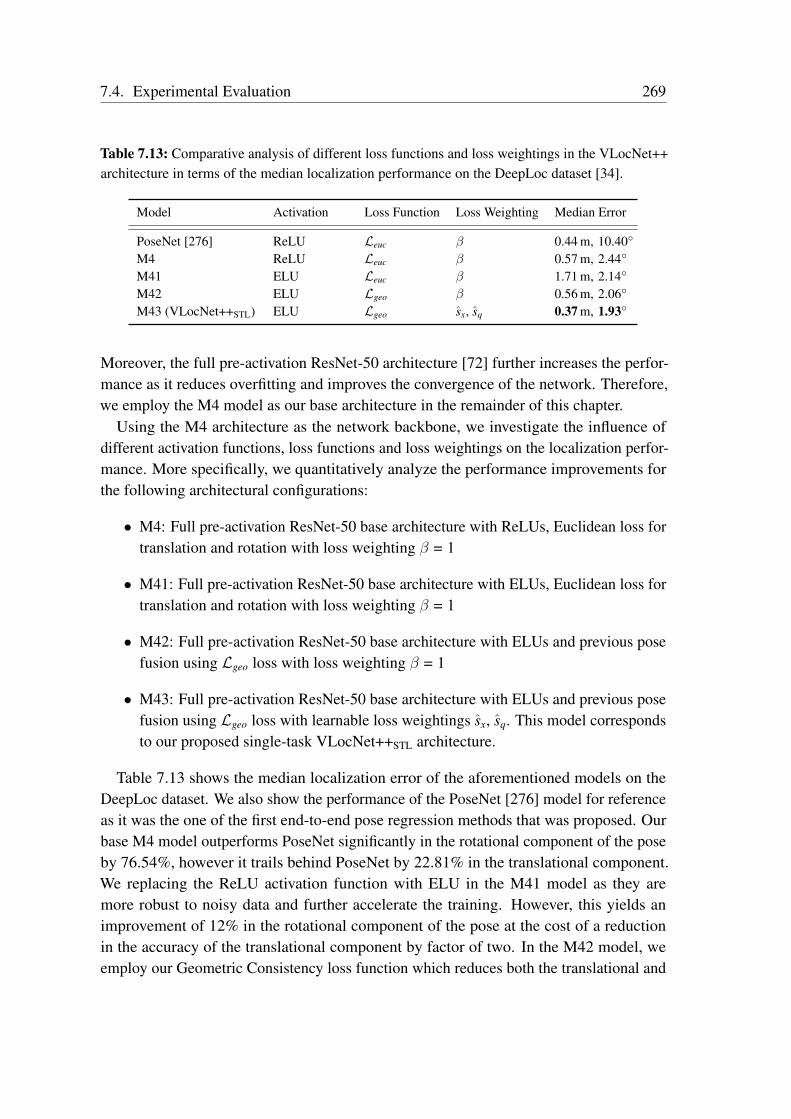
7.4. Experimental Evaluation 269
Table 7.13: Comparative analysis of different loss functions and loss weightings in the VLocNet++architecture in terms of the median localization performance on the DeepLoc dataset [34].
Model Activation Loss Function Loss Weighting Median Error
PoseNet [276] ReLU Leuc β 0.44 m, 10.40
M4 ReLU Leuc β 0.57 m, 2.44
M41 ELU Leuc β 1.71 m, 2.14
M42 ELU Lgeo β 0.56 m, 2.06
M43 (VLocNet++STL) ELU Lgeo sx, sq 0.37 m, 1.93
Moreover, the full pre-activation ResNet-50 architecture [72] further increases the perfor-mance as it reduces overfitting and improves the convergence of the network. Therefore,we employ the M4 model as our base architecture in the remainder of this chapter.
Using the M4 architecture as the network backbone, we investigate the influence ofdifferent activation functions, loss functions and loss weightings on the localization perfor-mance. More specifically, we quantitatively analyze the performance improvements forthe following architectural configurations:
• M4: Full pre-activation ResNet-50 base architecture with ReLUs, Euclidean loss fortranslation and rotation with loss weighting β = 1
• M41: Full pre-activation ResNet-50 base architecture with ELUs, Euclidean loss fortranslation and rotation with loss weighting β = 1
• M42: Full pre-activation ResNet-50 base architecture with ELUs and previous posefusion using Lgeo loss with loss weighting β = 1
• M43: Full pre-activation ResNet-50 base architecture with ELUs and previous posefusion using Lgeo loss with learnable loss weightings sx, sq. This model correspondsto our proposed single-task VLocNet++STL architecture.
Table 7.13 shows the median localization error of the aforementioned models on theDeepLoc dataset. We also show the performance of the PoseNet [276] model for referenceas it was the one of the first end-to-end pose regression methods that was proposed. Ourbase M4 model outperforms PoseNet significantly in the rotational component of the poseby 76.54%, however it trails behind PoseNet by 22.81% in the translational component.We replacing the ReLU activation function with ELU in the M41 model as they aremore robust to noisy data and further accelerate the training. However, this yields animprovement of 12% in the rotational component of the pose at the cost of a reductionin the accuracy of the translational component by factor of two. In the M42 model, weemploy our Geometric Consistency loss function which reduces both the translational and
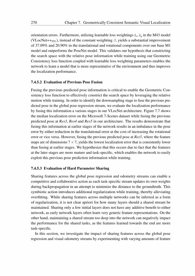
270 Chapter 7. Geometrically Consistent Semantic Visual Localization
orientation errors. Furthermore, utilizing learnable loss weightings sx, sq in the M43 model(VLocNet++STL), instead of the constant weighting β, yields a substantial improvementof 37.09% and 20.90% in the translational and rotational components over our base M1model and outperforms the PoseNet model. This validates our hypothesis that constrictingthe search space with the relative pose information while training using our GeometricConsistency loss function coupled with learnable loss weighting parameters enables thenetwork to learn a model that is more representative of the environment and thus improvesthe localization performance.
7.4.5.2 Evaluation of Previous Pose Fusion
Fusing the previous predicted pose information is critical to enable the Geometric Con-sistency loss function to effectively constrict the search space by leveraging the relativemotion while training. In order to identify the downsampling stage to fuse the previous pre-dicted pose in the global pose regression stream, we evaluate the localization performanceby fusing this information a various stages in our VLocNet architecture. Figure 7.7 showsthe median localization error on the Microsoft 7-Scenes dataset while fusing the previouspredicted pose at Res3, Res4 and Res5 in our architecture. The results demonstrate thatfusing this information at earlier stages of the network results in an imbalance in the poseerror by either reduction in the translational error at the cost of increasing the rotationalerror or vice versa. However, fusing the previous predicted pose at Res5, where the featuremaps are of dimensions 7× 7, yields the lowest localization error that is consistently lowerthan fusing at earlier stages. We hypothesize that this occurs due to fact that the featuresat the later stages are more mature and task-specific, which enables the network to easilyexploit this previous pose prediction information while training.
7.4.5.3 Evaluation of Hard Parameter Sharing
Sharing features across the global pose regression and odometry streams can enable acompetitive and collaborative action as each task-specific stream updates its own weightsduring backpropagation in an attempt to minimize the distance to the groundtruth. Thissymbiotic action introduces additional regularization while training, thereby alleviatingoverfitting. While sharing features across multiple networks can be inferred as a formof regularization, it is not clear apriori for how many layers should a shared stream bemaintained. Sharing only a few initial layers does not have any additive benefit to eithernetwork, as early network layers often learn very generic feature representations. On theother hand, maintaining a shared stream too deep into the network can negatively impactthe performance for the shared tasks, as the features learned towards the end are moretask-specific.
In this section, we investigate the impact of sharing features across the global poseregression and visual odometry streams by experimenting with varying amounts of feature
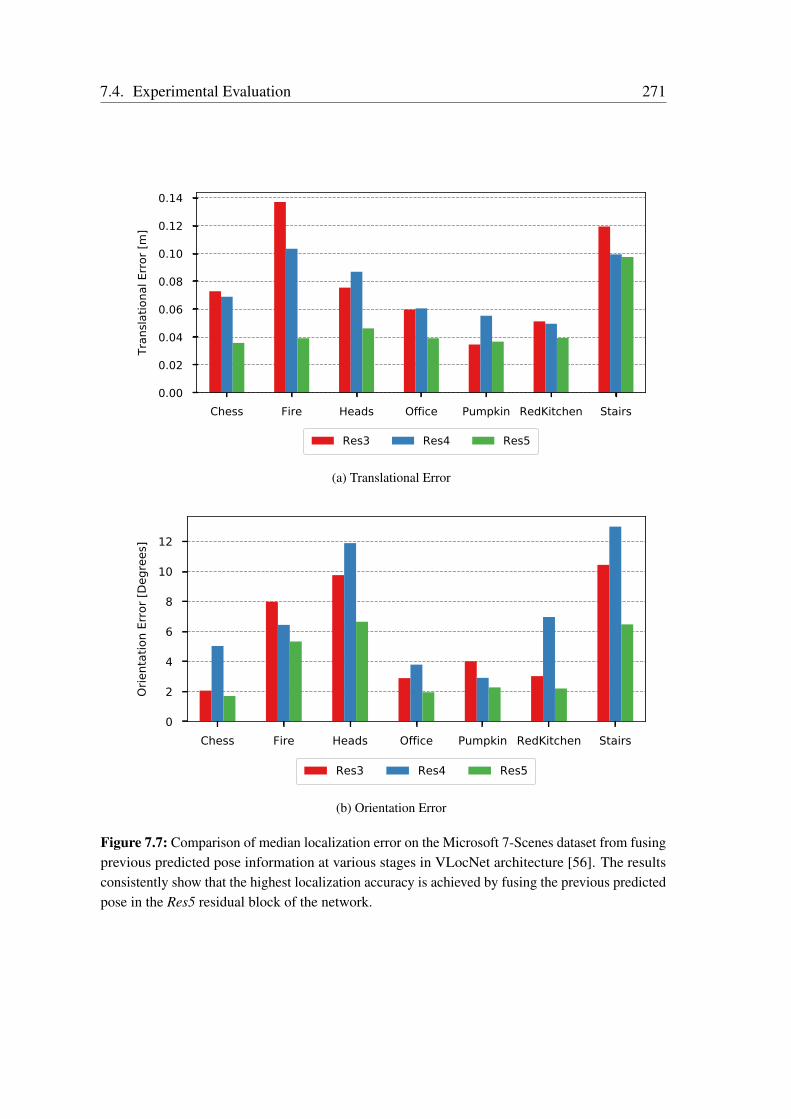
7.4. Experimental Evaluation 271
Chess Fire Heads Office Pumpkin RedKitchen Stairs0.00
0.02
0.04
0.06
0.08
0.10
0.12
0.14
Tran
slatio
nal E
rror [
m]
Res3 Res4 Res5
(a) Translational Error
Chess Fire Heads Office Pumpkin RedKitchen Stairs0
2
4
6
8
10
12
Orie
ntat
ion
Erro
r [De
gree
s]
Res3 Res4 Res5
(b) Orientation Error
Figure 7.7: Comparison of median localization error on the Microsoft 7-Scenes dataset from fusingprevious predicted pose information at various stages in VLocNet architecture [56]. The resultsconsistently show that the highest localization accuracy is achieved by fusing the previous predictedpose in the Res5 residual block of the network.
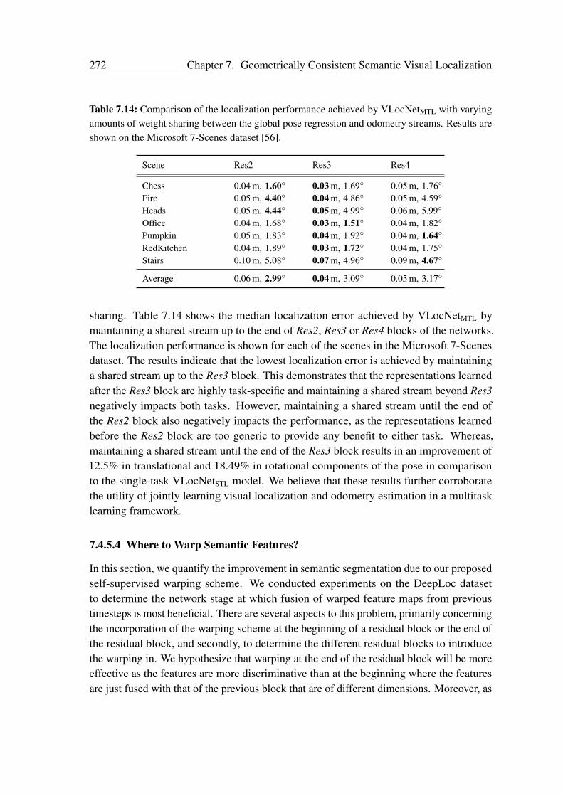
272 Chapter 7. Geometrically Consistent Semantic Visual Localization
Table 7.14: Comparison of the localization performance achieved by VLocNetMTL with varyingamounts of weight sharing between the global pose regression and odometry streams. Results areshown on the Microsoft 7-Scenes dataset [56].
Scene Res2 Res3 Res4
Chess 0.04 m, 1.60 0.03 m, 1.69 0.05 m, 1.76
Fire 0.05 m, 4.40 0.04 m, 4.86 0.05 m, 4.59
Heads 0.05 m, 4.44 0.05 m, 4.99 0.06 m, 5.99
Office 0.04 m, 1.68 0.03 m, 1.51 0.04 m, 1.82
Pumpkin 0.05 m, 1.83 0.04 m, 1.92 0.04 m, 1.64
RedKitchen 0.04 m, 1.89 0.03 m, 1.72 0.04 m, 1.75
Stairs 0.10 m, 5.08 0.07 m, 4.96 0.09 m, 4.67
Average 0.06 m, 2.99 0.04 m, 3.09 0.05 m, 3.17
sharing. Table 7.14 shows the median localization error achieved by VLocNetMTL bymaintaining a shared stream up to the end of Res2, Res3 or Res4 blocks of the networks.The localization performance is shown for each of the scenes in the Microsoft 7-Scenesdataset. The results indicate that the lowest localization error is achieved by maintaininga shared stream up to the Res3 block. This demonstrates that the representations learnedafter the Res3 block are highly task-specific and maintaining a shared stream beyond Res3negatively impacts both tasks. However, maintaining a shared stream until the end ofthe Res2 block also negatively impacts the performance, as the representations learnedbefore the Res2 block are too generic to provide any benefit to either task. Whereas,maintaining a shared stream until the end of the Res3 block results in an improvement of12.5% in translational and 18.49% in rotational components of the pose in comparisonto the single-task VLocNetSTL model. We believe that these results further corroboratethe utility of jointly learning visual localization and odometry estimation in a multitasklearning framework.
7.4.5.4 Where to Warp Semantic Features?
In this section, we quantify the improvement in semantic segmentation due to our proposedself-supervised warping scheme. We conducted experiments on the DeepLoc datasetto determine the network stage at which fusion of warped feature maps from previoustimesteps is most beneficial. There are several aspects to this problem, primarily concerningthe incorporation of the warping scheme at the beginning of a residual block or the end ofthe residual block, and secondly, to determine the different residual blocks to introducethe warping in. We hypothesize that warping at the end of the residual block will be moreeffective as the features are more discriminative than at the beginning where the featuresare just fused with that of the previous block that are of different dimensions. Moreover, as
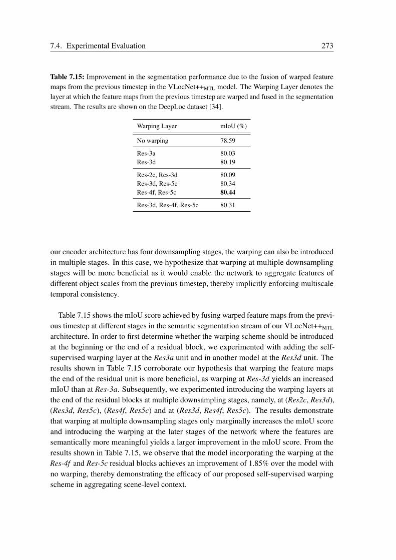
7.4. Experimental Evaluation 273
Table 7.15: Improvement in the segmentation performance due to the fusion of warped featuremaps from the previous timestep in the VLocNet++MTL model. The Warping Layer denotes thelayer at which the feature maps from the previous timestep are warped and fused in the segmentationstream. The results are shown on the DeepLoc dataset [34].
Warping Layer mIoU (%)
No warping 78.59
Res-3a 80.03Res-3d 80.19
Res-2c, Res-3d 80.09Res-3d, Res-5c 80.34Res-4f, Res-5c 80.44
Res-3d, Res-4f, Res-5c 80.31
our encoder architecture has four downsampling stages, the warping can also be introducedin multiple stages. In this case, we hypothesize that warping at multiple downsamplingstages will be more beneficial as it would enable the network to aggregate features ofdifferent object scales from the previous timestep, thereby implicitly enforcing multiscaletemporal consistency.
Table 7.15 shows the mIoU score achieved by fusing warped feature maps from the previ-ous timestep at different stages in the semantic segmentation stream of our VLocNet++MTL
architecture. In order to first determine whether the warping scheme should be introducedat the beginning or the end of a residual block, we experimented with adding the self-supervised warping layer at the Res3a unit and in another model at the Res3d unit. Theresults shown in Table 7.15 corroborate our hypothesis that warping the feature mapsthe end of the residual unit is more beneficial, as warping at Res-3d yields an increasedmIoU than at Res-3a. Subsequently, we experimented introducing the warping layers atthe end of the residual blocks at multiple downsampling stages, namely, at (Res2c, Res3d),(Res3d, Res5c), (Res4f, Res5c) and at (Res3d, Res4f, Res5c). The results demonstratethat warping at multiple downsampling stages only marginally increases the mIoU scoreand introducing the warping at the later stages of the network where the features aresemantically more meaningful yields a larger improvement in the mIoU score. From theresults shown in Table 7.15, we observe that the model incorporating the warping at theRes-4f and Res-5c residual blocks achieves an improvement of 1.85% over the model withno warping, thereby demonstrating the efficacy of our proposed self-supervised warpingscheme in aggregating scene-level context.
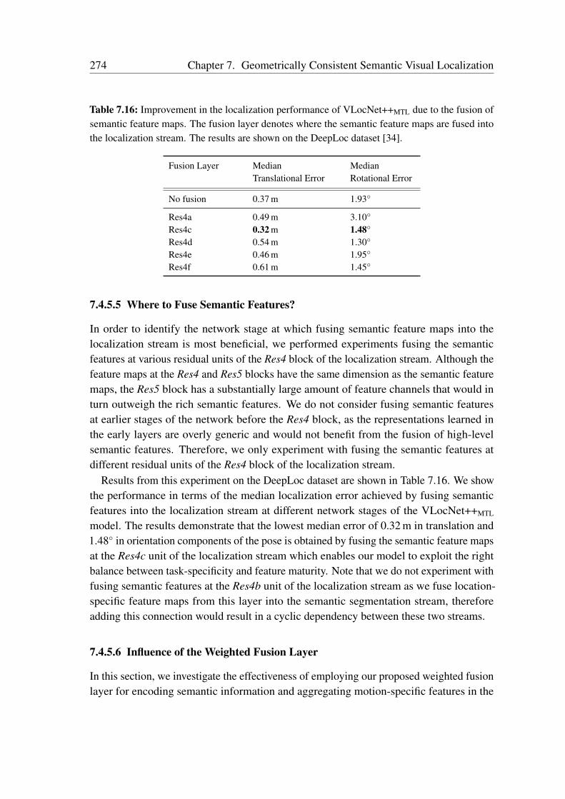
274 Chapter 7. Geometrically Consistent Semantic Visual Localization
Table 7.16: Improvement in the localization performance of VLocNet++MTL due to the fusion ofsemantic feature maps. The fusion layer denotes where the semantic feature maps are fused intothe localization stream. The results are shown on the DeepLoc dataset [34].
Fusion Layer Median MedianTranslational Error Rotational Error
No fusion 0.37 m 1.93
Res4a 0.49 m 3.10
Res4c 0.32 m 1.48
Res4d 0.54 m 1.30
Res4e 0.46 m 1.95
Res4f 0.61 m 1.45
7.4.5.5 Where to Fuse Semantic Features?
In order to identify the network stage at which fusing semantic feature maps into thelocalization stream is most beneficial, we performed experiments fusing the semanticfeatures at various residual units of the Res4 block of the localization stream. Although thefeature maps at the Res4 and Res5 blocks have the same dimension as the semantic featuremaps, the Res5 block has a substantially large amount of feature channels that would inturn outweigh the rich semantic features. We do not consider fusing semantic featuresat earlier stages of the network before the Res4 block, as the representations learned inthe early layers are overly generic and would not benefit from the fusion of high-levelsemantic features. Therefore, we only experiment with fusing the semantic features atdifferent residual units of the Res4 block of the localization stream.
Results from this experiment on the DeepLoc dataset are shown in Table 7.16. We showthe performance in terms of the median localization error achieved by fusing semanticfeatures into the localization stream at different network stages of the VLocNet++MTL
model. The results demonstrate that the lowest median error of 0.32 m in translation and1.48 in orientation components of the pose is obtained by fusing the semantic feature mapsat the Res4c unit of the localization stream which enables our model to exploit the rightbalance between task-specificity and feature maturity. Note that we do not experiment withfusing semantic features at the Res4b unit of the localization stream as we fuse location-specific feature maps from this layer into the semantic segmentation stream, thereforeadding this connection would result in a cyclic dependency between these two streams.
7.4.5.6 Influence of the Weighted Fusion Layer
In this section, we investigate the effectiveness of employing our proposed weighted fusionlayer for encoding semantic information and aggregating motion-specific features in the

7.4. Experimental Evaluation 275
Figure 7.8: Comparison of the median localization error of VLocNet++MTL with baseline multitaskmodels that fuse semantic features into the localization stream. Results are shown on the DeepLocdataset [34].
global pose regression stream. We compare the localization accuracy of VLocNet++MTL
which incorporates our fusion scheme against the single-task models as well as threecompetitive multitask baselines. The topologies of the three baselines are as follows:
• MTL_input-concat: A simple technique that can be employed for incorporatingsemantic features into the global pose regression stream is by concatenating thepredicted semantic segmentation output Mt with input image It as a fourth-channeland feeding the resulting four-channel tensor as input to the localization stream.
• MTL_mid-concat: As a second baseline, we concatenate the semantic featuremaps with intermediate representations of the global pose regression stream. As theexperiments that we presented in Section 7.4.5.5 demonstrated that fusing semanticfeatures with the Res4c unit is most beneficial, we similarly fuse semantic featuremaps at Res4c using simple concatenation as opposed to employing our proposedweighted fusion layer.
• MTL_shared: Finally, we compare with an approach [294] that shares the latentspaces of both the semantic segmentation and global pose regression streams. Shar-ing the latent space can be realized by sharing the weights of a specific layer acrossdifferent networks. In our implementation, we share the weights of the Res4c unitbetween both the global pose regression and semantic segmentation streams.
Figure 7.8 shows the results from this experiment on the DeepLoc dataset in termsof the median localization error metric. The results clearly show that employing thenaive MTL-input-concat approach drastically reduces the performance over our single-taskVLocNet++STL model. Furthermore, we observe that the MTL_mid-concat model achieveslower localization error than our single-task VLocNet++STL demonstrating that fusing
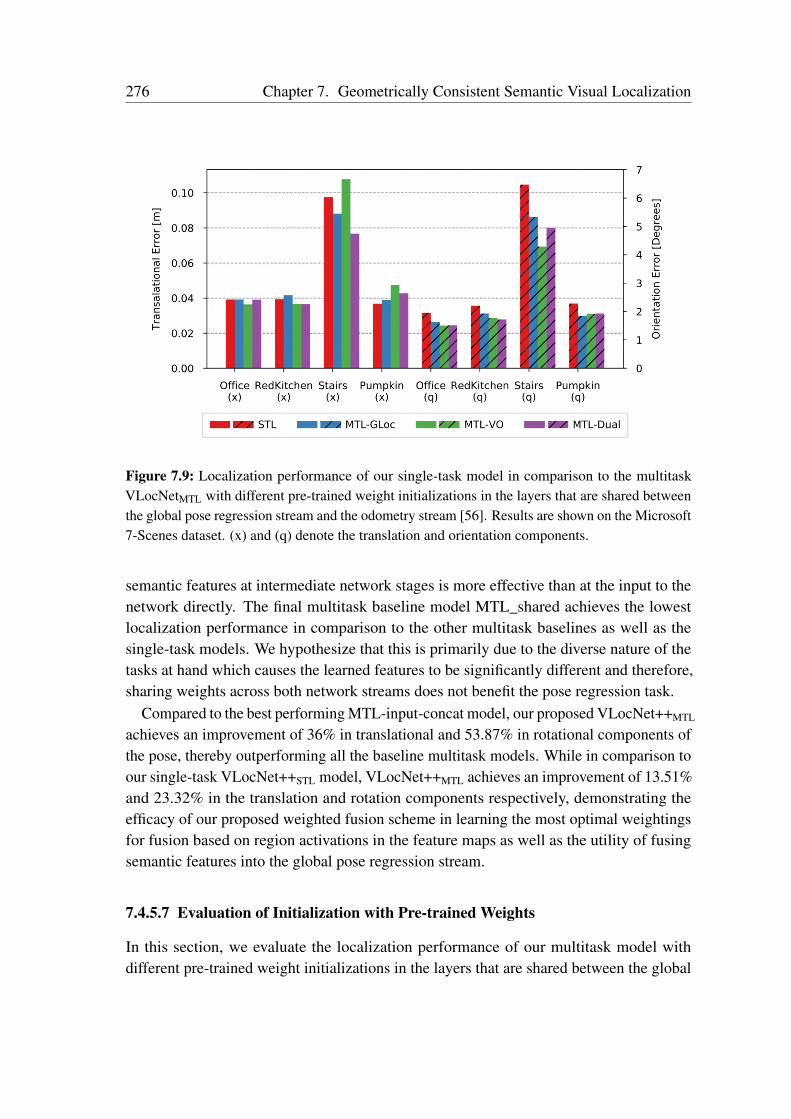
276 Chapter 7. Geometrically Consistent Semantic Visual Localization
Figure 7.9: Localization performance of our single-task model in comparison to the multitaskVLocNetMTL with different pre-trained weight initializations in the layers that are shared betweenthe global pose regression stream and the odometry stream [56]. Results are shown on the Microsoft7-Scenes dataset. (x) and (q) denote the translation and orientation components.
semantic features at intermediate network stages is more effective than at the input to thenetwork directly. The final multitask baseline model MTL_shared achieves the lowestlocalization performance in comparison to the other multitask baselines as well as thesingle-task models. We hypothesize that this is primarily due to the diverse nature of thetasks at hand which causes the learned features to be significantly different and therefore,sharing weights across both network streams does not benefit the pose regression task.
Compared to the best performing MTL-input-concat model, our proposed VLocNet++MTL
achieves an improvement of 36% in translational and 53.87% in rotational components ofthe pose, thereby outperforming all the baseline multitask models. While in comparison toour single-task VLocNet++STL model, VLocNet++MTL achieves an improvement of 13.51%and 23.32% in the translation and rotation components respectively, demonstrating theefficacy of our proposed weighted fusion scheme in learning the most optimal weightingsfor fusion based on region activations in the feature maps as well as the utility of fusingsemantic features into the global pose regression stream.
7.4.5.7 Evaluation of Initialization with Pre-trained Weights
In this section, we evaluate the localization performance of our multitask model withdifferent pre-trained weight initializations in the layers that are shared between the global
7.4. Experimental Evaluation 277
pose regression stream and the odometry stream. As each task-specific network stream isinitially trained separately, it alters the weights of the convolution layers in a way that bestminimizes the respective loss function. Combining the task-specific networks in a multitasklearning framework to jointly learn multiple tasks requires an initialization strategy thatenables effective feature sharing. Therefore, we evaluated various initialization strategiesthat facilitate the learning of inter-task correlations. Using the model trained on oursingle-task global pose regression stream VLocNetSTL (STL) as a baseline, we evaluate thelocalization performance of the joint model with different pre-trained weight initializations.More precisely, we compare the performance of the following models:
• MTL-GLoc: Initializing the shared layers of the global pose regression stream withthe weights from the pre-trained task-specific global pose regression model and theremaining layers with the Xavier initialization [108].
• MTL-VO: Initializing the shared layers of the global pose regression stream with theweights from the pre-trained task-specific visual odometry model and the remaininglayers with the Xavier initialization [108].
• MTL-Dual: Utilizing the combined weights from each task-specific network toinitialize the joint model.
Figure 7.9 shows the results from this experiment on the Microsoft 7-Scenes dataset interms of the median localization error of our VLocNetMTL model employing the aforemen-tioned initialization strategies. The results demonstrate our multitask model outperformsits single-task counterpart which further validates the efficacy of jointly learning globalpose regression and visual odometry estimation tasks in a multitask learning framework.The improvement is clearly seen in the Stairs scene which is the most challenging scene tolocalize in the Microsoft 7-Scenes dataset as it contains repetitive structures and texturelesssurfaces.
On closer examination of the results, we find that the dual initialization of both networkstreams with weights from their task-specific models results in the best performance,contrary to initializing only one of the task-specific streams in the joint model and learningthe other from scratch. This can be attributed to the training data that is insufficient totrain large multitask networks without any pre-trained weight initialization. Furthermore,we observe that initializing only the global pose regression stream (MTL-GLoc) yieldsthe least reduction in the localization error while compared to the single-task model. Wehypothesize that this occurs due to the visual odometry stream needing to be trainedfrom scratch and as a result, it does not provide reasonable relative pose estimates atthe beginning of the training. Therefore, the localization stream cannot benefit from themotion-specific features from the odometry stream.
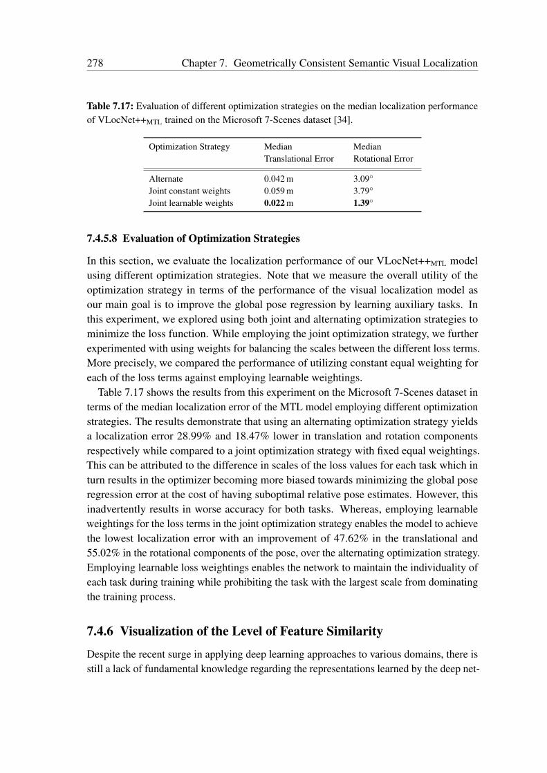
278 Chapter 7. Geometrically Consistent Semantic Visual Localization
Table 7.17: Evaluation of different optimization strategies on the median localization performanceof VLocNet++MTL trained on the Microsoft 7-Scenes dataset [34].
Optimization Strategy Median MedianTranslational Error Rotational Error
Alternate 0.042 m 3.09
Joint constant weights 0.059 m 3.79
Joint learnable weights 0.022 m 1.39
7.4.5.8 Evaluation of Optimization Strategies
In this section, we evaluate the localization performance of our VLocNet++MTL modelusing different optimization strategies. Note that we measure the overall utility of theoptimization strategy in terms of the performance of the visual localization model asour main goal is to improve the global pose regression by learning auxiliary tasks. Inthis experiment, we explored using both joint and alternating optimization strategies tominimize the loss function. While employing the joint optimization strategy, we furtherexperimented with using weights for balancing the scales between the different loss terms.More precisely, we compared the performance of utilizing constant equal weighting foreach of the loss terms against employing learnable weightings.
Table 7.17 shows the results from this experiment on the Microsoft 7-Scenes dataset interms of the median localization error of the MTL model employing different optimizationstrategies. The results demonstrate that using an alternating optimization strategy yieldsa localization error 28.99% and 18.47% lower in translation and rotation componentsrespectively while compared to a joint optimization strategy with fixed equal weightings.This can be attributed to the difference in scales of the loss values for each task which inturn results in the optimizer becoming more biased towards minimizing the global poseregression error at the cost of having suboptimal relative pose estimates. However, thisinadvertently results in worse accuracy for both tasks. Whereas, employing learnableweightings for the loss terms in the joint optimization strategy enables the model to achievethe lowest localization error with an improvement of 47.62% in the translational and55.02% in the rotational components of the pose, over the alternating optimization strategy.Employing learnable loss weightings enables the network to maintain the individuality ofeach task during training while prohibiting the task with the largest scale from dominatingthe training process.
7.4.6 Visualization of the Level of Feature Similarity
Despite the recent surge in applying deep learning approaches to various domains, there isstill a lack of fundamental knowledge regarding the representations learned by the deep net-
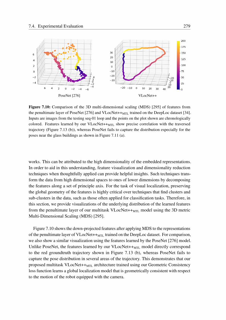
7.4. Experimental Evaluation 279
PoseNet [276] VLocNet++
Figure 7.10: Comparison of the 3D multi-dimensional scaling (MDS) [295] of features fromthe penultimate layer of PoseNet [276] and VLocNet++MTL trained on the DeepLoc dataset [34].Inputs are images from the testing seq-01 loop and the points on the plot shown are chronologicallycolored. Features learned by our VLocNet++MTL show precise correlation with the traversedtrajectory (Figure 7.13 (b)), whereas PoseNet fails to capture the distribution especially for theposes near the glass buildings as shown in Figure 7.11 (a).
works. This can be attributed to the high dimensionality of the embedded representations.In order to aid in this understanding, feature visualization and dimensionality reductiontechniques when thoughtfully applied can provide helpful insights. Such techniques trans-form the data from high dimensional spaces to ones of lower dimensions by decomposingthe features along a set of principle axis. For the task of visual localization, preservingthe global geometry of the features is highly critical over techniques that find clusters andsub-clusters in the data, such as those often applied for classification tasks. Therefore, inthis section, we provide visualizations of the underlying distribution of the learned featuresfrom the penultimate layer of our multitask VLocNet++MTL model using the 3D metricMulti-Dimensional Scaling (MDS) [295].
Figure 7.10 shows the down-projected features after applying MDS to the representationsof the penultimate layer of VLocNet++MTL trained on the DeepLoc dataset. For comparison,we also show a similar visualization using the features learned by the PoseNet [276] model.Unlike PoseNet, the features learned by our VLocNet++MTL model directly correspondto the red groundtruth trajectory shown in Figure 7.13 (b), whereas PoseNet fails tocapture the pose distribution in several areas of the trajectory. This demonstrates that ourproposed multitask VLocNet++MTL architecture trained using our Geometric Consistencyloss function learns a global localization model that is geometrically consistent with respectto the motion of the robot equipped with the camera.
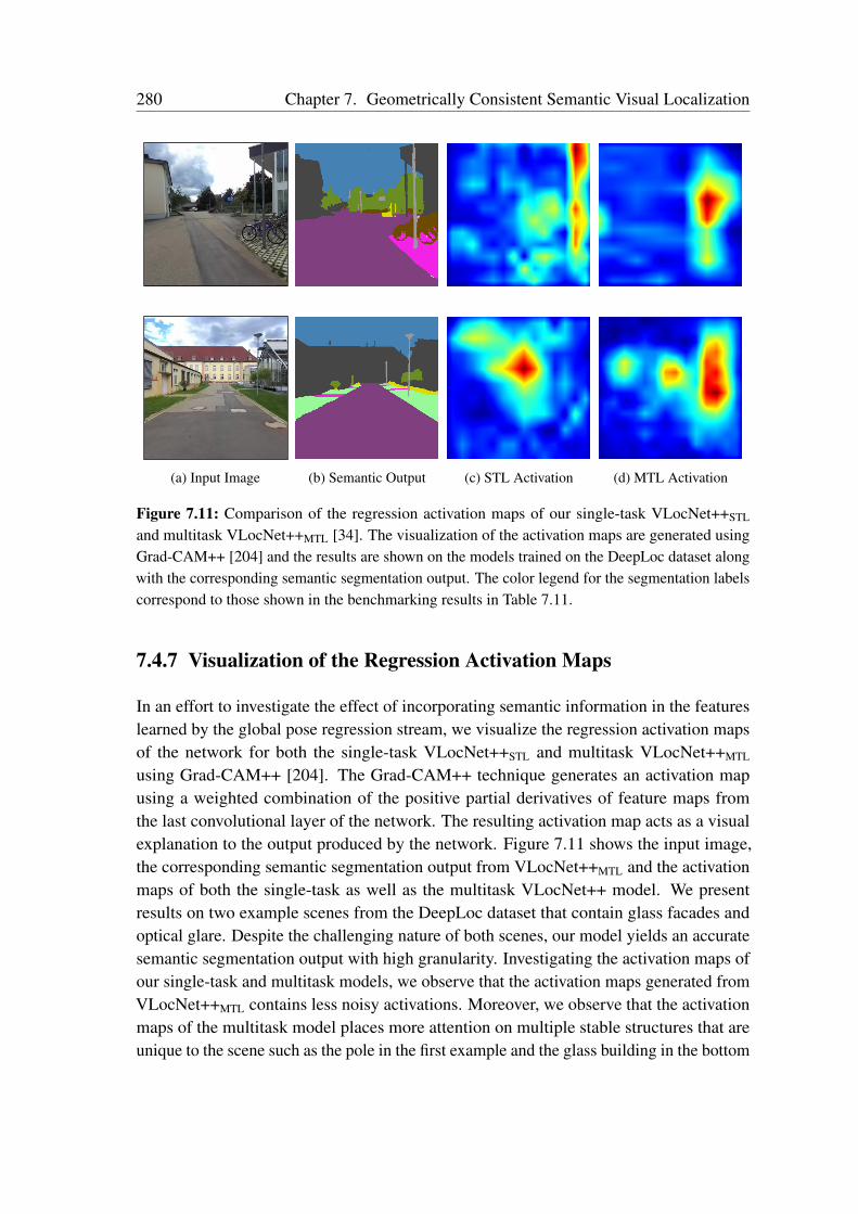
280 Chapter 7. Geometrically Consistent Semantic Visual Localization
(a) Input Image (b) Semantic Output (c) STL Activation (d) MTL Activation
Figure 7.11: Comparison of the regression activation maps of our single-task VLocNet++STL
and multitask VLocNet++MTL [34]. The visualization of the activation maps are generated usingGrad-CAM++ [204] and the results are shown on the models trained on the DeepLoc dataset alongwith the corresponding semantic segmentation output. The color legend for the segmentation labelscorrespond to those shown in the benchmarking results in Table 7.11.
7.4.7 Visualization of the Regression Activation Maps
In an effort to investigate the effect of incorporating semantic information in the featureslearned by the global pose regression stream, we visualize the regression activation mapsof the network for both the single-task VLocNet++STL and multitask VLocNet++MTL
using Grad-CAM++ [204]. The Grad-CAM++ technique generates an activation mapusing a weighted combination of the positive partial derivatives of feature maps fromthe last convolutional layer of the network. The resulting activation map acts as a visualexplanation to the output produced by the network. Figure 7.11 shows the input image,the corresponding semantic segmentation output from VLocNet++MTL and the activationmaps of both the single-task as well as the multitask VLocNet++ model. We presentresults on two example scenes from the DeepLoc dataset that contain glass facades andoptical glare. Despite the challenging nature of both scenes, our model yields an accuratesemantic segmentation output with high granularity. Investigating the activation maps ofour single-task and multitask models, we observe that the activation maps generated fromVLocNet++MTL contains less noisy activations. Moreover, we observe that the activationmaps of the multitask model places more attention on multiple stable structures that areunique to the scene such as the pole in the first example and the glass building in the bottom
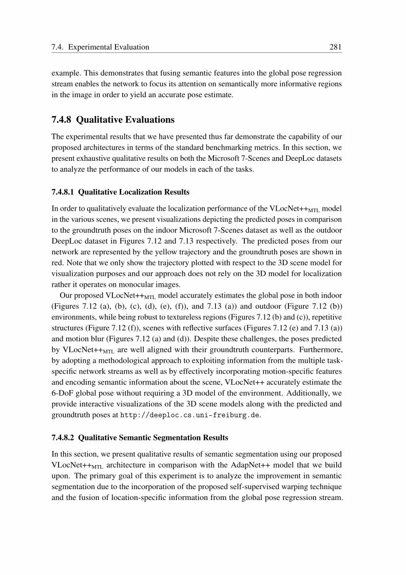
7.4. Experimental Evaluation 281
example. This demonstrates that fusing semantic features into the global pose regressionstream enables the network to focus its attention on semantically more informative regionsin the image in order to yield an accurate pose estimate.
7.4.8 Qualitative Evaluations
The experimental results that we have presented thus far demonstrate the capability of ourproposed architectures in terms of the standard benchmarking metrics. In this section, wepresent exhaustive qualitative results on both the Microsoft 7-Scenes and DeepLoc datasetsto analyze the performance of our models in each of the tasks.
7.4.8.1 Qualitative Localization Results
In order to qualitatively evaluate the localization performance of the VLocNet++MTL modelin the various scenes, we present visualizations depicting the predicted poses in comparisonto the groundtruth poses on the indoor Microsoft 7-Scenes dataset as well as the outdoorDeepLoc dataset in Figures 7.12 and 7.13 respectively. The predicted poses from ournetwork are represented by the yellow trajectory and the groundtruth poses are shown inred. Note that we only show the trajectory plotted with respect to the 3D scene model forvisualization purposes and our approach does not rely on the 3D model for localizationrather it operates on monocular images.
Our proposed VLocNet++MTL model accurately estimates the global pose in both indoor(Figures 7.12 (a), (b), (c), (d), (e), (f)), and 7.13 (a)) and outdoor (Figure 7.12 (b))environments, while being robust to textureless regions (Figures 7.12 (b) and (c)), repetitivestructures (Figure 7.12 (f)), scenes with reflective surfaces (Figures 7.12 (e) and 7.13 (a))and motion blur (Figures 7.12 (a) and (d)). Despite these challenges, the poses predictedby VLocNet++MTL are well aligned with their groundtruth counterparts. Furthermore,by adopting a methodological approach to exploiting information from the multiple task-specific network streams as well as by effectively incorporating motion-specific featuresand encoding semantic information about the scene, VLocNet++ accurately estimate the6-DoF global pose without requiring a 3D model of the environment. Additionally, weprovide interactive visualizations of the 3D scene models along with the predicted andgroundtruth poses at http://deeploc.cs.uni-freiburg.de.
7.4.8.2 Qualitative Semantic Segmentation Results
In this section, we present qualitative results of semantic segmentation using our proposedVLocNet++MTL architecture in comparison with the AdapNet++ model that we buildupon. The primary goal of this experiment is to analyze the improvement in semanticsegmentation due to the incorporation of the proposed self-supervised warping techniqueand the fusion of location-specific information from the global pose regression stream.
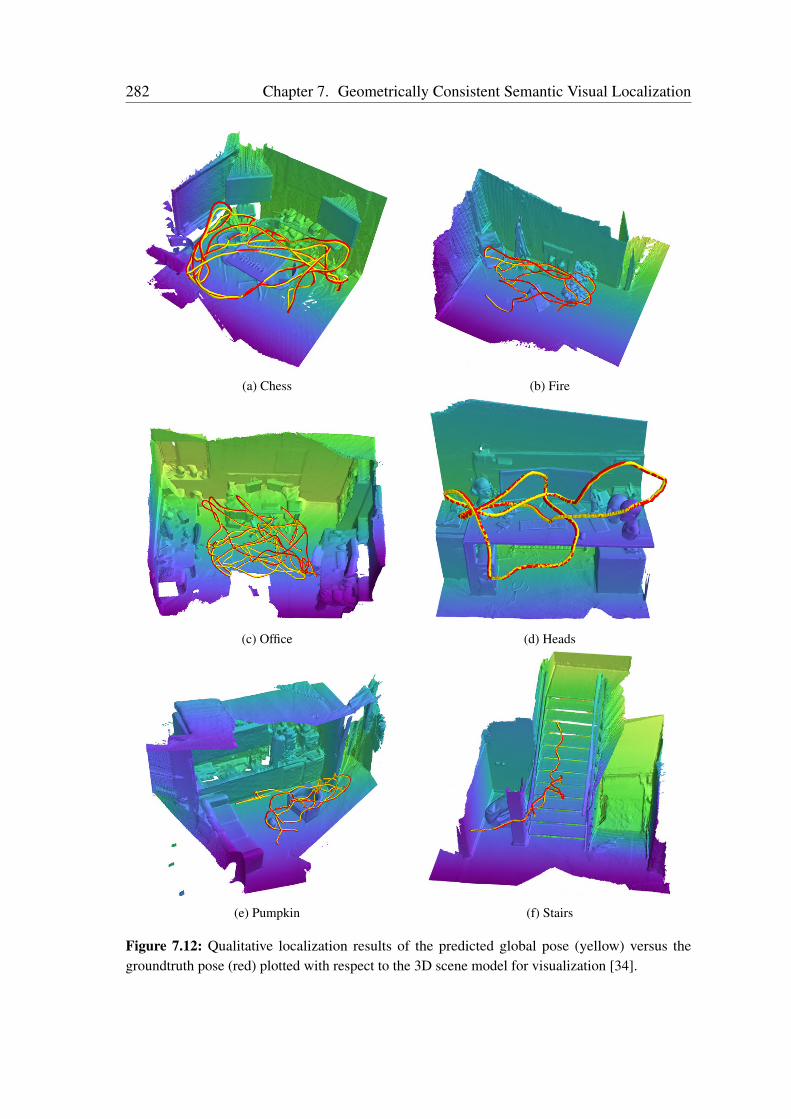
282 Chapter 7. Geometrically Consistent Semantic Visual Localization
(a) Chess (b) Fire
(c) Office (d) Heads
(e) Pumpkin (f) Stairs
Figure 7.12: Qualitative localization results of the predicted global pose (yellow) versus thegroundtruth pose (red) plotted with respect to the 3D scene model for visualization [34].
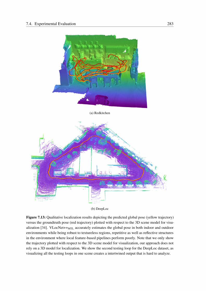
7.4. Experimental Evaluation 283
(a) Redkitchen
(b) DeepLoc
Figure 7.13: Qualitative localization results depicting the predicted global pose (yellow trajectory)versus the groundtruth pose (red trajectory) plotted with respect to the 3D scene model for visu-alization [34]. VLocNet++MTL accurately estimates the global pose in both indoor and outdoorenvironments while being robust to textureless regions, repetitive as well as reflective structuresin the environment where local feature-based pipelines perform poorly. Note that we only showthe trajectory plotted with respect to the 3D scene model for visualization, our approach does notrely on a 3D model for localization. We show the second testing loop for the DeepLoc dataset, asvisualizing all the testing loops in one scene creates a intertwined output that is hard to analyze.
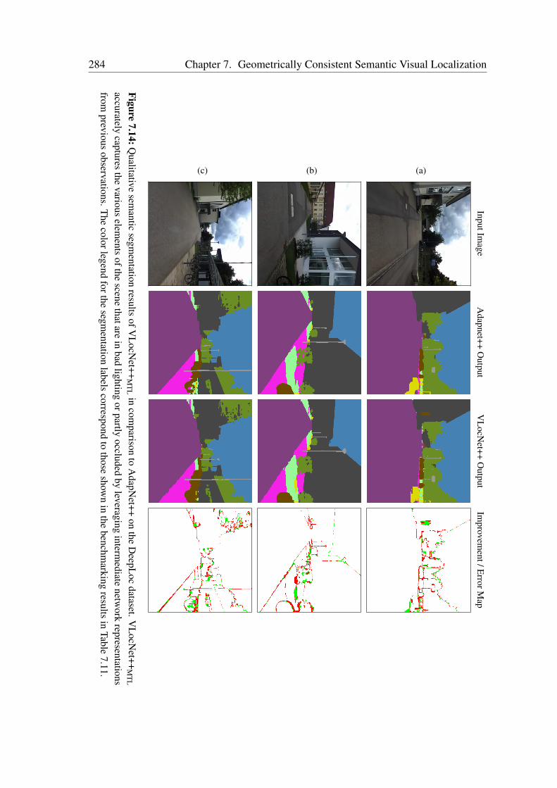
284 Chapter 7. Geometrically Consistent Semantic Visual LocalizationInputIm
ageA
dapnet++O
utputV
LocN
et++O
utputIm
provement/E
rrorMap
(a)(b)(c)
Figure7.14:Q
ualitativesem
anticsegm
entationresults
ofVL
ocNet++
MT
Lin
comparison
toA
dapNet++
onthe
DeepL
ocdataset.V
LocN
et++M
TL
accuratelycaptures
thevarious
elements
ofthescene
thatarein
badlighting
orpartlyoccluded
byleveraging
intermediate
network
representationsfrom
previousobservations.T
hecolorlegend
forthesegm
entationlabels
correspondto
thoseshow
nin
thebenchm
arkingresults
inTable
7.11.
7.4. Experimental Evaluation 285
We present results on the DeepLoc dataset and show the improvement / error map whichindicates the improvement over the segmentation output of AdapNet++ in green and themisclassifications by the VLocNet++MTL model with respect to the groundtruth in red.
Figures 7.14 and 7.15 show the qualitative results from this experiment. Figure 7.14 (a)depicts a scene where the improvement in semantic segmentation output of VLocNet++MTL
can primarily be seen in the detection of the person standing next to the building onthe left as belonging to the dynamic object class, identification of the vegetation behindthe underpassage in the center of the image, detection of the entire sidewalk that thebicyles are parked on in the center of the image and parts of the road on the right beingcorrected predicted. While, in Figure 7.14 (b), the manhole cover near the grass on theright of the image is accurately classified as the other object class, whereas AdapNet++entirely misclassifies the manhole over as sidewalk. In addition, the third pole in theend of the street is entirely captured in the segmentation of VLocNet++MTL, althoughit is missing in the segmentation output of the AdapNet++ model. Subsequently, in theoutput of VLocNet++MTL shown in Figure 7.14 (c), we observe that the corner of theshed on the right which is translucent, is precisely predicted as the building class and thebicycles on the right as well as in the center of the image are more accurately predictedin comparison to the segmentation output of the AdapNet++ model. Moreover, in all theexamples shown in Figure 7.14, the boundaries between the vegetation and its surroundingsare more precisely predicted in the output of the VLocNet++MTL model. Most of theseimprovements can be attributed to our proposed self-supervised warping scheme thatfuses the intermediate representations from the previous timestep into the current view toimprove the segmentation performance by aggregating more scene-level context. Thereforein the aforementioned scenarios where bad lighting and occlusion cause misclassifications,leveraging and incorporating features of the same location from another view improves theoverall prediction.
Figure 7.15 shows the second set of examples on the DeepLoc dataset where in Fig-ure 7.15 (a), our proposed VLocNet++MTL accurately classifies the entire shed in the centerof the image as the building class and captures the whole stretch of the sidewalk nearthe trashcan in the center of the image. Whereas, AdapNet++ misclassifies these regions.Moreover, in the output of AdapNet++, we observe that in the center of the image, thenetwork predicts parts of the building behind the trees as a tree trunk (vegetation) and thediscolored road near the edge of the building on the left as the building class, where ourVLocNet++MTL accurately predicts the object category of these pixels. In Figure 7.15 (b),we observe that VLocNet++MTL more precisely captures the boundaries between grassand vegetation, accurately segments the entire sidewalk path near the trashcan in the rightand captures more of the structure of the rails on the left of the image. In the last exampleshown in Figure 7.15 (c), we can see that VLocNet++MTL accurately captures the trashcan in the center-right of the road, while the structure is entirely missing the segmentationoutput of the AdapNet++ model. Another challenging aspect is to identify the boundary

286 Chapter 7. Geometrically Consistent Semantic Visual LocalizationInputIm
ageA
dapnet++O
utputV
LocN
et++O
utputIm
provement/E
rrorMap
(a)(b)(c)
Figure7.15:Q
ualitativesem
anticsegm
entationresults
ofVL
ocNet++
MT
Lin
comparison
toA
dapNet++
inchallenging
scenariosin
theD
eepLoc
dataset.VLocN
et++accurately
predictsthe
boundariesofobjects
andcaptures
entirethin
pole-likestructures.The
colorlegendforthe
segmentation
labelscorrespond
tothose
shown
inthe
benchmarking
resultsin
Table7.11.
7.5. Related Work 287
between road and sidewalk and well as sidewalk and grass, which can be often challengingeven for humans when viewing from large distances. Inspecting the examples, we see thatour VLocNet++MTL model precisely detects these boundaries.
In the examples where an object is entirely missing in the segmentation output of theAdapNet++ model, but it is accurately captured in the output of the VLocNet++MTL model,the improvement can be attributed to both the fusion of location specific informationand the fusion of warped intermediate representations from the previous timesteps. Mostof the scenes have thin pole-like structures such as lamp posts, sign posts, and fencesare the hardest to fully segment for any semantic segmentation network. Although theVLocNet++MTL architecture utilizes a considerably small input image, it is still able todetect the entire structure of pole-like objects more accurately than AdapNet++ due to theaggregation of information from previous observations. One of the challenging aspects ofthe DeepLoc dataset is the presence of glass buildings which are reflective or translucentthat makes classifying them in images extremely challenging. Despite the presence ofseveral glass-constructs (Figures 7.14 (b) and (c)), our network classifies the correspondingpixels as their correct semantic object categories. Finally, we observe several challengingperceptual conditions in these examples such as varying lighting conditions that causeshadows (Figure 7.15 (b)), glare (Figures 7.14 (a) and (c)) and over/under exposure due tosunlight (Figures 7.14 (c), 7.15 (a) and 7.15(b)). In all these scenarios, our models yield anaccurate representation of the scene while being robust to these disturbances.
7.5 Related Work
In this chapter, we presented novel convolutional neural network architectures that simulta-neously learn to regress the global pose, predict the semantics of the scene and estimatethe visual odometry in a joint multitask learning framework. Our framework is structuredto enable inductive transfer by leveraging domain specific information from each of thetasks for their mutual benefit. More importantly, we introduced a principled approach toembed geometric and semantic knowledge of the world into the pose regression networkto learn a model that is geometrically consistent with respect to the motion. Over the pastdecade, there has been a gradual shift from employing traditional handcrafted pipelines tolearning-based approaches. Although significant strides have been made, most of these ap-proaches have been particularly proposed to address perception related tasks. However, theapplicability of these learning-based techniques have also been explored for tasks in otherdomains. In Chapter 4, we presented a thorough review of the literature on semantic scenesegmentation. In this section, we discuss some of the recent developments in multitasklearning, visual localization and odometry estimation.
288 Chapter 7. Geometrically Consistent Semantic Visual Localization
Multitask Learning can be defined as an inductive transfer mechanism that improvesgeneralization by leveraging domain specific information from related tasks [296]. Ithas been applied to a wide range of tasks from different domains including image under-standing [297, 298], sentiment prediction [299], language modelling and translation [300],semantic segmentation [301, 302] and even recently on learning from demonstration [303].Yu et al. propose a model based on convolutional neural networks and denoising autoen-coders for the task of face detection and object recognition using RGB-D images [297].Their joint model consists of individual streams for each task, while sharing the inputlayer and the final hidden layer. Their approach demonstrates substantial increase inperformance by employing their joint model in comparison to individually trained mod-els. Bilen et al. [298] propose the use of a instance normalization layer to normalize theinformation across a single network that is trained to recognize across multiple visualdomains including objects, digits, signs and faces. X-ResNets [299] are residual modelswith cross connections that have less than 40% of the parameters than their single-taskcounterparts and achieve competitive performance for visual sentiment concept detection.Shazeer et al. [300] introduce a model with a sparsely-gated mixture of experts layer withthousands of feed-forward sub-networks for the task of language modelling and machinetranslation.
Teichmann et al. propose the Multinet [301] architecture consisting of a shared en-coder and task-specific decoders for classification, detection and semantic segmentation.Lu et al.[304] introduce an automatic approach to learn compact multitask networks forperson attribute classification in which the method first starts with a thin network modeland expands it during training using a multi-round branching mechanism which determineswith whom each task shares features in each layer. Kuga et al. [305] introduce a multitaskarchitecture that consists of multimodal encoder-decoder streams that are connected viashared latent representation as well as shared skip connections. They demonstrate thatsharing representations across different modalities improves the multitask learning perfor-mance. Misra et al. propose Cross-stitch networks [306] for multitask learning in whichthey introduce the cross-stitch unit that combines activations from multiple networks bymodeling shared representations as linear combinations. They demonstrate that cross-stitched networks acheive better performance than networks found by brute-force search.For combining different loss functions in a multitask model, Kendall et al. [302] proposea loss function based on maximizing the Gaussian likelihood using homoscedastic taskuncertainty. Rouhollah et al. propose an architecture that takes raw images as input andgenerates arm trajectories for the robot to perform different manipulation actions [303].Their work demonstrates that sharing weights across different tasks and using VAE-GAN-based reconstruction improves the generalization capability. Most of these approaches haveshared sections of the network (encoders in some cases) that learn low-level representations,followed by individual task-specific branches that learn specialized features for a particulartask. In this work, we proposed a novel multitask learning framework that incorporates our
7.5. Related Work 289
weighted fusion layer at multiple network stages between different task-specific streams tolearn the optimal weightings for the fusion of feature maps based on region activations forthe mutual benefit of the tasks.
Visual Localization approaches can be broadly classified into metric and appearance-based techniques. Metric approaches [307, 308] estimate the 6-DoF pose of an imageby computing local image features to establish correspondences and use the matches toestimate the geometric relationship with a 3D model built using SfM or SLAM. Whereas,appearance-based localization techniques [309, 310] provide a coarse location estimate byemploying image retrieval techniques to find the closest match against a database of images.The approach that we present in this chapter tackles the problem of metric localization.Sparse feature-based localization approaches learn a set of feature descriptors from trainingimages which are then employed to learn a codebook of 3D descriptors against whicha query image can be matched [274, 311]. Some approaches terminate the matchingprocedure as soon as a fixed threshold has been reached [312, 313], while other approachesreduce the number of full codebook searches using bidirectional matching [310, 314, 315]or employ a two-stage matching technique [316]. Relying on bidirectional informationor multiple matching stages also helps to improve the accuracy by eliminating incorrectmatches before the pose estimation stage. Recent methods [275, 284] that efficiently findfeature correspondences within the codebook train regression forests on 3D scene dataand use RANSAC to infer the final location of the query image. Donoser et al. propose adiscriminative classification approach using random ferns which demonstrates improvedpose accuracy while allowing for faster run-time [317]. Despite the accurate pose estimatesprovided by these methods, they still require a cumbersome feature selection step forbuilding a codebook and the overall run-time depends on the size of the 3D model as wellas the number of feature correspondences that are found. This in turn results in suboptimalperformance when employed in large environments and scenes that contain textureless orrepetitive structures.
Recently, pre-trained CNNs designed for classification tasks have been successfullyadapted for pose regression. 6-DoF pose regression models can also be considered asmultitask models as they regress for both translation and rotation components individually.Kendall et al. proposed the first end-to-end approach for directly regressing the 6-DoFcamera pose from a monocular image using a CNN called PoseNet [276]. Since then sev-eral improvements have been proposed in terms of estimating the uncertainty of the posesusing Bayesian CNNs [287], incorporating Long-Short Term Memory (LSTM) units for di-mensionality reduction [277], symmetric encoder-decoder architecture for regression [291]and an improved loss function based on scene geometry [282]. Laskar et al. [286] proposea hybrid approach in which first a convolutional neural network trained on relative camerapose estimation is employed for feature extraction. Subsequently, the extracted featuresare then used to identify the nearest neighbors of the query image from a set of database
290 Chapter 7. Geometrically Consistent Semantic Visual Localization
images.Deep learning approaches require large amounts of training data, however most existing
visual localization datasets have sparse pose information. In order to alleviate this problem,Naseer et al. [285] and Wu et al. [283] propose augmentation strategies to increasethe 3D pose coverage of images. Additionally, Wu et al. propose to use the Euler6representation to counteract ambiguities of quaternions in representing angles. Recently,Brachmann et al. proposed a differentiable version of RANSAC termed DSAC [292] forcamera localization. DSAC introduces two methods to make RANSAC differentiable;by replacing the deterministic hypothesis section using soft argmax selection or with aprobabilistic selection. Subsequently, Brachmann et al.[293] propose DSAC2 in which theyintroduce an entropy controlled soft inlier count to score the hypotheses produced by theneural network. Most of the aforementioned end-to-end approaches append branches withinner-product layers to a pre-trained classification network and utilize naive loss functionsfor pose regression that yield a substantially lower performance than state-of-the-art localfeature-based approaches. In this chapter, we introduced our Geometric Consistencyloss function that constricts the search space with the relative motion information duringtraining to obtain pose estimates that are globally consistent. Furthermore, we proposed aweighted fusion layer that enables aggregation of motion-specific temporal features whilesimultaneously encoding semantic features into the pose regression stream.
Visual Odometry: Another closely related problem in robotics is estimating the incre-mental motion of the robot using only sequential camera images. In one of the initiallyproposed methods, Konda et al. [318] adopt a classification approach to this problem,where a convolutional neural network with a softmax layer is used to infer the relativetransformation between two images using a prior set of discretized velocities and directions.Nicholai et al. [288] introduce an end-to-end approach in which they combine both imageand LiDAR information to estimate the ego-motion from a consecutive frames. Theyproject the point cloud onto the 2D image and feed this information to a simple Siamesearchitecture with alternating convolution and pooling layers to estimate the visual odom-etry. Similarly, Mohanty et al. [289] propose a Siamese-type architecture for odometryestimation called DeepVO in which the translational and rotational components of the poseare regressed through a Euclidean loss layer with equal weight values. The architecture wasbased on the AlexNet model [22] and they also experiment with appending FAST featuresalong with the images as input to the network. Melekhov et al. [290] add a constantweighting term to balance both the translational and rotational components of the loss,thereby yielding an improved ego-motion estimate. Furthermore, they incorporate a spatialpyramid pooling layer in their architecture which renders their model robust to varyinginput image resolutions. Yin et al. [319] addresses the critical problem of recoveringthe scale in monocular visual odometry by employing a convolutional neural fields tosimultaneously estimate depth along with the ego-motion.
7.6. Conclusions 291
More recently, there are a class of methods that formulate structure from motion asa learning problem. Ummenhofer et al. [320] propose the DeMoN architecture thatlearns to estimate depth and camera motion from unconstrained image pairs using annovel loss function based on spatial relative differences. Their architecture consisting ofmultiple stacked encoder-decoder networks and an iterative network that improves its ownpredictions. Zhou et al. [321] introduce a unsupervised learning framework that uses thetask of view synthesis for supervision of monocular depth and camera motion estimationfrom video sequences. Vijayanarasimhan et al. propose the SfM-Net [322] architecturethat predicts pixel-wise depth, camera motion, object motion and object masks whilelearning in a self-supervised fashion from video sequences. Self-supervision is achievedusing gradients from pixel matching across consecutive frames, constrained by forward-backward consistency on the computed motion and 3D structure. While the aforementionedtechniques focus on learning supervised and unsupervised specialized models for ego-motion estimation, our goal in this work is to learn a joint multitask model for three diversetasks and achieve superior performance compared to its single-task counterparts. Inspiredby the success of residual networks in various visual recognition tasks, we proposed aSiamese-type dual stream architecture built upon the full pre-activation ResNet-50 [27]model for visual odometry estimation.
Contrary to the aforementioned task-specific methods that train individual models for aspecific task, we proposed a joint end-to-end trainable multitask architecture for 6-DoFvisual localization, odometry estimation and semantic segmentation from consecutivemonocular images. In order to exploit the inherent interdependencies between the threetasks and to enable inductive transfer of information, we structure our multitask learningframework to be interdependent on the outputs as well as the intermediate representationsof the task-specific network streams. Our approach enables a competitive and collaborativeaction that regularizes the network and substantially improves the performance of thejoint model in comparison to individual specialized models as well as state-of-the-arttechniques.
7.6 Conclusions
In this chapter, we introduced two novel end-to-end trainable multitask convolutionalneural network architectures for 6-DoF visual localization, semantic segmentation andodometry estimation from consecutive monocular images. The goal of our architectureis to exploit the complex interdependencies within these tasks for their mutual benefit.At the lowest level, our architecture incorporates a hard parameter sharing scheme andemploys a joint optimization strategy with multitask learnable loss weightings for learninginter-task correlations. We presented a new strategy for simultaneously encoding geometricand structural constraints into the the pose regression network by temporally aggregat-
292 Chapter 7. Geometrically Consistent Semantic Visual Localization
ing learned motion-specific information and effectively fusing semantically meaningfulrepresentations. To this end, we proposed a weighted fusion layer that learns the mostoptimal weightings for fusion based on region activations. Furthermore, we presenteda self-supervised warping technique that fuses feature maps from multiple views andresolutions using the representational warping concept from multi-view geometry, forscene-level context aggregation. This enables our model to be robust to camera angledeviations, object scale and frame-level distortions, while implicitly introducing featureaugmentation which facilitates faster convergence. More importantly, we introduced thenovel Geometric Consistency loss function that constricts the search space of the globalpose regression stream while training by leveraging the relative motion information fromthe shared auxiliary odometry stream and by exploiting the aggregated motion-specificinformation to learn a model that is geometrically consistent.
In order to facilitate learning of joint multitask models for visual localization, odometryestimation and semantic segmentation, we introduced a first-of-a-kind large-scale urbanoutdoor localization dataset with multiple loops captured at different times of the day. Wemade our dataset consisting of 6-DoF camera poses and manually annotated pixel-levelsemantic groundtruth labels, publicly available to encourage future progress. The datasetcan be utilized for benchmarking a number of perception and localization tasks as itcontains challenging scenarios such as varying lighting conditions, reflective glare fromthe sun, shadows, motion-blur, buildings with similar facades, repetitive structures andtranslucent as well as reflective buildings made of glass. We presented comprehensivebenchmarking results on the indoor Microsoft 7-Scenes and outdoor DeepLoc datasets.Extensive experimental evaluations demonstrate that both our single-task and multitaskmodels achieve state-of-the-art performance on each of the tasks, compared to existingdeep learning-based approaches as well as their single-task counterparts. Our proposedVLocNet++ architecture outperforms the state-of-the-art end-to-end learning model forvisual localization on the Microsoft 7-Scenes benchmark by 93.81% and 91.72% in thetranslational and rotational components of the pose respectively. More importantly, ourVLocNet++ architecture exceeds the overall state-of-the-art on the benchmark by 67.5%in the translational and 25.9% in the rotational components of the pose, while being 60.5%faster and simultaneously performing multiple tasks. The approach presented in thischapter is the first to close the performance gap between local feature-based and deeplearning-based methods for visual localization. Additionally, VLocNet++ outperformsthe previous state-of-the-art semantic segmentation architecture by 6.94% in the mIoUscore, and demonstrates an improvement of 40.80% in the orientation for visual odometryestimation. We also presented detailed ablation studies, intuitive visual explanations andcomprehensive qualitative results that demonstrate the capabilities our models. Our resultsindicate the feasibility of learning deep multitask models for critical robotic tasks beyondthe visual perception domain. Overall, our findings are an encouraging sign that learningmultitask models for various robotic tasks is a promising research direction.

Chapter 8
Conclusions and Discussion
This thesis addresses a number of problems related to robot perception and localizationby learning to leverage the inherent structure from various modalities and across differenttasks. We presented multiple innovative end-to-end convolutional neural network archi-tectures for classifying terrains using proprioceptive sensor data, learning to semanticallyclassify various objects present in scenes at the pixel-level, learning to dynamically fuseinformation from multiple modalities in a self-supervised manner, learning to jointly esti-mate the semantics as well the motion of objects in scenes at the pixel-level, and finallylearning to visually localize, semantically segment scenes and estimate the visual odometryin a multitask framework. Using extensive experiments on standard benchmark datasetsand in different real-world environments, we demonstrated that our proposed architec-tures substantially exceed the state-of-the-art while enabling efficient deployment on realrobot systems. Additionally, we also addressed several important fundamental scientificquestions in deep learning while tackling these complex problems. We believe that thesetechniques play a crucial role in enabling our contributions to be practical solutions forreal robot systems.
We first tackled the challenge of learning to classify terrains from vehicle-terrain inter-action sounds in an end-to-end manner. Typically, handcrafted audio features were usedalong with specialized preprocessing steps that do not generalize due to the unstructurednature of the vehicle-terrain interaction sounds. We proposed two novel convolutionalneural network architectures that incorporate our new global statistical pooling strategy toachieve the time-series representation learning. Furthermore, we also proposed a recurrentarchitecture that exploits the temporal dynamics of the signal to further improve upon theperformance. In order to enable our model to be robust to different ambient environmentalnoises, we proposed a noise-aware training scheme that randomly injects ambient noisesamples during training to regularize the network and to learn more generalizable models.Our contribution is the first approach to address the problem using an end-to-end learningtechnique. We extensively evaluated our networks on over six hours of vehicle-terraininteraction data that contains nine different indoor and outdoor terrains. The resultsdemonstrate that both our networks significantly outperform existing techniques therebyachieving state-of-the-art performance with a substantially faster inference time. We also
294 Chapter 8. Conclusions and Discussion
presented experiments with an inexpensive low-quality microphone in a new environmentthat demonstrates the significant noise robustness and the hardware independence of ourapproach.
As accurate scene understanding is precursor for autonomous navigation, our secondcontribution enables a robot to efficiently understand the semantics of the environmentfrom visual images. We proposed two fully-convolutional neural network architecturesthat are based on the encoder-decoder design topology. These architectures incorporateour multiscale residual units that are effectively better at learning multiscale features thanthe commonly employed multigrid method. We also proposed the efficient atrous spatialpyramid pooling module that has a large effective receptive field to capture long-rangecontext and to aggregate multiscale representations. This module substantially improvesthe performance over the standard atrous spatial pyramid pooling while consuming lessthan ten-times the amount of parameters. In order to obtain a high resolution segmentationoutput, we proposed a new decoder with skip refinement stages, complemented with amulti-resolution supervision scheme to deeply supervise the training. Our proposed decodersubstantially improves the segmentation along object boundaries and effectively recoversthe structure of thin pole-like objects. In order to enable efficient deployment on embeddedGPUs, we proposed a network-wide holistic pruning approach that compresses our modelswithout leading to a drop in the performance. Comprehensive benchmarking results onCityscapes, Synthia, SUN RGB-D, ScanNet and Freiburg Forest datasets demonstrate thatour architectures achieve state-of-the-art performance while consuming lesser number ofparameters and having a faster inference time than existing methods. We also presentedreal-world experiments using our AIS perception car that demonstrates the generalizationability of our models.
Subsequently, we addressed the problem of multimodal semantic segmentation in aneffort to adaptively exploit complementary features to improve the robustness of the model.Existing techniques for multimodal perception, naively concatenate features from multipleindividual modality streams, however this does not enable the model to leverage thefeatures according to critical factors that influence the fusion. We tackled this problemfrom two perspectives. Our first architecture probabilistically fuses semantically maturecomplementary features according to the object classes present in the scene. Whileour second architecture dynamically fuses multimodal features at different intermediatenetwork stages according to the semantic objects, their spatial location in the world and thescene context. In order to enable the network to optimally exploit complementary features,we adopt a self-supervised learning approach to train the fusion model. Our proposedfusion schemes are independent of the base architecture and can be easily employedwith any semantic segmentation framework. We evaluated our fusion approaches usingmultiple modalities including visual images, depth and near-infrared on the Cityscapes,Synthia, SUN RGB-D, ScanNet and Freiburg Forest datasets. We demonstrated that bothour fusion models exceed the performance of unimodal segmentation as well as existing
295
multimodal fusion techniques and achieve state-of-the-art performance on each of theaforementioned datasets. More importantly, we presented results in adverse perceptualconditions including snow, rain, fog, night-time, motion blur and optical glare that showsthe exceptional robustness of our models. Furthermore, we presented real-world navigationexperiments using our Viona robot that employs only our multimodal fusion model as aperception module while autonomously navigating several kilometers of an unstructuredforested environment.
In an effort to learn a more informative scene understanding model, we further tackledthe problem of joint semantic motion segmentation with the additional goal of exploitingrepresentations from both tasks for their mutual benefit. Most existing semantic seg-mentation networks do not exploit motion information and existing motion segmentationnetworks do not exploit semantics of the scene. However, both motion and semantics canprovide complementary information that we exploit in our proposed architectures. Ourfirst contribution for this problem is a two-stream fully-convolutional architecture thatsimultaneously learns semantic features using an encoder-decoder network and motionfeatures from self-generated optical flow maps. The network then fuses semantic featuresinto the motion segmentation stream to yield the pixel-wise segmentation output in whicheach pixel is assigned to a semantic object class as well as a static or moving motionlabel. As the ego-motion of the robot itself creates spurious optical flow magnitudes thatdo not represent the motion of moving objects in the scene, we proposed an ego-flowsuppression technique that we incorporated in our architectures to compensate for thiseffect. Our second architecture that we introduced simultaneously exploits motion cuesto improve leaning of semantics and adaptively fuses semantic features into the motionsegmentation stream to further improve motion segmentation. Our temporal warpingscheme first transforms the ego-flow suppressed optical flow maps into an edge-enhancedflow representation which is then used to warp and dynamically fuse intermediate networkrepresentations in the semantic stream across the temporal dimension. Our warping schemesubstantially improves the semantic segmentation performance along the boundaries ofthe objects. Using extensive experiments on the Cityscapes-Motion, KITTI-Motion andApolloScape-Motion datasets, we demonstrated that our architectures outperform existingsemantic motion segmentation techniques, as well as specialized task-specific networks,thereby achieving state-of-the-art performance. Our experiments show that fusing semanticfeatures into the motion segmentation network makes the model more robust to segmentingmultiple moving objects in extremely cluttered scenes and the adaptive fusion preventsover-segmentation of the moving objects. Additionally, we presented real-world experi-ments using our AIS perception car that demonstrates the effectiveness of our model inchallenging scenarios and the generalization ability to previously unseen environments.
Furthermore, a key contribution of this thesis is the multitask learning architectures thatwe proposed for geometrically consistent semantic visual localization. These architecturesenable robots to simultaneously localize, understand the semantics of the scene and esti-
296 Chapter 8. Conclusions and Discussion
mate their ego-motion using a single coherent framework. Thus far, most existing networksthat learn to regress the 6-DoF global pose employ the standard Euclidean loss functionthat does enable the network to exploit geometric information about the environment. Inorder to address this problem, we proposed two novel architectures complemented with anew Geometric Consistency loss function. Our first architecture consists of a single streamfor learning the global pose and a Siamese-type double stream architecture for odometryestimation. Our proposed Geometric consistency loss function exploits the relative motioninformation from the auxiliary odometry stream to constrict the search space of the globalpose regression stream to learn a model that is globally consistent. In order to conserve theamount of parameters consumed by the network and enable inter-task learning, our networkstreams employ hard parameter sharing that enables exploiting the complex interdepen-dencies between the tasks. We additionally proposed an improved architecture that fusessemantically meaningful representations into the global pose regression stream to encodestructural constraints and simultaneously aggregates motion-specific information using ourweighted fusion layer to enable our Geometric Consistency loss to effectively leverage thisinformation. Our proposed weighted fusion layer enables learning of optimal weightingsfor the fusion based on region activations. Furthermore, we proposed a self-supervisedwarping technique that exploits the estimated relative motion from the odometry streamto warp semantic features from the previous frame with the representations of the currentframe to implicitly introduce feature augmentation that accelerates the training and im-proves the semantic segmentation performance. We presented comprehensive experimentalevaluations on the indoor Microsoft 7-Scenes dataset and the outdoor DeepLoc dataset thatdemonstrate that our networks outperform their single-task counterparts as well as existingmultitask methods, thereby setting the new state-of-the-art on both these benchmarks whilesimultaneously performing multiple tasks. The results highlight that our network is the firstdeep learning approach to outperform local-feature based techniques in visual localization,in addition to being more robust in situations that contain textureless regions and glassconstructs. Overall, our results demonstrate the benefit in learning these three diverse tasksin a multitask learning framework to obtain a more accurate and compact model.
In summary, we proposed several contributions in this thesis that enable robots toreliably perceive and understand our complex dynamic world using multiple modalities,and robustly localize themselves in the environment using only visual images. Ourproposed models generalize effectively to different challenging scenarios and adverseperceptual conditions by dynamically adapting their weights as well as by learning in aself-supervised manner. Moreover, our architectures outperform the state-of-the-art ineach of the addressed tasks with a faster inference time while consuming substantiallylesser number of parameters. These factors are critical enablers for efficient real worlddeployment. We believe that our proposed methods have brought us closer to deployingintelligent robots in increasingly complex environments and we hope that this thesisinspires future work that will lead to revolutionary new applications.
297
Future Work
There are several avenues for future research as well as straightforward extension ofthe work that we presented in this thesis. We presented highly accurate approaches forterrain classification using proprioceptive sensors that enables a robot to classify the terrainunderneath its wheels. However, robots also need to estimate the traversability of distantterrains that are in front of it, in order to plan trajectories that are more efficient fortraversal. We can leverage our proprioceptive terrain classifier to provide labels for trainingan exteroceptive classifier in a self-supervised manner. This technique will alleviate theneed of requiring annotated groundtruth labels. For example, consider a patch of terrainin front of the robot that an exteroceptive sensor such as a camera is used to capture andassume that the robot is equipped with a microphone as well as our audio-based vehicle-terrain interaction classifier. The robot can acquire terrain labels for the previously observedvisual patch captured by the camera by traversing to that location and assigning the outputof the audio classifier as the label for the visual patch. A similar technique [323] waspreviously explored for planetary rovers where an SVM was trained to classify the terrainusing handcrafted features. However, in the previous work, the exteroceptive classifierwas trained in a supervised manner once enough data was gathered. For future work, wepropose to utilize our CNN-based proprioceptive classifier to train an unsupervised visualclassifier using a deep clustering approach [324] in a self-supervised manner. Furthermore,an exploration planner with a suitable cost function can be employed in conjunction withthis system to enable the robot to traverse to locations consisting of terrains that theexteroceptive classifier is more uncertain about. This would enable the robot to traverse theenvironment and learn in a self-supervised manner from experience leading to a life-longlearning framework.
Semantic scene understanding is one of the fundamental problems in robotics andcomputer vision for which there are numerous challenges to overcome. Recently, morelight-weight classification networks have been proposed than the residual network architec-ture that we build upon for the encoder of our semantic segmentation models. Architecturessuch as ShuffleNet v2 [325] and MobileNet v2 [326] utilize group convolutions and depth-wise separable convolutions to keep the number of FLOPS low, thereby demonstratingfaster inference time. This also enables building deeper architectures with the number of pa-rameters still substantially lower than residual networks. An interesting research directionwould be to employ either ShuffleNet v2 or MobileNet v2 as the base encoder architectureand build upon it to effectively learn multiscale features. In this thesis, we proposed theeASPP module to aggregate multiscale features with a large receptive fields. However, weuse the same dilation rate in the consecutive atrous convolutions in a branch of the eASPP.Using a larger dilation rate in the second atrous convolution is one straightforward solutionto learn larger effective receptive fields and therefore capture larger context. Solutionsto other challenges such as developing an efficient decoder that learns to upsample as

298 Chapter 8. Conclusions and Discussion
opposed to simple bilinear upsampling and more aggressive automatic pruning strategieshave to be explored.
In this thesis, we presented robust techniques for multimodal perception that adapts tothe observed scene in order to optimally leverage complementary features. For future workin this domain, we propose to first extend our SSMA fusion mechanism for multimodalfusion of more than two modalities. This extension is straightforward as the topology of ourSSMA unit can take multiple tensors as input and it would yield output weights with thedimensions of the concatenated input tensors correspondingly for suppressing or enhancingthe modality-specific feature maps. Subsequently, we propose to develop a network to firstestimate the usefulness of a particular modality and then act as a switch that activates ordeactivates the modality-specific streams based on this factor. This technique will alsomake the perception system more robust to sensor failures as the network would detect thatthere is no information from a specific modality and disconnect the corresponding stream.No such known approach exists to the best of our knowledge.
We addressed the problem of semantic motion segmentation in this thesis where ournetwork simultaneously predicts the pixel-wise semantic object labels as well as the themotion status of each pixel in the image. One future direction would be to exploit themotion cues to infer the instances of the objects which can be utilized by robots forreasoning about the environment more effectively. Currently, there are several methods thathave been proposed for instance segmentation [327, 328, 329], motion segmentation [54,269, 330] and semantic segmentation [59, 133, 135] individually, however to the bestof our knowledge there are no approaches that exploit motion information to implicitlyinfer instances for semantic segmentation. Instance separation boundaries can be learnedfrom the motion of moving objects assuming that two objects do not move with the samevelocity adjacent to each other. This problem is significantly more challenging withoutmaking this assumption and therefore poses an interesting research problem. Anotherpotential research direction relates to how the ego-flow suppression is introduced in thenetwork and the supervised learning of optical flow. Currently the IMU measurementsare leveraged to compute the relative motion with a predicted depth map of scene froma CNN and the optical flow maps are learned using the FlowNet3 architecture that weembed in our network. Recently, several techniques have been proposed for unsupervisedlearning of optical flow and ego-motion [331, 332] that demonstrate impressive resultswithout needing any labeled training data. An interesting research direction would be toreformulate our semantic motion segmentation problem in the context of multitask learningof semantics, motion segmentation, instance segmentation, optical flow and ego-motion ina single coherent framework. In this framework, only the semantic segmentation networkhas to be supervised, the other tasks can be learned in an unsupervised manner. Thiswould also pose an interesting challenge for the optimization of the model as it involvessimultaneously training five different diverse classification and regression tasks.
The VLocNet++ architecture that we presented is the first deep learning approach to
299
achieve state-of-the-art performance for visual localization. The effectiveness of ourarchitecture is primarily due to the efficient aggregation of motion-specific information andthe Geometric Consistency loss function that constricts the search space with respect tothe relative motion. Our architecture only uses two consecutive images as input to learn aglobally consistent model. The performance of the model can be substantially improved byconsidering a temporal window of images. This involves incorporating recurrent units suchas Long Short-Term Memory Units (LSTMs) [96] or Gated Recurrent Units (GRUs) [333]in the end of the global pose regression stream as well as in the odometry stream. Secondly,our Geometric Consistency loss function has to be adapted to minimize the loss withrespect to a sequence of relative poses. Furthermore, the robustness of the network indynamic environments can be substantially improved by additionally feeding the predictedpixel-wise ephemerality mask [334] as inputs to the odometry network stream. This woulddefinitely be a fruitful research avenue.
In conclusion, the aforementioned research directions are only a small subset of theinteresting problems that can be solved as an extension of this thesis. There are severalnew challenges that are arising every day due to the fast paced development of this field.This is the most exciting time to be working in this domain of robotics and we believe thebest is yet to come.


Appendices

Appendix A
Detailed Multimodal SemanticSegmentation Results
In this appendix, we present detailed multimodal semantic segmentation results on theCityscapes [143], Synthia [144], SUN RGB-D [145], ScanNet [146] and Freiburg For-est [50] datasets. We compare the individual object class IoU scores of our proposedCMoDE and SSMA fusion models that were introduced in Chapter 5 with each of theunimodal semantic segmentation models (RGB, Depth, HHA, and EVI), baseline fusiontechniques (Average, Maximum, Stacking, and Late Fusion) as well as the state-of-the-artfusion approaches (LFC [50] and FuseNet [162]). The mIoU scores for these models werepresented in the benchmarking results shown in Section 5.3.2 and the topology of thebaseline architectures are described in Section 5.2.3.
A.1 Evaluation on the Cityscapes Dataset
Table A.1 shows the results on the Cityscapes dataset. Our SSMA_msf model that per-forms RGB-HHA fusion outperforms the other techniques in 8 out of the 11 semanticobject classes thereby achieving the state-of-the-art performance. The unimodal modelsare outperformed by the multimodal fusion approaches in each of the semantic objectcategories, demonstrating the utility of employing multimodal fusion not only for increas-ing the robustness in challenging perceptual conditions but also improving the overallperformance in terms of the IoU scores. Comparing the multimodal fusion performance ofour proposed SSMA_msf model with the previous state-of-the-art LFC model, we observethat our model outperforms LFC substantially in each of the semantic object categoriesfor both RGB-D fusion and RGB-HHA fusion. Analyzing the performance of RGB-HHAfusion in comparison to RGB-D fusion, we see that the sky and person classes are moreaccurately classified using RGB-D data, where all the other classes are more accuratelyclassified with RGB-HHA fusion. The better performance of the RGB-D fusion for thesky class can be attributed to the fact that the depth maps have no information for the skyclass and it appears as a homogeneous region as seen in Figure 4.11 (d), whereas the HHA
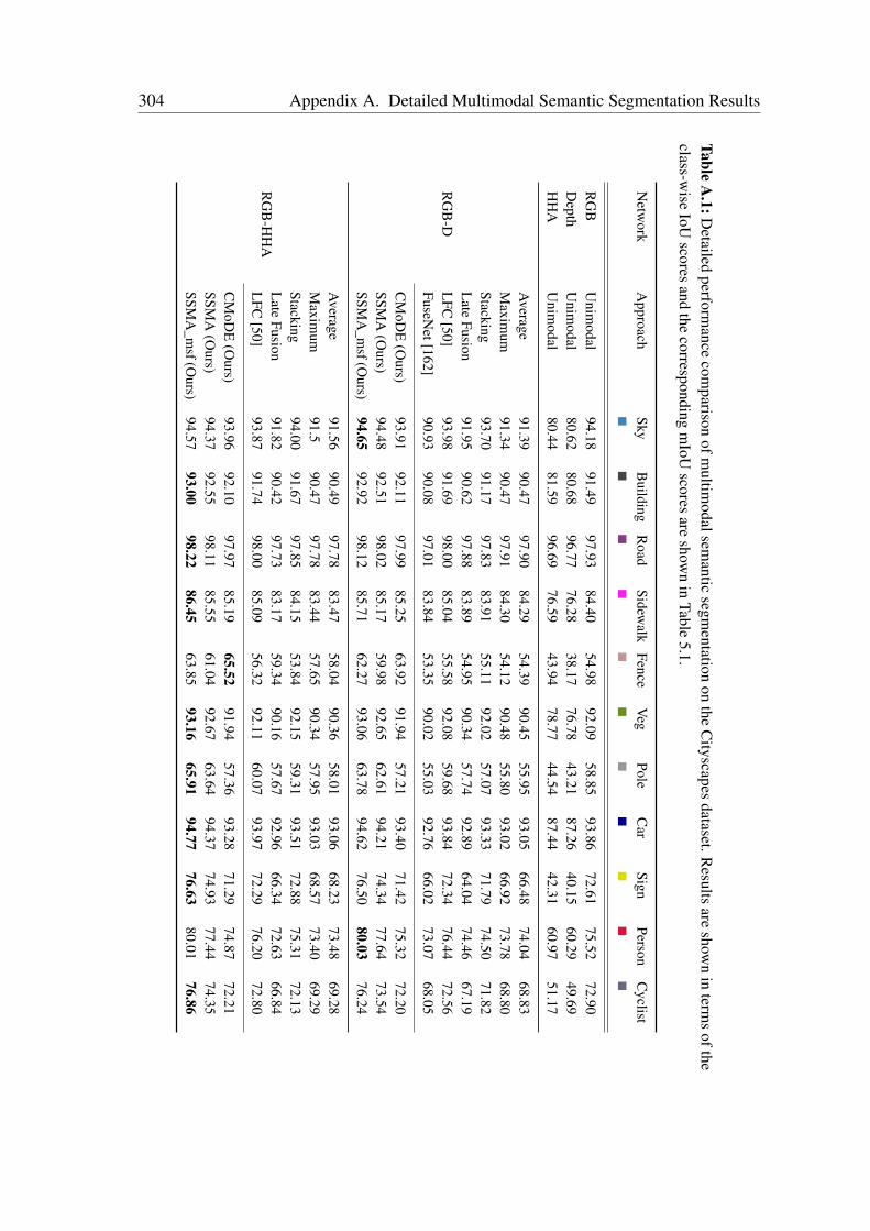
304 Appendix A. Detailed Multimodal Semantic Segmentation Results
TableA
.1:Detailed
performance
comparison
ofmultim
odalsemantic
segmentation
onthe
Cityscapes
dataset.Results
areshow
nin
terms
oftheclass-w
iseIoU
scoresand
thecorresponding
mIoU
scoresare
shown
inTable
5.1.
Netw
orkA
pproachSky
Building
Road
Sidewalk
FenceV
egPole
Car
SignPerson
Cyclist
RG
BU
nimodal
94.1891.49
97.9384.40
54.9892.09
58.8593.86
72.6175.52
72.90D
epthU
nimodal
80.6280.68
96.7776.28
38.1776.78
43.2187.26
40.1560.29
49.69H
HA
Unim
odal80.44
81.5996.69
76.5943.94
78.7744.54
87.4442.31
60.9751.17
RG
B-D
Average
91.3990.47
97.9084.29
54.3990.45
55.9593.05
66.4874.04
68.83M
aximum
91.3490.47
97.9184.30
54.1290.48
55.8093.02
66.9273.78
68.80Stacking
93.7091.17
97.8383.91
55.1192.02
57.0793.33
71.7974.50
71.82L
ateFusion
91.9590.62
97.8883.89
54.9590.34
57.7492.89
64.0474.46
67.19L
FC[50]
93.9891.69
98.0085.04
55.5892.08
59.6893.84
72.3476.44
72.56FuseN
et[162]90.93
90.0897.01
83.8453.35
90.0255.03
92.7666.02
73.0768.05
CM
oDE
(Ours)
93.9192.11
97.9985.25
63.9291.94
57.2193.40
71.4275.32
72.20SSM
A(O
urs)94.48
92.5198.02
85.1759.98
92.6562.61
94.2174.34
77.6473.54
SSMA
_msf(O
urs)94.65
92.9298.12
85.7162.27
93.0663.78
94.6276.50
80.0376.24
RG
B-H
HA
Average
91.5690.49
97.7883.47
58.0490.36
58.0193.06
68.2373.48
69.28M
aximum
91.590.47
97.7883.44
57.6590.34
57.9593.03
68.5773.40
69.29Stacking
94.0091.67
97.8584.15
53.8492.15
59.3193.51
72.8875.31
72.13L
ateFusion
91.8290.42
97.7383.17
59.3490.16
57.6792.96
66.3472.63
66.84L
FC[50]
93.8791.74
98.0085.09
56.3292.11
60.0793.97
72.2976.20
72.80
CM
oDE
(Ours)
93.9692.10
97.9785.19
65.5291.94
57.3693.28
71.2974.87
72.21SSM
A(O
urs)94.37
92.5598.11
85.5561.04
92.6763.64
94.3774.93
77.4474.35
SSMA
_msf(O
urs)94.57
93.0098.22
86.4563.85
93.1665.91
94.7776.63
80.0176.86

A.2. Evaluation on the Synthia Dataset 305
image appears noisy in the sky region due to the angle between the gravity and the localsurface normal that is computed in the HHA transformation. The performance differencebetween the RGB-D model and the RGB-HHA model for the person class is only 0.02%,therefore it is within the bounds of being model noise. Another interesting result that canbe seen is that the fence class performs better with the CMoDE approach in comparison tothe SSMA fusion technique by 1.67% in the IoU score. It appears that the probabilisticclass-wise fusion in CMoDE is more beneficial in this case than the dynamic weightingthat is performed by the SSMA module. Furthermore, comparing the performance of themultimodal SSMA_msf model with the unimodal RGB model for RGB-HHA fusion, weobserve that the largest improvement of 8.87% and 7.06% in the IoU score is achieved bythe fence and pole classes respectively, which are the hardest semantic object classes tosegment due to their thin structure. Subsequently, semantic classes such as sign and personalso demonstrate a notable improvement of 4.02% and 4.49% in the IoU score respectively.
A.2 Evaluation on the Synthia Dataset
Table A.2 shows the detailed multimodal semantic segmentation results on the Synthiadataset. As the Synthia dataset does not provide camera calibration parameters, it is infea-sible to compute the HHA encoding, therefore we only report results for the RGB-D fusion.Unlike the performance on the Cityscapes dataset, it can be seen that our SSMA_msfmodel outperforms both the unimodal models, all the baseline fusion techniques andthe state-of-the-art fusion approaches in each of the individual object class IoU scores.Comparing the individual class IoU scores of our SSMA_msf model with the unimodalRGB model, once again we observe that the largest improvement in object classes thathave thin structures and irregular geometric shapes. A significant improvement of 10.28%,9.83% and 7.36% is observed for the sign, pole and fence classes respectively. Objectclasses that have irregular geometric shapes such as vegetation, person and cyclist alsoshow a substantial improvement due to the multimodal fusion. Moreover, as this dataset issynthetic, the unimodal model trained on the depth modality outperforms the visual RGBmodel in each of the object classes. This demonstrates the benefit of employing modalitiesthat capture the geometry of the environment. Our proposed SSMA_msf model effectivelyfuses geometric and appearance features thereby substantially outperforming the existingfusion techniques.
A.3 Evaluation on the SUN RGB-D Dataset
The SUN RGB-D dataset has 37 semantic object classes making it one of the hardestdatasets to benchmark on. Moreover, object classes such as blinds, desk, shelves, floor matand shower curtain, only have a few examples making it even more challenging to learn

306 Appendix A. Detailed Multimodal Semantic Segmentation Results
TableA
.2:D
etailedperform
ancecom
parisonof
multim
odalsemantic
segmentation
onthe
Synthiadataset.
Results
areshow
nin
terms
ofthe
class-wise
IoUscores
andthe
correspondingm
IoUscores
areshow
nin
Table5.2.
Netw
orkA
pproachSky
Building
Road
Sidewalk
FenceV
egPole
Car
SignPerson
Cyclist
RG
BU
nimodal
97.7796.98
96.6095.70
79.8789.63
74.9494.22
71.9983.64
72.31D
epthU
nimodal
97.7897.97
97.3496.04
83.4894.63
74.5695.34
70.8682.65
75.90
RG
B-D
Average
98.4198.07
97.6096.72
83.3494.04
77.5495.98
76.3886.61
76.69M
aximum
98.4098.06
97.5896.70
83.2193.99
77.3895.92
76.0386.55
76.56Stacking
98.4898.14
97.4996.65
80.6494.24
79.7796.10
75.0686.53
75.32L
ateFusion
98.4898.15
97.6396.78
84.2494.56
78.0496.12
76.4586.43
77.37L
FC[50]
98.4998.14
97.5596.57
84.1694.59
76.5895.88
75.7585.33
77.37FuseN
et[162]97.27
96.2695.93
95.3479.02
89.1474.59
93.3571.76
82.8271.66
CM
oDE
(Ours)
98.3298.16
97.6596.94
81.6394.41
80.0296.55
77.2187.35
77.07SSM
A(O
urs)98.80
98.5298.12
97.4585.17
95.4483.34
97.2180.54
89.4479.65
SSMA
_msf(O
urs)98.91
98.6698.34
97.7387.33
95.9284.77
97.4982.27
90.5381.18

A.3. Evaluation on the SUN RGB-D Dataset 307Ta
ble
A.3
:Det
aile
dpe
rfor
man
ceco
mpa
riso
nof
mul
timod
alR
GB
-Dse
man
ticse
gmen
tatio
non
the
SUN
RG
B-D
data
set.
Net
wor
kW
all
Floo
rC
abnt
Bed
Cha
irSo
faTa
ble
Doo
rW
ndw
Bsh
elf
Pict
ure
Cnt
erB
linds
Des
kSh
lves
Crta
inD
resr
Pillo
wM
irr
RG
B73
.81
84.7
947
.45
64.3
165
.76
52.1
549
.97
41.6
646
.99
32.8
345
.19
32.7
134
.72
21.1
65.
0350
.32
37.4
532
.35
25.8
9D
epth
69.5
484
.51
40.1
970
.81
63.2
152
.13
48.2
024
.57
30.4
628
.02
28.5
932
.21
10.9
217
.51
3.92
50.7
637
.02
40.1
537
.83
Ave
rage
74.7
986
.70
48.3
272
.23
69.5
356
.84
52.6
938
.09
46.3
734
.12
42.6
235
.51
23.7
922
.58
3.88
56.2
343
.30
40.8
438
.69
Max
imum
74.9
186
.69
48.1
172
.05
69.3
956
.63
52.5
038
.00
45.9
933
.55
42.8
535
.17
24.0
322
.45
4.00
55.9
843
.13
40.8
038
.36
Stac
king
75.4
686
.90
43.3
962
.02
67.4
949
.89
50.1
137
.57
43.9
127
.66
45.5
829
.15
28.4
912
.24
3.65
51.4
636
.44
31.8
128
.38
Lat
eFu
sion
76.0
887
.53
47.8
171
.18
69.8
656
.06
53.8
243
.07
49.5
435
.11
48.9
036
.44
34.8
523
.83
7.22
57.6
943
.11
37.6
737
.57
LFC
[50]
74.7
387
.68
47.2
471
.79
70.8
657
.54
55.0
641
.19
49.6
234
.34
44.4
234
.88
25.5
619
.72
6.33
57.3
942
.22
40.2
142
.16
Fuse
Net
[162
]72
.83
83.3
746
.16
63.6
465
.41
50.0
147
.03
40.9
345
.80
29.8
145
.97
31.0
833
.37
21.4
34.
2847
.73
36.4
132
.62
26.1
1
CM
oDE
(Our
s)76
.93
88.6
448
.51
71.3
571
.55
60.0
554
.39
45.1
750
.84
40.5
248
.56
61.0
846
.81
27.0
44.
8861
.09
46.8
041
.21
39.3
2SS
MA
(Our
s)79
.77
90.7
746
.91
71.0
571
.71
56.9
053
.96
45.5
750
.89
28.9
553
.42
35.3
47.
613.
646.
5062
.02
41.6
845
.18
45.5
9SS
MA
_msf
(Our
s)80
.12
91.0
148
.01
72.3
672
.54
58.1
954
.35
46.5
851
.75
29.8
854
.03
35.9
96.
012.
765.
8463
.19
42.9
346
.18
46.5
2
Net
wor
kFM
atC
lths
Cei
lB
ooks
Frid
geT
vPa
per
Tow
elSh
wrC
Box
Wbr
dPe
rson
NSt
ndTo
ilet
Sink
Lam
pB
thtu
bB
ag
RG
B0.
1221
.68
60.6
532
.41
46.9
618
.81
20.7
927
.95
1.32
22.7
051
.08
33.7
720
.59
71.2
855
.31
36.7
438
.60
15.3
4D
epth
0.00
18.4
957
.89
22.8
229
.55
23.1
87.
8920
.33
9.71
17.5
222
.86
31.1
817
.52
67.2
650
.95
34.9
754
.42
11.1
2
Ave
rage
0.00
21.9
267
.31
31.9
945
.98
25.2
715
.72
27.5
75.
6225
.77
43.2
440
.92
20.3
575
.97
57.7
541
.41
55.3
316
.48
Max
imum
0.00
21.8
367
.16
31.8
145
.85
25.4
315
.38
27.2
05.
8325
.50
43.6
440
.73
20.2
175
.84
57.6
441
.24
55.2
616
.34
Stac
king
0.00
14.7
858
.84
33.6
138
.10
31.8
818
.44
21.9
81.
2321
.09
47.7
926
.10
20.9
466
.34
55.6
736
.75
29.0
215
.70
Lat
eFu
sion
0.00
22.7
768
.22
36.2
046
.81
27.1
119
.22
29.0
81.
2525
.72
49.0
235
.76
21.6
977
.30
59.7
041
.55
51.3
417
.09
LFC
[50]
0.00
23.6
370
.81
35.0
948
.46
27.5
815
.89
27.9
23.
2124
.70
48.6
940
.76
20.3
077
.10
59.0
742
.49
55.7
817
.30
Fuse
Net
[162
]0.
0020
.40
62.0
130
.09
45.1
013
.26
20.6
226
.38
1.10
21.2
548
.27
36.1
821
.40
71.6
953
.06
35.8
237
.83
16.1
1
CM
oDE
(Our
s)0.
0023
.27
68.9
528
.04
47.1
521
.91
19.8
122
.61
9.62
27.4
352
.74
33.9
222
.03
68.8
960
.97
36.9
045
.95
14.1
1SS
MA
(Our
s)0.
0027
.11
72.3
135
.88
50.9
854
.21
19.1
937
.28
32.4
728
.33
59.7
642
.16
20.6
176
.77
61.0
041
.68
51.1
015
.96
SSM
A_m
sf(O
urs)
0.00
27.7
772
.80
36.8
052
.27
58.7
219
.46
38.2
131
.00
29.7
060
.26
44.6
219
.42
78.4
661
.87
42.3
748
.67
16.5
7

308 Appendix A. Detailed Multimodal Semantic Segmentation Results
TableA
.4:Detailed
performance
comparison
ofmultim
odalRG
B-H
AA
semantic
segmentation
onthe
SUN
RG
B-D
dataset.Results
areshow
nin
terms
oftheclass-w
iseIoU
scoresand
thecorresponding
mIoU
scoresare
shown
inTable
5.3.
Netw
orkW
allFloor
Cabnt
Bed
Chair
SofaTable
Door
Wndw
Bshelf
PictureC
nterB
lindsD
eskShlves
Crtain
Dresr
PillowM
irror
RG
B73.81
84.7947.45
64.3165.76
52.1549.97
41.6646.99
32.8345.19
32.7134.72
21.165.03
50.3237.45
32.3525.89
HH
A67.39
85.5842.08
68.5665.56
50.5649.89
25.9233.54
25.8329.06
29.318.28
15.905.57
48.9838.24
42.3339.06
Average
73.0887.30
47.4470.83
70.6156.47
53.0438.49
47.7032.29
42.4934.64
24.7321.05
4.2554.55
44.1042.09
37.82M
aximum
73.2387.28
47.3770.69
70.4756.33
52.8638.51
47.4732.09
42.5734.36
24.9221.05
44.6854.43
43.9042.08
37.54Stacking
73.5886.04
45.4362.61
66.0248.31
50.7137.97
43.3831.38
46.7530.01
33.6018.25
7.3838.84
32.7831.77
31.81L
ateFusion
75.8787.43
47.6471.03
70.5456.59
54.7543.55
49.9135.99
48.5336.49
34.4020.97
6.4657.50
44.1238.68
40.39L
FC[50]
76.5487.74
47.0572.85
69.7657.09
54.3740.36
49.0937.53
43.5836.21
32.9022.11
8.3959.38
45.4638.87
42.19
CM
oDE
(Ours)
76.1888.73
49.5572.24
71.4356.09
55.4646.26
50.3642.19
47.5839.21
25.3124.87
48.8460.61
48.6742.98
44.06SSM
A(O
urs)78.94
90.7048.03
70.0472.15
55.5354.29
45.5250.22
38.4752.68
38.1716.97
4.054.14
58.4443.63
43.7145.40
SSMA
_msf(O
urs)79.52
91.0150.50
71.4073.26
56.9655.17
47.1952.29
40.4954.89
37.8516.18
3.023.77
60.3843.94
45.8247.53
Netw
orkFM
atC
lthsC
eilB
ooksFridge
Tv
PaperTow
elShw
rCB
oxW
brdPerson
NStnd
ToiletSink
Lamp
Bthtub
Bag
RG
B0.12
21.6860.65
32.4146.96
18.8120.79
27.951.32
22.7051.08
33.7720.59
71.2855.31
36.7438.60
15.34H
HA
0.0018.00
58.4324.77
36.3525.26
8.5419.75
13.8015.68
27.8729.16
15.3666.26
48.7235.98
51.8812.22
Average
0.0022.24
68.5434.12
49.2428.41
16.6726.21
9.7124.37
46.2344.19
19.5475.72
57.3541.19
52.4218.17
Maxim
um0.00
22.1968.27
34.0349.13
28.5616.28
26.089.97
24.1346.28
43.4619.47
75.6257.12
41.0952.56
17.86Stacking
0.1116.03
61.3833.31
44.5930.36
21.1523.32
0.0020.71
48.6432.62
20.1773.70
54.9435.17
39.7414.57
Late
Fusion0.00
25.6069.74
36.0048.27
28.6718.86
27.065.44
25.3351.77
38.1921.02
76.2060.23
41.9058.70
15.73L
FC[50]
0.0023.09
70.2034.24
47.6028.63
14.1128.32
2.7225.41
46.0336.97
21.0977.71
59.5742.88
56.8813.86
CM
oDE
(Ours)
0.0024.12
68.5128.75
50.2324.29
19.0328.05
6.0625.89
57.2241.41
19.3471.22
58.7636.28
52.1116.48
SSMA
(Ours)
0.0027.25
74.6336.47
49.0647.30
21.6632.20
29.2427.36
54.0247.30
23.3177.07
59.5241.94
57.9117.86
SSMA
_msf(O
urs)0.00
28.3375.14
38.1952.34
57.8622.68
35.3429.90
30.2356.24
48.9823.44
78.6160.08
43.8360.12
19.57
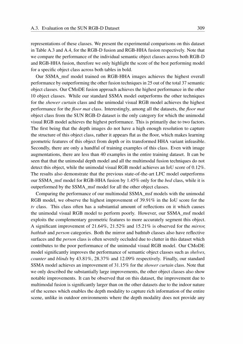
A.3. Evaluation on the SUN RGB-D Dataset 309
representations of these classes. We present the experimental comparisons on this datasetin Table A.3 and A.4, for the RGB-D fusion and RGB-HHA fusion respectively. Note thatwe compare the performance of the individual semantic object classes across both RGB-Dand RGB-HHA fusion, therefore we only highlight the score of the best performing modelfor a specific object class across both tables in bold.
Our SSMA_msf model trained on RGB-HHA images achieves the highest overallperformance by outperforming the other fusion techniques in 25 out of the total 37 semanticobject classes. Our CMoDE fusion approach achieves the highest performance in the other10 object classes. While our standard SSMA model outperforms the other techniquesfor the shower curtain class and the unimodal visual RGB model achieves the highestperformance for the floor mat class. Interestingly, among all the datasets, the floor matobject class from the SUN RGB-D dataset is the only category for which the unimodalvisual RGB model achieves the highest performance. This is primarily due to two factors.The first being that the depth images do not have a high enough resolution to capturethe structure of this object class, rather it appears flat as the floor, which makes learninggeometric features of this object from depth or its transformed HHA variant infeasible.Secondly, there are only a handful of training examples of this class. Even with imageaugmentations, there are less than 40 examples in the entire training dataset. It can beseen that that the unimodal depth model and all the multimodal fusion techniques do notdetect this object, while the unimodal visual RGB model achieves an IoU score of 0.12%.The results also demonstrate that the previous state-of-the-art LFC model outperformsour SSMA_msf model for RGB-HHA fusion by 1.45% only for the bed class, while it isoutperformed by the SSMA_msf model for all the other object classes.
Comparing the performance of our multimodal SSMA_msf models with the unimodalRGB model, we observe the highest improvement of 39.91% in the IoU score for thetv class. This class often has a substantial amount of reflections on it which causesthe unimodal visual RGB model to perform poorly. However, our SSMA_msf modelexploits the complementary geometric features to more accurately segment this object.A significant improvement of 21.64%, 21.52% and 15.21% is observed for the mirror,bathtub and person categories. Both the mirror and bathtub classes also have reflectivesurfaces and the person class is often severely occluded due to clutter in this dataset whichcontributes to the poor performance of the unimodal visual RGB model. Our CMoDEmodel significantly improves the performance of semantic object classes such as shelves,counter and blinds by 43.81%, 28.37% and 12.09% respectively. Finally, our standardSSMA model achieves an improvement of 31.15% for the shower curtain class. Note thatwe only described the substantially large improvements, the other object classes also shownotable improvements. It can be observed that on this dataset, the improvement due tomultimodal fusion is significantly larger than on the other datasets due to the indoor natureof the scenes which enables the depth modality to capture rich information of the entirescene, unlike in outdoor environments where the depth modality does not provide any
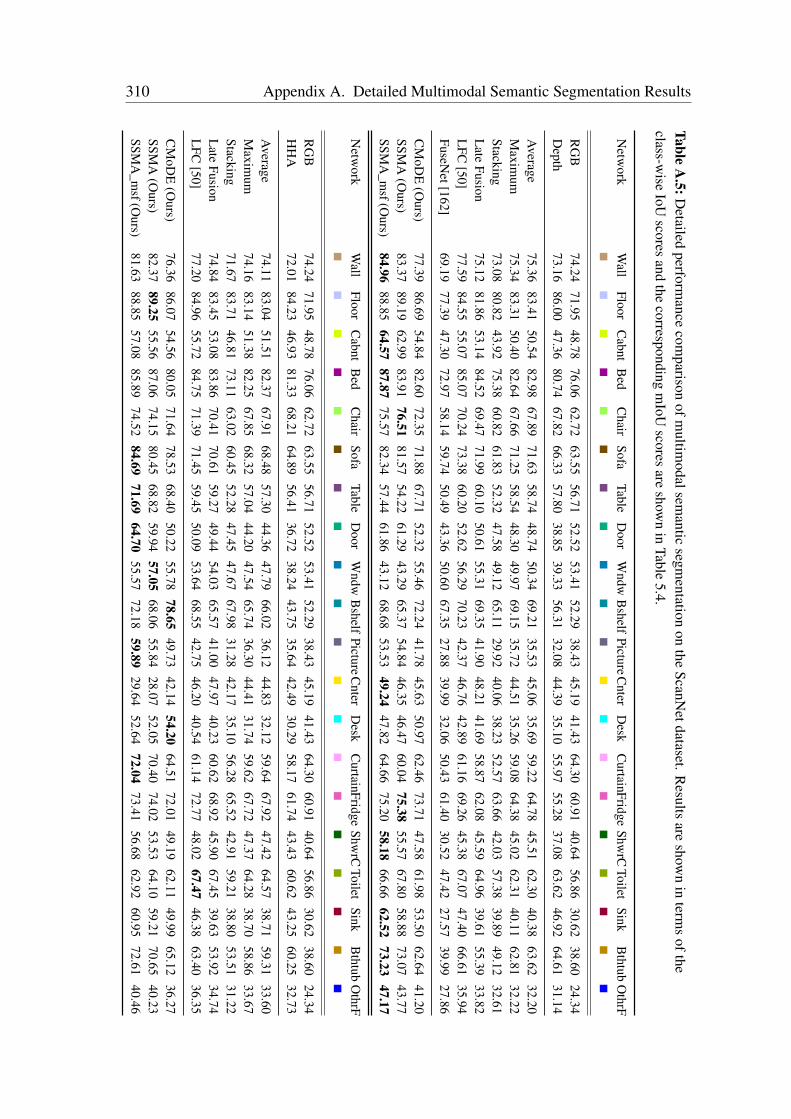
310 Appendix A. Detailed Multimodal Semantic Segmentation ResultsTable
A.5:D
etailedperform
ancecom
parisonof
multim
odalsemantic
segmentation
onthe
ScanNetdataset.
Results
areshow
nin
terms
ofthe
class-wise
IoUscores
andthe
correspondingm
IoUscores
areshow
nin
Table5.4.
Netw
orkW
allFloor
Cabnt
Bed
Chair
SofaTable
Door
Wndw
Bshelf
PictureCnter
Desk
CurtainFridge
ShwrC
ToiletSink
Bthtub
OthrF
RG
B74.24
71.9548.78
76.0662.72
63.5556.71
52.5253.41
52.2938.43
45.1941.43
64.3060.91
40.6456.86
30.6238.60
24.34D
epth73.16
86.0047.36
80.7467.82
66.3357.80
38.8539.33
56.3132.08
44.3935.10
55.9755.28
37.0863.62
46.9264.61
31.14
Average
75.3683.41
50.5482.98
67.8971.63
58.7448.74
50.3469.21
35.5345.06
35.6959.22
64.7845.51
62.3040.38
63.6232.20
Maxim
um75.34
83.3150.40
82.6467.66
71.2558.54
48.3049.97
69.1535.72
44.5135.26
59.0864.38
45.0262.31
40.1162.81
32.22Stacking
73.0880.82
43.9275.38
60.8261.83
52.3247.58
49.1265.11
29.9240.06
38.2352.57
63.6642.03
57.3839.89
49.1232.61
Late
Fusion75.12
81.8653.14
84.5269.47
71.9960.10
50.6155.31
69.3541.90
48.2141.69
58.8762.08
45.5964.96
39.6155.39
33.82L
FC[50]
77.5984.55
55.0785.07
70.2473.38
60.2052.62
56.2970.23
42.3746.76
42.8961.16
69.2645.38
67.0747.40
66.6135.94
FuseNet[162]
69.1977.39
47.3072.97
58.1459.74
50.4943.36
50.6067.35
27.8839.99
32.0650.43
61.4030.52
47.4227.57
39.9927.86
CM
oDE
(Ours)
77.3986.69
54.8482.60
72.3571.88
67.7152.32
55.4672.24
41.7845.63
50.9762.46
73.7147.58
61.9853.50
62.6441.20
SSMA
(Ours)
83.3789.19
62.9983.91
76.5181.57
54.2261.29
43.2965.37
54.8446.35
46.4760.04
75.3855.57
67.8058.88
73.0743.77
SSMA
_msf(O
urs)84.96
88.8564.57
87.8775.57
82.3457.44
61.8643.12
68.6853.53
49.2447.82
64.6675.20
58.1866.66
62.5273.23
47.17
Netw
orkW
allFloor
Cabnt
Bed
Chair
SofaTable
Door
Wndw
Bshelf
PictureCnter
Desk
CurtainFridge
ShwrC
ToiletSink
Bthtub
OthrF
RG
B74.24
71.9548.78
76.0662.72
63.5556.71
52.5253.41
52.2938.43
45.1941.43
64.3060.91
40.6456.86
30.6238.60
24.34H
HA
72.0184.23
46.9381.33
68.2164.89
56.4136.72
38.2443.75
35.6442.49
30.2958.17
61.7443.43
60.6243.25
60.2532.73
Average
74.1183.04
51.5182.37
67.9168.48
57.3044.36
47.7966.02
36.1244.83
32.1259.64
67.9247.42
64.5738.71
59.3133.60
Maxim
um74.16
83.1451.38
82.2567.85
68.3257.04
44.2047.54
65.7436.30
44.4131.74
59.6267.72
47.3764.28
38.7058.86
33.67Stacking
71.6783.71
46.8173.11
63.0260.45
52.2847.45
47.6767.98
31.2842.17
35.1056.28
65.5242.91
59.2138.80
53.5131.22
Late
Fusion74.84
83.4553.08
83.8670.41
70.6159.27
49.4454.03
65.5741.00
47.9740.23
60.6268.92
45.9067.45
39.6353.92
34.74L
FC[50]
77.2084.96
55.7284.75
71.3971.45
59.4550.09
53.6468.55
42.7546.20
40.5461.14
72.7748.02
67.4746.38
63.4036.35
CM
oDE
(Ours)
76.3686.07
54.5680.05
71.6478.53
68.4050.22
55.7878.65
49.7342.14
54.2064.51
72.0149.19
62.1149.99
65.1236.27
SSMA
(Ours)
82.3789.25
55.5687.06
74.1580.45
68.8259.94
57.0568.06
55.8428.07
52.0570.40
74.0253.53
64.1059.21
70.6540.23
SSMA
_msf(O
urs)81.63
88.8557.08
85.8974.52
84.6971.69
64.7055.57
72.1859.89
29.6452.64
72.0473.41
56.6862.92
60.9572.61
40.46
A.4. Evaluation on the ScanNet Dataset 311
information for distant objects.
A.4 Evaluation on the ScanNet Dataset
Table A.5 presents the multimodal fusion results on the recently introduced ScanNetdataset. Our proposed SSMA_msf model outperforms the unimodal models as well asthe multimodal fusion approaches in 13 out of the total of 20 semantic object classesin the dataset. While our standard SSMA model achieves the highest performance for4 of the other classes and our CMoDE model achieves the highest performance for thebookshelf and desk classes. Interestingly the previous state-of-the-art LFC fusion techniqueoutperforms our SSMA_msf model by 4.55% for the toilet class, while our model achievesa higher performance for all the other semantic object classes. Nevertheless, comparingthe performance of our SSMA_msf model with the unimodal visual RGB model, weobserve a significant improvement of 34.63% and 31.90% for the bathtub and sink classesrespectively. In addition, we observe a substantial improvement of over 20% for severalsemantic object classes including sofa, picture and other furniture.
Comparing the performance of our proposed SSMA_msf model with the FuseNet modelfor RGB-D fusion, we observe that our model outperforms FuseNet significantly in 19 outof the total of 20 semantic object categories. Our model is outperformed by FuseNet by7.46% for the window class. However, our model outperforms FuseNet in the window classusing RGB-HHA fusion. Similar to the performance of our models on the SUN RGB-Ddataset, the large improvement due to multimodal fusion on this dataset can be attributedto the indoor scenes for which the depth modality contains rich information. The depthmaps in the ScanNet dataset are considerably less noisy than those in the SUN RGB-Ddataset. This correlates to the larger improvement that we obtain due to multimodal fusionon this dataset. Moreover, this is the first real world dataset in which the unimodal modeltrained on depth images outperforms the corresponding visual RGB model. This showsthat geometry information can be more informative for learning semantics of the scenethan visual appearance information as long at it accurately captures the geometry of theentire scene. Our results demonstrate that the performance of multimodal fusion is largelylimited by the quality of complementary information captured in the modalities as well asthe noise in the sensor data.
A.5 Evaluation on the Freiburg Forest Dataset
Finally, Table A.6 shows the multimodal fusion results on the Freiburg Forest dataset. Thisdataset consists of three inherently different modalities that provide appearance, geometryand reflectance information. It contains scenarios in challenging perceptual conditionsincluding low lighting, shadows, glare on the optics, motion blur, snow, over exposure and
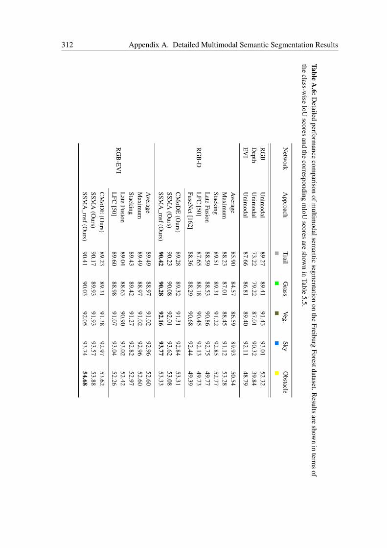
312 Appendix A. Detailed Multimodal Semantic Segmentation Results
TableA
.6:Detailed
performance
comparison
ofmultim
odalsemantic
segmentation
onthe
FreiburgForestdataset.R
esultsare
shown
interm
sof
theclass-w
iseIoU
scoresand
thecorresponding
mIoU
scoresare
shown
inTable
5.5.
Netw
orkA
pproachTrail
Grass
Veg.
SkyO
bstacle
RG
BU
nimodal
89.2789.41
91.4393.01
52.32D
epthU
nimodal
73.2279.22
87.0190.32
39.84E
VI
Unim
odal87.66
86.8189.40
92.1148.79
RG
B-D
Average
85.9084.57
86.5989.93
50.54M
aximum
88.2387.01
88.4591.12
53.28Stacking
89.5189.31
91.2292.85
52.77L
ateFusion
88.5988.53
90.8692.75
49.77L
FC[50]
87.6588.18
90.4592.13
49.73FuseN
et[162]88.36
88.2990.68
92.4449.39
CM
oDE
(Ours)
89.2889.32
91.3192.84
53.31SSM
A(O
urs)90.23
90.0892.01
93.6253.08
SSMA
_msf(O
urs)90.42
90.2892.16
93.7753.33
RG
B-E
VI
Average
89.4988.97
91.0292.96
52.60M
aximum
89.4988.97
91.0292.96
52.60Stacking
89.4389.42
91.2792.82
52.97L
ateFusion
89.0488.63
90.9093.02
52.42L
FC[50]
89.6088.98
91.0793.04
52.26
CM
oDE
(Ours)
89.2389.31
91.3892.97
53.62SSM
A(O
urs)90.17
89.9391.93
93.5753.88
SSMA
_msf(O
urs)90.41
90.0392.05
93.7454.68
A.5. Evaluation on the Freiburg Forest Dataset 313
under exposure. However the improvement due to multimodal fusion is not significantlyobserved in terms of the performance metrics but rather more in the qualitative resultsas shown in Section 5.3.5. The results demonstrate that each of our proposed models:CMoDE, SSMA and the SSMA_msf variant, outperforms the previous state-of-the-art LFCmodel in each of the semantic object categories for both RGB-D and RGB-EVI fusion.Moreover, it can be seen the performance of our SSMA_msf model for RGB-D fusionand RGB-EVI fusion, both show similar improvement in comparison to the unimodalvisual RGB model. The results also show that our SSMA_msf model outperforms theunimodal models as well the other multimodal fusion techniques in each of the semanticobject classes in the dataset. For most semantic object categories, a marginally higherimprovement can be seen using RGB-D fusion. However only the obstacle class achievesa higher performance using RGB-EVI fusion. Overall, we observe that simple fusiontechniques such as direct concatenation of feature maps from individual modality-specificnetwork streams at different intermediate network stages are significantly outperformed bymore intelligent dynamic approaches that adapt the fusion of the modality-specific featuremaps based on the observed scene. Nevertheless, the results presented in this sectiondemonstrate the complexity of multimodal perception.

List of Figures
1.1 The Viona and Obelix robots that we use in our experiments. . . . . . . . 131.2 The AIS perception car that we use in our experiments. . . . . . . . . . . 14
2.1 The pinhole camera model. . . . . . . . . . . . . . . . . . . . . . . . . . 192.2 Depiction of the biological neuron cell. . . . . . . . . . . . . . . . . . . 212.3 Depiction of the artificial neuron cell. . . . . . . . . . . . . . . . . . . . 222.4 Three-layer neural network with two hidden layers. . . . . . . . . . . . . 232.5 Example architectural topology of a CNN. . . . . . . . . . . . . . . . . . 252.6 Topology of residual units. . . . . . . . . . . . . . . . . . . . . . . . . . 30
3.1 Ambiguous appearances of terrains. . . . . . . . . . . . . . . . . . . . . 343.2 The Pioneer P3-DX platform that we use in our experiments. . . . . . . . 363.3 Overview of the data preprocessing pipeline. . . . . . . . . . . . . . . . . 383.4 Depiction of our proposed TerrainNet architecture. . . . . . . . . . . . . 403.5 Depiction of our proposed TerrainNet++ architecture. . . . . . . . . . . . 423.6 Depiction of the Long Short-Term Memory (LSTM) unit. . . . . . . . . . 433.7 Examples of terrain categories from our dataset. . . . . . . . . . . . . . . 493.8 Comparison of classification error rate of TerrainNet and TerrainNet++. . 533.9 Comparison of the recall of the various architecture configurations. . . . . 553.10 Inference time comparison of TerrainNet and TerrainNet++. . . . . . . . 573.11 Performance comparison of TerrainNet with our recurrent TerrainNet++. . 593.12 Comparison of the per-class recall of TerrainNet and TerrainNet++. . . . 603.13 Evaluation of TerrainNet++ when subject to different ambient noises. . . 613.14 Precision of TerrainNet++ when subject to ambient noises. . . . . . . . . 623.15 Precision of TerrainNet++ when subject to white Gaussian noise. . . . . . 633.16 Classification error of TerrainNet++ and the noise-aware TerrainNet++. . 653.17 Classification error due white Gaussian noise. . . . . . . . . . . . . . . . 663.18 Trajectory that the robot followed during the classification experiments. . 673.19 Predictions made while the robot was traversing the path. . . . . . . . . . 683.20 Comparison on audio data collected using a phone microphone. . . . . . 69
4.1 Example segmentation output from our proposed AdapNet++ model. . . . 764.2 Depiction of our AdapNet architecture for semantic segmentation. . . . . 824.3 Overview of our proposed Adapnet++ architecture. . . . . . . . . . . . . 85
316 List of Figures
4.4 Depiction of our proposed Adapnet++ encoder. . . . . . . . . . . . . . . 864.5 Depiction of the ASPP module and our efficient eASPP module. . . . . . 884.6 Illustration of pixel sampling in different 1-D convolutions. . . . . . . . . 894.7 Depiction of our proposed AdapNet++ decoder. . . . . . . . . . . . . . . 904.8 Depiction of our proposed AdapNet++ decoder with auxiliary losses. . . . 904.9 The Viona robot platform that we used for data collection . . . . . . . . . 944.10 Example images from our Freiburg Forest dataset. . . . . . . . . . . . . . 954.11 Example image from the Cityscapes dataset. . . . . . . . . . . . . . . . . 984.12 Example image from the Synthia dataset. . . . . . . . . . . . . . . . . . 994.13 Example image from the SUN RGB-D dataset. . . . . . . . . . . . . . . 994.14 Example image from the ScanNet dataset. . . . . . . . . . . . . . . . . . 1004.15 Example data augmentation strategies. . . . . . . . . . . . . . . . . . . . 1014.16 Evaluation of network compression approaches. . . . . . . . . . . . . . . 1114.17 Comparison of the receptive field of ASPP and our proposed eASPP. . . . 1174.18 Influence of the proposed decoder in AdapNet++. . . . . . . . . . . . . . 1194.19 Qualitative segmentation results on Cityscapes and Synthia datasets. . . . 1224.20 Qualitative segmentation results on SUN RGB-D and ScanNet datasets. . 1244.21 Qualitative segmentation results on the Freiburg Forest dataset. . . . . . . 1254.22 Example failure modes of our AdapNet++ model. . . . . . . . . . . . . . 1264.23 Qualitative results demonstrating the generalization ability. . . . . . . . . 128
5.1 Misclassifications in real-world scenarios. . . . . . . . . . . . . . . . . . 1345.2 Topology of our proposed CMoDE fusion module. . . . . . . . . . . . . 1395.3 The late-fusion architecture incorporating the CMoDE module. . . . . . . 1415.4 The topology of our proposed SSMA fusion module. . . . . . . . . . . . 1425.5 Topology of our modified AdapNet++ used for multimodal fusion. . . . . 1445.6 Depiction of the early and late-fusion approaches. . . . . . . . . . . . . . 1475.7 Evaluation of the SMMA fusion on the Synthia-Sequences dataset. . . . . 1535.8 Visualization of activation maps on Cityscapes and Synthia datasets. . . . 1615.9 Visualization of activation maps on SUN RGB-D and ScanNet datasets. . 1625.10 Visualization of activation maps on Freiburg Forest dataset. . . . . . . . . 1635.11 Qualitative multimodal fusion on Cityscapes and Synthia datasets. . . . . 1655.12 Qualitative multimodal fusion results on SUN and ScanNet datasets. . . . 1675.13 Qualitative multimodal fusion results on the Freiburg Forest dataset. . . . 1695.14 Qualitative results in summer, fall, winter, and spring. . . . . . . . . . . . 1715.15 Qualitative results in dawn, sunset, night, and rain. . . . . . . . . . . . . 1725.16 Qualitative results in soft-rain, fog, night-rain and winter-night. . . . . . . 1735.17 Our Viona robot autonomously navigating a forested environment. . . . . 1745.18 Trajectory traversed by our robot using our multimodal network. . . . . . 175
List of Figures 317
6.1 Illustration of semantic motion segmentation using our proposed model. . 1826.2 Topology of our proposed SMSnet architecture. . . . . . . . . . . . . . . 1886.3 Motion and semantic encoder streams of our proposed SMSnet++. . . . . 1916.4 Topology of the flow transformation module used in SMSnet++. . . . . . 1936.5 Motion and semantic decoder streams of our proposed SMSnet++. . . . . 1956.6 Example training data from the Cityscapes-Motion dataset. . . . . . . . . 1976.7 Example training data from the KITTI-Motion dataset. . . . . . . . . . . 1986.8 Example training data from the ApolloScape-Motion dataset. . . . . . . . 1996.9 Motion segmentation at different ranges on Cityscapes & KITTI. . . . . . 2106.10 Motion segmentation at different ranges on ApolloScape. . . . . . . . . . 2116.11 Comparison of motion segmentation with different flow transformations. . 2166.12 Examples of the edge-enhanced optical flow transformation. . . . . . . . 2186.13 Comparison of motion segmentation with movable and full label sets. . . 2206.14 Qualitative semantic motion segmentation on Cityscapes dataset. . . . . . 2226.15 Qualitative semantic motion segmentation on KITTI dataset. . . . . . . . 2246.16 Qualitative semantic motion segmentation on ApolloScape dataset. . . . . 2276.17 Qualitative semantic motion segmentation on Freiburg dataset. . . . . . . 230
7.1 Output of our multitask VLocNet++ model. . . . . . . . . . . . . . . . . 2387.2 Topology of our proposed VLocNet architecture . . . . . . . . . . . . . . 2457.3 Schematic representation of our proposed VLocNet++ architecture. . . . 2487.4 Example images from our DeepLoc dataset. . . . . . . . . . . . . . . . . 2547.5 Example images from the Microsoft 7-Scenes benchmark. . . . . . . . . 2567.6 Benchmarking 6DoF localization on Microsoft 7-Scenes dataset. . . . . . 2637.7 Influence of previous pose fusion in our VLocNet architecture. . . . . . . 2717.8 Influence of our proposed weighted fusion layer in VLocNet++MTL. . . . 2757.9 Evaluation of different weight initializations in VLocNetMTL. . . . . . . . 2767.10 3D multi-dimensional scaling of features on the DeepLoc dataset. . . . . 2797.11 Comparison of the regression activation maps of VLocNet++. . . . . . . 2807.12 Qualitative localization results on Microsoft 7-Scenes dataset. . . . . . . 2827.13 Qualitative localization results of VLocNet++MTL on DeepLoc. . . . . . . 2837.14 Qualitative segmentation results on the DeepLoc dataset. . . . . . . . . . 2847.15 Challenging qualitative segmentation results. . . . . . . . . . . . . . . . 286

List of Tables
3.1 Comparison of classification accuracies of TerrainNet and TerrainNet++. . 513.2 Performance comparison of various architecture configurations. . . . . . 543.3 Performance for varying audio clip and LSTM window lengths. . . . . . 563.4 Performance comparison of TerrainNet and TerrainNet++ model. . . . . . 563.5 Influence of ambient noises on the accuracy of TerrainNet++. . . . . . . . 613.6 Influence of ambient noises on accuracy of noise-aware TerrainNet++. . . 64
4.1 Comparison of AdapNet and AdapNet++ on the Cityscapes dataset. . . . 1044.2 Comparison of AdapNet and AdapNet++ on the Synthia dataset. . . . . . 1044.3 Benchmarking results on the Cityscapes dataset. . . . . . . . . . . . . . . 1054.4 Comparison of AdapNet and AdapNet++ on the SUN RGB-D dataset. . . 1064.5 Comparison of AdapNet and AdapNet++ on the ScanNet dataset. . . . . . 1084.6 Comparison of AdapNet and AdapNet++ on the Freiburg Forest dataset. . 1084.7 Bechmarking results on the ScanNet dataset. . . . . . . . . . . . . . . . . 1094.8 Comparison of network compression approaches on AdapNet++. . . . . . 1104.9 Effect of the contributions proposed in AdapNet and AdapNet++. . . . . 1134.10 Evaluation of various atrous spatial pyramid pooling configurations. . . . 1154.11 Effect on varying the number of filters in the skip refinement connection. . 1184.12 Effect on varying the weighting factor of the auxiliary losses. . . . . . . . 1184.13 Effect on varying the number of filters in the skip refinement connection. . 1194.14 Effect on using higher resolution image and multiscale testing. . . . . . . 121
5.1 Comparison of multimodal fusion on the Cityscapes dataset. . . . . . . . 1515.2 Comparison of multimodal fusion on the Synthia dataset. . . . . . . . . . 1525.3 Comparison of multimodal fusion on the SUN RGB-D dataset. . . . . . . 1545.4 Comparison of multimodal fusion on the ScanNet dataset. . . . . . . . . 1555.5 Comparison of multimodal fusion on the Freiburg Forest dataset. . . . . . 1565.6 Effect on varying the output units in the inner-product layer of the AGN. . 1585.7 Effect of the various contributions that we proposed in SMMA. . . . . . . 1595.8 Effect of varying the SSMA bottleneck downsampling rate. . . . . . . . . 159
6.1 Comparison of semantic motion segmentation on the Cityscapes. . . . . . 2036.2 Comparison of semantic motion segmentation on the KITTI. . . . . . . . 2046.3 Comparison of semantic motion segmentation on the ApolloScape. . . . . 205
320 List of Tables
6.4 Comparison of semantic segmentation performance. . . . . . . . . . . . . 2076.5 Influence of the contributions proposed in SMSnet and SMSnet++. . . . . 2136.6 Evaluation of ego-flow suppression. . . . . . . . . . . . . . . . . . . . . 2166.7 Evaluation of warping semantic features using edge-enhanced flow. . . . 2176.8 Evaluation of network configurations for learning the flow field. . . . . . 219
7.1 Median localization error on the Microsoft 7-Scenes dataset. . . . . . . . 2587.2 Localization error on the DeepLoc dataset. . . . . . . . . . . . . . . . . . 2597.3 6DoF visual odometry on the Microsoft 7-Scenes dataset. . . . . . . . . . 2607.4 6DoF visual odometry on the on the DeepLoc dataset. . . . . . . . . . . . 2607.5 Benchmarking single-task models on the Microsoft 7-Scenes dataset. . . . 2627.6 Benchmarking multitask models on the Microsoft 7-Scenes dataset. . . . 2627.7 Summary of benchmarking on the Microsoft 7-Scenes dataset. . . . . . . 2637.8 Benchmarking our multitask models on the DeepLoc dataset. . . . . . . . 2647.9 Benchmarking visual odometry on the Microsoft 7-Scenes dataset. . . . . 2657.10 Benchmarking visual odometry on the on the DeepLoc dataset. . . . . . . 2657.11 Semantic segmentation results on the DeepLoc dataset. . . . . . . . . . . 2677.12 Comparison of the VLocNet++ base architecture topology. . . . . . . . . 2687.13 Comparative analysis of different loss functions and loss weightings. . . . 2697.14 Localization performance with varying amounts of sharing. . . . . . . . . 2727.15 Improvement in segmentation due to fusion of warped feature maps. . . . 2737.16 Improvement in performance due to fusion of semantic features. . . . . . 2747.17 Evaluation of different optimization strategies. . . . . . . . . . . . . . . . 278
A.1 Detailed multimodal segmentation results on the Cityscapes dataset. . . . 304A.2 Detailed multimodal segmentation results on the Synthia dataset. . . . . . 306A.3 Detailed RGB-D segmentation results on the SUN RGB-D dataset. . . . . 307A.4 Detailed RGB-HHA segmentation results on the SUN RGB-D dataset. . . 308A.5 Detailed multimodal segmentation results on the ScanNet dataset. . . . . 310A.6 Detailed multimodal segmentation results on the Freiburg Forest dataset. . 312
Bibliography
[1] J. McCarthy, M. L. Minsky, N. Rochester, and C. E. Shannon, “A proposal for thedartmouth summer research project on artificial intelligence, august 31, 1955,” AImagazine, vol. 27, no. 4, p. 12, 2006.
[2] H. Simon, “The shape of automation for men and management,” Harper and Row,vol. 40, 1965.
[3] D. Crevier, AI: the tumultuous history of the search for artificial intelligence. BasicBooks, 1993.
[4] “Ai expert newsletter: W is for winter archived 9 november 2013 at the waybackmachine.” https://web.archive.org/web/20131109201636/http://www.ainewsletter.com/newsletters/aix_0501.htm, 2005, accessed: 10-11-2018.
[5] S. Thrun, W. Burgard, and D. Fox, Probabilistic robotics. MIT press, 2005.
[6] D. A. Forsyth and J. Ponce, “A modern approach,” Computer vision: a modernapproach, pp. 88–101, 2003.
[7] C. M. Bishop, Pattern Recognition and Machine Learning (Information Science andStatistics). Berlin, Heidelberg: Springer-Verlag, 2006.
[8] Y. LeCun, Y. Bengio et al., “Convolutional networks for images, speech, and timeseries,” The handbook of brain theory and neural networks, vol. 3361, no. 10, p.1995, 1995.
[9] I. F. of Robotics, “Executive summary world robotics 2018 industrial robots,” Avail-able online on http://www. ifr. org, pp. 13–22, 2018.
[10] D. Wettergreen, G. Foil, P. M. Furlong, and D. R. Thompson, “Science autonomyfor rover subsurface exploration of the atacama desert,” AI Magazine, vol. 35, no. 4,October 2014.
[11] A. R. Lanfranco, A. E. Castellanos, J. P. Desai, and W. C. Meyers, “Robotic surgery:a current perspective,” Annals of surgery, vol. 239, no. 1, p. 14, 2004.
322 Bibliography
[12] A. D. Bowen, D. R. Yoerger, C. Taylor, R. McCabe, J. Howland, D. Gomez-Ibanez,J. C. Kinsey, M. Heintz, G. McDonald, D. B. Peters et al., “The nereus hybridunderwater robotic vehicle for global ocean science operations to 11,000 m depth,”in OCEANS 2008, 2008, pp. 1–10.
[13] “irobot corp. irobot: Our history,” http://www.irobot.com/us/Company/About/Our_History.aspx, 2018, accessed: 10-11-2018.
[14] I. F. of Robotics, “Executive summary world robotics 2018 service robots,” Availableonline on http://www. ifr. org, pp. 13–16, 2018.
[15] “Fetch robotics,” http://fetchrobotics.com, 2018, accessed: 10-11-2018.
[16] “Beam robot, suitable technologies,” https://www.suitabletech.com/, 2018, accessed:10-11-2018.
[17] A. K. Singh and G. Nandi, “Nao humanoid robot,” Robotics Autonomous Systems,vol. 79, no. C, pp. 108–121, 2016.
[18] T. Shibata, “Development and spread of therapeutic medical robot, paro: Innova-tion of non-pharmacological therapy for dementia and mental health,” Journal ofInformation Processing and Management, vol. 60, no. 4, pp. 217–228, 2017.
[19] “Mars science laboratory curiosity rover,” https://mars.jpl.nasa.gov/msl, 2018, ac-cessed: 10-11-2018.
[20] Y. LeCun, Y. Bengio, and G. Hinton, “Deep learning,” nature, vol. 521, no. 7553, p.436, 2015.
[21] M. Minsky, “Neural nets and the brain-model problem,” Doctoral dissertation,Princeton University, NJ, 1954.
[22] A. Krizhevsky, I. Sutskever, and G. E. Hinton, “Imagenet classification with deepconvolutional neural networks,” in Advances in Neural Information ProcessingSystems, 2012, pp. 1097–1105.
[23] O. Russakovsky, J. Deng, H. Su, J. Krause, S. Satheesh, S. Ma, Z. Huang, A. Karpa-thy, A. Khosla, M. Bernstein et al., “Imagenet large scale visual recognition chal-lenge,” International Journal of Computer Vision, vol. 115, no. 3, pp. 211–252,2015.
[24] J. Long, E. Shelhamer, and T. Darrell, “Fully convolutional networks for semanticsegmentation,” in Proceedings of the IEEE International Conference on ComputerVision and Pattern Recognition (CVPR), 2015.
Bibliography 323
[25] R. Girshick, J. Donahue, T. Darrell, and J. Malik, “Rich feature hierarchies foraccurate object detection and semantic segmentation,” in Proceedings of the IEEEInternational Conference on Computer Vision and Pattern Recognition (CVPR),2014, pp. 580–587.
[26] A. Graves and N. Jaitly, “Towards end-to-end speech recognition with recurrentneural networks,” in Proceedings of the 31st International Conference on MachineLearning (ICML-14), T. Jebara and E. P. Xing, Eds., 2014, pp. 1764–1772.
[27] K. He, X. Zhang, S. Ren, and J. Sun, “Deep residual learning for image recognition,”in Proceedings of the IEEE International Conference on Computer Vision andPattern Recognition (CVPR), 2015.
[28] J. Devlin, M.-W. Chang, K. Lee, and K. Toutanova, “Bert: Pre-training ofdeep bidirectional transformers for language understanding,” arXiv preprintarXiv:1810.04805, 2018.
[29] P. Rajpurkar, J. Zhang, K. Lopyrev, and P. Liang, “Squad: 100,000+ questions formachine comprehension of text,” arXiv preprint arXiv:1606.05250, 2016.
[30] “Waymo,” https://waymo.com, 2018, accessed: 10-11-2018.
[31] “Uber,” https://uber.com, 2018, accessed: 10-11-2018.
[32] “Navya,” https://navya.tech, 2018, accessed: 10-11-2018.
[33] P. Gao, H.-W. Kaas, D. Mohr, and D. Wee, “Automotive revolution–perspectivetowards 2030 how the convergence of disruptive technology-driven trends couldtransform the auto industry,” Advanced Industries, McKinsey & Company, 2016.
[34] N. Radwan, A. Valada, and W. Burgard, “Vlocnet++: Deep multitask learning forsemantic visual localization and odometry,” IEEE Robotics And Automation Letters(RA-L), vol. 3, no. 4, pp. 4407–4414, 2018.
[35] C. Galindo, A. Saffiotti, S. Coradeschi, P. Buschka, J.-A. Fernandez-Madrigal, andJ. González, “Multi-hierarchical semantic maps for mobile robotics,” in Interna-tional Conference on Intelligent Robots and Systems (IROS), 2005, pp. 2278–2283.
[36] R. Drouilly, P. Rives, and B. Morisset, “Semantic representation for navigation inlarge-scale environments,” in Proceedings of the IEEE International Conference onRobotics and Automation (ICRA), 2015, pp. 1106–1111.
[37] M. Johnson-Roberson, J. Bohg, G. Skantze, J. Gustafson, R. Carlson, B. Rasolzadeh,and D. Kragic, “Enhanced visual scene understanding through human-robot dialog,”
324 Bibliography
in International Conference on Intelligent Robots and Systems (IROS), 2011, pp.3342–3348.
[38] “Marble - urban last-mile robots,” https://angel.co/marble-1l, 2018, accessed: 10-11-2018.
[39] M. Joerss, J. Schröder, F. Neuhaus, C. Klink, and F. Mann, “Parcel delivery: Thefuture of last mile,” McKinsey & Company, 2016.
[40] S. S. Srinivasa, D. Ferguson, C. J. Helfrich, D. Berenson, A. Collet, R. Diankov,G. Gallagher, G. Hollinger, J. Kuffner, and M. V. Weghe, “Herb: a home exploringrobotic butler,” Autonomous Robots, vol. 28, no. 1, p. 5, 2010.
[41] J. Zhang and S. Singh, “Loam: Lidar odometry and mapping in real-time.” inRobotics: Science and Systems, vol. 2, 2014, p. 9.
[42] T. Sattler, W. Maddern, C. Toft, A. Torii, L. Hammarstrand, E. Stenborg, D. Safari,M. Okutomi, M. Pollefeys, J. Sivic et al., “Benchmarking 6dof outdoor visuallocalization in changing conditions,” in Proceedings of the IEEE InternationalConference on Computer Vision and Pattern Recognition (CVPR), vol. 1, 2018.
[43] W. Winterhalter, F. Fleckenstein, B. Steder, L. Spinello, and W. Burgard, “Accurateindoor localization for RGB-D smartphones and tablets given 2D floor plans,” inInternational Conference on Intelligent Robots and Systems (IROS), 2015.
[44] T. Naseer, G. Oliveira, T. Brox, and W. Burgard, “Semantics-aware visual lo-calization under challenging perceptual conditions,” in Proceedings of the IEEEInternational Conference on Robotics and Automation (ICRA), 2017.
[45] R. Kümmerle, M. Ruhnke, B. Steder, C. Stachniss, and W. Burgard, “Autonomousrobot navigation in highly populated pedestrian zones,” Journal of Field Robotics,vol. 32, no. 4, pp. 565–589, 2015.
[46] J. Maye, P. Furgale, and R. Siegwart, “Self-supervised calibration for robotic sys-tems,” in 2013 IEEE Intelligent Vehicles Symposium (IV), 2013, pp. 473–480.
[47] A. Valada, L. Spinello, and W. Burgard, “Deep feature learning for acoustics-basedterrain classification,” in Proceedings of the International Symposium of RoboticsResearch, 2015.
[48] G. Oliveira, A. Valada, C. Bollen, W. Burgard, and T. Brox, “Deep learning for hu-man part discovery in images,” in Proceedings of the IEEE International Conferenceon Robotics and Automation (ICRA), 2016.
Bibliography 325
[49] A. Valada, G. L. Olivera, T. Brox, and W. Burgard, “Towards robust semanticsegmentation using deep fusion,” in In Proceedings of the Workshop on Limits andPotentials of Deep Learning in Robotics at Robotics: Science and Systems (RSS),2016.
[50] A. Valada, G. Oliveira, T. Brox, and W. Burgard, “Deep multispectral semantic sceneunderstanding of forested environments using multimodal fusion,” in Proceedingsof the International Symposium for Experimental Robotics, 2016.
[51] A. Valada, A. Dhall, and W. Burgard, “Convoluted mixture of deep experts forrobust semantic segmentation,” in IEEE/RSJ International Conference on IntelligentRobots and Systems (IROS) Workshop, State Estimation and Terrain Perception forAll Terrain Mobile Robots, 2016.
[52] A. Valada and W. Burgard, “Deep spatiotemporal models for robust proprioceptiveterrain classification,” International Journal of Robotics Research, vol. 36, no. 13-14,pp. 1521i–1539, 2017.
[53] A. Valada, J. Vertens, A. Dhall, and W. Burgard, “Adapnet: Adaptive semanticsegmentation in adverse environmental conditions,” in Proceedings of the IEEEInternational Conference on Robotics and Automation (ICRA), 2017.
[54] J. Vertens, A. Valada, and W. Burgard, “Smsnet: Semantic motion segmentationusing deep convolutional neural networks,” in International Conference on Intelli-gent Robots and Systems (IROS), 2017.
[55] W. Burgard, A. Valada, N. Radwan, T. Naseer, J. Zhang, J. Vertens, O. Mees,A. Eitel, and G. Oliveira, “Perspectives on deep multimodel robot learning,” inProceedings of the International Symposium of Robotics Research, 2017.
[56] A. Valada, N. Radwan, and W. Burgard, “Deep auxiliary learning for visual local-ization and odometry,” in Proceedings of the IEEE International Conference onRobotics and Automation (ICRA), 2018.
[57] A. Valada and W. Burgard, “Learning reliable and scalable representations usingmultimodal multitask deep learning,” in In Proceedings of RSS Pioneers at Robotics:Science and Systems (RSS), 2018.
[58] A. Valada, N. Radwan, and W. Burgard, “Incorporating semantic and geometricpriors in deep pose regression,” in In Proceedings of the Workshop on Learningand Inference in Robotics: Integrating Structure, Priors and Models at Robotics:Science and Systems (RSS), 2018.

326 Bibliography
[59] A. Valada, R. Mohan, and W. Burgard, “Self-supervised model adaptation formultimodal semantic segmentation,” arXiv preprint arXiv:1808.03833, 2018.
[60] F. Boniardi, A. Valada, W. Burgard, and G. D. Tipaldi, “Autonomous indoor robotnavigation using sketched maps and routes,” in RSS Workshop on Model Learningfor Human-Robot Communication, 2015.
[61] ——, “Autonomous indoor robot navigation using a sketch interface for drawningmaps and routes,” in Proceedings of the IEEE International Conference on Roboticsand Automation (ICRA), 2016.
[62] N. Radwan, A. Valada, and W. Burgard, “Multimodal interaction-aware motionprediction for autonomous street crossing,” arXiv preprint arXiv:1808.06887, 2018.
[63] M. Mittal, A. Valada, and W. Burgard, “Vision-based autonomous landing incatastrophe-struck environments,” in In Proceedings of the Workshop on Vision-based Drones: What’s Next? at the IEEE/RSJ International Conference on Intelli-gent Robots and Systems (IROS), 2018.
[64] B. Blaus, “Medical gallery of blausen medical 2014,” WikiJournal of Medicine,vol. 1, no. 2, 2014.
[65] V. Nair and G. E. Hinton, “Rectified linear units improve restricted boltzmannmachines,” in Proceedings of the International Conference in Machine Learning(ICML), 2010, pp. 807–814.
[66] D.-A. Clevert, T. Unterthiner, and S. Hochreiter, “Fast and accurate deep networklearning by exponential linear units (elus),” arXiv preprint arXiv:1511.07289, 2015.
[67] F. Yu and V. Koltun, “Multi-scale context aggregation by dilated convolutions,” inInternational Conference on Learning Representations (ICLR), 2016.
[68] Y. Gal and Z. Ghahramani, “Dropout as a bayesian approximation: Representingmodel uncertainty in deep learning,” in Proceedings of the International Conferencein Machine Learning (ICML), 2016, pp. 1050–1059.
[69] M. Lin, Q. Chen, and S. Yan, “Network in network,” arXiv preprint arXiv:1312.4400,2013.
[70] C. Szegedy, W. Liu, Y. Jia, P. Sermanet, S. Reed, D. Anguelov, D. Erhan, V. Van-houcke, and A. Rabinovich, “Going deeper with convolutions,” arXiv preprintarXiv:1409.4842, 2014.
[71] G. Huang, Z. Liu, K. Q. Weinberger, and L. van der Maaten, “Densely connectedconvolutional networks,” arXiv preprint arXiv:1608.06993, 2016.

Bibliography 327
[72] K. He, X. Zhang, S. Ren, and J. Sun, “Identity mappings in deep residual networks,”in The European Conference on Computer Vision (ECCV), 2016, pp. 630–645.
[73] S. Thrun, M. Montemerlo, H. Dahlkamp, D. Stavens, A. Aron, J. Diebel, P. Fong,J. Gale, M. Halpenny, G. Hoffmann, K. Lau, C. Oakley, M. Palatucci, V. Pratt,P. Stang, S. Strohband, C. Dupont, L.-E. Jendrossek, C. Koelen, C. Markey, C. Rum-mel, J. van Niekerk, E. Jensen, P. Alessandrini, G. Bradski, B. Davies, S. Ettinger,A. Kaehler, A. Nefian, and P. Mahoney, “Stanley: The robot that won the darpagrand challenge,” Journal of Field Robotics, vol. 23, no. 9, pp. 661–692, 2006.
[74] B. Suger, B. Steder, and W. Burgard, “Traversability analysis for mobile robots inoutdoor environments: A semi-supervised learning approach based on 3d-lidar data,”in Proc. of the IEEE Int. Conf. on Robotics & Automation (ICRA), 2015.
[75] C. A. Brooks and K. Iagnemma, “Vibration-based terrain classification for planetaryexploration rovers,” IEEE Transactions on Robotics, vol. 21, no. 6, pp. 1185–1191,Dec 2005.
[76] J. Libby and A. T. Stentz, “Using sound to classify vehicle-terrain interactions inoutdoor environments,” in Proceedings of the IEEE International Conference onRobotics and Automation (ICRA), May 2012.
[77] J. Christe and N. Kottege, “Acoustics based terrain classification for legged robots,”in Proceedings of the IEEE International Conference on Robotics and Automation(ICRA), 2016.
[78] M. C. Ozkul, A. Saranli, and Y. Yazicioglu, “Acoustic surface perception fromnaturally occurring step sounds of a dexterous hexapod robot,” Mechanical Systemsand Signal Processing, vol. 40, no. 1, pp. 178–193, 2013.
[79] J. Eriksson, L. Girod, B. Hull, R. Newton, S. Madden, and H. Balakrishnan, “Thepothole patrol: Using a mobile sensor network for road surface monitoring,” inThe Sixth Annual International conference on Mobile Systems, Applications andServices (MobiSys 2008), Breckenridge, U.S.A., June 2008.
[80] C. Weiss, H. Frohlich, and A. Zell, “Vibration-based terrain classification usingsupport vector machines,” in International Conference on Intelligent Robots andSystems (IROS), Oct 2006, pp. 4429–4434.
[81] G.-Y. Sung, D.-M. Kwak, and J. Lyou, “Neural network based terrain classificationusing wavelet features,” Journal of Intelligent & Robotic Systems, vol. 59, no. 3, pp.269–281, 2010.

328 Bibliography
[82] X. Tan and B. Triggs, “Enhanced local texture feature sets for face recognition underdifficult lighting conditions,” IEEE Transactions on Image Processing, vol. 19, no. 6,pp. 1635–1650, 2010.
[83] S. Otte, S. Laible, R. Hanten, M. Liwicki, and A. Zell, “Robust visual terrainclassification with recurrent neural networks,” in In Proc. of European Symposiumon Artificial Neural Networks, 2015.
[84] A. Santamaria-Navarro, E. H. Teniente, M. Morta, and J. Andrade-Cetto, “Terrainclassification in complex three-dimensional outdoor environments,” Journal of FieldRobotics, vol. 32, no. 1, pp. 42–60, 2015.
[85] S. T. Namin, M. Najafi, and L. Petersson, “Multi-view terrain classification usingpanoramic imagery and lidar,” in International Conference on Intelligent Robotsand Systems (IROS), Sept 2014, pp. 4936–4943.
[86] I. Posner, M. Cummins, and P. Newman, “Fast probabilistic labeling of city maps,”Proceedings of Robotics: Science and Systems IV, Zurich, Switzerland, 2008.
[87] R. Hadsell, P. Sermanet, J. Ben, A. Erkan, M. Scoffier, K. Kavukcuoglu, U. Muller,and Y. LeCun, “Learning long-range vision for autonomous off-road driving,” Jour-nal of Field Robotics, vol. 26, no. 2, pp. 120–144, Feb. 2009.
[88] U. A. Muller, L. D. Jackel, Y. LeCun, and B. Flepp, “Real-time adaptive off-roadvehicle navigation and terrain classification,” Proc. SPIE, vol. 8741, pp. 87 410A–87 410A–19, 2013.
[89] P. A. Plonski, P. Tokekar, and V. Isler, “Energy-efficient path planning for solar-powered mobile robots,” Journal of Field Robotics, vol. 30, no. 4, pp. 583–601,2013.
[90] J. Thiemann, N. Ito, and E. Vincent, “The diverse environments multi-channelacoustic noise database (demand): A database of multichannel environmental noiserecordings,” in 21st International Congress on Acoustics, 2013.
[91] P. Khunarsal, C. Lursinsap, and T. Raicharoen, “Very short time environmentalsound classification based on spectrogram pattern matching,” Information Sciences,vol. 243, pp. 57 – 74, 2013.
[92] G. E. Hinton, N. Srivastava, A. Krizhevsky, I. Sutskever, and R. Salakhutdinov,“Improving neural networks by preventing co-adaptation of feature detectors,” arXivpreprint arXiv:1207.0580, 2012.
Bibliography 329
[93] K. He, X. Zhang, S. Ren, and J. Sun, “Delving deep into rectifiers: Surpassinghuman-level performance on imagenet classification,” in The IEEE InternationalConference on Computer Vision (ICCV), 2015.
[94] I. Sutskever, O. Vinyals, and Q. V. Le, “Sequence to sequence learning with neuralnetworks,” in Advances in neural information processing systems, 2014, pp. 3104–3112.
[95] J. Donahue, L. A. Hendricks, S. Guadarrama, M. Rohrbach, S. Venugopalan,K. Saenko, and T. Darrell, “Long-term recurrent convolutional networks for vi-sual recognition and description,” in CVPR, 2015.
[96] S. Hochreiter and J. Schmidhuber, “Long short-term memory,” Neural Computation,vol. 9, no. 8, pp. 1735–1780, Nov. 1997.
[97] B. E. Kingsbury, N. Morgan, and S. Greenberg, “Robust speech recognition usingthe modulation spectrogram,” Speech communication, vol. 25, no. 1-3, pp. 117–132,1998.
[98] P. Boersma and D. Weenink, “Praat: doing phonetics by computer [computerprogram],” in Version 5.3.51, retrieved 2 June 2013 from http://www.praat.org/,2013.
[99] T. Giannakopoulos, D. Kosmopoulos, A. Aristidou, and S. Theodoridis, Advancesin Artificial Intelligence: 4th Helenic Conference on AI, SETN 2006, Heraklion,Crete, Greece, May 18-20, 2006. Proceedings. Springer Berlin Heidelberg, 2006,ch. Violence Content Classification Using Audio Features, pp. 502–507.
[100] M. C. Wellman, N. Srour, and D. B. Hillis, “Feature extraction and fusion of acousticand seismic sensors for target identification,” Proc. SPIE, vol. 3081, pp. 139–145,1997.
[101] D. P. W. Ellis, “Classifying music audio with timbral and chroma features,” in 8thInternational Conference on Music Information Retrieval, 2007.
[102] G. Tzanetakis and P. Cook, “Musical genre classification of audio signals,” IEEETransactions on Speech and Audio Processing, vol. 10, no. 5, pp. 293–302, Jul 2002.
[103] B. Verma, Pattern Recognition Technologies and Applications: Recent Advances:Recent Advances. IGI Global, 2008.
[104] F. Zheng, G. Zhang, and Z. Song, “Comparison of different implementations ofmfcc,” Journal of Computer science and Technology, vol. 16, no. 6, pp. 582–589,2001.
330 Bibliography
[105] M. A. Bartsch and G. H. Wakefield, “Audio thumbnailing of popular music usingchroma-based representations,” IEEE Transactions on multimedia, vol. 7, no. 1, pp.96–104, 2005.
[106] Y. Jia, E. Shelhamer, J. Donahue, S. Karayev, J. Long, R. Girshick, S. Guadarrama,and T. Darrell, “Caffe: Convolutional architecture for fast feature embedding,” arXivpreprint arXiv:1408.5093, 2014.
[107] W. Zaremba and I. Sutskever, “Learning to execute,” arxiv preprint arxiv: 1410.4615,2014.
[108] X. Glorot and Y. Bengio, “Understanding the difficulty of training deep feedforwardneural networks,” in In Proceedings of the International Conference on ArtificialIntelligence and Statistics (AISTATS’10). Society for Artificial Intelligence andStatistics, 2010.
[109] J. Snoek, H. Larochelle, and R. P. Adams, “Practical bayesian optimization ofmachine learning algorithms,” in Advances in neural information processing systems,2012, pp. 2951–2959.
[110] F. Pedregosa, G. Varoquaux, A. Gramfort, V. Michel, B. Thirion, O. Grisel, M. Blon-del, P. Prettenhofer, R. Weiss, V. Dubourg et al., “Scikit-learn: Machine learning inPython,” Journal of Machine Learning Research, vol. 12, pp. 2825–2830, 2011.
[111] C.-C. Chang and C.-J. Lin, “Libsvm: a library for support vector machines,” ACMtransactions on intelligent systems and technology (TIST), vol. 2, no. 3, p. 27, 2011.
[112] P. C. Loizou, Speech Enhancement: Theory and Practice, ser. Signal processingand communications. CRC press, 2007.
[113] L. Ojeda, J. Borenstein, G. Witus, and R. Karlsen, “Terrain characterization andclassification with a mobile robot,” Journal of Field Robotics, vol. 23, no. 2, pp.103–122, 2006.
[114] E. Trautmann and L. Ray, “Mobility characterization for autonomous mobile robotsusing machine learning,” Autonomous Robots, vol. 30, no. 4, pp. 369–383, 2011.
[115] M. A. Hoepflinger, C. D. Remy, M. Hutter, L. Spinello, and R. Siegwart, “Hapticterrain classification for legged robots,” in 2010 IEEE International Conference onRobotics and Automation, May 2010, pp. 2828–2833.
[116] G. Best, P. Moghadam, N. Kottege, and L. Kleeman, “Terrain classification using ahexapod robot,” in Australasian Conference on Robotics and Automation, 2013.
Bibliography 331
[117] C. A. Brooks and K. D. Iagnemma, “Self-supervised classification for planetaryrover terrain sensing,” in Aerospace Conference, 2007 IEEE, March 2007, pp. 1–9.
[118] R. S. Durst and E. P. Krotkov, “Object classification from analysis of impact acous-tics,” in Intelligent Robots and Systems 95.’Human Robot Interaction and Cooper-ative Robots’, Proceedings. 1995 IEEE/RSJ International Conference on, vol. 1,1995, pp. 90–95.
[119] L. Fei-Fei, C. Koch, A. Iyer, and P. Perona, “What do we see when we glance at ascene?” Journal of Vision, vol. 4, no. 8, pp. 863–863, 2004.
[120] Y. Xiang and D. Fox, “Da-rnn: Semantic mapping with data associated recurrentneural networks,” arXiv preprint arXiv:1703.03098, 2017.
[121] N. Audebert, B. Le Saux, and S. Lefèvre, “Beyond rgb: Very high resolution urbanremote sensing with multimodal deep networks,” ISPRS Journal of Photogrammetryand Remote Sensing, vol. 140, pp. 20–32, 2018.
[122] O. Ronneberger, P. Fischer, and T. Brox, “U-net: Convolutional networks forbiomedical image segmentation,” in International Conference on Medical imagecomputing and computer-assisted intervention, 2015, pp. 234–241.
[123] H. Noh, A. Araujo, J. Sim, T. Weyand, and B. Han, “Largescale image retrieval withattentive deep local features,” in The IEEE International Conference on ComputerVision (ICCV), 2017, pp. 3456–3465.
[124] N. Silberman, D. Hoiem, P. Kohli, and R. Fergus, “Indoor segmentation and supportinference from rgbd images,” in The European Conference on Computer Vision(ECCV), 2012, pp. 746–760.
[125] Y. Zhu, R. Urtasun, R. Salakhutdinov, and S. Fidler, “segdeepm: Exploiting seg-mentation and context in deep neural networks for object detection,” in Proceedingsof the IEEE International Conference on Computer Vision and Pattern Recognition(CVPR), 2015, pp. 4703–4711.
[126] A. Ošep, A. Hermans, F. Engelmann, D. Klostermann, M. Mathias, and B. Leibe,“Multi-scale object candidates for generic object tracking in street scenes,” in Pro-ceedings of the IEEE International Conference on Robotics and Automation (ICRA),2016, pp. 3180–3187.
[127] H. Zhang, A. Geiger, and R. Urtasun, “Understanding high-level semantics bymodeling traffic patterns,” in The IEEE International Conference on ComputerVision (ICCV), 2013, pp. 3056–3063.
332 Bibliography
[128] A. Kundu, Y. Li, F. Dellaert, F. Li, and J. M. Rehg, “Joint semantic segmentationand 3d reconstruction from monocular video,” in The European Conference onComputer Vision (ECCV), 2014, pp. 703–718.
[129] J. Shotton, J. Winn, C. Rother, and A. Criminisi, “Textonboost for image understand-ing: Multi-class object recognition and segmentation by jointly modeling texture,layout, and context,” International Journal of Computer Vision, vol. 81, no. 1, pp.2–23, 2009.
[130] L. Ladicky, C. Russell, P. Kohli, and P. H. Torr, “Associative hierarchical crfsfor object class image segmentation,” in The IEEE International Conference onComputer Vision (ICCV), 2009, pp. 739–746.
[131] S. Gould, R. Fulton, and D. Koller, “Decomposing a scene into geometric and se-mantically consistent regions,” in The IEEE International Conference on ComputerVision (ICCV), 2009, pp. 1–8.
[132] L.-C. Chen, G. Papandreou, F. Schroff, and H. Adam, “Rethinking atrous convolu-tion for semantic image segmentation,” arXiv preprint arXiv:1706.05587, 2017.
[133] L.-C. Chen, Y. Yang, J. Wang, W. Xu, and A. L. Yuille, “Attention to scale: Scale-aware semantic image segmentation,” in Proceedings of the IEEE InternationalConference on Computer Vision and Pattern Recognition (CVPR), 2016, pp. 3640–3649.
[134] G. Papandreou, I. Kokkinos, and P.-A. Savalle, “Modeling local and global defor-mations in deep learning: Epitomic convolution, multiple instance learning, andsliding window detection,” in Proceedings of the IEEE International Conference onComputer Vision and Pattern Recognition (CVPR), 2015, pp. 390–399.
[135] H. Zhao, J. Shi, X. Qi, X. Wang, and J. Jia, “Pyramid scene parsing network,” inProceedings of the IEEE International Conference on Computer Vision and PatternRecognition (CVPR), 2017.
[136] V. Badrinarayanan, A. Kendall, and R. Cipolla, “Segnet: A deep convolutionalencoder-decoder architecture for image segmentation,” arXiv preprint arXiv:1511.00561, 2015.
[137] G. L. Oliveira, C. Bollen, W. Burgard, and T. Brox, “Efficient and robust deepnetworks for semantic segmentation,” International Journal of Robotics Research,vol. 37, no. 4-5, pp. 472–491, 2018.

Bibliography 333
[138] L.-C. Chen, G. Papandreou, I. Kokkinos, K. Murphy, and A. L. Yuille, “Deeplab:Semantic image segmentation with deep convolutional nets, atrous convolution, andfully connected crfs,” arxiv preprint arXiv: 1606.00915, 2016.
[139] B. Hariharan, P. Arbeláez, R. Girshick, and J. Malik, “Hypercolumns for objectsegmentation and fine-grained localization,” in Proceedings of the IEEE Interna-tional Conference on Computer Vision and Pattern Recognition (CVPR), 2015, pp.447–456.
[140] P. Molchanov, S. Tyree, T. Karras, T. Aila, and J. Kautz, “Pruning convolutionalneural networks for resource efficient inference,” International Conference onLearning Representations (ICLR), 2017.
[141] Z. Liu, J. Li, Z. Shen, G. Huang, S. Yan, and C. Zhang, “Learning efficient convolu-tional networks through network slimming,” in The IEEE International Conferenceon Computer Vision (ICCV), 2017.
[142] S. Anwar, K. Hwang, and W. Sung, “Structured pruning of deep convolutionalneural networks,” ACM Journal on Emerging Technologies in Computing Systems(JETC), vol. 13, no. 3, p. 32, 2017.
[143] M. Cordts, M. Omran, S. Ramos, T. Rehfeld, M. Enzweiler, R. Benenson, U. Franke,S. Roth, and B. Schiele, “The cityscapes dataset for semantic urban scene under-standing,” in Proceedings of the IEEE International Conference on Computer Visionand Pattern Recognition (CVPR), 2016.
[144] G. Ros, L. Sellart, J. Materzynska, D. Vazquez, and A. M. Lopez, “The SYNTHIADataset: A large collection of synthetic images for semantic segmentation of urbanscenes,” in Proceedings of the IEEE International Conference on Computer Visionand Pattern Recognition (CVPR), 2016.
[145] S. Song, S. P. Lichtenberg, and J. Xiao, “Sun rgb-d: A rgb-d scene understand-ing benchmark suite.” in Proceedings of the IEEE International Conference onComputer Vision and Pattern Recognition (CVPR), vol. 5, 2015, p. 6.
[146] A. Dai, A. X. Chang, M. Savva, M. Halber, T. Funkhouser, and M. Nießner, “Scan-net: Richly-annotated 3d reconstructions of indoor scenes,” in Proceedings ofthe IEEE International Conference on Computer Vision and Pattern Recognition(CVPR), 2017.
[147] K. He, X. Zhang, S. Ren, and J. Sun, “Spatial pyramid pooling in deep convolutionalnetworks for visual recognition,” IEEE transactions on pattern analysis and machineintelligence, vol. 37, no. 9, pp. 1904–1916, 2015.
334 Bibliography
[148] C. Liang-Chieh, G. Papandreou, I. Kokkinos, K. Murphy, and A. Yuille, “Semanticimage segmentation with deep convolutional nets and fully connected crfs,” inInternational Conference on Learning Representations (ICLR), 2015.
[149] C.-Y. Lee, S. Xie, P. Gallagher, Z. Zhang, and Z. Tu, “Deeply-supervised nets,” inArtificial Intelligence and Statistics, 2015, pp. 562–570.
[150] Y. LeCun, J. S. Denker, and S. A. Solla, “Optimal brain damage,” in Advances inNeural Information Processing Systems, 1990, pp. 598–605.
[151] W. Wen, C. Wu, Y. Wang, Y. Chen, and H. Li, “Learning structured sparsity in deepneural networks,” in Advances in Neural Information Processing Systems, 2016, pp.2074–2082.
[152] H. Li, A. Kadav, I. Durdanovic, H. Samet, and H. P. Graf, “Pruning filters forefficient convnets,” International Conference on Learning Representations (ICLR),2017.
[153] K. Simonyan and A. Zisserman, “Very deep convolutional networks for large-scaleimage recognition,” arXiv preprint arXiv:1409.1556, 2014.
[154] D. G. Lowe, “Distinctive image features from scale-invariant keypoints,” Interna-tional Journal of Computer Vision, vol. 60, no. 2, pp. 91–110, 2004.
[155] M. A. Fischler and R. C. Bolles, “Random sample consensus: a paradigm for modelfitting with applications to image analysis and automated cartography,” Communi-cations of the ACM, vol. 24, no. 6, pp. 381–395, 1981.
[156] A. Huete, C. Justice, and W. Van Leeuwen, “Modis vegetation index (mod13),”Algorithm theoretical basis document, vol. 3, p. 213, 1999.
[157] H. Hirschmuller, “Accurate and efficient stereo processing by semi-global matchingand mutual information,” in Proceedings of the IEEE International Conference onComputer Vision and Pattern Recognition (CVPR), vol. 2, 2005, pp. 807–814.
[158] F. Liu, C. Shen, and G. Lin, “Deep convolutional neural fields for depth estimationfrom a single image,” in Proceedings of the IEEE International Conference onComputer Vision and Pattern Recognition (CVPR), 2015, pp. 5162–5170.
[159] M. Abadi, A. Agarwal, P. Barham, E. Brevdo, Z. Chen, C. Citro, G. S. Corrado,A. Davis, J. Dean, M. Devin, S. Ghemawat, I. Goodfellow, A. Harp, G. Irving, M. Is-ard, Y. Jia, R. Jozefowicz, L. Kaiser, M. Kudlur, J. Levenberg, D. Mané, R. Monga,S. Moore, D. Murray, C. Olah, M. Schuster, J. Shlens, B. Steiner, I. Sutskever,K. Talwar, P. Tucker, V. Vanhoucke, V. Vasudevan, F. Viégas, O. Vinyals, P. Warden,
Bibliography 335
M. Wattenberg, M. Wicke, Y. Yu, and X. Zheng, “TensorFlow: Large-scale machinelearning on heterogeneous systems,” 2015, software available from tensorflow.org.
[160] J. Ku, A. Harakeh, and S. L. Waslander, “In defense of classical image processing:Fast depth completion on the cpu,” arXiv preprint arXiv:1802.00036, 2018.
[161] S. Gupta, R. Girshick, P. Arbeláez, and J. Malik, “Learning rich features from rgb-dimages for object detection and segmentation,” in The European Conference onComputer Vision (ECCV), 2014.
[162] C. Hazirbas, L. Ma, C. Domokos, and D. Cremers, “Fusenet: incorporating depthinto semantic segmentation via fusion-based cnn architecture,” in Proceedings ofthe Asian Conference on Computer Vision, 2016.
[163] A. Eitel, J. T. Springenberg, L. Spinello, M. A. Riedmiller, and W. Burgard, “Multi-modal deep learning for robust rgb-d object recognition,” in International Confer-ence on Intelligent Robots and Systems (IROS), 2015.
[164] N. Silberman, D. Hoiem, P. Kohli, and R. Fergus, “Indoor segmentation and supportinference from rgbd images,” in The European Conference on Computer Vision(ECCV), 2012.
[165] A. Janoch, S. Karayev, Y. Jia, J. T. Barron, M. Fritz, K. Saenko, and T. Darrell, “Acategory-level 3d object dataset: Putting the kinect to work,” in Proceedings of theIEEE International Conference on Consumer Depth Cameras for Computer Vision,2013, pp. 141–165.
[166] J. Xiao, A. Owens, and A. Torralba, “Sun3d: A database of big spaces reconstructedusing sfm and object labels,” in The IEEE International Conference on ComputerVision (ICCV), 2013.
[167] J. Deng, W. Dong, R. Socher, L.-J. Li, K. Li, and L. Fei-Fei, “Imagenet: A large-scale hierarchical image database,” in Proceedings of the IEEE International Con-ference on Computer Vision and Pattern Recognition (CVPR), 2009.
[168] W. Liu, A. Rabinovich, and A. C. Berg, “Parsenet: Looking wider to see better,”arXiv preprint arXiv: 1506.04579, 2015.
[169] H. Noh, S. Hong, and B. Han, “Learning deconvolution network for semanticsegmentation,” in The IEEE International Conference on Computer Vision (ICCV),2015, pp. 1520–1528.
[170] S. R. Bulò, L. Porzi, and P. Kontschieder, “In-place activated batchnorm for memory-optimized training of dnns,” in Proceedings of the IEEE International Conferenceon Computer Vision and Pattern Recognition (CVPR), 2018.
336 Bibliography
[171] L.-C. Chen, Y. Zhu, G. Papandreou, F. Schroff, and H. Adam, “Encoder-decoderwith atrous separable convolution for semantic image segmentation,” arXiv preprintarXiv:1802.02611, 2018.
[172] L.-C. Chen, M. Collins, Y. Zhu, G. Papandreou, B. Zoph, F. Schroff, H. Adam,and J. Shlens, “Searching for efficient multi-scale architectures for dense imageprediction,” in Advances in Neural Information Processing Systems, 2018, pp.8713–8724.
[173] Y. Zhuang, F. Yang, L. Tao, C. Ma, Z. Zhang, Y. Li, H. Jia, X. Xie, and W. Gao,“Dense relation network: Learning consistent and context-aware representation forsemantic image segmentation,” in 2018 25th IEEE International Conference onImage Processing (ICIP), 2018, pp. 3698–3702.
[174] A. Paszke, A. Chaurasia, S. Kim, and E. Culurciello, “Enet: A deep neural networkarchitecture for real-time semantic segmentation,” arXiv preprint arXiv:1606.02147,2016.
[175] A. Dai and M. Nießner, “3dmv: Joint 3d-multi-view prediction for 3d semanticscene segmentation,” arXiv preprint arXiv:1803.10409, 2018.
[176] B. Zhou, A. Khosla, A. Lapedriza, A. Oliva, and A. Torralba, “Object detectorsemerge in deep scene cnns,” arXiv preprint arXiv:1412.6856, 2014.
[177] P. Kohli, L. Ladicky, and P. H. Torr, “Robust higher order potentials for enforcinglabel consistency,” International Journal of Computer Vision, vol. 82, no. 3, pp.302–324, 2009.
[178] S. Xie, R. Girshick, P. Dollár, Z. Tu, and K. He, “Aggregated residual transforma-tions for deep neural networks,” in Proceedings of the IEEE International Confer-ence on Computer Vision and Pattern Recognition (CVPR), 2017, pp. 5987–5995.
[179] J. Hu, L. Shen, and G. Sun, “Squeeze-and-excitation networks,” arXiv preprintarXiv:1709.01507, 2017.
[180] F. Chollet, “Xception: Deep learning with depthwise separable convolutions,” arXivpreprint arXiv:1610.02357, 2016.
[181] B. Fulkerson, A. Vedaldi, and S. Soatto, “Class segmentation and object localizationwith superpixel neighborhoods,” in The IEEE International Conference on ComputerVision (ICCV), 2009.
[182] P. Sturgess, K. Alahari, L. Ladicky, and P. H. S. Torr, “Combining Appearance andStructure from Motion Features for Road Scene Understanding,” in Proceedings ofthe British Machine Vision Conference, 2009.
Bibliography 337
[183] J. Shotton, M. Johnson, and R. Cipolla, “Semantic texton forests for image catego-rization and segmentation,” in Proceedings of the IEEE International Conferenceon Computer Vision and Pattern Recognition (CVPR), 2008.
[184] G. J. Brostow, J. Shotton, J. Fauqueur, and R. Cipolla, “Segmentation and recog-nition using structure from motion point clouds,” in The European Conference onComputer Vision (ECCV), D. Forsyth, P. Torr, and A. Zisserman, Eds., 2008.
[185] C. Zhang, L. Wang, and R. Yang, “Semantic segmentation of urban scenes usingdense depth maps,” in The European Conference on Computer Vision (ECCV),K. Daniilidis, P. Maragos, and N. Paragios, Eds., 2010.
[186] N. Plath, M. Toussaint, and S. Nakajima, “Multi-class image segmentation usingconditional random fields and global classification,” in Proceedings of the Interna-tional Conference in Machine Learning (ICML), 2009.
[187] D. Grangier, L. Bottou, and R. Collobert, “Deep convolutional networks for sceneparsing,” in ICML Workshop on Deep Learning, 2009.
[188] C. Farabet, C. Couprie, L. Najman, and Y. LeCun, “Scene parsing with multiscalefeature learning, purity trees, and optimal covers,” in Proceedings of the Interna-tional Conference in Machine Learning (ICML), 2012.
[189] P. O. Pinheiro and R. Collobert, “Recurrent convolutional neural networks for scenelabeling,” in Proceedings of the International Conference in Machine Learning(ICML), 2014.
[190] G. Lin, A. Milan, C. Shen, and I. D. Reid, “RefineNet: Multi-path refinementnetworks for high-resolution semantic segmentation,” in Proceedings of the IEEEInternational Conference on Computer Vision and Pattern Recognition (CVPR), Jul.2017.
[191] P. Krähenbühl and V. Koltun, “Efficient inference in fully connected crfs withgaussian edge potentials,” in Advances in Neural Information Processing Systems,2011, pp. 109–117.
[192] G. Lin, C. Shen, A. Van Den Hengel, and I. Reid, “Efficient piecewise training ofdeep structured models for semantic segmentation,” in Proceedings of the IEEEInternational Conference on Computer Vision and Pattern Recognition (CVPR),2016, pp. 3194–3203.
[193] S. Zheng, S. Jayasumana, B. Romera-Paredes, V. Vineet, Z. Su, D. Du, C. Huang,and P. H. Torr, “Conditional random fields as recurrent neural networks,” in TheIEEE International Conference on Computer Vision (ICCV), 2015, pp. 1529–1537.
338 Bibliography
[194] Z. Liu, X. Li, P. Luo, C.-C. Loy, and X. Tang, “Semantic image segmentation viadeep parsing network,” in The IEEE International Conference on Computer Vision(ICCV), 2015, pp. 1377–1385.
[195] R. Vemulapalli, O. Tuzel, M.-Y. Liu, and R. Chellapa, “Gaussian conditional randomfield network for semantic segmentation,” in Proceedings of the IEEE InternationalConference on Computer Vision and Pattern Recognition (CVPR), 2016, pp. 3224–3233.
[196] M. Mostajabi, P. Yadollahpour, and G. Shakhnarovich, “Feedforward semanticsegmentation with zoom-out features,” in Proceedings of the IEEE InternationalConference on Computer Vision and Pattern Recognition (CVPR), 2015, pp. 3376–3385.
[197] D. Eigen and R. Fergus, “Predicting depth, surface normals and semantic labelswith a common multi-scale convolutional architecture,” in Proceedings of the IEEEInternational Conference on Computer Vision and Pattern Recognition (CVPR),2015, pp. 2650–2658.
[198] Z. Wu, C. Shen, and A. v. d. Hengel, “Bridging category-level and instance-levelsemantic image segmentation,” arXiv preprint arXiv:1605.06885, 2016.
[199] P. Wang, P. Chen, Y. Yuan, D. Liu, Z. Huang, X. Hou, and G. Cottrell, “Under-standing convolution for semantic segmentation,” arXiv preprint arXiv:1702.08502,2017.
[200] J. Dai, H. Qi, Y. Xiong, Y. Li, G. Zhang, H. Hu, and Y. Wei, “Deformable convolu-tional networks,” arXiv preprint arXiv:1703.06211, 2017.
[201] L. Schneider, M. Jasch, B. Fröhlich, T. Weber, U. Franke, M. Pollefeys, andM. Rätsch, “Multimodal neural networks: Rgb-d for semantic segmentation andobject detection,” in Image Analysis, P. Sharma and F. M. Bianchi, Eds., Cham,2017, pp. 98–109.
[202] R. M. Cichy, D. Pantazis, and A. Oliva, “Similarity-based fusion of meg and fmrireveals spatio-temporal dynamics in human cortex during visual object recognition,”Cerebral Cortex, vol. 26, no. 8, pp. 3563–3579, 2016.
[203] S. W. Running, R. Nemani, J. M. Glassy, and P. E. Thornton, “Modis daily photo-synthesis (psn) and annual net primary production (npp) product (mod17) algorithmtheoretical basis document,” University of Montana, SCF At-Launch AlgorithmATBD Documents, 1999.
Bibliography 339
[204] A. Chattopadhyay, A. Sarkar, P. Howlader, and V. N. Balasubramanian, “Grad-cam++: Generalized gradient-based visual explanations for deep convolutionalnetworks,” arXiv preprint arXiv:1710.11063, 2017.
[205] X. Ren, L. Bo, and D. Fox, “Rgb-(d) scene labeling: Features and algorithms,” inProceedings of the IEEE International Conference on Computer Vision and PatternRecognition (CVPR), 2012.
[206] L. Bo, X. Ren, and D. Fox, “Unsupervised feature learning for rgb-d based objectrecognition,” in Experimental Robotics, 2013, pp. 387–402.
[207] ——, “Hierarchical matching pursuit for image classification: Architecture andfast algorithms,” in Advances in Neural Information Processing Systems, 2011, pp.2115–2123.
[208] D. Munoz, J. A. Bagnell, and M. Hebert, “Co-inference for multi-modal sceneanalysis,” in The European Conference on Computer Vision (ECCV), 2012.
[209] A. Hermans, G. Floros, and B. Leibe, “Dense 3d semantic mapping of indoorscenes from rgb-d images,” in Proceedings of the IEEE International Conferenceon Robotics and Automation (ICRA), 2014.
[210] D.-K. Kim, D. Maturana, M. Uenoyama, and S. Scherer, “Season-invariant semanticsegmentation with a deep multimodal network,” in Field and Service Robotics,2017.
[211] Z. Li, Y. Gan, X. Liang, Y. Yu, H. Cheng, and L. Lin, “Lstm-cf: Unifying con-text modeling and fusion with lstms for rgb-d scene labeling,” in The EuropeanConference on Computer Vision (ECCV), 2016.
[212] W. Wang and U. Neumann, “Depth-aware cnn for rgb-d segmentation,” arXivpreprint arXiv:1803.06791, 2018.
[213] C. Couprie, C. Farabet, L. Najman, and Y. LeCun, “Indoor semantic segmentationusing depth information,” arXiv preprint arXiv:1301.3572, 2013.
[214] J. Jiang, L. Zheng, F. Luo, and Z. Zhang, “Rednet: Residual encoder-decodernetwork for indoor rgb-d semantic segmentation,” arXiv preprint arXiv:1806.01054,2018.
[215] D. Lin, G. Chen, D. Cohen-Or, P.-A. Heng, and H. Huang, “Cascaded featurenetwork for semantic segmentation of rgb-d images,” in The IEEE InternationalConference on Computer Vision (ICCV), 2017, pp. 1320–1328.
340 Bibliography
[216] X. Qi, R. Liao, J. Jia, S. Fidler, and R. Urtasun, “3d graph neural networks for rgbdsemantic segmentation,” in Proceedings of the IEEE International Conference onComputer Vision and Pattern Recognition (CVPR), 2017, pp. 5199–5208.
[217] D. Lin, S. Fidler, and R. Urtasun, “Holistic scene understanding for 3d objectdetection with rgbd cameras,” in The IEEE International Conference on ComputerVision (ICCV), 2013, pp. 1417–1424.
[218] R. Socher, B. Huval, B. Bath, C. D. Manning, and A. Y. Ng, “Convolutional-recursive deep learning for 3d object classification,” in Advances in Neural Informa-tion Processing Systems, 2012, pp. 656–664.
[219] R. A. Jacobs, M. I. Jordan, S. J. Nowlan, and G. E. Hinton, “Adaptive mixtures oflocal experts,” Neural computation, vol. 3, no. 1, pp. 79–87, 1991.
[220] D. Eigen, M. Ranzato, and I. Sutskever, “Learning factored representations in adeep mixture of experts,” arXiv preprint arXiv:1312.4314, 2013.
[221] Y. LeCun, C. Cortes, and C. Burges, “Mnist handwritten digit database,” AT&TLabs [Online]. Available: http://yann. lecun. com/exdb/mnist, vol. 2, 2010.
[222] Y. Cheng, R. Cai, Z. Li, X. Zhao, and K. Huang, “Locality-sensitive deconvolutionnetworks with gated fusion for rgb-d indoor semantic segmentation,” in Proceedingsof the IEEE International Conference on Computer Vision and Pattern Recognition(CVPR), vol. 3, 2017.
[223] O. Mees, A. Eitel, and W. Burgard, “Choosing smartly: Adaptive multimodal fusionfor object detection in changing environments,” in International Conference onIntelligent Robots and Systems (IROS), 2016, pp. 151–156.
[224] B. K. Horn and B. G. Schunck, “Determining optical flow,” Artificial intelligence,vol. 17, no. 1-3, pp. 185–203, 1981.
[225] E. Ilg, N. Mayer, T. Saikia, M. Keuper, A. Dosovitskiy, and T. Brox, “Flownet2.0: Evolution of optical flow estimation with deep networks,” in Proceedings ofthe IEEE International Conference on Computer Vision and Pattern Recognition(CVPR), vol. 2, 2017, p. 6.
[226] S. Vedula, S. Baker, P. Rander, R. Collins, and T. Kanade, “Three-dimensional sceneflow,” in The IEEE International Conference on Computer Vision (ICCV), vol. 2,1999, pp. 722–729.
[227] E. Ilg, T. Saikia, M. Keuper, and T. Brox, “Occlusions, motion and depth boundarieswith a generic network for disparity, optical flow or scene flow estimation,” arXivpreprint arXiv:1808.01838, 2018.
Bibliography 341
[228] P. Bideau and E. Learned-Miller, “It’s moving! a probabilistic model for causal mo-tion segmentation in moving camera videos,” in European Conference on ComputerVision, 2016, pp. 433–449.
[229] P. H. Torr, “Geometric motion segmentation and model selection,” Philosophi-cal Transactions of the Royal Society of London A: Mathematical, Physical andEngineering Sciences, vol. 356, no. 1740, pp. 1321–1340, 1998.
[230] P. Ochs, J. Malik, and T. Brox, “Segmentation of moving objects by long term videoanalysis,” IEEE transactions on pattern analysis and machine intelligence, vol. 36,no. 6, pp. 1187–1200, 2014.
[231] A. Papazoglou and V. Ferrari, “Fast object segmentation in unconstrained video,” inThe IEEE International Conference on Computer Vision (ICCV), 2013, pp. 1777–1784.
[232] D. Reddy, P. Singhal, and M. Krishna, “Semantic motion segmentation using densecrf formulation,” in Proceedings of the 2014 Indian Conference on Computer VisionGraphics and Image Processing, 2014, p. 56.
[233] Q. Fan, Y. Yi, L. Hao, F. Mengyin, and W. Shunting, “Semantic motion segmentationfor urban dynamic scene understanding,” in Automation Science and Engineering(CASE), 2016 IEEE International Conference on, 2016, pp. 497–502.
[234] T.-H. Lin and C.-C. Wang, “Deep learning of spatio-temporal features withgeometric-based moving point detection for motion segmentation,” in Proceed-ings of the IEEE International Conference on Robotics and Automation (ICRA),2014, pp. 3058–3065.
[235] P. Tokmakov, K. Alahari, and C. Schmid, “Learning motion patterns in videos,” inProceedings of the IEEE International Conference on Computer Vision and PatternRecognition (CVPR), 2017, pp. 531–539.
[236] K. Fragkiadaki, P. Arbelaez, P. Felsen, and J. Malik, “Learning to segment mov-ing objects in videos,” in Proceedings of the IEEE International Conference onComputer Vision and Pattern Recognition (CVPR), 2015, pp. 4083–4090.
[237] N. Haque, D. Reddy, and M. Krishna, “Joint semantic and motion segmen-tation for dynamic scenes using deep convolutional networks,” arXiv preprintarXiv:1704.08331, 2017.
[238] R. Gadde, V. Jampani, and P. V. Gehler, “Semantic video cnns through representationwarping,” in The IEEE International Conference on Computer Vision (ICCV), Oct.2017.
342 Bibliography
[239] N. Haque, D. Reddy, and M. Krishna, “Kitti semantic ground truth,” https://github.com/native93/KITTI-Semantic-Ground-Truth/, 2016.
[240] X. Huang, X. Cheng, Q. Geng, B. Cao, D. Zhou, P. Wang, Y. Lin, and R. Yang, “Theapolloscape dataset for autonomous driving,” arXiv preprint arXiv: 1803.06184,2018.
[241] E. Shelhamer, K. Rakelly, J. Hoffman, and T. Darrell, “Clockwork convnets forvideo semantic segmentation,” in The European Conference on Computer Vision(ECCV), 2016, pp. 852–868.
[242] R. Gadde, V. Jampani, M. Kiefel, D. Kappler, and P. V. Gehler, “Superpixel con-volutional networks using bilateral inceptions,” in The European Conference onComputer Vision (ECCV), 2016, pp. 597–613.
[243] N. Mayer, E. Ilg, P. Hausser, P. Fischer, D. Cremers, A. Dosovitskiy, and T. Brox,“A large dataset to train convolutional networks for disparity, optical flow, and sceneflow estimation,” in Proceedings of the IEEE International Conference on ComputerVision and Pattern Recognition (CVPR), 2016, pp. 4040–4048.
[244] F. Perazzi, J. Pont-Tuset, B. McWilliams, L. Van Gool, M. Gross, and A. Sorkine-Hornung, “A benchmark dataset and evaluation methodology for video objectsegmentation,” in Proceedings of the IEEE International Conference on ComputerVision and Pattern Recognition (CVPR), 2016.
[245] D. J. Butler, J. Wulff, G. B. Stanley, and M. J. Black, “A naturalistic open sourcemovie for optical flow evaluation,” in The European Conference on Computer Vision(ECCV), Oct. 2012, pp. 611–625.
[246] T. Brox and J. Malik, “Object segmentation by long term analysis of point trajecto-ries,” in The European Conference on Computer Vision (ECCV), 2010.
[247] M. Menze and A. Geiger, “Object scene flow for autonomous vehicles,” in Pro-ceedings of the IEEE International Conference on Computer Vision and PatternRecognition (CVPR), 2015.
[248] G. Ros, S. Ramos, M. Granados, A. Bakhtiary, D. Vazquez, and A. M. Lopez,“Vision-based offline-online perception paradigm for autonomous driving,” in IEEEWinter Conference on Applications of Computer Vision (WACV), 2015, pp. 231–238.
[249] P. Xu, F. Davoine, J.-B. Bordes, H. Zhao, and T. Denœux, “Multimodal informationfusion for urban scene understanding,” Machine Vision and Applications, vol. 27,no. 3, pp. 331–349, 2016.
Bibliography 343
[250] M. Siam, H. Mahgoub, M. Zahran, S. Yogamani, M. Jagersand, and A. El-Sallab,“Modnet: Moving object detection network with motion and appearance for au-tonomous driving,” arXiv preprint arXiv:1709.04821, 2017.
[251] A. Kundu, K. M. Krishna, and J. Sivaswamy, “Moving object detection by multi-view geometric techniques from a single camera mounted robot,” in InternationalConference on Intelligent Robots and Systems (IROS), 2009, pp. 4306–4312.
[252] R. Vidal and S. Sastry, “Optimal segmentation of dynamic scenes from two per-spective views,” in Proceedings of the IEEE International Conference on ComputerVision and Pattern Recognition (CVPR), vol. 2, 2003, pp. II–II.
[253] P. Spagnolo, T. Orazio, M. Leo, and A. Distante, “Moving object segmentationby background subtraction and temporal analysis,” Image and Vision Computing,vol. 24, no. 5, pp. 411–423, 2006.
[254] P. Gao, X. Sun, and W. Wang, “Moving object detection based on kirsch operatorcombined with optical flow,” in International Conference on Image Analysis andSignal Processing (IASP), 2010, pp. 620–624.
[255] M. P. Patel and S. K. Parmar, “Moving object detection with moving backgroundusing optic flow,” in Recent Advances and Innovations in Engineering (ICRAIE),2014, pp. 1–6.
[256] C. S. Royden and K. D. Moore, “Use of speed cues in the detection of movingobjects by moving observers,” Vision research, vol. 59, pp. 17–24, 2012.
[257] R. K. Namdev, A. Kundu, K. M. Krishna, and C. Jawahar, “Motion segmentationof multiple objects from a freely moving monocular camera,” in Proceedings ofthe IEEE International Conference on Robotics and Automation (ICRA), 2012, pp.4092–4099.
[258] P. Lenz, J. Ziegler, A. Geiger, and M. Roser, “Sparse scene flow segmentationfor moving object detection in urban environments,” in IEEE Intelligent VehiclesSymposium (IV), 2011, pp. 926–932.
[259] A. Wedel, A. Meißner, C. Rabe, U. Franke, and D. Cremers, “Detection and seg-mentation of independently moving objects from dense scene flow,” in InternationalWorkshop on Energy Minimization Methods in Computer Vision and Pattern Recog-nition, 2009, pp. 14–27.
[260] J.-Y. Kao, D. Tian, H. Mansour, A. Vetro, and A. Ortega, “Moving object segmenta-tion using depth and optical flow in car driving sequences,” in IEEE InternationalConference on Image Processing (ICIP), 2016, pp. 11–15.

344 Bibliography
[261] W. Choi, C. Pantofaru, and S. Savarese, “A general framework for tracking multiplepeople from a moving camera,” IEEE transactions on pattern analysis and machineintelligence, vol. 35, no. 7, pp. 1577–1591, 2013.
[262] B. Drayer and T. Brox, “Object detection, tracking, and motion segmentation forobject-level video segmentation,” arXiv preprint arxiv:1608.03066, 2016.
[263] V. Romero-Cano and J. I. Nieto, “Stereo-based motion detection and tracking from amoving platform,” in IEEE Intelligent Vehicles Symposium (IV), 2013, pp. 499–504.
[264] T.-H. Lin and C.-C. Wang, “Deep learning of spatio-temporal features withgeometric-based moving point detection for motion segmentation,” in Proceed-ings of the IEEE International Conference on Robotics and Automation (ICRA),2014, pp. 3058–3065.
[265] S. Tourani and K. M. Krishna, “Using in-frame shear constraints for monocularmotion segmentation of rigid bodies,” Journal of Intelligent & Robotic Systems,vol. 82, no. 2, pp. 237–255, 2016.
[266] F. Perazzi, A. Khoreva, R. Benenson, B. Schiele, and A. Sorkine-Hornung, “Learn-ing video object segmentation from static images,” in Proceedings of the IEEEInternational Conference on Computer Vision and Pattern Recognition (CVPR),2017.
[267] S. Caelles, K.-K. Maninis, J. Pont-Tuset, L. Leal-Taixé, D. Cremers, andL. Van Gool, “One-shot video object segmentation,” in Proceedings of the IEEEInternational Conference on Computer Vision and Pattern Recognition (CVPR),2017.
[268] J. Cheng, Y.-H. Tsai, S. Wang, and M.-H. Yang, “Segflow: Joint learning for videoobject segmentation and optical flow,” in The IEEE International Conference onComputer Vision (ICCV), 2017, pp. 686–695.
[269] S. D. Jain, B. Xiong, and K. Grauman, “Fusionseg: Learning to combine motionand appearance for fully automatic segmention of generic objects in videos,” inProceedings of the IEEE International Conference on Computer Vision and PatternRecognition (CVPR), 2017.
[270] T. Chen and S. Lu, “Object-level motion detection from moving cameras,” IEEETransactions on Circuits and Systems for Video Technology, vol. 27, no. 11, pp.2333–2343, 2017.
[271] R. Arandjelovic, P. Gronat, A. Torii, T. Pajdla, and J. Sivic, “Netvlad: Cnn ar-chitecture for weakly supervised place recognition,” in Proceedings of the IEEE

Bibliography 345
International Conference on Computer Vision and Pattern Recognition (CVPR),2016.
[272] M. Cummins and P. Newman, “Fab-map: Probabilistic localization and mapping inthe space of appearance,” International Journal of Robotics Research, vol. 27, no. 6,2008.
[273] N. Sünderhauf, S. Shirazi, F. Dayoub, B. Upcroft, and M. Milford, “On the perfor-mance of convnet features for place recognition,” in International Conference onIntelligent Robots and Systems (IROS), 2015.
[274] T. Sattler, B. Leibe, and L. Kobbelt, “Efficient & effective prioritized matching forlarge-scale image-based localization,” IEEE Transactions on Pattern Analysis &Machine Intelligence, pp. 1744–1756, 2017.
[275] J. Valentin, M. Nießner, J. Shotton, A. Fitzgibbon, S. Izadi, and P. Torr, “Exploitinguncertainty in regression forests for accurate camera relocalization,” in Proceedingsof the IEEE International Conference on Computer Vision and Pattern Recognition(CVPR), 2015.
[276] A. Kendall, M. Grimes, and R. Cipolla, “Posenet: A convolutional network forreal-time 6-dof camera relocalization,” in The IEEE International Conference onComputer Vision (ICCV), 2015.
[277] F. Walch, C. Hazirbas, L. Leal-Taixe, T. Sattler, S. Hilsenbeck, and D. Cremers,“Image-based localization using lstms for structured feature correlation,” in TheIEEE International Conference on Computer Vision (ICCV), 2017.
[278] R. Clark, S. Wang, A. Markham, A. Trigoni, and H. Wen, “Vidloc: 6-dof video-cliprelocalization,” arXiv preprint arXiv:1702.06521, 2017.
[279] N. Kobyshev, H. Riemenschneider, and L. Van Gool, “Matching features correctlythrough semantic understanding,” in 2nd International Conference on 3D Vision(3DV), vol. 1, 2014, pp. 472–479.
[280] G. Singh and J. Košecká, “Semantically guided geo-location and modeling in urbanenvironments,” Large-Scale Visual Geo-Localization, 2016.
[281] N. Rader, M. Bausano, and J. E. Richards, “On the nature of the visual-cliff-avoidance response in human infants,” Child Development, pp. 61–68, 1980.
[282] A. Kendall and R. Cipolla, “Geometric loss functions for camera pose regressionwith deep learning,” Proceedings of the IEEE International Conference on ComputerVision and Pattern Recognition (CVPR), 2017.
346 Bibliography
[283] J. Wu, L. Ma, and X. Hu, “Delving deeper into convolutional neural networks forcamera relocalization,” in Proceedings of the IEEE International Conference onRobotics and Automation (ICRA), 2017.
[284] J. Shotton, B. Glocker, C. Zach, S. Izadi, A. Criminisi, and A. Fitzgibbon, “Scenecoordinate regression forests for camera relocalization in rgb-d images,” in Pro-ceedings of the IEEE International Conference on Computer Vision and PatternRecognition (CVPR), 2013, pp. 2930–2937.
[285] T. Naseer and W. Burgard, “Deep regression for monocular camera-based 6-dofglobal localization in outdoor environments,” in International Conference on Intelli-gent Robots and Systems (IROS), 2017.
[286] Z. Laskar, I. Melekhov, S. Kalia, and J. Kannala, “Camera relocalization by com-puting pairwise relative poses,” arXiv preprint arXiv:1707.09733, 2017.
[287] A. Kendall and R. Cipolla, “Modelling uncertainty in deep learning for camerarelocalization,” Proceedings of the IEEE International Conference on Robotics andAutomation (ICRA), 2016.
[288] A. Nicolai, R. Skeele, C. Eriksen, and G. A. Hollinger, “Deep learning for laser basedodometry estimation,” in RSS workshop Limits and Potentials of Deep Learning inRobotics, 2016.
[289] V. Mohanty, S. Agrawal, S. Datta, A. Ghosh, V. D. Sharma, and D. Chakravarty,“Deepvo: A deep learning approach for monocular visual odometry,” arXiv preprintarXiv:1611.06069, 2016.
[290] I. Melekhov, J. Ylioinas, J. Kannala, and E. Rahtu, “Relative camera pose estimationusing convolutional neural networks,” arXiv preprint arXiv:1702.01381, 2017.
[291] ——, “Image-based localization using hourglass networks,” arXiv preprintarXiv:1703.07971, 2017.
[292] E. Brachmann, A. Krull, S. Nowozin, J. Shotton, F. Michel, S. Gumhold, andC. Rother, “DSAC - differentiable RANSAC for camera localization,” in Pro-ceedings of the IEEE International Conference on Computer Vision and PatternRecognition (CVPR), 2017.
[293] E. Brachmann and C. Rother, “Learning less is more - 6d camera localization via 3dsurface regression,” arXiv preprint arXiv:1711.10228, 2017.
[294] A. H. Abdulnabi, G. Wang, J. Lu, and K. Jia, “Multi-task cnn model for attributeprediction,” IEEE Transactions on Multimedia, vol. 17, no. 11, pp. 1949–1959,2015.
Bibliography 347
[295] I. Borg and P. Groenen, “Modern multidimensional scaling: theory and applications,”Journal of Educational Measurement, vol. 40, no. 3, pp. 277–280, 2003.
[296] R. Caruana, “Multitask learning,” Machine Learning, 1997.
[297] B. Yu and I. Lane, “Multi-task deep learning for image understanding,” in 2014 6thInternational Conference of Soft Computing and Pattern Recognition (SoCPaR),2014, pp. 37–42.
[298] H. Bilen and A. Vedaldi, “Universal representations: The missing link betweenfaces, text, planktons, and cat breeds,” arXiv preprint arXiv:1701.07275, 2017.
[299] B. Jou and S.-F. Chang, “Deep cross residual learning for multitask visual recog-nition,” in Proceedings of the 2016 ACM on Multimedia Conference, 2016, pp.998–1007.
[300] N. Shazeer, A. Mirhoseini, K. Maziarz, A. Davis, Q. Le, G. Hinton, and J. Dean,“Outrageously large neural networks: The sparsely-gated mixture-of-experts,” arXivpreprint arXiv:1701.06538, 2017.
[301] M. Teichmann, M. Weber, M. Zoellner, R. Cipolla, and R. Urtasun, “Multi-net: Real-time joint semantic reasoning for autonomous driving,” arXiv preprintarXiv:1612.07695, 2016.
[302] A. Kendall, Y. Gal, and R. Cipolla, “Multi-task learning using uncertainty to weighlosses for scene geometry and semantics,” arXiv preprint arXiv:1705.07115, 2017.
[303] R. Rahmatizadeh, P. Abolghasemi, L. Bölöni, and S. Levine, “Vision-based multi-task manipulation for inexpensive robots using end-to-end learning from demonstra-tion,” arXiv preprint arXiv:1707.02920, 2017.
[304] Y. Lu, A. Kumar, S. Zhai, Y. Cheng, T. Javidi, and R. S. Feris, “Fully-adaptive featuresharing in multi-task networks with applications in person attribute classification.” inProceedings of the IEEE International Conference on Computer Vision and PatternRecognition (CVPR), 2017.
[305] R. Kuga, A. Kanezaki, M. Samejima, Y. Sugano, and Y. Matsushita, “Multi-tasklearning using multi-modal encoderdecoder networks with shared skip connections,”in The IEEE International Conference on Computer Vision (ICCV) Workshops,2017.
[306] I. Misra, A. Shrivastava, A. Gupta, and M. Hebert, “Cross-stitch networks for multi-task learning,” Proceedings of the IEEE International Conference on ComputerVision and Pattern Recognition (CVPR), 2016.
348 Bibliography
[307] C. McManus, B. Upcroft, , and P. Newman, “Scene signatures: Localised andpoint-less features for localisation,” in Robotics: Science and Systems, 2014.
[308] T. Sattler, B. Leibe, and L. Kobbelt, “Fast image-based localization using direct2d-to-3d matching,” in The IEEE International Conference on Computer Vision(ICCV), 2011.
[309] A. Torii, R. Arandjelovic, J. Sivic, M. Okutomi, and T. Pajdla, “24/7 place recogni-tion by view synthesis,” in Proceedings of the IEEE International Conference onComputer Vision and Pattern Recognition (CVPR), 2015.
[310] T. Sattler, M. Havlena, K. Schindler, and M. Pollefeys, “Large-scale location recogni-tion and the geometric burstiness problem,” in Proceedings of the IEEE InternationalConference on Computer Vision and Pattern Recognition (CVPR), 2016.
[311] Q. Hao, R. Cai, Z. Li, L. Zhang, Y. Pang, and F. Wu, “3d visual phrases for landmarkrecognition,” in Proceedings of the IEEE International Conference on ComputerVision and Pattern Recognition (CVPR), 2012.
[312] S. Choudhary and P. Narayanan, “Visibility probability structure from sfm datasetsand applications,” in The European Conference on Computer Vision (ECCV), 2012,pp. 130–143.
[313] Y. Li, N. Snavely, and D. P. Huttenlocher, “Location recognition using prioritizedfeature matching,” in The European Conference on Computer Vision (ECCV), 2010,pp. 791–804.
[314] Y. Li, N. Snavely, D. Huttenlocher, and P. Fua, “Worldwide pose estimation using3D point clouds,” in The European Conference on Computer Vision (ECCV), 2012.
[315] T. Sattler, M. Havlena, F. Radenovic, K. Schindler, and M. Pollefeys, “Hyperpointsand fine vocabularies for large-scale location recognition,” in The IEEE InternationalConference on Computer Vision (ICCV), 2015, pp. 2102–2110.
[316] J. Wang, H. Zha, and R. Cipolla, “Coarse-to-fine vision-based localization by index-ing scale-invariant features,” IEEE Transactions on Systems, Man, and Cybernetics,Part B (Cybernetics), vol. 36, no. 2, pp. 413–422, 2006.
[317] M. Donoser and D. Schmalstieg, “Discriminative feature-to-point matching inimage-based localization,” in Proceedings of the IEEE International Conference onComputer Vision and Pattern Recognition (CVPR), 2014.
[318] K. Konda and R. Memisevic, “Learning visual odometry with a convolutionalnetwork,” in International Conference on Computer Vision Theory and Applications(VISAPP), 2015.
Bibliography 349
[319] X. Yin, X. Wang, X. Du, and Q. Chen, “Scale recovery for monocular visualodometry using depth estimated with deep convolutional neural fields,” in The IEEEInternational Conference on Computer Vision (ICCV), 2017, pp. 5870–5878.
[320] B. Ummenhofer, H. Zhou, J. Uhrig, N. Mayer, E. Ilg, A. Dosovitskiy, and T. Brox,“Demon: Depth and motion network for learning monocular stereo,” in Proceedingsof the IEEE International Conference on Computer Vision and Pattern Recognition(CVPR), 2017.
[321] T. Zhou, M. Brown, N. Snavely, and D. G. Lowe, “Unsupervised learning of depthand ego-motion from video,” in Proceedings of the IEEE International Conferenceon Computer Vision and Pattern Recognition (CVPR), 2017.
[322] S. Vijayanarasimhan, S. Ricco, C. Schmid, R. Sukthankar, and K. Fragkiadaki, “Sfm-net: Learning of structure and motion from video,” arXiv preprint arXiv:1704.07804,2017.
[323] C. A. Brooks and K. Iagnemma, “Self-supervised terrain classification for planetarysurface exploration rovers,” Journal of Field Robotics, vol. 29, no. 3, pp. 445–468,2012.
[324] M. Caron, P. Bojanowski, A. Joulin, and M. Douze, “Deep clustering for unsuper-vised learning of visual features,” arXiv preprint arXiv:1807.05520, 2018.
[325] N. Ma, X. Zhang, H.-T. Zheng, and J. Sun, “Shufflenet v2: Practical guidelines forefficient cnn architecture design,” arXiv preprint arXiv:1807.11164, 2018.
[326] M. Sandler, A. Howard, M. Zhu, A. Zhmoginov, and L.-C. Chen, “Mobilenetv2:Inverted residuals and linear bottlenecks,” in Proceedings of the IEEE InternationalConference on Computer Vision and Pattern Recognition (CVPR), 2018, pp. 4510–4520.
[327] L.-C. Chen, A. Hermans, G. Papandreou, F. Schroff, P. Wang, and H. Adam,“Masklab: Instance segmentation by refining object detection with semantic anddirection features,” arXiv preprint arXiv:1712.04837, 2017.
[328] J. Uhrig, E. Rehder, B. Fröhlich, U. Franke, and T. Brox, “Box2pix: Single-shotinstance segmentation by assigning pixels to object boxes,” in IEEE IntelligentVehicles Symposium (IV), 2018.
[329] S. Liu, L. Qi, H. Qin, J. Shi, and J. Jia, “Path aggregation network for instancesegmentation,” in Proceedings of the IEEE International Conference on ComputerVision and Pattern Recognition (CVPR), 2018, pp. 8759–8768.
350 Bibliography
[330] L. Shao, P. Shah, V. Dwaracherla, and J. Bohg, “Motion-based object segmentationbased on dense rgb-d scene flow,” arXiv preprint arXiv:1804.05195, 2018.
[331] Z. Yin and J. Shi, “Geonet: Unsupervised learning of dense depth, optical flow andcamera pose,” in Proceedings of the IEEE International Conference on ComputerVision and Pattern Recognition (CVPR), vol. 2, 2018.
[332] A. Ranjan, V. Jampani, K. Kim, D. Sun, J. Wulff, and M. J. Black, “Adversarialcollaboration: Joint unsupervised learning of depth, camera motion, optical flowand motion segmentation,” arXiv preprint arXiv:1805.09806, 2018.
[333] K. Cho, B. Van Merriënboer, C. Gulcehre, D. Bahdanau, F. Bougares, H. Schwenk,and Y. Bengio, “Learning phrase representations using rnn encoder-decoder forstatistical machine translation,” arXiv preprint arXiv:1406.1078, 2014.
[334] D. Barnes, W. Maddern, G. Pascoe, and I. Posner, “Driven to distraction: Self-supervised distractor learning for robust monocular visual odometry in urban envi-ronments,” in Proceedings of the IEEE International Conference on Robotics andAutomation (ICRA), 2018, pp. 1894–1900.