MULTIMODAL FLAVOUR PERCEPTION:

The impact of sweetness, bitterness, alcohol content and

carbonation level on flavour perception

By Rebecca A Clark BSc (HODS)

UNIVERSIlY OF NOmNGHAM JAMES CAMERON-Gi~RD U8RARV

Thesis submitted to the University of Nottingham for the degree of

Doctor in Philosophy, December 2011

ACKNOWLEDGEMENTS

This thesis would not have been mine to write if it wasn't for Paul,

it was your encouragement and belief that made me realise that I

could do this in the first place. Your continued support throughout

has made my life so easy whilst at Nottingham. You've been there

every step of the way, from the 1000's of miles you must have

covered driving to see me at the weekends, listening patiently to

presentations, giving great advice and proof reading thesis

chapters; now that's love!

Thank you to my Mum and sister for understanding when things

have been hectic and stressful. When I've needed someone, you've

always been on the end of the phone or a drive away. Thank you

for being there for me, not just for the past 4 years, but always.

To Joanne, your knowledge, focus, direction, advice and support is

appreciated more than you could ever know. I feel so very lucky to

have had you as a supervisor and I know I have left Nottingham

with a friend and mentor for life. You have made my experience at

Nottingham one that I have thoroughly enjoyed; brimming with

opportunities and experiences that have shaped the person I am

today. It's been life changing and I've loved every minute.

To Louise, you've been a true friend and fantastic support, guiding

me in Joanne's absence, stepping so admirably into her shoes.

Thank you to all those who tasted endless creations of model beer

during the development stages; David Cook, Tracey Hollowood,

Joanne and Louise - it wasn't easy for any of us but we got there

in the end! I am grateful to Rob Linforth for helping me so much

during my first two years and especially for helping me write my

first paper.

I would like to express my appreciation to Sue Francis, Sally

Eldeghaidy and Amelia Draper who made the fMRI study possible,

we have fantastic results and I couldn't have done it without you.

To all my friends (past and present) in Food Science; Vicky Whelan,

Margarida Carvalho da Silva, May Ng, Gareth Payne, Helen Davies,

Rachel Edwards-Stuart and Tracey Hollowood. Your laughter,

understanding, friendship and advice is always appreciated.

Margarida - you have been and continue to be an inspiration to me.

Finally and very importantly, to my funding bodies; BBSRC and

SABMilier. Especially, Francis Bealin-Kelly and Barry Axcell from

SABMiller. It's been a pleasure to have been supervised by you and

I very much hope that our paths will cross again in the future.

The end of an era! Thank you all

TABLE OF CONTENTS

ACKNOWLEDGEMENTS ............................................................ ii

ABSTRACT ..... I. I •••••••• I •••••••• I. I •• I •••• I I •••••••••••••••••••• I. I I •••••• I •••• I." vii

PREFACE I •••• I •••••• I ••••••• I ••••• I. I •• I. I •••••••••••• I ••••• 1'1. I ••••• I. I ••••••• I ••• I'" x

THESIS STRUCTURE ............................................................ XI

1. GENERAL INTRODUCTION .................................................. 1

1.1 THE GUSTATORY SySTEM .............................................. 3

1.1.1 Sweetness perception ............. I •• ' I ••••••••• I •••••••••••••••• 6

1.1.2 Bitterness Perception ............................................. 7

1. 2 TH E OLFACTORY SySTEM ............................................... 9

1.3 THE TRIGEMINAL SySTEM ............................................ 11

1.3.1 Carbonation perception ........................................ 14

1.3.2 Ethanol perception .............................................. 16

1.4 MULTIMODAL FLAVOUR PERCEPTION ............................ 17

1.4.1 Investigating multimodal flavour perception ........... 19

1.5 VARIATION IN ORAL SENSITIVITY .............................. 21

1.6 EXPERIMENTAL APPROACH .......................................... 23

2. DEVELOPMENT OF THE MODEL BEER SYSTEM ....................... 26

2.1. INTRODUCTION .................................................. I •••••••• 26

2.1.1 Overview of the brewing process ........................... 27

2.2 THE MODEL BEER SySTEM ............................................. 30

2.2.1 Sweetness .............................................................. 31

2.2.2 Bitterness .............................................................. 31

2.2.3 Alcohol content ....................................................... 32

2.2.4 Carbonation Level ........................................... 11 •••••• 32

2.3 MODEL BEER MANUFACTURE .......................................... 37

2.4 EXPERIMENTAL DESIGN ................................................ 38

3. PHYSICOCHEMICAL INTERACTIONS ..................................... 41

3.1 INTRODUCTION ....................................................... 41

3.1.1 Instrumental measurement of volatile partitioning ....... 42

3.1.2 Effect of ethanol on volatile partitioning ..................... 44

3.1.3 Effect of carbonation on volatile partitioning ............... 45

3.1.4 Effect of solutes on volatile partitioning ...................... 45

3.2 MATERIALS AND METHODS ....................................... 47

3.2.1 Instrumental measurement of volatile partitioning ....... 47

3.2.2 Effect of ethanol, C02 and hop acids on static

headspace volatile partitioning .......................................... 48

3.2.3 Effect of ethanol, carbonation and hop acids on in-vivo

volatile partitioning ................ II •••••••••••••••••••••••••••••••••••••••• 50

3.3 RESULTS .................... II ••••••••••••••••••••••••••••••••••••••••••••••• 53

ii

3.3.1 Effect of ethanol, carbonation and hop acids on

headspace volatile partitioning .......................................... 53

3.3.2 Effect of ethanol, carbonation and hop acids on in-vivo

volatile partitioning ..... II •• II •• II. II •• 11.1.1 ••••• 1.1'1 •• II ••• II •• II ••• 1. II •• 55

3.4 DISCUSSION ................................................................ 62

3.4.1 Effect of ethanol, carbonation and hop acids on

equilibrium headspace volatile partitioning ......................... 62

3.4.2 Effect of ethanol, carbonation and hop acids on in-vivo

volatile partitioning .......................................................... 65

3.5 CONCLUSION ............................................................... 68

4. MULTIMODAL INTERACTIONS ............................................. 71

4.1 INTRODUCTION ............................................................ 71

4.1.1 Taste interactions .................................................... 72

4.2 MATERIALS AND METHODS ............................................ 81

4.2.1 Sensory panel selection ........................................... 81

4.2.2 Experimental deSign space ....................................... 84

4.2.3 Sample preparation and presentation ........................ 86

4.2.4 Sensory evaluation. II ••••••••••••••••••••••••••• I ••••••••••••••••••• 86

4.2.5 Data analysis and panel performance monitoring ........ 88

4. 3 RESULTS ..................................................................... 90

4.3.1 Panel performance monitoring .................................. 90

4.3.2 Model Validation ...................................................... 91

iii

4.3.3 Tingly and Carbonation ............................................ 96

4.3.4 Astringency ............................................................ 97

4.3.5 Warming and alcohol flavour .................................... 98

4.3.6 Sweetness .............................................................. 99

4.3.7 Bitterness ............................................................ 100

4.3.8 Complexity of flavour ............................................. 102

4.4 DISCUSSION .............................................................. 103

4.4.1 Mouthfeel attributes .............................................. 104

4.4.2 Complexity of flavour ............................................. 106

4.4.3 Taste attributes .................................................... 107

4.5 CONCLUSIONS AND SUMMARy ..................................... 109

S. TASTER STATUS ............................................................ 112

5.1 INTRODUCTION .......................................................... 112

5.1.1 PROP taster status and beer ............................... 115

5.1.2 Thermal taster status ............................................ 117

5.2 MATERIALS AND METHODS .......................................... 120

5.2.1 Subjects .............................................................. 120

5.2.2 Scale use and training ........................................... 120

5.2.3 PROP taster status and tastant sensitivity ................ 122

5.2.4 Thermal taster screening .................................... 123

5.2.5 Data analysis .................................................... 127

iv

5.3 RESULTS ................................................................... 127

5.3.1 PROP taster status ................................................ 127

5.3.2 Thermal taster status ............................................ 132

5.4 DISCUSSION .............................................................. 136

5.4.1 PROP taster status and taste sensitivity ................... 136

5.4.2 Thermal taster status and taste sensitivity ............... 141

5.5 CONCLUSIONS AND SUMMARy ..................................... 146

6. THE CORTICAL RESPONSE OF CARBONATION ON TASTE AND

VARIATION WITH TASTE PHENOTYPE .................................... 149

6.1 INTRODUCTION TO MRI .............................................. 149

6.1.1 Basic principles of Magnetic Resonance .................... 150

6.1.2 Image formation ................................................... 158

6.1.3 Introduction to fMRI and brain physiology ................ 162

6.1.4 Cortical representation of taste ............................... 167

6.1.5 Cortical representation of trigeminal stimuli .............. 169

6.1.6 Effect of taster status on cortical activity .................. 172

6.1.7 Data analysis ........................................................ 173

6.2 MATERIALS AND METHODS .......................................... 177

6.2.1 Subjects .............................................................. 177

6.2.2 Stimuli ................................................................. 177

6.2.3 Preference data .................................................... 178

v

6.2.4 Stimulus delivery .................................................. 178

6.2.5 fMRI paradigm ...................................................... 180

6.2.6 EMG .................................................................... 182

6.2.7 MRI data acquisition .............................................. 184

6.2.8 MRI Data analysis ................................................. 185

6.3 RESULTS ................................................................... 188

6.3.1 Effect of PROP taster status on cortical activity ......... 190

6.3.2 Effect of thermal taster status on cortical activity ...... 201

6.4 DISCUSSION .............................................................. 214

6.4.1 Effect of PROP taster status on cortical activity ......... 214

6.4.2 Effect of thermal taster status on cortical activity ...... 217

6.5 CONCLUSIONS AND SUMMARy ..................................... 218

7. CONCLUSIONS .............................................................. 223

7.1 FURTHER WORK ....................................................... 227

Appendix 1: University of Nottingham MagnetiC Resonance Centre

safety screening questionnaire .............................................. 230

Appendix 2: Brain areas activated by stimuli in PROP taster groups

•••••••••••••••••••• I ••••••• I •• I •••••••• I •• I ••••• I I. I I I I I ••• I I I •• I I I I I • I I • I I I I ••••• I. I •• 232

Appendix 3: Brain areas activated by stimuli in thermal taster

groups ...... I •••• I I ••••••••••• I I •• I •• 1.1 •• I I. I ••••• I •• I ••• I •• I. I •• I' I I I •• I I I. I I I I I. I. 235

Appendix 4: Achievements I I. I ••••• I', I 1'1 I. I 11.1 •••••••••• I I. II I I I I 1.1 I II •• I 237

REFERENCES ... I •••••••• I. I' I I ••••• I •• I ••• I •• I', I I I I I 1.1 •• I I •••••• I I ••• I •••• I •• I.' 238

vi

ABSTRACT

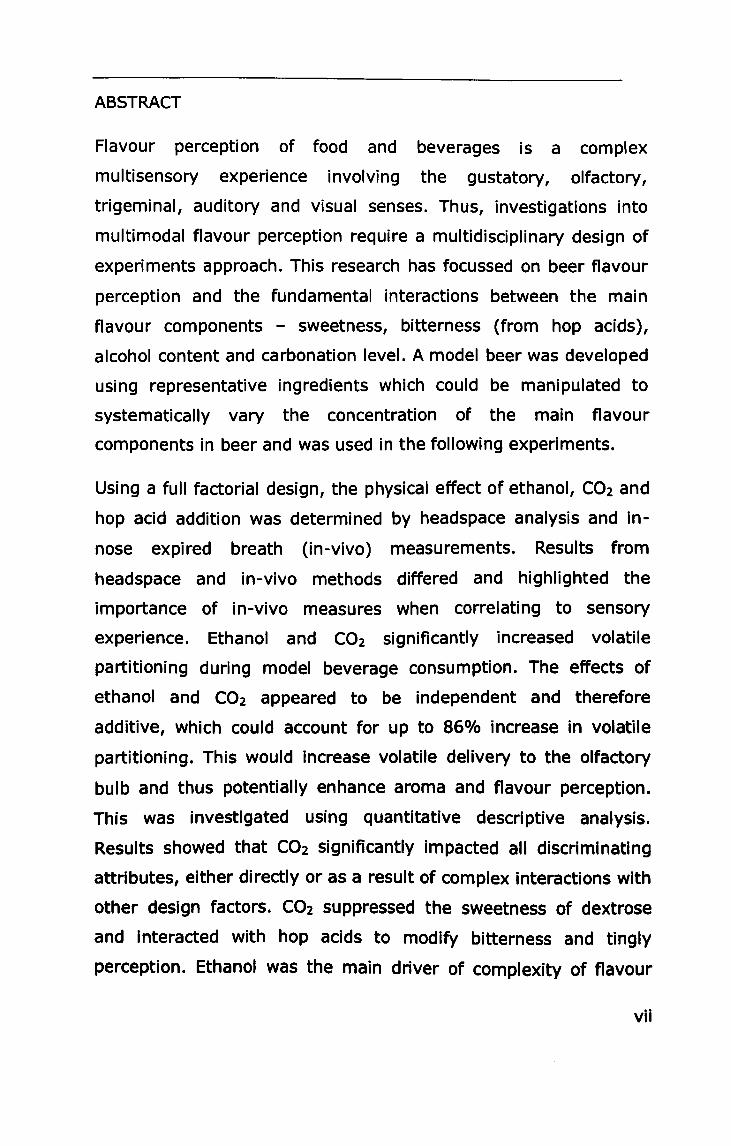
Flavour perception of food and beverages is a complex

multisensory experience involving the gustatory, olfactory,

trigeminal, auditory and visual senses. Thus, investigations into

multimodal flavour perception require a multidisciplinary design of

experiments approach. This research has focussed on beer flavour

perception and the fundamental interactions between the main

flavour components - sweetness, bitterness (from hop acids),

alcohol content and carbonation level. A model beer was developed

using representative ingredients which could be manipulated to

systematically vary the concentration of the main flavour

components in beer and was used in the following experiments.

Using a full factorial design, the physical effect of ethanol, C02 and

hop acid addition was determined by headspace analysis and in­

nose expired breath (in-vivo) measurements. Results from

headspace and in-vivo methods differed and highlighted the

importance of in-vivo measures when correlating to sensory

experience. Ethanol and C02 significantly increased volatile

partitioning during model beverage consumption. The effects of

ethanol and C02 appeared to be independent and therefore

additive, which could account for up to 86% increase in volatile

partitioning. This would increase volatile delivery to the olfactory

bulb and thus potentially enhance aroma and flavour perception.

This was investigated using quantitative descriptive analysis.

Results showed that C02 significantly impacted all discriminating

attributes, either directly or as a result of complex interactions with

other design factors. C02 suppressed the sweetness of dextrose

and interacted with hop acids to modify bitterness and tingly

perception. Ethanol was the main driver of complexity of flavour

vii

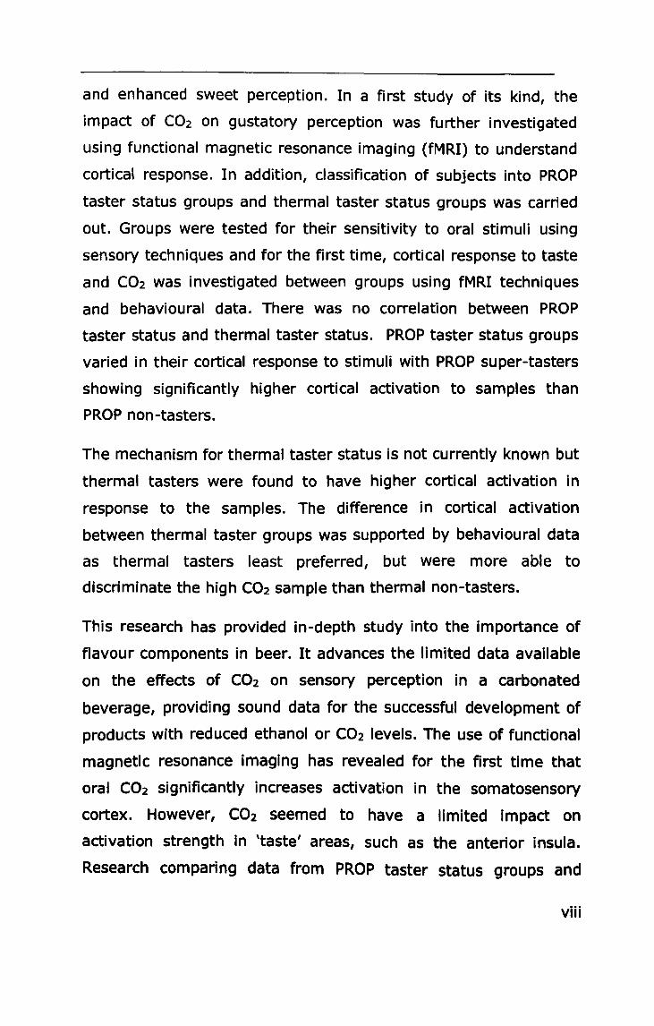
and enhanced sweet perception. In a first study of its kind, the

impact of C02 on gustatory perception was further investigated

using functional magnetic resonance imaging (fMRI) to understand

cortical response. In addition, classification of subjects into PROP

taster status groups and thermal taster status groups was carried

out. Groups were tested for their sensitivity to oral stimuli using

sensory techniques and for the first time, cortical response to taste

and C02 was investigated between groups using fMRI techniques

and behavioural data. There was no correlation between PROP

taster status and thermal taster status. PROP taster status groups

varied in their cortical response to stimuli with PROP super-tasters

showing significantly higher cortical activation to samples than

PROP non-tasters.

The mechanism for thermal taster status is not currently known but

thermal tasters were found to have higher cortical activation in

response to the samples. The difference in cortical activation

between thermal taster groups was supported by behavioural data

as thermal tasters least preferred, but were more able to

discriminate the high C02 sample than thermal non-tasters.

This research has provided in-depth study into the importance of

flavour components in beer. It advances the limited data available

on the effects of C02 on sensory perception in a carbonated

beverage, providi ng sound data for the successful development of

products with reduced ethanol or C02 levels. The use of functional

magnetic resonance imaging has revealed for the first time that

oral C02 significantly increases activation in the somatosensory

cortex. However, C02 seemed to have a limited impact on

activation strength in 'taste' areas, such as the anterior insula.

Research comparing data from PROP taster status groups and

viii

thermal taster status groups has given insight into the possible

mechanisms accounting for differences in oral intensity of stimuli.

ix

PREFACE

Much is known about the impact of individual components on beer

quality but only limited published research exists concerning the

interactions between different sensory stimuli. This research has

taken a scientifically controlled approach to investigate the physical

and perceptual interactions between the primary flavour

components in beer; sweetness, bitterness, alcohol and

carbonation and their affect on flavour perception. In order for the

individual components to independently manipulated, a model beer

system was developed that systematically varied in bitter and

sweet components, alcohol content and carbonation level.

Interactions between components were investigated at three levels;

physico-chemically, sensorially and cortically. Chemical interactions

between matrix components in the solution may impact flavour

perception independent of peripheral or cortical interactions. Such

interactions were investigated and then validated by human

sensory assessments. The resultant data was used to construct

mathematical models to represent the contribution of the various

stimuli and their interactions to the sensory properties of the beer

system. In humans, investigations beyond this point present a

significant number of ethical and technical difficulties. Fortunately

cutting edge neuroimaging techniques such as Functional Magnetic

Resonance Brain Imaging allow scientific advancement to further

the understanding of flavour perception. This method was

employed using innovative sample delivery techniques to

investigate the interaction between taste and carbonation. Little

data exists in the literature concerning the effects of carbonation

on flavour perception presumably due to the difficult nature of

creating and working with pressurised systems. As a result the

pathways responsible for C02 perception in combination with taste

x

stimuli are not fully understood. Using the approach described

above, the research aims to uncover the effects of carbonation in

combination with other primary flavour components in beer on

flavour perception and the possible mechanisms responsible for the

interactions.

In addition, the population varies in their sensitivity to oral stimuli

which may alter perception adding another layer of complexity

multimodal flavour research. Two markers of genetic oral

sensitivity, PROP taster status and the newly discovered thermal

taster status were investigated sensorially and cortically. Results

provide novel insight into the possible mechanisms contributing to

oral sensitivity. This fundamental research will provide

understanding of the chemical and perceptual sensory interactions

in a model beer system and some understanding of the

mechanisms behind them. It will provide direction and a sound

basis for follow-on studies which address the understanding

consumer perception and differences between the population's oral

sensitivity.

THESIS STRUCTURE

Chapter 1 gives a general introduction to the individual sensory

systems and interactions between them. It introduces the

experimental approach taken and methods employed. Chapter 2

details the development of the model beer system which was used

in subsequent experimental chapters. Chapters 3, 4, 5 and 6 detail

experimental work undertaken. Each chapter includes an

introduction with a detailed literature review specific to that

investigation; followed by materials and methods, results, and in

depth discussion sections. Chapter 3 reports an investigation into

xi

the physico-chemical interactions between the components in the

beverage matrix. Chapter 4 details the sensory evaluation of the

model beverages. Chapter 5 focuses on investigating genetiC

differences in oral sensitivity using sensory sensitivity measures

and served as a screening tool for subjects selected for

participation in the following study. Chapter 6 reports the

experimental results from conducting an fMRI study to investigate

the cortical effect of carbonation on taste perception and

differences in cortical activity between different population groups.

Finally, Chapter 7 provides an overview of major findings from all

experimental work conducted, general conclusions and further

work.

xii

Chapter 1

xiii

1. GENERAL INTRODUCTION

Despite a reduction in the consumption of alcohol across the UK

population, beer continues to be a popular alcoholic beverage,

worth more than any other drink type (in sales value), (Mintel

2007). The discovery of beer is said to be the result of widespread

cereal grain farming at around 10,000 Be (Hornsey 2003). It was

soon discovered that when the grains were mixed with water they

began to sprout and taste sweet (now known as malting). After

being left for a few days the mixture became fizzy and pleasantly

intoxicating (fermentation by wild yeasts). Presumably many years

of trial and error has improved the quality and now modern man

understands the science behind beer production a vast variety of

products are available. Each product varies in either the ingredients

used or the production method, but all have primary flavour

elements; alcohol, bitterness and carbon dioxide (Meilgaard 1975;

Meilgaard 1982). The concentration of each of these elements

varies depending upon the style of beer to be produced. Sweetness

results from unfermentable residual carbohydrates comprising of a

complex mixture of dextrins. Bitterness results from hop addition;

whilst both alcohol and carbon dioxide are by-products of yeast

fermentation. The brewing process produces a large number of

volatile compounds and whilst each on their own does not

dominate the flavour, they combine to contribute to the beer's

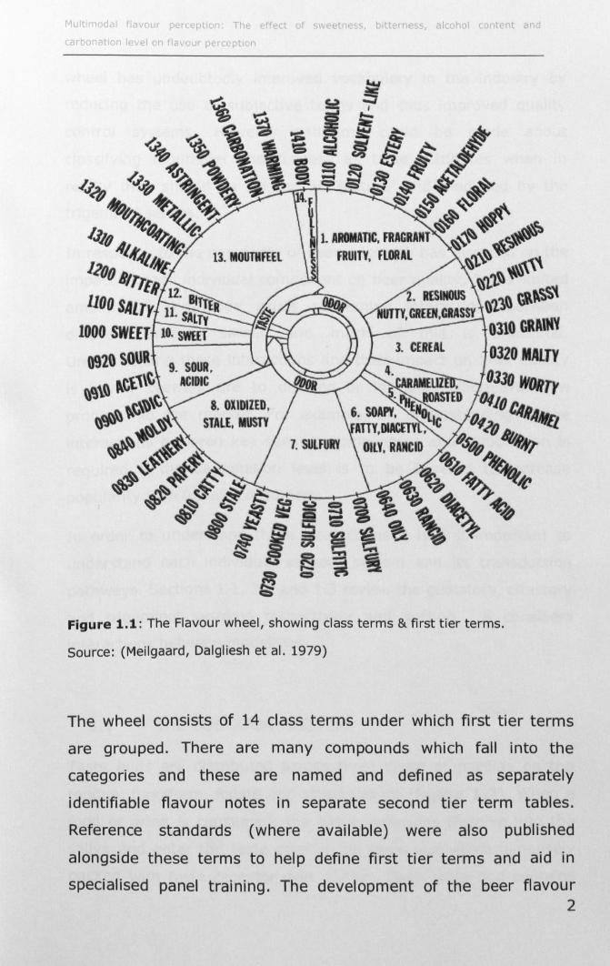
secondary flavour components (Meilgaard 1975). In 1979,

Meilgaard et al introduced the beer flavour wheel (figure 1.1) as a

unified system to communicate flavour terminology within the

industry.

1

ou e tt s I ho

Figure 1.1: The Flavour wheel, showing class terms & first tier terms.

Source: (Meilgaard, Dalgliesh et al. 1979)

The wheel consists of 14 class terms under which first tier terms

are grouped. There are many compounds which fall into the

categories and these are named and defined as separately

identifiable flavour notes in separate second tier term tables.

Reference standards (where available) were also published

alongside these terms to help define first tier terms and aid in

specialised panel training. The development of the beer flavour 2

wheel has undoubtedly improved vocabulary in the industry by

reducing the use of subjective terms and thus improved quality

control systems. However criticisms could be made about

classifying mouthfeel and fullness as taste attributes when in

reality they should be classed as 'texture' and mediated by the

trigeminal senses.

In response to the popularity of beer, research has focussed on the

impact of each individual component on beer quality, but a limited

amount of knowledge exists concerning interactions between

different sensory stimuli and much of this is anecdotal.

Understanding these interactions and their impact on beer quality

is key if brewers are to develop or introduce successful new

products to the market. For example, an understanding of the

interactions between key sensory components and carbonation is

required if the carbonation level is to be lowered to increase

popularity with female consumers.

In order to understand these interactions it is first important to

understand each individual sensory system and its transduction

pathways. Sections 1.1, 1.2 and 1.3 review the gustatory, olfactory

and trigeminal systems respectively and section 1.4 considers

interactions between modalities.

1.1 THE GUSTATORY SYSTEM

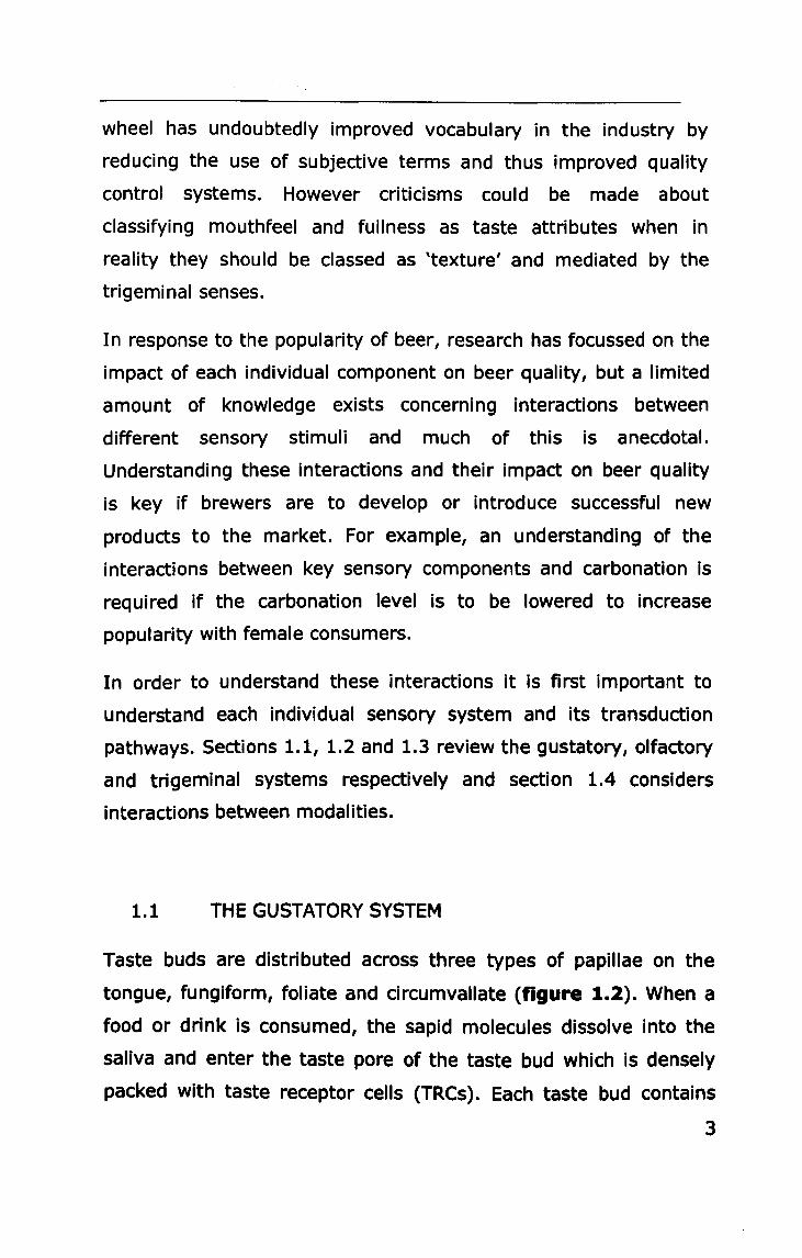
Taste buds are distributed across three types of papillae on the

tongue, fungiform, foliate and circumvallate (figure 1.2). When a

food or drink is consumed, the sapid molecules dissolve into the

saliva and enter the taste pore of the taste bud which is densely

packed with taste receptor cells (TRCs). Each taste bud contains

3

between 50-150 TRC's which are specialised epithelial cells that

respond to all five taste modalities (Hoon, Adler et al. 1999; Adler,

Hoon et al. 2000; Chandrashekar, Hoon et al. 2006).

T s e po

Figure 1.2: Taste receptor anatomy and location of papillae on tongue. Source: (Chandrashekar, Hoon et al. 2006)

When activated by a tastant, TRCs depolarise, leading to

neurotransmitter release and projection of action potentials along

the axons of the sensory nerves that innervate the tongue and soft

palate (Lindemann 2001). The chorda tympani branch of the facial

nerve (cranial nerve VII) innervates the anterior two thirds of the

tongue where the fungiform papillae are located. The

glossopharyngeal nerve (cranial nerve IX) innervates the remaining

third where the foliate and circumvallate papillae are situated and

the vagus nerve (cranial nerve X) innervates the epiglottis and

larynx (Chandrashekar, Hoon et al. 2006; Sugita 2006). Together

these nerves send taste information along the brainstem to the

4

r

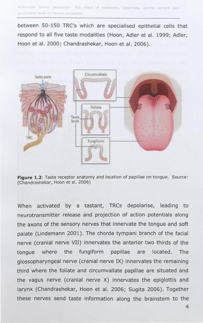
nucleus of the solitary tract (NTS) and onwards to the thalamus

and the gustatory cortex (Boucher, Simons et al. 2003). The

primary gustatory cortex consists of the insula cortex and the

frontal operculum (Kobayakawa, Endo et al. 1996) which covers

part of the insula. Taste projections may then continue to the

amygdala, orbito-frontal cortex (OFC) (the secondary gustatory

cortex) and anterior cingulated cortex (ACC) as illustrated by

figure 1.3.

Figure 1.3: Taste transduction and associated cortical areas. Source: http://quizlet.com/4414696/biopsych-midterm-2-flash-ca rdsl

There are two opposing views of how different tastes are detected.

The view that TRCs are individually tuned to respond to specific

taste qualities with individually tuned nerve fibres is called the

labelled-line theory. The across-fibre model proposes that TRC's

5

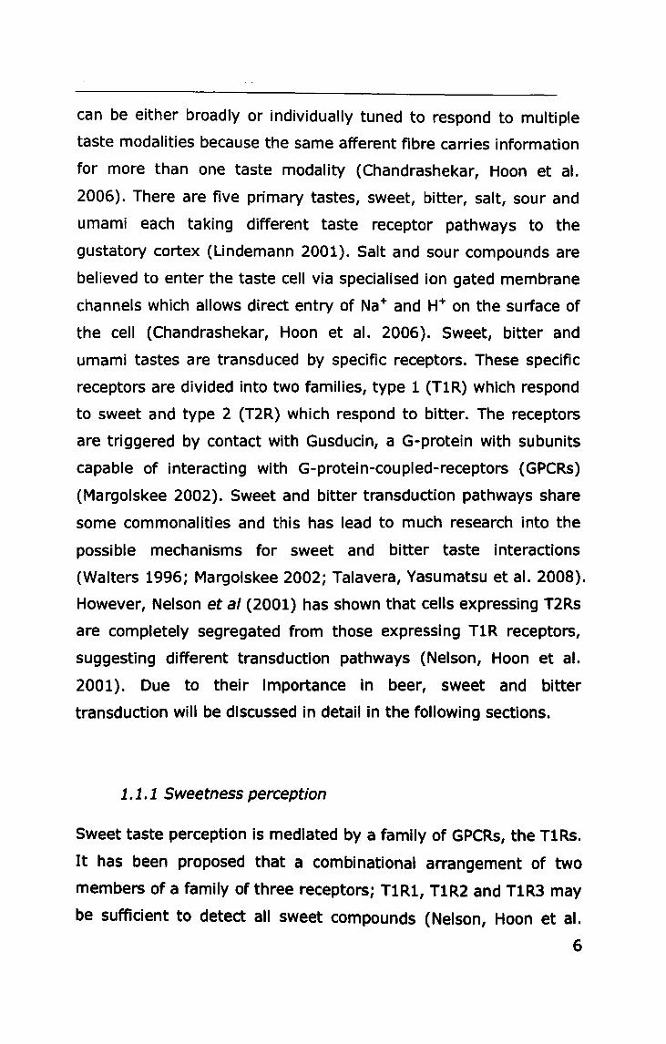
can be either broadly or individually tuned to respond to multiple

taste modalities because the same afferent fibre carries information

for more than one taste modality (Chandrashekar, Hoon et al.

2006). There are five primary tastes, sweet, bitter, salt, sour and

umami each taking different taste receptor pathways to the

gustatory cortex (Lindemann 2001). Salt and sour compounds are

believed to enter the taste cell via specialised ion gated membrane

channels which allows direct entry of Na+ and H+ on the surface of

the cell (Chandrashekar, Hoon et al. 2006). Sweet, bitter and

umami tastes are transduced by specific receptors. These specific

receptors are divided into two families, type 1 (T1R) which respond

to sweet and type 2 (T2R) which respond to bitter. The receptors

are triggered by contact with Gusducin, a G-protein with subunits

capable of interacting with G-protein-coupled-receptors (GPCRs)

(Margolskee 2002). Sweet and bitter transduction pathways share

some commonalities and this has lead to much research into the

possible mechanisms for sweet and bitter taste interactions

(Walters 1996; Margolskee 2002; Talavera, Yasumatsu et al. 2008).

However, Nelson et a/ (2001) has shown that cells expressing T2Rs

are completely segregated from those expressing T1R receptors,

suggesting different transduction pathways (Nelson, Hoon et al.

2001). Due to their importance in beer, sweet and bitter

transduction will be discussed in detail in the following sections.

1.1.1 Sweetness perception

Sweet taste perception is mediated by a family of GPCRs, the T1Rs.

It has been proposed that a combinational arrangement of two

members of a family of three receptors; T1Rl, T1R2 and T1R3 may

be sufficient to detect all sweet compounds (Nelson, Hoon et al.

6

2001; Li, Staszewski et al. 2002). Experiments using laboratory

mice and genome sequencing led to the breakthrough that two

taste receptor proteins, T1R2 and T1R3, form a complex to produce

a GPCR that demonstrates broad selectivity by responding to many

structurally different sweet molecules (Hoon, Adler et al. 1999;

Nelson, Hoon et al. 2001; Li, Staszewski et al. 2002). These

findings suggest that the T1R2+3 complex is the predominant

sweet taste receptor (Nelson, Hoon et al. 2001; Chandrashekar,

Hoon et al. 2006).

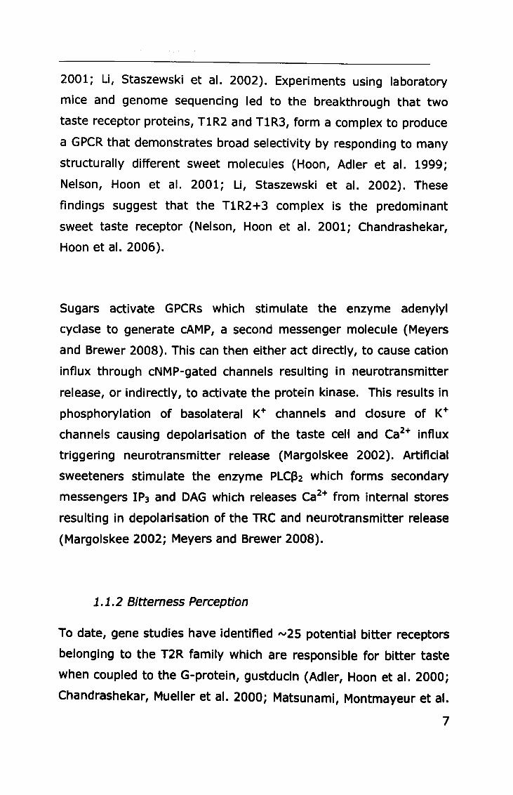
Sugars activate GPCRs which stimulate the enzyme adenylyl

cyclase to generate cAMP, a second messenger molecule (Meyers

and Brewer 2008). This can then either act directly, to cause cation

influx through cNMP-gated channels resulting in neurotransmitter

release, or indirectly, to activate the protein kinase. This results in

phosphorylation of basolateral K+ channels and closure of K+

channels causing depolarisation of the taste cell and Ca2+ influx

triggering neurotransmitter release (Margolskee 2002). Artificial

sweeteners stimulate the enzyme PLC(32 which forms secondary

messengers IP3 and DAG which releases Ca2+ from internal stores

resulting in depolarisation of the TRC and neurotransmitter release

(Margolskee 2002; Meyers and Brewer 2008).

1.1.2 Bitterness Perception

To date, gene studies have identified 1V25 potential bitter receptors

belonging to the T2R family which are responsible for bitter taste

when coupled to the G-protein, gustducin (Adler, Hoon et al. 2000;

Chandrashekar, Mueller et al. 2000; Matsunami, Montmayeur et al.

7

2000; Meyerhof, Behrens et al. 2005; Behrens, Foerster et al.

2007). When activated they mediate one of two responses in the

TRCs. Activated a-gustducin stimulates the enzyme POE to

hydrolyse cAMP which may decrease cNMP, with the subsequent

steps in this pathway remaining uncertain (Margolskee 2002;

Behrens and Meyerhof 2006). The second transduction pathway

involves activated PLCfh to generate IP3. Both pathways result in

elevated intracellular levels of Ca2+ and neurotransmitter release

(Behrens and Meyerhof 2006).

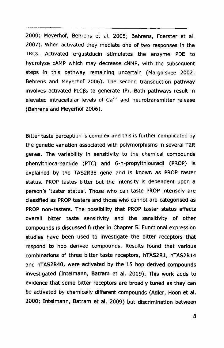
Bitter taste perception is complex and this is further complicated by

the genetic variation associated with polymorphisms in several T2R

genes. The variability in sensitivity to the chemical compounds

phenylthiocarbamide (PTC) and 6-n-propylthiouracil (PROP) is

explained by the TAS2R38 gene and is known as PROP taster

status. PROP tastes bitter but the intensity is dependent upon a

person's 'taster status'. Those who can taste PROP intensely are

classified as PROP tasters and those who cannot are categorised as

PROP non-tasters. The possibility that PROP taster status effects

overall bitter taste sensitivity and the sensitivity of other

compounds is discussed further in Chapter 5. Functional expression

studies have been used to investigate the bitter receptors that

respond to hop derived compounds. Results found that various

combinations of three bitter taste receptors, hTAS2R1, hTAS2R14

and hTAS2R40, were activated by the 15 hop derived compounds

investigated (Intelmann, Batram et al. 2009). This work adds to

eVidence that some bitter receptors are broadly tuned as they can

be activated by chemically different compounds (Adler, Hoon et al.

2000; Intelmann, Batram et al. 2009) but discrimination between

8

T

them is difficult, thus supporting the across fibre pattern theory of

taste detection.

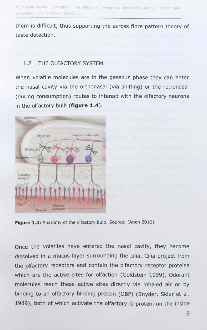
1.2 THE OLFACTORY SYSTEM

When volatile molecules are in the gaseous phase they can enter

the nasal cavity via the orthonasal (via sniffing) or the retronasal

(during consumption) routes to interact with the olfactory neurons

in the olfactory bulb (figure 1.4).

Figure 1.4: Anatomy of the olfactory bulb. Source: (Anon 2010)

Once the volatiles have entered the nasal cavity, they become

dissolved in a mucus layer surrounding the cilia. Cilia project from

the olfactory receptors and contain the olfactory receptor proteins

which are the active sites for olfaction (Goldstein 1999). Odorant

molecules reach these active sites directly via inhaled air or by

binding to an olfactory binding protein (OBP) (Snyder, Sklar et al.

1989), both of which activate the olfactory G-protein on the inside

9

of the olfactory neuron which activates the lyase enzyme, alenylate

cyclase to convert ATP to cAMP (Buck and Axel 1991). cAMP opens

cyclic nucleotide gated ion channels which allows Ca2+ and Na+

influx, depolarising the receptor neuron and sending input directly

to the glomeruli in the ipsilateral olfactory bulb (Brand 2006). Each

glomeruli receives information from one particular type of receptor

(Buck and Axel 1991) and sends it to the mitral cells (Goldstein

1999). An action potential transmits the signal along the olfactory

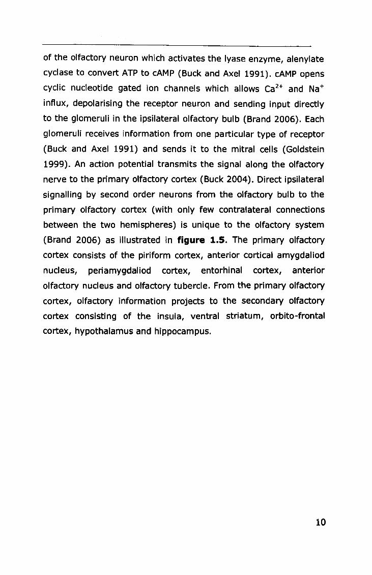
nerve to the primary olfactory cortex (Buck 2004). Direct ipsilateral

signalling by second order neurons from the olfactory bulb to the

primary olfactory cortex (with only few contralateral connections

between the two hemispheres) is unique to the olfactory system

(Brand 2006) as illustrated in figure 1.5. The primary olfactory

cortex consists of the piriform cortex, anterior cortical amygdaliod

nucleus, periamygdaliod cortex, entorhinal cortex, anterior

olfactory nucleus and olfactory tubercle. From the primary olfactory

cortex, olfactory information projects to the secondary olfactory

cortex consisting of the insula, ventral striatum, orbito-frontal

cortex, hypothalamus and hippocampus.

10

Olfactory bulb

Orbitofronta I cortex PYriform

cortex F ntrohinal cortex

Thalamus

Cerebellum

Figure 1.5: Direct signalling to piriform cortex and entrohinal cortex (primary olfactory cortex) before projecting to the orbitofrontal cortex and thalamus (secondary olfactory cortex). Source: http://mva . me/educational/brai n_a reas/smel l.jpg

Each olfactory receptor is capable of detecting multiple odorants

and each is detected by multiple receptors (Buck 2004). There are

1V350 olfactory receptors used in a combinational manner to

encode odour identities resulting in detection of over 100,000

aroma compounds (Buck 2004). While humans can detect a vast

array of aromas, they lack discrimination ability both in

identification and detecting differences in intenSity (Desor and

Beauchamp 1974; Laing and Francis 1989; Laska and Hudson

1992). The former can be increased by training (Desor and

Beauchamp 1974) as it relies on the memory which can be

improved.

1.3 THE TRIGEMINAL SYSTEM

The trigeminal system provides tactile, proprioceptive and

nociceptive afference from the mouth, providing information on the

11

r t T ff ct r hoi

texture, consistency and chemical irritation of foods and beverages.

The free nerve endings that innervate the tongue are high in

density in and around the taste papillae (Nagy, Goedert et al. 1982;

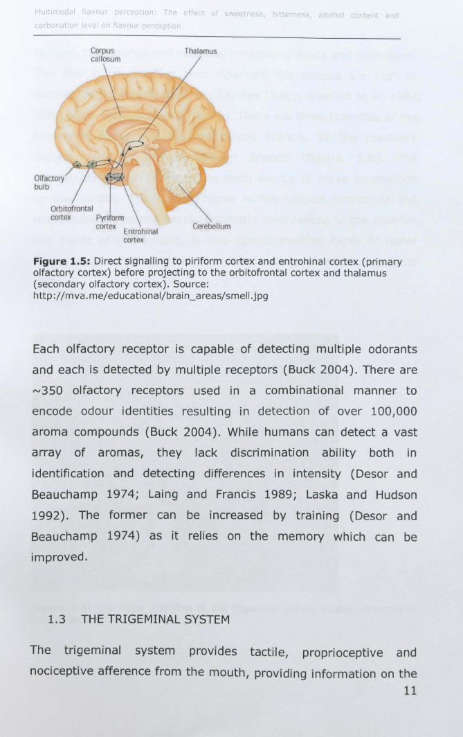
Whitehead, Ganchrow et al. 1999). There are three branches of the

trigeminal nerve; Vi the ophthalmic branch, V2 the maxillary

branch and V3 the mandibular branch (figure 1.6). The

mandibular branch provides the main source of nerve innervation

to the mouth. The lingual nerve is the largest branch of the

mandibular nerve and supplies somatic innervations to the anterior

two thirds of the tongue. It also carries multiple types of nerve

fibres, such as those from the chorda tympani which innervate

taste.

Figure 1.6: The three branches of the trigeminal nerve. Source : (Kaufmann, Patel et al. 2001)

12

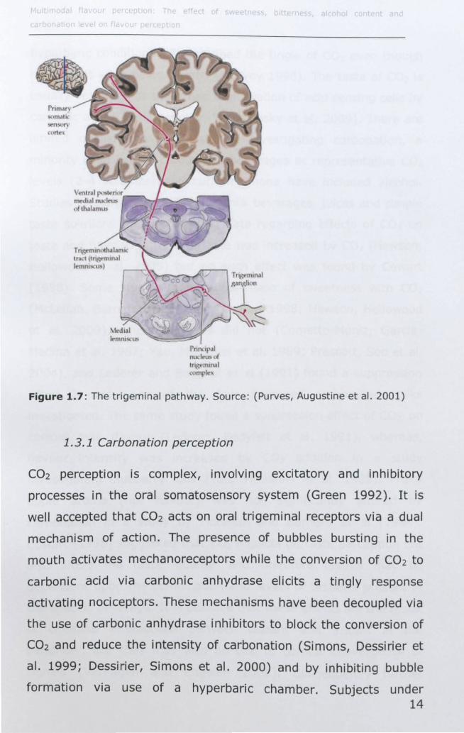
Trigeminal information from the face is carried by first order

neurons to the principle nucleus of the trigeminal complex (Brand

2006) where secondary fibres cross the midline and ascend along

the medial lemniscal pathway via the trigeminal lemniscus to the

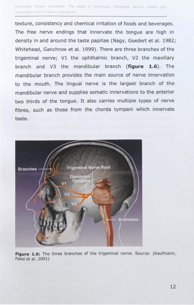
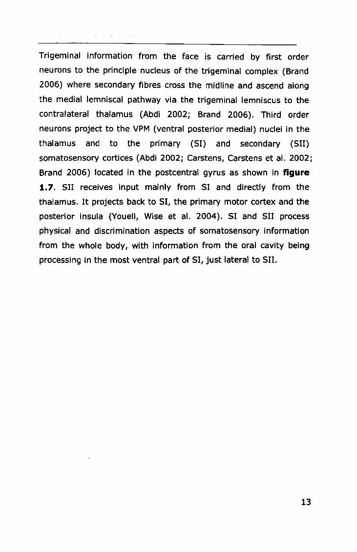
contralateral thalamus (Abdi 2002; Brand 2006). Third order

neurons project to the VPM (ventral posterior medial) nuclei in the

thalamus and to the primary (51) and secondary (511)

somatosensory cortices (Abdi 2002; Carstens, Carstens et al. 2002;

Brand 2006) located in the postcentral gyrus as shown in figure

1.7. 511 receives input mainly from 51 and directly from the

thalamus. It projects back to 51, the primary motor cortex and the

posterior insula (Youell, Wise et al. 2004). 51 and 511 process

physical and discrimination aspects of somatosensory information

from the whole body, with information from the oral cavity being

processing in the most ventral part of 51, just lateral to 511.

13

rnndpl nudt't,l ul Ir, mlllJI

,,'m!,'"

Figure 1.7: The trigeminal pathway. Source: (Purves, Augustine et al. 2001 )

1.3.1 Carbonation perception

C02 perception is complex, involving excitatory and inhibitory

processes in the oral somatosensory system (Green 1992). It is

well accepted that C02 acts on oral trigeminal receptors via a dual

mechanism of action. The presence of bubbles bursting in the

mouth activates mechanoreceptors while the conversion of C02 to

carbonic acid via carbonic anhydrase elicits a tingly response

activating nociceptors. These mechanisms have been decoupled via

the use of carbonic anhydrase inhibitors to block the conversion of

CO2 and reduce the intensity of carbonation (Simons, Dessirier et

al. 1999; Dessirier, Simons et al. 2000) and by inhibiting bubble

formation via use of a hyperbaric chamber. Subjects under 14

hyperbaric conditions still described the tingle of C02 even though

no bubbles were being formed (McEvoy 1998). The taste of C02 is

usually described as acidic due to activation of acid sensing cells by

carbonic acid (Chandrashekar, Yarmolinsky et al. 2009). There are

limited published sensory studies investigating carbonation, a

minority used typical carbonated beverages at representative C02

levels (2-4 volumes) and currently none have included alcohol.

Studies investigating carbonated milk beverages, juices and Simple

taste solutions found conflicting data regarding effects of C02 on

taste and flavour. Bitter aftertaste was increased by C02 (Hewson,

Hollowood et al. 2009) but no such effect was found by Cowart

(1998). Some studies found suppression of sweetness with C02

(McLellan, Barnard et al. 1984; Cowart 1998; Hewson, Hollowood

et al. 2009), whereas others did not (Cometto-Muniz, Garcia­

Medina et al. 1987; Yau, McDaniel et al. 1989; Prescott, 500 et al.

2004), and Lederer and Bodyfelt et al (1991) found a suppression

effect in only one of the four flavoured carbonated milks

investigated. The same study found a suppression effect of C02 on

cooked milk flavour (Lederer, Bodyfelt et al. 1991), whereas,

flavour intensity was increased by C02 addition in a study

investigating blueberry milk (Yau, McDaniel et al. 1989). Fruity

apple aroma (not flavour) was not significantly altered by

carbonation in a study by McLellan and Barnard et al (1984).

Cowart (1998) suggested that C02 impacts on taste perception but

also alters the taste 'quality' and therefore results may be

dependent upon the combination and levels of tastants present in

the speCific beverage. It is possible that these effects are the result

of chemical interactions between tastant and irritant at the

periphery, but they may also be due to cortical convergence of

signals (Verhagen and Engelen 2006). Consequently further

15

research with commonly carbonated beverages at appropriate C02

levels is important to further this understanding. In addition,

research investigating interactions between taste and C02 in beer

are needed as there are currently no studies reporting this.

1.3.2 Ethanol perception

Ethanol is a complex stimulus which acts on multiple modalities

(Green 1988; Kiefer and Morrow 1991; Mattes and DiMeglio 2001;

Cometto-Muniz and Abraham 2008) and ethanol has been found to

interact with beverage components to modify sensations. For

example ethanol has been shown to contribute to the sweetness of

sucrose and the bitterness of quinine (Martin and Pangborn 1970),

the astringency and bitterness of tannins (Fontoin, Saucier et al.

2008), irritation (Prescott and Swain-Campbell 2000), hotness

(Jones, Gawel et al. 2008) and perceived complexity of wine

(Meillon, Viala et al. 2010) as well as aroma (Goldner, Zamora et al.

2009). In sensory studies, the taste of ethanol has been found to

include both sweet and bitter components depending on the

concentration (Wilson, Obrien et al. 1973; Scinska, Koros et al.

2000; Mattes and DiMeglio 2001). Neuronal taste response of

ethanol, investigated in vitro using the rhesus monkey (Hellekant,

Danilova et al. 1997), rats (Lemon, Brasser et al. 2004) and mice

(Brasser, Norman et al. 2010) supports evidence that ethanol

stimulates fibres which respond best to sweet compounds (sweet­

best fibres) and that central processing follows a similar pathway to

sucrose. Ethanol stimulation of the trigeminal system seems to be

multifaceted, evoking both chemical irritation pathways and

mechanoreceptors (Green 1991; Trevisani, Smart et al. 2002;

Ellingson, Silbaugh et al. 2009; Goldner, Zamora et al. 2009).

16

Ethanol is said to contribute to mouthfeel characteristics with the

flavour being described as solvent-like (Langstaff and Lewis 1993).

1.4 MULTIMODAL FLAVOUR PERCEPTION

Current understanding is that flavour perception is multimodal

where-by information detected at the receptors located at each of

the five senses has the capacity to merge and interact physically in

the product matrix itself, at the periphery or centrally in the brain

to influence sensation (Verhagen and Engelen 2006). Physical

interactions between aroma compounds and other components in

foods and beverages have been widely researched and will be

discussed further in Chapter 2. Sensory integration from

independent modalities (gustatory, olfactory, trigeminal, visual and

auditory) all contribute to give a final percept of flavour.

Investigations using sensory evaluation and magnetic resonance

imaging methods provide understanding of interactions between

different modalities. Within-modal interactions, such as taste-taste

interactions, bring about either an enhancement or a suppression

effect dependent upon the tastant and the concentration (Breslin

1996; Keast and Breslin 2003). Cross-modal interactions, such as

the interaction between anatomically separate organs are well

documented (Dalton, Doolittle et al. 2000; Hort and Hollowood

2004; pfeiffer, Hollowood et al. 2005). Dalton and Doolittle et al

(2000) used sub-threshold levels of saccharin and benzaldehyde to

demonstrate the central neural integration of a congruent taste and

aroma. When the sub-threshold stimuli were presented

simultaneously they could be detected demonstrating taste-aroma

interactions between congruent pairings. However, this was not the

case when incongruent stimuli (MSG and benzaldehyde) were

17

presented together (Dalton, Doolittle et al. 2000). Interactions

between the olfactory and trigeminal systems have been

investigated. Trigeminal fibres innervate the olfactory epithelium

and seem to respond to olfactory stimuli but may also modify the

olfactory response (Cain and Murphy 1980; Prescott and Stevenson

1995). A study by Laska (1997) showed that chemical compounds

with a strong trigeminal component can be discriminated and

described by olfaction alone in anosmic subjects suggesting that

the trigeminal system contributes to the perception of odour (Laska,

Distel et al. 1997). However, interactions between the two systems

are not clearly established due to the complex nature of the

interactions which appear to differ dependently of molecules,

intensity or context of inhalation (Brand 2006). Gustatory and

trigeminal systems have also been found to interact. Temperature

(Moskowit.Hr 1973; Bartoshuk, Rennert et al. 1982), irritation

(Prescott, Allen et al. 1984; Lawless, Rozin et al. 1985; Cometto­

Muniz, Garcia-Medina et al. 1987) and texture (viscosity) (Cook,

Hollowood et al. 2002) have all been found to interact with taste.

The influence of temperature will be discussed further in Chapter

5. The influence capsaicin has on taste is the most researched

irritant and generally produces a suppression effect (Lawless and

Stevens 1984; Prescott, Allen et al. 1984; Lawless, Rozin et al.

1985; Simons, Q'Mahony et al. 2002; Simons, Boucher et al. 2003).

Many psychophysical studies have investigated perceptual

multimodal interactions and have alluded to possible mechanisms

but few have investigated these mechanisms in humans. fMRI

techniques have been used to study taste-aroma interactions

(Cerf-Ducastel and Murphy 2001; Marciani, Pfeiffer et al. 2006;

Rolls, Critchley et al. 2010) and taste-tactile interactions (de Araujo

18

and Rolls 2004; Alonso, Marciani et al. 2007; Eldeghaidy, Marciani

et al. 2010) and have found integrations between cortical areas.

1.4.1 Investigating multimodal flavour perception

Interactions between chemical components in a beer could alter

the partitioning of volatiles from the aqueous phase to the gaseous

phase. Consequently this could impact on delivery to the olfactory

bulb and the perception of odour quality and intensity. The

relationship between the volatile concentration in the gaseous and

aqueous phases can be explored by measuring the changes in

headspace volatile concentration in a static system. Any changes in

the partitioning of aroma volatiles as a result of variation in matrix

components can therefore be determined. Headspace

measurements are traditionally carried out by collecting a sample

of the headspace at equilibrium, commonly by the use of Tenax

traps or coated fibres (Solid Phase Micro Extraction, SPME), which

extract the analytes from the gas phase. The analytes are then

desorped and separated by gas chromatography and the individual

molecules ionised and quantified by mass spectrometry. An

alternative is to use a soft ionisation technique based on proton

transfer such as atmospheric pressure chemical ionisation (APel)

or proton transfer reaction (PTR), followed by mass spectrometry.

Taylor and Linforth (2000) developed a novel interface for APCI-MS

analysis which allows headspace sampling directly into the mass

spectrometer in real-time. Advantages of this method are that it

can cope with water and air and can operate at pressures which

allow easy and safe sampling of breath (Taylor, Linforth et al.

2000), so it can successfully be used for collecting in-vivo breath

samples. The use of these techniques is paramount to gain a full

19

understanding of chemical interactions between matrix components

and volatiles which could alter human flavour perception.

In order to validate instrumental analysis and further understand

human perception, sensory evaluation techniques such as

quantitative descriptive analysis (QDA)® (Stone and Sidel 2004)

and Spectrum TM are commonly used. Sensory panellists are

preselected based on their sensory ability and then undergo

general training to enhance detection, discrimination and

descriptive skills. Product-specific training follows where panellists

are exposed to all samples, from which attributes and references

(where applicable) are generated. These product-specific attributes

are refined to include only objective terms and the perceptual

meaning is clearly defined. Assessment protocol is determined and

the panel are trained to rate the intensity on an appropriate scale.

Panel performance is reviewed and further training given if needed

before the final set of data is generated. The use of sensory

evaluation in combination with instrumental analysis provide

insights into the level at which interactions are taking place.

Further analysis of perceptual interactions requires in depth study

of the mechanisms responsible at receptor, neural and cortical

levels. Animal studies have gone a long way to increase

understanding but do not always correlate to human perception.

Electrophysiological and neuroimaging techniques are direct and

indirect measures of researching brain activity. In

Electroencephalography (EEG) and Magneto-encephalography

(MEG) the scalp is covered with electrodes which directly measure

rapid changes in neuronal activity by recording the electrical (EEG)

or magnetic (MEG) activity generated inside the brain. Excellent

temporal resolution makes these techniques valuable for studying

the timing of brain processes but limited spatial resolution makes

20

identifying the origin of activity difficult (Huettel, Song et al. 2009).

Nuclear imaging techniques such as positron emission tomography

(PET) and functional magnetic resonance imaging (fMRI) can

however provide high spatial resolution but at the cost of limited

temporal resolution as changes in brain activity are detected over

seconds (Huettel, Song et al. 2009). Both techniques are indirect

measures of brain activity with PET measuring metabolic activity

and fMRI measuring blood flow. PET relies on the injection of a

radioactive tracer compound which gives the brain metabolic

activity. PET is then able to detect parts of the brain metabolically

associated with a given function. However, the radioactive

injections are expensive and invasive making PET undesirable for

research purposes with healthy subjects. In contrast, fMRI is a

non-invasive technique using strong magnetic fields to measure

changes in blood oxygenation associated with a certain sensory,

motor or cognitive tasks. Spatial resolution is such that the locus of

activity can be identified within millimetres of origin (Huettel, Song

et al. 2009). Consequently fMRI can be used repeatedly with the

same subject to research the effects of multiple stimuli and

interactions between stimuli on brain function.

1.5 VARIATION IN ORAL SENSITIVITY

Investigating multimodal flavour perception is further complicated

by a variety of population variations in oral sensitivity which can

originate from medical, environmental and genetic differences.

Ageusia (total loss of taste) due to damage of taste nerves is very

rare and in most cases the cause of taste dysfunction is olfactory in

nature (Deems, Doty et al. 1991). The reduced ability to smell is

known as anosmia, which can be specific to one particular odour, a

21

temporary disorder or permanent due to olfactory nerve damage

from head trauma or brain damage. Congenital anosmia is the

genetic inability to smell from birth. Aging usually brings with it

some level of olfactory dysfunction altering flavour perception,

usually described as a decreased ability to taste. Environmental

factors such as medications, changes in hormonal status and

exposure can also alter perception (Duffy 2007). Genetic variation

in the ability to taste the compound 6-n-propylthiouracil (PROP)

splits the population into PROP tasters and PROP non-tasters.

Approximately 70% of people are PROP tasters which can be

further divided into those who taste PROP intensely (super-tasters)

and those who taste it moderately (medium-tasters), leaving the

remaining 30% unable to taste the compound (non-tasters).

Furthermore, the number of fungiform papillae on the anterior

tongue has also been correlated to PROP sensitivity,

somatosensation and taste sensitivity (Miller and Reedy 1990;

Zuniga, Davis et al. 1993; Duffy and Bartoshuk 2000; Duffy,

Peterson et al. 2004). The newly discovered thermal taster status

describes an ability to perceive a phantom taste when the tongue is

warmed or cooled (Cruz and Green 2000). Those who perceive a

taste are called thermal tasters and have been found to have

increased oral sensitivity to tastes, flavour, somatosensory stimuli

(Green and George 2004; Green, Alvarez-Reeves et al. 2005; Bajec

and Pickering 2008; Bajec and Pickering 2010; Pickering, Moyes et

al. 2010; Pickering, Bartolini et al. 2010). Variation in oral

sensitivity has also been associated with preference for high-fat

foods (Duffy, Bartoshuk et al. 1996; Duffy and Bartoshuk 2000;

Thomassen, Faraday et al. 2005), vegetables (Dinehart, Hayes et

al. 2006; Bajec and Pickering 2010) and alcoholic beverages

(Intranuovo and Powers 1997; Duffy, Davidson et al. 2004; Duffy,

22

Peterson et al. 2004) which may influence food and beverage

intake.

1.6 EXPERIMENTAL APPROACH

Interactions between the primary flavour components (sweetness,

bitterness, alcohol and carbonation) in beer have not been

investigated previously. This research bridges the gap in the

literature using a design of experiments approach.

The objectives of this research were to: develop a model system

which models the essential characteristics of lager beer but which

can be easily manipulated and manufactured for use in laboratory

experiments; determine physico-chemical interactions between

matrix components which could alter flavour perception;

understand the impact and interactions of the varying ingredients

on sensory perception; investigate differences in oral sensitivity

between population groups; explore the effect of C02 on the

cortical response to taste.

The first experiment detailed in chapter 3 investigates physico­

chemical interactions between matrix components using

instrumental measurements. Human sensory assessments are

employed in the following chapter to generate an understanding of

perceptual interactions (chapter 4). Chapter 5 investigates genetiC

variation in taste sensitivity and chapter 6 explores cortical

activation to oral stimuli and compares activation differences

between population groups. For the design of experiments to be

successful, strict control of the matrix components within the beer

system is needed. Consequently 6 months were spent developing a

23

realistic but simple model beer system. The development of the

system is detailed in the next chapter (2).

24

Chapter 2

25

2. DEVELOPMENT OF THE MODEL BEER SYSTEM

2.1. INTRODUCTION

The model beverage developed for this investigation was intended

to be recognised by the panel as 'beer' whilst also allowing strict

control of each of the components (sweetness, bitterness, alcohol

content and carbonation). A model system (rather than brewed

beer) was necessary in order to be able to manipulate each

element independently for a sCientifically controlled approach.

Consequently, a model system was created using ingredients which

were determined the most appropriate, including; sweetener, bitter

hop acids, ethanol, CO2 , water, aroma volatiles, soluble fibre and

colouring. An understanding of the contribution of raw materials

and the generation of flavours during the brewing process was

needed in order to create a realistic model beer system.

The main ingredients and contributors to beer flavour are water,

malted barley, yeast and hops (Briggs, Boulton et al. 2004).

Alcohol and carbon dioxide are by-products of fermentation and

highly important characteristics of beer flavour. However, it is not

only the beer's ingredients that give final flavour but also the

processing techniques, as a vast majority of flavour compounds are

formed by yeast during fermentation. The general brewing process

consists of the following steps; malting, kilning, milling, mashing,

hop boil, fermentation, maturation and finishing. The flavour of the

final product can be manipulated by changes to this process. In

particular, time, temperature and pH control all contribute towards

producing the correct flavour profile. The following sections review

the stages of beer production giving an overview on the main

flavours created from each process and the development of the

model beer system.

26

2.1.1 Overview of the brewing process

2.1.1.1 Malts and malting

Many hundreds of potentially flav-our active substances are derived

from malts or adjuncts (cereals, sugars or flavourings) and include

aldehydes, ketones, amines, thiols and other sulphur-containing

substances and phenols (Briggs, Boulton et al. 2004). Dimethyl

sulphide (OMS) is a characteristic flavour active volatile of lagers,

imparting a cooked cabbage aroma. It is produced by the thermal

decomposition of S-methyl methionine (SMM) during the

germination process which is converted to OMS during light kilning

of lager malt (O'Rourke 2002).

2.1.1.2 Milling and mashing

The kilned malt is milled into 'grist' and is intimately mixed with

water into the mashing vessel at a controlled rate and temperature

allowing the starch to gelatinize. The mash is held for a period of

conversion to allow a mixture of enzymes (diastase) to convert the

starch and dextrins to soluble sugars and cause partial breakdown

of proteins. A sweet wort results, containing mainly carbohydrates

and is rich in flavour extracts dissolved from the malt and adjuncts.

Other products include non-starch polysaccharides, proteins and

polypeptides, which may have positive effects on beer qualities

such as increased viscosity and foam stability. After the mashing

process is complete, the sweet wort is separated from the spent

grains using a mash filter. The wort is run into the kettle where it is

boiled with hops.

2.1.1.3 Hops and the hop boil

Historically hops were added to preserve the beer during

fermentation. However, in modern day processing their main

27

function is to provide flavour. Bitter taste is one of the most

important flavours in beer (Meilgaard, Dalgliesh et al. 1979),

derived from the addition of hops during boiling or the addition of

hop extracts to the wort or even the final beer. Hop resins provide

bitterness and essential oils provide aroma which can be flowery,

citrus, fruity or herbal, depending upon the variety (Briggs, Boulton

et al. 2004). Hops are added to the sweet wort and boiled for 1-2

hours, which isomerizes the a-acids in the hop resins to bitter iso­

a-acids (Briggs, Boulton et al. 2004). The degree of bitterness

imparted by the hops depends on the degree to which the a-acids

are isomerised during the boil and can be estimated by the light

absorbance of a solvent extract. The European Brewing Congress

(EBC) Analysis Committee has simplified the calculation and results

are reported in Bitterness Units (BU) which has been adopted

internationally (lBU).

During isomerisation, an intermolecular rearrangement results in

two series of five-membered ring compounds, the trans-iso-a-acids

and the cis-iso-a-acids (Briggs, Boulton et al. 2004). Each is a

mixture of three compounds (r-groups), isocohumulone,

isohumulone and isoadhumulone, the ratios of which (and therefore

bitterness) vary according to hop variety. Iso-a-acids are not light

stable and form the undesirable highly 'sunstruck' flavoured

compound 3-methyl-2-butene-l-thiol over time. One way to avoid

the formation of this compound is to use the chemically modified

iso-a-acids which are formed by reduction of the iso-a-acids with

sodium borohydride to produce rho-(p)-iso-a-acids, or reduction of

tetrahydroiso-a-acids to produce hexahydroiso-a-acids (Briggs,

Boulton et al. 2004). These compounds are light stable and can be

added to beer as partial or complete replacement of the native iso­

a-acids (O'Rourke 2003). A desirable characteristic of pale lager

28

beers is generally low hop bitterness with high hop aroma, thus

lager brewers tend to use varieties that are traditionally low in

bitterness and high in aroma thus containing high hop oil to alpha

acid ratio (Briggs, Boulton et al. 2004).

2.1.1.4 Fermentation

The hopped wort is cooled, aerated and pitched with yeast. During

fermentation yeast metabolizes the sugary extract in the wort to

produce ethanol, carbon dioxide and heat, reducing final gravity.

Ethanol is present in all beers and is an important characteristic

(Meilgaard, Dalgliesh et al. 1979) contributing to taste (Hellekant,

Danilova et al. 1997; Mattes and DiMeglio 2001) and perceived

viscosity (Nurgel and Pickering 2005). Carbon dioxide also

contributes to taste (Chandrashekar, Yarmolinsky et al. 2009) and

is essential to the mouthfeel of beer (Langstaff, Guinard et al.

1991), contributing significantly to overall drinking experience

(Guinard, Souchard et al. 1998).

A significant number of flavour compounds are also produced

during fermentation which are highly dependent upon the type of

yeast strain used, the composition of the wort and the fermentation

conditions (Briggs, Boulton et al. 2004). The principal flavour

metabolites of yeast fermentation are higher alcohols, aldehydes,

organic and fatty acids, esters of alcohols and fatty acids which are

formed as by-products of the metabolism of sugars and amino

acids (Meilgaard 1975). Esters are the most important group of

flavour active compounds in beer (Meilgaard 1975). The most

abundant is ethyl acetate, with others in much lower

concentrations (Briggs, Boulton et al. 2004). Higher alcohols (such

as isoamyl alcohol) also significantly contribute to beer flavour

(Meilgaard 1975) and are said to impart a warming character to

29

beers and intensify the flavour of ethanol (Briggs, Boulton et al.

2004).

2.1.1.5 Maturation and finishing

Once the primary fermentation is complete, the beer must be

matured to allow flavour and aroma compounds to be refined and

developed. Alterations can also be made to the colour and flavour

of the beer if desired. For example, caramel colours are often

added to bring the colour up to specification and chemically

modified isomerized hop extracts, to alter the bitterness. They can

be used to derive as much as 1000/0 of bitterness post fermentation

(Briggs, Boulton et al. 2004). Most beers are then chilled, filtered

(to remove residual yeast), carbonated and packaged.

2.2 THE MODEL BEER SYSTEM

Various components, such as polydextrose to create a base level of

viscosity, aroma compounds and colouring were added at constant

levels to create a model system which was reminiscent of beer.

polydextrose is a polysaccharide composed of randomly crossed

linked glucose with glycosidic bonds and has very low sweetness.

When dissolved in water it produces a completely clear liquid with

no taste associations, at high levels it imparts a slight sweetness. A

lager colour was developed by mixing red, yellow and green food

colouring. Blending a lager aroma is considered a difficult task and

is the job of flavour chemists. After analytical work analysing

commercial lager flavours (using gas-chromatography mass­

spectrometry), consultation of the literature and many attempts at

blending various volatile compounds it was decided to use a blend

(created in-house) containing ethyl actete, isoamyl acetate,

30

phenethyl alcohol, isoamyl alcohol (2-methylbutanol) and dimethyl

sulphide. Using the literature as a guideline for concentrations, the

volatiles were blended using trial and error method to create a

base beer flavour. At every stage these were tasted against

benchmark lagers for aroma/flavour comparisons and also at the

different levels of variable components (ethanol, dextrose, hop

acids and carbonation levels) to get the final dosage levels correct.

This was a lengthy process which took approximately four months

to complete. The ingredients selected to represent the components

under investigation (sweetness, bitterness, alcohol content and

carbonation) were carefully chosen as it was important that they

elicited the correct flavour profile.

2.2.1 Sweetness

The residual sugars present in beer are a complex mixture of

higher dextrins which cannot be metabolised by yeast. Dextrins are

a group of low molecular weight carbohydrates produced by the

hydrolysis of starch and contribute to the viscosity and

consequently the mouthfeel of the beer (Sadosky, Schwarz et al.

2002). Dextrose (MyProtein, Manchester, UK) is 70-80% as sweet

as sucrose and was chosen as it provided a similar taste profile to

beer according to a small untrained panel (n=6). Dextrose was

added up to a maximum of 30g/L (30/0) in order to investigate the

effects of sweetness and interactions on taste perception .

2.2.2 Bitterness

Reduced isomerized hop extracts were used to create the desired

bitterness level as these are used in industry post fermentation to

31

either create or adjust bitterness. They are produced by liquid C02

extraction from hops. A mixture of 4 parts tetrahydroiso-a-acids

(Tetrahop®) and 1 part rho-iso-alpha-acids (Redihop®) (Botanix,

Kent, UK) were used to create a desirable bitterness profile. The

level of bitterness in most commercial beer ranges from 10 to 60

International bitterness units (IBU), with some reported with up to

100 IBU (Briggs, Boulton et al. 2004). As bitterness is a very

important characteristic of beer taste and flavour, it was decided

that the maximum bitterness level in the model system would be

",SO IBU to incorporate the majority of commercial beers on the

market.

2.2.3 Alcohol content

Food grade ethanol «990/0) (VWR International, UK) was sourced.

Alcohol levels in beers can contain up to 12.5% ABV (Briggs,

Boulton et al. 2004) with the average content of lager

approximately 4-5% ABV. The maximum level at which ethanol

could be added in this research was decided upon based on levels

commonly found in beer and also ethics, for human sensory

assessments. The maximum level was set at 4.5%. The risk of

alcohol intoxication does not make it experimentally feasible to test

higher levels and this would have significantly reduced the sample

set allowed per sensory session.

2.2.4 Carbonation Level

The average C02 level of standard lager beer is around 2.5

volumes (sg/L) and 3 volumes for bottled lagers (Briggs, Boulton

et al. 2004). In order to determine the effect of C02 and possible

32

interactions on flavour perception the C02 level was varied at 3

categorical levels; None = 0 volumes, Low = ",2 volumes and High

= ",3.6 volumes. 1 volume equates to 1 litre of C02 in 1 litre of

water. Food grade C02 (BOC, UK) was sourced for all experiments.

The importance of carbonation method is two-fold. The levels

generated must be accurately measured and easily changed or

manipulated from sample to sample and the process must be fairly

simple as many hundreds of samples were to be produced

throughout the course of this investigation. The use of a pressure

gauge is the one recommended by home brewing companies, it

produces quick results and is relatively easy and cheap to purchase

and set up compared to other methods used to measure C02 such

as the Orbisphere probe (Stavely, Derbyshire), (Barker, Jefferson

et al. 1999). This process is also ideal for carbonating batches of

samples. Accurate maintenance of C02 pressure and therefore C02

levels in the samples during batch carbonation is difficult but

paramount to the success of this research. Consequently, time and

monetary investment was made developing a batch carbonation

system described in the following sections. The original system will

first be described as this was used for the first experiment detailed

in Chapter 3, followed by the development of the new system used

for experiments detailed in chapters 4 and 6.

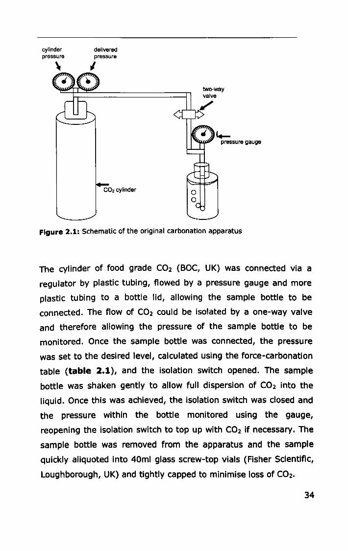
2.2.4.1 The original system

The original laboratory carbonating apparatus is illustrated in

figure 2.1.

33

cylinder pressure

" delivered pressure

I

C02 cylinder

two-way valve

pressure gauge

Figure 2.1: Schematic of the original carbonation apparatus

The cylinder of food grade C02 (BOC, UK) was connected via a

regulator by plastic tubing, flowed by a pressure gauge and more

plastic tubing to a bottle lid, allowing the sample bottle to be

connected. The flow of C02 could be isolated by a one-way valve

and therefore allowing the pressure of the sample bottle to be

monitored. Once the sample bottle was connected, the pressure

was set to the desired level, calculated using the force-carbonation

table (table 2.1), and the isolation switch opened. The sample

bottle was shaken gently to allow full dispersion of C02 into the

liquid. Once this was achieved, the isolation switch was closed and

the pressure within the bottle monitored using the gauge,

reopening the isolation switch to top up with C02 if necessary. The

sample bottle was removed from the apparatus and the sample

quickly aliquoted into 40ml glass screw-top vials (Fisher SCientific,

Loughborough, UK) and tightly capped to minimise loss of C02.

34

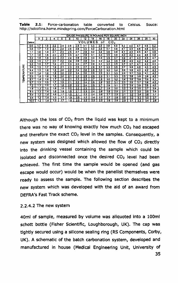
Table 2.1: Force-carbonation table converted to Celsius. Souce: http://sdcollins.home.mindspring.com/ForceCarbonation.html

GAUGE PRESSURE IN POUNDS PER SQUARE INCH o I 2 I 4 I 6 I 8 I 10 I 12 I 14 I 16 I 18 I 20 I 22 I 24 I 26 I 28 I 30

Celsius VOLUMES of CO 2

0.0 1.7 1.9 2.2 2.4 2.6 2.9 3.1 3.3 3.5 3.8 4.0 4.2 4.4 4.7 4.9 5.2 0.6 1.7 1.9 2.1 2.4 2.6 2.8 3.0 3.2 3.5 3.7 3.9 4.1 4.3 4.6 4.8 5.1 1.1 1.6 1.9 2.1 2.3 2.5 2.7 2.9 3.2 3.4 3.6 3.8 4.1 4.3 4.5 4.7 4.9 1.7 1.6 1.8 2.0 2.3 2.5 2.7 2.9 3.1 3.3 3.5 3.8 4.0 4.2 4.4 4.6 4.8 2.2 1.6 1.8 2.0 2.2 2.4 2.6 2.8 3.0 3.3 3.5 3.7 3.9 4.1 4.3 4.5 4.7 2.8 1.5 1.7 2.0 2.2 2.4 2.6 2.8 3.0 3.2 3.4 3.6 3.8 4.0 4.2 4.4 4.6

w 3.3 1.5 1.7 1.9 2.1 2.3 2.5 2.7 2.9 3.1 3.3 3.5 3.7 3.7 4.1 4.3 4.5 IX: 3.9 1.5 1.7 1.9 2.1 2.3 2.5 2.7 2.9 3.1 3.3 3.5 3.7 3.9 4.0 4.3 4.5 :::>

i 4.4 1.5 1.6 1.8 2.0 2.2 2.4 2.6 2.8 3.0 3.2 3.4 3.6 3.8 4.0 4.2 4.3 5.0 1.4 1.6 1.8 2.0 2.2 2.4 2.6 2.8 2.9 3.1 3.3 3.5 3.7 3.9 4.1 4.2

w 5.5 1.4 1.6 1.8 2.0 2.1 2.3 2.5 2.8 2.9 3.1 3.3 3.5 3.6 3.8 3.9 4.2 Q.

~ 6.1 1.4 1.6 1.7 1.9 2.1 2.3 2.5 2.7 2.8 3.0 3.2 3.4 3.6 3.8 3.9 4.1 w I- 6.7 1.3 1.5 1.7 1.9 2.1 2.2 2.4 2.6 2.8 3.0 3.1 3.3 3.5 3.7 3.9 4.0

7.2 1.3 1.5 1.7 1.8 2.0 2.2 2.4 2.5 2.7 2.9 3.1 3.3 3.4 3.6 3.8 4.0 7.8 1.3 1.5 1.6 1.8 2.0 2.2 2.3 2.5 2.7 2.8 3.0 3.2 3.4 3.5 3.7 3.9 8.3 1.3 1.4 1.6 1.8 1.9 2.1 2.3 2.4 2.6 2.8 2.9 3.1 3.3 3.5 3.6 3.8 8.9 1.2 1.4 1.6 1.7 1.9 2.1 2.2 2.4 2.6 2.7 2.9 3.1 3.2 3.4 3.6 3.7 9.4 1.2 1.4 1.5 1.7 1.9 2.0 2.2 2.4 2.5 2.7 2.8 3.0 3.2 3.3 3.5 3.7 10.0 1.2 1.4 1.5 1.7 1.8 2.0 2.2 2.3 2.5 2.6 2.8 2.9 3.1 3.3 3.4 3.6

Although the loss of C02 from the liquid was kept to a minimum

there was no way of knowing exactly how much C02 had escaped

and therefore the exact C02 level in the samples. Consequently, a

new system was designed which allowed the flow of C02 directly

into the drinking vessel containing the sample which could be

isolated and disconnected once the desired C02 level had been

achieved. The first time the sample would be opened (and gas

escape would occur) would be when the panellist themselves were

ready to assess the sample. The following section describes the

new system which was developed with the aid of an award from

DEFRA's Fast Track scheme.

2.2.4.2 The new system

40ml of sample, measured by volume was aliquoted into a lOOml

schott bottle (Fisher SCientific, Loughborough, UK). The cap was

tightly secured using a silicone sealing ring (RS Components, Corby,

UK). A schematic of the batch carbonation system, developed and

manufactured in house (Medical Engineering Unit, University of

35

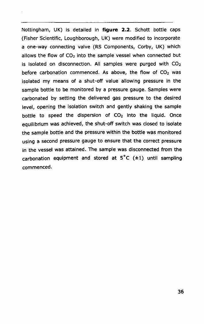
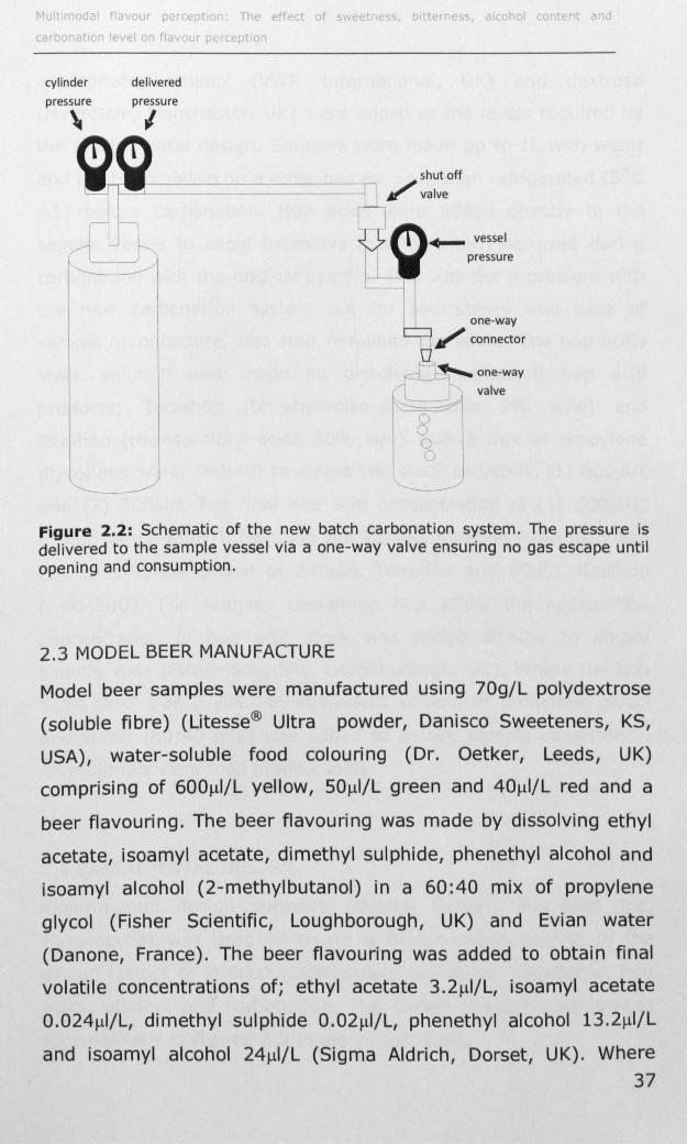
Nottingham, UK) is detailed in figure 2.2. Schott bottle caps

(Fisher SCientific, Loughborough, UK) were modified to incorporate

a one-way connecting valve (RS Components, Corby, UK) which

allows the flow of C02 into the sample vessel when connected but

is isolated on disconnection. All samples were purged with C02

before carbonation commenced. As above, the flow of C02 was

isolated my means of a shut-off value allowing pressure in the

sample bottle to be monitored by a pressure gauge. Samples were

carbonated by setting the delivered gas pressure to the desired

level, opening the isolation switch and gently shaking the sample

bottle to speed the dispersion of C02 into the liquid. Once

equilibrium was achieved, the shut-off switch was closed to isolate

the sample bottle and the pressure within the bottle was monitored

using a second pressure gauge to ensure that the correct pressure

in the vessel was attained. The sample was disconnected from the

carbonation equipment and stored at SoC (±1) until sampling

commenced.

36

cylinder

pressure

\

-

- -

delivered

pressure

I

o tt

shut off - ==n / valve

• a oh 0 t t

tr tT\+- vessel I I _ pressure

f L i I one-way b / connector

f\~ f < ~one-way

1 J i valve -----::~

8 ~ J

Figure 2.2: Schematic of the new batch carbonation system. The pressure is delivered to the sample vessel via a one-way valve ensuring no gas escape until opening and consumption.

2.3 MODEL BEER MANUFACTURE

Model beer samples were manufactured using 70g/L polydextrose

(soluble fibre) (Litesse® Ultra powder, Danisco Sweeteners, KS,

USA), water-soluble food colouring (Dr. Oetker, Leeds, UK)

comprising of 600J,!I/L yellow, SOJ,!I/L green and 40J,!I/L red and a

beer flavouring. The beer flavouring was made by dissolving ethyl

acetate, isoamyl acetate, dimethyl sulphide, phenethyl alcohol and

isoamyl alcohol (2-methylbutanol) in a 60:40 mix of propylene

glycol (Fisher SCientific, Loughborough, UK) and Evian water

(Danone, France). The beer flavouring was added to obtain final

volatile concentrations of; ethyl acetate 3.2J,!I/L, isoamyl acetate

O.024J,!I/L, dimethyl sulphide 0.02J,!I/L, phenethyl alcohol 13.2J,!I/L

and isoamyl alcohol 24J,!I/L (Sigma Aldrich, Dorset, UK). Where 37

appropriate, ethanol (VWR International, UK) and dextrose

(MyProtein, Manchester, UK) were added at the levels required by

the experimental design. Samples were made up to lL with water

and left to solubilise on a roller bed for >6h, then refrigerated (SoC

±1) before carbonation. Hop acids were added directly to the

sample vessel to avoid excessive foaming which occurred during

carbonation with the original system. This was not a problem with

the new carbonation system but for consistency and ease of

sample manufacture, this step remained the same. The hop acids

stock solution was made by dissolving isomerised hop acid

products; Tetrahop (tetrahydroiso-alpha-acids g% w/w) and

Redihop (rho-iso-alpha-acids 30% w/v) with a mix of propylene

glycol and water (60:40) to create two stock solutions, (1) 600J,lI/L

and (2) 300J,lI/L The final hop acid concentration of (1) 600J,lI/L,

comprised of 480J,lI/L Tetrahop and 120J,lI/L Redihop ( .... 80 IBU) and

(2) 300J,lI/L, comprised of 240J,lI/L Tetrahop and 60J,lI/L Redihop

( .... 40 IBU). For samples containing hop acids, the appropriate

concentration of hop acid stock was added directly to empty

sample vials (Fisher SCientific, Loughborough, UK). Where the hop

acids level was 0 J,ll/L, an equivalent volume of propylene glycol

and water (60:40 mix) was added to ensure sample consistency.

All materials were food grade quality.

2.4 EXPERIMENTAL DESIGN

Experimental design software (Design Expert, Stat-Ease Inc,

Minneapolis) was used to create a design space varying in the

design factors of interest (independent variables); sweetener, hop

acids, ethanol and carbonation. The design space is represented

schematically in figure 2.3 to aid visualisation.

38

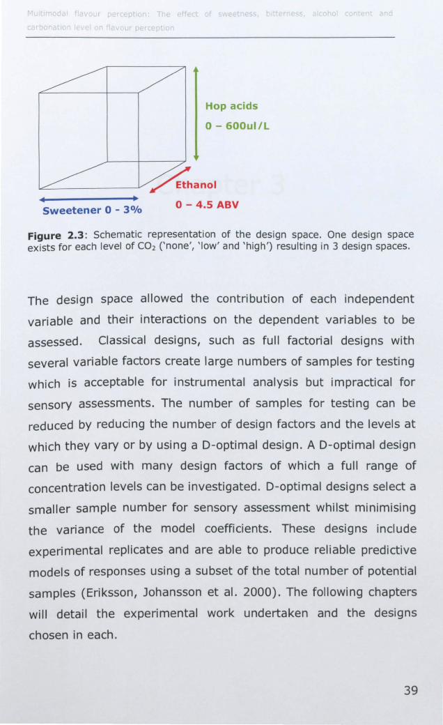
Hop acids

0- 600ul/L

IL:-_____ ~ ~anol Sweetener 0 - 3% 0- 4.5 ABV

Figure 2.3: Schematic representation of the design space. One design space exists for each level of CO2 ('none', 'low' and 'high') resulting in 3 design spaces.

The design space allowed the contribution of each independent

variable and their interactions on the dependent variables to be

assessed. Classical designs, such as full factorial designs with

several variable factors create large numbers of samples for testing

which is acceptable for instrumental analysis but impractical for

sensory assessments. The number of samples for testing can be

reduced by reducing the number of design factors and the levels at

which they vary or by using a D-optimal design. A D-optimal design

can be used with many design factors of which a full range of

concentration levels can be investigated. D-optimal designs select a

smaller sample number for sensory assessment whilst minimising

the variance of the model coefficients. These designs include

experimental replicates and are able to produce reliable predictive

models of responses using a subset of the total number of potential

samples (Eriksson, Johansson et al. 2000). The following chapters

will detail the experimental work undertaken and the designs

chosen in each.

39

Chapter 3

40

3. PHYSICOCHEMICAL INTERACTIONS

3.1 INTRODUCTION

In simple water based solutions, the strength of aroma perception

is governed by the volatility of the molecules in the aqueous phase.

Compounds partition between air and water depending on their

affinity for each phase (Taylor 1998). The partitioning between the

aqueous and the gaseous phase is important when investigating

aroma delivery to the olfactory bulb via both the ortho-nasal and

retro-nasal routes, as changes in partitioning could alter perception

and consequently impact upon consumer liking.

Typically, in water based beverages, aroma compounds are present

at extremely low concentrations which are considered infinitely

dilute and therefore obey Henry's Law. Henry's Law states that "the

mass of vapour dissolved in a certain volume of solvent is directly

proportional to the partial pressure of the vapour that is in

equilibrium with the solution" (Taylor 1998). Therefore, in a closed

aqueous system at eqUilibrium, the concentration of the gaseous

phase is directionally proportional to the concentration in the

aqueous phase. However, most beverages are not simple aqueous

solutions as they contain solutes and other matrix components

which could alter the partitioning behaviour of aroma compounds.

Furthermore, beverages are not consumed in a closed system at

equilibrium and factors such as temperature and dynamic air flow

(as opposed to static) may also have an impact.

41

3.1.1. Instrumental measurement of volatile partitioning

3.1.1.1 Headspace

Classic techniques for analysing flavour volatiles, such as Gas

Chromatography-Mass Spectrometry (GC-MS) give detailed

structural information but the temporal resolution is not capable of

real-time analysis of volatile partitioning (Taylor, Linforth et al.

2000). At the expense of structural information, it is possible to

collect real-time data on a mixture of compounds using soft

ionisation (providing little fragmentation of ions), followed by mass

spectrometry (Taylor, Linforth et al. 2000). Atmospheric Pressure

Chemical Ionisation-Mass Spectrometry (APCI-MS) consists simply

of an inlet and an ionisation source. The sample is drawn into the

heated fused silica capillary inlet. An initial reactant ion is formed

from water which transfers its charge to any molecule with a higher

proton affinity, such as most organic compounds, at atmospheric

pressure. The compounds are ionised by a corona discharge pin

and the resultant ions are protonated by the transfer of charge

from the reactant ion. Soft ionisation gives sufficient energy to the

reagent ions to ionise the molecule, reducing fragmentation which

can be controlled by altering the cone voltage. Once formed, the

resultant ions are sampled into a standard quadrupole MS under

vacuum for quantification. This technique allows controlled

sampling of a small amount of equilibrium headspace, therefore

reducing disturbance of the equilibrium state. Sampling time Is

short (commonly <60secs) and takes place in real time. The

resultant spectra provide information on the compound's ability to

partition from the sample matrix into the gaseous phase (partition

coefficient), compared to other matrices. This method can also be

used to successfully measure dynamic headspace. An inert gas

(nitrogen) dilutes the equilibrium headspace and is sampled into 42

the APCI-MS to study the stability of volatile headspace

concentration in conditions which are closer to those experienced

during food and beverage consumption.

3.1.1.2 In-Vivo

Equilibrium conditions are rarely achieved during the consumption

of food and beverages. Mastication, swallowing, saliva addition and

temperature changes create a dynamic situation (Taylor and

Linforth 1996). Liquids are held for a short period in the mouth

before swallowing allowing only a short period for aroma release.

Swallowing forces the bolus of liquid into the pharynx by the

tongue, the velum retracts and elevates preventing the liquid from

entering the nasal caVity. After the liquid has passed the epiglottis,

the velum is reopened allowing a pulse of aroma into the nasal

cavity (Hodgson, Linforth et al. 2003; Hodgson, Langridge et al.

2005; Salles, Chagnon et al. 2011). The highest aroma signal is

usually in the first breath after swallowing (Linforth and Taylor

2000). Measuring volatile partitioning in-vivo therefore requires a

quick sampling method (such as the APCI-MS) capable of detecting

changes in volatile concentration in the breath during consumption

(temporal resolution as low as 0.01 sec) whilst not interfering with

normal eating patterns. Taylor and Linforth (2000) created a novel

interface for the APCI-MS to sample the air from the nose during

consumption allowing the study of retro-nasal volatile delivery

(Taylor, Linforth et al. 2000). A small disposable plastic tube

(10mm diameter and 40-50mm length) is inserted into one nostril

so that the assessors could breathe and drink normally with the

other end connected to the capillary inlet. The expelled air is

sampled and analysed creating traces of breath by breath volatile

concentrations. Acetone is a metabolic by-product of blood

43

oxygenation and is transferred to the breath during exhalation.

Consequently, acetone is used as a marker to ensure that the

assessors are breathing through their nose during consumption and

that the volatiles are entering via the retro-nasal route. This

technique has been used to successfully determine volatile

partitioning into the breath during mastication and has also been

used alongside other techniques to determine the temporal pattern

of combined taste and aroma release (Davidson, Linforth et al.

1999).

3.1.2 Effect of ethanol on volatile partitioning

It is important to note that when measuring flavour release from

ethanolic samples by APCI-MS, ethanol can interfere with ionisation

(Aznar, Tsachaki et al. 2004). However, Aznar (2004) successfully

developed a method to control ionisation by adding ethanol to the

source to act as the proton transfer reagent ion (Aznar, Tsachaki et

al. 2004). Using this method, Aznar (2004) measured the

equilibrium headspace of 12% ethanol samples and found that

compared to water, 120/0 ethanol decreased the partitioning of

most aroma compounds tested by 4-42% (Aznar, Tsachaki et al.

2004). This is thought to be due to the amphiphilic nature of

ethanol, thus decreasing partitioning to the liquid interface for

gaseous exchange. Other studies using much higher levels of

ethanol have found conflicting results (Conner, Birkmyre et al.

1998; Aprea, Biasioli et al. 2007). Dynamic headspace experiments

can be carried out to give a better understanding of the situation

which occurs during drinking as the headspace is constantly diluted

by gas. Under these conditions there is a reduction in the

concentration of volatiles compared to static headspace (Tsachaki,

44

Linforth et al. 2005). Tsachaki et al (2005) showed that 12%

ethanol addition actually boosted the delivery of the majority of

volatiles tested to a level which was close to their initial headspace

concentration (Tsachaki, Linforth et al. 2005). No literature can be

found on the physico-chemical effects of ethanol on volatile

partitioning in-vivo and also no current data is available in

combination with carbonation.

3.1.3 Effect of carbonation on volatile partitioning

Headspace investigations into the effects of carbonation on volatile

partitioning are limited due to the difficult nature of measuring at

static equilibrium. Pressurised samples will inevitably become

dynamic systems as soon as the sample is opened and the

pressure released. This may be the cause of inconsistent results

found in other studies (Hewson 2007; Pozo-Bayon, Santos et at.

2009; Saint-Eve, Deleris et at. 2009). Consequently, measures of

volatile partitioning from carbonated systems during drinking may

provide more meaningful data.

3.1.4 Effect of solutes on volatile partitioning

Volatile partition coefficients could be affected by the solutes in

beer such as; inorganic salts, sugars, amino acids, nucleotides,

polyphenols and hop resins (Briggs, Boulton et at. 2004) which

could physically enhance or decrease solubility of the other

compounds within the solution (Taylor and Roberts 2004). No

published studies have investigated the effect of hop acids on

volatile partitioning. Isomerised hop acids are water soluble up to

circa. 120mg/1 (Briggs, Boulton et at. 2004) and thus unlikely to

45

alter volatile partitioning on their own in this system. However,

they may interact with other components in the matrix as they

create foam when in combination with C02 which could indirectly

alter the surface activity (Briggs, Boulton et al. 2004). Previous

research found that sugars, added to water at very high levels (up

to 65%) have been found to change the volatility of aroma

compounds (Friel, Linforth et al. 2000), which was thought to be

due to a phenomenon known as 'salting out' (Voilley, Simatos et al.

1977) rather than a physico-chemical interaction.

Overall, this research project aimed to investigate the multimodal

interactions between sweetness, bitterness, alcohol and

carbonation on flavour perception. Therefore, it was important to

explore if these factors interact at a physico-chemical level within

the model system. It is unlikely that the level of sweetener added

to the model system in this investigation (3%) would impact due to

the very low concentration compared to other studies (Voilley,

Simatos et al. 1977; Friel, Linforth et al. 2000) and consequently

this was not investigated here. There is limited data on the

physico-chemical effects of the individual components (ethanol,

carbonation and hop acids) on in-vivo volatile release and they

have not been investigated in combination. The aim of this study

was to determine the physico-chemical effects of ethanol,

carbonation and hop acid addition on volatile partitioning by

measuring the volatiles released in the (1) headspace above the

samples at equilibrium, (2) headspace above the samples shortly

after decanting and (3) exhaled air of people as they consume the

beverage.

46

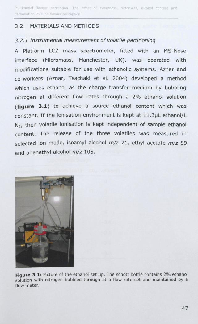
3.2 MATERIALS AND METHODS

3.2.1 Instrumental measurement of volatile partitioning

A Platform LCZ mass spectrometer, fitted with an MS-Nose

interface (Micromass, Manchester, UK), was operated with

modifications suitable for use with ethanolic systems. Aznar and

co-workers (Aznar, Tsachaki et al. 2004) developed a method

which uses ethanol as the charge transfer medium by bubbling

nitrogen at different flow rates through a 2% ethanol solution

(figure 3.1) to achieve a source ethanol content which was

constant. If the ionisation environment is kept at 11.3\-1L ethanol/L

N2, then volatile ionisation is kept independent of sample ethanol

content. The release of the three volatiles was measured in

selected ion mode, isoamyl alcohol m/z 71, ethyl acetate m/z 89

and phenethyl alcohol m/z 105.

Figure 3.1: Picture of the ethanol set up. The schott bottle contains 2% ethanol solution with nitrogen bubbled through at a flow rate set and maintained by a flow meter.

47

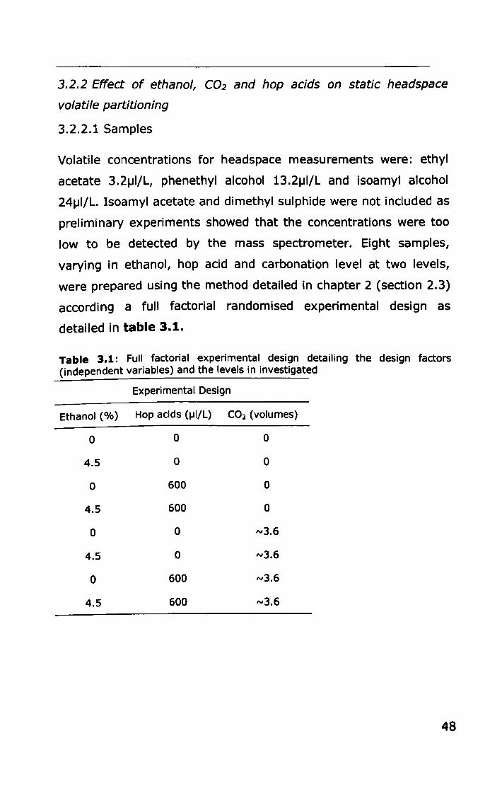
3.2.2 Effect of ethanol, C02 and hop acids on static headspace

volatile partitioning

3.2.2.1 Samples

Volatile concentrations for headspace measurements were: ethyl

acetate 3.21JI/L, phenethyl alcohol 13.21J1/L and isoamyl alcohol

241J1/L. Isoamyl acetate and dimethyl sulphide were not included as

preliminary experiments showed that the concentrations were too

low to be detected by the mass spectrometer. Eight samples,

varying in ethanol, hop acid and carbonation level at two levels,

were prepared using the method detailed in chapter 2 (section 2.3)

according a full factorial randomised experimental design as

detailed in table 3.1.

Table 3.1: Full factorial experimental design detailing the design factors (independent variables) and the levels in investigated

Experimental Design

Ethanol (%) Hop acids (\JilL) CO2 (volumes)

0 0 0

4.5 0 0

0 600 0

4.5 600 0

0 0 ,.,3.6

4.5 0 "'3.6

0 600 ,.,3.6

4.5 600 "'3.6

48

3.2.2.2 Headspace sampling

Static headspace measurements were taken after equilibration and

also straight after decanting to mimic volatile delivery similar to a

real drinking context. This method is potentially more variable, but

may reveal differences in short term release that may not be

observed with longer equilibration. For static sampling, aliquots

(40ml) of model beer were placed in 100ml Schott bottles (Fisher

SCientific, Loughborough, UK) fitted with a one port lid that allowed

headspace sampling and were equilibrated at 6°C (± 1) for 2h.

Products to be evaluated straight after decanting (short term

decanting) were poured from a capped 40ml glass vial directly into

a 100ml Schott bottle. A one port lid was fitted and air containing

the volatile compounds was sampled into the ionisation source via

a silica capillary tube heated to 150°C. Headspace sampling in both

cases was at a rate of sml/min, for lmin per sample with a dwell

time of O.ls and cone voltage of lsV. Each sample was measured

in triplicate following a fully randomised design.

3.2.2.3 Data processing and analysis

The output generated a chromatogram trace of the intensity of the

three monitored ions in the headspace during sampling, measured

as a percentage of maximum peak height. These values were used

in subsequent analysis to show the number of ions formed by

ionisation of the sample headspace with a mass to charge ratio of

71, 89 or 105. The average of three replicate peak heights

(arbitrary units) for each sample was determined for each

compound using MassLynx software (Micromass, Manchester, UK).

The mean peak height can then be compared directly between

samples to elucidate trends and differences between samples.

Analysis of variance (ANOVA) was conducted to identify significant

49

differences between the samples for each compound measured.

Where differences were found predictive polynomial models were

generated using Design Expert v6.0.2 (Stat-Ease Inc, Minneapolis)

to explain variation in delivery of compounds as a function of

ethanol, hop acid and carbonation level. Non-significant terms, as

determined by ANOVA were removed to give a mathematical model

which best represented the data.

3.2.3 Effect of ethanol, carbonation and hop acids on in-vivo

volatile partitioning

3.2.3.1 Samples

Typically in-nose concentrations of volatile compounds are 10 to

100 x lower in than in the breath (Linforth, Martin et al. 2002).

Therefore, to increase signal detection, volatile concentrations for

in-vivo measurements were increased 2-fold: ethyl acetate 6.4IJI/L,

phenethyl alcohol 26.4IJI/L and isoamyl alcohol 481J1/L. Samples

were prepared in the same way as previously detailed in chapter 2,

section 2.3. Eight samples, varying in ethanol, hop acid and

carbonation level, were prepared according to a full factorial

randomised experimental design as detailed in table 3.1.

3.2.3.2 In-Vivo Sampling

Panellists opened and immediately consumed approximately two

thirds of the 40ml model beer sample directly from the sample vial.

A small plastic tube, leading to the MS, was immediately inserted

into the left nostril. Once in place, the sample was swallowed and

the panellist was instructed to breathe normally through the nose,

keeping the mouth closed for the duration of the sampling period.

Breath was sampled from the panellist (30ml/min) over a lmin

50

period after swallowing (dwell time 0.02s, cone voltage 18V). Each

sample was consumed in triplicate by 4 panellists using a

randomised block design. Each panellist was placed into a separate

block to account for individual differences in aroma partitioning

caused by differences in physiology and breath flow rates between

people (Salles, Chagnon et al. 2011).

3.2.3.3 Data processing and analysis

Mean relative amounts of each compound were determined by

comparison of AreaTotal, Areal, Area2, Imaxl and Imax2

parameters (in arbitrary units) which were extracted from

chromatograms and integrated using Masslynx software. Figure

3.2 identifies these parameters on a typical release profile

generated from a panellist consuming a sample. The peaks and

troughs are the subject breathing out and in respectively. The area

of the first peak (Areal) is black and the area of the remaining

peaks (Area2) is white. These were combined to give the total area

(AreaTotal). The height of the peaks can also be measured, Imaxl

is the height of the first peak and Imax2 is the height of the

subsequent peak. Volatile air-water partition coefficients (Kaw

values) were taken from EPI-Suite V4 (Environmental Protection

Agency, America).

51

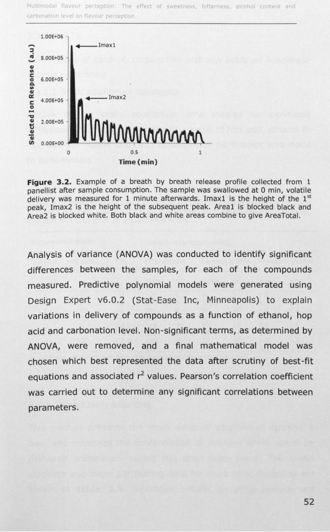
It rr od for Th f t we t e s hoi a

1.008-06

- 4 Imaxl =! ..,

8.008-05 -II '" C 0 6.00E+05 A

'" II 0:: 4 Imax2 c 4.00E+05 0 ... ." II 2.00E+05 ti II 'ii (I) O.OOE+OO

0 0.5 1

Time{min)

Figure 3.2. Example of a breath by breath release profile collected from 1 panellist after sample consumption. The sample was swallowed at 0 min, volatile delivery was measured for 1 minute afterwards. Imaxl is the height of the 1st

peak, Imax2 is the height of the subsequent peak. Areal is blocked black and Area2 is blocked white. Both black and white areas combine to give AreaTotal.

Analysis of variance (ANOVA) was conducted to identify significant

differences between the samples, for each of the compounds

measured. Predictive polynomial models were generated using

Design Expert v6.0.2 (Stat-Ease Inc, Minneapolis) to explain

variations in delivery of compounds as a function of ethanol, hop

acid and carbonation level. Non-significant terms, as determined by

ANOVA, were removed, and a final mathematical model was

chosen which best represented the data after scrutiny of best-fit

equations and associated r2 values. Pearson's correlation coefficient

was carried out to determine any significant correlations between

parameters.

52

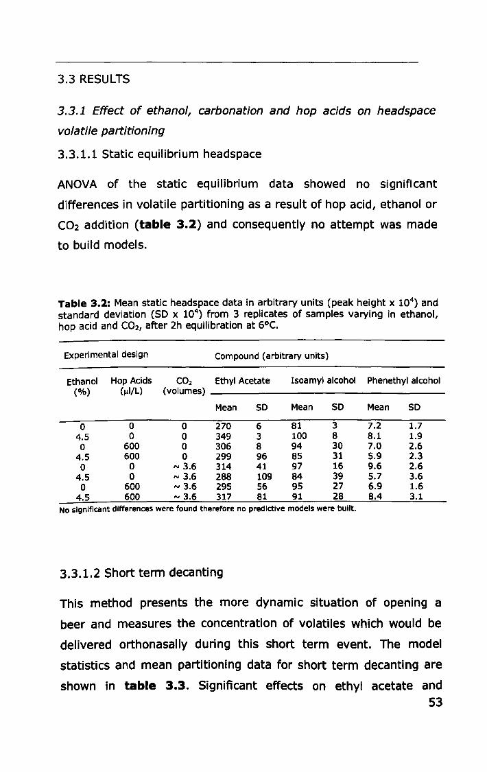
3.3 RESULTS

3.3.1 Effect of ethanol, carbonation and hop acids on headspace

volatile partitioning

3.3.1.1 Static equilibrium headspace

ANOVA of the static equilibrium data showed no significant

differences in volatile partitioning as a result of hop acid, ethanol or

C02 addition (table 3.2) and consequently no attempt was made

to build models.

Table 3.2: Mean static headspace data in arbitrary units (peak height x 104) and

standard deviation (SO x 104) from 3 replicates of samples varying in ethanol,

hop acid and CO2, after 2h equilibration at 6°C.

Experimental design Compound (arbitrary units)

Ethanol Hop Acids CO2 Ethyl Acetate Isoamyl alcohol Phenethyl alcohol (%) (!JilL) (volumes)

Mean SO Mean SO Mean SO

0 0 0 270 6 81 3 7.2 1.7 4.5 0 0 349 3 100 8 8.1 1.9 0 600 0 306 8 94 30 7.0 2.6

4.5 600 0 299 96 85 31 5.9 2.3 0 0 '" 3.6 314 41 97 16 9.6 2.6

4.5 0 '" 3.6 288 109 84 39 5.7 3.6 0 600 '" 3.6 295 56 95 27 6.9 1.6

4.5 600 '" 3.6 317 81 91 28 8.4 3.1 No significant differences were found therefore no predictive models were built.

3.3.1.2 Short term decanting

This method presents the more dynamic situation of opening a

beer and measures the concentration of volatiles which would be

delivered orthonasally during this short term event. The model

statistics and mean partitioning data for short term decanting are

shown in table 3.3. Significant effects on ethyl acetate and 53

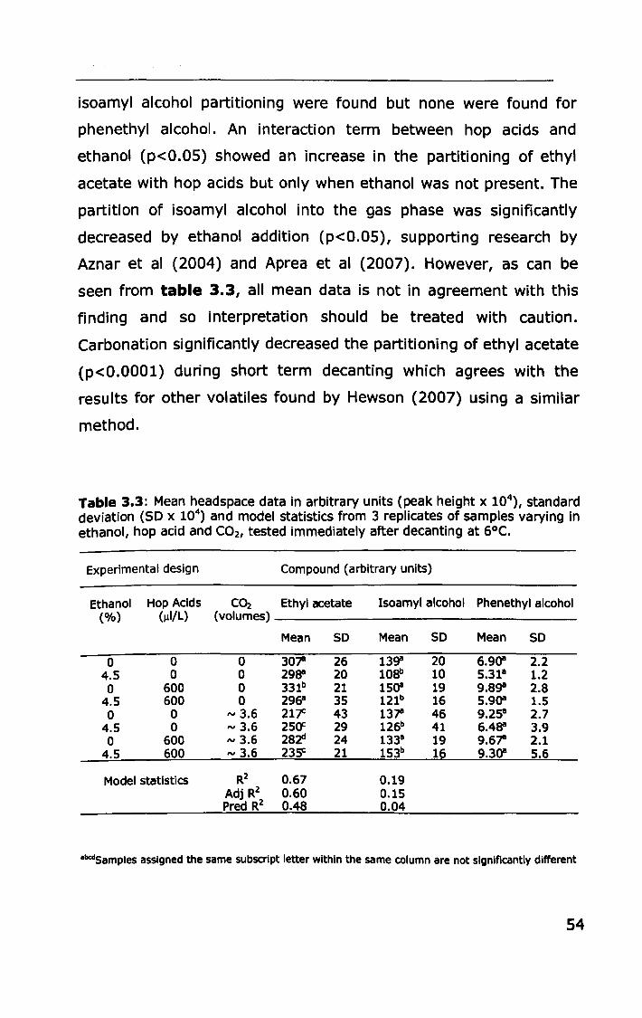
isoamyl alcohol partitioning were found but none were found for

phenethyl alcohol. An interaction term between hop acids and

ethanol (p<O.OS) showed an increase in the partitioning of ethyl

acetate with hop acids but only when ethanol was not present. The

partition of isoamyl alcohol into the gas phase was significantly

decreased by ethanol addition (p<O.OS), supporting research by

Aznar et al (2004) and Aprea et al (2007). However, as can be

seen from table 3.3, all mean data is not in agreement with this

finding and so interpretation should be treated with caution.

Carbonation Significantly decreased the partitioning of ethyl acetate

(p<O.OOOl) during short term decanting which agrees with the

results for other volatiles found by Hewson (2007) using a similar

method.

Table 3.3: Mean headspace data in arbitrary units (peak height x 104), standard

deviation (SO x 104) and model statistics from 3 replicates of samples varying in

ethanol, hop acid and CO2, tested immediately after decanting at 6°C.

Experimental design Compound (arbitrary units)

Ethanol Hop Acids c~ Ethyl acetate Isoamyl alcohol Phenethyl alcohol (%) (~I/L) (volumes)

Mean SO Mean SO Mean SO

0 0 0 301' 26 139'1 20 6.9Q1 2.2 4.5 0 0 29se 20 108b 10 5.3111 1.2 0 600 0 331b 21 15Q1 19 9.89" 2.8

4.5 600 0 296' 35 121b 16 5.9Q11 1.5 0 0 tv 3.6 217= 43 131' 46 9.2511 2.7

4.5 0 tv 3.6 25(1 29 126b 41 6.4se 3.9 0 600 tv 3.6 28:zd 24 13311 19 9.61' 2.1

4.5 600 tv 3.6 23SC 21 153b 16 9.3Q1 5.6

Model statistics R2 0.67 0.19 Adj R2 0.60 0.15 Pred R2 0.48 0.04

abcdSamples assigned the same subscript letter within the same column are not Significantly different

54

3.3.2 Effect of ethanol, carbonation and hop acids on in-vivo

volatile partitioning

Measuring volatile partitioning in-vivo directly quantifies the volatile

delivery experienced during consumption (retronasal release).

Drinking is a short-time scale event and the volatiles do not reach

an equilibrium state during the process (Linforth, Martin et al.

2002). The addition of ethanol, carbonation and hop acids could

change volatile behaviour through differences in surface tension

and surface creation not seen in-vitro. These may influence volatile

behaviour differently when in contact with the surfaces of the

mouth and throat.

Data from the in-vivo breath by breath experiments were

expressed as the AreaTotal, which was further divided into Areal

and Area2 (measuring area of the first peak and persistence

respectively) and also by height parameters, Imaxl and Imax2

(measuring intensity of first and second peaks), as illustrated in

figure 3.2. Due to the high level of temporal resolution, Areal and

Area2 can be separated from AreaTotal and quantified, which is

important because the two phases result from different processes

(Hodgson, Linforth et al. 2003). The volatiles that are released in

the first exhalation to form Areal do so immediately after the

sample is swallowed (Hodgson, Linforth et al. 2003). The volatiles

released into the breath in subsequent exhalations (Area2) are

from a thin layer of residual sample coating the throat during the

dynamic gas flow conditions of inhalation and exhalation (Linforth

and Taylor 2006). Tables 3.4 and 3.S show the mean Area and

Imax parameters respectively, and indicate where significant

differences occur in a sample. Significant model terms and

associated statistics for each compound and parameter are

presented in table 3.6. The values obtained for Areal and Imaxl 55

showed a strong positive correlation, with r2 values greater

than >0.93 for all 3 compounds. Consequently, the two

measurements would be expected to show similar trends.

56

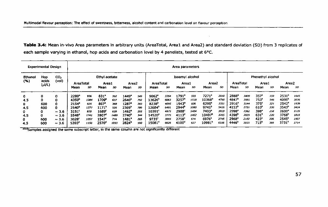
Multimodal flavour perception: The effect of sweetness, bitterness, alcohol content and carbonation level on flavour perception

Table 3.4: Mean in-vivo Area parameters in arbitrary units (AreaTotal, Areal and Area2) and standard deviation (SO) from 3 replicates of

each sample varying in ethanol, hop acids and carbonation level by 4 panelists, tested at 6°C.

Experimental Design Area parameters

Ethanol Hop CO2 Ethyl acetate Isoamyl alcohol Phenethyl alcohol (%) adds (vol)

AreaTotal (11I/L) Areal Area2 AreaTotal Areal Area2 AreaTotal Areal Area2 Mean so Mean so Mean so Mean so Mean so Mean so Mean so Mean so Mean SD

0 0 0 2280" 936 831" 392 1449" 549 9062" 3354 1791" 555 7271- 2810 2888- 1800 357- 159 2531- 1645

4.5 0 0 4350b 1384 1709b 637 2640b 792 13626b 6063 3257b 1518 10368b 4790 4847b 3581 753b 546 4095b 3036

0 600 0 2154" 625 867" 368 1287" 283 8238" 4095 1943" 836 6295" 3351 2916a 2144 375- 221 2542a 1939

4.5 600 0 2540b 1277 1171b 526 2369b 789 12684b 6491 2944b 1080 9741b 5426 4153b 2751 610b 330 3543b 2424

0 0 "" 3.6 3151c 820 1689c 639 1462" 255 10391C 4975 2988c 1404 7403- 3919 2998a 2362 398" 258 2600" 2129

4.5 0 "" 3.6 5548d 1741 280Jd 1489 2740b 344 14520d 3775 4113d 1462 10407b 3265 4398b 2029 631b 220 3768b 1819

0 600 "" 3.6 3028c 1057 154]C 774 1481" 285 9735c 3095 2758c 674 6976" 2745 2968a 2102 423" 206 2545a 1907

4.5 600 "" 3.6 5393d 1150 2570d 1033 2824b 590 15081d 6626 4100d 627 10981b 6106 4446b 3015 715b 388 3731b 2714

- 'Samples assigned the same subscript letter, in the same column are not significantly different

57

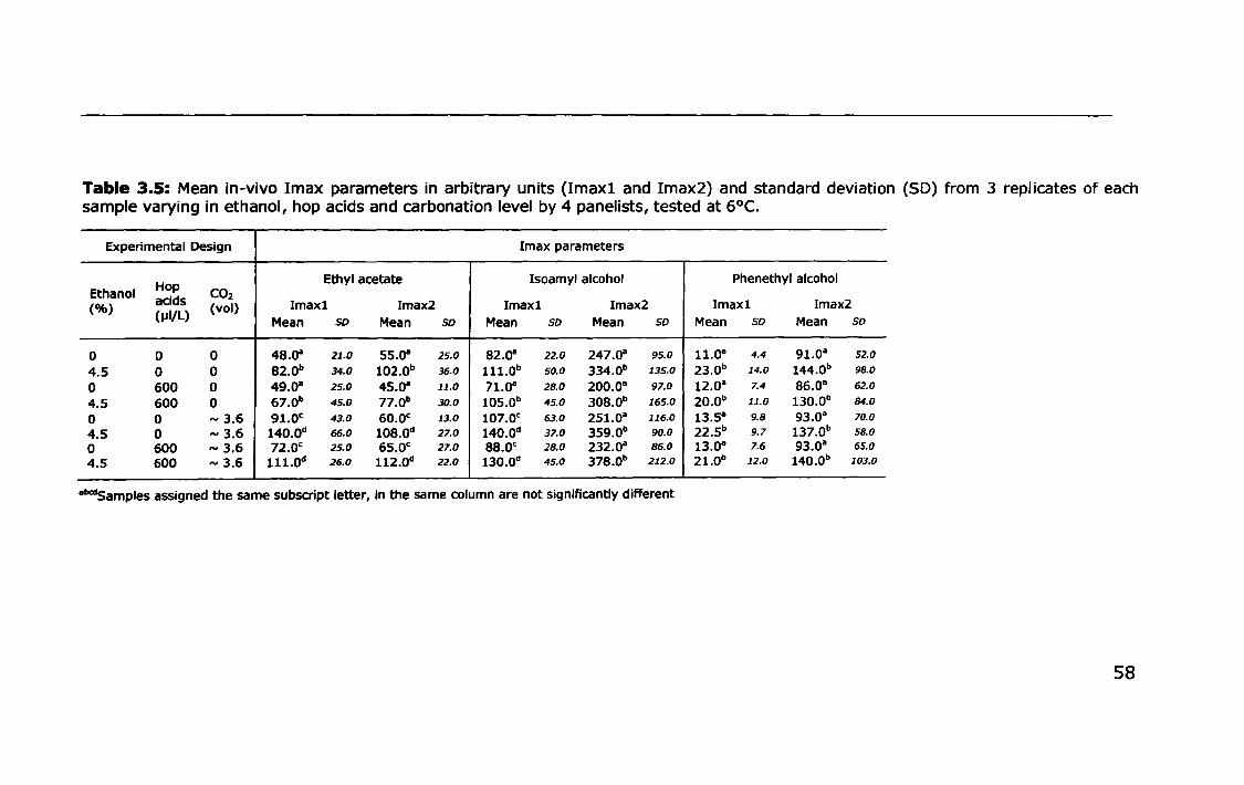
Table 3.5: Mean in-vivo Imax parameters in arbitrary units (Imaxl and Imax2) and standard deviation (SO) from 3 replicates of each sample varying in ethanol, hop acids and carbonation level by 4 panelists, tested at G°e.

Experimental Design Imax parameters

Hop Ethyl acetate Isoamyl alcohol Phenethyl alcohol Ethanol CO2 (%)

acids (vol) Imaxl Imax2 Imaxl Imax2 Imaxl Imax2 h·II/L) Mean so Mean so Mean so Mean so Mean so Mean so

0 0 0 48.oa 21.0 55.0- 25.0 82.0- 22.0 247.0" 95.0 11.0" 4.4 91.0" 52.0

4.5 0 0 82.0b 34.0 102.0b 36.0 lll.0b 50.0 334.0b 135.0 23.0b 14.0 144.0b 98.0

0 600 0 49.0" 25.0 45.0" 11.0 71.0" 28.0 200.0· 97.0 12.0" 7.4 86.0a 62.0

4.5 600 0 67.0b 45.0 77.0b 30.0 10s.Ob 45.0 308.0b 165.0 20.0b 11.0 130.0b 84.0

0 0 "" 3.6 91.0e 43.0 60.0e 13.0 107.0c 63.0 251.0· 116.0 13.5" 9.8 93.0" 70.0

4.5 0 '" 3.6 140.0d 66.0 108.0d 27.0 140.0d 37.0 359.0b 90.0 22.5b 9.7 137.0b 58.0

0 600 "" 3.6 72.0c 25.0 6s.0e 27.0 88.0c 28.0 232.0" 86.0 13.0a 7.6 93.0" 65.0

4.5 600 "" 3.6 111.0d 26.0 112.0d 22.0 130.0d 45.0 378.0b 212.0 21.0b 12.0 140.0b 103.0 _.- -

abcdSamples assigned the same subscript letter, in the same column are not significantly different

58

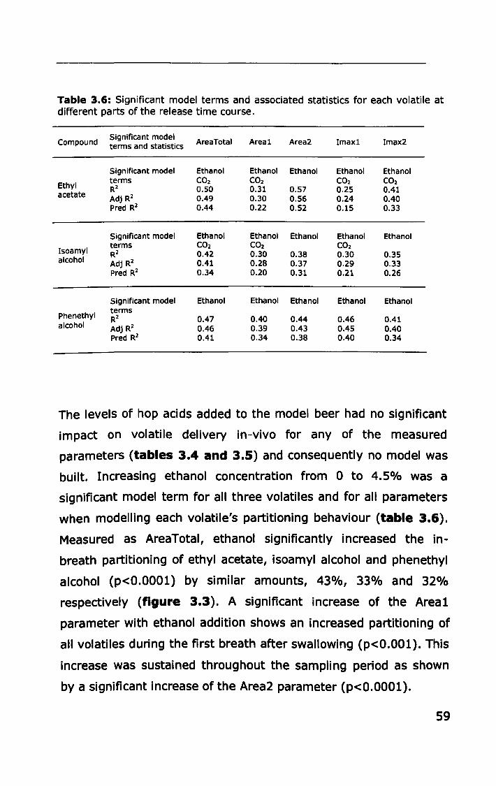
Table 3.6: Significant model terms and associated statistics for each volatile at different parts of the release time course.

Compound Significant model

AreaTotal Areal Area2 Imaxl Imax2 terms and statistics

Significant model Ethanol Ethanol Ethanol Ethanol Ethanol

Ethyl terms CO2 CO2 CO2 CO2 R2 0.50 0.31 0.57 0.25 0.41

acetate Adj R2 0.49 0.30 0.56 0.24 0.40 Pred R2 0.44 0.22 0.52 0.15 0.33

Significant model Ethanol Ethanol Ethanol Ethanol Ethanol

Isoamyl terms CO2 CO2 CO2 R2 0.42 0.30 0.38 0.30 0.35

alcohol Adj R2 0.41 0.28 0.37 0.29 0.33 Pred R2 0.34 0.20 0.31 0.21 0.26

Significant model Ethanol Ethanol Ethanol Ethanol Ethanol

Phenethyl terms R2 0.47 0.40 0.44 0.46 0.41

alcohol Adj R2 0.46 0.39 0.43 0.45 0.40 Pred R2 0.41 0.34 0.38 0.40 0.34

The levels of hop acids added to the model beer had no significant

impact on volatile delivery in-vivo for any of the measured

parameters (tables 3.4 and 3.S) and consequently no model was

built. Increasing ethanol concentration from 0 to 4.5% was a

significant model term for all three volatiles and for all parameters

when modelling each volatile's partitioning behaviour (table 3.6).

Measured as AreaTotal, ethanol significantly increased the in­

breath partitioning of ethyl acetate, isoamyl alcohol and phenethyl

alcohol (p<O.OOOl) by similar amounts, 430/0, 33% and 32%

respectively (figure 3.3). A significant increase of the Areal

parameter with ethanol addition shows an increased partitioning of

all volatiles during the first breath after swallowing (p<O.OOl). This

increase was sustained throughout the sampling period as shown

by a significant increase of the Area2 parameter (p<O.OOOl).

59

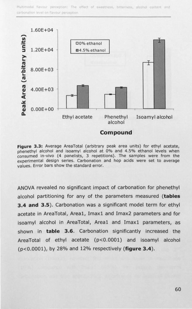
p pt T

~ CI) .... I-

1.60E+04

e ::J 1.20E+04

> a-ftJ .... :c 8.00E+03 a­ftJ

-....,;

~ 4.00E+03 a-ct ~

~ O.OOE+OO D.

00% ethanol

C4.S% ethanol

Ethyl acetate Phenethyl alcohol

Compound

Isoamyl alcohol

Figure 3.3: Average AreaTotal (arbitrary peak area units) for ethyl acetate, phenethyl alcohol and isoamyl alcohol at 0% and 4.5% ethanol levels when consumed in -vivo (4 panelists, 3 repetitions). The samples were from the experimental design series. Carbonation and hop acids were set to average values. Error bars show the standard error.

ANOVA revealed no significant impact of carbonation for phenethyl

alcohol partitioning for any of the parameters measured (tables

3.4 and 3.5). Carbonation was a significant model term for ethyl

acetate in AreaTotal, Areal, Imaxl and Imax2 parameters and for

isoamyl alcohol in AreaTotal, Areal and Imaxl parameters, as

shown in table 3.6. Carbonation significantly increased the

AreaTotal of ethyl acetate (p<O.OOOl) and isoamyl alcohol

(p<O.OOOl), by 28% and 12% respectively (figure 3.4).

60

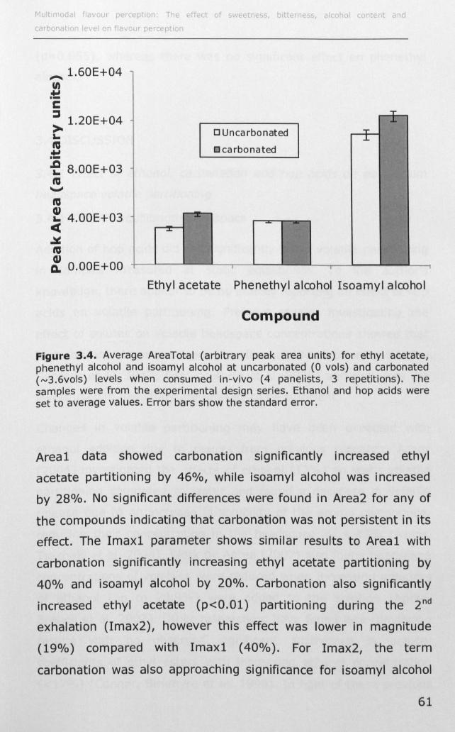
~ 1.60E+04 U) ..., .-e ~ 1.20E+04 ... ta ..., .--e 8.00E+03 ta

"'-' ta ~ 4.00E+03 ct ~ ta :. O.OOE+OO

o Unca rbonated

carbonated

Ethyl acetate Phenethyl alcohol Isoamyl alcohol

Compound

Figure 3.4. Average AreaTotal (arbitrary peak area units) for ethyl acetate, phenethyl alcohol and isoamyl alcohol at uncarbonated (0 vols) and carbonated (IV3.6vols) levels when consumed in-vivo (4 panelists, 3 repetitions). The samples were from the experimental design series. Ethanol and hop acids were set to average values. Error bars show the standard error.

Areal data showed carbonation significantly increased ethyl

acetate partitioning by 460/0, while isoamyl alcohol was increased

by 28%. No significant differences were found in Area2 for any of

the compounds indicating that carbonation was not perSistent in its

effect. The Imaxl parameter shows similar results to Areal with

carbonation significantly increasing ethyl acetate partitioning by

400/0 and isoamyl alcohol by 20%. Carbonation also significantly

increased ethyl acetate (p<O.Ol) partitioning during the 2nd

exhalation (lmax2), however this effect was lower in magnitude

(19%) compared with Imaxl (40%). For Imax2, the term

carbonation was also approaching Significance for isoamyl alcohol

61

(p=O.OSS), whereas there was no significant effect on phenethyl

alcohol.

3.4 DISCUSSION

3.4.1 Effect of ethanol, carbonation and hop acids on equilibrium

headspace volatile partitioning

3.4.1.1 Static equilibrium headspace

Addition of hop acids did not significantly affect volatile partitioning

in samples measured at static equilibrium. To the author's

knowledge, there appear to be no studies reporting an effect of hop

acids on volatile partitioning. Previous studies investigating the

effect of solutes on volatile headspace concentrations showed that

high concentrations are needed to alter volatile partitioning (Voilley,

Simatos et al. 1977; Friel, Linforth et al. 2000) and therefore the

levels used in this study are unlikely to be sufficient.

Changes in volatile partitioning may have been expected with

ethanol addition due to results from previous research. Aznar

(2004) investigated the effects of ethanol (12%) on static volatile

partitioning compared to water and found a decrease in volatile

release due to an increase in solubility of the aroma compounds,

reducing their concentration in the headspace by 4-42% (Aznar,

Tsachaki et al. 2004). Work by Aprea (2007) also found headspace

concentrations of volatiles were reduced when increasing amounts

of ethanol (up to 20.9%) were added to the solution (Aprea,

Biasioli et al. 2007). Other researchers have found less convincing

results with no observed significant differences in activity

coefficients of ethyl esters with increasing ethanol concentration

« 17%) (Conner, Birkmyre et al. 1998). In light of these previous 62

studies, a minor decrease in volatile partitioning with ethanol

during the static headspace measurements may have been

expected in the present study. However, the level of ethanol added

(4.5%) was evidently too low to cause a significant decrease.

The addition of carbonation was not found to alter static volatile

partitioning as found in other studies (Hewson 2007; Pozo-Bayon,

Santos et al. 2009; Saint-Eve, Deleris et al. 2009), however,

previous research is limited and results are inconclusive. Saint-Eve

et al (2009) reported an increase in headspace volatile partitioning

into the gas phase due to carbonation (Saint-Eve, Deleris et al.

2009), while another study found decreases (Hewson 2007) and

one found the effects to be compound specific (Pozo-Bayon, Santos

et al. 2009). This variation in data may be due to differences in

methodology. In this study the headspace was sampled at serving

temperature (6°C ±1), whereas others sampled at room

temperature which may have affected C02 evolution (Liger-Belair,

Villaume et al. 2009) and volatile partitioning (Tsachaki, Gady et al.

2008). C02 losses are slower over time at lower temperatures

(Liger-Belair, Villaume et al. 2009) which may result in a reduced

quantity of volatiles being carried away with the escaping gas. In

addition, with direct sampling techniques such as APCI-MS and

proton transfer reaction-mass spectrometry (PTR-MS), the

headspace is often diluted by air as the sample is drawn into the

MS. Differences in dilution rates between methods may also affect

results. Headspace sampling rates in the present study were

equivalent to 8% of the total headspace volume per minute

resulting in minimal dilution with time, whereas those carried out

by Pozo-Sayon et al (2009) had a headspace sampling rate

equivalent to almost two headspace volumes per minute.

63

Carbonation may have a different effect on volatile behaviour with

this level of headspace sweeping.

3.4.1.2 Short term decanting

Hop acids increased ethyl acetate partitioning into the headspace

during short term decanting in the absence of ethanol. This could

be due to their amphiphilic structure (Briggs, Boulton et al. 2004)

which could modify volatile partitioning due to surface tension

effects. Ethanol is surface active (Briggs, Boulton et al. 2004) and

its addition could have affected the surface tension and/or volatile

solubility so that the effect of hop acids is no longer seen. Due to

limited research concerning the effects of hop acids on volatile

partitioning, interpretation of data requires further study. It should

be noted that the predictability of the model (table 3.3) is fairly

low but this is often the case when the nature of the samples

results in conSiderable variability due to carbonation. Isoamyl

alcohol partitioning into the gas phase was significantly decreased

by ethanol addition (p<O.OS). This agrees with previous literature

on the effect of ethanol on volatile partitioning as previously

discussed (Aznar, Tsachaki et al. 2004; Aprea, Biasioli et al. 2007).

The magnitude of this effect was relatively small which may have

been due to the level of ethanol addition as this was at a typical

beer concentration (4.5%) and consequently lower than those used

by other researchers. In addition, interpretation of this result

should be treated with caution as the predictive r2 value of the

model is extremely weak (0.04). A significant decrease in the

partitioning of ethyl acetate with C02 addition was not surprising as

this method was designed to capture the effect in the initial

pressure change brought about by a carbonated system and agrees

with the results found by Hewson (2007) using a similar method.

64

The initial gas escape could have carried aroma volatiles into the

surrounding air at a greater rate than in non-carbonated samples.

However this effect was only seen with ethyl acetate and not

isoamyl alcohol or phenethyl alcohol.

3.4.2 Effect of ethanol, carbonation and hop acids on in-vivo

volatile partitioning

No significant effects of hop acid addition were seen when

measured in-vivo. Hop acids are amphiphilic (Briggs, Boulton et al.

2004) and could have affected the formation of the ethanol

monolayer affecting surface tension and the Marangoni effect (see

below). Despite this, hop acids had no significant effect as a single

factor, or in combination with ethanol or carbonation. This is in

contrast to the results seen in short term decanting headspace

experiments and emphasises the importance of in-vivo

measu rements.

The significant increases in volatile partitioning into the breath as a

result of ethanol addition differ to both the headspace data

presented in this paper and work by Aznar (2004). This is not

surprising as in-vivo delivery is different to headspace

measurements and is similar to those experienced during beverage

consumption and hence measured during sensory analysis. This

effect may be a result of changes in surface tension, solubility, or

the Marangoni effect. Surface tension changes may affect the

distribution of the liquid in the mouth and pharynx during

consumption (Hodgson, Linforth et al. 2003; Hodgson, Langridge et

al. 2005) effectively allowing the sample to spread out and create a

larger surface for volatile partitioning. The capacity of ethanol to

increase solubility (Aznar, Tsachaki et al. 2004) may help solubilise

65

the aroma compounds in the aqueous coating of the mouth and

throat and prevent losses to other hydrophobic domains. Volatile

compounds may also be solubilised at higher concentrations at the

aqueous-gaseous interface enhancing release. Ethanol evaporates

at the interface transferring volatiles into the gaseous phase. After

this initial surface evaporation, ethanol streams to the interface,

creating a stirring effect and carrying more volatiles to the surface

and via the Marangoni effect (Hosoi and Bush 2001) and this may

have caused the increase. A previous study found that under

dynamic gas flow conditions, ethanol streaming stirs the sample,

increasing volatile partitioning into the gas phase (Tsachaki,

Linforth et al. 2005), as found with the present investigation. All of

the above effects may alter volatile behaviour resulting in greater

delivery into the breath.

The significant increases in volatile partitioning into the breath

seem to be limited to the start of the release curve which implies

that different mechanisms may be responsible for the more

perSistent effects seen with ethanol. A study by Saint-Eve et al

(2009) investigated the influence of C02 on in-vivo aroma

partitioning of menthol, menthone and Z-3-hexenol and also split

the release profile into separate parameters. When comparing the

data presented here and those reported by Saint-Eve et al (2009)

several parameters are broadly comparable. In this study, Area2

was the measure of persistence and could be compared to AUCSO-60

(area at 50-60 seconds after swallowing), both showing no

significant effect of C02 on volatile partitioning. Furthermore, data

collected immediately after swallowing, Areal in present study and

AUC2 in Saint-Eve's data set, are broadly comparable measures

and show similarities. Comparisons between studies show that

menthone (Saint-Eve, Deleris et al. 2009) and ethyl acetate

66

(present study) partitioning into the breath was increased by a

similar magnitude, 50% for menthone and 46% for ethyl acetate.

The compounds also have a similar air-water partition coefficient

(Kaw), menthone (6.49xl0-3) and ethyl acetate (4.68xl0-3

). Equally,

menthol (Saint-Eve, Deleris et al. 2009) and isoamyl alcohol have

similar percentage increases (26% and 28% respectively) in

delivery due to carbonation and similar Kaw values, menthol

(1.05xl0-3) and isoamyl alcohol (6.70xl0-4

). Phenethyl alcohol did

not show a significant effect of carbonation and has the lowest Kaw

(4.17xl0-6). The effect of carbonation on volatile partitioning into

the gas phase appears to follow a trend related to the compound's

Kaw.

Ethyl acetate has the highest Kaw. This could facilitate

understanding as to why this compound is significantly more active

in its release due to carbonation compared to other compounds

investigated in this study. Isoamyl alcohol has a lower Kaw than

ethyl acetate which could be why the increased effects of

carbonation on Imax2 did not quite reach significance. Volatiles

with a high Kaw become depleted at air-water interfaces during

equilibration of liquids with a gas phase. This is because of the

proportion of the molecules that have to be transferred (relative to

low Kaw compounds) to achieve equilibration are larger and is

primarily caused by the lack of exchange of molecules between the

bulk phase and the interface. The efficiency of delivery can be

increased by factors that transfer molecules from the bulk to the

interface, which in this case could be C02 bubbles.

Ethyl acetate was the only compound to be significantly affected by

carbonation in-vitro and in-vivo. However, in-vitro methods showed

the oPPosite effect to those seen in-vivo. Experiments by POlO-

67

Bayon et al (2009) using a model mouth found some compounds

increased partitioning into the gas phase while some decreased due

to carbonation (Pozo-Bayon, Santos et al. 2009). These results

represent in-vitro modelling and could be different to actual in-vivo

behaviour both in magnitude as well as direction. This illustrates

the importance of collecting in-vivo data in order to gain a true

representation of interactions influencing volatile partitioning

during consumption.

The effect of increased volatile partitioning into the breath by

ethanol and carbonation are clearly mediated by different

mechanisms. Ethanol remains in the solution and so the increased

effect on volatile partitioning is seen throughout the release curve.

Whereas C02 bubbles disperse and the effect created is only seen

at the beginning of the release curve. The cumulative effects of

both ethanol and carbonation on volatile release could possibly

impact on perceived flavour perception as high partitioning

compounds in a mixture could be increased by as much as 860/0,

while lower partitioning compounds are less significantly enhanced,

altering the balance of the flavour as found in other studies

(Goldner, Zamora et al. 2009). However, further investigation with

more compounds is needed to develop understanding of this effect.

3.5 CONCLUSION

The results of the present study show that hop acid, ethanol and

carbonation addition does not affect the static partitioning of

volatiles at 6°C. However, it should be noted that the samples used

were designed to be representative of beer and higher component

levels may have an impact. Short term decanting headspace

68

measurements did reveal some significant effects of the

components. Hop acids interacted with ethanol to increase ethyl

acetate release, ethanol decreased isoamyl alcohol partitioning and

carbonation decreased the release of ethyl acetate. However these

were contrary to those found in-vivo and the models produced

were very weak. In-vivo experiments showed that ethanol

increased the release of all compounds and carbonation increased

the release of high partitioning compounds only, suggesting a

relationship between each compound's Kaw and their delivery into

the breath. The results presented here are of importance to the

brewing industry because the combined effects of ethanol and

carbonation could increase volatile delivery of high partitioning

compounds in the first exhalation after consumption by as much as

860/0 and thus impact on flavour perception. As results differ

between headspace and in-vivo measures, it questions the

relevance of relating headspace data to sensory evaluation. Further

work is required to compare in-vivo partitioning to human

assessments and see if the increases found here are perceivable.

The next chapter will investigate the perceptual interactions

between the sensory stimuli.

69

Chapter 4

70

4. MULTIMODAL INTERACTIONS

4.1 INTRODUCTION

Factors influencing consumer perception are complex and include

interactions between flavour components as well as interactions

between sensory modalities. There are three levels at which this

interaction could occur, (1) physico-chemical interactions occurring

in the matrix, (2) interactions at the periphery between one

component and the receptors of another and (3) cognitive effects

of different stimuli being processed together. Physico-chemical

interactions between volatiles and non-volatiles within the matrix

may modify perception by altering aroma delivery to the olfactory

bulb as investigated in the previous chapter. However, it is

currently unknown if these changes are perceivable and what

impact this could have on multimodal flavour perception. Flavour is

perceived by the detection and integration of stimuli from the

gustatory, olfactory and trigeminal systems and interactions

between these stimuli can considerably modify sensory perception

(Verhagen and Engelen 2006). Beer presents an interesting system

to investigate multimodality, as some of the main flavour

components are sensed by multiple sensory systems as described

in chapter 1.

C02 perception is sensed by the trigeminal system but it also

stimulates the gustatory system via acid sensing taste receptor

cells due to the conversion of C02 to carbonic acid (Chandrashekar,

Yarmolinsky et al. 2009). Ethanol is perceived by multiple

modalities; the gustatory (Wilson, Obrien et al. 1973; Scinska,

Koros et al. 2000; Mattes and DiMeglio 2001) olfactory (Laska,

Distel et al. 1997; Cometto-Muniz and Abraham 2008) and

trigeminal (Green 1991; Trevisani, Smart et al. 2002; Ellingson,

71

Silbaugh et al. 2009; Goldner, Zamora et al. 2009) systems,

although taste seems to be the predominant cue (Mattes and

DiMeglio 2001). Sweet and bitter taste is mediated by the G­

protein-coupled-receptors (GPCR). The similarities in sweet and

bitter transduction has lead to considerable research regarding

interactions between the two tastes (Margolskee 2002). Recent

research has focussed on specific taste receptor cells (TRC) and

their role in sweet and bitter taste interactions indicating peripheral

gustatory integration (Talavera, Yasumatsu et al. 2008).

4.1.1 Taste interactions

Taste perception changes when taste stimuli are presented

simultaneously and the effect could be that of additivity,

enhancement, suppression or possibly even the generation of a

new taste. Generally when two tastants are presented together the

result is mixture suppression (Pangborn 1960). Research over the

years concludes that the outcome of a taste-taste interaction

seems to be dependent upon the taste quality,

concentration/intensity and temporal aspects (Keast and Breslin

2002). While the detection threshold of a specific tastant in a

mixture would seem to increase, thus showing suppression, the

overall detection threshold of complex taste mixtures seems to

decrease with an increasing number of compounds demonstrating

integration (Stevens 1995; Stevens 1997). Integration between

tastants in a mixture using concentrations proportional to their

separate taste detection level showed that 3, 6, 12 and 24

compound mixtures were detected at concentrations that could not

be detected when each compound was presented in isolation.

However, while this might suggest simple additivity (complete

72

addition of the individual components' intensities when rated in

isolation), other research would suggest hyperadditivity (the

intensity of a mixture is less than the sum of the individual

component intensities) (Bartoshuk 1975). In the study by

Bartoshuck (1975), subjects were asked to rate the overall

perceived intensity of 2, 3 and 4 tastant mixtures and found

suppression compared to the simple addition of components when

rated in isolation. Therefore, in taste mixtures overall detection

threshold could decrease even though the individual compound

threshold could increase.

4.1.1.1 Sweet-bitter interactions

Similarities between sweet and bitter taste transduction has led to

considerable research between the two tastes. The addition of a

sweetener seems to decrease bitterness perception (Kamen, Kroll

et al. 1961; Indow 1969; Bartoshuk 1975; Lawless 1979; Calvino,

Garciamedina et al. 1990; Calvi no, Garciamedina et al. 1993;

Frank, Vanderklaauw et al. 1993; Prescott, Ripandelli et al. 2001)

and vice versa (Indow 1969; Bartoshuk 1975; Lawless 1979;

Calvino, Garciamedina et al. 1990; Calvino, Garciamedina et al.

1993; Prescott, Ripandelli et al. 2001) Sweet-bitter taste

interactions have also been investigated in different matrices and

have found similar results (Pangborn, Ough et al. 1964; Calvino,

Garciamedina et al. 1990; Calvino, Garciamedina et al. 1993)

although the extent of the interaction seems to be dependent upon

compound and concentration. Schiffman et al (1994) investigated

the effect of various sweeteners on the bitter taste of different

bitter compounds at both threshold and suprathreshold. The

suppression effect of sweetener addition on detection and

recognition thresholds of the bitter compounds was found to be

73

dependent upon the chemical classification of the sweetener

(natural sweeteners were most effective) and the concentration

(Schiffman, Gatlin et al. 1994). At suprathreshold levels,

sweeteners had a greater effect suppressing bitterness than at

threshold (Schiffman, Gatlin et al. 1994).

Work by both Lawless et al (1979) and Prescott et al (2001)

determined differences between suppression effects based on

PTC/PROP taster status. The suppression of sweetness by PTC

(Lawless 1979) and quinine (Prescott, Ripandelli et al. 2001) was

found in the taster groups only. As PTC/PROP non-tasters do not

have the receptor to detect thiouracil containing compounds, the

addition of PTC (Lawless 1979) or quinine hydrochloride (QHCL)

(Prescott, Ripandelli et al. 2001) to sucrose did not impact on

sweetness perception suggesting peripheral or central interactions.

Early work by Kroeze and Bartoshuk (1985) using a split tongue

taste paradigm demonstrated that bitterness suppression of

quinine by sucrose seemed to be centrally mediated because there

was no difference in the level of suppression by sucrose in spatially

mixed and the spatially separate 'split tongue' conditions (Kroeze

and Bartoshuk 1985). However, more recent work on specific taste

receptor cells showed that sweet transduction is directly inhibited

by bitter tastants and strongly supports evidence that part of the

sweet-bitter interaction is peripherally mediated at the level of the

taste receptor cells (Talavera, Yasumatsu et al. 2008).

4.1.1.2 Taste (sweet/bitter)-ethanol interactions

Many alcoholic drinks contain both sweet and bitter taste

components, yet the effect of ethanol on taste is unclear. Ethanol

has been found to taste predominantly bitter near threshold

(Mattes and DiMeglio 2001) and when added at suprathreshold 74

levels to quinine (Martin and Pangborn 1970; Panovska, Sediva et

al. 2008) or to model white wine (Jones, Gawel et al. 2008),

bitterness perception was enhanced suggesting an additive effect.

However, other psychophysical studies have shown that various

levels of ethanol addition increased the sweetness of sucrose

(Martin and Pangborn 1970; Panovska, Sediva et al. 2008), while

Hoopman et al (1993) found the interaction to be dependent on

ethanol concentration. At 10% ethanol, they found increased

sweetness intensity and persistence of glucose, sorbitol and xylitol,

but the opposite was found at higher ethanol (20-300/0) levels

(Hoopman, Birch et al. 1993). An investigation into the possible

adaptation effects of beer on sweet (12% sucrose) and bitter

(0.001 and 0.003% quinine) perception found that both were

reduced compared to non-alcoholic beer. Results suggest ethanol

may have a suppression effect on both sweetness and bitterness.

However, this effect could be ethanol-independent as the alcoholic

and non-alcoholic beers were not matched (Mattes and DiMeglio

2001).

Electrophysiological studies have recorded the activation of ethanol

from the chorda tympani (Hellekant, Danilova et al. 1997), the

glossopharyngeal (Danilova and Hellekant 2000) and lingual branch

of the trigeminal nerve (Danilova and Hellekant 2002) in the rhesus

monkey, Macaca mulatta, in an attempt to uncover the

mechanisms behind ethanol taste perception. The chorda tympani

nerve (CT) mediates taste from the anterior part of the tongue and

therefore the fungiform papillae; while the posterior part is

innervated by the glossopharyngeal nerve (GN), providing

response from the foliate and circumvallate papillae. The lingual

nerve (LN) is part of the trigeminal system innervating the anterior

tongue supplying somatic information of oral sensation. CT nerve

75

responses revealed that ethanol stimulated sweet-best fibres.

When 1M (5%) ethanol was mixed with 0.3M sucrose, the

stimulation in these sweet-best fibres was significantly increased

suggesting ethanol increases the sweetness intensity of sucrose.

Furthermore, a cluster of fibres found to respond best to bitter

compounds (QHCL and caffeine) did not respond to ethanol. In fact

there was a trend that ethanol reduced the response to QHCL in a

QHCL/ethanol mixture indicating that ethanol does not taste bitter

and actually suppresses bitter taste perception (Hellekant, Danilova

et al. 1997). Recordings from bitter-best fibres from the

glossopharyngeal nerve in the rhesus monkey support this

suppression effect (Danilova and Hellekant 2000).

Evidence from Hellekant et al (1997) that ethanol activates sweet

taste receptors is further supported by recordings from gustatory

neurons of the nucleus of the solitary tract in rats (Lemon, Brasser

et al. 2004). Activation by ethanol was significantly greater in

sucrose responsive neurons than unresponsive neurons which

increased in a concentration dependant manner and was

significantly correlated to sucrose response. Further analysis using

multidimensional scaling showed across-neuron patterns of ethanol

response to be highly similar to those generated by sweeteners and

similarity increased with ethanol concentrations. Furthermore,

when a sucrose inhibitor (gurmarin) was applied, both ethanol and

sucrose responses were selectively and similarly inhibited, leaving

responses to other tastants unaltered providing evidence that

ethanol and sucrose stimulate a common gustatory receptor

mechanism.

The oral sensation of ethanol was investigated from recordings of

the lingual branch of the trigeminal nerve in the rhesus monkey.

76

The majority (69%) of non-gustatory lingual receptors tested

showed increased activity to ethanol suggesting that ethanol elicits

a trigeminal response (Danilova and Hellekant 2002). Furthermore,

simultaneous ethanol administration with mechanical and

temperature evoked stimulation, revealed that the majority of

ethanol-responsive fibres were polymodal (also responded to

mechanical stimulation and cooling) but were not nociceptive

(Danilova and Hellekant 2002). Therefore it seems that ethanol­

taste interactions could be complex and involve both gustatory and

trigeminal systems.

4.1.1.3 Taste (sweet/bitter)-carbonation interactions

Carbonation has been found to suppress sweetness (McLellan,

Barnard et al. 1984; Passe, Horn et al. 1997; Cowart 1998; Odake

2001; Hewson, Hollowood et al. 2009) and increase sourness

(Hewson, Hollowood et al. 2009) although data for sweetness

suppression is inconsistent (Cometto-Muniz, Garcia-Medina et al.

1987; Yau, McDaniel et al. 1989; Odake 2001; Prescott, Soo et al.

2004; Kappes, Schmidt et al. 2007). The addition of carbonation

seems to have no direct effect on bitterness perception in some

systems (Cowart 1998; Kappes, Schmidt et al. 2007) but

contributes to bitterness or bitter aftertaste in others when no

bitter compounds were added in the system (Cometto-Muniz,

Garcia-Medina et al. 1987; Cowart 1998; Hewson, Hollowood et al.

2009). The lack of agreement amongst studies varying both in their

tastant concentration and C02 level indicates that taste­

carbonation interactions could be concentration dependent.

Furthermore, C02 itself seems to act on multiple modalities; oral

trigeminal receptors (Simons, Dessirier et al. 1999; Dessirier,

Simons et al. 2000; Dessirier, Simons et al. 2001), olfactory

77

trigeminal receptors (Hu, Zhong et al. 2007) and gustatory

receptors (Chandrashekar, Yarmolinsky et al. 2009) which could

create complex interactions at a number levels along the gustatory

pathway.

4.1.1.4 Taste-aroma interactions

When taste and aroma are perceived together, 'flavour' perception

occurs (Taylor and Roberts 2004). The extent to which taste

impacts on the aroma and vice-versa has been found to be

dependent upon the congruency of the mixture (Frank,

Vanderklaauw et al. 1993; Schifferstein 1995; Stevenson, Prescott

et al. 1999; Dalton, Doolittle et al. 2000; Hort and Hollowood

2004). Work by Dalton et al (2000) demonstrated that a congruent

subthreshold taste (saccharin) and aroma (benzaldehyde)

combination could provide an additive effect by significantly

reducing the detection threshold of the benzaldehyde when

presented simultaneously, which is supported by others (Frank,

Vanderklaauw et al. 1993; Schifferstein 1995; Stevenson, Prescott

et al. 1999; Dalton, Doolittle et al. 2000; Hort and Hollowood 2004;

Pfeiffer, Hollowood et al. 2005). No such effect was found with an

incongruent pairing (MSG and benzaldehyde) (Dalton, Doolittle et

al. 2000). Results present the possibility of additive integration at a

central level which is dependent upon learned experiences. The use

of functional magnetiC resonance imaging (fMRI) has provided

evidence of superadditive responses in cortical regions (anterior

cingulate cortex, insula and orbitofrontal cortex) to a congruent

bimodal taste and aroma compared to their unimodal entities

(Small, Voss et al. 2004). This result was not replicated with an

incongruent mixture of NaCI and vanillin (Small, Voss et al. 2004)

suggesting that flavour perception is experience-dependent.

78

Results from both psychophysical and neuroimaging studies

strongly indicate that flavour perception is a result of central

integration between taste and aroma information in certain cortical

regions which is more than the sum of its parts (Small, Jones­

Gotman et al. 1997). The extent of this integration would appear to

be dependent upon the congruency of the mixture.

4.1.1.5 Carbonation-aroma interactions

There are limited published sensory investigations on the effect of

carbonation on aroma perception and conflicting results have been

found. Yau (Yau, McDaniel et al. 1989) found that C02 significantly

increased flavour intensity of a blueberry flavoured milk drink,

whereas Lederer (Lederer, Bodyfelt et al. 1991) found that C02

suppressed the cooked flavour of milk in flavoured milk products.

Both researchers used lower levels of carbonation than is usually

found in beer, and milk is a very different system as it includes fat.

The melting of fat in the mouth or inversion of emulsion phases can

cause substantial changes in volatile partitioning (Taylor and

Linforth 1996). Sensory studies on fruit drinks found ratings of

fruity apple aroma (McLellan, Barnard et al. 1984) and citrus

flavour (Hewson 2007) to be unaffected by carbonation, whereas

Kappes et al (2007) found a significant and positive correlation

between citrus aroma and carbonation (both sensory attributes).

Inconclusive results from these studies may be attributable to the

different levels of carbonation used in each study and interactions

with other matrix components. Simultaneous presentation of an

odour (amyl butyrate) and C02 to the nasal cavity has shown

suppression effect (Cain and Murphy 1980) suggesting interaction

between the olfactory and trigeminal systems. The mechanism for

this interaction is unclear and may include peripheral, neural and

79

central levels dependent upon the odorant, concentration and

delivery context (Brand 2006). Interactions could be further

complicated by physico-chemical interactions which seem to be

compound specific. Instrumental analyses of volatile partitioning

from carbonated systems have found conflicting results (Hewson

2007; Pozo-Bayon, Santos et al. 2009; Saint-Eve, Deleris et al.

2009). Findings from the previous chapter (chapter 3) showed that

carbonation increased the delivery of high partitioning aroma

compounds from a model beer system into the first breath after

swallowing but it is currently unknown if this increase is enough to

bring about a perceivable difference.

4.1.1.6 Ethanol-aroma interactions

Interactions between ethanol and aroma have been studied at a

physico-chemical level where ethanol has been found to increase

volatile solubility and thus decrease headspace partitioning (Aznar,

Tsachaki et al. 2004) but increase dynamic (Tsachaki, Linforth et al.

2005) and in-vivo delivery (chapter 3). However, it is unknown

whether the increases documented in these studies are large

enough to be sensorially perceivable. Various aroma attributes of a

model white wine containing a reconstructed volatile mixture at

700/0 to that of original wine concentration were assessed in a

study by Jones, Gawel et al. (2008). In samples containing 10g/L

glycerol as a sweetener, overall aroma was significantly enhanced

when ethanol level was increased from 11% to 13% (Jones, Gawel

et al. 2008) indicating that even small increases in ethanol level

could impact aroma perception.

80

4.1.1. 7 Ethanol-carbonation interactions

Ethanol and carbonation are often presented together in ciders,

beers, wines and alcohol based fruit beverages. There are no

studies in the literature investigating the possible interactions

between ethanol and carbonation. However, both stimuli have been

found to individually alter taste and aroma perception and activate

trigeminal pathways, indicating that interactions at receptor and

neural levels are possible. It is apparent that there is a lack of

knowledge in this area and the current project aims to provide

novel research in this domain.

The development of a model beer as discussed in chapter 2,

allowed the levels of sweetness, bitterness, alcohol and carbonation

to be systematically modified allowing multimodal flavour

perception to be investigated. Dextrose, isomerised hop acids,

ethanol and C02 were included as design factors and the

concentration varied within a suitable range for beer. The levels of

aroma volatiles, colouring and soluble fibre (polydextrose) were

kept constant throughout. This created a model design space from

which samples were selected for sensory analysis. The objective of

this study was to determine the impact of each design factor on

flavour perception.

4.2 MATERIALS AND METHODS

4.2.1 Sensory panel selection

Approval from the University of Nottingham ethics committee was

granted before the study commenced. Posters and information

sheets with details about the study were displayed in the University

of Nottingham Sensory Science Centre to recruit subjects from the 81

University of Nottingham external sensory panel. Nineteen

assessors (3 males) from the external panel volunteered to take

part in the screening tests. All assessors had extensive previous

experience of sensory evaluation methods with a wide variety of

products. Informed consent was obtained from all assessors after

the nature of the methods, alcohol content and nutritional

consumption per session were fully explained.

Screening tests involved identifying and rating samples varying in

ethanol, sweetener, hop acids and C02 level for typical attributes in

order to establish their ability to discriminate between samples

within the model beer design space.

Volunteers were also asked to complete a short alcoholism

screening questionnaire (Mayfield, McLeod et al. 1974) which

indicates alcohol dependency. The questionnaire asks 4 questions

about the volunteer's relationship with alcohol. A positive response

to 2 or more of the questions is an indication of alcohol dependency.

Any individual scoring 2 or more was not invited to partiCipate in

the study and would have been advised to see their General

Practitioner.

The volunteers were also screened for their sensitivity to the

compound 6-n-propylthiouracil (PROP) as this varies genetically

(Blakeslee 1932; Glanvill and Kaplan 1965; Bartoshuk, Duffy et al.

1994; Duffy and Bartoshuk 2000; Driscoll, Perez et al. 2006) and

has been linked to higher, sensitivity of taste, fat perception,

liking/preference of certain foods (Mela 1990; Miller and Reedy

1990; Karrer and Bartoshuk 1991; Duffy and Bartoshuk 2000;

Keller, Steinmann et al. 2000; Duffy, Peterson et al. 2004; Lanier,

Hayes et al. 2005; Chang, Chung et al. 2006) as well as the

number of fungiform papillae present on the tongue (Miller and

82

Reedy 1990; Duffy and Bartoshuk 2000; Duffy, Peterson et al.

2004). This procedure involves placing a piece of filter paper on the

tongue which is supersaturated with 6-n-propylthiouracil (PROP)

(Sigma Aldrich, UK). PROP is a medication used to treat Grave's

disease (hyperactive thyroid). One paper contains a maximum of

1.2mg of PROP which is less than 1/10th of the amount in a single

pill. Judges were asked to rate the intensity of bitterness on a

general labelled magnitude scale (gLMS) (Bartoshuk et al 1994).

Those who rated above moderate were classified to be supertasters,

those who rated above barely detectable but below moderate are

medium tasters and those who detect very little or who cannot

detect anything rated PROP below barely detectable and were

classified as non-tasters (Lim, Urban et al. 2008). Fungiform

papillae counts were determined using the following method.

Commercially available cotton buds (Johnson and Johnson, New

Jersey, US) were used to gently apply blue food grade dye (Dr.

Oetker, Leeds, UK) to the tongue tip to highlight the amount of

taste buds present. Subjects were asked to extend their tongue

and a magnifying glass was used to help identify and count the

number of fungiform papillae present in a 7mm circle positioned on

the tongue. The PROP taster status of each subject was carefully

considered before selecting volunteers because of the possibility of

sensitivity issues with bitterness perception in the model beer.

19 subjects (3 males) took part in the screening tests. None of the

assessors had to be rejected due to failure of the alcoholism

questionnaire. 12 subjects scored above 66% on the identification

and rating tests were invited to take part, 10 of which agreed.

Eight were classified as tasters of PROP and two were classified as

super-tasters.

83

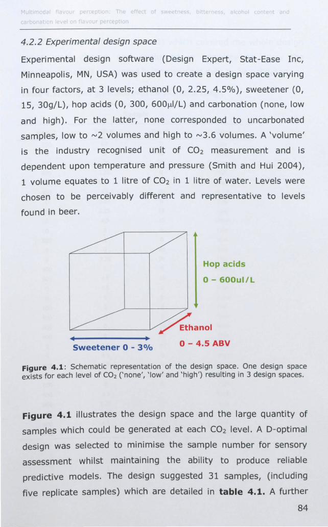
4.2.2 Experimental design space

Experimental design software (Design Expert, Stat-Ease Inc,

Minneapolis, MN, USA) was used to create a design space varying

in four factors, at 3 levels; ethanol (0, 2.25, 4.50/0), sweetener (0,

15, 30g/L), hop acids (0, 300, 600IlI/L) and carbonation (none, low

and high). For the latter, none corresponded to uncarbonated

samples, low to 1'12 volumes and high to "'3.6 volumes. A 'volume'

is the industry recognised unit of CO2 measurement and is

dependent upon temperature and pressure (Smith and Hui 2004),

1 volume equates to 1 litre of C02 in 1 litre of water. Levels were

chosen to be perceivably different and representative to levels

found in beer.

Hop acids

0- 600ul/L

~ ____________ -v ~anOI Sweetener 0 - 3 0/0

0- 4.5 ABV

Figure 4.1: Schematic representation of the design space. One design space exists for each level of CO2 ('none', 'low' and 'high') resulting in 3 design spaces.

Figure 4.1 illustrates the design space and the large quantity of

samples which could be generated at each CO2 level. AD-optimal

design was selected to minimise the sample number for sensory

assessment whilst maintaining the ability to produce reliable

predictive models. The design suggested 31 samples, (including

five replicate samples) which are detailed in table 4.1. A further

84

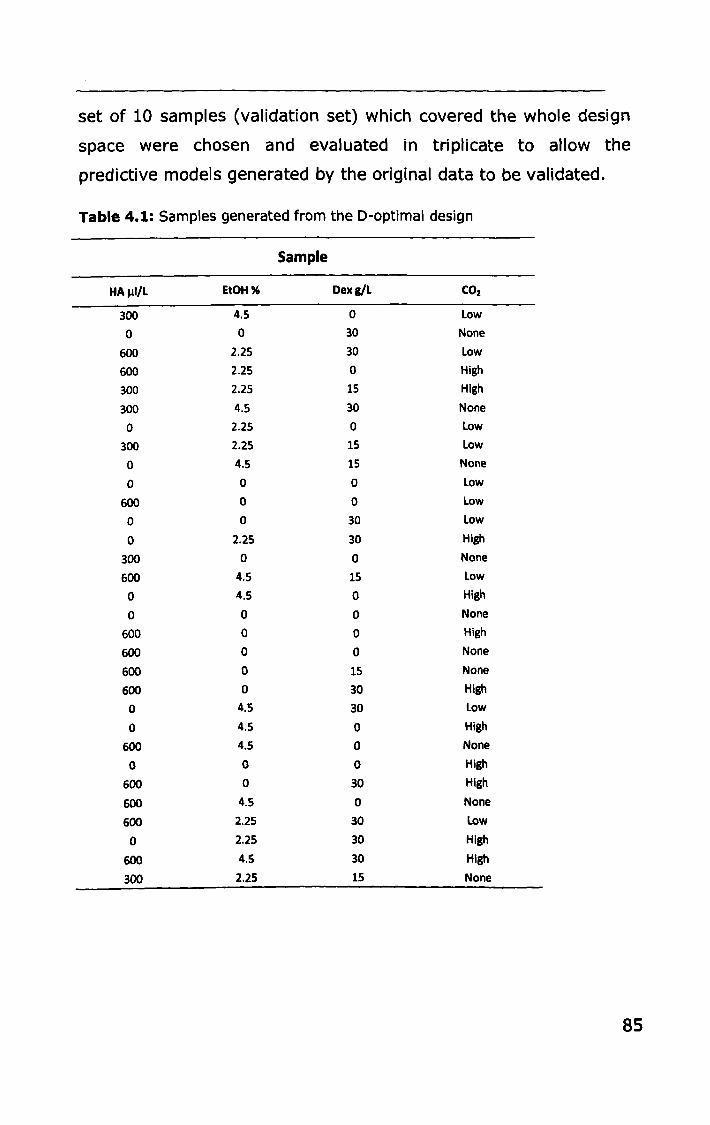
set of 10 samples (validation set) which covered the whole design

space were chosen and evaluated in triplicate to allow the

predictive models generated by the original data to be validated.

Table 4.1: Samples generated from the O-optimal design

Sample

HAIJI/L EtOH% Dexg/L COz

300 4.5 0 low

0 0 30 None

600 2.25 30 low

600 2.25 0 High

300 2.25 15 High

300 4.5 30 None

0 2.25 0 low

300 2.25 15 low

0 4.5 15 None

0 0 0 low

600 0 0 low

0 0 30 low

0 2.25 30 High

300 0 0 None

600 4.5 15 low

0 4.5 0 High

0 0 0 None

600 0 0 High

600 0 0 None

600 0 15 None

600 0 30 High

0 4.5 30 low

0 4.5 0 High

600 4.5 0 None

0 0 0 High

600 0 30 High

600 4.5 0 None

600 2.25 30 low

0 2.25 30 High

600 4.5 30 High

300 2.25 15 None

85

4.2.3 Sample preparation and presentation

The preparation of the samples has been described previously in

chapter 2, section 2.3. The new carbonation system was used to

carbonate the samples, described previously in chapter 2, section

2.2.4.2. Samples (40ml) were served at SoC (±1) and presented

monadically, with 10 minute breaks between each sample. A

maximum of 8 samples were evaluated per 2 hour session to

ensure no carry over effects or intoxication of alcohol. Each sample

was evaluated in triplicate by each panellist over 12 sessions.

Samples were presented in a balanced, and randomised

presentation order. Unsalted crackers (Rakusens, Leeds, UK),

green apple (Asda, Leeds, UK) and Evian mineral water (Danone,

PariS, France) were provided for palate cleansing. All tests were

performed over a three month period from April - June 2009, at

room temperature in an air-conditioned room, under Northern

Hemisphere daylight and in individual booths. Data was collected

using Fizz software (Biosystems, Cergy-Pontoise, France).

4.2.4 Sensory evaluation

Modified Quantitative Descriptive Analysis (QDA) (Stone, Sidel et al.

1974) was used to profile the sensory attributes of the samples.

This method uses the panel's own vocabulary to generate

consensus attributes and definitions which were fully discussed to

remove any uncertainty of meaning. This method was chosen to be

the most appropriate as it benefits from reducing errors associated

with 'dumping' of sensations into inappropriate attribute ratings

when response alternatives are limited (Clark and Lawless 1994).

Samples from the extreme corners of the design space were used

86

during training to aid with attribute generation, definition,

discussion, consolidation, agreement and protocol development.

Attribute references were therefore the samples themselves and

were used in combination with attribute definitions to standardise

language and minimise misunderstanding. Training sessions (40 x

2h) were dedicated to attribute generation, definition, discussion,

agreement and protocol development. Rank-rating of selected

samples in the sensory booths aided this process. Once the

attributes had been consolidated, agreed upon and protocols

developed (including order of assessment), practice rating sessions,

including replicate data were carried out until the panel could

repeatedly quantify between samples for generated attributes.

Panel performance during these sessions was monitored by

analysing coefficient of variance (CV) between replicates. CV values

of less than 25% were considered an acceptable level of variance.

Only attributes which the panel agreed upon by consensus and

which discriminated between the samples was used. However,

cheesy aroma, floral aroma, cheesy flavour and floral flavour were

highlighted as difficult attributes during the practice sessions but

after discussion with the panel it was decided to keep them in the

final attribute list (table 4.2). Re-training was given where

necessary.

The final set of attributes, their definitions and scale anchors can

be found in table 4.2. A continuous, unstructured line scale was

used to score each attribute. Marks were converted to a score

between 0 and 10 for data analysis purposes. All scales were

study-specific and labelled with verbal 'anchors' for scale ends

which were discussed and agreed upon by the panel.

87

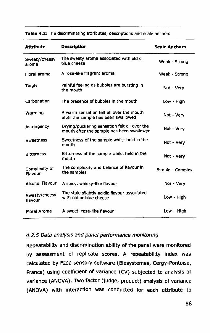
Table 4.2: The discriminating attributes, descriptions and scale anchors

Attribute Description Scale Anchors

Sweaty/cheesy The sweaty aroma associated with old or Weak - Strong

aroma blue cheese

Floral aroma A rose-like fragrant aroma Weak - Strong

Tingly Painful feeling as bubbles are bursting in Not - Very the mouth

Carbonation The presence of bubbles in the mouth Low - High

Warming A warm sensation felt all over the mouth Not - Very after the sample has been swallowed

Astringency Drying/puckering sensation felt all over the Not - Very mouth after the sample has been swallowed

Sweetness Sweetness of the sample whilst held in the Not - Very mouth

Bitterness Bitterness of the sample whilst held in the Not - Very mouth

Complexity of The complexity and balance of flavour in Simple - Complex Flavour the samples

Alcohol Flavour A spicy, whisky-like flavour. Not - Very

Sweaty/cheesy The stale slightly acidic flavour associated

flavour with old or blue cheese Low - High

Floral Aroma A sweet, rose-like flavour Low - High

4.2.5 Data analysis and panel performance monitoring

Repeatability and discrimination ability of the panel were monitored

by assessment of replicate scores. A repeatability index was

calculated by FIZZ sensory software (Biosystemes, Cergy-Pontoise,

France) using coefficient of variance (CV) subjected to analysis of

variance (ANOVA). Two factor (judge, product) analysis of variance

(ANOVA) with interaction was conducted for each attribute to

88

identify significant differences between the samples for each of the

attributes assessed. Where appropriate, Tukey's HSD post-hoc

tests were used to determine where samples were significantly

different (a= 0.05). Predictive polynomial models from panel

means were generated using Design Expert to explain variations in

perception of each attribute as a function of sweetener, hop acids,

ethanol and carbonation levels. Non-significant terms, as

determined by ANOVA, were removed. After examination of model

statistics, (R2, adjusted R2, predicted R2 and adequate precision), a

mathematical model was selected which best represented the data

(table 4.3). R2 is a measure of the amount of variation about the

mean explained by the model; a value close to 1 shows little

variation. The adjusted R2 (Adj R2) should be close to the R2 value

to signify that there are only terms in the model which add value.

Predicted R2 (Pred R2) is calculated by systematically removing

each observation from the data-set and estimating the regression

equation and determining how well the model predicts the removed

observation. This value can range between 0 and 1, with larger

values suggesting models of greater predictive ability (Design

Expert, Stat-Ease Inc, Minneapolis, MN, USA). Adequate precision

(Adeq Precision) measures signal to noise ratio, a value greater

than 4 indicates adequate model discrimination (Design Expert,

Stat-Ease Inc, Minneapolis, MN, USA). Interaction plots generated

by the predictive models were used to visualise key interactions

between the design factors. These are not plots of the data pOints

themselves but instead they give a visual representation of the

predictive model and are considered more illustrative than the

predictive model equations.

The predictive ability of the models was validated by the evaluation

of a separate set of 10 samples (validation set) which were taken

89

from within the design space, representing the full range of

compositional factors, but were not part of the original model data

set. These predicted values were then compared and plotted

against the actual values given by the panel.

4.3 RESULTS

4.3.1 Panel performance monitoring

The repeatability and discrimination ability of the panel was

assessed to determine the reliability of the raw data before

undergoing full data analysis. Individual panellist performance was

assessed by scrutinisation of judge interactions, variation of

replicate data and by calculating a repeatability index using

coefficient of variance (CV) and the probability value (FPROD)

which shows the level of discrimination between products. Results

demonstrated that the panel were able to repeatedly discriminate

between samples for all attributes (P<O.OS) except sweaty/cheesy

aroma, floral aroma, sweaty/cheesy flavour and floral flavour, as

illustrated by figure 4.2. Consequently the increases in volatile

partitioning caused by ethanol and carbonation as previously found

in chapter 3 do not appear to result in perceivable differences in

these samples. These non-discriminating attributes were omitted

from further study. After exami~ing judge interactions, it became

evident that viscosity provided considerable intra-panel variation

and consequently could not be used to reliably discriminate

between the samples. This is not surprising as it is very difficult for

the human palate to significantly discriminate between Newtonian

fluids (i .e. lager beer) within such a narrow range (Ragot, Guinard

et al. 1989). Furthermore, C02 adds a level of complexity to this

measurement when it is made in the mouth, increasing turbulence

which will impact on shearing stresses and consequently sensory

90

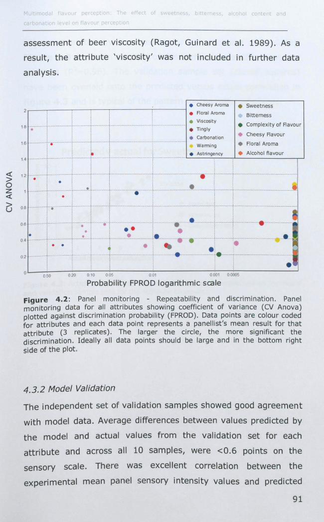
a

assessment of beer viscosity (Ragot, Guinard et al. 1989). As a

result, the attribute 'viscosity' was not included in further data

analysis.

• Cheesy Aroma 2~--~--~~--;---;-------~~----~

• Floral Aroma

• Sweetness

Bitterness • Viscosity

18 .. ......... j ................ [ ........... + ... ······i···························.;.-···················· • Tingly • Complexity of Aavour

•i. .: .1 :.: Cheesy Aavour

• Carbonat ion

:: . C·I:·r·IT • :,::::"" : ~'::O~;'::", :; 12·· ........ ;.. .............. 1... ....... 1. ...... ! ....................... + .............................. ! .... · ...... t· .... · ................................. .

~ ,: ...I: ·:'.J .••. C .. ~.I.~·.'I:··

:: .:! ; •• ;~i ::.T .. :: ·J:».~::!: ...: ·;::]~ ~ ::. ~ : : : : i i . •

o L---~----~--~--~--------~------------~--~----------~ o~.o 020 010 OO~ 001 0001 00005

Probability FPROD logarithmic scale

Figure 4.2: Panel monitoring - Repeatability and discrimination. Panel monitoring data for all attributes showing coefficient of variance (CV Anova) plotted against discrimination probability (FPROD). Data pOints are colour coded for attributes and each data pOint represents a panel list's mean result for that attribute (3 replicates). The larger the circle, the more significant the discrimination. Ideally all data points should be large and in the bottom right side of the plot.

4.3.2 Model Validation

The independent set of validation samples showed good agreement

with model data. Average differences between values predicted by

the model and actual values from the validation set for each

attribute and across all 10 samples, were <0.6 points on the

sensory scale. There was excellent correlation between the

experimental mean panel sensory intensity values and predicted

91

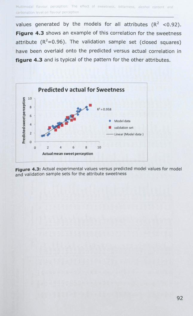
values generated by the models for all attributes (R2 <0.92).

Figure 4.3 shows an example of this correlation for the sweetness

attribute (R2 =0.96). The validation sample set (closed squares)

have been overlaid onto the predicted versus actual correlation in

figure 4.3 and is typical of the pattern for the other attributes.

r- -Predicted v actual for Sweetness

c 10 0

.~

c. 8 CII

~ R2 = 0.958 CII

• Modeldata

c. 6 ., .... CII

4 J CII 3 \II

~ "0 CII

• validation set

t 2 ~ :s - Linear (Model data)

CII ... 0 Q.

0 2 4 6 8 10

Actual mean sweet perception

Figure 4.3: Actual experimental values versus predicted model values for model and validation sample sets for the attribute sweetness

92

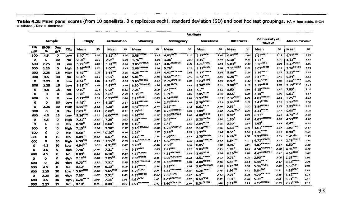
Table 4.3: Mean panel scores (from 10 panellists, 3 x replicates each), standard deviation (SO) and post hoc test groupings. HA = hop acids, EtOH = ethanol, Dex = dextrose

Attribute

Sample nnsly carbonation Warm Ins Astrlnsency Sweetness Bitterness Complexity of

Alcohol flavour flavour

HA EtOH Dex ul/l " ell

COz Mean SD Mean SD Mean so Mean so Mean so Mean 50 Mean so Mean so

300 4.5 0 low 5.40CDEF 2.36 S.12CDEF 2.50 3.880EFGHU 2.49 4.82ABCD 2.25 3.27'KlM 2.46 6.87CDE 2.46 S.6S

ABC 2.29 4.22cOEF 2.75

0 0 30 No O.08G 0.10 O.06G 0.08 1.76

MN 1.92 1.36K 2.67 8.190. 1.41 0.18G 0.31 1.74'K 2.70 1. 12'Kl 1.59

600 2.25 30 low 5.29 CDEF 2.68 S.24CDE 2.85 3.8SO£FGHUK 2.27 4.02BCDEFGHI 2.42 4.S6EFGHU 2.51 S.83EF 2.44 5.38

ABCO 2.28 3.42OEFGH 1.95

600 2.25 0 High 5.9SA8CD£ 2.20 7.00'" 2.43 2.68HUKlMN 1.84 5.780. 2.18 2.12

lMNO 1.64 7.11ABCDE 2.21 S.Or

BCDEF 2.17 2.36FGHUKl 1.89

300 2.25 15 High 6.49A8CO 2.73 6.6SABC 2.80 4.26CDEFGHI 2.58 4.42ABCDEFGHI 2.65 4. 17EFGHUK 2.66 S.80EF 2.14 S.36ABCO 2.29 3.S2

0EFGH 2.87

300 4.5 30 No O.08G 0.12 o.or 0.12 S.SlABC 2.40 4.S8

ABCDEFG 2.40 6.73ABCD 2.60 6.2S0EF 2.64 S.47

ABCO 2.49 S.848C 2.52

0 2.25 0 low 4.44EF 2.84 4.39EF 2.69 3.60EFGHIJKl 2.71 2.76CDEFGHU 2.88 3.84GHIJKl 1.85 0.92G 1.37 3.16GHUK 1.86 2.8SEFGHIJK 3.00

300 2.25 15 low 5.33CDEF 2.68 4.67D£F 2.69 3.50EFGHUKlM 2.28 4.62AJtCDE 2.41 3.78GHUKl 2.67 5.980EF 2.13 S.12ABCDE 2.05 2.79EFGHIlK 2.41

0 4.5 15 No 0.106 0.14 O.08G 0.11 7.Oft 2.09 2.4rHUK 2.63 7. lAB 2.51 O.60G 0.94 4.15

CDEFGH 2.40 7.930. 2.01

0 0 0 low 3.7SF 2.36 3.65

F 2.59 1.86LMN 1.95 1.91'K 2.86 3.05

KlMN 1.76 0.66G 1.24 2.15

uK 2.02 0.91Kl 1.33

600 0 0 low 6.2rBCD 2.37 6.23ABCO 2.68 2.23'KLMN 2.09 4.61ABCDEF 2.28 1.97MNO 2.63 7.3r

BCO 1.76 4.03COEFGH 2.58 1. 25'Kl 1.13

0 0 30 low 4.49EF 2.67 4.15EF 2.67 2.81HUKlMN 2.29 2.74OEFGHIJ 2.66 5.59

8CDEF 2.53 0.63

BCOE 0.79 3.43EFGHU 2.53 1.72HIJKl 2.00

0 2.25 30 High 6.59ABC 2.43 7.28" 2.18 3.65DEFGHUK 2.74 2.65FGHU 2.72 6.61"BCD 2.40 0.63G 0.70 3.86OEFGHI 2.61 2.93EFGHIl 2.92

300 0 0 No 0.09 6 0.13 O.08G

0.11 1.7~N 1.39 4.25ABCDEFGHI 2.73 1.090 2.22 7.26ABCDE 2.33 3.31FGHUK 2.47 0.9S'Kl 1.08

600 4.5 15 low 5.36CD£F 2.51 6.~ 2.62 4.92BCD£ 2.22 3.96BCDEFGHI 2.40 4.80EFGHU 3.31 6.97G 2.29 6.17" 2.28 4.74

BCOE 2.39

0 4.5 0 High 7.21'" 2.45 7.290. 2.62 4.658CDEFG 2.98 2.49

GHUK 2.87 5.23CDEFGH 2.38 I.S0

G 1.63 4.63ABCDEFGH 2.62 4.53CDEF 3.42

0 0 0 No 0.10G 0.13 O.08G 0.10 1.19N 1.29 l.4SK 2.45 2.94KLMN 1.66 0.30G 0.53 1.65K 1.49 0.67l 0.93

600 0 0 High 7.13AB 2.54 7.so" 2.57 3. 16FGHUKlM 2.68 4.2S

ABCDEFGH 2.82 2. 18lMNO 1.86 6.68cOE 2.45 4.61ABCDEFGH 2.33 1.93GHIJKl 2.17

600 0 0 No O.09G 0.14 0.10

G 0.14 1.24N 1.17 S.2S'" 2.63 1.37

NO 1.44 8.510. 1.55 3.26GHUK 2.91 0.90

Kl 1.01

600 0 15 No O.09 G 0.23 O.OT O.U 2.12KlMN 1.78 4.99ABCD 2.45 2.75KlMNO 2.53 8.490.8 1.58 3.9SCDEFGH 2.35 1.41'lKl 1.59

600 0 30 High 6.5gABC 2.35 7.11'" 2.23 3.42EFGHUKLM 2.44 4.5O"BCDEFG 2.75 3.58GHUKlM 2.82 5.840EF 2.20 4.72ABCOEFG 2.42 2.28FGHUKl 2.33

0 4.5 30 low 4.94O£F 2.62 4.91DEF 2.47 6.2S'" 2.46 2.30"K

3.30 8.050. 1.69 0.96G 0.97 4.87"BCDEFG 2.67 6.500.8 2.80

0 4.5 0 High 7.480. 2.26 7.210. 2.16 5.3J"BCD 2.80 2.41H1lK 3.32 5.83BCDE 2.45 1.01G 1.15 4.58o.BCDEFGH 2.50 4.96

BCD 3.49

600 4.S 0 No 0.096 0.13 0.10G 0.14 4.S7BCDEFG 2.62 4.S1"BCDEFG 2.34 3.4S"KlM 2.98 8. 19o.BC

2.09 4.47ABCDEFGH 2.47 4.S4BCDE 3.08

0 0 0 High 7.12'" 2.40 7.0S'" 2.23 2.SSUKLMN 2.45 3.07BCDEFGHU 3.22 3.51HUKlM 2.02 0.78G 1.25 2.90

HUK 2.08 1.63

HUKl 1.93

600 0 30 High 6.73ABC 2.52 7.310. 2.59 3.S0EFGHUKlM 2.10 4.3~FGH 2.78 4.OSFGHUK 2.86 6.45OEF 2.11 S.44

o.BCO 2.12 3.38OEFGHI 2.74

600 4.S 0 No 0.126 0.20 0.136 0.29 5.34AJtCDE 2.34 5.28ABC 2.86 3.67FGHUKLM 2.90 8.26o.BC 2.80 5.34

o.BCDE 2.83 5.S3BCD 2.95

600 2.25 30 low 5.67BCD£ 2.66 S.6SBCDE 2.99 4.75BCDEF 2.34 4.33

o.BCDEFGH 2.95 S.26CDEFG 2.76 5.96

0EF 2.91 5.64o.BC 2.31 4.69

BCDE 2.41

0 2.25 30 High 7.33" 2.07 7.51" 2.OS 4.35CDEFGH 2.67 2.66

EFGHIJ 2.97 6.9ABC 2.42 0.93

G 1.08 4.7o"BCDEFG 2.88 3.82

OEFG 3.14

600 4.S 30 High 6.28ABCD 2.90 7.23" 2.55 4.97BCDE 2.45 4.078CDEFGH1 2.67 6.69"BCD 2.39 S.OlF 2.70 5.990.8 2.65 5.21BCD 2.47

300 2.25 lS No 0.106 0.15 0.086 0.13 2.91

GHUKlMN 1.42 3.60BCDEFGH1 2.44 5.040EFGHI 2.69 6.19

0EF 2.23 4.27BCDEFGH 2.20 2.92EFGHIJ 2.19

93

The panel means, standard deviations and results of Tukey's HSD

post-hoc analysis are shown in table 4.3. The Tukey's HSD test

showed that samples could be split into 7-16 groups (table 4.3)

indicating a good level of discrimination between the samples

across the attributes. ANOVA (judge and product factors) were

performed on the panel data (three replicates). Using the global

mean of the panellists, polynomial predictive models were

generated for each attribute using multiple linear regression

(Design Expert, Stat-Ease Inc., Minneapolis). These models

described the perceptual results in terms of the design factors

(sweetener, hop acids, carbonation and ethanol) for each attribute

assessed. The resulting model equations, along with associated

statistics describing the model fit (adequate precision) and

predictive capability (adjusted and predictive R-squared values)

can be found in table 4.4.

94

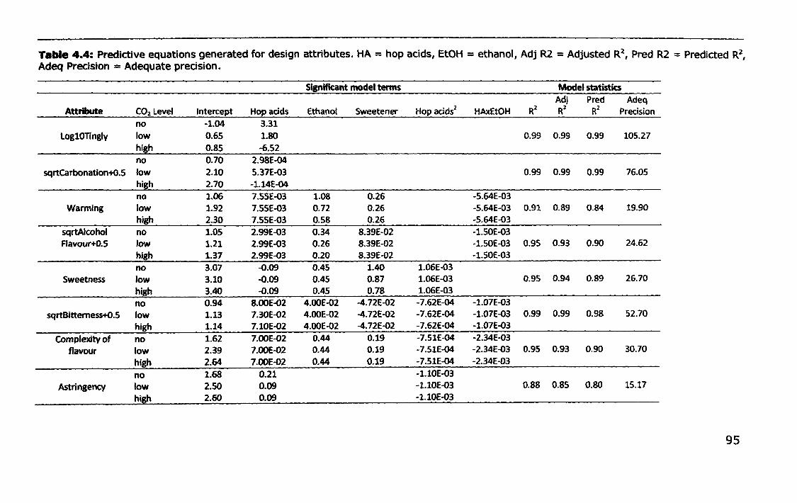
Table 4.4: Predictive equations generated for design attributes. HA = hop acids, EtOH = ethanol, Adj R2 = Adjusted R2, Pred R2 = Predicted R2, Adeq Precision = Adequate precision.

Sisnificant model terms Model statistics Adj Pred Adeq

Attribute CO2 Level Intercept Hop acids Ethanol Sweetener Hop acids2 HAxEtOH R2 R2 R2 Precision no -1.04 3.31

log10TIngly low 0.65 1.80 0.99 0.99 0.99 105.27 high 0.85 -6.52 no 0.70 2.98E-04

sqrt(arbonation+O.5 low 2.10 5. 37E-03 0.99 0.99 0.99 76.05 high 2.70 -1. 14E-04 no 1.06 7.55E-03 1.08 0.26 -S.64E-03

Warming low 1.92 7.SSE-03 0.72 0.26 -S.64E-03 0.91 0.89 0.84 19.90 high 2.30 7.55E-03 0.58 0.26 -5.64E-03

sqrtAlcohoi no 1.05 2.99E-03 0.34 8.39E-02 -1.S0E-03 Flavour+O.5 low 1.21 2.99E-03 0.26 8.39E-02 -1.50E-03 0.95 0.93 0.90 24.62

high 1.37 2.99E-03 0.20 8.39E-02 -1.50E-03 no 3.07 -0.09 0.45 1.40 I.06E-03

Sweetness low 3.10 -0.09 0.45 0.87 1.06E-03 0.95 0.94 0.89 26.70

high 3.40 -0.09 0.45 0.78 1.06E-03

no 0.94 8.00E-02 4.00E-02 -4.72E-02 -7.62E-04 -1.07E-03 sqrtBitterness+O.S low 1.13 7.30E-02 4.00E-02 -4.72E-02 -7.62E-04 -1.07E-03 0.99 0.99 0.98 52.70

high 1.14 7.10E-02 4.00E-02 -4.72E-02 -7.62E-04 -1.07E-03

Complexity of no 1.62 7.00E-02 0.44 0.19 -7.51E-04 -2. 34E-03

flavour low 2.39 7.00E-02 0.44 0.19 -7.51E-04 -2.34E-03 0.95 0.93 0.90 30.70

high 2.64 7.00E-02 0.44 0.19 -7.51E-04 -2.34E-03

no 1.68 0.21 -1.10E-03

Astringency low 2.50 0.09 -1.10E-03 0.88 0.85 0.80 15.17

high 2.60 0.09 -1.10E-03

95

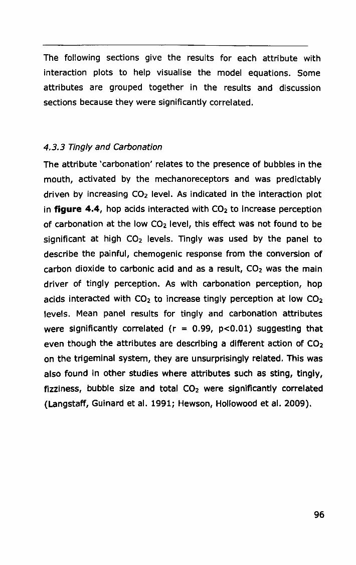
The following sections give the results for each attribute with

interaction plots to help visualise the model equations. Some

attributes are grouped together in the results and discussion

sections because they were significantly correlated.

4.3.3 Tingly and Carbonation

The attribute 'carbonation' relates to the presence of bubbles in the

mouth, activated by the mechanoreceptors and was predictably

driven by increasing C02 level. As indicated in the interaction plot

in figure 4.4, hop acids interacted with C02 to increase perception

of carbonation at the low C02 level, this effect was not found to be

significant at high C02 levels. Tingly was used by the panel to

describe the painful, chemogenic response from the conversion of

carbon dioxide to carbonic acid and as a result, C02 was the main

driver of tingly perception. As with carbonation perception, hop

acids interacted with C02 to increase tingly perception at low C02

levels. Mean panel results for tingly and carbonation attributes

were significantly correlated (r = 0.99, p<O.Ol) suggesting that

even though the attributes are describing a different action of C02

on the trigeminal system, they are unsurprisingly related. This was

also found in other studies where attributes such as sting, tingly,

fizziness, bubble size and total C02 were Significantly correlated

(Langstaff, Guinard et al. 1991; Hewson, Hollowood et al. 2009).

96

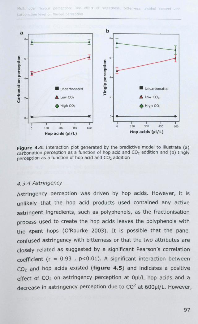
a

8 1~--------------41

c o 6 ~ Q.

~ Q.I Q.

C 4 o ~ C o .D ~ 2 U

• Uncarbonated

A Low C02

• High CO2

o •• ________________ ~E

o 150 300 450 600

Hop acids (J.l I/L)

c o

b

i Q.I ~

8

6

Q.I 4 Q.

> CI C j:

2

• Uncarbonated

• High CO2

o •• ------------------••

o 150 300 450 600

Hop acids (J.lI/L)

Figure 4.4: I nteracti on plot generated by the predictive model to illustrate (a) carbonation perception as a function of hop acid and CO2 addit ion and (b) t ing ly perception as a function of hop acid and CO2 addit ion

4.3.4 Astringency

Astringency perception was driven by hop acids. However, it is

unlikely that the hop acid products used contained any active

astringent ingredients, such as polyphenols, as the fractionisation

process used to create the hop acids leaves the polyphenols with

the spent hops (O'Rourke 2003). It is possible that the panel

confused astringency with bitterness or that the two attributes are

closely related as suggested by a significant Pearson's correlation

coefficient (r = 0.93 , p<O.Ol). A significant interaction between

C02 and hop acids existed (figure 4.5) and indicates a positive

effect of C02 on astringency perception at OIJI/L hop acids and a

decrease in astringency perception due to C02 at 6001J1/L. However,

97

the effect of C02 on astringency perception was very small, less

than 1 unit on the sensory scale (1-10).

c:: o '.t:i Q.

6

5

8 4 ... ell Q.

~ c:: 3 ell CI c:: ·C ... III 2 c(

o

• Uncarbonated

• High CO2

150 300 450 600

Hop acids (1l1/L)

Figure 4.5: Interaction plot generated by the predictive model to illustrate astringency perception as a function of hop acid and CO2 addition

4.3.5 Warming and alcohol flavour

Warming describes the mouthfeel of ethanol while alcohol flavour

was a separate attribute used to discriminate between the samples

for the flavour of ethanol. It is likely that the panel were unable to

decouple the flavour and trigeminal components of ethanol

resulting in significant correlation (r = 0.97, p<O.Ol) and

generation of similar predictive models. As a result the two

attributes will be discussed together here-after. Warming/alcohol

perception was primarily driven by ethanol addition in a

concentration dependent manner. Hop acids interacted with

ethanol to suppress warming perception at 4.5% (ethanol) but

contributed slightly when no ethanol was in the system (0%). CO2

98

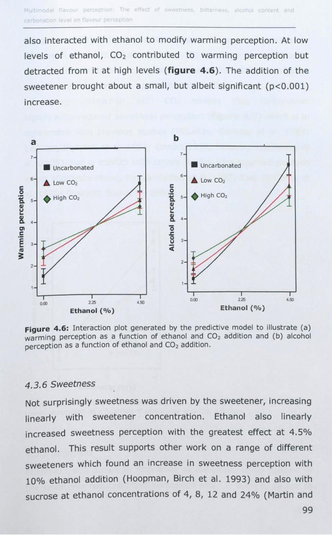
~ 0

also interacted with ethanol to modify warming perception. At low

levels of ethanol, C02 contributed to warming perception but

detracted from it at high levels (figure 4.6). The addition of the

sweetener brought about a small, but albeit significant (p<O.OOl)

increase.

a b

7 7

• Uncarbonated • Unca rbonated

6 6

.. Low CO2 .. Low CO2 ~ 0

i 5 • High CO2 i 5 High CO2 G.I G.I

~ 8-CI .5 E &.. ftI

J

4

3

2

0.00 2.25

Ethanol (Ofo) 4.50

U &..

8-'0 J: 0 U

Ci

4

3

2

0.00 2.25

Ethanol (Ofo) 4.50

Figure 4.6: Interaction plot generated by the predictive model to illustrate (a) warming perception as a function of ethanol and CO2 addition and (b) alcohol perception as a function of ethanol and CO2 addition.

4.3.6 Sweetness

Not surprisingly sweetness was driven by the sweetener, increasing

linearly with sweetener concentration. Ethanol also linearly

increased sweetness perception with the greatest effect at 4.5%

ethanol. This result supports other work on a range of different

sweeteners which found an increase in sweetness perception with

10% ethanol addition (Hoopman, Birch et al. 1993) and also with

sucrose at ethanol concentrations of 4, 8, 12 and 24% (Martin and

99

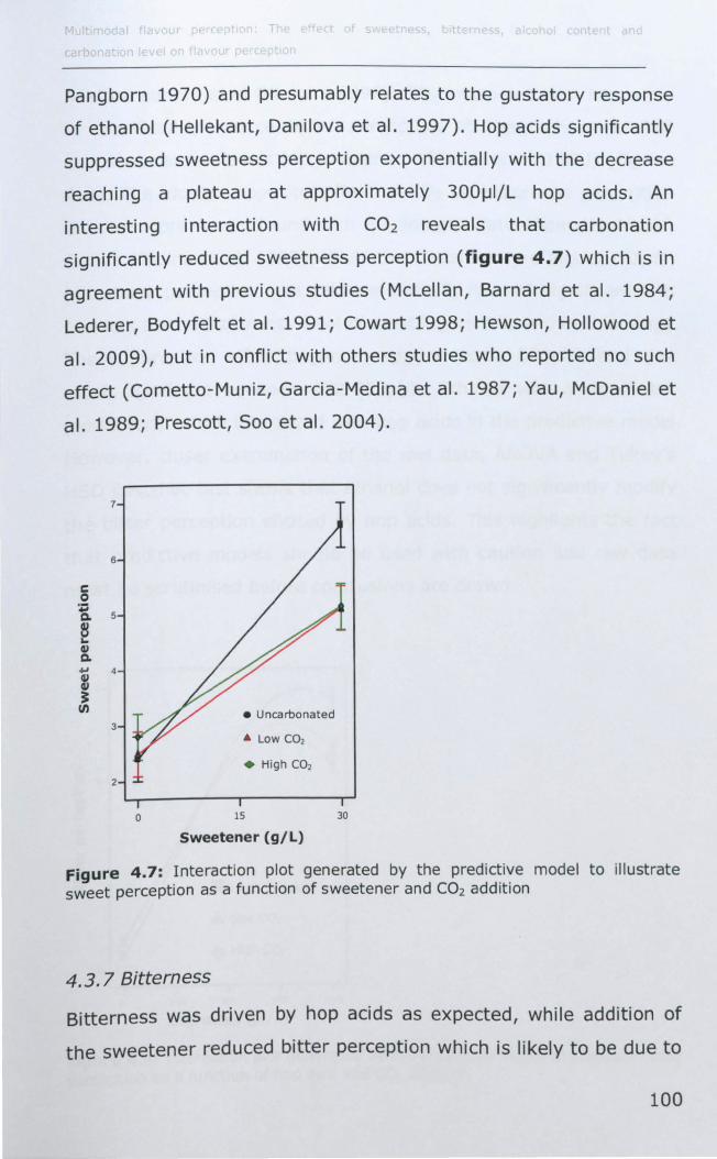
Pangborn 1970) and presumably relates to the gustatory response

of ethanol (Hellekant, Danilova et al. 1997). Hop acids significantly

suppressed sweetness perception exponentially with the decrease

reaching a plateau at approximately 3001-ll/L hop acids. An

interesting interaction with C02 reveals that carbonation

significantly reduced sweetness perception (figure 4.7) which is in

agreement with previous studies (McLellan, Barnard et al. 1984;

Lederer, Bodyfelt et al. 1991; Cowart 1998; Hewson, Hollowood et

a!. 2009), but in conflict with others studies who reported no such

effect (Cometto-Muniz, Garcia-Medina et al. 1987; Yau, McDaniel et

a I. 1989; Prescott, 500 et al. 2004).

7

6

• Uncarbonated 3

• High C02

2

o 15 30

Sweetener (gIL)

Figure 4.7: Interaction plot generated by the predictive model to illustrate sweet perception as a function of sweetener and CO2 addition

4.3.7 Bitterness

Bitterness was driven by hop acids as expected, while addition of

the sweetener reduced bitter perception which is likely to be due to

100

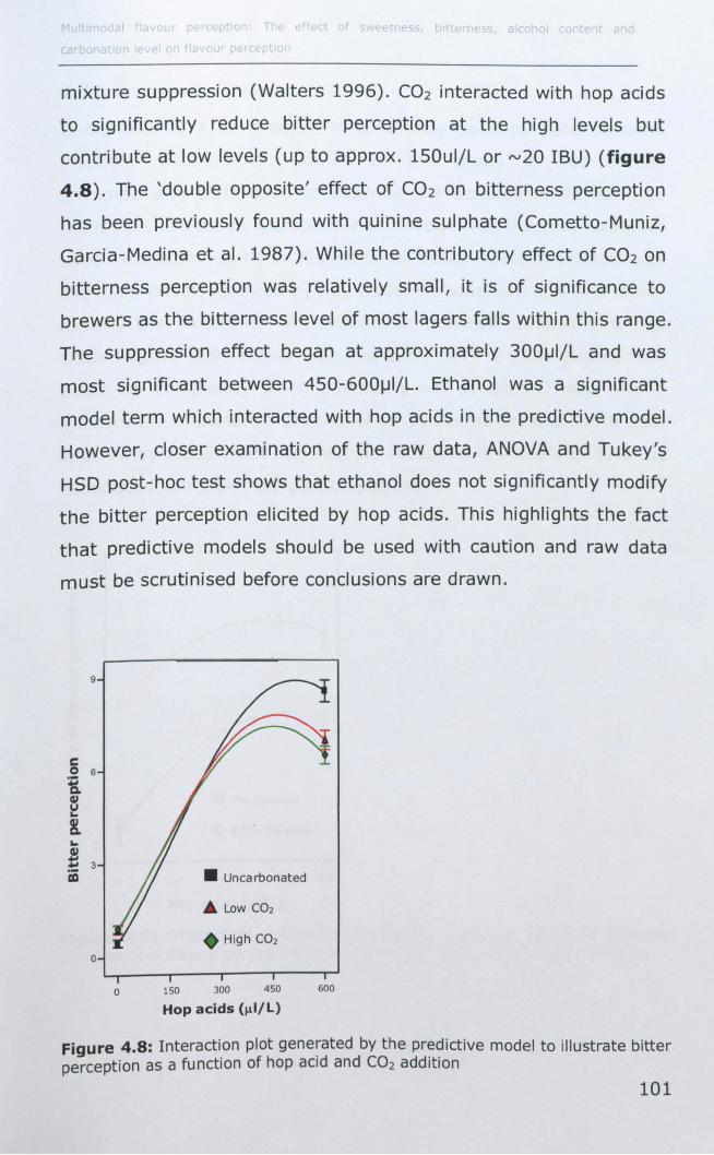
mixture suppression (Walters 1996). CO2 interacted with hop acids

to significantly reduce bitter perception at the high levels but

contribute at low levels (up to approx. lS0uljL or ",20 rBU) (figure

4.8). The 'double opposite' effect of C02 on bitterness perception

has been previously found with quinine sulphate (Cometto-Muniz,

Garcia-Medina et al. 1987). While the contributory effect of C02 on

bitterness perception was relatively small, it is of significance to

brewers as the bitterness level of most lagers falls within this range.

The suppression effect began at approximately 300IJI/L and was

most significant between 4S0-600IJI/L. Ethanol was a significant

model term which interacted with hop acids in the predictive model.

However, closer examination of the raw data, ANOVA and Tukey's

HSD post-hoc test shows that ethanol does not significantly modify

the bitter perception elicited by hop acids. This highlights the fact

that predictive models should be used with caution and raw data

must be scrutinised before conclusions are drawn.

9

c o 6

i ~ 8.

o

o

• Unca rbonated

• High C02

150 300 450 600

Hop acids bLl/ L)

Figure 4.8: Interaction plot gene~ated by the predictive model to illustrate bitter perception as a function of hop aCid and CO2 addition

101

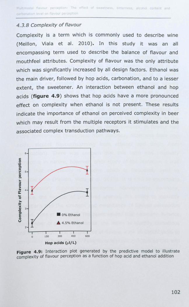
4.3.8 Complexity of flavour

Complexity is a term which is commonly used to describe wine

(Meillon, Viala et al. 2010). In this study it was an all

encompassing term used to describe the balance of flavour and

mouthfeel attributes. Complexity of flavour was the only attribute

which was significantly increased by all design factors. Ethanol was

the main driver, followed by hop acids, carbonation, and to a lesser

extent, the sweetener. An interaction between ethanol and hop

acids (figure 4.9) shows that hop acids have a more pronounced

effect on complexity when ethanol is not present. These results

indicate the importance of ethanol on perceived complexity in beer

which may result from the multiple receptors it stimulates and the

associated complex transduction pathways.

c o i ~

6

~ 5

8. ... ~ > ftI 4 Ii:

~ .~ 3

Q. E o u

2

.0% Ethanol

• 4.5% Ethanol

o 150 300 450 600

Hop acids (1l1/L)

Figure 4.9: Interaction plo.t generated by the predictive model to illustrate complexity of flavour perception as a function of hop acid and ethanol addition

102

4.4 DISCUSSION

The attributes generated in this study were similar to those

previously used to describe alcoholic and soft beverages (Lyman

and Green 1990; Keast and Breslin 2002; Kappes, Schmidt et al.

2006; Bajec and Pickering 2008; Hewson, Hollowood et al. 2009)

and some are detailed on the beer and whisky flavour wheels

(Meilgaard, Dalgliesh et al. 1979; Shortreed, Rickards et al. 1979).

Complexity of flavour was discussed at length by the panel and it

was decided that it described the combination and balance of

flavour; encompassing tastes, aromas and tactile qualities in the

model beer. Samples described as 'more complex' in flavour had

more components (sweetness from dextrose, bitterness from hop

acids, alcohol flavour/warming from ethanol and tingle from

carbonation). There was concern that this term was relatively

subjective in nature, however, after study of the literature it was

found that complexity is a term which is frequently used to

describe wine (Meillon, Viala et al. 2010). It is said to encompass

eight sensory dimensions: familiarity, homogeneity, harmony,

balance, the number of perceived aromas, the ability to indentify

sensations and the strength and persistence of flavour perception

(Medel, Viala et al. 2009). The panel agreed that harmony, balance,

the number of perceived aromas, the ability to identify sensations

and the strength and persistence of flavour were all contributors to

complexity of beer flavour. Familiarity was not included as this was

thought to bring about a subjective element to the measurement.

103

4.4.1 Mouthfee/ attributes

Figure 4.4a illustrates the interaction between hop acids and C02

for carbonation perception. Modelling of tingly data produced a

similar interaction plot (figure 4.4a). It appears that increasing

hop acid concentration is capable of increasing both mechanical

and nociceptive response at the low C02 level, an effect which is

not seen at the high CO2 level. Informal discussions with the panel

revealed that carbonated samples with high hop acid content

seemed to have a larger quantity of smaller 'more tingly' bubbles

than those without. It is possible that the hop acids interact with

the C02 to create an increased number of smaller bubbles,

increasing surface area and filling the mouth resulting in increased

carbonation perception and activating more nociceptors providing

an increased tingly response. This seems possible as the

isomerised hop acid products used to elicit bitterness could alter

surface tension (Briggs, Boulton et al. 2004) and bubble formation.

It is likely that this effect is not seen at the high C02 level because

of C02 saturation of both mechanoreceptors and nociceptors, thus

any increased effect of the hop acids is not perceivable. With

hindsight it would have been beneficial to include bubble size as an

attribute in this sensory profile in order to investigate this

mechanism further.

Hop acids were the main driver of astringency perception.

Considerable time was spent during training to ensure the panel

could differentiate between bitterness and astringency. However,

astringency has been described as a "complex, multifaceted

sensation" by Bajec and Pickering (2008) and its assessment is

made difficult by a number of variables. They concluded in their

review paper that astringency is sensed by both taste and tactile

sensations, suggesting physiological and psychological mechanisms

104

underly its perception. Polyphenols would usually be the main

tactile trigger of astringency in beer, however they were not

present in the model beer. Therefore, it is not surprising that in the

absence of polyphenols, the bitter taste from the hop acids may

contribute to astringency and supports the theory put forward by

Bajec and Pickering (2008) that astringency can be sensed by the

taste receptors (Bajec and Pickering 2008).

Ethanol stimulates multiple modalities; the gustatory (Hellekant,

Danilova et al. 1997; Danilova and Hellekant 2000; Mattes and

DiMeglio 2001), olfactory (Laska, Distel et al. 1997) and trigeminal

systems (Green 1987; Danilova and Hellekant 2002) resulting in

polymodal sensation. Activation of the trigeminal system by

ethanol has been found to be (in-part) due to the vanilloid

receptor-1 (VR1) (Brasser, Norman et al. 2010) which is the

nociceptor responsible for the burning sensation elicited by

capsaicin and a wide variety of mechanical, thermal and physical

chemical stimuli. It is feasible that this is also the receptor

responsible for detecting the warming perception of ethanol.

However, the origin of warming perception is currently unknown

and could be a result of a non-capsaicin sensitive pathway (Green

1991; Brasser, Norman et al. 2010).

An interaction between ethanol and C02 would suggest competition

between the trigeminal aspects of both stimuli thus suppressing

warming perception (figure 4.6). The contributory effect of C02 to

warming perception at 00/0 ethanol levels is supportive of this

hypothesis. Research focussing on cross-desensitization with

capsaicin on ethanol (300/0) found a significant decrease in

perceived irritation and intenSity of 'burning', 'stinging' and

'prickling' sensations of ethanol after treatment of the tongue with

105

capsaicin (Green 1991) suggesting a suppressive effect when two

trigeminal stimuli are presented sequentially. However, further

research is needed to determine if this effect is seen when the two

stimuli are presented simultaneously.

A minor interaction of hop acids with ethanol suppressed warming

perception in a concentration dependent manner with the greatest

effect seen at the highest level of hop acid addition eliciting a high

level of bitterness to the system. Lim & Green (2007) investigated

the relationship between bitter taste and burning sensations and

cluster analysis showed that bitterness was more qualitatively

similar to 'burning' than any other taste despite being mediated by

different sensory modalities. The interaction found in the present

study could be due to this similarity.

4.4.2 Complexity of flavour

The significant impact of all four factors on complexity perception

illustrates the importance of each in beer flavour perception and

also the complex nature of each in a beverage. The ability of

ethanol to impact on an array of stimuli and activate multiple

modalities means that it is not surprising that it is the main driver

of complexity and supports other studies which have also linked

increased complexity due to ethanol with liking (Meillon, Viala et al.

2010). Carbonation adds a further level of complexity which Is a

vital characteristic of beer and has been found to increase thirst­

quenching character and drinkability (Guinard, Souchard et al.

1998). Additional work could focus on the contribution of each

stimulus on complexity and liking.

106

4.4.3 Taste attributes

From current knowledge regarding sweet-bitter taste interactions,

it is unsurprising that hop acids suppressed sweetness perception.

Multiple mechanisms have been proposed for this interaction, with

the more recent studies narrowing the locus to the gustatory

periphery (Talavera, Yasumatsu et al. 2008) as opposed to higher

central neural processing due to similarities between taste

transduction mechanisms (Walters 1996; Margolskee 2002). A

large body of research exists on bitter-sweet taste interactions with

almost exclusive use of quinine as the bitter stimulus. In one such

study, quinine was reported to directly inhibit the sweet taste

transduction cation channel, TRPMS (Talavera, Yasumatsu et al.

2008). While sweet perception is not exclusively TRPMS-dependant,

this work suggests that other bitter compounds may affect the

perception of sweet taste by altering TRPMS function and

significantly suppressing sweet perception, as suggested by the

results in the present study. However, research of the pathways

responsible for hop acid transduction is required before concluSions

about the mechanism of this interaction can be made. Furthermore,

the above mechanism does not support the suppression of bitter

perception with sweetener addition because bitter signal detection

and processing was found to be unaltered by four different

sweeteners; sucrose, fructose, saccharin and SC-4S647 (Talavera,

Yasumatsu et al. 2008). Further investigation into both TRPMS­

dependent and independent sweet and bitter transduction

pathways are required to determine the source of the interaction.

The additive effect of ethanol to sweetness perception has been

previously reported (Martin and Pangborn 1970) and ethanol itself

has been described as sweet (Wilson, Obrien et al. 1973). The

mechanism for this seems to be a taste-taste interaction as ethanol

107

has been found to stimulate sweet best fibres in the rhesus

monkey (Hellekant, Danilova et al. 1997) and neuronal response to

ethanol was similar to that evoked by sucrose in rats (Lemon,

2004). This mechanism has also been extended to humans where

ethanol has been suggested to activate some nerve fibres sensitive

to sugar (Scinska, Koros et al. 2000) which could explain the

source of the interaction as found in this study.

The effect of C02 on taste perception is interesting. CO2 is able to

significantly decrease the sweetness of dextrose and modify the

bitterness of hop acids. Whether the mechanism of these

interactions is peripheral or as a result of higher central processing

requires further investigation. However, similarities can be drawn

from the study of capsaicin as different classes of oral irritants

have been suggested to be mediated partly by a common

population of capsaicin sensitive fibres (Carstens, Kuenzler et al.

1998). Physiological interactions between oral irritation by

capsaicin and various tastants has been investigated in

electrophysiological experiments with rats and also in human

sensory studies (Lawless and Stevens 1984; Simons, Boucher et al.

2003). Results found significant suppression of capsaicin on taste

which is in agreement with the present study using C02. Gustatory

neuronal stimulation recordings in the nucleus tractus solitaries

(NTS) of rats before and after capsaicin application provide strong

evidence that the mechanism of this suppression is peripheral,

acting directly on the taste receptor to alter gustatory response

(Simons, Boucher et al. 2003). However this does not explain the

contributory effect of C02 on bitterness perception when no

bitterness is in the system or at low levels of hop acid addition.

Green & Hayes (2003) investigated the relationship between bitter

taste and chemesthesis using capsaicin and suggested two

108

mechanisms; (1) capsaicin may stimulate the taste neurons which

express VRl and thus stimulate bitterness or (2) capsaicin may

stimulate one or more members of the heterogeneous family of

T2Rs that encode for bitter taste. Conversely, C02 is also mediated

by non-capsaicin sensitive pathways (Carstens, Kuenzler et al.

1998) which may interact with gustatory stimuli via centrally

mediated integration. The effect of C02 on taste perception

requires further study as its comprehensive understanding is

important for many food and beverage industries.

4.5 CONCLUSIONS AND SUMMARY

The interaction between C02 (at low levels) and hop acids on

enhancement of carbonation and tingly perception is interesting

and requires further study especially at a time when the brewing

industry is moving towards reducing C02 levels in beers (Bridge

2011). It is possible that with the right combination of ingredients,

C02 levels could be reduced without significant effect on

carbonation and tingly perception. C02 interacted with the other

variable components in the system (ethanol, sweetener and hop

acids) to suppress the perception of warming, sweetness and

bitterness attributes respectively at the higher end of component

concentration but contributed to perception at the lower end,

showing a double and opposite effect. Therefore these results

highlight that adjustments and careful consideration would need to

be made to the brewing process and ingredients used in order to

maintain acceptable levels of sweetness, bitterness and warming

perception in low C02 beers.

This research has provided understanding into the interactions of

ethanol and varying alcohol content on flavour perception. For

109

example, ethanol was the main driver of flavour complexity which

illustrates the importance of its presence in beer. The recent

announcement of the 50% reduction on taxation of beers at 2.8%

ABV and under (GreatBritian 2011) is likely to increase motivation

to develop low alcohol beers. This research also supports the

knowledge that ethanol is a complex stimulus acting on different

receptors and capable of modifying flavour perception as well as

aroma partitioning during consumption.

Hop acids were found to act in a similar way to the much

researched quinine on suppression of sweetness perception

suggesting that hop acids can also act directly on the gustatory

periphery as well as centrally to inhibit the sweet taste transduction

pathway. Results support previously inconclusive evidence that C02

addition suppresses sweetness perception. The mechanism of this

is unknown and could be the result of suppression at the periphery

or integration of higher central processing.

110

Chapter 5

111

s. TASTER STATUS

5.1 INTRODUCTION

Population differences in taste perception have been the subject of

study for many years. A discovery was made in the 1930's that

there is a genetic difference in the way the population responds to

thiourea containing compounds such as phenyl-thio-carbamide

(PTC) and 6-n-propylthiouracil (PROP) (Blakeslee 1932). Variability

in PROP taster status is, in part, explained by the TAS2R38 gene

(Duffy, Davidson et al. 2004). There are 2 forms of this gene as a

result of a single nucleotide polymorphism. The proline-alanine­

valine (PAV) amino acid substitution is associated with 'tasting',

whereas alanine-valine-isoleucine (AVI) associates with 'non­

tasting'. This results in 3 common genotypes across the population.

PAV homozygotes (PAV/PAV) are called 'super-tasters,

heterozygotes (PAV/AVI) called 'medium-tasters' and AVI

homozygotes (AVI/AVI) called 'non-tasters'. Duffy and Davidson

(2004) found that PAV homozygotes taste greater bitterness from

PROP than heterozygotes but it seems that other factors may be

linked.

Fungiform papillae are most dense at the anterior of the tongue

and house taste buds and receptor cells which respond to taste

stimuli. A connection has been made that an increased number of

fungiform papillae could lead to an increased sensitivity to all

tastes (Miller and Reedy 1990; Zuniga, Davis et al. 1993) and

somatosensation (EsSick, Chopra et al. 2003; Hayes and Duffy

2007). Fungiform papillae density has also been found to be

significantly higher in PROP super-tasters and women (Blakeslee

1932; Glanvill and Kaplan 1965; Bartoshuk, Duffy et al. 1994;

Duffy and Bartoshuk 2000; Duffy, Davidson et al. 2004; Lanier,

112

Hayes et al. 2005; Driscoll, Perez et al. 2006; Hayes, Bartoshuk et

al. 2008) suggesting that this could be the source of increased

sensitivity to PROP/PTC as well as overall oral sensitivity (Duffy

2007; Duffy 2007; Bajec and Pickering 2008).

Studies have linked PROP taster status to increased sensitivity of

the followi ng;

• bitter (Hall, Bartoshuk et al. 1975; Bartoshuk 1979; Gent

and Bartoshuk 1983; Bartoshuk, Rifkin et al. 1988; Mela

1990; Drewnowski, Henderson et al. 1997; Neely and Borg

1999; Chang, Chung et al. 2006; Dinehart, Hayes et al. 2006;

Intelmann, Batram et al. 2009),

• sweet (Bartoshuk 1979; Gent and Bartoshuk 1983; Miller and

Reedy 1990; Drewnowski, Henderson et al. 1997; Lucchina,

Curtis et al. 1998; Chang, Chung et al. 2006),

• salty (Miller and Reedy 1990; Bartoshuk, Duffy et al. 1997),

• fat (Duffy, Bartoshuk et al. 1996; Eldeghaidy, Marciani et al.

2010),

• oral temperature (Manrique and Zald 2006; Bajec and

Pickering 2008),

• oral irritants (Karrer and Bartoshuk 1991; Prutkin, Fast et al.

1999; Prescott and Swain-Campbell 2000; Duffy, Davidson et

al. 2004; Duffy, Peterson et al. 2004)

This increased sensitivity has also been linked to hedonic responses

and food preference in some studies (Glanvill and Kaplan 1965;

Guinard, ZoumasMorse et al. 1996; Intranuovo and Powers 1997;

Duffy and Bartoshuk 2000; Keller, Steinmann et al. 2000; Duffy,

Davidson et al. 2004 ; Duffy, Peterson et al. 2004; Lanier, Hayes et 113

al. 2005). However, other studies have failed to find such

correlations (Hall, Bartoshuk et al. 1975; Gent and Bartoshuk 1983;

Leach and Noble 1986; Schifferstein and Frijters 1991; Drewnowski,

Henderson et al. 1997; Drewnowski, Henderson et al. 1998;

Delwiche, Buletic et al. 2001; Lim, Lenka et al. 2008). Conflicting

results in the literature could be due to considerable variability in

the methods used for classifying subjects into taster status groups

between studies.

Green and Dalton et al (1996) introduced the general labelled

magnitude scale (gLMS) as a more accurate measure of taste and

smell between individuals and it has been widely adopted with

positive results (Bartoshuk, Duffy et al. 2002). However, the

concentration and procedure for administering PROP to subjects,

along with the classification system of assigning subjects into

'taster groups' is still a source of variation. Studies vary in the

procedure of PROP application from filter papers impregnated with

supersaturated PROP to aqueous solutions of different

concentrations used to determine detection thresholds or a single

concentration applied either using a cotton swab to a particular

part of the tongue or by whole mouth rinses. A unified approach

towards research in this domain could improve disparity but there

are still major challenges to overcome.

Research in this area is largely driven by the potential that food

choice and preference could be influenced by individual or group

differences (Dinehart, Hayes et al. 2006). The relationship between

increased taste sensitivity and food liking or preference is complex

involving many environmental, psychological and physiological

factors. Trying to account for these factors presents a considerable

challenge and it is likely that these could account for some of the

114

inconsistencies relating the PROP genotype to hedonic responses.

Research focussing on beer is reviewed below.

5.1.1 PROP taster status and beer

Bitterness is a primary flavour component of beer and contributes

to liking and consumption (Intranuovo and Powers 1997). The main

compounds which impart bitterness in beer are the iso-Q-acids,

comprising of isohumulone, isoadhumulone and isocohumulone.

The bitter receptors which respond to these and other bitter

compounds found in beer have been identified from the group of

",25 which have been discovered to date. Encoded by the TAS2R

gene family, hTAS2R1, hTAS2R14 and hTAS2R40 are activated in

various combinations by the different chemical compounds eliciting

bitterness in beer (lntelmann, Batram et al. 2009).

Research to date suggests that some bitter receptors recognise a

wide variety of bitter compounds while other receptors are more

specific (Maehashi and Huang 2009). It is therefore understandable

why correlations between PROP taster status and general

bitterness sensitivity are inconclusive. An investigation into the

chemoreception and perception of isohumulones suggested that

PROP has a different receptor mechanism to all other bitter stimuli,

including isohumulones (Guinard, Hong et al. 1994). However,

when the bitter intensity of a commercial beer (Pilsner Urquell) was

rated in another study, super-tasters rated it significantly higher

than non-tasters (Intranuovo and Powers 1997). In addition, the

same study found that non-tasters self reported consuming

significantly more beer when they first started drinking which

agrees with other studies relating high levels of beer consumption

115

to non-tasting of PROP (Guinard, ZoumasMorse et al. 1996; Duffy,

Peterson et al. 2004).

There are many factors which drive liking and consumption of beer

and it is currently unknown whether these correlate with PROP

taster status. The added complication of the physical effects of

alcohol intake could override some of the negative associations

with bitter taste so that consumption levels and liking do not

correlate to taste sensitivity.

It is currently unknown if there is a relationship between the

trigeminal system and PROP taster status. The trigeminal nerves

receive information on sensation from the face. Free nerve endings

from the lingual nerve branch surround the taste buds in the mouth

(Whitehead, Beeman et al. 1985; Whitehead, Ganchrow et al.

1999). Increased activation of these nerves has been linked to a

greater perception of oral burn from trigeminal stimuli such as

alcohol and carbonation in PROP taster groups. Prescott and Swain­

Campbell found that irritation from whole mouth rinses of 47.5%

ethanol was more intense in tasters than non-tasters P=0.026

(Prescott and Swain-Campbell 2000). Duffy and Peterson found a

link between activation from the chorda tympani (taste nerve) and

greater intensity of an alcohol probe as well as higher fungiform

papillae numbers and PROP intensities (Duffy, Peterson et al. 2004).

Activation of the nerves surrounding, and in some people possibly

innervating, the taste receptors has led to the further

investigations of another population variation in oral sensitivity

called thermal taster status.

116

5.1.2 Thermal taster status

In 2000, Cruz and Green published evidence of another taste

phenotype that could be a better predictor of oral sensitivity than

PROP. Thermal stimulation to the tongue was found to elicit a

phantom taste in some individuals, classified as 'thermal tasters'.

Sweetness was the quality most often tasted in these individuals

when the tongue was warmed from 20-350 C, whereas reducing

tongue temperature to N200 C induced a sour taste that turned into

saltiness at temperatures below looe (Cruz and Green 2000). The

authors hypothesised that the mechanism could be a temperature

sensitive chemosensory pathway. This was supported by discovery

that the TRPM5 cation channel which responds to sweet, bitter and

umami tastes is heat activated and highly temperature sensitive

(Talavera et al 2005). Therefore the TRPM5 could mediate the

phenomenon of thermal taste by depolarising the taste cells though

thermal activation.

The discovery that thermal stimuli can act on the taste receptors

has led to investigations comparing thermal tasters (TIs) and

thermal non-tasters (TnTs). A series of experiments by Green and

George (2004) revealed that thermal tasters were more sensitive

to sucrose, saccharin, NaCI, citric acid, quinine sulphate, PROP,

MSG, warming temperature, vanillin presented both orthonasally

and retronasally and a sucrose-vanillin mixture. Variation in scale

use between the groups may have been the causal factor; however

the authors could not attribute this when a further experiment

showed there was no significant difference in temperature ratings

at non-gustatory sites (lip and hand). The results suggest that in

addition to peripheral factors suggested previously, central neural

processes may also contribute to individual differences in

perception of both taste and flavour. Further research has

117

confirmed the increased taste sensitivity of TTs (Green 2005) but

failed to find a link to other oral chemosensory sensations such as

capsaicin and menthol (Green 2005). However, another paper

found that TTs rated trigeminal (alum), gustatory (sucrose, NaCI)

and olfactory (iron sulfate) stimuli significantly higher than TnTs

(Bajec and Pickering 2008). Subsequent research by the same

group has focussed on connections with food liking (Bajec and

Pickering 2010) and alcoholic beverages such as wine (Pickering,

Moyes et al. 2010) and beer (Pickering, Bartolini et al. 2010).

Bajac and Pickering (2010) investigated the difference between

both thermal and PROP taster status for food liking, food neophobia,

body mass index (BMI) and waist circumference. No significant

differences were found between thermal taster groups for BMI,

waist circumference and food neophobia. However differences were

found between groups for food liking. TTs gave lower liking scores

of cooked fruits and vegetables and the 'Mushy food group'

(comprising of soft cheeses, hot cereal (oat and wheat), creamed

corn, raw and cooked mushroom, cooked tofu, cooked peas,

cooked squash, cooked turnip, cooked zucchini, cooked apples, raw

avocado and raw banana) suggesting that they liked soft foods less

than TnTs. This may be indicative of an increased sensitivity to oral

tactile sensitivity which agrees with previous work by the same

group using alum as an astringent tactile stimulus (Bajec and

Pickering 2008). TnTs reported higher liking for a 'bitter correlation

group' of foods (comprising of espresso, cooked turnip, cooked

rutabaga, cooked mustard greens, cooked collard greens created

by grouping bitter foods that were correlated with TIS). Conversely,

two other studies by the same research group found no significant

difference between TIs and TnTs for the overall liking of wine

(Pickering, Moyes et al. 2010) and beer (Pickering, Bartolini et al.

118

2010) both of which have tactile elements (astringency and

carbonation). However, in agreement with other studies, there was

a trend that TIs rated the intensity of wine and beer attributes

encompassing taste, flavour and tactile sensations higher than

TnTs (Pickering, Bartolini et al. 2010; Pickering, Moyes et al. 2010).

The ability to taste PROP and/or the ability of a thermal stimulus to

produce a taste response seems to function via independent

mechanisms of separate genetic control as an interaction between

PTS and TIS has so far not been found (Bajec and Pickering 2008).

Current evidence would point to a correlation between PTS and

increased fungiform papillae as the mechanism of increased taste

response from tasters of PROP and this correlation has not

currently been found with TIs (Bajec and Pickering 2008). The

existing hypothesis for the mechanism of the TT advantage is that

of a central gain mechanism (Green and George 2004; Green,

Alvarez-Reeves et al. 2005; Bajec and Pickering 2008), the idea

that 'something centrally' is accounting for the increased sensitivity

in this group, as well as by variations in peripheral sensory factors

such as co-innervations between taste and temperature receptors.

Current data shows that thermal taste is associated with stronger

perceptions of taste and flavour irrespective of which sensory nerve

is stimulated (Green and George 2004).

The objectives of this study were to; (1) investigate the taste and

thermal sensitivity of PROP taster status groups and thermal taster

status groups, (2) screen subjects for further investigation into

cortical response to taste and trigeminal stimuli.

119

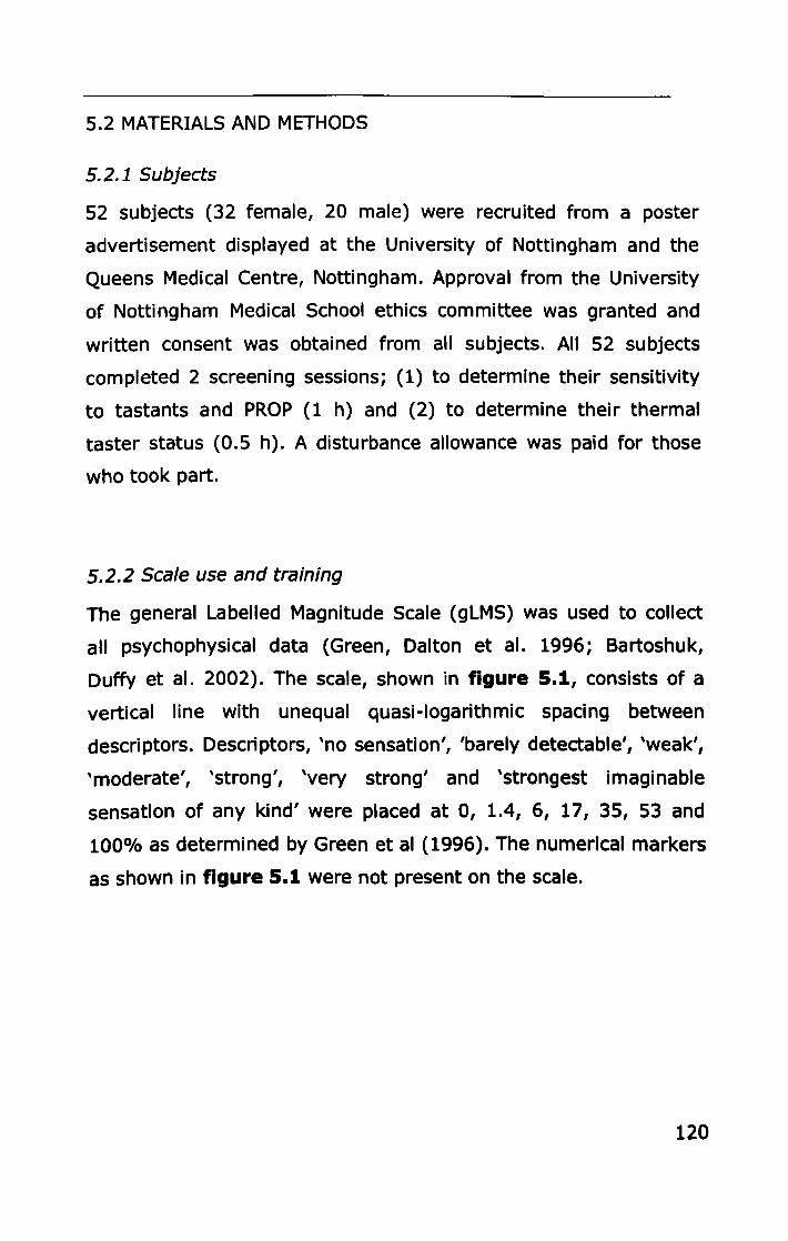
5.2 MATERIALS AND METHODS

5.2.1 Subjects

52 subjects (32 female, 20 male) were recruited from a poster

advertisement displayed at the University of Nottingham and the

Queens Medical Centre, Nottingham. Approval from the University

of Nottingham Medical School ethics committee was granted and

written consent was obtained from all subjects. All 52 subjects

completed 2 screening sessions; (1) to determine their sensitivity

to tastants and PROP (1 h) and (2) to determine their thermal

taster status (0.5 h). A disturbance allowance was paid for those

who took part.

5.2.2 Scale use and training

The general Labelled Magnitude Scale (gLMS) was used to collect

all psychophysical data (Green, Dalton et al. 1996; Bartoshuk,

Duffy et al. 2002). The scale, shown in figure 5.1, consists of a

vertical line with unequal quasi-logarithmic spacing between

descriptors. Descriptors, 'no sensation', 'barely detectable', 'weak',

'moderate', 'strong', 'very strong' and 'strongest imaginable

sensation of any kind' were placed at 0, 1.4, 6, 17, 35, 53 and

100% as determined by Green et al (1996). The numerical markers

as shown in figure 5.1 were not present on the scale.

120

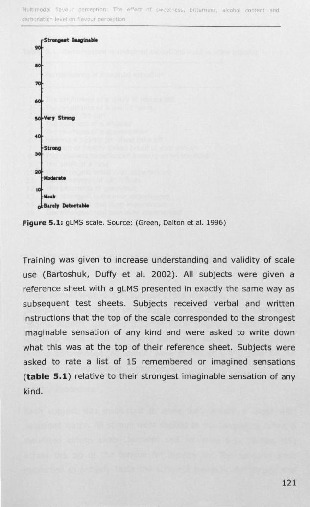
"'lu!tl"'1odal Flavour percept 10f' Tr ,ct of sw etnes:>, bjtt~! n ,5, a ohol conte"'t and

carb

Figure 5.1: gLMS scale. Source: (Green, Dalton et al. 1996)

Training was given to increase understanding and validity of scale

use (Bartoshuk, Duffy et al. 2002). All subjects were given a

reference sheet with a gLMS presented in exactly the same way as

subsequent test sheets. Subjects received verbal and written

instructions that the top of the scale corresponded to the strongest

imaginable sensation of any kind and were asked to write down

what this was at the top of their reference sheet. Subjects were

asked to rate a list of 15 remembered or imagined sensations

(table 5.1) relative to their strongest imaginable sensation of any

kind.

121

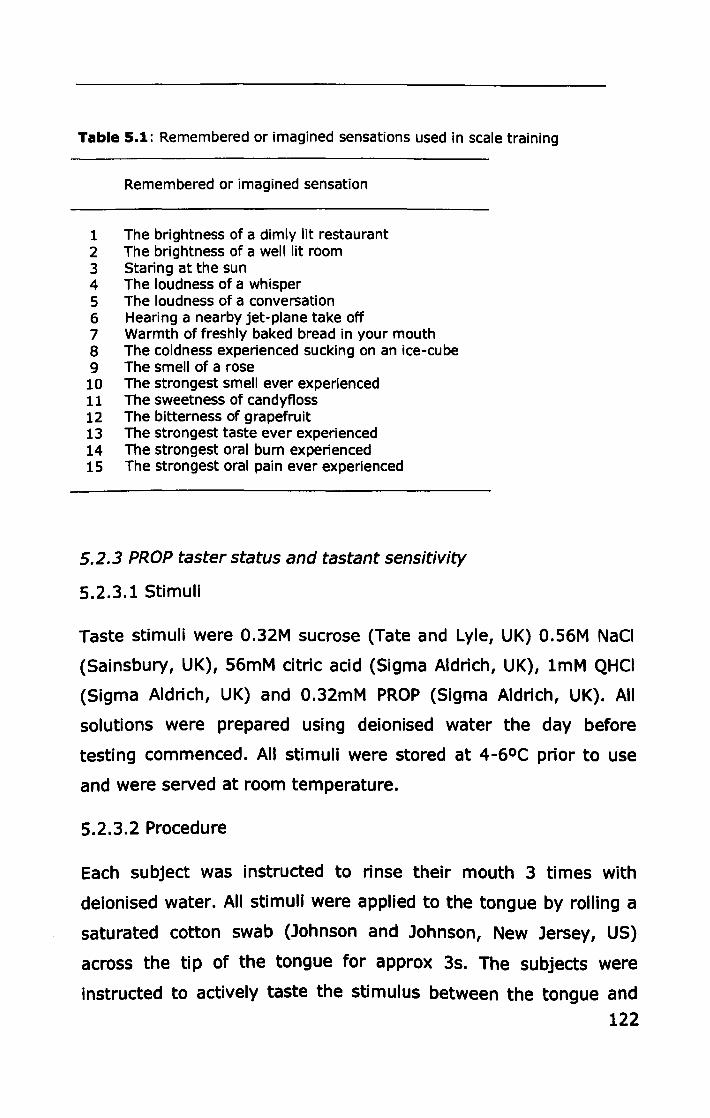
Table 5.1: Remembered or imagined sensations used in scale training

Remembered or imagined sensation

1 The brightness of a dimly lit restaurant 2 The brightness of a well lit room 3 Staring at the sun 4 The loudness of a whisper 5 The loudness of a conversation 6 Hearing a nearby jet-plane take off 7 Warmth of freshly baked bread in your mouth 8 The coldness experienced sucking on an ice-cube 9 The smell of a rose 10 The strongest smell ever experienced 11 The sweetness of candyfloss 12 The bitterness of grapefruit 13 The strongest taste ever experienced 14 The strongest oral burn experienced 15 The strongest oral pain ever experienced

5.2.3 PROP taster status and tastant sensitivity

5.2.3.1 Stimuli

Taste stimuli were O.32M sucrose (Tate and Lyle, UK) O.56M NaCI

(Sainsbury, UK), 56mM citric acid (Sigma Aldrich, UK), lmM QHCI

(Sigma Aldrich, UK) and O.32mM PROP (Sigma Aldrich, UK). All

solutions were prepared using deionised water the day before

testing commenced. All stimuli were stored at 4-60 C prior to use

and were served at room temperature.

5.2.3.2 Procedure

Each subject was instructed to rinse their mouth 3 times with

deionised water. All stimuli were applied to the tongue by rolling a

saturated cotton swab (Johnson and Johnson, New Jersey, US)

across the tip of the tongue for approx 3s. The subjects were

instructed to actively taste the stimulus between the tongue and

122

the hard palate using a gentle 'smacking' motion and rate the

perceived intensity of the taste once it had reached its maximum

using the gLMS provided. Separate gLMS were provided for each

stimulus. Subjects were encouraged to refer to their reference

sheet for guidance on where to rate the intensity of the taste. The

four taste stimuli were presented first in a randomised order, PROP

was presented last to avoid any cross over effects in PROP

sensitive individuals. Subjects were given a 1 minute inter­

stimulus-interval (lSI) and instructed to take longer if needed.

During the lSI, subjects cleansed their palate with the deionised

water and unsalted crackers (Rakusens, Leeds, UK) provided. After

a 5 min break, the procedure was repeated to collect duplicate

ratings of each stimulus. PROP taster status was defined based on

the mean intensity ratings of PROP: pNTs < barely detectable

«1.4% ) (n=19); pMTs above barely detectable (1.4%) but below

moderate (17%) (n=lS); pST> moderate (> 17%) (n=15) (Lim,

Lenka et al. 200S).

5.2.4 Thermal taster screening

5.2.4.1 Procedure

A circular intra-oral ATS (advanced thermal stimulator) thermode

(Medoc, Israel) with a truncated cone area of 2S.26mm2 at the top

and 7S.5mm2 at the base (2mm height) (figure 5.2a) was

connected to a PATHWAY pain and sensory evaluation system

(Medoc, Israel) and controlled using PATHWAY software (version 4,

Medoc, Israel) as shown in figure 5.2b.

123

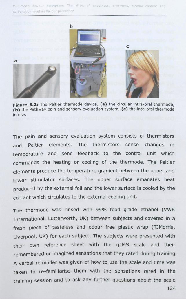
c

a

Figure 5.2: The Peltier thermode device. (a) the circular intra-oral thermode, (b) the Pathway pain and sensory evaluation system, (e) the inta-oral thermode in use.

The pain and sensory evaluation system consists of thermistors

and Peltier elements. The thermistors sense changes in

temperature and send feedback to the control unit which

commands the heating or cooling of the thermode. The Peltier

elements produce the temperature gradient between the upper and

lower stimulator surfaces. The upper surface emanates heat

produced by the external foil and the lower surface is cooled by the

coolant which circulates to the external cooling unit.

The thermode was rinsed with 99% food grade ethanol (VWR

International, Lutterworth, UK) between subjects and covered in a

fresh piece of tasteless and odour free plastic wrap (TJMorris,

Liverpool, UK) for each subject. The subjects were presented with

their own reference sheet with the gLMS scale and their

remembered or imagined sensations that they rated during training.

A verbal reminder was given of how to use the scale and time was

taken to re-familiarise them with the sensations rated in the

training session and to ask any further questions about the scale

124

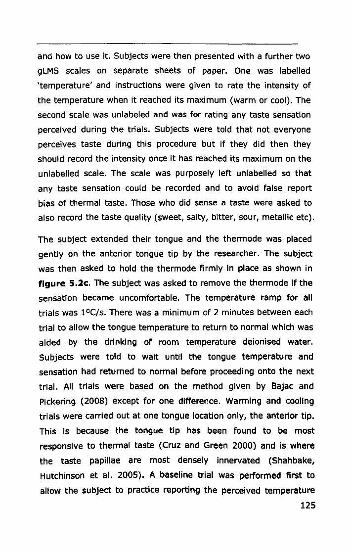
and how to use it. Subjects were then presented with a further two

gLMS scales on separate sheets of paper. One was labelled

'temperature' and instructions were given to rate the intensity of

the temperature when it reached its maximum (warm or cool). The

second scale was unlabeled and was for rating any taste sensation

perceived during the trials. Subjects were told that not everyone

perceives taste during this procedure but if they did then they

should record the intensity once it has reached its maximum on the

unlabelled scale. The scale was purposely left unlabelled so that

any taste sensation could be recorded and to avoid false report

bias of thermal taste. Those who did sense a taste were asked to

also record the taste quality (sweet, salty, bitter, sour, metallic etc).

The subject extended their tongue and the thermode was placed

gently on the anterior tongue tip by the researcher. The subject

was then asked to hold the thermode firmly in place as shown in

figure S.2e. The subject was asked to remove the thermode if the

sensation became uncomfortable. The temperature ramp for all

trials was 1 eels. There was a minimum of 2 minutes between each

trial to allow the tongue temperature to return to normal which was

aided by the drinking of room temperature deionised water.

Subjects were told to wait until the tongue temperature and

sensation had returned to normal before proceeding onto the next

trial. All trials were based on the method given by Bajac and

Pickering (2008) except for one difference. Warming and cooling

trials were carried out at one tongue location only, the anterior tip.

This is because the tongue tip has been found to be most

responsive to thermal taste (Cruz and Green 2000) and is where

the taste papillae are most densely innervated (Shah bake,

Hutchinson et al. 2005). A baseline trial was performed first to

allow the subject to practice reporting the perceived temperature

125

and any other taste sensations. During this trial the thermode was

applied to the tongue tip at body temperature (370 C) and held for

10 s. Warming trials started at 350 C, cooled to 150 C and re ­

warmed to 400 C and held for 1 s as shown in figure S.3a. The

cooling trial started at 35 0 C and was cooled to SOC and held for lOs

as illustrated in figure S.3b.

a WarmingTrial

40

U 35 . cu 30 ~

25 ::l ... n:J 20 ... ~ 15 E 10 ~ 5

0

0 10 20 30

Time (sec)

c

40 35 30 25 20 15 10 5 0

40 0

Cooling Trial

10 20

Time (sec)

30

Figure 5.3: Graphic representations of the warming trial and cool i n~ trials. (a) the warm ing trial started at 3SoC, cooled to lSoC, re-warmed to 40 C and held for 1 s, (b) the cooling trial started at 3SoC and was cooled to SoC and held for 10 s.

Subjects were instructed to 'attend now' as soon as the warming

began in the warming trial and the cooling began in the cooling

trial and were asked to rate the temperature once it had reached

its maximum perceived intensity (usually at the end of the trial).

Trials were duplicated to provide replicate data but the subjects

were unaware of this. Warming trials always preceded cooling trails

to avoid possible adaptation from the intense, sustained cold

stimulation (Green and George 2004). TIs were defined as those

who reported a taste sensation during either the warming or

cooling trials. Those who did not perceive any taste sensations

were classified as TnTs.

126

5.2.5 Data analysis

All data was IOg10 transformed, with 0 ratings converted to 0.4

prior to transformation. A 3 factor ANOVA (group, replicate and

stimulus) with interactions was performed on the log intensity

ratings of the 4 taste stimuli, PROP and temperature to investigate

overall effects of group, replicate and stimulus. A 2-factor (group,

stimulus) ANOVA with interaction was then performed

independently on each individual stimulus to investigate the effect

of group on each stimulus. PROP taster groups were analysed

separately to thermal taster groups. Where appropriate, Tukey's

HSD post-hoc tests were used to determine significant differences

between groups and/or stimulus.

5.3 RESULTS

5.3.1 PROP taster status

Fifty two subjects took part in the screening sessions of which 19

were PROP non-tasters (pNTs), 18 were medium-tasters (pMTs)

and 15 were super-tasters (pSTs) as shown in table 5.2.

127

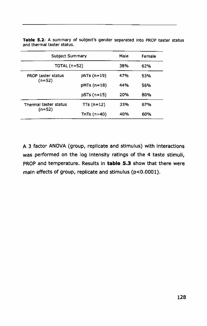
Table 5.2: A summary of subject's gender separated into PROP taster status and thermal taster status.

Subject Summary Male Female

TOTAL (n=52) 38% 62%

PROP taster status pNTs (n=19) 47% 53% (n=52)

pMTs (n=18) 44% 56%

pSTs (n=15) 20% 80%

Thermal taster status TIs (n=12) 33% 67% (n=52)

TnTs (n=40) 40% 60%

A 3 factor ANOVA (group, replicate and stimulus) with interactions

was performed on the log intensity ratings of the 4 taste stimuli,

PROP and temperature. Results in table S.3 show that there were

main effects of group, replicate and stimulus (p<O.0001).

128

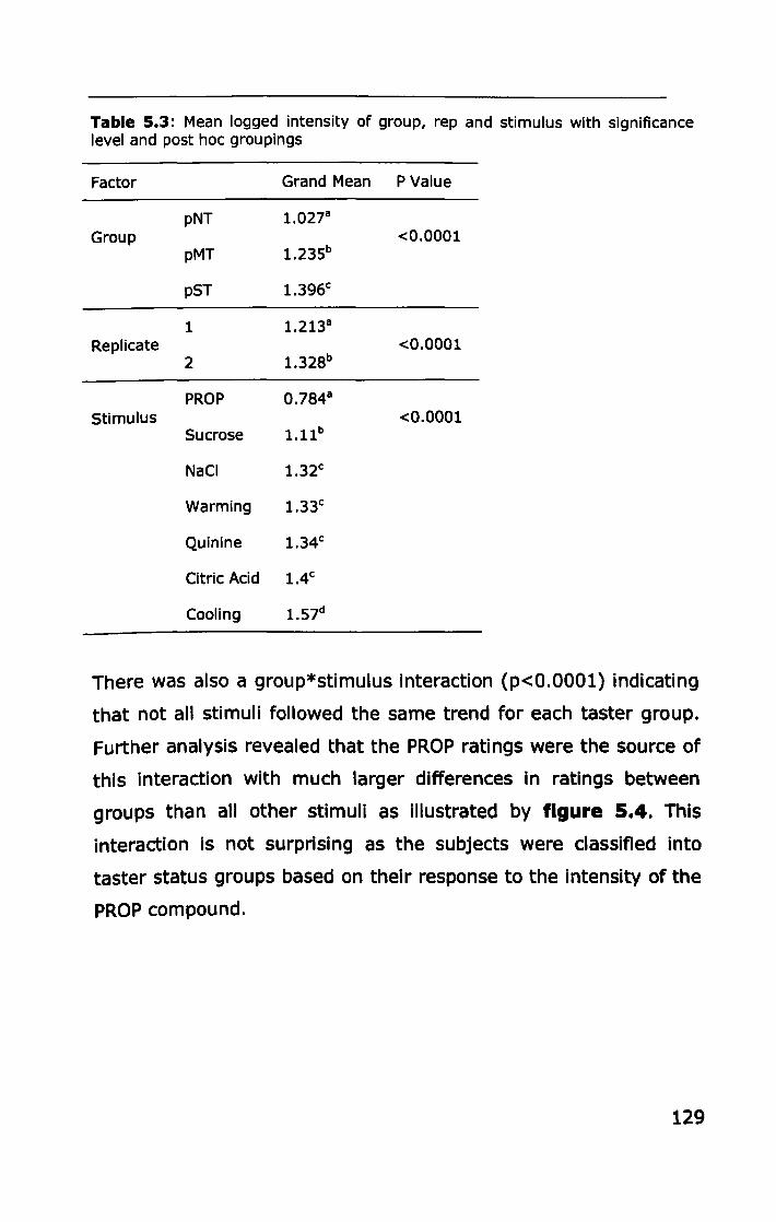
Table 5.3: Mean logged intensity of group, rep and stimulus with significance level and post hoc groupings

Factor Grand Mean P Value

pNT 1.027a

Group 1.23Sb pMT

<0.0001

pST 1. 396c

1 1.213a

Replicate 1.328b 2

<0.0001

PROP 0.784a Stimulus <0.0001

Sucrose 1.11b

NaCi 1.32c

Warming 1.33c

Quinine 1.34c

Citric Acid l.4c

Cooling 1.57d

There was also a group*stimulus interaction (p<O.OOOl) indicating

that not all stimuli followed the same trend for each taster group.

Further analysis revealed that the PROP ratings were the source of

this interaction with much larger differences in ratings between

groups than all other stimuli as illustrated by figure 5.4. This

interaction is not surprising as the subjects were classified into

taster status groups based on their response to the intensity of the

PROP compound.

129

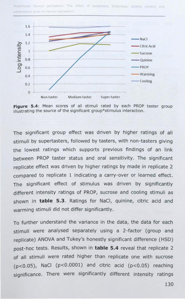
1.6

1.4

~ 1.2

en c:: 1 Q)

+oJ C 0.8 0> 0 0.6

...-J 0.4

0.2

0 - -..,. --,-

Non-taster Medium-taster Super-t aster

h

- NaCI

- Cit ricAcid

- Sucrose

- Quinine

- PROP

- Warming

Cooling

Figure 5.4: Mean scores of all stimuli rated by each PROP taster group il lustrating the source of the significant group* stimulus interaction.

The significant group effect was driven by higher ratings of all

stimuli by supertasters, followed by tasters, with non-tasters giving

the lowest ratings which supports previous findings of an link

between PROP taster status and oral sensitivity. The significant

replicate effect was driven by higher ratings by made in replicate 2

compared to replicate 1 indicating a carry-over or learned effect.

The significant effect of stimulus was driven by significantly

different intensity ratings of PROP, sucrose and cooling stimuli as

shown in table 5.3. Ratings for NaCl, quinine, citric acid and

warming stimuli did not differ significantly.

To further understand the variance in the data, the data for each

stimuli were analysed separately using a 2-factor (group and

replicate) ANOVA and Tukey's honestly significant difference (HSD)

post-hoc tests. Results, shown in table 5.4 reveal that replicate 2

of all stimuli were rated higher than replicate one with sucrose

(p<O.OS), NaCI (p<O.OOOl) and citric acid (p<O.OS) reaching

significance. There were significantly different intensity ratings

130

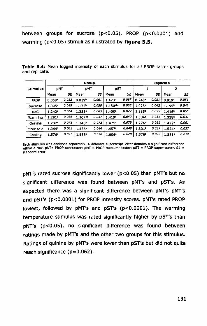
between groups for sucrose (p<O.OS), PROP (p<O.OOOl) and

warming (p<O.OS) stimuli as illustrated by figure 5.5.

Table 5.4: Mean logged intensity of each stimulus for all PROP taster groups and replicate.

Group Replicate

Stimulus pNT pMT pST 1 2

Mean SE Mean SE Mean SE Mean SE Mean SE PROP 0.Os9a 0.052 0.819b 0.061 l.473e 0.067 0.748- 0.051 0.819- 0.051

Sucrose 1.00sa 0.049 1.17sb 0.050 1.150lb 0.055 1.025- 0.042 1.195b 0.042

NaCI 1.242- 0.064 1.3351 0.065 1.400· 0.072 1.235- 0.055 1.416b 0.055

Warming 1.281- 0.036 1.307ab 0.037 1.419b 0.040 1.334- 0.031 1.338- 0.031

Quinine 1.2321 0.071 1.3401 0.073 1.47sa 0.079 1.276- 0.061 1.422a 0.061

Citric Acid 1.3441 0.043 1.4361 0.044 1.457a 0.048 1.301- 0.037 1.524b 0.037

Cooling 1.s76a 0.025 1.5551 0.026 1.6061 0.028 1.5761 0.022 1.581' 0.022

Each stimulus was analysed separately. A different superscript letter denotes a significant difference within a row. pNT= PROP non-taster; pMT = PROP medium- taster; pST = PROP super-taster. SE = standard error

pNT's rated sucrose Significantly lower (p<O.OS) than pMT's but no

significant difference was found between pNT's and pST's. As

expected there was a Significant difference between pNT's pMT's

and pST's (p<O.OOOl) for PROP intensity scores. pNT's rated PROP

lowest, followed by pMT's and pST's (p<O.OOOl). The warming

temperature stimulus was rated Significantly higher by pST's than

pNT's (p<O.OS), no Significant difference was found between

ratings made by pMT's and the other two groups for this stimulus.

Ratings of quinine by pNT's were lower than pST's but did not quite

reach significance (p=O.062).

131

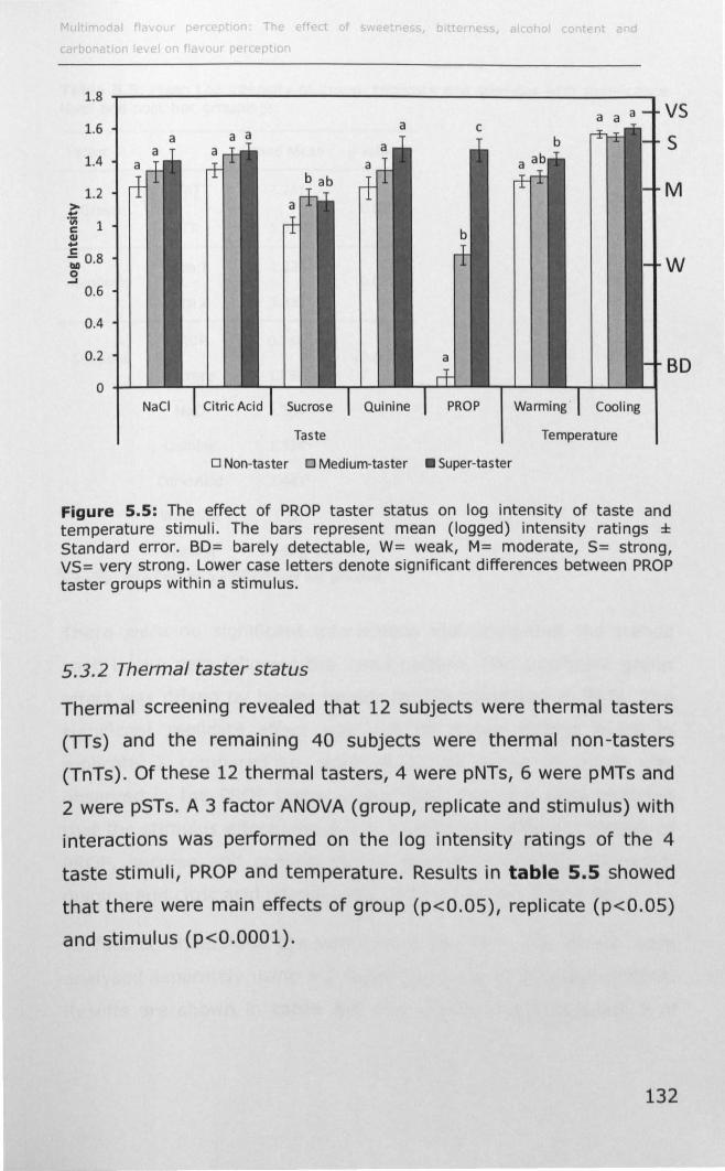
fV' t diOll f v r ton Th f t f , b t n te • and

1.8 'T""""'--------------------------. 1.6

1.4

1.2 > .. . ~ 1 aI .. C -;, 0.8 .9

0.6

0.4

0.2

a a a VS

S

M

w

SD

Taste Temperature

o Non-taster 0 Medium-taster • Super-taster

Figure 5.5: The effect of PROP taster status on log intensity of taste and temperature stimuli. The bars represent mean (logged) intensity ratings ± Standard error. BD= barely detectable, W= weak, M= moderate, S= strong, VS= very strong. Lower case letters denote significant differences between PROP taster groups within a stimulus.

5.3.2 Thermal taster status

Thermal screening revealed that 12 subjects were thermal tasters

(TIs) and the remaining 40 subjects were thermal non-tasters

(TnTs). Of these 12 thermal tasters, 4 were pNTs, 6 were pMTs and

2 were pSTs. A 3 factor ANOVA (group, replicate and stimulus) with

interactions was performed on the log intensity ratings of the 4

taste stimuli, PROP and temperature. Results in table 5.5 showed

that there were main effects of group (p<O.OS), replicate (p<O.OS)

and stimulus (p<O.OOOl).

132

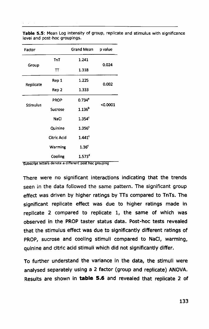
Table 5.5: Mean Log intensity of group, replicate and stimulus with significance level and post-hoc groupings.

Factor Grand Mean p value

TnT 1.241 Group 0.024

n 1.318

Replicate Rep 1 1.225

0.002 Rep 2 1.333

PROP Stimulus <0.0001

Sucrose

NaCI

Quinine

Citric Acid

Warming

Cooling

Subscript letters denote a different post hoc grouping

There were no significant interactions indicating that the trends

seen in the data followed the same pattern. The significant group

effect was driven by higher ratings by TIs compared to TnTs. The

significant replicate effect was due to higher ratings made in

replicate 2 compared to replicate 1, the same of which was

observed in the PROP taster status data. Post-hoc tests revealed

that the stimulus effect was due to significantly different ratings of

PROP, sucrose and cooling stimuli compared to NaCI, warming,

quinine and citric acid stimuli which did not significantly differ.

To further understand the variance in the data, the stimuli were

analysed separately using a 2 factor (group and replicate) ANOVA.

Results are shown in table 5.6 and revealed that replicate 2 of

133

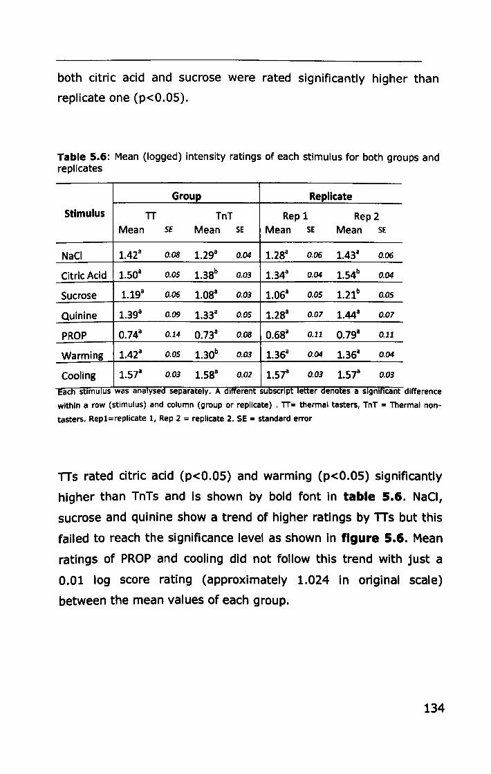
both citric acid and sucrose were rated significantly higher than

replicate one (p<O.OS).

Table 5.6: Mean (logged) intensity ratings of each stimulus for both groups and replicates

Group Replicate

Stimulus TT TnT Rep 1 Rep 2 Mean Sf Mean SE Mean SE Mean SE

NaCI 1.42a 0.08 1.29a 0.04 1.2Sa 0.06 1.43a 0.06

Citric Acid 1.50a 0.05 1.3sb 0.03 1.34a 0.04 1.54b 0.04

Sucrose 1.19a 0.06 1.0Sa 0.03 1.06a 0.05 1.21b 0.05

Quinine 1.39a 0.09 1.33a 0.05 1.2Sa 0.07 l.44a 0.07

PROP 0.74a 0.14 0.73a 0.08 0.6Sa 0.11 0.793 0.11

Warming 1.423 0.05 1.30b 0.03 1.36a 0.04 1.363 0.04

Cooling 1.57a 0.03 1.5s3 0.02 1.57a 0.03 1.573 0.03

Each stimulus was analysed separately. A different SubSCript letter denotes a significant difference

within a row (stimulus) and column (group or replicate) . TT= thermal tasters, TnT = Thermal non­

tasters. Rep1=replicate 1, Rep 2 = replicate 2. SE = standard error

TIs rated citric acid (p<O.OS) and warming (p<O.OS) significantly

higher than TnTs and is shown by bold font in table 5.6. NaCI,

sucrose and quinine show a trend of higher ratings by TIs but this

failed to reach the significance level as shown in figure 5.6. Mean

ratings of PROP and cooling did not follow this trend with just a

0.01 log score rating (approximately 1.024 In original scale)

between the mean values of each group.

134

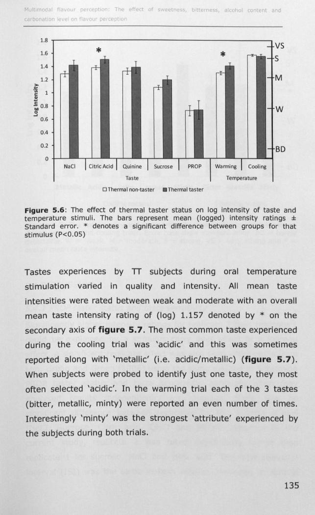
<;s Ie. 01 ont t a c

1.8

1.6 * vs

1.4

1.2 > ..

' jj; 1 c III .. C -;0 0.8 0 -'

0.6

0.4

0.2

0

Taste Temperature

o Thermal non-taster .Thermal taster

Figure 5.6: The effect of thermal taster status on log intensity of taste and temperature stimuli. The bars represent mean (logged) intensity ratings ± Standard error, * denotes a significant difference between groups for that stimulus (P<O,OS)

Tastes experiences by TT subjects during oral temperature

stimulation varied in quality and intensity. All mean taste

intensities were rated between weak and moderate with an overall

mean taste intensity rating of (log) 1.157 denoted by * on the

secondary axis of figure 5.7. The most common taste experienced

during the cooling trial was 'acidic' and this was sometimes

reported along with 'metallic' (Le. acidic/metallic) (figure 5.7).

When subjects were probed to identify just one taste, they most

often selected 'acidic'. In the warming trial each of the 3 tastes

(bitter, metallic, minty) were reported an even number of times.

Interestingly 'minty' was the strongest 'attribute' experienced by

the subjects during both trials.

135

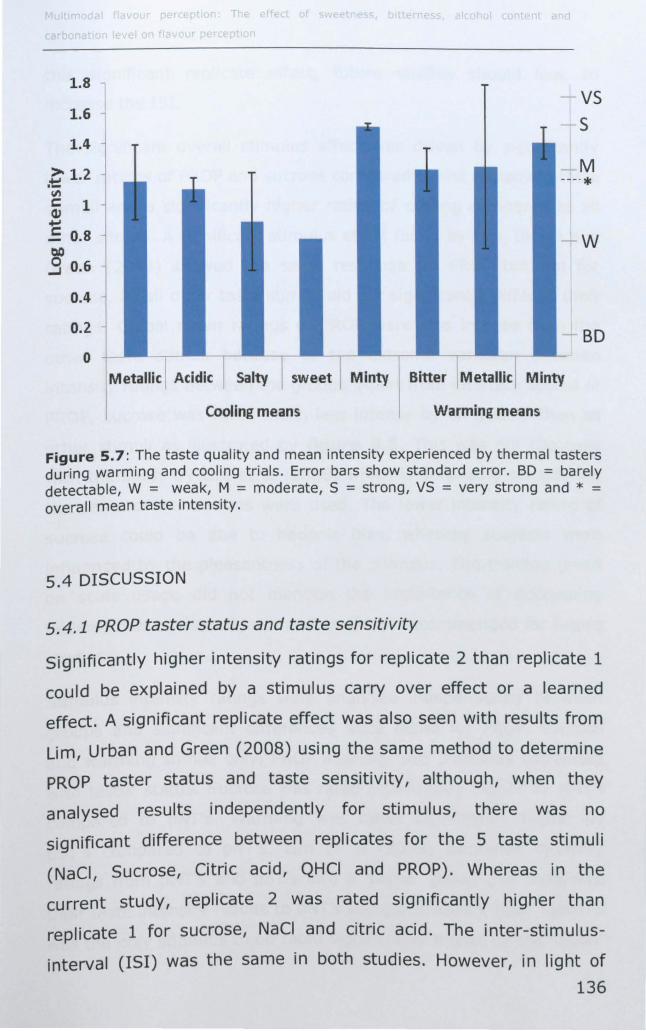
1.8

1.6

1.4

.~1.2 ~

c 1 Q.l +-' .= 0.8 00 ..9 0.6

0.4

0.2

o

T E

VS 5

M ---- *

w

BO

sweet Minty Bitter Metallic Minty

Cooling means I Warming means

Figure 5.7: The taste quality and mean intensity experienced by thermal tasters during warming and cooling trials. Error bars show standard error. BD = barely detectable, W = weak, M = moderate,S = strong, VS = very strong and * = overall mean taste intensity.

5.4 DISCUSSION

5.4.1 PROP taster status and taste sensitivity

Significantly higher intensity ratings for replicate 2 than replicate 1

could be explained by a stimulus carry over effect or a learned

effect. A significant replicate effect was also seen with results from

Lim, Urban and Green (2008) using the same method to determine

PROP taster status and taste sensitivity, although, when they

analysed results independently for stimulus, there was no

significant difference between replicates for the 5 taste stimuli

(NaCI, Sucrose, Citric acid, QHCI and PROP). Whereas in the

current study, replicate 2 was rated significantly higher than

replicate 1 for sucrose, NaCI and citric acid. The inter-stimulus­

interval (lSI) was the same in both studies. However, in light of

136

this significant replicate effect, future studies should look to

increase the lSI.

The significant overall stimulus effect was driven by significantly

lower ratings of PROP and sucrose compared to the remaining taste

stimuli and a significantly higher rating of cooling compared to all

other stimuli. A significant stimulus effect found by Lim, Urban and

Green (2008) showed the same response for PROP but not for

sucrose, as all other taste stimuli did not significantly differ in their

ratings. Global mean ratings of PROP were less intense than the

other taste stimuli because of the extreme variation between

intensity ratings between the groups. Apart from intensity scores of

PROP, sucrose was rated much less intense by all groups than all

other stimuli as illustrated by figure 5.5. This was not the case

with the study by Lim et al (2008) which is surprising considering

the same concentrations were used. The lower intensity rating of

sucrose could be due to hedonic bias, whereby subjects were

influenced by the pleasantness of the stimulus. The training given

on scale usage did not mention the importance of decoupling

hedonic bias to the subjects and would be recommended for future

studies.

Stimulus intensity ratings were analysed independently between

groups and significant differences were found for PROP, sucrose

and warming stimuli only. PROP intensity was positively correlated

with taster status. Sucrose was rated significantly higher by pMT's

compared to pNT's. Warming was rated significantly higher by

pST's compared to pNT's. Lim et al (2008) combined intensity

ratings from pMT's and pST's into a 'taster' group and compared

their taste intensity results to pNT's using a student t-test. Quinine

was the only stimulus to be rated significantly higher by the 'taster'

137

subjects. When the group was split into pMT's and pST's, the

difference between intensity ratings, analysed by t-test, found that

pST's rated all 4 taste stimuli (and PROP) significantly higher than

pMT's indicating that the PROP genotype advantage is much

greater for pST. In the current study, ANOVA did not reveal any

significant differences between pMT's and pST's for any of the

prototypical taste stimuli (sucrose, citric acid, NaCi or quinine)

tested here. The t-tests carried out in the Lim, Urban and Green

(2008) paper may have increased the probability of finding

significant differences between groups for taste stimuli.

The warming stimulus was rated significantly higher by pST's than

pNT's but no significant difference was found between groups for

the cooling stimulus which is contradictory to other work (Manrique

and Zald 2006), although much higher target temperatures were

used for the cooling stimuli (21, 24 and 27°C) than in the current

study (SoC). Response to both warming and cooling temperature

stimuli was investigated between PROP taster groups at 3 different

locations on the tongue by Bajac and Pickering (2008). Results

showed that pST's rated all temperature stimuli significantly higher

than both pNT's and pMT's. The increased temperature sensitivity

in pST's was thought to be linked to fungiform papillae density

which was higher in pST's compared to the other two groups (Bajec

and Pickering 2008). Fungiform papillae density was not measured

in the current study so this hypothesis cannot be investigated but it

is likely since the nerve endings that respond to temperature and

other trigeminal stimuli are innervated with the taste receptor cells

(Whitehead, Beeman et al. 1985; Whitehead, Ganchrow et al.

1999). An increased number of fungiform papillae in pST's

compared to pMT's should therefore result in an increased number

of trigeminal receptors responding to temperature and contributing

138

to the increased intensity response. However, the link between

PROP taster status and fungiform papillae density is not fully

conclusive and the genetic control for fungiform papillae density is

not clear (Duffy, Davidson et al. 2004).

The significant group effect in PROP ratings is due to the genetic

ability to taste PROP as previously discussed. pNT's had the lowest

ratings, followed by pMT's and then pST's which confirms the

genetic effect. Sucrose and warming were also rated significantly

differently between the groups. It is interesting to note that

sucrose was the taste stimulus rated overall least intense and

warming was the temperature stimulus rated overall least intense.

Therefore, it may be possible that the PROP advantage is greater at

lower stimulus intensities. This could be a plausible explanation

considering the connection between PROP taster status and

fungiform papillae density. For example, in percentage terms, a

difference in fungiform papillae density could bring about a greater

difference in receptor activation and therefore signals sent to the

brain, resulting in greater differences in perception at lower

stimulus intensities between groups. Higher stimulus intensities

may saturate the receptors and subsequent signalling to the brain

could bring about a perceptual response which is similar between

groups. Another explanation could be that sucrose and warming

stimuli are generally more pleasant stimuli than the others and the

PROP advantage is more susceptible to this.

pST's rated all stimuli higher than pNT's however, the magnitude of

the difference between the groups is stimulus dependant (table

5.4). As expected, the difference between group mean intensity

ratings for PROP was much larger than any other stimulus but

when comparing the taste stimuli alone there was a larger

139

difference between intensity ratings between the pNT's and pMT's.

However, with the temperature stimuli, there was a greater

magnitude of difference between pMT's and pST's. The mechanism

for the PROP taster advantage is reported to be a combined effect

of allelic variation of TAS2R38 and an increased number of

fungiform papillae on the anterior tongue. Tasters must have at

least one PAV allele but it is the density of fungiform papillae on

the anterior tongue that separates pMT's and pST's (Bartoshuk,

Duffy et al. 1994; Delwiche, Buletic et al. 2001; Duffy, Davidson et

al. 2004). It is possible that the presence of the functional receptor

for PROP contributes to increased taste sensitivity and would

suggest why there was a greater difference between pNT's and

pMT's for taste stimuli found here, whereas the increased density in

fungiform papillae between pMT's and pST's (found in other works)

accounts for the increased temperature sensitivity found here and

possibly other stimuli sensed by the trigeminal nerve. This

hypothesis is supported by temperature intensity ratings collected

by Bajec and Pickering (2008) where the magnitude of difference

was greater between pMTs and pSTs, but not the taste intensity

ratings collected by Bajec and Pickering (2008) and Lim, Urban and

Green (2008) where greater differences were also seen between

pMT's and pST's.

The mechanism for an increased perceptual response by tasters of

PROP (both pMTs and pSTs) to taste stimuli and temperature found

in the current study could be a combination of anatomy and

receptor genetics which would both increase signal response and

central activation. Neurophysiological studies into brain activation

between taster groups of various taste and tactile stimuli would

increase understanding of the mechanisms that give the PROP

taster advantage.

140

5.4.2 Thermal taster status and taste sensitivity

A significant effect that replicate 2 was rated higher than replicate

1 suggests the same carry over effect as discussed in the previous

section. In addition, the significant global effect of stimulus showed

that PROP, sucrose and cooling stimuli were rated significantly

differently to all other stimuli and is the same result found in the

PROP group analysis. The parity between the replicate and stimulus

effect seen between groups is not surprising considering this group

comprises of the same subjects but classified for thermal taster

status as opposed to PROP taster status.

PROP taster status was spread relatively evenly across the thermal

taster group and there was no significant difference found between

PROP intensity ratings between thermal groups indicating that the

two markers of oral sensitivity function independently. This agrees

with some research (Bajec and Pickering 2008; Bajec and Pickering

2010) but disagrees with others (Green and George 2004). Green

& George (2004) tested PROP sensitivity between thermal taster

groups on both the front and back of the tongue. At both locations,

PROP was rated significantly higher in intensity by TIs but the

magnitude of difference between the groups was much larger on

the back of the tongue than on the front. The same was true for

another bitter stimulus, quinine, but not for sucrose, NaCI or citric

acid taste stimuli. In the current study, PROP was applied to the

anterior tongue and it is the posterior tongue that is densely

populated with circumvallate papillae (Chandrashekar, Hoon et al.

2006) which express all 25 TAS2R (bitter receptor) genes (Behrens,

Foerster et al. 2007). Therefore, future investigations should test

for sensitivity to bitter tastants using either whole mouth rinses or

141

if using cotton swabs, both the anterior and posterior tongue

should be tested.

A significant group effect revealed that TIs rated all stimuli

significantly higher than TnTs which agrees with other studies

(Green and George 2004; Bajec and Pickering 2008). When each

stimulus was subjected to independent 2-factor (group and

stimulus) ANOVA, the citric acid taste stimulus and the warming

temperature stimulus were the only stimuli to reach significance,

although all other taste stimuli followed the same trend. However,

the mean group intensity ratings of the cooling stimuli did not differ

between groups; in fact there was only a 0.01 log difference (1.024

in original scale) between mean group ratings (table 5.6).

Previous studies have found conflicting evidence regarding the

impact of the TI advantage on trigeminal stimuli. Burning, stinging

and prickling induced by capsaicin and menthol were not rated

differently by thermal groups in a series of experiments by Green

et al (2005) but the astringency of alum and temperature of warm

and cold stimuli were rated Significantly higher by TIs in a study by

Bajec and Pickering (2008). The log mean intensity of warm stimuli

was rated Significantly higher by TIs at three locations on the

tongue; the tip, and the left and right sides, which is in agreement

with results here on the tongue tip. However, the cooling stimulus

was only significant at the right and left sides and no significant

difference was found at the tongue tip which again agrees with

results found here.

Thermal tasters seem to perceive tactile and temperature stimuli

more intensely which may influence food liking and preference.

Thermal tasters have reduced liking for soft foods (Bajec and

Pickering 2010) providing evidence that differences between TIs

142

and TnTs could be texturally driven. The mechanism for this would

not appear to be associated with fungiform papillae density as no

correlation has been found previously (Bajec and Pickering 2008).

Differences in trigeminal sensitivity may differ between the two

groups based on interaction with a taste stimulus. Carbonation and

fullness were rated higher by thermal tasters in a study on beer

(Pickering, Bartolini et al. 2010) and astringency was rated

significantly higher in red wine (Pickering, Moyes et al. 2010) but

when capsaicin and menthol were investigated in isolation, no

significant differences were found between groups. A similar

interaction mechanism has been proposed for increased aroma

sensitivity in TIs (Green and George 2004).

The magnitude of the difference between intensity ratings between

thermal taster groups is lower than those found in other studies

(Green and George 2004; Bajec and Pickering 2008). In the

current study the TT screening test involved thermal testing at just

one site on the tongue (anterior tip), whereas other studies also

tested to the right and left of the anterior tip therefore providing

stricter criteria for TT classification. Sensitivity to thermal taste is

not uniformly distributed as with chemical taste (Cruz and Green

2000) and the best sites for thermal sweetness (sweet-best sites)

have been found on the tongue tip whereas sites for thermal

sourness (sour-best sites) have been found nearly always lateral to

the tip (Cruz and Green 2000). Cruz and Green (2000) found that

when sucrose was applied to sweet-best sites in TTs, ratings were

higher than when applied to sour-best sites. In addition, in the

study by Green and George (2004) taste intensity to sucrose,

sodium saccharin and NaCI was tested at the site most sensitive to

thermal taste, with all TnTs being tested at the tongue tip which

may have increased the difference between results. Therefore

143

classifying subjects into TT groups based upon thermal stimulation

at just one tongue location and testing oral sensitivity at the same

location may have led to wrongly classifying some subjects in the

present study and thus reducing the magnitude of the difference

between groups. It would be recommended to test 3 tongue

locations in future studies and to reject subjects if a clear

classification cannot be made. Nevertheless, this study

demonstrates that time or cost restrictions make it possible to test

at the tongue tip only for quick screening purposes.

Another explanation for the magnitude of difference between

groups in different studies could be dependent upon stimuli

concentration. Green and George (2004) tested the sensitivity to

the same stimuli as in the current study using cotton swabs but at

lower concentrations (concentrations taken from the text as

opposed to the graph labels in Green and George (2004) as there

is a discrepancy between the two). Greater differences were found

between groups for taste sensitivity than in the present study

indicating that as the concentration of the stimulus increases, the

TT advantage decreases. Another study by Green et al (2005)

using very similar concentrations of the same taste stimuli as in the

present study and applied in the same way, showed similar results

in terms of magnitude of difference between the groups.

Taste intensities experienced during temperature stimulation in

thermal tasters (figure 5.7) were within the same intensity range

(between weak and strong on the gLMS scale) as those

experienced during the taste sensitivity testing (figure 5.6). This

suggests that trigeminal (temperature) nerves may be capable of

delivering a taste sensation that is equally comparable in intensity

to those achieved by the taste compounds. The impact this has on

144

the way thermal tasters experience more complex foods and

beverages is yet to be understood.

The quality of the taste varied between subjects and each of the

tastes reported during the warming trial were given an equal

number of times with no one taste dominating. Cruz and Green

(2000) found that 'sweet' was the most common taste reported by

thermal tasters during warming trail which was not the case in the

present study. However, the term 'minty' was reported in both

warming and cooling trials and could be a combination of tingly

sensation from the swift temperature change combined with a

sweet taste. The most common taste experienced during the

cooling trial was 'acidic' which agrees with other trials, followed by

'metallic'. Metallic has not been a taste which has been reported by

other authors. This may be due to the fact that in this study the

subjects were free to place their own label on the taste sensation

experienced so as to not introduce response bias. Whereas in other

studies, subjects have been provided with gLMS scales labelled

with the basic tastes (sweet, salty, sour, bitter, (umami) and

'other'). In this case, 'metallic' could in fact be the label put to

acidic taste because it was sometimes accompanied by the term

'acidic' in the subject's initial description (i.e. acidic/metallic). When

the subject was asked to use just one word to describe the taste,

they most often chose 'acidic' for the cooling trial. In the cases

where 'metallic' was chosen it is likely that the subjects used this

term to describe a taste that they were having difficulty identifying

because they could see the metal contact plate of the thermode,

thus responding to the visual cue of the thermode. It is not

possible for a metallic taste to have transferred from the thermode

contact plate to the subject because it was covered with plastic film

wrap.

145

Subjects could record the taste sensation at any point during the

trails and the specific temperature at which the taste was perceived

is unknown as this served as a screening test and so full analysis of

the differences between taste quality and warming and cooling

cannot be made.

5.5 CONCLUSIONS AND SUMMARY

An increased sensitivity of general bitterness, overall taste

sensitivity or indeed overall oral sensation in different PROP groups

has been extensively researched. This study confirms that PROP

and thermal taster status are different markers of genetic taste

variation in the population. It is possible that the disparity in

results from studies investigating PROP taster status could occur

from differences in stimuli concentrations and application method.

Results to date suggest that PROP super-tasters sense oral stimuli

more intensely due to a combination of a dominant PAV allele and

high fungiform papillae density. The genetic mechanism for

fungiform papillae density is currently not known but seems to be

linked to the sensation of tactile stimuli. Further work should

investigate PROP sensitivity and sensory interactions between

modalities. Thermal taster status was a significant predictor of

sensitivity to taste stimuli and further work should investigate

gustatory-trigeminal interactions to investigate the mechanism of

the thermal taste advantage. If the intensity of all oral sensations

is greater in thermal tasters due to activation of both trigeminal

and taste fibres which are co-innervated and intertwined then it is

likely that activation in cortical areas involved in gustatory and

somatosensory processing will be also increased. Psychophysical

studies rely on the subject to verbalise these perceptions. However,

146

neuroimaging techniques can provide a detailed account of cortical

activation which can be correlated to genetic phenotype, perception

and preference if measured concurrently. An increased knowledge

of neural and cortical responses between groups is needed to

further understanding in this domain and is explored in the next

chapter.

147

Chapter 6

148

6. THE CORTICAL RESPONSE OF CARBONATION ON TASTE

AND VARIATION WITH TASTE PHENOTYPE

Carbonation was found to reduce sweetness perception in a model

beer system (chapter 4) and it is unknown whether this is the

result of a peripheral or cortical interaction. In addition, chapter 5

explored variation of taste phenotype and found differences

between groups for taste and temperature perception. The

objectives of this study were to use functional magnetic resonance

imaging (fMRI) to; (1) investigate the cortical response to (sweet)

taste and the effects of carbonation and (2) compare the cortical

response between taste phenotype groups. The following sections

introduce magnetic resonance imaging as a tool to investigate

activation from sensory neurons.

6.1 INTRODUCTION TO MRI

Magnetic resonance imaging (MRI) uses strong magnetic fields,

expressed in units of Tesla, which can be manipulated to create

images of specific biological tissue. Atomic nuclei in the tissue

absorb electromagnetic energy emitted by the scanner at a

particular frequency. This absorbed electromagnetic energy is then

released by the nuclei, the intensity of which is dependent upon the

number and type of nuclei present in the tissue. To create the

images, the scanner uses a complex sequence of magnetic

gradients and radiofrequency (RF) pulses, together comprising

what is known as a pulse sequence, from which an image is formed.

The type of imaging pulse sequence used depends upon the

different tissue properties to be detected. For example, a different

pulse sequence would be used to create structural images of the

foot or brain, compared to functional images of the brain. MRI can

be used to create high resolution structural (anatomical) images of

149

the brain to define anatomy using pulse sequences which take a

number of minutes to acquire an image. Functional studies (which

are termed functional Magnetic Resonance Imaging (fMRI» on the

other hand, rapidly acquire a typically coarse image on the order of

milliseconds to measure short term physiological changes

associated with active functioning of the brain. fMRI can provide

valuable information on where particular mental processes occur

and the spatial patterns and intensities of activation associated

with them. The following sections will describe the basic principles

of magnetic resonance imaging including pulse sequences and

image formation. This is followed by an outline of the use of Blood

Oxygenation Level Dependent (BOLD) contrast in functional MRI

and an overview of data collection and analysis methods. The

introduction will conclude with a review of the cortical

representation of taste and trigeminal stimuli.

6.1.1 Basic principles of Magnetic Resonance

Magnetic resonance imaging relies on the fact that atomic nuclei

possess four fundamental physical properties: mass, electric

charge, spin and magnetic moment. Nuclei which contain an odd

number of protons, or an odd mass number (number of protons

and neutrons) possess intrinsic spin, and have spin angular

momentum (l). A hydrogen nucleus eH, proton) possesses spin

1/2 and this gives rise to a magnetic moment (J!) which is

described by eqn. 6.1. r is the gyromagnetic ratio, which is a

fundamental property of the nucleus.

Eqn.6.1 J! = rl

150

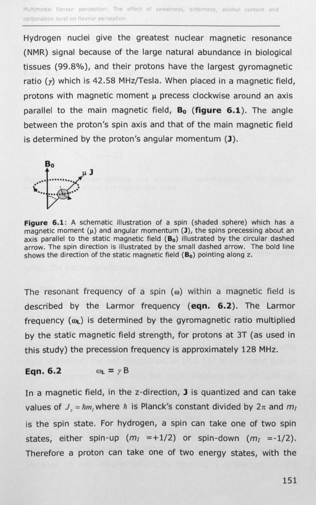
"'1" Imoda fl v p pt on Th J t" C, bl te c ale I I 0 nt d

Hydrogen nuclei give the greatest nuclear magnetic resonance

(NMR) signal because of the large natural abundance in biological

tissues (99.80/0), and their protons have the largest gyromagnetic

ratio (r) which is 42.58 MHz/Tesla. When placed in a magnetic field,

protons with magnetic moment ~ precess clockwise around an axis

parallel to the main magnetic field, Bo (figure 6.1). The angle

between the proton's spin axis and that of the main magnetic field

is determined by the proton's angular momentum (1).

Bo

Figure 6.1: A schematic illustration of a spin (shaded sphere) which has a magnetic moment (~) and angular momentum (l), the spins precessing about an axis parallel to the static magnetic field (80 ) illustrated by the circular dashed arrow. The spin direction is illustrated by the small dashed arrow. The bold line shows the direction of the static magnetic field (80 ) pointing along z.

The resonant frequency of a spin (0») within a magnetic field is

described by the Larmor frequency (eqn. 6.2). The Larmor

frequency (rod is determined by the gyromagnetic ratio multiplied

by the static magnetic field strength, for protons at 3T (as used in

this study) the precession frequency is approximately 128 MHz.

Eqn.6.2 roL = r B

In a magnetic field, in the z-direction, 1 is quantized and can take

values of J z = hmJ where 11 is Planck's constant divided by 2n and m!

is the spin state. For hydrogen, a spin can take one of two spin

states, either spin-up (m! =+1/2) or spin-down (m! =-1/2).

Therefore a proton can take one of two energy states, with the

151

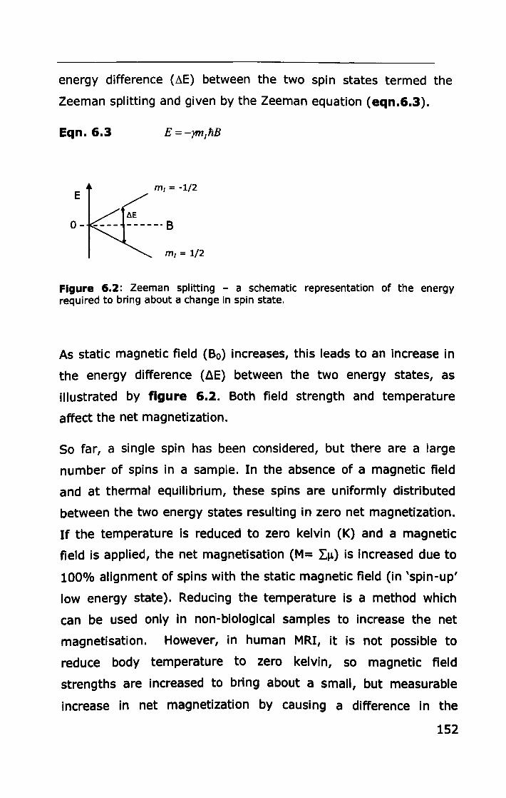
energy difference (~E) between the two spin states termed the

Zeeman splitting and given by the Zeeman equation (eqn.6.3).

Eqn. 6.3

E m1 = -1/2

0-

Figure 6.2: Zeeman splitting - a schematic representation of the energy required to bring about a change in spin state.

As static magnetic field (Bo) increases, this leads to an increase in

the energy difference (~E) between the two energy states, as

illustrated by figure 6.2. Both field strength and temperature

affect the net magnetization.

So far, a single spin has been considered, but there are a large

number of spins in a sample. In the absence of a magnetic field

and at thermal equilibrium, these spins are uniformly distributed

between the two energy states resulting in zero net magnetization.

If the temperature is reduced to zero kelvin (K) and a magnetic

field is applied, the net magnetisation (M= L~) is increased due to

1000/0 alignment of spins with the static magnetic field (in 'spin-up'

low energy state). Reducing the temperature is a method which

can be used only in non-biological samples to increase the net

magnetisation. However, in human MRI, it is not possible to

reduce body temperature to zero kelvin, so magnetic field

strengths are increased to bring about a small, but measurable

increase in net magnetization by causing a difference in the

152

populations of spins in the two energy levels. With an excess of

spins in the 'spin-up' state, this gives rise to a net magnetization

parallel to the static magnetic field (Bo) called the bulk or net

longitudinal magnetization (Mo). However, only a small proportional

of the spins are in the 'spin-up' state and so the net magnetisation

is very small. For protons at 3T and 300K, 10 parts per million

(ppm) of the total spins are in the 'spin-up' state which is aligned

with the static field. By applying RF pulses this magnetisation can

be knocked into the xy-plane perpendicular to Bo, this is known as

the transverse plane and the corresponding magnetisation the

transverse magnetisation (Mxy).

6.1.1.1 Excitation: radio frequency pulse

When a subject is placed in a magnetic field, such as that created

by an MR magnet, there is an excess of spins in the 'spin-up' state

resulting in net magnetization (Mo) which is parallel to the static

magnetic field (Bo). When the net magnetization of spins (Mo) is

parallel to the static magnetic field (Bo), the net magnetisation

cannot be measured because it is very small and swamped by the

static field (which is of the order of Tesla). Therefore, a

radiofrequency (RF) magnetic field of the appropriate

electromagnetic energy is applied to cause transitions of spins

between the Zeeman energy levels and knock the magnetisation

from the longitudinal plane (Mz) into the transverse plane (Mxy).

The energy of this RF pulse must match the Zeeman energy

splitting IlE =;#iBo = h{J) by applying an RF pulse of frequency (J) = rBo.

Thus these RF fields are not static, they rotate at the Larmor

frequency (COl,). The angle through which the magnetisation is

flipped (flip angle, a) is determined by the amplitude of the RF

153

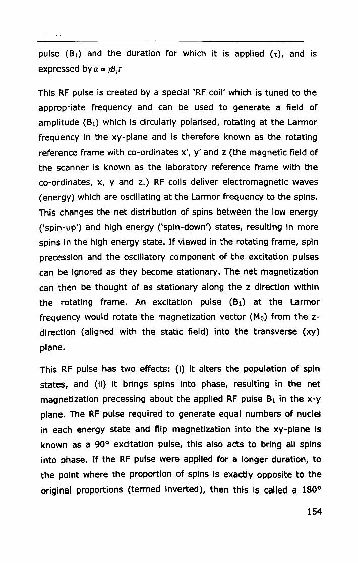
pulse (61) and the duration for which it is applied (t), and is

expressed bya = rBI'

This RF pulse is created by a special 'RF coil' which is tuned to the

appropriate frequency and can be used to generate a field of

amplitude (61) which is circularly polarised, rotating at the Larmor

frequency in the xy-plane and is therefore known as the rotating

reference frame with co-ordinates x', y' and z (the magnetic field of

the scanner is known as the laboratory reference frame with the

co-ordinates, x, y and z.) RF coils deliver electromagnetic waves

(energy) which are oscillating at the Larmor frequency to the spins.

This changes the net distribution of spins between the low energy

('spin-up') and high energy ('spin-down') states, resulting in more

spins in the high energy state. If viewed in the rotating frame, spin

precession and the oscillatory component of the excitation pulses

can be ignored as they become stationary. The net magnetization

can then be thought of as stationary along the z direction within

the rotating frame. An excitation pulse (81) at the Larmor

frequency would rotate the magnetization vector (Mo) from the z­

direction (aligned with the static field) into the transverse (xy)

plane.

This RF pulse has two effects: (i) it alters the population of spin

states, and (ii) it brings spins into phase, resulting in the net

magnetization precessing about the applied RF pulse 81 in the x-y

plane. The RF pulse required to generate equal numbers of nuclei

in each energy state and flip magnetization into the xy-plane is

known as a 900 excitation pulse, this also acts to bring all spins

into phase. If the RF pulse were applied for a longer duration, to

the point where the proportion of spins is exactly opposite to the

original proportions (termed inverted), then this is called a 1800

154

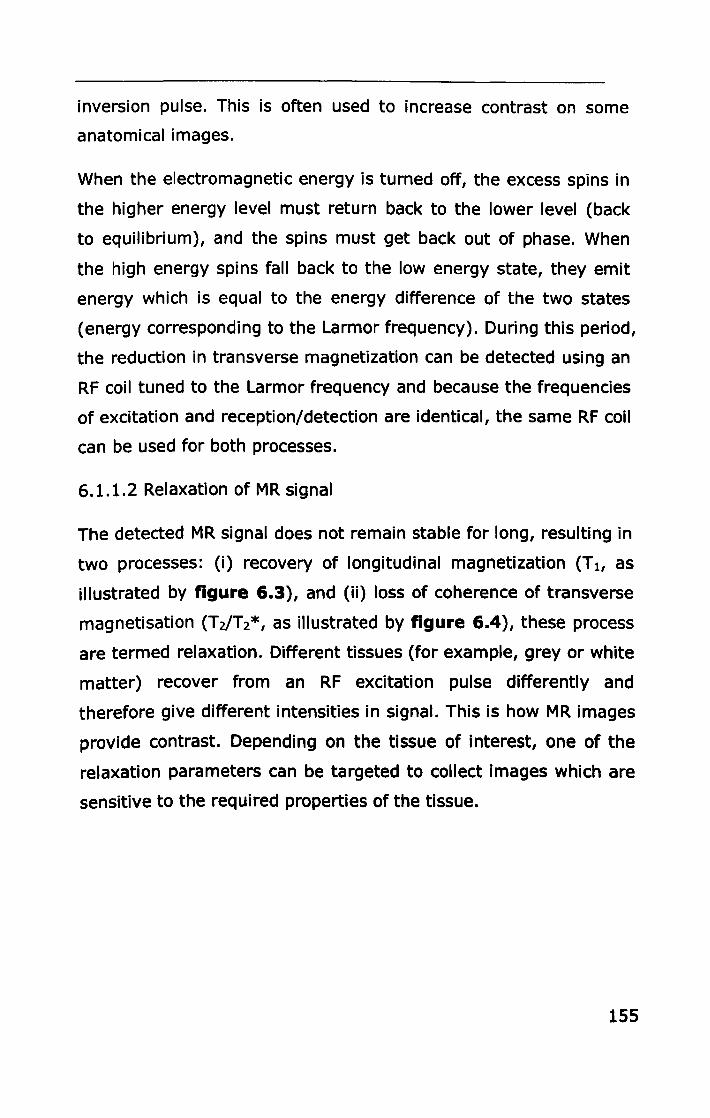
inversion pulse. This is often used to increase contrast on some

anatomical images.

When the electromagnetic energy is turned off, the excess spins in

the higher energy level must return back to the lower level (back

to equilibrium), and the spins must get back out of phase. When

the high energy spins fall back to the low energy state, they emit

energy which is equal to the energy difference of the two states

(energy corresponding to the Larmor frequency). During this period,

the reduction in transverse magnetization can be detected using an

RF coil tuned to the Larmor frequency and because the frequencies

of excitation and reception/detection are identical, the same RF coil

can be used for both processes.

6.1.1.2 Relaxation of MR signal

The detected MR signal does not remain stable for long, resulting in

two processes: (i) recovery of longitudinal magnetization (T 1, as

illustrated by figure 6.3), and (ii) loss of coherence of transverse

magnetisation (T 21T2*, as illustrated by figure 6.4), these process

are termed relaxation. Different tissues (for example, grey or white

matter) recover from an RF excitation pulse differently and

therefore give different intensities in signal. This is how MR images

provide contrast. Depending on the tissue of interest, one of the

relaxation parameters can be targeted to collect images which are

sensitive to the required properties of the tissue.

155

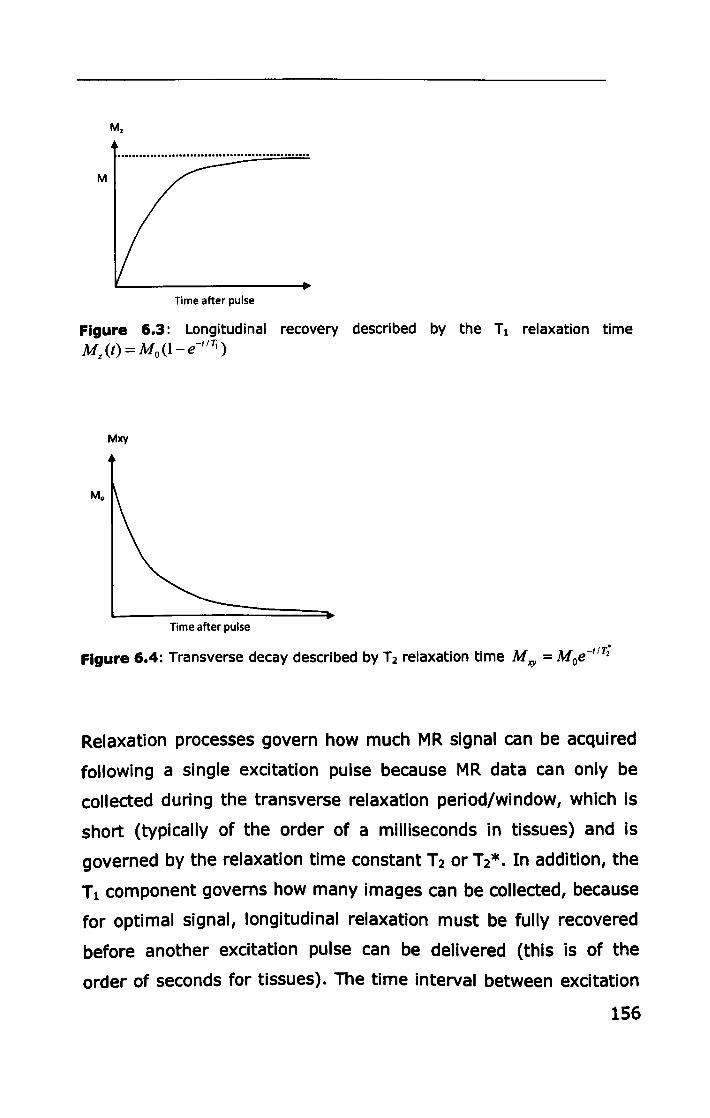
M,

..................................................... M

Time after pulse

Figure 6.3: Longitudinal recovery described by the T 1 relaxation time Mz{t) = Mo(l- e-tl1i

)

Mxy

Time after pulse

Figure 6.4: Transverse decay described by T2 relaxation time Mxy = Moe-tiT;

Relaxation processes govern how much MR signal can be acquired

following a single excitation pulse because MR data can only be

collected during the transverse relaxation period/window, which is

short (typically of the order of a milliseconds in tissues) and is

governed by the relaxation time constant T 2 or T 2*. In addition, the

Tl component governs how many images can be collected, because

for optimal signal, longitudinal relaxation must be fully recovered

before another excitation pulse can be delivered (this is of the

order of seconds for tissues). The time interval between excitation

156

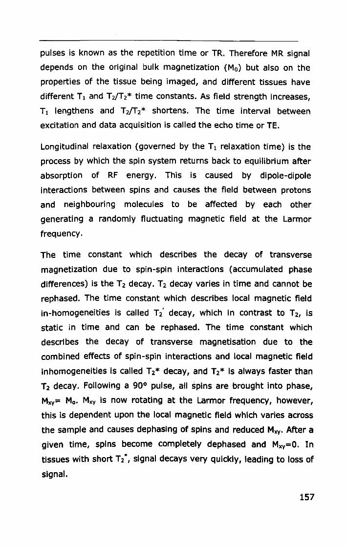
pulses is known as the repetition time or TR. Therefore MR signal

depends on the original bulk magnetization (Mo) but also on the

properties of the tissue being imaged, and different tissues have

different Tl and Tu'T2* time constants. As field strength increases,

T 1 lengthens and T u'T 2* shortens. The time interval between

excitation and data acquisition is called the echo time or TE.

Longitudinal relaxation (governed by the Tl relaxation time) is the

process by which the spin system returns back to equilibrium after

absorption of RF energy. This is caused by dipole-dipole

interactions between spins and causes the field between protons

and neighbouring molecules to be affected by each other

generating a randomly fluctuating magnetic field at the Larmor

frequency.

The time constant which describes the decay of transverse

magnetization due to spin-spin interactions (accumulated phase

differences) is the T2 decay. T2 decay varies in time and cannot be

rephased. The time constant which describes local magnetic field

in-homogeneities is called T2' decay, which in contrast to T2, is

static in time and can be rephased. The time constant which

descri bes the decay of transverse magnetisation due to the

combined effects of spin-spin interactions and local magnetic field

inhomogeneities is called T2* decay, and T2* is always faster than

T2 decay. Following a 90° pulse, all spins are brought into phase,

Mxy= Mo. Mxy is now rotating at the Larmor frequency, however,

this is dependent upon the local magnetic field which varies across

the sample and causes dephaslng of spins and reduced Mxy. After a

given time, spins become completely dephased and Mxy=O. In

tissues with short T 2 *, signal decays very quickly, leading to loss of

signal.

157

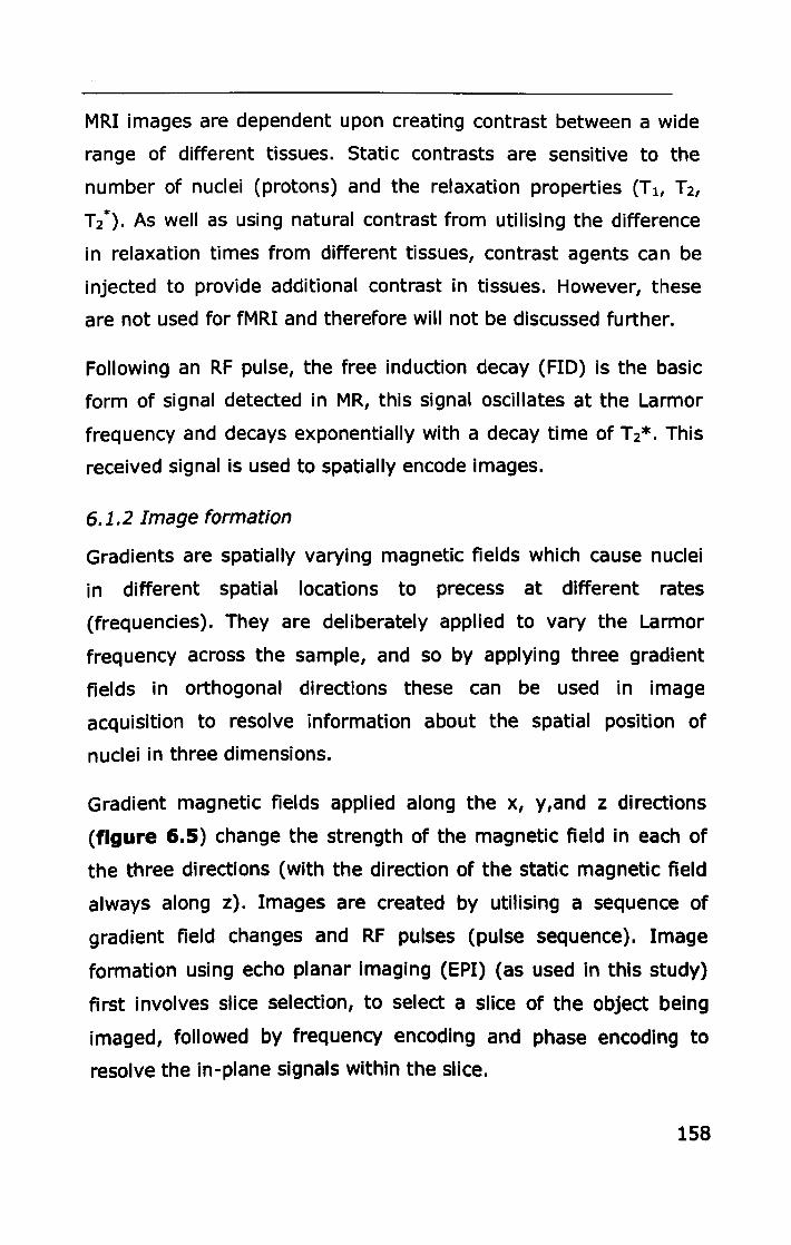
MRI images are dependent upon creating contrast between a wide

range of different tissues. Static contrasts are sensitive to the

number of nuclei (protons) and the relaxation properties (T 1, T2,

T2*)' As well as using natural contrast from utilising the difference

in relaxation times from different tissues, contrast agents can be

injected to provide additional contrast in tissues. However, these

are not used for fMRI and therefore will not be discussed further.

Following an RF pulse, the free induction decay (FlO) is the basic

form of signal detected in MR, this signal oscillates at the Larmor

frequency and decays exponentially with a decay time of T2*' This

received signal is used to spatially encode images.

6.1.2 Image formation

Gradients are spatially varying magnetic fields which cause nuclei

in different spatial locations to precess at different rates

(frequencies). They are deliberately applied to vary the Larmor

frequency across the sample, and so by applying three gradient

fields in orthogonal directions these can be used in image

acquisition to resolve information about the spatial position of

nuclei in three dimensions.

Gradient magnetic fields applied along the x, y,and z directions

(figure 6.5) change the strength of the magnetic field in each of

the three directions (with the direction of the static magnetic field

always along z). Images are created by utilising a sequence of

gradient field changes and RF pulses (pulse sequence). Image

formation using echo planar imaging (EPI) (as used in this study)

first involves slice selection, to select a slice of the object being

imaged, followed by frequency encoding and phase encoding to

resolve the in-plane signals within the slice.

158

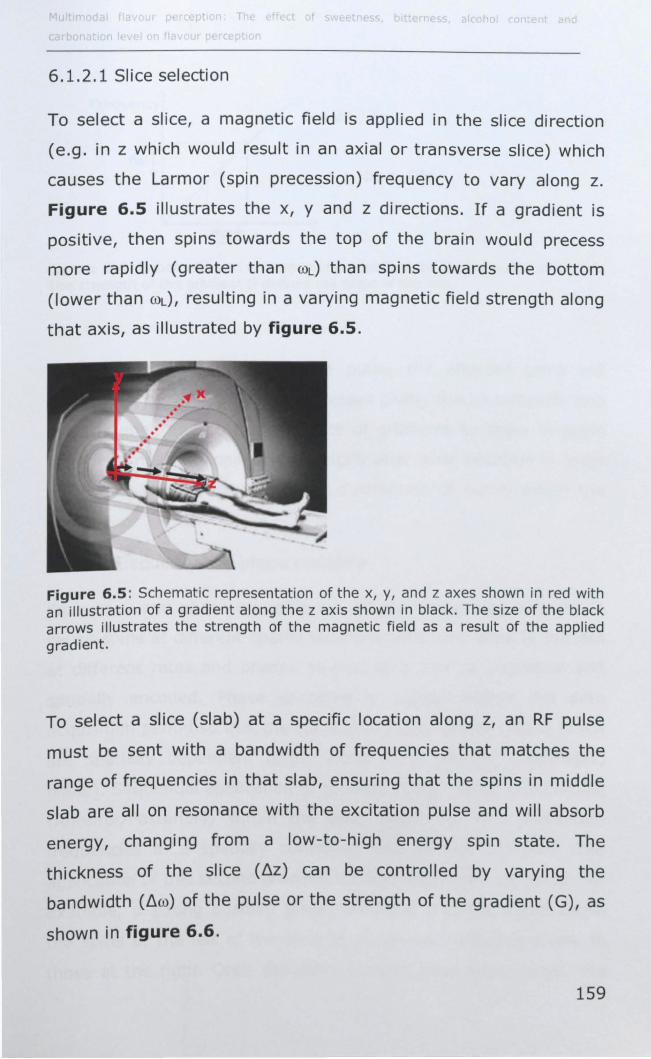
6.1.2.1 Slice selection

To select a slice, a magnetic field is applied in the slice direction

(e.g. in z which would result in an axial or transverse slice) which

causes the Larmor (spin precession) frequency to vary along z.

Figure 6.S illustrates the x, y and z directions. If a gradient is

positive, then spins towards the top of the brain would precess

more rapidly (greater than COL) than spins towards the bottom

(lower than COL), resulting in a varying magnetic field strength along

that axis, as illustrated by figure 6.S.

Figure 6.5: Schematic representation of the X, Y, and z axes shown in red with an illustration of a gradient along the z axis shown in black. The size of the black arrows illustrates the strength of the magnetic field as a result of the applied gradient.

To select a slice (slab) at a specific location along z, an RF pulse

must be sent with a bandwidth of frequencies that matches the

range of frequencies in that slab, ensuring that the spins in middle

slab are all on resonance with the excitation pulse and will absorb

energy, changing from a low-to-high energy spin state. The

thickness of the slice (ilz) can be controlled by varying the

bandwidth (ilco) of the pulse or the strength of the gradient (G), as

shown in figure 6.6.

159

Frequency G = dBzI dz

f).(j) = yGf).z

z

Figure 6.6: Schematic and corresponding equations to illustrate slice selection. The strength of the gradient G defines the slope of the line.

Immediately after the excitation pulse, the affected spins will

undergo Tl and T2 relaxation processes giving rise to complete loss

in MR signal, and so the sequence of gradients to apply in-plane

encoding must be applied very quickly after slice-selection in order

to resolve information about the distribution of nuclei within the

slice.

6.1.2.2 Frequency and phase encoding

Frequency and phase encoding are intertwined processes used to

cause spins at different spatial locations within the slice to precess

at different rates and phases so that they can be measured and

spatially encoded. Phase encoding is applied before the data

acquisition period so that the spins accumulate phase offsets which

are spatially dependent (e.g.: along x, in sagittal (Left/Right)

plane). Sequential application of gradients (e.g. along Y, in coronal

(Anterior/Posterior» within the slice alters the spin precession

frequencies in a spatially controlled way in that direction. The

application of this second gradient is called frequency encoding. For

example, a strong positive phase encoding gradient would cause

the spins at the left of the slice to accumulate different phase to

those at the right. Once the spins along x have been varied, the 160

application of another gradient along y will alter the frequency of

the spins and this is repeated. Phase and frequency encoding are

repeated until all signal across the slice has been collected.

Anatomical images are collected in this way but this can take tens

of seconds/minutes. Therefore, this method is not ideal for fMRI, as

images need to be acquired rapidly. The pulse sequence used for

fMRI (EPI) rapidly acquires images on the order of milliseconds,

and is described below.

6.1.2.3 EPI pulse sequence

K-space is the Fourier transform of image space. Converting k­

space data into an image is known as image reconstruction. In the

acquisition scheme described above each line of k-space is

acquired following an excitation pulse which is time consuming.

Echo planar imaging (EPI) uses fast switching of gradients to

collect all lines of K-space after a single RF excitation. EPI is a fast

and efficient encoding technique, acquiring an entire MR image in a

fraction of a second. This sequence has the advantage of temporal

resolution, but has coarser resolution compared to structural scans

and so cannot be used for anatomical detail and diagnosis. Instead,

this pulse sequence is fast enough to allow imaging of rapid

physiological changes in the human body and is therefore used in

functional MRI studies, with its contrast optimised to detect such

changes. The following sections describe how the changes in brain

physiology during sensory tasks can be utilised indirectly to collect

data on brain function (cortical activation).

161

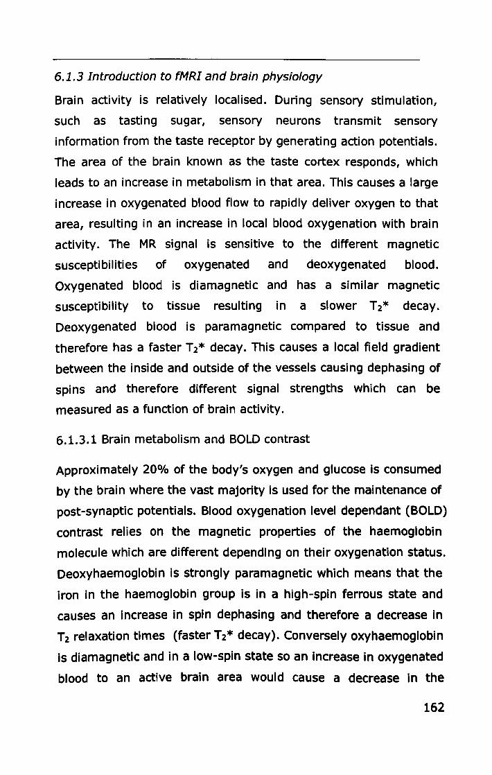
6.1.3 Introduction to fMRI and brain physiology

Brain activity is relatively localised. During sensory stimulation,

such as tasting sugar, sensory neurons transmit sensory

information from the taste receptor by generating action potentials.

The area of the brain known as the taste cortex responds, which

leads to an increase in metabolism in that area. This causes a large

increase in oxygenated blood flow to rapidly deliver oxygen to that

area, resulting in an increase in local blood oxygenation with brain

activity. The MR signal is sensitive to the different magnetic

susceptibilities of oxygenated and deoxygenated blood.

oxygenated blood is diamagnetic and has a similar magnetic

susceptibility to tissue resulting in a slower T2* decay.

Deoxygenated blood is paramagnetic compared to tissue and

therefore has a faster T 2* decay. This causes a local field gradient

between the inside and outside of the vessels causing dephasing of

spins and therefore different signal strengths which can be

measured as a function of brain activity.

6.1.3.1 Brain metabolism and BOLD contrast

Approximately 200/0 of the body's oxygen and glucose is consumed

by the brain where the vast majority is used for the maintenance of

post-synaptic potentials. Blood oxygenation level dependant (BOLD)

contrast relies on the magnetic properties of the haemoglobin

molecule which are different depending on their oxygenation status.

Deoxyhaemoglobi n is strongly paramagnetic which means that the

iron in the haemoglobin group is in a high-spin ferrous state and

causes an increase in spin dephasing and therefore a decrease in

T2 relaxation times (faster T2* decay). Conversely oxyhaemoglobin

is diamagnetic and in a low-spin state so an increase in oxygenated

blood to an active brain area would cause a decrease in the

162

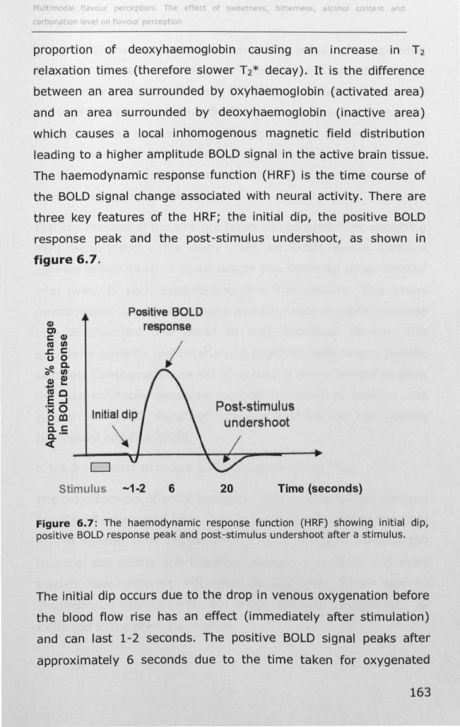
r f t f d

proportion of deoxyhaemoglobin causing an increase in T 2

relaxation times (therefore slower T 2* decay). It is the difference

between an area surrounded by oxyhaemoglobin (activated area)

and an area surrounded by deoxyhaemoglobin (inactive area)

which causes a local inhomogenous magnetic field distribution

leading to a higher amplitude BOLD signal in the active brain tissue.

The haemodynamic response function (HRF) is the time course of

the BOLD signal change associated with neural activity. There are

three key features of the HRF; the initial dip, the positive BOLD

response peak and the post-stimulus undershoot, as shown in

figure 6.7.

Q) C) C Q) ca en ,cC o 0 ~Q, o en Q) Q) +J~

cae E-I .- 0 ~al Q,C Co .-ct

Positive BOLD re pon e

Stimulus -1-2 6

Post-stimul us undershoot

20 Time (seconds)

Figure 6.7: The haemodynamic response function (HRF) showing initial dip, positive BOLD response peak and post-stimulus undershoot after a stimulus.

The initial dip occurs due to the drop in venous oxygenation before

the blood flow rise has an effect (immediately after stimulation)

and can last 1-2 seconds. The positive BOLD signal peaks after

approximately 6 seconds due to the time taken for oxygenated

163

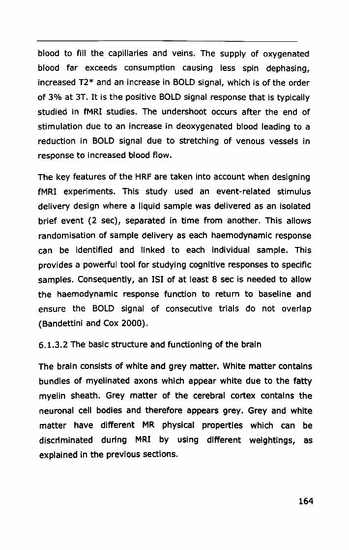
blood to fill the capillaries and veins. The supply of oxygenated

blood far exceeds consumption causing less spin dephasing,

increased T2* and an increase in BOLD signal, which is of the order

of 3% at 3T. It is the positive BOLD signal response that is typically

studied in fMRI studies. The undershoot occurs after the end of

stimulation due to an increase in deoxygenated blood leading to a

reduction in BOLD signal due to stretching of venous vessels in

response to increased blood flow.

The key features of the HRF are taken into account when designing

fMRI experiments. This study used an event-related stimulus

delivery design where a liquid sample was delivered as an isolated

brief event (2 sec), separated in time from another. This allows

randomisation of sample delivery as each haemodynamic response

can be identified and linked to each individual sample. This

provides a powerful tool for studying cognitive responses to specific

samples. Consequently, an lSI of at least 8 sec is needed to allow

the haemodynamic response function to return to baseline and

ensure the BOLD signal of consecutive trials do not overlap

(Bandettini and Cox 2000).

6.1.3.2 The basiC structure and functioning of the brain

The brain consists of white and grey matter. White matter contains

bundles of myelinated axons which appear white due to the fatty

myelin sheath. Grey matter of the cerebral cortex contains the

neuronal cell bodies and therefore appears grey. Grey and white

matter have different MR physical properties which can be

discriminated during MRI by using different weightings, as

explained in the previous sections.

164

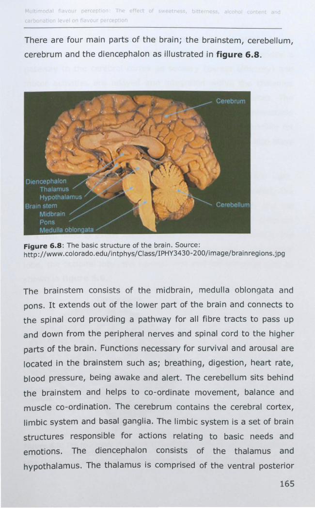
There are four main parts of the brain; the brainstem, cerebellum,

cerebrum and the diencephalon as illustrated in figure 6.8.

Figure 6.8: The basic structure of the brain. Source: http://www.colorado.edu/intphys/Class/IPHY3430-200/image/brainregions.jpg

The brainstem consists of the midbrain, medulla oblongata and

pons. It extends out of the lower part of the brain and connects to

the spinal cord providing a pathway for all fibre tracts to pass up

and down from the peripheral nerves and spinal cord to the higher

parts of the brain. Functions necessary for survival and arousal are

located in the brainstem such as; breathing, digestion, heart rate,

blood pressure, being awake and alert. The cerebellum sits behind

the brainstem and helps to co-ordinate movement, balance and

muscle co-ordination. The cerebrum contains the cerebral cortex,

limbic system and basal ganglia. The limbic system is a set of brain

structures responsible for actions relating to basic needs and

emotions. The diencephalon consists of the thalamus and

hypothalamus. The thalamus is comprised of the ventral posterior

165

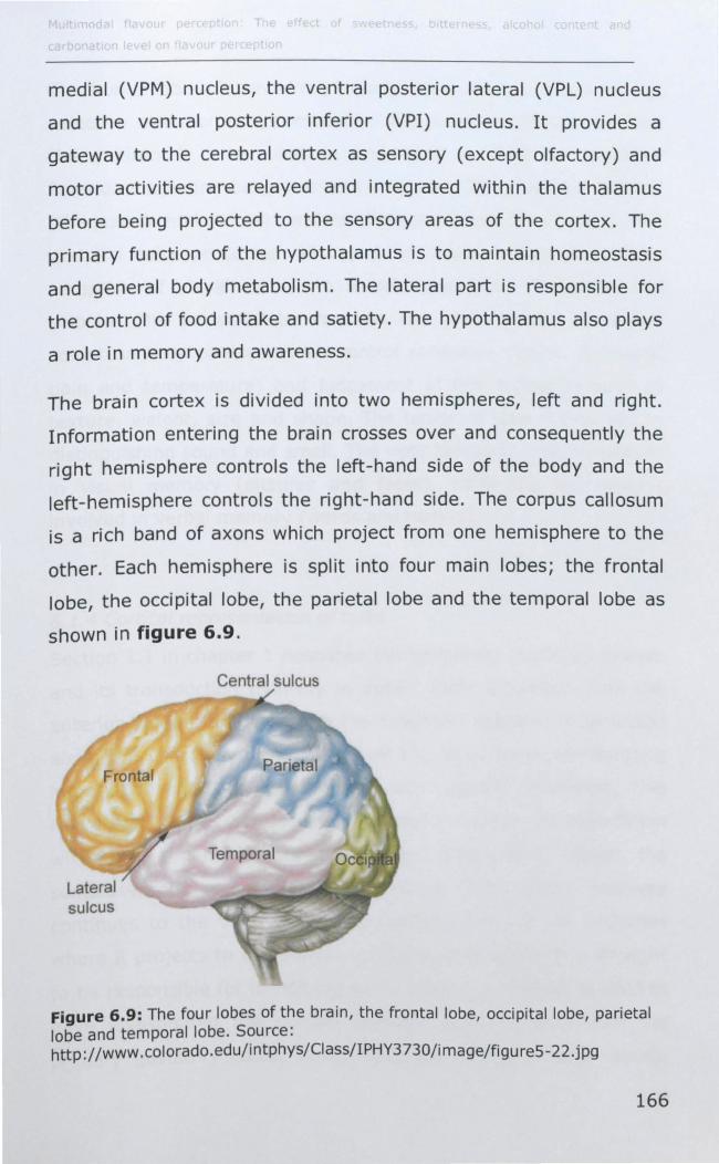
medial (VPM) nucleus, the ventral posterior lateral (VPL) nucleus

and the ventral posterior inferior (VPI) nucleus. It provides a

gateway to the cerebral cortex as sensory (except olfactory) and

motor activities are relayed and integrated within the thalamus

before being projected to the sensory areas of the cortex. The

primary function of the hypothalamus is to maintain homeostasis

and general body metabolism. The lateral part is responsible for

the control of food intake and satiety. The hypothalamus also plays

a role in memory and awareness.

The brain cortex is divided into two hemispheres, left and right.

Information entering the brain crosses over and consequently the

right hemisphere controls the left-hand side of the body and the

left-hemisphere controls the right-hand side. The corpus callosum

is a rich band ofaxons which project from one hemisphere to the

other. Each hemisphere is split into four main lobes; the frontal

lobe, the occipital lobe, the parietal lobe and the temporal lobe as

shown in figure 6.9.

Lateral sulcus

Central sulcus

Figure 6.9: The four lobes of the brain, the frontal lobe, occipital lobe, parietal lobe and temporal lobe. Source: http://www.colorado.edu/intphys/Class/IPHY3730/image/figures-22.jpg

166

The frontal lobe is involved in planning, organising, problem solving,

selective attention and personality. The anterior portion is called

the prefrontal cortex and is important for 'higher' cognitive

functions including behaviour and emotions. The posterior portion

(the post-frontal cortex) consists of premotor and motor areas. The

occipital lobe processes all types of visual information, from

reception of visual stimuli to visual recognition of shapes and

colours. The parietal lobe contains the primary and secondary

somatosensory cortices which control sensation (touch, pressure,

pain and temperature) and judgement of fine sensation such as

texture, weight, size and shape. The temporal lobe is involved in

distinguishing sound and smell. The right temporal lobe is involved

in visual memory (pictures and faces), while the left lobe is

involved in verbal memory (words and names).

6.1.4 Cortical representation of taste

Section 1.1 in chapter 1 describes the peripheral gustatory system

and its transduction pathway in detail. Taste activation from the

anterior tongue (and therefore the fungiform papillae) is projected

along the chorda tympani branch of the facial nerve transmitting

information about the taste quality and quantity (intenSity). This

nerve also carries somatosensory afferents which (in association

with the trigeminal nerve) provide information about the

somatosensory aspects of the stimulus. The central pathway

continues to the ventral-posterior-medial (VPM) of the thalamus

where it projects to the primary gustatory cortex which is thought

to be responsible for identifying taste quality. A number of studies

have investigated the cortical representation of taste with the

primary gustatory cortex being identified as the anterior insula,

167

frontal operculum (Kobayakawa, Endo et al. 1996) and postcentral

gyrus. Taste projections may then continue to the amygdala,

orbito-frontal cortex (OFC) (the secondary taste cortex) and

anterior cingulate cortex (ACC). The OFC and the ACC have been

associated with afferent aspects of taste (Francis, Rolls et al. 1999).

Therefore the main brain areas expected to be activated during

gustatory stimulation are; thalamus, insula cortex, amygdala, ACC

and the OFC. The anatomy of each is discussed below.

The thalamus, situated in the cerebellum at the top of the

brainstem, is considered the gateway to the cerebral cortex

because all sensory (except olfaction) and motor activities are

projected here before being received by their respective sensory

areas. The insula lay deep beneath the frontal, parietal and

temporal opercula surrounded by a sulcus that separates it from

the frontal, parietal and temporal lobes. It is subdivided into three

parts; anterior insula, mid-insula and the posterior insula. The

amygdala is a major component of the limbic system playing an

important role in the pleasure (Zald, Lee et al. 1998; O'Doherty,

Rolls et al. 2001) and the intenSity of food (Small, Gregory et al.

2003). The cingulate cortex is divided into anterior (ACC) and

posterior (PCC) portions. The ACC has been shown to have a

'hedonic' response to afferent aspects of food (Rolls; Zald, Lee et al.

1998; Francis, Rolls et al. 1999; de Araujo and Rolls 2004;

Grabenhorst, Rolls et al. 2007; Grabenhorst, Rolls et al. 2010). The

OFC is part of the ventral surface of the prefrontal cortex. It

receives input from gustatory, olfactory, somatosensory, visual and

auditory simulation and for this reason is considered a 'multimodal'

area (Rolls and Baylis 1994; Kadohisa, Rolls et al. 2004; Verhagen

and Engelen 2006; Rolls, Critchley et al. 2010). The OFC is termed

the secondary taste cortex (Baylis, Rolls et al. 1995) because it has

168

been discovered to act as a higher order taste centre involved in

emotional values of taste (Heinzel and Northoff 2009). For example,

the OFC has been found to respond to hunger but not satiety

(Haase, Cerf-Ducastel et al. 2009). However, subjects will not be in

a fasted state of hunger during scanning and therefore the

potential activation in the OFC in this study is unknown.

6.1.5 Cortical representation of trigeminal stimuli

The oral trigeminal system and the processing of somatosensory

(tactile, temperature and pain) stimuli experienced during food and

beverage consumption was reviewed in chapter 1, section 1.3. C02

dissolved in beverages elicits two somatosensory receptors; the

'tingle' of C02 is sensed by the nociceptors which detect pain, and

the tactile aspect of the bubbles is detected by the

mechanoreceptors. The pathway of both receptors leads ultimately

to the primary (51) and secondary (511) somatosensory cortices,

located in the postcentral gyrus which process somatosensory

information from the body. The surface of the body is

topographically represented in the primary somatosensory cortex

in a manner dependent on the density of the neurons. Neuron

density is greatest in the oral cavity (including lips) and hands, as

illustrated by the somatosensory homunculus (figure 6.10).

Somatosensory activation in the oral cavity (pharynx, tongue, jaw

and lips) is represented in the most ventral part of 51 (Tamura,

Shibukawa et al. 2008), lateral to 511.

169

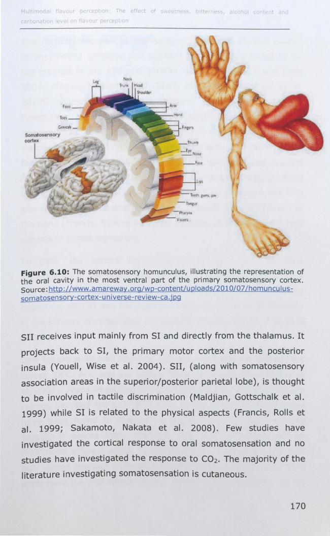
r p q n T rt

Figure 6.10: The somatosensory homunculus, illustrating the representation of the oral cavity in the most ventral part of the primary somatosensory cortex. Source: http://www . amareway.org/wp-content/u ploads/20 1 Ol07/homuncu lus­somatosensory-cortex-universe-review-ca.jpg

511 receives input mainly from 51 and directly from the thalamus. It

projects back to 51, the primary motor cortex and the posterior

insula (Youell, Wise et al. 2004). 511, (along with somatosensory

association areas in the superior/posterior parietal lobe), is thought

to be involved in tactile discrimination (Maldjian, Gottschalk et al.

1999) while 51 is related to the physical aspects (Francis, Rolls et

al. 1999; Sakamoto, Nakata et al. 2008). Few studies have

investigated the cortical response to oral somatosensation and no

studies have investigated the response to CO2 . The majority of the

literature investigating somatosensation is cutaneous.

170

The cortical response to oral texture (viscosity) elicited by fat,

carboxymethyl cellulose and alginate gel has been found to be

represented in the mid and anterior insula (de Araujo and Rolls

2004; Alonso, Marciani et al. 2007; Eldeghaidy, Marciani et al.

2010), somatosensory cortex (Alonso, Marciani et al. 2007;

Eldeghaidy, Marciani et al. 2010), rolandic operculum (Alonso,

Marciani et al. 2007), frontal operculum and amygdala (Eldeghaidy,

Marciani et al. 2010), and Ace (de Araujo and Rolls 2004;

Eldeghaidy, Marciani et al. 2010). The OFC was activated by oral

fat (de Araujo and Rolls 2004) but not by viscosity/texture elicted

by alginate gel (Alonso, Marciani et al. 2007). However, the OFC

was significantly activated by pleasant afferent aspects of touch to

the hand (Francis, Rolls et al. 1999) implying an role in the afferent

aspects of somatosensation.

To date, the cortical representation of pain has not been

investigated in the oral cavity. A study investigating pain from a

e02 laser on the calf showed activation in 51, 511, insula cortex and

thalamus, with SI and the thalamus being proposed to be involved

in the sensory discriminative components of pain (Youell, Wise et al.

2004).

Oral temperature was found to activate the insula, somatosensory

cortex, OFC, ACe and the ventral striatum (Guest, Grabenhorst et

al. 2007). Areas correlated to the pleasantness of oral temperature

ratings included the OFC and ACC. Given that both these areas

have been found to respond to pleasantness of other sensory

stimuli, it seems likely that the OFC and Ace could act as

multimodal afferent areas. Furthermore, activation in the OFC and

ACC during thermal stimulation to the hand was correlated with

unpleasant thermal stimuli (Rolls, Grabenhorst et al. 2008). In the

171

same study, SI and the posterior insula were correlated with

intensity but not pleasantness of thermal stimuli (Rolls,

Grabenhorst et al. 2008). Therefore the cortical areas that respond

to the affective value of thermal stimuli seem to be different to

those that respond to the intensity.

6.1.6 Effect of taster status on cortical activity

Taster status, as reviewed and investigated in the previous chapter

seems to impact on population differences in taste perception. To

date, only one study, which was also within our faculty, has

investigated the cortical response between PROP taster groups

using different fat levels in liquid emulsions as the stimuli. Results

showed a strong correlation of PROP taster status with cortical

response in the somatosensory areas supporting the theory that

super-tasters have greater somatosensory acuity (Eldeghaidy,

Marciani et al. 2010). Fourteen subjects took part in the study (S x

PROP non-tasters, 4 x PROP medium-tasters and S x super-tasters)

which allowed a correlation with PROP intensity to be assessed.

Whilst the combined group of 14 subjects is sufficient for a group

analysis of cortical activation correlated to fat, the differences

between PROP taster groups requires at least 10 subjects in each

group. The current study took a controlled approach to determine

the difference in cortical response between PROP taster groups

(PROP non-tasters, PROP medium-tasters and PROP super-tasters)

and thermal taster groups (thermal tasters and thermal non­

tasters).

172

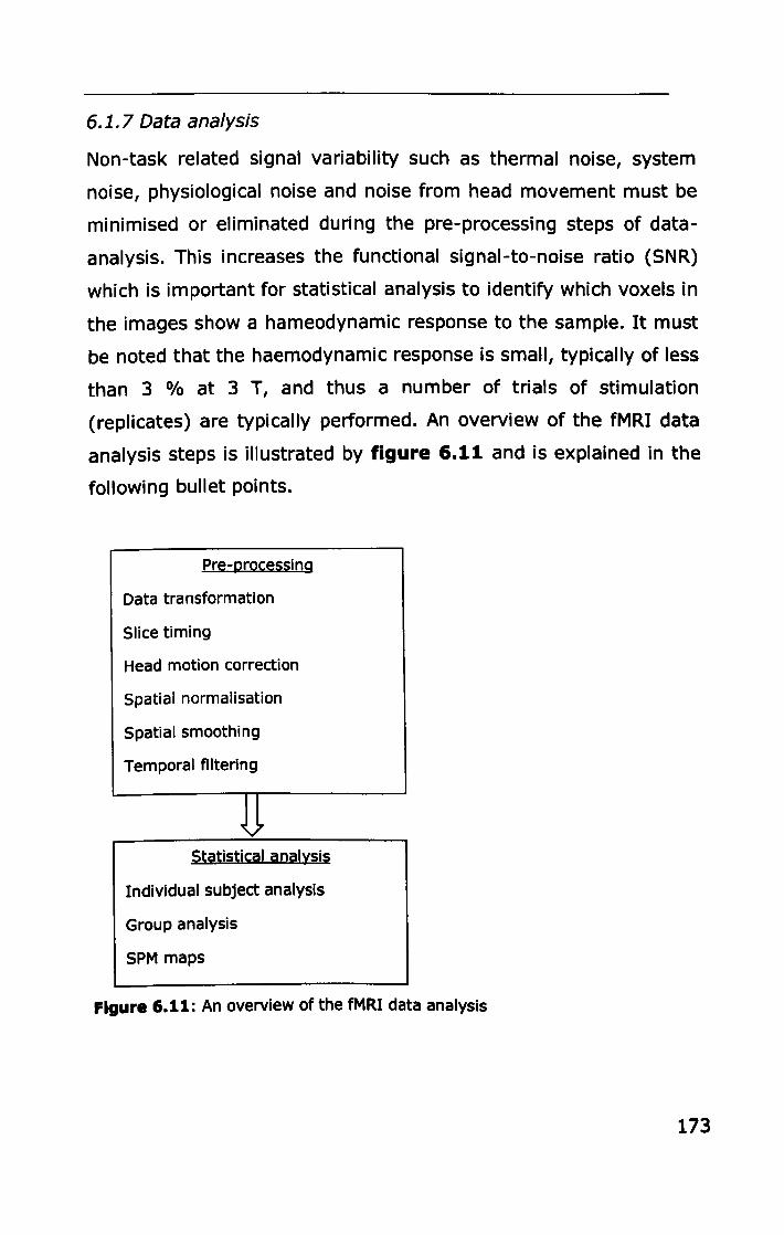
6.1.7 Data analysis

Non-task related signal variability such as thermal noise, system

noise, physiological noise and noise from head movement must be

minimised or eliminated during the pre-processing steps of data­

analysis. This increases the functional signal-to-noise ratio (SNR)

which is important for statistical analysis to identify which voxels in

the images show a hameodynamic response to the sample. It must

be noted that the haemodynamic response is small, typically of less

than 3 % at 3 T, and thus a number of trials of stimulation

(replicates) are typically performed. An overview of the fMRI data

analysis steps is illustrated by figure 6.11 and is explained in the

following bullet pOints.

Pre-processing

Data transformation

Slice timing

Head motion correction

Spatial normalisation

Spatial smoothing

Temporal filtering

JJ Statistical analysis

Individual subject analysis

Group analysis

SPM maps

Figure 6.11: An overview of the fMRI data analysis

173

• Data transformation: Data is first transformed from K-space

into image space.

• Slice timing correction: Slices are acquired at slightly

different times which can cause a phase shift in the BOLD

haemodynamic response. Therefore slice timing correction

shifts each voxel's time series (within a slice) to a reference

slice so that all voxels in the same volume appear to be

acquired at the same time.

• Head motion correction: small head movements during

scanning can lead to a change in the same voxel's location

over the fMRI time series. Motion correction eliminates the

extent of the head motion across the time series by

comparing it to a reference image using a 6-parameter rigid

body correction. All images are then realigned to the

reference image. The transformations should be scrutinised

for excessive motion. Any subject moving more than one

voxel should be removed from the study.

• Spatial normalisation: In fMRI studies, data is usually

collected from a number of subjects (typically 10-12) and a

group map is formed. However, individual brains differ in

shape, size and orientation so the data from each subject is

transformed to a standard 'template' space so that group

activation maps can be formed. The most commonly used

template spaces are the Montreal Neurological Institute (MNI

space) and Talairach space. MNI space was used in this study.

• Spatial smoothing: Spatial normalisation does not solve the

problem that subjects have different cortical organisation.

Spatial smoothing must therefore be applied to allow group

174

analysis of data to take place. This increases the likelihood of

overlapping activity across subjects by blurring the sharp

edges of the image which removes high spatial frequency

noise and consequently enhances SNR.

• Temporal filtering: A high pass temporal filter is applied to

remove unwanted slow varying signals in the fMRI time

series such as, scanner drift and physiological noise

(respiration and cardiac pulsation).

After the pre-processing steps are complete, each of the individual

subject's data sets can be subjected to statistical analysis. The

general linear model (GLM) is the most common way to analyse

fMRI data with many dependant variables. It assumes that the

BOLD responses can be linearly modelled by convolving the

stimulus waveform with the haemodynamic response function. The

experimental design is represented by a data matrix consisting of

rows of time pOints (volumes) in the BOLD time series and columns

of experimental stimuli/samples and confounds such as the

estimated motion parameters. Noise is independently distributed

across voxels and the resulting data is able to reliably identify

regions showing a significant experimental effect of interest.

In fMRI, there are two main forms of group statistical analysis,

fixed effects analysis (FFX) and random effects analysis (RFX). FFX

assumes that the experiment effect is constant and all subjects are

affected similarly by the stimulus, thereby only taking into account

the within subject variability. Conclusions can therefore only be

made about those particular subjects in the group using FFX. RFX

takes into account the variability across subjects as well as within

subject variability. Therefore conclusions about the population

(from which the subjects represent) can be made using this

175

method. In RFX, a design matrix and statistical analysis are

performed on each individual subject, (producing a statistical map

for each subject in each sample/condition). The statistical map

from each subject is then pooled for second level RFX analysis to

give a combined statistical map for the group (for the

sample/condition selected). The significantly activated areas which

overlap when the individual subject statistical maps are combined

at group level are shown as the statistically active areas. A

parametric test (T - or F- statistic) is carried out to test the

statistical significance of the activated voxels on a voxel-by-voxel

basis. The resulting T or F values are converted to z-scores and

probability (P) maps. The statistical parametric maps (SPMs) are

colour coded to show significant activation and superimposed onto

anatomical T 1 weighted images such as a MNI template. Data can

be displayed at uncorrected probability (typically p<O.OOl) or a

corrected probability (FWE or FOR) typically p<O.OS, which corrects

for false positives. Family wise error (FWE) rate controls the chance

of any false positives using random theory and is more

conservative than the false discovery rate (FOR) which is less strict

and controls the fraction of false positives.

The resulting data shows areas of the brain significantly activated

in response to the sample or stimulus, and brain structures can be

correlated to certain functions. The objectives of this study were to;

investigate the cortical activation to sweet taste as elicited by

dextrose and the effects of oral trigeminal stimulation elicited by

carbon dioxide (C02); compare the differences in cortical activation

between population groups with different oral sensitivity.

176

6.2 MATERIALS AND METHODS

6.2.1 Subjects

Procedures were conducted with University of Nottingham Medical

School ethics committee approval and written consent was

obtained from all subjects. Subjects were asked to complete an MR

scanner safety screening questionnaire (appendix 1) prior to the

scan session. Only those subjects who were considered 'MR safe'

were invited to take part in the study. From the 52 subjects

screened for PROP and thermal taster status in Chapter 5, 36

subjects (24 females, 12 males) were invited to take part in this

study comprising 12 PROP non-tasters (pNT's) (7 females,S males),

12 PROP medium-tasters (pMT's) (8 female, 4 male) and 12 PROP

super-tasters (pST's) (9 female, 3 male). Twelve subjects were

classified as thermal tasters (TT) (8 females, 4 males) and the first

12 of the remaining 24 thermal non-tasters (TnTs) scanned were

selected as the TnT group (7 females,S males). All 36 subjects

took part in the fMRI scan session. Subjects were in the scanner for

approximately 1 hour. The whole session lasted approximately 2

hours including study explanation and behavioural assessments. A

disturbance allowance was paid to those subjects who participated.

6.2.2 Stimuli

Three samples, differing only in their C02 level were prepared by

dissolving 70g/L of polydextrose (Utesse® Ultra powder, Danisco

Sweeteners, New Century, KS, USA) and 30g/L of dextrose

(MyProtein, Manchester, UK) into mineral water (Danone, Paris,

France) and mixed on a roller bed for 6h to ensure full dispersion.

Samples were refrigerated until they reached 60C (:1). The

177

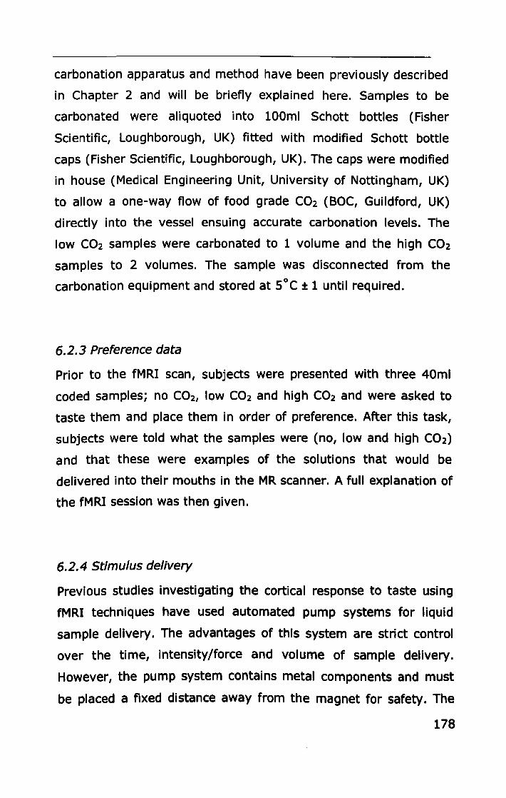
carbonation apparatus and method have been previously described

in Chapter 2 and will be briefly explained here. Samples to be

carbonated were aliquoted into 100ml Schott bottles (Fisher

Scientific, Loughborough, UK) fitted with modified Schott bottle

caps (Fisher SCientific, Loughborough, UK). The caps were modified

in house (Medical Engineering Unit, University of Nottingham, UK)

to allow a one-way flow of food grade C02 (BOC, Guildford, UK)

directly into the vessel ensuing accurate carbonation levels. The

low C02 samples were carbonated to 1 volume and the high C02

samples to 2 volumes. The sample was disconnected from the

carbonation equipment and stored at SoC ± 1 until required.

6.2.3 Preference data

Prior to the fMRI scan, subjects were presented with three 40ml

coded samples; no C02, low C02 and high C02 and were asked to

taste them and place them in order of preference. After this task,

subjects were told what the samples were (no, low and high C02)

and that these were examples of the solutions that would be

delivered into their mouths in the MR scanner. A full explanation of

the fMRI session was then given.

6.2.4 Stimulus delivery

Previous studies investigating the cortical response to taste using

fMRI techniques have used automated pump systems for liquid

sample delivery. The advantages of this system are strict control

over the time, intensity/force and volume of sample delivery.

However, the pump system contains metal components and must

be placed a fixed distance away from the magnet for safety. The

178

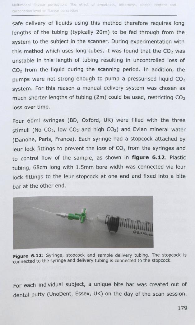
safe delivery of liquids using this method therefore requires long

lengths of the tubing (typically 20m) to be fed through from the

system to the subject in the scanner. During experimentation with

this method which uses long tubes, it was found that the C02 was

unstable in this length of tubing resulting in uncontrolled loss of

C02 from the liquid during the scanning period. In addition, the

pumps were not strong enough to pump a pressurised liquid CO2

system. For this reason a manual delivery system was chosen as

much shorter lengths of tubing (2m) could be used, restricting CO 2

loss over time.

Four 60ml syringes (BD, Oxford, UK) were filled with the three

stimuli (No C02, low C02 and high C02) and Evian mineral water

(Danone, Paris, France). Each syringe had a stopcock attached by

leur lock fittings to prevent the loss of C02 from the syringes and

to control flow of the sample, as shown in figure 6.12. Plastic

tubing, 68cm long with 1.5mm bore width was connected via leur

lock fittings to the leur stopcock at one end and fixed into a bite

bar at the other end.

Figure 6.12: Syringe, stopcock and sample delivery tubing. The stopcock is connected to the syringe and delivery tubing is connected to the stopcock.

For each individual subject, a unique bite bar was created out of

dental putty (UnoDent, Essex, UK) on the day of the scan session.

179

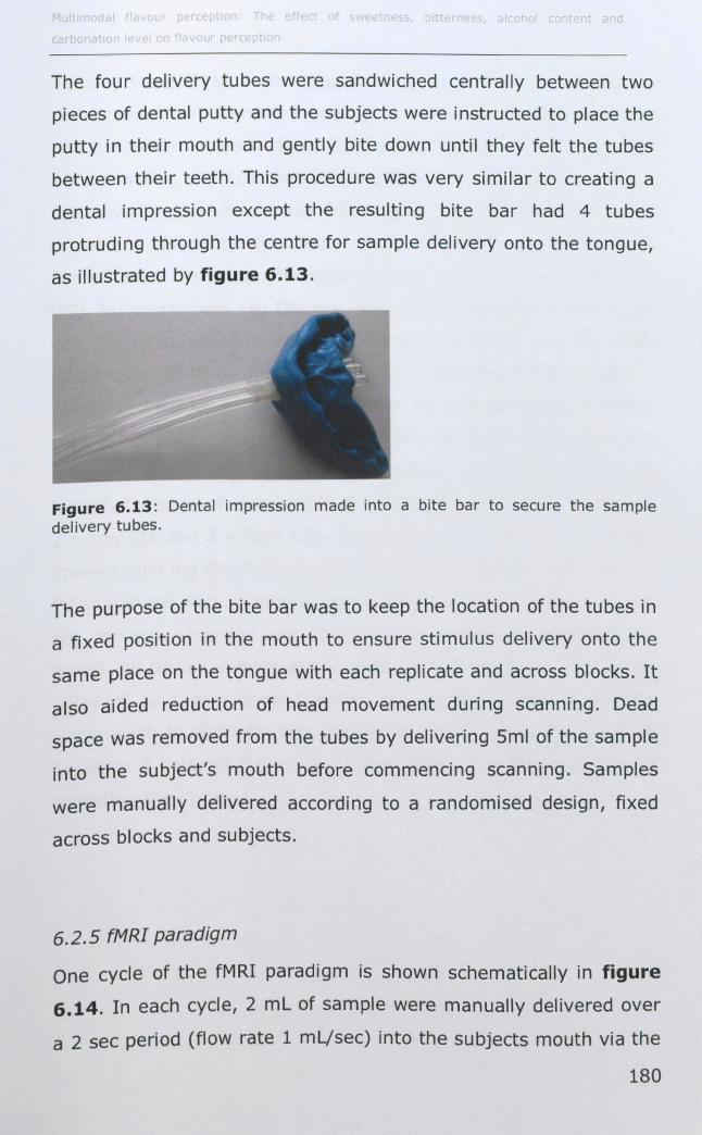
The four delivery tubes were sandwiched centrally between two

pieces of dental putty and the subjects were instructed to place the

putty in their mouth and gently bite down until they felt the tubes

between their teeth. This procedure was very similar to creating a

dental impression except the resulting bite bar had 4 tubes

protruding through the centre for sample delivery onto the tongue,

as illustrated by figure 6.13.

Figure 6.13: Dental impression made into a bite bar to secure the sample delivery tubes.

The purpose of the bite bar was to keep the location of the tubes in

a fixed position in the mouth to ensure stimulus delivery onto the

same place on the tongue with each replicate and across blocks. It

also aided reduction of head movement during scanning. Dead

space was removed from the tubes by delivering Sml of the sample

into the subject's mouth before commencing scanning. Samples

were manually delivered according to a randomised design, fixed

across blocks and subjects.

6.2.5 fMRI paradigm

One cycle of the fMRI paradigm is shown schematically in figure

6.14. In each cycle, 2 mL of sample were manually delivered over

a 2 sec period (flow rate 1 mL/sec) into the subjects mouth via the

180

delivery tubes fixed in the subject's bite bar. Samples differing in

carbonation level were delivered in a random order, the order of

which was fixed in each block. Each block consisted of 10 x No C02,

10 x low C02 and lOx high C02 samples. Subjects were cued to

swallow after the sample was delivered by a visual cue (small cross)

presented immediately after each stimulus delivery using

Presentation Software (Neurobehavioral System, San Fransisco,

US). Subjects could see the cue via a mirror attached to the head

coil. To minimise visual stimulation from the visual cue, the cross

was presented throughout the paradigm and altered from white to

purple to instruct subjects to swallow. All subjects were provided

with a MR compatible button box with three buttons. On the cue

following swallowing, subjects were asked to press a button to

identify the level of carbonation in the sample received, 1 = No C02,

2 = low C02 and 3 = high C02. The responses were collected in the

Presentation log file. Following the delivery of each stimulus, 1ml of

Evian mineral water (Danone, Paris, France) was delivered over a 1

sec period to clear the oral cavity of any lingering stimulus (water

wash). All stimuli and the water wash were delivered at 6°C ±1. A

delay of 12 s was given between the stimulus delivery and the

water wash to allow for data acquisition and the HRF to return to

baseline. A delay of 7.S s was allowed after the water wash before

repeating the cycle.

181

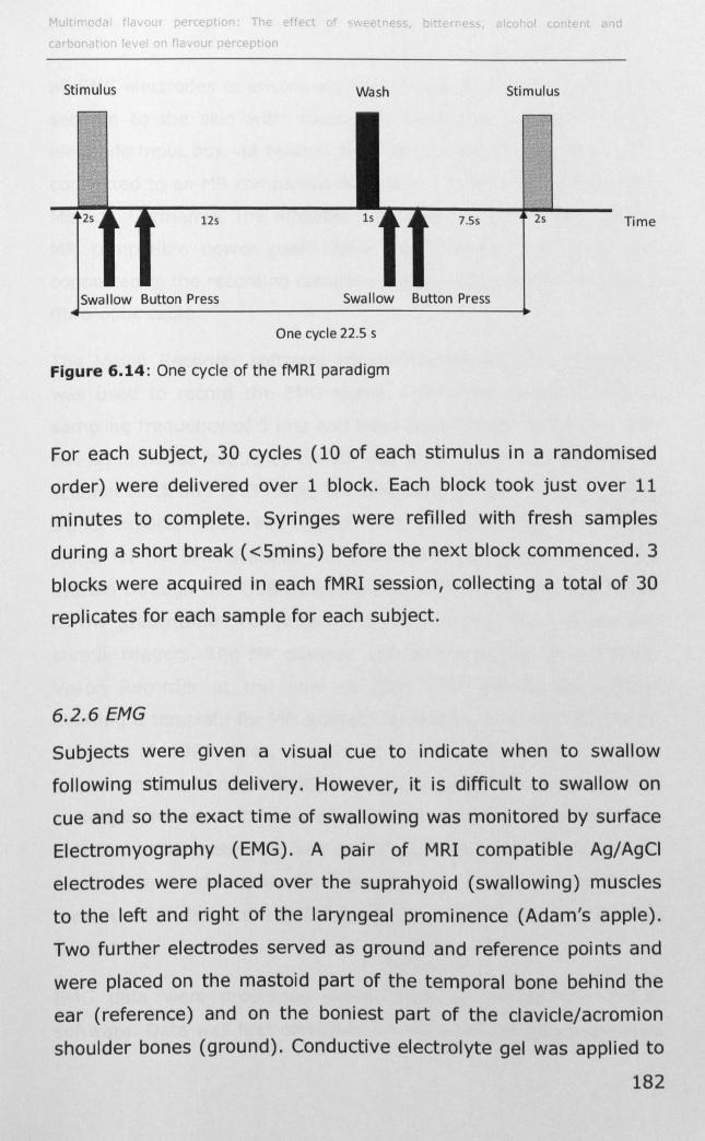
Mu t oda f 0 T ff t f b tt r c t nt d

carbonat

Stimulus Wash Stimulus

125 7.55 25 Time

Swallow Button Press Swallow Button Press

One cycle 22.5 s

Figure 6.14 : One cycle of the fMRI paradigm

For each subject, 30 cycles (10 of each stimulus in a randomised

order) were delivered over 1 block. Each block took just over 11

minutes to complete. Syringes were refilled with fresh samples

during a short break «5mins) before the next block commenced. 3

blocks were acquired in each fMRI session, collecting a total of 30

replicates for each sample for each subject.

6.2.6 EMG

Subjects were given a visual cue to indicate when to swallow

following stimulus delivery. However, it is difficult to swallow on

cue and so the exact time of swallowing was monitored by surface

Electromyography (EMG). A pair of MRI compatible Ag/AgCI

electrodes were placed over the suprahyoid (swallowing) muscles

to the left and right of the laryngeal prominence (Adam's apple).

Two further electrodes served as ground and reference pOints and

were placed on the mastoid part of the temporal bone behind the

ear (reference) and on the boniest part of the clavicle/acromion

shoulder bones (ground). Conductive electrolyte gel was applied to

182

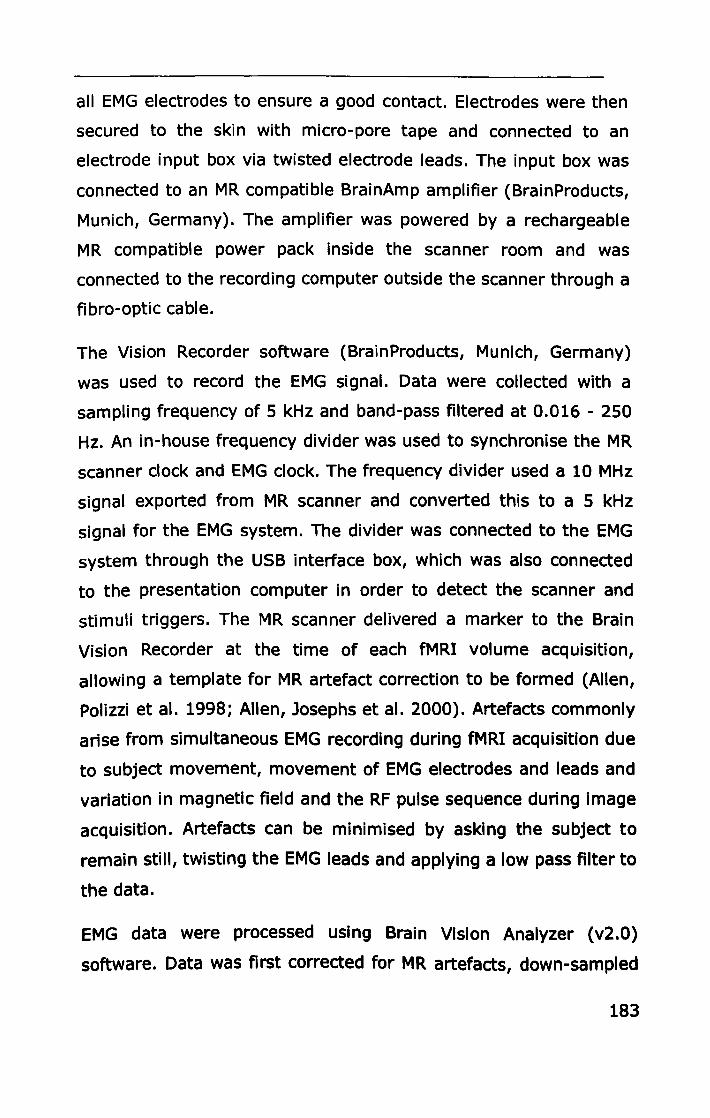
all EMG electrodes to ensure a good contact. Electrodes were then

secured to the skin with micro-pore tape and connected to an

electrode input box via twisted electrode leads. The input box was

connected to an MR compatible BrainAmp amplifier (BrainProducts,

Munich, Germany). The amplifier was powered by a rechargeable

MR compatible power pack inside the scanner room and was

connected to the recording computer outside the scanner through a

fibro-optic cable.

The Vision Recorder software (BrainProducts, Munich, Germany)

was used to record the EMG signal. Data were collected with a

sampling frequency of 5 kHz and band-pass filtered at 0.016 - 250

Hz. An in-house frequency divider was used to synchronise the MR

scanner clock and EMG clock. The frequency divider used a 10 MHz

signal exported from MR scanner and converted this to a 5 kHz

signal for the EMG system. The divider was connected to the EMG

system through the USB interface box, which was also connected

to the presentation computer in order to detect the scanner and

stimuli triggers. The MR scanner delivered a marker to the Brain

Vision Recorder at the time of each fMRI volume acquisition,

allowing a template for MR artefact correction to be formed (Allen,

Polizzi et aJ. 1998; Allen, Josephs et aJ. 2000). Artefacts commonly

arise from simultaneous EMG recording during fMRI acquisition due

to subject movement, movement of EMG electrodes and leads and

variation in magnetic field and the RF pulse sequence during image

acquisition. Artefacts can be minimised by asking the subject to

remain still, twisting the EMG leads and applying a low pass filter to

the data.

EMG data were processed using Brain Vision Analyzer (v2.0)

software. Data was first corrected for MR artefacts, down-sampled

183

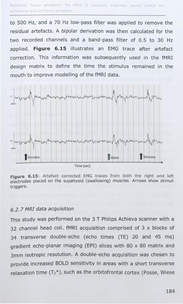
to 500 Hz, and a 70 Hz low-pass filter was applied to remove the

residual artefacts. A bipolar derivation was then calculated for the

two recorded channels and a band-pass filter of 0.5 to 30 Hz

applied. Figure 6.15 illustrates an EMG trace after artefact

correction. This information was subsequently used in the fMRI

design matrix to define the time the stimulus remained in the

mouth to improve modelling of the fMRI data.

I I twater t Stimulus

)

Time (sec)

Figure 6.15: Artefact corrected EMG traces from both the right and left electrodes placed on the supahyoid (swallowing) muscles. Arrows show stimuli triggers.

6.2.7 MRI data acquisition

This study was performed on the 3 T Philips Achieva scanner with a

32 channel head coil. fMRI acquisition comprised of 3 x blocks of

34 transverse double-echo (echo times (TE) 20 and 45 ms)

gradient echo-planar imaging (EPI) slices with 80 x 80 matrix and

3mm isotropic resolution. A double-echo acquisition was chosen to

provide increased BOLD sensitivity in areas with a short transverse

relaxation time (T2*). such as the orbitofrontal cortex (Posse, Wiese

184

et al. 1999; Marciani, Pfeiffer et al. 2006; Gowland and Sowtell

2007)

The volume repetition time (TR) was 2.5 s (jittered). Padding was

used where necessary to minimise head movements. A T 1 weighted

MPRAGE anatomical image comprising of 160 slices with 256 x 256

matrix and lmm isotropic resolution was acquired. Each MRI

session lasted approximately 2 hours including scanner set-up and

briefing for each subject.

6.2.8 MRI Data analysis

All fMRI data was processed using SPMS (Statistical Parametric

Mapping, Wellcome Department of Imaging Neuroscience;

www.fil.ion.ucl.ac.uk/spm). Three blocks of data were collected for

each subject: a, band C. The following pre-processing steps were

carried out for each subject (36 subjects in total) and each block (3

blocks per subject) totalling 108 data sets. The orientations of

images from both echo time data sets were set to the AC-PC pOint.

The first echo images were then realigned to correct for motion and

the realignment transforms applied to the second echo data sets.

Each realignment plot was individually visually inspected for excess

motion (greater than a voxel) during each acquisition block. A

weighted summation (Posse, Wiese et al. 1999) of the double echo

fMRI data set was then performed based on the average T2* in

each voxel, as determined by averaging across the fMRI data set

for each echo data set. Each first echo data set was then

normalised to a standard template in MNI space, and the weighted

data then moved to this space. The weighted data set was then

smoothed with an 8-mm full width half-maximum (FWHM) isotropic

185

Gaussian kernel to improve the signal-to-noise ratio and to account

for anatomical differences between subjects in the group analysis.

After pre-processing was complete, a general linear model was

formed for each subject which would combine sample replicates

across blocks to give one individual map of activated areas for each

sample (no C02, low C02 and high C02), and all samples combined

(all) representing the average response to CO2 and taste combined.

Convolution of the haemodynamic response function (HDF) with

the stimulus onset and the time of swallow (from the EMG traces)

were carried out for each individual and each block. The water

wash and the button press onset were included in the design

matrix as covariates of no interest. The individual subject-stimuli

maps were then combined at a random effects (RFX) group level to

assess the difference in brain activity between PROP and thermal

population groups (group analysis). These SPM maps were then

subjected to the following statistical analysis.

A one-sample t-test was created for each sample and all samples

combined resulting in 4 group maps (p FDR< 0.05) for each

stimulus (No C02, low C02, high C02 and 'all') in each population

group. For example; 4 group maps for PROP non-tasters (pNTs), 4

group maps for PROP medium-tasters (pMTs) and so on. Significant

activity was shown at FDR <0.05. In a second step, a linear (1st

order) parametric modulation using C02 concentration as the

modulation parameter was adopted to identify areas of the brain

showing haemodynamic response that increased (positive

correlation) or decreased (negative correlation) linearly with C02

concentration. An explicit mask of all attributes of oral perception

(p<0.05) was applied as a priori areas of interest and significant

activity was shown at P<O.OOl uncorrected. A 2-sample t-test was

186

carried out between groups for each sample to determine any

significant difference in strength of activation (BOLD response)

between the groups (P< 0.01 uncorrected). Paired t-tests were

carried out within groups to determine which samples (no C02, low

C02, high C02) significantly differed in their activation (P<O.Ol

uncorrected) .

6.2.B.l Region of Interest (ROI) analysis

The variability of BOLD activations within and across the different

taste phenotype groups was assessed by calculating the activation

strength (T-scores) in 7 brain regions of interest (ROls). The ROls

were anatomically defined by the WFU PickAtlas tool in 5PM5 and a

mask was created for each region and hemisphere. The following

masks were created;

• 51 (mouth) defined as an Bmm sphere centred at 60, -6, 20

• 511 defined as Brodmann area (BA) 43 dilated by 1

• Insula which was sub-divided into anterior-insula defined by

an Bm sphere centred at 40, 10, -2; mid-insula defined as an

Bm sphere centred at 40, 0, 0; posterior insula defined by an

Bmm sphere, dilated by 1 centred at 44, -32, 12

• Thalamus, determined anatomically (aal)

• ACC defined by a 14mm sphere, dilated by 1 and centred at

2, -10, 56

• Amygdala, determined anatomically (aal)

187

• OFC which was subdivided into lateral-OFC defined as an

Smm sphere centred at 2S, 30, -10 and medial-OFC defined

as an Smm sphere centred at 6, 44, -2.

T-scores from each ROI were interrogated for each group and each

stimulus using an in-house program written by Dr. Susan Francis.

6.2.S.2 Behavioural data

Behavioural data of discrimination of C02 level was analysed by

calculating the percentage number of correctly identified stimuli for

each subject and associated d' values (Ennis 1993). 0' is a

measure of sensitivity representing probability of correct responses

for that group. A value over 1 represents an ability to discriminate

(Lawless and Heymann 2010). Significant differences between d'

values between groups were calculated using the student t-test.

Samples were ranked by each subject for preference, ranging from

most preferred to least preferred. The quantity of subjects who

most and least preferred each sample was determined in each

group and was compared against the other groups.

6.3 RESULTS

No data had to be discarded due to excessive motion as all

realignment plots were within one voxel.

Thirty six subjects (12 males, 24 females) took part in the scanning

sessions of which 12 (5 males, 7 females) were PROP non-tasters

(pNTs), 12 (4 males, S females) were medium tasters (pMTs) and

12 (3 males, 9 females) were super-tasters (pSTs). Of the 36

subjects, a total of 24 (12 thermal tasters (TTs) and 12 thermal

non-tasters (TnTs» formed the thermal taster groups. The

188

remaining 12 subjects were TnTs but only the first 12 of that group

to be scanned were selected to form the TnT group analysis. This

ensures a balanced design for data analysis so that group

comparisons can be made. In the TT group (4 males, 8 females), 4

were pNTs, 6 were pMTs and 2 were pSTs. In the TnT group (5

males, 7 females), 4 were pNTs, 6 were pMTs and 2 were pSTs.

Table 6.1 shows a summary of the subject's gender and their

taster status (PROP or thermal) group classifications.

189

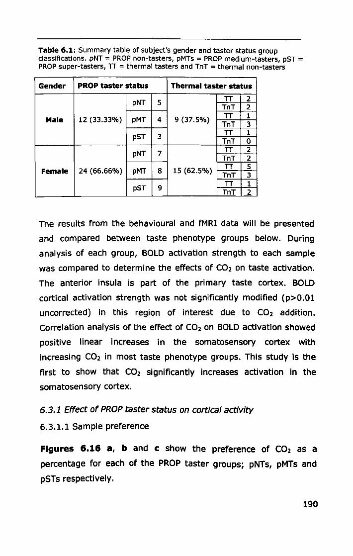
Table 6.1: Summary table of subject's gender and taster status group classifications. pNT = PROP non-tasters, pMTs = PROP medium-tasters, pST = PROP super-tasters, IT = thermal tasters and TnT = thermal non-tasters

Gender PROP taster status Thermal taster status

pNT 5 IT 2 TnT 2

Male 12 (33.33%) pMT 4 9 (37.5%) IT 1 TnT 3

pST 3 IT 1 TnT 0

pNT 7 IT 2 TnT 2

Female 24 (66.66%) pMT 8 15 (62.5%) TT 5 TnT 3

pST 9 TT 1

TnT 2

The results from the behavioural and fMRI data will be presented

and compared between taste phenotype groups below. During

analysis of each group, BOLD activation strength to each sample

was compared to determine the effects of C02 on taste activation.

The anterior insula is part of the primary taste cortex. BOLD

cortical activation strength was not Significantly modified (p>O.Ol

uncorrected) in this region of interest due to C02 addition.

Correlation analysis of the effect of C02 on BOLD activation showed

positive linear increases in the somatosensory cortex with

increasing C02 in most taste phenotype groups. This study is the

first to show that C02 significantly increases activation in the

somatosensory cortex.

6.3.1 Effect of PROP taster status on cortical activity

6.3.1.1 Sample preference

Figures 6.16 a, band c show the preference of C02 as a

percentage for each of the PROP taster groups; pNTs, pMTs and

pSTs respectively.

190

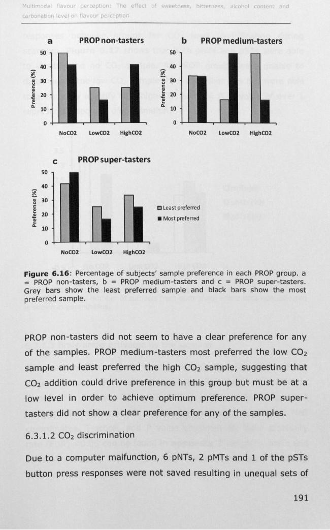
M tl od I vo r p rc pt on 1 e eH t f <; C;. bl tE r e

a 50

40

fl 30 c 2! G/ 20 ~ Q. 10

o

50

40

fl 30 c G/

~ 20 G/ ..

Q. 10

o

PROP non-tasters

NoC02 LowC02 HighC02

c PROP super-tasters

NoC02 LowC02 HighC02

50

40

fl 30 c 2! J!! 20 G/ .. Q. 10

o

b PROP medium-tasters

NoC02 LowC02 HighC02

C Least preferred

• Most preferred

Figure 6.16: Percentage of subjects' sample preference in each PROP group. a = PROP non-tasters, b = PROP medium-tasters and c = PROP super-tasters. Grey bars show the least preferred sample and black bars show the most preferred sample.

PROP non-tasters did not seem to have a clear preference for any

of the samples. PROP medium-tasters most preferred the low C02

sample and least preferred the high C02 sample, suggesting that

C02 addition could drive preference in this group but must be at a

low level in order to achieve optimum preference. PROP super­

tasters did not show a clear preference for any of the samples.

6.3.1.2 C02 discrimination

Due to a computer malfunction, 6 pNTs, 2 pMTs and 1 of the pSTs

button press responses were not saved resulting in unequal sets of

191

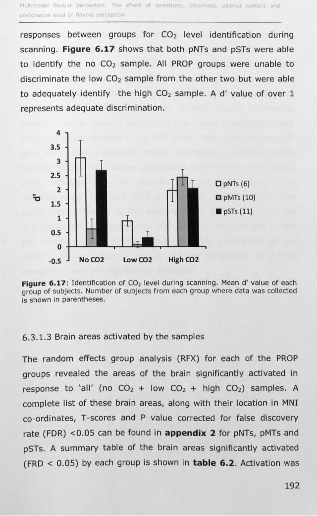
'vlultl odal favour p entlon T hoi ...

responses between groups for CO2 level identification during

scanning. Figure 6.17 shows that both pNTs and pSTs were able

to identify the no C02 sample. All PROP groups were unable to

discriminate the low C02 sample from the other two but were able

to adequately identify the high C02 sample. A d' value of over 1

represents adequate discrimination.

-"'C

4

3.5

3

2.5

2

1.5

1

0.5

o +--oL...-L...-

-0.5 No C02 Low C02 High C02

[J pNTs (6)

C pMTs (10)

• pSTs (11)

Figure 6.17: Identification of C02 level during scanning. Mean d' value of each group of subjects. Number of subjects from each group where data was collected is shown in parentheses.

6.3.1.3 Brain areas activated by the samples

The random effects group analysis (RFX) for each of the PROP

groups revealed the areas of the brain Significantly activated in

response to 'all' (no C02 + low C02 + high C02) samples. A

complete list of these brain areas, along with their location in MNI

co-ordinates, T -scores and P value corrected for false discovery

rate (FDR) <0.05 can be found in appendix 2 for pNTs, pMTs and

pSTs. A summary table of the brain areas Significantly activated

(FRD < 0.05) by each group is shown in table 6.2. Activation was

192

found in the somatosensory (51 and 511, and posterior insula,) and

taste (anterior insula, mid-insula, posterior insula, rolandic

operculum and frontal operculum) areas. It is interesting to note

that the orbito-frontal cortex (OFC) was not significantly activated

by the samples. Examining the differences between groups, the

somatosensory (51 and 511), taste (anterior-insula, mid-insula,

posterior-insula, rolandic operculum) and reward areas (ACC) were

activated by the samples in the pNT group. The somatosensory (51

and 511), taste (anterior-insula, mid-insula, posterior-insula,

rolandic operculum, frontal operculum) and reward areas (ACC)

were activated by the samples in the pMT group. The

somatosensory (51 and 511) and reward areas (ACC) were

significantly activated by the samples in the pST group. Only the

mid-insula from the taste area was Significantly activated in the

pST group, showing limited activation in the taste areas as the

anterior insula, posterior insula, rolandic operculum or frontal

operculum were not significantly activated.

193

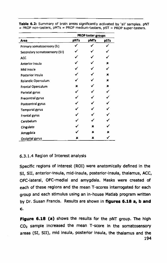
Table 6.2: Summary of brain areas significantly activated by 'all' samples. pNT = PROP non-tasters, pMTs = PROP medium-tasters, pST = PROP super-tasters.

PROP taster groups

Area pNTs pMTs pSTs

Primary somatosensory (51) ,/ ,/ ,/

Secondary somatosensory (SII) ,/ ,/ ,/

ACC ,/ ,/ ,/

Anterior insula ,/ ,/ X

Mid insula ,/ ,/ ,/

Posterior insula ,/ ,/ X

Rolandic Operculum ,/ ,/ X

Frontal Operculum X ,/ X

Parietal gyrus ,/ ,/ ,/

Precentral gyrus ,/ ,/ ,/

postcentral gyrus ,/ ,/ ,/

Temporal gyrus ,/ ,/ ,/

Frontal gyrus ,/ ,/ ,/

Cerebelum ,/ ,/ ,/

Cingulate ,/ X ,/

Amygdala ,/ X X

Occipital gyrus X X ,/

6.3.1.4 Region of Interest analysis

Specific regions of interest (ROI) were anatomically defined in the

SI, SII, anterior-insula, mid-insula, posterior-insula, thalamus, ACC,

OFC-Iateral, OFC-medial and amygdala. Masks were created of

each of these regions and the mean T -scores interrogated for each

group and each stimulus using an in-house Matlab program written

by Dr. Susan Francis. Results are shown in figures 6.18 a, band

c.

Figure 6.18 <a) shows the results for the pNT group. The high

C02 sample increased the mean T -score in the somatosensory

areas (SI, SII), mid insula, posterior insula, the thalamus and the 194

amygdala. The main taste area, (anterior insula) and the Ace seemed relatively unaffected by C02. Activation in the lateral OFC

was just above 0 and activation in the medial OFC was below 0 and

therefore ROI analysis shows that it was not activated by the

samples in this study.

195

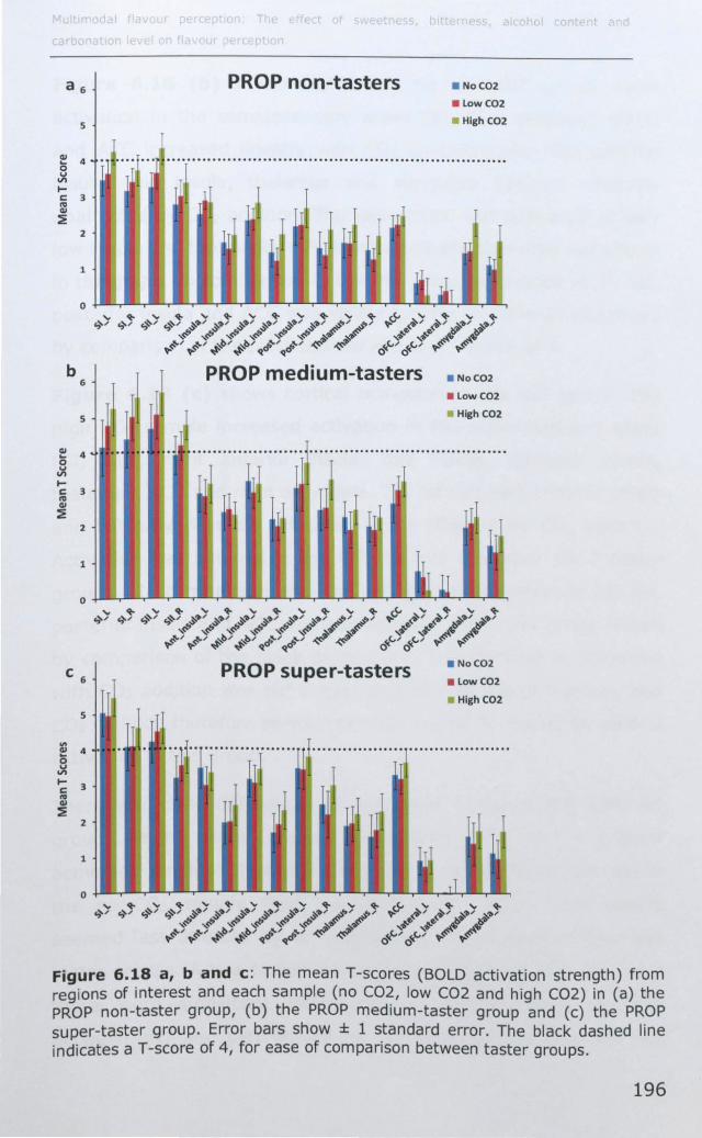
a 6

5

~ 4 o .;; l-e 3 ro CII

~ 2

1

b 6

5

2

1

C 6

5

II> CII 4 0 .;; l-e 3 ro CII ~

2

1

0

d

PROP non-tasters • No C02

• low C02

• High C02

~ .... , .................................................................. ..

~

r

" ~ c}, c},

PROP medium-tasters • NoC02

• low C02

t .................................................. ~~~.~~:. I ,

I

PROP super-tasters • NoC02

• low C02

High C02

Figure 6.18 a, band c: The mean T-scores (BOLD activation strength) from regions of interest and each sample (no C02, low C02 and high C02) in (a) the PROP non-taster group, (b) the PROP medium-taster group and (c) the PROP super-taster group. Error bars show ± 1 standard error. The black dashed line indicates a T-score of 4, for ease of comparison between taster groups.

196

Figure 6.18 (b) shows the results for the pMT group. Mean

activation in the somatosensory areas (51, 511), posterior insula

and ACC increased linearly with C02 concentration. The anterior

insula, mid insula, thalamus and amygdala seemed relatively

unaffected by C02 addition. The lateral OFC was activated at very

low levels and the medial OFC inactivated and therefore not shown

in the graph. In comparison to the pNT group, activation in 51, 511,

posterior insula and ACC was visibly greater in pMTs as illustrated

by comparison of the black dashed line at aT-score of 4.

Figure 6.18 (e) shows cortical activation in the pST group. The

high C02 sample increased activation in the somatosensory areas

(51, 511), right anterior insula, mid insula, posterior insula,

thalamus, ACC and right amygdala. The left 511, left anterior insula

and left amygdala did not seem to be affected by C02 addition.

Activation was minimal in the OFC as with the other PROP taster

groups. In comparison with the pNT group, activation in 51, 511,

posterior insula and ACC was much greater in the pST group shown

by comparison of the black dashed line. The increase in activation

with C02 addition was not linear, as shown in the pMT group, and

C02 addition therefore seemed to have less of an impact on cortical

activation in this group.

There are clear differences in activation between the different

groups. Both 'taster' groups (pMTs and pSTs) had a greater

activation strength (higher T-score) in the somatosensory areas to

the no C02 sample than the pNT group. PROP super-tasters

seemed less affected by an increase in C02 than the other two

taster groups. A two sample t-test was carried out to determine if

there were significant differences in the activation strength

between pNT and pMT groups for 'all' samples (no C02, low C02

197

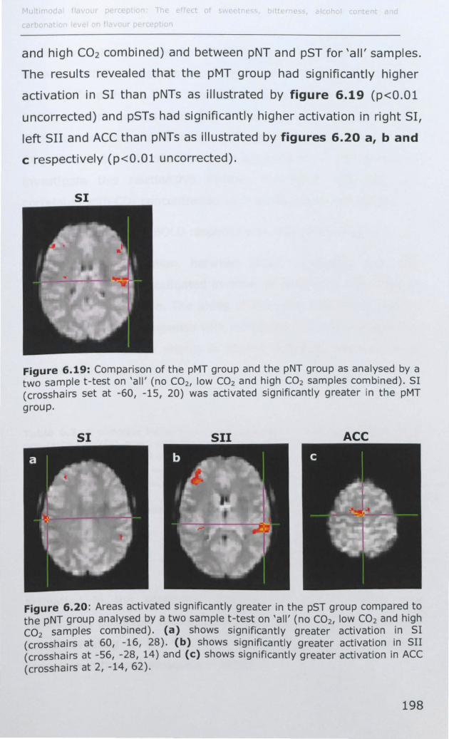
and high C02 combined) and between pNT and pST for 'all' samples.

The results revealed that the pMT group had Significantly higher

activation in 51 than pNTs as illustrated by figure 6.19 (p<O.Ol

uncorrected) and pSTs had significantly higher activation in right 51,

left 511 and ACe than pNTs as illustrated by figures 6.20 at band

c respectively (p<O.Ol uncorrected).

SI

Figure 6.19: Comparison of the pMT group and the pNT group as analysed by a two sample t-test on 'all' (no CO2 , low CO2 and high CO2 samples combined). 51 (crosshairs set at -60, -15, 20) was activated significantly greater in the pMT group.

51 SII ACC

Figure 6.20: Areas activated significantly greater in the pST group compared to the pNT group analysed by a two sample t-test on 'all' (no CO2, low CO2 and high C0 2 samples combined). (a) shows significantly greater activation in SI (crosshairs at 60, -16, 28). (b) shows significantly greater activation in SII (crosshairs at -56, -28, 14) and (e) shows significantly greater activation in ACC (crosshairs at 2, -14, 62).

198

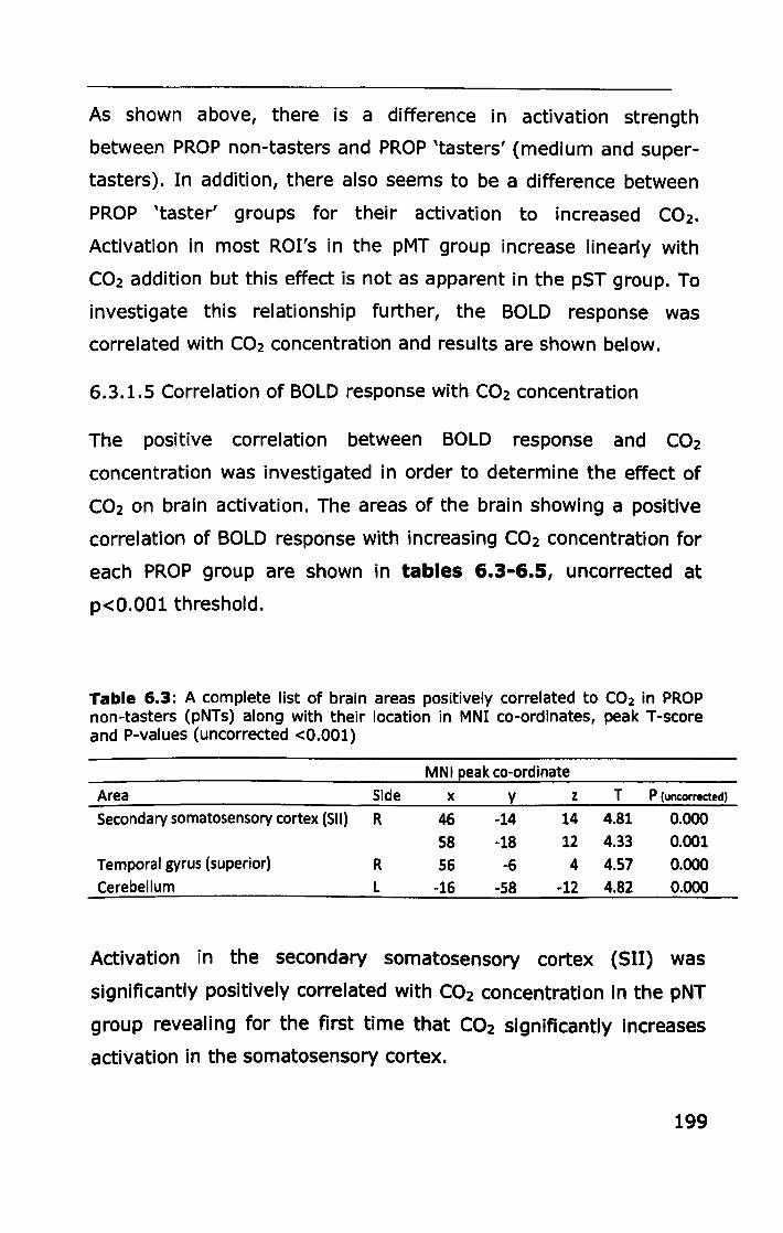
As shown above, there is a difference in activation strength

between PROP non-tasters and PROP 'tasters' (medium and super­

tasters). In addition, there also seems to be a difference between

PROP 'taster' groups for their activation to increased CO2.

Activation in most ROI's in the pMT group increase linearly with

C02 addition but this effect is not as apparent in the pST group. To

investigate this relationship further, the BOLD response was

correlated with C02 concentration and results are shown below.

6.3.1.5 Correlation of BOLD response with C02 concentration

The positive correlation between BOLD response and C02

concentration was investigated in order to determine the effect of

C02 on brain activation. The areas of the brain showing a positive

correlation of BOLD response with increasing C02 concentration for

each PROP group are shown in tables 6.3-6.5, uncorrected at

p<O.OOl threshold.

Table 6.3: A complete list of brain areas positively correlated to CO2 in PROP non-tasters (pNTs) along with their location in MNI co-ordinates, peak T -score and P-values (uncorrected <0.001)

MNI peak co-ordinate

Area 5ide x y z T P (uncorrected)

Secondary somatosensory cortex (511) R 46 -14 14 4.81 0.000

58 -18 12 4.33 0.001 Temporal gyrus (superior) R 56 -6 4 4.57 0.000 Cerebellum L -16 -58 -12 4.82 0.000

Activation in the secondary somatosensory cortex (511) was

significantly positively correlated with C02 concentration in the pNT

group revealing for the first time that C02 significantly increases

activation in the somatosensory cortex.

199

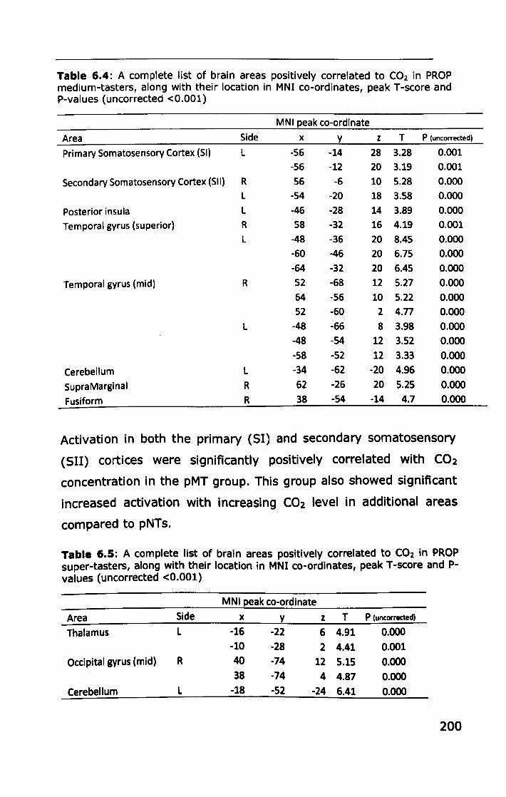
Table 6.4: A complete list of brain areas positively correlated to C02 in PROP medium-tasters, along with their location in MNI co-ordinates, peak T -score and P-values (uncorrected <0.001)

MNI peak co-ordinate

Area Side x y z T P (uncorrected)

Primary Somatosensory Cortex (51) L -56 -14 28 3.28 0.001

-56 -12 20 3.19 0.001

Secondary Somatosensory Cortex (511) R 56 -6 10 5.28 0.000

L -54 -20 18 3.58 0.000

Posterior insula L -46 -28 14 3.89 0.000

Temporal gyrus (superior) R 58 -32 16 4.19 0.001

L -48 -36 20 8.45 0.000 -60 -46 20 6.75 0.000

-64 -32 20 6.45 0.000

Temporal gyrus (mid) R 52 -68 12 5.27 0.000

64 -56 10 5.22 0.000 52 -60 2 4.77 0.000

L -48 -66 8 3.98 0.000 -48 -54 12 3.52 0.000

-58 -52 12 3.33 0.000

Cerebellum L -34 -62 -20 4.96 0.000

SupraMarginal R 62 -26 20 5.25 0.000

Fusiform R 38 -54 -14 4.7 0.000

Activation in both the primary (51) and secondary somatosensory

(511) cortices were Significantly positively correlated with C02

concentration in the pMT group. This group also showed significant

increased activation with increasing C02 level in additional areas

compared to pNTs.

Table 6.5: A complete list of brain areas positively correlated to C02 in PROP super-tasters, along with their location in MNI co-ordinates, peak T -score and P­values (uncorrected <0.001)

MNI peak co-ordinate

Area Side x y z T P (uncorrected)

Thalamus L -16 -22 6 4.91 0.000 -10 -28 2 4.41 0.001

Occipital gyrus (mid) R 40 -74 12 5.15 0.000 38 -74 4 4.87 0.000

Cerebellum L -18 -52 -24 6.41 0.000

200

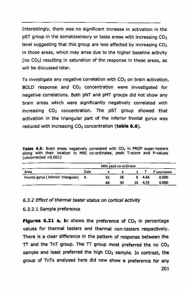
Interestingly, there was no significant increase in activation in the

pST group in the somatosensory or taste areas with increasing C02

level suggesting that this group are less affected by increasing C02

in those areas, which may arise due to the higher baseline activity

(no C02) resulting in saturation of the response in these areas, as

will be discussed later.

To investigate any negative correlation with C02 on brain activation,

BOLD response and C02 concentration were investigated for

negative correlations. Both pNT and pMT groups did not show any

brain areas which were significantly negatively correlated with

increasing C02 concentration. The pST group showed that

activation in the triangular part of the inferior frontal gyrus was

reduced with increasing C02 concentration (table 6.6).

Table 6.6: Brain areas negatively correlated with C02 in PROP super-tasters along with their location in MNI co-ordinates, peak T-score and P-values (uncorrected <0.001)

MNI peak co-ordinate

Area Side x y z Frontal gyrus ( Inferior triangular) R S2 38 8

44 30 16

6.3.2 Effect of thermal taster status on cortical activity

6.3.2.1 Sample preference

T P (uncorrected)

4.64 0.000 4.55 0.000

Figures 6.21 a, b: shows the preference of C02 in percentage

values for thermal tasters and thermal non-tasters respectively.

There is a clear difference in the pattern of response between the

TT and the TnT group. The TT group most preferred the no C02

sample and least preferred the high CO2 sample. In contrast, the

group of TnTs analysed here did now show a preference for any

201

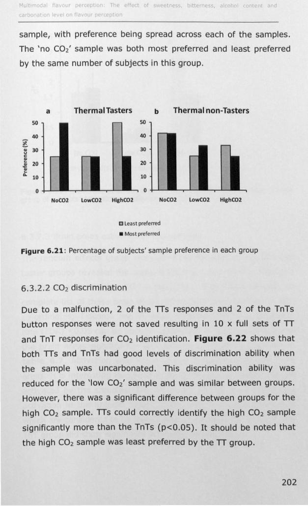
ML. t Ilod I flav lot perc plon Tt- ff ct of sweptncc;s, b ttern 5. al (''1 I ont t a 10

sample, with preference being spread across each of the samples.

The 'no C02' sample was both most preferred and least preferred

by the same number of subjects in this group.

a 50

40

~ Q/ 30 u C QI ...

20 ~ Q/ ... a.

10

0

NoC02

Thermal Tasters b Thermal non-Tasters 50

40

30

20

10

0

LowC02 HighC02 NoC02 LowC02 HighC02

C least preferred

• Most preferred

Figure 6.21: Percentage of subjects' sample preference in each group

6.3.2.2 C02 discrimination

Due to a malfunction, 2 of the TIs responses and 2 of the TnTs

button responses were not saved resulting in 10 x full sets of n and TnT responses for C02 identification. Figure 6.22 shows that

both TIs and TnTs had good levels of discrimination ability when

the sample was uncarbonated. This discrimination ability was

reduced for the 'low C02' sample and was similar between groups.

However, there was a significant difference between groups for the

high C02 sample. TIs could correctly identify the high C02 sample

significantly more than the TnTs (p<O.OS). It should be noted that

the high C02 sample was least preferred by the TI group.

202

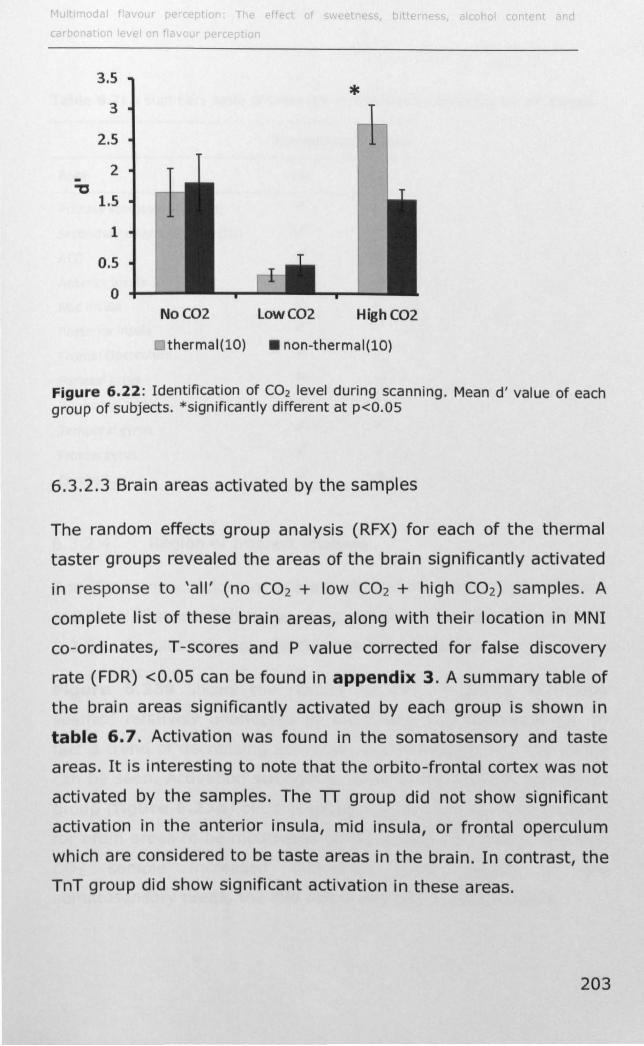
-'"D

3.5

3

2.5

2

1.5

1

0.5

o

r p T

*

No C02 low C02 High C02

. thermal(lO) • non-thermal(lO)

Figure 6.22: Identification of CO2 level during scanning. Mean d' value of each group of subjects. *significantly different at p<O.OS

6.3.2.3 Brain areas activated by the samples

The random effects group analysis (RFX) for each of the thermal

taster groups revealed the areas of the brain significantly activated

in response to 'all' (no C02 + low C02 + high C02) samples. A

complete list of these brain areas, along with their location in MNI

co-ordinates, T -scores and P value corrected for false discovery

rate (FDR) <0.05 can be found in appendix 3 . A summary table of

the brain areas significantly activated by each group is shown in

table 6.7. Activation was found in the somatosensory and taste

areas. It is interesting to note that the orbito-frontal cortex was not

activated by the samples. The n group did not show significant

activation in the anterior insula, mid insula, or frontal operculum

which are considered to be taste areas in the brain. In contrast, the

TnT group did show significant activation in these areas.

203

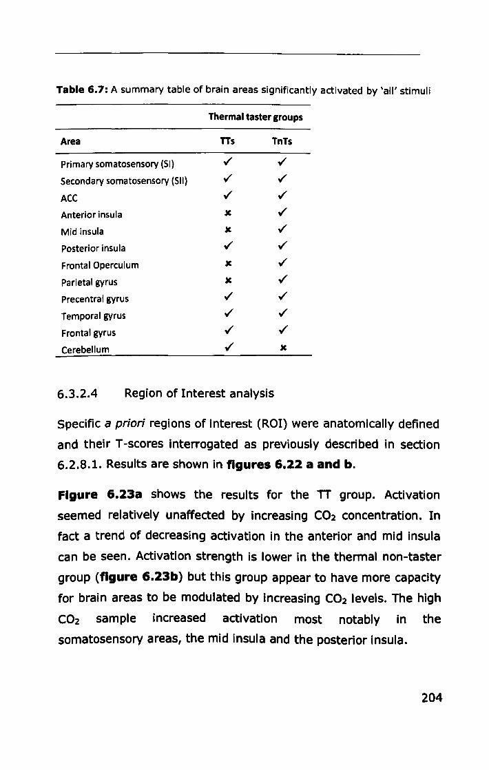
Table 6.7: A summary table of brain areas significantly activated by 'all' stimuli

Thermal taster groups

Area TTs TnTs

Primary somatosensory (SI) ./ ./

Secondary somatosensory (511) ./ ./

ACC ./ ./

Anterior insula JC ./

Mid insula JC ./

Posterior insula ./ ./

Frontal Operculum JC ./

Parietal gyrus JC ./

Precentral gyrus ./ ./

Temporal gyrus ./ ./

Frontal gyrus ./ ./

Cerebellum ./ JC

6.3.2.4 Region of Interest analysis

Specific a priori regions of interest (ROI) were anatomically defined

and their T -scores interrogated as previously described in section

6.2.8.1. Results are shown in figures 6.22 a and b.

Figure 6.23a shows the results for the TT group. Activation

seemed relatively unaffected by increasing C02 concentration. In

fact a trend of decreasing activation in the anterior and mid insula

can be seen. Activation strength is lower in the thermal non-taster

group (figure 6.23b) but this group appear to have more capacity

for brain areas to be modulated by increasing CO2 levels. The high

C02 sample increased activation most notably in the

somatosensory areas, the mid insula and the posterior insula.

204

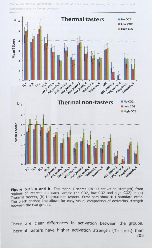
a 6

5

~ 4--o u VI ~ c 3 ra QI

~ 2

1

o

5

~ 4- --- --S V)

~ c 3 to QI

~ 2

1

o

Thermal tasters • No C02

• Low C02

• High C02

.................................................

Thermal non-tasters • NoC02

• Low C02

High C02

Figure 6.23 a and b: The mean T-scores (BOLD activation strength) from regions of interest and each sample (no C02, low C02 and high C02) in (a) Thermal tasters, (b) thermal non-tasters. Error bars show ± 1 standard error. The black dashed line allows for easy visual comparison of activation strength between the two groups.

There are clear differences in activation between the groups.

Thermal tasters have higher activation strength (T -scores) than 205

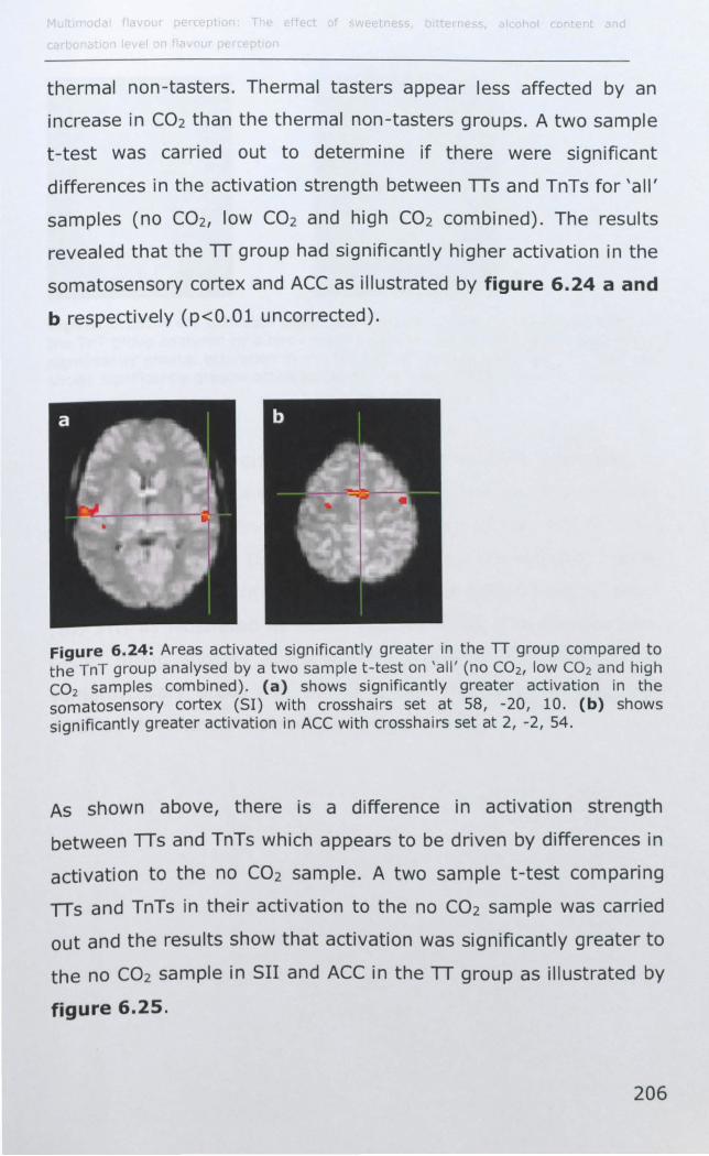
thermal non-tasters. Thermal tasters appear less affected by an

increase in C02 than the thermal non-tasters groups. A two sample

t-test was carried out to determine if there were significant

differences in the activation strength between TIs and TnTs for 'all'

samples (no C02, low C02 and high C02 combined). The results

revealed that the TI group had significantly higher activation in the

somatosensory cortex and ACC as illustrated by figure 6.24 a and

b respectively (p<O.Ol uncorrected).

Figure 6.24: Areas activated significantly greater in the TT group compared to the TnT group analysed by a two sample t-test on 'all' (no CO2, low CO2 and high C02 samples combined). (a) shows significantly greater activation in the somatosensory cortex (51) with crosshairs set at 58, -20, 10. (b) shows significantly greater activation in ACC with crosshairs set at 2, -2, 54.

As shown above, there is a difference in activation strength

between TIs and TnTs which appears to be driven by differences in

activation to the no C02 sample. A two sample t-test comparing

TTs and TnTs in their activation to the no C02 sample was carried

out and the results show that activation was significantly greater to

the no C02 sample in SII and Ace in the TT group as illustrated by

figure 6.25.

206

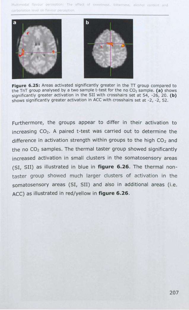
Figure 6.25: Areas activated significantly greater in the n group compared to the TnT group analysed by a two sample t-test for the no CO2 sample. (a) shows significantly greater activation in the SII with crosshairs set at 54, -26, 20. (b) shows significantly greater activation in ACC with crosshairs set at -2, -2, 52.

Furthermore, the groups appear to differ in their activation to

increasing C02. A paired t-test was carried out to determine the

difference in activation strength within groups to the high C02 and

the no C02 samples. The thermal taster group showed significantly

increased activation in small clusters in the somatosensory areas

(51, 511) as illustrated in blue in figure 6.26. The thermal non­

taster group showed much larger clusters of activation in the

somatosensory areas (51, 511) and also in additional areas (i.e.

ACC) as illustrated in red/yellow in figure 6.26.

207

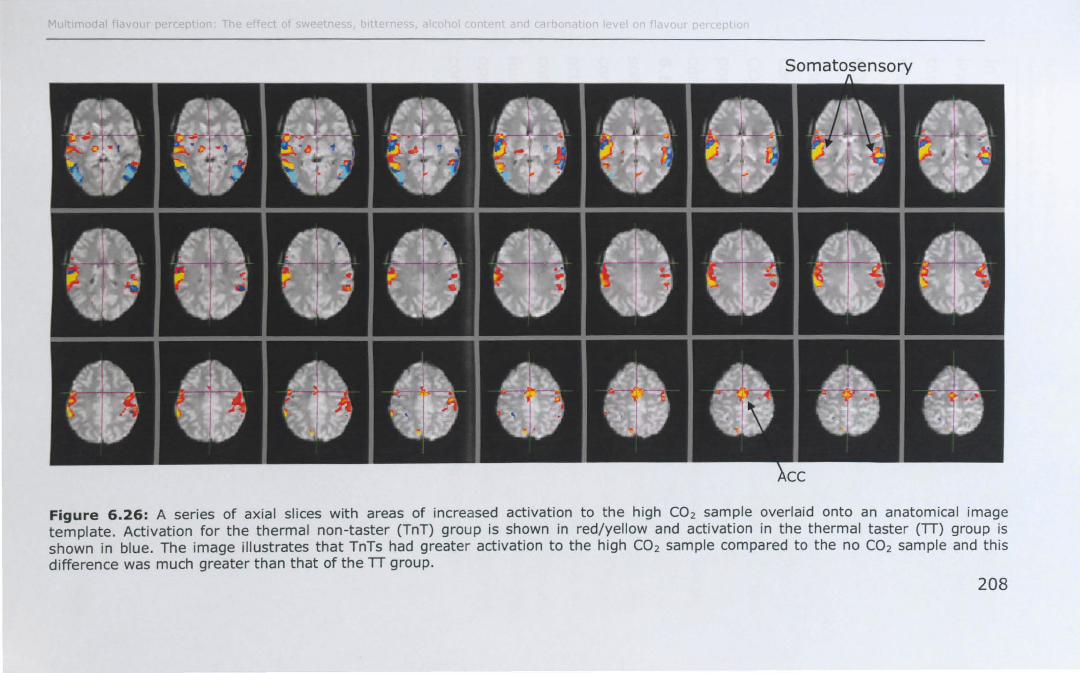
Somatosensory

Figure 6.26: A series of axial slices with areas of increased activation to the high CO 2 sample overlaid onto an anatomical image template. Activation for the thermal non-taster (TnT) group is shown in red/yellow and activation in the thermal taster (TT) group is shown in blue. The image illustrates that TnTs had greater activation to the high CO 2 sample compared to the no CO2 sample and this difference was much greater than that of the TT group.

208

In addition, activation in most ROI's in the TnT group increase

linearly with C02 addition. To investigate this relationship further,

the BOLD response was correlated with C02 concentration and

results are shown below.

6.3.2.5 Correlation of BOLD response with C02 concentration

The positive correlation between BOLD response and C02

concentration was calculated in order to investigate the effect of

C02 on brain activation further. The areas of the brain showing a

positive correlation of BOLD response with increasing CO2

concentration for each thermal taster group are shown in tables

6.8-6.9, uncorrected at p<O.OOl threshold. The secondary

somatosensory cortex (511) was positively correlated with C02

concentration in thermal tasters. More areas showed increased

activation with increasing C02 concentration in thermal non-tasters

compared to thermal tasters. Significant positive correlation was

found in the somatosensory areas, postcentral gyrus, rolandic

operculum and the ACC. No areas were significantly negatively

correlated with C02 level in either of the thermal taster groups.

209

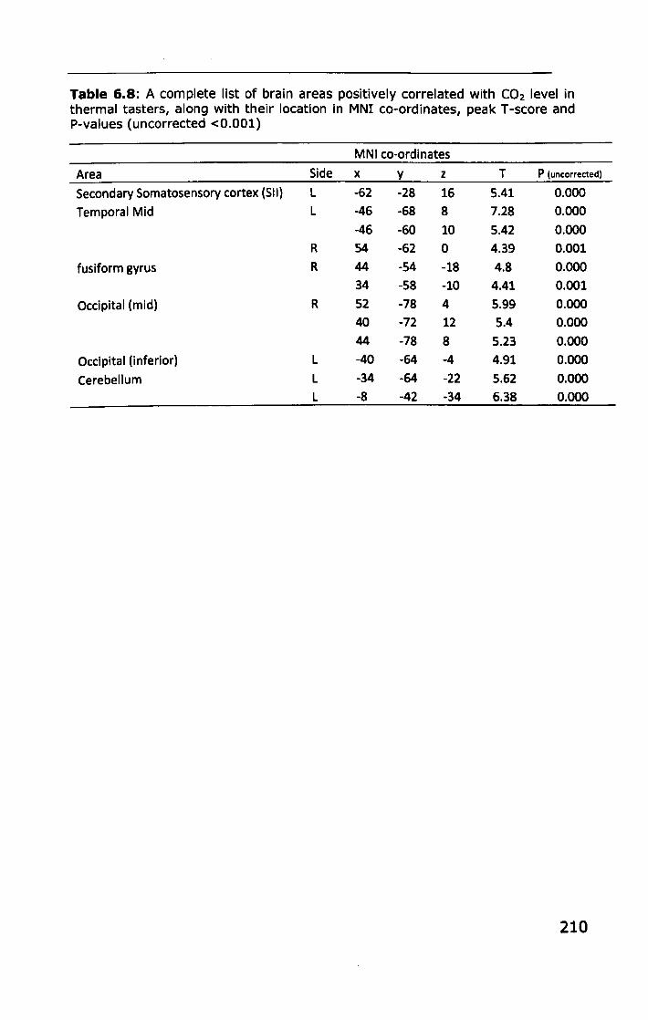
Table 6.8: A complete list of brain areas positively correlated with CO2 level in thermal tasters, along with their location in MNI co-ordinates, peak T -score and P-values (uncorrected <0.001)

MNI co-ordinates

Area Side x y z T P (uncorrected)

Secondary Somatosensory cortex (SII) L -62 -28 16 5.41 0.000

Temporal Mid L -46 -68 8 7.28 0.000

-46 -60 10 5.42 0.000 R 54 -62 0 4.39 0.001

fusiform gyrus R 44 -54 -18 4.8 0.000 34 -58 -10 4.41 0.001

Occipital (mid) R 52 -78 4 5.99 0.000 40 -72 12 5.4 0.000 44 -78 8 5.23 0.000

Occipital (inferior) L -40 -64 -4 4.91 0.000

Cerebellum L -34 -64 -22 5.62 0.000 L -8 -42 -34 6.38 0.000

210

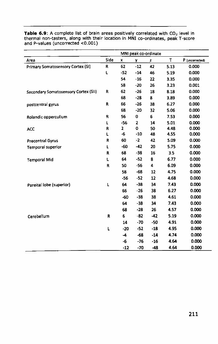
Table 6.9: A complete list of brain areas positively correlated with CO2 level in thermal non-tasters, along with their location in MNI co-ordinates, peak T-score and P-values (uncorrected <0.001)

MNI peak co-ordinate

Area Side x y z T P (uncorrected)

Primary Somatosensory Cortex (51) R 62 -12 42 5.13 0.000

L -52 -14 46 5.19 0.000

54 -16 22 3.35 0.000

58 -20 26 3.23 0.001

Secondary Somatosensory Cortex (511) R 62 -26 18 8.18 0.000

68 -28 8 3.89 0.000

postcentral gyrus R 66 -26 38 6.27 0.000

68 -20 32 5.06 0.000

Rolandic oppercullum R 56 a 6 7.53 0.000

L -56 2 14 5.01 0.000

ACC R 2 a 50 4.48 0.000 L -6 -10 48 4.55 0.000

Precentral Gyrus R 60 -2 42 5.09 0.000

Temporal superior L -60 -42 20 5.75 0.000

R 68 -38 16 3.5 0.000

Temporal Mid L 64 -52 8 6.77 0.000

R SO -56 4 6.09 0.000

58 -68 12 4.75 0.000

-56 -52 12 4.68 0.000

Pareitallobe (superior) L 64 -38 34 7.43 0.000

66 -26 38 6.27 0.000

-60 -38 38 4.61 0.000

64 -38 34 7.43 0.000

68 -28 26 4.57 0.000

Cerebellum R 6 -82 -42 5.19 0.000

14 -70 -50 4.91 0.000

L -20 -52 -18 4.95 0.000

-4 -68 -14 4.74 0.000

-6 -76 -16 4.64 0.000

-12 -70 -48 4.64 0.000

211

Tables 6.8 and 6.9 show that TnTs had additional areas that were

positivity correlated to C02 than TIs. The difference between the

two groups is illustrated by figure 6.27. Significant positive

correlation with C02 is shown in red/yellow for TnTs and in blue for

TIs. Specific regions of interest (ROI) (inserts a-h) have been

highlighted and enlarged with crosshairs set to MNI coordinates to

illustrate the location of the areas positively correlated in each

group. Inserts a and c show activation in SII in TnTs. Inserts d, f, 9

and h show activation in SI in TnTs. Insert e shows activation in

the ACe in TnTs and insert b shows activation in SII in TIs.

212

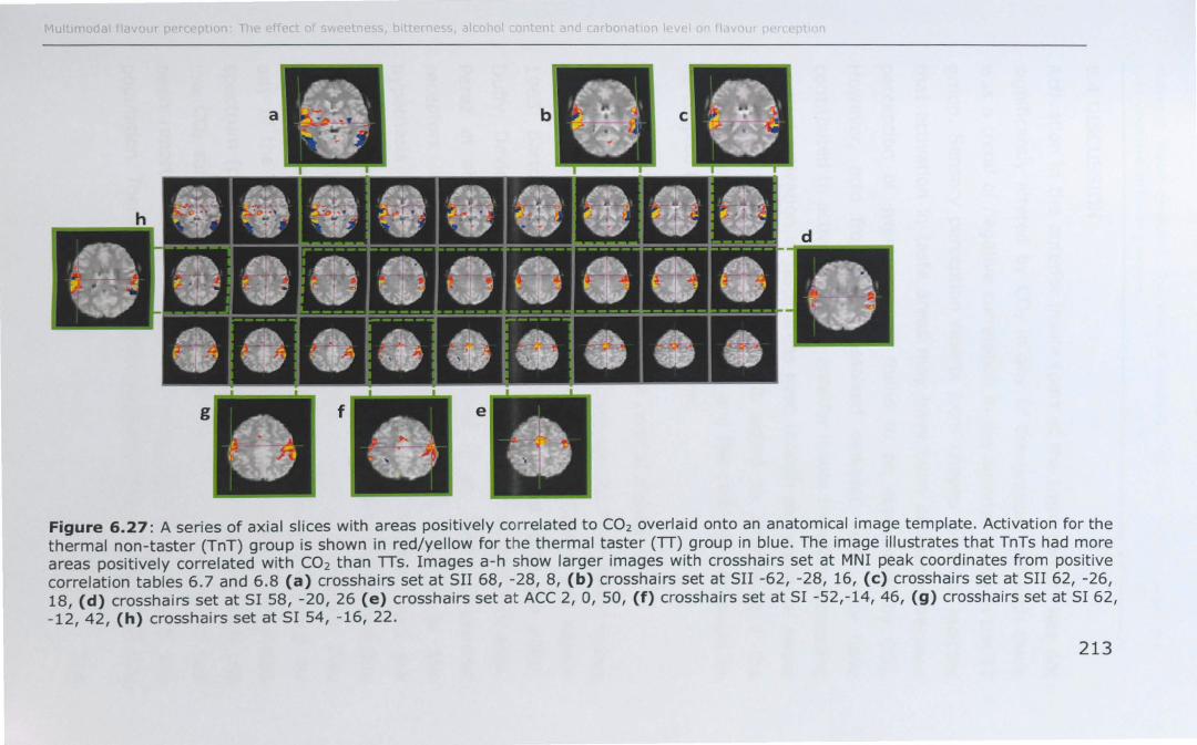
Figure 6.27: A series of axial slices with areas positively correlated to CO2 overla id onto an anatomical image template. Activation for the thermal non-taster (TnT) group is shown in red/yellow for the thermal taster (TI) group in blue. The image illustrates that TnTs had more areas positively correlated with CO2 than TIs. Images a-h show larger images with crosshairs set at MNI peak coordinates from positive correlation tables 6.7 and 6.8 (a) crosshairs set at 511 68, -28, 8, (b) crosshairs set at 511 -62, -28, 16, (e) crosshairs set at 511 62, -26, 18, (d) crosshairs set at 51 58, -20, 26 (e) crosshairs set at ACC 2, 0, 50, (f) crosshairs set at 51 -52,-14,46, (g) crossha irs set at 51 62, -12, 42, (h) crosshairs set at 51 54, -16, 22.

213

6.4 DISCUSSION

Activation in the anterior insula (part of the taste cortex) was not

significantly altered by C02 in any of the groups; although there

was a trend of negative correlation in the anterior insula in the TT

group. Sensory perception results from chapter 5 would indicate

that activation in taste areas may have been decreased because

perception of sweetness was found to be suppressed by C02.

However, acid from C02 (dissolved carbonic acid) may have

contributed to activation in the anterior insula therefore increasing

cortical activation in taste areas even though perception of sweet

taste was significantly reduced. It would be interesting if the

trigeminal effects of C02 (bubbles) and the carbonic acid could be

de-coupled to investigate this further.

6.4.1 Effect of PROP taster status on cortical activity

Papillae count has been positively correlated to PROP taster status

in a number of publications (Blakeslee 1932; Glanvill and Kaplan

1965; Bartoshuk, Duffy et al. 1994; Duffy and Bartoshuk 2000;

Duffy, Davidson et al. 2004; Lanier, Hayes et al. 2005; Driscoll,

Perez et al. 2006; Hayes, Bartoshuk et al. 2008). Trigeminal

receptors innervate the fungiform papillae leading to the

hypothesis that pSTs have more trigeminal receptors and are

therefore more sensitive to trigeminal stimuli and texture, and this

could lead to a preference for certain foods and beverages. This

study however did not find any clear behavioural preference for

any of the samples in both extremes of the PROP taster status

spectrum (pNTs or pSTs). Interestingly, pMTs most preferred the

low C02 sample and least preferred the high C02 sample. It has

been reported that pMTs account for approximately 50% of the

population. Therefore, if this data suggests that preference for C02

214

level in carbonated drinks could be within a very narrow range,

then soft drink companies and breweries need to find the optimum

C02 level for their products in order to increase preference and

ultimately liking. However, preference data from much larger

sample sets would be needed to confirm this.

PROP taster status did not seem to directly impact on C02

discrimination ability as all groups were able to adequately

discriminate the high C02 sample, with no group showing a

superior ability as may have been expected if they have more

trigeminal nerves in the oral cavity as previously suggested. It is

interesting to note that pMTs were the only group to show a clear

preference for any of the samples and yet they seemed to have a

poor discrimination ability for the sample they most preferred (low

C02). This data would not support that PROP taster status is

correlated to preference or sensitivity of trigeminal stimuli as

elicited by C02. However, this data is unbalanced and subject

numbers were low which may have influenced the outcome.

PROP 'tasters' (medium and super) tended to have overall higher

trend T-scores (higher BOLD response) than pNTs in the

somatosensory areas (51, 511) anterior insula, mid insula, posterior

insula and ACC, with 51, 511 and ACC reaching significantly higher

(p<O.Ol uncorrected) T-scores in pSTs compared to pNTs. This

increase in activation strength may be due to an increased signal

from an increased number of fungiform papillae in 'tasters'

compared to 'non-tasters' of PROP. Furthermore, there was a

difference between groups in activation strength (BOLD response)

to modulations in C02. PROP super-tasters did not have any

regions of interest positively correlated in a linear manner with C02,

whereas the other two groups (pNTs and pMTs) showed linear

215

increases in the primary somatosensory cortex (pMTs), secondary

somatosensory cortex (pNTs and pMTs) and the posterior insula

(pMTs). This may be because the cortical response was saturated

by the unimodal taste sample (no C02) in pSTs due to an increased

signal from an increased number of fungiform papillae. Further

increases in activation in regions of interest due to C02 addition

were therefore not possible in the pST group. This result would

support an increased intensity response to taste stimuli by pSTs as

previously found in this thesis (chapter 5) and in other studies (see

introduction).

The addition of C02 did not seem to alter sample preference in the

pST group with almost an equal number of subjects both 'least' and

'most' preferring each sample. When this data is considered along

with the cortical activation data, it would seem possible that taste

activation and preference is relatively unaffected by C02 addition in

the pST group.

The discrimination ability of pSTs to detect the difference in C02

levels was not significantly different to the pNT group. Previous

studies have found that pSTs have increased somatosensory acuity

(ESSick, Chopra et al. 2003) and that activation to oral fat in 51, SII,

anterior insula, mid-insula, posterior insula was correlated with

PROP taster status (Eldeghaidy, Marciani et al. 2010). These

studies suggest that pSTs have an increased number of trigeminal

receptors resulting in an increased sensitivity. However, this does

not seem to be the case when a tastant is present as with the

current study. Future research should investigate the relative

contribution of taste to overall oral sensitivity in multimodal food

and beverage systems.

216

6.4.2 Effect of thermal taster status on cortical activity

Thermal tasters seemed to have a better C02 discrimination ability

than thermal non-tasters as they correctly identified the high C02

sample significantly more times than the thermal non-tasters. One

hypothesis is that the innervations of trigeminal nerves in the

fungiform papillae are intertWined, therefore increasing sensitivity

in the oral cavity as trigeminal stimuli (temperature) are able to

activate the taste nerves in this group of subjects. Therefore, taste

sensations could activate the trigeminal nerves, increasing

sensitivity in the oral cavity, especially when both stimuli are

present. This seems plausible in light of the preference data.

Thermal tasters ranked the uncarbonated (no C02) sample as most

preferred and the high C02 sample as least preferred. This would

suggest that the increased sensitivity of this group to trigeminal

stimuli is driving preference. Thermal tasters seemed to be more

sensitive to the high C02 sample and they least preferred this

sample. In addition, the thermal taster group had higher cortical

activation to the no C02 sample than thermal non-tasters

supporting this hypothesis. Thermal tasters had overall higher T­

scores than TnTs. TT also rated taste and temperature stimuli

significantly higher in intenSity than TnTs (chapter 5). It is

therefore likely that the increase in taste and temperature intenSity

is a direct result of increased cortical activation in TTs.

C02 addition had a much greater impact on cortical activation in

the TnT group than the TT group with more areas showing

significant positive correlation with increasing CO2. There was no

significant negative correlation with increasing C02 level. However,

a trend of reduced brain activation with increasing C02 level can be

seen in the taste areas in the thermal taster group. It seems that a

taste stimulus (the no C02 sample in this study) is activating the

217

brain in areas found to be correlated with taste at a very similar

strength to those with an added trigeminal stimulus (the low C02

and high C02 samples). This supports the hypothesis that the taste

and trigeminal nerves are intertwined at the periphery in thermal

tasters. Both nerves are capable of being activated by just one

chemical leading to an increased intensity response to prototypical

taste stimuli and a taste response from a temperature stimulus (as

shown in the previous chapter) However, the results presented

here also support the central gain mechanism as proposed by

Green and George (Green, Alvarez-Reeves et al. 2005). It is

possible that thermal tasters have a general natural heightened

ability which increases the intensity to all sensations. However, a

study by Green and George (2004) found that this ability seems to

be restricted to the oral cavity. Temperature intensity testing in the

oral cavity was compared to the lip and hand in both TIs and TnTs.

Results found that TIs rated the temperature stimuli in the oral

cavity significantly more intense than TnTs but no significant

differences between intensity ratings on the lip and hand were

found between groups (Green and George 2004).

Investigations into thermal taster status are an exciting new area

of research and the results presented here contribute to the

growing body of evidence in this domain. Further research is

needed to determine the mechanism for the thermal taster

advantage and the hypotheses proposed here.

6.5 CONCLUSIONS AND SUMMARY

This is the first study to show the cortical response of C02 in the

oral cavity. C02 activated the somatosensory areas and C02

concentration was found to be positivity correlated to cortical

218

activation in the somatosensory areas, with the strength of this

activation being dependent upon the population group. Taste

activation, as represented by activation in the anterior-insula, was

not significantly affected by C02 but this could be a combinational

response to both the sweet taste of the dextrose and acid from

carbonic acid in the samples, thus reducing perception without

significantly altering activation.

Studies investigating population differences between groups have

been widely researched with focus on the difference between PROP

taster status groups. Some studies have found significant

differences in taste and oral somatosensation whereas others have

not. This study has shown that there are differences in PROP taster

groups for cortical activation of taste (sweet) and trigeminal (C02)

stimuli. PROP non-tasters had lower overall T -scores than the pMTs

and pSTs which may be explained by differences in the number and

density of fungiform papillae. However, fungiform papillae counts

were not investigated in this study and so this conclusion cannot be

made. PROP medium-tasters had higher overall T -scores than pNTs.

C02 addition had the greatest impact on cortical activation in pMTs

as shown by positive correlation in Significantly more regions of

interest than pNTs. These results may be explained by an increased

density in fungiform papillae and therefore trigeminal receptors in

pMTs compared to pNTs. PROP super-tasters had higher overall T­

scores than pNTs and less positive correlation with C02 than pMTs.

This could be explained again by a higher number of fungiform

papillae resulting in a saturation of response to the no C02 sample

so that a further increase in activation with CO2 is not possible in

this group.

219

The discovery of thermal tasters is an exciting new area of

research. Thermal tasters respond to taste and temperature stimuli

more intensely that TnTs (chapter 5). The mechanism for this

increase in intensity has been proposed to be due to both

peripheral and central mechanisms. This is the first study to

investigate the difference in cortical activation to gustatory (sweet

taste) and trigeminal stimuli (C02) between thermal and non­

thermal taster groups. Thermal tasters seem to be more sensitive

to trigeminal stimuli than thermal non-tasters as they were able to

discriminate the high C02 sample significantly more than TnTs. In

addition, this increased sensitivity in the TT group seemed to shape

preference, as the high C02 sample was ranked as the least

preferred sample and the no C02 sample was the most preferred.

These findings were represented cortically with thermal tasters

showing a higher cortical response to the no C02 (taste) sample

than TnTs which may be driving preference in this group. Thermal

tasters had higher overall T-scores than TnTs possibly resulting

from increased activation due to interaction of taste and trigeminal

nerves or from a central gain mechanism as proposed by Green

and George (2005). This could also be the reason for less positive

correlation of BOLD response with C02 addition in this group

compared to the TnT group.

PROP taster status and possible correlations to overall oral

sensitivity, food preference, obesity and alcoholism have been

studied for over 80 years and so far evidence is inconclusive. In

contrast, thermal stimulation of taste (thermal taster status) was

discovered a little over 10 years ago. To date, only seven studies

have been published investigating thermal taster status and

evidence seems much less variable compared to research

investigating PROP taster status. Dedicated research is required to

220

further understanding but it seems increasingly likely that thermal

tasters could be the new PROP super-tasters.

221

Chapter 7

222

7. CONCLUSIONS

The primary aim of this research was to investigate the interactions

between sweetness, bitterness, alcohol content and carbonation

level on flavour perception. A model beer was created using

sweetener (dextrose), hop acids, ethanol, C02, aroma volatiles

(simple blend of five compounds commonly found in beer),

colouring and polydextrose (to give a base level of viscosity). This

fundamental investigation into multimodal interactions on flavour

perception will not only be of interest to researchers but also the

food and beverage industry such as the alcoholic and soft drinks

sectors. In particular, there has been recent interest in the

development of reduced ethanol and C02 beers to increase market

share by targeting different consumers and to reduce costs to the

consumer due to increased taxation of alcohol.

A large body of research continues to focus on population

differences in flavour perception and consumer attitudes towards

food in terms of preference, liking, purchase intent and buying

behaviour. Therefore, a secondary aim of this research was to

investigate differences in population groups for their genetic

sensitivity to oral sti muli.

This research has taken a multidisciplinary and systematically

controlled approach to investigate multimodal flavour perception

using a design of experiments comprising of instrumental flavour

chemistry, descriptive sensory evaluation and functional magnetic

resonance imaging.

Results found that C02 and ethanol both increased volatile

partitioning from the breath during consumption which, when

added together could contribute an 86% increase in volatile

delivery to the olfactory cavity. Sensory profiling techniques

223

however, did not find that this increase significantly altered aroma

perception sensorially. However, the mixture of volatiles in the

model system was basic, comprising of just five compounds. It

would be pertinent to investigate more volatiles, given the

complexity and number of volatiles present in beer, to understand

the true impact a reduction in ethanol and CO2 could have on

flavour perception.

Sensory analysis found ethanol to be the main driver of warming

perception, complexity of flavour and also it also contributed to

sweetness perception in the model beer. It would be hypothesised

therefore, that if ethanol was reduced to <2.8% (the levels

required to reduce taxation), then this would bring about a

reduction in complexity of flavour, warming perception and possibly

sweetness perception. The impact that this could have on

consumer liking should be investigated by means of a consumer

study. Results would give insight into which attributes are

significantly affected amongst consumers and this could be used

alongside the trained panel data to ensure successful product

development.

C02 significantly affected all discriminating attributes showing an

ability to interact and modify flavour perception in a complex

manner. Efforts at reducing C02 levels in beer would benefit from

this research to know what attributes are being affected, how this

combines to alter flavour perception and then start to investigate

ways of boosting or balancing flavour perception to match that of

the standard C02 versions.

Successful product development is made increasingly difficult due

to population differences in oral sensitivity. A reduced ethanol and

C02 product may not appeal to someone with low oral sensitivity

224

but may appeal to someone with high oral sensitivity. Two markers

of genetic sensitivity were investigated, PROP taster status and

thermal taster status. PROP taster status is the ability to taste the

compound, 6-n-propylthiouracil (PROP). Those who cannot taste

the compound are classified as PROP non-tasters and those who

can taste the compound are classified as PROP tasters. PROP

tasters can be further split into two groups, those who taste the

compound with 'medium' intensity are called PROP medium-tasters

and those who taste the compound at a high intensity are called

PROP super-tasters. Thermal tasting on the other hand describes

an ability of thermal stimulation (to the tongue) to evoke a taste

response. In contrast, thermal non-tasters do not taste anything

during thermal stimulation. Volunteers were screened for their

PROP and thermal tasters status. This study used a simplified

method with more relaxed criteria for screening thermal tasters to

those previously published and found that the simplified method

was valid.

Taste and temperature intensity data were collected on each

subject and found that differences in the population's oral

sensitivity could be explained by PROP taster status and thermal

taster status. PROP tasters gave significantly (p<O.05) higher

intensity ratings for each stimuli than PROP non-tasters. Thermal

tasters rated the intensity of the stimuli significantly (p<O.05)

higher than thermal non-tasters. However, both PROP and thermal

markers of oral sensitivity cannot be explained by the same

mechanism as thermal tasters were relatively evenly distributed

across PROP taster groups and vice-versa. Future research should

attempt to uncover the mechanisms behind thermal taster status

by first understanding if increased intensity perception is limited to

oral stimuli. Studies investigating the response to aroma and other

225

sensory stimuli between thermal taster groups would facilitate

understanding of the mechanisms responsible. Furthermore, it is

currently unknown if thermal taster status has a genetic basis and

so family studies should be employed to determine this.

Sensory response to C02 is via a dual mechanism of action; the

nociceptive response (tingle) and inevitable taste from carbonic

acid and the mechanical response from the presence of bubbles. It

would be interesting if the two aspects could be de-coupled and

investigated to further understand the contribution from each on

flavour perception and cortical activation. This would help to

determine the contribution of C02 on taste perception due to the

acidic and mechanical components. C02 did not significantly impact

activation in the primary taste areas of the brain (anterior insula)

in this study. However, interesting trends in the data were found

between thermal taster groups. Investigations into how C02

impacts on cortical activation using fMRI have for the first time

shown that C02 significantly increases activation in the

somatosensory cortex. Furthermore, there were differences in

cortical activation strength in certain regions of interest between

PROP taster groups and thermal taster groups which reflected the

differences seen in intensity ratings of oral stimuli. The increased

cortical activation in thermal tasters also seemed to explain

behavioural data. Thermal tasters least preferred the high C02

sample and most preferred the no C02 (uncarbonated) sample and

were significantly better discriminators of high C02 than the

thermal non-tasters. These findings may be due to an increased

sensitivity to C02 in thermal tasters. It is currently unknown why,

and how this is happening but the hypothesis presented here is

that it could be caused by a connection between the taste and

trigeminal nerves in thermal tasters. This would allow a taste

226

response to come from a trigeminal stimulus (temperature) and

similarly allowing both nerves to be activated to a taste stimulus,

increasing intensity response and cortical activation and influencing

preference. Future work should investigate this proposed

mechanism. Animal studies have given insight into the activation of

groups of neurons to certain oral stimuli. Further research

investigating the peripheral biology of the taste and temperature

nerves in the fungiform papillae and how this may be linked to

possible differences in strength of activation from taste and

temperature stimuli on the relevant neurons may begin to uncover

the mechanism of thermal taster status.

There are currently only seven papers published on thermal taster

status and so research in this area is very limited. Considering the

implications of the results found here, future work should

concentrate on the link between the thermal taster advantage and

hedonic liking as is seems increasingly likely that a proportion of

the population (thermal tasters) sense oral stimuli differently which

could shape their liking, consumer behaviour and ultimately their

health. From a sensory scientist's poi nt of view, the possi bility of

screening for thermal taster status to create a trained panel of

thermal tasters could increase sensitivity and reduce variability in

sensory data.

7.1 FURTHER WORK

Throughout this thesis, suggestions have been made for areas of

further work which are summarised below.

• Further investigations into the physico-chemical effects of

ethanol and carbonation with more compounds than used in

this study (chapter 3) should be carried out following a

similar method. This will provide additional data to test the

227

hypothesis of the relationship between a compounds's Kaw

and the effects of ethanol and carbonation on partitioning

into the breath. It will also give more insight into the

cumulative effects of ethanol and carbonation on aroma

delivery and therefore perception.

• A study should be carried out to determine if the effects of

C02 addition on flavour perception found in the model beer

system used in this study can be applied to real beer.

Standard lager beer could be de-gassed using sonication and

then re-carbonated to different levels and compared for their

sensory attributes.

• An investigation to determine if hop acid addition alters the

bubble size of carbonated samples would establish if the

interaction between hop acids and C02 on tingly and

carbonation perception at low C02 levels as found in chapter

4 is due to differences in surface tension and bubble

formation. Bubble size could be measured by photographing

samples and measuring the bubble diameter.

• Further investigate the mechanism of the ethanol-C02

interactions found in this study (chapter 4) by studying if

ethanol and C02 leads to cross-desensitisation when

presented simultaneously using a similar method to Green

(1991).

• The contri bution of sweetness, bitterness, alcohol content

and carbonation to consumer liking could be measured in a

consumer study and used alongside the sensory data

collected in chapter 4 to provide more information to new

product developers and marketing teams.

228

• Investigations into the effect of hop acids on the sweet

transduction cation channel, TRPMS, to determine the source

of the sweetener-hop acid interaction found in chapter 4.

• Further investigations into the possible differences between

PROP taster groups and thermal taster groups for sensory

interactions between modalities should be explored to

understand the effect of taste phenotype on more complex

food and beverage systems. Specifically the relative

contribution of taste on overall oral sensitivity should be

explored in multimodal food and beverage systems.

• Studies investigating the intensity of olfactory perception

and cutaneous pain would further understanding into the

origins of the thermal taster mechanism. In addition, family

studies would give indication if thermal taster status is

genetiC in origin.

• De-couple the mechanical aspect of C02 and the nociceptive

carbonic acid to determine the contribution of each on flavour

perception.

• C02 preference data from larger sample sets of each PROP

taster group and both thermal taster groups would confirm if

the trends found in this thesIs (chapter 6) between each

marker of taste sensitivity and liking of C02 are valid.

229

Appendix 1: University of Nottingham Magnetic Resonance

Centre safety screening questionnaire

[SAFETY SCREENING QUESTIONNAIRE]

1h Unl rsltyof

Nottingham Sir Peter Mansfield Magnetic Resonance Centre

Safety Screening Questionnaire For ANYONE entering the INNER CONTROLLED AREA marked by red and white tape on the doors (Magnetic field safety information is available in the SPMMRC website)

» Shaded boxes to be filled in by scan volunteers and patients only «

NAME Date of Visit Phone Number

ADDRESS Volunteer Number

Date of Birth

Study Ethics Code (or reason for visit) Hospital No (If applicable)

Weight (Philips scanners only)

MR scanning uses strong magnetic fields, for your own safety and the safety of others it is very important that you do not go into the magnet halls with any metal In or on your body or clothing. Please answer the following questions carefully and ask if anything is not clear.

All information is held in the strictest confidence.

1. Do you have any Implants In your body? e.g. replacement joints, drug pumps

2. Do you have aneurysm clips (clips put around blood vessels during surgery)?

YIN

YIN

3. Do you have a pacemaker or artificial heart valve? (These stop working near MR Scanners) YIN

4. Have you ever had any surgery? Please give brief details* YIN

( * We do not need to know about uncomplicated caesarian del/very, vasectomy or termination of pregnancy)

5. Do you have any foreign bodies in your body (e.g. shrapnel)? YIN

6. Have you ever worked In a machine tool shop without eye protection? YIN

7. Do you wear a hearing aid or cochlear Implant? YIN

8. Could you be pregnant? You must use the pregnancy tests available in the female toilets If you are unsure. YIN

9. Have you ever suffered from tinnitus?

10. Do you wear dentures, a dental plate or a brace?

11. Are you susceptlOle to claustropnoOla (

12. Do you suffer from blackouts, epilepsy or fits?

13. Do you have any trans-dermal patches (skin patches)?

230

YIN

YIN

YIN

YIN

YIN

6. Do you have any tattoos? YIN

7. Will you remove all metal Including coins, body-piercing jewellery, false-teeth, hearing aids

etc before entering the magnet haiL? (lockers available by the changing rooms) YIN

16. Is there anything else you think we should know? YIN

I have read, understood, and answered all questions

Signature: Date:

Verified by:

SPMMRC Staff Signature: Date:

231

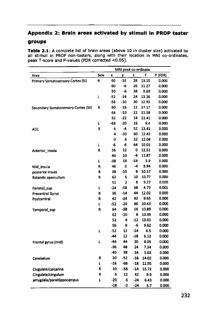
Appendix 2: Brain areas activated by stimuli in PROP taster

groups

Table 2.1: A complete list of brain areas (above 10 in cluster size) activated by all stimuli in PROP non-tasters, along with their location in MNI co-ordinates, peak T -score and P-values (FOR corrected <0.05).

MNI peak co-ordinate

Area Side x y z T P (FOR)

Primary Somatosensory Cortex (51) R 60 -16 28 13.15 0.000

60 -6 26 11.27 0.000

50 -8 38 9.69 0.000

L -52 -14 24 13.36 0.000

-58 -10 30 12.93 0.000

Secondary Somatosensory Cortex (511) R 60 -16 12 17.17 0.000

64 -10 22 11.58 0.000

52 -22 14 11.41 0.000

L -66 -20 16 9.4 0.000

ACC R 6 -4 52 13.41 0.000

4 -10 60 12.42 0.000

0 6 52 12.04 0.000

L -6 -6 64 10.01 0.000

Anteriorjnsula R 36 12 0 12.51 0.000

40 10 -4 11.87 0.000

L -38 18 -14 5.9 0.000

MidJnsula R 46 0 -4 9.94 0.000

posterior insula R 38 -10 8 10.17 0.000

Rolandic opercullum R 62 6 10 10.77 0.000

52 2 8 9.27 0.000

ParietaLsup L -24 -58 68 4.73 0.001

Precentral Gyrus R 36 -14 44 12.02 0.000

Postcentral R 42 -24 42 9.65 0.000

L -52 -20 46 10.43 0.000

Temporal_sup R 64 -38 16 10.89 0.000

62 -10 6 10.39 0.000

52 4 -12 10.01 0.000

56 6 -6 9.62 0.000

L -52 12 -14 6.5 0.000

-44 12 -18 6.13 0.000

Frontal gyrus (mid) L -44 44 20 8.05 0.000

-36 48 24 7.34 0.000

-40 38 34 5.63 0.000

Cerebelum R 20 -52 -18 14.02 0.000

L -16 -68 -18 12.95 0.000

Cingulate/calcarlne R 10 -58 -14 15.72 0.000

Clngulate/clngulum R 6 12 42 9.9 0.000

amygdala/paraHlppocampus L -20 6 -24 6.43 0.000 -18 -2 -24 5.7 0.000

232

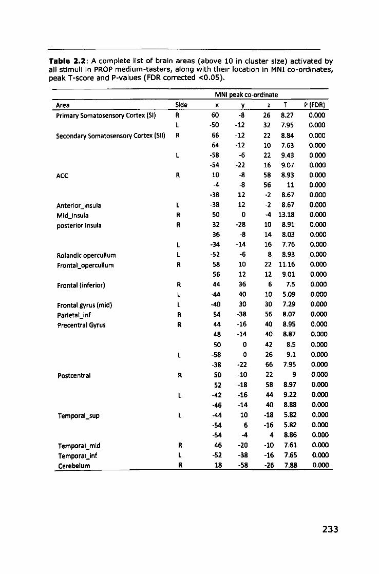
Table 2.2: A complete list of brain areas (above 10 in cluster size) activated by all stimuli in PROP medium-tasters, along with their location in MNI co-ordinates, peak T -score and P-values (FOR corrected <0.05).

MNI peak co-ordinate

Area Side x y z T P (FOR)

Primary Somatosensory Cortex (51) R 60 -8 26 8.27 0.000

L -50 -12 32 7.95 0.000

Secondary Somatosensory Cortex (511) R 66 -12 22 8.84 0.000 64 -12 10 7.63 0.000

L -58 -6 22 9.43 0.000 -54 -22 16 9.07 0.000

ACC R 10 -8 58 8.93 0.000 -4 -8 56 11 0.000

-38 12 -2 8.67 0.000

Anteriorjnsula L -38 12 -2 8.67 0.000

MidJnsula R 50 0 -4 13.18 0.000

posterior insula R 32 -28 10 8.91 0.000

36 -8 14 8.03 0.000

L -34 -14 16 7.76 0.000

Rolandic opercullum L -52 -6 8 8.93 0.000

Frontal_opercullum R 58 10 22 11.16 0.000

56 12 12 9.01 0.000

Frontal (inferior) R 44 36 6 7.5 0.000

L -44 40 10 5.09 0.000

Frontal gyrus (mid) L -40 30 30 7.29 0.000

ParietaUnf R 54 -38 56 8.07 0.000

Precentral Gyrus R 44 -16 40 8.95 0.000

48 -14 40 8.87 0.000

50 0 42 8.5 0.000

L -58 0 26 9.1 0.000

-38 -22 66 7.95 0.000

Postcentral R 50 -10 22 9 0.000

52 -18 58 8.97 0.000

L -42 -16 44 9.22 0.000

-46 -14 40 8.88 0.000

Temporal_sup L -44 10 -18 5.82 0.000

-54 6 -16 5.82 0.000

-54 -4 4 8.86 0.000

TemporaLmid R 46 -20 -10 7.61 0.000

TemporaUnf L -52 -38 -16 7.65 0.000

Cerebelum R 18 -58 -26 7.88 0.000

233

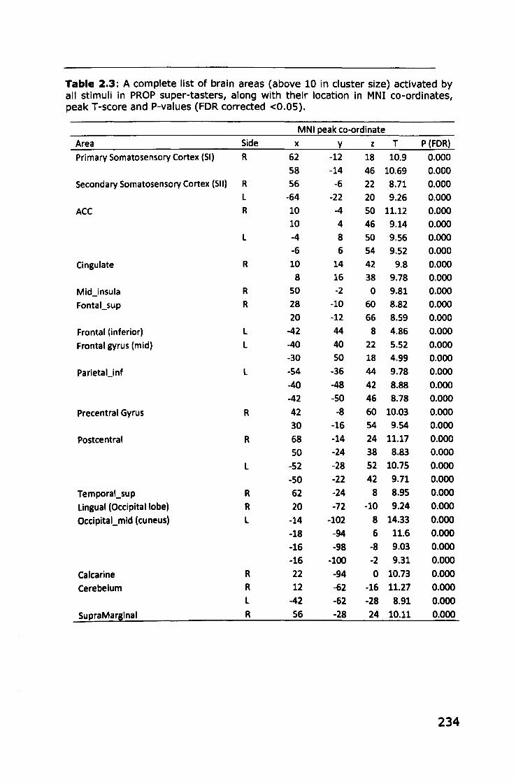
Table 2.3: A complete list of brain areas (above 10 in cluster size) activated by all stimuli in PROP super-tasters, along with their location in MNI co-ordinates, peak T -score and P-values (FOR corrected <0.05).

MNI peak co-ordinate

Area Side x y z T P (FOR)

Primary Somatosensory Cortex (51) R 62 -12 18 10.9 0.000 58 -14 46 10.69 0.000

Secondary Somatosensory Cortex (511) R 56 -6 22 8.71 0.000 L -64 -22 20 9.26 0.000

ACC R 10 -4 50 11.12 0.000 10 4 46 9.14 0.000

L -4 8 50 9.56 0.000 -6 6 54 9.52 0.000

Cingulate R 10 14 42 9.8 0.000 8 16 38 9.78 0.000

Midjnsula R 50 -2 0 9.81 0.000

Fontal_sup R 28 -10 60 8.82 0.000 20 -12 66 8.59 0.000

Frontal (inferior) L -42 44 8 4.86 0.000

Frontal gyrus (mid) L -40 40 22 5.52 0.000 -30 50 18 4.99 0.000

ParietaUnf L -54 -36 44 9.78 0.000 -40 -48 42 8.88 0.000 -42 -50 46 8.78 0.000

Precentral Gyrus R 42 -8 60 10.03 0.000

30 -16 54 9.54 0.000

Postcentral R 68 -14 24 11.17 0.000

50 -24 38 8.83 0.000

L -52 -28 52 10.75 0.000

-50 -22 42 9.71 0.000

Temporal_sup R 62 -24 8 8.95 0.000

Lingual (Occipital lobe) R 20 -72 -10 9.24 0.000

OccipitaLmid (cuneus) L -14 -102 8 14.33 0.000

-18 -94 6 11.6 0.000

-16 -98 -8 9.03 0.000 -16 -100 -2 9.31 0.000

Calcarine R 22 -94 0 10.73 0.000

Cerebelum R 12 -62 -16 11.27 0.000 L -42 -62 -28 8.91 0.000

SupraMarlinal R 56 -28 24 10.11 0.000

234

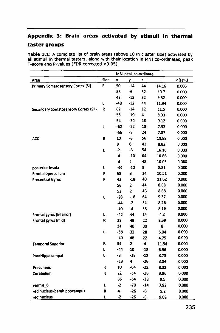
Appendix 3: Brain areas activated by stimuli in thermal

taster groups

Table 3.1: A complete list of brain areas (above 10 in cluster size) activated by all stimuli in thermal tasters, along with their location in MNI co-ordinates, peak T-score and P-values (FOR corrected <0.05)

MNI peak co-ordinate

Area Side x y z T P (FOR)

Primary Somatosensory Cortex (SI) R 50 -14 44 14.16 0.000

58 -6 32 10.7 0.000

48 -12 32 9.82 0.000

l -48 -12 44 11.94 0.000

Secondary Somatosensory Cortex (SII) R 62 -14 12 11.5 0.000

58 -10 4 8.93 0.000

54 -30 18 9.12 0.000

l -62 -22 18 7.93 0.000

-56 -8 24 7.87 0.000

ACC R 10 -8 56 10.89 0.000

8 6 42 8.82 0.000

l -2 -6 54 16.16 0.000

-4 -10 64 10.86 0.000

-4 2 48 10.05 0.000

posterior insula l -44 -12 8 8.81 0.000

Frontalopercullum R 58 8 24 10.51 0.000

Precentral Gyrus R 42 -18 40 11.62 0.000

56 2 44 8.68 0.000

52 2 46 8.68 0.000

l -28 -18 64 9.37 0.000

-44 -2 54 8.26 0.000

-40 -4 58 8.19 0.000

Frontal gyrus (inferior) l -42 44 14 4.2 0.000

Frontal gyrus (mid) R 38 48 22 8.39 0.000

34 40 30 8 0.000

l -38 32 28 5.04 0.000

-40 48 22 4.75 0.000

Temporal Superior R 54 2 -4 11.54 0.000

l -44 10 -18 6.86 0.000

Para Hippocampal l -8 -28 -12 8.73 0.000

-18 4 -26 3.04 0.000

Precuneus R 10 -64 -22 8.32 0.000

Cerebelum R 22 -54 -26 9.96 0.000

36 -54 -38 9.5 0.000

vermis_6 l -2 -70 -14 7.92 0.000

red nucleus/parahippocampus R 4 -26 -8 9.2 0.000

red nucleus l -2 -26 -6 9.08 0.000

235

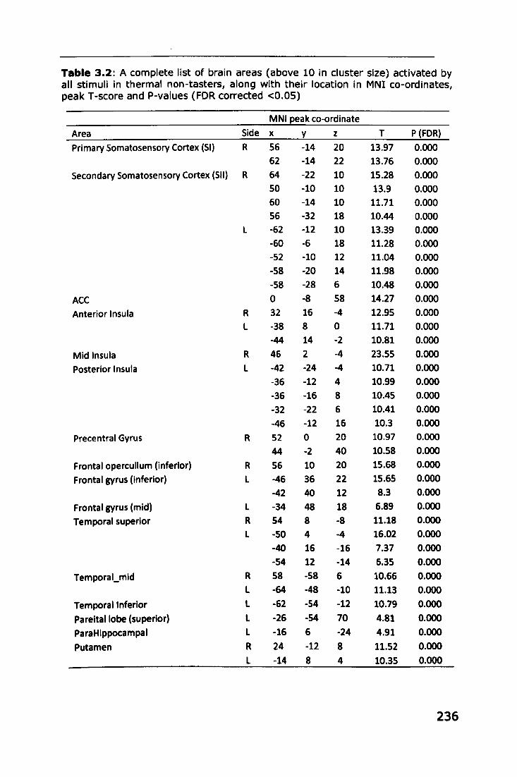
Table 3.2: A complete list of brain areas (above 10 in cluster size) activated by all stimuli in thermal non-tasters, along with their location in MNI co-ordinates, peak T -score and P-values (FOR corrected <0.05)

MNI peak co-ordinate

Area Side x y z T P (FOR)

Primary Somatosensory Cortex (SI) R 56 -14 20 13.97 0.000 62 -14 22 13.76 0.000

Secondary Somatosensory Cortex (SII) R 64 -22 10 15.28 0.000 50 -10 10 13.9 0.000 60 -14 10 11.71 0.000 56 -32 18 10.44 0.000

l -62 -12 10 13.39 0.000 -60 -6 18 11.28 0.000 -52 -10 12 11.04 0.000 -58 -20 14 11.98 0.000 -58 -28 6 10.48 0.000

ACC 0 -8 58 14.27 0.000

Anterior Insula R 32 16 -4 12.95 0.000

l -38 8 0 11.71 0.000

-44 14 -2 10.81 0.000

Mid Insula R 46 2 -4 23.55 0.000

Posterior Insula l -42 -24 -4 10.71 0.000

-36 -12 4 10.99 0.000

-36 -16 8 10.45 0.000

-32 -22 6 10.41 0.000

-46 -12 16 10.3 0.000

Precentral Gyrus R 52 0 20 10.97 0.000

44 -2 40 10.58 0.000

Frontal opercullum (inferior) R 56 10 20 15.68 0.000

Frontal gyrus (Inferior) l -46 36 22 15.65 0.000

-42 40 12 8.3 0.000

Frontal gyrus (mid) l -34 48 18 6.89 0.000

Temporal superior R 54 8 -8 11.18 0.000

l -50 4 -4 16.02 0.000

-40 16 -16 7.37 0.000 -54 12 -14 6.35 0.000

Temporal_mid R 58 -58 6 10.66 0.000 l -64 -48 -10 11.13 0.000

Temporal Inferior L -62 -54 -12 10.79 0.000

Pareitallobe (superior) L -26 -54 70 4.81 0.000

ParaHippocampal l -16 6 -24 4.91 0.000

Putamen R 24 -12 8 11.52 0.000

L -14 8 4 10.35 0.000

236

Appendix 4: Achievements

REFEREED PUBLICATIONS

Clark, R., Linforth, R., Bealin-Kelly, F., Hort, J. (2011) Effects of

ethanol, carbonation and hop acids on volatile delivery in a model

beer system. Journal of the Institute of Brewing. 117(1): 74-S1

Clark, R.A., Hewson, L., Bealin-Kelly, F., Hort, J. (2011) The

interactions of C02, ethanol, hop acids and sweetener on flavour

perception in a model beer. Chemosensory Perception. 4:42-54

SYMPOSIA PRESENTATIONS

Oral: Royal Chemistry Conference, Queens College, Belfast (200S)

Poster: European Brewing Congress, Hamburg (2009)

Poster: Pangborn Sensory Science Symposium, Florence (2009)

Oral: 2nd International Symposium for Young Scientists and

Technologists in Malting, Brewing and Distilling, Weihenstephan,

Germany (2010)

Oral: Eurosense symposium, Spain, (2010). Successful applicant of

PFSG's travel award (2010)

Oral: Pangborn Sensory Science Symposium, Toronto (2011)

237

REFERENCES

Abdi, H. (2002). "What can cognitive psychology and sensory evaluation learn from each other?" Food Ouality and preference 13(7-8}: 445-451.

Adler, E., M. A. Hoon, et al. (2000). "A novel family of mammalian taste receptors." ~ 100(6}: 693-702.

Allen, P. J., O. Josephs, et al. (2000). "A method for removing imaging artifact from continious EEG recorded during functional fMRI." NeuroImage 12: 230-239.

Allen, P. J., G. Polizzi, et al. (1998). "Identification of EEG events in the MR scanner. The problem of pulse artifact and a method for its subtraction." NeuroImage 8: 229-239.

Alonso, B. D. C., L. Marciani, et al. (2007). "Functional magnetic resonance imaging assessment of the cortical representation of oral viscosity." Journal of Texture Studies 38(6}: 725-737.

Anon. (2010). "A review of the Universe: Structures, Evolutions, Observations and Theories." Retrieved 4th July, 2011, from http://universe-review .ca/RI0-16-ANS.htm.

Aprea, E., F. Biasioli, et al. (2007). "PTR-MS study of esters in water and water/ethanol solutions: Fragmentation patterns and partition coefficients." International Journal of Mass Spectrometry 262(1-2}: 114-121.

Aznar, M., M. Tsachaki, et al. (2004). "Headspace analysis of volatile organic compounds from ethanolic systems by direct APCI-MS." International Journal of Mass Spectrometry 239(1): 17-25.

Bajec, M. R. and G. J. Pickering (2008). "Astringency: Mechanisms and perception." Critical Reyiews in Food Science and Nutrition 48(9): 858-875.

Bajec, M. R. and G. J. Pickering (2008). "Thermal taste, PROP responsiveness, and perception of oral sensations." Physiology &. Behavior 95(4): 581-590.

Bajec, M. R. and G. J. Pickering (2010). "Association of thermal taste and PROP responsiveness with food liking, neophobia, body mass index, and waist circumference." Food Quality and preference 21(6): 589-601.

Bandettini, P. A. and R. W. Cox (2000). "Event-related fMRI contrast when using constant interstlmulus interval: Theory and experiment." JOurnal of Magnetic Resonance Imaging 43: 540-548.

Barker, G., S., B. Jefferson, et al. (1999). Measuring Techniques for the Determination of CO2 in Beverages. Bubbles in Food. G. Campbell, M., C. Webb, S. Pandiella, S. and K. Niranjan. St. Paul, Minn, Eagan Press: 191-196.

Bartoshuk, L. M. (1975). "Taste mixtures - Is mixture supresslon related to compression." Physiology &. Behavior 14(5): 643-649.

Bartoshuk, L. M. (1979). "Bitter taste of saccharin related to the genetiC ability to taste the bitter substance 6-n-propylthiouracil." Science 205(4409): 934-935.

Bartoshuk, L. M., V. B. Duffy, et al. (2002). "Labeled scales {e.g., category, Likert, VAS} and Invalid across-group comparisons: what we have learned from genetiC variation in taste." Food Ouality and Preference 14: 125-138.

Bartoshuk, L. M., V. B. Duffy, et al. {1997}. PROP (6-n-prooylthiouracil) supertasters and the saltiness of NaCI. International Symposium on Olfaction and Taste XII, San Diego, California.

Bartoshuk, L. M., V. B. Duffy, et al. {1994}. "PTe/PROP tasting: anatomy psychophysics and sex effects." Physiology &. Behaylor 56: 1165-71.

238

Bartoshuk, L. M., K. Rennert, et al. (1982). "Effects of temperature on the perceived sweetness of sucrose." Physiology & Behayior 28(5): 905-910.

Bartoshuk, L. M., B. Rifkin, et al. (1988). "Bitterness of KCI and benzoate -related to genetic status for sensitivity to PTC/PROP." Chemical Senses 13(4): 517-528.

Baylis, L. L., E. T. Rolls, et al. (1995). "AFFERENT CONNECTIONS OF THE CAUDOLATERAL ORBITOFRONTAL CORTEX TASTE AREA OF THE PRIMATE." Neuroscience 64(3): 801-812.

Behrens, M., S. Foerster, et al. (2007). "Gustatory expression pattern of the human TAS2R bitter receptor gene family reveals a heterogenous population of bitter responsive taste receptor cells." Journal of Neuroscience 27(46): 12630-12640.

Behrens, M. and W. Meyerhof (2006). "Bitter taste receptors and human bitter taste perception." Cellular and Molecular Life Sciences 63(13): 1501-1509.

Blakeslee, A. F. (1932). "Genetics of sensory thresholds taste for phenylthio carbamide." Proceedings of the National Academy of Sciences of the United States of America 18: 120-130.

Boucher, Y., C. T. Simons, et al. (2003). ''Trigeminal modulation of gustatory neurons in the nucleus of the solitary tract." Brain Research 973(2): 265-274.

Brand, G. (2006). "Olfactory/trigeminal interactions in nasal chemoreception." Neuroscience and Biobehayioral Reyiews 30(7): 908-917.

Brasser, S. M., M. B. Norman, et al. (2010). "Tlr3 taste receptor involvement in gustatory neural responses to ethanol and oral ethanol preference." Physiological Genomics 41(3): 232-243.

Breslin, P. A. S. (1996). "Interactions among salty, sour and bitter compounds." Trends in Food Science & Technology 7(12): 390-399.

Bridge, S. (2011). Molson Coors develops beer for women. Mail on Sunday. London, Mail Newspapers.

Briggs, D. E., C. A. Boulton, et al. (2004). Brewing science and practice. Cambridge, Woodhead Publishing.

Buck, L. and R. Axel (1991). "A novel multigene family may encode odorant receptors - A molecular-basis for odor recognition." ~ 65(1): 175-187.

Buck, L. B. (2004). "Olfactory receptors and odor coding in mammals." Nutrition Reyiews 62(11): S184-S188.

Cain, W. S. and C. Murphy (1980). "Interactions between chemoreceptive modalities of odour and irritation." Nature 284(20): 255-257.

Calvino, A. M., M. R. Garclamedina, et al. (1990). "Interactions in caffeine­sucrose and coffee-sucrose mixtures - evidence of taste and flavor supresslon." Chemical Senses 15(5): 505-519.

Calvino, A. M., M. R. Garclamedina, et al. (1993). "Perception of sweetness and bitterness In different vehicles." perception & PSychophysics 54(6): 751-758.

Carstens, E., M. I. Carstens, et al. (2002). "It hurts so good: oral irritation by spices and carbonated drinks and the underlying neural mechanisms." Food Quality and preference 13{7-8): 431-443.

Carstens, E., N. Kuenzler, et al. (1998). "Activation of neurons in rat trigeminal subnucleus caudalls by different irritant chemicals applied to oral or ocular mucosa." Journal of Neyrophysiology 80(2): 465-492.

Cerf-Ducastel, B. and C. Murphy (2001). "fMRI activation in response to odorants orally delivered In aqueous solutions." Chemical Senses 26(6): 625-637.

239

Chandrashekar, J., M. Hoon, A., et al. (2006). "The receptors and cells for mammalian taste." Nature 444(16): 288-294.

Chandrashekar, J., K. L. Mueller, et al. (2000). "T2Rs function as bitter taste receptors." 00 100(6): 703-711.

Chandrashekar, J., D. Yarmolinsky, et al. (2009). ''The Taste of Carbonation." Science 326(5951): 443-445.

Chang, W. 1., J. W. Chung, et al. (2006). "The relationship between phenylthiocarbamide (PTC) and 6-n-propylthiouracil (PROP) taster status and taste thresholds for sucrose and quinine." Archives of Oral Biology 51(5): 427-432.

Clark, C. C. and H. T. Lawless (1994). "Limiting Response Alternatives in Time­Intensity Scaling - an Examination of the Halo-Dumping Effect." Chemical Senses 19(6): 583-594.

Cometto-Muniz, J. E. and M. H. Abraham (2008). "Human olfactory detection of homologous n-alcohols measured via concentration-response functions." Pharmacology Biochemistry and Behavior 89(3): 279-291.

Cometto-Muniz, J. E., M. R. Garcia-Medina, et al. (1987). "Interactions between C02 Oral Pungency and Taste." Perception 16(5): 629-640.

Conner, J. M., L. Birkmyre, et al. (1998). "Headspace concentrations of ethyl esters at different alcoholic strengths." Journal of the SCience of Food and Agriculture 77(1): 121-126.

Cook, D. J., T. A. Hollowood, et al. (2002). "Perception of taste intenSity in solutions of random-coil polysaccharides above and below c." fQQd. Ouality and preference 13(7-8): 473-480.

Cowart, B. J. (1998). "The addition of C02 to traditional taste solutions alters taste quality." Chemical Senses 23(4): 397-402.

Cruz, A. and B. G. Green (2000). "Thermal stimulation of taste." Nature 403(6772): 889-892.

Dalton, P., N. Doolittle, et al. (2000). "The merging of the senses: integration of subthreshold taste and smell." Nat Neurosci 3(5): 431-432.

Danilova, V. and G. Hellekant (2000). "The taste of ethanol in a primate model. II. Glossopharyngeal nerve response in Macaca mulatta." Alcohol 21(3): 259-269.

Danilova, V. and G. Hellekant (2002). "Oral sensation of ethanol in a primate model III: responses in the lingual branch of the trigeminal nerve of Macaca mulatta." Alcohol 26(1): 3-16.

Davidson, J. M., R. Linforth, et al. (1999). "Effect of sucrose on the perceived flavour intenSity of chewing gum." Journal of Agricultural Food Chemistry 47: 4336-4340.

de Araujo, I. E. and E. T. Rolls (2004). "Representation in the human brain of food texture and oral fat." Journal of Neuroscience 24(12): 3086-3093.

Deems, D. A., R. L. Doty, et al. (1991). "Smell and taste disorders, a study of 750 patients from the University of Pennsylvania smell and taste center." Archlyes of Otolaryngology-Head & Neck Surgery 117(5): 519-528.

Delwiche, l. F., Z. Buletic, et al. (2001). "Covariation in individuals' sensitivities to bitter compounds: Evidence supporting multiple receptor/transduction mechanisms." perception & Psychophysics 63(5): 761-776.

Desor, J. A. and G. K. Beauchamp (1974). "Human capacity to transmit olfactory Imformatlon." perception & psychophysics 16(3): 551-556.

Desslrier, J. M., C. T. Simons, et al. (2000). "Psychophysical and neurobiological evidence that the oral sensation elicited by carbonated water is of chemogenlc origin." Chemical Senses 25(3): 277-284.

240

Dessirier, J. M., C. T. Simons, et al. (2001). "The oral sensation of carbonated water: Cross-desensitization by capsaicin and potentiation by amiloride." Chemical Senses 26(6): 639-643.

Dinehart, M. E., J. E. Hayes, et al. (2006). "Bitter taste markers explain variability in vegetable sweetness, bitterness, and intake." Physiology & Behavior 87(2): 304-313.

Drewnowski, A., S. A. Henderson, et al. (1998). "Genetic sensitivity to 6-n­propylthiouracil and sensory responses to sugar and fat mixtures." Physiology & Behavior 63(5): 771-777.

Drewnowski, A., S. A. Henderson, et al. (1997). "Genetic sensitivity to 6-n­propylthiouracil (PROP) and hedonic responses to bitter and sweet tastes." Chemical Senses 22(1): 27-37.

Drewnowski, A., S. A. Henderson, et al. (1997). "Taste responses to naringin, a flavonoid, and the acceptance of grapefruit juice are related to genetic sensitivity to 6-n-propylthiouracil." American Journal of Clinical Nutrition 66(2): 391-397.

Driscoll, K. A., M. Perez, et al. (2006). "Associations of phenylthiocarbamide tasting to alcohol problems and family history of alcoholism differ by gender." psychiatry Research 143(1): 21-27.

Duffy, V. B. (2007). "Variation in oral sensation: implications for diet and health." Current Opinion in Gastroenterology 23: 171-177.

Duffy, V. B. (2007). "Variation in oral sensation: implications for diet and health." Current Opinion in Gastroenterology 23(2): 171-177.

Duffy, V. B. and L. M. Bartoshuk (2000). "Food acceptance and genetiC variation in taste." Journal of the American DietetiC Association 100(6): 647-655.

Duffy, V. B., L. M. Bartoshuk, et al. (1996). "Supertasters of PROP (6-n­propylthiouracil) rate the highest creaminess to high-fat milk products." Chemical Senses 21(5): 598.

Duffy, V. B., A. C. DaVidson, et al. (2004). "Bitter receptor gene (TAS2R38), 6-n-propylthlouracll (PROP) bitterness and alcohol intake." Alcoholism­Clinical and Experimental Research 28(11): 1629-1637.

Duffy, V. B., J. M. Peterson, et al. (2004). "Associations between taste genetics, oral sensation and alcohol Intake." Physiology & Behayior 82(2-3): 435-445.

Eldeghaidy, S., L. Marciani, et al. (2010). "The cortical response to the oral preceprtion of fat emulsions and the effect of taster status." Journal of Neurophysiology 105: 2572-2581.

Ellingson, J., B. Silbaugh, et al. (2009). "Reduced Oral Ethanol Avoidance in Mice Lacking Transient Receptor Potential Channel Vanilloid Receptor 1." BehaVior GenetiCS 39(1): 62-72.

EnniS, D. M. (1993). ''The power of sensory discrimination methods." Journal of Sensory Stydles: 353-370.

Eriksson, L., E. Johansson, et al. (2000). Design of Exoeriments: principles and applications. Umea, Sweeden, Umetrics academy.

ESSick, G. K., A. Chopra, et al. (2003). "Lingual tactile acuity, taste perception, and the density and diameter of fungiform papillae in female subjects." Physiology & Behavior 80(2-3): 289-302.

Fontoin, H., C. Saucier, et al. (2008). "Effect of pH, ethanol and acidity on astringency and bitterness of grape seed tannin oligomers in model wine solution." Food Qyallty and Preference 19(3): 286-291.

FranciS, S., E. T. Rolls, et al. (1999). ''The representation of pleasant touch in the brain and Its relationship with taste and olfactory areas." Neyroreport 10(3): 453-459.

241

Frank, R. A., N. J. Vanderklaauw, et al. (1993). "BOTH PERCEPTUAL AND CONCEPTUAL FACTORS INFLUENCE TASTE-ODOR AND TASTE-TASTE INTERACTIONS." Perception & psychophysics 54(3): 343-354.

Friel, E. N., R. S. T. Linforth, et al. (2000). "An empirical model to predict the headspace concentration of volatile compounds above solutions containing sucrose." Food Chemistry 71(3): 309-317.

Gent, J. F. and L. M. Bartoshuk (1983). "SWEETNESS OF SUCROSE, NEOHESPERIDIN DIHYDROCHALCONE, AND SACCHARIN IS RELATED TO GENETIC ABILITY TO TASTE THE BmER SUBSTANCE 6-N­PROPYLTHIOURACIL." Chemical Senses 7{3-4): 265-272.

Glanvill, E. V. and A. R. Kaplan (1965). "Food preference and sensitivity of taste for bitter compounds." Nature 205(4974): 851-&.

Goldner, M. c., M. C. Zamora, et al. (2009). "Effect of Ethanol Level in the Perception of Aroma Attributes and the Detection of Volatile Compounds in Red Wine." Journal of Sensory Studies 24(2): 243-257.

Goldstein, B. E. (1999). The Chemical Senses. Sensation and Perception. California, Wadsworth: 473-505.

Gowland, P. A. and R. Bowtell (2007). "Theoretical optimization of multi-echo fMRI data accuisition." Physics in Medicine and Biology 52: 1801-1813.

Grabenhorst, F., E. T. Rolls, et al. (2007). "How pleasant and unpleasant stimuli combine in different brain regions: Odor mixtures." Journal of Neuroscience 27(49): 13532-13540.

Grabenhorst, F., E. T. Rolls, et al. (2010). "How the Brain Represents the Reward Value of Fat in the Mouth." Cerebral Cortex 20(5): 1082-1091.

GreatBritian (2011). Rates and allowances. London, HM Revenue and Customs: pl0.

Green, B. G. (1987). ''The Sensitivity of the Tongue to Ethano!," Annals of the New York Academy of Sciences 510: 315-317.

Green, B. G. (1988). "Spatial and Temporal Factors in the Perception of Ethanol Irritation on the Tongue." perception & psychophysics 44(2): 108-116.

Green, B. G. (1991). "Capsaicin Cross-Desensitization on the Tongue -Psychophysical Evidence that Oral Chemical Irritation is Mediated by More than One Sensory Pathway." Chemical Senses 16(6): 675-689.

Green, B. G. (1992). ''The Effects of Temperature and Concentration on the Perceived Intensity and Quality of Carbonation." Chemical Senses 17(4): 435-450.

Green, B. G., M. Alvarez-Reeves, et al. (2005). "Chemesthesis and taste: Evidence of independent processing of sensation IntenSity." Physiology & Behavior 86(4): 526-537.

Green, B. G., P. Dalton, et al. (1996). "Evaluating the 'Labeled Magnitude Scale' for measuring sensations of taste and smell." Chemical Senses 21: 323-334.

Green, B. G. and P. George (2004). "'Thermal taste' predicts higher responsiveness to chemical taste and flavor." Chemical Senses 29(7): 617-628.

Guest, S., F. Grabenhorst, et al. (2007). "Human cortical representation of oral temperature." Physiology & Behayior 92(5): 975-984.

Gulnard, l. X., D. Y. Hong, et al. (1994). "Chemoreception and Perception of the Bitterness of Isohumulones." Physiology & Behayior 56(6): 1257-1263.

Guinard, l. X., A. Souchard, et al. (1998). "Sensory determinants of the thirst­quenching character of beer." Appetite 31(1): 101-115.

Gulnard, l. X., C. ZoumasMorse, et al. (1996). "Does consumption of beer, alcohol, and bitter substances affect bitterness perception?" Physiology & Behaylor 59(4-5): 625-631.

242

Haase, L., B. Cerf-Ducastel, et al. (2009). "Cortical activation in response to pure taste stimuli during the physiological states of hunger and satiety." Neurojmage 44(3): 1008-1021.

Hall, M. J., L. M. Bartoshuk, et al. (1975). "PTC TASTE BLINDNESS AND TASTE OF CAFFEINE." Nature 253(5491): 442-443.

Hayes, J. E., L. M. Bartoshuk, et al. (2008). "Supertasting and PROP bitterness depends on more than the TAS2R38 gene." Chemical Senses 33(3): 255-265.

Hayes, J. E. and V. B. Duffy (2007). "Revisiting sugar-fat mixtures: Sweetness and creaminess vary with phenotypic markers of oral sensation." Chemical Senses 32(3): 225-236.

Heinzel, A. and G. Northoff (2009). "Emotional feeling and the orbitomedial prefrontal cortex: Theoretical and empirical considerations." Philosophical Psychology 22(4): 443-464.

Hellekant, G., V. Danilova, et al. (1997). "The taste of ethanol in a primate model .1. Chorda tympani nerve response in Macaca mulatta." Alcohol 14(5}: 473-484.

Hewson, L. (2007). Multimodal Interactions in a Carbonated Beverage System. Food Sciences. Nottingham, The University of Nottingham. Ph.D: 206.

Hewson, L., T. Hollowood, et al. (2009). "Gustatory, Olfactory and Trigeminal Interactions in a Model Carbonated Beverage." Chemosensory perception 2(2): 94-107.

Hodgson, M., R. S. T. Linforth, et al. (2003). "Simultaneous real-time measurements of mastication, swallowing, nasal airflow, and aroma release." Journal of Agricultural and Food Chemistry 51(17}: 5052-5057.

Hodgson, M. D., J. P. Langridge, et al. (2005). "Aroma release and delivery following the consumption of beverages." Journal of AgriCultural and Food Chemistry 53(5}: 1700-1706.

Hoon, M. A., E. Adler, et al. (1999). "Putative mammalian taste receptors: A class of taste-specific GPCRs with distinct topographic selectivity." .ceIJ. 96(4}: 541-551.

Hoopman, T., G. Birch, et al. (1993). "Solute-Solvent Interactions and the Sweet Taste of Small Carbohydrates. 2. Sweetness Intensity and Persistence in Ethanol Water Mixtures." food Chemistry 46(2): 147-153.

Hornsey, I. S. (2003). The history of beer and brewing. Cambridge, UK, Royal Society of Chemistry.

Hort, J. and T. Hollowood (2004). "Controlled continuous flow delivery system for investigating taste-aroma Interactions." Journal of Agricultural and food Chemistry 52(15): 4834-4843.

Hosol, A. E. and J. W. M. Bush (2001). "Evaporative instabilities In climbing films." Journal of fluid Mechanics 442: 217-239.

Hu, J., C. Zhong, et al. (2007). "Detection of near-atmospheriC concentrations of C02 by an olfactory subsystem in the mouse." Science 317(5840): 953-957.

Huettel, S. A., A. W. Song, et a!. (2009). functional MagnetiC Resonance Imaging. Sunderland, MA, USA, Sinauer Associates.

Indow, T. (1969). "AN APPUCATION Of TAU-SCALE Of TASTE - INTERACTION AMONG 4 QUAUTIES Of TASTE." perception & Psychophysics 5(6): 347-&.

Intelmann, D., C. Batram, et al. (2009). "Three TAS2R Bitter Taste Receptors Mediate the Psychophysical Responses to Bitter Compounds of Hops (Humulus lupulus L.) and Beer." Chemosensorv Perception 2(3): 118-132.

243

Intranuovo, L. R. and A. S. Powers (1997). The perceived bitterness of beer and 6-n-propylthiouracil (PROP) taste sensitivity. International Symposium on Olfaction and Taste XII, San Diego, California.

Jones, P. R., R. Gawel, et al. (2008). "The influence of interactions between major white wine components on the aroma, flavour and texture of model white wine." Food Ouality and Preference 19(6): 596-607.

Kadohisa, M., E. T. Rolls, et al. (2004). "Orbitofrontal cortex: Neuronal representation of oral temperature and capsaicin in addition to taste and texture." Neuroscience 127(1): 207-221.

Kamen, J. M., B. J. Kroll, et al. (1961). "INTERACTIONS OF SUPRATHRESHOLD TASTE STIMUU." Journal of Experimental Psychology 62(4): 348-&.

Kappes, S. M., S. I. Schmidt, et al. (2006). "Descriptive analysis of cola and lemon/lime carbonated beverages." Journal of Food Science 71(8): 5583-5589.

Kappes, S. M., S. J. Schmidt, et al. (2007). "Relationship between physical properties and sensory attributes of carbonated beverages." Journal of Food Science 72(1): 51-511.

Karrer, T. and L. Bartoshuk (1991). "Capsaicin desensitization and recovery on the human tongue." Physiology & Behayior 49(4): 757-764.

Kaufmann, A. M., M. Patel, et al. (2001). "Trigeminal Neuralgia Online Tutorial." Retrieved 4th July, 2011, from http://www.umanjtoba.ca/cranial nerves/trigeminal neuralgia/tutorial/in dex.html.

Keast, S. J. R. and P. A. S. Breslin (2002). "An overview of binary taste-taste interactions." Food Ouality and preference 14(2): 111-124.

Keast, S. J. R. and P. A. S. Breslin (2003). "An overview of binary taste-taste interactions." Food Quality and preference 14(2): 111-124.

Keller, K. L., L. Steinmann, et al. (2000). GenetiC taste sensitivity to 6-n­propylthiouracil influences food preference and reported intake in preschool children. SSIB Annual Meeting, Dublin, Ireland.

Kiefer, S. W. and N. S. Morrow (1991). "Odor Cue Mediation of Alcohol Aversion Learning In Rats Lacking Gustatory Neocortex." Behavioral Neuroscjence 105(1): 25-32.

Kobayakawa, T., H. Endo, et al. (1996). "The primary gustatory area in human cerebral cortex studied by magnetoencephalography." Neuroscience Letters 212(3): 155-158.

Kroeze, J. H. A. and L. M. Bartoshuk (1985). "Bitterness supression as revealed by split-tongue taste stimulation In humans." Physiology & Behayior 35(5): 779-783.

laing, D. G. and G. W. Francis (1989). "THE CAPACITY OF HUMANS TO IDENTIFY ODORS IN MIXTURES." Physiology & Behaylor 46(5): 809-814.

Langstaff, S. A., J. X. Gulnard, et al. (1991). "Sensory Evaluation of the Mouthfeel of Beer." American Society of Brewing Chemists. Inc. 49(2}: 54-59.

Langstaff, S. A. and M. J. Lewis (1993). "The Mouthfeel of Beer - A Review." Journal of the Institute of Brewing 99: 31-37.

lanier, S. A., J. E. Hayes, et al. (2005). "Sweet and bitter tastes of alcoholic beverages mediate alcohol intake in of-age undergraduates." Physiology & Behaylor 83(5}: 821-831.

Laska, M., H. Distel, et al. (1997). "Trigeminal perception of odorant quality in congenitally anosmic subjects." Chemical Senses 22(4}: 447-456.

Laska, M. and R. Hudson (1992). "ABIUTY TO DISCRIMINATE BETWEEN RELATED ODOR MIXTURES." Chemical Senses 17(4): 403-415.

244

Lawless, H., P. Rozin, et al. (1985). "Effects of oral capsaicin on gustatory, olfactory and irritant sensations and flavour identification in humans who regularly or rarely consume chili pepper." Chemical Senses 10(4): 579-589.

Lawless, H. and D. A. Stevens (1984). "Effects of Oral Chemical Irritation on Taste." Physiology & Behavior 32(6): 995-998.

Lawless, H. T. (1979). "EVIDENCE FOR NEURAL INHIBITION IN BmERSWEET TASTE MIXTURES." Journal of Comparative and Physiological Psychology 93(3): 538-547.

Lawless, H. T. and H. Heymann (2010). Sensory Evaluation of Food. New York, USA, Springer.

Leach, E. J. and A. C. Noble (1986). "COMPARISON OF BITTERNESS OF CAFFEINE AND QUININE BY A TIME INTENSITY PROCEDURE." Chemical Senses 11(3): 339-345.

Lederer, C. L., F. W. Bodyfelt, et al. (1991). "The Effect of Carbonation Level on the Sensory Properties of Flavored Milk Beverages." Journal of Dairy Science 74(7): 2100-2108.

Lemon, C. H., S. M. Brasser, et al. (2004). "Alcohol activates a sucrose­responsive gustatory neural pathway." Journal of Neurophysiology 92(1): 536-544.

Li, X. D., L. Staszewski, et al. (2002). "Human receptors for sweet and umami taste." proceedings of the National Academy of Sciences of the United States of America 99(7): 4692-4696.

Liger-Belair, G., S. Villaume, et al. (2009). "Kinetics of C02 Fluxes Outgassing from Champagne Glasses in Tasting Conditions: The Role of Temperature." Journal of Agricultural and Food Chemistry 57(5): 1997-2003.

Lim, J., U. Lenka, et al. (2008). "Measures of Individual Differences in Taste and Creaminess Perception." Chemical Senses 33: 493-501.

Lim, J., L. Urban, et al. (2008). "Measures of individual differences in taste and creaminessperception." Chemical Senses 33: 493-501.

Lindemann, B. (2001). "Receptors and transduction in taste." Nature 413(6852): 219-225.

Linforth, R., F. Martin, et al. (2002). "Retronasal Transport of Aroma Compounds." Journal of AgriCultural and Food Chemistry 50(5): 1111-1117.

Linforth, R. and A. J. Taylor (2000). "Persistence of volatile compounds in the breath after their consumption in aqueous solutions." Journal of Agricultural and Food Chemistry 48(11): 5419-5423.

Linforth, R. and A. J. Taylor (2006). The process of flavour release. f1avoyr in fQQd. A. Voilley and P. Etievant. Cambridge, Woodhead Publishing Limited.

Lucchina, L. A., O. F. CurtiS, et al. (1998). Psychophysical measurement of 6-n­propylthiouracil (PROP) taste perception. Olfaction and Taste Xii - an International Symposium. C. Murphy. 855: 816-819.

Lyman, B. J. and B. G. Green (1990). "Oral Astringency - Effects of Repeated Exposure and Interactions with Sweeteners." Chemical Senses 15(2): 151-164.

Maehashl, K. and L. Huang (2009). "Bitter peptides and bitter taste receptors." Cellular and Molecular Ufe Sciences &&(10): 1661-1671.

Maldjlan, J. A., A. Gottschalk, et al. (1999). "Mapping of secondary somatosensory cortex activation induced by vibrational stimulation: an fMRI study." Brain Research 824: 291-295.

Manrique, S. and D. H. Zald (2006). "Individual differences in oral thermosensation." Physiology & Behavior 88: 417-424.

245

Marciani, L., J. C. Pfeiffer, et al. (2006). "Improved methods for fMRI studies of combined taste and aroma stimUli." Journal of Neuroscience Methods 158: 186-194.

Margolskee, R., F. (2002). "Molecular Mechanisms of Bitter and Sweet Taste Transduction." The Journal of Biological Chemistry 277(1): 1-4.

Martin, S. and R. M. Pangborn (1970). "Taste Interaction of Ethyl Alcohol with Sweet, Salty, Sour and Bitter Compounds." Journal of the Science of Food and Agriculture 21(12): 653-&..

Matsunami, H., J. P. Montmayeur, et a!. (2000). "A family of candidate taste receptors in human and mouse." Nature 404(6778): 601-+.

Mattes, R. D. and D. DiMeglio (2001). "Ethanol perception and ingestion." Physiology &. Behavior 72(1-2): 217-229.

Mayfield, D., G. McLeod, et al. (1974). "The Cage Questionnaire: validation of a new alcoholism screening instrument." American Journal of Phychology 131: 1121-3.

McEvoy (1998). "Sensory evaluation of carbonated beverages utilizing a hyperbaric chamber or what would soda taste like if you could get inside the can? In: Chemical senses day XIV abstracts. santa Rosa, CA." Chemical Senses.

McLellan, M. R., J. Barnard, et al. (1984). "Sensory Analysis of Carbonated Apple Juice using Response-Surface Methodology." Journal of Food Science 49(6): 1595-1597.

Medel, M., D. Viala, et al. (2009). A questionnaire for assessing the percieved complexity of wine: Application to the study of the effect of expertise on perception of wine complexity. 8th Pangborn Sensory Science Symposium. Florence, Italy, Elsevier.

Meilgaard, M. C. (1975). "Flavour Chemistry of Beer. Part 2 Flavour and Threshold of 239 aroma volatiles." Technical Quarterly of the Master Brewers Association of the Americas 3(12): 151-68.

Meilgaard, M. C. (1982). "Prediction of Flavor Differences between Beers from Their Chemical-Composition." Journal of Agricyltural and Food Chemistry 30(6): 1009-1017.

Meilgaard, M. C., C. E. Dalgliesh, et al. (1979). "Beer Flavor Terminology." Journal of the Institute of Brewing 85(1}: 38-42.

Meillon, S., D. Vlala, et al. (2010). "Impact of partial alcohol reduction in Syrah wine on perceived complexity and temporality of sensations and link with preference." Food Qyallty and preference 21(7}: 732-740.

Mela, D. J. (1990). "Gustatory perception of isohumulones - influence of sex and thiourea taster status." Chemical Senses 15(4): 485-490.

Meyerhof, W., M. Behrens, et al. (2005). "Human bitter taste perception." Chemical Senses 30: 114-115.

Meyers, B. and M. S. Brewer (2008). "Sweet taste in man: A review." Journal of Food Science 73(6}: R81-R90.

Miller, I. J. and F. E. Reedy (1990). "Variations in human taste bud density and taste Intensity perception." Physiology &. Behavior 47(6): 1213-1219.

Mintel (2007). Lager UK, Mlntel. Moskowlt.Hr (1973). "EFFECTS OF SOLUTION TEMPERATURE ON TASTE

INTENSIlY IN HUMANS." Physiology &. BehaVior 10(2}: 289-292. Nagy, J. I., M. Goedert, et al. (1982). "THE NATURE OF THE SUBSTANCE P­

CONTAINING NERVE-FIBERS IN TASTE PAPILLAE OF THE RAT TONGUE." Neuroscience 7(12}: 3137-3151.

Neely, G. and G. Borg (1999). ''The perceived intensity of caffeine aftertaste: Tasters versus nontasters." Chemical Senses 24(1}: 19-21.

246

Nelson, G., M. A. Hoon, et al. (2001). "Mammalian sweet taste receptors." Qill 106(3): 381-390.

Nurgel, C. and G. Pickering (2005). "Contribution of glycerol, ethanol and sugar to the perception of viscosity and density elicited by model white wines." Journal of Texture Studies 36(3): 303-323.

O'Doherty, J., E. T. Rolls, et al. (2001). "Representation of pleasant and aversive taste in the human brain." Journal of Neurophysiology 85(3): 1315-1321.

O'Rourke, T. (2002). "Malt Specifications & brewing performance." The Brewer International Technical Summarv 2(10): 27-30.

O'Rourke, T. (2003). "Hop and Hop Products." The Brewer International Technical Summarv 3(1): 21-25.

Odake, S. (2001). "Sweetness intensity in low-carbonated beverages." Biomolecular Engineering 17(4-5): 151-156.

Pangborn, R. M. (1960). "Taste interrelationships." Food Research 25(2): 245-256.

Pangborn, R. M., C. S. Ough, et al. (1964). "Taste interrelationships of sucrose, tartaric acid and caffeine in white table wine." American Journal of Enology and Viticulture 15(3): 154-161.

Panovska, Z., A. Sediva, et al. (2008). "Effect of ethanol on interactions of bitter and sweet tastes In aqueous solutions." Czech Journal of Food Science 26(2): 139-145.

Passe, D. H., M. Horn, et al. (1997). "The effects of beverage carbonation on sensory responses and voluntary fluid intake following exercise." International Journal of Sport Nutrition 7(4): 286-297.

Pfeiffer, J. C., T. Hollowood, et al. (2005). "Temporal synchrony and integration of sub-threshold taste and smell signals." Chemical Senses 30(7): 539-545.

Pfeiffer, J. C., T. A. Hollowood, et al. (2005). "Temporal synchrony and integration of sub-threshold taste and smell signals." Chemical Senses 30(7): 539-545.

Pickering, G. J., J. A. Bartolini, et a!. (2010). "Perception of Beer Flavour Associates with Thermal Taster Status." Journal of the Institute of Brewing 116(3): 239-244.

Pickering, G. J., A. Moyes, et al. (2010). "Thermal taster status associates with oral sensations elicited by wine." Australian Journal of Grape and Wine Research 16(2): 361-367.

Posse, S., S. Wiese, et al. (1999). "Enhancement of BOLD-contrast sensitivity by single-shot multl- echo functional MR imaging." Magn Reson Med. 42(1): 87-97.

Posse, S., S. Wiese, et al. (1999). "Enhancement of BOLD-contrast sensitivity by single-shot multi-echo functional MR imaging." MagnetiC Resonance in Medicine 42: 87-97.

pozo-Bayon, M. A., M. Santos, et al. (2009). "Influence of carbonation on aroma release from liquid systems using an artificial throat and a proton transfer reaction-mass spectrometric technique (PTR-MS)." Flavour and Fragrance Journal 24(5): 226-233.

Prescott, J., S. Allen, et al. (1984). "Interactions between oral chemical irritation, taste and temperature." Chemical Senses 18(4): 389-404.

Prescott, l., N. Ripandelll, et al. (2001). "Binary taste mixture interactions in PROP non-tasters, medium-tasters and super-tasters." Chemical Senses 26(8): 993-1003.

Prescott, J., l. Soo, et al. (2004). "Responses of PROP taster groups to variations in sensory qualities within foods and beverages." Physiology & Behavior 82(2-3): 459-469.

247

Prescott, J. and R. J. Stevenson (1995). "Effects of oral chemical irritation on tastes and flavours in frequent and infrequent users of chili." Physiology & Behavior 58(6): 1117-1127.

Prescott, J. and N. Swain-Campbell (2000). "Responses to repeated oral irritation by capsaicin, cinnamaldehyde and ethanol in PROP tasters and non-tasters." Chemical Senses 25(3): 239-246.

Prutkin, J., K. Fast, et al. (1999). "Prop (6-n-propylthiouracil) genetics and trigeminal innervation of fungiform papillae." Chemical Senses 24: 243.

Purves, D., G. J. Augustine, et al. (2001). Neuroscience. Sunderland, Sinauer Associates.

Ragot, F., J. X. Guinard, et al. (1989). "The contribution of dextrins to beer sensory properties. Part I.Mouthfeel." Journal of the Institute of Brewing 95(6): 427-430.

Rolls, E. T. "Taste, olfactory and food texture reward processing in the brain and obesity." International Journal of Obesity 35(4): 550-561.

Rolls, E. T. and L. L. Baylis (1994). "Gustatory, Olfactory, and Visual Convergence within the Primate Orbitofrontal Cortex." Journal of Neuroscience 14(9): 5437-5452.

Rolls, E. T., H. D. Critchley, et al. (2010). "The Representation of Information About Taste and Odor in the Orbitofrontal Cortex." Chemosensory perception 3(1): 16-33.

Rolls, E. T., F. Grabenhorst, et al. (2008). "Warm pleasant feelings in the brain." Neuroimage 41(4): 1504-1513.

Sadosky, P., P. B. Schwarz, et al. (2002). "Effect of arabinoxylans, beta-glucans, and dextrins on the viscosity and membrane filterability of a beer model solution." Journal of the American Society of Brewing Chemists 60(4): 153-162.

Saint-Eve, A., I. Deleris, et al. (2009). "Influence of Composition(C02 and Sugar) on Aroma Release and Perception of Mint-Flavored Carbonated Beverages." Journal of Agricultural and Food Chemistry 57(13): 5891-5898.

Sakamoto, K., H. Nakata, et al. (2008). "Somatosensory-evoked magnetic fields following stimulation of the tongue in humans." Clinical Neurophysiology 119(7): 1664-1673.

Salles, C., M. C. Chagnon, et al. (2011). "In-Mouth Mechanisms leading to Flavor Release and Perception." Critical Reviews In Food Science and Nutrition 51(1): 67-90.

Schlfferstein, H. N. J. (1995). "Role of congruency in odor taste interactions." Appetite 24(3): 299-299.

Schiffersteln, H. N. J. and J. E. R. Frijters (1991). ''THE PERCEPTION OF THE TASTE OF KCl, NACl AND QUININEHCl IS NOT RELATED TO PROP­SENSITIVITY." Chemical Senses 16(4): 303-317.

schiffman, S. S., L. A. Gatlin, et al. (1994). "The effect of sweeteners on bitter taste In young and elderly subjects." Brain Research Bulletin 35(3): 189-204.

Sclnska, A., E. Koros, et a!. (2000). "Bitter and sweet components of ethanol taste In humans." prug and Alcohol pependence 60(2): 199-206.

Shahbake, M., I. Hutchinson, et al. (2005). "Rapid quantitative assessment of fungiform papillae density in the human tongue." Brain Research 1052(2): 196-201.

Shortreed, G. W., P. Rickards, et al. (1979). ''The flavour terminology of Scotch Whisky." Brewers' Guardian(November).

Simons, C. T., Y. Boucher, et al. (2003). "Suppression of central taste transmission by oral capsaicin." Journal of Neuroscience 23(3): 978-985.

248

Simons, C. T., J. M. Dessirier, et al. (1999). "Neurobiological and psychophysical mechanisms underlying the oral sensation produced by carbonated water (vol 19, pg 8134, 1999)." Journal of Neuroscience 19(22): 10191-10191.

Simons, C. T., M. O'Mahony, et al. (2002). "Taste suppression following lingual capsaicin pre-treatment in humans." Chemical Senses 27(4): 353-365.

Small, D. M., M. D. Gregory, et al. (2003). "Dissociation of neural representation of intensity and affective valuation in human gustation." Neuron 39(4): 701-711.

Small, D. M., M. Jones-Gotman, et al. (1997). "Flavor processing: more than the sum of its parts." Neuroreport 8(18): 3913-3917.

Small, D. M., J. Voss, et al. (2004). "Experience-dependent neural integration of taste and smell in the human brain." Journal of Neurophysiology 92(3): 1892-1903.

Smith, J. S. and Y. H. Hui (2004). Food Processing: principles and applications. Oxford, Blackwell Publishing.

Snyder, S. H., P. B. Sklar, et al. (1989). "Molecular mechanisms of olfaction." Trends in Neuroscjences 12(1): 35-38.

Stevens, J. C. (1995). "Detection of heteroquality taste mixtures." Perception & psychophysics 57(1): 18-26.

Stevens, J. C. (1997). "Detection of very complex taste mixtures: Generous integration across constituent compounds." Physiology & Behavior 62(5): 1137-1143.

Stevenson, R. J., J. Prescott, et al. (1999). "Confusing tastes and smells: How odours can Influence the perception of sweet and sour tastes." Chemical Senses 24(6): 627-635.

Stone, H., J. Sidel, et al. (1974). "Sensory evaluation by quantitative descriptive analysis." Food Technology 28(11): 24-&.

Stone, H. and J. L. Sidel (2004). Sensorv Evaluation practices, Academic Press. Sugita, M. (2006). ''Taste perception and coding in the periphery." Cellular and

Molecular Ufe Sciences 63(17): 2000-2015. Talavera, K., K. Yasumatsu, et al. (2008). ''The taste transduction channel

TRPM5 Is a locus for bitter-sweet taste interactions." Faseb Journal 22(5): 1343-1355.

Tamura, Y., Y. Shlbukawa, et al. (200S). "Oral structure representation in human somatosensory cortex." Neuroimage 43(1): 12S-135.

Taylor, A. J. (199S). "Physical chemistry of flavour." International Journal of Food Science and Technology 33(1): 53-62.

Taylor, A. l. and R. Llnforth (1996). "Flavour Release in the Mouth." Trends in Food Science & Technology 7(Speclal Issue on Flavour Perception): 444-44S.

Taylor, A. l., R. S. T. Llnforth, et al. (2000). "Atmospheric pressure chemical ionisation mass spectrometry for in vivo analysis of volatile flavour release." Food Chemistry 71(3): 327-338.

Taylor, A. l. and D. D. Roberts, Eds. (2004). Flavour Perception. Oxford, Blackwell Publishing.

Tepper, B. l. (1999). "Does genetiC taste sensitivity to PROP Influence food preferences and body weight?" Appetite 32(3): 422-422.

Thomassen, l. K., D. B. F. Faraday, et al. (2005). ''The effect of varying transmembrane pressure and crossflow velocity on the microflltration fouling of a model beer." Separation and Puriflcatjon Technology 41(1): 91-100.

Trevlsanl, M., D. Smart, et al. (2002). "Ethanol elicits and potentiates nOCiceptor responses via the vanllloid receptor-l. It Nature NeurOscience 5(6): 546-SSt.

249

Tsachaki, M., A. L. Gady, et al. (2008). "Effect of ethanol, temperature, and gas flow rate on volatile release from aqueous solutions under dynamic headspace dilution conditions." Journal of Agricultural and Food Chemistry 56(13): 5308-5315.

Tsachaki, M., R. S. T. Linforth, et al. (2005). "Dynamic headspace analysis of the release of volatile organic compounds from ethanolic systems by direct APCI-MS." Journal of Agricultural and Food Chemistry 53(21): 8328-8333.

Verhagen, J. V. and L. Engelen (2006). "The neurocognitive bases of human multimodal food perception: Sensory integration." Neuroscience & Biobehavjoral Reviews 30(5): 613-650.

Voilley, A., D. Simatos, et al. (1977). "Gas-Phase Concentration of Volatiles in Equilibrium with a Liquid Aqueous Phase." Lebensmittel-Wissenschaft & Technologie 10(1): 45-49.

Walters, E. D. (1996). "How are bitter and sweet tastes related?" Trends in Food Science & Technology 7(12): 399-403.

Whitehead, M. C., C. S. Beeman, et al. (1985). "Distribution of taste and general sensory nerve endings in fungiform papillae of the hamster." ~ American Journal of Anatomy 173: 185-201.

Whitehead, M. C., J. R. Ganchrow, et al. (1999). "Organization of geniculate and trigeminal ganglion cells innervating single fungiform taste papillae: A study with tetramethylrhodamine dextran amine labeling." NeurOSCience 93(3): 931-941.

Wilson, C. W. M., C. Obrien, et al. (1973). "Effect of Metronidazole on Human Taste Threshold to Alcohol." Bdtish Journal of Addiction 68(2): 99-110.

Yau, N. J. N., M. R. McDaniel, et al. (1989). "Sensory Evaluation of Sweetened Flavored Carbonated Milk Beverages." Journal of Dairy SCjence 72(2}: 367-377.

Youell, P. D., R. G. Wise, et al. (2004). "Lateralisation of nociceptive processing in the human brain: a functional magnetic resonance imaging study." Neurojmage 23(3): 1068-1077.

Zald, D. H., J. T. Lee, et al. (1998). "Aversive gustatory stimulation activates limbic circuits in humans." 1ka.i.D.121: 1143-1154.

Zuniga, J. R., S. H. Davis, et al. (1993). "Taste performance on the anterior human tongue varies with fungiform taste bud denSity." Chemical Senses 18(5): 449-460.

250