quark-flavour phenomenology of models with extended
TRANSCRIPT
Physik-DepartmentInstitut fur Theoretische Physik
Lehrstuhl Prof. Dr. Andrzej J. Buras
Quark-Flavour Phenomenology
of Models with
Extended Gauge Symmetries
Dissertation von
Maria Valentina Carlucci
Munchen, Mai 2013

Anlage 4
Muster für das TITELBLATT DER DISSERTATION
....................................................................................................................................................
(Fakultät bzw. promotionsführende Einrichtung) ....................................................................................................................................................
(Lehrstuhl bzw. Fachgebiet des Doktorvaters oder der Doktormutter) ....................................................................................................................................................
....................................................................................................................................................
....................................................................................................................................................
(Titel der wissenschaftlichen Abhandlung)
.................................................................... (Vornamen und Name)
Vollständiger Abdruck der von der Fakultät für ..........................................................................
der Technischen Universität München zur Erlangung des akademischen Grades eines
Doktors ........................................................
genehmigten Dissertation.
Vorsitzende(r): ...............................................
Prüfer der Dissertation:
1. ...............................................
2. ...............................................
3. ...............................................
Die Dissertation wurde am ......................................bei der Technischen Universität München
eingereicht und durch die Fakultät für .......................................................................................
am ...................................... angenommen.
Technische Universitat MunchenFakultat fur PhisikInstitut fur Theoretische ElementarteilchenphysikLehrstuhl T31 Prof. Dr. Andrzej J. Buras
Quark-Flavour Phenomenology of Models
with Extended Gauge Symmetries
Maria Valentina Carlucci
Vollstandiger Abdruck der von der Fakultat fur Physik der Technischen Universitat
Munchen zur Erlangung des akademischen Grades eines
Doktors der Naturwissenschaften (Dr. rer. nat.)
genehmigten Dissertation.
Vorsitzender: Univ.-Prof. Dr. Lothar Oberauer
Prufer der Dissertation: 1. Univ.-Prof. Dr. Andrzej J. Buras, i.R.
2. Hon.-Prof. Dr. Wolfgang F. L. Hollik
Die Dissertation wurde am 27.05.2013 bei der Technischen Universitat Munchen
eingereicht und durch die Fakultat fur Physik am 11.06.2013 angenommen.


Sarebbe tutto piu semplice se non ti avessero inculcatoquesta storia del finire da qualche parte, se solo ti avesseroinsegnato, piuttosto, a essere felice rimanendo immobile.Tutte quelle storie sulla tua strada. Trovare la tua strada.Andare per la tua strada. Magari invece siamo fatti pervivere in una piazza, o in un giardino pubblico [...]
Alessandro Baricco, City

Abstract
Gauge invariance is one of the fundamental principles of the Standard Model ofparticles and interactions, and it is reasonable to believe that it also regulates thephysics beyond it. In this thesis we have studied the theory and phenomenologyof two New Physics models based on gauge symmetries that are extensions of theStandard Model group. Both of them are particularly interesting because they pro-vide some answers to the question of the origin of flavour, which is still unexplained.Moreover, the flavour sector represents a promising field for the research of indirectsignatures of New Physics, since after the first run of LHC we do not have any directhint of it yet.
The first model assumes that flavour is a gauge symmetry of nature, SU(3)3f ,
spontaneously broken by the vacuum expectation values of new scalar fields; thesecond model is based on the gauge group SU(3)c × SU(3)L × U(1)X , the simplestnon-abelian extension of the Standard Model group. We have traced the completetheoretical building of the models, from the gauge group, passing through the non-anomalous fermion contents and the appropriate symmetry breakings, up to thespectra and the Feynman rules, with a particular attention to the treatment of theflavour structure, of tree-level Flavour Changing Neutral Currents and of new CP-violating phases. In fact, these models present an interesting flavour phenomenology,and for both of them we have analytically calculated the contributions to the ∆F = 2and ∆F = 1 down-type transitions, arising from new tree-level and box diagrams.
Subsequently, we have performed a comprehensive numerical analysis of the phe-nomenology of the two models. In both cases we have found very effective the strat-egy of first to identify the quantities able to provide the strongest constraints tothe parameter space, then to systematically scan the allowed regions of the latterin order to obtain indications about the key flavour observables, namely the mixingparameters of the neutral K0, B0 and Bs meson systems and the most sensitivedecay channels. The approach we have used has been oriented to the understandingof how these models will face more precise data, considering several sample scenarioswith reduced uncertainties. In fact, the results of our work are complete patterns ofpredictions ready to be compared with the experiments of the very next future, inorder to soon provide conclusive statements about the viability of the models.
Kurzfassung
In dieser Doktorarbeit studieren wir die Erweiterung der Eichgruppe des Standard-modells der Teilchenphysik und betrachten insbesondere zwei Neue Physik Mod-elle: Ein Modell mit geeichter Flavoursymmetrie und ein 331 Modell. Zuerst legenwir die Theorie der Modelle von den grundlegenden Prinzipien bis zu den Feyn-man Regeln dar. Dann untersuchen wir die Phanomenologie mit Fokus auf denQuark-Flavoursektor: Wir berechnen die Effekte in Prozessen mit flavour-anderndenneutralen Stromen analytisch und fuhren eine numerische Analyse durch. UnsereVorhersagen konnen mit den experimentellen Daten des LHC in naher Zukunft ver-glichen werden um eine endgultige Aussage uber die betrachteten Modelle liefern zukonnen.
v

Contents
Abstract v
Introduction 1
1 Flavour physics: the state of the art 71.1 Theoretical tools . . . . . . . . . . . . . . . . . . . . . . . . . . . . . 7
1.1.1 Operator Product Expansion . . . . . . . . . . . . . . . . . . 71.1.2 Penguin-Box Expansion . . . . . . . . . . . . . . . . . . . . . 8
1.2 Relevant processes . . . . . . . . . . . . . . . . . . . . . . . . . . . . 91.2.1 ∆F = 2 transitions . . . . . . . . . . . . . . . . . . . . . . . . 91.2.2 ∆F = 1 transitions . . . . . . . . . . . . . . . . . . . . . . . . 15
1.3 Tensions in flavour observables . . . . . . . . . . . . . . . . . . . . . . 201.3.1 The εK − SψKS tension . . . . . . . . . . . . . . . . . . . . . . 201.3.2 The determination of Vub . . . . . . . . . . . . . . . . . . . . . 201.3.3 More discrepancies and anomalies . . . . . . . . . . . . . . . . 22
1.4 Patterns of flavour violation . . . . . . . . . . . . . . . . . . . . . . . 241.4.1 The NP flavour problem . . . . . . . . . . . . . . . . . . . . . 241.4.2 Constrained Minimal Flavour Violation . . . . . . . . . . . . . 251.4.3 Minimal Flavour Violation at Large . . . . . . . . . . . . . . . 271.4.4 Beyond Minimal Flavour Violation . . . . . . . . . . . . . . . 29
2 Theory and phenomenology of Gauged Flavour Symmetries 312.1 The model . . . . . . . . . . . . . . . . . . . . . . . . . . . . . . . . . 31
2.1.1 Gauge group and field content . . . . . . . . . . . . . . . . . . 312.1.2 Lagrangian and symmetry breaking . . . . . . . . . . . . . . . 36
2.2 Preliminary considerations . . . . . . . . . . . . . . . . . . . . . . . . 412.2.1 Exploring the parameter space . . . . . . . . . . . . . . . . . . 412.2.2 Spectrum . . . . . . . . . . . . . . . . . . . . . . . . . . . . . 44
2.3 Phenomenological analysis . . . . . . . . . . . . . . . . . . . . . . . . 462.3.1 Impact on the observables . . . . . . . . . . . . . . . . . . . . 462.3.2 Numerical analysis . . . . . . . . . . . . . . . . . . . . . . . . 52
3 Theory and phenomenology of 331 models 573.1 General theory . . . . . . . . . . . . . . . . . . . . . . . . . . . . . . 57
3.1.1 Gauge group and fermion representations . . . . . . . . . . . . 573.1.2 Spontaneous symmetry breaking . . . . . . . . . . . . . . . . . 60
vii
viii Contents
3.2 Aspects of the models . . . . . . . . . . . . . . . . . . . . . . . . . . 703.2.1 Number of generations . . . . . . . . . . . . . . . . . . . . . . 703.2.2 Peccei-Quinn simmetry . . . . . . . . . . . . . . . . . . . . . . 76
3.3 The 331 model . . . . . . . . . . . . . . . . . . . . . . . . . . . . . . 793.3.1 Model content . . . . . . . . . . . . . . . . . . . . . . . . . . . 793.3.2 Quark mixing and FCNCs . . . . . . . . . . . . . . . . . . . . 82
3.4 Phenomenology of the 331 model . . . . . . . . . . . . . . . . . . . . 853.4.1 Impact on the master functions . . . . . . . . . . . . . . . . . 853.4.2 Correlations . . . . . . . . . . . . . . . . . . . . . . . . . . . . 883.4.3 Numerical analysis . . . . . . . . . . . . . . . . . . . . . . . . 90
Conclusions and outlook 105
A Feynman rules of the GFS model 109
B Feynman rules of the 331 model 113
C Input Values 115
Bibliography 137
Acknowledgments 139
Introduction
“Not only God does play dice, but he sometimes confuses us by throwing them wherethey can’t be seen” [1]. Stephen Hawking was talking about black holes when hemade this consideration, but this seems very appropriate to comment the situationafter the first run of the Large Hadron Collider (LHC) at CERN: we know that thereshould be something beyond the Standard Model (SM) of particles and interactions,but even if we are searching better and better investigating the smallest distancesever reached, nature is not giving us any hint of what or where yet.
On March 30, 2010, the first proton-proton collisions at a center-of-mass energyof 7 TeV marked the beginning of a long-awaited new era in particle physics. Andthe LHC did not disappoint the expectations: on July 4, 2012, the experimentsATLAS [2] and CMS [3] announced to the world the discovery of a boson of mass125 GeV compatible with the Higgs boson. Then, after months of prudence duringwhich people preferred to refer to this particle as a Higgs-like, Higgs-ish or evenHiggsy boson [4], CERN general director Rolf Heuer and CERN research directorSergio Bertolucci considered the evidences gathered by the experiments sufficient tobreak the taboo and call it ‘a’ Higgs boson. However, trying to contain the greatenthusiasm for this historical discovery and to look objectively to the things, thereis a fil rouge through all the results obtained by the LHC experiments in these firstthree years of data taking: the triumph of the SM. In fact, the Higgs boson we havefound seems more and more compatible with its SM description, which is just littlemore than a toy model. Moreover, not only no hints of new particles have been found,but the measured mass of the Higgs boson seems discouraging for the most popularextensions of the SM: it suggests that the energy scale of Supersymmetry could beso high to make it hardly detectable at the LHC [5–7], it disfavors several typesof composite-Higgs models [8], and it seems to put in difficulty some realizationsof the Randall-Sundrum model [9–11]. Finally, on the side of precision physics,nothing in disagreement with the SM predictions has been found (for example, thebranching ratio of the rare decay Bs → µ+µ− [12]), and the previous few weakhints of discrepancies have been withdrawn (for example, the mixing phase in theBs-meson system [13]). “It is too early to despair, but there is more than enough tostart a depression!” Guido Altarelli said, commenting the first LHC results alreadyin 2011 [14].
The reason why this uncontested experimental success of the SM is sometimes so
1
2 Introduction
frustrating is that it is well known that the SM cannot be the ultimate particle the-ory. Of course, the most evident aspect for which the SM is incomplete is that it doesnot describe everything, for example dark matter, baryogenesis, and especially grav-ity. In fact, the SM does not include the gravitational interaction, and, even worse, itcannot, because a quantum theory of gravity is necessarily non-renormalizable [15].However, the absence of the gravity is not the main problem in itself, at least becausephenomenologically quantum gravitational effects are not expected to play an im-portant role below energies around the Planck mass MPl =
√hc/2πGN ' O(1019)
GeV, but it is just this huge energy scale that leads to a severe problem in theSM. In fact, the energy scale of the electroweak interactions is set by the vacuumexpectation value (vev) of the Higgs boson, v ' 246 GeV. Now, differently fromgauge boson masses and fermion masses which are protected respectively by thegauge symmetry and by an approximate chiral symmetry, the Higgs mass receivesquadratic corrections which can only be limited by introducing a new explicit high-energy scale Λ in the theory as a cut-off. If one assumes that the SM is the onlyvalid theory up to the gravity energy scale, the only possible cut-off is MPl. Thismeans that the Higgs boson has a bare squared mass of O(1038) GeV, and that thereare quantum corrections of O(1034) GeV that bring its renormalized squared massto the electroweak scale. The fact that there are two huge effects from completelydifferent origins that cancel almost exactly each other would be extraordinary, andusually in physics one does not believe in coincidences. This severe problem of nat-uralness1 is known as the gauge hierarchy problem of the SM [17], and it clearlyindicates that the SM must be extended beyond the electroweak energies. Morover,if this were not enough, there are two other serious theoretical problems of the SM,both due to the assumption that the SM is valid up to the Planck scale: they arethe vacuum instability problem [18], confirmed this year by the determination of theHiggs mass [19], and the cosmological constant problem [20]. In summary, the com-munity of physicists believes that there is a more fundamental theory of particlesand interactions at the TeV scale (they generally refer to it as New Physics, NP),which should reduce to the SM at low energies in order to explain its experimentalsuccess.
From this point of view, the most puzzling sector of the SM is the flavour sector.It provides predictions confirmed with incredible accuracy by experiments, within afew percent and often much less. Yet, it has been built totally ad hoc to reproducethe quark masses and mixing without any explanation about its origin, and itsstructure is definitely not appealing, presenting 13 free parameters (to be comparedwith the four parameters of the gauge sector), which span over more than fiveorders of magnitude. The cornerstones of the SM flavour sector are mainly theCKM description of quark mixing and CP violation [21,22], and the suppression ofthe Flavour Changing Neutral Currents (FCNCs) through the GIM mechanism [23].Generally NP models do not present these features, and in order to be in agreement
1We underline that in this case naturalness is not only an aesthetic criterion. Intuitively, it statesthat a physical theory that is valid within a certain scale range cannot be critically influenced bythe behavior of nature at much lower distances. An enlightening discussion about naturalnessis [16].
Introduction 3
with the experimental constraints they need either to be pushed up to energy scalesmuch higher than the few TeV one would need, or to be fine-tuned. This is knownas the NP flavour problem [24]: it seems that NP presents the same flavour patternas the SM, and this pattern has not been identified yet because the SM does notposses an exact flavour symmetry, but instead simply a flavour structure that couldonly be learnt from data.
What we have discussed up to now shows the twofold interest in flavour: onone hand, together with the whole Higgs sector of which it is part, it is the sectorof the SM that most urgently calls for some NP, possibly explaining its origin andhierarchy; on the other hand, because of the absence of direct signals, the searchfor indirect signatures in precision physics, with the joint efforts of the accuracy im-provements in the predictions and the high intensity in the experiments, representsa powerful tool to reveal NP imprints, and the present existence of a few tensionsat the level of 1-3σ in this sector is encouraging. The work presented in this thesisexplores flavour physics in both these aspects: we analyze two NP models whichpretend to explain some features of the flavour structure of the SM, in both casesmaking use of extended gauge symmetries, and we study their phenomenologicalpredictions about the flavour observables. Gauge invariance is an elegant and pow-erful principle in physical theories; it led to the formulation both of the theory ofelectroweak interactions and of Quantum Chromodynamics, and to impressing suc-cesses like the prediction of the W and Z bosons or the explanation of asymptoticfreedom. More generally, the success of the SM, which describes all its forces asgauge interactions, makes the gauge invariance very appealing as a starting pointfor building NP models.
The first model under consideration has been proposed by Grinstein, Redi andVilladoro in 2010 [25]; since it is based on the assumption that flavour is a sponta-neously broken gauge symmetry, we will call it the Gauged Flavour Symmetry (GFS)model. The existence of three generations of fermions in the SM can be formalizedby the presence in the gauge sector of a global flavour symmetry Gf = U(3)3; ofcourse, since the masses and mixings of quarks distinguish flavour, this symmetryshould be broken, and in order to avoid the presence of Goldstone bosons it shouldalso be gauged. This idea is very fascinating as an explanation of flavour, and forthis reason it has been already explored some years ago [26–35]; nevertheless, ithas never been considered really viable because in this framework the gauge bosonsassociated with the flavour gauge group generally mediate large FCNCs. However,with the only SM fermion content the theory is anomalous, and the authors of [25]noticed that the minimal fermion content needed to remove the anomalies automat-ically generates a mechanism of inverted hierarchy [36–38], for which the vevs of theflavour-breaking fields are proportional to the inverse of the SM Yukawa couplings,so that the FCNCs will be roughly proportional to positive powers of the Yukawacouplings, suppressing effectively flavour violating effects for the light generations.Therefore, the GFS model presents itself as an elegant explanation of flavour as a
4 Introduction
fundamental symmetry of nature, with a plausible phenomenology which is definitelyworth of investigation.
The second model we study is based on the extension of the left gauge symmetryof the SM from SU(2)L to SU(3)L; the gauge group of this class of models is thenSU(3)c × SU(3)L × U(1)X and therefore they are known as 331 models. A minimalversion of 331 models was first introduced in 1992 by Frampton [39] and Pisano andPleitez [40], motivated mainly by the investigation of lepton flavour violation dueto the presence of a doubly-charged gauge boson. When it was pointed out that inthis model the cancellation of anomalies does not happen within the single fermiongeneration as in the SM, and that exactly three fermion generations are needed tomake the model anomaly free, it started to draw much interest. 331 models canbe concretely built in many ways: in literature, besides the minimal version, onecan find realizations with different quantum numbers, with right-handed neutrinos,with different Higgs sectors, with supersymmetric extensions, with further discretesymmetries and many others. In the work of this thesis we have chosen to analyzea specific version with no exotic charges and with a particularly interesting flavourphenomenology.
This thesis is organized as follows. In Chapter 1 we collect an updated reviewabout the different aspects of flavour physics that will be often treated throughout allthe rest of the work. After introducing the theoretical basics of the study of flavourphysics, in particular the Operator Product Expansion, we present a catalogue of therelevant flavour processes in their theoretical details and experimental status. Thenwe discuss the 1-3σ tensions that are present today between the SM predictions andthe experimental values of some flavour observables; finally, we introduce the conceptof Minimal Flavour Violation as a framework to recognize the flavour structure ofNP models to be the same as the one of the SM or to identify deviations from it.Chapter 2 is devoted to the study of the GFS model. First of all we build themodel, starting from its gauge group and its non-anomalous fermion content, thenperforming the appropriate symmetry breaking; we list the obtained Feynman rulesin Appendix A. Subsequently, we proceed with the phenomenological analysis: firstwe investigate the parameter space in order to obtain a first rough idea of the allowedregions and we discuss a realization of the model with a plausible sample point;then, we move to a deeper analysis by deriving the effects on the relevant flavourobservables and studying how the model faces the flavour tensions. In Chapter 3we treat 331 models, starting with a general theoretical presentation that coversalmost all the possible realizations. To this aim, we build the model, with its gaugeand Higgs sectors, with a generic fermion content; then we analyze in detail theanomaly cancellation obtaining a systematic list of the possible quantum numbersand fermion contents. Subsequently we move to analyze the specific realization thatwe have chosen, which we call the 331 model: we apply to it the results that we haveobtained for the general case, drawing out at the end the Feynman rules that arelisted in Appendix B; then we focus on the flavour sector discussing the tree-levelFCNCs and their impact on the relevant flavour observables. The phenomenological

Introduction 5
analysis consists in a first step in which we constrain the parameter space makinguse of the data coming from the Bd,s mixing2, and in a second step in which wescan the allowed regions in order to verify the effects on the other observables. Inthe Conclusions we summarize for each model the pattern of effects in the flavoursector, highlighting their strong and weak aspects and how they can be tested inorder to obtain more definitive statements. The numerical quantities used in thework as input values or for comparisons are collected in Appendix C.
2Throughout all the text we have indicated the B0 meson as Bd in order to lighten the notation.

Chapter 1
Flavour physics:the state of the art
1.1 Theoretical tools
1.1.1 Operator Product Expansion
The interactions relevant for flavour physics are the electroweak interactions, sincethey are the only ones that distinguish flavour. The hadronic processes are generatedby quark interactions; quarks are bounded into hadrons through strong interactions,which are characterized by the typical hadronic energy scales of O(1 GeV), muchlower than the energy scale of O(mW ) characterizing the weak interactions. Inorder to describe the weak interactions of quarks, one needs therefore to work atlow energies; however, the presence of these two widely separated scales makes thecalculation of the decay amplitudes from the full Hamiltonian quite complicated,since large logarithms may appear, leading to the breakdown of ordinary pertur-bation theory. The problem can be solved building an effective low energy theory,and the formal framework to achieve this is known as Operator Product Expansion(OPE) [41–43].
OPE allows to write the product of two operators in the same point of thespace-time as a convergent series of local operators; this means that one integratesout the high-energy effects into effective low-energy operators, separating the short-distance and long-distance contributions. The hadronic process will be described byan effective Hamiltonian
Heff =∑i
Ci(µ)Qi , (1.1)
where the Qi’s are a complete basis of the local operators that govern the process,and the Ci’s, known as Wilson coefficients, describe the strength each of them con-tributes with. The mass µ is the energy scale that separates the effects coming fromdifferent distances; the dependence from it cancels when one evaluates the amplitudeof the process
A(I → F ) = 〈F |Heff |I〉 =∑i
Ci(µ) 〈Qi(µ)〉 , (1.2)
7
8 Chapter 1. Flavour Physics
where the Ci(µ) contain the short-distance perturbative contributions, while thelong-distance effects are left as explicit degrees of freedom through the matrix ele-ments 〈Qi(µ)〉, that are generally non-perturbative. In principle, the value of µ canbe chosen arbitrarily, but the convenient choice is of course the typical low scale ofthe considered process; the standard values are O(mb) and O(mc) for the B and Ddecays respectively, and O(1−2 GeV) for K decays, since O(mK) would be too lowfor perturbative calculations; as a result, the Wilson coefficients usually include thecontributions from the top quark, the W and Z bosons, and all the possible heavierNP particles.
The calculation of the Wilson coefficients is performed in the context of ordinaryperturbation theory through the matching of the full theory into the effective theory,i.e. imposing the amplitude in the full theory to be reproduced by the correspond-ing amplitude in the effective one. Since for low energy processes the scale µ issmall, the large logarithms ln(mW/µ) are compensated by the smallness of αs(µ) inthe evaluation of Ci(µ); the resummation of the large logarithms can be efficientlyperformed using the renormalization group methods.
On the other hand, the matrix elements 〈Qi(µ)〉 are evaluated by means of non-perturbative methods, such as lattice calculations, 1/N expansion, QCD sum rules,chiral perturbation, heavy-quark effective theory and so on.
Exhaustive treatments about the construction of the effective low-energy theoriesfor weak interactions can be found for example in [44] for a formal review, and [45]for a didactical appoach.
1.1.2 Penguin-Box Expansion
As we have discussed, it is standard to set the OPE scale µ at values ofO(1−5 GeV).However, if the aim is to expose the short distance structure of flavour physics and inparticular the NP contributions, it is more useful to choose a scale µH ∼ O(MW ,mt),as high as possible but still low enough so that below it the physics is fully describedby the SM [46]. In this case the relevant Wilson coefficients are obtained as
Ci(µ) =∑j
Uij(µ, µH)Cj(µH) , (1.3)
where Uij(µ, µH) are the elements of the renormalization group evolution matrix,and the coefficients Cj(µH) are the ones found in the process of matching the full andthe effective theory; the latter will be a linear combination of certain loop functionsFk
Cj(µH) = gj +∑k
hjkFk(mt, ρNP), (1.4)
which will derive from the calculations of penguin and box diagrams containing thetop quark and possible NP particles, and hence will depend on the parameters ρNP
of the NP model; the other SM contributions will be contained in the constant term.As a consequence, the process amplitude will take the form
A(I → F ) = P0(I → F ) +∑k
Pk(I → F )Fk(mt, ρNP) , (1.5)
Chapter 1. Flavour Physics 9
in which the coefficients Pi collect different contributions:
Pi(I → F ) ∝ V iCKMBiη
iQCD , (1.6)
where V iCKM denote the relevant combinations of elements of the flavour matrix, ηiQCD
stand symbolically for the renormalization group factors coming from Uij(µ, µH),and Bi are non-perturbative parameters deriving from the hadronic matrix elements〈Qi(µ)〉.
The advantages of this approach, known as penguin-box expansion [47], becomeevident when one considers the properties of the contributions involved.
• In the SM, since the only source of flavour and CP violation is the mass matrix,which has been factored out, the master functions Fi are universal (i.e., processindependent), and real.
• As there are no right-handed charged current weak interactions, in the SMonly certain number of local operators is present, and hence only a particu-lar set of parameters Bi is relevant. Similarly, if a careful treatment of theQCD corrections is performed, the factors ηiQCD can be calculated within theSM independently from the choice of the operator basis in the effective weakHamiltonian. In conclusion, the Pi coefficients are process dependent, but theydepend only on the operator structure of the model.
The master functions, which we have generically called Fi, often known as Inami-Lim functions [48], are obtained from the calculation of the penguin diagrams(they are commonly known as C(mt, ρNP) for the Z-penguin, D(mt, ρNP) for theγ-penguins, D′(mt, ρNP) for the γ-magnetic penguin, E(mt, ρNP) for the gluon pen-guin, E ′(mt, ρNP) for the chromomagnetic penguin), and box diagrams (S(mt, ρNP)for ∆F = 2 transitions, Bνν(mt, ρNP) and B`+`−(mt, ρNP) for ∆F = 1 transitions);the functions C, D, Bνν , B`+`− are gauge dependent, and are combined into thegauge-independent functions X(mt, ρNP), Y (mt, ρNP), Z(mt, ρNP). The result is aset of seven gauge independent functions which govern the FCNC processes, given byS, X, Y , Z, E, D′, E ′; the subscript ‘0’ is used to indicate when these functions donot include QCD corrections, but in many cases these corrections at various ordershave been calculated. The expressions for all the master functions at the leadingorder in the SM can be found in [45].
1.2 Relevant processes
1.2.1 ∆F = 2 transitions
Formalism of the oscillation of neutral mesons
The systems of neutral meson-antimeson M − M are described as a two-state quan-tum system governed by the non-hermitian Hamiltonian
H = M− iΓ =
(M11 − i
2Γ11 M12 − i
2Γ12
M∗12 − i
2Γ∗12 M11 − i
2Γ11
), (1.7)
10 Chapter 1. Flavour Physics
where M21 = M∗12, Γ21 = Γ∗12 for the hermiticity of M,Γ, and M22 = M11, Γ22 = Γ11
for the CPT invariance; this kind of effective hamiltonian can describe the mix-ing and the decay of the mesons. In fact, it can be derived in the context of theWigner-Weisskopf approximation [49], which permits to obtain from the fundamen-tal hermitian Hamiltionian H of the system of the mesons plus the final states f theeffective non-hermitian Hamiltonian H for the systems of the mesons, with
Mij = mMδij + 〈i|H |j〉+ PV∑f
〈i|H |f〉 〈f |H |j〉mM − Ef
, (1.8a)
Γij = 2π∑f
δ(mM − Ef ) 〈i|H |f〉 〈f |H |j〉 . (1.8b)
Now, M, M mix into the eigenstates of mass and width ML,MS:
|ML,S〉 = p |M〉 ± q∣∣M⟩ with
p
q=
√M12 − i
2Γ12
M∗12 − i
2Γ∗12
, (1.9)
whose eigenvalues are
µL,S =
(M11 −
i
2Γ11
)±Q with Q =
√(M12 −
i
2Γ12
)(M∗
12 −i
2Γ∗12
).
(1.10)Introducing the formal quantities
mL,S = Re(µL,S) = M11 ± ReQ , ΓL,S = −2 Im(µL,S) = Γ11 ∓ 2 ImQ , (1.11a)
m =mL +mS
2= M11 , Γ =
ΓL + ΓS2
= Γ11 , (1.11b)
∆M = mS −mL = 2 ReQ , ∆Γ = ΓL − ΓS = −4 ImQ , (1.11c)
the time evolution of the meson states reads
|M(t)〉 = g+(t) |M〉+q
pg−(t)
∣∣M⟩ , (1.12a)∣∣M(t)⟩
=p
qg+(t) |M〉+ g−(t)
∣∣M⟩ , (1.12b)
where
g±(t) = e−imte−Γ2t
(cos
∆M t
4cosh
∆Γ t
4± i sin
∆M t
4sinh
∆Γ t
4
); (1.13)
the interpretation of these expressions is clear: starting from a pure M (M) state, ofmass m, this self-interacts making transitions to M (M) with oscillations governedby the quantity ∆M , and meanwhile the mixing of states decays according to theparameter Γ.
In general ML, MS are not CP eigenstates: this would be true only if |p| = |q|,i.e. if the phase
φ = arg
(−M12
Γ12
)(1.14)
Chapter 1. Flavour Physics 11
were zero; we will see that the quantity ∆Γ is linked to this phase.What we have discussed until now can be applied to all the systems of neutral
mesons. For a specific system one can apply approximations due to the hierarchy ofthe parameters and consider the relevant CP-violating observables; in the followingwe are going to analyze the meson systems which will be considered in this work.
• K0 − K0 system
For this system, experimentally one finds that |p/q| ∼ 1 +O(10−3), and henceImMK
12 � ReMK12 , ImΓK12 � ReΓK12; in the SM this is due to the hierarchy of the
Yukawa matrix elements. These relations imply that one can write explicitly
∆MK ' 2 ReMK12 , ∆ΓK ' 2 ReΓK12 , (1.15)
obtaining the observable quantities as functions of the entries of the effectiveHamiltonian.
As regards the CP violation in the kaon system, it is well known that the masseigenstates KS and KL preferably decay to 2π and 3π respectively, and thatthe violation of this rule is a proof of indirect CP violation1. As a consequence,a relevant quantity to charachterize the CP violation in the K0 − K0 systemis
εK ≡〈(ππ)I=0|KL〉〈(ππ)I=0|KS〉
, (1.16)
where selecting the states with zero strong isospin one eliminates the depen-dance from phase conventions [50]. Following the non-trivial derivation of [50],and including the most recent computations (see for example [51]), the theo-retical formula for εK reads
εK = eiϕεκεImMK
12
2√
2 ReMK12
, (1.17)
where ϕε and κε parametrize the corrections due to the dropping of somesmall phases and contributions to the approximate formula; moreover, in orderto reduce the amount of error, in this formula one can substitute the term2 ReMK
12 with the experimental value of ∆MK .
• Bq − Bq systems
In the case of the Bd and the Bs systems, experimentally the hierarchy |Γq12| �|M q
12| (q = d, s) is found instead; this implies
∆Mq ' 2|M q12| , ∆Γq ' 2|Γq12| cosφq (1.18)
for the relations between the observables and the effective Hamiltonian.
1This kind of CP violation is called indirect as it does not proceed via explicit breaking of theCP symmetry in the decay itself, but via the mixing of states with opposite CP parity into theinitial state.
12 Chapter 1. Flavour Physics
For the study of CP violation in these systems, it is interesting to consider thedecays to a final state f , CP eigenstate with eigenvalue ηf , which is accessibleto both Bq and Bq mesons (for a recent review, see [52]). In these cases onecan introduce the key quantity
λf =q
p
⟨f |Bq
⟩〈f |Bq〉
, (1.19)
which permits to estimate the CP violations
Adirf =
1− |λf |2
1 + |λf |2, Amix
f = − 2 Imλf1 + |λf |2
, (1.20)
where the first one is non-vanishing in presence of CP violation in the oscil-lation Bq − Bq, while the second is non-vanishing in presence of CP violationin the interference between the two possible decay channels Bq → f andBq → Bq → f . These quantities are experimentally accessible through themeasurement of the time-dependent asymmetry
aCP(t) ≡ Γ(Bq(t)→ f)− Γ(Bq(t)→ f)
Γ(Bq(t)→ f) + Γ(Bq(t)→ f), (1.21)
which can be written as
aCP(t) = −Adirf cos(∆Mq t) +Amix
f sin(∆Mq t)
cosh(
∆Γq t
2
)− 2 Reλf
1+|λf |2sinh
(∆Γq t
2
) . (1.22)
In the Bq decays dominated by the b → ccs transition, one has simply λf =ηfe−iφq ; therefore Adir
f = 0, and it is common to denote the mixing-inducedCP asymmetry as Sf ; it reads simply
Sf ≡ Amixf = ηf sinφq (1.23)
and permits to access directly to the phase φq.
Theoretical predictions and experimental status
The absorptive part of the ∆F = 2 effective Hamiltonian H, Γ12, is hardly affectedby NP effects in most of the models beyond the SM, since it receives contributionsonly from on-shell transitions; moreover, its phase can be considered negligible forall purposes. On the other hand, the dispersive part of H, M12, is sensitive to newshort distance dynamics, and hence the most interesting observables under the NPpoint of view are the ones that depend on its modulus and phase, namely the massdifferences and the CP-violating parameters that we have presented. At the leadingorder M12 is just the matrix element of the ∆F = 2 M −M transition Hamiltonian:
MM12 =
〈M |H∆F=2eff
∣∣M⟩2mM
, (1.24)
Chapter 1. Flavour Physics 13
normalized to the meson mass. In the OPE formalism, the most general effectivehamiltonian for the ∆F = 2 transitions can contain eight different local operators:
H∆F=2eff =
G2F
16π2
8∑i=1
Ci(µ)Qi , (1.25)
QVLL1 = (qαi γµPLq
αj )(qβi γ
µPLqβj ) , QVRR
1 = (qαi γµPRqαj )(qβi γ
µPRqβj ) , (1.26a)
QLR1 = (qαi γµPLq
αj )(qβi γ
µPRqβj ) , (1.26b)
QLR2 = (qαi PLq
αj )(qβi PRq
βj ) , (1.26c)
QSLL1 = (qαi PLq
αj )(qβi PLq
βj ) , QSRR
2 = (qαi σµνPRqαj )(qβi σ
µνPRqβj ) , (1.26d)
QSLL2 = (qαi σµνPLq
αj )(qβi σ
µνPLqβj ) , QSRR
1 = (qαi PRqαj )(qβi PRq
βj ) , (1.26e)
with α, β being color indices and σµν = 12
[γµ, γν ].In the SM only the operator QVLL
1 contributes, and the calculation of its matrixelement and its Wilson coefficient gives, for the considered mesons,
(MK12)∗SM =
G2F
12π2F 2KBKmKm
2W
[(V ∗csVcd)
2η1S0(xc)
+(V ∗tsVtd)2η2S0(xt) + 2(V ∗tsVtd)(V
∗csVcd)η3S0(xt, xc)
], (1.27a)
(M q12)∗SM =
G2F
12π2F 2BqBBqmBqm
2W (V ∗tbVtq)
2ηBS0(xt) . (1.27b)
The Wilson coefficients contain two non-trivial contributions. The first one con-sists in the Inami-Lim functions S0, which are the loop functions obtained from thecalculations of the two box diagrams that generate the M−M transition in the SM;S0(xt) is the dominant contribution, and the contributions from the charm quarkare totally negligible for the Bq mesons. The second is represented by the factors ηi;they contain the corrections obtained from the QCD evolution from the scale mW tothe hadronic scales that characterize the meson systems; they have been evaluatedat NLO [53–57] and some of them at NNLO [58,59].
The matrix element 〈M |QV LL1 (µ)
∣∣M⟩ implies the appearance of the non-per-
turbative factors FM and BM ; they represent the largest source of error in the SMpredictions of the ∆F = 2 observables. While the decay constants are already knownwith good precision (1-3%), in the very last years significant improvements have beenreached also for the other parameters [60–64]: the accuracy of BK has been lowered
below the 3%, and in the B sector the best results are in the combinations FBq
√Bq
(5%) and ξ = (FBs√Bs)/(FBd
√Bd) (less than 3%).
Concerning the CP violation in the Bd, Bs systems, the expression in Eq. (1.27b)shows that in the SM the phases of Md
12 and M s12 are given only by the contributions
of Vtd and Vts respectively, and hence their measurement through the mixing inducedCP-asymmetries Sf provides direct access to the angles β and βs of the unitaritytriangles. The golden modes for the measurements of these phases are respectivelyB → J/ψKS and B → J/ψ φ, because of their clean experimental signatures. In
14 Chapter 1. Flavour Physics
presence of NP effects on M q12, separating in the new contributions the modulus CBq
and the phase φq according to
M q12 = |(M q
12)SM | e2iβ(s)CBqe2iϕq , (1.28)
the expressions of the CP-asymmetries are modified2:
SψKS = sin(2β + 2ϕd) , Sψϕ = sin(2|βs| − 2ϕs) . (1.29)
These expressions can be interpreted in two ways when compared with experiments:on one hand, possible deviations of the experimental data from the SM prediction inthese quantities can be attributed to NP phases; on the other hand, the agreementof the SM predictions of these observables with the experimental measurementswould not exclude completely the presence of NP phases, since they could insteadmodify the extraction of the angles of the unitarity triangles. An example of thelast possibility can be found in the so-called 2HDMMFV (see Sec. 1.4.3).
Experimentally [65], the ∆F = 2 observables in the K sector are know withvery high precision: the values of ∆MK and |εK | present uncertainties of the 0.1%and 0.5% respectively. In the B sector, also the mass differences ∆Md and ∆Ms areknown within errors of less than 1%; as regards the mixing-induced CP asymmetries,while for SψKS we can count on a moderate uncertainty of the 3.4%, the experimentalestimation of Sψφ has been very debated in the last years (see Sec. 1.3.3), butrecent measurements can be considered reliable even if they still present a hugeuncertainty [66].
The like-sign dimuon charge asymmetry
We conclude analyzing an observable involving ∆Γ that is particularly interestingtoday due to the discrepancy between its SM prediction and its first experimentaldeterminations. The like-sign dimuon charge asymmetry Absl for semileptonic decaysof b hadrons produced in proton-antiproton collisions is defined as
Absl =N++b −N−−b
N++b +N−−b
, (1.30)
where N++b and N−−b are the numbers of events containing two b hadrons that
decay semileptonically via b → µX, producing two positive or two negative muonsrespectively. It can be expressed as [67]
Absl =fdZda
dsl + fsZsa
ssl
fdZd + fsZs, (1.31)
where Zq are functions of the Bq mixing parameters Γq,∆Mq and ∆Γq, the quantitiesfq are the production fractions for b→ Bq, and aqsl is the charge asymmetry for the
2We recommend to be careful not to confuse the similar symbols φq, which indicates the totalphase of Mq
12, and ϕq, which is only the possible NP contribution to that phase.
Chapter 1. Flavour Physics 15
“wrong-charge” (i.e. a muon charge opposite to the charge of the original b quark)semileptonic Bq-meson decay induced by oscillation:
aqsl =Γ(Bq(t)→ µ+X)− Γ(Bq(t)→ µ−X)
Γ(Bq(t)→ µ+X) + Γ(Bq(t)→ µ−X); (1.32)
the latter is time-independent, and can be written as
aqsl =∆Γq∆Mq
tanφq . (1.33)
In this way, substituting the experimental values, the like-sign dimuon charge asym-metry reads [68,69]
Absl = (0.532± 0.039)adsl + (0.468± 0.039)assl , (1.34)
showing explicitly the dependence on the relevant parameters ∆Γq and φq.The most recent determination of the like-sign dimuon asymmetry, obtained in
2010 in 6.1 fb−1 of pp collisions recorded with the D0 detector at a center-of-massenergy
√s = 1.96 TeV [70], differs by 3.2σ from the SM prediction [71].
1.2.2 ∆F = 1 transitions
The OPE effective Hamiltonian for the ∆F = 1 transitions di → dj is
H∆F=1eff =
4GF√2
∑i=1
Ci(µ)Qi , (1.35)
Q(′)1 = (dαi γµPL(R)q
α)(qβγµPL(R)dβj ) , Q
(′)2 = (dαi γµPL(R)q
β)(qβγµPL(R)dαj ) ,
(1.36a)
Q(′)3 = (dαi γµPL(R)d
αj )∑q
(qβγµPLqβ) , Q
(′)4 = (dαi γµPL(R)d
βj )∑q
(qβγµPLqα) ,
(1.36b)
Q(′)5 = (dαi γµPL(R)d
αj )∑q
(qβγµPRqβ) , Q
(′)6 = (dαi γµPL(R)d
βj )∑q
(qβγµPRqα) ,
(1.36c)
Q(′)7 = (diσµνPL(R)dj)F
µν , Q(′)8 = (diσµνT
aPL(R)dj)Gµν a , (1.36d)
Q(′)9 = (diγµPL(R)dj)(¯γµ`) , Q
(′)10 = (diγµPL(R)dj)(¯γµγ5`) , (1.36e)
Q(′)S = (diPL(R)dj)(¯ ) , Q
(′)P = (diPL(R)dj)(¯γ5`) . (1.36f)
The operators that are most sensitive to NP are the magnetic (Q(′)7 ), chromomagnetic
(Q(′)8 ), semileptonic (Q
(′)9 and Q
(′)10), scalar (Q
(′)S ) and pseudoscalar (Q
(′)P ) penguins3.
3 In principle there are also tensor penguins, QT (5) = (diσµνdj)(¯σµν(γ5)`), which could berelevant for some observables.
16 Chapter 1. Flavour Physics
Bd,s → µ+µ−
These decays are of particular interest among the electroweak penguin processes,because in the SM they presents a double suppression, due to the FCNC transitionand to the chirality suppression; moreover, beyond SM they are dominated by scalarand pseudoscalar operators, and hence they are particularly sensitive to the exchangeof new scalar and pseudoscalar particles; several NP models, especially those withan extended Higgs sector, can significantly enhance the branching ratios even in thepresence of other existing constraints.
The branching fraction can be expressed as [72–74]
B(Bq → µ+µ−) =G2Fα
2
64π3FBqτBqm
3Bq |V
∗tqVtb|2
√1−
4m2µ
m2Bq
×
{(1−
4m2µ
m2Bq
)|CS − C ′S|2 +
∣∣∣∣(CP − C ′P ) + 2mµ
mBq
(C10 − C ′10)
∣∣∣∣2}
, (1.37)
and within the SM the Wilson coefficients CS and CP are negligibly small, whilethe dominant contribution of C10 is helicity suppressed, so that the branching ratiobecomes [75]
B(Bq → µ+µ−)SM =G2Fα
16π3 sin4 θWFBqτBqmBqm
2µ
√1−
4m2µ
m2Bq
∣∣V ∗tqVtb∣∣2 Y (xt) , (1.38)
where Y (xt) is the relevant loop function obtained through the calculation of thepenguin diagrams. The decay constraints FBq represent the main source of error inthe SM prediction, but as we have discussed there has been significant progress inthe computation of these quantities in recent years.
Also recently more theoretical improvements have been made in the comprehen-sion of the Bs → µ+µ− decay channel in particular. First of all, experimentally themeasured branching fraction is the time-averaged branching fraction, which, as firstpointed out by [76–78], differs from the theoretical value because of the sizable widthdifference between the heavy and light Bs mesons. This requires the introductionof a correction factor:
B(Bs → µ+µ−)theor =1− y2
s
1 + A∆ΓysB(Bs → µ+µ−)exp , (1.39)
with ys = τBs∆Γs/2 ' 0.088, and
A∆Γ =|P |2 cos(2 arg(P )− ϕs)− |S|2 sin(2 arg(S)− ϕs)
|P |2 + |S|2, (1.40)
where P and S are combinations of the Wilson coefficients and ϕs is the possibleNP phase in the Bs mixing; A∆Γ can deviate from 1 beyond SM for the presenceof scalar and pseoduscalar operators and new phases. It is a matter of choice toinclude the correction factor in the experimental value or in the theoretical calcu-lation, provided this factor is not significantly affected by NP; including it in the
Chapter 1. Flavour Physics 17
]2c [MeV/−µ+µm5000 5500 6000
)2 cC
andi
date
s / (
50 M
eV/
0
2
4
6
8
10
12
14LHCb
(8TeV)1−(7TeV) +1.1 fb1−1.0 fb
BDT > 0.7
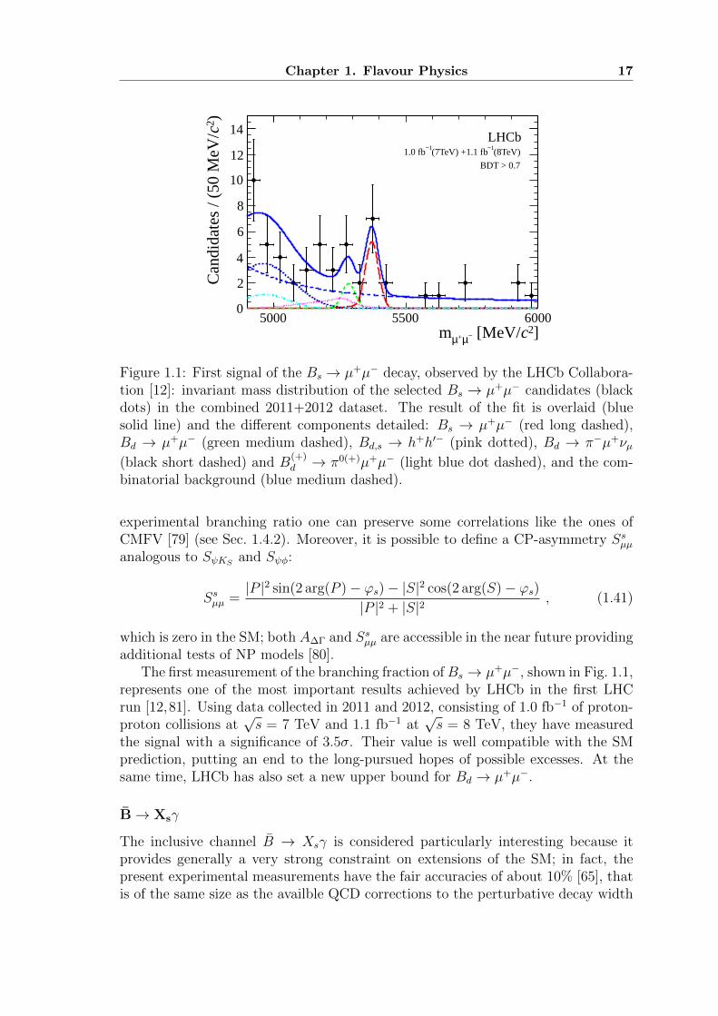
Figure 1.1: First signal of the Bs → µ+µ− decay, observed by the LHCb Collabora-tion [12]: invariant mass distribution of the selected Bs → µ+µ− candidates (blackdots) in the combined 2011+2012 dataset. The result of the fit is overlaid (bluesolid line) and the different components detailed: Bs → µ+µ− (red long dashed),Bd → µ+µ− (green medium dashed), Bd,s → h+h′− (pink dotted), Bd → π−µ+νµ(black short dashed) and B
(+)d → π0(+)µ+µ− (light blue dot dashed), and the com-
binatorial background (blue medium dashed).
experimental branching ratio one can preserve some correlations like the ones ofCMFV [79] (see Sec. 1.4.2). Moreover, it is possible to define a CP-asymmetry Ssµµanalogous to SψKS and Sψφ:
Ssµµ =|P |2 sin(2 arg(P )− ϕs)− |S|2 cos(2 arg(S)− ϕs)
|P |2 + |S|2, (1.41)
which is zero in the SM; both A∆Γ and Ssµµ are accessible in the near future providingadditional tests of NP models [80].
The first measurement of the branching fraction ofBs → µ+µ−, shown in Fig. 1.1,represents one of the most important results achieved by LHCb in the first LHCrun [12,81]. Using data collected in 2011 and 2012, consisting of 1.0 fb−1 of proton-proton collisions at
√s = 7 TeV and 1.1 fb−1 at
√s = 8 TeV, they have measured
the signal with a significance of 3.5σ. Their value is well compatible with the SMprediction, putting an end to the long-pursued hopes of possible excesses. At thesame time, LHCb has also set a new upper bound for Bd → µ+µ−.
B→ Xsγ
The inclusive channel B → Xsγ is considered particularly interesting because itprovides generally a very strong constraint on extensions of the SM; in fact, thepresent experimental measurements have the fair accuracies of about 10% [65], thatis of the same size as the availble QCD corrections to the perturbative decay width
18 Chapter 1. Flavour Physics
Γ(b → sγ), and larger than the known nonperturbative corrections to the relationΓ(B → Xsγ) ' Γ(b→ sγ) [82].
The effective Hamiltonian of the b → sγ transitions receives the contributionsfrom the four-fermion operators Q1 . . . Q6 and from the magnetic penguins Q7, Q8.The magnetic γ-penguin plays the crucial role in this decay, but the role of thedominant current-current operator Q2 is very important too, since the short dis-tance QCD effects involving in particular the mixing between Q2 and Q7 enhancethe Wilson coefficient C7(µb) significantly, so that the final branching ratio turnsout to be by a factor of 3 higher than it would be at LO. A peculiar feature ofthe renormalization group analysis in B → Xsγ is that the mixing under infiniterenormalization between the set Q1 . . . Q6 and the operators (Q7, QG) vanishes atthe one-loop level [45]; consequently, in order to calculate the coefficients C7(µb)and C8(µb) in the leading logarithmic approximation, two-loop calculations are nec-essary. The corresponding NLO analysis requires the evaluation of the mixing inquestion at the three-loop level. Because of this peculiar feature, the first fully cor-rect calculation of the leading anomalous dimension matrix relevant for this decaywas obtained only in 1993 [83,84], and the NLO correction in 1996 [85].
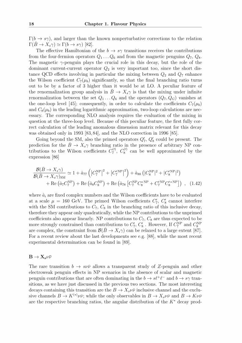
Going beyond the SM, also the primed operators Q′7, Q′8 could be present. Theprediction for the B → Xsγ branching ratio in the presence of arbitrary NP con-tributions to the Wilson coefficients C
(′)7 , C
(′)8 can be well approximated by the
expression [86]
B(B → Xsγ)
B(B → Xsγ)SM
' 1 + a77
(∣∣CNP7
∣∣2 +∣∣C ′NP
7
∣∣2)+ a88
(|CNP
8 |2 + |C ′NP8 |2
)+ Re
(a7C
NP7
)+ Re
(a8C
NP8
)+ Re
(a78
[CNP
7 C∗NP8 + C ′NP
7 C ′ ∗NP8
]), (1.42)
where ai are fixed complex numbers and the Wilson coefficients have to be evaluatedat a scale µ = 160 GeV. The primed Wilson coefficients C ′7, C ′8 cannot interferewith the SM contributions to C7, C8 in the branching ratio of this inclusive decay,therefore they appear only quadratically, while the NP contributions to the unprimedcoefficients also appear linearly. NP contributions to C7, C8 are thus expected to bemore strongly constrained than contributions to C ′7, C ′8 . However, If CNP
7 and CNP8
are complex, the constraint from B(B → Xsγ) can be relaxed to a large extent [87].For a recent review about the last developments see e.g. [88], while the most recentexperimental determination can be found in [89].
B→ Xsνν
The rare transition b → sνν allows a transparent study of Z-penguin and otherelectroweak penguin effects in NP scenarios in the absence of scalar and magneticpenguin contributions that are often dominating in the b→ s`+`− and b→ sγ tran-sitions, as we have just discussed in the previous two sections. The most interestingdecays containing this transition are the B → Xsνν inclusive channel and the exclu-sive channels B → K(∗)νν; while the only observables in B → Xsνν and B → Kννare the respective branching ratios, the angular distribution of the K∗ decay prod-
Chapter 1. Flavour Physics 19
ucts in the B → K∗(→ Kπ)νν decay allows to extract additional information aboutthe polarization of the K∗.
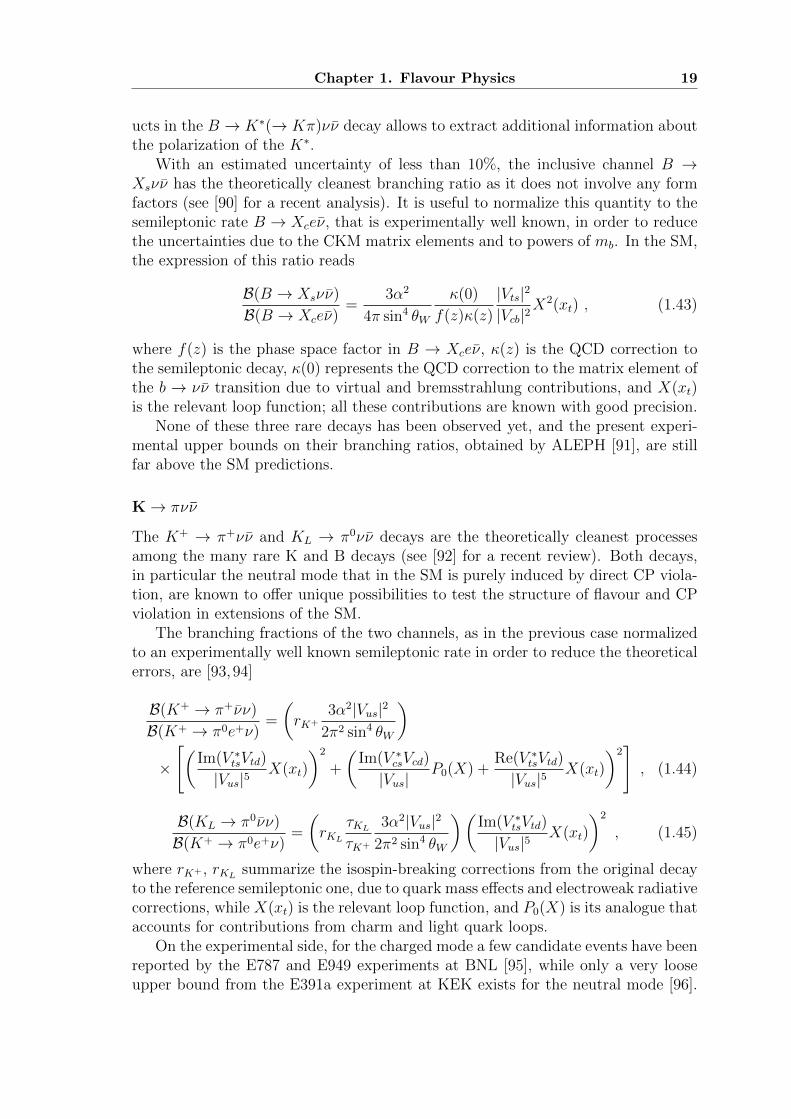
With an estimated uncertainty of less than 10%, the inclusive channel B →Xsνν has the theoretically cleanest branching ratio as it does not involve any formfactors (see [90] for a recent analysis). It is useful to normalize this quantity to thesemileptonic rate B → Xceν, that is experimentally well known, in order to reducethe uncertainties due to the CKM matrix elements and to powers of mb. In the SM,the expression of this ratio reads
B(B → Xsνν)
B(B → Xceν)=
3α2
4π sin4 θW
κ(0)
f(z)κ(z)
|Vts|2
|Vcb|2X2(xt) , (1.43)
where f(z) is the phase space factor in B → Xceν, κ(z) is the QCD correction tothe semileptonic decay, κ(0) represents the QCD correction to the matrix element ofthe b → νν transition due to virtual and bremsstrahlung contributions, and X(xt)is the relevant loop function; all these contributions are known with good precision.
None of these three rare decays has been observed yet, and the present experi-mental upper bounds on their branching ratios, obtained by ALEPH [91], are stillfar above the SM predictions.
K→ πνν
The K+ → π+νν and KL → π0νν decays are the theoretically cleanest processesamong the many rare K and B decays (see [92] for a recent review). Both decays,in particular the neutral mode that in the SM is purely induced by direct CP viola-tion, are known to offer unique possibilities to test the structure of flavour and CPviolation in extensions of the SM.
The branching fractions of the two channels, as in the previous case normalizedto an experimentally well known semileptonic rate in order to reduce the theoreticalerrors, are [93,94]
B(K+ → π+νν)
B(K+ → π0e+ν)=
(rK+
3α2|Vus|2
2π2 sin4 θW
)×
[(Im(V ∗tsVtd)
|Vus|5X(xt)
)2
+
(Im(V ∗csVcd)
|Vus|P0(X) +
Re(V ∗tsVtd)
|Vus|5X(xt)
)2], (1.44)
B(KL → π0νν)
B(K+ → π0e+ν)=
(rKL
τKLτK+
3α2|Vus|2
2π2 sin4 θW
)(Im(V ∗tsVtd)
|Vus|5X(xt)
)2
, (1.45)
where rK+ , rKL summarize the isospin-breaking corrections from the original decayto the reference semileptonic one, due to quark mass effects and electroweak radiativecorrections, while X(xt) is the relevant loop function, and P0(X) is its analogue thataccounts for contributions from charm and light quark loops.
On the experimental side, for the charged mode a few candidate events have beenreported by the E787 and E949 experiments at BNL [95], while only a very looseupper bound from the E391a experiment at KEK exists for the neutral mode [96].
20 Chapter 1. Flavour Physics
The central value of the measured branching ratio of K+ → π+νν is a factor of 2above the SM prediction, but it is perfectly consistent with the SM, given the largeexperimental error at present. In the near future the NA62 experiment at CERNand the K0TO experiment at JPARC will aim to improve the sensitivity for thecharged and neutral channels respectively.
1.3 Tensions in flavour observables
1.3.1 The εK − SψKStension
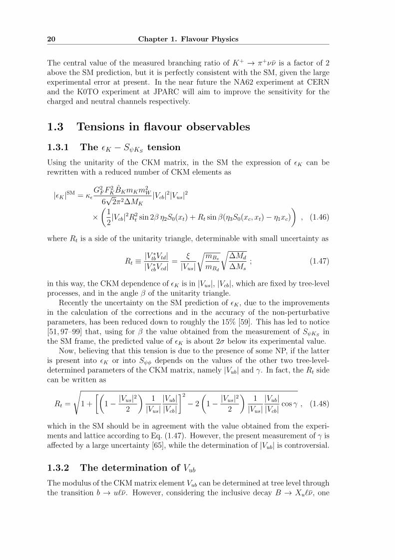
Using the unitarity of the CKM matrix, in the SM the expression of εK can berewritten with a reduced number of CKM elements as
|εK |SM = κεG2FF
2KBKmKm
2W
6√
2π2∆MK
|Vcb|2|Vus|2
×(
1
2|Vcb|2R2
t sin 2β η2S0(xt) +Rt sin β(η3S0(xc, xt)− η1xc)
), (1.46)
where Rt is a side of the unitarity triangle, determinable with small uncertainty as
Rt ≡|V ∗tbVtd||V ∗cbVcd|
=ξ
|Vus|
√mBs
mBd
√∆Md
∆Ms
; (1.47)
in this way, the CKM dependence of εK is in |Vus|, |Vcb|, which are fixed by tree-levelprocesses, and in the angle β of the unitarity triangle.
Recently the uncertainty on the SM prediction of εK , due to the improvementsin the calculation of the corrections and in the accuracy of the non-perturbativeparameters, has been reduced down to roughly the 15% [59]. This has led to notice[51, 97–99] that, using for β the value obtained from the measurement of SψKS inthe SM frame, the predicted value of εK is about 2σ below its experimental value.
Now, believing that this tension is due to the presence of some NP, if the latteris present into εK or into Sψφ depends on the values of the other two tree-level-determined parameters of the CKM matrix, namely |Vub| and γ. In fact, the Rt sidecan be written as
Rt =
√1 +
[(1− |Vus|
2
2
)1
|Vus||Vub||Vcb|
]2
− 2
(1− |Vus|
2
2
)1
|Vus||Vub||Vcb|
cos γ , (1.48)
which in the SM should be in agreement with the value obtained from the experi-ments and lattice according to Eq. (1.47). However, the present measurement of γ isaffected by a large uncertainty [65], while the determination of |Vub| is controversial.
1.3.2 The determination of Vub
The modulus of the CKM matrix element Vub can be determined at tree level throughthe transition b → u`ν. However, considering the inclusive decay B → Xu`ν, one
Chapter 1. Flavour Physics 21
Scenario 1 Scenario 2Experiment|Vub| = 3.23(31)× 10−3 |Vub| = 4.41(32)× 10−3
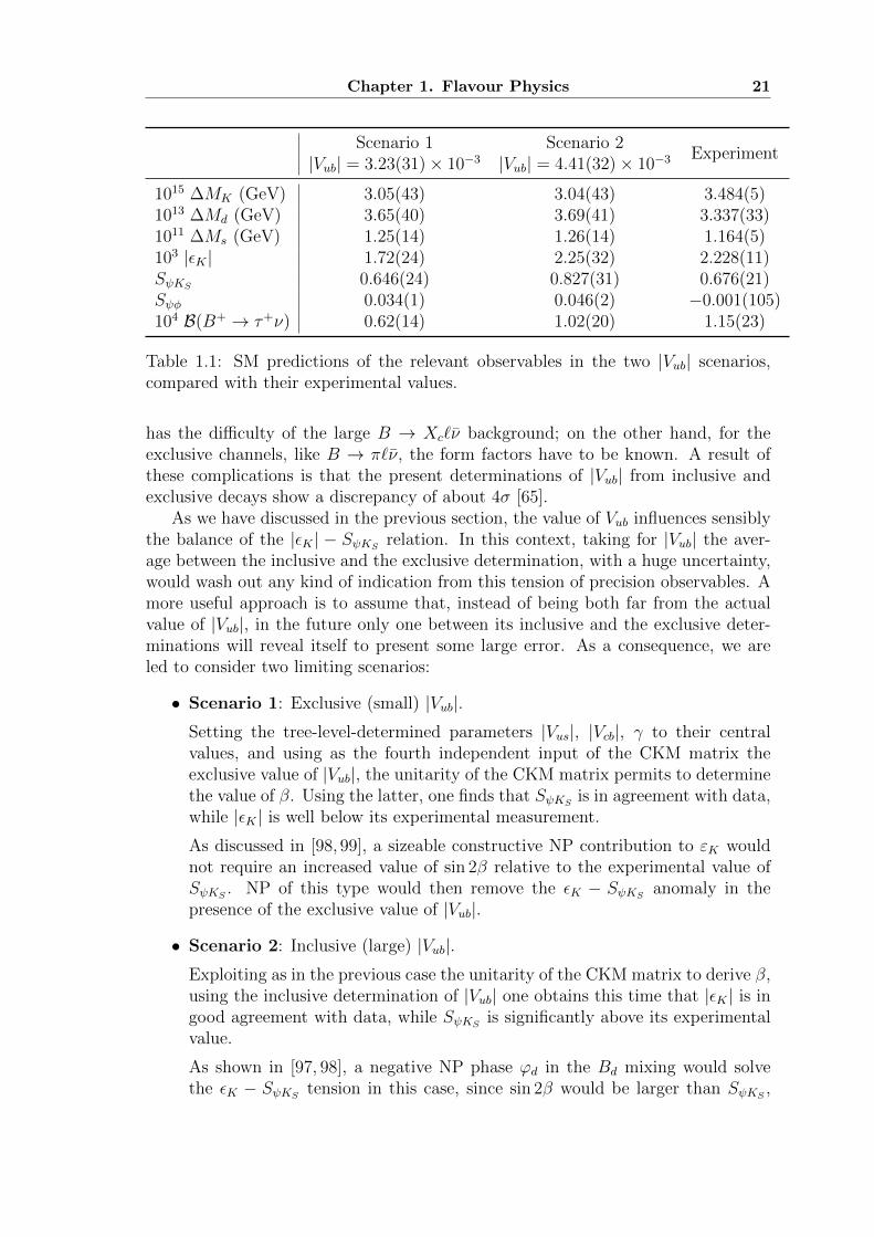
1015 ∆MK (GeV) 3.05(43) 3.04(43) 3.484(5)1013 ∆Md (GeV) 3.65(40) 3.69(41) 3.337(33)1011 ∆Ms (GeV) 1.25(14) 1.26(14) 1.164(5)103 |εK | 1.72(24) 2.25(32) 2.228(11)SψKS 0.646(24) 0.827(31) 0.676(21)Sψφ 0.034(1) 0.046(2) −0.001(105)104 B(B+ → τ+ν) 0.62(14) 1.02(20) 1.15(23)
Table 1.1: SM predictions of the relevant observables in the two |Vub| scenarios,compared with their experimental values.
has the difficulty of the large B → Xc`ν background; on the other hand, for theexclusive channels, like B → π`ν, the form factors have to be known. A result ofthese complications is that the present determinations of |Vub| from inclusive andexclusive decays show a discrepancy of about 4σ [65].
As we have discussed in the previous section, the value of Vub influences sensiblythe balance of the |εK | − SψKS relation. In this context, taking for |Vub| the aver-age between the inclusive and the exclusive determination, with a huge uncertainty,would wash out any kind of indication from this tension of precision observables. Amore useful approach is to assume that, instead of being both far from the actualvalue of |Vub|, in the future only one between its inclusive and the exclusive deter-minations will reveal itself to present some large error. As a consequence, we areled to consider two limiting scenarios:
• Scenario 1: Exclusive (small) |Vub|.Setting the tree-level-determined parameters |Vus|, |Vcb|, γ to their centralvalues, and using as the fourth independent input of the CKM matrix theexclusive value of |Vub|, the unitarity of the CKM matrix permits to determinethe value of β. Using the latter, one finds that SψKS is in agreement with data,while |εK | is well below its experimental measurement.
As discussed in [98, 99], a sizeable constructive NP contribution to εK wouldnot require an increased value of sin 2β relative to the experimental value ofSψKS . NP of this type would then remove the εK − SψKS anomaly in thepresence of the exclusive value of |Vub|.
• Scenario 2: Inclusive (large) |Vub|.Exploiting as in the previous case the unitarity of the CKM matrix to derive β,using the inclusive determination of |Vub| one obtains this time that |εK | is ingood agreement with data, while SψKS is significantly above its experimentalvalue.
As shown in [97, 98], a negative NP phase ϕd in the Bd mixing would solvethe εK − SψKS tension in this case, since sin 2β would be larger than SψKS ,
22 Chapter 1. Flavour Physics
implying a higher value on |εK |, in reasonable agreement with data, and abetter fit of the unitarity triangle.
This kind of analysis imply that the structure of a certain NP model could prefera specific determination of |Vub|; then, the correlated effects on other observables,especially ∆Ms,d, would represent a powerful test for such a model. This will bethe case of the two models studied is this work: we will show that the GFS modelselects the Scenario 1, while the 331 model selects the Scenario 2.
In Tab. 1.1 we report the SM predictions for the crucial flavour observables thatare sensitive to |Vub| in the two scenarios; the request of the agreement with theexperiment values will guide the analysis of the NP models.
1.3.3 More discrepancies and anomalies
∆Md,s versus εK
Using the most recent lattice inputs, it results that the SM predictions for both ∆Md
and ∆Ms are slightly above the data, of about 1σ once the hadronic uncertaintieshave been taken into account. While this is not a severe discrepancy in itself, itcan become more problematic when also εK is considered. In fact, ∆Md,s are oftencorrelated with εK in NP models, and if an enhancement of |εK | is required, as inthe case of the |Vub| Scenario 1, the weak agreement of ∆Md,s with experiment couldbe worsened. As we will discuss in Sec. 1.4.2 and Sec. 2.3.2 respectively, this is thecase of models with CMFV and of the GFS model.
The anomalous like-sign dimuon asymmetry
As we have anticipated in Sec. 1.2.1, the experimental value of Absl differs by 3.2σfrom it SM prediction. In [69] a detailed model-independent analysis of NP in theBd,s − Bd,s mixing has been performed; it has been found that in order to reconcileAbsl with its experimental value, accounting at the same time the constraints comingfrom Sψφ, NP is required not only in Md,s
12 , but also in Γd,s12 .
The anomaly in B(B→ D(∗)τν)/B(B→ D(∗)`ν)
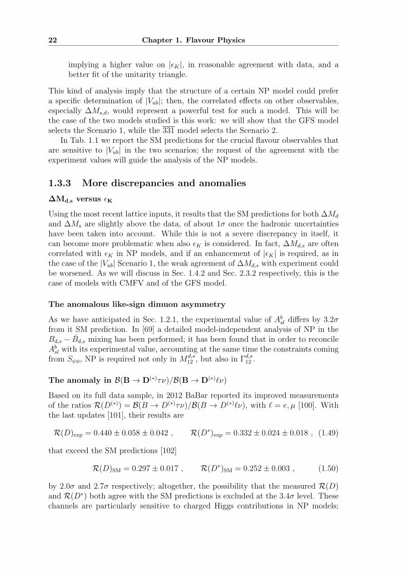
Based on its full data sample, in 2012 BaBar reported its improved measurementsof the ratios R(D(∗)) = B(B → D(∗)τν)/B(B → D(∗)`ν), with ` = e, µ [100]. Withthe last updates [101], their results are
R(D)exp = 0.440± 0.058± 0.042 , R(D∗)exp = 0.332± 0.024± 0.018 , (1.49)
that exceed the SM predictions [102]
R(D)SM = 0.297± 0.017 , R(D∗)SM = 0.252± 0.003 , (1.50)
by 2.0σ and 2.7σ respectively; altogether, the possibility that the measured R(D)and R(D∗) both agree with the SM predictions is excluded at the 3.4σ level. Thesechannels are particularly sensitive to charged Higgs contributions in NP models;
Chapter 1. Flavour Physics 23
æ æ æ æ æ æ æ æà à à à à à à à
ì ì
ìì ì ì
ì
ì
D02007
CDF2007
D02008
CDF2010
D02011
CDF2011
LHCb2011
LHCb2012
-0.2
0.0
0.2
0.4
0.6
0.8
1.0
1.2
S ΨΦ
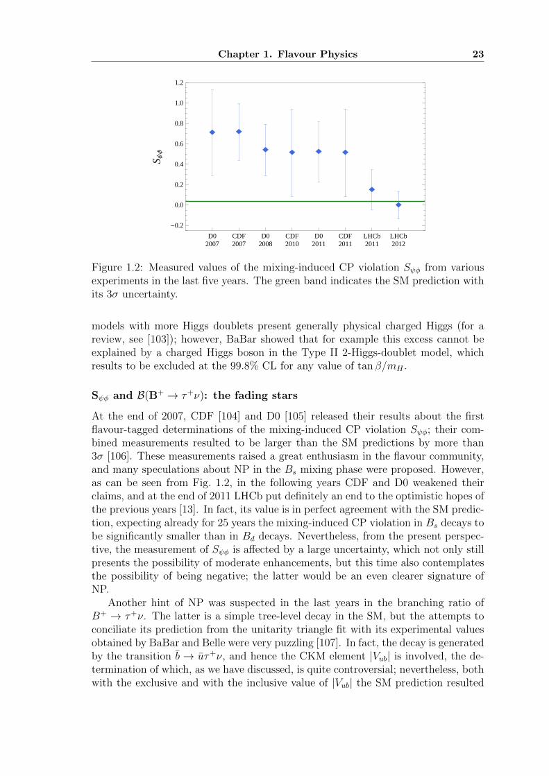
Figure 1.2: Measured values of the mixing-induced CP violation Sψφ from variousexperiments in the last five years. The green band indicates the SM prediction withits 3σ uncertainty.
models with more Higgs doublets present generally physical charged Higgs (for areview, see [103]); however, BaBar showed that for example this excess cannot beexplained by a charged Higgs boson in the Type II 2-Higgs-doublet model, whichresults to be excluded at the 99.8% CL for any value of tan β/mH .
Sψφ and B(B+ → τ+ν): the fading stars
At the end of 2007, CDF [104] and D0 [105] released their results about the firstflavour-tagged determinations of the mixing-induced CP violation Sψφ; their com-bined measurements resulted to be larger than the SM predictions by more than3σ [106]. These measurements raised a great enthusiasm in the flavour community,and many speculations about NP in the Bs mixing phase were proposed. However,as can be seen from Fig. 1.2, in the following years CDF and D0 weakened theirclaims, and at the end of 2011 LHCb put definitely an end to the optimistic hopes ofthe previous years [13]. In fact, its value is in perfect agreement with the SM predic-tion, expecting already for 25 years the mixing-induced CP violation in Bs decays tobe significantly smaller than in Bd decays. Nevertheless, from the present perspec-tive, the measurement of Sψφ is affected by a large uncertainty, which not only stillpresents the possibility of moderate enhancements, but this time also contemplatesthe possibility of being negative; the latter would be an even clearer signature ofNP.
Another hint of NP was suspected in the last years in the branching ratio ofB+ → τ+ν. The latter is a simple tree-level decay in the SM, but the attempts toconciliate its prediction from the unitarity triangle fit with its experimental valuesobtained by BaBar and Belle were very puzzling [107]. In fact, the decay is generatedby the transition b → uτ+ν, and hence the CKM element |Vub| is involved, the de-termination of which, as we have discussed, is quite controversial; nevertheless, bothwith the exclusive and with the inclusive value of |Vub| the SM prediction resulted
24 Chapter 1. Flavour Physics
to be largely below the experimental value. Even trying to remove the dependencefrom |Vub| by using the unitarity of the CKM matrix, so that the branching ratiodepends on the CKM parameters |Vud|, β and γ, the SM prediction was still 2.8σlower than the measurement. Now, in 2012 both BaBar [108] and Belle [109] pre-sented their updates about the measurement of B(B+ → τ+ν); in particular, thelatter reported a very smaller value, such to lower the world average and weakenthe tension to 1.6σ [110].
1.4 Patterns of flavour violation
1.4.1 The NP flavour problem
In general, new sources of flavour and CP violation are present in NP models. Model-independent considerations can be developed by means of a generic effective theoryapproach, assuming that the energy scale of NP is a certain ΛNP and integratingout the NP degrees of freedom; their effects will be described by higher dimensionaloperators O
(d)i in the resulting effective Lagrangian
Leff = LSM +∑i, d>4
c(d)i
ΛdNP
O(d)i , (1.51)
where cdi are unknown effective couplings.Now, as we have discussed in the Introduction, the solution of SM gauge hierarchy
problem would require some NP at a scale ΛNP that should not exceed a few TeV.On the other hand, the term with the higher dimensional operators contains forexample dimension six ∆F = 2 four-quark operators that lead to contributions toneutral meson mixing; the very good agreement between the SM predictions formeson mixing and the experimental data can then be translated into bounds forc
(d)i /ΛNP. If the coefficients c
(d)i are assumed to be generic, i.e. all of O(1), then
the most stringent bounds that come from CP violation in the K mixing imply forΛNP values of the order O(104 − 105) TeV: the examination of models with genericflavour structure has shown that large new sources of flavour symmetry breakingbeyond the SM are already excluded at the TeV scale [24]. The large discrepancybetween these two determinations of ΛNP is a manifestation of what in differentspecific NP frameworks (supersymmetry, technicolor, etc.) goes under the name offlavour problem [111].
These considerations have raised the interest in the understanding the flavourstructure of the NP models, and in signatures of deviations of it from the flavourstructure of the SM. The formalization of this solution to the flavour problem, i.e. therecognition or imposition of the SM flavour structure in a certain NP model, iscalled Minimal Flavour Violation (MFV), and it has been developed and analyzedin different ways during the last years; in particular, two relevant frameworks [112]are the pragmatic approach called Constrained Minimal Flavour Violation (CMFV),and a more formal approach that makes use of group methods and effective theories,and which at the same time allows more freedom. We stress however that MFV is
Chapter 1. Flavour Physics 25
not a theory of flavour, since it does not provide an explanation for the hierarchicalflavour structure that is already present in the SM.
1.4.2 Constrained Minimal Flavour Violation
CMFV can be seen as a brute-force method of extrapolating the flavour structureof the SM. It is defined by two conditions [113,114]:
• all flavour changing transitions are governed by the CKM matrix with theCKM phase being the only source of CP violation;
• the only relevant operators in the effective Hamiltonian below the weak scaleare those that are also relevant in the SM.
The use of the penguin-box expansion is very useful for the study of CMFV. Infact, the properties of universality and realness of the Fi master functions dependonly on the flavour and CP structure of the SM, and the form of the Pi coefficientsdepends only on the operator structure of the SM. Both the flavour and CP structureand the operator structure of the SM are preserved by definition in models withCMFV, and hence the Pi are model independent within the whole class of CMFVmodels, while the details of the single models are contained into the master functionsFi, which mantain their universality and realness. Since the SM belongs itself to theclass of CMFV, in these models the formulae of the observables will have the sameform as in the SM with the only substitution Fi(xt)→ Fi(xt, ρNP), where the latterare obtained by the calculation of the relevant diagrams in the NP model.
Universal Unitarity Triangle
The analysis of the unitarity triangle provides a powerful test of the flavour patternof CMFV in a model independent way; in fact, a triangle common to the whole classof CMFV models, known as Universal Unitarity Triangle (UUT) [113], can be built,and comparing it with the Reference Unitarity Triangle (RUT), can give informationnot only on the possible presence of NP, but also about its flavour structure (Fig. 1.3,left).
Once the parameters λ ≡ |Vus| and A = |Vcb|/λ2, unaffected by NP, have beendetermined, the determination of the apex (ρ, η) requires the knowledge of one sideand one angle of the triangle, provided the CKM matrix is unitary. Two choices ofsets with different characteristics are possible.
• Rb and γ . Rb ∝ |Vub| and γ = arg(Vub) are extracted from tree-level pro-cesses, and hence are very unlikely modified by NP. The triangle obtained withthis method is the RUT.
• Rt and β . With a very good approximation Rt ∝ |Vtd/Vts|, while β =arg(Vtd); the presence of the top quark implies that these can be only deter-mined from loop processes. However, the universality of the master functions
26 Chapter 1. Flavour Physics
Γ Β
Rb Rt
0.0 0.2 0.4 0.6 0.8 1.00.0
0.1
0.2
0.3
0.4
0.5
Ρ
Η
1.6 1.7 1.8 1.9 2.0 2.1 2.2 2.3
1
2
3
4
5
103 ΕK ¤
1013
DM
d,1
011D
Ms
HGeV
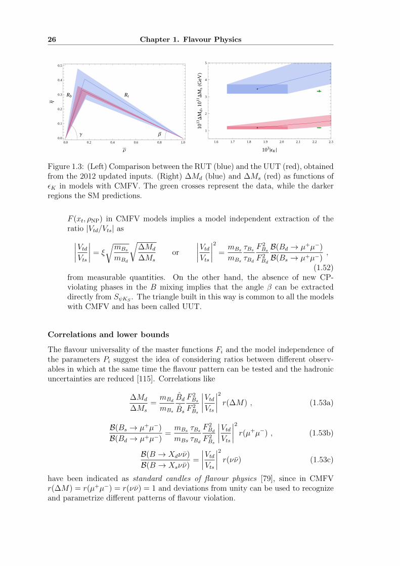
L
Figure 1.3: (Left) Comparison between the RUT (blue) and the UUT (red), obtainedfrom the 2012 updated inputs. (Right) ∆Md (blue) and ∆Ms (red) as functions ofεK in models with CMFV. The green crosses represent the data, while the darkerregions the SM predictions.
F (xt, ρNP) in CMFV models implies a model independent extraction of theratio |Vtd/Vts| as∣∣∣∣VtdVts
∣∣∣∣ = ξ
√mBs
mBd
√∆Md
∆Ms
or
∣∣∣∣VtdVts∣∣∣∣2 =
mBs
mBs
τBsτBd
F 2Bs
F 2Bd
B(Bd → µ+µ−)
B(Bs → µ+µ−),
(1.52)from measurable quantities. On the other hand, the absence of new CP-violating phases in the B mixing implies that the angle β can be extracteddirectly from SψKS . The triangle built in this way is common to all the modelswith CMFV and has been called UUT.
Correlations and lower bounds
The flavour universality of the master functions Fi and the model independence ofthe parameters Pi suggest the idea of considering ratios between different observ-ables in which at the same time the flavour pattern can be tested and the hadronicuncertainties are reduced [115]. Correlations like
∆Md
∆Ms
=mBd
mBs
Bd
Bs
F 2Bs
F 2Bs
∣∣∣∣VtdVts∣∣∣∣2 r(∆M) , (1.53a)
B(Bs → µ+µ−)
B(Bd → µ+µ−)=mBs
mBs
τBsτBd
F 2Bd
F 2Bs
∣∣∣∣VtdVts∣∣∣∣2 r(µ+µ−) , (1.53b)
B(B → Xdνν)
B(B → Xsνν)=
∣∣∣∣VtdVts∣∣∣∣2 r(νν) (1.53c)
have been indicated as standard candles of flavour physics [79], since in CMFVr(∆M) = r(µ+µ−) = r(νν) = 1 and deviations from unity can be used to recognizeand parametrize different patterns of flavour violation.
Chapter 1. Flavour Physics 27
Less intuitive but still simple calculations permit also to find that the observablesrelated to the meson mixing like εK and ∆Md,s are not only correlated, but also canonly be enhanced with respect to the SM [116].
Comparison with experiments
First of all one observes that, since in this context SψKS cannot receive new contri-butions, CMFV models prefer what we have called the Scenario 2 for Vub. Now, aswe have discussed, positive contributions to εK are allowed, and hence the SψKS−εKtension can be solved. Nevertheless, the enhancement of εK would determine a cor-related enhancement of both ∆Md and ∆Ms, worsening the ∆Md,s− εK tension [79](Fig. 1.3, right).
The previous considerations, even if only qualitative, point out the difficultiesthat CMFV models have in accommodating the tensions in flavour data, due to thepresence of few free parameters and strict correlations. A more quantitative andcomplete study has recently been performed [117].
1.4.3 Minimal Flavour Violation at Large
The flavour symmetry of the SM can be formalized in the framework of grouptheory. In fact, it can be identified with the largest group of unitary quark fieldtransformations that commutes with the SM gauge Lagrangian [118,119]
Gq = (SU(3)× U(1))3 , (1.54)
i.e. a SU(3) symmetry and a phase symmetry for each electroweak multiplet:
SU(3)3 = SU(3)QL × SU(3)UR × SU(3)DR , U(1)3 = U(1)B × U(1)Y × U(1)PQ ,(1.55)
where the three U(1) symmetries can be rearranged as the baryon number, thehypercharge, and a Peccei-Quinn symmetry [120] (see Sec. 3.2.2). In the SM thissymmetry (with the exception of U(1)B) is explicitly broken by the two Yukawacouplings
LY = −QLYdDRH − QLYuURH + h.c. . (1.56)
Now, the flavour symmetry Gq can be formally recovered by promoting the Yukawamatrices to spurions, i.e. dimensionless auxiliary fields transforming as
Yu ∼ (3, 3,1)SU(3)3 , Yd ∼ (3,1, 3)SU(3)3 . (1.57)
One defines an effective theory as satisfying the criterion of MFV if all higher-dimensional operators, constructed from SM and spurion fields, are formally invari-ant under the flavour group Gq [119].
In practice, one can build effective couplings and higher-dimensional operatorsin which the only relevant non-diagonal structures are polynomials P(YuY
†u , YdY
†d )
of the two basic spurions
YuY†u , YdY
†d ∼ (8,1,1)SU(3)3
q⊕ (1,1,1)SU(3)3
q. (1.58)
28 Chapter 1. Flavour Physics
As an example of this mechanism at work, we shortly discuss the application ofthis formulation of MFV to a generic model with two Higgs doublets, resulting in aNP scenario called 2HDMMFV [121].
The 2HDMMFV
In a generic model with two-Higgs doublets, H1 and H2, with hypercharges Y = 1/2and Y = −1/2 respectively, the most general renormalizable and gauge-invariantinteraction of them with the SM quarks is
−LY = QLXd1DRH1 + QLXu1URHc1 + QLXd2DRH
c2 + QLXu2URH2 + h.c. , (1.59)
where Hc1(2) = −iτ2H
∗1(2) and the Xi are 3 × 3 matrices with a generic flavour
structure. By performing a global rotation of angle β = arctan(v2/v1) of the Higgsfields, the mass terms and the interaction terms are separated, but they cannot bediagonalized simultaneously for generic Xi and dangerous FCNC couplings to theneutral Higgses appear.
If the MFV hypothesis is imposed instead, the Xi are forced to assume theparticular structure
Xd1 = Yd (1.60a)
Xd2 = Pd2(YuY†u , YdY
†d )× Yd = ε0Yd + ε1YdY
†d Yd + ε2YuY
†uYd + . . . (1.60b)
Xu1 = Pu1(YuY†u , YdY
†d )× Yu = ε′0Yu + ε′1YuY
†uYu + ε′2YdY
†d Yu + . . . (1.60c)
Xu2 = Yu (1.60d)
that is renormalization group invariant [121]. At higher orders in YiY†i FCNCs are
generated, and in order to investigate them one can perform an expansion in powersof suppressed off-diagonal CKM elements, so that the effective down-type FCNCinteraction can be written as
LFCNCMFV ∝ diL
[(a0V
†λ2uV + a1V
†λ2uV∆ + a2∆V †λ2
uV)λd]ijdjR
S2 + iS3√2
+ h.c. ,
(1.61)where λu,d ∝ 1/v diag (mu,d,mc,s,mt,b), ∆ = diag (0, 0, 1), and the ai are parametersnaturally of O(1); this structure shows a large suppression due to the presence oftwo off-diagonal CKM elements and the down-type Yukawas [121], demonstratingexplicitly how MFV is effective and natural.
It is remarkable that the mechanisms of flavour and CP violation do not nec-essarily need to be related: in MFV the Yukawa matrices are the only sources offlavour breaking, but other sources of CP violation could be present, provided thatthey are flavour-blind: this happens when the FCNC parameters ai are allowed tobe complex, as well as for the phases that can be present in the Higgs potential.
With a more detailed analysis the following relevant properties have been found[121]:
• the impact in K, Bd and Bs mixing amplitudes scales with msmd, mbmd andmbms respectively;
Chapter 1. Flavour Physics 29
• new flavour-blind phases φs = (ms/md)φd can contribute to the Bd and Bs
systems, and they are not present in the K system instead.
The previous observations imply that εK can receive only tiny new contributionswhile SψKS could be in principle sizeably modified; as a consequence, for the reasonsthat have been discussed in the previous section, the 2HDMMFV selects the inclusive|Vub|. However, in this framework a suppression of SψKS would determine a cor-related enhancement of Sψφ, an effect that was considered very welcome until lastyear, when LHCb excluded a large NP phase in the Bs mixing, putting thereforethis model in difficulty [79].
The flavour-blind phases of the Higgs potential imply instead φs = φd [122], andcould be used to remove the SψKS − εK tension, but the necessary size of φd wouldimply in turn Sψφ > 0.15, which is 2σ away from the LHCb central value [79].
1.4.4 Beyond Minimal Flavour Violation
From the discussion in the previous two sections it results that models with CMFVand MFV seem to present visible difficulties in describing all ∆F = 2 observables inthe K and Bd,s meson systems simultaneously. More definite conclusions will onlybe possible when |Vub| and γ will be known from tree level decays with a much betterprecision and the lattice input will further improve. Nevertheless, these results seemto indicate that the tensions in the flavour observables could be hints of a new flavourstructure different from the one of the SM. Both the models that we are going tostudy in this work go beyond MFV.
Models that do not satisfy the MFV hypothesis, neither by construction nor byimposition, present in general large flavour violating effects, unless fine tuning isapplied or some other suppression mechanism occurs. As we will discuss, the firstis the case of the 331 model, the second of the GFS model.
In fact, in the 331 model, in order to obtain phenomenological results in agree-ment with the experimental data, one needs both a quite high NP energy scale,coinciding with the mass of the FCNCs-mediating Z ′ new boson, and to force themixing matrix to be very similar the CKM matrix.
On the other hand, we will see that a very elegant feature of the GFS modelis that the minimal fermion content required for the theory to be consistent gener-ates a mechanism of inverted hierarchy in the Yukawa couplings that automaticallysuppresses FCNCs. Nevertheless, even if this model presents a number of analogieswith MFV models, the most evident of them being the fact that it is just basedon the restoring of the flavour symmetry and that NP effects are controlled by theflavour group, it does not satisfy the MFV requirement: in fact, one can find a limitin which all Yukawa couplings vanish but flavour breaking effects remain finite.

Chapter 2
Theory and phenomenologyof Gauged Flavour Symmetries
2.1 The model
2.1.1 Gauge group and field content
As we have discussed in Sec. 1.4.3, the SM presents the large flavour symmetry Gq =(SU(3)× U(1))3, explicitly broken by the two Yukawa couplings. This symmetrywould be restored not only formally, but truly if instead of the Yukawa constantmatrix there were physical fields transforming as (3, 3,1) and (3,1, 3) under SU(3)3.
In the model that we are going to build, Gq is assumed to be an exact symmetryof nature, spontaneously broken by the vevs of the two scalar fields Yu and Yd,which opportunely transform under it, called flavons. In order to avoid problematicflavour-violating Goldstone bosons, the symmetry should be gauged. Since we areinterested mainly in the flavour breaking, we choose to gauge only the subgroup
GGFS = SU(3)QL × SU(3)UR × SU(3)DR (2.1)
and not to concentrate on the abelian part. We will call GFS model the model withthese Gauged Flavour Symmetries and scalar content, and with the fermion contentthat we are going to introduce. In fact, we are going to discuss how new fermionshave to be added in order to cancel the gauge anomalies.
Basic notions about anomalies
We recall here the relevant theoretical aspects of the perturbation theory anomalies,following mainly [123–125].
A symmetry of a classic theory is not necessary preserved when such theory isquantized. In fact, if a field transformation φ → φ + δφ leaves the classical actionS(φ) invariant, the path integral
∫Dφ eiS(φ) is not necessarily invariant, depending
on the behavior of the measure Dφ. If a symmetry of a classical theory is spoiledin its quantized version, one says that there is an anomaly. While an anomaly in aglobal symmetry is not problematic, if there were an anomaly in a gauge symmetry
31
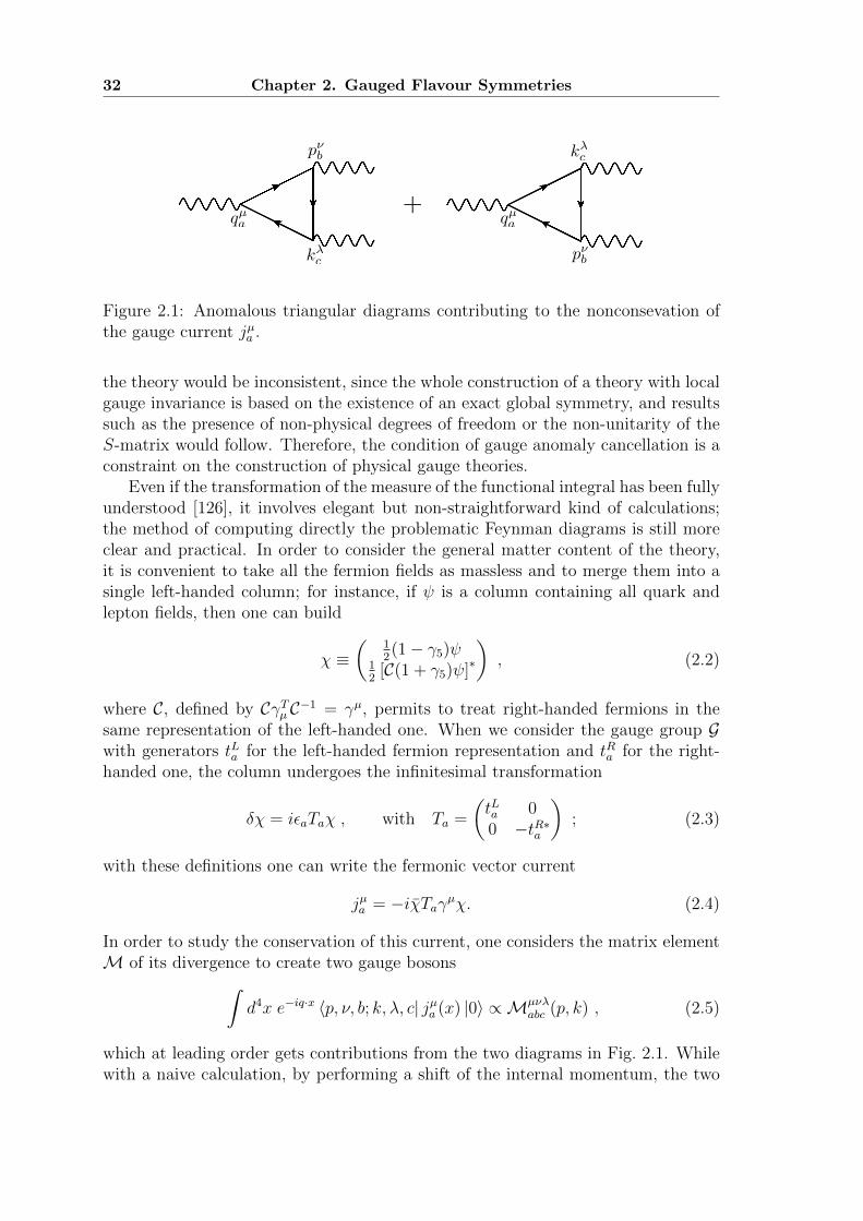
32 Chapter 2. Gauged Flavour Symmetries
qµa qµ
a
p⌫b
p⌫bk�c
k�c
+
Figure 2.1: Anomalous triangular diagrams contributing to the nonconsevation ofthe gauge current jµa .
the theory would be inconsistent, since the whole construction of a theory with localgauge invariance is based on the existence of an exact global symmetry, and resultssuch as the presence of non-physical degrees of freedom or the non-unitarity of theS-matrix would follow. Therefore, the condition of gauge anomaly cancellation is aconstraint on the construction of physical gauge theories.
Even if the transformation of the measure of the functional integral has been fullyunderstood [126], it involves elegant but non-straightforward kind of calculations;the method of computing directly the problematic Feynman diagrams is still moreclear and practical. In order to consider the general matter content of the theory,it is convenient to take all the fermion fields as massless and to merge them into asingle left-handed column; for instance, if ψ is a column containing all quark andlepton fields, then one can build
χ ≡(
12(1− γ5)ψ
12
[C(1 + γ5)ψ]∗
), (2.2)
where C, defined by CγTµ C−1 = γµ, permits to treat right-handed fermions in thesame representation of the left-handed one. When we consider the gauge group Gwith generators tLa for the left-handed fermion representation and tRa for the right-handed one, the column undergoes the infinitesimal transformation
δχ = iεaTaχ , with Ta =
(tLa 00 −tR∗a
); (2.3)
with these definitions one can write the fermonic vector current
jµa = −iχTaγµχ. (2.4)
In order to study the conservation of this current, one considers the matrix elementM of its divergence to create two gauge bosons∫
d4x e−iq·x 〈p, ν, b; k, λ, c| jµa (x) |0〉 ∝ Mµνλabc (p, k) , (2.5)
which at leading order gets contributions from the two diagrams in Fig. 2.1. Whilewith a naive calculation, by performing a shift of the internal momentum, the two
Chapter 2. Gauged Flavour Symmetries 33
diagrams seems to cancel each other and hence the current to be conserved, treatingthe problem more carefully one has to notice that the two diagrams are divergentand that this shift can not be allowed by the regularization. Using dimensional reg-ularization in order to preserve gauge invariance and the ‘t Hooft-Veltman definitionof the γ5 matrix in d dimensions to perform the calculation, one finds the generallynonvanishing result
〈p, ν, b; k, λ, c| jµa |0〉 =g2
8π2εανβλpαkβ · Aabc , (2.6)
with
Aabc = Tr[T a{T b, T c
}], (2.7)
where, as defined before, T a is the representation of the gauge algebra on the setof all left-handed fermion and antifermion fields, and the trace denotes the sumover these fermion and antifermion species. This anomalous contribution is a con-sequence of the fact that in order to preserve gauge invariance one has to work in ddimensions, but γ5, which is a fundamental object in chiral theories1, is an intrinsi-cally 4-dimensional object. The following further results validate the correctness ofEq. (2.6).
• Even if the previous calculation has been developed with massless fermions,the result is correct since one can show that no fermion that is allowed bya given symmetry to have a mass can contribute to the anomaly for thatsymmetry [124]. It is known that mass terms for Dirac fermions are notallowed by the SM gauge symmetry and hence neither by any of its possibleextensions, and therefore they contribute to the anomalies as massless fermionsbefore the spontaneous symmetry breaking.
• The higher order corrections to the matrix element, consisting both in prop-agators internal to the loop and in more external currents, vanish becausethey make the integral sufficiently convergent to allow to shift the internalmomentum without problems [127].
For the consistency of a gauge theory the current jµa must be conserved also atquantum level, and hence, as a consequence of the previous calculation, the conditionfor a gauge theory to be anomaly-free is Aabc = 0 when Ta, Tb and Tc run over all thegenerators of the gauge group. The following general results simplify this analysis.
• Of course, one needs only to consider those combinations of generators forwhich their product contains a singlet under the gauge group, since Aabc ob-viously vanishes for all the others. For example, one can make invariants outof any number of U(1) generators, zero, two or three SU(2) generators (since2 × 2 and 2 × 2 × 2 both contain singlets), and zero, two or three SU(3)generators.
1A theory is said to be chiral if it treats differently fields of different chiralities, if otherwise itis parity-symmetric is said to be vector.
34 Chapter 2. Gauged Flavour Symmetries
• For a fermion representation that is equivalent to its complex conjugate, i.e. inwhich its generators are related to the ones of its complex conjugate by unitarytransformations, it is straightforward to calculate Aabc = −Aabc = 0; as aconsequence, if the fermion content of a theory forms a representation that isreal or pseudoreal, the theory is anomaly-free, and if a gauge group admitsonly real or pseudoreal representations (like for example SU(2), SO(10), E6),it is automatically anomaly-free for any matter content.
• Besides the fields of the gauge group, also the gravitational field should beconsidered. All species of fermions interact with gravitation in the same way,and the calculation of the loop graph yields to an anomaly proportional to
Tr[Ta]εµνρσRµνκλRρσ
κλ ; (2.8)
it automatically vanishes if the gauge group is non-Abelian, while, if the lattercontains U(1) factors, the theory cannot be consistently coupled to gravityunless each of the U(1) generators is traceless [128].
Anomalies in the GFS model
In order to analyze the gauge anomalies of the model in relation with its fermioncontent, as described in the previous paragraph, we have to consider all the possiblecombinations of three generators of the gauge group, except the ones that containa single SU(3) or SU(2) factor.
• SU(3)3QL, SU(3)3UR
, SU(3)3DR
All the new groups present a cubic anomaly, because the SM quarks providenon-real representations of them. In order to obtain (pseudo)real representa-tions, one needs to add two new fermions Ψa, Ψb, whose right-handed compo-nents ΨaR, ΨbR transform as triplets under SU(3)3
QL, and whose left-handed
components ΨaL, ΨbL transform as triplets under SU(3)3UR
and SU(3)3DR
re-spectively.
• SU(3)3c
This anomaly vanishes if the new fermions, as the ones of the SM, are vector-like with respect to SU(3)c. This means that ΨaL and ΨaR have to belong tothe same SU(3)c representation (and hence for the number of colors one hasNc(ΨaL) = Nc(ΨaR) ≡ Nc(Ψa)), as well as ΨbL and ΨbR (and hence Nc(ΨbL) =Nc(ΨbR) ≡ Nc(Ψb)). Of course the simplest solutions, i.e. the singlets or thetriplets (Nc = 1 or Nc = 3), are preferable, in order to obtain a more elegantand predictive theory.
• SU(2)3L
Since SU(2) has only real or pseudoreal representations, this combination isalways non anomalous, independently from the fermion content.
Chapter 2. Gauged Flavour Symmetries 35
• U(1)3Y
The contribution from the SM fermions cancels as usual, as regards the NPcontributions the condition for the cancellation is
−Nc(Ψa)Y (ψaR)3 −Nc(Ψb)Y (ψbR)3 +Nc(Ψa)Y (ψaL)3 +Nc(Ψb)Y (ψbL)3 ≡ 0 .(2.9)
• SU(3)2QL×U(1)Y, SU(3)2UR
×U(1)Y, SU(3)2DR×U(1)Y
Also the conditions for the cancellation of these anomalies give informationabout the hypercharge and color of the new fermions:∑3[SU(3)QL ]
(YSM + YGFS) = 3
(1
6+
1
6
)−Nc(Ψa)Y (ΨaR)−Nc(Ψb)Y (ΨbR) ≡ 0 ,
(2.10a)∑3[SU(3)UR ]
(YSM + YGFS) = 3
(−2
3
)+Nc(Ψa)Y (ΨaL) ≡ 0 , (2.10b)
∑3[SU(3)UR ]
(YSM + YGFS) = 3
(1
3
)+Nc(Ψb)Y (ΨbL) ≡ 0 . (2.10c)
• SU(3)2c ×U(1)Y
Again, since the SM contribution to this anomaly regularly cancels, the NPcontribution has to vanish by itself, giving the condition∑
3[SU(3)c]
YGFS ≡ 0 , (2.11)
where the new fermions enter or not depending if they are color triplets orsinglets. This provides another relation for the hypercharges.
• SU(2)2L ×U(1)Y
Similarly to the previous case, the NP contribution has to vanish by itself,giving ∑
2[SU(3)L]
YGFS ≡ 0 , (2.12)
where the new fermions enter only if they are SU(2)L doublets. In the SM,given the specific hypercharges, this conditions implies that the number ofquark doublets has to be the same as the one of lepton doublets; here it givesanalogous information.
• [Grav]2 ×U(1)Y
The condition for the cancellation of the gravitational anomaly is
−Nc(Ψa)Y (ψaR)−Nc(Ψb)Y (ψbR) +Nc(Ψa)Y (ψaL) +Nc(Ψb)Y (ψbL) ≡ 0 ,(2.13)
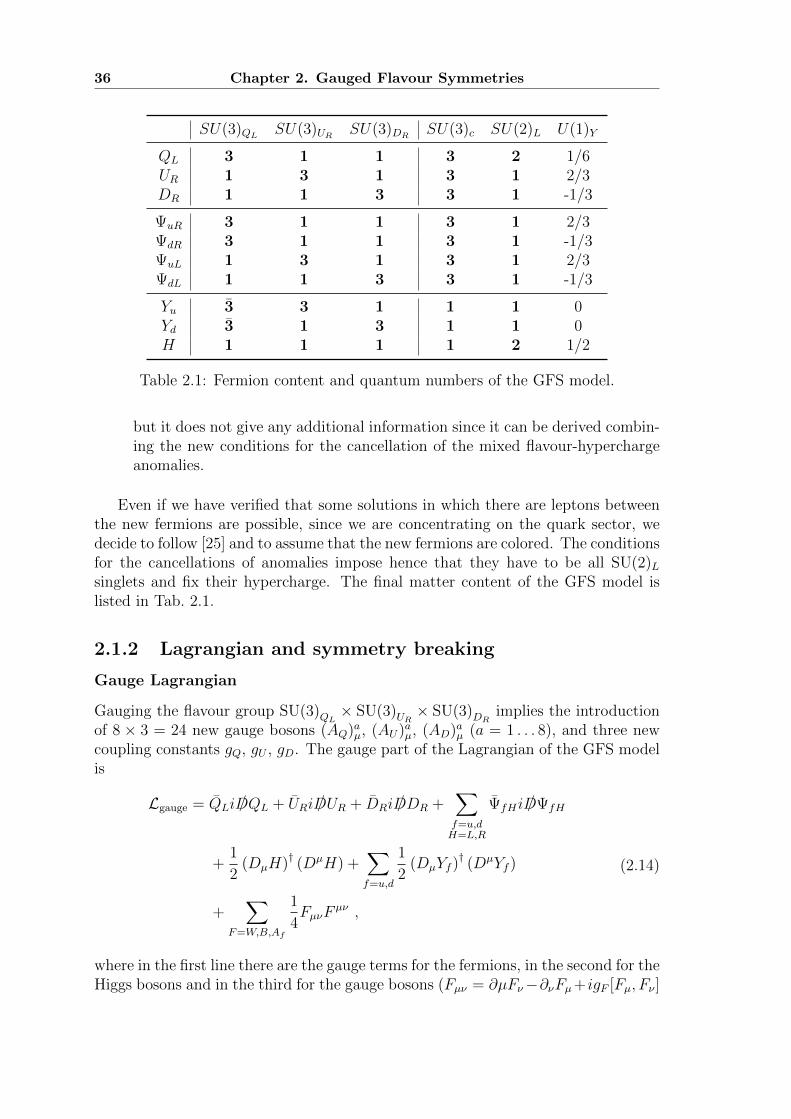
36 Chapter 2. Gauged Flavour Symmetries
SU(3)QL SU(3)UR SU(3)DR SU(3)c SU(2)L U(1)Y
QL 3 1 1 3 2 1/6UR 1 3 1 3 1 2/3DR 1 1 3 3 1 -1/3
ΨuR 3 1 1 3 1 2/3ΨdR 3 1 1 3 1 -1/3ΨuL 1 3 1 3 1 2/3ΨdL 1 1 3 3 1 -1/3
Yu 3 3 1 1 1 0Yd 3 1 3 1 1 0H 1 1 1 1 2 1/2
Table 2.1: Fermion content and quantum numbers of the GFS model.
but it does not give any additional information since it can be derived combin-ing the new conditions for the cancellation of the mixed flavour-hyperchargeanomalies.
Even if we have verified that some solutions in which there are leptons betweenthe new fermions are possible, since we are concentrating on the quark sector, wedecide to follow [25] and to assume that the new fermions are colored. The conditionsfor the cancellations of anomalies impose hence that they have to be all SU(2)Lsinglets and fix their hypercharge. The final matter content of the GFS model islisted in Tab. 2.1.
2.1.2 Lagrangian and symmetry breaking
Gauge Lagrangian
Gauging the flavour group SU(3)QL × SU(3)UR × SU(3)DR implies the introductionof 8 × 3 = 24 new gauge bosons (AQ)aµ, (AU)aµ, (AD)aµ (a = 1 . . . 8), and three newcoupling constants gQ, gU , gD. The gauge part of the Lagrangian of the GFS modelis
Lgauge = QLi /DQL + URi /DUR + DRi /DDR +∑f=u,dH=L,R
ΨfHi /DΨfH
+1
2(DµH)† (DµH) +
∑f=u,d
1
2(DµYf )
† (DµYf )
+∑
F=W,B,Af
1
4FµνF
µν ,
(2.14)
where in the first line there are the gauge terms for the fermions, in the second for theHiggs bosons and in the third for the gauge bosons (Fµν = ∂µFν−∂νFµ+igF [Fµ, Fν ]
Chapter 2. Gauged Flavour Symmetries 37
are the usual field strength tensors of all the gauge bosons). The covariant derivativeis
Dµ = ∂µ + igIWWµ + ig′YWBµ +∑
f=Q,U,D
igfNf (Af )µ ; (2.15)
IW , YW and Wµ and Bµ are respectively the usual quantum numbers and gaugebosons associated to the electroweak group (we are not considering QCD in theseexpressions); analogously, NQ, NU , ND are the quantum numbers of the fermionswith respect to the flavour group, and
(Af )µ =8∑
a=1
(Af )aµ
λa
2(f = Q,U,D) , (2.16)
being λa’s the Gell-Mann matrices.
Symmetry breaking
The pattern of electroweak symmetry breaking can be implemented as usual byexpanding, in the unitary gauge,
H =1√2
(0
v + h
). (2.17)
As regards the flavour breaking, a bit of manipulation is worth. The flavon fields(two complex 3 × 3 matrices for a total amount of 36 degrees of freedom) can beparametrized as
Yu = UUρuU†Q , (2.18a)
Yd = UDρdU†Q , (2.18b)
where UQ,U,D are the three unitary matrices parametrizing the 26 Goldstone modes(since the whole flavour group (SU(3)×U(1))3 is broken to U(1)B, there are 9+9+8broken generators); in the unitary gauge UQ,U,D = I3. Hence we are left with36− 26 = 10 degrees of freedom contained into ρu and ρd, which can be interpretedas the field excitations around the six SM masses and the four angles of the CKMmatrix. In fact, we can conveniently rewrite
ρu = ΣRuDuΣ†LuVGFS , (2.19a)
ρd = ΣRdDdΣ†Ld , (2.19b)
where Du,d are real diagonal matrices that get vevs Zu,d, VGSM is a unitary matrix(we will see later how it is linked to the CKM matrix), and ΣRu,Lu,Rd,Ld are fourunitary matrices parametrizing the remaining four angle modes. In fact, requiringthe radial modes in ρu,d to be orthogonal to the Goldstone modes corresponds inthe unitary gauge to the condition that cross product terms of the type ∂µρA
µ
vanish [25]; this corresponds to the three sets of conditions
AU : Im Tr[ρu∂ρ†uλ
α] = 0 , α = 1 . . . 9 , (2.20a)
AD : Im Tr[ρd∂ρ†dλ
α] = 0 , α = 1 . . . 9 , (2.20b)
AQ : Im Tr[(∂ρ†uρu + ∂ρ†dρd)λα] = 0 , α = 1 . . . 8 , (2.20c)
38 Chapter 2. Gauged Flavour Symmetries
where λ9 is the unitary matrix. Now, if we write
ΣX = eiΠX = exp
(iλα
2παX
), (2.21)
Eq. (2.20a)-(2.20c) are 26 conditions on the 36 παX , and 8 further conditions comefrom Eq. (2.19a)-(2.19b), leaving four independent combinations out of the παRu,Lu,Rd,Ld;we will call them π1,2,3,4 (notice that they mediate FCNCs).
In summary, the flavon fields and the breaking of the flavour symmetry can bewritten as
Yu = eiλα
2παRuDue
−iλα
2παLuV
Yd = eiλα
2παRdDde
−iλα
2παLd
(2.22)
where
Du,d = Zu,d + Tu,d ≡
zu,d zc,szt,b
+
tu,d tc,stt,b
, (2.23)
and παX are functions of π1, π2, π3, π4 with 〈πi〉 = 0; in particular
〈Yu〉 = ZuVGFS , 〈Yd〉 = Zd . (2.24)
Concerning the mechanism for the generation of this particular symmetry-breakingpattern, it can be shown that there exists no renormalizable potential for only twobifundamentals from which the correct pattern can arise [25]. One possibility tosolve this problem is to introduce a non-renormalizable potential: as long as thecut-off suppressing higher-dimensional operators is larger than the largest flavonvev, its effects can be treated as perturbations. Another possibility is to assumethat Yu,d are combinations of several fields transforming as bifundamentals underthe flavour group.
Mass eigenstates and interactions of fermions and gauge bosons
The most general interaction of the quarks with the Higgs fields is
Lint = λuQLHΨuR + λ′uΨuLYuΨuR +MuΨuLUR+
λdQLHΨdR + λ′uΨdLYdΨdR +MdΨdLDR + h.c. ,(2.25)
where Mu,d are universal mass parameters and λ(′)u,d are coupling constants, both of
which can be always chosen to be real. Building the fermion mass matrices, onefinds that both the SM and new quarks mix each other separately for up-type anddown-type, according to the rotations(
uiR,Lu′iR,L
)=
(cu(R,L)i
−su(R,L)i
su(R,L)icu(R,L)i
)(U iR,L
ΨiuR,L
), (2.26)
Chapter 2. Gauged Flavour Symmetries 39
with
suLi =
√Cu − (2Mu − v2λ2
u + 2z2uiλ′u
2)
2Cu, (2.27a)
suRi =
√Cu + (2Mu − v2λ2
u − 2z2uiλ′u
2)
2Cu, (2.27b)
where
Cu =√
(2Muv2λ2u + 2z2
uiλ′u
2)− 8M2uv
2λ2u , (2.28)
and cu(R,L)iand su(R,L)i
are the cosines and sines; for the down-quark sector theformulae are analogous. We obtain hence two sets of six quarks, whose masses are
(mu,d,mc,s,mt,b) = λu,dv√2
(s(u,d)R1
c(u,d)L1
,s(u,d)R2
c(u,d)L2
,s(u,d)L3
c(u,d)L3
),
(mu′,d′ ,mc′,s′ ,mt′,b′) = Mu,d
(c(u,d)L1
s(u,d)R1
,c(u,d)L2
s(u,d)R2
,c(u,d)L3
s(u,d)L3
);
(2.29)
we identify the ones in the first row with the SM quarks, and we observe that oncetheir masses are fixed, the masses of the new quarks are determined by the relationsof inverse proportionality
m(u,d)im(u,d)′i= Mu,dλu,d
v√2. (2.30)
In this sense, considering the masses of the SM quarks as inputs, one can rewritethe formulae for the rotations and expand them for m(u,d)′i
� m(u,d)i :
suLi =
√√√√mui
Mu
∣∣∣∣∣λuvmu′i−√
2Mumui√2(m2
u′i−m2
ui)
∣∣∣∣∣ '√mui
mu′i
λuv√2Mu
, (2.31a)
suRi =
√√√√mui
λuv
∣∣∣∣∣−λuvmu′i+√
2Mumui
(m2u′i−m2
ui)
∣∣∣∣∣ '√mui
mu′i
√2Mu
λuv, (2.31b)
finding the transparent expressions for the masses
mui 'λuvMu√2λ′uzui
, mu′i' λ′uvzui ; (2.32)
the first one shows explicitly the mechanism of inverted hierarchy [25], for whichthe masses of the SM are proportional to the inverse of the vevs of the Yukawafields, conversely to the SM in which the masses are proportional to the Yukawacouplings. On the other hand, the exotic quark masses are directly proportional tothese vevs, so that the lightest partner is the one associated with the t quark. Forthis reason, mt′ � mt is not necessarily a good approximation, and we can expectlarge corrections to the previous relations.
40 Chapter 2. Gauged Flavour Symmetries
The presence of new exotic quarks has a relevant impact on the SM couplings.The most relevant effect can be observed in the charged current that couples to theW boson, which reads
uL(cuLVGFScdL)γµdL + uL(cuLV
GFSsdL)γµd′L
+ u′L(suLVGFScdL)γµdL + u′L(suLV
GFSsdL)γµd′L , (2.33)
(in which we consider cu,dL and su,dL are diagonal matrices, whose entries are cu,dLiand su,dLi , respectively); this can be opportunely rewritten by putting SM and exoticquarks in the same vectors
UT = (u, c, t, u′, c′, t′) , DT = (d, s, b, d′, s′, b′) , (2.34)
so that it becomes
UL(cuLV
GFScdL cuLVGFSsdL
suLVGFScdL suLV
GFSsdL
)DL , (2.35)
showing that it is governed by a 6×6 unitary matrix. However, if one considers onlythe SM quarks, the impact is very relevant: effectively the CKM matrix becomes
V CKM = cuL · V GFS · cdL , (2.36)
that is not even unitary; this implies also that the GIM mechanism is broken, even ifa generalized version of it is recovered after that also the exotic quarks are included.
The masses and mixings of the SM gauge bosons are unchanged. On the otherhand, the vevs of the flavon fields determine the masses and the mixing of the gaugebosons. If we build a vector with the gauge bosons,
χT =(A1Q, . . . , A
8Q, A
1U , . . . , A
8U , A
1D, . . . , A
8D,), (2.37)
then the Lagrangian mass term will read
Lmass =1
2χT(M2
A
)χ , (2.38)
where
M2A =
M2QQ M2
QU M2QD
M2UQ M2
UU 0M2
DQ 0 M2DD
, (2.39)
with (M2
)ab
=1
4g2QTr
[Zu{λa, λb
}Z†u + Zd
{λa, λb
}Z†d
], (2.40a)(
M2UU
)ab
=1
4g2UTr
[Zu{λa, λb
}Z†u], (2.40b)(
M2DD
)ab
=1
4g2DTr
[Zd{λa, λb
}Z†d
], (2.40c)(
M2QU
)ab
=− 1
2gQgUTr
[λaZ†uλ
bZu], (2.40d)(
M2UQ
)ab
=(M2
QU
)ba, (2.40e)(
M2QD
)ab
=− 1
2gQgDTr
[λaZ†dλ
bZd
], (2.40f)(
M2DQ
)ab
=(M2
QD
)ba. (2.40g)
Chapter 2. Gauged Flavour Symmetries 41
In general, M2A can be diagonalized only numerically, even if from its structure,
which contains many zeroes and symmetries, some properties can be inferred, forexample that AU and AD do not mix. Formally, one obtains the mass eigenstatesof the gauge bosons
χ =(A1, . . . , A24
)(2.41)
through the unitary transformation
χ =Wχ , (2.42)
whereW(Am, AaF ) are the elements of the matrix that permits to obtain the diagonalmass matrix
M2A =WTM2
AW . (2.43)
If the coupling of the flavour gauge bosons to the quarks is described by
Uiγµ(GuL + GuR)ij,mUj · χm + Diγµ(GdL + GdR)ij,mDj · χm , m = 1, . . . , 24 , (2.44)
the rotation to the mass-eigenstates of the heavy gauge bosons redefines the cou-plings:
Uiγµ(GuL + GuR)ij,kUj · χk + Diγµ(GdL + GdR)ij,kUj · χk , (2.45)
where (Gu,dL,R
)ij,m
=∑k
W(χm, χk)(Gu,dL,R
)ij,m
. (2.46)
The Feynman rules of the GFS model are listed in Appendix A. We have alreadydiscussed the impact on the charged currents; of course, the couplings of quarksto the photon are protected by gauge invariance and are not modified. As regardsthe neutral currents, since the right handed quarks only mix with singlets of equalcharge, their couplings to the Z (proportional to their electric charge) are not mod-ified either; the coupling of left handed quarks to the Z is modified instead. Finally,the couplings of quarks to the Higgs are also modified relatively to the ones in theSM.
2.2 Preliminary considerations
2.2.1 Exploring the parameter space
The GFS model presents nine new parameters with respect to the SM (non consid-ering the Higgs sector for the difficulties that we have explained): seven couplings
gQ,U,D, λ(′)u,d, and two masses Mu,d. As a preliminary step towards a deep phe-
nomenological flavour analysis of the GFS model, we examine the parameter spacelooking for indications coming from the model structure itself and the strictest ex-perimental constraints.
42 Chapter 2. Gauged Flavour Symmetries
• Order of magnitudes and unphysical regions
As regards the couplings, we assume all of them to be at most of O(1) at theconsidered energies, in order to stay in the perturbative regime of the theory.Concerning the mass parameters, too small values can be excluded since themasses of the exotic quarks are proportional to them; on the other hand, toohigh values would produce effects undetectable by the present experiments;therefore, we assume them to be of O(102 − 103) GeV.
In order to be consistent, from expressions in Eq. (2.31a)-(2.31b) one mustobtain values |s(u,d)(L,R)i
| ≤ 1. Even stronger constraints come observing theequivalences
x(u,d)i =Mu,d
mui
≡c(u,d)Li
s(u,d)Ri
, y(u,d)i =λu,dv√2mui
≡c(u,d)Ri
s(u,d)Li
, (2.47)
for which the physical regions correspond to x(u,d)i , y(u,d)i ≥ 1 or x(u,d)i , y(u,d)i <1; however, the second case corresponds to m(u,d)′i
< m(u,d)i , which can beexcluded (even if, as we will discuss in the next point, not completely). Theseconditions impose clear bounds on Mu,d and λu,d; however, as it can be seenin Fig. 2.2, they are significant only for xu3 , yu3 , and hence for Mu and λu.
Moreover, from the approximations in Eq. (2.31a)-(2.31b) it can be seen thatall the sines are small, with the exception of su(L,R)3
for which those approxi-mations are not always valid.
• Experimental bounds from the down sector
From the expressions of the masses and the mixing sines it is evident that theones on the up and down sector depend only on Mu, λu and Md, λd respectively;as a consequence, looking only at quantities depending only from them it ispossible to obtain constraints on the two pairs of parameters separately.
In the down sector, a strong constraint comes from the lower bounds of apossible b′ quark. The most recent limits, coming from CDF [129] and CMS[130], give respectively mb′ > 372 GeV and mb′ > 361 GeV. However, theselower bounds are given assuming B(b′ → Zb) = 100% for 100 GeV . mb′ .268 GeV, and B(b′ → Wt) = 100% for mb′ = mt +mW = 253 GeV, for whichtheWt channel opens up. These assumptions may not apply in the GFS model,because the couplings of the b′ to Wt and Zb include a suppression factorof sdL3
, and on the other hand the channel b′ → bh can become important[25]. Without the previous assumptions, LEP gave mb′ > 46 GeV [131]. Theconstraints coming from both these limits on mb′ to Mu − λu are shown inFig. 2.2 (left).
Another strict constraint comes from the fact that in the GFS model thecouplings to the Z boson are not universal, in the sense that, as we have seen,they do not depend only on the charge but also on the specific generation.Since the effects are larger for heavier quarks, the most important deviations
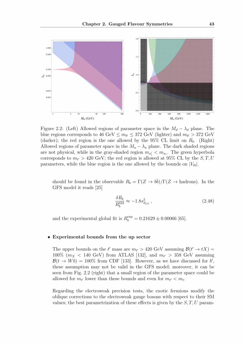
Chapter 2. Gauged Flavour Symmetries 43
1 5 10 50 100 500
0.005
0.010
0.050
0.100
0.500
1.000
Md HGeVL
Λd
0 200 400 600 800 1000 1200 1400
0.0
0.5
1.0
1.5
2.0
Mu HGeVL
Λu
Figure 2.2: (Left) Allowed regions of parameter space in the Md − λd plane. Theblue regions corresponds to 46 GeV ≤ mb′ ≤ 372 GeV (lighter) and mb′ > 372 GeV(darker); the red region is the one allowed by the 95% CL limit on Rb. (Right)Allowed regions of parameter space in the Mu − λu plane. The dark shaded regionsare not physical, while in the gray-shaded region mu′i
< mui . The green hyperbolacorresponds to mt′ > 420 GeV; the red region is allowed at 95% CL by the S, T, Uparameters, while the blue region is the one allowed by the bounds on |Vtb|.
should be found in the observable Rb = Γ(Z → bb)/Γ(Z → hadrons). In theGFS model it reads [25]
δRb
RSMb
≈ −1.8s2dL3
, (2.48)
and the experimental global fit is Rexpb = 0.21629± 0.00066 [65].
• Experimental bounds from the up sector
The upper bounds on the t′ mass are mt′ > 420 GeV assuming B(t′ → tX) =100% (mX < 140 GeV) from ATLAS [132], and mt′ > 358 GeV assumingB(t → Wb) = 100% from CDF [133]. However, as we have discussed for b′,these assumption may not be valid in the GFS model; moreover, it can beseen from Fig. 2.2 (right) that a small region of the parameter space could beallowed for mt′ lower than these bounds and even for mt′ < mt.
Regarding the electroweak precision tests, the exotic fermions modify theoblique corrections to the electroweak gauge bosons with respect to their SMvalues; the best parametrization of these effects is given by the S, T, U param-
44 Chapter 2. Gauged Flavour Symmetries
eters [134]. In the GFS model they are given by [25]
S =s2uL3
6π
[(3c2uL3
(m2t′ +m2
t )(m4t′ − 4m2
t′m2t +m4
t )
(m2t′ −m2
t )3
− 1
)log(m2
t′
m2t
)(2.49a)
−c2uL3
5m4t′ − 22m2
t′m2t + 5m4
t
(m2t′ −m2
t )2
],
T =3 s2
uL3
8π s2wc
2w
m2t
M2Z
[c2uL3
(m2t′
m2t′ −m2
t
log(m2
t′
m2t
)− 1
)+s2uL3
2
(m2t′
m2t
− 1
)],
(2.49b)
U =s2uL3
6π
[−3
(c2uL3
(m2t′ +m2
t )(m4t′ − 4m2
t′m2t +m4
t )
(m2t′ −m2
t )3
− 1
)log(m2
t′
m2t
)(2.49c)
+c2uL3
5m4t′ − 22m2
t′m2t + 5m4
t
(m2t′ −m2
t )2
],
obtained at one loop, considering only the dominant contributions of the thirdfamily in the limit mb → 0. The correction to the T -parameter is generatedby the violation of the custodial symmetry due to the mixing of the quarkdoublets with the left singlets, whose amount is proportional to λu. On theother hand, the contribution of the exotic fermions to the S-parameter isalways small and its sign is not fixed, and U only affects the results in a minorway. The most recent fit for the S, T, U parameters, performed for the firsttime with the actual mass of the Higgs boson, gives
S = 0.03± 0.10 , T = 0.05± 0.12 , U = 0.03± 0.10 , (2.50)
with correlation coefficients of +0.89 between S and T , and −0.54(−0.83)between S and U (T and U) [135].
In the up sector another important constraint comes from the CKM matrix. Infact, as we have discussed, in the GFS model the effective CKM matrix differsfrom the SM one and it is not unitary. The unitarity of the CKM matrix ispresently tested with good accuracy only in the first two rows [65], but sincethey contain only light quarks, the resulting bounds are very weak. On theother hand, in the third row, looking at Eq. (2.36), the measured smallnessof |V CKM
td | and |V CKMts | and the fact that c(u,d)L(1,2)
' 1 imply that |V GFStb | = 1
with high accuracy; hence, since also cdL3' 1, the direct measurement of the
t−b−W coupling constrains cuL3. The determination of |Vtb| from top decays,
recently measured by CMS at 7 TeV, gives the bound |V CKMtb | > 0.92 [136].
2.2.2 Spectrum
Once we have performed a first analysis of the space parameter, and before scan-ning the allowed regions to look for more indications from flavour physics, we chooseone between the possible points in order to obtain a representative spectrum of thequarks and flavour bosons of the GFS model and make some qualitative considera-tions. In particular we use the following parameters.
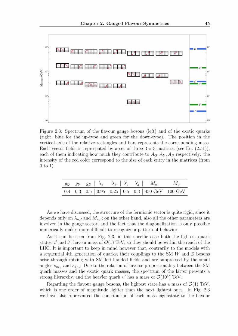
Chapter 2. Gauged Flavour Symmetries 45
u'
c'
t'
d'
s'
b'
1
100
104
106
108
1
100
104
106
108
MassesHG
eVL
asd
Figure 2.3: Spectrum of the flavour gauge bosons (left) and of the exotic quarks(right, blue for the up-type and green for the down-type). The position in thevertical axis of the relative rectangles and bars represents the corresponding mass.Each vector fields is represented by a set of three 3 × 3 matrices (see Eq. (2.51)),each of them indicating how much they contribute to AQ, AU , AD respectively: theintensity of the red color correspond to the size of each entry in the matrices (from0 to 1).
gQ gU gD λu λd λ′u λ′d Mu Md
0.4 0.3 0.5 0.95 0.25 0.5 0.3 450 GeV 100 GeV
As we have discussed, the structure of the fermionic sector is quite rigid, since itdepends only on λu,d and Mu,d; on the other hand, also all the other parameters areinvolved in the gauge sector, and the fact that the diagonalization is only possiblenumerically makes more difficult to recognize a pattern of behavior.
As it can be seen from Fig. 2.3, in this specific case both the lightest quarkstates, t′ and b′, have a mass of O(1) TeV, so they should be within the reach of theLHC. It is important to keep in mind however that, contrarily to the models witha sequential 4th generation of quarks, their couplings to the SM W and Z bosonsarise through mixing with SM left-handed fields and are suppressed by the smallangles suL3
and sdL3. Due to the relation of inverse proportionality between the SM
quark masses and the exotic quark masses, the spectrum of the latter presents astrong hierarchy, and the heavier quark u′ has a mass of O(105) TeV.
Regarding the flavour gauge bosons, the lightest state has a mass of O(1) TeV,which is one order of magnitude lighter than the next lightest ones. In Fig. 2.3we have also represented the contribution of each mass eigenstate to the flavour
46 Chapter 2. Gauged Flavour Symmetries
eigenstates, with matrices according to
AQ = A1
(W1,1
λ1
2+ . . .+W1,8
λ8
2
)︸ ︷︷ ︸
1st matrix of the lightest boson
+ . . .+ A24
(W24,1
λ1
2+ . . .+W24,8
λ8
2
),
AU = A1
(W1,9
λ1
2+ . . .+W1,16
λ8
2
)︸ ︷︷ ︸
2nd matrix of the lightest boson
+ . . .+ A24
(W24,9
λ1
2+ . . .+W24,16
λ8
2
),
AD = A1
(W1,17
λ1
2+ . . .+W1,24
λ8
2
)︸ ︷︷ ︸
3rd matrix of the lightest boson
+ . . .+ A24
(W24,17
λ1
2+ . . .+W24,24
λ8
2
).
(2.51)
The lightest boson couples to fermions through the λ8 flavour generator and withequal strength to left/right up/down type fermions (the unequal intensity of mag-nitude is compensated by the different values of the gauge couplings). Although itscoupling to the third generation is the largest, the lightest vector couples also tothe first two generations, which makes it accessible at the LHC. For all practicalpurposes it corresponds to a flavour non-universal leptophobic Z ′ [25]. Tevatronexcludes this kind of resonances in the tt channel only for mZ′ < 900 GeV at 95%confidence level [137].
2.3 Phenomenological analysis
2.3.1 Impact on the observables
∆F = 2 transitions
In the GFS model the ∆F = 2 observables with external down-type quarks receivetwo kinds of new contributions at the leading order, as shown in Fig. 2.4: one fromthe usual SM box diagrams in which also the new up-type quarks participate, andone due to the tree-level exchange of the flavour gauge bosons. We can include thesecontributions in the effective Hamiltonian
H∆F=2eff =
G2F m
2W
4π2
∑i
Ci(µ)Qi (2.52)
through a modification of the Wilson coefficients
C(M)i = C
(M)i,SM + ∆
(M)box Ci + ∆
(M)treeCi , (2.53)
where M is the meson system under consideration, and µ is the energy scale atwhich the coefficient has to be evaluated.
In principle one should also consider box-diagrams with flavour gauge bosonexchanges, but they are negligible with respect to the tree-level contributions. Alsonegligible can be considered the tree-level exchanges of the πi Higgs states.
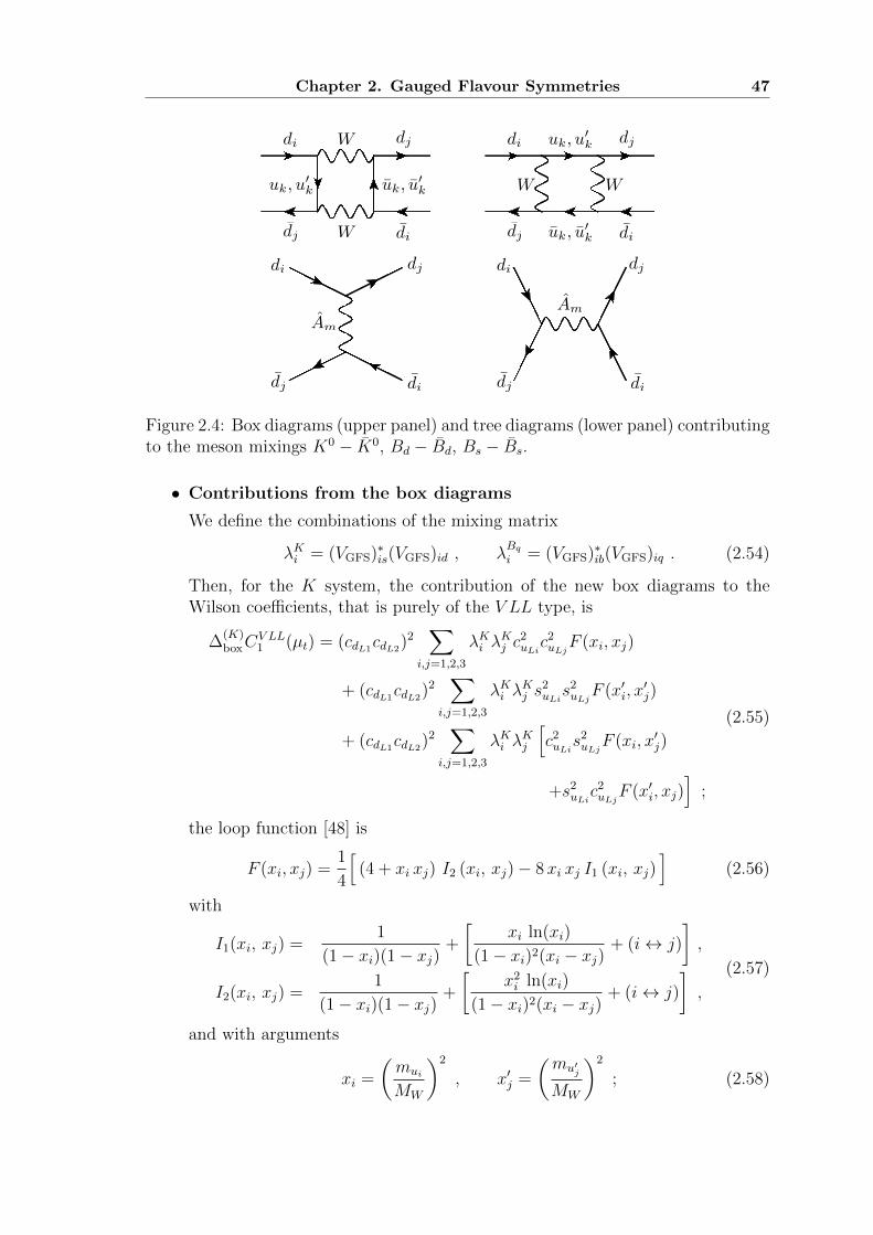
Chapter 2. Gauged Flavour Symmetries 47
di di
di di
dj dj
dj dj
dj dj
dj dj
di di
di di
W
W
W Wuk, u0k
uk, u0k
uk, u0k
uk, u0k
Am
Am
Figure 2.4: Box diagrams (upper panel) and tree diagrams (lower panel) contributingto the meson mixings K0 − K0, Bd − Bd, Bs − Bs.
• Contributions from the box diagrams
We define the combinations of the mixing matrix
λKi = (VGFS)∗is(VGFS)id , λBqi = (VGFS)∗ib(VGFS)iq . (2.54)
Then, for the K system, the contribution of the new box diagrams to theWilson coefficients, that is purely of the V LL type, is
∆(K)boxC
V LL1 (µt) = (cdL1
cdL2)2
∑i,j=1,2,3
λKi λKj c
2uLic2uLjF (xi, xj)
+ (cdL1cdL2
)2∑
i,j=1,2,3
λKi λKj s
2uLis2uLjF (x′i, x
′j)
+ (cdL1cdL2
)2∑
i,j=1,2,3
λKi λKj
[c2uLis2uLjF (xi, x
′j)
+s2uLic2uLjF (x′i, xj)
];
(2.55)
the loop function [48] is
F (xi, xj) =1
4
[(4 + xi xj) I2 (xi, xj)− 8xi xj I1 (xi, xj)
](2.56)
with
I1(xi, xj) =1
(1− xi)(1− xj)+
[xi ln(xi)
(1− xi)2(xi − xj)+ (i↔ j)
],
I2(xi, xj) =1
(1− xi)(1− xj)+
[x2i ln(xi)
(1− xi)2(xi − xj)+ (i↔ j)
],
(2.57)
and with arguments
xi =
(mui
MW
)2
, x′j =
(mu′j
MW
)2
; (2.58)
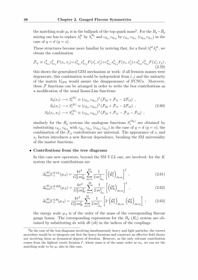
48 Chapter 2. Gauged Flavour Symmetries
the matching scale µt is in the ballpark of the top quark mass2. For the Bq−Bq
mixing one has to replace λKi by λBqi and cdL1
cdL2by cdL1
cdL3(cdL2
cdL3) in the
case of q = d (q = s).
These structures become more familiar by noticing that, for a fixed λMi λMj , we
obtain the combination
Fij ≡ c2uLic2uLjF (xi, xj)+s
2uLis2uLjF (x′i, x
′j)+c
2uLis2uLjF (xi, x
′j)+s
2uLic2uLjF (x′i, xj) ;
(2.59)this shows the generalized GIM mechanism at work: if all fermion masses weredegenerate, this combination would be independent from i, j and the unitarityof the matrix VGFS would assure the disappearance of FCNCs. Moreover,these F functions can be arranged in order to write the box contributions asa modification of the usual Inami-Lim functions:
S0(xt) −→ S(K)t ≡ (cdL1
cdL2)2 (F33 + F11 − 2F13) ,
S0(xc) −→ S(K)c ≡ (cdL1
cdL2)2 (F22 + F11 − 2F12) ,
S0(xc, xt) −→ S(K)ct ≡ (cdL1
cdL2)2 (F23 + F11 −F13 −F12) ;
(2.60)
similarly for the Bq systems the analogous functions S(Bq)i are obtained by
substituting cdL1cdL2
with cdL1cdL3
(cdL2cdL3
) in the case of q = d (q = s); thecombination of the Fij contributions are universal. The appearance of ci andsj factors introduces a new flavour dependence, breaking the SM universalityof the master functions.
• Contributions from the tree diagrams
In this case new operators, beyond the SM V LL one, are involved: for the Ksystem the new contributions are
∆(K)treeC
V LL1 (µA) =
4π2
G2Fm
2W
24∑m=1
1
2m2Am
[(GdL)ds,m
]2
, (2.61)
∆(K)treeC
V RR1 (µA) =
4π2
G2Fm
2W
24∑m=1
1
2m2Am
[(GdR)ds,m
]2
, (2.62)
∆(K)treeC
LR1 (µA) =
4π2
G2Fm
2W
24∑m=1
1
2m2Am
[2(GdL)ds,m
(GdR)ds,m
]; (2.63)
the energy scale µA is of the order of the mass of the corresponding flavourgauge boson. The corresponding expressions for the Bd (Bs) system are ob-tained by substituting ds with db (sb) in the indices of the couplings.
2In the case of the box-diagrams involving simultaneously heavy and light particles, the correctprocedure would be to integrate out first the heavy fermions and construct an effective field theorynot involving them as dynamical degrees of freedom. However, as the only relevant contributioncomes from the lightest exotic fermion t′, whose mass is of the same order as mt, we can set thematching scale to be µt also in this case.
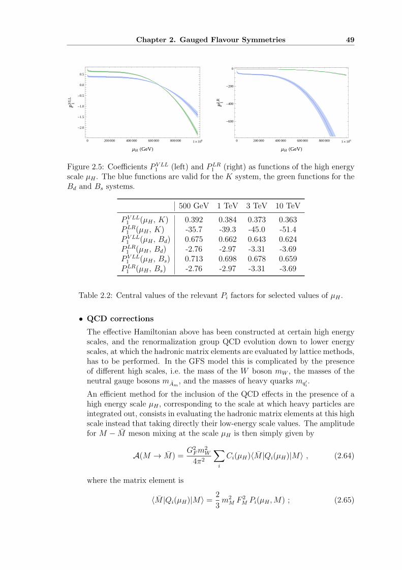
Chapter 2. Gauged Flavour Symmetries 49
0 200 000 400 000 600 000 800 000 1 ´ 106
-2.0
-1.5
-1.0
-0.5
0.0
0.5
ΜH HGeVL
P1V
LL
asd
asd
0 200 000 400 000 600 000 800 000 1 ´ 106
-600
-400
-200
0
ΜH HGeVL
P1L
R
asd
asd
Figure 2.5: Coefficients P V LL1 (left) and PLR
1 (right) as functions of the high energyscale µH . The blue functions are valid for the K system, the green functions for theBd and Bs systems.
500 GeV 1 TeV 3 TeV 10 TeV
P V LL1 (µH , K) 0.392 0.384 0.373 0.363PLR
1 (µH , K) -35.7 -39.3 -45.0 -51.4P V LL
1 (µH , Bd) 0.675 0.662 0.643 0.624PLR
1 (µH , Bd) -2.76 -2.97 -3.31 -3.69P V LL
1 (µH , Bs) 0.713 0.698 0.678 0.659PLR
1 (µH , Bs) -2.76 -2.97 -3.31 -3.69
Table 2.2: Central values of the relevant Pi factors for selected values of µH .
• QCD corrections
The effective Hamiltonian above has been constructed at certain high energyscales, and the renormalization group QCD evolution down to lower energyscales, at which the hadronic matrix elements are evaluated by lattice methods,has to be performed. In the GFS model this is complicated by the presenceof different high scales, i.e. the mass of the W boson mW , the masses of theneutral gauge bosons mAm
, and the masses of heavy quarks mq′i.
An efficient method for the inclusion of the QCD effects in the presence of ahigh energy scale µH , corresponding to the scale at which heavy particles areintegrated out, consists in evaluating the hadronic matrix elements at this highscale instead that taking directly their low-energy scale values. The amplitudefor M − M meson mixing at the scale µH is then simply given by
A(M → M) =G2Fm
2W
4π2
∑i
Ci(µH)〈M |Qi(µH)|M〉 , (2.64)
where the matrix element is
〈M |Qi(µH)|M〉 =2
3m2M F 2
M Pi(µH ,M) ; (2.65)
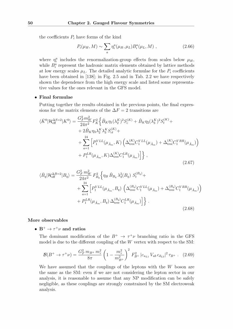
50 Chapter 2. Gauged Flavour Symmetries
the coefficients Pi have forms of the kind
Pi(µH ,M) ∼∑a
ηai (µH , µL)Bai (µL,M) , (2.66)
where ηai includes the renormalization-group effects from scales below µH ,while Ba
i represent the hadronic matrix elements obtained by lattice methodsat low energy scales µL. The detailed analytic formulae for the Pi coefficientshave been obtained in [138]; in Fig. 2.5 and in Tab. 2.2 we have respectivelyshown the dependence from the high energy scale and listed some representa-tive values for the ones relevant in the GFS model.
• Final formulae
Putting together the results obtained in the previous points, the final expres-sions for the matrix elements of the ∆F = 2 transitions are
〈K0|H∆S=2eff |K0〉 =
G2Fm
2W
24π2F 2K
{BKη1(λK2 )2S(K)
c + BKη2(λK3 )2S(K)t +
+ 2BKη3λK2 λ
K3 S
(K)ct +
+24∑a=1
[P V LL
1 (µAm , K)(
∆(K)treeC
V LL1 (µAm) + ∆
(K)treeC
V RR1 (µAm)
)+ PLR
1 (µAm , K)∆(K)treeC
LR1 (µAm)
]},
(2.67)
〈Bq|H∆B=2eff |Bq〉 =
G2F m
2W
24π2F 2Bq
{ηB BBq λ
23(Bq) S
(Bq)t +
+24∑a=1
[P V LL
1 (µAm , Bq)(
∆(Bq)tree C
V LL1 (µAm) + ∆
(Bq)tree C
V RR1 (µAm)
)+ PLR
1 (µAm , Bq) ∆(Bq)tree C
LR1 (µAm)
]}.
(2.68)
More observables
• B+ → τ+ν and ratios
The dominant modification of the B+ → τ+ν branching ratio in the GFSmodel is due to the different coupling of the W vertex with respect to the SM:
B(B+ → τ+ν) =G2F mB+ m2
τ
8π
(1− m2
τ
m2B+
)2
F 2B+ |cuL1
Vub cdL3|2 τB+ . (2.69)
We have assumed that the couplings of the leptons with the W boson arethe same as the SM: even if we are not considering the lepton sector in ouranalysis, it is reasonable to assume that any NP modification can be safelynegligible, as these couplings are strongly constrained by the SM electroweakanalysis.
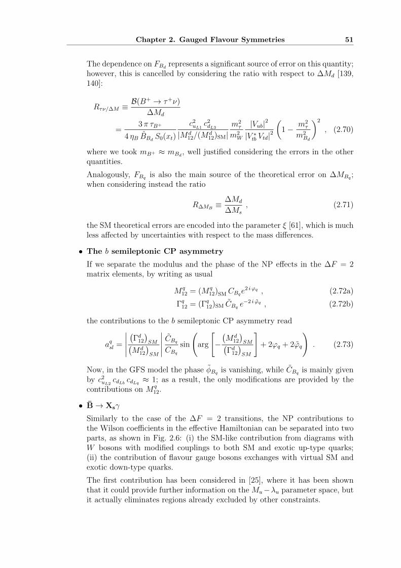
Chapter 2. Gauged Flavour Symmetries 51
The dependence on FBd represents a significant source of error on this quantity;however, this is cancelled by considering the ratio with respect to ∆Md [139,140]:
Rτν/∆M ≡B(B+ → τ+ν)
∆Md
=3π τB+
4 ηB BBd S0(xt)
c2uL1
c2dL3
|Md12/(M
d12)SM|
m2τ
m2W
|Vub|2
|V ∗tb Vtd|2
(1− m2
τ
m2Bd
)2
, (2.70)
where we took mB+ ≈ mBd , well justified considering the errors in the otherquantities.
Analogously, FBq is also the main source of the theoretical error on ∆MBq ;when considering instead the ratio
R∆MB≡ ∆Md
∆Ms
, (2.71)
the SM theoretical errors are encoded into the parameter ξ [61], which is muchless affected by uncertainties with respect to the mass differences.
• The b semileptonic CP asymmetry
If we separate the modulus and the phase of the NP effects in the ∆F = 2matrix elements, by writing as usual
M q12 = (M q
12)SM CBqe2 i ϕq , (2.72a)
Γq12 = (Γq12)SM CBq e−2 i ϕq , (2.72b)
the contributions to the b semileptonic CP asymmetry read
aqsl =
∣∣∣∣∣(Γd12
)SM(
Md12
)SM
∣∣∣∣∣ CBqCBqsin
(arg
[−(Md
12
)SM(
Γd12
)SM
]+ 2ϕq + 2ϕq
). (2.73)
Now, in the GFS model the phase φBq is vanishing, while CBq is mainly givenby c2
uL2cdLb cdLq ≈ 1; as a result, the only modifications are provided by the
contributions on M q12.
• B→ Xsγ
Similarly to the case of the ∆F = 2 transitions, the NP contributions tothe Wilson coefficients in the effective Hamiltonian can be separated into twoparts, as shown in Fig. 2.6: (i) the SM-like contribution from diagrams withW bosons with modified couplings to both SM and exotic up-type quarks;(ii) the contribution of flavour gauge bosons exchanges with virtual SM andexotic down-type quarks.
The first contribution has been considered in [25], where it has been shownthat it could provide further information on the Mu−λu parameter space, butit actually eliminates regions already excluded by other constraints.
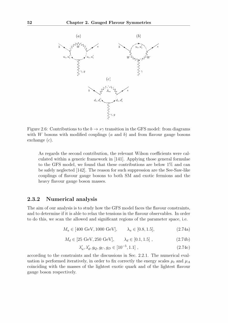
52 Chapter 2. Gauged Flavour Symmetries
b b
b
s s
s
��, g
�, g
W
W W
Am
ui, u0i ui, u
0i
ui, u0i
di, d0i di, d
0i
(a) (b)
(c)
Figure 2.6: Contributions to the b→ sγ transition in the GFS model: from diagramswith W bosons with modified couplings (a and b) and from flavour gauge bosonsexchange (c).
As regards the second contribution, the relevant Wilson coefficients were cal-culated within a generic framework in [141]. Applying those general formulaeto the GFS model, we found that these contributions are below 1% and canbe safely neglected [142]. The reason for such suppression are the See-Saw-likecouplings of flavour gauge bosons to both SM and exotic fermions and theheavy flavour gauge boson masses.
2.3.2 Numerical analysis
The aim of our analysis is to study how the GFS model faces the flavour constraints,and to determine if it is able to relax the tensions in the flavour observables. In orderto do this, we scan the allowed and significant regions of the parameter space, i.e.
Mu ∈ [400 GeV, 1000 GeV], λu ∈ [0.8, 1.5], (2.74a)
Md ∈ [25 GeV, 250 GeV], λd ∈ [0.1, 1.5] , (2.74b)
λ′u, λ′d, gQ, gU , gD ∈ [10−5, 1.1] , (2.74c)
according to the constraints and the discussions in Sec. 2.2.1. The numerical eval-uation is performed iteratively, in order to fix correctly the energy scales µt and µAcoinciding with the masses of the lightest exotic quark and of the lightest flavourgauge boson respectively.
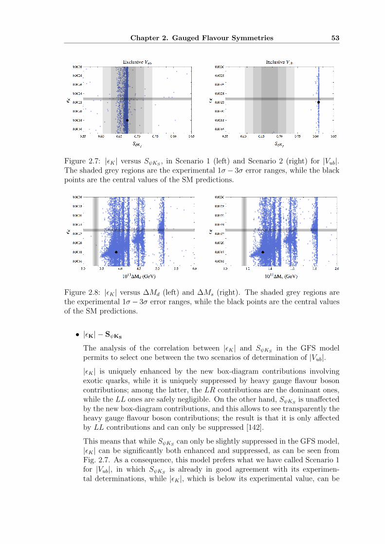
Chapter 2. Gauged Flavour Symmetries 53
Figure 2.7: |εK | versus SψKS , in Scenario 1 (left) and Scenario 2 (right) for |Vub|.The shaded grey regions are the experimental 1σ− 3σ error ranges, while the blackpoints are the central values of the SM predictions.
Figure 2.8: |εK | versus ∆Md (left) and ∆Ms (right). The shaded grey regions arethe experimental 1σ− 3σ error ranges, while the black points are the central valuesof the SM predictions.
• |εK| − SψKS
The analysis of the correlation between |εK | and SψKS in the GFS modelpermits to select one between the two scenarios of determination of |Vub|.
|εK | is uniquely enhanced by the new box-diagram contributions involvingexotic quarks, while it is uniquely suppressed by heavy gauge flavour bosoncontributions; among the latter, the LR contributions are the dominant ones,while the LL ones are safely negligible. On the other hand, SψKS is unaffectedby the new box-diagram contributions, and this allows to see transparently theheavy gauge flavour boson contributions; the result is that it is only affectedby LL contributions and can only be suppressed [142].
This means that while SψKS can only be slightly suppressed in the GFS model,|εK | can be significantly both enhanced and suppressed, as can be seen fromFig. 2.7. As a consequence, this model prefers what we have called Scenario 1for |Vub|, in which SψKS is already in good agreement with its experimen-tal determinations, while |εK |, which is below its experimental value, can be
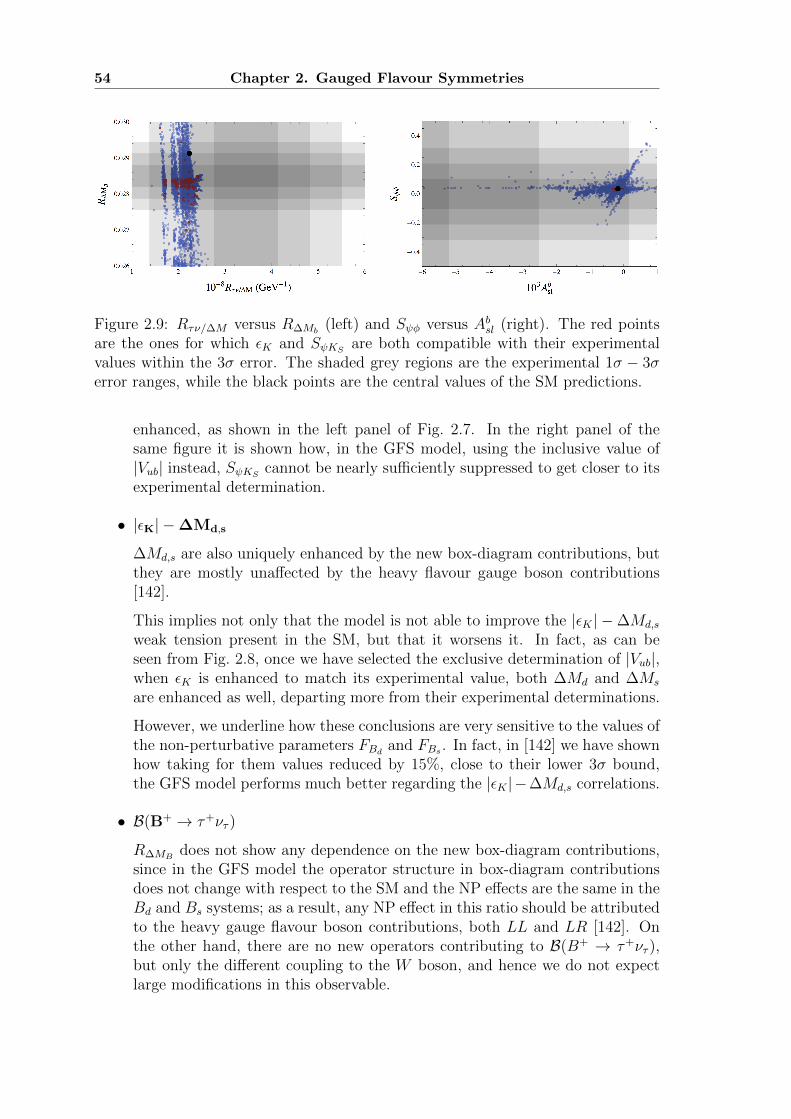
54 Chapter 2. Gauged Flavour Symmetries
Figure 2.9: Rτν/∆M versus R∆Mb(left) and Sψφ versus Absl (right). The red points
are the ones for which εK and SψKS are both compatible with their experimentalvalues within the 3σ error. The shaded grey regions are the experimental 1σ − 3σerror ranges, while the black points are the central values of the SM predictions.
enhanced, as shown in the left panel of Fig. 2.7. In the right panel of thesame figure it is shown how, in the GFS model, using the inclusive value of|Vub| instead, SψKS cannot be nearly sufficiently suppressed to get closer to itsexperimental determination.
• |εK| −∆Md,s
∆Md,s are also uniquely enhanced by the new box-diagram contributions, butthey are mostly unaffected by the heavy flavour gauge boson contributions[142].
This implies not only that the model is not able to improve the |εK | −∆Md,s
weak tension present in the SM, but that it worsens it. In fact, as can beseen from Fig. 2.8, once we have selected the exclusive determination of |Vub|,when εK is enhanced to match its experimental value, both ∆Md and ∆Ms
are enhanced as well, departing more from their experimental determinations.
However, we underline how these conclusions are very sensitive to the values ofthe non-perturbative parameters FBd and FBs . In fact, in [142] we have shownhow taking for them values reduced by 15%, close to their lower 3σ bound,the GFS model performs much better regarding the |εK |−∆Md,s correlations.
• B(B+ → τ+ντ )
R∆MBdoes not show any dependence on the new box-diagram contributions,
since in the GFS model the operator structure in box-diagram contributionsdoes not change with respect to the SM and the NP effects are the same in theBd and Bs systems; as a result, any NP effect in this ratio should be attributedto the heavy gauge flavour boson contributions, both LL and LR [142]. Onthe other hand, there are no new operators contributing to B(B+ → τ+ντ ),but only the different coupling to the W boson, and hence we do not expectlarge modifications in this observable.

Chapter 2. Gauged Flavour Symmetries 55
Figure 2.10: Masses of the lightest exotic quark t′ and of the lightest flavour gaugeboson A24 of the GFS model. For the red points, εK , SψKS , R∆MB
, Rτν/∆M agreewith the experimental data at 3σlevel. The visible correlations corresponds to pointsof the parameter space with the same values of Mu,d and λu,d.
Both R∆MBand Rτν/∆M have small theoretical uncertainties and are therefore
very useful to provide information on the parameter space of the GFS model.From Fig. 2.9 (left) we can see that the values of the GFS parameters thatsatisfy the |εK | −SψKS constraints also improve the accordance of R∆MB
withits measurement, but neither of them is able to significantly improve the dis-crepancy with the experimental value of B(B+ → τ+ντ ), that however, as wehave discussed, is now less problematic due to the recent determinations.
• Absl
Absl is not affected by box-diagram contributions, the LR contributions arealmost completely negligible and the LL are the only relevant ones, enhancing|Absl| towards the central value of its experimental determination. This is simi-lar to what happens to Sψφ: like SψKS it is unaffected by the new box-diagramcontributions, but, differently from the latter, it depends on both LL andLR contributions; interestingly, the NP contributions interfere destructivelywith the SM contribution so that its sign can in principle be reversed in thismodel [142].
Fig. 2.9 (right) shows that the GFS model predicts only tiny deviations fromthe SM predictions for both Absl and Sψφ, especially when the indications from|εK | − SψKS are taken into account. This is beneficial for Sψφ, since the lastmeasurements agree on a SM-like value, while concerning Absl until now onlya measurement from D0 is available, and hence an independent determinationfrom LHCb will be very relevant in the near future.
• Masses for direct observations
The analysis of the parameter space and the constraints derived from flavour
56 Chapter 2. Gauged Flavour Symmetries
observables in this section permit to obtain more precise estimations of reliablemasses of the exotic particles possibly detectable at the LHC. In Fig. 2.10 themasses obtained with values of the parameters for which the majority of flavourconstraints are satisfied are highlighted; it results that relatively light massesof the lightest flavour boson A24 are preferred, while both for low and for highmasses of the lightest exotic quark t′ the predictions in the flavour sector canbe satisfactory.
• Comparison with MFV
Despite the numerous similarities in the principles and in the realization, theGFS model do not satisfy the MFV requirements. This can be seen by notic-ing that while in MFV in the limit of vanishing Yukawa couplings the fullflavour symmetry is restored, in the GFS model there exists a limit in whichall Yukawa couplings vanish but flavour-breaking contributions remain finite:when Mu,d → 0 with all the other parameters, the four-fermion operators,generated by the exchange of the flavour bosons, still break flavour [25].
The deviations from the MFV patterns can be experimentally recognized.Comparing the GFS model with the CMFV frameworks, one observes that inboth cases they prefer the exclusive value of Vub, solving the εK−SψKS tensionthrough the enhancement of |εK |, but worsening the εK − ∆Md,s agreement.Nevertheless, the distinction can be provided by ∆F = 1 processes: for ex-ample, considering B → Xsγ, while in the GFS model the NP contributionsuniquely enhance the branching ratio, in CMFV this can be also suppressed.
Concerning MFV at large, taking for example the 2HDMMFV, in the latter NPcontributions to εK are tiny and hence the inclusive value of |Vub| is selected,contrarily to the GFS model.
Chapter 3
Theory and phenomenologyof 331 models
3.1 General theory
3.1.1 Gauge group and fermion representations
We want to build a model with gauge group SU(3)c× SU(3)L×U(1)X .We indicatewith T a (a = 1 . . . 8) the generators of SU(3)L, and with T 9 the generator of U(1)X ,defined as
T a =1
2λa , T 9 =
1√6I3 , (3.1)
where λa are the Gell-Mann matrices and I3 is the 3×3 identity matrix, so that thenormalization condition
Tr(T aT b) =1
2δab (3.2)
holds for a, b = 1 . . . 9.The electric charge must be a linear combination of the diagonal generators of
the SU(3)L × U(1)X gauge group1:
Q = T 3 + βT 8 +XI3 . (3.3)
In the specific representations it reads
Q =
12
+ β
2√
3+X
−12
+ β
2√
3+X
− β√3
+X
; (3.4a)
Q =
−12− β
2√
3+X
12− β
2√
3+X
β√3
+X
; (3.4b)
1We will denote a general operator O by a hat, to distinguish them from their representationsas operator matrices that we will denote by O for the 3 representation, O for the 3 representation,and by O(r) for other representations.
57
58 Chapter 3. 331 models
Q6 =
1 + β√3
+ 2X β√3
+ 2X 12− β
2√
3+ 2X
β√3
−1 + β√3
−12− β
2√
3+ 2X
12− β
2√
3+ 2X −1
2− β
2√
3+ 2X − 2β√
3+ 2X
; (3.4c)
Q8 =
0 1 1
2+√
3β2
−1 0 −12
+√
3β2
−(
12
+√
3β2
)−(−1
2+√
3β2
)0
; (3.4d)
where we have used the properties TaΦ = ΦTa + T Ta Φ for the symmetric sextet, andT a = −(T a)T and T a8T
b = [T a, T b] for the adjoint octet.The gauge invariance is obtained by building a covariant derivative introducing
the gauge bosons W aµ (a = 1 . . . 8) and Xµ, and the coupling constants g and gX :
Dµ = ∂µ − igT aW aµ − igX T 9Xµ , (3.5)
where the representation of the generators depends on the representation of theobjects on which the derivative is applied. The gauge bosons associated to SU(3)Ltransform according to the adjoint representation (8, 0) and can be rewritten as
Wµ = W aµT
a =1
2
W3µ + 1√
3W 8µ
√2W+
µ
√2Y QY
µ√2W−
µ −W 3µ + 1√
3W 8µ
√2V QV
µ√2Y −QYµ
√2V −QVµ − 2√
3W 8µ
, (3.6)
from which one can recognize one singly-charged boson
W±µ =
1√2
(W 1µ ∓ iW 2
µ
), (3.7a)
two generically-charged bosons
Y ±QYµ =1√2
(W 4µ ∓ iW 5
µ
)with QY =
1
2+
√3β
2, (3.7b)
V ±QVµ =1√2
(W 6µ ∓ iW 7
µ
)with QV = −1
2+
√3β
2, (3.7c)
and three neutral states that are linearly-independent combinations of W 3µ and W 8
µ .The lowest possible fermion representations under this gauge group SU(3)L are
the singlet ψ(1), the triplet ψ(3), and the antitriplet ψ(3), that are of quark or ofleptonic type depending on if they are respectively triplets or singlets under SU(3)c:
ψ(1) =
{q(1) : (3,1, X)
`(1) : (1,1, X), (3.8a)
ψ(3) =
{q(3) : (3,3, X)→ (3,2, Y )⊕ (3,1, Y )
`(3) : (1,3, X)→ (1,2, Y )⊕ (1,1, Y ) ,(3.8b)
Chapter 3. 331 models 59
ψL QψL XψL ψR QψR = XψR
q(m)L =
U (m)
D(m)
J (m)
L
23
−13
16−√
3β2
16− β
2√
3
U(m)R
23
D(m)R −1
3
J(m)R
16−√
3β2
q(m∗)L =
D(m∗)
−U (m∗)
J (m∗)
L
−13
23
16
+√
3β2
−16− β
2√
3
D(m∗)R −1
3
U(m∗)R
23
J(m∗)R
16
+√
3β2
`(n)L =
ν(n)
e(n)
E(n)
L
0−1
−12−√
3β2
−12− β
2√
3
ν(n)R 0
e(n)R −1
E(n)R −1
2−√
3β2
`(n∗)L =
e(n∗)
−ν(n∗)
E(n∗)
L
−10
−12
+√
3β2
12− β
2√
3
e(n∗)R −1
ν(n∗)R 0
E(n∗)R −1
2+√
3β2
Table 3.1: Generic fermionic content of 331 models, requiring only one lepton andone quark SU(3)L multiplet for each generation, and no more than one right-handedsinglet for each left-handed field. U and D are generic up-type and down-type quarksrespectively, as well as e and ν are a generic lepton and neutrino; m and n labelthe quark and lepton left-handed triplets, respectively, while m∗ and n∗ label theantitriplets.
ψ(3) =
{q(3) : (3, 3, X)→ (3,2, Y )⊕ (3,1, Y )
`(3) : (1, 3, X)→ (1,2, Y )⊕ (1,1, Y ); (3.8c)
due to the branching rules SU(2) ⊂ SU(3), after the breaking of SU(3)L both thetriplet and the antitripet embed a doublet and a singlet of SU(2)L.
Trying to embed the SM fermions in the 331 multiplets, in general one couldintroduce sets of multiplets with different quantum numbers, meaning that one rep-resents each generation as a set of triplets with particles of the SM plus exotic parti-cles. However, this would at the same time enlarge the exotic spectrum and hugelyincrease the number of free parameters; hence, we decide as a minimal assumptionto associate only one lepton and one quark multiplet for each generation, and atmost one right-handed singlet associated with each left-handed fermion. Based onthis criterium, the possible fermion multiplets are the ones listed in Tab. 3.1 [143].
From Eq. (3.8b)–(3.8c) it is evident that the SM left-handed doublets can be em-bedded in SU(3)L triplets or antitriplets. Reproducing their correct electric chargefixes the values of the multiplet hypercharge and consequently the (β-dependent)charge of the third exotic component.
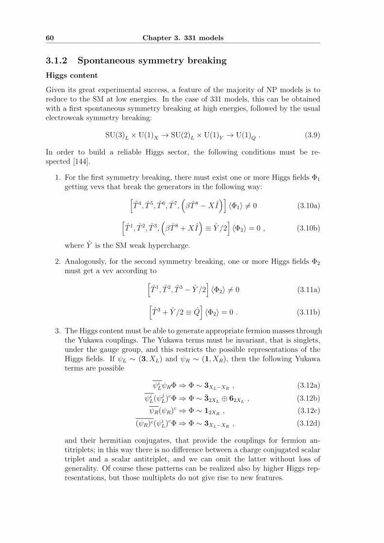
60 Chapter 3. 331 models
3.1.2 Spontaneous symmetry breaking
Higgs content
Given its great experimental success, a feature of the majority of NP models is toreduce to the SM at low energies. In the case of 331 models, this can be obtainedwith a first spontaneous symmetry breaking at high energies, followed by the usualelectroweak symmetry breaking:
SU(3)L × U(1)X → SU(2)L × U(1)Y → U(1)Q . (3.9)
In order to build a reliable Higgs sector, the following conditions must be re-spected [144].
1. For the first symmetry breaking, there must exist one or more Higgs fields Φ1
getting vevs that break the generators in the following way:[T 4, T 5, T 6, T 7,
(βT 8 −XI
)]〈Φ1〉 6= 0 (3.10a)[
T 1, T 2, T 3,(βT 8 +XI
)≡ Y /2
]〈Φ2〉 = 0 , (3.10b)
where Y is the SM weak hypercharge.
2. Analogously, for the second symmetry breaking, one or more Higgs fields Φ2
must get a vev according to[T 1, T 2, T 3 − Y /2
]〈Φ2〉 6= 0 (3.11a)[
T 3 + Y /2 ≡ Q]〈Φ2〉 = 0 . (3.11b)
3. The Higgs content must be able to generate appropriate fermion masses throughthe Yukawa couplings. The Yukawa terms must be invariant, that is singlets,under the gauge group, and this restricts the possible representations of theHiggs fields. If ψL ∼ (3, XL) and ψR ∼ (1, XR), then the following Yukawaterms are possible
ψiLψRΦ⇒ Φ ∼ 3XL−XR , (3.12a)
ψiL(ψjL)cΦ⇒ Φ ∼ 32XL ⊕ 62XL , (3.12b)
ψR(ψR)c ⇒ Φ ∼ 12XR , (3.12c)
(ψR)c(ψiL)cΦ⇒ Φ ∼ 3XL−XR , (3.12d)
and their hermitian conjugates, that provide the couplings for fermion an-titriplets; in this way there is no difference between a charge conjugated scalartriplet and a scalar antitriplet, and we can omit the latter without loss ofgenerality. Of course these patterns can be realized also by higher Higgs rep-resentations, but those multiplets do not give rise to new features.
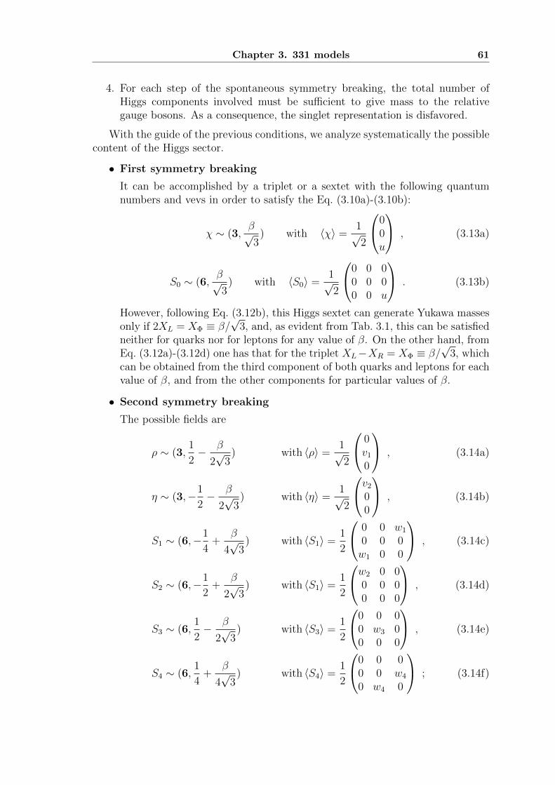
Chapter 3. 331 models 61
4. For each step of the spontaneous symmetry breaking, the total number ofHiggs components involved must be sufficient to give mass to the relativegauge bosons. As a consequence, the singlet representation is disfavored.
With the guide of the previous conditions, we analyze systematically the possiblecontent of the Higgs sector.
• First symmetry breaking
It can be accomplished by a triplet or a sextet with the following quantumnumbers and vevs in order to satisfy the Eq. (3.10a)-(3.10b):
χ ∼ (3,β√3
) with 〈χ〉 =1√2
00u
, (3.13a)
S0 ∼ (6,β√3
) with 〈S0〉 =1√2
0 0 00 0 00 0 u
. (3.13b)
However, following Eq. (3.12b), this Higgs sextet can generate Yukawa massesonly if 2XL = XΦ ≡ β/
√3, and, as evident from Tab. 3.1, this can be satisfied
neither for quarks nor for leptons for any value of β. On the other hand, fromEq. (3.12a)-(3.12d) one has that for the triplet XL−XR = XΦ ≡ β/
√3, which
can be obtained from the third component of both quarks and leptons for eachvalue of β, and from the other components for particular values of β.
• Second symmetry breaking
The possible fields are
ρ ∼ (3,1
2− β
2√
3) with 〈ρ〉 =
1√2
0v1
0
, (3.14a)
η ∼ (3,−1
2− β
2√
3) with 〈η〉 =
1√2
v2
00
, (3.14b)
S1 ∼ (6,−1
4+
β
4√
3) with 〈S1〉 =
1
2
0 0 w1
0 0 0w1 0 0
, (3.14c)
S2 ∼ (6,−1
2+
β
2√
3) with 〈S1〉 =
1
2
w2 0 00 0 00 0 0
, (3.14d)
S3 ∼ (6,1
2− β
2√
3) with 〈S3〉 =
1
2
0 0 00 w3 00 0 0
, (3.14e)
S4 ∼ (6,1
4+
β
4√
3) with 〈S4〉 =
1
2
0 0 00 0 w4
0 w4 0
; (3.14f)
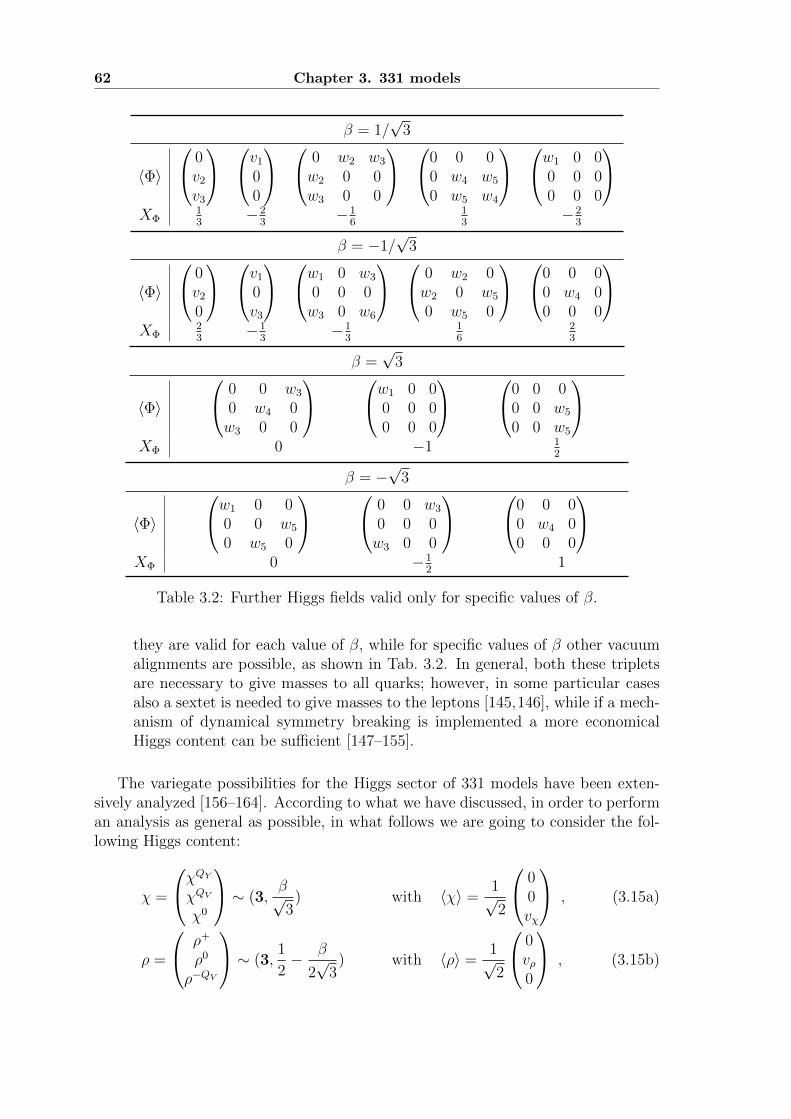
62 Chapter 3. 331 models
β = 1/√
3
〈Φ〉
0v2
v3
v1
00
0 w2 w3
w2 0 0w3 0 0
0 0 00 w4 w5
0 w5 w4
w1 0 00 0 00 0 0
XΦ
13
−23
−16
13
−23
β = −1/√
3
〈Φ〉
0v2
0
v1
0v3
w1 0 w3
0 0 0w3 0 w6
0 w2 0w2 0 w5
0 w5 0
0 0 00 w4 00 0 0
XΦ
23
−13
−13
16
23
β =√
3
〈Φ〉
0 0 w3
0 w4 0w3 0 0
w1 0 00 0 00 0 0
0 0 00 0 w5
0 0 w5
XΦ 0 −1 1
2
β = −√
3
〈Φ〉
w1 0 00 0 w5
0 w5 0
0 0 w3
0 0 0w3 0 0
0 0 00 w4 00 0 0
XΦ 0 −1
21
Table 3.2: Further Higgs fields valid only for specific values of β.
they are valid for each value of β, while for specific values of β other vacuumalignments are possible, as shown in Tab. 3.2. In general, both these tripletsare necessary to give masses to all quarks; however, in some particular casesalso a sextet is needed to give masses to the leptons [145,146], while if a mech-anism of dynamical symmetry breaking is implemented a more economicalHiggs content can be sufficient [147–155].
The variegate possibilities for the Higgs sector of 331 models have been exten-sively analyzed [156–164]. According to what we have discussed, in order to performan analysis as general as possible, in what follows we are going to consider the fol-lowing Higgs content:
χ =
χQYχQV
χ0
∼ (3,β√3
) with 〈χ〉 =1√2
00vχ
, (3.15a)
ρ =
ρ+
ρ0
ρ−QV
∼ (3,1
2− β
2√
3) with 〈ρ〉 =
1√2
0vρ0
, (3.15b)
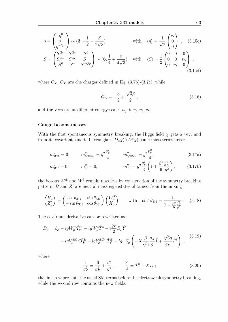
Chapter 3. 331 models 63
η =
η0
η−
η−QY
∼ (3,−1
2− β
2√
3) with 〈η〉 =
1√2
vη00
, (3.15c)
S =
SQY SQV S0
SQV SQC S−
S0 S− S−QY
∼ (6,1
4+
β
4√
3) with 〈S〉 =
1
2
0 0 00 0 vS0 vS 0
,
(3.15d)
where QY , QV are che charges defined in Eq. (3.7b)-(3.7c), while
QC = −3
2+
√3β
2, (3.16)
and the vevs are at different energy scales vχ � vρ, vη, vS.
Gauge bosons masses
With the first spontaneous symmetry breaking, the Higgs field χ gets a vev, andfrom its covariant kinetic Lagrangian (Dµχ)†(Dµχ) some mass terms arise:
m2W± = 0, m2
V ±QV = g2v2χ
4, m2
Y ±QY = g2v2χ
4, (3.17a)
m2W 3 = 0, m2
B = 0, m2Z′ = g2
v2χ
3
(1 +
β2
6
g2X
g2
); (3.17b)
the bosons W± and W 3 remain massless by construction of the symmetry breakingpattern; B and Z ′ are neutral mass eigenstates obtained from the mixing(
Bµ
Z ′µ
)=
(cos θ331 sin θ331
− sin θ331 cos θ331
)(W 8µ
Xµ
)with sin2 θ331 =
1
1 + β2
6
g2X
g2
. (3.18)
The covariant derivative can be rewritten as
Dµ = ∂µ − igW±µ T
±W − igW
3µ T
3 − igY2BµY
− igV ±QVµ T±V − igY±QYµ T±Y − igYZ
′µ
(−X β√
6
gXgI +
√6g
gXT 8
),
(3.19)
where
1
g2Y
=6
g2X
+β2
g2,
Y
2= T 8 +XI3 ; (3.20)
the first row presents the usual SM terms before the electroweak symmetry breaking,while the second row contains the new fields.
64 Chapter 3. 331 models
When with the second step of spontaneous symmetry breaking also the Higgsfields ρ, η and S get a vev, the masses of the charged gauge bosons become
m2W± = g2v
2+
4, (3.21a)
m2V ±QV = g2
v2χ
4
(1 +
v2+
2v2χ
−v2−
2v2χ
+4v2
S
v2χ
), (3.21b)
m2Y ±QY = g2
v2χ
4
(1 +
v2+
2v2χ
+v2−
2v2χ
), (3.21c)
where v2± = ±v2
ρ + v2η + v2
S. It is evident that, while the charged boson W± hasa mass of the order of the electroweak symmetry breaking scale, and hence shouldbe identified with the SM charged gauge boson, the new bosons are significantlyheavier [165].
As regards the neutral bosons, the mass terms read
Bµ
W 3µ
Z ′µ
T
v2+
4g2Y −v2
+
4ggY 0
−v2+
4ggY
v2+
4g2 0
0 0 g4
3(g2−g2Y β
2)
(v2χ +
v2+
4
(1 +
3g4Y β
2
g4
)+
v2−4
√3g2Y β
g2
)
+g2
4√
3√g2 − g2
Y β2
(v2− + v2
+
√3g2
Y β
g2
) 0 0 gY0 0 −ggY −g 0
Bµ
W 3µ
Z ′µ
; (3.22)
it is evident that the mixing with the Z ′µ is small, and with a rotation of
sin θW =gY√g2 + g2
Y
(3.23)
one can recognize the SM neutral bosons Aµ and Zµ:AµZµZ ′µ
=
cos θW sin θW 0− sin θW cos θW 0
0 0 1
Bµ
W 3µ
Z ′µ
; (3.24)
the mass eigentstates are obtained with a further rotation of
sin δZ−Z′ =
√3√g2 + g2
Y
√g2 − g2
Y β2
4g2
(√3g2
Y β
g2
v2+
v2χ
+v2−
v2χ
), (3.25)
that gives AµZ1µ
Z2µ
=
1 0 00 cos δZ−Z′ sin δZ−Z′0 − sin δZ−Z′ cos δZ−Z′
AµZµZ ′µ
. (3.26)
The phenomenological effects of the Z − Z ′ mixing are not relevant, being δZ−Z′ .O(10−3) [166–169], and hence one can approximate Zµ ≈ Z1
µ, Z ′µ ≈ Z2µ, obtaining
Chapter 3. 331 models 65
the following masses:
m2A = 0 , (3.27a)
m2Z =
v2+
4
g2
cos2 θW, (3.27b)
m2Z′ = v2
χ
g2 cos2 θW3(1− sin2 θW (1 + β2))
[1 +
v2+
4v2χ
(1 +
3β2 sin4 θWcos4 θW
)+v2−
4v2χ
√3β sin2 θWcos2 θW
];
(3.27c)
the massless boson is identified with the photon, and comparing Eq. (3.21a) andEq. (3.27b) one observes that
m2W
m2Z
= cos2 θW , (3.28)
and hence θW is just the SM Weinberg angle; moreover, the mass of the new bosonZ ′ is at the scale vχ, much larger than the SM masses. It is clear that both gY and
cos θ331 = β tan θW (3.29)
are not fundamental parameters, and the neutral mass eigenstates can be writtenas a function of the original neutral bosons as
Aµ = sin θWW3µ + cos θW
(β tan θWW
8µ +
√1− β2 tan2 θWXµ
), (3.30a)
Zµ = cos θWW3µ − sin θW
(β tan θWW
8µ +
√1− β2 tan2 θWXµ
), (3.30b)
Z ′µ = −√
1− β2 tan2 θWW8µ + β tan θWXµ . (3.30c)
Finally, it is very interesting to note the relation between gX and g
g2X
g2=
6 sin2 θW1− (β2 + 1) sin2 θW
, (3.31)
that, even if obtained at tree level, remains valid at higher orders. It shows thatthe theory can present a Landau pole at sin2 θW = 1/(β2 + 1). This is particularlyrelevant for example in the minimal model, in which β =
√3: since sin2 θW (mZ) =
0.233, the constraint sin2 θW (mZ) < 1/4 would restrict the 331 breaking scale to beof about a few TeV [170–174].
More phenomenological studies on the 331 gauge bosons can be found in [175–183].
Yukawa interactions
The requirement of being able to obtain SU(3)L × U(1)Y -invariant Yukawa termshas been used for the construction of the Higgs sector; now, from the comparison of
66 Chapter 3. 331 models
Tab. 3.1 with Eq. (3.12a)-(3.12d) and Eq. (3.15a)-(3.15d), one obtains directly themost generic Yukawa Lagrangian; in the quark sector this is
LqY = λJm,m′Q(m)χJ
(m′)R + λJm∗,m′∗Q
(m′∗)χ∗J (m′∗)
+ λDm,iQ(m)ρD
(i)R + λUm∗,iQ
(m∗)ρ∗U(i)R
+ λUm,iQ(m)ηU
(i)R + λDm∗,iQ
(m∗)η∗D(i)R + h.c. ,
(3.32)
where the indices m,m′ run over the quark triplets, m∗,m′∗ over the quark an-titriplets, and i over all the quark generations. We observe that the χ Higgs bosoncan only give mass to the third elements of the (anti)triplets J (m(∗)), and hence theseexotic quarks get a mass proportional to the high scale u; on the contrary, the U -and D-type quarks get a mass at the lower scales. As usual, the mass eigenstatescan be obtained by diagonalizing the Yukawa couplings for each type of quark withunitary matrices:
U ′L(1)
...U ′L
(M)
= (V UL )−1
U(1)L...
U(M)L
,
D′L(1)
...D′L
(M)
= (V DL )−1
D(1)L...
D(M)L
, (3.33a)
J′L
(1)
...J ′L
(k)
= (V JL )−1
J(1)L...
J(k)L
,
J′L
(k+1)
...J ′L
(M)
= (V J∗
L )−1
J(k+1)∗
L...
J(M)∗
L
; (3.33b)
however, since triplets and antitriplets couple differently with the Z ′, the unitarymatrices can appear explicitly in these neutral currents and hence one could not beable to absorb all of them in CKM-like matrices as in the SM [184,185].
As regards the lepton sector, the form of the Yukawa Lagrangian depends onthe presence of right-handed leptons. If right-handed leptons are available to buildYukawa terms, the lepton Yukawa Lagrangian is analogue to the quark one; if themodel does not contain them one has to conveniently combine the left-handed mul-tiplets. For example, in the minimal 331 model the most general lepton YukawaLagrangian reads
L`Y = λ`,ρn,n′εijk ¯(n)
i (`(n′)j )cρk + λ`,Sn,n′
¯(n)S†(`(n′))c + h.c. , (3.34)
where the introduction of the Higgs sextet S is necessary to give (Majorana) massesto the neutrinos.
Chapter 3. 331 models 67
Higgs potential
The most general gauge-invariant renormalizable potential for the Higgs contentthat we are considering reads
V = µ21χ†χ+ µ2
2ρ†ρ+ µ2
3η†η
+ λ1(χ†χ)2 + λ2(ρ†ρ)2 + λ3(η†η)2
+ λ4(χ†χ)(ρ†ρ) + λ5(ρ†ρ)(η†η) + λ6(η†η)(χ†χ)
+ λ7(χ†ρ)(ρ†χ) + λ8(ρ†η)(η†ρ) + λ9(η†χ)(χ†η)
+ f(εijkχiρjηk + h.c.)
+ µ24S†S + λ10(S†S)(χ†χ) + λ11(S†S)(ρ†ρ) + λ12(S†S)(η†η)
+ λ13(χ†S)(S†χ) + λ14(ρ†S)(S†ρ) + λ15(η†S)(S†η)
+ λ16(S†S)2 + λ17(S†(S(S†S))) .
(3.35)
For specific values of β, the fact that some Higgs fields happen to have the samehypercharge imply that other terms are allowed; for example, for β = 1/
√3 there is
the further contribution
V1/√
3 = + µ25(χ†ρ+ h.c.) + λ18(χ†χ)(χ†ρ+ h.c.) + λ19(ρ†ρ)(χ†ρ+ h.c.)
+ λ20(η†η)(χ†ρ+ h.c.) + λ21
((χ†ρ)(χ†ρ) + h.c.
)+ λ22
((η†χ)(ρ†η) + h.c.
)+ f2(χ†Sχ+ h.c.) + λ23(χiS
ijηkρlεjkl + h.c.)
+ λ24(S†S)(ρ†χ+ h.c.) + λ25(ρ†(S(S†ρ)) + h.c.) ;
(3.36)
however, in these cases there are terms containing combinations like χ†Sχ and(η†χ)(ρ†η) that violate leptonic number, and discrete symmetries have to be in-troduced in order to remove them.
For an overall analysis we are going to consider the case of generic β, and toconcentrate on the quark sector in which the S Higgs boson is never required; hencein what follows the Higgs potential will be the one on Eq. (3.35) without the lastthree lines. We write the Higgs triplets
χ =
χQY
χQV
vχ + ξχ + iζχ
, ρ =
ρ+
vρ + ξρ + iζρρ−QV
, η =
vη + ξη + iζηη−
η−QY
;
(3.37)moreover, from the minimization of the potential, one finds that, in order to obtain asuitable spontaneous symmetry breaking, the first coefficients in the potential musttake the form:
µ21 = −λ1v
2χ −
λ4
2v2ρ −
λ6
2v2η + f
vρvηvχ
, (3.38a)
µ22 = −λ2v
2ρ −
λ4
2v2χ −
λ5
2v2η + f
vχvηvρ
, (3.38b)
µ23 = −λ3v
2η −
λ6
2v2χ −
λ5
2v2ρ + f
vχvρvη
, (3.38c)
68 Chapter 3. 331 models
Besides, since as we will see some of the Higgs bosons deriving from the first sym-metry breaking have a squared mass proportional to fvχ, in order to prevent theintroduction of a third energy scale one can assume |f | ∼ |vχ|. Then, the spectrumof the Higgs fields results to be the following, where we have defined
sin βab =va√v2a + v2
b
. (3.39)
• Charge 1 (φ±WH±1
)=
(− sin βρη cos βρηcos βρη sin βρη
)(ρ±
η±
); (3.40)
m2φ±W
= 0 , (3.41a)
m2H±1
=(v2ρ + v2
η)(2fvχ + λ8vρvη)
2vρvη' 1
sin βρη cos βρηfvχ . (3.41b)
We obtain the Goldstone boson that gives mass to the W±, and a heavycharged physical Higgs.
• Charge QY (φ±QYY
H±QY2
)=
(− sin βχη cos βχηcos βχη sin βχη
)(η±QY
χ±QY
); (3.42)
m2
φ±QYY
= 0 , (3.43a)
m2
H±QY2
=(v2χ + v2
η)(2fvρ + λ9vχvη)
2vχvη' tan βρηfvχ +
λ9
2v2χ . (3.43b)
The Goldstone boson gives mass to the new Y ±QY gauge bosons, and there isalso a heavy physical Higgs.
• Charge QV (φ±QVV
H±QV3
)=
(− sin βχρ cos βχρcos βχρ sin βχρ
)(ρ±QV
χ±QV
); (3.44)
m2
φ±QVV
= 0 , (3.45a)
m2
H±QV3
=(v2χ + v2
ρ)(2fvη + λ7vχvρ)
2vχvρ' cot βρηfvχ +
λ7
2v2χ . (3.45b)
Again, the Goldstone boson gives mass to the new V ±QV gauge bosons, andthere is another heavy physical Higgs.
Chapter 3. 331 models 69
• Neutral pseudoscalars
The mass matrix of the ζχ, ζρ, ζη pseudoscalar fields reads
M2ζ = f
vρvηvχ
vη vρvη
vχvηvρ
vχvρ vχ
vχvρvη
; (3.46)
it can be diagonalized, obtainingφ0Z
φ0Z′
H04
' −1 0 cot βχη− cot βχη cos βρη sin βρη − cos βρηcot βχρ cos βρη cos βρη sin βρη
ζχζρζη
; (3.47)
m2φ0Z
= 0 , (3.48a)
m2φ0Z′
= 0 , (3.48b)
m2H0
4=f(v2
χv2ρ + v2
χv2η + v2
ρv2η)
vχvρvη' 1
sin βρη cos βρηfvχ ; (3.48c)
where two Goldstone bosons give mass to the Z and Z ′, and a heavy neutralpseudoscalar Higgs fields results too.
• Netral scalars
This time the mass matrix is
M2ξ =
2λ1v2χ + f vρvη
vχλ4vχvρ − fvη λ6vχvη − fvρ
λ4vχvρ − fvη 2λ2v2ρ + f vχvη
vρλ5vρvη − fvχ
λ6vχvη − fvρ λ5vρvη − fvχ 2λ3v2η + f vχvρ
vη
. (3.49)
The diagonalization is more complicated; keeping only the terms of O(v2χ) it
becomes block-diagonal:
Mξ =
2λ1v2χ 0 0
0 f vχvηvρ
−fvχ0 −fvχ f vχvρ
vη
, (3.50)
and in the second block higher orders have to be included in order not to losethe light masses. One obtains three neutral scalar fields that are all physical:H0
5
H06
H07
'1 0 0
0 sin βρη cos βρη0 − cos βρη sin βρη
ξχξρξη
; (3.51)
m2H0
5' 2λ1v
2χ , (3.52a)
m2H0
6'
2(λ2v4ρ + λ3v
4η + λ5v
2ρv
2η)
v2ρ + v2
η
, (3.52b)
m2H0
7' 1
sin βρη cos βρηfvχ ; (3.52c)
70 Chapter 3. 331 models
while H05 and H0
7 have mass at the high scale vχ, H06 gets mass at the elec-
troweak scale and can be identified with the SM Higgs boson.
3.2 Aspects of the models
3.2.1 Number of generations
We perform the analysis of anomalies in 331 models considering a 331 model witha generic fermion content of M quark generations and N lepton generations, trans-forming as
q(m)L with m = 1 . . . k︸ ︷︷ ︸
3k triplets
; q(m∗)L with m∗ = k + 1 . . .M︸ ︷︷ ︸
3(M−k) antitriplets
(3.53a)
`(n)L with n = 1 . . . j︸ ︷︷ ︸
j triplets
; `(n∗)L with n∗ = j + 1 . . . N︸ ︷︷ ︸
N−j antitriplets
. (3.53b)
As described in the Sec. 2.1.1, we have to consider all the possible combinations ofthree generators, except the ones that contain a single SU(3) factor.
• SU(3)c × SU(3)c × SU(3)c
If we require the SU(3)c representations to be vectorlike as in the SM, thefermonic representation is
3k · 3 + 3k · 3 + 3(M − k) · 3 + 3(M − k) · 3+N · 1 + (a 1 term for each right-handed lepton) , (3.54)
that is real and hence do not contribute to the anomaly, in the same way asthe SM.
• SU(3)L × SU(3)L × SU(3)L
As before, we need the SU(3)L representation to be real, that is obtainedwhen the number of left-handed triplets equals the number of left-handedantitriplets. This gives the condition
3k + j = 3(M − k) + (N − j) . (3.55)
• U(1)X × SU(3)c × SU(3)cWe have to take the trace of the X-hypercharges over the colored fermions,obtaining the conditions
3XLq(m) −
(XRU(m) +XR
D(m) +XRJ(m)
)= 0 ∀ m , (3.56a)
− 3XLq(m∗) −
(XRU(m∗) +XR
D(m∗) +XRJ(m∗)
)= 0 ∀ m∗ ; (3.56b)
since they are already satisfied by the SM left-handed doublets, they are auto-matically satisfied by the 331 left-handed triplets when we embed the doubletsand impose the charge.
Chapter 3. 331 models 71
• U(1)X × SU(3)L × SU(3)L
This time the trace runs over the X-hypercharges of the left-handed triplets:
j∑n=1
(XL`(n)) +
N∑n∗=j+1
(−XL`(n∗)) + 3
k∑m=1
(XLq(m)) + 3
M∑m∗=k+1
(−XLq(m∗)) = 0 , (3.57)
which, substituting the actual values of the hypercharges, gives the condition
− 3
2M +
3√
3β
2(M − 2k) = −3
2N +
√3β
2(N − 2j) . (3.58)
• U(1)X × [Grav]× [Grav]Since gravity acts on all the fields, the anomaly is
3
j∑n=1
(XL`(n)) + 3
N∑n∗=j+1
(−XL`(n∗)) + 9
k∑m=1
(XLq(m)) + 9
M∑m∗=k+1
(−XLq(m∗))
−j∑
n=1
(XRν(n) +XR
e(n) +XRE(n))−
N∑n∗=j+1
(XRν(n∗) +XR
e(n∗) +XR
E(n∗))
− 3k∑
m=1
(XRU(m) +XR
D(m) +XRJ(m))− 3
M∑m∗=k+1
(XRU(m∗) +XR
D(m∗) +XRJ(m∗)) = 0 .
(3.59)
Now, while for each left-handed quark its right-handed partner must always bepresent, this is not necessary for leptons, not only for right-handed neutrinosbut also for the other leptons, since in some cases a right-handed lepton couldbe embedded into the third place of a left-handed triplet, or because the exoticfermion could be neutral. The right-handed neutrinos, being electrically neu-tral, do not contribute to the anomalies, but we have to take into account thepossible absence of right-handed charged leptons, by introducing the symbol
Θ` ≡
{1 for models with charged `R
0 for models without charged `R. (3.60)
With this notation we substitute the hyper charges obtaining
− 3
2N +
√3β
2(N − 2j) = −jΘe(1) − j
(1
2+
√3β
2
)ΘE(1)
− (N − j)Θe(j+1) − (N − j)
(1
2−√
3β
2
)ΘE(j+1) , (3.61)
that is a condition on the lepton sector.
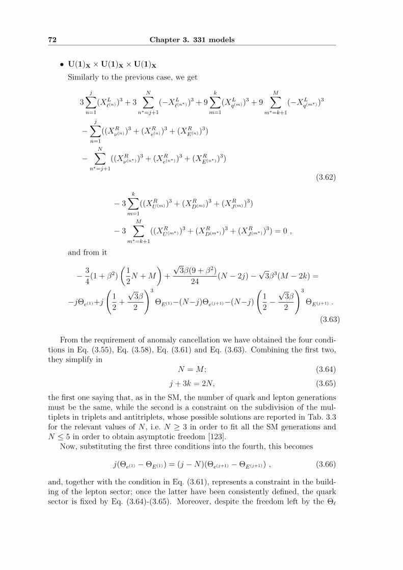
72 Chapter 3. 331 models
• U(1)X ×U(1)X ×U(1)X
Similarly to the previous case, we get
3
j∑n=1
(XL`(n))
3 + 3N∑
n∗=j+1
(−XL`(n∗))
3 + 9k∑
m=1
(XLq(m))
3 + 9M∑
m∗=k+1
(−XLq(m∗))
3
−j∑
n=1
((XRν(n))
3 + (XRe(n))
3 + (XRE(n))
3)
−N∑
n∗=j+1
((XRν(n∗))
3 + (XRe(n∗))
3 + (XRE(n∗))
3)
(3.62)
− 3k∑
m=1
((XRU(m))
3 + (XRD(m))
3 + (XRJ(m))
3)
− 3M∑
m∗=k+1
((XRU(m∗))
3 + (XRD(m∗))
3 + (XRJ(m∗))
3) = 0 ,
and from it
− 3
4(1 + β2)
(1
2N +M
)+
√3β(9 + β2)
24(N − 2j)−
√3β3(M − 2k) =
−jΘe(1)+j
(1
2+
√3β
2
)3
ΘE(1)−(N−j)Θe(j+1)−(N−j)
(1
2−√
3β
2
)3
ΘE(j+1) .
(3.63)
From the requirement of anomaly cancellation we have obtained the four condi-tions in Eq. (3.55), Eq. (3.58), Eq. (3.61) and Eq. (3.63). Combining the first two,they simplify in
N = M ; (3.64)
j + 3k = 2N, (3.65)
the first one saying that, as in the SM, the number of quark and lepton generationsmust be the same, while the second is a constraint on the subdivision of the mul-tiplets in triplets and antitriplets, whose possible solutions are reported in Tab. 3.3for the relevant values of N , i.e. N ≥ 3 in order to fit all the SM generations andN ≤ 5 in order to obtain asymptotic freedom [123].
Now, substituting the first three conditions into the fourth, this becomes
j(Θe(1) −ΘE(1)) = (j −N)(Θe(j+1) −ΘE(j+1)) , (3.66)
and, together with the condition in Eq. (3.61), represents a constraint in the build-ing of the lepton sector; once the latter have been consistently defined, the quarksector is fixed by Eq. (3.64)-(3.65). Moreover, despite the freedom left by the Θ`
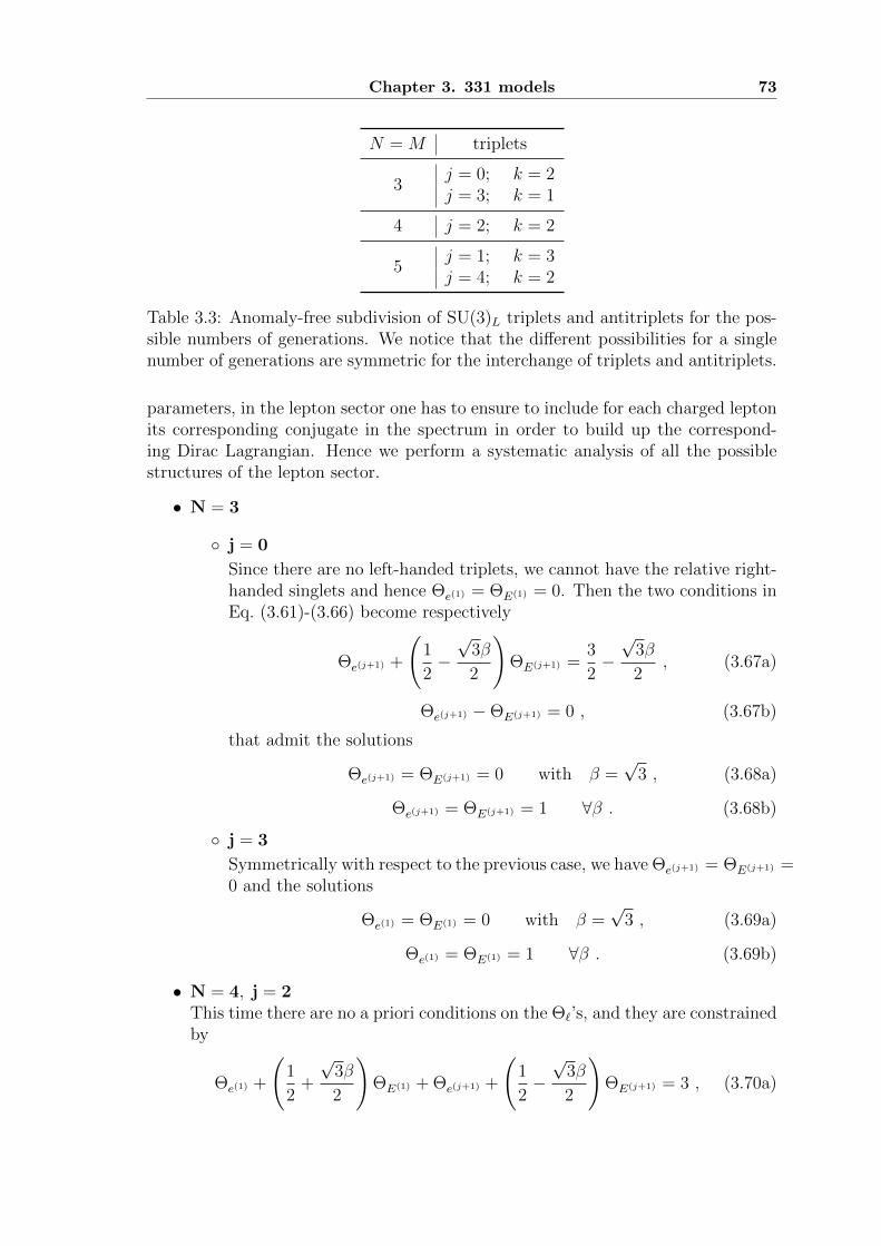
Chapter 3. 331 models 73
N = M triplets
3j = 0; k = 2j = 3; k = 1
4 j = 2; k = 2
5j = 1; k = 3j = 4; k = 2
Table 3.3: Anomaly-free subdivision of SU(3)L triplets and antitriplets for the pos-sible numbers of generations. We notice that the different possibilities for a singlenumber of generations are symmetric for the interchange of triplets and antitriplets.
parameters, in the lepton sector one has to ensure to include for each charged leptonits corresponding conjugate in the spectrum in order to build up the correspond-ing Dirac Lagrangian. Hence we perform a systematic analysis of all the possiblestructures of the lepton sector.
• N = 3
◦ j = 0
Since there are no left-handed triplets, we cannot have the relative right-handed singlets and hence Θe(1) = ΘE(1) = 0. Then the two conditions inEq. (3.61)-(3.66) become respectively
Θe(j+1) +
(1
2−√
3β
2
)ΘE(j+1) =
3
2−√
3β
2, (3.67a)
Θe(j+1) −ΘE(j+1) = 0 , (3.67b)
that admit the solutions
Θe(j+1) = ΘE(j+1) = 0 with β =√
3 , (3.68a)
Θe(j+1) = ΘE(j+1) = 1 ∀β . (3.68b)
◦ j = 3
Symmetrically with respect to the previous case, we have Θe(j+1) = ΘE(j+1) =0 and the solutions
Θe(1) = ΘE(1) = 0 with β =√
3 , (3.69a)
Θe(1) = ΘE(1) = 1 ∀β . (3.69b)
• N = 4, j = 2This time there are no a priori conditions on the Θ`’s, and they are constrainedby
Θe(1) +
(1
2+
√3β
2
)ΘE(1) + Θe(j+1) +
(1
2−√
3β
2
)ΘE(j+1) = 3 , (3.70a)
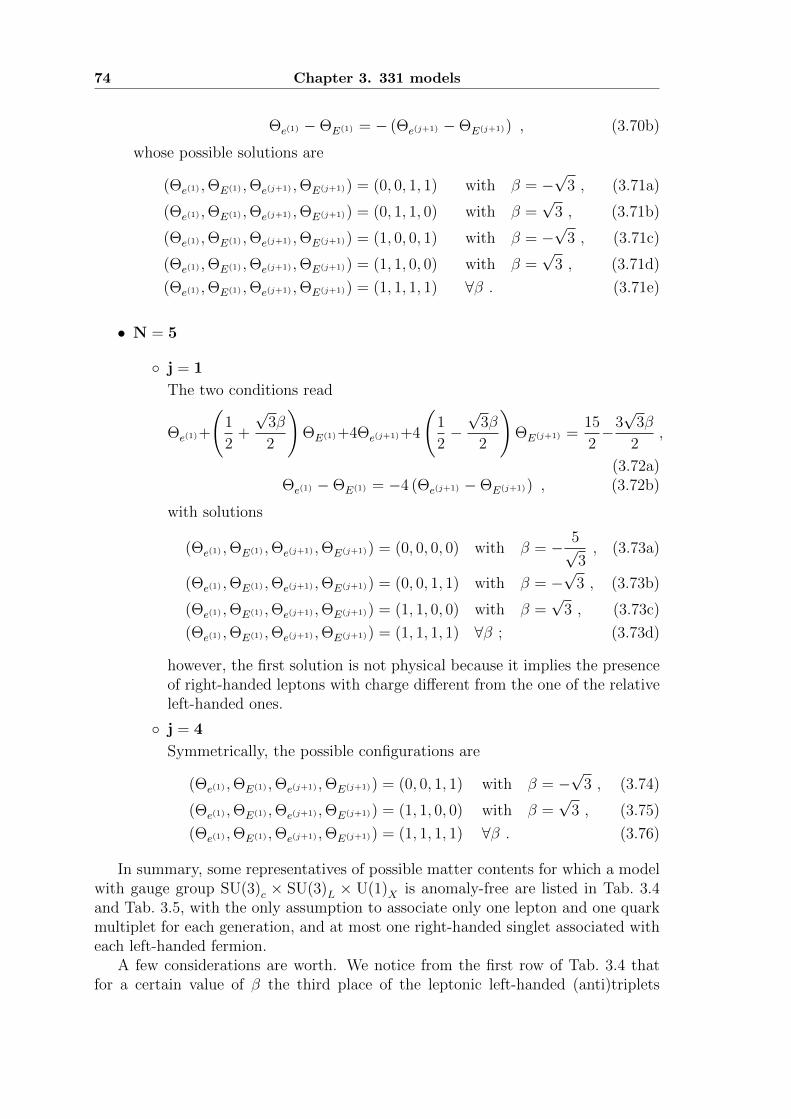
74 Chapter 3. 331 models
Θe(1) −ΘE(1) = − (Θe(j+1) −ΘE(j+1)) , (3.70b)
whose possible solutions are
(Θe(1) ,ΘE(1) ,Θe(j+1) ,ΘE(j+1)) = (0, 0, 1, 1) with β = −√
3 , (3.71a)
(Θe(1) ,ΘE(1) ,Θe(j+1) ,ΘE(j+1)) = (0, 1, 1, 0) with β =√
3 , (3.71b)
(Θe(1) ,ΘE(1) ,Θe(j+1) ,ΘE(j+1)) = (1, 0, 0, 1) with β = −√
3 , (3.71c)
(Θe(1) ,ΘE(1) ,Θe(j+1) ,ΘE(j+1)) = (1, 1, 0, 0) with β =√
3 , (3.71d)
(Θe(1) ,ΘE(1) ,Θe(j+1) ,ΘE(j+1)) = (1, 1, 1, 1) ∀β . (3.71e)
• N = 5
◦ j = 1
The two conditions read
Θe(1)+
(1
2+
√3β
2
)ΘE(1)+4Θe(j+1)+4
(1
2−√
3β
2
)ΘE(j+1) =
15
2−3√
3β
2,
(3.72a)Θe(1) −ΘE(1) = −4 (Θe(j+1) −ΘE(j+1)) , (3.72b)
with solutions
(Θe(1) ,ΘE(1) ,Θe(j+1) ,ΘE(j+1)) = (0, 0, 0, 0) with β = − 5√3, (3.73a)
(Θe(1) ,ΘE(1) ,Θe(j+1) ,ΘE(j+1)) = (0, 0, 1, 1) with β = −√
3 , (3.73b)
(Θe(1) ,ΘE(1) ,Θe(j+1) ,ΘE(j+1)) = (1, 1, 0, 0) with β =√
3 , (3.73c)
(Θe(1) ,ΘE(1) ,Θe(j+1) ,ΘE(j+1)) = (1, 1, 1, 1) ∀β ; (3.73d)
however, the first solution is not physical because it implies the presenceof right-handed leptons with charge different from the one of the relativeleft-handed ones.
◦ j = 4
Symmetrically, the possible configurations are
(Θe(1) ,ΘE(1) ,Θe(j+1) ,ΘE(j+1)) = (0, 0, 1, 1) with β = −√
3 , (3.74)
(Θe(1) ,ΘE(1) ,Θe(j+1) ,ΘE(j+1)) = (1, 1, 0, 0) with β =√
3 , (3.75)
(Θe(1) ,ΘE(1) ,Θe(j+1) ,ΘE(j+1)) = (1, 1, 1, 1) ∀β . (3.76)
In summary, some representatives of possible matter contents for which a modelwith gauge group SU(3)c × SU(3)L × U(1)X is anomaly-free are listed in Tab. 3.4and Tab. 3.5, with the only assumption to associate only one lepton and one quarkmultiplet for each generation, and at most one right-handed singlet associated witheach left-handed fermion.
A few considerations are worth. We notice from the first row of Tab. 3.4 thatfor a certain value of β the third place of the leptonic left-handed (anti)triplets
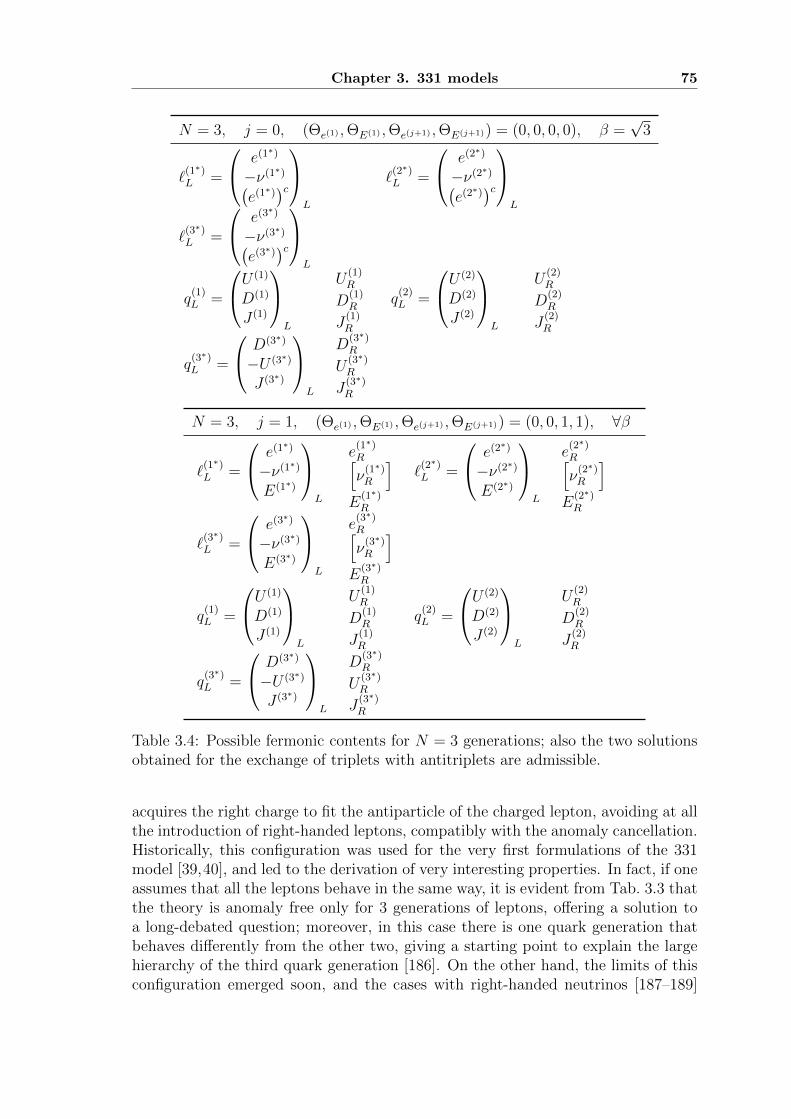
Chapter 3. 331 models 75
N = 3, j = 0, (Θe(1) ,ΘE(1) ,Θe(j+1) ,ΘE(j+1)) = (0, 0, 0, 0), β =√
3
`(1∗)L =
e(1∗)
−ν(1∗)(e(1∗)
)cL
`(2∗)L =
e(2∗)
−ν(2∗)(e(2∗)
)cL
`(3∗)L =
e(3∗)
−ν(3∗)(e(3∗)
)cL
q(1)L =
U (1)
D(1)
J (1)
L
U(1)R
q(2)L =
U (2)
D(2)
J (2)
L
U(2)R
D(1)R D
(2)R
J(1)R J
(2)R
q(3∗)L =
D(3∗)
−U (3∗)
J (3∗)
L
D(3∗)R
U(3∗)R
J(3∗)R
N = 3, j = 1, (Θe(1) ,ΘE(1) ,Θe(j+1) ,ΘE(j+1)) = (0, 0, 1, 1), ∀β
`(1∗)L =
e(1∗)
−ν(1∗)
E(1∗)
L
e(1∗)R
`(2∗)L =
e(2∗)
−ν(2∗)
E(2∗)
L
e(2∗)R[
ν(1∗)R
] [ν
(2∗)R
]E
(1∗)R E
(2∗)R
`(3∗)L =
e(3∗)
−ν(3∗)
E(3∗)
L
e(3∗)R[ν
(3∗)R
]E
(3∗)R
q(1)L =
U (1)
D(1)
J (1)
L
U(1)R
q(2)L =
U (2)
D(2)
J (2)
L
U(2)R
D(1)R D
(2)R
J(1)R J
(2)R
q(3∗)L =
D(3∗)
−U (3∗)
J (3∗)
L
D(3∗)R
U(3∗)R
J(3∗)R
Table 3.4: Possible fermonic contents for N = 3 generations; also the two solutionsobtained for the exchange of triplets with antitriplets are admissible.
acquires the right charge to fit the antiparticle of the charged lepton, avoiding at allthe introduction of right-handed leptons, compatibly with the anomaly cancellation.Historically, this configuration was used for the very first formulations of the 331model [39,40], and led to the derivation of very interesting properties. In fact, if oneassumes that all the leptons behave in the same way, it is evident from Tab. 3.3 thatthe theory is anomaly free only for 3 generations of leptons, offering a solution toa long-debated question; moreover, in this case there is one quark generation thatbehaves differently from the other two, giving a starting point to explain the largehierarchy of the third quark generation [186]. On the other hand, the limits of thisconfiguration emerged soon, and the cases with right-handed neutrinos [187–189]
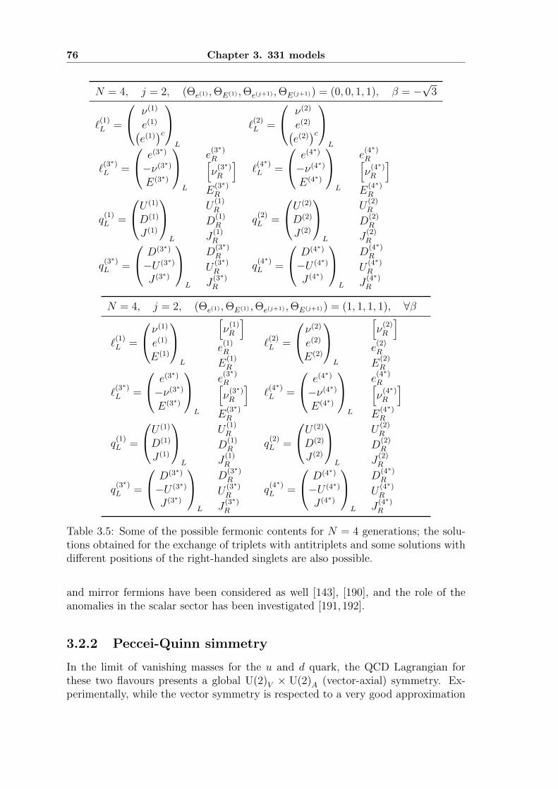
76 Chapter 3. 331 models
N = 4, j = 2, (Θe(1) ,ΘE(1) ,Θe(j+1) ,ΘE(j+1)) = (0, 0, 1, 1), β = −√
3
`(1)L =
ν(1)
e(1)(e(1))cL
`(2)L =
ν(2)
e(2)(e(2))cL
`(3∗)L =
e(3∗)
−ν(3∗)
E(3∗)
L
e(3∗)R
`(4∗)L =
e(4∗)
−ν(4∗)
E(4∗)
L
e(4∗)R[
ν(3∗)R
] [ν
(4∗)R
]E
(3∗)R E
(4∗)R
q(1)L =
U (1)
D(1)
J (1)
L
U(1)R
q(2)L =
U (2)
D(2)
J (2)
L
U(2)R
D(1)R D
(2)R
J(1)R J
(2)R
q(3∗)L =
D(3∗)
−U (3∗)
J (3∗)
L
D(3∗)R
q(4∗)L =
D(4∗)
−U (4∗)
J (4∗)
L
D(4∗)R
U(3∗)R U
(4∗)R
J(3∗)R J
(4∗)R
N = 4, j = 2, (Θe(1) ,ΘE(1) ,Θe(j+1) ,ΘE(j+1)) = (1, 1, 1, 1), ∀β
`(1)L =
ν(1)
e(1)
E(1)
L
[ν
(1)R
]`
(2)L =
ν(2)
e(2)
E(2)
L
[ν
(2)R
]e
(1)R e
(2)R
E(1)R E
(2)R
`(3∗)L =
e(3∗)
−ν(3∗)
E(3∗)
L
e(3∗)R
`(4∗)L =
e(4∗)
−ν(4∗)
E(4∗)
L
e(4∗)R[
ν(3∗)R
] [ν
(4∗)R
]E
(3∗)R E
(4∗)R
q(1)L =
U (1)
D(1)
J (1)
L
U(1)R
q(2)L =
U (2)
D(2)
J (2)
L
U(2)R
D(1)R D
(2)R
J(1)R J
(2)R
q(3∗)L =
D(3∗)
−U (3∗)
J (3∗)
L
D(3∗)R
q(4∗)L =
D(4∗)
−U (4∗)
J (4∗)
L
D(4∗)R
U(3∗)R U
(4∗)R
J(3∗)R J
(4∗)R
Table 3.5: Some of the possible fermonic contents for N = 4 generations; the solu-tions obtained for the exchange of triplets with antitriplets and some solutions withdifferent positions of the right-handed singlets are also possible.
and mirror fermions have been considered as well [143], [190], and the role of theanomalies in the scalar sector has been investigated [191,192].
3.2.2 Peccei-Quinn simmetry
In the limit of vanishing masses for the u and d quark, the QCD Lagrangian forthese two flavours presents a global U(2)V × U(2)A (vector-axial) symmetry. Ex-perimentally, while the vector symmetry is respected to a very good approximation
Chapter 3. 331 models 77
(in fact U(2)V = SU(2)I × U(1)B), this is not true for the axial symmetry: quarkcondensates with 〈uu〉 =
⟨dd⟩6= 0 form, breaking down the axial symmetry spon-
taneously; four pseudo-Goldostone bosons would be expected, but, apart for thepions, there are no signs of another light state in the hadronic spectrum.
A possible solution to this problem seems to be provided by the breaking of theU(2)A symmetry at loop level. In fact, considering the triangle loop of an axialcurrent with two gluons, one finds the anomalous current
∂µjµ5 =
g2
32π2Gµνa Gaµν , (3.77)
with Gaµν = 12εµναβG
µνa . One can notice that the pseudoscalar density entering this
anomaly is a total divergence:
Gµνa Gaµν = ∂µK
µ with Kµ = εµαβγAaα
[Gaβγ −
g
3fabcAbβAcγ
]; (3.78)
however, this do not vanish when integrated into the action, because the usualboundary condition Aµa = 0 at spatial infinity is not gauge invariant; the correctboundary condition to use is that any gauge transformation of Aµa should vanish atthe spatial infinity [193]. This nontrivial structure of the QCD vacuum brings outa free parameter θ from the gauge transformation, with the result of adding to theLagrangian the effective contribution
Lθ = θg2
32π2Gµνa Gaµν . (3.79)
Moreover, when electroweak interactions are included, the diagonalization of themass matrix M implies a chiral transformation that changes θ → θ = θ+arg(detM).The term in Eq. (3.79) is C-conserving and P - and T -violating, and hence violatesCP . It is directly linked to the neutron electric dipole moment dn ' eθmq/m
2N ,
and the strong bounds on the latter, |dn| < 2.9 e·cm [194] imply that the phase θ isextremely small, if not vanishing; this is known as the strong CP problem and it isan open problem of the SM.
The most popular solution to the CP problem is the introduction of the Peccei-Quinn symmetry [120,195] and hence of the axion [196,197]. If the theory presents aglobal axial symmetry U(1)PQ that is spontaneously broken, the relative Goldstoneboson, called the axion, exhibits a triangle anomaly that, due to the effective poten-tial generated by the interaction with the gluons, exactly cancels the axial anomaly.Due to the anomaly, the axion acquires a mass and hence is not incompatible withexperiments.
A theory that naturally presents such a symmetry has the appealing advantage ofnot suffering of the strong CP problem. This is the case of at least some realizationsof the 331 model [198–201].
• In its minimal version [39,40], with 3 generations without right-handed leptonsinglets and β =
√3, the fermion content of the model is
`(1∗, 2∗, 3∗)L ∼ (1, 3, 0) , Q
(1, 2)L ∼
(3,3,−1
3
), Q
(3∗)L ∼
(3, 3,
2
3
); (3.80a)
78 Chapter 3. 331 models
U(1, 2, 3∗)R ∼
(3,1,
2
3
), D
(1, 2, 3∗)R ∼
(3,1,−1
3
); (3.80b)
J(1, 2)R ∼
(3,1,−4
3
), J
(3∗)R ∼
(3,1,
5
3
); (3.80c)
while the Higgs sector contains
χ ∼ (1,3, 1) , ρ ∼ (1,3, 0) , η ∼ (1,3,−1) , S ∼ (1,6, 0) ; (3.81)
the most general Yukawa Lagrangian is
LY = λ`,ρab εijk ¯
ia`cjbρk + λ`,Sab
¯aS†`cb
+ λQ,χij QiLχJ
jR + λQ,χ3 Q3
Lχ†TR
+ λQ,ρia QiLρd
aR + λQ,ρ3 Q3
Lρ†uR
+ λQ,ηia QiLηu
aR + λQ,η3 Q3
Lη†dR + h.c. ;
(3.82)
and the most general Higgs potential
V = λ1(χ†χ− v2χ)2 + λ2(ρ†ρ− v2
ρ)2 + λ3(η†η − v2
η)2 + λ4(Tr(S†S)− v2
S)2
+ λ5(Tr(S†SS†S)− v4S) + λ6(χ†χρ†ρ− v2
χv2ρ) + λ7(ρ†ρη†η − v2
ρv2η)
+ λ8(η†ηχ†χ− v2ηv
2χ) + λ9(χ†χTr(S†S)− v2
χv2S) + λ10(ρ†ρTr(S†S)− v2
ρv2S)
+ λ11(η†ηTr(S†S)− v2ηv
2S) + λ12(χ†ρρ†χ) + λ13(ρ†ηη†ρ) + λ14(η†χχ†η)
+ µ1ηρχ+ µ2ρTS†χ+ h.c. .
(3.83)
The gauge Lagrangian and the Yukawa Lagrangian are invariant with respectto the global chiral U(1) symmetry [198]
Multiplet `(i∗)L Q
(i)L Q
(3∗)L qR χ, η, ρ S
Charge 1 1 −1 0 1 2
as well as the Higgs potential, with the exception of the trilinear term ηρχthat can be dropped out without consequences.
This scenario presents therefore a symmetry of the type advocated by Peccei-Quinn. However the model is not realistic in this way: at the high scale vχ,although the U(1)PQ breaks, the combination U(1)PQ+U(1)X is unbroken andacts as a Peccei-Quinn symmetry; hence the axion emerges at the lower scalevρ ∼ vη and this is ruled out by experiments. The model has to be extendedin order to make the axion invisible.
• If one wants to include right-handed neutrinos, one can choose β = −1/√
3and a fermionic content
`(1, 2, 3)L ∼
(1, 3,−1
3
), Q
(1∗, 2∗)L ∼ (3, 3, 0) , Q
(3)L ∼
(3,3,
1
3
)(3.84a)
Chapter 3. 331 models 79
e(1, 2, 3)R ∼ (1,1,−1) ; (3.84b)
U(1∗, 2∗, 3)R , J
(3)R ∼
(3,1,
2
3
), D
(1∗, 2∗, 3)R , J
(1∗, 2∗)R ∼
(3,1,−1
3
); (3.84c)
the Higgs sector is reduced to
χ ∼(
1,3,−1
3
), ρ ∼
(1,3,
2
3
), η ∼
(1,3,−1
3
); (3.85)
the Yukawa Lagrangian and the Higgs potential2 read respectively
LY = λ`,LLij `iL`jLρ+ λ`,LRij
¯iL`
jRρ
+ λQ,χij QiLχ†J jR + λQ,χ3 Q3
LχTR
+ λQ,ρia QiLρ†daR + λQ,ρ3 Q3
LρuR
+ λQ,ηia QiLη†uaR + λQ,η3 Q3
LηdR + h.c. ;
(3.86)
V = λ1(χ†χ− v2χ)2 + λ2(ρ†ρ− v2
ρ)2 + λ3(η†η − v2
η)2
+ λ4(χ†χ− v2χ)(η†η − v2
η) + λ5(η†η − v2η)(ρ
†ρ− v2ρ)
+ λ6(ρ†ρ− v2ρ)(χ
†χ− v2χ) + λ7(χ†η + η†χ)2
+ λ8(χ†η)(η†χ) + λ9(η†ρ)(ρ†η) + λ10(ρ†χ)(χ†ρ) .
(3.87)
Also in this case there is a Peccei-Quinn symmetry [198]
Multiplet `(i)L `
(i)R Q
(i∗)L Q
(3)L qR χ, η, ρ
Charge −12−3
2−1 1 0 1
which however presents the same axion problem as the previous scenario.
3.3 The 331 model
3.3.1 Model content
As we have discussed in the previous sections, a specific realization of a 331 modelis defined by a value of the β parameter and by the assignment of a consequent non-anomalous fermionic content. The specific scenario that we are going to consider,that we will call 331 model, has
β =1√3
(3.88)
and the fermionic content listed in Tab. 3.6. We introduce three fermion generations;the three lepton families are arranged into antitriplets, and their third componentcan fit the charged-conjugated neutrinos, so that neutrinos can get a mass withoutthe explicit introduction of their right-handed component; on the other hand, the
2In [187] the following discrete symmetry is imposed: χ→ −χ, TR → −TR, DjR → Dj
R.
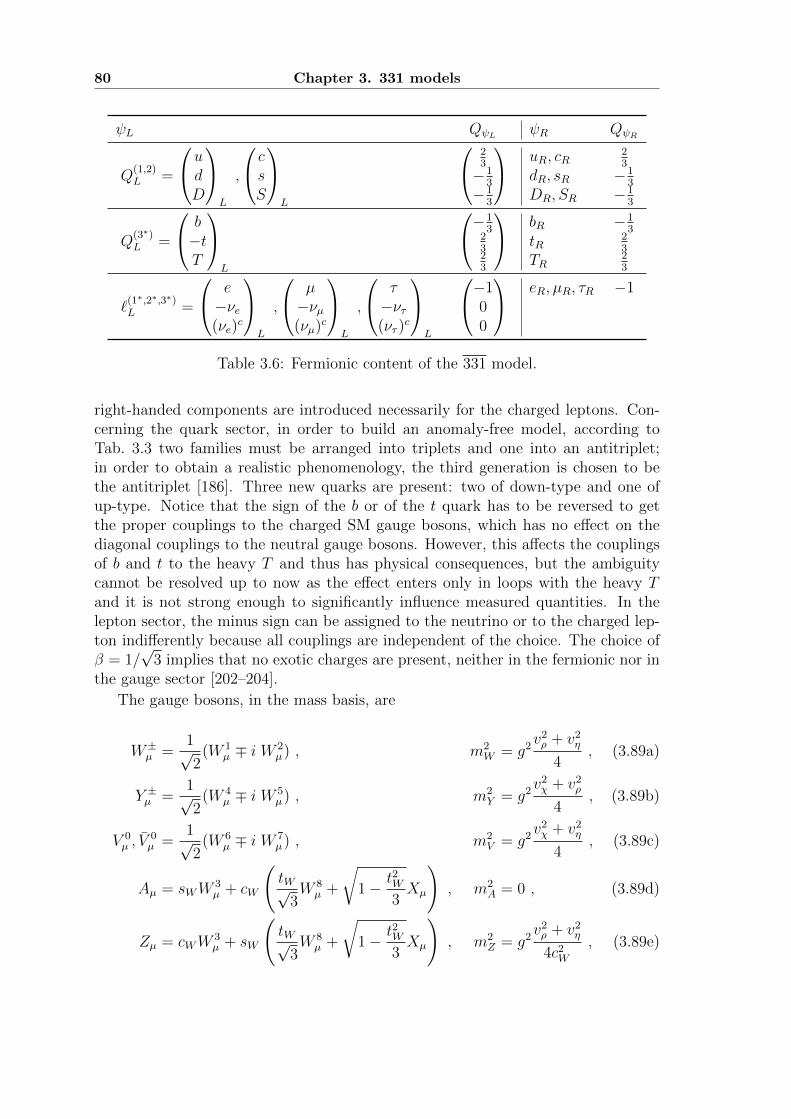
80 Chapter 3. 331 models
ψL QψL ψR QψR
Q(1,2)L =
udD
L
,
csS
L
23
−13
−13
uR, cR23
dR, sR −13
DR, SR −13
Q(3∗)L =
b−tT
L
−13
2323
bR −13
tR23
TR23
`(1∗,2∗,3∗)L =
e−νe(νe)
c
L
,
µ−νµ(νµ)c
L
,
τ−ντ(ντ )
c
L
−100
eR, µR, τR −1
Table 3.6: Fermionic content of the 331 model.
right-handed components are introduced necessarily for the charged leptons. Con-cerning the quark sector, in order to build an anomaly-free model, according toTab. 3.3 two families must be arranged into triplets and one into an antitriplet;in order to obtain a realistic phenomenology, the third generation is chosen to bethe antitriplet [186]. Three new quarks are present: two of down-type and one ofup-type. Notice that the sign of the b or of the t quark has to be reversed to getthe proper couplings to the charged SM gauge bosons, which has no effect on thediagonal couplings to the neutral gauge bosons. However, this affects the couplingsof b and t to the heavy T and thus has physical consequences, but the ambiguitycannot be resolved up to now as the effect enters only in loops with the heavy Tand it is not strong enough to significantly influence measured quantities. In thelepton sector, the minus sign can be assigned to the neutrino or to the charged lep-ton indifferently because all couplings are independent of the choice. The choice ofβ = 1/
√3 implies that no exotic charges are present, neither in the fermionic nor in
the gauge sector [202–204].
The gauge bosons, in the mass basis, are
W±µ =
1√2
(W 1µ ∓ i W 2
µ) , m2W = g2
v2ρ + v2
η
4, (3.89a)
Y ±µ =1√2
(W 4µ ∓ i W 5
µ) , m2Y = g2
v2χ + v2
ρ
4, (3.89b)
V 0µ , V
0µ =
1√2
(W 6µ ∓ i W 7
µ) , m2V = g2
v2χ + v2
η
4, (3.89c)
Aµ = sWW3µ + cW
(tW√
3W 8µ +
√1− t2W
3Xµ
), m2
A = 0 , (3.89d)
Zµ = cWW3µ + sW
(tW√
3W 8µ +
√1− t2W
3Xµ
), m2
Z = g2v2ρ + v2
η
4c2W
, (3.89e)
Chapter 3. 331 models 81
Z ′µ = −√
1− t2W3W 8µ +
tW√3Xµ ,
m2Z′ '
g2c2W
3− 4s2W
[v2χ +
v2ρ
4
(t2W +
1
c4W
)+v2η
4
(1 +
1
c4W
)]. (3.89f)
W±µ , Aµ, Zµ are the gauge bosons of the SM, while Y ±µ , V 0
µ , V0µ and Z ′µ are new heavy
gauge bosons.The scalar sector contains the three triplets
χ =
χ+A
χ0B
vχ + ξχ + iζχ
, ρ =
ρ+A
vρ + ξρ + iζρρ0B
, η =
vη + ξη + iζηη−Aη−B
,
(3.90)for which the mass eigenstates are
φ±W = −sβρ±A + cβη±A , m2φW
= 0 , (3.91a)
φ±Y ' −η±B , m2
φY= 0 , (3.91b)
φ0V , φ
0V ' −ρ0
B,−ρ0B , m2
φV= 0 , (3.91c)
φ0Z ' −ζχ , m2
φZ= 0 , (3.91d)
φ0Z′ ' sβζρ − cβζη , m2
φZ′= 0 , (3.91e)
H±1 = cβρ±A + sβη
±A , m2
H1=
1
sβcβfvχ , (3.91f)
H±2 ' χ±A , m2H2
= tβfvχ +λ9
2v2χ , (3.91g)
H03 , H
03 ' χ0
B, χ0B , m2
H3=
1
tβfvχ +
λ7
2v2χ , (3.91h)
H04 ' cβζρ + sβζη , m2
H4=
1
sβcβfvχ , (3.91i)
H05 ' ξχ , m2
H5= 2λ1v
2χ , (3.91j)
H06 ' sβξρ + cβξη , m2
H6=
2(λ2v4ρ + λ4v
4η + λ5v
2ρv
2η)
v2ρ + v2
η
, (3.91k)
H07 ' −cβξρ + sβξη , m2
H7=
1
sβcβfvχ , (3.91l)
(3.91m)
where sβ ≡ sin βρη = vρ√v2ρ+v2
η
. The φ’s are the Goldstone bosons that give mass to
the five gauge bosons, H6 is the neutral scalar field that can be identified with theSM Higgs boson, while H1 . . . H5 and H7 are heavy (pseudo)scalar fields.
The Feynman rules of the 331 model are listed in Appendix B. It is interestingto notice that the SM quark sector is strictly not affected by the effects of the gaugegroup enlargement, in the sense that, if we consider only the SM quarks and gaugebosons, their interactions are exactly the same as in the SM. On the contrary, in thelepton sector the new gauge bosons can couple two SM leptons; they are assigned
82 Chapter 3. 331 models
lepton number L = ∓2, but carry no lepton generation number since they canmediate lepton-flavour violating processes at tree level. Consequently, strict boundson the model come from the upper bounds on the µ → eγ decay set by the MEGexperiment [205]; detailed studies on lepton-flavour violation have been performedin [206–211], and more insights into lepton masses, see-saw mechanisms and neutrinophysics in 331 models can be found in [212–226].
We mention here that, in addition to consider realizations of the 331 modelwith different values of β and different fermionic contents, a variety of extensionswith more NP features has been studied: supersymmetric extensions [227–242], theadditions of further symmetries [243–251], the inclusion into GUTs [252–256], thedark matter candidates [257–259].
3.3.2 Quark mixing and FCNCs
The most general gauge-invariant Yukawa Lagrangian in the quark sector is
LqY = λJijQi,LχJj,R + λJ33Q3,Lχ∗TR
+ λDiaQi,Lρda,R + λD3aQ3,Lη∗da,R
+ λUiaQi,Lηua,R + λU3aQ3ρ∗ua,R + h.c. ,
(3.92)
where i = 1, 2 so that Jj = D,S, while a = 1, 2, 3 so that ua = u, c, t and da = d, s, b.The pattern is similar to the 2HDM or to the SUSY one, with up- and down- quarksgetting mass from different Higgs multiplets; instead, the new quarks get mass fromanother different multiplet at a different scale.
As in the SM, the mass eigenstates of the SM quarks can be obtained throughunitary transformations of the left-handed multiplets:u′Lc′L
t′L
= U−1L
uLcLtL
,
d′Ls′Lb′L
= V −1L
dLsLbL
. (3.93)
As regards the exotic quarks, obviously the D and S quarks do not mix with thedifferently charged T quark; on the other hand, the mixing of D and S can bereabsorbed by a suitable parametrization of the rotation matrices. In fact, theexotic mass matrix MJ can be diagonalized by two block-diagonal unitary matricesWL and WR, and WR can be removed by a redefinition of the right-handed heavyquark fields, while WL can be absorbed into the definition of UL and VL. As aconsequence, one can treat D,S, T as physical fields.
The rotation of the SM quarks affects the charged currents: the W -mediatedcurrent becomes
JµW = uLγµU †LVLdL , (3.94)
and hence the relevant matrix is the combination
VCKM ≡ U †LVL , (3.95)
that is just the SM CKM matrix. Nonetheless, differently from the SM, the UL andVL matrices are physical quantities: first of all they appear explicitly in the vertices
Chapter 3. 331 models 83
of the Y and V gauge bosons, but moreover they have also an important impacton the neutral currents. In fact, the quark mixing has no consequences on the Aand Z interactions, as in the SM, but this is not true for the Z ′, due to its differenttreatment of the third generation. Explicitly, we consider the Z ′-mediated current,keeping only the phenomenologically interesting contributions, i.e. the left handedones leaving out the exotic quarks that are too heavy as external states:
JµZ′ = uLγµU †L
−1 + 43s2W
−1 + 43s2W
1− 23s2W
ULu
+ dLγµV †L
−1 + 43s2W
−1 + 43s2W
1− 23s2W
VLd
= (−1 +4
3s2W )(uLγ
µuL + dLγµdL)
+ 2c2W uLγ
µU †L
00
1
ULuL + 2c2W dLγ
µV †L
00
1
VLdL ,
(3.96)
i.e. the Z ′ can mediate tree-level FCNCs governed by the UL and VL matrices,introducing new sources of CP violation. This holds for all the 3-generations 331models, since by construction two generations are treated equally and differentlyfrom the third. On the other hand, the universality of the coupling of the Z ′ toto right-handed quarks implies that the FCNCs are purely left-handed, and theuniversality of its coupling to leptons guarantees that no FCNCs show up in this case.In addition, we underline that instead the new V 0 gauge boson does not generatetree-level FCNCs between SM quarks, since it only mediates interactions betweenSM and exotic quarks. FCNCs in 331 models have been analyzed theoretically andphenomenologically in [260–271], and CP violation in [272–274].
In order to analyze the structure of these matrices, it is convenient to take VLand VCKM as the independent matrices. The structure of the CKM matrix is thesame as in the SM since the form of the W -vertex is exactly the same and one canstill rotate five independent, unphysical phases. The matrix VL is a unitary matrixas well and therefore it is determined by nine parameters. As there are three newquarks in the theory, three phases are unphysical, and in VL six parameters remain,three angles and three mixing phases. In order to draw out a parametrization of VL,one has to analyze the structure of the other vertices in which it appears, i.e. withthe currents
JµV = diLγµV †L
1 00 10 0
ia
DaL + TLγ
µ(0 0 1
)iULu
iL , (3.97a)
JµY = uiLγµU †L
1 00 10 0
ia
DaL − TLγµ
(0 0 1
)iVLd
iL ; (3.97b)
84 Chapter 3. 331 models
from the second term in Eq. (3.97b) we see that rotating T by a complex phase θamounts to multiplying the third line in VL by θ; in the first term in Eq. (3.97a)one can rotate the first and second line of VL through an arbitrary phase rotationof each D and S. Therefore the transformations allowed for the VL matrix are anindependent phase rotation in every line. It is convenient to choose a parameteriza-tion that has a simple structure and as little parameters as possible in the third line,since these are the elements that will occur in the down-type FCNCs. Moreover,the parametrization must be compatible with the choice to treat D and S both asmasses and interaction eigenstates. We will use the following parametrization [263]:
VL =
c12c13 s12c23eiδ3 − c12s13s23e
i(δ1−δ2) c12c23s13eiδ1 + s12s23e
i(δ2+δ3)
−c13s12e−iδ3 c12c23 + s12s13s23e
i(δ1−δ2−δ3) −s12s13c23ei(δ1−δ3) − c12s23e
iδ2
−s13e−iδ1 −c13s23e
−iδ2 c13c23
.
(3.98)Moreover, we will use the following notation for the Z ′-mediated FCNCs of downquarks:
iLFCNC = i[∆sd(sLγ
µdL) + ∆bd(bLγµdL) + ∆bs(bLγ
µsL)]Z ′µ , (3.99)
and similarly ∆µµL,R and ∆νν for the couplings of Z ′ to leptons. For a generic 331
model with 3 generations the ∆’s are
∆ij =gc2
W√3cW
√1− (1 + β2)s2
W
v∗3iv3j , (3.100a)
∆ji = (∆ij)∗ , (3.100b)
∆µµL =
g[1− (1 +
√3β)s2
W
]2√
3cW√
1− (1 + β2)s2W
, (3.100c)
∆µµR =
−gβs2W
cW√
1−(1+β2)s2Wβ 6=√
3
g√
1−4s2W√3cW
β =√
3, (3.100d)
∆νν = ∆µµL , (3.100e)
(3.100f)
where vij = (VL)ij; in particular, in the 331 model and using the value of theWeinberg angle, they read
∆sd = 0.61gs13s23c13ei(δ2−δ1) , (3.101a)
∆bd = −0.61gs13c13c23e−iδ1 , (3.101b)
∆bs = −0.61gs23c213c23e
−iδ2 , (3.101c)
∆µµL = 0.213g , (3.101d)
∆µµR = −0.183g , (3.101e)
∆νν = 0.213g . (3.101f)
Chapter 3. 331 models 85
3.4 Phenomenology of the 331 model
The previous phenomenological analyses of different kinds of 331 models can befound in [275–290] for hadron colliders and in [291–299] for lepton colliders.
3.4.1 Impact on the master functions
General structure
The key observation about the structure of the 331 model is that it presents thesame operators as the SM: neither left-right nor right-right effective vertices areintroduced, and, neglecting the Higgs-mediated transition, the left-left operator isvectorial. As a consequence, the penguin-box expansion approach can be used with-out the definition of new master functions. However, the presence of the VL matrixelements is a new source of both flavour violation and CP violation, and this impliesthat the master functions loose respectively their universality and their realness. Insummary, the phenomenological effects of the 331 model can be incorporated intothe SM formulae for the relevant observables simply by performing a substitutionof the master functions
F (xt)→ Fi(xt; ρ331) ≡ |Fi|eiθiF , (3.102)
where ρ331 indicates the new parameters of the model, the i index indicates that themaster function is flavour-dependent, and the θiF are the new CP-violating phases.
∆F = 2 transitions
The master function involved is S, that becomes
Si(xt;mZ′ , VL) = S0(xt) + ∆S(Z′)i (mZ′ , VL) + ∆S
(Box)i ≡ |Si|eiθ
iS , (3.103)
where S0 is the SM contribution, ∆S(Z′)i is the contribution due to the tree-level
Z ′ exchange, and ∆S(Box)i is the contribution coming from the exchange of the new
particles into the box diagram.As regards the first contribution, from Fig. 3.1a we find
∆S(Z′){sd,bd,bs}(mZ′ , VL) =
[∆{sd,bd,bs}
λ(sd,bd,bs)t
]24r
g2SMm
2Z′, (3.104)
where we have defined
λ(ij)t = (VCKM)∗ti(VCKM)tj , g2
SM =2GFα√
2π sin2 θW. (3.105)
The r coefficient includes the renormalization group effects. It reads
r =CV LL
1 (mZ′)
0.985η
6/216
[1 + 1.371
α(6)s (mt)
4π(1− η6)
], (3.106)
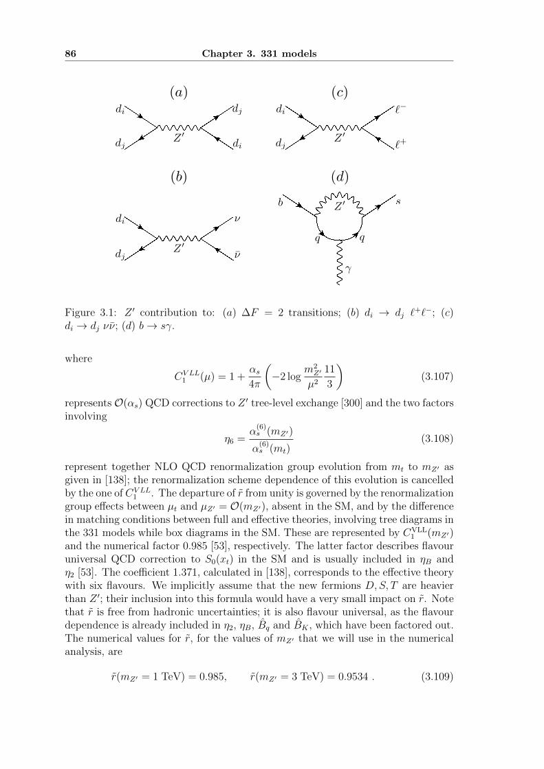
86 Chapter 3. 331 models
Z 0 Z 0
Z 0
Z 0
di di
di
didj
dj
dj
dj
b s
�
⌫
⌫
`�
`+
q q
(a)
(b)
(c)
(d)
Figure 3.1: Z ′ contribution to: (a) ∆F = 2 transitions; (b) di → dj `+`−; (c)
di → dj νν; (d) b→ sγ.
where
CV LL1 (µ) = 1 +
αs4π
(−2 log
m2Z′
µ2
11
3
)(3.107)
represents O(αs) QCD corrections to Z ′ tree-level exchange [300] and the two factorsinvolving
η6 =α
(6)s (mZ′)
α(6)s (mt)
(3.108)
represent together NLO QCD renormalization group evolution from mt to mZ′ asgiven in [138]; the renormalization scheme dependence of this evolution is cancelledby the one of CV LL
1 . The departure of r from unity is governed by the renormalizationgroup effects between µt and µZ′ = O(mZ′), absent in the SM, and by the differencein matching conditions between full and effective theories, involving tree diagrams inthe 331 models while box diagrams in the SM. These are represented by CVLL
1 (mZ′)and the numerical factor 0.985 [53], respectively. The latter factor describes flavouruniversal QCD correction to S0(xt) in the SM and is usually included in ηB andη2 [53]. The coefficient 1.371, calculated in [138], corresponds to the effective theorywith six flavours. We implicitly assume that the new fermions D,S, T are heavierthan Z ′; their inclusion into this formula would have a very small impact on r. Notethat r is free from hadronic uncertainties; it is also flavour universal, as the flavourdependence is already included in η2, ηB, Bq and BK , which have been factored out.The numerical values for r, for the values of mZ′ that we will use in the numericalanalysis, are
r(mZ′ = 1 TeV) = 0.985, r(mZ′ = 3 TeV) = 0.9534 . (3.109)
Chapter 3. 331 models 87
In principle one should also include new box diagram contributions with newcharged and neutral gauge bosons and new quark exchanges; charged Higgs parti-cles can also contribute. However it is possible to show that these contributionsare negligible even without explicit calculations. Indeed, compared to the SMcontributions, the new box contributions are suppressed automatically by a fac-tor m2
W/m2V ≤ 0.006, where mV ≥ 1 TeV stands for the masses of the new gauge
bosons. In models with new left-right operators this suppression could be compen-sated by enhanced hadronic matrix elements of new operators and QCD renormal-ization group effects; however, in 331 models only the SM operator is present andsuch enhancements are absent. Another enhancement could be present through in-creased values of the elements of the mixing matrix VL, but our analysis shows that,in order to suppress sufficiently tree-level Z ′ contributions to ∆F = 2 processes,the hierarchical structure of VL resembles the structure of the CKM matrix. Boxdiagrams are also suppressed with respect to the tree-level contributions by a loopfactor 1/(16π2) and two additional vertices. In summary, it is safe to keep onlyZ ′ contributions; this simplifies significantly the analysis as new box diagrams de-pend generally on many more new parameters, like masses of new gauge bosons andfermions and new mixing angles.
∆F = 1 transitions
According to what we have just discussed, we will neglect the loop contributionsalso in this case.
• di → dj νν
In the SM, the Z-penguin and the box diagram that contribute to this processare contained in the X master function, which with the Z ′ contribution inFig. 3.1c becomes here
X{sd,bd,bs}(mt;mZ′ , VL) = X(xt) +∆νν
g2SMm
2Z′
∆{sd,bd,bs}
λ(sd,bd,bs)t
≡ |Xi|eiθiX . (3.110)
• di → dj `+`−
In this transition the relevant loop functions is the Y , which in the SM is alinear combination of the V − A component of the Z-penguin and the boxdiagrams with final leptons with weak isospin T3 = −1/2, and Z, which isa linear combination of the vector component of the Z-penguin and the γpenguin; they are modified as follows by the contribution in Fig. 3.1b:
Y{sd,bd,bs}(mt;mZ′ , VL) = Y (xt) +∆µµA
g2SMm
2Z′
∆{sd,bd,bs}
λ(sd,bd,bs)t
≡ |Yi|eiθiY , (3.111)
Z{sd,bd,bs}(mt;mZ′ , VL) = Z(xt) +2
4 sin2 θW
∆µµR
g2SMm
2Z′
∆{sd,bd,bs}
λ(sd,bd,bs)t
≡ |Zi|eiθiZ ,
(3.112)
where we have defined ∆µµA = ∆µµ
R + ∆µµL .
88 Chapter 3. 331 models
• b→ s γ
Very detailed analyses of B → Xsγ decay in 331 models have been presentedin [260], [266], and it has been found that the dominant NP contributions comefrom the Higgs sector. In the numerical analysis that we are going to perform,we will not consider the parameters involved in this sector, which being par-ticularly rich do not provide significant predictions. Similarly, the subleadingcontributions involving the new gauge bosons V 0 and Y ± and the new heavyquarks involve new parameters and their contributions can be suppressed ifnecessary without any impact on our analysis. The only contributing diagramthat involves only the Z ′ as a new particle is shown in Fig. 3.1d; we haveperformed a novel analysis regarding its QCD corrections, founding that itdetermines a correction of O(10−4) with respect to the SM prediction, andhence is negligible as expected [301].
3.4.2 Correlations
The 331 model does not satisfy Constrained Minimal Flavour Violation, since themaster functions are neither flavour universal nor real; the pattern of flavour viola-tion can be investigated by looking at the deviation from unity of the r parameters,that in this case read:
r(∆M) =
∣∣∣∣SbdSbs∣∣∣∣ , r(µ+µ−) =
∣∣∣∣YbdYbs∣∣∣∣2 , r(νν) =
∣∣∣∣Xbd
Xbs
∣∣∣∣2 . (3.113)
On the other hand, due to the small number of new parameters, a noticeablepattern of correlations can be recognized. In fact, we make the following observa-tions.
• The good consistence of the CKM theory with experiments implies that theangles and the phases of the new VL matrix should be very small; as a con-sequence, it is a good approximation to set c12 ' c13 ' c23 ' 1, providedthat a post-check is made with the obtained values of the relative sine terms.Then, fixing the mass of the Z ′, the 331 contributions depend only on fournew parameters:
s13 , s23 , δ1 , δ2 . (3.114)
• Going further, we notice that:
◦ ∆bd depends only on s13 and δ1. As a consequence, we expect directcorrelations between the Bd-related observables, such as ∆Md, SψKS inthe mixing, Bd → µ+µ−, Sdµ+µ− in the dimuon decay.
◦ ∆bs depends only on s33 and δ2. As a consequence, analogously to theprevious case, we expect direct correlations between the Bs-related ob-servables, i.e. ∆Ms, Sψφ in the mixing, Bs → µ+µ−, Ssµ+µ− , Aλ∆Γ in thedimuon decay, the rare decays B → Xsνν.
Chapter 3. 331 models 89
◦ ∆ds depends on all the four parameters, and (weaker) correlations canbe expected between the observables in the K system. Moreover, whenexperimental constraints are taken into account, this will provide indirectcorrelations between the Bd- and Bs-observables.
Given the simple structure of the Z ′ contribution, the form of these correlationscan be derived in analytical form even for arbitrary values of β.
• In order to estimate the correlation between the mixing in the K sector andin the Bd,s sector, we consider the ratio
∆Ssd∆Sbd∆S∗bs
=m2Z′g
2SM
4r
[∆sd
∆bd(∆bs)∗
]2
= 0.41(mZ′
TeV
)2 1− (1 + β2)s2W
r
β=1/√
3−−−−→ 0.28(mZ′
TeV
)2 1
r. (3.115)
This relation implies that after the experimental constraints on ∆Md,s havebeen taken into account, the effects in εK are smaller than in ∆Md,s for valuesmZ′ ≤ 3 TeV. Indeed, NP contributions in ∆Md,s are constrained to be atmost 10% of the SM values and therefore the absolute values of ∆{bd,bs} canbe at most 0.25. As r ≈ 1, we find ∆{ds} ≤ 0.16, which implies a correction ofat most 6%. However, for much larger values of mZ′ these effects can increasesignificantly.
• In order to estimate the impact of the variation in the mixing observables tothe νν decays, the relevant comparison is
∆X{bd,bs}√∆S∗{bd,bs}
= {±} ∆νν
√rgSMmZ′
= {∓}0.255
(TeV
mZ′
)1− (1 +
√3β)s2
W
r√
1− (1 + β2)s2W
β=1/√
3−−−−→ {∓}0.165(mZ′
TeV
) 1√r. (3.116)
This result implies that NP effects in the processes with νν in the final stateare rather small for mZ′ = 3 TeV: requiring again that ∆{bd,bs} ≤ 0.25 we findthat only effects of at most 5% on branching ratios are expected for b→ sννtransitions; these effects are even smaller for the K decays. For mZ′ = 1 TeVthe relevant mixing parameters s13 and s23 have to be lowered by roughly afactor of 3 to satisfy the ∆Md,s constraint. The inspection of the dependenceon mixing angles shows that the decrease of the latter is compensated approxi-mately by the decrease of mZ′ in the case of K+ → π+νν and KL → π0νν, andit is overcompensated in the case of b→ sνν transitions, so that modificationsof the branching ratios by 15% are possible in this case.
• As regards the correlation between the decays with νν and µ+µ− in the finalstate, the ratio
∆Yi∆Xi
= −1− (1−√
3β)s2W
1− (1 +√
3β)s2W
β=1/√
3−−−−→ −1.86 (3.117)
90 Chapter 3. 331 models
implies that NP effects in the µ+µ− decays can be larger than in the case of νν.This is not only because of the factor −1.9 in this relation, but also because,concerning the SM contributions, Y (xt) is smaller than X(xt); thus for mZ′ =3 TeV effects of 10-15% on the branching ratio are still allowed in Bd,s →µ+µ− and these effects are expected to increase up to 30% for mZ′ = 1 TeV.Interestingly the NP effects in Bd,s → µ+µ− and B → Xsνν are anticorrelated,and similarly for K+ → π+νν and KL → µ+µ−; unfortunately, due to smallNP effects in decays with νν in the final states, these anticorrelations will bedifficult to test.
Moreover, these relations allow to point out that, once the constraints on ∆Md,s aretaken into account, the NP effects for β =
√3 both in εK and in all rare decays are
so small that it will be difficult to distinguish this model from the SM on the basisof flavour violation in meson decays.
3.4.3 Numerical analysis
Strategy
Since in all the 331 contributions that we are going to consider the key role is playedby the new Z ′ boson, first of all it is fundamental to determine a plausible workingrange for its mass. Lower bounds on mZ′ within 331 models were discussed inliterature, from the study of µ decay [165, 186, 206], Z ′ decays to e+ e− or µ+µ−
[302], or from the analysis of S, T , U parameters [167]; however, the resultingbounds are model dependent, since they depend also on the entries of the matricesthat transform the quark gauge eigenstates into mass eigenstates. Concerning thedirect lower bound on mZ′ from collider experiments, the most stringent boundsare provided by CMS experiment [303]; the precise value depends on the modelconsidered: while for the so-called sequential Z ′ the lower bound for mZ′ is of about2.5 TeV, in other models values as low as 1 TeV are still possible, and we will usethe latter in order to be more general. As regards the upper bounds on mZ′ , aswe have discussed about Eq. (3.31), some realization of the 331 model present theinteresting feature of an upper limit to the breaking scale and consequently to themass of the Z ′; however, it can be seen that this is not the case of the models withβ = 1/
√3. Hence we choose to investigate the range 1 TeV ≤ mZ′ ≤ 3 TeV, that is
testable in the nearby future by present experiments, and we will discuss the casein which Z ′ is beyond the LHC reach at the end.
As our discussion about the correlations in the 331 model indicates, the imposi-tion of the experimental constraints on ∆Md,s for the chosen range of mZ′ impliesvery small effects in εK . Moreover, in the 331 model there are no new tree-levelcontributions to B+ → τ+ντ . Both these aspects favor a value of |Vub| that is closerto inclusive determinations, i.e. to what we have called Scenario 2, in which εK is ingood agreement with data and B+ → τ+ντ is closer to the experimental value thanin the SM. Therefore we perform our numerical analysis setting |Vub| = 4.0 · 10−3,and the other three CKM input parameters |Vus|, |Vcb| = 0.0406, γ at their centralvalues measured in tree level decays; we checked that varying |Vub| within ±5% has
Chapter 3. 331 models 91
only minor impact on our results. Once four parameters have been fixed, we derivethe other entries requiring the unitarity of the CKM matrix; defining [45]
λ = |Vus| , A =|Vcb|λ2
, (3.118a)
Rb =
(1− λ2
2
)1
Aλ3|Vub| , Rt =
√1 +R2
b − 2Rb cos γ . (3.118b)
the elements that we are going to use are:
|Vtd| = Aλ3Rt = 8.49 · 10−3 , (3.118c)
β = −arg(Vtd) = arctan
(Rb sin γ
1−Rb sin γ
)= 25.2◦ , (3.118d)
|Vts| =∣∣∣∣−Aλ2
[(1− λ2
2
)+
(2λ2
2− λ2
)(1−Rte
iβ)]∣∣∣∣ = 0.0399 , (3.118e)
βs = arg(−Vts) = 1.2◦ , (3.118f)
Vtb = 1− 1
2A2λ4 = 0.9992 . (3.118g)
Now, having fixed the CKM matrix and a range for mZ′ , the goals of our nu-merical analysis are: (i) to explore the space of the new parameters in order to seeif it is constrained by the experimental data; (ii) to study if the freedom in the al-lowed regions permits to solve the anomalies in the flavour data. The first step canbe realized in an elegant and straightforward way by using the particular patternof dependences that we have recognized in the previous section, and in particularusing only the experimental limits on the two pairs of observables (∆Md, SψKS) and(∆Ms, Sψφ), which constrain separately the pairs of parameters (s13, δ1) and (s23, δ2)respectively. Once the possible regions of the parameter space have been identifiedin this way, we let the parameters vary into them and study the impact of this onall the other relevant observables in the K, Bd, Bs mixing and decays, in order toverify where their experimental limits are respected and then if the present tensionscan be relaxed.
Identification of the space parameter regions
As we have anticipated, in order to perform a first analysis of the parameter space,we consider the ∆F = 2 pairs of observables (∆Ms, Sψφ) and (∆Md, SψKS) indepen-dently. We set all the other input parameters at their central values, and in order totake partially hadronic and experimental uncertainties into account we require the331 model to reproduce the data for ∆Ms,d within ±5% and the data on Sψ{φ,KS}within experimental 2σ, i.e. we allow the ranges
1.112 · 10−11 GeV ≤ ∆Ms ≤ 1.231 · 10−11 GeV −0.18 ≤ Sψφ ≤ 0.18 , (3.119a)
3.159 · 10−13 GeV ≤ ∆Md ≤ 3.488 · 10−13 GeV 0.64 ≤ SψKS ≤ 0.72 . (3.119b)
We underline that in this scenario for Vub the SM predictions for both ∆Md and ∆Ms
and also for SψKS fall outside this ranges; in fact, one of our aims is to see if the
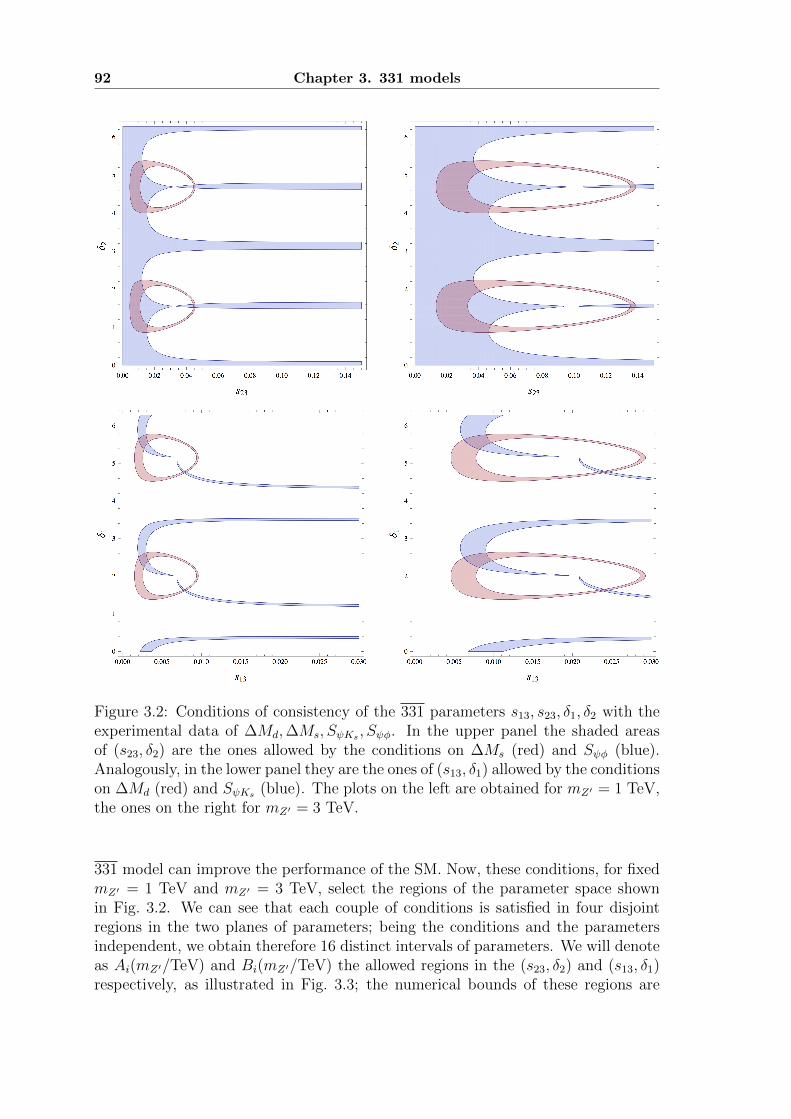
92 Chapter 3. 331 models
Figure 3.2: Conditions of consistency of the 331 parameters s13, s23, δ1, δ2 with theexperimental data of ∆Md,∆Ms, SψKs , Sψφ. In the upper panel the shaded areasof (s23, δ2) are the ones allowed by the conditions on ∆Ms (red) and Sψφ (blue).Analogously, in the lower panel they are the ones of (s13, δ1) allowed by the conditionson ∆Md (red) and SψKs (blue). The plots on the left are obtained for mZ′ = 1 TeV,the ones on the right for mZ′ = 3 TeV.
331 model can improve the performance of the SM. Now, these conditions, for fixedmZ′ = 1 TeV and mZ′ = 3 TeV, select the regions of the parameter space shownin Fig. 3.2. We can see that each couple of conditions is satisfied in four disjointregions in the two planes of parameters; being the conditions and the parametersindependent, we obtain therefore 16 distinct intervals of parameters. We will denoteas Ai(mZ′/TeV) and Bi(mZ′/TeV) the allowed regions in the (s23, δ2) and (s13, δ1)respectively, as illustrated in Fig. 3.3; the numerical bounds of these regions are
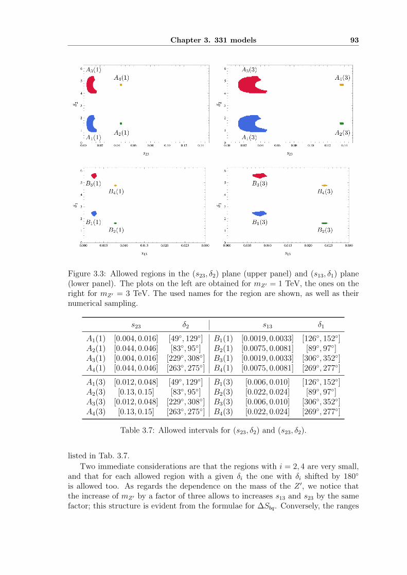
Chapter 3. 331 models 93
Figure 3.3: Allowed regions in the (s23, δ2) plane (upper panel) and (s13, δ1) plane(lower panel). The plots on the left are obtained for mZ′ = 1 TeV, the ones on theright for mZ′ = 3 TeV. The used names for the region are shown, as well as theirnumerical sampling.
s23 δ2 s13 δ1
A1(1) [0.004, 0.016] [49◦, 129◦] B1(1) [0.0019, 0.0033] [126◦, 152◦]A2(1) [0.044, 0.046] [83◦, 95◦] B2(1) [0.0075, 0.0081] [89◦, 97◦]A3(1) [0.004, 0.016] [229◦, 308◦] B3(1) [0.0019, 0.0033] [306◦, 352◦]A4(1) [0.044, 0.046] [263◦, 275◦] B4(1) [0.0075, 0.0081] [269◦, 277◦]
A1(3) [0.012, 0.048] [49◦, 129◦] B1(3) [0.006, 0.010] [126◦, 152◦]A2(3) [0.13, 0.15] [83◦, 95◦] B2(3) [0.022, 0.024] [89◦, 97◦]A3(3) [0.012, 0.048] [229◦, 308◦] B3(3) [0.006, 0.010] [306◦, 352◦]A4(3) [0.13, 0.15] [263◦, 275◦] B4(3) [0.022, 0.024] [269◦, 277◦]
Table 3.7: Allowed intervals for (s23, δ2) and (s23, δ2).
listed in Tab. 3.7.
Two immediate considerations are that the regions with i = 2, 4 are very small,and that for each allowed region with a given δi the one with δi shifted by 180◦
is allowed too. As regards the dependence on the mass of the Z ′, we notice thatthe increase of mZ′ by a factor of three allows to increases s13 and s23 by the samefactor; this structure is evident from the formulae for ∆Sbq. Conversely, the ranges
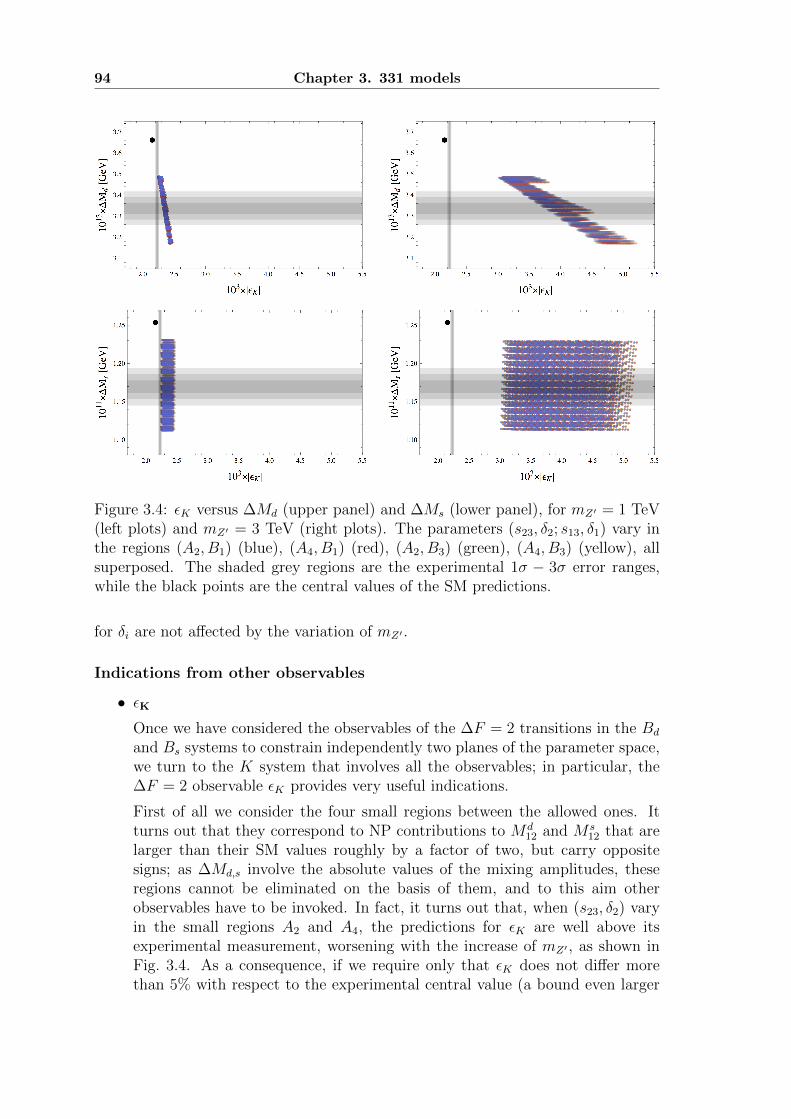
94 Chapter 3. 331 models
Figure 3.4: εK versus ∆Md (upper panel) and ∆Ms (lower panel), for mZ′ = 1 TeV(left plots) and mZ′ = 3 TeV (right plots). The parameters (s23, δ2; s13, δ1) vary inthe regions (A2, B1) (blue), (A4, B1) (red), (A2, B3) (green), (A4, B3) (yellow), allsuperposed. The shaded grey regions are the experimental 1σ − 3σ error ranges,while the black points are the central values of the SM predictions.
for δi are not affected by the variation of mZ′ .
Indications from other observables
• εKOnce we have considered the observables of the ∆F = 2 transitions in the Bd
and Bs systems to constrain independently two planes of the parameter space,we turn to the K system that involves all the observables; in particular, the∆F = 2 observable εK provides very useful indications.
First of all we consider the four small regions between the allowed ones. Itturns out that they correspond to NP contributions to Md
12 and M s12 that are
larger than their SM values roughly by a factor of two, but carry oppositesigns; as ∆Md,s involve the absolute values of the mixing amplitudes, theseregions cannot be eliminated on the basis of them, and to this aim otherobservables have to be invoked. In fact, it turns out that, when (s23, δ2) varyin the small regions A2 and A4, the predictions for εK are well above itsexperimental measurement, worsening with the increase of mZ′ , as shown inFig. 3.4. As a consequence, if we require only that εK does not differ morethan 5% with respect to the experimental central value (a bound even larger
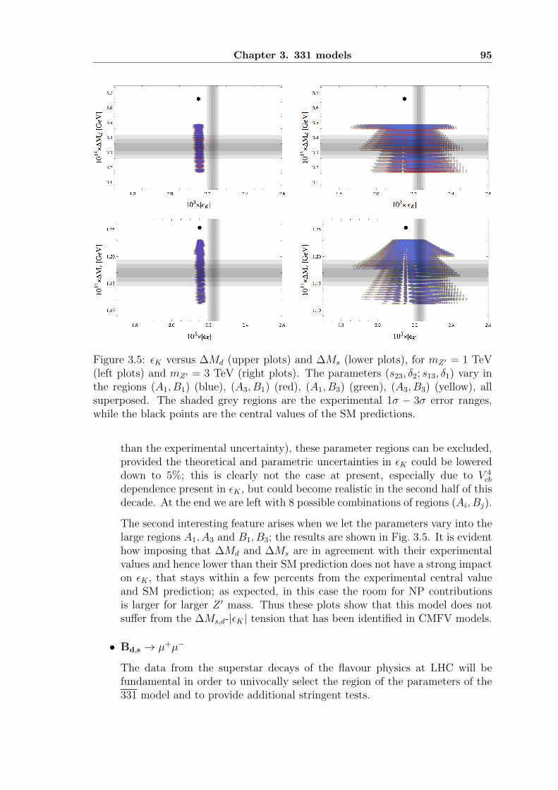
Chapter 3. 331 models 95
Figure 3.5: εK versus ∆Md (upper plots) and ∆Ms (lower plots), for mZ′ = 1 TeV(left plots) and mZ′ = 3 TeV (right plots). The parameters (s23, δ2; s13, δ1) vary inthe regions (A1, B1) (blue), (A3, B1) (red), (A1, B3) (green), (A3, B3) (yellow), allsuperposed. The shaded grey regions are the experimental 1σ − 3σ error ranges,while the black points are the central values of the SM predictions.
than the experimental uncertainty), these parameter regions can be excluded,provided the theoretical and parametric uncertainties in εK could be lowereddown to 5%; this is clearly not the case at present, especially due to V 4
cb
dependence present in εK , but could become realistic in the second half of thisdecade. At the end we are left with 8 possible combinations of regions (Ai, Bj).
The second interesting feature arises when we let the parameters vary into thelarge regions A1, A3 and B1, B3; the results are shown in Fig. 3.5. It is evidenthow imposing that ∆Md and ∆Ms are in agreement with their experimentalvalues and hence lower than their SM prediction does not have a strong impacton εK , that stays within a few percents from the experimental central valueand SM prediction; as expected, in this case the room for NP contributionsis larger for larger Z ′ mass. Thus these plots show that this model does notsuffer from the ∆Ms,d-|εK | tension that has been identified in CMFV models.
• Bd,s → µ+µ−
The data from the superstar decays of the flavour physics at LHC will befundamental in order to univocally select the region of the parameters of the331 model and to provide additional stringent tests.
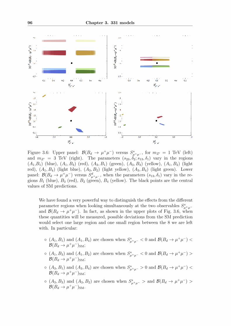
96 Chapter 3. 331 models
Figure 3.6: Upper panel: B(Bd → µ+µ−) versus Ssµ+µ− , for mZ′ = 1 TeV (left)and mZ′ = 3 TeV (right). The parameters (s23, δ2; s13, δ1) vary in the regions(A1,B1) (blue), (A1, B3) (red), (A3, B1) (green), (A3, B3) (yellow), (A1, B2) (lightred), (A1, B4) (light blue), (A3, B2) (light yellow), (A3, B4) (light green). Lowerpanel: B(Bd → µ+µ−) versus Sdµ+µ− , when the parameters (s13, δ1) vary in the re-gions B1 (blue), B3 (red), B2 (green), B4 (yellow). The black points are the centralvalues of SM predictions.
We have found a very powerful way to distinguish the effects from the differentparameter regions when looking simultaneously at the two observables Ssµ+µ−
and B(Bd → µ+µ−). In fact, as shown in the upper plots of Fig. 3.6, whenthese quantities will be measured, possible deviations from the SM predictionwould select one large region and one small region between the 8 we are leftwith. In particular:
◦ (A1, B1) and (A1, B4) are chosen when Ssµ+µ− < 0 and B(Bd → µ+µ−) <B(Bd → µ+µ−)SM;
◦ (A1, B3) and (A1, B2) are chosen when Ssµ+µ− < 0 and B(Bd → µ+µ−) >B(Bd → µ+µ−)SM;
◦ (A3, B1) and (A3, B4) are chosen when Ssµ+µ− > 0 and B(Bd → µ+µ−) <B(Bd → µ+µ−)SM;
◦ (A3, B3) and (A3, B2) are chosen when Ssµ+µ− > and B(Bd → µ+µ−) >B(Bd → µ+µ−)SM.
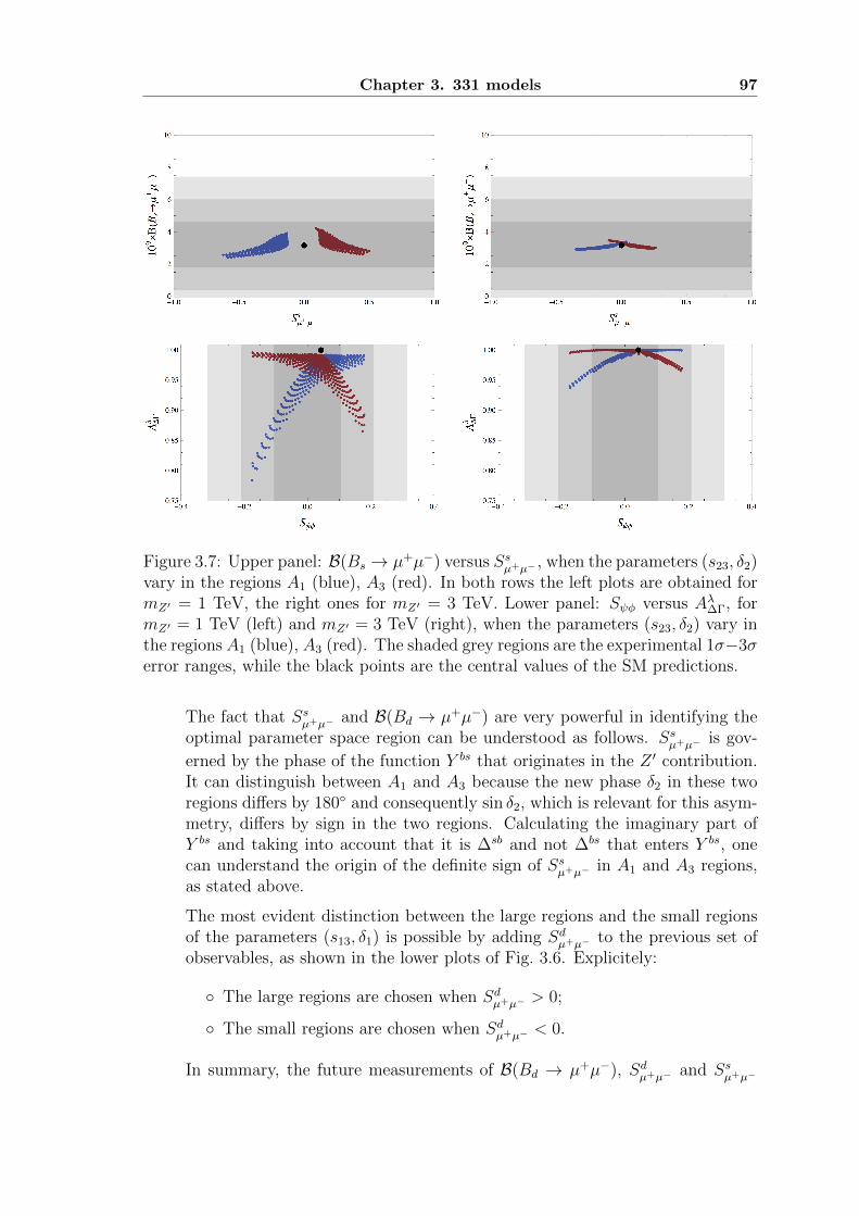
Chapter 3. 331 models 97
Figure 3.7: Upper panel: B(Bs → µ+µ−) versus Ssµ+µ− , when the parameters (s23, δ2)vary in the regions A1 (blue), A3 (red). In both rows the left plots are obtained formZ′ = 1 TeV, the right ones for mZ′ = 3 TeV. Lower panel: Sψφ versus Aλ∆Γ, formZ′ = 1 TeV (left) and mZ′ = 3 TeV (right), when the parameters (s23, δ2) vary inthe regions A1 (blue), A3 (red). The shaded grey regions are the experimental 1σ−3σerror ranges, while the black points are the central values of the SM predictions.
The fact that Ssµ+µ− and B(Bd → µ+µ−) are very powerful in identifying theoptimal parameter space region can be understood as follows. Ssµ+µ− is gov-
erned by the phase of the function Y bs that originates in the Z ′ contribution.It can distinguish between A1 and A3 because the new phase δ2 in these tworegions differs by 180◦ and consequently sin δ2, which is relevant for this asym-metry, differs by sign in the two regions. Calculating the imaginary part ofY bs and taking into account that it is ∆sb and not ∆bs that enters Y bs, onecan understand the origin of the definite sign of Ssµ+µ− in A1 and A3 regions,as stated above.
The most evident distinction between the large regions and the small regionsof the parameters (s13, δ1) is possible by adding Sdµ+µ− to the previous set ofobservables, as shown in the lower plots of Fig. 3.6. Explicitely:
◦ The large regions are chosen when Sdµ+µ− > 0;
◦ The small regions are chosen when Sdµ+µ− < 0.
In summary, the future measurements of B(Bd → µ+µ−), Sdµ+µ− and Ssµ+µ−
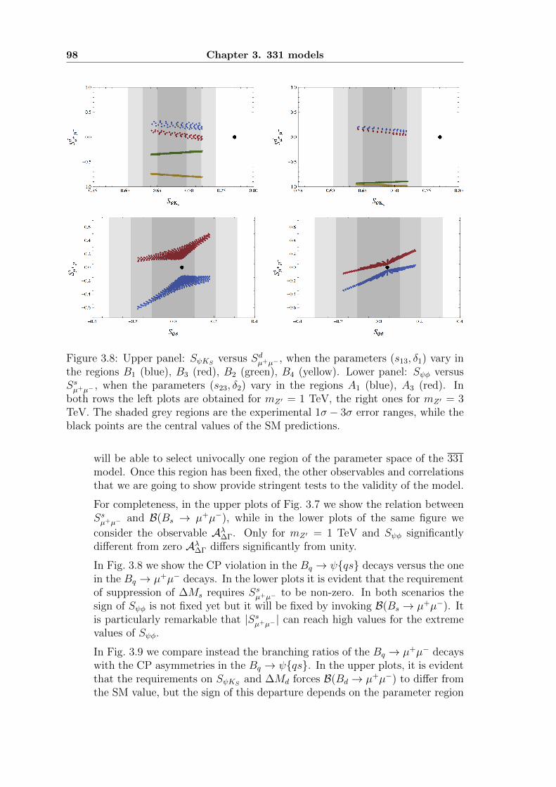
98 Chapter 3. 331 models
Figure 3.8: Upper panel: SψKS versus Sdµ+µ− , when the parameters (s13, δ1) vary inthe regions B1 (blue), B3 (red), B2 (green), B4 (yellow). Lower panel: Sψφ versusSsµ+µ− , when the parameters (s23, δ2) vary in the regions A1 (blue), A3 (red). Inboth rows the left plots are obtained for mZ′ = 1 TeV, the right ones for mZ′ = 3TeV. The shaded grey regions are the experimental 1σ − 3σ error ranges, while theblack points are the central values of the SM predictions.
will be able to select univocally one region of the parameter space of the 331model. Once this region has been fixed, the other observables and correlationsthat we are going to show provide stringent tests to the validity of the model.
For completeness, in the upper plots of Fig. 3.7 we show the relation betweenSsµ+µ− and B(Bs → µ+µ−), while in the lower plots of the same figure we
consider the observable Aλ∆Γ. Only for mZ′ = 1 TeV and Sψφ significantlydifferent from zero Aλ∆Γ differs significantly from unity.
In Fig. 3.8 we show the CP violation in the Bq → ψ{qs} decays versus the onein the Bq → µ+µ− decays. In the lower plots it is evident that the requirementof suppression of ∆Ms requires Ssµ+µ− to be non-zero. In both scenarios thesign of Sψφ is not fixed yet but it will be fixed by invoking B(Bs → µ+µ−). Itis particularly remarkable that |Ssµ+µ− | can reach high values for the extremevalues of Sψφ.
In Fig. 3.9 we compare instead the branching ratios of the Bq → µ+µ− decayswith the CP asymmetries in the Bq → ψ{qs}. In the upper plots, it is evidentthat the requirements on SψKS and ∆Md forces B(Bd → µ+µ−) to differ fromthe SM value, but the sign of this departure depends on the parameter region
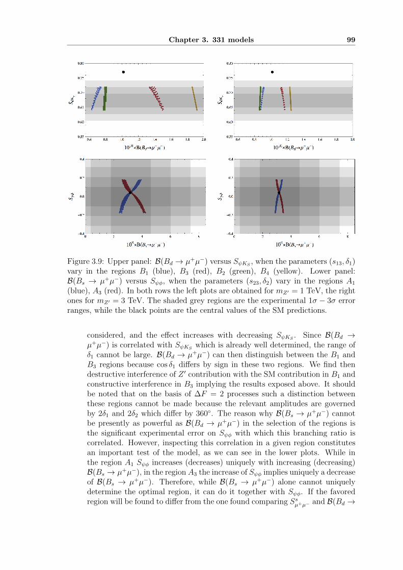
Chapter 3. 331 models 99
Figure 3.9: Upper panel: B(Bd → µ+µ−) versus SψKS , when the parameters (s13, δ1)vary in the regions B1 (blue), B3 (red), B2 (green), B4 (yellow). Lower panel:B(Bs → µ+µ−) versus Sψφ, when the parameters (s23, δ2) vary in the regions A1
(blue), A3 (red). In both rows the left plots are obtained for mZ′ = 1 TeV, the rightones for mZ′ = 3 TeV. The shaded grey regions are the experimental 1σ − 3σ errorranges, while the black points are the central values of the SM predictions.
considered, and the effect increases with decreasing SψKS . Since B(Bd →µ+µ−) is correlated with SψKS which is already well determined, the range ofδ1 cannot be large. B(Bd → µ+µ−) can then distinguish between the B1 andB3 regions because cos δ1 differs by sign in these two regions. We find thendestructive interference of Z ′ contribution with the SM contribution in B1 andconstructive interference in B3 implying the results exposed above. It shouldbe noted that on the basis of ∆F = 2 processes such a distinction betweenthese regions cannot be made because the relevant amplitudes are governedby 2δ1 and 2δ2 which differ by 360◦. The reason why B(Bs → µ+µ−) cannotbe presently as powerful as B(Bd → µ+µ−) in the selection of the regions isthe significant experimental error on Sψφ with which this branching ratio iscorrelated. However, inspecting this correlation in a given region constitutesan important test of the model, as we can see in the lower plots. While inthe region A1 Sψφ increases (decreases) uniquely with increasing (decreasing)B(Bs → µ+µ−), in the region A3 the increase of Sψφ implies uniquely a decreaseof B(Bs → µ+µ−). Therefore, while B(Bs → µ+µ−) alone cannot uniquelydetermine the optimal region, it can do it together with Sψφ. If the favoredregion will be found to differ from the one found comparing Ssµ+µ− and B(Bd →
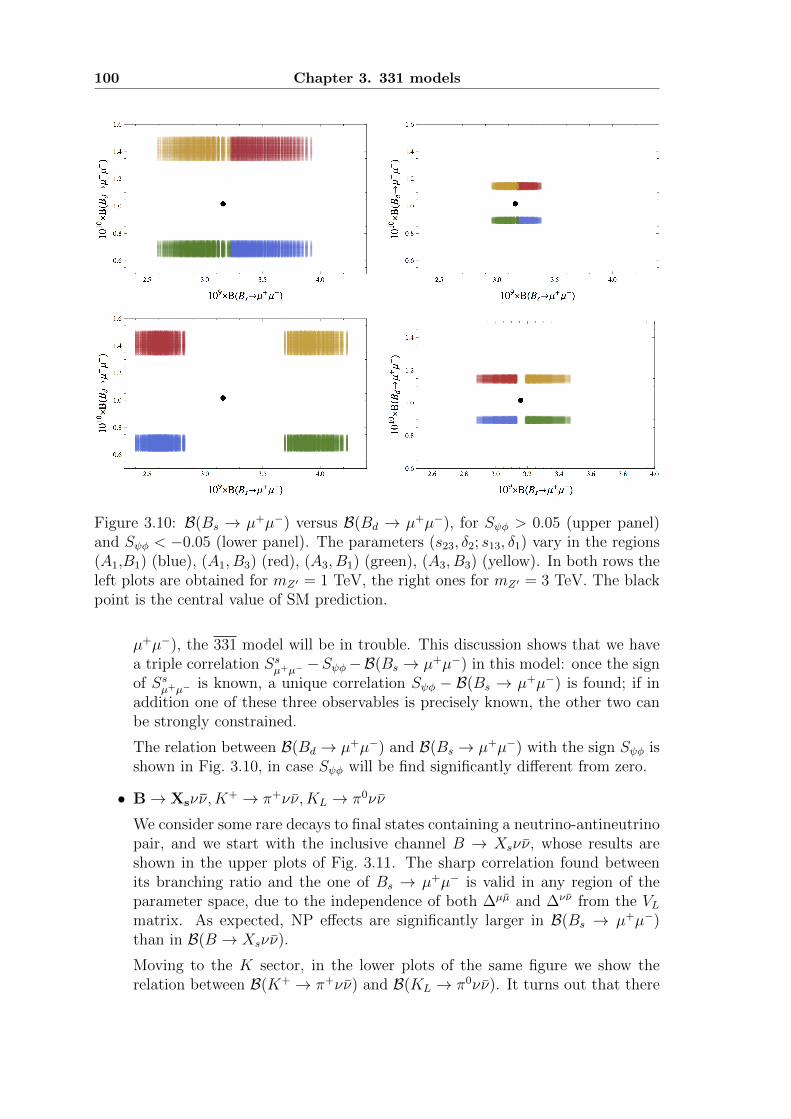
100 Chapter 3. 331 models
Figure 3.10: B(Bs → µ+µ−) versus B(Bd → µ+µ−), for Sψφ > 0.05 (upper panel)and Sψφ < −0.05 (lower panel). The parameters (s23, δ2; s13, δ1) vary in the regions(A1,B1) (blue), (A1, B3) (red), (A3, B1) (green), (A3, B3) (yellow). In both rows theleft plots are obtained for mZ′ = 1 TeV, the right ones for mZ′ = 3 TeV. The blackpoint is the central value of SM prediction.
µ+µ−), the 331 model will be in trouble. This discussion shows that we havea triple correlation Ssµ+µ− −Sψφ−B(Bs → µ+µ−) in this model: once the signof Ssµ+µ− is known, a unique correlation Sψφ − B(Bs → µ+µ−) is found; if inaddition one of these three observables is precisely known, the other two canbe strongly constrained.
The relation between B(Bd → µ+µ−) and B(Bs → µ+µ−) with the sign Sψφ isshown in Fig. 3.10, in case Sψφ will be find significantly different from zero.
• B→ Xsνν,K+ → π+νν,KL → π0νν
We consider some rare decays to final states containing a neutrino-antineutrinopair, and we start with the inclusive channel B → Xsνν, whose results areshown in the upper plots of Fig. 3.11. The sharp correlation found betweenits branching ratio and the one of Bs → µ+µ− is valid in any region of theparameter space, due to the independence of both ∆µµ and ∆νν from the VLmatrix. As expected, NP effects are significantly larger in B(Bs → µ+µ−)than in B(B → Xsνν).
Moving to the K sector, in the lower plots of the same figure we show therelation between B(K+ → π+νν) and B(KL → π0νν). It turns out that there
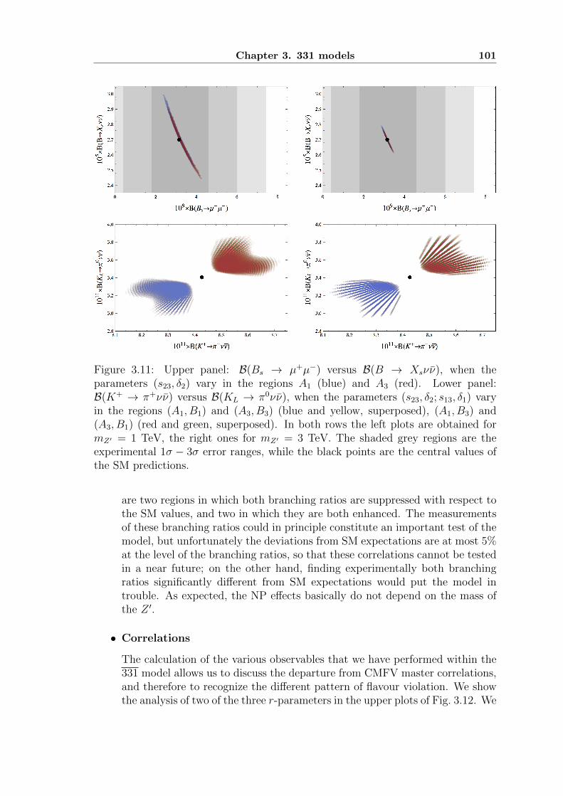
Chapter 3. 331 models 101
Figure 3.11: Upper panel: B(Bs → µ+µ−) versus B(B → Xsνν), when theparameters (s23, δ2) vary in the regions A1 (blue) and A3 (red). Lower panel:B(K+ → π+νν) versus B(KL → π0νν), when the parameters (s23, δ2; s13, δ1) varyin the regions (A1, B1) and (A3, B3) (blue and yellow, superposed), (A1, B3) and(A3, B1) (red and green, superposed). In both rows the left plots are obtained formZ′ = 1 TeV, the right ones for mZ′ = 3 TeV. The shaded grey regions are theexperimental 1σ − 3σ error ranges, while the black points are the central values ofthe SM predictions.
are two regions in which both branching ratios are suppressed with respect tothe SM values, and two in which they are both enhanced. The measurementsof these branching ratios could in principle constitute an important test of themodel, but unfortunately the deviations from SM expectations are at most 5%at the level of the branching ratios, so that these correlations cannot be testedin a near future; on the other hand, finding experimentally both branchingratios significantly different from SM expectations would put the model introuble. As expected, the NP effects basically do not depend on the mass ofthe Z ′.
• Correlations
The calculation of the various observables that we have performed within the331 model allows us to discuss the departure from CMFV master correlations,and therefore to recognize the different pattern of flavour violation. We showthe analysis of two of the three r-parameters in the upper plots of Fig. 3.12. We
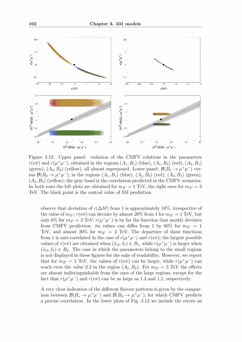
102 Chapter 3. 331 models
Figure 3.12: Upper panel: violation of the CMFV relations in the parametersr(νν) and r(µ+µ−), obtained in the regions (A1, B1) (blue), (A1, B3) (red), (A3, B1)(green), (A3, B3) (yellow), all almost superposed. Lower panel: B(Bs → µ+µ−) ver-sus B(Bd → µ+µ−), in the regions (A1, B1) (blue), (A1, B3) (red), (A3, B1) (green),(A3, B3) (yellow); the gray band is the correlation predicted in the CMFV scenarios.In both rows the left plots are obtained for mZ′ = 1 TeV, the right ones for mZ′ = 3TeV. The black point is the central value of SM prediction.
observe that deviation of r(∆M) from 1 is approximately 10%, irrespective ofthe value of mZ′ ; r(νν) can deviate by almost 20% from 1 for mZ′ = 1 TeV, butonly 6% for mZ′ = 3 TeV; r(µ+µ−) is by far the function that mostly deviatesfrom CMFV prediction: its values can differ from 1 by 60% for mZ′ = 1TeV, and almost 20% for mZ′ = 3 TeV. The departure of these functionsfrom 1 is anti-correlated in the case of r(µ+µ−) and r(νν); the largest possiblevalues of r(νν) are obtained when (s13, δ1) ∈ B1, while r(µ+µ−) is larger when(s13, δ1) ∈ B3. The case in which the parameters belong to the small regionsis not displayed in these figures for the sake of readability. However, we reportthat for mZ′ = 1 TeV, the values of r(νν) can be larger, while r(µ+µ−) canreach even the value 2.2 in the region (A1, B2). For mZ′ = 3 TeV the effectsare almost indistinguishable from the ones of the large regions, except for thefact that r(µ+µ−) and r(νν) can be as large as 1.3 and 1.1, respectively.
A very clear indication of the different flavour patterns is given by the compar-ison between B(Bs → µ+µ−) and B(Bd → µ+µ−), for which CMFV predictsa precise correlation. In the lower plots of Fig. 3.12 we include the errors on
Chapter 3. 331 models 103
the experimental determinations of ∆Ms, ∆Md, τ(Bs), τ(Bd), and as regardsthe non-perturbative inputs we used the central value of the last lattice de-terminations but we reduced the size of the uncertainty. An improvement inthis direction would indeed substantially help understanding if and how muchCMFV relations are violated in the 331 model.
The correlations of the 331 model allow also to distinguish it from generalMFV scenarios. Taking as a reference example the 2HDMMFV, in both casesthe NP contributions to εK are small, favoring the inclusive value of |Vub|.However, while in the 2HDMMFV the data on SψKS imply then automaticallya positive value of Sψφ ≥ 0.15 [79], in the 331 model this is not required,and any value within the LHCb range is still possible. Concerning ∆F = 1transitions, in the 2HDMMFV there is a tendency for which with increasingSψφ also the lower bound on B(Bs → µ+µ−) increases; in the 331 model thecorrelation between Sψφ and B(Bs → µ+µ−) is much more transparent. Inboth models B(Bs → µ+µ−) can be smaller or larger than the SM value, butin 2HDMMFV the deviations can be larger, a characteristic property of scalarcurrents.
More inspections
• Until now we have considered the case in which the Z ′ is detectable by theLHC, but the only indirect effects of a heavier mass are of course worth ofinvestigation as well.
As we can see from the trend in Fig. 3.2, increasing the mass of the Z ′ impliesthat the allowed regions of the space parameter are shifted in order to satisfythe constraints of the ∆F = 2 Bd,s-observables; in particular, s13 and s23 haveto be increased proportionally. Since ∆sd depends on the product s13s23, theeffects on εK increase with mZ′ , as evident from Fig 3.5; on the contrary, since∆µµ and ∆νν do not depend on these parameters, the NP contributions to theconsidered rare decays are suppressed by the mass of the FCNC-mediating Z ′
boson.
The consideration that a heavy Z ′ can significantly modify εK respecting theexperimental bounds on the B-observables suggests that the experimentalvalue of εK could be even obtained in the context of the Scenario 1, i.e. usingthe exclusive determination of |Vub|. In fact, using the representative value ofmZ′ = 10 TeV, and imposing the additional constraints∣∣∣∣ ∆MK
(∆MK)exp
∣∣∣∣ < 25% , 2.0 · 10−3 ≤ |εK | ≤ 2.5 · 10−3 , (3.120)
which are necessary because of the strong effects on the K sector, we find thatthe Scenario 1 with |Vub| = 3.1 · 10−3 is allowed for approximately
0.05 ≤ s23 ≤ 0.12 , 0.016 ≤ s13 ≤ 0.030 , (3.121)
to be compared with the ranges in Tab. 3.7.
104 Chapter 3. 331 models
When ∆sd reaches its maximal value, further increase of mZ′ will also decreaseNP contributions to εK , so that for very large masses of the Z ′ SM-like resultsare obtained as required by decoupling of NP; however, this happens only formZ′ ≥ 3000 TeV. This result is just a confirmation of the known fact that ifthe FCNC Z ′ couplings to quarks are O(1), εK puts very strong constraintson the scale of NP.
• In our analysis we have used the most recent lattice inputs, for which the SMvalues for ∆Ms and ∆Md are significantly above the data, when the hadronicand CKM uncertainties are reduced down to ±5%. However, some of thecorrelations that we have found would change if ∆Ms and ∆Md were bothfound below the data instead. For example, if the values of BBq were reducedby 20%, the values of the allowed δi would change significantly, going closeto 0◦ or 180◦. This changes radically the quantitative and sometimes thequalitative results of the 331 analysis; for example, in the Bd meson system,the general structure of correlations is unchanged, but this time the NP effectsin Bd → µ+µ− are found to be much larger than in Sdµ+µ− ; the impact on theBs system is much larger; now the roles of Bs → µ+µ− and Ssµ+µ− in the searchfor the optimal space parameter region are interchanged, and B(Bs → µ+µ−)is bound to be different from the SM values [301]. These considerations showclearly the importance of precise determinations of flavour observables withinthe SM in order to be able to search indirectly for NP.
Conclusions and outlook
The LHC has just concluded its first run, and despite all the strong efforts andthe accurate analyses, it has not given us any direct hint of NP. Therefore, thecomplementary research of indirect signatures in precision physics represents theonly viable route at least waiting for higher energies. In particular, the flavoursector represents an especially interesting field of investigation, both because itsorigin is an open question of the SM, and because the accuracy of the available datatogether with the improvements of the SM predictions provide a powerful startingpoint.
In this thesis we have considered two NP models, particularly interesting becausethey provide some answers about the nature of flavour using as only assumption anextended gauge symmetry. We have found that the phenomenological analysis ofthese models, as well as of several other NP models, returns very interesting signa-tures, like deviations and correlations, that unfortunately are washed out becauseof the relatively large uncertainties of some non-perturbative parameters and someexperimental values. We have chosen therefore to adopt an approach that is in somesense a bit futuristic: we have tried to understand how these NP model will face thefuture more precise data. We have done this by considering independent limitingscenarios with small errors that together cover the majority of the ranges allowedby the present uncertainties.
The GFS model [25] provides an elegant description of flavour as a spontaneouslybroken gauge symmetry; moreover, it is particularly elegant the fact that the mini-mal non-anomalous fermion content generates a mechanism of inverted hierarchy ofthe Yukawa couplings that automatically suppresses FCNCs in an effective way.
In this work we have first of all retraced the complete building of the model inthe quark sector, from the gauge group to the Feynman rules; the main concretefeatures of the model are the presence of six new quarks associated to the SMones, the presence of 24 new neutral flavour gauge bosons that mediate tree-levelFCNCs and introduce new CP-violating phases, the facts that the CKM matrix isnot unitary and that the couplings of the SM quarks with the Z boson and withthe Higgs boson are modified. As regards in particular the ∆F = 2 and ∆F = 1transitions between down-type quarks, we have calculated all the new contributions,both the ones due to the tree-level exchange of the flavour bosons and the ones dueto the exchange of the new heavy quarks into the box diagrams.
In order to put the basis of a phenomenological analysis, we have first exploredthe parameter space, consisting in nine new parameters, looking for constraints com-
105
106 Conclusions and outlook
ing from consistency, reasonableness and from the strictest experimental bounds, likethe lower limits to the b′ and t′ quark masses and the restrictions from electroweakprecision physics. Then we have moved to a more detailed and systematic scan ofthe allowed regions of the parameter space, finding the following results [142].
• In the most favorite regions of the parameter space, the masses of exotic quarksb′ and t′ as well as of the lightest flavour boson (which for all practical purposesit corresponds to a flavour non-universal leptophobic Z ′), can be within thereach of LHC. On the other hand, even in the absence of direct detections,there are anyway good regions of parameters in which these exotic particlesare much heavier.
• |εK | is enhanced by the new box-diagram contributions and suppressed by thetree exchange of flavour bosons; on the other hand, SψKS can only be slightlysuppressed by the left-left tree-level contributions. As a consequence, choosingthe exclusive determination of |Vub|, the GFS model can be able to remove theεK − SψKS tension present in the SM.
• The box diagrams that enhance |εK | enhance also both ∆Md and ∆Ms, whichare almost unaffected by the tree-level contributions. This implies that, wherethe εK − SψKS tension is solved, the weak SM equilibrium between εK and∆Md,s is automatically worsened.
• Concerning other relevant observables: (i) the branching ratio of B → Xsγis generally enhanced, but only very small modifications are allowed by the∆F = 2 bounds; (ii) also the dimuon asymmetry Absl, which could receivelarge contributions from the tree-level flavour boson diagrams, remains closeto the SM prediction if |εK | is required to be in agreement with data; (iii) thebranching ratio of B+ → τ+ν is modified through the modified CKM matrix,and hence provides important constraints in the parameter space.
• This model does not satisfy MFV, and its signatures can prove this. In fact,even if, by choosing the exclusive |Vub| and by allowing an enhancement of|εK |, it resembles the CMFV behavior, as well as for the worsening of theεK −∆Md,s tension, ∆F = 1 processes can provide a distinction: for example,B(B → Xsγ) can be suppressed in CMFV models. On the other hand, takingas an example of MFV at large the 2HDMMFV, the GFS model can be easilydistinguished from it: in the latter only tiny contributions to |εK | are allowedand hence the inclusive value of |Vub| is required.
In summary, besides its appealing theoretical form, a great virtue of the GFSmodel is that it presents a relatively small number of free parameters, the structure ofwhich makes it well predictive. A first decisive test for it will be a more unambiguousdetermination of |Vub|: if this will be found to be closer to its present inclusive value,the GFS model will be definitely in difficulty. On the other hand, even with theexclusive value of |Vub| the model is not able to correctly describe all the flavour
Conclusions and outlook 107
data at the same time; in this case, because of its sensitivity to the non-perturbativeparameters, improved calculations of them will play a key role.
The group SU(3)c×SU(3)L×U(1)X is the simplest non-abelian extension of theSM gauge group; some realizations of these so-called 331 models [39,40] provide anexplanation about why there are just three generations of fermions.
In this work we have presented a complete theoretical treatment of 331 modelsin their most general form; in particular, we have performed a detailed analysisof anomaly cancellation in order to obtain a list of the possible realizations, givenby specific combinations of electric charges with fermion content. Subsequently, wehave chosen a particular realization, which we have indicated as 331, characterized byinteresting phenomenological features, and we have studied its gauge and symmetry-breaking structure in detail up to the derivation of the Feynman rules. In the 331model there are three exotic quarks, two of down-type and one of up-type, generallyvery heavy; there are moreover three new gauge bosons, and between them a Z ′,which can have mass at the electroweak scale, mediates FCNCs; finally, the CKMmatrix is flanked by a new unitary mixing matrix. The impact on ∆F = 2 and∆F = 1 transitions is due only to the contribution of the Z ′ tree-level exchange,and since there are no new local operators it can be implemented by modificationsof the master loop functions.
In the phenomenological analysis five free parameters are relevant: the mass ofthe Z ′ and four angles of the new mixing matrix. We have chosen two representativeand significant values for mZ′ , namely 1 TeV and 3 TeV, and we have proceeded asfollows [301].
• As a preliminary consideration, we have shown that only small contributionsto |εK | are possible, and hence the inclusive determination of |Vub| is preferred.
• Requiring the predictions of the model to be in agreement with the experimen-tal bounds of the two pairs of observables (∆Md, SψKS) and (∆Ms, Sψφ) of theBd,s mixing, there are 4× 4 limited regions in the parameter space of the mix-ing matrix that are allowed. Requiring also |εK | to be in agreement with datareduces the allowed regions to 8. This means that in these regions the experi-mental values of |εK |, SψKS and ∆Md,s are all simultaneously accommodated,differently from the SM.
• Precise data from the decays Bd,s → µ+µ− will be able to provide more defini-tive statements about the model. In fact, we have shown that the three ob-servables B(Bd → µ+µ−), Ssµµ and Sdµµ provide 23 = 8 combinations of possibledeviations from the SM predictions that would be able to univocally select onebetween the remaining allowed regions.
• Other characteristics of the model are a well defined correlation between Bs →µ+µ− and Sψφ, an anti-correlation between Bs → µ+µ− and B(B → Xsνν),small contributions to the transitions B → Xsνν, K+ → π+νν, KL → π0νν.
108 Conclusions and outlook
• 331 models are not included in the MFV framework. In particular, the typ-ical correlations of CMFV are clearly violated in the 331, especially the onebetween the Bd,s → µ+µ− decays. On the other hand, in contrast to the2HDMMFV, it does not present a correlation between SψKS and Sψφ.
In summary, the 331 model presents a very interesting phenomenology that, de-spite the small number of free parameters, could be able to solve the main tensionsbetween the flavuor prediction of the SM and the experimental data. The exper-imental deep investigation of different observables in Bd,s → µ+µ−, which will bemost likely performed in the next future, will be able to provide some conclusive in-formation about this model at least at the TeV scale, which should be also exploredsearching for the possible Z ′ boson.
We are aware that we are living during the most exciting years for particle physicssince decades. We have found the Higgs boson and the LHC is warming up to hit thesmallest distances ever explored. In spite of this, at least in the last years the searchof NP has been quite frustrating, because it has consisted only in feeble hints thathave been timely retracted. Nevertheless we believe that NP is around the corner,and with the work of this thesis we have shown how the flavour physics communityis preparing itself to face all the surprises that the future experiments are savingfor us.
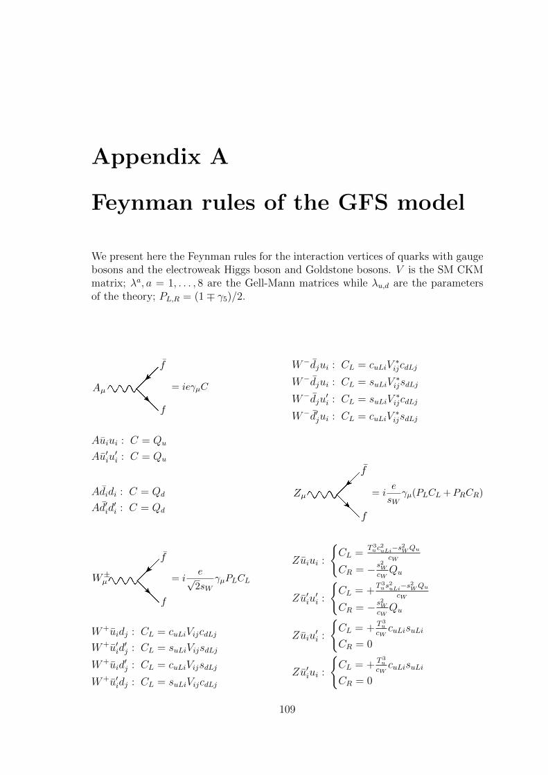
Appendix A
Feynman rules of the GFS model
We present here the Feynman rules for the interaction vertices of quarks with gaugebosons and the electroweak Higgs boson and Goldstone bosons. V is the SM CKMmatrix; λa, a = 1, . . . , 8 are the Gell-Mann matrices while λu,d are the parametersof the theory; PL,R = (1∓ γ5)/2.
Aµ
f
f
= ieγµC
Auiui : C = Qu
Au′iu′i : C = Qu
Adidi : C = Qd
Ad′id′i : C = Qd
f
f
W±µ = i
e√2sW
γµPLCL
W+uidj : CL = cuLiVijcdLj
W+u′id′j : CL = suLiVijsdLj
W+uid′j : CL = cuLiVijsdLj
W+u′idj : CL = suLiVijcdLj
W−djui : CL = cuLiV∗ijcdLj
W−djui : CL = suLiV∗ijsdLj
W−dju′i : CL = suLiV
∗ijcdLj
W−d′jui : CL = cuLiV∗ijsdLj
f
f
Zµ = ie
sWγµ(PLCL + PRCR)
Zuiui :
{CL =
T 3uc
2uLi−s
2WQu
cW
CR = − s2WcWQu
Zu′iu′i :
{CL = +
T 3us
2uLi−s
2WQu
cW
CR = − s2WcWQu
Zuiu′i :
{CL = + T 3
u
cWcuLisuLi
CR = 0
Zu′iui :
{CL = + T 3
u
cWcuLisuLi
CR = 0
109
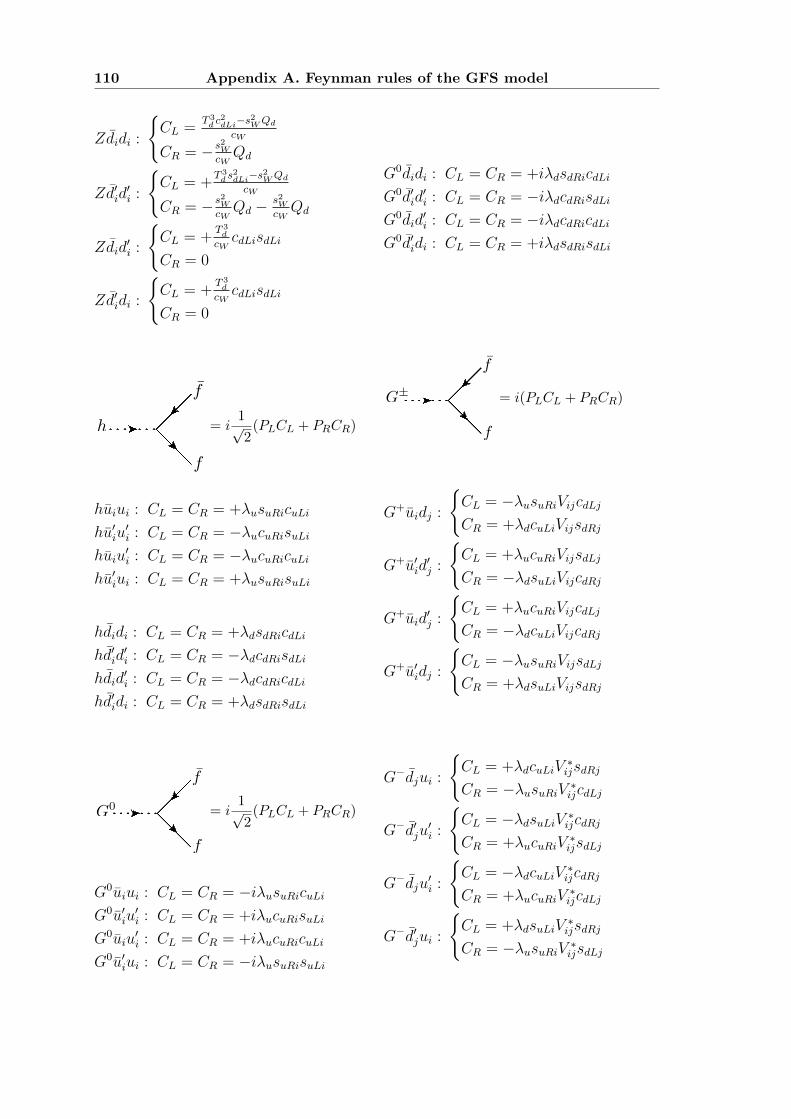
110 Appendix A. Feynman rules of the GFS model
Zdidi :
{CL =
T 3d c
2dLi−s
2WQd
cW
CR = − s2WcWQd
Zd′id′i :
{CL = +
T 3d s
2dLi−s
2WQd
cW
CR = − s2WcWQd −
s2WcWQd
Zdid′i :
{CL = +
T 3d
cWcdLisdLi
CR = 0
Zd′idi :
{CL = +
T 3d
cWcdLisdLi
CR = 0
f
f
h = i1√2
(PLCL + PRCR)
huiui : CL = CR = +λusuRicuLi
hu′iu′i : CL = CR = −λucuRisuLi
huiu′i : CL = CR = −λucuRicuLi
hu′iui : CL = CR = +λusuRisuLi
hdidi : CL = CR = +λdsdRicdLi
hd′id′i : CL = CR = −λdcdRisdLi
hdid′i : CL = CR = −λdcdRicdLi
hd′idi : CL = CR = +λdsdRisdLi
f
f
G0 = i1√2
(PLCL + PRCR)
G0uiui : CL = CR = −iλusuRicuLiG0u′iu
′i : CL = CR = +iλucuRisuLi
G0uiu′i : CL = CR = +iλucuRicuLi
G0u′iui : CL = CR = −iλusuRisuLi
G0didi : CL = CR = +iλdsdRicdLi
G0d′id′i : CL = CR = −iλdcdRisdLi
G0did′i : CL = CR = −iλdcdRicdLi
G0d′idi : CL = CR = +iλdsdRisdLi
f
f
G± = i(PLCL + PRCR)
G+uidj :
{CL = −λusuRiVijcdLjCR = +λdcuLiVijsdRj
G+u′id′j :
{CL = +λucuRiVijsdLj
CR = −λdsuLiVijcdRj
G+uid′j :
{CL = +λucuRiVijcdLj
CR = −λdcuLiVijcdRj
G+u′idj :
{CL = −λusuRiVijsdLjCR = +λdsuLiVijsdRj
G−djui :
{CL = +λdcuLiV
∗ijsdRj
CR = −λusuRiV ∗ijcdLj
G−d′ju′i :
{CL = −λdsuLiV ∗ijcdRjCR = +λucuRiV
∗ijsdLj
G−dju′i :
{CL = −λdcuLiV ∗ijcdRjCR = +λucuRiV
∗ijcdLj
G−d′jui :
{CL = +λdsuLiV
∗ijsdRj
CR = −λusuRiV ∗ijsdLj

Appendix A. Feynman rules of the GFS model 111
f
f
(AQ)aµ = i
gQ√2γµ(PLCL + PRCR)
AaQuiuj :
{CL = +cuLi(V λ
aV †)ijcuLj
CR = +suRi(V λaV †)ijsuRj
AaQu′iu′j :
{CL = +suLi(V λ
aV †)ijsuLj
CR = +cuRi(V λaV †)ijcuRj
AaQuiu′j :
{CL = +cuLi(V λ
aV †)ijsuLj
CR = −suRi(V λaV †)ijcuRj
AaQu′iuj :
{CL = +suLi(V λ
aV †)ijcuLj
CR = −cuRi(V λaV †)ijsuRj
AaQdidj :
{CL = +cdLi(λ
a)ijcdLj
CR = +sdRi(λa)ijsdRj
AaQd′id′j :
{CL = +sdLi(λ
a)ijsdLj
CR = +cdRi(λa)ijcdRj
AaQdid′j :
{CL = +cdLi(λ
a)ijsdLj
CR = −sdRi(λa)ijcdRj
AaQd′idj :
{CL = +sdLi(λ
a)ijcdLj
CR = −cdRi(λa)ijsdRj
f
f
(AU )aµ = i
gU√2γµ(PLCL + PRCR)
AaU uiuj :
{CL = +suLi(λ
a)ijsuLj
CR = +cuRi(λa)ijcuRj
AaU u′iu′j :
{CL = +cuLi(λ
a)ijcuLj
CR = +suRi(λa)ijsuRj
AaU uiu′j :
{CL = −suLi(λa)ijcuLjCR = +cuRi(λ
a)ijsuRj
AaU u′iuj :
{CL = −cuLi(λa)ijsuLjCR = +suRi(λ
a)ijcuRj
f
f
(AD)aµ = i
gD√2γµ(PLCL + PRCR)
AaDdidj :
{CL = +sdLi(λ
a)ijsdLj
CR = +cdRi(λa)ijcdRj
AaDd′id′j :
{CL = +cdLi(λ
a)ijcdLj
CR = +sdRi(λa)ijsdRj
AaDdid′j :
{CL = −sdLi(λa)ijcdLjCR = +cdRi(λ
a)ijsdRj
AaDd′idj :
{CL = +sdRi(λ
a)ijcdRj
CR = −cdLi(λa)ijsdLj

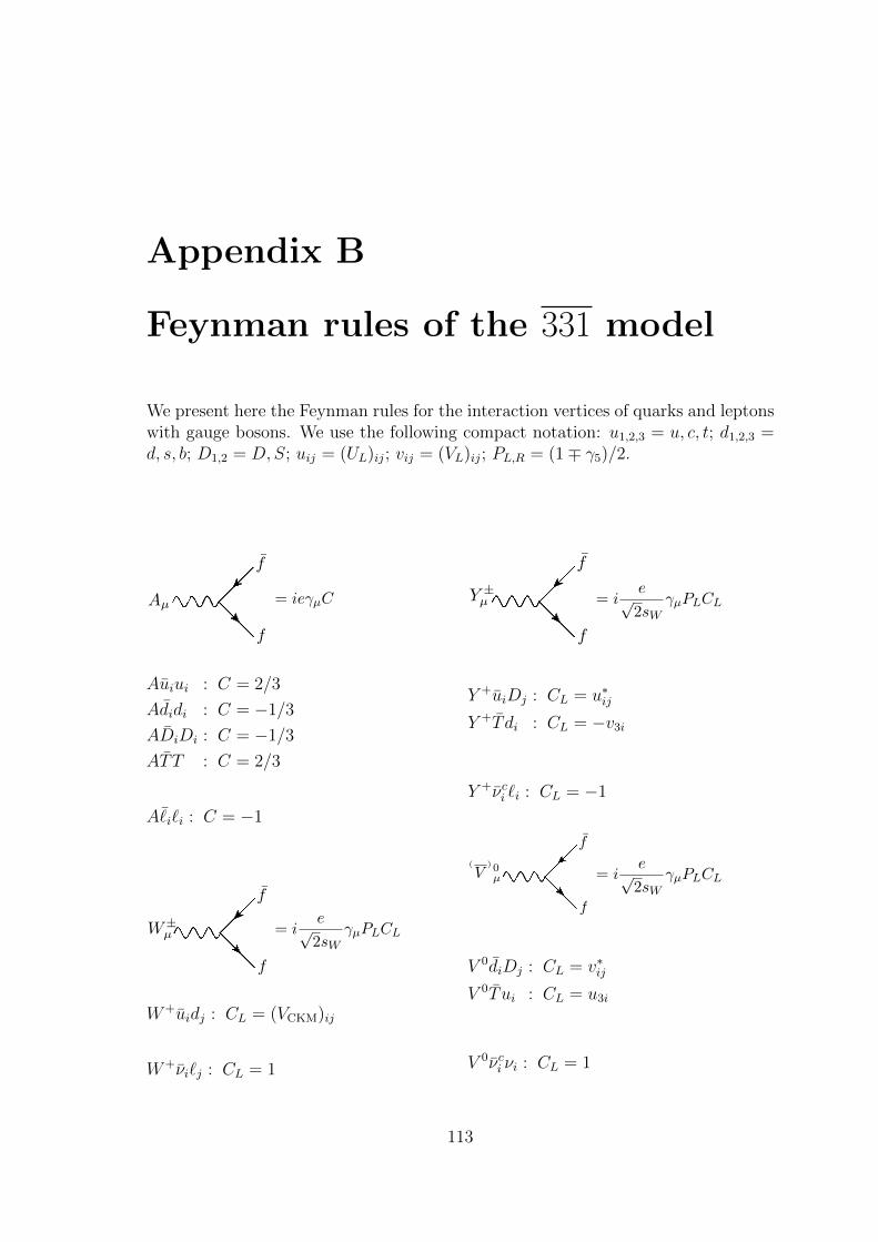
Appendix B
Feynman rules of the 331 model
We present here the Feynman rules for the interaction vertices of quarks and leptonswith gauge bosons. We use the following compact notation: u1,2,3 = u, c, t; d1,2,3 =d, s, b; D1,2 = D,S; uij = (UL)ij; vij = (VL)ij; PL,R = (1∓ γ5)/2.
Aµ
f
f
= ieγµC
Auiui : C = 2/3
Adidi : C = −1/3
ADiDi : C = −1/3
ATT : C = 2/3
A¯i`i : C = −1
f
f
W±µ = i
e√2sW
γµPLCL
W+uidj : CL = (VCKM)ij
W+νi`j : CL = 1
f
f
Y ±µ = i
e√2sW
γµPLCL
Y +uiDj : CL = u∗ij
Y +T di : CL = −v3i
Y +νci `i : CL = −1
f
f
(
V)0µ = i
e√2sW
γµPLCL
V 0diDj : CL = v∗ij
V 0T ui : CL = u3i
V 0νci νi : CL = 1
113
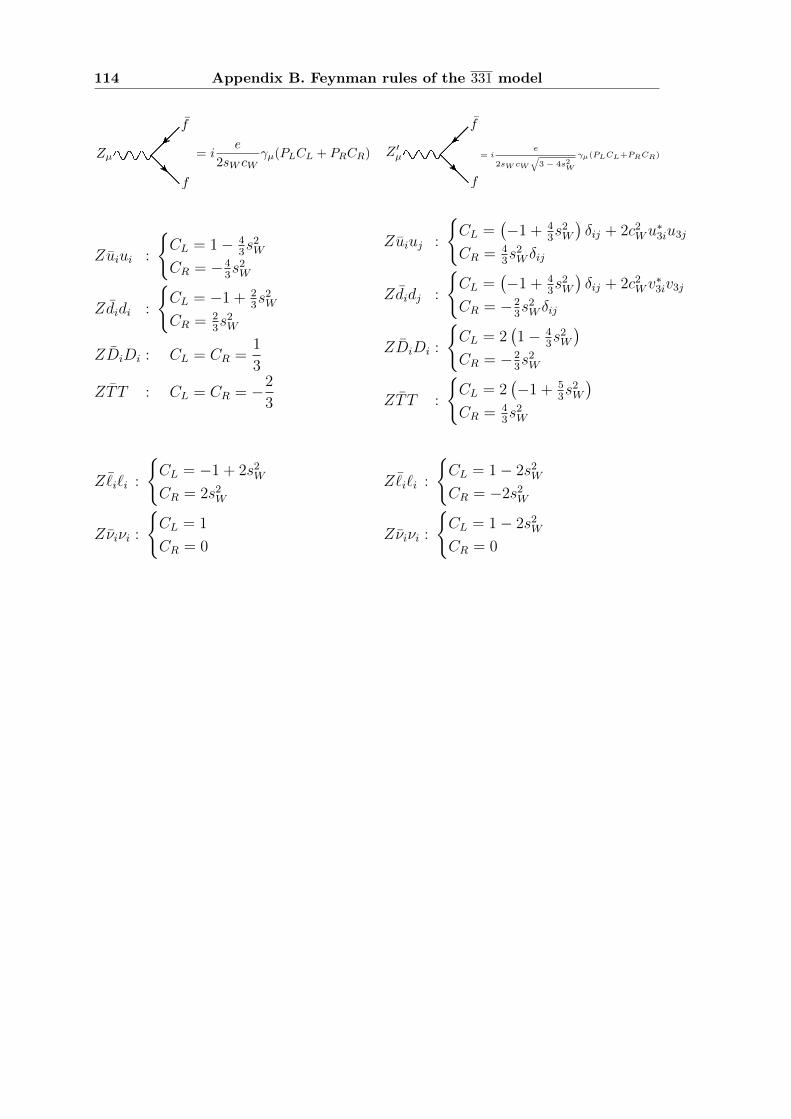
114 Appendix B. Feynman rules of the 331 model
f
f
Zµ = ie
2sW cWγµ(PLCL + PRCR)
Zuiui :
{CL = 1− 4
3s2W
CR = −43s2W
Zdidi :
{CL = −1 + 2
3s2W
CR = 23s2W
ZDiDi : CL = CR =1
3
ZTT : CL = CR = −2
3
Z ¯i`i :
{CL = −1 + 2s2
W
CR = 2s2W
Zνiνi :
{CL = 1
CR = 0
f
f
Z 0µ = i
e
2sW cW
√3− 4s2
W
γµ(PLCL+PRCR)
Zuiuj :
{CL =
(−1 + 4
3s2W
)δij + 2c2
Wu∗3iu3j
CR = 43s2W δij
Zdidj :
{CL =
(−1 + 4
3s2W
)δij + 2c2
Wv∗3iv3j
CR = −23s2W δij
ZDiDi :
{CL = 2
(1− 4
3s2W
)CR = −2
3s2W
ZTT :
{CL = 2
(−1 + 5
3s2W
)CR = 4
3s2W
Z ¯i`i :
{CL = 1− 2s2
W
CR = −2s2W
Zνiνi :
{CL = 1− 2s2
W
CR = 0
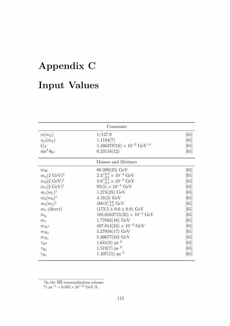
Appendix C
Input Values
Constants
α(mZ) 1/127.9 [65]αs(mZ) 1.1184(7) [65]GF 1.1663787(6)× 10−5 GeV−2 [65]sin2 θW 0.23116(12) [65]
Masses and lifetimes
mW 80.399(23) GeV [65]mu(2 GeV)1 2.3+0.7
−0.5 × 10⁻³ GeV [65]md(2 GeV)1 4.8+0.7
−0.3 × 10⁻³ GeV [65]ms(2 GeV)1 95(5)× 10−3 GeV [65]mc(mc)
1 1.275(25) GeV [65]mb(mb)
1 4.18(3) GeV [65]mt(mt)
1 160.0+4.8−4.3 GeV [65]
mt (direct) (173.5± 0.6± 0.8) GeV [65]mµ 105.6583715(35)× 10−3 GeV [65]mτ 1.77682(16) GeV [65]mK0 497.614(24)× 10−3 GeV [65]mBd 5.27958(17) GeV [65]mBs 5.36677(24) GeV [65]τB± 1.641(8) ps 2 [65]τBd 1.519(7) ps 2 [65]τBs 1.497(15) ps 2 [65]
1In the MS renormalization scheme.21 ps−1 = 6.582× 10⁻¹³ GeV/~.
115
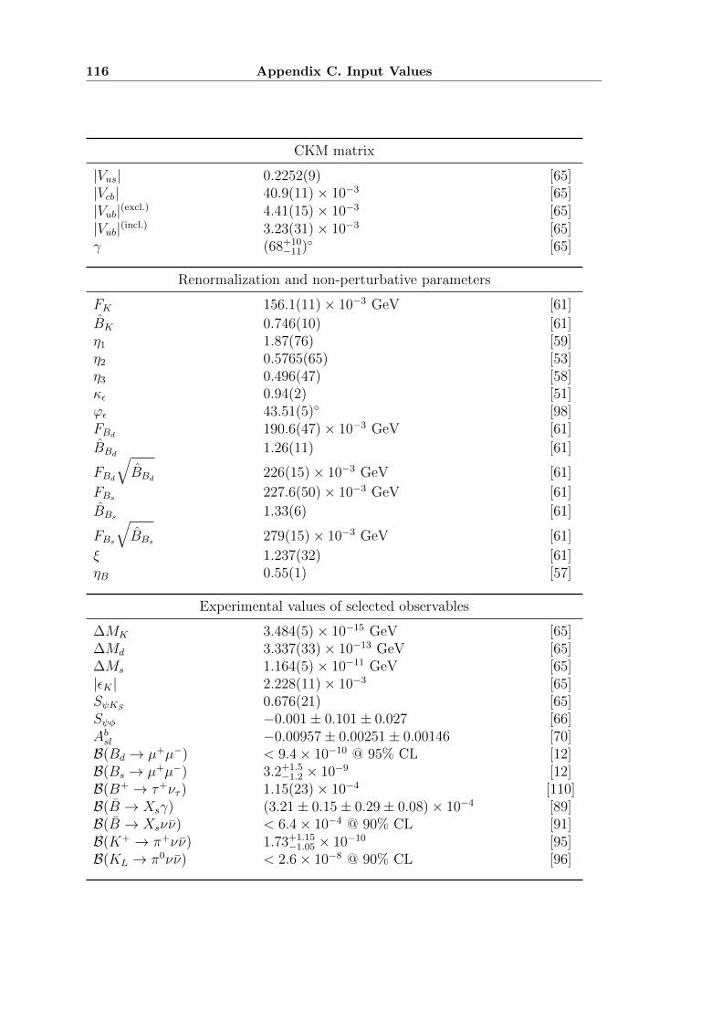
116 Appendix C. Input Values
CKM matrix
|Vus| 0.2252(9) [65]|Vcb| 40.9(11)× 10−3 [65]|Vub|(excl.) 4.41(15)× 10−3 [65]|Vub|(incl.) 3.23(31)× 10−3 [65]γ (68+10
−11)◦ [65]
Renormalization and non-perturbative parameters
FK 156.1(11)× 10−3 GeV [61]
BK 0.746(10) [61]η1 1.87(76) [59]η2 0.5765(65) [53]η3 0.496(47) [58]κε 0.94(2) [51]ϕε 43.51(5)◦ [98]FBd 190.6(47)× 10−3 GeV [61]
BBd 1.26(11) [61]
FBd
√BBd 226(15)× 10−3 GeV [61]
FBs 227.6(50)× 10−3 GeV [61]
BBs 1.33(6) [61]
FBs
√BBs 279(15)× 10−3 GeV [61]
ξ 1.237(32) [61]ηB 0.55(1) [57]
Experimental values of selected observables
∆MK 3.484(5)× 10−15 GeV [65]∆Md 3.337(33)× 10−13 GeV [65]∆Ms 1.164(5)× 10−11 GeV [65]|εK | 2.228(11)× 10−3 [65]SψKS 0.676(21) [65]Sψφ −0.001± 0.101± 0.027 [66]Absl −0.00957± 0.00251± 0.00146 [70]B(Bd → µ+µ−) < 9.4× 10⁻¹⁰ @ 95% CL [12]B(Bs → µ+µ−) 3.2+1.5
−1.2 × 10⁻⁹ [12]B(B+ → τ+ντ ) 1.15(23)× 10−4 [110]B(B → Xsγ) (3.21± 0.15± 0.29± 0.08)× 10−4 [89]B(B → Xsνν) < 6.4× 10⁻⁴ @ 90% CL [91]B(K+ → π+νν) 1.73+1.15
−1.05 × 10⁻¹⁰ [95]B(KL → π0νν) < 2.6× 10⁻⁸ @ 90% CL [96]

Bibliography
[1] S. Hawking, Nature of space and time, hep-th/9409195.
[2] ATLAS Collaboration, G. Aad et al., Combined search for the StandardModel Higgs boson using up to 4.9 fb−1 of pp collision data at
√s = 7
TeV with the ATLAS detector at the LHC, Phys.Lett. B710 (2012) 49–66,[arXiv:1202.1408].
[3] CMS Collaboration, S. Chatrchyan et al., Combined results of searches forthe standard model Higgs boson in pp collisions at
√s = 7 TeV, Phys.Lett.
B710 (2012) 26–48, [arXiv:1202.1488].
[4] P. Gagnon, It looks very much like we have “a” Higgs boson,http://www.quantumdiaries.org.
[5] G. F. Giudice and A. Strumia, Probing High-Scale and Split Supersym-metry with Higgs Mass Measurements, Nucl.Phys. B858 (2012) 63–83,[arXiv:1108.6077].
[6] A. Arbey, M. Battaglia, A. Djouadi, and F. Mahmoudi, The Higgs sector ofthe phenomenological MSSM in the light of the Higgs boson discovery, JHEP1209 (2012) 107, [arXiv:1207.1348].
[7] H. An, T. Liu, and L.-T. Wang, 125 GeV Higgs Boson, Enhanced Di-photonRate, and Gauged U(1)PQ-Extended MSSM, Phys.Rev. D86 (2012) 075030,[arXiv:1207.2473].
[8] J. Ellis and T. You, Global Analysis of the Higgs Candidate with Mass ∼ 125GeV, JHEP 1209 (2012) 123, [arXiv:1207.1693].
[9] V. Barger and M. Ishida, Randall-Sundrum Reality at the LHC, Phys.Lett.B709 (2012) 185–191, [arXiv:1110.6452].
[10] B. Grzadkowski, J. F. Gunion, and M. Toharia, Higgs-Radion interpretationof the LHC data?, Phys.Lett. B712 (2012) 70–80, [arXiv:1202.5017].
[11] K. Cheung and T.-C. Yuan, Could the excess seen at 124-126 GeV bedue to the Randall-Sundrum Radion?, Phys.Rev.Lett. 108 (2012) 141602,[arXiv:1112.4146].
117
118 Bibliography
[12] LHCb Collaboration, R. Aaij et al., First evidence for the decay Bs → µ+µ−,Phys.Rev.Lett. 110 (2013) 021801, [arXiv:1211.2674].
[13] LHCb Collaboration, R. Aaij et al., Measurement of the CP-violatingphase φs in the decay B0
s → J/ψφ, Phys.Rev.Lett. 108 (2012) 101803,[arXiv:1112.3183].
[14] P. Gagnon, Too early to despair! New physics is bound to show up,http://www.quantumdiaries.org.
[15] R. P. Feynman, F. B. Morinigo, W. G. Wagner, and B. Hatfield, Feynmanlectures on gravitation, Westview Press (1995).
[16] G. F. Giudice, Naturally Speaking: The Naturalness Criterion and Physics atthe LHC, arXiv:0801.2562.
[17] E. Gildener and S. Weinberg, Symmetry Breaking and Scalar Bosons,Phys.Rev. D13 (1976) 3333.
[18] P. Frampton, Vacuum Instability and Higgs Scalar Mass, Phys.Rev.Lett. 37(1976) 1378.
[19] G. Degrassi, S. Di Vita, J. Elias-Miro, J. R. Espinosa, G. F. Giudice, et al.,Higgs mass and vacuum stability in the Standard Model at NNLO, JHEP 1208(2012) 098, [arXiv:1205.6497].
[20] S. Weinberg, The Cosmological Constant Problem, Rev.Mod.Phys. 61 (1989)1–23.
[21] N. Cabibbo, Unitary Symmetry and Leptonic Decays, Phys.Rev.Lett. 10(1963) 531–533.
[22] M. Kobayashi and T. Maskawa, CP Violation in the Renormalizable Theoryof Weak Interaction, Prog.Theor.Phys. 49 (1973) 652–657.
[23] S. Glashow, J. Iliopoulos, and L. Maiani, Weak Interactions with Lepton-Hadron Symmetry, Phys.Rev. D2 (1970) 1285–1292.
[24] G. Isidori, Y. Nir, and G. Perez, Flavor Physics Constraints forPhysics Beyond the Standard Model, Ann.Rev.Nucl.Part.Sci. 60 (2010) 355,[arXiv:1002.0900].
[25] B. Grinstein, M. Redi, and G. Villadoro, Low Scale Flavor Gauge Symmetries,JHEP 1011 (2010) 067, [arXiv:1009.2049].
[26] S. M. Barr and A. Zee, Calculating the electron mass in terms of measuredquantities, Phys.Rev. D17 (1978) 1854.
[27] F. Wilczek and A. Zee, Horizontal Interaction and Weak Mixing Angles,Phys.Rev.Lett. 42 (1979) 421.
Bibliography 119
[28] C. Ong, Adding a horizontal gauge symmetry to the Weinberg-Salam model:an eight quark model, Phys.Rev. D19 (1979) 2738.
[29] J. Chakrabarti, Horizontal gauge symmetry and a new picture for the b quark,Phys.Rev. D20 (1979) 2411–2415.
[30] T. Maehara and T. Yanagida, Gauge Symmetry of Horizontal Flavor,Prog.Theor.Phys. 61 (1979) 1434.
[31] A. Davidson, M. Koca, and K. C. Wali, U(1) as the minimal horizontal gaugesymmetry, Phys.Rev.Lett. 43 (1979) 92.
[32] A. Davidson, M. Koca, and K. C. Wali, Horizontal gauge symmetry as anatural CP violation source at the two generation level, Phys.Lett. B86 (1979)47.
[33] D.-d. Wu, Multi-Higgs doublets and a model to calculate KM matrix usinghorizontal gauge, High Energy Phys.Nucl.Phys. 4 (1980) 455.
[34] T. Yanagida, Horizontal symmetry and mass of the top quark, Phys.Rev. D20(1979) 2986.
[35] A. Davidson and K. C. Wali, Horizontal QFD approach to the fermion massspectrum, Phys.Rev. D21 (1980) 787.
[36] Z. Berezhiani and J. Chkareuli, Quark-leptonic families in a model with SU(5)× SU(3) symmetry. (in Russian), Sov.J.Nucl.Phys. 37 (1983) 618–626.
[37] Z. Berezhiani, The Weak Mixing Angles in Gauge Models with HorizontalSymmetry: A New Approach to Quark and Lepton Masses, Phys.Lett. B129(1983) 99–102.
[38] Z. Berezhiani and M. Y. Khlopov, The Theory of broken gauge symmetry offamilies. (In Russian), Sov.J.Nucl.Phys. 51 (1990) 739–746.
[39] P. Frampton, Chiral dilepton model and the flavor question, Phys.Rev.Lett.69 (1992) 2889–2891.
[40] F. Pisano and V. Pleitez, An SU(3) × U(1) model for electroweak interactions,Phys.Rev. D46 (1992) 410–417, [hep-ph/9206242].
[41] K. G. Wilson, Nonlagrangian models of current algebra, Phys.Rev. 179 (1969)1499–1512.
[42] K. Wilson and W. Zimmermann, Operator product expansions and compos-ite field operators in the general framework of quantum field theory, Com-mun.Math.Phys. 24 (1972) 87–106.
[43] E. Witten, Anomalous Cross-Section for Photon - Photon Scattering in GaugeTheories, Nucl.Phys. B120 (1977) 189–202.
120 Bibliography
[44] G. Buchalla, A. J. Buras, and M. E. Lautenbacher, Weak decays beyond leadinglogarithms, Rev.Mod.Phys. 68 (1996) 1125–1144, [hep-ph/9512380].
[45] A. J. Buras, Weak Hamiltonian, CP violation and rare decays,hep-ph/9806471.
[46] A. J. Buras, Minimal flavor violation, Acta Phys.Polon. B34 (2003) 5615–5668, [hep-ph/0310208].
[47] G. Buchalla, A. J. Buras, and M. K. Harlander, Penguin box expansion: Flavorchanging neutral current processes and a heavy top quark, Nucl.Phys. B349(1991) 1–47.
[48] T. Inami and C. Lim, Effects of Superheavy Quarks and Leptons in Low-EnergyWeak Processes KL → µ+µ−, K+ → π+νν and K0 ↔ K0, Prog.Theor.Phys.65 (1981) 297.
[49] V. Weisskopf and E. P. Wigner, Calculation of the natural brightness of spectrallines on the basis of Dirac’s theory, Z.Phys. 63 (1930) 54–73.
[50] L.-L. Chau, Quark Mixing in Weak Interactions, Phys.Rept. 95 (1983) 1–94.
[51] A. J. Buras, D. Guadagnoli, and G. Isidori, On εK beyond lowest or-der in the Operator Product Expansion, Phys.Lett. B688 (2010) 309–313,[arXiv:1002.3612].
[52] I. Dunietz, R. Fleischer, and U. Nierste, In pursuit of new physics with Bs
decays, Phys.Rev. D63 (2001) 114015, [hep-ph/0012219].
[53] A. J. Buras, M. Jamin, and P. H. Weisz, Leading and Next-To-Leading QCDcorrections to epsilon parameter and B0 − B0 mixing in presence of a heavytop quark, Nucl.Phys. B347 (1990) 491–536.
[54] S. Herrlich and U. Nierste, Enhancement of the KL −KS mass difference byshort distance QCD corrections beyond leading logarithms, Nucl.Phys. B419(1994) 292–322, [hep-ph/9310311].
[55] S. Herrlich and U. Nierste, Indirect CP violation in the neutral kaon system be-yond leading logarithms, Phys.Rev. D52 (1995) 6505–6518, [hep-ph/9507262].
[56] S. Herrlich and U. Nierste, The Complete |∆S| = 2 - Hamiltonian in thenext-to-leading order, Nucl.Phys. B476 (1996) 27–88, [hep-ph/9604330].
[57] J. Urban, F. Krauss, U. Jentschura, and G. Soff, Next-to-leading order QCDcorrections for the B0 − B0 mixing with an extended Higgs sector, Nucl.Phys.B523 (1998) 40–58, [hep-ph/9710245].
[58] J. Brod and M. Gorbahn, εK at Next-to-Next-to-Leading Order: The Charm-Top-Quark Contribution, Phys.Rev. D82 (2010) 094026, [arXiv:1007.0684].
Bibliography 121
[59] J. Brod and M. Gorbahn, Next-to-Next-to-Leading-Order Charm-Quark Con-tribution to the CP Violation Parameter εK and ∆MK , Phys.Rev.Lett. 108(2012) 121801, [arXiv:1108.2036].
[60] RBC, UKQCD Collaboration, D. Antonio et al., Neutral kaon mixingfrom 2+1 flavor domain wall QCD, Phys.Rev.Lett. 100 (2008) 032001,[hep-ph/0702042].
[61] J. Laiho, E. Lunghi, and R. S. Van de Water, Lattice QCD inputs to the CKMunitarity triangle analysis, Phys.Rev. D81 (2010) 034503, [arXiv:0910.2928].
[62] HPQCD Collaboration, E. Gamiz, C. T. Davies, G. P. Lepage, J. Shigemitsu,and M. Wingate, Neutral B Meson Mixing in Unquenched Lattice QCD,Phys.Rev. D80 (2009) 014503, [arXiv:0902.1815].
[63] C. Bouchard, E. Freeland, C. Bernard, A. El-Khadra, E. Gamiz, et al., NeutralB mixing from 2 + 1 flavor lattice-QCD: the Standard Model and beyond, PoSLATTICE2011 (2011) 274, [arXiv:1112.5642].
[64] H. Na, C. J. Monahan, C. T. Davies, R. Horgan, G. P. Lepage, et al., TheB and Bs Meson Decay Constants from Lattice QCD, Phys.Rev. D86 (2012)034506, [arXiv:1202.4914].
[65] Particle Data Group Collaboration, J. Beringer et al., Review of ParticlePhysics (RPP), Phys.Rev. D86 (2012) 010001.
[66] LHCb Collaboration, P. Clarke, Results on CP-violation in Bs mixing, LHCb-CONF-2012-002 (2012).
[67] Y. Grossman, Y. Nir, and G. Raz, Constraining the phase of Bs − Bs mixing,Phys.Rev.Lett. 97 (2006) 151801, [hep-ph/0605028].
[68] Heavy Flavor Averaging Group Collaboration, D. Asner et al., Averagesof b-hadron, c-hadron, and tau-lepton Properties, arXiv:1010.1589.
[69] A. Lenz, U. Nierste, J. Charles, S. Descotes-Genon, H. Lacker, et al., Con-straints on new physics in B − B mixing in the light of recent LHCb data,Phys.Rev. D86 (2012) 033008, [arXiv:1203.0238].
[70] D0 Collaboration, V. M. Abazov et al., Evidence for an anoma-lous like-sign dimuon charge asymmetry, Phys.Rev. D82 (2010) 032001,[arXiv:1005.2757].
[71] A. Lenz and U. Nierste, Theoretical update of Bs − Bs mixing, JHEP 0706(2007) 072, [hep-ph/0612167].
[72] C. Bobeth, T. Ewerth, F. Kruger, and J. Urban, Analysis of neutral Higgsboson contributions to the decays B( s) → `+`− and B → K`+`−, Phys.Rev.D64 (2001) 074014, [hep-ph/0104284].

122 Bibliography
[73] C. Bobeth, A. J. Buras, F. Kruger, and J. Urban, QCD corrections to B →Xd,sνν, Bd,s → `+`−, K → πνν and KL → µ+µ− in the MSSM, Nucl.Phys.B630 (2002) 87–131, [hep-ph/0112305].
[74] A. J. Buras, P. H. Chankowski, J. Rosiek, and L. Slawianowska,∆Md,s, B
0d, s → µ+µ− and B → Xsγ in supersymmetry at large tan β,Nucl.Phys. B659 (2003) 3, [hep-ph/0210145].
[75] A. J. Buras, J. Girrbach, D. Guadagnoli, and G. Isidori, On the Stan-dard Model prediction for BR(Bs,d → µ+µ−), Eur.Phys.J. C72 (2012) 2172,[arXiv:1208.0934].
[76] S. Descotes-Genon, J. Matias, and J. Virto, An analysis of Bd,s mixing anglesin presence of New Physics and an update of B → K0∗K0∗, Phys.Rev. D85(2012) 034010, [arXiv:1111.4882].
[77] K. De Bruyn, R. Fleischer, R. Knegjens, P. Koppenburg, M. Merk, et al.,Branching Ratio Measurements of Bs Decays, Phys.Rev. D86 (2012) 014027,[arXiv:1204.1735].
[78] K. De Bruyn, R. Fleischer, R. Knegjens, P. Koppenburg, M. Merk, et al.,Probing New Physics via the B0
s → µ+µ− Effective Lifetime, Phys.Rev.Lett.109 (2012) 041801, [arXiv:1204.1737].
[79] A. J. Buras and J. Girrbach, BSM models facing the recent LHCb data: AFirst look, Acta Phys.Polon. B43 (2012) 1427–1472, [arXiv:1204.5064].
[80] A. J. Buras, R. Fleischer, J. Girrbach, and R. Knegjens, Probing New Physicswith the Bs → µ+ µ− Time-Dependent Rate, arXiv:1303.3820.
[81] LHCb Collaboration, R. Aaij et al., Implications of LHCb measurements andfuture prospects, arXiv:1208.3355.
[82] M. Misiak, H. Asatrian, K. Bieri, M. Czakon, A. Czarnecki, et al., Estimate ofB(B → Xsγ) at O(α2
s), Phys.Rev.Lett. 98 (2007) 022002, [hep-ph/0609232].
[83] M. Ciuchini, E. Franco, G. Martinelli, L. Reina, and L. Silvestrini, Schemeindependence of the effective Hamiltonian for b → sγ and b → sg decays,Phys.Lett. B316 (1993) 127–136, [hep-ph/9307364].
[84] M. Ciuchini, E. Franco, L. Reina, and L. Silvestrini, Leading order QCD correc-tions to b→ sγ and b→ sg decays in three regularization schemes, Nucl.Phys.B421 (1994) 41–64, [hep-ph/9311357].
[85] K. G. Chetyrkin, M. Misiak, and M. Munz, Weak radiative B meson decay be-yond leading logarithms, Phys.Lett. B400 (1997) 206–219, [hep-ph/9612313].
[86] E. Lunghi and J. Matias, Huge right-handed current effects in B →K∗(Kπ)`+`− in supersymmetry, JHEP 0704 (2007) 058, [hep-ph/0612166].
Bibliography 123
[87] S. Pokorski, J. Rosiek, and C. A. Savoy, Constraints on phases of su-persymmetric flavor conserving couplings, Nucl.Phys. B570 (2000) 81–116,[hep-ph/9906206].
[88] U. Haisch, B → Xsγ: Standard Model and Beyond, arXiv:0805.2141.
[89] BABAR Collaboration, J. Lees et al., Measurement of B(B → Xsγ), theB → Xsγ photon energy spectrum, and the direct CP asymmetry in B →Xs+dγ decays, Phys.Rev. D86 (2012) 112008, [arXiv:1207.5772].
[90] W. Altmannshofer, A. J. Buras, D. M. Straub, and M. Wick, New strategiesfor New Physics search in B → K∗νν, B → Kνν and B → Xsνν decays,JHEP 0904 (2009) 022, [arXiv:0902.0160].
[91] ALEPH Collaboration, R. Barate et al., Measurements of BR(b → τ−ντX)and BR(b→ τ−ντD
∗+−X) and upper limits on BR(B− → τ−ντ ) and BR(b→sνν), Eur.Phys.J. C19 (2001) 213–227, [hep-ex/0010022].
[92] A. J. Buras, F. Schwab, and S. Uhlig, Waiting for precise measurementsof K+ → π+νν and KL → π0νν, Rev.Mod.Phys. 80 (2008) 965–1007,[hep-ph/0405132].
[93] F. Mescia and C. Smith, Improved estimates of rare K decay matrix-elementsfrom Kl3 decays, Phys.Rev. D76 (2007) 034017, [arXiv:0705.2025].
[94] J. Brod and M. Gorbahn, Electroweak Corrections to the Charm Quark Con-tribution to K+ → νν, Phys.Rev. D78 (2008) 034006, [arXiv:0805.4119].
[95] E949 Collaboration, A. Artamonov et al., New measurement of the K+ →π+νν branching ratio, Phys.Rev.Lett. 101 (2008) 191802, [arXiv:0808.2459].
[96] E391a Collaboration, J. Ahn et al., Experimental study of the decay K0L →
π0νν, Phys.Rev. D81 (2010) 072004, [arXiv:0911.4789].
[97] E. Lunghi and A. Soni, Possible Indications of New Physics in Bd -mixing and in sin(2β) Determinations, Phys.Lett. B666 (2008) 162–165,[arXiv:0803.4340].
[98] A. J. Buras and D. Guadagnoli, Correlations among new CP violating effectsin ∆ F = 2 observables, Phys.Rev. D78 (2008) 033005, [arXiv:0805.3887].
[99] A. J. Buras and D. Guadagnoli, On the consistency between the observedamount of CP violation in the K− and Bd-systems within minimal flavor vi-olation, Phys.Rev. D79 (2009) 053010, [arXiv:0901.2056].
[100] BaBar Collaboration, J. Lees et al., Evidence for an excess of B → D(∗)τ−ντdecays, Phys.Rev.Lett. 109 (2012) 101802, [arXiv:1205.5442].
[101] BaBar Collaboration, J. Lees et al., Measurement of an Excess of B → D(∗)τνDecays and Implications for Charged Higgs Bosons, arXiv:1303.0571.
124 Bibliography
[102] S. Fajfer, J. F. Kamenik, and I. Nisandzic, On the B → D∗τ ντ Sensitivity toNew Physics, Phys.Rev. D85 (2012) 094025, [arXiv:1203.2654].
[103] E. Accomando, A. Akeroyd, E. Akhmetzyanova, J. Albert, A. Alves, et al.,Workshop on CP Studies and Non-Standard Higgs Physics, hep-ph/0608079.
[104] CDF Collaboration, T. Aaltonen et al., First Flavor-Tagged Determina-tion of Bounds on Mixing-Induced CP Violation in B0
s → J/ψφ Decays,Phys.Rev.Lett. 100 (2008) 161802, [arXiv:0712.2397].
[105] D0 Collaboration, V. Abazov et al., Measurement of B0s mixing parameters
from the flavor-tagged decay B0s → J/ψφ, Phys.Rev.Lett. 101 (2008) 241801,
[arXiv:0802.2255].
[106] UTfit Collaboration, M. Bona et al., First Evidence of New Physics in b←→ sTransitions, PMC Phys. A3 (2009) 6, [arXiv:0803.0659].
[107] E. Lunghi and A. Soni, Possible evidence for the breakdown ofthe CKM-paradigm of CP-violation, Phys.Lett. B697 (2011) 323–328,[arXiv:1010.6069].
[108] BaBar Collaboration, J. Lees et al., Evidence of B → τν decays with hadronicB tags, arXiv:1207.0698.
[109] Belle Collaboration, I. Adachi et al., Measurement of B− → τ−ντ with aHadronic Tagging Method Using the Full Data Sample of Belle, Phys. Rev.Lett. 110 (2013) 131801, [arXiv:1208.4678].
[110] CKMFitter Collaboration, J. Charles et al., Constraint from the B+ → τ+νbranching ratio, ICHEP 2012 (2012).
[111] G. Isidori, Kaon decays and the flavor problem, Annales Henri Poincare 4(2003) S97–S109, [hep-ph/0301159].
[112] M. V. Carlucci, Patterns of flavour violation at the dawn of the LHC era,arXiv:1210.5419.
[113] A. Buras, P. Gambino, M. Gorbahn, S. Jager, and L. Silvestrini, Universalunitarity triangle and physics beyond the standard model, Phys.Lett. B500(2001) 161–167, [hep-ph/0007085].
[114] M. Blanke, A. J. Buras, D. Guadagnoli, and C. Tarantino, Minimal FlavourViolation Waiting for Precise Measurements of ∆Ms, Sψφ, ASL, |Vub|, γ andB0s,d → µ+µ−, JHEP 0610 (2006) 003, [hep-ph/0604057].
[115] A. J. Buras, Relations between ∆ M(s, d) and B(s, d) → µµ in models withminimal flavor violation, Phys.Lett. B566 (2003) 115–119, [hep-ph/0303060].
[116] M. Blanke and A. J. Buras, Lower bounds on ∆ M(s, d) from constrainedminimal flavour violation, JHEP 0705 (2007) 061, [hep-ph/0610037].
Bibliography 125
[117] A. J. Buras and J. Girrbach, Stringent Tests of Constrained Minimal FlavourViolation through ∆F = 2 Transitions, arXiv:1304.6835.
[118] R. S. Chivukula and H. Georgi, Composite Technicolor Standard Model,Phys.Lett. B188 (1987) 99.
[119] G. D’Ambrosio, G. Giudice, G. Isidori, and A. Strumia, Minimal flavor vio-lation: An Effective field theory approach, Nucl.Phys. B645 (2002) 155–187,[hep-ph/0207036].
[120] R. Peccei and H. R. Quinn, Constraints Imposed by CP Conservation in thePresence of Instantons, Phys.Rev. D16 (1977) 1791–1797.
[121] A. J. Buras, M. V. Carlucci, S. Gori, and G. Isidori, Higgs-mediated FCNCs:Natural Flavour Conservation vs. Minimal Flavour Violation, JHEP 1010(2010) 009, [arXiv:1005.5310].
[122] A. J. Buras, G. Isidori, and P. Paradisi, EDMs versus CPV in Bs,d mixingin two Higgs doublet models with MFV, Phys.Lett. B694 (2011) 402–409,[arXiv:1007.5291].
[123] M. E. Peskin and D. V. Schroeder, An Introduction to quantum field theory,Addison-Wesley (1995).
[124] S. Weinberg, The quantum theory of fields. Vol. 2: Modern applications, Cam-bridge University Press (2005).
[125] A. Zee, Quantum field theory in a nutshell, Princeton University Press (2003).
[126] K. Fujikawa, Path Integral Measure for Gauge Invariant Fermion Theories,Phys.Rev.Lett. 42 (1979) 1195.
[127] S. L. Adler and W. A. Bardeen, Absence of higher order corrections in theanomalous axial vector divergence equation, Phys.Rev. 182 (1969) 1517–1536.
[128] L. Alvarez-Gaume and E. Witten, Gravitational Anomalies, Nucl.Phys. B234(1984) 269.
[129] CDF Collaboration, T. Aaltonen et al., Search for heavy bottom-like quarksdecaying to an electron or muon and jets in pp collisions at
√s = 1.96 TeV,
Phys.Rev.Lett. 106 (2011) 141803, [arXiv:1101.5728].
[130] CMS Collaboration, S. Chatrchyan et al., Search for a Heavy Bottom-likeQuark in pp Collisions at
√s = 7 TeV, Phys.Lett. B701 (2011) 204–223,
[arXiv:1102.4746].
[131] ALEPH Collaboration, D. Decamp et al., A Search for New Quarks andLeptons from Z0 Decay, Phys.Lett. B236 (1990) 511.
126 Bibliography
[132] ATLAS Collaboration, G. Aad et al., Search for New Phenomena in tt EventsWith Large Missing Transverse Momentum in Proton-Proton Collisions at√s = 7 TeV with the ATLAS Detector, Phys.Rev.Lett. 108 (2012) 041805,
[arXiv:1109.4725].
[133] CDF Collaboration, T. Aaltonen et al., Search for a Heavy Top-Like Quarkin pp Collisions at
√s = 1.96 TeV, Phys.Rev.Lett. 107 (2011) 261801,
[arXiv:1107.3875].
[134] M. E. Peskin and T. Takeuchi, Estimation of oblique electroweak corrections,Phys.Rev. D46 (1992) 381.
[135] M. Baak, M. Goebel, J. Haller, A. Hoecker, D. Kennedy, et al., The Elec-troweak Fit of the Standard Model after the Discovery of a New Boson at theLHC, Eur.Phys.J. C72 (2012) 2205, [arXiv:1209.2716].
[136] C. Collaboration, First measurement of B(t→ Wb)/B(t→ Wq) in the dilep-ton channel in pp collisions at
√s = 7 TeV, .
[137] CDF Collaboration, T. Aaltonen et al., A Search for resonant production oftt pairs in 4.8 fb−1 of integrated luminosity of pp collisions at
√s = 1.96 TeV,
Phys.Rev. D84 (2011) 072004, [arXiv:1107.5063].
[138] A. J. Buras, S. Jager, and J. Urban, Master formulae for ∆F = 2 NLO QCDfactors in the standard model and beyond, Nucl.Phys. B605 (2001) 600–624,[hep-ph/0102316].
[139] Belle Collaboration, K. Ikado et al., Evidence of the Purely Leptonic DecayB− → τ−ντ , Phys.Rev.Lett. 97 (2006) 251802, [hep-ex/0604018].
[140] G. Isidori and P. Paradisi, Hints of large tan β in flavour physics, Phys.Lett.B639 (2006) 499–507, [hep-ph/0605012].
[141] A. J. Buras, L. Merlo, and E. Stamou, The Impact of Flavour Changing NeutralGauge Bosons on B → Xsγ, JHEP 1108 (2011) 124, [arXiv:1105.5146].
[142] A. J. Buras, M. V. Carlucci, L. Merlo, and E. Stamou, Phenomenology of aGauged SU(3)3 Flavour Model, JHEP 1203 (2012) 088, [arXiv:1112.4477].
[143] R. A. Diaz, R. Martinez, and F. Ochoa, SU(3)c × SU(3)L × U(1)X models forβ arbitrary and families with mirror fermions, Phys.Rev. D72 (2005) 035018,[hep-ph/0411263].
[144] R. A. Diaz, R. Martinez, and F. Ochoa, The Scalar sector of the SU(3)c ×SU(3)L × U(1)X model, Phys.Rev. D69 (2004) 095009, [hep-ph/0309280].
[145] R. Foot, O. F. Hernandez, F. Pisano, and V. Pleitez, Lepton massesin an SU(3)L × U(1)N gauge model, Phys.Rev. D47 (1993) 4158–4161,[hep-ph/9207264].
Bibliography 127
[146] M. Tully and G. C. Joshi, Generating neutrino mass in the 331 model,Phys.Rev. D64 (2001) 011301, [hep-ph/0011172].
[147] A. G. Dias, C. de S. Pires, V. Pleitez, and P. Rodrigues da Silva, Dynamicallyinduced spontaneous symmetry breaking in 3-3-1 models, Phys.Lett. B621(2005) 151–159, [hep-ph/0503192].
[148] D. A. Gutierrez, W. A. Ponce, and L. A. Sanchez, Study of the SU(3)c ×SU(3)L × U(1)X model with the minimal scalar sector, Int.J.Mod.Phys. A21(2006) 2217–2235, [hep-ph/0511057].
[149] P. V. Dong, H. N. Long, and D. Van Soa, Higgs-gauge boson interactions in theeconomical 3-3-1 model, Phys.Rev. D73 (2006) 075005, [hep-ph/0603108].
[150] P. Dong, D. Huong, T. Huong, and H. N. Long, Fermion masses in the eco-nomical 3-3-1 model, Phys.Rev. D74 (2006) 053003, [hep-ph/0607291].
[151] P. Dong, H. N. Long, and D. Soa, Neutrino masses in the economical 3-3-1model, Phys.Rev. D75 (2007) 073006, [hep-ph/0610381].
[152] D. Soa, D. Thuy, L. Thuc, and T. Huong, Charged Higgs boson in the econom-ical 3-3-1 model, J.Exp.Theor.Phys. 105 (2007) 1107–1118.
[153] Y. Giraldo, W. A. Ponce, and L. A. Sanchez, Stability of the Scalar Poten-tial and Symmetry Breaking in the Economical 3-3-1 Model, Eur.Phys.J. C63(2009) 461–475, [arXiv:0907.1696].
[154] J. Ferreira, J.G., P. Pinheiro, C. S. Pires, and P. R. da Silva, The Mini-mal 3-3-1 model with only two Higgs triplets, Phys.Rev. D84 (2011) 095019,[arXiv:1109.0031].
[155] A. Doff and A. Natale, Dynamical Symmetry Breaking in a Minimal 3-3-1Model, Int.J.Mod.Phys. A27 (2012) 1250156, [arXiv:1210.3390].
[156] M. Tonasse, The Scalar sector of 3-3-1 models, Phys.Lett. B381 (1996) 191–201, [hep-ph/9605230].
[157] T. A. Nguyen, N. A. Ky, and H. N. Long, The Higgs sector of the minimal 33 1 model revisited, Int.J.Mod.Phys. A15 (2000) 283–305, [hep-ph/9810273].
[158] M. Tully and G. C. Joshi, The Scalar sector in 331 models, Int.J.Mod.Phys.A18 (2003) 1573–1586, [hep-ph/9810282].
[159] N. T. Anh, N. A. Ky, and H. N. Long, The Higgs sector in the mini-mal 3-3-1 model with the most general lepton number conserving potential,Int.J.Mod.Phys. A16 (2001) 541–556, [hep-ph/0011201].
[160] A. G. Dias, V. Pleitez, and M. Tonasse, Realistic extremely flat scalar potentialin 3-3-1 models, hep-ph/0204121.
128 Bibliography
[161] W. A. Ponce, Y. Giraldo, and L. A. Sanchez, Minimal scalar sector of 3-3-1 models without exotic electric charges, Phys.Rev. D67 (2003) 075001,[hep-ph/0210026].
[162] N. A. Ky and N. T. H. Van, Scalar sextet in the 331 model with right-handedneutrinos, Phys.Rev. D72 (2005) 115017, [hep-ph/0512096].
[163] O. Ravinez, H. Diaz, and D. Romero, Physical scalar mass particles in the 331model, AIP Conf.Proc. 947 (2007) 497–498.
[164] Y. Giraldo and W. A. Ponce, Scalar Potential Without Cubic Term in 3-3-1 Models Without Exotic Electric Charges, Eur.Phys.J. C71 (2011) 1693,[arXiv:1107.3260].
[165] D. Ng, The Electroweak theory of SU(3) × U(1), Phys.Rev. D49 (1994) 4805–4811, [hep-ph/9212284].
[166] P. Jain and S. D. Joglekar, Z ′ in the 3-3-1 model, Phys.Lett. B407 (1997)151–154, [hep-ph/9612461].
[167] H. N. Long and T. Inami, S, T, U parameters in SU(3)c × SU(3)L ×U(1) model with right-handed neutrinos, Phys.Rev. D61 (2000) 075002,[hep-ph/9902475].
[168] F. Ochoa and R. Martinez, Z-Z’ mixing in SU(3)c × SU(3)L × U(1)X modelswith β arbitrary, hep-ph/0508082.
[169] D. Cogollo, H. Diniz, C. de S. Pires, and P. Rodrigues da Silva, Fermion familynumber and the Z−Z ′ mixing in the 3-3-1 model with right-handed neutrinos,Mod.Phys.Lett. A23 (2009) 3405–3410, [arXiv:0709.2913].
[170] A. G. Dias, R. Martinez, and V. Pleitez, Concerning the Landau pole in 3-3-1models, Eur.Phys.J. C39 (2005) 101–107, [hep-ph/0407141].
[171] A. G. Dias, Evading the few TeV perturbative limit in 3-3-1 models, Phys.Rev.D71 (2005) 015009, [hep-ph/0412163].
[172] A. G. Dias, J. Montero, and V. Pleitez, 3-3-1 models at electroweak scale,Phys.Lett. B637 (2006) 85–89, [hep-ph/0511084].
[173] R. Martinez and F. Ochoa, The Landau pole and Z-prime decays in the 331bilepton model, Eur.Phys.J. C51 (2007) 701–711, [hep-ph/0606173].
[174] A. G. Dias and V. Pleitez, Stabilization of the Electroweak Scale in 3-3-1Models, Phys.Rev. D80 (2009) 056007, [arXiv:0908.2472].
[175] N. A. Ky, H. N. Long, D. V. Soa, L. P. Trung, and V. T. Van, Bounds onmasses of new gauge bosons in the 3 - 3 - 1 models, hep-ph/0009187.
Bibliography 129
[176] G. Tavares-Velasco and J. Toscano, Bilepton gauge boson contribution to thestatic electromagnetic properties of the W boson in the minimal 331 model,Phys.Rev. D65 (2002) 013005, [hep-ph/0108114].
[177] M. Perez, G. Tavares-Velasco, and J. Toscano, Two body Z ′ decays in theminimal 331 model, Phys.Rev. D69 (2004) 115004, [hep-ph/0402156].
[178] G. Gonzalez-Sprinberg, R. Martinez, and O. Sampayo, Bilepton and exoticquark mass limits in 331 models from Z → bb decay, Phys.Rev. D71 (2005)115003, [hep-ph/0504078].
[179] J. B. Florez and Y. Giraldo, Z′0Z
′0, K+K− and K0K0 boson production withdefinite helicity amplitudes through e+e− collisions in the 3-3-1 models withoutexotic electric charges, arXiv:0710.1087.
[180] E. Ramirez Barreto, Y. Coutinho, and J. Sa Borges, Neutral bilepton bosonproduction in p p collisions from 3-3-1 model, Braz.J.Phys. 38 (2008) 495–498.
[181] A. Flores-Tlalpa, J. Montano, F. Ramirez-Zavaleta, and J. Toscano, DecaysX → ggγ and Z ′ → ggγ in the minimal 331 model, Phys.Rev. D80 (2009)077301, [arXiv:0908.3728].
[182] R. Martinez and F. Ochoa, Heavy quark signals from radiative correctionsto the Z ′ boson decay in 3-3-1 models, Phys.Rev. D80 (2009) 075020,[arXiv:0909.1121].
[183] J. Montano, M. Perez, F. Ramirez-Zavaleta, and J. Toscano, Decays Z ′ → γγγand Z → γγγ in the minimal 331 model, Phys.Rev. D85 (2012) 035012,[arXiv:1110.3446].
[184] J. Florez, W. Ponce, and L. Sanchez, Fermion mass matrices for a 3-3-1 model,AIP Conf.Proc. 670 (2003) 323–328.
[185] C. Alvarado, R. Martinez, and F. Ochoa, Quark mass hierarchy in 3-3-1 mod-els, Phys.Rev. D86 (2012) 025027, [arXiv:1207.0014].
[186] J. T. Liu, Generation nonuniversality and flavor changing neutral currents inthe 331 model, Phys.Rev. D50 (1994) 542–547, [hep-ph/9312312].
[187] R. Foot, H. N. Long, and T. A. Tran, SU(3)L × U(1)N and SU(4)L ×U(1)N gauge models with right-handed neutrinos, Phys.Rev. D50 (1994) 34–38, [hep-ph/9402243].
[188] H. N. Long, The 331 model with right handed neutrinos, Phys.Rev. D53 (1996)437–445, [hep-ph/9504274].
[189] H. N. Long, SU(3)L × U(1)N model for right-handed neutrino neutral currents,Phys.Rev. D54 (1996) 4691–4693, [hep-ph/9607439].
130 Bibliography
[190] R. A. Diaz, R. Martinez, and F. Ochoa, 331 vector-like models with mirrorfermions as a possible solution for the discrepancy in the b-quark asymmetries,and for the neutrino mass and mixing pattern, hep-ph/0508051.
[191] T. Kiyan, T. Maekawa, M. Masuda, and H. Taira, On nature of right-handedsinglet in 331 model and anomalies before and after SSB, hep-ph/0206180.
[192] T. kiyan, T. Maekawa, and S. Yokoi, Note on triangle anomalies and as-signment of singlet in 331 like model, Mod.Phys.Lett. A17 (2002) 1813,[hep-ph/0206019].
[193] G. ’t Hooft, Symmetry Breaking Through Bell-Jackiw Anomalies,Phys.Rev.Lett. 37 (1976) 8–11.
[194] C. Baker, D. Doyle, P. Geltenbort, K. Green, M. van der Grinten, et al.,An Improved experimental limit on the electric dipole moment of the neutron,Phys.Rev.Lett. 97 (2006) 131801, [hep-ex/0602020].
[195] R. Peccei and H. R. Quinn, CP Conservation in the Presence of Instantons,Phys.Rev.Lett. 38 (1977) 1440–1443.
[196] S. Weinberg, A New Light Boson?, Phys.Rev.Lett. 40 (1978) 223–226.
[197] F. Wilczek, Problem of Strong P and T Invariance in the Presence of Instan-tons, Phys.Rev.Lett. 40 (1978) 279–282.
[198] P. B. Pal, The Strong CP question in SU(3)C × SU(3)L × U(1)N models,Phys.Rev. D52 (1995) 1659–1662, [hep-ph/9411406].
[199] A. G. Dias and V. Pleitez, Stabilizing the invisible axion in 3-3-1 models,Phys.Rev. D69 (2004) 077702, [hep-ph/0308037].
[200] J. Montero and B. Sanchez-Vega, Natural PQ symmetry in the 3-3-1 model with a minimal scalar sector, Phys.Rev. D84 (2011) 055019,[arXiv:1102.5374].
[201] P. Dong, H. Long, and H. Hung, Question of Peccei-Quinn symmetry andquark masses in the economical 3-3-1 model, Phys.Rev. D86 (2012) 033002,[arXiv:1205.5648].
[202] W. A. Ponce, J. B. Florez, and L. A. Sanchez, Analysis of SU(3)c ×SU(3)L x U(1)X local gauge theory, Int.J.Mod.Phys. A17 (2002) 643–660,[hep-ph/0103100].
[203] W. A. Ponce, Y. Giraldo, and L. A. Sanchez, Systematic study of 3-3-1 models,hep-ph/0201133.
[204] D. Romero, O. Ravinez, H. Diaz, and J. Reyes, Exotic gauge bosons in the 331model, AIP Conf.Proc. 1123 (2009) 232–234.
Bibliography 131
[205] MEG Collaboration, J. Adam et al., New limit on the lepton-flavour violatingdecay µ+ → e+γ, Phys.Rev.Lett. 107 (2011) 171801, [arXiv:1107.5547].
[206] J. T. Liu and D. Ng, Lepton flavor changing processes and CP violation in the331 model, Phys.Rev. D50 (1994) 548–557, [hep-ph/9401228].
[207] V. Pleitez, A Remark on the muonium to anti-muonium conversion in a 331model, Phys.Rev. D61 (2000) 057903, [hep-ph/9905406].
[208] A. Gusso, C. de S. Pires, and P. Rodrigues da Silva, Minimal 3-3-1 model,lepton mixing and muonium - antimuonium conversion, J.Phys. G30 (2004)37–44, [hep-ph/0208062].
[209] P. Dong and H. N. Long, Neutrino masses and lepton flavor violation inthe 3-3-1 model with right-handed neutrinos, Phys.Rev. D77 (2008) 057302,[arXiv:0801.4196].
[210] I. Cortes Maldonado, A. Moyotl, and G. Tavares-Velasco, Lepton flavor violat-ing decay Z → lilj in the 331 model, Int.J.Mod.Phys. A26 (2011) 4171–4185,[arXiv:1109.0661].
[211] J. Cabarcas, J. Duarte, and J.-A. Rodriguez, Lepton Flavor Violation processesin 331 Models, PoS HQL2012 (2012) 072, [arXiv:1212.3586].
[212] J. Montero, C. A. de Sousa Pires, and V. Pleitez, Neutrinoless double betadecay with and without Majoron - like boson emission in a 3-3-1 model,Phys.Rev. D64 (2001) 096001, [hep-ph/0003284].
[213] J. Montero, C. de S. Pires, and V. Pleitez, Seesaw tau lepton mass and cal-culable neutrino masses in a 3-3-1 model, Phys.Rev. D65 (2002) 093017,[hep-ph/0103096].
[214] J. Montero, C. de S. Pires, and V. Pleitez, Lepton masses from a TeV scalein a 3-3-1 model, Phys.Rev. D66 (2002) 113003, [hep-ph/0112203].
[215] J. Montero, C. De S. Pires, and V. Pleitez, Neutrino masses through the seesawmechanism in 3-3-1 models, Phys.Rev. D65 (2002) 095001, [hep-ph/0112246].
[216] A. Gusso, C. de S. Pires, and P. Rodrigues da Silva, Neutrino mixing and theminimal 3-3-1 model, Mod.Phys.Lett. A18 (2003) 1849, [hep-ph/0305168].
[217] A. G. Dias, A. Doff, C. de S. Pires, and P. Rodrigues da Silva, Neutrino decayand neutrinoless double beta decay in a 3-3-1 model, Phys.Rev. D72 (2005)035006, [hep-ph/0503014].
[218] A. G. Dias, C. de S. Pires, and P. Rodrigues da Silva, Naturally lightright-handed neutrinos in a 3-3-1 model, Phys.Lett. B628 (2005) 85–92,[hep-ph/0508186].
132 Bibliography
[219] D. L. Anderson and M. Sher, 3-3-1 models with unique lepton generations,Phys.Rev. D72 (2005) 095014, [hep-ph/0509200].
[220] D. Van Soa, P. V. Dong, T. T. Huong, and H. N. Long, Bilepton contri-butions to the neutrinoless double beta decay in the economical 3-3-1 model,J.Exp.Theor.Phys. 108 (2009) 757–763, [arXiv:0805.4456].
[221] D. Cogollo, H. Diniz, C. de S. Pires, and P. Rodrigues da Silva, The See-saw mechanism at TeV scale in the 3-3-1 model with right-handed neutrinos,Eur.Phys.J. C58 (2008) 455–461, [arXiv:0806.3087].
[222] D. Cogollo, H. Diniz, and C. de S. Pires, KeV right-handed neutrinos fromtype II seesaw mechanism in a 3-3-1 model, arXiv:0903.0370.
[223] F. Queiroz, C. de S. Pires, and P. R. da Silva, A minimal 3-3-1 model with nat-urally sub-eV neutrinos, Phys.Rev. D82 (2010) 065018, [arXiv:1003.1270].
[224] M. Medina and P. de Holanda, Non-Standard Neutrinos Interactions in A331 Model with Minimum Higgs Sector, Adv.High Energy Phys. 2012 (2012)763829, [arXiv:1108.5228].
[225] M. Catano, R. Martinez, and F. Ochoa, Neutrino masses in a 331model with right-handed neutrinos without doubly charged Higgs bosons viainverse and double seesaw mechanisms, Phys.Rev. D86 (2012) 073015,[arXiv:1206.1966].
[226] W. Caetano, D. Cogollo, C. de S. Pires, and P. Rodrigues da Silva, Combiningtype I and type II seesaw mechanisms in the minimal 3-3-1 model, Phys.Rev.D86 (2012) 055021, [arXiv:1206.5741].
[227] M. Capdequi-Peyranere and M. Rodriguez, Charginos and neutralinos pro-duction at 3-3-1 supersymmetric model in e− e− scattering, Phys.Rev. D65(2002) 035001, [hep-ph/0103013].
[228] J. Montero, V. Pleitez, and M. Rodriguez, Lepton masses in a supersymmetric3-3-1 model, Phys.Rev. D65 (2002) 095008, [hep-ph/0112248].
[229] J. Montero, V. Pleitez, and M. Rodriguez, A Supersymmetric 3-3-1 model,Phys.Rev. D65 (2002) 035006, [hep-ph/0012178].
[230] J. Montero, V. Pleitez, and M. Rodriguez, Supersymmetric 3-3-1 model withright-handed neutrinos, Phys.Rev. D70 (2004) 075004, [hep-ph/0406299].
[231] M. Rodriguez, Proton decay in supersymmetric 331 model, hep-ph/0408153.
[232] D. Huong and H. Long, Non-thermal leptogenesis in supersymmetric3-3-1 model with inflationary scenario, J.Phys. G38 (2011) 015202,[arXiv:1004.1246].
Bibliography 133
[233] S. Sen and A. Dixit, A Supersymmetric 3-3-1 model with MSSM-like scalarsector, hep-ph/0510393.
[234] M. Rodriguez, Scalar sector in the minimal supersymmetric 3-3-1 model,Int.J.Mod.Phys. A21 (2006) 4303–4322, [hep-ph/0510333].
[235] P. Dong, T. Huong, N. Thuy, and H. N. Long, Sfermion masses inthe supersymmetric economical 3-3-1 model, JHEP 0711 (2007) 073,[arXiv:0708.3155].
[236] P. Dong, D. Huong, M. Rodriguez, and H. N. Long, Supersymmetric econom-ical 3-3-1 model, Nucl.Phys. B772 (2007) 150–174, [hep-ph/0701137].
[237] H. N. Long, Right-handed sneutrinos as self-interacting dark matter in super-symmetric economical 3-3-1 model, Adv.Stud.Theor.Phys. 4 (2010) 173–196,[arXiv:0710.5833].
[238] D. Huong and H. N. Long, Neutralinos and charginos in supersymmetric eco-nomical 3-3-1 model, JHEP 0807 (2008) 049, [arXiv:0804.3875].
[239] P. Dong, D. Huong, N. Thuy, and H. N. Long, Higgs phenomenology ofsupersymmetric economical 3-3-1 model, Nucl.Phys. B795 (2008) 361–384,[arXiv:0707.3712].
[240] M. Rodriguez, Mass Spectrum in the Minimal Supersymmetric 3-3-1 model,arXiv:1007.0981.
[241] D. T. Huong and H. N. Long, Inflationary scenario in the super-symmetric economical 3-3-1 model, Phys.Atom.Nucl. 73 (2010) 791–804,[arXiv:0807.2346].
[242] D. Huong, L. Hue, M. Rodriguez, and H. Long, Supersymmetric reduced min-imal 3-3-1 model, Nucl.Phys.B 870 (2013) 293–322, [arXiv:1210.6776].
[243] M. Tully and G. C. Joshi, Fermion masses and mixing in 331 models with hor-izontal symmetry, Mod.Phys.Lett. A13 (1998) 2065–2076, [hep-ph/9807201].
[244] I. Gogoladze, Y. Mimura, and S. Nandi, Orbifold breaking of 3-3-1 model,Phys.Lett. B554 (2003) 81–91, [hep-ph/0210320].
[245] A. G. Dias, C. A. de S. Pires, and P. S. R. da Silva, Discrete symmetries,invisible axion and lepton number symmetry in an economic 3 3 1 model,Phys.Rev. D68 (2003) 115009, [hep-ph/0309058].
[246] N. V. Cortez and M. D. Tonasse, Calculable lepton masses, seesaw rela-tions and four neutrino mixings in a 3-3-1 model with extra U(1) symmetry,Phys.Rev. D72 (2005) 073005, [hep-ph/0510143].
[247] F. Yin, Neutrino mixing matrix in the 3-3-1 model with heavy leptons andA(4) symmetry, Phys.Rev. D75 (2007) 073010, [arXiv:0704.3827].
134 Bibliography
[248] P. Dong, L. Hue, H. Long, and D. Soa, The 3-3-1 model with A4 flavor sym-metry, Phys.Rev. D81 (2010) 053004, [arXiv:1001.4625].
[249] P. Dong, H. Long, D. Soa, and V. Vien, The 3-3-1 model with S4 flavor sym-metry, Eur.Phys.J. C71 (2011) 1544, [arXiv:1009.2328].
[250] P. Dong, H. Long, C. Nam, and V. Vien, The S3 flavor symmetry in 3-3-1models, Phys.Rev. D85 (2012) 053001, [arXiv:1111.6360].
[251] P. Dong, V. Huyen, H. Long, and H. Thuy, Gauge boson mixing in the 3-3-1models with discrete symmetries, Adv.High Energy Phys. 2012 (2012) 715038.
[252] L. A. Sanchez, W. A. Ponce, and R. Martinez, SU(3)c × SU(3)L × U(1)X asan E6 subgroup, Phys.Rev. D64 (2001) 075013, [hep-ph/0103244].
[253] R. Martinez, W. A. Ponce, and L. A. Sanchez, SU(3)c × SU(3)L ×U(1)X as an SU(6) x U(1)X subgroup, Phys.Rev. D65 (2002) 055013,[hep-ph/0110246].
[254] R. A. Diaz, D. Gallego, and R. Martinez, Renormalization group andgrand unification with 331 models, Int.J.Mod.Phys. A22 (2007) 1849–1874,[hep-ph/0505096].
[255] R. Gaitan and R. Martinez, A possible grand unification theory with 331 mod-els, AIP Conf.Proc. 1116 (2009) 470–472.
[256] R. Martinez, F. Ochoa, and P. Fonseca, A 3-3-1 Model with SU(8) Unification,arXiv:1105.4623.
[257] S. Filippi, W. A. Ponce, and L. A. Sanchez, Dark matter from the scalar sectorof 3-3-1 models without exotic electric charges, Europhys.Lett. 73 (2006) 142–148, [hep-ph/0509173].
[258] J. Mizukoshi, C. de S. Pires, F. Queiroz, and P. Rodrigues da Silva, WIMPsin a 3-3-1 model with heavy Sterile neutrinos, Phys.Rev. D83 (2011) 065024,[arXiv:1010.4097].
[259] D. Huong, C. Kim, H. Long, and N. Thuy, Probing Dark Matter in the Eco-nomical 3-3-1 Model, arXiv:1110.1482.
[260] J. Agrawal, P. H. Frampton, and J. T. Liu, The Decay b → sγ in the 3-3-1model, Int.J.Mod.Phys. A11 (1996) 2263–2280, [hep-ph/9502353].
[261] J. A. Rodriguez and M. Sher, FCNC and rare B decays in 3-3-1 models,Phys.Rev. D70 (2004) 117702, [hep-ph/0407248].
[262] A. Carcamo Hernandez, R. Martinez, and F. Ochoa, Z and Z ′ decayswith and without FCNC in 331 models, Phys.Rev. D73 (2006) 035007,[hep-ph/0510421].
Bibliography 135
[263] C. Promberger, S. Schatt, and F. Schwab, Flavor Changing Neutral CurrentEffects and CP Violation in the Minimal 3-3-1 Model, Phys.Rev. D75 (2007)115007, [hep-ph/0702169].
[264] J. Cabarcas, D. Gomez Dumm, and R. Martinez, Constraints on economical331 models from mixing of K, Bd and Bs neutral mesons, Phys.Rev. D77(2008) 036002, [arXiv:0711.2467].
[265] R. Martinez and F. Ochoa, Mass-matrix ansatz and constraints on B0s - B0
s
mixing in 331 models, Phys.Rev. D77 (2008) 065012, [arXiv:0802.0309].
[266] C. Promberger, S. Schatt, F. Schwab, and S. Uhlig, Bounding the Minimal331 Model through the Decay B → Xsγ, Phys.Rev. D77 (2008) 115022,[arXiv:0802.0949].
[267] F. Schwab, Flavor mixing and rare B and K decays in the minimal 331 model,J.Phys.Conf.Ser. 110 (2008) 072039.
[268] J. Cabarcas, D. Gomez Dumm, and R. Martinez, Flavor changing neutralcurrents in 331 models, J.Phys. G37 (2010) 045001, [arXiv:0910.5700].
[269] R. H. Benavides, Y. Giraldo, and W. A. Ponce, FCNC in the 3-3-1 model withright-handed neutrinos, Phys.Rev. D80 (2009) 113009, [arXiv:0911.3568].
[270] D. Cogollo, A. V. de Andrade, F. Queiroz, and P. Rebello Teles, Novel sourcesof Flavor Changed Neutral Currents in the 331RHN model, Eur.Phys.J. C72(2012) 2029, [arXiv:1201.1268].
[271] V. Huyen, T. Lam, H. Long, and V. Phong, Neutral currents in reduced min-imal 3-3-1 model, arXiv:1210.5833.
[272] J. Montero, V. Pleitez, and O. Ravinez, Concerning CP violation in 331 mod-els, hep-ph/9804422.
[273] J. Montero, V. Pleitez, and O. Ravinez, Soft superweak CP violation in a 331model, Phys.Rev. D60 (1999) 076003, [hep-ph/9811280].
[274] A. Doff, C. de S. Pires, and P. R. da Silva, Spontaneous CP violation inthe 3-3-1 model with right-handed neutrinos, Phys.Rev. D74 (2006) 015014,[hep-ph/0604021].
[275] P. H. Frampton, J. T. Liu, B. C. Rasco, and D. Ng, SSC phenomenology of the331 model of flavor, Mod.Phys.Lett. A9 (1994) 1975–1984, [hep-ph/9304294].
[276] T. Gregoire, Vector dilepton production at hadron colliders in the 3-3-1 model,.
[277] Y. D. A. Coutinho, P. Queiroz Filho, and M. Tonasse, 3-3-1 Exoticquark search at CERN LEP-2 - LHC, Phys.Rev. D60 (1999) 115001,[hep-ph/9907553].
136 Bibliography
[278] L. D. Ninh and H. N. Long, SM Higgs boson production at CERN LHCin 3-3-1 model with right-handed neutrinos, Phys.Rev. D72 (2005) 075004,[hep-ph/0507069].
[279] J. Cieza Montalvo, N. V. Cortez, J. Sa Borges, and M. D. Tonasse, Searchingfor doubly charged Higgs bosons at the LHC in a 3-3-1 model, Nucl.Phys. B756(2006) 1–15, [hep-ph/0606243].
[280] N. Gutierrez, R. Martinez, and F. Ochoa, Z ′ boson signal at Tevatron andLHC in a 331 model, arXiv:0802.0310.
[281] J. Cabarcas, D. Gomez Dumm, and R. Martinez, Phenomenological as-pects of the exotic T quark in 331 models, Eur.Phys.J. C58 (2008) 569–578,[arXiv:0809.0821].
[282] J. Duenas, R. Martinez, and F. Ochoa, Z ′ production in 331 models,Braz.J.Phys. 38 (2008) 421–424.
[283] J. Cieza Montalvo, N. V. Cortez, and M. Tonasse, Doubly charged Higgs in3-3-1 model at the CERN LHC: Prospects for Charged Higgs Discovery atColliders 16-19 September 2008, Uppsala, Sweden, arXiv:0812.4000.
[284] J. Duenas, N. Gutierrez, R. Martinez, and F. Ochoa, Z ′ boson signal atFermilab-Tevatron and CERN-LHC in a 331 model, Eur.Phys.J. C60 (2009)653–659.
[285] R. Martinez and F. Ochoa, Neutral currents production in LHC for 331 models,AIP Conf.Proc. 1259 (2010) 136–145.
[286] A. Alves, E. R. Barreto, and A. Dias, Production of Charged Higgs Bosonsin a 3-3-1 Model at the CERN LHC, Phys.Rev. D84 (2011) 075013,[arXiv:1105.4849].
[287] A. Alves, E. Ramirez Barreto, A. Dias, C. de S. Pires, F. Queiroz, et al.,Probing 3-3-1 Models in Diphoton Higgs Boson Decay, Phys.Rev. D84 (2011)115004, [arXiv:1109.0238].
[288] A. Mekahlia, N. Mebarki, and M. Haouchine, Top anti-top forward-backwardasymmetry in the economical 331 model, AIP Conf.Proc. 1444 (2011) 430–433.
[289] J. C. Montalvo, R. G. Ramirez, G. R. Ulloa, A. R. Mendoza, and M. Tonasse,Neutral 3-3-1 Higgs Bosons at LHC, arXiv:1205.4042.
[290] R. Martinez and F. Ochoa, Production of multiple charged Higgs bosons in3-3-1 models, Phys.Rev. D86 (2012) 065030, [arXiv:1208.4085].
[291] G. Tavares-Velasco and J. Toscano, Photon photon scattering in a 3-3-1 model,Europhys.Lett. 53 (2001) 465–470, [hep-ph/9911226].
Bibliography 137
[292] E. Ramirez Barreto, Y. D. A. Coutinho, and J. Sa Borges, Four leptons pro-duction in e− e+ collisions from 3-3-1 model, Phys.Lett. B632 (2006) 675–679,[hep-ph/0509355].
[293] E. Ramirez Barreto, Y. D. A. Coutinho, and J. Sa Borges, Bounds for Z ′
mass in 3-3-1 Models from e+ e− Collisions at ILC and CLIC Energies,hep-ph/0605098.
[294] D. Van Soa and D. Le Thuy, Study of the singly charged Higgs in the economicat 3-3-1 model at e+ e− colliders, hep-ph/0610297.
[295] E. Ramirez Barreto, Y. D. A. Coutinho, and J. Sa Borges, Extra neutralgauge boson from two versions of the 3-3-1 model in future linear colliders,Eur.Phys.J. C50 (2007) 909–917, [hep-ph/0703099].
[296] J. Cieza Montalvo, N. V. Cortez, and M. Tonasse, Probing doubly chargedHiggs in e+ e− Colliders in 3-3-1 Model, Phys.Rev. D78 (2008) 116003,[arXiv:0804.0618].
[297] J. Cieza Montalvo, N. V. Cortez, and M. Tonasse, Doubly charged Higgsthrough photon photon collisions in 3-3-1 models, Phys.Rev. D77 (2008)095015, [arXiv:0804.0033].
[298] A. Gutierrez-Rodriguez, Bounds on the dipole moments of the tau-neutrinovia the process e+e− → ννγ in a 331 model, Eur.Phys.J. C71 (2011) 1819,[arXiv:1112.0268].
[299] J. C. Montalvo, G. R. Ulloa, and M. Tonasse, Doubly charged Higgsfrom e-γ scattering in the 3-3-1 Model, Eur.Phys.J. C72 (2012) 2210,[arXiv:1205.3822].
[300] A. J. Buras and J. Girrbach, Complete NLO QCD Corrections for Tree Level∆F = 2 FCNC Processes, JHEP 1203 (2012) 052, [arXiv:1201.1302].
[301] A. J. Buras, F. De Fazio, J. Girrbach, and M. V. Carlucci, The Anatomy ofQuark Flavour Observables in 331 Models in the Flavour Precision Era, JHEP1302 (2013) 023, [arXiv:1211.1237].
[302] P. Langacker and M. Plumacher, Flavor changing effects in theories with aheavy Z ′ boson with family nonuniversal couplings, Phys.Rev. D62 (2000)013006, [hep-ph/0001204].
[303] CMS Collaboration, S. Chatrchyan et al., Search for narrow resonances indilepton mass spectra in pp collisions at
√s = 7 TeV, Phys.Lett. B714 (2012)
158–179, [arXiv:1206.1849].

Acknowledgments
The years of Ph.D. school are notoriously a key period during the life of a youngaspiring scientist, but I would have never imagined they would have been so crucialfor me. At the end of this experience, I would like to thank the people that havebeen part of it.
I have many reasons to thank with sincere gratitude my ‘Doktorvater’ AndrzejBuras. First of all because he gave me the honor of accepting me as his last doctoralstudent, giving me the possibility to join his intensely stimulating research group.Then, for teaching me his way of being a great physicist, combining intelligence, pas-sion, deep knowledge of the subjects, indefatigable diligence, and at the same timea great person, rich in wisdom and interests (especially classical music and Chopin).Most important, for really being a fatherly figure for me, with his comprehensionand suggestions.
I warmly thank all the people whom for different reasons I have worked with.Fulvia de Fazio for renewing her partnership with me, Gino Isidori for the insightfulexperience with him, and moreover Jennifer Girrbach, Stefania Gori, Luca Merlo,Emmanuel Stamou for the fruitful collaborations. All the former and present mem-bers of the T31 and IAS Fundamental Physics groups for the daily company anddiscussions. My officemates Bjorn Duling, Katrin Gemmler, Tillman Heidsieck forthe relaxed working environment, as well as Stefan Recksiegel and Elke Krugerfor their practical help. Otmar Biebel from the DFG Graduiertenkolleg ‘ParticlePhysics at the Energy Frontier of New Phenomena’ for his precious support, andFrank Steffen and Monika Goldammer for the wonderful activities at the Interna-tional Max Planck Research School. Nora Brambilla and Alexander Lenz for theformative experience of the exercise tutorials for their lectures, together with thecolleagues I joined for those.
Concerning in particular this work of thesis, I thank very much Marco Bardosciaand Roberto Preghenella for their computational consulting, them together withAndrzej Buras for their critical reading of the drafts, and Jennifer Girrbach for herkind help with the German language.
Finally, and from the deepest of my heart.My parents, my unbreakable certainty.My brother, refund but always fugitive.All my family, especially nonna Mena, whom I feel close as she had never left.Aida, always there to remember me that with some purring everything is ok.Marco, my anchor and my pole star.Roby, a totally unexpected shot of life and emotions.My best friends, with whom I always feel at home: Anastasia, Antonella, Felice,Anna, Marco, Nicoletta, Annarita, Ylenia, Alfonso and his family.
139
