influence of a horizontal magnetic field on the natural convection of paramagnetic fluid in a cube...

International Journal of Thermal Sciences 47 (2008) 668–679www.elsevier.com/locate/ijts

Influence of a horizontal magnetic field on the natural convection ofparamagnetic fluid in a cube heated and cooled from two vertical side walls

Tomasz Bednarz a,b,∗, Elzbieta Fornalik c, Hiroyuki Ozoe b, Janusz S. Szmyd c,John C. Patterson a, Chengwang Lei a

a School of Engineering, James Cook University, Townsville, Queensland 4811, Australiab Kyushu University, Fukuoka, Japan

c AGH University of Science and Technology, Krakow, Poland

Received 8 January 2007; received in revised form 18 June 2007; accepted 19 June 2007

Available online 6 August 2007

Abstract

A cube was filled with an aqueous solution of glycerol with the addition of gadolinium nitrate hexahydrate to make the working fluid paramag-netic. A very small amount of liquid crystal slurry was then added in order to visualize the local temperature inside the enclosure. One verticalwall of the cube was uniformly heated by nichrome wire from a DC power supply while the opposite one was cooled by cold water flowing froma thermostatic circulator. The system was placed close to the solenoid of a superconducting magnet which was horizontally oriented. Two caseswere considered in the experiment: the first with the cooled wall close to the solenoid and the second with the heated wall close to the magnet’selectric multi-wires. Natural convection was investigated for both cases: first without a magnetic field and second with various strengths of mag-netic force acting on the system. The experimental results showed clearly suppression and enhancement of natural convection. Correspondingnumerical computations were carried out for comparison with the experimental data. For this purpose, isotherms of the experimental data wereextracted from the color images using the Particle Image Thermometry method and were compared with the numerical results.© 2007 Elsevier Masson SAS. All rights reserved.

Keywords: Natural convection; Magnetic field; Particle image thermometry; Numerical simulation; Flow visualization

1. Introduction

Extensive studies have been carried out on natural convec-tion in enclosures. These include both experimental and nu-merical simulations. The earliest theoretical analysis of naturalconvection in an enclosure heated and cooled from sidewallsappears to be Batchelor [1]. He derived some features of theflow field and showed how to estimate the Nusselt number forconvection. He also demonstrated that the flow is uniquely de-termined by three dimensionless parameters: the Rayleigh num-ber, the Prandtl number and the aspect ratio. In 1961 Eckertand Carlson [2] reported some experimental results in a dif-ferentially heated cavity. They used interferometry to obtainthe temperature field and local heat transfer. They also demon-

* Corresponding author. Tel.: +61 7 4781 5218; fax: +61 7 4781 6788.E-mail address: [email protected] (T. Bednarz).

1290-0729/$ – see front matter © 2007 Elsevier Masson SAS. All rights reserved.doi:10.1016/j.ijthermalsci.2007.06.019

strated that in tall slender cavities, the core is vertically strati-fied. The development of electronic computers in 1960s enabledthe first numerical computation of the natural convection prob-lem. One of the earliest models was introduced by Wilkes andChurchill [3] and de Vahl Davis [4]. In 1979, Jones [5] com-pared the steady state problem with the experiment. In 1980Patterson and Imberger [6] portrayed the physical features ofthe development of natural convection in a differentially heatedcavity by detailed scaling analysis. They were able to character-ize different stages of the flow development including thermalboundary layer growth, the horizontal intrusion and attainmentof the steady state.

In all the above-mentioned works on natural convection inenclosures, researchers were trying first to investigate the phe-nomena and later to enhance the heat transfer rates. The en-hancement of heat transfer can be achieved using many meth-ods, for example by placing fins on the heated wall, which wasreported in [7]. Ozoe and his co-workers have studied the ef-

T. Bednarz et al. / International Journal of Thermal Sciences 47 (2008) 668–679 669

Nomenclature

�b magnetic induction (bx, by, bz) . . . . . . . . . . . . . . . Tb0 reference magnetic induction,

= μmi/l = 1–10 T . . . . . . . . . . . . . . . . . . . . . . . . . . T�B dimensionless magnetic induction,

�b/b0 = (Bx,By,Bz)

C dimensionless momentum parameter for paramag-netic fluid, = (1 + 1/(βθ0))

�ez unit vector in the vertical directiong gravitational acceleration . . . . . . . . . . . . . . . . . m s−2

i electric current in coil . . . . . . . . . . . . . . . . . . . . . . . Al length of the cubical enclosure . . . . . . . . . . . . . . . mmH2O mass of water . . . . . . . . . . . . . . . . . . . . . . . . . . . . . . kgmglyc mass of glycerol . . . . . . . . . . . . . . . . . . . . . . . . . . . . kgmgado mass of gadolinium nitrate hexahydrate . . . . . . . kgp pressure . . . . . . . . . . . . . . . . . . . . . . . . . . . . . . . . . . . Pap0 reference pressure, = ρ0α

2/l2 . . . . . . . . . . . . . . . PaP dimensionless pressure, = p/p0Pr Prandtl number, = ν/α

Ra Rayleigh number, = gβ(θh − θc)l3/(αν)

t time . . . . . . . . . . . . . . . . . . . . . . . . . . . . . . . . . . . . . . . . st0 reference time, = l2/α = 10138.6 s . . . . . . . . . . . . sT dimensionless temperature, = (θ − θ0)/(θh − θc)

�u velocity vector (u,v,w) . . . . . . . . . . . . . . . . . m s−1

u0 reference velocity, = α/l . . . . . . . . . . . . . . . . . m s−1

�U dimensionless velocity vector, = �u/u0 = (U,V,W)

x0, y0, z0 reference lengths, = l = 0.032 m . . . . . . . . . . . . mxc distance between center of the cube and center of

the solenoid . . . . . . . . . . . . . . . . . . . . . . . . . . . . . . . . m

Xc non-dimensional distance between center of thecube and center of the solenoid, = xc/x0

X,Y,Z = x/x0, y/y0, z/z0

Greek symbols

α thermal diffusivity . . . . . . . . . . . . . . . . . . . . . . m2 s−1

β thermal expansion coefficient . . . . . . . . . . . . . . K−1

γ dimensionless gamma parameter, = χ0b20/(μmgl)

λ thermal conductivity . . . . . . . . . . . . . . . W m−1 K−1

μm magnetic permeability . . . . . . . . . . . . . . . . . . . H m−1

ν kinematic viscosity . . . . . . . . . . . . . . . . . . . . . m2 s−1

θ temperature . . . . . . . . . . . . . . . . . . . . . . . . . . . . . . . . . Kθ0 average temperature, = (θh + θc)/2 . . . . . . . . . . . Kθc temperature of cooled wall . . . . . . . . . . . . . . . . . . . Kθh temperature of heated wall . . . . . . . . . . . . . . . . . . . Kρ density . . . . . . . . . . . . . . . . . . . . . . . . . . . . . . . . kg m−3

ρ0 reference density at temperature θ0 . . . . . . . kg m−3

τ dimensionless time, = t/t0χ mass magnetic susceptibility . . . . . . . . . . . m3 kg−1

χm volumetric magnetic susceptibility, = χ · ρSubscripts

0 reference pointc coldgado gadolinium nitrate hexahydrateglyc glycerinh hotH2O water

fects of magnetic field on various convective phenomena [8,9]. Previously, Bednarz et al. have shown how to enhance theheat transfer by the application of a magnetic field [10]. Itwas achievable due to the recent development of super con-ducting magnets and the application of the magnetic force.Tagawa et al. [8] derived a model equation for magnetic con-vection using a method similar to the Boussinesq approxima-tion and carried out numerical simulations in a cubic cavity.Kaneda et al. [9] studied the effect of a gradient magnetic fieldwith a four-pole electric magnet. They placed a cubic enclo-sure filled with air inside the magnetic field and heated the airfrom above and cooled it from below at the center of the four-pole magnet. The stagnant conduction of air in the cube wasdisturbed and the convection of air was visualized with incensesmoke, which was injected downwards from the center of thehot top plate toward the cold bottom plate, opposing the grav-itational buoyancy force. This peculiar behavior of air agreedwell with their corresponding numerical analysis. More infor-mation about magnetic convection and its application can befound in the book of Ozoe [11].

The present paper considers the magnetic field as a mech-anism to change the character of the convective motion of aparamagnetic fluid in a cubic cavity heated from one verticalwall and cooled from the opposite wall. It is a supplement to the

investigation reported in [10], in which heat transfer measure-ments with a 5-Tesla super-conducting magnet were presentedand enhancement of convection heat transfer was reported. Thepresent paper shows improved visualization experiments for thecorresponding case with a 10-Tesla super-conducting magnet. Italso shows an additional case where the convective flow is sup-pressed by the magnetic field.

2. The working fluid

In the present experiment an 80% mass aqueous glycerolsolution was used as the working fluid. A mixture of waterand glycerol is diamagnetic (both fluids are diamagnetic andhave a negative magnetic susceptibility); therefore the solu-tion was additionally mixed with crystals of gadolinium nitratehexahydrate [Gd(NO3)3·6H2O] to make it paramagnetic. Ta-ble 1 gives all measured data concerning the magnetic suscepti-bility of the 80% mass glycerol aqueous solution with differentconcentrations of gadolinium nitrate hexahydrate. The mea-surements were carried out at a temperature of 298 [K] withthe Magnetic Susceptibility Balance MSB, based on the Evan’smethod [12].

The 0.8 [mol (kg of solution)−1] concentration of Gd(NO3)3·6H2O, which has a mass magnetic susceptibility χ = 23.0936×10−8 [m3 kg−1], was chosen for further experiments. The work-

670 T. Bednarz et al. / International Journal of Thermal Sciences 47 (2008) 668–679

Table 1Mass magnetic susceptibility data of 80% mass glycerol aqueous solution withdifferent concentrations Cgado of gadolinium nitrate hexahydrate

mH20 mglyc mgado Cgado ρ χ × 108 �χ × 108

[kg] [kg] [kg] [mol kg−1] [kg m−3] [m3 kg−1] [m3 kg−1]

0.00000 0.04370 0.00000 0.00 1253 −0.7403 0.00450.01072 0.04365 0.00432 0.16 1246 4.0687 0.04410.01090 0.04368 0.00966 0.33 1294 9.3184 0.04100.01068 0.04370 0.01627 0.51 1356 14.3300 0.03830.01068 0.04370 0.02469 0.69 1418 20.1899 0.03540.01067 0.04373 0.03080 0.80 1463 23.0936 0.02900.01068 0.04370 0.03595 0.88 1491 25.7915 0.03750.01070 0.04369 0.04477 1.00 1546 29.1874 0.0280

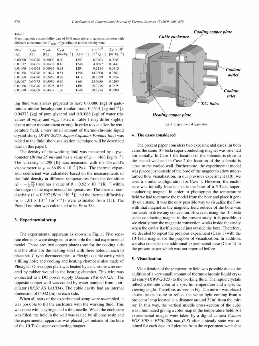
ing fluid was always prepared to have 0.03080 [kg] of gado-linium nitrate hexahydrate (molar mass 0.4514 [kg mol−1]),0.04373 [kg] of pure glycerol and 0.01068 [kg] of water (thevalues of mH2O and mglyc listed in Table 1 may differ slightlydue to minor measurement errors). In order to visualize the tem-perature field, a very small amount of thermo-chromic liquidcrystal slurry (KWN-20/25, Japan Capsular Product Inc.) wasadded to the fluid (the visualization technique will be describedlater in this paper).

The density of the working fluid was measured by a pyc-nometer (Brand 25 ml) and has a value of ρ = 1463 [kg m−3].The viscosity at 298 [K] was measured with the Ostwald’sviscosimeter as μ = 86.89 × 10−3 [Pa s]. The thermal expan-sion coefficient was calculated based on the measurements ofthe fluid density at different temperatures from the definition(β = − 1

ρ∂ρ∂T

) and has a value of β = 0.52 × 10−3 [K−1] withinthe range of the experimental temperatures. The thermal con-ductivity (λ = 0.397 [W m−1 K−1]) and the thermal diffusivity(α = 1.01 × 10−7 [m2 s−1]) were estimated from [13]. ThePrandtl number was calculated to be Pr = 584.

3. Experimental setup

The experimental apparatus is shown in Fig. 1. Five sepa-rate elements were designed to assemble the final experimentalmodel. Those are: two copper plates (one for the cooling sideand the other for the heating side) with three holes in each toplace six T -type thermocouples; a Plexiglas cubic cavity witha filling hole; and cooling and heating chambers also made ofPlexiglas. One copper plate was heated by a nichrome wire cov-ered by rubber wound in the heating chamber. This wire wasconnected to a DC power supply (Kikusui PAK 60-12A). Theopposite copper wall was cooled by water pumped from a cir-culator (RK20 KS LAUDA). The cubic cavity had an internaldimension of 0.032 [m] on each side.

When all parts of the experimental setup were assembled, itwas possible to fill the enclosure with the working fluid. Thiswas done with a syringe and a thin needle. When the enclosurewas filled, the hole in the wall was sealed by silicone resin andthe experimental apparatus was placed just outside of the boreof the 10-Tesla super-conducting magnet.

Fig. 1. Experimental apparatus.

4. The cases considered

The present paper considers two experimental cases. In bothcases the same 10-Tesla super-conducting magnet was orientedhorizontally. In Case 1 the location of the solenoid is close tothe heated wall and in Case 2 the location of the solenoid isclose to the cooled wall. Furthermore, the experimental modelwas placed just outside of the bore of the magnet to allow undis-turbed flow visualization. In our previous experiment [10], weused a similar configuration for Case 1. However, the enclo-sure was initially located inside the bore of a 5-Tesla super-conducting magnet. In order to photograph the temperaturefield we had to remove the model from the bore and place it gen-tly on a stand. It was the only possible way to visualize the flowwith that magnet as the magnetic field outside of the bore wastoo weak to drive any convection. However, using the 10-Teslasuper-conducting magnet in the present study, it is possible tosee clearly how the magnetic convection works inside the cavitywhen the cavity itself is placed just outside the bore. Therefore,we decided to repeat the previous experiment (Case 1) with the10-Tesla magnet for the purpose of visualization. In addition,we also consider one additional experimental case (Case 2) inthe present paper which was not reported before.

5. Visualization

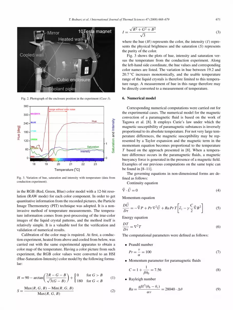
Visualization of the temperature field was possible due to theaddition of a very small amount of thermo-chromic liquid crys-tal slurry (KWN-20/25) to the working fluid. The liquid crystalsreflect a definite color at a specific temperature and a specificviewing angle. Therefore, as seen in Fig. 2, a mirror was placedabove the enclosure to reflect the white light coming from aprojector lamp located at a distance around 3 [m] from the mir-ror. In this way, the vertical middle cross-section of the cubewas illuminated giving a color map of the temperature field. Allexperimental images were taken by a digital camera (CanonEOS 10D + EF70-200 mm f2.8) after a steady state was at-tained for each case. All pictures from the experiment were shot


Fig. 2. Photograph of the enclosure position in the experiment (Case 1).

Fig. 3. Variation of hue, saturation and intensity with temperature (data fromconduction experiment).

in the RGB (Red, Green, Blue) color model with a 12-bit reso-lution (RAW mode) for each color component. In order to getquantitative information from the recorded pictures, the ParticleImage Thermometry (PIT) technique was adopted. It is a non-invasive method of temperature measurements. The tempera-ture information comes from post-processing of the true-colorimages of the liquid crystal patterns, and the method itself isrelatively simple. It is a valuable tool for the verification andvalidation of numerical results.

Calibration of the color map is required. At first, a conduc-tion experiment, heated from above and cooled from below, wascarried out with the same experimental apparatus to obtain acolor map of the temperature. Having a color picture from suchexperiment, the RGB color values were converted to an HSI(Hue-Saturation-Intensity) color model by the following formu-lae:

H = 90 − arctan

(2R − G − B√

3(G − B)

)+

{0 for G > B

180 for G < B(1)

S = Max(R,G,B) − Min(R,G,B)(2)

Max(R,G,B)

I =√

R2 + G2 + B2√

3(3)

where the hue (H ) represents the color, the intensity (I ) repre-sents the physical brightness and the saturation (S) representsthe purity of the color.

Fig. 3 shows the plots of hue, intensity and saturation ver-sus the temperature from the conduction experiment. Alongthe left-hand side coordinate, the hue values and correspondingcolor names are listed. The variation in hue between 19.2 and20.7 ◦C increases monotonically, and the usable temperaturerange of the liquid crystals is therefore limited to this tempera-ture range. A measurement of hue in this range therefore maybe directly converted to a measurement of temperature.

6. Numerical model

Corresponding numerical computations were carried out forthe experimental cases. The numerical model for the magneticconvection of a paramagnetic fluid is based on the work ofTagawa et al. [8]. It employs Curie’s law under which themagnetic susceptibility of paramagnetic substances is inverselyproportional to its absolute temperature. For not very large tem-perature differences, the magnetic susceptibility may be rep-resented by a Taylor expansion and the magnetic term in themomentum equation becomes proportional to the temperatureT based on the approach presented in [8]. When a tempera-ture difference occurs in the paramagnetic fluids, a magneticbuoyancy force is generated in the presence of a magnetic field.Examples of our previous computations on the same topic canbe found in [8–11].

The governing equations in non-dimensional forms are de-fined as follows:

Continuity equation

�∇ · �U = 0 (4)

Momentum equation

D �UDτ

= −�∇P + Pr ∇2 �U + Ra Pr T

[�ez − γ

C

2�∇B2

](5)

Energy equation

DT

Dτ= ∇2T (6)

The computational parameters were defined as follows:

• Prandtl number

Pr = ν

α= 100 (7)

• Momentum parameter for paramagnetic fluids

C = 1 + 1

βθ0= 7.56 (8)

• Rayleigh number

Ra = gβl3(θh − θc)

αν= 28040 · �θ (9)


• Gamma parameter

γ = χ0b20

μmgl= 0.586 · b2

0 (10)

Non-dimensionalization was done using the following for-mulae:

X = x/x0, Y = y/y0, Z = z/z0, U = u/u0

V = v/v0 W = w/w0 τ = t/t0, P = p/p0

�B = �b/b0, T = (θ − θ0)/(θh − θc), x0 = y0 = z0 = l

u0 = v0 = w0 = α/l, t0 = l2/α

b0 = μmi/l, p0 = ρ0α2/l2

It should be mentioned here that the steady flow characteris-tics are almost independent of the Pr number for higher Prandtlnumber fluids (Pr > 10) which has been confirmed in prelimi-nary computations (for Pr > 10 the effect of inertia is negligi-ble). Therefore, in this case the Ra number becomes the uniqueparameter to characterize the buoyant convection in the absenceof a magnetic field. A similar comparison was reported by Shyyand Chen [14]. It should be mentioned that the transient statehowever, may differ depending on the Prandtl number. In thisstudy, we arbitrarily chose Pr = 100 for the simulations. Thisshortened the time needed for convergence to steady state in thenumerical simulations.

Distribution of the magnetic field was computed using theBiot–Savart’s law for a multi-coil system (the 10-Tesla super-conducting magnet has two solenoids, Sumitomo Heavy Indus-tries Ltd.).

The boundary conditions for this system were as follows:

U = V = W = 0 at all walls of the cube

T = 0.5 at X = −0.5

T = −0.5 at X = 0.5

∂T /∂Y = 0 at Y = −0.5,0.5

∂T /∂Z = 0 at Z = −0.5,0.5

A conduction state was arbitrarily selected as an initial condi-tion.

U = V = W = 0, T = −X where − 0.5 � X � 0.5

The average Nusselt number was computed on the hot wallfrom the following definition:

Nu =∫ 0.5−0.5

∫ 0.5−0.5(∂T /∂X)convection

X=−0.5 dY dZ∫ 0.5−0.5

∫ 0.5−0.5(∂T /∂X)conduction

X=−0.5 dY dZ(11)

The normalized governing equations were approximated with afinite difference method. The Highly Simplified Marker AndCell method was used to iterate mutually the pressure andvelocity fields. The inertial terms were approximated usingthe UTOPIA scheme [15]. The grid number employed was40 × 40 × 40. A grid dependency test for the same modelequations was reported in [16] which showed that the effectof the grid size was insignificant comparing with a mesh of30 × 30 × 30.

7. Results and discussion

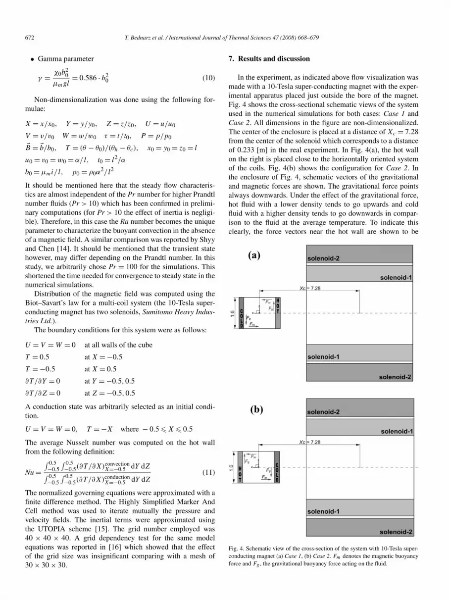
In the experiment, as indicated above flow visualization wasmade with a 10-Tesla super-conducting magnet with the exper-imental apparatus placed just outside the bore of the magnet.Fig. 4 shows the cross-sectional schematic views of the systemused in the numerical simulations for both cases: Case 1 andCase 2. All dimensions in the figure are non-dimensionalized.The center of the enclosure is placed at a distance of Xc = 7.28from the center of the solenoid which corresponds to a distanceof 0.233 [m] in the real experiment. In Fig. 4(a), the hot wallon the right is placed close to the horizontally oriented systemof the coils. Fig. 4(b) shows the configuration for Case 2. Inthe enclosure of Fig. 4, schematic vectors of the gravitationaland magnetic forces are shown. The gravitational force pointsalways downwards. Under the effect of the gravitational force,hot fluid with a lower density tends to go upwards and coldfluid with a higher density tends to go downwards in compar-ison to the fluid at the average temperature. To indicate thisclearly, the force vectors near the hot wall are shown to be

Fig. 4. Schematic view of the cross-section of the system with 10-Tesla super-conducting magnet (a) Case 1, (b) Case 2. Fm denotes the magnetic buoyancyforce and Fg , the gravitational buoyancy force acting on the fluid.


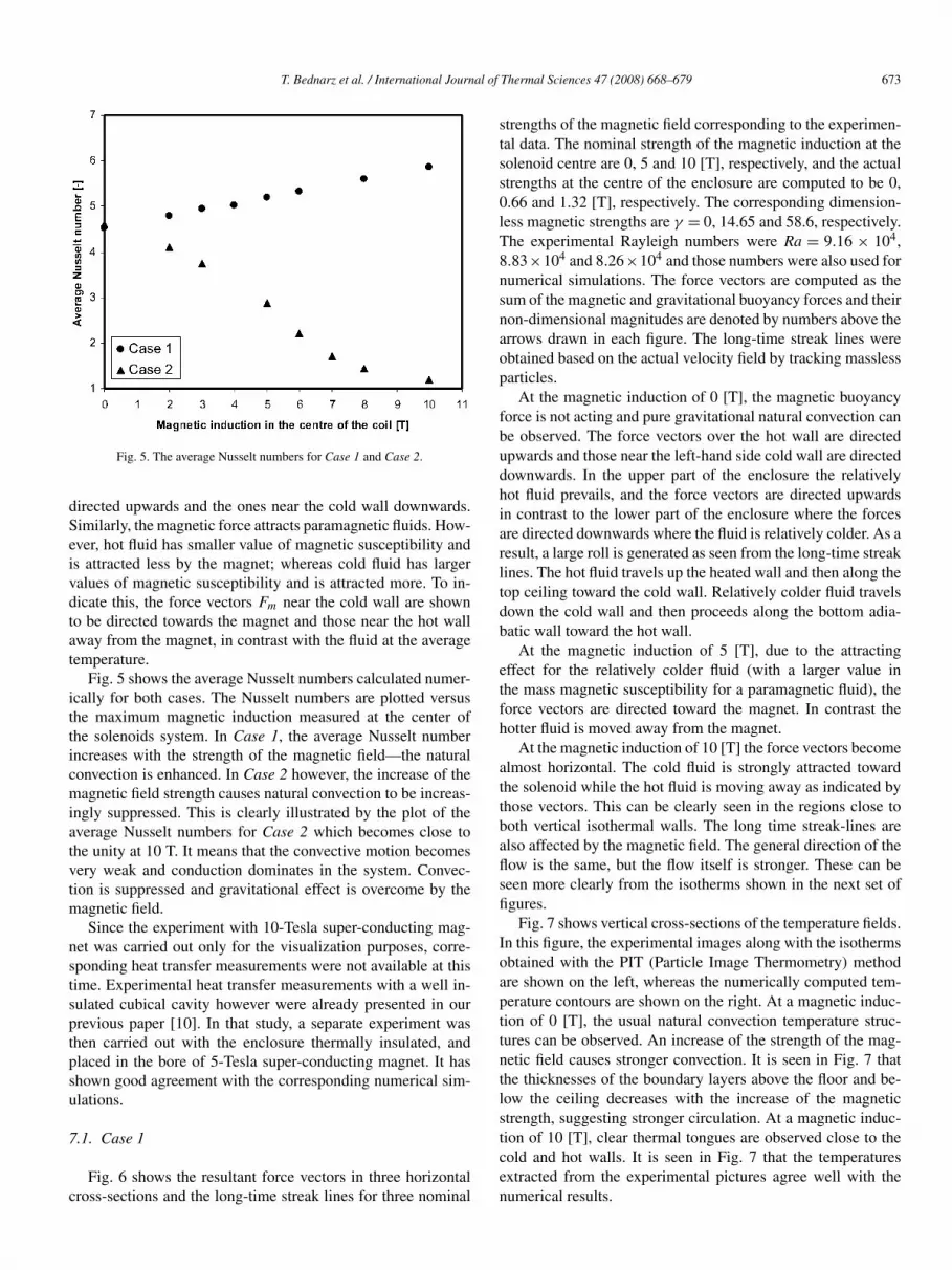
Fig. 5. The average Nusselt numbers for Case 1 and Case 2.

directed upwards and the ones near the cold wall downwards.Similarly, the magnetic force attracts paramagnetic fluids. How-ever, hot fluid has smaller value of magnetic susceptibility andis attracted less by the magnet; whereas cold fluid has largervalues of magnetic susceptibility and is attracted more. To in-dicate this, the force vectors Fm near the cold wall are shownto be directed towards the magnet and those near the hot wallaway from the magnet, in contrast with the fluid at the averagetemperature.

Fig. 5 shows the average Nusselt numbers calculated numer-ically for both cases. The Nusselt numbers are plotted versusthe maximum magnetic induction measured at the center ofthe solenoids system. In Case 1, the average Nusselt numberincreases with the strength of the magnetic field—the naturalconvection is enhanced. In Case 2 however, the increase of themagnetic field strength causes natural convection to be increas-ingly suppressed. This is clearly illustrated by the plot of theaverage Nusselt numbers for Case 2 which becomes close tothe unity at 10 T. It means that the convective motion becomesvery weak and conduction dominates in the system. Convec-tion is suppressed and gravitational effect is overcome by themagnetic field.

Since the experiment with 10-Tesla super-conducting mag-net was carried out only for the visualization purposes, corre-sponding heat transfer measurements were not available at thistime. Experimental heat transfer measurements with a well in-sulated cubical cavity however were already presented in ourprevious paper [10]. In that study, a separate experiment wasthen carried out with the enclosure thermally insulated, andplaced in the bore of 5-Tesla super-conducting magnet. It hasshown good agreement with the corresponding numerical sim-ulations.

7.1. Case 1

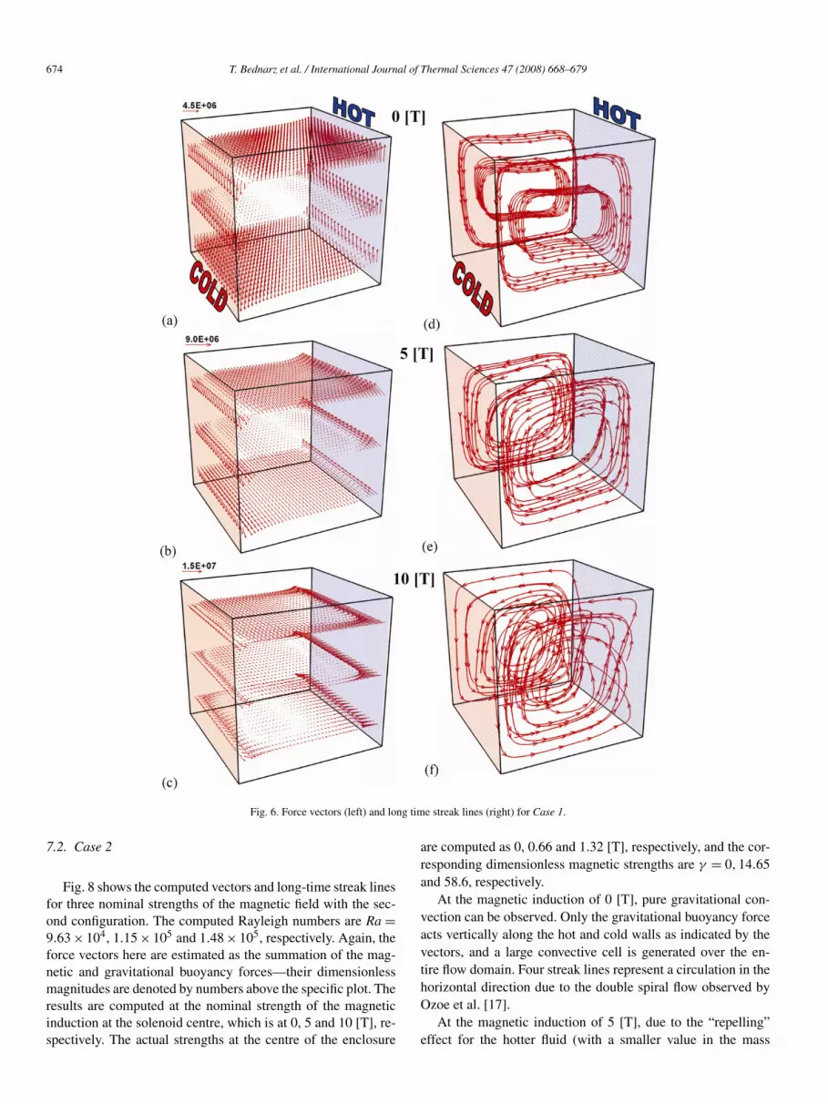
Fig. 6 shows the resultant force vectors in three horizontalcross-sections and the long-time streak lines for three nominal

strengths of the magnetic field corresponding to the experimen-tal data. The nominal strength of the magnetic induction at thesolenoid centre are 0, 5 and 10 [T], respectively, and the actualstrengths at the centre of the enclosure are computed to be 0,0.66 and 1.32 [T], respectively. The corresponding dimension-less magnetic strengths are γ = 0, 14.65 and 58.6, respectively.The experimental Rayleigh numbers were Ra = 9.16 × 104,8.83×104 and 8.26×104 and those numbers were also used fornumerical simulations. The force vectors are computed as thesum of the magnetic and gravitational buoyancy forces and theirnon-dimensional magnitudes are denoted by numbers above thearrows drawn in each figure. The long-time streak lines wereobtained based on the actual velocity field by tracking masslessparticles.

At the magnetic induction of 0 [T], the magnetic buoyancyforce is not acting and pure gravitational natural convection canbe observed. The force vectors over the hot wall are directedupwards and those near the left-hand side cold wall are directeddownwards. In the upper part of the enclosure the relativelyhot fluid prevails, and the force vectors are directed upwardsin contrast to the lower part of the enclosure where the forcesare directed downwards where the fluid is relatively colder. As aresult, a large roll is generated as seen from the long-time streaklines. The hot fluid travels up the heated wall and then along thetop ceiling toward the cold wall. Relatively colder fluid travelsdown the cold wall and then proceeds along the bottom adia-batic wall toward the hot wall.

At the magnetic induction of 5 [T], due to the attractingeffect for the relatively colder fluid (with a larger value inthe mass magnetic susceptibility for a paramagnetic fluid), theforce vectors are directed toward the magnet. In contrast thehotter fluid is moved away from the magnet.

At the magnetic induction of 10 [T] the force vectors becomealmost horizontal. The cold fluid is strongly attracted towardthe solenoid while the hot fluid is moving away as indicated bythose vectors. This can be clearly seen in the regions close toboth vertical isothermal walls. The long time streak-lines arealso affected by the magnetic field. The general direction of theflow is the same, but the flow itself is stronger. These can beseen more clearly from the isotherms shown in the next set offigures.

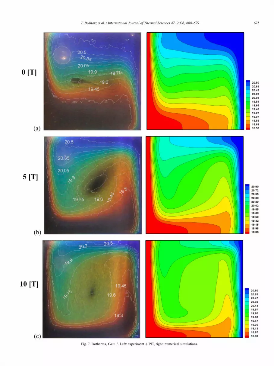
Fig. 7 shows vertical cross-sections of the temperature fields.In this figure, the experimental images along with the isothermsobtained with the PIT (Particle Image Thermometry) methodare shown on the left, whereas the numerically computed tem-perature contours are shown on the right. At a magnetic induc-tion of 0 [T], the usual natural convection temperature struc-tures can be observed. An increase of the strength of the mag-netic field causes stronger convection. It is seen in Fig. 7 thatthe thicknesses of the boundary layers above the floor and be-low the ceiling decreases with the increase of the magneticstrength, suggesting stronger circulation. At a magnetic induc-tion of 10 [T], clear thermal tongues are observed close to thecold and hot walls. It is seen in Fig. 7 that the temperaturesextracted from the experimental pictures agree well with thenumerical results.


Fig. 6. Force vectors (left) and long time streak lines (right) for Case 1.

7.2. Case 2

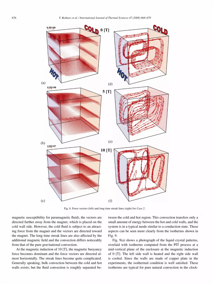
Fig. 8 shows the computed vectors and long-time streak linesfor three nominal strengths of the magnetic field with the sec-ond configuration. The computed Rayleigh numbers are Ra =9.63 × 104, 1.15 × 105 and 1.48 × 105, respectively. Again, theforce vectors here are estimated as the summation of the mag-netic and gravitational buoyancy forces—their dimensionlessmagnitudes are denoted by numbers above the specific plot. Theresults are computed at the nominal strength of the magneticinduction at the solenoid centre, which is at 0, 5 and 10 [T], re-spectively. The actual strengths at the centre of the enclosure

are computed as 0, 0.66 and 1.32 [T], respectively, and the cor-responding dimensionless magnetic strengths are γ = 0,14.65and 58.6, respectively.

At the magnetic induction of 0 [T], pure gravitational con-vection can be observed. Only the gravitational buoyancy forceacts vertically along the hot and cold walls as indicated by thevectors, and a large convective cell is generated over the en-tire flow domain. Four streak lines represent a circulation in thehorizontal direction due to the double spiral flow observed byOzoe et al. [17].

At the magnetic induction of 5 [T], due to the “repelling”effect for the hotter fluid (with a smaller value in the mass


Fig. 7. Isotherms, Case 1. Left: experiment + PIT, right: numerical simulations.


Fig. 8. Force vectors (left) and long time streak lines (right) for Case 2.

magnetic susceptibility for paramagnetic fluid), the vectors aredirected further away from the magnet, which is placed on thecold wall side. However, the cold fluid is subject to an attract-ing force from the magnet and the vectors are directed towardthe magnet. The long time streak lines are also affected by theadditional magnetic field and the convection differs noticeablyfrom that of the pure gravitational convection.

At the magnetic induction of 10 [T], the magnetic buoyancyforce becomes dominant and the force vectors are directed al-most horizontally. The streak lines become quite complicated.Generally speaking, bulk convection between the cold and hotwalls exists; but the fluid convection is roughly separated be-

tween the cold and hot region. This convection transfers only asmall amount of energy between the hot and cold walls, and thesystem is in a typical mode similar to a conduction state. Theseaspects can be seen more clearly from the isotherms shown inFig. 9.

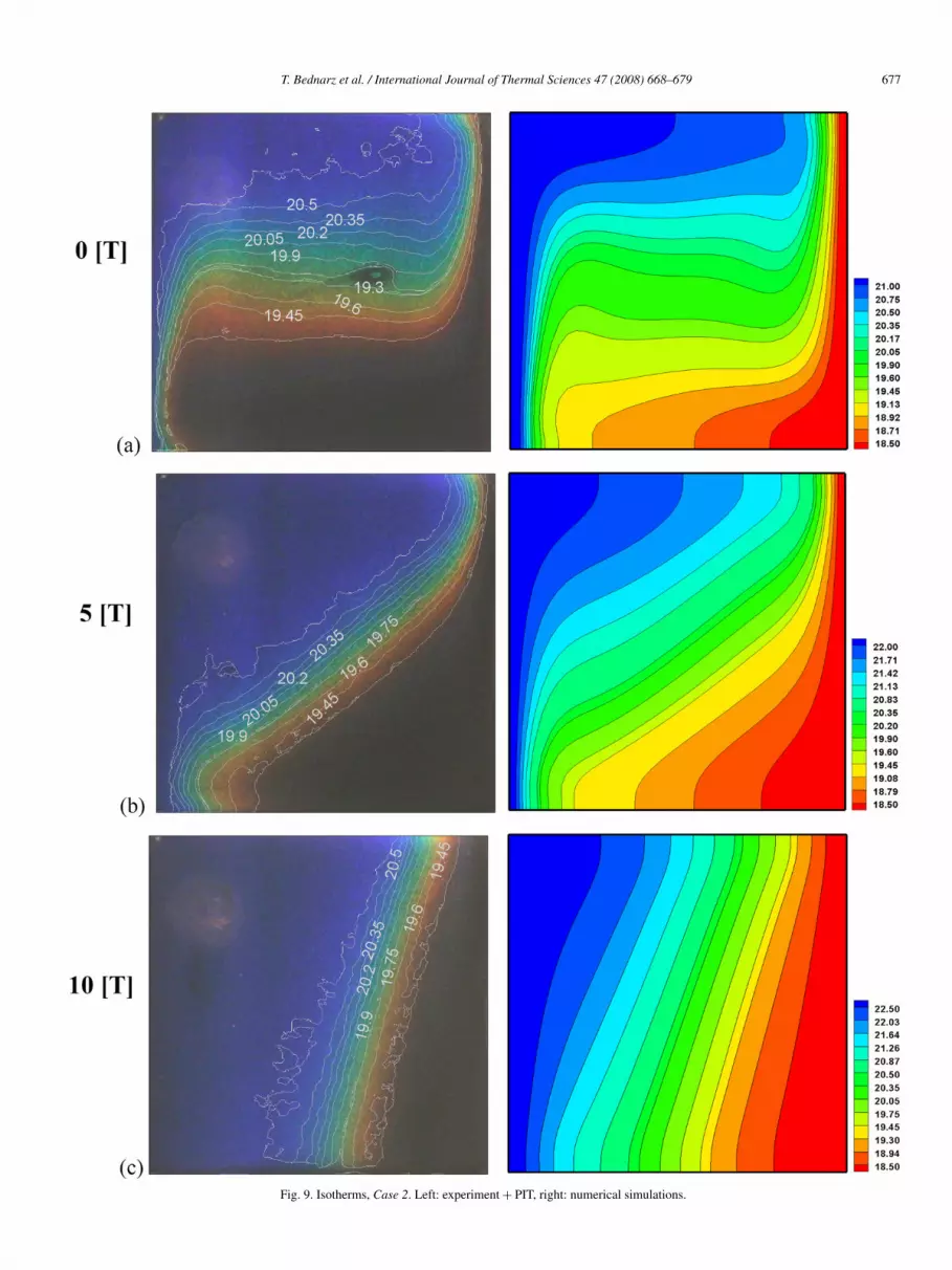
Fig. 9(a) shows a photograph of the liquid crystal patterns,overlaid with isotherms computed from the PIT process at amid-vertical plane of the enclosure at the magnetic inductionof 0 [T]. The left side wall is heated and the right side wallis cooled. Since the walls are made of copper plate in theexperiments, the isothermal condition is well satisfied. Theseisotherms are typical for pure natural convection in the clock-


Fig. 9. Isotherms, Case 2. Left: experiment + PIT, right: numerical simulations.


Fig. 10. Isothermal surfaces for Case 1 (left) and Case 2 (right).

wise direction with a thermal stratification in the core region,and a quasi two-dimensional mode is established. The right pic-ture shows the isotherms at the mid-vertical plane computedfrom the three-dimensional numerical analyses. It is seen inFig. 9(a) that the experimental and numerical isotherms matchquite well with each other.

Fig. 9(b) shows the results obtained at the magnetic induc-tion of 5 [T]. The isotherms become more inclined and thecorresponding numerical isotherms show similar features.

Fig. 9(c) shows the results at the magnetic induction of10 [T]. It is seen in this figure that the isotherms become al-

most vertical, indicating a conduction-like situation. Again, thecorresponding numerical results are consistent with the experi-mental data.

7.3. Effect of the front and rear walls

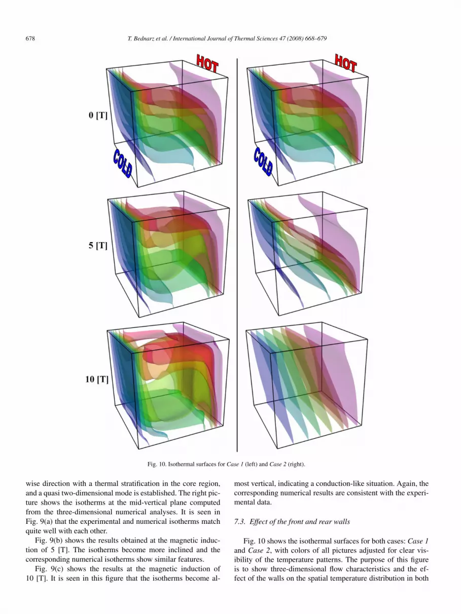
Fig. 10 shows the isothermal surfaces for both cases: Case 1and Case 2, with colors of all pictures adjusted for clear vis-ibility of the temperature patterns. The purpose of this figureis to show three-dimensional flow characteristics and the ef-fect of the walls on the spatial temperature distribution in both


cases. At 0 T, both cases have the usual natural convection pro-files which can be assumed to be almost two dimensional inthe analysis. In the regions very close to the front and rearwalls, delicate curling is observed and is caused by the non-slip boundary condition. Increasing the strength of the magneticfield changes the temperature distribution characteristics. It isseen in Fig. 10 that Case 1 becomes more three dimensionalwhen the magnetic strength is increased. However Case 2 be-comes even more two dimensional due to the weakening con-vection effect. In Case 1, at 10 T three-dimensional effects areeasily observed, for instance along the top horizontal edgeswhere hot fluid moves toward the cold wall is squeezed out tothe sides by the relatively colder fluid.

8. Conclusions

Experiments and numerical computations were carried outfor natural convection of a paramagnetic fluid in a cubic enclo-sure heated and cooled from opposing vertical walls with fourother walls thermally insulated. The computed conditions weretaken from the accompanying flow visualization experimentand the computed isotherms agree well with the observed onesfor the aqueous glycerol solution with the dissolved gadolin-ium nitrate hexahydrate. The good agreement between the ex-perimental and numerical isotherms strongly suggests that thepresent numerical model can be applied to modeling such typeof experiments with confidence.

It is worth noting that the configuration of Case 1 in thepresent experiments is similar to the experiment reportedin [10], which suffered a deficiency in the experimental pro-cedures due to limitations of the experimental system in thatcase. The previous experiment was carried out with a 5-Teslasuper-conducting magnet, and the experimental model had tobe placed inside the bore of the magnet in order to have a suffi-ciently strong magnetic field. Once a steady state condition wasachieved, the enclosure was then taken out from the bore of themagnet for photographing purpose. Unfortunately, that was theonly possible way to visualize the flow at that time due to thelimitations of the magnet. Although the previous experimentalresults clearly showed similar enhancement of natural convec-tion, they were strongly influenced by the gravity force [10].This is because the magnetic force acting on the fluid was re-duced significantly when the model was taken out of the boredespite that this procedure happened within a very short time.As a consequence, a disturbed picture of what was actuallyhappening in the enclosure was recorded; the thermal tonguesobserved in the present experiments were not clearly visible inthe previous experiment, and direct comparison with numericalsimulation was not possible then.

With the 10-Tesla strong magnet, we have repeated the sameexperiment in the present study without disturbing the flow. Inthis experiment, the experimental cube was placed just outsidethe bore, and the magnetic field was strong enough to drive theconvective motion. The visualization was made properly with-

out any disturbances to the flow field, and thus the obtainedexperimental results compare favorably with the numerical sim-ulations. Also it should be mentioned, that no instabilities wereobserved in experimental and numerical results.

Acknowledgements

The authors gratefully acknowledge the financial support ofthe Australian Research Council. Also, a part of this work wassupported by Grant AGH-UST No. 11.11.180.375.

References

[1] G.K. Batchelor, Heat transfer by free convection across a close cavity be-tween vertical boundaries at different temperatures, Quarterly Journal ofApplied Mathematics 12 (1954) 209–233.

[2] E.R.G. Eckert, W.O. Carlson, Natural convection in an air layer enclosedbetween two vertical plates with different temperatures, International Jour-nal of Heat and Mass Transfer 2 (1961) 106–120.

[3] J.O. Wilkes, S.W. Churchill, The finite-difference computation of naturalconvection in a rectangular enclosure, AIChE Journal 12 (1966) 161–166.

[4] G. de Vahl Davis, Laminar natural convection in an enclosed rectangularcavity, International Journal of Heat and Mass Transfer 11 (1968) 1675–1693.

[5] I.P. Jones, A numerical study of natural convection in an air-filled cavity:comparison with experiment, Numerical Heat Transfer 2 (1979) 193–213.

[6] J.C. Patterson, J. Imberger, Unsteady natural convection in a rectangularcavity, Journal of Fluid Mechanics 100 (1980) 65–86.

[7] F. Xu, J.C. Patterson, C. Lei, Experimental observations of the thermalflow around a square obstruction on a vertical wall in a differentiallyheated cavity, Experiments in Fluids 40 (2006) 364–371.

[8] T. Tagawa, R. Shigemitsu, H. Ozoe, Magnetizing force modeled and nu-merically solved for natural convection of air in a cubic enclosure: Effectof the direction of the magnetic field, International Journal of Heat andMass Transfer 45 (2002) 267–277.

[9] M. Kaneda, T. Tagawa, H. Ozoe, Convection induced by a cusp-shapedmagnetic field for air in a cube heated from above and cooled from below,Journal of Heat Transfer 124 (2002) 17–25.

[10] T. Bednarz, E. Fornalik, T. Tagawa, H. Ozoe, J.S. Szmyd, Experimentaland numerical analyses of magnetic convection of paramagnetic fluid in acube heated and cooled from opposing vertical walls, International Journalof Thermal Sciences 44 (2005) 933–943.

[11] H. Ozoe, Magnetic Convection, Imperial College Press, ISBN 1-86094-578-3, 2005.

[12] Sherwood Scientific Ltd., Magnetic Susceptibility Balance InstructionManual, second ed., Cambridge, 2001.

[13] D.R. Lide (Ed.), Handbook of Chemistry and Physics, 82 ed., ChemicalRubber Company Press, Boca Raton, FL, 2001–2002.

[14] W. Shyy, M.H. Chen, Effect of Prandtl number on buoyancy-inducedtransport processes with and without solidification, International Journalof Heat Mass Transfer 33 (11) (1990) 2565–2578.

[15] T. Tagawa, H. Ozoe, Effect of Prandtl number and computational schemeson the oscillatory natural convection in an enclosure, Numerical HeatTransfer A 30 (1996) 271–282.

[16] T. Bednarz, T. Tagawa, M. Kaneda, H. Ozoe, J.S. Szmyd, Numerical studyof joint magnetisation and gravitational convection of air in a cubic en-closure with an inclined electric coil, Progress in Computational FluidDynamics 5 (3/4/5) (2005).

[17] H. Ozoe, N. Sato, S.W. Churchill, Experimental confirmation of the three-dimensional helical streaklines previously computed for natural convec-tion in inclined rectangular enclosure, Int. Chem. Eng. 19 (3) (1979) 454–462.

influence of a horizontal magnetic field on the natural convection of paramagnetic fluid in a cube...

Documents