cooled heat exchangers using open source

DEVELOPMENT OF A LOW COST DESIGN TOOLKIT FOR SIZING AIR-

COOLED HEAT EXCHANGERS USING OPEN SOURCE HEAT TRANSFER

CORRELATIONS.

A THESIS SUBMITTED IN PARTIAL FULFILLMENT OF THE REQUIREMENTS FOR THE DEGREE

OF

MASTER OF PHILOSOPHY

IN

MECHANICAL ENGINEERING

BY

UGONNA CHIDERA MBAEZUE

REG. NO: 201384951

Department of Mechanical and Aerospace Engineering

University of Strathclyde

Glasgow

2019

SUPERVISOR: Dr. WILLIAM DEMPSTER

i

Declaration

This thesis is the result of the author’s original research. It has been composed by the author and has

not been previously submitted for the examination which has led to the award of a degree.

The copyright of this thesis belongs to the author under the terms of the United Kingdom Copyright

Acts as qualified by the University of Strathclyde Regulation 3.50. Due acknowledgement must

always be made of the use of any material contained in, or derived from, this thesis

Signed: Ugonna Chidera Mbaezue Date: 06/06/2019

ii

Abstract: The exorbitant costs associated with heat exchanger design software e.g. ASPEN EDR, HTRI X-Suite

etc., means that most engineering firms especially SMEs, struggle to purchase and use these tools for

in-house design purposes. Therefore, heat exchanger design for these engineering firms is dependent

on charts, graphs and ‘passed down’ knowledge. Unfortunately in most cases, the accuracy of these

design data sources cannot be verified which means that every heat exchanger designed, is not sized

correctly to deliver the heat duty required.

The aim of this project was to build a low cost toolkit capable of designing and rating Circular – Fin,

Tube-in-Plate Fin and Plain Tube Heat Exchangers air-cooled heat exchangers.

Heat transfer correlations were obtained from publicly available data and the validation process

involved designing air-cooled heat exchangers using these correlations. Thereafter, the design

process was repeated using the industry standard software, ASPEN Exchanger Design & Rating (EDR).

The results were then compared. The outcome indicated that when geometrical characteristics and

operating conditions stayed within the boundaries specified by the open source correlations, the

largest deviation will occur in the Tube-in-Plate heat exchanger with an over-prediction of 14% of the

area ratio (Gas side vs. Fluid side of the heat exchanger) when compared with the ASPEN EDR results.

The Plain Tube heat exchanger showed a 7.5% over-prediction for the staggered tube layout and an

8% over-prediction for the inline tube layout. The Circular-Fin heat exchanger gave the best result

with a 6% over-prediction for the compared area ratios.

Based on these results, the toolkit was developed using the Excel Visual Basic for Applications (VBA)

programming language. The NIST Reference fluid Properties (REFPROP) database was used to obtain

the thermophysical properties of the interacting fluids and was also integrated into the toolkit using

the VBA programming language.

iii

Table of Contents Declaration ................................................................................................................................................ i

Abstract: ................................................................................................................................................... ii

List of Figures ........................................................................................................................................... v

List of Tables .......................................................................................................................................... vii

Nomenclature ....................................................................................................................................... viii

Chapter 1 ................................................................................................................................................. 1

1.1 Introduction: ............................................................................................................................ 1

1.2 Background: ......................................................................................................................... 1

1.3 Classification of Heat Exchangers ........................................................................................ 2

1.4 Objectives of thesis: ............................................................................................................. 7

1.5 Outline of thesis: .................................................................................................................. 8

Chapter 2 ............................................................................................................................................... 11

Air-Cooled Heat Exchangers .............................................................................................................. 11

2.1 Introduction: ...................................................................................................................... 11

2.2 Heat Transfer Enhancement: ............................................................................................. 12

Chapter 3 ............................................................................................................................................... 21

Convective Heat Transfer Coefficient for Forced Convection Heat Transfer .................................... 21

3.1 Introduction: ...................................................................................................................... 21

3.2 Empirical evaluation of the heat transfer coefficient: ....................................................... 21

3.3 Evaluating the heat transfer coefficient across cylindrical tube banks: ............................ 23

3.4 Heat transfer coefficient across tube banks: ..................................................................... 26

3.5 Heat Exchanger Geometrical Characteristics..................................................................... 32

Chapter 4 ............................................................................................................................................... 36

Validation of Heat Transfer Correlations ........................................................................................... 36

4.1 Introduction: ...................................................................................................................... 36

4.2 ASPEN Exchanger Design & Rating: ................................................................................... 36

4.3 ASPEN EDR Methods and Correlations for Air Cooled Heat Exchangers ................................. 40

4.3.1 Circular – Fin Heat Exchangers: ..................................................................................... 40

Experimental results showed that the correlations predicted 98% of the data to within ±20% for

air coolers. For open literature correlations, the HTFS3 predicts 79% of the data to within ±20%.

....................................................................................................................................................... 42

4.3.2 Plain – Tube Heat Exchangers: ....................................................................................... 42

4.3.3 Tube –in – Plate Fin Tube Heat Exchangers: .................................................................. 42

4.4 Thermal Design Results and Comparison: ......................................................................... 43

Chapter 5 ............................................................................................................................................... 54

iv

Heat Exchanger Design Optimization ................................................................................................ 54

5.1 Introduction: ...................................................................................................................... 54

5.2 Literature Review: .............................................................................................................. 56

5.4 Optimization Exercise: ....................................................................................................... 61

5.4 Conclusion: ......................................................................................................................... 68

Chapter 6 ............................................................................................................................................... 69

Conclusion and Recommendations ................................................................................................... 69

6.1 Introduction: ...................................................................................................................... 69

6.2 Conclusion: ......................................................................................................................... 69

6.3 Recommendations: ............................................................................................................ 70

References ............................................................................................................................................. 71

Appendix A ............................................................................................................................................. 78

Heat Exchanger Design ...................................................................................................................... 78

Introduction: .................................................................................................................................. 78

Modes of Heat Transfer: ................................................................................................................ 78

Heat Exchanger Design Methodology: .......................................................................................... 83

Design theories: ............................................................................................................................. 88

Thermal Conductance, UA: ............................................................................................................ 96

Appendix B ............................................................................................................................................. 99

Introduction: .................................................................................................................................. 99

Toolkit Requirements: ................................................................................................................... 99

Appendix C ........................................................................................................................................... 114

GRG Non – Linear Solver .................................................................................................................. 114

Appendix D ........................................................................................................................................... 118

Toolkit Design and Development..................................................................................................... 118

Introduction: ................................................................................................................................ 118

General information: ................................................................................................................... 118

System Summary ......................................................................................................................... 119

Getting Started ............................................................................................................................ 119

Using the System ......................................................................................................................... 125

Reporting ..................................................................................................................................... 149

Troubleshooting ........................................................................................................................... 152

v

List of Figures Figure 1: Forced draft air-cooled heat exchanger [Source: Kraus, Aziz & Welty, 2001] ................................... 11

Figure 2: Induced draft air-cooled heat exchanger [Source: Kraus, Aziz & Welty, 2001] ................................. 12

Figure 3: Integral finned heat exchanger tube (Source: ESDU 86022, 1998) .................................................... 13

Figure 4: Bimetal fin heat exchanger tube (Source: ESDU 86022, 1998) .......................................................... 14

Figure 5: Tension-wound L-shape fin heat exchanger tube (Source: ESDU 86022, 1998) ................................. 14

Figure 6: Embedded G-fin heat exchanger tube (Source: Ref. [14]) ................................................................. 15

Figure 7: Plain fin tube heat exchanger (Source: Bhuiyan & Islam, 2016) ........................................................ 18

Figure 8: Wavy fin tube heat exchanger (Source: Bhuiyan & Islam, 2016) ...................................................... 19

Figure 9: Offset strip fin tube heat exchanger (Source: Bhuiyan & Islam, 2016) .............................................. 19

Figure 10: Depiction of fluid flow across the surface of a smooth cylinder ..................................................... 24

Figure 11: Depiction of flow separation across the surface of a smooth cylinder ............................................ 24

Figure 12: Inline arrangement for plain tube heat exchangers (Source: Shah, 1985) ....................................... 32

Figure 13: Staggered arrangement for plain tube heat exchangers (Source: Shah, 1985) ................................ 33

Figure 14: Arrangement for circular tube heat exchangers (Source: Shah, 1985) ............................................ 34

Figure 15: Staggered arrangement for circular tube heat exchangers (Source: Shah, 1985) ............................ 35

Figure 16: General outline of ASPEN – Air Cooled Exchanger (Input Section) .................................................. 38

Figure 17: Selection of operating conditions within ASPEN – Air Cooled Exchanger (Input Section) ............... 39

Figure 18: Selection of geometrical characteristics within ASPEN – Air Cooled Exchanger (Input Section) ...... 39

Figure 19: Results Section within ASPEN – Air Cooled Exchanger (input Section) ............................................ 39

Figure 20: Comparison of (a) conventional design method and (b) optimum design method, Source:

Introduction to Optimum Design, 2012 .................................................................................................. 55

Figure 21: Conduction heat transfer through a plane wall .............................................................................. 78

Figure 22: Boundary layer formed by fluid flow over a flat smooth surface .................................................... 80

Figure 24: Temperature flow in single-phase counterflow arrangement heat exchanger with no boiling or

condensation ........................................................................................................................................ 86

Figure 25: Temperature flow in a single-phase parallel flow arrangement heat exchanger with no boiling

or condensation (Shah & Sekulić, 2003). .............................................................................................. 87

Figure 26: Temperature flow at the inlet and outlet of an unmixed-unmixed crossflow arrangement heat

exchanger .............................................................................................................................................. 88

Figure 27: Types of mixing in crossflow heat exchanger (Shah & Sekulić, 2003). ....................................... 88

Figure 28: LMTD correction factors for heat exchangers (Source: Green & Perry, 2008) ................................. 93

Figure 29: Thermal resistance to heat flow across a smooth surface (Source: Shah & Sekulić, 2003) .............. 97

Figure 30: Toolkit calculation process. .......................................................................................................... 100

Figure 31: Sample Graphic User Interface (GUI) for selection based on type of heat exchanger ................... 100

Figure 32: Sample Graphic User Interface (GUI) for selection of process conditions ..................................... 104

Figure 33: Sample Graphic User Interface (GUI) for selection of heat exchanger characteristics ................... 106

Figure 34: Sample Graphic User Interface (GUI) for display of calculation results ......................................... 107

Figure 35: Sizing calculation process ............................................................................................................. 108

Figure 36: Sample GUI for the Sizing design option....................................................................................... 109

Figure 37: Depiction of toolkit back – end .................................................................................................... 110

Figure 38: Toolkit activation button.............................................................................................................. 120

Figure 39: Design tabs available within toolkit ............................................................................................. 120

Figure 40: Heat exchanger design Graphic User Interface (GUI) .................................................................... 121

Figure 41: Heat exchanger structural calculations Graphic User Interface (GUI) ........................................... 122

Figure 42: Heat exchanger weld calculations Graphic User Interface (GUI) ................................................... 123

Figure 43: Heat exchanger conversion tool Graphic User Interface (GUI) ...................................................... 124

Figure 44: Display of results from a Sizing calculation process ...................................................................... 135

Figure 45: Sizing Results ............................................................................................................................... 139

Figure 46: Saving option ............................................................................................................................... 150

Figure 47: Calculations result sheet .............................................................................................................. 150

vi

Figure 48: Saving the results sheet ............................................................................................................... 151

Figure 49: Closing the calculation result sheet .............................................................................................. 151

Figure 50: Error message display .................................................................................................................. 153

vii

List of Tables Table 1: Values for C0, C1, C2 and C3 ................................................................................................................. 26

Table 2: Values for ‘a’ and ‘m’ in an inline plain tube arrangement ................................................................ 27

Table 3: Values for ‘a’ and ‘m’ in a staggered plain tube arrangement........................................................... 27

Table 4: Correction factors for F2 based on number of tube rows ................................................................... 29

Table 5: Process conditions and dimensions for plain tube heat exchanger .................................................... 43

Table 6: Assessment of inline tube arrangement design parameters for plain tube heat exchangers ............. 44

Table 7: Assessment of staggered tube arrangement design parameters for plain tube heat exchangers ...... 44

Table 8: Assessment of inline tube arrangement design parameters for plain tube heat exchangers ............. 44

Table 9: Assessment of staggered tube arrangement design parameters for plain tube heat exchangers ...... 44

Table 10: Plain tube staggered arrangement results ....................................................................................... 45

Table 11: Plain tube Inline arrangement results ............................................................................................. 45

Table 12: Process conditions and dimensions for circular-fin heat exchanger ................................................. 48

Table 13: Assessment of design parameters for circular-fin tube heat exchanger........................................... 48

Table 14: Assessment of design parameters for circular-fin tube heat exchanger........................................... 49

Table 15: Circular-fin staggered arrangement results ..................................................................................... 49

Table 16: Process conditions and dimensions for tube-in-plate fin heat exchanger ........................................ 51

Table 17: Assessment of design parameters for tube-in-plate fin heat exchanger .......................................... 51

Table 18: tube-in-plate fin staggered arrangement results ............................................................................. 51

Table 19: Conventional design results ............................................................................................................ 65

Table 20: Lower boundary: 118 fins/m ........................................................................................................... 65









Table 29: ......................................................................................................................................................... 91

viii

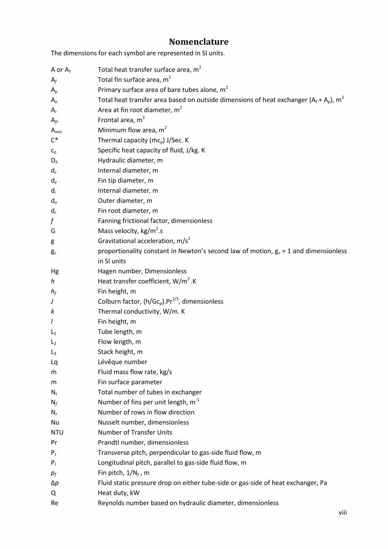
Nomenclature The dimensions for each symbol are represented in SI units.

A or AT Total heat transfer surface area, m2

Af Total fin surface area, m2

Ap Primary surface area of bare tubes alone, m2

Ao Total heat transfer area based on outside dimensions of heat exchanger (Af + Ap), m2

Ar Area at fin root diameter, m2

Afr Frontal area, m2

Amin Minimum flow area, m2

C* Thermal capacity (ṁcp) J/Sec. K

cp Specific heat capacity of fluid, J/kg. K

Dh Hydraulic diameter, m

dc Internal diameter, m

de Fin tip diameter, m

di Internal diameter, m

do Outer diameter, m

dr Fin root diameter, m

f Fanning frictional factor, dimensionless

G Mass velocity, kg/m2.s

g Gravitational acceleration, m/s2

gc proportionality constant in Newton’s second law of motion, gc = 1 and dimensionless

in SI units

Hg Hagen number, Dimensionless

h Heat transfer coefficient, W/m2 .K

hf Fin height, m

J Colburn factor, (h/Gcp).Pr2/3, dimensionless

k Thermal conductivity, W/m. K

l Fin height, m

L1 Tube length, m

L2 Flow length, m

L3 Stack height, m

Lq Lévêque number

ṁ Fluid mass flow rate, kg/s

m Fin surface parameter

Nt Total number of tubes in exchanger

Nf Number of fins per unit length, m-1

Nr Number of rows in flow direction

Nu Nusselt number, dimensionless

NTU Number of Transfer Units

Pr Prandtl number, dimensionless

Pt Transverse pitch, perpendicular to gas-side fluid flow, m

Pl Longitudinal pitch, parallel to gas-side fluid flow, m

pf Fin pitch, 1/Nf , m

∆p Fluid static pressure drop on either tube-side or gas-side of heat exchanger, Pa

Q Heat duty, kW

Re Reynolds number based on hydraulic diameter, dimensionless

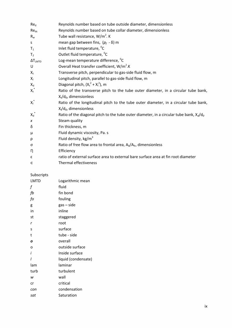
ix

Red Reynolds number based on tube outside diameter, dimensionless

Redc Reynolds number based on tube collar diameter, dimensionless

Rw Tube wall resistance, W/m2. K

s mean gap between fins, (pf - δ) m

T1 Inlet fluid temperature, 0C

T2 Outlet fluid temperature, 0C

∆TLMTD Log-mean temperature difference, 0C

U Overall Heat transfer coefficient, W/m2.K

Xt Transverse pitch, perpendicular to gas-side fluid flow, m

Xl Longitudinal pitch, parallel to gas-side fluid flow, m

Xd Diagonal pitch, (Xt2 + Xl

2), m

Xt* Ratio of the transverse pitch to the tube outer diameter, in a circular tube bank,

Xt/d0, dimensionless

Xl* Ratio of the longitudinal pitch to the tube outer diameter, in a circular tube bank,

Xl/d0, dimensionless

Xd* Ratio of the diagonal pitch to the tube outer diameter, in a circular tube bank, Xd/d0

x Steam quality

δ Fin thickness, m

μ Fluid dynamic viscosity, Pa. s

ρ Fluid density, kg/m3

σ Ratio of free flow area to frontal area, A0/Afr, dimensionless

Ƞ Efficiency

ɛ ratio of external surface area to external bare surface area at fin root diameter

∈ Thermal effectiveness

Subscripts

LMTD Logarithmic mean

f fluid

fb fin bond

fo fouling

g gas – side

in inline

st staggered

r root

s surface

t tube - side

o overall

o outside surface

i Inside surface

l liquid (condensate)

lam laminar

turb turbulent

w wall

cr critical

con condensation

sat Saturation

x

vap vaporisation

1 inlet

2 outlet

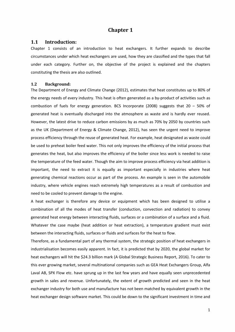
1

Chapter 1

1.1 Introduction: Chapter 1 consists of an introduction to heat exchangers. It further expands to describe

circumstances under which heat exchangers are used, how they are classified and the types that fall

under each category. Further on, the objective of the project is explained and the chapters

constituting the thesis are also outlined.

1.2 Background:

The Department of Energy and Climate Change (2012), estimates that heat constitutes up to 80% of

the energy needs of every industry. This heat is often generated as a by-product of activities such as

combustion of fuels for energy generation. BCS Incorporate (2008) suggests that 20 – 50% of

generated heat is eventually discharged into the atmosphere as waste and is hardly ever reused.

However, the latest drive to reduce carbon emissions by as much as 70% by 2050 by countries such

as the UK (Department of Energy & Climate Change, 2012), has seen the urgent need to improve

process efficiency through the reuse of generated heat. For example, heat designated as waste could

be used to preheat boiler feed water. This not only improves the efficiency of the initial process that

generates the heat, but also improves the efficiency of the boiler since less work is needed to raise

the temperature of the feed water. Though the aim to improve process efficiency via heat addition is

important, the need to extract it is equally as important especially in industries where heat

generating chemical reactions occur as part of the process. An example is seen in the automobile

industry, where vehicle engines reach extremely high temperatures as a result of combustion and

need to be cooled to prevent damage to the engine.

A heat exchanger is therefore any device or equipment which has been designed to utilise a

combination of all the modes of heat transfer (conduction, convection and radiation) to convey

generated heat energy between interacting fluids, surfaces or a combination of a surface and a fluid.

Whatever the case maybe (heat addition or heat extraction), a temperature gradient must exist

between the interacting fluids, surfaces or fluids and surfaces for the heat to flow.

Therefore, as a fundamental part of any thermal system, the strategic position of heat exchangers in

industrialisation becomes easily apparent. In fact, it is predicted that by 2020, the global market for

heat exchangers will hit the $24.3 billion mark (A Global Strategic Business Report, 2016). To cater to

this ever growing market, several multinational companies such as GEA Heat Exchangers Group, Alfa

Laval AB, SPX Flow etc. have sprung up in the last few years and have equally seen unprecedented

growth in sales and revenue. Unfortunately, the extent of growth predicted and seen in the heat

exchanger industry for both use and manufacture has not been matched by equivalent growth in the

heat exchanger design software market. This could be down to the significant investment in time and

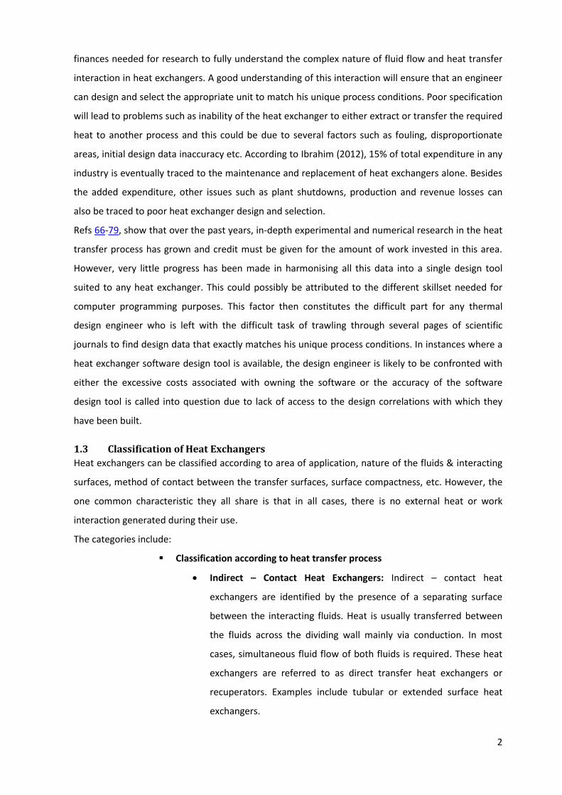
2

finances needed for research to fully understand the complex nature of fluid flow and heat transfer

interaction in heat exchangers. A good understanding of this interaction will ensure that an engineer

can design and select the appropriate unit to match his unique process conditions. Poor specification

will lead to problems such as inability of the heat exchanger to either extract or transfer the required

heat to another process and this could be due to several factors such as fouling, disproportionate

areas, initial design data inaccuracy etc. According to Ibrahim (2012), 15% of total expenditure in any

industry is eventually traced to the maintenance and replacement of heat exchangers alone. Besides

the added expenditure, other issues such as plant shutdowns, production and revenue losses can

also be traced to poor heat exchanger design and selection.

Refs 66-79, show that over the past years, in-depth experimental and numerical research in the heat

transfer process has grown and credit must be given for the amount of work invested in this area.

However, very little progress has been made in harmonising all this data into a single design tool

suited to any heat exchanger. This could possibly be attributed to the different skillset needed for

computer programming purposes. This factor then constitutes the difficult part for any thermal

design engineer who is left with the difficult task of trawling through several pages of scientific

journals to find design data that exactly matches his unique process conditions. In instances where a

heat exchanger software design tool is available, the design engineer is likely to be confronted with

either the excessive costs associated with owning the software or the accuracy of the software

design tool is called into question due to lack of access to the design correlations with which they

have been built.

1.3 Classification of Heat Exchangers

Heat exchangers can be classified according to area of application, nature of the fluids & interacting

surfaces, method of contact between the transfer surfaces, surface compactness, etc. However, the

one common characteristic they all share is that in all cases, there is no external heat or work

interaction generated during their use.

The categories include:

Classification according to heat transfer process

Indirect – Contact Heat Exchangers: Indirect – contact heat

exchangers are identified by the presence of a separating surface

between the interacting fluids. Heat is usually transferred between

the fluids across the dividing wall mainly via conduction. In most

cases, simultaneous fluid flow of both fluids is required. These heat

exchangers are referred to as direct transfer heat exchangers or

recuperators. Examples include tubular or extended surface heat

exchangers.

3

In another scenario, heat is first transferred to one medium (e.g. a

permeable solid material) by the hot fluid and then, the cooler fluid

is allowed to flow through the material for the heat transfer to

occur. These heat exchangers are referred to as storage type heat

exchangers or regenerators. An example of the latter is the storage

type exchanger.

In the final category of indirect-contact heat exchangers, you have

the Fluidized-Bed Heat Exchangers. In these heat exchangers, a side

of the heat transfer unit is buried in a bed of fine material, e.g. sand

or coal. The second fluid is then allowed to flow in an upward

direction through this bed of fine particles. If the velocity of flow is

low, the fine particles remain fixed in their position and the gas

simply flows through. However, if flow velocity is high, the fine

particles are suspended acting almost as fluids. This characteristic is

referred to as the fluidized state. In this state, the cold fluid is given

more time to interact with the hot fluid within the confines of the

bed, thus high heat transfer coefficients are common in these beds.

Where coal is used as the packed bed, chemical reactions could

occur in the form of combustion with by-products tapped off at the

bottom of the heat transfer unit. The possibility of combustion or

chemical reactions further adds to the complexity in the design of

these units.

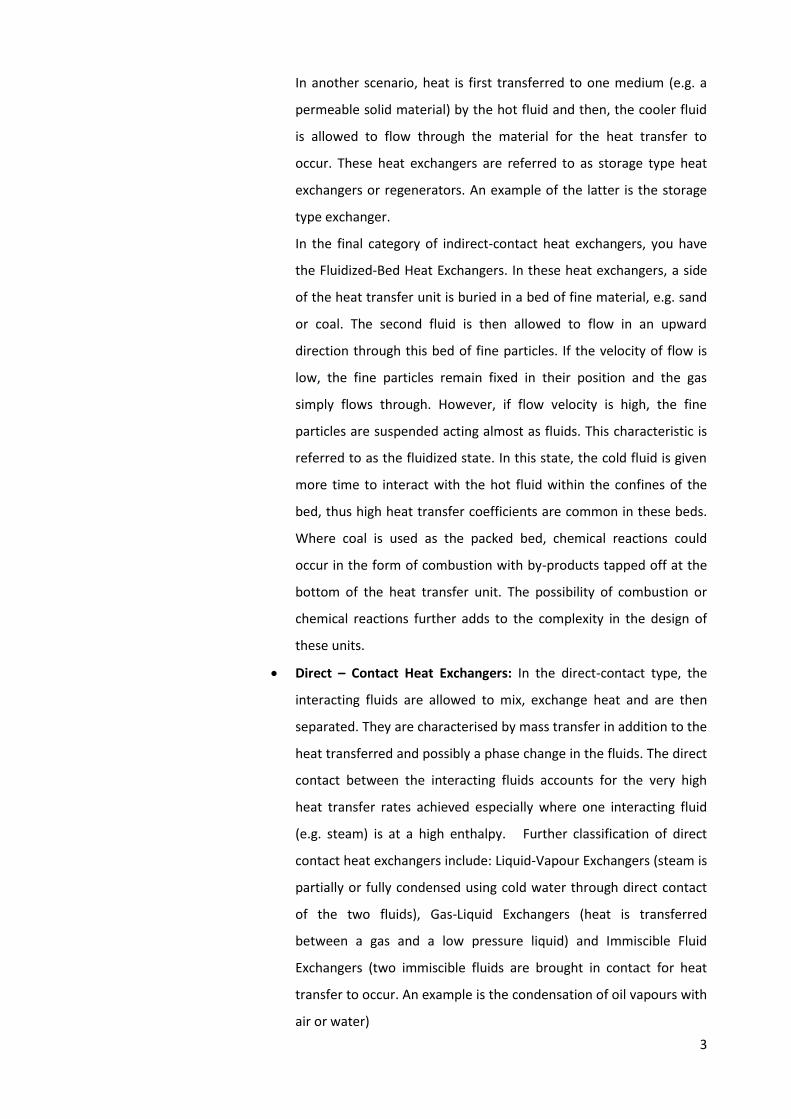
Direct – Contact Heat Exchangers: In the direct-contact type, the

interacting fluids are allowed to mix, exchange heat and are then

separated. They are characterised by mass transfer in addition to the

heat transferred and possibly a phase change in the fluids. The direct

contact between the interacting fluids accounts for the very high

heat transfer rates achieved especially where one interacting fluid

(e.g. steam) is at a high enthalpy. Further classification of direct

contact heat exchangers include: Liquid-Vapour Exchangers (steam is

partially or fully condensed using cold water through direct contact

of the two fluids), Gas-Liquid Exchangers (heat is transferred

between a gas and a low pressure liquid) and Immiscible Fluid

Exchangers (two immiscible fluids are brought in contact for heat

transfer to occur. An example is the condensation of oil vapours with

air or water)

4

Number of interacting fluids:

In most heat exchangers, heat transfer is predominantly between two fluids.

However, Sekulić and Shah (2003) points out that chemical processes e.g. air-

separation systems utilise as much as 12 fluid streams in heat transfer

processes. As the number of interacting fluids increases, so does the

complexity involved in the design of these heat exchangers.

Surface compactness: Compact heat exchangers refer to exchangers with a

much larger heat transfer surface area per unit volume of the heat

exchanger. This arrangement produces a unit with less energy requirements,

less space, better heat transfer design and weight when compared to heat

exchangers such as shell and tube heat exchangers where the per unit

volume is much more than the heat transfer surface available.

Compact exchangers are common where one fluid has very poor heat

transfer properties (i.e. heat transfer coefficient) in comparison to the other

fluid. The larger surface area therefore serves to improve the ability of the

poorer heat transfer fluid to either reject or acquire heat during the heat

exchange process, thereby reducing the overall surface needed for heat

transfer. An example is a gas-to-fluid heat exchanger which has a heat

transfer surface area per unit volume greater than 700m2/m3 in the gas

stream and 400m2/m3 for operating in the fluid stream. In comparison, shell

and tube heat exchangers will have a surface area per unit volume of less

than 100m2/m3 on the side with plain tubes and two or three times that on

the high fin density side (Sekulić and Shah 2003). Compact heat exchangers

are not entirely restricted to gas-to-fluid heat transfer processes. They are

also common in gas-to-liquid and gas-to-phase change heat exchangers, so

long as one fluid has a heat transfer coefficient significantly less than the

other fluid.

Construction features: Examples under these include; tubular, plate-type,

extended surface and regenerative heat exchangers.

The tubular type exchangers are made predominantly of cylindrical tubes

which are arranged in any configuration ranging from spiral, straight or

rectangular to elliptical. Tubular heat exchangers are used mainly in high

pressure environments or conditions where high pressure differences exist

between the interacting fluids. Their application covers liquid-to-liquid,

liquid-to-phase change, gas-to-liquid or gas-to-gas heat transfer processes.

5

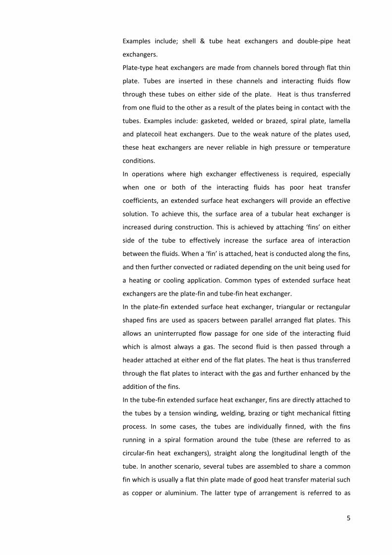
Examples include; shell & tube heat exchangers and double-pipe heat

exchangers.

Plate-type heat exchangers are made from channels bored through flat thin

plate. Tubes are inserted in these channels and interacting fluids flow

through these tubes on either side of the plate. Heat is thus transferred

from one fluid to the other as a result of the plates being in contact with the

tubes. Examples include: gasketed, welded or brazed, spiral plate, lamella

and platecoil heat exchangers. Due to the weak nature of the plates used,

these heat exchangers are never reliable in high pressure or temperature

conditions.

In operations where high exchanger effectiveness is required, especially

when one or both of the interacting fluids has poor heat transfer

coefficients, an extended surface heat exchangers will provide an effective

solution. To achieve this, the surface area of a tubular heat exchanger is

increased during construction. This is achieved by attaching ‘fins’ on either

side of the tube to effectively increase the surface area of interaction

between the fluids. When a ‘fin’ is attached, heat is conducted along the fins,

and then further convected or radiated depending on the unit being used for

a heating or cooling application. Common types of extended surface heat

exchangers are the plate-fin and tube-fin heat exchanger.

In the plate-fin extended surface heat exchanger, triangular or rectangular

shaped fins are used as spacers between parallel arranged flat plates. This

allows an uninterrupted flow passage for one side of the interacting fluid

which is almost always a gas. The second fluid is then passed through a

header attached at either end of the flat plates. The heat is thus transferred

through the flat plates to interact with the gas and further enhanced by the

addition of the fins.

In the tube-fin extended surface heat exchanger, fins are directly attached to

the tubes by a tension winding, welding, brazing or tight mechanical fitting

process. In some cases, the tubes are individually finned, with the fins

running in a spiral formation around the tube (these are referred to as

circular-fin heat exchangers), straight along the longitudinal length of the

tube. In another scenario, several tubes are assembled to share a common

fin which is usually a flat thin plate made of good heat transfer material such

as copper or aluminium. The latter type of arrangement is referred to as

6

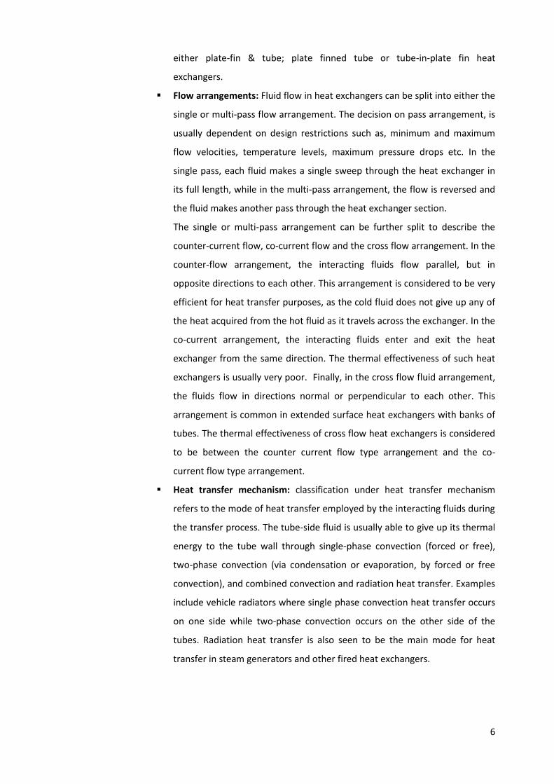
either plate-fin & tube; plate finned tube or tube-in-plate fin heat

exchangers.

Flow arrangements: Fluid flow in heat exchangers can be split into either the

single or multi-pass flow arrangement. The decision on pass arrangement, is

usually dependent on design restrictions such as, minimum and maximum

flow velocities, temperature levels, maximum pressure drops etc. In the

single pass, each fluid makes a single sweep through the heat exchanger in

its full length, while in the multi-pass arrangement, the flow is reversed and

the fluid makes another pass through the heat exchanger section.

The single or multi-pass arrangement can be further split to describe the

counter-current flow, co-current flow and the cross flow arrangement. In the

counter-flow arrangement, the interacting fluids flow parallel, but in

opposite directions to each other. This arrangement is considered to be very

efficient for heat transfer purposes, as the cold fluid does not give up any of

the heat acquired from the hot fluid as it travels across the exchanger. In the

co-current arrangement, the interacting fluids enter and exit the heat

exchanger from the same direction. The thermal effectiveness of such heat

exchangers is usually very poor. Finally, in the cross flow fluid arrangement,

the fluids flow in directions normal or perpendicular to each other. This

arrangement is common in extended surface heat exchangers with banks of

tubes. The thermal effectiveness of cross flow heat exchangers is considered

to be between the counter current flow type arrangement and the co-

current flow type arrangement.

Heat transfer mechanism: classification under heat transfer mechanism

refers to the mode of heat transfer employed by the interacting fluids during

the transfer process. The tube-side fluid is usually able to give up its thermal

energy to the tube wall through single-phase convection (forced or free),

two-phase convection (via condensation or evaporation, by forced or free

convection), and combined convection and radiation heat transfer. Examples

include vehicle radiators where single phase convection heat transfer occurs

on one side while two-phase convection occurs on the other side of the

tubes. Radiation heat transfer is also seen to be the main mode for heat

transfer in steam generators and other fired heat exchangers.

7

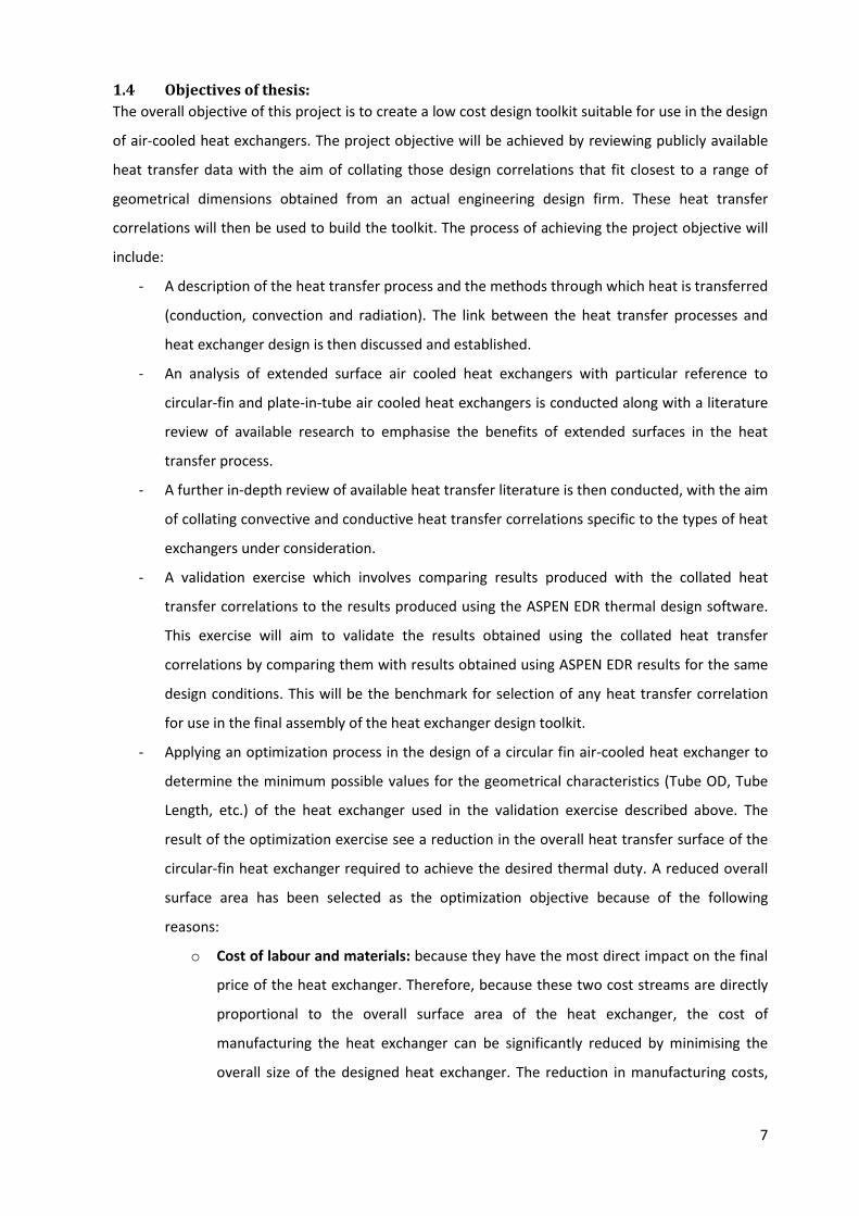
1.4 Objectives of thesis:

The overall objective of this project is to create a low cost design toolkit suitable for use in the design

of air-cooled heat exchangers. The project objective will be achieved by reviewing publicly available

heat transfer data with the aim of collating those design correlations that fit closest to a range of

geometrical dimensions obtained from an actual engineering design firm. These heat transfer

correlations will then be used to build the toolkit. The process of achieving the project objective will

include:

- A description of the heat transfer process and the methods through which heat is transferred

(conduction, convection and radiation). The link between the heat transfer processes and

heat exchanger design is then discussed and established.

- An analysis of extended surface air cooled heat exchangers with particular reference to

circular-fin and plate-in-tube air cooled heat exchangers is conducted along with a literature

review of available research to emphasise the benefits of extended surfaces in the heat

transfer process.

- A further in-depth review of available heat transfer literature is then conducted, with the aim

of collating convective and conductive heat transfer correlations specific to the types of heat

exchangers under consideration.

- A validation exercise which involves comparing results produced with the collated heat

transfer correlations to the results produced using the ASPEN EDR thermal design software.

This exercise will aim to validate the results obtained using the collated heat transfer

correlations by comparing them with results obtained using ASPEN EDR results for the same

design conditions. This will be the benchmark for selection of any heat transfer correlation

for use in the final assembly of the heat exchanger design toolkit.

- Applying an optimization process in the design of a circular fin air-cooled heat exchanger to

determine the minimum possible values for the geometrical characteristics (Tube OD, Tube

Length, etc.) of the heat exchanger used in the validation exercise described above. The

result of the optimization exercise see a reduction in the overall heat transfer surface of the

circular-fin heat exchanger required to achieve the desired thermal duty. A reduced overall

surface area has been selected as the optimization objective because of the following

reasons:

o Cost of labour and materials: because they have the most direct impact on the final

price of the heat exchanger. Therefore, because these two cost streams are directly

proportional to the overall surface area of the heat exchanger, the cost of

manufacturing the heat exchanger can be significantly reduced by minimising the

overall size of the designed heat exchanger. The reduction in manufacturing costs,

8

will allow the manufacturer either make more profit from sales or become more

competitive by reducing the cost of sale of his heat exchanger units.

o End-user requirements: The argument to support the selection of the overall heat

transfer surface area as the optimization (minimization) objective has been further

strengthened by the observation that the heat exchanger industry is predominantly a

bespoke manufacturing industry. This means that the overall size of each heat

exchanger unit is solely dependent on the operating conditions or dimensional

constraints specified by the end user. Therefore, the requirement to minimise

operational factors such as pressure drop will vary from unit to unit and in some

cases, will not be marked as a criterion by the end user. This is because air-cooled

heat exchanger components such as fans and duct transitions are only specified and

purchased based on the final overall size of the heat exchanger. In addition to this,

the requirement for a reasonably sized heat exchanger unit which still delivers the

desired thermal duty will always be important to the end user because of issues such

as space constraint and manual handling.

o Sizing: Lastly, optimizing the overall heat transfer surface area of the air cooled heat

exchanger unit will eliminate the issue of oversizing heat exchangers at the design

stage. The issue of heat exchanger oversizing will always lead to an increase in costs

for both labour and materials. In addition to an increase in cost of labour and

material, an oversized heat exchanger will deliver a heat duty outside of the

requirements of the overall system and eventually lead to an imbalanced system.

- An outline of technical specifications which will show the step-by-step approach required for

data input, data analysis and data output when the toolkit is used for the thermal design of

air cooled heat exchangers.

- Development of the toolkit using a widely available, easy access programming language such

as Microsoft Excel visual basic for applications (VBA).

1.5 Outline of thesis:

- Chapter 1 (Introduction): discusses means of improving plant efficiency through the use of

heat exchangers to recycle heat developed during a process. This discussion thus establishes

the importance of heat exchangers in most plant processes. Once the need for heat

exchangers has been established, chapter 1 then discusses the results of investigations

carried out in an attempt to find a low cost thermal design tool that can accurately design

heat exchangers. These investigations show that although there has been in-depth research

into heat transfer, little or no effort has been made towards developing low cost tools for the

9

design of heat exchangers. This gap in the market thus justifies the need to develop a low

cost thermal design tool, which forms the foundation of the project.

Finally, Chapter 1 discusses the methods of classification of heat exchangers, describes the

objectives of the project and provides an outline of the structure of the thesis.

- Chapter 2 (Air-Cooled Heat Exchanger): this chapter focuses on air-cooled heat exchangers

which have been selected for the project. This chapter begins by describing the method of

heat transfer in air cooled heat exchangers, the advantages of air-cooled heat exchangers

and the types of configuration of these units. Chapter 2 goes on to describe methods of

improving heat transfer through the use of extended surfaces in air-cooled heat exchangers.

Types of extended surfaces are presented and discussed along with results of a literature

research conducted to validate the argument that extended surfaces improve heat transfer.

- Chapter 3 (Convective Heat Transfer Coefficient for Forced Convective Heat Transfer): marks

the start of the toolkit design process by identifying the elements of the heat transfer

process that must be calculated in every heat exchanger design. The chapter begins with

providing the reader with an in-depth analysis of the process of heat transfer between the

tube-side and the gas-side fluids with respect to the heat transfer coefficient of the

interacting fluids. The gas-side fluid (e.g. air) is identified as possessing the poorer thermal

conductivity and thus requires more accurate prediction of its heat transfer capabilities when

it interacts with the tube-side fluid. Empirical and numerically derived heat transfer

correlations for the prediction of the gas-side heat transfer coefficient are then presented

and discussed in detail. These correlations cover the types of air-cooled heat exchangers

under review and were obtained from research data available in the public domain. Attempts

were also made to select those correlations that cover a wide range of design conditions and

geometry. Heat exchanger geometry equations needed to calculate the overall heat transfer

area of heat exchangers are finally presented.

- Chapter 4 (Validation of Heat Transfer Correlations): ASPEN Exchanger Design and Rating

(ASPEN EDR) was selected as the industry standard software against which the results

obtained using open source correlations will be validated. Therefore, chapter 4 begins with a

description of the physical layout of the ASPEN EDR software. The subsequent sub-section

then describes in detail, the sources and validation process for the air-side heat transfer

correlations used in ASPEN EDR. To test the accuracy of the open source heat transfer

correlations, a case study was selected for circular-fin, tube-in-plate fin and plain tube heat

exchangers. Thermal design calculations of the selected case studies were conducted using

both ASPEN EDR and the open source correlations. Results from these calculations are

discussed in the final section of this chapter.

10

- Chapter 5 (Heat Exchanger Design Optimization): Since the open source heat transfer

correlations have been validated in the preceding chapter, an attempt is made to optimize

the process of air-cooled heat exchanger design using the GRG non-linear solver available in

Microsoft Excel. The optimization exercise, concentrates on optimising the geometric

dimensions of a circular-fin heat exchanger without forfeiting the desired heat duty. A

literature review is carried out prior to the onset of the optimization exercise and results are

presented in the first half of this chapter. A comparison between the results obtained using

the GRG non-linear solver and the conventional design process, is presented and then

discussed in the concluding section of the chapter.

- Chapter 6 (Conclusion and Recommendations): involves further discussion of the results

obtained in the validation section and the development process of the tool.

Recommendations for further development of the tool are discussed in the final section of

this chapter.

- Appendix A (Heat Exchanger Design): describes in detail, the process of heat transfer and the

heat exchanger design methodology. Design theories such as the ε-NTU and the LMTD

method are also presented and discussed.

- Appendix B (Toolkit Specification): The specifications and requirements of the toolkit are

outlined and discussed. The structure of the graphic user interface (GUI) and the step-by-step

calculation process required from the fully developed tool are discussed in detail.

- Appendix C (Toolkit Design and Development): outlines a step-by-step process for carrying

out design calculations using the developed tool. The graphic user interface (physical layout)

of the complete design tool is described along with the functionality of each section. A heat

exchanger design example is carried out using the tool, and the results presented. A trouble

shooting section is included as the last section in this chapter.

11

Chapter 2

Air-Cooled Heat Exchangers

2.1 Introduction:

These heat exchangers predominantly utilise ambient air to cool or condense the tube-side fluid

which is in contrast to using a liquid as seen in shell and tube heat exchanger where water or any

other liquid is used. The advantages of air cooling lies in its free availability, where little or no added

investment is required to accommodate it. Conditions such as fouling are also non-existent on the

air-side of air-cooled heat exchangers, which means that maintenance costs are kept at the very

minimum. Lestina and Robert, 2014, [14] state that although the capital cost of air cooled heat

exchangers has been known to be quite high, operating cost has however been found to be

significantly lower than that of the water-cooled heat exchanger.

In air-cooled heat exchangers, the hot fluid is channelled through the tubes while the cold fluid

(mostly air) is allowed to flow on the outside of banks of tubes. In single phase heat transfer, these

tubes banks are aligned in the horizontal and in cases where condensation could occur, tube banks

are arranged in an A-Frame, to allow for the collection of steam condensate at the heat exchanger

bottom header. When tube bundles are aligned horizontally in condensation heat transfer, the

condensed fluid tends to lie within the tubes and could lead to an onset of tube corrosion.

In a bid to improve the heat transfer process, a fan assembly can be used to increase the volume of

air flow through these heat exchangers. Two types of arrangement exist and they are:

- Forced draft: in this arrangement, the fans are located below the heat exchanger unit and air

forcefully pushed across the unit. This arrangement ensures that the fan assembly is kept

clear of the hot air generated from the heat transfer process in addition to giving easy access

for the inspection and maintenance of the fan assembly. The downside to this arrangement

lies in their susceptibility to hot air recirculation as indicated by Lestina and Robert, 2014,

[14]. Hot air recirculation tends to reduce the capacity of the exchanger unit leading to the

requirement of higher air flow rates or even greater heat transfer surface area.

Figure 1: Forced draft air-cooled heat exchanger [Source: Kraus, Aziz & Welty, 2001]

12

- Induced draft: In the induced draft assembly, the fan is mounted above the heat exchanger

bundle, and ambient air drawn across the unit. More power is consumed in this arrangement

as a result of the hot air generated during the heat transfer process which has to be handled

by the fans (Lestina and Robert, 2014 [14]). However, more uniform flow distribution is

achieved and there exists a lesser possibility of hot air recirculation as opposed to the forced

draft fan arrangement. Minto, 1991, [26] states that owing to this advantage; induced-draft

fan assemblies sometimes require less power than the forced-draft fan assemblies. In the

induced draft assembly, the fan drive could be placed below the heat exchanger unit.

However, this arrangement sees the drive shaft pass through the tube bank which means

that a few tubes will be omitted in the bundle and could effectively reduce the capacity of

the unit.

Figure 2: Induced draft air-cooled heat exchanger [Source: Kraus, Aziz & Welty, 2001]

2.2 Heat Transfer Enhancement:

To overcome air-side thermal resistance and improve the overall efficiency of the heat transfer

process, several methods have been employed and several more being researched. Ref. [17]

describes these methods as either active or passive heat transfer enhancement methods. In the

active process, external power is used to improve and sustain the heat transfer process e.g. via

stirring or constant surface vibration. Karmatskii, Nesis and Shatalov (1994) [18] and Hagge and

Junkhan (1975), [19] give examples of active methods that can be used to improve the heat transfer

process. In the passive method, the heat exchanger unit does not require the use of an external

power to improve or sustain the heat transfer process. Abdulhafiz, Boukhary, Khaled and Siddique,

2010, [20] provide examples where the passive method is applied which include the use of treated

surfaces, extended surfaces, fluid additives or rough surfaces on either the tubes or on the extended

surfaces, use of surface tension devices, displaced enhancement devices etc.

In the use of extended surfaces, the surface area of the heat exchanger tubes in contact with the gas

of lesser or poorer heat transfer capability is increased through the use of fins. These fins are

designed to induce turbulence or better mixing in fluid flow on the gas-side of the heat exchanger.

They are also designed to give the gas-side fluid more contact surface to interact with the tube-side

13

fluid. As a result of their usefulness, fins have found application in several industries such as

electronics, gas turbine blade cooling, the automobile industry, thermal storage systems which

include phase change materials Refs. [21-24] etc.

Extended surfaces are available in various forms; however the ones of importance to this project

have been described below along with studies which have been conducted to show the advantage

they present in heat transfer.

2.1.0 Circular or High-Fin Heat Exchangers:

Most ACHE tubes have fins attached to them (hence the term extended surface). This is done, to

compensate for the poor heat transfer coefficient of the cooling air. These fins could be rectangular,

annular or triangular as seen in Lestina and Robert (2014). Only the circular or High-Fin arrangement

on the tubes will be discussed. Several configurations of the circular fin exist and they include:

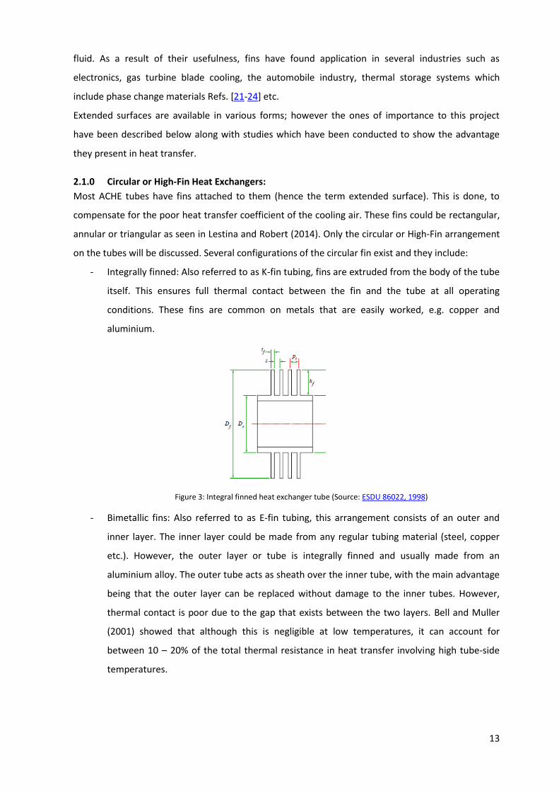
- Integrally finned: Also referred to as K-fin tubing, fins are extruded from the body of the tube

itself. This ensures full thermal contact between the fin and the tube at all operating

conditions. These fins are common on metals that are easily worked, e.g. copper and

aluminium.

Figure 3: Integral finned heat exchanger tube (Source: ESDU 86022, 1998)

- Bimetallic fins: Also referred to as E-fin tubing, this arrangement consists of an outer and

inner layer. The inner layer could be made from any regular tubing material (steel, copper

etc.). However, the outer layer or tube is integrally finned and usually made from an

aluminium alloy. The outer tube acts as sheath over the inner tube, with the main advantage

being that the outer layer can be replaced without damage to the inner tubes. However,

thermal contact is poor due to the gap that exists between the two layers. Bell and Muller

(2001) showed that although this is negligible at low temperatures, it can account for

between 10 – 20% of the total thermal resistance in heat transfer involving high tube-side

temperatures.

14

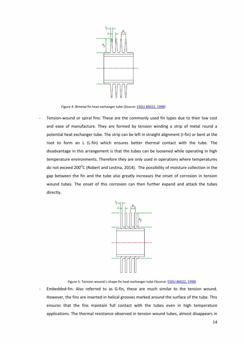
Figure 4: Bimetal fin heat exchanger tube (Source: ESDU 86022, 1998)

- Tension-wound or spiral fins: These are the commonly used fin types due to their low cost

and ease of manufacture. They are formed by tension winding a strip of metal round a

potential heat exchanger tube. The strip can be left in straight alignment (I-fin) or bent at the

root to form an L (L-fin) which ensures better thermal contact with the tube. The

disadvantage in this arrangement is that the tubes can be loosened while operating in high

temperature environments. Therefore they are only used in operations where temperatures

do not exceed 200OC (Robert and Lestina, 2014). The possibility of moisture collection in the

gap between the fin and the tube also greatly increases the onset of corrosion in tension

wound tubes. The onset of this corrosion can then further expand and attack the tubes

directly.

Figure 5: Tension-wound L-shape fin heat exchanger tube (Source: ESDU 86022, 1998)

- Embedded-fin: Also referred to as G-fin, these are much similar to the tension wound.

However, the fins are inserted in helical grooves marked around the surface of the tube. This

ensures that the fins maintain full contact with the tubes even in high temperature

applications. The thermal resistance observed in tension wound tubes, almost disappears in

15

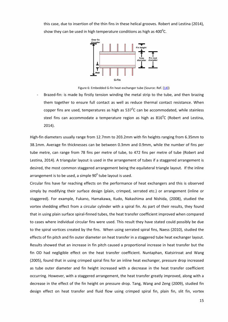
this case, due to insertion of the thin fins in these helical grooves. Robert and Lestina (2014),

show they can be used in high temperature conditions as high as 4000C.

Figure 6: Embedded G-fin heat exchanger tube (Source: Ref. [14])

- Brazed-fin: is made by firstly tension winding the metal strip to the tube, and then brazing

them together to ensure full contact as well as reduce thermal contact resistance. When

copper fins are used, temperatures as high as 5370C can be accommodated, while stainless

steel fins can accommodate a temperature region as high as 8160C (Robert and Lestina,

2014).

High-fin diameters usually range from 12.7mm to 203.2mm with fin heights ranging from 6.35mm to

38.1mm. Average fin thicknesses can be between 0.3mm and 0.9mm, while the number of fins per

tube metre, can range from 78 fins per metre of tube, to 472 fins per metre of tube (Robert and

Lestina, 2014). A triangular layout is used in the arrangement of tubes if a staggered arrangement is

desired, the most common staggered arrangement being the equilateral triangle layout. If the inline

arrangement is to be used, a simple 900 tube layout is used.

Circular fins have far reaching effects on the performance of heat exchangers and this is observed

simply by modifying their surface design (plain, crimped, serrated etc.) or arrangement (inline or

staggered). For example, Fukano, Hamakawa, Kudo, Nakashima and Nishida, (2008), studied the

vortex shedding effect from a circular cylinder with a spiral fin. As part of their results, they found

that in using plain surface spiral-finned tubes, the heat transfer coefficient improved when compared

to cases where individual circular fins were used. This result they have stated could possibly be due

to the spiral vortices created by the fins. When using serrated spiral fins, Naess (2010), studied the

effects of fin pitch and fin outer diameter on heat transfer in a staggered tube heat exchanger layout.

Results showed that an increase in fin pitch caused a proportional increase in heat transfer but the

fin OD had negligible effect on the heat transfer coefficient. Nuntaphan, Kiatsiriroat and Wang

(2005), found that in using crimped spiral fins for an inline heat exchanger, pressure drop increased

as tube outer diameter and fin height increased with a decrease in the heat transfer coefficient

occurring. However, with a staggered arrangement, the heat transfer greatly improved, along with a

decrease in the effect of the fin height on pressure drop. Tang, Wang and Zeng (2009), studied fin

design effect on heat transfer and fluid flow using crimped spiral fin, plain fin, slit fin, vortex

16

generator fins (with longitudinal delta wings) and mixed fin (6 front row vortex generators and 6-rear

row slit fins). Observations showed that the crimped spiral fin provided better heat transfer and

pressure drop than the other fin designs. Using L-footed spiral fins, Tang, Wang and Zeng, (2009), as

well as Pikulkajorn, Pongsoi, and Wongwises, (2013), studied the effect of the fin outside diameter

and pitches on a heat exchanger with a multi-pass parallel and counter cross-flow at high air-side

Reynolds numbers. Observations indicated that fin pitch had negligible effect on the air-side heat

transfer coefficient and Colburn factor, but significantly featured on the rate of heat transfer,

pressure drop across the heat exchanger and the frictional factor. Observations also showed that fin

OD had a significant effect on the pressure drop, as it increased proportionally with the former.

Kiatpachai, Pikulkajorn and Wongwises (2015) also studied the impact serrated welded spiral fins had

on heat transfer. Their observations showed that fin pitch had a significant impact on both the heat

transfer coefficient and the Colburn factor (j) at high Reynolds numbers. Pressure drop was also

found to increase as fin pitch increased. They concluded that serrated welded spiral fins produced

higher Colburn factors and frictional factors than any other circular fin. In contrast, Anoop, Balaji, and

Velusamy (2015) studied the heat transfer properties of serrated finned tubes and conclusions

showed that serrating the fins did not show any improvement to heat transfer when compared to

the solid fins. The only advantage they state is the reduction in weight of the heat exchanger as a

result of the fin serrations. Cho, Ha, Jung, and Lee (2012) studied the effect of punching holes directly

on the circular fins. For 2-hole punched fins, heat transfer improved by 3.55% while for the 4-hole

punched fins, heat transfer improved by 3.31%. As for pressure drop, an increase of 0.68% and 2.08%

was observed in the 2-hole and 4-hole fins respectively. They attributed the improvement in the heat

transfer coefficient to the presence of holes on the fins which reduced the effect of recirculation

zones created at flow separation regions on the fins. Joo, Kang, Kim, and Lee, (2011), studied the

heat transfer properties of a spiral coiled finned tube under frost conditions by varying the fin pitch

and number of tube rows in the heat exchanger. Their observations showed that pressure drop per

unit increase in tube length, increased as the fin pitch increased. They also showed that the rate of

heat transfer increased as fin pitch decreased and number of tube rows increased. The latter, they

attributed to the increase in available heat transfer surface area.

To indicate the effectiveness of a solid circular fin in transferring heat in a given application, the term

fin efficiency is used. It follows the form as indicated by McQuiston, and Tree (1972) for fins with

plane parallel sides on a flat surface with mean thickness:

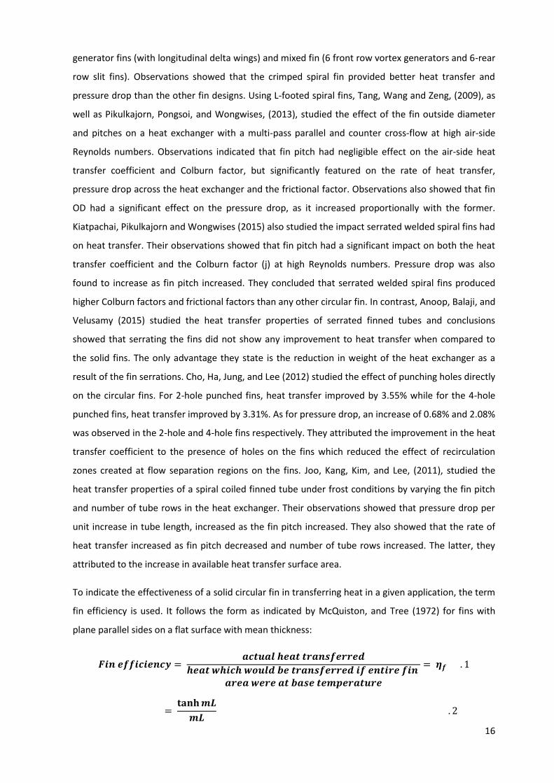
𝑭𝒊𝒏 𝒆𝒇𝒇𝒊𝒄𝒊𝒆𝒏𝒄𝒚 = 𝒂𝒄𝒕𝒖𝒂𝒍 𝒉𝒆𝒂𝒕 𝒕𝒓𝒂𝒏𝒔𝒇𝒆𝒓𝒓𝒆𝒅

𝒉𝒆𝒂𝒕 𝒘𝒉𝒊𝒄𝒉 𝒘𝒐𝒖𝒍𝒅 𝒃𝒆 𝒕𝒓𝒂𝒏𝒔𝒇𝒆𝒓𝒓𝒆𝒅 𝒊𝒇 𝒆𝒏𝒕𝒊𝒓𝒆 𝒇𝒊𝒏 𝒂𝒓𝒆𝒂 𝒘𝒆𝒓𝒆 𝒂𝒕 𝒃𝒂𝒔𝒆 𝒕𝒆𝒎𝒑𝒆𝒓𝒂𝒕𝒖𝒓𝒆

= 𝜼𝒇 . 1

= 𝐭𝐚𝐧𝐡 𝒎𝑳

𝒎𝑳 . 2

17

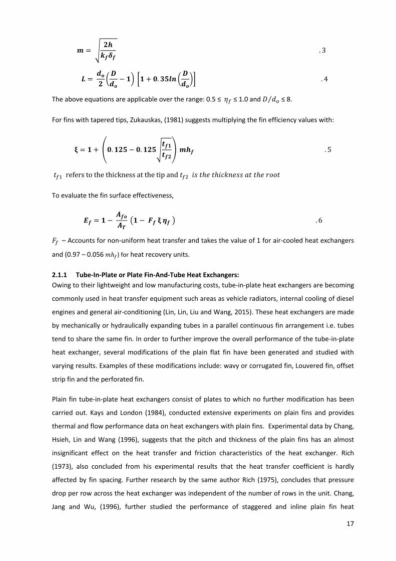
𝒎 = √𝟐𝒉

𝒌𝒇𝜹𝒇 . 3

𝑳 = 𝒅𝒐

𝟐(

𝑫

𝒅𝒐− 𝟏) [𝟏 + 𝟎. 𝟑𝟓𝒍𝒏 (

𝑫

𝒅𝒐)] . 4

The above equations are applicable over the range: 0.5 ≤ 𝜂𝑓 ≤ 1.0 and 𝐷 𝑑𝑜⁄ ≤ 8.

For fins with tapered tips, Zukauskas, (1981) suggests multiplying the fin efficiency values with:

𝛏 = 𝟏 + (𝟎. 𝟏𝟐𝟓 − 𝟎. 𝟏𝟐𝟓√𝒕𝒇𝟏

𝒕𝒇𝟐) 𝒎𝒉𝒇 . 5

𝑡𝑓1 refers to the thickness at the tip and 𝑡𝑓2 𝑖𝑠 𝑡ℎ𝑒 𝑡ℎ𝑖𝑐𝑘𝑛𝑒𝑠𝑠 𝑎𝑡 𝑡ℎ𝑒 𝑟𝑜𝑜𝑡

To evaluate the fin surface effectiveness,

𝑬𝒇 = 𝟏 − 𝑨𝒇𝒐

𝑨𝑻 (𝟏 − 𝑭𝒇 𝛏 𝜼𝒇 ) . 6

𝐹𝑓 – Accounts for non-uniform heat transfer and takes the value of 1 for air-cooled heat exchangers

and (0.97 – 0.056 𝑚ℎ𝑓) for heat recovery units.

2.1.1 Tube-In-Plate or Plate Fin-And-Tube Heat Exchangers:

Owing to their lightweight and low manufacturing costs, tube-in-plate heat exchangers are becoming

commonly used in heat transfer equipment such areas as vehicle radiators, internal cooling of diesel

engines and general air-conditioning (Lin, Lin, Liu and Wang, 2015). These heat exchangers are made

by mechanically or hydraulically expanding tubes in a parallel continuous fin arrangement i.e. tubes

tend to share the same fin. In order to further improve the overall performance of the tube-in-plate

heat exchanger, several modifications of the plain flat fin have been generated and studied with

varying results. Examples of these modifications include: wavy or corrugated fin, Louvered fin, offset

strip fin and the perforated fin.

Plain fin tube-in-plate heat exchangers consist of plates to which no further modification has been

carried out. Kays and London (1984), conducted extensive experiments on plain fins and provides

thermal and flow performance data on heat exchangers with plain fins. Experimental data by Chang,

Hsieh, Lin and Wang (1996), suggests that the pitch and thickness of the plain fins has an almost

insignificant effect on the heat transfer and friction characteristics of the heat exchanger. Rich

(1973), also concluded from his experimental results that the heat transfer coefficient is hardly

affected by fin spacing. Further research by the same author Rich (1975), concludes that pressure

drop per row across the heat exchanger was independent of the number of rows in the unit. Chang,

Jang and Wu, (1996), further studied the performance of staggered and inline plain fin heat

18

exchangers and concluded that the heat transfer coefficient for staggered tube arrangements,

surpassed that for inline tube arrangement by as much as 15 – 27% while the pressure drop of the

former exceeding that of the latter by as much as 20 – 25%. Their observations also showed that

beyond four rows, the heat exchanger had very little improvement in terms of the heat transfer

coefficient. Abu Madi, Heikal and Johns (1998), studied the effects of flat and corrugated fins along

with variations in number of tube rows, fin pitch and fin thickness on a heat exchangers. Their results

showed that number of rows had an insignificant effect on the heat exchanger friction factor and

that the Colburn factor (j) increased with a decrease in fin thickness. They also found that the

thickness of the fin had very little effect on the friction factor of the heat exchanger. In a bid to

further improve the efficiency of the plain fin, Jacobi and Joardar (2006), studied the effect of using

winglet type vortex generators on plain fins in an inline heat exchanger bundle. They found that by

using 3 vortex generators on alternating tube rows, the Colburn factor (j) in the inline heat exchanger

improved by as much as 74% but however caused an increase in the pressure drop of about 41%.

Jacobi and Joardar (2008) also analysed the same effect under dry conditions for single and three-

row heat exchangers. Observations showed that for the single row unit, heat transfer coefficient

improved from 16.5% to 44%, with a pressure drop of less than 12%. For the three-row unit, heat

transfer improved from 29.9% to 68.8%; however a penalty was paid in the increase in pressure drop

observed that rose from 26% to 87.5%. ElSherbini, and Jacobi (2011), studied the impact of vortex

generators for a conventional refrigerator evaporator. They omitted punching the vortex generators

on the first row of the heat exchanger. Results showed that the Colburn factor improved by up to

31% without any serious pressure drop consequences.

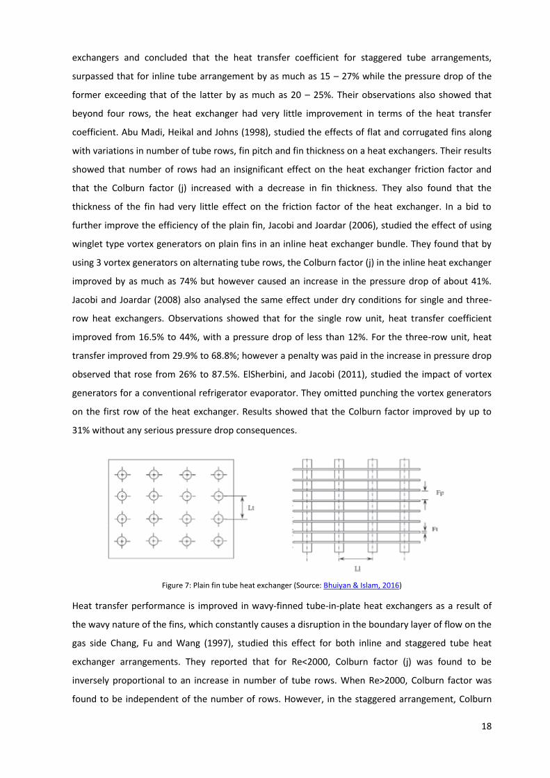
Figure 7: Plain fin tube heat exchanger (Source: Bhuiyan & Islam, 2016)

Heat transfer performance is improved in wavy-finned tube-in-plate heat exchangers as a result of

the wavy nature of the fins, which constantly causes a disruption in the boundary layer of flow on the

gas side Chang, Fu and Wang (1997), studied this effect for both inline and staggered tube heat

exchanger arrangements. They reported that for Re<2000, Colburn factor (j) was found to be

inversely proportional to an increase in number of tube rows. When Re>2000, Colburn factor was

found to be independent of the number of rows. However, in the staggered arrangement, Colburn

19

factor (j) only reduced slightly when Re<900 and number of tube rows was increased. When Re>900,

(j) increased rapidly with every increase in number of tube rows. To explain this phenomenon, they

state that at low Reynold numbers, the thermal boundary layer formed along the wavy fin, tends to

grow and deter heat transfer. However, at much higher Reynold numbers, a disruption in the

boundary layer occurs which enhances the process of heat transferred. Factors which affect the heat

transfer performance of wavy fins tend to be mostly geometrical and include the wave pitch,

corrugation angle and the fin spacing. Chang, Du, Tao and Wang (1999), studied the extent of effect

these parameters have on frictional factors and the Colburn factor (j) for herringbone wavy finned

heat exchangers under wet conditions. Results showed that the frictional factor decreased as the fin

pitch increased and got stronger as tube rows increased. Colburn factor (j) was found to increase as

fin pitch and row number increased.

Figure 8: Wavy fin tube heat exchanger (Source: Bhuiyan & Islam, 2016)

In the offset strip tube-in-plate heat exchangers, improvement in heat transfer performance is

achieved as a result of the boundary layers formed along the length of the offset strips. These

boundary layers are then further disrupted as they pass between the gaps in the strips. In

experimental data provided by Kays and London (1984), the thermal and flow performance of wavy

finned tube-in-plate heat exchangers, is found to be very similar to that of the offset strip tube-in-

plate heat exchanger. In comparison to the plain fin, the offset strip fins were found to have a

Colburn factor, j, with a value 2.5 times greater. Their research data also showed that heat transfer

increased by 150% and friction by 83% when offset strip fins were compared to plain fins.

Figure 9: Offset strip fin tube heat exchanger (Source: Bhuiyan & Islam, 2016)

20

Louver-fins bear a similarity in terms of manufacture to the offset-fins. The only difference being that

the slit fins are not offset like the offset strips; they are rather rotated 20-450 relative to the direction

of air flow. Sheen and Yan (2000) observed that at the same Reynolds number, the Louver-fin had a

higher Colburn factor (j) and frictional factor (f) when compared with the plain fin tube-in-plate heat

exchanger.

Perforated fins are made by perforating even spaced slots or holes in a plain fin. The punched fins are

then folded to a V-shape to create flow channels. Improvement in heat transfer performance is thus

achieved by the boundary layer disturbance caused by the punched holes. Shah (1975) showed that

the heat transfer performance of these fins were less than that of the offset-strip fins. Shah (1975)

also suggests that this factor, combined with high levels of material waste generated during

manufacture has made these fins unpopular with heat exchanger manufacturers.

21

Chapter 3

Convective Heat Transfer Coefficient for Forced Convection Heat Transfer

3.1 Introduction:

This chapter is a summary of the literature review conducted to determine correlations to use in

evaluating the convective heat transfer coefficient for both the gas-side and the tube-side of the heat

exchanger. The review covered the types of heat exchangers under consideration: Circular-fin, Tube-

in Plate and Plain tube exchangers.

A summary of correlations used to evaluate the geometrical properties of the heat exchanger is also

presented. The correlations reviewed and presented, also cover the circular-fin, tube-in-plate and

plain tube heat exchangers.

3.2 Empirical evaluation of the heat transfer coefficient:

In the preceding chapters, the convective heat transfer coefficient ‘h’ was identified as the most

important factor in the convection heat transfer equation as it defines the process through which

heat is conveyed by the motion of the fluid. However, due to its dependency on characteristics such

as geometry, fluid thermal properties and process conditions, no single value or constant can be

assigned to define it.

Holman (1992) provides the analytical process through which ‘h’ can be evaluated. Unfortunately,

due to the time consuming efforts required and the constantly changing conditions experienced in

fluid flow, the use of these analytical methods in the design of heat exchangers will not always be

practical. Therefore, the designer is forced to resort to the use of experimental data expressed in the

form of empirical equations or graphical charts. These equations are usually evaluated at the bulk

temperature of the fluid and are found to give a good level of accuracy if used within the parameters

they were developed from.

The Nusselt number (Nu) defined as the ratio of convective heat transfer to conduction heat transfer

is expressed in the equation below and is used to evaluate the convective heat transfer coefficient.

𝑵𝒖 = 𝒉

𝒌 𝒅𝒉⁄ . 7

Depending on flow conditions, the relationship of the Nusselt number to fluid flow condition varies.

In laminar flow, it is found to be strongly reliant on both the geometry of the flow passage and the

thermal boundary formed by the fluid. However, Sekulić and Shah (2003) indicate that for fully

developed turbulent flow, it is found to depend on the Reynolds and Prandtl number of the fluid.

Several forms of the Nusselt number – Reynolds & Prandtl number relationship exist for both internal

and external fluid flow. Some of these relationships are described below.

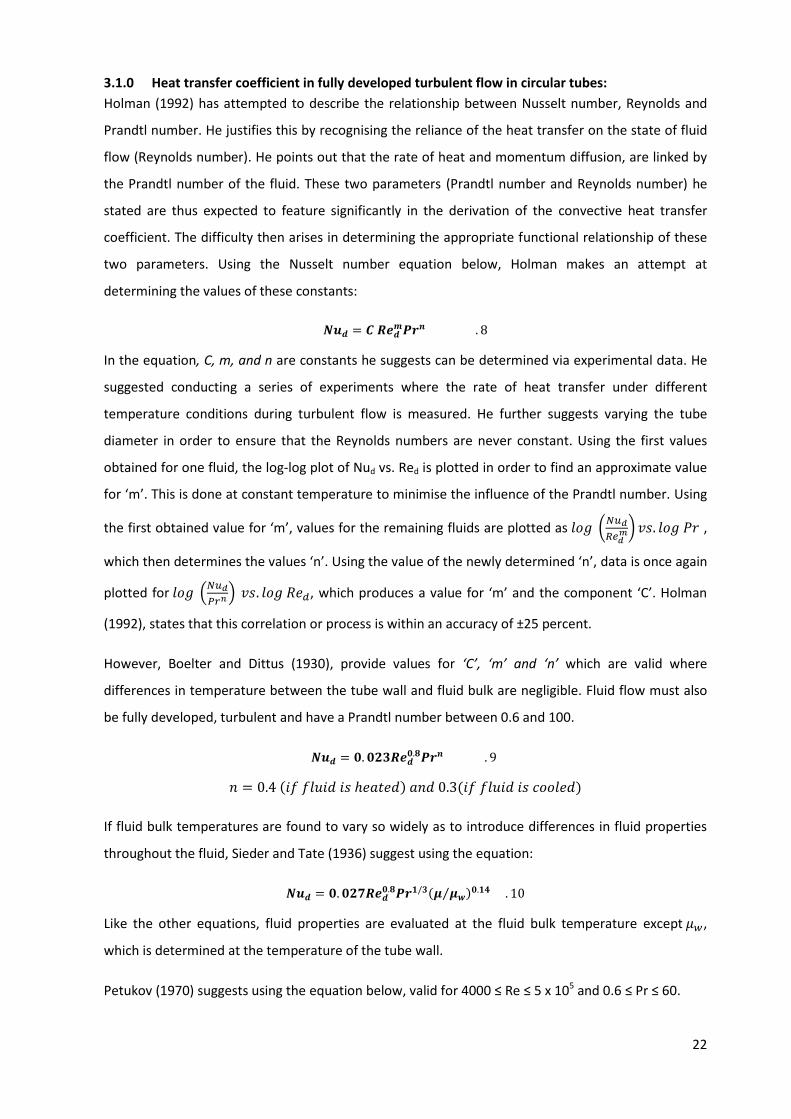
22

3.1.0 Heat transfer coefficient in fully developed turbulent flow in circular tubes:

Holman (1992) has attempted to describe the relationship between Nusselt number, Reynolds and

Prandtl number. He justifies this by recognising the reliance of the heat transfer on the state of fluid

flow (Reynolds number). He points out that the rate of heat and momentum diffusion, are linked by

the Prandtl number of the fluid. These two parameters (Prandtl number and Reynolds number) he

stated are thus expected to feature significantly in the derivation of the convective heat transfer

coefficient. The difficulty then arises in determining the appropriate functional relationship of these

two parameters. Using the Nusselt number equation below, Holman makes an attempt at

determining the values of these constants:

𝑵𝒖𝒅 = 𝑪 𝑹𝒆𝒅𝒎𝑷𝒓𝒏 . 8

In the equation, C, m, and n are constants he suggests can be determined via experimental data. He

suggested conducting a series of experiments where the rate of heat transfer under different

temperature conditions during turbulent flow is measured. He further suggests varying the tube

diameter in order to ensure that the Reynolds numbers are never constant. Using the first values

obtained for one fluid, the log-log plot of Nud vs. Red is plotted in order to find an approximate value

for ‘m’. This is done at constant temperature to minimise the influence of the Prandtl number. Using

the first obtained value for ‘m’, values for the remaining fluids are plotted as 𝑙𝑜𝑔 (𝑁𝑢𝑑

𝑅𝑒𝑑𝑚) 𝑣𝑠. 𝑙𝑜𝑔 𝑃𝑟 ,

which then determines the values ‘n’. Using the value of the newly determined ‘n’, data is once again

plotted for 𝑙𝑜𝑔 (𝑁𝑢𝑑

𝑃𝑟𝑛 ) 𝑣𝑠. 𝑙𝑜𝑔 𝑅𝑒𝑑, which produces a value for ‘m’ and the component ‘C’. Holman

(1992), states that this correlation or process is within an accuracy of ±25 percent.

However, Boelter and Dittus (1930), provide values for ‘C’, ‘m’ and ‘n’ which are valid where

differences in temperature between the tube wall and fluid bulk are negligible. Fluid flow must also

be fully developed, turbulent and have a Prandtl number between 0.6 and 100.

𝑵𝒖𝒅 = 𝟎. 𝟎𝟐𝟑𝑹𝒆𝒅𝟎.𝟖𝑷𝒓𝒏 . 9

𝑛 = 0.4 (𝑖𝑓 𝑓𝑙𝑢𝑖𝑑 𝑖𝑠 ℎ𝑒𝑎𝑡𝑒𝑑) 𝑎𝑛𝑑 0.3(𝑖𝑓 𝑓𝑙𝑢𝑖𝑑 𝑖𝑠 𝑐𝑜𝑜𝑙𝑒𝑑)

If fluid bulk temperatures are found to vary so widely as to introduce differences in fluid properties

throughout the fluid, Sieder and Tate (1936) suggest using the equation:

𝑵𝒖𝒅 = 𝟎. 𝟎𝟐𝟕𝑹𝒆𝒅𝟎.𝟖𝑷𝒓𝟏/𝟑(𝝁 𝝁𝒘⁄ )𝟎.𝟏𝟒 . 10

Like the other equations, fluid properties are evaluated at the fluid bulk temperature except 𝜇𝑤,

which is determined at the temperature of the tube wall.

Petukov (1970) suggests using the equation below, valid for 4000 ≤ Re ≤ 5 x 105 and 0.6 ≤ Pr ≤ 60.

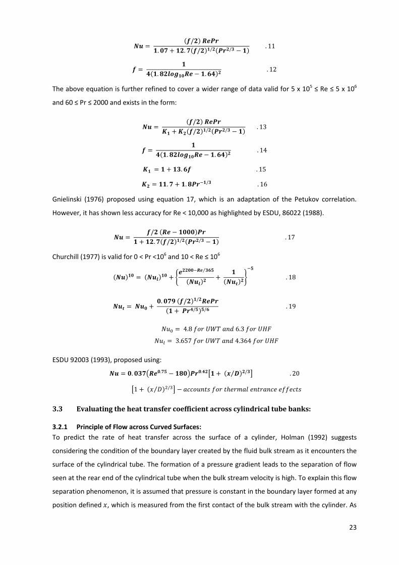
23

𝑵𝒖 = (𝒇/𝟐) 𝑹𝒆𝑷𝒓

𝟏. 𝟎𝟕 + 𝟏𝟐. 𝟕(𝒇/𝟐)𝟏/𝟐(𝑷𝒓𝟐/𝟑 − 𝟏) . 11

𝒇 = 𝟏

𝟒(𝟏. 𝟖𝟐𝒍𝒐𝒈𝟏𝟎𝑹𝒆 − 𝟏. 𝟔𝟒)𝟐 . 12

The above equation is further refined to cover a wider range of data valid for 5 x 105 ≤ Re ≤ 5 x 106

and 60 ≤ Pr ≤ 2000 and exists in the form:

𝑵𝒖 = (𝒇/𝟐) 𝑹𝒆𝑷𝒓

𝑲𝟏 + 𝑲𝟐(𝒇/𝟐)𝟏/𝟐(𝑷𝒓𝟐/𝟑 − 𝟏) . 13

𝒇 = 𝟏

𝟒(𝟏. 𝟖𝟐𝒍𝒐𝒈𝟏𝟎𝑹𝒆 − 𝟏. 𝟔𝟒)𝟐 . 14

𝑲𝟏 = 𝟏 + 𝟏𝟑. 𝟔𝒇 . 15

𝑲𝟐 = 𝟏𝟏. 𝟕 + 𝟏. 𝟖𝑷𝒓−𝟏/𝟑 . 16

Gnielinski (1976) proposed using equation 17, which is an adaptation of the Petukov correlation.

However, it has shown less accuracy for Re < 10,000 as highlighted by ESDU, 86022 (1988).

𝑵𝒖 = 𝒇/𝟐 (𝑹𝒆 − 𝟏𝟎𝟎𝟎)𝑷𝒓

𝟏 + 𝟏𝟐. 𝟕(𝒇/𝟐)𝟏/𝟐(𝑷𝒓𝟐/𝟑 − 𝟏) . 17

Churchill (1977) is valid for 0 < Pr <106 and 10 < Re ≤ 106

(𝑵𝒖)𝟏𝟎 = (𝑵𝒖𝒍)𝟏𝟎 + {

𝒆𝟐𝟐𝟎𝟎−𝑹𝒆 𝟑𝟔𝟓⁄

(𝑵𝒖𝒍)𝟐

+ 𝟏

(𝑵𝒖𝒕)𝟐}

−𝟓

. 18

𝑵𝒖𝒕 = 𝑵𝒖𝟎 + 𝟎. 𝟎𝟕𝟗 (𝒇/𝟐)𝟏/𝟐𝑹𝒆𝑷𝒓

(𝟏 + 𝑷𝒓𝟒/𝟓)𝟓/𝟔 . 19

𝑁𝑢0 = 4.8 𝑓𝑜𝑟 𝑈𝑊𝑇 𝑎𝑛𝑑 6.3 𝑓𝑜𝑟 𝑈𝐻𝐹

𝑁𝑢𝑙 = 3.657 𝑓𝑜𝑟 𝑈𝑊𝑇 𝑎𝑛𝑑 4.364 𝑓𝑜𝑟 𝑈𝐻𝐹

ESDU 92003 (1993), proposed using:

𝑵𝒖 = 𝟎. 𝟎𝟑𝟕(𝑹𝒆𝟎.𝟕𝟓 − 𝟏𝟖𝟎)𝑷𝒓𝟎.𝟒𝟐[𝟏 + (𝒙 𝑫⁄ )𝟐/𝟑] . 20

[1 + (𝑥 𝐷⁄ )2/3] − 𝑎𝑐𝑐𝑜𝑢𝑛𝑡𝑠 𝑓𝑜𝑟 𝑡ℎ𝑒𝑟𝑚𝑎𝑙 𝑒𝑛𝑡𝑟𝑎𝑛𝑐𝑒 𝑒𝑓𝑓𝑒𝑐𝑡𝑠

3.3 Evaluating the heat transfer coefficient across cylindrical tube banks:

3.2.1 Principle of Flow across Curved Surfaces:

To predict the rate of heat transfer across the surface of a cylinder, Holman (1992) suggests

considering the condition of the boundary layer created by the fluid bulk stream as it encounters the

surface of the cylindrical tube. The formation of a pressure gradient leads to the separation of flow

seen at the rear end of the cylindrical tube when the bulk stream velocity is high. To explain this flow

separation phenomenon, it is assumed that pressure is constant in the boundary layer formed at any

position defined 𝑥, which is measured from the first contact of the bulk stream with the cylinder. As

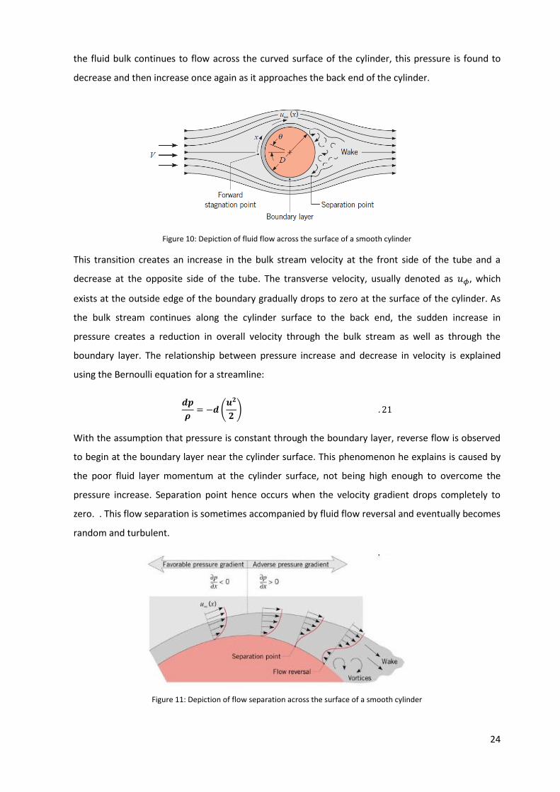
24

the fluid bulk continues to flow across the curved surface of the cylinder, this pressure is found to

decrease and then increase once again as it approaches the back end of the cylinder.

Figure 10: Depiction of fluid flow across the surface of a smooth cylinder

This transition creates an increase in the bulk stream velocity at the front side of the tube and a

decrease at the opposite side of the tube. The transverse velocity, usually denoted as 𝑢𝜙, which

exists at the outside edge of the boundary gradually drops to zero at the surface of the cylinder. As

the bulk stream continues along the cylinder surface to the back end, the sudden increase in

pressure creates a reduction in overall velocity through the bulk stream as well as through the

boundary layer. The relationship between pressure increase and decrease in velocity is explained

using the Bernoulli equation for a streamline:

𝒅𝒑

𝝆= −𝒅 (

𝒖𝟐

𝟐) . 21

With the assumption that pressure is constant through the boundary layer, reverse flow is observed

to begin at the boundary layer near the cylinder surface. This phenomenon he explains is caused by

the poor fluid layer momentum at the cylinder surface, not being high enough to overcome the

pressure increase. Separation point hence occurs when the velocity gradient drops completely to

zero. . This flow separation is sometimes accompanied by fluid flow reversal and eventually becomes

random and turbulent.

Figure 11: Depiction of flow separation across the surface of a smooth cylinder

25

The consequences of flow separation and flow reversal will clearly influence the rate of convective

heat transfer between the cylindrical surface and the bulk stream as a result of the turbulence

created. The extent of this influence was studied by Giedt (1949) for heat transferred from a heated

tube to free air. His results showed that minimum values for the heat transfer coefficient occurred at

Reynolds numbers between 70,800 and 101,300, which corresponded to the point at which flow

separation occurred. At the opposite end of the tube, an increase in the heat transfer coefficient

occurred as a result of the flow turbulence created. At even higher Reynolds numbers, he recorded 2

minimum values. The first occurring when flow transited from laminar to turbulent in the boundary

layer and the second minimum was record at the point when the turbulent boundary layer

separated. Heat transfer was found to increase rapidly when the boundary layer became turbulent

and also when eddy motion occurred during flow separation.

Due to the complexity of the flow phenomenon described earlier, it is somewhat difficult and

complicated to analytically evaluate the heat transfer coefficient for cases of flow over cylindrical

surfaces. However, as also stated earlier, correlations of experimental data exist which can be

applied with acceptable levels of success. For example, Drake and Eckert (1972) developed the

equations below to evaluate the heat transfer coefficient in cross-flow from a heated tube to air:

𝑵𝒖 = (𝟎. 𝟒𝟑 + 𝟎. 𝟓𝟎𝑹𝒆𝟎.𝟓) 𝑷𝒓𝟎.𝟑𝟖 (𝑷𝒓𝒇

𝑷𝒓𝒘

)𝟎.𝟐𝟓

𝒂𝒑𝒑𝒍𝒊𝒄𝒂𝒃𝒍𝒆 𝒐𝒗𝒆𝒓 𝒕𝒉𝒆 𝒓𝒂𝒏𝒈𝒆 𝟏 < 𝑹𝒆

< 𝟏𝟎𝟑 . 22

𝑵𝒖 = (𝟎. 𝟐𝟓 𝑹𝒆𝟎.𝟔𝑷𝒓𝟎.𝟑𝟖) (𝑷𝒓𝒇

𝑷𝒓𝒘

)𝟎.𝟐𝟓

𝒂𝒑𝒑𝒍𝒊𝒄𝒂𝒃𝒍𝒆 𝒐𝒗𝒆𝒓 𝒕𝒉𝒆 𝒓𝒂𝒏𝒈𝒆 𝟏𝟎𝟑 < 𝑹𝒆

< 𝟐 𝒙𝟏𝟎𝟓 . 23

Bernstein and Churchill (1977) also produced a correlation applicable over a large range of data:

𝑵𝒖𝒅 𝒇 = 𝟎. 𝟑 + 𝟎. 𝟔𝟐 𝑹𝒆𝒇

𝟏/𝟐𝑷𝒓𝒇

𝟏/𝟑

[𝟏 + (𝟎. 𝟒𝑷𝒓𝒇

)𝟐/𝟑

]

𝟏/𝟒 [𝟏 + (

𝑹𝒆𝒇

𝟐𝟖𝟐, 𝟎𝟎𝟎)

𝟓/𝟖

]

𝟒/𝟓

𝒇𝒐𝒓 𝟏𝟎𝟐 < 𝑹𝒆𝒅 < 𝟏𝟎𝟕; 𝑷𝒆𝒅 > 𝟎. 𝟐 . 24

This equation was further modified to produce better accuracy and cover a larger range of data:

𝑵𝒖𝒅 𝒇 = 𝟎. 𝟑 + 𝟎. 𝟔𝟐 𝑹𝒆𝒅

𝟏/𝟐𝑷𝒓𝒇

𝟏/𝟑

[𝟏 + (𝟎. 𝟒𝑷𝒓𝒇

)𝟐/𝟑

]

𝟏/𝟒[𝟏 + (

𝑹𝒆𝒅

𝟐𝟖𝟐, 𝟎𝟎𝟎)

𝟏/𝟐

] 𝟐𝟎, 𝟎𝟎𝟎 < 𝑹𝒆𝒅 < 𝟒𝟎𝟎, 𝟎𝟎𝟎; 𝑷𝒆𝒅

> 𝟎. 𝟐 . 25

Nakai and Okazaki (1975), proposed using:

𝑵𝒖𝒅 𝒇 = [𝟎. 𝟖𝟐𝟑𝟕 − 𝒍𝒏(𝑷𝒆𝒅𝟏/𝟐

)]−𝟏

𝑷𝒆𝒅 > 𝟎. 𝟐 . 26

Fluid properties in the equations above are evaluated at the film temperature and Ped = 0.2.

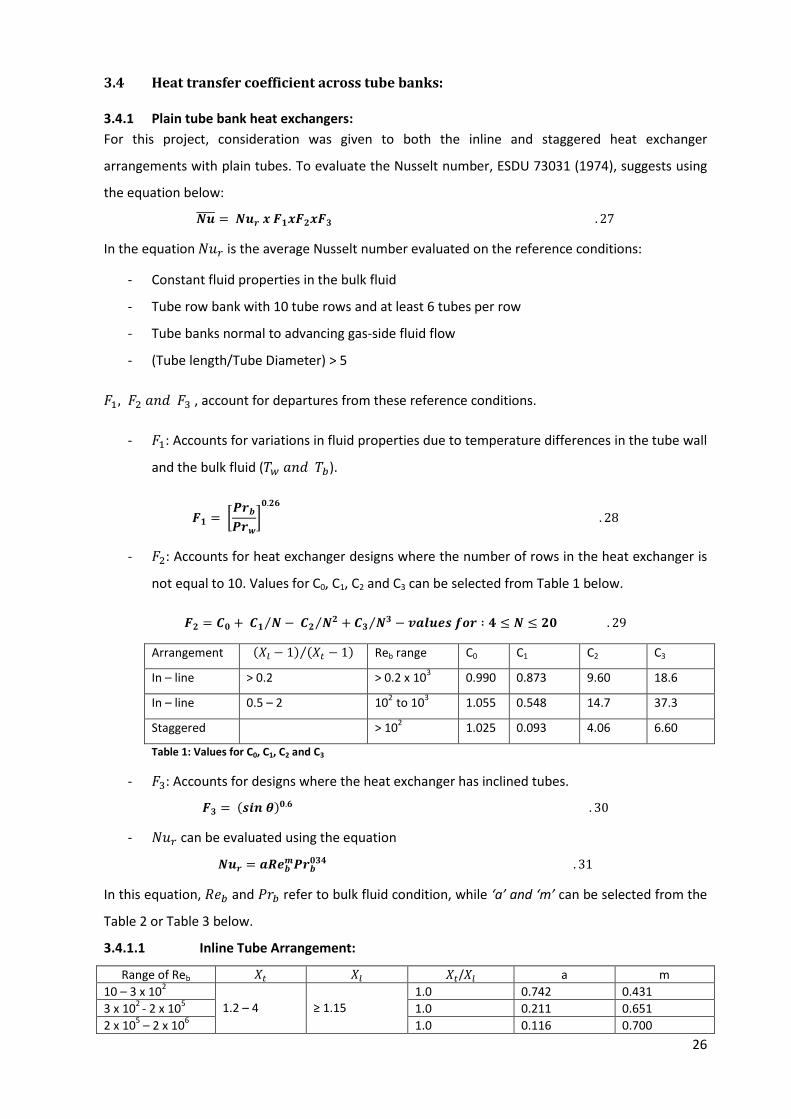
26

3.4 Heat transfer coefficient across tube banks:

3.4.1 Plain tube bank heat exchangers:

For this project, consideration was given to both the inline and staggered heat exchanger

arrangements with plain tubes. To evaluate the Nusselt number, ESDU 73031 (1974), suggests using

the equation below:

𝑵𝒖̅̅ ̅̅ = 𝑵𝒖𝒓 𝒙 𝑭𝟏𝒙𝑭𝟐𝒙𝑭𝟑 . 27

In the equation 𝑁𝑢𝑟 is the average Nusselt number evaluated on the reference conditions:

- Constant fluid properties in the bulk fluid

- Tube row bank with 10 tube rows and at least 6 tubes per row

- Tube banks normal to advancing gas-side fluid flow

- (Tube length/Tube Diameter) > 5

𝐹1, 𝐹2 𝑎𝑛𝑑 𝐹3 , account for departures from these reference conditions.

- 𝐹1: Accounts for variations in fluid properties due to temperature differences in the tube wall

and the bulk fluid (𝑇𝑤 𝑎𝑛𝑑 𝑇𝑏).

𝑭𝟏 = [𝑷𝒓𝒃

𝑷𝒓𝒘

]𝟎.𝟐𝟔

. 28

- 𝐹2: Accounts for heat exchanger designs where the number of rows in the heat exchanger is

not equal to 10. Values for C0, C1, C2 and C3 can be selected from Table 1 below.

𝑭𝟐 = 𝑪𝟎 + 𝑪𝟏 𝑵⁄ − 𝑪𝟐 𝑵𝟐⁄ + 𝑪𝟑 𝑵𝟑⁄ − 𝒗𝒂𝒍𝒖𝒆𝒔 𝒇𝒐𝒓 ∶ 𝟒 ≤ 𝑵 ≤ 𝟐𝟎 . 29

Arrangement (𝑋𝑙 − 1) (𝑋𝑡 − 1)⁄ Reb range C0 C1 C2 C3

In – line > 0.2 > 0.2 x 103 0.990 0.873 9.60 18.6

In – line 0.5 – 2 102

to 103 1.055 0.548 14.7 37.3

Staggered > 102 1.025 0.093 4.06 6.60

Table 1: Values for C0, C1, C2 and C3

- 𝐹3: Accounts for designs where the heat exchanger has inclined tubes.

𝑭𝟑 = (𝒔𝒊𝒏 𝜽)𝟎.𝟔 . 30

- 𝑁𝑢𝑟 can be evaluated using the equation

𝑵𝒖𝒓 = 𝒂𝑹𝒆𝒃𝒎𝑷𝒓𝒃

𝟎𝟑𝟒 . 31

In this equation, 𝑅𝑒𝑏 and 𝑃𝑟𝑏 refer to bulk fluid condition, while ‘a’ and ‘m’ can be selected from the

Table 2 or Table 3 below.

3.4.1.1 Inline Tube Arrangement:

Range of Reb 𝑋𝑡 𝑋𝑙 𝑋𝑡/𝑋𝑙 a m

10 – 3 x 102

1.2 – 4 ≥ 1.15

1.0 0.742 0.431

3 x 102

- 2 x 105 1.0 0.211 0.651

2 x 105 – 2 x 10

6 1.0 0.116 0.700

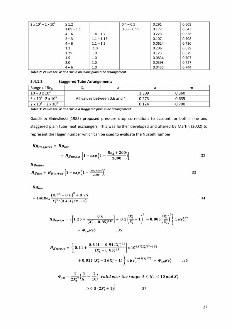
27

2 x 102 – 2 x 10

5 ≥ 1.2

1.05 – 1.1 4 – 6 2 – 3 4 – 6 1.1 1.25 1.5 2.0 4 – 6

1.4 – 1.7 1.1 – 1.15 1.1 – 1.2 1.0 1.0 1.0 1.0 1.0

0.4 – 0.5 0.35 – 0.55

0.291 0.177 0.223 0.107 0.0624 0.206 0.123 0.0834 0.0593 0.0435

0.609 0.643 0.626 0.708 0.730 0.639 0.679 0.707 0.727 0.744

Table 2: Values for ‘a’ and ‘m’ in an inline plain tube arrangement

3.4.1.2 Staggered Tube Arrangement:

Range of Reb 𝑋𝑡 𝑋𝑙 a m

10 – 3 x 102 All values between 0.6 and 4

1.309 0.360

3 x 102 - 2 x 105 0.273 0.635

2 x 105 – 2 x 106 0.124 0.700 Table 3: Values for ‘a’ and ‘m’ in a staggered plain tube arrangement

Gaddis & Gnieslinski (1985) proposed pressure drop correlations to account for both inline and

staggered plain tube heat exchangers. This was further developed and altered by Martin (2002) to

represent the Hagen number which can be used to evaluate the Nusselt number:

𝑯𝒈𝒔𝒕𝒂𝒈𝒈𝒆𝒓𝒆𝒅 = 𝑯𝒈𝒍𝒂𝒎

+ 𝑯𝒈𝒕𝒖𝒓𝒃,𝒔𝒕 [𝟏 − 𝒆𝒙𝒑 (𝟏 − 𝑹𝒆𝒅 + 𝟐𝟎𝟎

𝟏𝟎𝟎𝟎)] . 32

𝑯𝒈𝒊𝒏𝒍𝒊𝒏𝒆 =

𝑯𝒈𝒍𝒂𝒎 + 𝑯𝒈𝒕𝒖𝒓𝒃,𝒊𝒏 [𝟏 − 𝒆𝒙𝒑 (𝟏 − 𝑹𝒆𝒅+𝟐𝟎𝟎

𝟐𝟎𝟎𝟎)] . 33

𝑯𝒈𝒍𝒂𝒎

= 𝟏𝟒𝟎𝑹𝒆𝒅

(𝑿𝒍∗𝟎.𝟓 − 𝟎. 𝟔)

𝟐+ 𝟎. 𝟕𝟓

𝑿𝒕∗𝟏.𝟔(𝟒 𝑿𝒕

∗𝑿𝒍∗ 𝝅⁄ − 𝟏)

. 34

𝑯𝒈𝒕𝒖𝒓𝒃,𝒔𝒕 = {[𝟏. 𝟐𝟓 + 𝟎. 𝟔

(𝑿𝒕∗ − 𝟎. 𝟖𝟓)𝟏.𝟎𝟖

] + 𝟎. 𝟐 (𝑿𝒍

∗

𝑿𝒕∗ − 𝟏)

𝟑

− 𝟎. 𝟎𝟎𝟓 (𝑿𝒍

∗

𝑿𝒕∗)

𝟑

} 𝒙 𝑹𝒆𝒅𝟏.𝟕𝟓

+ 𝜱𝒕,𝒏𝑹𝒆𝒅𝟐 . 35

𝑯𝒈𝒕𝒖𝒓𝒃,𝒊𝒏 = {[𝟎. 𝟏𝟏 + 𝟎. 𝟔 (𝟏 − 𝟎. 𝟗𝟒 𝑿𝒍

∗⁄ )𝟎.𝟔

(𝑿𝒕∗ − 𝟎. 𝟖𝟓)𝟏.𝟑

] 𝒙 𝟏𝟎𝟎.𝟒𝟕(𝑿𝒍∗ 𝑿𝒕

∗⁄ −𝟏.𝟓)

+ 𝟎. 𝟎𝟏𝟓 (𝑿𝒕∗ − 𝟏)(𝑿𝒍

∗ − 𝟏) } 𝒙 𝑹𝒆𝒅

𝟐−𝟎.𝟏(𝑿𝒍∗ 𝑿𝒕

∗⁄ )+ 𝜱𝒕,𝒏𝑹𝒆𝒅

𝟐 . 36

𝜱𝒕,𝒏 = 𝟏

𝟐𝑿𝒕∗𝟐

(𝟏

𝑵𝒓

− 𝟏

𝟏𝟎) 𝒗𝒂𝒍𝒊𝒅 𝒐𝒗𝒆𝒓 𝒕𝒉𝒆 𝒓𝒂𝒏𝒈𝒆: 𝟓 ≤ 𝑵𝒓 ≤ 𝟏𝟎 𝒂𝒏𝒅 𝑿𝒍

∗

≥ 𝟎. 𝟓 (𝟐𝑿𝒕∗ + 𝟏)

𝟏𝟐 . 37

28

𝜱𝒕,𝒏 = 𝟐 [𝑿𝒅

∗ − 𝟏

𝑿𝒕∗(𝑿𝒕

∗ − 𝟏)]

𝟐

(𝟏

𝑵𝒓

− 𝟏

𝟏𝟎) 𝒗𝒂𝒍𝒊𝒅 𝒐𝒗𝒆𝒓 𝒕𝒉𝒆 𝒓𝒂𝒏𝒈𝒆: 𝟓 ≤ 𝑵𝒓 ≤ 𝟏𝟎 𝒂𝒏𝒅 𝑿𝒍

∗

< 𝟎. 𝟓 (𝟐𝑿𝒕∗ + 𝟏)

𝟏𝟐 . 38

𝜱𝒕,𝒏 = 𝟎 𝒇𝒐𝒓 𝑵𝒓 > 𝟏𝟎 . 39

The Hagen number (𝐻𝑔𝑙𝑎𝑚), is valid for inline as well as staggered tube bundles except Xt*1.6 changes

to Xd*1.6 for staggered tube arrangements.

Both 𝐻𝑔𝑠𝑡𝑎𝑔𝑔𝑒𝑟𝑒𝑑 and 𝐻𝑔𝑖𝑛𝑙𝑖𝑛𝑒

, are valid over the ranges, 1≤Red≤300’000, 7.9≤d0≤73mm & Nr≥5 (inline

& staggered arrangement), 1.25≤Xt*≤3.0, 0.6≤Xl

*≤3.0 & Xd*≥1.25, for staggered layout and

1.25≤Xt*≤3.0 & 1.2≤Xl

*≤3.0 for inline layout

𝑳𝒒𝒔𝒕𝒂𝒈𝒈𝒆𝒓𝒆𝒅 = 𝟎. 𝟗𝟐 𝑯𝒈 𝐏𝐫 [(𝟒𝑿𝒕

∗ 𝝅⁄ ) − 𝟏

𝑿𝒅∗ ] 𝒗𝒂𝒍𝒊𝒅 𝒇𝒐𝒓 𝒃𝒖𝒏𝒅𝒍𝒆𝒔 𝒘𝒊𝒕𝒉 𝑿𝒍

∗ ≥ 𝟏 . 40

𝑳𝒒𝒔𝒕𝒂𝒈𝒈𝒆𝒓𝒆𝒅 = 𝟎. 𝟗𝟐 𝑯𝒈 𝐏𝐫 [(𝟒𝑿𝒕

∗𝑿𝒍∗ 𝝅⁄ ) − 𝟏

𝑿𝒍∗𝑿𝒅

∗ ] 𝒗𝒂𝒍𝒊𝒅 𝒇𝒐𝒓 𝒃𝒖𝒏𝒅𝒍𝒆𝒔 𝒘𝒊𝒕𝒉 𝑿𝒍∗ < 𝟏 . 41

𝑳𝒒𝒊𝒏𝒍𝒊𝒏𝒆 = 𝟏. 𝟏𝟖 𝑯𝒈 𝐏𝐫 [(𝟒𝑿𝒕

∗ 𝝅⁄ ) − 𝟏

𝑿𝒍∗ ] . 42

𝑵𝒖𝒔𝒕𝒂𝒈𝒈𝒆𝒓𝒆𝒅 = 𝟎. 𝟒𝟎𝟒𝑳𝒒𝟏/𝟑 . 43

𝑵𝒖𝒊𝒏𝒍𝒊𝒏𝒆 = 𝟎. 𝟒𝟎𝟒𝑳𝒒𝟏𝟑 (

𝑹𝒆𝒅 + 𝟏

𝑹𝒆𝒅 + 𝟏𝟎𝟎𝟎)

𝟎.𝟏

. 44

Nusselt number 𝑁𝑢 is valid over the range:

1≤Red≤2’000’000, 0.7≤Pr≤700, 7.9≤d0≤73mm, 1.02≤Xt*≤3.0, 0.6≤Xl

*≤3.0 and 4≤Nr≤80 for staggered

tube bundles with a 300, 450 or 600 tube layout arrangement. For inline tube bundles, it is valid over

the range2≤Nr≤15.

Using the Nusselt number Nu equation, prediction was within ±14% for staggered tube bundle.

To evaluate the pressure drop across the unit, the equation below is suggested by Sekulić and Shah

(2003), which includes the Hagen number derived from equation 32:

∆𝑷 = 𝝁𝟐

𝝆𝒈𝒄

𝑵𝒓

𝑫𝒐𝟐

𝑯𝒈 . 45

3.4.2 Circular finned tube bank heat exchangers:

Briggs and Young (1963) predicted that for individually finned tubes in a staggered arrangement, the

Colburn factor 𝑗 could be determined using:

𝒋 = 𝟎. 𝟏𝟑𝟒𝑹𝒆𝒅−𝟎.𝟑𝟏𝟗 (

𝒔

𝒍)

𝟎.𝟐

(𝒔

𝜹)

𝟎.𝟏𝟏

. 46

The equation was predicted to cover the ranges: 1100≤Red≤18,000; 0.13 ≤𝑠 𝑙⁄ ≤0.63; 1.01 ≤𝑠 𝛿⁄ ≤7.62;

0.09 ≤𝑙 𝑑𝑜⁄ ≤7.62; 0.011 ≤𝛿 𝑑𝑜⁄ ≤0.15; 1.54≤𝑋𝑡 𝑑𝑜⁄ ≤8.23; 11.1≤do≤40.9mm and 246≤Nf≤768fins/m.

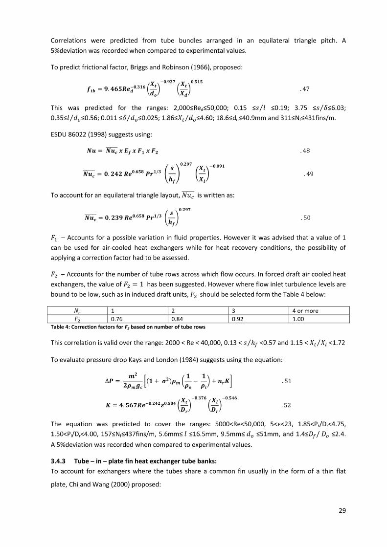
29

Correlations were predicted from tube bundles arranged in an equilateral triangle pitch. A

5%deviation was recorded when compared to experimental values.

To predict frictional factor, Briggs and Robinson (1966), proposed:

𝒇𝒕𝒃 = 𝟗. 𝟒𝟔𝟓𝑹𝒆𝒅−𝟎.𝟑𝟏𝟔 (

𝑿𝒕

𝒅𝒐

)−𝟎.𝟗𝟐𝟕

(𝑿𝒕

𝑿𝒅

)𝟎.𝟓𝟏𝟓

. 47

This was predicted for the ranges: 2,000≤Red≤50,000; 0.15 ≤𝑠 𝑙⁄ ≤0.19; 3.75 ≤𝑠 𝛿⁄ ≤6.03;

0.35≤𝑙 𝑑𝑜⁄ ≤0.56; 0.011 ≤𝛿 𝑑𝑜⁄ ≤0.025; 1.86≤𝑋𝑡 𝑑𝑜⁄ ≤4.60; 18.6≤do≤40.9mm and 311≤Nf≤431fins/m.

ESDU 86022 (1998) suggests using:

𝑵𝒖 = 𝑵𝒖𝒄̅̅ ̅̅ ̅̅ 𝒙 𝑬𝒇 𝒙 𝑭𝟏 𝒙 𝑭𝟐 . 48

𝑵𝒖𝒄̅̅ ̅̅ ̅ = 𝟎. 𝟐𝟒𝟐 𝑹𝒆𝟎.𝟔𝟓𝟖 𝑷𝒓𝟏/𝟑 (𝒔

𝒉𝒇

)

𝟎.𝟐𝟗𝟕

(𝑿𝒕

𝑿𝒍

)−𝟎.𝟎𝟗𝟏

. 49

To account for an equilateral triangle layout, 𝑁𝑢𝑐̅̅ ̅̅ ̅ is written as:

𝑵𝒖𝒄̅̅ ̅̅ ̅̅ = 𝟎. 𝟐𝟑𝟗 𝑹𝒆𝟎.𝟔𝟓𝟖 𝑷𝒓𝟏/𝟑 (

𝒔

𝒉𝒇

)

𝟎.𝟐𝟗𝟕

. 50

𝐹1 – Accounts for a possible variation in fluid properties. However it was advised that a value of 1

can be used for air-cooled heat exchangers while for heat recovery conditions, the possibility of

applying a correction factor had to be assessed.

𝐹2 – Accounts for the number of tube rows across which flow occurs. In forced draft air cooled heat

exchangers, the value of 𝐹2 = 1 has been suggested. However where flow inlet turbulence levels are

bound to be low, such as in induced draft units, 𝐹2 should be selected form the Table 4 below:

𝑁𝑟 1 2 3 4 or more

𝐹2 0.76 0.84 0.92 1.00 Table 4: Correction factors for F2 based on number of tube rows

This correlation is valid over the range: 2000 < Re < 40,000, 0.13 < 𝑠 ℎ𝑓⁄ <0.57 and 1.15 < 𝑋𝑡 𝑋𝑙⁄ <1.72

To evaluate pressure drop Kays and London (1984) suggests using the equation:

∆𝑷 = 𝒎𝟐

𝟐𝝆𝒎𝒈𝒄

[(𝟏 + 𝝈𝟐)𝝆𝒎 (𝟏

𝝆𝒐

− 𝟏

𝝆𝒊

) + 𝒏𝒓𝑲] . 51

𝑲 = 𝟒. 𝟓𝟔𝟕𝑹𝒆−𝟎.𝟐𝟒𝟐𝜺𝟎.𝟓𝟎𝟒 (𝑿𝒕

𝑫𝒓

)−𝟎.𝟑𝟕𝟔

(𝑿𝒍

𝑫𝒓

)−𝟎.𝟓𝟒𝟔

. 52

The equation was predicted to cover the ranges: 5000<Re<50,000, 5<ε<23, 1.85<Pt/Dr<4.75,

1.50<Pl/Dr<4.00, 157≤Nf≤437fins/m, 5.6mm≤ 𝑙 ≤16.5mm, 9.5mm≤ 𝑑𝑜 ≤51mm, and 1.4≤𝐷𝑓/ 𝐷𝑜 ≤2.4.

A 5%deviation was recorded when compared to experimental values.

3.4.3 Tube – in – plate fin heat exchanger tube banks:

To account for exchangers where the tubes share a common fin usually in the form of a thin flat

plate, Chi and Wang (2000) proposed:

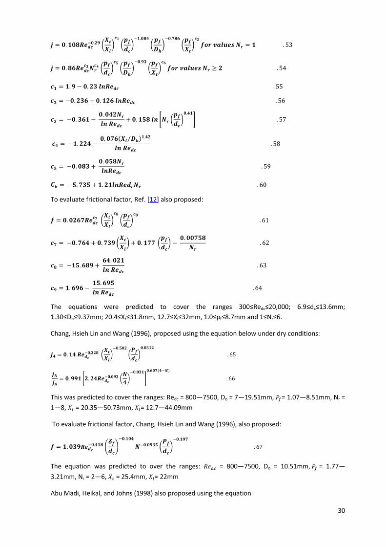
30

𝒋 = 𝟎. 𝟏𝟎𝟖𝑹𝒆𝒅𝒄−𝟎.𝟐𝟗 (

𝑿𝒕

𝑿𝒍

)𝒄𝟏

(𝒑𝒇

𝒅𝒄

)−𝟏.𝟎𝟖𝟒

(𝒑𝒇

𝑫𝒉

)−𝟎.𝟕𝟖𝟔

(𝒑𝒇

𝑿𝒕

)𝒄𝟐

𝒇𝒐𝒓 𝒗𝒂𝒍𝒖𝒆𝒔 𝑵𝒓 = 𝟏 . 53

𝒋 = 𝟎. 𝟖𝟔𝑹𝒆𝒅𝒄𝒄𝟑 𝑵𝒓

𝒄𝟒 (𝒑𝒇

𝒅𝒄

)𝒄𝟓

(𝒑𝒇

𝑫𝒉

)−𝟎.𝟗𝟑

(𝒑𝒇

𝑿𝒕

)𝒄𝟔

𝒇𝒐𝒓 𝒗𝒂𝒍𝒖𝒆𝒔 𝑵𝒓 ≥ 𝟐 . 54

𝒄𝟏 = 𝟏. 𝟗 − 𝟎. 𝟐𝟑 𝒍𝒏𝑹𝒆𝒅𝒄 . 55

𝒄𝟐 = −𝟎. 𝟐𝟑𝟔 + 𝟎. 𝟏𝟐𝟔 𝒍𝒏𝑹𝒆𝒅𝒄 . 56

𝒄𝟑 = −𝟎. 𝟑𝟔𝟏 − 𝟎. 𝟎𝟒𝟐𝑵𝒓

𝒍𝒏 𝑹𝒆𝒅𝒄

+ 𝟎. 𝟏𝟓𝟖 𝒍𝒏 [𝑵𝒓 (𝒑𝒇

𝒅𝒄

)𝟎.𝟒𝟏

] . 57

𝒄𝟒 = −𝟏. 𝟐𝟐𝟒 − 𝟎. 𝟎𝟕𝟔(𝑿𝒍 𝑫𝒉⁄ )𝟏.𝟒𝟐


. 58

𝒄𝟓 = −𝟎. 𝟎𝟖𝟑 + 𝟎. 𝟎𝟓𝟖𝑵𝒓

𝒍𝒏𝑹𝒆𝒅𝒄

. 59

𝑪𝟔 = −𝟓. 𝟕𝟑𝟓 + 𝟏. 𝟐𝟏𝒍𝒏𝑹𝒆𝒅𝒄𝑵𝒓 . 60

To evaluate frictional factor, Ref. [12] also proposed:

𝒇 = 𝟎. 𝟎𝟐𝟔𝟕𝑹𝒆𝒅𝒄𝒄𝟕 (

𝑿𝒕

𝑿𝒍

)𝒄𝟖

(𝒑𝒇

𝒅𝒄

)𝒄𝟖

. 61

𝒄𝟕 = −𝟎. 𝟕𝟔𝟒 + 𝟎. 𝟕𝟑𝟗 (𝑿𝒕

𝑿𝒍

) + 𝟎. 𝟏𝟕𝟕 (𝒑𝒇

𝒅𝒄

) − 𝟎. 𝟎𝟎𝟕𝟓𝟖

𝑵𝒓

. 62

𝒄𝟖 = −𝟏𝟓. 𝟔𝟖𝟗 + 𝟔𝟒. 𝟎𝟐𝟏


. 63

𝒄𝟗 = 𝟏. 𝟔𝟗𝟔 − 𝟏𝟓. 𝟔𝟗𝟓


. 64

The equations were predicted to cover the ranges 300≤Redc≤20,000; 6.9≤dc≤13.6mm;

1.30≤Dh≤9.37mm; 20.4≤Xt≤31.8mm, 12.7≤Xl≤32mm, 1.0≤pf≤8.7mm and 1≤Nr≤6.

Chang, Hsieh Lin and Wang (1996), proposed using the equation below under dry conditions:

𝒋𝟒 = 𝟎. 𝟏𝟒 𝑹𝒆𝒅𝒄

−𝟎.𝟑𝟐𝟖 (𝑿𝒕

𝑿𝒍)

−𝟎.𝟓𝟎𝟐

(𝑷𝒇

𝒅𝒄)

𝟎.𝟎𝟑𝟏𝟐

. 65

𝒋𝑵

𝒋𝟒= 𝟎. 𝟗𝟗𝟏 [𝟐. 𝟐𝟒𝑹𝒆𝒅𝒄

−𝟎.𝟎𝟗𝟐 (𝑵

𝟒)

−𝟎.𝟎𝟑𝟏

]

𝟎.𝟔𝟎𝟕(𝟒−𝑵)

. 66

This was predicted to cover the ranges: Redc = 800—7500, Do = 7—19.51mm, 𝑃𝑓= 1.07—8.51mm, Nr =

1—8, 𝑋𝑡 = 20.35—50.73mm, 𝑋𝑙= 12.7—44.09mm

To evaluate frictional factor, Chang, Hsieh Lin and Wang (1996), also proposed:

𝒇 = 𝟏. 𝟎𝟑𝟗𝑹𝒆𝒅𝒄

−𝟎.𝟒𝟏𝟖 (𝜹𝒇

𝒅𝒄

)

−𝟎.𝟏𝟎𝟒

𝑵−𝟎.𝟎𝟗𝟑𝟓 (𝑷𝒇

𝒅𝒄

)−𝟎.𝟏𝟗𝟕

. 67

The equation was predicted to over the ranges: 𝑅𝑒𝑑𝑐 = 800—7500, Do = 10.51mm, 𝑃𝑓 = 1.77—

3.21mm, Nr = 2—6, 𝑋𝑡 = 25.4mm, 𝑋𝑙= 22mm

Abu Madi, Heikal, and Johns (1998) also proposed using the equation

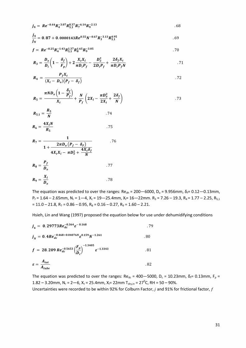
31

𝒋𝟒 = 𝑹𝒆−𝟎.𝟒𝟒𝑹𝟒−𝟑.𝟎𝟕𝑹𝟓,𝟏

𝟎.𝟑𝟕𝑹𝟕−𝟔.𝟏𝟒𝑹𝟗

−𝟐.𝟏𝟑 . 68

𝒋𝟒

𝒋𝑵

= 𝟎. 𝟖𝟕 + 𝟎. 𝟎𝟎𝟎𝟎𝟏𝟒𝟑𝑹𝒆𝟎.𝟓𝟓𝑵−𝟎.𝟔𝟕𝑹𝟑−𝟑.𝟏𝟑𝑹𝟓,𝟏

𝟒.𝟗𝟓 . 69

𝒇 = 𝑹𝒆−𝟎.𝟐𝟓𝑹𝟒−𝟏.𝟒𝟑𝑹𝟓,𝟏

𝟏.𝟑𝟕𝑹𝟖𝟏.𝟔𝟓𝑹𝟗

−𝟑.𝟎𝟓 . 70

𝑹𝟑 = 𝑫𝒐

𝑫𝒊

(𝟏 − 𝜹𝒇

𝑭𝒑

) + 𝟐𝑿𝒕𝑿𝒍

𝝅𝑫𝒊𝑷𝒇

− 𝑫𝒐

𝟐

𝟐𝑫𝒊𝑷𝒇

+ 𝟐𝜹𝒇𝑿𝒕

𝝅𝑫𝒊𝑷𝒇𝑵 . 71

𝑹𝟒 = 𝑷𝒇𝑿𝒕

(𝑿𝒕 − 𝑫𝒐)(𝑷𝒇 − 𝜹𝒇) . 72

𝑹𝟓 =

𝝅𝑵𝑫𝒐 (𝟏 − 𝜹𝒇

𝑷𝒇)

𝑿𝒕

+ 𝑵

𝑷𝒇

(𝟐𝑿𝒍 − 𝝅𝑫𝒐

𝟐

𝟐𝑿𝒕

+ 𝟐𝜹𝒇

𝑵) . 73

𝑹𝟓,𝟏 = 𝑹𝟓

𝑵 . 74

𝑹𝟔 = 𝟒𝑿𝒍𝑵

𝑹𝟓

. 75

𝑹𝟕 = 𝟏

𝟏 +𝟐𝝅𝑫𝒐 (𝑷𝒇 − 𝜹𝑭)

𝟒𝑿𝒕𝑿𝒍 − 𝝅𝑫𝒐𝟐 +

𝟒𝑿𝒕𝜹𝒇

𝑵

. 76

𝑹𝟖 = 𝑷𝒇

𝑫𝒐

. 77

𝑹𝟗 = 𝑿𝒍

𝑫𝒐

. 78

The equation was predicted to over the ranges: Redh = 200—6000, Do = 9.956mm, δf= 0.12—0.13mm,

Pf = 1.64 – 2.65mm, Nr = 1—4, Xt = 19—25.4mm, Xl= 16—22mm. R3 = 7.26 – 19.3, R4 = 1.77 – 2.25, R5,1

= 11.0 – 21.8, R7 = 0.86 – 0.95, R8 = 0.16 – 0.27, R9 = 1.60 – 2.21.

Hsieh, Lin and Wang (1997) proposed the equation below for use under dehumidifying conditions

𝒋𝟒

= 𝟎. 𝟐𝟗𝟕𝟕𝟑𝑹𝒆𝒅𝒄−𝟎.𝟑𝟔𝟒𝜺− 𝟎.𝟏𝟔𝟖 . 79

𝒋𝑵

= 𝟎. 𝟒𝑹𝒆𝒅𝒄−𝟎.𝟒𝟔𝟖+𝟎.𝟎𝟒𝟎𝟕𝟔𝑵𝜺𝟎.𝟏𝟓𝟗𝑵−𝟏.𝟐𝟔𝟏 . 80

𝒇 = 𝟐𝟖. 𝟐𝟎𝟗 𝑹𝒆𝒅𝒄−𝟎.𝟓𝟔𝟓𝟑 (

𝑭𝒑

𝑫𝒄

)−𝟏.𝟑𝟒𝟎𝟓

𝜺−𝟏.𝟑𝟑𝟒𝟑 . 81

𝜺 = 𝑨𝒕𝒐𝒕

𝑨𝒕𝒖𝒃𝒆

. 82

The equation was predicted to over the ranges: Redc = 400—5000, Dc = 10.23mm, δf= 0.13mm, Fp =

1.82 – 3.20mm, Nr = 2—6, Xt = 25.4mm, Xl= 22mm Tdry,in = 270C, RH = 50 – 90%.

Uncertainties were recorded to be within 92% for Colburn Factor, 𝑗 and 91% for frictional factor, 𝑓

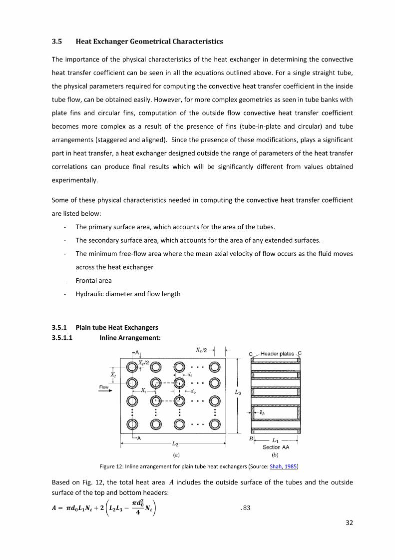
32

3.5 Heat Exchanger Geometrical Characteristics

The importance of the physical characteristics of the heat exchanger in determining the convective

heat transfer coefficient can be seen in all the equations outlined above. For a single straight tube,

the physical parameters required for computing the convective heat transfer coefficient in the inside

tube flow, can be obtained easily. However, for more complex geometries as seen in tube banks with

plate fins and circular fins, computation of the outside flow convective heat transfer coefficient

becomes more complex as a result of the presence of fins (tube-in-plate and circular) and tube

arrangements (staggered and aligned). Since the presence of these modifications, plays a significant

part in heat transfer, a heat exchanger designed outside the range of parameters of the heat transfer

correlations can produce final results which will be significantly different from values obtained

experimentally.

Some of these physical characteristics needed in computing the convective heat transfer coefficient

are listed below:

- The primary surface area, which accounts for the area of the tubes.

- The secondary surface area, which accounts for the area of any extended surfaces.

- The minimum free-flow area where the mean axial velocity of flow occurs as the fluid moves

across the heat exchanger

- Frontal area

- Hydraulic diameter and flow length

3.5.1 Plain tube Heat Exchangers

3.5.1.1 Inline Arrangement:

Figure 12: Inline arrangement for plain tube heat exchangers (Source: Shah, 1985)

Based on Fig. 12, the total heat area 𝐴 includes the outside surface of the tubes and the outside

surface of the top and bottom headers:

𝑨 = 𝝅𝒅𝟎𝑳𝟏𝑵𝒕 + 𝟐 (𝑳𝟐𝑳𝟑 − 𝝅𝒅𝟎

𝟐

𝟒𝑵𝒕) . 83

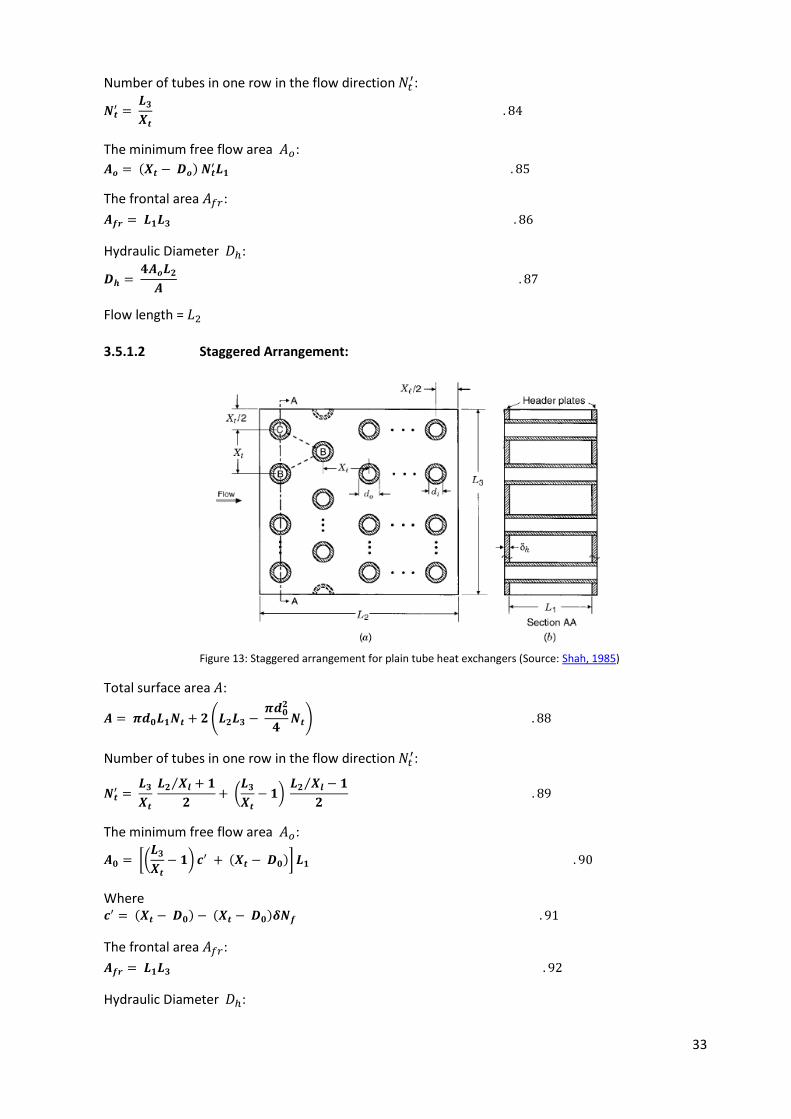
33

Number of tubes in one row in the flow direction 𝑁𝑡′:

𝑵𝒕′ =

𝑳𝟑

𝑿𝒕

. 84

The minimum free flow area 𝐴𝑜:

𝑨𝒐 = (𝑿𝒕 − 𝑫𝒐) 𝑵𝒕′𝑳𝟏 . 85

The frontal area 𝐴𝑓𝑟:

𝑨𝒇𝒓 = 𝑳𝟏𝑳𝟑 . 86

Hydraulic Diameter 𝐷ℎ:

𝑫𝒉 = 𝟒𝑨𝒐𝑳𝟐

𝑨 . 87

Flow length = 𝐿2

3.5.1.2 Staggered Arrangement:

Figure 13: Staggered arrangement for plain tube heat exchangers (Source: Shah, 1985)

Total surface area 𝐴:

𝑨 = 𝝅𝒅𝟎𝑳𝟏𝑵𝒕 + 𝟐 (𝑳𝟐𝑳𝟑 − 𝝅𝒅𝟎

𝟐

𝟒𝑵𝒕) . 88

Number of tubes in one row in the flow direction 𝑁𝑡′:

𝑵𝒕′ =

𝑳𝟑

𝑿𝒕

𝑳𝟐 𝑿𝒍 + 𝟏⁄

𝟐+ (

𝑳𝟑

𝑿𝒕

− 𝟏) 𝑳𝟐 𝑿𝒍⁄ − 𝟏

𝟐 . 89


𝑨𝟎 = [(𝑳𝟑

𝑿𝒕

− 𝟏) 𝒄′ + (𝑿𝒕 − 𝑫𝟎)] 𝑳𝟏 . 90

Where

𝒄′ = (𝑿𝒕 − 𝑫𝟎) − (𝑿𝒕 − 𝑫𝟎)𝜹𝑵𝒇 . 91


𝑨𝒇𝒓 = 𝑳𝟏𝑳𝟑 . 92


34


𝑨 . 93

Flow length = 𝐿2

3.5.2 Circular – Fin tube Heat Exchangers:

Figure 14: Arrangement for circular tube heat exchangers (Source: Shah, 1985)

To evaluate the primary surface area, the total surface area equation for a staggered or inline plain

tube arrangement is used. However, the area covered by the fins, are deducted:

𝑨𝒑 = 𝝅𝒅𝟎(𝑳𝟏 − 𝜹𝑵𝒇𝑳𝟏)𝑵𝒕 + 𝟐 (𝑳𝟐𝑳𝟑 − 𝝅𝒅𝟎

𝟐

𝟒⁄ 𝑵𝒕) . 94

The secondary surface area 𝐴𝑓:

𝑨𝒇 = [𝟐𝝅(𝒅𝒆

𝟐 − 𝒅𝟎𝟐)

𝟒+ 𝝅𝒅𝒆𝜹] 𝑵𝒇𝑳𝟏𝑵𝒕 . 95

Therefore, total heat transfer surface area 𝐴:

𝑨 = 𝑨𝒑 + 𝑨𝒇 . 96

The minimum free flow area 𝑨𝒐:

𝑨𝟎 = [(𝑳𝟑

𝑿𝒕

− 𝟏) 𝒄′ + (𝑿𝒕 − 𝒅𝟎) − (𝒅𝒆 − 𝒅𝟎)𝜹𝑵𝒇] 𝑳𝟏 . 97

𝒘𝒉𝒆𝒓𝒆 𝒄′ = (𝑿𝒕 − 𝒅𝟎) − (𝒅𝒆 − 𝒅𝟎)𝜹𝑵𝒇 . 98


𝑨𝒇𝒓 = 𝑳𝟏𝑳𝟑 . 99



𝑨 . 100

Flow length = 𝐿2

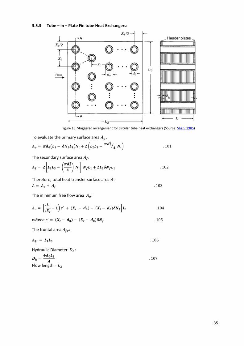
35

3.5.3 Tube – in – Plate Fin tube Heat Exchangers:

Figure 15: Staggered arrangement for circular tube heat exchangers (Source: Shah, 1985)

To evaluate the primary surface area 𝐴𝑝:


𝟐

𝟒⁄ 𝑵𝒕) . 101

The secondary surface area 𝐴𝑓:

𝑨𝒇 = 𝟐 [𝑳𝟐𝑳𝟑 − (𝝅𝒅𝟎

𝟐

𝟒) 𝑵𝒕] 𝑵𝒇𝑳𝟏 + 𝟐𝑳𝟑𝜹𝑵𝒇𝑳𝟏 . 102

Therefore, total heat transfer surface area 𝐴:

𝑨 = 𝑨𝒑 + 𝑨𝒇 . 103


𝑨𝒐 = [(𝑳𝟑

𝑿𝒕

− 𝟏) 𝒄′ + (𝑿𝒕 − 𝒅𝟎) − (𝑿𝒕 − 𝒅𝟎)𝜹𝑵𝒇] 𝑳𝟏 . 104

𝒘𝒉𝒆𝒓𝒆 𝒄′ = (𝑿𝒕 − 𝒅𝟎) − (𝑿𝒕 − 𝒅𝟎)𝜹𝑵𝒇 . 105


𝑨𝒇𝒓 = 𝑳𝟏𝑳𝟑 . 106


𝑫𝒉 = 𝟒𝑨𝟎𝑳𝟐

𝑨 . 107

Flow length = 𝐿2

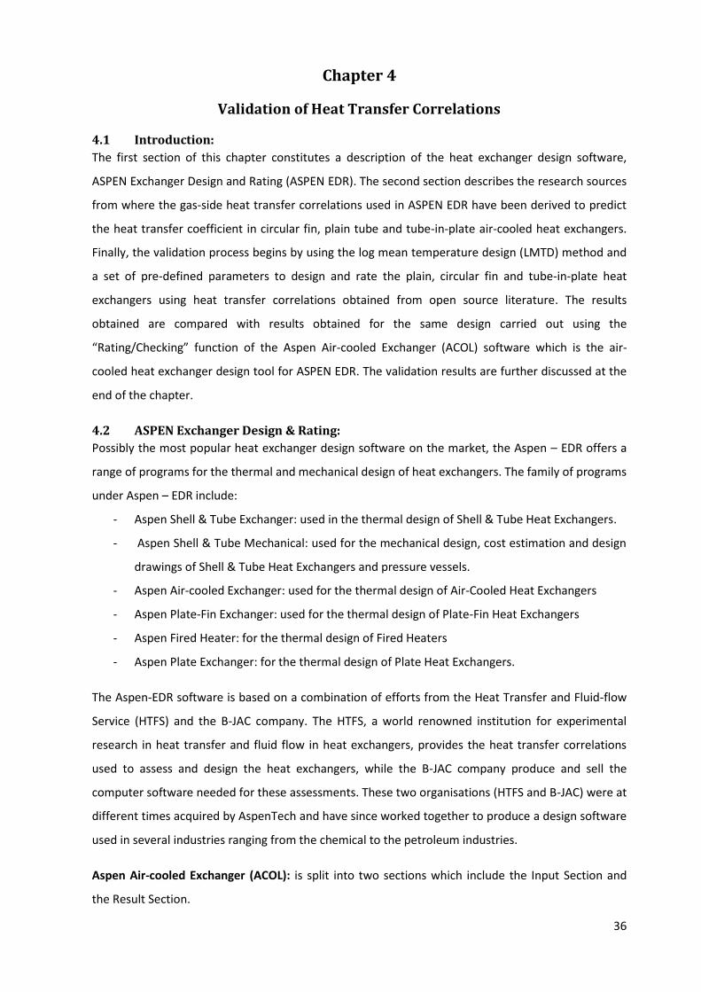
36

Chapter 4

Validation of Heat Transfer Correlations

4.1 Introduction:

The first section of this chapter constitutes a description of the heat exchanger design software,

ASPEN Exchanger Design and Rating (ASPEN EDR). The second section describes the research sources

from where the gas-side heat transfer correlations used in ASPEN EDR have been derived to predict

the heat transfer coefficient in circular fin, plain tube and tube-in-plate air-cooled heat exchangers.

Finally, the validation process begins by using the log mean temperature design (LMTD) method and

a set of pre-defined parameters to design and rate the plain, circular fin and tube-in-plate heat

exchangers using heat transfer correlations obtained from open source literature. The results

obtained are compared with results obtained for the same design carried out using the

“Rating/Checking” function of the Aspen Air-cooled Exchanger (ACOL) software which is the air-

cooled heat exchanger design tool for ASPEN EDR. The validation results are further discussed at the

end of the chapter.

4.2 ASPEN Exchanger Design & Rating:

Possibly the most popular heat exchanger design software on the market, the Aspen – EDR offers a

range of programs for the thermal and mechanical design of heat exchangers. The family of programs

under Aspen – EDR include:

- Aspen Shell & Tube Exchanger: used in the thermal design of Shell & Tube Heat Exchangers.

- Aspen Shell & Tube Mechanical: used for the mechanical design, cost estimation and design

drawings of Shell & Tube Heat Exchangers and pressure vessels.

- Aspen Air-cooled Exchanger: used for the thermal design of Air-Cooled Heat Exchangers

- Aspen Plate-Fin Exchanger: used for the thermal design of Plate-Fin Heat Exchangers

- Aspen Fired Heater: for the thermal design of Fired Heaters

- Aspen Plate Exchanger: for the thermal design of Plate Heat Exchangers.

The Aspen-EDR software is based on a combination of efforts from the Heat Transfer and Fluid-flow

Service (HTFS) and the B-JAC company. The HTFS, a world renowned institution for experimental

research in heat transfer and fluid flow in heat exchangers, provides the heat transfer correlations

used to assess and design the heat exchangers, while the B-JAC company produce and sell the

computer software needed for these assessments. These two organisations (HTFS and B-JAC) were at

different times acquired by AspenTech and have since worked together to produce a design software

used in several industries ranging from the chemical to the petroleum industries.

Aspen Air-cooled Exchanger (ACOL): is split into two sections which include the Input Section and

the Result Section.

37

- Input Section: This section is provided for the input and definition of the design problem.

Process conditions such as the fluid operating conditions (temperatures, pressures, mass

flow rates etc.) and geometrical characteristics (tube outer diameters, wall thickness, tube

layout, extended surface type, manufacturing material etc.) are defined within this section.

The sub-sections listed below make up the Input Section.

o Problem definition: Headings/Remarks Application options Process Data

o Physical property data Stream Composition Stream Properties

o Exchanger Geometry Geometry Summary Unit Geometry Tubes Bundle Headers & Nozzles Fans Structures/Walkways

o Construction Specifications Materials of Construction Design Specifications

o Program Options Design options Thermal Analysis Methods/correlations Outside Distribution

- Result Section: The Result section provides the analysis based on the values provided in the

input section. The area ratio is the most important information provided because it tells the

designer by how much he has either undersized or oversized the heat exchanger. Further

analysis such as pressure drops, heat transfer coefficients, outlet temperatures, etc. are also

provided.

o Input Summary Input summary

o Result Summary Warning & Messages Optimization Path Recap of Designs API Sheet Overall Summary

o Thermal /Hydraulic Summary Performance Heat Transfer Pressure Drop

o Mechanical Summary Exchanger Data Setting Plan / Tubesheet Layout

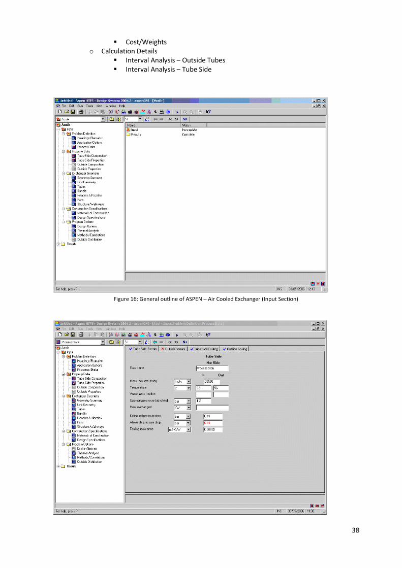
38

Cost/Weights o Calculation Details

Interval Analysis – Outside Tubes Interval Analysis – Tube Side

Figure 16: General outline of ASPEN – Air Cooled Exchanger (Input Section)

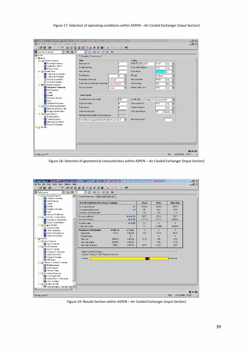
39

Figure 17: Selection of operating conditions within ASPEN – Air Cooled Exchanger (Input Section)

Figure 18: Selection of geometrical characteristics within ASPEN – Air Cooled Exchanger (Input Section)

Figure 19: Results Section within ASPEN – Air Cooled Exchanger (input Section)

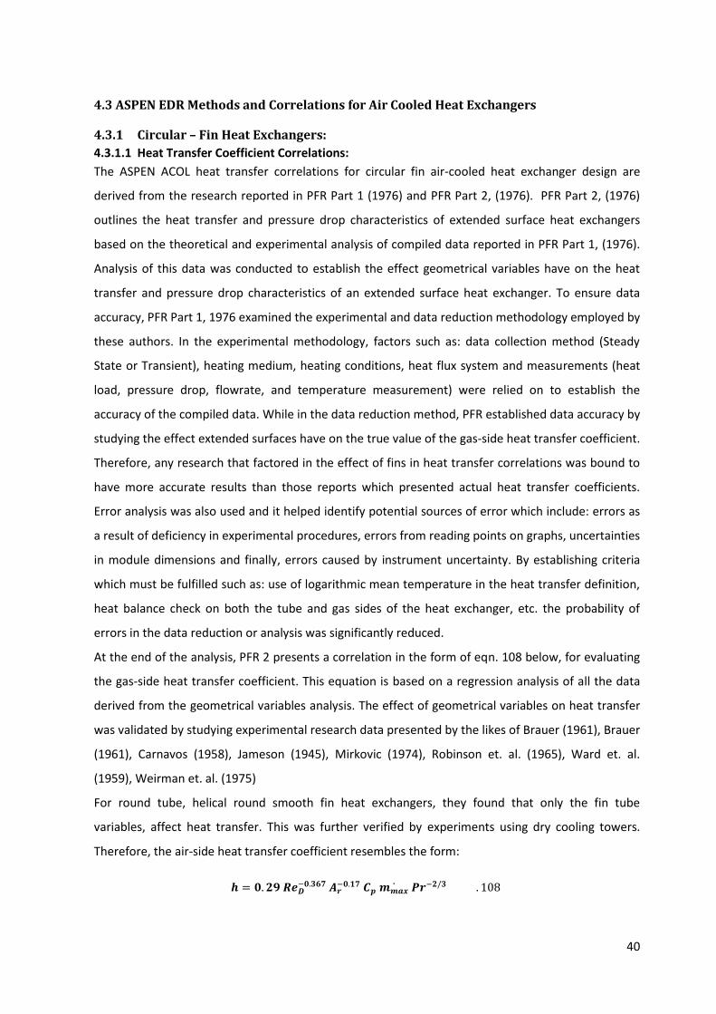
40

4.3 ASPEN EDR Methods and Correlations for Air Cooled Heat Exchangers

4.3.1 Circular – Fin Heat Exchangers:

4.3.1.1 Heat Transfer Coefficient Correlations:

The ASPEN ACOL heat transfer correlations for circular fin air-cooled heat exchanger design are

derived from the research reported in PFR Part 1 (1976) and PFR Part 2, (1976). PFR Part 2, (1976)

outlines the heat transfer and pressure drop characteristics of extended surface heat exchangers

based on the theoretical and experimental analysis of compiled data reported in PFR Part 1, (1976).

Analysis of this data was conducted to establish the effect geometrical variables have on the heat

transfer and pressure drop characteristics of an extended surface heat exchanger. To ensure data

accuracy, PFR Part 1, 1976 examined the experimental and data reduction methodology employed by

these authors. In the experimental methodology, factors such as: data collection method (Steady

State or Transient), heating medium, heating conditions, heat flux system and measurements (heat

load, pressure drop, flowrate, and temperature measurement) were relied on to establish the

accuracy of the compiled data. While in the data reduction method, PFR established data accuracy by

studying the effect extended surfaces have on the true value of the gas-side heat transfer coefficient.

Therefore, any research that factored in the effect of fins in heat transfer correlations was bound to

have more accurate results than those reports which presented actual heat transfer coefficients.

Error analysis was also used and it helped identify potential sources of error which include: errors as

a result of deficiency in experimental procedures, errors from reading points on graphs, uncertainties

in module dimensions and finally, errors caused by instrument uncertainty. By establishing criteria

which must be fulfilled such as: use of logarithmic mean temperature in the heat transfer definition,

heat balance check on both the tube and gas sides of the heat exchanger, etc. the probability of

errors in the data reduction or analysis was significantly reduced.

At the end of the analysis, PFR 2 presents a correlation in the form of eqn. 108 below, for evaluating

the gas-side heat transfer coefficient. This equation is based on a regression analysis of all the data

derived from the geometrical variables analysis. The effect of geometrical variables on heat transfer

was validated by studying experimental research data presented by the likes of Brauer (1961), Brauer

(1961), Carnavos (1958), Jameson (1945), Mirkovic (1974), Robinson et. al. (1965), Ward et. al.

(1959), Weirman et. al. (1975)

For round tube, helical round smooth fin heat exchangers, they found that only the fin tube

variables, affect heat transfer. This was further verified by experiments using dry cooling towers.

Therefore, the air-side heat transfer coefficient resembles the form:

𝒉 = 𝟎. 𝟐𝟗 𝑹𝒆𝑫−𝟎.𝟑𝟔𝟕 𝑨𝒓

−𝟎.𝟏𝟕 𝑪𝒑 𝒎𝒎𝒂𝒙̇ 𝑷𝒓−𝟐/𝟑 . 108

41

Experiments showed that PFR (1976) was accurate over the range of geometric dimensions indicated

below, the equation predicted 80% of the data collected to within ±10% and 95% of the data

collected to within ±18%.

1,000 ≤RED ≤40,000, Nr≥2 and 4≤Ar≤34,

To predict pressure drop, PFR Part 2 (1976) suggests that consideration must be given to both the

tube pitch and the finned tube variables. In addition to this, they state that the hydraulic diameter

was better suited for the evaluation of pressure drop than the base diameter. The frictional factor

therefore takes the form:

𝒇 = (𝟏𝟓𝟎 𝑹𝒆𝒉−𝟏.𝟎 + 𝟏. 𝟖 𝑹𝒆𝒉

−𝟎.𝟐) (𝑷𝒍 𝒅𝒉⁄ )𝟎.𝟑𝟓 (𝑷𝒍 𝒅𝒉⁄ )>𝟒 . 109

𝒇 = 𝚫𝑷 𝑵𝒕⁄

𝝆𝒂𝒗 𝑮𝒎𝒂𝒙𝟐 𝟐𝒈𝒄⁄

. 110

The pressure drop correlation covers the range:

400 < Reh < 10,000 and 1.5 ≤ Pl/dr ≤ 3.8

If 1.5 ≤ Pl/dr ≥ 4.0, then frictional factor is evaluated using:

𝒇 = (𝟏𝟑. 𝟔 𝑹𝒆𝒉−𝟎.𝟑) (𝑷𝒍 𝒅𝒉⁄ )𝟎.𝟑𝟓 (𝑷𝒍 𝒅𝒉⁄ )≤𝟒 . 111

4.3.1.2 Pressure Drop Correlations:

For the prediction of pressure drop, ASPEN EDR has invested a lot of resources in an attempt to

accurately predict the gas-side pressure drop of air cooled heat exchangers. This can be seen in the

works of PFR (1976), HTFS1 (HTFS RS1016, 1997), HTFS2 (HTFS RS1036 1998), HTFS3 (HTFS RS1118,

2002) and HTFS3A. The most accurate of the lot, the HTFS3A method is based on experiments

reported in HTFS RS1171 and HTFS RS1186. HTFS3A was conducted to illustrate the dependence of

the gas-side pressure drop on the changing properties of the gas as it is heated on passing through

the heat exchanger. This dependence was predicted to a degree by PFR (1976) and Weierman (1976)

but not by the HTFS2 and HTFS3 methods. To illustrate this dependence, HTFS RS1171 measured

pressure drop under isothermal conditions of 20OC and thermal conditions of mean bulk

temperature 56OC while HTFS RS1186 measured pressure drop under isothermal conditions of 20OC,

45OC, 56OC and 75OC and thermal conditions of mean bulk temperature of 75OC. Results led them to

develop a correction factor of 0.91 for mean air temperature at 20OC and 1.0 at an air inlet

temperature of 56OC and above for the pressure drop correlation reported by HTFS3. These

correction factors have been incorporated into ASPEN EDR. The HTFS3 correlations are outlined

below.

42

∆𝑷

𝝆= 𝟏. 𝟎𝟖𝟏𝑲𝑩𝒖𝟎

𝟏.𝟕 . 112

Experimental results showed that the correlations predicted 98% of the data to within ±20% for air

coolers. For open literature correlations, the HTFS3 predicts 79% of the data to within ±20%.

4.3.2 Plain – Tube Heat Exchangers:


To evaluate heat transfer coefficient, ASPEN EDR outlines a methodology in HTFS SM4 which is based

on correlations adopted from ESDU 73031 (1973). The ESDU equations were developed for 10 tube

rows or more, but have correction factors that allow for the same equations to be used for inline

tube bundles and designs where the tube rows are less than 10 in number. These correction factors

have been outlined and discussed earlier in Chapter 3. However, the heat transfer coefficient

correlation takes the form:

𝜶𝒄 = 𝒂𝝀𝒃

𝑫𝑹𝒆𝒄

𝒎𝑷𝒓𝒃𝟎.𝟑𝟒 . 113


To evaluate pressure drop, a methodology is outlined in HTFS SM3, which uses ESDU (1980) to

evaluate pressure drop without bypassing. The bypassing effect is accounted for, by using the Russell

and Wills (1983) equation. The pressure drop equation is outlined below:

∆𝒑𝒄 = 𝑪𝑳

𝑫𝝆𝒃

𝒖𝒔𝟐

𝟐𝝋𝟏𝝋𝟐 . 114

∆𝒑𝑩 = 𝟒𝒇𝑵𝑹𝝆𝒃

𝒖𝑩𝟐

𝟐 (𝒇𝒐𝒓 𝒃𝒚𝒑𝒂𝒔𝒔 𝒑𝒓𝒆𝒔𝒔𝒖𝒓𝒆 𝒅𝒓𝒐𝒑) . 115

Where: ∆𝑝𝑐 = 𝑐𝑟𝑜𝑠𝑠𝑓𝑙𝑜𝑤 𝑝𝑟𝑒𝑠𝑠𝑢𝑟𝑒 𝑑𝑟𝑜𝑝, 𝑁𝑚−2 𝑢𝑠 = 𝑠𝑢𝑝𝑒𝑟𝑓𝑖𝑐𝑖𝑎𝑙 𝑣𝑒𝑙𝑜𝑐𝑖𝑡𝑦, 𝑚𝑠−2 𝜑1 = 𝑣𝑖𝑠𝑐𝑜𝑠𝑖𝑡𝑦 𝑐𝑜𝑟𝑟𝑒𝑐𝑡𝑖𝑜𝑛 𝑓𝑎𝑐𝑡𝑜𝑟, (−) 𝜑2 = 𝑟𝑜𝑢𝑔ℎ𝑛𝑒𝑠𝑠 𝑐𝑜𝑟𝑟𝑒𝑐𝑡𝑖𝑜𝑛 𝑓𝑎𝑐𝑡𝑜𝑟, (−) ∆𝑝𝐵 = 𝑏𝑦𝑝𝑎𝑠𝑠 𝑝𝑟𝑒𝑠𝑠𝑢𝑟𝑒 𝑑𝑟𝑜𝑝, 𝑁𝑚−2 𝑓 = 𝑓𝑟𝑖𝑐𝑡𝑖𝑜𝑛 𝑓𝑎𝑐𝑡𝑜𝑟, (−) 𝑁𝑅 = 𝑛𝑢𝑚𝑏𝑒𝑟 𝑜𝑓 𝑡𝑢𝑏𝑒 𝑟𝑜𝑤𝑠 𝑐𝑟𝑜𝑠𝑠𝑒𝑑 𝑖𝑛 𝑑𝑖𝑟𝑒𝑐𝑡𝑖𝑜𝑛 𝑜𝑓 𝑓𝑙𝑜𝑤, (−) 𝑢𝐵 = 𝑏𝑦𝑝𝑎𝑠𝑠 𝑣𝑒𝑙𝑜𝑐𝑖𝑡𝑦, 𝑚𝑠−2

4.3.3 Tube –in – Plate Fin Tube Heat Exchangers:


To evaluate heat transfer coefficient in tube-in-plate heat exchangers, ASPEN EDR outlines a

methodology in HTFS ZM2 which is based on correlations adopted from PFR Part 2 (1976). PFR Part 2

(1976) carried out regression analysis on data provided by Rich (1973), Cox (27) and the Trane

Company data presented by Kays and London (1) to represent the form:

𝒉 = 𝟎. 𝟏𝟑 𝑹𝒆𝑫−𝟎.𝟑𝟑 𝑪𝒑 𝒎𝒎𝒂𝒙̇ 𝑷𝒓−𝟐/𝟑 . 116

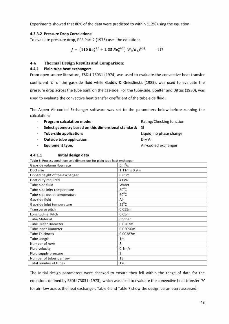
43

Experiments showed that 80% of the data were predicted to within ±12% using the equation.


To evaluate pressure drop, PFR Part 2 (1976) uses the equation;

𝒇 = (𝟏𝟏𝟎 𝑹𝒆𝒉−𝟏.𝟎 + 𝟏. 𝟑𝟓 𝑹𝒆𝒉

−𝟎.𝟐) (𝑷𝒍 𝒅𝒉⁄ )𝟎.𝟑𝟓 . 117

4.4 Thermal Design Results and Comparison:

4.4.1 Plain tube heat exchanger:

From open source literature, ESDU 73031 (1974) was used to evaluate the convective heat transfer

coefficient ‘h’ of the gas-side fluid while Gaddis & Gnieslinski, (1985), was used to evaluate the

pressure drop across the tube bank on the gas-side. For the tube-side, Boelter and Dittus (1930), was

used to evaluate the convective heat transfer coefficient of the tube-side fluid.

The Aspen Air-cooled Exchanger software was set to the parameters below before running the

calculation:

- Program calculation mode: Rating/Checking function

- Select geometry based on this dimensional standard: SI

- Tube-side application: Liquid, no phase change

- Outside tube application: Dry Air

- Equipment type: Air-cooled exchanger

4.4.1.1 Initial design data Table 5: Process conditions and dimensions for plain tube heat exchanger

Gas-side volume flow rate 5m3/s

Duct size 1.11m x 0.9m

Finned height of the exchanger 0.85m

Heat duty required 41kW

Tube-side fluid Water

Tube-side inlet temperature 800C

Tube-side outlet temperature 600C

Gas-side fluid Air

Gas-side inlet temperature 250C

Transverse pitch 0.055m

Longitudinal Pitch 0.05m

Tube Material Copper

Tube Outer Diameter 0.0267m

Tube Inner Diameter 0.02096m

Tube Thickness 0.00287m

Tube Length 1m

Number of rows 8

Fluid velocity 0.1m/s

Fluid supply pressure 2

Number of tubes per row 15

Total number of tubes 120

The initial design parameters were checked to ensure they fell within the range of data for the

equations defined by ESDU 73031 (1973), which was used to evaluate the convective heat transfer ‘h’

for air flow across the heat exchanger. Table 6 and Table 7 show the design parameters assessed.

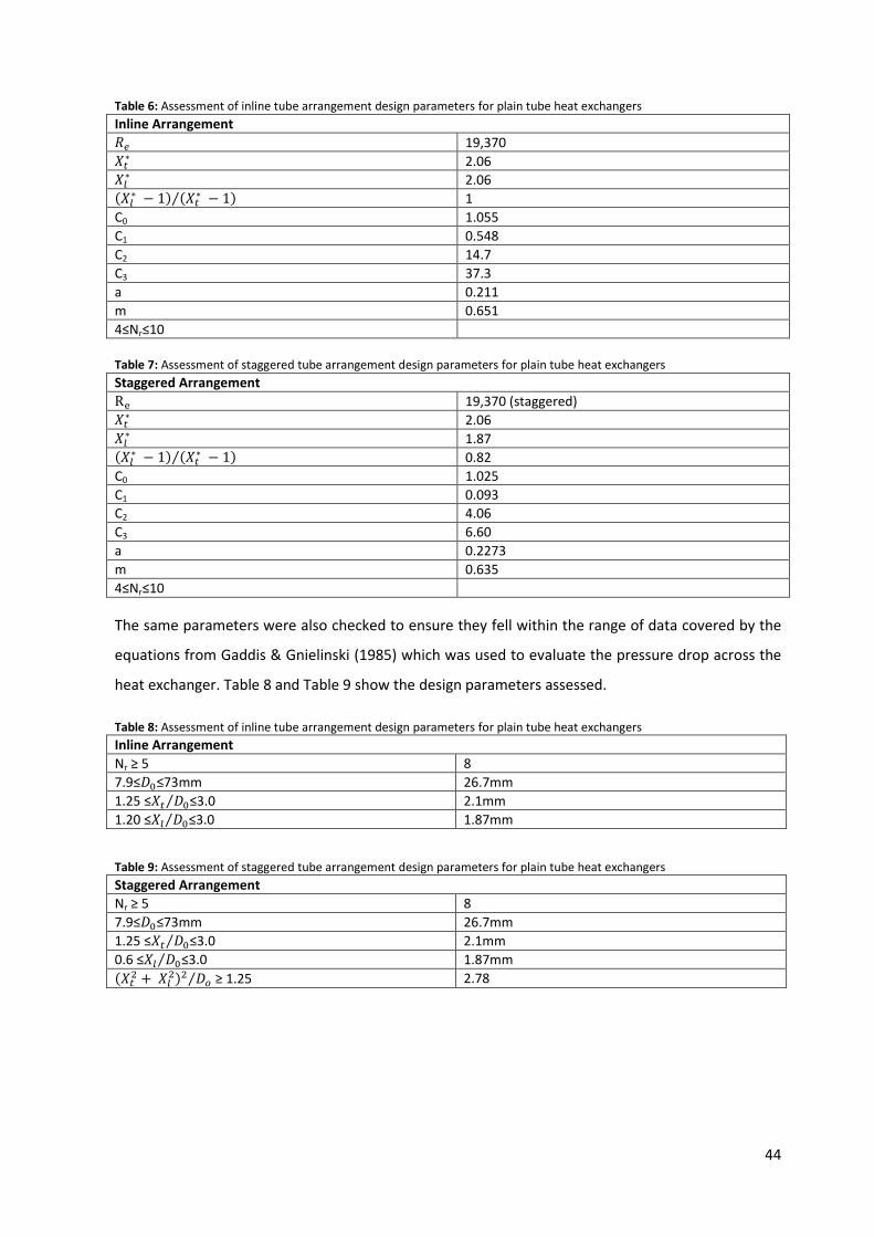
44

Table 6: Assessment of inline tube arrangement design parameters for plain tube heat exchangers

Inline Arrangement

𝑅𝑒 19,370

𝑋𝑡∗ 2.06

𝑋𝑙∗ 2.06

(𝑋𝑙∗ − 1) (𝑋𝑡

∗ − 1)⁄ 1

C0 1.055

C1 0.548

C2 14.7

C3 37.3

a 0.211

m 0.651

4≤Nr≤10

Table 7: Assessment of staggered tube arrangement design parameters for plain tube heat exchangers

Staggered Arrangement

Re 19,370 (staggered)

𝑋𝑡∗ 2.06

𝑋𝑙∗ 1.87

(𝑋𝑙∗ − 1) (𝑋𝑡

∗ − 1)⁄ 0.82

C0 1.025

C1 0.093

C2 4.06

C3 6.60

a 0.2273

m 0.635

4≤Nr≤10

The same parameters were also checked to ensure they fell within the range of data covered by the

equations from Gaddis & Gnielinski (1985) which was used to evaluate the pressure drop across the

heat exchanger. Table 8 and Table 9 show the design parameters assessed.

Table 8: Assessment of inline tube arrangement design parameters for plain tube heat exchangers

Inline Arrangement

Nr ≥ 5 8

7.9≤𝐷0≤73mm 26.7mm

1.25 ≤𝑋𝑡 𝐷0⁄ ≤3.0 2.1mm

1.20 ≤𝑋𝑙 𝐷0⁄ ≤3.0 1.87mm

Table 9: Assessment of staggered tube arrangement design parameters for plain tube heat exchangers

Staggered Arrangement

Nr ≥ 5 8

7.9≤𝐷0≤73mm 26.7mm

1.25 ≤𝑋𝑡 𝐷0⁄ ≤3.0 2.1mm

0.6 ≤𝑋𝑙 𝐷0⁄ ≤3.0 1.87mm

(𝑋𝑡2 + 𝑋𝑙

2)2 𝐷𝑜⁄ ≥ 1.25 2.78

45

4.4.1.2 Results

Staggered Arrangement:

Comparisons of the results for the staggered tube arrangement are presented in Table 10 below.

Table 10: Plain tube staggered arrangement results

Open Source Correlation Equations

Aspen Air-cooled Exchanger

% Deviation

Area ratio 1.14 1.06 7.5% over-prediction

Gas pressure drop, Pa 192 237 23% under-prediction

Total heat transfer surface area, m2 10.75 9.3 15% over-prediction

Gas – outlet temperature 32 32 No deviation

Tube – side Reynolds number 5,078 4,877 4% over-prediction

Gas – side Reynolds number 19,370 21,798 13% under-prediction

Tube-side mass flow rate, kg/sec 0.4893 0.4893 No deviation

Gas mass flowrate, kg/sec. 5.92 5.92 No deviation

Number of passes 8 8 No deviation

Number of tubes per pass 15 15 No deviation

Average pressure drop of flow entering tubes, Pa 7 7.1 1% under-prediction

Average pressure drop of flow through tubes, Pa 9 9.7 7% under-prediction

Overall Heat Transfer Coefficient, w/m.K 107 113 6% under-prediction

LMTD 41 41.21 0.5% under-prediction

Face velocity, m/s 6.0 6.35 5.8% under-prediction

Heat transfer coefficient – gas side, W/m.K 135 124 8% over-prediction

Heat transfer coefficient – tube side, W/m.K 796 716 11% over-prediction

Inline Arrangement:

To represent an inline arrangement, the longitudinal dimension of the tube pitch was changed from

50mm to 55mm to match the transverse pitch. The same design routine was then repeated with the

new inline tube arrangement and the results in Table 11 were obtained.

Table 11: Plain tube Inline arrangement results

Correlation Equations Aspen Air-cooled Exchanger % Deviation

Area ratio 1.04 0.96 8% over-prediction

Gas pressure drop, Pa 144 184 27% under-prediction

Heat transfer coefficient – gas side, W/m.K 110 121.5 9.8% under-prediction

Heat transfer coefficient – tube side, W/m.K 796 718 11% over-prediction

4.4.1.3 Result discussion:

4.4.1.3.1 Staggered arrangement:

Area ratio: The area ratio is the most important value to the designer because it tells the designer by

how much the heat exchanger unit has either been undersized or oversized compared to the

operating requirements and the initial design data. Oversizing within reason, is common in the heat

exchanger industry because operating conditions are not always as accurate as presented by the

end-user. Therefore, to ensure that the heat exchanger unit continues to deliver the desired heat

duty, an oversize of the unit “within reason”, is necessary.

The open source design correlation predicts a heat exchanger oversize of 14% while ASPEN ACOL

indicates an oversize of just 6% based on the initial design parameters. This represents an over

prediction of 7.5% by the open source design correlations. To put this context, it means that 7.5%

46

more material will be used when the heat exchanger is manufactured using heat transfer correlations

from open source literature.

Total heat transfer area: The total heat transfer area evaluated using open source literature (eqn.88

– eqn.93), showed that the heat exchanger will be 10.75m2 overall. When this value is compared to

the ASPEN ACOL result (9.3m2), an over prediction of 15% is observed.

Overall heat transfer coefficient: The overall heat transfer coefficient is the summation of the

resistance to heat transfer via conduction and convection on the tube and gas sides of the heat

exchanger respectively. It constitutes a combination of heat transfer surface areas and heat transfer

coefficients on both sides of the heat exchanger (fluid and gas sides). From Table 10 above, it is

observed that the open source heat transfer correlations under-predicts the overall heat transfer

coefficient by just 6% compared to the value obtained using ASPEN ACOL. The under-prediction is

minute and will not affect the performance of the heat exchanger.

Gas – side pressure drop: The gas-side pressure drop result obtained using open source data shows a

23% under prediction from the ASPEN results. The consequence of the under prediction will manifest

at the heat exchanger fan selection stage. Based on the results, fan pressure drop requirements will

be under predicted and any fan selected based on these results, will deliver a duty less than required.

Therefore, any pressure drop results obtained using the open source correlations for staggered plain

tube heat exchangers will be treated as conservative and factored into any decision making regarding

selection of heat exchanger components such as fans and transition ducts.

Tube – side pressure drop: Open source equations predict pressure drop to within 1% and 7% for

fluid flow entering the tubes and through the tubes respectively when compared to the values

obtained using ASPEN ACOL. The difference in both calculations is very small and within acceptable

ranges of deviation.

Gas-side heat transfer coefficient: The open source heat transfer correlations over predict the gas-

side heat transfer coefficient by 8% even though the two design methods (open source and ASPEN

ACOL) use the same heat transfer correlations obtained from ESDU 73031. The over prediction is

rather small and could be as a result of the more advanced computation power of ASPEN ACOL.

Tube-side heat transfer coefficient: The heat transfer coefficient on the tube-side of the heat

exchanger is over predicted by 11% when open source heat transfer correlations are used. Although

this represents a fairly high value, the controlling resistance is on the gas side of the heat exchanger

and thus any over-prediction on the tube side will have very little effect on the overall design of the

heat exchanger.

47

4.4.1.3.2 Inline arrangement:

Area ratio: The area ratio obtained using open source data over predicted the size of the unit

required by 8% when compared to the result obtained with ASPEN ACOL. This result suggests that

better prediction is obtained when the open source correlations are used for designing plain tube

heat exchangers with staggered tube arrangement. In addition, the result clearly illustrates the

advantage of a staggered heat exchanger tube arrangement over an inline arrangement.

Gas – side pressure drop: The gas-side pressure drop is under predicted by 27% and indicates that

the open source pressure drop correlations will under predict the gas-side pressure drops in both the

inline and staggered tube arrangements. The use of these correlations must be treated with caution

in heat exchanger design.

Gas-side heat transfer coefficient: A reverse of the case seen in the staggered arrangement, the heat

transfer coefficient is under predicted by the open source design method even though both methods

depend on ESDU 73031 (1973) to predict the heat transfer coefficient on the gas-side of the heat

exchanger.

Tube-side heat transfer coefficient: The prediction of the heat transfer coefficient on the tube side is

also over by 11% which ideally should remain the same for both cases because the tube-side fluid is

not affected by tube pitch arrangement.

4.4.1.4 Summary:

In the case of the staggered arrangement, the key design parameters such as gas-side heat transfer

coefficient, area ratio, overall heat transfer coefficient gas-side, tube-side pressure drop etc., were all

within acceptable ranges of deviation compared to the values obtained using ASPEN ACOL and could

thus be used for developing the design toolkit. However, the gas-side pressure drop was considerably

under predicted by the open source correlation equations and must be treated with caution when

used in the design toolkit.

While in the case of the inline arrangement, the gas-side pressure drop is once again under predicted

and thus must be treated with caution when used in the design toolkit. All other parameters are

within acceptable ranges of deviation.

4.4.2 Circular-fin heat exchanger:

The Briggs and Young (1963) equation, was used to evaluate the Colburn Factor (j), which is used to

evaluate the heat transfer coefficient of the gas-side fluid. Kays & London (1984) was used to

evaluate the pressure drop across the tube bank on the gas-side. Finally, the Boelter and Dittus

(1930) equation, was used to evaluate the heat transfer coefficient of the tube-side fluid.

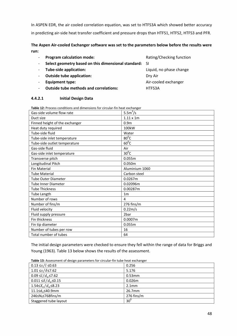
48

In ASPEN EDR, the air cooled correlation equation, was set to HTFS3A which showed better accuracy

in predicting air-side heat transfer coefficient and pressure drops than HTFS1, HTFS2, HTFS3 and PFR.

The Aspen Air-cooled Exchanger software was set to the parameters below before the results were

run:






- Outside tube methods and correlations: HTFS3A

4.4.2.1 Initial Design Data

Table 12: Process conditions and dimensions for circular-fin heat exchanger

Gas-side volume flow rate 5.5m3/s

Duct size 1.11 x 1m


Heat duty required 100kW




Gas-side fluid Air




Fin Material Aluminium 1060

Tube Material Carbon steel




Tube Length 1m

Number of rows 4

Number of fins/m 276 fins/m


Fluid supply pressure 2bar

Fin thickness 0.0007m

Fin tip diameter 0.055m



The initial design parameters were checked to ensure they fell within the range of data for Briggs and

Young (1963). Table 13 below shows the results of the assessment.

Table 13: Assessment of design parameters for circular-fin tube heat exchanger

0.13 ≤𝑠 𝑙⁄ ≤0.63 0.256

1.01 ≤𝑠 𝛿⁄ ≤7.62 5.176

0.09 ≤𝑙 𝑑𝑜⁄ ≤7.62 0.53mm

0.011 ≤𝛿 𝑑𝑜⁄ ≤0.15 0.026m

1.54≤𝑋𝑡 𝑑𝑜⁄ ≤8.23 2.1mm

11.1≤do≤40.9mm 26.7mm

246≤Nf≤768fins/m 276 fins/m

Staggered tube layout 300

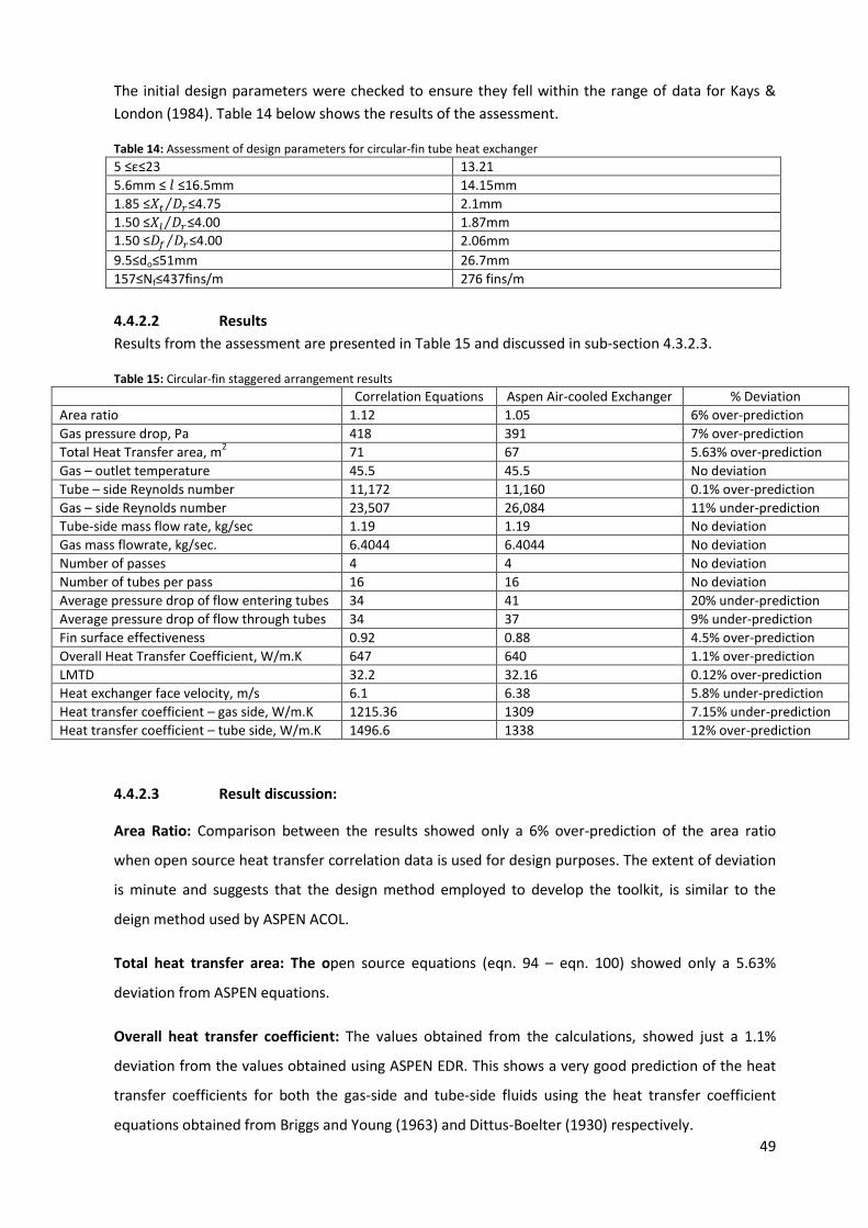
49

The initial design parameters were checked to ensure they fell within the range of data for Kays &

London (1984). Table 14 below shows the results of the assessment.

Table 14: Assessment of design parameters for circular-fin tube heat exchanger

5 ≤ε≤23 13.21

5.6mm ≤ 𝑙 ≤16.5mm 14.15mm

1.85 ≤𝑋𝑡 𝐷𝑟⁄ ≤4.75 2.1mm

1.50 ≤𝑋𝑙 𝐷𝑟⁄ ≤4.00 1.87mm

1.50 ≤𝐷𝑓 𝐷𝑟⁄ ≤4.00 2.06mm

9.5≤do≤51mm 26.7mm

157≤Nf≤437fins/m 276 fins/m

4.4.2.2 Results

Results from the assessment are presented in Table 15 and discussed in sub-section 4.3.2.3.

Table 15: Circular-fin staggered arrangement results

Correlation Equations Aspen Air-cooled Exchanger % Deviation


Gas pressure drop, Pa 418 391 7% over-prediction

Total Heat Transfer area, m2 71 67 5.63% over-prediction

Gas – outlet temperature 45.5 45.5 No deviation

Tube – side Reynolds number 11,172 11,160 0.1% over-prediction

Gas – side Reynolds number 23,507 26,084 11% under-prediction





Average pressure drop of flow entering tubes 34 41 20% under-prediction

Average pressure drop of flow through tubes 34 37 9% under-prediction

Fin surface effectiveness 0.92 0.88 4.5% over-prediction

Overall Heat Transfer Coefficient, W/m.K 647 640 1.1% over-prediction

LMTD 32.2 32.16 0.12% over-prediction

Heat exchanger face velocity, m/s 6.1 6.38 5.8% under-prediction

Heat transfer coefficient – gas side, W/m.K 1215.36 1309 7.15% under-prediction

Heat transfer coefficient – tube side, W/m.K 1496.6 1338 12% over-prediction


Area Ratio: Comparison between the results showed only a 6% over-prediction of the area ratio

when open source heat transfer correlation data is used for design purposes. The extent of deviation

is minute and suggests that the design method employed to develop the toolkit, is similar to the

deign method used by ASPEN ACOL.

Total heat transfer area: The open source equations (eqn. 94 – eqn. 100) showed only a 5.63%

deviation from ASPEN equations.

Overall heat transfer coefficient: The values obtained from the calculations, showed just a 1.1%

deviation from the values obtained using ASPEN EDR. This shows a very good prediction of the heat

transfer coefficients for both the gas-side and tube-side fluids using the heat transfer coefficient

equations obtained from Briggs and Young (1963) and Dittus-Boelter (1930) respectively.

50

Gas – side pressure drop: using the Kays and London (1984) gas-side pressure drop equations, a 7%

deviation was observed when compared to the results produced by ASPEN EDR. This showed a good

prediction of the gas-side pressure drop considering that extra measures have been taken to improve

the accuracy of the ASPEN correlations in HTFS3A.

Tube – side pressure drop: Open source equations under predict pressure drops by 18% and 9% for


obtained using ASPEN ACOL. The same pressure drop equations and tube sizes were used in the plain

tube validation exercise with smaller deviations observed. However, tube side velocity was less

(0.1m/s) and suggests that larger tube side velocities could introduce larger deviations in the tube

side pressure drop values.

Gas – side heat transfer coefficient: The Briggs and Young (1963) correlation closely predicted the

same results as the PFR equations from ASPEN with only a 7.15% deviation.

Tube – side heat transfer coefficient: The heat transfer coefficient on the tube-side of the heat

exchanger is over predicted by 12% when open source heat transfer correlations are used. This

indicates almost the same deviation observed in the plain tube validation exercise which suggests

that the ASPEN ACOL equations for the tube-side heat transfer coefficient, is used across all 3 types

of air-cooled heat exchangers.

4.4.2.4 Summary:

The circular fin air-cooled heat exchanger validation exercise showed the most impressive results of

all three types of air-cooled heat exchangers when compared to the ASPEN ACOL results. All the key

design parameters such as gas-side heat transfer coefficient, gas-side pressure drop, area ratio,

overall heat transfer coefficient gas-side, etc., were within acceptable ranges of deviation and

strongly indicates that the equations available in the public domain, are the same as those used in

ASPEN ACOL.

4.4.3 Tube-in-plate fin heat exchanger:

Wang and Chi (2000) was used to evaluate the Colburn Factor (j), which was eventually used to

evaluate the heat transfer coefficient of the gas-side fluid. Wang and Chi (2000), was also used to

evaluate the frictional factor needed for pressure drop calculations across the tube bank on the gas-

side and Dittus and Boelter (1930), was used to evaluate the heat transfer coefficient of the tube-

side fluid.

The Aspen Air-cooled Exchanger software was set to the parameters below before the results were

run:

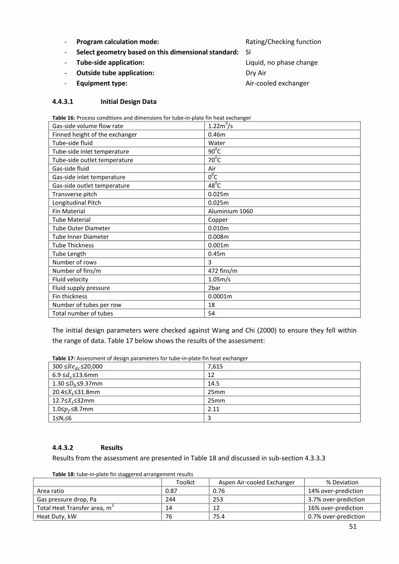
51






4.4.3.1 Initial Design Data

Table 16: Process conditions and dimensions for tube-in-plate fin heat exchanger

Gas-side volume flow rate 1.22m3/s





Gas-side fluid Air


Gas-side outlet temperature 480C



Fin Material Aluminium 1060

Tube Material Copper




Tube Length 0.45m

Number of rows 3

Number of fins/m 472 fins/m


Fluid supply pressure 2bar

Fin thickness 0.0001m



The initial design parameters were checked against Wang and Chi (2000) to ensure they fell within

the range of data. Table 17 below shows the results of the assessment:

Table 17: Assessment of design parameters for tube-in-plate fin heat exchanger

300 ≤𝑅𝑒𝑑𝑐≤20,000 7,615

6.9 ≤𝑑𝑐≤13.6mm 12

1.30 ≤𝐷ℎ≤9.37mm 14.5

20.4≤𝑋𝑡≤31.8mm 25mm

12.7≤𝑋𝑙≤32mm 25mm

1.0≤𝑝𝑓≤8.7mm 2.11

1≤Nr≤6 3

4.4.3.2 Results

Results from the assessment are presented in Table 18 and discussed in sub-section 4.3.3.3

Table 18: tube-in-plate fin staggered arrangement results

Toolkit Aspen Air-cooled Exchanger % Deviation


Gas pressure drop, Pa 244 253 3.7% over-prediction

Total Heat Transfer area, m2 14 12 16% over-prediction

Heat Duty, kW 76 75.4 0.7% over-prediction

52

Tube – side Reynolds number 23,055 22,556 2.2% over-prediction

Gas – side Reynolds number 7,615 8,866 16% over-prediction





Average pressure drop of flow entering tubes

776 800 3.1% under-prediction

Average pressure drop of flow through tubes

760 874 15% under-prediction

Fin surface effectiveness 0.92 0.87 5.7% over-prediction

Overall Heat Transfer Coefficient 1,280 1,498 17% under-prediction

LMTD 55 55.6 1% under-prediction

Minimum free flow area, mm2 0.1125 0.0990 14% over-prediction

Face velocity, m/s 6.0 6.59 10% under-prediction

Heat transfer coefficient – gas side, W/m.K 1235.32 1494.73 21% under-prediction

Heat transfer coefficient – tube side, W/m.K 6819 5987 13.9% over-prediction


Area ratio: Both area ratio results indicate that the current heat exchanger geometry will not achieve

the desired duty. However, the toolkit over predicts this deficiency by up to 14% when compared to

the results of ASPEN ACOL.

Total heat transfer area: The toolkit over predicts the overall surface area of the heat exchanger by

16% when compared with the results of ASPEN ACOL. The extent of the disparity has not been tested

on larger heat exchangers to determine if this value increases proportionally with the size of the heat

exchanger. However, at this stage it can be said that the disparity is little and equations 101 – 103

could be deemed suitable for use in the toolkit.

Overall heat transfer coefficient: An under-prediction of 17% by the open source correlations

indicates that either the gas-side or the tube-side heat transfer coefficient value will differ

considerably with those of ASPEN ACOL. The size of the deviation is significant, considering that it a

combination of both the gas-side and tube-side heat transfer coefficients.

Gas – side pressure drop: Open source correlations, under predicted the gas-side pressure drop by

3.7% compared to the ASPEN ACOL results. It indicates good predictability of Chi and Wang (2000)

(eqn. 53) for the gas-side pressure drop in tube-in-plate heat exchangers.

Tube – side pressure drop: Open source equations under predict pressure drops by 3.1% and 15% for


obtained using ASPEN ACOL. Results from the earlier exercises, had indicated that larger deviations

are likely to occur as the velocity of flow increases.

53

Gas – side heat transfer coefficient: With an under-prediction of 21%, the Wang and Chi (20002)

heat transfer correlations deviation showed the largest deviation of all the heat exchanger designs

considered.

Tube – side heat transfer coefficient: The heat transfer coefficient on the tube-side of the heat

exchanger was over predicted by 14% by the open source heat transfer correlations. Once again, it

follows the trend observed earlier in both the plain tube and tube-in-plate heat exchangers.

4.4.3.4 Summary:

The tube-in-plate fin air-cooled heat exchanger validation exercise showed the largest deviations of

all three types of air-cooled heat exchangers when compared with the ASPEN ACOL results. Although

the gas-side pressure drop value was less than 4% off the value predicted by ASPEN ACOL, the more

important gas-side heat transfer coefficient showed an under-prediction of as much as 21%. This

under-prediction will ultimately affect the final value of the overall heat transfer coefficient and

possibly lead to an oversized heat exchanger.

54

Chapter 5

Heat Exchanger Design Optimization

5.1 Introduction:

Due to the several possible combinations with design variables that include: number of tube rows,

tube length, tube OD, tube pitch layout, fin pitch etc., the design and analysis stage of air cooled heat

exchangers can become a time consuming and expensive process. Therefore to minimise time spent

at this stage, the conventional method of design is applied. This method would involve keeping one

constraining variable constant and iterating the other variables one-at-a-time until the design

requirements are met. For example using the “Rating” design method, the tube diameter could be

kept constant and other factors such as tube length, number of rows, number of fins, etc. varied and

once the desired solution is reached, no further consideration is given to altering these variables to

determine if the design requirements can be met using a different combination. This invariably

means the rating design method could prove more expensive to the manufacturer based on the

theory that the larger the overall surface area of the unit, the more manufacturing materials will be

required to build it. This also means that the unit will take longer to manufacture thus leading to an

increase in labour costs. A combination of these two costs (materials and labour) could easily price

any small-to-medium scale enterprise (SME) out of the highly competitive heat exchanger market.

Other factors which could increase the final cost of manufacturing include: material surface

treatment (galvanizing or painting), type of manufacturing material (e.g. stainless steel), non-

destructive testing (NDT) etc. Although these are special requirements specified by the consumer,

they increase the final cost of the heat exchanger since they also increase proportionally to the size

of the heat exchanger unit. However, in most cases, the consumer is willing to pay more for these

“extras”.

On-the-other hand, when using the optimization solution methods in the thermal design process, all

independent design variables (tube length, tube OD etc.), are considered simultaneously in various

combinations in order to deliver a solution that satisfies all design requirements even if one or more

of the design variables has to be kept constant. An example of optimization in the design process is

to aim to optimize the final overall heat transfer surface area of the heat exchanger while still

ensuring the unit delivers the duty required. Optimization in this instance means that the final overall

surface area matches exactly what will be required to deliver the required duty. This problem

statement thus becomes the focal point of design unlike the conventional method where any size is

deemed satisfactory as long as it satisfies the design requirements. Thus, the final solution in the

optimization process not only ensures that all design requirements are met but also that the optimal

configuration of the geometrical dimensions is used to achieve it. Ideally, optimization will eliminate

the need to carry out several iterations of any particular variable which saves design time.

55

In an attempt to replicate the optimization design methods, a “Sizing” design option has been added

to the heat exchanger design toolkit. The “Sizing” option will enable the designer specify minimum

and maximum values of specific heat exchanger variables along with desired increments. The design

process then involves running a combination of all the variables through the heat transfer equations,

along with the increments as specified by the designer one step at a time. The final results will show

the best combination of the design variables that will give the optimum heat exchanger surface area

which will achieve the desired heat duty. In other to prevent a glut of unnecessary results, the toolkit

has been designed to ensure that only thermal conductance ratio values less than 1.5 times the

required thermal conductance are displayed.

𝑈𝐴𝑟𝑒𝑞𝑢𝑖𝑟𝑒𝑑 ≤ 1.5 𝑥 𝑈𝐴𝑑𝑒𝑠𝑖𝑔𝑛

The difference between the conventional and optimization methods of design can be seen the flow

chart below:

Figure 20: Comparison of (a) conventional design method and (b) optimum design method, Source: Introduction to Optimum Design, 2012

5.1.1 Aim:

The aim of this exercise is to validate the ‘Sizing’ design option which will be made available in the

heat exchanger toolkit using the optimization tool ‘GRG nonlinear Solver’ available in Microsoft Excel.

This exercise will determine the values of the design variables that will produce the optimum heat

transfer surface area in the design of an air-cooled heat exchanger while still achieving the specified

heat duty.

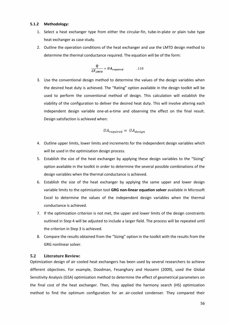
56

5.1.2 Methodology:

1. Select a heat exchanger type from either the circular-fin, tube-in-plate or plain tube type

heat exchanger as case study.

2. Outline the operation conditions of the heat exchanger and use the LMTD design method to

determine the thermal conductance required. The equation will be of the form:

𝑸

∆𝑻𝑳𝑴𝑻𝑫= 𝑼𝑨𝒓𝒆𝒒𝒖𝒊𝒓𝒆𝒅 . 118

3. Use the conventional design method to determine the values of the design variables when

the desired heat duty is achieved. The “Rating” option available in the design toolkit will be

used to perform the conventional method of design. This calculation will establish the

viability of the configuration to deliver the desired heat duty. This will involve altering each

independent design variable one-at-a-time and observing the effect on the final result.

Design satisfaction is achieved when:

𝑈𝐴𝑟𝑒𝑞𝑢𝑖𝑟𝑒𝑑 = 𝑈𝐴𝑑𝑒𝑠𝑖𝑔𝑛

4. Outline upper limits, lower limits and increments for the independent design variables which

will be used in the optimization design process.

5. Establish the size of the heat exchanger by applying these design variables to the “Sizing”

option available in the toolkit in order to determine the several possible combinations of the

design variables when the thermal conductance is achieved.

6. Establish the size of the heat exchanger by applying the same upper and lower design

variable limits to the optimization tool GRG non-linear equation solver available in Microsoft

Excel to determine the values of the independent design variables when the thermal

conductance is achieved.

7. If the optimization criterion is not met, the upper and lower limits of the design constraints

outlined in Step 4 will be adjusted to include a larger field. The process will be repeated until

the criterion in Step 3 is achieved.

8. Compare the results obtained from the “Sizing” option in the toolkit with the results from the

GRG nonlinear solver.

5.2 Literature Review:

Optimization design of air cooled heat exchangers has been used by several researchers to achieve

different objectives. For example, Doodman, Fesanghary and Hosseini (2009), used the Global

Sensitivity Analysis (GSA) optimization method to determine the effect of geometrical parameters on

the final cost of the heat exchanger. Then, they applied the harmony search (HS) optimization

method to find the optimum configuration for an air-cooled condenser. They compared their

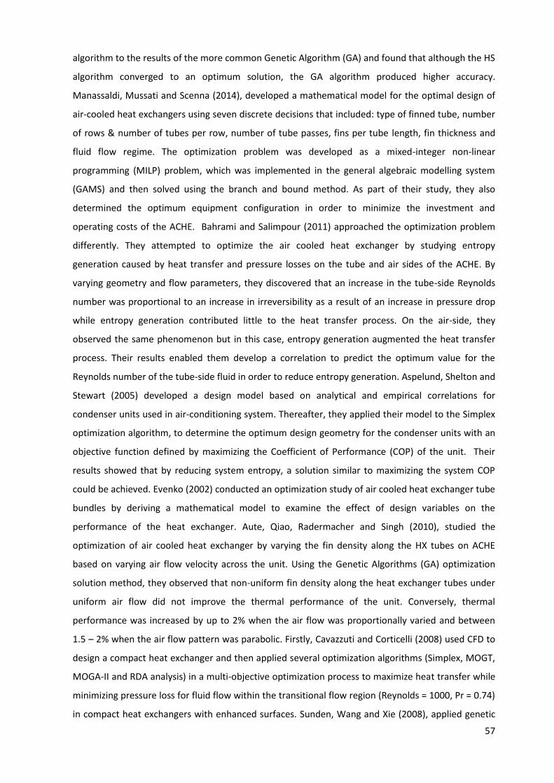
57

algorithm to the results of the more common Genetic Algorithm (GA) and found that although the HS

algorithm converged to an optimum solution, the GA algorithm produced higher accuracy.

Manassaldi, Mussati and Scenna (2014), developed a mathematical model for the optimal design of

air-cooled heat exchangers using seven discrete decisions that included: type of finned tube, number

of rows & number of tubes per row, number of tube passes, fins per tube length, fin thickness and

fluid flow regime. The optimization problem was developed as a mixed-integer non-linear

programming (MILP) problem, which was implemented in the general algebraic modelling system

(GAMS) and then solved using the branch and bound method. As part of their study, they also

determined the optimum equipment configuration in order to minimize the investment and

operating costs of the ACHE. Bahrami and Salimpour (2011) approached the optimization problem

differently. They attempted to optimize the air cooled heat exchanger by studying entropy

generation caused by heat transfer and pressure losses on the tube and air sides of the ACHE. By

varying geometry and flow parameters, they discovered that an increase in the tube-side Reynolds

number was proportional to an increase in irreversibility as a result of an increase in pressure drop

while entropy generation contributed little to the heat transfer process. On the air-side, they

observed the same phenomenon but in this case, entropy generation augmented the heat transfer

process. Their results enabled them develop a correlation to predict the optimum value for the

Reynolds number of the tube-side fluid in order to reduce entropy generation. Aspelund, Shelton and

Stewart (2005) developed a design model based on analytical and empirical correlations for

condenser units used in air-conditioning system. Thereafter, they applied their model to the Simplex

optimization algorithm, to determine the optimum design geometry for the condenser units with an

objective function defined by maximizing the Coefficient of Performance (COP) of the unit. Their

results showed that by reducing system entropy, a solution similar to maximizing the system COP

could be achieved. Evenko (2002) conducted an optimization study of air cooled heat exchanger tube

bundles by deriving a mathematical model to examine the effect of design variables on the

performance of the heat exchanger. Aute, Qiao, Radermacher and Singh (2010), studied the

optimization of air cooled heat exchanger by varying the fin density along the HX tubes on ACHE

based on varying air flow velocity across the unit. Using the Genetic Algorithms (GA) optimization

solution method, they observed that non-uniform fin density along the heat exchanger tubes under

uniform air flow did not improve the thermal performance of the unit. Conversely, thermal

performance was increased by up to 2% when the air flow was proportionally varied and between

1.5 – 2% when the air flow pattern was parabolic. Firstly, Cavazzuti and Corticelli (2008) used CFD to

design a compact heat exchanger and then applied several optimization algorithms (Simplex, MOGT,

MOGA-II and RDA analysis) in a multi-objective optimization process to maximize heat transfer while

minimizing pressure loss for fluid flow within the transitional flow region (Reynolds = 1000, Pr = 0.74)

in compact heat exchangers with enhanced surfaces. Sunden, Wang and Xie (2008), applied genetic

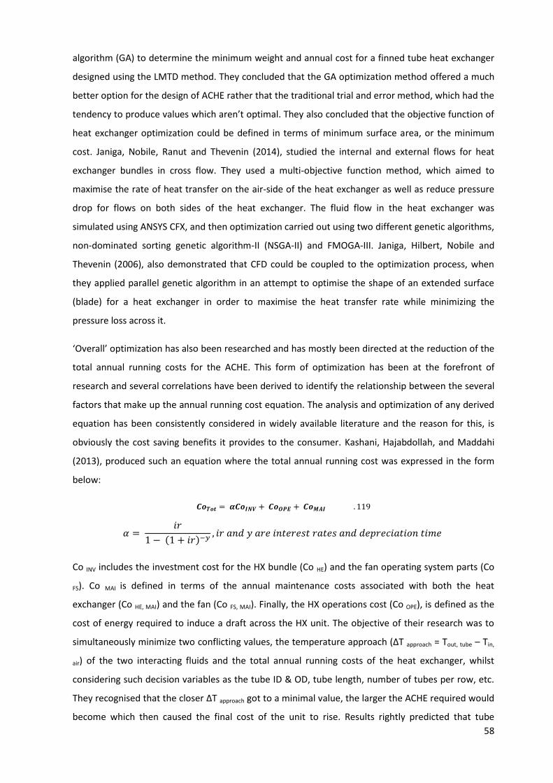
58

algorithm (GA) to determine the minimum weight and annual cost for a finned tube heat exchanger

designed using the LMTD method. They concluded that the GA optimization method offered a much

better option for the design of ACHE rather that the traditional trial and error method, which had the

tendency to produce values which aren’t optimal. They also concluded that the objective function of

heat exchanger optimization could be defined in terms of minimum surface area, or the minimum

cost. Janiga, Nobile, Ranut and Thevenin (2014), studied the internal and external flows for heat

exchanger bundles in cross flow. They used a multi-objective function method, which aimed to

maximise the rate of heat transfer on the air-side of the heat exchanger as well as reduce pressure

drop for flows on both sides of the heat exchanger. The fluid flow in the heat exchanger was

simulated using ANSYS CFX, and then optimization carried out using two different genetic algorithms,

non-dominated sorting genetic algorithm-II (NSGA-II) and FMOGA-III. Janiga, Hilbert, Nobile and

Thevenin (2006), also demonstrated that CFD could be coupled to the optimization process, when

they applied parallel genetic algorithm in an attempt to optimise the shape of an extended surface

(blade) for a heat exchanger in order to maximise the heat transfer rate while minimizing the

pressure loss across it.

‘Overall’ optimization has also been researched and has mostly been directed at the reduction of the

total annual running costs for the ACHE. This form of optimization has been at the forefront of

research and several correlations have been derived to identify the relationship between the several

factors that make up the annual running cost equation. The analysis and optimization of any derived

equation has been consistently considered in widely available literature and the reason for this, is

obviously the cost saving benefits it provides to the consumer. Kashani, Hajabdollah, and Maddahi

(2013), produced such an equation where the total annual running cost was expressed in the form

below:

𝑪𝒐𝑻𝒐𝒕 = 𝜶𝑪𝒐𝑰𝑵𝑽 + 𝑪𝒐𝑶𝑷𝑬 + 𝑪𝒐𝑴𝑨𝑰 . 119

𝛼 = 𝑖𝑟

1 − (1 + 𝑖𝑟)−𝑦, 𝑖𝑟 𝑎𝑛𝑑 𝑦 𝑎𝑟𝑒 𝑖𝑛𝑡𝑒𝑟𝑒𝑠𝑡 𝑟𝑎𝑡𝑒𝑠 𝑎𝑛𝑑 𝑑𝑒𝑝𝑟𝑒𝑐𝑖𝑎𝑡𝑖𝑜𝑛 𝑡𝑖𝑚𝑒

Co INV includes the investment cost for the HX bundle (Co HE) and the fan operating system parts (Co

FS). Co MAI is defined in terms of the annual maintenance costs associated with both the heat

exchanger (Co HE, MAI) and the fan (Co FS, MAI). Finally, the HX operations cost (Co OPE), is defined as the

cost of energy required to induce a draft across the HX unit. The objective of their research was to

simultaneously minimize two conflicting values, the temperature approach (ΔT approach = Tout, tube – Tin,

air) of the two interacting fluids and the total annual running costs of the heat exchanger, whilst

considering such decision variables as the tube ID & OD, tube length, number of tubes per row, etc.

They recognised that the closer ΔT approach got to a minimal value, the larger the ACHE required would

become which then caused the final cost of the unit to rise. Results rightly predicted that tube

59

length, number of tubes per row, fin height, fin density, air velocity, fin thickness and tube ID & OD,

caused the conflict between the objective functions. Using the non-dominated sorting genetic

algorithm (NSGA) optimization technique, they were able to minimize these two constraints and

obtain an optimum solution. Martin (1999) considered deriving a cost based equation of the form

below, to predict the capital costs (C) associated with the ACHE:

𝑪 = 𝑪𝟏 + 𝑪𝟎 . 120

C1 accounts for the capital costs and Co accounting for operations costs. He achieved his aim, by

deriving the optimal value for the Reynolds number of fluid flow across the heat exchanger. He chose

to optimize the Reynolds number because he discovered that the fluid flow velocity was proportional

to the annual cost of investment (C1, associated with the overall surface area of the ACHE) and the

operating costs (C0, associated with pumping fluid through the exchanger). Buys and Kroger, (1989)

used the optimization technique, to determine the optimal dimensions for a finned tube bundle that

would be installed in an existing cooling system using a cost structure of the form:

𝑪𝒇𝒕 = [𝑪𝒘𝒇(𝑪𝒕 + 𝑪𝒇) + 𝑪𝒇𝒊𝒙]𝑳𝒕𝒏𝒕𝒃𝒏𝒃 . 121

Cwf is defined as the weighting factor, Ct as cost per unit length of core tube, Cf as cost of fin material

per unit length of tube, Cfix as the fixed cost per unit length of tube, L as tube length, ntb as number of

tubes in bundle and finally nb as number of tube bundles. Caputo, Pelagagge and Salini (2016),

developed a mathematical model for the cost estimation of shell and tube heat exchangers, based on

the HXs geometrical features and manufacturing procedures for the subassembly parts that make up

the heat exchanger.

The cost equation is of the form:

𝑪𝑬 = ∑ (𝑪𝒎𝒂𝒕𝒙 + ∑ 𝑪𝒐𝒑𝒙

𝑵𝒐𝒑

𝒌=𝟏

)

𝒙

. 122

𝐶𝑚𝑎𝑡𝑥, is defined as the cost estimate for the x-th subassembly material and ∑ 𝐶𝑜𝑝𝑥𝑁𝑜𝑝𝑘=1 , is defined

as the cost estimate for the k-th manufacturing procedure needed for the x-th subassembly part.

Hewitt and Pugh (2007), reviewed and presented work that had been conducted by ESDU 94043

(1994), for the costing of heat exchangers. They presented “data items” for the quick selection, sizing

and costing for different heat exchangers at the initial stage of design. The costing method they

examined, was for two-stream heat exchangers and is based on the use of a ‘C’ value, which is

defined by 𝑄 ∆𝑇𝑚⁄ . They explain that the use of the ‘C’ method provides a quick comparison between

different heat exchangers without consideration for the total area of the unit ‘A’ and overall heat

transfer coefficient ‘U’, two values which are directly linked and can prove quite difficult most times

60

to evaluate. ESDU 94043 (1994), provides a quick method for roughly estimating the cost of an ACHE

based on the model:

𝑪 = 𝑪𝒕 + 𝑪𝑴 + 𝑪𝑳 . 123

Where CL accounts for labour costs, Cm accounts for acquiring/manufacturing items such as fans,

structures, etc. and Ct refers to cost associated with acquiring heat exchanger tubes.

Unfortunately, the ESDU cost model and all the other cost models mentioned are hardly realistic in

the real world. To support this argument, we examine the ESDU model; the CL values used in the

equation are based on labour costing codes proprietary to the company selected for the study. With

the possibility of manufacturing cheaply abroad now available, labour costs will vary widely when

compared across companies. Even when compared locally, costs will be seen to vary across the

spectrum. Therefore, applying the CL values provided will produce inaccurate results for another

company. The model for Ct was based on a fixed set of design variables for the heat exchanger tube.

The first variable was a 25.4mmOD with a fin pitch of 433 fins per meter and a fin OD of 57mm. The

second design variable was based on a 19mm OD tube with a fin pitch of 430 fins per meter and fin

OD of 38mm. Unfortunately, experience has shown that in certain cases, tubes can be pitched

transversely from as low as 45mm, fin heights can range from 14mm to 16mm and fins per tube

metre can range from 118 to 433, depending on the unit design. Certain SMEs sometimes go as far as

‘gilling’ their own heat exchanger tubes, which is the process of tension winding a metal strip around

a tube, to form a spiral fin. The evaluation of Ct model has also been based on a constant heat

exchanger tube length of 12.2m and a bare tube surface area of 25m2 and above. Manufacturing

experience has shown that handling difficulties can be experienced when heat exchanger tubes are

longer than 6m. To solve this problem, designers would reduce the length of tube used, inadvertently

increasing number of rows required in the heat exchanger. This means that the total surface area can

sometimes be less or more than the 25m2 used in the ESDU cost model. To be fair, ESDU, tested the

effect of varying the tube type (extruded, & L-fin), tube length (1.65m, 3.05m, 6.1m, 9.1m and 15m)

and noise reduction (75dBA) on the costing model. Unfortunately, they omitted testing the effect of

varying the number of rows, as well as the tube fin pitch, both factors which add considerably to the

final cost of an ACHE. Finally, the CM model used in the model was also developed by a company

selected for the study, so hardly applicable to other companies.

Overall, it was observed that the level of research into minimizing the costs associated with

manufacturing (which will be of immense benefit to the manufacturer) has not been at the same

level as that associated with minimizing the annual running costs of the heat exchanger (beneficial to

only the end user/ client). When examined, the difference between the two cost structures is that for

the end-user/client, the equation for the annual running costs of the ACHE will resemble the forms

61

detailed above and include such factors as the operating costs, investment costs, replacement costs

etc. On-the-other hand for the small-to-medium scale (SME) designer/manufacturer, the cost

equation will ultimately resemble the equation below:

𝑪𝑻𝒐𝒕𝒂𝒍 = 𝑪𝑴𝒂𝒕𝒆𝒓𝒊𝒂𝒍𝒔 + 𝑪𝑴𝒂𝒏𝒖𝒇𝒂𝒄𝒕𝒖𝒓𝒊𝒏𝒈 . 124

𝐶𝑀𝑎𝑛𝑢𝑓𝑎𝑐𝑡𝑢𝑟𝑖𝑛𝑔 = 𝐶𝑇𝑖𝑚𝑒 𝑥 𝐶£/𝑚𝑎𝑛𝑝𝑜𝑤𝑒𝑟 (𝑙𝑎𝑏𝑜𝑢𝑟 𝑐𝑜𝑠𝑡)

Even if the cost models in the literature review could be proven to be beneficial to the SME

designer/manufacturer, implementation in the design process can be far too complex for an SME

with little or no experience in the use/ownership of the software upon which these cost models were

developed. Hence the reason why this present study is being simulated using the GRG Non-Linear

Solver available in Microsoft Excel. The Generalised Reduced Gradient (GRG) Non-Linear solution

methods are examined in Appendix C.

5.4 Optimization Exercise:

1. Project/Problem Description: The project aim is to determine the optimum values for the

design variables used in the thermal sizing of a circular-fin air-cooled heat exchanger (ACHE).

These optimum values must be able to achieve all design requirements for the heat

exchanger.

2. Data and Information Collection: Based on the overall heat transfer equation,

𝑼𝑨𝑻𝒐𝒕𝒂𝒍 = 𝑸

∆𝑻𝑳𝑴𝑻𝑫

The total heat transfer surface area of the heat exchanger 𝑨𝑻𝒐𝒕𝒂𝒍 is evaluated using the

essential equations which comprise of the primary surface area, 𝐴𝑝 (accounting for the

surface area of the heat exchanger tubes) and the secondary surface area, 𝐴𝑓 (accounting for

the surface area of the fins). These two sub-equations (𝐴𝑝 & 𝐴𝑓) consist of design variables

such as tube OD, fin OD, number of rows, fin thickness, transverse pitch, longitudinal pitch,

etc. that directly influence the final size of the heat exchanger.

The overall heat transfer coefficient , 𝑼, is evaluated using secondary equations which

include the heat transfer correlation equations (gas and tube side), Reynolds number

evaluation equations etc.

3. Definition of Design Variables: The design variables also referred to as the optimization

variables, are a set of variables used to describe the geometrical characteristics of the heat

exchanger. The design variables are split into two categories; the independent and

dependent variables. Variables are described as “independent” when any initial numerical

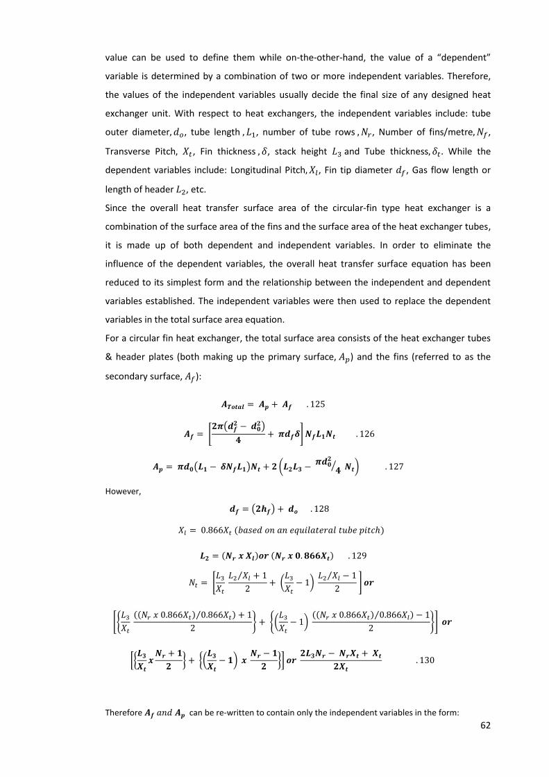
62

value can be used to define them while on-the-other-hand, the value of a “dependent”

variable is determined by a combination of two or more independent variables. Therefore,

the values of the independent variables usually decide the final size of any designed heat

exchanger unit. With respect to heat exchangers, the independent variables include: tube

outer diameter, 𝑑𝑜, tube length , 𝐿1, number of tube rows , 𝑁𝑟, Number of fins/metre, 𝑁𝑓,

Transverse Pitch, 𝑋𝑡, Fin thickness , 𝛿, stack height 𝐿3 and Tube thickness, 𝛿𝑡 . While the

dependent variables include: Longitudinal Pitch, 𝑋𝑙, Fin tip diameter 𝑑𝑓, Gas flow length or

length of header 𝐿2, etc.

Since the overall heat transfer surface area of the circular-fin type heat exchanger is a

combination of the surface area of the fins and the surface area of the heat exchanger tubes,

it is made up of both dependent and independent variables. In order to eliminate the

influence of the dependent variables, the overall heat transfer surface equation has been

reduced to its simplest form and the relationship between the independent and dependent

variables established. The independent variables were then used to replace the dependent

variables in the total surface area equation.

For a circular fin heat exchanger, the total surface area consists of the heat exchanger tubes

& header plates (both making up the primary surface, 𝐴𝑝) and the fins (referred to as the

secondary surface, 𝐴𝑓):

𝑨𝑻𝒐𝒕𝒂𝒍 = 𝑨𝒑 + 𝑨𝒇 . 125

𝑨𝒇 = [𝟐𝝅(𝒅𝒇

𝟐 − 𝒅𝟎𝟐)

𝟒+ 𝝅𝒅𝒇𝜹] 𝑵𝒇𝑳𝟏𝑵𝒕 . 126


𝟐

𝟒⁄ 𝑵𝒕) . 127

However,

𝒅𝒇 = (𝟐𝒉𝒇) + 𝒅𝒐 . 128

𝑋𝑙 = 0.866𝑋𝑡 (𝑏𝑎𝑠𝑒𝑑 𝑜𝑛 𝑎𝑛 𝑒𝑞𝑢𝑖𝑙𝑎𝑡𝑒𝑟𝑎𝑙 𝑡𝑢𝑏𝑒 𝑝𝑖𝑡𝑐ℎ)

𝑳𝟐 = (𝑵𝒓 𝒙 𝑿𝒍)𝒐𝒓 (𝑵𝒓 𝒙 𝟎. 𝟖𝟔𝟔𝑿𝒕) . 129

𝑁𝑡 = [𝐿3

𝑋𝑡

𝐿2 𝑋𝑙⁄ + 1

2+ (

𝐿3

𝑋𝑡

− 1) 𝐿2 𝑋𝑙⁄ − 1

2 ] 𝒐𝒓

[{𝐿3

𝑋𝑡

((𝑁𝑟 𝑥 0.866𝑋𝑡) 0.866𝑋𝑡⁄ ) + 1

2} + {(

𝐿3

𝑋𝑡

− 1) ((𝑁𝑟 𝑥 0.866𝑋𝑡) 0.866𝑋𝑙⁄ ) − 1

2}] 𝒐𝒓

[{𝑳𝟑

𝑿𝒕

𝒙𝑵𝒓 + 𝟏

𝟐} + {(

𝑳𝟑

𝑿𝒕

− 𝟏) 𝒙 𝑵𝒓 − 𝟏

𝟐}] 𝒐𝒓

𝟐𝑳𝟑𝑵𝒓 − 𝑵𝒓𝑿𝒕 + 𝑿𝒕

𝟐𝑿𝒕

. 130

Therefore 𝑨𝒇 𝑎𝑛𝑑 𝑨𝒑 can be re-written to contain only the independent variables in the form:

63

𝑨𝒇

= (𝟖𝝅𝒉𝒇

𝟐𝑵𝒓𝑵𝒇𝑳𝟑𝑳𝟏 + 𝟖𝝅𝒉𝒇𝒅𝒐𝑵𝒇𝑵𝒓𝑳𝟑𝑳𝟏 + 𝟖𝝅𝜹𝒉𝒇𝑵𝒇𝑵𝒓𝑳𝟑𝑳𝟏 + 𝟒𝝅𝜹𝒅𝒐𝑵𝒇𝑵𝒓𝑳𝟑𝑳𝟏 − 𝟒𝝅𝒉𝒇𝟐𝑵𝒇𝑵𝒓𝑳𝟏𝑿𝒕 − 𝟒𝝅𝒉𝒇𝒅𝒐𝑵𝒇𝑵𝒓𝑳𝟏𝑿𝒕 − 𝟒𝝅𝜹𝒉𝒇𝑵𝒇𝑵𝒓𝑳𝟏𝑿𝒕 − 𝟐𝝅𝜹𝒅𝒐𝑵𝒇𝑵𝒓𝑳𝟏𝑿𝒕 + 𝟒𝝅𝒉𝒇

𝟐𝑵𝒇𝑳𝟏𝑿𝒕 + 𝟒𝝅𝒉𝒇𝒅𝒐𝑵𝒇𝑳𝟏𝑿𝒕 + 𝟒𝝅𝜹𝒉𝒇𝑵𝒇𝑳𝟏𝑿𝒕 + 𝟐𝝅𝜹𝒅𝒐𝑵𝒇𝑳𝟏𝑿𝒕)

𝟒𝑿𝒕 . 131

𝑨𝒑 = 𝟒𝝅𝑵𝒓𝒅𝒐𝑳𝟏𝑳𝟑 − 𝟒𝝅𝑵𝒓𝜹𝑵𝒇𝑳𝟏𝑳𝟑𝒅𝒐 − 𝟐𝝅𝑵𝒓𝑿𝒕𝒅𝒐𝑳𝟏 + 𝟐𝝅𝒅𝒐𝑵𝒇𝑵𝒓𝑿𝒕 𝜹𝑳𝟏 + 𝟐𝝅𝑿𝒕𝒅𝒐𝑳𝟏 − 𝟐𝝅𝒅𝒐𝑿𝒕𝜹𝑵𝒇𝑳𝟏 + 𝟔. 𝟗𝟐𝟖𝑿𝒕

𝟐𝑵𝒓𝑳𝟑 − 𝟐𝝅𝒅𝒐𝟐𝑵𝒓𝑳𝟑 − 𝝅𝒅𝒐

𝟐𝑵𝒓𝑿𝒕 + 𝝅𝒅𝒐𝟐𝑿𝒕

𝟒𝑿𝒕 . 132

64

4. Optimization Criterion: At this stage, we define the optimization criterion for the design, which

ideally should be the objective of the whole process. The object function must be influenced

directly or indirectly by the independent design variables stated at Step 3. Since the aim is to

optimize the size of the heat exchanger, the objective in this instance would be the optimization

of the total heat transfer surface area of the circular-fin heat exchanger. This must be achieved

along with ensuring that the thermal conductance based on the operating conditions is at least

equal to the thermal conductance achieved by a combination of the design variables.

𝑈𝐴𝑟𝑒𝑞𝑢𝑖𝑟𝑒𝑑 = 𝑈𝐴𝑜𝑝𝑡𝑖𝑚𝑖𝑧𝑎𝑡𝑖𝑜𝑛

5. Operating conditions: The same operating conditions used in the validation of the heat transfer

correlations (refer to Chapter 4) for the circular fin heat exchanger, will be used to test the

optimization process.

6. Formulation of constraints: Based on the operating conditions outlined in Step 5, the

constraints placed on the objective function are defined and have to be satisfied by the

optimization process. These constraints are tied in directly with the design variables outlined

earlier in the overall heat transfer equation. These constraints are outlined below:

118 ≤ 𝑁𝑓 ≤ 433

0.040𝑚 ≤ 𝑋𝑡 ≤ 0.055𝑚

0.9 ≤ 𝐿1 ≤ 1𝑚

2 ≤ 𝑁𝑟 ≤ 6

0.014𝑚 ≤ ℎ𝑓 ≤ 0.016𝑚

𝐿3 = 0.9𝑚

𝛿 = 0.0007𝑚

𝑑𝑜 = 26.7𝑚𝑚

𝑈𝐴 = 3105

Results:

The optimization exercise began by running the GRG nonlinear solver within the boundaries outlined in

section 6 above. Thereafter, the lower boundary constraint for the “number of fins” was shifted

upwards to lessen the group size. The latter exercise was used to study the influence of boundary values

or initialization variables on the results produced by the solver as well as compare any results with those

produced by the “Sizing” option in the toolkit.

For each boundary, GRG non-linear solver found a solution for the overall heat transfer surface area

equation to satisfy the thermal conductance requirement. The results obtained and presented in Table

20 – Table 24 shows that the “Sizing” design option in the toolkit accurately predicted the same results

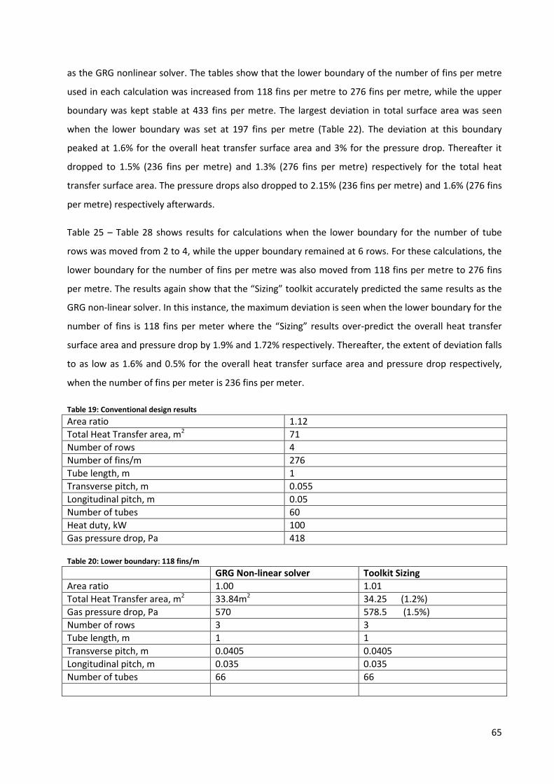
65

as the GRG nonlinear solver. The tables show that the lower boundary of the number of fins per metre

used in each calculation was increased from 118 fins per metre to 276 fins per metre, while the upper

boundary was kept stable at 433 fins per metre. The largest deviation in total surface area was seen

when the lower boundary was set at 197 fins per metre (Table 22). The deviation at this boundary

peaked at 1.6% for the overall heat transfer surface area and 3% for the pressure drop. Thereafter it

dropped to 1.5% (236 fins per metre) and 1.3% (276 fins per metre) respectively for the total heat

transfer surface area. The pressure drops also dropped to 2.15% (236 fins per metre) and 1.6% (276 fins

per metre) respectively afterwards.

Table 25 – Table 28 shows results for calculations when the lower boundary for the number of tube

rows was moved from 2 to 4, while the upper boundary remained at 6 rows. For these calculations, the

lower boundary for the number of fins per metre was also moved from 118 fins per metre to 276 fins

per metre. The results again show that the “Sizing” toolkit accurately predicted the same results as the

GRG non-linear solver. In this instance, the maximum deviation is seen when the lower boundary for the

number of fins is 118 fins per meter where the “Sizing” results over-predict the overall heat transfer

surface area and pressure drop by 1.9% and 1.72% respectively. Thereafter, the extent of deviation falls

to as low as 1.6% and 0.5% for the overall heat transfer surface area and pressure drop respectively,

when the number of fins per meter is 236 fins per meter.

Table 19: Conventional design results

Area ratio 1.12

Total Heat Transfer area, m2 71

Number of rows 4

Number of fins/m 276

Tube length, m 1

Transverse pitch, m 0.055

Longitudinal pitch, m 0.05

Number of tubes 60

Heat duty, kW 100

Gas pressure drop, Pa 418

Table 20: Lower boundary: 118 fins/m

GRG Non-linear solver Toolkit Sizing

Area ratio 1.00 1.01

Total Heat Transfer area, m2 33.84m2 34.25 (1.2%)

Gas pressure drop, Pa 570 578.5 (1.5%)

Number of rows 3 3

Tube length, m 1 1

Transverse pitch, m 0.0405 0.0405

Longitudinal pitch, m 0.035 0.035

Number of tubes 66 66

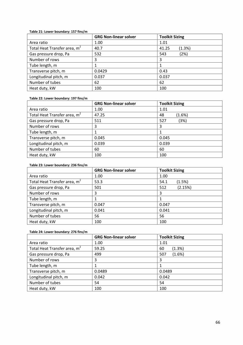
66




Total Heat Transfer area, m2 40.7 41.25 (1.3%)

Gas pressure drop, Pa 532 543 (2%)

Number of rows 3 3

Tube length, m 1 1




Heat duty, kW 100 100




Total Heat Transfer area, m2 47.25 48 (1.6%)

Gas pressure drop, Pa 511 527 (3%)

Number of rows 3 3

Tube length, m 1 1









Gas pressure drop, Pa 501 512 (2.15%)

Number of rows 3 3

Tube length, m 1 1










Number of rows 3 3

Tube length, m 1 1





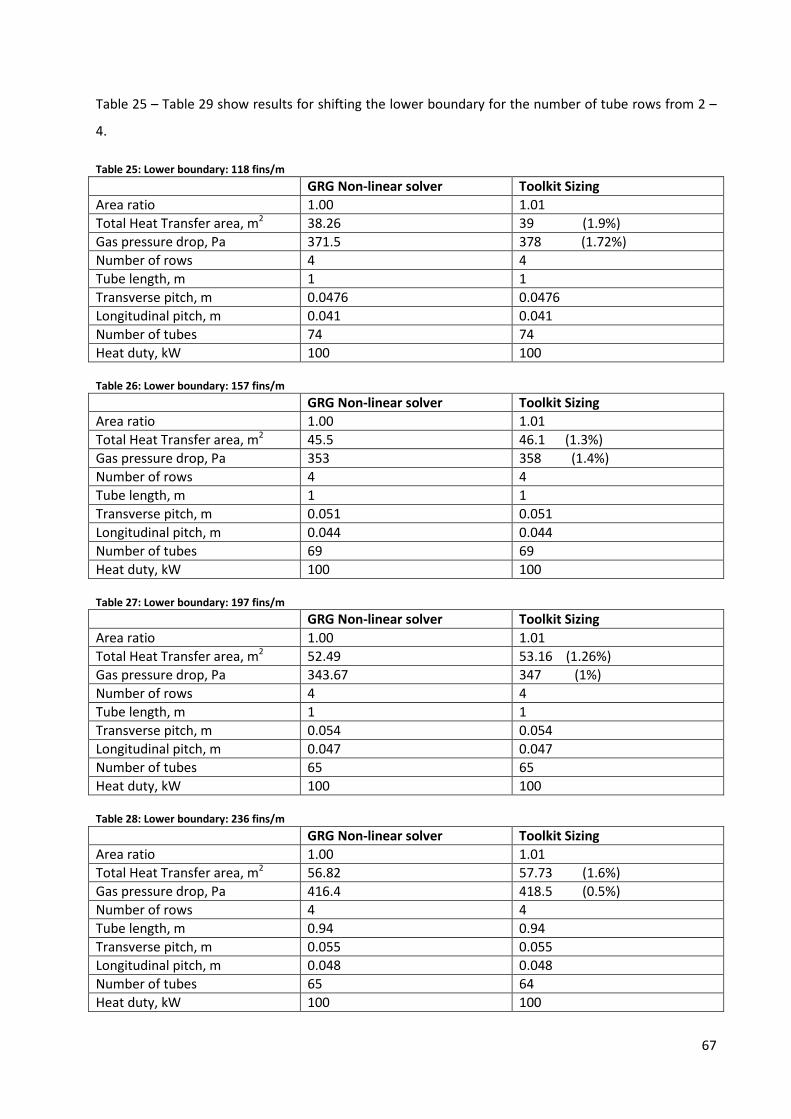
67

Table 25 – Table 29 show results for shifting the lower boundary for the number of tube rows from 2 –

4.





Gas pressure drop, Pa 371.5 378 (1.72%)

Number of rows 4 4

Tube length, m 1 1










Number of rows 4 4

Tube length, m 1 1









Gas pressure drop, Pa 343.67 347 (1%)

Number of rows 4 4

Tube length, m 1 1









Gas pressure drop, Pa 416.4 418.5 (0.5%)

Number of rows 4 4

Tube length, m 0.94 0.94





68

5.4 Conclusion:

The exercise conducted showed that both the GRG non-linear solver and the “Sizing” option in the

toolkit could be used as cost saving tools in the design of heat exchangers. This cost saving is achieved

by optimizing the initial geometrical design variables such that the final overall size of the heat

exchanger matches the required thermal conductance.

The results from the GRG non-linear solver showed a higher degree of accuracy when the initialization

variables were selected from within the upper and lower boundary limits. These results only differed

from the “Sizing” option results by only as much as 1.6% for the overall surface area and 3% for the gas

side pressure drop (197 fins per metre and 3 tube rows) and 1.9% for the overall surface area and 1.72%

for the gas side pressure drop (118 fins per metre and 4 tube rows).

Unfortunately, although the GRG non-linear solver still converged when the initialization values were

randomised or selected from outside the limit boundaries or design constraints, the results proved too

inconsistent to be relied upon. As noted by Manassaldi et. al. (2013), the initialization values in any

optimization problem, plays an important role in both convergence and accuracy of obtained results.

They found this to be very important where the model size was large and included several non-linear

constraints. The inconsistency of the GRG non-linear solver results with random initial values showed

the solver cannot be relied on for day-to-day heat exchanger design.

On-the-other hand, the accuracy and consistency of the “Sizing” option in the toolkit in predicting the

same results as the GRG non-linear solver when the initial values were within the boundary limits,

demonstrates its reliability for day-to-day heat exchanger design.

69

Chapter 6

Conclusion and Recommendations

6.1 Introduction:

The final chapter provides inferences drawn from the entire toolkit development process, right from

heat transfer correlation selection to the GUI development of the toolkit. Recommendations are also

given that will increase the potential of the heat exchanger design toolkit.

6.2 Conclusion:

The aim of this project has been the development of a toolkit specifically for the design of air-cooled

heat exchangers. The types of air-cooled heat exchangers considered were the circular fin, tube-in-plate

and the plain tube heat exchanger. In order to perform these designs, heat transfer correlations for

both the gas and tube side fluids had to be obtained from research data available in the public domain.

Comparison of design results produced with these correlations showed various degrees of deviation

from those produced with the industry standard software ASPEN-EDR. Aspects of the design results

which were compared include: total heat transfer surface area, gas heat transfer coefficient, area ratio,

tube side heat transfer coefficient, pressure drops, etc. The largest deviation was recorded in the design

of the tube-in-plate heat exchanger, with a 14% over-prediction of the area ratio by the toolkit results

compared to the ASPEN results. The least deviation was seen in the circular-fin where only a 6% over

prediction was recorded. The results from the design of the plain tube heat exchanger, recorded a 7.5%

and 8% over prediction by the toolkit for the staggered and inline arrangement respectively. The

conclusion drawn from these results was that for any heat exchanger design where the geometrical

characteristics and operating conditions stayed within the range specified in the publicly available heat

transfer correlations, the final results were more likely to be accurate. Unfortunately, the extent of

inaccuracy was not explored for conditions where the geometrical characteristics and operating

conditions of the heat exchanger strayed outside the defined parameters.

In addition to the validation exercise described above, an attempt was made to incorporate overall heat

transfer surface area optimization as part of the design capability of the toolkit. This design capability

was referred to as “Sizing” and could be selected as a design option in the toolkit. When this option is

selected, the designer is able to specify the minimum and maximum values along with desired

increments for specific characteristics of the heat exchanger. Thereafter, the optimised solution

produced by the toolkit will be based on a permutation and combination of these characteristics. In

order to validate this functionality, an exercise was conducted which compared the results produced by

Excel GRG nonlinear equation solver with those obtained from the toolkit. The results recorded showed

that when the log mean temperature difference (LMTD) design method is used, the overall heat transfer

surface area could be optimised to suit the required thermal conductance. The first validation exercise

70

showed the largest deviations recorded were 1.6% for the overall heat transfer surface area and 3% for

the pressure drop at 197 fins per metre. While in the second exercise, the largest deviations recorded at

197f fins per meter, were 1.9% and 1.72% for the overall heat transfer surface and pressure drops

respectively.

Development of the toolkit involved considering several programming languages such as C+, C++, Excel

VBA and Java in terms of ease of use and accessibility. Excel Visual Basic for Applications (VBA) was

finally selected because it could incorporate a graphic user interface (GUI) and also gave the developer,

the freedom to modify the toolkit to suit the changing needs. Another reason for the selection of Excel

VBA was that the Microsoft Office package which contains the Excel package is easily accessible and

could be installed simultaneously on several computer systems. During its development, the toolkit

went through several modifications before a final version was settled on. One such modification was the

inclusion of heat transfer fluids such as Ethylene glycol, Transcal N, etc. in the list of available fluids.

6.3 Recommendations:

To determine the convective heat transfer coefficients, correlations were used which covered only a

certain range of data. This in itself presents a problem which must be resolved if a high level of result

accuracy is desired for any thermal design where the initial parameters lie outside of the specified

range. Consideration should be given to developing heat transfer correlations that are adaptable to any

geometrical dimensions and operating conditions.

The design toolkit is currently only capable of rating and sizing air-cooled heat exchangers. Its further

development is encouraged to the point where it is capable of producing CAD drawings of the heat

exchanger as well as complete material and labour costs needed to manufacture the heat exchanger.

These additional features will save the time devoted to these separate activities as well as give the

designer a feel for how the heat exchanger will look after manufacture and also what final costs will

most likely be, especially if he is working on a tight budget

The capability of the design toolkit should be extended to sizing and rating other types of heat

exchangers such as shell & tube, Plate, serpentine coils etc. This capability, will give the designer greater

freedom to choose the best kind of heat exchanger that suits his process conditions.

The design toolkit has been developed using Excel Visual Basic for Applications (VBA), which is a widely

available Microsoft based software package. However, not all computers run on the Microsoft

Operating System. This means that any potential user of the toolkit must have a system running on the

Microsoft OS. It is recommended that the toolkit is developed as a stand-alone version. This means that

afterwards, the toolkit can be installed on virtually any computer system.

71

References 1. M. S. Bhatti and R. K. Shah, 1987, Turbulent and transition convective heat transfer in ducts, in

Handbook of Single-Phase Convective Heat Transfer, S. Kakaҫ, R. K Shah, and W. Aung, eds.,

Wiley, New York, Chap. 4.

2. D. E. Briggs and E. H. Young, 1963, Convection heat transfer and pressure drop of air flowing

across triangular pitch banks of finned tubes, Chem. Eng. Prog. Symp. Ser. 41, Vol. 59, pp. 1-10.

3. A. P. Colburn,1933, A method of correlating forced convection heat transfer data and a

comparison with fluid friction, Trans. Am. Inst. Chem. Eng., Vol. 29, pp. 174 – 210; reprinted in

Int. J. Heat Mass Transfer , Vol. 7, pp. 1359 – 1358, 1964

4. F. W. Dittus, and L.M.K Boelter, 1930, Heat transfer in automobile radiators of tubular type,

University of Calif. Publications in Engineering, Vol. 2, pp. 443 – 461

5. Engineering Services Data Unit (ESDU, 86022), 1988, High-fin staggered tube banks: heat

transfer and pressure drop for turbulent single phase gas flow.

6. S. G. Kandilikar, 1991, development of a flow boiling map for sub-cooled and saturated flow

boiling of different fluids in circular tubes, ASME J. Heat Transfer, Vol. 113, pp. 190 – 200

7. S. G. Kandilikar, M. Shoji, and V. K. Dhir, eds., 1999, Handbook of Phase Change: Boiling and

Condensation, Taylor & Francis, New York

8. W. Kays and, A.L. London, 1984, Compact heat exchangers. 3rd edition, McGraw-Hill.

9. H. Martin, 2002, The generalized Lévêque equation and its practical use for the prediction of

heat and mass transfer rates from pressure drop, Chem. Eng. Sci., Vol. 57, pp. 3217 – 3223.

10. K. K. Robinson and D. E. Briggs, 1966, Pressure drop of air flowing across triangular pitch banks

of finned tubes, Chem. Eng. Prog. Symp. Series 64, Vol. 62, pp. 177 – 184.

11. M. M. Shah, 197S.E7, a general correlation for heat transfer during sub-cooled boiling in pipes

and annuli, ASHRAE Trans., Vol. 83, No. 1, pp. 205 – 215; also, M. M. Shah, 1982, Chart

correlation for saturated boiling heat transfer: equations and further study, ASHRAE Trans., Vol.

88, No. 1, pp. 85 – 196.

12. C. C. Wang, and K. U. Chi, 2000, Heat transfer and friction characteristics of plain fin-and-tube

heat exchangers; Part 2; Correlation, Int. J. Heat Mass Transfer, Vol. 43, pp. 2692 – 2700.

13. A. Žukauskas, 1987, Convective heat transfer in cross flow, Handbook of Single-Phase

Convective Heat Transfer, S. Kakac¸ , R. K. Shah, and W. Aung, eds., Wiley, New York, Chap. 6.

14. S.W. Robert, G. T. Lestina, Air-Cooled Heat Exchangers, 2014, Process Heat Transfer (Second

Edition), Academic Press, pp. 509 – 553.

15. A.D. Kraus, A. Aziz and J. Welty, 2001, Extended Surface Heat Transfer. New York: Wiley.

16. A. E. Bergles, 1998, Handbook of Heat Transfer, 3rd edition, 1998. McGraw-Hill, New York, NY,

USA

17. A. E. Bergles, 2001, “The implications and challenges of enhanced heat transfer for the chemical

process industries,” Chemical Engineering Research and Design, Vol. 79, no. 4, pp. 437 – 444.

18. E. I. Nesis, A. F. Shatalov, and N. P. Karmatskii, 1994 “Dependence of the heat transfer

coefficient on the vibration amplitude and frequency of a vertical thin heater,” Journal of

Engineering Physics and Thermophysics, vol. 67, no. 1-2, pp. 696–698.

19. J. K. Hagge and G. H. Junkhan, 1975, “Experimental study of a method of mechanical

augmentation of convective heat transfer in air,” Tech. Rep. HTL3, ISU-ERI-Ames-74158, Iowa

State University, Amsterdam, The Netherlands.

20. M. Siddique, A.R.A. Khaled, N. I. Abdulhafiz, and A.Y. Boukhary, 2010, International Journal of

Chemical Engineering, Vol. 2010, pp. 1-28. Hindawi Publishin Corporation.

72

21. J. C. Choi and S. D. Kim, 1992 “Heat-transfer characteristics of a latent heat storage system using

MgCl2· 6H2O,” Energy, vol. 17, no. 12, pp. 1153–1164.

22. B. Horbaniuc, G. Dumitrascu, and A. Popescu , 1999, “Mathematical models for the study of

solidification within a longitudinally finned heat pipe latent heat thermal storage system,”

Energy Conversion and Management, vol. 40, no. 15, pp. 1765–1774.

23. Y. Zhang and A. Faghri, 1996, “Heat transfer enhancement in latent heat thermal energy storage

system by using the internally finned tube,” International Journal of Heat and Mass Transfer,

vol. 39, no. 15, pp. 3165–3173.

24. F. Agyenim, P. Eames, and M. Smyth, 2009, “A comparison of heat transfer enhancement in a

medium temperature thermal energy storage heat exchanger using fins,” Solar Energy, vol. 83,

no. 9, pp. 1509–1520.

25. K. J. Bell and A. C. Mueller, 2001. Wolverine Engineering Data Book II. Wolverine Tube, Inc;

www.wlv.com.

26. Minton PE. Heat exchanger design, 1991. In: McKetta JJ, editor. Heat Transfer Design Methods.

New York: Marcel Dekker.

27. H. Hamakawa, K. Nakashima, T. Kudo, E. Nishida, T. Fukano, (2008), Vortex shedding from a

circular cylinder with spiral fin, J. Fluid Sci. Technol. 3 (6) 787–795.

28. E. Naess, 2010, Experimental investigation of heat transfer and pressure drop in serrated-fin

tube bundles with staggered tube layouts, Appl. Therm. Eng. 30 1531–1537.

29. A. Nuntaphan, T. Kiatsiriroat, C.C. Wang, 2005, Air side performance at low Reynolds number of

cross-flow heat exchanger using crimped spiral fins, Int. Commun. Heat Mass Transfer 32 (1–2)

151–165.

30. L.H. Tang, M. Zeng, Q.W. Wang, 2009, Experimental and numerical investigation on air-side

performance of fin-and-tube heat exchangers with various fin patterns, Exp. Therm. Fluid Sci. 33

818–827.

31. P. Pongsoi, S. Pikulkajorn, S. Wongwises, 2012, Experimental study on the air-side performance

of a multipass parallel and counter cross-flow L-footed spiral fin-and-tube heat exchanger, Heat

Transfer Eng. 33 (15) 1–13.

32. P. Pongsoi, P. Promoppatum, S. Pikulkajorn, S. Wongwises, 2013, Effect of fin pitches on the air-

side performance of L-footed spiral fin-and-tube heat exchangers, Int. J. Heat Mass Transfer 59

75–82

33. P. Kiatpachai, S. Pikulkajorn, S. Wongwises, 2015, Air-side performance of serrated welded

spiral fin-and-tube heat exchangers, Int. J of Heat and Mass Transfer, Vol. 89. Pp. 724-732

34. B. Anoop, C. Balaji, K. Velusamy, 2015, A characteristic correlation for heat transfer over

serrated finned tubes, Annals of Nuclear Energy Vol. 85, pp. 1052 – 1065

35. D.H. Lee, J.M Jung, J.H Ha, Y.I.Cho, 2012, Improvement of heat transfer with perforated circular

holes in finned tubes of air-cooled heat exchanger, Int. communications in heat and mass

transfer, vol. 39, issue 2, pp. 161 – 166

36. M. Lee, T. Kang, Y. Joo, Y. Kim, (2011), Heat transfer characteristics of spirally-coiled circular fin-

tube heat exchangers operating under frosting conditions, Int. J of Refrigeration, Vol. 34, issue

1, pp. 328 – 336

37. F. McQuiston, D.R. Tree, Optimum space envelopes of the finned tube heat transfer surface,

1972, ASHRE Trans., Vol. 78, Part II, pp. 144 – 152.

38. A. Zukauskas, 1981, Air-cooled heat exchangers. In Heat exchangers: thermal-hydraulic

fundamentals and design, eds. S.Kakac, A.E.Bergels and F.Mayinger, McGraw-Hill, 1981

http://www.wlv.com/

73

39. Z. Lin, C. Liu, M. Lin, L. Wang, 2015, Numerical study of flow and heat transfer of circular tube

bank fin heat exchanger with curved delta-winglet vortex generators, Applied thermal

engineering, 88, pp. 198 – 210

40. C.C. Wang, Y.J Chang, Y.C. Hsieh, Y.T. Lin, 1996, Sensible heat and friction characteristics of plate

fin-and-tube heat exchangers having plane fins, Int. J. Refrig. Vol. 19, No. 4, pp. 223 – 230

41. D.G. Rich, 1973, The effect of fin spacing on the heat transfer and friction performance of multi-

row plate fin-and-tube heat exchangers, ASHRAE Trans. Vol. 79(2), pp.137 – 145

42. D.G. Rich, 1975, The effect of number of tube rows on heat transfer performance of smooth

plate fin-and-tube heat, ASHRAE Trans, 81(1), pp. 307 - 317

43. J. Jang, M. Wu, W. Chang, 1996, Numerical and experimental studies of three-dimensional

plate-fin and tube heat exchangers, Int. J. Heat Mass Transfer, Vol. 39, No. 14, pp 3057 – 3066

44. M. Abu Madi, R.A. Johns, M.R. Heikal, 1998, Performance characteristics correlation’s for round

tube and plate finned heat exchangers, Int. J. of Refrigeration, Vol. 21, Issue 7, pp. 507 – 517

45. A. Joardar and A.M. Jacobi, 2006, A numerical study of flow and heat transfer enhancement

using an array of delta-winglet vortex generators in a fin-and-tube heat exchanger, J. Heat

Transfer 129(9), pp. 1156 – 1167

46. A. Joadar and A.M. Jacobi, 2008, Heat transfer enhancement by winglet-type vortex generator

arrays in compact plain-fin-and-tube heat exchangers. Int. J. of Refrigeration Vol. 31, Issue 1,

pp. 87 – 97

47. A.I. ElSherbini, A.M. Jacobi, 2011, The thermal-hydraulic impact of delta-wing vortex generators

on the performance of a plain fin-and-tube heat exchanger. HVAC & R Research, Volume 8,

Issue 4.

48. C.C. Wang, W.L. Fu, C.T. Chang, 1997, Heat transfer and friction characteristics of typical wavy

fin-and-tube heat exchangers, Exp. Thermal Fluid Sci., Vol. 14(2), pp. 174 – 186

49. C.C. Wang, Y.J. Du, Y.J. Chang, W.H. Tao, 1999, Airside performance of herringbone fin-and-tube

heat exchangers in wet conditions, Canadian J. Chemical Engineering, Vol. 77 (6), pp. 1225 –

1230

50. W.M. Yan, P. J. Sheen, 2000, Heat transfer and friction characteristics of fin-and-tube heat

exchangers, Int. J. Heat Mass Transfer, Vol. 43, pp. 1651-1659

51. R. Shah, (1975), Perforated heat exchanger surfaces, Part 2 – Heat transfer and flow friction

characteristics, ASME Paper 75

52. J.P.Holman, 1992, Heat Transfer, 7th Edition, McGraw-Hill International (UK) Limited.

53. E.N. Sieder, C.E. Tate, 1936, Heat transfer and pressure drop of liquids in tubes, Ind. Eng. Chem.,

vol. 28, p. 1426.

54. B.S. Petukhov, 1970, Heat transfer and friction in turbulent pipe flow with variable physical

properties. Advances in Heat Transfer, Academic Press, vol. 6, pp. 503-564.

55. V. Gnielinski, 1976. New equations for heat and mass transfer in turbulent pipe and channel

flow. Int. Chem. Eng., vol. 16, No. 2, pp. 359-366.

56. S.W. Churchill, 1977. Comprehensive correlating equation for heat, mass and momentum

transfer in fully developed flow in smooth tubes. Ind. Eng. Chem. Fundam., vol. 16, No. 1, pp.

109-116.

57. R.K. Shah, M.S. Bhatti, 1987, Handbook of single phase convective heat transfer, Chapter 4, John

Wiley.

58. W.H. Giedt, 1949, Investigation of variation of point unit-heat-transfer coefficient around a

cylinder normal to an air stream, Trans ASME, VOL. 71, PP. 375-381.

74

59. E.R.G. Eckert, R.M. Drake, 1972, Analysis of Heat and Mass Transfer, McGraw-Hill Book

Company, New York.

60. S.W. Churchill, M. Bernstein, 1977. A correlating equation for forced convection from gases and

liquids to a circular cylinder in cross flow, J, Heat Transfer, vol. 99, pp. 300-306.

61. S. Nakai, T. Okazaki, 1975, Heat transfer from a horizontal circular wire at small Reynolds and

Grashof numbers – 1 pure convection, Int. J. Heat Mass Transfer, vol. 18, pp. 387.

62. C.C. Wang, Y.C. Hsieh, Y.T. Lin, 1997, Performance of Plate Finned Tube Heat Exchangers under

Dehumidifying Conditions, J. Heat Transfer. Vol. 119, pp. 109 – 117

63. E.S. Gaddis, V. Gnielinski, 1985, Pressure drop in cross flow across tube bundles, Int. Chem. Eng.,

Vol. 25, pp. 1 – 15.

64. Engineering Services Data Unit (ESDU, 73031), 1973, Convective heat transfer during crossflow

of fluids over plain tube banks.

65. R.K. Shah, D.P. Sekulic, 2003, Fundamentals of Heat Exchanger Design. John Wiley & Sons Inc.

Hoboken, New Jersey. USA.

66. R.J Goldstein, W.E. Ibele, S.V Patantar, T.W Simon, T.H. Kuehn, P.J.Strykowski, K.K. Tamma,

J.V.R. Heberlein, J.H. Davidson, J.Bischof, F.A. Kulacki, U. Kortshagen, S. Garrick, V. Srininvasan,

2006, Heat Transfer – A review of 2003 Literature, Int. J of Heat and Mass Transfer, Vol. 49,

Issue 3 – 4, pp. 451 – 534.



K. Ghosh, R. Mittal, 2010, Heat Transfer – A review of 2005 Literature, Int. J of Heat and Mass

Transfer, Vol. 53, Issue 21 – 22, pp. 4397 – 4447.




Issue 5, pp. 819 – 927.

69. R.J Goldstein, E.R.G. Eckert, S.V Patantar, T.W Simon, T.H. Kuehn, P.J.Strykowski, K.K. Tamma,

J.V.R. Heberlein, J.H. Davidson, J.Bischof, F.A. Kulacki, U. Kortshagen, S. Garrick, 2003, Heat

Transfer – A review of 2001 Literature, Int. J of Heat and Mass Transfer, Vol. 46, Issue 11, pp.

1887 – 1992.

70. R.J Goldstein, E.R.G. Eckert, S.V Patantar, T.W Simon, T.H. Kuehn, P.J.Strykowski, K.K. Tamma, A.

Bar-Cohen, W.E.Ibele, J.V.R. Heberlein, J.H. Davidson, J.Bischof, F.A. Kulacki, U. Kortshagen, S.

Garrick, 2001, Heat Transfer – A review of 1999 Literature, Int. J of Heat and Mass Transfer, Vol.

44, Issue 19, pp. 3579 – 3699.


Bar-Cohen, W.E. Ibele, J.V.R. Heberlein, J.H. Davidson, J.Bischof, F.A. Kulacki, U. Kortshagen,


Issue 15, pp. 2717 – 2797.


Bar-Cohen, W.E.Ibele, J.V.R. Heberlein, J.H. Davidson, J.Bischof, F.A. Kulacki, U. Kortshagen, D.L.

Hofeldt, K.A. Stelson, 1996, Heat Transfer – A review of 1993 Literature, Int. J of Heat and Mass

Transfer, Vol. 39, Issue 5, pp. 885 – 963.



75


44, Issue 2, pp. 253 – 366.




43, Issue 14, pp. 2431 – 2528.




43, Issue 8, pp. 1273 – 1371.


Bar-Cohen, W.E.Ibele, J.V.R. Heberlein, J.H. Davidson, J.Bischof, F.A. Kulacki, U. Kortshagen, D.L.

Hofeldt, 1997, Heat Transfer – A review of 1994 Literature, Int. J of Heat and Mass Transfer, Vol.

40, Issue 16, pp. 3729 – 3804.

77. R.J Goldstein, E.R.G. Eckert, S.V Patantar, T.W Simon, T.H. Kuehn, E. Pfender, H.O. Lee, S.L.

Girshick, W.E.Ibele, 1987, Heat Transfer – A review of 1986 Literature, Int. J of Heat and Mass

Transfer, Vol. 30, Issue 12, pp. 2449 – 2523.


Bar-Cohen, W.E.Ibele, J.V.R. Heberlein, J.H. Davidson, K.A. Stelson, D.L. Hofeldt, 1994, Heat

Transfer – A review of 1992 Literature, Int. J of Heat and Mass Transfer, Vol. 37, Issue 9, pp.

1285 – 1375.

79. R.J Goldstein, E.R.G. Eckert, S.V Patantar, T.W Simon, T.H. Kuehn, E. Pfender, N. Decker, D.L.

Hofeldt, 1984, Heat Transfer – A review of 1983 Literature, Int. J of Heat and Mass Transfer, Vol.

27, Issue 12, pp. 2179 – 2214.

80. H.A. Ibrahim, 2012, Fouling in Heat Exchangers, MATLAB – A Fundamental Tool for Scientific

Computing and Engineering Applications, Vol. 3, Prof. Vasilios Katsikis (Ed.), InTech.

81. BCS Incorporated, 2008, Waste Heat Recovery: Technology and Opportunities in U.S. Industry,

U.S Department of Energy Industrial Technologies Program.

82. The Future of Heating: A strategic framework for low carbon heat in the UK, 2012, Department

of Energy & Climate Change.

83. MCP – 1159: Heat exchangers: A Global Strategic Business Report

http://www.strategyr.com/pressMCP-1159.asp

84. D.W. Green, R.H. Perry, 2008, Perry’s Chemical Engineer’s Handbook. 8th Edition. McGraw-Hill

New York. USA.

85. A.A Bhuiyan, A.K.M. Sadrul Islam, 2016, Thermal and hydraulic performance of finned-tube heat

exchnagers under different flow ranges: A review of modelling and experiment. Int. J of Heat

and Mass Transfer, 101, pp. 38 – 59.

86. R.K.Shah, 1985, Compact heat exchangers, in Handbook of Heat Transfer Application, 2nd ed.

W.M. Rohsenow, J.P. Hartnett, and E.N. Ganic, eds., McGraw-Hill, New York., pp. 4 – 174 to 4 –

311.

87. Engineering Services Data Unit (ESDU, 92003), 1993, Forced convection heat transfer in straight

pipes. Part 1: turbulent flow.

88. Engineering Services Data Unit (ESDU, 98003), 1998, Design and performance evaluation of heat

exchangers: The effectiveness – NTU method. Part 1: Introduction

http://www.strategyr.com/pressMCP-1159.asp

76

89. A.R Doodman, M. Fesanghary and R. Hosseini, 2009, A robust stochastic approach for design

optimization of air cooled heat exchangers. Applied Energy 86, pp. 1240 – 1245.

90. J.I. Manassaldi, N.J. Scenna and S.F. Mussati, 2014, Optimization mathematical model for the

detailed design of air cooled heat exchangers. Energy 64, pp. 734 – 746.

91. M.R. Salimpour, Z. Bahrami, 2011, Thermodynamic analysis and optimization of air cooled heat

exchangers. Heat Mass Transfer 47, pp. 35 – 44.

92. S.W. Stewart, S.V. Shelton and K.A. Aspelund, 2005, Finned tube heat exchanger optimization

methodology. Heat Transfer Engineering 26(7) pp. 22 – 28.

93. V.I. Evenko, 2002, Optimizing air cooled heat exchanger tube bundle parameters Vol. 38, Nos.

1–2.

94. H. Qiao, V. Singh, V. Aute and R. Radermacher, 2010, Optimization of fin density for air cooled

heat exchanger. International Refrigeration and air conditioning conference, 2313 pp. 1 – 8.

95. M. Cavazzuti, M.A. Corticelli, 2008, Optimization of heat exchanger enhanced surfaces through

multi-objective genetic algorithms. Numerical Heat Transfer, Part A, 54, pp. 603 – 624.

96. G. Xie, Q. Wang and B. Sunden, 2008, Application of a genetic algorithm for thermal design of

fin-and-tube heat exchangers. Heat Transfer Engineering 29(7) pp. 597 – 607.

97. P. Ranut, G. Janiga, E. Nobile and D. Thevenin, 2014, Multi-objective shape optimization of a

tube-bundle in cross-flow. International Journal of Heat and Mass Transfer Engineering 68 pp.

585 – 598.

98. R. Hilbert, G. Janiga, E. Nobile and D. Thevenin, 2006, Multi-objective shape optimization of a

heat exchanger using parallel genetic algorithms. International Journal of Heat and Mass

Transfer Engineering 49 pp. 2567 – 2577.

99. A.H.A. Kashani, A. Maddahi, and H. Hajabdollahi, 2013, Thermal-economic optimization of an

air-cooled heat exchanger unit. Applied Thermal Engineering 54 pp. 43 – 55.

100. H. Martin, 1999, Economic optimization of compact heat exchangers. EF-Conference on

compact heat exchangers and enhancement technology for the process industries, Banff,

Canada, July 18-23, 1999.

101. J.D. Buys, D.G. Kroger, 1989, Dimensioning heat exchangers for existing dry cooling

towers. Energy Conversion Management Vol. 29, No. 1, pp. 63 – 71.

102. A.C Caputo, P.M. Pelagagge and P. Salini, 2016, Manufacturing cost model for heat

exchangers optimization. Applied Thermal Engineering 94, pp. 513 – 533.

103. M. Cavazzuti, M.A. Corticelli, 2008, Optimization of heat exchanger enhanced surfaces

through multi-objective genetic algorithms. Numerical Heat Transfer, Part A, 54, pp. 603 – 624.

104. G.F. Hewitt, S.J.Pugh, 2007, Approximate design and costing methods for heat

exchangers. Heat Transfer Engineering, 28(2), pp. 76 – 86.

105. Engineering Services Data Unit (ESDU, 94043), 1994, Selection and costing of heat

exchangers, Air-cooled type.

106. D.G., Rich, June 24 – 28, 1973, paper presented at the ASHRAE Annual Meeting,

Louisville, Kentucky, USA.

107. HTFS – ZM1, 1980, Pressure drop of air through tube-in-plate heat exchangers.

108. HTFS – ZM2, 1979, Convective heat transfer of air through tube-in-plate heat

exchangers.

109. B., Cox, 1973, Performance of compact heat transfer surfaces – finned & bare tube

banks. Union Carbide Corporation, Nuclear Division, Oak Ridge Gaseous Diffusion Plant, Oak

Ridge, Tennessee USA.

77

110. M.A., RUSSELL, and M.J.N., WILLS, 1983, "The development of a friction factor

relationship for crossflow bypass", AERE-R 11154

111. PFR Engineering Systems, Inc., 1976, "Heat transfer and pressure drop characteristics of

dry tower extended surfaces. Part II: Data analysis and correlations." BNWL-PFR-7-102, PFR Inc.,

Marina del Rey, California, USA

112. HTFS – SM3, 1984, Friction Pressure Drop for plain tube banks in crossflow with or

without bypassing.

113. HTFS – SM4, 1992, Crossflow heat transfer on a bank of tubes. First published January,

1985

114. Engineering Sciences Data Unit, 1980, Crossflow pressure loss over banks of plain tubes

in square and triangular arrays including effects of flow direction.

115. H., Brauer, 1961, Chemie-Ing-Tech, 33, Part II, 431 – 438

116. H., Brauer, 1961, Kaltetchnik, 13 Jahrgang, Heft 8, 274 – 279

117. T.C., Carnavos, 1958, U.S. Department of Commerce Clearing House, Report No. AECU-

3970

118. S.L., Jameson, 1945, Trans. ASME, No. 67, 633 – 642,

119. Z., Mirkovic, (1974), “Heat Exchangers: Design and Theory Source Book”. By Afgan and

Schlunder, McGraw-Hilll Book Co. Chapter 20.

120. K.K., Robinson, and D.E., Briggs, 1965, AIChE, Eighth National Heat Transfer Conference

121. C., Weirman, J., Taborek, and W.J., Marner, 1975 paper presented at the 15th National

Heat Transfer Conference, San Francisco.

122. D.J., Ward, and E.H., Young, 1959, CEP Symposium, Series No. 29, Vol. 55, 37.

123. A., Kenbar, 2005, Performance characteristics of staggered finned-tube bundles with

small fin tip gap, RS1171.

124. S.R., Mcilwain, A., Kenbar, and T., Brisbane, 2002, HTFS3: Improvements to HTFS2

method for heat transfer and pressure drop in staggered arrangement of plain high finned

tubes, RS1118.

125. T., Ralston, R. K., Byskov, P. E., Farrant, C. M., Chu, 1997, ‘HTFS Models for Heat transfer

and pressure drop applied to staggered arrangements of tubes with plain helical fins’, HTFS

RS1016

126. T., Ralston, C. M., Chu, 1998, ‘HTFS2: Improved models for heat transfer and pressure

drop applied to staggered arrangements of tubes with plain helical fins’, HTFS RS1036.

127. C., Weierman, 1976, Correlations ease the selection of finned tubes, Oil and Gas

Journal, September, 1976.

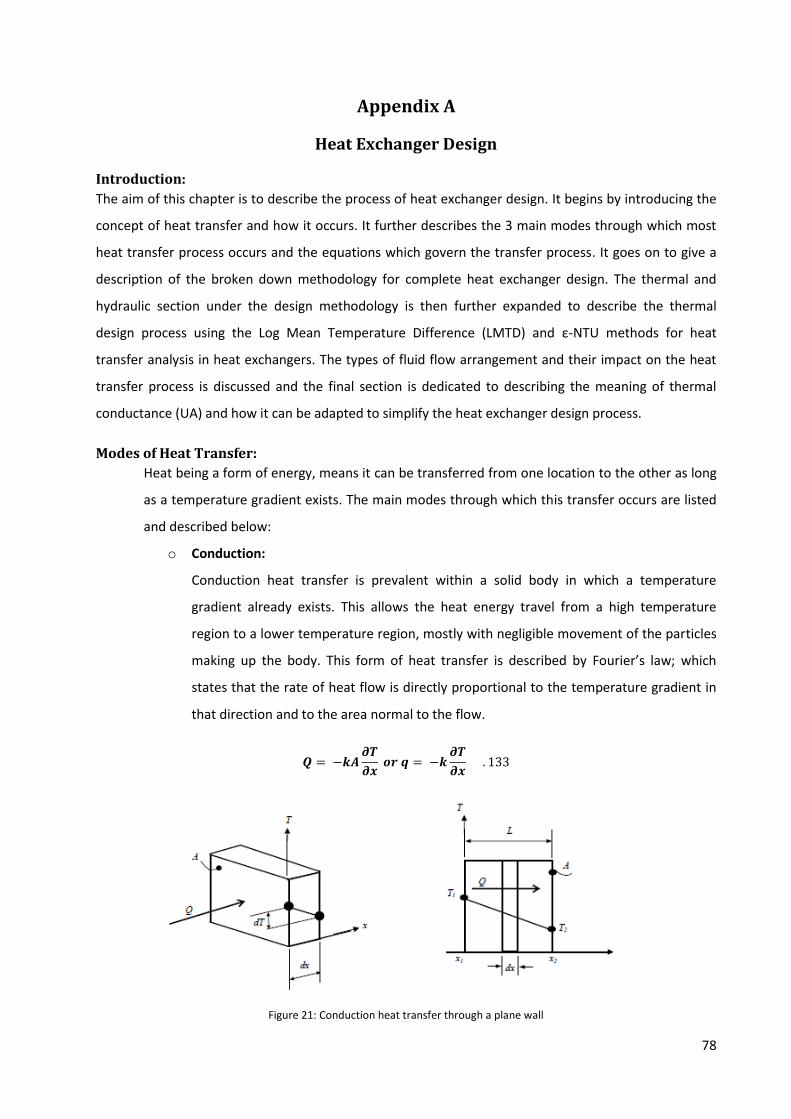
78

Appendix A

Heat Exchanger Design

Introduction:

The aim of this chapter is to describe the process of heat exchanger design. It begins by introducing the

concept of heat transfer and how it occurs. It further describes the 3 main modes through which most

heat transfer process occurs and the equations which govern the transfer process. It goes on to give a

description of the broken down methodology for complete heat exchanger design. The thermal and

hydraulic section under the design methodology is then further expanded to describe the thermal

design process using the Log Mean Temperature Difference (LMTD) and ε-NTU methods for heat

transfer analysis in heat exchangers. The types of fluid flow arrangement and their impact on the heat

transfer process is discussed and the final section is dedicated to describing the meaning of thermal

conductance (UA) and how it can be adapted to simplify the heat exchanger design process.

Modes of Heat Transfer:

Heat being a form of energy, means it can be transferred from one location to the other as long

as a temperature gradient exists. The main modes through which this transfer occurs are listed

and described below:

o Conduction:

Conduction heat transfer is prevalent within a solid body in which a temperature

gradient already exists. This allows the heat energy travel from a high temperature

region to a lower temperature region, mostly with negligible movement of the particles

making up the body. This form of heat transfer is described by Fourier’s law; which

states that the rate of heat flow is directly proportional to the temperature gradient in

that direction and to the area normal to the flow.

𝑸 = −𝒌𝑨𝝏𝑻

𝝏𝒙 𝒐𝒓 𝒒 = −𝒌

𝝏𝑻

𝝏𝒙 . 133

Figure 21: Conduction heat transfer through a plane wall

79

𝑄 or 𝑞 in the equation represents the heat transfer rate, 𝜕𝑇

𝜕𝑥 represent the temperature

gradient in the direction of heat flow; 𝑘 represents the thermal conductivity of the

body/material and the negative sign indicates that the second law of thermodynamics

which states that heat is transferred in the direction of decreasing temperature, is

satisfied. It is assumed that the transfer process happens under steady state conditions,

which means that the temperature at each point in the body is invariant with time;

hence;𝜕𝑇

𝜕𝑥= 0. It is also assumed that the heat travels in one-dimension and

temperature is uniform in directions perpendicular to this direction;𝜕𝑇

𝜕𝑦=

𝜕𝑇

𝜕𝑧= 0.

When heat travels in the 𝑥 direction, 𝑇 = 𝑇(𝑥) and Fourier’s equation becomes:

𝑸 = −𝒌𝑨𝒅𝑻

𝒅𝒙 . 134

Considering a plane wall of thickness 𝐿, and elemental thickness; 𝑑𝑥,

𝒒 = −𝒌𝒅𝑻

𝒅𝒙 𝒐𝒓 𝒒𝒅𝒙 = −𝒌𝒅𝑻 . 135

When integrated between the limits of 𝑥 and 𝑇, the equation takes on the form,

𝒒(𝒙𝟐 − 𝒙𝟏) = ∫ 𝒌 𝒅𝑻𝑻𝟏

𝑻𝟐

. 136

Assume the thermal conductivity; 𝑘 is constant across the material,

𝒒𝑳 = 𝒌(𝑻𝟏 − 𝑻𝟐) 𝒐𝒓 𝒒 = 𝒌(𝑻𝟏 − 𝑻𝟐)

𝑳 . 137

𝑸 = 𝒌𝑨 (𝑻𝟏 − 𝑻𝟐)

𝑳 . 138

For a multi-layered wall,

𝑸 = 𝒌𝟏𝑨 (𝑻𝟏 − 𝑻𝟐)

𝑳𝟏

= 𝒌𝟐𝑨 (𝑻𝟐 − 𝑻𝟑)

𝑳𝟐

= 𝒌𝟑𝑨 (𝑻𝟑 − 𝑻𝟒)

𝑳𝟑

. 139

Where 𝑘1, 𝑘2 𝑎𝑛𝑑 𝑘3 represent the thermal conductivities of the wall layers.

Rearranging the equation yields:

𝑸𝑳𝟏

𝒌𝟏𝑨= 𝑻𝟏 − 𝑻𝟐 . 140

𝑸𝑳𝟐

𝒌𝟐𝑨= 𝑻𝟐 − 𝑻𝟑 . 141

𝑸𝑳𝟑

𝒌𝟑𝑨= 𝑻𝟑 − 𝑻𝟒 . 142

If these are added and 𝑇2 , 𝑇3 are eliminated:

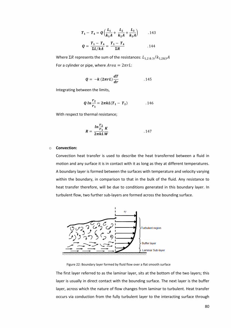
80

𝑻𝟏 − 𝑻𝟒 = 𝑸 (𝑳𝟏

𝒌𝟏𝑨+

𝑳𝟐

𝒌𝟐𝑨+

𝑳𝟑

𝒌𝟑𝑨) . 143

𝑸 = 𝑻𝟏 − 𝑻𝟒

𝚺𝑳 𝒌𝑨⁄=

𝑻𝟏 − 𝑻𝟒

𝚺𝑹 . 144

Where Σ𝑅 represents the sum of the resistances: 𝐿1,2 & 3 𝑘1,2&3𝐴⁄

For a cylinder or pipe, where 𝐴𝑟𝑒𝑎 = 2𝜋𝑟𝐿:

𝑸 = −𝒌 (𝟐𝝅𝒓𝑳)𝒅𝑻

𝒅𝒓 . 145

Integrating between the limits,

𝑸 𝒍𝒏𝒓𝟐

𝒓𝟏

= 𝟐𝝅𝒌𝑳(𝑻𝟏 − 𝑻𝟐) . 146

With respect to thermal resistance;

𝑹 = 𝒍𝒏

𝒓𝟐

𝒓𝟏

𝟐𝝅𝒌𝑳

𝑲

𝑾 . 147

o Convection:

Convection heat transfer is used to describe the heat transferred between a fluid in

motion and any surface it is in contact with it as long as they at different temperatures.

A boundary layer is formed between the surfaces with temperature and velocity varying

within the boundary, in comparison to that in the bulk of the fluid. Any resistance to

heat transfer therefore, will be due to conditions generated in this boundary layer. In

turbulent flow, two further sub-layers are formed across the bounding surface.

Figure 22: Boundary layer formed by fluid flow over a flat smooth surface

The first layer referred to as the laminar layer, sits at the bottom of the two layers; this

layer is usually in direct contact with the bounding surface. The next layer is the buffer

layer, across which the nature of flow changes from laminar to turbulent. Heat transfer

occurs via conduction from the fully turbulent layer to the interacting surface through

81

the buffer and laminar layers. It then follows that turbulence or the disruption within

these layers, greatly enhances the ease with which heat is transferred.

Convection heat transfer is categorized based on the nature of flow of the fluid moving

across the interacting surface. In natural convection heat transfer, the nature of this

flow is governed by density differences caused by temperature variations in the bulk of

the fluid. While in the forced convection heat transfer, an external mechanical means

such as a fan or pump is used to generate turbulence in the fluid.

To evaluate the heat transferred in convection, Newton’s law of cooling equation is

used.

𝑄 = ℎ𝐴(𝑇𝑠 − 𝑇𝑓) . 148

Where ℎ refers to the convection heat transfer coefficient. This value (convection heat

transfer coefficient) ′ℎ′ is evaluated from the factors which affect the extent to which

heat is transferred. Based on the condition of flow (natural or forced), these factors will

vary.

In forced convection heat transfer, these factors include: surface geometry or

dimension ‘𝑙′, flow velocity ‘𝑣′, fluid viscosity ‘𝜇′, fluid thermal conductivity ‘𝑘′, fluid

specific heat capacity ‘𝐶𝑝′, and fluid density ‘𝜌′. Using dimensional analysis to derive a

relationship between these factors,

𝒉 = 𝝓𝒍𝒃𝒗𝒂𝒌𝒄𝝁𝒊𝑪𝒑𝒋𝝆𝒏 . 149

Where ‘𝜙′ represents the dimensionless factor and ‘𝑎′‘b′‘c′‘ i′‘ j′ and ‘n′ represent the

dimensionless exponents. Solving the equation using the primary dimensions: mass (M),

length (L), time (t), temperature (T) and heat (H), gives:

𝒉𝒍

𝒌= 𝝓 (

𝝆𝒗𝒍

𝝁)

𝒏

(𝝁𝑪𝒑

𝒌)

𝒋

. 150

If a function ′𝑓′ is used,

𝒉𝒍

𝒌= 𝒇 (

𝝆𝒗𝒍

𝝁,𝝁𝑪𝒑

𝒌) . 151

𝑵𝒖 = 𝒇 (𝑹𝒆, 𝑷𝒓) . 152

Where:

𝑵𝒖𝒔𝒔𝒆𝒍𝒕 𝒏𝒖𝒎𝒃𝒆𝒓, 𝑵𝒖 = 𝒉𝒍

𝒌 . 153

𝑹𝒆𝒚𝒏𝒐𝒍𝒅𝒔 𝒏𝒖𝒎𝒃𝒆𝒓, 𝑹𝒆 = 𝝆𝒗𝒍

𝝁 . 154

𝑷𝒓𝒂𝒏𝒅𝒕𝒍 𝒏𝒖𝒎𝒃𝒆𝒓, 𝑷𝒓 = 𝝁𝑪𝒑

𝒌 . 155

82

Experimental data for forced convection heat transfer ′ℎ′ is thus expressed in the form

of these parameters.

For natural convection heat transfer, velocity is excluded from equation above, as flow

is dependent on the buoyancy forces acting within the fluid. To account for the

buoyancy forces acting per unit volume, the temperature difference between a warm

fluid with density 𝜌 and an undisturbed cold fluid 𝜌𝑓 is used and often designated

as Δ𝑇.

𝒈(𝝆𝒈 − 𝝆) = 𝝆𝜷𝒈𝚫𝑻 . 156

𝒄𝒐𝒆𝒇𝒇𝒊𝒄𝒊𝒆𝒏𝒕 𝒐𝒇 𝒄𝒖𝒃𝒊𝒄𝒂𝒍 𝒆𝒙𝒑𝒂𝒏𝒔𝒊𝒐𝒏, 𝜷 = 𝝆𝒇 − 𝝆

𝝆(𝑻 − 𝑻𝒇) . 157

Therefore, the dimensional relations for natural heat transfer convection can be written

as:

𝒉 = 𝝓𝚫𝑻𝒂𝒍𝒃𝒌𝒄𝝁𝒊𝑪𝒑𝒋𝝆𝒏(𝝆𝜷)𝒑 . 158

Solution of the equation, using the primary dimensions: mass (M), length (L), time (t),

temperature (T), and heat (H) yields:

𝒉𝒍

𝒌= 𝝓 (

𝜷𝒈𝚫𝑻𝒍𝟑𝝆𝟐

𝝁𝟐)

𝒑

(𝝁𝑪𝒑

𝒌)

𝒋

. 159

Where the function 𝑓 is used,

𝒉𝒍

𝒌= 𝒇 (

𝜷𝒈𝚫𝑻𝒍𝟑𝝆𝟐

𝝁𝟐,𝝁𝑪𝒑

𝒌) . 160

𝑵𝒖 = 𝒇 (𝑮𝒓, 𝑷𝒓) . 161

Where:

𝑵𝒖𝒔𝒔𝒆𝒍𝒕 𝒏𝒖𝒎𝒃𝒆𝒓, 𝑵𝒖 = 𝒉𝒍

𝒌 . 162

𝑮𝒓𝒂𝒔𝒉𝒐𝒇 𝒏𝒖𝒎𝒃𝒆𝒓, 𝑮𝒓 = 𝜷𝒈(𝑻𝒔 − 𝑻𝒇)𝒍𝟑𝝆𝟐

𝝁 . 163

𝑷𝒓𝒂𝒏𝒅𝒕𝒍 𝒏𝒖𝒎𝒃𝒆𝒓, 𝑷𝒓 = 𝝁𝑪𝒑

𝒌 . 164

Experimental data for natural convection heat transfer ′ℎ′ is expressed in the form of

these parameters.

o Radiation

Also referred to as thermal radiation, is the form of heat transfer that occurs via

electromagnetic waves when a temperature difference occurs within a vacuum. The

83

rate of emission from such a body referred to as a “Black-body”, is described in the

equation below, and referred to as the Stefan-Boltzmann law of thermal radiation:

𝒒𝒆𝒎𝒊𝒕𝒕𝒆𝒅 = 𝝈𝑨𝑻𝟒 . 165

Where σ is a constant of proportionality and referred to as the Stefan-Boltzmann

constant with a value equivalent to 5.669 x 10-8 W/m2K4. This equation applies only to

black-bodies, which are described as perfect radiation absorbers and emitters.

For the heat transmitted and exchanged between two bodies:

𝒒𝒏𝒆𝒕 𝒆𝒙𝒄𝒉𝒂𝒏𝒈𝒆

𝑨 ∝ 𝝈(𝑻𝟏

𝟒 − 𝑻𝟐𝟒) . 166

Considering that not all bodies are entirely ‘black’, a factor referred to as the emissivity

factor is introduced. Consideration must also then be given to the fact that emitted

radiation can be lost to the environment during transmission. Therefore, the final heat

transfer equation thus becomes:

𝒒 = 𝑭𝝐𝑭𝑮𝝈𝑨(𝑻𝟏𝟒 − 𝑻𝟐

𝟒) . 167

Where Fϵ is the emissivity function and FG is the geometric view factor function. These

two values differ across body configurations and must thus be determined before an

accurate value for radiation heat transfer can be determined.

Heat Exchanger Design Methodology:

Heat exchanger design is based on an iterative process due to the several operational conditions which

must all be satisfied before assurance is given that the exchanger will do the required duty. Kays and

London (1984) [8] broke the steps required for the optimum design of heat exchangers into the

following based on the figure below:

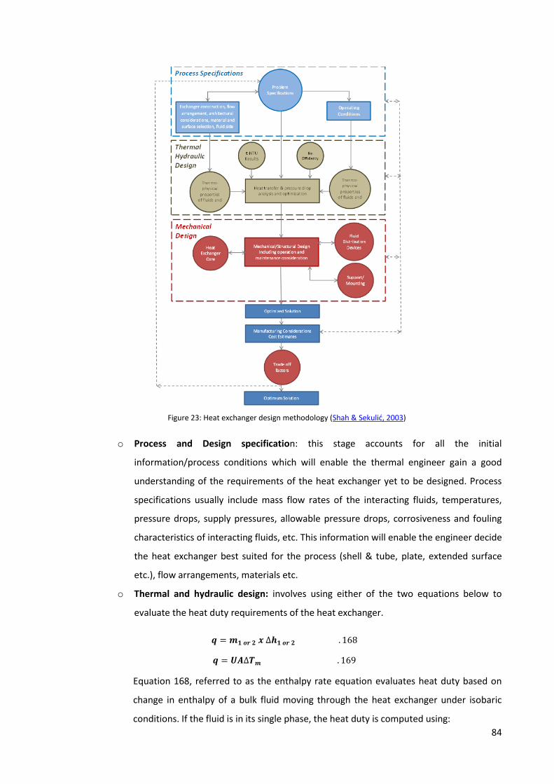
84

Figure 23: Heat exchanger design methodology (Shah & Sekulić, 2003)

o Process and Design specification: this stage accounts for all the initial

information/process conditions which will enable the thermal engineer gain a good

understanding of the requirements of the heat exchanger yet to be designed. Process

specifications usually include mass flow rates of the interacting fluids, temperatures,

pressure drops, supply pressures, allowable pressure drops, corrosiveness and fouling

characteristics of interacting fluids, etc. This information will enable the engineer decide

the heat exchanger best suited for the process (shell & tube, plate, extended surface

etc.), flow arrangements, materials etc.

o Thermal and hydraulic design: involves using either of the two equations below to

evaluate the heat duty requirements of the heat exchanger.

𝒒 = 𝒎𝟏 𝒐𝒓 𝟐 𝒙 ∆𝒉𝟏 𝒐𝒓 𝟐 . 168

𝒒 = 𝑼𝑨∆𝑻𝒎 . 169

Equation 168, referred to as the enthalpy rate equation evaluates heat duty based on

change in enthalpy of a bulk fluid moving through the heat exchanger under isobaric

conditions. If the fluid is in its single phase, the heat duty is computed using:

85

𝒒 = 𝒎𝑪𝒑𝟏 𝒐𝒓 𝟐∆𝑻𝟏 𝒐𝒓 𝟐, 𝒊𝒏𝒍𝒆𝒕 & 𝒐𝒖𝒕𝒍𝒆𝒕 . 170

Equation 169, evaluates heat transfer based on the different heat transfer modes

(conduction, convection and radiation) prevalent in the heat exchanger. The heat

transferred, is seen to be directly proportional to the area, A, and mean temperature

difference of the interacting fluids ΔTm. The mean temperature difference in this case,

refers to the mean temperature difference of the interacting fluids, based on their entry

and exit temperatures. The factor ‘U’ is defined as the overall heat transfer coefficient

which accounts for the different heat transfer methods occurring in the heat exchanger.

Within the thermal and hydraulic design block, several subsets of design parameters are

required to produce an appropriate design solution. These subsets include: surface heat

transfer and flow friction characteristics, geometrical properties and thermophysical

properties of the fluids.

o Mechanical design: Mechanical design of heat exchangers ensures that the units are

structurally stable under specified operational conditions. These conditions include:

steady-state, start-up, shutdown or even earthquake conditions. Each section of the

heat exchanger undergoes a mechanical assessment to determine its behaviour under

these conditions. For example, the thermal stress developed in the heat exchanger as a

result of the changes in temperature of the interacting fluids, will be determined as part

of the mechanical design process to ensure that the tubes, nozzles and headers can

bear the thermal stress developed. If mechanical bonding techniques such as brazing or

welding are used, the joints under question must be assessed to ensure they can bear

the loads generated in the heat exchanger to avoid failure during operation. Several

international codes and standards such as the ASME pressure vessel codes,

Specification for unfired fusion welded pressure vessels (PD5500) are available solely

for this purpose.

o Manufacturing considerations and cost: During design, consideration must be given to

method of manufacture. Design complexity will determine if new tools are needed, all

which must be available before manufacturing can begin. Lead times, quality control

and availability of workshop staff are lumped into factors which must be considered in

this phase. Costs associated with a heat exchanger must also be considered. These costs

include: capital, installation, operating and in some cases, disposal.

o Trade-off factors and system-based optimization: As a result of the iterative process

involved in heat exchanger design, trade-offs are inevitable at the design stage. An

example is where a heat transfer fluid such as Ethylene Glycol is added to water as anti-

freeze. This process ensures the frost protection of pipes but however reduces the heat

86

transfer capability of the fluid and also adds to the pumping requirements of the

system. Another example is the use of stainless steel for the manufacture of heat

exchangers meant for use in corrosive operating environments. Stainless steel will

always be the preferred construction material to mild steel even though it is more

expensive and has lesser heat conducting capabilities than mild steel.

An optimized heat exchanger design therefore constitutes a balance of all the quantitative and

qualitative factors mentioned above.

Thermal & Hydraulic Design:

Flow arrangements:

The arrangement/alignment of flow of the interacting fluids plays a vital role in the heat transferred

across the heat exchanger as research has shown that certain arrangements have more merits than

other arrangements. Flow arrangement therefore plays a role in the design of heat exchangers and

must be considered and agreed on before design commences. Arrangements include:

- Counter-current or Counter-flow: this arrangement sees the interacting fluids flow past each

other in parallel but opposite directions. If temperature variation is assumed to occur entirely in

one dimension, then counter-current flow is considered the most efficient in transferring heat

across interacting fluids when compared to all other flow arrangements [Ref. (65)]. They also

describe this arrangement as one where the least thermal stress is produced in the tube wall

when compared to other flow arrangements. The figure below shows the direction heat flow

occurs for such flow arrangements:

Figure 24: Temperature flow in single-phase counterflow arrangement heat exchanger with no boiling or condensation

(Shah & Sekulić, 2003).

- Parallel or Co-current flow: in this flow arrangement, the interacting fluids are

introduced into the heat exchanger from the same direction and also tend to exit the

heat exchanger in the same direction. Figure 25 shows how heat is transferred in a

heat exchanger with such a fluid flow arrangement. This flow arrangement is

described as the flow arrangement with the poorest effectiveness amongst single

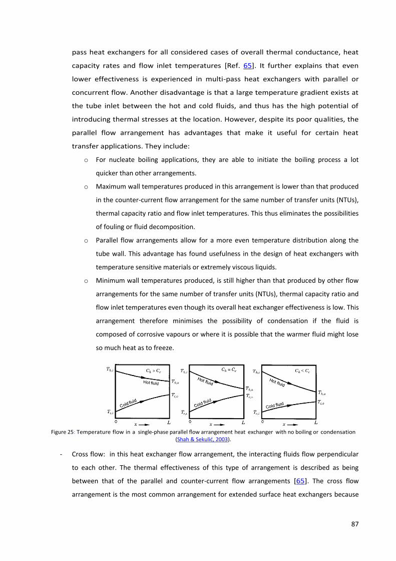
87

pass heat exchangers for all considered cases of overall thermal conductance, heat

capacity rates and flow inlet temperatures [Ref. 65]. It further explains that even

lower effectiveness is experienced in multi-pass heat exchangers with parallel or

concurrent flow. Another disadvantage is that a large temperature gradient exists at

the tube inlet between the hot and cold fluids, and thus has the high potential of

introducing thermal stresses at the location. However, despite its poor qualities, the

parallel flow arrangement has advantages that make it useful for certain heat

transfer applications. They include:

o For nucleate boiling applications, they are able to initiate the boiling process a lot

quicker than other arrangements.

o Maximum wall temperatures produced in this arrangement is lower than that produced

in the counter-current flow arrangement for the same number of transfer units (NTUs),

thermal capacity ratio and flow inlet temperatures. This thus eliminates the possibilities

of fouling or fluid decomposition.

o Parallel flow arrangements allow for a more even temperature distribution along the

tube wall. This advantage has found usefulness in the design of heat exchangers with

temperature sensitive materials or extremely viscous liquids.

o Minimum wall temperatures produced, is still higher than that produced by other flow

arrangements for the same number of transfer units (NTUs), thermal capacity ratio and

flow inlet temperatures even though its overall heat exchanger effectiveness is low. This

arrangement therefore minimises the possibility of condensation if the fluid is

composed of corrosive vapours or where it is possible that the warmer fluid might lose

so much heat as to freeze.

Figure 25: Temperature flow in a single-phase parallel flow arrangement heat exchanger with no boiling or condensation


- Cross flow: in this heat exchanger flow arrangement, the interacting fluids flow perpendicular

to each other. The thermal effectiveness of this type of arrangement is described as being

between that of the parallel and counter-current flow arrangements [65]. The cross flow

arrangement is the most common arrangement for extended surface heat exchangers because

88

headers can be used as the inlet and outlet of the tube-side fluid, while the second fluid

referred to as the gas-side fluid flows across the tubes.

Figure 26: Temperature flow at the inlet and outlet of an unmixed-unmixed crossflow arrangement heat exchanger


The cross flow arrangement further introduces the concept of mixed or unmixed flows for both

fluid streams. The tube-side or gas-side fluid is considered completely mixed when a

temperature gradient ceases to exist within the fluid. When either fluid is unmixed, there exists

a temperature gradient in at least one direction perpendicular to the flow of the fluid. In the

case of multiple row heat exchangers, the tube-side fluid is completely mixed in the headers.

However, when they split and flow into individual tubes, they are considered to be unmixed.

The presence of extended surfaces can also introduce an unmixed flow arrangement for the

gas-side fluid especially where plates are used for extended surface purposes. Several other

fluid combinations exist: unmixed – mixed, both fluids mixed, both fluids unmixed, partially

unmixed – partially mixed and mixed – partially mixed.

Figure 27: Types of mixing in crossflow heat exchanger (Shah & Sekulić, 2003).

Other flow arrangements exist which include; Divided-flow TEMA J Shell, Split-Flow TEMA G Shell.

However, these are common to shell and tube heat exchangers and will thus not be considered.

Design theories:

Several thermal design theories are available for the design of heat exchangers, e.g. the ɛ-NTU method,

the P-NTU method, the LMTD method, the P1 – P2 method and the ψ – P method [Ref. 65]. However,

only the first three methods listed were studied during the design stage of the toolkit. Each of these

89

theories comes with its own merits and demerits. Only the LMTD method and the ɛ-NTU method will be

discussed due to their specific application to the design of extended surface heat exchangers.

The validity of the ɛ-NTU and the LMTD method theories are based on a number of assumptions which

are outlined below:

o The heat exchanger operates solely under steady-state conditions. Flow rates and fluid

temperatures are constant and are independent of time.

o There are no heat energy sources or sinks in either the interacting fluids or the heat

exchanger walls.

o Heat loss to surroundings is negligible.

o Fluid temperatures are uniform across the heat exchanger cross-section in both

counterflow and parallel flow conditions. This means that within the heat exchanger,

there is prefect transverse mixing and no temperature gradient normal to the direction

of flow.

o Thermal resistances in the tube walls are distributed uniformly in the heat exchanger.

o Phase change does not occur in any of the fluids. If it does occur, it does under constant

temperature conditions, same as a single-component fluid at constant pressure.

o Longitudinal heat conduction both in the fluids and heat exchanger walls are negligible.

o Overall heat transfer coefficients are constant throughout the heat exchanger.

Independent of temperature, position or time. This requirement also applies to phase-

changing fluids.

o The specific heat capacity for each fluid is constant through the heat exchanger.

o For extended surfaces, the surface efficiency of the extended surface is constant and

uniform.

o The heat transfer surface area A of the heat exchanger is distributed uniformly on each

fluid side regardless of single or multi-pass arrangements.

o Fluid velocities and temperatures at entry on each fluid side, is uniform across the heat

exchanger cross-section. Uneven fluid distribution does not occur.

o Rate of fluid flow is distributed uniformly in the heat exchanger for each fluid. No flow

bypassing, leaks or flow stratification occurs in the unit. Flow conditions are

characterized by mean or bulk velocities at any cross-section.

However, It must be stated that in cases where the fluids on both sides of heat exchanger walls are in

two-phase states, then these assumptions are rendered invalid as a result of the mass transfer that

occurs which will invariably change the thermal properties, flow rates and heat transfer coefficients of

the interacting fluids.

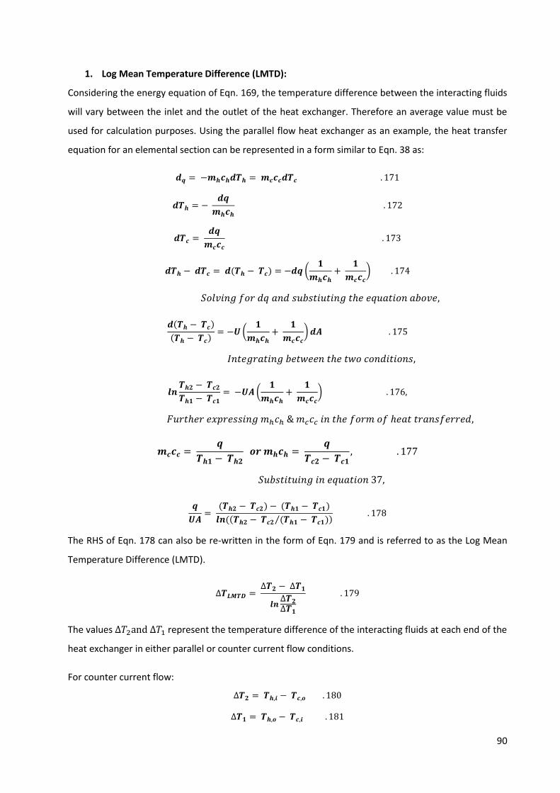
90

1. Log Mean Temperature Difference (LMTD):

Considering the energy equation of Eqn. 169, the temperature difference between the interacting fluids

will vary between the inlet and the outlet of the heat exchanger. Therefore an average value must be

used for calculation purposes. Using the parallel flow heat exchanger as an example, the heat transfer

equation for an elemental section can be represented in a form similar to Eqn. 38 as:

𝒅𝒒 = −𝒎𝒉𝒄𝒉𝒅𝑻𝒉 = 𝒎𝒄𝒄𝒄𝒅𝑻𝒄 . 171

𝒅𝑻𝒉 = − 𝒅𝒒

𝒎𝒉𝒄𝒉

. 172

𝒅𝑻𝒄 = 𝒅𝒒

𝒎𝒄𝒄𝒄

. 173

𝒅𝑻𝒉 − 𝒅𝑻𝒄 = 𝒅(𝑻𝒉 − 𝑻𝒄) = −𝒅𝒒 (𝟏

𝒎𝒉𝒄𝒉

+ 𝟏

𝒎𝒄𝒄𝒄

) . 174

𝑆𝑜𝑙𝑣𝑖𝑛𝑔 𝑓𝑜𝑟 𝑑𝑞 𝑎𝑛𝑑 𝑠𝑢𝑏𝑠𝑡𝑖𝑢𝑡𝑖𝑛𝑔 𝑡ℎ𝑒 𝑒𝑞𝑢𝑎𝑡𝑖𝑜𝑛 𝑎𝑏𝑜𝑣𝑒,

𝒅(𝑻𝒉 − 𝑻𝒄)

(𝑻𝒉 − 𝑻𝒄)= −𝑼 (

𝟏

𝒎𝒉𝒄𝒉

+ 𝟏

𝒎𝒄𝒄𝒄

) 𝒅𝑨 . 175

𝐼𝑛𝑡𝑒𝑔𝑟𝑎𝑡𝑖𝑛𝑔 𝑏𝑒𝑡𝑤𝑒𝑒𝑛 𝑡ℎ𝑒 𝑡𝑤𝑜 𝑐𝑜𝑛𝑑𝑖𝑡𝑖𝑜𝑛𝑠,

𝒍𝒏𝑻𝒉𝟐 − 𝑻𝒄𝟐

𝑻𝒉𝟏 − 𝑻𝒄𝟏

= −𝑼𝑨 (𝟏

𝒎𝒉𝒄𝒉

+ 𝟏

𝒎𝒄𝒄𝒄

) . 176,

𝐹𝑢𝑟𝑡ℎ𝑒𝑟 𝑒𝑥𝑝𝑟𝑒𝑠𝑠𝑖𝑛𝑔 𝑚ℎ𝑐ℎ & 𝑚𝑐𝑐𝑐 𝑖𝑛 𝑡ℎ𝑒 𝑓𝑜𝑟𝑚 𝑜𝑓 ℎ𝑒𝑎𝑡 𝑡𝑟𝑎𝑛𝑠𝑓𝑒𝑟𝑟𝑒𝑑,

𝒎𝒄𝒄𝒄 = 𝒒

𝑻𝒉𝟏 − 𝑻𝒉𝟐 𝒐𝒓 𝒎𝒉𝒄𝒉 =

𝒒

𝑻𝒄𝟐 − 𝑻𝒄𝟏, . 177

𝑆𝑢𝑏𝑠𝑡𝑖𝑡𝑢𝑖𝑛𝑔 𝑖𝑛 𝑒𝑞𝑢𝑎𝑡𝑖𝑜𝑛 37,

𝒒

𝑼𝑨=

(𝑻𝒉𝟐 − 𝑻𝒄𝟐) − (𝑻𝒉𝟏 − 𝑻𝒄𝟏)

𝒍𝒏 ((𝑻𝒉𝟐 − 𝑻𝒄𝟐 (𝑻𝒉𝟏 − 𝑻𝒄𝟏)⁄ ) . 178

The RHS of Eqn. 178 can also be re-written in the form of Eqn. 179 and is referred to as the Log Mean

Temperature Difference (LMTD).

∆𝑻𝑳𝑴𝑻𝑫 = ∆𝑻𝟐 − ∆𝑻𝟏

𝒍𝒏∆𝑻𝟐

∆𝑻𝟏

. 179

The values ∆𝑇2and ∆𝑇1 represent the temperature difference of the interacting fluids at each end of the

heat exchanger in either parallel or counter current flow conditions.

For counter current flow:

∆𝑻𝟐 = 𝑻𝒉,𝒊 − 𝑻𝒄,𝒐 . 180

∆𝑻𝟏 = 𝑻𝒉,𝒐 − 𝑻𝒄,𝒊 . 181

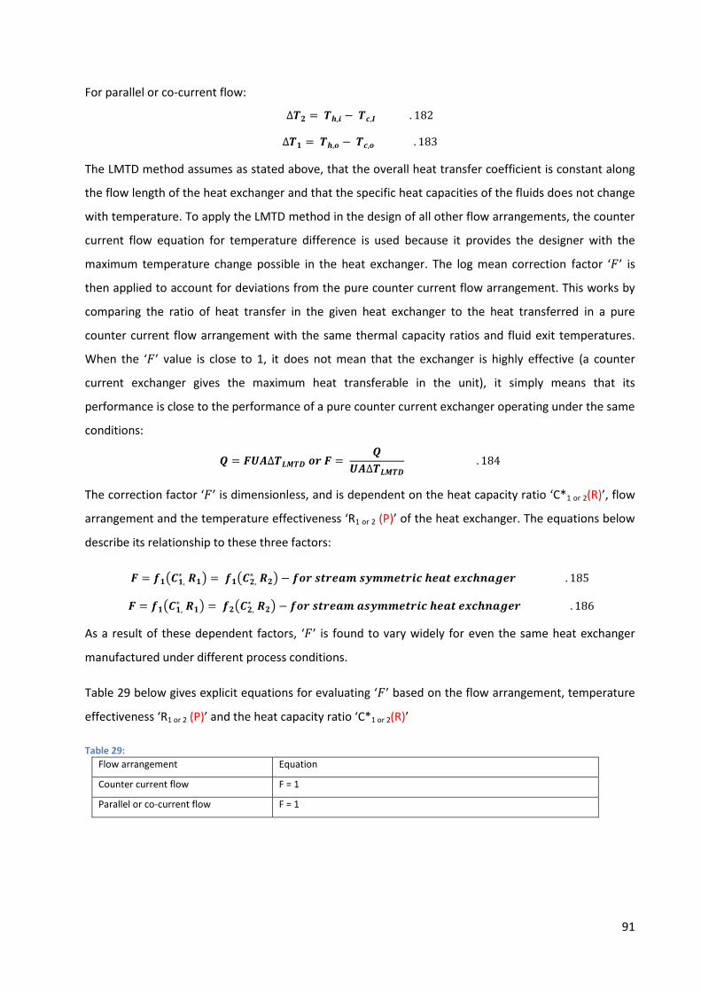
91

For parallel or co-current flow:

∆𝑻𝟐 = 𝑻𝒉,𝒊 − 𝑻𝒄,𝑰 . 182

∆𝑻𝟏 = 𝑻𝒉,𝒐 − 𝑻𝒄,𝒐 . 183

The LMTD method assumes as stated above, that the overall heat transfer coefficient is constant along

the flow length of the heat exchanger and that the specific heat capacities of the fluids does not change

with temperature. To apply the LMTD method in the design of all other flow arrangements, the counter

current flow equation for temperature difference is used because it provides the designer with the

maximum temperature change possible in the heat exchanger. The log mean correction factor ‘𝐹’ is

then applied to account for deviations from the pure counter current flow arrangement. This works by

comparing the ratio of heat transfer in the given heat exchanger to the heat transferred in a pure

counter current flow arrangement with the same thermal capacity ratios and fluid exit temperatures.

When the ‘𝐹’ value is close to 1, it does not mean that the exchanger is highly effective (a counter

current exchanger gives the maximum heat transferable in the unit), it simply means that its

performance is close to the performance of a pure counter current exchanger operating under the same

conditions:

𝑸 = 𝑭𝑼𝑨∆𝑻𝑳𝑴𝑻𝑫 𝒐𝒓 𝑭 = 𝑸

𝑼𝑨∆𝑻𝑳𝑴𝑻𝑫

. 184

The correction factor ‘𝐹’ is dimensionless, and is dependent on the heat capacity ratio ‘C*1 or 2(R)’, flow

arrangement and the temperature effectiveness ‘R1 or 2 (P)’ of the heat exchanger. The equations below

describe its relationship to these three factors:

𝑭 = 𝒇𝟏(𝑪𝟏,∗ 𝑹𝟏) = 𝒇𝟏(𝑪𝟐,

∗ 𝑹𝟐) − 𝒇𝒐𝒓 𝒔𝒕𝒓𝒆𝒂𝒎 𝒔𝒚𝒎𝒎𝒆𝒕𝒓𝒊𝒄 𝒉𝒆𝒂𝒕 𝒆𝒙𝒄𝒉𝒏𝒂𝒈𝒆𝒓 . 185

𝑭 = 𝒇𝟏(𝑪𝟏,∗ 𝑹𝟏) = 𝒇𝟐(𝑪𝟐,

∗ 𝑹𝟐) − 𝒇𝒐𝒓 𝒔𝒕𝒓𝒆𝒂𝒎 𝒂𝒔𝒚𝒎𝒎𝒆𝒕𝒓𝒊𝒄 𝒉𝒆𝒂𝒕 𝒆𝒙𝒄𝒉𝒏𝒂𝒈𝒆𝒓 . 186

As a result of these dependent factors, ‘𝐹’ is found to vary widely for even the same heat exchanger

manufactured under different process conditions.

Table 29 below gives explicit equations for evaluating ‘𝐹’ based on the flow arrangement, temperature

effectiveness ‘R1 or 2 (P)’ and the heat capacity ratio ‘C*1 or 2(R)’

Table 29:

Flow arrangement Equation

Counter current flow F = 1

Parallel or co-current flow F = 1

92

Cross flow (single-pass):

- Hot fluid unmixed, cold fluid

mixed, with stream

asymmetric

- Hot fluid mixed, cold fluid

unmixed, with stream

asymmetric

𝐹 = 𝑙𝑛[(1 − 𝐶1

∗𝑃1) (1 − 𝑃1)⁄ ]

(𝐶1∗ − 1) 𝑙𝑛[1 + (1 𝐶1

∗⁄ ) 𝑙𝑛(1 − 𝐶1∗𝑃1)]

= 𝑙𝑛[(1 − 𝐶1

∗𝑃2) (1 − 𝑃2)⁄ ]

(1 − 1 𝐶2∗⁄ ) 𝑙𝑛[1 + 𝐶2

∗𝑙𝑛(1 − 𝑃2)]

𝐹 = 𝑙𝑛[(1 − 𝐶2

∗𝑃2) (1 − 𝑃2)⁄ ]

(𝐶2∗ − 1) 𝑙𝑛[1 + (1 𝐶2

∗⁄ ) 𝑙𝑛(1 − 𝐶2∗𝑃2)]

= 𝑙𝑛[(1 − 𝐶1

∗𝑃1) (1 − 𝑃1)⁄ ]

(1 − 1 𝐶1∗⁄ ) 𝑙𝑛[1 + 𝐶1

∗𝑙𝑛(1 − 𝑃1)]

Where explicit equations are not available, graphs are provided, and Fig. 28 [84] below gives an example

of such a graph provided for the selection of the appropriate correction factor, ‘F’.

93

Figure 28: LMTD correction factors for heat exchangers (Source: Green & Perry, 2008)

When the temperature values for the interacting fluids is constant as seen in phase change conditions,

or the thermal capacity ratio C* = 0:

𝑭 = 𝟏 . 187

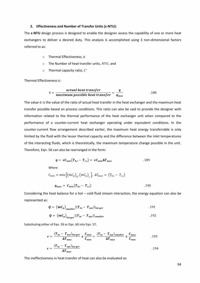
94

2. Effectiveness and Number of Transfer Units (ɛ-NTU):

The ɛ-NTU design process is designed to enable the designer assess the capability of one or more heat

exchangers to deliver a desired duty. This analysis is accomplished using 3 non-dimensional factors

referred to as:

o Thermal Effectiveness, ∈

o The Number of heat transfer units, 𝑁𝑇𝑈, and

o Thermal capacity ratio, 𝐶∗

Thermal Effectiveness ∈:

∈ = 𝒂𝒄𝒕𝒖𝒂𝒍 𝒉𝒆𝒂𝒕 𝒕𝒓𝒂𝒏𝒔𝒇𝒆𝒓

𝒎𝒂𝒙𝒊𝒎𝒖𝒎 𝒑𝒐𝒔𝒔𝒊𝒃𝒍𝒆 𝒉𝒆𝒂𝒕 𝒕𝒓𝒂𝒏𝒔𝒇𝒆𝒓=

𝒒

𝒒𝒎𝒂𝒙

. 188

The value ∈ is the value of the ratio of actual heat transfer in the heat exchanger and the maximum heat

transfer possible based on process conditions. This ratio can also be said to provide the designer with

information related to the thermal performance of the heat exchanger unit when compared to the

performance of a counter-current heat exchanger operating under equivalent conditions. In the

counter-current flow arrangement described earlier, the maximum heat energy transferrable is only

limited by the fluid with the lesser thermal capacity and the difference between the inlet temperatures

of the interacting fluids, which is theoretically, the maximum temperature change possible in the unit.

Therefore, Eqn. 56 can also be rearranged in the form:

𝒒 = 𝝐𝑪𝒎𝒊𝒏(𝑻𝒉,𝒊 − 𝑻𝒄,𝒊) = 𝝐𝑪𝒎𝒊𝒏𝚫𝑻𝒎𝒂𝒙 . 189

Where

𝐶𝑚𝑖𝑛 = 𝑚𝑖𝑛 [(�̇�𝐶𝑝)ℎ

, (�̇�𝐶𝑝)𝑐 ], Δ𝑇𝑚𝑎𝑥 = (𝑇ℎ,𝑖 − 𝑇𝑐,𝑖)

𝒒𝒎𝒂𝒙 = 𝑪𝒎𝒊𝒏(𝑻𝒉,𝒊 − 𝑻𝒄,𝒊) . 190

Considering the heat balance for a hot – cold fluid stream interaction, the energy equation can also be

represented as:

𝑸 = (�̇�𝑪𝒑)𝒔𝒎𝒂𝒍𝒍𝒆𝒓

|(𝑻𝒊𝒏 − 𝑻𝒐𝒖𝒕)|𝒍𝒂𝒓𝒈𝒆𝒓 . 191

𝑸 = (�̇�𝑪𝒑)𝒍𝒂𝒓𝒈𝒆𝒓

|(𝑻𝒊𝒏 − 𝑻𝒐𝒖𝒕)|𝒔𝒎𝒂𝒍𝒍𝒆𝒓 . 192

Substituting either of Eqn. 59 or Eqn. 60 into Eqn. 57,

𝝐 = (𝑻𝒊𝒏 − 𝑻𝒐𝒖𝒕)𝒍𝒂𝒓𝒈𝒆𝒓

𝚫𝑻𝒎𝒂𝒙

𝒙 𝑪𝒎𝒊𝒏

𝑪𝒎𝒊𝒏

= (𝑻𝒊𝒏 − 𝑻𝒐𝒖𝒕)𝒔𝒎𝒂𝒍𝒍𝒆𝒓


𝒙 𝑪𝒎𝒂𝒙

𝑪𝒎𝒊𝒏

. 193

𝝐 = (𝑻𝒊𝒏 − 𝑻𝒐𝒖𝒕)𝒍𝒂𝒓𝒈𝒆𝒓


. 194

The ineffectiveness in heat transfer of heat can also be evaluated as:

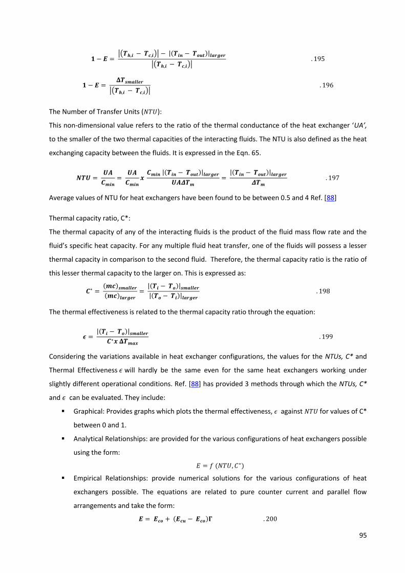
95

𝟏 − 𝑬 = |(𝑻𝒉,𝒊 − 𝑻𝒄,𝒊)| − |(𝑻𝒊𝒏 − 𝑻𝒐𝒖𝒕)|𝒍𝒂𝒓𝒈𝒆𝒓

|(𝑻𝒉,𝒊 − 𝑻𝒄,𝒊)| . 195

𝟏 − 𝑬 = 𝚫𝑻𝒔𝒎𝒂𝒍𝒍𝒆𝒓

|(𝑻𝒉,𝒊 − 𝑻𝒄,𝒊)| . 196

The Number of Transfer Units (𝑁𝑇𝑈):

This non-dimensional value refers to the ratio of the thermal conductance of the heat exchanger ‘UA’,

to the smaller of the two thermal capacities of the interacting fluids. The NTU is also defined as the heat

exchanging capacity between the fluids. It is expressed in the Eqn. 65.

𝑵𝑻𝑼 = 𝑼𝑨

𝑪𝒎𝒊𝒏

= 𝑼𝑨

𝑪𝒎𝒊𝒏

𝒙 𝑪𝒎𝒊𝒏 |(𝑻𝒊𝒏 − 𝑻𝒐𝒖𝒕)|𝒍𝒂𝒓𝒈𝒆𝒓

𝑼𝑨𝜟𝑻𝒎

= |(𝑻𝒊𝒏 − 𝑻𝒐𝒖𝒕)|𝒍𝒂𝒓𝒈𝒆𝒓

𝜟𝑻𝒎

. 197

Average values of NTU for heat exchangers have been found to be between 0.5 and 4 Ref. [88]

Thermal capacity ratio, C*:

The thermal capacity of any of the interacting fluids is the product of the fluid mass flow rate and the

fluid’s specific heat capacity. For any multiple fluid heat transfer, one of the fluids will possess a lesser

thermal capacity in comparison to the second fluid. Therefore, the thermal capacity ratio is the ratio of

this lesser thermal capacity to the larger on. This is expressed as:

𝑪∗ = (𝒎𝒄)𝒔𝒎𝒂𝒍𝒍𝒆𝒓

(𝒎𝒄)𝒍𝒂𝒓𝒈𝒆𝒓

= |(𝑻𝒊 − 𝑻𝒐)|𝒔𝒎𝒂𝒍𝒍𝒆𝒓

|(𝑻𝒐 − 𝑻𝒊)|𝒍𝒂𝒓𝒈𝒆𝒓

. 198

The thermal effectiveness is related to the thermal capacity ratio through the equation:

𝝐 = |(𝑻𝒊 − 𝑻𝒐)|𝒔𝒎𝒂𝒍𝒍𝒆𝒓

𝑪∗𝒙 𝚫𝑻𝒎𝒂𝒙

. 199

Considering the variations available in heat exchanger configurations, the values for the NTUs, C* and

Thermal Effectiveness 𝜖 will hardly be the same even for the same heat exchangers working under

slightly different operational conditions. Ref. [88] has provided 3 methods through which the NTUs, C*

and 𝜖 can be evaluated. They include:

Graphical: Provides graphs which plots the thermal effectiveness, 𝜖 against 𝑁𝑇𝑈 for values of C*

between 0 and 1.

Analytical Relationships: are provided for the various configurations of heat exchangers possible

using the form:

𝐸 = 𝑓 (𝑁𝑇𝑈, 𝐶∗)

Empirical Relationships: provide numerical solutions for the various configurations of heat

exchangers possible. The equations are related to pure counter current and parallel flow

arrangements and take the form:

𝑬 = 𝑬𝒄𝒐 + (𝑬𝒄𝒖 − 𝑬𝒄𝒐)𝚪 . 200

96

𝑬𝒄𝒖 = 𝟏 − 𝒆𝒙𝒑[𝑵𝑻𝑼 (𝟏 − 𝑪∗)]

𝑪∗ − 𝒆𝒙𝒑[𝑵𝑻𝑼 (𝟏 − 𝑪∗)] . 201

𝑬𝒄𝒖 = 𝟏 − 𝒆𝒙𝒑[𝑵𝑻𝑼 (𝟏 − 𝑪∗)]

𝑪∗ − 𝒆𝒙𝒑[𝑵𝑻𝑼 (𝟏 − 𝑪∗)] . 202

𝛤 − 𝑝𝑟𝑜𝑣𝑖𝑑𝑒𝑠 𝑡ℎ𝑒 𝑒𝑚𝑝𝑖𝑟𝑖𝑐𝑎𝑙 𝑓𝑢𝑛𝑐𝑡𝑖𝑜 𝑡𝑜 𝑠𝑜𝑙𝑣𝑒 𝑜𝑡ℎ𝑒𝑟 ℎ𝑒𝑎𝑡 𝑒𝑥𝑐ℎ𝑎𝑛𝑎𝑔𝑒𝑟 𝑓𝑙𝑜𝑤 𝑎𝑟𝑟𝑎𝑛𝑔𝑚𝑒𝑛𝑡𝑠

𝜞 = 𝜞𝒂𝒔𝒚𝒎𝒑 + 𝜞𝒄𝒐𝒓𝒓. . 203

𝜞𝒂𝒔𝒚𝒎𝒑 = 𝒂𝟎 + 𝒂𝟏𝑪∗ + 𝒂𝟐𝑪∗𝟐 . 204

𝜞𝒄𝒐𝒓𝒓. = 𝑩𝑪∗[𝒂𝒓𝒄𝒕𝒂𝒏(𝒄𝟎𝑵𝑻𝑼)][𝒆𝒙𝒑(𝑫 𝑵𝑻𝑼)] . 205

𝑩 = 𝒃𝟎 + 𝒃𝟏𝑪∗ + 𝒃𝟐𝑪∗𝟐 + 𝒃𝟑𝑪∗𝟑 + 𝒃𝟒𝑪∗𝟒 . 206

𝑫 = 𝒅𝟎 + 𝒅𝟏𝑪∗ + 𝒅𝟐𝑪∗𝟐 + 𝒅𝟑𝑪∗𝟑 + 𝒅𝟒𝑪∗𝟒 . 207

Values for the coefficients vary for different heat exchangers and are available from ESDU 98003, Part 3.

Thermal Conductance, UA:

In ideal conditions, where there is steady state heat transfer (assumption 1 above), the process of heat

transfer occurs by the hot fluid giving up its energy to the cold fluid firstly via convection to the wall

then conduction through the tube wall and finally via convection from the tube wall to the cold fluid.

The presence of a layer of material (scale or deposits) with poor thermal conductivity increases the

resistance path over which the heat energy must travel before an exchange can take place. This layer

resistance is referred to as the fouling resistance and usually represented by:

𝒓𝒇 = 𝟏

𝒉𝒇

. 208

Factoring the possibility of fouling in the heat transfer process, the rate of heat transfer per unit area

across a section 𝑑𝑥 of a tube wall section is represented by the equation below:

𝒅𝒒 = 𝑻𝒉 − 𝑻𝒉,𝒇

𝒅𝑹𝒉

= 𝑻𝒉,𝒇 − 𝑻𝒘,𝒉

𝒅𝑹𝒉,𝒇

= 𝑻𝒘,𝒉 − 𝑻𝒘,𝒄

𝒅𝑹𝒘

= 𝑻𝒘,𝒄 − 𝑻𝒄,𝒇

𝒅𝑹𝒄,𝒇

= 𝑻𝒄,𝒇 − 𝑻𝒄

𝒅𝑹𝒄

. 209

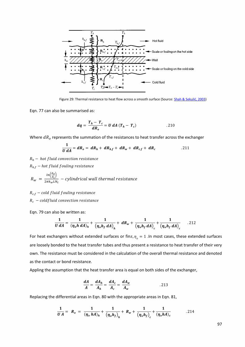
97

Figure 29: Thermal resistance to heat flow across a smooth surface (Source: Shah & Sekulić, 2003)

Eqn. 77 can also be summarised as:

𝒅𝒒 = 𝑻𝒉 − 𝑻𝒄

𝒅𝑹𝒐

= 𝑼 𝒅𝑨 (𝑻𝒉 − 𝑻𝒄) . 210

Where 𝑑𝑅𝑜 represents the summation of the resistances to heat transfer across the exchanger

𝟏

𝑼 𝒅𝑨= 𝒅𝑹𝒐 = 𝒅𝑹𝒉 + 𝒅𝑹𝒉,𝒇 + 𝒅𝑹𝒘 + 𝒅𝑹𝒄,𝒇 + 𝒅𝑹𝒄 . 211

𝑅ℎ − ℎ𝑜𝑡 𝑓𝑙𝑢𝑖𝑑 𝑐𝑜𝑛𝑣𝑒𝑐𝑡𝑖𝑜𝑛 𝑟𝑒𝑠𝑖𝑠𝑡𝑎𝑛𝑐𝑒

𝑅ℎ,𝑓 − ℎ𝑜𝑡 𝑓𝑙𝑢𝑖𝑑 𝑓𝑜𝑢𝑙𝑖𝑛𝑔 𝑟𝑒𝑠𝑖𝑠𝑡𝑎𝑛𝑐𝑒

𝑅𝑤 = 𝑙𝑛(

𝑑𝑜𝑑𝑖

)

2𝜋𝑘𝑤𝐿𝑁𝑡 − 𝑐𝑦𝑙𝑖𝑛𝑑𝑟𝑖𝑐𝑎𝑙 𝑤𝑎𝑙𝑙 𝑡ℎ𝑒𝑟𝑚𝑎𝑙 𝑟𝑒𝑠𝑖𝑠𝑡𝑎𝑛𝑐𝑒

𝑅𝑐,𝑓 − 𝑐𝑜𝑙𝑑 𝑓𝑙𝑢𝑖𝑑 𝑓𝑜𝑢𝑙𝑖𝑛𝑔 𝑟𝑒𝑠𝑖𝑠𝑡𝑎𝑛𝑐𝑒

𝑅𝑐 − 𝑐𝑜𝑙𝑑𝑓𝑙𝑢𝑖𝑑 𝑐𝑜𝑛𝑣𝑒𝑐𝑡𝑖𝑜𝑛 𝑟𝑒𝑠𝑖𝑠𝑡𝑎𝑛𝑐𝑒

Eqn. 79 can also be written as:

𝟏

𝑼 𝒅𝑨=

𝟏

(𝜼𝒐𝒉 𝒅𝑨)𝒉

+ 𝟏

(𝜼𝒐𝒉𝒇 𝒅𝑨)𝒉

+ 𝒅𝑹𝒘 + 𝟏

(𝜼𝒐𝒉𝒇 𝒅𝑨)𝒄

+𝟏

(𝜼𝒐𝒉𝒇 𝒅𝑨)𝒄

. 212

For heat exchangers without extended surfaces or fin𝑠, 𝜂𝑜

= 1 .In most cases, these extended surfaces

are loosely bonded to the heat transfer tubes and thus present a resistance to heat transfer of their very

own. The resistance must be considered in the calculation of the overall thermal resistance and denoted

as the contact or bond resistance.

Appling the assumption that the heat transfer area is equal on both sides of the exchanger,

𝒅𝑨

𝑨=

𝒅𝑨𝒉

𝑨𝒉

= 𝒅𝑨𝒄

𝑨𝒄

= 𝒅𝑨𝒘

𝑨𝒘

. 213

Replacing the differential areas in Eqn. 80 with the appropriate areas in Eqn. 81,

𝟏

𝑼 𝑨= 𝑹𝒐 =

𝟏

(𝜼𝒐 𝒉𝑨)𝒉

+ 𝟏

(𝜼𝒐𝒉𝒇)𝒉

+ 𝑹𝒘 + 𝟏

(𝜼𝒐𝒉𝒇)𝒄

+𝟏

(𝜼𝒐𝒉𝑨)𝒄

. 214

98

The heat transfer equation thus becomes:

𝒒 = 𝑼𝑨∆𝑻𝒎 = 𝑼𝑨(𝑻𝒉 − 𝑻𝒄) = (𝑻𝒉 − 𝑻𝒄)

𝑹𝒐

. 215

One set of the thermal resistances listed on the RHS of Eqns. 79 and 82 will be referred to as the

controlling resistance if it represents over 80% of the overall resistance [65]. The aim of every heat

exchanger design should therefore be to improve the efficiency of heat exchange by lowering the value

of the controlling thermal resistance by as much as possible. This can be achieved by the addition of the

extended surfaces especially on the gas side which usually has the controlling resistance. Therefore,

where any side has a low heat transfer coefficient ℎ, A is increased such that:

(𝜂𝑜 ℎ𝐴)ℎ ≈ (𝜂𝑜ℎ𝐴)𝑐

Alternatively, the overall heat transfer coefficient can be defined in terms of the areas of either fluid

stream or the tube wall area.

𝑼𝑨 = 𝑼𝒉𝑨𝒉 = 𝑼𝒄𝑨𝒄 = 𝑼𝒘𝑨𝒘 . 216

The value 𝑈𝐴 is referred to as the overall thermal conductance of the heat exchanger. To evaluate the

thermal conductance 𝑈𝐴, the total Area, 𝐴 must not be explicitly defined. On the other hand, the areas

𝐴ℎ, 𝐴𝑐 𝑎𝑛𝑑 𝐴𝑤 must be defined before U can be evaluated since 𝐴ℎ ≠ 𝐴𝑐.

For heat transfer based on a unit surface area, the rate equation becomes:

𝒒

𝑨= 𝑼∆𝑻𝒎 . 217

Eqn. 208 becomes, 𝑅𝑜 = 1 𝑈⁄ and each resistance is evaluated on a unit area basis with 𝐴ℎ or 𝐴𝑐 used

as the basis for evaluating the overall thermal resistance.

𝟏

𝑼𝒉

= 𝟏

(𝜼𝒐

𝒉)𝒉

+ 𝟏

(𝜼𝒐

𝒉𝒇)𝒉

+ 𝑹𝒘𝑨𝒉 + 𝑨𝒉 𝑨𝒄⁄

(𝜼𝒐

𝒉𝒇)𝒄

+ 𝑨𝒉 𝑨𝒄⁄

(𝜼𝒐

𝒉)𝒄

. 218

𝟏

𝑼𝒄

= 𝟏

(𝜼𝒐

𝒉)𝒄

+ 𝟏

(𝜼𝒐

𝒉𝒇)𝒄

+ 𝑹𝒘𝑨𝒄 + 𝑨𝒄 𝑨𝒉⁄

(𝜼𝒐

𝒉𝒇)𝒉

+ 𝑨𝒉 𝑨𝒄⁄

(𝜼𝒐

𝒉)𝒉

. 219

For a plain tube 𝜂𝑜

= 1 and:

𝑹𝒘 = 𝜹𝒘

𝒌𝒘

. 220

Based on the inner and outer surfaces of the tube:

𝟏

𝑼𝒐

= 𝟏

𝒉𝒐

+ 𝟏

𝒉𝒐,𝒇

+ 𝒅𝒐 𝒍𝒏(𝒅𝒐 𝒅𝒊⁄ )

𝟐𝒌𝒘

+ 𝒅𝒐

𝒉𝒊,𝒇𝒅𝒊

+ 𝒅𝒐

𝒉𝒊𝒅𝒊

. 221

𝟏

𝑼𝒊

= 𝟏

𝒉𝒊

+ 𝟏

𝒉𝒊,𝒇

+ 𝒅𝒊 𝒍𝒏(𝒅𝒐 𝒅𝒊⁄ )

𝟐𝒌𝒘

+ 𝒅𝒊

𝒉𝒐,𝒇𝒅𝒐

+ 𝒅𝒊

𝒉𝒐𝒅𝒐

. 222

99

Appendix B

Introduction:

This chapter attempts to outline the requirements the heat exchanger design toolkit must fulfil to

ensure it is suitable for the purposes of heat exchanger design. These requirements are not strict and

should only act as guidelines to be considered by the toolkit developer. The final approval will be given

by the end-users after much testing has been conducted.

Toolkit Requirements:

1. User – manual:

The toolkit will be used by a design team familiar with input values required at each stage of

heat exchanger design or at least as specified by a client. However, it should be anticipated that

users with little or no technical knowledge of engineering terms would be able to operate the

toolkit with ease based on a set of requirements sent in by a potential customer. Hence there

exists a need for a user manual accompanied by a user manual to explain the meaning of terms

and guide end – users on how to apply the toolkit for design purposes.

2. Toolkit Description:

The general outline of the toolkit has been split into two parts, comprising the Front-End and

the Back-End. The front-end comprises the visual part through which the designer interacts with

the toolkit while the back-end is the section ‘hidden’ away from the designer and is the location

where all calculations will be performed. These two parts are further described below:

A. Toolkit Front – End: To ensure ease of operation, data input into the toolkit should be made

possible through a graphic user interface (GUI) environment. Button controls present on the

graphic user interface (GUI) should be able to trigger commands which in turn activate

equations and produce desired results. Design results produced will be also need to be

displayed on the GUI. The GUI will comprise:

o Drop-down menus: that allow the designer choose design parameters such as fluid type,

design approach desired (rating or sizing), etc. The drop-down menu functions should

also allow for the selection of specific dimensions to which the potential designer

already manufactures to, such as fin pitch, tube OD etc.

o Blank input boxes: into which the designer would fill the initial conditions or

information provided by the customer. The drop-down and the blank spaces would

possibly be aligned side-by-side in most instances.

o Button controls: that would be used to activate commands which in turn, activate the

equations at the back-end of the toolkit, thus allowing the output of results.

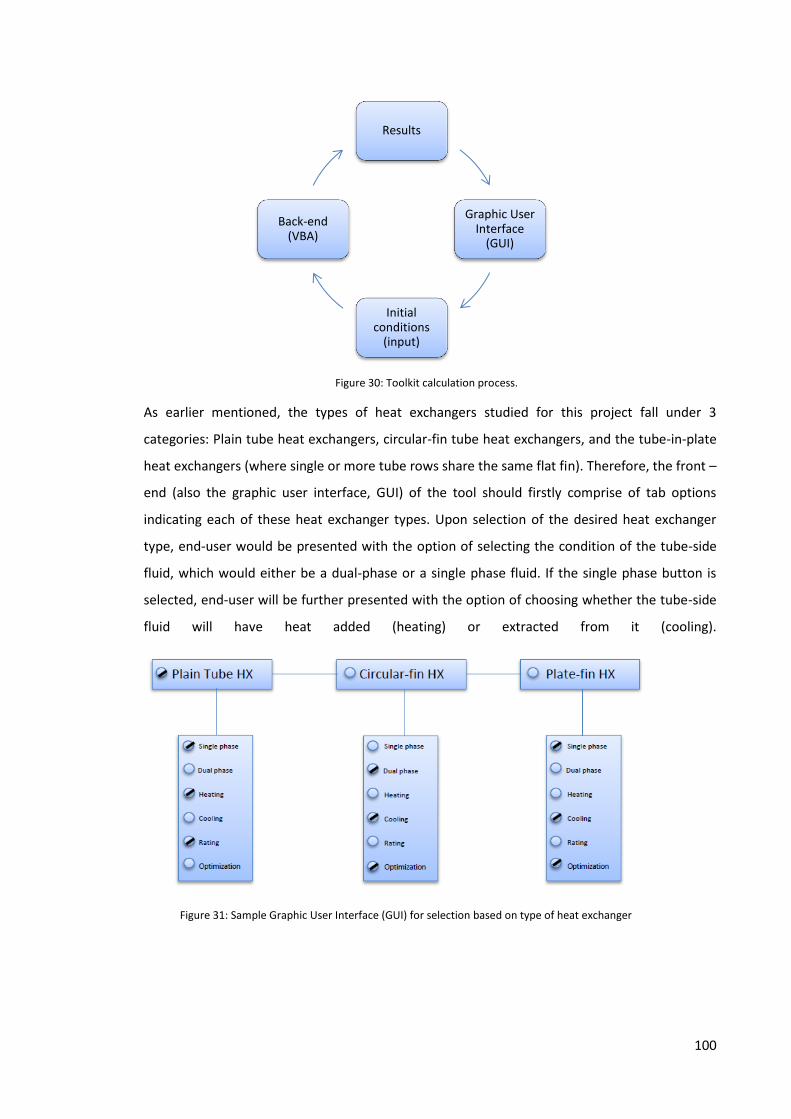
100

Figure 30: Toolkit calculation process.

As earlier mentioned, the types of heat exchangers studied for this project fall under 3

categories: Plain tube heat exchangers, circular-fin tube heat exchangers, and the tube-in-plate

heat exchangers (where single or more tube rows share the same flat fin). Therefore, the front –

end (also the graphic user interface, GUI) of the tool should firstly comprise of tab options

indicating each of these heat exchanger types. Upon selection of the desired heat exchanger

type, end-user would be presented with the option of selecting the condition of the tube-side

fluid, which would either be a dual-phase or a single phase fluid. If the single phase button is

selected, end-user will be further presented with the option of choosing whether the tube-side

fluid will have heat added (heating) or extracted from it (cooling).

Figure 31: Sample Graphic User Interface (GUI) for selection based on type of heat exchanger

Results

Graphic User Interface

(GUI)

Initial conditions

(input)

Back-end (VBA)

101

Once these initial conditions are set, the next stage of design would be largely dependent on

the calculation process chosen by the end-user. The possible calculation processes are

described below:

Calculation process:

Bearing in mind the relationship between geometrical characteristics, process conditions and

eventual heat transfer, two calculation processes have been identified that will impact on the

final structure of the front-end GUI. The first calculation process will be such that an initial set of

values comprising process conditions and geometrical characteristics can be entered via the

GUI, and results produced that will indicate the capability of the proposed dimensions to do the

required duty whilst still staying within design boundaries. This calculation process will be

termed the ‘Rating’ process. In the second calculation process, several results will be produced,

giving the designer the freedom to choose which heat exchanger dimensions that not only best

suits his needs but will also do the required duty. This calculation process will be referred to as

the ‘Sizing’ process. The outline of the GUI depending on the designer selecting the ‘Rating’ or

‘Sizing’ calculation process, is described below.

Rating:

As described earlier, the rating calculation process refers to the calculations which are

conducted to ‘check’ that pre-defined heat exchanger dimensions are able to deliver a set of

design requirements. For example, due to space restrictions, the maximum allowable length for

the heat exchanger could be so short as to cause an increase in the pressure drop across the

unit. Therefore, the designer must ‘rate’ a heat exchanger unit made of that specific length

against the desired pressure drop. The main advantage of the rating process is that it prevents

the iterative process needed to arrive at an ideal heat exchanger size.

If the rating option is chosen, only one set of results will be produced which will give the

designer a clear picture of the heat exchanger’s efficiency under those operating conditions.

It is proposed, that the front-end, be split into 3 sections, consisting:

Part A: Fluid flow conditions

Part B: Bundle specifications

Part C: Results.

If the rating process is chosen, then the end-user should be presented with the options listed

below:

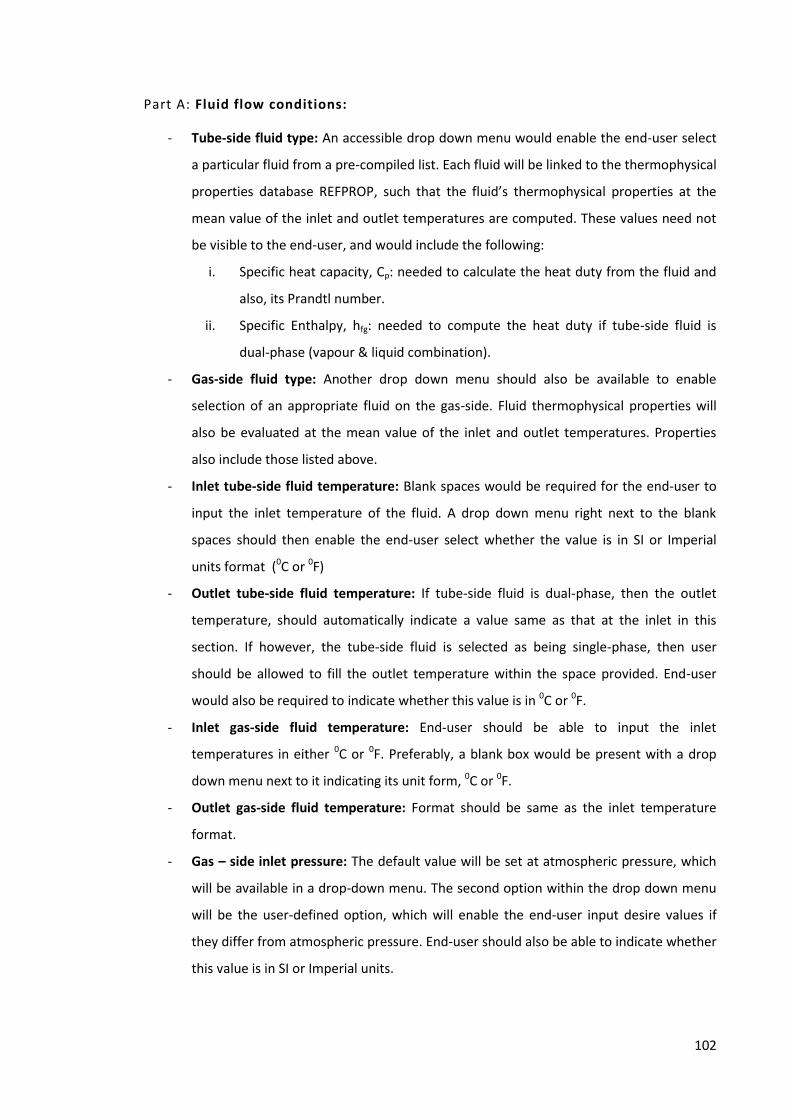
102

Part A: Fluid flow conditions:

- Tube-side fluid type: An accessible drop down menu would enable the end-user select

a particular fluid from a pre-compiled list. Each fluid will be linked to the thermophysical

properties database REFPROP, such that the fluid’s thermophysical properties at the

mean value of the inlet and outlet temperatures are computed. These values need not

be visible to the end-user, and would include the following:

i. Specific heat capacity, Cp: needed to calculate the heat duty from the fluid and

also, its Prandtl number.

ii. Specific Enthalpy, hfg: needed to compute the heat duty if tube-side fluid is

dual-phase (vapour & liquid combination).

- Gas-side fluid type: Another drop down menu should also be available to enable

selection of an appropriate fluid on the gas-side. Fluid thermophysical properties will

also be evaluated at the mean value of the inlet and outlet temperatures. Properties

also include those listed above.

- Inlet tube-side fluid temperature: Blank spaces would be required for the end-user to

input the inlet temperature of the fluid. A drop down menu right next to the blank

spaces should then enable the end-user select whether the value is in SI or Imperial

units format (0C or 0F)

- Outlet tube-side fluid temperature: If tube-side fluid is dual-phase, then the outlet

temperature, should automatically indicate a value same as that at the inlet in this

section. If however, the tube-side fluid is selected as being single-phase, then user

should be allowed to fill the outlet temperature within the space provided. End-user

would also be required to indicate whether this value is in 0C or 0F.

- Inlet gas-side fluid temperature: End-user should be able to input the inlet

temperatures in either 0C or 0F. Preferably, a blank box would be present with a drop

down menu next to it indicating its unit form, 0C or 0F.

- Outlet gas-side fluid temperature: Format should be same as the inlet temperature

format.

- Gas – side inlet pressure: The default value will be set at atmospheric pressure, which

will be available in a drop-down menu. The second option within the drop down menu

will be the user-defined option, which will enable the end-user input desire values if

they differ from atmospheric pressure. End-user should also be able to indicate whether

this value is in SI or Imperial units.

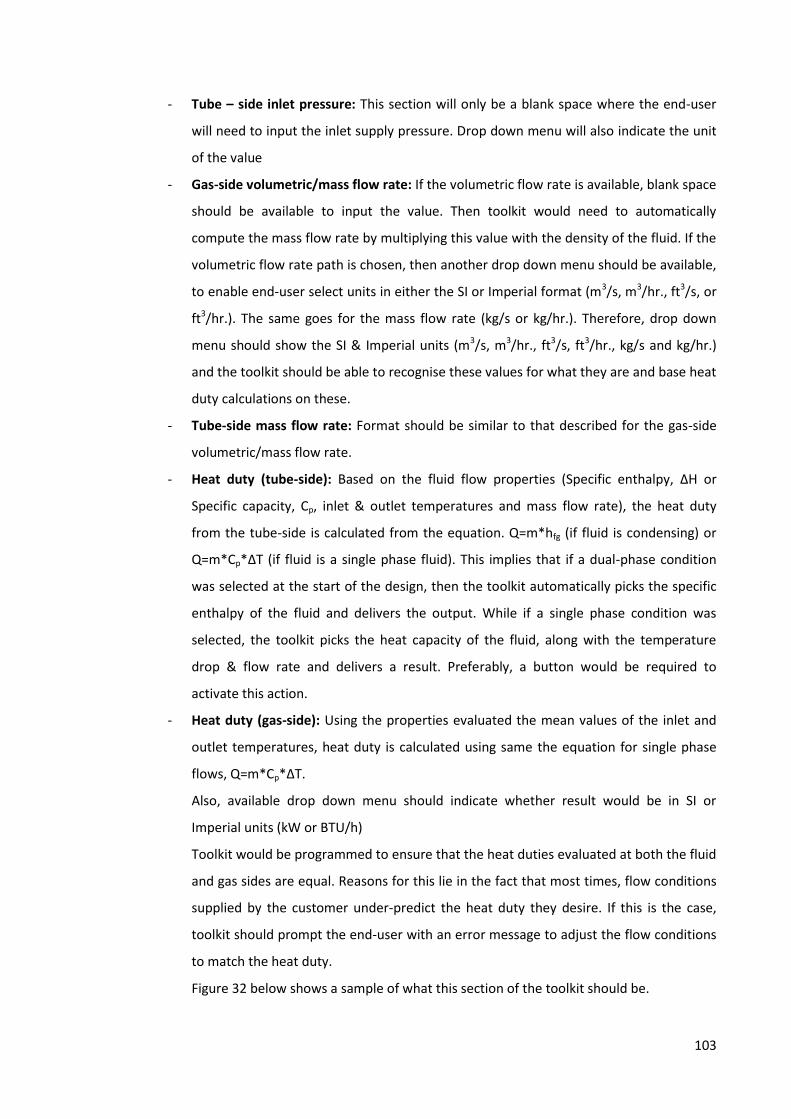
103

- Tube – side inlet pressure: This section will only be a blank space where the end-user

will need to input the inlet supply pressure. Drop down menu will also indicate the unit

of the value

- Gas-side volumetric/mass flow rate: If the volumetric flow rate is available, blank space

should be available to input the value. Then toolkit would need to automatically

compute the mass flow rate by multiplying this value with the density of the fluid. If the

volumetric flow rate path is chosen, then another drop down menu should be available,

to enable end-user select units in either the SI or Imperial format (m3/s, m3/hr., ft3/s, or

ft3/hr.). The same goes for the mass flow rate (kg/s or kg/hr.). Therefore, drop down

menu should show the SI & Imperial units (m3/s, m3/hr., ft3/s, ft3/hr., kg/s and kg/hr.)

and the toolkit should be able to recognise these values for what they are and base heat

duty calculations on these.

- Tube-side mass flow rate: Format should be similar to that described for the gas-side

volumetric/mass flow rate.

- Heat duty (tube-side): Based on the fluid flow properties (Specific enthalpy, ΔH or

Specific capacity, Cp, inlet & outlet temperatures and mass flow rate), the heat duty

from the tube-side is calculated from the equation. Q=m*hfg (if fluid is condensing) or

Q=m*Cp*ΔT (if fluid is a single phase fluid). This implies that if a dual-phase condition

was selected at the start of the design, then the toolkit automatically picks the specific

enthalpy of the fluid and delivers the output. While if a single phase condition was

selected, the toolkit picks the heat capacity of the fluid, along with the temperature

drop & flow rate and delivers a result. Preferably, a button would be required to

activate this action.

- Heat duty (gas-side): Using the properties evaluated the mean values of the inlet and

outlet temperatures, heat duty is calculated using same the equation for single phase

flows, Q=m*Cp*ΔT.

Also, available drop down menu should indicate whether result would be in SI or

Imperial units (kW or BTU/h)

Toolkit would be programmed to ensure that the heat duties evaluated at both the fluid

and gas sides are equal. Reasons for this lie in the fact that most times, flow conditions

supplied by the customer under-predict the heat duty they desire. If this is the case,

toolkit should prompt the end-user with an error message to adjust the flow conditions

to match the heat duty.

Figure 32 below shows a sample of what this section of the toolkit should be.

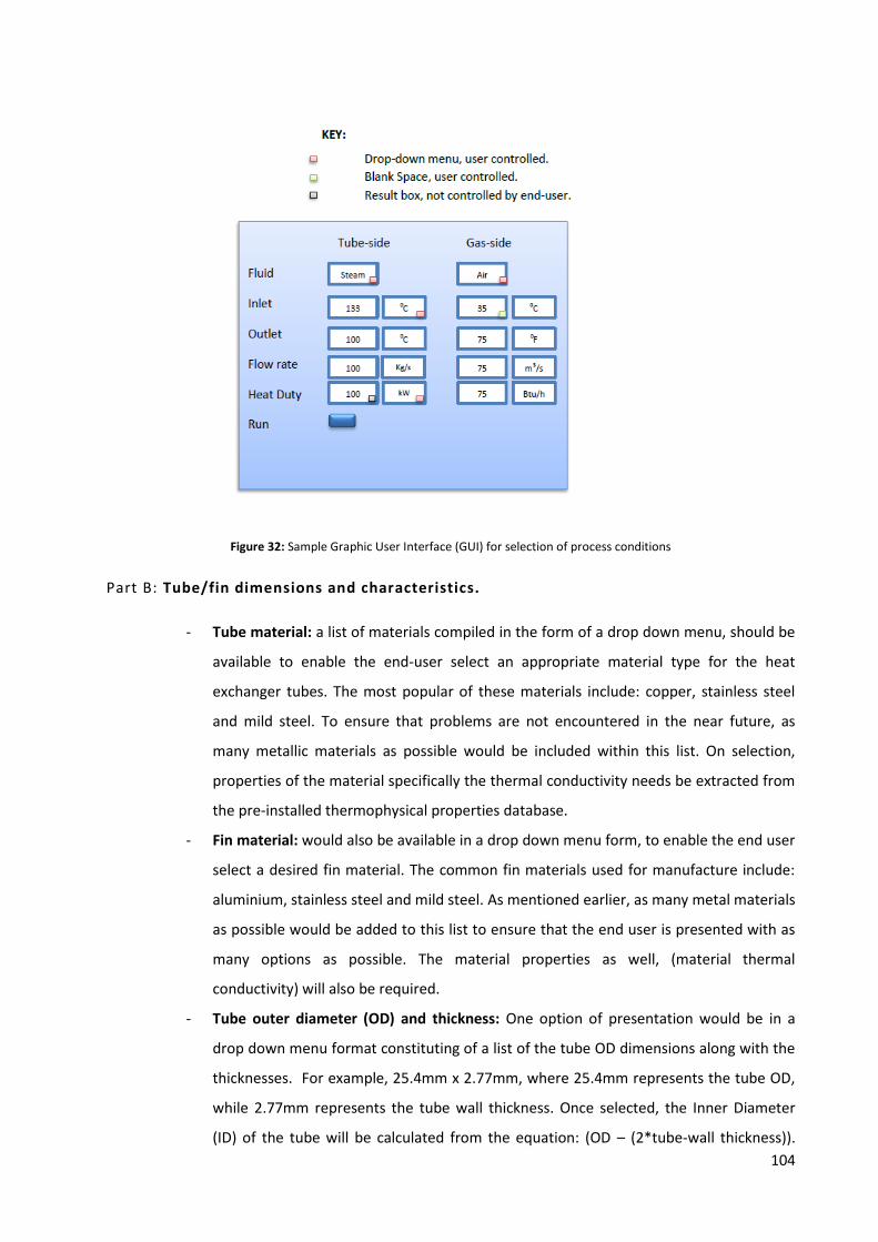
104

Figure 32: Sample Graphic User Interface (GUI) for selection of process conditions

Part B: Tube/fin dimensions and characteristics.

- Tube material: a list of materials compiled in the form of a drop down menu, should be

available to enable the end-user select an appropriate material type for the heat

exchanger tubes. The most popular of these materials include: copper, stainless steel

and mild steel. To ensure that problems are not encountered in the near future, as

many metallic materials as possible would be included within this list. On selection,

properties of the material specifically the thermal conductivity needs be extracted from

the pre-installed thermophysical properties database.

- Fin material: would also be available in a drop down menu form, to enable the end user

select a desired fin material. The common fin materials used for manufacture include:

aluminium, stainless steel and mild steel. As mentioned earlier, as many metal materials

as possible would be added to this list to ensure that the end user is presented with as

many options as possible. The material properties as well, (material thermal

conductivity) will also be required.

- Tube outer diameter (OD) and thickness: One option of presentation would be in a

drop down menu format constituting of a list of the tube OD dimensions along with the

thicknesses. For example, 25.4mm x 2.77mm, where 25.4mm represents the tube OD,

while 2.77mm represents the tube wall thickness. Once selected, the Inner Diameter

(ID) of the tube will be calculated from the equation: (OD – (2*tube-wall thickness)).

105

Alternatively, the tube thickness space could be offered to the end user as a drop down

menu, with pre-filled values along with a user-defined option. Upon selection of the

user defined section, a blank space will become available for the end-user to fill in the

available thickness. To ensure consistency in values and units, end-user should be

allowed to select whether this value is in mm or m.

- Fin thickness: also available in a drop down menu, this list will constitute all the fin

thickness values used generally for manufacture. All the end-user need do, is select the

desired one.

- Tube length: value would be fed manually, since this is a bundle rating exercise. Ideally,

this value should remain in SI units of either m or mm, but end-user should be given the

option of choosing Imperial units in the form of feet (ft.). Hence, a drop-down menu will

also be available to indicate what unit the input values are in.

- Number of fins/m: Already limited in possible combinations, (98, 118, 157, 197, 236,

276, 315, 354, 394, 433 & 472 fins per m). A drop down menu will be made available

with these values for the end-user to select from.

- Number of rows: End – user would be given the option to indicate the number of rows

they want for that particular bundle. This will be in the form of a blank space, where the

end user can simply fill in the desired number of rows.

- Transverse Pitch: End-user will be presented with a blank space, to input this value

manually, drop down menu next to this blank space, should also indicate the unit of the

value entered.

- Longitudinal Pitch: Outline will be same as the transverse pitch section.

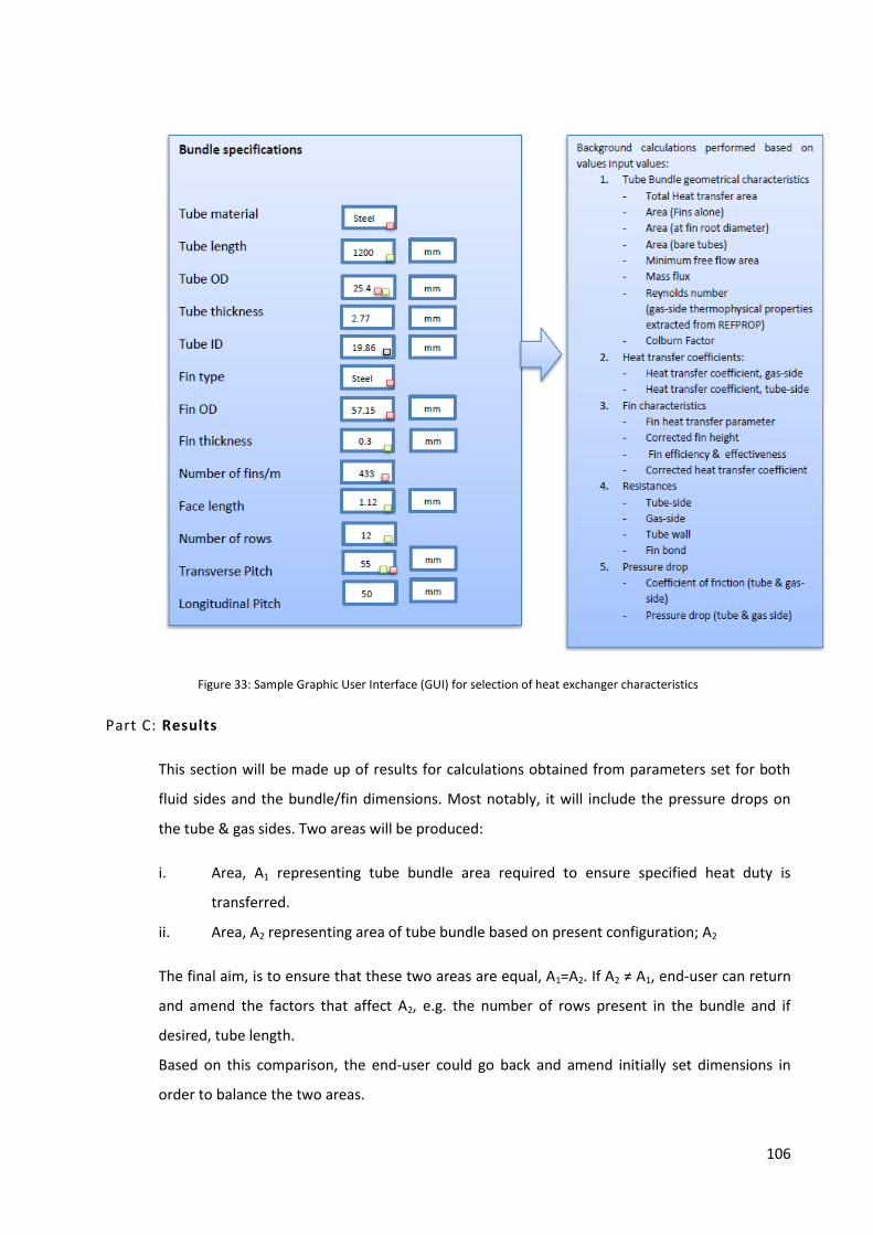
106

Figure 33: Sample Graphic User Interface (GUI) for selection of heat exchanger characteristics

Part C: Results

This section will be made up of results for calculations obtained from parameters set for both

fluid sides and the bundle/fin dimensions. Most notably, it will include the pressure drops on

the tube & gas sides. Two areas will be produced:

i. Area, A1 representing tube bundle area required to ensure specified heat duty is

transferred.

ii. Area, A2 representing area of tube bundle based on present configuration; A2

The final aim, is to ensure that these two areas are equal, A1=A2. If A2 ≠ A1, end-user can return

and amend the factors that affect A2, e.g. the number of rows present in the bundle and if

desired, tube length.

Based on this comparison, the end-user could go back and amend initially set dimensions in

order to balance the two areas.

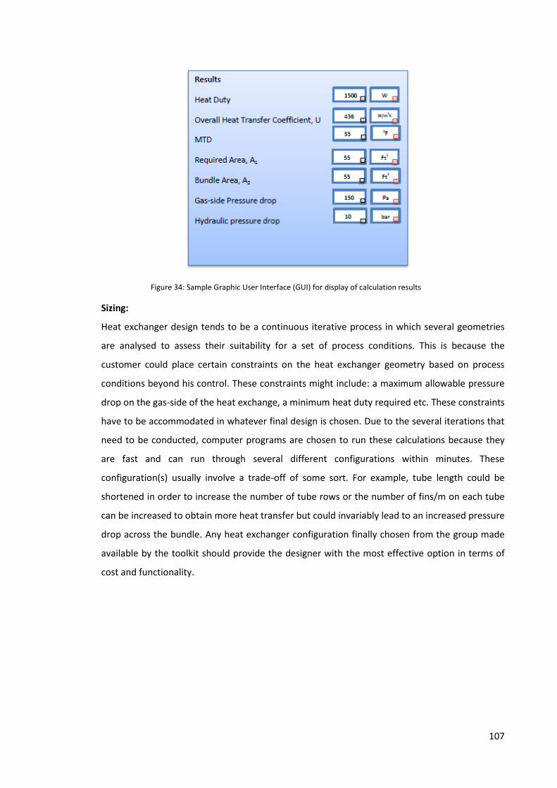
107

Figure 34: Sample Graphic User Interface (GUI) for display of calculation results

Sizing:

Heat exchanger design tends to be a continuous iterative process in which several geometries

are analysed to assess their suitability for a set of process conditions. This is because the

customer could place certain constraints on the heat exchanger geometry based on process

conditions beyond his control. These constraints might include: a maximum allowable pressure

drop on the gas-side of the heat exchange, a minimum heat duty required etc. These constraints

have to be accommodated in whatever final design is chosen. Due to the several iterations that

need to be conducted, computer programs are chosen to run these calculations because they

are fast and can run through several different configurations within minutes. These

configuration(s) usually involve a trade-off of some sort. For example, tube length could be

shortened in order to increase the number of tube rows or the number of fins/m on each tube

can be increased to obtain more heat transfer but could invariably lead to an increased pressure

drop across the bundle. Any heat exchanger configuration finally chosen from the group made

available by the toolkit should provide the designer with the most effective option in terms of

cost and functionality.

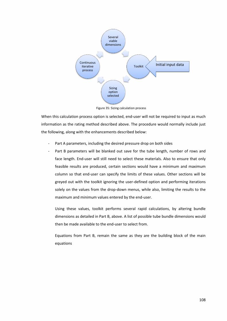
108

Figure 35: Sizing calculation process

When this calculation process option is selected, end-user will not be required to input as much

information as the rating method described above. The procedure would normally include just

the following, along with the enhancements described below:

- Part A parameters, including the desired pressure drop on both sides

- Part B parameters will be blanked out save for the tube length, number of rows and

face length. End-user will still need to select these materials. Also to ensure that only

feasible results are produced, certain sections would have a minimum and maximum

column so that end-user can specify the limits of these values. Other sections will be

greyed out with the toolkit ignoring the user-defined option and performing iterations

solely on the values from the drop-down menus, while also, limiting the results to the

maximum and minimum values entered by the end-user.

Using these values, toolkit performs several rapid calculations, by altering bundle

dimensions as detailed in Part B, above. A list of possible tube bundle dimensions would

then be made available to the end-user to select from.

Equations from Part B, remain the same as they are the building block of the main

equations

Several viable

dimensions

Toolkit

Sizing option

selected

Continuous iterative process

Initial input data

109

Figure 36: Sample GUI for the Sizing design option.

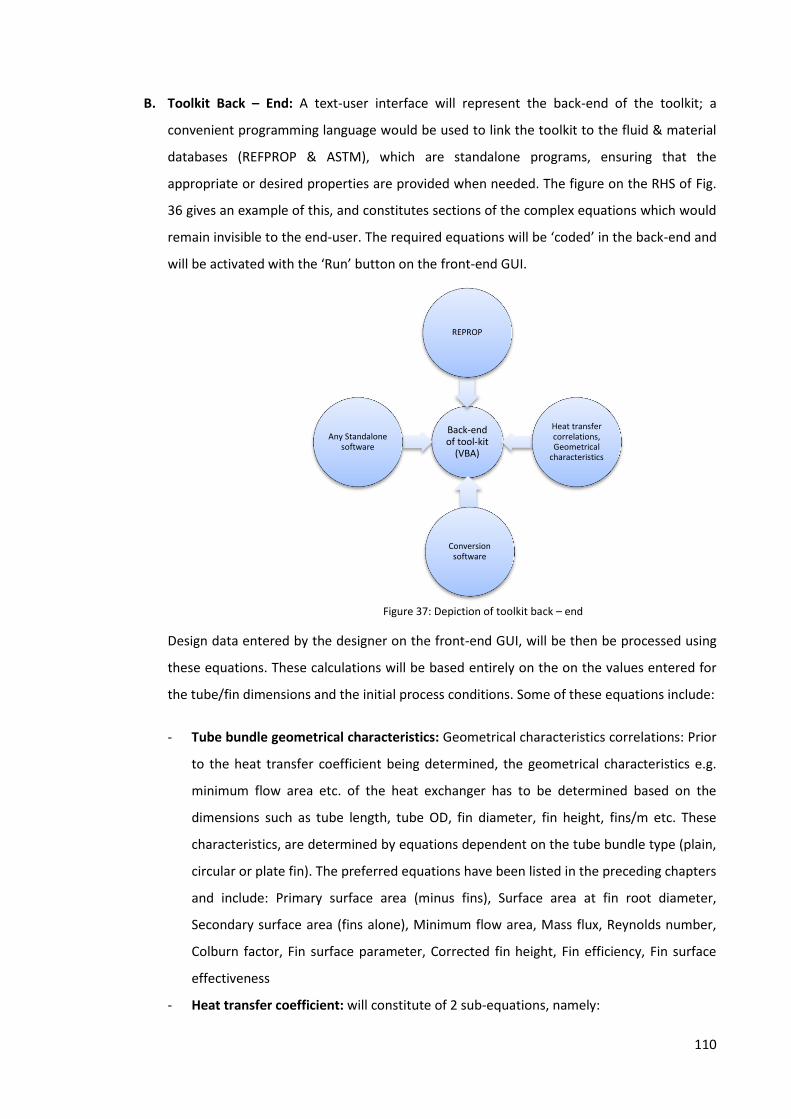
110

B. Toolkit Back – End: A text-user interface will represent the back-end of the toolkit; a

convenient programming language would be used to link the toolkit to the fluid & material

databases (REFPROP & ASTM), which are standalone programs, ensuring that the

appropriate or desired properties are provided when needed. The figure on the RHS of Fig.

36 gives an example of this, and constitutes sections of the complex equations which would

remain invisible to the end-user. The required equations will be ‘coded’ in the back-end and

will be activated with the ‘Run’ button on the front-end GUI.

Figure 37: Depiction of toolkit back – end

Design data entered by the designer on the front-end GUI, will be then be processed using

these equations. These calculations will be based entirely on the on the values entered for

the tube/fin dimensions and the initial process conditions. Some of these equations include:

- Tube bundle geometrical characteristics: Geometrical characteristics correlations: Prior

to the heat transfer coefficient being determined, the geometrical characteristics e.g.

minimum flow area etc. of the heat exchanger has to be determined based on the

dimensions such as tube length, tube OD, fin diameter, fin height, fins/m etc. These

characteristics, are determined by equations dependent on the tube bundle type (plain,

circular or plate fin). The preferred equations have been listed in the preceding chapters

and include: Primary surface area (minus fins), Surface area at fin root diameter,

Secondary surface area (fins alone), Minimum flow area, Mass flux, Reynolds number,

Colburn factor, Fin surface parameter, Corrected fin height, Fin efficiency, Fin surface

effectiveness

- Heat transfer coefficient: will constitute of 2 sub-equations, namely:

Back-end of tool-kit

(VBA)

REPROP

Heat transfer correlations, Geometrical

characteristics

Conversion software

Any Standalone software

111

Heat transfer coefficient, h1 (tube-side): The equations required to calculate this

value, will depend on state of fluid (single or dual-phase). If fluid is single phase,

then the heat transfer coefficient will be computed using the Dittus-Boelter

equation: Nu=0.024Re0.8.Pr0.4 (heating conditions) or Nu=0.026Re0.8.Pr0.3 (cooling

conditions). If it is a dual phase fluid, then the appropriate equations should have

been activated once the end user highlighted the single phase button at the

beginning of the exercise.

Heat transfer coefficient, h2 (gas-side): begins initially with the calculation of the

geometric characteristics of the tube bundle. The dimension calculations will be

based on the initial input values for the tube bundle, i.e. tube length, transverse &

longitudinal pitch, number of fins/m, and heat exchanger type (circular, plate or

plain tubes). From these calculations (geometric characteristics & Reynolds

number), the Colburn factor is extracted and from this, the gas-side heat transfer

coefficient. The transfer coefficient equation used, will also depend on the type of

heat exchanger being designed (circular-fin, plain or tube-in-plate)

- Thermal resistances:

Tube-side: will be the inverse of the heat transfer coefficient obtained earlier using

the Dittus-Boelter equation, multiplied by the tube OD/ID ratio.

Gas-side: will be the inverse of the heat transfer coefficient obtained from the gas

side.

Tube wall: is the resistance to heat transfer as a result of both the tube wall

thickness, and it material. Hence, the tube material’s thermal conductivity will also

be extracted from REFPROP.

Fin-bond resistance: computes the resistance produced as a result of incomplete

adhesion of spiral bound fins on tubes. This equation, will only be required if the

finned tubes are produced by as spiral wound fins. If they are sourced externally, it

is highly likely they will be G-fins (fins are filled into grooves marked on the tube

body)

Summation of these values will be displayed in the overall heat transfer coefficient,

U, block within the results section.

- Pressure drop:

Co-efficient of friction: will be required to compute pressure drop on both the gas and

tube-side. Using a combination of both the frictional coefficient and relevant equations,

112

pressure drop across the bundle and the tube, will be computed and displayed in the

results section of the user-interface

To ensure accurate results, potential tampering of the building blocks of the toolkit, must be

prevented by ensuring that the back-end is never accessible to front-end users. On the

other hand, the back end must be ‘coded’ with low-level programming language such that

any modifications required in the future can be carried out by people with little or no

experience in computer programming. An example is the software referred to as REFPROP,

which will enable the designer evaluate fluid thermophysical properties required for heat

transfer calculations without resorting to manual data sheets.

3. Further Development:

It should be anticipated that the toolkit will be continuously upgraded to include features that

will improve its productivity. Examples of some these features are outlined below and by no

means represent an end to the list. As the project unfolds, ideas would come up and this would

be built into the toolkit.

Data storage: Toolkit should allow the designer store bundle dimension output,

against a particular customer’s name. This would ensure that in the absence of the

designer, tube bundle specifications for a particular customer can still be recalled if

needed.

Costing: Prices based on the chosen tube bundle should be one of the added

functions of the toolkit.

CAD drawing: toolkit should include a functionality which allows it produce a

dimensioned CAD drawing of the tube bundle.

Structural analysis: as part of the project, toolkit should be able to carry out

structural analysis on the tube bundle based on codes governing pressure vessels

and certify them safe to be installed within a human occupied environment. Hence,

an addition to the rating process earlier described, would be that the end-user

should select a design code to base the bundle dimensions on. These codes will

include ASME & EN 13445 and when they are selected, bundle sizing for rating or

optimization will be based on the prescribed equations.

Weld-type recommendations: Based on the results of the structural analysis, toolkit

would recommend best type of weld to append to certain joints to ensure complete

safety.

Complete bundle design: Presently, toolkit is being designed to specify just the tube

bundle dimensions. Further parameters, like the flanges and headers sizes are

113

excluded. Future development should include these features so that the end

product can go straight to manufacturing without further design.

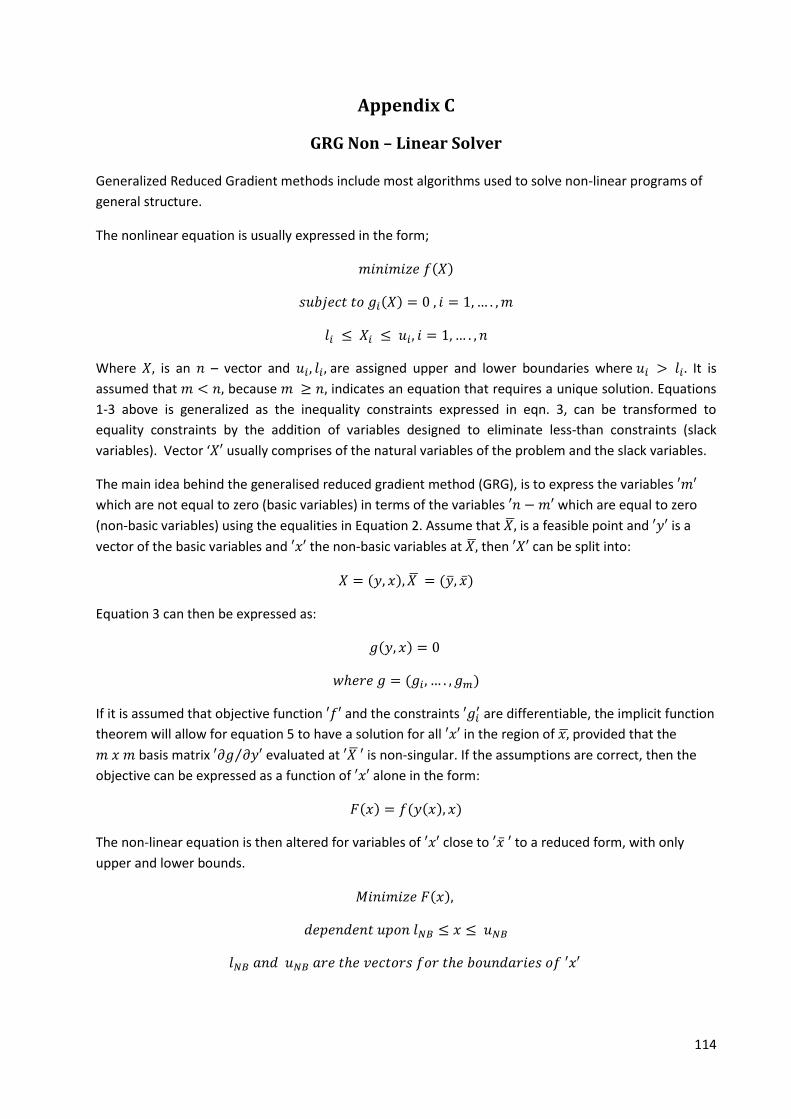
114

Appendix C

GRG Non – Linear Solver

Generalized Reduced Gradient methods include most algorithms used to solve non-linear programs of

general structure.

The nonlinear equation is usually expressed in the form;

𝑚𝑖𝑛𝑖𝑚𝑖𝑧𝑒 𝑓(𝑋)

𝑠𝑢𝑏𝑗𝑒𝑐𝑡 𝑡𝑜 𝑔𝑖(𝑋) = 0 , 𝑖 = 1, … . , 𝑚

𝑙𝑖 ≤ 𝑋𝑖 ≤ 𝑢𝑖, 𝑖 = 1, … . , 𝑛

Where 𝑋, is an 𝑛 – vector and 𝑢𝑖, 𝑙𝑖, are assigned upper and lower boundaries where 𝑢𝑖 > 𝑙𝑖. It is

assumed that 𝑚 < 𝑛, because 𝑚 ≥ 𝑛, indicates an equation that requires a unique solution. Equations

1-3 above is generalized as the inequality constraints expressed in eqn. 3, can be transformed to

equality constraints by the addition of variables designed to eliminate less-than constraints (slack

variables). Vector ‘𝑋′ usually comprises of the natural variables of the problem and the slack variables.

The main idea behind the generalised reduced gradient method (GRG), is to express the variables ′𝑚′

which are not equal to zero (basic variables) in terms of the variables ′𝑛 − 𝑚′ which are equal to zero

(non-basic variables) using the equalities in Equation 2. Assume that 𝑋,̅ is a feasible point and ′𝑦′ is a

vector of the basic variables and ′𝑥′ the non-basic variables at 𝑋,̅ then ′𝑋′ can be split into:

𝑋 = (𝑦, 𝑥), 𝑋 ̅ = (�̅�, �̅�)

Equation 3 can then be expressed as:

𝑔(𝑦, 𝑥) = 0

𝑤ℎ𝑒𝑟𝑒 𝑔 = (𝑔𝑖, … . , 𝑔𝑚)

If it is assumed that objective function ′𝑓′ and the constraints ′𝑔𝑖′ are differentiable, the implicit function

theorem will allow for equation 5 to have a solution for all ′𝑥′ in the region of 𝑥,̅ provided that the

𝑚 𝑥 𝑚 basis matrix ′𝜕𝑔 𝜕𝑦′⁄ evaluated at ′𝑋 ̅′ is non-singular. If the assumptions are correct, then the

objective can be expressed as a function of ′𝑥′ alone in the form:

𝐹(𝑥) = 𝑓(𝑦(𝑥), 𝑥)

The non-linear equation is then altered for variables of ′𝑥′ close to ′�̅� ′ to a reduced form, with only

upper and lower bounds.

𝑀𝑖𝑛𝑖𝑚𝑖𝑧𝑒 𝐹(𝑥),

𝑑𝑒𝑝𝑒𝑛𝑑𝑒𝑛𝑡 𝑢𝑝𝑜𝑛 𝑙𝑁𝐵 ≤ 𝑥 ≤ 𝑢𝑁𝐵

𝑙𝑁𝐵 𝑎𝑛𝑑 𝑢𝑁𝐵 𝑎𝑟𝑒 𝑡ℎ𝑒 𝑣𝑒𝑐𝑡𝑜𝑟𝑠 𝑓𝑜𝑟 𝑡ℎ𝑒 𝑏𝑜𝑢𝑛𝑑𝑎𝑟𝑖𝑒𝑠 𝑜𝑓 ′𝑥′

115

The generalised reduced gradient (GRG) method, finds an optimal solution to a non-linear equation of

the form eqns. (1) – (3) by following the sequence of eqns. (8) – (9). , for eqns. (8)-(9) to produce any

meaningful results ′𝑥′ must have the freedom to vary about point �̅�. Unfortunately the boundaries of

restrict the movement of 𝑥, but it is still easy for 𝑥 to move in directions which keep the boundaries

satisfied. On the other hand, if components of �̅� are at their boundaries, an adjustment in 𝑥 from �̅� will

likely cause a violation of the boundaries. To ensure this does not happen and that the function

𝑦(𝑥) remains, the following assumptions are made.

i. Assumption of non-degeneracy: which states that at any point 𝑋 which satisfies the

objective function and constraints [eqns. (2) & (3)], there should exist a demarcation of

𝑋 into ′𝑚′ basic variables ′𝑦′ and ′𝑛 − 𝑚′ non-basic variables ′𝑥′ such that

𝑙𝐵 < 𝑦 < 𝑢𝐵

𝑤ℎ𝑒𝑟𝑒 𝑙𝐵 𝑎𝑛𝑑 𝑢𝐵 𝑎𝑟𝑒 𝑣𝑒𝑐𝑡𝑜𝑟𝑠 𝑜𝑓 𝑏𝑜𝑢𝑛𝑑𝑠 𝑦

𝑎𝑛𝑑 𝐵 = 𝜕𝑔 𝜕𝑦⁄ 𝑖𝑠 𝑛𝑜𝑛 − 𝑠𝑖𝑛𝑔𝑢𝑙𝑎𝑟

With the above assumption, consider beginning from′𝑋 ̅′ with 𝑦 and 𝑥 which are basic and non-basic

variables respectively, then attempt to solve eqns. (8)-(9). At eqn. (7), in order to evaluate 𝐹(𝑥), the

values of the basic variables 𝑦(𝑥), must be known. Unfortunately, 𝑦(𝑥), cannot be determined in its

closed form except for linear and nonlinear conditions. However 𝑦(𝑥) can be evaluated for any values

of 𝑥 via iteration which solves the equalities in eqn. 5; therefore, a procedure to solve the reduced

problem beginning from 𝑋𝑜 ≡ 𝑋 ,̅̅ ̅ 𝑖𝑠:

Set 𝑖 = 0

Substitute 𝑥𝑖 into eqn. 5 and evaluate the equivalent values for 𝑖, 𝑦𝑖 by an iterative

process for solving nonlinear equations.

Determine a direction of motion 𝑑𝑖 for the non-basic variables 𝑥.

Select a step size 𝛼𝑖 to give 𝑥𝑖+1 = 𝑥𝑖 + 𝛼𝑖𝑑𝑖. This is achieved by solving the one

dimensional problem

𝑚𝑖𝑛𝑖𝑚𝑖𝑧𝑒 𝐹(𝑥𝑖+ ∝ 𝑑𝑖),

𝑤ℎ𝑒𝑟𝑒 ∝ 𝑖𝑠 𝑟𝑒𝑠𝑡𝑟𝑖𝑐𝑡𝑒𝑑 𝑡𝑜 𝑒𝑛𝑠𝑢𝑟𝑒 𝑡ℎ𝑎𝑡 𝑥𝑖+ ∝ 𝑑𝑖 𝑠𝑎𝑡𝑖𝑠𝑓𝑖𝑒𝑠 𝑡ℎ𝑒 𝑏𝑜𝑢𝑛𝑑𝑎𝑟𝑖𝑒𝑠 𝑜𝑛 𝑥.

𝑇ℎ𝑖𝑠 𝑠𝑒𝑎𝑟𝑐ℎ 𝑛𝑒𝑒𝑑 𝑎 𝑟𝑒𝑝𝑒𝑎𝑡𝑒𝑑 𝑎𝑝𝑝𝑙𝑖𝑐𝑎𝑡𝑜𝑛 𝑜𝑓 𝑠𝑡𝑒𝑝 (1)𝑖𝑛 𝑜𝑟𝑑𝑒𝑟 𝑡𝑜 𝑒𝑣𝑎𝑙𝑢𝑎𝑡𝑒 𝐹 𝑓𝑜𝑟 𝑡ℎ𝑒 𝑣𝑎𝑙𝑢𝑒𝑠 𝑜𝑓 ∝

Test the present point 𝑋𝑖 = (𝑦𝑖 , 𝑥𝑖) for optimality. If optimality is not reached, set

𝑖 = 𝑖 + 1 and return to Step (1).

From Step (1), one or more components of 𝑦𝑖 may exceed their bounds, if this happens, then the

iterative process must be interrupted. To illustrate this, assume only one basic variable violates a bound.

This variable must then be made non-basic and a component of 𝑥 which is not bounded will be made

basic. When this change of basis occurs, new functions 𝑦(𝑥), 𝐹(𝑥) and anew reduced problem are

formed.

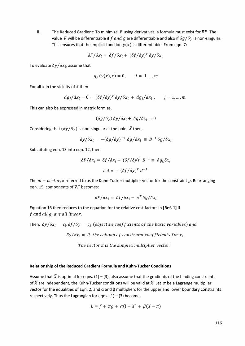
116

ii. The Reduced Gradient: To minimize 𝐹 using derivatives, a formula must exist for ∇𝐹. The

value 𝐹 will be differentiable if 𝑓 𝑎𝑛𝑑 𝑔 are differentiable and also if 𝛿𝑔 𝛿𝑦⁄ is non-singular.

This ensures that the implicit function 𝑦(𝑥) is differentiable. From eqn. 7:

𝛿𝐹 𝛿𝑥𝑖⁄ = 𝛿𝑓 𝛿𝑥𝑖⁄ + (𝛿𝑓 𝛿𝑦⁄ )𝑇 𝛿𝑦 𝛿𝑥𝑖⁄

To evaluate 𝛿𝑦 𝛿𝑥𝑖⁄ , assume that

𝑔𝑗 (𝑦(𝑥), 𝑥) = 0 , 𝑗 = 1, … , 𝑚

For all 𝑥 in the vicinity of �̅� then

𝑑𝑔𝑗 𝑑𝑥𝑖⁄ = 0 = (𝛿𝑓 𝛿𝑦⁄ )𝑇 𝛿𝑦 𝛿𝑥𝑖⁄ + 𝑑𝑔𝑗 𝑑𝑥𝑖⁄ , 𝑗 = 1, … , 𝑚

This can also be expressed in matrix form as,

(𝛿𝑔 𝛿𝑦⁄ ) 𝛿𝑦 𝛿𝑥𝑖⁄ + 𝛿𝑔 𝛿𝑥𝑖⁄ = 0

Considering that (𝛿𝑦 𝛿𝑦⁄ ) is non-singular at the point �̅� then,

𝛿𝑦 𝛿𝑥𝑖⁄ = −(𝛿𝑔 𝛿𝑦⁄ )−1 𝛿𝑔 𝛿𝑥𝑖⁄ ≡ 𝐵−1 𝛿𝑔 𝛿𝑥𝑖⁄

Substituting eqn. 13 into eqn. 12, then

𝛿𝐹 𝛿𝑥𝑖⁄ = 𝛿𝑓 𝛿𝑥𝑖⁄ − (𝛿𝑓 𝛿𝑦⁄ )𝑇 𝐵−1 ≡ 𝜕𝑔𝑘𝛿𝑥𝑖

𝐿𝑒𝑡 𝜋 = (𝛿𝑓 𝛿𝑦⁄ )𝑇 𝐵−1

The 𝑚 − 𝑣𝑒𝑐𝑡𝑜𝑟, 𝜋 referred to as the Kuhn-Tucker multiplier vector for the constraint 𝑔. Rearranging

eqn. 15, components of ∇𝐹 becomes:

𝛿𝐹 𝛿𝑥𝑖⁄ = 𝛿𝑓 𝛿𝑥𝑖⁄ − 𝜋𝑇 𝛿𝑔 𝛿𝑥𝑖⁄

Equation 16 then reduces to the equation for the relative cost factors in [Ref. 1] if

𝑓 𝑎𝑛𝑑 𝑎𝑙𝑙 𝑔𝑖 𝑎𝑟𝑒 𝑎𝑙𝑙 𝑙𝑖𝑛𝑒𝑎𝑟.

Then, 𝛿𝑦 𝛿𝑥𝑖⁄ = 𝑐𝑖, 𝛿𝑓 𝛿𝑦⁄ = 𝑐𝐵 (𝑜𝑏𝑗𝑒𝑐𝑡𝑖𝑣𝑒 𝑐𝑜𝑒𝑓𝑓𝑖𝑐𝑖𝑒𝑛𝑡𝑠 𝑜𝑓 𝑡ℎ𝑒 𝑏𝑎𝑠𝑖𝑐 𝑣𝑎𝑟𝑖𝑎𝑏𝑙𝑒𝑠) 𝑎𝑛𝑑

𝛿𝑦 𝛿𝑥𝑖⁄ = 𝑃𝑖, 𝑡ℎ𝑒 𝑐𝑜𝑙𝑢𝑚𝑛 𝑜𝑓 𝑐𝑜𝑛𝑠𝑡𝑟𝑎𝑖𝑛𝑡 𝑐𝑜𝑒𝑓𝑓𝑖𝑐𝑖𝑒𝑛𝑡𝑠 𝑓𝑜𝑟 𝑥𝑖 .

𝑇ℎ𝑒 𝑣𝑒𝑐𝑡𝑜𝑟 𝜋 𝑖𝑠 𝑡ℎ𝑒 𝑠𝑖𝑚𝑝𝑙𝑒𝑥 𝑚𝑢𝑙𝑡𝑖𝑝𝑙𝑖𝑒𝑟 𝑣𝑒𝑐𝑡𝑜𝑟.

Relationship of the Reduced Gradient Formula and Kuhn-Tucker Conditions

Assume that �̅� is optimal for eqns. (1) – (3), also assume that the gradients of the binding constraints

of 𝑋 ̅are independent, the Kuhn-Tucker conditions will be valid at 𝑋.̅ Let 𝜋 be a Lagrange multiplier

vector for the equalities of Eqn. 2, and α and β multipliers for the upper and lower boundary constraints

respectively. Thus the Lagrangian for eqns. (1) – (3) becomes

𝐿 = 𝑓 + 𝜋𝑔 + 𝛼(𝑙 − 𝑋) + 𝛽(𝑋 − 𝜋)

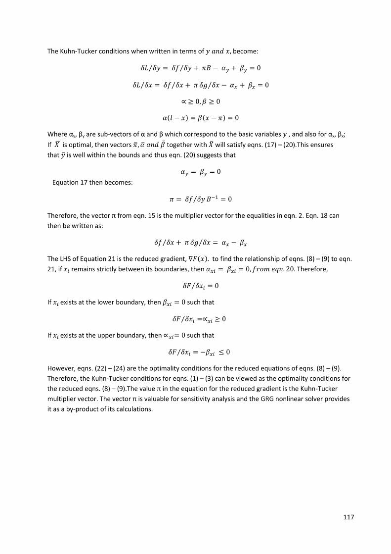
117

The Kuhn-Tucker conditions when written in terms of 𝑦 𝑎𝑛𝑑 𝑥, become:

𝛿𝐿 𝛿𝑦⁄ = 𝛿𝑓 𝛿𝑦⁄ + 𝜋𝐵 − 𝛼𝑦 + 𝛽𝑦 = 0

𝛿𝐿 𝛿𝑥⁄ = 𝛿𝑓 𝛿𝑥⁄ + 𝜋 𝛿𝑔 𝛿𝑥⁄ − 𝛼𝑥 + 𝛽𝑥 = 0

∝ ≥ 0, 𝛽 ≥ 0

𝛼(𝑙 − 𝑥) = 𝛽(𝑥 − 𝜋) = 0

Where αy, βy are sub-vectors of α and β which correspond to the basic variables 𝑦 , and also for αx, βx;

If 𝑋 ̅ is optimal, then vectors �̅�, �̅� 𝑎𝑛𝑑 �̅� together with �̅� will satisfy eqns. (17) – (20).This ensures

that �̅� is well within the bounds and thus eqn. (20) suggests that

𝛼𝑦 = 𝛽𝑦 = 0

Equation 17 then becomes:

𝜋 = 𝛿𝑓 𝛿𝑦⁄ 𝐵−1 = 0

Therefore, the vector π from eqn. 15 is the multiplier vector for the equalities in eqn. 2. Eqn. 18 can

then be written as:

𝛿𝑓 𝛿𝑥⁄ + 𝜋 𝛿𝑔 𝛿𝑥⁄ = 𝛼𝑥 − 𝛽𝑥

The LHS of Equation 21 is the reduced gradient, ∇𝐹(𝑥). to find the relationship of eqns. (8) – (9) to eqn.

21, if 𝑥𝑖 remains strictly between its boundaries, then 𝛼𝑥𝑖 = 𝛽𝑥𝑖 = 0, 𝑓𝑟𝑜𝑚 𝑒𝑞𝑛. 20. Therefore,

𝛿𝐹 𝛿𝑥𝑖⁄ = 0

If 𝑥𝑖 exists at the lower boundary, then 𝛽𝑥𝑖 = 0 such that

𝛿𝐹 𝛿𝑥𝑖⁄ =∝𝑥𝑖 ≥ 0

If 𝑥𝑖 exists at the upper boundary, then ∝𝑥𝑖= 0 such that

𝛿𝐹 𝛿𝑥𝑖⁄ = −𝛽𝑥𝑖 ≤ 0

However, eqns. (22) – (24) are the optimality conditions for the reduced equations of eqns. (8) – (9).

Therefore, the Kuhn-Tucker conditions for eqns. (1) – (3) can be viewed as the optimality conditions for

the reduced eqns. (8) – (9).The value π in the equation for the reduced gradient is the Kuhn-Tucker

multiplier vector. The vector π is valuable for sensitivity analysis and the GRG nonlinear solver provides

it as a by-product of its calculations.

118

Appendix D

Toolkit Design and Development

Introduction:

This chapter describes the actual development of the design toolkit with the incorporation of some the

guidelines from the preceding chapters. It has been written such that it doubles as the user manual for

the toolkit. It is split into five sections; General Information, System Summary, Getting Started, Using

the System, Reporting and Troubleshooting. Each section is further described below and where

appropriate, the end – user has been given a sample exercise to work through, to ensure that the toolkit

is installed correctly and is producing accurate results.

General information:

General Information section explains in general terms, the toolkit and the purpose for which it is

intended.

Toolkit Description

This tool is a design toolkit comprised of 3 Excel Workbooks, from which 3 macros have been developed

using Visual Basic for Applications (VBA). These spreadsheets are titled:

i. Circular-Fin Heat Exchangers: used primarily for the thermal design of circular-fin heat

exchanger bundles.

ii. Plate-Fin Heat Exchangers: used primarily for the thermal design of plate-fin heat

exchanger bundles.

iii. Plain Tube Heat Exchangers: used primarily for the thermal design of plain tube heat

exchanger bundles.

An activation button is located within each spreadsheet, with which the macros can be “called”. Each

macro consists of 4 tabs named:

i. Heat Exchanger Design: developed to enable the designer correctly size a heat exchanger

bundle. Its final results, will tell the designer how sufficient his actual dimensions are, when

compared to the required size that should do the desired heat duty. It is further sub-divided

into:

- Air-cooled

- Heat Recovery

- Steam coil

Equations used in these calculations, were collated from the fundamental heat transfer

equations and fluid flow equations outlined in the preceding chapters. Please refer to the

reference for sources of these equations.

119

ii. Structural Calculations: were developed, using fundamental equations to determine the

stresses in the heat exchangers as a result of pressure loading only. The design strengths for

the tubes and plates were obtained from the PD5500, with the appropriate factors of safety

already worked in.

iii. Weld Calculations: should enable the designer determine the volume of each weld and the

load it can carry with respect to the current pressure loading.

iv. Conversion tool: was designed for quick conversions between the SI and Imperial unit

systems.

System Summary

This section provides information on the additional software that must be installed on the user’s

computer for full functionality of the toolkit. It also provides information on the disk size required for

installation.

System Configuration

The toolkit is designed to operate on computers running on a Microsoft Operating System. It has not

been tested on any other OS. It is compatible with Microsoft Office 2007 and higher versions. The

toolkit requires Microsoft Excel in order to run because it is written in the Excel Visual Basic for

Applications (VBA) code, Microsoft Word for saving results and most importantly, connection to the

thermal fluids database Reference Fluid Thermodynamic and Transport Properties (REFPROP), which it

requires for extracting the thermal properties of fluids used in the heat exchanger sizing calculations.

REFPROP is a standalone program, which must be installed on any computer system prior to installing

the design toolkit.

Internet connection is not required for functionality of this design toolkit.

User should have a disk space of roughly, 1.00 MB (1,056,768 bytes) on their computer for installation.

User Access Levels

Anyone can use this toolkit, so long as they have the Microsoft Office Application and the REFPROP

program installed on their computer system.

Getting Started

This section describes where the toolkit can be obtained, and how to install it on the users’ computer

system. This section also presents briefly, the individual menus of the tabs in the toolkit.

Installation

The toolkit can be obtained by copying the main Excel spreadsheet files from any computer system it

has been installed. This can be transferred via any storage device to the new computer bearing in the

mind the minimum system requirements mentioned earlier. To transfer, highlight and copy all the Excel

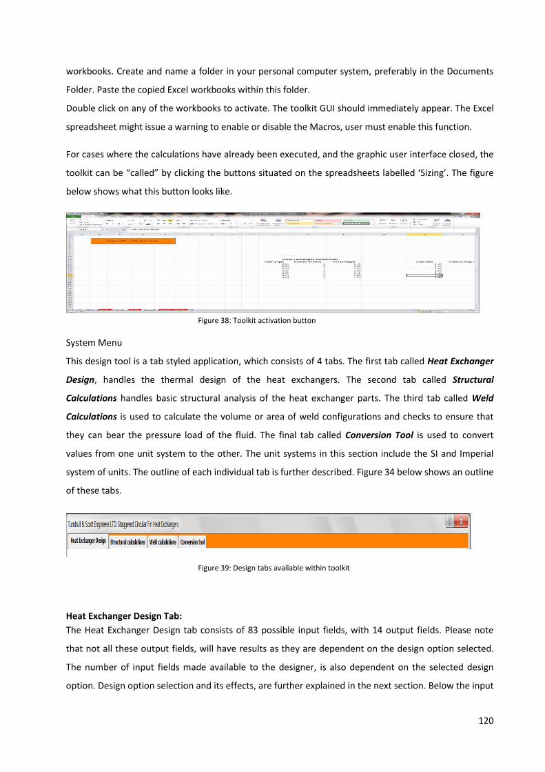
120

workbooks. Create and name a folder in your personal computer system, preferably in the Documents

Folder. Paste the copied Excel workbooks within this folder.

Double click on any of the workbooks to activate. The toolkit GUI should immediately appear. The Excel

spreadsheet might issue a warning to enable or disable the Macros, user must enable this function.

For cases where the calculations have already been executed, and the graphic user interface closed, the

toolkit can be “called” by clicking the buttons situated on the spreadsheets labelled ‘Sizing’. The figure

below shows what this button looks like.

Figure 38: Toolkit activation button

System Menu

This design tool is a tab styled application, which consists of 4 tabs. The first tab called Heat Exchanger

Design, handles the thermal design of the heat exchangers. The second tab called Structural

Calculations handles basic structural analysis of the heat exchanger parts. The third tab called Weld

Calculations is used to calculate the volume or area of weld configurations and checks to ensure that

they can bear the pressure load of the fluid. The final tab called Conversion Tool is used to convert

values from one unit system to the other. The unit systems in this section include the SI and Imperial

system of units. The outline of each individual tab is further described. Figure 34 below shows an outline

of these tabs.

Figure 39: Design tabs available within toolkit

Heat Exchanger Design Tab:

The Heat Exchanger Design tab consists of 83 possible input fields, with 14 output fields. Please note

that not all these output fields, will have results as they are dependent on the design option selected.

The number of input fields made available to the designer, is also dependent on the selected design

option. Design option selection and its effects, are further explained in the next section. Below the input

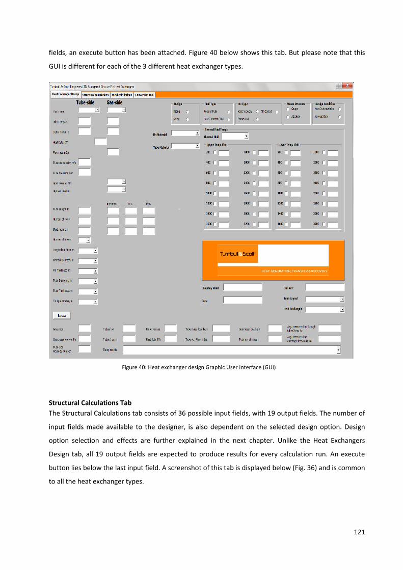
121

fields, an execute button has been attached. Figure 40 below shows this tab. But please note that this

GUI is different for each of the 3 different heat exchanger types.

Figure 40: Heat exchanger design Graphic User Interface (GUI)

Structural Calculations Tab

The Structural Calculations tab consists of 36 possible input fields, with 19 output fields. The number of

input fields made available to the designer, is also dependent on the selected design option. Design

option selection and effects are further explained in the next chapter. Unlike the Heat Exchangers

Design tab, all 19 output fields are expected to produce results for every calculation run. An execute

button lies below the last input field. A screenshot of this tab is displayed below (Fig. 36) and is common

to all the heat exchanger types.

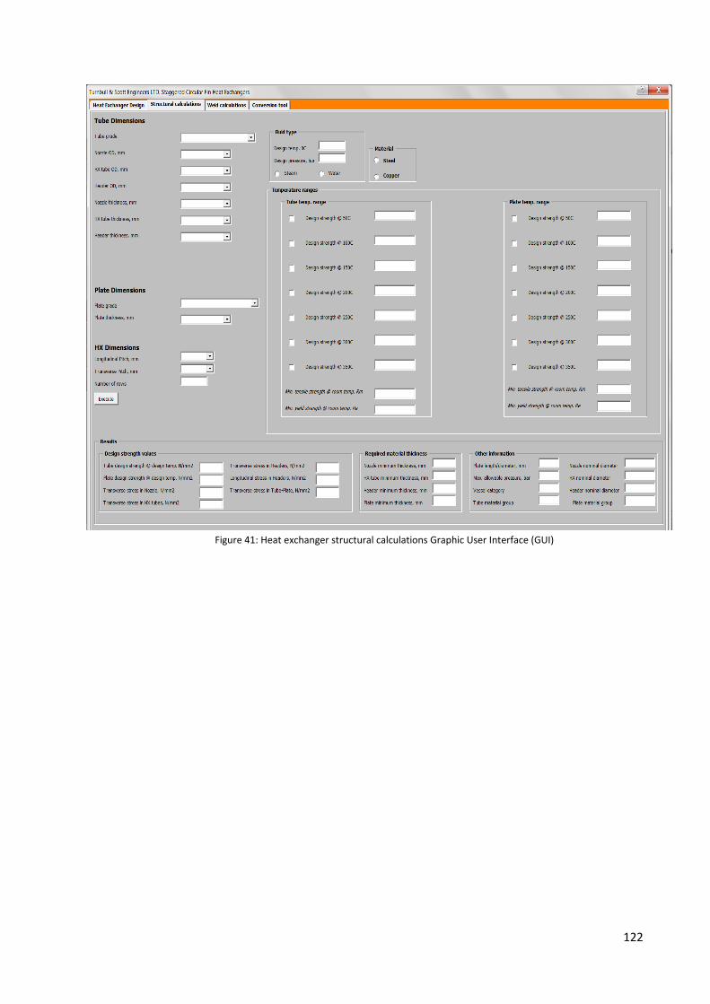
122

Figure 41: Heat exchanger structural calculations Graphic User Interface (GUI)

123

Weld Calculations Tab

The Weld Calculations tab, consists of 3 sub-tabs named; Fillet Weld, Butt Weld and Bevelled Butt Weld.

Each sub-tab has a combination of option buttons, and input fields, with an output field section. Each

sub-tab, has an execute button to execute calculations for that particular sub-tab. A screenshot is

shown below (Fig. 41).

Figure 42: Heat exchanger weld calculations Graphic User Interface (GUI)

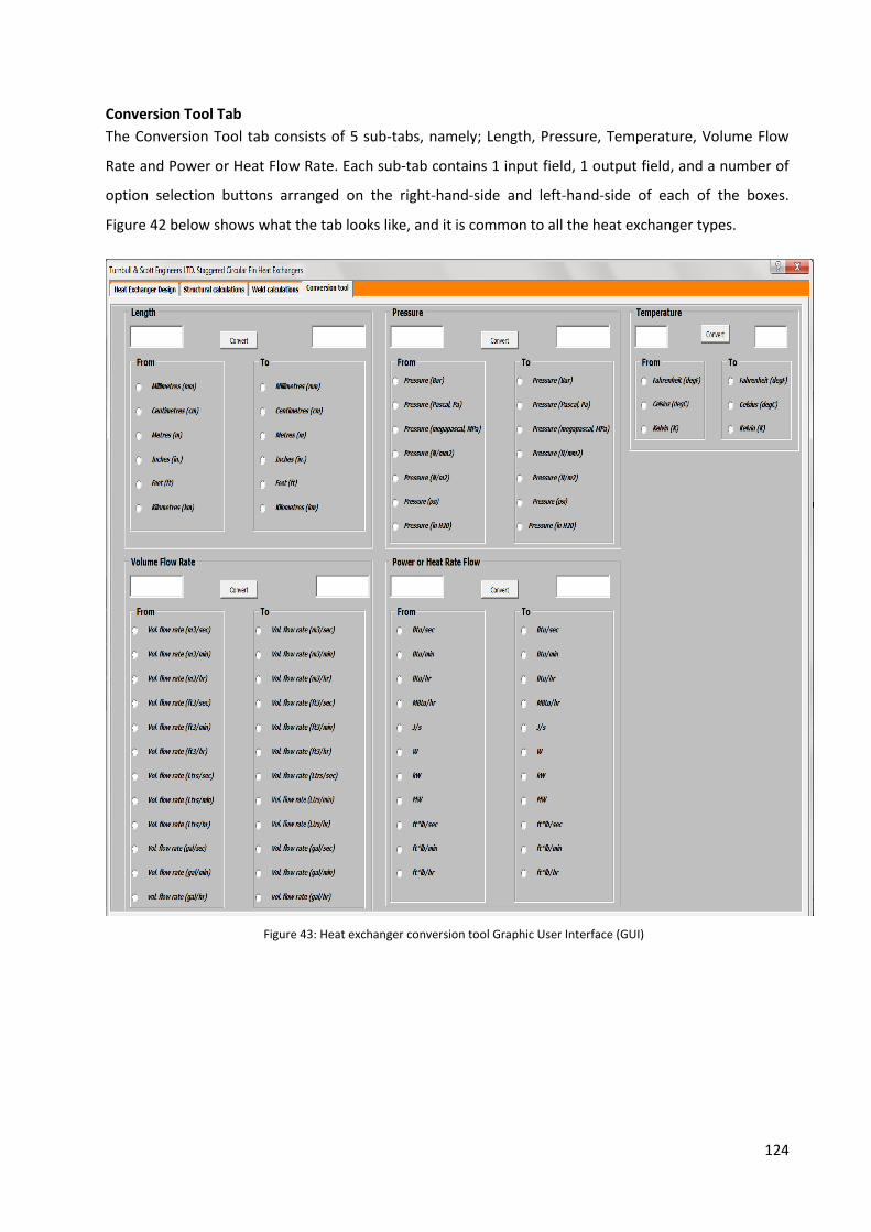
124

Conversion Tool Tab

The Conversion Tool tab consists of 5 sub-tabs, namely; Length, Pressure, Temperature, Volume Flow

Rate and Power or Heat Flow Rate. Each sub-tab contains 1 input field, 1 output field, and a number of

option selection buttons arranged on the right-hand-side and left-hand-side of each of the boxes.

Figure 42 below shows what the tab looks like, and it is common to all the heat exchanger types.

Figure 43: Heat exchanger conversion tool Graphic User Interface (GUI)

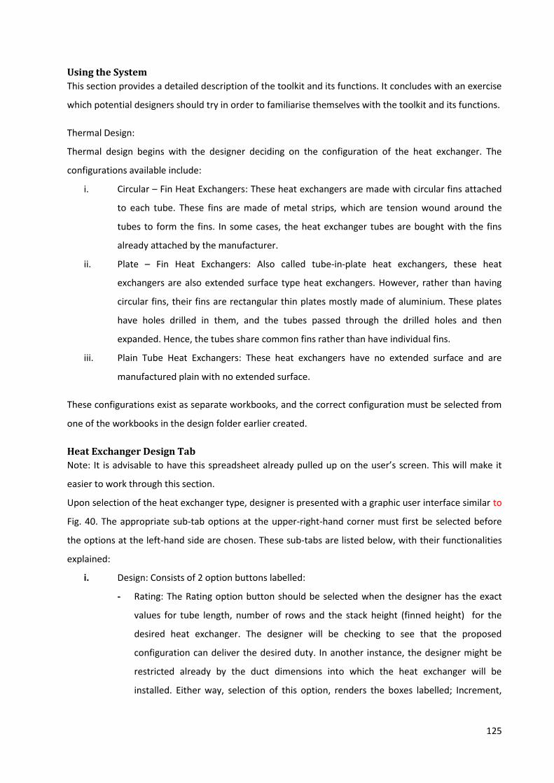
125

Using the System

This section provides a detailed description of the toolkit and its functions. It concludes with an exercise

which potential designers should try in order to familiarise themselves with the toolkit and its functions.

Thermal Design:

Thermal design begins with the designer deciding on the configuration of the heat exchanger. The

configurations available include:

i. Circular – Fin Heat Exchangers: These heat exchangers are made with circular fins attached

to each tube. These fins are made of metal strips, which are tension wound around the

tubes to form the fins. In some cases, the heat exchanger tubes are bought with the fins

already attached by the manufacturer.

ii. Plate – Fin Heat Exchangers: Also called tube-in-plate heat exchangers, these heat

exchangers are also extended surface type heat exchangers. However, rather than having

circular fins, their fins are rectangular thin plates mostly made of aluminium. These plates

have holes drilled in them, and the tubes passed through the drilled holes and then

expanded. Hence, the tubes share common fins rather than have individual fins.

iii. Plain Tube Heat Exchangers: These heat exchangers have no extended surface and are

manufactured plain with no extended surface.

These configurations exist as separate workbooks, and the correct configuration must be selected from

one of the workbooks in the design folder earlier created.

Heat Exchanger Design Tab

Note: It is advisable to have this spreadsheet already pulled up on the user’s screen. This will make it

easier to work through this section.

Upon selection of the heat exchanger type, designer is presented with a graphic user interface similar to

Fig. 40. The appropriate sub-tab options at the upper-right-hand corner must first be selected before

the options at the left-hand side are chosen. These sub-tabs are listed below, with their functionalities

explained:

i. Design: Consists of 2 option buttons labelled:

- Rating: The Rating option button should be selected when the designer has the exact

values for tube length, number of rows and the stack height (finned height) for the

desired heat exchanger. The designer will be checking to see that the proposed

configuration can deliver the desired duty. In another instance, the designer might be

restricted already by the duct dimensions into which the heat exchanger will be

installed. Either way, selection of this option, renders the boxes labelled; Increment,

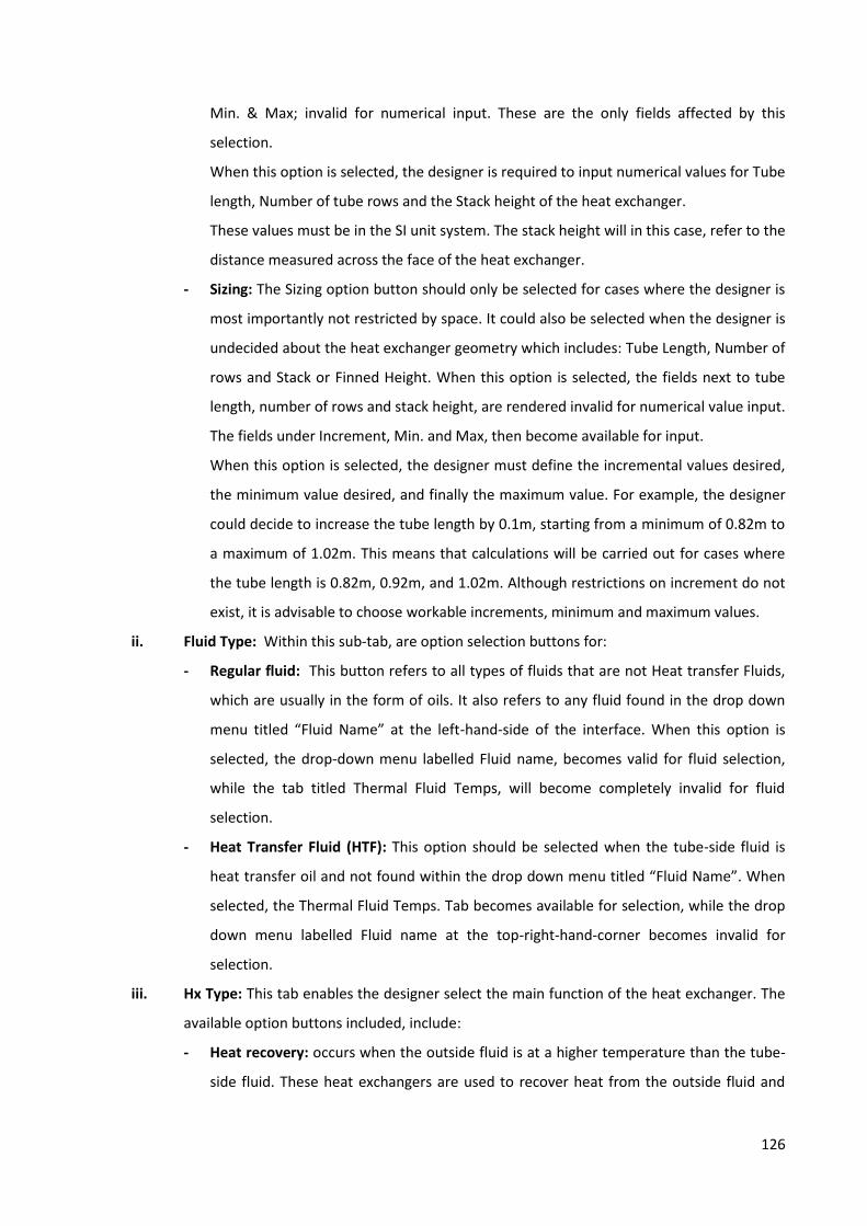
126

Min. & Max; invalid for numerical input. These are the only fields affected by this

selection.

When this option is selected, the designer is required to input numerical values for Tube

length, Number of tube rows and the Stack height of the heat exchanger.

These values must be in the SI unit system. The stack height will in this case, refer to the

distance measured across the face of the heat exchanger.

- Sizing: The Sizing option button should only be selected for cases where the designer is

most importantly not restricted by space. It could also be selected when the designer is

undecided about the heat exchanger geometry which includes: Tube Length, Number of

rows and Stack or Finned Height. When this option is selected, the fields next to tube

length, number of rows and stack height, are rendered invalid for numerical value input.

The fields under Increment, Min. and Max, then become available for input.

When this option is selected, the designer must define the incremental values desired,

the minimum value desired, and finally the maximum value. For example, the designer

could decide to increase the tube length by 0.1m, starting from a minimum of 0.82m to

a maximum of 1.02m. This means that calculations will be carried out for cases where

the tube length is 0.82m, 0.92m, and 1.02m. Although restrictions on increment do not

exist, it is advisable to choose workable increments, minimum and maximum values.

ii. Fluid Type: Within this sub-tab, are option selection buttons for:

- Regular fluid: This button refers to all types of fluids that are not Heat transfer Fluids,

which are usually in the form of oils. It also refers to any fluid found in the drop down

menu titled “Fluid Name” at the left-hand-side of the interface. When this option is

selected, the drop-down menu labelled Fluid name, becomes valid for fluid selection,

while the tab titled Thermal Fluid Temps, will become completely invalid for fluid

selection.

- Heat Transfer Fluid (HTF): This option should be selected when the tube-side fluid is

heat transfer oil and not found within the drop down menu titled “Fluid Name”. When

selected, the Thermal Fluid Temps. Tab becomes available for selection, while the drop

down menu labelled Fluid name at the top-right-hand-corner becomes invalid for

selection.

iii. Hx Type: This tab enables the designer select the main function of the heat exchanger. The

available option buttons included, include:

- Heat recovery: occurs when the outside fluid is at a higher temperature than the tube-

side fluid. These heat exchangers are used to recover heat from the outside fluid and

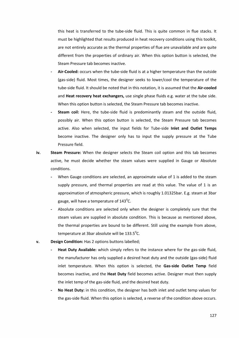
127

this heat is transferred to the tube-side fluid. This is quite common in flue stacks. It

must be highlighted that results produced in heat recovery conditions using this toolkit,

are not entirely accurate as the thermal properties of flue are unavailable and are quite

different from the properties of ordinary air. When this option button is selected, the

Steam Pressure tab becomes inactive.

- Air-Cooled: occurs when the tube-side fluid is at a higher temperature than the outside

(gas-side) fluid. Most times, the designer seeks to lower/cool the temperature of the

tube-side fluid. It should be noted that in this notation, it is assumed that the Air-cooled

and Heat recovery heat exchangers, use single phase fluids e.g. water at the tube side.

When this option button is selected, the Steam Pressure tab becomes inactive.

- Steam coil: Here, the tube-side fluid is predominantly steam and the outside fluid,

possibly air. When this option button is selected, the Steam Pressure tab becomes

active. Also when selected, the input fields for Tube-side Inlet and Outlet Temps

become inactive. The designer only has to input the supply pressure at the Tube

Pressure field.

iv. Steam Pressure: When the designer selects the Steam coil option and this tab becomes

active, he must decide whether the steam values were supplied in Gauge or Absolute

conditions.

- When Gauge conditions are selected, an approximate value of 1 is added to the steam

supply pressure, and thermal properties are read at this value. The value of 1 is an

approximation of atmospheric pressure, which is roughly 1.01325bar. E.g. steam at 3bar

gauge, will have a temperature of 1430C.

- Absolute conditions are selected only when the designer is completely sure that the

steam values are supplied in absolute condition. This is because as mentioned above,

the thermal properties are bound to be different. Still using the example from above,

temperature at 3bar absolute will be 133.50C.

v. Design Condition: Has 2 options buttons labelled;

- Heat Duty Available: which simply refers to the instance where for the gas-side fluid,

the manufacturer has only supplied a desired heat duty and the outside (gas-side) fluid

inlet temperature. When this option is selected, the Gas-side Outlet Temp field

becomes inactive, and the Heat Duty field becomes active. Designer must then supply

the inlet temp of the gas-side fluid, and the desired heat duty.

- No Heat Duty: in this condition, the designer has both inlet and outlet temp values for

the gas-side fluid. When this option is selected, a reverse of the condition above occurs.

128

The Outlet field of the Gas-side fluid temp becomes active, while the Heat Duty field

becomes inactive. Designer must then supply these 2 values.

vi. Thermal Fluid Temps: In the 2nd tab described above, the designer is presented with the

Regular Fluid & Heat Transfer Fluid options. When the Heat Transfer Fluid option is

selected, this tab becomes available for selection. Thermal fluids are mostly oils used as the

tube-side heat transfer medium. Within this tab, 3 options are available, which must be

filled by the designer.

- Thermal Fluid: This exists as a drop-down menu, from which the designer must select

the desired thermal fluid.

- Upper Temp. Limit: is a combination of numerical values, check boxes and output

fields. In this section, the designer simply has to check the box corresponding to the

temperature just greater than the thermal fluid upper temperature. In the output field,

the density of the thermal fluid at that temperature will be displayed. This acts as a

check, to ensure that thermal property values exist at that temperature for that fluid.

For example, if the thermal fluid is supplied at 830C, then the designer must select

1000C as the upper temp limit value. In cases where there are no values for the selected

temperature, an error message in the form of “Fluid properties are not available for …

Please try the next lower or higher value”. When this happens, designer only has to

check the box for the next higher value. However, if the Fluid is supplied at 800C, then

designer must first select 800C at the table. This is because, the large the distance

between the interpolated, the larger will be the deviation for the final answer.

Note that when the thermal fluid is changed, the appropriate check box must be

unchecked and checked again, to ensure that the properties actually exist at that

temperature. This should only be done when the thermal fluid has been changed.

- Lower Temp. Limit: Designer must select the temperature values lower than that for

the outlet temperature of the thermal fluid. For example, if the fluid exits at 650C, then

the designer must select the Lower Temp. Limit at 600C. All other factors as seen in the

Upper Temp. Limit case, are also applicable. Most importantly, if the thermal fluid is

changed, the appropriate check box must be unchecked and then checked again to

ensure that the properties exist at that temperature.

PLEASE NOTE THAT THIS FIELD IS ONLY AVAILABLE FOR THE THERMAL DESIGN OF

CIRCULAR-FIN HEAT EXCHANGERS. IT IS NOT AVAILABLE FOR THE PLATE-FIN AND

PLAIN TUBE HEAT EXCHANGERS DESIGN TOOLKIT.

129

vii. Fin Material: is the drop-down menu from where the designer must select the material

from which the fins of the heat exchanger are to be made. Please note that this option does

not exist for the Plain Tube heat exchanger design tool. Designer must select a material

from this list before the execute button is activated.

viii. Tube Material: is the drop-down menu of materials from which the heat exchanger tubes

will be made from. Designer must select a material from this list before the execute button

is activated.

ix. Tube-side conditions: Refers to parameters pertaining to the tube-side fluid.

- Fluid name: is the drop-down menu, from which the fluid at the tube-side will be

selected. This option becomes invalid for selection, when the Heat Transfer Fluid option

under Fluid Type is selected. However, when the Regular Fluid option is selected, this

option once again becomes valid for selection.

- Inlet Temp: is the field where the inlet temperature of the tube-side fluid must be

indicated. Please note the units for each term and ensure that whatever value you are

calculating for, corresponds to this unit. For temperature, the units are all in Degrees C

(0C).

Also note that when the Steam Coil option in the Hx Type tab is selected, this field

becomes invalid for selection.

- Outlet Temp: is the field where designer should indicate the outlet temperature of the

tube-side fluid. However, also note that when the Steam Coil option in the Hx Type tab

is selected, this option will become invalid for selection, and only becomes valid when

either the Air-Cooled or Heat Recovery options are selected.

- Tube-side velocity: in this field, the designer must decide at what velocity he wants the

tube-side fluid to flow per tube. This value should ideally be anything from 0.5m/s –

1.0m/s for water. This will ensure that the flow is sufficiently turbulent to get the best

heat transfer. For thermal fluids, this value will be considerably higher as a result of the

viscosity of thermal oils. Note that when the Steam Coil option is selected, this field

becomes invalid for selection.

- Tube Pressure: refers to the supply pressure of the tube-side fluid and must be supplied

for both Fluid Type and Hx Type conditions. When the Steam Coil option is selected,

designer must be careful to indicate whether the supply pressure is in Gauge or

Absolute conditions.

x. Gas-side conditions: Refers to parameters pertaining to the gas-side fluids. That is, fluids

flowing on the outside of the tubes.

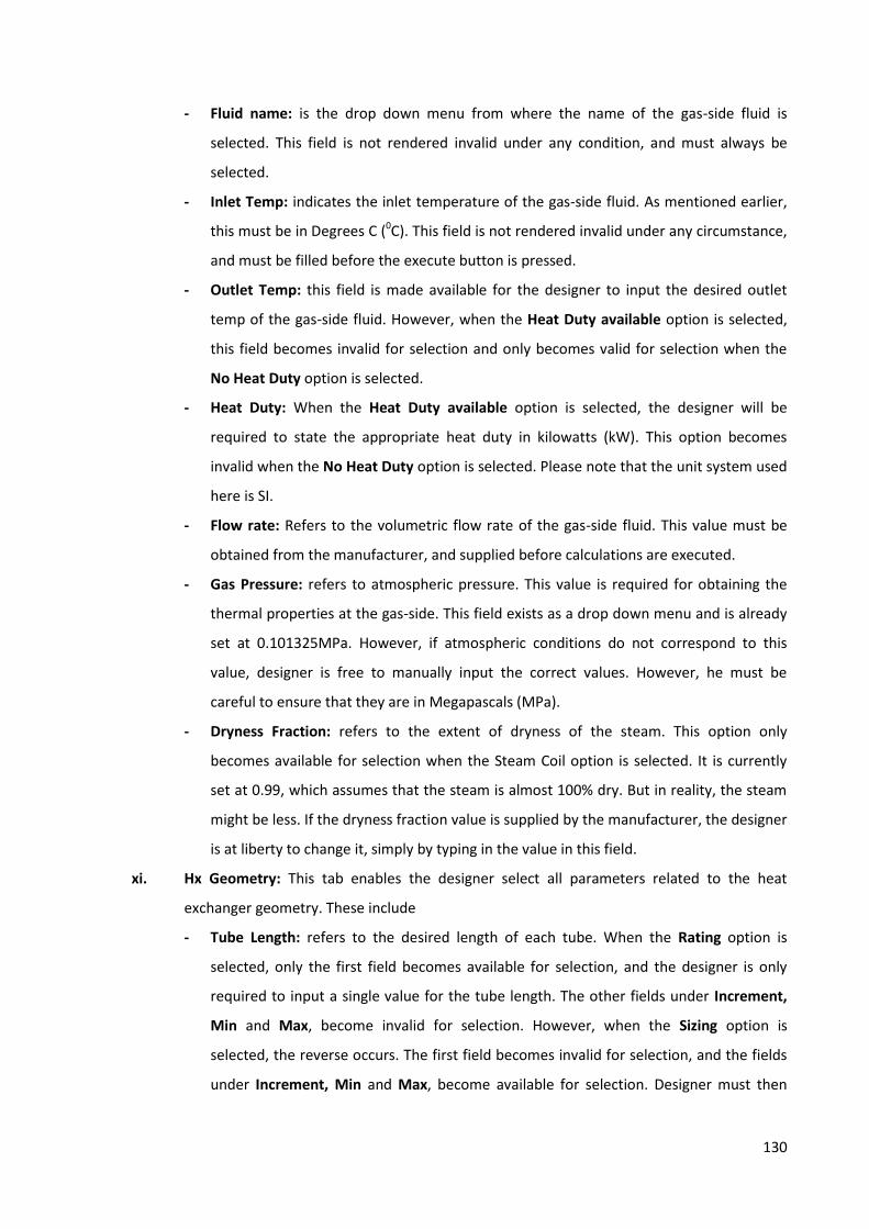
130

- Fluid name: is the drop down menu from where the name of the gas-side fluid is

selected. This field is not rendered invalid under any condition, and must always be

selected.

- Inlet Temp: indicates the inlet temperature of the gas-side fluid. As mentioned earlier,

this must be in Degrees C (0C). This field is not rendered invalid under any circumstance,

and must be filled before the execute button is pressed.

- Outlet Temp: this field is made available for the designer to input the desired outlet

temp of the gas-side fluid. However, when the Heat Duty available option is selected,

this field becomes invalid for selection and only becomes valid for selection when the

No Heat Duty option is selected.

- Heat Duty: When the Heat Duty available option is selected, the designer will be

required to state the appropriate heat duty in kilowatts (kW). This option becomes

invalid when the No Heat Duty option is selected. Please note that the unit system used

here is SI.

- Flow rate: Refers to the volumetric flow rate of the gas-side fluid. This value must be

obtained from the manufacturer, and supplied before calculations are executed.

- Gas Pressure: refers to atmospheric pressure. This value is required for obtaining the

thermal properties at the gas-side. This field exists as a drop down menu and is already

set at 0.101325MPa. However, if atmospheric conditions do not correspond to this

value, designer is free to manually input the correct values. However, he must be

careful to ensure that they are in Megapascals (MPa).

- Dryness Fraction: refers to the extent of dryness of the steam. This option only

becomes available for selection when the Steam Coil option is selected. It is currently

set at 0.99, which assumes that the steam is almost 100% dry. But in reality, the steam

might be less. If the dryness fraction value is supplied by the manufacturer, the designer

is at liberty to change it, simply by typing in the value in this field.

xi. Hx Geometry: This tab enables the designer select all parameters related to the heat

exchanger geometry. These include

- Tube Length: refers to the desired length of each tube. When the Rating option is

selected, only the first field becomes available for selection, and the designer is only

required to input a single value for the tube length. The other fields under Increment,

Min and Max, become invalid for selection. However, when the Sizing option is

selected, the reverse occurs. The first field becomes invalid for selection, and the fields

under Increment, Min and Max, become available for selection. Designer must then

131

indicate what he desires his incremental values to be, at what minimum value the

calculation should start and at what maximum value they should end. Please note that

the tube length units are in meters (m).

- Number of rows: refers to the number of rows desired in the heat exchanger. When

this value is certain, the designer sets it simply by selecting the Rating option as

explained earlier. However, if this value is not known for certain, then the Sizing option

is to be selected and the same procedure as described above must be followed.

- Stack height: also referred to as the finned height, refers to the length measured across

the face of the heat exchanger, perpendicular to the direction of the incoming gas-side

fluid. Just as before, when this value is known beforehand, such as when the heat

exchanger is to be fitted in a duct, the designer simply supplies this value within this

field. However, when this is not for certain, the Sizing option should be selected and the

same procedure followed for the Tube Length and Number of rows method stated

above. Calculations are executed in meters (m) for this value.

Note: The sizing option is only applicable to the three (3) parameters; Tube Length,

Number of rows and Stack height mentioned above.

- Number of fins: refers to the number of fins per tube required in the heat exchanger.

Designer must note that rather than the traditional fins per inch (F.P.I), these values

have been changed to fins per meter (F.P.M). Also, this field is not affected or rendered

invalid by selecting any of the tabs described above. This field is currently in the form of

a drop-down menu from which designer simply selects an appropriate value. When the

values indicated are outside the values desired by the designer, he is at liberty to input

the appropriate figures. This option is unavailable for the design of plain tube type heat

exchangers.

- Transverse Pitch: refers the distance measured from one centreline to the other of two

tubes, along the distance perpendicular to the direction of flow of the gas-side fluid.

This field exists as a drop down menu, with values already made available in meters (m).

However, if the designer wishes to change them, he is free to do so simply by typing in

the values manually. Transverse Pitch values, apply to all heat exchangers; Circular-fin,

Plate-fin and Plain tube.

- Longitudinal Pitch: refers to the distance measured from one centreline to the next of

two tubes, along the distance in the direction of flow of the gas-side fluid. This field

exists as a drop down menu, with values already made available in meters (m).

However, if the designer wishes to change these, he is free to do so simply by typing in

132

the values manually. The Longitudinal Pitch values apply to all heat exchangers;

Circular-fin, Plate-fin and Plain tube heat exchangers.

- Fin thickness: refers to the thickness of the fins. This applies to just the Circular and

Plate fin type heat exchangers. This field is unavailable for the plain tube heat

exchanger. Designer is required to select the fin thickness value from an available drop-

down menu. If the desired values are not in this list, he can provide them manually.

- Tube Diameter: refers to the outside diameter (OD) and not the nominal bore (NB) of

the tube. An already populated drop-down menu is available for the designer to select

an appropriate value. However, he is also at liberty to input a desired figure, if it is not

found within this list.

- Tube thickness: refers to the thickness of the selected tube. Again, this already exists as

a prepopulated drop down menu, which designer can choose to ignore and manually

input his desired figures. However, note that these values are in meters (m).

- Fin tip diameter: refers to the overall diameter of the fins attached to the tubes. This

field is absent for plain tube heat exchanger types. It is also available as a prepopulated

drop down menu which can be overridden by the designer with desired values.

xii. Execute: is the button which must be depressed in order to activate the calculation

process. DESIGNER MUST ENSURE THAT ALL THE REQUIRED FIELDS HAVE BEEN

CORRECTLY FILLED BEFORE THIS ACTION IS PERFORMED.

xiii. Results: Relates to all fields below the EXECUTE button. All the fields except the Sizing

results field are almost all populated when the Rating option is selected. However, when

the Sizing option is selected, these fields become void except the Sizing results field. The

fields and meanings are described below:

- Area ratio: This field offers the designer a comparison between the actual areas of the

current configuration of the heat exchanger to the area required to meet the specified

heat duty. Designer should aim to get this ratio to at least 1.10, which would be

interpreted as being that “the actual area based on the current heat exchanger

configuration from calculations, is 10% greater than the area required to meet the

specified heat duty”. This value should always be slightly greater than 1, in order to

accommodate calculation errors.

- Tubes/row: This field tells the designer the number of tubes required for each row of

the heat exchanger. As a result of approximations encountered in design, designer

might need to approximate sometimes for this value.

133

- No. of Passes: Tells the designer, the number of passes required in the heat exchanger.

When the Steam Coil option is selected, this field is void as all steam coils are designed

with a single-pass configuration. As mentioned earlier, due to approximation issues

encountered during calculations with Microsoft Excel, the number of passes might not

tally entirely with the total number of tubes, Tubes / Pass and Tubes / Row. Please

note, that this does not render the calculations invalid at all. Designer will only have to

use his discretion to either approximate by adding an extra tube, to ensure that each

pass contains the same number of tubes, or remove the extra tube in order to achieve

the same purpose.

- Tube mass flow rate: refers to the mass flow rate of the tube-side fluid. This value is

calculated from the inlet and outlet temperatures of the tube-side fluid, earlier

specified before the calculation was executed. This must not be confused with the

volume flow rate of the tube.

- Gas mass flow rate: refers to the mass flow rate of the gas-side fluid. Designer must

also not confuse this with the value for the volume flow rate of the fluid.

- Avg. pressure drop through tubes/Pass: is the pressure drop experienced per pass by

the fluid, as it flows through the tubes. Designer should take note that this is expressed

in Pascal, Pa. Please note that for the Steam Coil heat exchanger design, this value, is

not calculated. It exists only for single phase fluid condition.

- Gas pressure drop: is the pressure drop experienced by the gas-side fluid, as it flows

across the heat exchanger. This value is produced for all the heat exchanger types;

Circular-fin, Plate-fin and Plain tube.

- Tubes / pass: Value produced in this field, tells the designer how many tubes will be

segregated for each pass. As mentioned in the No. of Passes section, this value might

not entirely correlate with the total number of tubes, Number of passes and

Tubes / Row. Designer must ensure that the results are as accurate as possible. For

Steam Coil conditions, this value is also void.

- Heat Duty: Field indicates the heat duty required from the heat exchanger. For cases

where the Heat Duty Available option has been selected, a result is still produced in this

field. This acts as further confirmation that the proper heat duty is being calculated.

- Tube vol. Flow: is the volume flow rate value for the tube-side fluid. This value is

different from the tube-side mass flow rate, and must never be confused with it.

- Total no. of tubes: is the total number of tubes in the heat exchanger bundle.

134

- Avg. pressure drop entering tubes/Pass: is the pressure drop experienced by the fluid

as it enters each tube for each pass.

NOTE: DESIGNER MUST EVALUATE THE TOTAL PRESSURE DROP PER PASS AND

THROUGH THE TUBES, FOR THE TOTAL NUMBER OF PASSES, AND ENSURE THAT THIS

VALUE IS BELOW THE SUPPLY PRESSURE AT THE TUBE-SIDE. IF THIS VALUE IS HIGHER

THAN THE SUPPLY PRESSURE, PROBLEMS WILL BE EXPERIENCED WITH THE HEAT

EXCHANGER AS THE EXCESSIVE PRESSURE DROP WILL HINDER FLUID FLOW.

- Tube-side Reynolds number: indicates the Reynolds number for the fluid at the tube-

side. When this value exceeds 50’000, a warning message flashes to indicate that the

fluid is too turbulent. When it is below 10’000, a warning message also flashes

indicating that flow is too laminar to ensure proper heat transfer. In the first condition,

designer should lower the value of the velocity of fluid flow and in the second condition;

designer should increase the tube-side fluid flow velocity.

- Sizing results: When the Sizing option is selected in the Design tab, appropriate fields

populated and the execute button clicked. The Tube Length will be increased from the

minimum to the maximum value as specified in the Increment section. The same

process is carried out for the Number of rows and Stack height sections. These values

are then inserted into the spreadsheet, incrementally and results produced. E.g. when

the tube length is increased from 0.85 (min.) to 0.92m (max.) at intervals of 0.1m , the

values produced are 0.85m, 0.86m, 0.87m, 0.88m, 0.89m, 0.90m, 0.91m and 0.92m.

Each of these values is then placed in the heat transfer equations and results for when

the tube length is 0.85m – 0.92m, are produced. The calculations have been written, to

delete all Area Ratios below 1.0 and above 1.5. This will enable the designer make a

quick decision as to what configuration best suits his manufacturing process. Selected

configuration must also conform to the manufacturer’s requirements, e.g. allowable

pressure drop in heat exchanger.

When a configuration is selected, the designer heads back to the Design tab and

changes it to from Sizing to Rating. The Increment, Min and Max fields become invalid

for selection, while the fields right of Tube Length, Number of Rows and Stack height

become valid for selection. Designer must then insert the chosen configuration in these

fields and click the Execute button. Figure 44 shows a typical sizing calculation and the

results produced.

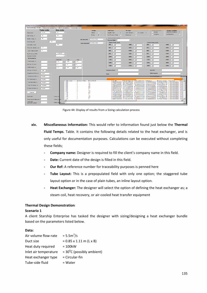
135

Figure 44: Display of results from a Sizing calculation process

xiv. Miscellaneous Information: This would refer to information found just below the Thermal

Fluid Temps. Table. It contains the following details related to the heat exchanger, and is

only useful for documentation purposes. Calculations can be executed without completing

these fields;

- Company name: Designer is required to fill the client’s company name in this field.

- Date: Current date of the design is filled in this field.

- Our Ref: A reference number for traceability purposes is penned here

- Tube Layout: This is a prepopulated field with only one option; the staggered tube

layout option or in the case of plain tubes, an inline layout option.

- Heat Exchanger: The designer will select the option of defining the heat exchanger as; a

steam coil, heat recovery, or air-cooled heat transfer equipment

Thermal Design Demonstration:

Scenario 1

A client Starship Enterprise has tasked the designer with sizing/designing a heat exchanger bundle

based on the parameters listed below.

Data:

Air volume flow-rate = 5.5m3/s

Duct size = 0.85 x 1.11 m (L x B)

Heat duty required = 100kW

Inlet air temperature = 300C (possibly ambient)

Heat exchanger type = Circular-fin

Tube-side fluid = Water

136

Gas-side fluid = air

Solution:

Based on preferred in-house manufacturing dimensions, designer has selected the following parameters

for the design.

Transverse pitch = 0.055m

Longitudinal pitch = 0.050m

Tube OD = 0.0267m

Tube thickness = 0.00287m

Fin material = Carbon steel

Tube material = Carbon steel

Step 1: Since the duct dimensions have already been given, heat exchanger dimensions (length &

breath) will have to conform to it. Therefore this will be a rating exercise and the designer

selects the Rating option under Design.

Step 2: The Regular fluid option button is selected under the Fluid Type heading, since the fluid type is

water. This renders the Thermal Fluid Temps, option box invalid.

Step 3: Select the Air-Cooled option under Hx Type. This action renders the next field invalid.

Step 4: Select the Heat Duty available option under the Design Condition box. This is because we have

been given the desired heat duty, an inlet air temperature, but no outlet air temperature.

Step 5: Under the Tube-side heading, input the following values under the appropriate headings:

Fluid name = Water

Inlet Temp = 80

Outlet Temp = 60

Heat Duty = 100

Tube-side velocity = 0.45

Tube Pressure = 2

Step 6: Under the Gas-side heading, input the following values under the appropriate headings:

Fluid name = Air

Inlet Temp = 30

Outlet Temp = should have been rendered invalid because Heat Duty available was

selected earlier, so ignore it.

Flow rate = 5.5

Gas pressure = 0.101325MPa

Dryness Fraction = has been rendered invalid because Air-Cooled option was selected

earlier.

Step 7: Under the HX Geometry heading, select the following values under appropriate headings:

Tube Length = 0.85

Number of rows = 4

Stack height = 1.11

Number of fins = 236

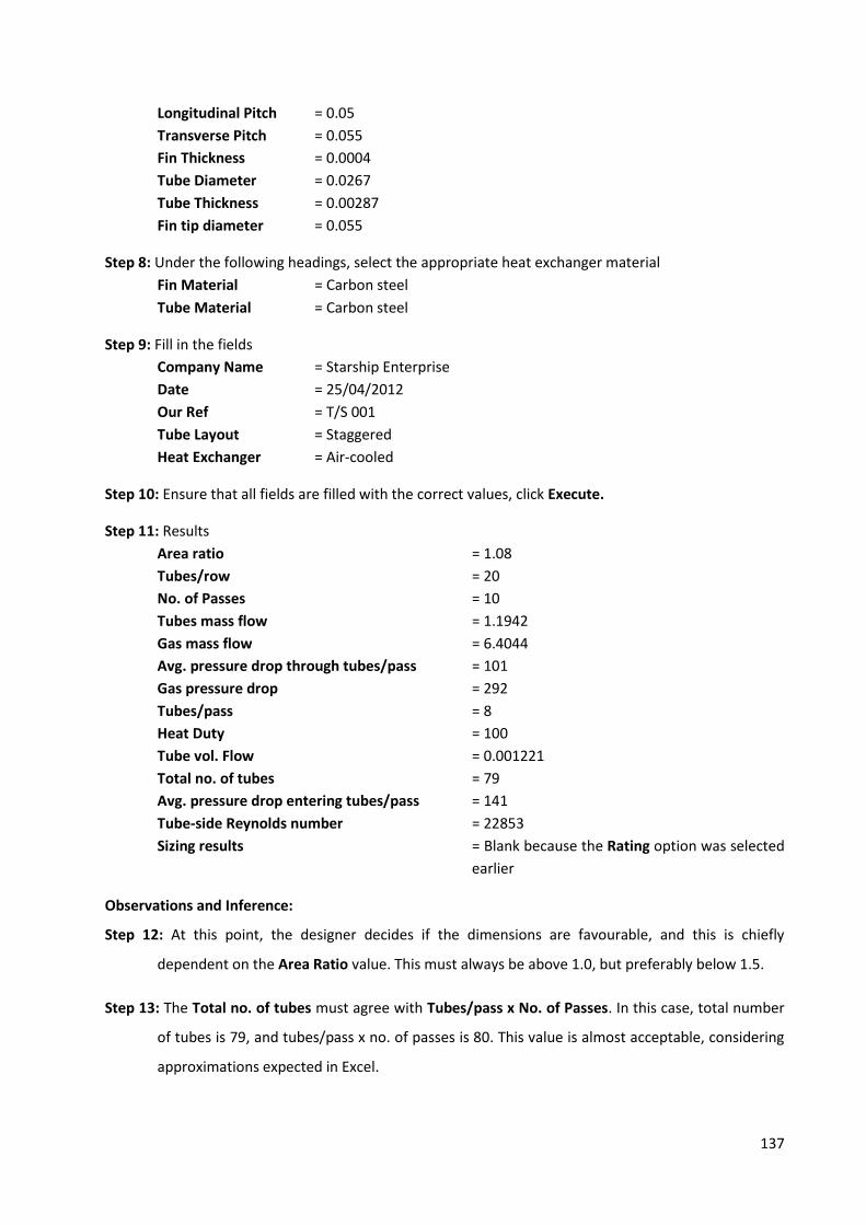
137

Longitudinal Pitch = 0.05

Transverse Pitch = 0.055

Fin Thickness = 0.0004

Tube Diameter = 0.0267

Tube Thickness = 0.00287

Fin tip diameter = 0.055

Step 8: Under the following headings, select the appropriate heat exchanger material

Fin Material = Carbon steel

Tube Material = Carbon steel

Step 9: Fill in the fields

Company Name = Starship Enterprise

Date = 25/04/2012

Our Ref = T/S 001

Tube Layout = Staggered

Heat Exchanger = Air-cooled

Step 10: Ensure that all fields are filled with the correct values, click Execute.

Step 11: Results

Area ratio = 1.08

Tubes/row = 20

No. of Passes = 10

Tubes mass flow = 1.1942

Gas mass flow = 6.4044

Avg. pressure drop through tubes/pass = 101

Gas pressure drop = 292

Tubes/pass = 8

Heat Duty = 100

Tube vol. Flow = 0.001221

Total no. of tubes = 79

Avg. pressure drop entering tubes/pass = 141

Tube-side Reynolds number = 22853

Sizing results = Blank because the Rating option was selected

earlier

Observations and Inference:

Step 12: At this point, the designer decides if the dimensions are favourable, and this is chiefly

dependent on the Area Ratio value. This must always be above 1.0, but preferably below 1.5.

Step 13: The Total no. of tubes must agree with Tubes/pass x No. of Passes. In this case, total number

of tubes is 79, and tubes/pass x no. of passes is 80. This value is almost acceptable, considering

approximations expected in Excel.

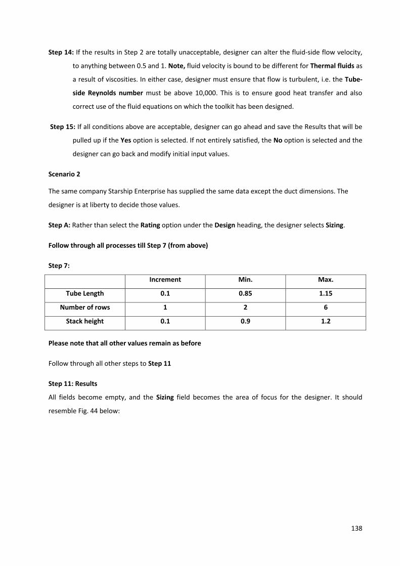
138

Step 14: If the results in Step 2 are totally unacceptable, designer can alter the fluid-side flow velocity,

to anything between 0.5 and 1. Note, fluid velocity is bound to be different for Thermal fluids as

a result of viscosities. In either case, designer must ensure that flow is turbulent, i.e. the Tube-

side Reynolds number must be above 10,000. This is to ensure good heat transfer and also

correct use of the fluid equations on which the toolkit has been designed.

Step 15: If all conditions above are acceptable, designer can go ahead and save the Results that will be

pulled up if the Yes option is selected. If not entirely satisfied, the No option is selected and the

designer can go back and modify initial input values.

Scenario 2

The same company Starship Enterprise has supplied the same data except the duct dimensions. The

designer is at liberty to decide those values.

Step A: Rather than select the Rating option under the Design heading, the designer selects Sizing.

Follow through all processes till Step 7 (from above)

Step 7:

Increment Min. Max.

Tube Length 0.1 0.85 1.15

Number of rows 1 2 6

Stack height 0.1 0.9 1.2

Please note that all other values remain as before

Follow through all other steps to Step 11

Step 11: Results

All fields become empty, and the Sizing field becomes the area of focus for the designer. It should

resemble Fig. 44 below:

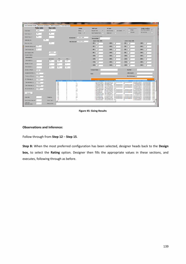
139

Figure 45: Sizing Results

Observations and Inference:

Follow through from Step 12 – Step 15.

Step B: When the most preferred configuration has been selected, designer heads back to the Design

box, to select the Rating option. Designer then fills the appropriate values in these sections, and

executes, following through as before.

140

Structural Calculations Tab

For cases where the designer needs to ensure that the thicknesses of the materials used in the

manufacture of the heat exchanger are suitable to hold the pressure loading from the fluid, he employs

the use of the structural calculations tab. This is the second tab in the toolkit, and it functions

independent of the other tabs:

- Provides the designer with minimum thickness requirements for the tubes and plates

used in the heat exchanger manufacture.

- Provides the designer with the design strength for the materials used in the heat

exchanger manufacture.

- Calculates the stresses experienced by the components as a result of pressure loading

from the fluids only.

- Classifies the heat exchanger according to PED requirements.

When the structural calculations tab is selected, the designer is required to fill the following fields

before calculations can be executed;

i. Tube Dimensions: This section covers all cylindrical shaped materials in the heat exchanger

manufacture.

- Tube grade: This is exists as a prepopulated dropdown menu, from which the designer

is required to select the grade of tube used in the manufacture. The designer IS NOT at

liberty to fill in a desired tube grade because these materials were selected from the

materials made available and recognized by the Pressure Vessel Code, PD5500. In

addition to this, the PD5500 has made available design strengths for these materials

with the appropriate factors of safety built in according to working temperature of the

heat exchanger. Therefore if the tube materials used by the designer are not in the

group provided, he must notify the senior design engineer.

- Nozzle OD: Designer is then required to select the inlet nozzle outer diameter (OD).

Although this drop-down menu is already prepopulated with values, designer is at

liberty to insert a value missing from the list. However, a corresponding DN value will

not be available. Please note these values are in millimetres (mm) and refer to the

Outer Diameter (OD) and not the Nominal Diameter (DN) of the inlet nozzle.

- HX tube OD: This refers to the outer diameter of the heat exchanger tubes, and this

menu is exactly the same as the menu for the Nozzle OD. Same restrictions are also

applicable.

- Header OD: Conditions applicable in the Nozzle and HX tube, are also applicable here,

and should be treated as such by the designer.

141

- Nozzle thickness: Designer simply selects the thickness of the inlet nozzle. Designer can

also populate this field with preferred data. Please also note that this field takes only

values in SI units, millimetres (mm) to be exact.

- HX tube thickness: The same conditions seen in the nozzle thickness field are also seen

here. Designer should also treat this field with the same restrictions as the nozzle

thickness field.

- Header thickness: Same conditions are applicable as the field above.

ii. Plate Dimensions: refers to all plates used in the heat exchanger manufacture. These

mostly include the tube-plate and the end-blanks. The fields found under this section

include:

- Plate grade: Designer is required to select the grade of the plate material used for

manufacture. As mentioned for the tube section, the designer IS NOT at liberty to fill in

preferred materials, for the same reasons already explained in the tube section.

- Plate thickness: Designer only has to indicate the thickness of the plates used. Designer

is at liberty to populate this field with his preferred values.

iii. HX Dimensions:

- Longitudinal Pitch: Designer selects the design longitudinal pitch from a prepopulated

dropdown menu. Designer can also populate this field with preferred values.

- Transverse Pitch: Same conditions as in the longitudinal pitch field mentioned above,

are also applicable in this field

- Number of rows: Number of rows in the heat exchanger is required in this field.

iv. Fluid type:

- Design temp: The designer will be required to specify the maximum tube-side fluid

temperature that the vessel will experience while in service, within this field. This value

must never be lower than the exit temperature of this fluid. Preferably, it should be

slightly higher than the inlet temperature of the tube-side fluid.

- Design pressure: This field requires the designer to specify the supply pressure of the

tube side fluid.

- Steam: When steam is the heat transfer medium at the tube-side, designer will be

required to check this option button.

- Water: When water is the heat transfer medium within the tubes, then this option

button should be checked.

v. Temperature ranges: Consists of 2 sub-tabs namely;

142

- Tube temp range: This tab is a combination of checkboxes and output fields. As earlier

mentioned, the design temperature specified for structural calculations should be

governed by the upper temperature of the tube-side fluid. Bearing this in mind,

designer will be required to select two of the checkboxes, with the design temperature

lying between these values. For example, if the upper design temperature is 1700C, then

the designer will be required to select the checkboxes for 1500c and 2000C.

This is all the action required of the designer for this section.

- Plate temp range: Involves the same procedure as for the section described above.

Please note that the temperature range selected for the plate temperature range must

always be the same as selected for the tube temperature range. This is because, it is

expected that the heat exchanger components will experience the same temperature

increase. As mentioned earlier, the designer simply selects the appropriate check boxes

for temperatures between which the design temperature lies.

vi. Execute button: This button is used to activate the calculations required for structural

analysis. It should only be depressed when the designer has filled the input fields as

described above.

vii. Results: This tab consists of 3 sub-tabs, which represent results obtained from the structural

analysis calculation. They include:

- Design strength values:

Tube design strength at design temp: will give the designer, the strength of the

tube material at the elevated working temperature of the heat exchanger. This

value is interpolated from the design strength values for tube materials in

Annex K of the PD5500 pressure vessel code.

Plate design strength at design temp: producing the same values as above but

only for plates, this section will give the strength values of the plate at its

elevated working temperature. This information is also based on interpolated

values from the PD5500.

Transverse stress in Nozzle: gives the designer results for the transverse stress

experienced by the nozzle, as a result of fluid pressure loading only. Calculations

have been done, to ensure that if this value exceeds the design strength of the

nozzle material at the design temperature, a warning message appears.

Transverse stress in HX tubes: same as above, results are given for the primary

stresses in the heat exchanger tubes as a result of fluid pressure loading only. If

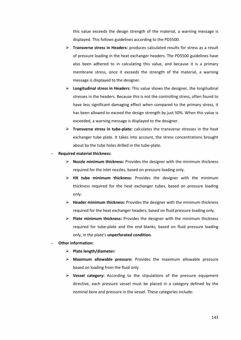
143

this value exceeds the design strength of the material, a warning message is

displayed. This follows guidelines according to the PD5500.

Transverse stress in Headers: produces calculated results for stress as a result

of pressure loading in the heat exchanger headers. The PD5500 guidelines have

also been adhered to in calculating this value, and because it is a primary

membrane stress, once it exceeds the strength of the material, a warning

message is displayed to the designer.

Longitudinal stress in Headers: This value shows the designer, the longitudinal

stresses in the headers. Because this is not the controlling stress, often found to

have less significant damaging effect when compared to the primary stress, it

has been allowed to exceed the design strength by just 50%. When this value is

exceeded, a warning message is displayed to the designer.

Transverse stress in tube-plate: calculates the transverse stresses in the heat

exchanger tube plate. It takes into account, the stress concentrations brought

about by the tube holes drilled in the tube-plate.

- Required material thickness:

Nozzle minimum thickness: Provides the designer with the minimum thickness

required for the inlet nozzles, based on pressure loading only.

HX tube minimum thickness: Provides the designer with the minimum

thickness required for the heat exchanger tubes, based on pressure loading

only.

Header minimum thickness: Provides the designer with the minimum thickness

required for the heat exchanger headers, based on fluid pressure loading only.

Plate minimum thickness: Provides the designer with the minimum thickness

required for tube-plate and the end blanks, based on fluid pressure loading

only, in the plate’s unperforated condition.

- Other information:

Plate length/diameter:

Maximum allowable pressure: Provides the maximum allowable pressure

based on loading from the fluid only.

Vessel category: According to the stipulations of the pressure equipment

directive, each pressure vessel must be placed in a category defined by the

nominal bore and pressure in the vessel. These categories include:

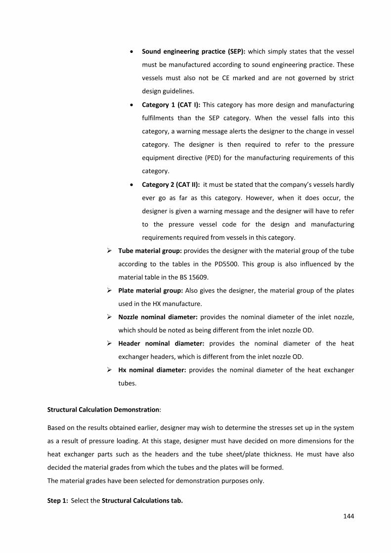
144

Sound engineering practice (SEP): which simply states that the vessel

must be manufactured according to sound engineering practice. These

vessels must also not be CE marked and are not governed by strict

design guidelines.

Category 1 (CAT I): This category has more design and manufacturing

fulfilments than the SEP category. When the vessel falls into this

category, a warning message alerts the designer to the change in vessel

category. The designer is then required to refer to the pressure

equipment directive (PED) for the manufacturing requirements of this

category.

Category 2 (CAT II): it must be stated that the company’s vessels hardly

ever go as far as this category. However, when it does occur, the

designer is given a warning message and the designer will have to refer

to the pressure vessel code for the design and manufacturing

requirements required from vessels in this category.

Tube material group: provides the designer with the material group of the tube

according to the tables in the PD5500. This group is also influenced by the

material table in the BS 15609.

Plate material group: Also gives the designer, the material group of the plates

used in the HX manufacture.

Nozzle nominal diameter: provides the nominal diameter of the inlet nozzle,

which should be noted as being different from the inlet nozzle OD.

Header nominal diameter: provides the nominal diameter of the heat

exchanger headers, which is different from the inlet nozzle OD.

Hx nominal diameter: provides the nominal diameter of the heat exchanger

tubes.

Structural Calculation Demonstration:

Based on the results obtained earlier, designer may wish to determine the stresses set up in the system

as a result of pressure loading. At this stage, designer must have decided on more dimensions for the

heat exchanger parts such as the headers and the tube sheet/plate thickness. He must have also

decided the material grades from which the tubes and the plates will be formed.

The material grades have been selected for demonstration purposes only.

Step 1: Select the Structural Calculations tab.

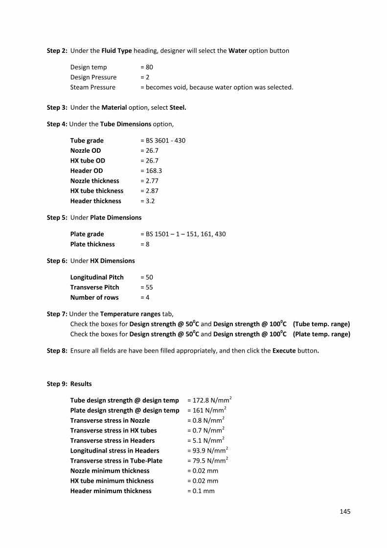
145

Step 2: Under the Fluid Type heading, designer will select the Water option button

Design temp = 80

Design Pressure = 2

Steam Pressure = becomes void, because water option was selected.

Step 3: Under the Material option, select Steel.

Step 4: Under the Tube Dimensions option,

Tube grade = BS 3601 - 430

Nozzle OD = 26.7

HX tube OD = 26.7

Header OD = 168.3

Nozzle thickness = 2.77

HX tube thickness = 2.87

Header thickness = 3.2

Step 5: Under Plate Dimensions

Plate grade = BS 1501 – 1 – 151, 161, 430

Plate thickness = 8

Step 6: Under HX Dimensions

Longitudinal Pitch = 50

Transverse Pitch = 55

Number of rows = 4

Step 7: Under the Temperature ranges tab,

Check the boxes for Design strength @ 500C and Design strength @ 1000C (Tube temp. range)

Check the boxes for Design strength @ 500C and Design strength @ 1000C (Plate temp. range)

Step 8: Ensure all fields are have been filled appropriately, and then click the Execute button.

Step 9: Results

Tube design strength @ design temp = 172.8 N/mm2

Plate design strength @ design temp = 161 N/mm2

Transverse stress in Nozzle = 0.8 N/mm2

Transverse stress in HX tubes = 0.7 N/mm2

Transverse stress in Headers = 5.1 N/mm2

Longitudinal stress in Headers = 93.9 N/mm2

Transverse stress in Tube-Plate = 79.5 N/mm2

Nozzle minimum thickness = 0.02 mm

HX tube minimum thickness = 0.02 mm

Header minimum thickness = 0.1 mm

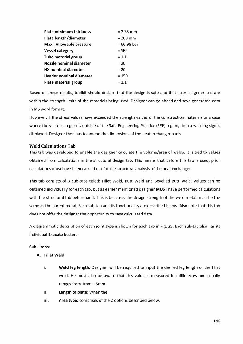
146

Plate minimum thickness = 2.35 mm

Plate length/diameter = 200 mm

Max. Allowable pressure = 66.98 bar

Vessel category = SEP

Tube material group = 1.1

Nozzle nominal diameter = 20

HX nominal diameter = 20

Header nominal diameter = 150

Plate material group = 1.1

Based on these results, toolkit should declare that the design is safe and that stresses generated are

within the strength limits of the materials being used. Designer can go ahead and save generated data

in MS word format.

However, if the stress values have exceeded the strength values of the construction materials or a case

where the vessel category is outside of the Safe Engineering Practice (SEP) region, then a warning sign is

displayed. Designer then has to amend the dimensions of the heat exchanger parts.

Weld Calculations Tab

This tab was developed to enable the designer calculate the volume/area of welds. It is tied to values

obtained from calculations in the structural design tab. This means that before this tab is used, prior

calculations must have been carried out for the structural analysis of the heat exchanger.

This tab consists of 3 sub-tabs titled: Fillet Weld, Butt Weld and Bevelled Butt Weld. Values can be

obtained individually for each tab, but as earlier mentioned designer MUST have performed calculations

with the structural tab beforehand. This is because; the design strength of the weld metal must be the

same as the parent metal. Each sub-tab and its functionality are described below. Also note that this tab

does not offer the designer the opportunity to save calculated data.

A diagrammatic description of each joint type is shown for each tab in Fig. 25. Each sub-tab also has its

individual Execute button.

Sub – tabs:

A. Fillet Weld:

i. Weld leg length: Designer will be required to input the desired leg length of the fillet

weld. He must also be aware that this value is measured in millimetres and usually

ranges from 1mm – 5mm.

ii. Length of plate: When the

iii. Area type: comprises of the 2 options described below.

147

- Weld leg length: When this option is selected, the area of the weld is calculated using

the length of the plate earlier indicated.

- Throat thickness: This calculation is independent of the length of the plate, and only

depends on the leg length of the fillet weld. The area of the weld is calculated through

the throat of the weld.

iv. Material type: The designer has to indicate whether the material is a Tube or Plate. This

is necessary because the design strengths for tubes, will differ from that of plates, and

this would have been seen from the Structural calculations tab

v. Results: The results section has two sub-tabs named:

- Area 1 (Leg lengths): is the area calculated when the Weld leg length option has been

selected. Its value is in mm2, and the following results are also produced;

Force at joint due to inlet pressure: Indicates the pressure experienced by the

joint as a result of inlet pressure only. Please note that this value is in Newton

(N)

Maximum allowable force on joint: Tells the designer, the bearable load on this

joint, based on the area earlier calculated. This is also in Newton (N).

- Area 2 (throat thickness): is the area measured when the Throat thickness area

calculation option has been selected. Its value is in mm2, and the following results are

also produced;

Required throat thickness: Indicates to the designer, the minimum throat

thickness required to bear the pressure load.

Force at joint due to inlet pressure: also as described above, this result tells the

designer the force experience by this joint as a result of pressure loading,

especially when calculated through the throat of the weld. This is especially

useful when calculating stresses at the fillet weld around a tube diameter.

Maximum allowable force on joint: shows the maximum allowable force, this

joint can bear. This value is also in Newton (N)

B. Butt weld:

i. Root gap: Here, the designer indicates the space to be allowed between the plates in

millimetres (mm).

ii. Weld or Plate thickness: is an indication of the thickness of the plate, which must also

correspond to the thickness of the weld metal. This value is also in millimetres (mm)

148

iii. Material type: User selects whether the material is a tube or plate. The reason why

this selection is necessary has already been mentioned.

iv. Results: Presents the results of calculations based on the initial input data. It also

consists of the following output fields, similar to the Fillet Weld field.

- Total area: measures the area of the weld metal in mm2.

- Force at joint due to inlet pressure: measures the force experienced by the joint, as

result of the inlet pressure of the fluid. This is also in Newton (N).

- Maximum allowable force on joint: gives the designer, the maximum allowable load for

that joint.

C. Bevelled Butt Weld: This type of joint preparation, applies to parts where the edges have been

machined. Examples are shown in the diagrams under this tab.

i. Bevelled angle: refers to the angle made by the machined edges. This is usually in

degrees.

ii. Excess weld metal height, h: refers to the desired height of the weld metal on the joint.

This is indicated in the diagram as ‘h’.

iii. Root gap: refers to the smallest distance between the edges to be joined. This is

indicated as ‘b’ in the diagram.

iv. Weld or Plate thickness: refers to the thickness of the edges to be joined.

v. Root face: refers to the face height at the end of the bevels. This height is usually no

greater than 2-5mm.

vi. Material Type: Has been described above.

vii. Bevel type: Designer will be required to select the edge condition of the edges.

- Full Bevel: means the two edges have been machined at an angle.

- Half Bevel: means just one of the edges has been machined, while the other is left

intact.

viii. Result:

- Total area: Tells the designer, the total area of the joint. This value will be dependent

on the Bevel Type option earlier selected. This value is in mm2.

- Force at joint due to inlet pressure: as described earlier, this is the force experienced

by the joint as a result of pressure loading from the tube-side fluid. This value is also

bound to be different for the Full & Half Bevel conditions.

- Maximum allowable force: measured in Newton (N), this refers to the maximum

allowable force on the joint. This value is also bound to be different for the Full & Half

Bevel conditions.

149

Conversion Tool Tab

This is the fourth tab in the toolkit design group. The conversion tool, offers the designer a quick and

easier means to make conversions between selected values in the Imperial and SI unit format. It

consists of 5 sub-tabs. These sub-tabs are composed of a heading stating the dimension (e.g. length,

pressure, etc.), 1 input field (Left-Hand-Side), 1 output field (Right-Hand-Side) and 2 side-by-side aligned

option buttons labelled “From” & “To”.

Process of calculation is common across all the sub-tabs. User is required to follow the steps outlined

below:

i. User decides which dimensions to convert. The dimension available include: Length,

Pressure, Temperature, Volume flow rate, and Power or Heat Rate Flow.

ii. User types the value he needs converted in the LHS textbox.

iii. User selects the current dimension of this unit in the “From” box.

iv. User selects the new desired dimension of this unit in the “To” box.

v. User finally clicks the convert button located between the two textboxes.

vi. The converted value is produced in the RHS textbox field.

Available Sub-tabs:

i. Length: User can choose from 5 options that include; Millimetres, Centimetres, Metres,

Inches, Feet, and Kilometres.

ii. Pressure: available dimensions include; Bar Pascal, Megapascals, Newton/millimetres2,

Newton/metres2, Pounds per Square Inch, and Inches water column.

iii. Temperature: dimensions include; Fahrenheit, Celsius, and Kelvin.

iv. Volume Flow Rate: includes; metres3/sec, metres3/min, metres3/hr., feet3/sec, feet3/min,

feet3/hr., Litres/second, Litres/min, Litres/hr., gallons/second, gallons/min, and gallons/hr.

v. Power or Heat Rate Flow: British Thermal Units/sec, British Thermal Units/min, British

Thermal Units/hr., Mega British Thermal Units/hr., Joules/sec, Watts, Kilowatt, Megawatt,

Foot-pounds/sec, Foot-pounds/min, Foot-pounds/hr.

Reporting

This section describes actions the designer is bound to encounter after the thermal design and

structural calculations only.

Saving the document

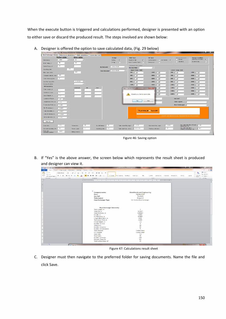
150

When the execute button is triggered and calculations performed, designer is presented with an option

to either save or discard the produced result. The steps involved are shown below:

A. Designer is offered the option to save calculated data, (Fig. 29 below)

Figure 46: Saving option

B. If “Yes” is the above answer, the screen below which represents the result sheet is produced

and designer can view it.

Figure 47: Calculations result sheet

C. Designer must then navigate to the preferred folder for saving documents. Name the file and

click Save.

151

Figure 48: Saving the results sheet

D. This is the final produced screen, and designer just needs to close this by clicking the red box at

the top right hand corner of the screen. Indicated below.

Figure 49: Closing the calculation result sheet

WARNING: IF THE DESIGNER OPTS NOT TO SAVE THE GENERATED DATA, HE MUST SELECT A “NO”

ANSWER AT STEP 1. IF THE CANCEL BUTTON IS CHOSEN AT STEP 3, THE TOOLKIT IS BOUND TO

DEVELOP PROBLEMS.

152

Troubleshooting

This section explains common type problems experienced with the toolkit, and ways to fix them.

To ensure that immediate issues are not encountered, designer must ensure that the thermal fluids

software REFROP is installed on their individual computer systems. To install REFPROP, user should

double-click the installation file and follow the instructions. Once installed, user should follow the steps

below to ensure that REFPROP is properly linked to the spread sheets.

The following outlines the procedure for using REFPROP within any spreadsheet in Office 2007 or

2010:

1. Open REFPROP.xls and save it as an add-in, REFPROP.xla or REFPROP.xlam, in the main REFPROP

folder, C:\Program Files\REFPROP.

2. Go to File/Options/Trust Centre/Trust centre Settings (bottom at bottom right).

3. Select “Trusted Locations” on the left. Click “Add new location”. Browse to C:\Program

Files\REFPROP, select “Subfolders of this location are also trusted”, and click “OK”.

4. Go to File/Options/Add-Ins and select “Excel Add-ins” in the Manage drop-down box at the

bottom, and click Go

5. Click “Browse”, and navigate to C:\Program Files\REFPROP, select REFPROP.xlam and click “OK”.

IMPORTANT: Do not simply select REFPROP.xlam when it first comes up, as this will be in the

wrong folder (c:\Documents and Settings\Username\Application Data\Microsoft\Addins), which

is not trusted and will not work.

6. Select the Data tab, and click on Edit Links. Select REFPROP.xlam. Click on “Change Source” and

navigate to C:\Program Files\RREFPROP. Select REFPROP.xlam there and click “OK”.

This is just to make sure you are connected to the correct Add-in. If the Data tab is greyed out,

start typing in a REFPROP command such as; “=Density (“water”, “TP”, 300, 1)” and the button

should become active.

7. Once you have the .xla or .xlam file set up, you can open a brand new workbook and the

functions should be available to you. Do not continue working with the REFPROP.xls file since it

still contains the VB code that is also in the .xlam file. In this manner, future updates from NIST

of the REFPROP.xls file can be resaved as the .xlam file, and all of your workbooks will have

access to the most recent code.

Tips

1. In some cases, the macros may not work. Try saving the file as A MACRO-ENABLED WORKBOOK

(under Save As…)

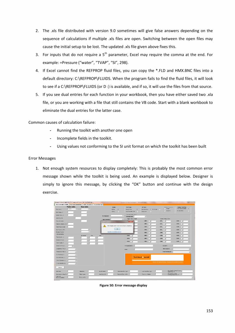
153

2. The .xls file distributed with version 9.0 sometimes will give false answers depending on the

sequence of calculations if multiple .xls files are open. Switching between the open files may

cause the initial setup to be lost. The updated .xls file given above fixes this.

3. For inputs that do not require a 5th parameter, Excel may require the comma at the end. For

example: =Pressure (“water”, “TVAP”, “SI”, 298).

4. If Excel cannot find the REFPROP fluid files, you can copy the *.FLD and HMX.BNC files into a

default directory: C:\REFPROP\FLUIDS. When the program fails to find the fluid files, it will look

to see if a C:\REFPROP\FLUIDS (or D :) is available, and if so, it will use the files from that source.

5. If you see dual entries for each function in your workbook, then you have either saved two .xla

file, or you are working with a file that still contains the VB code. Start with a blank workbook to

eliminate the dual entries for the latter case.

Common causes of calculation failure:

- Running the toolkit with another one open

- Incomplete fields in the toolkit.

- Using values not conforming to the SI unit format on which the toolkit has been built

Error Messages

1. Not enough system resources to display completely: This is probably the most common error

message shown while the toolkit is being used. An example is displayed below. Designer is

simply to ignore this message, by clicking the “OK” button and continue with the design

exercise.

Figure 50: Error message display

154

Common Errors

1. Excel is not very smart and this also unfortunately applies to the developer who worked with it.

Therefore, Designer must ensure that the other calculation sheets are closed before running

any calculation or at least activate the user-form from the buttons located on the excel sheets

titled “sizing”.

2. Not filling all the necessary fields before the “Execute button” is hit. This is bound to cause

errors in the computer program.