implementation and testing of an underwater communication

Defence University Center

Spanish Naval Academy

FINAL YEAR PROYECT

Implementation and testing of an

underwater communication protocol.

Mechanical Engineering Bachelor Degree

STUDENT: Santiago María de Colsa Iglesias

SUPERVISOR: Alfonso Rodríguez-Molares

ACADEMIC YEAR: 2020-2021

Defence University Center

Spanish Naval Academy

FINAL YEAR PROYECT

Implementation and testing of an

underwater communication protocol.

Mechanical Engineering Bachelor Degree

Naval Technology Specialization

Naval Branch

IMPLEMENTATION AND TESTING OF AN UNDERWATER COMMUNICATION PROTOCOL

i

Abstract

The submarine environment has become more important in recent years. As a result, the biggest

navies in the world have started using Underwater Unmanned Vehicles (UUVs) for all kind of missions

such as exploration and resource exploitation. This sudden proliferation has in turn led into the need of

better and more reliable underwater communications. NATO Centre for Maritime Research and

Experimentation (CMRE) has recently developed JANUS, a protocol whose aim is to standardize

underwater communications between all kind of devices.

The purpose of this thesis is to implement and test an underwater communication protocol based on

JANUS. The implementation has been carried out in Python, following the JANUS specification. It has

been tested both in a controlled environment, and in the sea, in Pontevedra’s estuary.

Our results indicate that communication is feasible up to a data transfer rate of 60 bps. The

experiments allowed us to study the method capabilities as well as its limitations.

KEY WORDS

SONAR, UUV, link, JANUS, Frequency-Hopping.

IMPLEMENTATION AND TESTING OF AN UNDERWATER COMMUNICATION PROTOCOL

iii

Resumen El entorno submarino está adquiriendo gran importancia dentro del marco de desarrollo tecnológico

durante estos últimos años. Como resultado, las grandes marinas del mundo están centrando sus recursos

en desarrollar vehículos submarinos no tripulados (UUVs) para todo tipo de misiones, entre ellas la de

exploración y explotación de los recursos que proporciona el medio marino.

España no se queda atrás en este proceso de adquisición y desarrollo de drones submarinos. La

Dirección de Armamento y Material del Ministerio de Defensa ha mostrado su interés en dotar a la nueva

serie de submarinos S80 de estas plataformas. Así lo ha hecho saber al iniciar la fase I del Programa

BARRACUDA (embarcaciones submarinas Autónomas y Controladas por Umbilical para Defensa) [1].

La aparición de un nuevo frente de investigación tan innovador trae consigo la necesidad de adquirir

y desarrollar comunicaciones submarinas más fiables y robustas. Después de analizar los principales

métodos y equipos utilizados para enlazar dos equipos sumergidos, se llega a la conclusión de que las

ondas acústicas ofrecen la mejor relación entre de ancho de banda y alcance.

El NATO Centre for Maritime Research and Experimentation (CMRE) ha trabajado estos últimos

años en desarrollar JANUS, un protocolo de comunicaciones que tiene como objetivo estandarizar las

comunicaciones submarinas entre todo tipo de módems y equipos. JANUS está llamado a sustituir todos

los protocolos ya existentes, tanto en el ámbito militar como civil de los países influenciados por la

Alianza Atlántica.

JANUS es un protocolo pensado para inicar comunicaciones entre dos equipos a través una

modulación FH-BFSK (Frequency Hopped-Binary Frequency Shift Key). La estructura del mensaje

JANUS incluye un paquete de bits utilizado para informar al receptor de las características y capacidades

del transmisor.

Los objetivos del presente Trabajo de Fin de Grado son implementar y comprobar los resultados de

un protocolo de comunicaciones acústicas submarinas basado en JANUS. El lenguaje de programación

Python ha sido el utilizado para crear un protocolo basado en las especificaciones de JANUS, pero

diferenciándose del protocolo de la OTAN en algunos aspectos, debido a falta de recursos y tiempo.

Una vez dispuesta, la implementación ha sido probada en un medio controlado, y en el mar, en la

ría de Pontevedra. Los resultados de los experimentos permitieron estudiar las capacidades y

limitaciones del protocolo utilizado, permitiendo aplicar correcciones y modificaciones para optimizar

su funcionamiento. Los resultados obtenidos indican que el enlace es factible hasta una tasa de

transmisión de 60 bits por segundo.

PALABRAS CLAVE

SONAR, UUV, enlace, JANUS, salto de frecuencia.

iv

Acknowledgments

First, I would like to thank to my tutor, Professor Alfonso Rodríguez-Molares, who has supported and

helped me during the elaboration of the thesis, assisting me to overcome the language barrier.

Secondly, I would like to appreciate support of my “Promoción 421-151” mates, specially to my

colleague José Luis González del Tánago, who has accompanied and assisted me during the countless

hours of experiments; and my roommates José Antonio and Álvaro, who have endured with

unfathomable patience the numerous tests carried out in the room during my quarantine.

Finally, I want to dedicate this thesis to my family, especially to my parents Cristina and Santiago, my

grandparents Mavía, Vivi, Padre and Ramón, and to Marta de Colsa and Chicho Iglesias, who have

always ensured to offer me the best scientific and humanistic education during my career as a student;

to my siblings Bea, Iñigo and Fede; and my cousin Rocío de Colsa, who have supported me

unconditionally during these last five years at the “Escuela Naval Militar de Marín”.

IMPLEMENTATION AND TESTING OF AN UNDERWATER COMUNICATION PROTOCOL

1

INDEX

Index ................................................................................................................................................... 1

Figure index ........................................................................................................................................ 4

Table index ......................................................................................................................................... 6

1 Objectives ........................................................................................................................................ 7

1.1 Background. .............................................................................................................................. 7

1.2 Objectives. ................................................................................................................................. 8

1.3 Project structure. ....................................................................................................................... 8

2 State of the art .................................................................................................................................. 9

2.1 History of underwater acosutics. ............................................................................................... 9

2.2 Underwater data transmision. ................................................................................................. 13

2.3 Current protocols to communicate with a submerged submarine. .......................................... 15

2.3.1 Underwater telephone. ...................................................................................................... 15

2.3.2 ELF- Extremely low frequency. ....................................................................................... 15

2.3.3 Callisto. ............................................................................................................................. 16

2.3.4 TARF (Translational acoustic-RF communication). ........................................................ 17

2.3.5 UWOC (Underwater Optical Wireless Communications)................................................ 18

2.4 Morse Code. ............................................................................................................................ 18

2.5 JANUS. ................................................................................................................................... 19

2.5.1 Frequency-Hopped Binary Frequency Shift Key (FH-BFSK) modulation. ..................... 20

2.5.2 Encoding ........................................................................................................................... 21

2.5.3 Decoding. .......................................................................................................................... 23

2.5.4 Propagation effects. .......................................................................................................... 23

2.6 Reed-Solomon Codes. ............................................................................................................. 24

3 Materials and methods ................................................................................................................... 25

3.1 Software. ................................................................................................................................. 25

3.1.1 Python. .............................................................................................................................. 25

3.1.2 Audacity. ........................................................................................................................... 25

3.2 “Morse Code” scripts. ............................................................................................................. 26

3.2.1 Morse Code encoder. ........................................................................................................ 26

3.2.2 Morse Code decoding. ...................................................................................................... 26

3.2.3 Morse code experiments. .................................................................................................. 27

3.3 Implementation of the communication protocol. .................................................................... 27

3.3.1 Transmission script. .......................................................................................................... 28

3.3.2 Reception script. ............................................................................................................... 28

SANTIAGO MARÍA DE COLSA IGLESIAS

2

3.4 In air experiment. .................................................................................................................... 29

3.5 Swimming pool experiment I. ................................................................................................. 29

3.5.1 Objectives. ........................................................................................................................ 29

3.5.2 Transducer setup. .............................................................................................................. 29

3.5.3 Hydrophone set up. ........................................................................................................... 30

3.5.4 Experimental procedure. ................................................................................................... 31

3.6 Modification I of the communication protocol. ...................................................................... 32

3.7 Swimming pool experiment II. ............................................................................................... 32

3.7.1 Objectives. ........................................................................................................................ 33

3.7.2 Experimental setup. .......................................................................................................... 33


3.8 Harbour experiment I. ............................................................................................................. 35

3.8.1 Objectives. ........................................................................................................................ 35

3.8.2 Experimental setup. .......................................................................................................... 35


3.9 Modification II of the communication protocol. ..................................................................... 37

3.9.1 Transmission script modification. .................................................................................... 37

3.9.2 Reception script modification. .......................................................................................... 38

3.10 Noisy channel simulator. ....................................................................................................... 39

3.11 Channel simulation experiment. ........................................................................................... 39

3.11.1 Objectives. ...................................................................................................................... 39

3.11.2 Experimental procedure. ................................................................................................. 40

3.12 Harbour experiment II. .......................................................................................................... 40

3.12.1 Objectives. ...................................................................................................................... 40

3.12.2 Experimental setup ......................................................................................................... 40

3.12.3 Experimental procedure .................................................................................................. 41

3.13 Tambo experiment. ............................................................................................................... 42

3.13.1 Objectives. ...................................................................................................................... 42

3.13.2 Experimental setup ......................................................................................................... 42

3.13.3 Experimental procedure .................................................................................................. 43

4 Results ........................................................................................................................................... 45

4.1 Morse Code experiments. ....................................................................................................... 45

4.1.1 On air experiment results. ................................................................................................. 45



4.4 Harbour experiment I. ............................................................................................................. 49


3

4.5 Channel simulation experiment results and conclussions. ...................................................... 50

4.6 Harbour experiment II. ............................................................................................................ 54

4.7 Tambo experiment. ................................................................................................................. 55

4.8 Tambo experiments. ................................................................................................................ 56

5 Discussion and Conclussions ........................................................................................................ 59

5.1 Morse code experiments. ........................................................................................................ 59



5.4 Harbour experiment I .............................................................................................................. 60

5.5 Noisy channel simulation ........................................................................................................ 60

5.6 Harbour experiment II. ............................................................................................................ 61

5.7 Tambo experiment .................................................................................................................. 61

5.8 General conclusions and future work. ..................................................................................... 62

6 Bibliography .................................................................................................................................. 64


4

FIGURE INDEX

Figure 1. Drawing of Jean-Daniel Colladon [11]. .............................................................................. 9

Figure 2. Submarine Signal Company engineer with Fessenden Oscilator (1914) [16]. ................. 10

Figure 3. SONAR operator on board U-124 [19]. ............................................................................ 11

Figure 4. Drawing of a bathythermograph [26]. .............................................................................. 12

Figure 5. SOFAR channel [30]. ........................................................................................................ 12

Figure 6. First SOSUS stations placed on the US East Coast [34]. ................................................. 13

Figure 7. Schematic of a NOAA DART 4G Buoy Station [38]. ...................................................... 14

Figure 8. Wave Glider USV [40]. .................................................................................................... 14

Figure 9. ELF Transmission Station, Lake Clam, Wisconsin [43]. ................................................. 16

Figure 10. Comparison between the Guardamar tower of the Spanish Navy and the highest structures

in Spain [44]. ........................................................................................................................................... 16

Figure 11. Schematic drawing of Callisto working [46]. ................................................................. 17

Figure 12. TARF system [48]. .......................................................................................................... 17

Figure 13. Aqua-Fi procedure [51]. .................................................................................................. 18

Figure 14. Morse code alphabet [55]. ............................................................................................... 19

Figure 15. JANUS protocol. ............................................................................................................. 19

Figure 16. Frequency hopped BPSK signal (MATLAB) [59]. ........................................................ 20

Figure 17. JANUS signal Frequency-Time graphic [60]. ................................................................ 21

Figure 18. JANUS bit allocation table [61]. ..................................................................................... 22

Figure 19. Possible FH sequence and bit values for 11.5 kHz. ........................................................ 22

Figure 20. Block diagram for the JANUS baseline packet encoding. .............................................. 23

Figure 21. Scheme of how the decipher code works [66]. ............................................................... 26

Figure 22. Morse code experiments set up. ..................................................................................... 27

Figure 23. Swimming pool experiment I transducer set up.............................................................. 30

Figure 24. Vibration transducer inside the plastic box. .................................................................... 30

Figure 25. Swimming pool experiment I hydrophone set up. .......................................................... 30

Figure 26. Sensibility loop in reception script. ................................................................................ 32

Figure 27. Swimming pool experiment II transducer set up. ........................................................... 33

Figure 28. Structure of the message. ................................................................................................ 34

Figure 29. Harbour experiment I hydrophone set up. ...................................................................... 35

Figure 30. Harbour experiment I transducer set up. ......................................................................... 36

Figure 31. Location of sea experiment I. .......................................................................................... 36

Figure 32. Wake-up tones code. ....................................................................................................... 38

Figure 33. Central frequency adjusting code. ................................................................................... 38


5

Figure 34. Three wake-up tones and first bit´s spectrogram of a message. ..................................... 38

Figure 35. Wake-up tones detection code. ....................................................................................... 39

Figure 36. Hydrophone set up modification. .................................................................................... 40

Ilustración 37. Tambo experiment transducer set up........................................................................ 43

Figure 38. Location of Tambo experiment. ...................................................................................... 43

Figure 39. A 128 bit-length message after and before applying a low-band pass filter in Audacity.

................................................................................................................................................................. 46

Figure 40. BER-Chip duration graphic. Swimming pool experiment I. .......................................... 47

Figure 41. 0-10 kHz frequency sweep in swimming pool experiment (II). ..................................... 47

Figure 42. A 1008 bit-length message after and before applying a band pass filter in Audacity. ... 48

Figure 43. Bit Error Rate plot for the recordings acquired in the Swimming Pool experiment II. .. 48

Figure 44. 0 Hz-20000 Hz chirp. ...................................................................................................... 49

Figure 45. Bit Error Rate Graphic in Harbour experiment I. ........................................................... 50

Figure 46. Good conditions simulation results. ................................................................................ 51

Figure 47. Moderate channel simulation results. ............................................................................. 52

Figure 48. Harsh channel simulation results. ................................................................................... 53

Figure 49. 0 Hz-20 kHz frequency sweep of the sea experiment (II). ............................................. 54

Figure 50. Bit Error Rate in the second harbour experiment (II). .................................................... 54

Figure 51. Bit Error Rate of 7000 Hz and 8000 Hz in the second harbour experiment. .................. 55

Figure 52. 0 Hz-20 kHz frequency sweep of the sea experiment (II). ............................................. 56

Figure 53. Frequency sweep spetrogram received from the boat on the way to "Isla de Tambo". .. 56

Figure 54. Frequency sweep comparaition between the left and the right transducers. ................... 56

Figure 55. Frequency sweep comparaition between hydrophone gain 2, 4 and 6, respectively. ..... 57

Figure 56. Spanish Navy Ship "Intermares" sailing during the sea experiment (III) measures. ...... 57

Figure 57. Bit Error Rate of 7000 Hz and 8000 Hz in JANUS sea experiment (III). ...................... 58

Figure 58. Spectrogram showing the effects of the hydrophone with the rocks. ............................. 58

Figure 59. Background sound generated by a ship docking at the Marin harbour. .......................... 61

Figure 60. Spectrogram of a 7 kHz message extract during Tambo experiments. ........................... 62


6

TABLE INDEX

Table 1. Parameters used in "Morse Code experiments". ................................................................ 27

Table 2. Transmission parameters used in first swimming pool experiments. ................................ 31

Table 3. Central frequencies-Chip duration used in first swimming pool experiments. .................. 31

Table 4. Cutoff frequencies used for each central frequency in the swimming pool experiment (I).

................................................................................................................................................................. 32

Table 5. Central frequencies-Chip duration used in the second swimming pool experiment. ......... 34

Table 6. Cutoff frequencies used for each centre frequency in the swimming pool experiment II. 35

Table 7. Centre frequencies-Chip duration used in the first sea experiment.................................... 37

Table 8. Cutoff frequencies used for each central frequency in the harbour experiment I. ............. 37

Table 9. Transmission parameters used in the harbour experiment I. .............................................. 41

Table 10. Cutoff frequencies for Harbour experiment II. ................................................................ 41

Table 11. Centre frequencies-Chip duration used in the second sea experiment. ............................ 42

Table 12. Centre frequencies-Chip duration used in Tambo experiment. ........................................ 44

Table 13. On air experiments results (2 meters)............................................................................... 45

Table 14. On air experiments results (4 meters)............................................................................... 45

Table 15. Best data transmission rate achieved for each combination in good conditions. ............. 51

Table 16. Best data transmission rate achieved for each combination in moderate conditions. ...... 52

Table 17. Best data transmission rate achieved for each combination in harsh conditions. ............ 53

Table 18. Best data transmission rate for each channel conditions. ................................................. 60


7

1 OBJECTIVES

1.1 Background.

The need for underwater wireless communications has grown exponentially in the last decade.

Nowadays there are many fields in which having a stable underwater communication network is

imperative [2]. Underwater communication systems are essential in military operations to contact with

a submerged submarine. But they are also used for commercial purposes, such as exploration and

explotation of certain resources, such as oil and gas.

Furthermore, underwater links are used by scientists for research and data collection. They are also

employed in monitoring the environment by linking numerous sensors with stations ashore.

But perhaps the most decisive factor has been the recent ploriferation of Unmaned Underwater

Vehicles (UUV) which is playing an important role in the development of underwater wireless

communications.

UUV are being developed to replace submarines in life-threatening operations. However, the lack

of range of present underwater communications systems is still a challenge. The most accepted solution

up to date is to use a buoy as communication relay that receives data from the submarine and transmits

it to the UUV.

The most reliable way to establish underwater communication is by means of acoustic waves. The

use of extremely-low frequency acoustic waves (30 Hz - 300 Hz) seem to be the only available way to

transmit data over long distances in the sea. However, these frequencies have very limited bandwidth,

and suffer from multipath propagation, time variations of the channel and strong signal attenuation.

Radio signals can not replace acoustic since, at the frequency range where radio signals can penetrate

in sea water, they require of extremely long antennae. In addition to this fact, a duplex underwater

communication transmission from a submerged submarine will be affected by seawater, which is

conductive, and reduces dramatically the antenna radiation efficiency.

There are also other options, for example, the use of optical waves. However, they are affected by

attenuation and scattering, which make them usable only for ranges of about a hundred meters.


8

1.2 Objectives.

The main objective of this thesis is to implement an underwater communication protocol to be tested

in realistic conditions. For this, a reception and transmission piece of code will be developed based on

the JANUS protocol. The implemented protocol will be tested in real conditions and its reliability will

be studied.

1.3 Project structure.

The thesis is organized as follows. Chapter 2 introduces the state-of-the-art in underwater acoustic

communications, reviewing the development of underwater acoustics from Ancient Greece up to modern

times. This chapter describes the current protocols to communicate with a submerged submarine,

reviewing such as the underwater telephone, and other more innovate methods, such as TARF. Finally,

Chapter 2 introduces the JANUS protocol, an underwater communication protocol that has been

proposed to standardize underwater acoustic communication.

Chapter 3 starts by explaining the software programs that have been used to develop the transmission

and reception codes (Python and Audacity), showing its features and advantages over other programs

with similar characteristics. Chapter 3 describes in detail the pieces of codes that has been developed

during this project, to implement most of the features that integrate the JANUS communication protocol.

It also presents all the instrumentation and experiments carried out to study the performance of the

algorithm.

Chapter 4 shows the results obtained in the experiments that have been run and are meticulously

described in the previous chapter.

Chapter 5 discuss some of the results that have been obtained during the experiments and offers

some conclusions for each experiment and a general conclusion of the thesis.


9

2 STATE OF THE ART

2.1 History of underwater acosutics.

The first records about sound propagation underwater were written by Aristotle (384-322 b.C.). The

Greek philosopher remarked that “everything that makes a sound does so by the impact of something

against something else, across a space filled with air” [3]. 2000 years later, Leonardo da Vinci carried

out an experiment in which he proved that ships could be heard at great distances (“if you cause your

ship to stop and place the head of a long tube in the water and place the outer extremity to your ear, you

will hear ships at a great distance from you” [4]).

In 1636, after discovering the laws of vibrating strings, Marin Merssene published “L´Harmonie

Universelle” [5], a work in which he explained the nature and behaviour of sound. This text combines

discussion of music, sound, and experimental science, bringing together a decade of research [6]

Over 50 years later, Isaac Newton published “Philosophiae Naturalis Principa Mathematica” [7],

considered the first mathematical theory of how sound travels. He defended that the propagation of sound

through any fluid depended solely on the physical properties of the fluid itself, such as its elasticity and

density [8].

In 1743, J.A. Nollet carried out some experiments to prove that sound could travel underwater [9].

He reported hearing a pistol shot, a bell, whistle, and shouts while his head was submerged.

In 1826, Jean-Daniel Colladon made the first recorded attempt to calculate the speed of sound in

water, listening to a bell 10 miles away. At a water temperature of 8ºC, they determined the speed of

sound in fresh water to be 1435 m/s. Other measurements were made years later by Françoise Sulpice

Beudant for sea water. The speed results were about 1500 m/s [10].

Figure 1. Drawing of Jean-Daniel Colladon [11].


10

In 1838, Charles Bonnycastle proposed a system that could measure the depth by using sound

echoes. These experiments were followed by Lt. Matthew Fontaine Maury, commander of the US Navy.

However, Bonnycastle´s prototype failed, due to the lack of an appropriate underwater hydrophone that

could receive the faint echoes.

In 1877, the British scientist John William Strut, also known as Lord Rayleigh, published “The

Theory of Sound”, a book that is considered the beginning of the modern study of acoustics, in which

he was the first to formulate the wave equation, opening a new era of progress in underwater acoustics

[12].

At the beginning of the 20th century, ship traffic was increasing exponentially. The lights and sirens

from the lighthouses were used as a help to navigate. However, the range of the lights was not enough.

Caused by this, in 1901, a group of scientists who believed in using an underwater bell to warn the ships,

formed the Submarine Signal Company [13]. The set up comprised of underwater bells mounted

under lightships or near lighthouses and hydrophones (underwater microphones) installed on ships that

could detect the noise made by the bell.

Obviously, the hydrophones also picked up background noise. Reginald A. Fessenden was asked by

the Submarine Signal Company to redesign the hydrophones, in order to filter out such noise [14].

Initially, Fessenden proposed changing the bells for louder, electric-powered sound generators designed

to produce an audible noise. The Submarine Signal Company was not interested in developing an

improved source, so Fessenden concentrated on designing a more selective hydrophone.

A historical milestone that pushed forward the development of underwater acoustics was the sinking

of the Titanic in 1912. Weeks after the sinking, L. R. Richardson filed a patent for an invention that used

sound and its echoes to calculate distances in air. A month later, he filed a patent for using the sound

echoes underwater [15]. However, there was not an appropriate acoustic source yet.

Fulfilling the Submarine Signal Company´s objective for an improved hydrophone and his own

wishes for an improved sound source, Fessenden designed an echo ranging device that became known

as the “Fessenden Oscillator”.

Figure 2. Submarine Signal Company engineer with Fessenden Oscilator (1914) [16].

In January 1913, he used the oscillator to transmit messages several miles between two boats. A

year later, while conducting echo ranging trials, he was able to detect a 130-foot high, 450-foot long

iceberg more than two miles away. He also detected the seafloor at a depth of 186 feet. Despite the

results, the Submarine Signal Company decided not to market the echo ranging system. It was not until

1923, when the Company decided to market an echosounder to measure depths by using echos [17].

The use of submarines and underwater mines in the First World War (1914-1918) also motivated

the development of underwater acoustics. German submarines (U-boats) took an important role in this

conflict, sinking nearly 10 million tons of cargo in two years, between 1915 and 1918.


11

The word Sonar (SOund Navigation and Ranging) is an American therm that was first used during

the Second World War. The British called it ASDICS, which stands for Anti-Submarine Detection

Investigation Committee [18].

During WWI Underwater sound devices were used by the Allies to detect submarines and mines.

Submarines were detected by listening for the engines and propellers. The sonar operator determined the

direction form which the sound arrived by mechanically rotating the receiver.

Figure 3. SONAR operator on board U-124 [19].

Towed receivers were also developed during WWI. They were used by surface ships to put the

hydrophones further from the noise produced by the own ship.

During the War, in 1917, the French physicist, Paul Langevin, used the piezoelectric effect

(discovered by Paul-Jacques and Pierre Curie in 1880) to build an echo-ranging system [20]. This system

was based on the sound wave generated when a changing voltage is applied to a piezoelectric crystal at

its resonance frequency.

The period between wars (1918-1939) was a time of progress in underwater acoustics. Scientist

started to understand some fundamental concepts about sound propagation. Among other concepts, the

German scientist H. Lichte developed a theory on the refraction of sound waves in sea water [21]. In in

1919, Lichte deduced that sound waves were refracted when they encountered layers with different

temperature, salinity, and pressure. The sound waves could also be affected by ocean currents and

changes in seasons.

Echosounders, which were used to measure depth by using echoes, became commercially available,

after First World War [22]. They revolutionized our knowledge of seafloor structure.

After this discovery, echosounders became essential in fisheries. K. Kimura was the first who

published a successful experiment demonstrating the acoustic detection of fish [23].

After the end of WWI, British scientist efforts were focused in quieting their submarines to such a

degree that they could not be detected by passive listening. Due to that, the Royal Navy and the US Navy

became focused on developing echo ranging systems to detect submarines [24]. Just before the start of

the Second World War, US Navy ships were equipped with echosounders for measuring depths and

improved echo ranging systems that could detect a submarine up to several thousand yards away.

Nevertheless, the echo ranging systems proved unreliable. Carl-Gustaf Rossby worked on the

development of an instrument called bathythermograph (BT), that recorded temperature and pressure on

a smoked glass slide [25]. This instrument allowed to discover different temperature layers depending

on the depth. Sound speed in the surface layer was much larger than in the colder water below, and, due

to this, sound waves refracted, bending away toward layers with lower sound speeds.

The knowledge of the bathythermographic records translated into a better use of echo ranging

devices.


12

Figure 4. Drawing of a bathythermograph [26].

The start of the Second World War marked the start of numerous studies about underwater acoustics.

However, due to firm secrecy policies, the results of most investigations were not made public until the

end of the war, when the US National Defense Research Committee published a Summary Technical

Report that included four volumes on research results.

The effort of the US Navy was focused on making careful measurements of factors that affected the

performance of sonars, such as source level, sound spreading, sound absorption, reflection losses,

ambient noise, and receiver characteristics. All these factors are included in the “sonar equation” [27].

During the Second World War, the research effort was directed towards high-frequency acoustics,

with the objective of locating submarines and mines. Thanks to this work, it was discovered the deep

scattering layer, which is a layer in the ocean consisting of a variety of marine animals [28]. The depth

of this layer changes, depending on the diel vertical migration. This layer was often mistaken for the

seabed.

Improvements were also made on the region of low frequency, mostly used as a lifesaving tool, due

to its long range. Survivors of a sinking ship could drop a small explosive charge set to explode in the

ocean sound channel. The explosion generated a sound signal that could be heard from an onshore

listening station. The name of the project was SOFAR (SOund Fixing and Ranging) channel [29].

Figure 5. SOFAR channel [30].

Finally, during this period, researchers acquired a deeper knowledgement on the measurements of

background noise levels in the sea [31].

At the beginning of the Cold War the US Navy realized that Soviet submarines had become a great

threat to America´s security. Frederick Hunt, the head of Harvard University´s Underwater Sound

Laboratory during WWII, argued that US Navy could use the SOFAR channel to detect submarines at

distances of hundreds of miles by listening the noises that they generate [32].


13

In 1950, the Office of Naval Research (ONR) hired the American Telephone and Telegraph

Company (AT&T) and its manufacturing arm, Western Electric, to develop a new system designed to

detect and track Soviet submarines using the SOFAR channel. The system was called SOund

SUrveillance System (SOSUS) [33].

Figure 6. First SOSUS stations placed on the US East Coast [34].

Arrays and hydrophones were placed on the ocean bottom. The hydrophones were connected by

underwater cables to processing centers located on shore. The first prototype of a SOSUS system was

located on Bahamas. After several successful tests in which the array detected a US submarine, the Navy

decided to install similar arrays along the US East Coast (see Figure 6). Two years later, arrays were

instaled along West Coast and Hawai. To analyze the signals, the US Navy used a device called sound

spectrogram. The SOSUS gave the US Navy the capability to detect diesel and nuclear Soviet

submarines.

In the 1980s, improved cable technology allowed the arrays to be located farther from the processing

centers. In addition, the network detection capacity was augmented by using ships that carried a towed

line array over 8000 feet long, which was called the Surveillance Towed Array Sensor System

(SURTASS). The overall system, including the ships and the arrays, was called the Integrated Undersea

Surveillance System (IUSS) [35].

When Soviet intelligence learned of the existence of SOSUS they responded by quietting their

submarines. In the late 1980´s, the ability of IUSS to detect Soviet submarines at long ranges had

decreased significantly.

The SOSUS has also been used by scientist and oceanographers for basic research [36]. It has been

used to measure the speed and direction of deep ocean currents by using floats; to study underwater

volcanic eruptions and earthquakes; to study marine mammals and their vocalizations; and finally, it has

been used to measure large-scale ocean temperature variability.

2.2 Underwater data transmision.

Submerged submarines rely on sound as the principal way to send and receive data, by using special

acoustic modems, that can successfully transmit digital data underwater.

These modems are used to convert digital data into underwater sound signals that can be transmitted

between ships and submarines. The sound signals can represent words and pictures, allowing submarines

to share differents types of files. It must be reminded that acoustic communication systems use a much

lower frequency than the radio communication systems we have on land, which reduces dramatically


14

their available bandwidth. In other words, underwater acoustic modems are much slower than telephone

and cable modems [37].

The modems are not just used by submarines, but researchers and scientists also need to send and

receive data underwater. This technology is also used to control underwater instruments, such as

unmanned submarines, or to collect data remotely.

There are systems that combine underwater acoustic data links with satellite data links, which are

used to share information in real time to stations ashore. For example, this technique is used by the

NOAA (US National Oceanic and Atmospheric Administration) to provide early warnings of tsunamis

generated by underwater earthquakes. They set pressure sensors on the seafloor that can detect tsunamis.

Pressure data from seafloor bottom is transmitted to near-by surface buoys using underwater acoustic

modems. The data is sent to researchers on land via satellite (see Figure 7).

Figure 7. Schematic of a NOAA DART 4G Buoy Station [38].

Finally, acoustic communication technology is also used to search for underwater objects. An

underwater robot carries an acoustic modem, a camera, and a digital signal-processing unit. When an

object is found, the robot sends a message to the station. Afterwards, the robot can be commanded to

take a photo, compress the image, and transfer it back as an acoustic signal. One example of this type of

technology is Wave Glider Hot Spot, which is a system composed of several wirelesss modems and a

Wave Glider, which is an Autonomous Surface Vehicle (ASV) that serves as a communication link

between UUVs and instruments onshore [39].

Figure 8. Wave Glider USV [40].


15

2.3 Current protocols to communicate with a submerged submarine.

Communication with submerged submarines has always been one strategic priority for developed

countries. The capability of giving orders without putting at risk such a valuable unit has promoted the

development of numerous systems that allow to transmit data underwater.

2.3.1 Underwater telephone.

During the Second World War, the US Navy developed the Underwater Telephone (AN/BQC-1),

also known as “Gertrude” [41]. It was installed in submarines and other ships related with the Anti

Submarine Warfare (ASW).

This device made it possible to link a submerged submarine with any other craft that had an

Underwater Telephone on board.

This instrument was self-contained and completely portable, except for the hull-mounted transducer.

It had three modes of operation.

Voice mode. It modulated the original audio signal to a high enough frequency (from 8.3

kHz to 11.08 kHz) single sideband (SSB). The receiver filtered the signal to remove the

carrier wave and one of the side bands, so it could play the recovered audio. This mode

allowed to maintain a two-way conversation. The estimated range was about 500 yards, but

it depended on sound condition and noise level.

Morse code. This device permited to send messages by using the Morse Code.

Pinger mode. This mode was used to be detected in a submarine rescue. The Underwater

Telephone could send an omnidirectional ping using a frequency of 24.26 kHz. The range

of the pings was about 5000 yards.

However, the three modes shared the same problem. The messages sent by the Underwater

Telephone were not crypted and they were all easily detected by the enemy with a sonar or by near-by

divers.

The AN/BQC-1 remained in service through the end of World War II and during the Cold War. It

was substituted by a modern version, AN/WQC-2, which was put into service in 1945 and it remains in

many vessels to this day. However, this device still uses the same frequencies and the same modulation

scheme of the original Gertrude.

2.3.2 ELF- Extremely low frequency.

During the Cold War, the role that submarines played on the WWII changed completely. The

appearance of ballistic missile submarines (SSBN) required of a communication link between

submerged submarines and naval headquarters, so that submarines could receive orders without having

to stay on the surface [42]. Due to the limited range of the Underwater Telephone, they could not use it

to link with stations ashore, so they had to find another way.

Acoustic waves were not just the only way that submerged submarines used to communicate. They

also used electromagnetic waves in the ELF range (3-30 Hz) because ELF radio waves can penetrate

seawater. Just a few nations have built ELF transmitters, due to the size and the power that these types

of antennas need.


16

Figure 9. ELF Transmission Station, Lake Clam, Wisconsin [43].

Compared with other radio waves, ELF propagates with almost no attenuation, which makes

possible communication through extraordinary long ranges. However, the use of such a low frequency

range results in a very low transmission rate.

This is a one-way communication system: submarines can only receive ELF signals from ashore.

Submarines do not have transmitters on board (because of size and power). ELF signals are just used to

order the submarine to rise where it could link using other methods.

The Spanish Navy owns a LF Radio Station with 380 meters long antennae placed in Guardamar

del Segura, Alicante (see Figure 10). LF radio waves are used to transmit orders from headquarters to

submerged submarines.

Figure 10. Comparison between the Guardamar tower of the Spanish Navy and the highest structures in Spain

[44].

Other Navies make use of VLF radio waves for that purpose such as the Skelton Transmitting Station

of the British Navy, the Station in the Kattabomman naval base of the Indian Navy, or the NATO Novika

Station in Norway.

2.3.3 Callisto.

The project “Callisto” was developed by German Navy in 2007, to equip submerged submarines

with a satellite communications system [45].

“Callisto” consists of a combination of hoistable mast and a communication buoy (see Figure 11).

The buoy is attached to the hoistable mast. It can be operated as a conventional antenna or as a floating

buoy on the surface.

The buoy is connected to the submarine by a fiber optic cable, which is used to recover the buoy.


17

Figure 11. Schematic drawing of Callisto working [46].

Callisto buoy incorporates UHF SATCOM, UHF, VHF, HF, GPS L1/L2 reception and ESM

(Electronic Support Measures) facilities. The buoy can also be used as a rescue transmitter in an

emergency.

The use of fiber optic cables makes this system flexible to future changes and adjustments, including

video and photography equipment.

2.3.4 TARF (Translational acoustic-RF communication).

TARF is a system that is being devised by MIT researchers, which development started on 2018.

They are trying to cross the air-water boundary to establish communications between a submarine and

an airplane [47]

TARF uses underwater sound microwaves produced by a transducer. These waves (100-200 Hz) hit

the surface, causing tiny ripples. Above the surface, an extremely high sensitive radar is used to detect

these vibrations, so as to decode the signal (see Figure 12). To achieve higher data rates, the device uses

orthogonal frequency-division multiplexing. This allows the system to transmit multiple frequencies at

the same time.

Figure 12. TARF system [48].

Natural waves seem to be a problem to this underwater to air link. To solve this, MIT researchers

have developed sophisticated signal-processing algorithms. The results of the tests that have been run in

MIT pools, show that the radar is able to decode the signal with waves lower than 16 centimeters.

According to MIT sources, they are working on refining the system to make it practical on all days and

weathers.


18

In addition to communicating submarines and airplanes, it could be also used in finding airplanes

that go missing underwater, by including the transducer inside the airplane black box.

2.3.5 UWOC (Underwater Optical Wireless Communications).

The limited bandwith and high bit error rates of underwater acoustic communications made

researchers look for an alternative way to transmit data underwater. One of these alternatives is

Underwater Optical Wireless Communications [49]. It is a technology that can solve these problems.

The principal problem of this communications is the short-range limitation. Due to this, some researchers

are carrying out studies about hybrid acoustic/optic communications.

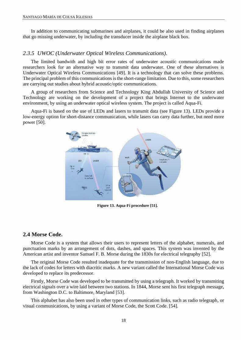
A group of researchers from Science and Technology King Abdullah University of Science and

Technology are working on the development of a project that brings Internet to the underwater

environment, by using an underwater optical wireless system. The project is called Aqua-Fi.

Aqua-Fi is based on the use of LEDs and lasers to transmit data (see Figure 13). LEDs provide a

low-energy option for short-distance communication, while lasers can carry data further, but need more

power [50].

Figure 13. Aqua-Fi procedure [51].

2.4 Morse Code.

Morse Code is a system that allows their users to represent letters of the alphabet, numerals, and

punctuation marks by an arrangement of dots, dashes, and spaces. This system was invented by the

American artist and inventor Samuel F. B. Morse during the 1830s for electrical telegraphy [52].

The original Morse Code resulted inadequate for the transmission of non-English language, due to

the lack of codes for letters with diacritic marks. A new variant called the International Morse Code was

developed to replace its predecessor.

Firstly, Morse Code was developed to be transmitted by using a telegraph. It worked by transmiting

electrical signals over a wire laid between two stations. In 1844, Morse sent his first telegraph message,

from Washington D.C. to Baltimore, Maryland [53].

This alphabet has also been used in other types of communication links, such as radio telegraph, or

visual communications, by using a variant of Morse Code, the Scott Code. [54].


19

The International Morse Code has remained practically unaltered since its creation, and it has been

used in many conflicts, such as Second World War, and in the Korean and Vietnam wars.

Figure 14. Morse code alphabet [55].

2.5 JANUS.

NATO has recently standarized a new protocol for Underwater Communications [56]. Underwater

transmission protocols, based on acoustic waves, may finally be unified as a NATO Standard (see Figure

15). JANUS is a simple multiple-acces acoustic protocol that has been designed and tested by the NATO

Centre for Maritime Research and Experimentation (CMRE) since 2008.

This protocol is intended to be used not only for military purposes, but also fot civil and international

adoption.

Before JANUS, there existed no general interoperable capabilities between modems from different

manufacturers. There was no specific protocol or message structure defined. Furthermore, different

modems used different encoding methods: Frequency Shift Keying, Phase Shift Keying, Frequency

Hopping Spread Spectrum or Orthogonal Frequency-Division Multiplexing.

These differences made impossible the link between two devices that did not work with the same

protocols.

Figure 15. JANUS protocol.


20

JANUS combines the public need for a standard and the NATO need for interoperability. The

principal purposes for this protocol are to announce the presence of a node and to establish an initial

contact between two nodes.

For the start of the link, JANUS will use a commonly known frequency (11.5 kHz). When both

devices are linked, they could switch to a different frequency or transmission method for faster data

rates. Depending on channel characteristics, SNR (Signal to Noise Ratio) and hardware characteristics,

JANUS may choose the more bandwith efficient methods of communication.

The data protocols used for underwater acoustic communication will be near identical to radio

communications, including parity bits and error correction.

The JANUS standard has been designed to be deliberately robust. The digital coding that has been

used in Frequency-Hopped (FH) Binary Frequency Shift Keying (BFSK), which has been selected for

its robustness in the harsh underwater acoustic propagation environment and its simplicity of

implementation.

2.5.1 Frequency-Hopped Binary Frequency Shift Key (FH-BFSK) modulation.

Frequency Shift Key (FSK) is a frequency modulation schem in which digital information is

transmitted through discrete frequency changes of a carrier signal. These frequencies lie within the

bandwith of the transmission channel [57].

Its simplest way to implement is binary FSK (BFSK), which uses just a pair of discrete frequencies

to transmit binary (0s and 1s) information.

This signal modulation can be easily detected and interpreted by the enemies. Due to that, the

security of these types of modulation is usually reinforced with the Frequency-hopping spread spectrum

(FHSS), which is a method of transmiting signals by rapidly changing the carrier frequency among many

different frequencies [58]. Both nodes (sender and receiver) must know the frequency hopping sequence.

Figure 16. Frequency hopped BPSK signal (MATLAB) [59].


21

2.5.2 Encoding

The communication protocol starts with a preamble that consists of a three wake-up tones at

frequencies: Fc-Bandwidth/2; Fc; and Fc+Bandwidth/2 Hz. These tones are used when needs to “wake-

up” form a sleep mode.

After the tones, the system can append a Hyperbolic Frequency Modulated (HFM) sweep.

The HFM sweep, which is a type of wave that minimizes the degradation of matched filter

processing caused by Doppler shifting, takes advantage of its ability to synchronize in time both nodes.

After the opening, the transducer waits a period of silence to allow the sleeping hardware to be

prepared for the synchronization.

There is also another period of silence after the HFM sweep and before the start of the message to

allow for dispersion of the preamble energy before the arrival of the first bits.

Figure 17. JANUS signal Frequency-Time graphic [60].

About the encoding of the main message, the first 64 bits are required for the baseline. The allocation

of each bit is shown in Figure 18.

Packet integrity is ensured by an 8-bit Cyclic Redundacy Check (CRC). These bits are appended to

the 56 bits of the main Baseline JANUS Packet.

A ½ rate convolutional encoder is applied to the baseline, resulting in 128 bits of output. Eight zeros

are appended to the baseline before the encoding. So, due to this, the final length of the baseline is 144

bits.

The baseline JANUS Packet may be followed by additional data.

Once the packet is prepared to be transmitted, an interleaver separates each consecutive bit by a

constant depth value of 13. This allows for burst of consecutive bits to translate into multiple small gaps,

but without affecting the possibility of successful decoding.

This protocol, in order to provide optimal Inter-Symbol Interference (ISI) rejection, the FH order in

which the 13 pairs of tones are used is previously chosen. Otherwise, this rejection could be caused by

multipath or collision with JANUS packets from other users. Due to this, when the pseudo-orthogonal

sequence is fixed, it is made known to all potential receivers.


22

Figure 18. JANUS bit allocation table [61].

The FH indices are derived from Galois Field arithmetic using a number to generate 13 frequency

slots to provide good orthogonality properties. Figure 19 shows mapping of the FH sequence and bit

values for the JANUS initial frequency band.

Figure 19. Possible FH sequence and bit values for 11.5 kHz.

Tha JANUS standard is anticipated to be used at different centre frequencies, to face diverse

environments, ranges, and applications. The JANUS protocol uses 1/3 of the centre frequency as its

bandwidth (Bw). Bw is divided into 13 pairs of Frequency Slots (each of width Fsw= Bw/26). The chip

duration is the inverse of the Frequency Slot width (Cd=1/Fsw). The Cd may optionally, at the discretion

of the sender, be set to a multiple of the Baseline Chip Duration, to achieve grater robustness. As an

example, the initial JANUS acoustic frequency band has the following specifications. Fc=11520 Hz,

Bw= 4160 Hz, FSw= 160 Hz and Cd=6.25 ms.

To conlude, Figure 20 shows a block diagram that resumes the JANUS baseline packet encoding

process.


23

Figure 20. Block diagram for the JANUS baseline packet encoding.

2.5.3 Decoding.

About the decoding process, a matched filter is used to recognize the wake-up tones and the HFM

sweep.

Each insonification existing during each period is evaluated as being 0s or 1s, using the Fast Fourier

Transform algorithm, which purpose is to compute the Discret Fourier Transform (DFT). It converts a

signal from its original time or space domain to a representation in the frequency domain [62].

The resulting sequence of 0s and 1s is de-interleaved by applying Viterbi decoding. Viterbi is a

dynamic programming algorithm for finding the most likely sequence of hidden states (“Viterbi path”)

that results in a sequence of observed events. It has traditionally been used to decode the convolutional

codes. In addition, it has also been used in speech recognition.

The decodification provides other outputs, such as the number of errors in each packet (before and

after applying Viterbi or duration of each chip.

2.5.4 Propagation effects.

The acoustic energy, representing each bit, can arrive at the receiver across different paths, due to

sound speed variations, ambient noise fluctuations, sea surface roughness and bottom reflections. This

phenomenon is referred to as multipath. The time from the first arrival to the time of the last arrival is

called time spread. A link with interfering multipath arrivals generally results in more decoding errors.


24

2.6 Reed-Solomon Codes.

Reed-Solomon codes are block-based error correcting codes that are commonly used in

communications systems [63].

This system is based on redundant bits. It divides digital data into blocks and appends extra

“redundant” bits to each data block.

When the Reed-Solomon decoder processes each block, it attempts to correct errors and recover the

original data. The number and type of errors can be corrected depending on the characteristics of the

Reed-Solomon code and its redundancy.

Reed Solomon (n, k) block code can correct (n-k)/2 erroneous bits.


25

3 MATERIALS AND METHODS

Before implementing a communication protocol based on the JANUS specification, a protocol based on

the Morse code was developed to help us familiarize the innerworkings of Python sound libraries. But

before that, Section 3.1 defines the software programs that have been used during this project.

3.1 Software.

Two different pieces of software have been used during the development of the thesis.

3.1.1 Python.

Python is the programming language that has been used to develop the codes that have been used to

implement the underwater communication protocol [64].

Its philosophy is based on the importance of the readability of the code. It is a multiparadigm

programming language, because it supports not only object orientation, but imperative and functional

programming. All these features make Python an interpreted, dynamic and multiplatform language

program. This open-source program was designed to be easily readed. It uses logic words where other

codes use symbols.

Furthermore, Python counts with a vast selection of open-source modules, most of them developed

by the user community, that can be easily integrated into your own software. That makes Python a

convenient tool for rapid prototyping.

3.1.2 Audacity.

Audacity is a free and open-source digital audio editor and recording application. The principal

Audacity’s features include recording and playing back sounds, audio analysis and edition, and a large

collection of digital effects and plug-ins, such as noise reduction, or filters, and audio spectrum analysis

using the Fourier transform algorithm [65].


26

3.2 “Morse Code” scripts.

With the purpose of approaching the task in an iterative way, two Python scripts were developped

to communicate two computers using the Morse Code. This first iteration allows us to get familiar with

Python programming and the sound libraries needed to generate and process the audio files.

3.2.1 Morse Code encoder.

The first script converts text into Morse Code symbols: dots and dashes tones. First, it receives a

group of words as input. These words are encoded using the Morse Code alphabet.

In order to transmit the Morse Code message, a tone generator is used to converts a Morse Code

message into a sound file (.wav). As seen in Figure 21, this code generates a silence just after each

symbol and pauses. The silence has the same duration than a mark.

Figure 21. Scheme of how the decipher code works [66].

In the example of Figure 21, the dot is made up of two marks (one reserved for the dot and the other

one for the silence), and the dash is made up of four marks (three reserved for the string and one for the

silence). The space between characters is represented by two marks (both silence marks). Between

words, the space is composed of three silence marks.

This tone generator allows the user to change some parameters, such as the duration of each mark,

the frequency of the tones or the sample rate. The user can also change the number of marks of each

point or string.

The last part of the code takes as an input the morse code message and records and audio file

(morsetransmission.wav) by using the tone generator.

3.2.2 Morse Code decoding.

In order to decode a Morse signal for an audio file, it is necessary to divide the sound file into

different slots or windows. Each window is analized with the tone amplitude is estimated. If the

amplitude falls from a given threshold the windows is supposed to be a silence, othwerwise is supposed

to be an active mark. This information is converted into binary information, as a binary sequence. Then

the script estiates the duration of each symbol by counting the number of active bits, and hence

determines if the sound is a dot, a string, or a space. After converting the audio file into a Morse Code

sequence, the code translates it into text.

In order to solve the synchronization problem, the program works with a window size that is several

times smaller than the mark duration.


27

3.2.3 Morse Code experiments.

The main objective of this first set of experiments was to test the performance of the Morse Code

algorithm by changing the transmission frequency and the distance between the transmitter and receiver.

The set up that was used included a microphone (Eivotor Professional Microphone), a JVC speaker

(CS-J620X JVC) which was connected to an amplifier (LMRA410BT Marine Amplifier). Both the

microphone and the speaker were connected to the same laptop, that was used to transmit messages by

using the speaker and to receive them using the microphone.

Figure 22. Morse code experiments set up.

The parameters that were used to generate the tones during the test are shown in Table 1.

The sentence that has been chosen was a 13-character lenght: “DIVE TO 150 M”. Taking into

account the parameters that were used to transmit this message, the data transmission rate was about 1

character per second.

Table 1. Parameters used in "Morse Code experiments".

3.3 Implementation of the communication protocol.

A communication protocol was implemented based on the JANUS specification. Two Pyhton scripts

were developed for off-line processing, one for transmission and one for reception.

Parameters of the tone generator

Time for each mark 0.1 s Time of a dot 0.1 s

Sample rate 44100 Hz Parts of a point 8

Number of marks of the point

(including pause) 2

Tolerance 0.8

Number of marks of the string

(including pause) 4

Threshold 0.075

Volume [0,1) 1


28

3.3.1 Transmission script.

The first lines of the transmission script are used to set each part that compose the baseline packet

of the message to be sent. The distribution of each bit is shown in Figure 18. The code packs all the parts

of the baseline in the same bit array, with a final length of 56 bits. After the baseline packet, the code

allows the user to introduce a bit array message to be sent, also know as payload, which is appended to

the first 56 bits.

As specified by the JANUS protocol, the script includes eight extra bits using Cyclic Redundancy

Check (CRC) to detect errors in the reception.

The JANUS specification includes a 2 to 1 convolutional encoding to detect and correct for error

bits. However, the implementation of this convolutional encoding, and its corresponding decoding, could

not be accomplished in the time available to the execution of this project. Because of that we decided to

use a Reed Solomon code instead; as a Python module was readily available and it was quite straight

forward to incorporate it into the protocol. In addition, Reed-Salomon encoding (previously described

in Section 2.6) have proven its reliability in other communication systems. In order to keep the same

packet format, a Reed-Salomon code was selected that doubled the length of the original message. The

selected configuration of Reed-Solomon that has been used allows te system to correct up to 3.125% of

the errors in the received message.

The transmission code uses a tone generator that integrates the parameters of transmission of the

JANUS protocol, previously explained in 2.5, including the “one to three” relation between the centre

frequency and the bandwidth of the signal (Bw=Fc/3), the frequency slot bandwidth (Fsw=Bw/26), and

the scheme for frequency hopping. It also includes three wake-up tones used to synchronize the start of

the message.

Once the tones are generated, the program samples the signal, and the result is saved as a “.wav” audio

file.

3.3.2 Reception script.

The reception script allows the user to demodulate the JANUS message recorded into an audio file

and outputs the received message.

The first part of the code is used to set the parameters that the received tones should have, and a

table that includes the FH sequence that has been used to modulate the signal.

The code then looks for the wake-up tones using a matched filter technique. Once the wake-up tones

are detected the message has been synchronized and the signal can be divided into windows of the same

length as the chip duration. For each window, the script computes the Fast Fourier Transforms (FFT)

and estimates the frequency using quadratic interpolation.

After demodulation, the result is a stream of bits that can be decoded using the Reed-Solomon

decoding module. If the number of errors is less than 3.125% of the total length of the message, the

message can be decoded successfully. But if the error rate exceeds that threshold, the message cannot

be decoded. In case of positive decodification, the bits of the baseline packet are passed through a Cyclic

Redundancy Check to detect if there are remaining errors. If the CRC does not detect any errors, the

integrity of baseline packet has been kept, and the corresponding bits can be unpacked and distributed

into the different blocks of information. This allows the system to keep an open communication channel

even if there are errors in the payload, and even try to diagnose the error sources.

In order to analyze the resulting BER, some additional lines of code have been added to compare

the deciphered message with the originally transmitted message. This way, we can study how many


29

errors occurred during transmission and determine the performance of a given configuration of the

communication protocol.

3.4 In air experiment.

Before testing it underwater, the performance of the protocol was tested in air. The main objective

of this experiment was to validate the developed python scripts in a convenient setup.

The experimental setup included a microphone (Eivotor Professional Microphone); an amplifier

(PLMRA410BT Marine Amplifier) with an output power of 100 Watts; a JVC speaker (CS-J620X JVC)

with a power rating of up to 300 Watts; and a laptop (Surface Pro 6). The distance between the

microphone and the speaker was 2 meters.

The message to be transmitted was the baseline of the JANUS message, that included 56 bits. In

addition to these bits, the message included 8 more bits for CRC.

Reed Solomon (16,8) combination was used to correct error bits. This combination appended 64

more bits to the message, resulting in 128 bits. Following that combination, the reception script was able

to correct up to 4 error bits.

3.5 Swimming pool experiment I.

After validating the developed script in air, a different set up was prepared to transmit the audio

underwater. The experimental setup was divided into two parts: an underwater transducer and an

underwater hydrophone.

3.5.1 Objectives.

The main objective of this experiment was to validate the developed script in an underwater

environment. As secondary objective, the performance of the protocol was studied for different

frequencies and chip duration.

3.5.2 Transducer setup.

The transducer set up was composed of a 20W vibration transducer that was encapsulated into a

IP67 circuit box. The box was made waterproof by further sealing the input cable with silicon and a

cable gland. The transducer was driven by a PLMRA410BT Marine amplifier (the same used in the

experiment describe in Section 3.4). The amplifier was powered by a 12V battery (FIAMM battery,

nominal capacity of 18Ah and a 20 mΩ resistance when fully charged). Finally, the amplifier was

connected to a laptop (Surface Pro 6) used to play the audio files through its internal sound card.


30

Figure 23. Swimming pool experiment I transducer set up.

Figure 24. Vibration transducer inside the plastic box.

3.5.3 Hydrophone set up.

On the other end of the swimming pool a DolphinEar DE200 hydrophone was used to receive the

messages. The hydrophone was connected to a custom amplifier that allowed us to change the input

gain. The amplifier was then connected to an external Behringer UCA202 sound card, and this sound

card was finally connected to a laptop via USB.

Figure 25. Swimming pool experiment I hydrophone set up.


31

3.5.4 Experimental procedure.

This experiment consisted of placing the hydrophone and the transducer, one in front of the other,

on both sides of the shortest length of the swimming pool of the Spanish Naval Academy. The distance

between the transducer and the hydrophone was about 12 meters. During this experiment, the poole

pumps were running which added some background noise. Before starting the experiment, a number of

audio files were generated using a different combination of chip duration and central frequency.

All the generated files were transmitted through this underwater channel. The final length of the

message was 128 bits, including 64 redundancy bits from a (16,8) Reed-Solomon code. The messages

were recorded using the hydrophone and the commercial software Audacity, that allowed us to rapidly

check out the spectrum of the received signal. The parameters used in this experiment are sumarized in

Table 2.

Table 2. Transmission parameters used in first swimming pool experiments.

According to the secondary objective, the code was modified to use different central frequencies

and chip durations (1/Frequency slot bandwith). The different combination of tested parameters is shown

in Table 3.

In order to decode the signals, the audio files have been passed through a low band pass filter in

order remove part of the background noise.


Amplitude 0.9

Bandwidth Fc/3

Fsw Bw/26

Hydrophone gain 2

Sample rate 44100 Hz

Centre frequencies Chip duration

3000 Hz 1/Fsw

1/Fsw

5000 Hz

1/Fsw

1/Fsw

2/Fsw

2/Fsw

3/Fsw

3/Fsw

Table 3. Central frequencies-Chip duration used in first swimming pool experiments.


32

The filter was applied by using the Audacity tool “Filter Curve”, and its cutoff frequency depended

on the central frequency that was selected to transmit the message. The cutoff frequencies that were used

in this experiment are shown in Table 4.

Table 4. Cutoff frequencies used for each central frequency in the swimming pool experiment (I).

3.6 Modification I of the communication protocol.

After the results obtained in the first swimming pool experiment (that are presented in Section 3.5),

some changes were included in the implementations of the reception script. First, as seen in Figure 26,

a loop was included to make the code decrease the sensibility, until 128 bits are received. This loop

automated the process of selecting the right sensibility parameter, in order to receive the correct number

of bits.

We also modified a part of the code that removed the silence before the bit array reception. The

parameter was setted so high that it did not allow the first bits to be received. This parameter was changed

from 0.5 to 0.25.

Figure 26. Sensibility loop in reception script.

3.7 Swimming pool experiment II.

After modifying the reception script another experiment was carried out in the swimming pool of

the Spanish Naval Academy.

Frequency (Hz) Cutoff frequency (Hz)

3000 2000

5000 3500


33

3.7.1 Objectives.

The main objective of this experiment was to test the changes in the reception script using longer

messages, that allowed us to estimate the BER of a given protocol configuration. As a secondary

objective, a different combination of frequencies and chip durations was aimed to be studied.

3.7.2 Experimental setup.

The set up used for this experiment was the same that the one described in Sections 3.5.2 and 3.5.3,

except that the transmitting transducer was this time mounted on a structure designed to keep the

transducer immersed.

Figure 27. Swimming pool experiment II transducer set up.


The way to proceed to run this experiment was the same that was described in Section 3.5.4, using

the same distance between transducer and hydrophone (12 meters). The only significant difference was

that, this time, the swimming pool pumps were stopped to reduce the level of background noise.

This time, the message length was a 1008 bit. It included the JANUS baseline (56 bits); a 440-bit

message; 8 CRC bits to detect errors; and 504 bits of redundancy from a (126,63) Reed Solomon code,

that corrected the 3.125% of the erroneous bits (31 errors) by doubling the length of the message.


34

Figure 28. Structure of the message.

The transmission and hydrophone parameters used in this experiment were the same than in the

previous experiment, which are shown Table 2. The different combinations of frequencies and chip

duration tested are shown in Table 5. Each audio was transmitted twice.

Instead of the low pass filter used in 4.2, it was applied a band pass filter (as shown in Figure 42

to remove the background noise produced in the higher frequencies. It has been applied by using the

Audacity tool “Filter Curve”. The cutoff frequencies that were used in this experiment are shown in

Table 6.


3000 Hz

1/Fsw

2/Fsw

3/Fsw

4000 Hz

1/Fsw

2/Fsw

3/Fsw

5000 Hz

1/Fsw

2/Fsw

3/Fsw

Table 5. Central frequencies-Chip duration used in the second swimming pool experiment.


35

Table 6. Cutoff frequencies used for each centre frequency in the swimming pool experiment II.

3.8 Harbour experiment I.

The results obtained in the swimming pool on the first and the second experiments showed that the

protocol performance was heavily affected by reverberation. To see if that was also the case in a more

realistic scenario the experiment was moved to the harbour of the Spanish Naval Academy. In addition,

this was the first time that the protocol was tested in the sea.

3.8.1 Objectives.

The purpose of this experiment was to check the behaviour of the transmission and reception scripts

at longer distances, as they could be affected by the sea background noise, generated by the wind, the

waves, and nearby ships. The protocol performance was stutided using different combinations of

frequency and chip duration. The BER was estimated to try to find a relationship between both quantities.

3.8.2 Experimental setup.

The set up of the transducer and the hydrophone was the same as described in Section 3.7.2, with

the only difference of the location of the equipment. Figure 29 and Figure 30 show some pictures that

were taken during this experiment.

Figure 29. Harbour experiment I hydrophone set up.

Frequency (Hz) Cutoff frequencies (Hz)

3000 1500-4000

4000 2000-5000

5000 2500-7000


36

Figure 30. Harbour experiment I transducer set up.


The experiment was carried out at the harbor of the Spanish Naval Academy. The sound source, mounted

on the immersion rig, was was placed in “Muelle de Torpedos” near the lighthouse, and the hydrophone

was located in “Muelle de Chereguini”. As seen in Figure 31, the distance between transmitter and

receiver was about 305 meters. The procedure in this experiment was the same that was described in

Section 3.5.4.

Figure 31. Location of sea experiment I.

During the experiment, the messages were sent when no ships were inside the harbour, to avoid the

radiated noise of their propulsion and auxiliary machinery.

The final message that was sent was the same as described in Figure 28. It was a 1008 bit-length

message that included the JANUS baseline (56 bits), a 440-bit data message, 8 bits from CRC, and 504

redundancy bits generated using a (126, 63) Reed Solomon code, to correct 31 erroneous bits.

The transmission and reception parameters, as well as the hydrophone parameters, were the ones

described in Section 3.5. However, since higher frequencies were going to be used, we decided to


37

increase the sample rate from 44100 Hz (which was the one that has been used for the swimming pool

experiments) to 60000 Hz.

The different combinations of frequencies and chip durations that were tested are shown in Table 7.

The messages recorded with the hydrophone were filtered using a band pass filter to remove part of

the background noise, in the same way that was removed in Section 4.2. The selected cutoff frequencies

that were used for each central frequency are shown in Table 8.

Table 8. Cutoff frequencies used for each central frequency in the harbour experiment I.

3.9 Modification II of the communication protocol.

The results of the harbour experiment I led to some improvements in the transmission and reception

scripts aimed to reduce the BER and correct some deficiencies that were revealed only after analyzing

the audio files recorded in the sea.

3.9.1 Transmission script modification.

3.9.1.1 Wake-up tones.

In order to solve problems with the synchronizationa of the message few lines of code were included

in order to include 3 wake-up tones, that followed the JANUS specification. The frequencies of each

tone were: Fc - Bw/2, Fc, and Fc+Bw/2 respectively; and the duration of each tone was four times the

chip duration Cd.

Centre frequencies Chip duration Centre frequencies Chip duration

3000 Hz 1/Fsw

6000 Hz 1/Fsw

2/Fsw 2/Fsw

4000 Hz 1/Fsw

7000 Hz 1/Fsw

2/Fsw 2/Fsw

5000 Hz 1/Fsw 8000 Hz 1/Fsw

2/Fsw 2/Fsw

Table 7. Centre frequencies-Chip duration used in the first sea experiment.


3000 1500-4000

4000 2000-5000

5000 2500-7000


38

Figure 32. Wake-up tones code.

3.9.1.2 Centre frequency modification.

The transmission and reception code were modified in order to adjust slightly the central frequency.

The code changes the desired central frequency selected by the user, into a close frequency value, but

that can divide the sample rate into an integer number. In this way we avoided any jitter between the

sample rate and the central frequency.

Figure 33. Central frequency adjusting code.

Figure 34 shows the spectrogram obtained by Audacity of an audio file generated with the new

implementation of the JANUS transmission code.

Figure 34. Three wake-up tones and first bit´s spectrogram of a message.

3.9.2 Reception script modification.

3.9.2.1 Wake-up tones detection.

The detection of the wake-up tones was based on a matched filter, which is the optimal way to detect

a known signal embeeded in background noise, as it maximizes SNR. Matched filtering is implemented


39

by correlating the received signal with a copy of the signal that we aim to detect. This detection method

provides two important advantages: it requires a short detection time and it has a high detection gain

[67].

Figure 35. Wake-up tones detection code.

3.10 Noisy channel simulator.

In order to understand better the relationship between BER and the channel characteristics, a script

was developed to reproduce the effect of background noise and reverberation. This script allows the user

to try different parameters in a computer, before taking the test to the sea.

This code takes an audio file, and adds white noise following a selected SNR (Signal to Noise Ratio).

It also adds reverberation, by modifying the time constantof an exponential function that emulates the

channel impulse response. The time constant is the time needed for the reverberation tail to drop by

given factor, and hence the shorter the time constant, the less reverberation is added to the audio sample.

When the time constant is longer than the chip duration, the transmitted symbols overlap.

Once selected the input audio file, the SNR and the time constant, the code records an audio file

with the selected background noise and reverberation.

3.11 Channel simulation experiment.

The code described in Section 3.10 has been used to check the modifications made on the

communication protocol. Three different scenarios were defined with different SNR and reverberation

values. All the values have been chosen based on the experience of the last experiments.

A scenario with “good conditions” was defined to simulate a channel with little background noise

and reverberation. The values chosen for this simulation were a SNR = 10 dB and time constant of 0.01

s. A scenario with “moderate conditions” was defined using a SNR = 6 dB and twice as much as

reverberation, with a time constant of 0.02 s. Finally, a scenario with “harsh conditions” was defined to

test the protocol performance with extremely adverse conditions, with a SNR=3 dB and a time constant

of 0.05 s.

3.11.1 Objectives.

The main objective of this simulation was to obtain the BER for each frequency-chip duration

combination for each scenario and identify the configuration that can be successfully decoded while

providing the maximum data transmission rate.


40


Messages were generated using the central frequencies: 1 kHz, 2 kHz, 3 kHz, 4 kHz, 5 kHz, 6 kHz,

7 kHz, 8 kHz, 9 kHz, and 10 kHz. For each central frequency, five different chip durations were tested:

1/Fsw, 2/Fsw, 3/Fsw, 4/Fsw and 5/Fsw. A 1008-bit length message was used for this test.

The generated audio files were processed with the Noisy channel generator code, using the

aforementioned SNR and time constant, for each considered scenario. The output audio file was then

decoded with the reception script, and the BER was estimated.

3.12 Harbour experiment II.

After the results obtained in the channel simulator, a new configuration of the communication

protocol was defined to be tested in the sea, facing the variable conditions of the Naval Academy’s

harbour.

3.12.1 Objectives.

The purpose of this second harbour experiment was to study the performance of the new protocol

configurations, and to determine which is the one that produce the highest data transmission rate.

3.12.2 Experimental setup

The hydrophone rig was improved to prevent it moving under the action of the waves. That way we

eliminated some noise present in previous recordings, as the hydrophone changed position and, in some

occasions, it even hit nearby structures, completely hindering the decodification. The metallic structure

shown in Figure 28 was designed to keep the hydrophone in a stable position.

Figure 36. Hydrophone set up modification.


41

3.12.3 Experimental procedure

The procedure followed was like the one used in the previous harbour experiment. Messages with a

different combination of central frequencies and chip duration were generated and transmitted from the

“Muelle de Torpedos”, while recording with the improved hydrophone setup from the “Muelle de

Chereguini”. After reception, the recorded messages were decoded and the BER was estimated.

Before transmitting the messages, a frequency sweep was sent with the transducer to characterize

the channel frequency response and to estimate the SNR at different frequencies. It must be noted that

during the execution of the experiment some ships were docking or in operation in the harbour area.

The final message that was sent was the same that is described in Section 3.7. However, some

parameters were changed to accomate the improvements made in the protocol configuration, such as the

sample rate and the Fsw, which was increased in order to separate more the frequencies that composed

the frequency hopping. The final parameters are shown in Table 9.

The different combinations of frequencies and chip duration that were tested are shown in Table 11.

These combinations have been chosen after the results obtained in Section 3.10, supposing that the

protocol would have to face “harsh” conditions.

Table 10 shows the cutoff frequnecies that defines the band pass filter that has been applied with

Audacity.


Amplitude 0.9

Bandwidth Fc/3

Fsw Bw/6.5

Hydrophone gain 2

Sample rate 44100 Hz

Table 9. Transmission parameters used in the harbour experiment I.


1000 0-3000

3000 1500-4000

5000 2500-7000

6000 4000-8000

7000 5000-9000

8000 7000-9000

9000 8000-10000

Table 10. Cutoff frequencies for Harbour experiment II.


42

Table 11. Centre frequencies-Chip duration used in the second sea experiment.

3.13 Tambo experiment.

After obtaining positive results on the last harbour experiment, the communication protocol was

tested in the estuary of Ponteverda.

3.13.1 Objectives.

The objective of this final experiment was to test different protocol configurations over a longer

distance, an in presence of the background noise present in the estuary of Pontevedra.

3.13.2 Experimental setup

The set up that has been used for this experiment was the same that was used in the previous

experiment (3.12.2).

Centre frequencies Chip duration Centre frequencies Chip duration

1000 Hz 2/Fsw

7000 Hz

5/Fsw

3/Fsw 6/Fsw

3000 Hz

4/Fsw 7/Fsw

5/Fsw 8/Fsw

6/Fsw

8000 Hz

5/Fsw

5000 Hz

4/Fsw 6/Fsw

5/Fsw 7/Fsw

6/Fsw 8/Fsw

7/Fsw 9/Fsw

6000 Hz

5/Fsw

9000 Hz

5/Fsw

6/Fsw 6/Fsw

7/Fsw 7/Fsw

8/Fsw 8/Fsw


43

Ilustración 37. Tambo experiment transducer set up.

3.13.3 Experimental procedure

The transmitter set up was located in the northern face of the “Muelle de Torpedos”, in the Spanish

Naval Academy, while the hydrophone set up was place in the southern face of the “Isla de Tambo”.

The total distance between transmitter and receiver was 990 meters (see Figure 38).

Figure 38. Location of Tambo experiment.

It must be noted that while the experiment was being conducted the area was crowed with activity:

all the instruction boats were at sea, and both the Intermares instruction ship an the Tabarca patrol ship

were in operation, crossing the the line of sight between transmitter and receiver on several occasions.

The message structure was the same that has been used in the previous experiments, as described in

Figure 28. The communication script used for this experiment is the one described in Section 3.9. The

configuration parameters are the same used in the previous experiment, which are shown in Table 9.

In order to check the signal level halfway, the boat that transported the equipment to the “Isla de

Tambo” made a quick stop. The engines were stopped, stayed adrift for a couple of minutes, during

which a frequency sweep was transmitted to measure the signal level received from the transducer. When

the boat arrived at the “Isla de Tambo”, the hydrophone set up was moved to a rock in the southest point


44

of the island, in the vicinity of the “Tenlo Chico” lighthouse. Once there, the hydrophone was submerged

to a depth of approximately one meter.

Once both set ups were prepared, a first 0 kHz- 20 kHz frequency sweep was used to characterize

the channel and estimate the SNR at different frequencies. After that, some messages with different

frequencies and chip duration, were transmitted which are shown in Table 12.


5000 Hz 5/Fsw

6/Fsw

6000 Hz

5/Fsw

6/Fsw

6/Fsw

7000 Hz

4/Fsw

5/Fsw

6/Fsw

7/Fsw

8000 Hz

4/Fsw

5/Fsw

6/Fsw

7/Fsw

Table 12. Centre frequencies-Chip duration used in Tambo experiment.


45

4 RESULTS

4.1 Morse Code experiments.

4.1.1 On air experiment results.

Table 13 shows the results of the first experiment, in which the distance of the microphone and the

speaker was 2 meters. All the messages that were transmitted were successfully decoded.

Table 13. On air experiments results (2 meters).

Table 14 shows the results of the second experiment, with a longer distance (4 meters) between the

microphone and the speaker. Four of the six messages (75%) were correctily deciphered.

Table 14. On air experiments results (4 meters).

Frequency (Hz) Deciphered message

4000 CORRECT

3000 CORRECT

2000 CORRECT

1000 CORRECT

Frequency (Hz) Deciphered message

400 CORRECT

500 CORRECT

4000 INCORRECT

3000 CORRECT

2000 CORRECT

1000 INCORRECT


46


The results of the first underwater experiments were characterized by being much noisier that the

results in air. The background noise was generated by the pumps of the pool, and the reverberation

produced by nearby walls.

Figure 39 shows how the low band pass filter was applied with Audacity.

Figure 39. A 128 bit-length message after and before applying a low-band pass filter in Audacity.

The chosen way of interpreting the results was to compare the BER (Bit Error Rate) between the

different frequencies and chip duration.

Figure 40 shows the BER for increasing chip duration from 1/Fsw, to 3/Fsw, where it has been

defined N in N/Fsw for convenience. We observe that, expected, the BER decreases when the chip

duration in increased, going from a BER = 9.38 %, for 1/Fsw down to 0.78% for 3/Fsw. However, it

must be noted that by increasing chip duration, the data transmission rate is reduced. Decodification was

succesfully by using a frequency of 5000 Hz and a chip duration higher than 2/Fsw.

As seen in Figure 40, just a sample (chip duration= 1/Fsw) of 3000 Hz as centre frequency was

obtained during this experiment.


47

Figure 40. BER-Chip duration graphic. Swimming pool experiment I.

About the performance of the different frequencies, the code was tested with 3000 Hz and 5000 Hz,

by using a chip duration of Cd=1/Fsw.


This test was characterized by being less noisy than the first pool experiment, since the filtration

pumps were stopped during the execution of the experiment. As shown in Figure 41, during the

transmission of the frequencies form 1 kHz to 3 kHz some harmonics appeared.

Figure 41. 0-10 kHz frequency sweep in swimming pool experiment (II).

Figure 42 shows how the band pass filter has been applied with Audacity.


48

Figure 42. A 1008 bit-length message after and before applying a band pass filter in Audacity.

Figure 43 shows the results adquired in the second swimming pool test, comparing the obtained

BER with different frequencies and chip duration. The showed BER is the average between two

measurements that were taken for each combination. The limit for correct decodication is also shown.

We observe that for the 3 kHz and 4 kHz the BER decreases as the chip duration increases. For Fc=3

kHz the BER goes from around 40% for Cd = 1/Fsw down to 22% for Cd= 3/Fsw. For Fc=4 kHz the

BER goes from around 31% for Cd = 1/Fsw down to 25% for Cd = 3/Fsw. However, for these two

frequencies decodification was uncessessful, since the BER stayed well above the required 3.4 %.

Figure 43. Bit Error Rate plot for the recordings acquired in the Swimming Pool experiment II.

The transmission using Fc=5 kHz performed much better with a BER of around 1% for 1/Fsw.

Surprisinly the BER increased for chip durations 2/Fsw and 3/Fsw, reaching values of 6%.


49

4.4 Harbour experiment I.

The first sea experiment was used to test how the generated messages were transmitted over longer

distances. Figure 44 shows the spectrogram, computed with Audacity, for a 30-second frequency sweep

ranging from 0 Hz to 20 kHz, with the gain knob set to 2 in the hydrophone amplifier. Figure 44 shows

that background noise was present between 2 kHz and 4 kHz.

Figure 44. 0 Hz-20000 Hz chirp.

Apparently, the best SNR conditions are obtained between 5 kHz and 12 kHz.

Figure 45 shows the results adquired in this experiment, comparing the obtained BER with different

frequencies and chip duration. The limit for correct decodication is also shown. We observe that for Fc

= 3 kHz the BER decreases as the chip duration increases, as expected. For Fc=3 kHz the BER goes

from around 39% for Cd = 1/Fsw down to 22% for Cd= 3/Fsw. For Fc=4 kHz the BER behaviour is less

clear as it fluctuates from 45% down to 25%, with no clear trend. This erratic behaviour is probably due

to the presence of background noise both at 3 kHz and 4 kHz.

At 5 kHz the BER stays around 1%, independently of the chip duration. This result is also expected

as no noise is present at 5 kHz, and no large variations in the BER are expected under such circumstances.

For the rest of the frequencies that were proved (6000 Hz, 7000 Hz and 8000 Hz), the results were

corrupted due to the presence of some ships radiating noise inside the harbour.


50

Figure 45. Bit Error Rate Graphic in Harbour experiment I.

4.5 Channel simulation experiment results and conclussions.

Simulation results allowed us to study in greater detail the performance of the communication

protocol under different conditions.

Figure 46 show the BER vs chip duration for a channel with good propagation conditions (SNR =

10 dB and time constant = 0.1). As expected, we see that the BER decreases as the chip duration

increases, for all tested frequencies. We observe that for all frequencies, the communication becomes

successful from Cd = 3/Fsw onwards. We observe that, with execption of Fc=4 kHz and Fc = 10 kHz,

all tested frequencies are below the BER limit for Cd = 2/Fsw.

It is however surprising to find that the performance of some frequencies, such as 4 kHz which has

BER of almost 40% for Cd = 1/Fsw, to be much worse than that of Fc = 3 kHz, which has a BER of 2%

for Cd = 1/Fsw.

The transfer datarate for the protocol configurations that were successfully decoded is shown in

Table 15, with a maximum data rate of 67.2 bps for Fc= 6 kHz and Cd = 1/Fsw.


51

Figure 46. Good conditions simulation results.

Table 15. Best data transmission rate achieved for each combination in good conditions.

Figure 47 show the BER vs chip duration for a channel with moderate propagation conditions (SNR=

10 dB and time constant = 0.1). As expected, the BER average was higher than in the previous

experiment. We observe that all the frequencies needed Cd=3/Fsw to perform a successful

communication link, except for Fc=10 kHz (that needed Fc=4/Fsw).

The best results were achieved with Fc=1 kHz and Fc=3000 kHz, which just needed Cd=1/Fsw to

be decoded.

Frequency (Hz) Chip duration needed Data transmission

rate (bps)

1000 1 12.29

2000 2 12.29

3000 1 33.6

4000 3 16.25

5000 2 28.8

6000 2 36

7000 2 42

8000 2 42

9000 2 48

10000 3 42


52


Table 16, with a maximum data rate of 36 bps for Fc= 6 kHz and Cd = 2/Fsw.

Figure 47. Moderate channel simulation results.

Table 16. Best data transmission rate achieved for each combination in moderate conditions.

Finally, Figure 48 show the graph of a channel with harsh propagation conditions (SNR= 10 dB and

time constant = 0.1). These transmission conditions resulted in many unsuccessful decodings. Fc=1000

Hz was the one that best behaved to the increase in SNR and reverberation, (decoded with Cd=2/Fsw).

The other centre frequencies that were deciphered were 2 kHz, 3 kHz and 5 kHz (with Cd=4/Fsw) and

8 kHz (with Cd=5/Fsw).


rate (bps)

1000 1 12.29

2000 2 12.29

3000 1 33.6

4000 3 16.26

5000 3 19.76

6000 2 36

7000 3 28.8

8000 3 28.8

9000 3 33.6

10000 4 32.52


53


Table 16, with a maximum data rate of 17.68 bps for Fc= 8 kHz and Cd = 5/Fsw.

Figure 48. Harsh channel simulation results.

Table 17. Best data transmission rate achieved for each combination in harsh conditions.


rate (bps)

1000 2 6.26

2000 4 6.26

3000 4 9.08

4000 - -

5000 4 15.04

6000 - -

7000 - -

8000 5 17.68

9000 - -

10000 - -


54


Figure 49 shows the spectrogram of a frequency sweep transmitted in the harbour of the Spanish

Naval Academy for the second harbour experiment. We observe a strong signal and good SNR from 3

to 12 kHz, followed by a drop in power from 12 kHz to 15 kHz, and a recovery of the signal strength

from 15 to 20 kHz.

We can also observe in Figure 49 a sudden increase in the background noise, allegedly produced

by the engine of a ship which started a docking maneuver inside the harbour. We observed background

noise concentrated between 2 and 6 kHz. Prior to the introduction of the engine noise, the ambient noise

inside the harbourstayed between 2 and 4 kHz.

Figure 49. 0 Hz-20 kHz frequency sweep of the sea experiment (II).

Figure 50 shows the BER vs the chip duration for the tested frequencies. We see that only the

frequencies above 7 kHz yielded BER lower than 10%, with the exception of a couple of, probably

lucky, transmissions at 1 kHz and 3 kHz. No clear trend is observed with the chip duration.

Figure 50. Bit Error Rate in the second harbour experiment (II).


55

Figure 51 shows the results for these two frequencies, 7 kHz and 8 kHz. Even in this case, only two

of the transmissions were successful with a BER value below the BER limit. Again, no clear trend is

observed with the chip duration, contrary to what was expected according to the simulation results.

Figure 51. Bit Error Rate of 7000 Hz and 8000 Hz in the second harbour experiment.

4.7 Tambo experiment.

The spectrogram of the frequency sweep that was transmitted from the transducer shows that the

signal is well differenced from frequencies from 3 kHz to 12 kHz, due to a higher SNR. A slight power

change can be seen from 12 kHz to 15 kHz. But the signal gains strength when the frequency exceeds

15 kHz and until 20 kHz.

The power levels and frequencies of the background noise undergoes a significant change during

the transmission. It was presumed to be caused by the noise emitted by a ship which started the docking

maneuver inside the harbour while the frequency sweep was being transmitted.

The background noise produced by the ship was concentrated in the 2 kHz- 6 kHz band of

frequencies. Without the ship noise inside the harbour, the background noise stayed between 2 kHz and

4 kHz.


56

Figure 52. 0 Hz-20 kHz frequency sweep of the sea experiment (II).

4.8 Tambo experiments.

Figure 53 shows the frequency sweep that was transmitted halfway to “Isla de Tambo”. During this

experiment, the transducer was not completely submerged due to the waves. This could be the cause of

why the frequency line is cut for certain frequency values.

Figure 53. Frequency sweep spetrogram received from the boat on the way to "Isla de Tambo".

Figure 54. Frequency sweep comparaition between the left and the right transducers.


57

With an eye on the results obtained in Figure 54, the left transducer was the one selected to be used

to carry out the experiment.

Figure 55. Frequency sweep comparaition between hydrophone gain 2, 4 and 6, respectively.

Figure 55 shows the frequency sweep comparaition between different hydrophone gains. While

proving gain 4, a ship appeared in the line of sight of the hydrophone, increasing the detected background

noise.

The first messages that were tested where the ones with 7000 Hz and 8000 Hz as centre frequency,

with a chip duration from 4/Fsw to 7/Fsw. The results are shown in Figure 57. While the 7000 Hz

messages were being recorded, the Spanish Navy Ship “Intermares” crossed the transducer-hydrophone

line of sight. Due to this fact, the BER increased with the Chip duration.

Figure 56. Spanish Navy Ship "Intermares" sailing during the sea experiment (III) measures.


58

Figure 57. Bit Error Rate of 7000 Hz and 8000 Hz in JANUS sea experiment (III).

Lower frequencies were also tested, such as 1 kHz, 3 kHz, 5 kHz and 6 kHz. These measurements

were affected by an increase in wave force, which caused a lower SNR and some hits of the hydrophone

with the rocks (as seen in Figure 58). In addition, during the recordings of these messages, some ships

approached the vicinity of “Muelle de Torpedos”, generating an increase in background noise.

Figure 58. Spectrogram showing the effects of the hydrophone with the rocks.


59

5 DISCUSSION AND CONCLUSSIONS

5.1 Morse code experiments.

The aim of these experiments was to approach the problem of underwater communication in a

simplified way, and to get used to the tools needed to tackle a more advance algorithm. Thanks to the

results of these experiments, we soon realized what were the parameters that allowes us to optimize the

performance of the communication protocol. As shown in Table 13 and Table 14, the communication

was feasible over a two-meter distance.


The main objective of this experiment was to check the performance of the codes in an underwater

environment. Even with the noise generated by the pumps and the reverberation produced by the nearby

walls, the system was able to decode some of the sent messages.

As expected, the BER decreased with increasing chip duration, as with longer symbols the protocol

becomes more robuts against noise and reverberation. Given that the pump noise extended up to 3 kHz,

it was also expected to find a better performance at Fc = 5 kHz than at Fc = 3 kHz.

Thanks to this test, we discovered that some modifications were needed to improve the detection of

the start of the message and solve synchronization problems.


In the second swimming pool experiment we had a lower background noise, since the pumps were

stopped during the execution of the experiment. The general results for the Fc = 3 kHz frequency

followed the expected trend. However, for Fc = 4 kHz the BER did not decrease for an increasing chip

duration. This result cannot be easily explained, and we must therefore infer that there was some

unaccounted error in the experimental procedure.

As expected, the result obtained for Fc = 5 kHz was better than the one obtained in the swimming

pool experiment I, due to the lower background noise. However, it surprising to find that the transmission

using Fc = 5 kHz performed better than the transmission using Fc = 4 kHz, and, in turn, that the latter

performed better than Fc = 3 kHz. Given that, in this experiment, the background noise stayed below1

kHz, and assuming and that the reverberation time is almost constant for all the tested frequencies, one


60

would expect the BER to increase as it the chip duration decreases. And since the chip duration

Cd=1/Fsw for Fc = 5 kHz is 1.6 times shorter than the chip duration Cd=1/Fsw for Fc = 3 kHz, one

whould have expected the former to have a worse BER. Since this is not the case, we must therefore

assume that there was a problem in the experimental procedure.

5.4 Harbour experiment I

In the first harbour experiment the background noise covered in the 2 - 4 kHz band completely

masked the messages using these frequencies. The frequency that better worked was 5 kHz.

All these proved that the results obtained in Section 3.7 were not only affected by the reverberation

of the swimming pool walls, but some implementations needed to be made in order to improve the

performance of the transmission and reception code to deal with lower SNR and higher reverberation.

One of the remaining problems to be solved was that the reception script had some synchronization

issues that prevented collecting all the bits in correct order. This made that some of the messages were

completely wrong just because of a missing bit at the beginning of the message.

On the other hand, when higher frequencies were transmitted, the spectrogram showed that the final

frequency was not well transmitted. The most reasonable cause that could have induced these

deficiencies was the use of a non stadard sample rate like 60 kHz.

Finally, some of the noise was produced because the hydrophone was banging against the rocks of

the pier.

5.5 Noisy channel simulation

The reception script resulted in successful decodification in the three channels. A expected, the lower

SNR and the higher time constant, the lower data transmission rate the system can achieve.

The results obtained show that correct decodification was feasible for the three proposed channels.

So, having a constant level of the background noise and a costant level of reverberation, the best data

transmission rate for each channel is shown in Table 18.

The results have shown that the new implementations introduced to the code in Section 3.9 worked.

The preamble of the three wake-up tones made it possible to solve the synchronization problems.

Furthermore, the adjustment of the central frequency fixed the jittering that introduced errors in long

messages.

Channel Data transmision rate Fc-Cd combination

Good conditions 67.2 bps 6000 Hz- 1/Fsw

Moderate conditions 36 bps 6000 Hz- 2/Fsw

Harsh conditions 17.68 bps 8000 Hz- 5/Fsw

Table 18. Best data transmission rate for each channel conditions.


61


Some of the results have been conditioned for some changes of environment conditions. During

several transmissions, some transmissions have suffered radically increases background noise, due to

the effects of the propulsion and auxiliary machinery.

As seen in Figure 59, when a ship appeared on the line of sight of the hydrophone, the hydrophone

detected a drastic change of background conditions. If this variation was produced during the

transmission of a message, it obstructed the decoding process.

Figure 59. Background sound generated by a ship docking at the Marin harbour.

Exept for the messages that were affected by the entrance of some ships on the harbour, the main

objective of the experiment was accomplished. The new implementations made to the JANUS

transmission and reception code seemed to do a correct performance on the underwater sea environment.

The best data transmission rate (14.4 bps) was obtained y using 8000 Hz as central frequency and 6/Fsw

as the chip duration.

5.7 Tambo experiment

The results of this experiment were affected by adverse weather conditions, and momentary

increases in SNR, due to the ships that were sailing in the vicinity of the hydrophone. These irregular

circumstances made it difficult to predict the hydrophone gain to be used, difficulting the decoding.

During the experiment, when transmitting using a centre frequency of 7000 Hz and 8000 Hz, the

spectrogram presented a spectrogram clear enough to try to decipher the message (see Figure 60). Still,

the BER was not low enough to decode the messages. This leads us to believe that a proper SONAR

transducer and a powerful transmitter could have made possible to decode the messages.


62

Figure 60. Spectrogram of a 7 kHz message extract during Tambo experiments.

The use of lower frequencies resulted unuseful due to the background conditions.

5.8 General conclusions and future work.

The experiments that have been carried out with the implemented underwater communication

protocol, based on JANUS, were successful in two out of the three scenarios tested. Some of the

messages were successfully decoded in swimming pool and in the harbour. Adverse weather conditions

and low SNR prevented the decodification of all the messages transmitted to Tambo island.

The principal limitation that we faced was how our transmissions were affected by background

noise. The presence of any ship in the vicinity of the hydrophone made impossible the decodification of

the message. This, however, might not be a limitation of the protocol we used, but of the equipment that

was available to us for conducting the experiment. If we had a more powerful equipment, we would have

observed a better performance of the protocol.

We were able to prove, however, that the longer the chip duration, the more robust communications

become. This comes, of course, with a reduction in the data transmission rate. However, one way of

solving this limitation would be to use a transducer able to transmit higher frequencies, in the order of

50 to 100 kHz.

It must be also noted that the implementation of the JANUS protocol was not complete. Some parts

of the protocol were omitted, or replaced, due to the project tight time constrains. In order to finalize the

implementation of JANUS, some features must be included such as the Convolutional Coding or the

HFM sweep. It would be interesting to test how the implementation of these features affect the

performance of the protocol, and whether they help into making the method more robust against

background noise.

Very soon the use of JANUS will be standarized among all navies in the NATO. The development

of UUVs and other underwater robotic devices make it necessary to improve and harmonize

communications. And the Spanish Navy must be at the forefront of this initiative, leading the research

of new underwater technologies that improve the safety and efficacy of our forces.


63


64

6 BIBLIOGRAPHY

[1] DGAM, «Programa BARRACUDA Fase I,» [En línea]. Available:

https://www.tecnologiaeinnovacion.defensa.gob.es/es-

es/Contenido/Paginas/detalleevento.aspx?eventoID=535.

[2] "The benefits of underwater communication systems," DSP Comm, 1 March 2018.

[Online]. Available: https://www.dspcommgen2.com/the-benefits-of-underwater-

communication-systems-2/.

[3] J. Brans, Aristotle, De Anima (On the Soul), in The Complete Works of Aristotle: The

Revised Oxford Translation, Oxford: Princeton University Press, 1991.

[4] «da Vini, Leonardo,» 1490.

[5] M. Mersenne, Harmonie universelle, Paris, 1636.

[6] HUMBOLDT UNIVERSITAT, «Sound & Science: Digital Histories,» [En línea].

Available: https://soundandscience.de/node/1391.

[7] I. Newton, Philosophiae naturalis principa mathematica, Londres, 1687.

[8] Milhaud, «NAUKAS,» [En línea]. Available: https://naukas.com/2010/11/18/como-se-

midio-por-primera-vez-la-velocidad-del-sonido-de-forma-

precisa/#:~:text=En%201687%2C%20Isaac%20Newton%20publicaba,y%20la%20densida

d%20del%20mismo..

[9] J. A. Nollet, Lecciones de físcia experimental, 1743.

[10] «The First Studies of Underwater Acoustics: The 1800s,» dosits.org, [En línea].

Available: https://dosits.org/people-and-sound/history-of-underwater-acoustics/the-first-

studies-of-underwater-acoustics-the-1800s/.

[11] «The First Studies of Underwater Acoustics: The 1800s,» dosits.org, [En línea].

Available: https://dosits.org/people-and-sound/history-of-underwater-acoustics/the-first-

studies-of-underwater-acoustics-the-

1800s/#:~:text=In%201826%20on%20Lake%20Geneva,gunpowder%20on%20the%20first

%20boat..

[12] L. Rayleigh, The Theory of Sound, 1877.


65

[13] «The First Practical Uses of Underwater Acoustics: The Early 1900s,» dosits.org, [En

línea]. Available: https://dosits.org/people-and-sound/history-of-underwater-acoustics/the-

first-practical-uses-of-underwater-acoustics-the-early-1900s/.

[14] G. L. Frost, Inventing Schemes and Strategies: The Making and Selling of the Fessenden

Oscillator, 2001.

[15] «The First Practical Uses of Underwater Acoustics:The Early 1900s,» dosits.org, [En



[16] J. Dinneen, «Reginald Fessenden and the Invention of Sonar,» 19 May 2020. [En línea].

Available: https://www.sciencehistory.org/distillations/reginald-fessenden-and-the-

invention-of-sonar.

[17] «The First Practical Uses of Underwater Acoustics: The Early 1900s,» dosits.org, [En



[18] M. Bellis, «The History of Sonar,» ThoughtCo, 2020. [En línea].

[19] T. r. crews, «The Radio crew,» U-boat Crews, [En línea]. Available:

https://uboat.net/men/crew/radio.htm.

[20] A. D. a. R. P. Pittenger, «A Brief History of Active Sonar,» 2009.

[21] «History of Underwater Acoustics: Between World War I and World War II: The 1920s

and 1930s,» dosits.org, [En línea]. Available: https://dosits.org/people-and-sound/history-of-

underwater-acoustics/between-world-war-i-and-world-war-ii-the-1920s-and-1930s/.

[22] Dosits, «History of underwater acoustics: Between World War I and World War II:The

1920s and 1930s,» dosits.org, [En línea]. Available: https://dosits.org/people-and-

sound/history-of-underwater-acoustics/between-world-war-i-and-world-war-ii-the-1920s-

and-1930s/.

[23] D. Chu, Technology Evolution and Advances in Fisheries Acoustics, 2011.

[24] C. D. Parry, «RN Subs,» Barrow Submarine Association, [En línea]. Available:

http://rnsubs.co.uk/articles/development/sonar.html.

[25] «Bathythermograph,» Wikipedia, [En línea]. Available:

https://en.wikipedia.org/wiki/Bathythermograph.

[26] T. Carter, «7 Navy inventions patendetd during World War II,» TechLink, 5 October

2017. [En línea]. Available: https://techlinkcenter.org/news/7-navy-inventions-patented-

world-war-ii.

[27] «SONAR Equation,» Dosits.org, [En línea]. Available:

https://dosits.org/science/advanced-topics/sonar-equation/.

[28] K. Fulton-Bennett, «Undersea robot reveals "schools" of animal in deep scattering

layers,» Monterey Bay Aquarium Research Institute, [En línea]. Available:

https://www.mbari.org/undersea-robot-reveals-schools-of-animals-in-deep-scattering-

layers/#:~:text=Deep%20scattering%20layers%20were%20first,small%20fish%20or%20ot

her%20animals..


66

[29] «The SOFAR channel,» Offshore, 1999. [En línea]. Available: https://www.offshore-

mag.com/regional-reports/article/16757876/the-sofar-

channel#:~:text=The%20SOFAR%20(sound%20fixing%20and,the%20coast%20of%20Per

th%2C%20Australia..

[30] «What Is the SOFAR Channel? Probably Not What You Think,» Flypaper, 2019. [En

línea]. Available: https://flypaper.soundfly.com/discover/what-is-the-sofar-channel-

probably-not-what-you-think/.

[31] «History of underwater acoustics: World War II: 1941-1945,» dosits.org, [En línea].

Available: https://dosits.org/people-and-sound/history-of-underwater-acoustics/world-war-

ii-1941-1945/.

[32] «History of Underwater Acoustics: The Cold War: History of the SOund SUrveillance

System (SOSUS),» dosits.org, [En línea]. Available: https://dosits.org/people-and-

sound/history-of-underwater-acoustics/the-cold-war-history-of-the-sound-surveillance-

system-sosus/.

[33] «Sound Surveillance System (SOSUS),» dosits.org, [En línea]. Available:

https://dosits.org/galleries/technology-gallery/locating-objects-by-listening-to-their-

sounds/sound-surveillance-system-sosus/.

[34] «SOSUS,» Wikipedia, [En línea]. Available: https://en.wikipedia.org/wiki/SOSUS.

[35] «About IUSS,» Submarine Force Pacific, [En línea]. Available:

https://www.csp.navy.mil/cus/About-IUSS/.

[36] «SOund SUrveillance System (SOSUS). Scientific Applications.,» PMEL Acoustic

Program, [En línea]. Available: https://www.pmel.noaa.gov/acoustics/sosus_apps.html.

[37] «How is sound used ti transmit data underwater?,» dosits.org, [En línea]. Available:

https://dosits.org/people-and-sound/communication/how-is-sounds-used-to-transmit-data-

underwater/.

[38] «DART 4G,» Pacific Marine Enviromental Laboratory (PMEL), [En línea]. Available:

https://nctr.pmel.noaa.gov/Pdf/brochures/dart4G_Brochure.pdf.

[39] «Wave Glider Hot Spot: Enabling autonomous devices to talk back.,» MBARI (Monterey

Bay Aquarium Research Institute), [En línea]. Available:

https://www.mbari.org/technology/emerging-current-tools/communications/wave-glider-

based-communications-hotspot/.

[40] O. Jiménez, «Waver: Un robot que recorre el Atlántico escuchando al océano,» [En

línea]. Available: https://soynuevaprensadigital.com/npd/wave-glider-un-robot-que-recorre-

el-atlantico-escuchando-al-oceano/.

[41] D. Maloney, «The many methods of communicating with submarines,» Hackaday, [En

línea]. Available: https://hackaday.com/2020/07/15/the-many-methods-of-communicating-

with-submarines/.

[42] «Communication with submarines: Very low frequency,» Wikipedia, [En línea].

Available:

https://en.wikipedia.org/wiki/Communication_with_submarines#ELF_transmissions.

[43] «Project Sanguine,» Wikipedia, [En línea]. Available:

https://en.wikipedia.org/wiki/Project_Sanguine.


67

[44] A. Latorre, «La antena de los americanos,» Almoradí 1829, [En línea]. Available:

http://almoradi1829.blogspot.com/2014/04/la-antena-de-los-americanos.html.

[45] «Sistema de comunicaciones "Callisto",» Comunidad Submarina Latinoamericana, [En

línea]. Available: https://www.elsnorkel.com/2008/07/sistema-de-

comunicaciones_1103.html.

[46] «Sistema de comunicaciones "Callisto",» Comunidad Submarina Latinoamericana, [En

línea]. Available: https://www.elsnorkel.com/2008/07/sistema-de-

comunicaciones_1103.html.

[47] «Wirelesss communications breaks through water-air barrier,» MIT Media Lab, [En

línea]. Available: https://www.media.mit.edu/articles/wireless-communication-breaks-

through-water-air-barrier/.

[48] B. McEvoy, «Submarine to plane: Can you hear me now? The hydrophone radar

connection,» Hackaday, [En línea]. Available: https://hackaday.com/2018/09/23/submarine-

to-plane-can-you-hear-me-now-the-hydrophone-radar-connection/.

[49] L. C. a. F. L. Giuseppe Schirripa Spagnolo, «Underwater Optical Wireless

Communications: Overview,» MDPI, [En línea]. Available: https://www.mdpi.com/1424-

8220/20/8/2261/htm.

[50] «Laser systems provides wireless internet underwater,» Engineering and Technology,

[En línea]. Available: https://eandt.theiet.org/content/articles/2020/06/laser-system-

provides-wireless-internet-underwater.

[51] «Scientists bring wireless internet underwater for the first time after testing a "gateway"

device that uses LASERS to transmit data to the surface.,» dailymail.co.uk, [En línea].

Available: https://www.dailymail.co.uk/sciencetech/article-8423719/Scientists-bring-

wireless-internet-underwater-time-using-Aqui-fi.html.

[52] The Editors of Encyclopaedia Britannica, «Morse Code,» Britannica , [En línea].

Available: https://www.britannica.com/topic/Morse-Code.

[53] History.com Editors, «Morse Code & the Telegraph,» History, 6 June 2018. [En línea].

Available: https://www.history.com/topics/inventions/telegraph.

[54] The Editors of Encyclopaedia Britannica, «Radiotelegraphy,» Britannica , [En línea].

Available: https://www.britannica.com/technology/radiotelegraphy.

[55] CA-SOULS, «Morse Code History,» CA-SOULS , [En línea]. Available:

https://www.casouls.com/pages/morse-code-history.

[56] K. M. B. T. G. Z. McC, «JANUS: the genesis, propagation and use of an underwater

standard,» 2010.

[57] «Frequency-shift keying,» Wikipedia, [En línea]. Available:

https://en.wikipedia.org/wiki/Frequency-shift_keying.

[58] K. Patel, «What is frequency hopping?,» atlasRFIDstore, 2018. [En línea]. Available:

https://www.atlasrfidstore.com/rfid-insider/what-is-frequency-hopping.

[59] H. Mehmood, «MATLAB and Comumunication Systems,» [En línea]. Available:

http://hasanengineer.blogspot.com/2013/07/fhss-implemented-in-matlab.html.


68

[60] NATO CMRE Research, «cmre.nato.int,» [En línea]. Available:

https://www.cmre.nato.int/rockstories-blog-display/398-janus-the-cmre-underwater-

communication-protocol-becomes-a-nato-standard.

[61] J. Potter, «JANUS Underwater Communications Standard,» 2014.

[62] Wikipedia, «Fast Fourier Transform,» [En línea]. Available:

https://en.wikipedia.org/wiki/Fast_Fourier_Transform.

[63] M. R. a. I. Richardson, «Reed-Solomon Codes».

[64] Python, [En línea]. Available: phyton.org.

[65] «Audacity,» [En línea]. Available: audacity.es.

[66] E. d. Rosario, «Morse Decodificador de un tono,» ESPOL, [En línea]. Available:

http://blog.espol.edu.ec/estg1003/morse-decodificador-de-untono/.

[67] Science Direct, «Matched Filter,» [En línea]. Available:

https://www.sciencedirect.com/topics/engineering/matched-filter.

[68] «Web de La Moncloa,» [En línea]. Available: http://www.lamoncloa.gob.es. [Último

acceso: 13 enero 2015].


69

implementation and testing of an underwater communication

Documents