1 1

HYDROLOGICAL STUDIES FOR SMALL HYDROPOWER PLANNING1

D. Bashir

National Water Resources Institute, Kaduna

1.0 INTRODUCTION

The basic principle of hydropower is that the flow of water, from a certain level to a lower level,

can be directed such that the resultant water pressure can be utilized to do work. The idea is

to convert the potential energy of the flowing water into mechanical energy by directing the

water pressure to move a mechanical device. In this case, the device is a hydro turbine that

converts the water pressure into mechanical shaft power, which is then used to drive an

electricity generator.

1.1 Small hydropower schemes

Up to the early 1980s large hydropower schemes were considered as the solution to the energy

crisis, especially in developing countries. Large-scale hydro power stations are equipped with

large dams and huge water storage reservoirs. Thus, they are associated with high investment

and operating costs and long investment recovery periods. In addition, there are huge

environmental implications that include; losses of fertile arable land, forced migration of large

groups of people and health hazards inherent in non-moving water. Consequently, emphasis on

such large schemes has now shifted to small hydropower projects.

Aliyu and Elegba (1990) have classified small hydropower schemes as installations with

generating capacities of 1 to 10 MW. The major advantage of these small schemes is that they

can be used decentralized and be locally implemented and managed. In addition, they are not

associated with costly distribution of energy, no huge environmental costs and no expensive

maintenance. Harvey et. al. (1993) recognized two types of small hydropower schemes; ‘storage’

schemes and ‘run-of-the-river’ schemes.

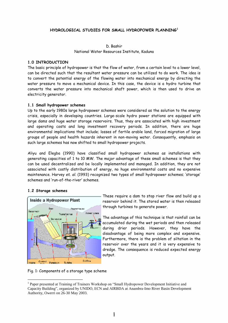
1.2 Storage schemes

These require a dam to stop river flow and build up a

reservoir behind it. The stored water is then released

through turbines to generate power.

The advantage of this technique is that rainfall can be

accumulated during the wet periods and then released

during drier periods. However, they have the

disadvantage of being more complex and expensive.

Furthermore, there is the problem of siltation in the

reservoir over the years and it is very expensive to

dredge. The consequence is reduced expected energy

output.

Fig. 1: Components of a storage type scheme

1 Paper presented at Training of Trainers Workshop on “Small Hydropower Development Initiative and

Capacity Building”, organized by UNIDO, ECN and AIRBDA at Anambra-Imo River Basin Development

Authority, Owerri on 26-30 May 2003.

2 2

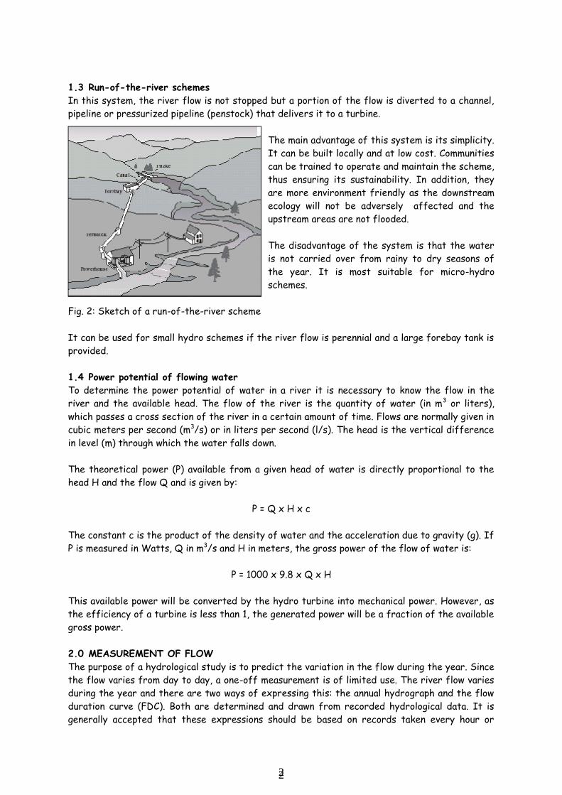
1.3 Run-of-the-river schemes

In this system, the river flow is not stopped but a portion of the flow is diverted to a channel,

pipeline or pressurized pipeline (penstock) that delivers it to a turbine.

The main advantage of this system is its simplicity.

It can be built locally and at low cost. Communities

can be trained to operate and maintain the scheme,

thus ensuring its sustainability. In addition, they

are more environment friendly as the downstream

ecology will not be adversely affected and the

upstream areas are not flooded.

The disadvantage of the system is that the water

is not carried over from rainy to dry seasons of

the year. It is most suitable for micro-hydro

schemes.

Fig. 2: Sketch of a run-of-the-river scheme

It can be used for small hydro schemes if the river flow is perennial and a large forebay tank is

provided.

1.4 Power potential of flowing water

To determine the power potential of water in a river it is necessary to know the flow in the

river and the available head. The flow of the river is the quantity of water (in m3 or liters),

which passes a cross section of the river in a certain amount of time. Flows are normally given in

cubic meters per second (m3/s) or in liters per second (l/s). The head is the vertical difference

in level (m) through which the water falls down.

The theoretical power (P) available from a given head of water is directly proportional to the

head H and the flow Q and is given by:

P = Q x H x c

The constant c is the product of the density of water and the acceleration due to gravity (g). If

P is measured in Watts, Q in m3/s and H in meters, the gross power of the flow of water is:

P = 1000 x 9.8 x Q x H

This available power will be converted by the hydro turbine into mechanical power. However, as

the efficiency of a turbine is less than 1, the generated power will be a fraction of the available

gross power.

2.0 MEASUREMENT OF FLOW

The purpose of a hydrological study is to predict the variation in the flow during the year. Since

the flow varies from day to day, a one-off measurement is of limited use. The river flow varies

during the year and there are two ways of expressing this: the annual hydrograph and the flow

duration curve (FDC). Both are determined and drawn from recorded hydrological data. It is

generally accepted that these expressions should be based on records taken every hour or

3 3

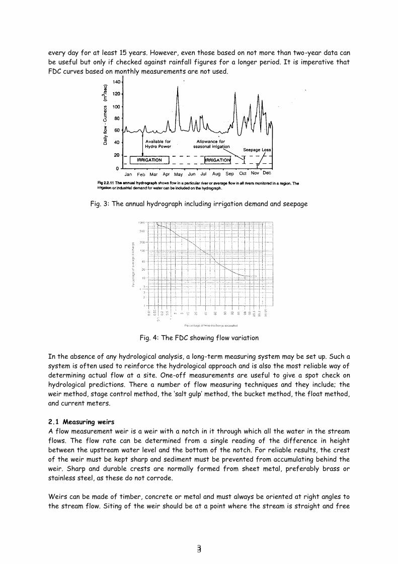
every day for at least 15 years. However, even those based on not more than two-year data can

be useful but only if checked against rainfall figures for a longer period. It is imperative that

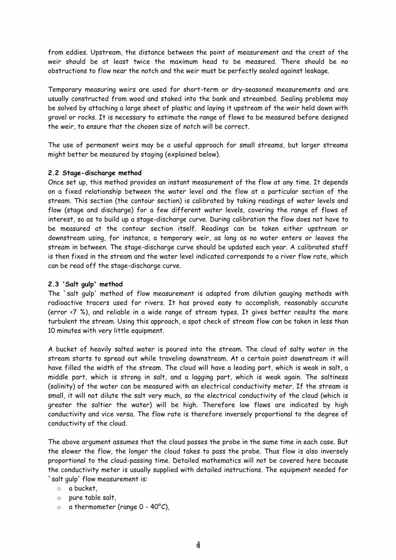
FDC curves based on monthly measurements are not used.

Fig. 3: The annual hydrograph including irrigation demand and seepage

Fig. 4: The FDC showing flow variation

In the absence of any hydrological analysis, a long-term measuring system may be set up. Such a

system is often used to reinforce the hydrological approach and is also the most reliable way of

determining actual flow at a site. One-off measurements are useful to give a spot check on

hydrological predictions. There a number of flow measuring techniques and they include; the

weir method, stage control method, the ‘salt gulp’ method, the bucket method, the float method,

and current meters.

2.1 Measuring weirs

A flow measurement weir is a weir with a notch in it through which all the water in the stream

flows. The flow rate can be determined from a single reading of the difference in height

between the upstream water level and the bottom of the notch. For reliable results, the crest

of the weir must be kept sharp and sediment must be prevented from accumulating behind the

weir. Sharp and durable crests are normally formed from sheet metal, preferably brass or

stainless steel, as these do not corrode.

Weirs can be made of timber, concrete or metal and must always be oriented at right angles to

the stream flow. Siting of the weir should be at a point where the stream is straight and free

4 4

from eddies. Upstream, the distance between the point of measurement and the crest of the

weir should be at least twice the maximum head to be measured. There should be no

obstructions to flow near the notch and the weir must be perfectly sealed against leakage.

Temporary measuring weirs are used for short-term or dry-seasoned measurements and are

usually constructed from wood and staked into the bank and streambed. Sealing problems may

be solved by attaching a large sheet of plastic and laying it upstream of the weir held down with

gravel or rocks. It is necessary to estimate the range of flows to be measured before designed

the weir, to ensure that the chosen size of notch will be correct.

The use of permanent weirs may be a useful approach for small streams, but larger streams

might better be measured by staging (explained below).

2.2 Stage-discharge method

Once set up, this method provides an instant measurement of the flow at any time. It depends

on a fixed relationship between the water level and the flow at a particular section of the

stream. This section (the contour section) is calibrated by taking readings of water levels and

flow (stage and discharge) for a few different water levels, covering the range of flows of

interest, so as to build up a stage-discharge curve. During calibration the flow does not have to

be measured at the contour section itself. Readings can be taken either upstream or

downstream using, for instance, a temporary weir, as long as no water enters or leaves the

stream in between. The stage-discharge curve should be updated each year. A calibrated staff

is then fixed in the stream and the water level indicated corresponds to a river flow rate, which

can be read off the stage-discharge curve.

2.3 'Salt gulp' method

The `salt gulp' method of flow measurement is adapted from dilution gauging methods with

radioactive tracers used for rivers. It has proved easy to accomplish, reasonably accurate

(error <7 %), and reliable in a wide range of stream types. It gives better results the more

turbulent the stream. Using this approach, a spot check of stream flow can be taken in less than

10 minutes with very little equipment.

A bucket of heavily salted water is poured into the stream. The cloud of salty water in the

stream starts to spread out while traveling downstream. At a certain point downstream it will

have filled the width of the stream. The cloud will have a leading part, which is weak in salt, a

middle part, which is strong in salt, and a lagging part, which is weak again. The saltiness

(salinity) of the water can be measured with an electrical conductivity meter. If the stream is

small, it will not dilute the salt very much, so the electrical conductivity of the cloud (which is

greater the saltier the water) will be high. Therefore low flows are indicated by high

conductivity and vice versa. The flow rate is therefore inversely proportional to the degree of

conductivity of the cloud.

The above argument assumes that the cloud passes the probe in the same time in each case. But

the slower the flow, the longer the cloud takes to pass the probe. Thus flow is also inversely

proportional to the cloud-passing time. Detailed mathematics will not be covered here because

the conductivity meter is usually supplied with detailed instructions. The equipment needed for

`salt gulp' flow measurement is:

o a bucket,

o pure table salt,

o a thermometer (range 0 - 40°C),

5 5

o a conductivity meter (range 0-1000 mS),

o an electrical integrator (Optional).

2.4 Bucket method

The bucket method is a simple way of measuring flow in very small streams. The entire flow is

diverted into a bucket or barrel and the time for the container to fill is recorded. The flow rate

is obtained simply by dividing the volume of the container by the filling time. Flows of up to 20

l/s can be measured using a 200-liter oil barrel.

2.5 Float method

The principle of all velocity-area methods is that flow Q equals the mean velocity Vmeans times

cross-sectional A:

Q = A x Vmean (m3/s)

One way of using this principle is for the cross-sectional profile of a streambed to be charted

and an average cross-section established for a known length of stream. A series of floats,

perhaps convenient pieces of wood, are then timed over a measured length of stream. Results

are averaged and a flow velocity is obtained. This velocity must then be reduced by a correction

factor, which estimates the mean velocity as opposed to the surface velocity. By multiplying

averaged and corrected flow velocity, the volume flow rate can be estimated.

2.6 Current meters

These consist of a shaft with a propeller or revolving cups connected to the end. The propeller

is free to rotate and the speed of rotation is related to the stream velocity. A simple

mechanical counter records the number of revolutions of a propeller placed at a desired depth.

By averaging readings taken evenly throughout the cross section, an average speed can be

obtained which is more accurate than with the float method.

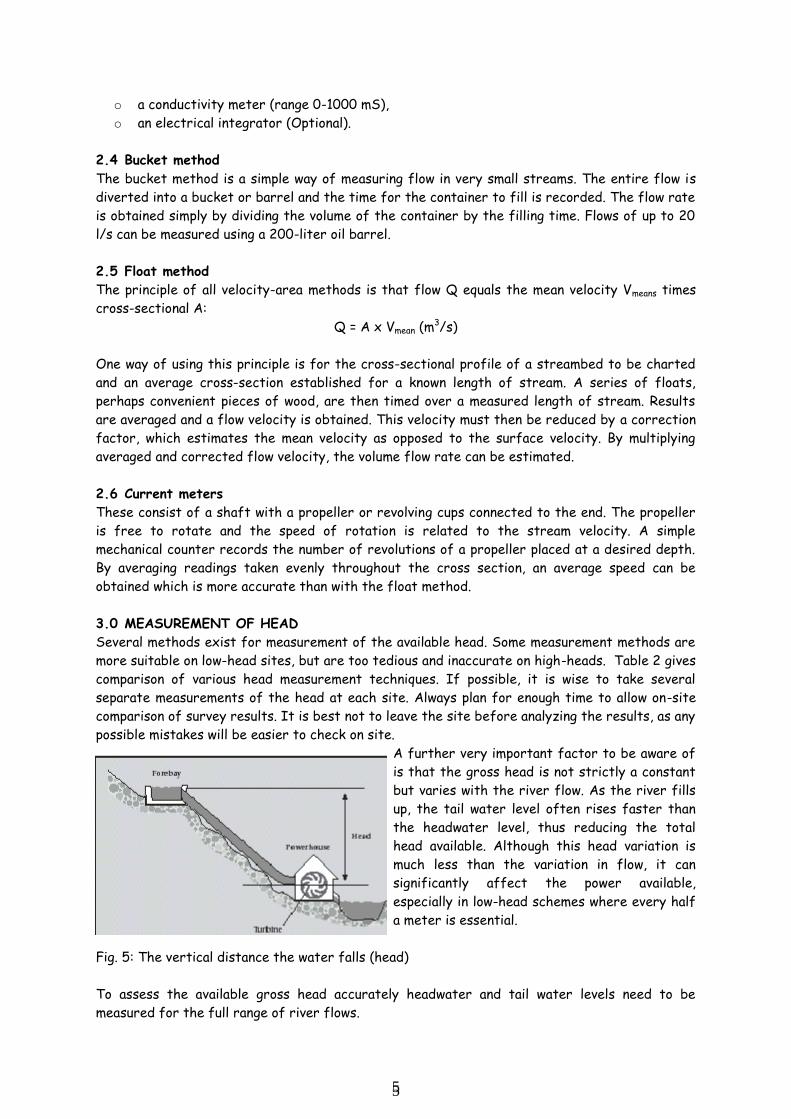
3.0 MEASUREMENT OF HEAD

Several methods exist for measurement of the available head. Some measurement methods are

more suitable on low-head sites, but are too tedious and inaccurate on high-heads. Table 2 gives

comparison of various head measurement techniques. If possible, it is wise to take several

separate measurements of the head at each site. Always plan for enough time to allow on-site

comparison of survey results. It is best not to leave the site before analyzing the results, as any

possible mistakes will be easier to check on site.

A further very important factor to be aware of

is that the gross head is not strictly a constant

but varies with the river flow. As the river fills

up, the tail water level often rises faster than

the headwater level, thus reducing the total

head available. Although this head variation is

much less than the variation in flow, it can

significantly affect the power available,

especially in low-head schemes where every half

a meter is essential.

Fig. 5: The vertical distance the water falls (head)

To assess the available gross head accurately headwater and tail water levels need to be

measured for the full range of river flows.

6 6

Table 1. Comparison of head measurement techniques

S/N

Method

Comments

Advantages and

Limitations

Accuracy

Precautions

1. Dumpy levels and

theodolite

Weight: Heavy

Expense: can be

hired, since in

common use

- Fast

- Not good on

wooded sites

Very good Liable to error.

Calculations can

introduce errors

2. Sighting meters

(clinometers or

Abney levels)

Weight: Light

Expense: Moderate

- Fast in clear

ground

- 2 people required

Good (5%) Experience, skill and

calibration needed

3. Water-filled tube

and pressure gauge

Weight: Light

Expense: Low

Fast, quite

foolproof, and can

measure penstock

length at the same

time

Good (<5%) if

gauge

calibrated

-Calibration chart

must be drawn up.

-Recalibrate the

gauge.

-Repeat

measurements

4. Water filled tube

and rod

Weight: Light

Expense: Low

Long-winded for

high heads

Approx. 5% Repeat

measurements

5. Spirit level and plank Weight: Light

Expense: Low

-Unsuitable for

long, gentle slopes.

-Slow to use

-Best with 2 people

-Approx. 5% on

steep slopes.

-10-20% on

gentle slopes

(1:10)

Repeat

measurements

6. Maps Weight: Light

Expense: Low

-High heads only.

-Wrong site may be

identified

Depends on

quality and

scale of map

Map reading skills

required.

-Map may be

incorrect

-Check if correct

site is identified

7. Altimeter Weight: Can be

heavy, some are

light.

Expense: High

-Useful on medium

and high heads (>40

m).

-Can be fast, but

more reliable with

continuous

monitoring

-Gross error

(30%) possible.

-2% at high

heads

-Experience and skill

needed.

Must be calibrated

and temp. corrected

Source: Harvey, A. et. al. (1993). Micro-Hydro Design Manual: A Guide to Small-scale Water Power Schemes.

Intermediate Technology Publication, London.

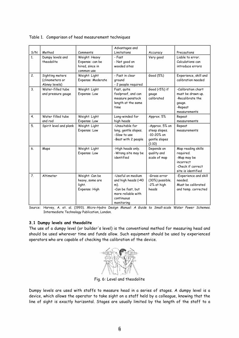
3.1 Dumpy levels and theodolite

The use of a dumpy level (or builder's level) is the conventional method for measuring head and

should be used wherever time and funds allow. Such equipment should be used by experienced

operators who are capable of checking the calibration of the device.

Fig. 6: Level and theodolite

Dumpy levels are used with staffs to measure head in a series of stages. A dumpy level is a

device, which allows the operator to take sight on a staff held by a colleague, knowing that the

line of sight is exactly horizontal. Stages are usually limited by the length of the staff to a

7 7

height change of no more than 3 m. A clear unobstructed view is needed, so wooded sites can be

frustrated with this method. Dumpy levels only allow a horizontal sight but theodolite can also

measure vertical and horizontal angles, giving greater versatility and allowing faster work.

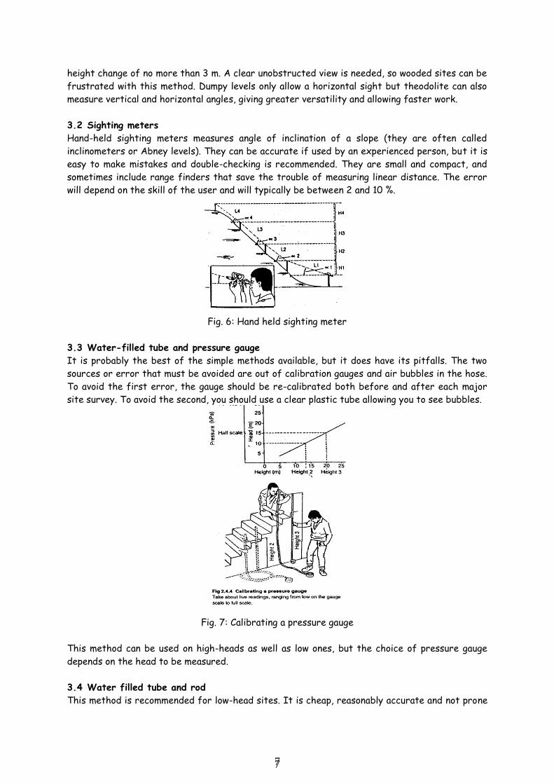
3.2 Sighting meters

Hand-held sighting meters measures angle of inclination of a slope (they are often called

inclinometers or Abney levels). They can be accurate if used by an experienced person, but it is

easy to make mistakes and double-checking is recommended. They are small and compact, and

sometimes include range finders that save the trouble of measuring linear distance. The error

will depend on the skill of the user and will typically be between 2 and 10 %.

Fig. 6: Hand held sighting meter

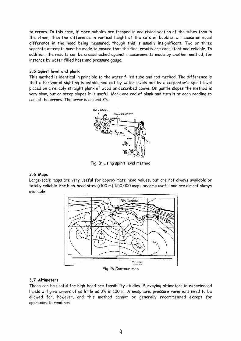
3.3 Water-filled tube and pressure gauge

It is probably the best of the simple methods available, but it does have its pitfalls. The two

sources or error that must be avoided are out of calibration gauges and air bubbles in the hose.

To avoid the first error, the gauge should be re-calibrated both before and after each major

site survey. To avoid the second, you should use a clear plastic tube allowing you to see bubbles.

Fig. 7: Calibrating a pressure gauge

This method can be used on high-heads as well as low ones, but the choice of pressure gauge

depends on the head to be measured.

3.4 Water filled tube and rod

This method is recommended for low-head sites. It is cheap, reasonably accurate and not prone

8 8

to errors. In this case, if more bubbles are trapped in one rising section of the tubes than in

the other, then the difference in vertical height of the sets of bubbles will cause an equal

difference in the head being measured, though this is usually insignificant. Two or three

separate attempts must be made to ensure that the final results are consistent and reliable. In

addition, the results can be crosschecked against measurements made by another method, for

instance by water filled hose and pressure gauge.

3.5 Spirit level and plank

This method is identical in principle to the water filled tube and rod method. The difference is

that a horizontal sighting is established not by water levels but by a carpenter's spirit level

placed on a reliably straight plank of wood as described above. On gentle slopes the method is

very slow, but on steep slopes it is useful. Mark one end of plank and turn it at each reading to

cancel the errors. The error is around 2%.

Fig. 8: Using spirit level method

3.6 Maps

Large-scale maps are very useful for approximate head values, but are not always available or

totally reliable. For high-head sites (>100 m) 1:50,000 maps become useful and are almost always

available.

Fig. 9: Contour map

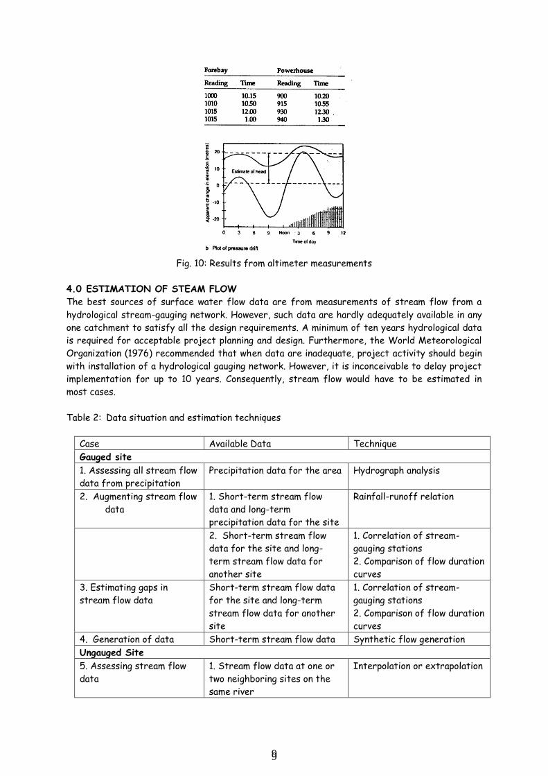
3.7 Altimeters

These can be useful for high-head pre-feasibility studies. Surveying altimeters in experienced

hands will give errors of as little as 3% in 100 m. Atmospheric pressure variations need to be

allowed for, however, and this method cannot be generally recommended except for

approximate readings.

9 9

Fig. 10: Results from altimeter measurements

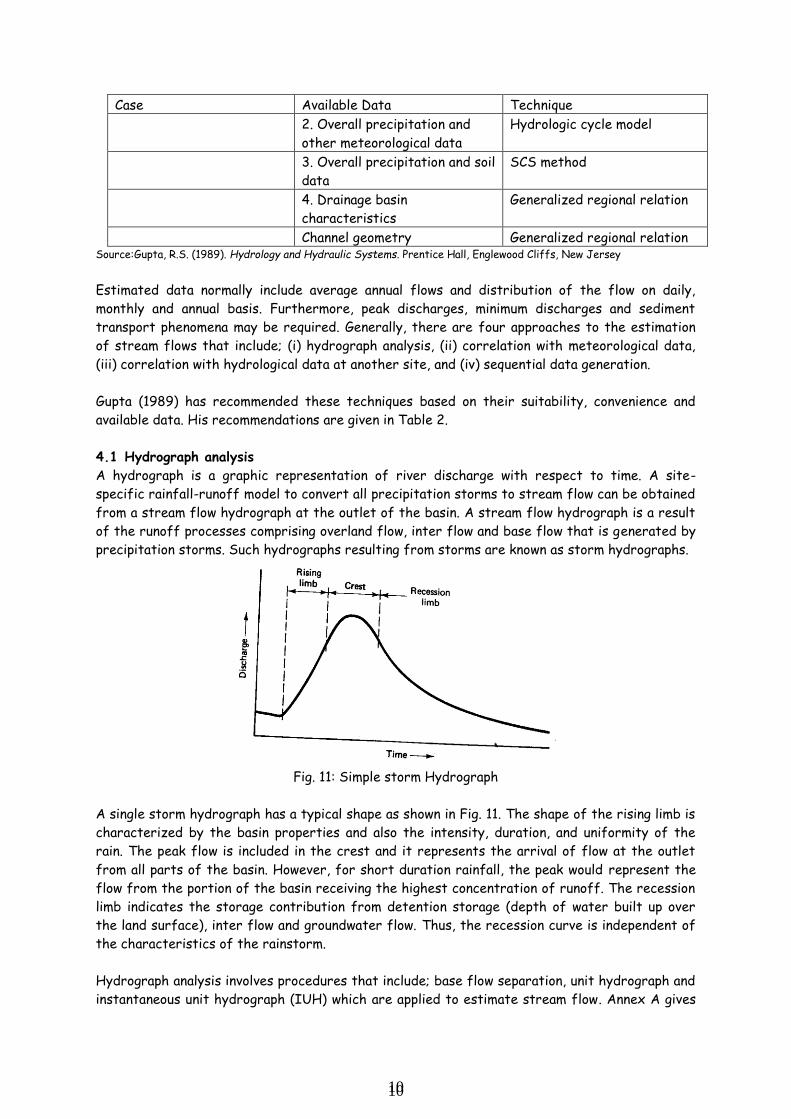
4.0 ESTIMATION OF STEAM FLOW

The best sources of surface water flow data are from measurements of stream flow from a

hydrological stream-gauging network. However, such data are hardly adequately available in any

one catchment to satisfy all the design requirements. A minimum of ten years hydrological data

is required for acceptable project planning and design. Furthermore, the World Meteorological

Organization (1976) recommended that when data are inadequate, project activity should begin

with installation of a hydrological gauging network. However, it is inconceivable to delay project

implementation for up to 10 years. Consequently, stream flow would have to be estimated in

most cases.

Table 2: Data situation and estimation techniques

Case Available Data Technique

Gauged site

1. Assessing all stream flow

data from precipitation

Precipitation data for the area Hydrograph analysis

2. Augmenting stream flow

data

1. Short-term stream flow

data and long-term

precipitation data for the site

Rainfall-runoff relation

2. Short-term stream flow

data for the site and long-

term stream flow data for

another site

1. Correlation of stream-

gauging stations

2. Comparison of flow duration

curves

3. Estimating gaps in

stream flow data

Short-term stream flow data

for the site and long-term

stream flow data for another

site

1. Correlation of stream-

gauging stations

2. Comparison of flow duration

curves

4. Generation of data Short-term stream flow data Synthetic flow generation

Ungauged Site

5. Assessing stream flow

data

1. Stream flow data at one or

two neighboring sites on the

same river

Interpolation or extrapolation

10 10

Case Available Data Technique

2. Overall precipitation and

other meteorological data

Hydrologic cycle model

3. Overall precipitation and soil

data

SCS method

4. Drainage basin

characteristics

Generalized regional relation

Channel geometry Generalized regional relation Source: Gupta, R.S. (1989). Hydrology and Hydraulic Systems. Prentice Hall, Englewood Cliffs, New Jersey

Estimated data normally include average annual flows and distribution of the flow on daily,

monthly and annual basis. Furthermore, peak discharges, minimum discharges and sediment

transport phenomena may be required. Generally, there are four approaches to the estimation

of stream flows that include; (i) hydrograph analysis, (ii) correlation with meteorological data,

(iii) correlation with hydrological data at another site, and (iv) sequential data generation.

Gupta (1989) has recommended these techniques based on their suitability, convenience and

available data. His recommendations are given in Table 2.

4.1 Hydrograph analysis

A hydrograph is a graphic representation of river discharge with respect to time. A site-

specific rainfall-runoff model to convert all precipitation storms to stream flow can be obtained

from a stream flow hydrograph at the outlet of the basin. A stream flow hydrograph is a result

of the runoff processes comprising overland flow, inter flow and base flow that is generated by

precipitation storms. Such hydrographs resulting from storms are known as storm hydrographs.

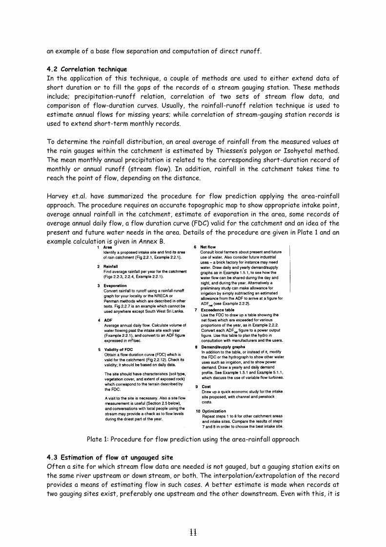
Fig. 11: Simple storm Hydrograph

A single storm hydrograph has a typical shape as shown in Fig. 11. The shape of the rising limb is

characterized by the basin properties and also the intensity, duration, and uniformity of the

rain. The peak flow is included in the crest and it represents the arrival of flow at the outlet

from all parts of the basin. However, for short duration rainfall, the peak would represent the

flow from the portion of the basin receiving the highest concentration of runoff. The recession

limb indicates the storage contribution from detention storage (depth of water built up over

the land surface), inter flow and groundwater flow. Thus, the recession curve is independent of

the characteristics of the rainstorm.

Hydrograph analysis involves procedures that include; base flow separation, unit hydrograph and

instantaneous unit hydrograph (IUH) which are applied to estimate stream flow. Annex A gives

11 11

an example of a base flow separation and computation of direct runoff.

4.2 Correlation technique

In the application of this technique, a couple of methods are used to either extend data of

short duration or to fill the gaps of the records of a stream gauging station. These methods

include; precipitation-runoff relation, correlation of two sets of stream flow data, and

comparison of flow-duration curves. Usually, the rainfall-runoff relation technique is used to

estimate annual flows for missing years; while correlation of stream-gauging station records is

used to extend short-term monthly records.

To determine the rainfall distribution, an areal average of rainfall from the measured values at

the rain gauges within the catchment is estimated by Thiessen’s polygon or Isohyetal method.

The mean monthly annual precipitation is related to the corresponding short-duration record of

monthly or annual runoff (stream flow). In addition, rainfall in the catchment takes time to

reach the point of flow, depending on the distance.

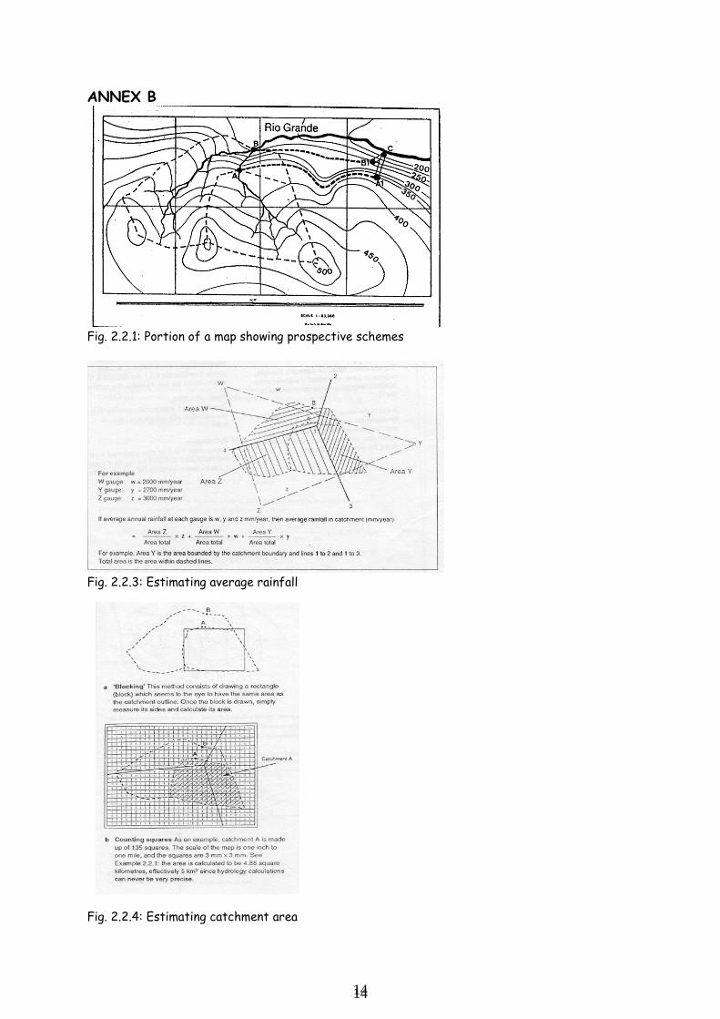
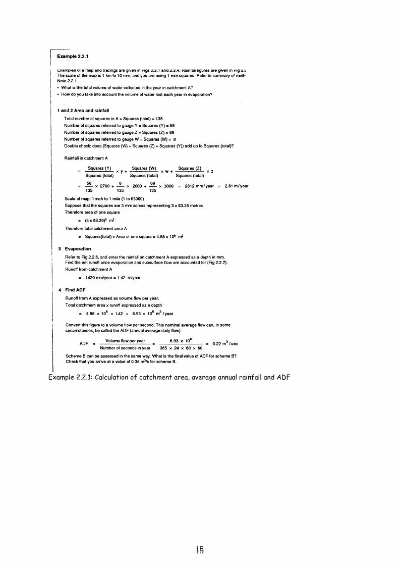
Harvey et.al. have summarized the procedure for flow prediction applying the area-rainfall

approach. The procedure requires an accurate topographic map to show appropriate intake point,

average annual rainfall in the catchment, estimate of evaporation in the area, some records of

average annual daily flow, a flow duration curve (FDC) valid for the catchment and an idea of the

present and future water needs in the area. Details of the procedure are given in Plate 1 and an

example calculation is given in Annex B.

Plate 1: Procedure for flow prediction using the area-rainfall approach

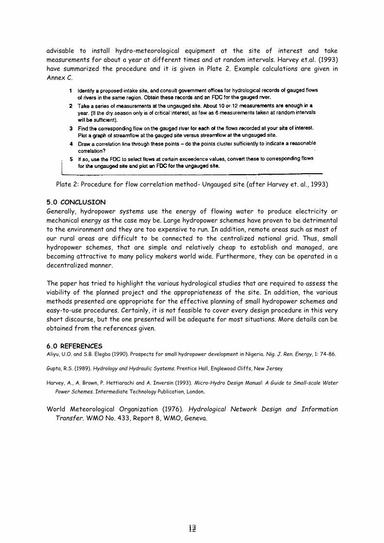
4.3 Estimation of flow at ungauged site

Often a site for which stream flow data are needed is not gauged, but a gauging station exits on

the same river upstream or down stream, or both. The interpolation/extrapolation of the record

provides a means of estimating flow in such cases. A better estimate is made when records at

two gauging sites exist, preferably one upstream and the other downstream. Even with this, it is

12 12

advisable to install hydro-meteorological equipment at the site of interest and take

measurements for about a year at different times and at random intervals. Harvey et.al. (1993)

have summarized the procedure and it is given in Plate 2. Example calculations are given in

Annex C.

Plate 2: Procedure for flow correlation method- Ungauged site (after Harvey et. al., 1993)

5.0 CONCLUSION

Generally, hydropower systems use the energy of flowing water to produce electricity or

mechanical energy as the case may be. Large hydropower schemes have proven to be detrimental

to the environment and they are too expensive to run. In addition, remote areas such as most of

our rural areas are difficult to be connected to the centralized national grid. Thus, small

hydropower schemes, that are simple and relatively cheap to establish and managed, are

becoming attractive to many policy makers world wide. Furthermore, they can be operated in a

decentralized manner.

The paper has tried to highlight the various hydrological studies that are required to assess the

viability of the planned project and the appropriateness of the site. In addition, the various

methods presented are appropriate for the effective planning of small hydropower schemes and

easy-to-use procedures. Certainly, it is not feasible to cover every design procedure in this very

short discourse, but the one presented will be adequate for most situations. More details can be

obtained from the references given.

6.0 REFERENCES Aliyu, U.O. and S.B. Elegba (1990). Prospects for small hydropower development in Nigeria. Nig. J. Ren. Energy, 1: 74-86.

Gupta, R.S. (1989). Hydrology and Hydraulic Systems. Prentice Hall, Englewood Cliffs, New Jersey

Harvey, A., A. Brown, P. Hettiarachi and A. Inversin (1993). Micro-Hydro Design Manual: A Guide to Small-scale Water

Power Schemes. Intermediate Technology Publication, London.

World Meteorological Organization (1976). Hydrological Network Design and Information

Transfer. WMO No. 433, Report 8, WMO, Geneva.

13 13

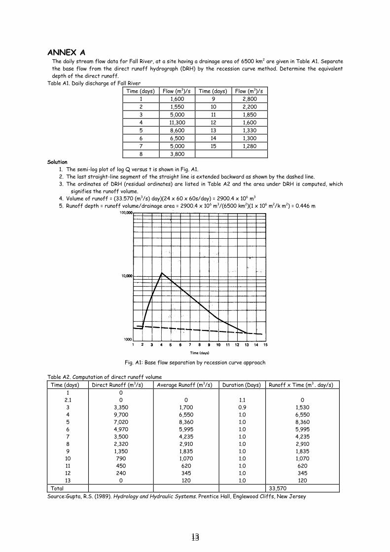
ANNEX A The daily stream flow data for Fall River, at a site having a drainage area of 6500 km2 are given in Table A1. Separate

the base flow from the direct runoff hydrograph (DRH) by the recession curve method. Determine the equivalent

depth of the direct runoff.

Table A1. Daily discharge of Fall River

Time (days) Flow (m3)/s Time (days) Flow (m3)/s

1 1,600 9 2,800

2 1,550 10 2,200

3 5,000 11 1,850

4 11,300 12 1,600

5 8,600 13 1,330

6 6,500 14 1,300

7 5,000 15 1,280

8 3,800

Solution

1. The semi-log plot of log Q versus t is shown in Fig. A1.

2. The last straight-line segment of the straight line is extended backward as shown by the dashed line.

3. The ordinates of DRH (residual ordinates) are listed in Table A2 and the area under DRH is computed, which

signifies the runoff volume.

4. Volume of runoff = (33.570 (m3/s) day)(24 x 60 x 60s/day) = 2900.4 x 106 m3

5. Runoff depth = runoff volume/drainage area = 2900.4 x 106 m3/(6500 km2)(1 x 106 m2/k m2) = 0.446 m

Fig. A1: Base flow separation by recession curve approach

Table A2. Computation of direct runoff volume

Time (days) Direct Runoff (m3/s) Average Runoff (m3/s) Duration (Days) Runoff x Time (m3 . day/s)

1

2.1

3

4

5

6

7

8

9

10

11

12

13

0

0

3,350

9,700

7,020

4,970

3,500

2,320

1,350

790

450

240

0

0

1,700

6,550

8,360

5,995

4,235

2,910

1,835

1,070

620

345

120

1.1

0.9

1.0

1.0

1.0

1.0

1.0

1.0

1.0

1.0

1.0

1.0

0

1,530

6,550

8,360

5,995

4,235

2,910

1,835

1,070

620

345

120

Total 33,570

Source: Gupta, R.S. (1989). Hydrology and Hydraulic Systems. Prentice Hall, Englewood Cliffs, New Jersey

14 14

ANNEX B

Fig. 2.2.1: Portion of a map showing prospective schemes

Fig. 2.2.3: Estimating average rainfall

Fig. 2.2.4: Estimating catchment area

15 15

Example 2.2.1: Calculation of catchment area, average annual rainfall and ADF

16 16

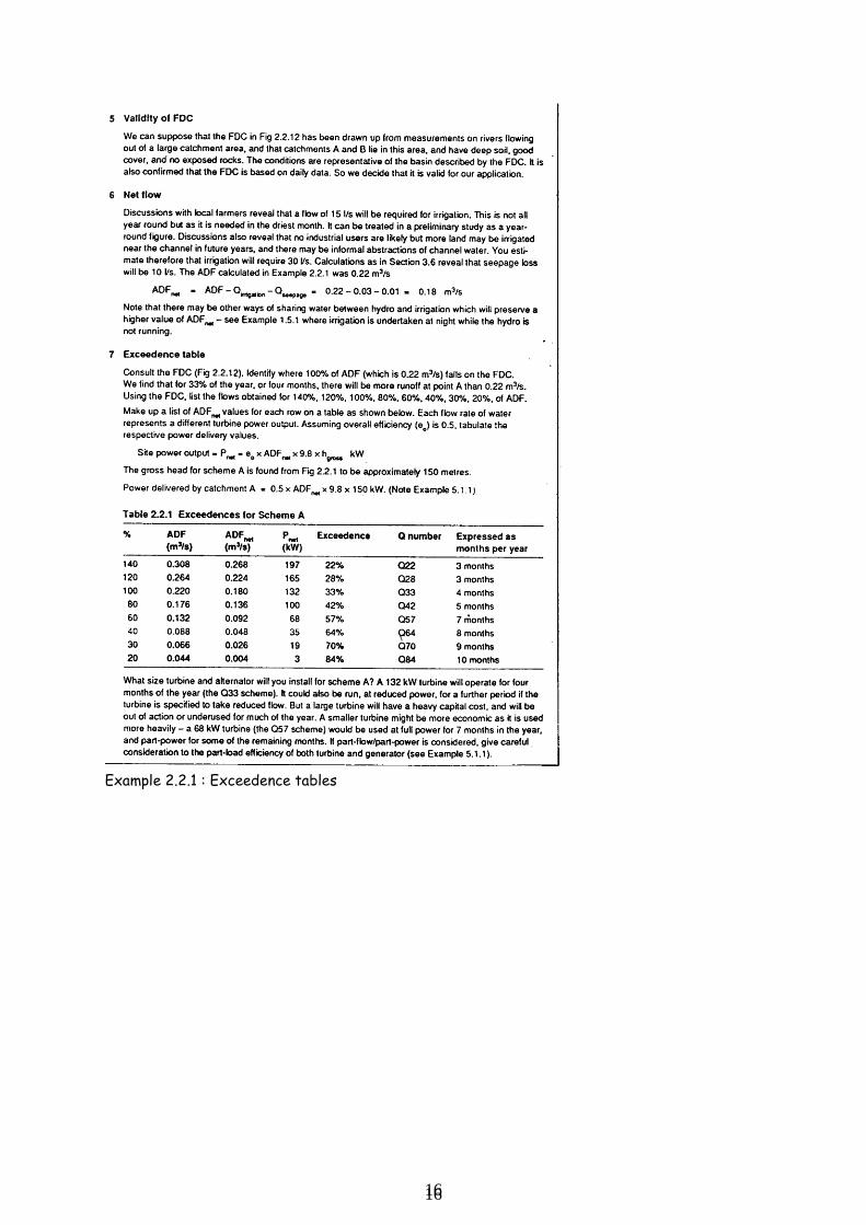
Example 2.2.1 : Exceedence tables

17 17

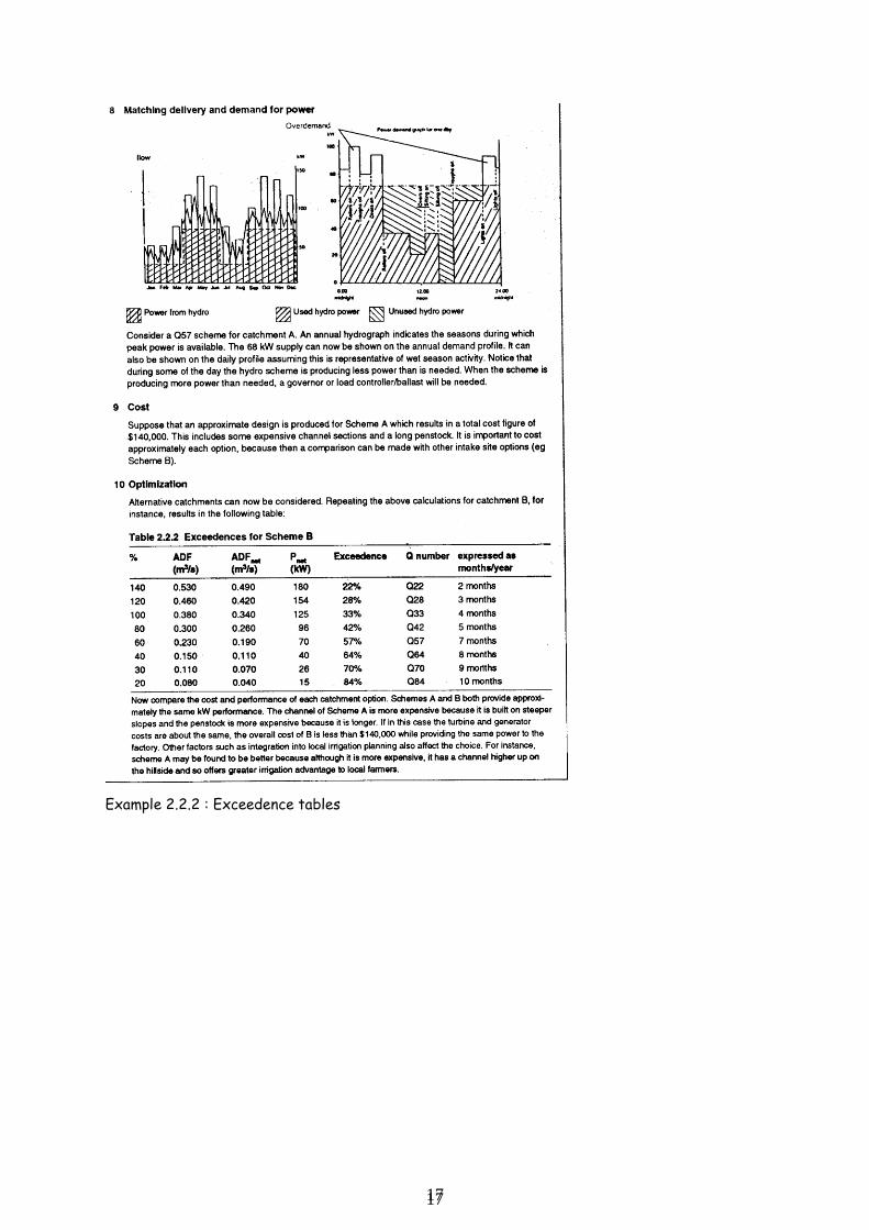
Example 2.2.2 : Exceedence tables

18 18

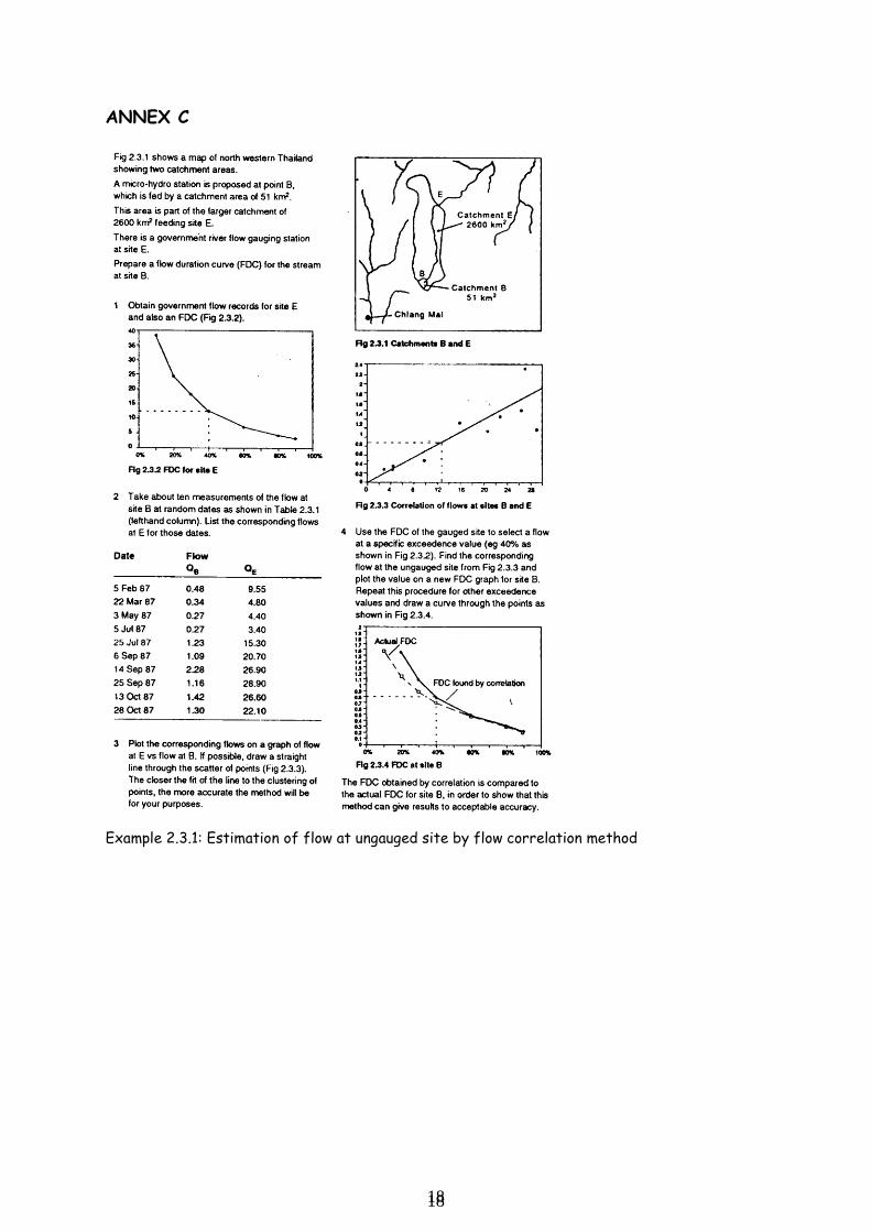
ANNEX C

Example 2.3.1: Estimation of flow at ungauged site by flow correlation method