Environ Fluid Mech (2013) 13:279–307DOI 10.1007/s10652-013-9274-7

ORIGINAL ARTICLE

Flow and turbulence in an industrial/suburban roughnesscanopy

A. Dallman · S. Di Sabatino · H. J. S. Fernando

Received: 12 September 2012 / Accepted: 6 February 2013 / Published online: 7 March 2013© Springer Science+Business Media Dordrecht 2013

Abstract A field study conducted to investigate the flow and turbulence structure of theurban boundary layer (UBL) over an industrial/suburban area is described. The emphasis wason morning and evening transition periods, but some measurements covered the entire diur-nal cycle. The data analysis incorporated the dependence of wind direction on morphometricparameters of the urban canopy. The measurements of heat and momentum fluxes showed thepossibility of a constant flux layer above the height z ≈ 2H , wherein the Monin-ObukhovSimilarity Theory (MOST) is valid; here H is the averaged building height. For the nocturnalboundary layer, the mean velocity and temperature profiles obeyed classical MOST scalingup to ∼ 0.5�(∼ 6H), where� is the Obukhov length scale, beyond which stronger stratifi-cation may disrupt the occurrence of constant fluxes. For unstable and neutral cases, MOSTscaling described the mean data well up to the maximum measured height (∼ 6H). AvailableMOST functions, however, could not describe the measured turbulence structure, indicatingthe influence of additional governing parameters. Alternative turbulence parameterizationswere tested, and some were found to perform well. Calculation of integral length scales forconvective and neutral cases allowed a phenomenological description of eddy characteristicswithin and above the urban canopy layer. The development of a significant nocturnal surfaceinversion occurred only on certain days, for which a criterion was proposed. The nocturnalUBL exhibited length scale relationships consistent with the evening collapse of the convec-tive boundary layer and maintenance of buoyancy-affected turbulence overnight. The length

A. Dallman (B) · S. Di Sabatino · H. J. S. FernandoEnvironmental Fluid Dynamics Laboratories, Department of Civil and Environmental Engineering andEarth Sciences, University of Notre Dame, Notre Dame, IN 46556, USAe-mail: ardallm@gmail.com

S. Di SabatinoLaboratorio di Micrometeorologia, Dipartimento di Scienze e Tecnologie Biologiche ed Ambientali,Università del Salento, Lecce, Italy

H. J. S. FernandoDepartment of Aerospace and Mechanical Engineering, University of Notre Dame,Notre Dame, IN 46556, USA

123

280 Environ Fluid Mech (2013) 13:279–307

and velocity scales so identified are useful in parameterizing turbulent dispersion coefficientsin different diurnal phases of the UBL.

Keywords Urban effects · Turbulence scales · Thermal stratification ·Nocturnal boundary layer · Morphometric analyses

1 Introduction

With urban areas now accounting for more than 50 % of where the world population lives[1], and continued rapid urbanization at a rate of 1.5 % per year, much recent focus hasbeen placed on understanding and managing of an urban metabolism—which deals with theflow of material, heat, air and water; infrastructure; utilization of resources; environmentalchange, and human and social dynamics [2,3]. Of critical importance in such studies isthe lowest atmospheric layer affected by the ground, known as the urban boundary layer(UBL), which hosts a variety of ecosystems, including human activities. This is the layerthrough which exchanges of heat, momentum, species and moisture between the groundsurface and atmosphere take place, which in turn determine the microclimate, dispersion ofpollutants/contaminants and hydrologic cycle. Given its complexity, the UBL is studied byinvoking processes occurring over a repertoire of scales, and interactions therein determinethe nature and evolution of the UBL. For example, the properties averaged over a suitableurban footprint from a ‘bird’s eye view’ may provide a large (� meso) scale perspective. Inregulatory enforcement, representative microcosms within a large urban area (e.g., pollutantor temperature hot-spots) are defined by ‘neighborhood’ scales [4]. An area encompassing acluster of downtown buildings is used in emergency [5,6] and city planning [7]. The flow ina single urban street canyon is used for evaluating pedestrian comfort [8,9].

The UBL is divided into several vertically stacked layers, each selected on the basis ofdynamical characteristics and having specific length and time scales [10–12]. The layer upto the roof heights, the urban canopy layer (UCL), develops between roughness elements,wherein the flow is highly inhomogeneous, dependent on local urban morphometry and sen-sitive to small-scale features within urban canyons. The roughness sub-layer (RSL) extendsfrom the ground up to about two to five times the height of roughness elements (i.e., buildingheight H ). Within the RSL the flow is three-dimensional, turbulence is inhomogeneous andvertical diffusion is as important as horizontal advection. Upward expanding wakes of indi-vidual buildings are felt in this layer, and due to the merging of wakes, the role of individualbuildings disappears upwards. The inertial sub-layer or constant flux layer (CFL) is abovethe RSL, in which the signatures of individual building wakes and upstream conditions areabsent and turbulence is determined by the ‘averaged’ building morphology. A (perhaps mis-leadingly called) mixed layer (ML) with varying shear stresses tops the CFL, and extendsupwards to the edge of the UBL where transition to free stream (with geostrophic flow UG )is completed, the ground influence is lost and entrainment of free-stream air is a key feature.

Naturally, the parameterization of flow and turbulence in the UCL and RSL is a difficultchallenge, given their dependence on the details of the underlying urban surface. On theother hand, given the perceived horizontal homogeneity and nearly constant upward turbulentfluxes, Monin-Obukhov similarity theory (MOST) has been applied to the CFL, but the banehas been acquiring measurements within the CFL [8] to verify the applicability of MOST.On physical grounds, MOST functions are expected to depend on the urban roughness. Verylittle information is available on the ML.

123

Environ Fluid Mech (2013) 13:279–307 281

A substantial amount of meteorological measurements have been reported in urban areas,including large experimental programs with hundreds of investigators, observations acrossmultiple scales and with the deployment of extensive instrumentation. Some examples areURBAN 2000 [13], Joint Urban 2003 [14], DAPPLE [15], UBL/CLU-ESCOMPTE [16], andBUBBLE [17]. There are also many studies conducted by smaller groups of investigatorsdealing with specific problems [8]. Informative review material on past work can be found inRoth [11], Britter and Hanna [8], and Wood et al. [18]. The parameterization of turbulencein the UBL has been a topic of much interest, given its importance in modeling the fateof airborne releases and local air pollution. Most studies have been focused on the CFL,considering the prospects of universal parameterizations based on MOST. By consideringhorizontally homogeneous turbulence in the CFL determined by the momentum flux orthe friction velocity u∗ and the bulk integral scale � of turbulence at its lower boundary, adimensional analysis approach can be attempted to identify key parameters. Any propertyP can thus be written as

P = P [u∗, �, (z − d) , qo, hu] , (1)

where qo = gw′θ ′/θ0 is the buoyancy flux (with g being the acceleration of gravity, θ0 thereference potential temperature, andw′θ ′ the flux of temperature), hu the height of the UBL,z the distance from the ground, and d the displacement height that accounts for the virtualorigin from which the distances are measured for the CFL, z′ = (z − d). Note that d and� are functions of the aerodynamic roughness height (z0) of the underlying surface. Thenon-dimensional form of Eq. 1 is

P∗ = P∗[z′/�, �/�, �/hu] (2)

where� = −u3∗/κq0 is the Obukhov length scale and ζ = z′/� is a stability parameter. For�/hu � 1, assuming that eddies of size ∼ hu do not penetrate the CFL, self-similarity ofthe first kind [19] yields,

P∗ = P∗1

[z′/�, �/�

]. (3a)

On the other hand, when the influence of eddies of size ∼ hu are present, self-similarity ofthe second kind may produce

P∗ =(�

hu

)m

P∗2

[z′

�,

�

� (�/hu)n

], (3b)

where m and n are unknown exponents. Similarly, for the neutral case (� → ∞),

P∗ = P∗3

[z′/�

], (4a)

or

P∗ =(�

hu

)m1

P∗4

[z′

�

(�

hu

)n1], (4b)

where � can be replaced by the independent length scale at the top of the RSL, z0. Althoughgeneral equations for the UBL are given by Eq. 3(a,b), it has been customary to use the form

P∗ = G∗ [z′/�

], (5)

[11], and naturally, the function G∗ is expected to depend on �/� and �/hu (or hu/�), thatis on the site and the thermal stratification [20]. The observance of varying functions andthe scatter of data in previous studies, at least partly, can be attributed to this dependence.

123

282 Environ Fluid Mech (2013) 13:279–307

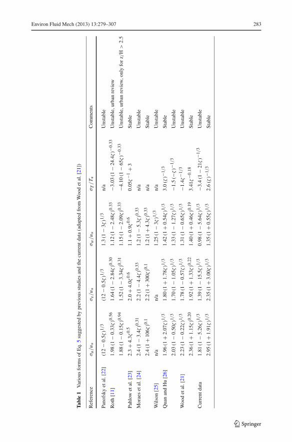
Table 1 shows various forms of G∗ for root mean square (rms) velocities (σi , i = u, v, w)and the rms temperature (σT ), where T∗ = −w′θ ′/u∗, for stable (ζ > 0) and unstable(ζ < 0) atmospheric conditions noted in previous studies (and for current data). Alternativeparameterizations are also available for specific cases. Involvement of a large number ofparameters clearly adds to the difficulty of UBL analysis.

Another unexplored issue is the formation of a stable layer near the ground at night[12,27]. In dense urban canopies, wakes of obstructions cause strong mechanical mixing,which, when augmented by the urban heat island (UHI), can overshadow the stabilizinginfluence of cooling [28,29]. Measurements in London [18] and Rome [30], however, showthat near surface stable stratification may occur in large urban areas rather frequently.

While previous field [11], laboratory [31,32] and numerical [33] studies have made signif-icant advances, substantial knowledge gaps exist on flow and turbulence in urban canopies.Some of the overarching issues are:

• Is there a CFL and is it horizontally homogeneous? What are the velocity and temperatureprofiles in various layers of the UBL?

• Can MOST work well over urban areas, and what are its limitations?• Are the varying MOST functions at different locations a result of z0 and hu dependence?• How do available alternative (to MOST) turbulence parameterizations perform for the

UBL?• When a stably stratified flow approaches a roughness canopy, how do the competing

effects of mechanical turbulence and buoyancy sway the structure of the UBL?• Can a stably stratified boundary layer develop near the surface of built up areas? What

is its structure and what are the scales of turbulence?• What is the scale of the UBL under different stability conditions, and what is the role of

the so-called ML in effacing the ground effects at greater heights?

The data from a field study conducted in the Hermoso Park neighborhood of SouthwestPhoenix during Nov/Dec 2009 were employed to address the above questions. The site ismade up of mixed urban-industrial land use, and heightened health problems of local residentswere a driving factor of the field study. It has been argued that anomalous airborne particulatematter (PM) concentration in the area, both due to local re-entrainment and transport fromelsewhere, may be responsible for the health woes. This PM is further contaminated by smallconcentrations of lead particles in the soil, deposited from past (1991, 2000) fires at twolocal circuit board manufacturing facilities. Since PM is re-entrained by turbulence, flow andsurface turbulence in the area (as well as in urban canopies in general) were of prime interest,and are the theme of this paper.

Phoenix is located in complex terrain, and hence, is characterized by up-valley (daytime)and down-valley (nighttime) winds [2,34]. Two towers were used, each instrumented withthree sonic anemometers, and depending on the wind direction and stability conditions, theywere representative of different layers of the UBL. Because of the non-uniformity of theurban area, the urban morphological parameters used in the analysis were different for differ-ent approach directions of wind. Measurements were recorded over the diurnal cycle, withtethered balloon launches in the early evening (1400–2000 LST) and morning (0500–1100LST) whence the PM concentrations are highest due to weak flow during evening/morningtransition periods.

The detailed experimental procedure is given in Sect. 2, including the evaluation of mor-phometric parameters. Sections 3.1 and 3.2 present overall diurnal meteorological and tur-bulence fields over a selected design period, which characterize the overall experiment.Section 3.3 deals with the measurement of turbulence, focusing on the parameterization of

123

Environ Fluid Mech (2013) 13:279–307 283

Tabl

e1

Var

ious

form

sof

Eq.

5su

gges

ted

bypr

evio

usst

udie

san

dth

ecu

rren

tdat

a(a

dapt

edfr

omW

ood

etal

.[21

])

Ref

eren

ceσ

u/u∗

σv/u∗

σw/u∗

σT/

T ∗C

omm

ents

Pano

fsky

etal

.[22

](1

2−

0.5ζ)1/3

(12

−0.

5ζ)1/3

1.3(1

−3ζ)1/3

n/a

Uns

tabl

e

Rot

h[1

1]1.

98(1

−0.

33ζ)0.5

61.

64(1

−2.

84ζ)0.3

01.

12(1

−2.

48ζ)0.3

3−3.0

3(1

−24.4ζ)−

0.33

Uns

tabl

e,ur

ban

revi

ew

1.88(1

−0.

15ζ)0.9

41.

52(1

−3.

34ζ)0.3

11.

15(1

−2.

09ζ)0.3

3−4.1

0(1

−65ζ)−

0.33

Uns

tabl

e,ur

ban

revi

ew,o

nly

for

z/H>

2.5

Pahl

owet

al.[

23]

2.3

+4.

3ζ0.

52.

0+

4.0ζ

0.6

1.1

+0.

9ζ0.

60.

05ζ−1

+3

Stab

le

Mor

aes

etal

.[24

]2.

4(1

−3.

4ζ)0.3

12.

2(1

−4.

4ζ)0.3

31.

2(1

−5.

3ζ)0.3

3n/

aU

nsta

ble

2.4(1

+10

6ζ)0.1

2.2(1

+30

0ζ)0.1

1.2(1

+4.

3ζ)0.3

3n/

aSt

able

Wils

on[2

5]n/

an/

a1.

25(1

−3ζ)1/3

n/a

Uns

tabl

e

Qua

nan

dH

u[2

6]1.

96(1

+2.

07ζ)1/3

1.80(1

+1.

78ζ)1/3

1.42(1

+0.

54ζ)1/3

3.0(ζ)−

1/3

Stab

le

2.03(1

−0.

50ζ)1/3

1.70(1

−1.

05ζ)1/3

1.33(1

−1.

27ζ)1/3

−1.5(−ζ)−

1/3

Uns

tabl

e

Woo

det

al.[

21]

2.23(1

−0.

22ζ)1/3

1.78(1

−0.

57ζ)1/3

1.31(1

−0.

65ζ)1/3

−1.4ζ−1/3

Uns

tabl

e

2.36(1

+1.

15ζ)0.2

01.

92(1

+1.

33ζ)0.2

21.

40(1

+0.

46ζ)0.1

93.

41ζ−0.1

8St

able

Cur

rent

data

1.81(1

−5.

26ζ)1/3

1.39(1

−15.5ζ)1/3

0.98(1

−5.

64ζ)1/3

−3.4(1

−21ζ)−

1/3

Uns

tabl

e

2.95(1

+1.

91ζ)1/3

2.35(1

+3.

00ζ)1/3

1.35(1

+0.

55ζ)1/3

2.6(ζ)−

1/3

Stab

le

123

284 Environ Fluid Mech (2013) 13:279–307

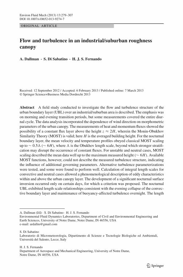
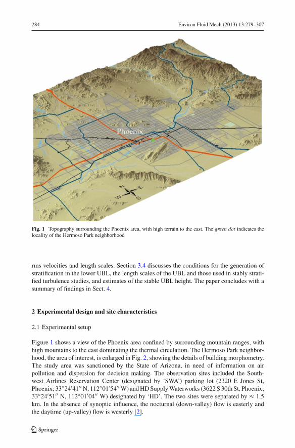
Fig. 1 Topography surrounding the Phoenix area, with high terrain to the east. The green dot indicates thelocality of the Hermoso Park neighborhood

rms velocities and length scales. Section 3.4 discusses the conditions for the generation ofstratification in the lower UBL, the length scales of the UBL and those used in stably strati-fied turbulence studies, and estimates of the stable UBL height. The paper concludes with asummary of findings in Sect. 4.

2 Experimental design and site characteristics

2.1 Experimental setup

Figure 1 shows a view of the Phoenix area confined by surrounding mountain ranges, withhigh mountains to the east dominating the thermal circulation. The Hermoso Park neighbor-hood, the area of interest, is enlarged in Fig. 2, showing the details of building morphometry.The study area was sanctioned by the State of Arizona, in need of information on airpollution and dispersion for decision making. The observation sites included the South-west Airlines Reservation Center (designated by ‘SWA’) parking lot (2320 E Jones St,Phoenix; 33◦24′41′′ N, 112◦01′54′′ W) and HD Supply Waterworks (3622 S 30th St, Phoenix;33◦24′51′′ N, 112◦01′04′′ W) designated by ‘HD’. The two sites were separated by ≈ 1.5km. In the absence of synoptic influence, the nocturnal (down-valley) flow is easterly andthe daytime (up-valley) flow is westerly [2].

123

Environ Fluid Mech (2013) 13:279–307 285

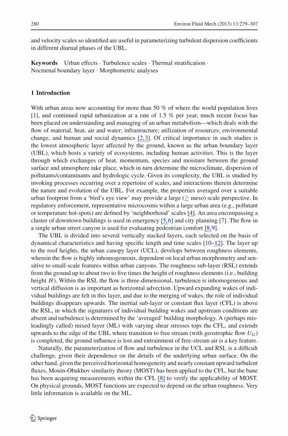
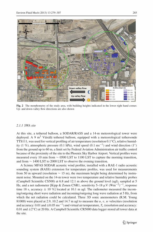
Fig. 2 The morphometry of the study area, with building heights indicated in the lower right hand corner.Up- and down-valley flow directions are also shown

2.1.1 SWA site

At this site, a tethered balloon, a SODAR/RASS and a 14-m meteorological tower weredeployed. A 9 m3 Väisälä tethered balloon, equipped with a meteorological tethersondeTTS111, was used for vertical profiling of air temperature (resolution 0.1◦C), relative humid-ity (1 %), atmospheric pressure (0.1 hPa), wind speed (0.1 ms−1) and wind direction (1◦)from the ground up to 60 m, a limit set by Federal Aviation Administration air traffic controlbecause of the proximity of the site to the Phoenix Sky Harbor Airport. Vertical profiles weremeasured every 10 min from ∼ 0500 LST to 1100 LST to capture the morning transition,and from ∼ 1400 LST to 2000 LST to observe the evening transition.

A Scintec MFAS SODAR acoustic wind profiler, installed with a RAE-1 radio acousticsounding system (RASS) extension for temperature profiles, was used for measurementsfrom 50 m upward (resolution ∼ 15 m), the maximum height being determined by instru-ment noise. Mounted on the 14-m tower were two temperature and relative humidity probes(Campbell Scientific CS500) at 6.8 and 12.1 m above the ground level (agl), sampled at 5Hz, and a net radiometer [Kipp & Zonen CNR1, sensitivity 5–18 µV (Wm−2)−1, responsetime 18 s, accuracy ± 10 %] located at 10.1 m agl. The radiometer measured the incom-ing/outgoing short wave radiation and incoming/outgoing long wave radiation at 5 Hz, fromwhich the net radiation could be calculated. Three 3D sonic anemometers (R.M. Young81000) were placed at 2.9, 10.2 and 14.7 m agl to measure the u, v, w velocities (resolutionand accuracy: 0.01 and ±0.05 ms−1) and virtual air temperature, Tv (resolution and accuracy:0.01 and ±2◦C) at 20 Hz. A Campbell Scientific CR5000 data logger stored all tower data atthe site.

123

286 Environ Fluid Mech (2013) 13:279–307

2.1.2 HD site

This site also had a 14-m tower with two thermistors and relative humidity sensors mounted at6.9 and 12.2 m agl, and three sonic anemometers (Campbell Scientific CSAT3; R.M. Young81000) at 3.0, 10.3 and 14.6 m. All data were stored in a CR3000 data logger. Also placed at anearby location was a Väisälä CL31 ceilometer, which can detect multiple cloud layers in theatmosphere up to several kilometers. The height of the convective boundary layer could beestimated by post-processing of data using standard algorithms provided with the instrument.

2.2 Morphological parameters

Given the locational dependence of Eq. 5, a detailed investigation of site morphology wasrequired prior to any flow analyses. The morphology analysis provided, with an adequatedegree of accuracy for full-scale conditions, relevant parameters required for interpretingthe results. The study area varied from bare land with sparse urban development directlynorth of each site to a residential and industrial neighborhood to the south of the sites, withthe fully-developed urban settlement of the city of Phoenix located a few kilometers north-west. For the analysis, the study area was subdivided into two main sectors, considering thatsurface roughness characteristics approaching from the west and east are different. Usingthree-dimensional digital building data, known as urban digital elevation models (DEMs),the methodology described in Di Sabatino et al. [35] was used to calculate relevant flowparameters.

The methodology consists of two parts: direct building data analysis and calculationof synthetic morphometric parameters using MATLAB based algorithms. Urban DEMs,typically produced in a CAD© format, are transformed into a gray-scale image (raster format)in which each pixel has a color value that is proportional to the building height. Imageprocessing techniques are then used to calculate the morphometric parameters (see Ratti et al.[36] for a review), namely the effective building height H , frontal area density λ f andplanar area density λp; these were used to estimate z0 and d . Two different DEMs, eachencompassing a set of buildings surrounding a site, were analyzed separately for the twomain flow directions of interest (270 ± 22.5◦ for westerly winds and 90 ± 22.5◦ for easterlywinds). The radii for the sites were selected to be greater than the adjustment length scale(Sect. 2.3). The ±22.5◦ arcs used for the calculations of H, λ f , and λp are shown in Fig. 2,and z0 and d were estimated using the formulae of Macdonald et al. [37]:

d

H= 1 + (

λp − 1)α−λp (6)

z0

H=

[1 − d

H

]exp

{

−[

0.5βCDλ f

κ2

(1 − d

H

)]−0.5}

, (7)

with α = 4.43, β = 1.0, κ = 0.4 (the von Karman constant), and drag coefficient CD ∼ 1.This methodology is known to give better estimates than other geometric-based parameteri-zations [38]. Table 2 reports building statistics and related morphometric parameters for thetwo sites, based on two wind directions.

Table 2 suggests that the roughness canopy in point is rather sparse. According to thespecifications of Grimmond and Oke [39], z0/H and d/H , as functions of λp and λ f , ingeneral fall in the category of suburban areas. Accordingly, for westerly flow, both sitesare in the wake interference regime, and for easterly flow both are in the isolated roughnessregime. Although z0/H and d/H are calculated from λp and λ f rather than profile mea-

123

Environ Fluid Mech (2013) 13:279–307 287

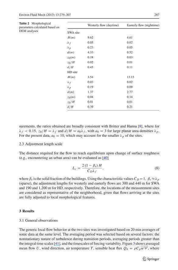
Table 2 Morphologicalparameters calculated based onDEM analyses

Westerly flow (daytime) Easterly flow (nighttime)

SWA site

H(m) 9.62 4.61

λ f 0.05 0.02

λp 0.23 0.05

d(m) 4.33 0.52

z0(m) 0.18 0.03

z0/H 0.02 0.01

d/H 0.45 0.11

HD site

H(m) 3.54 13.13

λ f 0.03 0.02

λp 0.19 0.09

d(m) 1.37 2.77

z0(m) 0.04 0.14

z0/H 0.01 0.01

d/H 0.39 0.21

surements, the ratios obtained are broadly consistent with Britter and Hanna [8], where forλ f < 0.15, z0/H = λ f and d/H = a0λ f , with a0 = 3 for large planar area densities λp .For the present data, a0 = 10, which may account for the smaller λp of the sites.

2.3 Adjustment length scale

The distance required for the flow to reach equilibrium upon change of surface roughness(e.g., encountering an urban area) can be evaluated as [40]

Lc = 2 (1 − βs) H

CDλ f, (8)

whereβs is the solid fraction of the buildings. Using the characteristic values CD =1, βs ≈λp

(sparse), the adjustment lengths for westerly and easterly flows are 300 and 440 m for SWAand 190 and 1,200 m for HD, respectively. Therefore, the locations of the measurement sitesare considered as representative of the neighborhood, given that flows arriving at the sitesare fully adjusted to local morphological features.

3 Results

3.1 General observations

The generic local flow behavior at the two sites was investigated based on 20 min averages ofsonic data at the same level. The averaging period was selected based on several factors: thenonstationary nature of turbulence during transition periods, averaging periods greater thanthe integral time scales [41], and the timescales of forcing variability. Figure 3 shows averagedmean flow U , wind direction, air temperature T , sensible heat flux Qh = ρC pw′θ ′, where

123

288 Environ Fluid Mech (2013) 13:279–307

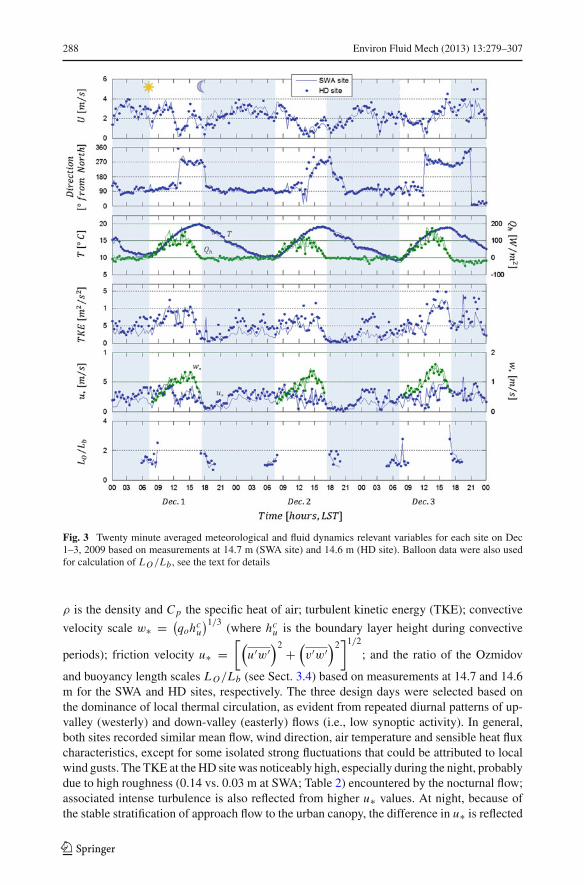
Fig. 3 Twenty minute averaged meteorological and fluid dynamics relevant variables for each site on Dec1–3, 2009 based on measurements at 14.7 m (SWA site) and 14.6 m (HD site). Balloon data were also usedfor calculation of L O/Lb , see the text for details

ρ is the density and C p the specific heat of air; turbulent kinetic energy (TKE); convective

velocity scale w∗ = (qohc

u

)1/3 (where hcu is the boundary layer height during convective

periods); friction velocity u∗ =[(

u′w′)2 +

(v′w′

)2]1/2

; and the ratio of the Ozmidov

and buoyancy length scales L O/Lb (see Sect. 3.4) based on measurements at 14.7 and 14.6m for the SWA and HD sites, respectively. The three design days were selected based onthe dominance of local thermal circulation, as evident from repeated diurnal patterns of up-valley (westerly) and down-valley (easterly) flows (i.e., low synoptic activity). In general,both sites recorded similar mean flow, wind direction, air temperature and sensible heat fluxcharacteristics, except for some isolated strong fluctuations that could be attributed to localwind gusts. The TKE at the HD site was noticeably high, especially during the night, probablydue to high roughness (0.14 vs. 0.03 m at SWA; Table 2) encountered by the nocturnal flow;associated intense turbulence is also reflected from higher u∗ values. At night, because ofthe stable stratification of approach flow to the urban canopy, the difference in u∗ is reflected

123

Environ Fluid Mech (2013) 13:279–307 289

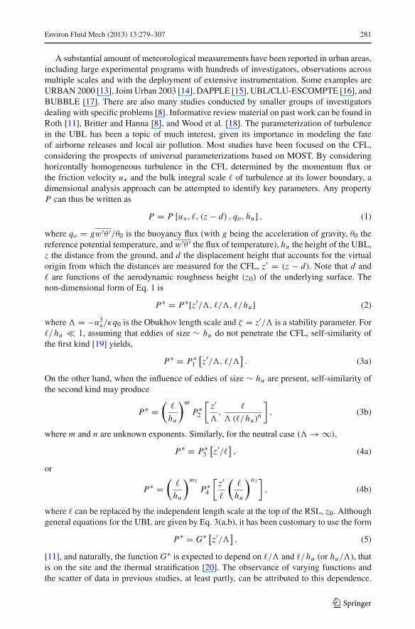
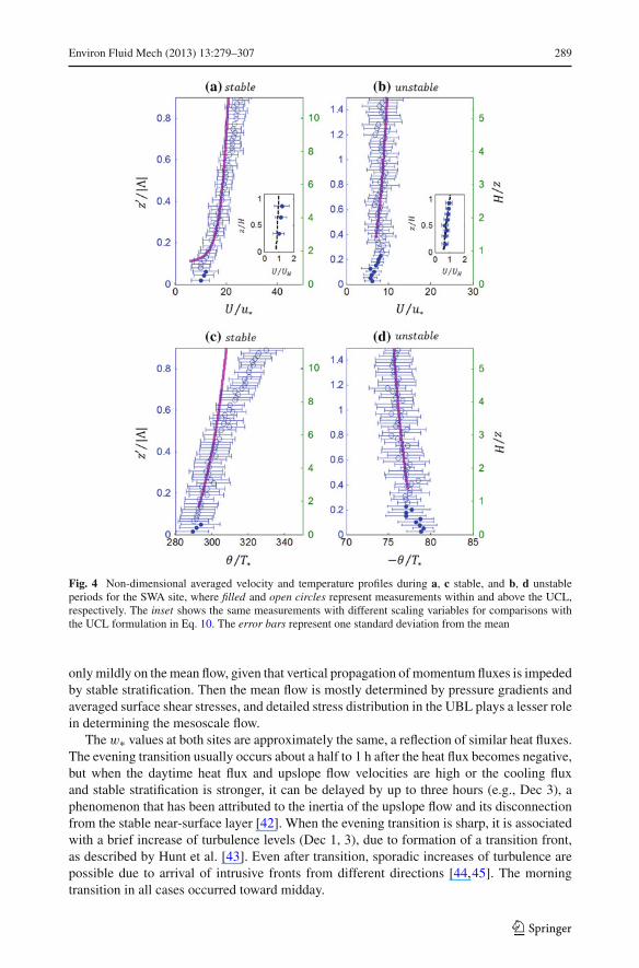
Fig. 4 Non-dimensional averaged velocity and temperature profiles during a, c stable, and b, d unstableperiods for the SWA site, where filled and open circles represent measurements within and above the UCL,respectively. The inset shows the same measurements with different scaling variables for comparisons withthe UCL formulation in Eq. 10. The error bars represent one standard deviation from the mean

only mildly on the mean flow, given that vertical propagation of momentum fluxes is impededby stable stratification. Then the mean flow is mostly determined by pressure gradients andaveraged surface shear stresses, and detailed stress distribution in the UBL plays a lesser rolein determining the mesoscale flow.

Thew∗ values at both sites are approximately the same, a reflection of similar heat fluxes.The evening transition usually occurs about a half to 1 h after the heat flux becomes negative,but when the daytime heat flux and upslope flow velocities are high or the cooling fluxand stable stratification is stronger, it can be delayed by up to three hours (e.g., Dec 3), aphenomenon that has been attributed to the inertia of the upslope flow and its disconnectionfrom the stable near-surface layer [42]. When the evening transition is sharp, it is associatedwith a brief increase of turbulence levels (Dec 1, 3), due to formation of a transition front,as described by Hunt et al. [43]. Even after transition, sporadic increases of turbulence arepossible due to arrival of intrusive fronts from different directions [44,45]. The morningtransition in all cases occurred toward midday.

123

290 Environ Fluid Mech (2013) 13:279–307

3.2 Mean velocity and temperature profiles

The balloon data were used to obtain vertical profiles of mean velocity U and potentialtemperature θ for stable (a, c) and unstable (b, d) periods at the SWA site (Fig. 4). The profileswere selected from Dec 1, 2 and 3, and were categorized into ‘stability classes’ accordingto the background averaged Brunt–Väisälä (buoyancy) frequency N 2 = (g/θ0) (∂θ/∂z)between 30 and 50 m. For N 2 > 0.001s−2 the flow was considered stable, for N 2 <

−0.001s−2 unstable, and for −0.001s−2 < N 2 < 0.001s−2 neutral. For both nocturnal anddaytime periods, this N 2 corresponded to that of the CFL (z/H > 2), and therefore is notdirectly affected by surface inhomogeneity. Figure 4 displays an average of individual profilesfor each stability class, plotted as a function of the non-dimensional effective height z′/ |�|based on the balloon data. The scaling parameter � was selected to illustrate the regions ofdifferent dynamical characteristics (e.g., shear dominated at z < � and buoyancy dominatedfor z > �) and to validate MOST. The right ordinate shows an alternative normalizationz/H . The error bars refer to one standard deviation from the mean values. The frictionvelocity u∗ and the temperature scale T∗ were calculated based on the 14.7 m sonic, whichis representative of CFL. For completeness, Fig. 5 shows a vertically extended plot (up to ∼150 m agl) to illustrate the consistency of SODAR/RASS and tethered balloon profiles.

Shown in Fig. 4 are the vertical profiles predicted by MOST, which is strictly valid in theCFL z � 2H (see Sect. 3.3.1). We have used the canonical profiles [46],

u (z) = u∗κ

ln

(z′

z0

)(9a)

for neutral,

u (z) = u∗κ

[ln

(z′

z0

)− 5

z

�

](9b)

for stable, and

u (z) = u∗κ

[ln

(z′

z0

)− ψm

](9c)

for unstable cases, where ψm is the integral of(1 − (1 + 16 |ζ |)−1/4) /ζ . During stable

periods (Fig. 4a, c), the data accord with Eq. 9b well up to ∼ �/2 (2H � z � 6H) andclearly deviate for z′ � 0.6 |�|, where z0 and d are from Table 2.

In the stable boundary layer, mechanical turbulence dominates to a height on the order�, and this limiting height may be identified as � ≈ (0.5 − 0.6)�. For z > �, the flow isbuoyancy dominated, including strong internal waves (see the lidar observations of Wang etal. [47] for the SBL over Oklahoma City). This aspect can be further studied by calculating

relevant length scales of stratified turbulence, such as the Ozmidov [L0 = (ε/N 3

)1/2] andbuoyancy [Lb = σw/N ] length scales; here ε is the rate of dissipation of turbulent kineticenergy and σw is the vertical rms velocity. They represent the vertical scale where the buoy-ancy starts strongly influencing turbulence [48]. According to laboratory studies [49,50],the vertical scale of a fully turbulent region generated mechanically in a backdrop of stablestratification and shear, analogous to the lower UBL, is given by h p ≈ 3Lb (and this scalingalso holds true even for shear-free turbulence [51]). Beyond this height, turbulence is stronglydamped by buoyancy effects, essentially disconnecting different horizontal layers stacked upvertically. Ensuing failure of MOST can be estimated by inspecting profiles of Fig. 4, and thisoccurs at a height z′/� ∼ 0.6 which corresponds to z ∼ 30 m, consistent with Lb ≈10 m.

123

Environ Fluid Mech (2013) 13:279–307 291

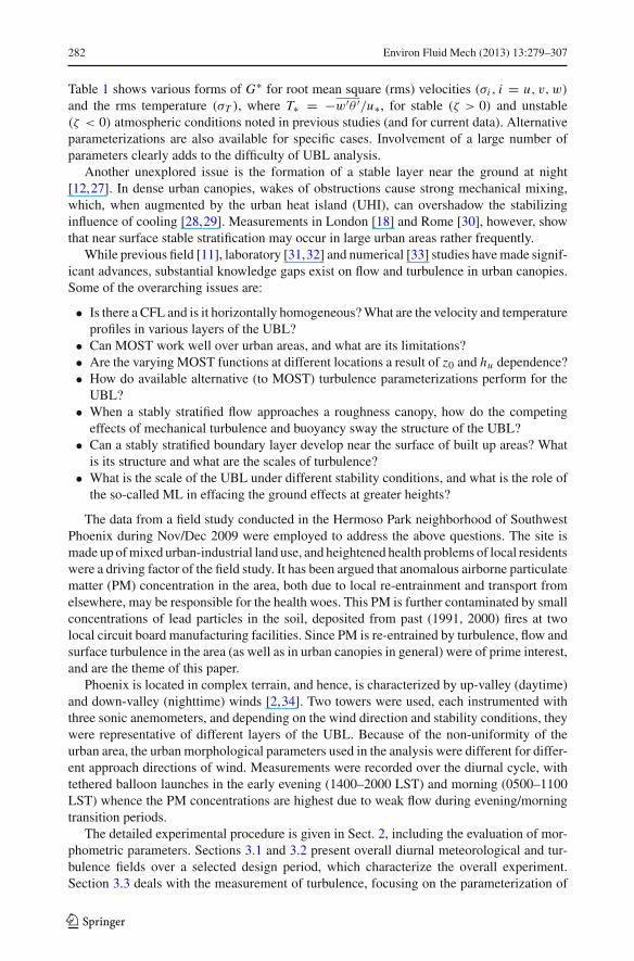
Fig. 5 Individual velocity and temperature profiles (single realizations) during stable and unstable periods atthe SWA site. Filled circles are sodar data, and open circles are from the tethered balloon

Beyond 3Lb the fluxes are damped by stratification, and u∗ is not a suitable scale (also seeSect. 3.4).

Conversely, in the convective regime, ground information first propagates upward bymechanical and then by convective turbulence. Hence, MOST is expected to be valid overmuch larger vertical extents (� 60m), as evident from Fig. 4b, d.

Neutral conditions last only for a short duration, usually during transition periods. Corre-sponding data from the morning transition with prevalent downslope flow is shown in Fig. 6,with Eq. 9c fitted over 2 < z/H < 11. The existence of a logarithmic layer is indicated,which allows calculation of profile-based roughness height z0p ≈ 0.12 m, which is aboutfour times that computed via DEM (z0 ≈ 0.03m). Note that z0 calculated from the DEM

123

292 Environ Fluid Mech (2013) 13:279–307

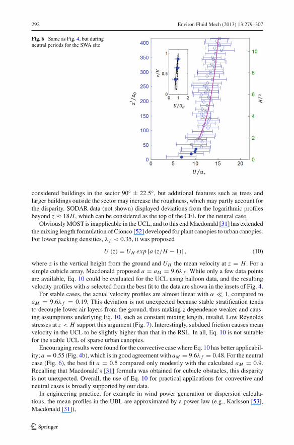
Fig. 6 Same as Fig. 4, but duringneutral periods for the SWA site

considered buildings in the sector 90◦ ± 22.5◦, but additional features such as trees andlarger buildings outside the sector may increase the roughness, which may partly account forthe disparity. SODAR data (not shown) displayed deviations from the logarithmic profilesbeyond z ≈ 18H , which can be considered as the top of the CFL for the neutral case.

Obviously MOST is inapplicable in the UCL, and to this end Macdonald [31] has extendedthe mixing length formulation of Cionco [52] developed for plant canopies to urban canopies.For lower packing densities, λ f < 0.35, it was proposed

U (z) = UH exp [a (z/H − 1)] , (10)

where z is the vertical height from the ground and UH the mean velocity at z = H . For asimple cubicle array, Macdonald proposed a = aM = 9.6λ f . While only a few data pointsare available, Eq. 10 could be evaluated for the UCL using balloon data, and the resultingvelocity profiles with a selected from the best fit to the data are shown in the insets of Fig. 4.

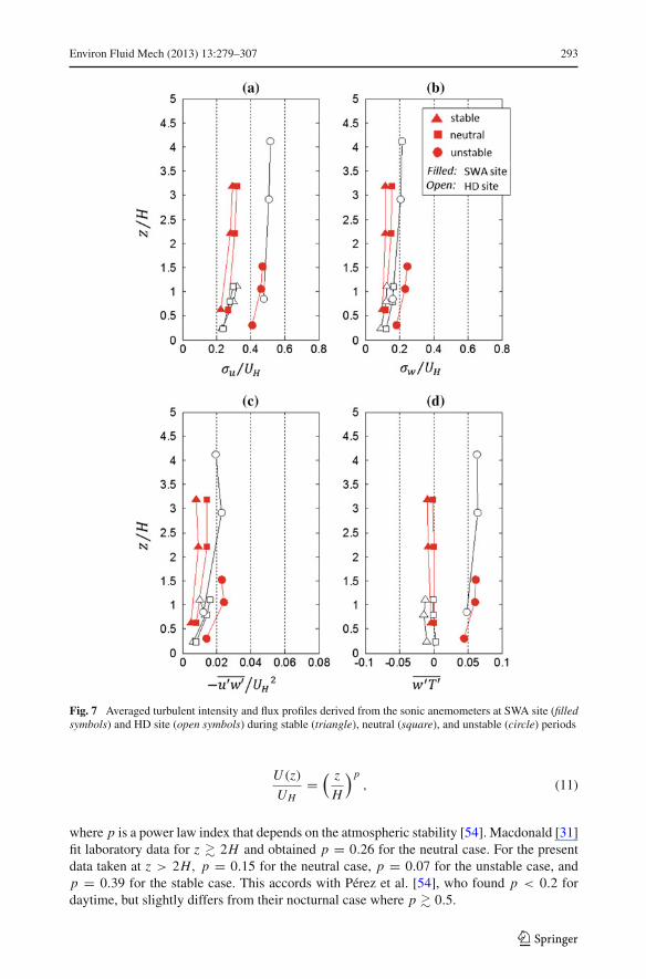
For stable cases, the actual velocity profiles are almost linear with α � 1, compared toaM = 9.6λ f = 0.19. This deviation is not unexpected because stable stratification tendsto decouple lower air layers from the ground, thus making z dependence weaker and caus-ing assumptions underlying Eq. 10, such as constant mixing length, invalid. Low Reynoldsstresses at z < H support this argument (Fig. 7). Interestingly, subdued friction causes meanvelocity in the UCL to be slightly higher than that in the RSL. In all, Eq. 10 is not suitablefor the stable UCL of sparse urban canopies.

Encouraging results were found for the convective case where Eq. 10 has better applicabil-ity; a = 0.55 (Fig. 4b), which is in good agreement with aM = 9.6λ f = 0.48. For the neutralcase (Fig. 6), the best fit a = 0.5 compared only modestly with the calculated aM = 0.9.Recalling that Macdonald’s [31] formula was obtained for cubicle obstacles, this disparityis not unexpected. Overall, the use of Eq. 10 for practical applications for convective andneutral cases is broadly supported by our data.

In engineering practice, for example in wind power generation or dispersion calcula-tions, the mean profiles in the UBL are approximated by a power law (e.g., Karlsson [53],Macdonald [31]),

123

Environ Fluid Mech (2013) 13:279–307 293

Fig. 7 Averaged turbulent intensity and flux profiles derived from the sonic anemometers at SWA site (filledsymbols) and HD site (open symbols) during stable (triangle), neutral (square), and unstable (circle) periods

U (z)

UH=

( z

H

)p, (11)

where p is a power law index that depends on the atmospheric stability [54]. Macdonald [31]fit laboratory data for z � 2H and obtained p = 0.26 for the neutral case. For the presentdata taken at z > 2H, p = 0.15 for the neutral case, p = 0.07 for the unstable case, andp = 0.39 for the stable case. This accords with Pérez et al. [54], who found p < 0.2 fordaytime, but slightly differs from their nocturnal case where p � 0.5.

123

294 Environ Fluid Mech (2013) 13:279–307

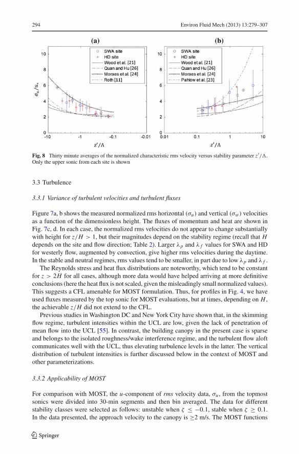
Fig. 8 Thirty minute averages of the normalized characteristic rms velocity versus stability parameter z′/�.Only the upper sonic from each site is shown

3.3 Turbulence

3.3.1 Variance of turbulent velocities and turbulent fluxes

Figure 7a, b shows the measured normalized rms horizontal (σu) and vertical (σw) velocitiesas a function of the dimensionless height. The fluxes of momentum and heat are shown inFig. 7c, d. In each case, the normalized rms velocities do not appear to change substantiallywith height for z/H > 1, but their magnitudes depend on the stability regime (recall that Hdepends on the site and flow direction; Table 2). Larger λp and λ f values for SWA and HDfor westerly flow, augmented by convection, give higher rms velocities during the daytime.In the stable and neutral regimes, rms values tend to be smaller, in part due to low λp and λ f .

The Reynolds stress and heat flux distributions are noteworthy, which tend to be constantfor z > 2H for all cases, although more data would have helped arriving at more definitiveconclusions (here the heat flux is not scaled, given the misleadingly small normalized values).This suggests a CFL amenable for MOST formulation. Thus, for profiles in Fig. 4, we haveused fluxes measured by the top sonic for MOST evaluations, but at times, depending on H ,the achievable z/H did not extend to the CFL.

Previous studies in Washington DC and New York City have shown that, in the skimmingflow regime, turbulent intensities within the UCL are low, given the lack of penetration ofmean flow into the UCL [55]. In contrast, the building canopy in the present case is sparseand belongs to the isolated roughness/wake interference regime, and the turbulent flow aloftcommunicates well with the UCL, thus elevating turbulence levels in the latter. The verticaldistribution of turbulent intensities is further discussed below in the context of MOST andother parameterizations.

3.3.2 Applicability of MOST

For comparison with MOST, the u-component of rms velocity data, σu , from the topmostsonics were divided into 30-min segments and then bin averaged. The data for differentstability classes were selected as follows: unstable when ζ ≤ −0.1, stable when ζ ≥ 0.1.In the data presented, the approach velocity to the canopy is ≥2 m/s. The MOST functions

123

Environ Fluid Mech (2013) 13:279–307 295

Table 3 Turbulence parameterizations

Authors Parameterization Conditions

Hanna and Britter [56] σu/u∗ = 2.4; σv/u∗ = 1.9; σw/u∗ = 1.3 Neutral

André et al. [57] σA =(

1.75u2∗ + w2∗)1/2

Convective

Deardorff [58] σD =(w3∗ + η3u3∗

)1/3, η = 1.8 Convective

Clarke et al. [59] σC = Cu

(w3∗ + u3∗λmax/ (κz)

)1/3,Cu ≈ 0.4 − 0.6 Convective, λmax

is the energycontaining wavelength

derived are given in Table 1 and the data are plotted in Fig. 8, together with some of thepreviously reported parameterizations that have semblance to the functions obtained in ourwork. Referencing Table 2, for the unstable case, the top sonics at HD and SWA are at z =4H and z = 1.5 H, respectively, and for the stable case, they are at z = 1.9 H and z = 3.2 H.In both cases, the data from the two sites collapse reasonably well with u∗, pointing to theusefulness of MOST (thus giving credence to underlying assumptions). The present data isclosest to Moraes et al. [24], who considered data from above a rice plantation in a valley. Allseem to converge to a constant neutral value σu/u∗ ≈ 2.2, which is similar to that reportedin numerous studies [8,56]. Overall, the disparity between the MOST functions in Table 1points to the non-universality of MOST when applied to the UBL, consistent with the notionof site dependence of G∗ in Eq. 5.

3.3.3 Alternative parameterizations for convective turbulence

Alternative parameterizations may be sought for scaling turbulence statistics of the UBL.Table 3 presents parameterizations proposed by André et al. [57] for convective boundarylayers (σA), Deardorff [58] for oceanic boundary layers (σD), and that by Clarke et al. [59]for urban boundary layers (σC ). They all utilize a composite of mechanical and buoyancyproduction of turbulence, represented by the friction and convective velocities, respectively.

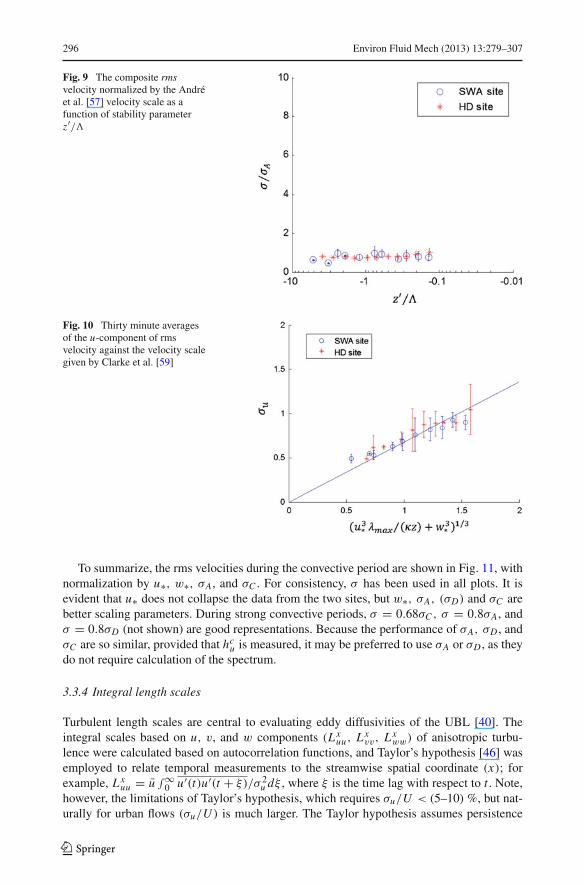
Figure 9 shows the composite rms velocity σ = √T K E scaled by the André et al. [57]

parameterization σA as a function of the stability parameter ζ for unstable cases; the resultsfor the upper sonic are shown. It appears that σ/σA is a constant (≈ 0.8) for unstable caseswith an excellent collapse of data. When σ is scaled with σD , a collapse similar to that inFig. 9 was obtained (not shown). A combination of friction and convective velocities appearsto be a useful parameterization for convective periods, arguably better than the utility ofMOST shown in Fig. 8a. The bane, however, is the necessity of hc

u in the former.The Clarke et al. [59] parameterization also produced a good correlation with the rms

velocity σu (Fig. 10) when plotted for the most vigorous convective period (1230–1700LST). Here the energy containing wavelength,λmax , was obtained by calculating longitudinalvelocity spectrum for 5 min segments, averaging over a total length of 30 min, and locatingthe wavelength at the spectral peak. Clarke et al. [59] found Cu ≈0.4–0.6, but it was notedto be a weak function of urban morphology. The current data has a fit of Cu ≈ 0.68, whichis close to the range previously found, and the variation can be attributed to morphologicaldifferences between the cases.

123

296 Environ Fluid Mech (2013) 13:279–307

Fig. 9 The composite rmsvelocity normalized by the Andréet al. [57] velocity scale as afunction of stability parameterz′/�

Fig. 10 Thirty minute averagesof the u-component of rmsvelocity against the velocity scalegiven by Clarke et al. [59]

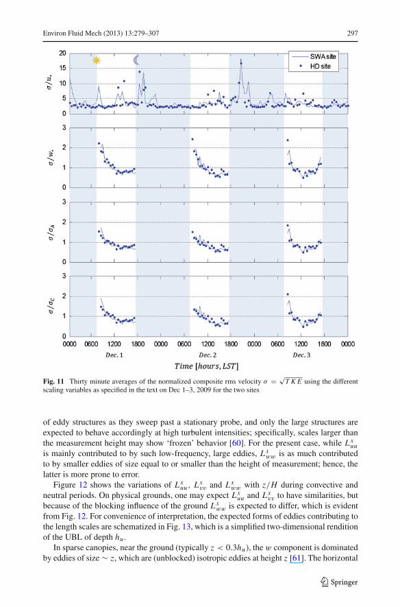
To summarize, the rms velocities during the convective period are shown in Fig. 11, withnormalization by u∗, w∗, σA, and σC . For consistency, σ has been used in all plots. It isevident that u∗ does not collapse the data from the two sites, but w∗, σA, (σD) and σC arebetter scaling parameters. During strong convective periods, σ = 0.68σC , σ = 0.8σA, andσ = 0.8σD (not shown) are good representations. Because the performance of σA, σD , andσC are so similar, provided that hc

u is measured, it may be preferred to use σA or σD , as theydo not require calculation of the spectrum.

3.3.4 Integral length scales

Turbulent length scales are central to evaluating eddy diffusivities of the UBL [40]. Theintegral scales based on u, v, and w components (Lx

uu, Lxvv, Lx

ww) of anisotropic turbu-lence were calculated based on autocorrelation functions, and Taylor’s hypothesis [46] wasemployed to relate temporal measurements to the streamwise spatial coordinate (x); forexample, Lx

uu = u ∫∞0 u′(t)u′(t + ξ)/σ 2

u dξ , where ξ is the time lag with respect to t . Note,however, the limitations of Taylor’s hypothesis, which requires σu/U < (5–10) %, but nat-urally for urban flows (σu/U ) is much larger. The Taylor hypothesis assumes persistence

123

Environ Fluid Mech (2013) 13:279–307 297

Fig. 11 Thirty minute averages of the normalized composite rms velocity σ = √T K E using the different

scaling variables as specified in the text on Dec 1–3, 2009 for the two sites

of eddy structures as they sweep past a stationary probe, and only the large structures areexpected to behave accordingly at high turbulent intensities; specifically, scales larger thanthe measurement height may show ‘frozen’ behavior [60]. For the present case, while Lx

uuis mainly contributed to by such low-frequency, large eddies, Lx

ww is as much contributedto by smaller eddies of size equal to or smaller than the height of measurement; hence, thelatter is more prone to error.

Figure 12 shows the variations of Lxuu, Lx

vv and Lxww with z/H during convective and

neutral periods. On physical grounds, one may expect Lxuu and Lx

vv to have similarities, butbecause of the blocking influence of the ground Lx

ww is expected to differ, which is evidentfrom Fig. 12. For convenience of interpretation, the expected forms of eddies contributing tothe length scales are schematized in Fig. 13, which is a simplified two-dimensional renditionof the UBL of depth hu .

In sparse canopies, near the ground (typically z < 0.3hu), the w component is dominatedby eddies of size ∼ z, which are (unblocked) isotropic eddies at height z [61]. The horizontal

123

298 Environ Fluid Mech (2013) 13:279–307

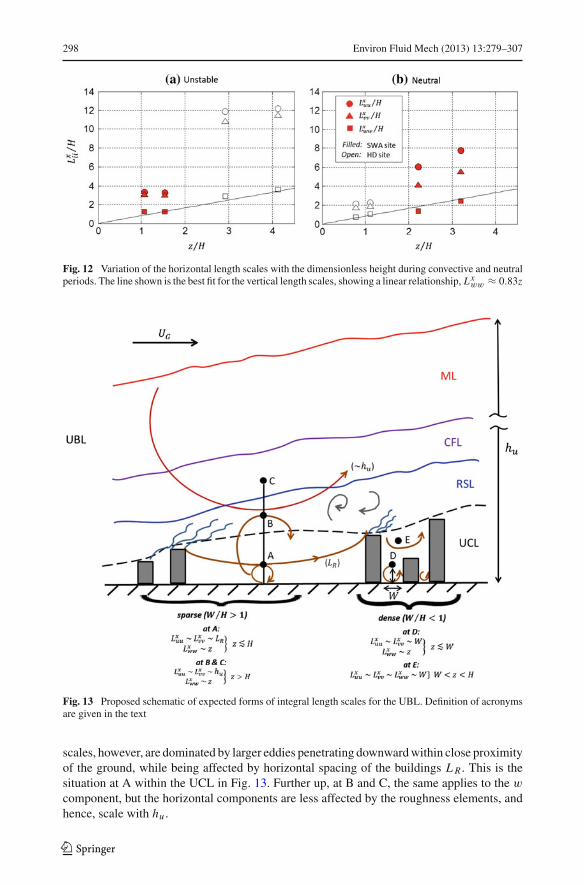
Fig. 12 Variation of the horizontal length scales with the dimensionless height during convective and neutralperiods. The line shown is the best fit for the vertical length scales, showing a linear relationship, Lx

ww ≈ 0.83z

Fig. 13 Proposed schematic of expected forms of integral length scales for the UBL. Definition of acronymsare given in the text

scales, however, are dominated by larger eddies penetrating downward within close proximityof the ground, while being affected by horizontal spacing of the buildings L R . This is thesituation at A within the UCL in Fig. 13. Further up, at B and C, the same applies to the wcomponent, but the horizontal components are less affected by the roughness elements, andhence, scale with hu .

123

Environ Fluid Mech (2013) 13:279–307 299

Fig. 14 The variation of Lxuu

and Lxvv (normalized by λ−1.8

p )with H , according to Eq. 12. Thesolid line shows the best fit forLx

uu and the dotted line is for Lxvv

On the other hand, within the UCL of dense canopies, the width of the urban canyonseverely limits the size of eddies. As before, for z < W , the rms vertical velocity is dominatedby isotropic eddies of size � z whilst the horizontal velocity is dominated by eddies of size∼ W . For z > W , isotropic motions are determined by recirculating eddies of size ∼ W , notby ∼ z, and the length scale W remains important up to z ∼ H .

The data of Fig. 12 are consistent with the scenario described above for sparse canopies.The Lx

ww component increases proportionately to z, Lxww ≈ 0.83z. Near the ground, Lx

uuand Lx

vv are somewhat higher (∼ L R) than Lxww, but in the RSL and CFL there is a rapid

increase of Lxuu and Lx

vv , perhaps approaching the order of the UBL thickness hu . Based onceilometer measurements during convection hc

u ≈ 900 m, and therefore the integral scaleabove the UCL can be represented as Lx

uu ∼ Lxvv ≈ (0.03 − 0.06) hc

u . Fernando et al. [29]argued that for the neutral case in the CFL and upper part of the RSL, the normalized turbulentquantities should be a function of the planar area density λp , and in the UCL and RSL, theyshould additionally depend on parameters such as the frontal area density λ f and frontalsolidarity λ f s . Thus, for the non-neutral case in the CFL and upper RSL, the length scalesLx

uu and Lxvv can be represented as

Lxuu

H∼ Lx

vv

H∼ F

(λp, stabili t y

) ∼ λnp�(stabili t y) , (12)

where the stability of the function� is specified using an appropriate parameter such as z′/�and/or hu/�. Note that Lx

ww is excluded, because of its sole dependence on z. Figure 14 showsthe dependence of

(Lx

uu, Lxvv

)/λn

p on H for data taken in the RSL and CFL (upper two sonics)under neutral conditions, for which � is a constant; a good agreement with Eq. 12 could beseen for n = −1.8, and the best fits are Lx

uu/λnp = 3 × 10−2 H (solid line in Fig. 14) and

Lxvv/λ

np = 2.4 × 10−2 H (dotted line). Because of the limited availability of data and the

dependence on multiple parameters, the stable and unstable cases are not discussed here.

3.4 Nocturnal urban boundary layer

The nocturnal boundary layer is one of the least understood forms of the atmospheric bound-ary layer [27], and previous studies suggest that either stable or unstable stratification mayprevail in urban areas at night. During evening transition, convective turbulence decays, thuslowering the overall turbulent intensity, leaving shear induced (mechanical) turbulence and

123

300 Environ Fluid Mech (2013) 13:279–307

Fig. 15 Individual vertical profiles of potential temperature during the development of stable stratification

UHI as contributors to σw. In sparse building canopies the UHI is negligible and when thewinds are low, the mechanical turbulence is weak, all providing conditions for stable strati-fication. This is evident from TKE measurements during the evening transition of Dec 1 and2 in Fig. 3. The development of stratification, turbulence within this stratified layer, and theheight to which ground influence propagates (nocturnal UBL height) are discussed below.

3.4.1 Development of surface stable stratification

The formation of surface stratification in the UBL can be discussed by considering theopposing influences of ground cooling and mechanical turbulence. If the cooling buoyancyflux is |q0|, then a stable layer of thickness δs can be generated by a balance between the shearproduction and (negative) buoyancy flux, |q0| ∼ σ 3

w/δs , or δs = csσ3w/ |q0|; the thickness

scale here has similarities to that of MOST but with a different velocity scale. In the oceaniccontext, Kitaigorodskii [62] proposed cs ≈ 2, and Hopfinger and Linden [63] noted, basedon laboratory experiments, cs ≈ 2 − 7 (also see the numerical experiments of Noh andFernando [64]). In urban canopies, for the stable layer to develop in the UCL, δs < H , orcs < H |q0| /σ 3

w. In selecting H , it was assumed that if the stratification does not developnear the ground, the possibility of developing it in the lower atmosphere is very low, givenenhanced turbulence at the top of the UCL due to shear-layer separation. Note that smaller|q0| and larger σ 3

w do not facilitate surface stratification.Figure 15 shows the balloon profiles for the three design days, for which the magnitudes

of H |q0| /σ 3w are ≈ 5, 2, and 0.2 for Dec 1, 2 and 3 respectively. The development of stable

stratification can be clearly seen on Dec 1 and 2, but no indications of such could be seenon Dec 3. Here σw and q0 values were obtained from sonics located in the CFL. Based onthose observations, the range for the stable criterion is cs ≈ 0.2 (no stratification) to 2 (withstratification). Taken together with the laboratory and oceanic results discussed above, cs ≈ 2is a reasonable value.

3.4.2 Turbulence in the stratified layer

Gibson [65] argued that stratification impedes the growth of turbulence when the verticalinertia forces of energy containing eddies of size Lv (i.e., σ 2

w/Lv) become the same orderas their characteristic buoyancy forces (N 2 Lv). This yields the limiting vertical length scale

123

Environ Fluid Mech (2013) 13:279–307 301

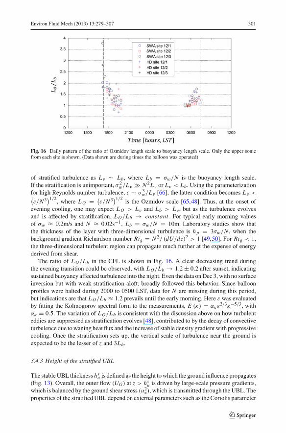
Fig. 16 Daily pattern of the ratio of Ozmidov length scale to buoyancy length scale. Only the upper sonicfrom each site is shown. (Data shown are during times the balloon was operated)

of stratified turbulence as Lv ∼ Lb, where Lb = σw/N is the buoyancy length scale.If the stratification is unimportant, σ 2

w/Lv � N 2 Lv or Lv < Lb. Using the parameterizationfor high Reynolds number turbulence, ε ∼ σ 3

w/Lv [66], the latter condition becomes Lv <(ε/N 3

)1/2, where L O = (

ε/N 3)1/2

is the Ozmidov scale [65,48]. Thus, at the onset ofevening cooling, one may expect L O > Lv and Lb > Lv , but as the turbulence evolvesand is affected by stratification, L O/Lb → constant . For typical early morning valuesof σw ≈ 0.2m/s and N ≈ 0.02s−1, Lb = σw/N = 10m. Laboratory studies show thatthe thickness of the layer with three-dimensional turbulence is h p = 3σw/N , when thebackground gradient Richardson number Rig = N 2/ (dU/dz)2 > 1 [49,50]. For Rig < 1,the three-dimensional turbulent region can propagate much further at the expense of energyderived from shear.

The ratio of L O/Lb in the CFL is shown in Fig. 16. A clear decreasing trend duringthe evening transition could be observed, with L O/Lb → 1.2 ± 0.2 after sunset, indicatingsustained buoyancy affected turbulence into the night. Even the data on Dec 3, with no surfaceinversion but with weak stratification aloft, broadly followed this behavior. Since balloonprofiles were halted during 2000 to 0500 LST, data for N are missing during this period,but indications are that L O/Lb ≈ 1.2 prevails until the early morning. Here ε was evaluatedby fitting the Kolmogorov spectral form to the measurements, E (κ) = ακε

2/3κ−5/3, withακ = 0.5. The variation of L O/Lb is consistent with the discussion above on how turbulenteddies are suppressed as stratification evolves [48], contributed to by the decay of convectiveturbulence due to waning heat flux and the increase of stable density gradient with progressivecooling. Once the stratification sets up, the vertical scale of turbulence near the ground isexpected to be the lesser of z and 3Lb.

3.4.3 Height of the stratified UBL

The stable UBL thickness hsu is defined as the height to which the ground influence propagates

(Fig. 13). Overall, the outer flow (UG) at z > hsu is driven by large-scale pressure gradients,

which is balanced by the ground shear stress (u2∗), which is transmitted through the UBL. Theproperties of the stratified UBL depend on external parameters such as the Coriolis parameter

123

302 Environ Fluid Mech (2013) 13:279–307

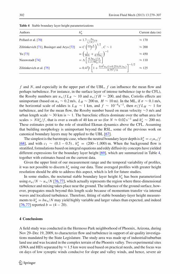
Table 4 Stable boundary layer height parameterizations

Authors hsu Current data (m)

Pollard et al. [70] = 1.7 u∗( f N )1/2

≈ 170

Zilitinkevich [71], Businger and Arya [72] = C(κu∗�

f

)1/2,C ∼ 1 ≈ 200

Yu [73] =(

130� + f

0.35u∗)−1 ≈ 450

Nieuwstadt [74] = �[

0.3u∗/ f�1+1.9hs

u/L

]≈ 110

Zilitinkevich et al. [75] = 0.4 u∗f

[1 + 0.42u∗(1+0.25�N/u∗)

0.752 f�

]−1/2≈ 125

f and N , and especially in the upper part of the UBL, f can influence the mean flow andperhaps turbulence. For instance, in the surface layer of intense turbulence (up to the CFL),the Rossby numbers are u∗/ f L R ∼ 10 and u∗/ f H ∼ 200, and thus, Coriolis effects areunimportant (based on u∗ ∼ 0.2 m/s, L R ∼ 200 m, H ∼ 10 m). In the ML, if σ ∼ 0.1 m/s,the horizontal scale of eddies is L H ∼ 1 km, and f ∼ 10−4s−1, then σ/ f L H ∼ 1 forturbulence, and for the mean flow, the Rossby number based on mean velocity ∼3 m/s andurban length scale ∼ 30 km is ∼ 1. The baroclinic effects dominate over the urban area forscales > Nhs

u/ f , that is over a swath of 40 km or so (for N ≈ 0.02 s−1 and hsu ∼ 200 m).

These estimates point to the role of stratified Ekman dynamics above the CFL. Assumingthat building morphology is unimportant beyond the RSL, some of the previous work oncanonical boundary layers may be applied to the UBL [67].

The simplest is the barotropic case, where the neutral boundary layer depth is hnu = c1u∗/ f

[68], and with c1 ∼ (0.1 − 0.5) , hnu = (200−1,000)m. When the background flow is

stratified, formulations based on integral equations and eddy diffusivity concepts have yieldeddifferent expressions for the boundary layer height [69], which are summarized in Table 4,together with estimates based on the current data.

Given the upper limit of our measurement range and the temporal variability of profiles,it was not possible to discern hs

u using our data. Time averaged profiles with greater heightresolution should be able to address this aspect, which is left for future studies.

In some studies, the nocturnal stable boundary layer height hsu has been parameterized

using σw/N ∼ u∗/N [76,77], which actually represents the region where three-dimensionalturbulence and mixing takes place near the ground. The influence of the ground surface, how-ever, propagates much beyond this length scale because of momentum transfer via internalwaves and localized turbulence. Therefore, fitting of stable boundary-layer height measure-ments to hs

u = bu∗/N may yield highly variable and larger values than expected, and indeed[76,77] reported b = (4 − 20).

4 Conclusions

A field study was conducted in the Hermoso Park neighborhood of Phoenix, Arizona, duringNov 29–Dec 19, 2009, to characterize flow and turbulence in support of air quality investiga-tions mandated by the State Legislature. The study area was made up of industrial/suburbanland use and was located in the complex terrain of the Phoenix valley. Two experimental sites(SWA and HD) separated by ≈ 1.5 km were used based on practical needs, and the focus wason days of low synoptic winds conducive for slope and valley winds, and hence, severe air

123

Environ Fluid Mech (2013) 13:279–307 303

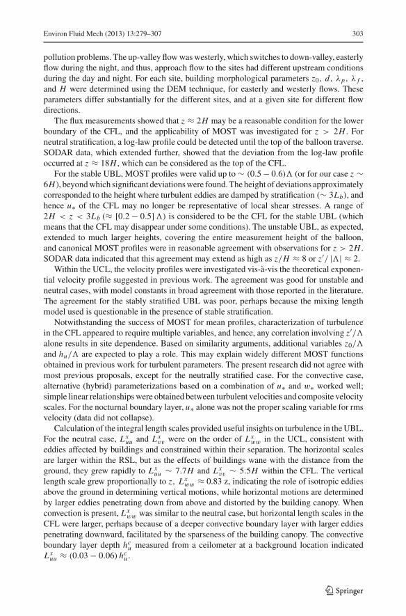
pollution problems. The up-valley flow was westerly, which switches to down-valley, easterlyflow during the night, and thus, approach flow to the sites had different upstream conditionsduring the day and night. For each site, building morphological parameters z0, d, λp, λ f ,and H were determined using the DEM technique, for easterly and westerly flows. Theseparameters differ substantially for the different sites, and at a given site for different flowdirections.

The flux measurements showed that z ≈ 2H may be a reasonable condition for the lowerboundary of the CFL, and the applicability of MOST was investigated for z > 2H . Forneutral stratification, a log-law profile could be detected until the top of the balloon traverse.SODAR data, which extended further, showed that the deviation from the log-law profileoccurred at z ≈ 18H , which can be considered as the top of the CFL.

For the stable UBL, MOST profiles were valid up to ∼ (0.5 − 0.6)� (or for our case z ∼6H ), beyond which significant deviations were found. The height of deviations approximatelycorresponded to the height where turbulent eddies are damped by stratification (∼ 3Lb), andhence u∗ of the CFL may no longer be representative of local shear stresses. A range of2H < z < 3Lb (≈ [0.2 − 0.5]�) is considered to be the CFL for the stable UBL (whichmeans that the CFL may disappear under some conditions). The unstable UBL, as expected,extended to much larger heights, covering the entire measurement height of the balloon,and canonical MOST profiles were in reasonable agreement with observations for z > 2H .SODAR data indicated that this agreement may extend as high as z/H ≈ 8 or z′/ |�| ≈ 2.

Within the UCL, the velocity profiles were investigated vis-à-vis the theoretical exponen-tial velocity profile suggested in previous work. The agreement was good for unstable andneutral cases, with model constants in broad agreement with those reported in the literature.The agreement for the stably stratified UBL was poor, perhaps because the mixing lengthmodel used is questionable in the presence of stable stratification.

Notwithstanding the success of MOST for mean profiles, characterization of turbulencein the CFL appeared to require multiple variables, and hence, any correlation involving z′/�alone results in site dependence. Based on similarity arguments, additional variables z0/�

and hu/� are expected to play a role. This may explain widely different MOST functionsobtained in previous work for turbulent parameters. The present research did not agree withmost previous proposals, except for the neutrally stratified case. For the convective case,alternative (hybrid) parameterizations based on a combination of u∗ and w∗ worked well;simple linear relationships were obtained between turbulent velocities and composite velocityscales. For the nocturnal boundary layer, u∗ alone was not the proper scaling variable for rmsvelocity (data did not collapse).

Calculation of the integral length scales provided useful insights on turbulence in the UBL.For the neutral case, Lx

uu and Lxvv were on the order of Lx

ww in the UCL, consistent witheddies affected by buildings and constrained within their separation. The horizontal scalesare larger within the RSL, but as the effects of buildings wane with the distance from theground, they grew rapidly to Lx

uu ∼ 7.7H and Lxvv ∼ 5.5H within the CFL. The vertical

length scale grew proportionally to z, Lxww ≈ 0.83 z, indicating the role of isotropic eddies

above the ground in determining vertical motions, while horizontal motions are determinedby larger eddies penetrating down from above and distorted by the building canopy. Whenconvection is present, Lx

ww was similar to the neutral case, but horizontal length scales in theCFL were larger, perhaps because of a deeper convective boundary layer with larger eddiespenetrating downward, facilitated by the sparseness of the building canopy. The convectiveboundary layer depth hc

u measured from a ceilometer at a background location indicatedLx

uu ≈ (0.03 − 0.06) hcu .

123

304 Environ Fluid Mech (2013) 13:279–307

A condition for stable stratification in the lower UBL was proposed, H |q0| /σ 3w > cs ,

where cs ≈ 2 was identified. Previous work shows that when turbulence is arrested bybuoyancy, certain relationships ought to prevail between specific length scales, in particular,between the Ozmidov scale and buoyancy scale. For the case studied, these relationships wereachieved in the evening, and presumably maintained until the morning transition, pointingto quasi-stationary, buoyancy-dominated turbulence in the UBL. This may not be viable fordensely built urban canopies that are dominated by the urban heat island phenomenon and/orwhen the criterion for the development of stratification is not satisfied.

Acknowledgements The experiments described in this paper were funded by the Arizona Department ofEnvironmental Quality as part of the Hermoso Park Study. The data were analyzed with the support ofthe National Science Foundation CMG Program and the Office of Naval Research Award # N00014-11-1-0709, Mountain Terrain Atmospheric Modeling and Observations (MATERHORN) Program. The authorsare grateful to Dr. Laura Leo for assistance in the morphometric analysis and to the students at Arizona StateUniversity for their help in setting up the equipment and running balloon flights.

References

1. UNEP. Population Division of the Department of Economic and Social Affairs of United Nations Secre-tariat (2011) World Population Prospects: The 2010 Revision, Highlights and Advanced Tables.WorkingPaper ESA/P/WP.220, 142 pp. [Available online at http://www.esa.un.org/unpd/wpp/Documentation/pdf/WPP2010_Highlights.pdf]

2. Fernando HJS, Lee SM, Anderson J, Princevac M, Pardyjak E, Grossman-Clarke S (2001) Urban fluidmechanics: air circulation and contaminant dispersion in cities. Environ Fluid Mech 1:107–164. doi:10.1023/A:1011504001479

3. Li K, Zhang P, Crittenden JC, Guhathakurta S, Chen Y, Fernando HJS, Sawhney A, McCartney P, GrimmN, Kahhat R, Joshi H, Konjevod G, Choi Y-J, Fonseca E, Allenby B, Gerrity D, Torrens PM (2007) Devel-opment of a framework for quantifying the environmental impacts of urban development and constructionpractices. Environ Sci Technol 41:5130–5136. doi:10.1021/es062481d

4. Ching JS, Dupont S, Gilliam R, Burian S, Tang R (2004) Neighborhood scale air quality modeling inHouston using urban canopy parameters in MM5 and CMAQ with improved characterization of mesoscalelake-land breeze circulation. In: Proceeding of 5th Symposium of Urban Environment. Vancouver, August23–27

5. Settles GS (2006) Fluid mechanics and homeland security. Annu Rev Fluid Mech 38:87–1106. Andrews MJ, Ginstein FF, Kwicklis E, Linn R (2012) Security and environmental fluid dynamics. In:

Fernando HJS (ed) Handbook of environmental fluid dynamics vol 1. CRC Press, Boca Raton, pp 107–1217. Hang J, Li Y, Sandberg M, Buccolieri R, Di Sabatino S (2012) The influence of building height variability

on pollutant dispersion and pedestrian ventilation in idealized high-rise urban areas. Build Environ 56:346–360

8. Britter RE, Hanna SR (2003) Flow and dispersion in urban areas. Annu Rev Fluid Mech 35:469–496.doi:10.1146/annurev.fluid.35.101101.161147

9. Britter RE, Di Sabatino S (2012) Flow through urban canopies. In: Fernando HJS (ed) Handbook ofenvironmental fluid dynamics vol 2. CRC Press, Boca Raton, pp 85–96

10. Oke TR (1988) Boundary layer climates. Routledge, New York11. Roth M (2000) Review of atmospheric turbulence over cities. Q J R Meteorol Soc 126:941–99012. Fernando HJS (2010) Fluid dynamics of urban atmospheres in complex Terrain. Annu Rev Fluid Mech

42:365–38913. Allwine KJ, Shinn JH, Streit GE, Clawson KL, Brown M (2002) Overview of URBAN 2000: A Multiscale

Field Study of Dispersion through an Urban Environment. Bull Amer Meteor Soc 83:521–536. http://dx.doi.org.proxy.library.nd.edu/10.1175/1520-0477(2002)083<0521:OOUAMF>2.3.CO;2

14. Allwine KJ, Leach MJ, Stockham LW, Shinn JS, Hosker RP, Bowers JF, Pace JC (2004) Overview of jointurban 2003—an atmospheric dispersion study in Oklahoma City. Bull Am Meteorol Soc 83:745–753

15. Arnold SJ, ApSimon H, Barlow J, Belcher S, Bell M, Boddy JW, Britter R, Cheng H, Clark R, ColvileRN, Dimitroulopoulou S, Dobre A, Greally B, Kaur S, Knights A, Lawton T, Makepeace A, Martin D,Neophytou M, Neville S, Nieuwenhuijsen M, Nickless G, Price C, Robins A, Shallcross D, Simmonds

123

Environ Fluid Mech (2013) 13:279–307 305

P, Smalley RJ, Tate J, Tomlin AS, Wang H, Walsh P (2004) Introduction to the DAPPLE air pollutionproject. Sci Total Environ 332:139–153. doi:10.1016/j.scitotenv.2004.04.020

16. Mestayer PG, Durand P, Augustin P, Bastin S, Bonnefond JM, Bénech B, Campistron B, Coppalle A,Delbarre H, Dousset B, Drobinski P, Druilhet A, Fréjafon E, Grimmond CSB, Groleau D, Irvine M,Kergomard C, Kermadi S, Lagouarde J-P, Lemonsu A, Lohou F, Long N, Masson V, Moppert C, NoilhanJ, Offerle B, Oke TR, Pigeon G, Puygrenier V, Roberts S, Rosant J-M, Sanïd F, Salmond J, Talbaut M,Voogt J (2005) The urban boundary-layer field campaign in Marseille (UBL/CLU-ESCOMPTE): set-upand first results. Bound Layer Meteorol 114:315–365

17. Rotach MW, Vogt R, Bernhofer C, Batchvarova E, Christen A, Clappier A, Feddersen B, Gryning S-E,Martucci G, Mayer H, Mitev V, Oke TR, Parlow E, Richner H, Roth M, Roulet Y-A, Ruffieux D, SalmondJA, Schatzmann M, Voogt JA (2005) BUBBLE—an urban boundary layer meteorology project. TheorAppl Climatol 81:231–261

18. Wood CR, Arnold SJ, Balogun AA, Barlow JF, Belcher SE, Britter RE, Cheng H, Dobre A, Lingard JJN,Martin D, Neophytou MK, Petersson FK, Robins AG, Schallcross DE, Smalley RJ, Tate JE, Tomlin AS,White IR (2009) Dispersion experiments in central London: the 2007 DAPPLE project. Bull Am MetrolSoc 90:955–969

19. Barenblatt GI (1996) Scaling, self-similarity, and intermediate asymptotics: dimensional analysis andintermediat asymptotics. Cambridge University Press, Cambridge

20. Brost RA, Wyngaard JC (1978) A model study of the stably stratified planetary boundary layer. J AtmosSci 35:1427–1440

21. Wood CR, Lacser A, Barlow JF, Padhra A, Belcher SE, Nemitz E, Helfter C, Famulari D, GrimmondCSB (2010) Turbulent flow at 190m height above London during 2006–2008: a climatology and theapplicability of similarity theory. Bound Layer Meteorol 137:77–96

22. Panofsky HA, Tennekes H, Lenschow DH, Wyngaard JC (1977) The characteristics of turbulent velocitycomponents in the surface layer under convective conditions. Bound Layer Meteorol 11:355–361

23. Pahlow M, Parlange MB, Porte-Agel F (2001) On Monin-Obukhov similarity in the stable atmosphericboundary layer. Bound Layer Meteorol 99:225–248

24. Moraes OLL, Acevedo OC, Degrazia GA, Anfossi D, da Silva R, Anabor V (2005) Surface layer turbulenceparameters over a complex terrain. Atmos Environ 39:3103–3112

25. Wilson JD (2008) Monin-Obukhov functions for standard deviations of velocity. Bound Layer Meteorol129:353–369

26. Quan L, Hu F (2009) Relationship between turbulent flux and variance in the urban canopy. MeteorolAtmos Phys 104:29–36

27. Fernando HJS, Weil JC (2010) Whither the stable boundary layer? Bull Am Meteorl Soc 91:1475–1484.doi:10.1175/2010BAMS2770.1

28. Grimmond CSB, Salmond JA, Oke TR, Offerle B, Lemonsu A (2004) Flux and turbulence measurementsat a densely built-up site in Marseille: heat, mass (water and carbon dioxide), and momentum. J GeophysRes 109:D24101

29. Fernando HJS, Zajic D, Di Sabatino S, Dimitrova R, Hedquist B, Dallman A (2010) Flow, turbulence,and pollutant dispersion in urban atmospheres. Phys Fluids 22:051301–20

30. Pelliccioni A, Monti P, Gariazzo C, Leuzzi G (2012) Some characteristics of the urban boundary layerabove Rome, Italy, and applicability of Monin-Obukhov similarity. Environ Fluid Mech, OnlineFirst.doi:10.1007/s10652-012-9246-3

31. Macdonald RW (2000) Modelling the mean velocity profile in the urban canopy layer. Bound LayerMeteorol 97:25–45

32. Kastner-Klein P, Rotach MW (2004) Mean flow and turbulence characteristics in an urban roughnesssublayer. Bound Layer Meteorol 111:55–84

33. Baik J-J, Kim J-J, Fernando HJS (2003) A CFD Model for simulating urban flow and dispersion. J ApplMeteorol 42:1636–1648

34. Ellis AW, Hildebrandt ML, Thomas WM, Fernando HJS (2000) Analysis of the climatic mechanisms con-tributing to the summertime transport of lower atmospheric ozone across metropolitan Phoenix, Arizona,USA. Clim Res 15:13–31

35. Di Sabatino S, Leo LS, Cataldo R, Ratti C, Britter RE (2010) Construction of digital elevation models fora southern european city and a comparative morphological analysis with respect to northern Europeanand North American cities. J Appl Meteorol Climatol 49:1377–1396. doi:10.1175/2010JAMC2117.1

36. Ratti C, Di Sabatino S, Britter RE (2006) Urban texture analysis with image processing techniques: windsand dispersion. Theor Appl Climatol 84:77–90

37. Macdonald RW, Griffiths RF, Hall DJ (1998) A comparison of results from scaled field and wind tunnelmodelling of dispersion in arrays of obstacles. Atmos Environ 32:3845–3862

123

306 Environ Fluid Mech (2013) 13:279–307

38. Di Sabatino S, Solazzo E, Paradisi P, Britter R (2008) A simple model for spatially-averaged wind profileswithin and above an urban canopy. Bound Layer Meteorol 127:131–151

39. Grimmond CSB, Oke TR (1999) Aerodynamic properties of urban areas derived from analysis of surfaceform. J Appl Meteorol 38:1262–1292

40. Belcher SE, Jerram N, Hunt JCR (2003) Adjustment of a turbulent boundary layer to a canopy of roughnesselements. J Fluid Mech 488:369–398. doi:10.1017/S0022112003005019

41. Lenschow DH, Mann J, Kristensen L (1994) How long is long enough when measuring fluxes and otherturbulence statistics? J Atmos Ocean Technol 11:661–673

42. Brazel AJ, Fernando HJS, Hunt JCR, Selover N, Hedquist BC, Pardyjak E (2005) Evening transitionobservations in Phoenix, Arizona. J Appl Meteorol 44:99–112

43. Hunt JCR, Fernando HJS, Princevac M (2003) Unsteady thermally driven flows on gentle slopes. J AtmosSci 60:2169–2182

44. Lee S-M, Fernando HJS, Princevac M, Zajic D, Sinesi M, McCulley JL, Anderson J (2003) Transport anddiffusion of ozone in the nocturnal and morning planetary boundary layer of the Phoenix valley. EnvironFluid Mech 3:331–362

45. Fernando HJS, Verhoef B, Di Sabatino S, Leo LS, Park S (2013) The Phoenix evening transition flowexperiment (TRANSFLEX). Bound Layer Meteorol. doi:10.1007/s10546-012-9795-5

46. Kaimal JC, Finnigan JJ (1994) Atmospheric boundary layer flows: their structure and measurement.Oxford University Press, Oxford

47. Wang Y, Klipp CL, Garvey DM, Ligon DA, Williamson CC, Chang SS (2007) Nocturnal low-level-jet-dominated atmospheric boundary layer observed by a doppler lidar over Oklahoma City during JU2003.J Appl Meteorol Clim 46:2098–2109

48. Gibson CH (1991) Laboratory, numerical, and oceanic fossil turbulence in rotating and stratified flows.J Geophys Res 96:12549–12566

49. Fernando HJS (2003) Turbulent patches in stratified shear flows. Phys Fluids 15:3164–316950. Fernando HJS (2005) Turbulent patches in a stratified shear flow. Phys Fluids 17:07810251. De Silva IPD, Fernando HJS (1992) Some aspects of mixing in a stratified turbulent patch. J Fluid Mech

240:601–62552. Cionco RM (1965) A mathematical model for air flow in a vegetative canopy. J Appl Meteorol 4:517–52253. Karlsson S (1986) The applicability of wind profile formulas to an urban-rural interface site. Bound Layer

Meteorol 34:333–35554. Pérez IA, García MA, Sánchez ML, de Torre B (2005) Analysis and parameterization of wind profiles in

the low atmosphere. Sol Energy 78:809–82155. Hicks BB, Callahan WJ, Dobosy RJ, Novakovskaia E (2012) Urban turbulence in space and in time.

J Appl Meterol Clim 51:205–21856. Hanna SR, Britter RE (2002) Wind flow and vapor cloud dispersion at industrial sites. Am. Inst. Chem

Eng, New York57. André JC, De Moor G, Lacarrere P, Therry G, Du Vachat R (1978) Modeling the 24-hour evolution of

the mean and turbulent structures of the planetary boundary layer. J Atmos Sci 35:1861–188358. Deardorff JW (1983) A multi-limit mixed-layer entrainment formulation. J Phys Oceanogr 13:988–100259. Clarke JF, Ching JKS, Godowitch JM (1982) An experimental study of turbulence in an urban environment.

Technical Report US EPA, Research Triangle Park. NMS PB 22608560. Higgins CW, Froidevaux M, Simeonov V, Vercauteren N, Barry C, Parlange MB (2012) The effect of

scale on the applicability of Taylor’s Frozen turbulence hypothesis in the atmospheric boundary layer.Bound Layer Meteorol 143:379–391

61. Hunt JCR (1984) Turbulence structure in thermal convection and shear-free boundary layers. J FluidMech 138:161–184

62. Kitaigorodskii SA (1960) On the computation of the thickness of the wind-mixing layer in the ocean.Bull Acad Sci USSR Geophys Ser 3:284–287

63. Hopfinger EJ, Linden PF (1982) Formation of thermoclines in zero-mean-shear turbulence subjected toa stabilizing buoyancy flux. J Fluid Mech 114:157–173

64. Noh Y, Fernando HJS (1991) A numerical study on the formation of a thermocline in shear-free turbulence.Phys Fluids A 3:422–426

65. Gibson CH (1982) Alternative interpretations for microstructure patches in the thermocline. J PhysOceanogr 12:374–383

66. Batchelor GK (1967) An introduction to fluid dynamics. Cambridge University Press, Cambridge67. Dobbins RA (1977) Observations of the barotropic Ekman layer over an urban terrain. Bound Layer

Meteorol 11:39–5468. Rossby CG, Montgomery RB (1935) The layer of frictional influence in wind and ocean currents. Pap

Phys Oceanogr Meteorol 3:1–101

123

Environ Fluid Mech (2013) 13:279–307 307

69. Vickers D, Mahrt L (2004) Evaluating formulations of stable boundary layer height. J Appl Meteorol43:1736–1749

70. Pollard RT, Rhines PB, Thompson RORY (1973) The deepening of the wind-mixed layer (in the ocean).Geophys Fluid Dyn 4:381–404

71. Zilitinkevich S (1972) On the determination of the height of the Ekman boundary layer. Bound LayerMeteorol 3:141–145

72. Businger JA, Arya SPS (1975) Heights of the mixed layer in the stably stratified planetary boundary layer.In: Frenkiel FN, Munn RE (eds) Advances in geophysics vol 18A. Elsevier, Engelska, pp 73–92

73. Yu TW (1978) Determing the height of the nocturnal boundary layer. J Appl Meteorol 17:28–3374. Nieuwstadt FTM (1981) The steady-state height and resistance laws of the nocturnal boundary layer:

theory compared with Cabauw observations. Bound Layer Meteorol 20:3–1775. Zilitinkevich S, Baklanov A, Rost J, Smedman AS, Lykosov V, Calanca P (2002) Diagnostic and prog-

nostic equations for the depth of the stably stratified Ekman boundary layer. Quart J Roy Meteorol Soc128:25–46

76. Kitaigorodskii SA (1988) A note on similarity theory for atmospheric boundary layers in the presence ofbackground stable stratification. Tellus 40A:434–438

77. Kitaigorodskii SA, Joffre SM (1988) In search of simple scaling for the heights of the stratified atmosphericboundary layer. Tellus 40A:419–433

123