Citation: Johnson, J.B. An

Introduction to Atmospheric

Pollutant Dispersion Modelling.

Environ. Sci. Proc. 2022, 19, 18.

https://doi.org/10.3390/

ecas2022-12826

Academic Editor: Anthony Lupo

Published: 14 July 2022

Publisher’s Note: MDPI stays neutral

with regard to jurisdictional claims in

published maps and institutional affil-

iations.

Copyright: © 2022 by the author.

Licensee MDPI, Basel, Switzerland.

This article is an open access article

distributed under the terms and

conditions of the Creative Commons

Attribution (CC BY) license (https://

creativecommons.org/licenses/by/

4.0/).

Proceeding Paper

An Introduction to Atmospheric Pollutant DispersionModelling †

Joel B. Johnson

School of Health, Medical & Applied Sciences, Central Queensland University, North Rockhampton, QLD 4701,Australia; joel.johnson@cqumail.com† Presented at the 5th International Electronic Conference on Atmospheric Sciences, 16–31 July 2022; Available

online: https://ecas2022.sciforum.net/.

Abstract: Modelling the dispersion of atmospheric pollutants plays an important role in regulatoryand epidemiological settings. Although the majority of modelling concepts were developed in the1980s, a significant amount of optimisation and refinement of dispersion models has occurred sincethis time. In addition, some completely novel models such as computational fluid dynamics haveemerged. Furthermore, next generation models are continually improving the accuracies of theresults obtained. This review provides a non-technical outline of the mechanisms of atmosphericpollutant dispersion modelling and discusses common model types and their applications.

Keywords: Gaussian model; Eulerian model; computational fluid dynamic (CFD) model; Lagrangianmodel

1. Introduction

With the well-established link between various forms of air pollution and detrimentalhealth conditions including respiratory conditions [1–3], cardiovascular disease [4–6],cancer [7,8] and other systemic conditions [9,10], the importance of maintaining air qualityhas never been more accentuated. Particularly in light of the continuing decrease in ambientair quality in regions such as East Asia [11], the modelling of atmospheric pollutantsplays a vitally important role in guiding regulatory decisions relating to existing andfuture air quality [12–14]. In addition to providing the ability to predict (i.e., forecast)pollutant levels at a given timepoint [15], pollutant modelling allows for specific pollutionevents to be traced back to their most likely origin [16]. Amongst the numerous potentialuses, this is particularly important for regulatory decision making or planning [12,17,18],epidemiological studies [19,20] and forensic purposes (i.e., identification of the polluter(s)responsible for an observed reduction in air quality) [16,21,22]. Air quality monitoringalso plays in important role in allowing industries to demonstrate their compliance withnational air quality standards [23].

The choice of pollutant dispersion model plays a key factor in the accuracy of theresults obtained [24]. The available modelling techniques were reviewed by Daly andZannetti [25] over a decade ago, and more recently by Barratt [26] and Colls and Tiwary [27].In addition, several recent reviews have focussed on the modelling techniques specificallyassociated with traffic-derived atmospheric pollution [28,29]. However, the technical jargonassociated with such reviews may render them unintelligible for the layperson. This reviewaims to provide a simple introduction to atmospheric pollutant dispersion modellingin terminology accessible to the uninitiated and outline the currently available models.Particular emphasis is given to models and applications reported over the past five years.

Environ. Sci. Proc. 2022, 19, 18. https://doi.org/10.3390/ecas2022-12826 https://www.mdpi.com/journal/environsciproc

Environ. Sci. Proc. 2022, 19, 18 2 of 14

2. The Basics of Dispersion Modelling2.1. Data Input

The basic inputs of a pollutant dispersion model include the emission source(s) andpollutant emission levels, meteorological conditions and any changes, topography and anychemical processes (if applicable). A range of possible inputs is given in Table 1.

Table 1. Some possible data inputs for a dispersion model.

Emission Characteristics Source Characteristics Location Characteristics Meteorological Characteristics

Pollutants Source types (e.g., point, line,area, volume) Location (e.g., urban vs. rural) Temperature

Pollutant characteristics Source dimensions (ifapplicable) Terrain (simple vs. complex) Wind speed

Distribution of source(s) Volume emission rates Surface roughness (z0) Wind direction

Emission rates Temperature Interfaces of land & water(if any)

Atmosphericstability/turbulence

Moisture content Existing (background)pollutant levels

Solar radiation (particularlyimportant for photochemical

modelling)

Presence of buildings or otherinfrastructure Cloud cover

Moisture

2.2. Data Processing—The “Black Box”

For many, the model comprises a “black box” wherein the necessary data is entered,the start button is pressed and the outputs consequently analysed. Indeed, with the risingcomplexity of the models available, it would be impractical for most users to spend the timenecessary to gain a complete understanding of the operations of the model they are using.

At the most basic level, atmospheric models comprise one or more mathematicalformulae that take into account the input parameters to calculate the concentrations of oneor more pollutants at specific locations at any point downwind or downtime. Clearly, themost accurate results would be gained from modelling the trajectory of every pollutantmolecule over the simulation period. However, this would require an inordinate amountof processing power. Rather, models must simulate pollutants as a number of discretecomponents, typically taking either a fixed grid (Eulerian) or trajectory approach. With thefixed grid approach, the area in question is divided into a grid; the air quality within eachgrid is calculated at each time point based on its previous air quality and that of adjacentgrids, taking into account the prevailing meteorological conditions [23]. In the simplertrajectory approach, the emissions are chunked into either a single block or a number of“puffs”, each comprising a potentially variable (albeit known) amount of pollutant [30].The directional and temporal spread of each puff is then simulated.

In order to do this, processing power is divided among a number of modules, eachconnected to the core “dispersion” module. Each module simulates a specific aspectwithin the simulation, such as the identity and concentrations of any pollutants present,any chemical reactions, effects of buildings or terrain, effects of meteorology, plume rise,and deposition of pollutants. Other modules may be added onto a model. For example,the module PRIME (Plume RIse Model Enhancements) is included in many regulatorydispersion models (e.g., ISC, AERMOD, CALPUFF, TAPM, AUSPLUME), allowing for theprediction of turbulent flow and mixing induced by buildings.

Some models (“reactive models”) also allow for chemical reactions between compo-nents to be simulated. This allows for more realistic prediction of the true atmosphericquality, albeit at a higher processor cost. Concentrations of compounds such as CO and SO2

Environ. Sci. Proc. 2022, 19, 18 3 of 14

are often forecast using non-reactive models due to their relative inertness, while the morechemically reactive species NO, NO2 and O3 necessitate the use of reactive models [23].

2.3. Data Output

Although outputs will depend on the specific application to which the model isapplied, the most important output is typically the predicted concentrations of specificpollutants at given point(s) surrounding the emission source, at specified points in time.

Before being released to the general public, the outputs of a new pollutant dispersionmodel will be calibrated against the true pollutant levels across a number of sites, obtainedfrom air quality monitoring stations. Particularly with the rise of cheaper air qualitymonitoring stations which could be implemented more widely [31,32], the validation ofdispersion models, both pre- and post-release, is expected to only increase in the future.

2.4. Data Analysis

From the data output, an assessment of likely environmental or health effects can thenbe made. Despite its seeming simplicity, accurate interpretation of the model output is ofthe utmost concern. If the model results are not interpreted correctly, then there is littlepoint in running the model in the first place.

2.5. Simulation Timeframe

Models can either be short-term (hours to days) or long-term (months to years) [23,33].Short-term modelling is typically used for predicting pollutant levels under “worst case”scenarios. On the other hand, long-term modelling is often used for epidemiological andatmospheric deposition studies [23].

3. Box Models3.1. Introduction

Box modelling is one of the earliest and simplest forms of pollutant dispersion mod-elling. Traditionally, box models found particular use in situations requiring the simulationof chemical interactions between pollutants, as the simplified spatial and temporal disper-sion allowed for a greater focus on the chemical aspects.

In a box model, the airshed is assumed to be a simple box of set dimensions, with allemissions released into the box. Once released, the emissions are assumed to be evenlydistributed throughout the box. As expected, the accuracy of such a model is quite limited,as shown in comparative studies [34]. The main advantage of the box model is its simplicity,thus requiring very little processing power and allowing for very fast simulation runtimes.In addition, very little input data are required.

3.2. Examples of Simple Box ModelsEKMA

The model EKMA (Empirical Kinematic Modelling Approach) was used as an earlymethod of assessing the likelihood of photochemical smog formation in urban settings [35].In this model, the concentrations of VOCs and NOx were assumed to remain constantfrom their values measured in the early morning. EKMA is in fact a type of Lagrangiansimulation, albeit limited to a box model system [36,37]. Despite its age, EKMA is stilloccasionally used for the study of ozone-NOx-VOCs relationships in simple settings [38–40].

3.3. Uses

Given their overt simplicity, box models are not commonly used in contemporary reg-ulatory settings except for preliminary assessment purposes [41]. However, they do retaina place in pollutant dispersion modelling, particularly in small anthropogenic enclosedspaces. For example, Lin, et al. [42] applied a box model to investigate the disappearance offormaldehyde from indoor air spaces via photodegradation. Given the relatively small airspaces indoors coupled with the frequent lack of ventilation to the outdoor environment,

Environ. Sci. Proc. 2022, 19, 18 4 of 14

the use of a box model is quite appropriate in such circumstances. Nevertheless, morecomplicated models have also been applied to the indoor environment [43].

Modified versions of the box model, such as a two-box model, have been utilised inmodelling photochemical pollutant levels in street canyons (i.e., a street enclosed by tallbuildings on each side) [44,45], amongst other uses [46]. Many other models designedspecifically for street canyons are based off the box model, albeit typically modelling eachstreet as an individual box. Examples include the STREET and STREET-BOX models [47,48].

4. Eulerian Models4.1. Introduction

Eulerian models take a strictly mathematical approach to pollution modelling. Thearea of study is divided into a number of grid cells, both horizontally and vertically, and theaverage pollutant concentration within each cell is calculated at each time point. Euleriandispersion modelling was introduced by Reynolds, et al. [49]. Although initially used formodelling time periods of only a few days per simulation, more recent versions may beused for longer periods of time.

As Eulerian models are based on the average grid concentrations rather than followingan entire plume, they easily account for removal of the constituent particles throughdeposition or chemical reactions [50].

4.2. Examples4.2.1. TAPM

The Air Pollution Model (TAPM), developed by CSIRO [51], is unusual for a dispersionmodel in that it can use either a Eulerian grid or Lagrangian particle model to calculatedispersion [52]. The latter is considered to be more accurate at locations close to the emissionsource. Another remarkable aspect is its ability to extract meteorological conditions fromsynoptic charts (past, present or forecast). Surface measurements can also be incorporated.

TAPM functions particularly well in complex situations, such as locations with a seabreeze or complex terrain [53]. The incorporated prognostic meteorological model has alsobeen used to provide meteorological input data for other dispersion models [54,55]. Asexpected for a mathematical-based simulation, TAPM is quite computationally intensive.

Recent applications of TAPM include use in a complex, mountainous terrain [53],modelling of heavy metal deposition around a copper smelter [56] and evaluation of healthrisks resulting from VOC emissions from municipal waste [57].

4.2.2. Variable K-Theory Model

A Eulerian Variable K-Theory model has been found to provide the highest accuracycompared to box, Gaussian plume and Lagrangian models, when simulating NO2 and SO2concentrations across 17 sites [34].

5. Gaussian Models5.1. Introduction

Based off the assumption that plume spread is due to the diffusion of the constituentpollutants, Gaussian models take the pollutant concentrations to follow a normal (Gaus-sian) distribution in both the horizontal and vertical aspects [23], as determined throughexperimental measurements of plume spread [58]. These models have been in regulatoryuse in the USA for almost 60 years [23]. Gaussian plume models assume the pollutantsare emitted at a continuous rate, modelling the pollutants as a single, continuous plume(Figure 1). Gaussian plumes expand in two dimension over time (y and z). Gaussian plumemodels require the following assumptions: the emission and meteorological conditionsmust remain constant, no chemical transformations occur, and wind speeds always equalor exceed 1 m s−1 [23].

Environ. Sci. Proc. 2022, 19, 18 5 of 14

Environ. Sci. Proc. 2022, 19, 18 5 of 14

emitted at a continuous rate, modelling the pollutants as a single, continuous plume (Fig-ure 1). Gaussian plumes expand in two dimension over time (y and z). Gaussian plume models require the following assumptions: the emission and meteorological conditions must remain constant, no chemical transformations occur, and wind speeds always equal or exceed 1 m s−1 [23].

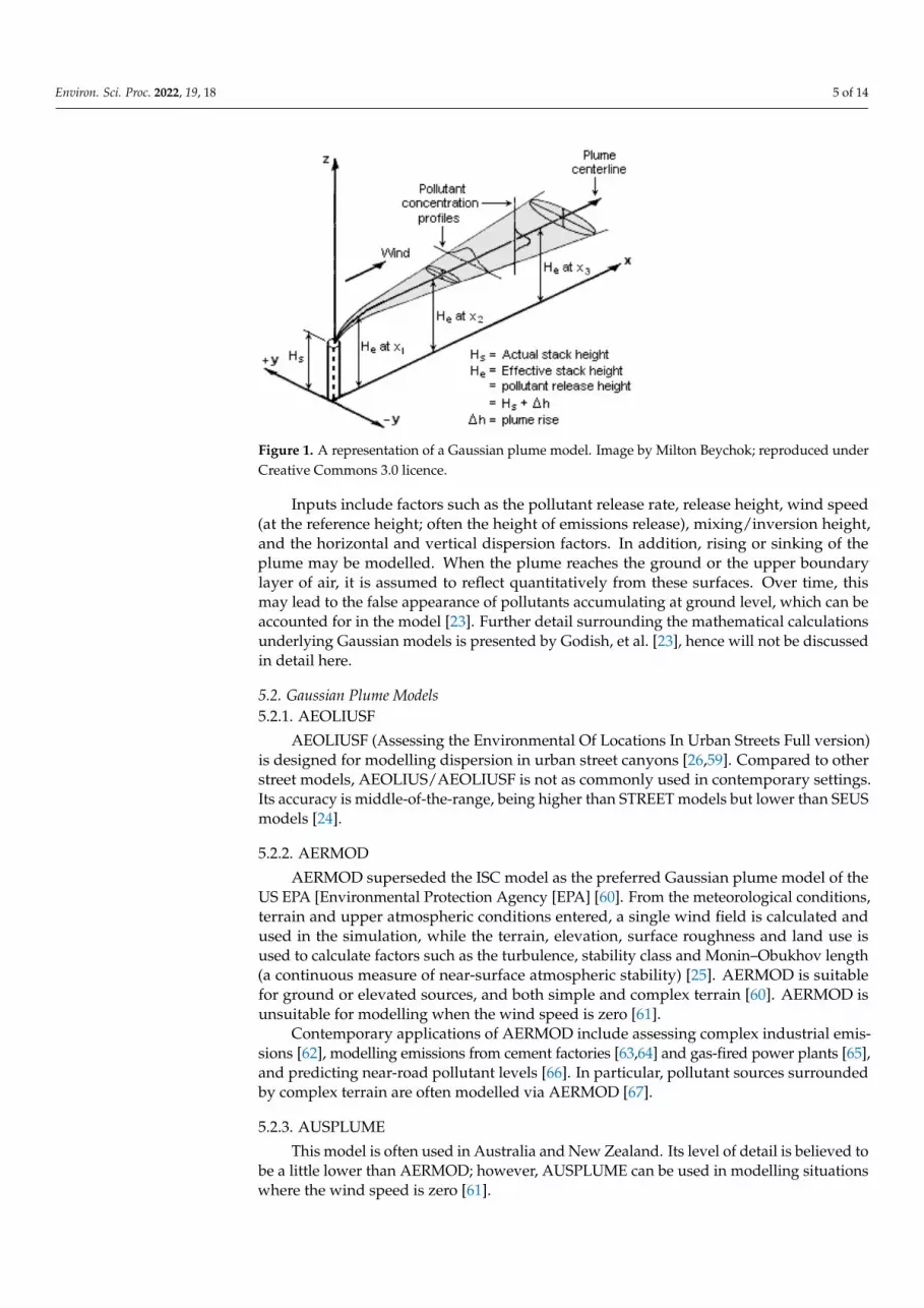
Figure 1. A representation of a Gaussian plume model. Image by Milton Beychok; reproduced under Creative Commons 3.0 licence.

Inputs include factors such as the pollutant release rate, release height, wind speed (at the reference height; often the height of emissions release), mixing/inversion height, and the horizontal and vertical dispersion factors. In addition, rising or sinking of the plume may be modelled. When the plume reaches the ground or the upper boundary layer of air, it is assumed to reflect quantitatively from these surfaces. Over time, this may lead to the false appearance of pollutants accumulating at ground level, which can be ac-counted for in the model [23]. Further detail surrounding the mathematical calculations underlying Gaussian models is presented by Godish, et al. [23], hence will not be dis-cussed in detail here.

5.2. Gaussian Plume Models 5.2.1. AEOLIUSF

AEOLIUSF (Assessing the Environmental Of Locations In Urban Streets Full version) is designed for modelling dispersion in urban street canyons [26,59]. Compared to other street models, AEOLIUS/AEOLIUSF is not as commonly used in contemporary settings. Its accuracy is middle-of-the-range, being higher than STREET models but lower than SEUS models [24].

5.2.2. AERMOD AERMOD superseded the ISC model as the preferred Gaussian plume model of the

US EPA [Environmental Protection Agency [EPA] [60]. From the meteorological condi-tions, terrain and upper atmospheric conditions entered, a single wind field is calculated and used in the simulation, while the terrain, elevation, surface roughness and land use is used to calculate factors such as the turbulence, stability class and Monin–Obukhov length (a continuous measure of near-surface atmospheric stability) [25]. AERMOD is suitable for ground or elevated sources, and both simple and complex terrain [60]. AERMOD is unsuitable for modelling when the wind speed is zero [61].

Contemporary applications of AERMOD include assessing complex industrial emis-sions [62], modelling emissions from cement factories [63,64] and gas-fired power plants

Figure 1. A representation of a Gaussian plume model. Image by Milton Beychok; reproduced underCreative Commons 3.0 licence.

Inputs include factors such as the pollutant release rate, release height, wind speed(at the reference height; often the height of emissions release), mixing/inversion height,and the horizontal and vertical dispersion factors. In addition, rising or sinking of theplume may be modelled. When the plume reaches the ground or the upper boundarylayer of air, it is assumed to reflect quantitatively from these surfaces. Over time, thismay lead to the false appearance of pollutants accumulating at ground level, which can beaccounted for in the model [23]. Further detail surrounding the mathematical calculationsunderlying Gaussian models is presented by Godish, et al. [23], hence will not be discussedin detail here.

5.2. Gaussian Plume Models5.2.1. AEOLIUSF

AEOLIUSF (Assessing the Environmental Of Locations In Urban Streets Full version)is designed for modelling dispersion in urban street canyons [26,59]. Compared to otherstreet models, AEOLIUS/AEOLIUSF is not as commonly used in contemporary settings.Its accuracy is middle-of-the-range, being higher than STREET models but lower than SEUSmodels [24].

5.2.2. AERMOD

AERMOD superseded the ISC model as the preferred Gaussian plume model of theUS EPA [Environmental Protection Agency [EPA] [60]. From the meteorological conditions,terrain and upper atmospheric conditions entered, a single wind field is calculated andused in the simulation, while the terrain, elevation, surface roughness and land use isused to calculate factors such as the turbulence, stability class and Monin–Obukhov length(a continuous measure of near-surface atmospheric stability) [25]. AERMOD is suitablefor ground or elevated sources, and both simple and complex terrain [60]. AERMOD isunsuitable for modelling when the wind speed is zero [61].

Contemporary applications of AERMOD include assessing complex industrial emis-sions [62], modelling emissions from cement factories [63,64] and gas-fired power plants [65],and predicting near-road pollutant levels [66]. In particular, pollutant sources surroundedby complex terrain are often modelled via AERMOD [67].

5.2.3. AUSPLUME

This model is often used in Australia and New Zealand. Its level of detail is believed tobe a little lower than AERMOD; however, AUSPLUME can be used in modelling situationswhere the wind speed is zero [61].

Environ. Sci. Proc. 2022, 19, 18 6 of 14

Recent applications of this model include mapping the dispersion of radon releasedfrom a Romanian uranium mine [68] and modelling odour dispersion from rubber factoriesin Malaysia [69].

5.2.4. CALINE3

CALINE is a modified Gaussian plume model, where the emission source is a linerather than a point [70]. Its main use is in modelling pollutant dispersion from roads; theroad geometry can be varied rather than being restricted to a straight line. CALINE3 re-mains an EPA-recommended Gaussian line model [60], while the updated CALINE4 modelis also used in some contemporary applications [71]. CALINE3 is designed for relativelysimple terrain and forms the basis of models such as CAL3QHC and CAL3QHCR [60].

Ref [71] used CALINE4, combined with ISCST3, to predict NO2 and PM10 concentra-tions along a road line source.

5.2.5. CAL3QHC and CAL3QHCR

Both models are based off CALINE3, but are specifically designed for determining thebuild-up of CO hotspots resulting from traffic stagnation, particularly at intersections [60].CAL3QHCR is the “refined” version of CAL3QHC and consequently requires a greaterdata input, in particular localised meteorological data [60].

In recent years, CAL3QHC has been applied to the epidemiological study of thecongenital effects of vehicular pollutants [72] and assessing the spread of CO, NOx andVOCs from intersections in India [73].

5.2.6. CTDMPLUS

As suggested by its name, Complex Terrain Dispersion Model Plus Algorithms forUnstable Situations (CTDMPLUS) is designed for use in complex terrain situations [74].However, it can be used in all stability conditions (including stable and neutral condi-tions) [60]. From a review of the literature, it does not appear to be commonly used incontemporary settings.

5.2.7. ISC

The ISC (Industrial Source Complex) model, as reported and evaluated byBowers, et al. [75], was previously the approved Gaussian plume model of the US En-vironmental Protection Agency (EPA) [25]. Recent applications of the ISC model includemodelling VOCs downwind of a petrochemical manufacturing plant [76] and monitoringa number of pollutants (CO, VOC, NOx and PM10) in Italian agricultural land [77,78].Some authors also combine the ISC model with AEROMOD for improved accuracy of theresults [79,80].

5.2.8. OCD

The Offshore and Coastal Dispersion (OCD) model is a straight-line Gaussian model,designed for predicting the dispersion of pollutants over marine or coastal regions [60].Changes as the plume crosses the coastline are incorporated [60]. This model has been usedacross a range of environments, including the Gulf of Mexico [81].

6. Lagrangian Models6.1. Introduction

Lagrangian models simulate a number of “puffs” of pollutants emitted from the source,usually at regular intervals. The most common is a “Gaussian puff” model, where each puffis assumed to follow a Gaussian distribution as it moves downwind and expands. The puffsare 3D elements that expand in all dimensions (x, y and z) over time, concurrently movingdownwind from the emission source. A model may comprise hundreds to hundredsof thousands of these theoretical puffs [25]. As each puff is treated independently, theycan have varying rates of dispersion and move in various directions, allowing for more

Environ. Sci. Proc. 2022, 19, 18 7 of 14

realistic modelling of local conditions within the simulation. Another related model of thistype is the Lagrangian random walk model, where the plume is discretised as numerousindependent tracer particles. The particles are transported by the mean wind field withlocal turbulence accounted for using a stochastic ‘random walk’ algorithm. In particular,Lagrangian models show improved accuracy in models with complex topography orflow patterns (e.g., recirculation of the pollutants) and temporal variation in emissionsor meteorology.

Lagrangian models are often used for modelling across longer distances and time-frames (up to several years long) [25]. In contrast, Gaussian plume models are typicallyrestricted to predictions up to 50 km from the point source [23]. The field of Lagrangianmodelling was introduced by Rodhe [82], Rodhe [83] and has gathered momentum rapidlysince that time.

Time steps of between 1 and 180 s may be used [14,84]. As with Gaussian plumemodelling, the assumption of complete pollutant reflection from the ground and upperatmospheric boundary layer may result in misleading conclusions unless this is taken intoaccount [85,86].

6.2. Examples6.2.1. AFTOX

The AFTOX (Air Force Toxic) chemical dispersion model was created by Kunkel [87].It assumes that four Gaussian puffs are released from the source every minute. As itdoes not account for decay or settling of the pollutants, AFTOX often provides higherpollutant concentrations and a lower accuracy compared to other model types [34]. AFTOXis restricted to neutrally buoyant gases, but is particularly useful for modelling liquid spillswhich subsequently evaporate [88].

AFTOX was recently used as the basis for modelling investigating the relationshipbetween raindrop size and the scavenging efficiency of aerosol particles [89].

6.2.2. CALPUFF

CALPUFF is the approved long-range (>80 km) atmospheric emissions model of theUS EPA [25]. However, CALPUFF also finds use in short-range simulations with complexsurface topography [90], being widely used as a regulatory model in Australian and NewZealand. CALPUFF is versatile at both short-range and long-range simulations [25]. Withmore recent software such as VISTAS version 6, CALPUFF can be run at timescales of lessthan one hour [91].

Applications include the modelling of odour dispersion [92,93], dispersion of variouspollutants produced by industrial facilities [62] and in the study of shipping emissions ina Western Australian port [94]. One application of particular note was the modelling ofatmospheric mercury released from a coal-fired power plant in Mexico [95]. Numerousstudies have also utilised CALPUFF in modelling dispersion over complex terrain [90,96].

6.2.3. Hybrid Eulerian–Lagrangian Dispersion Models (HDMs)

Hybrid models combining the Eulerian and Lagrangian methods, as outlined byAndrén [97], remain relatively common, particularly for simulating dispersion close topoint-line sources [14]. The emissions are initially modelled as puffs using the Lagrangianmethod, then after travelling a specified distance or expanding to a specified level, thepuffs are assumed to approximate a volume emission. The Eulerian method then takes overto calculate the long-range pollutant dispersal [14]. The major advantage of this method isthe reduction in required processing power compared to using a Lagrangian model at allscales [14].

Hybrid models have been used in complex environments such as complex urban [98]and mixed industrial-residential environments [99], and in combination with CFD mod-elling to predict PM10 levels [100] and other pollutants [101] in complex scenarios.

Environ. Sci. Proc. 2022, 19, 18 8 of 14

7. Computational Fluid Dynamics Models7.1. Introduction

Computational fluid dynamics (CFD) has been a well-established modelling techniquein engineering disciplines for many years. However, it is only relatively recently that itwas turned toward the application of modelling atmospheric pollutants. CFD is based offNavier–Stokes equations, which are 3-dimensional, unsteady, non-linear, partial-differentialequations that can exactly model the flow of atmospheric gases. The number of unknownsexceeds the number of discretised equations, hence different techniques are used to modelunknown turbulence terms to find a solution. A Langrangian or Eulerian framework isincorporated into the model in order to calculate the transport and dispersion of contami-nants through the atmosphere. Depending on the fidelity and resolution of the simulation,CFD models can require very large amounts of computing power.

There are three major classes of CFD models: Reynolds-Averaged Navier Stokes(RANS), Large Eddy Simulation (LES) and Direct Numerical Simulation (DNS).

7.2. Examples and Uses

Brown, et al. [102] compared the Quick Urban and Industrial Complex (QUIC) dis-persion model, based off empirical parameterizations of the flow around and betweenbuildings in order to model wind flow in an urban environment. Although the results ofthe model provided a similar accuracy to standard CFD modelling in this instance, theadvantage of CFD models is that wind flow through novel building configurations and/orcombinations can be simulated, rather than relying on empirical data.

Mocho, et al. [43] used a CFD model to investigate the movement of formaldehydein an indoor setting. As expected, the accuracy of the results was improved over a simplebox model.

CFD has been used for modelling the near-field dispersion of pollutants, when plumesof varying buoyancies were present [103]. Other uses include the modelling of PM10movement [100] and the movement of reactive chemical components [104].

8. Street Network Models8.1. Introduction

The street network model is currently the least utilised contemporary modellingtechnique [105]. This method, designed for the analysis of vehicle emissions in built-upurban environments, typically treats each street as a line source of emissions, with thequantity of emissions calculated from the traffic volume along that street.

8.2. ExamplesSIRANE

The SIRANE model, developed by Soulhac, et al. [106], is specifically designed formodelling pollutant dispersal from traffic in urban regions. To date, it is the main streetnetwork model reported in the literature [105]. Each street is modelled as a box, withtransfer of pollutants occurring along the box (i.e., along the street), between boxes (atstreet intersections) and between boxes and the atmospheric boundary layer [106]. Atmo-spheric conditions may change hourly, but are assumed to be constant in between thesetimepoints. The model has been validated against wind tunnel data [107] and against ayear of NO2 emissions data [105]. However, work by Wang, et al. [108] has suggested thatthe output of SIRANE shows a poor correlation with near-road NO2 concentrations, butbetter correlation with the average NO2 values. Nevertheless, SIRANE has been used inseveral epidemiological studies, particularly in France [109–111].

Derivative street pollution models have been created based off SIRANE, includingMUNICH (Model of Urban Network of Intersecting Canyons and Highways), which utilisesa grid modelling method [112].

Environ. Sci. Proc. 2022, 19, 18 9 of 14

9. Other Models

Specialised models are available for modelling pollutant dispersion over long ranges,in complex terrain, and for photochemically reactive pollutants [23]. One example is theOperational Street Pollution Model (OSPM) for modelling the chemistry of photochem-ical smog formation [108,113]. Other common photochemical models include CMAQ(Community Multiscale Air Quality), CAMx (Comprehensive Air quality Model withextensions), UAM (Urban Airshed Model®) and CALGRID [25]. Of particular note areCAMx, an open-source model [114], and UAM, the most widely used photochemical airquality model [25].

Statistical models are available for the short-term forecasting of air quality, based offrecent and current air quality measurements [115]. Such models do not seek to establishcause and effect, rather solely aiming to link patterns in emission trends to the air qual-ity [25]. In a similar fashion, machine-learning algorithms have also been trialled for theprediction of O3, NO2 and SO2 concentrations [116].

Due in part to the short lifespan and unique properties of odorous compounds, airquality models specifically designed for predicting the dispersion of such compounds areavailable [25], such as ModOdor [117].

10. Conclusions

Atmospheric pollutant dispersion models have played an enormous role in setting andregulating atmospheric emission levels and have likely played a vital role in the improve-ment in air quality observed across many westernised countries over the past few decades.With new applications and models reported on a weekly basis, the emissions modelleris faced with a baffling array of models to choose from. However, a basic understandingof the mechanisms behind each model and the strengths and limitations of each shouldassist in guiding this choice. Particularly with advances in computer processing power andsimulation abilities, the results produced by atmospheric pollutant dispersion models aremore detailed and accurate than ever before. It is hoped that regulatory bodies will be ableto utilise this accuracy in such a way that the world’s air quality continues to improve overthe coming years.

Funding: This research received no external funding.

Institutional Review Board Statement: Not applicable.

Informed Consent Statement: Not applicable.

Data Availability Statement: Not applicable.

Conflicts of Interest: The author declares that no conflict of interest exist.

References1. Xu, Q.; Li, X.; Wang, S.; Wang, C.; Huang, F.; Gao, Q.; Wu, L.; Tao, L.; Guo, J.; Wang, W. Fine particulate air pollution and hospital

emergency room visits for respiratory disease in urban areas in Beijing, China, in 2013. PLoS ONE 2016, 11, e0153099. [CrossRef][PubMed]

2. Horne, B.D.; Joy, E.A.; Hofmann, M.G.; Gesteland, P.H.; Cannon, J.B.; Lefler, J.S.; Blagev, D.P.; Korgenski, E.K.; Torosyan, N.;Hansen, G.I. Short-term elevation of fine particulate matter air pollution and acute lower respiratory infection. Am. J. Respir. Crit.Care Med. 2018, 198, 759–766. [CrossRef] [PubMed]

3. Johannson, K.A.; Balmes, J.R.; Collard, H.R. Air pollution exposure: A novel environmental risk factor for interstitial lung disease?Chest 2015, 147, 1161–1167. [CrossRef] [PubMed]

4. Xie, W.; Li, G.; Zhao, D.; Xie, X.; Wei, Z.; Wang, W.; Wang, M.; Li, G.; Liu, W.; Sun, J. Relationship between fine particulate airpollution and ischaemic heart disease morbidity and mortality. Heart 2015, 101, 257–263. [CrossRef] [PubMed]

5. Pope III, C.A.; Turner, M.C.; Burnett, R.T.; Jerrett, M.; Gapstur, S.M.; Diver, W.R.; Krewski, D.; Brook, R.D. Relationships betweenfine particulate air pollution, cardiometabolic disorders, and cardiovascular mortality. Circ. Res. 2015, 116, 108–115. [CrossRef]

6. Zhang, Y.; Wang, S.G.; Xia, Y.; Shang, K.Z.; Cheng, Y.F.; Xu, L.; Ning, G.C.; Zhao, W.J.; LI, N.R. Association between ambient airpollution and hospital emergency admissions for respiratory and cardiovascular diseases in Beijing: A time series study. Biomed.Environ. Sci. 2015, 28, 352–363.

Environ. Sci. Proc. 2022, 19, 18 10 of 14

7. Gharibvand, L.; Shavlik, D.; Ghamsary, M.; Beeson, W.L.; Soret, S.; Knutsen, R.; Knutsen, S.F. The association between ambientfine particulate air pollution and lung cancer incidence: Results from the AHSMOG-2 study. Environ. Health Perspect. 2016, 125,378–384. [CrossRef]

8. Chen, X.; Zhang, L.-w.; Huang, J.-j.; Song, F.-j.; Zhang, L.-p.; Qian, Z.-m.; Trevathan, E.; Mao, H.-j.; Han, B.; Vaughn, M. Long-termexposure to urban air pollution and lung cancer mortality: A 12-year cohort study in Northern China. Sci. Total. Environ. 2016,571, 855–861. [CrossRef]

9. Bernatsky, S.; Smargiassi, A.; Barnabe, C.; Svenson, L.W.; Brand, A.; Martin, R.V.; Hudson, M.; Clarke, A.E.; Fortin, P.R.;van Donkelaar, A. Fine particulate air pollution and systemic autoimmune rheumatic disease in two Canadian provinces. Environ.Res. 2016, 146, 85–91. [CrossRef]

10. Alves, A.G.F.; de Azevedo Giacomin, M.F.; Braga, A.L.F.; Sallum, A.M.E.; Pereira, L.A.A.; Farhat, L.C.; Strufaldi, F.L.;Lichtenfels, A.J.d.F.C.; de Santana Carvalho, T.; Nakagawa, N.K. Influence of air pollution on airway inflammation and diseaseactivity in childhood-systemic lupus erythematosus. Clin. Rheumatol. 2018, 37, 683–690. [CrossRef]

11. Geddes, J.A.; Martin, R.V.; Boys, B.L.; van Donkelaar, A. Long-term trends worldwide in ambient NO2 concentrations inferredfrom satellite observations. Environ. Health Perspect. 2015, 124, 281–289. [CrossRef] [PubMed]

12. Chalabi, Z.; Milojevic, A.; Doherty, R.M.; Stevenson, D.S.; MacKenzie, I.A.; Milner, J.; Vieno, M.; Williams, M.; Wilkinson, P.Applying air pollution modelling within a multi-criteria decision analysis framework to evaluate UK air quality policies. Atmos.Environ. 2017, 167, 466–475. [CrossRef]

13. Kumar, A.; Patil, R.S.; Dikshit, A.K.; Islam, S.; Kumar, R. Evaluation of control strategies for industrial air pollution sources usingAmerican Meteorological Society/Environmental Protection Agency Regulatory Model with simulated meteorology by WeatherResearch and Forecasting Model. J. Clean. Prod. 2016, 116, 110–117. [CrossRef]

14. Sachdeva, S.; Baksi, S. Air Pollutant Dispersion Models: A Review. In Advances in Health and Environment Safety; Springer: Cham,Switzerland, 2017; pp. 203–207. [CrossRef]

15. Forsyth, T. Public concerns about transboundary haze: A comparison of Indonesia, Singapore, and Malaysia. Glob. Environ.Chang. 2014, 25, 76–86. [CrossRef]

16. Ling, Z.; Zhao, J.; Fan, S.; Wang, X. Sources of formaldehyde and their contributions to photochemical O3 formation at an urbansite in the Pearl River Delta, southern China. Chemosphere 2017, 168, 1293–1301. [CrossRef]

17. Po, L.; Rollo, F.; Viqueira, J.R.R.; Lado, R.T.; Bigi, A.; López, J.C.; Nesi, P. TRAFAIR: Understanding Traffic Flow to Improve AirQuality. In Proceedings of the 1st IEEE African Workshop on Smart Sustainable Cities and Communities (IEEE ASC2 2019)-Inconjunction with the 5th IEEE International Smart Cities Conference (ISC2 2019), Casablanca, Morocco, 14–17 October 2019;pp. 14–17.

18. Li, M.; Zhang, L. Haze in China: Current and future challenges. Environ. Pollut. 2014, 189, 85–86. [CrossRef]19. Khreis, H.; Kelly, C.; Tate, J.; Parslow, R.; Lucas, K.; Nieuwenhuijsen, M. Exposure to traffic-related air pollution and risk of

development of childhood asthma: A systematic review and meta-analysis. Environ. Int. 2017, 100, 1–31. [CrossRef]20. Wang, M.; Gehring, U.; Hoek, G.; Keuken, M.; Jonkers, S.; Beelen, R.; Eeftens, M.; Postma, D.S.; Brunekreef, B. Air pollution

and lung function in dutch children: A comparison of exposure estimates and associations based on land use regression anddispersion exposure modeling approaches. Environ. Health Perspect. 2015, 123, 847–851. [CrossRef]

21. Xin, Y.; Wang, G.; Chen, L. Identification of long-range transport pathways and potential sources of PM10 in Tibetan Plateauuplift area: Case study of Xining, China in 2014. Aerosol Air Qual. Res 2016, 16, 1044–1054. [CrossRef]

22. Squizzato, S.; Masiol, M. Application of meteorology-based methods to determine local and external contributions to particulatematter pollution: A case study in Venice (Italy). Atmos. Environ. 2015, 119, 69–81. [CrossRef]

23. Godish, T.; Davis, W.T.; Fu, J.S. Air quality; CRC Press: Boca Raton, FL, USA, 2014.24. Dezzutti, M.; Berri, G.; Venegas, L. Intercomparison of Atmospheric Dispersion Models Applied to an Urban Street Canyon of

Irregular Geometry. Aerosol Air Qual. Res. 2018, 18, 820–828. [CrossRef]25. Daly, A.; Zannetti, P. Air pollution modeling–An overview. In Ambient Air Pollution; Zannetti, P., Al-Ajmi, D., Al-Rashied, S., Eds.;

The EnviroComp Institute: Half Moon Bay, CA, USA, 2007; pp. 15–28.26. Barratt, R. Atmospheric Dispersion Modelling: An Introduction to Practical Applications; Routledge: Abingdon-on-Thames, UK, 2013.27. Colls, J.; Tiwary, A. Air Pollution: Measurement, Modelling and Mitigation; CRC Press: Boca Raton, FL, USA, 2017.28. Forehead, H.; Huynh, N. Review of modelling air pollution from traffic at street-level-The state of the science. Environ. Pollut.

2018, 241, 775–786. [CrossRef] [PubMed]29. Khan, J.; Ketzel, M.; Kakosimos, K.; Sørensen, M.; Jensen, S.S. Road traffic air and noise pollution exposure assessment–A review

of tools and techniques. Sci. Total. Environ. 2018, 634, 661–676. [CrossRef]30. Cécé, R.; Bernard, D.; Brioude, J.; Zahibo, N. Microscale anthropogenic pollution modelling in a small tropical island during weak

trade winds: Lagrangian particle dispersion simulations using real nested LES meteorological fields. Atmos. Environ. 2016, 139,98–112. [CrossRef]

31. Cavaliere, A.; Carotenuto, F.; Di Gennaro, F.; Gioli, B.; Gualtieri, G.; Martelli, F.; Matese, A.; Toscano, P.; Vagnoli, C.; Zaldei, A.Development of Low-Cost Air Quality Stations for Next Generation Monitoring Networks: Calibration and Validation of PM2.5and PM10 Sensors. Sensors 2018, 18, 2843. [CrossRef]

32. Schneider, P.; Castell, N.; Vogt, M.; Dauge, F.R.; Lahoz, W.A.; Bartonova, A. Mapping urban air quality in near real-time usingobservations from low-cost sensors and model information. Environ. Int. 2017, 106, 234–247. [CrossRef] [PubMed]

Environ. Sci. Proc. 2022, 19, 18 11 of 14

33. Raffee, A.F.; Rahmat, S.N.; Hamid, H.A.; Jaffar, M.I. A Review on Short-Term Prediction of Air Pollutant Concentrations. Int. J.Eng. Technol. 2018, 7, 32–35. [CrossRef]

34. Gronwald, F.; Chang, S.-Y. Evaluation of the Precision and Accuracy of Multiple Air Dispersion Models. J. Atmos. Pollut. 2018, 6,1–11.

35. Carter, W.P.; Winer, A.M.; Pitts Jr, J.N. Effects of kinetic mechanisms and hydrocarbon composition on oxidant-precursorrelationships predicted by the EKMA isopleth technique. Atmos. Environ. 1982, 16, 113–120. [CrossRef]

36. Martinez, J.; Maxwell, C.; Javitz, H.; Bowol, R. Evaluation of the Empirical Kinetic Modeling Approach (EKMA); NTIS: Springfield, VA,USA, 1983.

37. Martinez, J.R.; Maxwell, C.; Javitz, H.S.; Bawol, R. Performance evaluation of the Empirical Kinetic Modeling Approach (EKMA).In Air Pollution Modeling and Its Application II; Springer: Cham, Switzerland, 1983; pp. 199–211.

38. Luo, H.; Yuan, Z.; Zheng, J.; Duan, Y. Source-based dynamic control strategies of ozone in different functional areas in Shanghai,China. In Proceedings of the EGU General Assembly, Vienna, Austria, 8–13 April 2018; p. 3237.

39. Collet, S.; Kidokoro, T.; Karamchandani, P.; Shah, T. Future-Year Ozone Isopleths for South Coast, San Joaquin Valley, andMaryland. Atmosphere 2018, 9, 354. [CrossRef]

40. Su, R.; Lu, K.; Yu, J.; Tan, Z.; Jiang, M.; Li, J.; Xie, S.; Wu, Y.; Zeng, L.; Zhai, C. Exploration of the formation mechanism and sourceattribution of ambient ozone in Chongqing with an observation-based model. Sci. China Earth Sci. 2018, 61, 23–32. [CrossRef]

41. Singh, K. Air pollution modeling. Int. J. Adv. Res. Ideas Innov. Technol. 2018, 4, 951–959. [CrossRef]42. Lin, M.-W.; Jwo, C.-S.; Ho, H.-J.; Chen, L.-Y. Using box modeling to determine photodegradation coefficients describing the

removal of gaseous formaldehyde from indoor air. Aerosol Air Qual. Res. 2017, 17, 330–339. [CrossRef]43. Mocho, P.; Desauziers, V.; Plaisance, H.; Sauvat, N. Improvement of the performance of a simple box model using CFD modeling

to predict indoor air formaldehyde concentration. Build. Environ. 2017, 124, 450–459. [CrossRef]44. Zhong, J.; Cai, X.-M.; Bloss, W.J. Modelling photochemical pollutants in a deep urban street canyon: Application of a coupled

two-box model approximation. Atmos. Environ. 2016, 143, 86–107. [CrossRef]45. Zhong, J.; Cai, X.-M.; Bloss, W.J. Modelling the dispersion and transport of reactive pollutants in a deep urban street canyon:

Using large-eddy simulation. Environ. Pollut. 2015, 200, 42–52. [CrossRef]46. Jensen, A.; Dal Maso, M.; Koivisto, A.; Belut, E.; Meyer-Plath, A.; Van Tongeren, M.; Sánchez Jiménez, A.; Tuinman, I.; Domat, M.;

Toftum, J. Comparison of geometrical layouts for a multi-box aerosol model from a single-chamber dispersion study. Environments2018, 5, 52. [CrossRef]

47. Johnson, W.; Ludwig, F.; Dabberdt, W.; Allen, R. An urban diffusion simulation model for carbon monoxide. J. Air Pollut. Control.Assoc. 1973, 23, 490–498. [CrossRef]

48. Mensink, C.; Lewyckyj, N. A simple model for the assessment of air quality in streets. Int. J. Veh. Des. 2001, 27, 242–250. [CrossRef]49. Reynolds, S.D.; Roth, P.M.; Seinfeld, J.H. Mathematical modeling of photochemical air pollution—I: Formulation of the model.

Atmos. Environ. 1973, 7, 1033–1061. [CrossRef]50. Niceno, B.; Dhotre, M.; Deen, N. One-equation sub-grid scale (SGS) modelling for Euler–Euler large eddy simulation (EELES) of

dispersed bubbly flow. Chem. Eng. Sci. 2008, 63, 3923–3931. [CrossRef]51. Hurley, P.J.; Edwards, M.; Physick, W.L.; Luhar, A.K. TAPM V3-model description and verification. Clean Air Environ. Qual. 2005,

39, 32.52. Hurley, P. Development and verification of TAPM. In Air Pollution Modeling and Its Application XIX; Springer: Cham, Switzerland,

2008; pp. 208–216.53. Matthaios, V.N.; Triantafyllou, A.G.; Albanis, T.A.; Sakkas, V.; Garas, S. Performance and evaluation of a coupled prognostic

model TAPM over a mountainous complex terrain industrial area. Theor. Appl. Climatol. 2018, 132, 885–903. [CrossRef]54. Bang, H.Q.; Nguyen, H.D.; Vu, K.; Hien, T.T. Photochemical Smog Modelling Using the Air Pollution Chemical Transport Model

(TAPM-CTM) in Ho Chi Minh City, Vietnam. Environ. Modeling Assess. 2019, 24, 295–310. [CrossRef]55. Trieu, T.; Duc, H.N.; Scorgie, Y. Performance of TAPM-CTM as an airshed modelling tool for the sydney region. In Proceedings of

the 22nd International Clean Air & Environment Conference, Melbourne, Australia, 20–23 September 2015.56. Pollard, A.S.; Williamson, B.J.; Taylor, M.; Purvis, W.O.; Goossens, M.; Reis, S.; Aminov, P.; Udachin, V.; Osborne, N.J. Integrating

dispersion modelling and lichen sampling to assess harmful heavy metal pollution around the Karabash copper smelter, RussianFederation. Atmos. Pollut. Res. 2015, 6, 939–945. [CrossRef]

57. Sarkhosh, M.; Shamsipour, A.; Yaghmaeian, K.; Nabizadeh, R.; Naddafi, K.; Mohseni, S.M. Dispersion modeling and health riskassessment of VOCs emissions from municipal solid waste transfer station in Tehran, Iran. J. Environ. Health Sci. Eng. 2017, 15, 4.[CrossRef]

58. Nieuwstadt, F.; van Dop, H. Atmospheric Turbulence and Air Pollution Modeling; D. Reidel Publishing Company: Dordrecht,The Netherlands, 1982; p. 358.

59. Buckland, A. Validation of a street canyon model in two cities. Environ. Monit. Assess. 1998, 52, 255–267. [CrossRef]60. EPA. Air Quality Dispersion Modeling-Preferred and Recommended Models. Available online: https://www.epa.gov/scram/

air-quality-dispersion-modeling-preferred-and-recommended-models (accessed on 15 October 2021).61. Goldstone, M. AERMOD; assessment of meteorlogical files and comparison with Ausplume for Area Source Modelling. Air Qual.

Clim. Chang. 2015, 49, 38.

Environ. Sci. Proc. 2022, 19, 18 12 of 14

62. Gulia, S.; Kumar, A.; Khare, M. Performance evaluation of CALPUFF and AERMOD dispersion models for air quality assessmentof an industrial complex. J. Sci. Ind. Res. 2015, 74, 302–307.

63. Yazdi, M.N.; Arhami, M.; Ketabchy, M.; Delavarrafeei, M. Modeling of Cement Factory Air Pollution Dispersion by AERMOD. InProceedings of the A&WMA’s 109th Annual Conference & Exhibition, New Orleans, LA, USA, 20–23 June 2016.

64. Jayadipraja, E.; Daud, A.; Assegaf, A.; Maming, M. The application of the AERMOD model in the environmental health to identifythe dispersion area of total suspended particulate from cement industry stacks. J. Res. Med. Sci. 2016, 4, 2044–2049. [CrossRef]

65. Singh, D.; MukeshSharma, A.; Shukla, S. Ambient Air Quality Modeling of 355 MW Gas Based Combined Cycle Power Plant inComplex Terrain. Indian J. Air Pollut. Control. 2016, 16, 10–16.

66. Askariyeh, M.H.; Kota, S.H.; Vallamsundar, S.; Zietsman, J.; Ying, Q. AERMOD for near-road pollutant dispersion: Evaluation ofmodel performance with different emission source representations and low wind options. Transp. Res. Part D Transp. Environ.2017, 57, 392–402. [CrossRef]

67. ul Haq, A.; Nadeem, Q.; Farooq, A.; Irfan, N.; Ahmad, M.; Ali, M.R. Assessment of AERMOD modeling system for application incomplex terrain in Pakistan. Atmos. Pollut. Res. 2019, 10, 1492–1497. [CrossRef]

68. Madear, G.; Traista, E.; Pop, I. Radon Dispersion Air Modeling in Banat Mining Area. In Mine Planning and Equipment Selection2000; Routledge: Abingdon-on-Thames, UK, 2018; pp. 919–924.

69. Idris, N.; Kamarulzaman, N.; Nor, Z.M. Odour Dispersion Modelling for Raw Rubber Processing Factories. J. Rubber Res. 2017, 20,223–241. [CrossRef]

70. Benson, P.E. A review of the development and application of the CALINE3 and 4 models. Atmos. Environment. Part B. UrbanAtmos. 1992, 26, 379–390. [CrossRef]

71. Majumder, S. Emission load distribution and prediction of NO2 and PM10 using ISCST3 and CALINE4 line source modeling.Appl. J. Environ. Eng. Sci. 2019, 5, 2121–2135.

72. Beamer, P.I.; Guerra, S.; Lothrop, N.; Stern, D.A.; Lu, Z.; Billheimer, D.; Halonen, M.; Wright, A.L.; Martinez, F.D. B46 Healtheffects of air pollution and nanoparticles: Childhood Cc16 Levels Are Associated with Diesel Exposure At Birth. Am. J. Respir.Crit. Care Med. 2015, 191, 1.

73. Dhyani, R.; Sharma, N.; Advani, M. Estimation of fuel loss and spatial-temporal dispersion of vehicular pollutants at a signalizedintersection in Delhi City, India. WIT Trans. Ecol. Environ. 2019, 236, 233–243.

74. Perry, S.G. CTDMPLUS: A dispersion model for sources near complex topography. Part I: Technical formulations. J. Appl. Meteorol.1992, 31, 633–645. [CrossRef]

75. Bowers, J.; Anderson, A.J.; Huber, A. Evaluation study of the industrial source complex (ISC) dispersion model. Paper 81.20. 4. InProceedings of the 74th APCA Annual Meeting, Philadelphia, PA, USA, 21–26 June 1981.

76. Chen, M.-H.; Yuan, C.-S.; Wang, L.-C. A feasible approach to quantify fugitive VOCs from petrochemical processes by integratingopen-path fourier transform infrared spectrometry measurements and industrial source complex (ISC) dispersion model. AerosolAir Qual. Res. 2015, 15, 1110–1117. [CrossRef]

77. Iodice, P.; Senatore, A. Appraisal of pollutant emissions and air quality state in a critical I talian region: Methods and results.Environ. Prog. Sustain. Energy 2015, 34, 1497–1505. [CrossRef]

78. Iodice, P.; Senatore, A. Air pollution and air quality state in an Italian National Interest Priority Site. Part 2: The pollutantdispersion. Energy Procedia 2015, 81, 637–643. [CrossRef]

79. Roy, D.; Singh, G.; Yadav, P. Identification and elucidation of anthropogenic source contribution in PM10 pollutant: Insight gainfrom dispersion and receptor models. J. Environ. Sci. 2016, 48, 69–78. [CrossRef] [PubMed]

80. Esbrí, J.M.; López-Berdonces, M.A.; Fernández-Calderón, S.; Higueras, P.; Díez, S. Atmospheric mercury pollution around achlor-alkali plant in Flix (NE Spain): An integrated analysis. Environ. Sci. Pollut. Res. 2015, 22, 4842–4850. [CrossRef] [PubMed]

81. Muriel-García, M.; Cerón-Bretón, R.M.; Cerón-Bretón, J.G. Air pollution in the Gulf of Mexico. Open J. Ecol. 2016, 6, 32. [CrossRef]82. Rodhe, H. Some aspects of the use of air trajectories for the computation of large-scale dispersion and fallout patterns. In Advances

in Geophysics; Elsevier: Amsterdam, The Netherlands, 1975; Volume 18, pp. 95–109.83. Rodhe, H. A study of the sulfur budget for the atmosphere over Northern Europe. Tellus 1972, 24, 128–138. [CrossRef]84. Inthavong, K.; Tian, L.; Tu, J. Lagrangian particle modelling of spherical nanoparticle dispersion and deposition in confined flows.

J. Aerosol Sci. 2016, 96, 56–68. [CrossRef]85. Monin, A. Smoke propagation in the surface layer of the atmosphere. In Advances in Geophysics; Elsevier: Amsterdam,

The Netherlands, 1959; Volume 6, pp. 331–343.86. Boughton, B.; Delaurentis, J.; Dunn, W. A stochastic model of particle dispersion in the atmosphere. Bound. Layer Meteorol. 1987,

40, 147–163. [CrossRef]87. Kunkel, B. User’s Guide for the Air Force Toxic Chemical Dispersion Model (AFTOX); Interim report, October 1985–December 1987;

Air Force Geophysics Lab: Hanscom Air Force Base, MA, USA, 1988.88. Abbasi, T.; Tauseef, S.; Suganya, R.; Abbasi, S. Types of accidents occurring in chemical process industries and approaches to their

modeling. Int. J. Eng. Sci. Math 2017, 6, 424–455.89. Elperin, T.; Fominykh, A.; Krasovitov, B. Effect of raindrop size distribution on scavenging of aerosol particles from Gaussian air

pollution plumes and puffs in turbulent atmosphere. Process. Saf. Environ. Prot. 2016, 102, 303–315. [CrossRef]

Environ. Sci. Proc. 2022, 19, 18 13 of 14

90. Tomasi, E.; Giovannini, L.; Falocchi, M.; Zardi, D.; Antonacci, G.; Ferrero, E.; Bisignano, A.; Alessandrini, S.; Mortarini, L.Dispersion Modeling Over Complex Terrain in the Bolzano Basin (IT): Preliminary Results from a WRF-CALPUFF ModelingSystem. In Proceedings of the 35th International Technical Meeting on Air Pollution Modelling and Its Application, Crete, Greece,3–7 October 2016; pp. 157–161.

91. Exponent Engineering and Science Consulting. CALPUFF Modeling System. Available online: http://www.src.com/ (accessedon 3 July 2022).

92. Yaacof, N.; Qamaruzzaman, N.; Yusup, Y. Comparison method of odour impact evaluation using calpuff dispersion modellingand on-site odour monitoring. Eng. Herit. J. 2017, 1, 1–5. [CrossRef]

93. Çetin Dogruparmak, S.; Pekey, H.; Arslanbas, D. Odor dispersion modeling with CALPUFF: Case study of a waste and residuetreatment incineration and utilization plant in Kocaeli, Turkey. Environ. Forensics 2018, 19, 79–86. [CrossRef]

94. Formentin, G. Estimating the Dispersion of Shipping Emissions from Fremantle Port, Western Australia; Murdoch University: Perth,Australia, 2017.

95. García, G.F.; Álvarez, H.B.; Echeverría, R.S.; de Alba, S.R.; Rueda, V.M.; Dosantos, E.C.; Cruz, G.V. Spatial and temporal variabilityof atmospheric mercury concentrations emitted from a coal-fired power plant in Mexico. J. Air Waste Manag. Assoc. 2017, 67,973–985. [CrossRef] [PubMed]

96. Sagan, V.; Pasken, R.; Zarauz, J.; Krotkov, N. SO2 trajectories in a complex terrain environment using CALPUFF dispersion model,OMI and MODIS data. Int. J. Appl. Earth Obs. Geoinf. 2018, 69, 99–109. [CrossRef]

97. Andrén, A. A meso-scale plume dispersion model. Preliminary evaluation in a heterogeneous area. Atmos. Environ. Part A. Gen.Top. 1990, 24, 883–896. [CrossRef]

98. Bahlali, M.; Dupont, E.; Carissimo, B. Adaptation of the Lagrangian module of a CFD code for atmospheric dispersion of pollutantsin complex urban geometries and comparison with existing Eulerian results. In Proceedings of the 18th International conferenceon Harmonisation within Atmospheric Dispersion Modelling for Regulatory Purposes, Bologna, Italy, 9–12 October 2017.

99. Bonafé, G.; Montanari, F.; Stel, F. A hybrid Eulerian-Lagrangian-statistical approach to evaluate air quality in a mixed residential-industrial environment. Int. J. Environ. Pollut. 2018, 64, 246–264. [CrossRef]

100. Brusca, S.; Famoso, F.; Lanzafame, R.; Mauro, S.; Messina, M.; Strano, S. PM10 Dispersion Modeling by means of CFD 3D andEulerian–Lagrangian models: Analysis and comparison with experiments. Energy Procedia 2016, 101, 329–336. [CrossRef]

101. Bahlali, M.L.; Dupont, E.; Carissimo, B. A hybrid CFD RANS/Lagrangian approach to model atmospheric dispersion of pollutantsin complex urban geometries. Int. J. Environ. Pollut. 2018, 64, 74–89. [CrossRef]

102. Brown, M.J.; Gowardhan, A.A.; Nelson, M.A.; Williams, M.D.; Pardyjak, E.R. QUIC transport and dispersion modelling of tworeleases from the Joint Urban 2003 field experiment. Int. J. Environ. Pollut. 2013, 52, 263–287. [CrossRef]

103. Tominaga, Y.; Stathopoulos, T. CFD simulations of near-field pollutant dispersion with different plume buoyancies. Build. Environ.2018, 131, 128–139. [CrossRef]

104. Sanchez, B.; Santiago, J.-L.; Martilli, A.; Palacios, M.; Kirchner, F. CFD modeling of reactive pollutant dispersion in simplifiedurban configurations with different chemical mechanisms. Atmos. Chem. Phys. 2016, 16, 12143–12157. [CrossRef]

105. Soulhac, L.; Nguyen, C.V.; Volta, P.; Salizzoni, P. The model SIRANE for atmospheric urban pollutant dispersion. PART III:Validation against NO2 yearly concentration measurements in a large urban agglomeration. Atmos. Environ. 2017, 167, 377–388.[CrossRef]

106. Soulhac, L.; Salizzoni, P.; Cierco, F.-X.; Perkins, R. The model SIRANE for atmospheric urban pollutant dispersion; part I,presentation of the model. Atmos. Environ. 2011, 45, 7379–7395. [CrossRef]

107. Salem, N.B.; Garbero, V.; Salizzoni, P.; Lamaison, G.; Soulhac, L. Modelling pollutant dispersion in a street network. Bound.-LayerMeteorol. 2015, 155, 157–187. [CrossRef]

108. Wang, A.; Fallah-Shorshani, M.; Xu, J.; Hatzopoulou, M. Characterizing near-road air pollution using local-scale emission anddispersion models and validation against in-situ measurements. Atmos. Environ. 2016, 142, 452–464. [CrossRef]

109. Padilla, C.; Kihal-Talantikit, W.; Vieira, V.; Deguen, S. City-specific spatiotemporal infant and neonatal mortality clusters: Linkswith socioeconomic and air pollution spatial patterns in France. Int. J. Environ. Res. Public Health 2016, 13, 624. [CrossRef]

110. Ouidir, M.; Giorgis-Allemand, L.; Lyon-Caen, S.; Morelli, X.; Cracowski, C.; Pontet, S.; Pin, I.; Lepeule, J.; Siroux, V.; Slama, R.Estimation of exposure to atmospheric pollutants during pregnancy integrating space–time activity and indoor air levels: Does itmake a difference? Environ. Int. 2015, 84, 161–173. [CrossRef]

111. Morelli, X.; Rieux, C.; Cyrys, J.; Forsberg, B.; Slama, R. Air pollution, health and social deprivation: A fine-scale risk assessment.Environ. Res. 2016, 147, 59–70. [CrossRef]

112. Kim, Y.; Wu, Y.; Seigneur, C.; Roustan, Y. Multi-scale modeling of urban air pollution: Development and application of aStreet-in-Grid model (v1. 0) by coupling MUNICH (v1. 0) and Polair3D (v1. 8.1). Geosci. Model Dev. 2018, 11, 611–629. [CrossRef]

113. Hertel, O.; Berkowicz, R.; Larssen, S. The operational street pollution model (OSPM). In Air Pollution Modeling and Its ApplicationVIII; Springer: Cham, Switzerland, 1991; pp. 741–750.

114. Ciarelli, G.; Aksoyoglu, S.; Crippa, M.; Jimenez, J.-L.; Nemitz, E.; Sellegri, K.; Äijälä, M.; Carbone, S.; Mohr, C.; O’Dowd, C.Evaluation of European air quality modelled by CAMx including the volatility basis set scheme. Atmos. Chem. Phys. 2016, 16,10313–10332. [CrossRef]

Environ. Sci. Proc. 2022, 19, 18 14 of 14

115. Finzi, G.; Nunnari, G. Air Quality Forecast and Alarm Systems. Chapter 16A. In Air Quality Modelling—Theories, Methodologies,Computational Techniques and Available Databases and Software; Zannetti, P., Ed.; AWMA: Pittsburgh, PA, USA, 2005; Volume II,pp. 397–452.

116. Shaban, K.B.; Kadri, A.; Rezk, E. Urban air pollution monitoring system with forecasting models. IEEE Sens. J. 2016, 16, 2598–2606.[CrossRef]

117. Liu, Y.; Zhao, Y.; Lu, W.; Wang, H.; Huang, Q. ModOdor: 3D numerical model for dispersion simulation of gaseous contaminantsfrom waste treatment facilities. Environ. Model. Softw. 2019, 113, 1–19. [CrossRef]