ARTICLE IN PRESS

1352-2310/$ - se

doi:10.1016/j.at

�Correspondfax: +5551 477

E-mail addr

Atmospheric Environment 39 (2005) 3643–3650

www.elsevier.com/locate/atmosenv

Plume dispersion simulation in low wind conditions in stableand convective boundary layers

Davidson M. Moreiraa,�, Tiziano Tirabassib, Jonas C. Carvalhoa

aUniversidade Luterana do Brasil, ULBRA, Environmental Engineering, Rua Miguel Tostes, 101 Predio 11-Sala 230, Canoas, RS, BrazilbInstitute of Atmospheric and Climate Sciences, ISAC/CNR, Italy

Received 24 June 2004; received in revised form 27 February 2005; accepted 4 March 2005

Abstract

The present study proposes a steady-state mathematical model for dispersion of contaminants in low winds that takes

into account the along-wind diffusion. The solution of the advection–diffusion equation for these conditions is obtained

applying the Laplace transform, considering the planetary boundary layer as a multilayer system. The eddy diffusivities

used in the K-diffusion model were derived from the local similarity and Taylor’s diffusion theory. The eddy diffusivities

are functions of distance from the source and correctly represent the near-source diffusion in weak winds. The

performances of the model were evaluated against the field experiments carried out at the Idaho National Engineering

Laboratory and during the convective conditions at the Indian Institute of Technology. Furthermore, the study

suggests that the inclusion of the longitudinal diffusion, important at short distance diffusion from a continuous point

source in low wind conditions, can improve the description of the turbulent transport of atmospheric contaminants.

r 2005 Elsevier Ltd. All rights reserved.

Keywords: Low winds; Turbulence parameterization; Down-wind diffusion; Eulerian dispersion models; Laplace transform method;

Solution of advection–diffusion equation

1. Introduction

The importance of dispersion modelling in low wind

conditions lies in the fact that such conditions occur

frequently and are crucial for air pollution episodes. In

such conditions, the pollutants are not able to travel far

and thus the near-source areas are affected the most.

The classical approach based on conventional models,

such as the Gaussian puff/plume or the K-theory with

suitable assumptions, are known to work reasonably

well during most meteorological regimes, except for

weak and variable wind conditions. This is because (i)

e front matter r 2005 Elsevier Ltd. All rights reserve

mosenv.2005.03.004

ing author. Tel.: +5551 477 9285;

1313.

ess: davidson@ulbra.tche.br (D.M. Moreira).

down-wind diffusion is neglected with respect to

advection, (ii) the concentration is inversely propor-

tional to wind speed, (iii) the average conditions are

stationary and (iv) there is a lack of appropriate

estimates of dispersion parameters in low wind condi-

tions. In view of such restrictions, various attempts have

been made in the literature to explain dispersion in the

presence of low wind conditions by relaxing some of the

limitations (Seinfeld, 1986; Arya, 1995; Sharan and

Gopalakrishnan, 2003).

Several models have been developed to describe

dispersion processes under low winds conditions. Sharan

and Yadav (1998) used a model including streamwise

diffusion and variable eddy diffusivities. The eddy

diffusivities were specified as linear functions of the

downwind distance. The model of Cirillo and Poli (1992)

d.

ARTICLE IN PRESSD.M. Moreira et al. / Atmospheric Environment 39 (2005) 3643–36503644

gave almost identical results when compared with those

of the model of Sharan and Yadav (1998) for the INEL

data set. Sagendorf and Dickson (1974) used a Gaussian

model and also divided each computation period into 2-

min time intervals, summing the results to determine the

total concentration. The limitations of the said models

arise from built-in assumptions of a homogeneous wind

field and restrictions concerning the shape of the source.

Brusasca et al. (1992) used a Lagrangian particle model

to take meandering of the flow into account. More

recently, Oettl et al. (2001) attempted to simulate

ground-level concentrations in low wind conditions,

utilizing a Lagrangian dispersion model with random

time steps and a negative intercorrelation parameter for

the horizontal wind components.

In the present work, we investigate the problem of

modelling contaminant dispersion from ground-level

sources in low wind situations for stable and convective

conditions. The novel aspect is that we formulated a

steady-state mathematical model for dispersion of con-

taminants in low winds by taking into account the along-

wind diffusion in the advection–diffusion equation.

Additionally, we used a parameterization that is depen-

dent on the source distance and correctly represents near-

source diffusion in weak winds (Arya, 1995). The low

wind data collected during stable conditions, from the

series of field experiments conducted at the Idaho

National Engineering Laboratory (INEL) (Sagendorf

and Dickson, 1974), and during convective conditions

at the Indian Institute of Technology (IIT), Delhi (Sharan

et al., 1996a, b), have been simulated using a recent

solution of the advection–diffusion equation.

2. Diffusion model

Considering a Cartesian coordinate system, in which

the x-axis coincides with the direction of the average

wind and z is the vertical axis, the time-dependent

advection–diffusion equation can be written as (Black-

adar, 1997)

qC

qtþ u

qC

qx¼

qqx

KxqC

qx

� �þ

qqy

KyqC

qy

� �

þqqz

KzqC

qz

� �, ð1Þ

where C denotes the average concentration, u the mean

wind speed in x direction and Kx, Ky and Kz the eddy

diffusivities. The cross-wind integration of Eq. (1) (in

stationary conditions) leads to

uqcy

qx¼

qqx

Kxqcy

qx

� �þ

qqz

Kzqcy

qz

� �(2)

subject to the boundary conditions of zero flux at the

ground and PBL at the top, and a Q rate source

emission at plume height Hs:

Kzqcy

qz¼ 0 at z ¼ 0; h, (3)

ucyð0; zÞ ¼ Qdðz � HsÞ at x ¼ 0, (4)

where cy now represents the average cross-wind inte-

grated concentration.

Recalling the dependence of the Kx and Kz coefficients

and wind speed profile u on variable z, the height h of a

PBL is discretized in N sub-intervals in such a manner

that within each interval Kx(z), Kz(z) and u(z) can be well

approximated with their average values:

Knx;z ¼

1

znþ1 � zn

Z znþ1

zn

Kx;zðzÞ dz, (5)

un ¼1

znþ1 � zn

Z znþ1

zn

uðzÞ dz; (6)

where Knx;z ¼ Kn

x or Knz . For the eddy diffusivity

depending on x and z, initially we take the average in

the z variable:

Knx;zðxÞ ¼

1

znþ1 � zn

Z znþ1

zn

Kx;zðx; zÞ dz. (7)

The procedure is similar for the x variable: we take

the average in the x variable. Then, in this work,

the following average value for eddy diffusivity is

considered:

Knx;z ¼

1

x

Z x

0

Kx;zðx0Þ dx0. (8)

At this point, it is important to remark that this

procedure transforms the domain of problem (2) into a

multilayered slab in the z direction. Again Knx and Kn

z

assume a constant value at znpzpznþ1 and x direction.

Therefore, the solution of problem (2) is reduced to

the solution of N problems of the following type:

un

qcyn

qx¼ Kn

x

q2cyn

qx2þ Kn

z

q2cyn

qz2(9)

for n ¼ 1:N, where cyn denotes the concentration at the

nth layer. To determine the 2N integration constants, the

additional (2N�2) conditions, namely the continuity of

concentration and flux at interface, are considered:

cyn ¼ c

ynþ1; n ¼ 1; 2; . . . ; ðN � 1Þ, (10)

Knz

qcyn

qz¼ Knþ1

z

qcynþ1

qz; n ¼ 1; 2; . . . ; ðN � 1Þ. (11)

At this point, we are in a position to apply an

analytical solution proposed by Vilhena et al. (1998) and

Moreira et al. (1999, 2004, 2005) using the Laplace

transform method to problem (9) in the x variable.

Finally, by applying the interface and boundary condi-

tions, we obtain a linear system for the integration

ARTICLE IN PRESSD.M. Moreira et al. / Atmospheric Environment 39 (2005) 3643–3650 3645

constants. Henceforth, the concentration is obtained by

numerically inverting the transformed concentration cy

by the Gaussian quadrature scheme:

cynðx; zÞ ¼

X8j¼1

wj

Pj

xAne

�ffiffiffiffiffiffiffiffiffiffiffiffiffiffiffiffiffiffiffiffiffiffiffiffiffiffiffiffiffiffiffiffið1�Pj=PeÞðPj un=xKn

z Þp� �

z

�

þBneffiffiffiffiffiffiffiffiffiffiffiffiffiffiffiffiffiffiffiffiffiffiffiffiffiffiffiffiffiffiffiffið1�Pj=PeÞðPjun=xKn

z Þp� �

z

�. ð12Þ

These solutions are only valid for x40, since the

quadrature scheme of Laplace inversion does not work

for x ¼ 0. Here, wj and Pj are the weights and roots of

the Gaussian quadrature scheme and are tabulated in

the book by Stroud and Secrest (1966). It is also

important to mention that the above solution is valid

only for layers that do not contain the contaminant

source. For the layer that contains the source, the

concentration has the form

cynðx; zÞ ¼

X8j¼1

wj

Pj

xAne

�ffiffiffiffiffiffiffiffiffiffiffiffiffiffiffiffiffiffiffiffiffiffiffiffiffiffiffiffiffiffiffiffið1�Pj=PeÞðPj un=xKn

z Þp� �

z

�

þ Bneffiffiffiffiffiffiffiffiffiffiffiffiffiffiffiffiffiffiffiffiffiffiffiffiffiffiffiffiffiffiffiffið1�Pj=PeÞðPj un=xKn

z Þp� �

z

þQ

2

1� Pj=Pe

PjKnzun=x

� �1=2

� e�ðz�HsÞ

ffiffiffiffiffiffiffiffiffiffiffiffiffiffiffiffiffiffiffiffiffiffiffiffiffiffiffiffiffiffiffiffiffi1�Pj=Peð ÞðPjun=xKn

z Þ

p� ��

� eðz�HsÞffiffiffiffiffiffiffiffiffiffiffiffiffiffiffiffiffiffiffiffiffiffiffiffiffiffiffiffiffiffiffiffið1�Pj=PeÞðPjun=xKn

z Þp� ��

, ð13Þ

where Pe ¼ unx=Knx is the well known Peclet number and

essentially represents the ratio between the advective

transport and diffusive transport. This can be physically

interpreted as the parameter whose magnitude indicates

the atmospheric conditions in terms of wind strength.

Small values of this number can be related to weak

winds, when the downwind diffusion becomes important

and the region of interest remains close to the source.

Conversely, large values imply moderate to strong

winds, when the downwind diffusion is neglected with

respect to the advective and the region of interest

extends to a larger distance from the source. In the case

Kx ! 0, Pe ! 1, on these assumptions, we obtained

the solutions of Moreira et al. (1999).

In the present study, N ¼ h=50 was considered,

because this value provides the required accuracy with

small computational effort. Obviously, the greater the

number of layers (N), the more accurate the concentra-

tion pattern calculated, although the relative code

running time is consequently greater.

The above formulas deal with cross-wind integrated

concentration cyðx; zÞ. If we want to calculate the three-

dimensional concentration Cðx; y; zÞ, lateral diffusion

needs to be included. If we assume that the plume has a

Gaussian concentration distribution in the lateral, then,

to calculate the concentration in the K-model, the

following expression is assumed:

Cðx; y; zÞ ¼ cyðx; zÞeð�y2=2s2yÞffiffiffiffiffiffi

2pp

sy

, (14)

where cy is computed from Eqs. (12) and (13).

3. Turbulent parameterizations

In the atmospheric diffusion problems, the turbulent

parameterization represents a fundamental aspect of

contaminant dispersion modelling. The reliability of

each model strongly depends on the way turbulent

parameters are calculated and related to the current

understanding of the PBL (Mangia et al., 2002). The

dispersion parameters and eddy diffusivities for applica-

tion in the K-model in the stable and unstable cases are

described.

3.1. Stable case

The lateral dispersion parameter sy can be written

with the equation used to relate sy to sy (root mean

square value of horizontal wind direction). Cirillo and

Poli (1992) proposed the following relation to estimate

sy from sy:

sy ¼ x½sinhðs2yÞ�1=2. (15)

To represent the near-source diffusion in weak winds

the eddy diffusivities should be considered as functions

not only of turbulence (e.g., large eddy length and

velocity scales), but also of distance from the source

(Arya, 1995). Following this idea, Degrazia and Moraes

(1992) proposed for the stable boundary layer (SBL) an

integral formulation for the eddy diffusivities. It takes

the form

Ka

u h

¼0:64aið1� z=hÞa1=2z=h

8ffiffiffip

pðf mÞi

�

Z 1

0

sin½8ffiffiffip

paið1� z=hÞa1=2ðf mÞiX

0n0=ð1:5Þ3=5z=h�

ð1þ n05=3Þn0dn0,

ð16Þ

where u* is the friction velocity, h is the height of the

turbulent SBL, a1 is a constant that depends on the

evolution state of the SBL, ðf mÞi ¼ ðf mÞn;ið1þ 3:7z=LÞ isthe frequency of the spectral peak (i standing for the

turbulent velocity components u, v and w), ðf mÞn;i is the

frequency of the spectral peak in the neutral stratifica-

tion (ðf mÞn;w ¼ 0:33; ðf mÞn;v ¼ 0:22; ðf mÞn;u ¼ 0:045;Sorbjan, 1989), z is the height above the ground,

L ¼ Lð1� z=hÞð1:5a1�a2Þ (a1 ¼ 1:5; a2 ¼ 1; Nieuwstadt,

ARTICLE IN PRESSD.M. Moreira et al. / Atmospheric Environment 39 (2005) 3643–36503646

1984) is the local Monin–Obukhov length, ai ¼

ð2:7ciÞ1=2=ðf mÞ

1=3n;i , where cv;w ¼ 0:4 and cu ¼ 0:3 and,

finally, X 0 ¼ xu =uz represents the nondimensional

distance. The generalized eddy diffusivity (16), as a

function of down-wind distance, is dependent on z and

yields a description of turbulent dispersion in the near

fields of a source.

3.2. Unstable case

The lateral dispersion parameter sy for a convective

boundary layer (CBL) utilized in this work was derived

by Degrazia et al. (1998). It presents the form

s2yh2

¼0:21

p

Z 1

0

sin2ð2:26c1=3Xn0Þdn0

ð1þ n05=3Þn02, (17)

where X is a nondimensional distance ðX ¼ xw =uhÞ, w*

is the convective velocity scale and h is the top of the

CBL.

In terms of the convective scaling parameters, the

vertical eddy diffusivity can be formulated as (Degrazia

et al., 2001)

Ka

w h¼

0:09c1=2i c1=3

ðz=hÞ4=3

ðf mÞ

4=3i

�

Z 1

0

sinð7:84c1=2i c1=3

ðf mÞ

2=3i Xn0=ðz=hÞ2=3Þ

ð1þ n0Þ5=3dn0

n0, ð18Þ

where cw ¼ 0:36, cu ¼ 0:3 and ðf mÞi is the normalized

frequency of the spectral peak, regardless of stratifica-

tion. It can be written as

ðf mÞw ¼

z

ðlmÞw¼ 0:55

z

h

� �1� exp �

4z

h

� ��

�0:0003 exp8z

h

� ��1

ð19Þ

for the vertical component, where ðlmÞw ¼

1:8h 1� expð�4z=hÞ � 0:0003 expð8z=hÞ �

is the value of

the vertical wavelength at the spectral peak. The

longitudinal component obtained from Olesen et al.

(1984) is ðf mÞu ¼ 0:67.

Eqs. (17) and (18) contain the unknown function c.This molecular dissipation of turbulent velocity is one of

the leading destruction terms in equations for the budget

of second-order moments. Therefore, the CBL evolution

is dependent on this function. The dissipation function

used here is the average value c ¼ 0:4 in agreement with

Caughey (1982).

4. Experimental data and model evaluation

To evaluate the performance of the K-model, we used

statistical analysis considering the following statistical

indices (Hanna, 1989):

NMSE ¼ ðCo � CpÞ2=Co þ Cp

ðnormalizedmean square errorÞ,

FB ¼ ðCo � CpÞ=ð0:5ðCo þ CpÞÞ

ðfractional biasÞ,

FS ¼ 2ðso � spÞ=ðso þ spÞ

ðfractional standard deviationÞ,

R ¼ ðCo � CoÞðCp � CpÞ=sospðcorrelation coefficientÞ,

FA2 ¼ 0:5pCo=Cpp2

ðfactor 2Þ,

where C is the analyzed quantity (concentration) and the

subscripts ‘‘o’’ and ‘‘p’’ represent the observed and the

predicted values, respectively. The overbars in the

statistical indices indicate averages. The statistical index

FB indicates whether the predicted quantities under-

estimate or overestimate the observed ones. The

statistical index NMSE represents the quadratic error

of the predicted quantities in relation to the observed

ones. Best results are indicated by the values closest to

zero in NMSE, FB and FS, and to 1 in R and FA2.

4.1. Stable case

The data utilized to evaluate the performance of the

model are constituted by a series of diffusion tests

conducted under stable conditions for surface-based

releases with light winds over flat, even terrain: the

results are published in a US National Oceanic and

Atmospheric Administration (NOAA) report (Sagen-

dorf and Dickson, 1974).

Because of wind direction variability, a full 3601

sampling grid was implemented. Arcs were laid out at

radii of 100, 200 and 400m from the emission point.

Samplers were placed at intervals of 61 on each arc, for a

total of 180 sampling positions. The receptor height was

0.76m. The tracer SF6 was released at a height of 1.5m.

The 1 h average concentrations were determined by

means of an electron capture gas chromatograph. Wind

measurements were provided by lightweight cup anem-

ometers and bivanes at the 2, 4, 8, 16, 32 and 61m levels

of the 61-m tower located on the 200m arc. Table 1

summarizes the conditions of tests 4–14. In the table, the

hourly average wind speed, u, and the standard

deviation of the horizontal wind direction over the

averaging period considered, sy, are reported at the 2m

level.

The roughness length utilized by Brusasca et al. (1992)

and Sharan and Yadav (1998) was z0 ¼ 0:005m. The

ARTICLE IN PRESS

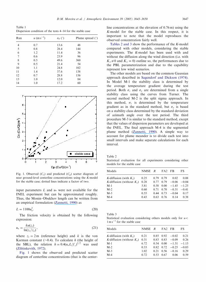
Fig. 1. Observed (Co) and predicted (Cp) scatter diagram of

near ground-level centerline concentrations using the K-model

for the stable case; dotted lines indicate a factor of two.

Table 1

Dispersion condition of the tests 4–14 for the stable case

Run u (m s�1) sy (1) Plume spread (1)

4 0.7 13.6 48

5 0.8 28.4 144

6 1.2 11.4 36

7 0.6 23.9 96

8 0.5 49.6 360

9 0.5 21.4 54

10 1.1 24.8 102

11 1.4 37.6 138

12 0.7 28.8 156

13 1.0 12.0 84

14 1.0 17.2 60

Table 2

Statistical evaluation for all experiments considering other

models for the stable case

Models NMSE R FA2 FB FS

K-diffusion (with Kx) 0.25 0.79 0.79 0.02 0.08

K-diffusion (without Kx) 0.28 0.77 0.79 �0.06 �0.04

M-1 5.81 0.58 0.00 �1.45 �1.25

M-2 0.60 0.71 0.70 �0.31 �0.41

M-3 0.55 0.44 0.73 �0.04 0.17

M-4 0.43 0.63 0.76 0.14 0.38

Table 3

Statistical evaluation considering others models only for uo1m s�1 for the stable case

Models NMSE R FA2 FB FS

K-diffusion (with Kx) 0.21 0.85 0.92 �0.02 0.21

K-diffusion (without Kx) 0.31 0.83 0.83 �0.09 0.26

M-1 6.72 0.54 0.00 �1.51 �1.15

M-2 0.33 0.82 0.72 �0.25 �0.03

M-3 1.02 0.21 0.56 �0.16 0.29

M-4 0.72 0.53 0.67 0.06 0.59

D.M. Moreira et al. / Atmospheric Environment 39 (2005) 3643–3650 3647

input parameters L and u* were not available for the

INEL experiment but can be approximated roughly.

Thus, the Monin–Obukhov length can be written from

an empirical formulation (Zannetti, 1990) as

L ¼ 1100u2 . (20)

The friction velocity is obtained by the following

expression:

u ¼kuðzrÞ

lnðzr=zoÞ, (21)

where zr ¼ 2m (reference height) and k is the von

Karman constant (�0.4). To calculate h (the height of

the SBL), the relation h ¼ 0:4ðu L=f cÞ1=2 was used

(Zilitinkevith, 1972).

Fig. 1 shows the observed and predicted scatter

diagram of centerline concentrations (that is the center-

line concentrations at the elevation of 0.76m) using the

K-model for the stable case. In this respect, it is

important to note that the model reproduces the

observed concentration fairly well.

Tables 2 and 3 show the performance of the K-model

compared with other models, considering the stable

experiments. The K-model has been used with and

without the diffusion along the wind direction (i.e. with

Kxa0 and Kx ¼ 0) outline so, the performances due to

the PBL parameterization and due to the capability

represent low wind scenarios.

The other models are based on the common Gaussian

approach described in Sagendorf and Dickson (1974).

In Model M-1 the stability class is determined by

the average temperature gradient during the test

period. Both sz and sy are determined from a single

stability class using the curves from Turner. The

second method M-2 is the split sigma approach. In

this method, sz is determined by the temperature

gradient as in the standard method, but sy is based

on a stability class determined by the standard deviation

of azimuth angle over the test period. The third

procedure M-3 is similar to the standard method, except

that the values of dispersion parameters are developed at

the INEL. The final approach M-4 is the segmented

plume method (Zannetti, 1990). A simple way to

account for plume meander is to divide each test into

small intervals and make separate calculations for each

interval.

ARTICLE IN PRESSD.M. Moreira et al. / Atmospheric Environment 39 (2005) 3643–36503648

Analyzing the statistical indices in Table 2, it is

possible to note that the model simulates satisfactorily

the observed concentrations, with NMSE, FB and FS

values relatively near zero and R and FA2 relatively near

1. The main test of the model performance is shown in

Table 3, which presents the results of the simulations

considering the experiments where wind velocity is

smaller than 1m s�1. We observed promptly that the

K-model presents a better performance when consider-

ing all experiments (Table 2) and for wind speed smaller

than 1m s�1 (Table 3). Moreover, it is possible to see

that, in the case of low wind scenarios, the model that

takes into account the along-wind diffusion presents the

best results.

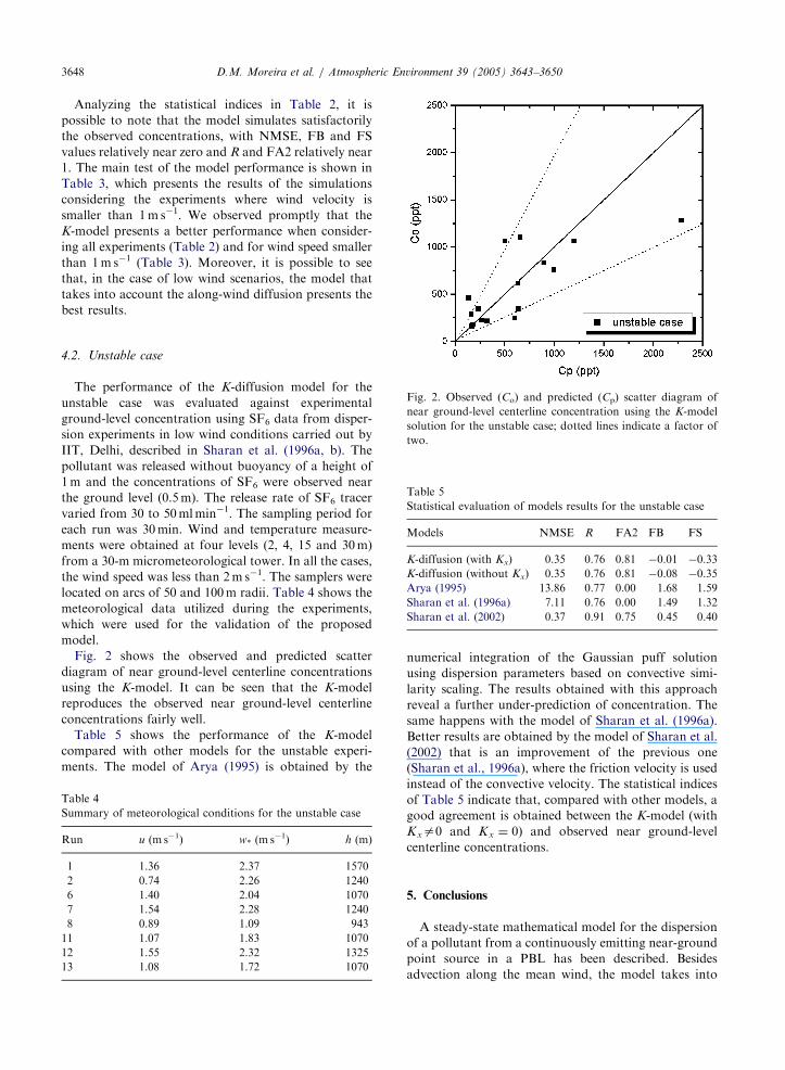
Fig. 2. Observed (Co) and predicted (Cp) scatter diagram of

near ground-level centerline concentration using the K-model

solution for the unstable case; dotted lines indicate a factor of

two.

Table 5

Statistical evaluation of models results for the unstable case

Models NMSE R FA2 FB FS

K-diffusion (with Kx) 0.35 0.76 0.81 �0.01 �0.33

K-diffusion (without Kx) 0.35 0.76 0.81 �0.08 �0.35

Arya (1995) 13.86 0.77 0.00 1.68 1.59

Sharan et al. (1996a) 7.11 0.76 0.00 1.49 1.32

Sharan et al. (2002) 0.37 0.91 0.75 0.45 0.40

4.2. Unstable case

The performance of the K-diffusion model for the

unstable case was evaluated against experimental

ground-level concentration using SF6 data from disper-

sion experiments in low wind conditions carried out by

IIT, Delhi, described in Sharan et al. (1996a, b). The

pollutant was released without buoyancy of a height of

1m and the concentrations of SF6 were observed near

the ground level (0.5m). The release rate of SF6 tracer

varied from 30 to 50mlmin�1. The sampling period for

each run was 30min. Wind and temperature measure-

ments were obtained at four levels (2, 4, 15 and 30m)

from a 30-m micrometeorological tower. In all the cases,

the wind speed was less than 2m s�1. The samplers were

located on arcs of 50 and 100m radii. Table 4 shows the

meteorological data utilized during the experiments,

which were used for the validation of the proposed

model.

Fig. 2 shows the observed and predicted scatter

diagram of near ground-level centerline concentrations

using the K-model. It can be seen that the K-model

reproduces the observed near ground-level centerline

concentrations fairly well.

Table 5 shows the performance of the K-model

compared with other models for the unstable experi-

ments. The model of Arya (1995) is obtained by the

Table 4

Summary of meteorological conditions for the unstable case

Run u (m s�1) w* (m s�1) h (m)

1 1.36 2.37 1570

2 0.74 2.26 1240

6 1.40 2.04 1070

7 1.54 2.28 1240

8 0.89 1.09 943

11 1.07 1.83 1070

12 1.55 2.32 1325

13 1.08 1.72 1070

numerical integration of the Gaussian puff solution

using dispersion parameters based on convective simi-

larity scaling. The results obtained with this approach

reveal a further under-prediction of concentration. The

same happens with the model of Sharan et al. (1996a).

Better results are obtained by the model of Sharan et al.

(2002) that is an improvement of the previous one

(Sharan et al., 1996a), where the friction velocity is used

instead of the convective velocity. The statistical indices

of Table 5 indicate that, compared with other models, a

good agreement is obtained between the K-model (with

Kxa0 and Kx ¼ 0) and observed near ground-level

centerline concentrations.

5. Conclusions

A steady-state mathematical model for the dispersion

of a pollutant from a continuously emitting near-ground

point source in a PBL has been described. Besides

advection along the mean wind, the model takes into

ARTICLE IN PRESSD.M. Moreira et al. / Atmospheric Environment 39 (2005) 3643–3650 3649

account the longitudinal diffusion. The closed form

analytical solution of the proposed problem is obtained

using the Laplace transform method.

The present model has been evaluated in both stable

(INEL diffusion experiment) and unstable (IIT diffusion

experiments) conditions for concentration distributions.

The eddy diffusivities used in the K-diffusion model were

derived from the local similarity and Taylor’s diffusion

theory. The eddy diffusivities are functions of distance

from the source and correctly represent the near-source

diffusion in weak winds. In spite of some limitations of

the INEL and IIT experimental data set, we were able to

obtain a reasonable agreement between the observed

concentrations and those calculated from the K-model.

In particular, for the stable case the results obtained

by the K-model agree very well with the experimental

data, indicating that the parameterization dependent on

the source distance for the vertical eddy diffusivity

correctly represents the dispersion process in low wind

conditions. Moreover, the best results are obtained in

the experiments where the wind velocity is smaller than

1m s�1. In this last case we obtained the best results of

the model with Kxa0 with respect to the model with

Kx ¼ 0.

It is important to note that, since the influencing

parameters are explicitly expressed in a mathematically

closed form, the analytical solutions allow an immediate

evaluation of the sensitivity of model parameters.

Moreover, computer codes based on analytical expres-

sions in general do not require prohibitive computa-

tional resources. The K-model solution by the Laplace

transform method is a robust method, from the

computational point of view, for simulating the pollu-

tant dispersion in the PBL. Indeed, besides the analytical

feature of the solution, the analytical method also

generates numerical results in short small computational

time.

The solution described in this study has a practical

limitation: it does not give the concentration field in the

region upstream of the source, although the upstream

diffusion may be expected near the source under low

wind convective conditions (Arya, 1995); moreover, it

does not consider the variable wind direction typical of

low wind.

In general, the present model performs well in all the

diffusion experiments considered here. However, the

data sets used are primarily for surface-based releases.

Thus, the model needs to be further validated for

diffusion data in elevated release under low wind

conditions.

Acknowledgments

The authors thank CNPq (Conselho Nacional de

Desenvolvimento Cientıfico e Tecnologico) and FA-

PERGS (Fundac- ao de Amparo a Pesquisa do Estado do

Rio Grande do Sul) for the partial financial support of

this work.

References

Arya, P., 1995. Modeling and parameterization of near-source

diffusion in weak winds. Journal of Applied Meteorology

34, 1112–1122.

Blackadar, A.K., 1997. Turbulence and Diffusion in the

Atmosphere: Lectures in Environmental Sciences. Springer,

Berlin 185pp.

Brusasca, G., Tinarelli, G., Anfossi, D., 1992. Particle model

simulation of diffusion in low wind speed stable conditions.

Atmospheric Environment 26A, 707–723.

Caughey, S.J., 1982. Observed characteristics of the atmo-

spheric boundary layer. In: Nieustadt, F.T.M., van Dop, H.

(Eds.), Atmospheric Turbulence and Air Pollution Model-

ling. Reidel, Boston.

Cirillo, M.C., Poli, A.A., 1992. An inter comparison of semi

empirical diffusion models under low wind speed, stable

conditions. Atmospheric Environment 26A, 765–774.

Degrazia, G.A., Mangia, C., Rizza, U., 1998. A comparison

between different methods to estimate the lateral dispersion

parameter under convective conditions. Journal of Applied

Meteorology 37, 227–231.

Degrazia, G.A., Moraes, O.L.L., 1992. A model for eddy

diffusivity in a stable boundary layer. Boundary-Layer

Meteorology 58, 205–214.

Degrazia, G.A., Moreira, D.M., Vilhena, M.T., 2001. Deriva-

tion of an eddy diffusivity depending on source distance for

vertically inhomogeneous turbulence in a convective

boundary layer. Journal of Applied Meteorology 40,

1233–1240.

Hanna, S.R., 1989. Confidence limit for air quality models as

estimated by bootstrap and jacknife resampling methods.

Atmospheric Environment 23, 1385–1395.

Mangia, C., Moreira, D.M., Schipa, I., Degrazia, G.A.,

Tirabassi, T., Rizza, U., 2002. Evaluation of a new eddy

diffusivity parameterization from turbulent Eulerian spectra

in different stability conditions. Atmospheric Environment

36, 67–76.

Moreira, D.M., Degrazia, G.A., Vilhena, M.T., 1999. Disper-

sion from low sources in a convective boundary layer: an

analytical model. Il Nuovo Cimento 22C (5), 685–691.

Moreira, D.M., Ferreira Neto, P.V., Carvalho, J.C., 2004.

Analytical solution of the Eulerian dispersion equation for

nonstationary conditions: development and evaluation.

Environmental Modeling and Software 20 (9), 1159–1165.

Moreira, D.M., Vilhena, M.T., Carvalho, J.C., Degrazia, G.A.,

2005. Analytical solution of the advection–diffusion equa-

tion with nonlocal closure of the turbulent diffusion.

Environmental Modeling and Software 20 (10), 1347–1351.

Nieuwstadt, F.T.M., 1984. The turbulent structure of the stable

nocturnal boundary layer. Journal of the Atmospheric

Sciences 41, 2202–2216.

Oettl, D., Almbauer, R.A., Sturm, P.J., 2001. A new method to

estimate diffusion in stable, low-wind conditions. Journal of

Applied Meteorology 40, 259–268.

ARTICLE IN PRESSD.M. Moreira et al. / Atmospheric Environment 39 (2005) 3643–36503650

Olesen, H.R., Larsen, S.E., Højstrup, J., 1984. Modelling

velocity spectra in the lower part of the planetary boundary

layer. Boundary-Layer Meteorology 29, 285–312.

Sagendorf, J.F., Dickson, C.R., 1974. Diffusion under low

wind-speed, inversion conditions. US National Oceanic and

Atmospheric Administration Technical Memorandum ERL

ARL-52.

Seinfeld, J.H., 1986. Atmospheric Chemistry and Physics of Air

Pollution. Wiley, New York 738pp.

Sharan, M., Gopalakrishnan, S.G., 2003. Mathematical mod-

eling of diffusion and transport of pollutants in the

atmospheric boundary layer. Pure and Applied Geophysics

160, 357–394.

Sharan, M., Yadav, A.K., 1998. Simulation of experiments

under light wind, stable conditions by a variable K-theory

model. Atmospheric Environment 32, 3481–3492.

Sharan, M., Singh, M.P., Yadav, 1996a. A mathematical model

for the atmospheric dispersion in low winds with eddy

diffusivities as linear functions of downwind distance.

Atmospheric Environment 30 (7), 1137–1145.

Sharan, M., Singh, M.P., Yadav, A.K., Agarwal, P., Nigam, S.,

1996b. A mathematical model for dispersion of air

pollutants in low wind conditions. Atmospheric Environ-

ment 30 (8), 1209–1220.

Sharan, M., Yadav, A.K., Modani, M., 2002. Simulation of

short-range diffusion experiment in low wind convective

conditions. Atmospheric Environment 36, 1901–1906.

Sorbjan, Z., 1989. Structure of the Atmospheric Boundary

Layer. Prentice Hall, Englewood Cliffs, NJ 317pp.

Stroud, A.H., Secrest, D., 1966. Gaussian Quadrature For-

mulas. Prentice Hall Inc., Englewood Cliffs, NJ.

Vilhena, M.T., Rizza, U., Degrazia, G.A., Mangia, C.,

Moreira, D.M., Tirabassi, T., 1998. An analytical air

pollution model: development and evaluation. Contribu-

tions to Atmospheric Physics 71 (3), 315–320.

Zannetti, P., 1990. Air Pollution Modelling. Computational

Mechanics Publications, Southampton 444pp.

Zilitinkevith, S.S., 1972. On the determination of the height of

the Ekman boundary layer. Boundary-Layer Meteorology

3, 141–145.