SIMULATION OF POLLUTANT DISPERSION IN THE ATMOSPHEREBY THE LAPLACE TRANSFORM: THE ADMM APPROACH

DAVIDSON M. MOREIRA1,∗, MARCO T. VILHENA1, TIZIANO TIRABASSI2,CAMILA COSTA1 and BARDO BODMANN1

1Universidade Federal do Rio Grande do Sul, UFRGS/PROMEC, Porto Alegre, Brazil; 2InstituteISAC of CNR, Bologna, Italy and Researcher Visitor/PPGMAP/UFRGS.

(∗author for correspondence, e-mail: davidson@mecanica.ufrgs.br)

(Received 22 September 2005; accepted 17 February 2006)

1. Introduction

Transport and diffusion models of air pollution are based either on simple tech-nique, such as the Gaussian approach, or on more complex algorithms, such as thenumerical solution of air dispersion differential equation, based on K-theory. TheGaussian equation is an easy and fast method which, however, cannot properly sim-ulate complex nonhomogeneous conditions. The K-theory can accept virtually anycomplex meteorological input, but generally requires numerical integration whichis computationally expensive and is often affected by large numerical advectionerrors. Conversely, Gaussian models are fast, simple, do not require complex me-teorological input, and describe the diffusive transport in an Eulerian framework,making easy use of the Eulerian nature of measurements.

For these reasons they are still widely used by the environmental agencies allover the world for regulatory applications. However, because of their well knownintrinsic limits, the reliability of a Gaussian model strongly depends on the waythe dispersion parameters are determined on the basis of the turbulence structure ofthe Planetary Boundary Layer (PBL) and the model’s ability to reproduce exper-imental diffusion data. The Gaussian model has to completed by empirically de-termined standard deviations (the so called “sigmas”) while some commonly mea-surable turbulent exchange coefficient has to introduce in the advection-diffusionequation.

Analytical solutions to the complete advection-diffusion equation cannot begiven but in a few specialized cases (Tirabassi, 2003), and numerical solutions areexpansive and cannot be easily “interpreted” as the simple Gaussian model. Asa consequence, the major part of applications to practical problems are currentlydone by using the Gaussian model, and great deal of empirical work has been donedo determinate the “sigmas” appropriate to the PBL under various meteorologi-cal conditions and to extend the basic formulation of this model and its range ofapplicability (Zannetti, 1990).

Water, Air, and Soil Pollution (2006) 177: 411–439DOI: 10.1007/s11270-006-9182-2 C© Springer 2006

412 D. M. MOREIRA ET AL.

Notwithstanding this, the numerical solution of advection-diffusion equationis believed to give a better representation of the effects due to the vertical strat-ification of the atmosphere. We face then the problem to finding a link betweenthe two approaches in the following sense: we utilised a semi-analytical solutionof advection-diffusion equation that accepts wind and eddy diffusivity coefficientsconstant with height, but subdividing the PBL in different layers, where an averagevalue for eddy diffusivity and wind speed are considered. Therefore, the aim ofthis work is report the state-of-art of the ADMM (Advection Diffusion MultilayerModel) model, with solutions of the one and two-dimensional, steady state andtime dependent advection-diffusion equation obtained by Laplace transform appli-cation. Furthermore, we present the novelty of solution of the advection-diffusionequation considering non-local effects in the turbulence closure and a critical eval-uation of the influence of Gaussian quadrature points in the solutions. The paper isoutlined as follows: in Section 2, we report the advection-diffusion equation and thestepwise approximation of the eddy diffusivity and wind speed. In Section 3, thesolutions are obtained. In Section 4, the solution of the advection-diffusion equationconsidering non-Fickian turbulence closure is reported. In Section 5, is presentedthe comparison with experimental data and analysis of the number of quadraturepoints, and finally in Section 6, the conclusions.

2. The Advection-Diffusion Equation

The advection-diffusion equation of air pollution in the atmosphere is essentially astatement of conservation of the suspended material and it can be written as:

∂C∂t

+ u∂C∂x

+ v∂C∂y

+ w∂C∂z

= −∂u′c′

∂x− ∂v′c′

∂y− ∂w′c′

∂z+ S (1)

where C denotes the average concentration, u, v, w are the Cartesian componentsof the wind and S is the source term. The terms u′c′, v′c′ and w′c′ represent,respectively, the turbulent fluxes of contaminants in the longitudinal, crosswindand vertical directions.

The concentration turbulent fluxes are assumed to be proportional to the meanconcentration gradient which is known as Fick-theory:

u′c′ = −Kx∂C∂x

; v′c′ = −Ky∂C∂y

; w′c′ = −Kz∂C∂z

(2)

This assumption, combined with the continuity equation, leads to the advection-diffusion equation. For a Cartesian coordinate system in which z is the height, we

SIMULATION OF POLLUTANT DISPERSION IN THE ATMOSPHERE 413

rewrite the advection-diffusion equation like (Blackadar, 1997):

∂C∂t

+ u∂C∂x

+ v∂C∂y

+ w∂C∂z

= ∂

∂x

(Kx

∂C∂x

)+ ∂

∂y

(Ky

∂C∂y

)+ ∂

∂z

(Kz

∂C∂z

)+ S (3)

where Kx , Ky , Kz are the Cartesian components of eddy diffusivity. The crosswindintegration of the Eq. (3) yields:

∂C∂t

+ u∂C∂x

+ w∂C∂z

= ∂

∂x

(Kx

∂C∂x

)+ ∂

∂z

(Kz

∂C∂z

)+ S (4)

where

C =+∞∫

−∞C (x, y, z) dy (5)

is the crosswind integrated concentration.

2.1. THE STEPWISE APPROXIMATION OF THE EDDY DIFFUSIVITY AND WIND

SPEED

To solve the advection-diffusion equation for nonhomogeneous turbulence we musttake into account the dependence of the eddy diffusivity K and wind speed profileu on the height variable (variable z). Therefore, to solve this kind of problem bythe Laplace transform technique, we have to perform a stepwise approximation ofthese coefficients.

To reach this goal we discretize the height zi of the PBL into N sub-intervalsin such manner that inside each sub-region, K (z) and u(z) assume respectively thefollowing average values:

Kn = 1

zn+1 − zn

zn+1∫zn

Kz(z)dz (6)

un = 1

zn+1 − zn

zn+1∫zn

u(z)dz (7)

for n = 1 : N .

414 D. M. MOREIRA ET AL.

On order to handle problems whereas the vertical eddy diffusivity depending onx and z, we proceeded in a similar manner. Initially, we perform the average in thez variable, namely:

Kn(x) = 1

zn+1 − zn

zn+1∫zn

Kz(x, z)dz (8)

Discretizing the x-variable into M sub-intervals with length �x , in each sub-region,we take the following averaged values:

Ki,n = 1

xi+1 − xi

xi+1∫xi

Kn(x ′)dx ′ (9)

for i = 1 : M .Now we are in position to solve the advection-diffusion equation by the Laplace

transform technique for each sub-interval.

3. The Laplace Transform Solution

In the sequel, we report the solution of the advection-diffusion equation for the fol-lowing cases: one-dimensional time-dependent equation, two-dimensional steady-state equation, two-dimensional steady-state equation with longitudinal diffusion,two-dimensional time-dependent equation, two-dimensional time-dependent equa-tion with longitudinal diffusion, vertical velocity and source term and the three-dimensional steady state equation with longitudinal diffusion.

3.1. THE ONE-DIMENSIONAL TIME-DEPENDENT ADVECTION-DIFFUSION

EQUATION

Let us consider the following advection-diffusion equation:

∂C∂t

= ∂

∂z

(Kz

∂C∂z

)(10)

for 0 < z < zi and t > 0, subject to the boundary conditions:

Kz∂C∂z

= 0 at z = 0, zi (11)

SIMULATION OF POLLUTANT DISPERSION IN THE ATMOSPHERE 415

and the initial condition:

C (z, 0) = Qδ (z − Hs) at t = 0 (12)

where Hs is the source height and Q is the emission rate.Assuming that the nonhomogeneous turbulence is modeled by an eddy diffusiv-

ity depending on the z-variable, in order to apply the Laplace transform techniquewe have to consider the stepwise approximation discussed in previous section.Therefore, after this procedure the Eq. (10) has the form for every sub-intervalzn < z < zn+1:

∂Cn

∂t= Kzn

∂2Cn

∂z2(13)

for n = 1 : N . Applying the Laplace transform to the above ansatz we come out:

d2

dz2

�

Cn(z, s) − sKzn

�

Cn(z, s) = − 1

Kzn

Cn(z, 0) (14)

Here�

Cn(z, s) denotes the Laplace transform of Cn(z, t) in the t variable, we mean�

Cn(z, s) = L{Cn(z, t); t → s

}, which has the well known solution (Boyce and Di

Prima, 2001):

�

Cn(z, s) = Ane−Rn z + BneRn z + Q2Ra

× (e−Rn(z−Hs ) − eRn(z−Hs )) H (z − Hs) (15)

where H (z − Hs) is the Heaviside function, and

Rn =√

sKzn

and Ra = √Kzn s

Now, given a closer look to the solution in Eq. (15), we promptly realize that exist2N integration constants. Therefore, to make possible the determination of theseintegration constants we need to impose (2N − 2) interface conditions, namely thecontinuity of concentration and flux concentration at interface. These conditionsare expressed as:

Cn = Cn+1 n = 1, 2, . . . (N − 1) (16)

Kzn

∂Cn

∂z= Kzn+1

∂Cn+1

∂zn = 1, 2, . . . (N − 1) (17)

416 D. M. MOREIRA ET AL.

Indeed, applying the boundary and interface conditions to the concentrationsolution given by equation (15) we obtain the system:

⎡⎢⎢⎢⎢⎢⎢⎢⎢⎢⎢⎣

M11 M12 0 0 0 0 · · · 0M21 M22 M23 M24 0 0 · · · 0M31 M32 M33 M34 0 0 · · · 0

0 0 M43 M44 M45 M46 · · · 00 0 M53 M54 M55 M56 · · · 0...

......

......

......

...0 0 0 0 Mn−1,n−3 Mn−1,n−2 Mn−1,n−1 Mn−1,n0 0 0 0 0 0 Mn,n−1 Mn,n

⎤⎥⎥⎥⎥⎥⎥⎥⎥⎥⎥⎦

×

⎡⎢⎢⎢⎢⎢⎢⎢⎢⎢⎢⎢⎣

A1

B1

A2

B2......AnBn

⎤⎥⎥⎥⎥⎥⎥⎥⎥⎥⎥⎥⎦=

⎡⎢⎢⎢⎢⎢⎢⎢⎢⎢⎢⎢⎣

00...Dn∗

D′n∗

...00

⎤⎥⎥⎥⎥⎥⎥⎥⎥⎥⎥⎥⎦

where Mi, j are given by:

M11 = R1

M12 = −R1

M2n,2n−1 = eRn zn

M2n,2n = e−Rn zn

M2n,2n+1 = −eRn zn

M2n,2n+2 = −e−Rn zn

M2n+1,2n−1 = Kn RneRn zn

M2n+1,2n = −Kn Rne−Rn zn

M2n+1,2n+1 = −Kn+1 Rn+1eRn+1zn

M2n+1,2n+2 = Kn+1 Rn+1e−Rn+1zn

Mn,n−1 = RN eRN zN

Mn,n = −RN e−RN zN

SIMULATION OF POLLUTANT DISPERSION IN THE ATMOSPHERE 417

and in the sub-layer of contaminant emission, Dn∗ and D′n∗ are written like:{

Dn∗ = Q2Ra

(e−Rn(z−Hs ) − eRn(z−Hs )

)D′

n∗ = Q2

(e−Rn(z−Hs ) − eRn(z−Hs )

)Solving this linear system and inverting the transformed concentration by the

Gaussian quadrature scheme we finally get:

Cn(z, t) =k∑

i=1

aipi

t

[Ane−Rn z + BneRn z + Q

2Ra(e−Rn(z−Hs ) − eRn(z−Hs )) H (z − Hs)

](18)

where H (z − Hs) is the Heaviside function, k is the number of the quadraturepoints, Rn and Ra are given by:

Rn =√

pi

t Kzn

and Ra =√

Kzn

pi

t

ai and pi are the Gaussian quadrature parameters tabulated in the book of Stroudand Secrest (1966). Therefore the solution of problem (10) is expressed by Eq. (18).To this point its relevant to underline that this solution is semi-analytical in the sensethe only approximations considered along its derivation are the stepwise approxi-mation of the parameters and the numerical Laplace inversion of the transformedconcentration. For more detail about numerical simulation and comparison withexperimental data see the works of Moura (1995) and Pires (1996).

3.2. THE TWO-DIMENSIONAL STEADY-STATE ADVECTION-DIFFUSION

EQUATION

The two-dimensional steady-state advection-diffusion equation reads like:

u∂C∂x

= ∂

∂z

(Kz

∂C∂z

)(19)

for 0 < z < zi and x > 0, subject to the boundary conditions:

Kz∂C∂z

= 0 at z = 0, zi (20)

and the source condition:

C (0, z) = Qu

δ(z − Hs) at x = 0 (21)

where Hs is the height source and Q is the contaminant continuous emission rate.

418 D. M. MOREIRA ET AL.

Proceeding in similar manner of the previous section we perform the stepwiseapproximation of the parameters, we apply the Laplace transform in the x-variable,we solve the resulting set of ordinary differential equations and we apply the bound-ary and interface conditions to determine the integration constants. This procedureleads to the solution:

Cn(x, z) =m∑

i=1

aipi

x

[Ane−Rn z + BneRn z + Q

2Ra

× (e−Rn(z−Hs ) − eRn(z−Hs )) H (z − Hs)

](22)

where m is the number of the quadrature points and,

Rn =√

un

Kzn

pi

xand Ra =

√un Kzn

pi

x

For more details regarding integration constants determination and applicationssee the works of Vilhena et al. (1998), Moreira et al. (1999, 2005c), Degrazia et al.(2001) and Carvalho et al. (2005). It is important also to mention that this solutionkeeps the semi-analytical feature discussed in previous section.

3.3. THE TWO-DIMENSIONAL STEADY-STATE EQUATION WITH LONGITUDINAL

DIFFUSION

Let us consider the problem:

u∂C∂x

= ∂

∂x

(Kx

∂C∂x

)+ ∂

∂z

(Kz

∂C∂z

)(23)

for 0 < z < zi and x > 0, subject to the boundary conditions:

Kz∂C∂z

= 0 at z = 0, zi (24)

and the source condition,

C (0, z) = Qu

δ (z − Hs) at x = 0 (25)

where Hs is the height source and Q is the contaminant emission rate.

SIMULATION OF POLLUTANT DISPERSION IN THE ATMOSPHERE 419

Similar procedure yields to:

Cn(x, z) =m∑

i=1

aipi

x

[Ane−Rn z + BneRn z + Q

2

Rb

Ra

× (e−Rn(z−Hs ) − eRn(z−Hs )) H (z − Hs)

](26)

where

Rn =√(

1 − pi

Pe

) (pi

xun

Kzn

),

Ra =√

un Kzn

pi

x, Rb =

(1 − pi

Pe

)

Here Pe = un xKxn

is the Peclet number which essentially represents the ratiobetween the advective and diffusive transport terms. The Peclet number can bephysically interpreted as the parameter whose magnitude indicates the atmosphericconditions relating the strength of the wind. Small values for this number are relatedto the weak wind. When this occurs the downwind diffusion becomes importantand the region of interest (i.e. region of height concentrations) remains close to thesource. On the other hand for large values of the Peclet number the downwind diffu-sion is neglected when compared to the transport advective term. This correspondsto large distance of the source. Besides the semi-analytical feature of this solutionit is necessary to remark that the solution (26) reduces to the solution (22) whenthe longitudinal eddy diffusivity goes to zero (Kx → 0) (Moreira et al., 2005b).

3.4. THE TWO-DIMENSIONAL TIME-DEPENDENT ADVECTION-DIFFUSION

EQUATION

Let us consider the following problem:

∂C∂t

+ u∂C∂x

= ∂

∂z

(Kz

∂C∂z

)(27)

for 0 < z < zi , x > 0 and t > 0, subject to the boundary conditions:

Kz∂C∂z

= 0 at z = 0, zi (28)

420 D. M. MOREIRA ET AL.

and the source condition,

C (0, z, t) = Qu

δ (z − Hs) at x = 0 (29)

and the initial condition:

C(x, z, 0) = 0 at t = 0 (30)

Proceeding in the same manner, we get:

Cn(x, z, t) =k∑

i=1

ai

( pi

t

) m∑j=1

a j

( p j

x

)×

[Ane−Rn z + BneRn z + Q

2Ra

(e−Rn(z−Hs )

−eRn(z−Hs )) H (z − Hs)

](31)

where

Rn =√

pi

t Kzn

+ un

Kzn

p j

xand

Ra =√

pi

tKzn + un Kzn

p j

x

The semi-analytical character of the solution (31) reduces to the solution (22)when the time goes to infinity (t → ∞). For more detail see the work of Moreiraet al. (2004).

3.5. THE TWO-DIMENSIONAL TIME-DEPENDENT EQUATION WITH

LONGITUDINAL DIFFUSION, VERTICAL VELOCITY AND DECAY SOURCE

TERM

Let us consider the following advection-diffusion equation considering decayingcontaminant (i.e. radioactive contaminant) emission as source term (S = −λC):

∂C∂t

+ u∂C∂x

+ w∂C∂z

= ∂

∂x

(Kx

∂C∂x

)+ ∂

∂z

(Kz

∂C∂z

)− λC (32)

SIMULATION OF POLLUTANT DISPERSION IN THE ATMOSPHERE 421

for 0 < z < zi , x > 0 and t > 0, where λ denotes the decay constant, subject tothe boundary conditions:

Kz∂C∂z

= 0 at z = 0, zi (33)

and the source condition,

C (0, z, t) = Qu

δ(z − Hs) at x = 0 (34)

and the initial condition:

C(x, z, 0) = 0 at t = 0 (35)

From likewise procedure, we obtain:

Cn(x, z, t) =k∑

i=1

ai

( pi

t

) m∑j=1

a j

( p j

x

)×

[Ane−Rn z + BneRn z + Q

2

Rb

Ra

(e−Rn(z−Hs )

−eRn(z−Hs )) H (z − Hs)

](36)

where

Rn = wn

2Kzn

± 1

2

√(wn

Kzn

)2

+ 4

Kzn

[p − α + sun

(1 − Kxn s

un

)]

Ra =√

w2n + 4Kzn

[p − α + sun

(1 − Kxn s

un

)],

Rb =(

1 − p j

Pe

)To this point it important to mention that the general semi-analytical feature of

the solution (36) reduces to the solution (22) when the longitudinal eddy diffusivitygoes to zero (Kx → 0), time goes to infinity (t → ∞) and α = w = 0. Formore details see the works de Vilhena et al. (1998), Moreira et al. (2005a) andDegrazia et al. (2001).

422 D. M. MOREIRA ET AL.

3.6. THE THREE-DIMENSIONAL STEADY STATE EQUATION WITH

LONGITUDINAL DIFFUSION

In order to solve the Eq. (3) we include the following assumptions: the pollutantsare inert and have no additional sinks or sources downwind from the point source.The vertical and lateral components of the mean flow are assumed to be zero. Themean horizontal flow is incompressible and horizontally homogeneous. Then, wehave:

u∂c∂x

= ∂

∂x

(Kx

∂c∂x

)+ ∂

∂y

(Ky

∂c∂y

)+ ∂

∂z

(Kz

∂c∂z

)(37)

for 0 < z < zi , 0 < y < L y and x > 0. The mathematical description of thedispersion problem (37) is completed by boundary conditions. In the z-direction,the pollutants are subjected to the boundary conditions of zero flux at ground andPBL top:

Kz∂c∂z

= 0 at z = 0, zi (38a)

In the y-direction, we have the conditions:

∂c∂y

= 0 at y = 0, Ly (38b)

and, for the source condition, a continuous point source of constant emission rateQ is assumed, with a fixed frame of reference with the x-axis coinciding with theplume (Arya, 2003):

uc(0, y, z) = Qδ(z − Hs)δ(y − yo) at x = 0 (38c)

where δ is the Dirac delta function and Hs is the height source.To solve the advection-diffusion equation for inhomogeneous turbulence by the

ADMM method, we must take into account the dependence of the eddy diffusivitiesand wind speed profiles on the height variable (variable z). Indeed, it is now pos-sible to recast problem (37) as a set of advective-diffusive problems with constantparameters, which for a generic sub-layer reads like:

un∂cn

∂x= Kxn

∂2cn

∂x2+ Kyn

∂2cn

∂y2

+Kzn

∂2cn

∂z2zn ≤ z ≤ zn+1 (39)

SIMULATION OF POLLUTANT DISPERSION IN THE ATMOSPHERE 423

for n = 1:N. Now, we are in position of applying the GITT method in the y-direction. The formal application of the GITT method (Cotta, 1993; Cotta andMikhaylov, 1997; Moreira et al., 2005d) begins with the choice of the problem ofassociated eigenvalues (also known in the literature as the auxiliary problem) andtheir respective boundary conditions:

ψ ′′i (y) + λ2

i ψi (y) = 0 at 0 <y < Ly (40a)ψ ′

i (y) = 0 at y = 0, L y (40b)

The solution is ψi (y) = cos(λi y), where λi are the positive roots of the expres-sion sin(λi L y) = 0. Then, λ0 = 0 and λi = iπ/L y . It is observed that the functionsψi (y) and λi , known respectively, as the eigenfunctions and eigenvalues associatedwith the problem of Sturm-Liouville, satisfy the following orthonormality condi-tion:

1

N 1/2m N 1/2

n

∫v

ψm(z)ψn(z)dv ={

0, m �= n1, m = n

}

where Nm is given by:

Nm =∫v

ψ2m(z)dv (41)

Following the formalism of GITT, the first step is to expand the variable c(x, y, z)into the following form:

cn(x, y, z) =∞∑

i=0

cni (x, z)ψi (y)

N 1/2i

(42)

Substituting Eq. (42) into Eq. (39) we obtain (Kx = Kxn ; Ky = Kyn ; Kz = Kzn ):

un

∞∑i=0

∂ cni (x, z)

∂xψi (y)

N 1/2i

= Kx

∞∑i=0

∂2cni (x, z)

∂x2

ψi (y)

N 1/2i

+ Ky

∞∑i=0

cni (x, z)ψ ′′

i (y)

N 1/2i

+ Kz

∞∑i=0

∂2cni (x, z)

∂z2

ψi (y)

N 1/2i

(43)

where ′and′′ are used to indicate derivatives of first and second order, respectively.

424 D. M. MOREIRA ET AL.

The next step is to apply the operator∫ L

0ψ j (y)

N1/2j

dy in the Eq. (43) and use the

Eq. (40a) to observe that ψ ′′ = −λ2 × ψ . Furthermore, using the property oforthogonality, the Eq. (43) can be rewritten as:

∂2cni (x, z)

∂z2+ Kx

Kz

∂2cni (x, z)

∂x2− un

Kz

∂ cni (x, z)

∂x

− Ky

Kzλ2

i cni (x, z) = 0 (44)

For the source condition (38c) we have:

∞∑i=0

uncni (0, z)

L∫0

ψ iψ j

N 1/2i N 1/2

j

dy

=L∫

0

Qδ(z − Hs)δ(y − yo)ψ j

N 1/2j

dy (45)

Then, performing the integrations, we obtain:

cn(0, z) = Qδ(z − Hs)ψi (yo)

unN1/2i

(46)

In the traditional GITT method the transformed problem is solved numerically.In this work the transformed problem is solved applying the Laplace transformtechnique:

L {cni (x, z)} = �cni (s, z) (47)

After the application of the Laplace transform procedure in the Eq. (44) results:

d2�cni (s, z)

dz2− An

�cni (s, z) = Bn Qδ(z − Hs) (48)

where

An = (sun − Kx s2 + Kyλ2i )

Kzand

Bn = (Kx s − un)

un Kz

ψi (yo)

N1/2i

SIMULATION OF POLLUTANT DISPERSION IN THE ATMOSPHERE 425

which has the well-known solution:

�cni (s, z) = C1neRn z + C2ne−Rn z

+ Q2Ra

(eRn(z−Hs ) − e−Rn(z−Hs )) (49)

where

Rn =√

1

Kz

(sunβ + Kyλ

2j

);

Ra = N 1/2i

ψi (y0)

√Kz

(sunβ + Kyλ

2j

)β

and

β =(

1 − Kx sun

)Then, the concentration is obtained by inverting numerically the transformed

concentration�cni by a Gaussian quadrature scheme:

cni (x, z) =m∑

i=1

pi

xai

[C1neGn z + C2ne−Gn z + Q

2Fa

× (eGn(z−Hs ) − e−Gn(z−Hs )) H (z − Hs)

](50)

where

Gn =√

1

Kz

( pi

xunβ∗ + Kyλ

2j

);

Fa = N 1/2i

ψi (y0)

√Kz

( pix unβ∗ + Kyλ

2i

)β∗ and

β∗ =(

1 − pi

Pe

)and H (z − Hs) is the Heaviside function and Pe = un x

Kxis the well known Peclet

number, essentially representing the ratio between the advective transport to diffu-sive transport (Moreira et al., 2005b).

Finally, using the form of the inverse (Eq. (42)), we obtain:

cn(x, y, z) =∞∑

i=0

ψi (y)

N 1/2i

{m∑

k=1

pk

xak

426 D. M. MOREIRA ET AL.

×[

C1neGn z + C2ne−Gn z + Q2Fa

(eGn(z−Hs )

−e−Gn(z−Hs ))H (z − Hs)

]}(51)

This equation is then truncated for a sufficiently large number of series summa-tion terms in order to obtain the final solution for the problem (39). Therefore, bythis methodology we get the solution for the three-dimensional advection-diffusionequation for a vertically inhomogeneous PBL.

4. The Advection-Diffusion Equation Considering Non-Fickian TurbulenceClosure

The down-gradient transport hypothesis is often inconsistent with observed featuresof turbulent diffusion in the upper portion of the mixed layer, where counter-gradientmaterial fluxes are known to occur (Deardoff and Willis, 1975).

In the sequel, we report the solution of the advection-diffusion equation con-sidering non-local effects in the turbulence closure for the following cases: one-dimensional time-dependent equation and two-dimensional steady-state equation.We begin considering the problem:

∂C∂t

= −∂w′c′

∂z(52)

for 0 < z < zi and t > 0, assuming the non-Fickian closure of turbulence proposedby van Dop and Verver (2001):[

1 +(

Sk TLwσw

2

)∂

∂z+ τ

∂

∂t

]w′c′ = −Kz

∂C∂z

(53)

where Sk is the skewness, TLwvertical Lagrangian time scale, σw is the vertical

turbulent velocity variance and τ is the relaxation time. Replacing the above ansatzin Eq. (52) we get the problem:

τ∂2C∂t2

+ ∂C∂t

+(

Sk TLwσw

2

)∂2C∂z∂t

= ∂

∂z

(Kz

∂C∂z

)(54)

subject to the boundary conditions:

Kz∂C∂z

= 0 at z = 0, zi (55)

SIMULATION OF POLLUTANT DISPERSION IN THE ATMOSPHERE 427

and the initial condition:

C (z, 0) = Qδ (z − Hs) at t = 0 (56)

Similar procedure of the previous sections yields the solution:

Cn(z, t) =k∑

i=1

a jpi

t

[Ane(F∗

n +R∗n)z + Bne(F∗

n −R∗n)z

+(τ Pj + t

)Q

R∗a

(e(F∗

n −R∗n)(z−Hs )

− e(F∗n +R∗

n)(z−Hs ))

H (z − Hs)

](57)

where the parameters R∗n , R∗

a and F∗n have the form:

R∗n =

√β2

n p2i + 4Kzn pi (τ pi + t)

2Kzn t;

R∗a =

√β2

n p2i + 4Kzn pi (τ pi + t);

F∗n = βn

2Kzn

pi

t

and βn = SkσwTLw

2 .Once again the semi-analytical feature of the solution (57) reduces to the solution

(18) when βn and τ goes to zero (βn, τ → 0). For more detail see the work ofBuligon (2003).

Finally, we analize the solution of the following advection-diffusion equation:

u∂C∂x

= −∂w′c′

∂z(58)

assuming the non-Fickian closure of turbulence:(1 + SkσwTLw

2

∂

∂z

)w′c′ = −Kz

∂c∂z

(59)

For this problem the advection-diffusion equation reads like:

u∂C∂x

+ ∂

∂z

(uSkσwTLw

2

∂C∂x

)= ∂

∂z

(Kz

∂C∂z

)(60)

428 D. M. MOREIRA ET AL.

for 0 < z < zi and x > 0, subject to the boundary conditions:

Kz∂C∂z

= 0 at z = 0, zi (61)

and the source condition,

C (0, z) = Qu

δ (z − Hs) at x = 0 (62)

Similar procedure leads to solution:

Cn(x, z) =m∑

i=1

aipi

x

[Ane(F∗

n −R∗n)z + Bne(F∗

n +R∗n)z

+ Q2R∗

a

(e(F∗

n −R∗n)(z−Hs )

− e(F∗n +R∗

n)(z−Hs ))

H (z − Hs)]

(63)

where the parameters R∗n , R∗

a and F∗n have the form:

R∗n = 1

2

√(βn

Kzn

pi

x

)2

+ 4un

Kzn

pi

x;

R∗a =

√(βn

pi

x

)2

+ 4un Kzn

pi

x; F∗

n = βn

2Kzn

pi

x

and βn = un SkσwTLw

2 . Here again the semi-analytical solution of (63) reduces to thesolution (22) when βn goes to zero (βn → 0). For more details see the work ofCosta (2003).

5. Model Performances Evaluation Against Experimental Data

In order to illustrate the suitability of the discussed formulation to simulate con-taminant dispersion in the PBL, we evaluate the performance of the solution (31)against experimental crosswind ground-level concentration using tracer SF6 datafrom two different dispersion experiments. The first one carried out in the northernpart of Copenhagen, described in Gryning et al. (1987). The tracer was releasedwithout buoyancy from a tower at a height of 115 m, and collected at the ground-level positions at a maximum of three crosswind arcs of tracer sampling units. Thesampling units were positioned at two to six kilometers from the point of release.The site was mainly residential with a roughness length of the 0.6 m. The PBL was

SIMULATION OF POLLUTANT DISPERSION IN THE ATMOSPHERE 429

parameterized assuming the eddy diffusivity proposed by Degrazia et al. (2001) forconvective conditions:

Kz = 0.55

4

σwz( f ∗

m)w(64)

where ( f ∗m)w is the vertical normalized frequency of spectral peak and σw is the

vertical wind velocity variance.The wind speed profile has been parameterized following the similarity theory

of Monin-Obukhov (Berkowicz et al., 1986):

u(z) = u∗k

[ln(z/z0) − m(z/L)

+ m(z0/L)] if z ≤ zb (65)

u(z) = u(zb) if z > zb (66)

where zb = min [|L| , 0.1h], and m is a stability function given by:

m = 2 ln

[1 + A

2

]+ ln

[1 + A2

2

]−2 tan−1(A) + π

2(67)

with

A = (1 − 16z/L)1/4 (68)

k = 0.4 is the Von Karman constant and zo roughness length, u∗ is the frictionvelocity and L is the Monin-Obukhov length.

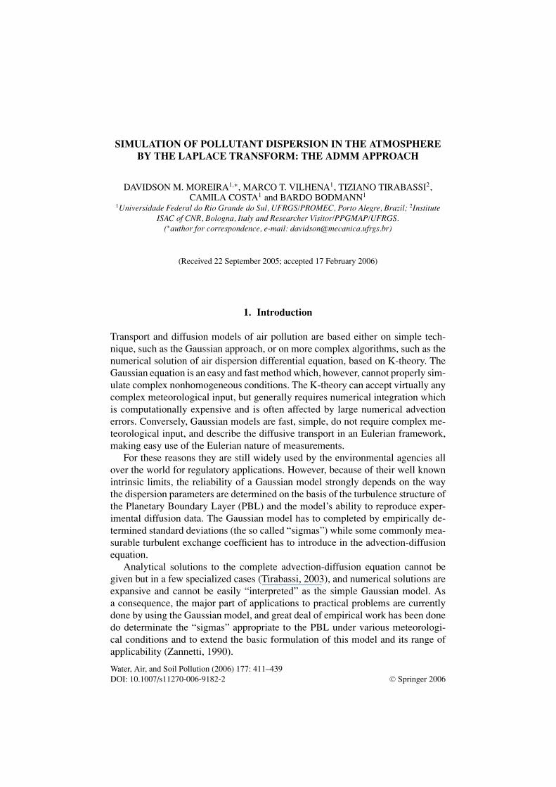
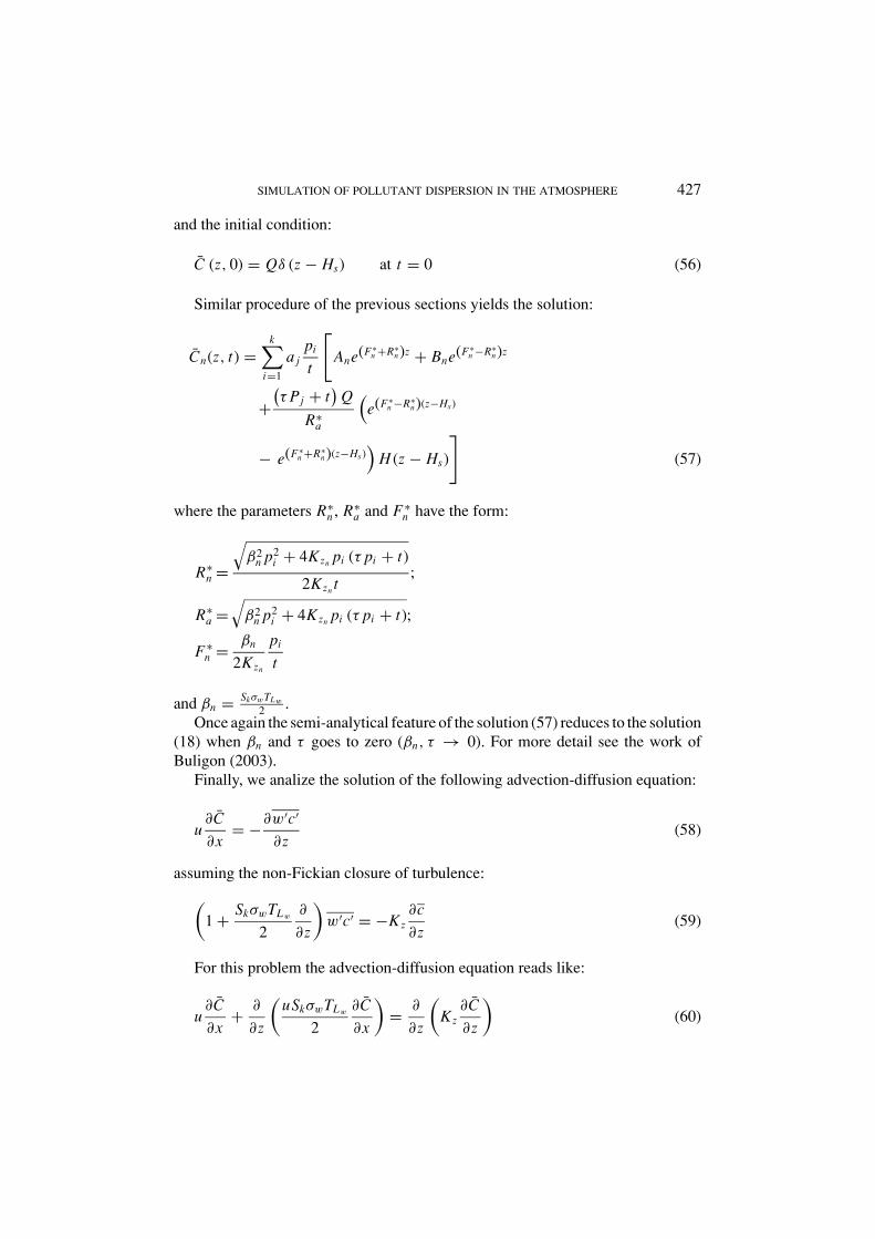
In Figure 1 it is shown the scatter diagrams between the measured and predictedcrosswind integrated concentrations using the above parameterizations for windand eddy diffusivities profiles.

Table I presents some performances measures obtained by using the statisticalevaluation procedure described by Hanna (1989) and defined in the following way:Nmse (normalized mean square error) = (Co − C p)2/ C p Co,Fa2 = fraction of data (%) for 0.5 ≤ (C p/Co) ≤ 2,

Cor (correlation coefficient) = (Co − Co)(C p − C p /σoσp, Fb (fractional bias)= Co − C p/0.5(Co + C p),Fs (fractional standard deviations) = (σo − σp)/0.5(σo + σp),

where the subscripts o and p refer to observed and predicted quantities, respectively,and the overbar indicates an averaged value. The statistical index Fb says if thepredicted quantity underestimate or overestimate the observed ones. The statistical

430 D. M. MOREIRA ET AL.

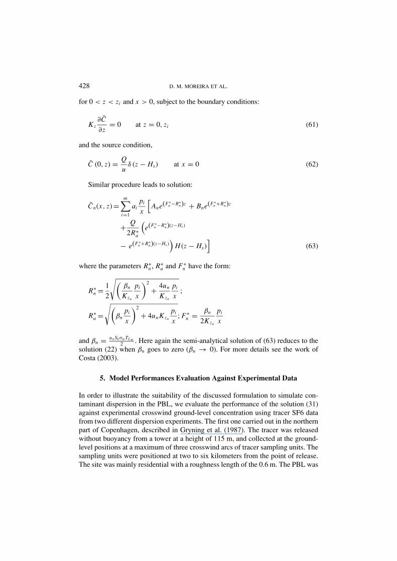
TABLE I

Statistical indices. Copenhagen experiment

Quadrature points �z (m) CPU time (s) Nmse Fa2 Cor Fb Fs

60 2 0.05 1.00 0.91 0.02 0.16k = 2; m = 8 40 9 0.07 1.00 0.90 0.09 0.22

20 120 0.06 1.00 0.91 0.05 0.1860 1 0.06 0.91 0.88 −0.03 0.17

k = 2; m = 4 40 5 0.05 0.96 0.90 −0.01 0.1420 60 0.06 0.91 0.88 0.00 0.1960 1 0.07 0.87 0.91 −0.16 −0.00

k = 2; m = 2 40 3 0.04 1.00 0.92 −0.02 0.0720 30 0.07 0.91 0.91 −0.14 0.03

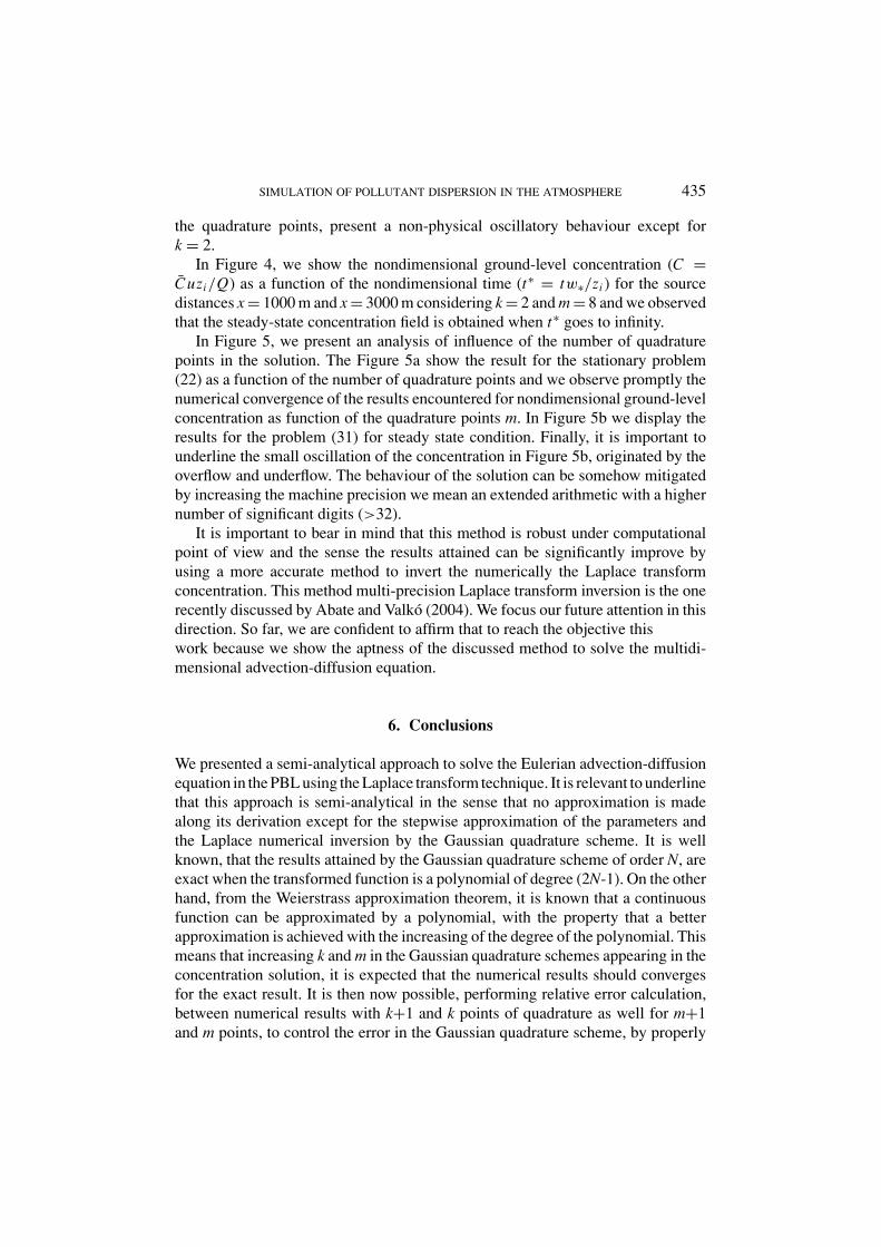
Figure 1. The scatter diagram for the semi-analytical solution (31) for Copenhagen experiment:Observed (Co) and predicted (Cp) crosswind ground-level integrated concentration (k = 2, m = 8,

�z = 40m). Points between lines have a factor of 2.

index Nmse represents the model values dispersion in respect to data dispersion.The best results are expected to have values near to zero for the indices Nmse, Fband Fs, and near to 1 in the indices Cor and Fa2.

Assuming different values of the Gaussian quadrature scheme (m, k = 2, 4, 8)and height discretization (�z = 20, 40, 60) initially it is important to observethat, for this problem, the size of height discretization pratically doesn’t affect thestatistical indices. But the Gaussian quadrature does. Finally, we must notice thatthe good results, under statistical point of view, attained for k = 2 and m = 2 matchthe practical interest of reduced computational effort.

SIMULATION OF POLLUTANT DISPERSION IN THE ATMOSPHERE 431

TABLE II

Statistical indices. Kinkaid experiment

Nmse Cor Fa2 Fb Fs

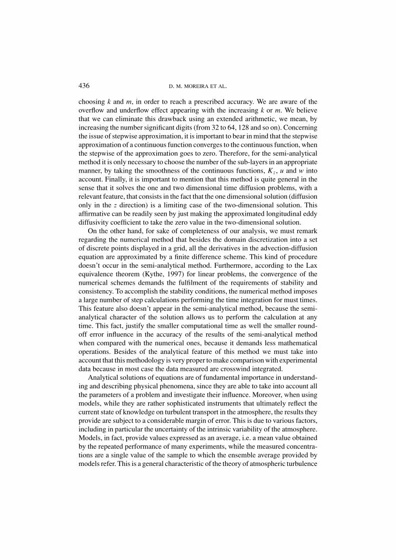
0.33 0.68 0.81 -0.04 -0.14

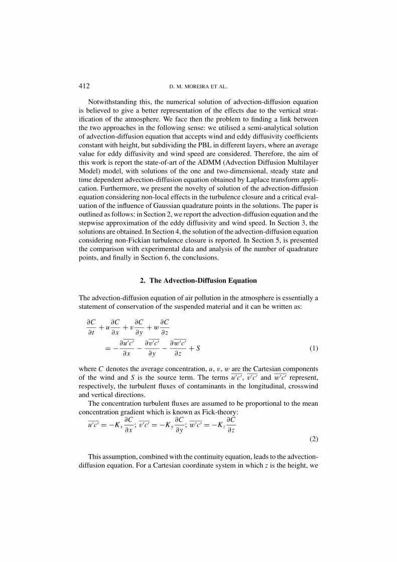
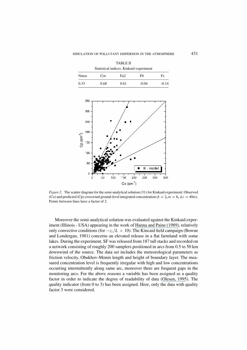
Figure 2. The scatter diagram for the semi-analytical solution (31) for Kinkaid experiment: Observed(Co) and predicted (Cp) crosswind ground-level integrated concentration (k = 2, m = 8, �z = 40m).Points between lines have a factor of 2.

Moreover the semi-analytical solution was evaluated against the Kinkaid exper-iment (Illinois - USA) appearing in the work of Hanna and Paine (1989), relativelyonly convective conditions (for −zi/L > 10). The Kincaid field campaign (Bowneand Londergan, 1981) concerns an elevated release in a flat farmland with somelakes. During the experiment, SF was released from 187 tall stacks and recorded ona network consisting of roughly 200 samplers positioned in arcs from 0.5 to 50 kmdownwind of the source. The data set includes the meteorological parameters asfriction velocity, Obukhov-Monin length and height of boundary layer. The mea-sured concentration level is frequently irregular with high and low concentrationsoccurring intermittently along same arc, moreover there are frequent gaps in themonitoring arcs. For the above reasons a variable has been assigned as a qualityfactor in order to indicate the degree of readability of data (Olesen, 1995). Thequality indicator (from 0 to 3) has been assigned. Here, only the data with qualityfactor 3 were considered.

432 D. M. MOREIRA ET AL.

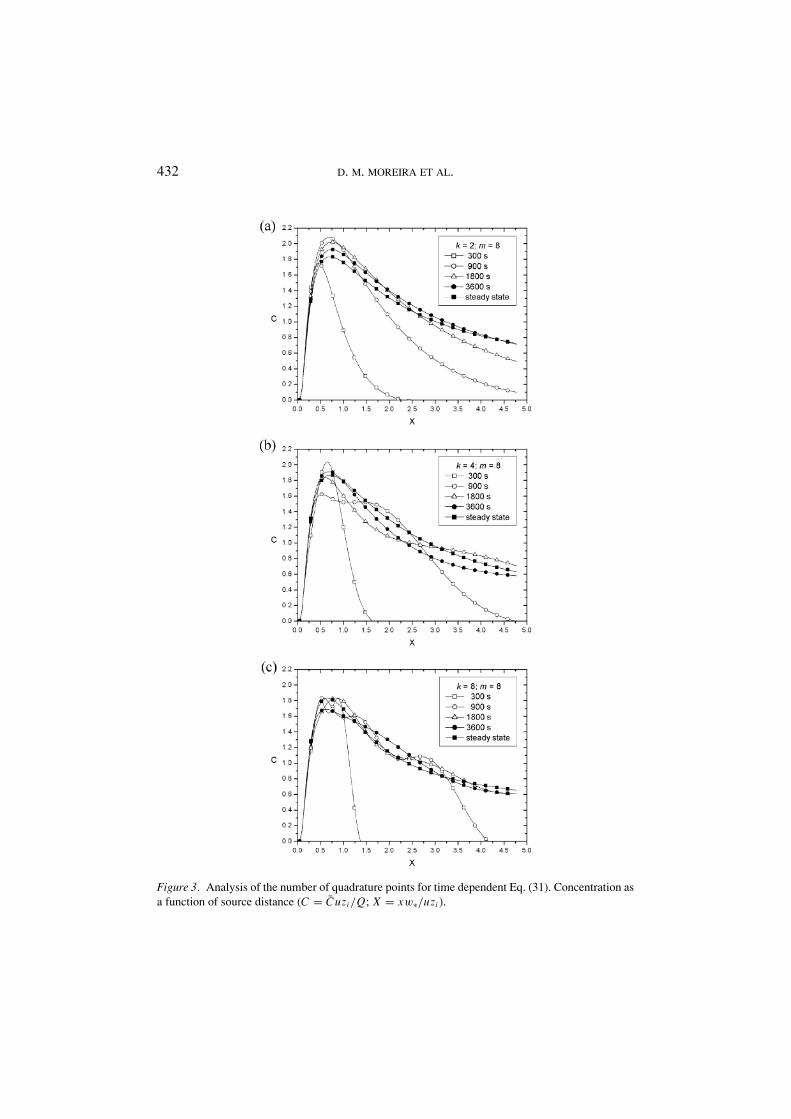
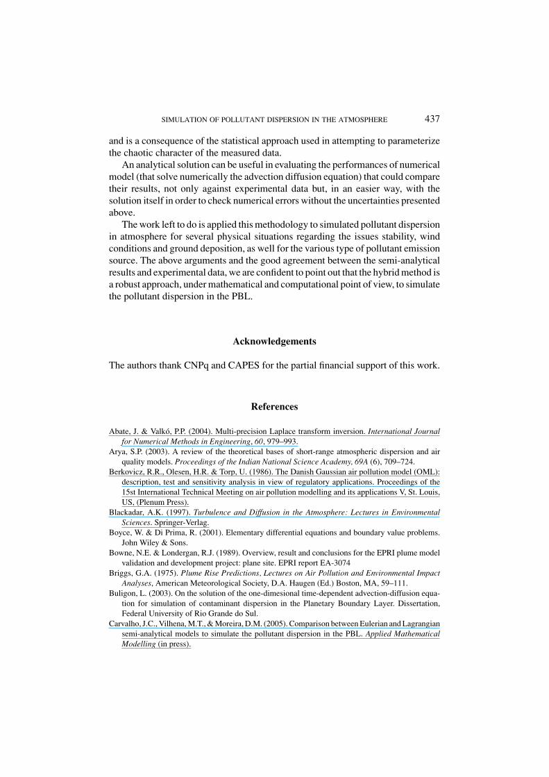
Figure 3. Analysis of the number of quadrature points for time dependent Eq. (31). Concentration asa function of source distance (C = Cuzi/Q; X = xw∗/uzi ).

SIMULATION OF POLLUTANT DISPERSION IN THE ATMOSPHERE 433

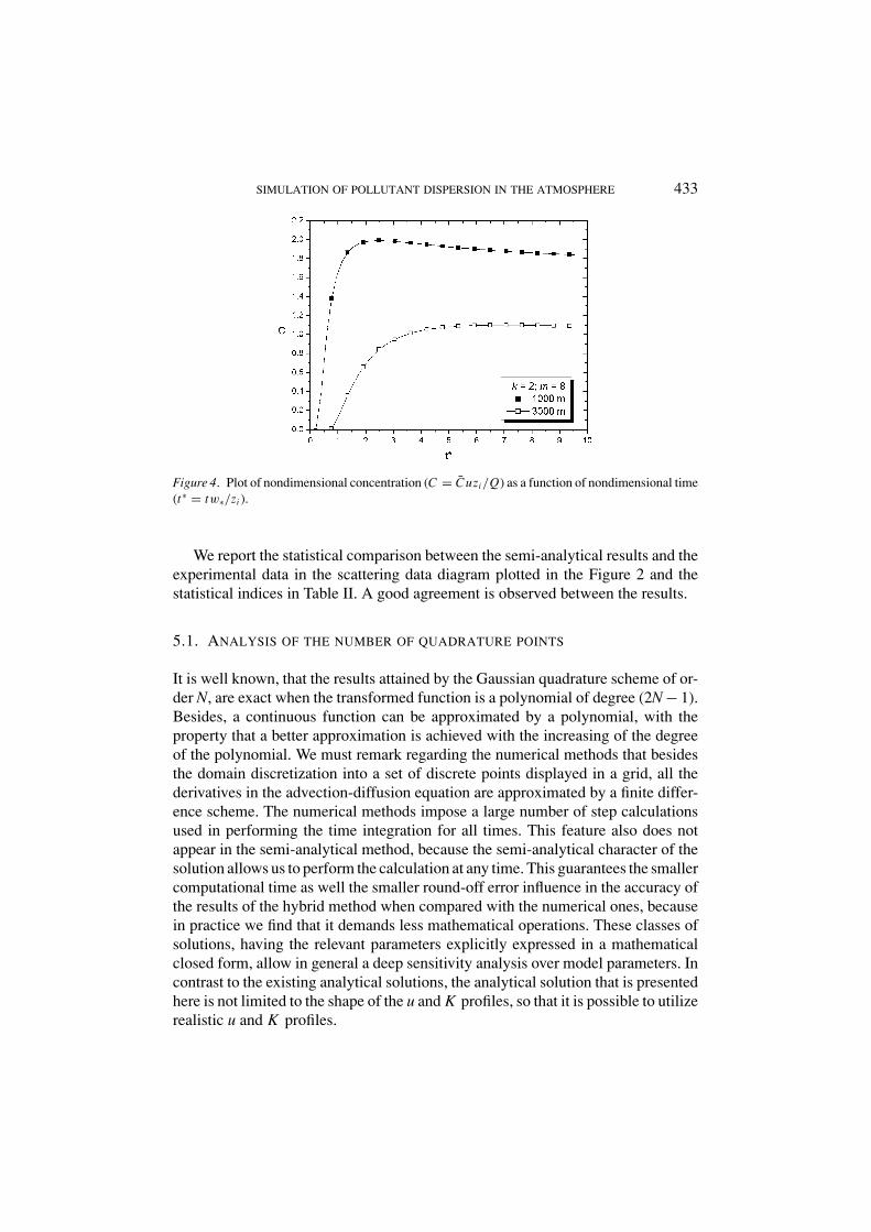
Figure 4. Plot of nondimensional concentration (C = Cuzi/Q) as a function of nondimensional time(t∗ = tw∗/zi ).

We report the statistical comparison between the semi-analytical results and theexperimental data in the scattering data diagram plotted in the Figure 2 and thestatistical indices in Table II. A good agreement is observed between the results.

5.1. ANALYSIS OF THE NUMBER OF QUADRATURE POINTS

It is well known, that the results attained by the Gaussian quadrature scheme of or-der N, are exact when the transformed function is a polynomial of degree (2N − 1).Besides, a continuous function can be approximated by a polynomial, with theproperty that a better approximation is achieved with the increasing of the degreeof the polynomial. We must remark regarding the numerical methods that besidesthe domain discretization into a set of discrete points displayed in a grid, all thederivatives in the advection-diffusion equation are approximated by a finite differ-ence scheme. The numerical methods impose a large number of step calculationsused in performing the time integration for all times. This feature also does notappear in the semi-analytical method, because the semi-analytical character of thesolution allows us to perform the calculation at any time. This guarantees the smallercomputational time as well the smaller round-off error influence in the accuracy ofthe results of the hybrid method when compared with the numerical ones, becausein practice we find that it demands less mathematical operations. These classes ofsolutions, having the relevant parameters explicitly expressed in a mathematicalclosed form, allow in general a deep sensitivity analysis over model parameters. Incontrast to the existing analytical solutions, the analytical solution that is presentedhere is not limited to the shape of the u and K profiles, so that it is possible to utilizerealistic u and K profiles.

434 D. M. MOREIRA ET AL.

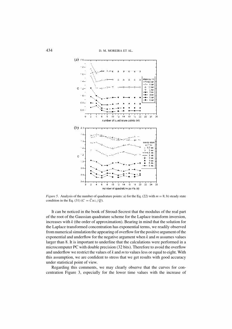
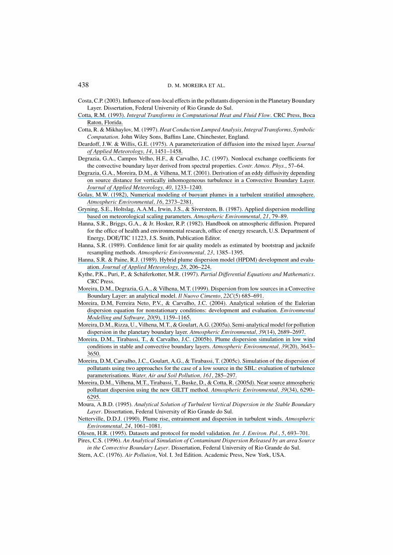
Figure 5. Analysis of the number of quadrature points: a) for the Eq. (22) with m = 8; b) steady statecondition in the Eq. (31) (C = Cuzi/Q).

It can be noticed in the book of Stroud-Secrest that the modulus of the real partof the root of the Gaussian quadrature scheme for the Laplace transform inversion,increases with k (the order of approximation). Bearing in mind that the solution forthe Laplace transformed concentration has exponential terms, we readily observedfrom numerical simulation the appearing of overflow for the positive argument of theexponential and underflow for the negative argument when k and m assumes valueslarger than 8. It is important to underline that the calculations were performed in amicrocomputer PC with double precision (32 bits). Therefore to avoid the overflowand underflow we restrict the values of k and m to values less or equal to eight. Withthis assumption, we are confident to stress that we get results with good accuracyunder statistical point of view.

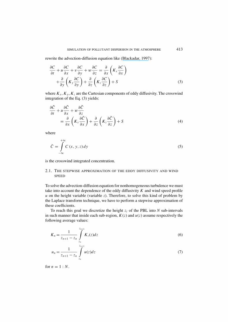
Regarding this comments, we may clearly observe that the curves for con-centration Figure 3, especially for the lower time values with the increase of

SIMULATION OF POLLUTANT DISPERSION IN THE ATMOSPHERE 435

the quadrature points, present a non-physical oscillatory behaviour except fork = 2.

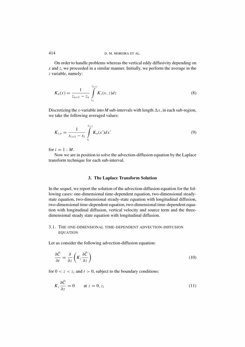
In Figure 4, we show the nondimensional ground-level concentration (C =Cuzi/Q) as a function of the nondimensional time (t∗ = tw∗/zi ) for the sourcedistances x = 1000 m and x = 3000 m considering k = 2 and m = 8 and we observedthat the steady-state concentration field is obtained when t∗ goes to infinity.

In Figure 5, we present an analysis of influence of the number of quadraturepoints in the solution. The Figure 5a show the result for the stationary problem(22) as a function of the number of quadrature points and we observe promptly thenumerical convergence of the results encountered for nondimensional ground-levelconcentration as function of the quadrature points m. In Figure 5b we display theresults for the problem (31) for steady state condition. Finally, it is important tounderline the small oscillation of the concentration in Figure 5b, originated by theoverflow and underflow. The behaviour of the solution can be somehow mitigatedby increasing the machine precision we mean an extended arithmetic with a highernumber of significant digits (>32).

It is important to bear in mind that this method is robust under computationalpoint of view and the sense the results attained can be significantly improve byusing a more accurate method to invert the numerically the Laplace transformconcentration. This method multi-precision Laplace transform inversion is the onerecently discussed by Abate and Valko (2004). We focus our future attention in thisdirection. So far, we are confident to affirm that to reach the objective thiswork because we show the aptness of the discussed method to solve the multidi-mensional advection-diffusion equation.

6. Conclusions

We presented a semi-analytical approach to solve the Eulerian advection-diffusionequation in the PBL using the Laplace transform technique. It is relevant to underlinethat this approach is semi-analytical in the sense that no approximation is madealong its derivation except for the stepwise approximation of the parameters andthe Laplace numerical inversion by the Gaussian quadrature scheme. It is wellknown, that the results attained by the Gaussian quadrature scheme of order N, areexact when the transformed function is a polynomial of degree (2N-1). On the otherhand, from the Weierstrass approximation theorem, it is known that a continuousfunction can be approximated by a polynomial, with the property that a betterapproximation is achieved with the increasing of the degree of the polynomial. Thismeans that increasing k and m in the Gaussian quadrature schemes appearing in theconcentration solution, it is expected that the numerical results should convergesfor the exact result. It is then now possible, performing relative error calculation,between numerical results with k+1 and k points of quadrature as well for m+1and m points, to control the error in the Gaussian quadrature scheme, by properly

436 D. M. MOREIRA ET AL.

choosing k and m, in order to reach a prescribed accuracy. We are aware of theoverflow and underflow effect appearing with the increasing k or m. We believethat we can eliminate this drawback using an extended arithmetic, we mean, byincreasing the number significant digits (from 32 to 64, 128 and so on). Concerningthe issue of stepwise approximation, it is important to bear in mind that the stepwiseapproximation of a continuous function converges to the continuous function, whenthe stepwise of the approximation goes to zero. Therefore, for the semi-analyticalmethod it is only necessary to choose the number of the sub-layers in an appropriatemanner, by taking the smoothness of the continuous functions, Kz , u and w intoaccount. Finally, it is important to mention that this method is quite general in thesense that it solves the one and two dimensional time diffusion problems, with arelevant feature, that consists in the fact that the one dimensional solution (diffusiononly in the z direction) is a limiting case of the two-dimensional solution. Thisaffirmative can be readily seen by just making the approximated longitudinal eddydiffusivity coefficient to take the zero value in the two-dimensional solution.

On the other hand, for sake of completeness of our analysis, we must remarkregarding the numerical method that besides the domain discretization into a setof discrete points displayed in a grid, all the derivatives in the advection-diffusionequation are approximated by a finite difference scheme. This kind of proceduredoesn’t occur in the semi-analytical method. Furthermore, according to the Laxequivalence theorem (Kythe, 1997) for linear problems, the convergence of thenumerical schemes demands the fulfilment of the requirements of stability andconsistency. To accomplish the stability conditions, the numerical method imposesa large number of step calculations performing the time integration for must times.This feature also doesn’t appear in the semi-analytical method, because the semi-analytical character of the solution allows us to perform the calculation at anytime. This fact, justify the smaller computational time as well the smaller round-off error influence in the accuracy of the results of the semi-analytical methodwhen compared with the numerical ones, because it demands less mathematicaloperations. Besides of the analytical feature of this method we must take intoaccount that this methodology is very proper to make comparison with experimentaldata because in most case the data measured are crosswind integrated.

Analytical solutions of equations are of fundamental importance in understand-ing and describing physical phenomena, since they are able to take into account allthe parameters of a problem and investigate their influence. Moreover, when usingmodels, while they are rather sophisticated instruments that ultimately reflect thecurrent state of knowledge on turbulent transport in the atmosphere, the results theyprovide are subject to a considerable margin of error. This is due to various factors,including in particular the uncertainty of the intrinsic variability of the atmosphere.Models, in fact, provide values expressed as an average, i.e. a mean value obtainedby the repeated performance of many experiments, while the measured concentra-tions are a single value of the sample to which the ensemble average provided bymodels refer. This is a general characteristic of the theory of atmospheric turbulence

SIMULATION OF POLLUTANT DISPERSION IN THE ATMOSPHERE 437

and is a consequence of the statistical approach used in attempting to parameterizethe chaotic character of the measured data.

An analytical solution can be useful in evaluating the performances of numericalmodel (that solve numerically the advection diffusion equation) that could comparetheir results, not only against experimental data but, in an easier way, with thesolution itself in order to check numerical errors without the uncertainties presentedabove.

The work left to do is applied this methodology to simulated pollutant dispersionin atmosphere for several physical situations regarding the issues stability, windconditions and ground deposition, as well for the various type of pollutant emissionsource. The above arguments and the good agreement between the semi-analyticalresults and experimental data, we are confident to point out that the hybrid method isa robust approach, under mathematical and computational point of view, to simulatethe pollutant dispersion in the PBL.

Acknowledgements

The authors thank CNPq and CAPES for the partial financial support of this work.

References

Abate, J. & Valko, P.P. (2004). Multi-precision Laplace transform inversion. International Journalfor Numerical Methods in Engineering, 60, 979–993.

Arya, S.P. (2003). A review of the theoretical bases of short-range atmospheric dispersion and airquality models. Proceedings of the Indian National Science Academy, 69A (6), 709–724.

Berkovicz, R.R., Olesen, H.R. & Torp, U. (1986). The Danish Gaussian air pollution model (OML):description, test and sensitivity analysis in view of regulatory applications. Proceedings of the15st International Technical Meeting on air pollution modelling and its applications V, St. Louis,US, (Plenum Press).

Blackadar, A.K. (1997). Turbulence and Diffusion in the Atmosphere: Lectures in EnvironmentalSciences. Springer-Verlag.

Boyce, W. & Di Prima, R. (2001). Elementary differential equations and boundary value problems.John Wiley & Sons.

Bowne, N.E. & Londergan, R.J. (1989). Overview, result and conclusions for the EPRI plume modelvalidation and development project: plane site. EPRI report EA-3074

Briggs, G.A. (1975). Plume Rise Predictions, Lectures on Air Pollution and Environmental ImpactAnalyses, American Meteorological Society, D.A. Haugen (Ed.) Boston, MA, 59–111.

Buligon, L. (2003). On the solution of the one-dimesional time-dependent advection-diffusion equa-tion for simulation of contaminant dispersion in the Planetary Boundary Layer. Dissertation,Federal University of Rio Grande do Sul.

Carvalho, J.C., Vilhena, M.T., & Moreira, D.M. (2005). Comparison between Eulerian and Lagrangiansemi-analytical models to simulate the pollutant dispersion in the PBL. Applied MathematicalModelling (in press).

438 D. M. MOREIRA ET AL.

Costa, C.P. (2003). Influence of non-local effects in the pollutants dispersion in the Planetary BoundaryLayer. Dissertation, Federal University of Rio Grande do Sul.

Cotta, R.M. (1993). Integral Transforms in Computational Heat and Fluid Flow. CRC Press, BocaRaton, Florida.

Cotta, R. & Mikhaylov, M. (1997). Heat Conduction Lumped Analysis, Integral Transforms, SymbolicComputation. John Wiley Sons, Baffins Lane, Chinchester, England.

Deardoff, J.W. & Willis, G.E. (1975). A parameterization of diffusion into the mixed layer. Journalof Applied Meteorology, 14, 1451–1458.

Degrazia, G.A., Campos Velho, H.F., & Carvalho, J.C. (1997). Nonlocal exchange coefficients forthe convective boundary layer derived from spectral properties. Contr. Atmos. Phys., 57–64.

Degrazia, G.A., Moreira, D.M., & Vilhena, M.T. (2001). Derivation of an eddy diffusivity dependingon source distance for vertically inhomogeneous turbulence in a Convective Boundary Layer.Journal of Applied Meteorology, 40, 1233–1240.

Golay, M.W. (1982), Numerical modeling of buoyant plumes in a turbulent stratified atmosphere.Atmospheric Environmental, 16, 2373–2381.

Gryning, S.E., Holtslag, A.A.M., Irwin, J.S., & Siversteen, B. (1987). Applied dispersion modellingbased on meteorological scaling parameters. Atmospheric Environmental, 21, 79–89.

Hanna, S.R., Briggs, G.A., & Jr. Hosker, R.P. (1982). Handbook on atmospheric diffusion. Preparedfor the office of health and environmental research, office of energy research, U.S. Department ofEnergy, DOE/TIC 11223, J.S. Smith, Publication Editor.

Hanna, S.R. (1989). Confidence limit for air quality models as estimated by bootstrap and jackniferesampling methods. Atmospheric Environmental, 23, 1385–1395.

Hanna, S.R. & Paine, R.J. (1989). Hybrid plume dispersion model (HPDM) development and evalu-ation. Journal of Applied Meteorology, 28, 206–224.

Kythe, P.K., Puri, P., & Schaferkotter, M.R. (1997). Partial Differential Equations and Mathematics.CRC Press.

Moreira, D.M., Degrazia, G.A., & Vilhena, M.T. (1999). Dispersion from low sources in a ConvectiveBoundary Layer: an analytical model. Il Nuovo Cimento, 22C(5) 685–691.

Moreira, D.M, Ferreira Neto, P.V., & Carvalho, J.C. (2004). Analytical solution of the Euleriandispersion equation for nonstationary conditions: development and evaluation. EnvironmentalModelling and Software, 20(9), 1159–1165.

Moreira, D.M., Rizza, U., Vilhena, M.T., & Goulart, A.G. (2005a). Semi-analytical model for pollutiondispersion in the planetary boundary layer. Atmospheric Environmental, 39(14), 2689–2697.

Moreira, D.M., Tirabassi, T., & Carvalho, J.C. (2005b). Plume dispersion simulation in low windconditions in stable and convective boundary layers. Atmospheric Environmental, 39(20), 3643–3650.

Moreira, D.M, Carvalho, J.C., Goulart, A.G., & Tirabassi, T. (2005c). Simulation of the dispersion ofpollutants using two approaches for the case of a low source in the SBL: evaluation of turbulenceparameterisations. Water, Air and Soil Pollution, 161, 285–297.

Moreira, D.M., Vilhena, M.T., Tirabassi, T., Buske, D., & Cotta, R. (2005d). Near source atmosphericpollutant dispersion using the new GILTT method. Atmospheric Environmental, 39(34), 6290–6295.

Moura, A.B.D. (1995). Analytical Solution of Turbulent Vertical Dispersion in the Stable BoundaryLayer. Dissertation, Federal University of Rio Grande do Sul.

Netterville, D.D.J. (1990). Plume rise, entrainment and dispersion in turbulent winds. AtmosphericEnvironmental, 24, 1061–1081.

Olesen, H.R. (1995). Datasets and protocol for model validation. Int. J. Environ. Pol., 5, 693–701.Pires, C.S. (1996). An Analytical Simulation of Contaminant Dispersion Released by an area Source

in the Convective Boundary Layer. Dissertation, Federal University of Rio Grande do Sul.Stern, A.C. (1976). Air Pollution, Vol. I. 3rd Edition. Academic Press, New York, USA.

SIMULATION OF POLLUTANT DISPERSION IN THE ATMOSPHERE 439

Stroud, A.H., & Secrest, D. (1966). Gaussian quadrature formulas. Englewood Cliffs, N.J., PrenticeHall Inc.

Tirabassi, T. (2003). Operational advanced air pollution modeling. PAGEOPH, 160 (1–2), 5–16.van Dop, H. & Verver, G. (2001). Countergradient transport revisited. Journal of Atmospheric Sci-

ences, 58, 2240–2247.Vilhena, M.T., Rizza, U., Degrazia, G.A., Mangia, C., Moreira, D.M., & Tirabassi, T. (1998). An

analytical air pollution model: development and evaluation. Contr. Atmos. Phys., 71(3), 315–320.Weil, J.C. (1988). Plume rise. Lectures on air pollution modeling. A. Venkatram, & J.C. Wyngaard,

(Ed). American Meteorological Society, Boston, 119–166.Weil, J.C. (1979). Assessment of plume rise and dispersion models using lidar data, PPSP-MP-24,

Prepared by environmental center, Martin Marietta Corporation, for Maryland department ofnatural resources.

Zanetti, P. (1990). Air pollution modeling. Comp. Mech. Publications, Southampton (UK).