factores mundiales y diferenciales de intereses en mercados emergentes

Inter-American Development Bank

Banco Interamericano de Desarrollo (BID) Research Department

Departamento de Investigación Working Paper #552

Global Factors and Emerging Market Spreads

by

Martín González Rozada* Eduardo Levy Yeyati**

*Universidad Torcuato Di Tella **Universidad Torcuato Di Tella and Inter-American Development Bank

May 2006

2

Cataloging-in-Publication data provided by the Inter-American Development Bank Felipe Herrera Library González Rozada, Martín.

Global factors and emerging market spreads / by Martín González Rozada, Eduardo Levy Yeyati.

p. cm. (Research Department Working paper series ; 552) Includes bibliographical references.

1. Bond market. I. Levy Yeyati, Eduardo. II. Inter-American Development Bank. Research

Dept. III. Title. IV. Series.

332.6323 G554--------dc21 ©2006 Inter-American Development Bank 1300 New York Avenue, N.W. Washington, DC 20577

The views and interpretations in this document are those of the authors and should not be attributed to the Inter-American Development Bank, or to any individual acting on its behalf. This paper may be freely reproduced provided credit is given to the Research Department, Inter-American Development Bank. The Research Department (RES) produces a quarterly newsletter, IDEA (Ideas for Development in the Americas), as well as working papers and books on diverse economic issues. To obtain a complete list of RES publications, and read or download them please visit our web site at: http://www.iadb.org/res

3

Abstract1

This paper shows that a large fraction of the variability of emerging market bond spreads is explained by the evolution of global factors such as risk appetite (as reflected in the spread of high yield corporate bonds in developed markets), global liquidity (measured by the international interest rates) and contagion (from systemic events like the Russian default). This link has remained relatively stable over the history of the emerging market class, is robust to the inclusion of country-specific factors, and helps provide accurate long-run predictions. Overall, the results highlight the critical role played by exogenous factors in the evolution of the borrowing cost faced by emerging economies.

JEL Classification Numbers: F34, E43, G15 Keywords: Sovereign Spreads, Risk Appetite, Global Liquidity, Emerging Markets

1 Martín González Rozada gratefully acknowledges financial assistance from the IDB. The authors would like to thank Jorge Morgenstern and Sebastián Castresana for excellent research assistance and participants at the RES brown bag seminar at the IDB for useful comments. The usual disclaimers apply.

4

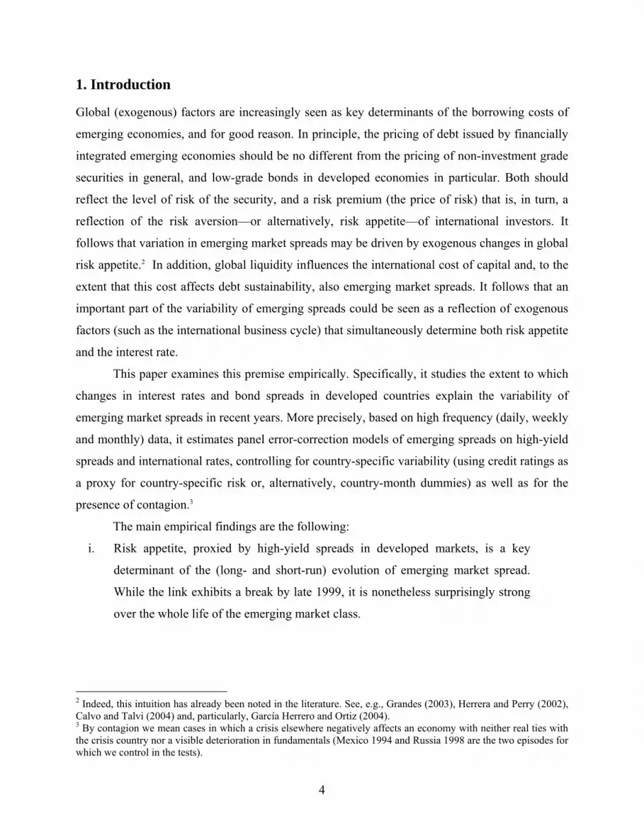
1. Introduction Global (exogenous) factors are increasingly seen as key determinants of the borrowing costs of

emerging economies, and for good reason. In principle, the pricing of debt issued by financially

integrated emerging economies should be no different from the pricing of non-investment grade

securities in general, and low-grade bonds in developed economies in particular. Both should

reflect the level of risk of the security, and a risk premium (the price of risk) that is, in turn, a

reflection of the risk aversion—or alternatively, risk appetite—of international investors. It

follows that variation in emerging market spreads may be driven by exogenous changes in global

risk appetite.2 In addition, global liquidity influences the international cost of capital and, to the

extent that this cost affects debt sustainability, also emerging market spreads. It follows that an

important part of the variability of emerging spreads could be seen as a reflection of exogenous

factors (such as the international business cycle) that simultaneously determine both risk appetite

and the interest rate.

This paper examines this premise empirically. Specifically, it studies the extent to which

changes in interest rates and bond spreads in developed countries explain the variability of

emerging market spreads in recent years. More precisely, based on high frequency (daily, weekly

and monthly) data, it estimates panel error-correction models of emerging spreads on high-yield

spreads and international rates, controlling for country-specific variability (using credit ratings as

a proxy for country-specific risk or, alternatively, country-month dummies) as well as for the

presence of contagion.3

The main empirical findings are the following:

i. Risk appetite, proxied by high-yield spreads in developed markets, is a key

determinant of the (long- and short-run) evolution of emerging market spread.

While the link exhibits a break by late 1999, it is nonetheless surprisingly strong

over the whole life of the emerging market class.

2 Indeed, this intuition has already been noted in the literature. See, e.g., Grandes (2003), Herrera and Perry (2002), Calvo and Talvi (2004) and, particularly, García Herrero and Ortiz (2004). 3 By contagion we mean cases in which a crisis elsewhere negatively affects an economy with neither real ties with the crisis country nor a visible deterioration in fundamentals (Mexico 1994 and Russia 1998 are the two episodes for which we control in the tests).

5

ii. International liquidity (proxied by US Treasury notes, 10-year constant maturity

yield) exhibits a significant benign influence on the long-run levels of emerging

spreads.

iii. These two exogenous factors explain around 30 percent of the long-run (dynamic)

variability of emerging market spreads (between 15 and 23 percent for the short-

run using weekly and monthly data, respectively).

iv. Contagion from crisis with systemic effects (as exemplified by the 1998 Russian

default) exerts a strong negative impact on spreads.

v. The results are relatively stable over the period under analysis (1994-2005,

corresponding to the existence of the emerging market debt class), although the

link strengthens slightly after 1999.

vi. Each of these results is robust to the introduction of additional variables,

including country-month controls to proxy available information about macro

fundamentals, and credit ratings.

These findings have several potentially important implications for the emerging markets

literature. First, they show that variations in emerging market spreads can be largely explained

by exogenous factors. In this way, the paper contributes to the discussion about the nature of

emerging market stability, specifically on the degree of exogeneity in the determination of the

highly volatile borrowing costs faced by emerging economies—a major source of financial

distress in the recent past. Moreover, it shifts the discussion on debt dynamics from sustainability

to vulnerability, as it emphasizes the exogenous component of external volatility, placing the

focus on factors that would make a country more or less resilient to sudden changes in the

external context. The exogenous nature of borrowing costs highlights the role of country-specific

fundamentals as determinants of exposure to external shocks—rather than as the drivers of

borrowing costs as proposed by the standard view of debt sustainability. In addition, the findings

shed new light on the connection between the borrowing costs faced by emerging economies and

the cycle in the industrial world (as captured by international interest rates), a link already noted

in the early literature on capital flows.4 In passing, the paper documents that, contrary to

4 See, among others, Calvo, Leiderman and Reinhart (1993), and Levy Yeyati and Sturzenegger (2000).

6

conventional wisdom, credit ratings respond to spreads more than they influence them, casting

doubt on their informational content.

The paper proceeds as follows. The next section introduces the reduced-form model that

underlies the empirical specification of our tests, presents the data and describes the empirical

methodology. Section 3 reports the main empirical findings and robustness tests. Section 4

concludes.

2. Emerging Market and Corporate Bond Pricing A Reduced-Form Model Interest rate arbitrage by risk-averse investors implies that

(1) (1 – q)(1 + r) + qV = (1 + rf) + ϕq , where q is the probability of default, V the recovery value after default, r and rf the interest rates

charged to the bond and to a risk-free asset of similar duration, and ϕ is a parameter that reflects

investors’ risk aversion. Then, we can express the emerging market spread as:

(2) spread ≡ r – rf = [ϕ + (1 + rf) – V][q/(1 – q)] or, more generally, assuming that recovery values are stable over time and comparable across

bonds, as

(3) spreadit = ρ(rft , ϕt) θ[q(Xit)] φi(rf

t , dctc)

where

• ρ denotes the price of credit risk, which depends on the international risk-free rate rft and

risk aversion ϕt ;

• θ measures the incidence of the default risk of the issuer, q, itself a function of country-

specific (in the case of sovereign debt) or firm-specific (in the case of corporate bonds)

fundamentals Xit.; and

• φi is a scale factor reflecting global factors that affect corporate and emerging market debt

differently, such as global liquidity (measured by the international risk-free rate rft ) and

7

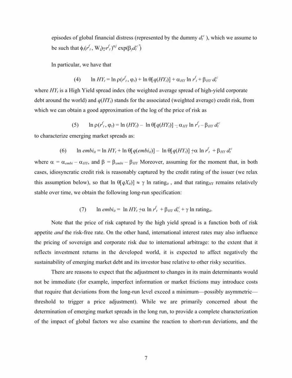
episodes of global financial distress (represented by the dummy dtc ), which we assume to

be such that φi(rft , Wt) = rf

t )αj exp(βjdtc )

In particular, we have that

(4) ln HYt = ln ρ(rft , ϕt) + ln θ[q(HYt)] + αHY ln rf

t + βHY dtc

where HYt is a High Yield spread index (the weighted average spread of high-yield corporate

debt around the world) and q(HYt) stands for the associated (weighted average) credit risk, from

which we can obtain a good approximation of the log of the price of risk as

(5) ln ρ(rft , ϕt) = ln (HYt) – ln θ[q(HYt)] – αHY ln rf

t – βHY dtc

to characterize emerging market spreads as:

(6) ln embiit = ln HYt + ln θ[q(embiit)] – ln θ[q(HYt)] + α ln rft + βHY dt

c

where α = αembi – αHY, and β = βembi – βHY Moreover, assuming for the moment that, in both

cases, idiosyncratic credit risk is reasonably captured by the credit rating of the issuer (we relax

this assumption below), so that ln θ[qXit)] ≈ γ ln ratingit , and that ratingHY remains relatively

stable over time, we obtain the following long-run specification:

(7) ln embiit = ln HYt + α ln rft + βHY dt

c + γ ln ratingit.

Note that the price of risk captured by the high yield spread is a function both of risk

appetite and the risk-free rate. On the other hand, international interest rates may also influence

the pricing of sovereign and corporate risk due to international arbitrage: to the extent that it

reflects investment returns in the developed world, it is expected to affect negatively the

sustainability of emerging market debt and its investor base relative to other risky securities.

There are reasons to expect that the adjustment to changes in its main determinants would

not be immediate (for example, imperfect information or market frictions may introduce costs

that require that deviations from the long-run level exceed a minimum—possibly asymmetric—

threshold to trigger a price adjustment). While we are primarily concerned about the

determination of emerging market spreads in the long run, to provide a complete characterization

of the impact of global factors we also examine the reaction to short-run deviations, and the

8

speed of convergence to the long-run level, by augmenting the previous long-run specification

with an error-correction equation.

The Data To proxy for the price of risk, we use Credit Swiss First Boston’s High Yield Index (HY), which

measures the spread over the US treasuries yield curve at the redemption date with the worst

yield (an alternative measure of high yield spreads prepared by J. P. Morgan yielded almost

identical results). Emerging market sovereign spreads are measured as the spread over Treasuries

of J. P. Morgan’s EMBI Global index (embi) for each of the 33 emerging economies included in

the Global portfolio (period coverage varies across countries, as reported in Appendix Table A2).

The credit rating variable (rating) is constructed based on Standard & Poor’s rating for long-term

debt in foreign currency. As a proxy for international liquidity, we use the 10-year US Treasury

rate (10YT), although we also run tests using the US$ and the DM/Euro 6-month LIBOR for

robustness (sourced from the Federal Reserve and the BBA, respectively). Also for robustness,

as an alternative measure of the price of risk, we test the volatility implicit in US stock options

(VIX) compiled by the Chicago Board Options Exchange. In all cases, we work alternatively with

monthly, weekly and (occasionally) daily data.

The Methodology The econometric model used in this paper describes a basic long-run relationship between the

market spreads, the high yield index and the international rate. The first step in analyzing this

equilibrium relationship is to check the individual statistical properties of the panel data series.

This is done using different panel data unit roots tests as explained below. If the variables in the

specific long-run equation have unit roots, the second step consists in verifying the existence of a

long run equilibrium relationship using panel cointegration tests. If there is panel cointegration,

then the next step is to estimate the parameters of the model.

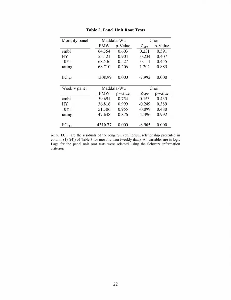
To analyze the statistical properties of each individual panel data series we performed

two types of panel unit root tests: Maddala and Wu (1999) and Choi (2001). All these tests are

based on variations of a standard autoregressive process of order one for panel data. Maddala and

Wu use an alternative approach to panel unit root tests based on Fisher’s (1932) results. We

report, for this test, the asymptotic χ22N statistic using augmented Dickey-Fuller individual unit

9

root tests. Choi proposes a similar standardized statistic as Maddala and Wu, but with a standard

normal asymptotic distribution. Table 2 shows the results of these panel unit root tests for all

individual variables in the long run equilibrium relationships for both the monthly (Panel A) and

weekly (Panel B) dataset.

It is clear from the table that all variables individually have a panel unit root using

standard statistical levels of significance. It follows that, if there exists any meaningful

relationship between the market spreads and the high yield index, it should be because they are

co-integrated. To explore this possibility we followed the Engle and Granger approach and

performed panel unit root tests on the residuals of the co-integration relationship. These results

are also shown in Table 2. As can be seen from the table, both tests reject the null of panel unit

root.

Since there is evidence of co-integration, according to the Granger Representation

Theorem, the variables in the long-run equilibrium relationship have a panel error correction

representation (PECM). This representation expresses the model in levels and differences in

order to separate out the long-run and short-run effects. We use the Engle-Granger methodology

(Engle and Granger, 1987) to estimate the PECM. This methodology is a two-stage modeling

strategy, which may be formalized as follows. In stage one, we estimate the long-run parameters

of the cointegration equation using a least squares dummy variable (LSDV) procedure

itittf ratingWr

tεααααα +++++= )ln()ln()ln( )(HYln )ln(embi(8) 432t10iit

where Xt is a vector of variables that could include some measure of credit rating, the

international interest rate, etc. The estimators in this first step are consistent even when some or

all the variables in the right hand side of the equation are endogenous because the estimates of

the parameters converge to their probability limits at a rate of T instead of at the usual

asymptotic rate of T1/2. From equation (8) we obtain the residuals (ži,t). Stage two uses the error

correction term lagged once, ži,t-1, and estimates a PECM to get the short-run dynamics. Out of

the steady state we do not know the lag structure of the short-term dynamics, therefore we begin

with a general specification of the form

10

iti,t-jjjtij

jf

jjti

u

Wrjtjt

+ΔΓ+ΔΓ+

+ΔΓ+ΔΓ+ΔΓ++=Δ

∑∑

∑∑∑

==−

===−−

r

1j4

n

0j,3

m

0j2

q

0j1

p

0jj-t01-ti,10i,

)(embiln )(ratingln

)(ln )(ln )(HYln z )ln(embi(9) (γγ

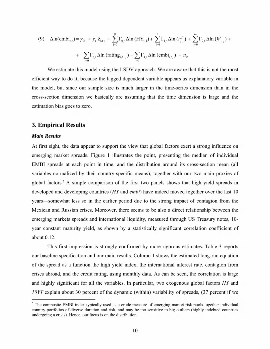
We estimate this model using the LSDV approach. We are aware that this is not the most

efficient way to do it, because the lagged dependent variable appears as explanatory variable in

the model, but since our sample size is much larger in the time-series dimension than in the

cross-section dimension we basically are assuming that the time dimension is large and the

estimation bias goes to zero.

3. Empirical Results

Main Results

At first sight, the data appear to support the view that global factors exert a strong influence on

emerging market spreads. Figure 1 illustrates the point, presenting the median of individual

EMBI spreads at each point in time, and the distribution around its cross-section mean (all

variables normalized by their country-specific means), together with our two main proxies of

global factors.5 A simple comparison of the first two panels shows that high yield spreads in

developed and developing countries (HY and embi) have indeed moved together over the last 10

years—somewhat less so in the earlier period due to the strong impact of contagion from the

Mexican and Russian crises. Moreover, there seems to be also a direct relationship between the

emerging markets spreads and international liquidity, measured through US Treasury notes, 10-

year constant maturity yield, as shown by a statistically significant correlation coefficient of

about 0.12.

This first impression is strongly confirmed by more rigorous estimates. Table 3 reports

our baseline specification and our main results. Column 1 shows the estimated long-run equation

of the spread as a function the high yield index, the international interest rate, contagion from

crises abroad, and the credit rating, using monthly data. As can be seen, the correlation is large

and highly significant for all the variables. In particular, two exogenous global factors HY and

10YT explain about 30 percent of the dynamic (within) variability of spreads, (37 percent if we 5 The composite EMBI index typically used as a crude measure of emerging market risk pools together individual country portfolios of diverse duration and risk, and may be too sensitive to big outliers (highly indebted countries undergoing a crisis). Hence, our focus is on the distribution.

11

add contagion to the list), while the inclusion of credit ratings brings this number to close to 60

percent. The short-run equation is also consistent with our priors (column 2). All variables have a

strong contemporaneous impact on spreads but no delayed effect, and roughly 7 percent of

deviations from the long-run level are eliminated per month, so that the average lag length is

about fourteen months. Weekly data tell the same story (columns 3 and 4): high correlation,

strong explanatory power (about 60 percent of dynamic variability), and fast convergence

(roughly 33 weeks).

Note that the influence of the international interest rate goes beyond the standard

arbitrage view that portfolio flows respond to increases in the international rate (Calvo,

Leiderman and Reinhart, 1993). Indeed, the evidence that sovereign spreads adjust close to one

to one to changes in the foreign rate implies that borrowing costs in emerging economies respond

more than proportionally to the interest rate cycle in the developed world.6

Robustness I: Global Factors Then and Now

A natural question regarding the connection between bond pricing in developed and developing

countries is whether it has changed (and, in particular, strengthened) over the years, due to the

growing familiarity with the emerging market asset and the increasing integration of capital

markets (and bondholders). In this section we analyze this aspect by looking at possible

structural breaks in the long-run equilibrium relationship. In particular, we study whether the

coefficient of HY changes over time.

The specification of the test is standard. Starting from the following long-run equilibrium

relationship

ititX εβαα +++= )ln( )(HYln )ln(embi(9) t10iit where Xt is a vector including all variables in our baseline regression. We would like to consider

a possible break in the α1 coefficient at an unknown date k. Under the null hypothesis of no

break, the alternative hypothesis implies that:

⎪⎩

⎪⎨⎧

++==

Tkktforktfor

H bk

ak

...,,2,1...,,2,1

:,1

,11 α

α

6 The USD and the DM/Euro LIBOR (both correlated with 10YT) yield comparable results (omitted here for conciseness and available from the authors on request).

12

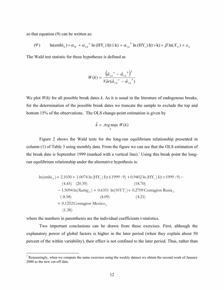
so that equation (9) can be written as:

ititb

ka

k X εβααα ++>+≤+= )ln( k)I(t )(HYln k)I(t )(HYln )ln(embi)(9' t,1t,10iit The Wald test statistic for these hypotheses is defined as

( ))ˆˆ(ˆ

ˆˆ)(

,1,1

2

,1,1b

ka

k

bk

ak

raVkW

αα

αα

−

−=

We plot W(k) for all possible break dates k. As it is usual in the literature of endogenous breaks,

for the determination of the possible break dates we truncate the sample to exclude the top and

bottom 15% of the observations. The OLS change-point estimation is given by

)(maxˆ kWArgkk

=

Figure 2 shows the Wald tests for the long-run equilibrium relationship presented in

column (1) of Table 3 using monthly data. From the figure we can see that the OLS estimation of

the break date is September 1999 (marked with a vertical line).7 Using this break point the long-

run equilibrium relationship under the alternative hypothesis is:

)38.1( MexicoContagion1252.0

)21.4((4.09)-8.58)(Rusia Contagion .27090)10ln( .63510)ln(1.5094

(18.70)(20.39))45.4( )9:1999I(t )(HY ln .94020)9:1999I(t )(HY ln 0074.1 1030.2 )ln(embi ttit

it

ittit YTRating

+

++−

−>+≤+=

where the numbers in parentheses are the individual coefficients t-statistics.

Two important conclusions can be drawn from these exercises. First, although the

explanatory power of global factors is higher in the later period (when they explain about 50

percent of the within variability), their effect is not confined to the later period. Thus, rather than

7 Reassuringly, when we compute the same exercises using the weekly dataset we obtain the second week of January 2000 as the new cut-off date.

13

a recent phenomenon, the connection appears to have been relevant since the beginning of

emerging market debt as an asset class—with only a minor strengthening (as measured by its

explanatory power) that appears to coincide with the aftermath of the Russian crisis. This latter

point is revealed by the robustness tests reported in Table 4. There, guided by our previous

results, we split the monthly sample into two sub-samples (1993-1999, and 2000-2005) and rerun

the regressions in columns (1)-(2) in Table 3. The results, presented in columns (1) to (4), clearly

show that, while the HY coefficients (both in the short- and long-run equation) are larger for the

earlier period, their explanatory power is comparable (and increases for the long-run equation) in

the later years. These findings are confirmed when we replicate the exercise for the full sample

and control the effect on the later period using an interaction of HY variables with a period

dummy (columns 5 and 6).

Given that emerging economies entered the EMBI portfolio at different points in time, it

is natural to ask whether the parameter change documented above is simply due to the

combination of cross-country differences and a changing sample composition. To dispel these

doubts, we replicate columns (1) to (4) for a balanced sample, focusing on three Latin American

countries that have been in the emerging market class since the very beginning and that have

historically represented a large portion of the whole emerging market portfolio: Argentina, Brazil

and Mexico (see columns 7 to 10). The messages for this balanced sample are surprisingly

consistent with the previous one: a strong impact of global factors throughout the sample, with

HY exhibiting increasing explanatory power over the years. At any rate, while the incidence of

global factors is not specific of a particular time, in light of the previous results, in what follows

we restrict our attention on the later period.

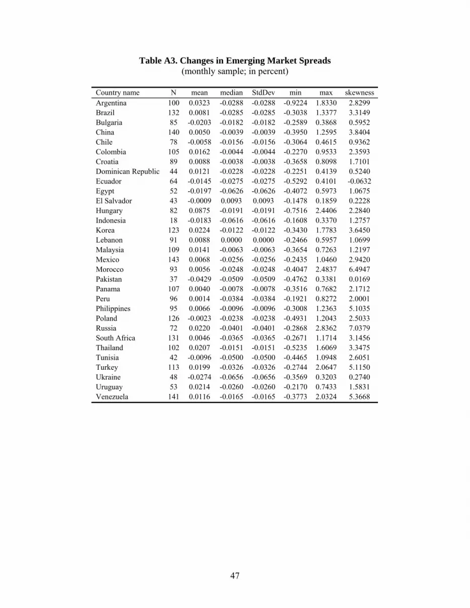
Robustness II: Asymmetries Conventional wisdom would indicate that, while emerging spreads tend to decline only

gradually, they go up in a rush. In fact, this asymmetry is readily verified by a cursory look at the

distribution of monthly changes (Table A3), which in most cases exhibits positive skewness

coefficients.

Accordingly, one should observe this fact reflected in the short-run portion of our

baseline specification, to the extent that the variables included there explain a major share of the

variability of spreads. Is the elasticity of emerging market spreads to changes in global

14

conditions the same irrespective of the sign of the change? Is the effect of a rating upgrade

comparable to that of a rating downgrade?

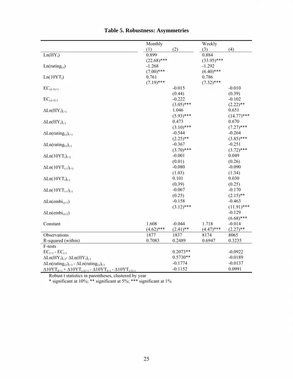
The evidence, summarized in Table 5, provides mixed answers. Columns (1) and (3)

reproduce the long-run estimates for ease of comparison. As can be seen from the short run

equation in column (2), emerging spreads react more rapidly to increases in risk aversion than to

declines. For monthly data, a 100-percent increase in HY raises the average emerging spread by

105 percent, while a comparable decline in HY only reduces the emerging spread by 47 percent.

But, using weekly data, column (4), one can see that emerging spreads react in the same way to

increases or declines in risk aversion. The F tests presented in columns (2) and (4) show that the

effect of changes in global liquidity and credit ratings does not display a statistically significant

asymmetry. Finally, the estimates indicate a faster speed of convergence for downward

deviations (about four months and a half or 10 weeks, using monthly and weekly data

respectively), again in line with the view that negative shocks (e.g., increases in risk appetite or

credit downgrades) are reflected in spreads more rapidly than positive ones. This evidence

suggests that the average lag length of about 14 months estimated by our baseline regression is

strongly affected by the upward deviations from the long-run equilibrium.

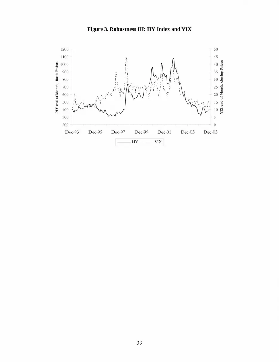
Robustness III: The VIX as an Alternative Measure of the Price of Risk

The economic literature and the financial markets have identified the VIX (a measure of the

volatility implied in the pricing of options on US stocks) as an indicator of investor risk appetite.8

While, in our view, this index should reflect the (time-varying) systemic volatility in the stock

market along with variations in risk appetite and, as such, should be an inferior barometer of the

latter, it is nonetheless an interesting measure of exogenous global factors and an opportunity to

assess the robustness of our previous results. Moreover, as Figure 3 illustrates, it is strongly

correlated with HY (the coefficient is above 50 percent and highly significant), which lends

support to the view that, to certain degree, it may be capturing some of the same aspects.

Table 6 provides reassuring results on both fronts. The first two columns report the

baseline long- and short-run regressions, substituting the VIX for the HY index. The results are

8 The VIX, compiled by the Chicago Board Options Exchange (CBOE) measures the expected stock market volatility over the next 30 calendar days, from the prices of the S&P 500 stock index options for a wide range of strike prices. The calculation is independent of any model and derives the expected volatility by averaging the weighted prices of out-of-the money puts and calls. Historically, in periods of financial stress accompanied by steep market declines, option prices—and VIX—tend to rise; the opposite happens when market sentiment improves.

15

broadly comparable to those in Table 3, with only a somewhat weaker explanatory power.

Indeed, when we include both indexes simultaneously, the HY appears part of the influence of

VIX on the behavior of spreads for the weekly sample (columns (7) and (8)), and most of it for

the monthly sample (where the VIX coefficient declines visibly and ceases to be significant for

the long-run equation, columns (3) and (4)). In sum, the VIX appears to be a sensible measure of

high-frequency changes in risk appetite as hypothesized by the literature, although HY reflects

market sentiment better over the long run.

Robustness IV: Missing Fundamentals In the previous tests, credit ratings were treated mainly as a control for country-specific

fundamentals, focusing the analysis on the results associated with risk. In so doing, we abstracted

from the influence of country fundamentals per se, beyond what is captured by the rating

assigned to the country. There are at least two reasons why one would like to have a closer look

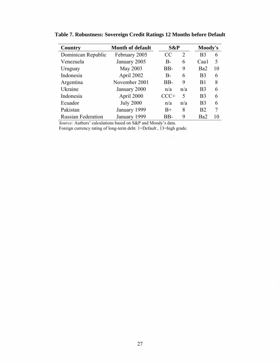
at the role of actual fundamentals. The first is the belief that ratings do not always reflect the

macroeconomic context. More precisely, many observers have pointed out that ratings provide,

at best, only a partial account of the actual likelihood of default of individual countries. In fact,

there is a growing belief that rating agencies tend to lag spreads in their reaction to significant

news and, more generally, to reflect credit risk only imperfectly –hence the substantial dispersion

of spreads within the same rating category. Table 7 illustrates the point: 12 months before recent

default episodes, sovereign ratings assigned by the main rating agencies failed in many cases to

sound the alarm. At any rate, to the extent that ratings are only a partial proxy for country-

specific factors, it is essential for our purposes to test whether the incidence of global factors

reported above is robust to a more parsimonious specification.

16

A second, related motivation is to evaluate the influence of ratings beyond and above the

evolution of country-specific fundamentals. While their information content has been questioned

on various grounds, the results reported above indicate that they exhibit a significant explanatory

power for both the long-run level and the short-run variation of emerging spreads. Is this result

indicating that they adequately capture relevant country information, or that they exert an

influence of its own, not necessarily related to the evolution of the country’s economy? In other

words, could ratings be considered an additional exogenous factor that influences the borrowing

cost of emerging economies, independently of whether they reveal valuable information?9

These considerations presume that actual fundamentals may influence both the level of

spreads and the way they comove with risk appetite beyond what is summarized by the credit

rating. To verify this view, we add to our long-run specification dummies per country-year and

country-month to capture the influence of fundamentals identified in the literature as

determinants of sovereign risk, such as the country’s leverage ratio, the degree of (financial and

institutional) development, or cyclical output fluctuations, which are typically sampled at those

frequencies.

Table 8 reports the results. The coefficients and explanatory power of the original

baseline equation variables remain notably stable using monthly, weekly and even daily datasets,

indicating that their influence is largely independent of country’s fundamentals, although the

power of the international rate is weakened by the inclusion of monthly dummies. While this is

reassuring for the two exogenous global factors, it is somewhat intriguing for the case of ratings

that, in principle, are conceived as summary indicators of the relevant country-specific factors

now included.

As noted, this may be due to the fact that, although investors generally recognize the

limitations that ratings display in practice, the norms that inform their decisions force them to

take credit ratings as an additional argument—suggesting that, to the extent that they reflect the

evolution of the country’s economy only partially, they may be regarded as a source of

variability that is partially exogenous to the policymaker. However, there is another, simpler

hypothesis that seems to match the evidence more closely: ratings are, in most cases, endogenous

9 If so, the influence of ratings on bond pricing could be regarded as an additional external source of volatility, bearing the question about the extent to which markets react to the relevant country-specific economic data. However, Mora (2004), in an updated assessment of this issue, emphasizes that the lagging nature of ratings may actually smooth out the impact of deteriorating fundamentals in the run-up to a crisis.

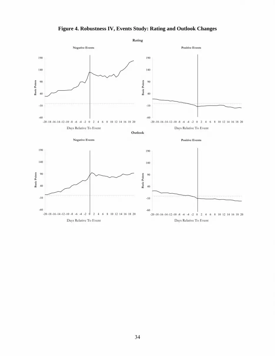
17

to spreads. Figure 4 illustrates this point graphically. Mimicking an event-study exercise, the first

panel shows the residuals from a regression using the specification of column (6) in Table 8

without the ratings variable, averaged over a 40-day window centered on the grading event,

where the latter coincides with positive and negative changes in the rating. As the figure clearly

shows, downgrades are preceded by increases in spreads and, apart from a mild

contemporaneous adjustment (of about 50 bps), exert no substantial impact. The opposite applies

to downgrades, although in this case the preceding decline in spreads is smaller.

Does this evidence prove that ratings are endogenous to market reaction (in this case,

spreads)? Not necessarily, since the market may be simply reacting in anticipation of regrading.

Moreover, agencies themselves typically anticipate regradings by changing their own credit

outlook—a reason to use the latter to refine the information contained in the rating. However, the

second panel of the figure casts doubt on this possibility. There, we replicate the event-study

exercise, this time defining an event as a change in the credit outlook given by the rating agency.

The logic is straightforward: if the rating does more than just validating the perceptions of the

market, then changes in outlook (the way agencies have to signal the presence of new

information that may merit a risk reassessment) should have an impact on asset prices. The

results, however, are strikingly similar to those in the first panel. This is in line with the

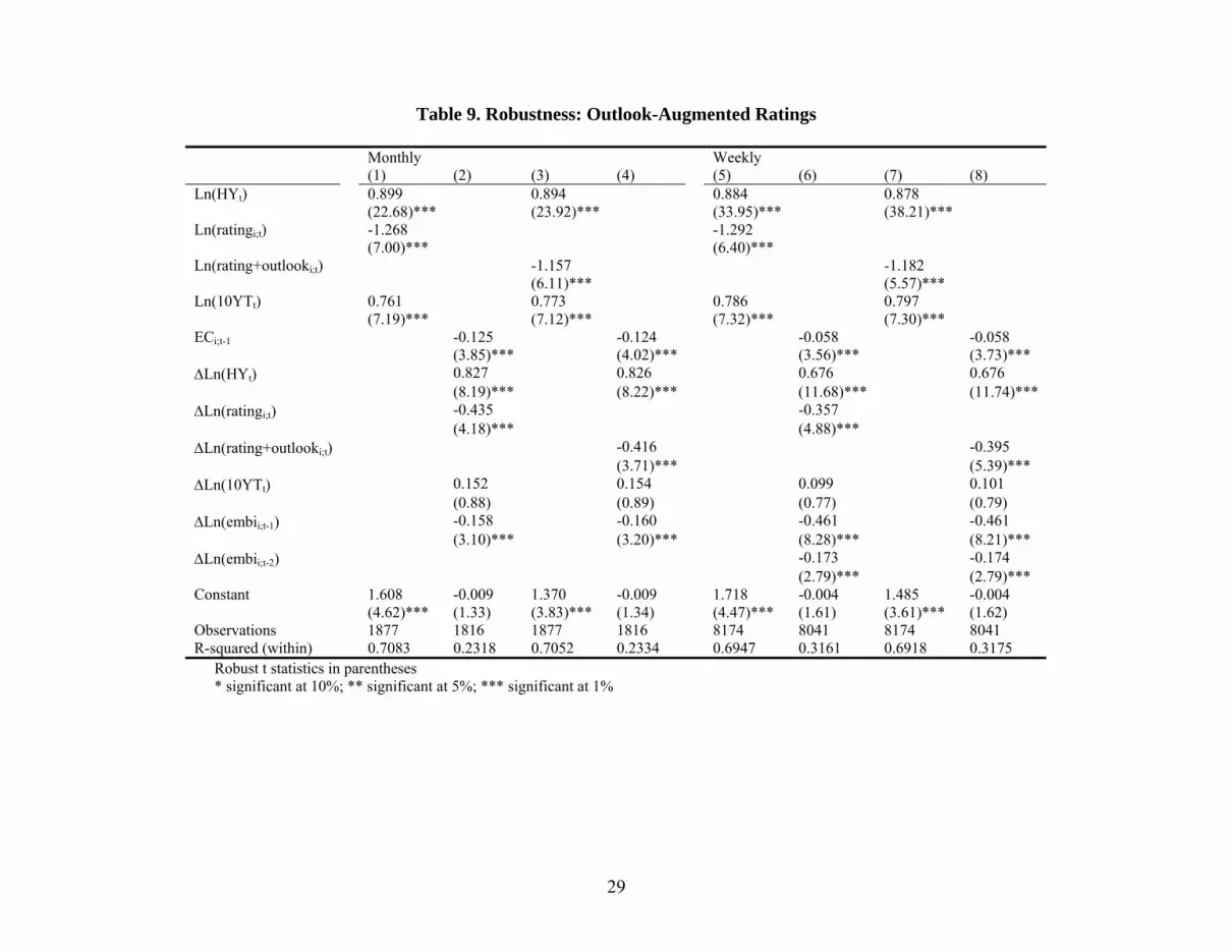
econometric test in Table 9, where our HY measure is adjusted to reflect changes in the credit

outlook (the first two columns reproduce the previous results for ease of comparison).10 Ratings

slightly improve their explanatory power, but the new specification does not introduce any

visible change into the remaining coefficients.

In sum, the presumption that ratings are a reasonable proxy for fundamental risk is

questioned by the data. While their inclusion as control may still be justified (since they appear

to exert a contemporaneous influences on spreads and, at any rate, their exogeneity should not

biased the estimation of the remaining coefficients), attributing the (strong) link between ratings

and spreads to the incidence of country-specific factors may be misleading, overstating the role

of the latter—and understating the influence of global factors.

10 The outlook could be thought of as a five-notch grading scale around the credit rating: positive, positive watch, neutral, negative watch, and negative. In the outlook-augmented ratings we give each notch a 0.2 value. Thus, if our rating variable takes the value 13 for a BBB bond, a BBB with negative watch outlook would take a value of 12.8 and one with negative outlook a value of 12.6.

18

Robustness V: Risk Appetite or Corporate Risk? Going back to our reduced-form model, one natural question is to what extent the assumption of

constant corporate risk influences the results and, more generally, whether the high-yield spread

is capturing changes in perceived risk together with changes in its price. In particular, how did an

episode such as the Enron scandal, presumably associated with a reassessment of corporate

default risk, affect the evolution of HY? The answer to these questions has important

implications for the interpretation of the previous results, which hold only if HY does not reflect

changes in global corporate risk.

A casual look at the evidence helps to dispel these concerns. Figure 5 shows the

evolution of the weighted average rating of the corporate bond sample based on which the high

yield spread is computed (rating(HY)). As can be seen, this rating moves within a very limited

range of less than a half-notch, hardly a significant source of variability. Moreover, increases in

HY in the latest period, while negatively correlated with the rating (as expected), do not appear to

reflect a visible deterioration of the risk (as perceived by the rating agencies).11 On the contrary,

the Enron crisis coincides with a downward revision of corporate risk, as reflected by the

improvement of corporate ratings (as a result, the correlation between the two turns positive

during the period).

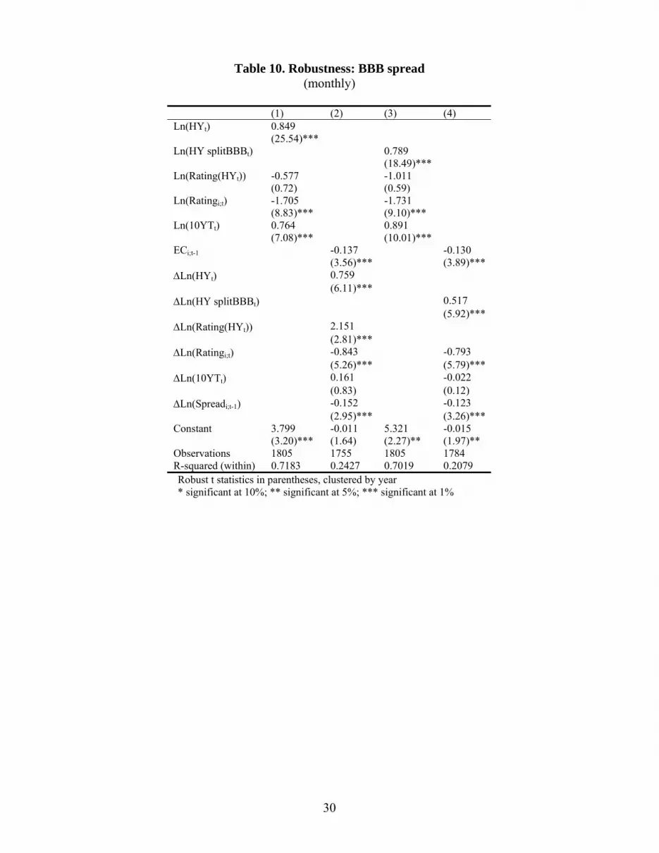
The implication of these findings (namely, that HY captures the price rather than the

quantity of risk) is confirmed by the regressions in Table 10, where we include the corporate

rating measure directly in the regression. As expected, the new control is not significant and has

no effect on the rest of the coefficients. The same message is given by the last two columns.

There, we replaced the HY index by the BBB spread, which should be less sensitive to risk

(lower than the one associated with the index) and risk changes, and a better gauge of changes in

the price of risk. Reassuringly, the new measure underperforms the HY index.12

Predictions

One way to gauge how much of the variation in emerging market spread can be explained by the

few exogenous variables identified in our baseline model consists in simulating the path of

11 Nor do they reflect increases in the incidence of U.S. corporate bankruptcies, which actually declined steadily in the period under study. 12 The same result is obtained when we proxy the price of risk by the spread on U.S. Baa bonds, which according to some authors is the best proxy for risk aversion (Blanchard, 2003).

19

individual spreads based solely on the long-run specification. We perform this test by calibrating

this equation using data through end-2001, and simulating the behavior of spreads for the

remaining period (January 2002- November 2005).13 Specifically, in order to assess the relative

predictive power of global factors, we re-estimate the long-run specification of Table 8, column

(1), and compute the out-of-sample path that results from variations in the global variables HY

and the international rate, keeping ratings fixed at their end-2001 levels.

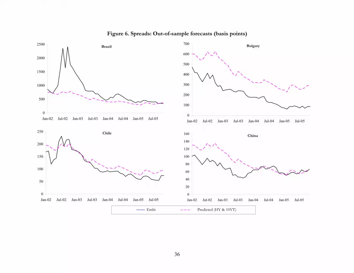
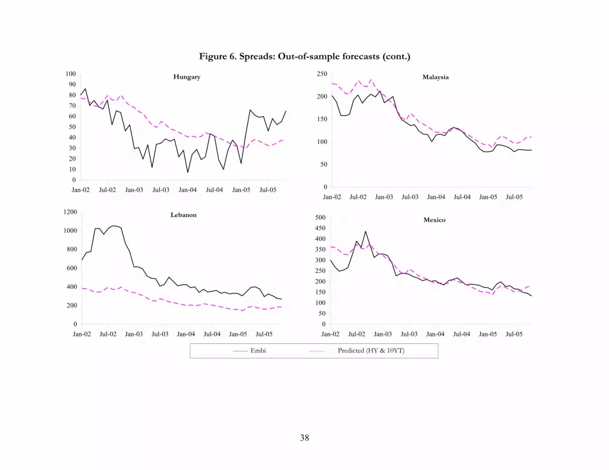
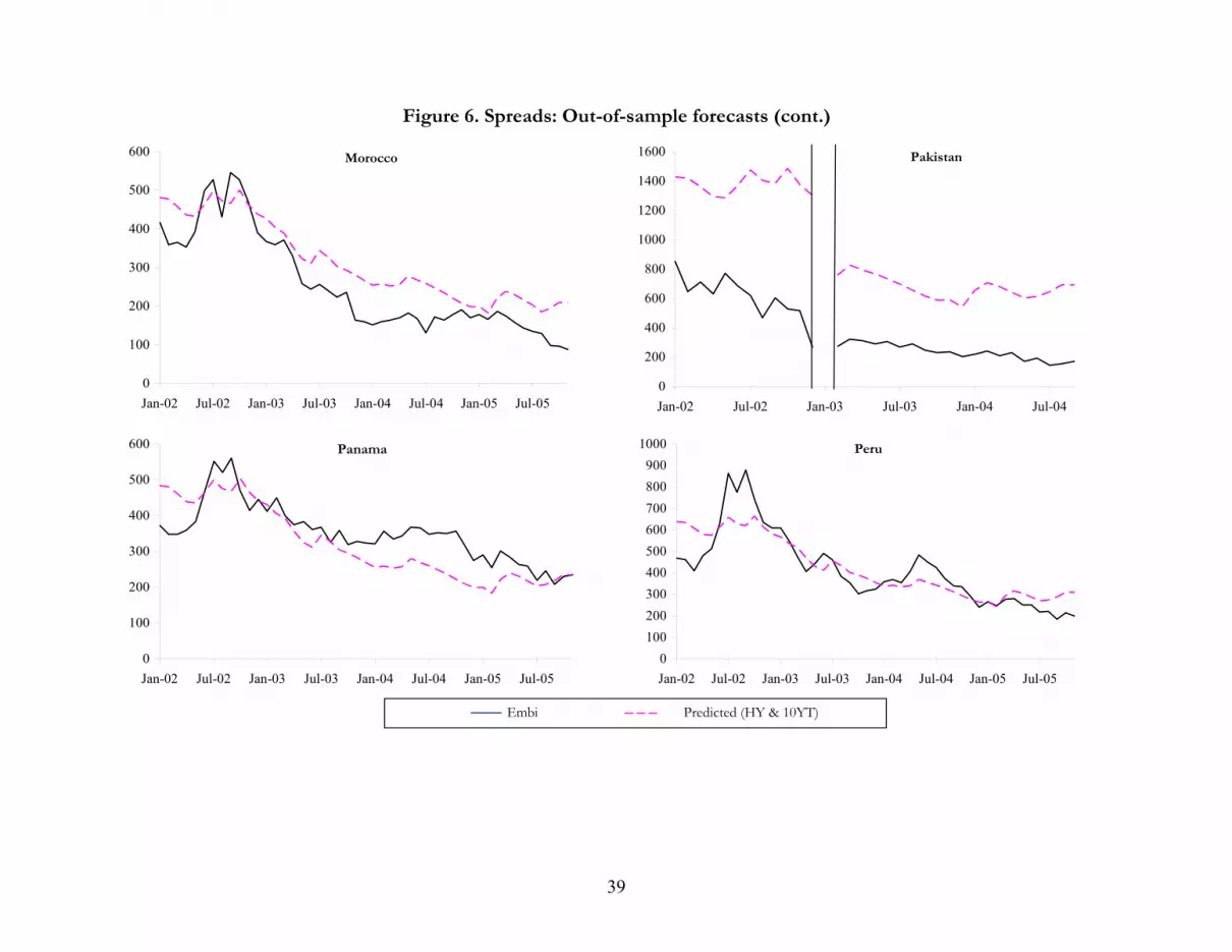
Figure 6 reports the results.14 It compares the actual EMBI spread with the predictions

from the long-run equation. Three aspects deserve to be stressed in the figures. First, the

predictions are generally quite good, including for many Latin American countries that

underwent severe episodes of capital account reversals in the period considered. Second, the

predictions highlight the explanatory power of the two exogenous variables: despite short-term,

transitory swings due to country-specific episodes, spread movements closely reflect these three

variables, and eventually converge to levels that are largely explained by them. Third, although

many of these episodes may have coincided with (and possibly been facilitated by) a

deterioration in those global factors, they far exceed the variability of the latter, suggesting that

some country-specific ingredient was crucially in place at the time. Brazil is a case in point: the

financial turmoil of late 2002 associated with the uncertainty surrounding the election and the

transition to a new government which was clearly independent of the evolution of global factors;

once over, spreads rapidly converged to their long-run levels.

An even more dramatic example of the incidence of long-run factors is provided by

Argentina. Figure 7 shows the evolution of the spread before and after the sovereign default, and

the predicted value for the post-default period, setting the rating at its levels as of end-2000. As

can be seen, the prediction yields a spread of about 500 immediately after the exchange was

concluded—very close to the level actually realized. Thus, using a model calibrated based on the

information available before the crisis, the dramatic decline in spreads experienced by the

country after the sovereign default was left behind could have been predicted simply as a result

of the increase in risk appetite and the decline in international interest rates that followed.

13 As a result, some countries that were included in the EMBI after (or shortly before) 2001 are dropped due to lack of observations. 14 Naturally, one could readily obtain much more precise one-period-ahead forecasts by estimating the short run equation and adding it to the long-run one, i.e., computing E(ln(embi)t )= E(ln(embilong,-1) + E(Δln(embi)). Since our interest is in the persistent effect of global factors, the results are omitted here (though they are available from the authors on request).

20

4. Final Remarks Our tests attempted to estimate the variability explained by global factors, but adopted an

agnostic approach to country-specific factors, which pose non-trivial empirical problems. Most

available country-specific controls are sampled at too low a frequency and, even when they are

available on a daily basis like credit ratings, are likely to be endogenous. Therefore, an accurate

decomposition of emerging market spreads into their systemic and idiosyncratic determinants is

a challenging and still pending task.

This does not detract from the validity of our main result: Global factors, such as global

liquidity and market sentiment, explain a large part of the (substantial) volatility of emerging

market spreads—a connection that, while not new, has tended to strengthen over the years. The

implications of these findings are immediate. On the one hand, no forecast of the borrowing cost

(and, as a result, the fiscal sustainability) of emerging economies can ignore these exogenous

factors (which, in addition, are often easier to predict than fundamentals). On the other hand,

besides improving macro fundamentals, emerging economies need to take into account their

exposure to global factors and to devise mechanisms to reduce that exposure. Financial

integration brings contagion not only from other emerging economies but also from the rest of

the developed world. In the absence of a concerted effort to reduce their effects, newcomers, like

infants, had better take their shot well in advance.

21

Table 1. Summary Statistics

(monthly sample) Variable Frequency N mean median Std Dev min max embi Monthly 3309 648.1935 402.7520 831.5839 7.0240 7078 HY Monthly 191 580.8115 523 203.5349 307 1080 rating Monthly 4351 10.8322 11 3.3172 1 18 10YT Monthly 191 5.9228 5.86 1.3511 3.37 9.04 VIX Monthly 191 19.4612 18.88 6.3882 10.63 44.28 rating+outlook Monthly 4283 10.8453 11 3.3537 1 18 Rating(HY) Monthly 131 4.4352 4.3925 0.1323 4.2347 4.7403HY(Split BBB) Monthly 131 250.8441 224.88 103.8955 114.25 563

(weekly sample)

Variable Frequency N mean median Std Dev min max embi Weekly 14370 645.7757 399 832.7009 -6 7222 HY Weekly 493 583.6755 556 211.4735 301 1116 rating Weekly 18919 10.8375 11 3.3125 1 18 10YT Weekly 834 5.9284 5.88 1.3443 3.18 9.07 VIX Weekly 836 19.4045 18.36 6.4250 9.48 45.74rating+outlook Weekly 18620 10.8489 11 3.3506 1 18

22

Table 2. Panel Unit Root Tests

Monthly panel Maddala-Wu Choi PMW p-Value ZMW p-Value embi 64.354 0.603 0.231 0.591 HY 55.121 0.904 -0.234 0.407 10YT 68.536 0.527 -0.111 0.455 rating 68.710 0.206 1.202 0.885 ECi;t-1 1308.99 0.000 -7.992 0.000 Weekly panel Maddala-Wu Choi PMW p-value ZMW p-value embi 59.691 0.754 0.163 0.435 HY 36.816 0.999 -0.289 0.389 10YT 51.306 0.955 -0.099 0.480 rating 47.648 0.876 -2.396 0.992 ECi;t-1 4310.77 0.000 -8.905 0.000

Note: ECi;t-1 are the residuals of the long run equilibrium relationship presented in column (1) ((4)) of Table 3 for monthly data (weekly data). All variables are in logs. Lags for the panel unit root tests were selected using the Schwarz information criterion.

23

Table 3. Global Factors and Emerging Market Spreads

Monthly Weekly (1) (2) (3) (4) Ln(HYt) 0.776 0.773 (10.84)*** (9.41)*** Ln(ratingi;t) -1.527 -1.537 (8.13)*** (7.96)*** Ln(10YTt) 1.094 0.964 (8.09)*** (7.07)*** Contagion Russia 0.610 0.568 (8.03)*** (4.36)*** Contagion Mexico 0.186 0.045 (2.20)** (4.58)*** ECi;t-1 -0.070 -0.030 (5.34)*** (3.25)*** ΔLn(HYt) 1.108 0.834 (6.02)*** (6.52)*** ΔLn(ratingi;t) -0.637 -0.429 (3.22)*** (3.76)*** ΔLn(10YTt) 0.272 0.134 (1.81)* (1.27) ΔLn(embii;t-1) -0.160 -0.411 (4.69)*** (8.41)*** ΔLn(embii;t-2) -0.191 (5.04)*** Constant 2.546 -0.007 2.774 -0.003 (3.22)*** (0.94) (3.31)*** (1.00) Observations 2767 2689 11141 10983 R-squared (within) 0.5826 0.2853 0.5918 0.3152 % Variance explained by HYt 17.0428 23.4124 %Variance explained by HYt & 10YTt 31.3530 32.6942 %Variance explained by HYt, 10YTt, & Contagion 37.0128 37.8266 %Variance explained by ΔHYt 21.8848 15.1797 %Variance explained by ΔHYt & Δ10YTt 22.5379 15.2855 %Variance explained by ΔHYt, Δ10YTt, & Contagion 22.5667

Robust t statistics in parentheses, clustered by year * significant at 10%; ** significant at 5%; *** significant at 1%

24

Table 4. Robustness: Global Factors and Emerging Market Spreads Over Time

Full (unbalanced) sample Argentina, Brazil & Mexico (balanced sample) 1993-1999 2000-2005 1993-2005 1993-1999 2000-2005 (1) (2) (3) (4) (5) (6) (7) (8) (9) (10) Ln(HYt) 1.032 0.899 0.991 1.266 0.966 (3.80)*** (22.68)*** (19.02)*** (2.76)*** (10.95)*** Ln(HYt)*d00-05 -0.065 (5.05)*** Ln(ratingi;t) -2.177 -1.268 -1.501 -1.915 -0.659 (4.89)*** (7.00)*** (8.69)*** (3.70)*** (6.56)*** Ln(10YTt) -0.547 0.761 0.571 0.589 0.072 (0.83) (7.19)*** (2.98)*** (2.32)** (0.40) Contagion Russia 0.043 0.290 0.062 (0.35) (4.87)*** (0.29) Contagion Mexico 0.336 0.058 0.159 0.045 0.333 0.111 (2.15)** (3.02)*** (1.90)* (4.80)*** (3.96)*** (8.22)*** ECi;t-1 -0.093 -0.125 -0.078 -0.149 -0.166 (4.86)*** (3.85)*** (6.30)*** (1.67)* (4.02)*** ΔLn(HYt) 1.617 0.827 1.534 1.836 0.896 (31.85)*** (8.19)*** (15.72)*** (14.28)*** (4.23)*** ΔLn(HYt)*d00-05 -0.676 (5.17)*** ΔLn(ratingi;t) -1.503 -0.435 -0.626 -0.869 -0.412 (4.97)*** (4.18)*** (3.20)*** (1.05) (3.93)*** ΔLn(10YTt) 0.431 0.152 0.184 1.302 0.099 (1.28) (0.88) (1.41) (3.34)*** (0.33) ΔLn(embii;t-1) -0.138 -0.158 -0.163 -0.089 -0.053 (2.62)*** (3.10)*** (4.70)*** (3.03)*** (0.54) Constant 5.666 -0.011 1.608 -0.009 2.271 -0.009 1.971 -0.012 1.302 -0.005 (2.07)** (0.73) (4.62)*** (1.33) (4.11)*** (1.65)* (0.54) (0.71) (2.45)** (0.45) Observations 890 852 1877 1816 2767 2689 203 197 170 165 R-squared (within) 0.5838 0.4535 0.7083 0.2318 0.6247 0.3090 0.5955 0.4587 0.7917 0.3285 % Variance explained by HYt 37.6916 46.5491 37.5119 38.1353 73.4962 % Var. explained by HYt & 10YTt 38.1161 51.9851 40.0107 48.1206 73.5161 % Var. explained by HYt, 10YTt, & Contagion 40.5705 41.0670 52.6127 % Variance explained by ΔHYt 35.3900 13.9484 24.2838 30.9003 21.1277 % Var. explained by ΔHYt & Δ10YTt 37.7223 14.0062 24.6459 37.7439 21.1931 % Var. expl. by ΔHYt, Δ10YTt, & Contagion 37.8838 24.6727 38.8135 Robust t statistics in parentheses, clustered by year, * significant at 10%; ** significant at 5%; *** significant at 1%

25

Table 5. Robustness: Asymmetries

Monthly Weekly (1) (2) (3) (4) Ln(HYt) 0.899 0.884 (22.68)*** (33.95)*** Ln(ratingi;t) -1.268 -1.292 (7.00)*** (6.40)*** Ln(10YTt) 0.761 0.786 (7.19)*** (7.32)*** ECi;t-1(+) -0.015 -0.010 (0.44) (0.39) ECi;t-1(-) -0.222 -0.102 (3.05)*** (2.22)** ΔLn(HYt)(+) 1.046 0.651 (5.93)*** (14.77)*** ΔLn(HYt)(-) 0.473 0.670 (3.10)*** (7.27)*** ΔLn(ratingi;t)(+) -0.544 -0.264 (2.25)** (3.85)*** ΔLn(ratingi;t)(-) -0.367 -0.251 (3.70)*** (3.72)*** ΔLn(10YTt)(+) -0.001 0.049 (0.01) (0.26) ΔLn(10YTt-1)(+) -0.080 -0.090 (1.03) (1.34) ΔLn(10YTt)(-) 0.101 0.030 (0.39) (0.25) ΔLn(10YTt-1)(-) -0.067 -0.170 (0.25) (2.15)** ΔLn(embii;t-1) -0.158 -0.463 (3.12)*** (11.91)*** ΔLn(embii;t-2) -0.129 (6.68)*** Constant 1.608 -0.044 1.718 -0.014 (4.62)*** (2.41)** (4.47)*** (2.27)** Observations 1877 1837 8174 8065 R-squared (within) 0.7083 0.2489 0.6947 0.3235 F-tests EC(+) - EC(-) 0.2073** -0.0922 ΔLn(HYt)(-)- ΔLn(HYt)(-) 0.5730** -0.0189 ΔLn(ratingi;t)(+) - ΔLn(ratingi;t)(-) -0.1774 -0.0137 Δ10YTt(+) + Δ10YTt-1(+) - Δ10YTt(-) - Δ10YTt-1(-) -0.1152 0.0991


26

Table 6. Robustness: VIX as an Alternative Measure of Risk Appetite

Monthly Weekly (1) (2) (3) (4) (5) (6) (7) (8) Ln(VIXt) 0.946 0.215 0.885 0.177 (17.20)*** (1.82)* (19.26)*** (2.56)** Ln(HYt) 0.722 0.737 (7.04)*** (13.26)*** Ln(ratingi;t) -1.263 -1.261 -1.306 -1.288 (6.83)*** (7.01)*** (6.23)*** (6.41)*** Ln(10YTt) 0.872 0.776 0.864 0.789 (8.31)*** (11.14)*** (8.65)*** (9.69)*** ECi;t-1 -0.149 -0.127 -0.067 -0.063 (4.81)*** (3.86)*** (4.59)*** (3.95)*** ΔLn(VIXt) 0.329 0.147 0.165 0.068 (10.78)*** (4.23)*** (6.78)*** (2.72)*** ΔLn(HYt) 0.685 0.567 (6.37)*** (7.64)*** ΔLn(ratingi;t) -0.417 -0.431 -0.306 -0.304 (3.75)*** (4.26)*** (4.76)*** (5.74)*** ΔLn(10YTt) -0.104 0.182 -0.165 0.077 (0.92) (1.28) (1.44) (0.70) ΔLn(embii;t-1) -0.106 -0.145 -0.493 -0.477 (2.55)** (2.86)*** (16.75)*** (15.91)*** ΔLn(embii;t-2) -0.182 -0.173 (3.50)*** (3.24)*** Constant 4.388 -0.012 2.068 -0.008 4.669 -0.005 2.122 -0.004 (8.50)*** (1.43) (5.08)*** (1.23) (8.58)*** (1.67)* (5.39)*** (1.86)* Observations 1877 1816 1877 1816 8174 8040 8174 8040 R-squared (within) 0.6692 0.1982 0.7113 0.2458 0.6449 0.3008 0.6973 0.3278 % Variance explained by VIXt 41.8499 39.6287 39.6287 % Variance explained by VIXt & 10YTt 48.8855 46.3942 46.3942 % Variance explained by ΔVIXt 9.4293 4.3181 4.3181 % Variance explained by ΔVIXt & Δ10YTt 10.0105 5.1297 5.1297


27

Table 7. Robustness: Sovereign Credit Ratings 12 Months before Default

Country Month of default S&P Moody's Dominican Republic February 2005 CC 2 B3 6 Venezuela January 2005 B- 6 Caa1 5 Uruguay May 2003 BB- 9 Ba2 10 Indonesia April 2002 B- 6 B3 6 Argentina November 2001 BB- 9 B1 8 Ukraine January 2000 n/a n/a B3 6 Indonesia April 2000 CCC+ 5 B3 6 Ecuador July 2000 n/a n/a B3 6 Pakistan January 1999 B+ 8 B2 7 Russian Federation January 1999 BB- 9 Ba2 10

Source: Authors’ calculations based on S&P and Moody’s data. Foreign currency rating of long-term debt. 1=Default , 13=high grade.

28

Table 8. Robustness: Country-Time Dummies

Monthly Weekly Daily (1) (2) (3) (4) (5) (6) (7)

Ln(HYt) 0.819 0.789 0.809 0.806 0.746 0.832 0.733 (22.80)*** (29.54)*** (26.41)*** (31.26)*** (6.08)*** (27.33)*** (10.08)*** Ln(ratingi;t) -1.720 -1.302 -1.732 -1.308 -0.209 -1.725 -0.318 (8.83)*** (11.75)*** (8.94)*** (8.18)*** (2.53)** (8.84)*** (2.88)*** Ln(10YTt) 0.779 0.301 0.800 0.318 -0.025 0.845 -0.081 (7.23)*** (3.47)*** (7.34)*** (3.48)*** (0.14) (8.30)*** (0.76) Constant 3.150 3.229 3.204 3.171 1.550 -0.906 2.390 (7.37)*** (7.47)*** (7.74)*** (5.69)*** (1.37) (2.23)** (2.05)** Observations 1747 1747 7650 7650 7650 36658 36658 R-squared (within) 0.7107 0.9018 0.6960 0.8856 0.8930 0.7025 0.9041 Fixed effects ctry ctry-year ctry-year ctry-month ctry-month Robust t-statistics in parentheses, clustered by year * significant at 10%; ** significant at 5%; *** significant at 1%

29

Table 9. Robustness: Outlook-Augmented Ratings

Monthly Weekly (1) (2) (3) (4) (5) (6) (7) (8) Ln(HYt) 0.899 0.894 0.884 0.878 (22.68)*** (23.92)*** (33.95)*** (38.21)*** Ln(ratingi;t) -1.268 -1.292 (7.00)*** (6.40)*** Ln(rating+outlooki;t) -1.157 -1.182 (6.11)*** (5.57)*** Ln(10YTt) 0.761 0.773 0.786 0.797 (7.19)*** (7.12)*** (7.32)*** (7.30)*** ECi;t-1 -0.125 -0.124 -0.058 -0.058 (3.85)*** (4.02)*** (3.56)*** (3.73)*** ΔLn(HYt) 0.827 0.826 0.676 0.676 (8.19)*** (8.22)*** (11.68)*** (11.74)*** ΔLn(ratingi;t) -0.435 -0.357 (4.18)*** (4.88)*** ΔLn(rating+outlooki;t) -0.416 -0.395 (3.71)*** (5.39)*** ΔLn(10YTt) 0.152 0.154 0.099 0.101 (0.88) (0.89) (0.77) (0.79) ΔLn(embii;t-1) -0.158 -0.160 -0.461 -0.461 (3.10)*** (3.20)*** (8.28)*** (8.21)*** ΔLn(embii;t-2) -0.173 -0.174 (2.79)*** (2.79)*** Constant 1.608 -0.009 1.370 -0.009 1.718 -0.004 1.485 -0.004 (4.62)*** (1.33) (3.83)*** (1.34) (4.47)*** (1.61) (3.61)*** (1.62) Observations 1877 1816 1877 1816 8174 8041 8174 8041 R-squared (within) 0.7083 0.2318 0.7052 0.2334 0.6947 0.3161 0.6918 0.3175

Robust t statistics in parentheses * significant at 10%; ** significant at 5%; *** significant at 1%

30

Table 10. Robustness: BBB spread (monthly)

(1) (2) (3) (4) Ln(HYt) 0.849 (25.54)*** Ln(HY splitBBBt) 0.789 (18.49)*** Ln(Rating(HYt)) -0.577 -1.011 (0.72) (0.59) Ln(Ratingi;t) -1.705 -1.731 (8.83)*** (9.10)*** Ln(10YTt) 0.764 0.891 (7.08)*** (10.01)*** ECi;t-1 -0.137 -0.130 (3.56)*** (3.89)*** ΔLn(HYt) 0.759 (6.11)*** ΔLn(HY splitBBBt) 0.517 (5.92)*** ΔLn(Rating(HYt)) 2.151 (2.81)*** ΔLn(Ratingi;t) -0.843 -0.793 (5.26)*** (5.79)*** ΔLn(10YTt) 0.161 -0.022 (0.83) (0.12) ΔLn(Spreadi;t-1) -0.152 -0.123 (2.95)*** (3.26)*** Constant 3.799 -0.011 5.321 -0.015 (3.20)*** (1.64) (2.27)** (1.97)** Observations 1805 1755 1805 1784 R-squared (within) 0.7183 0.2427 0.7019 0.2079 Robust t statistics in parentheses, clustered by year * significant at 10%; ** significant at 5%; *** significant at 1%

31

Figure 1. HY index and Embi Mean normalized values (mean= 100)

0

50

100

150

200

250

300

350

50% 25% embi (median) embi (mean)

0

50

100

150

200

HY

0

20

40

60

80

100

120

140

160

Dec-93 Dec-95 Dec-97 Dec-99 Dec-01 Dec-03 Dec-05

10YT

32

Figure 2. Robustness I: Structural Break (based on column (1) of Table 3)

0

5

10

15

20

25

30

Sep-94 Sep-95 Sep-96 Sep-97 Sep-98 Sep-99 Sep-00 Sep-01

W(k)

33

Figure 3. Robustness III: HY Index and VIX

200

300

400

500

600

700

800

900

1000

1100

1200

Dec-93 Dec-95 Dec-97 Dec-99 Dec-01 Dec-03 Dec-05

HY

end

of M

onth

, B

asic

Poi

nts

0

5

10

15

20

25

30

35

40

45

50

VIX

end

of M

onth

, clo

sing

Pri

ces

HY VIX

34

Figure 4. Robustness IV, Events Study: Rating and Outlook Changes

Days Relative To Event Days Relative To Event

Rating

Days Relative To Event Days Relative To Event

Outlook

Negative Events

-60

-10

40

90

140

190

-20 -18 -16 -14 -12 -10 -8 -6 -4 -2 0 2 4 6 8 10 12 14 16 18 20

Bas

ic P

oin

ts

Positive Events

-60

-10

40

90

140

190

-20 -18 -16 -14 -12 -10 -8 -6 -4 -2 0 2 4 6 8 10 12 14 16 18 20

Bas

ic P

oin

tsNegative Events

-60

-10

40

90

140

190

-20 -18 -16 -14 -12 -10 -8 -6 -4 -2 0 2 4 6 8 10 12 14 16 18 20

Bas

ic P

oin

ts

Positive Events

-60

-10

40

90

140

190

-20 -18 -16 -14 -12 -10 -8 -6 -4 -2 0 2 4 6 8 10 12 14 16 18 20

Bas

ic P

oin

ts

35

Figure 5. Robustness V: HY Yields and HY ratings

0

200

400

600

800

1000

1200

Jan-90 Jan-92 Jan-94 Jan-96 Jan-98 Jan-00 Jan-02 Jan-04

HY

, end

of M

onth

(ba

sis

poin

ts)

3.5

4

4.5

5

Rat

ing(

HY

), en

d of

Mon

th

HY Rating(HY)

36

Figure 6. Spreads: Out-of-sample forecasts (basis points)

Brazil

0

500

1000

1500

2000

2500

Jan-02 Jul-02 Jan-03 Jul-03 Jan-04 Jul-04 Jan-05 Jul-05

Bulgary

0

100

200

300

400

500

600

700


Chile

0

50

100

150

200

250


China

0

20

40

60

80

100

120

140

160


Embi Predicted (HY & 10YT)

37

Figure 6. Spreads: Out-of-sample forecasts (cont.)

Colombia

0

200

400

600

800

1000

1200


Croatia

0

50

100

150

200

250

300

350

Jan-02 Jul-02 Jan-03 Jul-03 Jan-04

Ecuador

0

500

1000

1500

2000

2500


Egypt

0

100

200

300

400

500

600



38


Hungary

0102030405060708090

100


Lebanon

0

200

400

600

800

1000

1200


Malaysia

0

50

100

150

200

250


Mexico

050

100150200250300350400450500



39


Morocco

0

100

200

300

400

500

600


Pakistan

0

200

400

600

800

1000

1200

1400

1600

Jan-02 Jul-02 Jan-03 Jul-03 Jan-04 Jul-04

Panama

0

100

200

300

400

500

600


Peru

0100200300400500600700800900

1000



40


Phillippines

0

100

200

300

400

500

600


Poland

0

50

100

150

200

250

300


Russia

0

100

200

300

400

500

600

700

800


South Africa

0

50

100

150

200

250

300

350



41


Thailand

0

20

40

60

80

100

120

140

160

180


Turkey

0

200

400

600

800

1000

1200


Ukraine

0

200

400

600

800

1000

1200


Uruguay

0

200

400

600

800

1000

1200

1400

1600

1800



42


Venezuela

0

200

400

600

800

1000

1200

1400

1600


Dominican Republic

0

200

400

600

800

1000

1200

1400

1600

1800

2000



43

Figure 7. Predicting Argentine spreads (basis points)

0

600

1200

1800

2400

3000

3600

Dec-00 Feb-01 Apr-01 Jun-01 Aug-01 Oct-01 May-05 Jul-05 Sep-05 Nov-05

Embi Predicted ( HY & 10YT )

References Blanchard, O. 2003. “Fiscal Dominance and Inflation Targeting: Lessons from Brazil.” NBER

Working Paper 10389. Cambridge, United States: National Bureau of Economic

Research.

Calvo, G., L. Leiderman and C. Reinhart. 1993. “Capital Inflows and Real Exchange Rate

Appreciation in Latin America.” IMF Staff Papers 40(1): 108-151.

Calvo, G., and E. Talvi. 2004. “Sudden Stops, Financial Factors and Economic Collapse in Latin

America: Learning from Argentina and Chile.” NBER Working Paper 11153.

Cambridge, United States: National Bureau of Economic Research.

Choi, I. 2001. “Unit Root Tests for Panel Data.” Journal of International Money and Finance 20:

249-272.

Engle, R.F., and C.W.J. Granger. 1987. “Co-Integration and Error Correction: Representation,

Estimation, and Testing.” Econometrica 55: 251-276.

Fisher, R.A. 1932. “Statistical Methods for Research Workers.” Fourth edition. Edinburgh,

United Kingdom: Oliver and Boyd.

García Herrero, A., and A. Ortiz. 2004. “The Role of Global Risk Aversion in Explaining Latin

American Sovereign Spreads.” Madrid, Spain: Bank of Spain. Mimeographed document.

Grandes, M. 2003. “Convergence and Divergence of Sovereign Bond Spreads: Theory and Facts

from Latin America.” Paris, France: Delta, ENS/EHESS.

Herrera, S., and G. Perry. 2002. “Determinants of Latin Spreads in the New Economy Era: The

Role of US Interest Rates and Other External Variables.” Washington, DC, United States:

World Bank. Mimeographed document.

Levy Yeyati, E., and F. Sturzenegger. 2000. “Implications of the Euro for Latin America’s

Financial and Banking Sectors.” Emerging Markets Review 1(1): 53-81.

Maddala, G.S., and S. Wu. 1999. “A Comparative Study of Unit Root Tests with Panel Data and

A New Simple Test.” Oxford Bulletin of Economics and Statistics 61: 631-52.

Mora, N. 2004. “Sovereign Credit Ratings: Guilty beyond Reasonable Doubt?” Beirut, Lebanon:

American University of Beirut.

45

Appendix

Table A1. Variable Definitions and Sources

Name Description Source embi JP Morgan EMBI global index blended spread, in bps Datastream HY CSFB high yield global index, USD, long term debt, in bps Bloomberg 10YT US Treasury notes, 10 year constant maturity yield, bps U.S. Treasury rating S&P rating, long term debt, end of period, foreign currency S&P Vix CBOE Volatility Index CBOE

rating+outlook S&P rating augmented using the S&P outlook. Long term debt, end of period, foreign currency S&P

Rating(HY) Weighted average rating of issues included in JP Morgan high yield global index JP Morgan

46

Table A2. Countries and Periods Covered

Country Monthly Weekly obs begins ends obs begins ends Argentina 101 12/31/93 11/30/05 307 7/4/96 11/24/05 Brazil 132 12/31/94 11/30/05 493 7/4/96 11/24/05 Bulgaria 85 11/30/98 11/30/05 368 11/26/98 11/24/05 China 141 3/31/94 11/30/05 493 7/4/96 11/24/05 Chile 79 5/31/99 11/30/05 341 6/3/99 11/24/05 Colombia 106 2/28/97 11/30/05 458 3/6/97 11/24/05 Croatia 89 1/31/97 5/31/04 388 1/23/97 6/24/04 Dominican Republic 45 11/30/01 11/30/05 189 12/6/01 11/24/05 Ecuador 64 8/31/00 11/30/05 276 8/31/00 11/24/05 Egypt 53 7/31/01 11/30/05 228 8/2/01 11/24/05 El Salvador 44 4/30/02 11/30/05 189 5/2/02 11/24/05 Hungary 83 1/31/99 11/30/05 358 2/4/99 11/24/05 Indonesia 19 5/31/04 11/30/05 80 6/3/04 11/24/05 Korea 124 12/31/93 3/31/04 409 7/4/96 4/29/04 Lebanon 92 4/30/98 11/30/05 398 4/30/98 11/24/05 Malaysia 110 10/31/96 11/30/05 476 10/31/96 11/24/05 Mexico 144 12/31/93 11/30/05 493 7/4/96 11/24/05 Morocco 93 3/31/98 11/30/05 406 3/5/98 11/24/05 Pakistan 39 6/30/01 11/30/05 168 7/5/01 11/24/05 Panama 107 1/31/97 11/30/05 464 1/23/97 11/24/05 Peru 96 12/31/97 11/30/05 417 12/18/97 11/24/05 Philippines 96 12/31/97 11/30/05 415 1/1/98 11/24/05 Poland 126 6/30/95 11/30/05 493 7/4/96 11/24/05 Russia 73 12/31/97 11/30/05 317 1/1/98 11/24/05 South Africa 132 12/31/94 11/30/05 493 7/4/96 11/24/05 Thailand 103 5/31/97 11/30/05 445 6/5/97 11/24/05 Tunisia 43 5/31/02 11/30/05 184 6/6/02 11/24/05 Turkey 114 6/30/96 11/30/05 493 7/4/96 11/24/05 Ukraine 48 12/31/01 11/30/05 207 12/27/01 11/24/05 Uruguay 54 5/31/01 11/30/05 235 5/31/01 11/24/05 Venezuela 142 12/31/93 11/30/05 487 7/4/96 11/24/05

47

Table A3. Changes in Emerging Market Spreads (monthly sample; in percent)

Country name N mean median StdDev min max skewness Argentina 100 0.0323 -0.0288 -0.0288 -0.9224 1.8330 2.8299 Brazil 132 0.0081 -0.0285 -0.0285 -0.3038 1.3377 3.3149 Bulgaria 85 -0.0203 -0.0182 -0.0182 -0.2589 0.3868 0.5952 China 140 0.0050 -0.0039 -0.0039 -0.3950 1.2595 3.8404 Chile 78 -0.0058 -0.0156 -0.0156 -0.3064 0.4615 0.9362 Colombia 105 0.0162 -0.0044 -0.0044 -0.2270 0.9533 2.3593 Croatia 89 0.0088 -0.0038 -0.0038 -0.3658 0.8098 1.7101 Dominican Republic 44 0.0121 -0.0228 -0.0228 -0.2251 0.4139 0.5240 Ecuador 64 -0.0145 -0.0275 -0.0275 -0.5292 0.4101 -0.0632 Egypt 52 -0.0197 -0.0626 -0.0626 -0.4072 0.5973 1.0675 El Salvador 43 -0.0009 0.0093 0.0093 -0.1478 0.1859 0.2228 Hungary 82 0.0875 -0.0191 -0.0191 -0.7516 2.4406 2.2840 Indonesia 18 -0.0183 -0.0616 -0.0616 -0.1608 0.3370 1.2757 Korea 123 0.0224 -0.0122 -0.0122 -0.3430 1.7783 3.6450 Lebanon 91 0.0088 0.0000 0.0000 -0.2466 0.5957 1.0699 Malaysia 109 0.0141 -0.0063 -0.0063 -0.3654 0.7263 1.2197 Mexico 143 0.0068 -0.0256 -0.0256 -0.2435 1.0460 2.9420 Morocco 93 0.0056 -0.0248 -0.0248 -0.4047 2.4837 6.4947 Pakistan 37 -0.0429 -0.0509 -0.0509 -0.4762 0.3381 0.0169 Panama 107 0.0040 -0.0078 -0.0078 -0.3516 0.7682 2.1712 Peru 96 0.0014 -0.0384 -0.0384 -0.1921 0.8272 2.0001 Philippines 95 0.0066 -0.0096 -0.0096 -0.3008 1.2363 5.1035 Poland 126 -0.0023 -0.0238 -0.0238 -0.4931 1.2043 2.5033 Russia 72 0.0220 -0.0401 -0.0401 -0.2868 2.8362 7.0379 South Africa 131 0.0046 -0.0365 -0.0365 -0.2671 1.1714 3.1456 Thailand 102 0.0207 -0.0151 -0.0151 -0.5235 1.6069 3.3475 Tunisia 42 -0.0096 -0.0500 -0.0500 -0.4465 1.0948 2.6051 Turkey 113 0.0199 -0.0326 -0.0326 -0.2744 2.0647 5.1150 Ukraine 48 -0.0274 -0.0656 -0.0656 -0.3569 0.3203 0.2740 Uruguay 53 0.0214 -0.0260 -0.0260 -0.2170 0.7433 1.5831 Venezuela 141 0.0116 -0.0165 -0.0165 -0.3773 2.0324 5.3668

factores mundiales y diferenciales de intereses en mercados emergentes

Documents