Effectively Presenting Call Path Profiles ofApplication Performance

Laksono Adhianto, John Mellor-Crummey and Nathan R. TallentDepartment of Computer Science

Rice UniversityHouston, TX

Email: {laksono,johnmc,tallent}@rice.edu

Abstract—Call path profiling is a scalable measurement tech-nique that has been shown to provide insight into the perfor-mance characteristics of complex modular programs. However,poor presentation of accurate and precise call path profilesobscures insight.

To enable rapid analysis of an execution’s performance bot-tlenecks, we make the following contributions for effectivelypresenting call path profiles. First, we combine a relatively smallset of complementary presentation techniques to form a coherentsynthesis that is greater than the constituent parts. Second, we ex-tend existing presentation techniques to rapidly focus an analyst’sattention on performance bottlenecks. In particular, we (1) showhow to scalably present three complementary views of calling-context-sensitive metrics; (2) treat a procedure’s static structureas first-class information with respect to both performancemetrics and constructing views; (3) enable construction of a largevariety of user-defined metrics to assess performance inefficiency;and (4) automatically expand hot paths based on arbitraryperformance metrics — through calling contexts and staticstructure — to rapidly highlight important program contexts.Our work is implemented within HPCTOOLKIT, which collectscall path profiles using low-overhead asynchronous sampling.

I. INTRODUCTION

Analyzing program performance to find performance bot-tlenecks is still challenging work, especially for parallel ap-plications. Although performance analysis tools have beenaround for decades, the complexity of microprocessors con-tinues to increase. Some new challenges include the impact ofshared-memory hierarchy such as false sharing, the growingimportance of thread-level parallelism, and the widespread useof multi-level parallelism (short vectors, multiple functionalunits, pipelining, multicore, hardware accelerators, multi-socket and multi-node).

To identify performance bottlenecks effectively, perfor-mance tools must gather both accurate and precise measure-ments and attribute those measurements to source code. Toolsmay also perform appropriate on-line and off-line analysesto highlight areas of computational inefficiency at the sourcecode level. Finally, tools must present the results in a way thatengages the analyst, focuses attention on what is important,and automates common analysis subtasks to reduce the mentaleffort and frustration of sifting through a sea of measurementdetails.

In this paper, we focus on techniques for effective presenta-tion of call path profiles. While detailed traces are very useful

for identifying some kinds of bottlenecks, they are difficult tocollect accurately for long-running or large-scale executions.As a consequence, we focus on call path profiles for threereasons. First, for modern modular software, calling contextis essential for understanding many performance problems.Second, using asynchronous statistical sampling, it is possibleto collect accurate and precise call path profiles for only afew percent overhead [1]. Third, call path profiling can beeffectively applied to long-running and large-scale applica-tions [15].

To enable rapid analysis of an execution’s performancebottlenecks, we make the following contributions. First, wecombine a relatively small set of complementary presentationtechniques to form a coherent synthesis that is greater thanthe constituent parts. When united within a single presentationtool, these techniques uniquely and rapidly focus an analyst’sattention on performance bottlenecks rather than on unim-portant information. Second, we extend existing presentationtechniques to facilitate the goal of rapidly focusing an analyst’sattention on performance bottlenecks. In particular, we (1)synthesize and present three complementary views of calling-context-sensitive metrics; (2) treat a procedure’s static struc-ture as first-class information with respect to both performancemetrics and constructing views; (3) enable a large varietyof user-defined metrics to describe performance inefficiency;and (4) automatically expand hot paths based on arbitraryperformance metrics — through calling contexts and staticstructure — to rapidly highlight important performance data.

Our work is part of HPCTOOLKIT, an integrated suite ofopen-source tools for measurement and analysis of programperformance on computers ranging from multicore desktopsystems to large supercomputers [1], [15]. HPCTOOLKITconsists of four primary tools: hpcrun for collecting low-overhead high-accuracy profiles using asynchronous statisticalsampling, hpcstruct for recovering static source codestructure, hpcprof for correlating dynamic profiles withstatic source code structure, and hpcviewer for interac-tively presenting the resulting experiment databases. Thispaper discusses the principles that undergird hpcviewer.To demonstrate hpcviewer’s capability, we analyze profiledata from a mesh generation benchmark and from real-worldapplications for turbulent combustion and reactive flow.

II. PRINCIPLES OF EFFECTIVE PRESENTATION

Our presentation techniques are all derived from the basicprinciple that the job of a presentation tool is to enable an ana-lyst to rapidly pinpoint and quantify performance bottlenecks.Based on this, we make the following observations.

a) Presentations should be flexible, showing data fromdifferent perspectives: Calling-context sensitive measurementscan be viewed in different ways. For example, the user canemphasize either the caller-callee (top-down) or the callee-caller (bottom-up) relationship. Depending on the nature ofthe performance problem, one view may be more informativethan another. A presentation tool that only supports one viewwill not be as effective as one that supports multiple views. InSection III, we introduce three different views supported byhpcviewer that complement each other.

b) Presentations should avoid visual clutter that distractsanalysts from focusing on real problems: A set of performancedata often includes measurements for procedures that consumevery few resources and are therefore unimportant from theperspective of diagnosing performance bottlenecks. A presen-tation tool should deemphasize this data unless it somehowbecomes relevant. As described in Section V, hpcviewerforces the user to approach performance data in a top-downfashion. It is designed to keep attention focused on programscopes where performance is of interest, where a programscope is a program component like a procedure, loop and callsite.

c) Presentations should emphasize potential performancebottlenecks: Tools should present performance data so as toemphasize potential bottlenecks. For instance, an effectivepresentation should guide users to rapidly drill down into acontext that represents a potential bottleneck. As shown inSection VI, an handful of techniques can effectively locatepotential bottleneck.

d) Presentations should be scalable: An effective pre-sentation should be able to handle any size of data, from smallto very large data, with modest memory requirements andacceptable speed and responsiveness. To handle large amountsof data, we need to process and store some data only when theyare needed. The discussion of scalability features implementedin hpcviewer is presented in Section VII.

III. THREE COMPLEMENTARY CONTEXT-SENSITIVEVIEWS

This section introduces three perspectives (known as views)implemented in hpcviewer: Calling Context View, CallersView and Flat View, as well as the integration of static anddynamic program scopes in the three views. hpcviewer’sinput data consists of static program structure (such as filesand loops), dynamic calling context represented by a sequenceof <call site, callee> pairs (also called calling context tree orCCT) and ”raw” metrics which are sample metrics generatedby the profiler. hpcviewer needs then to generate callerstree and flat tree, followed by metrics attribution (Section IV).Due to space constraints, the construction of callers tree and

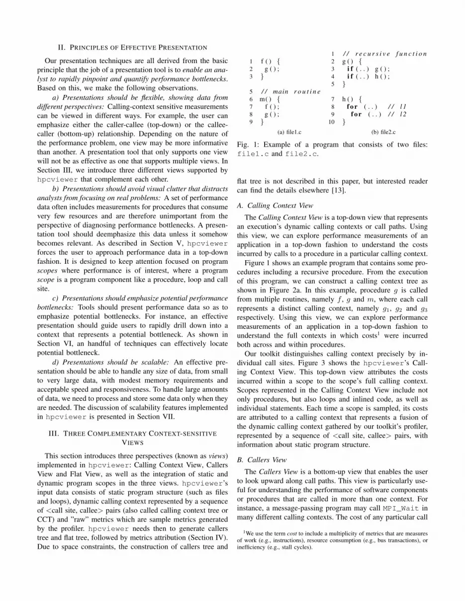
1 f ( ) {2 g ( ) ;3 }

5 / / main r o u t i n e6 m( ) {7 f ( ) ;8 g ( ) ;9 }

(a) file1.c

1 / / r e c u r s i v e f u n c t i o n2 g ( ) {3 i f ( . . ) g ( ) ;4 i f ( . . ) h ( ) ;5 }

7 h ( ) {8 f o r ( . . ) / / l 19 f o r ( . . ) / / l 2

10 }(b) file2.c

Fig. 1: Example of a program that consists of two files:file1.c and file2.c.

flat tree is not described in this paper, but interested readercan find the details elsewhere [13].

A. Calling Context View

The Calling Context View is a top-down view that representsan execution’s dynamic calling contexts or call paths. Usingthis view, we can explore performance measurements of anapplication in a top-down fashion to understand the costsincurred by calls to a procedure in a particular calling context.

Figure 1 shows an example program that contains some pro-cedures including a recursive procedure. From the executionof this program, we can construct a calling context tree asshown in Figure 2a. In this example, procedure g is calledfrom multiple routines, namely f , g and m, where each callrepresents a distinct calling context, namely g1, g2 and g3respectively. Using this view, we can explore performancemeasurements of an application in a top-down fashion tounderstand the full contexts in which costs1 were incurredboth across and within procedures.

Our toolkit distinguishes calling context precisely by in-dividual call sites. Figure 3 shows the hpcviewer’s Call-ing Context View. This top-down view attributes the costsincurred within a scope to the scope’s full calling context.Scopes represented in the Calling Context View include notonly procedures, but also loops and inlined code, as well asindividual statements. Each time a scope is sampled, its costsare attributed to a calling context that represents a fusion ofthe dynamic calling context gathered by our toolkit’s profiler,represented by a sequence of <call site, callee> pairs, withinformation about static program structure.

B. Callers View

The Callers View is a bottom-up view that enables the userto look upward along call paths. This view is particularly use-ful for understanding the performance of software componentsor procedures that are called in more than one context. Forinstance, a message-passing program may call MPI_Wait inmany different calling contexts. The cost of any particular call

1We use the term cost to include a multiplicity of metrics that are measuresof work (e.g., instructions), resource consumption (e.g., bus transactions), orinefficiency (e.g., stall cycles).

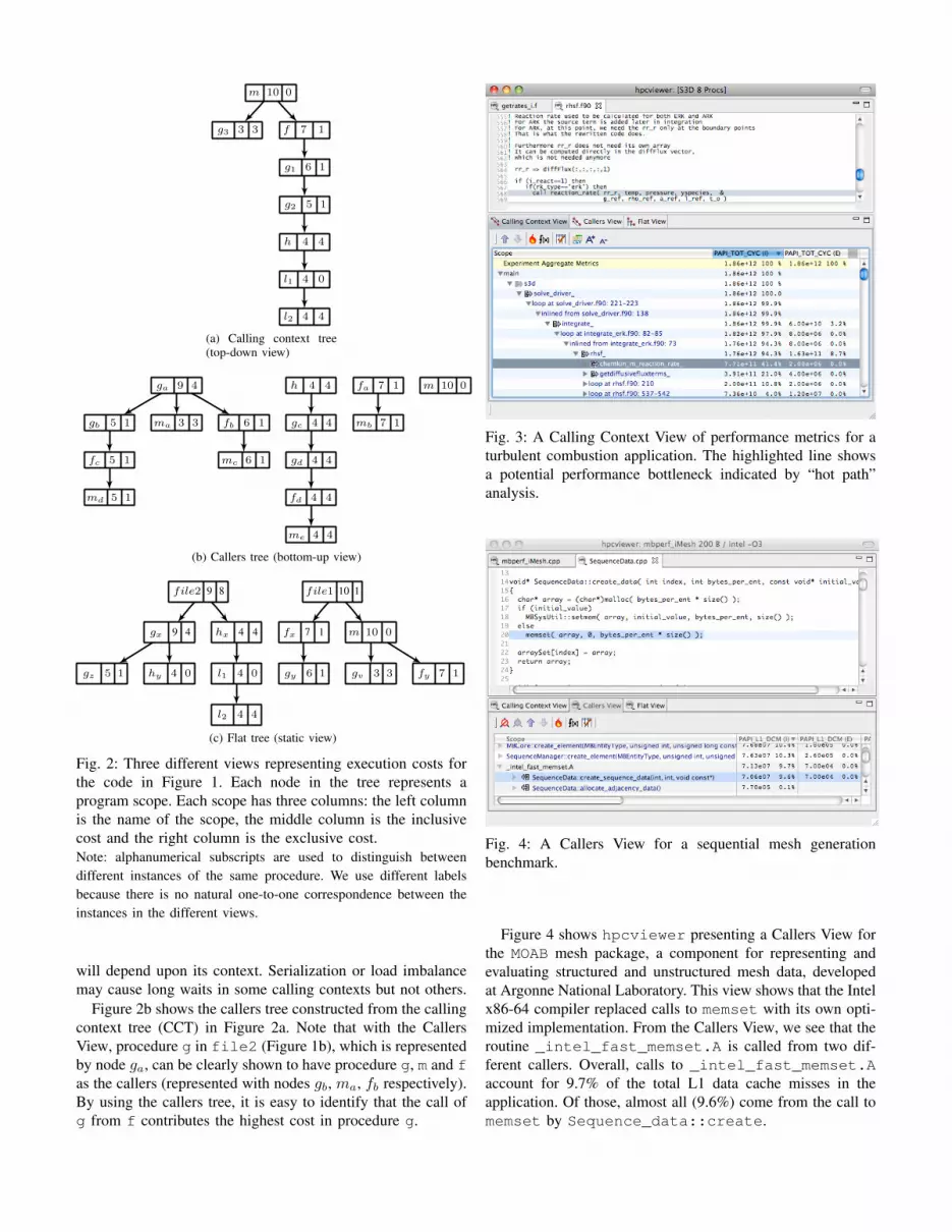
g3 3 3

g2 5 1

g1 6 1

f 7 1

h 4 4

m 10 0

l2 4 4

l1 4 0

(a) Calling context tree(top-down view)

gd 4 4

gc 4 4

fc 5 1

fd 4 4

gb 5 1

ga 9 4 fa 7 1h 4 4

fb 6 1

me 4 4

md 5 1

m 10 0

ma 3 3

mc 6 1

mb 7 1

(b) Callers tree (bottom-up view)

file2 9 8 file1 10 1

gx 9 4 fx 7 1hx 4 4 m 10 0

hy 4 0gz 5 1 gy 6 1

l2 4 4

l1 4 0 gv 3 3 fy 7 1

(c) Flat tree (static view)

Fig. 2: Three different views representing execution costs forthe code in Figure 1. Each node in the tree represents aprogram scope. Each scope has three columns: the left columnis the name of the scope, the middle column is the inclusivecost and the right column is the exclusive cost.Note: alphanumerical subscripts are used to distinguish betweendifferent instances of the same procedure. We use different labelsbecause there is no natural one-to-one correspondence between theinstances in the different views.

will depend upon its context. Serialization or load imbalancemay cause long waits in some calling contexts but not others.

Figure 2b shows the callers tree constructed from the callingcontext tree (CCT) in Figure 2a. Note that with the CallersView, procedure g in file2 (Figure 1b), which is representedby node ga, can be clearly shown to have procedure g, m and fas the callers (represented with nodes gb, ma, fb respectively).By using the callers tree, it is easy to identify that the call ofg from f contributes the highest cost in procedure g.

Fig. 3: A Calling Context View of performance metrics for aturbulent combustion application. The highlighted line showsa potential performance bottleneck indicated by “hot path”analysis.

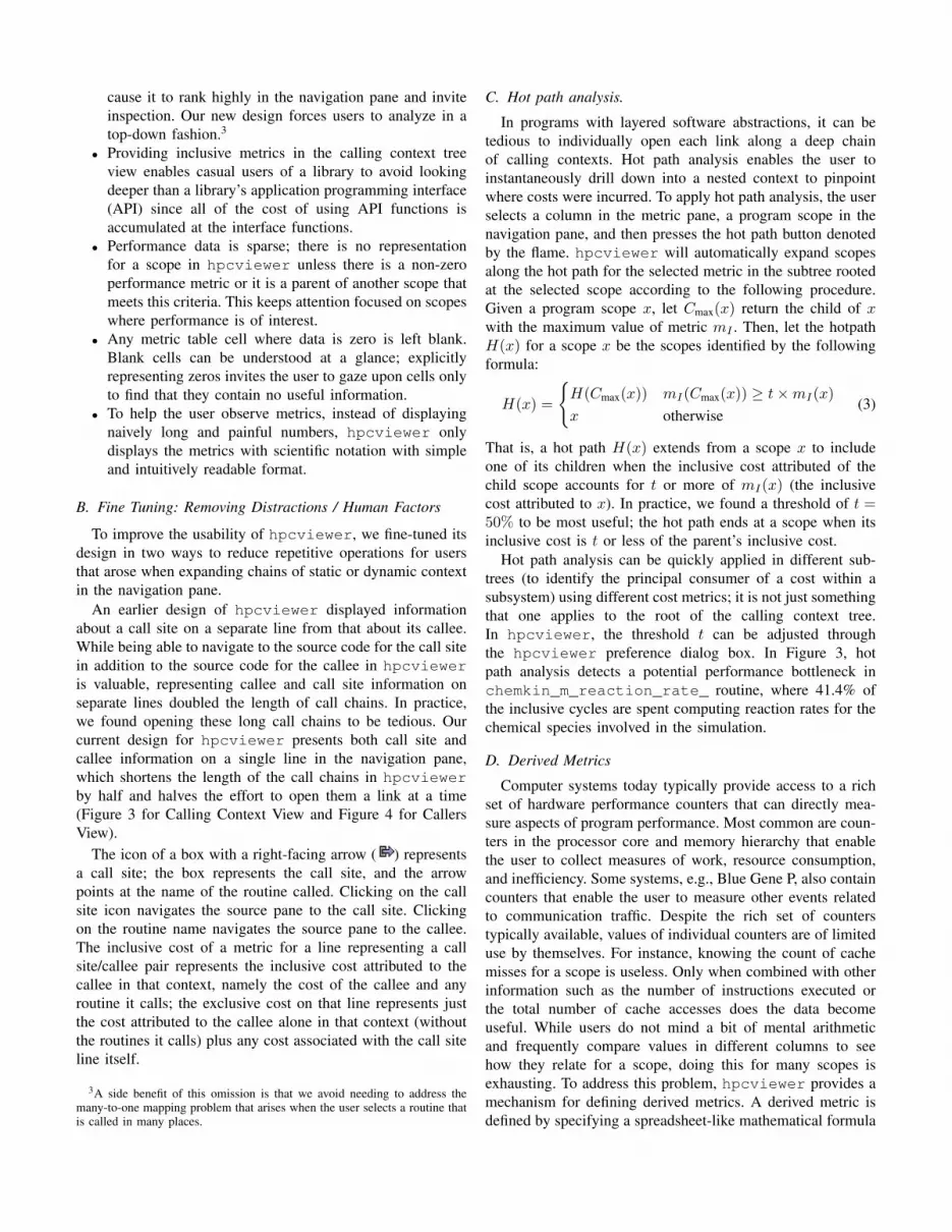
Fig. 4: A Callers View for a sequential mesh generationbenchmark.

Figure 4 shows hpcviewer presenting a Callers View forthe MOAB mesh package, a component for representing andevaluating structured and unstructured mesh data, developedat Argonne National Laboratory. This view shows that the Intelx86-64 compiler replaced calls to memset with its own opti-mized implementation. From the Callers View, we see that theroutine _intel_fast_memset.A is called from two dif-ferent callers. Overall, calls to _intel_fast_memset.Aaccount for 9.7% of the total L1 data cache misses in theapplication. Of those, almost all (9.6%) come from the call tomemset by Sequence_data::create.

Fig. 5: A Flat View showing the attribution of cache missesand cycles through routines, loops, and inlined code.

Fig. 6: Using a derived metric of floating-point waste to ana-lyze the performance of loop nests of a turbulent combustioncode.

C. Flat View

The Flat View correlates performance data to an applica-tion’s static structure such as load module, file, procedure,loop and statement. All costs incurred in any calling contextby a procedure are aggregated together in the Flat View. Thiscomplements the Calling Context View, in which the costsincurred by a particular procedure are represented separatelyfor each call to the procedure from a different calling context.

Figure 2c shows a flat view tree constructed from the callingcontext of Figure 2a. With this flat view, we can easily identify

that file2 has the highest exclusive cost over all files inthe view; similarly, procedures g and h have the highestexclusive cost among all procedures in the view. Figure 5shows a real example of using Flat View in a benchmarkused to study the performance of the MOAB mesh package.This view shows how the costs associated with the procedureMBCore::get_coords are attributed to a loop containinginlined code.hpcviewer also supports a feature that we call flattening.

Flattening elides a scope and shows its children instead.However, applying flattening to a childless scope (a leaf) hasno effect. Since scopes are displayed in a hierarchical fashion,flattening eliminates layers of hierarchical structure (e.g., filesand procedures) that prevent making direct comparisons be-tween loops in different routines. Figure 6 shows a Flat Viewwhere flattening is used to facilitate comparing costs for loopsin different routines.

D. Presenting Calling and Static Contexts

1) Fine-grain hierarchical attribution of costs to static pro-gram structure in the flat view: Figure 5 uses hpcviewer’sFlat View to focus on the performance of a single rou-tine MBCore::get_coords of the mbperf_IMesh meshbenchmark. The rightmost column of metrics shows the exclu-sive total cycles attributed to each scope. We can see that all ofthe cycles spent in the routine (18.9% of the total cycles in theexecution) is spent in the highlighted loop nested within theroutine. Within the loop, we can track attribution of this costthroughout a hierarchy of inlined code that represents the ap-plication of the find operation on the sequence_managerthat is called on line 686. The fourth line of the navigationpane shows an inlined loop to search sequences implementedusing the red-black tree implementation from the C++ stan-dard template library. The next line represents calls to theSequenceCompare operator that are inlined into this loop.Looking at the second metric column, we can see that applyingthe comparison operator accounts for 19.8% of the L1 datacache misses in the execution. Selecting any of the other linesin the lower left navigation pane navigates the source pane toshow the corresponding source code associated with the fileand line numbers. While this example showcases the abilityof our performance analysis toolkit to collect and attributedata with astonishing precision in the presence of inlining,that is not the purpose of including it here. For the purposeof this paper, the example highlights the viewer’s presentationcapabilities in the Flat View to attribute performance metricsthroughout a hierarchy of program structure within a routinethat includes nested loops, multiple levels of inlining, as wellas individual source lines.

2) Integration of static and dynamic program structure inthe Calling Context View: Figure 3 shows a Calling ContextView of the S3D turbulent combustion code developed atSandia National Laboratory. The sequence of lines shownin the navigation pane represents a call path through theapplication. At the top of the call chain is main shown in plainblack (as opposed to a blue hyperlink) because it corresponds

to routines that have no associated source code. Their imple-mentations are provided in binary-only form in the languagerun-time library for the compiler. On subsequent lines, thisview shows a long call chain from the main routine down intothe chemkin_m_reaction_rate_ routine, where 41.4%of the inclusive cycles is spent computing reaction rates for thechemical species involved in the simulation. It is notable thatin this top-down Calling Context View of the metric data forthe execution, we see that the call chain presented includesboth dynamic context (procedure calls) and the loop nestssurrounding these procedure calls. Our toolkit uses informationgleaned from the line map of an executable to determine whena call site is nested within a loop. The viewer then presents anintegrated view that includes both static and dynamic context.

IV. COMPUTING CONTEXT-SENSITIVE METRICS

Once the Callers View and Flat View are constructed basedon the Calling Context View, the next step is to attributemetrics to each scope in the views. We use the term metric torepresent measurements such as resource consumption (e.g.,bus transactions) as inefficiency (e.g., stall cycles). This sec-tion begins with a simple method for computing metric valuesfor each view and then introduces a technique to correctlyhandle recursive programs.

A. Metrics

The Calling Context View shown by hpcviewer repre-sents a data structure that we call a canonical calling contexttree (canonical CCT). This data structure is synthesized byhpcprof by integrating information about static programstructure into dynamic call chains. Consequently, a scope inthe CCT is classified as either a dynamic or static scope.A dynamic scope represents caller-callee relationship, whilea static scope represents static program structure such asload module, file, procedure, loop, line statement or inlinedprocedure.

We define two types of calling context metrics: inclusiveand exclusive. Inclusive metrics for a particular scope reflectcosts for the entire subtree rooted at that scope while exclusivemetrics, to some extent, do not. We have found it usefulto distinguish between two types of exclusive metric valuesbecause although one often thinks of procedure frames in thecontext of call chains, it is natural to think of loops in thecontext of a procedure. Therefore, we adopt a hybrid definitionof exclusive metrics based on whether metric values for ascope x should be computed with respect to dynamic callchains or a procedure’s static hierarchy:

1) Dynamic: sum every descendant statement of x that isnot across a call site.

2) Static: sum every child statement of x.The first rule indicates that the exclusive cost of a dynamicscope is the total of all its descendant statements withinprocedure frame, while the second rule specifies that theexclusive cost of a static scope is the sum of the exclusive costof its children statements. For instance, the CCT in Figure 2ashows that procedure h has a direct child loop l1, which is a

parent of loop l2; and the exclusive cost of l1 does not includethe cost of l2 (rule 2) since l2 is not a statement. Furthermore,the flat tree in Figure 2c shows that procedure h can be botha static procedure as represented by node hx, and a dynamiccall site as represented by node hy . As a static procedure,h includes the cost of all statements in l2 (rule 2), but as adynamic call site scope, its exclusive cost only includes thecost of its invocation as shown in node hy (rule 1).

The computation of metrics in the viewer consists of threedifferent steps:

1) initialization : initialize the exclusive and inclusive costs.2) multiple view creation: create Callers View and Flat

View and compute the metrics attribution.3) finalization : refine the metrics for all views. This step

is needed to compute metrics of parallel programs [14].In the initialization step, the viewer computes exclusive

values and inclusive values. Here we describe how these arecomputed. Initially, a CCT contains metric values only atsample points, which are typically leaf scopes. We definethese values to be exclusive metrics for scopes. For a scopex, the exclusive value mE(x) for metric m is defined to bethe number of samples at x multiplied by the sample period.For any dynamic scope x, we initialize mE(x) = 0. We thencompute exclusive values for each node x using the formula:

mE(x) =

∑s∈desc(x)

mE(xs) x: procedure frame∑s∈child(x)

mE(xs) x: other static

mE(x) x: dynamic

(1)

When x is a dynamic scope, case three simply returns thecost’s initial value. When x is a static scope that is not aprocedure frame, the second case uses the Static definition.Here, the function child(x) returns every scope that is a childof x. When x is a procedure frame, the first case applies theDynamic definition. The function desc(x) returns every scopes that is a descendant of x and for which the path between xand s contains no call site.

Using exclusive metric values from Equation 1, we defineinclusive values for metric m at node x as:

mI(x) =

nC(x)∑c=1

mI(xc) +mE(x) x: interior

mE(x) x: leaf

(2)

This simple inductive definition computes an interior scope’sinclusive metric value from its children’s inclusive values andits own exclusive value. The function nC(x) refers to thenumber of children for scope x.

Figure 3 clearly shows the importance of presenting in-clusive and exclusive costs of a metric. In this figure, theleftmost column in the table of performance metrics displaysthe total number of cycles (PAPI TOT CYC) consumed byeach program scope in the Calling Context View. Seven linesfrom the bottom of the figure, we see that the data for the

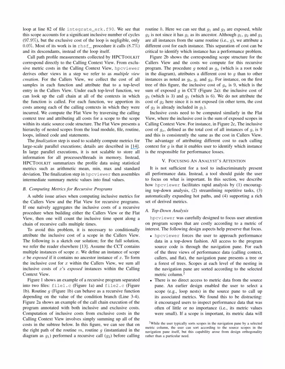
loop at line 82 of file integrate_erk.f90. We see thatthis scope accounts for a significant inclusive number of cycles(97.9%), but the exclusive cost of the loop is negligible, only0.0%. Most of its work is in rhsf_ procedure it calls (8.7%)and its descendants, instead of the loop itself.

Call path profile measurements collected by HPCTOOLKITcorrespond directly to the Calling Context View. From exclu-sive metric costs in the Calling Context View, hpcviewerderives other views in a step we refer to as multiple viewcreation. For the Callers View, we collect the cost of allsamples in each function and attribute that to a top-levelentry in the Callers View. Under each top-level function, wecan look up the call chain at all of the contexts in whichthe function is called. For each function, we apportion itscosts among each of the calling contexts in which they wereincurred. We compute the Flat View by traversing the callingcontext tree and attributing all costs for a scope to the scopewithin its static source code structure. The Flat View presents ahierarchy of nested scopes from the load module, file, routine,loops, inlined code and statements.

The finalization step is used to scalably compute metrics forlarge-scale parallel executions; details are described in [14].In large parallel executions, it is not scalable to store allinformation for all processes/threads in memory. Instead,HPCTOOLKIT summarizes the profile data using statisticalmetrics such as arithmetic mean, min, max and standarddeviation. The finalization step in hpcviewer then assemblesintermediate summary metric values into final values.

B. Computing Metrics for Recursive Programs

A subtle issue arises when computing inclusive metrics forthe Callers View and the Flat View for recursive programs.If one naıvely aggregates the inclusive costs of a recursiveprocedure when building either the Callers View or the FlatView, then one will count the inclusive time spent along achain of recursive calls multiple times.

To avoid this problem, it is necessary to conditionallyattribute the inclusive cost of a scope in the Callers View.The following is a sketch our solution; for the full solution,we refer the reader elsewhere [13]. Assume the CCT containsmultiple instances of scope x. We define an instance of scopex be exposed if it contains no ancestor instance of x. To formthe inclusive cost for x within the Callers View, we sum allinclusive costs of x’s exposed instances within the CallingContext View.

Figure 1 shows an example of a recursive program separatedinto two files: file1.c (Figure 1a) and file2.c (Figure1b). Routine g (Figure 1b) can behave as a recursive functiondepending on the value of the condition branch (Line 3-4).Figure 2a shows an example of the call chain execution of theprogram annotated with both inclusive and exclusive costs.Computation of inclusive costs from exclusive costs in theCalling Context View involves simply summing up all of thecosts in the subtree below. In this figure, we can see that onthe right path of the routine m, routine g (instantiated in thediagram as g1) performed a recursive call (g2) before calling

routine h. Here we can see that g1 and g3 are exposed, whileg2 is not since it has g1 as its ancestor. Although g1, g2 and g3are all instances from the same routine (i.e., g), we attribute adifferent cost for each instance. This separation of cost can becritical to identify which instance has a performance problem.

Figure 2b shows the corresponding scope structure for theCallers View and the costs we compute for this recursiveprogram. The procedure g noted as ga (which is a root nodein the diagram), attributes a different cost to g than to otherinstances as noted as gb, gc and gd. For instance, on the firsttree of this figure, the inclusive cost of ga is 9, which is thesum of exposed g in CCT (Figure 2a): the inclusive cost ofg3 (which is 3) and g1 (which is 6). We do not attribute thecost of g2 here since it is not exposed (in other term, the costof g2 is already included in g1).

Inclusive costs need to be computed similarly in the FlatView, where the inclusive cost is the sum of exposed scopes inCalling Context View. For instance, in Figure 2c, The inclusivecost of gx, defined as the total cost of all instances of g, is 9and this is consistently the same as the cost in Callers View.The advantage of attributing different cost to each callingcontext for g is that it enables user to identify which instanceis the responsible for performance losses.

V. FOCUSING AN ANALYST’S ATTENTION

It is not sufficient for a tool to indiscriminately presentall performance data. Instead, a tool should guide the userto focus on what is important. In this section, we describehow hpcviewer facilitates rapid analysis by (1) encourag-ing top-down analysis, (2) streamlining repetitive tasks, (3)automatically expanding hot paths, and (4) supporting a richset of derived metrics.

A. Top-Down Analysis

hpcviewer was carefully designed to focus user attentionon program scopes that are costly according to a metric ofinterest. The following design aspects help preserve that focus.• hpcviewer forces the user to approach performance

data in a top-down fashion. All access to the programsource code is through the navigation pane. For eachof the three views of performance data (calling context,callers, and flat), the navigation pane presents a tree ora forest of trees. Scopes at each level of the nesting inthe navigation pane are sorted according to the selectedmetric column.2

• There is no direct access to metric data from the sourcepane. An earlier design enabled the user to select ascope (e.g., loop nests) in the source pane to call upits associated metrics. We found this to be distracting:it encouraged users to inspect performance data that wasoften of little or no importance (i.e., its metric valueswere small). If a scope is important, its metric data will

2While the user typically sorts scopes in the navigation pane by a selectedmetric column, the user can sort according to the source scopes in thenavigation pane itself, but this capability arose from design orthogonalityrather than a particular need.

cause it to rank highly in the navigation pane and inviteinspection. Our new design forces users to analyze in atop-down fashion.3

• Providing inclusive metrics in the calling context treeview enables casual users of a library to avoid lookingdeeper than a library’s application programming interface(API) since all of the cost of using API functions isaccumulated at the interface functions.

• Performance data is sparse; there is no representationfor a scope in hpcviewer unless there is a non-zeroperformance metric or it is a parent of another scope thatmeets this criteria. This keeps attention focused on scopeswhere performance is of interest.

• Any metric table cell where data is zero is left blank.Blank cells can be understood at a glance; explicitlyrepresenting zeros invites the user to gaze upon cells onlyto find that they contain no useful information.

• To help the user observe metrics, instead of displayingnaively long and painful numbers, hpcviewer onlydisplays the metrics with scientific notation with simpleand intuitively readable format.

B. Fine Tuning: Removing Distractions / Human Factors

To improve the usability of hpcviewer, we fine-tuned itsdesign in two ways to reduce repetitive operations for usersthat arose when expanding chains of static or dynamic contextin the navigation pane.

An earlier design of hpcviewer displayed informationabout a call site on a separate line from that about its callee.While being able to navigate to the source code for the call sitein addition to the source code for the callee in hpcvieweris valuable, representing callee and call site information onseparate lines doubled the length of call chains. In practice,we found opening these long call chains to be tedious. Ourcurrent design for hpcviewer presents both call site andcallee information on a single line in the navigation pane,which shortens the length of the call chains in hpcviewerby half and halves the effort to open them a link at a time(Figure 3 for Calling Context View and Figure 4 for CallersView).

The icon of a box with a right-facing arrow ( ) representsa call site; the box represents the call site, and the arrowpoints at the name of the routine called. Clicking on the callsite icon navigates the source pane to the call site. Clickingon the routine name navigates the source pane to the callee.The inclusive cost of a metric for a line representing a callsite/callee pair represents the inclusive cost attributed to thecallee in that context, namely the cost of the callee and anyroutine it calls; the exclusive cost on that line represents justthe cost attributed to the callee alone in that context (withoutthe routines it calls) plus any cost associated with the call siteline itself.

3A side benefit of this omission is that we avoid needing to address themany-to-one mapping problem that arises when the user selects a routine thatis called in many places.

C. Hot path analysis.

In programs with layered software abstractions, it can betedious to individually open each link along a deep chainof calling contexts. Hot path analysis enables the user toinstantaneously drill down into a nested context to pinpointwhere costs were incurred. To apply hot path analysis, the userselects a column in the metric pane, a program scope in thenavigation pane, and then presses the hot path button denotedby the flame. hpcviewer will automatically expand scopesalong the hot path for the selected metric in the subtree rootedat the selected scope according to the following procedure.Given a program scope x, let Cmax(x) return the child of xwith the maximum value of metric mI . Then, let the hotpathH(x) for a scope x be the scopes identified by the followingformula:

H(x) =

{H(Cmax(x)) mI(Cmax(x)) ≥ t×mI(x)

x otherwise(3)

That is, a hot path H(x) extends from a scope x to includeone of its children when the inclusive cost attributed of thechild scope accounts for t or more of mI(x) (the inclusivecost attributed to x). In practice, we found a threshold of t =50% to be most useful; the hot path ends at a scope when itsinclusive cost is t or less of the parent’s inclusive cost.

Hot path analysis can be quickly applied in different sub-trees (to identify the principal consumer of a cost within asubsystem) using different cost metrics; it is not just somethingthat one applies to the root of the calling context tree.In hpcviewer, the threshold t can be adjusted throughthe hpcviewer preference dialog box. In Figure 3, hotpath analysis detects a potential performance bottleneck inchemkin_m_reaction_rate_ routine, where 41.4% ofthe inclusive cycles are spent computing reaction rates for thechemical species involved in the simulation.

D. Derived Metrics

Computer systems today typically provide access to a richset of hardware performance counters that can directly mea-sure aspects of program performance. Most common are coun-ters in the processor core and memory hierarchy that enablethe user to collect measures of work, resource consumption,and inefficiency. Some systems, e.g., Blue Gene P, also containcounters that enable the user to measure other events relatedto communication traffic. Despite the rich set of counterstypically available, values of individual counters are of limiteduse by themselves. For instance, knowing the count of cachemisses for a scope is useless. Only when combined with otherinformation such as the number of instructions executed orthe total number of cache accesses does the data becomeuseful. While users do not mind a bit of mental arithmeticand frequently compare values in different columns to seehow they relate for a scope, doing this for many scopes isexhausting. To address this problem, hpcviewer provides amechanism for defining derived metrics. A derived metric isdefined by specifying a spreadsheet-like mathematical formula

that refers to data in other columns in the metric table by using$n to refer to the value in the nth column.

Combined with the other capabilities of hpcviewer, de-rived metrics are much more useful than they first appear.First, a column filled with a derived metric value can be usedto sort scopes in the navigation pane. Being able to sort bya derived metric is much more useful than simply sorting byone of the terms upon which it was based and computingthe derived values with mental arithmetic; sorting on derivedmetrics improves user productivity. Second, derived metricscan focus user attention on tuning opportunities rather thanjust the raw costs that measured metrics typically represent.For instance, rather than sorting scopes in a scientific programto find out where the most cost was incurred, for tuning it isoften more useful to understand where the most importantinefficiencies are. A good way to focus on inefficiency is witha derived waste metric. Depending upon what the user expectsas the rate-limiting resource (e.g., floating-point computation,memory bandwidth, etc.), the user can define an appropriatewaste metric (e.g., FLOP opportunities missed, bandwidth notconsumed) and sort by that. Specifically, we have used ametric of floating-point waste, which we define as (the totalnumber of cycles spent in a scope) × (the peak number offloating-point operations per cycle that the processor supports)− (the actual number of floating-point operations executedin the scope) [3]. This metric tells us how many additionalFLOPS could have been executed in a scope if we werealways computing at peak rate. Sorting by this metric will rankorder scopes to show that contain the greatest opportunitiesfor improving overall program performance. This metric mayhighlight loops where• a lot of time is spent computing efficiently, but the

aggregate inefficiencies accumulate,• less time is spent computing, but the computation is rather

inefficient, and• scopes such as copy loops that contain no computation

at all, which represent a total waste of time according tothe metric.

Beyond identifying opportunities for tuning with a wastemetric, the user can compute a companion derived metricrelative efficiency metric to help understand how easy it mightbe to improve performance. A scope running at very highefficiency will typically be much harder to tune than runningat low efficiency. For our floating-point waste metric, wecomputed relative efficiency by dividing measured FLOPS bypotential peak FLOPS. For scopes that rank high accordingto a waste metric, a relative efficiency metric can indicate theease of improving the code.

VI. EFFECTIVE ANALYSIS

A. Effective Analysis with Derived Metrics

Here we show how derived metrics help to pinpoint andquantify scalability bottlenecks in context. We compute aderived metric that quantifies scaling loss by scaling anddifferencing call path profiles from a pair of executions [3].

Figure 6 shows an application of the aforementionedfloating-point waste metric to a turbulent combustion code.By computing and sorting by the floating point waste metric,we discovered that the most floating-point waste (13.5%) wasattributed to a flux diffusion loop that was streaming datathrough the memory hierarchy; code for this loop is shownin the source pane. The relative efficiency metric shows thatthis loop is running at 6% efficiency and represents a fat targetfor optimization. By using a tool to transform the loop nestto exploit data reuse in cache (by applying loop scalarization,fusion, unswitching, and unroll and jam), we were able toimprove its running time by a factor of 2.9. The second scopeshown in the figure represents a loop within the math library’sexponential routine.

The relative waste metric indicated that this was runningat about 39% efficiency, which means that it is fairly tightlytuned. Using the Callers View view (not shown) to identifysome of the contexts in which the exponential routine was usedshowed that there are opportunities for improving performanceby using a vectorized version of the primitive, which makesbetter use of the instruction pipeline by filling it with multipleindependent recurrences for separate computations.

B. Effective Analysis with Multiple Views

Often analysis begins with the Calling Context View tosee if there is any calling context in the computation thatparticularly dominates in terms of cost. This can be doneby using hot path analysis on a selected metric which thenshows the call path of a potential performance bottleneck (iffound). If not, the user typically moves to the Callers View tounderstand how much cost is incurred by each procedures atthe top of the rank ordered list. In this case, the user typicallyinvestigates a few of the important contexts. Once the userknows what procedures and contexts are costly, the user canmove to the Flat View to understand the costs associated witha procedure along with its loops and inlined code.

The three views play different roles. The Calling ContextView provides a context-centric presentation from the callers’perspectives. The Callers View provides a view of callingcontext from the perspective of each callee. The Flat Viewsupport detailed analysis of all costs incurred by a staticcontext.

C. Load Imbalance Identification

Load imbalance is one of the most common scaling prob-lems in single-program multiple-data (SPMD) scientific appli-cations. It is caused by uneven distribution of work that forcessome processes to idle between synchronization points. Wehave developed a scalable technique to visualize and identifyload imbalance of parallel programs by using call path profilesand scalable post-mortem analyses [14].

As a case study, we choose PFLOTRAN, a scientific pro-gram for modeling multi-phase, multi-component subsurfaceflow and reactive transport using massively parallel comput-ers [7]. We ran PFLOTRAN on the Cray XT5 partition ofJaguar, located at Oak Ridge National Laboratory’s National

Fig. 7: A Calling Context View of PFLOTRAN’s load imbal-ance.

Center for the Computational Sciences. The PFLOTRAN testproblem was a steady-state groundwater flow problem inheterogeneous porous media on an 850× 1000× 80 elementdiscretization with 15 chemical species per cell.

We can identify a load imbalance by sorting by totalinclusive idleness summed over all MPI processes and per-forming hot path analysis to drill down into the potential loadimbalance context, which is the main iteration loop at line384 in timestepper.F90. As shown in Figure 7, the firstgraph from the top shows scattered inclusive total cycles. Thesecond and the third graph shows the sorted metric and thehistogram respectively, confirming that there is uneven workpartition among processes.

Although this case study of an execution of PFLOTRAN isnot an exhaustive analysis, this case study does illustrate howhaving aggregate idleness metrics attributed to each node ofan execution’s canonical CCT can help pinpoint, quantify, andunderstand sources of performance load imbalance.

VII. SCALABLE PRESENTATION

Scalability is highly critical in any aspects of performanceanalysis tools, especially when the profile data is taken froma large scale parallel program that may run for days or evenweeks on hundred thousands of cores. HPCTOOLKIT was de-signed with scalability in mind. Its performance measurementhas significantly low overhead [15] and its data analysis isable to process thousands of MPI processes [14].

We have designed hpcviewer to support scalability aswell. Data presentation in hpcviewer is based on tree-tabular presentation, which is generally more scalable thana graph-oriented presentation, both in rendering speed andvisibility. Using a tree to represent calling contexts is muchclearer than a graph for complex applications. Using tableto represent metrics allows a user to select which metric toobserve and to automatically search for a possible performancebottleneck.hpcviewer is based on Eclipse and configured with lazy-

startup, which means all components (such as text editors,graph and HTML viewer) are loaded when needed. Further-more, in order to analyze large-scale application that runswith thousands of processors, we summarize metrics of allprocessors into mean, covariance, min and max [14], insteadof displaying thousands of metrics. Finally, the Callers View isconstructed dynamically, ensures scalability for both executiontime and memory consumption since we store and process dataonly when needed.

VIII. RELATED WORK

Presentation of program performance can be either graphi-cal or tabular. Tools that can be included in the first categoriesare CrayPat [9], VTune [6], LoopProf [8] and TAU [10].Tabular-based data presentation tools include gprof [16], IntelPTU [5], parallel performance wizard [11], Apple’s Shark [2],Sun Studio [12] and hpcviewer. While graphical presenta-tion style can be more appealing, we have found that tabularstyle is clearly more scalable and informative.

To the best of our knowledge, there is no other toolthat support all three views. gprof [16], Parallel performancewizard [11], Sun Studio [12] and Apple’s Shark [2] allsupport the Calling Context View with inclusive and exclusivemetrics. These tools, however, do not support Callers View.Intel PTU [5] supports Callers View and Flat View (withouthierarchical structure), but no inclusive metric is supported.

Some tools support (semi) automatic performance analysis.CrayPat [9] provides a feature to automatically pinpoint andquantify load imbalance in parallel applications. It is alsopossible to automatically detect scalability problems in TAUby using PerfExplorer [4].

The importance of derived metrics is widely acknowledged.Intel PTU supports a kind of derived metrics to comparedata between different experiments. TAU/PerfExplorer allowsa much higher flexibility by using a script to define derivedmetrics and even to automatize repetitive tasks [4].

Some tools only support specific programming models orplatform. Parallel performance wizard only supports some

PGAS languages [11]. Intel PTU [5], Intel VTune [6], Apple’sShark [2], Sun Studio [12] and CrayPat [9] supports onlyfor specific platforms. In contrast, our toolkit is designed forlanguage independent, application independent and problemindependent.

In summary, while none of the key features of hpcvieweris strikingly novel when taken in isolation, our focus has beenon what results from their combination. In hpcviewer, wehave selected and married a relatively small set of comple-mentary presentation techniques to form a coherent synthesisthat is greater than the constituent parts.

IX. CONCLUSIONS AND FUTURE WORK

We developed hpcviewer as part of HPCTOOLKIT forperformance analysis of serial and parallel codes. The featuresthat it supports today grew out of our own experiences oftrying to analyze and tune scientific applications. hpcviewerwas designed based on four principles: (a) support of multi-ple perspectives which complement each other for observingprofile data, (b) avoidance of visual clutter, (c) emphasis onpotential performance bottleneck, and (d) scalability. Thesefour principles are critical for guiding the user to performanalysis in a sea of performance data.

To our knowledge, hpcviewer is the only tool availablethat supports all three views of context-sensitive performancedata: Calling Context View, Callers View, and Flat View. Wehave shown that each view complements each other and candiscover different performance problems. hpcviewer’s top-down approach guides a user to focus on what is important,and its profile data is displayed in such a way as to reducedistractions. Our tool is also unique that it combines bothstatic structure and dynamic call paths as shown in the CallingContext View and Flat View.hpcviewer’s features effectively increase user productiv-

ity. Derived metrics quickly highlight tuning opportunities.The hot path analysis streamlines a repetitive task and rapidlyhighlights important program contexts.hpcviewer is designed to be scalable. Its components

are loaded on-demand, it supports dynamic creation of theCallers View, tabular-based data presentation and metricssummarization for parallel applications with large number ofprocessors.

Overall, we believe that we have converged on a usefulcorpus of features that serves the intended purpose. Usingour tools, often the user can pinpoint performance bottleneckseffectively, that need attention in a matter of minutes.

Ongoing work includes additional focus on scalability. Aswe apply hpcviewer to programs with large-scale paral-lelism, other issues that may be important are replacing ourXML format for profiles with a more compact binary format,and enhancing hpcviewer so that it need not have data forall processes resident in memory at once.

Other ongoing work includes identifying data reuse patternsand suggesting program transformations to improve programperformance. Another item of interest is effectively presentingmetrics correlated with object code. Although HPCTOOLKIT

supports a simple text-based presentation of such information,it is cumbersome to use.

X. ACKNOWLEDGMENTS

HPCTOOLKIT would not exist without the contributions ofthe other project members: Mike Fagan and Mark Krentel.

This research used resources at both Argonne’s LeadershipComputing Facility at Argonne National Laboratory, which issupported by the Office of Science of the U.S. Departmentof Energy under contract DE-AC02-06CH11357; and theNational Center for Computational Sciences at Oak RidgeNational Laboratory, which is supported by the Office ofScience of the U.S. Department of Energy under Contract No.DE-AC05-00OR22725

REFERENCES

[1] L. Adhianto, S. Banerjee, M. Fagan, M. Krentel, G. Marin, J. Mellor-Crummey, and N. R. Tallent. HPCToolkit: Tools for performanceanalysis of optimized parallel programs. Concurrency and Computation:Practice and Experience, 22(6):685–701, December 2009.

[2] Apple Computer. Shark. http://developer.apple.com/performance/.[3] Cristian Coarfa, John Mellor-Crummey, Nathan Froyd, and Yuri Dot-

senko. Scalability analysis of spmd codes using expectations. InICS ’07: Proceedings of the 21st annual international conference onSupercomputing, pages 13–22, New York, NY, USA, 2007. ACM.

[4] Kevin A. Huck, Oscar Hernandez, Van Bui, Sunita Chandrasekaran, Bar-bara Chapman, Allen D. Malony, Lois Curfman McInnes, and BoyanaNorris. Capturing performance knowledge for automated analysis. In SC’08: Proceedings of the 2008 ACM/IEEE conference on Supercomputing,pages 1–10, Piscataway, NJ, USA, 2008. IEEE Press.

[5] Intel Corporation. Intel PTU. http://software.intel.com/en-us/articles/intel-performance-tuning-utility/.

[6] Intel Corporation. Intel VTune performance analyzers. http://www.intel.com/software/products/vtune/.

[7] Richard Tran Mills, Chuan Lu, Peter C Lichtner, and Glenn E. Ham-mond. Simulating subsurface flow and transport on ultrascale computersusing PFLOTRAN. Journal of Physics Conference Series, 78(012051),2007.

[8] Tipp Moseley, Daniel A. Connors, Dirk Grunwald, and Ramesh Peri.Identifying potential parallelism via loop-centric profiling. In CF ’07:Proceedings of the 4th international conference on Computing frontiers,pages 143–152, New York, NY, USA, 2007. ACM.

[9] Luiz De Rose, Bill Homer, and Dean Johnson. Detecting applicationload imbalance on high end massively parallel systems. In Anne-MarieKermarrec, Luc Bouge, and Thierry Priol, editors, Euro-Par, volume4641 of Lecture Notes in Computer Science, pages 150–159. Springer,2007.

[10] Sameer S. Shende and Allen D. Malony. The Tau parallel performancesystem. Int. J. High Perform. Comput. Appl., 20(2):287–311, 2006.

[11] Hung-Hsun Su, M. Billingsley, and A.D. George. Parallel performancewizard: A performance analysis tool for partitioned global-address-spaceprogramming. Parallel and Distributed Processing, 2008. IPDPS 2008.IEEE International Symposium on, pages 1–8, April 2008.

[12] Sun Studio. Sun Studio Performance Analyzers. http://www.sunstudio.com.

[13] Nathan R. Tallent. Performance Analysis for Parallel Programs: FromMulticore to Petascale. Ph.D. dissertation, Department of ComputerScience, Rice University, March 2010.

[14] Nathan R. Tallent, Laksono Adhianto, and John M. Mellor-Crummey.Scalable identification of load imbalance in parallel executions using callpath proles. In The 2010 ACM/IEEE Conference on Supercomputing (toappear), New York, NY, USA, 2010.

[15] Nathan R. Tallent, John M. Mellor-Crummey, Laksono Adhianto,Michael W. Fagan, and Mark Krentel. Diagnosing performance bot-tlenecks in emerging petascale applications. In Proc. of the 2009ACM/IEEE Conference on Supercomputing, pages 1–11, New York, NY,USA, 2009. ACM.

[16] Dominic A. Varley. Practical experience of the limitations of gprof.Software: Practice and Experience, 23(4):461–463, 1993.