NBER WORKING PAPER SERIES

DYNAMIC TRADE, ENDOGENOUS INSTITUTIONS AND THE COLONIZATION OF HONG KONG:A STAGED DEVELOPMENT FRAMEWORK

T. Terry CheungTheodore Palivos

Ping WangYin-Chi WangChong K. Yip

Working Paper 23937http://www.nber.org/papers/w23937

NATIONAL BUREAU OF ECONOMIC RESEARCH1050 Massachusetts Avenue

Cambridge, MA 02138October 2017

We thank Ying Bai for sharing his data on opium trade. We are grateful for valuable comments and suggestions to Rick Bond, Mario Crucini, Gerhard Glomm, Boyan Jovanovic, Derek Laing, Douglass North, Pietro Peretto and Ray Riezman, as well as participants of the Summer Meetings of the Econometric Society and the Midwest Macro Meetings. Financial support from Academia Sinica, the Chinese University of Hong Kong, and the National Science Council (NSC 98-2911-H-001-001), which enabled this international collaboration, is gratefully acknowledged. JianTang, Long Ho Wong and Jianpo Xue provided excellent research assistance. Needless to say, theusual disclaimer applies. The views expressed herein are those of the authors and do notnecessarily reflect the views of the National Bureau of Economic Research.

NBER working papers are circulated for discussion and comment purposes. They have not been peer-reviewed or been subject to the review by the NBER Board of Directors that accompanies official NBER publications.

© 2017 by T. Terry Cheung, Theodore Palivos, Ping Wang, Yin-Chi Wang, and Chong K. Yip. All rights reserved. Short sections of text, not to exceed two paragraphs, may be quoted without explicit permission provided that full credit, including © notice, is given to the source.

Dynamic Trade, Endogenous Institutions and the Colonization of Hong Kong: A Staged DevelopmentFrameworkT. Terry Cheung, Theodore Palivos, Ping Wang, Yin-Chi Wang, and Chong K. YipNBER Working Paper No. 23937October 2017JEL No. E02,E65,F54,O11

ABSTRACT

To explore the interplays between trade and institutions, we construct a staged development framework with multi-period discrete choices to study the colonization of Hong Kong, which served to facilitate the trade of several agricultural and manufactured products, including opium, between Britain and China. Based on the historical data and documents that we collected from limited sources, we design our dynamic trade model to capture several key features of the colonization process and use it to characterize the endogenous transition from the pre-Opium War era, to the post-Opium War era and then to the post-opium trade era, which span the period 1773-1933. We show that while the low opium trading cost and the high warfare cost initially postponed any military action, the high valuation of the total volume of bilateral trade, the rising opium trading cost and the anticipated increase in the demand for opium eventually led the British government to declare the Opium Wars, legalizing opium trade via the colonial Hong Kong. We also show that, in response to a drastic drop in opium demand and a rising opium trading cost, it became optimal for the British government to abandon opium trade soon after the founding of the Republic of China.

T. Terry CheungDepartment of EconomicsWashington University in St. LouisSt. Louis, MO 63130cheung.t@wustl.edu

Theodore PalivosDepartment of EconomicsAthens University of Economics and BusinessAthens, Greecetpalivos@aueb.gr

Ping WangDepartment of EconomicsWashington University in St. LouisCampus Box 1208One Brookings DriveSt. Louis, MO 63130-4899and NBERpingwang@wustl.edu

Yin-Chi WangDepartment of EconomicsChinese University of Hong KongShatin, NT, Hong Kongycwang@cuhk.edu.hk

Chong K. YipDepartment of EconomicsChinese University of Hong KongShatin, NT, Hong Kongchongkeeyip@cuhk.edu.hk

“Attempting to understand economic, political, and social change ... requires a fun-damental recasting of the way we think. Can we develop a dynamic theory comparablein elegance to general equilibrium theory? The answer is probably not. But if we canachieve an understanding of the underlying process of change then we can develop some-what more limited hypotheses about change that can enormously improve the usefulnessof social science theory in confronting human problems”(North 2006, p. vii).

1 Introduction

The discovery of the New World and the navigation route to Asia around the Cape of Good Hope

in the late fifteenth century were followed by the birth and rise of maritime powers and the cross-

Atlantic and Europe-Asia trade. The rising opportunities for international trade shaped both po-

litical and economic institutions, from political regime and sovereignty, to contracting, property

rights protection and other trading laws and regulations. Such newly established institutions then

fed back to influence upon the activities and outcomes of trade.1 These interactions generated in

turn long-term consequences for economic development, leading to the observed “great divergence”

across countries. The primary purpose of this paper is to further advance our understanding of the

interplays between trade and institutions by providing a thorough investigation of the historical

case of colonial Hong Kong.

In spite of its rich economic history, the miraculous development of Hong Kong that unfolded

over the past two or three centuries remains largely unexplored. In this paper, we highlight the role

played by Hong Kong, prior to World War II (WWII), as the pearl of the Britain-China trade. It was

this unique and distinctive role in facilitating international trade that helped pave Hong Kong’s path

of phenomenal development, making it one of the most successful newly industrialized economies in

the world.2 Although the case of Hong Kong is highly controversial regarding the colony selection

process, an integrated study over the entire two-century horizon is as yet lacking. Interestingly,

however, once we put together a theory to explain the dynamic process of the colonization of Hong

Kong, good documentation can be achieved and quality data can be collected and organized to

confirm our testable hypotheses.

To fulfill the purpose of this study, we deviate from the commonly used political economy ap-

proach and instead propose a staged development framework with multi-period discrete choices to

endogenize institutions. The conventional wisdom in political economy does not suit for the com-

1This is best summarized by Engerman and Sokoloff (2008), who write: “The key connection between appropriate

institutions and economic growth is that institutions reduce the costs of production and distribution, allowing private

agents more scope to benefit from specialization, investment, and trade.”2Acemoglu, Johnson and Robinson (2005a) remark that, among Western European countries, Atlantic traders grew

much faster and in a more sustainable manner than nontraders. In this regard, the colonization of Hong Kong was

also significant in contributing to British development.

1

plicated colonization process of Hong Kong, which was centered on the trading relation between the

main power in the West (Britain) and the main power in the East (China), without any noticeable

feedback to the choice of political regimes.3 Our approach is not only suitable for the study of this

intriguing colonization process, but also analytically tractable, allowing us to conduct stage-by-stage

comparative statics that can be verified by historical data and documents.

To study this trade-induced colonization, it is most relevant to understand the historical devel-

opment of Hong Kong between the years 1709, when Britain authorized the East India Company

(EIC) to organize its trade with China, and 1941, when Japan occupied Hong Kong. In our paper,

however, we start with the year 1773, when the offi cial recording of opium trade began, and end

with 1933, the last year in which consistent trade data are available. We divide the chronicle of this

historical time span in the following three distinct subperiods (referred to as Phase I, II and III).

(i) The pre-Opium War era (1773-1839). Throughout almost this entire subperiod EIC essentially

monopolized the Britain-China bilateral trade. With the British government valuing both the

volume of trade and the induced net silver flow, opium trade became gradually so important

that eventually turned the British trade deficit into a surplus. Moreover, during this subperiod

we observe an upward trend in both the quantity and the price of opium.

(ii) The post-Opium War era (1861-1917). After the Opium Wars and the colonization of Hong

Kong (1840-1860), opium trade became legal.4 The share of opium in British exports to China

rose sharply over the next three decades following the last war, subsequently decreased gradu-

ally over the period 1892-1906 and finally dropped to zero a few years after the establishment

of the Republic of China, which formally took place in 1912.

(iii) The post-opium trade era (1918-1933). With all parts of the opium complex being regulated,

the bilateral trade between Britain and China gradually diminished; nevertheless, Hong Kong

continued to play its significant role as the pearl of the Britain-Orient commerce.

In his classic book, Rostow (1960, p.110) offered a punchy description of colonialism: “Colonies

were founded ... not mainly as a purposeful goal of national policy in pursuit of power, but ...

because some economic group wanted to expand its purchases or sales ... [by means of] organizing

3There are two other strands of literature that are much more remote from our study. One strand is the early

trade literature that investigates how trade opportunities affect contracting and property rights institutions. By 1750,

however, both Britain and China, despite the fact that the latter was rather not an open economy, had already well-

established institutional structures that supported long-distance trade. Another strand focuses on modern trade in a

strategic setting, examining tariff wars and the formation of trading blocs. These issues, however, were not present

over the period that this study analyzes.4The colonization of Hong Kong and the legalization of opium trade were among the provisions of the Treaty of

Nanking (1842), the Treaty of Tiensin (1858) and the Convention of Peking (1860) (see below).

2

a suitable political framework to ensure, at little cost [emphasis added], the benefits of expanded

trade.”Quite the opposite, however, the Hong Kong colony was not founded at little cost: it could

have not been founded without a series of costly wars (including the two major Opium Wars in

1840 and 1856) and continual diplomat fights (including The Treaties of Nanking and Tientsin and

many other localized negotiations) for selling the then-called devil’s good —opium —to Qing China.

Given the aforementioned distinctive historical features and the strong implications for later

economic development, there is no doubt that a thorough study of the dynamic process of Hong

Kong colonization is interesting. Yet, the big question is whether it is possible to develop a dynamic

theory that endogenizes the institution and takes into account economic, political and social changes

in this historic event. Despite North’s pessimism about such an endeavor (see North 2006 and

the quote before the Introduction), the political economy frameworks for endogenous institutions

constructed in Acemoglu and Robinson (2000, 2001, 2008) have convincingly shown the feasibility of

meeting this challenge (see also the survey by Acemoglu, Johnson and Robinson, 2005b). Viewing

different institutions across countries as outcomes of collective choices of different interest groups

in societies, the political economy approach treats institutions as a result of political equilibria.

Recent studies, however, illustrate that the political economy approach may not be the universal

framework applicable to all the cases concerning the development of economic institutions in history.

For instance, based on the actual experience of Venice in 800-1350, Puga and Trefler (2012) adopt

instead the occupational choice model of Banerjee and Newman (1993) to explain how long-distance

trade affects institutional dynamism. To be fair, their work can be regarded as a transition of moving

away from the political economy approach because they still “add in coercive political economy

consideration”(p.15) into their model. Nevertheless, the important point is that, depending on the

subject of study, the appropriate analytical model may have to be able to capture the key elements

of the evolution of the historical events.

Upon incorporating the historical background of colonial Hong Kong, we contribute to the liter-

ature by proposing a staged development framework with multi-period discrete choices to endogenize

institutions in a tractable manner. In this regard, we follow the work of Tsiang (1964) and Mat-

suyama (2002) on the analysis of the Rostovian stages of development. In this literature, a dynamic

model is adopted to understand the transition of the macroeconomy from one development stage into

another. In Tsiang (1964), the Solow growth model is extended with a general saving function to

mimic the growth experience from underdevelopment to takeoff. In Matsuyama (2002), the process

toward the final Rostovian stage of development (known as “the age of high mass-consumption”)

generates the “flying geese”pattern that a number of markets taking off sequentially.

To be more specific, this paper constructs a dynamic model with the staged development of the

colonization of Hong Kong captured in the aforementioned three phases. Based on the economic

data collected from limited sources and many historical documents, we take the following steps to

capture the key features of the colonization process:

3

(i) In addition to a composite good, we explicitly model opium production and trade.

(ii) We regard the British government and the East India Company (EIC) as the two main orga-

nizations in action and permit the institutions to change over the three phases. The major

institutions considered include the barriers that Britain faced in trading opium, the British

government’s subsidy rule to EIC, the declaration of wars, and the decision on banning opium

trade after the founding of the Republic of China.5

(iii) We allow the British government to value both the volume of trade with China and the

resultant net silver inflow. Moreover, we take into account both the resource cost involved in

the war and the moral cost associated with trading opium.

(iv) Given the addictive nature of opium, we model its demand as being not too sensitive to its

relative price. Also, given the observed comovement between the quantity and the relative

price of opium, we allow for the presence of an opium demand shock.

(v) Finally, given the evolutionary nature of history, we solve a multi-period discrete choice problem

and characterize the transition from Phase I (the pre-Opium War era), to Phase II (the post-

Opium War era), and then to Phase III (the post-opium trade era).

For theoretical tractability, the declaration of wars and the decision on banning opium trade are both

modeled as discrete choices, through which the endogenous transition from one phase to another

can be fully characterized.

Our main findings concerning the colonization of Hong Kong are three-fold. First, due to high

warfare and low opium trading costs initially, Phase I lasted for a long period of almost 70 years

(1773-1839). Second, due to high valuation of the total volume of trade, high opium trading costs

and the expectation of a continuously rising opium demand, the war was declared. This led to

the transition to Phase II, during which the Hong Kong colony was established and opium trade

became legal. Finally, due to a significant drop in opium demand and a rising opium trading cost,

opium trade was abandoned, causing the transition to the post-opium trade era (Phase III). In the

remainder of the paper, we shall elaborate on these underlying factors that drove the two critical

transitions and account for them theoretically, using comparative-static analysis, as well as offer

empirical support to the various channels with historical data and references to existing documents.

2 Historical Background

We first provide a brief chronicle of the historical development of Hong Kong from 1773 to 1933

and then highlight three important observations that will guide the design of our model.

5Following North (1994), we regard “organizations”as the players who are made up of groups of individuals with

common objective and “institutions”as the rules of the game.4

2.1 A Chronicle of the Development of Hong Kong

While there has been a long history of exchange between Britain and China, the high volume and

more organized form of trade between these two giants started after the turn of the seventeenth

century. Established in 1600 and merged with a new “parallel” company in 1709, EIC served as

“a means of regulating international trade” (Gull 1943, p. 3).6 The EIC era was terminated in

1833. Soon after, in 1840, there was the outbreak of the first Opium War. After fierce military and

political fights that lasted for two decades, the post-treaty period began; from 1860 and onward,

opium trade was fully legalized until 1917, that is, several years into the Republic of China era,

which formally began on January 1, 1912.7

The Pre-Opium War Era: 1773-1839

The British involvement, through EIC, in the trade of opium started in Canton in 1773 and is

estimated at 1000 chests per year (Gull 1943, p. 13).8 Throughout this era, the shipments of opium

rose. While the price of opium went up slightly from late 18th century to the eve of the Opium

War, the shipments of opium increased drastically. More specifically, between 1811 and 1835, the

annual average number of chests of opium exported to China rose more than five times indicating

that opium trade had become relatively more significant over time (see Chart 1).9 For example,

based on the record of EIC in 1828, opium accounted for more than 55% of the total export value

to China. In addition, in ten-years’time, from 1828 to 1838, the opium shipments to China rose by

almost threefold, from around 10,000 to 30,000 chests.

The Opium Wars and the Treaties: 1840-1860

The first Opium War formally began on June 9, 1840. Nevertheless, even before that day, it

was well recognized by British merchants that a settlement of their own was needed to establish

themselves “under the British flag, besides safe and unrestricted liberty of trade at the principal

marts of the Empire” (Tuck 2000, vol. 9, p. 212). In fact, for the British, the Opium War was

beyond opium trade. It was for “the future mode of conducting the foreign trade in China”(Tuck

2000, vol. 9, p. 212).

The first Opium War lasted for more than two years and led to the Treaty of Nanking, which

was signed on August 29, 1842. Among others, the treaty stipulated that (i) Hong Kong should

6Both James Mill and John Stuart Mill worked for EIC and eventually both became head of the offi ce at East

India House in London.7Opium imports from India (a British colony at the time) came to an end by 1917 under the agreement of the

British and Chinese governments. Historians often relate this date to the year after the death of the President of the

Republic of China, Shikai Yuan, in 1916.8Details on all units of measurement are given in the Data Appendix.9Gull (1943) also documents large increase in opium import: “[b]etween 1811 and 1821 the annual average of chests

imported ... was under 5,000." Also, "between 1828 and 1835 the annual average import was over 18,700”(p. 15).

5

become a British colony; (ii) Cohong (the Chinese counterpart of EIC) was to be abolished; (iii)

five coastal cities, namely, Amoy, Canton, Foochow, Ningpo and Shanghai, were to open as Treaty

Ports; and, (iv) there should be a decrease from 65% to 5% in the rates of duty on major trade

items, such as, silk, cotton, and woollens (but not tea); opium was not mentioned (Tuck 2000, vol.

9, p. 214).

The Treaty of Nanking changed the framework of foreign trade and gave Britain a most-favored-

nation status.10 Naturally, after the treaty, there was still a strong resentment against foreigners

in Canton. As a result, the terms of the treaty were not respected and the hostility between the

Chinese and the British started growing again. Eventually this led to the outbreak of the second

Opium War in October 1856, which ended with the Treaty of Tientsin in 1858.11 According to the

terms of this treaty: (i) Kowloon was ceded to Britain; (ii) ten new Treaty Ports opened; and most

importantly, (iii) opium trade was legalized (Nield 2010, pp. 130-132).

The two decades of the Opium Wars defined a transitional stage, which started with the prohi-

bition of opium trade and ended with its full legalization. In the interest of this paper, we will not

discuss this era in our model; instead, we will regard it simply as a transition point.

The Post-Opium War Era: 1861-1917

With the Treaty of Tientsin (1858) and the Convention of Peking (1860), opium trade was

legalized; consequently, opium imported to China reached a high level both in absolute quantity

and continued to be high as a share of total imports (more than 50%) in the two decades following

the Opium Wars (see Chart 2). Starting in the mid-1880s, it gradually began to drop and eventually

was reduced to zero a few years after the establishment of the Republic of China (see Chart 1).12

Nevertheless, the price of opium was quite stable for most of the period, both in absolute and in

relative terms.

The overall Britain-China trade diminished by the end of the nineteenth century due to the fact

that the trade of opium declined (see Chart 2). One of the main reasons for this decline is that the

legalization of opium trade led to a rapid increase in the domestic production of opium in China.

This Chinese production started in the provinces of Yunnan, Guizhou, and Sichuan, which together

contributed over 60% of the total domestic production of opium. Between 1866 and 1894, the total

area of plantation of opium, as a percentage of the total agricultural area, rose by more than seven

times, from 0.2% to 1.5%. The table below presents the consumption and production of opium10The previous system, known as the Canton System because it required that all foreign trade be conducted through

the port of Canton, had been in force since 1760.11The second Opium War was a joint effort of Britain and France; the French joined the British troops with the

excuse that one of their missionaries was killed in Canton. Also, the Treaty of Tientsin was ratified by Emperor

Hsien-Feng in the Convention of Peking in 1860.12Because of different measurement units, the pre- and post-Opium War data series are not directly comparable.

That is why we present each subperiod separately.

6

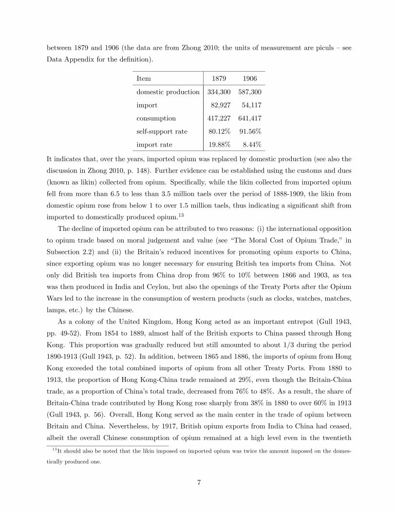
between 1879 and 1906 (the data are from Zhong 2010; the units of measurement are piculs —see

Data Appendix for the definition).

Item 1879 1906

domestic production 334,300 587,300

import 82,927 54,117

consumption 417,227 641,417

self-support rate 80.12% 91.56%

import rate 19.88% 8.44%

It indicates that, over the years, imported opium was replaced by domestic production (see also the

discussion in Zhong 2010, p. 148). Further evidence can be established using the customs and dues

(known as likin) collected from opium. Specifically, while the likin collected from imported opium

fell from more than 6.5 to less than 3.5 million taels over the period of 1888-1909, the likin from

domestic opium rose from below 1 to over 1.5 million taels, thus indicating a significant shift from

imported to domestically produced opium.13

The decline of imported opium can be attributed to two reasons: (i) the international opposition

to opium trade based on moral judgement and value (see “The Moral Cost of Opium Trade,” in

Subsection 2.2) and (ii) the Britain’s reduced incentives for promoting opium exports to China,

since exporting opium was no longer necessary for ensuring British tea imports from China. Not

only did British tea imports from China drop from 96% to 10% between 1866 and 1903, as tea

was then produced in India and Ceylon, but also the openings of the Treaty Ports after the Opium

Wars led to the increase in the consumption of western products (such as clocks, watches, matches,

lamps, etc.) by the Chinese.

As a colony of the United Kingdom, Hong Kong acted as an important entrepot (Gull 1943,

pp. 49-52). From 1854 to 1889, almost half of the British exports to China passed through Hong

Kong. This proportion was gradually reduced but still amounted to about 1/3 during the period

1890-1913 (Gull 1943, p. 52). In addition, between 1865 and 1886, the imports of opium from Hong

Kong exceeded the total combined imports of opium from all other Treaty Ports. From 1880 to

1913, the proportion of Hong Kong-China trade remained at 29%, even though the Britain-China

trade, as a proportion of China’s total trade, decreased from 76% to 48%. As a result, the share of

Britain-China trade contributed by Hong Kong rose sharply from 38% in 1880 to over 60% in 1913

(Gull 1943, p. 56). Overall, Hong Kong served as the main center in the trade of opium between

Britain and China. Nevertheless, by 1917, British opium exports from India to China had ceased,

albeit the overall Chinese consumption of opium remained at a high level even in the twentieth

13 It should also be noted that the likin imposed on imported opium was twice the amount imposed on the domes-

tically produced one.

7

century.

The Post-Opium Trade Era: 1918-1933

Although the use (and production) of opium resurfaced in China in this period, the trade of

opium between Britain and China basically disappeared from the international arena. In the 1920-30

period, UK’s exports of wool to China dropped significantly and were replaced by rice. Also, in 1929,

China raised tariffs from the level of 5% that was established in the Treaty of Nanking to a range of

7.5%-22.5% (Gull 1943, p. 115). Throughout this era, Britain’s relative role in China’s international

trade declined and the composition of trade between them underwent significant structural changes.

2.2 Three Important Observations

Based on historical documents, we would like to highlight three important observations that will

be incorporated in our theoretical framework in an attempt to understand the colonization of Hong

Kong as a crucial stage in the diachronic development of the Britain-China trade.

The British Objective

As documented in the preface and various chapters of Gull (1943), China was regarded by the

British government as the main target for its trade in Asia. The ultimate goal of Britain was to

facilitate such trade in a laissez faire manner. Moreover, it was emphasized that Britain and China

derived mutual benefits from trade; thus, it seems that there was value put to both exports and

imports (see, for example, Tuck 2000, vol. 2, Appendix G). Put differently, the motive of the British

colonization was to do business: “there is little doubt that the spirit of commercial enterprise was

the leading motive of the British colonial policy, and it was the British pursuit of trade in the East,

which brought China and Britain into confrontation”(Bard 2000, p. 7).

To illustrate the long-run trend and characteristics of the Britain-China trade volume, we must

construct the real trade series based on limited data from various sources. For the period before

the nineteenth century, there are no import and export price level data available. However, as we

will model behavior of EIC and the British government, price index in England, and later UK, will

be used. To obtain real trade statistics, we therefore deflate the data of total British exports and

imports to and from China using the computed prices. These are exhibited in Chart 3. We can see

that real imports and exports increased sharply, especially in 1780s.14 Although the magnitude of

trade was small when compared to the post Opium War, such increase in trade volume before the

19th century motivated Britain to pay more attention to its commercial relations with China. For

the post-Opium War period, we are able to cover most of our sample period by Sauerbeck-Statist’s

overall price index (Mitchell 1988). Chart 4 presents the results we obtained using the overall price

14Recall that opium trade started being offi cially recorded in 1773. This highlights the prominent role played by

opium in the development of the Britain-China trade around this year.

8

index.15 Again, this chart points to the important fact that trade between Britain and China rose

over time during the post-Opium War period.

With regard to the composition of the Britain-China trade in the pre-Opium War period and

especially before 1800, tea and silk were the two major British import items from China; they

accounted for more than 70% of the total British imports from China. On the export side, there

were three major items, wool, cotton and opium; these accounted for more than 80% of the total

British exports to China with Opium consistently accounts for around 50% of the total exports (see

Chart 2). In the first two decades of the post-Opium War period, tea and silk continued to be the

two major British import items, accounting together for about 80% of total imports. However, this

pattern changed after the turn of the twentieth century. For example, in the 1920s these two items

accounted for around a quarter of the total British imports. This was mainly due to the successful

policy of substituting imports from China with tea produced in India and Ceylon. Similarly, opium

was still the major export item of Britain, accounting for over 50% of total exports, in the first two

decades of the post-Opium War period; nevertheless, its trade was essentially eliminated after 1917.

Throughout the eighteenth century, Britain suffered a large and rising trade deficit in its trade

with China. This deficit was covered with silver purchased from continental Europe, as Britain had

been on the gold standard since the mid-eighteenth century. Chart 5 provides more details about

the British silver outflows and its net export during the pre-Opium War period. In order to stop

this trade imbalance, the EIC began to smuggle opium into China in the middle of the eighteenth

century. In fact, the traded volume of opium rose so drastically in the next few decades (see Chart 1)

that the British trade deficit and the silver outflows were initially mitigated and eventually reversed.

To facilitate the Britain-China trade, it was recommended “to obtain a grant of a small tract

of ground or detached Island, but in a more convenient situation than Canton, where our present

Warehouse are at a great distance from our Ships”(Tuck 2000, vol. 2, p. 237). In 1834, Lord Napier

recommended Hong Kong as the base for China trade: “if the lion’s paw is to be put down on any

part of the south side of China, let it be Hongkong”(Gull 1943, p. 20). In 1839, there were further

discussions about the choice of a base for the Britain-China trade. According to J. Matheson, the

cofounder of the conglomerate Jardine, Matheson & Co., “the advantage of Hongkong would be

that the more the Chinese obstructed the trade of Canton, the more they would drive trade to

the new English settlement. Moreover, Hongkong was admittedly one of the finest harbours in the

world” (Tuck 2000, vol. 9, p. 213). Indeed, as mentioned in the previous section, these views

were vindicated, since in the post-Opium War era Hong Kong became the most important entrepot

of trade between Britain and China. In short, the British colonization of Hong Kong was mainly

15Alternatively, we computed the aggregate export and import price indices as Cobb-Douglas aggregators, using

the expenditure shares as weights. Then, using these price levels, we deflated the trade statistics to obtain the

corresponding real measures. The results were similar to those in Chart 4.

9

driven by its geographical advantage in the promotion of trade.16

The Barrier to Opium Trade

The attitude of the Chinese offi cials towards opium was consistent over time: they regarded it as

evil and unjustified. The first Imperial edict, which prohibited the sale and the opening of opium-

smoking houses, was issued in 1729 (Rowntree 1905, p.11-12). Despite that, there was growing

consumption of opium, which raised the awareness and concerns, regarding its devastating effects,

of the Chinese high-ranking administrators even more. In 1799, another Imperial edict prohibited

the importation of the drug (Rowntree 1905, p.12-13).17 The situation was out of control by the

time of Emperor Daoguang (1821-1850). For this reason, there was a proposal for legalizing opium

trade and turning it into public profit. However, such a proposal was rejected by the Emperor

who replied: “It is true, I cannot prevent the introduction of the flowing poison; gain-seeking and

corrupt men will for profit and sensuality, defeat my wishes; but nothing will induce me to derive

a revenue from the vice and misery of my people”(Bard 1993, p. 30).

In September of 1836, the Imperial Government of China together with the Viceroy of Canton

started a campaign for the eradication of opium. According to William Jardine, an opium merchant

and a cofounder of Jardine, Matheson & Co., the Canton drug market was entirely closed down by

June 1837. In March 1839, Tse-hsu Lin, the recently appointed Chinese Commissioner in Canton,

ordered the immediate surrender of all opium brought to China. The loss of opium, because of this

new Chinese anti-opium campaign, was 20,283 chests, which was worth £ 2.4 million at that time

(Tuck 2000, vol. 9, pp. 202-3). In response, Chief Superintendent Charles Elliot proposed to the

British government to compensate the merchants for the full value of their opium loss. By then the

British government was directly drawn in (Tuck 2000, vol. 9, pp. 203-4). In May 1839, the Chinese

offi cials issued an edict that commanded all the foreigners to leave China unless they agreed to

sign an opium bond “assuming full responsibility before Chinese law for all ships consigned to their

charge”(Tuck 2000, vol. 9, p. 203). In June 1839, “Matheson and the other British merchants were

expelled from Canton for refusing to obey the orders of the Chinese Government”(Tuck 2000, vol.

9, p. 206). After that, the diplomatic relations between Britain and China became extremely tense.

As Tuck writes, “The greater the recourse to illicit trading from the receiving-ships at Lintin and

along the coast, the greater the danger of the Chinese Government stopping the trade ... After Lord

Napier’s unsuccessful attempt to force a change, Jardine observed that the Chinese seemed more

determined than ever to maintain the system ... It was now realised even in London that no change

16 In a broader aspect, Acemoglu, Johnson and Robinson (2000) emphasize the interplay between geography and

institutional development.17An even stricter edict followed in 1813. Also, in 1809 the Governor of Canton “ordered all incoming ships to be

searched and for the captain of each ship to file bonds declaring that there was no opium in the cargo. But the British

ignored the order”(Nield 2010, p. 67).

10

was possible without a show of force, which might lead to war”(Tuck 2000, vol. 9, pp. 196-7).

All the aforementioned documents highlight the fact that a barrier to opium trade was rising

over time prior to the Opium Wars. After the Opium Wars, the anti-opium attitude of the Chinese

government did not change. For example, an Imperial edict, which was issued in 1906, forbade the

sale of the drug (Hanes and Sanello 2002, p. 295). Moreover, the campaign that followed planned

to eliminate opium consumption in China within ten years.

The Moral Cost of Opium Trade

Although exporting opium to China helped Britain balance its trade deficit from tea imports

quickly, this was done with reluctance, disgrace and sinfulness, which will be referred to as the

“moral cost”of opium trade. In fact, the pressure on the British government to stop the traffi c of

opium on moral grounds came from two different sources: British offi cials and citizens, and other

Westerners.18

Several British offi cials were aware of the harmful effects of opium smoking. In fact, the British

government was reluctant to initiate a war for securing opium trade: “if it should be made a positive

requisition ... that none of that drug (opium) should be sent by us to China, you must accede to

it rather than risk any essential benefit by contending for a liberty in this respect, in which case

the sale of our Opium in Bengal must be left to take its chance in an open market” (Tuck 2000,

vol. 2, Appendix G, Instructions to Lord Macartney, Sept. 8, 1792 by Henry Dundas, p. 239).

Also, Charles Elliot, the Chief Superintendent at Canton from 1836 to 1841, detested opium trade:

“Elliot saw it as a disgrace and a sin and the blackest stain on the British character. It has even

been suggested that Elliot, under instructions to protect the opium traders - a task he resented

- deliberately disobeyed his orders and demanded less from the Chinese than the Government at

home had ordered him to do”(Bard 2000, p. 12).

In 1840, a bill of censure that condemned the government’s military action to the opium crisis

in China, which was introduced by Sir Robert Peel, the leader of the Tory opposition, was defeated

in the House of Commons by a close vote of 271 to 262.19 Later in 1857, when another bill of

censure was introduced to condemn the behavior of government offi cials in the second Opium War,18Although we emphasize the “moral” cost of opium trade in the paper, we regard it as a general indirect way of

modelling the dissatisfaction brought by opium trade to the British government, whose public image was damaged

because of it. Moreover, as Yan (2012) argues, in addition to the moral cost, the structural change in Britain’s

domestic production caused by the Industrial Revolution was another important factor leading to the termination of

opium trade, as that became an obstacle for British industrial capitalists to expand their exports to the Republic of

China.19During the debate on Peel’s motion, the thirty-year-old Tory MP, William Gladstone, the future Prime Minister,

delivered a powerful speech against the trade of opium. Gladstone’s zealousness came from personal acquaintance

with the drug’s harmul effects; his sister had been prescribed laudanum to help her cope with a painful illness and

had become addicted to it (see Hanes and Sanello, 2002).

11

a coalition of Radical and Tories (Conservatives) won the vote with 263-247, leading to the fall of

Palmerston’s government (see Hanes and Sanello, 2002).

Also, after the British victory in the first Opium War and the Treaty of Nanking, Lord Shaftes-

bury, Anthony Ashley Cooper (1801-1885), declared, “I cannot rejoice in our successes; we had

triumphed in one of the most lawless, unnecessary and unfair struggles in the records of history”

(Bard 2000, p. 13). Another example of a British offi cial who was fully aware of the devastating

effects of opium is Lord Elgin, the British negotiator in the Treaty of Tientsin (1858). He had

“supreme power, clear instructions, and strong backing, yet could not bring himself to tell the

Chinese that the time had come when they must legalise this lucrative, but demoralising traffi c”

(Rowntree 1905, p. 87). Finally, “In April 1906, a private member’s motion put by Liberal MP

Theodore Taylor again condemned the opium trade as ‘morally indefensible’and called on the new

government to take measures to bring it to a speedy end”(Blue 2000, pp. 40-41).

There was an even stronger anti-opium sentiment in the British public opinion. The best sum-

mary is perhaps found in Blue (2000, pp. 37-42), who writes “If before 1895 the international

balance of power allowed British authorities at home and in Asia to turn a deaf ear to protests

in China, successive governments in London were steadily subjected to denunciation by the vocal

anti-opium movements in Britain and the United States” (p. 37). Here we mention just a few

examples of this opposition from other sources. An editorial in The Times on December 3, 1842,

upon receiving the news of the Treaty of Nanking wrote that “the moment had come for Britain to

extricate herself from her involvement with opium ... some moral compensation was owed to China

for pillaging her towns and slaughtering her citizens in a quarrel which could never had arisen if

we had not been guilty of an international crime” (Bard 2000, p. 12-13). Also, in England, after

the Pharmacy Act of 1868, opium, along with other drugs, could be sold only by “pharmaceutical

chemists” and not without being labeled “poison.” Finally, a few years later, in November 1874,

an organization, called “The Anglo-Oriental Society for the Suppression of the Opium Trade,”was

founded in London, having as its main purpose to make the British parliament to outlaw the deeply

immoral opium trade with China. For almost forty years (1874-1916), this organization waged an

unrelenting and finally successful campaign against opium traffi c in China (see Brown 1973).

Opium trade was viewed as immoral by many other Westerners besides the British. Most

foreign companies trading with China during the same period did not engage in opium trade. The

American firms Olyphant & Co. and Nathan Dunn & Co. were two leading examples. This was

due to the fact that they were Quaker disciples and their strict moral principles prevented them

to participate in opium trade. In fact, the two most important anti-opium trade conferences in

the early twentieth century, the 1909 International Opium Commission held in Shanghai and the

1912 International Opium Convention signed at the Hague, were outcomes of the American zeal

against manufacturing and trading drugs. In sum, there was a rising anti-opium movement, based

12

on moral grounds, against opium trade, particularly after the turn of the twentieth century and

the establishment of the Republic of China. The pressure on the British government from this

world-wide movement resulted in what we call “the moral cost of opium trade.”

3 The Basic Model

In this section, we build a dynamic model with staged development to describe the three phases of

the colonization of Hong Kong. The model incorporates the three important observations delineated

in the previous section.

As mentioned in the previous section, during the second half of the eighteenth and the first half

of the nineteenth century (before the Opium War), the three most important export items from

Britain to China were opium, cotton and wool. The major import goods from China to Britain,

on the other hand, were tea and silk. Over this period, opium rose to become the single most

important trade item.20 It is therefore essential to separate opium from all other goods in the

model-economy constructed below. It should also be noted that the trade between Britain and

China was essentially monopolized by EIC until 1833 when the “free trade” regime emerged. To

ease the analysis, we shall group EIC and private traders together as a producer-trader entity.

Moreover, we shall consider a central-planner problem: given production and trading technologies

as well as the asset accumulation equation faced by the representative producer-trader, the British

government, who cares about the total volume of trade and the net silver inflow resulting from its

bilateral trade relations with China, seeks to optimize.21

Let Y o denote the output of opium and Y c the output of a composite consumption good com-

prising all other goods in the economy; this composite good is taken to be the numeraire and the

relative price of opium is denoted by p. Further, denote the exports from Britain (including British

India) to China and the imports from China to Britain as Xt andMt, respectively. The total volume

of trade (Tt) is then:

Tt = Xt +Mt. (1)

During the pre-OpiumWar period, Britain incurred regularly a sizable deficit in its trade with China,

which was covered with silver. In fact, the British government often injected bullion to subsidize

severe silver outflows suffered by EIC.22 This trade subsidy to the representative producer-trader is

denoted by St and takes the form of injection of bullion. The British government’s net silver inflow

from trading with China (Rt) equals its trade surplus net of its subsidy to the EIC:

Rt = Xt −Mt − ZTSt, (2)

20See Section 2.2 above for the related evidence.21See Section 2.2 under “The British Objective.”22See Chart 5 for related evidence.

13

where ZT is an indicator of trade deficit that takes on the value one if a deficit occurs and zero

otherwise; accordingly, a subsidy is provided only when a trade deficit occurs. We specify the trade

subsidy in terms of the following two possible rules:

St =

St under a fixed subsidy rule (FSR)

s (Mt −Xt) under a proportional subsidy rule (PSR).(3)

In the main text, we restrict our attention only to the FSR and relegate the analysis under the PSR

to the Appendix, where we show that our main findings remain qualitatively unchanged.

The production cost of each output is given by a standard quadratic function: qi(Y it

)2/2, where

i = c, o. In addition, fund (F ) and labor (L) are required for trading and marketing each product.

We denote the fund requirements per unit of opium and per unit of the composite good by αo

and αc, respectively, where αo > αc; that is, in line with historical documentation, we assume that

opium trade requires relatively more fund for networking and marketing due to the presence of legal

barriers.23 On the other hand, purely for convenience, we assume that the labor unit requirements

for the two goods are the same and we denote them by β. Thus, F it = αiY it and L

it = βY i

t , i = c, o.

Total fund and labor demands are then given by Ft = F ct + F ot and Lt = Lct + Lot , respectively.

Let At denote the total assets accumulated by the representative producer-trader and rt and

wt denote, respectively, the real interest rate and the real wage rate. Then, the evolution of At is

governed by,

At+1 = (1 + rt)At + (Xt −Mt) + ZTSt − wtLt − Ft −qc

2(Y ct )2 − qo

2(Y ot )2 , (4)

that is, the sources of asset accumulation include gross interest, trade surplus and government trade

subsidy, net of production, trading, networking and marketing costs.

Let Zo be an indicator of opium production that takes on the value one if opium is produced

and zero otherwise. Since opium is a “bad”to the Chinese civilians, its import is offi cially banned

by the Chinese government (even though the ban may not be fully effective). Thus, there must be

legal barriers associated with opium trade and the outbreak of an opium war can effectively lower

such barriers. We capture this unit cost of barriers in opium trade using the term (1− Zw) δ, where

Zw takes on the value one if a war has occurred in the past and zero otherwise; moreover,

δ =

δ before the Opium Wars when there existed trade barriers

0 after the Opium Wars when there existed free trade.

That is, had a war never been initiated (Zw = 0), the cost barrier per unit of opium would be δ > 0;

after a war has occurred (Zw = 1), this unit-cost barrier takes the value of zero. Since we will divide

23 In the 1830s, opium was the largest British export item to China (see Section 2.2 for supporting evidence). As

Nield (2000) wrote, “Opium had by now overtaken cotton as the most valuable import to China, and was therefore

well worth the considerable investment being made in its shipment and distribution”(p.70; italics added).

14

the time interval between the end of the Opium Wars and the end of our analysis into two periods

(the post-Opium War period and the post-opium trade period), it is necessary to employ both the

indicator function Zw and the measure of the size of such legal barriers δ (to be discussed in the

next section). Britain’s exports to China then can be written as

Xt = Y ct + ZoptY

ot [1− (1− Zw) δ] = Y c

t + ψ(pt)Yot , (5)

where ψ(pt) ≡ [1− (1− Zw) δ]Zopt represents the effective relative price of opium.

Based on the historical documents (see Section 2.2 under “The British Objective”), the period-

by-period objective of the British government is specified as: (1− ζ) [U(Rt) + θH (Tt)], where both

U and H are concave functions with positive but diminishing marginal utilities, θ > 0 and ζ ∈ (0, 1).

The interpretation of the flow utility is as follows. First, the British government gets utility directly

from having net silver inflows, as captured by the term U(Rt). Second, as emphasized in internal

correspondence and documents (see "The British Objective" above), other things equal, the British

government prefers a larger trade volume and this is indicated by H (Tt). The parameter θ measures

the weight that the government puts on the volume of trade relative to that of silver inflows. Third,

since opium is an addictive with detrimental socioeconomic consequences, its production and trade

are considered immoral (see Section 2.2 under “The Moral Cost of Opium Trade”). We use ζ to

measure the unit moral cost of selling opium (if it is produced), at which rate the overall flow utility

is discounted. It is obvious that, with greater self-awareness upon establishing national identity

and dignity in China, the unit moral cost associated with exporting opium to China rises.24 For

simplicity, we normalize the unit moral cost of trading opium to zero for the period before the

establishment of the Republic of China (when all opium imports from British India ceased) and

denote with ζ the differential unit moral cost during the Republic of China period. We thus have

the following specification:

ζ =

ζ during the Republic of China regime

0 before the Republic of China regime.

We can now write the Bellman equation associated with the value function of the British gov-

ernment as:

V (At) = max (1− Zoζ) [U(Rt) + θH (Tt)]+1

1 + ρV (At+1) , (6)

subject to (4), where ρ is the time discount rate of the British government. Substituting (2), (1),

(5) and the associated production/trading costs of opium into (4) and (6), we can then write the

24Under pressure from the international community “in 1913 Britain signed the Hague anti-opium treaty, committing

itself to the eventual elimination of the worldwide opium trade. The Hague treaties tied Great Britain to a new vision

of cooperative internationalism”(Baumler 2007, p. 82).

15

central planner’s optimization problem as:

V (At)=max(1-Zoζ)[U(Y ct +ψ(pt)Y

ot -Mt-ZTSt

)+θH (Y c

t +ψ(pt)Yot +Mt)

]+V (At+1)

1+ρ,

s.t. At+1= (1+rt)At+ZTSt-Mt+ (1-αc-βwt)Y ct + [ψ(pt)-αo-βwt]Y o

t -qc (Y c

t )2+qo (Y ot )2

2,

and Mt ≥ 0, St ≥ 0, Y ct ≥ 0, Y o

t ≥ 0, where the optimization is performed with respect to

Mt, St, Yct , Y

ot .

We note that viewing Britain’s behavior as the outcome of the central planner’s optimization

problem specified above is realistic given the documented cooperative relation between the British

government, on the one hand, and EIC/private traders, on the other (see Section 2 above). For

brevity, we present all first-order and the Benveniste-Scheinkman conditions in the Appendix.

To close the model, we let Do(p, κ) be the Chinese demand for British opium, where κ is an

autonomous component that stands for an increase in the opium demand function. The introduction

of κ facilitates the capture of the observed positive comovement between opium price and quantity

(see Section 2.1, under “The Pre-Opium War Era: 1773-1839”). Let also DM (I) be the British

demand for import goods from China, where I is the exogenously given income of the British. We

follow common practice and assume that ∂Do(p)/∂p < 0 and ∂DM (I)/∂I > 0, that is, the demand

for opium slopes downward (with price) and the British demand for importables rises with British

income. Equilibrium in the market of each of the two goods requires equating the demand with the

corresponding supply:

Do(pt) = Y ot , (7)

DM (It) = Mt. (8)

4 Equilibrium Analysis

We focus on the addictive nature of opium and assume:

Assumption 1: εop < 1.

That is, the demand for opium is not very sensitive to changes in its relative price.

Following the historical background delineated in Section 2.1, we shall divide the whole period

of pre-WWII Britain-China trade into three phases (see Figure 1 for the time line):

(i) Phase I (the pre-Opium War era): ZT = 1, Zw = 0, Zo = 1, ζ = 0, δ = δ > 0.

(ii) Phase II (the post-Opium War era): ZT = 0, Zw = 1, Zo = 1, ζ = 0, δ = 0.

(iii) Phase III (the post-opium trade era): ZT = 0, Zw = 1, Zo = 0, ζ = ζ > 0, δ = 0.

16

Phase I captures the pre-Opium War era of 1773-1839. Specifically, during this phase, opium trade

was undertaken (Zo = 1) either with local resistance or in an illegal environment, thereby implying

higher trading barriers (δ = δ > 0). In this phase, Britain had a deficit in its trade with China

(ZT = 1), which required injections of silver bullion. Phase II captures the post-Opium War era of

1861-1917. In Phase II, the British trade balance with China was reversed (ZT = 0). Moreover,

the Opium Wars (Zw = 1) forced the legal trade of opium (Zo = 1 with δ = 0). Finally, Phase

III captures the post-opium trade era of 1918-1933. In Phase III, the British trade surplus with

China continued (ZT = 0). At the same time, during the Republic of China regime, a period when

trading addictive goods incurred a higher moral cost (ζ = ζ > 0), opium trade ceased (Zo = 0).

The assignment of values to ZT is suggested by Charts 3 and 4, and to Zo by Charts 1 and 2.

Next, we provide a characterization of the stationary equilibrium for each of the three phases.

4.1 Phase I: The Pre-Opium War Era

Substituting the parameter values that describe this phase (ZT = 1, Zw = 0, Zo = 1, ζ = 0,

δ = δ > 0) into the stationary version of the first-order and market-equilibrium conditions under

FSR, we can obtain two critical relations concerning the outputs of the composite good and opium

(recall that ψ(p) ≡ [1− (1− Zw) δ]Zop):

αc + βw + qcY c = 4, (9)

αo + βw + qoDo(p) = 4ψ (p) , (10)

The first expression pins down the output of the composite good right away; notice that it does not

depend on the opium price p. The second equation together with the opium market-equilibrium

condition (7) yields a fixed-point mapping in the (relative) price of opium, p:

p = Π (p) ≡ 1

4(1− δ

) [αo + βw + qoDo(p)] , (11)

where Π (0) > 0 and dΠ/dp < 0. We thus have:

Lemma 1: (Equilibrium Price in Phase I) Under Assumption 1, there exists a unique relative price

of opium p∗ that solves Π (p∗) = 0 in stationary equilibrium.

Proof: All proofs are relegated to the Appendix.

Utilizing (11), we can obtain the comparative static effects on the relative price of opium p∗:

Lemma 2: (Characterization of the Equilibrium Price in Phase I) Under Assumption 1, the relative

price of opium in stationary equilibrium is increasing in the effective barrier(δ), the wage cost of

opium trade (w) and the production cost of opium (qo).

Intuitively, the relative price of opium goes up to reflect the increased costs resulting from the

tightening of the banning restriction(δ)or from the higher values of w and qo. Focusing on the

17

effect of barriers, an increase in δ shifts up the downward-sloping fixed-point mapping Π(p), thereby

leading to a higher fixed point of the relative price of opium.

To complete the analysis in this phase, we solve for the stationary equilibrium values of trade

subsidy and of the producer-trader’s assets using:

A =1

r

[DM (I)− S + 3Y c + 3ψ (p)Do(p)− qc

2(Y c)2 − qo

2Do(p)2

], (12)

U ′[Y c + ψ(p)Do(p)−DM (I)− S

]= θH ′ [Y c + ψ(p)Do(p) +M ] /2, (13)

where the notation “ ′ ”denotes total derivative. Note that equation (13) yields: S(p) = S. Next, we

define σU ≡ −RU ′′/U ′ as the elasticity of marginal utility of net silver inflow and σH ≡ −TH ′′/H ′

as the elasticity of marginal utility of total trade. We then impose:

Assumption 2: RTσHσU

> 1.

Under Assumption 2, the curvature of the H function is suffi ciently high compared with that of U .

We can then obtain:

Lemma 3: (Characterization of Equilibrium Trade Subsidy and Producer-Trader’s Assets in Phase

I) Under Assumptions 1 and 2, the trade subsidy in stationary equilibrium is negatively related to the

relative price of opium, whereas the producer-trader’s assets in stationary equilibrium are positively

related to the opium price.

The intuition is straightforward. If the demand for opium is price inelastic (Assumption 1) and

the curvature condition of the flow utility is met (Assumption 2), then an increase in p will raise

the British net silver inflow. Hence, the subsidy for offsetting the trade deficit can be reduced.25

The effects of a change in opium price on producer-trader’s assets involve both a cost effect and

a silver inflow effect, where the latter depends on the price elasticity of the opium demand. First,

when the price of opium goes up, the quantity demanded is reduced and hence more assets can be

accumulated due to cost saving. Moreover, if opium demand is inelastic (Assumption 1), then the

net silver inflow from exporting opium increases so that asset accumulation is even higher.

4.2 Phase II: The Post-Opium War Era

Given the terms that describe this phase (ZT = 0, Zw = 1, Zo = 1, ζ = 0, δ = 0, implying ψ (p) = p

and S = 0), we can manipulate the first-order and market-equilibrium conditions in stationary

25The prediction of Lemma 3 seems to be consistent with the existing empirical evidence. For instance, in the

pre-Opium War era (1773-1833), the correlation coeffi cient between the average opium price and the British silver

outflows (net exports to China) is -0.783 (0.777). It may be recalled that the trade subsidy is supposed to take the

form of bullion injection (silver flows) and is inversely related to net exports.

18

equilibrium to obtain:

αo + βw + qoY o

p− 1 = Ω(p, Y c, κ) ≡ U ′ + θH ′

−U ′ + θH ′, (14)

p =αo + βw + qoY o

αc + βw + qcY c. (15)

Using (14), we can write Y c as a function of p and further apply (15) to derive a fixed-point mapping

in p:

Y c = Y c(p) (16)

p =αo + βw + qoDo(p)

αc + βw + qcY c(p)≡ Ψ (p) (17)

Concerning now the composite good output schedule given by (16), Figure 2 gives the graphical

representation of Y c(p) in relation to the opium price. Under the realistic assumption of opium

demand being inelastic (Assumption 1), Y c is decreasing in p so that the supply curve of Y c is

downward sloping in the relative price of opium. Furthermore, producer-trader’s assets in stationary

equilibrium are given by:

A =1

r

DM (I) + (1− αc − βw)Y c + (p− αo − βw)Do(p)− qc

2(Y c)2 − qo

2[Do(p)]2

. (18)

Define the price elasticity of the composite good supply as ηcp=−(p/Y c)(∂Y c/∂p). The following

condition then imposes unity as an upper bound on this supply elasticity:

Assumption 3: ηcp ≤ 1.

We then obtain:

Lemma 4: (Equilibrium Price and Output of Opium in Phase II) Under Assumptions 1 and 3,

there exists a unique relative price of opium p∗ that solves Ψ (p∗) = 0 in stationary equilibrium.

Moreover, the supply of the composite good is decreasing in the relative price of opium and increasing

in the opium trading cost αo, whereas the equilibrium opium price rises with the opium trading cost.

The intuition of Lemma 4 can be understood with the help of Figure 2. A rising trading cost of

opium in this period lead to an upward shift of both the opium (Y o) and the composite-good (Y c)

supply curves. Hence, a new equilibrium resulted with a higher opium price and a larger quantity

of the composite good.26

There are two possible cases in steady state, depending on the slope of the fixed-point mapping.

The first case is Ψp < 0, where we have a downward sloping curve Ψ (p). The second case is

1 > Ψp > 0, which yields an upward sloping curve Ψ (p) , but with a slope less than unity. Both

cases give us a unique p∗.

26As a matter of fact, the correlation coeffi cient between the opium price and the output of the composite good for

the period of 1867-1917 is 0.56, which supports our findings.

19

4.3 Phase III: The Post-Opium Trade Era

We finally turn to the derivation of the key stationary equilibrium equations in Phase III, when

ZT = 0, Zw = 1, Zo = 0, δ = 0, ζ = ζ > 0 and hence with the opium supply and trade completely

banned Y o = 0 (and with the relative price p eliminated throughout):

Y c = Φ(Y c, w) ≡ 1

qc

(2θH ′

θH ′ − U ′ − αc − βw

), (19)

A =1

r

[DM (I) + (1− αc − βw)Y c − qc

2(Y c)2

]. (20)

Consider the following regularity condition,

Assumption 4: Φ(0, w) > 0 and ∂Φ/∂Y c < 1.

We can then establish:

Lemma 5: (Equilibrium-Composite-Good Output in Phase III) Under Assumptions 1 and 4, there

exists a unique composite-good output Y c∗ that solves Y c∗ = Φ(Y c∗ , w) and is decreasing in the cost

of labor w.

Since the fixed-point mapping Φ(Y c, w) is upward sloping but flatter than the 45 line, in response

to a higher wage and hence a higher trading cost, the output of the composite good must fall.

5 Phase Transitions

We can express the value function (6) in stationary equilibrium as:

V (Zw, Zo; δ, ζ) =1 + ρ

ρ(1-Zoζ)

[U(Y ct +ψ(pt)Y

ot -Mt-ZTSt

)+θH (Y c

t +ψ(pt)Yot +Mt)

]

where ψ(pt) ≡ [1− (1− Zw) δ]Zopt, and both R and T on the RHS take on their optimized values.

In each phase, this value function becomes:

VI (δ, ζ) ≡ V (0, 1; δ, ζ) , (21)

VII (δ, ζ) ≡ V (1, 1; δ, ζ) , (22)

VIII (δ, ζ) ≡ V (1, 0; δ, ζ) . (23)

From the information on the historical background (see Section 2.1), we know that the effective

barrier on opium trade imposed by the Chinese government varied during the first phase. In

particular, it has been recognized that in the early stages of Phase I, the effective barrier on opium

trade was very low, as the Chinese offi cials were bribed so that they did not take any banning

action in local communities. Toward the end of Phase I, however, the Ching Dynasty government

decided to take serious action by appointing Commissioner Lin to eradicate opium trade. This led

20

to a sharp increase in the effective barrier. After the Opium Wars, opium trade was legalized and

the effective barrier was removed. Based on the historical situation, we summarize the phases in

transition in terms of the binary parameterization of (δ, ζ) as follows:

Imperial China Republic of China

Before Opium Wars(δ, 0)

n.a.

After Opium War (0, 0)(0, ζ)

Note: n.a. stands for non-applicable.

Let G denote the British war expenses. We define the net welfare change from moving from

Phase i to Phase j as i∆j , i = I, II and j = II, III. Then, we conduct two counterfactual

experiments as follows. First of all, if there is no Opium Wars, then the value function of phase II is

VI(δ, 0). With Opium Wars, then instead the value function becomes VII (0, 0)−G. Thus we have

I∆II

(δ)

= VII (0, 0)−G− VI(δ, 0).

Secondly, as long as opium trade continues, the value function of phase III is VII(0, ζ). But when

opium trade ceases, then instead the value function becomes VIII(0, ζ). So the net welfare change

due to opium trade is

II∆III

(ζ)

= VIII(0, ζ)− VII

(0, ζ).

We now formulate multi-period discrete choices in our staged development framework to endog-

enize institutions. Specifically, for any given pair of differentials in opium trade barriers and moral

costs,(δ, ζ), we fully characterize how changes in economic primitives may cause an endogenous

regime switch in institutions, captured by the transition from one phase to another. Based on the

existing historical data and documents, the primitives that we analyze include government objec-

tives (especially the preference parameter θ) and warfare expenses (G), as well as the opium trading

cost (αo) and demand shocks (κ).

5.1 From Phase I to II: The Colonization of Hong Kong

The transition from Phase I to Phase II can be accounted for by the existence of a (unique) critical

level of trade barriers, denoted as δc, such that I∆II (δc) = 0. To show this, we must examine the

effects of the trade barriers δ on the welfare gain from moving from Phase I to Phase II. Consider,

Assumption 5: G < VII (0, 0)− VI (1, 0).

The interpretation of Assumption 5 is that the gain from moving from no trade to free trade in

opium is larger than the cost of wars. We can then plot the I∆II (δ) schedule in Figure 6, which

is upward sloping with I∆II (0) < 0 < I∆II (1). The first inequality comes from the fact that

VI (0, 0) = VII (0, 0) and the second follows Assumption 5. We therefore obtain:

21

Proposition 1: Under Assumptions 1-5, there exists a unique critical level of trade-barriers δcsuch that, for any δ ∈ (δc, 1), a war is instigated and Phase II emerges.

The intuition is clear. When the effective barrier is absent, there is no need to start a war. When

the effective barrier is at its maximum, so that all opium trade is banned, the war is unavoidable.

Thus, it is to the benefit of Britain to initiate an opium war as long as the effective trade barrier on

opium is above the threshold level δc. In particular, a decrease in the threshold δc, which is caused

by a change in the primitives G, θ, αo, or κ, is more likely to induce an institutional change and to

lead eventually to the colonization of Hong Kong and the legalization of opium trade.

5.2 From Phase II to III: The Abandonment of Opium Trade

The transition from Phase II to Phase III can be accounted for by the existence of a critical level

of moral cost denoted as ζc and defined by equation II∆III (ζc) = 0. To show this, we analyze the

effects of the differential moral cost ζ on the welfare gain from moving from Phase II to Phase III.

Figure 7 depicts the II∆III (ζ) schedule, which is increasing in ζ with II∆III (0) < 0 <II ∆III (1).

The first inequality comes from the intuition that opium trade is preferred in the absence of moral

cost and the second is due to the fact that VII (0, 1) = 0. This leads to:

Proposition 2: Under Assumptions 1-4, there exists a unique critical level of moral cost ζc such

that, for any ζ ∈ (ζc, 1), all opium trade ceases and Phase III emerges.

Intuitively, when the moral cost is absent, there is no incentive for moving into Phase III, because

it is strictly dominated by Phase II. When the moral cost is at its maximum, opium trade is not

conducted, since it does not yield any utility; thus, Phase III is the only choice. Hence, as long as

the moral cost exceeds the critical value ζc, it is to Britain’s benefit to move into Phase III and

abandon opium trade. Summarizing, a decrease in the threshold ζc, caused by a change in the

primitives θ, αo, or κ, is likely to induce an institutional change that will result in the abandonment

of opium trade.

6 Comparative Statics

In the comparative-static exercises performed below, we consider the following categories of shocks

on the critical levels of the transitional parameters δc and ζc: (i) a shock in the cost of warfare

(a change in G); (ii) two structural shocks: a preference shock (a change in θ) and a funding

requirement shock to opium supply (a change in αo); and (iii) an autonomous opium demand shock

(an increase in κ). To evaluate the changes in δc and ζc resulting from these shocks, we totally

differentiate I∆II (δc) = 0 and II∆III (ζc) = 0, respectively.

22

6.1 A Shock in the Cost of Warfare

Since the transition from Phase II to III does not involve G, the effect of a change in G falls only

on the critical level of effective barrier δc. We can establish:

Proposition 3: Under Assumptions 1-3, an increase in the warfare cost delays the transition from

Phase I to Phase II.

Graphically, a change in the military spending G shifts down the I∆II (δ) locus by the same mag-

nitude as depicted in Figure 6. Thus, an increase in G raises the critical level of δ, i.e., for a given

value of δ, as war becomes more costly, it is less likely for it to occur; hence, δc goes up.

6.2 Changes in Structural Parameters

We consider two types of structural shocks, one to preferences and another to opium trade cost.

6.2.1 A Preference Shock

We analyze the effects of a preference shock in favor of the volume of trade, i.e., an increase in θ.

We assume that the total volume of trade rises in the Republic of China regime, which is consistent

with the data (compare the total volume of trade before and after 1917 in Chart 4); that is,

Assumption 6: TIII > TII .

We then obtain:

Proposition 4: Under Assumptions 1-6, a preference shift toward the volume of trade speeds up

the transition from Phase I to Phase II as well as from Phase II to Phase III.

In Figure 6, we illustrate the effect of a rise in θ, which rotates the I∆II (δ) locus counterclockwise.

Thus, δc decreases. As we put more weight on the volume of trade in the preference function, the

critical trade barrier is more likely to decrease. Consequently, for any given δ, we are more likely

to enter Phase II. In Figure 7, we depict the effect of a rise in θ, which shifts the II∆III (ζ) locus

up; thus, ζc decreases. As we put more weight on the volume of trade in the preference function

(an increase in θ), less emphasis is put on opium trade due to its declining share in total trade.

This is also in accord with the actual experience. For instance, opium share was more than 40% in

total British exports to China in the mid nineteenth century, but declined to less than 10% in the

beginning of the twentieth century. As a result, for any given level of the moral cost ζ, we are more

likely to enter Phase III of no opium trade.

6.2.2 A Funding Requirement Shock to Opium Supply

We consider a funding requirement shock to opium supply for a proxy of the incentive measure of

conducting opium trade. This is designed by taking an increase in αo (a higher funding require-

23

ment) to represent a deterioration of the business environment within which opium is supplied. We

assume that the direct price effect is stronger than the cross-market spillover effect via consumption

substitution; that is,

Assumption 7: ∂Y c

∂αo +(∂Y c

∂pII+Do + pII

∂Do

∂pII

)dpIIdαo < 0.

We can now establish:

Proposition 5: Under Assumptions 1-5 and 7, a rise in the funding requirement of opium trade

delays the transition from Phase I to Phase II, but speeds up the transition from Phase II to Phase

III.

The intuition goes as follows. As the business environment within which opium is traded deteriorates

due to higher funding requirement (αo increases), there is less incentive to conduct opium trade.

So the British government is reluctant to put further effort (as mirrored by a war) into expanding

opium trade and the likelihood of starting an opium war diminishes, which is reflected in an increase

in δc. Similarly, ζc falls when the production cost of Yo increases. As αo goes up, the opium trading

environment deteriorates, and hence the cost of stopping opium trade is lower. Thus, for any given

level of the moral cost ζ, we are more likely to enter Phase III of no opium trade.

6.3 An Autonomous Opium Demand Shock

Finally, we analyze the effects of an autonomous demand shock to opium trade, which in terms of

our model is captured by an increase in κ. Consider,

Proposition 6: Under Assumptions 1-3, an autonomous increase in opium demand speeds up the

transition from Phase I to Phase II, but delays the transition from Phase II to Phase III.

The intuition is readily understood. If opium demand increases, then it is worth putting more effort

(e.g., initiating a war) to expand opium trade; hence, for any given δ, we are more likely to enter

Phase II of the legal opium trade period . On the other hand, if the demand for British opium drops,

as a result of the sharp increase in the domestic opium supply, there is less incentive to maintain

opium trade. Hence, for any given level of the moral cost ζ, we are more likely to enter Phase III

of no opium trade.

7 Toward Understanding the Colonization of Hong Kong

Before proceeding further in the analysis, we tabulate our comparative-statics results.

24

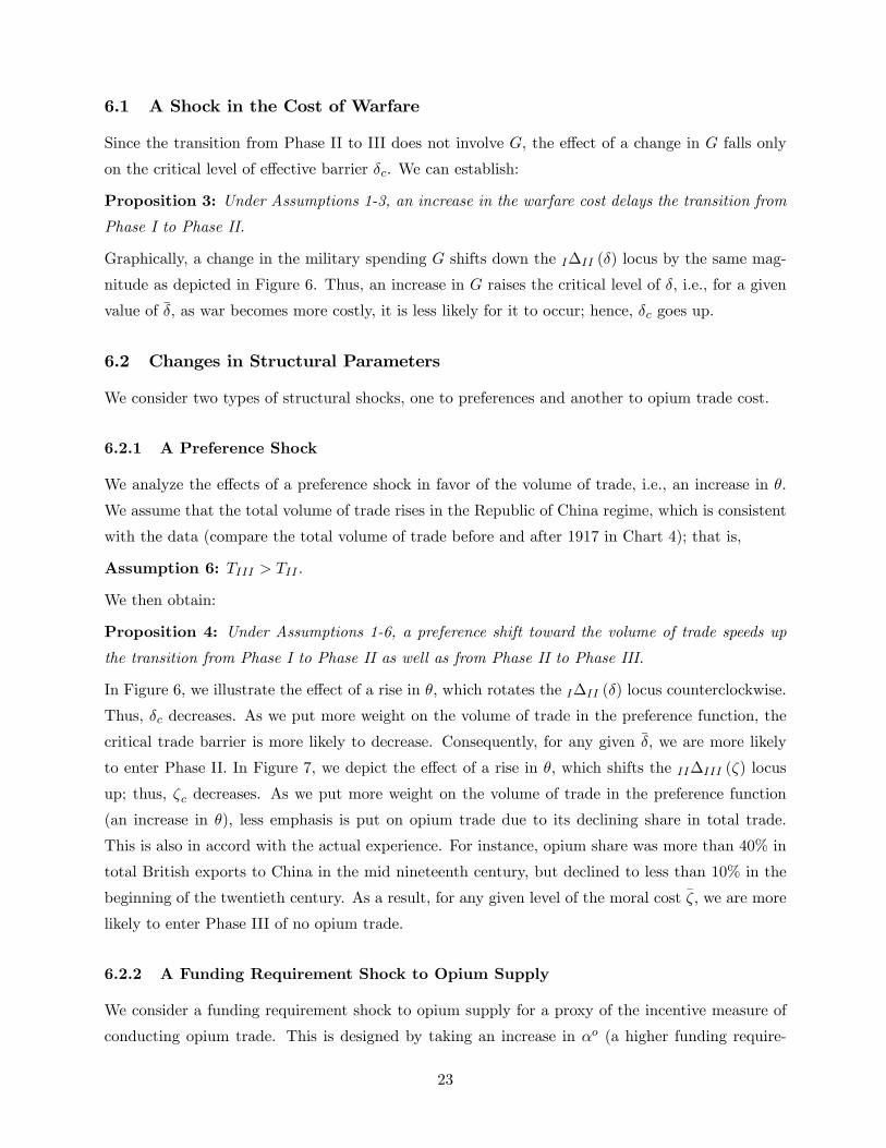
Comparative Critical Value Transition

Statics δc ζc I to II II to III

G ↑ + n.a. slower n.a.

θ ↑ − − faster faster

αo ↑ + − slower faster

κ ↑ − + faster slower

Using the comparative statics above, we would like to investigate the “alternative”history as

suggested in the following quote by Bard (2000, p. 13):

“The facts of history cannot be altered. Is there then any profit in speculating what might

have happened if certain events had or had not taken place? Perhaps, if there are lessons

to be learned from such speculations for, after all, events of today will become history

tomorrow, next year, or a century later.”

More specifically, we are now ready to introduce the following three hypotheses, which suggest how

the course of history might have been altered:

[Hypothesis 1] Due to high warfare and low opium trading costs, Phase I lasted for a long period

of 70 years (1773-1842).

[Hypothesis 2] Due to high valuation of the total volume of trade, high opium trading costs and

the expectation of continuously rising opium demand, the Opium Wars were declared and the

Hong Kong colony emerged, leading to a transition to Phase II.

[Hypothesis 3] Due to a significant drop in opium demand and a rising opium trading cost, opium

trade was abandoned, leading to a transition to Phase III.

These hypotheses are readily corroborated by our model, which is built to capture the historical

environment and some important observations of the particular era before and after the OpiumWars.

Of course, due to data limitation, it is impossible to formulate econometric tests of our hypotheses.

Nonetheless, the existing historical data and documents support the proposed underlying factors

driving the two transitions based on our theoretical model. They also indicate how opium trade

“had determined the course of history of that period and region, and how easily that course might

have been altered, preventing the conflict, and possibly subsequent imperialist policy of western

nations in China”(Bard, 2000, p. 14).

Next we present a selected sample of the existing evidence, found either in the data or in

historical documents, which provides support to our hypotheses. More specifically, according to our

25

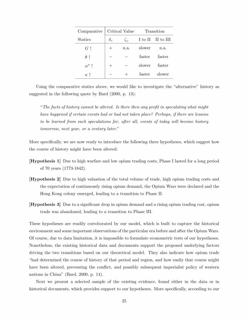
hypotheses, there are seven cases where the shocks that we consider played a pivotal role. These

cases are tabulated below and are labeled D-1 to D-7.

Supporting Evidence Hypothesis 1 Hypothesis 2 Hypothesis 3

G high (D-1) n.a. n.a.

θ n.a. high (D-3) n.a.

αo low (D-2) high (D-4) high (D-6)

κ n.a. high (D-5) low (D-7)

(D-1) This case refers to the role played by the cost of conducting a war (G). Morse (1910)

described the mission of William John Napier, the first Chief Superintendent of trade at

Canton, as follows: “The chief superintendent was instructed that every effort was to be made

to conform to all Chinese regulations and to consider all Chinese prejudices, and at the same

time was forbidden to call in the aid of the armed forces of the Crown” (p. 121). We take

this quote to indicate that Britain had no intention of initiating a war against China because

warfare was high. Britain would prefer to maintain the status quo (Phase I).

(D-2) Although the Chinese government banned opium trade right from the beginning, this did not

lead to a prohibitively high trading cost of opium. The reason is that the banning acts were

never seriously implemented by local Chinese offi cials, who were bribed by British merchants.

This is reflected in the rising opium shipments shown in Chart 1.

(D-3) As documented in Charts 3 and 4, the total real Britain-China trade was rising over time

during both the pre- and post-Opium War periods. This expansion of trade was one of

Britain’s important objectives. As Pritchard has pointed out, the basis of British-Chinese

relations was “the commercial intercourse”(Pritchard 1970, Preface). Moreover, according to

the instructions given to Lord Macartney by the Secretary of State for War Henry Dundas in

1792, in order to facilitate trade with China, the British government had been looking for “a

more convenient situation than Canton, where our present Warehouse are at a great distance

from our Ships” (Tuck 2000, vol. 2, p. 237). Naturally, the benefit from such a settlement

increased with the volume of trade.

(D-4) As depicted in Chart 5, opium trade reversed the British silver outflows. Thus, opium

trade had been a very important component of Britain-China trade. However, the growing

consumption of opium raised the awareness and concerns regarding its devastating effects of

the Chinese high-ranking administrators. In 1839, Commissioner Tse-hsu Lin ordered the

immediate surrender of all opium brought to China. This raised the opium trading cost to a

historically high level. Consequently, “It was now realised even in London that no change was

possible without a show of force, which might lead to war”(Tuck 2000, vol. 9, pp. 196-7).

26

(D-5) The expectation of a continuously rising opium demand, captured by the positive demand

shock (increase in κ), is supported by the positive comovement between opium quantity and

price during Phase I. Using the data on opium price and shipments in the period 1773-1838,

we computed the correlation coeffi cient to be 0.12, which verifies our claim.

(D-6) The cost of trading opium rose drastically following the success of the 1906 imperial edict

that banned opium. As Blue (2000) pointed out, the success “reflected the intensification in

China over the previous decade of aversion to the drug. The aversion was part of the rise in

nationalist sentiment at the turn of the century, stimulated by such factors as the 1895 defeat

at the hands of Japan, the subsequent new imperialist incursions by other powers, and the

humiliation delivered by the anti-Boxer expeditionary forces in 1900”(p.40). “The edict also

reflected new concepts of citizenship ... creating a new category of people who would be left

out of the modern concept of citizenship”(Baumler 2007, p. 56). Eventually, in 1911, Britain

agreed to stop all opium exports from India into China within seven years.

(D-7) In the post-Opium War period, the rapid increase in the domestic production of opium in

China led to a significant decline in the demand for imported opium. In terms of our model,

this negative shock on imported opium demand seen in the data can be understood as an

increase in the supply of opium. In other words, an increase in domestic supply is equivalent

to a decrease in import demand; thus, there should be a negative comovement between opium

quantity and price during Phase II. Indeed, the correlation coeffi cient between opium price

and quantity in the period 1867-1917 is −0.82, which is consistent with our analysis.

In sum, while high warfare (D-1) and low opium trading costs (D-2) were the primary factors

preventing initially the breakout of the Opium Wars, in the end the wars and the consequential

colonization of Hong Kong were mainly driven by the British government’s high valuation of the

total volume trade with China (D-3), the rising opium trading cost (D-4) and the anticipated

increase in China’s demand for opium (D-5). Also, as a result of the anticipated increase in the

opium trading cost (D-6) and the sharp drop in opium demand under the Republic of China regime

(D-7), opium trade was abandoned and a period of more conventional trade with China began.

8 Concluding Remarks

We have constructed a staged development framework with multi-period discrete choices to study

the trade-induced colonization of Hong Kong and the history of opium trade between Britain and

China. The framework has enabled us to characterize each of the three phases involved, namely,

the pre-Opium War era, the post-Opium War era and the post-opium trade era. We have also

illustrated theoretically how the transition between two phases emerged in response to some key

27

underlying factors. For the first transition, these factors included the British government’s high

valuation of the total volume of trade with China, the warfare cost, the cost of trading opium

and the expectation of a rising opium demand. For the second transition, the key factors were a

decrease in China’s import demand for opium and the British government’s moral cost of opium

trade. Thus, we are able to explain why Britain instigated the Opium Wars and colonized Hong

Kong in mid-nineteenth century (first transition) as well as why it abandoned opium trade a few

years after the turn of the twentieth century (second transition). Finally, we have put together

historical data and documentation that provide support to our theoretical results. With these data,

it is possible for us to calibrate the model and to draw meaning numerical conclusions.

While our model is specifically designed to capture the historical observations of the Britain-

China trade during the period 1773-1933 and the colonization of Hong Kong, the general method-

ology and framework can be readily modified to study the establishment of other colonies, such

as Korea, Macao and Taiwan, where trade also played a significant role. For example, over the

long period of 442 years (1557-1999), Macao was under Portuguese occupation and served as an

important center for Portuguese trade with China and Japan. During the sixteenth century and

from 1848 to early 1870s, it was also a traffi cking point for slaves from Southern China to Portugal

or South American ports.

Moreover, following the assassination of the Korean Empress Myeongseong by Japanese agents

in 1895 and the Russo-Japanese War of 1904-1905, Korea came under Japanese rule with the

Japan-Korea Annexation Treaty. This occupation lasted from 1910 to 1945. It formally ended with

Japan’s defeat in WWII. While imperialistic expansion to Northeast and Central Asia was one of

the primary factors leading to this colonization, its role for trade with China, Russia and, through

this, Europe was also important.

Similarly to the colonization of Korea, Taiwan was ceded to Japan from 1895 to 1945 with the

Treaty of Shimonoseki, which ended the First Sino-Japanese War in 1894. The primary reason

for the establishment of this colony was again Japan’s imperialistic expansion, only this time to

Southeast and South Asia. Yet, potential trade with Southern China and Southeast Asia played a

non-negligible role.

The development experiences of these colonies are also of particular interest. Although Macao

is just a short distance from Hong Kong and was also a colony of a Western European country, its

development has been drastically different from that of Hong Kong. Among others, Macao lacked

significantly in terms of growth compared to Hong Kong. On the contrary, Korea and Taiwan,

who were both under an entirely different Imperial Japanese rule, have grown rapidly during the

post-WWII period and joined Hong Kong in the group of the newly industrialized Asian Tigers.

Despite such noticeably disparate development patterns, to the best of our knowledge, there is no

systematic study of these colonial episodes. We regard this as a potentially avenue for future work.

28

References

[1] Acemoglu, Daron, Simon Johnson, and James A. Robinson (2000) “Reversal of Fortune: Ge-ography and Institutions in the Making of the Modern World Income Distribution,”QuarterlyJournal of Economics, 117, 1231-1294.

[2] Acemoglu, Daron, Simon Johnson and James A. Robinson (2001), “The Colonial Origins ofComparative Development,”American Economic Review, 91, 1369-1401.

[3] Acemoglu, Daron, Simon Johnson and James A. Robinson (2005a), “The Rise of Europe:Atlantic Trade, Institutional Change, and Economic Growth,”American Economic Review,95, 546-579.

[4] Acemoglu, Daron, Simon Johnson, and James A. Robinson (2005b) “Institutions as a Funda-mental Cause of Development,” in Philippe Aghion and Steven Durlauf (eds.), Handbook ofEconomic Growth, Elsevier, Amsterdam, The Netherlands, 386-347.

[5] Acemoglu, Daron, and James A. Robinson (2000) “Why Did the West Extend the Franchise?Democracy, Inequality, and Growth in Historical Perspective,”Quarterly Journal of Economics,115, 1167-1199.

[6] Acemoglu, Daron, and James A. Robinson (2001) “A Theory of Political Transitions,”Ameri-can Economic Review, 91, 938-963.

[7] Acemoglu, Daron, and James A. Robinson (2008), “Persistence of Power, Elites, and Institu-tions,”American Economic Review, 98, 267-293.

[8] Bai, Ying, and James K. Kung (2016), "Opium, Silver, and the Decline of Late Imperial China,1789-1910," Working Paper.

[9] Bard, Solomon (1993), Traders of Hong Kong: Some Foreign Merchant Houses, 1841-1899,Urban Council, Hong Kong.

[10] Banerjee, Abhijit V. and Andrew F. Newman (1993), “Occupational Choice and the Processof Development,”Journal of Political Economy, 101 (2), 274-298.

[11] Bard, Solomon (2000), “Tea and Opium,” Journal of the Royal Asiatic Society, Hong KongBranch, 40, 1-19.

[12] Baumler, Alan (2007), The Chinese and Opium under the Republic: Worse than Floods andWild Beasts, State University of New York Press, Albany, NY, USA.

[13] Blue, Gregory (2000), “Opium For China: The British Connection,”in Opium Regimes, ed. byTimothy Brook and Bob Tadashi Wakabayashi, University of California Press, Berkeley andLos Angeles, CA, USA.

[14] Brown, J. B. (1973), “Politics of the Poppy: The Society for the Suppression of the OpiumTrade, 1874-1916,”Journal of Contemporary History, 8, 97-111.

[15] Clark, G. (2010). "The macroeconomic aggregates for England, 1209—2008," Research in Eco-nomic History, 51-140.

29

[16] Engerman, Stanley L. and Kenneth L. Sokoloff (2008), “Debating the Role of Institutionsin Political and Economic Development: Theory, History, and Findings,”Annual Review ofPolitical Science, 11, 119-135.

[17] Gull, Edward Manico (1943), British Economic Interests in the Far East, Oxford UniversityPress, London, UK.

[18] Hanes, W. Travis III and Frank Sanello (2002), Opium Wars, Sourcebooks Inc., Naperville,Illinois, USA.

[19] Hsiao, Liang-Lin (1974), China’s Foreign Trade Statistics, 1864-1949, Harvard University AsiaCenter.

[20] Matsuyama, Kiminori (2002), “The Rise of Mass Consumption Societies,”Journal of PoliticalEconomy, 110 (5), 1035-1070.

[21] Mitchell, B.R. (1988), British Historical Statistics, Cambridge University Press.

[22] Morse, Hosea Ballou (1910), The International Relations of the Chinese Empire, vol.1, Long-mans, London, U.K.

[23] Nield, Robert (2010), The China Coast: Trade and the First Treaty Ports, Joint Publishing(H.K.) Co., Ltd, Hong Kong.

[24] North, Douglass C. (1994), “Economic Performance Through Time: The Limits to Knowledge,”American Economic Review, 84, 359-368.

[25] North, Douglass C. (2006), Understanding the Process of Economic Change, Princeton Univer-sity Press, Princeton, USA.

[26] Pritchard, E.H. (1970), Anglo-Chinese Relations During the Seventeenth and Eighteenth Cen-turies, Octagon Books, New York, U.S.

[27] Puga, Diego and Daniel Trefler (2012), “International Trade and Institutional Change: Me-dieval Venice’s Response to Globalization,” NBER Working Paper 18288, Cambridge, MA,USA.

[28] Rostow, Walt W. (1960), The Stages of Economic Growth, Cambridge University Press, Cam-bridge, U.K.

[29] Rowntree, Joshua (1905), The Imperial Drug Trade, Methuen and Co, London, U.K.

[30] Tsiang, S.C. (1964), “A Model of Economic Growth in Rostovian Stages,”Econometrica, 32(4), 619-648.

[31] Tuck, Patrick J.N. (2000), Britain and the China Trade, 1635-1842, Routledge, New York,USA.

[32] Yan, Se (2012), “Gentry Benevolence or Pursuit of Self-interest: The End of the Sino-BritishOpium Trade (Shenshi de Cibei Haishi Liyi de Zhuizhu? Zhongying Yapian Maoyi ZhongjieGuocheng de Yanjiu)”, The Qing History Journal (Qingshi Yanjiu; in Chinese), No. 3, pp88-99.

[33] Zhong, Wei-Min (2010), Tea and Opium: China in the Process of Economic Globalization inthe Nineteenth Century, SDX Joint Publishing Company, Beijing, China (in Chinese).

30

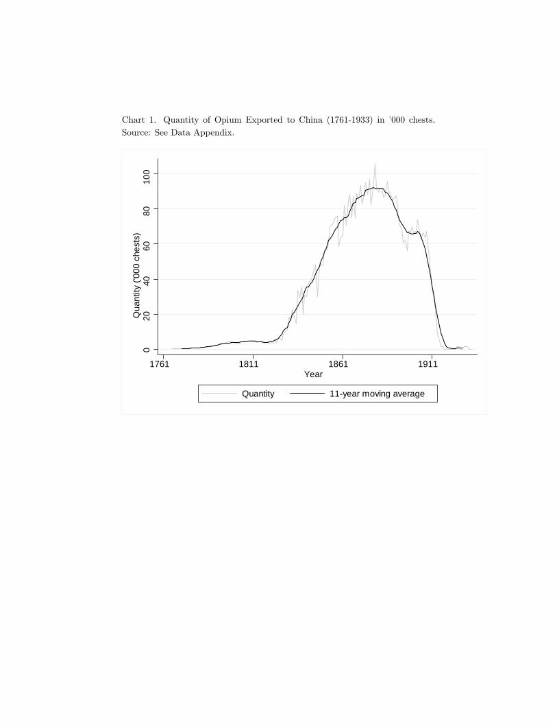
Chart 1. Quantity of Opium Exported to China (1761-1933) in 000 chests.Source: See Data Appendix.

020

4060

8010

0Q

uant

ity ('

000

ches

ts)

1761 1811 1861 1911Year

Quantity 11­year moving average

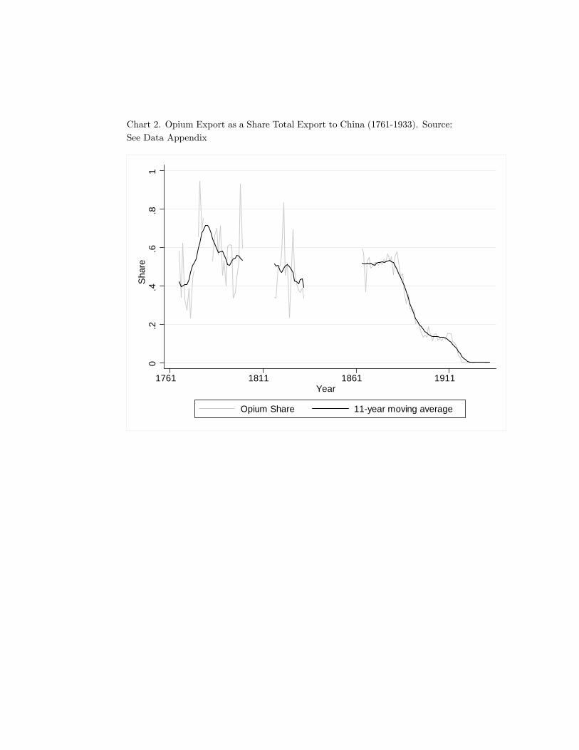
Chart 2. Opium Export as a Share Total Export to China (1761-1933). Source:See Data Appendix

0.2

.4.6

.81

Shar

e

1761 1811 1861 1911Year

Opium Share 11­year moving average

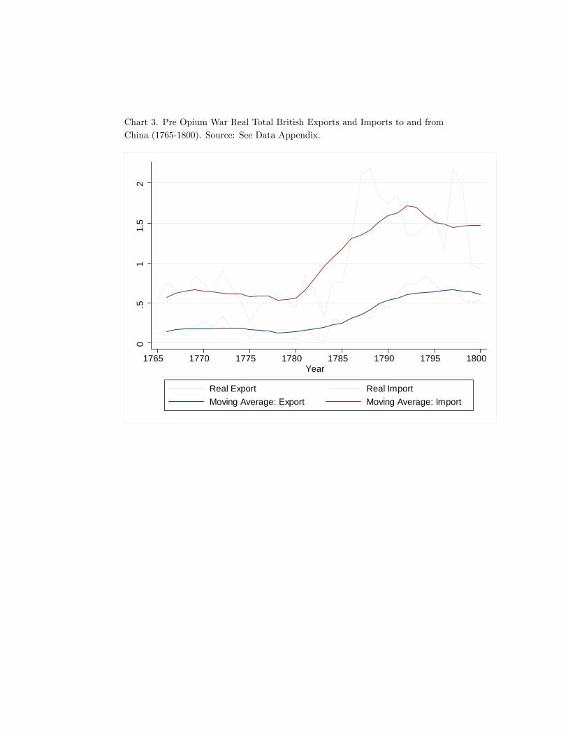
Chart 3. Pre Opium War Real Total British Exports and Imports to and fromChina (1765-1800). Source: See Data Appendix.

0.5

11.

52

1765 1770 1775 1780 1785 1790 1795 1800Year

Real Export Real ImportMoving Average: Export Moving Average: Import

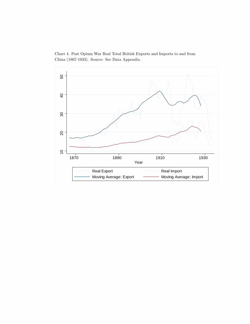
Chart 4. Post Opium War Real Total British Exports and Imports to and fromChina (1867-1933). Source: See Data Appendix.

1020

3040

50

1870 1890 1910 1930Year

Real Export Real ImportMoving Average: Export Moving Average: Import

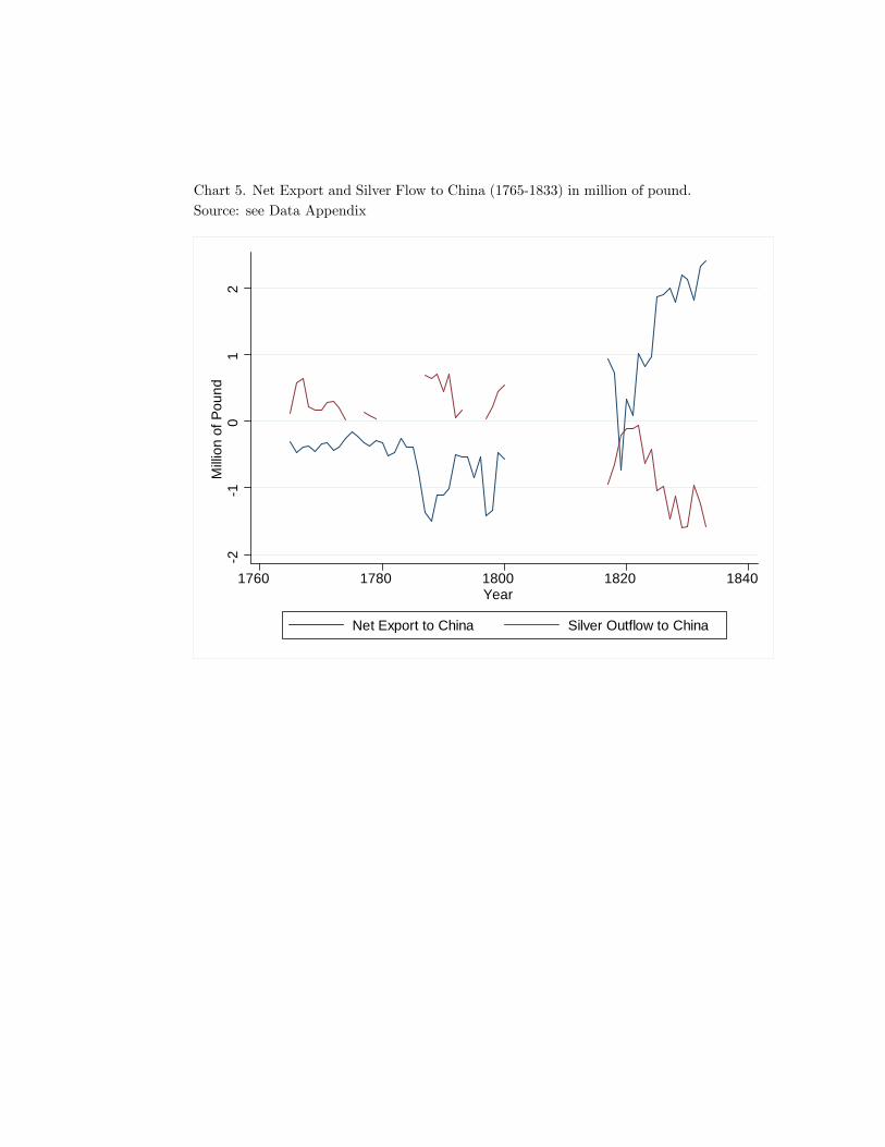
Chart 5. Net Export and Silver Flow to China (1765-1833) in million of pound.Source: see Data Appendix

­2­1

01

2M

illion

of P

ound

1760 1780 1800 1820 1840Year

Net Export to China Silver Outflow to China

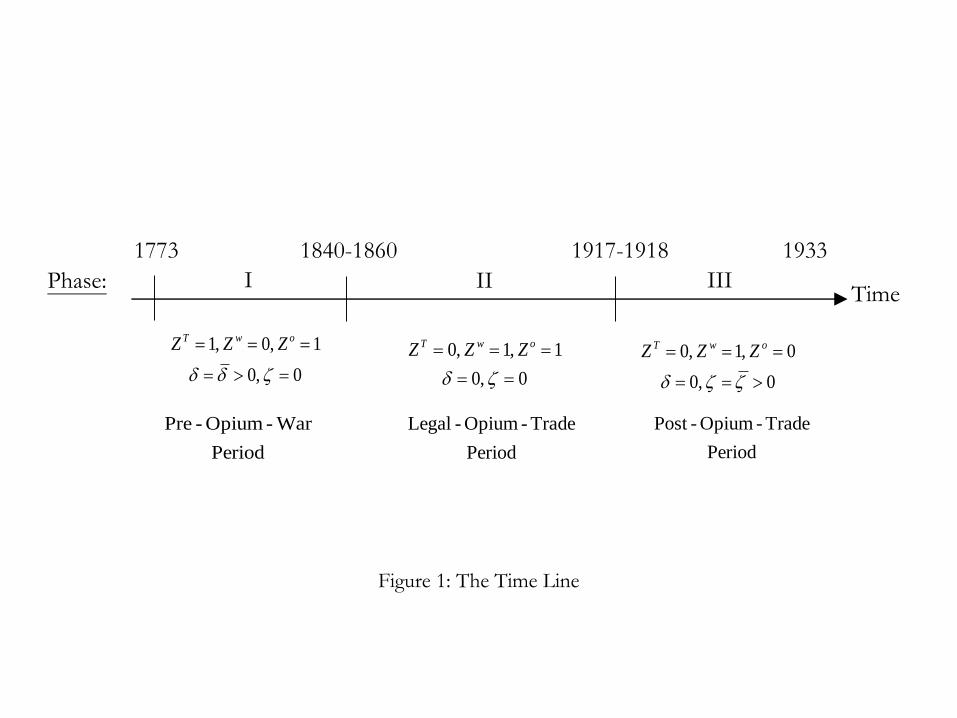
Phase:

1840-1860 1917-1918 1933

TimeI II III

Figure 1: The Time Line

0,0

1 ,0 ,1

owT ZZZ

0,0

1 ,1 ,0

owT ZZZ

0,0

0 ,1 ,0

owT ZZZ

1773

Period

War-Opium-Pre

Period

Trade-Opium-Legal

Period

Trade-Opium-Post

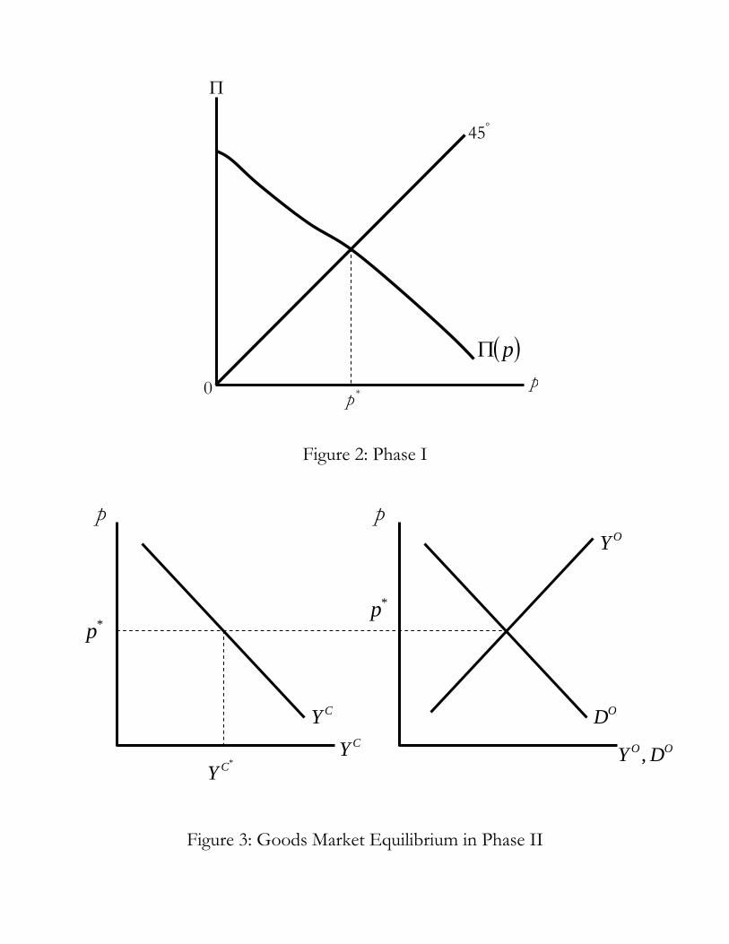
Figure 2: Phase I

*p0 p

Π

°45

( )pΠ

p

CY

*p

p

CY*CY

OD

OY

*p

OO DY ,

Figure 3: Goods Market Equilibrium in Phase II

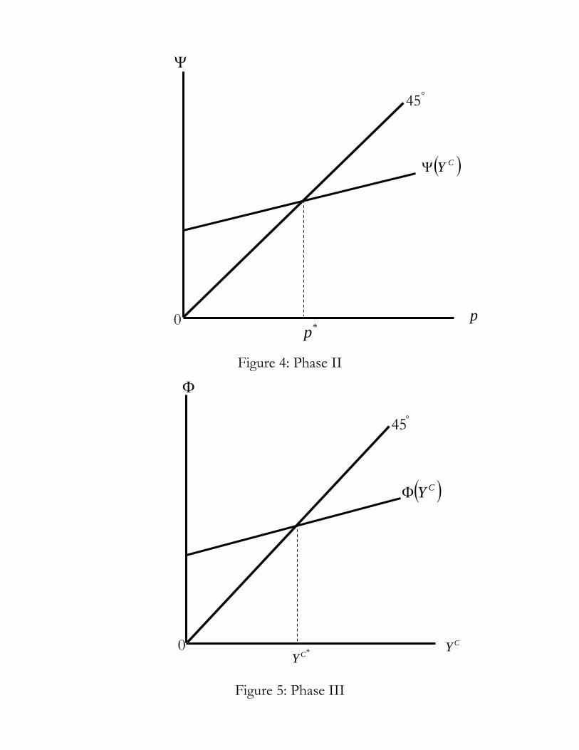
*p0

Ψ

°45

p

( )CYΨ

Figure 4: Phase II

*CY0

Φ

°45

CY

( )CYΦ

Figure 5: Phase III

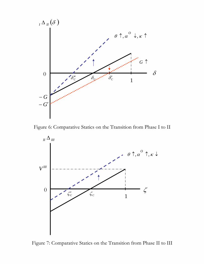
Figure 6: Comparative Statics on the Transition from Phase I to II

Cδ0 δ

1

G−

( )δIII Δ

Cδ ′

G′−

Cδ ′′

↑↓↑ καθ ,,O

↑G

01

IIIII Δ

Cζζ

Cζ ′

IIIV

↓↑↑ καθ ,,O

Figure 7: Comparative Statics on the Transition from Phase II to III

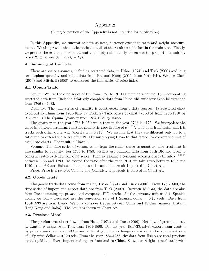
Appendix(A major portion of the Appendix is not intended for publication)

In this Appendix, we summarize data sources, currency exchange rates and weight measure-ments. We also provide the mathematical details of the results established in the main text. Finally,we present the results under an alternative subsidy rule, namely the case of the proportional subsidyrule (PSR), where St = s (Mt −Xt).

A. Summary of the Data

There are various sources, including scattered data, in Hsiao (1974) and Tuck (2000) and longterm opium quantity and value data from Bai and Kung (2016, henceforth BK). We use Clark(2010) and Mitchell (1988) to construct the time series of price index.

A1. Opium Trade

Opium. We use the data series of BK from 1789 to 1910 as main data source. By incorporatingscattered data from Tuck and relatively complete data from Hsiao, the time series can be extendedfrom 1766 to 1932.

Quantity. The time series of quantity is constructed from 3 data sources: 1) Scattered chestexported to China from 1761-1815 by Tuck; 2) Time series of chest exported from 1789-1910 byBK; and 3) The Opium Quantity from 1864-1949 by Hsiao.

The quantity in the year 1766 is 150 while that in the year 1796 is 4172. We interpolate thevalue in between assuming constant geometric growth rate of e0.1073. The data from Hsiao and BKtracks each other quite well (correlation: 0.813). We assume that they are different only up to aratio and to extend the series after 1910 by multiplying Hsiao to that factor (to convert the unit ofpicul into chest). The result is Chart 1.

Volume. The time series of volume come from the same source as quantity. The treatment isalso similar to quantity. For 1766 to 1789, we first use common data from both BK and Tuck toconstruct ratio to deflate our data series. Then we assume a constant geometric growth rate e0.06465

between 1766 and 1790. To extend the ratio after the year 1910, we take ratio between 1897 and1910 (from BK and Hsiao). The unit used is taels. The result is plotted in Chart A1.

Price. Price is a ratio of Volume and Quantity. The result is plotted in Chart A1.

A2. Goods Trade

The goods trade data come from mainly Hsiao (1974) and Tuck (2000). From 1761-1800, thetime series of import and export data are from Tuck (2000). Between 1817-33, the data are alsofrom Tuck summing up private and company (EIC) trade. As the currency unit used is Spanishdollar, we follow Tuck and use the conversion rate of 1 Spanish dollar = 0.72 taels. Data from1864-1933 are from Hsiao. We only consider trades between China and Britain (namely, Britain,Hong Kong and India). The result is shown in Chart A2.

A3. Precious Metal

The precious metal net flow is from Hsiao (1974) and Tuck (2000). Net flow of precious metalto Canton is available in Tuck from 1761-1800. For the year 1817-33, silver export from Cantonby private merchant and EIC is available. Again, the exchange rate is set to be a constant rateof 1 Spanish dollar = 0.72 taels. From the year 1864-1933, the data from Hsiao are total preciousmetal (gold and silver) import and export from and to China. So we use weight: (total trade with

i

UK/total trade with all trading partners) to calculate the share of precious metal flow into Chinafrom the UK. The result can be found in Chart A3.

A4. Exchange Rate and Price Index

Exchange Rate. From 1862-1933 the exchange rate between UK currency and tael can be foundin Hsiao (2000). The exchange rate involves converting s. (shilling) and d. (penny) into pound.The system is that: 1 pound = 20 shilling and 1 shilling = 12 pence. For the data before 1862, wefollow the assumption of Tuck and assume that 1 tael is roughly 1/3 pounds.

Price Index. 3 different index are used to cover the relevant time period that we are interestedin: 1) Clark (2010) is used before 1800; 2) Rousseaux’s Overall Index is used from 1801 to 1845;and 3) Sauerbeck-Statist’s Overall Index is used after 1846. All 3 indices are very comparable. Sowe only need to match their average value. The result is reported in Chart A4.

A6. Units

The following is a list of definition of units used in the paper.There were three major currencies used: the tael, the British pound and the Spanish dollar.

These were converted in the following manner: (i) the basic unit of Chinese currency is the tael(tls), known as “Yuan Pao”(silver sycee), which was worth 1.208 oz. of pure silver; and, (ii) 1 tael= £1/3 or $1.388 (Spanish dollar).

Also, there were several weight measurements with the following conversion rates: (i) the chestwas used as the basis for measuring opium weight; one chest of opium contained around 135 poundsof the substance; (ii) tael was also used as a weight measurement unit in China with 1 tael = 11

3

oz., 16 taels = 1 catty (Chinese kg) or 113 lbs; and, (iii) other weight measurement units include, 1

picul = 13313 lbs, 1 long ton = 16.8 piculs, and 1 short ton = 15 piculs.

B. Optimization under FSR

Under fixed subsidy rule (FSR), the first-order conditions with respect to M, S, Y c and Y o are:

(1− ζ)(−U ′ + θH ′

)− 1

1 + ρV ′+1 ≤ 0, M ≥ 0, (B1)

− (1− ζ)U ′ + 11+ρV

′+1 ≤ 0, S ≥ 0, if ZT = 1

S = 0, if ZT = 0(B2)

(1− ζ)(U ′ + θH ′

)+

V ′+1

1 + ρ(1− αc − βw − qcY c) ≤ 0, Y c ≥ 0, (B3)

(1− ζ)(U ′ + θH ′

)ψ (p) +

V ′+1

1 + ρ[ψ (p)− αo − βw − qoY o] ≤ 0, Y o ≥ 0, (B4)

with complementary slackness, where the subscript “+1”indicates the variable in the next-period.While the last two conditions regarding the levels of outputs are standard (they equate the marginalbenefit of production with the respective marginal cost), the first two deserve further comments.Concerning (B1), high imports, on the one hand, lower the British net silver inflow and reduce therepresentative producer-trader’s asset accumulation, but, on the other, raise the total volume oftrade. Imports are optimized when the marginal cost and marginal benefit are equalized. In thecase where a trade deficit occurs, (B2) indicates that the optimal level of the government subsidyto the representative producer-trader is to equalize the losses from the current net silver outflow

ii

to the gains from the higher assets accumulated in the future. Also, the Benveniste-Scheinkmanequation is:

V ′ =1 + r

1 + ρV ′+1. (B5)

C. Proofs of Lemmas and Propositions

Proof of Lemma 1: Substituting the restrictions associated with Phase I into the first-order condi-tions (B1)-(B4) and focusing on the interior solution, we have that in stationary equilibrium:

−U ′ + θH ′ − 1

1 + ρV ′ = 0, (C1)

−U ′ + 1

1 + ρV ′ = 0, (C2)

U ′ + θH ′ +V ′

1 + ρ[1− αc − βw − qcY c] = 0, (C3)

(U ′ + θH ′

)ψ (p) +

V ′

1 + ρ[ψ (p)− αo − βw − qoY o] = 0. (C4)

Evaluating the Benveniste-Scheinkman equation (B5) in a stationary equilibrium yields r = ρ,whereas the asset evolution equation implies:

rA−M + S + (1− αc − βw)Y c + [ψ (p)− αo − βw]Y o − qc

2(Y c)2 − qo

2(Y o)2 = 0. (C5)

Combining (C1) and (C2), we have:

U ′ =1

1 + ρV ′ =

θH ′

2. (C6)

Then (C3) and (C6) together yield (9). Also, (C4) and (C6) together give

αo + βw + qoY o = 4ψ (p) . (C7)

Combining (7) and (C7), we obtain (10), which can be manipulated to get (11). Finally, it isstraightforward to obtain the following properties of Π(p): Π (0) = 1

4(1−δ)[αo + βw + qoDo(0)] > 0

and dΠdp = qo

4(1−δ)∂Do(p)∂p < 0.

Proof of Lemma 2: Straightforward differentiation yields

dp∗

dδ=

∂Π/∂δ

1− ∂Π/∂p=

p∗

1− δ1

1 +(

qoDo

αo+βw+qoDo

)εop

> 0, (C8)

where εop is the price elasticity of opium demand. The other comparative statics follow in a similarmanner. Proof of Lemma 3: Equation (C6) can be manipulated to yield (13). Substituting (7), (8), (9), and(C7) into (C5), we get (12). Straightforward differentiation implies:

S′(p) =

(1− R

T

σHσU

)(1 +

p

Do

∂Do

∂p

)(1− δ)Do =

(1− R

T

σHσU

)(1− εop

)(1− δ)Do, (C9)

iii

rdA

dp= −qo∂D

o

∂p+

(2 +

R

T

σHσU

)(1− εop

)(1− δ)Do. (C10)

From (C9), it is clear that under Assumption 1, 1− εop > 0 and under Assumption 2, 1− RTσHσU

< 0.

Hence, S′(p) < 0. The result regarding the producer-trader’s assets follows from ∂Do

∂p < 0 andAssumption 1, which imply, respectively, that both the first and the second term in (C10) arepositive. Proof of Lemma 4: Substituting the restrictions associated with Phase II into the first-order condi-tions and focusing on an interior stationary equilibrium, we obtain:

−U ′ + θH ′ − 1

1 + ρV ′ = 0, (C11)

U ′ + θH ′ +V ′

1 + ρ(1− αc − βw − qcY c) = 0, (C12)

(U ′ + θH ′

)p+

V ′

1 + ρ(p− αo − βw − qoY o) = 0, (C13)

rA−M + (1− αc − βw)Y c + [p− αo − βw]Y o − qc

2(Y c)2 − qo

2(Y o)2 = 0. (C14)

Also, the Benveniste-Sheinkman equation yields r = ρ. From (C11), we have:

−U ′ + θH ′ =1

1 + ρV ′. (C15)

Then (C13) together with (C15) yield (14), while (C12) together with (C13) give (15). Substituting(7) and (8) into (C14), we get (18). Also, under Assumptions 1 and 2, straightforward differentiationof Ω(p, Y c, κ) yields the following:

Ωp =∂Ω

∂p=

2θH ′U ′′

(−U ′ + θH ′)2

(1− R

T

σHσU

)(1− εop

)Do > 0,

ΩY =∂Ω

∂Y c=

2θH ′U ′′

(−U ′ + θH ′)2

(1− R

T

σHσU

)> 0,

Ωκ =∂Ω

∂κ=

2θH ′U ′′

(−U ′ + θH ′)2

(1− R

T

σHσU

)p∂Do

∂κ> 0.

Substituting (7) and Ω(p, Y c, κ) into (14), we obtain (16), where dY c

dp = −Γ+ΩpΩY

< 0, dY c

dκ =

1ΩY

(qo

p∂Do

∂κ − Ωκ

), dY c

dαo = 1pΩY

> 0, and Γ ≡[αo + βw +

(1 + εop

)qoDo

]/p2 > 0. Next, substi-

tuting (7) and (16) into (15), we get (17), where

Ψp =∂Ψ

∂p= −

(qoDo

αo + βw + qoDo

)εop +

(qcY c

αc + βw + qcY c

)ηcp,

1−Ψp = 1 +

(qoDo

αo + βw + qoDo

)εop −

(qcY c

αc + βw + qcY c

)ηcp.

Then, under Assumptions 1 and 3, we have two alternative cases: either Ψp < 0 or 1 > Ψp > 0. Ineither case, a unique fixed point in p is ensured. Finally, totally differentiating (17), we obtain:

dp∗

dαo=

1

1−Ψp

1

αc + βw + qcY c(p)

(1− qc

ΩY

).

iv

Combining (7), (14), (15) and (17), we have: dYc

dp =Ωp

qc−ΩY. Since dY c

dp < 0 under Assumption 1, weconclude that qc < ΩY , which in turn yields dp∗/dαo > 0. Proof of Lemma 5: Substituting the restrictions associated with Phase III into the first-orderconditions and focusing on an interior stationary equilibrium, we obtain:(

−U ′ + θH ′)− 1

1 + ρV ′ = 0, (C16)

(U ′ + θH ′

)+

V ′

1 + ρ(1− αc − βw − qcY c) = 0, (C17)

and (20). Also, the Benveniste-Sheinkman equation yields r = ρ. From (C16), we have(−U ′ + θH ′

)=

1

1 + ρV ′. (C18)

Substituting (C18) in (C17) yields (19). Then direct differentiation of Φ(Y c, w) yields the followingpartial derivatives:

ΦY =∂Φ

∂Y c=

2θH ′U ′′

qc (θH ′ − U ′)2

(1− R

T

σHσU

)> 0,

Φw =∂Φ

∂w= − β

qc< 0.

Since a rise in the wage cost should reduce production (other things equal), we can conclude from(19):

∂Y c

∂w=

Φw

1− ΦY< 0 =⇒ 1− ΦY > 0,

So Φ(Y c, w) has a positive slope in Y c that is less than unity. This together with the other half ofAssumption 4, namely that Φ(0, w) > 0, ensures the existence of a unique fixed point. Proof of Proposition 1: It is clear that,

I∆II (0) = VII (0, 0)−G− VI (0, 0) = −G

Also, if the war expenses G are not too high, so that Assumption 5 is met, then

I∆II (1) = VII (0, 0)−G− VI (1, 0) > 0

since VII (0, 0)− VI (1, 0) > 0. In addition, we can derive:

dI∆II (δ)

dδ= −dVI (δ, 0)

dδ

=1 + ρ

ρU ′Do

(2 +

R

T

σHσU

)pεop (αo + βw + 2qoDo)

αo + βw +(1 + εop

)qoDo

> 0.

Thus, the I∆II (δ) schedule is monotone (positively sloped) with I∆II (0) < 0 < I∆II (1). By theMean Value Theorem, there exists a unique critical value δc ∈ (0, 1) such that I∆II (δc) = 0. Proof of Proposition 2: It is easily seen that

II∆III (0) = VIII (0, 0)− VII (0, 0) < 0

II∆III (1) = VIII (0, 0)− VII (0, 1) = VIII (0, 0) > 0.

v

Moreover, we have:dII∆III (ζ)

dζ= −dVII (0, ζ)

dζ=

1 + ρ

ρ(U + θH) > 0.

Straightforward application of the Mean Value Theorem proves the existence of a unique criticalvalue ζc ∈ (0, 1) such that I∆II (ζc) = 0.

Proof of Proposition 3: Recall the definition of the critical transitional parameter δc:

I∆II (δc) = VII (0, 0)−G− VI (δc, 0)

=1 + ρ

ρ[U (RII) + θH (TII)]−G−

1 + ρ

ρ[U (RI) + θH (TI)]

=1 + ρ

ρ[U (Y c + pIIY

o −M) + θH (Y c + pIIYo +M)]−G (C19)

−1 + ρ

ρU [Y c + (1− δc)pIY o −M − S] + θH [Y c + (1− δc)pIY o +M ]

= 0.

In response to a change in G, the endogenous variables Y c, p and S remain all unchanged. Hence,it follows from (C19) that

dI∆II (δc)

dG=∂I∆II (δc)

∂G= −1,

which proves the proposition. Proof of Proposition 4: Totally differentiating (C19) yields,

dδcdθ

= −∂I∆II (δc) /∂θ

∂I∆II (δc) /∂δ

= − H (TII)−H (TI) + U ′ (RI)Sθ

U ′ (RI) pIDoεop

(2 + R

TσHσU

)αo+βw+2qoDo

αo+βw+(1+εop)qoDo

< 0,

where Sθ = −H ′ (TI) /2U ′′ (RI) > 0 and H (TII)−H (TI) > 0 due to the fact that Phase II is thefree-trade regime after the Opium Wars and hence the trade volume is expected to increase.

Next, recall the definition of the critical transitional parameter ζc:

II∆III (ζc) = VIII (0, 0)− VII (0, ζc)

=1 + ρ

ρ[U (RIII) + θH (TIII)]−

1 + ρ

ρ(1− ζc) [U (RII) + θH (TII)]

=1 + ρ

ρ[U (Y c −M) + θH (Y c +M)] (C20)

−1 + ρ

ρ(1− ζc) [U (Y c + pIIY

o −M) + θH (Y c + pIIYo +M)]

= 0.

Totally differentiating (C20) gives,

dζcdθ

= −∂II∆III (ζc) /∂θ

∂II∆III (ζc) /∂ζ

= −H (TIII)− (1− ζc)H (TII)

U (RII) + θH (TII)< 0,

vi

where the numerator is positive because, under Assumption 6, TIII > TII . Proof of Proposition 5: Totally differentiating (C19), taking into account the first-order conditionsin each phase, we find:

dδcdαo

= −∂I∆II (δc) /∂αo

∂I∆II (δc) /∂δc− ∂I∆II (δc) /∂α

o

1+ρρ U ′ (RI) pIDoεop

(2 + R

TσHσU

)αo+βw+2qoDo

αo+βw+(1+εop)qoDo

,

so that

sign(dδcdαo

)= − sign

(∂I∆II (δc)

∂αo

). (C21)

The expression of ∂I∆II (δc) /∂αo can be written as:

ρ

1 + ρ

∂I∆II (δc)

∂αo=

[U ′ (RII) + θH ′ (TII)

] [∂Y c

∂αo+

(∂Y c

∂pII+Do + pII

∂Do

∂pII

)dpIIdαo

]-(1-δc)

[U ′ (RI)+θH ′ (TI)

](Do+pI

∂Do

∂pI

)dpIdαo

+U ′ (RI)SpdpIdαo

=[U ′ (RII) + θH ′ (TII)

] [∂Y c

∂αo+

(∂Y c

∂pII+Do + pII

∂Do

∂pII

)dpIIdαo

]-U ′ (RI) (1− δc)Do(1− εop)

(2 +

R

T

σHσU

)dpIdαo

.

If the direct price effect of the supply shock to opium demand dominates the spillover effects on Y c,

so that Assumption 7 holds, then ∂I∆II(δc)∂αo < 0 and, from (C21), dδcdαo > 0.

Similarly, differentiating (C20) yields:

dζcdαo

= −∂II∆III (ζc) /∂αo

∂II∆III (ζc) /∂ζc

=(1− ζc) [U ′ (RII) + θH ′ (TII)]

[∂Y c

∂αo +(∂Y c

∂pII+Do + pII

∂Do

∂pII

)dpIIdαo

]U (RII) + θH (TII)

,

which is negative under Assumption 7. Proof of Proposition 6: Totally differentiating (C19), we get:

dδcdκ

= −∂I∆II (δc) /∂κ

∂I∆II (δc) /∂δ

= − [U ′ (RII) + θH ′ (TII)] ΛII1+ρρ U ′ (RI) pIDoεop

(2 + R

TσHσU

)αo+βw+2qoDo

αo+βw+(1+εop)qoDo

< 0,

where ΛII ≡ qo

pIIΩY∂Do

∂κ −Γ

ΩY

dpIIdκ > 0.

Similarly, total differentiating (C20) implies:

dζcdκ

= − ∂II∆III (ζc) /∂κ

∂II∆III (ζc) /∂ζc

=(1− ζc) [U ′ (RII) + θH ′ (TII)] ΛII

U (RII) + θH (TII)> 0,

which completes the proof.

vii

D. The Case of PSR

Under PSR, St = s (Mt −Xt). The first-order conditions with respect to M, s, Y c, Y o are:

(1− ζ)[−(1 + s)U ′ + θH ′

]− 1− s

1 + ρV ′+1 ≤ 0, M ≥ 0, (D1)

(M −X)

[− (1− ζ)U ′ + 1

1+ρV′

+1

]≤ 0, s ≥ 0, if ZT = 1

s = 0, if ZT = 0

(D2)

(1− ζ)[(1 + s)U ′ + θH ′

]+

V ′+1

1 + ρ(1− s− αc − βw − qcY c) ≤ 0, Y c ≥ 0, (D3)

(1− ζ)[(1 + s)U ′ + θH ′

]ψ (p) +

V ′+1

1 + ρ[(1− s)ψ (p)− αo − βw − qoY o] ≤ 0, Y o ≥ 0, (D4)

with complementary slackness. The Benveniste-Scheinkman equation is the same as the one inthe FSR case (see equation (B5)). Substituting the restrictions that describe this phase (ZT = 1,

Zw = 0, Zo = 1, δ = δ, ζ = 0,) into (D1)-(D4) we have

− (1 + s)U ′ + θH ′ − 1− s1 + ρ

V ′+1 = 0, (D5)

−U ′ + 1

1 + ρV ′+1 = 0, (D6)

(1 + s)U ′ + θH ′ +V ′+1

1 + ρ[1− s− αc − βw − qcY c] = 0, (D7)

[(1 + s)U ′ + θH ′

]ψ (p) +

V ′+1

1 + ρ[(1− s)ψ (p)− αo − βw − qoY o] = 0, (D8)

Also, the asset accumulation equation is:

A+1 = (1 + r)A− (1− s)M + (1− s− αc − βw)Y c + (D9)

[(1− s)ψ (p)− αo − βw]Y o − qc

2(Y c)2 − qo

2(Y o)2 .

Combining (D5) and (D6), we have:

U ′ =1

1 + ρV ′+1 =

θH ′

2. (D10)

Then (D7) together with (D10) yield,

αc + βw + qcY c = 4. (D11)

Also, (D8) and (D10) give,αo + βw + qoY o = 4ψ (p) . (D12)

In the steady state, we have A+1 = A. Substituting (7), (8), (9) and (C7) into (D9), we get:

rA− (1− s)DM (I)− (3 + s)Y c − (3 + s)ψ (p)Do(p) +qc

2(Y c)2 +

qo

2Do(p)2 = 0. (D13)

viii

Notice that (C6)-(C7) are identical to (D10)-(D12), so our equilibrium analysis for p∗, Y c and s isthe same as the one under the FSR. Thus, proposition 1 is valid under both FSR and PSR.

Next, we write (D10) as:

U ′

(1 + s)[Y c + ψ(p)Do(p)−DM (I)

]= θH ′ [Y c + ψ(p)Do(p) +M ] /2,

which yields s = s(p). Direct differentiation shows that

s′(p) =1 + s− R

TσHσU

M −X(1− εop

) (1− δ

)Do. (D14)

Consider Assumption 2′, which is analogous to but stronger than Assumption 2.

Assumption 2′: RTσHσU− s > 1.

Then we can establish the results of Lemma 3, namely that under Assumptions 1 and 2′, the tradesubsidy in stationary equilibrium is negatively related to the relative price of opium, whereas theproducer-trader’s assets in stationary equilibrium are positively related to the opium price. Theformer result follows directly from equation (D14). To obtain the latter, differentiate (D13) toobtain exactly the same expression as in the case of FSR, namely equation (C10).

ix

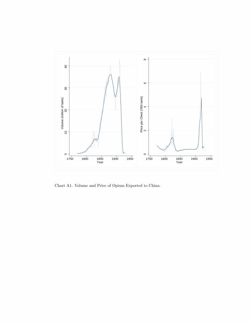
010

2030

40Vo

lum

e (m

illion

of t

aels

)

1750 1800 1850 1900 1950Year

02

46

8Pr

ice

per C

hest

('00

0 ta

els)

1750 1800 1850 1900 1950Year

Chart A1. Volume and Price of Opium Exported to China.

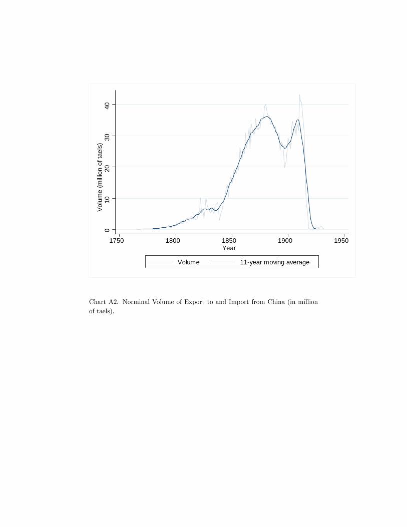
010

2030

40Vo

lum

e (m

illion

of t

aels

)

1750 1800 1850 1900 1950Year

Volume 11­year moving average

Chart A2. Norminal Volume of Export to and Import from China (in millionof taels).

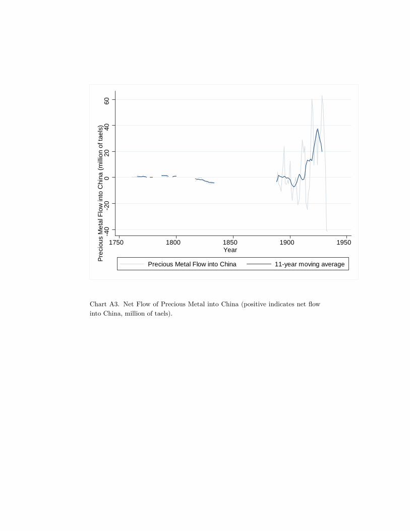
­40

­20

020

4060

Prec

ious

Met

al F

low

into

Chi

na (m

illion

of t

aels

)

1750 1800 1850 1900 1950Year

Precious Metal Flow into China 11­year moving average

Chart A3. Net Flow of Precious Metal into China (positive indicates net owinto China, million of taels).

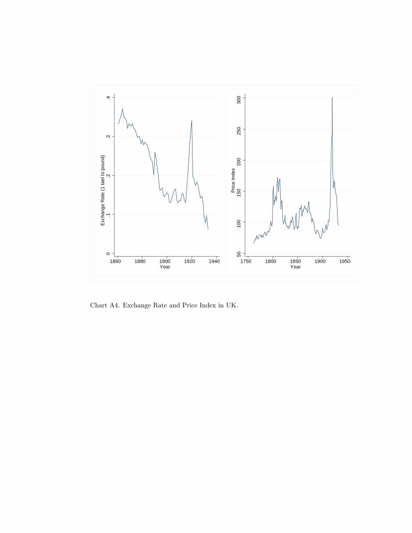
0.1

.2.3

.4Ex

chan

ge R

ate

(1 ta

el to

pou

nd)

1860 1880 1900 1920 1940Year

5010

015

020

025

030

0Pr

ice

Inde

x

1750 1800 1850 1900 1950Year

Chart A4. Exchange Rate and Price Index in UK.