Endogenous Group Formation∗

T.K. Ahn†

Florida State UniversityR. Mark Isaac‡

Florida State UniversityTimothy C. Salmon§

Florida State University

February 2006

Abstract

While the rules governing the formation of groups engaging in collective action may havesignificant impact on group size and behavior of members, most experiments on public goodshave been conducted with the subjects in exogenously fixed groups or of fixed sizes. We studyendogenous formation of groups in a public-goods provision game by allowing subjects to changegroups under three sets of rules: free entry/exit, restricted entry with free exit, and free entrywith restricted exit. We find that the rules governing entry and exit do have a significant impacton individual behavior and group-level outcomes.JEL Codes: C92, H41, D85Key Words: Public Goods, Entry and Exit Rules, Group Formation, Group Size.

“[T]he movement in and out of the group must no longer be ignored” — Mancur Olson,

Logic of Collective Action, p. 36.

1 Introduction

Groups that engage in collective action use a variety of rules that govern how each group is formed.

Olson (1971) argues that the nature of how groups form for the purpose of engaging in collective

∗The authors would like to thank the National Science Foundation, the Florida State University and the FSUFoundation as well as John Scholz for research support in funding these experiments. We owe a substantial debtof gratitude to Justin Esarey for programming the experiments. We also thank various participants in seminars orconference presentations at George Mason University, University of Central Florida, Indiana University - Bloomington,IUPUI, University of California - Davis, The New and Alternative Directions for Learning Workshop hosted atCarnegie Mellon University, The Southern Economics Association Conference, SAET conference in Vigo and the ESAconference in Montreal who provided many helpful comments that improved our experimental design and analysis ofdata.

†Department of Political Science, Florida State University, Tallahassee, FL, 32306-2230, tahn@fsu.edu. Phone:850-644-4540 Fax: 850-644-1367.

‡Department of Economics, Florida State University, Tallahassee, FL, 32306-2180, misaac@mailer.fsu.edu. Phone:850-644-7081 Fax: 850-644-4535.

§Department of Economics, Florida State University, Tallahassee, FL, 32306-2180, tsalmon@fsu.edu. Phone: 850-644-7207 Fax: 850-644-4535.

1

action is key to understanding the collective action behavior itself. Despite the importance of the

group formation process on group behavior, this aspect of the public goods provision problem has

received little attention until recently in the broad literature on public goods. In this paper, we

present a series of experiments designed to generate a better understanding of whether or not it is

possible to ignore the group formation process in studying public goods.

In naturally occurring situations, groups with collective action problems use a variety of entry

and exit rules to regulate their membership. One can join the Sierra Club simply by filling out a

card, but joining a country club or a law firm may require the approval of the existing members.

In most neighborhoods and apartments, current residents cannot block the entry and exit of other

residents. On the other hand, most of the residential property in Manhattan is owned by Co-

ops which may deny entry to potential residents. That can also have the effect of denying the

ability of current residents to sell their units, denying them the ability to exit without substantial

cost.1 Many other groups have similar restrictions on either entry or exit. Examples include joint

ventures from which capital withdrawal requires other members’ approval, closed or union shops

in which an employee cannot withdraw from the union without losing his job, and the laws of

most nations, cities and states that prohibit regions from de-annexing or seceding without approval

from the greater part. Due to the variety of rules in use, one is led to wonder what effects, if

any, these different group formation institutions may have on behavior. As a means of beginning

an investigation of these issues we will present the results from a series of experiments in which

subjects are engaged in a repeated public goods game under different group formation rules. These

experiments allow both the size and composition of each group to be truly endogenous. We have

chosen to investigate three different institutions for the group formation process; (1) free entry and

free exit, (2) restricted entry and free exit, and (3) free entry and restricted exit. In restricted

entry (exit) treatment of our experiments, an individual who wishes to join (leave) a group must

obtain approval from a majority of the relevant group members. These institutions are not meant

1There is recent, highly publicized evidence that the entry/exit regulation performed by Co-op boards does havean impact on behavior. A December 16, 2004 New York Post story reports a claim that one of the motivating factorsbehind Mary Tyler Moore’s activism against the Co-op board of 927 Fifth Ave. on behalf of two red tailed hawks(Pale Male and Lola) was the fact that the Co-op board had recently denied a potential buyer for her apartment inthe building. The man was denied because “He was just what you don’t want in a family building.” According tothe article, a source on the board stated that the event caused Ms. Moore to wage the campaign against the board“as a personal vendetta.” While the claim may be unfounded, this does suggest that the board realizes its decisionsmay have an important impact on the behavior of its residents.

2

to mimic precisely the rules used by any specific group or organization. Instead, we chose these

institutions because they can be considered boundary cases or perhaps component parts of many

different group formations institutions. Treating each rule separately should allow us to uncover

the partial effects of each institutional rule on behavior.

In most prior experimental literature on public goods, the question of how an existing group

performs has been considered a separate issue from how and why groups form in the way that

they do. Several earlier studies (Marwell and Ames (1979), Isaac and Walker (1988), Kim and

Walker (l984), Isaac, Walker, and Williams (1994)) investigate how group formation dynamics

might impact behavior by including group size as an experimental treatment. In these studies, it

is the comparative static influences of group size that are of concern, which might be viewed as a

partial equilibrium approach to studying how behavior changes as group size evolves.

Ours, however, is not the first paper to move beyond these initial fixed group studies. In

Gunnthorsdottir, Houser, McCabe, and Ameden (2001) experimenters match high contributors

with other high contributors, low contributors with other low contributors which leads to a form

of endogenous group formation although the groups are still formed somewhat exogenously by the

experimenter. Page, Putterman, and Unel (2002) moves toward the groups being formed by active

choices of the subjects. The subjects first ranked whom they would like to have in their new

groups. The experimenters then used an algorithm to reconstruct groups based on the subjects’

preferences. Cinyabuguma, Page, and Putterman (2005) subjects were allowed to vote to expel

other members using a majority rule procedure. In their design, group size becomes endogenous

but it can only decrease. The two papers closest to our approach are Coricelli, Fehr, and Fellner

(2003) and Ehrhart and Keser (1999). In the former, subjects chose partners according to two

different mechanisms. While this design allowed free choice of partners, group size was always fixed

at two.2 The latter study features complete endogeneity in group size and composition, but it

only investigates a single mechanism similar to our free entry/exit treatment. This prior literature

contains several different results all suggesting that how the group composition is determined can

certainly impact the level of contributions among group members.

Our study extends this existing literature by simultaneously allowing for fully endogenous group

formation including determination of group size while also examining how different group formation2Brosig, Margreiter, and Weimann (2005) also investigates partner selection in a three person public goods context

by allowing subjects to communicate prior to choosing one of three potential group members to keep out of the group.

3

rules affect the process. Our main interest is to investigate how the institutions affect the dynamics

of subject behavior rather than focusing exclusively on aggregate measures of contribution levels and

efficiency. The results will show that the mechanisms do lead to substantially different behavior

among our subjects. In particular we observe that subjects are able to use the restricted entry

mechanism to teach potential new group members to raise their contribution level and that this

teaching effect is not transitory. On the other hand, the restricted exit mechanism appears to be

effective in teaching high contributors to learn to contribute less over time.

In Section 2 we present design of the experiments as well as a discussion of the theoretical nature

of the environment including conjectures regarding how behavior might differ among treatments.

In Section 3, we present and discuss the results. In Section 4 we conclude the paper by summarizing

the key results and their implications and suggesting issues left for further investigation.

2 Experiment

2.1 Design

In each session of our experiments 12 subjects play a variant of a standard VCM game multiple

times. In each period, each subject belongs to a group of size N ∈ [1, 12] and makes a decision onhow to divide 15 “tokens” between his own individual account and the group account for the group

in which he is a member. The exact group size is endogenously determined within the extremes

of one and twelve in a manner we will discuss later. In the experiment the decisions are framed

as “investment” decisions. In the discussions that follow, we will often refer to the investment

in the group account as a “contribution” as this terminology is more natural for researchers, but

that was not the language used in the experiments. Let xi denote the number of tokens individual

i ∈ {1, 2, ..., 12} invests/contributes to the group account. Let Gi represent the set of other members

in i’s group (not including i). The monetary payoff to individual i is

πi = 0.5(15− xi) + 1.5(xi +Xj∈Gi

xj)− 1

27x3i . (1)

Investment to the private account yields .5 Experimental Currency Units (ECUs) to the subject

while contributions to the public account generate 1.5 ECUs for that subject and 1.5 ECUs per

4

Group Size 1 2 3 4 5 6 7 8 9 10 11 12Individual Optimum 3 3 3 3 3 3 3 3 3 3 3 3Group Optimum 3 5 6 7 8 9 9 10 11 11 12 13

Table 1: Optimal investment amounts into group account depending on the size of the group.

token to each other member of the group. Individual i also receives 1.5 ECUs for each of the tokens

that other group members contribute to the group account. Investment into the individual account

is costless but investing xi tokens into the group account costs that individual (1/27) ∗ x3i ECUs.This payoff function creates an environment with a pure public good (non-rivalrous, no congestion)

with increasing marginal cost of individual contributions.

An important feature of this design is that while there is a dominant strategy for contributions

to the group account in the stage game, it is not 0, or on the lower boundary of a subject’s choice

set, as in many public goods games. If we consider the one shot version of this public goods game,

the dominant strategy choice for each individual is to invest 3 tokens to the group account and 12

to the individual account. This is independent of the group size. Another key feature of this payoff

function is that there is no cost of having additional group members even if they do not contribute

to the group account. Thus an individual’s payoff is non-decreasing in N under any contribution

profile. The structure delivers clear incentives for subjects to form into the largest group possible

with all 12 subjects in the same group. This is true whether all subjects are purely self-interested

or interested in maximizing social welfare.

If all subjects are in the same group and all contribute 3 tokens then each individual earns

59 ECUs per period. Due to the externality on group account contributions, the group optimal

contribution level (i.e. the contribution that jointly maximizes payoffs for the entire group) is

different than 3 and is a function of group size as shown in table 1. The socially efficient or group

payoff maximizing arrangement involves all 12 subjects getting into (or remaining in) the same

group and investing 13 tokens each, returning a payoff of 153.6 ECUs per person per period. The

per person payoff in the social optimum is about 260% of what they would receive by contributing

according to the stage game equilibrium and forming the best group.

The fact that payoffs for group members are non-decreasing in N is certainly a non-standard

aspect to our public goods environment as adding a free-rider does not hurt the payoffs of other

group members. We chose this environment as a means of minimizing any potential effect coming

5

from the group formation mechanisms. This environment incorporates substantial returns to scale

from forming large groups. These large group returns should focus subjects on a simple strategy

of just getting into the largest group they can regardless of how others are contributing. Since

a subject’s earnings are enhanced even by “free-riders” who contribute only at the stage game

dominant strategy level, they should still be willing to allow these free-riders in their group. In other

possible environments in which additional group members are costly, however, gaining new group

members who are free riders may decrease the earnings of those already in the group. Consequently,

group composition should be more of a concern of the subjects when there is congestion to the public

good and the group formation mechanism may be more important. As a first look at how these

institutions work, though, we wanted to begin with a cleaner test case where group composition

should be expected to be less of a concern.3 The reason is that if we see any impact from the group

formation mechanisms in this extreme environment it will be a very strong demonstration of the

robustness of the underlying behavior.

Another important detail about this payoff schedule is that as group size goes up, investing the

socially or group optimal level begins to incur a greater risk of losing money. At a contribution level

of 8 (socially/group optimal for n = 5) the subject will make losses (net earnings -3.46 ECUs) unless

his fellow group members contribute positive amounts. As the group size goes up and the socially

optimal contribution level increases, the risk to the subject of losing money for contributing at the

socially optimal level increases. In a group of n = 12, contributing 13 tokens yields a personal

net payoff of -60.87 ECUs which requires an average contribution level of around 3. 64 for the

other 11 group members in order for the high contributor to break even. If all group members

are contributing at the stage game individual optimum, 3, the high contributor will lose money.4

Thus contributing at levels past 7 or 8 requires trust in the willingness of other group members to

contribute above the pure self-interest level.

3See our companion paper, Ahn, Isaac, and Salmon (2005), for a parallel investigation in which additional groupmembers are costly.

4The possibility of a loss in a period meant that we had to use a standard three part bankruptcy rule. First,all participants began each phase of the experiment with a 50 ECU balance. If the subject sustained losses, he wasallowed to continue as long as his overall balance including that initial balance, but not his show-up fee, remainedpositive. If losses took the accumulated earnings negative, those losses were cancelled one time and the subject wasreinitialized with a new 50 ECU starting balance. If the subject’s earning went negative a second time, he wouldhave been discharged from the experiment earning only his show-up fee. All of this was explained to the subjectsin the instructions. In the course of all of the experiments for this study, no subject ever had his or her earnings gonegative even the first time.

6

Our experiments began with a “preliminary phase” in which the subjects were placed into

groups by themselves (i.e. n = 1 ) and they were allowed to play this stage game for three rounds

in that configuration. The subjects were told that none of the other subjects would ever be able

to observe these choices which meant that there was no possibility to use those choices as signals

about the degree to which a subject was cooperative. These rounds were conducted in part to allow

them to be comfortable with the investment mechanism and also in part to allow us to observe

their behavior when there was no tension between individually and socially optimal behavior.

After the preliminary phase, the main phase began in which we randomly assigned subjects

to groups labeled A-L such that each subject was again in a group by him- or herself. In period

1, the subjects made an investment choice in those groups which meant that they again made a

choice in a group with n = 1. In all of the subsequent periods (a total of 20), a period would begin

with the subjects being asked if they wished to switch groups. The screen asking this question also

presented information showing the average contribution levels and group sizes of the 12 possible

groups over the previous 5 periods. This included the number of subjects in each group at the

end of the previous period. This allowed for subjects to send signals of various sorts through their

choices in period 1 as well as in later periods. If a subject indicated that she did wish to change

groups, she was presented with a new screen. The new screen was similar to the previous one

but showed, along with the aggregate contribution level for each group for the past 5 periods, the

number of subjects in each group who had chosen to remain in the group from the previous period.

Subjects were then allowed to choose which group they wished to enter. Subjects were labeled 1-12

and groups were labeled A-L. Choosing to move to a new group and choosing which group to move

to were both costless.

The three experimental treatments differ from one another in terms of the rules of entry and

exit: Free Entry/Free Exit, Restricted Entry/Free Exit, and Free Entry/Restricted Exit.5 In the

“Restricted Entry” treatment, exit is unrestricted but entry into a new group requires approval by

the majority of the members of the group to which the applying subject has applied to join. In

the “Restricted Exit” treatment, entry into a group is unrestricted, but exit from a group requires

5We chose not to run what some might consider an “obvious” control treatment which would have involved usingthe same payoff function with the groups exogenously determined and fixed. There are a number of problems withthis, not the least of which is determining what N should be used. Conducting control sessions with a broad rangeon N ’s is unfeasible and doing so with a single N would be insufficient.

7

Treatment Group Formation Rules Sessions Number of SubjectsTreatment 1 Free Entry, Free Exit 1,4,7,9 48Treatment 2 Restricted Entry, Free Exit 2,3,5,6 48Treatment 3 Free Entry, Restricted Exit 8,10,11,12 48

Table 2: Listing of experimental treatments and sessions run.

approval by the majority of the members of the group from which a subject has applied to depart.

The subjects who answered “no” to the question asking if they wished to change groups are the

ones who are allowed to vote. So when a subject applies to enter a new group in the restricted

entry treatment, only those members of the target group who answered “no” to that first question

vote on whether to approve the application. In the restricted exit treatment, those answering “no”

to that first question are the ones that vote on whether to allow any attempted departures from

their respective groups. In both cases, the applicant needs more than 50% of the relevant voters to

vote yes to be allowed to enter/exit a group. If an application to enter is denied, then that subject

is returned to his or her previous group. If an application to exit is denied, then that subject stays

in his or her previous group. Subjects could choose to re-enter the group they were in during the

previous period in which case no vote was necessary either to approve their entry or exit. A subject

who answers “yes” to the first question and then chooses to remain in the group by selecting it

again, however, does not get to vote on the entry or exit applications of others.

Four experimental sessions were run for each treatment. Twelve subjects participated in each

of the twelve sessions for a total of 144 subjects. Table 2 summarizes the overall design of the

experiment and the session identification numbers for each treatment. Subjects were recruited

mostly from economics courses at a variety of levels at Florida State University. All sessions were

conducted in a computer lab using software created with z-Tree (Fischbacher (1999)). In Sessions

1, 2 and 3, subjects were paid a $7 show-up fee and ECUs translated into dollars at a rate of 2

ECUs=$0.01. Average subject earnings were in the range of $12-13 in these sessions. In all other

sessions, subjects were paid a $10 show-up fee and ECUs translated into dollars at a rate of 1 ECU

= $0.01. Average subject earnings were in the range of $20-25 in these sessions.6 Sessions lasted

on average an hour and a half to two hours.

6The change in the show-up fee was an attempt to increase the show-up rate for our subjects. The change in theexchange rate was due to the fact that subject earnings in the first 3 sessions were much lower than predicted andwere increased to raise the implied hourly rate. We have tested the effects on behavior from the change and see nostatistically significant impact.

8

Due to the complexity of our payoff function there is reason to be concerned that subjects could

have had difficulty understanding it. Our payoff function is different and perhaps more complex

than the standard linear return public goods games used in most prior public goods experiments.

It is not clear, though, that subjects should have had any harder time understanding the incentives

with this payoff function than these previous linear return experiments, much less those previous

experiments with non-linear return functions such as Isaac and Walker (1998). Further, we believed

that it was important to have a game with an interior dominant strategy that does not vary with

N along with group optimal contribution levels that are in the interior and increase with N. This

also had to be achievable while insuring that the payoffs were bounded to a reasonable interval.

Linear functions would not achieve these goals and step-wise linear functions are not likely to be

more readily understandable than our non-linear function.

We also engaged in a variety of procedures to help subjects understand the payoff function.

We first ran them through an extensive help system explaining all stages of the decision process.

We provided hardcopies of extensive tables summarizing their earnings from any combination of

decisions they and their fellow group members might make that were designed to demonstrate all

of the relevant trade-offs. During the experiment when a subject was asked to make an investment

decision, the software included a test button that would allow the subjects to enter a proposed

investment level and then see all computations regarding the effect on their payoff and the payoff

of others though of course without including the effect from the contributions of others. The

instruction script we used can be found in appendix A while screenshots and the payoff tables used

are available from the authors upon request.

Finally, at the conclusion of sessions 4-12 we included a bonus question for our subjects that

was designed to determine if subjects could understand the group optimal contribution calculations.

The bonus question asks the subject to identify the group optimal level of contribution when group

size is 5. The answer to the question is 8 and subjects were paid an extra $1 if they got within one

token above or below. The exact wording of the question was the following:

This is a bonus question related to the experiment you just completed. If you answer

correctly (or within 1 token above or below) you will earn an extra $1.

Assume you are in a group of 5 people (4 plus you). What would be the number of

tokens that each group member would need to invest into the group account to lead to

9

the highest payoff to the entire group?

2.2 Discussion and Hypotheses

We can establish some baseline hypotheses regarding behavior we might observe in this environ-

ment. First, as previously noted, the stage game has a dominant strategy solution in which all

players invest 3 tokens into the group account. Because the experiments were run with known

finite repetitions of this stage game, if we ignore for the moment the group formation process this

would lead to the subgame perfect solution of the repeated game being the stage game equilibrium

repeated. Due to the finite repetition, trigger strategies could not be employed to deliver coopera-

tive play in equilibrium. Thus one baseline prediction regarding the contributions is that we should

see all subjects contributing 3 tokens per round. One could also establish a baseline hypothesis for

what we might observe based on the large volume of prior experimental results on public goods

games (Marwell and Ames (1979), Isaac and Walker (1988), Kim and Walker (l984), Isaac, Walker,

and Williams (1994) and Andreoni and Miller (1993)). These past studies show a general stylized

fact that subjects contribute more than the stage game self-interested optimum in the beginning

and then contributions decline over the rest of the experiment. One might well imagine that similar

results would be observed in our experiment.

Neither of these predictions, however, incorporate the group formation aspect of the game. As

discussed above, the incentive structure regarding group formation is quite straightforward; adding

one more group member is always better (or at least not worse). There are many equilibria of

these games and we do not propose to present an exhaustive discussion of them. We will focus

our attention on what we find to be the most reasonable class of such equilibria for use as a

benchmark which can be built off of the stage game dominant strategy regarding contributions. If

subjects employ any of a wide range of possible strategies in the group formation process aimed at

immediately forming the global group and then contribute 3 tokens per round, this will constitute

an equilibrium of the game.7 The nature of this equilibrium does not depend on the institution,

though technically how one would specify the full strategies to deal with the voting behavior would

depend upon the institution. In the restricted entry treatment any entrant should be allowed entry

7One class of group formation strategies that would deliver this result can be summarised as the strategy of“Always choose group x” where x ∈ {A,B, ..., L}. So long as x is common to all players this will represent anequilibrium. There would of course be many other ways of specifying such strategies.

10

and in the restricted exit treatment, any exit should be denied.8 This is certainly not a unique

equilibrium as there are many possible variants of it and there are certainly equilibria outside of

this broad class. This class of equilibria does have the property that elements of it are strategically

simple and easy to implement or at least approximate. Further, elements of this set of equilibria

Pareto dominate all other equilibria with the same contribution profile but which possess different

group formation strategies involving forming smaller groups or delaying the formation of the global

group. Thus we will use this as our benchmark equilibrium prediction. If subjects are attempting

to follow such an equilibrium, then we should see all subjects contributing 3 tokens per round and

attempting to form quickly and then maintain the global group of all 12 subjects. This prediction

will remain the same regardless of the group formation mechanism. The results from classic public

goods experiments might alter this prediction by suggesting that contributions will be above 3

and steadily decline, but these results provide no basis for suggesting how the group formation

mechanisms might alter that path or how large of groups might form.

From the more recent public goods literature such as Ehrhart and Keser (1999), Gunnthorsdot-

tir, Houser, McCabe, and Ameden (2001) and Page, Putterman, and Unel (2002), we can extract

another hypothesis regarding possible behavior, which is that the ability to engage in voluntary

association by itself might be an instrument for increasing the efficiency of public goods provision.

If there is such an effect that is independent of specific institutions, then we should see contri-

butions significantly greater than the benchmark prediction (and perhaps greater than one would

expect from classic public goods experiments) but again we should expect participants to form into

groups of size 12. This literature also provides no basis for generating specific predictions regarding

differences in behavior across treatments.

We can present hypotheses for how behavior might change depending upon the mechanism by

examining the behavioral incentives induced by the mechanisms. One might suppose that in the

Restricted Entry/Free Exit mechanism the very act of voting on potential entrants serves as an

additional, implicit boost to provision. An alternative hypothesis is that the entry voting condition

might be used even more purposefully by the participants through requiring potential entrants to

8 In the restricted exit treatment, this will not prevent the global group from forming. Along the equilibrium path,all subjects not in the main group should choose to move simultaneously leaving no one in their former group toconstrain their exit. Once in the main group, no exits should be attempted and all (dis-equilibrium) attempted exitsshould be disallowed.

11

signal that they will be cooperators before they are allowed entry into a group. The restriction on

entry can therefore be used as a training device to teach people to engage in pro-social behavior or

it can be thought of as a signaling device in which participants can signal their willingness/intention

to contribute high levels. The idea behind this is similar in spirit to the notion of strategic teaching

discussed in Camerer, Ho, and Chong (2002). This sort of “training” may entail keeping out

some “untrained entrants” which would lead to the observation of applicants with low contribution

histories being rejected. Empirically what this will lead to is contributions above the self interested

level in some groups, though perhaps not all, groups forming with fewer than 12 members and some

applications for entry being denied. Should such training be attempted, the intriguing point will

be whether participants continue in their “trained” ways once they are allowed entry into a group,

or if they revert to the stage game dominant strategy level of contributions. The net effect of this

process on overall provision efficiency is not obvious as it may lead to increased contributions but

also smaller groups forming or at least to the global group taking longer to form.

This training can also be thought of as a punishment device in which members of a group can

punish low contributing potential entrants by disallowing their entry. There are several studies that

have investigated the effect of allowing punishment in a public goods environment (see Ostrom,

Walker, and Gardner (1992), Fehr and Gächter (2000), Ones and Putterman (2004) and Sefton,

Shupp, and Walker (2002)) in which the punishment mechanism typically allows one subject to

pay a cost to punish a specific other subject. Denying someone entry into your group does cost

you something in foregone earnings from their contributions and it may decrease the earnings of

the person being rejected if they have to stay in a lesser group in terms of overall contribution

level. Thus the restricted entry mechanism allows for punishment of a similar nature to these prior

studies but in a different and perhaps less obvious form to the subjects since it is not labeled in a

way as to suggest specifically that voting against an entrant can be used for that purpose.

One can make similar behavioral conjectures regarding the Free Entry/Restricted Exit condi-

tion. In this case, it is not possible or necessary to signal your status as a high contributor to

potential new group members in order to gain entry. Those voting on your application are your

current group members. Their interest is in keeping high contributors in the group. A reasonable

hypothesis then is that we should see subjects unwilling to let high contributing group members

exit a group while low contributors might be allowed. This sets up perverse incentives for individ-

12

uals who would normally be high contributors but wish to change groups. The overall effect may

be that the low contributors may (inadvertently) use this mechanism to teach high contributors

to contribute less. This is in direct opposition to the idea behind the restricted entry mechanism

which seems likely to allow high contributors to teach low contributors to contribute more.

In all of the treatments subjects have another option for punishment. If a high contributor

wishes to punish a group he or she considers to be contributing too low then the high contributor

can choose to contribute even below the individually optimal level of 3. This incurs a cost to the

punisher and will also decrease the potential payoff to the rest of the group relative to the payoffs

they would have received if the punisher contributed even up to the individually optimal level.

This punishment mechanism is non-specific as it targets the entire group. Because of the limited

information available to the other group members it is possible that they will not even notice the

action nor be able to interpret it as punishment. Due to its shortcomings as a punishment technique,

it seems unlikely to be used in the treatments in which a subject can readily exit a group as that

would be the most punishment one could inflict by depriving the group of your contributions while

perhaps minimizing the cost to the punisher. In the Restricted Exit treatment, however, this form

of punishment may be more likely to be used as it is the only one available.

3 Experimental Results

Our analysis will consist of an exploration of the patterns in the data to identify and explain any

systematic behavioral differences that can be attributed to the group formation institutions. We

discussed above a series of hypotheses based upon different notions of behavior with some suggesting

that no differences will exist between mechanisms (benchmark equilibrium, standard public goods

experiments, pure self-association effect) while others suggest that differences will exist (behavioral

analysis). Our goal in this set of experiments is to determine if variations do exist and to then

determine if they match any of the stylized hypotheses of behavior mentioned above. This should

then establish a foundation upon which future theoretical analyses of group formation behavior can

be built.

The data set created by these experiments is quite rich because subjects may make two to

three of four different types of choices each period (i.e. contribution level, move or not, which

13

group to move to and vote yes or no). We will begin presenting our results in a series of graphical

and general statistical characterizations of the data in order to give the reader a good idea of the

general structure of the data. This will include presenting observations based on analyzing raw

distributions of choices and outcomes as well as graphical depictions of time paths. We will present

some statistical tests on this data but those results are not intended to be definitive as the tests will

not take into account the lack of independence across trials nor will they correct for the complex

interactions that may be driving any of the differences. This level of the analysis is simply to help

develop a picture of the data. In section 3.4 we will construct our formal results concerning the

nature of the individual choice behavior based on panel regressions designed to deal with both the

structure of the data and the complexity of the behavior.

3.1 Average Contribution Choices

The three preliminary periods of the experiment were run in part to familiarize subjects with the

investment decisions and also in part to observe subjects’ decisions when social efficiency is not an

issue. In these preliminary periods any deviations from the dominant strategy of investing 3 tokens

in the group account can only be interpreted as mistakes or a lack of understanding of the rules.

Figure 1 shows a histogram of these contributions.

In all three treatments 3 was the overwhelmingly modal response in the preliminary periods

with 3.30 being the average. Deviations from this contribution level are minimal and approximately

symmetric. Of the 432 choices, 256 (60%) were 3 while 67 (15.5%) were less than 3 and 106 (24.5%)

greater than 3. Further, contributions of either 2 or 4 represent very small differences in payoffs

to the subject9 and 336 (77.8%) of the choices are contained in the range of [2,4]. This is strong

evidence that the subjects understood the payoffs well despite their complexity and that with no

other considerations, they will play the self-interested choice as standard theory would predict.10 We

find no significant difference across treatments which is not surprising since the preliminary periods

were played in exactly the same manner regardless of treatment. The average contributions are

3.34, 3.33, and 3.24 across the Free Entry/Exit, Restricted Entry and Restricted Exit treatments

9 Investing 2 tokens yields 9.20 ECUs, investing 3 yields 9.50 ECUs and investing 4 yields 9.13 ECUs.10While we have pooled the choices over all three preliminary periods, one might reasonably ask if there were any

observed differences across the three periods perhaps indicating that it took subjects a period or two to learn theoptimal contribution level. The average contribution into the group account for the three periods were 3.22, 3.31 and3.36, indicating that most subjects figured it out from the first choice.

14

1 2 3 4 5 6 7 8 9 10 11 12 13 14 15 1 2 3 4 5 6 7 8 9 10 11 12 13 14 15

Contribution to Group Account

0.0

0.2

0.4

0.6

0.0

0.2

0.4

0.6

Free Entry/Exit Restricted Entry

Restricted Exit All Treatments

Frac

tion

of O

bser

ved

Cho

ices

in R

ange

Figure 1: Contributions to group account in preliminary periods.

respectively. None of the paired comparisons are statistically significant in t-tests or in Wilcoxon

rank-sum tests. The lack of a difference simply shows that there were no substantial differences

in the subject groups across treatments in regard to their ability to understand and find the stage

game dominant strategy.

Figure 2 shows the distributions of choices in the main periods for each treatment compared

with the combined results from all preliminary periods. In all three treatments we see that the

modal choice remains 3 but the percentage of choices less than and equal to 3 goes down as more

mass is added to higher contribution choices. Specifically, of the 2,880 choices made in the twenty

main periods, 1,071 (37.2%) were 3, 194 (6.74%) were below 3, and 1,615 (56.1%) were above 3.

The overall average contribution to the group account across all sessions in the main periods

is 4.53 tokens. Any statistical test comparing the contributions during the main and preliminary

phases will reveal a significant difference. The easiest way to see this is to note that only 20 out

of 144 subjects contributed on average less per round during the main phase than the preliminary

phase and in only 1 out of 12 sessions were the average per round contributions less (and only

15

0 1 2 3 4 5 6 7 8 9 10 11 12 13 14 150.0

0.1

0.2

0.3

0.4

Preliminary PeriodsFree Entry/ExitRestr EntryRestr Exit

Contribution Level

Figure 2: Density graphs of investment choices of all treatments compared to combined data ofpreliminary periods.

slightly so) in the main phase than the preliminary phase. Thus if one uses either sessions or

individuals as the basis for the test, a standard Wilcoxon test will show a statistically significant

difference. Of course, group size varies over the periods in the main phase which could drive this,

but that is only the case if subjects are concerned about social efficiency. If they do not, then

regardless of N, their contribution should be 3. Quite clearly then, we do see that subjects change

their contributions on average when social efficiency is a potential concern.

When broken down by treatment, the average contribution levels during the main phase are 4.34,

4.85 and 4.41 in the Free Entry/Exit, Restricted Entry and Restricted Exit treatments respectively.

Statistical tests will show that the contribution levels between the Restricted Entry treatment

and the other two treatments are statistically different using each individual choice as the unit

of observation. Using a more conservative test of each session as the unit of observation, the

distributions are no longer significantly different due to the small sample size. The contribution

levels in the Free Entry/Exit and Restricted Exit treatments are not significantly different in any

statistical test. One might be worried about the fact that the average contribution levels are not

very distinct. There are two reasons why we do not see this as a large concern. First, as we will

16

demonstrate later there are a number of interesting dimensions along which the treatments do

differ that are obscured by looking only at the averages uncorrected for these other variables. Thus

analyzing differences in treatments based on these simple averages masks important differences

among the treatments. Second, our main interest and our most important conclusions will be

based on the behavioral differences we will demonstrate below.

Another interesting comparison between the preliminary and main phase involves comparing

the contributions in the preliminary phase with those in period 1 of the main phase. This is

interesting because in both cases subjects are in groups of size 1 but in period 1 of the main phase,

subjects can now signal their potential willingness to contribute. A paired Wilcoxon Rank sum

test regarding whether or not the difference between the last choice in the preliminary phase and

the first choice in the main phase is equal to 0 reveals that there were 80 observations of the same

choice, 37 observations in which the subjects chose higher in the main phase and 27 subjects who

chose lower in the main phase. This results in a z-score of -1.457 and a p−value of 0.15. Thus thereis little evidence of substantial amounts of signaling in period 1 of the main phase. Anecdotally it

appeared that a few subjects would signal (perhaps unintentionally) in each experiment and this

provided a focal point for others to see what group to join. This seems sensible because if a signal

is necessary for coordination then it would be inefficient for all subjects to signal.

After seeing the results from the first 3 sessions and observing that subjects very clearly were

able to identify the dominant strategy, we wondered whether the subjects also clearly understood

the group optimal behavior. So in sessions 4 through 12, we added a bonus question described

above asking subjects what the group optimal contribution level was for a group of size 5. The

correct answer is 8 and subjects were paid for answers in the range 7-9. Out of 108 subjects, only

3 answered the question correctly, with 29 in the payoff zone of between 7 and 9. Only 25 of the

subjects failed to guess an amount greater than the stage game non-cooperative optimum, while

many guessed an amount even greater than the correct answer (16 subjects guessed the maximum

answer of 15). It is entirely possible that a subject’s propensity to answer the question correctly

depended upon the path of their experience during the experiment and we find limited evidence

in that regard. We have conducted some statistical tests on the pattern of answers to the bonus

question, but have not included them to save space. The results are available from the authors

upon request.

17

While some may be dismayed at the apparent inability of our subjects to solve the complicated

group optimal contribution problem, we are not convinced that this is a substantial problem. We

did not expect that many subjects could easily do this calculation precisely but we did hope subjects

could understand three things about the payoff function: 1. the individually optimal and socially

optimal contribution levels are different 2. the socially optimal contribution level is not at the

upper boundary and 3. the socially optimal contribution level is increasing in n. It was not feasible

to conduct enough bonus questions to determine if subjects were able to realize number 3, but

otherwise the subjects seemed to generally get the idea of 1 and 2.

We cannot draw many conclusions from this level of analysis regarding the impacts of the

institutions because there are a number of issues driving these contribution levels for which this

simple analysis does not correct. We can, however, make the following observations; (i) subjects

knew the self-interested choice and chose it overwhelmingly when there were no social efficiency

concerns, (ii) when social efficiency was added as a possible consideration, their contributions

increased (though they did not increase in round 1 of the main phase) (iii) at least at a raw level,

overall contribution levels were higher in the Restricted Entry treatment than in the other two

treatments and (iv) most of our subjects understand the difference between socially optimal and

individually optimal contribution levels. The rest of our analysis will contain several different ways

of disaggregating and refining these comparisons to achieve a better understanding of the details

behind these raw contribution levels.

3.2 Trends Over Time: Group Size, Contribution, and Earnings

Our first step towards disaggregation of the data will be to present some characterizations of the

time paths of the experiments. Figure 3 shows trends over time of contributions, group size,

contributions as a percent of the group optimal levels and earnings. The average group size is

computed by summing over subjects and dividing by 12 (the data is the size of the group the

subject is in) rather than summing over groups with a positive number of members and dividing

by the number of such groups.11 The results show that the average group size is the smallest

in the Restricted Entry treatment. In fact in all periods, the groups tend to be smallest in the

11The latter approach does not distinguish between a situation with two groups of 6 members each versus 1 groupwith 2 members and one with 10. According to the second approach, the average group size would be 6 in both caseswhile under the approach we used the average would be 6 for the first case and 8. 67 for the second.

18

2 4 6 8 10 12 14 16 18 20 2 4 6 8 10 12 14 16 18 20

2 4 6 8 10 12 14 16 18 20 2 4 6 8 10 12 14 16 18 20

Period

3.6

4.0

4.3

4.6

5.0

5.3

4.0

5.5

7.0

8.5

10.0

11.5

0.4

0.5

0.6

0.7

0.8

0.9

30.0

39.0

48.0

57.0

66.0

75.0

Avg. Contribution Avg. Group Size

Avg. Contribution / Group Optimal Avg. Earnings

Free Entry/ExitRestr EntryRestr Exit

Figure 3: Four figures showing the trends over time of key variables.

Restricted Entry treatment. Subjects were quite successful in forming large groups in the other two

treatments. The average group sizes are 10.10, 8.01, and 10.28, for the Free Entry/Exit, Restricted

Entry and Restricted Exit treatments respectively. The difference is statistically significant between

Free Entry/Exit and Restricted Entry and between Restricted Entry and Restricted Exit but not

significant between Free Entry/Exit and Restricted Exit.12

Examining the two charts on contribution levels, we see that the average contributions in the

restricted entry treatment are a bit higher than in the other two treatments. Since the size of the

groups in that treatment are lower, though, these higher contributions represent a much higher

contribution level as a percent of the group optimal levels. The overall averages of contributions as

a percent of the group optimal are 0.46, 0.62 and 0.47 respectively.13 Another interesting pattern

12The p-values for Wilcoxon tests for the respective comparisons are p < 0.001, p < 0.001 and p = 0.558. Thesetests are based on each subject being one observation a period. There are obvious independence issues with this butif one considers each session as the unit of observation the p-values for the tests become p = .1143, p = .1143 andp = .8857 delivering approximately the same interpretation though the smaller sample size reduces the significance.13The p-values of Wilcoxon rank sum tests comparing differences among treatments in contributions as a percent

of group optimum are as follows: Using individual data points as observations Free Entry/Exit to Restricted Entry

19

in the average contribution data is that in the Restricted Entry and Free Exit/Entry treatments,

while the contributions vary substantially over the sessions, the time trend is virtually flat. In the

Restricted Exit treatment, however, there is a negative and significant time trend.14

Finally, the average earnings chart shows that the lowest earnings are in the Restricted Entry

treatment. This may seem surprising since this treatment had the highest contribution levels, but

it is a demonstration of the earnings power of large groups. The overall average per period earnings

were 63.97, 52.42 and 65.29 respectively.15 These raw averages might give the impression that

all subjects earned less in the Restricted Entry sessions than in the other two treatments. This

was not the case. Examining the earnings distributions in finer detail reveals that the top earners

in the Restricted Entry sessions earned just as much as the top earners in the other treatments.

The average is so much lower though because there were relatively few of these top earners and

because the lowest earners in the Restricted Entry sessions were well below the lowest in the other

treatments. The cause for this is that the subjects in the small but high contributing groups did

about as well as the subjects in the large low contributing groups in the other treatments. The

subjects in the Restricted Entry treatment who were relegated to the small and low contributing

groups, however, earned very little and this is what drove the overall average so far down. A similar

effect occurred leading to the result noted above that the overall average contribution levels were

similar in magnitude. The existence of these groups of uniform low contributors in the Restricted

Entry treatment drew the overall average contribution level for those sessions back towards the

average for the other sessions partially masking the effectiveness of those smaller groups in obtaining

high cooperation. This is why the numbers at this aggregate level tend to be so close even though

later on we will show striking behavioral differences attributable to the institutions.

The observations we can draw from examining these time paths can be summarized as follows:

(i) the Restricted Entry treatment features the smallest average group sizes, while the group sizes

in the other two treatments are not distinguishable (ii) the contribution level is the highest in the

p < .001, Restricted Entry to Restricted Exit p = .002, Free Entry/Exit to Restricted Exit p = .935. Using Sessionaverages as observations: Free Entry/Exit to Restricted Entry p = .1143, Restricted Entry to Restricted Exit p = .2,Free Entry/Exit to Restricted Exit p = 114Statistical evidence for this claim will be provided in our regression analysis.15The p-values of Wilcoxon rank sum tests comparing differences among treatments in earnings are as follows: Using

each period as a unit of observations;Free Entry/Exit to Restricted Entry p < .001, Restricted Entry to RestrictedExit p < .001, Free Entry/Exit to Restricted Exit p = .718, Using session wide averages as unit of observations:Free Entry/Exit to Restricted Entry p = .1143, Restricted Entry to Restricted Exit p = .1143, Free Entry/Exit toRestricted Exit p = .8857

20

Restricted Entry treatment, while differences between the other treatments are again not significant,

(iii) the earnings are the lowest in the Restricted Entry treatment with earnings in the other two

treatments about the same, and (iv) a steady decline in contributions to group account is observed

only in the Restricted Exit treatment.

3.3 Movement Between Groups

Two of the more interesting decisions the subjects engage in are when they attempt to change

groups and then which group to attempt to join. These decisions are too complex to fully analyze

in our dataset but we will attempt to characterize some key components of it. The first point we

can make involves describing the general frequency with which subjects changed groups. In the

Free Entry/Exit treatment, the average subject changed groups 2.90 times. In the other two treat-

ments, we have to distinguish between attempted and successful group changes. In the Restricted

Entry treatment, subjects attempted to move 3.08 times but were successful only 2.10 times per

experiment. In the Restricted Exit treatment, subjects attempted to move 2.85 times on average

and were successful 1.73 of them. This suggests an overall low level of “churn” as might be expected

given the incentive structure to get into a large group and stay there. Figure 4 shows the pattern

of attempted and successful moves over time for each treatment by giving the total number of

attempted and successful moves seen in each treatment in each period. Notice that after the first

5 rounds there is relatively little movement in each round of the game. There are, however, a non

trivial number of attempts to enter and exit which are rejected. All of this suggests that group

structure was fairly stable.

One of the more important issues embedded into the decision of whether to change groups

is if moving to a new group improves the earnings of the subject. There are a number of ways

one might approach this question. First of all, we can run a cross-sectional regression using each

subject as an observation with total earnings as the dependent variable and then total number

of attempts and total successes as the independent variables. We have conducted this regression

including interactions with session dummies. The results show that the coefficients on attempted

moves and successful moves are large (in absolute value), negative and significant. That should

not be interpreted as evidence that changing groups lowers earnings. If a subject moves from a

small low contributing group to a large high contributing group, he would have lower session wide

21

2 4 6 8 10 12 14 16 18Period

0

10

20

30

0

10

20

30

0

10

20

30

Free Entry/Exit

Restricted Entry

Restricted Exit

Attempted MovesSuccessful Moves

Figure 4: Attempted vs. Successful moves over time by treatment. The data represent the totalattempted and successful moves for each treatment in each period.

22

earnings than those in the large group and may have moved more often if he gets in later than

the rest of the group. That pattern of events leads to a negative relationship between number of

moves and earnings, but by moving into the better group, the subject almost certainly increased

his earnings over what he would have achieved in his smaller group. The potential for events such

as this suggests that a cross-section regression of this sort is less useful than one might initially

believe.

What we really need to analyze then is the path of actual earnings after movement compared to

the path of earnings the subject would have had were he not to have moved. Unfortunately, due to

the complex interactions in the group dynamics this counterfactual path can not be constructed in

any meaningful way. We can, however, conduct panel regressions to provide evidence for whether

moving to a new group is correlated with higher immediate earnings. Table 3 provides the results

from a fixed effect regression of earnings in a given period for a given subject regressed on whether

they just moved into a new group or just attempted and failed to move interacted with treatment

dummies. To correct for the prime determinants of earnings, we also included the number of others

in the group as well as the subject’s own contributions. Using the subject’s own contributions in

their raw form is not appropriate though because of the interior maximum of 3. Marginal contribu-

tions below this level should have a positive impact on earnings while marginal contributions above

this level should have a negative impact. To correct for this we have constructed two variables. The

first is equal to the actual contribution made by the subject if that contribution is greater than or

equal to 3, 0 else. The second is the subjects actual contribution if that contribution is less than 3.

The results show that attempting to move and failing generally leads to negative earnings in

the round right after the failure. Attempting to move and succeeding has a positive immediate

effect on earnings in the Restricted Exit treatment, but the effect in the other two treatments

is not significant. While this was not of prime interest in forming this regression, we can also

provide evidence for another important result which is due to the fact that the dummy variable for

the Restricted Entry treatment is positive and significant. This shows that, holding other things

constant (group size being the most important), subjects in that treatment earned more per period

than in the other two treatments.

It is important to realize that even these panel regressions do not provide us with a complete

answer to the question, “Does moving to a new group improve your earnings?”, in part because

23

Coeff p-valueConstant 5.03 <0.001RstrEntry 2.46 0.057RstrExit 0.53 0.669Free x Success -0.27 0.802RstrEntry x Success 0.56 0.644RstrEntry x Fail -3.55 0.056RstrExit x Success 2.29 0.083RstrExit x Fail -5.79 0.000Num In Group 6.56 <0.001Contribution (if≥3) -1.38 <0.001Contribution (if<3) -0.86 0.164

Num Obs (Groups) 2880(144)σ(µ) 5.37σ(ε) 11.19ρ 0.187

Table 3: Fixed effect panel regression of earnings per period regressed on measures of groupchange and other standard determinants of earnings.

the regression does not take into account the future returns from being in the new group. Further

there is no way to restructure the regression to answer that question as the only way to do so would

be to have the counterfactual earnings path. The indication though is that attempting to move

and failing generates an immediate decline to earnings while in the Restricted Exit treatment a

successful move increases earnings at least for that period. Whether or not earnings increase over

the future path in the other treatments is unknown.

3.4 Panel Regressions on Individual Choices

The preceding graphs and aggregate statistics are quite useful in developing some intuition and

general understanding of the nature of the data but more careful treatment of the statistical analysis

is required to verify the exact nature of the behavioral impacts of the institutions. We will therefore

present a series of panel regressions to provide a more rigorous characterization of the factors

affecting subjects’ decisions on both contributions and votes.

Determinants of Individual Contributions Table 5 shows the results from a series of fixed

effects estimations of contribution to the group account as a function of several variables. The re-

gression results listed are from a separate regression for each treatment but we have also conducted

24

Variable ExplanationPeriods in Group Periods subject has been in their current groupNew Group t-2 1 if subject joined current group two periods back, 0 elseNew Group t-1 1 if subject joined current group in the prior period, 0 elseNew Group t 1 if subject joined current group in current period, 0 elseNew Group t+1 1 if subject moves to another group in the next period, 0 elseNew Group t+2 1 if subject moves to new group in 2 pds but not in 1 pd, 0 elseGroup Optimal Group optimal contribution given size of current groupTimes Move Denied Times a subject has attempted and failed to join (leave) a groupFailed Move t 1 if subject failed to join (leave) in current period, 0 elseFailed Move t-1 1 if subject failed to join (leave) in previous period, 0 elsePeriod Index for the current period (1, 2,..., 20)Endgame 1 if period=18, 19 or 20, 0 else

Table 4: Variables and explanations for contribution regressions.

the fully interacted model with all data points pooled using dummy variables for sessions inter-

acted with all independent variables. The interpretation is the same either way and we chose to

present these results because the coefficients are easier to interpret.16 According to the benchmark

equilibrium hypothesis, the only thing that should matter to a decision maker is the structure of

the incentives leading to a choice of 3. Thus our benchmark theoretical prediction suggests that

we should find a lack of significance in all variables except for the constant which should be 3 with

0 variance.

If we believe, however, that at least some subjects take social efficiency into account when

determining their contributions or try to send signals to others to contribute more, then several

other variables might be important. To be clear on the nature of each variable we have constructed

table 4 to provide an explanation of each one. The reason most of the variables have been included

should be self-explanatory (end game, period, group optimal etc. . ). Some of the key variables are

the New Group t ± x variables. These have been included in an attempt to pick up any signaling

behavior on the part of subjects (t + x group) and to detect any “backsliding” in contributions

upon entering a group (t−x group). This latter issue is also addressed on a longer run basis by theRounds in Group variable. Also of interest is the effect on contribution behavior of an application

to enter/exit being denied, which is why we have several variables included to examine this issue.

16Results of fully interacted model available from authors upon request. We have also run these regressions undera random effects specification and find the same results.

25

Free Entry/Exit Restricted Entry Restricted ExitCoeff p-value Coeff p-value Coeff p-value

Constant 3.033 <0.001 5.030 <0.001 5.988 <0.001Periods in Group 0.031 0.118 -0.044 0.133 0.027 0.432New Group t-2 0.491 0.012 0.369 0.171 -0.117 0.600New Group t-1 0.602 0.002 0.184 0.501 -0.562 0.013New Group t 0.325 0.126 0.113 0.702 -0.970 <0.001New Group t+1 -0.265 0.217 -0.052 0.863 -1.072 0.001New Group t+2 -0.029 0.904 -0.378 0.254 -1.046 0.004Group Optimal 0.092 0.001 -0.020 0.630 <0.001 1.000Times Move Denied - - 0.460 <0.001 -0.180 0.091Failed Move t - - -0.473 0.236 -0.574 0.037Failed Move t-1 - - -0.317 0.420 0.037 0.899Period 0.002 0.877 0.015 0.549 -0.130 <0.001Endgame -0.195 0.262 -0.527 0.033 0.088 0.652

Num Obs (Groups) 960(48) 912(48) 912(48)σ(µ) 1.466 1.536 1.127σ(ε) 1.482 1.976 1.529ρ 0.495 0.377 0.352

Table 5: Results of three fixed effects regressions (1 for each treatment) with contribution togroup account as the dependent variable. ρ is the fraction of the overall variance due to µi.

The specification of each regression is

Contributioni,t = α+ β ∗Xi,t + µi + εi,t

where i is the index across subjects, t is the index across periods, X is the matrix of regressors, µi

represents the fixed effect for subject i and εi,t is an error term.

Result 1 - In the Free Exit/Entry treatment, the benchmark equilibrium prediction of all subjects

contributing 3 is approximately accurate but there is a small positive effect on contributions upon

joining a new group.

In the Free Entry/Exit treatment, four variables have statistically significant coefficients: Con-

stant, New Group t− 2, New Group t− 1, and Group Optimal. The constant is highly significantand almost exactly 3, the stage game dominant strategy contribution level. The interpretation of

the New Group t− x coefficients is that subjects tend to increase their contribution level by about

half a token in the first couple of periods after joining a new group. Subjects in this treatment

also seem to respond to the group optimum, but not to a great degree as they raise their contribu-

26

tions by only one tenth of a token per one token increase in the level of the group optimum. The

benchmark equilibrium prediction therefore does a reasonable job of explaining the data from this

treatment although there were some deviations toward pro-social behavior.

Result 2 - In the Restricted Entry treatment, subjects can successfully use the mechanism to teach

potential entrants to raise their contributions. This effect is not transitory. That is, on average,

once a subject realizes he needs to increase his contributions to enter a group, he does not lower his

contributions once he is allowed to enter.

In the Restricted Entry treatment, we find that the constant and two other variables have

significant coefficients: Times Move Denied, and Endgame. The coefficient for Times Move Denied

indicates that on average each time a subject’s application for entry into a new group is denied, he

increases his contribution to the group account by half a token. As explained before, the voters were

able to see the contribution history of an applicant for the previous five periods. This result suggests

that rejected applicants were able to figure out that the best way to get into a group is to increase

their contribution to the group account. One might think that such signaling behavior should lead

to the New Group t+x coefficients to also be significant. They, however, would only be significant

if subjects on average figured out the need to signal prior to being rejected. These results suggest

that the signaling strategy is only learned by repeated rejection of a subject’s application. Further,

since Periods in Group does not have a significant coefficient, the indication is that subjects do not

appear to drop their contributions over time once they get into a group. This is quite important

as it suggests the “teaching” works and subjects do not increase their contributions to get into a

group and then immediately or even over time revert to contributing 3. The significance of the

Endgame variable indicates that the cooperation does seem to unravel a bit at the end as might be

expected since the subjects did know that there would be only 20 periods.

It is important to realize that the regression results are showing that “on average” some sub-

jects are able to use the restricted entry mechanism to successfully teach potential entrants to be

concerned about social efficiency.17 We do not intend to suggest that this must or will always

17 It was suggested to us that a way to determine the degree to which subjects learned the true nature of groupefficiency would have been to include a variable that takes on the size of the change in group size that period forthose subjects remaining in a group. A positive and significant coefficient would indicate that subjects understoodthe incentives well enough such that when their group size went up or down that they would immediately adjust theircontributions accordingly. We have conducted this regression and found the coefficients to be not significant. Theindication is that most of the subjects only learn to contribute high through the restricted entry mechanism. Fullresults are available from the authors upon request.

27

happen as we did not observe this to occur in all of the groups that formed in our Restricted Entry

sessions. It is also important to recall that we constructed our environment specifically to make

it quite difficult for subjects to effectively use the mechanism in this way due to the attraction of

being in a large group. The fact that we did observe enough successful uses of the mechanism to

generate these results suggests that it may be a particularly powerful mechanism in environments

where group composition is more of a binding concern.

Result 3 - In the Restricted Exit treatment, the predominant effect is that all subjects appear to

learn over the course of a session to decrease their contribution levels. Further, denying a subject’s

attempt to leave a group is a particularly good way to teach them to be a low contributor.

In the Restricted Exit treatment, the constant is 6 and highly significant, but all other significant

variables have negative coefficients. This suggests that the base contribution level for these groups

was quite high, but all of the experience based regressors were pulling the level of cooperation down.

In particular, in the Restricted Exit treatment we see that subjects reduce their contribution levels

before joining a new group, or perhaps in order to be allowed to exit a current group, as signified

by the negative and significant coefficients on the New Group t+ x variables. Further, each time a

subject attempts to leave his group and is voted down by his group members, that subject reduces

his contribution on average by one half of a token as indicated by the coefficient on Failed Move t

of -.574. Since all three coefficients are significant it appears that some subjects learn even without

being rejected, perhaps by observing the actions of others, that they have to cease contributing

to be let out of the group while others learn that lesson through their own experience in being

denied exit. We noticed many cases in which subjects would go from being high contributors to

contributing below the self interested optimum after being denied exit. This behavior could be seen

as punishment of their fellow group members as discussed before or a strategic choice in order to

be allowed to leave the group. The punishment explanation would cover those who dropped their

contributions and remained in the group while the strategic explanation covers those who continued

to try to leave the group. The existence of the latter is confirmed by these regression results. We

also note that even after taking all of these effects into account, Period still has a negative and

significant coefficient indicating that there is a steady decline in contributions over time due to some

dynamic not captured in our other variables. As suggested in figure 3 and verified in these results,

this decrease is only observed in this treatment. The overall picture is that in this Restricted Exit

28

Votes Outcomes of ApplicationsEntry Exit Entry Exit

YES 372 (62.5%) 147 (26.3%) SUCCESS 70 (59.8%) 17 (20.7%)NO 223 (37.5%) 411 (73.7%) FAILURE 47 (40.2%) 65 (79.3%)Total 595 (100%) 558 (100%) Total 117 (100%) 82 (100%)

Table 6: Summary of votes and their outcomes regarding entry/exit attempts in int ehRestricted Entry/Exit treatments respectively.

treatment, subjects began being highly cooperative but then learned through interactions in the

group formation mechanism to be gradually less so.

Voting Behavior and Outcomes The next issue we will examine is the determinants of sub-

jects’ voting decisions on the entry/exit applications of those attempting to enter/exit into/out of

a group. As a reminder, subjects always do better by having additional subjects in their group

even if those other subjects are only contributing 3 and they are not harmed, except in a relative

sense, even by group members who contribute 0. Therefore, according to a standard naive self-

interest model of behavior there is no reason to ever deny someone’s entry into a group or allow

someone to exit. Any reasonable alternative explanations for denying someone’s entry would in-

volve an attempt to teach them to engage in pro-social behavior by contributing more. Explaining

why someone would allow the departure of a fellow group member might involve a desire to avoid

frustrating them or simply to incur goodwill in hopes that they will eventually return and still be

a high contributor.

Result 4 - We observe a non-trivial number of votes to deny entry and to approve exit, both

of which are contrary to the benchmark equilibrium prediction. These votes lead to a non-trivial

number of subjects being denied entry and allowed to exit.

Table 6 shows the frequencies of YES and NO votes as well as the frequencies of successful and

unsuccessful attempts at entry and exit in the respective treatments. The existence of so many NO

votes on entry and YES votes on exit indicates that these are more than ε errors or trembles. To

uncover the structure we ran a fixed effects logit panel regression of the vote variable (1=yes, 0=no)

on a set of independent variables, explained in table 7. To compare the effects of the variables in

voting on entry and exit, we keep the same set of variables for the regression of vote on entry and

that of vote on exit. Table 8 shows the regression results.

29

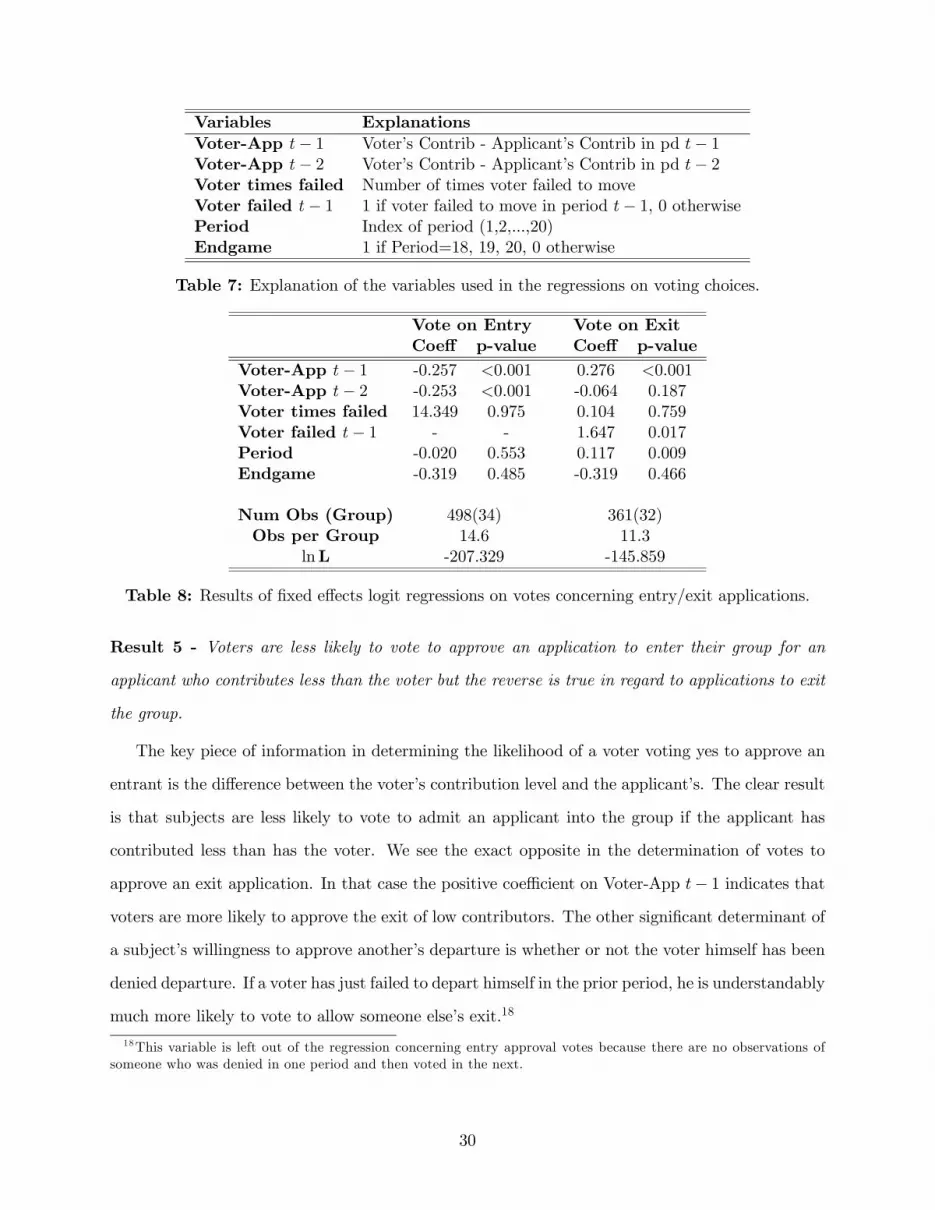
Variables ExplanationsVoter-App t− 1 Voter’s Contrib - Applicant’s Contrib in pd t− 1Voter-App t− 2 Voter’s Contrib - Applicant’s Contrib in pd t− 2Voter times failed Number of times voter failed to moveVoter failed t− 1 1 if voter failed to move in period t− 1, 0 otherwisePeriod Index of period (1,2,...,20)Endgame 1 if Period=18, 19, 20, 0 otherwise

Table 7: Explanation of the variables used in the regressions on voting choices.

Vote on Entry Vote on ExitCoeff p-value Coeff p-value

Voter-App t− 1 -0.257 <0.001 0.276 <0.001Voter-App t− 2 -0.253 <0.001 -0.064 0.187Voter times failed 14.349 0.975 0.104 0.759Voter failed t− 1 - - 1.647 0.017Period -0.020 0.553 0.117 0.009Endgame -0.319 0.485 -0.319 0.466

Num Obs (Group) 498(34) 361(32)Obs per Group 14.6 11.3

lnL -207.329 -145.859

Table 8: Results of fixed effects logit regressions on votes concerning entry/exit applications.

Result 5 - Voters are less likely to vote to approve an application to enter their group for an

applicant who contributes less than the voter but the reverse is true in regard to applications to exit

the group.

The key piece of information in determining the likelihood of a voter voting yes to approve an

entrant is the difference between the voter’s contribution level and the applicant’s. The clear result

is that subjects are less likely to vote to admit an applicant into the group if the applicant has

contributed less than has the voter. We see the exact opposite in the determination of votes to

approve an exit application. In that case the positive coefficient on Voter-App t− 1 indicates thatvoters are more likely to approve the exit of low contributors. The other significant determinant of

a subject’s willingness to approve another’s departure is whether or not the voter himself has been

denied departure. If a voter has just failed to depart himself in the prior period, he is understandably

much more likely to vote to allow someone else’s exit.18

18This variable is left out of the regression concerning entry approval votes because there are no observations ofsomeone who was denied in one period and then voted in the next.

30

Entry ExitCoeff p-value Coeff p-value

Constant -0.281 0.857 -3.794 0.128Applicant Contribution t− 1 0.416 0.028 -0.210 0.278Applicant Contribution t− 2 0.892 <0.001 -0.192 0.303Num of Voters in Relevant Group -0.062 0.539 -0.017 0.909Avg Contrib of Relevant Group t− 1 -0.874 0.003 0.210 0.056Avg Contrib of Relevant Group t− 2 0.208 0.366 0.789 0.092Period -0.058 0.286 -0.095 0.318

Num Obs 104 82lnL -46.725 -29.646

Table 9: Results of a logit regression with outcome of entry/exit application as dependentvariable. “Relevant” group refers to the one the applicant is attempting to enter/exit.

Result 6 - The likelihood of an application being accepted into a new group is increasing in his

own contribution level but decreasing in the contribution level of the group he is applying to get

into. Again, the opposite holds in regards to the success of applicants to exit a group.

We can also examine the outcome of the voting decisions to solidify the results on the deter-

minants of successfully exiting/entering a group. The frequencies of successful and unsuccessful

applications for entry and exit are previously shown in figure 6. We ran a logit regression (there

seems little reason to suspect individual specific effects here) with the result of application for entry

(exit) as dependent variable, which takes a value of 1 if the application is successful, 0 otherwise.

The independent variables should be self-explanatory. Table 9 shows the results.19 The very clear

result is that the prime determinant of whether or not an applicant is admitted into a group is

their recent contribution levels. Also notice that the higher the average contribution level of the

group being applied to in the previous period, the less likely is the applicant to succeed in their

application to enter. The implication is that groups that developed a norm of high contribution

are less likely to accept a new member. Examining the data directly reveals this quite clearly as

well. There were several subjects who would apply repeatedly to get into a group and be denied

until they increased their contribution levels. Some were never admitted. In session 2, one subject

applied to group 1, the high contribution group, 7 times and was never accepted. The subject

19Note that we have exlcuded from these regressions all cases in which a subject has applied to enter a group ofsize 0 (for the entry regression) and when a subject has applied to get back into the group they were in the previousperiod. In both cases acceptance to enter is automatic and in the second, acceptance to exit is automatic as well.

31

had contributed 3 in every period. Another subject applied 5 times with no success, again always

contributing 3, while another applied 5 times and was accepted on the fifth application after 2

periods of increasing his contributions from 3 to 7.

In regard to the outcomes of the exit applications, we see very little that is significant. We

see borderline significant results suggesting that groups with higher contribution are more likely

to approve an exit. Drawing strong conclusions on what leads to successful exits, though, is made

difficult by the fact that we observe only 17 successful applications to exit a group. While this

number is large enough to suggest these exits are not accidents, it is somewhat small for the

purposes of statistical analysis.

4 Conclusion

In this paper we presented an experimental examination of endogenous group formation in a public-

goods provision environment. The genesis for the study was a realization that in naturally occurring

collective action situations, groups use a variety of entry and exit rules to govern their membership

and this should affect the size of groups as well as the level of the collective goods provided. The

environmental and institutional features that we utilize to examine this issue are not intended to

cover all the complexities of endogenous group formation in naturally occurring situations. Instead,

we focused on examining the effects of a few simple mechanisms in an extreme environment that

contained large incentives for subjects to form a single large group and to ignore any issues arising

from the group formation mechanism. Our results show that even in this extreme environment,

group formation mechanisms can have an impact on how groups form as well as on the tendency

of individuals to provide the public good.

Our first clear result is that merely the ability to engage in voluntary self-association has little

positive effect on efficiency. Contributions in our Free Entry/Exit treatment were well explained

by the stage game dominant strategy prediction, though there were a non-negligible amount of

contributions above that level. Our second two main results show that the Restricted Entry and

Restricted Exit mechanisms have substantially different impacts on the dynamics of individual

contributions. It was shown that the Restricted Entry mechanism could be used by subjects to

teach others to engage in pro-social behavior. In the Restricted Exit mechanism, the only thing

32

subjects appeared to learn was to decrease their contributions over time. It is therefore clear that

the group formation mechanism chosen by a group can be expected to have substantial consequences

for how well that group will perform in solving a social dilemma.

In some respects, the dynamic effect of the Restricted Exit mechanism is the most intriguing.

In these experiments, applications to exit were rarely approved leading to an almost fixed group

treatment. This lack of mobility led to subjects who were initially among the highest contributors

dropping their contributions over time to the individually optimal level or even below. We were

able to show evidence that these below individually optimal contributions occur both as a form of

frustration with other group members and as a strategic means of convincing fellow group members

to allow a subject to exit the group. The latter is a particularly intriguing form of behavior not

previously experimentally identified that can have substantial implications for how one might want

to design group formation mechanisms outside of the laboratory. The essential lesson seems to

be that setting up rules that limit the ability for high contributors to exit leaves them only two

options: stay and punish or become such a bad group member that the rest of the group is happy

to be rid of them. Neither is a form of behavior that one would want to encourage.

One of the very active research areas in the public goods literature recently is the effect of

punishment mechanisms on the provision of the public good. Our design incorporated two differ-

ent forms of punishment mechanisms that were quite different than the standard ones found in

the literature. In the restricted entry treatment, low contributing subjects could be punished by

having their entry denied. In all three treatments, a subject could punish by contributing less than

the individually optimal level of 3. Previous papers typically show that overall contributions are

increased with the addition of a punishment mechanism. We, however, find that punishment of the

sort that involves contributions below the individually optimal level has no positive effect on con-

tributions. The punishment technique of denying entry to a low contributor, however, does appear

to be capable of increasing contributions. Our study was in no way designed as an examination of

the effect of punishment mechanisms on the provision of public goods, but the clear indication from

the juxtaposition of these two results is that the existence of punishment opportunities does not

necessarily increase contributions,20 but rather the specific nature of the punishment mechanism is

quite important to its efficacy. This suggests that future examinations of the effects of punishment

20See Denant-Boemont, Masclet, and Noussair (2005) for another demonstration of this point.

33

mechanisms on the provision of public goods should pay particular attention to the exact form

of the punishment mechanism including whether or not the mechanism is a “natural” part of the

interaction.

As we mentioned, though, the results from this study are only the beginning of the process to

fully understand the types and degree of effects from allowing groups to endogenously form over

time. This study establishes an important benchmark result showing that the effects of these forces

are so powerful that even in an environment with strong incentives to just form one group and stay

in it, i.e. an environment in which the group formation mechanism should have little importance,

the mechanism governing that process can still have substantial effects on the outcome. This leaves

open a wide range of future possible work involving the investigation of these and other mechanisms

in more “reasonable” settings to attempt to get a more accurate view of the magnitude of the effect

the group formation mechanism can have in less severe environments. A first extension of this

work will therefore involve a similar study in which the only change is to decrease the incentives

to form the global group leading to an optimal group size of less than the number of subjects in

the experiment. We hypothesize that in such an environment, the process of group formation will

become even more important leading to even stronger behavioral effects. This is left to future

investigation.

References

Ahn, T., R. M. Isaac, and T. C. Salmon (2005). Endogenous Group Formation with Costly Group

Size. Work In Progress, Florida State University.

Andreoni, J. and J. H. Miller (1993). Rational Cooperation in the Finitely Repeated Prisoner’s

Dilemma: Experimental Evidence. Economic Journal (103), 570—585.

Brosig, J., M. Margreiter, and J. Weimann (2005). Endogenous Group Formation and the Provi-

sion of Public Goods: The Role of Promises and Lies. Working Paper, University of Magdeburg.

Camerer, C. F., T.-H. Ho, and J.-K. Chong (2002). Sophisticated EWA Learning and Srtategic

Teaching in Repeated Games. Journal of Economic Theory 104 (1), 137—188.

34

Cinyabuguma, M., T. Page, and L. Putterman (2005). Cooperation under the Threat of Expulsion

in a Public Goods Experiment. Journal of Public Economics. forthcoming.

Coricelli, G., D. Fehr, and G. Fellner (2003). Partner Selection in Public Goods Experiments.

Working Paper.

Denant-Boemont, L., D. Masclet, and C. Noussair (2005). Punishment, Counterpunishment and

Sanction Enforcement in a Social Dilemma Experiment. Working Paper Emory University.

Ehrhart, K.-M. and C. Keser (1999). Mobility and Cooperation: On the Run. Working Paper.

Fehr, E. and S. Gächter (2000). Cooperation and Punishment. American Economic Review 90,

980—994.

Fischbacher, U. (1999). z-Tree: Zurich Toolbox For Readymade Economic Experiments. Zurich

University.

Gunnthorsdottir, A., D. Houser, K. McCabe, and H. Ameden (2001). Disposition, History and

Contributions in Public Goods Experiments. Working Paper Australian Graduate School of Man-

agement.

Isaac, R. M. and J. M. Walker (1988). Group Size Hypotheses of Public Goods Provision: An

Experimental Examination. Quarterly Journal of Economics 103, 179—199.

Isaac, R. M. and J. M. Walker (1998). Nash as an Organizing Principle in the Voluntary Provision

of Public Goods: Experimental Evidence. Experimental Economics 1, 191—206.

Isaac, R. M., J. M. Walker, and A. Williams (1994). Group Size and the Voluntary Provision of

Public Goods: Experimental Evidence Utilizing Large Groups. Journal of Public Economics 54 (1),

1—36.

Kim, O. and M.Walker (l984). The Free Rider Problem: Experimental Evidence. Public Choice 43,

3—24.

Marwell, G. and R. E. Ames (1979). Experiments on the Provision of Public Goods. I. Resources,

Interest, Group Size, and the Free Rider Problem. American Journal of Sociology 85 (6), 1335—60.

35

Olson, M. (1971). The Logic of Collective Action; Public Goods and the Theory of Groups. Cam-

bridge, Mass.: Harvard University Press.

Ones, U. and L. Putterman (2004). The Ecology of Collective Action: A Public Goods and

Sanctions Experiment with Controlled Group Formation. Department of Economics Working

Paper 2004-01, Brown University.

Ostrom, E., J. Walker, and R. Gardner (1992). Covenants with and without a Sword: Self-

Governance Is Possible. American Political Science Review 86, 404—417.

Page, T., L. Putterman, and B. Unel (2002). Voluntary Association in Public Goods Experiments:

Reciprocity, Mimicry and Efficiency. Working Paper Brown University.

Sefton, M., R. Shupp, and J. M. Walker (2002). The Effect of Reward and Sanctions in Provision

of Public Goods. Working Paper.

APPENDIX A: Sample Instructions

Verbal Instruction ScriptBase

[ ] — text to be used when entry is restricted\ \ - text for when exit is restricted

Thank you for participating in today’s experiment. I will read through a script to explain toyou the nature of today’s experiment as well as how to navigate the computer interface you will beworking with. I will be using this script to make sure that all sessions of this experiment receivethe same information, but please feel free to ask questions as they arise. We ask that you pleaserefrain from talking or looking at the monitors of other participants during the experiment. If youhave a question or problem please raise your hand and one of us will come to you.

In the instructions that follow, you will notice that all monetary amounts, earnings, costs, etc.are denominated in Experimental Currency Units (ECUs). At the end of the experiment, yourearnings in ECUs will be translated into US$ at the rate of 1 penny per ECU or 100 ECUs= $1.So if you end up with a balance of 5,000 ECUs at the end of the experiment you will be paid $50,2,500 ECUs $25 and 1,000 ECUs $10. In addition to your earnings from your decisions over thecourse of the experiment, you will receive your $10 show-up fee regardless of what happens. Wewill make our payment to you by check at the end of the experiment.

Description of Investment Task

In today’s experiment you will be engaged in a task that will be repeated many times. In eachperiod of this experiment you will be a member of a group and will be given 15 tokens that youwill be able to invest in two different “accounts”: your individual account and the group account.

36

You must invest all 15 tokens each period, but they can be split between the accounts any way youchoose.

To assist you in understanding this investment task we have provided you with three tables.Please look first at the one titled “Effect of your Choices on Your Payoff.” Since you have 15 tokensto invest, you have 16 different possible ways of allocating them between the two accounts. Thefirst two columns show you what each of those choices are. The third and fourth columns showyou the earnings to you from each allocation. Each token you invest in your individual accountearns .5 ECUs while each token invested in the group account yields 1.5 ECUs. Investing in yourindividual account is costless but investing in the group account is not. For any number of tokensx you invest in the group account you pay a cost of (1/27)*x3. We realize you may not be able todo this computation in your head so the table shows you the cost associated with any choice in thefifth column. Finally the last column shows you your net payoff which is the sum of your earningsfrom the two accounts less the cost of the investment into the group account.

For example, if you invest 0 tokens in the group account, all would be invested in your individualaccount and your total earnings would be 7.5 ECUs. If you invested 2 tokens in the group account,you would receive a net total of 9.2 ECUs with a breakdown of 6.5 from the individual account,3 from the group account and a cost of .3. You should be able to see what the earnings would befrom any other investment choice.

You will notice that in the Net Earnings column, your earnings in this example are listed as9.2+Y. The Y reflects the fact that you receive earnings from the group account from the amountsothers invest into it. For every token others invest in the group account, you receive 1.5 ECUs. Ifyou look at the second table, Effect of Choices of Others on Your Payoffs, you will see this effect.Each row represents a different possible total number of tokens other members in your group mightinvest. For example, if you have invested 2 tokens and the rest of your group invested 0, yourearnings are just the 9.2 we calculated above. If they have invested a total of 10 tokens, yourearnings rise to 24.2 and if they have invested a total of 100, you earn 159.2.

Note that not all possible amounts of group investments have been listed. If the rest of yourgroup had invested a total of 102, for example, you would earn something in between the amountslisted for 100 and 105. This table should give you a good idea of how your payoffs work.

Just as the choices of others affect your payoffs, your investment choices affect the payoffs ofthe other members of your group. For every token you invest into the group account, the othermembers of your group earn 1.5 ECU’s each. Please look at the third table, Effects of your Choiceson Rest of Group. Here you see for every possible choice you could make both what it generatesto you and then what it generates to the rest of your group for the size of any group you mightbe in. Each group size indicated would include you. So if you were in a group of size 5 (4 peopleand yourself), and you invested 6 tokens in the group account, you would generate 5.5 ECUs toyourself plus a total of 36 ECUs to the other members of your group for a net total group earningsof 41.5 ECUs. Your actual earnings, of course, would be 5.5 + Y where the Y is determined by theinvestments of others. The 41.5 is what your choice generates to the rest of the group.

As you can see from the payoff tables, it is possible for you to lose money. If you look backat the second table, Effect of Choices of Others on your Payoffs, you will see that if you selecthigh investments in the group account your earnings will be negative unless the rest of your groupinvests enough into the group account to make up for the loss. To allow for this possibility, everyonewill start with an initial balance of 50 ECUs. As you make investment decisions, this balance willrise as you make money and fall if you have periods with negative earnings. If you lose so muchmoney that your overall balance goes below 0, you will be declared bankrupt. The first time thishappens to you, we will re-initialize you, starting you over with a new positive initial balance of 50ECUs. If your earnings balance goes negative a second time, however, you will be asked to leave

37

the experiment with only your $10.00 show up fee.Note, these examples were not intended to be taken as suggested investment levels. We chose

these examples randomly simply to illustrate how the payoffs work. While we realize these payoffcalculations might seem complicated, the tables and the software you will be using should assist inseeing how they work. At this time, are there any questions about how the investment procedureworks or how the payoffs are determined?

Begin Software

If you turn to your computer screens now, you will see an investment choice screen similar towhat you will see in the experiment. Notice there is a single text box allowing you to enter thenumber of tokens you wish to invest into the Group Account. Any of your 15 tokens not investedinto the Group Account for your group will automatically be invested into your Individual Account.To the right and slightly below the textbox there is a grey button you can press to “test” yourchoice. If you enter a number of tokens into the box and press this button, at the bottom it willshow you the calculations of how many ECUs that choice generates to you and other members ofyour group. This information is identical to what is summarized in the tables we discussed before.Try a few test amounts now to see how it works. Note that you can not invest more than 15 tokensper period and you can not invest negative or fractional numbers.

Once you have decided on your investment decision you can press the red button at the bottomof the screen to accept it. For this practice choice we have placed each of you into a hypotheticalgroup of 5 other members who are just programmed to invest random amounts. In the actualperiods of the experiment the other members of your group will consist of other people in thisroom. Please make an investment decision now so you can see how the program works. Thisdecision will not count towards your actual earnings for the experiment.

Once each of you has made your decision in a period, you will see a screen reporting to you theoutcome. The top table reminds you which group you are in, how many people are in it as wellas what your choice was. The second row tells you what your payoff was and breaks it down byearnings from your individual account, earnings from your investment to the group account andearnings from the investments of others in your group into the group account.

Below this you see the combined total number of tokens invested by the other members of yourgroup into the group account.

Group Selection

In addition to your investments, you will also choose what group you wish to be a member of\[subject to certain restrictions]\.

In the main experiment periods, you will make an investment choice in a group consisting onlyof yourself in period 1. From then on, prior to making an investment choice in a period, you will beasked to choose what group you wish to be a member of. Please press the ok button on your screennow and you will see a screen asking you if you wish to change group. These next few screens alljust show you static information and are not affected by any choices you make. They have beendesigned to show you what the screens would look like in the real experiment.

On your screen you can see the recent history from each of 12 groups labeled A-L. For eachgroup you can see the number of members who were in the group at the end of the prior period.You can also see the total number of tokens that members of that group have invested in the groupaccount as well as the number of members of that group for the previous 5 periods. Note thatmany groups will have had 0 members over this time period. At the bottom of the screen you areasked to choose if you wish to remain in your current group or if you wish to move to a new group.

38

If you choose to move you will go through the following process: Please check the box indicatingyou wish to move to a new group and press ok.

The next screen will be very similar to the one you just saw. The only difference is that youwill now see each group listed with the number of members who have elected to stay in their groupas opposed to the total number who were in the group at the end of the previous period. Afterobserving this information, you can choose which group you wish to move to. You are allowed tochoose any group from the list, A-L. This includes groups with no current members. You are alsoallowed to choose to move back into the group you were in during any prior period including themost recent one. Those remaining in their group will see a waiting screen at this point until thosemoving have selected new groups.

Voting Mechanism

[Your entry to the group is not automatic. After everyone has selected which group they wishto join, the members of the group who chose not to stay in their group from the previous period willvote on whether or not to admit you into their group. After everyone has made a group selectiona sample voting screen will appear. Please make a group choice now. The current members ofa group will see a choice history for all current applicants to join their group consisting of theirinvestment to the Group Account as well as the size of the group they were in over the prior 5periods. Those who said “yes” to the question if they wished to move do not get to vote on newmembers even if they chose to move back into their previous group. They will then vote yes or noon each applicant. If more than 50% of the current members vote YES (to allow entrance). thatperson will be accepted into the group. If 50% or fewer of the current members vote YES on anapplicant, that applicant will return to his or her group from the previous period. After the votingstage has been completed, all subjects will see a new screen. Please note, if you have elected tostay in a group that no one has requested to enter, your voting screen will be blank and you justneed to press the ok button to continue.]

Exit Restriction

\ Your proposed move to a new group may, however, not be allowed. If you have chosen tomove into a new group, the members of the group you are proposing to leave vote on whether ornot to approve your departure from the group. After everyone has chosen which group they wouldlike to move to, a screen will appear to all those group members who answered “no” to the questionregarding whether they wished to move. If everyone will make a group selection now, a samplescreen will appear. Please make a group choice now. The current members of a group will see achoice history for all of the individuals choosing to leave the group consisting of their investmentto the Group Account as well as the size of the group they were in over the prior 5 periods. Thosewho said “yes” to the question if they wished to move do not get to vote on approving departureseven if they chose to move back into their previous group. Those that are eligible to vote will thenvote yes or no on each applicant. If more than 50% of the current members vote YES (to approvedeparture) that person will be allowed to exit the group and move into their chosen group. If50% or fewer of the current members vote YES on an applicant, that applicant will not be allowedto leave the group and will remain in the group. After the voting stage has been completed, allsubjects will see a new screen. Please note, if you have elected to stay in a group that no one hasrequested to exit, your voting screen will be blank and you just need to press the ok button tocontinue./

The next screen will tell you what group you are now in and the number of other subjects inthe group. Once this “group selection” phase is complete, you will then go on to make investmentchoices just as we discussed before.

39

Are there any questions about how the group choice procedure will work?To allow you to familiarize yourself with the investment phase, we will begin with three periods

in which everyone will make an investment choice in a group consisting only of themselves. Thesechoices will never be observable by other participants, but they will generate actual earnings. Wewill then begin the main experiment periods as explained before. In these preliminary periods youwill start with a 50 ECU balance and then when we begin the second series, we will restart youwith a 50 ECU balance. Your earnings from the preliminary periods will be included in your finalpayoff total but you can not draw against them to cover losses in the second series. In period 1 ofthis series, you will again be making a choice in a group consisting only of yourself and this choicewill be observable to other participants in the manner described before. From period 2 of the newseries to the end of the experiment, prior to making an investment choice in a period, you will beasked to choose what group you wish to be a member of. There will be a total of 20 periods in thissecond series.

We ask that you follow the rules of the experiment. Anyone who violates the rules may beasked to leave the experiment with only the $10.00 show-up fee.

40

APPENDIX B: Sample Sessions

We provide here a more extensive set of example paths to provide for a better understandingof some of the dynamics present in the experiment. Figures 5-7 show the average investment level,number of members and the group optimal level of investment for that group size for all groupsin the respective sessions (1, 2 and 8) that had positive group membership after period 2 of themain phase. We have chosen to present data from one “illustrative” session of each treatment. Byillustrative we do not mean “average.” Rather, we specifically chose these sessions because theyemphasize the differences between the treatments.

Figure 5 displays the path of the sample Free Entry/Exit session. In this session subjects werequickly able to form the global coalition with all subjects in the same group. The initially dominantgroup, 10, was made focal due to the subject who was initially in that group in period 1 of the mainseries contributing 7 in that period. In periods 5 through 12 all subjects were in a single group,group 10, but the contribution level was quite low and far below what would have been sociallyoptimal. In period 13 it appears one subject decided to form a new group, group 9, and attempt tosignal that contributions should be high. Others were happy to join, but the average contributionlevel quickly fell as they were not as willing to also contribute at the high level signaled by thesubject forming the group. Another subject tried again to form a new group in period 15 but hadlittle success in attracting members. By period 18, virtually all subjects had switched from group10 over to group 9. The result is somewhat consistent with those reported by Ehrhart and Keser(1999) in that allowing a free movement in and out of groups does not lead to a higher level ofcooperation.

Session 2, as detailed in figure 6, shows a substantial difference in behavior due to the restrictedentry mechanism. First, subjects never form into a single group. Groups 1 and 10 retain roughlyequal membership throughout the session. Group 10 gets larger faster but the contribution level ofthe group is low. Group 1 initially had a smaller number of members but the average contributionlevel was higher and exactly at the group optimal level. Slowly, subjects moved over from group10 into group 1 and, as they did so, group 1 was not only able to keep its contribution levelhigh, but also to increase the average contribution to keep it approximately at the group optimallevel as the group size increased. The reason group 1 did not grow in size faster is not due to alack of entry attempts but rather to the members of group 1 denying entrance to applicants withlow contribution histories. This point will be made clear in the regression analysis in the nextsubsection regarding the voting data. The intriguing part of the path, though, is that it appearsthat after entering into group 1, subjects keep their contributions high. One might expect that asubject would increase his contributions to gain entry into the group and then drop back to thedominant strategy level once he has gained membership in the group. The path from this sessionsuggests that the restricted entry mechanism might be effective in teaching people to increase theircontributions to gain entrance and then this teaching carries over once someone has entered thegroup even in the absence of any mechanism to punish “backsliding” in contributions.

The selected sample session from the Restricted Exit treatment is session 8, shown in figure 7.Most subjects initially joined group 3, but a competition between groups 1 and 3 soon developedover which group would be the focal point of the global group. The average contribution level ishigher in group 1 than that in group 3 and by period 12 all twelve subjects have joined group 1.The movement of subjects from group 3 to group 1 is somewhat delayed as some of the membersof group 3 voted “no” on multiple applications to exit. As subjects joined group 1, the averagecontribution level went rapidly down to the dominant strategy level of 3. The decline in the levelof contributions can be explained by the frustration of subjects who wanted to leave the group,but whose exit was denied. Those frustrated subjects often lowered their contribution levels even

41

12

34

56

78

910

1112

1314

1516

1718

1920

Period

0369

12

0369

12

0369

12

0369

12

0369

12

0369

12

0369

12

0369

12

Group: 3

Group: 5

Group: 7

Group: 8

Group: 9

Group: 10

Group: 11

Group: 12

Average Contribution LevelNumber in GroupGroup Optimal Contribution

Figure 5: Sample session (session 1) from the Free Exit/Entry treatment showing the time pathfor all groups with positive membership after period 2.

42

12

34

56

78

910

1112

1314

1516

1718

1920

Period

0369

12

0369

12

0369

12

0369

12

0369

12

0369

12

0369

12

0369

12

Group: 1

Group: 2

Group: 3

Group: 4

Group: 5

Group: 6

Group: 7

Group: 10

Average Contribution LevelNumber in GroupGroup Optimal Contribution

Figure 6: Sample session (session 2) from the Restricted Entry treatment showing the time pathfor all groups with positive membership after period 2.

43

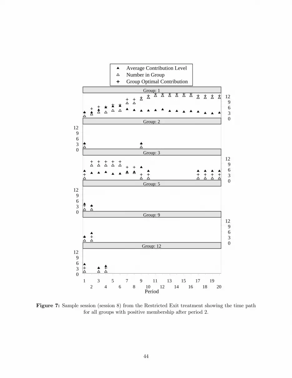
12

34

56

78

910

1112

1314

1516

1718

1920

Period

0369

12

0369

12

0369

12

0369

12

0369

12

0369

12

Group: 1

Group: 2

Group: 3

Group: 5

Group: 9

Group: 12

Average Contribution LevelNumber in GroupGroup Optimal Contribution

Figure 7: Sample session (session 8) from the Restricted Exit treatment showing the time pathfor all groups with positive membership after period 2.

44

below 3. In periods 1-10, when the big group was forming, there were 0 instances of subjectscontributing 0 or 1 token and only 2 cases of subjects contributing 2. During periods 11-20 therewere 22 attempts to exit the main group with only one being successful. During this time periodthere were 6 cases of a subject contributing 0, 3 incidents of contributing 1, and 7 incidents ofcontributing 2. The single successful exit was by the subject who returned to group 3 (as the lonemember) in period 17. The subject had contributed an average of 6.9 tokens per period to thegroup account between periods 1 and 10 and had attempted to leave the group in periods 11, 14, 15and 16, unsuccessfully and then successfully in period 17. The subject lowered their contributionto 0 in period 14, 3 in period 15 and back to 0 in period 16. After forming a group of one in period17, the subject contributes 5 for the remaining periods, perhaps as a way of telling the membersof group 1, “this is what you guys should be doing.” There were other similar examples of highcontributors dropping their contribution levels substantially after their exit was repeatedly deniedleading to a reasonable interpretation that the decline in their contributions was due in part to afeeling of frustration or perhaps a strategic move to convince the group to approve their departure.

45