International Journal of Industrial Organization xxx (2009) xxx–xxx

INDOR-01848; No of Pages 21

Contents lists available at ScienceDirect

International Journal of Industrial Organization

j ourna l homepage: www.e lsev ie r.com/ locate / i j io

ARTICLE IN PRESS

Endogenous location leadership☆

Sergio Meza a, Mihkel Tombak a,b,c,⁎a University of Toronto, 105 St. George St., Toronto, ON, Canada M5S 3E6b CIRANO, Montreal, Canadac ESMT, Berlin, Germany

☆ The authors would like to thank seminar participanUniversity; Université de Montreal; University of ToronWorkshop in “Stability in Competition” at UCL, Louvain-Associate Editor and two referees for their commentsversion of this paper. Meza would like to thank Univsupport from the Connaught Fund.⁎ Corresponding author. University of Toronto,105 St. G

M5S 3E6.E-mail addresses: Sergio.meza@rotman.utoronto.ca (

mihkel.tombak@rotman.utoronto.ca (M. Tombak).1 For a survey of the various explanations for persistent

firms and for an examination of when firm costs would dDesgagné (1996). For empirical evidence of such cost asym

0167-7187/$ – see front matter © 2009 Elsevier B.V. Aldoi:10.1016/j.ijindorg.2009.03.001

Please cite this article as: Meza, S., Tombadoi:10.1016/j.ijindorg.2009.03.001

a b s t r a c t

a r t i c l e i n f o

Article history:Received 26 June 2006Received in revised form 12 March 2009Accepted 18 March 2009Available online xxxx

JEL classification:L11D43

Keywords:AsymmetriesHorizontal differentiationStackelbergGames of timing

We analyze a game of timing where Sellers, which have marginal production cost asymmetries, can delayentry and a commitment to a location in a Hotelling type setting. When cost differences are large enough thegame becomes a war of attrition that yields Stackelberg behavior where the high cost firm will delaychoosing a location until the low cost firm commits to its position. We find interaction effects between timingand the degree of product differentiation and compute timing/location and mixed strategy equilibriathrough a range of marginal cost differences. The firms maximally differentiate with moderate costdifferences; with somewhat greater cost differences there is intermediate differentiation, and; with large costdifferences there is a blockading monopoly. The low cost firm always commits to entry immediately whereasthe high cost firm either enters immediately, shortly after the low cost leader, or never, depending on the costdifferences. Finally, we find that in equilibrium the duopoly is sustained for a larger range of cost differentialsand that differentiation is greater than the social optimum.

© 2009 Elsevier B.V. All rights reserved.

1. Introduction

Firms are not all created equal. Indeed, whole industries andinstitutions of higher learning are dedicated to creating and sustainingdifferences between firms. There is an abundant managementstrategy literature where such differences are characterized as“competitive advantages”, but rigorous studies and the preciseimplications of such advantages have been lacking in this area. Onesuch competitive advantage is having lower costs of production. Costdifferences between firms can arise from a myriad of causes rangingfrom differing technological opportunities, labor conditions, andmanagement qualities.1 Firms make significant investments to try to

ts at: EARIE, Toulouse; Purdueto, IIOC, Washington, and; thela-Neuve, BL, and especially anand suggestions on an earlierersity of Toronto for financial

eorge St., Toronto, ON, Canada

S. Meza),

differences between competingiverge, see Röller and Sinclair-metries see Syverson (2004).

l rights reserved.

k, M., Endogenous location

obtain lower costs with varying degrees of success.2 When these costdifferences exist managers of higher cost firms must find ways toremain competitive, i.e., they must differentiate their product. A lowcost firm may choose closer locations to capture most (or sometimesall) of the market. The higher cost firm then may delay entry andcommitment to a product positioning in order to be able to choose aposition differentiated from its lower cost rival. Alternatively, a firmmaywish to preempt its rival to secure the best position in themarket.In this paper we study how cost differences of firms affect the strategictiming of market entry and its interaction with market location.

What it means to enter and commit to a certain market is capturedwell in Bertrandmodels of horizontal differentiation (Hotelling,1929).However to ensure price equilibria and equilibrium in the locationgame (when firms are symmetric), for this paper we use the variationby D'Aspremont et al. (1979), (hereafter D'AGT) with quadratic cost oftransportation. Similar to Boyer et al. (2003) and Ziss (1993) we allowfor asymmetric firms by modeling different cost of production. Wedefine a game of timing of market entry where the product marketsubgame is the differentiated Bertrand model of D'AGT withasymmetric sellers to see how cost asymmetries result in the

2 Substantial long term investments are made by firms in: personnel training; newtechnologies; in seeking new and cheaper sources of raw materials, these investmentopportunities may not be available to all firms to the same extent or be effective in varyingdegrees. We treat the cost differences here as given, but the repercussions of any costadvantage obtained on how firms compete would be an important justification of thoseinvestments.

leadership, International Journal of Industrial Organization (2009),

2 S. Meza, M. Tombak / Int. J. Ind. Organ. xxx (2009) xxx–xxx

ARTICLE IN PRESS

imposition of a certain order of entry. Since firms may not be able tochange marginal cost in the short run, this variable is treated asexogenous in our study. But because firmsmay be strategic in decidingthe time of entrance to the market, to complete this framework, ourstudy endogenizes time of entry. Depending on their relative costs theequilibrium timing could then define which roles are taken by firms.That is, low cost firms may be leaders while high cost firms may befollowers.

By allowing the delay of entry3 and location choice, we find thatStackelberg behavior naturally arises under certain circumstances andyields unique location equilibria. In our analysis, beyond a certain levelof cost differences, the low cost firm takes the role of a Stackelbergleader and chooses a position anticipating that the followermaximallydifferentiates. In this timing/location game, we find the followingtypes of equilibria: (i) with lower cost differences firms enterimmediately, simultaneously and maximally differentiate, (ii) withsomewhat higher cost differences the low cost firm moves first withthe higher cost follower moving as soon as possible and still the firmsmaximally differentiate, (iii) with higher cost differences still the lowcost firm leads and chooses an interior point while the high costfollower chooses the boundary point farthest away from its rival, (iv)with even higher cost differences, there are no pure strategyequilibrium in the game of timing, and two equilibrium locations inmixed strategies emerge; and (v) finally with very high costdifferences, the low cost leader locates in the middle of the marketand blockades entry. Interestingly we find that the Stackelberg leadercan never obtain its first-best location and that the weakest firm (theone with higher marginal costs) wins what turns out to be a war ofattrition. We subsequently compute the welfare optimizing behaviorand find that cost asymmetries can be welfare improving (as Salantand Shaffer, 1999, find with the asymmetric Cournot model) and thatduopoly persists for much larger cost differences than is sociallyoptimal.

1.1. The related literature

The bulk of Industrial Organization theory assumes symmetricfirms but some recent studies have reexamined the seminal theory tostudy how the deviation from the usual assumption of symmetricfirms affects the previously derived results and yield new insights.4

There are two strands in the literature closely related to this study. Inthe first related tributary of studies the timing of the differentiatedBertrand game is fixed and location and price are endogenized (i.e.Ziss, 1993, for simultaneous location; and Boyer et al., 1994, 2003 andTyagi, 2000 for sequential location). Since our game embeds a similarlocation game in the game of timing, for a range of low cost differencesthe results of our model coincide with some of the previous results(e.g., for low cost differences firms locate simultaneously and as far aspossible from each other). When marginal cost differences increase,however, our results differ from those previously obtained. Forinstance, beyond some value of cost differences a location equilibriumdoes not always exist in the traditional location game (Ziss, 1993).Despite the high cost firm wanting to keep maximum differences, itcould be optimal for the low cost firm to sit on top of the high cost firmand thus monopolize the market. Previous studies avoided theproblem of a lack of location equilibrium by changing the choice set

3 We allow for the possibility that a seller may delay entry until a certain time or,that a seller may adopt a wait-and-see strategy. There may be a time lag for a rival'smove to be confirmed and for the seller to react, for the purposes of this analysis, weassume this time lag to be financially negligible.

4 For example, the impact of firm cost asymmetries has been explored: in a Cournotsetting (by Leahy and Neary, 2005; Röller and Sinclair-Desgagné, 1996; Röller et al.,2007, Salant and Shaffer, 1999, and Tombak, 2002); in a Bertrand setting (Marquez,1997; Thomas, 2002); in models of horizontal differentiation (Boyer et al., 2003; Vogel,2007; Ziss, 1993) and; in vertically differentiated models (Sutton, 1986; Anderson andDePalma, 2001).

Please cite this article as: Meza, S., Tombak, M., Endogenous locationdoi:10.1016/j.ijindorg.2009.03.001

of locations. Tyagi (2000) broadened the spectrum of possiblelocations of sellers to beyond the locations of the consumers as perGabszewicz and Thisse (1986) and Tabuchi and Thisse (1995). Boyeret al. (2003) limited the set of locations of each firm within their halfof the line. Differently, we allow the locations where the firms can playto be anywhere on the Hotelling line. Also, we solve for mixedstrategies where equilibrium did not exist for simultaneous game.Finally, the nature of the game of timing allows us to find perfectequilibrium for most of that region without any further restriction.Another difference with previous papers is that in our study thesequence of entrance is not imposed like in Tabuchi and Thisse (1995),Tyagi (2000), or Boyer et al. (2003) but instead it emerges naturallyfrom the endogenous choice of time of entrance of the firms. To ourknowledge, this is the first study to endogenize; timing, location, andprice.

In the second related strand of literature the timing of setting acertain strategic variable is endogenized. This strand is under therubric of endogenous leadership (Amir and Stepanova, 2006; Braid,1986; van Damme and Hurkens, 2004, when the strategic variable isprice; Amir and Grilo, 2001; Hamilton and Slutsky, 1990; van Dammeand Hurkens, 1999, where firms set quantities). In much of thisliterature (with the exception of Hendricks et al., 1988) the modelused is one of two discrete time periods. This facilitates tractability butcould in some cases sacrifice generalization. Instead, we allow time tobe continuous (from zero to infinity) and we also allow firms tochoose whether they would play an open-loop (firms commit to atiming and location at time zero) or feedback (firms employ strategiesthat are contingent on the history of the rival's moves) games. Sincethe variable firms choose in sequence is location and not price orquantity, there is a second way inwhich our paper differentiated fromthis strand. In this literature of endogenous leadership the models relyonwhether the strategic variable is a strategic substitute or a strategiccomplement to determine the nature of the timing equilibria. vanDamme and Hurkens (2004), in their price setting game, find thatalthough both firms prefer to follow, the low cost firm will emerge asthe price leader. Amir and Stepanova (2006) generalize these resultsto situations where the price could be strategic substitutes and/orcomplements and find unique equilibria with sufficient cost differ-ences where again the low cost firm is the price leader. Generally, inthesemodels, the high cost firm has a secondmover advantage. As ourstrategic variable is location, where the slope of the reaction functioncan change sign depending on cost differences, it is not possible toinfer the timing from the results of this literature.5 Instead, we need tosolve for the perfect equilibrium by analyzing the three stages insequence and for different ranges of cost differences.

In the following section we introduce our model; we describe ourhorizontally differentiated Bertrand game and how we modelmarginal cost differences and; we explain our game of timing. Aftercomputing the price equilibria, we examine equilibrium locationchoices and find the regions of cost differentials where thoseequilibria in pure strategies exist. A mixed strategy equilibrium inlocation choices are computed in this section for the entire spectrumof cost asymmetries. We find and characterize three possibleoutcomes — maximal differentiation, intermediate differentiation,and a blockadingmonopoly for each of the possible relative timings. InSection 3 we compute the timing equilibria. In Section 4 a welfareanalysis is conducted. In this section we find the first-best solution ofthe social planner (i.e., where the planner determines the location andprice) and compare that to the equilibrium outcomes of the previoussections. In this final section, we summarize and discuss our findings.

5 Anderson (1987) finds equilibria for the original linear transportation costHotelling model by imposing Stackelberg behavior for symmetric (zero) productioncost firms. He finds a profit advantage for the price leader which implies that therewould be a competition for the first move in that model.

leadership, International Journal of Industrial Organization (2009),

3S. Meza, M. Tombak / Int. J. Ind. Organ. xxx (2009) xxx–xxx

ARTICLE IN PRESS

2. The model

In this section we develop a model of two firms which may be asymmetric in their marginal costs playing a three stage game of perfectinformation. In the first stage firms decide on a time of entry. The relative timings chosen would then determine which firm is the leader andwhich firm is the follower or if the timing is simultaneous. In the second stage firms enter the market and choose a location. If the timing in thefirst stage differed then the follower would be informed of the location of the leader when making its location decision. In the third stage of thegame firms simultaneously choose prices given the locations as per D'AGT.

In the first stage two firms decide the planned time of entrance (T) from a continuum of possibilities from 0 to infinity. A strategy for player A(B) is a time TA∊ [0,∞](TB∊ [0,∞]) at which firm A (B) plans to enter given that its rival has not entered before that time. If rival firm B (A) enters ata time prior to TA (TB) firm A (B) may react by adjusting its time of entry to τA (τB). The actual times of entry (τA, τB), however, may deviate fromTi depending on the optimal strategy of the rival. Given a entry timing pair (τA, τB)∊ [0,∞]×[0,∞] a payoff to player A could then be defined aseither a Leader's payoff if τAbτB; a Follower's payoff if τANτB, or; a simultaneous payoff. We will further define these payoffs subsequently butthey would be the discounted equilibrium payoffs from the location and pricing subgames given their relative timing. In our completeinformation setting, the firms each have full knowledge of the history, in other words, we have a “noisy” game of timing. That is, the firmsinstantly learn when a rival has entered. A firm may adopt a wait-and-see strategy and thus we seek feedback equilibria to the timing game, i.e.,the strategy pair becomes (τA(Hτ), τB(Hτ)), where Hτ is the history of entry and location behavior until time τ. However, if no firm has entered themarket when time TA (TB) has elapsed, Seller A (Seller B) will immediately enter at time τA=TA (τB=TB). Also, if a firmwants to preempt its rival,the time cannot be below 0 and if immediate entry is chosen by both firms then they would enter simultaneously. Furthermore, we assume thatfirms will not enter unprofitable markets (i.e., there is a cost of entry). The order of entry time defines the sequence of entrance, so that we canhave sequential or simultaneous games. We assume that entry and response to entry take place in continuous time. If a firm wishes to be afollower as soon as possible after the leader has moved there would be a certain time lag to confirm that the rival has entered and committed to alocation but we assume that lag to be financially negligible. In this stage the strategy set is the respective planned time of entrance (TA and TB) aswell as the strategy (τA(Hτ), τB(Hτ)) to follow if the rival firm has entered before the planned time.

In the second stage the sellers enter at entry timing (τA, τB) and simultaneous to entry they play a location game on a Hotelling line. The sellersare located on a line of length l at respective distances a (for Seller A) and b (for Seller B) from the opposite ends of this line (a+b≤1; a, b≥0). Atthe time of entry τA (τB) they choose locations a (b). The location game is contingent on the two possible relative timings of entrance: sequential orsimultaneous.When the relative timing is sequential the location game played is Stackelbergwhere the follower has information of the location ofthe leader before entering. If firms enter simultaneously we assume that if both firms want to maximally differentiate they will always play inopposite locations. When a pure equilibrium doesn't exist, and firms choose the same time of entrance we solve for mixed strategy equilibrium.Once players choose a location, it remains fixed for the reminder of the game. At this stage the strategy set is the respective locations a and b in thecase of pure strategy equilibria or the distribution of probabilities for a and b in the case of mixed strategies.

In the third stage the firms play a Bertrand game given the degree of horizontal differentiation. Here firms have to simultaneously decidemill prices (pA and pB, where again, the subscripts denote the Sellers) given their respective locations. Firms decide prices by maximizingcurrent profits. Consumers are uniformly distributed across a line of unit length l. They continuously purchase and consume one unit of aproduct per unit of time from any of the two Sellers A and B that produce the homogeneous product. Consequently, in what follows wheneverwe refer to product market profits π it is to be understood as the profits in a time period τ. A customer will buy from the seller who quotes theleast delivered price and there are zero costs of switching suppliers. For the Hotelling model, transportation costs are linear (tx, where t is thetransportation cost, x is the distance from a consumer to the location of the seller). For D'AGT and our subsequent model, the transportationcost will be quadratic tx2 in order to guarantee the existence of price equilibria. Furthermore, as is common in such analyses, we assume thatprices and locations are such that there is full market coverage, i.e., that the reservation values of consumers are high enough and that thelimit prices are low enough to attract even the most distant consumer. We also assume low barriers to entry. This means that a firm whichforces its rival to exit (or prevents it from entering in the monopolistic case) must be cognizant of that firm potentially entering. In otherwords, the firm which finds it optimal to become a monopolist must engage in limit pricing. This limit price is a function of the location(Bonanno, 1987) and so blockading can be done via a combination of the location and price. We will henceforth refer to such a monopolist as a“blockading monopolist”.

Our modification to the previous horizontal differentiation models, analogous to Ziss (1993) and Boyer et al. (2003), will be to includeconstant marginal costs of production that are different for A and B. Somewhat differently from Ziss (1993), Seller A has a marginal cost ofproduction of (1−(r/2))c, while Seller B has marginal costs of (1+(r/2))c. Thus cr represents the difference in marginal costs, and we caninduce a mean preserving spread in those costs by increasing r. Note that r can take on any real value and consequently there is no loss ofgenerality.6 We introduce this cost structure which differs from Ziss and Boyer et al. as it allows us to change the difference in marginal costswithout changing the average industry costs and allows us to compare our results to those of Salant and Shaffer (1999) and Bergstrom and Varian(1985) which examine asymmetric Cournot models with a mean preserving spread in costs.

We seek subgame perfect equilibria and to solve this game we proceed in the reverse order of stages as is usually done in these multistageproblems. We first solve in Appendix A the third stage pricing game. Price equilibria are found for all locations a and b and the resulting priceequilibria profits are computed. Then we move in the next section to the second stage and solve all possible locations in three possible games:the two sequential games (Seller A being the leader, B being the follower; B being the leader and A being the follower); and, the simultaneousgame. For the simultaneous game we solve for pure strategy equilibria of the location game and we solve for the mixed strategy equilibria. Thederivation of the mixed strategy equilibrium allows us to: (i) compare the result with that under pure strategies, and (ii) find a solution for thecomplete range of cost differentials. Finally, we solve the first stage in which the feedback equilibria for the timing of market entrance arederived.

6 Our results translate precisely into those of Boyer et. al. for the relevant timing scenarios. Our cr is the same as their Δ/k (their difference in production costs divided by theirtransportation rate), which Boyer et. al. use throughout their analysis.

Please cite this article as: Meza, S., Tombak, M., Endogenous location leadership, International Journal of Industrial Organization (2009),doi:10.1016/j.ijindorg.2009.03.001

4 S. Meza, M. Tombak / Int. J. Ind. Organ. xxx (2009) xxx–xxx

ARTICLE IN PRESS

2.1. The location stage

With the equilibrium results of the pricing game (see Appendix A) we now proceed to examining the second stage of the game where firmschoose locations given a certain sequence of moves. This timing of moves could be sequential or simultaneous.We assume throughout that once alocation is chosen then the firm is committed to that location. The information sets differ according to their relative timing, under sequentialmoves the follower knows the leader's location. As we have no pure strategy location equilibria in a certain range of cost differentials undersimultaneous moves we compute a mixed strategy equilibrium in those cases. The outcomes will then be compared in the subsequent section toderive timing equilibria.

2.1.1. Location with simultaneous movesMoving forward to the location stage of the game, one can characterize the equilibrium location choices by taking the derivatives of the

equilibrium profits (Eq. (A2)) with respect to the respective firm location choices, and comparing the resulting optimumwith that obtained fromthe monopolistic region defined by Eq. (A5).

Proposition 1. (Ziss, 1993; Boyer et al., 2003; A.3, A.5) In duopoly, the incentives to change location are given by:

Aπ⁎AAa

= − Δt 3 + a − bð Þ + cr½ � Δt 1 + 3a + bð Þ− cr½ �18Δ2t

; and

Aπ⁎BAb

=Δt −3 + a − bð Þ + cr½ � Δt 1 + a + 3bð Þ + cr½ �

18Δ2t:

ð1Þ

where Δ=1−a−b, Δ, a, b≥0.When r=0, the results of D'AGT are obtained; that is, the derivatives are both negative and Sellers A and B both have an incentive to

maximally differentiate. With marginal cost differences, however, the signs of the derivatives may change.Substituting condition (A3) into Aπ⁎

BAb in Eq. (1), one can see that for all a, b and cr that satisfy this condition, the derivative is always negative.

Therefore, it is optimal for Seller B to locate as far as possible from A (b=0 if a≤1/2, b=1 if a≥1/2).Knowing that Seller B locates always as far as possible from Seller A, we can continue our analysis assuming b=0.7 Substituting b=0 into Aπ⁎

AAa

of Eq. (1), one obtains the condition,

cr=t b 1− að Þ 1 + 3að Þ ð2Þ

for this derivative to be negative. Such a condition always holds for cr/tb1 for all a that satisfy condition (A3). Therefore, if both firms participatein the market, they would prefer to maximally differentiate when cr/tb1. This means that the high cost firm always fears price competition andseeks to avoid it through product differentiation, but beyond a certain cost differential the low cost firm is no longer as afraid of price competitionand starts to decrease the degree to which its product is differentiated from its rival's product.

Recall, however, that Seller A can choose locations outside the region defined by condition (A3). Locations in this regionwould imply the exitof Seller B and monopolist profits for Seller A. The maximum monopoly rent can be easily derived from Eq. (A5) and would be obtained whenSeller A situates on top of Seller B (a=1−b). In that case, the profits of Seller A would be equal to cr. This profit would be greater than theduopolistic profit πA⁎(a,0) when,

crt

z 1− að Þ 6− að Þ− 3ffiffiffiffiffiffiffiffiffiffiffiffiffiffiffiffi3− 2a

p� �: ð3Þ

Note that the R.H.S. of condition (3) is decreasing in a in the relevant range of this variable. When a is zero, then the R.H.S. reduces tocr = t N 3 2−

ffiffiffi3

p� �≈0:804ð Þ. Thus, when 0 V cr = t b 3 2−

ffiffiffi3

p� �, then both firms prefer to maximally differentiate (a⁎, b⁎)=(0, 0) and obtain

duopoly rents. This location choice is a Nash equilibrium since Seller A, if its competitor locates at b=0, would find it optimal to locate at a⁎=0so long as cr = t b 3 2−

ffiffiffi3

p� �. Furthermore, for these values of a and cr/t, the derivative of Seller B's profits is negative so it will not deviate from

b=0. In this case, the equilibrium profits are:

π⁎A =3t + crð Þ2

18tand; π⁎B =

3t−crð Þ218t

: ð4Þ

The above analysis shows when pure strategy equilibrium in locations exists for simultaneous move games. It also implies, as Ziss (1993) hadfound, that there is no duopoly pure strategy location equilibrium for the simultaneous gamewhen cr = t N 3 2−

ffiffiffi3

p� �.8 That is, Seller B (the high

cost seller) continues to have a tendency to maximally differentiate, while Seller A (the low cost seller) wishes to minimally differentiate.Furthermore, marginal costs differences can become large enough (satisfying condition (3)), that Seller A prefers to become a monopolist ratherthan obtain the duopoly profits of Eq. (A2), regardless of the location choice a. Seller A becoming the monopolist implies that it minimallydifferentiates and undercuts Seller B to drive B out of the market regardless of the choice of b.

7 There is an analogous problem assuming that Seller B chooses location b=1.8 Ziss' condition for the nonexistence of location equilibria was 6− 3

32

� �cL2 where c is the transportation cost and L was the length of the Hotelling line which is analogous to the

value we obtain here.

Please cite this article as: Meza, S., Tombak, M., Endogenous location leadership, International Journal of Industrial Organization (2009),doi:10.1016/j.ijindorg.2009.03.001

5S. Meza, M. Tombak / Int. J. Ind. Organ. xxx (2009) xxx–xxx

ARTICLE IN PRESS

As marginal cost differences become large enough (cr/tN5/4) the equilibrium in the simultaneous game reemerges. It is easy to show that bylocating at the middle of the market (a=0.5) the low cost seller becomes a monopolist realizing profits of cr− t/4. Seller B will not enter themarket as it will not be able to make positive profits.

2.1.2. A mixed strategy solutionIn order to attain location equilibria in the duopoly throughout the parameter range, we solve for a mixed strategy equilibria.9

Proposition 2. When 0 b cr = t b 3 2−ffiffiffi3

p� �there exists a mixed strategy equilibrium of the simultaneous location subgame such that the expected

payoffs are equal to the firms' payoffs when they choose to maximally differentiate at a=0 and b=0.

Proof. See Appendix B.

The above proposition implies that the equilibrium expected profit from playing mixed strategies in this parameter region yields the sameprofit as the equilibrium in pure strategies. An equal weighting of probability mass extends to a region of greater cost asymmetry as shown in thenext proposition.

Proposition 3. When 3 2−ffiffiffi3

p� �b cr = t b 1 there exists a mixed strategy equilibrium of the simultaneous location subgame such that each firm

chooses location 0 or l with the probability 1/2.

Proof. This follows from Proposition B4 and Proposition B5 in Appendix B.

The equilibrium probabilities yield the expected payoffs for simultaneous location of

E πMSA

h i=

136t

18crt + 3t + crð Þ2h i

and E πMSB

h i=

136t

3t−crð Þ2: ð5Þ

In other words, in this region of cost differences the high cost firm and the low cost firmwould collocate and the high cost firmwould obtainzero rents if the low cost firm correctly anticipates the location of the high cost firm. The high cost firm, however, can still earn profits by introducingnoise into its decisionmaking process in the hopes that the low cost firmwould anticipate incorrectly the location of the high cost firm and locateat the opposite extreme.

Proposition 4. When 1bcr/tb1.7782 there exists a mixed strategy equilibrium of the simultaneous location subgame such that Seller B chooses b=0or b=1 each with the probabilities of 1/2, and Seller A chooses a=a or a=1 — ã each with the probabilities of 1/2.

Proof. See Appendix B.

Lemma 1. When cr/tN1.7782 then Seller A prefers to monopolize at a=1/2.

Proof. See Appendix B.

To summarize, when the moves by the firms are simultaneous then: when 0 V cr = t b 3 2−ffiffiffi3

p� �the firms maximally differentiate and earn

the duopoly profits in Eq. (8a,b); when 3 2−ffiffiffi3

p� �V cr = t b 1 then the firms play mixed strategies over the extreme points in the spectrum and

firms earn the expected profits in Eq. (5); when 1≤cr/tb1.778 then the firms playmixed strategies where there is intermediate differentiation bythe low cost firm,10 and; when cr/t is greater than 1.778 the low cost firm will locate in the center of the spectrum and monopolize the industryobtaining a profit of cr− t/4.

2.1.3. Location with sequential movesIn our setting there are two potential sequential games: one inwhich the high cost firm is the leader and the low cost firm locates afterwards,

and another game where the low cost firm takes the lead and the high cost firm locates afterwards. Once firms have chosen locations they arecommitted to those locales. The follower is able to observe the location of the leader before deciding its entry/location decision. In this sectionwesolve these two sequential games for the whole range of values of cr. Boyer et al. (2003) also solved the sequential game of location choice butfirms are restricted to locate on their half of the line. This constraint of where firms could locate negated the possibility of firms leapfrogging oneanother which helps in their obtaining location equilibria.

As already seen in Section 2.1.1, for the region of low cost differences when 0 V cr = t b 3 2−ffiffiffi3

p� �, both firms prefer to maximally

differentiate (a⁎, b⁎)=(0, 0) and obtain duopoly rents. Therefore even if the two firms play sequentially the firm playing second in this regionwould always choose a location that maximizes product differentiation. Consequently, order of entry does not have a material impact onlocation decisions when firms are so symmetric. Timing, however (as we shall see in Section 3), starts to play an important role when costasymmetries are larger.

9 Mixed strategy equilibria with symmetric cost firms have been computed: for price subgames in the original linear transportation cost model of Hotelling (Pitchik and Osborne,1987) and, for locations in the model of D'AGT (Bester et.al., 1996) whereas we consider location subgames of a broader game.10 In Appendix B we show that these mixed strategy equilibria have higher expected payoffs than any other possible mixed strategy equilibria and as such we use them as the basisfor comparison.

Please cite this article as: Meza, S., Tombak, M., Endogenous location leadership, International Journal of Industrial Organization (2009),doi:10.1016/j.ijindorg.2009.03.001

6 S. Meza, M. Tombak / Int. J. Ind. Organ. xxx (2009) xxx–xxx

ARTICLE IN PRESS

For higher cost differences (cr = t N 3 2−ffiffiffi3

p� �), as can be seen in Sections 2.1.1 and 2.1.2, there is no pure strategy equilibrium in the

simultaneous game because while the high cost firm prefers to maximally differentiate, the low firm instead prefers to locate on top of the highcost firm and thus monopolize the market. For the sequential case inwhich the high cost firm plays first the results are straightforward. After thehigh cost firm has chosen a location, the low cost firm enters and locates at the same place as its rival. Because of its cost advantage, the low costfirm has only to price slightly below themarginal cost of the high cost firm of c(1+(1/2)r). The high cost firm cannot reduce its price andwithoutany differentiation will not sell any product and will realize a profit of zero. The low cost firm would capture the whole market realizing themonopolistic profit of cr.

For the sequential case inwhich the low cost firm plays first the results are a little more complex. The low cost firm A is going to enter first andlet's assume that it chooses a location a, a∊ ⌊0,0.5⌋. As we know from Eq. (1) that for all values of a Aπ⁎

BAb is always negative, therefore the high cost

firm B is going to follow choosing the location that maximizes differences at b=0. If firm A chooses instead a location in the range (0.5, 1], thefirm B would choose the opposite location at b=1. Because this later problem is symmetric to the former one, we will focus only in the firstproblem where a∊ ⌊0,0.5⌋ and b=0.

The profit function that the low cost firm has tomaximize is that from Eq. (A2) knowing that player B is going to choose b=0, and constrainedto the values of a in the range a∊ ⌊0,0.5⌋. Also, given the cost advantages of firm A, monopolization is possible and the resulting profits areobtained by substituting b=0 in Eq. (A5). Monopolizationwould be obtainedwhen the profits computed from Eq. (A5) in this manner are higherthan the profits from the duopolistic game, i.e., πAMono(a)NπAL(α,0) this condition holds when a N 2−

ffiffiffiffiffiffiffiffiffiffiffiffiffiffiffit t + crð Þ

pt . In summary, the profits obtained

by Seller A for any choices of location a are:

πLA a;0ð Þ =

1−að Þ 3 + að Þt + crð Þ218 1− að Þt if 0 V a V 2−

ffiffiffiffiffiffiffiffiffiffiffiffiffiffiffiffiffiffiffiffit t + crð Þp

t

cr − t 1−að Þ2� �

if 2−ffiffiffiffiffiffiffiffiffiffiffiffiffiffiffiffiffiffiffiffit t + crð Þp

tb a V 1

8>>><>>>: ð6Þ

Solving for the first order conditions for the maximization of Eq. (6) with respect to a and comparing those results with the border conditionsresults in three solution regions for the optimal value of a. In the region 3 2−

ffiffiffi3

p� �b cr = t b 1 Seller A locates at a⁎=0, that is Seller A finds it

optimal to maximally differentiate. When cost asymmetries are such that 1 b cr = t b cr=t, where cr=t = 1128 −187 + 29

ffiffiffiffiffiffiffiffiffi145

p� �≈1:26724 Seller

A finds it optimal to move to a⁎ = 1= 3 1−ffiffiffiffiffiffiffiffiffiffiffiffiffiffiffiffiffi4− 3cr

p� �.11 That is, the Stackelberg leader chooses intermediate differentiation and can engage in

some degree of price competition and steal some business from the high cost seller. Finally when cr = t z cr=t, Seller A finds it optimal tomonopolize and locates at a⁎=1/2. Seller B will then not enter.

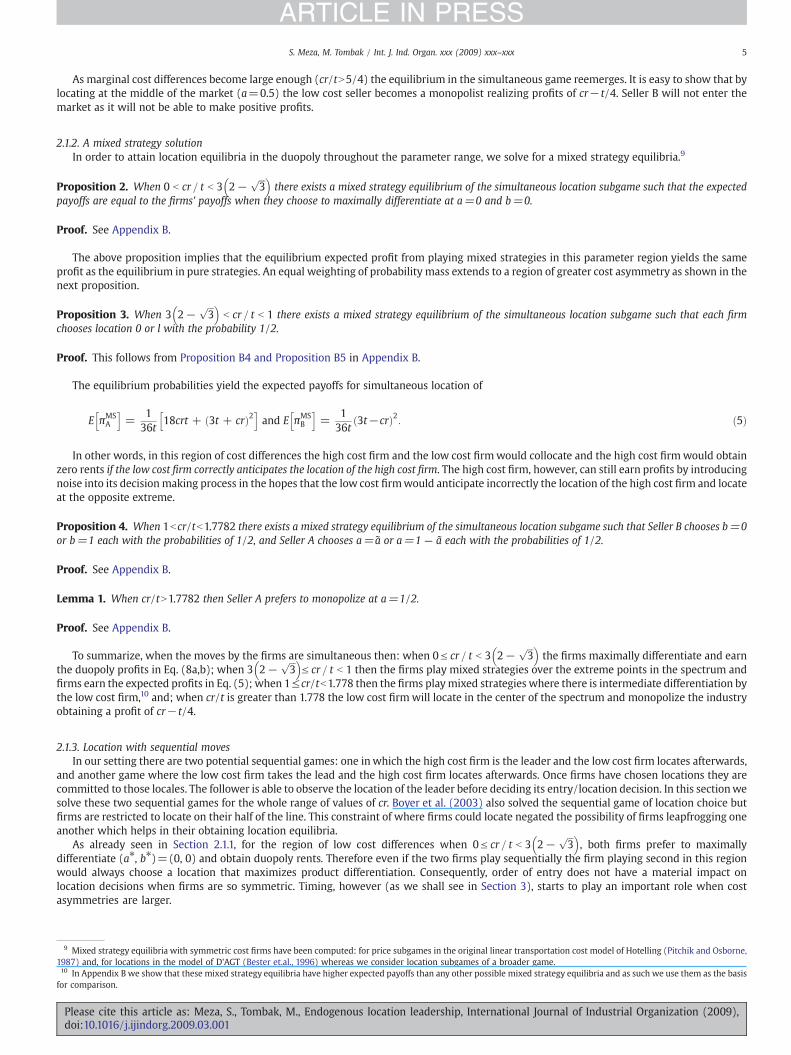
Summarizing the profits realized for the low cost producer being the Stackelberg leader for the various cost asymmetry and locationoutcomes

πA a⁎; b⁎� �

=

118

3t + crð Þ2 a⁎; b⁎� �

= 0;0ð Þ if 0 Vcrt

V 1

8 4t + 3cr + 2ffiffiffiffiffiffiffiffiffiffiffiffiffiffiffiffiffiffiffiffiffiffiffi4t−3crð Þtp� �2

243 2t +ffiffiffiffiffiffiffiffiffiffiffiffiffiffiffiffiffiffiffiffiffiffiffiffiffi4t − 3crð Þtp� � a⁎; b⁎

� �= 1 = 3 −

ffiffiffiffiffiffiffiffiffiffiffiffiffiffiffiffiffiffiffiffiffiffiffiffiffi4t − 3crð Þtp

3t; 0

!if 1 b

crt

b cr=t

cr − t4

� �a⁎; b⁎� �

= 1= 2; NEð Þ if cr=t Vcrt:

8>>>>>>>>><>>>>>>>>>:

Similarly, for Seller B (the high cost producer) being the Stackelberg follower obtains

πB a⁎; b⁎� �

=

118

3t−crð Þ2 a⁎; b⁎� �

= 0; 0ð Þ if 0 Vcrt

V 1

2 6cr−5 2t +ffiffiffiffiffiffiffiffiffiffiffiffiffiffiffiffiffiffiffiffiffiffiffi4t−3crð Þtp� �� �2

243 2t +ffiffiffiffiffiffiffiffiffiffiffiffiffiffiffiffiffiffiffiffiffiffiffiffiffi4t − 3crð Þtp� � a⁎; b⁎

� �= 1= 3 −

ffiffiffiffiffiffiffiffiffiffiffiffiffiffiffiffiffiffiffiffiffiffiffiffiffi4t − 3crð Þtp

3t; 0

!if 1 b

crt

b cr=t

0 a⁎; b⁎� �

= 1= 2; NEð Þ if cr=t Vcrt:

8>>>>>>>><>>>>>>>>:

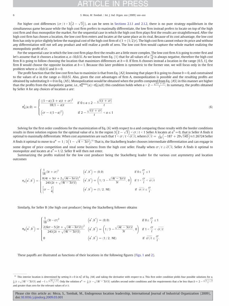
These payoffs are illustrated as functions of their locations in the following figures (Figs. 1 and 2).

11 This interior location is determined by setting b=0 in πA⁎ of Eq. (A4) and taking the derivative with respect to a. This first order condition yields four possible solutions for a,13t t F

ffiffiffiffiffiffiffiffiffiffiffiffiffiffiffiffiffiffiffiffiffiffiffiffiffi4t − 3crð Þtp� �

and −1Fffiffiffiffiffiffiffiffiffiffiffiffiffiffiffiffiffi4t + crð Þt

pt . Only the solution a⁎ = 1

3t t −ffiffiffiffiffiffiffiffiffiffiffiffiffiffiffiffiffiffiffiffiffiffiffiffiffi4t − 3crð Þtp� �

satisfies second order conditions and the requirements that a be less than a = 2−ffiffiffiffiffiffiffiffiffiffiffiffiffiffifficr + 1ð Þt

pt

and greater than zero for the relevant values of cr/t.

Please cite this article as: Meza, S., Tombak, M., Endogenous location leadership, International Journal of Industrial Organization (2009),doi:10.1016/j.ijindorg.2009.03.001

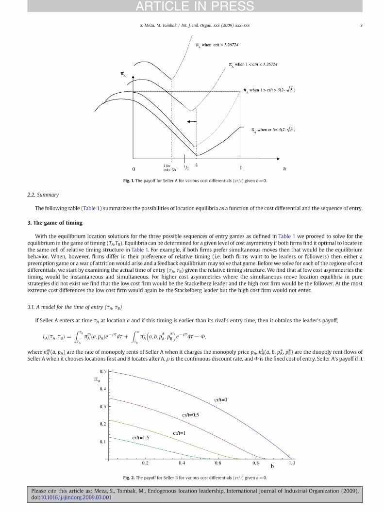
Fig. 1. The payoff for Seller A for various cost differentials (cr/t) given b=0.

7S. Meza, M. Tombak / Int. J. Ind. Organ. xxx (2009) xxx–xxx

ARTICLE IN PRESS

2.2. Summary

The following table (Table 1) summarizes the possibilities of location equilibria as a function of the cost differential and the sequence of entry.

3. The game of timing

With the equilibrium location solutions for the three possible sequences of entry games as defined in Table 1 we proceed to solve for theequilibrium in the game of timing (TA,TB). Equilibria can be determined for a given level of cost asymmetry if both firms find it optimal to locate inthe same cell of relative timing structure in Table 1. For example, if both firms prefer simultaneous moves then that would be the equilibriumbehavior. When, however, firms differ in their preference of relative timing (i.e. both firms want to be leaders or followers) then either apreemption game or awar of attritionwould arise and a feedback equilibriummay solve that game. Before we solve for each of the regions of costdifferentials, we start by examining the actual time of entry (τA, τB) given the relative timing structure. We find that at low cost asymmetries thetiming would be instantaneous and simultaneous. For higher cost asymmetries where the simultaneous move location equilibria in purestrategies did not exist we find that the low cost firm would be the Stackelberg leader and the high cost firm would be the follower. At the mostextreme cost differences the low cost firm would again be the Stackelberg leader but the high cost firm would not enter.

3.1. A model for the time of entry (τA, τB)

If Seller A enters at time τA at location a and if this timing is earlier than its rival's entry time, then it obtains the leader's payoff,

LA τA; τBð Þ =Z τB

τAπmA a;pAð Þe−ρτdτ +

Z ∞

τBπLA a; b;p⁎A ;p

⁎B

� �e−ρτdτ− Φ;

where πAm(a, pA) are the rate of monopoly rents of Seller A when it charges the monopoly price pA, πAL(a, b, pA⁎, pB⁎) are the duopoly rent flows ofSeller Awhen it chooses locations first and B locates after A, ρ is the continuous discount rate, andΦ is the fixed cost of entry. Seller A's payoff if it

Fig. 2. The payoff for Seller B for various cost differentials (cr/t) given a=0.

Please cite this article as: Meza, S., Tombak, M., Endogenous location leadership, International Journal of Industrial Organization (2009),doi:10.1016/j.ijindorg.2009.03.001

Table 1Types of equilibria for each sequence of entry game.

Range of cr/t Simultaneous game Low cost firm is Stackelberg leader High cost firm is Stackelberg leader

0 to 3 2−ffiffiffi3

p� �Duopoly/maximal differentiation Duopoly/maximal differentiation Duopoly/maximal differentiation

3 2−ffiffiffi3

p� �to 1 Duopoly/mixed strategies Duopoly/maximal differentiation Colocation/exit/monopoly

1 to cr= t Duopoly/mixed strategies Duopoly/intermediate differentiation Colocation/exit/monopoly

cr=t to 1:778 Duopoly/mixed strategies Monopoly a=1/2 Colocation/exit/monopoly1.778 to ∞ Monopoly/a=1/2 Monopoly Colocation/exit/monopoly

8 S. Meza, M. Tombak / Int. J. Ind. Organ. xxx (2009) xxx–xxx

ARTICLE IN PRESS

enters the market as the follower (τANτB) is then,

FA τB; τAð Þ =Z ∞

τAπFA a; b; p⁎A ;p

⁎B

� �e−ρτdτ − Φ:

Finally, if the Sellers enter and locate simultaneously the payoff will be

SA τSð Þ =Z ∞

τSπSA a; b;p⁎A ; p

⁎B

� �e−ρτdτ − Φ:

Note that the payoff for simultaneous moves has the same structure as the follower's payoff but the integrand is not deterministic for thesimultaneous gamewhen the location equilibrium in pure strategies does not exist. In that case, the expected payoffs are used. Analogously, thereare leader's and follower's payoffs for Seller B interchanging the A and B subscripts in the above payoffs.

The structure of these payoffs lead to the following.

Lemma 2. The follower, if it wishes to enter at all, would want to enter as soon as possible, i.e., τF→τL.

Proof. Using Leibnitz's rule, we can differentiate the follower's payoff with respect to its entry time and obtain the first order condition,AFBAτB

= − πFB a; b;p⁎A ; p

⁎B

� �e−ρτB , and AFA

AτA= − πF

A a; b;p⁎A ; p⁎B

� �e−ρτA , which are both negative. □

Taking the second derivative of the above follower's payoffs we can find that they are positive, i.e., the payoffs are convex. The above lemmaimplies that there is no possibility for either firm to obtain monopoly rents for some period of time if its rival wishes to enter. Thus the leaders'payoffs simplify to,

LA τA; τBð Þ =Z ∞

τAπLA a; b;p⁎A ; p

⁎B

� �e−ρτdτ− Φ;

and

LB τB; τAð Þ =Z ∞

τBπLB a; b; p⁎A ; p

⁎B

� �e−ρτdτ− Φ:

Similarly, for the leader's simultaneous payoffs we find,

Lemma 3. The payoffs are all diminishing and convex with time.

Proof. As in Lemma 2.

AiBAτB

= − πiB a; b;p⁎A ; p

⁎B

� �e−ρτB , and AiA

AτA= − πi

A a; b; p⁎A ;p⁎B

� �e−ρτA , for i=L, F, Swhich are both negative. Again the second derivatives of the

above are positive implying that the payoffs, regardless of the role of the firm, are convex in time. □

These Lemmas (2) and (3) imply;

Corollary 1. The leader, if it wishes to enter at all, would want to enter as soon as possible, i.e., τL⁎=0,

and,

Corollary 2. Simultaneously entering firms, if they wish to enter at all, would want to enter as soon as possible, i.e., τS⁎=0,

and that the follower, if it enters, would enter at time τF⁎→0, or τF⁎=0+.The above is an implication that there are product market profits to be had and so long as the discounted sum of those profits exceeds Φ, the

fixed cost of entry, then firms are capturing the maximum surplus by moving as rapidly as possible. Thus dominating timing of entry strategies(τA, τB) are: (0,0), (0, 0+), (0+, 0), (0,∞), (∞,0), (∞,∞). In the following subsections we derive the timing equilibria depending on the costasymmetries.

Please cite this article as: Meza, S., Tombak, M., Endogenous location leadership, International Journal of Industrial Organization (2009),doi:10.1016/j.ijindorg.2009.03.001

9S. Meza, M. Tombak / Int. J. Ind. Organ. xxx (2009) xxx–xxx

ARTICLE IN PRESS

3.2. Timing under low cost differences (cr = t b 3 2−ffiffiffi3

p� �)

In this sectionwe determine the equilibrium timingwhen there are small differences in cost. From the previous section (Section 3)we found thatfor this range of cost differential the equilibrium location regardless of the timing is maximal differentiation. As we can see from Table 1 the possibletimings are: (0,0) for the simultaneous game, (0, 0+) when the firm A is leader, and (0+, 0) when firm B is leader.

Proposition 5. For small marginal cost differences (cr = t b 3 2−ffiffiffi3

p� �) the equilibrium planned and entry timing is simultaneous at (TA,TB)=

(τA, τB)=(0, 0).

Proof. From Ziss, when cr = t b 3 2−ffiffiffi3

p� �, the unique location equilibrium entails maximal differentiation and then πBS(a⁎, b⁎, pA⁎, pB⁎)=πBF(a⁎,

b⁎, pA⁎, pB⁎) and πAS(a⁎, b⁎, pA⁎, pB⁎)=πAF(a⁎, b⁎, pA⁎, pB⁎) as the Sellers will locate such that a=b=0 and Lemma 1 still applies. The payoffs SA(0)NFA(0, 0+) and SB(0)NFB(0, 0+). In this case the unique equilibrium timing is simultaneous and immediate. □

In other words, with such slight cost differentials there is no difference in firm behavior with respect to location (which is maximaldifferentiation) and pricing whether the timing of entry is simultaneous and immediate or if any firm waits. As waiting entails a loss of productmarket profits during the delay there is no incentive to delay and the original results of Ziss hold.

3.3. The game of timing when cost differences become significant (3 2−ffiffiffi3

p� �b cr = t b cr=t)

For the parameter region cr = t N 3 2−ffiffiffi3

p� �ourmodel has the payoff structure of awar of attrition. Such games are often plagued bymultiple

equilibria (Hendricks et al., 1988). As Smith (1974) pointed out, “An initial asymmetry in the conditions of a contest can be used to settle it” and hedescribes some examples from the animal kingdom. This suggests that the asymmetries between firms that we describe above may help tosharpen the prognostic power of these models.

From Table 1 we can see that in this region of cost differentials the possible scenarios are: simultaneous entry withmixed strategy equilibria inlocations; the low cost firm acts as the Stackelberg leader and there is maximal differentiation, or; the high cost firm is the Stackelberg leader andthere is collocationwith the high cost firm forced to exit. Clearly this last scenario is dominated for the high cost firm by the other circumstanceswhere it obtains positive expected profits. Also, the low cost firm will always make positive profits by entering the game and so the strategy ofnever entering is dominated. This structure of payoffs leads to the next two propositions.

Lemma 4. When the timing/location game is a war of attrition the high cost firm, if it enters, will always follow (TB⁎=∞).

Proof. Say Seller B followed the strategy to enter after Seller A has entered until a maximum of TB=τB at which time it will enter. The discountedpayoffs to Seller B entering on or before τB (bτB+) for all possible timings of entry by Seller A are: LB(τA, τB) if τANτB+; LB(τA, τB) if τA=τB+; SB(τA,τB) if τA=τB; and, FB(τA, τA+) if τAbτB. If, however, Seller B were to enter after Seller A has entered or wait until time τB+ then its discountedpayoffs for all possible entry timings of Seller A would be: LB(τA, τB+) if τANτB+; SB(τA, τB+) if τA=τB+; FB(τA, τA+) if τA=τB; and, FB(τA, τA+)if τAbτB. This later stream of payoffs dominates the former as: LB(τA, τB)bLB(τA, τB+); LB(τA, τB) if τA=τB+=−ΦbSB(τA, τB+) if τA=τB+; and,FB(τA, τA+)NSB(τA, τB) if τA=τB. Consequently, τB+ ⪰τB∀τB+NτB⇒τB⁎=∞. □

Recall that T is the time of entry if no firm has entered by that time. The above proposition implies that at any time τ the high cost firm willalways be better off to wait and see whether the low cost firm has entered. This logic extends to the limit of waiting forever (TB⁎=∞). This meansthat if Seller A never enters then Seller B will also never enter. As the low cost firm (Seller A) can always profitably enter the market, theproposition above together with Corollary 1 imply that the game of timing reduces to include only the following timing:

Lemma 5. The equilibrium timing of the low cost firm is to enter immediately (TA⁎=0).

Proof. Given that the high cost firmwill always follow (Lemma 4) or never enter, the low cost firm's options are to either be the leader or to neverenter. As LA(τA, τA+)N0∀τA, leading always dominates never entering. The proposition then follows from Corollary 1. □

Thus the possible pure strategy equilibrium timings are: (0,0), (0, 0+), (0,∞). In what follows we endeavor to find the equilibrium timingpairs/locations for this region of significant cost differences. These equilibria differ in the high cost firm's timings and locations of both firms withthe extent of those cost differences and so we divide this region of cost differences into finer sub-regions.

3.3.1. Timing under moderate cost differences (3 2−ffiffiffi3

p� �b cr = t b 1)

For this subset of cost differences within that which cause a war of attrition we find,

Lemma 6. For moderate cost differences (3 2−ffiffiffi3

p� �b cr = t b 1) the dominant timing strategy for the high cost firm is to wait until the low cost rival

commits to a location and if that rival does not enter then it never enters (TB=∞).

Proof. LB(0+, 0)=−Φ as the low cost firm will collocate if allowed to move second (see Table 1). FB(0+, 0++)N0 as this involves maximaldifferentiation and the product market profit flows in the integrand are those given in Eq. (8a,b). FB(0, 0+)N0 and NSB(0),FB 0;0+� �

=R ∞0+

118 3−crð Þ2te−ρtdτ N SB 0ð Þ = R ∞

0136 3−crð Þ2te−ρtdt as

R∞0+

118 e

−ρtdt N 136ρ. □

In other words Lemma 6 states that the dominant strategy for the high cost firm is a feedback strategywhereby this Seller waits until the otherSeller has committed to a location. We are now in a position to determine the equilibrium timing.

Please cite this article as: Meza, S., Tombak, M., Endogenous location leadership, International Journal of Industrial Organization (2009),doi:10.1016/j.ijindorg.2009.03.001

10 S. Meza, M. Tombak / Int. J. Ind. Organ. xxx (2009) xxx–xxx

ARTICLE IN PRESS

Proposition 6. The equilibrium timing for moderate cost differences (3 2−ffiffiffi3

p� �b cr = t b 1) is where the low cost firm moves immediately and the

high cost firm follows immediately thereafter and they maximally differentiate (τA, τB)=(0, 0+).

Proof. Given Lemmas 5, 6 and that LA(0, 0+)NLA(0+, 0++) as both payoffs involve maximal differentiation but the latter involves some delay toobtaining the product market profits. □

Thus the result that the low cost firm takes the role of Stackelberg leader persists for these games of location for moderate cost differentials.The simultaneous game involves mixed strategies which yield some probability of zero or negative profits for the high cost firm whereas aslight delay by the high cost firm ensures that it will obtain the highest profits possible. As the cost differential grows larger still, as weobserved in Section 3.1, the optimal location for the low cost firm changes and this changes the profits in the integrand of the payoffs undervarious timings.

3.3.2. Timing under intermediate cost differences (1 b cr = t b cr=t)When cost asymmetries are such that 1 b cr = t b cr= t a duopoly has the timing of a Stackelberg equilibrium where the low cost firm is the

leader and there is intermediate differentiation. As shown in Section 2.1.1, when cr/tN1 then derivative of πAwith respect to a is no longer negativefor all values of a. In particular, for a=0 the derivative is positive and consequently there is an incentive for Seller A tomove into the interior. FromSection 2.1.3 we find that for cr = t b cr=t, even for the cases where Seller A couldmonopolize, Awould prefer obtaining the duopoly rents at someinterior value for a. The payoffs for Seller A for the region 1bcr/tb5/4 are illustrated in Fig. 1. So as in the previous cost difference region, theequilibrium timing is where the low cost firm moves immediately and the high cost firm follows immediately thereafter (τA, τB)=(0, 0+).

3.4. With large cost differences (cr=t b cr = t)

Here we can find two sub-regions that may result in with the same equilibrium outcome but they must be analyzed separately as the logic bywhich they arrive at that outcome is different.

3.4.1. With substantial cost differences (cr=t b cr = t b 1:778)From Table 1 we can see that if both firms play immediately and simultaneously than the equilibrium would involve a mixed strategy with

locations for the low cost firm being somewhere in the interior. These payoffs (shown in Appendix A), however, are lower in an expected valuesense for the low cost firm than if it were to delay entry and become the Stackelberg follower (in which case it would achieve a payoff of cr). Thehigh cost firm, however, would then deviate from its immediate entry andmixed strategy in locations to also delay as its expected payoff becomesnegative. The low cost firm, as it would achieve zero rents, would then want to deviate to becoming the Stackelberg leader. From the middlecolumn in Table 1, the high cost firm would then want to deviate to simultaneous entry and mixed strategies in locations. Thus we have no purestrategy equilibrium in the game of timing for this range of cost differentials. Alternatively we can try to solve the game in mixed strategies. Inmixed strategies the low cost Seller A can enter at each period with probability α. And the high cost seller can enter each period with probabilityβ. In equilibrium we must find β (and α) that makes Seller A (and Seller B) indifferent between entering this period τa (and τb) or waiting andenter some time after at τa+ (and τb+).

If Seller A decides to enter at time τa given that no seller has entered yet, the expected profit is:

E ΠA½ �@τa= β · SMS

A τa; τað Þ + 1− βð Þ · LA τa;∞ð Þ� �

ð7:aÞ

If instead Seller A decides to wait and enter at time τa+ the expected profit is:

E ΠA½ �@τ+a= β · FA τ+a ; τa

� �+ 1− βð Þ · β · SMS

A τ+a ; τ+a� �

+ 1− βð Þ · LA τ+a ;∞� �� �� ��

ð7:bÞ

In a similar way, if Seller B decides to enter at time given that no seller has entered yet, the expected profit is:

E ΠB½ �@τb= α · SMS

B τb; τbð Þ− 1− αð Þ · Φ · e−ρτb� �

ð8:aÞ

If instead Seller B decides to wait and enter at time the expected profit is:

E ΠB½ �@τ+b

= 1− αð Þ · a · SMSB τ+b ; τ+b� �

− 1− αð Þ · Φ · e−ρτ+b� �

ð8:bÞ

Proposition 7. For substantial cost differences (cr=t b cr = t b 1:778) and separate decisions for entrance and location, two possible timingequilibriums emerge:

i. One in which for each period Seller A and Seller B can enter the market with probabilities:

β⁎ =

α⁎ =Φ

Φ + SMSB τb; τbð Þ

ð1− 2d − 4 FA 1 + dð Þ− SMSA 1− dð Þ

� �−

ffiffiffiffiffiffiffiffiffiffiffiffiffiffiffiffiffiffiffiffiffiffiffiffiffiffiffiffiffiffiffiffiffiffiffiffiffiffiffiffiffiffiffiffiffiffiffiffiffiffiffiffiffiffiffiffiffiffiffiffiffiffiffiffiffiffiffiffiffiffiffiffiffiffiffiffiffiffiffiffiffiffiffiffiffiffiffiffiffiffiffiffiffiffiffiffiffiffiffiffiffiffiffiffiffiffiffiffiffiffiffiffiffiffiffiffiffiffiffiffiffiffiffiffiffiffiffiffiffiffiffiffiffiffiffiffiffiffiffiffiffiffiffiffiffiffiffiffiffiffiffiffiffiffiffiffiffiffiffiffiffiffiffiffiffiffiffiffiffiffiffiffiffiffiffiffiffi2d − 1 + 4 FA − SMS

A

� �· 1− dð Þ� �

− 4d 1− d − 4FA 1− dð Þð Þ 4 FA − SMSA

� �− 1

� �q2d · 4 FA − SMS

A

� �− 1

� �where d=e−ρ(τa+− τa)=e−ρ(τb+− τb) also, F and S are evaluated at τaii. One in which Seller A enters at times and locates at τa=1/2 Monopolizing the market, and Seller B never enters.

Please cite this article as: Meza, S., Tombak, M., Endogenous location leadership, International Journal of Industrial Organization (2009),doi:10.1016/j.ijindorg.2009.03.001

11S. Meza, M. Tombak / Int. J. Ind. Organ. xxx (2009) xxx–xxx

ARTICLE IN PRESS

Proof. For part (i) we make the substitution LA τ+a ;∞� �

= FA τ+a ;∞� �

− 14ρ e

−ρτ+a into Eqs. (7.a) and (7.b). We also make use of the propertythat Π(τa+)=Π(τa)·e−ρ(τa+− τa). Then α⁎ and β⁎ are obtained as the unique solutions in the range (0,1) that solves and E[ΠA]@τa=E[ΠA]@τa+

and E[ΠB]@τb=E[ΠB]@τb+·n For part (ii) we replaced α⁎ in Eqs. (8.a) or (8.b) and we obtain E[ΠB]@τb=E[ΠB]@τb+=0. This implies that Seller Bis indifferent to never entering the market. Since we are assuming that Seller B is risk neutral, never entering the market leads the same payoff asE[ΠB]@τb. As a response to the “never entering” solution of Seller B (or β⁎=0 in Eqs. (7.a) or (7.b)), Seller A will benefit for entering as soon aspossible at time τa=0, to realize profits LA by locating at a=1/2. □

The high cost firm is indifferent between the two possible equilibria above— it obtains zero expected economic rents in both cases. The mixedstrategy game, however, is sensitive to any perturbation of risk neutrality. The low cost firm, however, would prefer the mixed strategy game as itobtains some possibility of the payoff from the simultaneous game of mixed strategies in location. The mixed strategy equilibrium, however, isunstable. While we do not model this here, this means that there may be an incentive for the low cost firm to offer the high cost firm a sidepayment for committing to play the mixed strategy game. The expected time of the low cost firm entering the market is then τA = 1

1 − αð Þ ln 1−αð Þ2which then delays any payoff to the low cost Seller.

3.4.2. Under extreme cost differences (1.778bcr/t)For this range of cost differentials the low cost firmwill monopolize regardless of the mixed strategies in locations the high cost firm employs

(see Appendix B). The low cost monopolist would locate in the middle of the Hotelling line and engage in limit pricing. The timing of the low costfirm would thereby be immediate while the high cost firm would never enter, i.e., (TA, TB)=(τA⁎, τB⁎)=(0, ∞).

4. Summary and discussion

In this sectionwe summarize the results from our analysis of imperfectly competitive markets in the previous sections. We then compute thefirst-best welfare outcomes and compare the results of privately optimal behavior to the socially optimal. We then contrast our results with thedifferentiated Bertrand model with those of others using the Cournot model.

Summarizing the discussion in the above section, we have the following proposition.

Proposition 8. In a Stackelberg game of location choice, the equilibrium locations of Sellers A and B (a⁎, b⁎) depend on the marginal cost differences asfollows:

τA; τBð Þ a⁎; b⁎� �

=

0;0ð Þ 0;0ð Þ if 0 V cr = t V 3 2−ffiffiffi3

p� �0;0+� �

0;0ð Þ if 3 2−ffiffiffi3

p� �V cr = t V 1

0;0+� �

1= 3 1−ffiffiffiffiffiffiffiffiffiffiffiffiffiffiffiffiffi4− 3cr

p� �;0

� �if 1 b cr = t b cr

DE if cr b cr = t b 1:7780;∞ð Þ 1 = 2;NEð Þ if 1:778 V cr = t

8>>>>>>>><>>>>>>>>:where NE denotes “No Entry” and DE “Dual Equilibria” which are those defined in Proposition 7 — one equilibrium being where the low costfirm enters immediately and monopolizes at location a = 1

2, the other equilibriumwhere the firms play mixed strategies in timing. Interestingly,note that the low cost firm always enters immediately,12 while the high cost firm could enter immediately, delay entrance or never enter. Thisissue has important implications — by entering first the low cost firm relinquishes its potentially dominant position and must accept its secondbest profits (for most of the cost differential range). The high cost firm, however, “wins”whenever the game is a war of attrition in the sense thatit moves last in equilibrium.

Having determined the equilibrium behavior, we now compute the first-best solution for a total welfaremaximizing policymaker andwe thencompare this solution to that derived above. In this case the first-best involves the social planner setting both locations and prices for both thefirms. The total welfare given a reservation value of consumers of v is and the point of the indifferent consumer being x ,

S =Z x

0v − 1− r

2

� �c − t x−að Þ2

h idx +

Z 1

xv − 1 +

r2

� �c − t x− 1−bð Þð Þ2

h idx:

That is, the total surplus is the reservation values less the costs of production and the transportation costs for all the consumers served. Unlikethe symmetric cost case where the prices did not matter for total welfare computations, here the cost structure does affect total surplus throughthe allocation of consumers to either the high production cost firm or the low production cost firm. The social planner here must, on occasion,tradeoff some transportation cost with production costs.

Simultaneously solving the above expression for the minimum cost values of a, b, and x yields the socially optimal values,

a⁎⁎ =14

+crt; b⁎⁎ =

14

− crt; x ⁎⁎ =

12

+2crt

8 crt

V14:

Beyond cr/t=1/4 it is socially optimal to have the low cost firm monopolize the market at a location of a⁎⁎=1/2. The above show a verysimple and intuitive relationship between the socially optimal locations and the cost differential related to the socially optimal locations found forsymmetric firms (a⁎⁎, b⁎⁎)=(1/4,1/4) (see, for example, Tirole, 1989, pg. 282). That is, cost differentials (of a mean preserving spread) do notincrease the socially optimal degree of differentiation but shift both sellers and allocate more consumers to the lower cost firm. The other

12 With the exception of the region where one of the possible equilibrium is to enter immediately with probability α but, here too the low cost firm commits to begin playing themixed strategy game immediately.

Please cite this article as: Meza, S., Tombak, M., Endogenous location leadership, International Journal of Industrial Organization (2009),doi:10.1016/j.ijindorg.2009.03.001

12 S. Meza, M. Tombak / Int. J. Ind. Organ. xxx (2009) xxx–xxx

ARTICLE IN PRESS

interesting aspect to note is that the degree of cost differentiation at which monopoly becomes socially optimal is much lower than that derivedabove for the imperfect competition case. Monopoly becomes socially optimal at cr/t=1/4 whereas monopoly did not become the equilibriumuntil cr = t z 1:267 cr

� �. Thewelfaremaximizing timing is the immediate entry and location of firms. Recall that this result was predicated on the

social planner being able to set the first-best prices as well as locations where no consumer balks.Comparing our welfare results on the effects of asymmetries in a differentiated Bertrand setting to those of Salant and Shaffer (1999) with a

Cournot model we find both robust effects as well as some interesting differences. Under both product market competition models asymmetriesincrease welfare by allocating more output to themore efficient producer. Under differentiated Bertrand with small cost differences, this is achievedsolely throughprice competition but as those asymmetries grow the shift inmarket shares accelerate due to decreased differentiation.13 Unlike Salantand Shafferwhofind that private and social optima to coincide under Cournot (when developing those asymmetries do not involve additional costs),we find that with differentiated Bertrand they only coincide at the point where our cost differences cr = t 14 otherwise there are excessive privateincentives to differentiate. Also, we find that there are private incentives to maintain a duopoly market structure for greater cost differences than issocially optimal. This reinforces Salant and Shaffer's warning that an increase in the Hershmann–Herfindahl index need not be welfare decreasing.

The analysis here can be extended in a number of interesting ways. First, the order of entry may determine costs when phenomena such aslearning-by-doing are important.14 As we (and others) have shown the low cost firm obtains a profit premium in the equilibrium of adifferentiated Bertrand game. In this setup our game of timingmay revert to a competition for first move or a game of preemption rather than ourwar of attrition. Another possible interesting extensionwould be to examine the case where consumers had switching costs. This also, may makemoving first more valuable and change the structure of the game of timing. Another possible interesting extension of the above would be toexamine the timing of the game along the lines of Boyer et al. (1994), that is, under incomplete information. With incomplete information it maybe possible that each firm thinks it is the high cost firm and refuses to enter until after the other firm which may lead to an equilibrium whereneither firm enters, i.e., the timing of entry would signal what firms believe are their relative costs.

Finally, an interesting extension of the present analysis would be to expand the possible sets of locations to those beyond the locations ofconsumers. In our model, if we allowed locations beyond (0,1) then the difference in costs at which we no longer have an equilibrium(cr = t N 3 2−

ffiffiffi3

p� �) would increase. This is because the high cost firm would locate at bb0 which, in turn means that the duopoly rents for the

low cost firm would be higher than those illustrated in Fig. 1 while the monopoly rents would remain at cr. At some (higher) level of costdifference monopoly would be preferred and the war of attrition would resume and qualitatively our results would be similar. Tyagi (2000) hasexamined the case where Seller locations extend beyond the 0 and 1 points with a certain sequential timing imposed. In his model for a certainregion of cost differences both of the firmswouldwant to preempt and locate in themiddle of the spectrum forcing its rival to differentiate. In thatmodel, however, the location equilibrium would no longer be unique. In the Tyagi model, the game of timing changes in an essential way fromours — from a war of attrition to a war of preemption (Claim 1 of Tyagi). Thus, allowing a larger spectrum of location in our analysis may giveadditional advantages to the low cost firm.

Our results are generally consistent with the notion of having lower costs of production being a “competitive advantage” but the analysis ismore precise inwhat the nature of the advantages are andwhen they occur. We show that cost differences must go beyond a certain threshold forproduct positioning behavior to change, i.e., that low cost firmsmay seek less differentiationwhile managers of higher cost firmsmust wait for itsrival to enter to then be able to differentiate their product. This result has interesting implications for the concept of market leadershipadvantages. It has been argued that market leaders have an advantage over followers because they can capture the most advantageous location inthe market. Our results introduce endogeneity to that argument — it may not be that the firm that moves first thereby acquires an advantage,rather it could be that the firm with an advantage is the one that can enter first.

Appendix A. The price stage

In the price game players A and B have strategies pA and pB (where the prices could range from zero to infinity). The payoff functions for thetwo players are given by:

πA pA; pBð Þ = pA − 1− r2

� �c

� �a +

12Δ +

pB − pA2tΔ

� �and

πB pA;pBð Þ = pB − c 1 +r2

� �� �b +

12Δ +

pA − pB2tΔ

� �if

pB − t 1−að Þ2 − b2h i

V pA V pB + t 1−bð Þ2 − a2h i

;

πA pA; pBð Þ = pA − 1− r2

� �c and

πB pA;pBð Þ = 0 if pA b pB − t 1−að Þ2 − b2h i

;

πA pA; pBð Þ = 0 and

πB pA;pBð Þ = pB − 1 +r2

� �c if pA N pB + t 1−bð Þ2 − a2

h i:

ðA1Þ

where Δ=1−a−b, Δ, a, b≥0.The first part of the payoff function defines the region where duopoly is sustained. The second and third parts define the regions where one of the

firmsmonopolizes themarket bydecreasing thepricewith respect to the rival to thepoint inwhichno consumerswill go topurchase fromthe rival seller.

13 This finding has an analogous result in the trade literature where a more productive firm would engage in exporting (Melitz, 2003).14 This idea is attributable to Chung Yi Tse.

Please cite this article as: Meza, S., Tombak, M., Endogenous location leadership, International Journal of Industrial Organization (2009),doi:10.1016/j.ijindorg.2009.03.001

13S. Meza, M. Tombak / Int. J. Ind. Organ. xxx (2009) xxx–xxx

ARTICLE IN PRESS

Solving for the price equilibrium of the first part of the above system of Eq. (A1) yields (as in Ziss, 1993; Boyer et al., 2003, Appendix A.3) theduopoly price equilibria and profits:

p⁎A =16

2 3 + a − bð ÞΔt + 6c − crð Þ; p⁎B =16

2 3− a + bð ÞΔt + 6c + crð Þ

and,

π⁎A =3 + a−bð ÞΔt + crð Þ2

18Δtand; π⁎B =

3−a + bð ÞΔt−crð Þ218Δt

: ðA2Þ

And the region where duopoly can be sustained from Eq. (A1) is reduced to,

3− a + bð ÞΔ Ncrt: ðA3Þ15

For the secondand third part of the function in Eq. (A1), only SellerAhas in equilibrium theability tomonopolize themarket for somevalues ofa,band cr. Since Seller B cannot decrease its price below its marginal cost (pB≥c (1+r/2)), Seller A can take advantage of this and decrease its price,undercutting Seller B, and still having a price above its marginal cost (pA≥c (1−r/2)). The conditions for Seller A to monopolize the market are,

c 1− r2

� �b pA b c 1 +

r2

� �− t 1−að Þ2 − b2

h i: ðA4Þ

Thus Seller A's ability to monopolize depends on its proximity to Seller B and the marginal cost differences and it is possible in the region crN t(1−a)2−b2. Even though this region overlaps with some values in which duopoly is sustained it is easy to show16 that for Seller A monopoly isgoing to be the preferred outcome only outside of the duopoly region. Consequently for the region defined by 3− a + bð ÞΔ V cr

t the equilibriumprice and monopoly rents of Seller A are then:

p⁎A = c 1 +r2

� �− t 1−að Þ2 − b2

h iand

π⁎A = cr − t 1−að Þ2 − b2h i

ðA5Þ

Clearly, in equilibrium it is not possible for Seller B to monopolize, as any undercutting the marginal costs of Seller A would involve losses forSeller B.

Appendix B. Solution to the Mixed Strategy Game

In contrast with the deterministic choice of locations of the simultaneous game, for the mixed strategies game it is assumed that both sellersrandomly choose locations based on known probability distributions. A Nash equilibrium in mixed strategies is when each seller chooses aprobability distribution that maximizes its own expected profit given the choice of probability distribution of the other seller.

Let's assume Seller A locates at a∊ [0,1] with probability distribution fA(a), fA(.)∊F, where F represents the infinite number of linearlyindependent distribution functions fi(x) subject to

fi xð Þz 0 for all xa 0:1½ �; andZ 1

x = 0fi xð Þ;dx = 1:

In the same way, Seller B locates at b∊ [0.1] with probability distribution fB(b), fB(.)∊F. The expected profit for Seller A is then given by:

ΠMSA fA að Þ; fB bð Þð Þ = E ΠA½ � = RR 1;1

a = 0;b = 0 ΠA a; bð ÞfA að ÞfB bð Þdbda

and that for Seller B is given by,

ΠMSB fA að Þ; fB bð Þð Þ = E ΠB½ � = RR 1;1

b = 0;a = 0 ΠB a; bð ÞfA að ÞfB bð Þdadb

In equilibrium, the pair of probability distributions fA(a) and fB(b) has to simultaneously maximize the expected profits of both sellers. That is,we need to find fA(a) and fB(a) that solves:

maxfA að Þ

ΠMSA fA að Þ;

:f B bð Þ

� �and

maxfB bð Þ

ΠMSB

:f A að Þ; fB bð Þ

� �Theoretically a solution in mixed strategies always exists, however the finding of such solutions may be a nontrivial task. The structure of our

model leads to solutions to this problem and allows us to find Nash equilibria. To facilitate this process, we segregate the analysis into four ranges

15 Eq. (A3) is equivalent to Ziss' condition (6d) and to that of Boyer et al.'s (Appendix A.1).16 By solving for the region when profit πA⁎ defined by Eq. (A5) is larger than the profit πA⁎ defined in Eq. (A2) or cr − t 1−að Þ2 − b2

h iN 3 + a−bð ÞΔt + crð Þ2

18Δt .

Please cite this article as: Meza, S., Tombak, M., Endogenous location leadership, International Journal of Industrial Organization (2009),doi:10.1016/j.ijindorg.2009.03.001

14 S. Meza, M. Tombak / Int. J. Ind. Organ. xxx (2009) xxx–xxx

ARTICLE IN PRESS

of cost differentials. In the first region both sellers benefit from maximum differentiation. In the second region the low cost firmwould be betteroff by undercutting the high cost seller and if this option is not feasible, then the low cost firm seeks again maximum differentiation. The thirdregion is similar to the previous one, but it differs in that if no undercutting is possible, the low cost seller does not try to maximally differentiatebut instead moves to an intermediate region. Finally in the fourth region, the low cost seller monopolizes the market.

B1. Region for 0 V cr = t b 3 2−ffiffiffi3

p� �In this region, as was shown in Section 3.1, the pure strategy equilibrium locations for the simultaneous game are such that both sellers prefer

tomaximally differentiate. However it is important to verify that there is no other solution in themixed strategy games that could be preferred byeither of the two sellers. We start by redefining the simultaneous game solution in terms of a mixed strategies game solution. Then we need toshow that this solution is a Nash equilibrium and that it is also a perfect equilibrium solution of the mixed strategies game. That is, we will showthat neither of the sellers would benefit from playing any other strategy regardless of what the other player chooses. Then that pair of strategies isnot only a Nash equilibrium but also the perfect equilibrium solution of the mixed strategies game.

To redefine the solution in terms of a mixed strategies game, let's assume that Seller A locates following probability distribution fA0(a) defined

as locating at a=0with probability mass of 1. Seller B locates following probability distribution fB0(b) defined as location at b=0with probability

mass of 1.17 This solution is an identical representation of the solution a=0, b=0 of the simultaneous game. It is easy to see then that

ΠMSA f 0A að Þ; f 0B bð Þ� �

=RR 1;1

a = 0;b = 0 ΠA a; bð ÞfA að ÞfB bð Þdbda = ΠDuoA 0:0ð Þ

and

ΠMSB f 0A að Þ; f 0B bð Þ� �

=RR 1;1

b = 0;a = 0 ΠB a; bð ÞfA að ÞfB bð Þdadb = ΠDuoB 0:0ð Þ

Proposition B1. When 0 b cr b 3 2−ffiffiffi3

p� �Sellers A and B playing according to the probability distributions fA

0(a) and fB0(b) is the perfect equilibrium

for the mixed strategy game.

Proof. To show that playing strategies fA0(a) and fB0(b) is the perfect equilibrium solution we need to compare the expected profits under these

strategies with those of any other possible alternative strategy. Let's define a pair of alternative general strategies fA1(a) and fB1(b). Where fA

1(a) isthe strategy of Seller A defined as locating at a=0with mass probability of α, α∊ [0,1] and locating at all other points with mass probability 1−αand following probability distributionbf 1A að Þ, subject to R 1x = 0+bf 1A xð Þ;dx = 1. Seller B follows the probability distribution fB

1(b) that is defined aslocating at b=0 with mass probability of β, β∊ [0,1] and locating at all other points with mass probability 1−β and following probabilitydistributionbf 1B bð Þ, subject to R 1x = 0+

bf 1B xð Þ;dx = 1. Notice that when α=1 and β=1, the strategies fA1(a) and fB1(b) become fA

0(a), fB0(b).The expected profits of strategies fA1(a) and fB

1(b) are:

ΠMSA f 1A að Þ; f 1B bð Þ� �

= α · β · ΠDuoA 0:0ð Þ + α · 1− βð Þ ·

Z 1

b = 0+ΠA 0; bð Þbf 1B bð Þdb + α − 1ð Þ · β ·

Z 1

a = 0+ΠA a;0ð Þbf 1a að Þda

+ 1− αð Þ · 1− βð Þ · RR 1;1a = 0+ ;b = 0+ ΠA a; bð Þbf 1A að Þbf 1B bð Þdbda

ðB:1Þ

and,

ΠMSB f 1A að Þ; f 1B bð Þ� �

= α · β · ΠDuoB 0:0ð Þ + α · 1− βð Þ ·

Z 1

b = 0+ΠDuo

B 0; bð Þbf 1B bð Þdb + α − 1ð Þ · β ·Z 1

a = 0+ΠDuo

B a;0ð Þbf 1a að Þda

+ 1− αð Þ · 1− βð Þ · RR 1;1b = 0+ ;a = 0+ ΠDuoB a; bð Þbf 1A að Þbf 1B bð Þdadb

ðB:2Þ

Since profits ΠADuo and ΠB

Duo are at their maximum when a=0, and b=0, it is easy to see that:

RR 1;1a = 0+ ;b = 0+ ΠA a; bð Þbf 1A að Þbf 1B bð Þdbda b ΠDuo

A 0:0ð Þ; and R 1a = 0+ ΠA a;0ð Þbf 1A að Þda b ΠDuoA 0:0ð Þ

and also,

RR 1;1b = 0+ ;a = 0+ ΠDuo

B a; bð Þbf 1A að Þbf 1B bð Þdadb b ΠDuoB 0:0ð Þ; and R 1a = 0+ ΠDuo

B a;0ð Þbf 1A að Þda b ΠDuoB 0:0ð Þ:

Because duopolistic profits for both sellers decrease when the competitor moves closer (dΠDuoA

db b 0 and dΠDuoB

da b 0), andmonopolistic profits forthe low cost seller are never larger than the duopolistic profits at (0,0) it also holds that:Z 1

b = 0+ΠA 0; bð Þbf 1B bð Þdb b ΠDuo

A 0:0ð Þ andZ 1

b = 0+ΠDuo

B 0; bð Þbf 1B bð Þdb b ΠDuoB 0:0ð Þ

It follows then that for any value of α, α∊ [0,1) and β, β∊ [0,1) it is always true that:

ΠMSA f 0A að Þ; f 0B bð Þ� �

= ΠDuoA 0:0ð ÞN ΠMS

A f 1A að Þ; f 1B bð Þ� �

and;

ΠMSB f 0A að Þ; f 0B bð Þ� �

= ΠDuoB 0:0ð ÞN ΠMS

B f 1A að Þ; f 1B bð Þ� �

:

17 By symmetry this game is identical to the one in which seller A plays a=1 with probability 1 and seller B plays b=1 with probability 1.

Please cite this article as: Meza, S., Tombak, M., Endogenous location leadership, International Journal of Industrial Organization (2009),doi:10.1016/j.ijindorg.2009.03.001

15S. Meza, M. Tombak / Int. J. Ind. Organ. xxx (2009) xxx–xxx

ARTICLE IN PRESS

Since there is no other strategy that would give Seller A or B equal or higher profits than those obtained at fA0(a) and fB0, none of the two firms

has an incentive to deviate from this strategy. Consequently, the pair of strategies fA0(a) and fB0(b) is not only a Nash equilibrium but also a perfect

equilibrium for the mixed strategy game. □

B2. Region for 3 2−ffiffiffi3

p� �V cr = t b 1

In this region the low cost firm gets the highest profits by sitting on top of high cost seller. But the high cost seller still benefits from locating asfar as possible from the low cost seller. This situation leads to a structure similar to a generalized “tennis game” as inWalker andWooders (2001).Since no equilibrium exists in the simultaneous game, we seek Nash equilibrium in the mixed strategies game. We start by analyzing the simplestrategy in which both players randomly alternate between the two extreme locations a=0 and a=1 for the low cost Seller A, and b=0 andb=1 for the high cost Seller B. We find that for the game, in equilibrium both players will choose each of the two locations with identicalprobability of 1/2. We then show that this strategy is a Nash equilibrium. Finally we show that there is no other strategy that in equilibriumwillgive higher expected profits to either of the two sellers.

Proposition B2. If Seller A randomizes its location between location a=0 and a=1, with probabilities α and 1−α and Seller B randomizes its locationbetween location b=0 and b=1, with probabilities β and 1−β then the only equilibrium solution is when probabilities are α=β=1/2.

Proof. Suppose Seller A chooses a=0 with probability α. Seller B should then locate at b=0 if

α · πB 0;0ð Þ + 1− αð ÞπB 1;0ð ÞN α · πB 0;1ð Þ + 1− αð ÞπB 1;1ð Þ

Suppose Seller B chooses b=0 with probability β. Seller A should then locate at a=1 if

β · πB 1;0ð Þ + 1− βð ÞπB 1;1ð ÞN β · πB 0;0ð Þ + 1− βð ÞπB 0;1ð Þ

At equilibrium probabilities being:

α =πB 0;1ð Þ− πB 0;0ð Þ

πB 0;1ð Þ− πB 0;0ð Þ + πB 1;0ð Þ− πB 1;1ð Þð Þ ; and β =πA 0;1ð Þ− πA 0;0ð Þ

πA 0;1ð Þ− πA 0;0ð Þ + πA 1;0ð Þ− πA 1;1ð Þð Þ

that is, each seller chooses a probability that makes the other seller indifferent. As πB(0,1)=πB(1,0)=0 and πB(0,0)=πB(1,1) consequently,α=1−α=1/2. Similarly, πA(0,1)=πA(1,0) (monopoly rents for Seller A) and πA(0,0)=πA(1,1) (the profits with maximal differentiation) andconsequently, β=1−β=1/2. That is, with a probability of 1/2 Seller B obtains themaximal differentiation profits and Seller A obtainsmonopolyrents with a probability of 1/2 and maximal differentiation rents with probability of 1/2. □

We can now define these strategies in terms of the probability distributions fA2(a) and fB

2(b). Probability distribution fA2(a) is the strategy

of Seller A of locating at a=0 with mass probability of 1/2 and locating at a=1 with mass probability of 1/2. Similarly, probabilitydistribution fB

2(b) is the strategy of Seller B of locating at b=0 with mass probability of 1/2 and locating at b=1 with mass probabilityof 1/2.

Proposition B3. The mixed strategies in which Seller A (B) randomizes following probability distribution fA2(a) (fB2(b)) is a Nash equilibrium.

Proof. In order to prove that this is Nash equilibrium, we need to show: (i) when Seller B chooses to play following probability distribution fB2(b)

the best response (in terms of maximising expected profits) for Seller A is to play following probability distribution fA2(a), and; (ii) when Seller A

chooses to play following probability distribution fA2(a) the best response (in terms of maximising expected profits) for Seller B is to play

following probability distribution fB2(b).

Let's assume that Seller B chooses to play following probability distribution fB2(b). The expected profits of Seller A as a function of a are given by:

ΠMSA a; f 2B bð Þ� �

=Z 1

b = 0+ΠA a; bð Þf 2B bð Þdb = 1= 2ΠA a;0ð Þ + 1 = 2ΠA a;1ð Þ ðB:3Þ

Since

ΠA a;0ð Þ =3−2a−a2 + cr=t� �2

18 1− að Þ · t; if 0 b a V 2−ffiffiffiffiffiffiffiffiffiffiffiffiffiffiffiffiffiffiffiffiffi1 + cr = t

pcr − 1−að Þ2; if 2−

ffiffiffiffiffiffiffiffiffiffiffiffiffiffiffiffiffiffiffiffiffi1 + cr = t

pb a V 1

8>><>>:and

ΠA a;1ð Þ =cr − a2; if 0 b a V

ffiffiffiffiffiffiffiffiffiffiffiffiffiffiffiffiffiffiffiffiffi1 + cr = t

p− 1

3−2 1−að Þ− 1−að Þ2 + cr= t� �2

18a· t; if

ffiffiffiffiffiffiffiffiffiffiffiffiffiffiffiffiffiffiffiffiffi1 + cr = t

p− 1 b a V 1

8>><>>:

Please cite this article as: Meza, S., Tombak, M., Endogenous location leadership, International Journal of Industrial Organization (2009),doi:10.1016/j.ijindorg.2009.03.001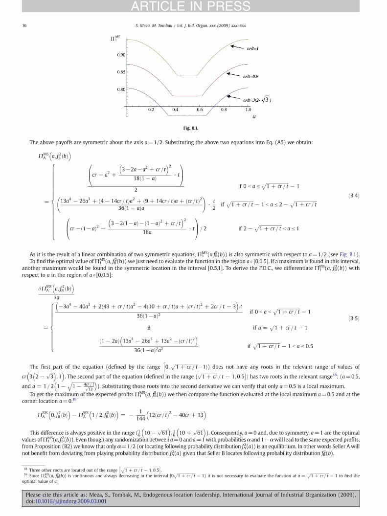

Fig. B.1.

16 S. Meza, M. Tombak / Int. J. Ind. Organ. xxx (2009) xxx–xxx

ARTICLE IN PRESS

The above payoffs are symmetric about the axis a=1/2. Substituting the above two equations into Eq. (A5) we obtain:

ΠMSA a; f 2B bð Þ� �

=

cr − a2 +3−2a−a2 + cr=t� �2

18 1− að Þ · t

0B@1CA

2if 0 b a V

ffiffiffiffiffiffiffiffiffiffiffiffiffiffiffiffiffiffiffiffiffi1 + cr = t

p− 1

13a4 − 26a3 + 4− 14cr = tð Þa2 + 9 + 14cr = tð Þa + cr=tð Þ236 1− að Þa

!·

t2

ifffiffiffiffiffiffiffiffiffiffiffiffiffiffiffiffiffiffiffiffiffi1 + cr = t

p− 1 b a V 2−

ffiffiffiffiffiffiffiffiffiffiffiffiffiffiffiffiffiffiffiffiffi1 + cr = t

p

cr − 1−að Þ2 +3−2 1−að Þ− 1−að Þ2 + cr=t� �2

18a· t

0B@1CA= 2 if 2−

ffiffiffiffiffiffiffiffiffiffiffiffiffiffiffiffiffiffiffiffiffi1 + cr = t

pb a V 1

8>>>>>>>>>>>>>>>>>>><>>>>>>>>>>>>>>>>>>>:

ðB:4Þ

As it is the result of a linear combination of two symmetric equations, Π1MS(a,fB2(b)) is also symmetric with respect to a=1/2 (see Fig. B.1).

To find the optimal value ofΠ1MS(a, fB2(b)) we just need to evaluate the function in the region a∊ [0,0.5]. If a maximum is found in this interval,

another maximum would be found in the symmetric location in the interval [0.5,1]. To derive the F.O.C., we differentiate Π1MS(a, fB2(b)) with

respect to a in the region of a∊ [0,0.5]:

AΠMSA a; f 2B bð Þ� �Aa

=

−3a4 − 40a3 + 2 43 + cr = tð Þa2 − 4 10 + cr = tð Þa + cr=tð Þ2 + 2cr = t − 3� �

:t

36 1−að Þ2 if 0 b a bffiffiffiffiffiffiffiffiffiffiffiffiffiffiffiffiffiffiffiffiffi1 + cr = t

p− 1

Z if a =ffiffiffiffiffiffiffiffiffiffiffiffiffiffiffiffiffiffiffiffiffi1 + cr = t

p− 1

1− 2að Þ 13a4 − 26a3 + 13a2 − cr=tð Þ2� �

36 1−að Þ2a2 ifffiffiffiffiffiffiffiffiffiffiffiffiffiffiffiffiffiffiffiffiffi1 + cr = t

p− 1 b a V 0:5

8>>>>>>>>>><>>>>>>>>>>:

ðB:5Þ

The first part of the equation (defined by the range 0;ffiffiffiffiffiffiffiffiffiffiffiffiffiffiffiffiffiffiffiffiffi1 + cr = t

p−1Þ

h) does not have any roots in the relevant range of values of

cr 3 2−ffiffiffi3

p� �;1

� �. The second part of the equation (defined in the range

ffiffiffiffiffiffiffiffiffiffiffiffiffiffiffi1 + cr

p= t − 1;0:5

� Þ has two roots in the relevant range18: (a=0.5,

and a = 1= 2 1−ffiffiffiffiffiffiffiffiffiffiffiffiffiffiffiffiffiffiffiffiffi1− 4cr = tffiffiffiffi

13p

q� �). Substituting those roots into the second derivative we can verify that only a=0.5 is a local maximum.

To get the maximum of the expected profits Π1MS(a, fB2(b)) we then compare the function evaluated at the local maximum a=0.5 and at the

corner location a=0.19

ΠMSA 0; f 2B bð Þ� �

− ΠMSA 1= 2; f 2B bð Þ� �

= − 1144

12 cr=tð Þ2 − 40cr + 13� �

This difference is always positive in the range (16 10−ffiffiffiffiffiffi61

p� �; 16 10 +

ffiffiffiffiffiffi61

p� �). Consequently, a=0 and, due to symmetry, a=1 are the optimal

values ofΠ1MS(a, fB2(b)). Even though any randomizationbetweena=0and a=1withprobabilitiesα and 1−αwill lead to the sameexpected profits,

from Proposition (B2) we know that only α=1/2 (or locating following probability distribution fA2(a)) is an equilibrium. In other words Seller Awill

not benefit from deviating from playing probability distribution fA2(a) given that Seller B locates following probability distribution fB

2(b).

18 Three other roots are located out of the rangeffiffiffiffiffiffiffiffiffiffiffiffiffiffiffiffiffiffiffiffiffi1 + cr = t

p− 1;0:5

h i.

19 Since ΠAMS(a, fB2(b)) is continuous and always decreasing in the interval [0

ffiffiffiffiffiffiffiffiffiffiffiffiffiffiffiffiffiffiffiffiffi1 + cr = t

p− 1) it is not necessary to evaluate the function at a =

ffiffiffiffiffiffiffiffiffiffiffiffiffiffiffiffiffiffiffiffiffi1 + cr = t

p− 1 to find the

optimal value of a.

Please cite this article as: Meza, S., Tombak, M., Endogenous location leadership, International Journal of Industrial Organization (2009),doi:10.1016/j.ijindorg.2009.03.001

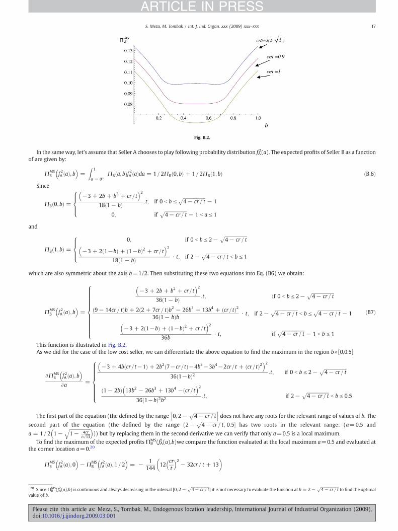
Fig. B.2.

17S. Meza, M. Tombak / Int. J. Ind. Organ. xxx (2009) xxx–xxx

ARTICLE IN PRESS

In the sameway, let's assume that Seller A chooses to play following probability distribution fA2(a). The expected profits of Seller B as a function

of are given by:

ΠMSB f 2A að Þ; b� �

=Z 1

a = 0+ΠB a; bð Þf 2A að Þda = 1= 2ΠB 0; bð Þ + 1 = 2ΠB 1; bð Þ ðB:6Þ

Since

ΠB 0; bð Þ =−3 + 2b + b2 + cr=t� �2

18 1− bð Þ :t; if 0 b b Vffiffiffiffiffiffiffiffiffiffiffiffiffiffiffiffiffiffiffiffi4− cr = t

p− 1

0; ifffiffiffiffiffiffiffiffiffiffiffiffiffiffiffiffiffiffiffiffi4− cr = t

p− 1 b a V 1

8>><>>:and

ΠB 1; bð Þ =0; if 0 b b V 2−

ffiffiffiffiffiffiffiffiffiffiffiffiffiffiffiffiffiffiffiffi4− cr = t

p−3 + 2 1−bð Þ + 1−bð Þ2 + cr=t� �2

18 1− bð Þ · t; if 2−ffiffiffiffiffiffiffiffiffiffiffiffiffiffiffiffiffiffiffiffi4− cr = t

pb b V 1

8>><>>:which are also symmetric about the axis b=1/2. Then substituting these two equations into Eq. (B6) we obtain:

ΠMSB f 2A að Þ; b� �

=

−3 + 2b + b2 + cr=t� �2

36 1− bð Þ :t; if 0 b b V 2−ffiffiffiffiffiffiffiffiffiffiffiffiffiffiffiffiffiffiffiffi4− cr = t

p9− 14cr = tð Þb + 2 2 + 7cr = tð Þb2 − 26b3 + 13b4 + cr=tð Þ2

36 1− bð Þb · t; if 2−ffiffiffiffiffiffiffiffiffiffiffiffiffiffiffiffiffiffiffiffi4− cr = t

pb b V

ffiffiffiffiffiffiffiffiffiffiffiffiffiffiffiffiffiffiffiffi4− cr = t

p− 1

−3 + 2 1−bð Þ + 1−bð Þ2 + cr=t� �2

36b· t; if

ffiffiffiffiffiffiffiffiffiffiffiffiffiffiffiffiffiffiffiffi4− cr = t

p− 1 b b V 1

8>>>>>>>>>>><>>>>>>>>>>>:ðB7Þ

This function is illustrated in Fig. B.2.As we did for the case of the low cost seller, we can differentiate the above equation to find the maximum in the region b∊ [0,0.5]

AΠMSB f 2A að Þ; b� �Aa =

−3 + 4b cr=t−1ð Þ + 2b2 7−cr= tð Þ−4b3−3b4−2cr= t + cr=tð Þ2� �2

36 1−bð Þ2 :t; if 0 b b V 2−ffiffiffiffiffiffiffiffiffiffiffiffiffiffiffiffiffiffiffiffi4− cr = t

p1− 2bð Þ 13b2 − 26b3 + 13b4 −ðcr=t

� �236 1−bð Þ2b2 :t; if 2−

ffiffiffiffiffiffiffiffiffiffiffiffiffiffiffiffiffiffiffiffi4− cr = t

pb b V 0:5

8>>>>>>><>>>>>>>:The first part of the equation (the defined by the range 0;2−

ffiffiffiffiffiffiffiffiffiffiffiffiffiffiffiffiffiffiffiffi4− cr = t

ph idoes not have any roots for the relevant range of values of b. The

second part of the equation (the defined by the range (2−ffiffiffiffiffiffiffiffiffiffiffiffiffiffiffiffiffiffiffiffiffiffi4− cr = t;

p0:5� has two roots in the relevant range: (a=0.5 and

a = 1= 2 1−ffiffiffiffiffiffiffiffiffiffiffiffiffiffiffiffiffiffiffi1− 4cr

tffiffiffiffi13

pq� �

)) but by replacing them in the second derivative we can verify that only a=0.5 is a local maximum.

To find the maximum of the expected profits ΠBMS(fA2(a),b)we compare the function evaluated at the local maximum a=0.5 and evaluated at

the corner location a=0.20

ΠMSB f 2A að Þ;0� �

− ΠMSB f 2A að Þ;1 = 2� �

= − 1144

12crt

� �2− 32cr = t + 13

�

20 SinceΠBMS(fA2(a),b) is continuous and always decreasing in the interval [0;2−

ffiffiffiffiffiffiffiffiffiffiffiffiffiffiffiffiffiffiffiffi4− cr = t

p] it is not necessary to evaluate the function at b = 2−

ffiffiffiffiffiffiffiffiffiffiffiffiffiffiffiffiffiffiffiffi4− cr = t

pto find the optimal

value of b.

Please cite this article as: Meza, S., Tombak, M., Endogenous location leadership, International Journal of Industrial Organization (2009),doi:10.1016/j.ijindorg.2009.03.001

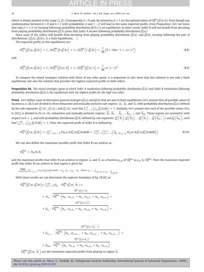
18 S. Meza, M. Tombak / Int. J. Ind. Organ. xxx (2009) xxx–xxx

ARTICLE IN PRESS

which is always positive in the range (12,136 ). Consequently, b=0 and, by symmetry, b=1 are the optimal values ofΠB

MS(fA2(a),b). Even though anyrandomization between b=0 and b=1 with probabilities β and 1−β will lead to the same expected profits, from Proposition (A2) we knowthat only β=1/2 (or locating following probability distribution fB

2(b)) is an equilibrium. In other words, Seller B will not benefit from deviatingfrom playing probability distribution fB

2(b) given that Seller A locates following probability distribution fA2(a).

Since none of the sellers will benefit from deviating from playing probability distribution fA2(a), and fB

2(b), locating following the pair ofdistributions (fA2(a), fB2(b)), is a Nash Equilibrium. □

The expected profits at this equilibrium are:

ΠMSA f 2A að Þ; f 2B bð Þ� �

= 1 = 2ΠMSA 0; f 2B bð Þ� �

+ 1 = 2ΠMSA 1; f 2B bð Þ� �

=136

9 + 24cr = t + cr=tð Þ2� �

ðB:8Þ

and,

ΠMSB f 2A að Þ; f 2B bð Þ� �

= 1 = 2ΠMSB f 2A að Þ;0� �

+ 1= 2ΠMSB f 2A að Þ;1� �

=136

cr=t−3ð Þ2 ðB:9Þ

To compare the mixed strategies solution with those of any other game, it is important to also show that this solution is not only a Nashequilibrium, but also the solution that provides the highest expected profits to both sellers.

Proposition B4. The mixed strategies game in which Seller A randomizes following probability distribution fA2(a) and Seller B randomizes following

probability distribution fB2(b) is the equilibrium with the highest profits for the high cost seller.

Proof. Let's define a pair of alternative general strategies fA3(a) and fB3(b) that are also in Nash equilibrium. Let's assume that all possible values of

location a, a∊ [0,1] are divided in three exhaustive and mutually exclusive sub-regions: a1 ; a2 , and a3 with probability distribution fA3(a) defined

by the sub-segments: f 3A a1ð Þ; f 3A a2 Þð , and f 3A a3 Þð such thatP3

1 = 1

Raif 3A að Þda

� �= 1. Similarly, let's assume that each of the possible values of b,

b∊ [0,1], is divided in 2n (n∊N), exhaustive and mutually exclusive regions: b1 ; b2 ; N bn ; N b2n−1 ; and b2n . These regions are symmetric with

respect to b = 12, and with probability distribution fB

3(b) defined by sub-segments: f 3B b1� �

; f 3B b2� �

; N f 3B bn� �

; N f 3B b2n−1

� �and f 3B b2n

� �, such

thatP2n

1 = 1

Rbif 3B bð Þdb

� �= 1. Then, the expected profit of Seller B is defined by:

ΠMSB f 3A að Þ; f 3B bð Þ� �

=RR 1;1

b = 0;a = 0 ΠB a; bð Þf 3A að Þf 3B bð Þdadb =P2n

j = 1P3

i = 1

RRbY bi ;aY ai

ΠB a; bð Þf 3A að Þf 3B bð Þdadb� �� �

ðB:10Þ

We can also define the maximum possible profit that Seller B can achieve as:

ΠMaxB = ΠB 0;0ð Þ;

and the maximum profits that Seller B can achieve in regions ai and bi as a fraction ρai,bi of ΠBMax as ρai, bi·ΠB

Max. Then the maximum expectedprofit that Seller B can achieve in that region is given by:

maxaaai ;babi

RRbY bi ;aYai

ΠB a;bð Þf 3A að Þf 3B bð Þdadb = αai· βbi

· ρaibi· ΠB ; Where αai

=Rai f

3A

að Þda and βbi=Rbi f

3B

bð Þdb

With these results we can determine the superior boundary of Eq. (B.10) as:

ΠMSB f 3A að Þ; f 3B bð Þ� �

VP2n

j = 1ðβb1· ΠMS

B ðf 3A að Þ; bi ÞÞ V

V βb1· ΠMax

B · αa1·ρa1 ;b1

+ αa2·ρa2 ;b1

+ αa3·ρa3 ;b1

� �zfflfflfflfflfflfflfflfflfflfflfflfflfflfflfflfflfflfflfflfflfflfflfflfflfflfflfflfflfflfflfflfflfflfflfflfflfflfflfflfflfflfflfflfflfflffl}|fflfflfflfflfflfflfflfflfflfflfflfflfflfflfflfflfflfflfflfflfflfflfflfflfflfflfflfflfflfflfflfflfflfflfflfflfflfflfflfflfflfflfflfflfflffl{ΠMaxB f 3A að Þ; b1¯ð Þ

+

+ βb2· ΠMax

B · αa1·ρa1 ;b2

+ αa2·ρa2 ;b2

+ αa3·ρa3 ;b2

� �zfflfflfflfflfflfflfflfflfflfflfflfflfflfflfflfflfflfflfflfflfflfflfflfflfflfflfflfflfflfflfflfflfflfflfflfflfflfflfflfflfflfflfflfflfflffl}|fflfflfflfflfflfflfflfflfflfflfflfflfflfflfflfflfflfflfflfflfflfflfflfflfflfflfflfflfflfflfflfflfflfflfflfflfflfflfflfflfflfflfflfflfflffl{+

ΠMaxB f 3A að Þ; b1� �

+ βb2n− 1· ΠMax

B · αa1·ρa1 ;bn− 1

+ αa2·ρa2 ;bn− 1

+ αa3·ρa3 ;bn− 1

� �zfflfflfflfflfflfflfflfflfflfflfflfflfflfflfflfflfflfflfflfflfflfflfflfflfflfflfflfflfflfflfflfflfflfflfflfflfflfflfflfflfflfflfflfflfflfflfflfflfflfflfflfflffl}|fflfflfflfflfflfflfflfflfflfflfflfflfflfflfflfflfflfflfflfflfflfflfflfflfflfflfflfflfflfflfflfflfflfflfflfflfflfflfflfflfflfflfflfflfflfflfflfflfflfflfflfflffl{+

:

:

ΠMaxB f 3A að Þ; b2n−1

� �

+ βb2n · ΠMaxB · αa1

·ρa1 ;bn+ αa2

·ρa2 ;bn+ αa3

·ρa3 ;bn

� �zfflfflfflfflfflfflfflfflfflfflfflfflfflfflfflfflfflfflfflfflfflfflfflfflfflfflfflfflfflfflfflfflfflfflfflfflfflfflfflfflfflfflfflfflfflffl}|fflfflfflfflfflfflfflfflfflfflfflfflfflfflfflfflfflfflfflfflfflfflfflfflfflfflfflfflfflfflfflfflfflfflfflfflfflfflfflfflfflfflfflfflfflffl{ΠMaxB f 3A að Þ;b2n� �

ΠMaxB f 3A að Þ; bi� �

are the maximum expected profits from playing in region bi

Please cite this article as: Meza, S., Tombak, M., Endogenous location leadership, International Journal of Industrial Organization (2009),doi:10.1016/j.ijindorg.2009.03.001

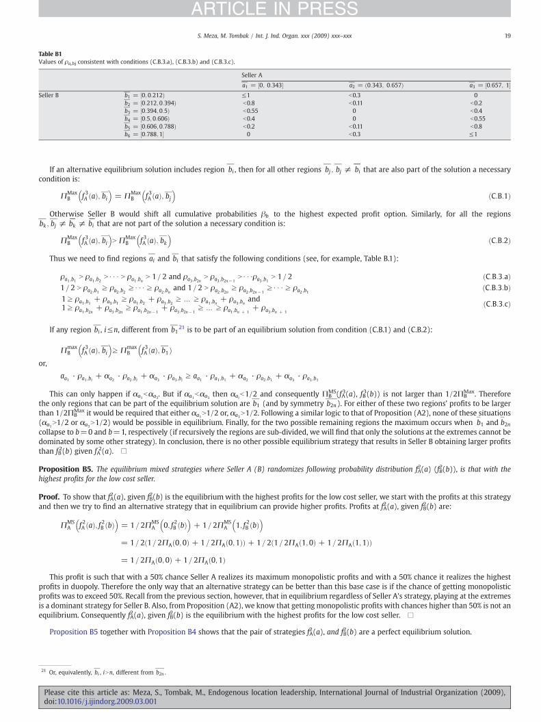
Table B1Values of ρai,bj consistent with conditions (C.B.3.a), (C.B.3.b) and (C.B.3.c).

Seller A

a1 = 0; 0:343½ � a2 = 0:343; 0:657ð Þ a3 = 0:657; 1½ �Seller B b1 = 0;0:212Þ½ ≤1 b0.3 0

b2 = 0:212; 0:394Þ½ b0.8 b0.11 b0.2b3 = 0:394; 0:5Þ½ b0.55 0 b0.4b4 = 0:5; 0:606Þ½ b0.4 0 b0.55b5 = 0:606; 0:788Þ½ b0.2 b0.11 b0.8b6 = 0:788; 1½ � 0 b0.3 ≤1

19S. Meza, M. Tombak / Int. J. Ind. Organ. xxx (2009) xxx–xxx

ARTICLE IN PRESS

If an alternative equilibrium solution includes region bi , then for all other regions bj ; bj ≠ bi that are also part of the solution a necessarycondition is:

ΠMaxB f 3A að Þ; bi� �

= ΠMaxB f 3A að Þ; bj� �

ðC:B:1Þ

Otherwise Seller B would shift all cumulative probabilities βb. to the highest expected profit option. Similarly, for all the regionsbk ; bj ≠ bk ≠ bi that are not part of the solution a necessary condition is:

ΠMaxB f 3A að Þ; bi� �

N ΠMaxB f 3A að Þ; bk� �

ðC:B:2Þ

Thus we need to find regions ai and bi that satisfy the following conditions (see, for example, Table B.1):

ρa1 ;b1N ρa1 ;b2

N : : : N ρa1 ;bnN 1 = 2 and ρa3 ;b2n

N ρa3 ;b2n− 1N : : :ρa3 ;b1

N 1 = 2 ðC:B:3:aÞ1= 2 N ρa2 ;b1

z ρa2 ;b2z : : : z ρa2 ;bn

and 1= 2 N ρa2 ;b2nz ρa2 ;b2n− 1

z : : : z ρa2 ;b1ðC:B:3:bÞ

1z ρa1 ;b1+ ρa3 ;b1

z ρa1 ;b2+ ρa3 ;b2

z N z ρa1 ;bn+ ρa3;bn

and1z ρa1 ;b2n

+ ρa3 ;b2nz ρa1 ;b2n− 1

+ ρa3 ;b2n− 1z N z ρa1 ;bn + 1

+ ρa3 ;bn + 1

ðC:B:3:cÞ

If any region bi , i≤n, different from b121 is to be part of an equilibrium solution from condition (C.B.1) and (C.B.2):

ΠmaxB f 3A að Þ; bi� �

z ΠmaxB f 3A að Þ; b1 Þ�

or,

aa1 · ρa1 ;bi+ αa2

· ρa2 ;bi+ αa3

· ρa3 ;biz aa1 · ρa1 ;b1

+ αa2· ρa2 ;b1

+ αa3· ρa3 ;b1

This can only happen if αa1bαa3. But if αa1bαa3 then αaib1/2 and consequently ΠBMS(fA3(a), fB3(b)) is not larger than 1/2ΠB

Max. Thereforethe only regions that can be part of the equilibrium solution are b1 (and by symmetry b2n). For either of these two regions' profits to be largerthan 1/2ΠB

Max it would be required that either αa1N1/2 or, αa3N1/2. Following a similar logic to that of Proposition (A2), none of these situations(αa1N1/2 or αa3N1/2) would be possible in equilibrium. Finally, for the two possible remaining regions the maximum occurs when b1 and b2ncollapse to b=0 and b=1, respectively (if recursively the regions are sub-divided, we will find that only the solutions at the extremes cannot bedominated by some other strategy). In conclusion, there is no other possible equilibrium strategy that results in Seller B obtaining larger profitsthan fB

2(b) given fA2(a). □

Proposition B5. The equilibrium mixed strategies where Seller A (B) randomizes following probability distribution fA2(a) (fB2(b)), is that with the

highest profits for the low cost seller.

Proof. To show that fA2(a), given fB2(b) is the equilibriumwith the highest profits for the low cost seller, we start with the profits at this strategy

and then we try to find an alternative strategy that in equilibrium can provide higher profits. Profits at fA2(a), given fB2(b) are:

ΠMSA f 2A að Þ; f 2B bð Þ� �

= 1 = 2ΠMSA 0; f 2B bð Þ� �

+ 1 = 2ΠMSA 1; f 2B bð Þ� �

= 1= 2 1= 2ΠA 0;0ð Þ + 1 = 2ΠA 0;1ð Þð Þ + 1 = 2 1 = 2ΠA 1;0ð Þ + 1= 2ΠA 1;1ð Þð Þ

= 1= 2ΠA 0;0ð Þ + 1= 2ΠA 0;1ð Þ

This profit is such that with a 50% chance Seller A realizes its maximum monopolistic profits and with a 50% chance it realizes the highestprofits in duopoly. Therefore the only way that an alternative strategy can be better than this base case is if the chance of getting monopolisticprofits was to exceed 50%. Recall from the previous section, however, that in equilibrium regardless of Seller A's strategy, playing at the extremesis a dominant strategy for Seller B. Also, from Proposition (A2), we know that getting monopolistic profits with chances higher than 50% is not anequilibrium. Consequently fA

2(a), given fB2(b) is the equilibrium with the highest profits for the low cost seller. □

Proposition B5 together with Proposition B4 shows that the pair of strategies fA2(a), and fB2(b) are a perfect equilibrium solution.

21 Or, equivalently, bi , iNn, different from b2n .

Please cite this article as: Meza, S., Tombak, M., Endogenous location leadership, International Journal of Industrial Organization (2009),doi:10.1016/j.ijindorg.2009.03.001

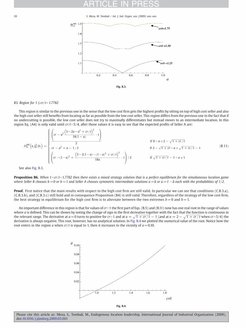
Fig. B.3.

20 S. Meza, M. Tombak / Int. J. Ind. Organ. xxx (2009) xxx–xxx

ARTICLE IN PRESS

B3. Region for 1≤cr/tb1.7782

This region is similar to the previous one in the sense that the low cost firm gets the highest profits by sitting on top of high cost seller and alsothe high cost seller still benefits from locating as far as possible from the low cost seller. This region differs from the previous one in the fact that ifno undercutting is possible, the low cost seller does not try to maximally differentiates but instead moves to an intermediate location. In thisregion Eq. (A4) is only valid until cr/tb5/4, after those values it is easy to see that the expected profits of Seller A are:

ΠMSA a; f 2B bð Þ� �

=

cr − a23−2a−a2 + cr=t� �2

18 1− að Þ · t

0B@1CA

2if 0 b a V 2−

ffiffiffiffiffiffiffiffiffiffiffiffiffiffiffiffiffiffiffiffiffi1 + cr = t

pcr − a2 + a − 1= 2 if 2−

ffiffiffiffiffiffiffiffiffiffiffiffiffiffiffi1 + cr

pb a V

ffiffiffiffiffiffiffiffiffiffiffiffiffiffiffiffiffiffiffiffiffi1 + cr = t

p− 1

cr − 1−að Þ2 +3−2 1−að Þ− 1−að Þ2 + cr=t� �2

18a· t

0B@1CA = 2 if

ffiffiffiffiffiffiffiffiffiffiffiffiffiffiffiffiffiffiffiffiffi1 + cr = t

p− 1 b a V 1

8>>>>>>>>>>>>>><>>>>>>>>>>>>>>:

ðB:11Þ

See also Fig. B.3.

Proposition B6. When 1bcr/tb1.7782 then there exists a mixed strategy solution that is a perfect equilibrium for the simultaneous location gamewhere Seller B chooses b=0 or b=1 and Seller A chooses symmetric intermediate solutions a=a or a=1− a each with the probabilities of 1/2.

Proof. First notice that the main results with respect to the high cost firm are still valid. In particular we can see that conditions (C.B.3.a),(C.B.3.b), and (C.B.3.c) still hold and in consequence Proposition (B4) is still valid. Therefore, regardless of the strategy of the low cost firm,the best strategy in equilibrium for the high cost firm is to alternate between the two extremes b=0 and b=1.

An important difference in this region is that for values of crN1 the first part of Eqs. (B.5) and (B.11) now has one real root in the range of valueswhere a is defined. This can be shown by noting the change of sign in the first derivative together with the fact that the function is continuous inthe relevant range. The derivative at a=0 turns to positive for crN1 and at a =

ffiffiffiffiffiffiffiffiffiffiffiffiffiffiffiffiffiffiffiffiffi1 + cr = t

p− 1 (and at a = 2−

ffiffiffiffiffiffiffiffiffiffiffiffiffiffiffiffiffiffiffiffiffi1 + cr = t

pwhen crN5/4) the

derivative is always negative. This root, however, has no analytical solution. In Fig. B.4 we plotted the numerical value of the root. Notice how theroot enters in the region a when cr/t is equal to 1, then it increases to the vicinity of a=0.10.

Fig. B.4.

Please cite this article as: Meza, S., Tombak, M., Endogenous location leadership, International Journal of Industrial Organization (2009),doi:10.1016/j.ijindorg.2009.03.001

21S. Meza, M. Tombak / Int. J. Ind. Organ. xxx (2009) xxx–xxx

ARTICLE IN PRESS

Similar to the procedure in Section B3 we compare the expected profits Π1MS(a, fB2(b)) evaluated at both local maximums22 and a=0.5 and

a=a . However since a has no analytical solution, it is not possible to make the comparison. To alleviate this problem we do the comparisonevaluation at a=0, this would serve as a lower boundary of the true solution at a= a.

ΠMSA 0; f 2B bð Þ� �

− ΠMSA 1= 2; f 2B bð Þ� �

=136

crt

� �2− 12cr = t + 18

�Which is always positive for values of cr b 3 2−

ffiffiffi2

p� �≈1:75736. This implies that up to some value larger than cr/t=1.75736, location a=a ,

and by symmetry location a=1− a are the locations where Seller A maximizes its expected profits. Using Mathematica we numerically solveΠA

MS(a , fB2(b))−ΠAMS(1/2, fB2(b))=0 and find as a unique solution:fcr=t≈1:77819; a≈0:095525.

With this result we can now define probability distribution fA4(a) as the strategy of Seller A of locating at a=a with probabilitymass of 1/2 and

locating at a=1−a with probability mass of 1/2. From here using Proposition (B2) the conclusion of Proposition (B3) can be extended to fA4(a).

The mixed strategies game in which Seller A randomizes following probability distribution fA4(a) and Seller B randomizes following probability

distribution fB2(b) is a Nash equilibrium. Moreover, since Proposition (B4) still holds, extending Proposition (B5) to this strategy is also straight

forward. This leads to the conclusion that the pair of strategies fA4(a), and fB2(b) form a perfect equilibrium solution. □

B4. Region for cr/t≥1.7782

Lemma B1. When c r/tN1.7782 then Seller A prefers to monopolizes at a=1/2 than trying to chase Seller B in the mixed strategies game.

Proof. As we saw in the previous section, when cr/tN1.7782 the expected profits of Seller A are maximized at a=0.5. But given that Seller Aalternates between a and 1−a. And given that the expected profits of Seller B at this location are equal to zero. This strategy is not different fromSeller A always monopolizing at a=0.5. □

References

Amir, R., Grilo, A., 2001. Stackelberg versus Cournot equilibrium. Games and EconomicBehavior 26, 1–21.

Amir, R., Stepanova, A., 2006. Second-mover advantage and price leadership in Bertrandduopoly. Games and Economic Behavior 55, 1–20.

Anderson, S., 1987. Spatial competition and price leadership. International Journal ofIndustrial Organization 5, 369–398.

Anderson, S., DePalma, A., 2001. Product diversity in asymmetric oligopoly: is thequality of consumer goods too low? The Journal of Industrial Economics XLIX (2),113–135 (June).

Bergstrom, T., Varian, H., 1985. When are Nash Equilibria independent of thedistribution of agents' characteristics? Review of Economic Studies LII, 715–718.

Bester, H., DePalma, A., Leininger, W., Thomas, J., von Thadden, E.L., 1996. ANoncooperative analysis of Hotelling's location game. Games and EconomicBehavior 12, 165–186.

Bonanno, G., 1987. Location choice, product proliferation and entry deterrence. Reviewof Economic Studies LIV, 37–45.

Boyer, M., Laffont, J.J., Mahenc, P.M., Moreaux, M., 1994. Location distortions underincomplete information. Regional Science and Urban Economics 24, 409–440.

Boyer, M., Mahenc, P.M., Moreaux, M., 2003. Asymmetric information and productdifferentiation. Regional Science and Urban Economics 33, 93–113.

Braid, R., 1986. Stackelberg price leadership in spatial competition. International Journalof Industrial Organization 4, 439–449.

D'Aspremont, C., Gabszewicz, J., Thisse, J.F., 1979. On Hotelling's ‘stability incompetition’. Econometrica 47 (5), 1145–1150 (Sept.).

Gabszewicz, J., Thisse, J.F., 1986. On the nature of competition with differentiatedproducts. The Economic Journal 96, 160–172 (March).

Hamilton, J.H., Slutsky, S.M., 1990. Endogenous timing in Duopoly Games: Stackelbergor Cournot Equilibrium. Games and Economic Behavior 2, 29–46.

Hendricks, K., Weiss, A., Wilson, C., 1988. The war of attrition in continuous time withcomplete information. International Economic Review 29 (4), 663–680.

Hotelling, H., 1929. Stability in competition. Economic Journal 39, 41–57.Leahy, D., Neary, P., 2005. Symmetric research joint ventures: cooperative substitutes

and complements. International Journal of Industrial Organization 23 (5–6),381–397.

Marquez, R., 1997. A note on Bertrand competition with asymmetric fixed costs.Economics Letters 57, 87–96.

22 It resulted for both Eqs. (B5) and (B11).

Please cite this article as: Meza, S., Tombak, M., Endogenous locationdoi:10.1016/j.ijindorg.2009.03.001

Melitz, M., 2003. The impact of trade on intra-industry reallocations and aggregateindustry Productivity. Econometrica 71 (6), 1695–1725.

Pitchik, C., Osborne, M., 1987. Equilibrium in Hotelling's model of spatial competition.Econometrica, 55 4, 911–922.

Röller, L.H., Siebert, R., Tombak, M., 2007. Why firms form (or do not form) RJVs. TheEconomic Journal 117, 1122–1144 July.

Röller, L.H., Sinclair-Desgagné, B., 1996. On the heterogeneity of firms. EuropeanEconomic Review 40, 531–539.

Salant, S., Shaffer, G., 1999. Unequal treatment of Identical Agents in Cournotequilibrium. American Economic Review 89 (3), 585–604.

Smith, M., 1974. The theory of games and the evolution of animal conflicts. Journal ofTheoretical Biology 47, 209–221.

Sutton, J., 1986. Vertical product differentiation — some basic themes. AmericanEconomic Review 76, 393–398.

Syverson, C., 2004. Product substitutability and productivity dispersion. Review ofEconomics and Statistics 86 (2), 534–550.

Tabuchi, T., Thisse, J.F., 1995. Asymmetric equilibria in spatial competition. InternationalJournal of Industrial Organization 13, 213–227.

Tirole, J., 1989. The Theory of Industrial Organization. The MIT Press, Cambridge, MA.Thomas, C.J., 2002. The effect of asymmetric entry costs on Bertrand competition.

International Journal of Industrial Organization 20, 589–609.Tombak, M., 2002. Mergers to monopoly. Journal of Economics and Management

Strategy 11 (3), 513–546 Fall.Tyagi, R.K., 2000. Sequential product positioning under differential costs. Management

Science 46 (7), 928–940.van Damme, E., Hurkens, S., 1999. Endogenous Stackelberg leadership. Games and

Economic Behavior 28, 105–129.van Damme, E., Hurkens, S., 2004. Endogenous price leadership. Games and Economic

Behavior 47, 404–420.Vogel, J., 2007, Spatial competition with heterogeneous firms. Dept. of Economics,

Princeton Unversity, mimeo.Walker, M., Wooders, J., 2001. Minimax play atWimbledon. American Economic Review

91 (5) (Dec.), 1521–1538.Ziss, S., 1993. Entry deterrence, cost advantage and horizontal product differentiation.

Regional Science and Urban Economics 23, 523–543.

leadership, International Journal of Industrial Organization (2009),