Central Bank Learning, Terms of TradeShocks & Currency Risk: Should OnlyIn�ation Matter for Monetary Policy?�

G.C. Limy and Paul D. McNelisz

December 2003

Abstract

This paper examines the role of interest rate policy in a small openeconomy subject to terms of trade shocks, and time-varying currencyrisks. The private sector makes optimal decisions in an intertempo-ral non-linear setting with rational, forward-looking expectations. Incontrast, the monetary authority chooses an optimal interest rate re-action function, given a loss function that is conditional on the stateof the economy and given its �least-squares learning�about the evo-lution of in�ation and exchange rate depreciation. The simulationresults of the e¤ects of di¤erent policy scenarios on welfare show that,on balance, the prefered stance should be strict in�ation targeting..Key words: policy targets, central bank learning, parameterized

expectations

.

�We would like to thank three anonymous referees for very helpful comments.yDepartment of Economics, University of Melbourne, Victoria 3010, Australia.

Email: g.lim@unimelb.edu.auzDepartment of Economics, Boston College. On leave, Department of Economics,

Georgetown University, Washington, D.C. 20057. Email: McNelisP@georgetown.edu.

1

1 Introduction

This paper examines the role of interest rate policy in a small open economysubject to terms of trade shocks, and time-varying currency risks. A centralbank committed to low in�ation controls neither the terms of trade nor theevolution of currency risk, both of which condition the response of in�ationto its policy instruments. In this context, the best the central bank cando is to �learn�the e¤ects indirectly, by frequently �updating�estimates ofin�ation dynamics and �re-adjusting�its policy rules accordingly.However, when an economy is subjected to large adverse external shocks

and the exchange rate depreciates rapidly, it should not be surprising if acentral bank also comes under strong pressure to incorporate exchange ratevolatility targets in its policy objectives. Should exchange rate changes thenbe included as one of the monetary policy targets along with in�ation targets?Much of the discussion of monetary policy is framed by the well-known

Taylor (1993, 1999) rule, whereby interest rates respond to their own lag, aswell as to deviations of in�ation and output from respective targets. Tay-lor (1993) points out that this �rule� need not be a mechanical formula,but something which can be operated �informally�, with recognition of the�general instrument responses which underlie the policy rule�. Not surpris-ingly, the speci�cation of this rule, which re�ect the underlying objectives ofmonetary policy, has been the subject of considerable controversy.1

In a closed-economy setting, Christiano and Gust (1999), for example,argue that only the in�ation variable should appear as a target. Rotembergand Woodford (1998) concur, but they argue that a higher average rate ofin�ation is required for monetary policy to be e¤ective over the mediumto long term. They base their argument on the zero lower bound for thenominal interest rate, since at very low in�ation rates there is little room forthis instrument to manoeuvre.2

In an open economy setting, McCallum (2000) takes issue with the Rotem-berg and Woodford �policy ine¤ectiveness�argument under low in�ation andzero �lower bounds�for nominal interest rates. McCallum argues that thecentral bank always has at its disposal a second tool, the exchange rate, so ifthe economy is stuck at a very low interest rate, there is the option of cur-rency intervention. Christiano (2000) disagrees: McCallum�s argument restson the assumption that currency depreciation is e¤ective. Furthermore, the

1Recent technical papers on all aspects of the Taylor rule may be found on the webpage, http://www.stanford.edu/~johntayl/PolRulLink.htm#Technical%20articles

2Erceg, Henderson and Levin (2000) argued that output deviations should also appearin the Taylor rule, but the output measure should be deviations of actual output from thelevel of output generated by a �exible-price economy.

2

central bank must be willing to undermine public �con�dence�that it standsready to cut interest rates in the event of major adverse shocks.For small emerging market economies, Taylor (2000) contends that pol-

icy rules that focus on a �smoothed in�ation measure and real output�andwhich do not �try to react too much�to the exchange rate might work well.However, he leaves open the question of a role for the exchange rate. Ball(1999) argues that in�ation targeting �can be dangerous� in an open econ-omy setting because exchange rate changes have a direct e¤ect on in�ationvia changes in import prices. Hence, adoption of a strict in�ation targetingstance can result in large output variations. More recently, Gali and Mona-celli (2002) found, in a small open economy setup with sticky price settingbehavior, that domestic in�ation targeting dominates, from a welfare pointof view, both CPI in�ation targeting and an exchange-rate peg. They basetheir argument on the "excess smoothness" induced in the exchange rate byCPI targeting or an exchange rate peg. This smoothness, in combinationwith the assumed stickiness in nominal prices, prevents relative prices fromadjusting "su¢ ciently fast", thus causing "a signi�cant deviation from the�rst best allocation" [Gali and Monacelli (2002), p.2].However, practically all of these studies are based on linear stochastic

and dynamic general equilibrium representations, or linearized approxima-tions of nonlinear models. The Taylor-type feedback rules are either imposedor derived by linear quadratic optimization. While these approaches may bevalid if the shocks impinging on the economy are indeed �small�and �sym-metric� deviations from a steady state, they may be inappropriate if theshocks are large, persistent, and asymmetric, as they are in many highlyopen economies.Furthermore, few if any of these studies incorporate �learning� on the

part of the monetary authority itself. Bullard and Mitra (2002) incorporateprivate sector �learning�of the speci�c Taylor rules used by the central bankin the Rotemberg-Woodford closed economy framework. They argue for Tay-lor rules based on expectations of current in�ation from target levels, ratherthan rules based on lagged values or forecasts further into the future.In contrast to Bullard and Mitra (2001), we assume that the private sec-

tor uses the true, stochastic dynamic, nonlinear model for formulating itsown �laws of motion�for consumption, investment, and trade, with forward-looking rational expectations. In this analysis, the monetary policy authoritylearns the �laws of motion�of in�ation dynamics from past data, throughcontinuously-updated least squares regression. From the results of these re-gressions, the monetary authority obtains an optimal interest rate feedbackrule based on linear quadratic optimization, using weights in the objectivefunction for in�ation which can vary with current conditions. The monetary

3

authority is thus �boundedly rational�, in the sense of Sargent (1999), with�rational�describing the use of least squares, and �bounded�meaning modelmisspeci�cation.Our results show that when a central banker is all-knowing and acts

to optimize the intertemporal welfare of the consumer, there is not muchdi¤erence in terms of welfare outcomes between �xed and �exible in�ationtargeting. In contrast, if the central bank decides to incorporate, in additionto in�ation, exchange rate dynamics in its learning and policy objectives, andprices are sticky, it does so at some welfare costs. In a learning environment,there is always the risk that the �perceived�laws of motion lag behind theactual laws of motion. Hence expanding the range of policy objectivesmay increase overall volatility and reduce welfare. For this reason, strictin�ation targeting dominates monetary policy based on multiple targets inan environment with central bank learning and sticky prices.The next section describes the theoretical structure of the model for the

private sector and the nature of the monetary authority �learning�. Thethird section discusses the calibration as well as the solution method, whilethe fourth section analyzes the simulation results of the model. The lastsection concludes.

2 The Model

The framework of analysis contains two modules - a module which describesthe behavior of the private sector and a module which describes the behaviorof the central bank.

2.1 Private Sector Behavior

The private sector is assumed to follow the standard optimizing behaviorcharacterized in dynamic stochastic general equilibrium models.

2.1.1 Consumption

The utility function for the private sector �representative agent�is given bythe following function:

U(Ct) =C1� t

1� (1)

where C is the aggregate consumption index and is the coe¢ cient of relativerisk aversion. Unless otherwise speci�ed, upper case variables denote the

4

levels of the variables while lower case letters denote logarithms of the samevariables. The exception is the nominal interest rate denoted as i:The representative agent as �household/�rm�optimizes the following in-

tertemporal welfare function, with an endogenous discount factor:

Wt = E

" 1Xi=0

#t+iU(Ct+i)

#(2)

#t+1+i = [1 + Ct]�� � #t+i (3)

#t = 1 (4)

where Et is the expectations operator, conditional on information availableat time t; while � approximates the elasticity of the endogenous discountfactor # with respect to the average consumption index, C: Endogenous dis-counting is due to Uzawa (1968) and Mendoza (2000) states that endogenousdiscounting is needed for the model to produce well-behaved dynamics withdeterministic stationary equilibria.3

The speci�cation used in this paper is due to Schmitt-Grohé and Uribe(2001). In our model, an individual agent�s discount factor does not dependon their own consumption, but rather their discount factor depends on theaverage level of consumption. Schmitt-Grohé and Uribe (2001) argue thatthis simpli�cation reduces the equilibrium conditions by one Euler equationand one state variable, over the standard model with endogenous discount-ing, it greatly facilitates the computation of the equilibrium dynamics, whiledelivering �virtually identical� predictions of key macroeconomic variablesas the standard endogenous-discounting model.4 In equilibrium, of course,the individual consumption index and the average consumption index areidentical. Hence,

Ct = Ct (5)

The consumption index is a composite index of non-tradeable goods nand tradeable goods f :

Ct =�Cft

��f(Cnt )

1��f (6)

where �f is the proportion of traded goods. Given the aggregate consump-tion expenditure constraint,

PtCt = P ft Cft + P nt C

nt (7)

3Endogenous discounting also allows the model to support equilibria in which creditfrictions may remain binding.

4Schmitt-Grohé and Uribe (2001) argue that if the reason for introducing endogenousdiscounting is solely for introducing stationarity, �computational convenience�should bethe decisive factor for modifying the standard Uzawa-type model. Kim and Kose (2001)reached similar conclusions.

5

and the de�nition of the real exchange rate,

Zt =P ftP nt

(8)

the following expressions give the demand for traded and non-traded goodsas functions of aggregate expenditure and the real exchange rate Z:

Cft =

�1� �f�f

��1+�fZ�1+�ft Ct (9)

Cnt =

�1� �f�f

��fZ�ft Ct (10)

Similarly, we can express the consumption of traded goods as a compositeindex of the consumption of export goods, Cx, and import goods Cm:

Cft = (Cxt )�xt (C

mt )

1��x (11)

where �x is the proportion of export goods. The aggregate expenditureconstraint for tradeable goods is given by the following expression:

P ft Cft = Pmt C

mt + P xt C

xt (12)

where P x and Pm are the prices of export and import type goods respectively.De�ning the terms of trade index J as:

J =P x

Pm(13)

yields the demand for export and import goods as functions of the aggregateconsumption of traded goods as well as the terms of trade index:

Cxt =

�1� �x�x

��1+�xJ�1+�xt Cft (14)

Cmt =

�1� �x�x

��xJ�xt Cft (15)

2.1.2 Production

Production of exports and imports is by the Cobb-Douglas technology:

Y xt = Axt (K

xt�1)

1��x (16)

Y mt = Amt (K

mt�1)

1��m (17)

6

where Ax; Am represents the labour factor productivity terms5 in the produc-tion of export and import goods, and (1� �x); (1� �m) are the coe¢ cients ofthe capital Kx and Km respectively. The time subscripts (t � 1) indicatesthat they are the beginning-of-period values. The production of non-tradedgoods, which is usually in services, is given by the labour productivity term,Ant :

Y nt = Ant (18)

Capital in each sector has the respective depreciation rates, �x and �m;and evolves according to the following identities:

Kxt = (1� �x)K

xt�1 + Ixt (19)

Kmt = (1� �m)K

mt�1 + Imt (20)

where Ixt and Imt represents investment in each sector.

2.1.3 Budget Constraint

The budget constraint faced by the household/�rm representative agent is:

PtCt = �t + St�L�t � L�t�1(1 + i

�t�1 + �t�1)

�� [Bt �Bt�1(1 + it�1)] (21)

where S is the exchange rate (de�ned as domestic currency per foreign),L�t is foreign debt in foreign currency, and Bt is domestic debt in domesticcurrency. Pro�ts � is de�ned by the following expression:

�t = P xt

�Axt�Kxt�1�1��x � �x

2Kxt�1(Ixt )

2 � Ixt

�+Pmt

�Amt (K

mt�1)

1��m � �m2Km

t�1(Imt )

2 � Imt

�+ P nt A

nt (22)

The aggregate resource constraint shows that the �rm faces quadratic ad-justment costs when they accumulate capital, with these costs given by theterms �x

2Kxt�1(Ixt )

2 and �m2Km

t�1(Imt )

2 :

As shown, the household/�rm lends to the domestic government and ac-cumulate bonds B which pay the nominal interest rate i. They also borrowinternationally and accumulate international debt L� at the �xed rate i�; in-cluding a time-varying risk premium �t:. The evolution of the currency riskterm �t is modelled as a GARCH process:

�t = �0 + �1�t�1 + �2�2t�1 (23)

5Since the representative agent determines both consumption and production decisions,we have simpli�ed the analysis by abstracting from issues about labour-leisure choice andwage determination.

7

We also assume, that the shocks, �t are drawn from a t-distribution to bettercapture the empirical leptokurtic characteristics of risk.6

2.1.4 Euler Equations

The household/�rm optimizes the expected value of the utility of consump-tion (2) subject to the budget constraint de�ned in (21) and (22) and theconstraints in (19) and (20).

Max : ×= Et1Xi=0

#t+ifU(Ct+i)

��t+i[Ct+i �P xt+iPt+i

�Axt+i(K

xt�1+i)

1��x � �x2Kx

t�1+i

�Ixt+i

�2 � Ixt+i

��Pmt+iPt+i

�Amt+i(K

mt�1+i)

1��m � �m2Km

t�1+i

�Imt+i

�2 � Imt+i

��P nt+iPt+i

Ant+i

�St+iPt+i

�L�t+i � L�t�1+i(1 + i

�t�1+i + �t�1+i

�) +

1

Pt+i(Bt+i �Bt�1+i(1 + it�1+i)) ]

�Qxt+i�Kxt+i � Ixt+i � (1� �x)K

xt�1+i

��Qmt+i

�Kmt+i � Imt+i � (1� �m)K

mt�1+i

�g

The variable � is the familiar Lagrangean multiplier representing the mar-ginal utility of wealth. The terms Qx and Qm; known as Tobin�s Q, representthe Lagrange multipliers for the evolution of capital in each sector - they arethe �shadow prices� for new capital. Maximizing the Lagrangean with re-spect to Ct; L�t ; Bt; K

xt ; K

mt ; I

xt ; I

mt yields the following �rst order conditions:

U 0(Ct)� �t = 0

#t�tStPt� Et

�#t+1�t+1

St+1Pt+1

(1 + i�t + �t)

�= 0

�#t�t1

Pt+ Et#t+1�t+1

1

Pt+1(1 + it) = 0

6The focus here is clearly on the design of policy in respond to exogenously determinedshocks on the exchange rate. The analysis can be further complicated by allowing currencyrisk to be endogenously conditioned by changes in domestic internal and foreign externaldebt as well as in�ation and exchange rate changes.

8

��#tQxt

+Et#t+1Qxt+1(1� �x)

�+ Et#t+1�t+1

P xt+1Pt+1

"Axt+1(1� �x)(K

xt )��x

+�x(Ixt+1)

2

2(Kxt )2

#= 0

��#tQmt

+Et#t+1Qmt+1(1� �m)

�+ Et#t+1�t+1

Pmt+1Pt+1

"Amt+1(1� �m)(K

mt )

��m

+�m(Imt+1)

2

2(Kmt )

2

#= 0

�#t�tP xtPt

��xI

xt

Kxt�1

+ 1

�+ #tQ

xt = 0

�#t�tPmtPt

��mI

mt

Kmt�1

+ 1

�+ #tQ

mt = 0

These equations can then be re-expressed as:

�t = U 0(Ct) (24)

#tU0(Ct) = Et#t+1U

0(Ct+1)(1 + it � �t+1) (25)

Et(st+1 � st) = it � i�t � �t (26)

�#tQ

xt

�Et#t+1Qxt+1(1� �x)

�= Et#t+1�t+1

P xt+1Pt+1

"Axt+1(1� �x)(K

xt )��x

+�x(Ixt+1)

2

2(Kxt )2

#(27)

�#tQ

mt

�Et#t+1Qmt+1(1� �m)

�= Et#t+1�t+1

Pmt+1Pt+1

"Amt+1(1� �m)(K

mt )

��m

+�m(Imt+1)

2

2(Kmt )

2

#(28)

Ixt =1

�x

�PtP xt

Qxt�t� 1�Kxt�1 (29)

Imt =1

�m

�PtPmt

Qmt�t

� 1�Kmt�1 (30)

where �pt+1 = log(Pt+1=Pt) is the per period in�ation; s is the logarithmof the nominal exchange rate S and (Etst+1 � st) is the expected rate ofexchange rate depreciation.

9

Equation (25) is the typical Euler equation for consumption. Using theutility function in (1) yields the consumption function:

Ct = Et�(1 + it � �t+1)#t+1C

� t+1

�� 1 (31)

which shows how current consumption depends on expectations of futurevalues. Equation (26) describes the interest arbitrage condition and theforwarding-looking behavior of the exchange rate.

st = Et(st+1)� it + i�t + �t (32)

The above equations (27) and (28) also show that the solutions for Qxtand Qmt , which determine investment and the evolution of capital in eachsector, come from forward-looking stochastic Euler equations.

Qxt = Et

24�#t+1#t

�0@ �t+1Pxt+1Pt+1

�Axt+1(1� �x)(K

xt )��x +

�x(Ixt+1)2

2(Kxt )2

�+Qxt+1(1� �x)

1A35(33)Qmt = Et

24�#t+1#t

�0@ �t+1Pmt+1Pt+1

�Amt+1(1� �m)(K

mt )

��m +�m(Imt+1)

2

2(Kmt )

2

�+Qmt+1(1� �m)

1A35(34)The shadow price or replacement value of capital in each sector is equal tothe discounted value of next period�s marginal productivity, the adjustmentcosts due to the new capital stock, and the expected replacement value netof depreciation.Thus the model has four �forward-looking� stochastic Euler equations,

which determine Ct; st; Qxt ; Qmt These variables, together with (24), in turn

determine current investment Ixt and Imt as describe by the conditions in (29)

and (30).

2.1.5 Relative prices, exchange rate pass-through and stickiness

There are 7 prices (absolute and relative) to be determined (P x; Pm; J; Z; P ft ;P nt ; P ). The price of export goods is determined exogenously for a small openeconomy (P x�) and its price in domestic currency is P x = SP x�. The priceof import goods is also determined exogenously for a small open economyPm�, but, we assume that price changes are incompletely passed-through(see Campa and Goldberg (2002) for a study on exchange rate pass-throughand import prices). Using the de�nition: Pm = SPm� and assuming partialadjustment, we obtain:

pmt = !(st + pm�t ) + (1� !)pmt�1 (35)

10

where ! = 1 indicates complete pass-through of foreign price changes.Thus, given P x and Pm; we have J = P x=Pm; and:

P ft =�(�x)

��x (1� �x)�1+�x� (P xt )�x (Pmt )1��x (36)

Finally, we obtain the aggregate consumption price de�ator as:

Pt =�(�f )

��f (1� �f )�1+�f � �P ft ��f (P nt )1��f (37)

While the exchange rate is determined by the forward-looking interestparity relation, and the terms of trade are determined exogenously, the priceof non-traded goods adjusts in response to demand and supply in this sector.

2.1.6 Macroeconomic Conditions And Market Clearing

The national accounting equation is:

P xt

�Y xt �

�x2Kx

t

(Ixt )2

�+ Pmt

�Y mt � �m

2Kmt

(Imt )2

�+ P nt Y

nt

= P xt (Cxt +Xt + Ixt ) + Pmt (C

mt �Mt + Imt ) + P nt (C

nt +Gt)

= PtCt + (Pxt I

xt + Pmt I

mt ) + (P

xt Xt � Pmt Mt) + P nt Gt (38)

Real gross domestic product is given as:

y =1

Pt

�P xt

�Y xt �

�x2Kx

t

(Ixt )2

�+ Pmt

�Y mt � �m

2Kmt

(Imt )2

�+ P nt Y

nt

�(39)

The change in bond holdings and foreign debt holdings evolves as follows:

P nt Gt = Bt+1 �Bt(1 + it) (40)

(P xt Xt � Pmt Mt) = �St�L�t+1 � L�t [1 + i

�t + �t]

�(41)

2.2 The Monetary Authority

The Central Bank adopts practices consistent with optimal control models,speci�cally, the linear quadratic regulator problem. It chooses an optimalinterest rate reaction function, given its loss function equation, and its per-ception of the evolution of the state variables, in�ation and growth. Thechange in the interest rate is the solution of the optimal linear quadraticregulator problem,with control variable �i solved as a feedback response tothe lagged state variables.

11

We assume, perhaps more realistically, that the monetary authority doesnot know the exact nature of the private sector model, instead it �learns�and updates the state-space model equation, which underpins its calculationof the optimal interest rate policy period by period. In other words, at eachperiod time t, the Central Bank updates its information about the evolutionof key economic variables, and re-estimates the state-space system to obtainnew estimates. The central bank then uses this information to determinethe optimal interest rate.The central bank makes use of a linear quadratic loss function, and up-

dates linear laws of motion of in�ation and depreciation for �nding its policyresponse. The response is a linear "reaction function". Admittedly thisrelatively simple linear quadratic framework of the central bank contrastswith the more complex nonlinear dynamic optimization process used by theprivate-sector decision makers. However, we note that the weights and coef-�cients of this linear quadratic framework are updated each period, and thatthe forecasting model used by the Central Bank generate in�ation forecaststhat do not deviate persistently from the underlying true in�ation rates.For this paper, two di¤erent policy scenarios are considered - a pure

in�ation targeting policy stance and an in�ation-exchange rate policy stance.The weights for in�ation and exchange rate depreciation in the loss functiondepend on the conditions at time t.

� Strict In�ation targeting

In the strict in�ation target case, the monetary authority estimates or�learns�the evolution of in�ation as a function of its own lag as well as ofchanges in the interest rate.

�1 = �1t(�t � ��)2 (42)

xt =

kXj=0

�1t;jxt�j�1 + �2t�it + et (43)

it+1 = it +

kXj=0

h(b�1t;j; b�2t; �1t)xt�j (44)

where xt contains the in�ation variable �t = log(Pt=Pt�4); an annualized rateof in�ation. �� is the target for in�ation, and k is the number of lags forforecasting the evolution of the state variable. The feedback function h isobtained by solving the linear quadratic regulator problem, as discussed inSargent (1999).

12

The weight on the loss function, �1t; shown in Table 1, re�ects the CentralBank�s concerns about in�ation and is dependent on the state of the economy.

Table I: Policy WeightsStrict In�ation Targeting� � �� �1 = 0:0� > �� �1 = 1:0

In this strict anti-in�ation scenario, if in�ation is less than the targetlevel ��; the central bank does not optimize; in other words, the interestrate remains at its level: it+1 = it: This is the �no intervention� case.However, if in�ation is above the target rate (� > ��), the monetary authorityimplements its optimal interest policy according to equation (44).

� Flexible In�ation Targeting with In�ation and Exchange Rate Targets

In the �exible in�ation targeting scenario, the central bank also considersthe behavior of the exchange rate. It learns the evolution of in�ation andexchange rate depreciations as functions of their own lags and of changes inthe interest rate.

�2 = �1t(�t � ��)2 + �2t(�t � ��)2 (45)

xt =kXj=0

�1t;jxt�j�1 + �2t�it + et (46)

it+1 = it +

kXj=0

h(b�1t;j; b�2t; �1t; �2t)xt�j (47)

where xt contains the in�ation variable �t as well as the depreciation variablent = log(St=St�4); the annualized rate of change of the exchange rate. Theterm �� represents the target for exchange rate depreciation. In this case,we have a bivariate forecasting model for the evolution of the state variables,�t and �t, with an equal number of lags. The coe¢ cient matrix �1t;j, for klags contains two (k � 1) recursively updated matrix coe¢ cients, represent-ing the e¤ects of lagged in�ation and depreciation on current in�ation anddepreciation. �Least squares learning�is used to forecast the future valuesof these �state�variables in each scenario.The weights (�1t; �2t) re�ects the �exible in�ation targeting stance of the

central bank. They are summarized in Table II.

13

Table II: Policy WeightsFlexible In�ation Targeting

Exchange Rate DepreciationIn�ation �t � �� �t > ��

� � �� �1 = 0:0 �1 = 0:1�2 = 0:0 �2 = 0:9

� > �� �1 = 0:9 �1 = 0:5�2 = 0:1 �2 = 0:5

In this policy scenario, if in�ation is below the target level �� and thechange in the exchange rate is also below the target, ��; then the centralbank does not optimize and hence does not change the policy interest rate.If in�ation is above the target rate (� > ��), with within target exchange ratechanges, (�t � ��) the monetary authority puts greater weight on in�ationin its objective function, �1t = 0:9. In contrast, when the depreciationof the exchange rate is above target (�t > ��), with in�ation below target(� � ��), the exchange rate in�ation weight dominates �2t = 0:9. Finally, ifboth in�ation and depreciation are above their respective targets, the centralbank puts equal weights on them in its objective function.Thus, corresponding to each scenario, the central bank optimizes a loss

function � with weights on the loss function, �t = f�1t; �2tg dependent onthe economic conditions at time t: The monetary authority estimates thestate-space system and uses the parameter set b�1tj to formulate an optimalinterest-rate feedback rule according to equation (47) which is the solution ofthe optimal linear quadratic �regulator�problem, with control variable �isolved as a feedback response to the state variables.In formulating its optimal interest-rate feedback rule, the government

acts at time t as if its estimated model for the evolution of the state variablesare true �forever�, and that its relative weights for in�ation, or deprecia-tion in the loss function are permanently �xed. However, as Sargent (1999)points out in a similar model, the monetary authority�s own procedure forre-estimation �falsi�es�this pretense as it updates the coe¢ cients f�1tj;�2tg;and re-solves the linear quadratic regulator problem for a new optimal re-sponse �rule�of the interest rate with every bit of new information.Sargent (1993) calls a system in which agents are "learning about a system

that is being in�uenced by the learning process of people like themselves" aself-referential system. He notes that the dynamics induced by such a systemare "transient", if the "adaptive algorithms" of the agents are "boundedlyrational" [Sargent (1993), p. 132]. We show, below, that the learningbehavior of the central bank is indeed "boundedly rational", so that thedynamics are indeed transient.

14

3 Calibration and Solution Algorithm

The section discusses the calibration of the parameters, the initial conditions,and the stochastic processes for the exogenous variables (P x�; Pm�) and therisk premia (�t). It also contains a brief discussion of the parameterizedexpectations algorithm (PEA) for solving the model.

3.1 Parameters and Initial Conditions

The parameter settings for the model appear in Table III.

Table III: Calibrated Parameters

Consumption: = 1:5; � = 0:009; �x = 0:5; �f = 0:5Production: �m = 0:7; �x = 0:3; �x = �m = 0:025; �x = �m = 0:03

Many of the parameter selections follow Mendoza (1995). The constantrelative risk aversion is set at 1.5 (to allow for high interest sensitivity).The shares of non-traded goods in overall consumption is set at 0.5, while

the shares of exports and imports in traded goods consumption is 50 percenteach. Production in the export goods sector is more capital intensive thanin the import goods sector.The initial values of the nominal exchange rate, the price of non-tradeables

and the price of importable and exportable goods are normalized at unitywhile the initial values for the stock of capital and �nancial assets (domesticand foreign debt) are selected so that they are compatible with the impliedsteady state value of consumption, C = 2:02; which is given by the interestrate and the endogenous discount factor. The values of C

x; C

m, and C

n

were calculated on the basis of the preference parameters in the sub-utilityfunctions and the initial values of B and L� deduced.Similarly, the initial shadow price of capital for each sector is set at its

steady state value. The production function coe¢ cients Am and Ax; alongwith the initial values of capital for each sector, are chosen to ensure that themarginal product of capital in each sector is equal to the real interest plusdepreciation, while the level of production meets demand in each sector.Finally, the foreign interest rate i� is also �xed at the annual rate of 0:04:

In the simulations, the e¤ect of initialization is mitigated by discarding the�rst 15% of the simulated values.

15

3.2 Terms of Trade and Currency Risk

The terms of trade shocks are modelled as follows:

px�t = px�t�1 + "x�t ; "x�t � N(0; 0:01)

pm�t = pm�t�1 + "m�t ; "m�t � N(0; 0:01)

where lower case denotes the logs of the respective prices. The evolutionof the price variables px�t and pm�t mimic actual data generating processes,namely that the variable is a unit-root autoregressive process, with a normallydistributed innovation with standard deviation set at 0.01. The errors areassumed to be independent.As noted earlier, the domestic price of export goods fully re�ect the ex-

ogenously determined prices, but the domestic price of import goods areonly partially passed on (see equation (35)) with ! as the coe¢ cient of ex-change rate pass-through. We consider two cases in the simulations - highpass-through (! = 0:8) and low pass-through (! = 0:4):The parameter values for the evolution of currency risk appear in Table

VII.

Table VII: Currency Risk Parameters

�0 = 0:0; �2 = 0:7; �3 = 0:2

There is no constant �currency risk�(�0 = 0): The other coe¢ cients arechosen to re�ect empirical evidence of a stronger lagged e¤ect (�2 = 0:7)and a lower but signi�cant response to unexpected shocks (�3 = 0:2): Theshocks �t are drawn from a t-distribution with 2 degrees of freedom, andwith �� = 0:1: This mimics reality better and yields risk premia that haveleptokurtic properties.In brief, this is a simulation study about the design of monetary policy for

an economy subjected to external shocks in the form of relative price shocksand currency risk shocks.

3.3 Solution Algorithm and Constraints

3.4 Solution Algorithm

Following Marcet (1988, 1993), Den Haan and Marcet (1990, 1994), andDu¤y and McNelis (2001), the approach of this study is to parameterize theforward-looking expectations in this model, with non-linear functional forms:

16

EtCt+1 = C(xt�1; C) (48)

Etst+1 = S(xt�1; S) (49)

EtQxt+1 = Q

x

(xt�1; Qx) (50)

EtQmt+1 = Q

m

(xt�1; Qm) (51)

The vector xt�1 contains a set of observable instrumental variables attime t and they are: consumption of import Cm and export goods Cx, themarginal utility of consumption �, the real interest rate r, the real exchangerate, Z, and the shadow prices of replacement capital for the two sectors, Qm

and Qx; all expressed in deviations from their initial steady state:

xt�1 = fCm � Cm; Cx � Cx; �� �; r � r; Z � Z;Qm �Qm; Qx �Qxg (52)

The symbols �;S;Qx, and Qm represent the parameters for the expecta-tion function, while C ; S; Q

x

and Qf

are the expectation approximationfunctions.Judd (1996) classi�es this approach as a �projection� or a �weighted

residual�method for solving functional equations, and notes that the ap-proach was originally developed by Williams and Wright (1982, 1984, 1991).The functional forms for S; C , Q

x

; Qf

are usually second-order polyno-mial expansions [see, for example, Den Haan and Marcet (1994)]. However,Du¤y and McNelis (2001) have shown that neural networks can produceresults with greater accuracy for the same number of parameters, or equalaccuracy with fewer parameters, than the second-order polynomial approx-imation. Judd (1996) notes that the neural networks provide us with an�inherently nonlinear functional form�for approximation, in contrast withmethods based on linear combinations of polynomial and trigonometric func-tions. Both Judd (1996) and Sargent (1997) have drawn attention to thework of Barron (1993), who found that neural networks do a better job of�approximating�any non-linear function than polynomials, in the sense thata neural network achieves the same degree of in-sample predictive accuracywith fewer parameters, or achieves greater accuracy, using the same num-ber of parameters. For this reason, the approach of this study uses neuralnetworks as the approximation functions.Since the parameterized expectation equations are relatively complex

non-linear functions, the optimization problem is solved with a repeated hy-brid approach. First a global search method, genetic algorithm,7 similar to

7De Falco (1998) applied the genetic algorithm to nonlinear neural network estimation,

17

the one developed by Du¤y and McNelis (2001), is used to �nd the initialparameter set, (�;S;Qx,Qm): These parameters together with xt�1 arethen used to determine the expectational variables identi�ed in equations(48)-(51). The entire model is then solved to yield values for all the endoge-nous variables and expectational errors for the four forward looking variablesare computed. The procedure is repeated for another set of values for fC ;S; Qx ; Qmg and convergence is obtained when the expectational errorsare minimized. In the repeated simulations, a local optimization, the BFGSmethod, based on the quasi-Newton algorithm, is used to ��ne tune�the ge-netic algorithm solution.8 In short, the solution algorithm for parameterizedexpectations makes use of neural network speci�cation for the expectationsfunctions, and a genetic algorithm for the iterative solution method, as wellas the quasi-Newton method.In the algorithm, the following non-negativity constraints for consump-

tion and the stocks of capital were imposed:

Cxt > 0; Kxt > 0; Km

t > 0 (53)

The latter was achieved by assuming irreversible investment for capital ineach sector, that is for i = X;M :

I it =

(1�i

�PtPxt

Qit�t� 1�Kit�1 if Pt

Pxt

Qit�t> 1

0 otherwise(54)

For domestic debt, we assume that su¢ cient tax is levied each period toservice the debt, that is Tt = it�1Bt�1; which implies that Bt = Bt�1(1 +it�1)� Tt + P nt Gt: Then with G = 0, B remains unchanged in this study.The usual no-Ponzi game applies to the evolution of foreign assets and

we ful�ll the transversality condition by keeping the foreign debt to GDP

and found that his results �proved the e¤ectiveness�of such algorithms for neural networkestimation. The main drawback of the genetic algorithm is that it is slow. For evena reasonable size or dimension of the coe¢ cient vector, the various combinations andpermutations of the coe¢ cients which the genetic search may �nd �optimal�or close tooptimal, at various generations, may become very large. This is another example of thewell-known �curse of dimensionality�in non-linear optimization. Thus, one needs to let thegenetic algorithm �run�over a large number of generations� perhaps several hundred� inorder to arrive at results which resemble unique and global minimum points.

8Quagliarella and Vicini (1998) point out that hybridization may lead to better solu-tions than those obtainable using the two methods individually. They argue that it is notnecessary to carry out the quasi-Newton optimization until convergence, if one is going torepeat the process several times. The utility of the quasi-Newton BFGS algorithm is itsability to improve the �individuals it treats�, so �its bene�cial e¤ects can be obtained justperforming a few iterations each time�[Quagliarella and Vicini (1998): 307].

18

ratio bounded by imposing the following constraints on the parameterizedexpectations algorithm9 �

jStL�t jPtyt

�< eL (55)

where eL is the critical foreign debt ratio. If the external debt grows abovea critical external debt/gdp ratio, fL�, the �scal authority will levy taxes inthe traded-goods sector in order to reduce or buy-back external debt.

4 Simulation Analysis

4.1 Base-Line Results

The aim of the simulations is to compare the outcomes for in�ation, growthand welfare for the two policy scenarios - strict in�ation policy (targeting� only) and �exible in�ation policy (targeting in�ation � and depreciation�) under two sticky-price scenarios - high pass-through (! = 0:8) and lowpass-through (! = 0:4): To ensure that the results are robust, we conducted1000 simulations (each containing a time-series of 220 realizations of termsof trade and currency risk shocks).Figure 1 shows the simulated paths for one time series realization of the

exogenous terms of trade index as well as the time-varying currency risk.The terms of trade shocks re�ect reality in that there were periods of im-provements (upward trend) and periods of deteriorations (downward trend).This particular realization of the currency risk variable also captures the typ-ical pattern of periods of low risk followed by periods of unexpectedly highrisks.The simulated values for the key variables (in�ation, growth, real ex-

change rate, current account) are well-behaved. Figure 2 presents the evo-lution of consumption for the 2 pass-through cases under the two policy sce-narios. As shown, in general, despite the large swings in the terms of tradeindex, consumption does not deviate appreciably and for long periods fromits steady-state value. Also in general, the adjustment of consumption is lessvolatile with the introduction of multiple targets for the monetary authorityand more volatile the higher the pass-through (i.e., less price stickiness).To ascertain which policy regime yields the higher welfare value, we exam-

ined the distribution of the welfare outcomes of the di¤erent policy regimes

9In the PEA algorithm, the error function will be penalized if the foreign debt/GDPratio is violated. Thus, the coe¢ cients for the optimal decision rules will yield debt/GDPratios which are well below levels at which the constraint becomes binding.

19

Figure 1: Shock Processes

20

for 1000 di¤erent realizations of the terms of trade and risk premia shocks.Before presenting these results, we evaluated the accuracy of the simulationresults as well as the rationality of the learning mechanism.

4.2 Den Haan-Marcet Accuracy Test

The accuracy of the simulations is checked by the Den Haan-Marcet statistic,originally developed for the parameterized expectations solution algorithmbut applicable to other procedures as well. This test makes use of the Eulerequation for consumption, under the assumption that with accurate expecta-tions, the path of consumption would be optimal, so that expectational termin the Euler equation may be replaced by the actual term and a random errorterm, �t :

#t+1�t+11

Pt+1(1 + it)� #t�t

1

Pt= �t

To test whether �t is signi�cantly di¤erent from zero, Den Haan andMarcet propose a transformation of �t which has a chi-squared distributionunder the hypothesis of accuracy. If the value of this statistic belongs to theupper or lower critical region of the chi-squared distribution, Den Haan andMarcet suggest that this is evidence �against the accuracy of the solution�.[Den Haan and Marcet (1994): p. 5].Table IV presents the percentage of realizations (out of 1000) in which

the Den Haan-Marcet statistics fell in the upper or lower critical regions ofthe chi-squared distribution, for each policy regime, under alternative pass-through coe¢ cients. As shown, the simulated results may be deemed to beaccurate.

Table IV: Distribution of Den-Haan Marcet StatisticPercentage in Upper/Lower Critical Region

pass-through coe¢ cientPolicy Regime ! = 0:8 ! = 0:4Targeting � 5.4/0.6 2.6/3.9Targeting �; � 4.8/0.4 3.0/10.6

4.3 Learning and Quasi-Rationality

In our model, the central bank learns the underlying process for in�ation inthe strict in�ation targeting regime and the underlying processes for in�ationand depreciation under the �exible in�ation targeting regime. The learningtakes place by updating recursively the least-squares estimates of a vector

21

Figure 2: Consumption: solid line (strict in�ation targeting); dotted line(�exible in�ation targeting)

22

autoregressive model. As we mentioned above, the dynamics induced bythis learning behavior are "transient dynamics" if the agents are "boundedlyrational".Marcet and Nicolini (1997) raise the issue of reasonable rationality re-

quirements in their discussion of recurrent hyperin�ations and learning be-havior. In our model, a similar issue arises. Given that the only shocksin the model are recurring shocks, with no abrupt, unexpected structuralchanges taking place, the learning behavior of the central bank should notdepart, for too long, from the rational expectations paths. The central bank,after a certain period of time, should develop forecasts which converge to thetrue in�ation and exchange rate depreciation paths of the economy, unless wewish to make some special assumption about monetary authority behavior.Marcet and Nicolini discuss the concepts of �asymptotic rationality�,

�epsilon-delta rationality�and �internal consistency�, as criteria for �bound-edly rational� solutions. They draw attention to the work of Bray andSavin (1996). These authors examine whether the learning model rejectsserially uncorrelated prediction errors between the learning model and therational expectations solution, with the use of the Durbin-Watson statistic.Marcet and Nicolini point out that the Bray-Savin method carries the �avorof �epsilon-delta� rationality in the sense that it requires that the learn-ing schemes be consistent �even along the transition� [Marcet and Nicolini(1997): p.16, footnote 22].Following Bray and Savin, we use the Durbin-Watson statistic to examine

whether the learning behavior is �boundedly rational�. Table V gives theDurbin-Watson statistics for the in�ation forecast errors of the central bank,under both policy regimes, and under alternative pass-through coe¢ cients.In all but one case, we see that the learning behavior does not violate therequirements of bounded rationality (the percentage is below 5%). In thecase of �exible in�ation targeting with ! = 0:4; there is evidence that learningis not bounded rationality, in other words, the implied evolution of exchangerate changes is not easily captured by our vector-autoregressive model.

Table V: Durbin-Watson Statistics for Forecast ErrorsPercentage in Lower and Upper Critical Region

! = 0:8 ! = 0:4Policy Regime In�ation Depreciation In�ation DepreciationIn�ation � 0.0/0.0 � 0.2/0.0 �Targeting �; � 0.0/0.2 3.4/0.1 1.1/0.0 13.1/0.0

23

4.4 Comparative Welfare Results

This section summarizes the results for 1000 alternate realizations of theterms-of-trade and currency risk shocks (each realization contains 220 obser-vations). For each realization we compute the mean welfare and the 1000sample means are presented in a distributional form. Figure 3 (upper panel)shows that there is indeed a reduction in the spread of welfare as the centralbank changes its targets from the strict in�ation targeting scenario to the�exible in�ation/depreciation scenario. However, the distributions in thetwo cases indicate di¤erent outcomes. In the case of high pass through,strict in�ation targeting may lead to lower welfare levels, whereas in the caseof lower pass through, it may lead to decidedly higher levels of welfare.

4.5 Relation to Optimal Monetary Policy

To better assess our results, we compare the welfare estimates obtained underlearning with those given by optimal monetary policy. The optimal monetarypolicy we take as the benchmark is the use of a Taylor rule, in which thechange in the interest rate, it+1�it; responds to the di¤erence between actualin�ation, �t;and target in�ation, ��; as well as between actual depreciationrate, �t; and target rate, �

� :

it+1 � it = ��(�t � ��) + ��(�t � ��) (56)

In this case, the policy coe¢ cients �� and �� are estimated along withthe other PEA coe¢ cients yielding the optimal decision rules for consump-tion, for the expected exchange rate, and the expected values of Tobin�s Q,through the parameterized expectations algorithm. In other words, we havean "altruistic" monetary authority, interested in optimizing the intertem-poral welfare of the representative consumer, by adjusting its interest raterule in response to deviations of in�ation and depreciation from their targetlevels.We compare the welfare outcomes under learning with two versions of the

optimal Taylor rule: one in which �� 6= 0; �� = 0; i.e., a restricted Taylorrule, in which interest rates only respond to in�ation targets; and one inwhich �� 6= 0; �� 6= 0; i.e, an unrestricted Taylor rule, in which interestrates respond to both in�ation and depreciation targets. While this verysimpli�ed Taylor rule is only one among many for the computation of optimalmonetary policy, it serves as a ready benchmark for determining how wellthe learning process and recursive updating of feedback coe¢ cients convergeto the welfare obtained by an optimal monetary policy framework where themonetary authorities act to maximize overall welfare.

24

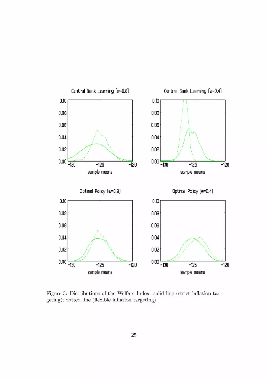
Figure 3: Distributions of the Welfare Index: solid line (strict in�ation tar-geting); dotted line (�exible in�ation targeting)

25

Figure 3 (bottom panel) pictures the distributions of the two optimalTaylor-type feedback monetary policy rules. A number of conclusions emerge.One is that under high pass through (and thus high price �exibility), as wellas relatively low pass-through, it does not matter which monetary policy ruleis used. The results are virtually identical. Optimal monetary policy rules,based on simple Taylor formulations, in our model, without any learning, donot give much support for �exible in�ation targeting.There is one other conclusion which comes from a comparison of the

welfare distributions in Figure 3. It is clear that "stickiness" in informationthrough central bank learning lowers welfare as in all comparable scenarios,the mean welfare under optimality dominates the mean welfare with centralbank learning.10 However, the overall welfare distributions obtained underlearning with high pass-through are not markedly worse than the welfaredistributions generated by optimal monetary policy with the simple Taylorframework. This indicates that the learning mechanism, with the continuousupdating of the laws of motion of in�ation and depreciation dynamics, as wellas the revision of the interest-rate rule, is approximating an optimal Taylorframework. Central bank learning rules can bring the economy to welfareoutcomes which are close to the simpli�ed optimal Taylor rules. In general,overall welfare falls as the degree of price stickiness increases, and the numberof the variables the central bank has to learn increases - the lowest meanwelfare in these eight scenarios is when ! = 0:4 and when the central bankis targeting and learning both in�ation and depreciation.

5 Conclusions

This paper has compared two alternative policy scenarios - strict and �exiblein�ation targeting - for an economy facing terms of trade shocks and time-varying currency risk. The central bank is also assumed not to have fullinformation about all behavioral aspects of the economy, instead it has tolearn the laws of motion for its key target variables in order to set the interestrate according to a feedback rule.The results show that including exchange rate changes in its learning

and policy targeting framework improves welfare under the case of very highexchange-rate pass-through in the sense that the probability of low welfare

10In may be argued that central banks have more sophisticated knowledge of underlyingin�ation dynamics than that which is implied by linear least squares learning. However,as shown here, linear least squares learning can be a good �tracking� mechanism formore complex dynamic processes and the recursive method describe here serves as anapproximation to the Kalman �ltering method for updating and learning.

26

outcomes is reduced. However, if "information" becomes more transparent,so that policy-makers can implement optimal welfare-maximizing rules, thereis little or no case for including exchange-rate depreciation targets. Thepolicy implication is that central banks which are already targeting in�ation,should resist pressures to adopt exchange-rate targets. This implication isparticular signi�cant the greater the degree of price stickiness in the system.

27

References

[1] Ball, Lawrence. (1999), �Policy Rules for Open Economies�, Chapter3 in J.Taylor (ed) Monetary Policy Rules, University of Chicago Press,127-156,

[2] Baron, A.R. (1993), �Universal Approximation Bounds for Superpo-sitions of a Sigmoidal Function�. IEEE Transactions on InformationTheory 39, 930-945.

[3] Bray, M.M. and N.E. Savin (1996), �Rational Expectations Equilibria,Learning, and Model Speci�cation�, Econometrica 54, 1129-1160.

[4] Bullard, James and Kaushik Mitra (2002) �Learning About MonetaryPolicy Rules", Journal of Monetary Economics, forthcoming.

[5] Campa, Jose Maneul and Linda S. Goldberg (2002) �Exchange RatePass-Through into Import Prices: A Macro or Micro Phenomenon?�.NBER Working Paper 8934.

[6] Christiano, Lawrence.J. (2000), �Comment on Ben McCal-lum,�Theoretical Analysis Regarding a Zero Lower Bound for NominalInterest Rates��, Working Paper, Department of Economics, North-western University.

[7] Christiano, Lawrence.J. and Gust, C.J. (1999), �Taylor Rules in aLimited Participation Model�, NBER Working Paper 7017. Web page:www.nber.org/papers/w7017.

[8] De Falco, Ivanoe (1998), �Nonlinear System Identi�cation By Meansof Evolutionarily Optimized Neural Networks�, in Quagliarella, D., J.Periaux, C. Poloni, and G. Winter, editors, Genetic Algorithms and Evo-lution Strategy in Engineering and Computer Science: Recent Advancesand Industrial Applications. West Sussex: England: Johns Wiley andSons, Ltd.

[9] Den Haan. W. and Marcet, Albert (1990), �Solving the StochasticGrowth Model by Parameterizing Expectations�, Journal of Businessand Economic Statistics 8, 31-34.

[10] __________ (1994), �Accuracy in Simulations�, Review of Eco-nomic Studies 61, 3-17.

28

[11] Du¤y, John and Paul D. McNelis (2001), �Approximating and Simulat-ing the Stochastic Growth Model: Parameterized Expectations, NeuralNetworks and the Genetic Algorithm�. Journal of Economic Dynamicsand Control, 25, 1273-1303. Web site: www.georgetown.edu/mcnelis.

[12] Erceg, Christopher J., Dale W. Henderson, and Andrew T. Levin (2000),�Optimal Monetary Policy with Staggered Contracts�, Journal of Mon-etary Economics 46, 281-313.

[13] Gali, Jordi and Monacelli, Tommaso (2002), "Optimal Monetary Policyand Exchange Rate Volatility in a Small Open Economy, NBERWorkingPaper #8905.

[14] Judd, Kenneth L. (1996), �Approximation, Perturbation, and Projec-tion Methods in Economic Analysis� in H.M. Amman, D.A. Kendrickand J. Rust, eds, Handbook of Computational Economics, Volume I.Amsterdam: Elsevier Science B.V.

[15] __________(1998), Numerical Methods in Economics. Cambridge,Mass: MIT Press.

[16] Kim, Sunghyun Henry and M. Ayhan Kose (2001), �Dynamics of OpenEconomy Business Cycle Methods: Understanding the Role of the Dis-count Factor�. Working Paper, Graduate School of International Eco-nomics and Finance, Brandeis University.

[17] Marcet, Albert (1988), �Solving Nonlinear Models by ParameterizingExpectations�. Working Paper, Graduate School of Industrial Adminis-tration, Carnegie Mellon University.

[18] __________(1993), �Simulation Analysis of Dynamic StochasticModels: Applications to Theory and Estimation�, Working Paper, De-partment of Economics, Universitat Pompeu Fabra.

[19] __________ and Juan Pablo Nicolini (1997), �Recurrent Hyper-in�ations and Learning�. Working Paper, Department of Economics,Universitat Pompeu Fabra, Barcelona, Spain. Forthcoming, AmericanEconomic Review.

[20] McCallum, Bennett (2000), �Theoretical Analysis Regarding a ZeroLower Bound on Nominal Interest Rates�. Journal of Money, Creditand Banking, 32 (4), 870-904.

29

[21] Mendoza, Enrique G. (1995), �The Terms of Trade, the Real ExchangeRate, and Economic Fluctuations�, International Economic Review 36,101-137.

[22] __________ (2000), �Credit, Prices and Crashes: Business Cycleswith a Sudden Stop�. Working Paper, Department of Economics, DukeUniversity.

[23] Quagliarella, Domenico and Alessandro Vicini (1998), �Coupling Ge-netic Algorithms and Gradient Based Optimization Techniques� inQuagliarella, D. J., Periaux, C. Poloni, and G. Winter, editors, Ge-netic Algorithms and Evolution Strategy in Engineering and ComputerScience: Recent Advances and Industrial Applications. West Sussex:England: Johns Wiles and Sons, Ltd.

[24] Rotemberg, Julio and Michael Woodford (1998), �An OptimizationBased Econometric Framework for the Evaluation of Monetary Policy:Expanded Version�. NBER Technical Paper No. 233.

[25] Sargent, Thomas J. (1993), Bounded Rationality in Macroeconomics.Oxford, U.K.: Clarendon Press.

[26] __________ (1999), The Conquest of American In�ation. Prince-ton, N.J.: Princeton University Press.

[27] Schmitt-Grohé, Stephanie and Martin Uribe (2001), �Closing SmallOpen Economy Models�. Working Paper, Economics Department, Uni-versity of Pennsylvania.

[28] Taylor, John B. (1993), �Discretion Versus Policy Rules in Practice�,Carnegie-Rochester Conference Series on Public Policy, 39, 195-214.

[29] _________ (1999), �The Robustness and E¢ ciency of MonetaryPolicy Rules as Guidelines for Interest Rate Setting by the EuropeanCentral Bank�, Journal of Monetary Economics 43, 655-679.

[30] _________ (2000), �Using Monetary Policy Rules in EmergingMarket Economies�. Manuscript, Department of Economics, StanfordUniversity.

[31] Wright, B.D. and J.C. Williams (1982), �The Economic Role of Com-modity Storage�, Economic Journal 92, 596-614.

[32] __________ (1984), �The Welfare E¤ects of the Introduction ofStorage�, Quarterly Journal of Economics, 99, 169-182.

30

[33] __________ (1991), Storage and Commodity Markets. Cambridge,UK: Cambridge University Press.

[34] Uzawa, H. (1968), �Time Preference, The Consumption Function, andOptimum Asset Holdings� in J. N. Wolfe, editor, Value, Capital andGrowth: Papers in Honor of Sir John Hicks. Edinburgh: Universityof Edinburgh Press.

31