CORE DISCUSSION PAPER

2007/52

Currency Areas and International Assistance

Pierre M. Picard1and Tim Worrall2

July 2007

Abstract

This paper considers a simple stochastic model of international trade with three

countries. Two of the tree countries are in an economic union. Comparisons are

made between equilibrium welfare for these two countries under fixed and flexi-

ble exchange rate regimes. Within the model it is shown that flexible exchange rate

regimes generate greater welfare. However, we then consider comparisons of wel-

fare when the two countries also engage in some international assistance in order to

share risk. Such risk-sharing is limited by enforcement constraints of cross border

assistance. It is shown that taking into account limited commitment risk-sharing

fixed exchange rates or currency areas can dominate flexible exchange rate regimes

reversing the previous result.

KEYWORDS: Monetary Union; Currency Areas; Fiscal Federalism; Limited Com-

mitment; Mutual Insurance

JEL CODES: F12; F15; F31; F33.

We thank Oscar Amerighi, Kristian Behrens and Jacques Drèze for helpful comments.

The scientific responsibility is assumed by the authors.

1School of Social Sciences, Manchester University and CORE, Université Catholique de Louvain.2School of Economic and Management Studies, Keele University.

1. INTRODUCTION

The present paper contributes to the theories of optimal currency areas and fiscal

federalism. In an often cited paper Mundell (1961) argues that business cycles should

be sufficiently (positively) correlated for a common currency area to be optimal. Bay-

oumi (1994) formally shows that when shocks are negatively correlated across countries

a currency union is less desirable. As a consequence, the discussion about the UK’s in-

tegration (or non-integration) into the Euro currency area has often been driven by the

fact that UK business cycles are not well correlated with continental Europe (see for ex-

ample Artis 2003). Equally the discussion of when the accession countries should join

the Euro currency area has been dominated by the debate about the congruence of the

economic cycles of the accession countries and the rest of Europe (see for example Hall

and Hondroyiannis 2006).

One aspect of monetary integration that has received relatively little attention is the

interaction of international assistance and business cycles on the optimality of currency

areas. Sala-i-Martin and Sachs (1992) identified the importance of fiscal taxes and trans-

fers for interregional assistance in the US and Drèze (2000) argues that transfers between

European regions can be used as a means of insurance against regional income shocks.1

Asdrubali et al. (1996) for the US and Sørensen and Yosha (1998) for the OECD and the EU

have examined channels of risk-sharing. They find that there is less risk-sharing through

fiscal channels in Europe and that risk-sharing is incomplete and occurs mainly through

savings. This confirms earlier results of French and Poterba (1991) and Baxter and Jer-

mann (1997) for the EU which have both shown that agents’ risk diversification is in-

sufficient suggesting that there are welfare gains if more insurance between regions can

be agreed. Further Forni and Reichlin (1999) have shown that shocks and the potential

gains to risk-sharing are large.2 Given these potential gains it is important to examine the

interaction between risk-sharing through interregional assistance and the optimality of

a currency union.

In this paper we model a situation where there are nominal wage and price rigidi-

ties. These wage and price rigidities would normally mean that there is a need for ex-

1Although interregional transfers in the EU are currently quite small (less than 1% GDP) they do increas-ingly depend on regional income (through EU Objective 1 Funds) and increasing integration is likely tomean that transfer play a more prominent role is smoothing interregional fluctuations.

2Asdrubali and Kim (2004) have examined the dynamics of risk-sharing channels and shown complexinteractions between various risk-smoothing mechanisms. They show however that tax and transfer mech-anism can absorb shocks long after they hit.

1

PIERRE M. PICARD AND TIM WORRALL

change rate flexibility to offset nominal rigidities and hence that monetary union is in-

efficient. However, if the importance of transfers between countries to offset regional

shocks is taken into account this result might be reversed.3 We model transfers between

countries by assuming that they are limited by self-enforcing constraints. This is a nat-

ural assumption. Although there exist supra-national institutions such as the European

Commission there is no supra-national authority to enforce transfers across nations.4

Hence countries will only make such transfers if they are in their own long-term interest.

This long-term interest will be determined by the future benefits of risk sharing and by

the punishment imposed for not making the requisite transfer. We shall assume that this

punishment is that the country will not subsequently receive future assistance. Since the

inefficiencies caused by nominal wage and price rigidities may increase the variance of

regional incomes in currency unions, they may make it easier to enforce transfers be-

cause there is an increased punishment threat or sanction that can be applied to any

country not making a transfer when it is called upon to do so. Countries may thus prefer

a monetary union because greater transfers and insurance can be sustained. That is the

benefit of insurance may outweigh the inefficiency cost of price rigidities. We shall show

that this is indeed possible and that there are circumstances where a monetary union

is preferred to the flexible exchange rate system.5 As our model is highly stylized the

importance of the paper is not in delineating exactly the circumstances under which a

currency union is optimal but in showing that the issue of currency integration cannot

be divorced from the issue of fiscal integration through regional risk sharing.

The paper is organized as it follows. Section 2 presents the model and studies the

equilibria under common currency area and flexible exchange rates. In Section 3 we

study an economy with negatively correlated shocks and show when transfers between

countries can be sustained and when a monetary union will deliver higher welfare than a

flexible exchange rate system. Section 4 considers extensions to the basic model. These

extensions quantitatively modify but do not qualitatively change the main results that

3It is important to distinguish the role of transfers in our model from that in standard models of fiscalfederalism where positive transfers between regions may take place mainly because of sharing of a publicgood, such as security (see also Alesina et al. 1995, Persson and Tabellini 1996), rather than sharing of risk.

4The analysis would not be qualitatively different if instead we assumed that it was possible to imposesome but limited sanctions on countries that reneged on transfer obligations.

5Drèze and Gollier (1993) also show that the presence of nominal rigidities in an uncertain world canimprove welfare. In their model however, the beneficial effect of rigidities is derived by firms optimallycreating wage rigidities as a mechanism to insure risk averse workers. In this paper, rigidities are exogenousand improve the substantiality of a transfer system.

2

CURRENCY AREAS

the common currency system sustains greater levels of transfers and may therefore lead

to higher welfare for certain parameter values. Section 5 concludes.

2. BASIC MODEL

We consider a simple model of international trade with three countries r = H ,F,W

(Home, Foreign and the rest of the World). We consider that Home and Foreign have

close economic ties or are in an economic union and shall be interested in whether

Home and Foreign should operate a currency union or retain a flexible exchange rate

regime. This is the situation of the UK or accession countries and the Euro area coun-

tries or between Canada or Mexico and the US. In order to make the comparison between

fixed and flexible exchange rates non-trivial we shall assume that there are some market

imperfections in the labor and product markets. Following much of the literature on cur-

rency areas we shall assume that labor is immobile across countries and that the labor

market is subject to nominal rigidities.6 However, we shall assume there is free trade be-

tween countries and in particular there are no transport or transactions costs to trade.7

Further we shall assume that the goods markets in the Home and Foreign countries is

monopolistically competitive with a continuum of varieties produced and price setting

by firms. In the rest of the world firms produce a homogenous good which we label W .

There is a unit mass of consumer-workers in country H and the same mass in coun-

try F . In country W there is also a unit mass of consumer-workers.8 Labor is supplied

inelastically. We shall assume that goods are non-storable and that consumers consume

both domestically produced and foreign produced goods. We shall index goods by ς or

ξ and let dr s(ξ) denote the demand for good of variety ξ from consumers in country r

which is produced in country s. Similarly we let dr W denote the demand for good W

in country r . Individuals in all countries have the same Dixit and Stiglitz (1977) type

preference function given by

(1) V (Cr ) =V

((∫ 1

0dr r (ς)

σ−1σ dς+

∫ 1

0dr s(ξ)

σ−1σ dξ

) σµ

σ−1

d 1−µr W

),

6Our assumption of labor immobility is common. However some mobility of labor does exist and mi-gration also acts as a risk-sharing mechanism as workers move from countries suffering bad productivityshocks to countries experiencing the good productivity shocks.

7Transport costs can be added to the model without substantially changing the conclusions of the paper.Without transport costs a currency union is never desirable without the insurance motives we model here.Thus introducing transportation costs will tend to strengthen our conclusions.

8Nothing will hinge on the relative size of country W and the assumption of a unit mass for the rest ofthe world is made purely for convenience.

3

PIERRE M. PICARD AND TIM WORRALL

where V is assumed to be strictly increasing and strictly concave so that agents are risk

averse,9 Cr is the aggregate composite good in country r and σ > 1 is the elasticity of

substitution. The elasticity σ will be a measure of the degree of competition between

firms and the higher is σ the greater will be the degree of competition between firms

across countries. The parameter µ measures the relative importance of the rest of the

World. If µ is close to one then the rest of the World has little importance and we are left

with a two country model. If µ is small then the rest of the world is more important so

there is a smaller need of insurance between countries H and F under flexible exchange

rates. Letting pr s(ς) denote the price of good ς sold in country r and produced in country

s, the budget constraint for the representative agent in country r is

∫ 1

0dr H (ς)pr H (ς)dς+

∫ 1

0dr F (ξ)pr F (ξ)dξ+pr W dr W = Yr +Tr

where Yr is the income of consumers in country r and Tr is the transfer income received

by country r expressed in the own countries currency. As we are examining an economic

union between H and F we shall consider transfers only between the Home and Foreign

country and ignore transfers with the rest of the world, that is we set TW ≡ 0.10 With

the utility function given in (1) the demand for variety ς produced in country s from

consumers in country r is given by

(2) dr s(ς) =µpr s(ς)−σ (Yr +Tr )

P 1−σr

and where Pr is a price index for goods produced in H and F and is given by

(3) Pr =(∫ 1

0pr r (ς)1−σdς+

∫ 1

0pr s(ξ)1−σdξ

) 11−σ

.

Likewise the demand for good W in country r is

dr W = (1−µ)(Yr +Tr )

pr W

where pr W is the price of good W in country r .

9For some of the subsequent analysis and the numerical calculations we shall assume that the utilityfunction exhibits constant relative risk aversion preferences.

10If transfers could be made to or received from the rest of the world this would tend to reduce the desirefor insurance from the other country and reduce the punishment for any country reneging on its transfersmaking self-enforcement more difficult. This issue could only be examined in a full three country modelwith enforcement constraints for each country.

4

CURRENCY AREAS

As is well-known the composite consumption is linear in income and simple calcu-

lation shows that

(4) Cr =µµ(1−µ)1−µ Yr +Tr

Pµr p1−µ

r W

.

It will be convenient to emphasize the dependence of the composite consumption on

the transfer and write it as a function of the transfer received Cr (T ).

The exchange rate between currencies in the two countries H and F will depend on

whether there is a single currency area or a flexible exchange rate. However, in either

case since we have assumed there is free and frictionless trade prices satisfy

pr s = εr s pss ∀r 6= s

where εr s is the exchange rate that converts currency of country s into the currency of

country r . Since trade is frictionless εr s = 1/εsr . With three countries there are effec-

tively two independent exchange rates and we shall write ε for εHF and η for εHW . Thus

εFW = ε/η. For convenience we shall also write pr (ς) for pr r (ς) and pW W = pW . There-

fore pHF (ς) = εpF (ς), pF H (ξ) = pH (ξ)/ε and pHW = ηpW . Then it is easy to check from

equation (3) that PH = εPF and that pFW = pHW /ε. Since there are no transfer from

outside H and F we shall have TH =−εTF . In the case of a common currency area ε= 1.

We now consider firm behavior. We shall let Y = YH +εYF +ηYW denote total world

income measured in the home currency.11 For firms producing variety ς in country H

the demand they face from Home and other consumers is

dH (ς) = dH H (ς)+dF H (ς)+dW H (ς)

=µ

pH (ς)−σ (YH +TH )

P 1−σH

+(

pF (ς)ε

)−σ(YF +TF )

P 1−σF

+(

pW

η

)−σYW

P 1−σW

=µ

pH (ς)−σ

P 1−σH

Y

(5)

where the second equality follows because PH = εPF and TH =−εTF . Similarly

(6) dF (ξ) =µpH (ς)−σ

P 1−σH

Y

εand dR = (1−µ)

1

pW

Y

η.

11Note that because of our specification of preferences transfers do not affect world demand.

5

PIERRE M. PICARD AND TIM WORRALL

Firms take demands as given and costs are determined by labor requirements. La-

bor requirement are given by a fixed coefficient technology where to produce one unit

of output in country r requires ar units of labor. The price of labor is denoted by wr .

However, we shall assume that the labor market is imperfect and that nominal wages are

fixed and therefore normalize wr = 1.12 With flexible exchange rates the exchange rates

will adjust to achieve full employment in each country. However, if there is a common

currency between countries H and F , the nominal rigidity in wages will cause unem-

ployment in the relatively unproductive country. In Section 3 we shall assume that aH

and aF are stochastic and specify a simple stochastic process. However, because input

decisions will be made once ar is known and since there are no intertemporal linkages

in production or consumption we can determine equilibria as if ar were fixed and given.

In country W , aW = 1 and we assume that firms are perfectly competitive. Thus we nor-

malize so that pW = 1 which in turn implies pHW = η and PFW = η/ε. In countries H

and F firms are assumed to be monopolistically competitive and will set prices to max-

imize profits given wage costs. Given the fixed coefficients and the iso-elastic demand

functions given in equation (2), prices are set at a mark-up over cost

(7) pr (ς) = σ

σ−1ar , r ∈ {H ,F }.

It follows from equation (7) that all firms in countries H and F set the same price which

is simply a mark-up over costs. This mark-up depends on the elasticity of substitution

between commodities and when substitution is perfect (σ=∞) there is perfect compe-

tition and price equal marginal cost. Equally it follows from equation (7) that demand

is the same for all varieties dr (ς) = dr in a given country. Thus total labor demand is

simply `r = ar dr . By assumption all profits accrue to firms owners and for convenience

we assume that all profits are spent locally. Thus the national income in country r is

Yr = pr dr = pr`r /ar . From equation (7) we may therefore write this national income as

(8) YH = σ

σ−1`H and YF = σ

σ−1`F .

Also since pW = 1, `W = 1 and aW = 1, national income in W is YW = 1. Equally the price

index of equation (3) can be re-written using equation (7) as

PH = (p1−σ

H +ε1−σp1−σF

) 11−σ = σ

σ−1

(a1−σ

H +ε1−σa1−σF

) 11−σ = εPF .

12Assuming that nominal wages are completely inflexible is obviously an extreme assumption which wemake for convenience only. As argued by Mundell (1961) this a priori makes a currency union less desirable.

6

CURRENCY AREAS

An equilibrium is then a set of prices and demands such that (i) consumers maxi-

mize their utility given their budget constraint and given prices, (ii) firms set their profit

maximizing prices and (iii) product markets clear. Since the labor market is imperfect in

countries H and F we do not assume that the labor market clears and there may be some

situations, discussed below, where labor markets do not clear. In either case the product

demand dr (ς) equals product supply `r /ar so that from equations (5) and (6) we have

(9) µpH (ς)−σY

P 1−σH

= `H

aHand µ

pF (ς)−σ(Yε

)P 1−σ

F

= `F

aF

for each variety ς. In addition we have the equivalent condition for the rest of the world

so that (1−µ)(Y /η) = 1. Using the fact that PH = εPF and pH /pF = aH /aF and taking the

ratio of the two equations in (9) gives

(10) ε=(

aH

aF

) σ−1σ

(`H

`F

) 1σ

and η= σ(1−µ)

(σ−1)µ(`H +ε`F ) .

These conditions will determine either the exchange rates ε and η or if ε is fixed the first

condition determines level of employment in either country H or F .

2.1. Common currency area

We now consider the equilibrium in which countries H and F form a common cur-

rency area so that ε= 1. In this case the price index is the same in both countries, PH = PF

and we let P denote this common index. Then

P = (p1−σ

H +p1−σF

) 11−σ = σ

σ−1

(a1−σ

H +a1−σF

) 11−σ .

There are two cases to consider depending on the sign of aH −aF . If aH < aF the Home

country is relatively more productive and requires less labor to produce any given quan-

tity of output. With this parametrization and fixed wages it is easy to check that a share of

country F ’s labor force will be unemployed, `F < 1, as its costs will be higher and hence

demand will fall. In contrast there will be full employment, `H = 1, in country H . It then

follows from equation (10) that `F = (aH /aF )σ−1 < 1. If on the other hand aH > aF then

there will be unemployment in the Home country and `H = (aH /aF )1−σ < 1 = `F . Using

equation (4) and the price index P given by equation (2.1), the composite consumption

7

PIERRE M. PICARD AND TIM WORRALL

in each of the two countries is given by

C cH (T ) =µ

(`H +

(σ−1

σ

)T

)(`H +`F )

(a1−σ

H +a1−σF

) µ

σ−1

C cF (T ) =µ

(`F +

(σ−1

σ

)T

)(`H +`F )C c

H (T )

where the superscript c denotes that the consumption is under a currency union. Hence

the level of employment in the two countries is given by

`H = min

{(aH

aF

)1−σ,1

}and `F = min

{(aH

aF

)σ−1

,1

}.

2.2. Flexible exchange rate system

We now consider equilibrium output and consumption under a flexible exchange

rate system. The introduction of an exchange rate provides an additional instrument

to allow relative prices to alter and production and employment to increase. Although

nominal wages are fixed at wH = wF = 1 the exchange rate allows the relative wages

εwF /wH to adapt. Under a flexible exchange rate system there is no real wage rigidity so

that labor market clears in the both the high and low productivity countries and hence

`H = `F = 1. Then equilibrium output in both H and F is YH = YF = σ/(σ−1) and the

exchange rates are determined from (10):

(11) ε=(

aH

aF

) σ−1σ

and η= σ(1−µ)

(σ−1)µ(1+ε).

If aH < aF then country F has relatively low productivity and its currency depreciates

making its exports relatively cheaper to the Home country. Likewise if aH > aF then

country F is relatively more productive and its currency will appreciate so that its exports

become relatively more expensive to the Home country. With this exchange rate adjust-

ment and remembering that PH = εPF , the composite consumption in each country is

given by from equation (4) as

C fH (T ) =µ

(1+

(σ−1

σ

)T

)(1+ε)µ−1 (

a1−σH +ε1−σa1−σ

F

) µ

σ−1

C fF (T ) = εC f

H (T )

8

CURRENCY AREAS

where the superscript f indicates that the consumption is calculated under flexible ex-

change rates and where the exchange rate ε is as given in equation (11).

In the absence of transfers, an appropriate exchange rate policy (common currency

or flexible exchange rate) also allows countries to achieve the highest aggregate con-

sumption. One readily shows that C fr (0) ≥C c

r (0) for r = H ,F . Thus we have the standard

result

PROPOSITION 1: In the absence of any transfers (Tr = 0), aggregate consumption at

any state is higher under flexible exchange rate system: C fr (0) ≥C c

r (0), r = H ,F .

PROOF: Take the case aH < aF . We have

C fH (0) =µ

(a1−σ

H +ε1−σa1−σF

) µ

σ−1 (1+ε)µ−1

C cH (0) =µ

(a1−σ

H +a1−σF

) µ

σ−1

(1+

(aH

aF

)σ−1)µ−1

.

Since aH < aF , ε1−σ > 1 and ε> (aH /aF )σ−1. Hence C fH (0) >C c

H (0). Also

C fH (0) = εC f

H (0)

C cH (0) =

(aH

aF

)σ−1

C cH (0).

Since ε > (aH /aF )σ−1 this shows that C fF (0) > C c

F (0). A similar argument applies in the

case where aH > aF . 2

Thus in this model if there are no transfers between countries H and F then a com-

mon currency area will always be dominated by a flexible exchange rate regime.

3. CURRENCY AREAS UNDER NEGATIVELY CORRELATED SHOCKS

We shall now consider transfers between countries H and F and how this affects

the result that a flexible exchange rate regime dominates a common currency area that

we have seen in Proposition 1. To do this we will need to specify a stochastic process

for productivity shocks so that there are some potential mutual gains to transfers. The

role of shocks has often played a key role in debates about common currency areas. Tak-

ing into account transactions costs Mundell (1961) argues that business cycles should be

sufficiently (positively) correlated for a common currency area to be optimal. Bayoumi

(1994) formally shows that negative correlation of shocks makes currency unions less de-

9

PIERRE M. PICARD AND TIM WORRALL

sirable. As a consequence, the discussion about the UK’s integration or non-integration

in the Euro currency area has often been driven by the fact that UK business cycles are

not well correlated with continental Europe.

In this section we shall show that the conclusion of Mundell (1961) can be reversed

when self-enforcing transfers are taken into account. That is we shall show that a com-

mon currency area can be optimal when shocks are negatively correlated. To do this we

take the extreme assumption that shocks are perfectly negatively correlated. Thus we

will make assumptions, absence of transactions costs and negatively correlated shocks,

that are usually seen as inimical to currency unions, yet show that a common currency

area can be optimal in these circumstances.13 Our argument lies in the fact that when

there are productivity shocks and income variability across countries it will be desir-

able to try and smooth these shocks by making transfers between countries. However,

transfers across countries may be difficult to legally enforce and therefore such insur-

ance transfers must be self-enforcing and enforcement may sometimes be helped by the

threat of a more severe punishment.

To proceed we shall assume that the technology in countries H and F is stochastic.

We shall assume there are just two symmetric states, so that the two countries either have

a good or a bad productivity shock. Further we suppose that these states are perfectly

negatively correlated states so that the labor requirements are (aH , aF ) = (z,1) in state

1 and (aH , aF ) = (1, z) in state 2. We assume that z < 1 so that the Home country has

a good productivity shock is state 1 and the Foreign country has the good productivity

shock in state 2. To preserve symmetry we assume that each state occurs with equal

probability. With these assumptions, the aggregate composite consumption under the

common currency in the two states is given by

C cG (T ) =µ

(1+

(σ−1

σ

)T

)z(µ−1)(σ−1) (1+ z1−σ) σ(µ−1)+1

σ−1

C cB (T ) =µ

(zσ−1 +

(σ−1

σ

)T

)z(µ−1)(σ−1) (1+ z1−σ) σ(µ−1)+1

σ−1

where C cG (T ) is the consumption of the Home (Foreign) country in state 1 (2) when it

experiences a good productivity shock and C cB (T ) is the consumption of the Home (For-

13The empirical evidence (see for example Artis 2003, Hall and Hondroyiannis 2006) suggests that thecorrelations of the UK and the CEECs with the rest of the EU is relatively weak. Our assumption of neg-ative correlation is made to keep the analysis simple and to take the case usually thought to be the mostunfavorable to the optimality of currency areas.

10

CURRENCY AREAS

eign) country in state 2 (1) when it experiences a bad productivity shock. The transfer

T is the amount received and expressed in the countries own currency. Since zσ−1 < 1 it

can be seen that absent any transfers the Home (Foreign) country has higher consump-

tion in state 1 (2), when it experiences a positive productivity shock.

Under the flexible exchange rate regime the exchange rate in state 1 is ε1 = zσ−1σ < 1

as the Foreign currency depreciates when the Home country has a positive productivity

shock. In contrast, in state 2 when the Foreign country has a positive productivity shock

its exchange rate appreciates to ε2 = z1−σσ > 1. Then calculating the aggregate composite

consumption in each state for the two countries gives:

C fG (T ) =µ

(1+

(σ−1

σ

)T

)z

1−σσ

(1+ z

1−σσ

) σ(µ−1)+1σ−1

C fB (T ) = z

σ−1σ C f

G (T ).

As zσ−1σ < 1 it can be seen that absent any transfers the Home (Foreign) country has

higher consumption in state 1 (2) when it has positive productivity shock than in state 2 (1),

so that C fG (0) >C f

B (0).

3.1. First-best transfers

In this section we determine the first-best transfers and show that if the first-best

transfers are implemented, then the flexible exchange rate regime yields greater welfare.

The first-best transfers will equalize composite consumptions whether countries have

good or bad productivity shocks. Let τi∗ denote the transfer received by the country with

the bad productivity shock under regime i ∈ {c, f }. This will be the transfer received by

the Home (Foreign) country in state 2 (1).

With a common currency the transfer received by the country with the bad produc-

tivity shock equals the transfer made by the country with the good productivity shock.

Thus the first-best transfer can be found by solving C cG (−τ) = C c

B (τ). Calculating this

transfer and the first-best composite consumption C c∗ gives

τc∗ =

1

2

σ

σ−1

(1− zσ−1) and C c

∗ =1

2µzµ(σ−1) (1+ z1−σ) µσ

σ−1 .

It can be seen that since zσ−1 < 1, the transfer τc∗ is positive and decreasing in z. It can

also be seen that in this simple model transfers are independent of the rest of the World

11

PIERRE M. PICARD AND TIM WORRALL

for two reasons. First, the transfer has no effect on world income Y and secondly it does

not depend on µ the degree of preference for rest of the World goods.

Under flexible exchange rates if τ f∗ is received by the country with the bad produc-

tivity shock then the transfer made by the country with the good productivity shock is

zσ−1σ τ

f∗. In state 1 (2) it is the Home (Foreign) country which has the good productivity

shock so the transfer made is ε1τf∗ (τ f

∗/ε2) where ε1 = zσ−1σ = 1/ε2. The first-best transfer

is therefore found by solving C fG (−z

σ−1σ τ

f∗) =C f

B (τ f∗). This gives the first-best transfer and

consumption as given by

τf∗ = 1

2

σ

σ−1

(z

1−σσ −1

)and C f

∗ = 1

2µ

(1+ z

1−σσ

) µσ

σ−1.

Since z1−σσ > 1, the transfer is positive and decreasing in z. Again this transfer does not

affect Y and is independent of µ.

It is natural to expect that lower consumption with no transfers implies lower con-

sumption under full insurance and this is demonstrated in the next proposition.

PROPOSITION 2: First best transfers yield higher aggregate utility under flexible ex-

change rate system: C f∗ ≥C c∗.

PROOF: Rewriting the formulas above for the composite consumptions so that

they can be compared gives

C c∗ =

1

2z−µ (

1+ zσ−1) µσ

σ−1 and C f∗ = 1

2z−µ

(1+ z

σ−1σ

) µσ

σ−1.

Since zσ−1σ > zσ−1 for z < 1 and σ> 1 it follows that C f

∗ ≥C c∗. 2

Thus if it were possible to sustain the first-best transfers then again the common

currency area would be sub-optimal. However, we shall be interested in cases where

the common currency regime sustains more insurance than the flexible exchange rate

regime. For some parameter values C fB (0) > C c∗ and in these cases the flexible exchange

rate regime will always dominate as the worst outcome in the flexible exchange rate

regime delivers more welfare than the first-best welfare with a common currency. The

next proposition describes the parameter values such that the common currency can

never be optimal.

12

CURRENCY AREAS

PROPOSITION 3: If z > (1/2)(1+ z)(1−µ) then a flexible exchange rate system is pre-

ferred for any system of transfers between country: C fB (0) >C c∗.

PROOF: The composite consumptions C fB (0) and C c∗ are both functions of z,σ and

µ. Therefore let g (z,σ,µ) =C fB (0)/C c∗ denote the ratio of the composite consumptions. It

can be checked that limσ→1 g (z,σ,µ) = 1 and that the function g (z,σ) asymptotes from

above so that limσ→∞ g (z,σ,µ) = 2z/(1+ z)(1−µ). Hence for values of z and µ such that

z > (1/2)(1+ z)(1−µ), g (z,σ,µ) ≥ 1 for all values of σ ∈ (1,∞). 2

3.2. Sustainable Assistance

There may be many reasons why the first-best transfers between countries H and

F cannot be achieved. We consider the case where the first-best transfers cannot be

achieved because there is no supra-legal authority to enforce transfer across countries.

To allow for the possibility of transfers we therefore consider that countries interact re-

peatedly over an infinite horizon. Since transfers cannot be legally enforced, countries

can renege on any agreement if they find it in their interest not to make a transfer and

hence any assistance programme has to be designed to be self-enforcing. Thomas and

Worrall (1988) examine self-enforcing wage contracts between an employer an an em-

ployee and a similar approach can be applied here. Thus we presume that countries

make a tacit agreement on a programme of mutual assistance and specify the transfers

to be made by the country with the good productivity shock and to be received by the

country with the bad productivity shock in every possible contingency. We shall assume

that any breach of this tacit agreement results in a breakdown in which no transfers are

made.14,15

To consider such self-enforcing transfers between countries H and F let ht denote

the history of good and bad outcomes for a particular country.16 Let G t denote the good

14A breakdown in which no transfers are made is the worst possible outcome and is sub-game perfect. Itis not however renegotiation-proof. Nevertheless it can be shown that in the current context replacing thesepunishments with one that are renegotiation-proof will not change the qualitative or quantitative propertiesof the assistance programme.

15There are other possible assumptions one could make about behavior in the breakdown. For examplea stricter punishment could be imposed whereby there is reversion to trade autarky. Alternatively a weakerpunishment would be to assume that following any breakdown in the insurance arrangements there wouldbe a total breakdown of the currency union itself and a return to a flexible exchange rate regime withouttransfers.

16As we have assumed that shocks are perfectly negatively correlated this history has only to be specifiedfor one arbitrary country and is equivalent to specifying a history of states. We are also assuming that allother aspects of the economy are unchanging over time.

13

PIERRE M. PICARD AND TIM WORRALL

productivity shock outcome at date t and B t denote bad productivity shock outcome at

date t . Then ht is a list of G’s and B ’s where h0 =;. An assistance programme in regime

i ∈ {c, f } then specifies a transfer τiB (ht−1) to made to the country with the bad produc-

tivity shock if the previous history is ht−1 and the transfer to be made by the country

with the good productivity shock τiG (ht−1). The short-term loss to the country with a

good productivity shock of making the required transfer at time t ≥ 1 relative to making

no transfer is

V (C iG (−τi

G (ht−1)))−V (C iG (0)).

Likewise the short-term gain at date t ≥ 1 for the country receiving a transfer is

V (C iB (τi

B (ht−1)))−V (C iB (0)).

To evaluate future gains and losses we shall assume that countries discount the future by

a common discount factor δ ∈ (0,1]. Then the discounted long-term gain from adhering

to the agreed transfers from the next period is (discounted back to period t +1)

E

[ ∞∑j=0

δ j{

1

2

[V (C i

G (−τiG (ht+ j )))−V (C i

G (0))]+ 1

2

[V (C i

B (τiB (ht+ j )))−V (C i

B (0))]}]

.

where the expectation E is taken over all future histories of good and bad productivity

shocks from date t onward, τiG (ht+ j ) is the transfer promised to be made by the country

with the good productivity shock at date t+ j+1 given that the history up to time t was ht

and τiB (ht+ j ) is the transfer to be received by the country with the bad productivity shock

at date t + j +1 given that the history up to time t was ht . Letting V iG (ht ) denote the net

discounted net utility from date t +1 for the country with the good productivity shock,

i.e. where the history is ht+1 = (ht ,G t+1), and V iB (ht ) be the net utility for a country with

a bad productivity shock, i.e. where the history is ht+1 = (ht ,B t+1), we have the recursive

equations

V iG (ht ) =V (C i

G (−τiG (ht−1)))−V (C i

G (0))+δ[

1

2V i

G (ht ,G t+1)+ 1

2V i

B (ht ,B t+1)

],

V iB (ht ) =V (C i

B (τiB (ht+ j )))−V (C i

B (0))+δ[

1

2V i

G (ht ,G t+1)+ 1

2V i

B (ht ,B t+1)

].

A country in the economic union will make a transfer if the expected discounted risk-

sharing benefits from future transfers exceed the costs of making the current transfer.

Since reneging leads to exclusion, the discounted net utilities must be non-negative at

14

CURRENCY AREAS

every history

(12) V iG (ht ) ≥ 0 and V i

B (ht ) ≥ 0 ∀ ht .

We shall say that an assistance programme is sustainable if equations (12) are satisfied.

In addition we shall only be interested in programmes where the amount received equals

the amount transferred. This means we impose τcG (ht ) = τc

B (ht ) for all ht under the com-

mon currency regime and τfG (ht ) = z

σ−1σ τ

fB (ht ) when the exchange rate is flexible.

0.3 0.6 0.9z

1.5

2

2.5

Σ

Γ=1.25 Γ=2.5 Γ=5

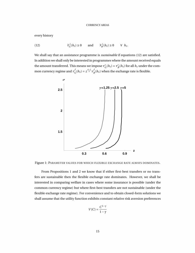
Figure 1: PARAMETER VALUES FOR WHICH FLEXIBLE EXCHANGE RATE ALWAYS DOMINATES.

From Propositions 1 and 2 we know that if either first-best transfers or no trans-

fers are sustainable then the flexible exchange rate dominates. However, we shall be

interested in comparing welfare in cases where some insurance is possible (under the

common currency regime) but where first-best transfers are not sustainable (under the

flexible exchange rate regime). For convenience and to obtain closed-form solutions we

shall assume that the utility function exhibits constant relative risk aversion preferences

V (C ) = C 1−γ

1−γ

15

PIERRE M. PICARD AND TIM WORRALL

where γ> 1 is the coefficient of relative risk aversion.17 We also know from Proposition 3

that welfare will only be higher under common currency areas for certain values of z and

σ. Figure 1 illustrates regions of the parameter space for which flexible exchange rates

always dominate because the welfare under flexible exchange rates with no transfers ex-

ceeds the welfare under common currency with first-best transfers. The figure is drawn

for parameter values µ = 0.0518 and three different values of γ. To the right of each line

the flexible exchange rate regime will always dominate for the given value of γ.19

Having established parameter values such that the flexible exchange rate regime al-

ways dominates no matter what transfers are sustainable the next two subsections there-

fore consider for what parameter values the first-best transfers can be sustained and for

what parameter values no transfers can be sustained. The next sub-section will then

compare welfare in the two regimes.

3.3. Sustainable first best

In this subsection we consider the discount factors for which the first best-best

transfers are sustainable and satisfy equations (12). The first-best transfers are history

independent and provide consumption of C i∗ in both countries. Because the first-best

transfers are independent of history and because a country will only breach when it has

a good productivity shock and is called upon to make a transfer, they are sustainable if

and only if

V (C i∗)−V (C i

G (0))+ δ

(1−δ)

{1

2

[V (C i

∗)−V (C iG (0))

]+ 1

2

[V (C i

∗)−V (C iB (0))

]}≥ 0.

Rewriting this equation shows that these transfers are sustainable for discount factors

above a critical level δi

where

δi ≡ V (C i

G (0))−V (C i∗)12

[V (C i

G (0))−V (C iB (0))

] .

17A similar analysis also applies in the case where γ = 1 and V (C ) = ln(C ). None of the results hinge onthe constant relative risk aversion formulation but the assumption is useful to illustrate the comparisonsbetween the two currency regimes.

18With this value of µ, 95% of consumer expenses are made on goods from the rest of the world. Using adifferent value of µ changes the scale but not the qualitative properties of this figure.

19If countries are risk-neutral then the the evaluation is simply in terms of expected consumption and theflexible exchange rate regime always dominates.

16

CURRENCY AREAS

Making use of the constant relative risk aversion specification of preferences the critical

values of the discount factors above which the first-best transfers are sustainable are

independent of µ and are given by

δf

(z) = δc(z

1σ ) = 2

1−[

12

(1+ z

σ−1σ

)]1−γ

1− zσ−1σ (1−γ)

One can show that for γ≥ 1, δc(z) is a positive and increasing function of z with δ

c(0) = 0

and limz→1δc(z) = 1. Therefore as z < z1/σ < 1, we get that δ

f(z) > δ

c(z).

3.4. Non-sustainability of assistance

We now consider the case where the two countries H and F cannot sustain any

transfers. We first define the ratio of the marginal utility of the country suffering the bad

productivity shock to the marginal utility of the country experiencing the good produc-

tivity shock when no transfers are made. This is given by

ρi (z) = dV (C iB (T ))/dT

dV (C iG (T ))/dT

∣∣∣∣∣T=0.

With constant relative risk aversion preferences we have

ρ f (z) = ρc (z1σ ) = z−γ σ−1

σ

which is again independent ofµ. To find circumstances where it is not possible to sustain

any transfers we need only consider some small and history independent transfers τiG

and τiB . If a country were to breach the agreement it would do so when it has a good

productivity shock and is called upon to make a transfer. Thus the transfers τiG and τi

B

are not sustainable if

V (C iG (−τi

G ))−V (C iG (0))

+ δ

(1−δ)

{1

2

[V (C i

G (−τiG ))−V (C i

G (0))]+ 1

2

[V (C i

B (τiB ))−V (C i

B (0))]}

< 0.(13)

Approximating the left hand side around τiB = τi

G = 0 gives the condition

(1− δ

2

)+ δ

2ρi (z) < 0.

17

PIERRE M. PICARD AND TIM WORRALL

This gives a critical discount factor δi below which no transfers can be sustained in

regime i ∈ {c, f }. Using the assumption of constant relative risk aversion preferences

gives

δ f = δc (z1σ ) = 2

1+ z−γ σ−1σ

.

One readily can show that δc (z) is an increasing function of z with limz→0δc (z) = 0 and

δc (1) = 1. Therefore δc < δ f . This together with the condition of the previous subsection

gives the following result.

PROPOSITION 4: Common currency areas are more likely to sustain an equilibrium

with first best transfers and less likely to sustain an equilibrium with zero transfers than

flexible exchange rate systems.

Figure 2 depicts the critical discount factors that sustain first best and zero transfers

for given values of σ, γ and µ. Below the line δi no transfers can be sustained in regime

i ∈ {c, f }. Above the line δi

the first-best transfers can be sustained. For these parameter

values of σ and γ the flexible exchange rate regime can sustain some transfers even for

discount factors low enough that the common currency regime cannot sustain the first-

best, δ f < δc. However, for different values of σ or γ it is easy to show that δ f > δ

cis

possible.

3.5. Self-enforcing transfers

Self-enforcing transfers will in general be history dependent. However, the results

of Thomas and Worrall (1988) show that the long-run distribution is ergodic. In the case

with just two states transfers will be history independent as soon as both states have

occurred. It easy to find the transfers after both states have been visited. Either the first-

best transfer is sustainable or no transfer is sustainable or the transfer will be set so that

(13) is binding. This is easy to see as if it weren’t binding the transfer could be increased

slightly and welfare could be improved.

Suppose that the parameters are such that the first-best transfer is not sustainable

but that some self-enforcing transfers are sustainable. Self-enforcing transfers are deter-

mined by the following equation

(14) φi (z,τi ) ≡ V (C iB (τi

B ))−V (C iB (0))

V (C iG (0))−V (C i

G (−τiG ))

= 2−δδ

18

CURRENCY AREAS

0.1 0.3 0.5 0.7z

0.3

0.6

0.9

∆

∆��c

∆��f

∆��c

∆��f

Figure 2: MAXIMUM AND MINIMUM DISCOUNT FACTORS WHICH SUSTAIN NO TRANSFERS

OR FIRST-BEST TRANSFERS: σ= 1.5 AND γ= 2.

where τi = τiG is the transfer made by the country with the good productivity shock and

where τcB = τc

G and τfB = z

σ−1σ τ

fG .

PROPOSITION 5: There is a unique value of τi satisfying equation (14) and this value

is strictly increasing in δ.

PROOF: Consider the case of the currency union. Differentiating φc (z,τc ) with

respect to τc shows that

sign∂φc (z,τc )

∂τc = signV ′(C c

B (τc ))

V ′(C cG (−τc ))

−φc (z,τc ).

By the concavity of V we have for any τc ∈ (0,τc∗),

V (C iB (τi

B ))−V (C iB (0))

C cB (τc )−C c

B (0)>V ′(C c

B (τc )) >V ′(C cG (−τc )) > V (C i

G (0))−V (C iG (−τi

G ))

C cG (0)−C c

G (−τc ).

19

PIERRE M. PICARD AND TIM WORRALL

In varying τc , C cG (0)−C c

G (−τc ) =C cB (τc )−C c

B (0) and hence

V ′(C cB (τc ))

V ′(C cG (−τc ))

−φc (z,τc ) < 0.

Thus φc (z,τc ) is monotonically decreasing in τc and hence there is a unique value of τc

satisfying equation (14). As the right hand side of equation (14) is strictly decreasing in

δ ∈ (0,1) the transfer that can be sustained is strictly increasing in δ. The proof for the

flexible exchange rate case is similar. 2

With constant relative risk aversion preferences the functionφi (z,τi ) of equation (14)

simplifies considerably so that the transfer τi can be found by solving the involves solv-

ing the equations

(15) φc (z,τc ) =φc (z1σ ,τ f ) = (2−δ)

δ

where

φc (z,τ) = z(σ−1)(1−γ)

(1+ z1−σ (

σ−1σ

)τ)1−γ−1

1− (1− (

σ−1σ

)τ)1−γ

With this specification it is clear that since z1/σ < z we have that τ f < τc so that a greater

transfer can be sustained under a currency union that under a flexible exchange rate. In

addition it is possible to show thatφi (z,τi ) is strictly decreasing in z. Thus a larger shock

(smaller value of z) will mean that a larger transfer τi can be sustained. We therefore

have the following result.

PROPOSITION 6: The larger the productivity shock the greater will be the transfer that

is sustained in either regime. The common currency union will sustain a greater transfer

than the flexible exchange rate regime.

As it is not possible to obtain an explicit solution for τi in equation (15) it is difficult

to give analytical results of the effect of the different regimes on welfare. We know from

Propositions 4 and 6 that the common currency regime sustains greater transfers. How-

ever, we also know from Propositions 1 and 2 that the flexible exchange rate system will

generate greater welfare if either no transfers or the first-best transfers can be sustained.

Thus in comparing welfare there are two opposing effects. The common currency area

allows for greater transfers and thus greater sharing of risk and greater welfare. However

it does not allow the inefficiencies in the labor market to be offset by adjustments in the

20

CURRENCY AREAS

0.75 0.8 0.85∆

Utility

Common Currency

Flexible

Figure 3: WELFARE COMPARISONS FOR COMMON CURRENCY AND FLEXIBLE EXCHANGE

RATE REGIMES WITH OPTIMAL SUSTAINABLE TRANSFERS: γ = 2, σ = 1.5, µ = 0.05 AND

z = 0.5.

exchange rate and this tends to lower welfare. However, using equation (15) it is possible

to compute the maximum sustainable transfers for any discount factor and hence com-

pute the expected welfare of each country under flexible exchange rates or a common

currency.

Computations show that either effect can dominate. Thus for some parameter val-

ues a flexible exchange rate regime generates greater welfare and for other parameter

values a common currency does. As the first-best transfers can be sustained under com-

mon currency when less or no transfers can be sustained with flexible exchange rates,

there are many parameter values for which higher welfare can be achieved with a com-

mon currency than with flexible exchange rates. More interesting perhaps are cases

where the common currency cannot sustain first-best transfer, the flexible exchange rate

regime can support some transfers but where the common currency yields higher wel-

fare for some parameter values. Such an example is illustrated in Figure 3. The darker

line plots the welfare under flexible exchange rates against the discount factor. It is ini-

tially horizontal and here no transfers can be sustained but then it rises as some transfers

can be sustained and it is again horizontal for higher discount factors when the first-best

21

PIERRE M. PICARD AND TIM WORRALL

transfers can be sustained. The lighter line represents expected utility under common

currency and it has a similar shape (the lower part where no transfers can be sustained is

not illustrated). Following on from Propositions 1 and 2 it is clear that flexible exchange

rates dominate for low discount factors where no transfers can be sustained in either

regime of for high discount factors where first-best transfers can be sustained in either

regime. However, as can be seen the common currency regime does produce higher wel-

fare in an intermediate range of discount factors where neither regime can sustain the

first-best transfers.

4. EXTENSIONS

The model can be extended in a number of directions without changing the sub-

stantive result that considerations of sustainable assistance are important in determin-

ing the relative efficiency of common currency and flexible exchange rate systems. This

section outlines some possible extensions.

4.1. Additional tradable sectors

In the model outlined both the Home and Foreign countries compete in all goods

produced. There may however, be specialized but tradable commodity sectors in each

country. Let Zr be the output of specialized locally produced goods in country r . For

simplicity consider only trade between H and F (setµ= 1) and suppose that the constant

elasticity of substitution preferences utility becomes

V (Cr ) =V

((∫ 1

0dr r (ς)

σ−1σ dς+

∫ 1

0msr (ξ)

σ−1σ dξ

) σχ

σ−1

Z1−χ

2r Z

1−χ2

s

)

where (1−χ) is the share of the specialized sectors (which for simplicity we’ve assumed

is evenly distributed between the two countries). Assuming that the two tradable sectors

have constant returns to scale and hire workers who produce at unit productivity, labor

demand is `r = ar dr +Zr and gross domestic product Yr = pr dr +Zr Prices of the com-

petitively produced manufacturing goods is the same as before pr = arσ/(σ−1) and the

size of the specialized sectors is

ZH = (1−χ)

2(YH +εYF ) = εZF .

22

CURRENCY AREAS

Then one can show that

(8′) YH = σ

σ−1`H

[1− (1−χ)

2

1

σ−χ(1+ε `F

`H

)]with a similar expression for YF . Equating demand and supply then gives the following

implicit condition for the exchange rate.

(10′)(

aH

aF

)1−σ= ε1−σ

[(σ−χ)`H − 1

2 (1−χ)σ(`H +ε`F )

(σ−χ)ε`F − 12 (1−χ)σ(`H +ε`F )

].

One can see that for χ = 1, equations (8′) and (10′) reduce to equations (8) and (10) re-

spectively. In the common currency case ε = 1 and either `H or `F is less than one de-

pending on the technology parameters aH and aF . In the flexible exchange rate case

there is full employment so `H = `F = 1. As expected experimentation shows that com-

mon currency areas is more likely to dominate for a large tradable sector χ. Yet the effect

of χ in the examples we computed is not very significant.

4.2. Transactions costs

It is possible to introduce transactions costs into the analysis of the flexible ex-

change rate regime by allowing for a bid-ask spread. The bid-ask spread can be taken

fixed percentage θ whereεbi d

εask= 1−θ.

The introduction of a bid-ask spread has two effects that reduce the attractiveness of the

the flexible exchange rate regime. First foreign goods become relative more expensive

reducing the efficiency gains from trade. Secondly, some of the transfer is lost in trans-

action and so insurance is also less effective.

4.3. Alternative stochastic processes

We have assumed that shocks in the two countries H and F are perfectly negatively

correlated. This is mainly for convenience and because it is known that under standard

assumptions without insurance this is the case in which a flexible exchange rate regime is

most dominant. The assumption of perfect negative correlation and symmetry (together

with the assumption of constant relative risk aversion) also allowed us to derive some

simple analytic formulae for critical discount factors.

23

PIERRE M. PICARD AND TIM WORRALL

It is possible to generalize the stochastic process and allow for any degree of corre-

lation between shocks and also allow for persistence of shocks within countries. With a

two state income distribution in each of the two countries, there will be four states for

the world economy (with perfect correlation there are just two). This complicates the

analysis slightly. With perfect negative correlation either full, partial or no insurance is

sustainable. With four income states there will typically be degrees of partial insurance

and this needs to be accounted for in the calculations. Nevertheless it is still possible

to calculate analytical results. If there are three income states for each country, high

medium and low, then there are up to nine states for the world economy and analytic

computation becomes difficult. It is possible to compute solutions by numerically by

computing and interpolating the appropriate value function. This is not too computa-

tionally expensive provided the number of states is relatively small. There is however the

further difficulty that with increases in the number of states the time taken to the steady-

state becomes longer, so that an appropriate comparison is not with the steady-state but

with the long-run expected discounted utility taking into account the transition to the

steady-state.

4.4. Labor market imperfections

A restrictive assumption of the analysis is that nominal wages are completely inflex-

ible and this stands in contrast to our assumption that the product market is monopolis-

tically competitive. It would be possible to introduce some wage-setting behavior to the

model (see for example Danthine and Hunt 1994) to relax this assumption. Introduce

wage setting would have two opposing effects. First introducing some flexibility into the

labor market would make the currency union less unattractive. Secondly it would make

the punishment of returning to zero transfers less severe and hence reduce the amount

of insurance that could be sustained. The net effect of reducing the labor market imper-

fections in the model is therefore ambiguous and something for further analysis.

5. CONCLUSIONS

This paper has examined the importance of mutual insurance between countries

on the decision to adopt either a common currency or a flexible exchange rate system.

Standard analysis suggests that absent any transactions costs the flexible exchange rate

system will dominate if either there is no insurance or alternatively if there is full in-

surance. However, we have shown that if there are restrictions caused by commitment

24

CURRENCY AREAS

constraints such that only partial insurance is achievable then this result can be reversed

and a common currency can generate higher welfare. The impediment to full insurance

we have assumed is that there is no supra-national authority to enforce insurance pay-

ments across countries and therefore such insurance must be self-enforcing. The impo-

sition of the constraints of self-enforcement mean that sometimes more insurance can

be enforced under a common currency system than a flexible exchange rate system be-

cause the threat of no future insurance if there is a breakdown in transfers is more severe

in the common currency case.

The paper has presented a simple model to illustrate this possibility. There has

been no attempt to calibrate the model as realistic calibration would have to involve a

much more sophisticated model of both production and labor market imperfections and

a more detailed specification of the stochastic structure of shocks. Rather we decided to

illustrate the importance of insurance on the currency union in a model designed to

make currency union a priori less desirable. Thus we assumed that there were no trans-

actions costs in the flexible exchange rate system, there was perfect inflexibility in the

labor market and shocks were perfectly negatively correlated. Despite these assump-

tions it has been shown that there are parameter values where a common currency can

generate greater welfare. The result should be of interest to policy makers as it shows

that any agreement on a system of insurance or fiscal transfers between countries can

have an important impact on the monetary decision to adopt a common currency.

25

REFERENCES

Alesina, A., R. Perotti, and E. Spolaore (1995, April). Together or separately? Issues on

the costs and benefits of political and fiscal unions. European Economic Review 39(3),

751–758.

Artis, M. J. (2003, October). Reflections on the optimal currency area (OCA) criteria in

the light of EMU. International Journal of Finance & Economics 8(4), 297–307.

Asdrubali, P. and S. Kim (2004, May). Dynamic risksharing in the United States and Eu-

rope. Journal of Monetary Economics 41(4), 809–836.

Asdrubali, P., B. E. Sørensen, and O. Yosha (1996, November). Channels of interstate risk

sharing: United States 1963-1990. The Quarterly Journal of Economics 111(4), 1081–

1110.

Baxter, M. and U. J. Jermann (1997, March). The international diversification puzzle is

worse than you think. American Economic Review 87(1), 170–180.

Bayoumi, T. A. (1994, December). A formal theory of optimum currency areas. IMF Staff

Papers 42(4), 537–554.

Danthine, J.-P. and J. Hunt (1994, May). Wage bargaining structure, employment and

economic integration. The Economic Journal 104(424), 528–541.

Dixit, A. K. and J. E. Stiglitz (1977, June). Monopolistic competition and optimum prod-

uct diversity. American Economic Review 67(3), 297–308.

Drèze, J. H. (2000, September). Economic and social securtiy in the twenty-first century,

with attention to Europe. Scandinavian Journal of Economics 102(3), 327–348.

Drèze, J. H. and C. Gollier (1993, December). Risk sharing on the labour market and

second-best wage rigidity. European Economic Review 37(8), 1457–1482.

Forni, M. and L. Reichlin (1999, June). Risk and potential insurance in Europe. European

Economic Review 43(7), 1237–1256.

French, K. R. and J. M. Poterba (1991, May). Investor diversification and international

equity markets. American Economic Review 81(2, Papers and Proceedings), 170–180.

Hall, S. G. and G. Hondroyiannis (2006, January). Measuring the correlation of shocks

between the EU15 and the new member countries. Working Papers 31, Bank of Greece.

Mundell, R. A. (1961, September). A theory of optimum currency areas. American Eco-

nomic Review 51(4), 657–665.

26

CURRENCY AREAS

Persson, T. and G. Tabellini (1996, May). Federal fiscal constitutions: Risk sharing and

moral hazard. Econometrica 64(3), 623–646.

Sala-i-Martin, X. and J. Sachs (1992). Fiscal federalism and optimum currency areas:

Evidence for Europe from the United States. In M. B. Canzoneri, V. Grilli, and P. R. Ma-

son (Eds.), Establishing a Central Bank: Issues in Europe and Lessons from the United

States, Chapter 7, pp. 195–220. Cambridge: Cambridge University Press.

Sørensen, B. E. and O. Yosha (1998, August). International risk sharing and European

monetary unification. Journal of International Economics 45(2), 211–238.

Thomas, J. P. and T. Worrall (1988, October). Self-enforcing wage contracts. Review of

Economic Studies 55(4), 541–554.

27