Alluvial gully erosion rates and processes in Northern Queensland: an example from the Mitchell River fluvial megafan

Shellberg, J.G., Brooks, A.P., Spencer, J., Knight, J., Pietsch, T.

December 2009 Australian Rivers Institute, Griffith University, Nathan, Queensland, 4111

Final Report for Pr ject GRU005176 o

Produced for:

The Caring for Our Country (CfoC) Program: P4-ESFAS - Ecosystem Services of Freshwater Assets Secure: Sub-Program: SP3 - Gully erosion

Managed by:

Northern Gulf Natural Resource Management Group Georgetown, Queensland, 4871

Land & Water Australia Braddon, Australian Capital Territory, 2612

Australian Rivers Institute

Executive Summary Considerable attention has been focused on the role of gullies as a contributor to contemporary sediment loads of rivers in Australia. In southern Australia rapid acceleration of colluvial or hillslope gully erosion has been widely documented in the post-European period (~ last 200 years). In the northern Australian tropics, however, gully erosion processes operating along alluvial plains have not been well documented and can differ substantially from those gullies eroding into colluvium on hillslopes. Aerial reconnaissance surveys in 2004 along 13,500 km of the main stem rivers that drain into the Gulf of Carpentaria (GoC), identified extensive areas of alluvial lands that have been impacted by a pervasive form of gully erosion. More detailed remote sensing based mapping within the 31,000 km2 Mitchell River fluvial megafan has identified that active gullying into alluvium occupies ~ 0.4% (129 km2) of the lower Mitchell catchment. These alluvial gullies are concentrated along main drainage channels and their scarp heights are highly correlated to the local relief between the floodplain and river thalweg. While river incision into the megafan since the Pleistocene has developed the relief potential for erosion, other factors such as floodplain hydrology, soil texture, chemistry and dispersibility, vegetation cover, land use, and land disturbance also influence the distribution and propagation of gullies, via changes in the driving and resisting forces. Rates of alluvial gully erosion were measured over different time scales using recent GPS surveys, historical air photograph analysis, tree ring analysis, and optical stimulated luminescence (OSL) dating of buried sand grains. Two dozen non-road influenced study sites were well distributed but locally randomly selected across the Mitchell megafan. Recent GPS measurements estimated the average annual rate of scarp retreat to be 0.23 m per year across 50,040m of common gully front. Maximum rates exceeded 14m per year, with scarp heights ranging between 0.3 and 8 m. Annual erosion rates calculated from historic photos were comparable to this average within the same order of magnitude, but slight larger at 0.37 m per year across 43,163m of common gully front. Historic air photo analysis and GPS surveys of changes in gully area over time (1949 to 2009) demonstrated rapid growth of gullies over that period, with gullies increasing in size by 2 to 10 times their initial area since 1949. Extrapolation of gully area growth trends backward in time suggests that the current phase of gullying initiated between 1870 and 1950. This is a time period of rapid increases in cattle grazing across the lower Mitchell catchment. These results of post-European settlement gully initiation suggest the contribution of land use intensification (cattle grazing and fire regime changes) to either gully initiation or acceleration. While some degree and form of gullying existed pre-European settlement and cattle introduction (Leichhardt 1847; Gilbert 1845), it appears that this gullying was limited in extent and rate as compared to the current distribution and style of gullying. It is hypothesized that intense cattle grazing concentrated in the riparian zones, in addition to fire regime modification and drought during the post-European settlement period, decreased vegetation cover along hollows and the steep banks of the rivers. This land use change pushed the landscape across a threshold towards instability, which it was already close to as a result of the riverine landscape evolution over geomorphic time. Once initiated on steep banks into dispersible sub-soils, alluvial gullies can rapidly progress in consuming and degrading the most productive part of the landscape, the riparian zone. A conceptual model of

2

the evolution of these alluvial gullies has been developed that describes their initiation, development, and potential stabilization over time. In corroboration with historical air photograph data of gully area changes over time, a ‘multiple lines of evidence’ approach from tree ring analysis and optical stimulated luminescence (OSL) of quartz grains also suggest relatively young ages of gullies. Tree rings at one site suggest that this gully is less than 60 years old, similar to air photo results. At another sites, very preliminary OSL data suggest that inset floodplain deposits on the bottom of the gully floor are less than 500 years old. Near future use of single-grain techniques should reduce the age “over-estimation” error in these preliminary data, and provide insight into the evolution of gullies closer to the contact period of European settlement. In parallel, while initial analysis of U/Th/Ra/Pb activities in these ferricrete nodules via gamma spectrometry has been disappointing due to secular equilibrium when the nodules are bulked in mass, future research into obtaining sub-samples of nodules in the “closed systems” of nodular cores could be fruitful. This is especially compelling due to the widespread and ubiquitous nature of the duricrusts across the northern Australian landscape, particularly in the floors of eroded gullies. A continued development of a deeper understanding of rates and processes of gully erosion pre- and post-European settlement will be essential to refining past and present human land use impacts and the sensitivity of the landscape to further development. At a minimum, future management plans and land use planning scenarios need to address these widespread gullying issues, which to date have not been included in landscape scale planning, development, rehabilitation, restoration, or preservation strategies. Furthermore, if realistic sediment budget models are to be developed for the catchments in the Australian tropical savanna, it is crucial that alluvial gullying be treated as a separate sediment source to colluvial or hillslope gullying, especially since most models treat the lower floodplains of large rivers as sediment sinks. In reality in the case of the Mitchell, over 4 million tonnes per year of fine sediment (fine sand, silt and clay) are being eroded from these “floodplains”, impacting the integrity of the downstream aquatic ecosystems and aboriginal cultures living in the Mitchell River Delta, the largest in Australia. Key words: alluvial gully erosion, fluvial megafan, relative relief, sediment budget, remote sensing, land use, cattle grazing, sediment dating, air photograph analysis, historical explorers, land management, restoration.

3

Table of Contents 1 INTRODUCTION ...........................................................................................................10

1.1 Background..............................................................................................................10 1.2 Study Purpose ..........................................................................................................11 1.3 Study Sites and Design ............................................................................................13

2 GULLY LITERATURE REVIEW..................................................................................15 2.1 Hillslope and Colluvial Gullies................................................................................15 2.2 Alluvial gullies.........................................................................................................15

3 LANDSCAPE SETTING ................................................................................................18 3.1 Monsoonal climate and hydrology...........................................................................18 3.2 Geology....................................................................................................................19 3.3 Megafan morphology...............................................................................................19 3.4 Soils..........................................................................................................................21 3.5 General catchment land use .....................................................................................21

4 METHODS ......................................................................................................................22 4.1 Alluvial gully distribution across the Mitchell megafan..........................................22 4.2 Gully position in relation to megafan geology and soils .........................................22 4.3 Gully pixel proximity to main channels...................................................................23 4.4 Elevation at gully pixels...........................................................................................23 4.5 Gully position in relation to megafan relief.............................................................23 4.6 Longitudinal gully profiles and scarp heights..........................................................23 4.7 Hydrological monitoring..........................................................................................23 4.8 Classification of alluvial gully forms.......................................................................24 4.9 Historical explorers..................................................................................................24 4.10 Land use and conditions during early European settlement ....................................25 4.11 Contemporary erosion rates at gully fronts using GPS surveys ..............................25 4.12 Historic erosion rates at gully fronts from aerial photos..........................................26 4.13 Erosion rates from dendrochronology .....................................................................27 4.14 Gully erosion chronologies from OSL dating..........................................................30 4.15 Uranium-Thorium series dating of Fe/Me nodular pisoliths ...................................32 4.16 Estimates of sediment production from alluvial gullies ..........................................32

5 RESULTS ........................................................................................................................33 5.1 Alluvial gully distribution across the Mitchell megafan..........................................33 5.2 Gully position in relation to megafan geology and soils .........................................34 5.3 Gully pixel proximity to main channels...................................................................34 5.4 Elevation at gullies pixels ........................................................................................35 5.5 Gully position in relation to megafan relief.............................................................36 5.6 Longitudinal gully profiles and scarp heights..........................................................36 5.7 Hydrological mechanisms for erosion .....................................................................39 5.8 Classification of alluvial gully forms.......................................................................45 5.9 Historical explorers..................................................................................................49 5.10 Land use and conditions during early European settlement ....................................55 5.11 Contemporary erosion rates at gully fronts using GPS surveys ..............................57 5.12 Historic erosion rates at gully fronts from aerial photos..........................................59 5.13 Historic changes in gully volume ............................................................................66 5.14 Erosion rates from dendrochronology .....................................................................67 5.15 Gully erosion chronologies from OSL dating..........................................................71 5.16 Estimates of sediment production from alluvial gullies ..........................................72

4

6 DISCUSSION..................................................................................................................74 6.1 Large spatial and temporal controls on distribution ................................................74 6.2 Rates of Gully Erosion.............................................................................................74 6.3 Anthropogenic and Climatic Triggers of Gully Erosion..........................................75 6.4 Conceptual model of alluvial gullying.....................................................................78

7 CONCLUSIONS..............................................................................................................81 8 ACKNOWLEDGEMENTS.............................................................................................82 9 REFERENCES ................................................................................................................83

5

Figures Figure 1 Study area along the lower Mitchell River fluvial megafan, and locations of

study sites. ........................................................................................................13 Figure 2 Annual rainfall totals at Palmerville Station between 1889 and 2009. ............18 Figure 3 Daily max, mean, and min discharge (m3/sec) at the Gamboola gauge

(919011a) on the Mitchell River. Data from DERM. ......................................19 Figure 4 a) Location and evolution of the Mitchell and Gilbert megafans from the

Pliocene to Holocene (modified from Grimes and Doutch 1978). b) MODIS image of the Mitchell/Staaten/Gilbert River megafans during flood, representing the inset dashed rectangular area in Figure 4a.............................20

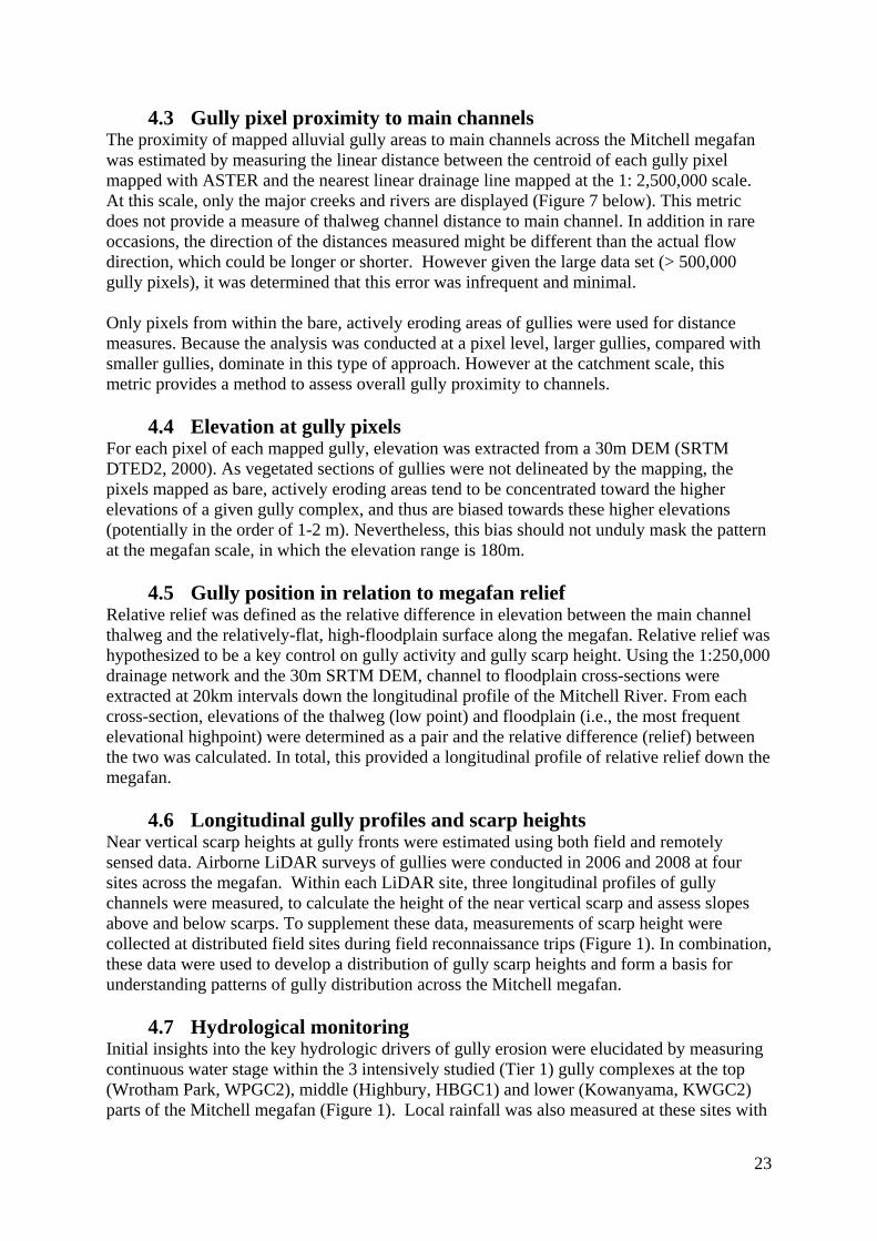
Figure 5 Examples of Coolibah trees (Eucalyptus microtheca) at KWGC2 showing a) exposed roots of a tree that was established before gully erosion and survived the passage of the gully front and lowering of the land surface by 1.5 meters, and b) a tree that has colonized the surface of an eroded gully floor and inset floodplain after the passage of the gully front. Note location of root flares relative to the ground surface. ..........................................................................28

Figure 6 a) Example of a polished tree cross-section showing rings, and b) detail of the inset white rectangle in a) showing light and dark bands and variations in vessel size and density used to locate ring boundaries.....................................29

Figure 7 Alluvial gully distribution and density (m2/km2) across the Mitchell fluvial megafan. The density grid resolution is 1 km2 pixels. Dashed line is the Palmerville fault. ..............................................................................................34

Figure 8 Gully pixel (15x15m) frequency from ASTER delineation in relation to main channels. ...........................................................................................................35

Figure 9 Gully pixel frequency from ASTER delineation in relation to pixel elevation determined from the 30m SRTM DEM. ..........................................................35

Figure 10 Longitudinal profile of the Mitchell River thalweg and adjacent megafan surface (floodplain or terrace). Upstream river tributary distances (km) are noted, as are current and past fluvial megafan apexes. ....................................36

Figure 11 Relationship between measured gully head scarp height and adjacent floodplain elevation derived from the 30m SRTM DEM. ...............................37

Figure 12 Longitudinal profiles of alluvial gully thalwegs between a main channel and adjacent floodplain. ..........................................................................................38

Figure 13 Conceptual model of different water sources influencing alluvial gully erosion, including direct local rainfall (Pin), local saturated overland flow (Qsw), off-channel flood backwater (Qbw), overbank river flood discharge (Qfw), emergence of shallow throughflow and groundwater (Qgw). Sc is the gully channel slope, while Sf is the floodplain slope.................................................40

Figure 14 Ground photos of a) mass failure, and b) fluting and carving at head scarps. .41 Figure 15 Sequential time lapse photographs over one wet season at WPGC2. ..............42 Figure 16 LiDAR hillshade map of WPGC2 showing the locations of the lower and

upper stage gauges, rain gauge, and time lapse camera. ..................................42 Figure 17 a) Rainfall and water stage at the lower gauge in the outlet of WPGC2, b)

rainfall and water stage at the upper gauge in the center of WPGC2. .............43 Figure 18 Sequential time lapse photographs over one wet season at KWGC2. .............44 Figure 19 Rainfall and water stage at the gauge in the outlet of KWGC2. ......................45 Figure 20 Examples of different planform morphologies of alluvial gullies. ..................46

6

Figure 21 a) Schematic of numerous alluvial gully complexes draining both proximal and distal portions of the Mitchell River floodplain near the Lynd River, b) Air photo of the same area as a) showing the white, bare portions of active alluvial gullies, c) Inset air photo from b. .....................................................................48

Figure 22 Map of the Lynd-Mitchell confluence where Leichhardt and Gilbert first joined the Mitchell River, and followed it downstream from the junction to Highbury Lagoon on the 16th of June 1845......................................................49

Figure 23 Boundary Creek between the Burke Road and the Mitchell River, 2009 ........52 Figure 24 Modern examples of highly eroded and dissected alluvial gully landscapes

near a) Highbury and b) the riparian zone of Boundary Creek. .......................52 Figure 25 1949 air photo examples of alluvial gullies scarp in 1949 and 1993 near a) the

banks of Boundary Creek, and b) a lagoon just west of Boundary Creek. ......53 Figure 26 Steep river bank near Highbury along the Mitchell River. ..............................53 Figure 27 Examples near Highbury of a) small gully draining floodwater directly into the

Mitchell River, and b) an unchanneled hollow draining floodwater into the Mitchell River. .................................................................................................53

Figure 28 Historic trends in the numbers of beef grazing cattle in Queensland, the historic Wrotham Park Aggregation cattle station (Wrotham Park, Gamboola, Gamboola South, Highbury, Drumduff). Data sources are from Historic Lease Applications, Queensland State Archives, Edye and Gillard (1985), Arnold (1997), and recent cattle estimates at Wrotham Park Station (Ian Rush personal communication), adjusted to include Highbury and Drumduff using a conservative estimate of 30 hectares per beast. Changes in cattle and land use conditions are denoted by the symbols $$$ (slumps in cattle prices 1922-1934, and others), @ (increase in wild pigs), *** (infestation of noogoora burr in riparian zone, 1933-1951, onward), !!! (infestation of rubber vine in the riparian zone, 1951 onward), and ### (introduction of Brahman and Santa Gertrudis cross cattle, 1963 onward), and introduction of Lucerne (Stylosanthes spp.) on <0.5% of the land area between 1963-1988 (Arnold 1997).................................................................................................................55

Figure 29 Annual gully scarp position between 2005 and 2009 at WPGC3. ...................57 Figure 30 Changes in gully scarp location at a Wrotham Park gully (WPGC2) digitized

from air photos. 1949 (red), 1960 (blue), 2008 (yellow), with the background photo from a) 1949 and b) 2008.......................................................................59

Figure 31 Changes in gully scarp location over historic time. a) Kowanyma (KWGC1), b) Gamboola (GBGC3), c) Mount Mulgrave (MMGC1), and d) Highbury (HBGC2). .........................................................................................................59

Figure 32 Relative changes in gully area over time, which is the ratio of the area at any time (A) and the initial gully area (A0) from the first air photo. ......................60

Figure 33 a) Equation 1 exponent k-values for 18 gully sites, and b) coefficient of determination values (r2) for the same sites. ....................................................61

Figure 34 Sub-set of study sites showing linear trends of gully area over time...............62 Figure 35 Sub-set of study sites showing logarithmic trends of gully area over time......62 Figure 36 Comparison of average linear erosion rates (area change / scarp perimeter,

m/year) measured from historic air photos (43,163m of scarp perimeter) and recent GPS surveys (50,040 m of scarp perimeter)..........................................63

Figure 37 Changes in the gully scarp location at KWGC2 between 1958 and 2007 from air photos, with a 2008 LiDAR image. ............................................................66

Figure 38 Gully area and volume changes over time at near KWGC2 Sandy Creek.......67

7

Figure 39 Locations and average ring counts of Coolibah trees that germinated before (red) and after (green) gully erosion, in addition to the 2007 scarp lines and 2008 LiDAR image. .........................................................................................68

Figure 40 Locations and average ring counts of Coolibah trees that colonized onto the inset gully floodplain (gully floor) after gully erosion, in addition to the 1958 and 2007 scarp lines and 1958 air photograph.................................................68

Figure 41 Relationships between tree location upstream from the gully outlet and the tree diameter and height. .........................................................................................69

Figure 42 Relationship between thalweg channel distance upstream from the outlet of the gully and the average ring count for Coolibah trees that have re-colonized onto the inset floodplain after the passage of the gully front (i.e., see trees in Figure 5a and Figure 40b)............................................................................................70

Figure 43 Cross-sectional transect through the center of WPGC2 with locations of OSL samples. ............................................................................................................71

Figure 44 Distribution and rates of alluvial gully erosion across the lower megafan, and location of erosion scarp height and rates sites. ...............................................73

Figure 45 Frequency of tropical cyclone ladings at Chillagoe as determined by the 18O/16O ratios in stalagmites in caves, from Nott et al. 2007. ..........................76

Figure 46 1880-2010 history of annual rainfall and 5-year average annual rainfall at Palmerville Station and cattle numbers at Wrotham Park Station, both near the upper part of the Mitchell River megafan. .......................................................78

Figure 47 LiDAR DEM hillshades of alluvial gullies at different stages of evolution. ...80

8

9

Tables Table 1 Data Parameter Collection at Tier 1 and Tier 2 Gully Complexes ..................14 Table 2 Journal entries by Leichhardt (1847) and Gilbert (1845) describing creek,

gullies, and hollows along the Mitchell River downstream of the Lynd. ........51 Table 3 Comments on mismanagement of the Wrotham Park Aggregation noted in

early “run files” located in the Queensland State Archives. ............................56 Table 4 GPS survey lengths and erosion rates at alluvial gully scarps sites. ................58 Table 5 Historic active scarp lengths and erosion rates at alluvial gully scarps sites. ..64 Table 6 Recent sediment production from alluvial gully erosion .................................72

1 INTRODUCTION 1.1 Background

Considerable interest has been expressed towards increasing land and water resource development (e.g., intensive grazing, pasture development, irrigated agriculture, inter-basin water transfers, mining) in the tropical savanna landscapes of northern Australia (e.g., Davidson, 1965; Nix, 1973; Tothill 1985; Woinarski and Dawson 1997; Yeates, 2001; Camkin et al., 2007 Ghassemi and White, 2007). This interest has continued despite severe economic and technical challenges (e.g., Davidson, 1965; 1969; Robinson and Sing, 1975; Bauer, 1978; Gillard et al., 1980; Basinski et al., 1985; Edye and Gillard, 1985; Shaw and Tincknell, 1993; Woinarski and Dawson, 1997), which are a partial result of the significant limitations imposed by the natural climate, hydrology, geomorphology, soil type, soil nutrient deficiently, and location of the region (e.g., Davidson, 1965; 1969; Smith et al., 1983; Mott et al, 1985; Hall and Walker, 2005; Petheram et al., 2008, CSIRO, 2009). To date, this region has experienced relatively low levels of agricultural and urban development compared with temperate and sub-tropical regions of Australia, notwithstanding the existing dominant land uses: cattle grazing, alluvial and hard rock mining, irrigated agriculture, Aboriginal land use and cultural management, commercial and recreation fishing, tourism, and biodiversity conservation. As a consequence, there has been limited scientific research into the sustainable carrying capacity of the landscape to support both human and ecosystem demands. In northern Australia, the extent to which current and past land use has had an impact on erosion rates and sediment loads within the regions extensive river systems has not been fully analyzed, unlike the extensive research on southern Australian sediment loads over time (e.g., gullying and valley fill incision: Eyles, 1977; Fryirs and Brierley, 1998; Fanning et al., 1999; Prosser, et al. 2001; Olley and Wasson, 2003). In southern Australia, gully erosion has been identified as a dominant sediment source in many regions (Olley and Wasson, 2003; Prosser, et al. 2001), locally contributing up to 90% of the total sediment yield and demonstrating major increased rates of activity (order of magnitude or more) in the post-European period (e.g. Olley and Wasson, 2003). Recent sediment budget modelling in northern Australia predicted a dominance of hillslope surface erosion sources in savanna landscapes (Prosser et al., 2001). However, field based tracing and monitoring studies suggest relative contributions of subsurface gully and channel erosion are more akin to the situation in southern Australia (Wasson et al., 2002; Bartley et al., 2007; Gary Caitcheon personal communication). Given the close relationship between sediment and nutrient fluxes, and the role of soils in agricultural production, there is a pressing need to better understand current and past soil erosion processes across northern Australia before decisions are made regarding future land use scenarios. Recent reconnaissance surveys and remote sensing research in northern Australia (Brooks et al., 2006; Knight et al. 2007; Brooks et al. 2007) have revealed that alluvial gully erosion of floodplain, terrace, and megafan deposits is widespread across the tropical savanna catchments draining into the Gulf of Carpentaria (GoC), a major epicontinental sea in northern Australia. It has been estimated that active gullying covers up to 1% of the land area of the lower alluvial portions of these catchments, but represents a more substantial component of the total sediment budget (Brooks et al., 2008). Such gully erosion in alluvium is often concentrated along the riparian margins of major river channels (Brooks et al., 2009), represents a highly connected sediment source, which degrades the most productive land for native flora and fauna, cattle grazing, and potentially agricultural development. It is clear that

10

this type of gully erosion differs fundamentally from the typical hillslope or colluvial gullies found in southern or northern Australia (see Section 2 below on literature and definitions).

1.2 Study Purpose Given the extent of alluvial gully erosion identified from initial reconnaissance survey work, the purpose of this study was to define alluvial gully erosion processes and rates in catchments draining into the Gulf of Carpentaria in Northern Queensland, using the lower Mitchell River fluvial megafan as a pilot area for the first year of study (2008-2009). Coupling process and rate data is essential to understanding both natural erosion cycles and accelerated erosion due to human land use. Effective land management to reduce human induced erosion can only be accomplished once a detailed understanding is available to define the processes that may be driving or resisting erosion, how erosion rates have changed over time with land management, and how future erosion may affect both the natural landscape and the good and services it provides to humans. Thus, the objectives of this pilot study in the Mitchell catchment were to:

1. Define alluvial gullying within the continuum of gully form-process models described within the international literature.

2. Define the spatial distribution of gullies within the Mitchell River catchment.

3. Describe the forms of alluvial gully erosion within the Mitchell River catchment.

4. Investigate the hydrogeomorphic, soil geochemical and vegetative processes that

are driving or resisting gully erosion.

5. Determine how gully erosion rates (linear and volumetric) have changed over different time scales: near-term (3-5 yrs), past contemporary (1940-present), post-European (1820-present), pre-European (pre-1820).

a. That is, has European settlement accelerated gully erosion rates?

6. Trial different tools to define erosion rates over different time scales: GPS, air photos, dendrochronology, OSL, U/Th/Ra.

7. Develop a conceptual model of the evolution of alluvial gully erosion in the

Mitchell River based on insights gained from erosion rates, the spatial pattern of gully distribution, and ground observations of erosion processes and forms.

8. Leverage additional funding using initial results to expand the project to sites all

across the Gulf plains to determine: a. Regional erosion rates from gully dating techniques b. Management strategies to ameliorate gully erosion accelerated by land

management practices

11

The detailed outcomes of objectives 1 to 7 are included in the sections below. Funding objective 8 has been accomplished by applying to grants for future gully erosion research, monitoring, and stabilization. To date, the following grant applications have been written:

1. “The Development of Best Management Practice (BMP) Standards for Alluvial Gully Stabilization in Northern Australia”. Proposer: Griffith University. Submitted to: Caring for our Country (CfoC), Medium Scale Proposal. (Outcome Not Successful)

2. “A Water Quality Risk Assessment and Monitoring Framework for south

eastern Cape York Catchments”. Proposer: Griffith University and CYSF. Gully erosion mapping, rates, and process

studies in the Normanby River. Submitted to: Reef Rescue/ Caring for our Country (CfoC), Medium Scale Proposal. (Outcome Successful)

3. “Catchment Response to Landuse Intensification in Northern Australia:

Evidence from Beach Ridge Geochemistry and Sediment Accumulation Rates in the Gulf”. Proposer: Griffith University. Submitted to: Australian Research Council (ARC Discovery) (Outcome Not Successful)

12

1.3 Study Sites and Design

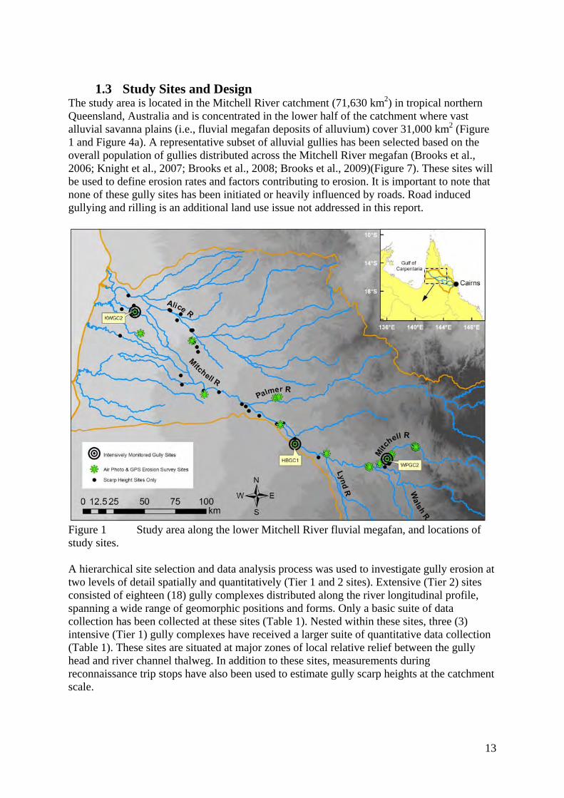
The study area is located in the Mitchell River catchment (71,630 km2) in tropical northern Queensland, Australia and is concentrated in the lower half of the catchment where vast alluvial savanna plains (i.e., fluvial megafan deposits of alluvium) cover 31,000 km2 (Figure 1 and Figure 4a). A representative subset of alluvial gullies has been selected based on the overall population of gullies distributed across the Mitchell River megafan (Brooks et al., 2006; Knight et al., 2007; Brooks et al., 2008; Brooks et al., 2009)(Figure 7). These sites will be used to define erosion rates and factors contributing to erosion. It is important to note that none of these gully sites has been initiated or heavily influenced by roads. Road induced gullying and rilling is an additional land use issue not addressed in this report.

Figure 1 Study area along the lower Mitchell River fluvial megafan, and locations of study sites. A hierarchical site selection and data analysis process was used to investigate gully erosion at two levels of detail spatially and quantitatively (Tier 1 and 2 sites). Extensive (Tier 2) sites consisted of eighteen (18) gully complexes distributed along the river longitudinal profile, spanning a wide range of geomorphic positions and forms. Only a basic suite of data collection has been collected at these sites (Table 1). Nested within these sites, three (3) intensive (Tier 1) gully complexes have received a larger suite of quantitative data collection (Table 1). These sites are situated at major zones of local relative relief between the gully head and river channel thalweg. In addition to these sites, measurements during reconnaissance trip stops have also been used to estimate gully scarp heights at the catchment scale.

13

Table 1 Data Parameter Collection at Tier 1 and Tier 2 Gully Complexes

Data Use Data Parameter Tier 2 Gully Complexes

Tier 1 Gully Complexes

Rate Gully Scarp Location-GPS ++ ++ Rate Historic Air Photos ++ ++ Rate OSL Stratagraphic Dating ++ Rate Dendrochronology ++ Rate Ur-Th-Ra Dating of Ferricrete Rate/Property/Process Time Lapse Photography ++ Property / Process Continuous Stream Gauging ++ Property / Process Rainfall ++ Property LiDAR Topography ++ Property Gully Morphology Metrics ++ Property Soil Characteristics ++

14

2 GULLY LITERATURE REVIEW

2.1 Hillslope and Colluvial Gullies Gully erosion has been described in a large variety of landscapes throughout the world (e.g., Poesen et al., 2003; Valentin et al., 2005) and indeed on other planets (Higgins 1982). The commonly accepted definition of gullies is that they are larger than rills, which can be ploughed or easily crossed (e.g., Poesen et al., 2003), but smaller than streams, creeks, arroyos, or river channels (e.g., Graf, 1983; Wells, 2004). The most commonly described gullies on Earth tend to be those that could be described as “hillslope gullies”, which are present in the upland portions of catchments in northern Australia (e.g., Hancock and Evans, 2006; Bartley et al., 2007), and are widespread in eastern Australia (e.g., Olley et al., 1993; Prosser and Abernethy, 1996; Beavis, 2000), and around the world (e.g., Graf, 1979; Harvey, 1992; Kennedy, 2001; Li et al., 2003; Bacellar et al., 2005; Kheir et al., 2006). Hillslope gullies are those that erode into colluvium, aeolium, saprolite, weak sedimentary rock, or other weathered rock, and have also been defined as valley-side or valley-head gullies (Brice, 1966; Schumm, 1999). Hillslope gullies are generally located in low stream-order headwater settings, where they are tributary to other gullies or channels of low stream-order. In general, the length of hillslope gullies is much greater than their width. The erosion mechanism is typically overland flow in which excess shear stress exceeds resisting forces (e.g., Montgomery and Dietrich, 1988; Prosser and Slade, 1994; Knapen et al., 2007). Erosional forces and channel head location are dependent on the local slope and upstream catchment area (i.e., a discharge surrogate) (Montgomery and Dietrich, 1988; 1989). The extension of the channel head highly depends on the available catchment area (Prosser and Abernethy 1996). Due to the relatively coarse sediment supply and headwater setting of hillslope gullies, their eroded sediment contributes to both bed and suspended loads (e.g., Rustomji 2006) and they have relatively low sediment delivery ratios due to ample opportunity for storage between the source and ultimate base level outlet (Walling, 1983; Wilkinson and McElroy, 2007).

2.2 Alluvial gullies In contrast to the hillslope gully model, various researchers have described valley-bottom gullies (e.g. Brice, 1966; Schumm, 1999) and bank gullies (Poesen 1993; Poesen and Hooke 1997; Vandekerckhove et al, 2000), in which the gully is eroding entirely into alluvium. In addition to this study, gullying into alluvial plains in Australia has been documented as a major land degradation process by Condon (1986) in the Victoria River District of the Northern Territory, by Pickup (1991) in central Australia, and by Pringle et al. (2006) in Western Australia. Internationally, alluvial gullying in the savanna riverine landscapes of subtropical Africa and India may prove to be the most similar to alluvial gullies forms and processes in northern Australia. In Kenyan savannas, Oostwoud and Bryan (2001) described the gullying of alluvial-lacustrine soils where gullying was influenced by base level and river incision, emergence of subsurface flow at gully heads and intensive surface runoff. In India, research into the causes and remediation of alluvial gully erosion (locally termed “ravines”) along major rivers has a long history. Research by Sharma (1982), Singh and Singh (1982), Sharma (1987), and Singh and Agnihotri (1987) indicated that river incision and rejuvenation of

15

surrounding alluvial deposits are major factors influencing alluvial gully development, while other factors such as climate, geology/soils, and land use (overgrazing, deforestation, agriculture) also play important roles. Haigh (1998) and Yadav and Bhushan (2002) provided contemporary overviews of the scientific and social challenges of land reclamation following alluvial gully erosion to maintain productive land for Indian society. Despite these above studies, rarely has a clear distinction been made between these “alluvial gullies” and the more commonly described colluvial or “hillslope gullies”. It is our contention that a clear continuum exists between colluvial and alluvial gully forms and that the two end members of this continuum represent distinct landforms, which have different form-process relationships. It is of critical importance to make this distinction when parameterising sediment budget models, such as SedNet (Prosser et al., 2001), as the existing hillslope gully models (e.g., Rustomji, et al. 2008) as yet do not adequately represent alluvial gullies. As such, we present a definition of an alluvial gully, and present a type example of this gully variant from the Mitchell River catchment in Northern Queensland, Australia. Alluvial gullies are here defined as relatively young incisional features entrenched into alluvium not previously incised since initial deposition. Alluvial gully complexes (up to several km2) are defined as actively eroding and expanding channel networks incised into and draining alluvial deposits. They often form a dense network of rills and small gullies nested hierarchically within larger macro-gully complexes (e.g., see cover photos). Alluvial gullies are variable in erosion process, form, landscape location, climate, relief, and texture of alluvium. However, they most often occur in vast deposits of alluvium along high stream-order main river channels or other large waterbodies such as lagoons or lakes. Thus they have high sediment delivery ratios and are highly connected sources of predominantly fine suspended sediment. They are often as wide or wider than they are long, due to the lack of structural control on their lateral expansion (e.g., see cover photos). By definition, alluvial gullies erode drainage networks into some form of alluvium, which is a time varying storage component of transported fluvial sediment. Therefore, alluvial gully erosion represents a secondary cycle of erosion, occurring sometime after initial storage but before physical or chemical conversion into sedimentary rock. Primary and secondary erosion cycles that differentiate production, transport, and sink zones have been discussed by Schumm and Hadley (1957) and Pickup (1985; 1991). Following initial deposition, sink zones can become sediment production zones during a secondary cycle following changes in intrinsic or extrinsic thresholds, such as the alteration of resisting forces due to vegetation reduction or changes in erosive forces due to base level change, or increased discharge. Alluvial gully complexes differ from badlands, which are most often formed in soft rock terrain, such as marl or shale sedimentary rock (Gallart et al., 2002; Harvey, 2004) often which has experienced some form of uplift or re-exposure due to base level change (Bryan and Yair, 1982). It is acknowledged, however, that the term badland is poorly defined and some could view certain stages and scales of alluvial gully complexes as examples of badland erosion. We contend that describing alluvial gully complexes as “badland erosion” does not help to explain the processes driving this form of erosion, and only serves to further cloud the literature on badland erosion. The features we describe clearly have much in common with the extensive literature on gullies and are best placed in the context of this literature.

16

Alluvial gullies also differ from the cut and fill incised landscapes that occur along preexisting linear channels in partially confined valleys filled with a mixture of alluvium, colluvium, weathered rock, and soil (e.g., Eyles, 1977; Prosser et al., 1994; Prosser and Winchester, 1996; Fryirs and Brierley, 1998), including arroyo (stream) channels (e.g., Schumm and Hadley, 1957; Cooke and Reeves, 1976; Graf, 1979). Fluvial processes along major stream channels that are structurally controlled by surrounding hillslopes and underlying bedrock differ significantly to the processes operating in smaller alluvial gully channels uninfluenced by these structural controls. While hillslope gullies and cut and fill channels in headwater areas can erode into linear patches of alluvium, they are closer to the hillslope end of the continuum between pure colluvial and pure alluvial deposits and processes.

17

3 LANDSCAPE SETTING 3.1 Monsoonal climate and hydrology

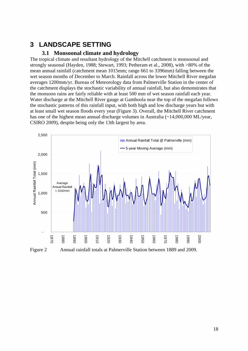
The tropical climate and resultant hydrology of the Mitchell catchment is monsoonal and strongly seasonal (Hayden, 1988; Stewart, 1993; Petheram et al., 2008), with >80% of the mean annual rainfall (catchment mean 1015mm; range 661 to 3396mm) falling between the wet season months of December to March. Rainfall across the lower Mitchell River megafan averages 1200mm/yr. Bureau of Meteorology data from Palmerville Station in the center of the catchment displays the stochastic variability of annual rainfall, but also demonstrates that the monsoon rains are fairly reliable with at least 500 mm of wet season rainfall each year. Water discharge at the Mitchell River gauge at Gamboola near the top of the megafan follows the stochastic patterns of this rainfall input, with both high and low discharge years but with at least small wet season floods every year (Figure 3). Overall, the Mitchell River catchment has one of the highest mean annual discharge volumes in Australia (~14,000,000 ML/year, CSIRO 2009), despite being only the 13th largest by area.

-

500

1,000

1,500

2,000

2,500

1870

1880

1890

1900

1910

1920

1930

1940

1950

1960

1970

1980

1990

2000

Ann

ual R

ainf

all T

otal

(mm

)_

Annual Rainfall Total @ Palmerville (mm)

5-year Moving Average (mm)

Average Annual Rainfall

= 1042mm

Figure 2 Annual rainfall totals at Palmerville Station between 1889 and 2009.

18

0

1000

2000

3000

4000

5000

6000

7000

8000

9000

10000

1970 1975 1980 1985 1990 1995 2000 2005

Dis

char

ge (m

3 / s)

Daily Max DischargeDaily Mean DischargeDaily Min Discharge

Figure 3 Daily max, mean, and min discharge (m3/sec) at the Gamboola gauge (919011a) on the Mitchell River. Data from DERM.

3.2 Geology The upper half of the Mitchell catchment is dominated by rugged hillslope terrain with a maximum elevation of 1236m and catchment mean of 245m. The geology of the upper catchment is a heterogeneous mixture of metamorphic, igneous and sedimentary rock (Whitaker et al., 2006). The major structural control in the Mitchell catchment is the south-north striking, steeply dipping Palmerville fault (Vos et al., 2006), which is considered a reactivated Precambrian structure (see Vos et al., 2006 for review). This fault separates the adjacent Palaeozoic Hodgkinson Province to the east from Proterozoic metamorphic rocks to the west, which are overlain by fluvial megafan deposits (Figure 7 below). The study area and lower half of the catchment below 200m elevation are located on the largest fluvial megafan in Australia (sensu Horton and DeCelles, 2001; Leier et al., 2005), with an alluvial extent of 31,000 km2. The Mitchell fluvial megafan was originally described in detail by Grimes and Doutch (1978), who defined and delineated distinct fan units from the Pliocene to Holocene (Figure 4a). Over this period, sea level and climate change have resulted in at least five cycles of fan building, with nested fan-in-fan forms developed as megafan units coalesced and prograded toward the current estuarine delta in the Gulf of Carpentaria.

3.3 Megafan morphology The morphological apex of the entire megafan is located near the confluence of the Lynd and Mitchell Rivers (Figure 4a and Figure 7 below), with narrower alluvial deposits backed up into the more confined river valleys upstream. Currently, the hydrologic apex of the Mitchell megafan is located below the confluence of the Palmer and Mitchell Rivers. The current Mitchell River Delta and its interconnected distributary deltas (including the North, Middle, and South Mitchell Arms; Topsy Creek; Nassau River) are in combination the largest river delta in Australia in terms of total mangrove area (>112 km2) and second largest in terms of total main channel length (>61 km) and perimeter (>300 km) (Heap et al., 2001).

19

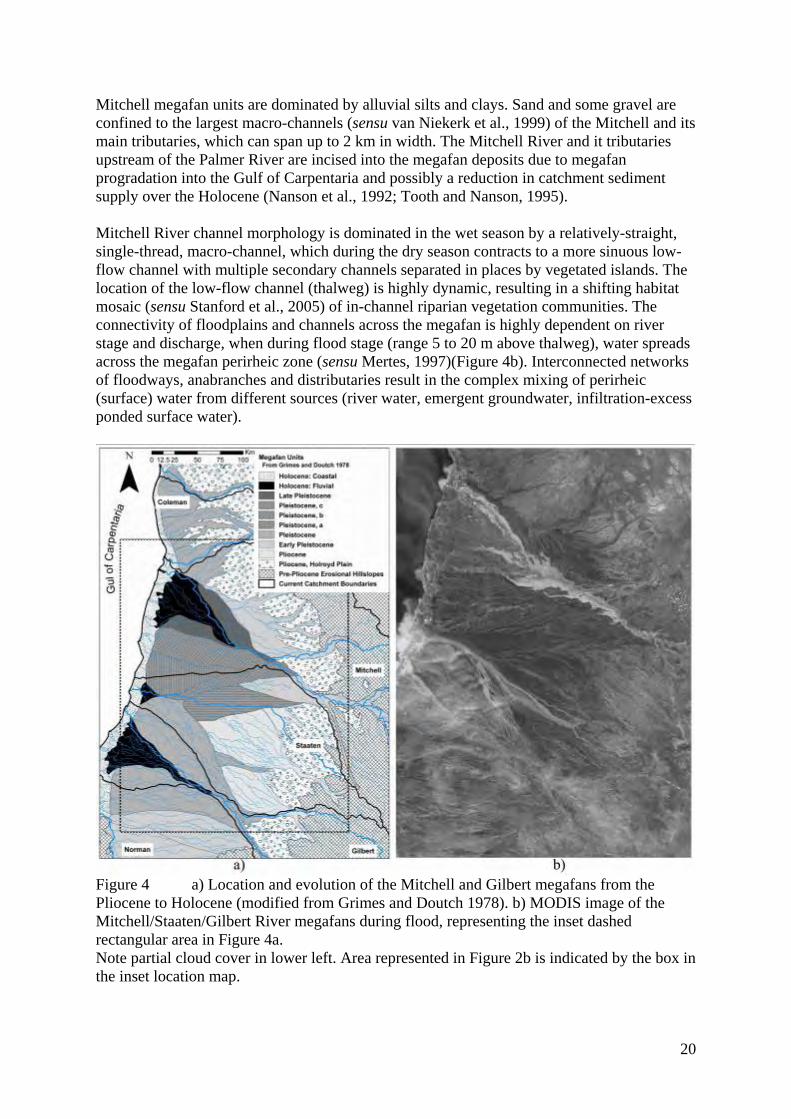
Mitchell megafan units are dominated by alluvial silts and clays. Sand and some gravel are confined to the largest macro-channels (sensu van Niekerk et al., 1999) of the Mitchell and its main tributaries, which can span up to 2 km in width. The Mitchell River and it tributaries upstream of the Palmer River are incised into the megafan deposits due to megafan progradation into the Gulf of Carpentaria and possibly a reduction in catchment sediment supply over the Holocene (Nanson et al., 1992; Tooth and Nanson, 1995). Mitchell River channel morphology is dominated in the wet season by a relatively-straight, single-thread, macro-channel, which during the dry season contracts to a more sinuous low-flow channel with multiple secondary channels separated in places by vegetated islands. The location of the low-flow channel (thalweg) is highly dynamic, resulting in a shifting habitat mosaic (sensu Stanford et al., 2005) of in-channel riparian vegetation communities. The connectivity of floodplains and channels across the megafan is highly dependent on river stage and discharge, when during flood stage (range 5 to 20 m above thalweg), water spreads across the megafan perirheic zone (sensu Mertes, 1997)(Figure 4b). Interconnected networks of floodways, anabranches and distributaries result in the complex mixing of perirheic (surface) water from different sources (river water, emergent groundwater, infiltration-excess ponded surface water).

Figure 4 a) Location and evolution of the Mitchell and Gilbert megafans from the Pliocene to Holocene (modified from Grimes and Doutch 1978). b) MODIS image of the Mitchell/Staaten/Gilbert River megafans during flood, representing the inset dashed rectangular area in Figure 4a. Note partial cloud cover in lower left. Area represented in Figure 2b is indicated by the box in the inset location map.

20

3.4 Soils Across the megafan, soils have developed where alluvial sands, silts and clays have been relatively undisturbed physically, but not chemically, since initial deposition. These soils have been described by the BRS (1991), and vary depending on age, elevation, and river connectivity. Near main river channels, “slightly elevated old filled channels and associated levees have sandy and loamy red earths, and occasionally lesser yellow earths” (soil unit Si14). Across most of the vast “alluvial plains fringing major rivers, often traversed by old infilled stream channels and associated low levees, silty or loamy surfaced grey-brown duplex soils are dominant and are strongly alkaline at shallow depths. The A horizon depth ranges from 8 to 15 cm, and many areas have a scalded surface” (soil unit Si14), due to the removal of the A horizon. Further away from the main river, “small swampy depressions and lower plains have grey cracking clays” (soil unit Si14)(BRS, 1991). Similar to the soil nutrient deficiencies across much of the northern Australian savannas (Mott et al. 1985), the alluvial soils along the lower Mitchell River are very low in the nutrients nitrogen and especially phosphorus (Edye and Gillard, 1985; Hall and Walker 2005). This is typified by the alluvial soils near Highbury Station, which are hard-setting, duplex, sesquioxide soils that are sodic at depth and low in nutrients (Edye et al. 1991; Hall and Walker 2005). These soils only produce nutritious grass during the 4-5 month wet season with green herbage, when the majority of the weight gain of introduced cattle occurs. Dry season weight loss in cattle is highly correlated to the number of weeks (months) without green feed for cattle (Tothill et al. 1985; Mott et al. 1985). The alluvial soils along the Mitchell River also appear to have a characteristic geochemistry, that to date has been poorly defined. Following the exposure of massive alluvial soils after gully erosion, nodules or pisoliths of ferricrete and calcrete readily form on the surface of exposed gullies (e.g., Pain and Ollier, 1992). Gully floors appear to be preferential zones of accumulation of cations (e.g., iron, manganese, and calcium) through local pedogenic processes (relative accumulation; e.g., McFarlane, 1991) and lateral groundwater input (absolute accumulation; e.g., McFarlane, 1976) or both (Goudie, 1973; 1984).

3.5 General catchment land use Within the study area along the lower catchment megafan, land use is currently dominated by cattle grazing across savanna woodlands, unimproved grasslands (e.g., Neldner et al., 1997), and to a lesser extent improved grasslands (e.g., Gillard et al. 1980; Edye and Gillard, 1985; Edye et al. 1991; Arnold 1997; Hall and Walker 2005). Due to the historic and ongoing scarcity of water during the long dry season, cattle grazing intensity and impacts are heavily concentrated along “water frontages” (or riparian zones) of main rivers and tributaries, where access to persistent in-channel pools and lagoons has allowed for the continuous stocking of cattle in near-river pastures throughout the year (Tothill et al. 1985). The savanna vegetation communities of the Mitchell catchment are dynamic over space and time and strongly controlled by disturbance regimes (grazing, fire, flood, erosion), which have changed following European settlement (Crowley and Garnett, 1998; 2000). Historical trends in land use and condition are analyzed further below. The upper Mitchell catchment is also dominated by hillslope grazing on unimproved pastures. However, developed agriculture covers 2.6 % of total catchment area in a relatively confined basaltic plain in the upper catchment (i.e., Mareeba-Dimbulah Irrigation Area) (Chapman et al. 1996). Locally significant areas of alluvial and hard rock mining occur throughout the catchment (McDonald and Dawson, 1994), with hard rock mining expanding in recent years.

21

4 METHODS 4.1 Alluvial gully distribution across the Mitchell megafan

For alluvial gully distribution analysis, the megafan limits were delineated from a surface geology data set that describes the extent of floodplain and channel alluvium at 1:1,000,000 (Whitaker et al., 2006), as well as the 1:2M soil landscapes data set (BRS, 1991). Also, marine influenced areas and salt plains in the delta were delineated and excluded from the extent of the megafan, as they are controlled by a different set of process. Mapping of alluvial gully erosion in the Mitchell River catchment was undertaken using Advanced Spaceborne Thermal Emission and Reflection Radiometer (ASTER) scenes subset to extents covering the catchment. The remote sensing methods used to delineate active gully erosion area were described in detail in Brooks et al. (2008). In summary, a total of 10 ASTER scenes acquired across a 5 year period from 2000, and across both the wet and dry season, were processed individually using a standard remote sensing decision tree methodology to detect gully areas. To calibrate the method, the extent of gullies in subset areas was delineated with both LiDAR (Light Detection And Ranging) generated DEMs (Digital Elevation Models) and aerial photography, with parameter adjustment for individual ASTER scene differences. Validation involved using high resolution Quickbird imagery publicly available through Google Earth. Detection accuracy was estimated by comparing gully detection in 250 1km cells randomly assigned and coincident with Quickbird coverage with the detection of gullies from the ASTER processing. Accuracy of gully delineation involved comparison of the aerial extent of gullies mapped from ASTER against manually digitised gully extent (bare, active gully areas) identified in 83 1km grid cells with active gullies, randomly selected from the 250 cells used in the detection validation process. For the current purposes, the delineation of individual gullies as mapped from ASTER imagery included the bare, actively eroding sections within the gully. Thus, where the inset lower surface of a gully was (re)vegetated, it was not mapped as a gully area. Validation of gully front length was conducted using the same 83 1km grid cells with Quickbird imagery as above. The total length of Quickbird gully fronts in each 1km cell was then compared to the total perimeter length of gullies mapped via ASTER. For each 1km cell, a ratio of Quickbird to ASTER length was calculated. The total length of gully front via Quickbird (km/km2) was used to adjust the total length of ASTER perimeter (km/km2). Validation of gully front lengths measured from Quickbird imagery amounted to comparing the mapped gully front length to field data at sites where detailed differential GPS field surveys had been conducted (total 25,485m). The ratio of the ground surveyed to remote sensing surveyed gully front lengths were then used to adjust ASTER and Quickbird gully front length estimates.

4.2 Gully position in relation to megafan geology and soils Mapped gully areas were additionally compared to mapped megafan geologic units (Grimes and Doutch, 1978) and soil units (BRS, 1991). The frequency of mapped gully pixels (i.e. 15 m2 pixels from the ASTER based mapping) in these units were analyzed to gain insight into the units that were most sensitive to gully erosion.

22

4.3 Gully pixel proximity to main channels The proximity of mapped alluvial gully areas to main channels across the Mitchell megafan was estimated by measuring the linear distance between the centroid of each gully pixel mapped with ASTER and the nearest linear drainage line mapped at the 1: 2,500,000 scale. At this scale, only the major creeks and rivers are displayed (Figure 7 below). This metric does not provide a measure of thalweg channel distance to main channel. In addition in rare occasions, the direction of the distances measured might be different than the actual flow direction, which could be longer or shorter. However given the large data set (> 500,000 gully pixels), it was determined that this error was infrequent and minimal. Only pixels from within the bare, actively eroding areas of gullies were used for distance measures. Because the analysis was conducted at a pixel level, larger gullies, compared with smaller gullies, dominate in this type of approach. However at the catchment scale, this metric provides a method to assess overall gully proximity to channels.

4.4 Elevation at gully pixels For each pixel of each mapped gully, elevation was extracted from a 30m DEM (SRTM DTED2, 2000). As vegetated sections of gullies were not delineated by the mapping, the pixels mapped as bare, actively eroding areas tend to be concentrated toward the higher elevations of a given gully complex, and thus are biased towards these higher elevations (potentially in the order of 1-2 m). Nevertheless, this bias should not unduly mask the pattern at the megafan scale, in which the elevation range is 180m.

4.5 Gully position in relation to megafan relief Relative relief was defined as the relative difference in elevation between the main channel thalweg and the relatively-flat, high-floodplain surface along the megafan. Relative relief was hypothesized to be a key control on gully activity and gully scarp height. Using the 1:250,000 drainage network and the 30m SRTM DEM, channel to floodplain cross-sections were extracted at 20km intervals down the longitudinal profile of the Mitchell River. From each cross-section, elevations of the thalweg (low point) and floodplain (i.e., the most frequent elevational highpoint) were determined as a pair and the relative difference (relief) between the two was calculated. In total, this provided a longitudinal profile of relative relief down the megafan.

4.6 Longitudinal gully profiles and scarp heights Near vertical scarp heights at gully fronts were estimated using both field and remotely sensed data. Airborne LiDAR surveys of gullies were conducted in 2006 and 2008 at four sites across the megafan. Within each LiDAR site, three longitudinal profiles of gully channels were measured, to calculate the height of the near vertical scarp and assess slopes above and below scarps. To supplement these data, measurements of scarp height were collected at distributed field sites during field reconnaissance trips (Figure 1). In combination, these data were used to develop a distribution of gully scarp heights and form a basis for understanding patterns of gully distribution across the Mitchell megafan.

4.7 Hydrological monitoring Initial insights into the key hydrologic drivers of gully erosion were elucidated by measuring continuous water stage within the 3 intensively studied (Tier 1) gully complexes at the top (Wrotham Park, WPGC2), middle (Highbury, HBGC1) and lower (Kowanyama, KWGC2) parts of the Mitchell megafan (Figure 1). Local rainfall was also measured at these sites with

23

automated-tipping-bucket rain gauges. The positioning of stage recorders within the gully floor as well as at the gully outlet channel distinguished between locally derived storm events and main stem river channel backwater and/or overbank events. The gauge network was also complemented with automatic time lapse cameras that capture daily images of gully head scarp retreat throughout the wet season (November – April). Analysis of the time lapse camera images coupled with the stage and rainfall records allows us to link the main hydrologic processes (rainsplash, surface runoff, groundwater sapping, gully backwater or overbank flooding) with the main periods of erosive activity. It is worth noting that the field area is completely inaccessible through the wet season, requiring all monitoring to be automated.

4.8 Classification of alluvial gully forms From initial remote sensing and field reconnaissance, Brooks et al. (2006) classified the diversity of alluvial gully forms along the riparian zones of the lower Mitchell River and tributaries. Here, their classification of these alluvial gullies is expanded to include new perspectives from an additional three years of remote sensing and field surveys.

4.9 Historical explorers Many early explorers traversed Cape York along different paths (see map in Fensham 1997), but few traversed the lower Mitchell River before extensive cattle grazing. Ludwig Liechhardt, accompanied by John Gilbert, explored and documented the lower Lynd and Mitchell Rivers in 1845. Transcripts of the separate but parallel diaries of Ludwig Liechhardt and John Gilbert (Gilbert 1845, Leichhardt 1847) were analyzed for location and description information in relation to soil erosion, gullies, creeks, rivers, and fluvial processes. Their traverse of the lower Lynd River and the Mitchell River downstream of the Lynd River in June 1845 provides a unique perspective of the lower Mitchell catchment before future intensive land use (mining and cattle grazing). Due to the fact that Gilbert was killed by Aboriginal people on 28 June 1845 near the bottom of the Mitchell catchment, Leichhardt’s journal has dominated historical analyses (Fensham 2008). However, Gilbert was also a talented explorer, ornithologist, and detailed note taker, making his diary invaluable. Fortuitously, his journal was re-located in 1938 in London (Chisholm 1940), and is now held in the Mitchell Library, New South Wales. In December 1864, the expedition of the Jardine Brothers crossed the lower Mitchell River Delta (Jardine and Jardine, 1867). They came west down the Staaten River towards the Gulf of Carpentaria, turned north and crossed the Scrutton River (Nassau) and other Mitchell River anabranches (upstream of present day Kowanyama) before crossing the Mitchell mainstem to the north and following its course downstream (northwest) towards the Alice and Colman Rivers. Their journals describe the floodplain country of the lower Mitchell and their encounters with the Aboriginal people that live in this deltaic country, many of which were murdered in document conflicts during the expedition. Another notable pre-cattle/mining explorer that traversed part of the lower Mitchell catchment was William Hann. In 1872, he traveled down the Lynd, Tate, and Walsh Rivers to near their junction with the Mitchell. Near these confluences, he confirmed and adjusted some of Liechhardt’s initial geographic observations (Jack, 1915). We have yet to obtain and analyze the Hann (1872) journal for its potential insight into alluvial gully erosion, which will occur in the near future.

24

4.10 Land use and conditions during early European settlement During the initial establishment of leases of Crown land in the lower Mitchell catchment for pastoral uses post-1870, numerous letters were written between lease applicants and the Queensland Department of Public Lands and Land Courts in Brisbane to establish cattle “runs”. Once specific leases and cattle stations were established, periodic lease renewal applications were submitted to the Public Lands Office. District Land Agents then conducted assessments of these lease agreements to ensure that the basic requirements for leasing public land were met (i.e., minimum cattle stocking, fencing and water improvements, etc.). These letters provide the only publically available quantitative data on land use conditions during early European settlement for the lower Mitchell River. For each leased cattle station, a “run file” was kept by the Public Lands Office. Pre-1960 run files are currently archived at the Queensland State Archives in Brisbane and are available to the public. The run files for the following stations were obtained from the State Achieves to assess the information they contained: Mount Mulgrave, Wrotham Park, Gamboola, Gamboola South, Highbury, Drumduff, and Frome #2. For much of this period, Wrotham Park, Gamboola, Gamboola South, Highbury, Drumduff were managed as one large aggregated cattle station (Arnold 1997).

4.11 Contemporary erosion rates at gully fronts using GPS surveys Detailed surveys of selected alluvial gully fronts (scarps) in the Mitchell megafan were conducted using in-situ differential GPS with sub-meter accuracy (Trimble with Omnistar High Precision). Accuracy depended on signal strength and vegetation cover, but was typically within 0.5 meters for repeat surveys. GPS surveys were conducted at 18 sites across the alluvial megafan, totalling 50,040m of gully front (Figure 1 and Table 4). Gully expansion indicated by average scarp retreat rate was determined from annual surveys in 2005 (partial), 2006 (partial), 2007, 2008, and 2009 (2010 forthcoming) with the average rate equalling the total erosion area of change during any given year divided by the total common survey length (active gully perimeter), for each gully surveyed. Error margins of gully area for a given survey year were calculated by buffering each survey line by ±1m of the survey line (2m total buffer width). Maximum linear rates were calculated for individual lobes, but only the average rate was applied across the entire length for budget purposes (see Brooks et al. 2008). In Brooks et al. (2008), it was assumed that the majority of new sediment contributed to the gully each year comes from primary vertical scarp retreat at the gully head. This is not to say that appreciable volumes of sediment are not coming from secondary erosion of incompletely eroded failed blocks, reworking of gully outwash deposits, or gully sidewall erosion. Indeed scarp retreat will slow if the deposited material is not reworked from the gully floor. Recent observations suggest, however, that due to the highly dispersible nature of the sediments and the fact that most of the sediment is erodes into suspension, material delivered from the head scarp is removed reasonably efficiently. The same observations, coupled with survey data, indicate that due to the high rates of head scarp retreat the majority of volumetric change in the gully void on an annual timescale is directly proportional to the head scarp retreat rate. Hence, head scarp retreat rate can provide an easily measurable indicator of minimum annual sediment supply from alluvial gullying when combined with gully scarp height data at individual gullies (Brooks et al. 2008).

25

4.12 Historic erosion rates at gully fronts from aerial photos Historical air photographs were obtained for the same 18 study sites (Figure 1) for different time periods to assess the location and rates of gully front erosion over time. The earliest photographs for the lower Mitchell catchment were taken in 1943 by the Royal Australian Air Force along the coast. However, most gully sites did not have air photographs taken until either 1949 or 1955. Repeat air photographs were taken approximately every decade at each site, with reduced frequency or absence during the 1980’s and 1990’s. More recently in the 2000’s, satellite photos were available (i.e., Quick Bird), in additional to air photos taken during LiDAR surveys during this project. Thus, the air photograph analysis covered a typical period of 58 years (1949 to 2007). Historic air photos were obtained from both the Queensland Department of Environment and Resource Management (DERM) and the National Library of Australia (NLA). Digital copies of photos were scanned by either 1) a desktop scanner at >2000 dpi for photo hardcopies, or 2) a Leica film negative scanner (DERM) down to the grain size of the photo (15um) for photo negatives. Digital files clipped to the general gully area of interest were then imported into a Geographic Information System (ArcMap 9.3) Georeferencing was conducted backward through time using recent LiDAR and air photos, GPS surveys of current gully locations, ASTER satellite imagery, and common trees and water body points in historic versus recent air photos. Extreme care in analysis was used to ensure that reference trees were identical positions and that water body points were unchanged between sequential photographs. Once rectified, the location of the gully head scarp was digitized and the total area occupied by the eroded area was calculated and compared between years. Error margins of gully area for a given survey year were calculated by buffering each survey line by ±3m of the survey line (6m total buffer width). The starting point for each gully was located at either 1) the confluence of the gully channel with the mainstem river or lagoon water body, 2) the confluence of the gully with a much larger well vegetated tributary creek, or 3) the well vegetated transition between wide amphitheater alluvial gully complexes and their very narrow, incised outlet channels (creeks) that may traverse well vegetated riparian zones. In the later case, these vegetated channels and their expansion over time are un-mappable from air photos or remote sensing. Thus in this case, the initial linear erosion and elongation of these channels through riparian zones is not quantified in this analysis. The change in exposed gully area over time for different sites was analyzed using a well known gully erosion and incision model called the Rate Law in Fluvial Geomorphology (Graf 1977). In general, this rate law describes the non-linear growth rates of unstable channels, which tend to have a negative exponential function of declining rates of growth (or incision) over time. This exponential function is fit to empirical data to describe the relaxation of erosion rates over time. However, the degree of negative exponential decay is determined by best fit, and in certain situation the function can relax to a more general linear form. A modified version of the rate law was used that is more applicable to incising channel (Simon and Rinaldi 2006). However, instead of length of channel to channel head (Graf 1977) or bed elevation changes over time (Simon and Rinaldi 2006), the function was modified to describe the growth in gully planform area over time.

)(

0

ktbeaAA −+= (1)

26

where A is the exposed gully area at time t, A0 is the initial gully area at t0 = 0 at the first air photograph, a and b are dimensionless coefficients determined by regression, k is a coefficient determined by regression that defines the rate of change in gully area over time, and t is the time (years) since the initial starting point or the first air photograph (after Simon and Rinaldi 2006). When k is very small, the Equation 1 approaches linearity. Since gully area always increases with time (regardless of rate), a in this case is always positive (a>0). A over A0 is a normalized measure of changes in Relative Gully Area over time. As a comparison to the negative exponential function of Equation 1, both linear and natural logarithmic trends were also fit to the data of gully area change over time using the following equations:

btaAA

−×= )(0

(2)

btaAA

−×= )ln(0

(3)

where A is the exposed gully area at time t, A0 is the initial gully area at t0 = 0 at the first air photograph, a and b are dimensionless coefficients determined by regression, and t is the time (years) since the initial starting point or the first air photograph.

4.13 Erosion rates from dendrochronology As alluvial gully fronts migrate away from mainstem river channels through riparian vegetation and woodlands, they leave in their wake dead trees, live trees that have survived gully erosion (Figure 5a), and new alluvial surfaces that are colonized by various tree species (Figure 5b). In the woodlands of the lower Mitchell River, Coolibah trees (Eucalyptus microtheca) grow on river floodplains in heavy sodic soils and are extremely hardy trees that can survive gully erosion and re-colonize the eroded landscape. Thus, trees growing in and around alluvial gullies have the potential to define the timing of gully erosion, through ring counting and dendrochronology analysis. Trees and tree roots have been successfully utilized to age erosion rates in gully systems on other continents (e.g., Vandekerckhove 2001; Gartner 2007). If trees can be aged via ring counting in these Australian gullies, live trees that have survived the passage of the gully front could provide a maximum date of erosion passage (Figure 5a). In contrast, live trees that have re-colonized the inset floodplains of gully floors could provide a minimum age for the passage of the gully front (Figure 5b).

27

a) b)

Figure 5 Examples of Coolibah trees (Eucalyptus microtheca) at KWGC2 showing a) exposed roots of a tree that was established before gully erosion and survived the passage of the gully front and lowering of the land surface by 1.5 meters, and b) a tree that has colonized the surface of an eroded gully floor and inset floodplain after the passage of the gully front. Note location of root flares relative to the ground surface. Trees in Australia (including Eucalyptus spp.) are notoriously difficult to date using traditional dendrochronology methods due to the inconsistency in laying down annual growth rings in due to highly episodic rainfall (e.g., Ogden 1978; 1981; Pearson and Searson 2002; Argent et al. 2004; Hancock et al. 2006). However, non-annual tree ring patterns and growth of Eucalyptus spp. have been correlated to rainfall, soil moisture and river discharge in climates with unpredictable moisture inputs (Downs et al. 1999; Leal et al. 2004; Argent et al. 2004), which provides hope for climate analysis. More importantly in strongly-seasonal monsoon-climates of tropical Australia, it has been found that Eucalyptus tree growth during the predicable summer wet season dominates the production of growth rings each year, resulting in near annual growth rings (Mucha 1979; Odgen 1981; Hancock et al. 2006). However, the assumption of annual growth rings can not be made without independent confirmation of tree age or growth from other dating techniques (direct observations, photographs, 14C dating, and other radionuclides). If growth rings are not perfectly annual but consistently identifiable, then correction factors are needed to determine, on average, how many rings per year are laid down. Hancock et al. (2006) have recently proven an independent tree aging technique for Australian trees that utilizes radionuclide concentrations in tree xylem tissues to determine temporal growth of tree rings. Radionuclides of radium (226Ra and 228Ra) are mobile in ground water, while their thorium parents (230Th and 232Th) are relatively immobile. Radium can become incorporated into tree xylem tissue and tree rings following initial water uptake during photosynthesis. After uptake, radium becomes immobile in tree heartwood where it begins to decay in a closed system (tree ring) at known half-lives without thorium. The half life of 228Ra is 5.8 years and thus decays quickly, whereas 226Ra has a half-life of 1600 years, and thus is stable over the life of a tree. Following Hancock et al. (2006), the tree age at any point tx across the tree radius is function of the half life of 228Ra and the initial (R0) versus final (Rx) activity ratios of 228Ra/226Ra (Hancock et al. 2006).

28

⎥⎦

⎤⎢⎣

⎡−=

0228

ln1RRt x

x λ (4)

Due to the equal mobility of 226Ra and 228Ra in groundwater and tree xylem, the activity of 226Ra across the radius of a tree is used to confirm that the tree is consistently uptaking radium from the groundwater system. For initial testing of dendrodrochronological dating techniques, one gully (KWGC2) near Kowanyama was selected as a pilot site (Figure 1), with the potential for expansion to the additional gully sites during subsequent years. During November 2008, wood samples for tree ring analysis were collected at KWGC2, with the permission of aboriginal Traditional Owners’. In total, forty-two (42) Coolibah trees (Eucalyptus microtheca) were sampled that had either survived during (20) or re-established after (22) the passage of the gully head cut front (e.g., Figure 5ab). Due to difficulty in tree coring, all trees were cut down to obtain cross-section samples (disks) of xylem and growth rings. However by May 2009, all cut trees had re-sprouted live branches and leaves from the cut stump. The diameter of each tree was measured at the cut location at the base of tree just above the root flare. The tree height was also measured after felling. Each tree was geo-referenced on the landscape with GPS. Using topographic survey equipment, the elevation above sea level for each tree was measured at the 1) cut location, 2) root flare location, and 3) ground surface below the tree. Overall, these trees represented a small percentage of trees growing in the poor habitat across the gully floor. Cut disks at least 100 mm in length were sanded sequentially with a belt sander and disk sander (sandpaper range 50, 200, 500, 1200 grit) and polished with a fine cloth. Tree rings were then analyzed using a 40x dissecting scope. Tree ring boundaries were identified using a combination of 1) transitions from light wood to dark wood and 2) where vessel size and density changes from dense vessels to sparse vessels (Figure 6b), following methods of Argent et al. (2004) and Hancock et al. (2006). For all tree disks, tree rings were counted onto tracing paper in four radial directions, producing an average and standard deviation for analysis.

a) b) Figure 6 a) Example of a polished tree cross-section showing rings, and b) detail of the inset white rectangle in a) showing light and dark bands and variations in vessel size and density used to locate ring boundaries.

29

For radium radionuclide activities, two (2) trees were selected to analyze the relationship between tree age and tree ring production. For these trees, ring boundaries were delineated from radial marks around the tree circumference. False rings were identified as rings that did not continuously circumnavigate the tree. True rings counts were then compared to the average number from radial counts, which were usually within one or two rings. The total full ring count was then divided into grouped ring bands, starting at zero at the center of the tree. The number of rings per band was varied across the radius to ensure that a minimal mass of 0.5 grams of ash was obtained. Thus, the smallest band in the center of the trees contained 5 rings, while this number decreased to 2 toward the edge of the tree due to increasing wood mass per ring. The tree disk was then cut into concentric bands of rings using a band saw. After cutting subsamples, the wood was pre-weighted and ashed at 500C for 24 hours, to obtain at least 0.5 grams of ash per band. The tree ash was analysed chemically at the Australian Nuclear Science and Technology Organization (ANSTO) environmental radiochemistry laboratory. Known activities of the laboratory tracers 133Be and 229Th were added to each ashed sample before analysis, to determine the % recovery following chemical separation. Chemical separation of radioisotopes Ra and Th was initiated by nitric acid digestion of the ash, followed by conversion via evaporation to a solution of hydrochloric acid. This solution was then passed sequentially through different pre-conditioned (HCl or HNO3) resins in ion exchange columns, to isolate the Ra and Th from each other and other contaminants (Martin and Hancock, 1992). Finally, Ra was co-precipitated using PbSO4 before source preparation onto a filter dish. Th was similarly co-precipitated using a cerium carrier onto filter paper. The % recovery of 133Be (and Ra) was first determined using gamma-spectrometry, before later α-particle counting on an alpha spectrometer. 229Th recovery was measured on an alpha spectrometer, in addition to the other naturally occurring Th radioisotopes. 228Ra is a beta-emitter, and can only be determined by measuring its alpha-emitting daughters 228Th after a 6 to 12 month ingrowth period.

Unfortunately due to the delay in daughter in-growth results, these results will not be available until May 2010.

4.14 Gully erosion chronologies from OSL dating The age of both in situ un-eroded floodplain soils being eroded by gullies and deposits of younger eroded alluvial sediment on the floors of gullies (i.e., inset floodplains) have the potential to constrain when erosion initiated, continued, and perhaps stopped. Erosion rates could be estimated by the thickness and ages of discrete sedimentary deposits, which should be genetically related to rates of erosion at gully headcuts within these small catchments. In this study, we chose one major gully complex (WPGC2) near Wrotham Park (Figure 1) as a pilot site to test the potential for sediment dating to constrain the timing of gully erosion, with the potential for expansion to the additional gully sites during subsequent years. Sampling sites were chosen toward the middle of the gully complex where inset floodplain deposition should be dominated by gully sediment, and not sediment deposited from river backwater conditions. Sediment profiles were exposed via digging into younger inset floodplain deposits to define major stratigraphic breaks (if any) and determine the contact between uneroded sediment and more recent deposition following gully retreat. Sediment profiles into un-eroded gully sediment at head cuts were also exposed via digging and scraping to analyze stratigraphy. Dating these older soils will provide a maximum potential age of the start of gully erosion, assuming gullying occurred after initial alluvium deposition without unconformities.

30

During July 2008, twenty (20) discrete sediment samples above and below stratagraphic contacts were dated using optically stimulated luminescence (OSL) (Olley et al., 2001; Olley et al., 2004). When quartz grains are buried within a sediment profile, they begin to accumulate a trapped charge in the mineral imperfections of quartz, due to stimulating radiation energy in the surrounding soil environment. Over burial time, they accumulate an electron charge in a predicable fashion. This charge can be measured from the luminescence signal of a grain(s) when stimulated with green light in a laboratory environment. In the natural environment, exposure to sunlight will also release the trapped charge within seconds and reset the OSL signal. The burial age (years) can be determined from the equivalent dose (De, grays) the grain(s) received cumulatively over time and the dose rate (Dr, grays/year) received from radiation in the surrounding environment.

r

eBurial D

DAge = (5)

To obtain samples that were not exposed to sunlight, stainless steel tubes were driven horizontally into vertical profiles. Sealed samples were reopened in a red-light (non-UV) laboratory environment, where the potentially contaminated end-sediments of the tubes were used for both water content determination and dose rate determination from the surrounding environment via gamma spectrometry (Olley et al., 2001). Sediment in the center of the sample tube was used for OSL analysis. Samples were sieved to the 180–212um size class, both heavy (zircon) and light (feldspar) minerals were separated from quartz using heavy-liquid density-separation, and quartz grains were then etched in 40% hydrofluoric acid for 50 min to remove the outer 10 um rind and to completely remove any feldspar (Olley et al., 2004). Similar to Olley et al. (2004), OSL measurements were made on a Risø TL/OSL DA-15 reader using a green (532 nm) laser for optical stimulation, and the ultraviolet emissions were detected by an Electron Tubes 9235QA photomultiplier tube fitted with 7.5 mm of Hoya U-340 filter. Laboratory irradiations were conducted using a calibrated 90Sr/90Y beta source mounted on the reader. A modified single-aliquot regenerative-dose (SAR) protocol was used (Olley et al. 2004), to determine the full dose response curve for each aliquot. For initial estimate of the age of a soil sample, a multiple-grain SAR protocol was used, where a 0.38mm mask was used to mount several hundred grains on a steel disk for OSL measurement. This was repeated at least 24 times per sediment sample to obtain a population of potential ages of the sediment. These preliminary results will be displayed below. However, Olley et al. (2004) have found that for fluvial sediment, partial bleaching and partial exposure to sunlight during sediment transport can incompletely reset the OSL signal for a percentage of grains, which can lead to an overestimation of age due to retained earlier dose. This is especially true when multiple grains are grouped together for OSL analysis, when each grain has a unique history of exposure to sunlight (i.e., partially bleached grains can skew the equivalent dose value). To circumvent this, Olley et al. (2004) have developed single grain techniques that analyze the equivalent dose of hundreds of individual grains and use a minimum age statistical model to determine the most probably age of initially well bleached grains.

Single-grain dating of these sediments has been delayed due to the recent closure of the CSIRO Canberra OSL Laboratory. However, a new OSL Laboratory has just opened at Griffith University, where single-grain analysis of these sediments will be conducted in the new year and data available by May 2010. Therefore, multiple-grain results displayed below are preliminary.

31

4.15 Uranium-Thorium series dating of Fe/Me nodular pisoliths

Following the exposure of massive alluvial soils after gully erosion, nodules or pisoliths of ferricrete and calcrete readily form on the surface of exposed gullies (e.g., Pain and Ollier, 1992), creating lag deposits and duricrusts on gully floors due to permanent oxidation and solute precipitation (i.e., relative accumulation via McFarlane, 1991; or absolute accumulation via McFarlane, 1976; Goudie 1973; 1984). The time of the formation of these pisoliths are potentially datable via the uranium-thurium-radium decay series. Dating pisoliths distributed across a gully floor, in addition to dating trees surviving or establishing after gully erosion, could provide a detailed chronology of gully position and erosion rates over time. This methodology could then be compared to measured rates of erosion from historic air photos or recent surveys. During November 2008, nodular pisoliths (iron-manganese-oxide and calcium-carbonate) were collected in a gridded fashion (50 samples) across the eroded gully floor of WPGC2. The intent was to date the formation of these nodules to calculate rates of gully erosion after the passage of the gully front and exposure of sub-surface sediment. Initial analysis of U/Th/Ra/Pb activities in these nodules via gamma spectrometry has been disappointing however, as the radionuclides in the U-238 decay series appear to be in secular equilibrium when the nodules are bulked in mass. This suggests that a sufficient amount of disequilibrium has not occurred in order to date these nodules in mass. However, attempts at dating these nodules have not been abandoned, as higher resolution analysis of the “closed systems” of nodular cores could be attempted using techniques such as Laser Ablated Inductively Coupled Plasma Mass Spectrometers (LA-ICP-MS).

4.16 Estimates of sediment production from alluvial gullies Gully distribution and perimeter data from remote sensing (Section 4.1 and 5.1), LiDAR and field measurements of gully scarp heights (Section 4.6 and 5.6), and field measurements of average linear erosion rates at head scarps using GPS (Section 4.11 and 5.11) were combined to estimate total volumetric erosion rates per year for contemporary alluvial gully erosion. Sediment production calculations were performed at a 1 km2 grid scale across the portion of the megafan covered with gullies (Section 4.1 and 5.1). Average scarp height within any one cell was estimated from the relationship between scarp height and floodplain elevation (Sections 4.6 and 5.6). ASTER derived gully-polygon perimeter data per km2 were used to estimate the density of gullying in each 1km grid cell. The ASTER gully perimeter data were adjusted to ground scarp lengths using relationships between Quickbird/ASTER and GPS/Quickbird length data. For both the distributions of Quickbird/ASTER lengths and GPS/Quickbird lengths, the median and 25th/75th percentile ratios were extracted to use in sediment budget calculations, in order to propagate potential error through the budget. Since GPS erosion rate data (m/yr) represented considerable ground distances but were not spatially well distributed across the catchment, these data were not stratified at the 1km grid scale or megafan subregions, but were applied across all sites using the median and 25th/75th percentiles.

32

5 RESULTS 5.1 Alluvial gully distribution across the Mitchell megafan

The detection accuracy of gullies varied between ASTER scenes because of acquisition time differences (both interannual and season) and variations in size and spectral responses of individual alluvial gullies. Based on the validation of gully detection from 250 randomly selected 1km cells, the ASTER image detected 45 (18%) false positives and 18 (7%) false negatives. These results indicate that significant classification errors can occur when using remote sensing to detect alluvial gullies. False negatives were a result of lack of resolution in the ASTER and ability to detect small linear gullies in heavily vegetated areas. False positives represented the detection of either 1) bare surfaces stripped of their shallow A-horizon and grass vegetation, 2) the bed of small, dry seasonal wetlands, or 3) road surfaces. Overall however, the ASTER classification was successful in detecting the largest alluvial gully complexes between 1 ha and 1 km2. After the initial validation exercise, roads (false positives) across the entire megafan were manually removed from the dataset, representing a 28 km2 reduction in ASTER detection area. The remaining error was corrected for via the Quickbird validation procedure, where gully area, gully perimeter, and scarp length adjustments were applied from the data derived from the 83 randomly selected 1 km cells manually digitized at high resolution. For the ratio of Quickbird scarp length to ASTER perimeter using the 83 1 km cells, the median ratio applied was 0.37 with a 75th percentile of 0.93 and 25th of 0.05. Thus ASTER perimeter estimates consistently underestimated gully front scarp lengths. Also, the ground surveyed GPS lengths were greater than Quickbird estimated scarp lengths (median ratio of 1.15, and a 75th percentile of 1.34 and 25th of 1.04), also attributed to the higher resolution of the in-situ surveys (Brooks et al. 2008). Mapped gully pixels and polygons were then amalgamated into 1 km2 gully density grids for final distribution map displayed in Figure 7. In total, the analysis identified 129 km2 of active alluvial gullies within the Mitchell megafan (31,000 km2), which represents 0.4% of the land area. This should be treated as an absolute minimum area of alluvial gullies, as gullies masked by vegetation were not detected and delineated. The estimated active front length of alluvial gullies was 5567 km.

33

Figure 7 Alluvial gully distribution and density (m2/km2) across the Mitchell fluvial megafan. The density grid resolution is 1 km2 pixels. Dashed line is the Palmerville fault.

5.2 Gully position in relation to megafan geology and soils Mapped gully pixels were most frequently located (56%) on megafan units described as Pleistocene by Grimes and Doutch (1978)(Figure 4a). Adjacent units mapped as Pliocene in age contained 41% of the mapped gully area, while Holocene units only contained 3% of the mapped gullies. These results indicate that older alluvium deposits in higher elevation floodplains of the megafan are most prone to erosion, while active Holocene aggradational areas are less prone to erosion. However, caution should be used when interpreting these results, due to the coarse nature of the original mapping exercise (Grimes and Doutch 1978; Figure 4a), and the lack of absolute dates for alluvium across the lower Mitchell catchment. In relation to published alluvial soil descriptions (BRS, 1991) across the Mitchell megafan, 50% of mapped gully pixel area had soils described as “alluvial plains….with silty or loamy surfaced grey-brown duplex soils [that] are strongly alkaline at shallow depths” (map unit Si14). A further 21% of the mapped gully pixel area was associated with “gently undulating plains with… sandy to loamy yellow earths...grey duplex soils…and ironstone nodules at depth” (map unit Mr11). While 13% of the mapped gully pixel area was associated with “slightly elevated old stream terraces, levees, and infilled channels associated with sandy or loamy red earths and yellow earths…that are usually stratified at depth” (map unit Mw40).

5.3 Gully pixel proximity to main channels The proximity of gullies and mapped gully pixels to main channels is evident in the 1km2 density grid in Figure 7, where the largest concentrations of gullies parallels main channels. This relationship is quantified in Figure 8, where the modal distance of gullies to channels is less than 2 km and the distribution is skewed toward channel margins. However, not all gully pixels are immediately adjacent to main channels, as seen in the right tail of the distribution extending out beyond 10 km (Figure 8). These gully pixels represent gullies that either drain

34

distally away from alluvial ridges and main channels, or represent channel adjacent gullies that drain into smaller water bodies not recorded within the 1:250,000 mapped drainage network. Field experience and high resolution air photo interpretation indicates that all gullies are associated with drainage channels of variable size.

Figure 8 Gully pixel (15x15m) frequency from ASTER delineation in relation to main channels.

5.4 Elevation at gullies pixels The distribution of gully pixel elevations across the Mitchell megafan is complex, but generally follows a bimodal distribution (Figure 9). The main mode of gully pixels occurs between 80 and 200m elevation, which is coincident with the segments of the Mitchell River and its tributaries that are most incised into older alluvial deposits toward the top of the Mitchell megafan. A second major mode of gullying occurs between 10 and 50m near the Mitchell Delta. A distinct lack of gullying is evident between 50 and 80m, which is coincident with the modern hydrologic apex of the Holocene megafan.

Figure 9 Gully pixel frequency from ASTER delineation in relation to pixel elevation determined from the 30m SRTM DEM.

35

5.5 Gully position in relation to megafan relief

From the spatial distribution of gullies (Figure 7), the elevational distribution of gullies along the Mitchell River longitudinal profile (Figure 9) and the evolution of megafan units (Figure 4a), it appears that megafan elevation and river channel incision influence gully distribution across the lower catchment. This relationship is further supported by longitudinal profiles of the Mitchell thalweg and floodplain, along with their difference in relative relief (Figure 10). The Mitchell River thalweg upstream of river length (RL) 150km (i.e. distance upstream of zero elevation on the 30m SRTM DEM) has incised into surrounding alluvial deposits over the Quaternary, resulting in an increase in relative relief upstream of this point. Near the top of the megafan at RL 350km, the relative relief is up to 20m, which effectively confines all but the largest floods. Towards the Holocene hydrologic apex of the megafan at RL 150km (Figure 4a; Figure 10), the relative relief is lowest and flood water readily distributes across the lower megafan into a series of distributaries. It is likely that both channel and floodplain accretion are most active in this area, resulting in few gullies (Figure 9) in this elevation band. Downstream of the Holocene apex, relative relief actually increases slightly. This small increase in relative relief is likely a factor controlling the second major mode of gullying between 10 and 50m elevation (Figure 9).

Figure 10 Longitudinal profile of the Mitchell River thalweg and adjacent megafan surface (floodplain or terrace). Upstream river tributary distances (km) are noted, as are current and past fluvial megafan apexes.

5.6 Longitudinal gully profiles and scarp heights As can be seen in Figure 10, floodplain elevation decreases relatively consistently down the longitudinal profile of the megafan. Scarp height also varies in a predicable pattern with floodplain elevation (Figure 11), and mimics the pattern of relative relief between the river channel and floodplain (Figure 10). Floodplain elevation ( ) adjacent to a gully (from 30m lE

36

SRTM DEM) can therefore be used to predict gully scarp heights (SH) with reasonable accuracy (R2=0.77) (see Figure 11). (6) 8373.10509.00004.0 2 +−= ll EESHThus, where the river is incised into the upper part of the megafan, the floodplain elevation, relative relief and scarp height are greatest. These values decrease downstream toward the Holocene hydrological apex of the megafan below the Palmer River junction, where scarp height is the lowest. Relief and scarp heights increase again toward the Mitchell delta and Sandy Creek, for reasons discussed below.

Figure 11 Relationship between measured gully head scarp height and adjacent floodplain elevation derived from the 30m SRTM DEM. Examples of longitudinal profiles of gully channel thalwegs measured using LiDAR are displayed in Figure 12. These profiles of gully tributaries are distributed down the greater longitudinal profile of the Mitchell (Figure 10). The correlation between gully scarp height (SH) and floodplain elevations (El) is evident from these profiles (Figure 12), similar to Figure 11. The thalweg bed slopes of gully outlet channels also appear to decrease downstream (Figure 12). However, the true nature of the relationship between gully channel slope and landscape positions is likely influenced by individual channel slope distances between a given head scarp and a local base level (e.g., main river channel). From these longitudinal profiles, it becomes apparent that alluvial gully channel slopes are steeper than the floodplain slopes they erode into by an order of magnitude (Figure 12). Indeed, some floodplain slopes dip slightly away from the main channel, which is indicative of the subtle ridge and swale topography on these floodplains. The importance of these slope differences during gully evolution will be discussed below.

37

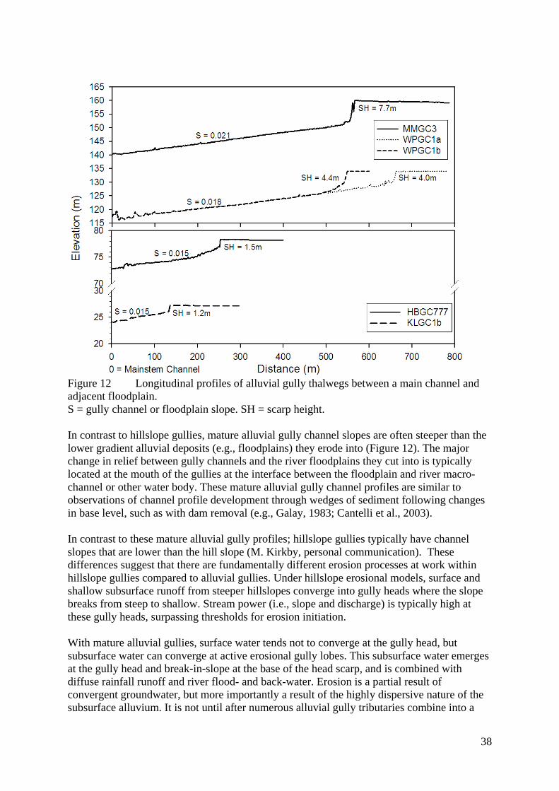
Figure 12 Longitudinal profiles of alluvial gully thalwegs between a main channel and adjacent floodplain. S = gully channel or floodplain slope. SH = scarp height. In contrast to hillslope gullies, mature alluvial gully channel slopes are often steeper than the lower gradient alluvial deposits (e.g., floodplains) they erode into (Figure 12). The major change in relief between gully channels and the river floodplains they cut into is typically located at the mouth of the gullies at the interface between the floodplain and river macro-channel or other water body. These mature alluvial gully channel profiles are similar to observations of channel profile development through wedges of sediment following changes in base level, such as with dam removal (e.g., Galay, 1983; Cantelli et al., 2003). In contrast to these mature alluvial gully profiles; hillslope gullies typically have channel slopes that are lower than the hill slope (M. Kirkby, personal communication). These differences suggest that there are fundamentally different erosion processes at work within hillslope gullies compared to alluvial gullies. Under hillslope erosional models, surface and shallow subsurface runoff from steeper hillslopes converge into gully heads where the slope breaks from steep to shallow. Stream power (i.e., slope and discharge) is typically high at these gully heads, surpassing thresholds for erosion initiation. With mature alluvial gullies, surface water tends not to converge at the gully head, but subsurface water can converge at active erosional gully lobes. This subsurface water emerges at the gully head and break-in-slope at the base of the head scarp, and is combined with diffuse rainfall runoff and river flood- and back-water. Erosion is a partial result of convergent groundwater, but more importantly a result of the highly dispersive nature of the subsurface alluvium. It is not until after numerous alluvial gully tributaries combine into a

38

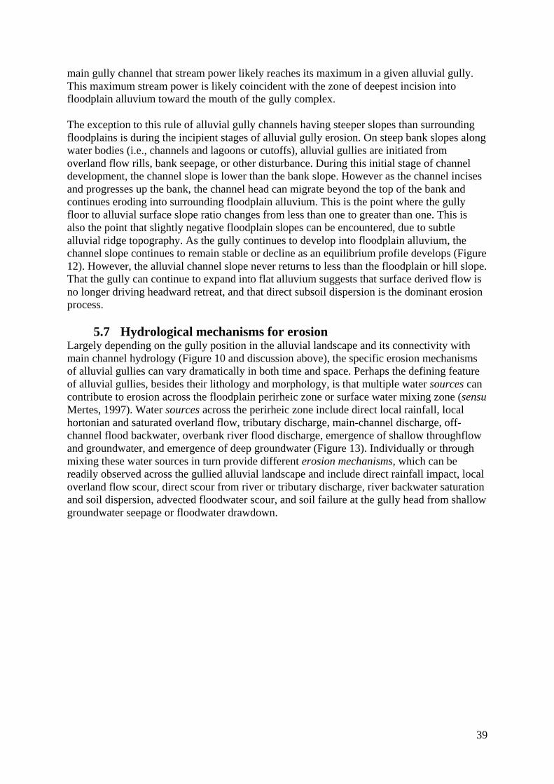
main gully channel that stream power likely reaches its maximum in a given alluvial gully. This maximum stream power is likely coincident with the zone of deepest incision into floodplain alluvium toward the mouth of the gully complex. The exception to this rule of alluvial gully channels having steeper slopes than surrounding floodplains is during the incipient stages of alluvial gully erosion. On steep bank slopes along water bodies (i.e., channels and lagoons or cutoffs), alluvial gullies are initiated from overland flow rills, bank seepage, or other disturbance. During this initial stage of channel development, the channel slope is lower than the bank slope. However as the channel incises and progresses up the bank, the channel head can migrate beyond the top of the bank and continues eroding into surrounding floodplain alluvium. This is the point where the gully floor to alluvial surface slope ratio changes from less than one to greater than one. This is also the point that slightly negative floodplain slopes can be encountered, due to subtle alluvial ridge topography. As the gully continues to develop into floodplain alluvium, the channel slope continues to remain stable or decline as an equilibrium profile develops (Figure 12). However, the alluvial channel slope never returns to less than the floodplain or hill slope. That the gully can continue to expand into flat alluvium suggests that surface derived flow is no longer driving headward retreat, and that direct subsoil dispersion is the dominant erosion process.

5.7 Hydrological mechanisms for erosion Largely depending on the gully position in the alluvial landscape and its connectivity with main channel hydrology (Figure 10 and discussion above), the specific erosion mechanisms of alluvial gullies can vary dramatically in both time and space. Perhaps the defining feature of alluvial gullies, besides their lithology and morphology, is that multiple water sources can contribute to erosion across the floodplain perirheic zone or surface water mixing zone (sensu Mertes, 1997). Water sources across the perirheic zone include direct local rainfall, local hortonian and saturated overland flow, tributary discharge, main-channel discharge, off-channel flood backwater, overbank river flood discharge, emergence of shallow throughflow and groundwater, and emergence of deep groundwater (Figure 13). Individually or through mixing these water sources in turn provide different erosion mechanisms, which can be readily observed across the gullied alluvial landscape and include direct rainfall impact, local overland flow scour, direct scour from river or tributary discharge, river backwater saturation and soil dispersion, advected floodwater scour, and soil failure at the gully head from shallow groundwater seepage or floodwater drawdown.

39

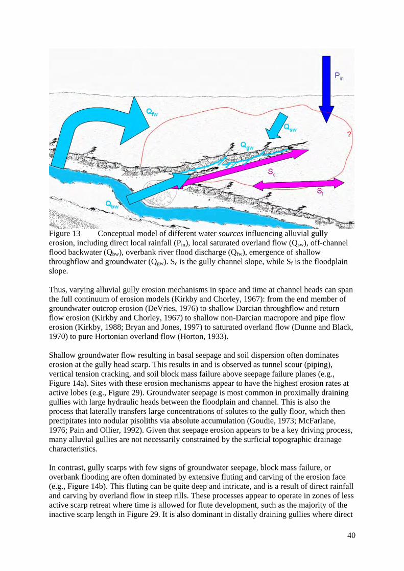
Figure 13 Conceptual model of different water sources influencing alluvial gully erosion, including direct local rainfall (Pin), local saturated overland flow (Qsw), off-channel flood backwater (Qbw), overbank river flood discharge (Qfw), emergence of shallow throughflow and groundwater (Qgw). Sc is the gully channel slope, while Sf is the floodplain slope. Thus, varying alluvial gully erosion mechanisms in space and time at channel heads can span the full continuum of erosion models (Kirkby and Chorley, 1967): from the end member of groundwater outcrop erosion (DeVries, 1976) to shallow Darcian throughflow and return flow erosion (Kirkby and Chorley, 1967) to shallow non-Darcian macropore and pipe flow erosion (Kirkby, 1988; Bryan and Jones, 1997) to saturated overland flow (Dunne and Black, 1970) to pure Hortonian overland flow (Horton, 1933). Shallow groundwater flow resulting in basal seepage and soil dispersion often dominates erosion at the gully head scarp. This results in and is observed as tunnel scour (piping), vertical tension cracking, and soil block mass failure above seepage failure planes (e.g., Figure 14a). Sites with these erosion mechanisms appear to have the highest erosion rates at active lobes (e.g., Figure 29). Groundwater seepage is most common in proximally draining gullies with large hydraulic heads between the floodplain and channel. This is also the process that laterally transfers large concentrations of solutes to the gully floor, which then precipitates into nodular pisoliths via absolute accumulation (Goudie, 1973; McFarlane, 1976; Pain and Ollier, 1992). Given that seepage erosion appears to be a key driving process, many alluvial gullies are not necessarily constrained by the surficial topographic drainage characteristics. In contrast, gully scarps with few signs of groundwater seepage, block mass failure, or overbank flooding are often dominated by extensive fluting and carving of the erosion face (e.g., Figure 14b). This fluting can be quite deep and intricate, and is a result of direct rainfall and carving by overland flow in steep rills. These processes appear to operate in zones of less active scarp retreat where time is allowed for flute development, such as the majority of the inactive scarp length in Figure 29. It is also dominant in distally draining gullies where direct

40

rainfall and overland flow are the main water sources. Fluting, carving, erosion of fine matrix material, and retention of resistant iron oxides (i.e., indurated mottles) results in the vertical concentration of solutes and nodular pisoliths, via relative accumulation per decensum (Goudie, 1973; McFarlane 1991; Pain and Ollier, 1992).

Figure 14 Ground photos of a) mass failure, and b) fluting and carving at head scarps. One end member example of alluvial gully erosion in the Mitchell catchment is displayed by the groundwater seepage erosion that dominates head cut retreat at WPGC2 near Wrotham Park (Figure 1). This gully is located in an area with high relative relief at the incised upper end of the fluvial megafan (Figure 10 and Figure 11). Time lapse photos suggested that little surface overland flow contributed to erosion at this head scarp, and that groundwater seepage was the dominant form of soil column failure. Headward retreat at this site was up to 5 meters in one year at the active lobes (Figure 15), whereas fluting and carving by direct rainfall dominated erosion on the interfluves between active lobes (right side of Figure 15). Two continuous stage gauges and one rain gauge were installed in the thalwegs of the outlet channels in this gully complex to quantify hydrological conditions (Figure 16). During both 2007-2008 and 2008-2009 wet seasons, peak stage conditions at this gauge were dominated by up to 7-8 m of river backwater from the mainstem Mitchell (Figure 17a). During non-backwater condition, local rainfall runoff in the gully catchment produced flashy runoff and smaller stage changes. In contest, the upper gauge in 2008-2009 experienced only small changes in stage (<0.5 m) in response to direct rainfall in the catchment and groundwater sapping at the gully head (Figure 17b). These stage data suggest that river backwater only inundated the lower end of the gully complex, and that river backwater did not influence erosion at the gully head, despite a 1-in-15 year recurrence interval peak flood in the Mitchell River in 2008-2009. Thus, the relative relief between the river channel and upper floodplain influenced the hydrologic processes driving erosion, with no river backwater at the gully head, but likely steeper hydraulic gradients driving groundwater sapping at the gully head.

41

Figure 15 Sequential time lapse photographs over one wet season at WPGC2. a) 14-Nov-08, b) 12-Jan-09, c) 10-Feb-09, d) 24-Feb-09. Note the groundwater sapping induced erosion at the undercut bank in the center right between a) and d).

Figure 16 LiDAR hillshade map of WPGC2 showing the locations of the lower and upper stage gauges, rain gauge, and time lapse camera.

42

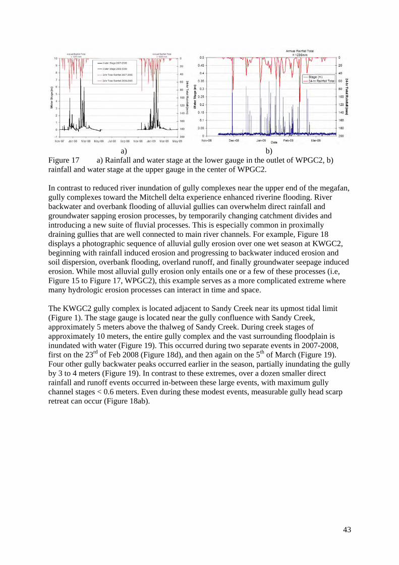
a) b) Figure 17 a) Rainfall and water stage at the lower gauge in the outlet of WPGC2, b) rainfall and water stage at the upper gauge in the center of WPGC2. In contrast to reduced river inundation of gully complexes near the upper end of the megafan, gully complexes toward the Mitchell delta experience enhanced riverine flooding. River backwater and overbank flooding of alluvial gullies can overwhelm direct rainfall and groundwater sapping erosion processes, by temporarily changing catchment divides and introducing a new suite of fluvial processes. This is especially common in proximally draining gullies that are well connected to main river channels. For example, Figure 18 displays a photographic sequence of alluvial gully erosion over one wet season at KWGC2, beginning with rainfall induced erosion and progressing to backwater induced erosion and soil dispersion, overbank flooding, overland runoff, and finally groundwater seepage induced erosion. While most alluvial gully erosion only entails one or a few of these processes (i.e, Figure 15 to Figure 17, WPGC2), this example serves as a more complicated extreme where many hydrologic erosion processes can interact in time and space. The KWGC2 gully complex is located adjacent to Sandy Creek near its upmost tidal limit (Figure 1). The stage gauge is located near the gully confluence with Sandy Creek, approximately 5 meters above the thalweg of Sandy Creek. During creek stages of approximately 10 meters, the entire gully complex and the vast surrounding floodplain is inundated with water (Figure 19). This occurred during two separate events in 2007-2008, first on the 23rd of Feb 2008 (Figure 18d), and then again on the 5th of March (Figure 19). Four other gully backwater peaks occurred earlier in the season, partially inundating the gully by 3 to 4 meters (Figure 19). In contrast to these extremes, over a dozen smaller direct rainfall and runoff events occurred in-between these large events, with maximum gully channel stages < 0.6 meters. Even during these modest events, measurable gully head scarp retreat can occur (Figure 18ab).

43

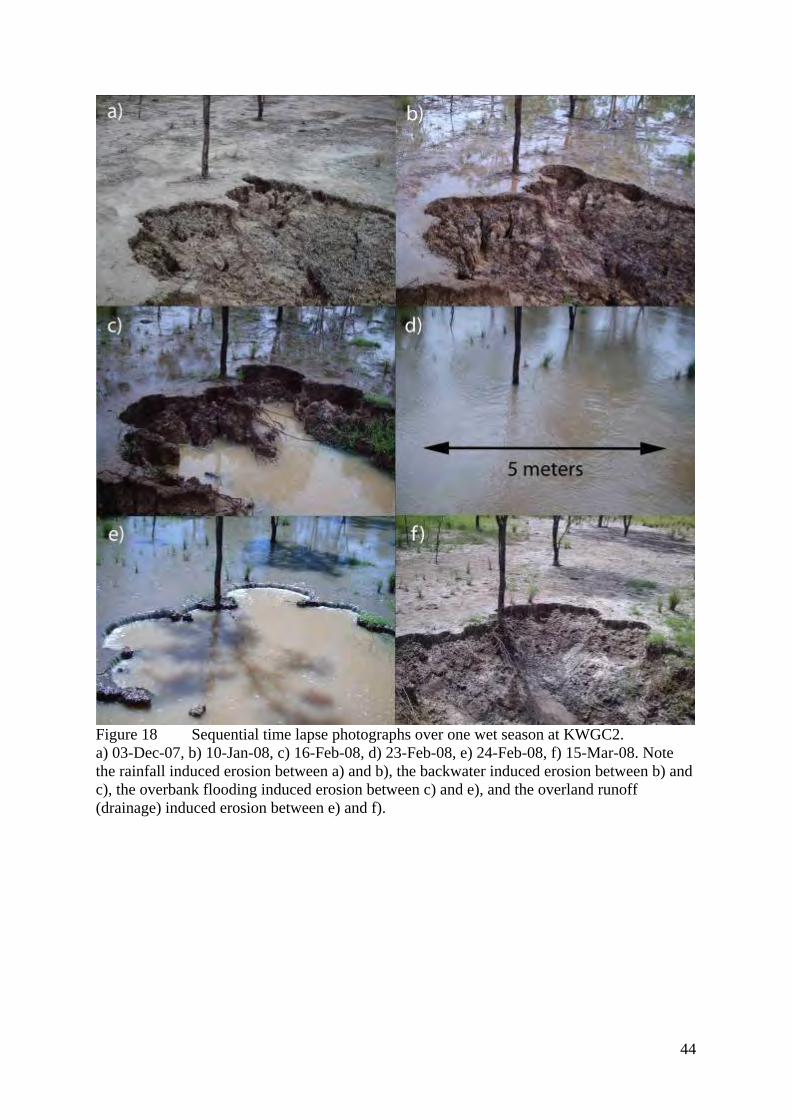
Figure 18 Sequential time lapse photographs over one wet season at KWGC2. a) 03-Dec-07, b) 10-Jan-08, c) 16-Feb-08, d) 23-Feb-08, e) 24-Feb-08, f) 15-Mar-08. Note the rainfall induced erosion between a) and b), the backwater induced erosion between b) and c), the overbank flooding induced erosion between c) and e), and the overland runoff (drainage) induced erosion between e) and f).

44

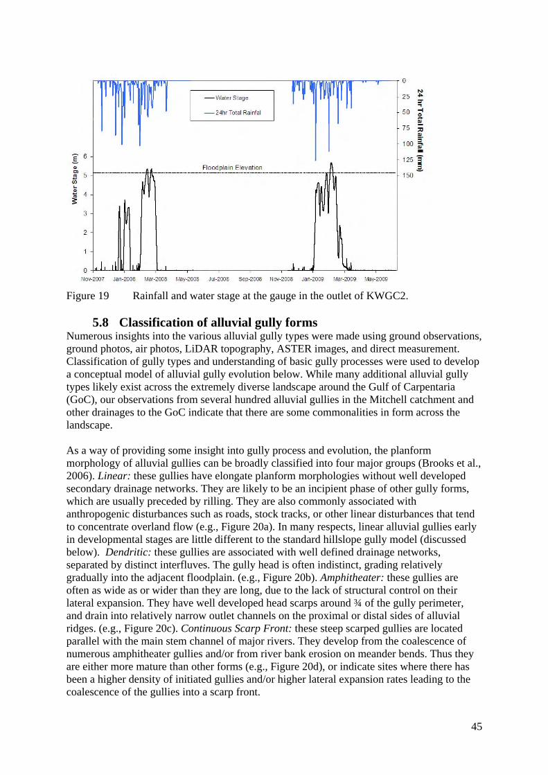
Figure 19 Rainfall and water stage at the gauge in the outlet of KWGC2.

5.8 Classification of alluvial gully forms Numerous insights into the various alluvial gully types were made using ground observations, ground photos, air photos, LiDAR topography, ASTER images, and direct measurement. Classification of gully types and understanding of basic gully processes were used to develop a conceptual model of alluvial gully evolution below. While many additional alluvial gully types likely exist across the extremely diverse landscape around the Gulf of Carpentaria (GoC), our observations from several hundred alluvial gullies in the Mitchell catchment and other drainages to the GoC indicate that there are some commonalities in form across the landscape. As a way of providing some insight into gully process and evolution, the planform morphology of alluvial gullies can be broadly classified into four major groups (Brooks et al., 2006). Linear: these gullies have elongate planform morphologies without well developed secondary drainage networks. They are likely to be an incipient phase of other gully forms, which are usually preceded by rilling. They are also commonly associated with anthropogenic disturbances such as roads, stock tracks, or other linear disturbances that tend to concentrate overland flow (e.g., Figure 20a). In many respects, linear alluvial gullies early in developmental stages are little different to the standard hillslope gully model (discussed below). Dendritic: these gullies are associated with well defined drainage networks, separated by distinct interfluves. The gully head is often indistinct, grading relatively gradually into the adjacent floodplain. (e.g., Figure 20b). Amphitheater: these gullies are often as wide as or wider than they are long, due to the lack of structural control on their lateral expansion. They have well developed head scarps around ¾ of the gully perimeter, and drain into relatively narrow outlet channels on the proximal or distal sides of alluvial ridges. (e.g., Figure 20c). Continuous Scarp Front: these steep scarped gullies are located parallel with the main stem channel of major rivers. They develop from the coalescence of numerous amphitheater gullies and/or from river bank erosion on meander bends. Thus they are either more mature than other forms (e.g., Figure 20d), or indicate sites where there has been a higher density of initiated gullies and/or higher lateral expansion rates leading to the coalescence of the gullies into a scarp front.

45

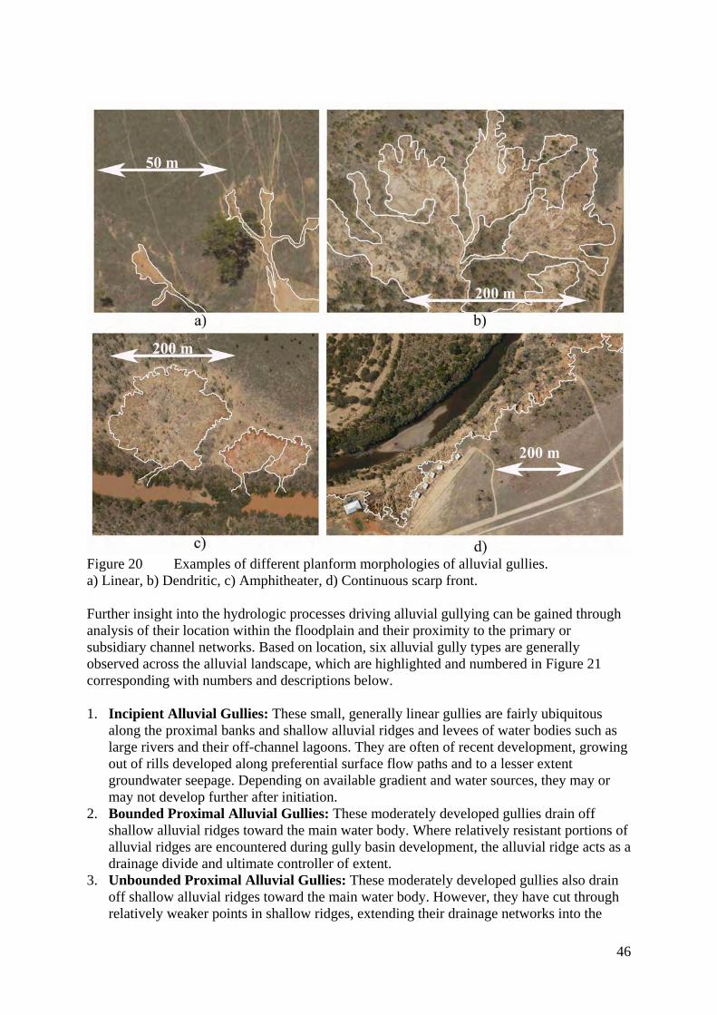
Figure 20 Examples of different planform morphologies of alluvial gullies. a) Linear, b) Dendritic, c) Amphitheater, d) Continuous scarp front. Further insight into the hydrologic processes driving alluvial gullying can be gained through analysis of their location within the floodplain and their proximity to the primary or subsidiary channel networks. Based on location, six alluvial gully types are generally observed across the alluvial landscape, which are highlighted and numbered in Figure 21 corresponding with numbers and descriptions below. 1. Incipient Alluvial Gullies: These small, generally linear gullies are fairly ubiquitous

along the proximal banks and shallow alluvial ridges and levees of water bodies such as large rivers and their off-channel lagoons. They are often of recent development, growing out of rills developed along preferential surface flow paths and to a lesser extent groundwater seepage. Depending on available gradient and water sources, they may or may not develop further after initiation.

2. Bounded Proximal Alluvial Gullies: These moderately developed gullies drain off shallow alluvial ridges toward the main water body. Where relatively resistant portions of alluvial ridges are encountered during gully basin development, the alluvial ridge acts as a drainage divide and ultimate controller of extent.

3. Unbounded Proximal Alluvial Gullies: These moderately developed gullies also drain off shallow alluvial ridges toward the main water body. However, they have cut through relatively weaker points in shallow ridges, extending their drainage networks into the

46

distal parts of the floodplain. Concepts of surface and groundwater divides breakdown with these gully types. Scarp retreat is not driven by surface runoff in this type of gully.

4. Unbounded Alluvial Gully Complexes: These relatively large catchments drain portions of distal floodplains. They have well developed gullied tributaries that each develops uniquely depending on their location and orientation. In sum, these gully complexes can form larger, fractal versions of smaller alluvial gullies. Since they cut through alluvial ridges either before or after ridge formation, they are relatively unbounded and unconstrained in their development.

5. Bounded Distal Gullies: These moderately developed gullies drain off relatively resistant portions of alluvial ridges away from the main channel, towards distal parts of the floodplain into tributaries, lagoons, backswamps, or larger gully complexes. Due to long channel slope distances to the main channel, their scarp heights are usually smaller than their adjacent proximal gullies, given the more gradual gully floor slope.

6. Unbounded Distal Gullies: These gullies are tributary to large gully complexes draining distal portions of the floodplain. They are relatively unconstrained by alluvial ridges near channels, but could be constrained by available water sources.

47

Figure 21 a) Schematic of numerous alluvial gully complexes draining both proximal and distal portions of the Mitchell River floodplain near the Lynd River, b) Air photo of the same area as a) showing the white, bare portions of active alluvial gullies, c) Inset air photo from b. Numbers in a) refer to gully location and evolutionary stage: 1) Incipient Proximal Alluvial Gullies, 2) Bounded Proximal Alluvial Gullies, 3) Unbounded Proximal Alluvial Gullies, 4) Unbounded Alluvial Gully Complexes, 5) Bounded Distal Gullies, and 6) Unbounded Distal Gullies.

48

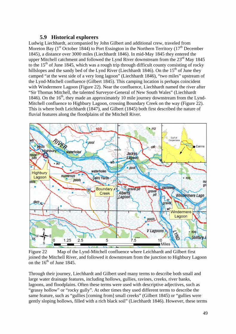
5.9 Historical explorers

Ludwig Liechhardt, accompanied by John Gilbert and additional crew, traveled from Moreton Bay (1st October 1844) to Port Essington in the Northern Territory (17th December 1845), a distance over 3000 miles (Liechhardt 1846). In mid-May 1845 they entered the upper Mitchell catchment and followed the Lynd River downstream from the 23rd May 1845 to the 15th of June 1845, which was a rough trip through difficult county consisting of rocky hillslopes and the sandy bed of the Lynd River (Liechhardt 1846). On the 15th of June they camped “at the west side of a very long lagoon” (Liechhardt 1846), “two miles” upstream of the Lynd-Mitchell confluence (Gilbert 1845). This camping location is perhaps coincident with Windermere Lagoon (Figure 22). Near the confluence, Liechhardt named the river after “Sir Thomas Mitchell, the talented Surveyor-General of New South Wales” (Liechhardt 1846). On the 16th, they made an approximately 10 mile journey downstream from the Lynd-Mitchell confluence to Highbury Lagoon, crossing Boundary Creek on the way (Figure 22). This is where both Leichhardt (1847), and Gilbert (1845) both first described the nature of fluvial features along the floodplains of the Mitchell River.

Figure 22 Map of the Lynd-Mitchell confluence where Leichhardt and Gilbert first joined the Mitchell River, and followed it downstream from the junction to Highbury Lagoon on the 16th of June 1845. Through their journey, Liechhardt and Gilbert used many terms to describe both small and large water drainage features, including hollows, gullies, ravines, creeks, river banks, lagoons, and floodplains. Often these terms were used with descriptive adjectives, such as “grassy hollow” or “rocky gully”. At other times they used different terms to describe the same feature, such as “gullies [coming from] small creeks” (Gilbert 1845) or “gullies were gently sloping hollows, filled with a rich black soil” (Liechhardt 1846). However, these terms

49

were used often enough to describe different fluvial conditions they encountered, and in mass their general meanings can be deduced from their usage during the days to weeks leading up to or during their trip along the Mitchell. Hollows were often defined as sloped drainage depressions “along river banks”, “densely grassed”, “generally without trees”, that “fill with water by the thunder-storms” (Liechhardt 1846). The terms “gullies”, “ravines”, and “creeks” were used more interchangeably. Gullies were often described as “little creek[s] and watercourse[s]” that were “deep”, on hill “slopes”, “filled with boulders and shingles” and generally harder to navigate than hollows (Liechhardt 1846). “Ravine” was used with “gully” in sentences, but referring to two different forms (i.e., “gullies and ravines”). “Creeks” were often described as more permanent water courses that were “large”, “good-sized”, “sandy bed”, “running”, “dry”, “deep”, “broad”, “rocky”, with “clayey flats”, and at times with flowing water and vegetated banks (Liechhardt 1846). It would seem that in Leichhardt’s and Gilbert’s usage, “hollows” are unchanneled valleys, and that “gullies” and “ravines” are smaller than “creeks”, all with channels in their valleys. However, in modern usage “creek” is a more general term used for all small channeled watercourses, while “gully” is used for a highly unstable and rapidly incising channel with raw eroded banks and beds (see Sections 2.1 and 2.2; and Poesen et al., 2003). Nowhere in either Liechhardt (1846) or Gilbert (1845) were the terms “erosion, eroded, bare, stripped, de-vegetated, dissected, unstable, incision, head cut, scarp, drop off, break-away, badland, or wasteland” used to describe the soil surface, gullies, hollows, or creeks. It is under the above context that Liechhardt’s and Gilbert’s journal entries along the Mitchell River must be interpreted. During their journey from the Lynd Junction to Highbury and beyond, Leichhardt and Gilbert noted the existence of gullies, creeks, and hollows that drained floodwater on the floodplain into the Mitchell River (Table 2). Their journey on the 16th of June 1845 would have taken them across Boundary Creek (Figure 22), which today is a sand bedded creek surrounded by rubbervine brush and woodlands (Figure 23). In places, parts of the riparian zone around the creek are almost competently stripped of soil by alluvial gullying (Figure 24b; Figure 25a). Undoubtably Boundary Creek is the “bad” and “deep creek” they encountered on the 16th of June (Table 2). From observation today, it is clearly not a “gully”, although it has more modern alluvial gullies around it (Figure 23; Figure 24b; Figure 25ab). However, they also eluded to the presence of other gullies and hollows along the “immediate banks of the river”, which were “very steep”, forcing them to “keep back from the river bank” (Table 2).

50

Table 2 Journal entries by Leichhardt (1847) and Gilbert (1845) describing creek, gullies, and hollows along the Mitchell River downstream of the Lynd. Date and Location Leichhardt (1847) Gilbert (1845) 16th June 1845 Boundary Creek Between Lynd Junction and Highbury Lagoon

“….the [floodplain] was interrupted by gullies, and occasionally by deep creeks, which [were] the outlets of the waters collecting on the [floodplain]”

“…we mostly kept back from the river bank to avoid deep gullies, which so frequently came into the river from small creeks, several of which we could not avoid, and two of which were as bad as any gully we had to cross from the first setting out of the expedition.”

19th June 1845 16˚ 22’ 16” Perhaps near 10-mile Lagoon today.

“The soil of the flat round the lagoon, was very stiff and suitable for making bricks.”

“The river was parallel with us most of the route, becoming necessary for us to keep well back to avoid the deep gullies frequent on the immediate banks of the river.”

20th June 1845 Perhaps near 20-mile and Mosquito Lagoons

“We…..avoided the gullies by keeping at a distance from the river. The banks of the river were so steep, that the access to its water was difficult.”

“The bed and banks of the river were broken instead of excellent travelling; we as usual had very distant gullies and hollows to cross; the banks of the river being very steep with very indifferent camping places”

These two journals and their descriptions of hollows, gullies, and creeks are some of the few historically written insights into the pre-European settlement conditions of the alluvial floodplain conditions of the Mitchell River. Unfortunately many of the descriptors are vague or incomplete. However, it is clear that numerous water courses and channels existed on the floodplain of the Mitchell River pre-European settlement, which at times during the Leichhardt-Gilbert expedition made overland travel by horse difficult. It can clearly be seen today that the Mitchell River indeed has very steep banks (Figure 26), caused by river incision into the fluvial megafan over the last two-million years (Figure 4 and Figure 10). “Gullies frequent on the immediate banks of the river” (Table 2) can also be observed near Highbury (Figure 27a), as well as unchanneled “hollows” further back from the river banks (Figure 27b). However, if the highly eroded alluvial gully landscape that we see today near the Lynd-Mitchell junctions and Highbury (Figure 24) truly existed during the Leichhardt-Gilbert expedition, then it would be very strange that they did not draw greater attention in their notes to these eroded wastelands. Air photo sequences of alluvial gullies near Boundary Creek in 1949 and 1993 (Figure 25) suggest that these alluvial gullies have grown considerably over historic times, and possibly did not exist in 1845 during the passage of Leichhardt and Gilbert. It is more likely that what Gilbert (1845) and Leichhardt (1847) observed were the precursor hollows and bank gullies (e.g., Figure 27) that subsequently evolved into the massive landscape degradation seen in the 21st century (Figure 7). However, the possibility can not be discounted that some smaller alluvial gullies did exist at the time of the Leichhardt expedition, initiated by natural forces.

51

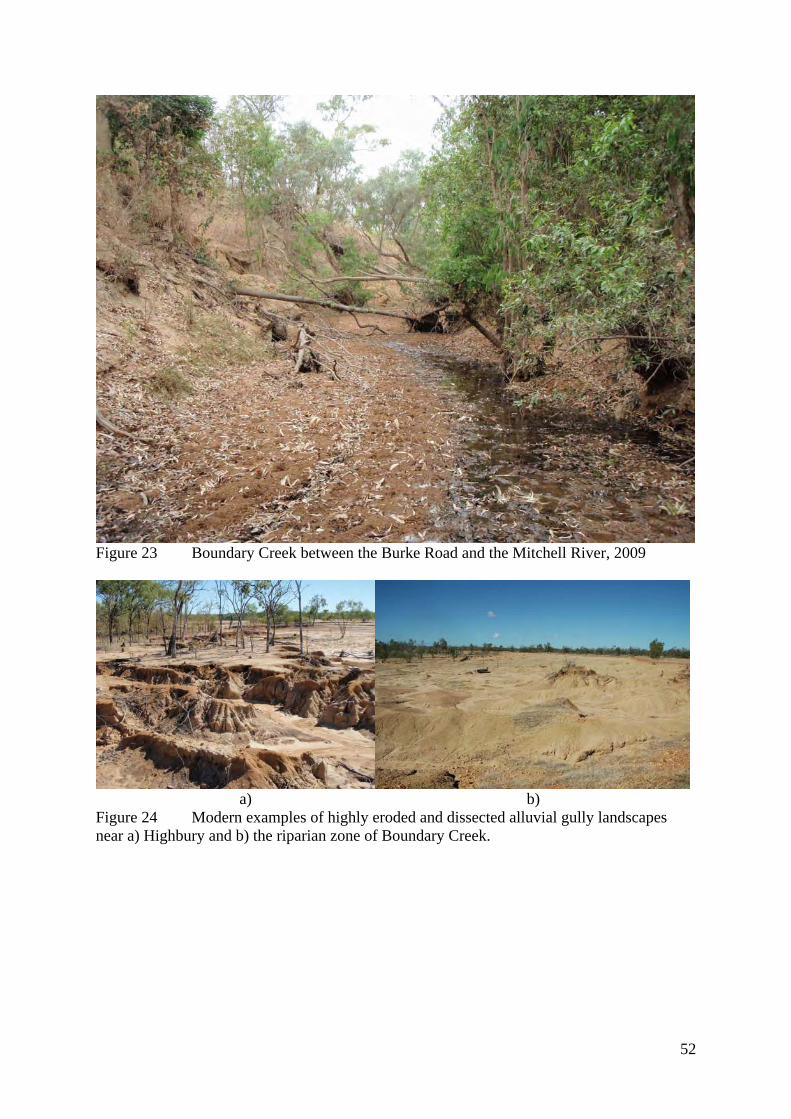
Figure 23 Boundary Creek between the Burke Road and the Mitchell River, 2009

a) b) Figure 24 Modern examples of highly eroded and dissected alluvial gully landscapes near a) Highbury and b) the riparian zone of Boundary Creek.

52

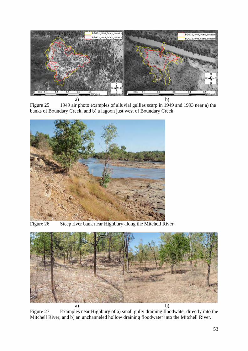
a) b) Figure 25 1949 air photo examples of alluvial gullies scarp in 1949 and 1993 near a) the banks of Boundary Creek, and b) a lagoon just west of Boundary Creek.

Figure 26 Steep river bank near Highbury along the Mitchell River.

a) b) Figure 27 Examples near Highbury of a) small gully draining floodwater directly into the Mitchell River, and b) an unchanneled hollow draining floodwater into the Mitchell River.

53

The Jardine Brothers lead an expedition in 1864 that crossed the lower Mitchell River Delta near the Scrutton River (Nassau) and other river anabranches (upstream of present day Kowanyama) has few references to erosional features or gullies. However, on 14 Dec 1864 they observed that "many gullies were crossed filled with the screw-palm (Pandanus Spirilas)”. On 15 Dec they came to a creek with that “came from the eastward, was tolerably watered, and presented some bad broken sandstone country on its north bank. Its shady appearance suggested the appropriate name of "Arbor Creek." For three miles the route lay over gullies, spurs, and walls of broken sandstone. The country beyond opened agreeably into flats, which might almost be called plains….”. This creek was an anabranch of the Mitchell and was southwest of the Mitchell mainstem, as they did not reach and cross the Mitchell till 16 Dec. On 18 Dec after crossing the Mitchell River, the “river was followed down to-day for 9 miles through a complete network of anabranches, gullies, and vine scrubs to another branch”. On 19 Dec they observed that “the banks were of clay and sandstone, from 20 to 30 feet high, the water was discolored to a kind of yellowish white. During the floods the stream must be eight or ten miles wide, for, two miles back from it, a fish weir was seen in a small gully”. From these observations, it is again unclear of the exact definition and usage of the term gully. In many earlier instances in their journey, many depression channels or small creeks were termed “gullies”. Often these “gullies” or channel depressions were described as having vegetation in them, such as Pandanus. On other instances they described a “fish weir in a small gully” which suggests that this was an anabranch channel or river slough, rather than a modern day unstable gully. However, their description of “broken sandstone” country suggests that they did observe some of the indurated ironstone alluvium or lateritic country south of the Mitchell perhaps near present day Kilpatrick Creek. Today, in places the cut banks of these anabranch channels have high exposed sections of cemented alluvium and the plains in places are capped by lateritic ironstone perhaps observed as sandstone. It remains unknown whether their observations of “gullies, spurs, and walls of broken sandstone” referred to small dry anabranch channels, vegetated interfluves, and creek cut banks into indurated alluvium, or whether they refer to the broken badlands and wasteland of alluvial gully erosion seen in a few places today in the Mitchell delta.

54

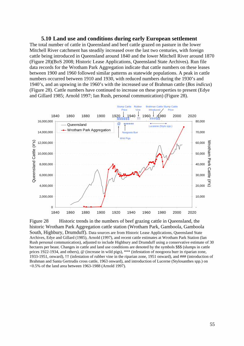
5.10 Land use and conditions during early European settlement

The total number of cattle in Queensland and beef cattle grazed on pasture in the lower Mitchell River catchment has steadily increased over the last two centuries, with foreign cattle being introduced in Queensland around 1840 and the lower Mitchell River around 1870 (Figure 28)(BoS 2008; Historic Lease Applications, Queensland State Archives). Run file data records for the Wrotham Park Aggregation indicate that cattle numbers on these leases between 1900 and 1960 followed similar patterns as statewide populations. A peak in cattle numbers occurred between 1910 and 1930, with reduced numbers during the 1930’s and 1940’s, and an upswing in the 1960’s with the increased use of Brahman cattle (Bos indicus) (Figure 28). Cattle numbers have continued to increase on these properties to present (Edye and Gillard 1985; Arnold 1997; Ian Rush, personal communication) (Figure 28).

0

2,000,000

4,000,000

6,000,000

8,000,000

10,000,000

12,000,000

14,000,000

16,000,000

1840 1860 1880 1900 1920 1940 1960 1980 2000 2020

Que

ensl

and

Cat

tle (#

's)_

-

10,000

20,000

30,000

40,000

50,000

60,000

70,000

80,000

1840 1860 1880 1900 1920 1940 1960 1980 2000 2020

Wrotham

Park Cattle (#'s)

QueenslandWrotham Park Aggregation

$$$$$$ ###$$

******!!!

Brahman Cattle Introduced

Slump CattlePrice

RubberVine

Noogoora Burr

@

Wild Pigs

Lucerene (Stylo spp.)

Slump CattlePrice

Figure 28 Historic trends in the numbers of beef grazing cattle in Queensland, the historic Wrotham Park Aggregation cattle station (Wrotham Park, Gamboola, Gamboola South, Highbury, Drumduff). Data sources are from Historic Lease Applications, Queensland State Archives, Edye and Gillard (1985), Arnold (1997), and recent cattle estimates at Wrotham Park Station (Ian Rush personal communication), adjusted to include Highbury and Drumduff using a conservative estimate of 30 hectares per beast. Changes in cattle and land use conditions are denoted by the symbols $$$ (slumps in cattle prices 1922-1934, and others), @ (increase in wild pigs), *** (infestation of noogoora burr in riparian zone, 1933-1951, onward), !!! (infestation of rubber vine in the riparian zone, 1951 onward), and ### (introduction of Brahman and Santa Gertrudis cross cattle, 1963 onward), and introduction of Lucerne (Stylosanthes spp.) on <0.5% of the land area between 1963-1988 (Arnold 1997).

55

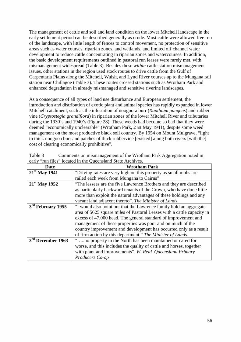
The management of cattle and soil and land condition on the lower Mitchell landscape in the early settlement period can be described generally as crude. Most cattle were allowed free run of the landscape, with little length of fences to control movement, no protection of sensitive areas such as water courses, riparian zones, and wetlands, and limited off channel water development to reduce cattle concentrating in riparian zones and watercourses. In addition, the basic development requirements outlined in pastoral run leases were rarely met, with mismanagement widespread (Table 3). Besides these within cattle station mismanagement issues, other stations in the region used stock routes to drive cattle from the Gulf of Carpentaria Plains along the Mitchell, Walsh, and Lynd River courses up to the Mungana rail station near Chillagoe (Table 3). These routes crossed stations such as Wrotham Park and enhanced degradation in already mismanaged and sensitive riverine landscapes. As a consequence of all types of land use disturbance and European settlement, the introduction and distribution of exotic plant and animal species has rapidly expanded in lower Mitchell catchment, such as the infestation of noogoora burr (Xanthium pungens) and rubber vine (Cryptostegia grandiflora) in riparian zones of the lower Mitchell River and tributaries during the 1930’s and 1940’s (Figure 28). These weeds had become so bad that they were deemed “economically unclearable” (Wrotham Park, 21st May 1941), despite some weed management on the most productive black soil country. By 1954 on Mount Mulgrave, “light to thick noogooa burr and patches of thick rubbervine [existed] along both rivers [with the] cost of clearing economically prohibitive". Table 3 Comments on mismanagement of the Wrotham Park Aggregation noted in early “run files” located in the Queensland State Archives.

Date Wrotham Park 21st May 1941 "Driving rates are very high on this property as small mobs are

railed each week from Mungana to Cairns" 21st May 1952 “The lessees are the five Lawrence Brothers and they are described

as particularly backward tenants of the Crown, who have done little more than exploit the natural advantages of these holdings and any vacant land adjacent thereto”. The Minister of Lands.

3rd February 1955 "I would also point out that the Lawrence family hold an aggregate area of 5625 square miles of Pastoral Leases with a cattle capacity in excess of 47,000 head. The general standard of improvement and management of these properties was poor and on much of the country improvement and development has occurred only as a result of firm action by this department.” The Minister of Lands.

3rd December 1963 "…..no property in the North has been maintained or cared for worse, and this includes the quality of cattle and horses, together with plant and improvements". W. Reid Queensland Primary Producers Co-op

56

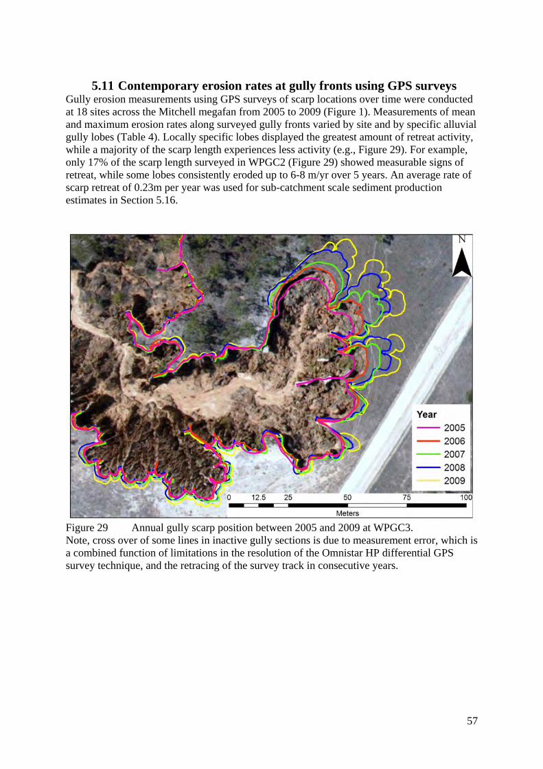
5.11 Contemporary erosion rates at gully fronts using GPS surveys

Gully erosion measurements using GPS surveys of scarp locations over time were conducted at 18 sites across the Mitchell megafan from 2005 to 2009 (Figure 1). Measurements of mean and maximum erosion rates along surveyed gully fronts varied by site and by specific alluvial gully lobes (Table 4). Locally specific lobes displayed the greatest amount of retreat activity, while a majority of the scarp length experiences less activity (e.g., Figure 29). For example, only 17% of the scarp length surveyed in WPGC2 (Figure 29) showed measurable signs of retreat, while some lobes consistently eroded up to 6-8 m/yr over 5 years. An average rate of scarp retreat of 0.23m per year was used for sub-catchment scale sediment production estimates in Section 5.16.

Figure 29 Annual gully scarp position between 2005 and 2009 at WPGC3. Note, cross over of some lines in inactive gully sections is due to measurement error, which is a combined function of limitations in the resolution of the Omnistar HP differential GPS survey technique, and the retracing of the survey track in consecutive years.

57

Table 4 GPS survey lengths and erosion rates at alluvial gully scarps sites. Years Site ID Survey Length (m) Max Retreat (m/yr) Mean Retreat (m/yr)

2007-2008 DBGC1 10.1 0.470 2008-2009 DBGC1 1952 11.1 0.598 2007-2008 DDGC1 4.5 0.355 2008-2009 DDGC1 5902 3.5 0.228 2007-2008 DDGC2 2.3 0.634 2008-2009 DDGC2 2977 1.8 0.402 2007-2008 GBGC1 1.8 0.204 2008-2009 GBGC1 1981 0.8 0.037 2007-2008 GBGC2 14.1 0.275 2008-2009 GBGC2 2179 11.4 0.368 2007-2008 GBGC3 3.5 0.132 2008-2009 GBGC3 2444 1.8 0.186 2006-2007 HBGC1a 3.9 0.660 2007-2008 HBGC1a 1.4 0.101 2008-2009 HBGC1a 3561 2.4 0.105 2006-2007 HBGC1b 2.6 0.391 2007-2008 HBGC1b 3.4 0.162 2008-2009 HBGC1b 3004 1.3 0.020 2007-2008 HBGC2b 5.8 0.008 2008-2009 HBGC2b 1953 3.8 0.482 2006-2007 KWGC1 3.2 1.721 2007-2008 KWGC1 5.3 0.077 2008-2009 KWGC1 5030 3.5 0.203 2007-2008 KWGC3 1.6 0.121 2008-2009 KWGC3 2879 3.1 0.110 2006-2007 WPGC2 10.3 0.325 2007-2008 WPGC2 4.8 0.161 2008-2009 WPGC2 5799 6.4 0.222 2005-2006 WPGC3 8.1 0.254 2006-2007 WPGC3 6.6 0.708 2007-2008 WPGC3 7.8 0.084 2008-2009 WPGC3 7046 7.4 0.285 2006-2007 MMGC1 8.1 0.657 2007-2008 MMGC1 4.5 0.234 2008-2009 MMGC1 1173 3.1 0.247 2007-2008 MMGC2 2.8 0.037 2008-2009 MMGC2 2158 2.7 0.069

Total 50,040 Median (50) 3.5 0.23

25th percentile 2.6 0.11 75th percentile 6.6 0.39

58

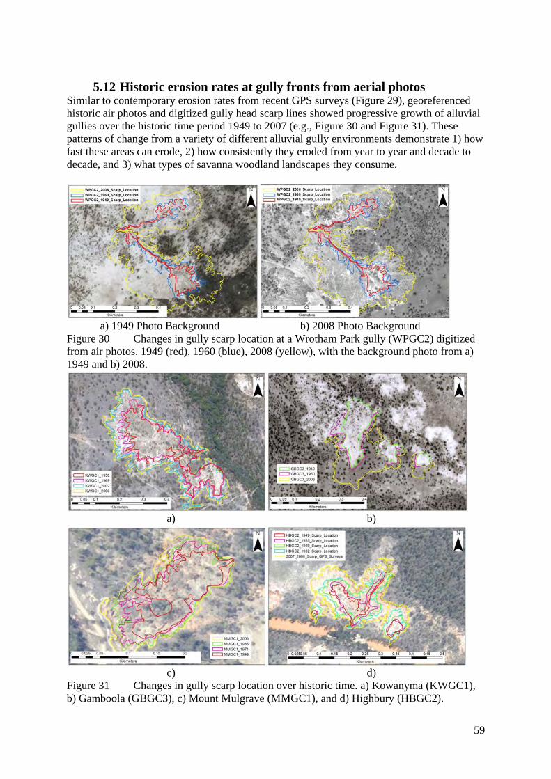
5.12 Historic erosion rates at gully fronts from aerial photos

Similar to contemporary erosion rates from recent GPS surveys (Figure 29), georeferenced historic air photos and digitized gully head scarp lines showed progressive growth of alluvial gullies over the historic time period 1949 to 2007 (e.g., Figure 30 and Figure 31). These patterns of change from a variety of different alluvial gully environments demonstrate 1) how fast these areas can erode, 2) how consistently they eroded from year to year and decade to decade, and 3) what types of savanna woodland landscapes they consume.

a) 1949 Photo Background b) 2008 Photo Background Figure 30 Changes in gully scarp location at a Wrotham Park gully (WPGC2) digitized from air photos. 1949 (red), 1960 (blue), 2008 (yellow), with the background photo from a) 1949 and b) 2008.

a) b)

c) d) Figure 31 Changes in gully scarp location over historic time. a) Kowanyma (KWGC1), b) Gamboola (GBGC3), c) Mount Mulgrave (MMGC1), and d) Highbury (HBGC2).

59

The planform area (m2) of 18 separate gully complexes was regressed against time (1949-2009), using the initial gully area (A0) as a normalizing factor to develop a measure of changes in relative gully area over time. Using Equation 1 above, a best fit trend line was fit to the empirical data, showing trends of both past and potentially future growth (Figure 32). These results show that different gully complexes grow at different rates compared to their initial photo gully area. Some gully complexes have grown 3 to 10 times greater than their initial area in the last 58 years, which tend to be the sites with the fastest eroding head cuts from groundwater seepage and block failure (e.g., WPGC2, Figure 30ab). Growth rates are largely linear, with small k-values from Equation 1 (Figure 33a). In contrast, other gully complexes have only doubled or tripled in size, which tend to be sites with slower erosion rates and a greater amount of fluting and carving from direct rainfall (e.g., MMGC1, Figure 31c). These sites tended to have larger k-values (Figure 33a) suggesting greater non-linear trends with rapid initial growth and slower growth over time. All but one of the gully complexes has high r2 values (>0.95) when the exponential decay function (Equation 1) was fit to their data. (Figure 33b)

-

1

2

3

4

5

6

7

8

9

10

11

121900

1910

1920

1930

1940

1950

1960

1970

1980

1990

2000

2010

2020

Air Photo Year

Rel

ativ

e G

ully

Are

a (A

/ A

0)_

DBGC1aDBGC1cHBGC1aHBGC1bHBGC2bDDGC1DDGC2GBGC1GBGC2GBGC3KWGC1KWGC3MMGC1MMGC2MMGC3MMGC5WPGC2aWPGC3

1890

1800

1810

1820

1830

1840

1850

1860

1870

1880

?Cattle Introduced

Figure 32 Relative changes in gully area over time, which is the ratio of the area at any time (A) and the initial gully area (A0) from the first air photo. For some gully complex, it is clear when in time and place they initiated from both planform trends in gully area (e.g., Figure 30, Figure 31d, Figure 40) and mathematical trends using the negative exponential function (Figure 32). These gullies had fast erosion rates from easily identifiable staring points near the banks of rivers or lagoons. If the trend lines in Figure 32 are extended backward in time toward a relative area of zero, the point of initiation in time for many of these gullies falls between 1905 and 1950 (post cattle introduction). In contrast, other slower growing gullies have less identifiable starting points and negative exponential growth curves that suggest initiation time around 1900 or before. However, the lack of air photo data for these gully complexes between 1900 and 1949 makes large extrapolations backward in time less certain (see below).

60

k-

valu

es (n

on-li

near

rate

of c

hang

e)

0.0000

0.0005

0.0010

0.0015

0.0020

0.0025

0.0030

r2 coe

ffici

ent o

f det

erm

inat

ion

0.00

0.05

0.100.80

0.85

0.90

0.95

1.00

a) b) Figure 33 a) Equation 1 exponent k-values for 18 gully sites, and b) coefficient of determination values (r2) for the same sites. According to disturbance and relaxation theory (Graf 1977), the early growth periods in gully evolution should have the fastest erosion rates, which then relax over time. The lack of pre-1949 air photo data makes it hard to empirically support one mathematical trend model vs. another to predict these early trends. For comparative purposes, other simple mathematical models were used as a comparison to the negative exponential function. The data sets from different sites were split into two groups that had either apparent linear trends (Equation 2; Figure 34), or apparent logarithmic trends (Equation 3; Figure 35). The linear group had an average coefficient of determination value of (r2) of 0.990 for linear trends, while for the same data the negative exponential trends yielded a value of 0.985 and a value of 0.975 for logarithmic trends. The logarithmic group had an average coefficient of determination value of (r2) of 0.978 for logarithmic trends, while for the same data the negative exponential trends yielded a value of 0.976 and a value of 0.969 for linear trends. These data suggest that all models fit the existing data generally well, with no major preference for model type. However, the linear group had slightly better fits under linear trends over negative exponential trends or logarithmic trends (Figure 34). The logarithmic group also had better fits under logarithmic trends over linear trends (Figure 35). In summary however, additional data are need to drive these different mathematical models early in the gully evolution cycle. In the near future, insightful data might come from OSL data, dendrochronology, or U/Th/Ra dating of ferricrete and calcrete.

61

-

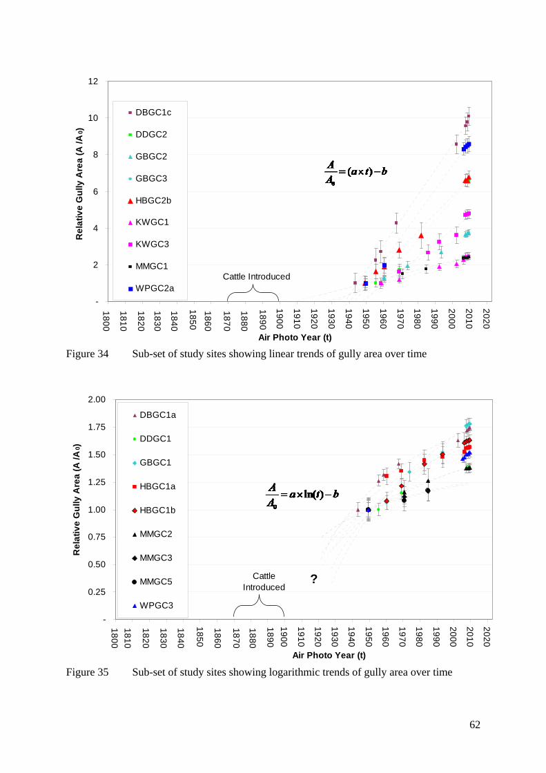
2

4

6

8

10

12

1900

1910

1920

1930

1940

1950

1960

1970

1980

1990

2000

2010

2020

Air Photo Year (t)

Rel

ativ

e G

ully

Are

a (A

/A 0)

_

DBGC1c

DDGC2

GBGC2

GBGC3

HBGC2b

KWGC1

KWGC3

MMGC1

WPGC2a1890

1800

1810

1820

1830

1840

1850

1860

1870

1880

Cattle Introduced

Figure 34 Sub-set of study sites showing linear trends of gully area over time

-

0.25

0.50

0.75

1.00

1.25

1.50

1.75

2.00

1900

1910

1920

1930

1940

1950

1960

1970

1980

1990

2000

2010

2020

Air Photo Year (t)

Rel

ativ

e G

ully

Are

a (A

/A 0)

DBGC1a

DDGC1

GBGC1

HBGC1a

HBGC1b

MMGC2

MMGC3

MMGC5

WPGC3

1890

18001810

1820

1830

1840

1850

1860

1870

1880

Cattle Introduced

?

Figure 35 Sub-set of study sites showing logarithmic trends of gully area over time

62

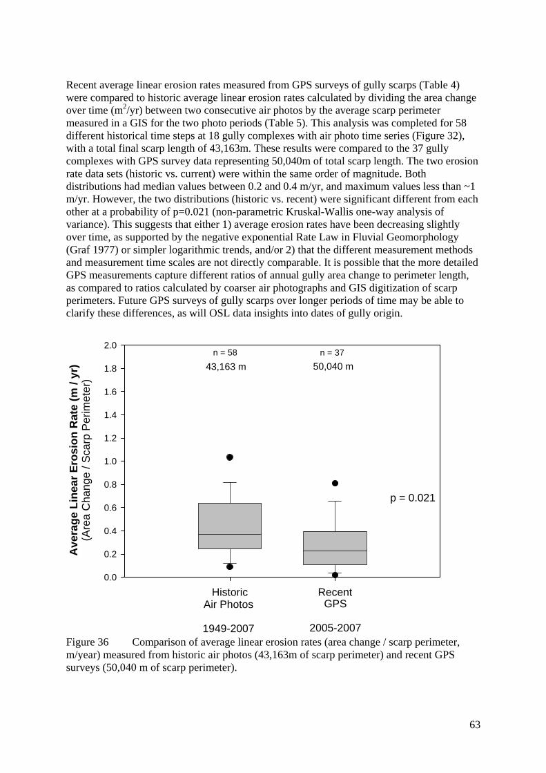
Recent average linear erosion rates measured from GPS surveys of gully scarps (Table 4) were compared to historic average linear erosion rates calculated by dividing the area change over time (m2/yr) between two consecutive air photos by the average scarp perimeter measured in a GIS for the two photo periods (Table 5). This analysis was completed for 58 different historical time steps at 18 gully complexes with air photo time series (Figure 32), with a total final scarp length of 43,163m. These results were compared to the 37 gully complexes with GPS survey data representing 50,040m of total scarp length. The two erosion rate data sets (historic vs. current) were within the same order of magnitude. Both distributions had median values between 0.2 and 0.4 m/yr, and maximum values less than ~1 m/yr. However, the two distributions (historic vs. recent) were significant different from each other at a probability of p=0.021 (non-parametric Kruskal-Wallis one-way analysis of variance). This suggests that either 1) average erosion rates have been decreasing slightly over time, as supported by the negative exponential Rate Law in Fluvial Geomorphology (Graf 1977) or simpler logarithmic trends, and/or 2) that the different measurement methods and measurement time scales are not directly comparable. It is possible that the more detailed GPS measurements capture different ratios of annual gully area change to perimeter length, as compared to ratios calculated by coarser air photographs and GIS digitization of scarp perimeters. Future GPS surveys of gully scarps over longer periods of time may be able to clarify these differences, as will OSL data insights into dates of gully origin.

Historic Recent

Ave

rage

Lin

ear E

rosi

on R

ate

(m /

yr)

(Are

a C

hang

e / S

carp

Per

imet

er)

0.0

0.2

0.4

0.6

0.8

1.0

1.2

1.4

1.6

1.8

2.0

Air Photos

1949-2007

GPS

2005-2007

n = 58 n = 37

p = 0.021

43,163 m 50,040 m

Figure 36 Comparison of average linear erosion rates (area change / scarp perimeter, m/year) measured from historic air photos (43,163m of scarp perimeter) and recent GPS surveys (50,040 m of scarp perimeter).

63

Table 5 Historic active scarp lengths and erosion rates at alluvial gully scarps sites.

Years Site ID Active Scarp Length (m)

Max Retreat (m/yr)

Mean Retreat (m/yr)

1943-1955 DBGC1 3.4 1.068 1955-1958 DBGC1 5.0 0.973

1958-1967 DBGC1 2.4 0.808

1967-2002 DBGC1 1.4 0.312

2002-2007 DBGC1 1365 3.7 0.728

1955-1969 DDGC1 2.8 0.577 1969-2007 DDGC1 5365 1.6 0.298 1955-1969 DDGC2 4.1 0.620 1969-2007 DDGC2 7308 3.7 1.032 1949-1960 GBGC1 1.6 0.151 1960-1974 GBGC1 2.0 0.548 1974-1993 GBGC1 1.3 0.193 1993-2007 GBGC1 1779 2.2 0.321 1949-1960 GBGC2 3.1 0.366 1960-1974 GBGC2 7.1 0.714 1974-1993 GBGC2 6.5 0.384 1993-2007 GBGC2 1479 4.4 0.506 1949-1960 GBGC3 4.9 0.626 1960-2007 GBGC3 1234 1.9 0.466 1949-1960 HBGC1a 5.5 1.172 1960-1969 HBGC1a 1.9 0.215 1969-1982 HBGC1a 1.8 0.270 1982-1993 HBGC1a 1.2 0.090 1993-2006 HBGC1a 1871 1.1 0.111 1949-1960 HBGC1b 1.1 0.350 1960-1969 HBGC1b 4.1 0.767 1969-1982 HBGC1b 2.1 0.593 1982-1993 HBGC1b 0.8 0.298 1993-2006 HBGC1b 1727 1.1 0.275 1949-1955 HBGC2b 4.4 0.715 1955-1960 HBGC2b 4.2 0.365 1960-1969 HBGC2b 1.8 0.659 1969-1982 HBGC2b 2.2 0.319 1982-2007 HBGC2b 1268 1.8 0.393 1958-1969 KWGC1 3.5 0.307 1969-1992 KWGC1 2.6 0.486 1992-2002 KWGC1 2.0 0.248

64

2002-2006 KWGC1 2975 9.0 0.718 1958-1969 KWGC3 5.6 0.564 1969-1986 KWGC3 6.2 0.520 1986-1992 KWGC3 4.5 0.631 1992-2002 KWGC3 3.2 0.247 2002-2007 KWGC3 1639 5.2 0.896 1949-1960 WPGC2 4.8 0.693 1960-2006 WPGC2 1796 3.3 0.376 1949-2005 WPGC3 5062 2.4 0.237

1949-1971 MMGC1 1.3 0.269 1971-1985 MMGC1 1.2 0.673 1985-2006 MMGC1 1064 1.1 0.582 1949-1971 MMGC2 1.1 0.198 1971-1985 MMGC2 1.4 0.195 1985-2007 MMGC2 1778 0.6 0.124 1949-1971 MMGC3 0.7 0.112 1971-1985 MMGC3 1150 0.6 0.080 1949-1971 MMGC5 0.8 0.083 1971-1985 MMGC5 780 1.3 0.140

Total 43,163 Median 2.2 0.37

25th 1.1 0.22 75th 4.1 0.59

65

5.13 Historic changes in gully volume

While gully area change over time is useful for determining initiation timing and growth over time, changes in gully area are only a surrogate for sediment yield over time. Therefore a measure of gully volume eroded over time would be more useful for sediment budget purposes. As a pilot site, LiDAR topographic raster data at KWGC2 were used in conjunction with scarp locations over time to analyze the changes in gully volume over time (Figure 37). A raster “lid” was constructed for the gully that was commensurate with and extrapolated from the relatively flat surrounding floodplain surface LiDAR data. To calculate gully volume at a given time, the gully bed raster within the scarp line was subtracted from the lid. This method assumes a vertical head scarp at the scarp line and complete export of sediment from the gully network, which are reasonable assumptions for a gully eroding into dispersible silts and clays. These results of gully volume over time suggest that both gully area and volume increased linearly over time at this site (Figure 38). However, additional analyses are need at other gully sites with LiDAR to determine whether these gully area/volume relationships are similar in other gully catchments, especially in gullies with more variability in gully depth with distance from the main river channel.

Figure 37 Changes in the gully scarp location at KWGC2 between 1958 and 2007 from air photos, with a 2008 LiDAR image.

66

R2 = 0.97

0

20,000

40,000

60,000

80,000

100,000

120,000

1930 1940 1950 1960 1970 1980 1990 2000 2010Air Photo Year

Gul

ly A

rea

(m 2 )_

0

20,000

40,000

60,000

80,000

100,000

120,000G

ully Volum

e (m 3)_

Total AreaTotal Volume

Figure 38 Gully area and volume changes over time at near KWGC2 Sandy Creek.

5.14 Erosion rates from dendrochronology While trees surviving gully erosion are important geomorphic indicators (Figure 5a; Figure 39), determination of erosion rates at KWGC2 focused on the analysis of those Coolibah trees (Eucalyptus microtheca) that had re-established after the passage of the gully head cut front (e.g., Figure 5b). These colonizing trees were well distributed across the floor of the alluvial gully complex (Figure 40), where they predominantly established along the new inset channels and small adjacent silt floodplains that drained the new gully complex. It was assumed that the growth of the gully network developed predominantly in a linear progression away from its confluence point with the main channel (Sandy Creek). This is supported by analysis of historic air photos that indicates elongation was the predominant growth direction, followed by widening (Figure 37). Thus, the channel thalweg distance upstream from the gully outlet was used as a location reference for the evolution of the gully and adjacent inset floodplain germination points for Coolibah trees.

67

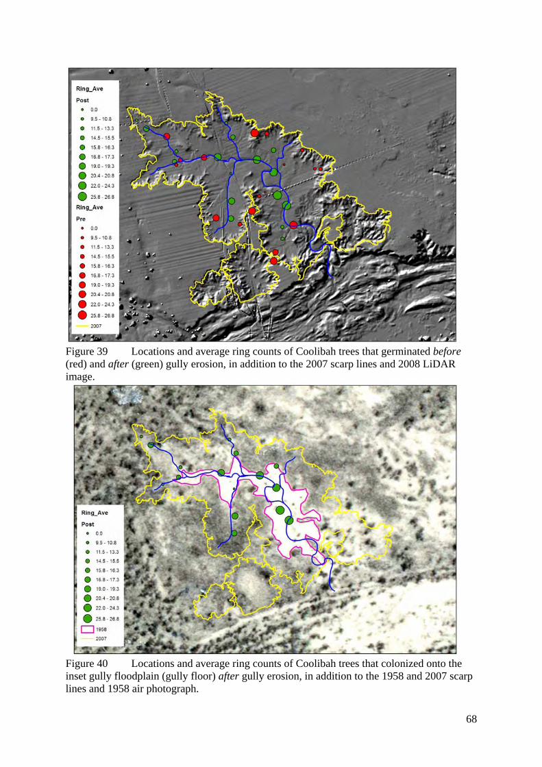
Figure 39 Locations and average ring counts of Coolibah trees that germinated before (red) and after (green) gully erosion, in addition to the 2007 scarp lines and 2008 LiDAR image.

Figure 40 Locations and average ring counts of Coolibah trees that colonized onto the inset gully floodplain (gully floor) after gully erosion, in addition to the 1958 and 2007 scarp lines and 1958 air photograph.

68

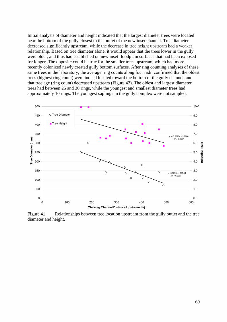
Initial analysis of diameter and height indicated that the largest diameter trees were located near the bottom of the gully closest to the outlet of the new inset channel. Tree diameter decreased significantly upstream, while the decrease in tree height upstream had a weaker relationship. Based on tree diameter alone, it would appear that the trees lower in the gully were older, and thus had established on new inset floodplain surfaces that had been exposed for longer. The opposite could be true for the smaller trees upstream, which had more recently colonized newly created gully bottom surfaces. After ring counting analyses of these same trees in the laboratory, the average ring counts along four radii confirmed that the oldest trees (highest ring count) were indeed located toward the bottom of the gully channel, and that tree age (ring count) decreased upstream (Figure 42). The oldest and largest diameter trees had between 25 and 30 rings, while the youngest and smallest diameter trees had approximately 10 rings. The youngest saplings in the gully complex were not sampled.

y = -0.0076x + 9.7786R2 = 0.3607

y = -0.5053x + 329.14R2 = 0.6913

0

50

100

150

200

250

300

350

400

450

500

0 100 200 300 400 500 600

Thalweg Channel Distance Upstream (m)

Tree

Dia

met

er (m

m)

0.0

1.0

2.0

3.0

4.0

5.0

6.0

7.0

8.0

9.0

10.0

Tree Height (m

)

Tree Diameter

Tree Height

Figure 41 Relationships between tree location upstream from the gully outlet and the tree diameter and height.

69

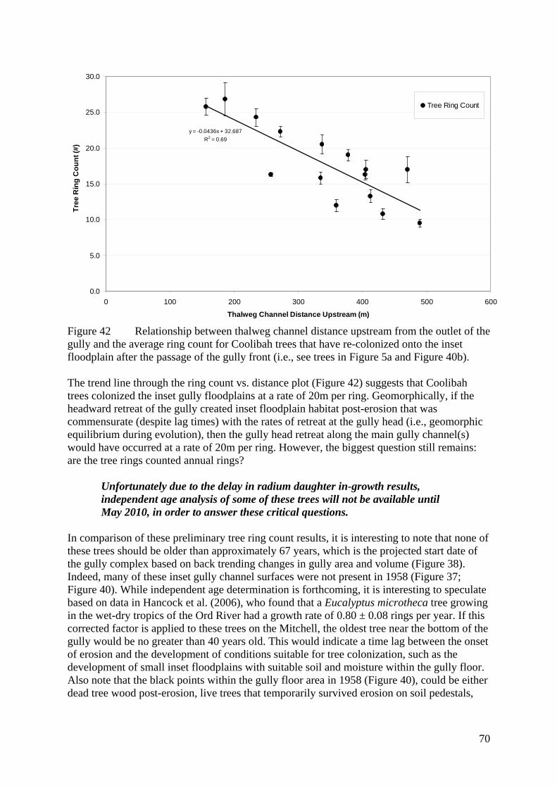
y = -0.0436x + 32.687R2 = 0.69

0.0

5.0

10.0

15.0

20.0

25.0

30.0

0 100 200 300 400 500 600

Thalweg Channel Distance Upstream (m)

Tree

Rin

g C

ount

(#)

Tree Ring Count

Figure 42 Relationship between thalweg channel distance upstream from the outlet of the gully and the average ring count for Coolibah trees that have re-colonized onto the inset floodplain after the passage of the gully front (i.e., see trees in Figure 5a and Figure 40b). The trend line through the ring count vs. distance plot (Figure 42) suggests that Coolibah trees colonized the inset gully floodplains at a rate of 20m per ring. Geomorphically, if the headward retreat of the gully created inset floodplain habitat post-erosion that was commensurate (despite lag times) with the rates of retreat at the gully head (i.e., geomorphic equilibrium during evolution), then the gully head retreat along the main gully channel(s) would have occurred at a rate of 20m per ring. However, the biggest question still remains: are the tree rings counted annual rings?

Unfortunately due to the delay in radium daughter in-growth results, independent age analysis of some of these trees will not be available until May 2010, in order to answer these critical questions.

In comparison of these preliminary tree ring count results, it is interesting to note that none of these trees should be older than approximately 67 years, which is the projected start date of the gully complex based on back trending changes in gully area and volume (Figure 38). Indeed, many of these inset gully channel surfaces were not present in 1958 (Figure 37; Figure 40). While independent age determination is forthcoming, it is interesting to speculate based on data in Hancock et al. (2006), who found that a Eucalyptus microtheca tree growing in the wet-dry tropics of the Ord River had a growth rate of 0.80 ± 0.08 rings per year. If this corrected factor is applied to these trees on the Mitchell, the oldest tree near the bottom of the gully would be no greater than 40 years old. This would indicate a time lag between the onset of erosion and the development of conditions suitable for tree colonization, such as the development of small inset floodplains with suitable soil and moisture within the gully floor. Also note that the black points within the gully floor area in 1958 (Figure 40), could be either dead tree wood post-erosion, live trees that temporarily survived erosion on soil pedestals,

70

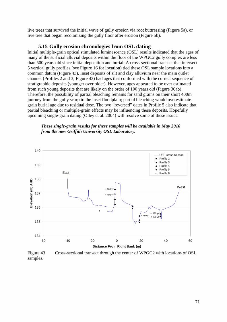
live trees that survived the initial wave of gully erosion via root buttressing (Figure 5a), or live tree that began recolonizing the gully floor after erosion (Figure 5b).

5.15 Gully erosion chronologies from OSL dating Initial multiple-grain optical stimulated luminescence (OSL) results indicated that the ages of many of the surficial alluvial deposits within the floor of the WPGC2 gully complex are less than 500 years old since initial deposition and burial. A cross-sectional transect that intersect 5 vertical gully profiles (see Figure 16 for location) tied these OSL sample locations into a common datum (Figure 43). Inset deposits of silt and clay alluvium near the main outlet channel (Profiles 2 and 3; Figure 43) had ages that conformed with the correct sequence of stratigraphic deposits (younger over older). However, ages appeared to be over estimated from such young deposits that are likely on the order of 100 years old (Figure 30ab). Therefore, the possibility of partial bleaching remains for sand grains on their short 400m journey from the gully scarp to the inset floodplain; partial bleaching would overestimate grain burial age due to residual dose. The two “reversed” dates in Profile 5 also indicate that partial bleaching or multiple-grain effects may be influencing these deposits. Hopefully upcoming single-grain dating (Olley et al. 2004) will resolve some of these issues.

These single-grain results for these samples will be available in May 2010 from the new Griffith University OSL Laboratory.

134

135

136

137

138

139

140

-60 -40 -20 0 20 40 60

Distance From Right Bank (m)

Elev

atio

n (m

) AH

D

OSL Cross-SectionProfile 2Profile 3Profile 4Profile 5Profile 8

< 390 yr< 920 yr< 480 yr

< 560 yr

< 400 yr

East

West

Figure 43 Cross-sectional transect through the center of WPGC2 with locations of OSL samples.

71

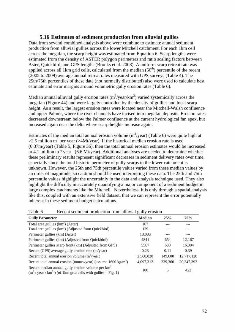
5.16 Estimates of sediment production from alluvial gullies

Data from several combined analysis above were combine to estimate annual sediment production from alluvial gullies across the lower Mitchell catchment. For each 1km cell across the megafan, the scarp height was estimated from Equation 6. Scarp lengths were estimated from the density of ASTER polygon perimeters and ratio scaling factors between Aster, Quickbird, and GPS lengths (Brooks et al. 2008). A uniform scarp retreat rate was applied across all 1km grid cells, calculated from the median (50th) percentile of the recent (2005 to 2009) average annual retreat rates measured with GPS surveys (Table 4). The 25th/75th percentiles of these data (not normally distributed) also were used to calculate best estimate and error margins around volumetric gully erosion rates (Table 6). Median annual alluvial gully erosion rates (m3/year/km2) varied systemically across the megafan (Figure 44) and were largely controlled by the density of gullies and local scarp height. As a result, the largest erosion rates were located near the Mitchell-Walsh confluence and upper Palmer, where the river channels have incised into megafan deposits. Erosion rates decreased downstream below the Palmer confluence at the current hydrological fan apex, but increased again near the delta where scarp heights increase again. Estimates of the median total annual erosion volume (m3/year) (Table 6) were quite high at >2.5 million m3 per year (>4Mt/year). If the historical median erosion rate is used (0.37m/year) (Table 5; Figure 36), then the total annual erosion estimates would be increased to 4.1 million m3/ year (6.6 Mt/year). Additional analyses are needed to determine whether these preliminary results represent significant decreases in sediment delivery rates over time, especially since the total historic perimeter of gully scarps in the lower catchment is unknown. However, the 25th and 75th percentile values varied from these median values by an order of magnitude, so caution should be used interpreting these data. The 25th and 75th percentile values highlight the uncertainly in the data and analysis technique used. They also highlight the difficulty in accurately quantifying a major component of a sediment budget in large complex catchments like the Mitchell. Nevertheless, it is only through a spatial analysis like this, coupled with an extensive field dataset, that we can represent the error potentially inherent in these sediment budget calculations. Table 6 Recent sediment production from alluvial gully erosion Gully Parameter Median 25% 75% Total area gullies (km2) (Aster) 167 --- --- Total area gullies (km2) (Adjusted from Quickbird) 129 --- --- Perimeter gullies (km) (Aster) 13,083 --- --- Perimeter gullies (km) (Adjusted from Quickbird) 4841 654 12,167 Perimeter gullies scarp front (km) (Adjusted from GPS) 5567 680 16,304 Recent (GPS) average gully erosion rate (m/year) 0.23 0.11 0.39 Recent total annual erosion volume (m3/year) 2,560,820 149,600 12,717,120Recent total annual erosion (tonnes/year) (assume 1600 kg/m3) 4,097,312 239,360 20,347,392Recent median annual gully erosion volume per km2 (m3 / year / km2 ) (of 1km grid cells with gullies – Fig. 1) 100 5 422

72

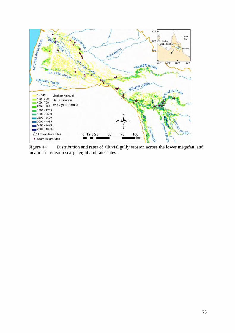
Figure 44 Distribution and rates of alluvial gully erosion across the lower megafan, and location of erosion scarp height and rates sites.

73

6 DISCUSSION 6.1 Large spatial and temporal controls on distribution

From this analysis of alluvial gully distribution across the lower Mitchell catchment and megafan, several primary factors controlling the potential development of alluvial gullies emerge. A prerequisite for the occurrence of alluvial gulling is the initial deposition of alluvium, which in this case, has largely been controlled by the development of the Mitchell megafan from the Pliocene to Holocene. While the Mitchell River traverses what initially appears to be a vast expanse of homogenous alluvium, the actual heterogeneity in depth, width, texture, and chemistry of the deposits strongly influences the potential for alluvial gully development. Silty or loamy duplex soils with alkalinity at depth are most prone to gully erosion, due to their texture, chemistry, and river proximity. Coarse sand deposits within and near the river macro-channel, and clay wetland deposits 10’s of kms away from the main- and palaeo-channels, appear less vulnerable to alluvial gully erosion. The erosional potential of these soils is enhanced by the incision of the Mitchell River into the upper sections of the megafan, which has increased local relative relief, and set up the potential energy needed for a secondary cycle of erosion into the adjacent Pliocene and Pleistocene alluvium. The strong relationships between local relative relief and gully scarp height and gully density support the idea that relief is a primary factor influencing the potential for alluvial gully erosion. The concept of relative relief and erosion potential is also applicable in the Mitchell River delta below the current hydrologic fan apex. Here, alluvial sediments have accumulated both behind and beyond the main Pleistocene chenier ridge. Over the last 6000 years, these sediments have been slightly elevated relative to sea level, due to a decline in regional sea levels (Chappell, 1983; Woodroffe and Chappell, 1993; Woodroffe and Horton, 2005) and/or hydroisostatic warping (uplift) (Rhodes, 1982; Chappell et al., 1982). Thus, in both the upper and lower sections of the Mitchell megafan, local base level (or the adjacent channel) influences potential energy available for gully erosion.

6.2 Rates of Gully Erosion While the long-term evolution of the Mitchell megafan created the potential for alluvial gully erosion, more local factors have influenced whether or not a given area will actually degrade via gully incision. Natural factors such as soil texture and chemistry, grass and tree cover, local slope and topographic irregularities, river and floodplain hydrology, climatic variability, and groundwater flow paths influence the gully initiation potential and the magnitude and direction of gullying once initiated. Initiation points for most alluvial gullies are located at the steepened banks of rivers, smaller creeks, or lagoons, where pre-existing hollows or bank disturbances (natural or anthropogenic) often guide initiation development. While some degree and form of gullying existed pre-European settlement and cattle introduction (Leichhardt 1847; Gilbert 1845; Jardine and Jardine 1867), it appears that this gullying was limited in extent and rate as compared to the current situation. Erosion rate and gully area data from historic air photos documented in this study provides strong evidence for rapidly increasing local extent and regional distribution of alluvial gullies. Most of the raw, bare, and denuded gully landscapes studied here did not exist in 1845, or if they did in part, they were locally steepened hollows without channels near to river banks (i.e., a preexisting form and process). The timing of the onset of this new wave of historic gullies was coincident with the widespread introduction of cattle across the Mitchell megafan, in addition to other

74

changes in fire use and plant species (i.e., weeds) after the widespread removal of Aboriginal land use practices. It is hypothesized that these major land use change associated with European settlement of savannas of Northern Australia pushed the landscape across a threshold towards instability (sensu Schumm 1973), which it was already close to as a result of landscape evolution over geomorphic time. In addition to historical data, this tropical landscape holds a vast quantity of information on erosion rates and processes, which are held as knowledge with the trees, sand grains, and ferricrete and calcrete nodules that are ubiquitous across the landscape. This study used a ‘multiple lines of evidence’ approach to determine current and past rates of gully erosion, building off this natural capital of knowledge. Tree ring and dendrochronology data suggest that these techniques are highly prospective for dating the development of alluvial gullies in northern Australia. In the example provided here, tree ring data coupled with historical air photo data, have been used to elucidate the recent initiation and evolution of an alluvial gully over timescales of less than 60 years. Additional results in the near future should strengthen and refine the uncertainty in these dating tools. The future use of tree ring analysis of Eucalyptus in the wet-dry tropics could be extended to a wide variety of eroded environments and possibly fill in the data gaps present in historical air photos. A vast amount of information also exists in the alluvial stratigraphy of this landscape and the quartz sand grains they contain. The preliminary optical stimulated luminescence (OSL) data from this study suggests that inset deposits in alluvial gullies are quite young (<500 years). Near future use of single-grain techniques should reduce the error in these data, and provide insight into the evolution of gullies closer to the contact period of European settlement. In parallel, while initial analysis of U/Th/Ra/Pb activities in these ferricrete nodules via gamma spectrometry has been disappointing due to secular equilibrium when the nodules are analysed as bulked samples, future research into obtaining sub-samples of nodules in the “closed systems” of nodular cores could be fruitful. This is especially compelling due to the widespread and ubiquitous nature of the duricrusts across the northern Australian landscape, particularly in the floors of eroded gullies. A continued development of a deeper understanding of rates of gully erosion pre- and post-European settlement will be essential to refining past and present human land use impacts and the sensitivity of the landscape to further development.

6.3 Anthropogenic and Climatic Triggers of Gully Erosion It is clear that the long-term evolution of the Mitchell megafan created the template for gully erosion potential (relief, soil chemistry, hydrology etc.). However, the key question is why did the landscape appear to unravel into a gullied wasteland after these alluvial soils remained relatively un-eroded for thousands to a million years (i.e., Grimes and Doutch 1978)? It appears that a geomorphic threshold (sensu Schumm 1973) was crossed at some point in the last several hundred years. But why? The geomorphic literature on gully erosion and channel incision is full of analyses of potential geomorphic, climatic and anthropogenic triggers of landscape instability (e.g., Schumm and Hadley, 1957; Cooke and Reeves, 1976; Graf, 1979; Prosser et al. 1994; Prosser and Slade 1994; Schumm, 1999), with climate change and anthropogenic land use change being the main extrinsic triggers or catalyses to push a landscape past a threshold, beyond intrinsic geomorphic thresholds. Compared to longer-term glacial-interglacial cycles, the monsoonal climate of the Cape York Peninsula has been relatively stable over the last 6000-years following the last glacial

75

maximum (Kershaw 1978; Kershaw and Nanson 1993). While there has undoubtably been decadal fluctuations in climate due to El Niño/Southern Oscillation cycles (e.g., Figure 2), these cycles have been ongoing for thousands of years (McGlone et al. 1992), with no major evidence for landscape unraveling via widespread gullying. At the century time scale, Nott et al. (2007) have calculated the frequency of tropical cyclone occurrences at the Chillagoe caves in the central Mitchell River catchment, by analyzing the ratios of 18O/16O in stalagmites in the limestone caves. Their results indicate that the frequency of cyclones landings was low during the last two-hundred years (Figure 45), when a majority of alluvial gullies initiated (Figure 32; Figure 34; Figure 35). In comparison, there were more frequent cyclone events between 1400 and 1800.

Figure 45 Frequency of tropical cyclone ladings at Chillagoe as determined by the 18O/16O ratios in stalagmites in caves, from Nott et al. 2007. In contrast or concert with climatic variability, the European settlement of Australia and the newly associated land uses post-1800 (i.e., grazing, logging, mining, road development, agriculture, urbanization) have been well documented to have destabilized the Australian landscape and promoted accelerated soil erosion (e.g., Eyles, 1977; Fanning et al., 1999; Olley and Wasson, 2003; Rustomji and Piestch 2007), especially for gully erosion triggered by widespread cattle and sheep grazing, reduced grass cover, and tree clearing (Pickup 1991; Prosser et al. 1994; Prosser and Slade 1994; Prosser and Winchester, 1996; Pringle et al. 2006; Bartley et al., 2007). The initiation of major alluvial gully erosion at the time of introduction of cattle has been observed in other alluvial plains in northern Australia (Condon 1986) and in Western Australia (Pringle et al. 2006). For example in the Victoria River District of the Northern Territory, Condon (1986) observed that

“[alluvial] gullies have been initiated from cattle pads over the high bank in earlier times when there would have been large concentrations of cattle watering on the rivers after the small waterholes in the backcountry had dried up towards the end of the dry season. Once channelized flow had reached the B horizon, the rate of down cutting and side cutting would be very rapid in these highly dispersible clay soils.”

This example of post-European alluvial gully erosion is strikingly similar to the land-use conditions and landforms in the lower Mitchell River documented in this report. Beyond the

76

gullies studied in this report, which were not influenced by roads, hundreds of other examples exist across the Mitchell catchment of road construction- and use-induced alluvial gully erosion. The initiation and continued erosion of alluvial gullies is influenced by a variety of driving and resisting factors, both naturally as reviewed above, but also anthropogenically during the last 200 years in Australia by ever accelerating direct and indirectly human land use change. Since most of the alluvial gully degradation in the lower Mitchell has been initiated after European settlement and cattle introduction (i.e., Figure 32; Figure 34; Figure 35), it is most probable that the additional erosional driving factors accompanying land use change pushed the landscape across a threshold toward instability. However, this is not to say that the other factors influencing gully erosion are also not currently operating or important in the Mitchell, but rather that the destabilizing factors now outweigh the stabilizing factors due to the addition of European-style land use pressures. As an example, the detailed analysis by McKeon et al. (2004) of pasture degradation and soil erosion in Australia’s rangelands emphasizes the combined influence of poor cattle/sheep management and the high variability of Australia’s climate on soil erosion. They emphasize the key lesson learned from history, which is to destock or reduce animal densities before or during drought conditions, especially in sensitive areas such as riparian zones or highly erodible soils, so as to not overwhelm the natural resiliency of both grassland communities and their soil protection properties. While the Mitchell River catchment has a less variable climate than other Australian bioclimates, climate variability still results in wet and dry years and decades, as shown below in Figure 46 of rainfall data from Palmerville Station. The superimposed numbers of cattle stocked on Wrotham Park Station (Figure 46) suggest that historic trends in cattle numbers generally tracked wet decades and dry decades during much of the 20th century. However, recent trends in stocking numbers have become less correlated to climatic trends, perhaps due to recent efforts for pasture improvement via introduced legume species (i.e., Edye and Gillard, 1985; Edye et al. 1991; Arnold 1997; Hall and Walker 2005). Regardless of recent trends, the early 20th century data in Figure 46 suggest that the initial spike in cattle numbers between 1910 and 1920 occurred during and after a substantially wet decade. The data show that cattle numbers remained relatively high for 5+ years into a drought period after this initial spike. It is thus plausible that this drought exacerbated the soil erosion impact of the major European-style land use change and the rapid introduction of tens of thousands of cattle to the lower Mitchell catchment. Other examples of the synergistic effects of poor land management and climatic variability abound in the rangelands of Australia (McKeon et al. 2004).

77

-

500

1,000

1,500

2,000

2,500

1900

1910

1920

1930

1940

1950

1960

1970

1980

1990

2000

2010

Ann

ual R

ainf

all T

otal

(mm

)

-

15,000

30,000

45,000

60,000

75,000W

rotham P

ark Cattle #'s

Palmerville Annual Rainfall (mm)Wrotham Park Aggregation Cattle #'s5 -year Moving Average Rainfall (mm)

1890

1860

1870

1880

Average Annual Rainfall

= 1042mm

Figure 46 1880-2010 history of annual rainfall and 5-year average annual rainfall at Palmerville Station and cattle numbers at Wrotham Park Station, both near the upper part of the Mitchell River megafan.

6.4 Conceptual model of alluvial gullying. From the above discussion, remote sensing and ground observations, a conceptual model is proposed for the evolution of alluvial gullies. A location-time substitution (Huggett, 2004) is utilized to identify different stages of evolution, which builds upon actual knowledge of gully evolution and erosion rates over the historical period. While this type of evolutionary approach can be misleading when heterogeneous landscape factors and processes other than time influence gully development, field observation of gully size and form in relatively uniform alluvial deposits on the same river bank suggests that general insight on evolution can be gained. Two hillshade depictions of LiDAR topography along alluvial channel banks are shown in Figure 47. While these two locations are quite different in terms of river connectivity, relative relief, and scarp height (Figure 10; Figure 11; Figure 12; Figure 47), they generally have similar stages of gully development. It is hypothesized that small incipient gullies on channel banks (1a in Figure 47ab) are the starting point of alluvial gully development. They can begin as rills, bank seepage points, small bank slumps, stock tracks, and roads, which all tend to concentrate both surface and subsurface flow (Dunne 1980; 1990). From their initially shallow channels and ubiquitous presence along steep alluvial banks, it is hypothesized that preferential groundwater flow paths are not requisite for channel initiation. Rather, concentrated overland flow following rainfall or overbank flooding over steep banks is the dominant initial erosion mechanism, which is enhanced or resisted by surface soil condition and vegetative cover. Erosion rate and gully area data from historic air photos documented in this study provides evidence for rapidly increasing local extent and regional distribution of alluvial gullies. While some degree and form of gullying existed pre-European settlement and cattle introduction

78

(Leichhardt 1847; Gilbert 1845), it appears that this gullying was limited in extent and rate as compared to the current situation. It is hypothesized that intense cattle grazing concentrated in the riparian zones, in addition to fire regime modification during the post-European settlement period, decreased vegetation cover along hollows and the steep banks of the rivers. Dense and deep stock tracks leading down to late-season water holes along the river would have also cut into the fragile soil surfaces, exacerbating the initial loss of vegetative grass cover and channelizing overland flow from rain and floodwater. These near bank modifications due to rapid human land use change increased the initiation of alluvial gully erosion, via the incipient stage (1a) (Figure 47). The long-term evolution of the Mitchell megafan created the template for gully erosion potential (relief, soil chemistry, climate, hydrology, etc.), however the shorter-term changes in soil erosion resistance (trails, grass reduction, fire changes) promoted the acceleration of erosion rates, thereby increasing gully density along previously productive riparian areas. Once initiated by surficial processes, alluvial gully erosion appears to become increasingly dominated by subsurface processes in highly dispersible sub-soils, which continue gully development until a new equilibrium drainage network and channel profile is developed. Over time, these incipient gullies (Figure 47, 1a) can develop further as they incise into alluvial banks and cut back into adjacent flat floodplains (Figure 47, 1b and 1c). Their further growth and development highly depends on available surface and subsurface water sources needed for erosion. The depth of gully development and the extent of lateral expansion also depend on the relative depth of dispersive sub-soil units, which is closely correlated with the relative relief. Alluvial gully growth potential can be stalled or truncated from either a reduction of future climatic or hydrologic events to drive erosion, or the development of adjacent gullies that capture available surface or ground water sources. For example, the development of gully stages 1a, 1b, and 1c in Figure 47 have been affected by the growth of adjacent gullies 2a and 2b. Gully development beyond these incipient stages (1a, 1b, and 1c) into larger bounded or unbounded proximal gully stages (2a to 2b) depends on chance, the heterogeneity of alluvial material composition, and the subtle differences in antecedent topography. For example, gully stage 2a in Figure 47a developed into a shallow preexisting depression that likely influenced the success of its development. Over time with further gully catchment development away from the initiation point, these antecedent topographic irregularities become inconspicuous due to erosion (2b in Figure 47). From field observations of these different gully stages (e.g., Figure 14; Figure 18; Figure 29), it is hypothesized that groundwater discharge and seepage erosion become progressively more important components over time, due to deeply incised preferential drainage points and steep hydraulic gradients. However, surface runoff from rainfall and flooding always remain components in drainage basin evolution, but with a less dominant role. The development of proximal bounded alluvial gullies into unbounded proximal alluvial gullies and gully complexes is less clear due to issues of scale and time. However, it is hypothesized that gullies that are initially bound by local alluvial ridges or levees can erode through low, weak, or irregular locations in these linear features (i.e., stages 2 to 3 in Figure 21). This process may be enhanced by extreme flood events and erosion from both sides of an alluvial ridge contributing to breaching. Once an alluvial ridge has been breached, the newly available surface and subsurface water sources strongly control gully complex development. Where large distal flood basins are encountered with previously poor drainage, large gully complexes can form through the erosion of dense channel networks into shallow alluvial

79

depressions (i.e., stages 4 in Figure 21). The evolutionary sequence continues as individual tributaries of distal gully complexes encounter their own development constraints (i.e., stages 5 and 6 in Figure 21).

Figure 47 LiDAR DEM hillshades of alluvial gullies at different stages of evolution. a) The Mitchell River at an upstream distance of 370 km (Figure 10) and floodplain elevation of 160 m (Figure 11). Note the longitudinal profile (MMGC3) in Figure 12 from the same area (black line). b) A lagoon and palaeochannel of the Mitchell River at an upstream distance of 210 km (Figure 10) and floodplain elevation of 85 m (Figure 11). Note the longitudinal profile (HBGC777) in Figure 12 from the same area (black line). Numbered gully labels in figures refer to stages of gully evolution: 1a to 1c are incipient gully stages, 2a and 2b are respectively, bounded and unbounded proximal gully stages.

80

7 CONCLUSIONS From this analysis of alluvial gully distribution, form, erosion rates and processes across the Mitchell River megafan, it is evident that alluvial gullies are a distinct end member along a continuum of gully form-process associations, from colluvial hillslope gullies at one extreme to alluvial gullies at the other. From the review of the international literature, our description of gullies in the lower Mitchell catchment is by no means the first record of alluvial gullies. However to date, similar types of alluvial gullies have simply been considered to be just another variant of generic “gully erosion”. Clearly, a fluvial megafan is not a prerequisite for alluvial gully formation, as alluvial gullies have been described across other Gulf of Carpentaria rivers that lack fluvial megafans (Brooks et al., 2006). It is our view that an understanding of the process initiating and propagating the vast gully networks documented in this study cannot be gained unless they are viewed as a distinct form of gully erosion with a characteristic suite of hydrologic processes and antecedent geomorphic controls (e.g., relative relief), which are a function of the particular climate and evolutionary sequence of the alluvium in which they are situated - in this case, the Mitchell fluvial megafan. However, the diversity in alluvial gully form and erosion process in the Mitchell, as well as across northern Australia and around the world prohibits using any one type example to define and represent their geomorphology. Further regional (Gulf of Carpentaria) and global research is needed to describe the unique varieties of alluvial gullies and document their rates and erosional processes across different landscapes. This research could then be synthesized with the existing but inconsistent international literature on gullies eroding into alluvium, to develop a complete classification system. Tropical savannas in Australia, as in many other parts of the world, have and are experiencing increasing developmental pressure. An improved understanding of alluvial gullying is likely to become increasingly more important if land use and development is to be appropriately managed in these landscapes. Continued research into the role of land use on gully initiation and erosion rates is key to predicting future impacts on these landscapes. At a minimum, future planning scenarios need to address these widespread gullying issues, which to date have not been included in landscape scale planning (e.g., Woinarski et al., 2007). Furthermore, if realistic sediment budget models are to be developed for the catchments in the Australian tropical savanna, it is crucial that alluvial gullying be treated as a separate sediment source to colluvial gullying. The contrast between the two types of gullying is exemplified by the fact that alluvial gullying is located in parts of the catchment that are generally considered and modeled to be sediment sinks (i.e., floodplains), which is clearly not always the case in the Mitchell catchment.

81

8 ACKNOWLEDGEMENTS Funding for this project was provided by Caring for Our Country funding managed by the Northern Gulf NRM Group and Land & Water Australia (GU 005176). This project built off the foundations of research from a previous grant from Land & Water Australia (GRU37). This project would not have been possible without the management efforts of Noeline Gross and Tim Hoogwerf at the Northern Gulf NRM Group. We would like to thank the many people in the Mitchell catchment who have provided us with assistance, in particular Fiona Barron, Deb Eastop, and Brynn Mathews from the Mitchell River Watershed Management Group, and Viv Sinnamon, Colin Lawrence, Paddy Yam, Willy Banjo, and Jim Monaghan from the Kowanyama Aboriginal Land and Natural Resources Management Office. To the dedicated land stewards and graziers on the ground, we greatly appreciate the access to your properties and the time to talk with your families about the beauty and challenges of the lower Mitchell catchment. We would also like to thank Jorg Hacker and Wolfgang Lieff from Airborne Research Australia for their efforts in acquiring and processing airborne data, and Hamish Anderson at Geoscience Australia and Jim Crouch at Defence for orchestrating the supply of the DTED2 SRTM data. Ken Mcmillan and Chris Leslie at CSIRO Canberra provided valuable advice and time toward initial OSL sample processing. Gary Hancock at CSIRO Canberra provided open advice for methods and techniques in radium dating tree rings. Collaboration with Atun Zawadski, Henk Heijnis, Daniela Ferro, Karthigah Shanmugarajah, and Svetislav Videnovic at the Australian Nuclear Science and Technology Organization was essential for determining the radium and thorium activities in trees, as part of supplementary funding from the Australian Institute of Nuclear Science and Engineering managed by Dennis Mather. Additional funding support from the Griffith University Postgraduate Research Scholarship, and the Tropical Rivers and Coastal Knowledge (TRaCK) program (Theme 4: Material Budgets) was also essential for providing a foundation for research support for Jeffrey Shellberg.

82

9 REFERENCES Argent, R.M., McMahon, T.A., Bowler, J.M. and Finlayson, B.L., 2004. The dendroecological potential of

Eucalyptus camaldulensis Dehnhardt (River Red Gum) from the Barmah Forest, Victoria, Australia. Australian Geographical Studies, 42(1): 89-102.

Arnold, G., 1997. Grazier experience with Stylosanthes technology. III. Wrotham Park, 1963-1988. Tropical Grasslands, 31: 522-526.

Bacellar, L.A.P., Coelho Netto, A.L. and Lacerda, W.A., 2005. Controlling factors of gullying in the Maracujá Catchment, southeastern Brazil. Earth Surface Processes and Landforms, 30(11): 1369-1385.

Bartley, R., Hawdon, A., Post, D.A. and Roth, C.H., 2007. A sediment budget for a grazed semi-arid catchment in the Burdekin basin, Australia. Geomorphology, 87: 302-321.

Basinski, J.J., Wood, I.M. and Hacker, J.B., 1985. The Northern Challenge. A History of CSIRO Crop Research in Northern Australia. Commonwealth Scientific and Industrial Research Organisation (CSIRO) Division of Tropical Crops and Pastures, Research Report No. 3, Canberra, Australia.

Bauer, F.H., 1978. Cropping in Northern Australia: Anatomy of Success and Failure. Australian National University, North Australia Research Unit, 25-27 August 1977, Darwin NT., Canberra, 267 pp.

Beavis, S.G., 2000. Structural controls on the orientation of erosion gullies in mid-western New South Wales, Australia. Geomorphology, 33(1-2): 59-72.

Brice, J.C., 1966. Erosion and Deposition in the Loess-Mantled Great Plains, Medicine Creek Drainage Basin, Nebraska. U.S. Geological Survey, Professional Paper 352-H, Reston, Virginia.

Brooks, A., Knight, J. and Spencer, J., 2006. A Remote Sensing Approach for Mapping and Classifying Riparian Gully Erosion in Tropical Australia. Australian Rivers Institute, Griffith University, Nathan, Qld, Australia, Report to Land and Water Australia, Project No – GRU37

Brooks, A., Spencer, J. and Knight, J., 2007. Alluvial gully erosion in Australia’s tropical rivers: a conceptual model as a basis for a remote sensing mapping procedure. In: A.L. Wilson et al. (Editors), Proceedings of the 5th Australian Stream Management Conference, pp. 43-48.

Brooks, A.P., Spencer, J., Shellberg, J.G., Knight, J., and Lymburner, L., 2008. Using remote sensing to quantify sediment budget components in a large tropical river - Mitchell River, Gulf of Carpentaria, Sediment Dynamics in Changing Environments (Proceedings of a symposium held in Christchurch, New Zealand, December 2008). IAHS Publ. 325, pp. 225 - 236.

Brooks, A.P., Shellberg, J.G., Spencer, J. and Knight, J., 2009. Alluvial gully erosion: an example from the Mitchell fluvial megafan, Queensland, Australia Earth Surface Processes and Landforms 34: 1951-1969.

Bryan, R.B. and Jones, J.A.A., 1997. The significance of soil piping processes: inventory and prospect. Geomorphology, 20(3-4): 209-218.

Bryan and Yair, 1982. Perspectives on studies of badland geomorphology. In: R. Bryan and A. Yair, Editors, Badland Geomorphology and Piping, GeoBooks, Norwich , pp. 1–12.

Bureau of Meteorology (BOM) http://www.bom.gov.au/climate/averages/tables/ca_qld_names.shtml Bureau of Rural Sciences (BRS) 1991. Digital Atlas of Australian Soils (ARC/INFO® Vector Format).

Originally compiled by K.H. Northcote et al. published in 1960 - 68 by the Commonwealth Scientific and Industrial Research Organisation (CSIRO) and Melbourne University Press known as the 'Atlas of Australian Soils', Melbourne.

Bureau of Statistics (BoS) 2008. 7124.0- Historical Selected Agriculture Commodities, by State (1861 to Present) Total cattle numbers. Australian Bureau of Statistics.

Camkin, J.K., Kellett, B.M. and Bristow, K.L., 2007. Northern Australia Irrigation Futures: Origin, Evolution and Future Directions for the Development of a Sustainability Framework. Cooperative Research Center (CRC) for Irrigation Futures, Technical Report No. 11/07; Commonwealth Scientific and Industrial Research Organisation (CSIRO Land and Water Science, Report 73/07, Wembley, Western Australia, 48 pp.

Cantelli, A., Paola, C. and Parker, G., 2003. Experiments on upstream-migrating erosional narrowing and widening of an incisional channel caused by dam removal. Water Resources Research, W03304.

Chapman, A.L., Sturtz, J.D., Cogle, A.L., Mollah, W.S. and Bateman, R.J., 1996. Farming systems in the Australian semi-arid tropics: a recent history. Australian Journal of Experimental Agriculture, 36: 915-928.

Chappell, J., Rhodes, E.G., Thom, B.G. and Wolanski, E., 1982. Hydro-isostasy and the sea-level isobase of 5500 Bp in North Queensland, Australia. Marine Geology, 49(1-2): 81-90.

Chappell, J., 1983. Evidence for smoothly falling sea-level relative to north Queensland, Australia, during the

83

past 6,000 yr. Nature, 302(5907): 406-408. Chisholm, A.H., 1940. The Story of John Gilbert. Emu, 39(3): 156-76. Condon, R.W., 1986. A Reconnaissance Erosion Survey of part of the Victoria River District, N.T., Hassall &

Associates, Canberra. Cooke, R.U. and Reeves, R., 1976. Arroyos and Environmental Change in the American South-West. Clarendon

Press, London. Crowley, G.M. and Garnett, S.T., 1998. Vegetation change in the grasslands and grassy woodlands of east-

central Cape York Peninsula, Australia. Pacific Conservation Biology, 4(2): 132-148. Crowley, G.M. and Garnett, S.T., 2000. Changing fire management in the pastoral lands of Cape York

Peninsula of Northeast Australia, 1623 to 1996. Australian Geographical Studies, 38(1): 10-26. CSIRO, 2009. Water in the Gulf of Carpentaria Drainage Division. A report to the Australian Government from

the CSIRO Northern Australia Sustainable Yields Project. Commonwealth Scientific and Industrial Research Organisation (CSIRO) Water for a Healthy Country Flagship, Australia, 479pp pp.

Davidson, B.R., 1965. The Northern Myth: A Study of the Physical and Economic Limits to Agricultural and Pastoral Development in Tropical Australia. Melbourne University Press, 1st ed., Carlton, Victoria, 283 pp.

Davidson, B.R., 1969. Australia Wet or Dry? The Physical and Economic Limits to the Expansion of Irrigation. Melbourne University Press, 264 pp.

De Vries, J.J., 1976. The groundwater outcrop-erosion model; evolution of the stream network in the Netherlands. Journal of Hydrology, 29(1/2): 43-50.

Downes, G.B., C.; Worledge, D., 1999. Daily stem growth patterns in irrigated Eucalyptus globulus and E. nitens in relation to climate. Trees, 14: 102-111.

Dunne, T. and Black, R.D., 1970. Partial area contributions to storm runoff in a small New England watershed. Water Resources Research, 6(5): 1296-1311.

Dunne, T., 1980. Formation and controls of channel networks, Progress in Physical Geography, pp. 211-239. Dunne, T., 1990. Hydrology, mechanics, and geomorphic implications of erosion by subsurface flow,

Groundwater Geomorphology. Geological Society of America Special Paper, pp. 1-28. Edye, L.A. and Gillard, P., 1985. Pasture improvement in semi-ard tropical savannas: a practical example in

northern Queensland. In: J.C. Tothill and J.J. Mott (Editors), Ecology and Management of the World's Savannas. Australian Academy of Science, Canberra, ACT, pp. 303-309.

Eyles, R.J., 1977. Changes in drainage networks since 1820, Southern Tablelands, N.S.W. Australian Geographer, 13: 377-386.

Fanning, P. C. 1999. Recent landscape history in arid western New South Wales, Australia: a model for regional change. Geomorphology 29(3-4): 191-209.

Fensham, R.J., 1997. Aboriginal fire regimes in Queensland, Australia: Analysis of the explorers' record. Journal of Biogeography, 24(1): 11-22.

Fensham, R.J., 2008. Leichhardt's maps: 100 Years of change in vegetation structure in inland Queensland. Journal of Biogeography, 35(1): 141-156.

Fryirs, K. and Brierley, G.J., 1998. The character and age structure of valley fills in upper Wolumla Creek, South Coast, New South Wales, Australia. Earth Surface Processes and Landforms, 23: 271-287.

Galay, V.J., 1983. Causes of river bed degradation. Water Resources Research, 19(5): 1057-1090. Gallart, F., Sole, A., Puigdefabregas, J. and Lazaro, R., 2002. Badland systems in the Mediterranean. In: L.J.

Bull and M.J. Kirkby (Editors), Dryland Rivers: Hydrology and Geomorphology of Semi-Arid Channels. Wiley, pp. 299-326.

Gartner, H., 2007. Tree roots - Methodological review and new development in dating and quantifying erosive processes. Geomorphology, 86(3-4): 243-251.

Ghassemi, F. and White, I., 2007. Inter-Basin Water Transfer: Case Studies from Australia, United States, Canada, China, and India. Cambridge University Press, International Hydrology Series, 435 pp.

Gilbert, J., 1845. Diary of the Port Essington Expedition, 18 Sept. 1844 - 28 June 1845. Mitchell Library: State Library of New South Wales, 226 pp.

Gillard, P., Edye, L.A. and Hall, R.L., 1980. Comparison of Stylosanthes humilis with S. hamata and S. subsericea in the Queensland Dry Tropics: effects on pasture composition and cattle liveweight gain. Australian Journal of Agricultural Research, 31: 205-220.

Goudie, A.S., 1973. Duricrusts in Tropical and Subtropical Landscapes. Clarendon Press, Oxford. Goudie, A.S., 1984. Duricrusts and landforms. In: K.S. Richards, R.R. Arnett and S. Ellis (Editors),

Geomorphology and Soils. George Allen, in association with the British Geomorphological Research Group, London, pp. 37-57.

Graf, W.L., 1977. The rate law in fluvial geomorphology. American Journal of Science, 277: 178-91. Graf, W.L., 1979. The development of montane arroyos and gullies. Earth Surface Processes, 4: 1-14. Graf, W.L., 1983. The arroyo problem - palaeohydrology and palaeohydraulics in the short term. In: K.J.

84

Gregory (Editor), Background to Palaeohydrology: A Perspective. John Wiley and Sons Ltd., Chichester, pp. 279-302.

Grimes, K.G. and Doutch, H.F., 1978. The late Cainozoic evolution of the Carpenteria Plains, Northern Queensland. BMR Journal of Australian Geology and Geophysics, 3: 101-112.

Hall, T.J. and Walker, R.W., 2005. Pasture legume adaptation to six environments of the seasonally dry tropics of north Queensland. Tropical Grasslands, 39: 182-196.

Hancock, G.R. and Evans, K.G., 2006. Gully position, characteristics and geomorphic thresholds in an undisturbed catchment in Northern Australia. Hydrological Processes, 20(14): 2935-2951.

Hancock, G. J., A. S. Murray, G. J. Brunskill, and R. M. Argent 2006. Ra isotopes in trees: Their application to the estimation of heartwood growth rates and tree ages. Global Biogeochemical Cycles, 20, GB4007.

Harvey, A.M, 2004. Badland. In: A. Goudie (Editor), Encyclopedia of Geomorphology, Volumes 1 and 2. Routledge, London, pp. 45-48.

Harvey, A.M., 1992. Process interactions, temporal scales and the development of hillslope gully systems - Howgill Fells, Northwest England. Geomorphology, 5(3-5): 323-344.

Hayden, B.P., 1988. Flood climates. In: V.R. Baker and et al. (Editors), Flood Geomorphology. Wiley-Interscience, pp. 13-26.

Heap, A.D., Bryce, S., Ryan, D., Radke, L., Smith, C., Smith, R., Harris, P. and Heggie, D., 2001. Australian Estuaries and Coastal Waterways: A Geoscience Perspective for Improved Integrated Resource Management. Record 2001/07., Australian Geological Survey Organisation, Canberra ACT.

Higgins, G.C., 1982. Drainage systems developed by sapping on Earth and Mars. Geology, 10: 147-152. Horton, B.K. and Decelles, P.G., 2001. Modern and ancient fluvial megafans in the foreland basin system of the

Central Andes, Southern Bolivia: Implications for drainage network evolution if foldthrust belts. Basin Research, 13(1): 43-63.

Horton, R.E., 1933. The role of infiltration in the hydrologic cycle. EOS, Transactions, American Geophysical Union, 14: 446-460.

Huggett, R., 2004. Ergodic hypothesis. In: A. Goudie (Editor), Encyclopedia of Geomorphology. Routledge, London, pp. 327-329.

Jack, R.L., 1915. The Exploration of Cape York Peninsula, 1606-1915. The Australian Historical Society, Journal and Proceedings, 3(5): 1-28. (Read before the Society, Nov. 30, 1915). Available online from the Project Gutenberg Australia, http://gutenberg.net.au

Jardine, F. and Jardine, A., 1867. Narrative of the overland expedition of the Messrs. Jardine, from Rockhampton to Cape York, Northern Queensland, 1864-1865. Compiled from the journals of the brothers, and edited by Frederick J. Byerley (engineer of roads, northern division of Queensland). J.W. Buxton Publisher, Brisbane. Available at www.gutenberg.net

Kennedy, B.A., 2001. Charles Lyell and 'Modern changes of the Earth': the Milledgeville Gully. Geomorphology, 40(1-2): 91-98.

Kershaw, A.P., 1978. Record of last interglacial cycle from northeast Queensland. Nature, 272: 159-61. Kershaw, A.P. and Nanson, G.C., 1993. The last full glacial cycle in the Australian region. Global and Planetary

Change, 7: 1-9. Kheir, R.B., Cerdan, O. and Abdallah, C., 2006. Regional soil erosion risk mapping in Lebanon.

Geomorphology, 82(3-4): 347-359. Kirkby, M., 1988. Hillslope runoff processes and models. Journal of Hydrology, 100: 315-339. Kirkby, M.J. and Chorley, R.J., 1967. Throughflow, overland flow and erosion. Bulletin of the International

Association of Scientific Hydrology, 12(3): 5-21. Knapen, A., Poesen, J., Govers, G., Gyssels, G. and Nachtergaele, J., 2007. Resistance of soils to concentrated

flow erosion: a review. Earth-Science Reviews, 80(1-2): 75-109. Knight, J., Spencer, J., Brooks, A. and Phinn, S., 2007. Large area, high-resolution remote sensing based

mapping of alluvial gully erosion in Australia’s tropical rivers. In: A.L. Wilson et al. (Editors), Proceedings of the 5th Australian Stream Management Conference, pp. 199-204.

Leal, S.P., H.; Grabner, M.; Wimmer, R., 2004. Tree ring structure and climate effects in young Eucalyptus globulus labill. grown at two Portuguese sites: preliminary results. Dendrochronologia, 21(3): 139-146.

Leichhardt, L., 1847. Journal of an Overland Expedition in Australia: from Moreton Bay to Port Essington, a distance of upwards of 3000 miles, during the years 1844-1845. T&W Boone, London, 544 pp.

Leier, A.L., Decelles, P.G. and Pelletier, J.D., 2005. Mountains, monsoons, and megafans. Geology, 33(4): 289-292.

Li, Y., Zhang, J.H., Poesen, J., Yang, J.C. and Fu, B., 2003. Evaluating gully erosion using 137Cs and 210Pb/137Cs ratio in a reservoir catchment. Soil and Tillage Research, 69(1-2): 107-115.

Martin, P. and Hancock, G.J., 1992. Routine analysis of naturally occurring radionuclides in environmental samples by alpha-particle spectrometry. Research Report No. 7, Supervising Scientist for the Alligator Rivers Region. Gov. Pub. Serv., Canberra, ACT, Australia.

85

McDonald, G.T. and Dawson, S.J., 2004. Northern Gulf Region, Natural Resource Management Plan. Tropical Savannas CRC and NGRMG Ltd, Georgetown, Queensland, Australia.

McGlone, M.S., Kershaw, A.P. and Markgraf, V., 1992. El Niño/Southern Oscillation climatic variability in Australasian and South American paleoenvironmental records. In: J.F. Diaz and V. Markgraf (Editors), El Niño. Historical and Paleoclimatic Aspects of the Southern Oscillation. Cambridge University Press, Cambridge and New York, pp. 435-62.

McFarlane, M.J., 1976. Laterites and Landscape. Academic Press, London. McFarlane, M.J., 1991. Some sedimentary aspects of lateritic weathering profile development in the major

bioclimatic zones of tropical Africa. Journal of African Earth Sciences, 12(1-2): 267-282. McKeon, G., Hall, W., Henry, B., Stone, G. and Watson, I., 2004. Pasture degradation and recovery in

Australia's rangelands: learning from history. Queensland Dept. of Natural Resources, Mines and Energy, Indooroopilly, Qld., 256 pp.

Mertes, L.A.K., 1997. Documentation and significance of the perirheic zone on inundated floodplains. Water Resources Research, 33(7): 1749-1762.

Montgomery, D.R. and Dietrich, W.E., 1988. Where do channels begin? Nature, 336: 232-234. Montgomery, D.R. and Dietrich, W.E., 1989. Source areas, drainage density, and channel initiation. Water

Resources Research, 25(8): 1907-1918. Mott, J.J., Williams, J., Andrew, M.H. and Gillison, A.N., 1985. Australian savannas ecosystems. In: J.C.

Tothill and J.J. Mott (Editors), Ecology and Management of the World's Savannas. Australian Academy of Science, Canberra, ACT, pp. 56-82.

Mucha, S.B., 1979. Estimation of tree ages from growth rings of Eucalyptus in northern Australia. Australian Forestry 42: 13-16.

Nanson, G.C., Price, D.M. and Short, S.A., 1992. Wetting and drying of Australia over the past 300 ka. Geology, 20: 791-4.

Neldner, V.J., Fensham, R.J., Clarkson, J.R. and Stanton, J.P., 1997. The natural grasslands of Cape York Peninsula, Australia: description, distribution and conservation status. Biological Conservation, 81(1-2): 121-136.

Nix, H.A., 1973. Land use planning for comercial agriculture, Proceedings of a symposium on land use planning in north Queensland. Australian Institute of Agricultural Science, Innisfail, Qld, Australia, 28th April, 1973.

Nott, J., Haig, J., Neil, H. and Gillieson, D., 2007. Greater frequency variability of landfalling tropical cyclones at centennial compared to seasonal and decadal scales. Earth and Planetary Science Letters, 255(3-4): 367-372.

Ogden, J., 1978. On the dendrochronological potential of Australian trees. Australian Journal of Ecology, 3: 339-356.

Ogden, J., 1981. Dendrochronological studies and the determination of tree ages in the Australian tropics. Journal of Biogeography, 8: 405-20.

Olley, J.M., Murray, A.S., Mackenzie, D.H. and Edwards, K., 1993. Identifying sediment sources in a gullied catchment using natural and anthropogenic radioactivity. Water Resources Research, 29(4): 1037-1043.

Olley, J.M., Caitcheon, G.G., Hancock, G. and Wallbrink, P.J., 2001. Tracing and Dating Techniques for Sediment and Associated Substances. CSIRO Land and Water, Canberra, Australia.

Olley, J. M. and R. J. Wasson., 2003. Changes in the flux of sediment in the Upper Murrumbidgee catchment, Southeastern Australia, since European settlement. Hydrological Processes 17(16): 3307-3320.

Olley, J.M., Pietsch, T. and Roberts, R.G., 2004. Optical dating of Holocene sediments from a variety of geomorphic setting using single grains of quartz. Geomorphology, 60: 337-358.

Oostwoud Wijdenes, D. and Bryan, R., 2001. Gully-head erosion processes on a semi-arid valley floor in Kenya: A case study into temporal variation and sediment budgeting. Earth Surface Processes and Landforms, 26(9): 911-933.

Pain, C.F. and Ollier, C.D., 1992. Ferricrete in Cape York Peninsula, Northern Queensland. BMR Journal of Australian Geology and Geophysics, 13: 207-212.

Pearson, S.G. and Searson, M.J., 2002. High-resolution data from Australian trees. Australian Journal of Botany, 50(4): 431-439.

Petheram, C., McMahon, T.A. and Peel, M.C., 2008. Flow characteristics of rivers in northern Australia: implications for development. Journal of Hydrology, doi: 10.1016/j.jhydrol.2008.05.008.

Pickup, G., 1985. The erosion cell: a geomorphic approach to landscape classification in range assessment. Australian Rangeland Journal, 7(2): 114-121.

Pickup, G., 1991. Event frequency and landscape stability on the floodplain systems of arid Central Australia. Quaternary Science Reviews, 10: 463-473.

Poesen, J., 1993 Gully typology and gully control measures in the European loess belt. In: S. Wicherek (Editor), Farm Land Erosion in Temperate Plains Environment and Hills Elsevier Amsterdam (Netherlands),

86

International Symposium on Farm Land Erosion. Paris (France), 25-29 May 1992, pp. 221-239. Poesen, J., Valentin, C., Nachtergaele, J. and Verstraeten, G., 2003. Gully erosion and environmental change:

importance and research needs. Catena, 50(2-4): 91-133. Poesen, J.W.A. and Hooke, J.M., 1997. Erosion, flooding and channel management in Mediterranean

environments of southern Europe. Progress in Physical Geography, 21(2): 157-199. Pringle, H.J.R., Watson, I.W. and Tinley, K.L., 2006. Landscape improvement, or ongoing degradation -

reconciling apparent contradictions from the rangelands of Western Australia. Landscape Ecology, 21(8): 1267-1279.

Prosser, I.P. and Abernethy, B., 1996. Predicting the topographic limits to a gully network using a digital terrain model and process thresholds. Water Resources Research, 32(7): 2289-2298.

Prosser, I.P., Chappell, J. and Gillespie, R., 1994. Holocene valley aggradation and gully erosion in headwater catchments, south-eastern highlands of Australia. Earth Surface Processes and Landforms, 19: 465-480.

Prosser, I.P., Rustomji, P., Young, W.J., Moran, C.J. and Hughes, A.O., 2001. Constructing River Basin Sediment Budgets for the National Land and Water Resources Audit. CSIRO Land and Water, Technical Report 15/01.

Prosser, I.P. and Slade, C.J., 1994. Gully formation and the role of valley-floor vegetation, southeastern Australia. Geology, 22(12): 1127-1130.

Prosser, I.P. and Winchester, S.J., 1996. History and processes of gully initiation and development in eastern Australia. Zeitschrift fur Geomorpholigie, Suppl Bnd 105: 91 - 109.

Queensland Department of Natural Resources and Water (QDNRW), 2008. http://www.nrw.qld.gov.au/watershed/

Rhodes, E.G., 1982. Depositional model for a chenier plain, Gulf of Carpentaria, Australia. Sedimentology, 29(2): 201-221.

Robinson, I.B. and Sing, N.C., 1975. Estimated profitability of investment in legume pasture development in far north Queensland. Tropical Grasslands, 9(3): 199-207.

Rustomji, P., 2006. Analysis of gully dimensions and sediment texture from southeast Australia for catchment sediment budgeting. Catena, 67(2): 119-127.

Rustomji, P. and Pietsch, T., 2007. Alluvial sedimentation rates from southeastern Australia indicate post-European settlement landscape recovery. Geomorpholgy, 90: 73-90.

Rustomji, P., Caitcheon, G. and Hairsine, P., 2008. Combining a spatial model with geochemical tracers and river station data to construct a catchment sediment budget. Water Resources Research, 44(1): 16.

Schumm, S.A., 1973. Geomorphic thresholds and complex response of drainage systems. In: M. Morisawa (Editor), Fluvial Geomorphology. Allen and Unwin, London, pp. 299-310.

Schumm, S.A., 1999. Causes and controls of channel incision, Incised River Channels. John Wiley & Sons Ltd., pp. 19-33.

Schumm, S.A. and Hadley, R.F., 1957. Arroyos and the semiarid cycle of erosion. American Journal of Science, 255: 161-74.

Sharma, H.S., 1982. Morphology of ravines of the Morel Basin Rajasthan (India). In: H.S. Sharma (Editor), Perspectives in geomorphology. Naurang Rai Concept Publishing Company, New Delhi, pp. 35-47.

Sharma, H.S., 1987. Morphology and origin of ravines. In: H.S. Sharma (Editor), Tropical geomorphology: a morphogenetic study of Rajasthan. Naurang Rai Concept Publishing Company, New Delhi, pp. 229-251.

Shaw, K.A. and Tincknell, I.W., 1993. Tropical pasture establishment: producer establishment practices and experiences in north Queensland. Tropical Grasslands, 27: 367-372.

Simon, A. and Rinaldi, M., 2006. Disturbance, stream incision, and channel evolution: The roles of excess transport capacity and boundary materials in controlling channel response. Geomorpholgy, 79: 361-383.

Singh, B.V. and Singh, A., 1982. Isostatic readjustments and their rejuvenation. In: H.S. Sharma (Editor), Perspectives in geomorphology. Naurang Rai Concept Publishing Company, New Delhi, pp. 145-164.

Singh, S. and Agnihotri, S.P., 1987. Rill and gully erosion in the subhumid tropical riverine environment of Teonthar Tansil, Madhya Pradesh, India. Geografiska Annaler, 69A: 227-236.

SRTM DTED2, 2000. Shuttle Radar Topography Mission, Digital Terrain Elevation Data Level 2. Australian Government, Defence Imagery and Geospatial Organisation

Smith, R.M., WK; Meyer, WS; Barrs, HD, 1983. Irrigation in Australia: development and prospects. Advances in Irrigation, 2: 99-153.

Stanford, J.A., Lorang, M.S. and Hauer, F.R., 2005. The shifting habitat mosaic of river ecosystems. Verh. Internat. Verein. Limnol.: 1-14.

Stewart, B.J., 1993. The hydrology and water resources of humid northern Australia and Papua New Guinea. In: M. Bonell, M.M. Hufschmidt and J.S. Gladwell (Editors), Hydrology and Water Management in the Humid Tropics: Hydrological Research Issues and Strategies for Water Management. Cambridge

87

88

University Press: International Hydrology Series, pp. 67-83. Tooth, S. and Nanson, G.C., 1995. The geomorphology of Australia's fluvial system: retrospect, perspective and

prospect. Progress in Physical Geography, 19(1): 35-60. Tothill, J.C., Nix, H.A., Stanton, J.P. and Russell, M.J., 1985. Land use and productive potentials of Australian

savanna lands. In: J.C. Tothill and J.J. Mott (Editors), Ecology and Management of the World's Savannas. Australian Academy of Science, Canberra, ACT, pp. 125-141.

Valentin, C., Poesen, J. and Li, Y., 2005. Gully erosion: Impacts, factors and control. Catena, 63(2-3): 132-153. van Niekerk, A.W., Heritage, G.L., Broadhurst, L.W. and Moon, B.P., 1999. Bedrock anastomosing channel

systems: morphology and dynamics in the Sabie River, Mpumalanga Province, South Africa. In: A.J. Miller and A. Gupta (Editors), Varieties Fluvial Form. John Wiley & Sons, Chichester, U.K., pp. 33-51.

Vandekerckhove, L., Poesen, J., Oostwound Wijdenes, D., Gyssels, G., Beuselinck, L. and de Luna, E. 2000. Characteristics and controlling factors of bank gullies in two semi-arid Mediterranean environments. Geomorphology, 33(1-2): 37-58.

Vandekerckhove, L., De Weerdt, B., Coppé, N., Muys, B. and Poesen, J., 2001. A method for dendrochronological assessment of medium-term gully erosion rates. Catena, 45(2): 123-161.

Vos, I.M.A., Bierlein, F.P., Barlow, M.A. and Betts, P.G., 2006. Resolving the nature and geometry of major fault systems from geophysical and structural analysis: the Palmerville Fault in NE Queensland, Australia. Journal of Structural Geology, 28(11): 2097-2108.

Walling, D.E., 1983. The sediment delivery problem. Journal of hydrology, 65: 209-237. Wasson, R.J., Quade, J., Caitcheon, G., Murray, A.S. and McCulloch, M., 2002. Sourcing sediment using

multiple tracers in the catchment of Lake Argyle, Northwestern Australia. Environmental Management, 29(5): 634-646.

Wells, N.A., 2004. Gully. In: A. Goudie (Editor), Encyclopedia of Geomorphology, Volumes 1 and 2. Routledge, London, pp. 503-506.

Whitaker, A.J. et al., 2006. Surface Geology of Australia 1:1,000,000 Scale, Eastern States [Digital Dataset]. The Commonwealth of Australia, Geoscience Australia. http://www.ga.gov.au, Canberra.

Wilkinson, B.H. and Mcelroy, B.J., 2007. The impact of humans on continental erosion and sedimentation. Geological Society of America Bulletin, 119(1-2): 140-156.

Woinarski, J. and Dawson, F., 1997. Limitless lands and limited knowledge: coping with uncertainty and ignorance in northern Australia. In: T.W. Norton, J.W. Handmer and S.R. Dovers (Editors), Ecology, Uncertainty and Policy: Managing Ecosystems for Sustainability. Prentice-Hall, pp. 83-115.

Woinarski, J., Mackey, B., Nix, H. and Traill, B., 2007. The Nature of Northern Australia: Its Natural Values, Ecological Processes and Future Prospects. Australian National University Press, Canberra.

Woodroffe, C.D. and Chappell, J., 1993. Holocene emergence and evolution of the McArthur River Delta, southwestern Gulf of Carpentaria, Australia. Sedimentary Geology, 83(3-4): 303-317.

Woodroffe, S.A. and Horton, B.P., 2005. Holocene sea-level changes in the Indo-Pacific. Journal of Asian Earth Sciences, 25(1): 29-43.

Yeates, S.J., 2001. Cotton Research and Development Issues in Northern Australia: A Review and Scoping Study. Cotton Catchment Communities CRC (Cooperative Research Center) and CSIRO (Commonwealth Scientific and Industrial Research Organisation) Plant Industry. Darwin, Northern Territory, Australia, 65 pp. Accessed on 15 June 2008 at: http://cotton.pi.csiro.au/content/industry/publications/northernproduction/northernaustraliascopingstudy.aspx