Analysis of Radioactivity in the

Chernobyl Exclusion Zone Domestic

Canine Population

An Interactive Qualifying Project Report

Submitted to the Faculty

of the

WORCESTER POLYTECHNIC INSTITUTE

by

Taylor Trottier

Date: 2 March, 2017

Submitted to:

Professor Germano Iannacchione

Dr. Marco Kaltofen

Professor David Medich

Professor Izabela Stroe

Abstract

A significant number of domesticated dogs were left to fend for themselves during the

evacuations following the Chernobyl nuclear disaster. In the years following the disaster,

enchroachment of wildlife has pushed the descendents of these dogs towards areas of hu-

man activity in and around the nuclear reactors outside of Pripyat. These dogs pose a

threat to workers as bites from rabid dogs can prove deadly. Along with human danger

and the impending closing of the sarcophagus around Reactor 4, the elimination of most

human activity in the area creates the imperative for a solution to the dog problem of

Chernobyl. Without intervention, they will breed with or be eaten by local predators cre-

ating environmental stress and altering the local biosphere. The mass elimination of these

dogs is suboptimal due to the poor optics of such a campaign. The Clean Futures Fund has

come to aid in the far more humane process of spaying and neutering the dogs and hopes

to potentially be able to remove them from the effected areas. Our research utilized a lim-

ited number of fecal and hair samples in an attempt to estimate the radioactivity of these

dogs and provide a decontamination scheme that would allow for their removal from the

exclusion zone. While limited in certainty due to collection issues, low sample counts, and

convenience bias, this paper is an effort to provide a first order estimation of a quarantine

process such that the Ukrainian government would allow these dogs to be adopted into

loving homes.

Contents1. Background 8

1. Radiation and Radioactivity . . . . . . . . . . . . . . . . . . . . . . . . . . . 81.1. Radioactivity . . . . . . . . . . . . . . . . . . . . . . . . . . . . . . . 81.2. Gamma Radiation . . . . . . . . . . . . . . . . . . . . . . . . . . . . 9

2. The Chernobyl Disaster . . . . . . . . . . . . . . . . . . . . . . . . . . . . . . 112.1. How did the Chernobyl Accident Happen? . . . . . . . . . . . . . . . 112.2. The Aftermath of the accident . . . . . . . . . . . . . . . . . . . . . . 112.3. Wildlife Effects . . . . . . . . . . . . . . . . . . . . . . . . . . . . . . 12

3. The Dogs of Chernobyl . . . . . . . . . . . . . . . . . . . . . . . . . . . . . . 14

2. Methods 171. Collection of Samples . . . . . . . . . . . . . . . . . . . . . . . . . . . . . . 172. Preparation of Samples . . . . . . . . . . . . . . . . . . . . . . . . . . . . . . 173. Radiation Detection and Measurement . . . . . . . . . . . . . . . . . . . . . 20

3.1. NaI(Tl) Scintillator Detector Mode of Operation . . . . . . . . . . . . 203.2. Detector Calibration . . . . . . . . . . . . . . . . . . . . . . . . . . . 213.3. Specific Hardware . . . . . . . . . . . . . . . . . . . . . . . . . . . . 23

3. Analysis 251. A Note on Statistical Analysis . . . . . . . . . . . . . . . . . . . . . . . . . . 252. Background Removal . . . . . . . . . . . . . . . . . . . . . . . . . . . . . . . 253. Peak Detection . . . . . . . . . . . . . . . . . . . . . . . . . . . . . . . . . . 264. Activity Found From Hair . . . . . . . . . . . . . . . . . . . . . . . . . . . . 275. Activity Detected From Feces . . . . . . . . . . . . . . . . . . . . . . . . . . 276. Decontamination and Quarantine . . . . . . . . . . . . . . . . . . . . . . . . 28

6.1. Acceptable Levels of Exposure . . . . . . . . . . . . . . . . . . . . . . 286.2. Cesium Lifetime in Dogs . . . . . . . . . . . . . . . . . . . . . . . . . 286.3. Time to Negligible Cesium Exposure . . . . . . . . . . . . . . . . . . 29

4. Conclusion 31

Appendices 32

A. Scan Data 331. Fecal Scan Mass . . . . . . . . . . . . . . . . . . . . . . . . . . . . . . . . . . 332. Fecal Scan Peak Data . . . . . . . . . . . . . . . . . . . . . . . . . . . . . . . 343. Hair Scan Log . . . . . . . . . . . . . . . . . . . . . . . . . . . . . . . . . . . 35

3

B. Raw Graphs 371. Background Data . . . . . . . . . . . . . . . . . . . . . . . . . . . . . . . . . 382. Fecal Graphs: Background Removed . . . . . . . . . . . . . . . . . . . . . . 393. Hair Graphs (Teddy) : Background Removed . . . . . . . . . . . . . . . . . . 414. Hair Graphs (23) : Background Removed . . . . . . . . . . . . . . . . . . . . 45

C. MATLAB Code 491. Background Removal (backsub.m) . . . . . . . . . . . . . . . . . . . . . . . 492. Standard Deviation Calculation from Peak Detection (calcpeak.m) . . . . . . 523. Graph Making Function (makegraph.m) . . . . . . . . . . . . . . . . . . . . 544. Calculation of Exponential Distribution . . . . . . . . . . . . . . . . . . . . . 55

4

List of Tables3.1. Fecal Scan Peak Data, note that CPS/g is a specific activity and gives a valid

comparison basis for the data and all counts are scaled for geometry . . . . 273.2. The above table shows the amounts of cesium that could be estimated for

dogs of different weights. All masses are in micrograms and activities inBecquerel . . . . . . . . . . . . . . . . . . . . . . . . . . . . . . . . . . . . . 29

A.1. Fecal Scan Masses . . . . . . . . . . . . . . . . . . . . . . . . . . . . . . . . 33A.2. Fecal Scan Peak Data, note that CPS/g is a specific activity and gives a valid

comparison basis for the data . . . . . . . . . . . . . . . . . . . . . . . . . . 34A.3. Hair Scan Data: Y Series and Background . . . . . . . . . . . . . . . . . . . 35A.4. Hair Scan Data: O Series . . . . . . . . . . . . . . . . . . . . . . . . . . . . . 36

5

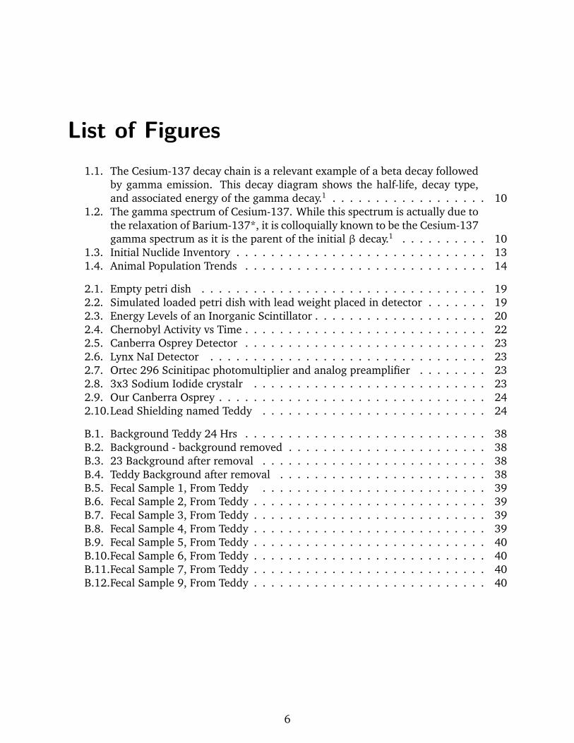
List of Figures1.1. The Cesium-137 decay chain is a relevant example of a beta decay followed

by gamma emission. This decay diagram shows the half-life, decay type,and associated energy of the gamma decay.1 . . . . . . . . . . . . . . . . . . 10

1.2. The gamma spectrum of Cesium-137. While this spectrum is actually due tothe relaxation of Barium-137*, it is colloquially known to be the Cesium-137gamma spectrum as it is the parent of the initial β decay.1 . . . . . . . . . . 10

1.3. Initial Nuclide Inventory . . . . . . . . . . . . . . . . . . . . . . . . . . . . . 131.4. Animal Population Trends . . . . . . . . . . . . . . . . . . . . . . . . . . . . 14

2.1. Empty petri dish . . . . . . . . . . . . . . . . . . . . . . . . . . . . . . . . . 192.2. Simulated loaded petri dish with lead weight placed in detector . . . . . . . 192.3. Energy Levels of an Inorganic Scintillator . . . . . . . . . . . . . . . . . . . . 202.4. Chernobyl Activity vs Time . . . . . . . . . . . . . . . . . . . . . . . . . . . . 222.5. Canberra Osprey Detector . . . . . . . . . . . . . . . . . . . . . . . . . . . . 232.6. Lynx NaI Detector . . . . . . . . . . . . . . . . . . . . . . . . . . . . . . . . 232.7. Ortec 296 Scinitipac photomultiplier and analog preamplifier . . . . . . . . 232.8. 3x3 Sodium Iodide crystalr . . . . . . . . . . . . . . . . . . . . . . . . . . . 232.9. Our Canberra Osprey . . . . . . . . . . . . . . . . . . . . . . . . . . . . . . . 242.10.Lead Shielding named Teddy . . . . . . . . . . . . . . . . . . . . . . . . . . 24

B.1. Background Teddy 24 Hrs . . . . . . . . . . . . . . . . . . . . . . . . . . . . 38B.2. Background - background removed . . . . . . . . . . . . . . . . . . . . . . . 38B.3. 23 Background after removal . . . . . . . . . . . . . . . . . . . . . . . . . . 38B.4. Teddy Background after removal . . . . . . . . . . . . . . . . . . . . . . . . 38B.5. Fecal Sample 1, From Teddy . . . . . . . . . . . . . . . . . . . . . . . . . . 39B.6. Fecal Sample 2, From Teddy . . . . . . . . . . . . . . . . . . . . . . . . . . . 39B.7. Fecal Sample 3, From Teddy . . . . . . . . . . . . . . . . . . . . . . . . . . . 39B.8. Fecal Sample 4, From Teddy . . . . . . . . . . . . . . . . . . . . . . . . . . . 39B.9. Fecal Sample 5, From Teddy . . . . . . . . . . . . . . . . . . . . . . . . . . . 40B.10.Fecal Sample 6, From Teddy . . . . . . . . . . . . . . . . . . . . . . . . . . . 40B.11.Fecal Sample 7, From Teddy . . . . . . . . . . . . . . . . . . . . . . . . . . . 40B.12.Fecal Sample 9, From Teddy . . . . . . . . . . . . . . . . . . . . . . . . . . . 40

6

Acknowledgement of Contribution

These students left the project before its completion

Joseph LeBlanc

– 6 Hours in lab– How did the Chernobyl Accident Happen?– The Aftermath of the Incident– Wildlife Effects

Yudith Sosa

– 6 Hours in lab– The Dogs of Chernobyl

7

1. Background

1. Radiation and Radioactivity

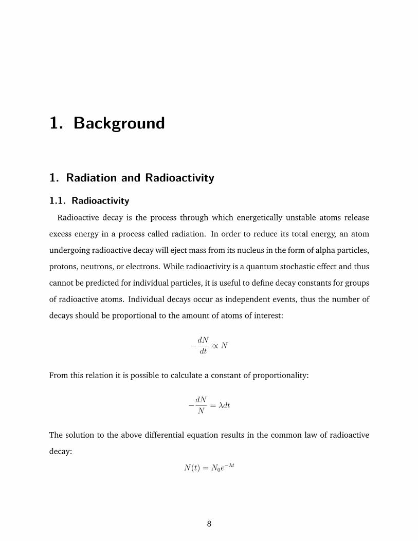
1.1. RadioactivityRadioactive decay is the process through which energetically unstable atoms release

excess energy in a process called radiation. In order to reduce its total energy, an atom

undergoing radioactive decay will eject mass from its nucleus in the form of alpha particles,

protons, neutrons, or electrons. While radioactivity is a quantum stochastic effect and thus

cannot be predicted for individual particles, it is useful to define decay constants for groups

of radioactive atoms. Individual decays occur as independent events, thus the number of

decays should be proportional to the amount of atoms of interest:

−dNdt∝ N

From this relation it is possible to calculate a constant of proportionality:

−dNN

= λdt

The solution to the above differential equation results in the common law of radioactive

decay:

N(t) = N0e−λt

8

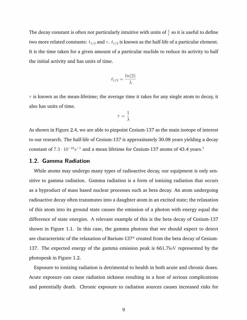
The decay constant is often not particularly intuitive with units of 1t

so it is useful to define

two more related constants: t1/2 and τ . t1/2 is known as the half-life of a particular element.

It is the time taken for a given amount of a particular nuclide to reduce its activity to half

the initial activity and has units of time.

t1/2 = ln(2)λ

τ is known as the mean-lifetime; the average time it takes for any single atom to decay, it

also has units of time.

τ = 1λ

As shown in Figure 2.4, we are able to pinpoint Cesium-137 as the main isotope of interest

to our research. The half-life of Cesium-137 is approximately 30.08 years yielding a decay

constant of 7.3 · 10−10s−1 and a mean lifetime for Cesium-137 atoms of 43.4 years.1

1.2. Gamma RadiationWhile atoms may undergo many types of radioactive decay, our equipment is only sen-

sitive to gamma radiation. Gamma radiation is a form of ionizing radiation that occurs

as a byproduct of mass based nuclear processes such as beta decay. An atom undergoing

radioactive decay often transmutes into a daughter atom in an excited state; the relaxation

of this atom into its ground state causes the emission of a photon with energy equal the

difference of state energies. A relevant example of this is the beta decay of Cesium-137

shown in Figure 1.1. In this case, the gamma photons that we should expect to detect

are characteristic of the relaxation of Barium-137* created from the beta decay of Cesium-

137. The expected energy of the gamma emission peak is 661.7keV represented by the

photopeak in Figure 1.2.

Exposure to ionizing radiation is detrimental to health in both acute and chronic doses.

Acute exposure can cause radiation sickness resulting in a host of serious complications

and potentially death. Chronic exposure to radiation sources causes increased risks for

9

cancer, genetic defects, birth defects, and organ failure. Due to the damaging potential of

ionizing radiation it is important to limit exposure to all involved parties.

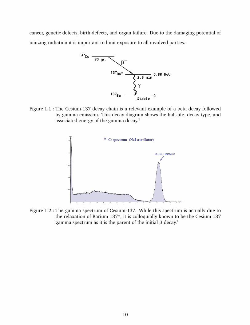
Figure 1.1.: The Cesium-137 decay chain is a relevant example of a beta decay followedby gamma emission. This decay diagram shows the half-life, decay type, andassociated energy of the gamma decay.1

Figure 1.2.: The gamma spectrum of Cesium-137. While this spectrum is actually due tothe relaxation of Barium-137*, it is colloquially known to be the Cesium-137gamma spectrum as it is the parent of the initial β decay.1

10

2. The Chernobyl Disaster

2.1. How did the Chernobyl Accident Happen?JOSEPH LEBLANC WITH TAYLOR TROTTIER

The accident that occurred at the Chernobyl nuclear power plant on April 26, 1986

is one of the worst industrial incidents of the 20th century with respect to environmental

contamination. The Chernobyl Nuclear Power Plant is located near Pripyat, a town located

presently in Ukraine.

A combination of cultural hubris and mechanical malfunction caused a meltdown of

reactor No. 4, ultimately ending in calamity. The accident began during a late-night

safety test simulating a blackout in the power station, during which all safety measures

were intentionally deactivated. Reactor design flaws and an arranging of the core by

operators in a way that was not suitable for the test overheated the fuel rods, which then

led to the rapid transfer of disproportionate heat to the coolant water, creating a shock

wave that ruptured the primary coolant system pipeline joins. Water in the cooling system

quickly changed into steam, initializing a vaporization of part of the reactor fuel, creating

a destructive explosion of steam and subsequent fires, which lasted for about nine days.2

2.2. The Aftermath of the accidentJOSEPH LEBLANC WITH TAYLOR TROTTIER

Most of the employees at the Chernobyl Plant lived in the town of Pripyat, located only

3 km from the site. Following the reactor meltdown, Pripyat’s 50,000 people were evac-

uated, many of whom were families of the Chernobyl employees. In initial containment

operations, two Chernobyl Plant engineers and five firefighters lost their lives.2 According

to the Journal of Public Economics, “. . . several hundred thousand people were exposed

11

to high radiation doses of 175 to 3000 times the average natural background radiation

(350-6000 millisievert, mSv) in the vicinity of the reactor.” Sievert, or Sv, is the SI unit of

ionizing radiation dosage, measuring the health impact on a biological recipient. The level

of dosage that towns surrounding Chernobyl received put their people at serious risk of

cancer development and other health issues.3 Following the initial accident, 134 contain-

ment workers expressed symptoms of acute radiation poisoning, and in the months that

followed, 28 patients died from such complications, despite intensive therapy and 13 bone

marrow transplantations. Compared to the bombing of Hiroshima in 1945, the nature of

radiation contamination by the Chernobyl meltdown were very different. Figure 1.3 lists

the wide spectrum of different isotopes that were released in Chernobyl.2 Furthermore,

there was irregular and patchy radioactive contamination of the environment. Even today,

background radiation levels on the regional scale are highly variable, with some locations

varying by two orders of magnitude at only hundreds of meters apart.4 According to the

Clinical Oncology journal, “The estimated release of radioactivity from the destroyed reac-

tor reached a total of about 13 EBq (1 EBq = 1018 Bq).” That is 400 times more radioactive

material than the Hiroshima bomb. A becquerel, or Bq, is the SI unit of radioactivity, which

measures the quantity of nuclear decays per second. The largest constituent of the radi-

ation contamination was caused by Cesium-137 activity, which amounted to around 64

TBq, or 1.7 MCi, of which Ukraine received 18%.22

2.3. Wildlife EffectsJOSEPH LEBLANC WITH TAYLOR TROTTIER

Today, there are many papers and journal articles that discuss the current state of wildlife

populations in the Chernobyl zone. However, there is significant debate among scientists

as to whether mammal abundances in the Chernobyl zone are in high levels or low lev-

els. To elaborate, consider the Bulletin of the Atomic Sciences journal 67(2), written by

Anders P. Møller PhD of the French National Centre from Scientific Research. MØreller ar-

12

Figure 1.3.: This table shows the initial nuclide inventory released from the Chernobylaccident, updated as of April 26 1986.2

gues most organisms are capable of quickly overpopulating their habitats when a predator

suddenly disappears from the ecosystem. In this case, the predators were the Chernobyl

workers.4 However, Møller argues that background radiation levels directly affect mammal

abundance in the exclusion zone, correlating with a strong pattern of declining abundance

and species richness.4

Some scientists argue that background radiation levels are not directly effecting local

wildlife populations, and are instead thriving through the absence of humans. It could be

possible for wildlife to develop a resistance to radiation through evolution, even among

organisms that have only recently been affected by nuclear accidents because the interven-

ing period of 30 years is sufficient for changes in phenotypes in standard selection experi-

ments.5 The Current Biology journal 25(19) argues that “extremely high dose rates during

the first six months after the accident significantly affected animal health and reproduction

at Chernobyl.” This caused initial mammal abundance decline in the short term after the

accident and you could expect this trend to continue as a consequence. But according to

Current Biology’s trend analysis of large mammal abundances, shown in Figure 1.4, there

is no apparent long-term radiation damage to wildlife populations.6

13

Figure 1.4.: Animal population trends for the areas around Chernobyl for years followingthe accident6

3. The Dogs of ChernobylYUDITH CHUM-SOSA WITH TAYLOR TROTTIER

There are many stray dogs in Chernobyl that were left behind by their owners. According

to Zinaida Kovalenko, a re-settler from Chernobyl, after the incident everyone evacuated,

“but they left their dogs and cats”.7 The owners did not leave them because they wanted to

but because they had to; since, they were told that they could only bring whatever they can

carry, and that excluded pets. Therefore, as a result there were many pets left to wander

the streets and the soviet soldiers were ordered to shoot and kill the abandoned dogs.

14

The soldiers went ahead and shot the dogs but they were not successful in killing all of

them. The dogs that survived the culling had to now defend for themselves against the

wolves that lived around the area; being driven out of the woods they went to seek refuge

in the Chernobyl Exclusion Zone. The dogs made the Exclusion Zone their home and now

the descendants of these dogs can today be found around the nuclear plant.8 Forced to

fend for themselves they became susceptible to an array of health problems. Many are

malnourished, and have rabies due to the rabid wild animals in the zone that spread it to

them.9 Overall, they have a short life expectancy, with many not living beyond the age of

six.10

In time, the workers at the power plant became fond of these dogs and started to take

care of them by giving them food and sometimes providing them shelter when it gets too

cold outside. And since, many of the dogs have not had their rabies vaccine, they could

become a hazard to the workers at the power plant, because by just interacting with them

the workers run a risk of contracting rabies from them.

Another problem concerning these dogs is that many are not spayed or neutered causing

the population of these strays to get out of control. In result, there are over 30,000 stray

cats and dogs that live around the reactor. Thus one of the ways that the nuclear plant

is protecting their workers and controlling the ever growing number of strays is by hiring

someone to capture and cull the dogs. The culling of the dogs is a rather extreme way to

control the population, which is why it is important to bring more light into this issue in

order for that there can be funds that can help spay or neuter the dogs.

This is why Clean Future Funds has made it their mission to raise funds for that they

can bring over veterinarians that can give out rabies shots to the dogs, as well as spay and

neuter them in order to control the population.8 The funds will be used to not only bring

in veterinarians but to also help purchase the vaccines, and anesthesia needed in order to

perform the surgeries. This will hopefully help stop the culling of the strays, and bring

down the current population of strays to a smaller and much more manageable size.10

15

The ultimate goal is to be able to put these strays up for adoption, but however there

are few hurdles in the way. The major problem is that the Ukrainian government does not

allow animals to be removed from the Exclusion Zone, therefore special permission has to

be granted.9 A step to be able to do this is to investigate these dogs a little more through

fecal and hair samples to determine if they are safe to be relocated to other countries, in

order to be able to go through the adoption process.

16

2. Methods

1. Collection of SamplesSample Collection was performed on site in Pripyat Ukraine by workers of the Clean Fu-

tures Fund. Initially, fecal samples were intended to be collected from dogs to be spayed,

but this proved impossible within the scope of the project. Opiate based sedatives were

used to incapacitate dogs for collection and spaying. The opiates caused constipation

preventing the dogs from passing fecal matter in a reasonable timeframe before being re-

turned to the reactor site. Because of this, uncorrelated fecal samples were collected from

the areas around the animal hospital. Samples were collected and labeled with collection

date, cardinal orientation to the hospital, and a number from 1-9 (note that sample 8

seems to have been lost somewhere in the collection process. Hair samples were collected

from dogs that were spayed and neutered by the veterans of the CFF. Upon receipt hair

samples were labeled in two series, Y-XXX and O-XX (Note: we have have no context for

this labeling scheme). Some of samples in the series seemed to be lost in the process of

collection and transport to the United States. Of the approximately one hundred samples

received, thirty seven were tested in the time given. A table of scanned samples can be

found in Appendix Table A.3

2. Preparation of SamplesAll samples were prepared identically and under similar conditions. All samples were

tested in disposable 56mm diameter petri dish tops. Images are included of a typical setup

17

below. A mass was taken before adding samples to the petri dish. Hair Samples were

transfered from paper bags to the petri dish in an even distribution and the bottom of the

petri dish placed on top with a circular lead weight to compress the hair into a denser

profile. Fecal samples were placed in a similar setup, but were first crushed in whirlpak

bags with lead bricks to a fine powder. While it wasn’t necessary for the fecal samples the

lead weight was placed on them for consistency in measurement. Petri dishes were massed

again to determine the sample mass before loading it into the detector. The petri dishes

were placed in the center of the detector and the lead shield closed.

18

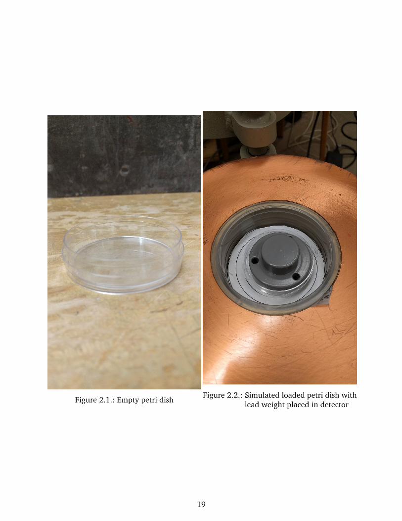
Figure 2.1.: Empty petri dishFigure 2.2.: Simulated loaded petri dish with

lead weight placed in detector

19

3. Radiation Detection and MeasurementEffective collection and measurement of gamma radiation is an essential factor in the

reliability of data. Two detectors were used to scan samples for this project, a Canberra

LynxNaI analog sodium iodide based detector, and a Canberra Osprey digital sodium iodide

detectors. Detector type and geometry determine a system’s overall collection efficiency

and will later be used to guide analysis.

3.1. NaI(Tl) Scintillator Detector Mode of OperationThe Canberra Lynx NaI, and Osprey are both Thallium-doped Sodium-Iodide scintilla-

tion detectors. NaI(Tl) is the most widely used scintillation material due to it being rela-

tively cheap and easy to produce. When exposed to ionizing radiation, the NaI(Tl) crystal

emits photons that are guided to a photomultiplier tube amplifying the optical signal.

These detectors operate on the principle of scintillation. A scintillating material excited by

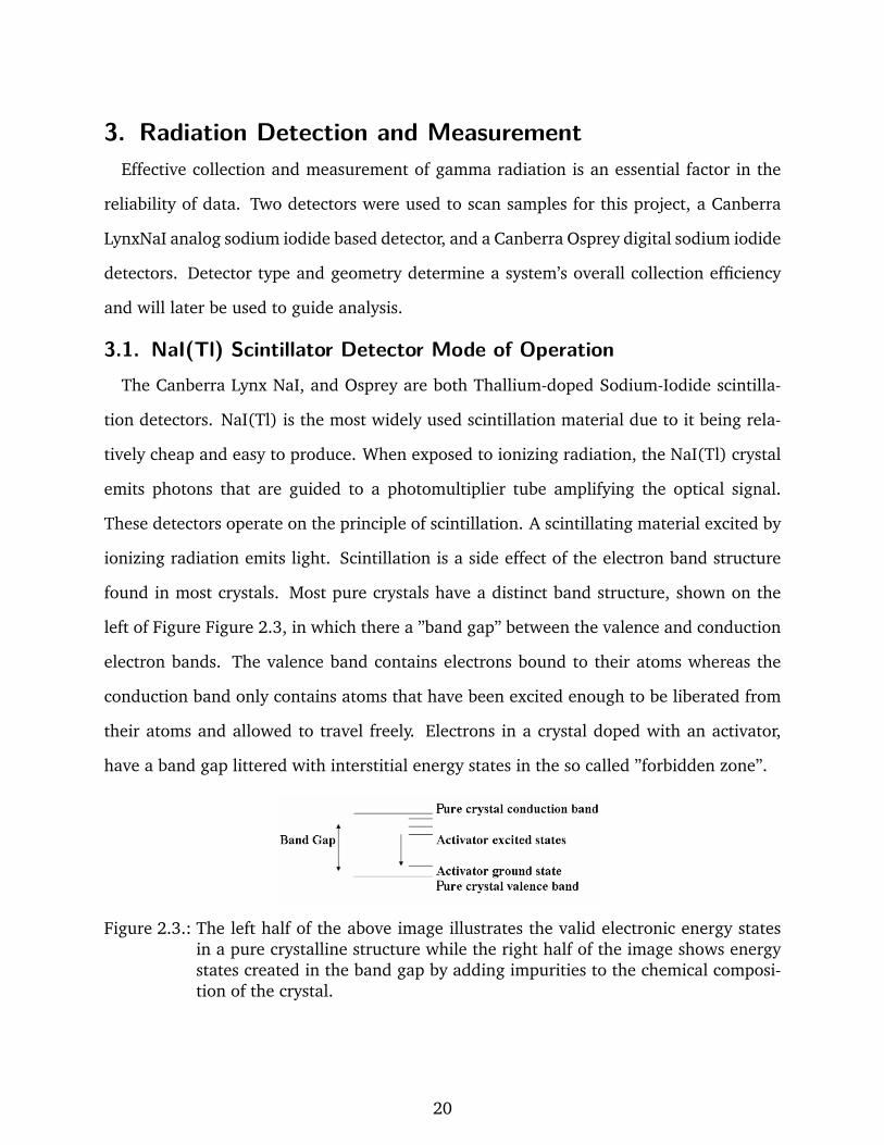
ionizing radiation emits light. Scintillation is a side effect of the electron band structure

found in most crystals. Most pure crystals have a distinct band structure, shown on the

left of Figure Figure 2.3, in which there a ”band gap” between the valence and conduction

electron bands. The valence band contains electrons bound to their atoms whereas the

conduction band only contains atoms that have been excited enough to be liberated from

their atoms and allowed to travel freely. Electrons in a crystal doped with an activator,

have a band gap littered with interstitial energy states in the so called ”forbidden zone”.

Figure 2.3.: The left half of the above image illustrates the valid electronic energy statesin a pure crystalline structure while the right half of the image shows energystates created in the band gap by adding impurities to the chemical composi-tion of the crystal.

20

When an electron is excited into a higher energy band a positively charged hole is left

behind. This pair is called an exciton; the exciton quasi-particle moves through the crystal

lattice until encountering the dopant atom which quickly absorbs the energy of the ex-

citon emitting a characteristic scintillation light. The wavelength of the light emitted is

determined by the impurities of the crystal. The amount of light emitted from the crys-

tal is determined by the energy of the incoming photon as it scatters inside the crystal.

The higher energy the photon, the more electrons it is able to scatter inside the crystal

allowing a greater production of secondary photons. The photomultiplier tube amplifies

the secondary photons and outputs a voltage based on the number of photons created.

The analog (in the case of the Lynx) or digital (in the case of Osprey) MultiChannel An-

alyzer (MCA) then interprets this signal as counts of specific energies. In Pulse Height

Analysis (PHA) mode, the detector determines the energy of the detected photon by by

the amplitude of the photomultiplier pulse. This data is then sent over ethernet cable to

the computer that interprets and saves this data.1

3.2. Detector CalibrationCalibration of detectors is important to allow the collection of accurate and reproducible

data. Detector calibration for sodium iodide detectors involves the use of known check

sources to modify the gain on amplifiers that receive a signal from the detection appara-

tus. Multi Channel Analyzer (MCA) gamma spectrometers in Pulse Height Analysis (PHA)

mode monitor channels based on amplitude. Using a source of Cesium-137 with known

activity located at the center of the detector, the gain is calibrated to locate the centroid

of the detected spectrum at 661.7keV. The centroid, which is the center of ”mass” of the

peak, must be selected due to uncertainty in the energies of collected gamma photons.

While one would expect that the transition energy of resultant Barium-137 to be constant,

thermal fluctuations in the detector crystals will cause shifts in energy levels and vibra-

tional modes in the crystal causing uncertainty in the measurement. Luckily, the thermal

disturbances will be normally distributed and the peak can be modeled as a scaled Gaus-

21

sian. Cesium-137 was selected as the calibration source due to it currently being the main

activity source in Chernobyl, and the only remaining long lived gamma emitter found in

significant quantities.11

Figure 2.4.: Time vs Air Dose at Chernobyl site

22

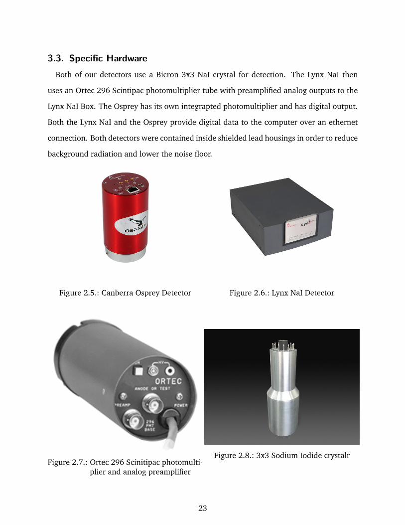
3.3. Specific HardwareBoth of our detectors use a Bicron 3x3 NaI crystal for detection. The Lynx NaI then

uses an Ortec 296 Scintipac photomultiplier tube with preamplified analog outputs to the

Lynx NaI Box. The Osprey has its own integrapted photomultiplier and has digital output.

Both the Lynx NaI and the Osprey provide digital data to the computer over an ethernet

connection. Both detectors were contained inside shielded lead housings in order to reduce

background radiation and lower the noise floor.

Figure 2.5.: Canberra Osprey Detector Figure 2.6.: Lynx NaI Detector

Figure 2.7.: Ortec 296 Scinitipac photomulti-plier and analog preamplifier

Figure 2.8.: 3x3 Sodium Iodide crystalr

23

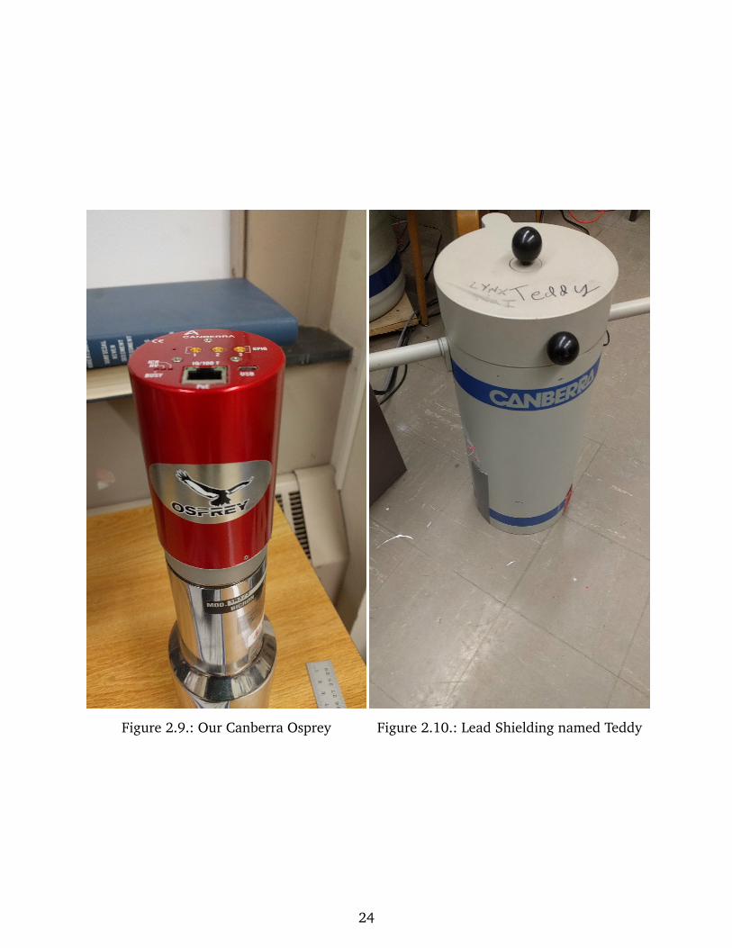
Figure 2.9.: Our Canberra Osprey Figure 2.10.: Lead Shielding named Teddy

24

3. Analysis

1. A Note on Statistical AnalysisOur analysis of all data, especially that of the fecal samples, is plagued by a number

of factors that eliminate all certainty from any statistical analysis performed. The low

number of samples, high variability, and convenience sampling alone make prediction

quite difficult. We have performed analysis as if our data set was larger and randomly

sampled.

2. Background RemovalIn order to allow the collection of only relevant spectra, we took background images for

each detector. These scans were used as a baseline for detector noise and natural back-

ground radiation. All scans were first divided by their scan time to allow a unit comparison

of Counts per Second or CPS. The background scan was then averaged for the seven values

above and below it to allow for a smooth background to be taken. This was done to avoid

large differences between channels caused by detector based effects and thermal fluctu-

ations that do not reflect the physically expected smooth distribution. This is acceptable

because we expect quantized energy effects on a scale so small that our detector resolution

is far too low to detect. In this case we expected a smooth detection distribution including

peaks which have a Gaussian shape.

25

3. Peak DetectionPeak detection is critical to the effective characterization of nuclear materials and their

activity. In the context of this project the only expected peak will be that of cesium-137.

Because of this, the peak detection algorithm finds the maximum value of all the data and

records this location. Due to the fact that the distribution of a decay peak is normally

distributed a relation can be drawn between the standard deviation and full width at half

max Equation 3.1. The full width at half max in this data represents the energy range

where counts exceed half the maximum value. Using the relationship Equation 3.1, we

can calculate the 95% peak interval and calculate the sum of counts over this region to

get a reasonable estimate of the net activity of the sample. This is discussed further in the

MATLAB code appendix section 2.

Also of importance to note is that the peaks were not detected directly at 662keV. While in

a perfect world it would have been possible to detect peaks directly at the expected points

our testing was plagued with temperature fluctuations due to volatile outdoor tempera-

tures and the poor climate control of our test location. Due to these fluctuations larger

than expected drift on the scale of many hours caused uncontrollable shifts of detection

energies. Optimally the shift experienced would be below 1%, we had shifts of about 1.5%.

[h]σ = FWHM√2 · ln 2

(3.1)

After the extraction of the peak, the count rate was multiplied by 2 in order to account

for the thin disk approximation, and divided by 0.2 to account for the efficiency of NaI

detectors. The thin disk approximation is based on an isotropic spherical distribution of

radiation. From a disk with radius much greater than its height, approximately all the

radiation will be emitted from above and below the faces of the disk. In this case it is

acceptable to double the count rate in order to account for radiation emitted away from the

detector. The efficiency of our sodium iodide detector is just over 20% across the entirety

26

of the face being exposed to the sample, thus it counts can be slightly overestimated by

dividing countrate by 0.2.

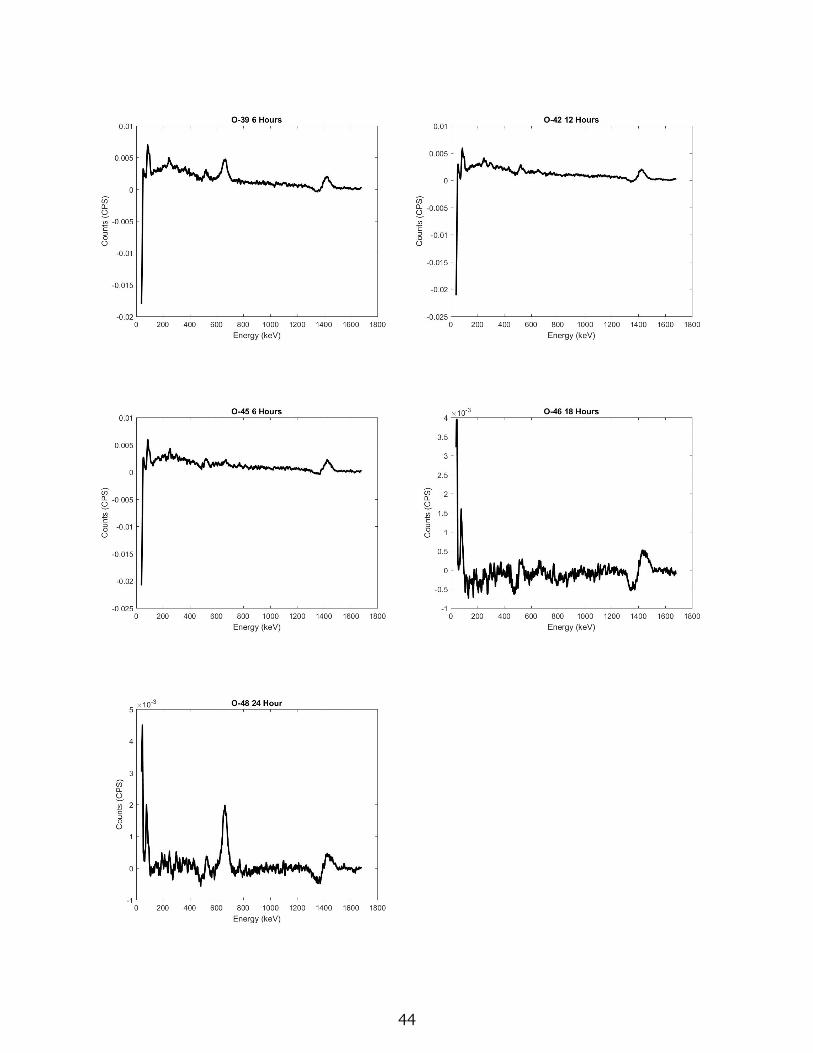
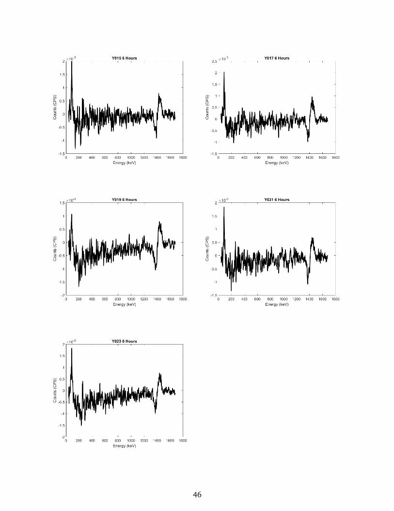
4. Activity Found From HairNo measurable activity was found in any hair tested. Confidence in this measurement is

quite high as nearly forty samples were tested and returned no measurable radioactivity.

The hair samples were taken from dogs being spayed and neutered. Because they were

being prepped for a surgical procedure, it is to be expected that any radioactive dirt was

lost in the washing process. Due to the fact that it distributes throughout the soft tissues

of the body, cesium was not expected in clean hair samples. A summary of all hair scans

can be found in the appendices Table A.3 , Table A.4. The gamma spectra of all hair scans

are located in the appendices section B.

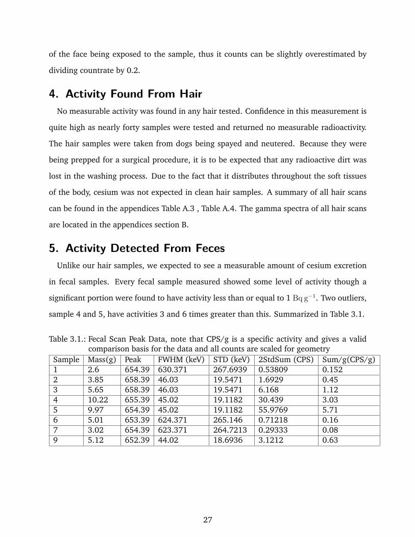
5. Activity Detected From FecesUnlike our hair samples, we expected to see a measurable amount of cesium excretion

in fecal samples. Every fecal sample measured showed some level of activity though a

significant portion were found to have activity less than or equal to 1 Bq g−1. Two outliers,

sample 4 and 5, have activities 3 and 6 times greater than this. Summarized in Table 3.1.

Table 3.1.: Fecal Scan Peak Data, note that CPS/g is a specific activity and gives a validcomparison basis for the data and all counts are scaled for geometry

Sample Mass(g) Peak FWHM (keV) STD (keV) 2StdSum (CPS) Sum/g(CPS/g)1 2.6 654.39 630.371 267.6939 0.53809 0.1522 3.85 658.39 46.03 19.5471 1.6929 0.453 5.65 658.39 46.03 19.5471 6.168 1.124 10.22 655.39 45.02 19.1182 30.439 3.035 9.97 654.39 45.02 19.1182 55.9769 5.716 5.01 653.39 624.371 265.146 0.71218 0.167 3.02 654.39 623.371 264.7213 0.29333 0.089 5.12 652.39 44.02 18.6936 3.1212 0.63

27

6. Decontamination and Quarantine

6.1. Acceptable Levels of ExposureAs a radionuclide, Cesium-137 is inherently carcinogenic and has exposure limits set by

the United States Nuclear Regulatory Commission. According to Appendix B of the NRC

Regulations Title 10 Code of Federal Regulations, the maximum yearly occupational ex-

posure to Cs-137 orally is 100µCi. Oral exposure is the most likely route of exposure, as

ingestion through crosscontamination is far more likely than exposure to any measurable

airborne dose originating from the dogs. Exposure to 100µCi of cesium causes an equiv-

alent full body dose of 50 mSv. This is approximately fifty times the allowable annual

dose to the public of approximately 1 mSv. This dose is approximately equal to 500 chest

x-rays.121314 To avoid the need for licensure and import import restrictions, dogs must

not be radioactive enough to expose anyone to even 1 mSv of radiation. In order soundly

satisfy this standard, the total activity of any single dog must be less than 40µCi.1514 Based

on this estimate an adoptable dog needs to have a total mass of Cesium-137 less than

0.5µg.

6.2. Cesium Lifetime in DogsWe can estimate the lifetime of radioactive cesium in exposed dogs using data from a

series of studies performed by the United States Department of Energy during the 1950s-

60s. We will then use these estimations to provide a sample quarantine procedure for dogs

with activities similar to the ranges we found. Based on the report, cesium was found to

behave in a two tailed manner upon exposure. Approximately 20% of cesium was excreted

within one day, with the remaining 80% being absorbed and distributing itself throughout

the body. This 80% was found to have an upper bound on half-life of 47 days, this time

increased with the age of the dog. The excretion of cesium was found to be split urine and

feces at a 10:1 ratio respectively.16

28

6.3. Time to Negligible Cesium ExposureThe expectation that cesium behaves in the body similarly to potassium must be heavily

relied upon along with the expectation that it distributes itself similarly in tissues. This is

due to a drought of data for cesium and a relative glut of data for potassium behavior in

the body.

With an excretion rate of 10:1 between urine and feces, activity found in the the feces

must be scaled by a factor of 11. From here we are able to estimate, using potassium

concentrations found in the urine, the unit activity of cesium in bodily tissues. Children

with a healthy concentration of potassium have a urine excretion concentration of approx-

imately 1400 mg L−1day−1. The concentration of most bodily tissues is roughly 6000 mg

L−1. Assuming an approximate density for both dog and its urine to be 1kg L−1 (a fair

assumption for mammals) the ratio of potassium in the body to the urine can be found to

be 4.3:1 g kg−1 or 4.3:1 mg g−1. It is quite a stretch to assume that concentration ratios

of cesium and potassium would be the same, but we lack a better way to estimate internal

concentration. Combining these ratios we arrive a the total concentration of cesium in

any given dog to be approximately 44 times that of the concentration in their given fecal

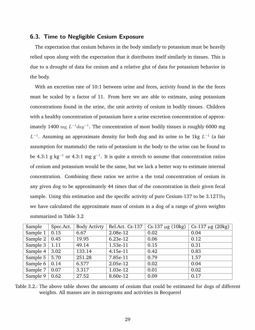
sample. Using this estimation and the specific activity of pure Cesium-137 to be 3.12TBq

we have calculated the approximate mass of cesium in a dog of a range of given weights

summarized in Table 3.2

Sample Spec.Act. Body Activty Rel.Act. Cs-137 Cs-137 µg (10kg) Cs-137 µg (20kg)Sample 1 0.15 6.67 2.08e-12 0.02 0.04Sample 2 0.45 19.95 6.23e-12 0.06 0.12Sample 3 1.11 49.14 1.53e-11 0.15 0.31Sample 4 3.02 133.14 4.15e-11 0.42 0.83Sample 5 5.70 251.28 7.85e-11 0.79 1.57Sample 6 0.14 6.577 2.05e-12 0.02 0.04Sample 7 0.07 3.317 1.03e-12 0.01 0.02Sample 9 0.62 27.52 8.60e-12 0.09 0.17

Table 3.2.: The above table shows the amounts of cesium that could be estimated for dogs of differentweights. All masses are in micrograms and activities in Becquerel

29

Based on our limited information and zeroth order estimation, we can now provide a

range of reasonable times for quarantine. Using the threshold 0.5 µg, the worst case dog

would need to be quarantined for a maximum of 3 half-lives. Assuming the longest exper-

imentally measured biological half-life this time is just over four months, or approximately

130 days. In order to reach levels ten times below the upper threshold of activity, we must

quarantine the dogs for five half-lives or 215 days. Given that most dogs, even those that

live in and around the reactor, live at least 6 years, a quarantine of even 215 days is an

amount of time such that an adoptive family could love this animal for an appreciable

amount of time. The quarantine process will be approximately the same to that of a nor-

mal shelter, feed and water dogs in a safe and comfortable location. Special precautions

will need to be taken to remove urine and feces from the premises. While the amount

of radioactive material these dogs will excrete is low, it is important to prevent further

spread of potentially harmful nuclides. The collection of urine will prove most difficult as

containment of the excreted liquid and preventing its comingling with noncontaminated

water supplies requires collection and filtration infrastructure.

30

4. Conclusion

Based on limited information, we have determined that potentially all the dogs living

in the Chernobyl exclusion zone could be transplanted after a quarantine of less than

one year. With the low concentration of Cesium-137 in the tested dogs and a relatively

short biological half-life in dogs, the worst option may yet be avoided. If allowed by the

Ukrainian government, these dogs are nearly guaranteed to be adopted by some of the

many Chernobyl buffs around the globe. While the Clean Futures Fund is more concerned

with these dogs not reproducing, it would be extremely fulfilling to move spayed and

vaccinated dogs into homes across the globe. At least then something positive will have

come from this failure of man.

31

Appendices

32

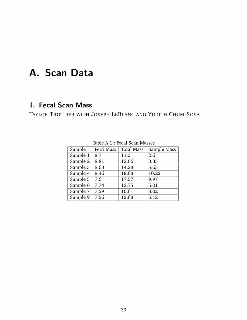
A. Scan Data

1. Fecal Scan MassTAYLOR TROTTIER WITH JOSEPH LEBLANC AND YUDITH CHUM-SOSA

Table A.1.: Fecal Scan MassesSample Petri Mass Total Mass Sample MassSample 1 8.7 11.3 2.6Sample 2 8.81 12.66 3.85Sample 3 8.63 14.28 5.65Sample 4 8.46 18.68 10.22Sample 5 7.6 17.57 9.97Sample 6 7.74 12.75 5.01Sample 7 7.59 10.61 3.02Sample 9 7.56 12.68 5.12

33

2. Fecal Scan Peak Data

Table A.2.: Fecal Scan Peak Data, note that CPS/g is a specific activity and gives a validcomparison basis for the data

Sample Mass(g) Peak FWHM (keV) STD (keV) 2StdSum (CPS) Sum/g(CPS/g)1 2.6 654.39 630.371 267.6939 0.53809 0.1522 3.85 658.39 46.03 19.5471 1.6929 0.453 5.65 658.39 46.03 19.5471 6.168 1.124 10.22 655.39 45.02 19.1182 30.439 3.035 9.97 654.39 45.02 19.1182 55.9769 5.716 5.01 653.39 624.371 265.146 0.71218 0.167 3.02 654.39 623.371 264.7213 0.29333 0.089 5.12 652.39 44.02 18.6936 3.1212 0.63

34

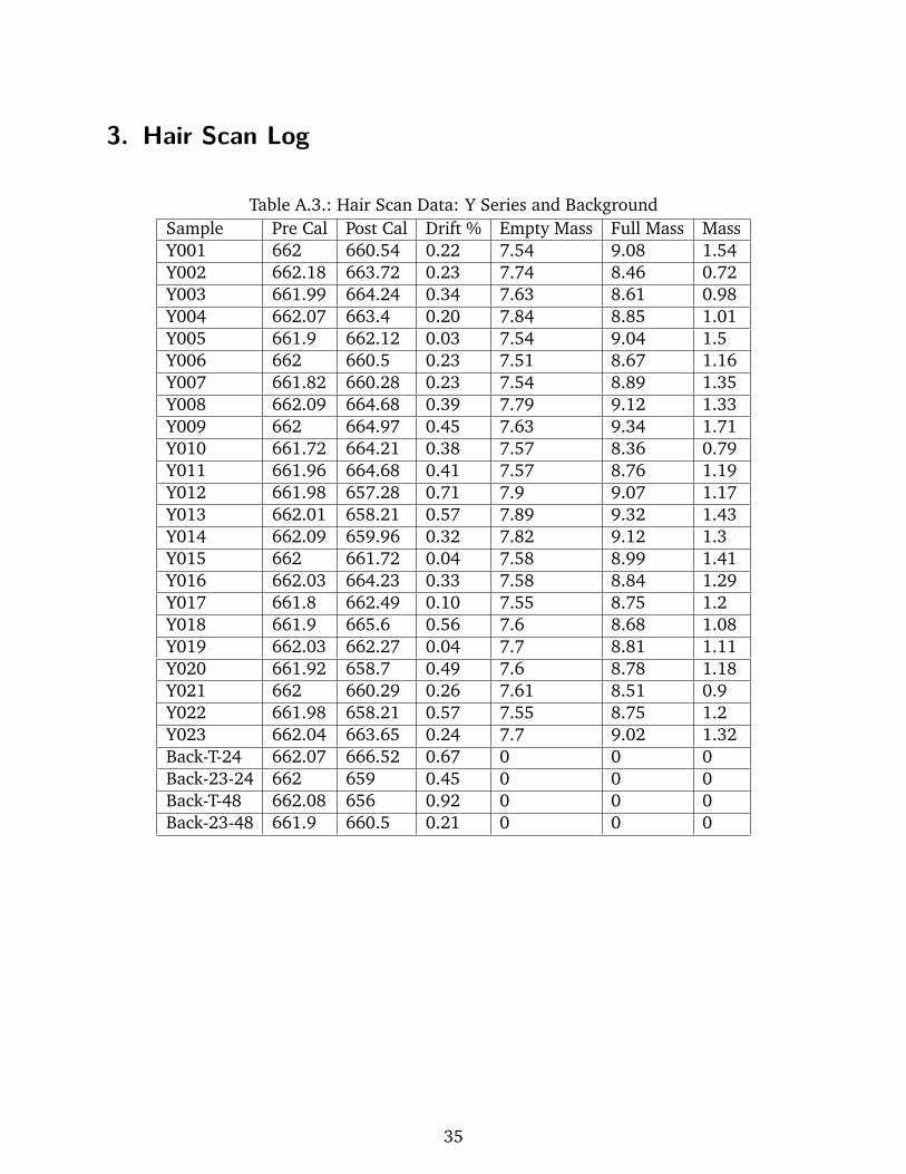
3. Hair Scan Log

Table A.3.: Hair Scan Data: Y Series and BackgroundSample Pre Cal Post Cal Drift % Empty Mass Full Mass MassY001 662 660.54 0.22 7.54 9.08 1.54Y002 662.18 663.72 0.23 7.74 8.46 0.72Y003 661.99 664.24 0.34 7.63 8.61 0.98Y004 662.07 663.4 0.20 7.84 8.85 1.01Y005 661.9 662.12 0.03 7.54 9.04 1.5Y006 662 660.5 0.23 7.51 8.67 1.16Y007 661.82 660.28 0.23 7.54 8.89 1.35Y008 662.09 664.68 0.39 7.79 9.12 1.33Y009 662 664.97 0.45 7.63 9.34 1.71Y010 661.72 664.21 0.38 7.57 8.36 0.79Y011 661.96 664.68 0.41 7.57 8.76 1.19Y012 661.98 657.28 0.71 7.9 9.07 1.17Y013 662.01 658.21 0.57 7.89 9.32 1.43Y014 662.09 659.96 0.32 7.82 9.12 1.3Y015 662 661.72 0.04 7.58 8.99 1.41Y016 662.03 664.23 0.33 7.58 8.84 1.29Y017 661.8 662.49 0.10 7.55 8.75 1.2Y018 661.9 665.6 0.56 7.6 8.68 1.08Y019 662.03 662.27 0.04 7.7 8.81 1.11Y020 661.92 658.7 0.49 7.6 8.78 1.18Y021 662 660.29 0.26 7.61 8.51 0.9Y022 661.98 658.21 0.57 7.55 8.75 1.2Y023 662.04 663.65 0.24 7.7 9.02 1.32Back-T-24 662.07 666.52 0.67 0 0 0Back-23-24 662 659 0.45 0 0 0Back-T-48 662.08 656 0.92 0 0 0Back-23-48 661.9 660.5 0.21 0 0 0

35

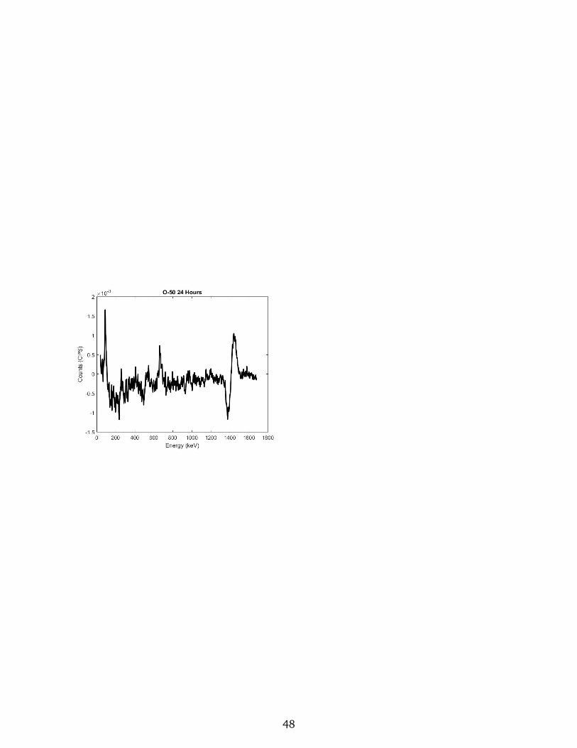
Table A.4.: Hair Scan Data: O SeriesO-35 661.93 662.96 0.16 7.59 7.84 0.25O-36 661.96 662.8 0.13 7.74 7.89 0.15O-37 661.92 660.42 0.23 7.55 8.45 0.9O-38 661.82 662.4 0.09 7.79 7.91 0.12O-39 662.05 660.63 0.21 7.57 7.92 0.35O-40 661.97 659 0.45 5.81 5.86 0.05O-42 661.95 659.04 0.44 5.9 6.05 0.15O-44 662.15 657 0.78 5.89 6.03 0.14O-45 661.98 662.1 0.02 5.96 7.03 1.07O-46 662.12 667 0.74 5.86 6.51 0.65O-47 662.06 665.2 0.47 5.86 6.14 0.28O-48 661.9 667 0.77 6 7.02 1.02O-49 662.1 666 0.59 5.81 6.16 0.35O-50 661.9 659 0.44 5.89 7.49 1.6

36

B. Raw Graphs

37

1. Background Data

Figure B.1.: Background Teddy 24 HrsFigure B.2.: Background - background re-

moved

Figure B.3.: 23 Background after removal Figure B.4.: Teddy Background after removal

38

2. Fecal Graphs: Background Removed

Figure B.5.: Fecal Sample 1, From Teddy Figure B.6.: Fecal Sample 2, From Teddy

Figure B.7.: Fecal Sample 3, From Teddy Figure B.8.: Fecal Sample 4, From Teddy

39

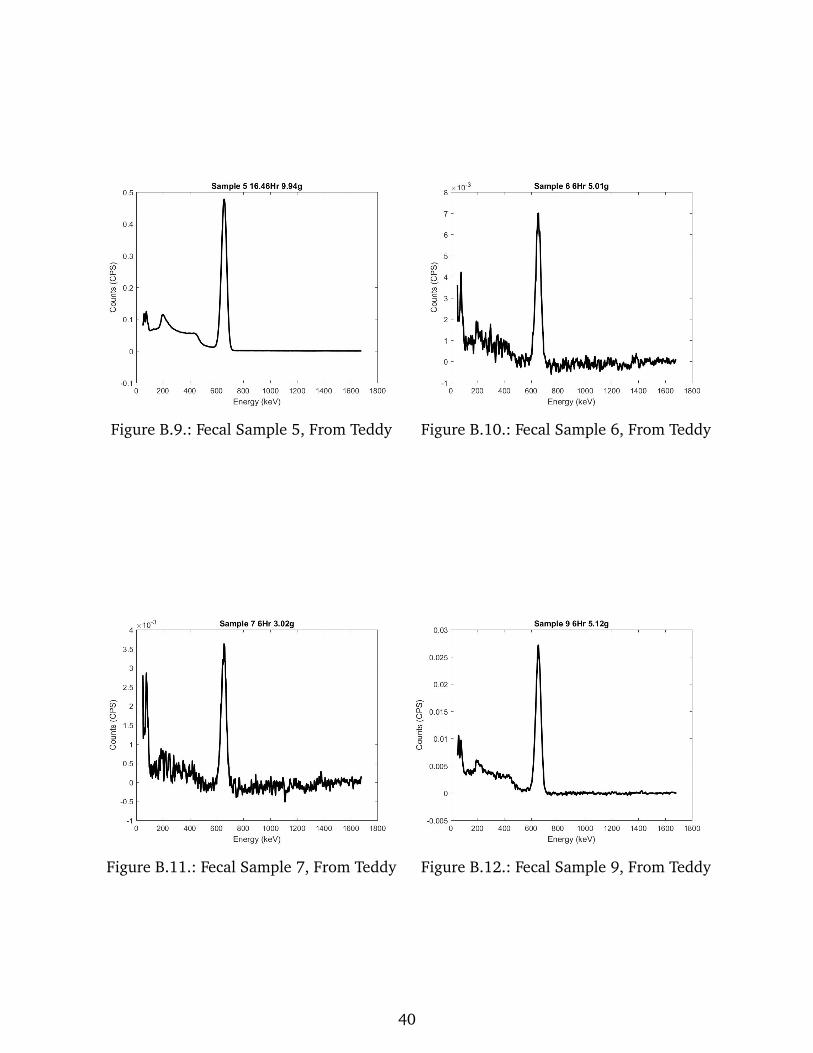
Figure B.9.: Fecal Sample 5, From Teddy Figure B.10.: Fecal Sample 6, From Teddy

Figure B.11.: Fecal Sample 7, From Teddy Figure B.12.: Fecal Sample 9, From Teddy

40

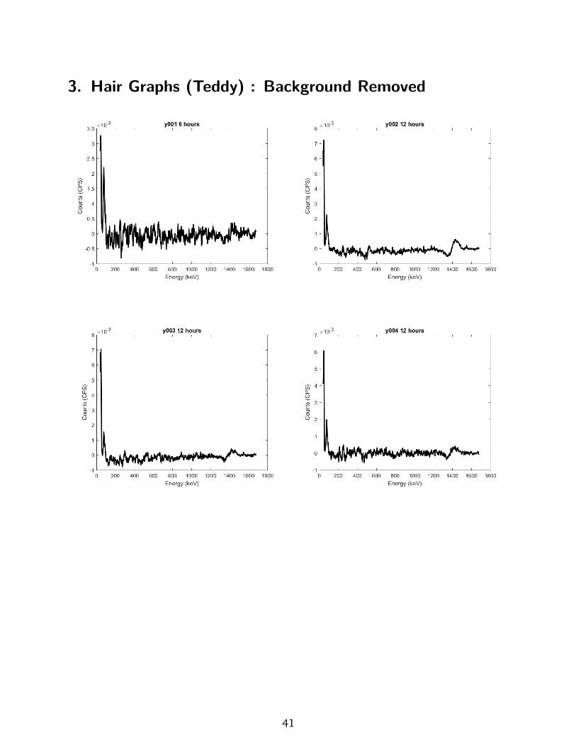
3. Hair Graphs (Teddy) : Background Removed

41

42

43

44

4. Hair Graphs (23) : Background Removed

45

46

47

48

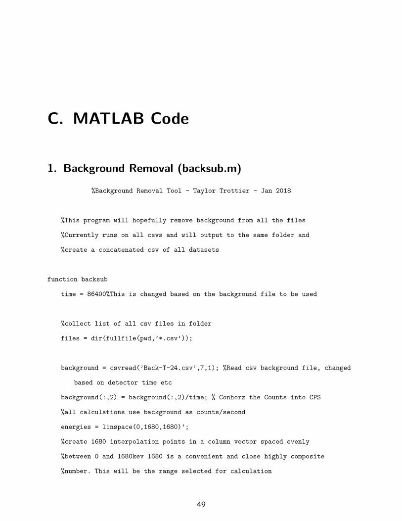
C. MATLAB Code

1. Background Removal (backsub.m)

%Background Removal Tool - Taylor Trottier - Jan 2018

%This program will hopefully remove background from all the files

%Currently runs on all csvs and will output to the same folder and

%create a concatenated csv of all datasets

function backsub

time = 86400%This is changed based on the background file to be used

%collect list of all csv files in folder

files = dir(fullfile(pwd,’*.csv’));

background = csvread(’Back-T-24.csv’,7,1); %Read csv background file, changed

based on detector time etc

background(:,2) = background(:,2)/time; % Conhorz the Counts into CPS

%all calculations use background as counts/second

energies = linspace(0,1680,1680)’;

%create 1680 interpolation points in a column vector spaced evenly

%between 0 and 1680kev 1680 is a convenient and close highly composite

%number. This will be the range selected for calculation

49

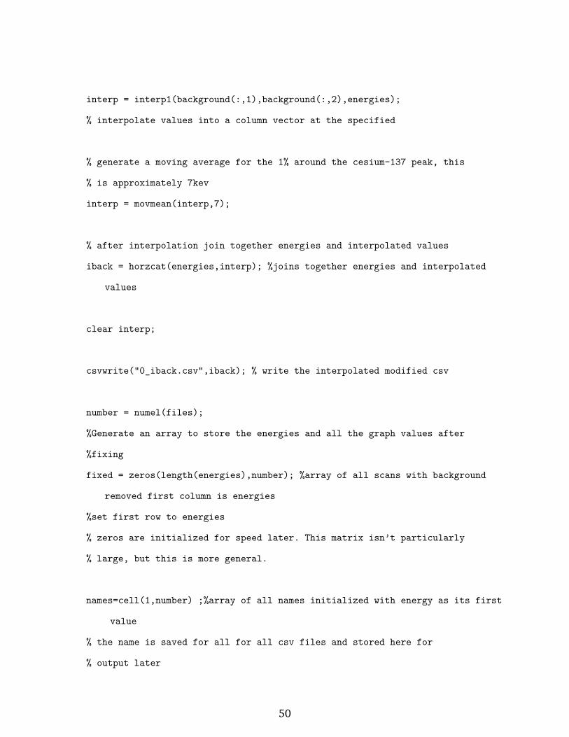
interp = interp1(background(:,1),background(:,2),energies);

% interpolate values into a column vector at the specified

% generate a moving average for the 1% around the cesium-137 peak, this

% is approximately 7kev

interp = movmean(interp,7);

% after interpolation join together energies and interpolated values

iback = horzcat(energies,interp); %joins together energies and interpolated

values

clear interp;

csvwrite("0_iback.csv",iback); % write the interpolated modified csv

number = numel(files);

%Generate an array to store the energies and all the graph values after

%fixing

fixed = zeros(length(energies),number); %array of all scans with background

removed first column is energies

%set first row to energies

% zeros are initialized for speed later. This matrix isn’t particularly

% large, but this is more general.

names=cell(1,number) ;%array of all names initialized with energy as its first

value

% the name is saved for all for all csv files and stored here for

% output later

50

for i=1:number

fname=files(i).name; %gets filename from file structure

disp(fname);

dtime = csvread(fname,2,1,[2,1,2,1]); %get scan runtime for calculating

cps

data = csvread(fname,7,1); %reads from ith file into data array in ith

position

data(:,2) = data(:,2)./dtime ; %calculates cps

disp(fname)

interp = interp1(data(:,1),data(:,2),energies); %interpolate datapoints

for the file

interp = movmean(interp,7); % average for the 7 values around the point

idata = horzcat(energies,interp); % Generate interpolated arrays

rdata = idata(:,2)-iback(:,2); %removed background data

rary = horzcat(energies,rdata);

fixed(:,i)=rdata; % add on removed background values to fixed

names{i+1}=cellstr(fname); %sets column header in fixed (concatenated)

array to the name of the file for that column

51

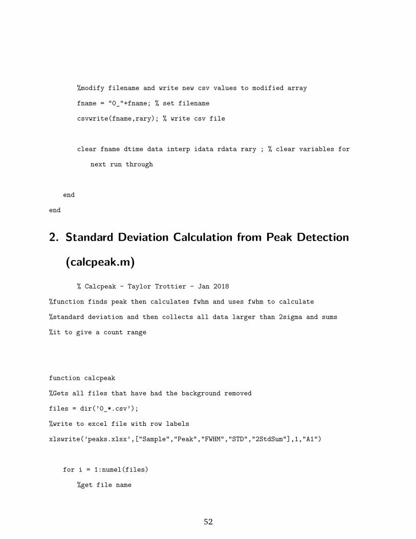
%modify filename and write new csv values to modified array

fname = "0_"+fname; % set filename

csvwrite(fname,rary); % write csv file

clear fname dtime data interp idata rdata rary ; % clear variables for

next run through

end

end

2. Standard Deviation Calculation from Peak Detection

(calcpeak.m)

% Calcpeak - Taylor Trottier - Jan 2018

%function finds peak then calculates fwhm and uses fwhm to calculate

%standard deviation and then collects all data larger than 2sigma and sums

%it to give a count range

function calcpeak

%Gets all files that have had the background removed

files = dir(’0_*.csv’);

%write to excel file with row labels

xlswrite(’peaks.xlsx’,["Sample","Peak","FWHM","STD","2StdSum"],1,"A1")

for i = 1:numel(files)

%get file name

52

fname=files(i).name;

%get data

data = csvread(fname);

%split data for readability

energy = data(50:end,1);

measurements= data(50:end,2);

%get the index and value of the max measurements

[maxVal,index]=max(measurements);

%find fwhm (boolean vector for values above fwhm)

above = measurements >= maxVal/2;

%gets upper and lower indexes by finding the first and last values

%that go above and below fwhm

lowerIndex = find(above,1);

upperIndex = find(above,1,’last’);

%calculates the fwhm d-energy

fwhm = energy(upperIndex) - energy(lowerIndex);

%using the gaussian relation between FWHM and StdDeviation

sigma = fwhm/(2*sqrt(2*log(2)));

centerIndex = find(measurements==max(measurements),1); %Find index of

center

minEnergy = energy(centerIndex) - 2*sigma;

maxEnergy = energy(centerIndex) + 2*sigma;

%range of two std and then sums the values in that range

rtwosig = (energy>=minEnergy);

rtwosig = energy<=maxEnergy;

53

%actual sum of the region in the range of two standard deviations

%if anyone actually reads this shoot me an email at

%tgtrottier@wpi.edu or tgtrottier@gmail.com

%double the value to account for the thin disk approximation

%divide by 0.23 for detector efficiency

twosig = 2*sum(measurements(rtwosig))/.2;

%writes to file and displays the sum and

disp(fname);

disp(twosig);

xlswrite(’peaks.xlsx’,[string(fname(3:end-4)),energy(index),fwhm,sigma,

twosig],1,strcat(’A’,int2str(i+1)));

end

end

3. Graph Making Function (makegraph.m)

%Makegraph - Taylor Trottier - Jan 2018

%creates a graph for every sample that has had its background removed

function makegraph

%collect list of all csv files in folder

files = dir(’0_*.csv’);

%for all files with bg removed

for i = 1:numel(files)

54

%open new figure

figures=figure;

%get file name

fname=files(i).name;

%read in data

data = csvread(fname);

%plot data above ˜50kev as data below this is unreliable

plot(data(50:end,1),data(50:end,2),’LineWidth’,2,’Color’,’Black’);

%creates a title from the filename

title(fname(3:end-4));

%labels the axes

xlabel(’Energy (keV)’);

ylabel(’Counts (CPS)’);

%prints to the console so I know its Running

disp((fname(3:end-4)));

saveas(figures,strcat(fname(1:end-4),’.jpg’));

close(figures);

end

end

4. Calculation of Exponential Distribution

%Find Cumulative Distribution Function - Taylor Trottier - Feb 2018

%Also Find Exponential; Distribution and use it to calculate 50% 75% and 99%

%case

55

function expfit

cdffig=figure;

%read peaks to extract the normalized cps

ncps = sort(xlsread(’peaks.xlsx’,’F2:F9’));

%size of dataset for calculation of step

n=size(ncps,1);

%calculate the step value for the CDF

% p_plot is the probability step for plotting

p_plot = ((1:n))’ ./ n;

%plot step function of probability

p1=stairs([0;ncps;10],[0;p_plot;1],’k-’);

xlim([0,6]);

hold on;

title(’Cumulative Probability Distribution of Fecal Data’);

xlabel(’CPS/g’);

ylabel(’Cum. Prob. (x)’);

%actual p we need to subtract a half to have our fit hit the center of

%the step instead of the tops

p = ((1:n)-0.5)’./n;

%fitting the results to 1-eˆ(-lambda*x) which should give us a fit to

%the cumulative probability and returns lambda

fitResult = fit(ncps,p,fittype(’1-exp(-lambda*x)’),’StartPoint’,1.2);

lambda = fitResult.lambda;

56

%define the plot for the exponential cdf

p2=plot ((0:0.05:6),1-exp(-lambda*(0:0.05:6)));

%creates the legend p1 is stair p2 is fit location is set to avoid

%graph conflict

legend([p1,p2],’CDF’, [’Exponential Fit:’ num2str(lambda)],’Location’,’

southeast’);

%saves and closes the image

saveas(cdffig,’CDF.jpg’);

close(cdffig);

%To Do; Create PDF Figure as well

% pdffig = figure;

% epdf = exppdf(ncps,lambda);

% x = 0:.1:6;

% plot(ncps,epdf);

% title("Exponential Probability Distribution Function")

% xlabel(’CPS/g’);

% ylabel(’P(x)’);

end

57

Bibliography

[1] Glenn F Knoll. Radiation detection and measurement, 1979. ISBN:9780471495451.

[2] V. Saenko, V. Ivanov, A. Tsyb, T. Bogdanova, M. Tronko, Yu. Demidchik, and

S. Yamashita. The chernobyl accident and its consequences. Clinical Oncology,

23(4):234–243, 2011.

[3] Alexander M. Danzer and Natalia Danzer. The long-run consequences of chernobyl:

Evidence on subjective well-being, mental health and welfare. Journal of Public Eco-

nomics, 135:47–60, 2016.

[4] Timothy A. Mousseau and Anders P. Møller. Landscape portrait: A look at the impacts

of radioactive contaminants on chernobyl’s wildlife. Bulletin of the Atomic Scientists,

67(2):38–46, 2011.

[5] Anders Pape Møller and Timothy Alexander Mousseau. Are organisms adapting to

ionizing radiation at chernobyl? Trends in Ecology & Evolution, 31(4):281–289, 2016.

[6] T.g. Deryabina, S.v. Kuchmel, L.l. Nagorskaya, T.g. Hinton, J.c. Beasley, A. Lerebours,

and J.t. Smith. Long-term census data reveal abundant wildlife populations at cher-

nobyl. Current Biology, 25(19), 2015.

[7] Svetlana Aleksievich. Voices of Chernobyl: chronicle of the future. Aurum Press, 1999.

[8] Clean futures fund - dogs of chernobyl.

58

[9] Clean futures fund - dogs of chernobyl update.

[10] Meet the dogs of chernobyl – the abandoned pets that formed their own canine

community, Feb 2018.

[11] Paul Hill-Gibbins. Radiation levels now, Jun 2017.

[12] M J Duggan. Natural background and dose limits for members of the public. Journal

of Radiological Protection, 10(1):59–60, Jan 1990.

[13] Stanford Environmental Health & Safety Board. Cs-137 radionuclide fact sheet.

[14] United states federal code: 56 fr 23398, May 21, 1991.

[15] George Shabot. Relationship between radionuclide gamma emission and exposure

rate.

[16] Roy C Thompson. Life span effects of ionizing radiation in the beagle dog. US

Department of Energy Office of Health and Environmental Research, page 38–39, 1989.

59