an introducion to signal analysis - pages personnelles telecom

An introducionto signal analysis

TELECOM Bretagne, Master of science MTS-102B

[email protected]

Brest 11-16 octobre 2011

SommaireIntroduction

1 Introduction

2 Basic concepts

Discrete signals and systems

Analog signals and systems

3 Further results

4 Conclusion

2/22 MsC 2013 MsC - september 2013

IntroductionIntroduction ◮ Contexte

� Context : advent of digital techniques to manipulate analog sources such as

audio or images.� In signal analysis, the signal is described and manipulated in a convenient way

to perform tasks such as filtering, source seperation or denoising.� Areas of application : speech and audio processing (compression, denoising,

watermarking, ...), telecommunications, astronomy, radar and sonar, healthcare

(ECG, imaging, ...), geology (earthquake surveillance), finance, biology, . . .� Most of this course is based on the first part of the book Signal analysis, by

Athanasios Papoulis, Mc Graw Hill 1977.

� Other references• S. K. Mitra, Digital Signal Processing, a computer-based

approach, Third edition, Mcgraw hill, 2005 ;• J. G. Proakis and D. K. Manolakis, Digital Signal Processing, 4th

edition, Prentice Hall, 2006 ;• A. V. Oppenheim and R. W. Schafer, Discrete-Time Signal

Processing, Third edition, Prentice Hall, 2009.


Goals of the courseIntroduction ◮ Goals of the course

� Understand basics of analog and discrete signals and systems modelling and in

particular concepts such as causality, periodicity, time and frequency

representation, . . .

� Know what a filter is

� Be able to calculate and use the z-transform and the Fourier transform

� Understand sampling principles

� Be able to manipulate above concepts to solve simple problems.


ScheduleIntroduction ◮ organization

Course : 12 hours, roughly organized as follows :

� 3 hours classes

� 3 hours exercices

� 3 hours practical training (Matlab programming)

Exam : 1 hour (no document)


Table of contentsIntroduction ◮ organization

1 Introduction

2 Basic concepts



3 Further results

4 Conclusion


SommaireBasic concepts

1 Introduction

2 Basic concepts



3 Further results

4 Conclusion


Discrete signals and systemsBasic concepts ◮ Discrete signals and systems

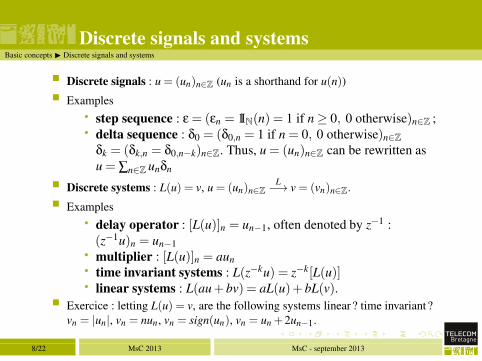
� Discrete signals : u = (un)n∈Z (un is a shorthand for u(n))

� Examples

• step sequence : ε = (εn = 1IN(n) = 1 if n ≥ 0, 0 otherwise)n∈Z ;• delta sequence : δ0 = (δ0,n = 1 if n = 0, 0 otherwise)n∈Z

δk = (δk,n = δ0,n−k)n∈Z. Thus, u = (un)n∈Z can be rewritten as

u = ∑n∈Z unδn

� Discrete systems : L(u) = v, u = (un)n∈ZL

−→ v = (vn)n∈Z.

� Examples

• delay operator : [L(u)]n = un−1, often denoted by z−1 :

(z−1u)n = un−1• multiplier : [L(u)]n = aun• time invariant systems : L(z−ku) = z−k[L(u)]• linear systems : L(au+ bv) = aL(u)+ bL(v).

� Exercice : letting L(u) = v, are the following systems linear? time invariant ?

vn = |un|, vn = nun, vn = sign(un), vn = un +2un−1.


Impulse response and filtersBasic concepts ◮ Impulse response and filters

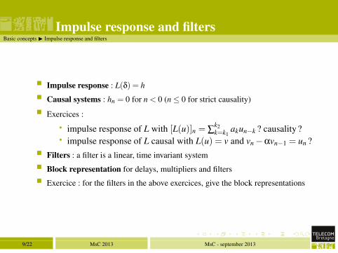
� Impulse response : L(δ) = h

� Causal systems : hn = 0 for n < 0 (n ≤ 0 for strict causality)

� Exercices :

• impulse response of L with [L(u)]n = ∑k2k=k1

akun−k ? causality ?• impulse response of L causal with L(u) = v and vn −αvn−1 = un ?

� Filters : a filter is a linear, time invariant system

� Block representation for delays, multipliers and filters

� Exercice : for the filters in the above exercices, give the block representations


ConvolutionBasic concepts ◮ Convolution

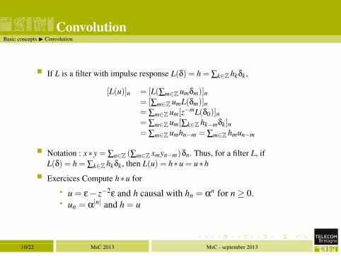
� If L is a filter with impulse response L(δ) = h = ∑k∈Z hkδk,

[L(u)]n = [L(∑m∈Z umδm)]n= [∑m∈Z umL(δm)]n= ∑m∈Z um[z

−mL(δ0)]n= ∑m∈Z um[∑k∈Z hk−mδk]n= ∑m∈Z umhn−m = ∑m∈Z hmun−m

� Notation : x∗y = ∑n∈Z (∑m∈Z xmyn−m)δn. Thus, for a filter L, if

L(δ) = h = ∑k∈Z hkδk, then L(u) = h∗u = u∗h

� Exercices Compute h∗u for

• u = ε− z−2ε and h causal with hn = αn for n ≥ 0.• un = α|n| and h = u


z-transformBasic concepts ◮ z-transform

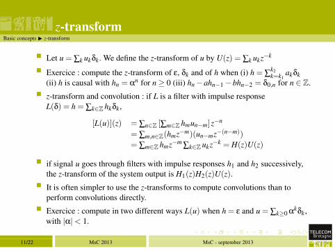
� Let u = ∑k ukδk. We define the z-transform of u by U(z) = ∑k ukz−k

� Exercice : compute the z-transform of ε, δk and of h when (i) h = ∑k2

k=k1akδk

(ii) h is causal with hn = αn for n ≥ 0 (iii) hn −ahn−1 −bhn−2 = δ0,n for n ∈ Z.

� z-transform and convolution : if L is a filter with impulse response

L(δ) = h = ∑k∈Z hkδk,

[L(u)](z) = ∑n∈Z [∑m∈Z hmun−m]z−n

= ∑m,n∈Z(hmz−m)(un−mz−(n−m))

= ∑m∈Z hmz−m ∑k∈Z ukz−k = H(z)U(z)

� if signal u goes through filters with impulse responses h1 and h2 successively,

the z-transform of the system output is H1(z)H2(z)U(z).

� It is often simpler to use the z-transforms to compute convolutions than to

perform convolutions directly.

� Exercice : compute in two different ways L(u) when h = ε and u = ∑k≥0 αkδk,

with |α|< 1.


Analog signals and systemsBasic concepts ◮ Analog signals and systems

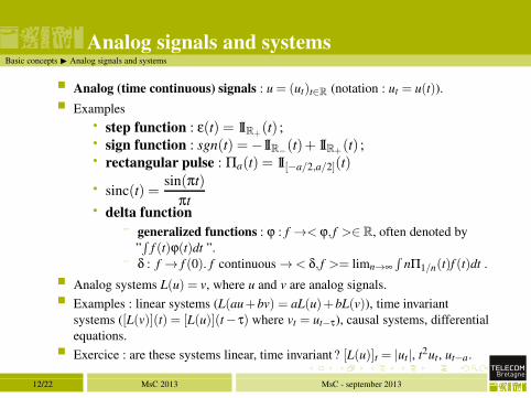
� Analog (time continuous) signals : u = (ut)t∈R (notation : ut = u(t)).� Examples

• step function : ε(t) = 1IR+(t) ;• sign function : sgn(t) =−1IR−(t)+ 1IR+(t) ;• rectangular pulse : Πa(t) = 1I[−a/2,a/2](t)

• sinc(t) =sin(πt)

πt• delta function

− generalized functions : ϕ : f →< ϕ, f >∈ R, often denoted by

”∫

f (t)ϕ(t)dt ”.− δ : f → f (0). f continuous →< δ, f >= limn→∞

∫nΠ1/n(t)f (t)dt .

� Analog systems L(u) = v, where u and v are analog signals.� Examples : linear systems (L(au+bv) = aL(u)+bL(v)), time invariant

systems ([L(v)](t) = [L(u)](t− τ) where vt = ut−τ), causal systems, differential

equations.� Exercice : are these systems linear, time invariant ? [L(u)]t = |ut|, t2ut, ut−a.


FiltersBasic concepts ◮ Filters

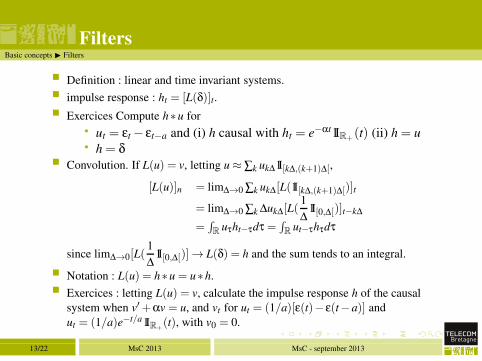
� Definition : linear and time invariant systems.� impulse response : ht = [L(δ)]t.� Exercices Compute h∗u for

• ut = εt − εt−a and (i) h causal with ht = e−αt1IR+(t) (ii) h = u• h = δ

� Convolution. If L(u) = v, letting u ≈ ∑k uk∆1I[k∆,(k+1)∆[,

[L(u)]n = lim∆→0 ∑k uk∆[L(1I[k∆,(k+1)∆[)]t

= lim∆→0 ∑k ∆uk∆[L(1

∆1I[0,∆[)]t−k∆

=∫R

uτht−τdτ =∫R

ut−τhτdτ

since lim∆→0[L(1

∆1I[0,∆[)]→ L(δ) = h and the sum tends to an integral.

� Notation : L(u) = h∗u = u∗h.� Exercices : letting L(u) = v, calculate the impulse response h of the causal

system when v′+αv = u, and vt for ut = (1/a)[ε(t)− ε(t−a)] and

ut = (1/a)e−t/a1IR+(t), with v0 = 0.


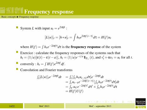
Frequency responseBasic concepts ◮ Frequency response

� System L with input ut = e2iπft :

[L(u)]t = [h∗u]t =

∫hτe2iπf (t−τ)dτ = H(f )ut

where H(f ) =∫

hτe−2iπf τdτ is the frequency response of the system

� Exercice : calculate the frequency responses of the systems such that

ht = (1/a)[ε(t)− ε(t−a)], ht = (1/a)e−t/a1IR+(t), and v′t +αvt = ut for all t.

� conversly : ht =∫

H(f )e2iπf df .

� Convolution and Fourier transforms

∫t[L(u)]te

−2iπftdt =∫

t[∫

τ hτut−τ)dτ]e−2iπftdt

=∫

t ut−τe−2iπf (t−τ)[∫

τ hτe−2iπf τdτ]dt

=∫

τ′ uτ′e−2iπf τ′dτ′×

∫τ hτe−2iπf τdτ

= H(f )U(f )


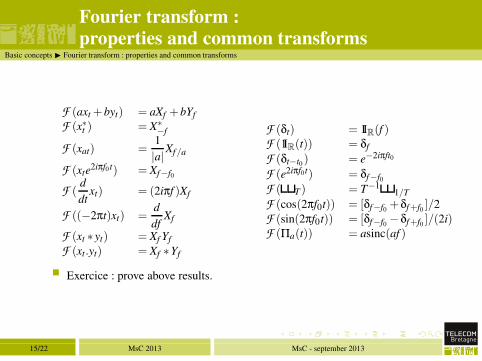
Fourier transform :

properties and common transformsBasic concepts ◮ Fourier transform : properties and common transforms

F (axt +byt) = aXf +bYf

F (x∗t ) = X∗−f

F (xat) =1

|a|Xf/a

F (xte2iπf0 t) = Xf−f0

F (d

dtxt) = (2iπf )Xf

F ((−2πt)xt) =d

dfXf

F (xt ∗yt) = Xf Yf

F (xt.yt) = Xf ∗Yf

F (δt) = 1IR(f )F (1IR(t)) = δf

F (δt−t0 ) = e−2iπft0

F (e2iπf0t) = δf−f0

F ( T) = T−11/T

F (cos(2πf0t)) = [δf−f0 +δf+f0 ]/2

F (sin(2πf0t)) = [δf−f0 −δf+f0 ]/(2i)F (Πa(t)) = asinc(af )

� Exercice : prove above results.


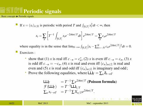
Periodic signalsBasic concepts ◮ Periodic signals

� If x = (xt)t∈R is periodic with period T and∫[0,T[ x

2t dt < ∞, then

xt =∑n

[

T−1∫[0,T[

xte−2iπnt/T dt

]

e2iπnt/T = ∑n

cne2iπnt/T

where equality is in the sense that limN→∞∫[0,T[[xt −∑N

n=−N cne2iπnt/T ]2dt = 0.

� Exercices :

• show that (1) x is real iff c−n = c∗n, (2) x is even iff c−n = cn, (3) x

is odd iff c−n =−cn, (4) x is real and even iff (cn)n∈Z is real and

even and (5) x is real and odd iff (cn)n∈Z is imaginary and odd ;• Prove the following equalities, where T = ∑n δt−nT

T = T−1 ∑e2iπnt/T (Poisson formula)

F ( T) = T−11/T

∑n xt−nT = T−1 ∑Xn/Te2iπnt/T .


SommaireFurther results

1 Introduction

2 Basic concepts



3 Further results

4 Conclusion


z-transformFurther results ◮ z-transform

� x = (xn)n∈Z → X(z) = ∑n xnz−n.� ∑n xnz−n converges in a ring r1 < z < r2 where r1,2 depend on xn as n →±∞.� Exercice : study and calculate Z[∑n≥0 anδn], Z[∑n6=0 bnδn],Z[∑n≥0 nanδn]. For

L(x) = y, calculate the transfer function if yn +∑pk=1 akyn−k = ∑

ql=1 blxn−l.

� Exercice (inversion) : Calculate Z−1[H(z)] forz

z−a,

z+2

2z2 −7z+3, zkX(z).

� Connection with Fourier transform : [X(z)]z=e2iπf = ∑n xne−2iπnf = F (x)(z = e2iπfT if T 6= 1).

� Plot the magnitude of the frequency response for H(z) = 1/(1−az−1) where

a = reiφ and 0 < r < 1, 1− z−k and ∑k−1n=0 z−n.

� Energy spectrum : SX(f ) = |X(e2iπf )|2 = [X(z)X∗(1/z)]z=e2iπf where X∗(.) is X

with conjugated coefficients.� Exercices : show that for a rational system H(z)H∗(1/z) is a function of z+1/z

and that |H(e2iπf )|2 is a function of cos(2πf ). For

|H(e2iπf )|2 =5−4cos(2πf )

10−6cos(2πf ), find H(z). Show that H(z) = ∏K

k=1

z∗k − z−1

1− zkz−1is

the transfer function of an allpass filter.


Fourier analysisFurther results ◮ Fourier analysis

� The Fourier transform and its inverse are defined as Cauchy principal values

limit integrals ”limA→∞∫ A−A ...”. If X(f ) =

∫ ∞−∞ xte

2iπftdt,∫ A−A X(f )e2iπftdt =

∫ A−A

∫ ∞−∞ e2iπf (t−τ)dfxτdτ

=∫ ∞−∞ sinc[A(t− τ)]xτdτ

If x is contionuous at t, the right hand side tends to xt as A → ∞.� Discontinuity points and Gibbs phenomenon� for real signals X−f = X∗

f

� Exercice : calculate the Fourier transform of xt = 1/t, e−a|t|, f (t)cos(2πf0t).� Parseval’s formula :

∫xty

∗t dt =

∫Xf Y∗

f df

� Energy theorem :∫|xt|

2dt =∫|Xf |

2df

� Exercice : prove above results ; calculate∫ ( sinat

t

)2

dt.

� Exercice : Show that F [εt] = (1/2)δf +1

2iπfand calculate

∫ t−∞ xτdτ as a

function of Xf .


Sampling and quantizationFurther results ◮ Sampling and quantization

� Sampling : (xat )t∈R → (xs

nT)n∈Z.

� Express xst using T and calculate Xs

f

� If Xaf = Xa

f 1I[−B,B](f ), express Xaf and xa

t from Xsf and (xs

nT )n∈Z respectively.

� Resampling

� Quantization : a signal x = (xsn)n∈Z, where xn ∈ [−A,A] and xn ∼ p(.) is

quantized uniformly over K bits.

• Calculate the mean square error E[(xn − xqn)2] caused by

quantization, where xqn is the quantized xn.

• Application : xn is uniform over [−A,A].


SommaireConclusion

1 Introduction

2 Basic concepts



3 Further results

4 Conclusion


ConclusionConclusion

� We have introduced discrete and continuous time signals and systems

� z-tranform and Fourier analysis of signals and systems have been considered

� Connection with random signals will be developped in next courses.


an introducion to signal analysis - pages personnelles telecom

Documents