Understanding Inkjet Printed Pattern Generation

Daniel Benjamin Soltman

Electrical Engineering and Computer SciencesUniversity of California at Berkeley

Technical Report No. UCB/EECS-2011-38

http://www.eecs.berkeley.edu/Pubs/TechRpts/2011/EECS-2011-38.html

May 5, 2011

Copyright © 2011, by the author(s).All rights reserved.

Permission to make digital or hard copies of all or part of this work forpersonal or classroom use is granted without fee provided that copies arenot made or distributed for profit or commercial advantage and that copiesbear this notice and the full citation on the first page. To copy otherwise, torepublish, to post on servers or to redistribute to lists, requires prior specificpermission.

Acknowledgement

The National Science Foundation Graduate Research Fellowshipsupported portions of this work, as did the U.S. Department of Energy.Also, the Semiconductor Research Corporation, Applied Materials, and theWorld Class University Program at Sunchon National University, SouthKorea funded this work.

Understanding Inkjet Printed Pattern Generation

By

Daniel Benjamin Soltman

A dissertation submitted in partial satisfaction of the

Requirements for the degree of

Doctor of Philosophy

in

Engineering - Electrical Engineering and Computer Sciences

in the

Graduate Division

of the

University of California, Berkeley

Committee in charge:

Professor Vivek Subramanian, Co-Chair Professor Stephen Morris, Co-Chair

Professor Michel Maharbiz Professor Clayton Radke

Spring 2011

Understanding Inkjet Printed Pattern Generation

© Copyright 2011

by

Daniel Benjamin Soltman

1

Abstract

Understanding Inkjet Printed Pattern Generation

by

Daniel Benjamin Soltman

Doctor of Philosophy in Engineering - Electrical Engineering and Computer Sciences

University of California, Berkeley

Professors S.J.S. Morris and Vivek Subramanian, Co-chairs

Inkjet printing has been actively pursued as a means of realizing integrated electronic

devices. To date, the vast majority of work on this topic has centered on the

development of inks and process integration, while little research has focused on the

details of pattern generation.

In this work, we first examine inkjet-printed conductive lines. We show several different

printed-line morphologies and explain the causes of these forms of varying utility. More

generally, we develop and demonstrate a methodology to optimize the raster-scan

printing of patterned, two-dimensional films. We show that any fixed line spacing can

not maintain the constant perimeter contact angle necessary for arbitrary patterned

footprints. We propose and demonstrate a printing algorithm that adjusts line spacing

to print optimal features.

Our work analyzing patterned drops reveals that drop contact angle is a function of

position and shape. Numerical solutions to the Young-Laplace equation enable us to

predict the sharpest corners possible in a rectangular bead with a given wetting

behavior. We verify our computational results with printed rectangles on substrates

with variable wetting. Finally, we motivate future research directions including general

solutions to a patterned drop’s surface in any corner and the behavior of line junctions

and other concave corners of printed lines.

i

ACKNOWLEDGMENTS

Study at Berkeley has provided me with gifted collaborators at all levels of academia.

My advisor, Professor Vivek Subramanian, provided a stable, productive research

environment and the freedom and support to pursue printing far outside of traditional

electrical engineering. Professor S. J. S. Morris has been an invaluable advisor and

collaborator since I approached him years ago with a hunch about printed lines and a

sparse knowledge of fluids. Since then he has provided assistance, sometimes

uncredited, on nearly every result presented in this work.

The collaboration between fellow researcher Ben Smith and me has been unusually

productive. His mathematical assistance on the analytic solution for a drop with a

square footprint kept the project moving along briskly. Furthermore, the results on the

convex corner wetting resolution limits, the first portion of Chapter 4, is substantially his

work. I am grateful that he has given me permission to share our results from this

collaboration in this thesis where they fit naturally into the development of an

understanding of printed patterning.

My colleague Hongki Kang bravely initiated our study of the printing formation of two-

dimensional films, sharing his techniques and data as the project continued while his

focus shifted elsewhere. Marwan Rammah and I have a promising start printing

concave-corner drops, a collaboration that I hope continues as the project develops and

grows. Finally, I am grateful to my family who has been consistently supportive through

the ups and downs of graduate school.

The National Science Foundation Graduate Research Fellowship supported portions of

this work, as did the U.S. Department of Energy. Also, the Semiconductor Research

Corporation, Applied Materials, and the World Class University Program at Sunchon

National University, South Korea funded this work.

ii

Contents 1 Introduction ............................................................................................................................. 1

1.1 Overview .......................................................................................................................... 1

1.2 Printing technologies ....................................................................................................... 3

1.3 Wetting and Patterned Bead Formation ......................................................................... 6

1.4 Impact and implications ................................................................................................... 9

1.5 Works cited .................................................................................................................... 10

2 Printed-line formation ........................................................................................................... 12

2.1 Introduction ................................................................................................................... 12

2.2 Experiment ..................................................................................................................... 14

2.3 Results ............................................................................................................................ 15

2.4 Temperature control of coffee rings .............................................................................. 18

2.5 Geometric explanation of principle printed line behaviors ........................................... 20

2.6 Process Integration ........................................................................................................ 28

2.7 Conclusion ...................................................................................................................... 30

2.8 Supporting Information ................................................................................................. 31

2.9 Works cited .................................................................................................................... 33

3 Printed-film formation ........................................................................................................... 35

3.1 Introduction ................................................................................................................... 35

3.2 Experimental section ..................................................................................................... 36

3.3 Evaporation extraction .................................................................................................. 38

3.4 Physical model for evaporation ..................................................................................... 40

3.5 Raster scan printing ....................................................................................................... 43

3.6 Model for the droplet shape .......................................................................................... 44

3.7 Variable line spacing ...................................................................................................... 50

3.8 Conclusion ...................................................................................................................... 56

3.9 Works cited .................................................................................................................... 57

4 Wetted corners ...................................................................................................................... 59

4.1 Introduction ................................................................................................................... 59

4.2 Convex corners: squarish squares................................................................................. 60

iii

4.2.1 Convex corners introduction ................................................................................. 60

4.2.2 Concave corners experimental .............................................................................. 62

4.2.3 Convex corners numerical ..................................................................................... 67

4.2.4 Convex Corners Conclusion.................................................................................... 72

4.3 Concave corners ............................................................................................................. 72

4.3.1 Concave corners introduction ................................................................................ 72

4.3.2 Concave corners analytic model ............................................................................ 74

4.3.3 Concave corners numerical simulations ................................................................ 77

4.3.4 Concave corners conclusion and future directions................................................ 82

4.4 Summary and fabrication implications .......................................................................... 83

4.5 Works cited .................................................................................................................... 84

5 Conclusion .............................................................................................................................. 86

5.1 Summary and key contributions .................................................................................... 86

5.2 Future directions ............................................................................................................ 86

5.2.1 Solution to Young-Laplace equation for drop corners ........................................... 87

5.2.2 Patterned printing on wetting substrates .............................................................. 88

5.3 Works cited .................................................................................................................... 89

1

1 Introduction

1.1 Overview

Printed electronics technology has the potential to lower sharply the manufacturing costs of a range of active electronic devices and enable the creation of novel ones. Flexible displays, low-cost circuits like radio-frequency identification tags, and embedded sensors, such as chemical vapor or shock wave sensors, can all be fabricated at a lower cost with printing, compared with traditional microfabrication techniques. Specifically, printing displaces the multistep process of photolithographic patterning which is composed of thin film deposition; resist deposition, patterning, and developing; thin film etching, and resist stripping. Patterned printing replaces this entire lithography process with one additive step. Furthermore, printing is compatible with low-cost, flexible substrates, such as polymer and metal foils, and the high throughput, roll-to-roll manufacturing that is used by the graphics arts printing industry. This further facilitates the reduction in cost of printed electronic systems. Finally, additive printing minimizes waste by printing only the necessary active material, sidestepping costly vacuum processes and the solvents and other chemicals required by photolithography, etch, and clean steps. In sum, by exploiting printing, electronic fabrication process flows are simplified and materials costs are reduced, enabling significantly cheaper device fabrication.

Drawing analogy to the development of photolithography, we seek design rules that will simplify the printing of arbitrary devices. In conventional photolithography layout, design rules specify a set of necessary spacings, overlaps, and permissible shapes for lithographic patterning that optimize the performance-reliability tradeoff. Figure 1.1 shows the most common design rules in integrated circuit layout; a modern process flow has more than 150 such rules.1 Figure 1.1 a) shows the minimum line width definition to ensure continuous lines with acceptable line edge roughness. In b) we see the minimum line spacing that prevents adjacent lines from merging. In photolithography, line width and spacing considerations are due to the wave nature of the light used for patterning. It is increasingly difficult to arranging incident waves in patterns smaller than the wavelength of light used. Figure 1.1 c) and d) show overlap and enclosure requirements needed for device layers to interact completely or reliably connect, respectively. The mechanical alignment of one layer to the next primarily sets these required overlaps. These design rules are chosen to produce the desired device yield.

2

Figure 1.1. CMOS design rules categories: a) minimum line width, b) minimum line spacing, c) minimum extension, and d) minimum enclosure.

1

The results in this work suggest that printed electronics design rules use different physical constants and laws than does photolithography to produce an intended manufacturing yield. For example, in inkjet-printing drop volume often adopts the role of light wavelength in photolithography, setting minimum feature size, as will be seen in the work on printed lines. In other work on printed rectangles we show that both drops size and contact-angle constraints may determine pattern fidelity, suggesting that wetting parameters also play a role in printing design rules. Notably, wet patterns at equilibrium have constant curvature, and we note that such surfaces maintain constant curvature with uniform scaling. Therefore, the contact-angle and curvature considerations dictate a nondimensional set of optimal shapes that scales from very small size, where continuum approximations break down, to larger sizes, where gravity flattens drop shape (and a new set of design rules will emerge). Such solution scaling is different from photolithography design rules in which a fixed light wavelength dictates the achievable resolution. Instead, a scalable set of constant curvature surfaces emerges.

Better understanding of a general set of printed shapes will also permit the introduction of techniques analogous to optical proximity correction in photolithography. For instance, if a sharp corner will naturally round to minimize surface energy, fabricators could deliberately pre-print or extrude that corner so that it will have a closer to

3

intended planform. Such optimizations and enhancements are only possible with an understanding of a set of printed shape primitives and their basic interactions. Although there exists a robust literature on the stability of fluid stripes wetting a substrate, considerably less work has been done to investigate the other wetted drop shapes necessary for arbitrary pattern generation.

Unlike earlier works on patterned, wetting drop shape, we utilize the fluid deposition step for patterning and rely on contact angle hysteresis, rather than surface energy pre-patterning, to form stable, shaped drops. Experimentally, drop-on-demand inkjet printing is well-suited to this line of inquiry, permitting many input degrees of freedom including timing, temperature, jetting order, etc. The results found through inkjetting generalize to other common additive printing schemes like those in the next section.

This work examines shapes necessary to create arbitrary printed patterns and is composed of four principal parts. Chapter 2 delves into the inkjet printing of lines subject to contact-line pinning, examining different line morphologies and the effect of different drying conditions. The third chapter concerns the creation of optimal two-dimensional films, by developing a model for the shape of a bead surface with a rectangular footprint. Chapter 4 examines drops confined to concave and convex right-angle corners, utilizing numerical models to corroborate empirical results. The final chapter summarizes this work and suggests future research.

1.2 Printing technologies

Electrically-active inks: ones that deposit films that are conducting, semiconducting, insulating, etc; may be patterned by additive printing technologies including the well-known technologies of gravure, screen, and inkjet printing. Researchers have demonstrated active devices and circuits for all three. Each technology has its strengths and weaknesses. Screen printing is best-suited for low resolutions and thick films whose performance is proportional to material delivered. In electronics applications, it is suited to applications including large, low resistance wires and battery films. Gravure printing produces high resolution patterning at high throughput and has the potential to produce low cost circuits like radio frequency identification chips once scaling laws and design rules are developed to enable sufficient yield at finer resolution. Inkjet printing is a flexible technology whose throughput scaling has already been demonstrated to industrial-sized arrays and is appropriate for a variety of applications requiring thin to intermediate film thicknesses, moderate to high printing resolutions, and a wide range of throughputs. In this work, all patterning is done by piezoelectric inkjet printing whose flexibility in pattern and ink makes it especially well-suited for research.

4

Each technology works best with inks of specific properties. Depending on the solubility and desired amount of material delivered, a particular printing technique may be best. For example, screen printing works best with viscous pastes and thus ink with high mass loading (or ones that tolerate the addition of a substantial amount of inert material). Gravure printing requires ink tuned to a precise viscosity depending on its resolution. Traditional gravure inks have been viscous pastes, although the optimal viscosity appears to decrease as resolution increases enabling the printing of inks with lower mass loadings. (An understanding of the ink-scaling relationship in gravure printing is the topic of ongoing research.) Inkjet printing requires an ink of intermediate viscosity, tuned to a particular jetting system. Inkjet cavities are usually designed to jet optimally at low and intermediate mass loading in common, volatile solvents, about 10 cP.

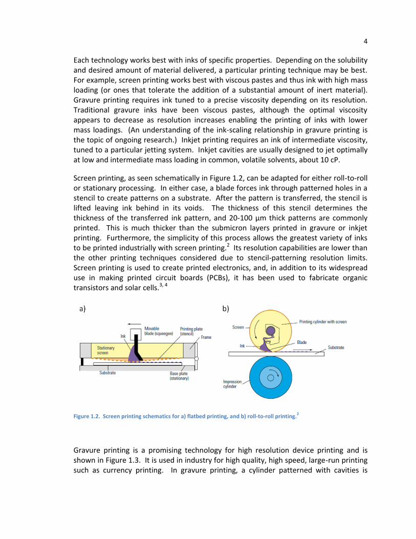
Screen printing, as seen schematically in Figure 1.2, can be adapted for either roll-to-roll or stationary processing. In either case, a blade forces ink through patterned holes in a stencil to create patterns on a substrate. After the pattern is transferred, the stencil is lifted leaving ink behind in its voids. The thickness of this stencil determines the thickness of the transferred ink pattern, and 20-100 μm thick patterns are commonly printed. This is much thicker than the submicron layers printed in gravure or inkjet printing. Furthermore, the simplicity of this process allows the greatest variety of inks to be printed industrially with screen printing.2 Its resolution capabilities are lower than the other printing techniques considered due to stencil-patterning resolution limits. Screen printing is used to create printed electronics, and, in addition to its widespread use in making printed circuit boards (PCBs), it has been used to fabricate organic transistors and solar cells.3, 4

Figure 1.2. Screen printing schematics for a) flatbed printing, and b) roll-to-roll printing.2

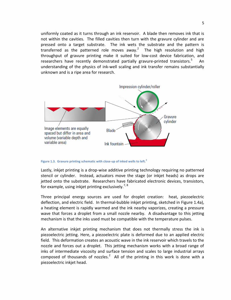
Gravure printing is a promising technology for high resolution device printing and is shown in Figure 1.3. It is used in industry for high quality, high speed, large-run printing such as currency printing. In gravure printing, a cylinder patterned with cavities is

5

uniformly coated as it turns through an ink reservoir. A blade then removes ink that is not within the cavities. The filled cavities then turn with the gravure cylinder and are pressed onto a target substrate. The ink wets the substrate and the pattern is transferred as the patterned role moves away.2 The high resolution and high throughput of gravure printing make it suited for low-cost device fabrication, and researchers have recently demonstrated partially gravure-printed transistors.5 An understanding of the physics of ink-well scaling and ink transfer remains substantially unknown and is a ripe area for research.

Figure 1.3. Gravure printing schematic with close-up of inked wells to left.2

Lastly, inkjet printing is a drop-wise additive printing technology requiring no patterned stencil or cylinder. Instead, actuators move the stage (or inkjet heads) as drops are jetted onto the substrate. Researchers have fabricated electronic devices, transistors, for example, using inkjet printing exclusively.7, 8

Three principal energy sources are used for droplet creation: heat, piezoelectric deflection, and electric field. In thermal-bubble inkjet printing, sketched in Figure 1.4a), a heating element is rapidly warmed and the ink nearby vaporizes, creating a pressure wave that forces a droplet from a small nozzle nearby. A disadvantage to this jetting mechanism is that the inks used must be compatible with the temperature pulses.

An alternative inkjet printing mechanism that does not thermally stress the ink is piezoelectric jetting. Here, a piezoelectric plate is deformed due to an applied electric field. This deformation creates an acoustic wave in the ink reservoir which travels to the nozzle and forces out a droplet. This jetting mechanism works with a broad range of inks of intermediate viscosity and surface tension and scales to large industrial arrays composed of thousands of nozzles.2 All of the printing in this work is done with a piezoelectric inkjet head.

6

A final jetting technology is notable for its ability to create small jetted drops, which are useful for printing the highest resolution circuits. Electrohydrodynamic printing, seen in Figure 1.4c), uses an electric field between a pendant drop of ink at the jetting nozzle and the substrate to deform the meniscus of this nozzle drop and force a small drop from its nadir.6 Unlike the previous two jetting mechanisms, the drop size can be far smaller than the nozzle diameter allowing small drops to form without the nozzle clogging and ink-drying problems that become increasingly prevalent with at small size scales in thermal and piezoelectric jetting. Disadvantages to electrohydrodynamic jetting include the need for an unshielded ground plane at or very near the substrate, which may be difficult or impossible in certain printing applications, and the fact that the scaling of such technologies to large arrays has not yet been achieved.

Figure 1.4. Inkjet printing technologies, a) thermal bubble, b) piezoelectric,2 and c) electrohydrodynamic.

6

1.3 Wetting and Patterned Bead Formation

The creation of patterned beads through printing is governed foremost by wetting, though other effects including colloidal dynamics, phase change, and chemical reactions may also play a role. A liquid drop impinging upon a substrate, with contact angle , flows and wets the substrate such that total interfacial energy is minimized. At minimum energy, the drop will adopt the form of a spherical cap that meets the substrate at an equilibrium contact angle, θeq, as given by the Young-Dupre equation below.

(1)

The fluid’s surface tension is , and and represent the substrate-liquid and substrate-air interfacial tensions, respectively, as shown in Figure 1.5.

7

Figure 1.5. Partially wetting drop cross section with interfacial tensions labeled.

The substrates in this work are rough and have defects, and the printed inks dry and deposit solute. For both of these reasons, the contact line’s advancing ( ) and receding ( ) contact angle separate in value leading to contact-angle hysteresis. The contact line is stable when , else it retreats or advances as appropriate. Evaporating colloidal inks often have zero retreating contact angle and are said to have pinned contact lines that may advance but never retreat.

Contact-angle hysteresis means that for a wetting drop of given volume, neither drop shape nor contact line are uniquely specified. For example, a spherical cap drop with a certain and zero is stable at any drop radius size with . There is a one parameter family of solutions, having circular contact lines and a contact angle lying between zero and . In Chapter 4, we propose to exploit this non-uniqueness to explore the equilibrium shapes of more complex drops. We will realize one solution for a given contact line and use time and mass loss as a parameter to reach other stable solutions.

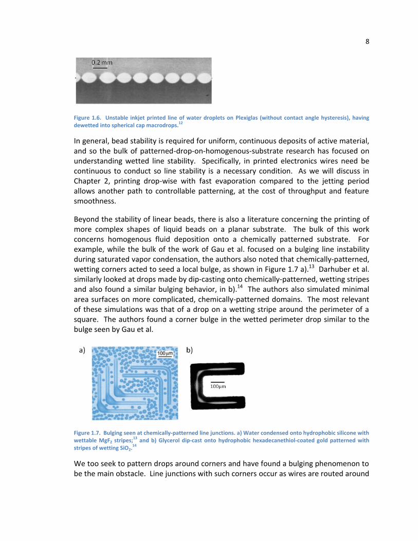
Cylinders of liquid in air, longer than π times their diameter, are unstable and break into drops, minimizing surface energy. This effect, known as the Rayleigh-Plateau instability, was first studied by Joseph Plateau and explained by Lord Rayleigh. 9, 10 Liquid rivulets on a substrate also tend to decompose into droplets, and considerable work has been devoted to this problem of wetted line (rivulet) stability. Davis derived the stability conditions for wetted beads for several contact line boundary conditions,11 and Schiaffino and Sonin further developed the stability model and provided experimental confirmation with printed lines, shown below in Figure 1.6.12 Davis showed that if the contact line is free to move and the contact angle is fixed by the Young condition, then a rivulet is always unstable and will always decompose into droplets. By contrast, if the contact line is pinned, the rivulet is stable for contact angles less than 90°.

8

Figure 1.6. Unstable inkjet printed line of water droplets on Plexiglas (without contact angle hysteresis), having dewetted into spherical cap macrodrops.

12

In general, bead stability is required for uniform, continuous deposits of active material, and so the bulk of patterned-drop-on-homogenous-substrate research has focused on understanding wetted line stability. Specifically, in printed electronics wires need be continuous to conduct so line stability is a necessary condition. As we will discuss in Chapter 2, printing drop-wise with fast evaporation compared to the jetting period allows another path to controllable patterning, at the cost of throughput and feature smoothness.

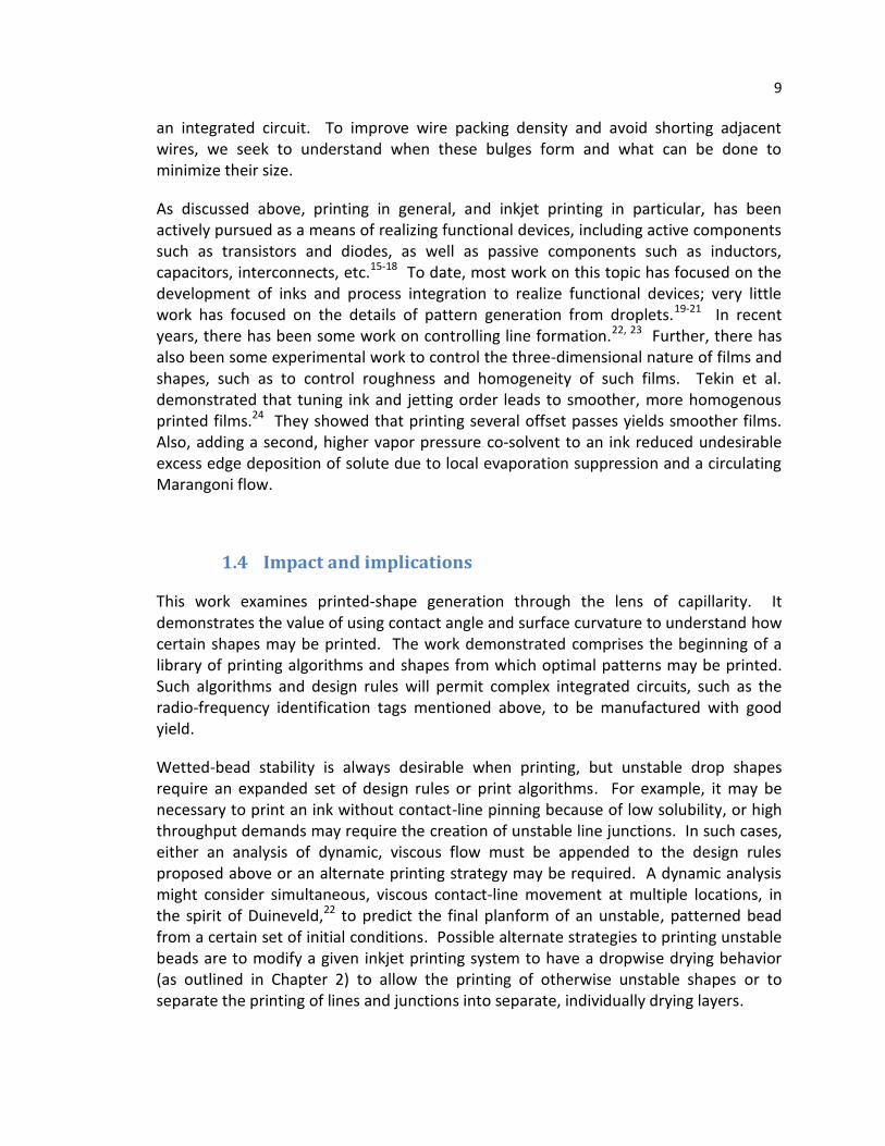
Beyond the stability of linear beads, there is also a literature concerning the printing of more complex shapes of liquid beads on a planar substrate. The bulk of this work concerns homogenous fluid deposition onto a chemically patterned substrate. For example, while the bulk of the work of Gau et al. focused on a bulging line instability during saturated vapor condensation, the authors also noted that chemically-patterned, wetting corners acted to seed a local bulge, as shown in Figure 1.7 a).13 Darhuber et al. similarly looked at drops made by dip-casting onto chemically-patterned, wetting stripes and also found a similar bulging behavior, in b).14 The authors also simulated minimal area surfaces on more complicated, chemically-patterned domains. The most relevant of these simulations was that of a drop on a wetting stripe around the perimeter of a square. The authors found a corner bulge in the wetted perimeter drop similar to the bulge seen by Gau et al.

Figure 1.7. Bulging seen at chemically-patterned line junctions. a) Water condensed onto hydrophobic silicone with wettable MgF2 stripes;

13 and b) Glycerol dip-cast onto hydrophobic hexadecanethiol-coated gold patterned with

stripes of wetting SiO2.14

We too seek to pattern drops around corners and have found a bulging phenomenon to be the main obstacle. Line junctions with such corners occur as wires are routed around

9

an integrated circuit. To improve wire packing density and avoid shorting adjacent wires, we seek to understand when these bulges form and what can be done to minimize their size.

As discussed above, printing in general, and inkjet printing in particular, has been actively pursued as a means of realizing functional devices, including active components such as transistors and diodes, as well as passive components such as inductors, capacitors, interconnects, etc.15-18 To date, most work on this topic has focused on the development of inks and process integration to realize functional devices; very little work has focused on the details of pattern generation from droplets.19-21 In recent years, there has been some work on controlling line formation.22, 23 Further, there has also been some experimental work to control the three-dimensional nature of films and shapes, such as to control roughness and homogeneity of such films. Tekin et al. demonstrated that tuning ink and jetting order leads to smoother, more homogenous printed films.24 They showed that printing several offset passes yields smoother films. Also, adding a second, higher vapor pressure co-solvent to an ink reduced undesirable excess edge deposition of solute due to local evaporation suppression and a circulating Marangoni flow.

1.4 Impact and implications

This work examines printed-shape generation through the lens of capillarity. It demonstrates the value of using contact angle and surface curvature to understand how certain shapes may be printed. The work demonstrated comprises the beginning of a library of printing algorithms and shapes from which optimal patterns may be printed. Such algorithms and design rules will permit complex integrated circuits, such as the radio-frequency identification tags mentioned above, to be manufactured with good yield.

Wetted-bead stability is always desirable when printing, but unstable drop shapes require an expanded set of design rules or print algorithms. For example, it may be necessary to print an ink without contact-line pinning because of low solubility, or high throughput demands may require the creation of unstable line junctions. In such cases, either an analysis of dynamic, viscous flow must be appended to the design rules proposed above or an alternate printing strategy may be required. A dynamic analysis might consider simultaneous, viscous contact-line movement at multiple locations, in the spirit of Duineveld,22 to predict the final planform of an unstable, patterned bead from a certain set of initial conditions. Possible alternate strategies to printing unstable beads are to modify a given inkjet printing system to have a dropwise drying behavior (as outlined in Chapter 2) to allow the printing of otherwise unstable shapes or to separate the printing of lines and junctions into separate, individually drying layers.

10

1.5 Works cited

1. Razavi, B., Design of analog CMOS integrated circuits. McGraw-Hill: Boston, MA, 2001; p xx, 684 p. 2. Kipphan, H., Handbook of print media : technologies and production methods. Springer: Berlin ; New York, 2001. 3. Bao, Z. N.; Feng, Y.; Dodabalapur, A.; Raju, V. R.; Lovinger, A. J., High-performance plastic transistors fabricated by printing techniques. Chemistry of Materials 1997, 9, (6), 1299-&. 4. Shaheen, S. E.; Radspinner, R.; Peyghambarian, N.; Jabbour, G. E., Fabrication of bulk heterojunction plastic solar cells by screen printing. Applied Physics Letters 2001, 79, (18), 2996-2998. 5. Vornbrock, A. D.; Sung, D. V.; Kang, H. K.; Kitsomboonloha, R.; Subramanian, V., Fully gravure and ink-jet printed high speed pBTTT organic thin film transistors. Organic Electronics 2010, 11, (12), 2037-2044. 6. Park, J. U.; Hardy, M.; Kang, S. J.; Barton, K.; Adair, K.; Mukhopadhyay, D. K.; Lee, C. Y.; Strano, M. S.; Alleyne, A. G.; Georgiadis, J. G.; Ferreira, P. M.; Rogers, J. A., High-resolution electrohydrodynamic jet printing. Nature Materials 2007, 6, (10), 782-789. 7. Sirringhaus, H.; Kawase, T.; Friend, R. H.; Shimoda, T.; Inbasekaran, M.; Wu, W.; Woo, E. P., High-resolution inkjet printing of all-polymer transistor circuits. Science 2000, 290, (5499), 2123-2126. 8. Tseng, H.-Y.; Subramanian, V., All inkjet-printed, fully self-aligned transistors for low-cost circuit applications. Organic Electronics 2011, 12, (2), 249-256. 9. Plateau, J., Statique expérimentale et théorique des liquides soumis aux seules forces moléculaires. Gauthier-Villars: 1873. 10. Rayleigh, B., Scientific papers. University press: 1900. 11. Davis, S. H., MOVING CONTACT LINES AND RIVULET INSTABILITIES .1. THE STATIC RIVULET. Journal of Fluid Mechanics 1980, 98, (MAY), 225-242. 12. Schiaffino, S.; Sonin, A. A., Formation and stability of liquid and molten beads on a solid surface. Journal of Fluid Mechanics 1997, 343, 95-110. 13. Gau, H.; Herminghaus, S.; Lenz, P.; Lipowsky, R., Liquid morphologies on structured surfaces: From microchannels to microchips. Science 1999, 283, (5398), 46-49. 14. Darhuber, A. A.; Troian, S. M.; Miller, S. M.; Wagner, S., Morphology of liquid microstructures on chemically patterned surfaces. Journal of Applied Physics 2000, 87, (11), 7768-7775. 15. Redinger, D.; Molesa, S.; Yin, S.; Farschi, R.; Subramanian, V., An ink-jet-deposited passive component process for RFID. Ieee Transactions on Electron Devices 2004, 51, (12), 1978-1983. 16. Noh, Y. Y.; Zhao, N.; Caironi, M.; Sirringhaus, H., Downscaling of self-aligned, all-printed polymer thin-film transistors (vol 2, pg 784, 2007). Nature Nanotechnology 2008, 3, (1), 58-58. 17. Sele, C. W.; von Werne, T.; Friend, R. H.; Sirringhaus, H., Lithography-free, self-aligned inkjet printing with sub-hundred-nanometer resolution. Advanced Materials 2005, 17, (8), 997-+.

11

18. Tseng, H.-Y.; Subramanian, V., All inkjet printed self-aligned transistors and circuits applications. In 2009 International Electron Devices Meeting (IEDM), IEEE International: 2009; pp 1-4. 19. Kawase, T.; Shimoda, T.; Newsome, C.; Sirringhaus, H.; Friend, R. H., Inkjet printing of polymer thin film transistors. Thin Solid Films 2003, 438, 279-287. 20. Paul, K. E.; Wong, W. S.; Ready, S. E.; Street, R. A., Additive jet printing of polymer thin-film transistors. Applied Physics Letters 2003, 83, (10), 2070-2072. 21. Subramanian, V.; Frechet, J. M. J.; Chang, P. C.; Huang, D. C.; Lee, J. B.; Molesa, S. E.; Murphy, A. R.; Redinger, D. R., Progress toward development of all-printed RFID tags: Materials, processes, and devices. Proceedings of the Ieee 2005, 93, (7), 1330-1338. 22. Duineveld, P. C., The stability of ink-jet printed lines of liquid with zero receding contact angle on a homogeneous substrate. Journal of Fluid Mechanics 2003, 477, 175-200. 23. Smith, P. J.; Shin, D. Y.; Stringer, J. E.; Derby, B.; Reis, N., Direct ink-jet printing and low temperature conversion of conductive silver patterns. Journal of Materials Science 2006, 41, (13), 4153-4158. 24. Tekin, E.; de Gans, B. J.; Schubert, U. S., Ink-jet printing of polymers - from single dots to thin film libraries. Journal of Materials Chemistry 2004, 14, (17), 2627-2632.

12

2 Printed-line formation

2.1 Introduction

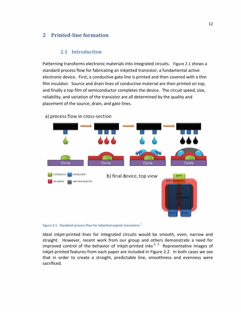
Patterning transforms electronic materials into integrated circuits. Figure 2.1 shows a

standard process flow for fabricating an inkjetted transistor, a fundamental active

electronic device. First, a conductive gate line is printed and then covered with a thin

film insulator. Source and drain lines of conductive material are then printed on top,

and finally a top film of semiconductor completes the device. The circuit speed, size,

reliability, and variation of the transistor are all determined by the quality and

placement of the source, drain, and gate lines.

Figure 2.1. Standard process flow for inkjetted organic transistors.1

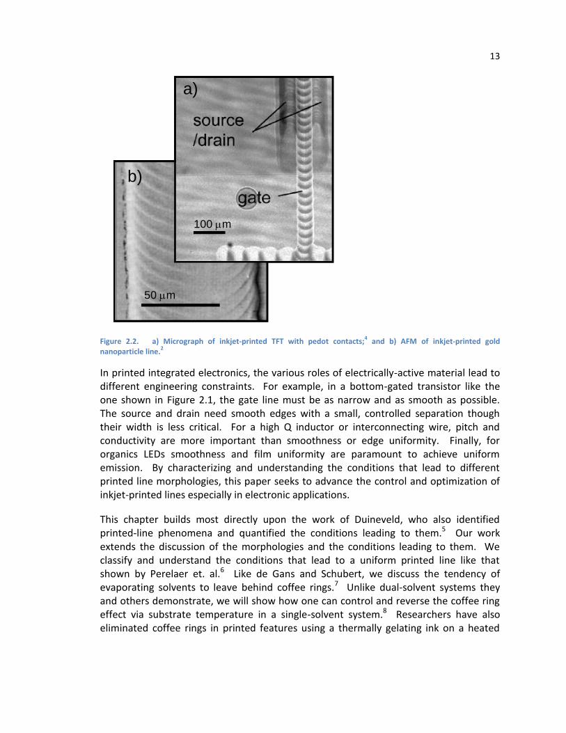
Ideal inkjet-printed lines for integrated circuits would be smooth, even, narrow and straight. However, recent work from our group and others demonstrate a need for improved control of the behavior of inkjet-printed inks.2, 3 Representative images of inkjet-printed features from each paper are included in Figure 2.2. In both cases we see that in order to create a straight, predictable line, smoothness and evenness were sacrificed.

13

Figure 2.2. a) Micrograph of inkjet-printed TFT with pedot contacts;4 and b) AFM of inkjet-printed gold

nanoparticle line.2

In printed integrated electronics, the various roles of electrically-active material lead to different engineering constraints. For example, in a bottom-gated transistor like the one shown in Figure 2.1, the gate line must be as narrow and as smooth as possible. The source and drain need smooth edges with a small, controlled separation though their width is less critical. For a high Q inductor or interconnecting wire, pitch and conductivity are more important than smoothness or edge uniformity. Finally, for organics LEDs smoothness and film uniformity are paramount to achieve uniform emission. By characterizing and understanding the conditions that lead to different printed line morphologies, this paper seeks to advance the control and optimization of inkjet-printed lines especially in electronic applications.

This chapter builds most directly upon the work of Duineveld, who also identified printed-line phenomena and quantified the conditions leading to them.5 Our work extends the discussion of the morphologies and the conditions leading to them. We classify and understand the conditions that lead to a uniform printed line like that shown by Perelaer et. al.6 Like de Gans and Schubert, we discuss the tendency of evaporating solvents to leave behind coffee rings.7 Unlike dual-solvent systems they and others demonstrate, we will show how one can control and reverse the coffee ring effect via substrate temperature in a single-solvent system.8 Researchers have also eliminated coffee rings in printed features using a thermally gelating ink on a heated

50 m

b)

a)

100 m

50 m

b)

a)

100 m

14

substrate.9 Finally, our work offers counter evidence to a theoretical result that coffee-ring features are enhanced when evaporation is decreased.10

2.2 Experiment

We carry out this portion of our experiments on a custom-built research inkjet printer.

We use Microfab piezoelectric drop-on-demand dispensing heads with a 60 m orifice.

Our stages have x, y and rotational degrees of freedom with 1 m accuracy. Operating in drop-on-demand mode, our printer has a base drop frequency of approximately 30 Hz, with the option to delay dropping further. Falling drops have a diameter similar to the dispensing head orifice, a volume of approximately 100 pL and eject at 1-2 m/s, though there is significant variation due to ink, atmospheric and substrate conditions.

The ink used throughout this experiment is poly(3,4-ethylenedioxythiophene) poly(styrenesulfonate), PEDOT:PSS 1.3% by weight in water from Aldrich, referred to as pedot hereafter. It is a common conductive polymer used for organic LEDs and as an antistatic coating. We printed onto 5 cm by 7 cm glass slides coated with spun poly(4-vinylphenol) dielectric, PVP, thermally cross-linked at 200°C. Since we commonly use PVP both as a smoothing layer on low-cost plastic and a thin printable dielectric, the PVP insured that our results will be transferable to low-cost substrates.11 AFM profiling reveals the PVP film to be exceptionally smooth, with RMS roughness of 3.34 Å. The static contact angle of pedot on the PVP-coated glass is 82.7±1.7°, as extracted from a sessile drop by a Kruss Contact Angle Measuring System. We assume that this approximates the advancing contact angle. Under no conditions do we observe the contact line to retreat and thus we assume zero retreating contact angle as others have seen when working with aqueous pedot ink.5

The independent variables used in this experiment are substrate temperature, drop spacing, and drop frequency. The PVP-coated glass substrate and pedot ink remain constant. The substrate is cooled to 17°C via a cooling water line and heated to as warm

as 60°C. Drop spacing varies from 5 m to 100 m center-to-center. At low spacing, an overflowing, irregular bead forms, and isolated drops land at large spacing. (Note: we refer to a printed bead when wet and to a printed line once dried.) Finally, as mentioned above, the minimum drop-on-demand delay is about 30 ms on our printer. Delays from 10 ms to 2000 ms seconds are appended, though at the one second timescale, clogging becomes a problem as the ink has sufficient time to form a skin at the nozzle. Misdirected drops and/or clogs often result from delays of 1000-2000ms; this limit places an upper limit on delay for low temperature substrates. Once printed, the resulting patterns are measured and quantified with a variety of tools, especially an optical microscope and mechanical-stylus profilometer.

15

2.3 Results

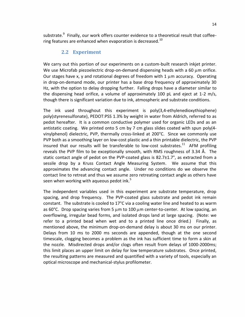
A few principal behaviors emerge when examining printed pedot patterns across a variety of drop spacings, delay periods and temperatures. We label these as individual drops, scalloped line, uniform line, bulging line, and stacked coins. Figure 2.3 shows these five basic morphologies.

Figure 2.3. Examples of principal printed-line behaviors: a) individual drops; b) scalloped; c) uniform; d) bulging; and e) stacked coins. Drop spacing decreases from left to right.

If one prints drops too far separated to interact, more than twice a drop’s radius, then isolated drops land and dry. Individual drops occur at drop spacings above about 100

m independent of temperature or delay in our system.

At lower temperature, as drop spacing decreases, isolated drops overlap and merge but retain individual rounded contact lines, and a scalloped pattern emerges. These

100 m

c)b)a) d) e)

150 m

100 m

c)b)a) d) e)

150 m

16

scalloped lines are narrower than an isolated drop as fluid expansion is partially arrested.

Further decreasing the drop spacing eliminates the scalloping and leads to a smooth, straight line. These lines have a uniform, smooth edge and top. They are the narrowest lines printed.

Printing drops even closer together leads to discrete bulging along the line’s length, separated by regions of uniform narrow line. These bulges tend to form periodically and also at the beginning of the line. Duineveld gives this striking behavior excellent consideration. Essentially additional fluid from printing exceeds a bead’s equilibrium contact angle and discreet regions of outflow result, leading to rounded bulges in the dried feature.5

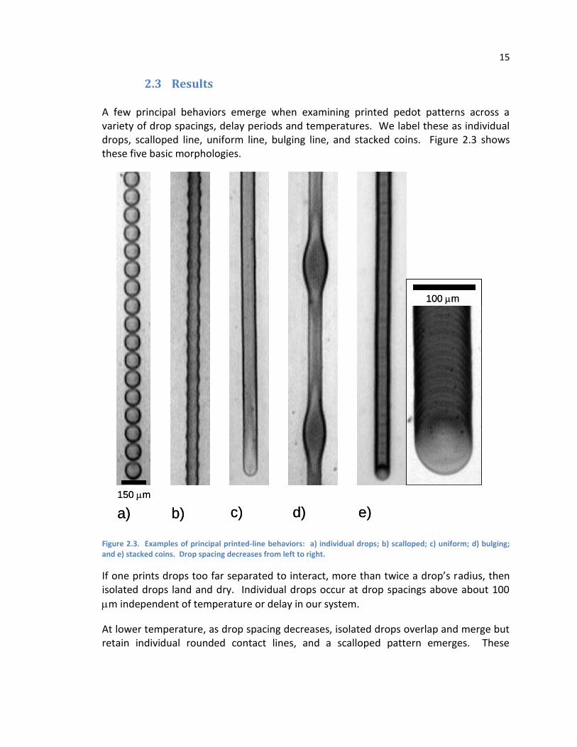
If the substrate temperature increases such that the evaporation time of a single drop is less than the drop jetting period, then each landing drop will dry individually regardless of overlap, leading to what look like offset stacked coins (as also shown in Figure 2.4). At a given substrate temperature, increasing drop delay will effect the onset of the stacked coin behavior. Drop spacing has no effect on the width of lines printed in this regime since each drop dries individually. Figure 2.4 schematically shows where each of these behaviors tend to be found relative to one another at an intermediate temperature.

Figure 2.4. Typical printed line behavior at an intermediate temperature.

By carefully optimizing drop frequency, temperature and spacing it is possible to print a smooth, narrow line with an even edge. Qualitatively, the ideal line avoids bulging by slowing down the drop frequency until the advancing contact angle is never exceeded, but is not so slow that drops dry within the period of one or two drops landing avoiding

drop spacing

delay scalloped

line

bulging

stacked coins

uniform

line

isolated

drops

drop spacing

delay scalloped

line

bulging

stacked coins

uniform

line

isolated

drops

drop spacing

delay scalloped

line

bulging

stacked coins

uniform

line

isolated

drops

17

stacked coins. It has a low enough drop spacing to avoid scalloping, and the delay is not so slow that the dropping frequency is comparable to the time it takes for the orifice to form a skin thereby avoiding unpredictable drop trajectories. Figure 2.5 shows the experimental conditions where this good profile is found for practical temperatures from 17°C to 60°C. As expected, acceptable delay and spacing decrease at higher temperature. In fact, at 45°C and above uniform lines could be printed at the native frequency of our printer. At temperatures above 60°C it is increasingly difficult to print uniform lines as the stacked coin behavior occurs at lower dropping frequency and solvent evaporation at the inkjet head leads to reliability issues.

Figure 2.5. Experimental space leading to a uniform line, 17°C to 60°C.

A second effect, important to the quality and utility of the printed line, is seen by comparing the cross-sections of these ideal lines across the range of temperatures. Figure 2.6 shows traces across uniform lines taken by a mechanical stylus profiler (Alpha-Step IQ Surface Profiler). Whereas the profile is smooth and convex at low temperature, the profile becomes increasingly concave at higher temperature. Indeed, at room temperature (30°C) this transition towards a concave profile appears as a squared cross-section. Interestingly, this temperature dependent coffee ring control is valid for any of the above five principal line behaviors. One can tune the relative distribution of material across the printed line by controlling drop temperature for any of the five line behaviors, a useful result for printing.

0

200

400

600

0 25 50 75

drop spacing (m)

dela

y (

ms)

17 C 30 C 45 C 60 C

18

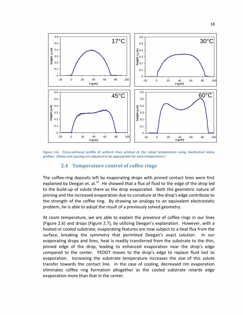
Figure 2.6. Cross-sectional profile of uniform lines printed at the noted temperature using mechanical stylus profiler. (Delay and spacing are adjusted to be appropriate for each temperature.)

2.4 Temperature control of coffee rings

The coffee-ring deposits left by evaporating drops with pinned contact lines were first explained by Deegan et. al.12 He showed that a flux of fluid to the edge of the drop led to the build-up of solute there as the drop evaporated. Both the geometric nature of pinning and the increased evaporation due to curvature at the drop’s edge contribute to the strength of the coffee ring. By drawing an analogy to an equivalent electrostatic problem, he is able to adopt the result of a previously solved geometry.

At room temperature, we are able to explain the presence of coffee rings in our lines (Figure 2.6) and drops (Figure 2.7), by utilizing Deegan’s explanation. However, with a heated or cooled substrate, evaporating features are now subject to a heat flux from the surface, breaking the symmetry that permitted Deegan’s exact solution. In our evaporating drops and lines, heat is readily transferred from the substrate to the thin, pinned edge of the drop, leading to enhanced evaporation near the drop’s edge compared to the center. PEDOT moves to the drop’s edge to replace fluid lost to evaporation. Increasing the substrate temperature increases the size of this solute transfer towards the contact line. In the case of cooling, decreased rim evaporation eliminates coffee ring formation altogether as the cooled substrate retards edge evaporation more than that in the center.

0

0.1

0.2

0.3

0.4

0.5

0.6

-20 0 20 40 60 80 100

x (m)

heig

ht

(m

)

0

0.1

0.2

0.3

0.4

0.5

0.6

-20 0 20 40 60 80 100x (m)

heig

ht

(m

)

0

0.1

0.2

0.3

0.4

0.5

0.6

-20 0 20 40 60 80 100

x (m)

heig

ht

(m

)

0

0.1

0.2

0.3

0.4

0.5

0.6

-20 0 20 40 60 80 100x (m)

heig

ht

(m

)

45°C

17°C 30°C

60°C

0

0.1

0.2

0.3

0.4

0.5

0.6

-20 0 20 40 60 80 100

x (m)

heig

ht

(m

)

0

0.1

0.2

0.3

0.4

0.5

0.6

-20 0 20 40 60 80 100x (m)

heig

ht

(m

)

0

0.1

0.2

0.3

0.4

0.5

0.6

-20 0 20 40 60 80 100

x (m)

heig

ht

(m

)

0

0.1

0.2

0.3

0.4

0.5

0.6

-20 0 20 40 60 80 100x (m)

heig

ht

(m

)

45°C

17°C 30°C

60°C

19

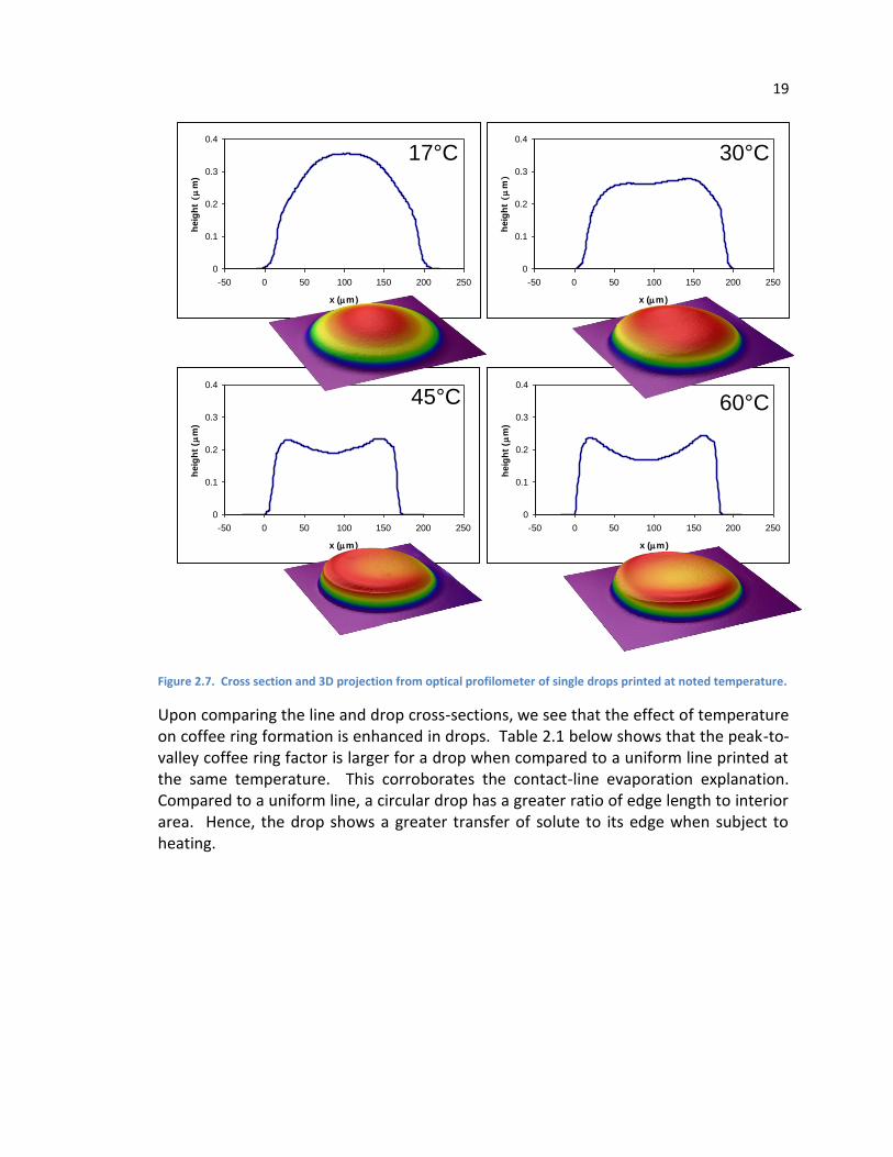
Figure 2.7. Cross section and 3D projection from optical profilometer of single drops printed at noted temperature.

Upon comparing the line and drop cross-sections, we see that the effect of temperature on coffee ring formation is enhanced in drops. Table 2.1 below shows that the peak-to-valley coffee ring factor is larger for a drop when compared to a uniform line printed at the same temperature. This corroborates the contact-line evaporation explanation. Compared to a uniform line, a circular drop has a greater ratio of edge length to interior area. Hence, the drop shows a greater transfer of solute to its edge when subject to heating.

0

0.1

0.2

0.3

0.4

-50 0 50 100 150 200 250

x (m)

heig

ht

(m

)

0

0.1

0.2

0.3

0.4

-50 0 50 100 150 200 250

x (m)

heig

ht

(m

)

0

0.1

0.2

0.3

0.4

-50 0 50 100 150 200 250

x (m)

heig

ht

(m

)

0

0.1

0.2

0.3

0.4

-50 0 50 100 150 200 250

x (m)

heig

ht

(m

)

45°C

17°C 30°C

60°C

0

0.1

0.2

0.3

0.4

-50 0 50 100 150 200 250

x (m)

heig

ht

(m

)

0

0.1

0.2

0.3

0.4

-50 0 50 100 150 200 250

x (m)

heig

ht

(m

)

0

0.1

0.2

0.3

0.4

-50 0 50 100 150 200 250

x (m)

heig

ht

(m

)

0

0.1

0.2

0.3

0.4

-50 0 50 100 150 200 250

x (m)

heig

ht

(m

)

45°C

17°C 30°C

60°C

20

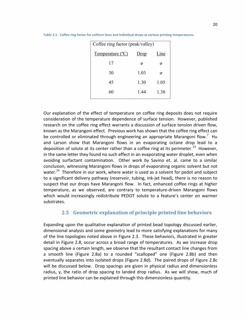
Table 2.1. Coffee ring factor for uniform lines and individual drops at various printing temperatures.

Coffee ring factor (peak/valley)

Temperature (ºC) Drop Line

17 ø ø

30 1.03 ø

45 1.30 1.05

60 1.44 1.38

Our explanation of the effect of temperature on coffee ring deposits does not require consideration of the temperature dependence of surface tension. However, published research on the coffee ring effect warrants a discussion of surface tension driven flow, known as the Marangoni effect. Previous work has shown that the coffee ring effect can be controlled or eliminated through engineering an appropriate Marangoni flow.7 Hu and Larson show that Marangoni flows in an evaporating octane drop lead to a deposition of solute at its center rather than a coffee ring at its perimeter.13 However, in the same letter they found no such effect in an evaporating water droplet, even when avoiding surfactant contamination. Other work by Savino et. al. came to a similar conclusion, witnessing Marangoni flows in drops of evaporating organic solvent but not water.14 Therefore in our work, where water is used as a solvent for pedot and subject to a significant delivery pathway (reservoir, tubing, ink-jet head), there is no reason to suspect that our drops have Marangoni flow. In fact, enhanced coffee rings at higher temperature, as we observed, are contrary to temperature-driven Marangoni flows which would increasingly redistribute PEDOT solute to a feature’s center on warmer substrates.

2.5 Geometric explanation of principle printed line behaviors

Expanding upon the qualitative explanation of printed bead topology discussed earlier, dimensional analysis and some geometry lead to more satisfying explanations for many of the line topologies noted above in Figure 2.3. These behaviors, illustrated in greater detail in Figure 2.8, occur across a broad range of temperatures. As we increase drop spacing above a certain length, we observe that the resultant contact line changes from a smooth line (Figure 2.8a) to a rounded “scalloped” one (Figure 2.8b) and then eventually separates into isolated drops (Figure 2.8d). The paired drops of Figure 2.8c will be discussed below. Drop spacings are given in physical radius and dimensionless radius, y, the ratio of drop spacing to landed drop radius. As we will show, much of printed line behavior can be explained through this dimensionless quantity.

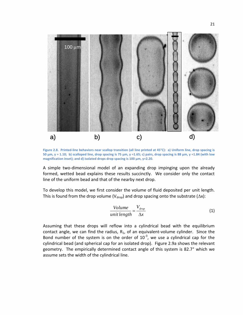
21

Figure 2.8. Printed-line behaviors near scallop transition (all line printed at 45°C): a) Uniform line, drop spacing is 50 μm, y = 1.10; b) scalloped line, drop spacing is 75 μm, y =1.65; c) pairs, drop spacing is 88 μm, y =1.84 (with low magnification inset); and d) isolated drops drop spacing is 100 μm, y=2.20.

A simple two-dimensional model of an expanding drop impinging upon the already formed, wetted bead explains these results succinctly. We consider only the contact line of the uniform bead and that of the nearby next drop.

To develop this model, we first consider the volume of fluid deposited per unit length.

This is found from the drop volume (Vdrop) and drop spacing onto the substrate (x):

x

V

lengthunit

Volume drop

(1)

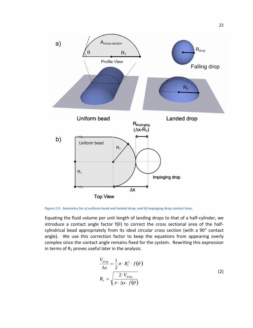
Assuming that these drops will reflow into a cylindrical bead with the equilibrium contact angle, we can find the radius, R1, of an equivalent-volume cylinder. Since the Bond number of the system is on the order of 10-3, we use a cylindrical cap for the cylindrical bead (and spherical cap for an isolated drop). Figure 2.9a shows the relevant geometry. The empirically determined contact angle of this system is 82.7° which we assume sets the width of the cylindrical line.

a) b) c) d)

100 m

a) b) c) d)

100 m100 m

22

Figure 2.9. Geometry for a) uniform bead and landed drop; and b) impinging drop contact lines.

Equating the fluid volume per unit length of landing drops to that of a half-cylinder, we

introduce a contact angle factor f() to correct the cross sectional area of the half-cylindrical bead appropriately from its ideal circular cross section (with a 90° contact angle). We use this correction factor to keep the equations from appearing overly complex since the contact angle remains fixed for the system. Rewriting this expression in terms of R1 proves useful later in the analysis.

( )

( )

fx

VR

fRx

V

drop

drop

2

2

1

1

2

1

(2)

23

The correction factor f() can be determined from the height equation for a wetting drop of radius R1 with a finite contact angle. Its height, h, is a function of the radial coordinate, r.

( ) tansin

12

2

2

1 Rr

Rrh (3)

In equation 4 below we calculate the actual cross-sectional area of the bead by integrating the height profile and then equate the resulting expression with a circular

cross-sectional area times a correction factor. We can then solve for f(), which in our particular system (with a single contact angle) is a scalar number, approximately 0.852.

( ) ( )

( )

( ) 852.07.82

cotsin

22

2

1

22

1

sec

2

1sec

1

1

f

R

Af

fRrhdrA

tioncross

R

Rtioncross

(4)

Based upon the observed radius of a falling drop, 28 m, we find that each drop has a volume of about 90 pL. Upon examining the printed substrate, we find that the isolated

drop radius, R0, is 42.3 m, larger than the 38.7 m radius of a landed 90 pL drop with an 82.7° contact angle. Thus, a printed drop overexpands and remains pinned. (Its contact angle is a reduced 76.1°.) In order to account for this overexpansion, we define another accommodation factor in equation 5, g(R0), to link drop volume and substrate R0. (We note that g depends on several factors including drop fluid, momentum, and size, and although it remains constant for our experiment, we expect that it would vary in other situations). The g parameter scales distances in our calculations in terms of R0,

which is easily observed and relevant to ultimate bead profile. For a 90pL drop with a

42.3 m landed radius, we find that g is about 0.568.

( )

( )

( ) 568.03.42

3

2

3

2

0

3

0

0

0

3

0

mRg

R

VRg

RgRV

drop

drop

(5)

To find a convenient dimensionless expression for cylindrical-bead radius, we scale R1

from equation 2 by R0 and introduce the dimensionless spacing y ≡ x/ R0 in equation 6. Substituting for drop volume from equation 5, we arrive at a convenient dimensionless

24

expression for R1/R0. For the system under consideration, we substitute our correction factors into this expression to yield the bead radius as a function of y only.

( )

( )

( )

( )( ) yf

Rg

yR

R

Rfx

RgR

R

R

Rfx

V

R

R drop

888.0

3

4

3

22

2

0

0

1

2

0

0

3

0

0

1

2

00

1

(6)

Note that bead width as an inverse square of spacing is seen in recent efforts working from similar assumptions.15, 16 We present our derivation that emphasizes dimensionless spacing for clarity and completeness. The following work exploring the geometry of drop impingement and the implications to bead morphology is unique.

Having determined the cylindrical bead radius as a function of drop spacing, we now consider the interaction between a landing drop and the already-formed uniform bead on the substrate. We compare the energetics of drop spreading on a dry substrate to that of a drop spreading on an existing liquid film, the bead in our case. An outward moving contact line of a drop on a dry substrate is facilitated by a thin precursor film with a thickness on the order of angstroms. De Gennes showed that viscous energy dissipation during spreading is proportional to the fluid viscosity, η, times the logarithm of the spreading drop radius, R0, divided by the precursor film thickness, b.17

b

RE 0ln (7)

Should a liquid film be present, its thickness replaces the precursor film thickness. We expect that the wetted bead will have a thickness on the order of microns, rather than the angstrom thickness of the precursor film. Thus, drop expansion into the bead is energetically favored by several hundred percent. An expanding drop in contact with a wetted bead and dry substrate flows preferentially into that bead.

Assuming that drops generally flow into the wetted bead when possible, we now consider the event of a drop landing as we increase drop spacing. Figure 2.9b shows the contact line of a landing drop as it impinges upon a uniform bead. It is reasonable to assume a semicircular contact line at the end of a uniform bead to minimize curvature and thereby surface-tension pressure. A new drop lands directly on the wetted bead

first when x is less than R1 (equivalently y < 0.89), and the drop flows into the existing bead rather than expands its contact line beyond that set by the advancing contact

25

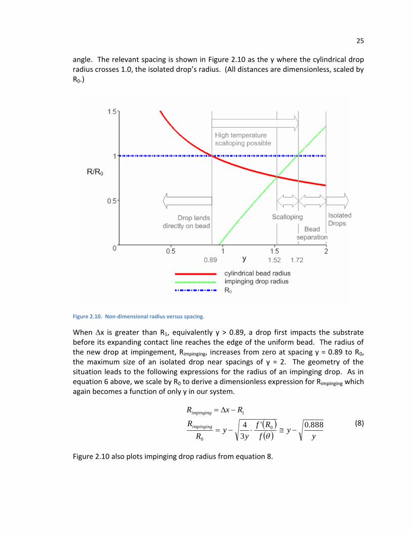
angle. The relevant spacing is shown in Figure 2.10 as the y where the cylindrical drop radius crosses 1.0, the isolated drop’s radius. (All distances are dimensionless, scaled by R0.)

Figure 2.10. Non-dimensional radius versus spacing.

When x is greater than R1, equivalently y > 0.89, a drop first impacts the substrate before its expanding contact line reaches the edge of the uniform bead. The radius of the new drop at impingement, Rimpinging, increases from zero at spacing y = 0.89 to R0, the maximum size of an isolated drop near spacings of y = 2. The geometry of the situation leads to the following expressions for the radius of an impinging drop. As in equation 6 above, we scale by R0 to derive a dimensionless expression for Rimpinging which again becomes a function of only y in our system.

( )( ) y

yf

Rf

yy

R

R

RxR

impinging

impinging

888.0'

3

4 0

0

1

(8)

Figure 2.10 also plots impinging drop radius from equation 8.

26

Comparing R1 and Rimpinging, we see that the cylindrical bead has a larger radius from y = 0.89 to a spacing of about 1.52. If we assume that the impinging drop immediately ceases contact-line expansion and preferentially flows into the cylindrical bead, then we would not expect to see scallops at spacings below y =1.52 since each landing drop is not wider than the bead width when it encounters the bead.

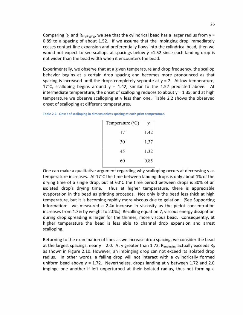
Experimentally, we observe that at a given temperature and drop frequency, the scallop behavior begins at a certain drop spacing and becomes more pronounced as that spacing is increased until the drops completely separate at y = 2. At low temperature, 17°C, scalloping begins around y = 1.42, similar to the 1.52 predicted above. At intermediate temperature, the onset of scalloping reduces to about y = 1.35, and at high temperature we observe scalloping at y less than one. Table 2.2 shows the observed onset of scalloping at different temperatures.

Table 2.2. Onset of scalloping in dimensionless spacing at each print temperature.

Temperature (ºC) y

17 1.42

30 1.37

45 1.32

60 0.85

One can make a qualitative argument regarding why scalloping occurs at decreasing y as temperature increases. At 17°C the time between landing drops is only about 1% of the drying time of a single drop, but at 60°C the time period between drops is 30% of an isolated drop’s drying time. Thus at higher temperature, there is appreciable evaporation in the bead as printing proceeds. Not only is the bead less thick at high temperature, but it is becoming rapidly more viscous due to gelation. (See Supporting Information: we measured a 2.4x increase in viscosity as the pedot concentration increases from 1.3% by weight to 2.0%.) Recalling equation 7, viscous energy dissipation during drop spreading is larger for the thinner, more viscous bead. Consequently, at higher temperature the bead is less able to channel drop expansion and arrest scalloping.

Returning to the examination of lines as we increase drop spacing, we consider the bead at the largest spacings, near y = 2.0. At y greater than 1.72, Rimpinging actually exceeds R0 as shown in Figure 2.10. However, an impinging drop can not exceed its isolated drop radius. In other words, a falling drop will not interact with a cylindrically formed uniform bead above y = 1.72. Nevertheless, drops landing at y between 1.72 and 2.0 impinge one another if left unperturbed at their isolated radius, thus not forming a

27

bead. (Circular drops overlap to y = 2.0.) This leads to the interesting contact-line separation behavior in Figure 2.8c.

At y between 1.72 and 2.0, a second drop will impinge upon a landed circular drop with radius R0 and flow into it as discussed above. Thus, it will not expand to its full isolated radius, and an elliptical contact line will form on the substrate. The next landing drop will not impinge upon this bead since it does not encounter the previous reflowed drop that did not fully expand to R0. It will instead land and remain at the isolated drop radius until the next drop lands and wets into it. This behavior will repeat in pairs indefinitely. As predicted, we see the onset of this contact line separation at y = 1.72 in our experimental data, and at 45°C we find optimal pairing around y = 1.84 (and similar behaviors at nearby spacings such as triples, alternating patterns, etc; see Supporting Information for micrographs of many printed lines with spacings around y = 1.72).

To summarize, we used a simple model utilizing contact lines to explain the transition between a uniform bead, a scalloped contact line and eventually bead separation. At low spacing, where the next drop lands directly on the bead, no scalloping takes place. At sufficient spacing the drop lands on the bare substrate first and its contact line expands from a point as a circle of growing radius. When the expanding drop diameter at bead impingement exceeds the bead width, scalloping occurs. Since the impinging drop radius exceeds the equilibrium bead radius at large spacings (nearly the drop diameter) drops may impinge upon a previous drop but not a formed bead. Paired groups and similar breakup phenomena result.

While the above discussion, based upon the meeting of contact lines, proves effective for predicting the line morphology as we vary drop spacing, it is not always useful in predicting outcomes including line width where several forces are in competition. For example at larger spacings before the onset of scalloping, circa y = 1.4, the spreading momentum of the falling drop on dry substrate competes with the flow into the bead once contact is made. Both effects compete, and an intermediate line width results (though the contact line does remain uniform). The interplay of these forces indicates that more sophisticated modeling would be useful for more precise predictions.

In order to corroborate the simple impingement flow model developed above and as an aid in visualization, we simulated the drop-landing-impinging event using commercial computational fluid dynamics software, Flow3D. It solves the three dimensional Navier-Stokes and mass continuity equations for a predetermined mesh using finite difference approximation with the volume-of-fluid method. The fluid is treated as a non-Newtonian, incompressible fluid with a sharply defined free surface. (In the volume-of-fluid method, the free interface is inferred from the fluid fraction of each grid cell. Since

each cell can contain at most one free-surface interface, the grid resolution, a 3 m cube in our case, determines when two free surfaces approaching one another are merged.) Heat transfer and phase change are not included for the relatively brief event

28

of drop impingement. The landing drop has the 82.7° contact angle with the impermeable planar substrate, and the preexisting bead has a pinned contact line which sets its initial contact angle to 82.7°. A no-slip condition is imposed on fluid in contact with the substrate.

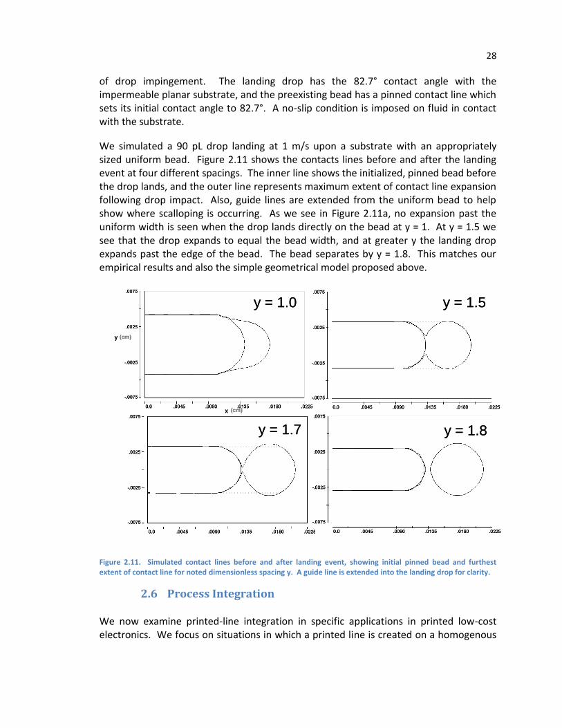
We simulated a 90 pL drop landing at 1 m/s upon a substrate with an appropriately sized uniform bead. Figure 2.11 shows the contacts lines before and after the landing event at four different spacings. The inner line shows the initialized, pinned bead before the drop lands, and the outer line represents maximum extent of contact line expansion following drop impact. Also, guide lines are extended from the uniform bead to help show where scalloping is occurring. As we see in Figure 2.11a, no expansion past the uniform width is seen when the drop lands directly on the bead at y = 1. At y = 1.5 we see that the drop expands to equal the bead width, and at greater y the landing drop expands past the edge of the bead. The bead separates by y = 1.8. This matches our empirical results and also the simple geometrical model proposed above.

Figure 2.11. Simulated contact lines before and after landing event, showing initial pinned bead and furthest extent of contact line for noted dimensionless spacing y. A guide line is extended into the landing drop for clarity.

2.6 Process Integration

We now examine printed-line integration in specific applications in printed low-cost electronics. We focus on situations in which a printed line is created on a homogenous

y = 1.0

(cm)

(cm)

y = 1.5

y = 1.7 y = 1.8

y = 1.0

(cm)

(cm)

y = 1.5

y = 1.7 y = 1.8

29

substrate. (There are times in printing in which substrate variations due to patterning or surface energy will dictate flow; these are outside the scope of printed-line behavior considered here.) We consider top and bottom-gated transistors, and printed resistors and interconnect wires.

Inkjet-printed transistors are often fabricated as bottom-gated devices. In manufacturing these devices, the gate is first printed followed by a printed planar dielectric and then source/drain contacts. Figure 2.12 below shows two variations on such a device printed by Dr. Steven Molesa, an alumnus of our research group. In this bottom-gate geometry, the solution-processable semiconductor is printed last and is, therefore, subject to the least processing which leads to better device performance with sensitive materials.

Figure 2.12. Bottom-gated inkjet-printed transistors using a) puddle gate and b) evaporated shadow-masked gate.18

In Figure 2.12 we see that neither printed device is optimal. Fabricators are forced to compensate for deficiencies in the printed conductive line with either a “puddle gate” or evaporated shadowed mask gate. Recalling Figure 2.2b, only the stacked coin morphology could be printed controllably with printed gold nanoparticle ink. Such lines are too rough for a bottom gate since their peak-to-peak roughness is commensurate with the desired 100 nm dielectric thickness. (The source/drain lines in Figure 2.12 are not printed in a stable behavior, showing extreme coffee rings in Figure 2.12a and instabilities in Figure 2.12b).

The reproducible printed feature, the puddle gate in Figure 2.12a, is not an acceptable solution for switching transistors. The source/drain overlap capacitances are extreme, become the dominant bottleneck factor in circuit switching, and manufacturability is clearly a problem due to puddle size and subsequent connection problems. A different choice was made in printing the device of Figure 2.12b. The printed-gate step was skipped to estimate the performance of a printed-gate device. The shadow-masked gold line is a place holder for what will be a controllable printed line. In the search for a working viable bottom gate, we have looked at gravure roll-to-roll printing and

a) b)a) b)

30

electroless plating. The uniform line from inkjet printing, shown in Figure 2.3c, is a candidate for a bottom-gated-printed transistor.

Another printed transistor design we examined is a top-gated device in which parallel source/drain lines are printed first. Ideally, these lines create a capillary trench into which a printed-gate line will flow. The uniform printed line is required to make this structure. Further, we need to control the coffee-ring effect in order to maximize the aspect ratio (height/width). We will need to calibrate the printing temperature in order to tune the uniform line’s cross-sectional profile to have steep sidewalls like those shown in Figure 2.6 at 30°C.

A different set of engineering optimizations apply to interconnect wires. Print speed is relevant to these longer wires. Delays of tenths of a second to one second per drop, needed for uniform pedot lines at low temperature, are unacceptably slow. At higher temperature, the strong coffee ring leads to an inefficient shaping of wires. The stacked-coin morphology at elevated temperature is acceptable, although care needs to be taken to ensure that that the process flow works for all materials, especially the semiconductor. If heat treatment is a concern, satisfactory interconnect wires may also be printed as scalloped lines (avoiding bulging), although care needs be taken to avoid bead separation that occurs relatively close to low-temperature scalloping. A printed resistor may also be printed as stacked coins or a scalloped line. However, one may prefer to use higher resistivity material to minimize a given resistor’s footprint. In that case, the uniform bead leads to more precise control over the resistance of a device.

2.7 Conclusion

We studied inkjet-printed features of PEDOT:PSS. We considered different printed-line topologies as they occur throughout the experimental space. At high temperatures and/or large delays between individual drops, a stacked-coin behavior is seen as each drop individually dries. At small spacings and lower temperatures, periodic overflow of a uniform bead is seen as fluid in the bead exceeds the equilibrium contact angle of the system. At intermediate spacings and temperature, a uniform bead can be printed. If the drop spacing is increased too far, the uniform bead forms scallops before the bead begins to separate, and then isolated drops land and dry.

For printed wires, two of these morphologies are appropriate. As we saw in Figure 2.2, wires in printed circuits have typically been printed as stacked coins. This results in reproducible features that are appropriate for interconnecting wires or a printed inductor. At high temperature, these predictable features can be printed quickly. However, for other electronic devices including transistors and capacitors the uneven line surface and edge lead to a loss of control over properties like dielectric thickness and channel length. Therefore, printing a uniform bead with a controlled coffee ring is appropriate even if there is a trade-off in fabrication speed.

31

By controlling the substrate temperature beneath the drying feature, we demonstrated control of its topology, reversing or enhancing the coffee ring. A heated substrate leads to greater evaporation at the bead’s edge which then yields an enhanced coffee ring, compared to room temperature drying. Analogously, a cooled substrate suppresses edge evaporation and eliminates the coffee ring at the feature’s edge. These effects occur more strongly in a circular drop than straight line due to its greater ratio of edge length to center area in the drop. Tuning the radial distribution of solute in a drying drop suggests applications beyond printed electronics, for instance calibrated micro-lenses.

Having studied the properties of this particular ink-substrate system in detail, we can enumerate the features that lead to a narrow, uniform bead. Contact-line pinning is essential; it permits adjustment of the evaporation profile to create a desired feature shape. It further provides stability to the wetted bead to prevent it from moving and separating as would occur with detached drops. Also, a large, wetting contact angle (approaching, but not larger than 90°) leads to better results. Small contact-angle systems are more susceptible to forming coffee rings due to their greater volume of fluid in proximity to the contact line, and for a given volume drop they have a thicker line. Finally, if the above conditions have been met, an absence of Marangoni flows allows control of a single solvent system. The development of a higher conductivity ink that meets these conditions would be useful to furthering the development of printed electronics since pedot falls many orders of magnitude shy of the conductivity of a good metal.

2.8 Supporting Information

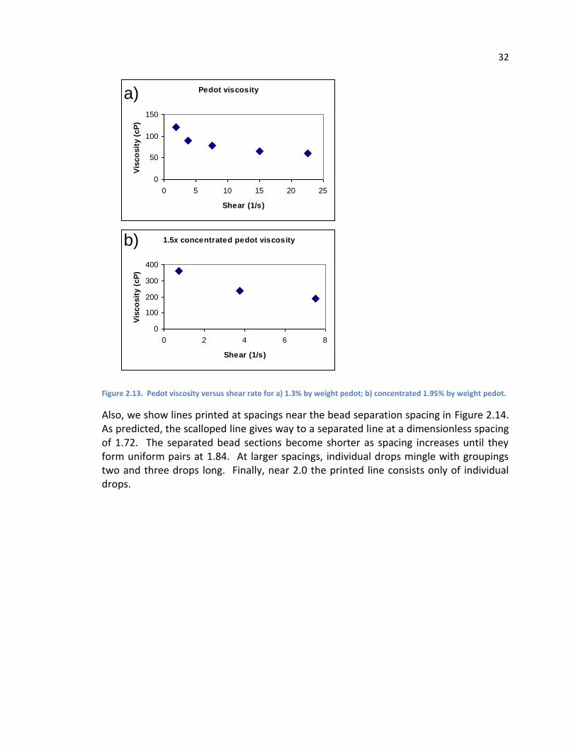
We provide detailed viscosity and surface tension measurements of the pedot ink (poly(3,4-ethylenedioxythiophene) poly(styrenesulfonate), PEDOT:PSS 1.3% by weight in water from Aldrich) used in our paper. As Figure 2.13a shows, pedot ink is shear thinning, with a viscosity of 121 cP at low shear rate, 1.9 1/s, and 79 cP at 22.5 1/s. Increasing the pedot concentration 50% using a rotary evaporator leads to a significantly greater viscosity, about three times greater at low shear and 2.4 times greater at higher

shear. (All viscosity measurements were taken after filtering the ink using a 5.0 m nylon filter as we do when inkjet printing.)

We measured PEDOT’s surface tension using a KSV Sigma Tensiometer at 71.25±0.06 mN/m at room temperature. (On the same apparatus, we measure the surface of deionized water at 72.61±0.08 mN/m.)

32

Figure 2.13. Pedot viscosity versus shear rate for a) 1.3% by weight pedot; b) concentrated 1.95% by weight pedot.

Also, we show lines printed at spacings near the bead separation spacing in Figure 2.14. As predicted, the scalloped line gives way to a separated line at a dimensionless spacing of 1.72. The separated bead sections become shorter as spacing increases until they form uniform pairs at 1.84. At larger spacings, individual drops mingle with groupings two and three drops long. Finally, near 2.0 the printed line consists only of individual drops.

Pedot viscosity

0

50

100

150

0 5 10 15 20 25

Shear (1/s)

Vis

co

sit

y (

cP

)

1.5x concentrated pedot viscosity

0

100

200

300

400

0 2 4 6 8

Shear (1/s)

Vis

co

sit

y (

cP

)

b)

a) Pedot viscosity

0

50

100

150

0 5 10 15 20 25

Shear (1/s)

Vis

co

sit

y (

cP

)

1.5x concentrated pedot viscosity

0

100

200

300

400

0 2 4 6 8

Shear (1/s)

Vis

co

sit

y (

cP

)

b)

a)

33

Figure 2.14. Printed lines at 45°C near the bead separation spacing of y = 1.72. (The isolated drop radius is 47.7±0.4 μm.)

2.9 Works cited

1. Tseng, H.-Y.; Subramanian, V., All inkjet-printed, fully self-aligned transistors for low-cost circuit applications. Organic Electronics 2011, 12, (2), 249-256. 2. Huang, D.; Liao, F.; Molesa, S.; Redinger, D.; Subramanian, V., Plastic-compatible low resistance printable gold nanoparticle conductors for flexible electronics. Journal of the Electrochemical Society 2003, 150, (7), G412-G417. 3. Kawase, T.; Shimoda, T.; Newsome, C.; Sirringhaus, H.; Friend, R. H., Inkjet printing of polymer thin film transistors. Thin Solid Films 2003, 438, 279-287. 4. Burns, S. E.; Cain, P.; Mills, J.; Wang, J. Z.; Sirringhaus, H., Inkjet printing of polymer thin-film transistor circuits. Mrs Bulletin 2003, 28, (11), 829-834. 5. Duineveld, P. C., The stability of ink-jet printed lines of liquid with zero receding contact angle on a homogeneous substrate. Journal of Fluid Mechanics 2003, 477, 175-200.

75 m

y = 1.57

80 m

y = 1.68

82 m

y = 1.72

85 m

y = 1.78

87 m

y = 1.82

88 m

y = 1.84

90 m

y = 1.89

92 m

y = 1.93

95 m

y = 1.99

75 m

y = 1.57

80 m

y = 1.68

82 m

y = 1.72

85 m

y = 1.78

87 m

y = 1.82

88 m

y = 1.84

90 m

y = 1.89

92 m

y = 1.93

95 m

y = 1.99

34

6. Perelaer, J.; de Gans, B. J.; Schubert, U. S., Ink-jet printing and microwave sintering of conductive silver tracks. Advanced Materials 2006, 18, (16), 2101-+. 7. de Gans, B. J.; Schubert, U. S., Inkjet printing of well-defined polymer dots and arrays. Langmuir 2004, 20, (18), 7789-7793. 8. Park, J.; Moon, J., Control of colloidal particle deposit patterns within picoliter droplets ejected by ink-jet printing. Langmuir 2006, 22, (8), 3506-3513. 9. van den Berg, A. M. J.; de Laat, A. W. M.; Smith, P. J.; Perelaer, J.; Schubert, U. S., Geometric control of inkjet printed features using a gelating polymer. Journal of Materials Chemistry 2007, 17, (7), 677-683. 10. Ozawa, K.; Nishitani, E.; Doi, M., Modeling of the drying process of liquid droplet to form thin film. Japanese Journal of Applied Physics Part 1-Regular Papers Short Notes & Review Papers 2005, 44, (6A), 4229-4234. 11. Molesa, S. E.; de la Fuente Vornbrock, A.; Chang, P. C.; Subramanian, V., Low-voltage inkjetted organic transistors for printed RFID and display applications. In Electron Devices Meeting, IEEE International: 2005; Vol. IEDM Technical Digest, pp 109-112. 12. Deegan, R. D.; Bakajin, O.; Dupont, T. F.; Huber, G.; Nagel, S. R.; Witten, T. A., Capillary flow as the cause of ring stains from dried liquid drops. Nature 1997, 389, (6653), 827-829. 13. Hu, H.; Larson, R. G., Marangoni effect reverses coffee-ring depositions. Journal of Physical Chemistry B 2006, 110, (14), 7090-7094. 14. Savino, R.; Paterna, D.; Favaloro, N., Buoyancy and Marangoni effects in an evaporating drop. Journal of Thermophysics and Heat Transfer 2002, 16, (4), 562-574. 15. Stringer, J.; Derby, B., The Impact and Spreading of Ink Jet Printed Droplets. In Organic Electronics Conference and Exhibition: 2007. 16. Smith, P. J.; Shin, D. Y.; Stringer, J. E.; Derby, B.; Reis, N., Direct ink-jet printing and low temperature conversion of conductive silver patterns. Journal of Materials Science 2006, 41, (13), 4153-4158. 17. Degennes, P. G., WETTING - STATICS AND DYNAMICS. Reviews of Modern Physics 1985, 57, (3), 827-863. 18. Molesa, S. E. Ultra-low-cost printed electronics. Thesis Ph D in Engineering-Electrical Engineering and Computer Sciences --University of California Berkeley Spring 2006, 2006.

35

3 Printed-film formation

3.1 Introduction

As discussed previously, solution processing presents a low-cost, environmentally-friendly alternative to traditional microfabrication techniques. Its additive processing presents an alternative to the slow, costly steps of vacuum deposition, photolithography, and etching. Solution-processing techniques include roll-to-roll patterning and inkjet printing, with the latter being the focus of this work. Researchers have fabricated various microelectronic devices with inkjet printing including transistors, displays, and sensors.1-3 All of these devices make use of combinations of printed rectilinear shapes. Thus, an understanding of the formation of a rectangle is a logical starting point to optimize the fabrication of arbitrary patterns. A specific application of printed rectangles, like those studied in this chapter, is the square pixel electrode in a display backplane. Arias et al. demonstrated a solution-processed, thin film transistor backplane with inkjet-printed square pixel electrodes about half a millimeter across, the same size scale as features in this work.4

Advancing inkjetted-device fabrication requires a better understanding of the behavior of printed fluids on an impermeable substrate. Considerable work has been devoted to the problem of wetted-line (rivulet) stability. Davis derived the stability conditions for wetted beads for several contact-line boundary conditions,5 and Schiaffino and Sonin further developed the stability model and provided experimental confirmation.6 Several later works continued development of the understanding of printed-line morphologies and stability.7-10 As will be seen later in Figure 3.11, individual lines printed in this work, with a narrow contact-angle hysteresis (θadv - θrec), are unstable and break into separate beads, consistent with Davis’ theory. However, as a printed rectangle’s aspect ratio approaches unity (as it becomes a square), its sub-beads merge into a single bead. Consequently, this chapter does not focus on the stability of long, wetted beads, but rather the equilibrium shape of rectangular beads.

Tekin et al. optimized the inkjet printing of two-dimensional polystyrene films.11 They found that printing several spatially offset layers at sufficiently low print-head velocity leads to more uniform dried films. By choosing a two solvent mixture with differentiated vapor pressures, they avoided mass transfer to the film edge, known as the coffee-ring effect. This work does not dwell upon such drying effects, but rather is concerned with the shape of beads during and shortly after a print. Kang et al.12 used a one-dimensional geometric approach to model basic printed-film properties including thickness and fluid bulging beyond an intended footprint.

In this chapter, we build upon the approach of Kang et al. to understand and optimize the shape of patterned beads during inkjet printing. We examine wetted-bead

36

properties under more general, two-dimensional conditions, rather than in the one-dimensional limit of high aspect ratio. We experimentally and analytically observe the limitations of fixed-spacing raster-scan printing. Instead, we propose a variable–line-spacing printing scheme to maintain a bead’s contact angle between its advancing and retreating values as it is printed. Implementation of this algorithm requires an understanding of the two-dimensional shape of a rectangular bead and of evaporation during the print. We experimentally demonstrate the effectiveness and limitations of this new approach. Finally, we discuss the use of deliberate contact-line pinning in patterning films by preprinting a feature’s border.

Contact-angle hysteresis plays an important role in the inkjet printing of patterned figures. Though a droplet on a substrate tends to adopt a circular footprint, the existence of contact-angle hysteresis means that other planforms can be printed. In the next chapter, we show this experimentally and theoretically. Deegan showed that particle deposition at the contact line due to evaporation leads to self-pinning of that contact line.13 For the realization of well-defined shapes, printers commonly choose systems that are fully pinned, that is, having zero retreating contact-angle, to avoid bead separation and reflow after printing. In practice, contact line pinning during printing is achieved through a combination of high mass loading of inks, surface heterogeneity, and ink-substrate interactions.7, 13

Though complete pinning is desirable, a partial pinning resulting in a nonzero retreating contact angle is unavoidable in some applications. These include inks with low mass loading (for thinner film deposition or due to low solubility of active material in volatile solvent), nonvolatile solvents, and smooth substrates. Because inks in printed electronics may be characterized by one or more of these properties, a study of an ink-substrate system with a positive retreating contact angle is necessary and generally applicable. In systems with zero retreating contact angle, our approach is still valid, though printed-film-breakup phenomena due to contact line retreat will not occur.

3.2 Experimental section

We print our films with a custom-built, drop-on-demand inkjet printer. The printer uses piezoelectric MicroFab inkjet print heads (Piano, TX) with a 60 µm orifice and has stages with 1 µm accuracy in the x and y directions. Lines in this work are printed with a 50 µm drop spacing, unless otherwise noted. We measure a jetting frequency of 22.3 Hz at this spacing.

In this work, we use an ink consisting of a polymer dissolved in a 1-hexanol (≥99.0%, from Sigma Aldrich; St. Louis, MO). We chose a polymer commonly used as a dielectric in organic, solution-processed devices, specifically poly-4-vinylphenol (PVP), MW ≈ 8000

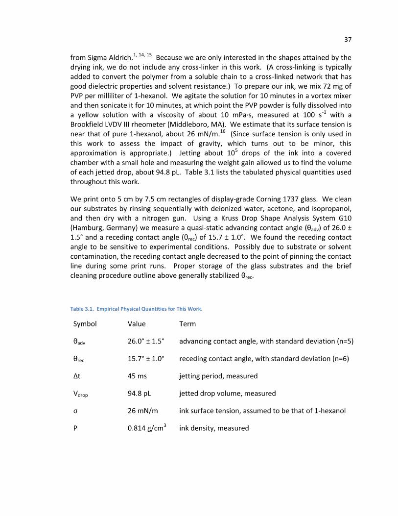
37

from Sigma Aldrich.1, 14, 15 Because we are only interested in the shapes attained by the drying ink, we do not include any cross-linker in this work. (A cross-linking is typically added to convert the polymer from a soluble chain to a cross-linked network that has good dielectric properties and solvent resistance.) To prepare our ink, we mix 72 mg of PVP per milliliter of 1-hexanol. We agitate the solution for 10 minutes in a vortex mixer and then sonicate it for 10 minutes, at which point the PVP powder is fully dissolved into a yellow solution with a viscosity of about 10 mPa·s, measured at 100 s-1 with a Brookfield LVDV III rheometer (Middleboro, MA). We estimate that its surface tension is near that of pure 1-hexanol, about 26 mN/m.16 (Since surface tension is only used in this work to assess the impact of gravity, which turns out to be minor, this approximation is appropriate.) Jetting about 105 drops of the ink into a covered chamber with a small hole and measuring the weight gain allowed us to find the volume of each jetted drop, about 94.8 pL. Table 3.1 lists the tabulated physical quantities used throughout this work.

We print onto 5 cm by 7.5 cm rectangles of display-grade Corning 1737 glass. We clean our substrates by rinsing sequentially with deionized water, acetone, and isopropanol, and then dry with a nitrogen gun. Using a Kruss Drop Shape Analysis System G10 (Hamburg, Germany) we measure a quasi-static advancing contact angle (θadv) of 26.0 ± 1.5° and a receding contact angle (θrec) of 15.7 ± 1.0°. We found the receding contact angle to be sensitive to experimental conditions. Possibly due to substrate or solvent contamination, the receding contact angle decreased to the point of pinning the contact line during some print runs. Proper storage of the glass substrates and the brief cleaning procedure outline above generally stabilized θrec.

Table 3.1. Empirical Physical Quantities for This Work.

Symbol Value Term

θadv 26.0° ± 1.5° advancing contact angle, with standard deviation (n=5)

θrec 15.7° ± 1.0° receding contact angle, with standard deviation (n=6)

Δt 45 ms jetting period, measured

Vdrop 94.8 pL jetted drop volume, measured

σ 26 mN/m ink surface tension, assumed to be that of 1-hexanol

Ρ 0.814 g/cm3 ink density, measured

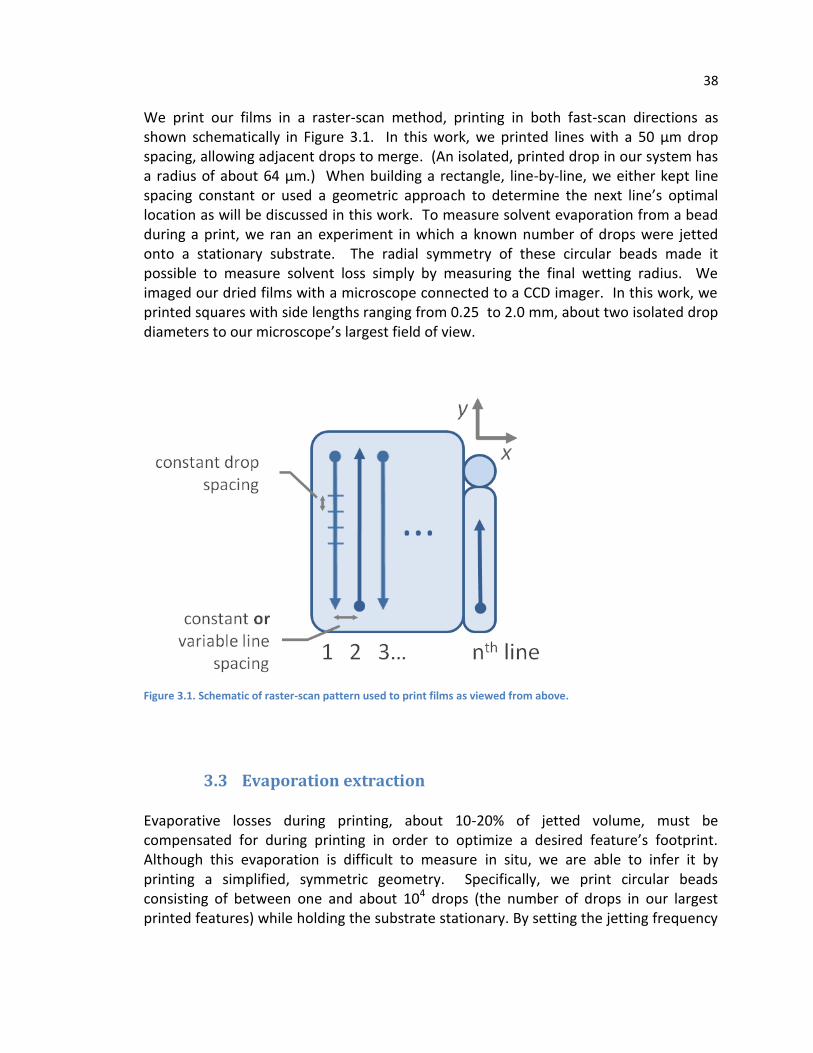
38

We print our films in a raster-scan method, printing in both fast-scan directions as shown schematically in Figure 3.1. In this work, we printed lines with a 50 µm drop spacing, allowing adjacent drops to merge. (An isolated, printed drop in our system has a radius of about 64 µm.) When building a rectangle, line-by-line, we either kept line spacing constant or used a geometric approach to determine the next line’s optimal location as will be discussed in this work. To measure solvent evaporation from a bead during a print, we ran an experiment in which a known number of drops were jetted onto a stationary substrate. The radial symmetry of these circular beads made it possible to measure solvent loss simply by measuring the final wetting radius. We imaged our dried films with a microscope connected to a CCD imager. In this work, we printed squares with side lengths ranging from 0.25 to 2.0 mm, about two isolated drop diameters to our microscope’s largest field of view.

Figure 3.1. Schematic of raster-scan pattern used to print films as viewed from above.

3.3 Evaporation extraction

Evaporative losses during printing, about 10-20% of jetted volume, must be compensated for during printing in order to optimize a desired feature’s footprint. Although this evaporation is difficult to measure in situ, we are able to infer it by printing a simplified, symmetric geometry. Specifically, we print circular beads consisting of between one and about 104 drops (the number of drops in our largest printed features) while holding the substrate stationary. By setting the jetting frequency

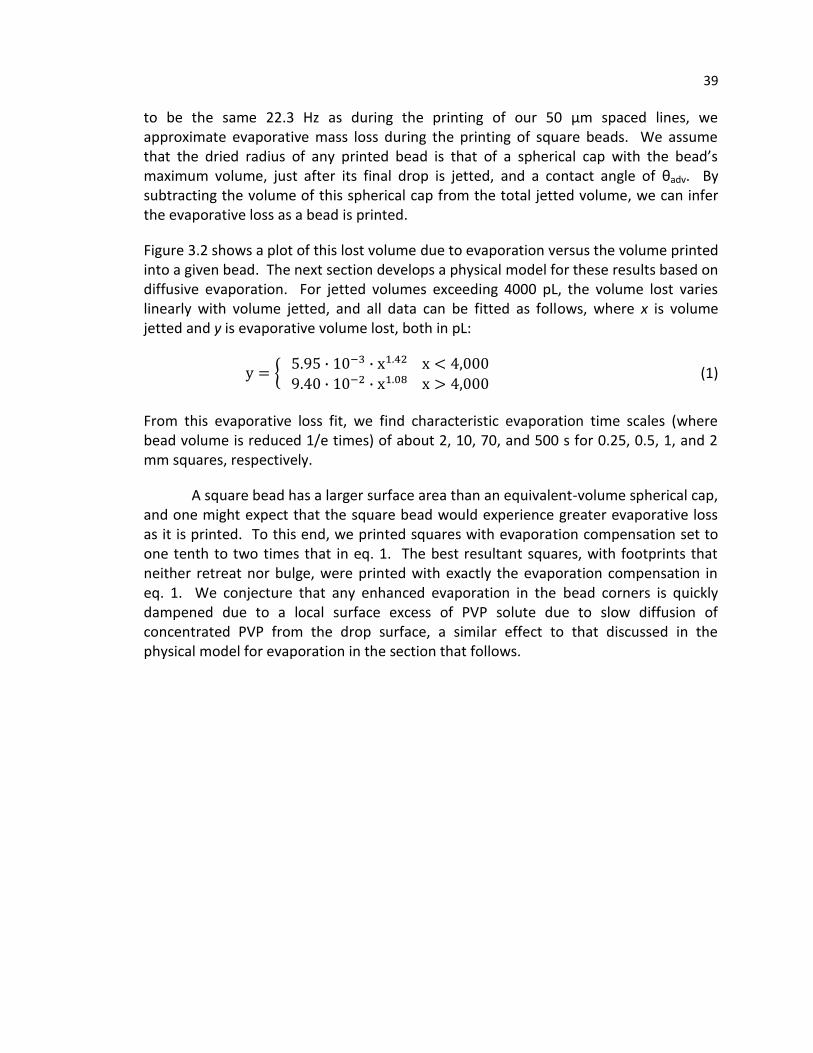
39

to be the same 22.3 Hz as during the printing of our 50 µm spaced lines, we approximate evaporative mass loss during the printing of square beads. We assume that the dried radius of any printed bead is that of a spherical cap with the bead’s maximum volume, just after its final drop is jetted, and a contact angle of θadv. By subtracting the volume of this spherical cap from the total jetted volume, we can infer the evaporative loss as a bead is printed.

Figure 3.2 shows a plot of this lost volume due to evaporation versus the volume printed into a given bead. The next section develops a physical model for these results based on diffusive evaporation. For jetted volumes exceeding 4000 pL, the volume lost varies linearly with volume jetted, and all data can be fitted as follows, where x is volume jetted and y is evaporative volume lost, both in pL:

(1)

From this evaporative loss fit, we find characteristic evaporation time scales (where bead volume is reduced 1/e times) of about 2, 10, 70, and 500 s for 0.25, 0.5, 1, and 2 mm squares, respectively.

A square bead has a larger surface area than an equivalent-volume spherical cap, and one might expect that the square bead would experience greater evaporative loss as it is printed. To this end, we printed squares with evaporation compensation set to one tenth to two times that in eq. 1. The best resultant squares, with footprints that neither retreat nor bulge, were printed with exactly the evaporation compensation in eq. 1. We conjecture that any enhanced evaporation in the bead corners is quickly dampened due to a local surface excess of PVP solute due to slow diffusion of concentrated PVP from the drop surface, a similar effect to that discussed in the physical model for evaporation in the section that follows.

40

Figure 3.2. Measured evaporation volume for circular beads versus ink volume jetted, shown with the piecewise power law fit in eq. 1 used for line width generation.

3.4 Physical model for evaporation

Here we develop a simple, physically-based model for evaporation from a bead as it is printed. We limit the discussion to a sufficiently small bead that its surface is well-approximated by a spherical cap. Hu and Larson developed a quasi-steady state model for evaporation from a sessile drop into still air.17 They assumed that the vapor concentration c is the saturated vapor pressure at the drop’s surface and zero far above the drop. Because the vapor concentration above the drop adjusts quickly to movement of the drop’s surface due to mass loss (as is verified below), the steady-state diffusion of vapor is governed by the Laplace equation for diffusion . They also ignore the effect of evaporative cooling, assuming that it does not significantly alter the evaporation rate. In order to calculate the increased diffusion due to contact angles less than π/2, Hu and Larson ran FEM simulations for a range of contact angles and fit the

1.E+00

1.E+01

1.E+02

1.E+03

1.E+04

1.E+05

1.E+06

1.E+02 1.E+03 1.E+04 1.E+05 1.E+06

volumelost (pL)

volume jetted (pL)

(drops jetted)

measured evaporation piecewise fit, Eq. 1

(1) (10) (104) (105)

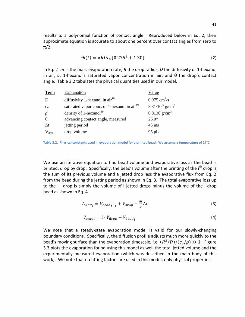
41

results to a polynomial function of contact angle. Reproduced below in Eq. 2, their approximate equation is accurate to about one percent over contact angles from zero to π/2.

(2)

In Eq. 2 is the mass evaporation rate, R the drop radius, D the diffusivity of 1-hexanol in air, cV 1-hexanol’s saturated vapor concentration in air, and θ the drop’s contact angle. Table 3.2 tabulates the physical quantities used in our model.

Term Explanation Value

D diffusivity 1-hexanol in air18

0.075 cm2/s

cv saturated vapor conc. of 1-hexanol in air19

5.31·10-5

g/cm3

ρ density of 1-hexanol19

0.8136 g/cm3

θ advancing contact angle, measured 26.0°

Δt jetting period 45 ms

Vdrop drop volume 95 pL

Table 3.2. Physical constants used in evaporation model for a printed bead. We assume a temperature of 27°C.

We use an iterative equation to find bead volume and evaporative loss as the bead is printed, drop by drop. Specifically, the bead’s volume after the printing of the ith drop is the sum of its previous volume and a jetted drop less the evaporative flux from Eq. 2 from the bead during the jetting period as shown in Eq. 3. The total evaporative loss up to the ith drop is simply the volume of i jetted drops minus the volume of the i-drop bead as shown in Eq. 4.

(3)

(4)

We note that a steady-state evaporation model is valid for our slowly-changing boundary conditions. Specifically, the diffusion profile adjusts much more quickly to the bead’s moving surface than the evaporation timescale, i.e. . Figure 3.3 plots the evaporation found using this model as well the total jetted volume and the experimentally measured evaporation (which was described in the main body of this work). We note that no fitting factors are used in this model, only physical properties.

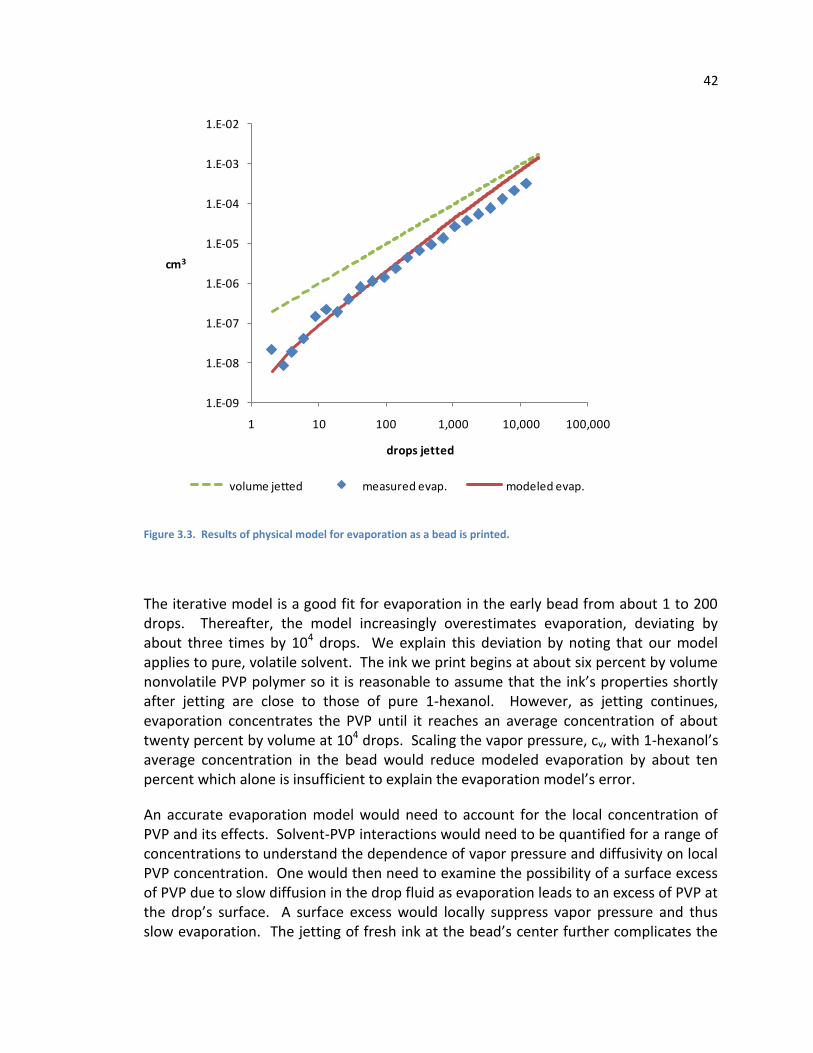
42

Figure 3.3. Results of physical model for evaporation as a bead is printed.

The iterative model is a good fit for evaporation in the early bead from about 1 to 200 drops. Thereafter, the model increasingly overestimates evaporation, deviating by about three times by 104 drops. We explain this deviation by noting that our model applies to pure, volatile solvent. The ink we print begins at about six percent by volume nonvolatile PVP polymer so it is reasonable to assume that the ink’s properties shortly after jetting are close to those of pure 1-hexanol. However, as jetting continues, evaporation concentrates the PVP until it reaches an average concentration of about twenty percent by volume at 104 drops. Scaling the vapor pressure, cv, with 1-hexanol’s average concentration in the bead would reduce modeled evaporation by about ten percent which alone is insufficient to explain the evaporation model’s error.

An accurate evaporation model would need to account for the local concentration of PVP and its effects. Solvent-PVP interactions would need to be quantified for a range of concentrations to understand the dependence of vapor pressure and diffusivity on local PVP concentration. One would then need to examine the possibility of a surface excess of PVP due to slow diffusion in the drop fluid as evaporation leads to an excess of PVP at the drop’s surface. A surface excess would locally suppress vapor pressure and thus slow evaporation. The jetting of fresh ink at the bead’s center further complicates the

1.E-09

1.E-08

1.E-07

1.E-06

1.E-05

1.E-04

1.E-03

1.E-02

1 10 100 1,000 10,000 100,000

cm3

drops jetted

volume jetted measured evap. modeled evap.

43

analysis. Noting that our model is valid for early evaporation, we leave such detailed, ink-specific treatments to future work.

3.5 Raster scan printing

A simple approach to printing a two-dimensional film, such as a square, is to print the feature by a raster-scan method, as shown in Figure 3.1, with a constant, identical spacing in both x and y directions. Figure 3.4 shows 2.0 to 0.25 mm dried squares at their respective best-case constant drop spacing, showing minimal bulging and/or separation. The border of dried beads in this and later figures is the most important feature in understanding the patterning of two-dimensional shapes. Each bead also shows a uniform interior and a “coffee-ring” transfer of solute to its border. The precise nature of the coffee ring is a function of local bead shape and evaporation but is irrelevant to this work concerned with the patterning of two-dimensional beads during a print. Recall that cosolvents can prevent this coffee-ring deposit, but in this work we did not wish to further complicate our system by using an ink whose contact angle varies with local evaporation.

Beginning with the 2.0 mm squares, we see that there is substantial bulging on the left side of the 20 µm spaced square where printing began. Increasing the drop spacing to 30 µm reduces this bulge, but the right side is now separated into small, isolated beads. The 1.0 and 0.5 mm squares show a similar transition in planform, from left side bulging to right side separation, although at larger spacings as the length scale shrinks. Finally, the smallest 0.25 mm squares show a large amount of rounding on all sides, deviating the most from a square footprint. Thus, we see that a fixed-spacing printing method is not viable for systems with a narrow contact angle hysteresis.

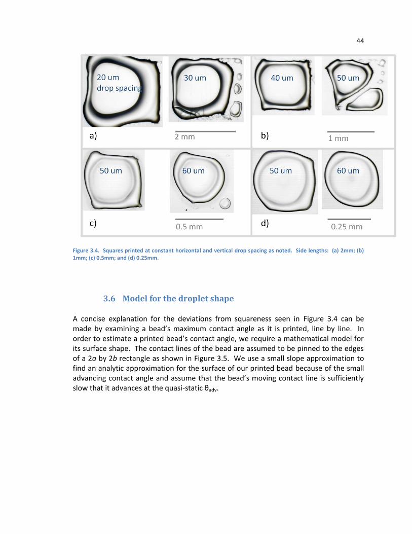
44

Figure 3.4. Squares printed at constant horizontal and vertical drop spacing as noted. Side lengths: (a) 2mm; (b) 1mm; (c) 0.5mm; and (d) 0.25mm.

3.6 Model for the droplet shape

A concise explanation for the deviations from squareness seen in Figure 3.4 can be made by examining a bead’s maximum contact angle as it is printed, line by line. In order to estimate a printed bead’s contact angle, we require a mathematical model for its surface shape. The contact lines of the bead are assumed to be pinned to the edges of a 2a by 2b rectangle as shown in Figure 3.5. We use a small slope approximation to find an analytic approximation for the surface of our printed bead because of the small advancing contact angle and assume that the bead’s moving contact line is sufficiently slow that it advances at the quasi-static θadv.

45

Figure 3.5. Top view and cross section of bead surface.

The Hoffman-Tanner relation,20 reprinted in Eq. 5 below, confirms that under our printing conditions the dynamic contact angle (θdyn) of the advancing triple line is well-approximated by its quasi-static advancing value (θadv).

(5)

In eq. 5 Ca is the Capillary number (µU/σ, where µ is the fluid’s viscosity and U is its contact-line velocity), R is the bead radius, and L is the microscopic length scale for contact line movement (about 50 nm here, from eq. 69 in Bonn et al.20). The contact line at the side of a rectangle being printed advances with a Capillary number of the order of 10-4 or less for which we find a viscous dynamic contact angle correction of 0.1% or less. Within the experimental error of our system, we safely assume that contact lines advance at their quasi-static θadv in Table 3.1.

The Young-Laplace equation and hydrostatic pressure determine the surface of our quasi-static rectangular bead, and here we develop an analytic solution. Because our ink-substrate system has a low contact angle, with errors vanishing as the square of the slope, we may approximate the curvature of the surface by . The pressure at any point at the bottom of the bead, pb in Figure 3.5, is the sum of the ambient, Young Laplace, and hydrostatic pressures.

(6)

The bead at equilibrium has constant pressure at its base, and specifying that , eq. 6 becomes:

glass substrate

θadvx*

y*

a-a

b

-b

Top view Cross section

x*a-a

u*(x*,y*)pg

pl

pbbead

air

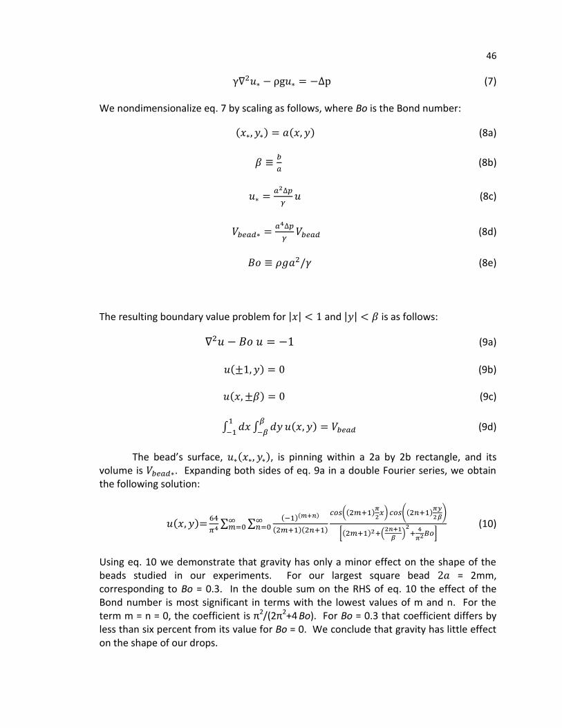
46

(7)

We nondimensionalize eq. 7 by scaling as follows, where Bo is the Bond number:

(8a)

(8b)

(8c)

(8d)

(8e)

The resulting boundary value problem for and is as follows:

(9a)

(9b)

(9c)

(9d)

The bead’s surface, , is pinning within a 2a by 2b rectangle, and its volume is . Expanding both sides of eq. 9a in a double Fourier series, we obtain the following solution:

(10)

Using eq. 10 we demonstrate that gravity has only a minor effect on the shape of the beads studied in our experiments. For our largest square bead = 2mm, corresponding to Bo = 0.3. In the double sum on the RHS of eq. 10 the effect of the Bond number is most significant in terms with the lowest values of m and n. For the term m = n = 0, the coefficient is π2/(2π2+4 Bo). For Bo = 0.3 that coefficient differs by less than six percent from its value for Bo = 0. We conclude that gravity has little effect on the shape of our drops.

47

Nonlinear numerical simulations provide further corroboration to gravity’s minor role in our square beads’ surfaces. We perform numerical solutions of our square beads with Surface Evolver3, a free software package by Ken Brakke that minimizes the total energy of free surfaces subject to constraints and boundary conditions. The bead’s surface is tiled with triangular facets, and the gradient descent method reflows the surface towards a minimum energy state subject to specified volume and contact-angle constraints.

Surface Evolver simulations confirm the validity of our choices to ignore gravity and approximate the bead surface as one with constant Laplacian. We performed a surface-energy minimization on a body with a free surface, fixed volume, and pinned vertices around its four edges. Using eq. 10 we find a fixed volume of 0.41 mm3 for a 2mm square with a θmax of 26.0°, which we use as the volume constraint for our simulations. Figure 3.6a shows a rendering of the minimum-energy surface that results. In Figure 3.6b we plot cross-sections through the simulated bead’s center, from edge center to opposite edge center for Surface Evolver-modeled beads with and without gravity as well as the equivalent-volume constant Laplacian surface. Extracting slope at the contact line from these traces, we find that the constant curvature with gravity contact angle is 27.22°, about a degree greater than the 25.98° in our simplified model (and three tenths greater than the constant curvature surface neglecting gravity).

Figure 3.6c renders the absolute and relative difference in bead height due to gravity. As expected, we see a modest shift towards the corners when gravity is considered, less than a percent difference in height at the bead’s center. Figure 3.6d plots the difference between the constant Laplacian bead and the constant-curvature bead with gravity. We find that our simple-model height is about two percent too tall at its center, with the largest relative error of about four percent near the edges centers where the Laplacian is a less valid curvature approximation. However, the single degree error between the θmax of our model and that found with numerical methods is acceptable for the purposes of this work.

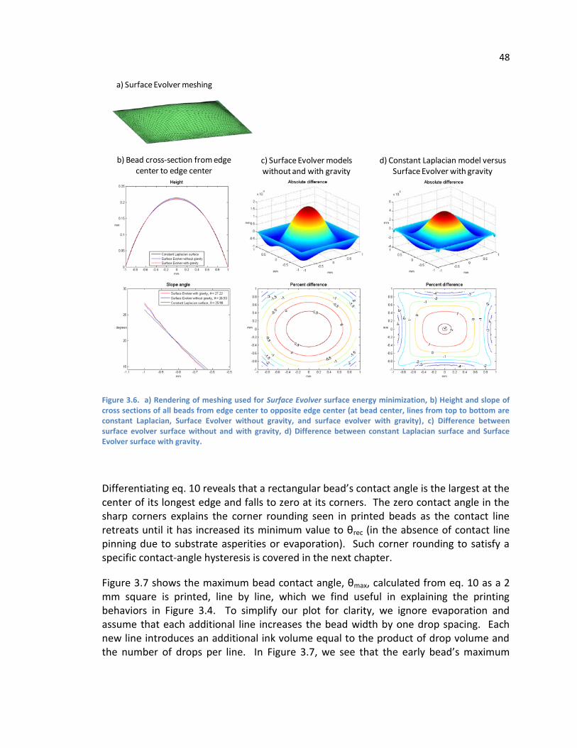
48

Figure 3.6. a) Rendering of meshing used for Surface Evolver surface energy minimization, b) Height and slope of cross sections of all beads from edge center to opposite edge center (at bead center, lines from top to bottom are constant Laplacian, Surface Evolver without gravity, and surface evolver with gravity), c) Difference between surface evolver surface without and with gravity, d) Difference between constant Laplacian surface and Surface Evolver surface with gravity.

Differentiating eq. 10 reveals that a rectangular bead’s contact angle is the largest at the center of its longest edge and falls to zero at its corners. The zero contact angle in the sharp corners explains the corner rounding seen in printed beads as the contact line retreats until it has increased its minimum value to θrec (in the absence of contact line pinning due to substrate asperities or evaporation). Such corner rounding to satisfy a specific contact-angle hysteresis is covered in the next chapter.

Figure 3.7 shows the maximum bead contact angle, θmax, calculated from eq. 10 as a 2 mm square is printed, line by line, which we find useful in explaining the printing behaviors in Figure 3.4. To simplify our plot for clarity, we ignore evaporation and assume that each additional line increases the bead width by one drop spacing. Each new line introduces an additional ink volume equal to the product of drop volume and the number of drops per line. In Figure 3.7, we see that the early bead’s maximum

c) Surface Evolver models without and with gravity

a) Surface Evolver meshing

d) Constant Laplacian model versusSurface Evolver with gravity

b) Bead cross-section from edge center to edge center

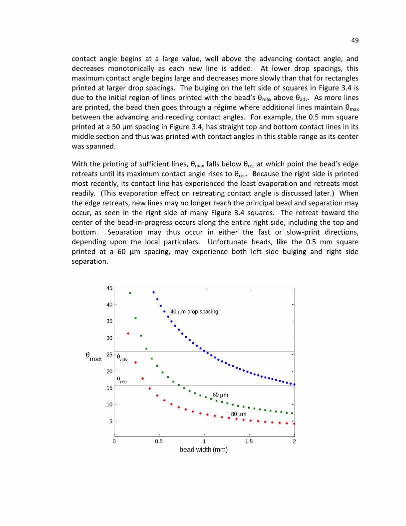
49

contact angle begins at a large value, well above the advancing contact angle, and decreases monotonically as each new line is added. At lower drop spacings, this maximum contact angle begins large and decreases more slowly than that for rectangles printed at larger drop spacings. The bulging on the left side of squares in Figure 3.4 is due to the initial region of lines printed with the bead’s θmax above θadv. As more lines are printed, the bead then goes through a régime where additional lines maintain θmax between the advancing and receding contact angles. For example, the 0.5 mm square printed at a 50 µm spacing in Figure 3.4, has straight top and bottom contact lines in its middle section and thus was printed with contact angles in this stable range as its center was spanned.

With the printing of sufficient lines, θmax falls below θrec at which point the bead’s edge retreats until its maximum contact angle rises to θrec. Because the right side is printed most recently, its contact line has experienced the least evaporation and retreats most readily. (This evaporation effect on retreating contact angle is discussed later.) When the edge retreats, new lines may no longer reach the principal bead and separation may occur, as seen in the right side of many Figure 3.4 squares. The retreat toward the center of the bead-in-progress occurs along the entire right side, including the top and bottom. Separation may thus occur in either the fast or slow-print directions, depending upon the local particulars. Unfortunate beads, like the 0.5 mm square printed at a 60 µm spacing, may experience both left side bulging and right side separation.

0 0.5 1 1.5 2

5

10

15

20

25

30

35

40

45

bead width (mm)

max

adv

rec

40 m drop spacing

60 m

80 m

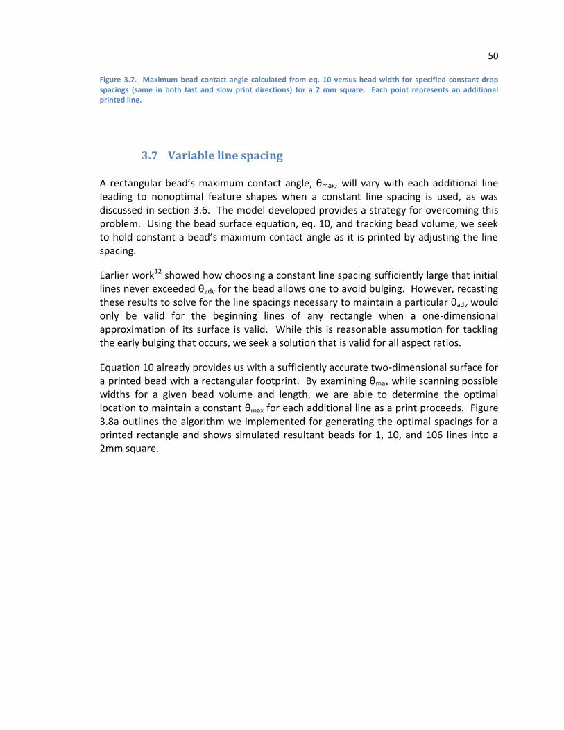
50

Figure 3.7. Maximum bead contact angle calculated from eq. 10 versus bead width for specified constant drop spacings (same in both fast and slow print directions) for a 2 mm square. Each point represents an additional printed line.

3.7 Variable line spacing

A rectangular bead’s maximum contact angle, θmax, will vary with each additional line leading to nonoptimal feature shapes when a constant line spacing is used, as was discussed in section 3.6. The model developed provides a strategy for overcoming this problem. Using the bead surface equation, eq. 10, and tracking bead volume, we seek to hold constant a bead’s maximum contact angle as it is printed by adjusting the line spacing.

Earlier work12 showed how choosing a constant line spacing sufficiently large that initial lines never exceeded θadv for the bead allows one to avoid bulging. However, recasting these results to solve for the line spacings necessary to maintain a particular θadv would only be valid for the beginning lines of any rectangle when a one-dimensional approximation of its surface is valid. While this is reasonable assumption for tackling the early bulging that occurs, we seek a solution that is valid for all aspect ratios.

Equation 10 already provides us with a sufficiently accurate two-dimensional surface for a printed bead with a rectangular footprint. By examining θmax while scanning possible widths for a given bead volume and length, we are able to determine the optimal location to maintain a constant θmax for each additional line as a print proceeds. Figure 3.8a outlines the algorithm we implemented for generating the optimal spacings for a printed rectangle and shows simulated resultant beads for 1, 10, and 106 lines into a 2mm square.

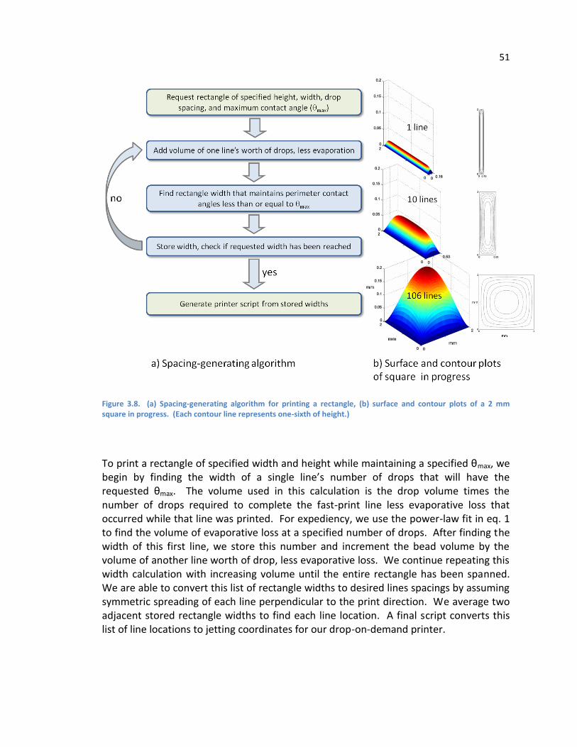
51

Figure 3.8. (a) Spacing-generating algorithm for printing a rectangle, (b) surface and contour plots of a 2 mm square in progress. (Each contour line represents one-sixth of height.)

To print a rectangle of specified width and height while maintaining a specified θmax, we begin by finding the width of a single line’s number of drops that will have the requested θmax. The volume used in this calculation is the drop volume times the number of drops required to complete the fast-print line less evaporative loss that occurred while that line was printed. For expediency, we use the power-law fit in eq. 1 to find the volume of evaporative loss at a specified number of drops. After finding the width of this first line, we store this number and increment the bead volume by the volume of another line worth of drop, less evaporative loss. We continue repeating this width calculation with increasing volume until the entire rectangle has been spanned. We are able to convert this list of rectangle widths to desired lines spacings by assuming symmetric spreading of each line perpendicular to the print direction. We average two adjacent stored rectangle widths to find each line location. A final script converts this list of line locations to jetting coordinates for our drop-on-demand printer.

52

For squarest squares, we set the printing θmax at θadv. As the contact angle is largest at a side’s center and decreases toward the corners, this maximizes the length of contact line between θmax and θrec without risking bulging. With θmax set at θadv and other input parameters set to the values in Table 3.1, we ran our algorithm for a variety of rectangle sizes and aspect ratios. In Figure 3.9a, we show the resultant drop location for a constant-spacing 1 mm square and 1 mm squares resulting from the algorithm outlined above, with and without evaporation compensation. The effect of evaporation compensation is clearer in Figure 3.9b, which plots the line location of each line spanning the square. Twenty five percent more lines are required when evaporative loss is matched in a 1 mm square bead.

Figure 3.9. Spanning a 1 mm square with constant line spacings and algorithm-generated spacings: (a) drop locations and (b) bead width versus line number.

After implementing our algorithm to find optimal line spacings and generate printer files, we printed an array of squares sized 0.5, 1, and 2 mm. We show the resultant dried patterns in Figure 3.10. Without evaporation compensation, printed beads at all three size scales separate and retreat from their designed footprint as seen in the leftmost column. When additional volume is added to match evaporation, all three beads print intact. The largest square remains closest to its desired footprint while the

53

smaller ones have progressively worse corner curvature where the bead has apparently withdrawn from the corner toward its center.

Figure 3.10. Squares printed using algorithm-generated spacings with evaporation compensation and preprinted border as noted.

By comparing the four corners of each smaller square, we see that the top-left corner is the farthest from the drop center. Apparently, this corner is the most pinned. Our prints begin at the corner and proceed down, indicating that here the time scale for contact-line pinning due to drying is on the same order as that of the print time. By deliberately preprinting and drying a feature’s border, we were able to improve its footprint. (We also point out that the initial bulging seen in the first line or lines of a rectangle creates a larger contact line radius of curvature that increases the corner contact angle and suppresses contact line retreat.) We preprinted isolated drop borders and allowed them to dry before returning to print the square beads themselves, as seen on the right side of Figure 3.10. The third column of this figure shows that preprinted edges lead to enhanced square fidelity. The predried edges have a greater contact-angle hysteresis than the clean substrate, and thus permit a planform that is less circular and has sharper corners.

54

The effect of the preprinted border can be understood further by stopping a print after a certain number of lines and imaging the resultant dried bead. See Figure 3.11 for an example of this procedure with a 2 mm square. Without a preprinted border the first line printed is unstable and dewets into three separate beads. These individual beads grow with each additional line, merging first into two beads and eventually into a single bead. The waviness beyond the desired square footprint on the left side of the final feature reflects the growing footprint of these separate beads before they merge. In contrast, the prebordered square is stabilized by the presence of the pre-dried ink, remaining as a single bead with a straighter contact line. The border also appears to help pin the top and bottom right side of the growing bead, preventing it from retreating toward the bead’s center, as seen when comparing the right side of the 50 line prints with and without a border.

Figure 3.11. Line-by-line printing of 2 mm evaporation compensated square, with and without border as noted. Drops to the right of the beads in the second row (cropped in all but the last column) are the preprinted border seen in the fourth column of Figure 3.10.

For the smallest squares, whose side length approaches the radius of a single, isolated drop, printing lines of 50 µm spaced drops is not an optimal approach. The bulging

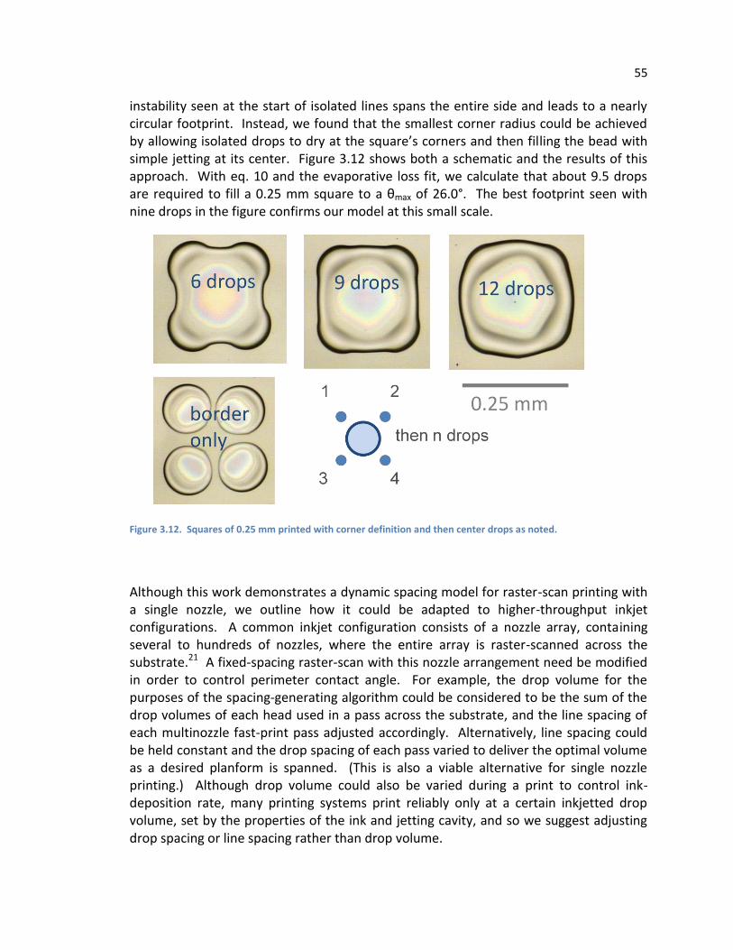
55

instability seen at the start of isolated lines spans the entire side and leads to a nearly circular footprint. Instead, we found that the smallest corner radius could be achieved by allowing isolated drops to dry at the square’s corners and then filling the bead with simple jetting at its center. Figure 3.12 shows both a schematic and the results of this approach. With eq. 10 and the evaporative loss fit, we calculate that about 9.5 drops are required to fill a 0.25 mm square to a θmax of 26.0°. The best footprint seen with nine drops in the figure confirms our model at this small scale.

Figure 3.12. Squares of 0.25 mm printed with corner definition and then center drops as noted.

Although this work demonstrates a dynamic spacing model for raster-scan printing with a single nozzle, we outline how it could be adapted to higher-throughput inkjet configurations. A common inkjet configuration consists of a nozzle array, containing several to hundreds of nozzles, where the entire array is raster-scanned across the substrate.21 A fixed-spacing raster-scan with this nozzle arrangement need be modified in order to control perimeter contact angle. For example, the drop volume for the purposes of the spacing-generating algorithm could be considered to be the sum of the drop volumes of each head used in a pass across the substrate, and the line spacing of each multinozzle fast-print pass adjusted accordingly. Alternatively, line spacing could be held constant and the drop spacing of each pass varied to deliver the optimal volume as a desired planform is spanned. (This is also a viable alternative for single nozzle printing.) Although drop volume could also be varied during a print to control ink-deposition rate, many printing systems print reliably only at a certain inkjetted drop volume, set by the properties of the ink and jetting cavity, and so we suggest adjusting drop spacing or line spacing rather than drop volume.

56

Faster yet printing schemes require similar modifications to the printing algorithm developed here. In the highest throughput inkjet printing, an array of nozzles spans the entire substrate that advances continuously underneath.21 Here, the line-to-line spacing is determined in a manner nearly identical to the single nozzle algorithm, and each “fast-print” vertical line in Figure 3.9a is printed all-at-once. Finally, for printing techniques that introduce an entire, partially wetting feature at once, such as gravure printing, the results here suggest that there is an optimal volume for each feature, where a bead’s maximum contact angle is the ink-substrate system’s quasi-static advancing contact angle. In the case of gravure printing, for optimal feature planform, a feature’s volume could be controlled by adjusting well volume and spacing.

3.8 Conclusion

We have demonstrated and then overcome difficulties in inkjet printing a patterned, two-dimensional film with a narrow contact-angle hysteresis. A fixed-line-spacing approach leads to a varying bead contact angle as new lines are printed, creating first bulging and later bead separation. We developed and implemented an algorithm to find the spacing that maintains a bead’s contact angle as it is printed by appropriately adjusting line spacing. We found that it is necessary to compensate for evaporation as the print progresses to maintain the optimal contact angle, and we were able to infer evaporative losses in our system by printing with radial symmetry. Using our spacing generator with evaporative compensation, we demonstrated printed squares with footprints superior to those printed at fixed spacing over a range of length scales. By seeding a feature’s edge with isolated dried drops, we further improved a feature’s footprint. This drying-induced pinning allowed us to print pattern squares with sides only twice as long as an isolated drop. However, preprinting a feature’s border introduces a manufacturing cost akin to the printing of an additional layer. We must print the border, wait for the isolated border drops to dry (on the time scale of milliseconds), and then proceed with the printing of the feature.

Our results suggest future research directions. The spacing algorithm developed here could be adopted for more general conditions. Interfacing it with a numerical surface-energy minimizer would extend it to all partially wetting contact angles, particularly larger angles where the Laplacian is an inaccurate curvature approximation. Further, a numerical technique would be able to generate lines spacings for arbitrary input footprints. We would also like a better understanding of the evaporation-induced pinning that we were able to exploit, its time scale and sensitivities. Additionally, a more thorough treatment of evaporation during printing geometries would improve the control of inkjet-film patterning, specifically an examination of two and three-

57

dimensional bead effects on evaporation as well as experiments examining solvent-solute interactions and diffusivity across a wide range of concentrations.

For printed-circuit applications (and many others), our technique is most useful when combined with an approach to leave behind uniform deposits by mitigating the coffee-ring effect. For example, Marangoni circulation in a drying drop, due to temperature gradients from evaporative cooling or locally varying surface tension in cosolvent inks, has been shown to reverse coffee-ring deposits.22, 23 However, a cosolvent system in which wetting is a property of local solvent composition requires further study for wetting-dependent spacing generation. Bhardwaj et al. presented simulations that show that reduced contact-line solute deposition due to a Marangoni flow may reduce contact-line pinning.24 Such narrowed contact-angle hysteresis would necessitate more precise perimeter contact angle control for patterned feature generation, along the lines presented in this work.

3.9 Works cited

1. Subramanian, V.; Chang, P. C.; Lee, J. B.; Molesa, S. E.; Volkman, S. K., Printed organic transistors for ultra-low-cost RFID applications. Ieee Transactions on Components and Packaging Technologies 2005, 28, (4), 742-747. 2. Chang, S. C.; Bharathan, J.; Yang, Y.; Helgeson, R.; Wudl, F.; Ramey, M. B.; Reynolds, J. R., Dual-color polymer light-emitting pixels processed by hybrid inkjet printing. Applied Physics Letters 1998, 73, (18), 2561-2563. 3. Mabrook, M. F.; Pearson, C.; Petty, M. C., Inkjet-printed polypyrrole thin films for vapour sensing. Sensors and Actuators B-Chemical 2006, 115, (1), 547-551. 4. Arias, A. C.; Daniel, J.; Krusor, B.; Ready, S.; Sholin, V.; Street, R., All-additive ink-jet-printed display backplanes: Materials development and integration. Journal of the Society for Information Display 2007, 15, (7), 485-490. 5. Davis, S. H., MOVING CONTACT LINES AND RIVULET INSTABILITIES .1. THE STATIC RIVULET. Journal of Fluid Mechanics 1980, 98, (MAY), 225-242. 6. Schiaffino, S.; Sonin, A. A., Formation and stability of liquid and molten beads on a solid surface. Journal of Fluid Mechanics 1997, 343, 95-110. 7. Duineveld, P. C., The stability of ink-jet printed lines of liquid with zero receding contact angle on a homogeneous substrate. Journal of Fluid Mechanics 2003, 477, 175-200. 8. Smith, P. J.; Shin, D. Y.; Stringer, J. E.; Derby, B.; Reis, N., Direct ink-jet printing and low temperature conversion of conductive silver patterns. Journal of Materials Science 2006, 41, (13), 4153-4158. 9. Soltman, D.; Subramanian, V., Inkjet-printed line morphologies and temperature control of the coffee ring effect. Langmuir 2008, 24, (5), 2224-2231. 10. Stringer, J.; Derby, B., Formation and Stability of Lines Produced by Inkjet Printing. Langmuir 2010, 26, (12), 10365-10372.

58

11. Tekin, E.; de Gans, B. J.; Schubert, U. S., Ink-jet printing of polymers - from single dots to thin film libraries. Journal of Materials Chemistry 2004, 14, (17), 2627-2632. 12. Kang, H.; Soltman, D.; Subramanian, V., Hydrostatic Optimization of Inkjet-Printed Films. Langmuir 2010. 13. Deegan, R. D., Pattern formation in drying drops. Physical Review E 2000, 61, (1), 475-485. 14. Kang, G. W.; Park, K. M.; Song, J. H.; Lee, C. H.; Hwang, D. H., The electrical characteristics of pentacene-based organic field-effect transistors with polymer gate insulators. Current Applied Physics 2005, 5, (4), 297-301. 15. Makela, T.; Jussila, S.; Kosonen, H.; Backlund, T. G.; Sandberg, H. G. O.; Stubb, H., Utilizing roll-to-roll techniques for manufacturing source-drain electrodes for all-polymer transistors. Synthetic Metals 2005, 153, (1-3), 285-288. 16. Chemical Rubber Company., Handbook of chemistry and physics. CRC Press: Cleveland, Ohio, 2004. 17. Hu, H.; Larson, R. G., Evaporation of a sessile droplet on a substrate. Journal of Physical Chemistry B 2002, 106, (6), 1334-1344. 18. Reid, R. C.; Prausnitz, J. M.; Poling, B. E., The properties of gases and liquids. 4th ed.; McGraw-Hill: New York, 1987; p x, 741 p. 19. Chemical Rubber Company., Handbook of chemistry and physics. CRC Press: Cleveland, Ohio, 2004; p 116 p. 20. Bonn, D.; Eggers, J.; Indekeu, J.; Meunier, J.; Rolley, E., Wetting and spreading. Reviews of Modern Physics 2009, 81, (2), 739-805. 21. Kipphan, H., Handbook of print media : technologies and production methods. Springer: Berlin ; New York, 2001. 22. Kim, D.; Jeong, S.; Park, B. K.; Moon, J., Direct writing of silver conductive patterns: Improvement of film morphology and conductance by controlling solvent compositions. Applied Physics Letters 2006, 89, (26), 3. 23. Hu, H.; Larson, R. G., Marangoni effect reverses coffee-ring depositions. Journal of Physical Chemistry B 2006, 110, (14), 7090-7094. 24. Bhardwaj, R.; Fang, X. H.; Attinger, D., Pattern formation during the evaporation of a colloidal nanoliter drop: a numerical and experimental study. New Journal of Physics 2009, 11.

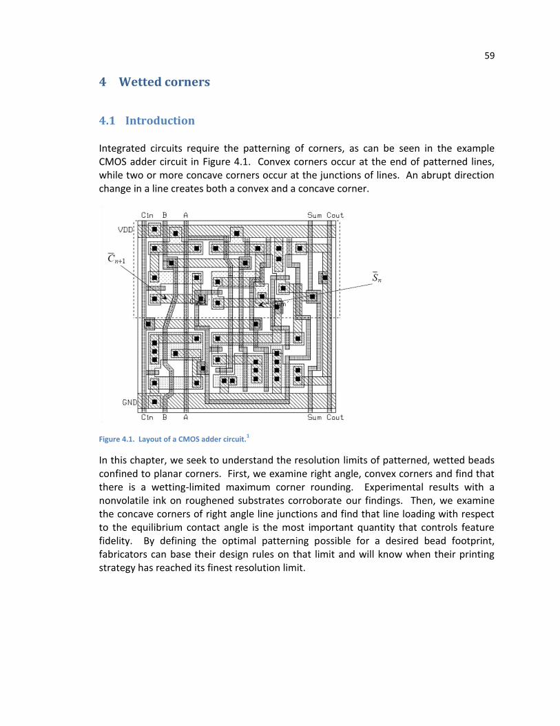
59

4 Wetted corners

4.1 Introduction

Integrated circuits require the patterning of corners, as can be seen in the example CMOS adder circuit in Figure 4.1. Convex corners occur at the end of patterned lines, while two or more concave corners occur at the junctions of lines. An abrupt direction change in a line creates both a convex and a concave corner.

Figure 4.1. Layout of a CMOS adder circuit.1

In this chapter, we seek to understand the resolution limits of patterned, wetted beads confined to planar corners. First, we examine right angle, convex corners and find that there is a wetting-limited maximum corner rounding. Experimental results with a nonvolatile ink on roughened substrates corroborate our findings. Then, we examine the concave corners of right angle line junctions and find that line loading with respect to the equilibrium contact angle is the most important quantity that controls feature fidelity. By defining the optimal patterning possible for a desired bead footprint, fabricators can base their design rules on that limit and will know when their printing strategy has reached its finest resolution limit.

60

4.2 Convex corners: squarish squares

4.2.1 Convex corners introduction

Motivated by the process of inkjet printing of electronics, we study experimentally and theoretically the processes limiting the printing of sharply defined corners. Using a non-volatile ionic liquid, we inkjet print rectangles with rounded corners on a substrate of roughened, display-grade glass. We show experimentally that with increasing roughness height, corner radius decreases, allowing more precisely defined features to be printed. To interpret these results in terms of contact-angle hysteresis (difference between the advancing and retreating contact angles θA and θR), we implement the following model with the Surface Evolver program. With drop volume fixed, we minimize drop surface energy subject to a prescribed contact line. We identify θA and θR as the minimum and maximum contact angles around the drop perimeter. We find that with decreasing corner fidelity, contact-angle hysteresis also decreases. We extend our calculations to rectangular drops and find the contact-angle hysteresis required to sustain long drops with large aspect ratio. We conclude that increasing contact-angle hysteresis allows the printing of more precisely defined and higher aspect ratio features.

Printed electronics technology has the potential to lower sharply the manufacturing costs of a range of active electronic devices and enable the creation of novel ones. Since it is an additive process (as opposed to subtractive processes used in conventional deposit-pattern-etch techniques), it is not only simpler but results in less waste, translating to lower cost. Researchers have used additive printing to fabricated circuit components, such as inductors, capacitors and transistors; and even low-cost integrated circuits such as active organic light emitting diode displays.2-5 To enable reliable printed devices, we seek design results that define the necessary spacings and permissible shapes in additive printing. This work represents an early step in the process of developing these design principles.

Though a droplet on a substrate tends to adopt a circular footprint, the existence of contact-angle hysteresis between advancing and retreating contact angles, θA and θR respectively, means that other planforms can be printed. Previously we showed that by reducing θR by utilizing solute deposition at the contact line, better corner definition in square-shaped drops could be achieved due to greater contact-line pinning.6 Here we extend this work and show how enhanced hysteresis determines the sharpest equilibrium corner definition possible in square and rectangular features. Although contact-angle hysteresis is the result of various causes including particles at the contact line, we use variable, controlled roughness in our experiment and note that the receding contact angle decreases as substrate roughness increases. Dettre and Johnson demonstrate this trend when they show, in Figure 8.5 of their work, a decreasing θR for several pure liquids as roughness increases.7

61

Using Surface Evolver8, we verify the relationship between sharpest possible corner rounding and θR for ink-substrate systems with θA less than or equal to 90°. We are thus able to predict the necessary corner curvature required for an equilibrium rectangular bead to have a contact line with its contact angle bounded by any pair of advancing and retreating contact angles. In particular, a lower θR allows for sharper corners in stable square and rectangular drops. Finally, as the aspect ratio of rectangles increases above unity, a minimum amount of contact-angle hysteresis is required for stable drops to be formed. We show that for a given θA, as aspect ratio increases, a larger amount of hysteresis is required.

As in our earlier work, the Bond number for our beads is 0.3 or less so we safely neglect the effects of gravity on their shape.9 Without gravity-induced flattening, our beads’ surfaces, solutions to the Young-Laplace equation subject to θA and θR constraints, have a constant curvature at every point on their free surface. Scaling a surface with constant curvature C uniformly in space by a factor , results in a new surface with a new constant curvature C/ . Further, contact angle is not affected by uniform scaling. Therefore, uniform spatial scaling of a solution to our problem that satisfies the governing equation and constraints produces another valid solution at a different length scale.

The scalability of bead solutions for small Bond number drops has implications for our experimental and numerical results. When printing, we expect that the sharpest possible square-bead shape remains constant when scaled in space; we examine this hypothesis in the experimental section. Numerically, we need only solve for square beads at a single side length, chosen as one for convenience, and then this solution can be applied to any length scale. (The same scaling applies to rectangles at each aspect ratio.)

As demonstrated in the experimental section, the wetting radius of a single, jetted drop sets the minimum achievable planform corner radius. This wetting radius scales with the cube root of jetted drop volume, and higher-fidelity, stable features may be printed by reducing drop volume. We chose to use our custom-built research inkjet printer with a relatively large inkjet nozzle due to the system’s flexibility, reliability, and solvent-resistant Teflon/glass ink delivery pathway. A modern consumer inkjet printer produces drops with volumes on the order of 1 pL, two orders of magnitude smaller than the approximately 100 pL drops produced by our system. Thus, the approximately 100 μm minimum corner radius in this work scales to an approximately 5 μm radius when printing with an up-to-date inkjet nozzle.

Due to the small contact angles exhibited by the system, we could not accurately measure advancing and receding contact angles using a conventional method such as the sessile-drop technique. Measurements yielded poor accuracy because of the narrow angle and the interference of the needle required to inject and suck fluid to

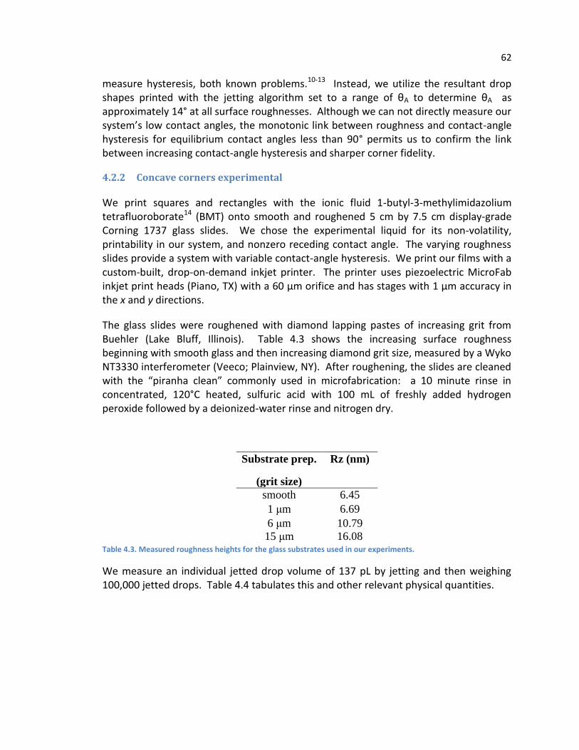
62

measure hysteresis, both known problems.10-13 Instead, we utilize the resultant drop shapes printed with the jetting algorithm set to a range of θA to determine θA as approximately 14° at all surface roughnesses. Although we can not directly measure our system’s low contact angles, the monotonic link between roughness and contact-angle hysteresis for equilibrium contact angles less than 90° permits us to confirm the link between increasing contact-angle hysteresis and sharper corner fidelity.

4.2.2 Concave corners experimental

We print squares and rectangles with the ionic fluid 1-butyl-3-methylimidazolium tetrafluoroborate14 (BMT) onto smooth and roughened 5 cm by 7.5 cm display-grade Corning 1737 glass slides. We chose the experimental liquid for its non-volatility, printability in our system, and nonzero receding contact angle. The varying roughness slides provide a system with variable contact-angle hysteresis. We print our films with a custom-built, drop-on-demand inkjet printer. The printer uses piezoelectric MicroFab inkjet print heads (Piano, TX) with a 60 µm orifice and has stages with 1 µm accuracy in the x and y directions.

The glass slides were roughened with diamond lapping pastes of increasing grit from Buehler (Lake Bluff, Illinois). Table 4.3 shows the increasing surface roughness beginning with smooth glass and then increasing diamond grit size, measured by a Wyko NT3330 interferometer (Veeco; Plainview, NY). After roughening, the slides are cleaned with the “piranha clean” commonly used in microfabrication: a 10 minute rinse in concentrated, 120°C heated, sulfuric acid with 100 mL of freshly added hydrogen peroxide followed by a deionized-water rinse and nitrogen dry.

Substrate prep.

(grit size)

Rz (nm)

smooth 6.45

1 μm 6.69

6 μm 10.79

15 μm 16.08 Table 4.3. Measured roughness heights for the glass substrates used in our experiments.

We measure an individual jetted drop volume of 137 pL by jetting and then weighing 100,000 jetted drops. Table 4.4 tabulates this and other relevant physical quantities.

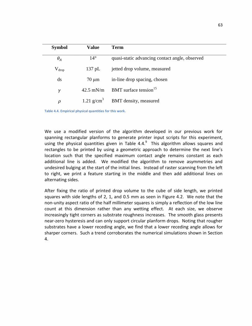
63

Symbol Value Term

14° quasi-static advancing contact angle, observed

Vdrop 137 pL jetted drop volume, measured

ds 70 μm in-line drop spacing, chosen

42.5 mN/m BMT surface tension15

1.21 g/cm3 BMT density, measured

Table 4.4. Empirical physical quantities for this work.

We use a modified version of the algorithm developed in our previous work for spanning rectangular planforms to generate printer input scripts for this experiment, using the physical quantities given in Table 4.4.9 This algorithm allows squares and rectangles to be printed by using a geometric approach to determine the next line’s location such that the specified maximum contact angle remains constant as each additional line is added. We modified the algorithm to remove asymmetries and undesired bulging at the start of the initial lines. Instead of raster scanning from the left to right, we print a feature starting in the middle and then add additional lines on alternating sides.

After fixing the ratio of printed drop volume to the cube of side length, we printed squares with side lengths of 2, 1, and 0.5 mm as seen in Figure 4.2. We note that the non-unity aspect ratio of the half millimeter squares is simply a reflection of the low line count at this dimension rather than any wetting effect. At each size, we observe increasingly tight corners as substrate roughness increases. The smooth glass presents near-zero hysteresis and can only support circular planform drops. Noting that rougher substrates have a lower receding angle, we find that a lower receding angle allows for sharper corners. Such a trend corroborates the numerical simulations shown in Section 4.

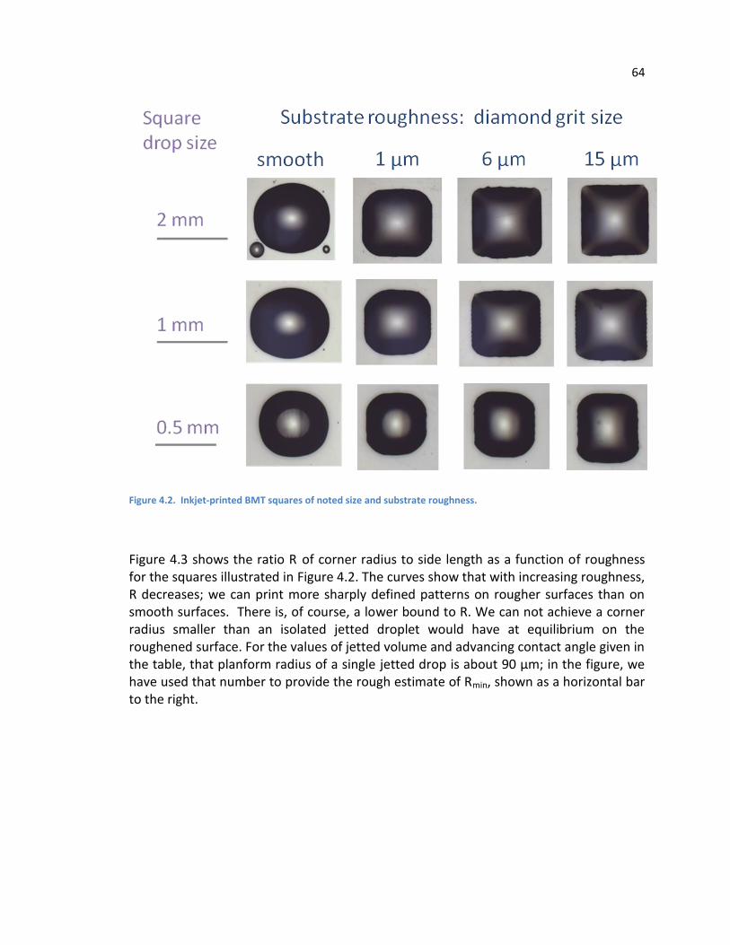
64

Figure 4.2. Inkjet-printed BMT squares of noted size and substrate roughness.

Figure 4.3 shows the ratio R of corner radius to side length as a function of roughness for the squares illustrated in Figure 4.2. The curves show that with increasing roughness, R decreases; we can print more sharply defined patterns on rougher surfaces than on smooth surfaces. There is, of course, a lower bound to R. We can not achieve a corner radius smaller than an isolated jetted droplet would have at equilibrium on the roughened surface. For the values of jetted volume and advancing contact angle given in the table, that planform radius of a single jetted drop is about 90 μm; in the figure, we have used that number to provide the rough estimate of Rmin, shown as a horizontal bar to the right.

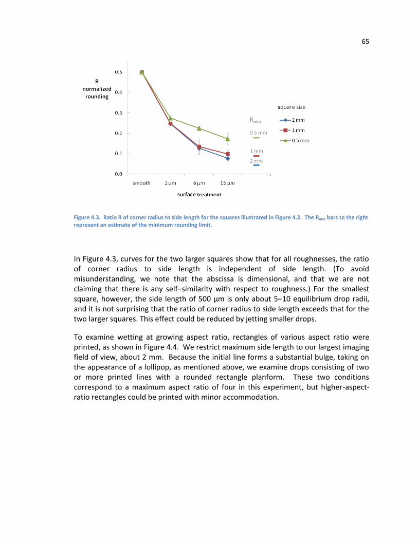
65

Figure 4.3. Ratio R of corner radius to side length for the squares illustrated in Figure 4.2. The Rmin bars to the right represent an estimate of the minimum rounding limit.

In Figure 4.3, curves for the two larger squares show that for all roughnesses, the ratio of corner radius to side length is independent of side length. (To avoid misunderstanding, we note that the abscissa is dimensional, and that we are not claiming that there is any self–similarity with respect to roughness.) For the smallest square, however, the side length of 500 μm is only about 5–10 equilibrium drop radii, and it is not surprising that the ratio of corner radius to side length exceeds that for the two larger squares. This effect could be reduced by jetting smaller drops.

To examine wetting at growing aspect ratio, rectangles of various aspect ratio were printed, as shown in Figure 4.4. We restrict maximum side length to our largest imaging field of view, about 2 mm. Because the initial line forms a substantial bulge, taking on the appearance of a lollipop, as mentioned above, we examine drops consisting of two or more printed lines with a rounded rectangle planform. These two conditions correspond to a maximum aspect ratio of four in this experiment, but higher-aspect-ratio rectangles could be printed with minor accommodation.

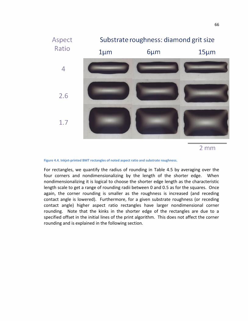
66

Figure 4.4. Inkjet-printed BMT rectangles of noted aspect ratio and substrate roughness.

For rectangles, we quantify the radius of rounding in Table 4.5 by averaging over the four corners and nondimensionalizing by the length of the shorter edge. When nondimensionalizing it is logical to choose the shorter edge length as the characteristic length scale to get a range of rounding radii between 0 and 0.5 as for the squares. Once again, the corner rounding is smaller as the roughness is increased (and receding contact angle is lowered). Furthermore, for a given substrate roughness (or receding contact angle) higher aspect ratio rectangles have larger nondimensional corner rounding. Note that the kinks in the shorter edge of the rectangles are due to a specified offset in the initial lines of the print algorithm. This does not affect the corner rounding and is explained in the following section.

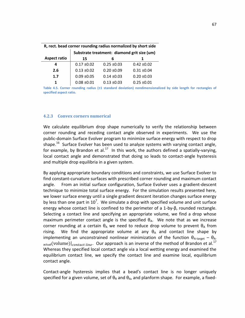
67

R, rect. bead corner rounding radius normalized by short side

Substrate treatment: diamond grit size (um) Aspect ratio 15 6 1

4 0.17 ±0.02 0.25 ±0.03 0.42 ±0.02

2.6 0.13 ±0.02 0.20 ±0.09 0.31 ±0.04

1.7 0.09 ±0.05 0.14 ±0.03 0.20 ±0.03

1 0.08 ±0.01 0.13 ±0.03 0.25 ±0.01 Table 4.5. Corner rounding radius (±1 standard deviation) nondimensionalized by side length for rectangles of specified aspect ratio.

4.2.3 Convex corners numerical

We calculate equilibrium drop shape numerically to verify the relationship between corner rounding and receding contact angle observed in experiments. We use the public-domain Surface Evolver program to minimize surface energy with respect to drop shape.16 Surface Evolver has been used to analyze systems with varying contact angle, for example, by Brandon et al.17 In this work, the authors defined a spatially-varying, local contact angle and demonstrated that doing so leads to contact-angle hysteresis and multiple drop equilibria in a given system.

By applying appropriate boundary conditions and constraints, we use Surface Evolver to find constant-curvature surfaces with prescribed corner rounding and maximum contact angle. From an initial surface configuration, Surface Evolver uses a gradient-descent technique to minimize total surface energy. For the simulation results presented here, we lower surface energy until a single gradient descent iteration changes surface energy by less than one part in 107. We simulate a drop with specified volume and unit surface energy whose contact line is confined to the perimeter of a 1-by-β, rounded rectangle. Selecting a contact line and specifying an appropriate volume, we find a drop whose maximum perimeter contact angle is the specified θA. We note that as we increase corner rounding at a certain θA we need to reduce drop volume to prevent θA from rising. We find the appropriate volume at any θA and contact line shape by implementing an unconstrained nonlinear minimization of the function θA-target – θA-

actual . Our approach is an inverse of the method of Brandon et al.17

Whereas they specified local contact angle via a local wetting energy and examined the equilibrium contact line, we specify the contact line and examine local, equilibrium contact angle.

Contact-angle hysteresis implies that a bead’s contact line is no longer uniquely specified for a given volume, set of θR and θA, and planform shape. For example, a fixed-

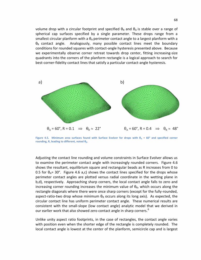
68

volume drop with a circular footprint and specified θR and θA is stable over a range of spherical cap surfaces specified by a single parameter. These drops range from a smallest circular planform with a θA perimeter contact angle to a largest planform with a θR contact angle. Analogously, many possible contact lines meet the boundary conditions for rounded squares with contact-angle hysteresis presented above. Because we experimentally observe corner retreat towards drop center, fitting increasing-size quadrants into the corners of the planform rectangle is a logical approach to search for best-corner-fidelity contact lines that satisfy a particular contact-angle hysteresis.

Figure 4.5. Minimum area surfaces found with Surface Evolver for drops with θA = 60° and specified corner rounding, R, leading to different, noted θR.

Adjusting the contact line rounding and volume constraints in Surface Evolver allows us to examine the perimeter contact angle with increasingly rounded corners. Figure 4.6 shows the resultant, equilibrium square and rectangular beads as R increases from 0 to 0.5 for θA= 30°. Figure 4.6 a,c) shows the contact lines specified for the drops whose perimeter contact angles are plotted versus radial coordinate in the wetting plane in b,d), respectively. Approaching sharp corners, the local contact angle falls to zero and increasing corner rounding increases the minimum value of θR, which occurs along the rectangle diagonals where there were once sharp corners (except for the fully-rounded, aspect-ratio-two drop whose minimum θR occurs along its long axis). As expected, the circular contact line has uniform perimeter contact angle. These numerical results are consistent with the small-slope (low contact angle) analytic model that we derived in our earlier work that also showed zero contact angle in sharp corners.6

Unlike unity aspect ratio footprints, in the case of rectangles, the contact angle varies with position even when the shorter edge of the rectangle is completely rounded. The local contact angle is lowest at the center of the planform, semicircle cap and is largest

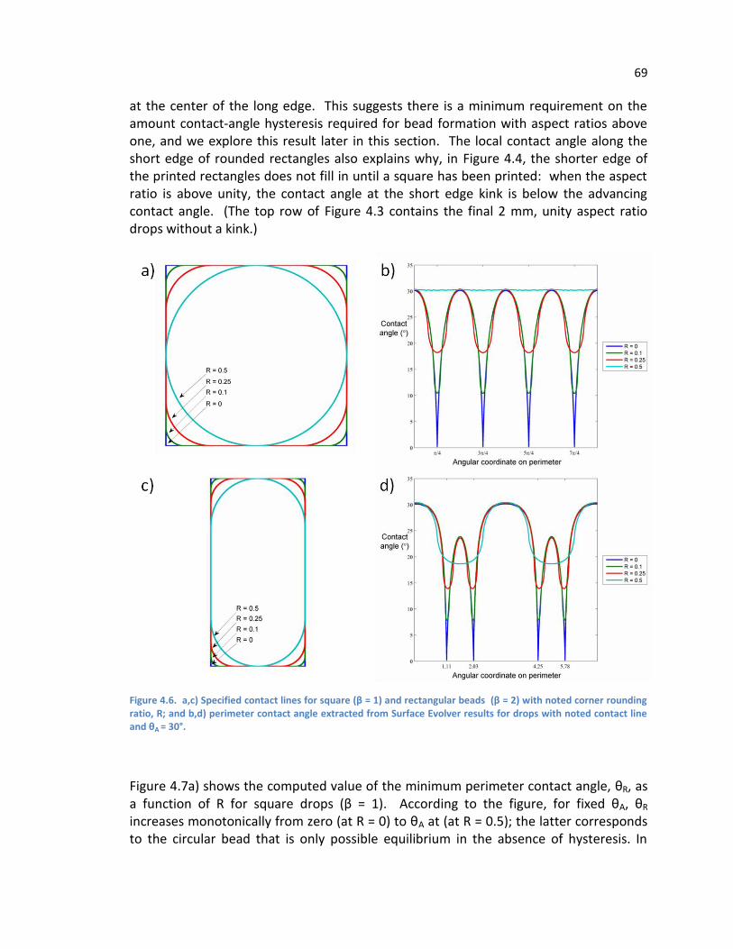
69

at the center of the long edge. This suggests there is a minimum requirement on the amount contact-angle hysteresis required for bead formation with aspect ratios above one, and we explore this result later in this section. The local contact angle along the short edge of rounded rectangles also explains why, in Figure 4.4, the shorter edge of the printed rectangles does not fill in until a square has been printed: when the aspect ratio is above unity, the contact angle at the short edge kink is below the advancing contact angle. (The top row of Figure 4.3 contains the final 2 mm, unity aspect ratio drops without a kink.)

Figure 4.6. a,c) Specified contact lines for square (β = 1) and rectangular beads (β = 2) with noted corner rounding ratio, R; and b,d) perimeter contact angle extracted from Surface Evolver results for drops with noted contact line and θA = 30°.

Figure 4.7a) shows the computed value of the minimum perimeter contact angle, θR, as a function of R for square drops (β = 1). According to the figure, for fixed θA, θR increases monotonically from zero (at R = 0) to θA at (at R = 0.5); the latter corresponds to the circular bead that is only possible equilibrium in the absence of hysteresis. In

70

other words, the smaller the value of θR, the more sharply defined the corner we can print. Further, for fixed θA, as R is increased from zero to intermediate values, θR becomes less sensitive to R, suggesting that little difference in hysteresis separates best-fidelity squares at intermediate rounding. We are unable to verify this prediction because the small contact angles of our system prevented independent measurements of θR and θA (as mentioned in the introduction).

Figure 4.7. Minimum perimeter contact angle, θR, as a function of ratio R of corner radius to side length with θA as a parameter varying from 10° to 90° as noted for a) squares, and b) rectangles of aspect ratio 2.

Figure 4.7b) shows the corresponding results for a rectangle of aspect ratio two; here R is formed using the shorter side as reference length. Comparing Figure 4.7b) with Figure 4.7a), we see for the rectangle that, for fixed θA, θR is about half as large. At larger aspect ratio, a larger contact-angle hysteresis, θA−θR, is required to sustain a given corner radius. As a consequence, because θR ≥ 0 it follows that for the rectangle described by Figure 4.7b), there is a range of R over which is θR less sensitive to variations in corner rounding than is the square. Within that range, small changes in θR produce large changes in R. A corollary result is that for a given set of θA and θR, as the aspect ratio is increased, one would expect the corner rounding R to increase. From Figure 4.4, we see that experimental result support this prediction. The large aspect-ratio rectangles created by depositing only a few lines have greater normalized corner rounding than do the smaller aspect-ratio shapes created by depositing many more lines.

Extending this analysis, we simulate rectangles of increasing aspect ratio with fully rounded short sides, such as those seen in Figure 4.8 a). As aspect ratio is increased, the

71

θR found in rectangles with fully rounded short sides (fully rounded sides require less hysteresis than partially rounded sides) monotonically decreases with decreasing magnitude slope. We note that long drops (aspect ratio above 50) with large θA (80-90°) tended to be unstable during surface energy minimization, forming a large, spherical bulge connected to a thin line wetting the prescribed contact line. This is because such drops approach the stability condition for linear beads with pinned contact lines, derived by Davis. He showed that long, wetted drops with pinned contact lines are unstable if their contact angle exceeds 90°.18 We omit any beads that formed such a bulge from the figure.

From Figure 4.8 we can determine whether a rectangle can be printed based on the advancing and receding contact angles. For a given system, it should be possible to print rectangles of a particular aspect ratio so long as the required θR to maintain this aspect ratio is not lower than the actual wetting θR. For example, consider an ink-substrate system with θA= 80° and θR= 30°. As shown in the figure, it is only possible to print rounded rectangles of aspect ratio less than 5; larger aspect-ratio shapes would dewet and shorten. For this system, we expect rectangles of aspect ratio 5 to be stable only with fully rounded ends, while rectangles of aspect ratio less than 5 can sustain sharper corners.

Figure 4.8. a) Contact line of fully-rounded rectangles (R = 0.5) with labeled aspect ratio and indicated location of θR; and b) receding contact angle as a function of aspect ratio for fully-rounded rectangles.

72

4.2.4 Convex Corners Conclusion

The work presented here demonstrates the value of approaching printed patterning from a surface-energy perspective. Experimentally, we show that for a given advancing contact angle, decreasing θR via substrate roughening allows the creation of sharper bead corners. Numerically, we show the link between decreasing θR and increasingly sharp stable drop corners to be valid for all systems with θA less than or equal to 90°. Given a set of advancing and receding angles, the minimum amount of corner rounding for stable square and rectangular drops can be determined.

For rectangles having an aspect ratio above unity, we determine the maximum receding angle required for stability given the advancing angle. Without sufficient hysteresis, the shorter edge retreats inward and the aspect ratio cannot be held. As the aspect ratio is increased, this required receding angle decreases. We show printed rectangles with constant wetting properties where corner fidelity decreases with increasing aspect ratio implying that hysteresis requirements for corner fidelity increase with aspect ratio. Although here we only illustrate drops with aspect ratio less than four because lengthy drops are harder to image, we have no difficulty printing longer drops. These drops are numerous and important in printed electronic applications.

The results in this paper suggest future research directions. The role of viscous flow in controlling equilibrium drop shape is unknown. How does equilibrium corner fidelity vary with viscosity for an initially square drop with a retreating contact line? Also, we have not exhausted the potential of approaching drop-pattern fidelity subject to surface energy minimization and wetting constraints. Such work may prove valuable in understanding the link between wetting and contact-line curvature. Specific areas worth examination include being able to understand and control initial bulge formation in a single printed line, and investigating drops confined to planar corners of any angle. A better understanding of drop patterning will allow for the formulation of algorithms and design rules for printing optimal, arbitrarily shaped features.

4.3 Concave corners

4.3.1 Concave corners introduction

Because connected wires in circuits have bends, both convex and convex contact line corners occur. Following the approach described above for convex corners, we now study concave corners. In the previous section, we established the fundamental convex corner fidelity limits for a given set of wetting properties, θadv and θrec, and the work that follows proposes that a different set of parameters controls concave corner wetting. Rather than use any arbitrary polygon as a test shape for this study, we chose

73

the shapes shown in Figure 4.9, containing the concave corners found in constant line-width, Manhattan layout of wires.

Figure 4.9. Concave corner test geometries.

Our experimental work examining concave corners is still in its early stages and will be the subject of follow-up work after the completion of this thesis. Fortunately, a colleague, Lakshmi Jagannathan, has provided her printing results that are useful in motivating the following analysis. She printed a gold nanoparticle ink from Harima Chemicals Inc. onto cleaned, borofloat glass substrates, as seen in Figure 4.10. Single pixel-wide raster scanned lines show pronounced bulging at their corners, several times wider than the line width. However, five pixel wide lines printed with the same system show no bulging at all with crisp corner definition. Unlike the modulated corner rounding seen above with printed convex corners, the concave corners formed by the meeting of high aspect ratio features are less stable, sometimes nearly draining their constituent lines and forming a large bulge at the intersection. We will attempt to explain the reasons for modulation of concave corner bulges in the following section.

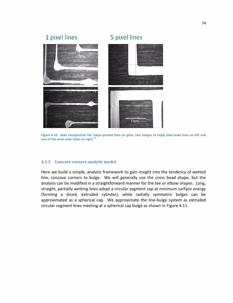
74

Figure 4.10. Gold nanoparticle ink, inkjet-printed lines on glass, two images of single pixel-wide lines on left and two of five pixel wide slides on right.

19

4.3.2 Concave corners analytic model

Here we build a simple, analytic framework to gain insight into the tendency of wetted line, concave corners to bulge. We will generally use the cross bead shape, but the analysis can be modified in a straightforward manner for the tee or elbow shapes. Long, straight, partially wetting lines adopt a circular segment cap at minimum surface energy (forming a sliced, extruded cylinder), while radially symmetric bulges can be approximated as a spherical cap. We approximate the line-bulge system as extruded circular segment lines meeting at a spherical cap bulge as shown in Figure 4.11.

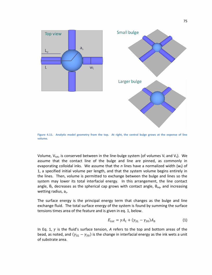
75

Figure 4.11. Analytic model geometry from the top. At right, the central bulge grows at the expense of line volume.

Volume, Vtot, is conserved between in the line-bulge system (of volumes Vl and Vs). We assume that the contact line of the bulge and line are pinned, as commonly in evaporating colloidal inks. We assume that the n lines have a normalized width (wl) of 1, a specified initial volume per length, and that the system volume begins entirely in the lines. Then, volume is permitted to exchange between the bulge and lines so the system may lower its total interfacial energy. In this arrangement, the line contact angle, θl, decreases as the spherical cap grows with contact angle, θeq, and increasing wetting radius, as.

The surface energy is the principal energy term that changes as the bulge and line exchange fluid. The total surface energy of the system is found by summing the surface tensions times area of the feature and is given in eq. 1, below.

(1)

In Eq. 1, is the fluid’s surface tension, A refers to the top and bottom areas of the bead, as noted, and is the change in interfacial energy as the ink wets a unit of substrate area.

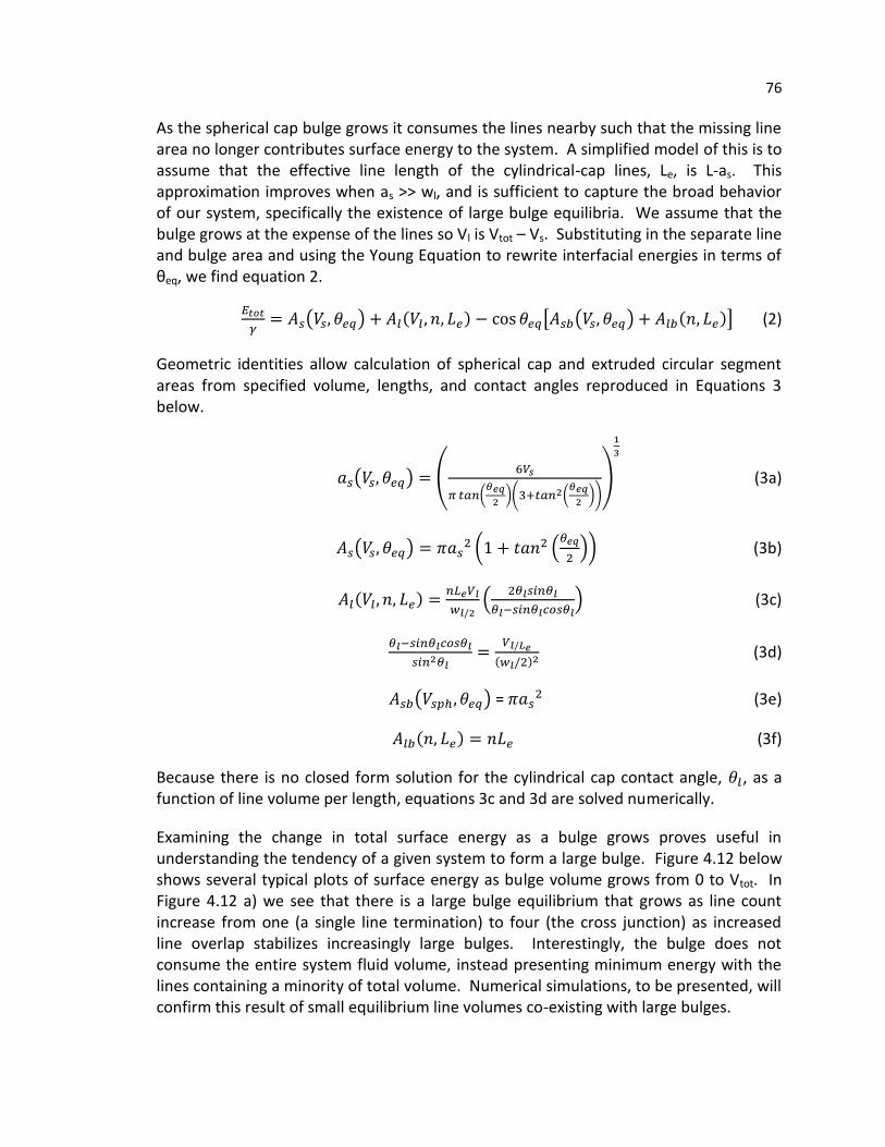
76

As the spherical cap bulge grows it consumes the lines nearby such that the missing line area no longer contributes surface energy to the system. A simplified model of this is to assume that the effective line length of the cylindrical-cap lines, Le, is L-as. This approximation improves when as >> wl, and is sufficient to capture the broad behavior of our system, specifically the existence of large bulge equilibria. We assume that the bulge grows at the expense of the lines so Vl is Vtot – Vs. Substituting in the separate line and bulge area and using the Young Equation to rewrite interfacial energies in terms of θeq, we find equation 2.

(2)

Geometric identities allow calculation of spherical cap and extruded circular segment areas from specified volume, lengths, and contact angles reproduced in Equations 3 below.

(3a)

(3b)

(3c)

(3d)

= (3e)

(3f)

Because there is no closed form solution for the cylindrical cap contact angle, , as a function of line volume per length, equations 3c and 3d are solved numerically.

Examining the change in total surface energy as a bulge grows proves useful in understanding the tendency of a given system to form a large bulge. Figure 4.12 below shows several typical plots of surface energy as bulge volume grows from 0 to Vtot. In Figure 4.12 a) we see that there is a large bulge equilibrium that grows as line count increase from one (a single line termination) to four (the cross junction) as increased line overlap stabilizes increasingly large bulges. Interestingly, the bulge does not consume the entire system fluid volume, instead presenting minimum energy with the lines containing a minority of total volume. Numerical simulations, to be presented, will confirm this result of small equilibrium line volumes co-existing with large bulges.

77

Varying the input parameters of L, θeq, and Vtot and plotting the Etot/ versus Vs reveals two important solution types, examples of which are shown below in Figure 4.12 b). When Vtot is sufficiently large such that the line contact angle with no bulge volume, θl0, is near θeq, we find a stable, large bulge equilibrium like that shown in Figure 4.12 b). When θl0 is sufficiently smaller than θeq, the equilibrium shifts to a small volume bulge like that in the right of Figure 4.12 b). Recalling that the line-bulge overlap accounting breaks down at small bulge size, the results of Figure 4.12 c) demonstrate that large bulges are not always energetically favorable, but should not be considered an accurate prediction of small bulge volume. In order to accurately simulate the entire range of bulge-line equilibria we now turn to numerical simulations.

Figure 4.12. Surface energy for line-bulge systems with unit surface tension; a) large bulge equilibrium growing with line count, θl0 = θeq = 60° and nL = 40 (Vtot = 8); and b) cross-footprint bulges demonstrating large and small bulge equilibrium θl0 = 30°, nL = 100 (Vtot = 8), and noted θeq .

4.3.3 Concave corners numerical simulations

We perform numerical solutions of our line-bulge bead with Surface Evolver to generate more accurate predictions and corroborate the analytic results.8 We implement the zero-retreating contact angle and positive advancing contact angle found in our, and many other, ink-substrate systems by instantiating the contact lines at the edges of an unbulged intersection, as drawn in Figure 4.9. Then, we impose one-sided

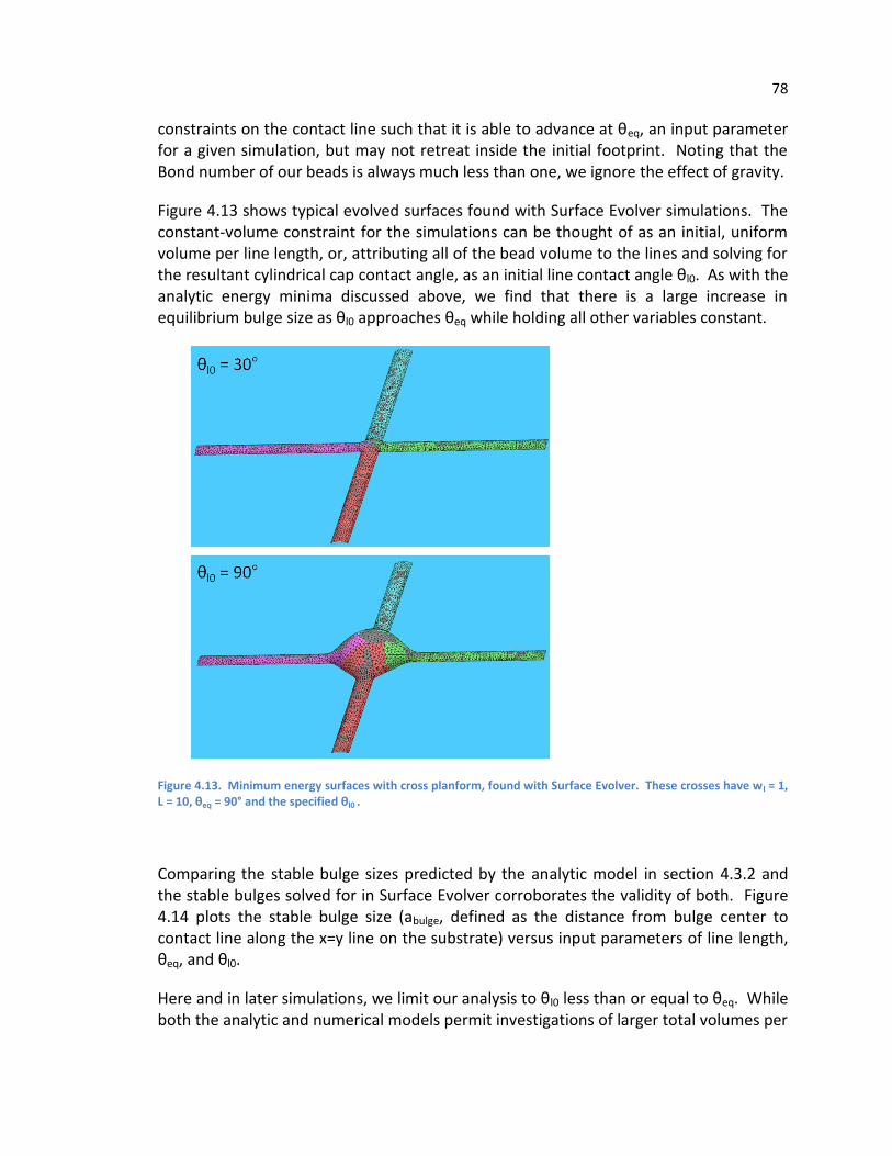
78

constraints on the contact line such that it is able to advance at θeq, an input parameter for a given simulation, but may not retreat inside the initial footprint. Noting that the Bond number of our beads is always much less than one, we ignore the effect of gravity.

Figure 4.13 shows typical evolved surfaces found with Surface Evolver simulations. The constant-volume constraint for the simulations can be thought of as an initial, uniform volume per line length, or, attributing all of the bead volume to the lines and solving for the resultant cylindrical cap contact angle, as an initial line contact angle θl0. As with the analytic energy minima discussed above, we find that there is a large increase in equilibrium bulge size as θl0 approaches θeq while holding all other variables constant.

Figure 4.13. Minimum energy surfaces with cross planform, found with Surface Evolver. These crosses have w l = 1, L = 10, θeq = 90° and the specified θl0 .

Comparing the stable bulge sizes predicted by the analytic model in section 4.3.2 and the stable bulges solved for in Surface Evolver corroborates the validity of both. Figure 4.14 plots the stable bulge size (abulge, defined as the distance from bulge center to contact line along the x=y line on the substrate) versus input parameters of line length, θeq, and θl0.

Here and in later simulations, we limit our analysis to θl0 less than or equal to θeq. While both the analytic and numerical models permit investigations of larger total volumes per

79

length, physically such a system may progress to many equilibria other than the corner bulge. With a uniform line contact angle in excess of θeq, the entire line is driven to spread simultaneously, and a race condition develops between uniform spreading and lower-energy, periodic bulging. The enhanced spreading near the junction due to the pre-existing wetting film of the other arms makes for an interesting system to analyze. Such a problem is beyond the scope of this work, and Duineveld’s work analyzing periodic bulging as a line is printed with a contact angle above equilibrium presents a good starting point for analyzing such a system.20

Returning to the comparison of our analytic and numerical results, we see good agreement between the two models, though there is an increasing deviation between the models when small bulges are predicted (at θl0 much less than θeq). First, Surface Evolver allows contact lines to advance but not retreat from their initial positions.

(Vertices are allowed to have Therefore, the minimum abulge is , a limit seen in the smaller simulated bulges but not present in the numerical model. Regarding the analytic model, the assumption of a spherical cap abutting an abruptly-terminated cylinder is an increasingly poor approximation as bulge size decreases. The discrepancy in predicted small bulge sizes between the two models is largely due to this analytic approximation. That said, the agreement in stable larger bulge sizes indicates that we have captured the essential physical elements that govern bulging behavior.

80

Figure 4.14. Equilibrium bulge size of cross feature as predicted by analytic model (blue diamond) and surface evolver simulations (red square). Length is sampled at 2.5, 10, 25 along the x axis; θeq is sampled at 30°, 60°, 90° along rows; and θl0 is sampled at about 30°, 60°, 90° along columns.

A more detailed understanding of the conditions that lead to bulge formation can be found by simulating many crosses while varying equilibrium contact angle, system volume (equivalently θl0), and cross arm length. Figure 4.15 presents the results of such simulations. It shows the contact line of the equilibrium, minimum energy surface in the first quadrant, including one quarter of the bulge, if present. Each plot is for the specified arm length (the top row has L = 10 and the bottom has L = 20), and θeq (columns of 20°, 45°, and 90°). Each plotted point represents a vertex from the contact line in the first quadrant region near the bulge, and each color represents θl0 descending from θeq in increments of 5°.

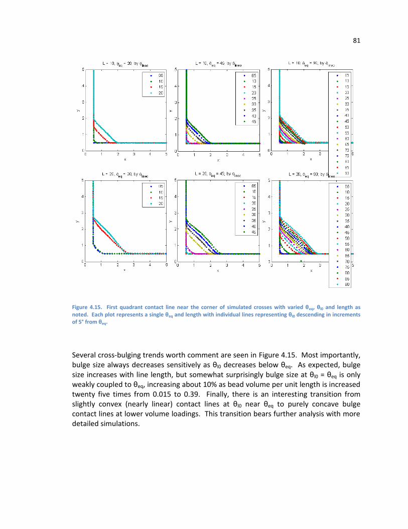
81

Figure 4.15. First quadrant contact line near the corner of simulated crosses with varied θeq, θl0 and length as noted. Each plot represents a single θeq and length with individual lines representing θl0 descending in increments of 5° from θeq.

Several cross-bulging trends worth comment are seen in Figure 4.15. Most importantly, bulge size always decreases sensitively as θl0 decreases below θeq. As expected, bulge size increases with line length, but somewhat surprisingly bulge size at θl0 = θeq is only weakly coupled to θeq, increasing about 10% as bead volume per unit length is increased twenty five times from 0.015 to 0.39. Finally, there is an interesting transition from slightly convex (nearly linear) contact lines at θl0 near θeq to purely concave bulge contact lines at lower volume loadings. This transition bears further analysis with more detailed simulations.

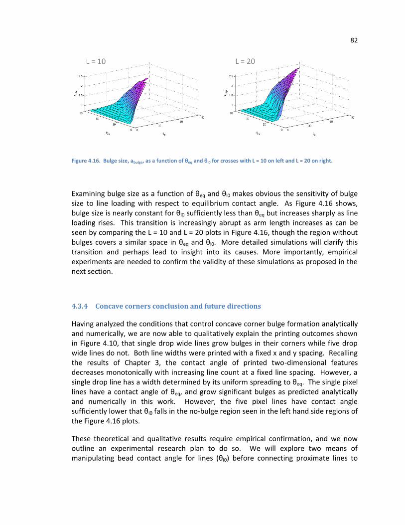
82

Figure 4.16. Bulge size, abulge, as a function of θeq and θl0 for crosses with L = 10 on left and L = 20 on right.

Examining bulge size as a function of θeq and θl0 makes obvious the sensitivity of bulge size to line loading with respect to equilibrium contact angle. As Figure 4.16 shows, bulge size is nearly constant for θl0 sufficiently less than θeq but increases sharply as line loading rises. This transition is increasingly abrupt as arm length increases as can be seen by comparing the L = 10 and L = 20 plots in Figure 4.16, though the region without bulges covers a similar space in θeq and θl0. More detailed simulations will clarify this transition and perhaps lead to insight into its causes. More importantly, empirical experiments are needed to confirm the validity of these simulations as proposed in the next section.

4.3.4 Concave corners conclusion and future directions

Having analyzed the conditions that control concave corner bulge formation analytically and numerically, we are now able to qualitatively explain the printing outcomes shown in Figure 4.10, that single drop wide lines grow bulges in their corners while five drop wide lines do not. Both line widths were printed with a fixed x and y spacing. Recalling the results of Chapter 3, the contact angle of printed two-dimensional features decreases monotonically with increasing line count at a fixed line spacing. However, a single drop line has a width determined by its uniform spreading to θeq. The single pixel lines have a contact angle of θeq, and grow significant bulges as predicted analytically and numerically in this work. However, the five pixel lines have contact angle sufficiently lower that θl0 falls in the no-bulge region seen in the left hand side regions of the Figure 4.16 plots.

These theoretical and qualitative results require empirical confirmation, and we now outline an experimental research plan to do so. We will explore two means of manipulating bead contact angle for lines (θl0) before connecting proximate lines to

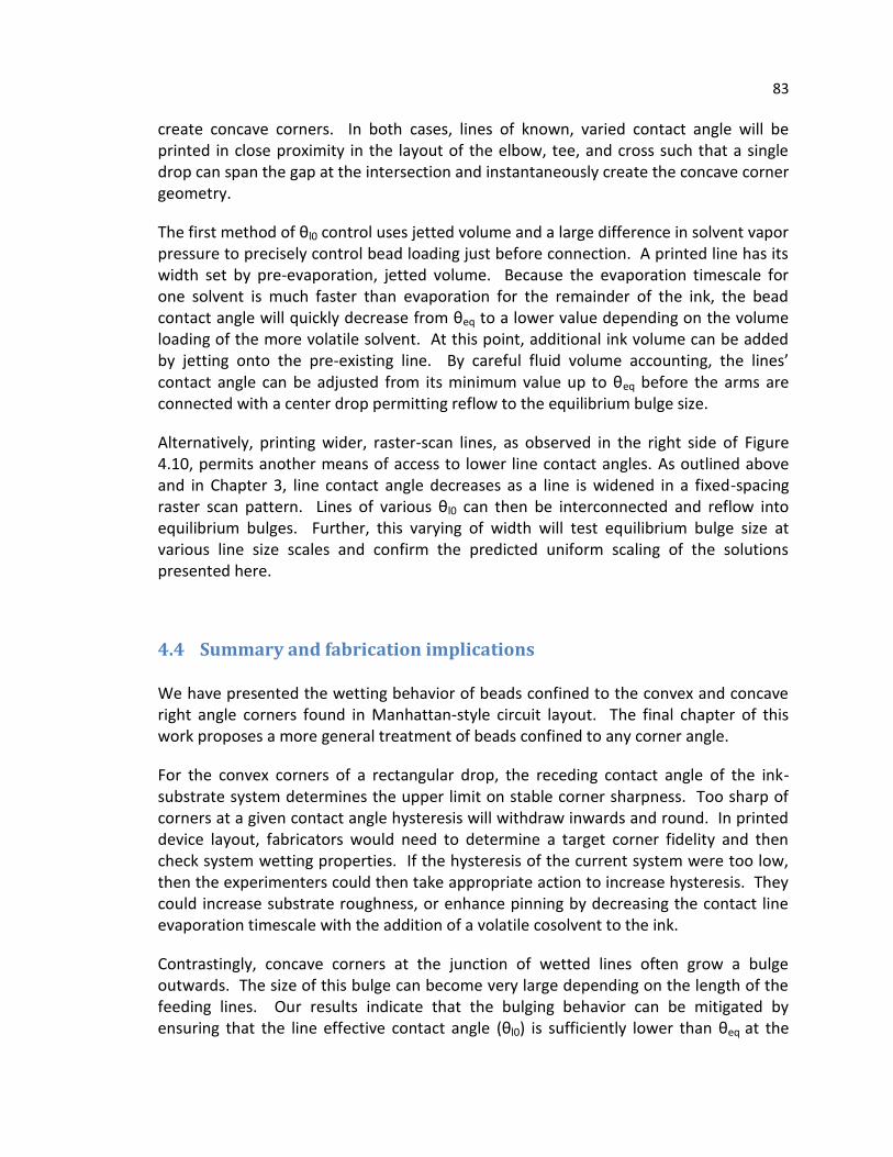
83

create concave corners. In both cases, lines of known, varied contact angle will be printed in close proximity in the layout of the elbow, tee, and cross such that a single drop can span the gap at the intersection and instantaneously create the concave corner geometry.

The first method of θl0 control uses jetted volume and a large difference in solvent vapor pressure to precisely control bead loading just before connection. A printed line has its width set by pre-evaporation, jetted volume. Because the evaporation timescale for one solvent is much faster than evaporation for the remainder of the ink, the bead contact angle will quickly decrease from θeq to a lower value depending on the volume loading of the more volatile solvent. At this point, additional ink volume can be added by jetting onto the pre-existing line. By careful fluid volume accounting, the lines’ contact angle can be adjusted from its minimum value up to θeq before the arms are connected with a center drop permitting reflow to the equilibrium bulge size.

Alternatively, printing wider, raster-scan lines, as observed in the right side of Figure 4.10, permits another means of access to lower line contact angles. As outlined above and in Chapter 3, line contact angle decreases as a line is widened in a fixed-spacing raster scan pattern. Lines of various θl0 can then be interconnected and reflow into equilibrium bulges. Further, this varying of width will test equilibrium bulge size at various line size scales and confirm the predicted uniform scaling of the solutions presented here.

4.4 Summary and fabrication implications

We have presented the wetting behavior of beads confined to the convex and concave right angle corners found in Manhattan-style circuit layout. The final chapter of this work proposes a more general treatment of beads confined to any corner angle.

For the convex corners of a rectangular drop, the receding contact angle of the ink-substrate system determines the upper limit on stable corner sharpness. Too sharp of corners at a given contact angle hysteresis will withdraw inwards and round. In printed device layout, fabricators would need to determine a target corner fidelity and then check system wetting properties. If the hysteresis of the current system were too low, then the experimenters could then take appropriate action to increase hysteresis. They could increase substrate roughness, or enhance pinning by decreasing the contact line evaporation timescale with the addition of a volatile cosolvent to the ink.

Contrastingly, concave corners at the junction of wetted lines often grow a bulge outwards. The size of this bulge can become very large depending on the length of the feeding lines. Our results indicate that the bulging behavior can be mitigated by ensuring that the line effective contact angle (θl0) is sufficiently lower than θeq at the

84

moment of junction creation. The simplest way to ensure that line junctions have θl0

lower than θeq is to print with an ink that has appreciable evaporation on the printing timescale, perhaps on the order of one percent evaporative mass loss on the substrate per jetting period. As such, line width will still be largely determined by initial ink wetting but junctions will always experience θl0 less than θeq. Another option is to first print isolated lines and then to print the line junctions after waiting an appropriate evaporation timescale (as a second “layer” in microfabrication terms) to ensure a low θl0 at the time of line junction formation.

4.5 Works cited

1. Baker, R. J.; Institute of Electrical and Electronics Engineers., CMOS circuit design, layout, and simulation. 2nd ed.; IEEE Press: New York, 2005; p xxxiii, 1038 p. 2. Redinger, D.; Molesa, S.; Yin, S.; Farschi, R.; Subramanian, V., An ink-jet-deposited passive component process for RFID. Ieee Transactions on Electron Devices 2004, 51, (12), 1978-1983. 3. Noh, Y. Y.; Zhao, N.; Caironi, M.; Sirringhaus, H., Downscaling of self-aligned, all-printed polymer thin-film transistors (vol 2, pg 784, 2007). Nature Nanotechnology 2008, 3, (1), 58-58. 4. Tseng, H.-Y.; Subramanian, V., All inkjet printed self-aligned transistors and circuits applications. In 2009 International Electron Devices Meeting (IEDM), IEEE International: 2009; pp 1-4. 5. Chang, S. C.; Bharathan, J.; Yang, Y.; Helgeson, R.; Wudl, F.; Ramey, M. B.; Reynolds, J. R., Dual-color polymer light-emitting pixels processed by hybrid inkjet printing. Applied Physics Letters 1998, 73, (18), 2561-2563. 6. Soltman, D.; Smith, B.; Kang, H. K.; Morris, S. J. S.; Subramanian, V., Methodology for Inkjet Printing of Partially Wetting Films. Langmuir 2010, 26, (19), 15686-15693. 7. Dettre, R. H.; Johnson, R. E., Contact Angle Hysteresis. In Contact Angle, Wettability, and Adhesion, AMERICAN CHEMICAL SOCIETY: 1964; Vol. 43, p 143. 8. Brakke, K. A., The surface evolver and the stability of liquid surfaces. Philosophical Transactions of the Royal Society of London Series a-Mathematical Physical and Engineering Sciences 1996, 354, (1715), 2143-2157. 9. Soltman, D.; Ben, S.; Kang, H. K.; Morris, S. J. S.; Subramanian, V., Methodology for Inkjet Printing of Partially Wetting Films. Langmuir 2010, 26, (19), 15686-15693. 10. Oliver, J. F.; Huh, C.; Mason, S. G., EXPERIMENTAL-STUDY OF SOME EFFECTS OF SOLID-SURFACE ROUGHNESS ON WETTING. Colloids and Surfaces 1980, 1, (1), 79-104. 11. Kwok, D. Y.; Neumann, A. W., Contact angle measurement and contact angle interpretation. Advances in Colloid and Interface Science 1999, 81, (3), 167-249. 12. Erbil, H. Y.; McHale, G.; Rowan, S. M.; Newton, M. I., Determination of the Receding Contact Angle of Sessile Drops on Polymer Surfaces by Evaporation. Langmuir 1999, 15, (21), 7378-7385. 13. Restagno, F. d. r.; Poulard, .; ohen, . l.; Vagharchakian, L.; L ger, L., Contact Angle and Contact Angle Hysteresis Measurements Using the Capillary Bridge Technique. Langmuir 2009, 25, (18), 11188-11196.

85

14. Dupont, J.; Consorti, C. S.; Suarez, P. A. Z.; de Souza, R. F., Preparation of 1-Butyl-3-Methyl Imidazolium-Based Room Temperature Ionic Liquids. Organic Syntheses 2002, 79, 236. 15. Kim, K. S.; Demberelnyamba, D.; Shin, B. K.; Yeon, S. H.; Choi, S.; Cha, J. H.; Lee, H.; Lee, C. S.; Shim, J. J., Surface tension and viscosity of 1-butyl-3-methylimidazolium iodide and 1-butyl-3-methylimidazolium tetrafluoroborate, and solubility of lithium bromide+1-butyl-3-methylimidazolium bromide in water. Korean Journal of Chemical Engineering 2006, 23, (1), 113-116. 16. Brakke, K. A., Surface Evolver Manual. Version 2.30 ed.; Susquehanna University: Selinsgrove, PA, 2008; p 241. 17. Brandon, S.; Wachs, A.; Marmur, A., Simulated contact angle hysteresis of a three-dimensional drop on a chemically heterogeneous surface: A numerical example. Journal of Colloid and Interface Science 1997, 191, (1), 110-116. 18. Davis, S. H., MOVING CONTACT LINES AND RIVULET INSTABILITIES .1. THE STATIC RIVULET. Journal of Fluid Mechanics 1980, 98, (MAY), 225-242. 19. Jagannathan, L., In University of California: Berkeley, 2010. 20. Duineveld, P. C., The stability of ink-jet printed lines of liquid with zero receding contact angle on a homogeneous substrate. Journal of Fluid Mechanics 2003, 477, 175-200.

86

5 Conclusion

5.1 Summary and key contributions

We define the patterning limits in the inkjet printing of wetting, patterned films and develop methodologies to enable optimal printing. Figure 5.1 presents key results of this work. In Chapter 2, we presented morphologies possible when inkjet printing a line and offered physical reasoning to explain the differences. We also demonstrated and explained temperature modulation of the coffee-ring effect. Chapter 3 demonstrated the limitations of a fixed spacing raster-scan when printing two-dimensional shapes. We offered an algorithm that enabled optimal planform fidelity by accounting for contact angle. Finally, in Chapter 4, we examined the wetting limits of right-angle concave and convex corners. We demonstrated the link between a growing retreating contact angle and increasingly rounded convex corners. For the concave corners that form at the junctions of lines, we showed how reducing line ink volume per length prevents the spontaneous formation of junction bulges. Not unlike the optical proximity correction used in computer chip photolithography, we are able to define fundamental patterning limits and the means to achieve them.

Figure 5.1. Key results from this work.

5.2 Future directions

The work presented here demonstrates the value of approaching print patterning from a capillary, surface energy perspective. Lines, patterned films, and corners can all be modeled and understood by minimizing surface energy subject to constant volume and

87

simple contact line constraints. We have not exhausted the value of such a methodology. We propose two projects as ripe for continuation, ones where we already have preliminary results. The first is abstract, seeking general insight into the shape of drops in sharp corners. The second exploits the line-bulge interaction discussed in Chapter 4 to demonstrate and explain higher resolution printing on low contact angle and totally wetting substrates. In sum, we seek a better understanding of a general set of printed shapes in order to introduce techniques analogous to optical proximity correction in photolithography.

5.2.1 Solution to Young-Laplace equation for drop corners

We suggest generalizing the treatment of wetted drops in the corner of a rectangle to solve the Young-Laplace equation for a drop with pinned contact lines confined to any corner angle between 0 and 2π. Our preliminary analytic results demonstrate that the contact angle of the triple line approaching the convex corner approaches zero. We will develop and present this solution as well as consider the case of concave contact line corners, using Surface Evolver to present numerical corroboration.

Figure 5.2 shows preliminary simulation results to this boundary value problem demonstrating a dramatic change in drop surface as the corner transitions from convex to concave. Our preliminary results indicate that the drop abruptly transitions from zero contact angle in the vertex to π contact angle as the planform corner angle passes through π itself. Printing such shapes is problematic due to the large variation in contact angle near the vertex, which would lead to contact-line movement into planforms other than those we seek to study. Our solution is to create wire frame soap bubbles with a positive pressure in the interior, analogous to the surface tension-induced Young-Laplace pressure. These soap film bubbles will demonstrate our analytic and numerical solutions.

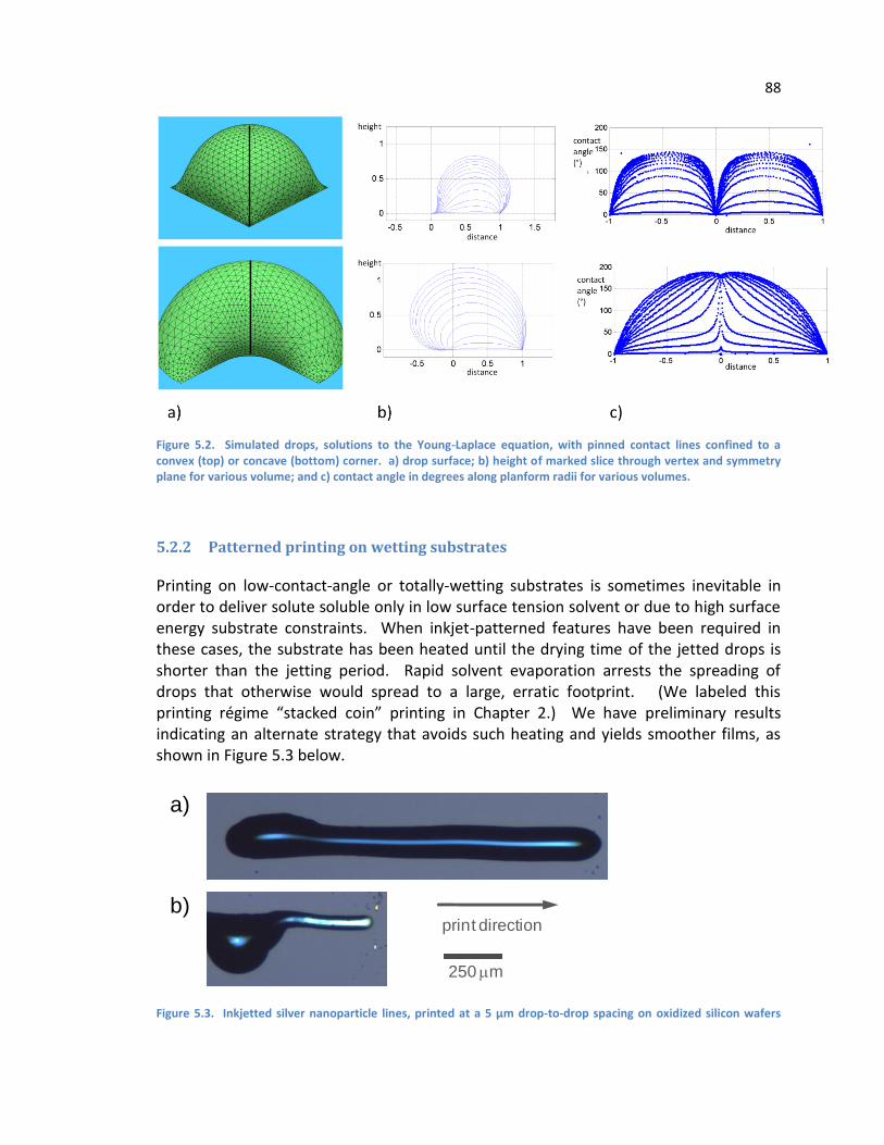
88

Figure 5.2. Simulated drops, solutions to the Young-Laplace equation, with pinned contact lines confined to a convex (top) or concave (bottom) corner. a) drop surface; b) height of marked slice through vertex and symmetry plane for various volume; and c) contact angle in degrees along planform radii for various volumes.

5.2.2 Patterned printing on wetting substrates

Printing on low-contact-angle or totally-wetting substrates is sometimes inevitable in order to deliver solute soluble only in low surface tension solvent or due to high surface energy substrate constraints. When inkjet-patterned features have been required in these cases, the substrate has been heated until the drying time of the jetted drops is shorter than the jetting period. Rapid solvent evaporation arrests the spreading of drops that otherwise would spread to a large, erratic footprint. (We labeled this printing r gime “stacked coin” printing in hapter 2.) We have preliminary results indicating an alternate strategy that avoids such heating and yields smoother films, as shown in Figure 5.3 below.

Figure 5.3. Inkjetted silver nanoparticle lines, printed at a 5 µm drop-to-drop spacing on oxidized silicon wafers

a)

b)

250 m

print direction

89

printed a) as a simple line; and b) with deliberate pre-seeding of a bulge to withdraw fluid. The ink-substrate system is totally wetting with zero equilibrium contact angle.

1

Deliberate capillary flow due to Young-Laplace pressure can be used to pattern inkjet-printed features that otherwise would wet to a large size. Specifically, the low pressure created inside a deliberately-printed bulge can be used to siphon fluid from a growing, printed line that otherwise would wet to a large size. (These bulges can be considered a deliberate, single-event version of the periodic bulging instability seen in long printed lines by Duineveld2). We suggest quantifying the possible advantages of this strategy by developing an analytic framework to understand the timing and length scales of this effect. Experimental confirmation will be provided by inkjet printing with a wetting ink-substrate system while varying print velocity and feature size.

5.3 Works cited

1. Chao, E.; Soltman, D., Unpublished research. In 2010. 2. Duineveld, P. C., The stability of ink-jet printed lines of liquid with zero receding contact angle on a homogeneous substrate. Journal of Fluid Mechanics 2003, 477, 175-200.