the ocean economy in mauritius: making it happen, making
TRANSCRIPT
The Ocean Economy in Mauritius:
Making it happen, making it last Volume 2 – Appendices
Unedited draft, November 2017
2
Appendix 1: The Economy-Wide Model ........................................................................ 7
The Base Model ...................................................................................................................... 7
Disaggregating the Ocean Economy Sectors .......................................................................... 8
The Non-Economic Sectors .................................................................................................... 9
The Complete Model ............................................................................................................ 10
The Multipliers ..................................................................................................................... 11
Sources of the Data and the Methodology ............................................................................ 15
The CGE Model .................................................................................................................... 16
Key Features of the Dynamic Model .................................................................................... 17
Calibrating and Testing the Dynamic Model ........................................................................ 19
Investing in the Ocean Economy .......................................................................................... 21
Sensitivity Analysis .............................................................................................................. 27
The CGE Model: a three-step procedure .............................................................................. 30
CGE Model Based on SAM Evolution ................................................................................. 33
Appendix 2: Fisheries: Supplemental Information ..................................................... 42
Provisional 2016 Fisheries Data ........................................................................................... 42
Fisheries Sector GDP ............................................................................................................ 44
Legal Framework and Violations of Fisheries and Environmental Rules ............................ 44
State of the Lagoons and Coastal Marine Ecosystem ........................................................... 45
Coastal Artisanal Fisheries ................................................................................................... 46
The Banks Fisheries .............................................................................................................. 48
Aquaculture ........................................................................................................................... 51
The Seafood Hub .................................................................................................................. 54
Institutional Arrangements and Challenges .......................................................................... 56
Baselines and Investment Scenarios ..................................................................................... 58
Appendix 3: Energy Modeling ....................................................................................... 60
LCOE Calculation................................................................................................................. 60
Detailed Scenario Results ..................................................................................................... 60
Job Creation Data Summary ................................................................................................. 65
References ............................................................................................................................. 66
Appendix 4: Marine Spatial Planning, Supplemental Information ........................... 67
MSP Mini-Workshop Participant List, September 2016 ...................................................... 67
UNESCO Guiding Principles for Marine Spatial Planning .................................................. 68
Summary of Discussions with Key Stakeholders ................................................................. 68

3
MSP Sample Work Plan for Option 2................................................................................... 72
Marine Protected Area Designations in Mauritius ................................................................ 74
Legal Instruments of Relevance for an MSP Process in Mauritius ...................................... 75
Appendix 5: Climate Change Modeling ........................................................................ 79
Description of Methods for Cyclone Event Set Modeling .................................................... 79
In-Depth Description of Synthetic Methods ......................................................................... 79
Dynamic CGE Simulations of Climate Change Economic Impact Scenarios ...................... 96
References ........................................................................................................................... 110
Appendix 6: Ocean Governance: The International Experience ............................. 113
Comprehensive Assessment Approach ............................................................................... 113
A Clearly Strategy, Communicated with Strong National Blue Economy Goals ............... 114
Engagement of All Stakeholders, with Dedicated Government Structures ........................ 115
Regulatory Framework ....................................................................................................... 115
Seed Funding and Investment Support ............................................................................... 116
Business Follow-Through ................................................................................................... 118
Long-term Sustainability .................................................................................................... 119
Conclusions ......................................................................................................................... 120
List of Figures Figure 1A.1. Value added multiplier ............................................................................................. 12
Figure 1A.2. Green value added multipliers.................................................................................. 13
Figure 1A.3. Institutions multipliers ............................................................................................. 14
Figure 1A.4. Natural institutions’ multipliers ............................................................................... 14
Figure 1A.5. Investment multiplier ............................................................................................... 15
Figure 1A.6. GDP growth in Mauritius 2006–2014 ...................................................................... 19
Figure 1A.7. Trend of value added ................................................................................................ 20
Figure 1A.8. Household consumption ........................................................................................... 21
Figure 1A.9. Better education and training boosts value added .................................................... 26
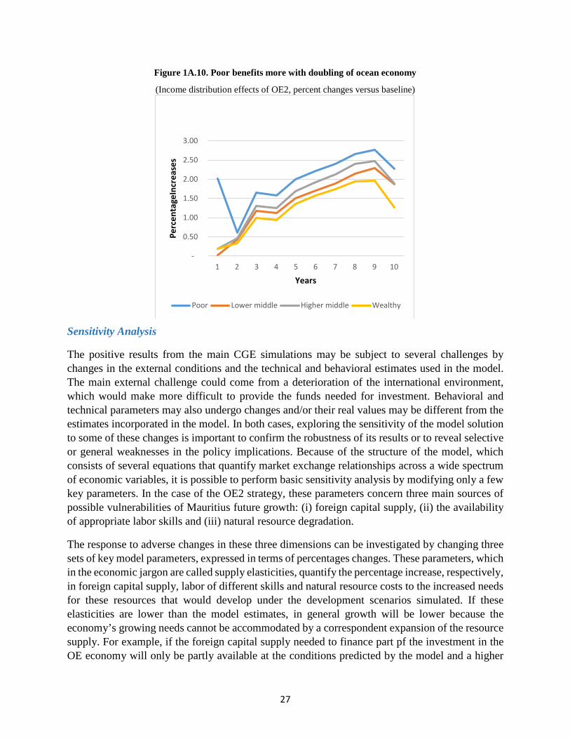
Figure 1A.10. Poor benefits more with doubling of ocean economy ............................................ 27
Figure 2A.1. Increasing violations of fisheries and environmental laws ...................................... 45
Figure 2A.2. Recorded numbers of coastal fishing vessels (Mauritius island only) ..................... 47
Figure 2A.3. Apparent trends in catch and effort in the lagoon and offshore fisheries ................. 48
Figure 2A.4. Most of the Bank’s catch comes from the Saya de Malha Bank .............................. 50
Figure 2A.5. Images of the Banks (left to right): bathymetry, shallow-water areas, primary productivity ................................................................................................................................... 51
Figure 2A.6. Potential aquaculture sites around Mauritius island ................................................. 54
4
Figure 2A.7. Most purse seining is outside Mauritius waters, most longlining inside .................. 56
Figure 3A.1. Generation, capacity, and investment in the reference land based RET .................. 60
Figure 5A.1. Example of a probability distribution generated using the random seeding genesis method ........................................................................................................................................... 82
Figure 5A.2. Example of random time series generated using (2) and (3) .................................... 83
Figure 5A.3. 1000 randomly selected tracks generated using statistics from the ERA40 reanalysis ....................................................................................................................................................... 85
Figure 5A.4. Comparison of 6-hour west-east (a) and south-north (b) North Atlantic track displacements between HURDAT (blue) and synthetic (red) tracks. ............................................ 86
Figure 5A.5. Annual exceedance frequencies of lifetime maximum wind speeds of 355 HURDAT events (blue) and 7064 synthetic events (red), during the period 1980–2010 ............................... 89
Figure 5A.6. Track (a) of the most intense storm among the random sample of 7064 Atlantic tropical cyclones, together with the evolution (b) of maximum wind speed (blue), potential intensity (red), translation speed (green) and 250–850 hPa wind shear magnitude (aqua) ........... 90
Figure 5A.7. Number of hurricane tracks per 2.5 degree latitude-longitude box for (a) nearly 3000 synthetic tracks, (b) 399 HURDAT tracks from 1970 to 2005, and (c) for a random sample of 399 synthetic tracks .............................................................................................................................. 90
Figure 5A.8. Annual exceedance frequencies of lifetime maximum wind speeds of 52 HURDAT events (blue) and 20048 synthetic events (red), passing within 500 km of Pointe-á-Pitre, Guadeloupe, during the period 1980–2010 ................................................................................... 92
Figure 5A.9. Track of the event that produces the highest wind speed at Pointe-á-Pitre, Guadeloupe, among the 20,048 events, as displayed in Google Earth .......................................... 92
Figure 5A.10. Return periods (inverse annual exceedance probabilities) of peak wind experienced within 150 km of New York City according to a set of 5022 events, compared to those estimated from 22 HURDAT events in the period 1900–2010 ..................................................................... 93
Figure 5A.11. Track of the synthetic event that produces the strongest peak wind in downtown New York ...................................................................................................................................... 94
Figure 5A.12. Contours of the peak wind experienced at every point, associated with the event illustrated in Figure 5A.16 ............................................................................................................. 94
Figure 5A.13. Contours of the accumulated rainfall (mm) associated with the event illustrated in Figure 5A.16 and Figure 5A.12 ..................................................................................................... 95
Figure 5A.14. Return periods of peak storm surge depths at the Battery (lower Manhattan) for the climate of the late 20th century (black) and for the late 21st century under IPCC emissions scenario A1b, with 1 m of mean sea level rise included (red and blue), as downscaled from four global climate models, CNRM, ECHAM, GFDL, and MIROC ................................................... 95
Figure 5A.15. Characteristics of projected tropical cyclones under high and low climate change scenarios, normalized to historical conditions ............................................................................. 103
Figure 5A.16. Projected annual direct damage from tropical cyclones, normalized to historical conditions .................................................................................................................................... 104
Figure 5A.17. Projected present value effect of tropical cyclones on GDP ................................ 105
Figure 5A.18. Increase in VAR ................................................................................................... 106
5
Figure 5A.19. Losses in GDP ...................................................................................................... 107
Figure 5A.20. GDP time paths .................................................................................................... 108
Figure 5A.21. Expected losses in GDP growth in the high impact scenario ............................... 108
Figure 5A.22. Expected losses in GDP in the high impact scenario ........................................... 109
Figure 5A.23. Hurricane frequency in the high impact scenario ................................................. 109
List of Tables Table 1A.1. Mauritius ocean economy activities ............................................................................ 8
Table 1A.2. Value added multipliers ............................................................................................. 12
Table 1A.3. Green value-added multipliers .................................................................................. 12
Table 1A.4. Institutions multipliers ............................................................................................... 13
Table 1A.5. Natural institutions’ multipliers ................................................................................. 14
Table 1A.6. Gross fixed capital formation at current prices by type and use, 2006–2016, million MR ................................................................................................................................................. 19
Table 1A.7. Doubling ocean economy can boost GDP ................................................................. 23
Table 1A.8. Larger Ocean economy gives small boost to fiscal picture ....................................... 23
Table 1A.9. Bigger ocean economy helps most old and new sub-sectors ..................................... 24
Table 1A.10. Doubling ocean economy offers more value added ................................................ 24
Table 1A.11. Doubling ocean economy offers more job creation ................................................. 25
Table 1A.12. Bigger ocean economy reduces income inequality ................................................. 26
Table 1A.13. Higher interest and equity rates would pose problems ............................................ 28
Table 1A.14. Skills mismatch could undercut OE’s potential ...................................................... 28
Table 1A.15. Natural resource constraint could undercut bigger OE gains .................................. 29
Table 1A.16. Bigger ocean economy holds its own even in tougher times ................................... 29
Table 2A.1. Fisheries data update for 2016 ................................................................................... 42
Table 2A.2. Overview of fisheries production 2006–2015 ........................................................... 43
Table 2A.3. Contribution of the seafood sector to Mauritius GDP for 2007 to 2014 (%) ............ 44
Table 2A.4. Recorded catches in small-scale fisheries in selected years (tons) ............................ 46
Table 2A.5. Catches (tons), numbers of fishers and fishing vessels - Rodrigues island ............... 48
Table 2A.6. The large-scale freezer-vessels dominated the Banks fishery in 2015 ...................... 50
Table 2A.7. Production of cultured seafood products (tons) ......................................................... 53
Table 2A.8. Fisheries traffic at Port Louis (2007–14) ................................................................... 56
Table 2A.9. Baseline - no government investment (business as usual) ......................................... 58
Table 2A.10. Existing sector development plans .......................................................................... 58
Table 2A.11. Scenarios for additional development options ......................................................... 58
Table 3A.1. Investment in the Baseline scenario .......................................................................... 61
6
Table 3A.2. Installed capacity in the Baseline scenario ................................................................ 61
Table 3A.3. Electricity generation in the Baseline scenario .......................................................... 62
Table 3A.4. Investment in the EDP scenario................................................................................. 62
Table 3A.5. Installed capacity in the EDP scenario ...................................................................... 63
Table 3A.6. Electricity generation in the EDP scenario ................................................................ 63
Table 3A.7. Investment in the ADO scenario ............................................................................... 64
Table 3A.8. Installed capacity in the ADO scenario ..................................................................... 64
Table 3A.9. Electricity generation in the ADO scenario ............................................................... 65
Table 3A.10. Investment and operation cost breakdown by technology ....................................... 65
Table 3A.11. Direct employment by technology during construction and operation .................... 66
Table 4A.1. Guiding principles identified by stakeholders ........................................................... 69
Table 5A.1. Summary of statistics for tropical cyclones, hurricane proportions and eastern North Atlantic Ocean Sea Surface Temperature (NATL SST) anomaly ................................................. 97
Table 5A.2. Descriptive statistics for compound Poisson model of adjusted damage (1995 US$ billion) from North Atlantic hurricanes, 1925–1995 ..................................................................... 97
Table 5A.3. Overview of future loss sensitivity studies ................................................................ 98
Table 5A.4. Summary for Mauritius by decade of consequence database for tropical cyclones, floods, and related secondary hazards ........................................................................................... 98
Table 5A.5. Distribution of damages .......................................................................................... 104
List of Boxes Box 1A.1. Productivity increases in the Dynamic CGE Model .................................................... 17
Box 1A.2 Optimality in the dynamic CGE ................................................................................... 18
Box 1A.3. Crowding out and counterfactuals ............................................................................... 22
Box 1A.4. Estimating environmental loss in the CGE Model ....................................................... 23
Box 2A.1. Selected fisheries and marine environmental legislation ............................................. 44
Box 2A.2. Declining catches in the Banks fisheries ..................................................................... 48
Box 2A.3. Recovery of the Rodrigues octopus fishery ................................................................. 52
Box 2A.4. Government’s strategic objectives for the Seafood Hub ............................................. 55
Box 2A.5. Linkages between the fisheries sector and the broader ocean Economy .................... 57
7
Appendix 1: The Economy-Wide Model
The Base Model
The Mauritius Social Accounting Matrix (SAM) used in the computable general equilibrium (CGE) model was estimated, taking as a point of reference the National SAM estimated by Statistics Mauritius (under the aegis of the Ministry of Finance & Economic Development) and published for year 2007, applying a maximum entropy algorithm according to the methodology outlined in Scandizzo and Ferrarese (2015). The model is disaggregated in various blocks of accounts as follows:
• Goods and Services Accounts refer to the total supply of goods and services.18 products (goods and services) have been identified:
o Sugar cane o Live animals and fishing o Other agriculture o Ores and minerals o Sugar milling o Textile manufacturing o Other manufacturing o Construction o Wholesale and retail trade o Lodging, food and beverage serving services o Transport and communication o Electricity and water distribution services o Public administration o Financial intermediation o Real estate and business services o Education o Health and social services o Other services
• The Production Activities show the costs of the production processes. They include intermediate consumption of the different product groups, factor income generated, and taxes on production paid to government.
• The Factor Income Accounts provide for an interface in the mapping of income generated in production to the institutions, including households. The factor accounts have been disaggregated as follows:
o Employees – primary education level o Employees – secondary education, lower than the School Certificate level o Employees – secondary education, with the School Certificate level or higher o Employees – tertiary education
8
o Own account o Employers o Operating surplus
• Institutions Current Accounts contain the outlays and incomes of households, corporate, and government. They include final consumption expenditure, property income, and transfers. In these accounts, households have been split into four groups using the monthly household income per adult equivalent on the basis of the results of the latest Household Budget Survey (2014).
• Other accounts represent the combined capital and the rest of the world accounts. The combined capital accounts include investment, changes in stocks, and capital transfers. The rest of the world accounts capture transactions with the rest of the world.
The model in base version is estimated at 2015 values, using national account historical series made by Statistics Mauritius, and disaggregated by a 2007 Input-Output classification for 30 economic sectors.
Disaggregating the Ocean Economy Sectors
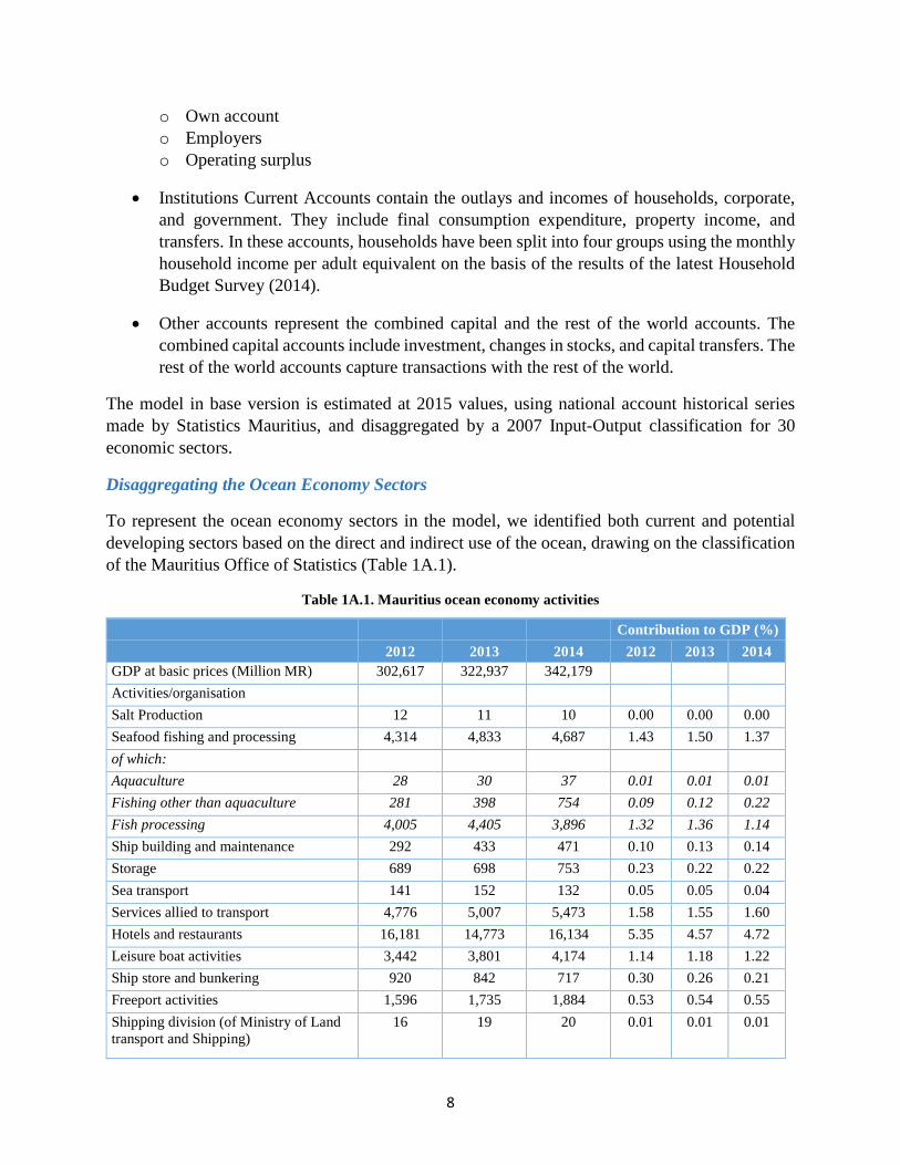
To represent the ocean economy sectors in the model, we identified both current and potential developing sectors based on the direct and indirect use of the ocean, drawing on the classification of the Mauritius Office of Statistics (Table 1A.1).
Table 1A.1. Mauritius ocean economy activities
Contribution to GDP (%) 2012 2013 2014 2012 2013 2014
GDP at basic prices (Million MR) 302,617 322,937 342,179 Activities/organisation Salt Production 12 11 10 0.00 0.00 0.00 Seafood fishing and processing 4,314 4,833 4,687 1.43 1.50 1.37 of which: Aquaculture 28 30 37 0.01 0.01 0.01 Fishing other than aquaculture 281 398 754 0.09 0.12 0.22 Fish processing 4,005 4,405 3,896 1.32 1.36 1.14 Ship building and maintenance 292 433 471 0.10 0.13 0.14 Storage 689 698 753 0.23 0.22 0.22 Sea transport 141 152 132 0.05 0.05 0.04 Services allied to transport 4,776 5,007 5,473 1.58 1.55 1.60 Hotels and restaurants 16,181 14,773 16,134 5.35 4.57 4.72 Leisure boat activities 3,442 3,801 4,174 1.14 1.18 1.22 Ship store and bunkering 920 842 717 0.30 0.26 0.21 Freeport activities 1,596 1,735 1,884 0.53 0.54 0.55 Shipping division (of Ministry of Land transport and Shipping)
16 19 20 0.01 0.01 0.01
9
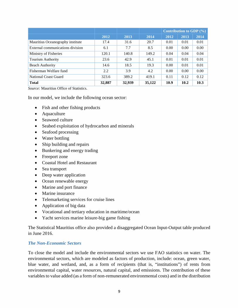
Contribution to GDP (%) 2012 2013 2014 2012 2013 2014
Mauritius Oceanography institute 17.4 31.6 20.7 0.01 0.01 0.01 External communications division 6.1 7.7 8.5 0.00 0.00 0.00 Ministry of Fisheries 120.1 140.8 149.2 0.04 0.04 0.04 Tourism Authority 23.6 42.9 45.1 0.01 0.01 0.01 Beach Authority 14.6 18.5 19.3 0.00 0.01 0.01 Fisherman Welfare fund 2.2 3.9 4.2 0.00 0.00 0.00 National Coast Guard 323.6 389.2 419.1 0.11 0.12 0.12 Total 32,887 32,939 35,122 10.9 10.2 10.3
Source: Mauritius Office of Statistics.
In our model, we include the following ocean sector:
• Fish and other fishing products • Aquaculture • Seaweed culture • Seabed exploitation of hydrocarbon and minerals • Seafood processing • Water bottling • Ship building and repairs • Bunkering and energy trading • Freeport zone • Coastal Hotel and Restaurant • Sea transport • Deep water application • Ocean renewable energy • Marine and port finance • Marine insurance • Telemarketing services for cruise lines • Application of big data • Vocational and tertiary education in maritime/ocean • Yacht services marine leisure-big game fishing
The Statistical Mauritius office also provided a disaggregated Ocean Input-Output table produced in June 2016.
The Non-Economic Sectors
To close the model and include the environmental sectors we use FAO statistics on water. The environmental sectors, which are modeled as factors of production, include: ocean, green water, blue water, and wetland, and, as a form of recipients (that is, “institutions”) of rents from environmental capital, water resources, natural capital, and emissions. The contribution of these variables to value added (as a form of non-remunerated environmental costs) and in the distribution
10
of rents are estimated through a combination of the maximum entropy and the Wolsky disaggregation algorithm (Scandizzo and Ferrarese, 2015).
The Complete Model
The CGE model is based on a 118-sector SAM and simulates an economy disaggregated in the following blocks:
• Goods and services accounts:
o 6 agriculture sectors (products of agriculture, horticulture and market gardening, forestry and logging products, sugar cane, live animals and animal products, fish and other fishing products, aquaculture, and seaweed culture).
o 11 industry sectors (ores and minerals, seabed exploitation of hydrocarbon and minerals, meat, fruit, vegetables, oils and fats, grain mill products, starches and starch products and beverages, seafood processing, sugar, yarn and thread; woven and tufted textile fabrics, knitted or crocheted fabrics; wearing apparel, other manufactured goods, manufacturing cosmetics and pharmaceuticals, agrochemicals, water bottling, and ship building and repairs);
o Construction and construction services.
o 30 services sectors (wholesale and retail trade services, bunkering and energy trading, Freeport zone, lodging; food and beverage serving services, coastal hotel and restaurant, land, air, supporting and auxiliary transport services, sea transport, services allied to transport, electricity distribution services; gas and water distribution services through mains, deep water application, ocean renewable energy, financial intermediation, insurance, and auxiliary services, marine and port finance, marine insurance, real estate services, telecommunications services; information retrieval and supply services, telemarketing services for cruise lines, application of big data, other business services, legaland accounting services, scientific research and development, public administration and other services to the community as a whole; compulsory social security services, education services, vocational and tertiary education in maritime/ocean, health and social services, sewage and refuse disposal, sanitation and other environmental protection services, services of membership organizations, recreational, cultural, and sporting services, yacht Services and marine leisure-big game fishing, and other services).
• Production activities include the intermediate consumption of the different product groups, factor income generated, and taxes on production paid to the government for the same disaggregated accounts of goods and services.
• The factor income accounts include:
o Primary education
11
o Secondary education <School Certificate
o Secondary education School Certificate and above
o Tertiary education
o Own account
o Employer
o Operating surplus
o Ocean
o Green water
o Blue water
o Wetland
• Institutions Accounts contain:
o Government and NPISH
o Poor
o Lower middle
o Higher middle
o Wealthy
o Corporations
• Other accounts represent:
o Rest of the world
o Capital formation
o Water resources
o Natural capital
o Emissions
The Multipliers
The SAM investment multiplier shows a total value-added multiplier equal to 1.92. Table 1A.2 and Figure 1A.1 show the value-added multipliers for its different labor and capital components.

12
Table 1A.2. Value added multipliers
Value added 1.92 Primary education 0.21 Secondary education <SC 0.16 Secondary education SC and above 0.16 Tertiary education 0.31 Own account 0.32 Employer 0.09 Operating surplus 0.67
Figure 1A.1. Value added multiplier
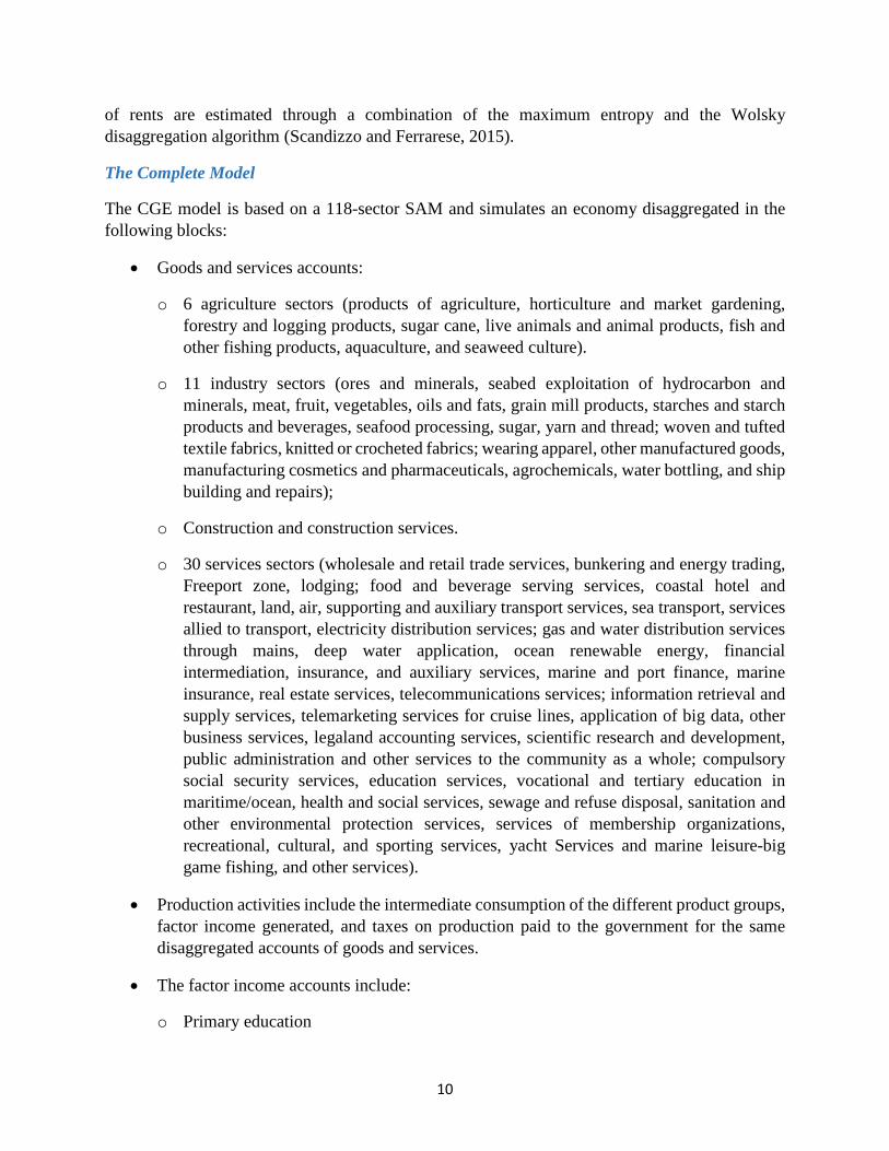
The value of the multiplier for the green component of value added is equal to 0.0198 (Table 1A.3).
Table 1A.3. Green value-added multipliers
Green value added 0.0198 Ocean 0.0136 Green water 0.0036 Blue water 0.0022 Wetland 0.0003
0.000.100.200.300.400.500.600.70
Value Added
13
Figure 1A.2. Green value added multipliers
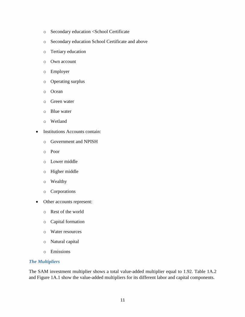
The value of the institutions multiplier is equal to 2.66, divided as shown in Table 1A.4 and Figure 1A.3.
Table 1A.4. Institutions multipliers
Institutions 2.66 Government and NPISH* 0.21 Poor 0.03 Lower middle 0.44 Higher middle 0.73 Wealthy 0.61 Corporations 0.64
Note: *Non-profit institutions serving households.
0.0000
0.0050
0.0100
0.0150
Ocean Green Water Blu Water Wetland
Green Value Added
14
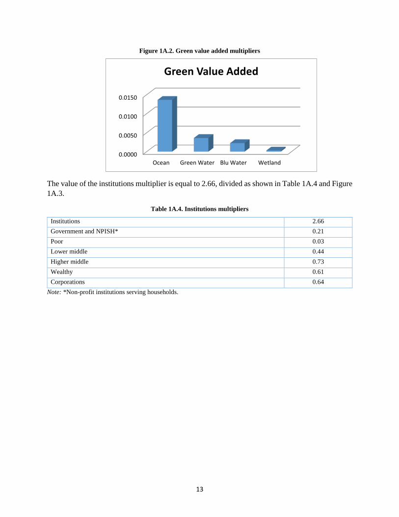
Figure 1A.3. Institutions multipliers
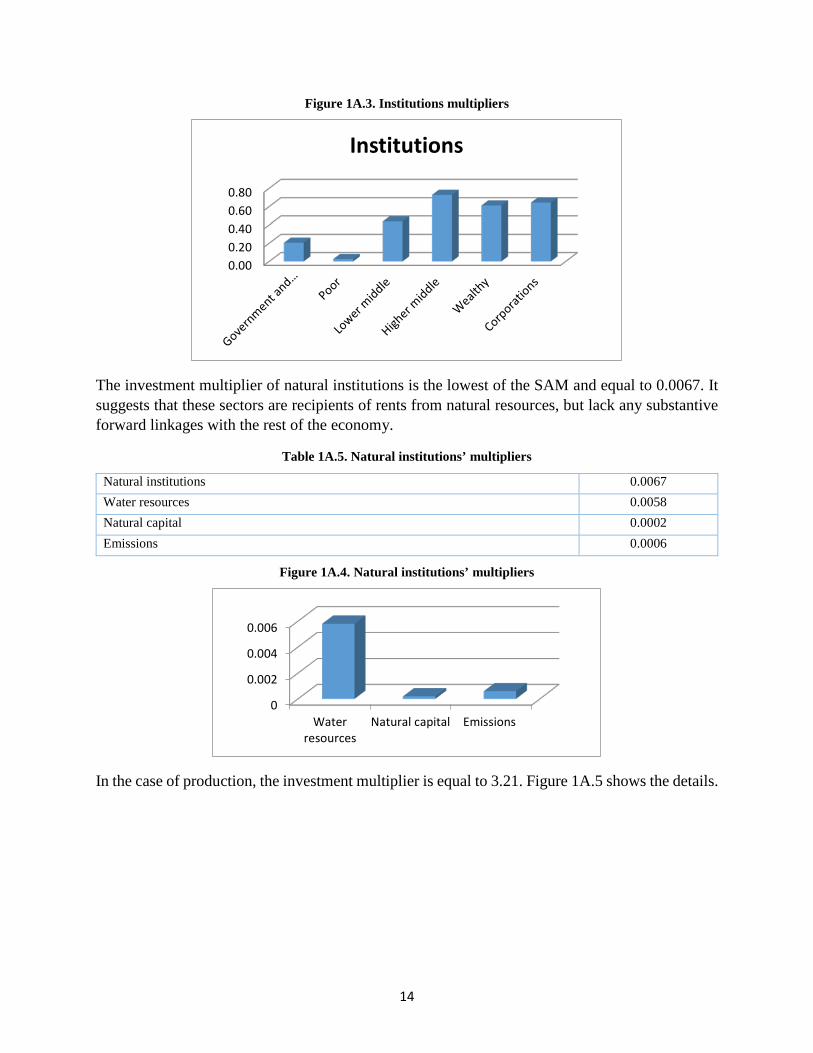
The investment multiplier of natural institutions is the lowest of the SAM and equal to 0.0067. It suggests that these sectors are recipients of rents from natural resources, but lack any substantive forward linkages with the rest of the economy.
Table 1A.5. Natural institutions’ multipliers
Natural institutions 0.0067 Water resources 0.0058 Natural capital 0.0002 Emissions 0.0006
Figure 1A.4. Natural institutions’ multipliers
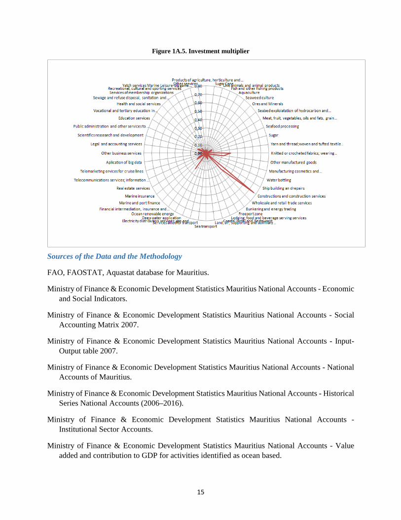
In the case of production, the investment multiplier is equal to 3.21. Figure 1A.5 shows the details.
0.000.200.400.600.80
Institutions
0
0.002
0.004
0.006
Waterresources
Natural capital Emissions
15
Figure 1A.5. Investment multiplier
Sources of the Data and the Methodology
FAO, FAOSTAT, Aquastat database for Mauritius.
Ministry of Finance & Economic Development Statistics Mauritius National Accounts - Economic and Social Indicators.
Ministry of Finance & Economic Development Statistics Mauritius National Accounts - Social Accounting Matrix 2007.
Ministry of Finance & Economic Development Statistics Mauritius National Accounts - Input-Output table 2007.
Ministry of Finance & Economic Development Statistics Mauritius National Accounts - National Accounts of Mauritius.
Ministry of Finance & Economic Development Statistics Mauritius National Accounts - Historical Series National Accounts (2006–2016).
Ministry of Finance & Economic Development Statistics Mauritius National Accounts - Institutional Sector Accounts.
Ministry of Finance & Economic Development Statistics Mauritius National Accounts - Value added and contribution to GDP for activities identified as ocean based.
16
Ministry of Finance & Economic Development Statistics Mauritius National Accounts - Ocean Input-Output table.
Scandizzo, P. L., and C. Ferrarese. 2015a. “Social Accounting Matrix: A New Estimation Methodology.” Journal of Policy Modeling 37 (1): 14–34.
———. 2015b. CGE Model an Application for Tanzania. The World Bank Technical Report.
United Nations Food and Agriculture Organization - Integrated Environmental and Economic Accounting for Fisheries, 2004.
WTTC (World Travel and Tourism Council). 2015. “Travel & Tourism Economic Impact 2014.”
The CGE Model
A SAM was estimated and used to assess the direct, induced, and indirect linkages of the Ocean Economy (OE) sectors with other parts of the economy and the broader macroeconomic impact of their activity. The SAM assessment was used to identify the backward and forward linkages between the OE sectors and other parts of the economy, and to suggest ways to minimize leakages from the economy. It reflects the structure of the UN extended accounts, in the framework of an integrated representation of the economic system that can be used as a proper basis for general equilibrium modeling. It contains an explicit set of accounts for biodiversity and the environmental components of the ocean economy and quantifies flow and stock relations of physical, human, and natural capital. Because of the nature of the policy questions addressed by the study, the SAM contains a detailed quantification of the relevant elements of the value chain that make, or might make, domestic activities most responsive to the OE development through backward and forward linkages. As in the other, recently implemented SAM cases, an estimation procedure based on secondary data and time series was utilized. The estimation procedure is based on an innovative maximum entropy methodology, combined with bootstrap Monte Carlo simulation estimates. The estimates obtained with this procedure have the advantage of being based on time series as well as cross section data, and accounting for the moments of the distribution of the main variables (including, in particular, means and variances).
A CGE model was also built and calibrated, based on the SAM and other complementary statistics. The CGE model reflects the detail and the logic of the SAM economic and environmental accounts, within a modified Walrasian framework, modeled to represent both formal and informal demand and supply relations between different stakeholders, commodities, and natural resources. The CGE model has been developed as an equilibrium representation of the economy, but it also accounts for the specific characteristics of the Mauritian economy (such as the unemployment and the skills mismatch). It uses an economic closure of the Keynesian type, apt to address structural policy questions for a medium-long term development target. It has also been further developed by adding dynamic features, considering alternative hypotheses of evolution of the economy, as well as of the balances between supply and demand of natural resources (renewable and non-renewable), for a single year and for sequences of years. Both the SAM and the CGE have been designed in ways that allow analyzing changes in the variables and in the structure of the economy –including
17
production and consumption parameters, natural resource availability, and input-output relations in the value chains of the production sectors that are, or could be, interested by the OE expansion.
The CGE model was used to run several experimental simulations in the course of a mission to Mauritius, and the results were presented and discussed with representatives of the government and other Mauritian institutions. The simulations concerned only three sectors – that is, fishery, port and marine transport, and energy – which were nevertheless sufficiently illustrative of the OE potential in terms of contributing to growth, investment needs, and implementation times. Basic assumptions and macroeconomic implications were also presented and discussed.
Key Features of the Dynamic Model
The dynamic CGE model aims to capture some of the relevant features of the Mauritius economy today and their potential evolution over time. The model is based on the SAM matrix described above for the entire economy of 118 sectors, factors, and institutions, and it projects the economy over time based on a moving equilibrium algorithm and a basic Solow-like structure of capital accumulation and growth. As a result of these hypotheses, the model tends to follow a time path converging to a steady state where growth is solely determined by technological progress (productivity increases) and population growth. If both these factors are ignored (in other words, the model converges to a zero-growth steady state), it can be used to simulate differential capital accumulation and resource allocation strategies and their trajectories over time.
The dynamic model presents several characteristics that are not shared with its static counterpart that was developed in the first phase of this study and that should be noted carefully before interpreting its results.
First, the model exhibits decreasing returns to scale due to convex technologies and general equilibrium effects (price changes) in each simulation period and over time. This means that investing in one sector will tend to increase less than proportionally its output within a single simulation period, and these diseconomies of scale in each period will also be path dependent – that is, they will be larger if the sector has already been the object of expansion in the preceding periods.
Box 1A.1. Productivity increases in the Dynamic CGE Model
Consider the following growth disaggregation equation: (1)dlogXi = ∑ aijn
j dlogXj + ∑ logXjdaijnj
whereaij = pjXj/piXi
Equation (1) can be interpreted as stating that in a SAM-CGE model where we interpret the input-output coefficients as value shares (that is, according to the hypothesis of a unit elasticity of substitution), growth occurs as a consequence of two phenomena: (i) an autonomous increase in the growth of production, and (ii) an increase in the output share. (2)daij = [(pjdXj + Xjdpj)/piXi] − [(pidXi + Xidpi)pjXj/piXi]
This implies that even if the coefficient Xj/Xi does not change, the share will change in response to a variation in the price ratio pj/pi. For factors of production, we will also have:
18
(3) dlogZl = ∑ fljLj dlogXj + ∑ logXjdfljL
j
Growth in capital employment, for example, will result from growth of production at the old capital share level plus the effect of a change in capital productivity. An increase in the capital share dfkj for a particular product j will thus determine an increase in the use of capital. Because ∑ ajin
i + ∑ fli = 1 Ll , the value share of the intermediate
goods for the same process of production should decrease. This decrease can result from either a decrease in the value of the input-output ratio at constant prices, or from a variation in the input-output price ratio, or both. The important thing, however, is that after the change, the new SAM incorporates both variations (quantities and prices).
Second, large changes may find equilibria that are unstable, in the sense that subsequent small shocks may tend to produce large effects.
Third, the impact of a single project or program will be different based on whether it is considered by itself or as part of a more complex strategy. This is also due to effects of scale, but in this case, because of possible complementarities between different projects, economies rather than diseconomies of scale may ensue.
Fourth, while all simulations should be compared to a counterfactual, unlike the static CGE case, the counterfactual cannot be unique and is necessarily specific, as its first best alternative, of each project or program that is simulated.
Fifth, the pattern of productivity increases will depend on specific hypotheses on the parameter changes of each simulation. These hypotheses are important to understand the potential of alternative policy strategies in the long run, since productivity changes may significantly modify, and even reverse, the merit order of policy alternatives that are ranked on the basis of current production and consumption parameters.
Sixth, the model solutions are based on the choice of an “optimal” trajectory for the multi-year investment pattern, whereby the government is assumed to choose investment in a way that optimizes the country welfare function, for a given pattern of short term behavior of households and firms in the economy.
Box 1A.2 Optimality in the dynamic CGE
Optimality is an ambiguous concept in economics, even though it is key to understanding why results differ among various types of exercises. In our dynamic CGE model, optimality has different facets according to whether we consider the behaviour of producers and consumers, the private and the public sector, and the choice of policies and growth strategies. Thus, it is essential to understand two different concepts of what is “best” and for whom in order to be clear on the results. First, all “decentralized” economic agents (including producing sectors, enterprises, households, and other institutions) are assumed to optimize by maximizing profits (in the case of producers) or utility (in all other cases) on the basis of power functions. For producers, these are the so-called Cobb-Douglas production functions that look at the technological relationship between inputs (like physical capital and labour) and the amount of output that can be produced by those inputs. For consumers, the sets of behavioural functions implied by maximizing utility of the functional forms used are called linear expenditure systems, with the property of expenditure being a linear function of prices and incomes. Parameters for these functions are taken from direct estimates, with the estimates reproducing the baseline SAM. Second, the government is assumed to choose the strategy of investment, in terms of investment size and sector composition over time, by choosing among a plurality of possible trajectories over time, given the model simulation
19
of the corresponding behaviour (both autonomous and reactive) of the economic agents. The choice is made by evaluating the effects of the different trajectories on the present value of a welfare function. This function is an indicator of social well-being, which weighs the consumption of the households of different income classes in a way that is inversely proportional to their level, thus giving progressively higher weights to less affluent consumers and favouring comparatively more pro-poor solution. The result is an intertemporal model (with current decisions now influencing possible options later), based on a mix of myopic (on the part of decentralized agents), and rational (on the part of the planning branch of the government) expectations –a model that we consider more realistic than the purely recursive or intertemporal dynamic equilibria suggested by the current literature.
Calibrating and Testing the Dynamic Model
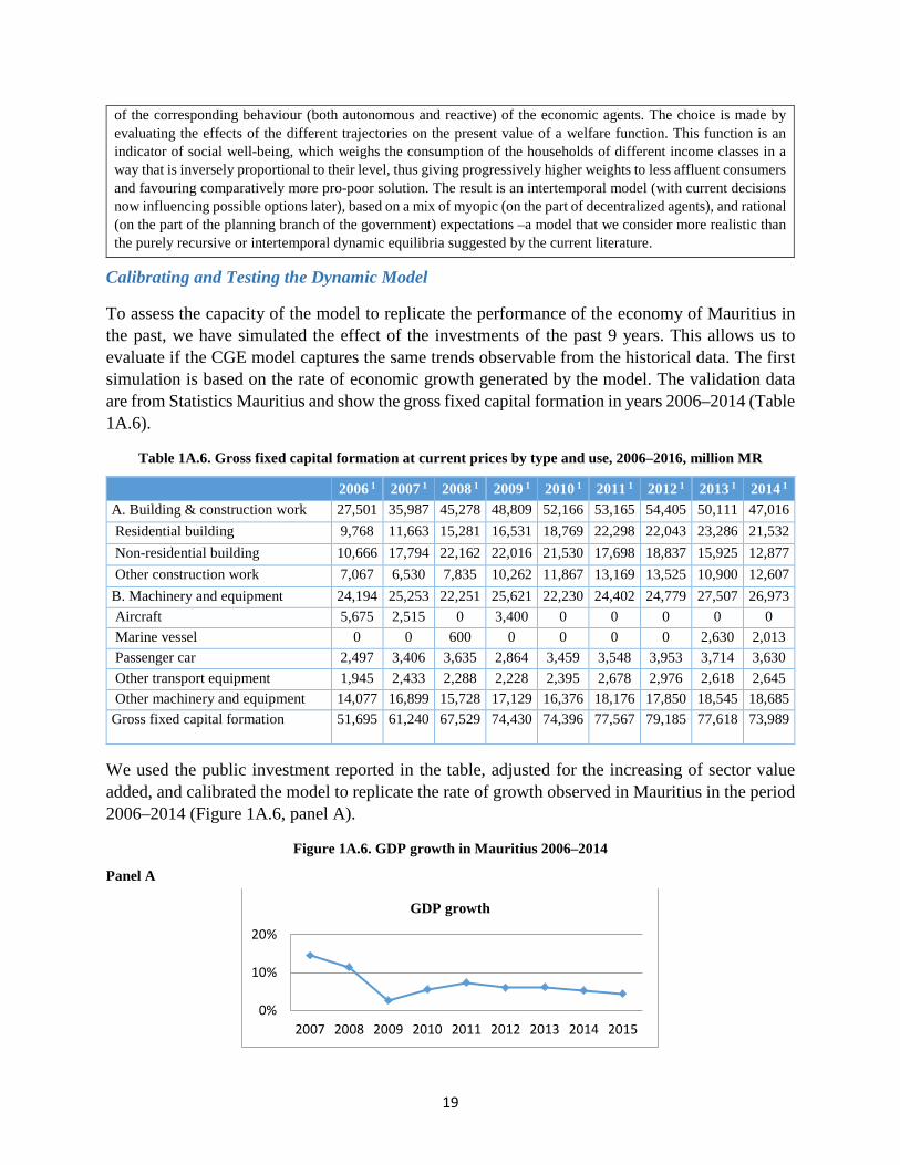
To assess the capacity of the model to replicate the performance of the economy of Mauritius in the past, we have simulated the effect of the investments of the past 9 years. This allows us to evaluate if the CGE model captures the same trends observable from the historical data. The first simulation is based on the rate of economic growth generated by the model. The validation data are from Statistics Mauritius and show the gross fixed capital formation in years 2006–2014 (Table 1A.6).
Table 1A.6. Gross fixed capital formation at current prices by type and use, 2006–2016, million MR
2006 1 2007 1 2008 1 2009 1 2010 1 2011 1 2012 1 2013 1 2014 1 A. Building & construction work 27,501 35,987 45,278 48,809 52,166 53,165 54,405 50,111 47,016 Residential building 9,768 11,663 15,281 16,531 18,769 22,298 22,043 23,286 21,532 Non-residential building 10,666 17,794 22,162 22,016 21,530 17,698 18,837 15,925 12,877 Other construction work 7,067 6,530 7,835 10,262 11,867 13,169 13,525 10,900 12,607 B. Machinery and equipment 24,194 25,253 22,251 25,621 22,230 24,402 24,779 27,507 26,973 Aircraft 5,675 2,515 0 3,400 0 0 0 0 0 Marine vessel 0 0 600 0 0 0 0 2,630 2,013 Passenger car 2,497 3,406 3,635 2,864 3,459 3,548 3,953 3,714 3,630 Other transport equipment 1,945 2,433 2,288 2,228 2,395 2,678 2,976 2,618 2,645 Other machinery and equipment 14,077 16,899 15,728 17,129 16,376 18,176 17,850 18,545 18,685 Gross fixed capital formation 51,695 61,240 67,529 74,430 74,396 77,567 79,185 77,618 73,989
We used the public investment reported in the table, adjusted for the increasing of sector value added, and calibrated the model to replicate the rate of growth observed in Mauritius in the period 2006–2014 (Figure 1A.6, panel A).
Figure 1A.6. GDP growth in Mauritius 2006–2014
Panel A
0%
10%
20%
2007 2008 2009 2010 2011 2012 2013 2014 2015
GDP growth
20
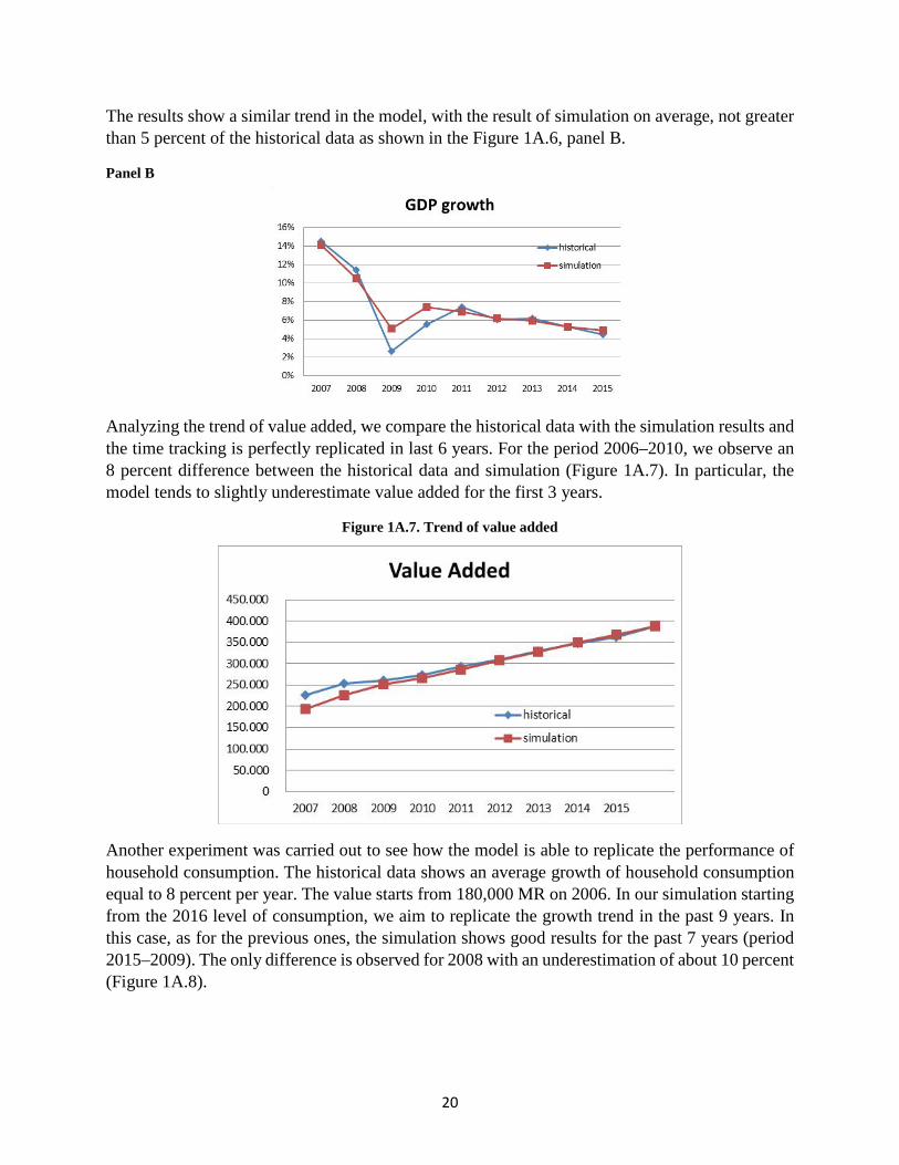
The results show a similar trend in the model, with the result of simulation on average, not greater than 5 percent of the historical data as shown in the Figure 1A.6, panel B.
Panel B
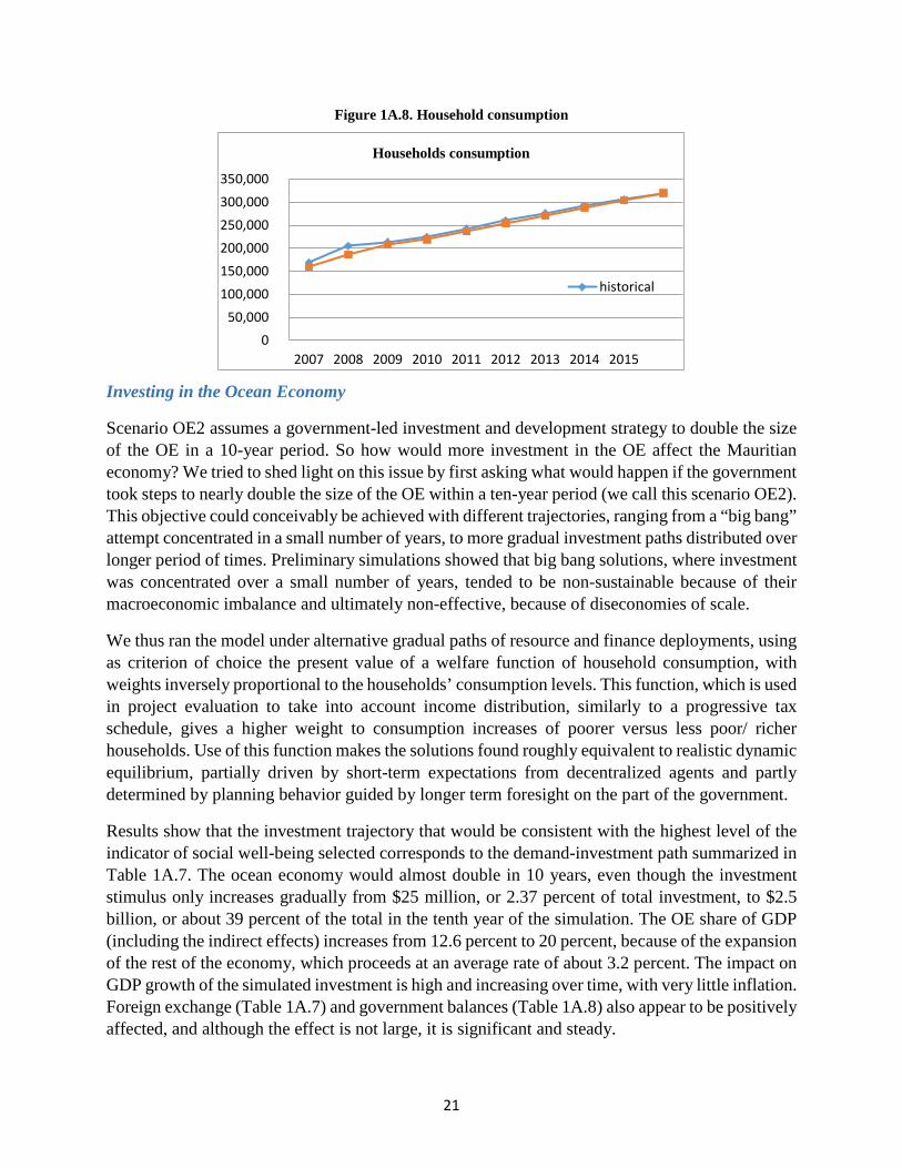
Analyzing the trend of value added, we compare the historical data with the simulation results and the time tracking is perfectly replicated in last 6 years. For the period 2006–2010, we observe an 8 percent difference between the historical data and simulation (Figure 1A.7). In particular, the model tends to slightly underestimate value added for the first 3 years.
Figure 1A.7. Trend of value added
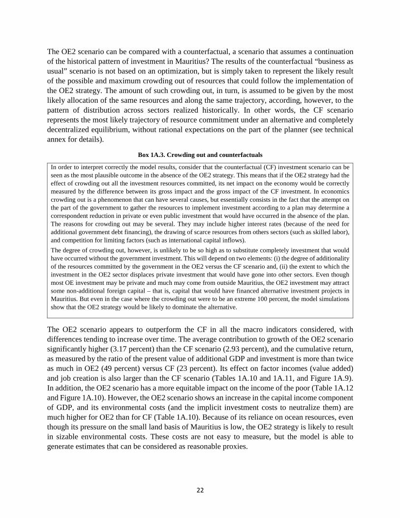
Another experiment was carried out to see how the model is able to replicate the performance of household consumption. The historical data shows an average growth of household consumption equal to 8 percent per year. The value starts from 180,000 MR on 2006. In our simulation starting from the 2016 level of consumption, we aim to replicate the growth trend in the past 9 years. In this case, as for the previous ones, the simulation shows good results for the past 7 years (period 2015–2009). The only difference is observed for 2008 with an underestimation of about 10 percent (Figure 1A.8).
21
Figure 1A.8. Household consumption
Investing in the Ocean Economy
Scenario OE2 assumes a government-led investment and development strategy to double the size of the OE in a 10-year period. So how would more investment in the OE affect the Mauritian economy? We tried to shed light on this issue by first asking what would happen if the government took steps to nearly double the size of the OE within a ten-year period (we call this scenario OE2). This objective could conceivably be achieved with different trajectories, ranging from a “big bang” attempt concentrated in a small number of years, to more gradual investment paths distributed over longer period of times. Preliminary simulations showed that big bang solutions, where investment was concentrated over a small number of years, tended to be non-sustainable because of their macroeconomic imbalance and ultimately non-effective, because of diseconomies of scale.
We thus ran the model under alternative gradual paths of resource and finance deployments, using as criterion of choice the present value of a welfare function of household consumption, with weights inversely proportional to the households’ consumption levels. This function, which is used in project evaluation to take into account income distribution, similarly to a progressive tax schedule, gives a higher weight to consumption increases of poorer versus less poor/ richer households. Use of this function makes the solutions found roughly equivalent to realistic dynamic equilibrium, partially driven by short-term expectations from decentralized agents and partly determined by planning behavior guided by longer term foresight on the part of the government.
Results show that the investment trajectory that would be consistent with the highest level of the indicator of social well-being selected corresponds to the demand-investment path summarized in Table 1A.7. The ocean economy would almost double in 10 years, even though the investment stimulus only increases gradually from $25 million, or 2.37 percent of total investment, to $2.5 billion, or about 39 percent of the total in the tenth year of the simulation. The OE share of GDP (including the indirect effects) increases from 12.6 percent to 20 percent, because of the expansion of the rest of the economy, which proceeds at an average rate of about 3.2 percent. The impact on GDP growth of the simulated investment is high and increasing over time, with very little inflation. Foreign exchange (Table 1A.7) and government balances (Table 1A.8) also appear to be positively affected, and although the effect is not large, it is significant and steady.
050,000
100,000150,000200,000250,000300,000350,000
2007 2008 2009 2010 2011 2012 2013 2014 2015
Households consumption
historical
22
The OE2 scenario can be compared with a counterfactual, a scenario that assumes a continuation of the historical pattern of investment in Mauritius? The results of the counterfactual “business as usual” scenario is not based on an optimization, but is simply taken to represent the likely result of the possible and maximum crowding out of resources that could follow the implementation of the OE2 strategy. The amount of such crowding out, in turn, is assumed to be given by the most likely allocation of the same resources and along the same trajectory, according, however, to the pattern of distribution across sectors realized historically. In other words, the CF scenario represents the most likely trajectory of resource commitment under an alternative and completely decentralized equilibrium, without rational expectations on the part of the planner (see technical annex for details).
Box 1A.3. Crowding out and counterfactuals
In order to interpret correctly the model results, consider that the counterfactual (CF) investment scenario can be seen as the most plausible outcome in the absence of the OE2 strategy. This means that if the OE2 strategy had the effect of crowding out all the investment resources committed, its net impact on the economy would be correctly measured by the difference between its gross impact and the gross impact of the CF investment. In economics crowding out is a phenomenon that can have several causes, but essentially consists in the fact that the attempt on the part of the government to gather the resources to implement investment according to a plan may determine a correspondent reduction in private or even public investment that would have occurred in the absence of the plan. The reasons for crowding out may be several. They may include higher interest rates (because of the need for additional government debt financing), the drawing of scarce resources from others sectors (such as skilled labor), and competition for limiting factors (such as international capital inflows). The degree of crowding out, however, is unlikely to be so high as to substitute completely investment that would have occurred without the government investment. This will depend on two elements: (i) the degree of additionality of the resources committed by the government in the OE2 versus the CF scenario and, (ii) the extent to which the investment in the OE2 sector displaces private investment that would have gone into other sectors. Even though most OE investment may be private and much may come from outside Mauritius, the OE2 investment may attract some non-additional foreign capital – that is, capital that would have financed alternative investment projects in Mauritius. But even in the case where the crowding out were to be an extreme 100 percent, the model simulations show that the OE2 strategy would be likely to dominate the alternative.
The OE2 scenario appears to outperform the CF in all the macro indicators considered, with differences tending to increase over time. The average contribution to growth of the OE2 scenario significantly higher (3.17 percent) than the CF scenario (2.93 percent), and the cumulative return, as measured by the ratio of the present value of additional GDP and investment is more than twice as much in OE2 (49 percent) versus CF (23 percent). Its effect on factor incomes (value added) and job creation is also larger than the CF scenario (Tables 1A.10 and 1A.11, and Figure 1A.9). In addition, the OE2 scenario has a more equitable impact on the income of the poor (Table 1A.12 and Figure 1A.10). However, the OE2 scenario shows an increase in the capital income component of GDP, and its environmental costs (and the implicit investment costs to neutralize them) are much higher for OE2 than for CF (Table 1A.10). Because of its reliance on ocean resources, even though its pressure on the small land basis of Mauritius is low, the OE2 strategy is likely to result in sizable environmental costs. These costs are not easy to measure, but the model is able to generate estimates that can be considered as reasonable proxies.
23
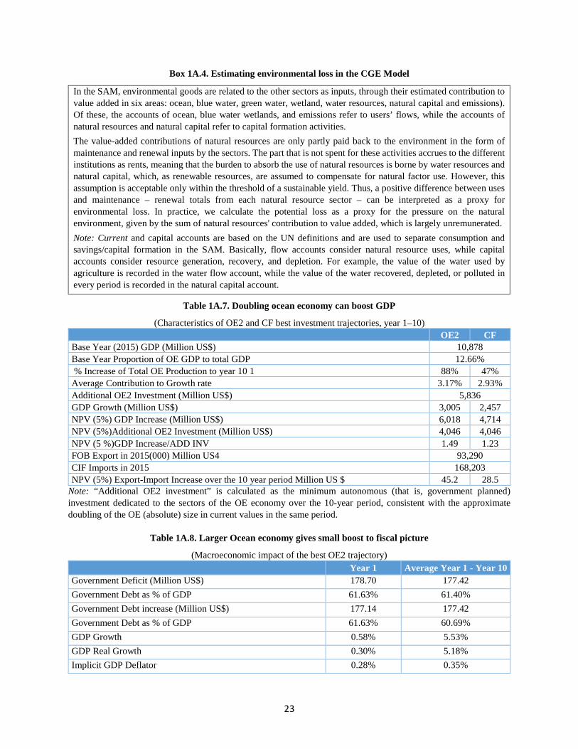
Box 1A.4. Estimating environmental loss in the CGE Model
In the SAM, environmental goods are related to the other sectors as inputs, through their estimated contribution to value added in six areas: ocean, blue water, green water, wetland, water resources, natural capital and emissions). Of these, the accounts of ocean, blue water wetlands, and emissions refer to users’ flows, while the accounts of natural resources and natural capital refer to capital formation activities. The value-added contributions of natural resources are only partly paid back to the environment in the form of maintenance and renewal inputs by the sectors. The part that is not spent for these activities accrues to the different institutions as rents, meaning that the burden to absorb the use of natural resources is borne by water resources and natural capital, which, as renewable resources, are assumed to compensate for natural factor use. However, this assumption is acceptable only within the threshold of a sustainable yield. Thus, a positive difference between uses and maintenance – renewal totals from each natural resource sector – can be interpreted as a proxy for environmental loss. In practice, we calculate the potential loss as a proxy for the pressure on the natural environment, given by the sum of natural resources' contribution to value added, which is largely unremunerated. Note: Current and capital accounts are based on the UN definitions and are used to separate consumption and savings/capital formation in the SAM. Basically, flow accounts consider natural resource uses, while capital accounts consider resource generation, recovery, and depletion. For example, the value of the water used by agriculture is recorded in the water flow account, while the value of the water recovered, depleted, or polluted in every period is recorded in the natural capital account.
Table 1A.7. Doubling ocean economy can boost GDP
(Characteristics of OE2 and CF best investment trajectories, year 1–10) OE2 CF
Base Year (2015) GDP (Million US$) 10,878 Base Year Proportion of OE GDP to total GDP 12.66% % Increase of Total OE Production to year 10 1 88% 47% Average Contribution to Growth rate 3.17% 2.93% Additional OE2 Investment (Million US$) 5,836 GDP Growth (Million US$) 3,005 2,457 NPV (5%) GDP Increase (Million US$) 6,018 4,714 NPV (5%)Additional OE2 Investment (Million US$) 4,046 4,046 NPV (5 %)GDP Increase/ADD INV 1.49 1.23 FOB Export in 2015(000) Million US4 93,290 CIF Imports in 2015 168,203 NPV (5%) Export-Import Increase over the 10 year period Million US $ 45.2 28.5
Note: “Additional OE2 investment” is calculated as the minimum autonomous (that is, government planned) investment dedicated to the sectors of the OE economy over the 10-year period, consistent with the approximate doubling of the OE (absolute) size in current values in the same period.
Table 1A.8. Larger Ocean economy gives small boost to fiscal picture
(Macroeconomic impact of the best OE2 trajectory) Year 1 Average Year 1 - Year 10
Government Deficit (Million US$) 178.70 177.42 Government Debt as % of GDP 61.63% 61.40% Government Debt increase (Million US$) 177.14 177.42 Government Debt as % of GDP 61.63% 60.69% GDP Growth 0.58% 5.53% GDP Real Growth 0.30% 5.18% Implicit GDP Deflator 0.28% 0.35%
24
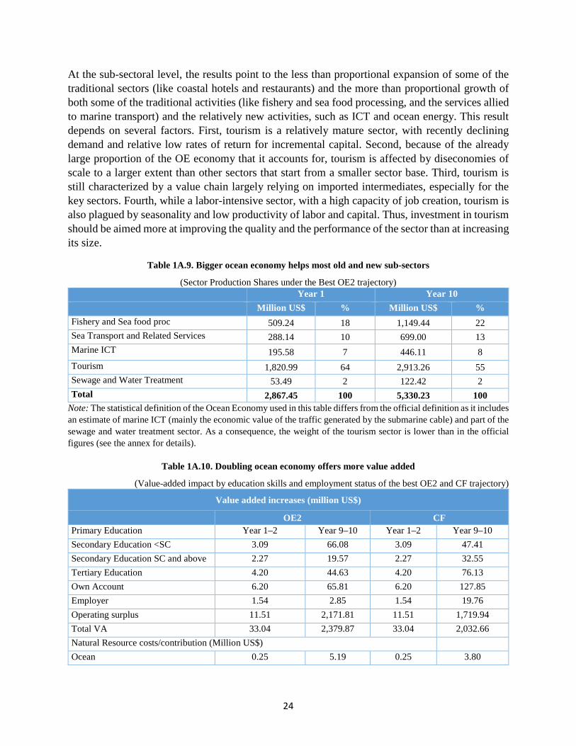
At the sub-sectoral level, the results point to the less than proportional expansion of some of the traditional sectors (like coastal hotels and restaurants) and the more than proportional growth of both some of the traditional activities (like fishery and sea food processing, and the services allied to marine transport) and the relatively new activities, such as ICT and ocean energy. This result depends on several factors. First, tourism is a relatively mature sector, with recently declining demand and relative low rates of return for incremental capital. Second, because of the already large proportion of the OE economy that it accounts for, tourism is affected by diseconomies of scale to a larger extent than other sectors that start from a smaller sector base. Third, tourism is still characterized by a value chain largely relying on imported intermediates, especially for the key sectors. Fourth, while a labor-intensive sector, with a high capacity of job creation, tourism is also plagued by seasonality and low productivity of labor and capital. Thus, investment in tourism should be aimed more at improving the quality and the performance of the sector than at increasing its size.
Table 1A.9. Bigger ocean economy helps most old and new sub-sectors
(Sector Production Shares under the Best OE2 trajectory) Year 1 Year 10 Million US$ % Million US$ %
Fishery and Sea food proc 509.24 18 1,149.44 22 Sea Transport and Related Services 288.14 10 699.00 13 Marine ICT 195.58 7 446.11 8 Tourism 1,820.99 64 2,913.26 55 Sewage and Water Treatment 53.49 2 122.42 2 Total 2,867.45 100 5,330.23 100
Note: The statistical definition of the Ocean Economy used in this table differs from the official definition as it includes an estimate of marine ICT (mainly the economic value of the traffic generated by the submarine cable) and part of the sewage and water treatment sector. As a consequence, the weight of the tourism sector is lower than in the official figures (see the annex for details).
Table 1A.10. Doubling ocean economy offers more value added
(Value-added impact by education skills and employment status of the best OE2 and CF trajectory)
Value added increases (million US$)
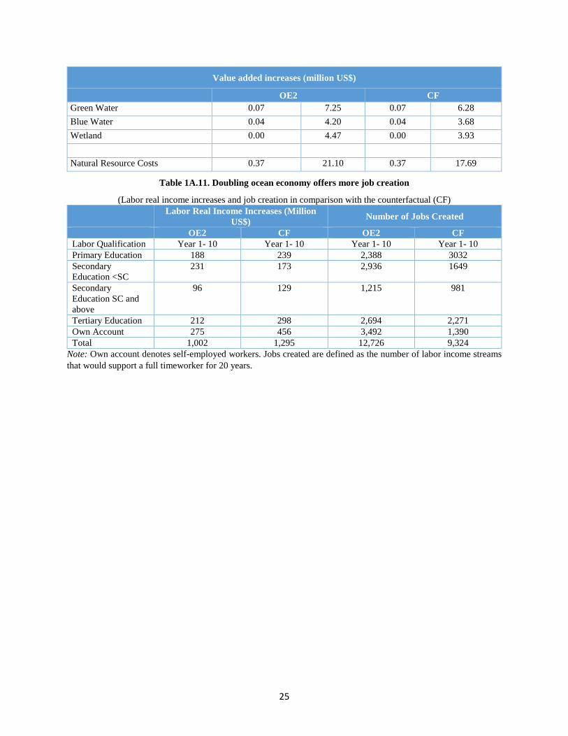
OE2 CF Primary Education Year 1–2 Year 9–10 Year 1–2 Year 9–10 Secondary Education <SC 3.09 66.08 3.09 47.41 Secondary Education SC and above 2.27 19.57 2.27 32.55 Tertiary Education 4.20 44.63 4.20 76.13 Own Account 6.20 65.81 6.20 127.85 Employer 1.54 2.85 1.54 19.76 Operating surplus 11.51 2,171.81 11.51 1,719.94 Total VA 33.04 2,379.87 33.04 2,032.66 Natural Resource costs/contribution (Million US$) Ocean 0.25 5.19 0.25 3.80
25
Value added increases (million US$)
OE2 CF Green Water 0.07 7.25 0.07 6.28 Blue Water 0.04 4.20 0.04 3.68 Wetland 0.00 4.47 0.00 3.93
Natural Resource Costs 0.37 21.10 0.37 17.69
Table 1A.11. Doubling ocean economy offers more job creation
(Labor real income increases and job creation in comparison with the counterfactual (CF)
Labor Real Income Increases (Million US$) Number of Jobs Created
OE2 CF OE2 CF Labor Qualification Year 1- 10 Year 1- 10 Year 1- 10 Year 1- 10 Primary Education 188 239 2,388 3032 Secondary Education <SC
231 173 2,936 1649
Secondary Education SC and above
96 129 1,215 981
Tertiary Education 212 298 2,694 2,271 Own Account 275 456 3,492 1,390 Total 1,002 1,295 12,726 9,324
Note: Own account denotes self-employed workers. Jobs created are defined as the number of labor income streams that would support a full timeworker for 20 years.
26
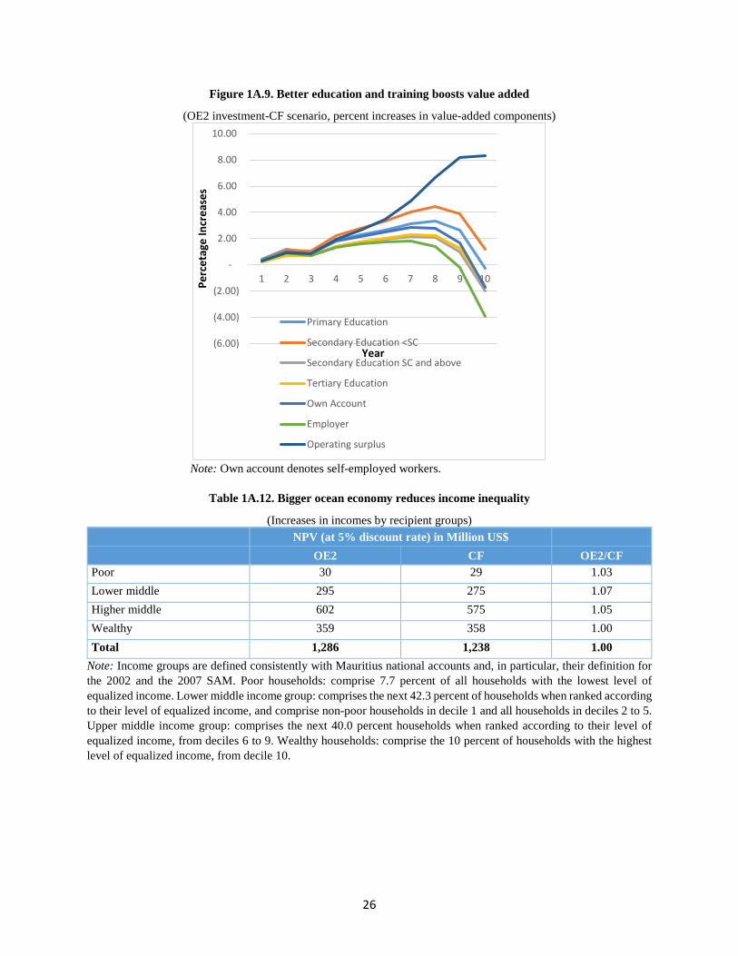
Figure 1A.9. Better education and training boosts value added
(OE2 investment-CF scenario, percent increases in value-added components)
Note: Own account denotes self-employed workers.
Table 1A.12. Bigger ocean economy reduces income inequality
(Increases in incomes by recipient groups) NPV (at 5% discount rate) in Million US$ OE2 CF OE2/CF
Poor 30 29 1.03 Lower middle 295 275 1.07 Higher middle 602 575 1.05 Wealthy 359 358 1.00 Total 1,286 1,238 1.00
Note: Income groups are defined consistently with Mauritius national accounts and, in particular, their definition for the 2002 and the 2007 SAM. Poor households: comprise 7.7 percent of all households with the lowest level of equalized income. Lower middle income group: comprises the next 42.3 percent of households when ranked according to their level of equalized income, and comprise non-poor households in decile 1 and all households in deciles 2 to 5. Upper middle income group: comprises the next 40.0 percent households when ranked according to their level of equalized income, from deciles 6 to 9. Wealthy households: comprise the 10 percent of households with the highest level of equalized income, from decile 10.
(6.00)
(4.00)
(2.00)
-
2.00
4.00
6.00
8.00
10.00
1 2 3 4 5 6 7 8 9 10Perc
etag
e In
crea
ses
Year
Primary Education
Secondary Education <SC
Secondary Education SC and above
Tertiary Education
Own Account
Employer
Operating surplus
27
Figure 1A.10. Poor benefits more with doubling of ocean economy
(Income distribution effects of OE2, percent changes versus baseline)
Sensitivity Analysis
The positive results from the main CGE simulations may be subject to several challenges by changes in the external conditions and the technical and behavioral estimates used in the model. The main external challenge could come from a deterioration of the international environment, which would make more difficult to provide the funds needed for investment. Behavioral and technical parameters may also undergo changes and/or their real values may be different from the estimates incorporated in the model. In both cases, exploring the sensitivity of the model solution to some of these changes is important to confirm the robustness of its results or to reveal selective or general weaknesses in the policy implications. Because of the structure of the model, which consists of several equations that quantify market exchange relationships across a wide spectrum of economic variables, it is possible to perform basic sensitivity analysis by modifying only a few key parameters. In the case of the OE2 strategy, these parameters concern three main sources of possible vulnerabilities of Mauritius future growth: (i) foreign capital supply, (ii) the availability of appropriate labor skills and (iii) natural resource degradation.
The response to adverse changes in these three dimensions can be investigated by changing three sets of key model parameters, expressed in terms of percentages changes. These parameters, which in the economic jargon are called supply elasticities, quantify the percentage increase, respectively, in foreign capital supply, labor of different skills and natural resource costs to the increased needs for these resources that would develop under the development scenarios simulated. If these elasticities are lower than the model estimates, in general growth will be lower because the economy’s growing needs cannot be accommodated by a correspondent expansion of the resource supply. For example, if the foreign capital supply needed to finance part pf the investment in the OE economy will only be partly available at the conditions predicted by the model and a higher
-
0.50
1.00
1.50
2.00
2.50
3.00
1 2 3 4 5 6 7 8 9 10
Perc
enta
geIn
crea
ses
Years
Poor Lower middle Higher middle Wealthy
28
price of capital (higher returns) will have to be paid to obtain it, both nominal and real growth rates may fall, while inflation may raise. Similar effects may occur if skilled labor is not promptly available, but will require more time to be supplied in the amount needed by OE expansion. For natural resources, a reduction in elasticity of supply would also imply that the contribution to GDP predicted by the base solution of the model could be achieved more slowly and require more than the 10-year timespan considered.
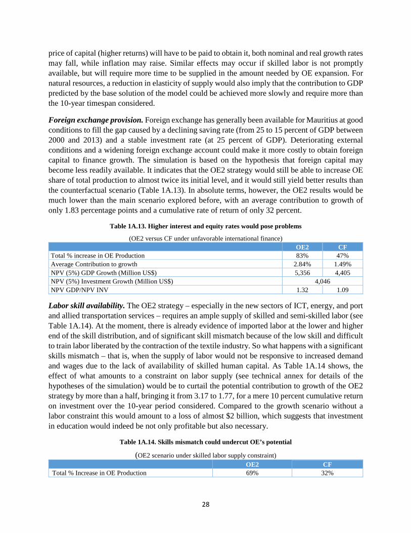
Foreign exchange provision. Foreign exchange has generally been available for Mauritius at good conditions to fill the gap caused by a declining saving rate (from 25 to 15 percent of GDP between 2000 and 2013) and a stable investment rate (at 25 percent of GDP). Deteriorating external conditions and a widening foreign exchange account could make it more costly to obtain foreign capital to finance growth. The simulation is based on the hypothesis that foreign capital may become less readily available. It indicates that the OE2 strategy would still be able to increase OE share of total production to almost twice its initial level, and it would still yield better results than the counterfactual scenario (Table 1A.13). In absolute terms, however, the OE2 results would be much lower than the main scenario explored before, with an average contribution to growth of only 1.83 percentage points and a cumulative rate of return of only 32 percent.
Table 1A.13. Higher interest and equity rates would pose problems
(OE2 versus CF under unfavorable international finance) OE2 CF
Total % increase in OE Production 83% 47% Average Contribution to growth 2.84% 1.49% NPV (5%) GDP Growth (Million US$) 5,356 4,405 NPV (5%) Investment Growth (Million US$) 4,046 NPV GDP/NPV INV 1.32 1.09
Labor skill availability. The OE2 strategy – especially in the new sectors of ICT, energy, and port and allied transportation services – requires an ample supply of skilled and semi-skilled labor (see Table 1A.14). At the moment, there is already evidence of imported labor at the lower and higher end of the skill distribution, and of significant skill mismatch because of the low skill and difficult to train labor liberated by the contraction of the textile industry. So what happens with a significant skills mismatch – that is, when the supply of labor would not be responsive to increased demand and wages due to the lack of availability of skilled human capital. As Table 1A.14 shows, the effect of what amounts to a constraint on labor supply (see technical annex for details of the hypotheses of the simulation) would be to curtail the potential contribution to growth of the OE2 strategy by more than a half, bringing it from 3.17 to 1.77, for a mere 10 percent cumulative return on investment over the 10-year period considered. Compared to the growth scenario without a labor constraint this would amount to a loss of almost $2 billion, which suggests that investment in education would indeed be not only profitable but also necessary.
Table 1A.14. Skills mismatch could undercut OE’s potential
(OE2 scenario under skilled labor supply constraint) OE2 CF
Total % Increase in OE Production 69% 32%
29
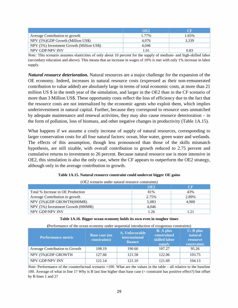
OE2 CF Average Contribution to growth 1.77% 1.65% NPV (5%)GDP Growth (Million US$) 4,076 3,339 NPV (5%) Investment Growth (Million US$) 4,046 NPV GDP/NPV INV 1.01 0.83
Note: This scenario assumes elasticities of only about 10 percent for the supply of medium- and high-skilled labor (secondary education and above). This means that an increase in wages of 10% is met with only 1% increase in labor supply.
Natural resource deterioration. Natural resources are a major challenge for the expansion of the OE economy. Indeed, increases in natural resource costs (expressed as their non-remunerated contribution to value added) are absolutely large in terms of total economic costs, at more than 21 million US $ in the tenth year of the simulation, and larger in the OE2 than in the CF scenario of more than 3 Million US$. These opportunity costs reflect the loss of efficiency due to the fact that the resource costs are not internalized by the economic agents who exploit them, which implies underinvestment in natural capital. Further, because they correspond to resource uses unmatched by adequate maintenance and renewal activities, they may also cause resource deterioration – in the form of pollution, loss of biomass, and other negative changes in productivity (Table 1A.15).
What happens if we assume a costly increase of supply of natural resources, corresponding to larger conservation costs for all four natural factors: ocean, blue water, green water and wetlands. The effects of this assumption, though less pronounced than those of the skills mismatch hypothesis, are still sizable, with overall contribution to growth reduced to 2.75 percent and cumulative returns to investment to 26 percent. Because natural resource use is more intensive in OE2, this simulation is also the only case, where the CF appears to outperform the OE2 strategy, although only in the average contribution to growth.
Table 1A.15. Natural resource constraint could undercut bigger OE gains
(OE2 scenario under natural resource constraints) OE2 CF
Total % Increase in OE Production 81% 43% Average Contribution to growth 2.75% 2.89% NPV (5%)GDP GROWTH(000MR) 5,083 4,900 NPV (5%) Investment Growth (000MR) 4,046 NPV GDP/NPV INV 1.26 1.21
Table 1A.16. Bigger ocean economy holds its own even in tougher times
(Performance of the ocean economy under sequential introduction of exogenous constraints)
Performance metric Base case (no constraints)
A. Unfavorable international
finance
B: A plus constrained skilled labor
supply
C: B plus natural resource
constraints Average Contribution to Growth 108.19 190.60 107.27 95.26 NPV (5%)GDP GROWTH 127.66 121.58 122.06 103.75 NPV GDP/NPV INV 121.14 121.10 121.69 104.13
Note: Performance of the counterfactual scenario =100. What are the values in the table – all relative to the baseline 100. Average of what in line 1? Why is B last line higher than base case (= constraint has positive effect?) but offset by B lines 1 and 2?
30
The bottom line is that a movement away from the base case to less favorable conditions shows no clear tendency for OE2 to become less attractive than CF, except for natural resources (Table 1A.16).
The CGE Model: a three-step procedure
In order to design an appropriate CGE model from the SAMs estimated for Mauritius (Scandizzo and Ferrarese, 2013) we follow the three-step procedure outlined by Norton, Scandizzo and Zimmerman (1986): (i) choosing the elements of the SAM that are to be regarded as endogenous; (ii) specifying equations or constraints for these elements; and (iii) specifying model closure.
For decision (i), all the cells in the different SAMs used are supposed to be endogenous, even when they correspond to an institution (such as, for example, the government) that acts as a source of exogenous injections in the policy experiments. This apparent discrepancy corresponds to the assumption that for these agents there is both an endogenous and an exogenous component to account for. For decision (iii), the model is closed with specific hypotheses on the exchange rate regime and to the various types of distortions that may affect or be the indirect result of imperfect property rights. For decision (ii), in order to specify the equations, note that the variables chosen are outputs, factor use, factor incomes, households, corporate and government incomes, government expenditures, savings by institution and quantities consumed, investment, foreign trade activities, international tourists, and prices of outputs, of final goods, and factors. The model is thus articulated into the following eight different modules, each of which corresponds to a block of equations:
Module I: Market Equilibrium Equations
Commodity balance equality is imposed for all activities and provides for market clearing requirement for all goods and factors. Because in all policy experiments domestic prices are endogenous, while some prices (such as international prices, tariffs, and rationing prices) are assumed to be exogenously given and invariant, market clearing is achieved by finding the appropriate price levels that ensure equilibrium. For those sectors that include exogenous prices, market clearing is enforced by either rationing or by exporting (or importing) the correspondent surplus (or deficit).
Thus, total domestic production for each activity must equal the total of the different sources of demand: intermediate input-output use, household, government and corporate consumption, uses as capital goods, and net exports. Each equilibrium equation is expressed in real terms (constant prices), but holds in current prices as well. Factor demand (labor, capital, natural resources, and biodiversity) also equals factor supply, factor prices being the endogenous element enforcing the equality.
Module II: Production, Factor use, and Factor Incomes
Factor substitution in production is allowed both by varying the composition of output (with variable endogenous substitution elasticities) and within sectors (with fixed elasticities of substitution). The combination of labor and capital capable of producing a given amount of output,
31
therefore, varies over time or alternative scenarios. As for factor use and incomes, they are both the joint consequence of factor demand and of factor supply equations, and market equilibrium conditions. Factors have all been posited to be supply and demand elastic with respect to own prices to reflect the fact that resources are unemployed or under-utilized. This implies that factor price percentage increases will not exceed the percentage increase in factor use, which appeared as the most reasonable upper bound in our calibration experiments with all the version of the model.
Factor incomes are defined as factor prices multiplied by factor utilization, so that value added at current prices varies both because of employment and of factor price variations. Since these variations are in the same direction and because product prices are supposed to be equal to production costs, demand stimuli in the model are unequivocally inflationary, while other types of shocks (such as on prices and budget shares) may have both inflationary or deflationary effects. For both commodities and factors, the base year physical levels were established by setting the corresponding prices equal to unity. This implies that all prices in the various solutions can be interpreted as percentage changes with respect to the base year.
Module III: Income Distribution
Factor and other incomes are distributed across institutions using the shares computed from the corresponding SAMs. These shares are assumed to reflect patterns of resource ownership and to be stable over different solutions. They correspond to the expenditure shares of factor and institutions computed along the columns and, while they are given for each SAM, their variation across the different SAMs considered is one of the key element of structural change. To study the impact of change in the pattern of asset ownership, furthermore, some of the experiments include, for a given SAM, a variation of income distribution shares.
Module IV: Consumption and Savings
All SAMs provide average propensities to save and consumption budget shares. To introduce marginal propensities to consume and price demand elasticities, however, it has been necessary to develop estimates of both sets of parameters using iterative model simulations and choosing the set of parameters that fit more closely the base year solution, under the assumption of want-separability (Frisch, 1959). The composition of total expenditure for each institution other than households is assumed to remain constant, both in terms of goods and income transfers. This implies that marginal propensities to save, except for households, are also constant and equal to average propensities.
Module V: Investment and Capital Stock
The SAM capital formation row represent the savings of each commodity and institutional account, while the corresponding column accounts for investment (in the sense of production available for capital accumulation). A similar interpretation holds for the row and column of natural resources, which can be interpreted as accounting, respectively for natural capital savings and investment. Although capital formation is treated as any institution, the interpretation of the
32
model coefficients is peculiar since the expenditure shares represent, along the column, the contribution of activities to capital formation and, along the row, for each institution, capital utilization. For each activity, the entry in the capital formation column is simply the amount of production that survives unconsumed the production period. For natural capital, the accounting is more complex and consists of four separate components: (i) activity and institution columns show in their intersection with the biodiversity rows, their use of natural capital;(ii) the natural resource (ocean, green and blue water, and wetland ) columns record, in their intersection with each activity , institution, and for water resources, the corresponding contribution to these sectors’ income;(iii) the row for natural capital records their use on the part of specific activities; and (iv) the column of natural capital records, at the intersection with all relevant activities and institutions, the net amount of natural capital created or destroyed as a consequence of their action.
For institutions, savings are shown in the intersection between their columns and capital formation and correspond to their contribution to national savings. Equality between savings and investment is ensured by Walras Law, which in turn derives from the simultaneous equality of demand and supply on commodity (physical balances), factor and natural resource markets, and prices and costs of production.
The SAMs used in the model specifies net exports without distinguishing between gross exports and gross imports. The Rest of the World (ROW) column and row are respectively used to specify demand for net exports and fixed expenditure shares for each institution. This implies that net exports for each sector are treated as demand levels of a foreign agent (the ROW account) who can purchase them at fixed prices (the world prices) and with a limited expenditure capacity. This in turn cannot exceed the demand for non-competitive imports resulting from the i-o coefficients or from the demand for imports of each institutional account. Balance of payment equilibrium is thus assured, but its components (in particular, trade and capital) may be in disequilibrium.
Module VI: The Government Accounts
The SAM expenditure coefficients in the government row account are used as coefficients of revenue collection and are assumed to be fixed. The shares in the government column account, instead, are assumed to be endogenous and depend on total revenue collected.
Module VII: Prices
Relative factor and activity prices are determined from the model solution, by enforcing demand supply equalities in all markets in some experiments, or alternatively assuming that some markets are open to foreign trade so that prices are exogenous. In these cases, domestic supply prices may either exceed (in the case of exports) or fall short (for imports) of production costs in equilibrium. The exchange rate is assumed to be fixed, and equilibrium values will reflect the shortage (or the surplus) of foreign exchange, so that an implicit shadow exchange rate can be calculated as an indicator of disequilibrium in the foreign sector.
33
CGE Model Based on SAM Evolution
This note presents the outline of the CGE model used in the analysis. In its complete form, the model is dynamic and is based on the idea that the impact of an exogenous shock on an economic system can be evaluated through a system of locally linear behavioral relations. The algorithm proposed uses an iterative method to obtain a solution to a multi-agent, multi-commodity general equilibrium problem, by linearizing demand and supply functions at a known equilibrium point and searching for new equilibrium prices and quantities in response to an exogenous shock.
A Recursive Short-term Model
Consider the SAM matrix of transactions. This matrix contains the input output matrix, which can be isolated and computed in terms of coefficients. Using the input-output coefficient sub-matrix extracted from the SAM (that is, first, in terms of values and then calculated inform of coefficient matrix with columns all summing to 1), we can specify the commodity balance relationship:
(1) tttttt dEdCdYdXAdX +++=
where:
tA =input-output matrix at time t
tdX = n x 1vector of variations of productive activities;
tdY = n x 1vector of variations of investment levels;
tdC = n x 1vector of variations of aggregate quantities consumed;
tdE = n x 1vector of variations of (net) quantities exported.
We can also specify the following equations for factor market equilibrium:
(2) tdt FdXdZ =
(3) 1−Π += ttftst dYGdPGdZ
(4) tst
dt dZdZdZ ==
Notice that equation (3) states that factor supply depends on the shocks of the previous period (one can easily generalize to more than one previous period, but we consider only one to keep the
algebra simple). In the case that this shock was an investment vector, the matrix tG represents the so-called capital matrix, that is, the matrix that maps capital goods produced in response to investment in period t-1 into increased productive capacity of the proprietary sectors in period t. All these equations can be explicitly or implicitly embedded in the SAM structure. The first of them represents factor demand on the part of the firms, In it:
34
dtdZ =m x 1bvector of variations of demand levels for them factors on the part of
the firms;
F =m x n matrix of input output coefficients for the m factors.
The hypothesis implicit in (2) is that factor demand is not a function of factor prices, but depends, given the fixed coefficient technology, only on the production levels of the various sectors.
Equation (3), on the other hand, represents factor supply with:
stdZ = m x 1 vector of variations of supply for them factors on the part of their
owners (households, firms, etc.);
ftdP =m x 1 vector of factor price variations;
1−tdY =n x 1 vector of investment levels in the previous period.
Factor supply, according to equation (3) is thus determined by factor prices and by the variation in productive capacity determined by past investment.
Equation (4), that represents the condition to maintain equilibrium between factor demand and factor supply, implies, together with (2) and (3):
(5) ( )11
−−Π −= tttft dYGFdXGdP
Because ΠG and tG are both positive matrices, the market theory contained in equations (2)–(4) implies that increases of production and investment determine, respectively a positive tension on past prices and a negative tension on future prices.
Factor income variations are described by the m,1 vector tdV , and are governed by the equation:
(6) ftttftt dPZdZPdV '+′=
or, upon substitution of (1) and (4):
(7) ( ) 111
−−Π
−Τ ′−′+′= tttttftt dYGGZFdXGZPdV
where the curl indicates the matrix obtained by diagonalizing the corresponding vector. Product prices vary with factor prices:
(8) ftt dPFAIdP ′′−Φ= −1)(
35
where Φ is a diagonal n x n matrix of flexibility parameters iw (i= 1,2…n). In particular, we
assume 0=iw for internationally tradable goods and 1=iw for the other goods1.
Substituting (5) into (8), we obtain:
(9) ( )111)( −−Π
− −′′−Φ= tttt dYGFdXGFAIdP
Consumption levels are function of prices and incomes:
(10) kttttt dWdPdCdXdC ιΓ+Λ==+ ∗
where kι is a k,1 sum vector, ∑Λ=Λk
hh , hΛ (h=1,2…k) being an n, n matrix of linearized demand
price elasticities,Γ is a n, k diagonal matrix of linearized Engel elasticities dVdW Ω= is a k,1 vector of households and other institutions’ incomes, and Ω is a 1,k vector of income distribution shares, with generic element hjω (h=1,…k; j=1,2..m).Note that expression (10) refers to aggregate consumption for each commodity. With many households represented in the SAM matrix, we can write:
(11) ktt dcdC ι*=∗ , where *tdc is an n, k matrix having as a generic element *
tihdc , that is, consumption of the ith commodity by the hth household (h=1,2, …k). This equation can be extended to the government and enterprises, but not to capital formation and rest of the world. Each household and the government can be assumed to have its own system of demand functions, according with the expression:
(12) hhhth dWdPdc Γ+Λ=*
Capital formation is considered exogenous: Alternatively, expression (12) may take the form of an investment function, by postulating that:
(12bis) 1−−+Ξ= ttKt HdXHdXdPdY
where KdP is the price of capital determined from equation (5)
Using (7) and (9):
1 We can also interpret price formation in terms of a neoclassical cost function: ),( fPPUP = .This implies:
][ ff
t dPPUdP
PUdP
∂∂
+∂∂
Φ= . By Shephard’s lemma, the derivative of the cost function w.r.t. prices defines the
demand for intermediate inputs 'APU
=∂∂
and for primary factors 'FPU
f
=∂∂
.
36
(13) ( ) ( )[ ]
( )[ ] 111
111
−−Π
−
−Π
−−Π
∗
′′−∆Φ+ΤΩ−
+′′−ΛΦ+′+′ΤΩ==−
ttt
ttftttt
dYGGFAIZ
FdXGFAIGZPdCdMdC
SinceΛ is a negative definite matrix, in accordance with consumer theory, both the effect of increases in production and of previous investment may be either positive or negative, according to whether the income or the price effect prevails. If production increases, in fact, this tends to increase factor prices with positive effects on their incomes, but also with the consequence of increasing the prices of goods and services in the economy. Final demand is thus pushed upward by the income effect and downward by the price effect. Vice versa, the increase in productive capacity determined by previous investment, by shifting outward factor supply, tends to reduce their prices. This causes a reduction of factor income, but a parallel reduction of prices of intermediate and final goods. The sign of the net result of these shifts will ultimately depend on the relative magnitude of the behavioral and technological parameters involved.
Substituting (13) into (1) and solving for tdX ,we obtain an equation that synthesizes the effect of investment (or any other exogenous shock2:
(14) ( ) ( )11
−− +−−= tttt dYdYAIdX ψθ
where3 ( ) ( )[ ]FGFAIGZP tftt111 −
Π−−
Π ′′−ΛΦ+′+′ΓΩ=θ
and ( )[ ] ttt GGFAIZ 11 −Π
− ′′−ΛΦ+′ΓΩ−=ψ
In order for equation (12) to be considered a general equilibrium, the system has to include an equation describing the formation f savings. If investment and foreign trade are exogenous (that is, capital formation and rest of the world are not in the SAM at the base of the CGE model), we have two alternatives to ensure that the sum of domestic and foreign savings are equal to investment.
Consider in fact the definition of the current account balance:
2 Instead than as an equality in quantity terms, the commodity balance may be re-defined in value terms, thereby implying that the input output coefficients represent value shares (corresponding to Cobb Douglas production functions, or to log-linear local approximations), according to the equation: (1bis) tttttttttt XPddMdCdYdXAPdXP ′+−++′=′ ][ 3 Note that, in order for (12) is derived from the equation:
( ) ( )1−+++= tttttt dYdYdXAdX ψθ , where ttA θ+ constitutes an “augmented” input output coefficient
matrix, which takes into account not only the transactions in the base year (through the initial i-o matrix tA , but also
of the endogenous income and price effects (through the matrix tθ ). This augmented i-o must contain all the information to construct a SAM that corresponds to a general equilibrium and must also be balanced, both in terms of transactions and coefficients (summing to 1 for each column), since the budget constraint will continue to hold for each sector when the endogenous incomes and prices are taken into account.
37
(13) →−=− tttt dMdEdYdS 0=−+ tRtdt dYdSdS
where tdM is imports of intermediates, and tdE exports of all goods minus imports of final goods,
dtdS is domestic savings and RtdS foreign savings. If investment is endogenous, on the other hand, we can specify a domestic savings function, whose simplest form is:
(13bis) tdt dVsSd Ω′=′
In (13) dtdS is an r x 1 vector of variation of savings of the r economic agents (households, government, etc.) and s a 1 x r vector of corresponding propensities to save.
To maintain equilibrium, factor income must be all spent:
(14) ( ) ththhthht dWsdPdWPdW +Λ+Γ′= for each institution (household, corporation or government) Hh ,...2,1= .
Sufficient conditions4 to satisfy equation (14) are the so-called Engel and Edgeworth conditions:
(15) 1=+Γ′ hht sP Engel condition
(16) htht CP ′−=Λ′ Edgeworth condition
These two conditions can be respected by iterating on prices and quantity variables. Alternatively, equation (14) can be satisfied by treating savings in each period as a residual, or by adjusting the propensities to save in each period to respect market equilibrium.
A second, necessary condition to ensure the “generality” of the economic equilibrium described is the so called Walras Law, according to which the value added from production must equal factor income. Starting from this budget constraint for the base year:
(17) ( ) tfttt ZPXAIP ′=−′ ,
the variations analyzed by running the model must respect the equation:
(18) ( ) ( ) ftttfttttt dPZdZPdPAIXdXAIP ′+′=′−′+−′
Given equation (17), equation (18) is automatically respected in the case of a closed economy. If we introduce a class of internationally tradable goods, however, the situation becomes more complex.
4 This can be simply shown by substituting (15) and (16) into (14), to obtain:
thtthttht dPCdPCdWdW '' −+=
38
Indicating with tr the Exchange rate that converts International prices into domestic currency, we can write:
(19) tt drPdP ∗= 11
(20) ttttt dPFdPAdrPAdP 2222122 ′+′+′= ∗
where:
tdP1 is an n x 1 vector of variations of domestic prices of internationally traded goods (CI);
∗1P is an n x 1 vector of international prices expressed in foreign currency (for example,
dollars) for (CI);
tdr the variation of the exchange rate (in domestic currency in units of foreign currency);
tdP2 i san 1nn − ,1 vector of internationally non-tradable goods (NCI);
22221 ,, FAA ′′′ are appropriate sub-partitions, respectively of matrices A′ and F ′ .
To satisfy Walras law, the variation tdr of the exchange rate must satisfy the equation:
(21) ( )[ ] ( )
( )[ ] ∗
∗
′′+′−′′+′−′′+′−′
−=1221111
111221111
PXAAIXdZPdPZrPXdAAIXd
drtt
tftftttttt
This equation, obtained by applying Walras Law to the system (17)-(18), expresses the amount of devaluation necessary to re-equilibrate the economic system in response to a variation of the equilibrium values of the quantities tdX1 , tdX 2 e dXFdZ t 11 ′= and of factor prices f
tdP
According to equation (21) such a devaluation should be equal to the variation of the net benefit from the increase in production of CI at international prices, in domestic currency, per unit of value of the production of the same goods in foreign currency.
A Modified SAM Representation of the Short-Term Model
The CGE model presented above can be represented by the following modified SAM matrix:
Products=dX
Factor employment= dZ
Factor Incomes=dV
Institutions’ incomes=dW
Factor prices=
fdP
Product prices=dP
Present shocks tdY
Previous Shocks=
1−tdY
dX A 0 0 Γ 0 Λ I 0 dZ F 0 0 0 0 0 0 0 dV 0 fP 0 0 Z 0 0 0
dW 0 0 Ω I 0 0 0 0

39
fdP 0 1−πG 0 0 0 0 0 GG 1−
π
dP 0 0 0 0 'F 'A 0 0
Products=
dX Factor employment= dZ
Institutions’ incomes=dW
Factor prices=
fdP
Product prices=dP
dX A 0 Γ 0 Λ dZ F 0 0 0 0 dW 0 0 I 0 0
fdP 0 1−πG +
)( Ψ+I
0 0
dP 0 0 0 'F 'A
Indicating this modified matrix with the symbol B , we can write:
(22) 1−++= tttt GdYdYBdd ξξ
where tdξ is a column vector of products, factors, income and prices unknown),,,,( tfttttt dPdPdVdYdZdX G is the capital matrix that maps the investment from producing
sectors to capital increases in the proprietary sectors, and 1−tGdY is a vector of effects of previous investment or other exogenous changes.
In general, one or more columns and rows of B can be considered exogenous and can be the object of an exogenous shock. For example, indicating with tdY a vector of exogenous shocks to the capital formation- investment account, and with YB the matrix B without the row and the column corresponding to the capital formation accountY ,and assuming 1−tGdY =0, we can write:
(22) tYt dYBId 1)( −−=ξ
Expression (22) indicates the CGE solution in response to an exogenous investment shock, consisting of an increase in the demand of goods and services from producing sectors that are directly able to contribute to capital building. Because of the general equilibrium structure of the matrix, the effects of these exogenous shocks will include the impact on the increased costs of endogenously priced factors and intermediate inputs, thereby taking into account opportunity costs from alternative resource use.
Recursive Long-term Model
Consider the following modification of the model in (21):
(21a) tttttt dBdYdBd ξξξ ++=
(21b) 1−= ttt GdYdBξ
40
(21c) 11
11 −−
−− +=+= tttttt GdYBdBBB ξ
where the curls indicate that the vector is diagonalized into a square matrix. Substituting (21b) and (21c) into (21a), we obtain:
(23) tttttttt dBdYdGdYBd ξξξξ +++= −−
− ][ 11
1 = tttiiii
t
idBdYddYGB ξξξ +++ −
−
=∑ ]][ 1
1
00
We can solve for tdξ and add a set of exogenous variables (for example a trend) that shift the relationship over time:
(24) tdξ = ttttiii
t
iLdBdYdYGBI ζξξ +++− −
−−
=∑ )()]([ 1
11
00
Taking fist differences of (24), on the other hand, yields:
(25) )()]()[()]([ 1111
1110
11 −−−−
−−−
−− −+−+−+−=− ttttttttittt LdBdBdYdYdYGBIdd ζζξξξξξ
This expression shows the effect of the policy variables (the investment changes 1−− tt dYdY and the structural changes 11 −−− tttt dBdB ξξ on the endogenous variables. While the endogenous changes are still function of the exogenous variables )( 1−− tt ζζ , in the case of linear trends (
btat += 0ζ ), they are reduced to a constant.
Consider in more detail the evolution of the SAM matrix over time, as capital and structural change accumulates. For example, assume that there is an investment tdY in period t that accrues entirely to sector j in period t-1. In this case, we can write:
(26) 1+= kjtt rdxdY
where 1+kjtrdx is the increase in value added given by the yearly remuneration of the new capital installed at the rate r. Since before balancing the totals do not change, the SAM coefficient before the matrix is balanced will simply be:
(27) )/( jtkjtkjt xxrdda =
where jtx is total supply of the jth sector at time t. Thus, from (26) and (27), we derive:
(28a) kjtjtt daxdY = and (28b) kjtjtkjtkjt daxaa +=+1

41
Expressions (28a) and (28b) will change after balancing the new matrix, since the new totals will be different and because of the constraint that the sum of the coefficients by column should be equal to one. Note also that the change will be incorporated permanently into the matrix, but should go to zero as the investment is amortized.
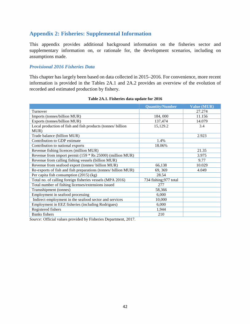
42
Appendix 2: Fisheries: Supplemental Information
This appendix provides additional background information on the fisheries sector and supplementary information on, or rationale for, the development scenarios, including on assumptions made.
Provisional 2016 Fisheries Data
This chapter has largely been based on data collected in 2015–2016. For convenience, more recent information is provided in the Tables 2A.1 and 2A.2 provides an overview of the evolution of recorded and estimated production by fishery.
Table 2A.1. Fisheries data update for 2016
Quantity/Number Value (MUR) Turnover 27.274 Imports (tonnes/billion MUR) 184, 000 11.156 Exports (tonnes/billion MUR) 137,474 14.079 Local production of fish and fish products (tonnes/ billion MUR)
15,129.2 3.4
Trade balance (billion MUR) 2.923 Contribution to GDP estimate 1.4% Contribution to national exports 18.06% Revenue fishing licences (million MUR) 21.35 Revenue from import permit (159 * Rs 25000) (million MUR) 3.975 Revenue from calling fishing vessels (billion MUR) 9.77 Revenue from seafood export (tonnes/ billion MUR) 66,138 10.029 Re-exports of fish and fish preparations (tonnes/ billion MUR) 69, 369 4.049 Per capita fish consumption (2015) (kg) 28.54 Total no. of calling foreign fisheries vessels (MPA 2016) 734 fishing;977 total Total number of fishing licenses/extensions issued 277 Transshipment (tonnes) 58,366 Employment in seafood processing 6,000 Indirect employment in the seafood sector and services 10,000 Employment in EEZ fisheries (including Rodrigues) 6,000 Registered fishers 1,944 Banks fishers 210
Source: Official values provided by Fisheries Department, 2017.
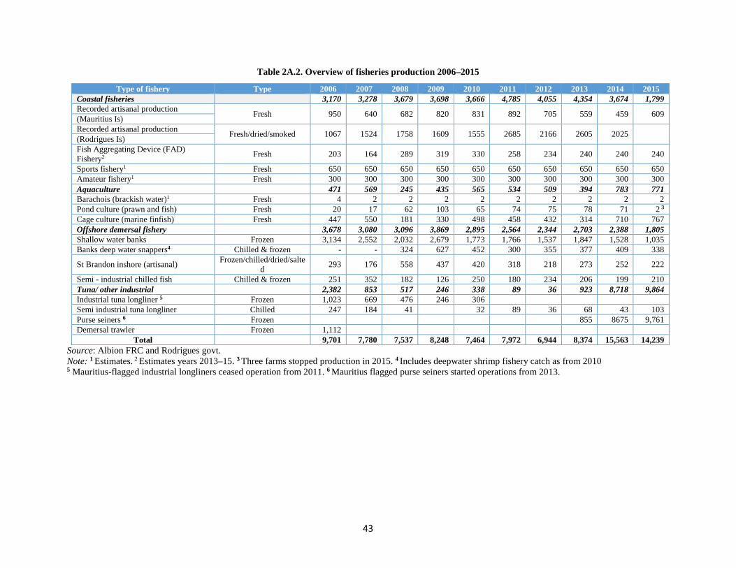
43
Table 2A.2. Overview of fisheries production 2006–2015
Type of fishery Type 2006 2007 2008 2009 2010 2011 2012 2013 2014 2015 Coastal fisheries 3,170 3,278 3,679 3,698 3,666 4,785 4,055 4,354 3,674 1,799 Recorded artisanal production Fresh 950 640 682 820 831 892 705 559 459 609 (Mauritius Is) Recorded artisanal production Fresh/dried/smoked 1067 1524 1758 1609 1555 2685 2166 2605 2025 (Rodrigues Is) Fish Aggregating Device (FAD) Fishery2 Fresh 203 164 289 319 330 258 234 240 240 240
Sports fishery1 Fresh 650 650 650 650 650 650 650 650 650 650 Amateur fishery1 Fresh 300 300 300 300 300 300 300 300 300 300 Aquaculture 471 569 245 435 565 534 509 394 783 771 Barachois (brackish water)1 Fresh 4 2 2 2 2 2 2 2 2 2 Pond culture (prawn and fish) Fresh 20 17 62 103 65 74 75 78 71 2 3 Cage culture (marine finfish) Fresh 447 550 181 330 498 458 432 314 710 767 Offshore demersal fishery 3,678 3,080 3,096 3,869 2,895 2,564 2,344 2,703 2,388 1,805 Shallow water banks Frozen 3,134 2,552 2,032 2,679 1,773 1,766 1,537 1,847 1,528 1,035 Banks deep water snappers4 Chilled & frozen - - 324 627 452 300 355 377 409 338
St Brandon inshore (artisanal) Frozen/chilled/dried/salted 293 176 558 437 420 318 218 273 252 222
Semi - industrial chilled fish Chilled & frozen 251 352 182 126 250 180 234 206 199 210 Tuna/ other industrial 2,382 853 517 246 338 89 36 923 8,718 9,864 Industrial tuna longliner 5 Frozen 1,023 669 476 246 306 Semi industrial tuna longliner Chilled 247 184 41 32 89 36 68 43 103 Purse seiners 6 Frozen 855 8675 9,761 Demersal trawler Frozen 1,112
Total 9,701 7,780 7,537 8,248 7,464 7,972 6,944 8,374 15,563 14,239 Source: Albion FRC and Rodrigues govt. Note: 1 Estimates. 2 Estimates years 2013–15. 3 Three farms stopped production in 2015. 4 Includes deepwater shrimp fishery catch as from 2010 5 Mauritius-flagged industrial longliners ceased operation from 2011. 6 Mauritius flagged purse seiners started operations from 2013.
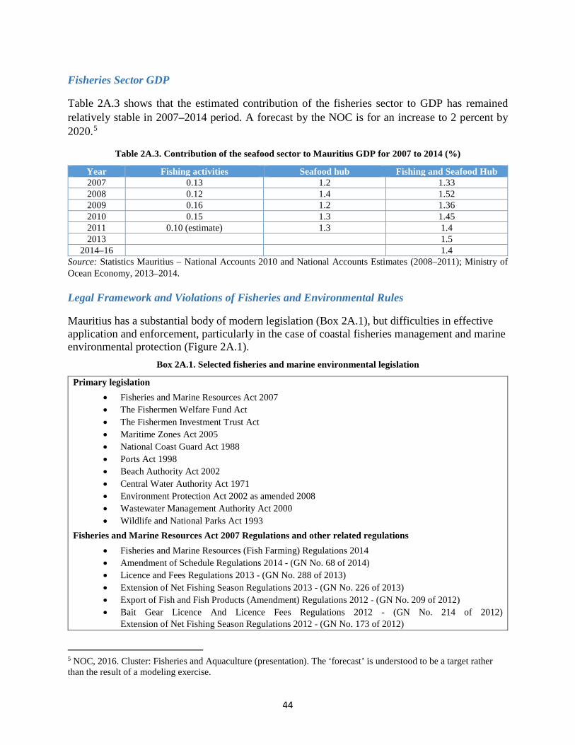
44
Fisheries Sector GDP
Table 2A.3 shows that the estimated contribution of the fisheries sector to GDP has remained relatively stable in 2007–2014 period. A forecast by the NOC is for an increase to 2 percent by 2020.5
Table 2A.3. Contribution of the seafood sector to Mauritius GDP for 2007 to 2014 (%)
Year Fishing activities Seafood hub Fishing and Seafood Hub 2007 0.13 1.2 1.33 2008 0.12 1.4 1.52 2009 0.16 1.2 1.36 2010 0.15 1.3 1.45 2011 0.10 (estimate) 1.3 1.4 2013 1.5
2014–16 1.4 Source: Statistics Mauritius – National Accounts 2010 and National Accounts Estimates (2008–2011); Ministry of Ocean Economy, 2013–2014.
Legal Framework and Violations of Fisheries and Environmental Rules
Mauritius has a substantial body of modern legislation (Box 2A.1), but difficulties in effective application and enforcement, particularly in the case of coastal fisheries management and marine environmental protection (Figure 2A.1).
Box 2A.1. Selected fisheries and marine environmental legislation
Primary legislation • Fisheries and Marine Resources Act 2007 • The Fishermen Welfare Fund Act • The Fishermen Investment Trust Act • Maritime Zones Act 2005 • National Coast Guard Act 1988 • Ports Act 1998 • Beach Authority Act 2002 • Central Water Authority Act 1971 • Environment Protection Act 2002 as amended 2008 • Wastewater Management Authority Act 2000 • Wildlife and National Parks Act 1993
Fisheries and Marine Resources Act 2007 Regulations and other related regulations • Fisheries and Marine Resources (Fish Farming) Regulations 2014 • Amendment of Schedule Regulations 2014 - (GN No. 68 of 2014) • Licence and Fees Regulations 2013 - (GN No. 288 of 2013) • Extension of Net Fishing Season Regulations 2013 - (GN No. 226 of 2013) • Export of Fish and Fish Products (Amendment) Regulations 2012 - (GN No. 209 of 2012) • Bait Gear Licence And Licence Fees Regulations 2012 - (GN No. 214 of 2012)
Extension of Net Fishing Season Regulations 2012 - (GN No. 173 of 2012)
5 NOC, 2016. Cluster: Fisheries and Aquaculture (presentation). The ‘forecast’ is understood to be a target rather than the result of a modeling exercise.
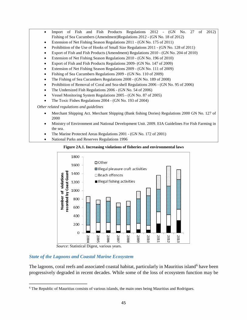
45
• Import of Fish and Fish Products Regulations 2012 - (GN No. 27 of 2012) Fishing of Sea Cucumbers (Amendment)Regulations 2012 - (GN No. 18 of 2012)
• Extension of Net Fishing Season Regulations 2011 - (GN No. 175 of 2011) • Prohibition of the Use of Hooks of Small Size Regulations 2011 - (GN No. 128 of 2011) • Export of Fish and Fish Products (Amendment) Regulations 2010 - (GN No. 204 of 2010) • Extension of Net Fishing Season Regulations 2010 - (GN No. 196 of 2010) • Export of Fish and Fish Products Regulations 2009- (GN No. 147 of 2009) • Extension of Net Fishing Season Regulations 2009 - (GN No. 111 of 2009) • Fishing of Sea Cucumbers Regulations 2009 - (GN No. 110 of 2009) • The Fishing of Sea Cucumbers Regulations 2008 - (GN No. 189 of 2008) • Prohibition of Removal of Coral and Sea-shell Regulations 2006 - (GN No. 95 of 2006) • The Undersized Fish Regulations 2006 - (GN No. 54 of 2006) • Vessel Monitoring System Regulations 2005 - (GN No. 87 of 2005) • The Toxic Fishes Regulations 2004 - (GN No. 193 of 2004)
Other related regulations and guidelines • Merchant Shipping Act. Merchant Shipping (Bank fishing Dories) Regulations 2000 GN No. 127 of
2000 • Ministry of Environment and National Development Unit. 2009. EIA Guidelines For Fish Farming in
the sea. • The Marine Protected Areas Regulations 2001 - (GN No. 172 of 2001) • National Parks and Reserves Regulations 1996
Figure 2A.1. Increasing violations of fisheries and environmental laws
Source: Statistical Digest, various years.
State of the Lagoons and Coastal Marine Ecosystem
The lagoons, coral reefs and associated coastal habitat, particularly in Mauritius island6 have been progressively degraded in recent decades. While some of the loss of ecosystem function may be
6 The Republic of Mauritius consists of various islands, the main ones being Mauritius and Rodrigues.
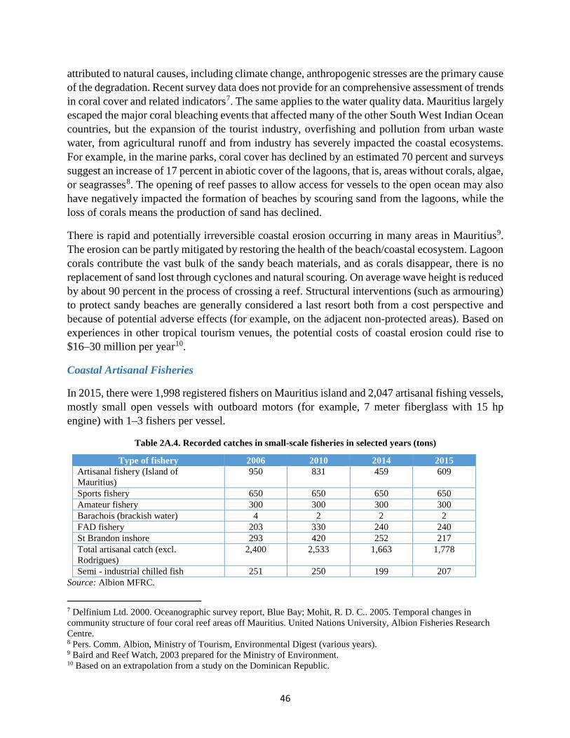
46
attributed to natural causes, including climate change, anthropogenic stresses are the primary cause of the degradation. Recent survey data does not provide for an comprehensive assessment of trends in coral cover and related indicators7. The same applies to the water quality data. Mauritius largely escaped the major coral bleaching events that affected many of the other South West Indian Ocean countries, but the expansion of the tourist industry, overfishing and pollution from urban waste water, from agricultural runoff and from industry has severely impacted the coastal ecosystems. For example, in the marine parks, coral cover has declined by an estimated 70 percent and surveys suggest an increase of 17 percent in abiotic cover of the lagoons, that is, areas without corals, algae, or seagrasses8. The opening of reef passes to allow access for vessels to the open ocean may also have negatively impacted the formation of beaches by scouring sand from the lagoons, while the loss of corals means the production of sand has declined.
There is rapid and potentially irreversible coastal erosion occurring in many areas in Mauritius9. The erosion can be partly mitigated by restoring the health of the beach/coastal ecosystem. Lagoon corals contribute the vast bulk of the sandy beach materials, and as corals disappear, there is no replacement of sand lost through cyclones and natural scouring. On average wave height is reduced by about 90 percent in the process of crossing a reef. Structural interventions (such as armouring) to protect sandy beaches are generally considered a last resort both from a cost perspective and because of potential adverse effects (for example, on the adjacent non-protected areas). Based on experiences in other tropical tourism venues, the potential costs of coastal erosion could rise to $16–30 million per year10.
Coastal Artisanal Fisheries
In 2015, there were 1,998 registered fishers on Mauritius island and 2,047 artisanal fishing vessels, mostly small open vessels with outboard motors (for example, 7 meter fiberglass with 15 hp engine) with 1–3 fishers per vessel.
Table 2A.4. Recorded catches in small-scale fisheries in selected years (tons)
Type of fishery 2006 2010 2014 2015 Artisanal fishery (Island of Mauritius)
950 831 459 609
Sports fishery 650 650 650 650 Amateur fishery 300 300 300 300 Barachois (brackish water) 4 2 2 2 FAD fishery 203 330 240 240 St Brandon inshore 293 420 252 217 Total artisanal catch (excl. Rodrigues)
2,400 2,533 1,663 1,778
Semi - industrial chilled fish 251 250 199 207 Source: Albion MFRC.
7 Delfinium Ltd. 2000. Oceanographic survey report, Blue Bay; Mohit, R. D. C.. 2005. Temporal changes in community structure of four coral reef areas off Mauritius. United Nations University, Albion Fisheries Research Centre. 8 Pers. Comm. Albion, Ministry of Tourism, Environmental Digest (various years). 9 Baird and Reef Watch, 2003 prepared for the Ministry of Environment. 10 Based on an extrapolation from a study on the Dominican Republic.
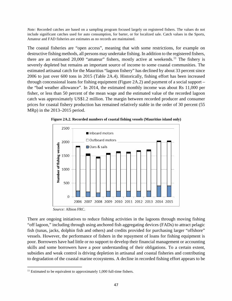
47
Note: Recorded catches are based on a sampling program focused largely on registered fishers. The values do not include significant catches used for auto consumption, for barter, or for localized sale. Catch values in the Sports, Amateur and FAD fisheries are estimates as no records are maintained.
The coastal fisheries are “open access”, meaning that with some restrictions, for example on destructive fishing methods, all persons may undertake fishing. In addition to the registered fishers, there are an estimated 20,000 “amateur” fishers, mostly active at weekends.11 The fishery is severely depleted but remains an important source of income to some coastal communities. The estimated artisanal catch for the Mauritius “lagoon fishery” has declined by about 33 percent since 2006 to just over 600 tons in 2015 (Table 2A.4). Historically, fishing effort has been increased through concessional loans for fishing equipment (Figure 2A.2) and payment of a social support – the “bad weather allowance”. In 2014, the estimated monthly income was about Rs 11,000 per fisher, or less than 50 percent of the mean wage and the estimated value of the recorded lagoon catch was approximately US$1.2 million. The margin between recorded producer and consumer prices for coastal fishery production has remained relatively stable in the order of 30 percent (55 MRp) in the 2013–2015 period.
Figure 2A.2. Recorded numbers of coastal fishing vessels (Mauritius island only)
Source: Albion FRC.
There are ongoing initiatives to reduce fishing activities in the lagoons through moving fishing “off lagoon,” including through using anchored fish aggregating devices (FADs) to attract pelagic fish (tunas, jacks, dolphin fish and others) and credits provided for purchasing larger “offshore” vessels. However, the performance of fishers in the repayment of loans for fishing equipment is poor. Borrowers have had little or no support to develop their financial management or accounting skills and some borrowers have a poor understanding of their obligations. To a certain extent, subsidies and weak control is driving depletion in artisanal and coastal fisheries and contributing to degradation of the coastal marine ecosystems. A decline in recorded fishing effort appears to be
11 Estimated to be equivalent to approximately 1,000 full-time fishers.

48
maintaining the recorded CPUE level in the Mauritius lagoon fishery, while poor economic performance may be driving the apparent decline in the off-lagoon fishery (Figures 2A.3). However, given that the recorded catch and effort information provides a very incomplete picture, these conclusions should be treated with caution. The weaknesses in application of effective environmental rules also extend to other stresses on the lagoons. Box 2A.2 and Table 2A.5 illustrate the recovery of the Rodrigues artisanal fisheries.
Figure 2A.3. Apparent trends in catch and effort in the lagoon and offshore fisheries
(Mauritius island only)
Source: Albion FRC.
Table 2A.5. Catches (tons), numbers of fishers and fishing vessels - Rodrigues island
2006 2007 2008 2009 2010 2011 2012 2013 2014 Vessels 1,714 1,728 1,748 1,806 1,821 1,828 1,856 1,873 1,973 Registered fishers 2,024 1,981 1,891 1,521 1,407 1,294 1,236 1,227 1,221 Fish - Lagoon 640.7 886.1 1,078.1 951.1 923.6 1,885.8 1,194.1 1,750.6 1,158.3 Fish - Off lagoon 160.3 383.7 398.2 384.2 362.6 416.8 401.2 293.2 363.6 Octopus - Lagoon 266.4 254.1 281.3 273.4 268.7 382.7 570.7 561.1 502.6 Total catch 1,067.4 1,523.9 1,757.6 1,608.7 1,554.9 2,685.3 2,166.0 2,604.9 2,024.5
Source: Rodrigues Regional Government.
The Banks Fisheries
The Banks fisheries (Box 2A.2) show considerable potential but require significant new investment, measures to foster cooperation among operators at sea and in export marketing. Financing new fleet investments will require innovative approaches including capitalization of fishing rights and measures to ensure profitability in order to mitigate investor risks.
Box 2A.2. Declining catches in the Banks fisheries
There are three distinct Banks fisheries in terms of target species and fishing areas: (a) The shallow water Banks fishery, which mainly targets emperor (Letherinidae) on the Banks plateaux,
usually in waters up to 70 meters depth. Three types of drop-line fishing operations take place: (i) freezer vessels; (ii) ice, or chill fish vessels; and (iii) freezer motherships with dories, which use fleet of small boats. The dory motherships are being phased out as the carriage of large quantities of gasoline on board is considered a hazard.
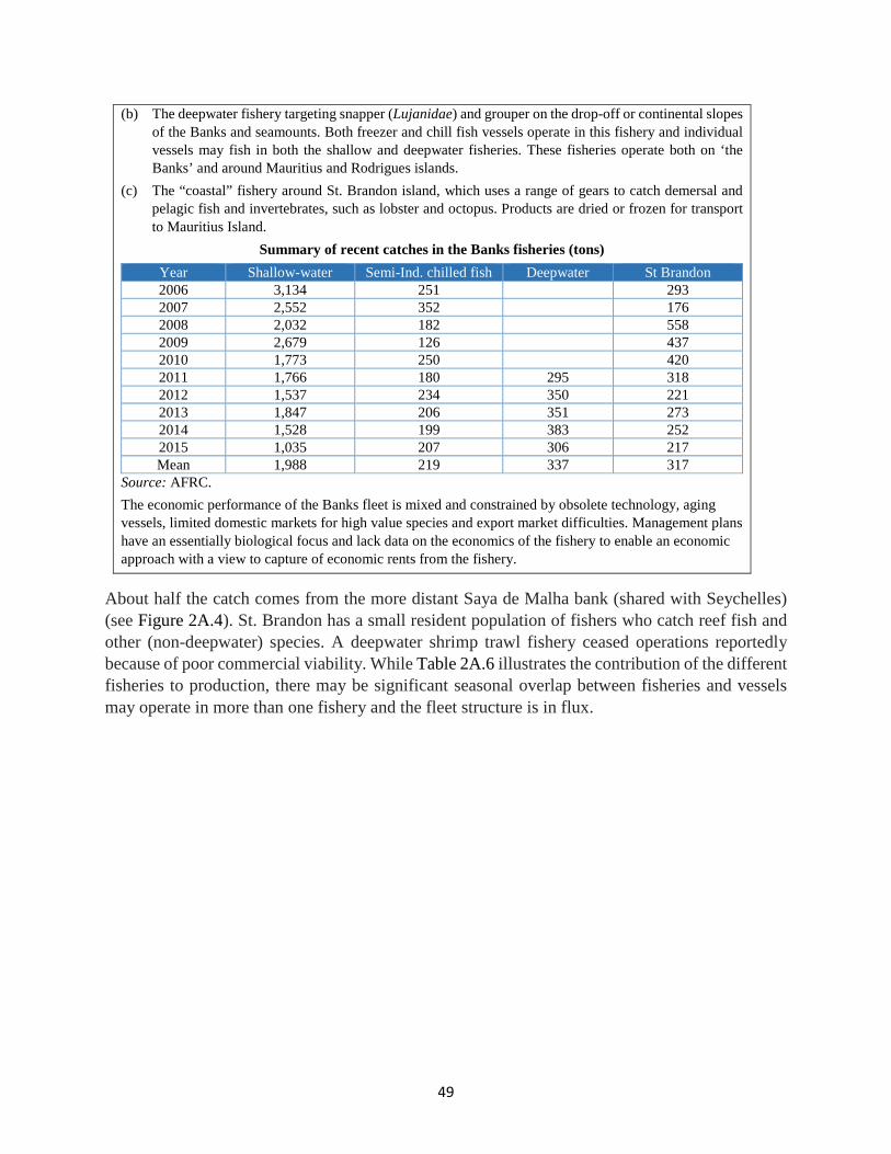
49
(b) The deepwater fishery targeting snapper (Lujanidae) and grouper on the drop-off or continental slopes of the Banks and seamounts. Both freezer and chill fish vessels operate in this fishery and individual vessels may fish in both the shallow and deepwater fisheries. These fisheries operate both on ‘the Banks’ and around Mauritius and Rodrigues islands.
(c) The “coastal” fishery around St. Brandon island, which uses a range of gears to catch demersal and pelagic fish and invertebrates, such as lobster and octopus. Products are dried or frozen for transport to Mauritius Island.
Summary of recent catches in the Banks fisheries (tons) Year Shallow-water Semi-Ind. chilled fish Deepwater St Brandon 2006 3,134 251
293
2007 2,552 352
176 2008 2,032 182
558
2009 2,679 126
437 2010 1,773 250
420
2011 1,766 180 295 318 2012 1,537 234 350 221 2013 1,847 206 351 273 2014 1,528 199 383 252 2015 1,035 207 306 217 Mean 1,988 219 337 317
Source: AFRC. The economic performance of the Banks fleet is mixed and constrained by obsolete technology, aging vessels, limited domestic markets for high value species and export market difficulties. Management plans have an essentially biological focus and lack data on the economics of the fishery to enable an economic approach with a view to capture of economic rents from the fishery.
About half the catch comes from the more distant Saya de Malha bank (shared with Seychelles) (see Figure 2A.4). St. Brandon has a small resident population of fishers who catch reef fish and other (non-deepwater) species. A deepwater shrimp trawl fishery ceased operations reportedly because of poor commercial viability. While Table 2A.6 illustrates the contribution of the different fisheries to production, there may be significant seasonal overlap between fisheries and vessels may operate in more than one fishery and the fleet structure is in flux.
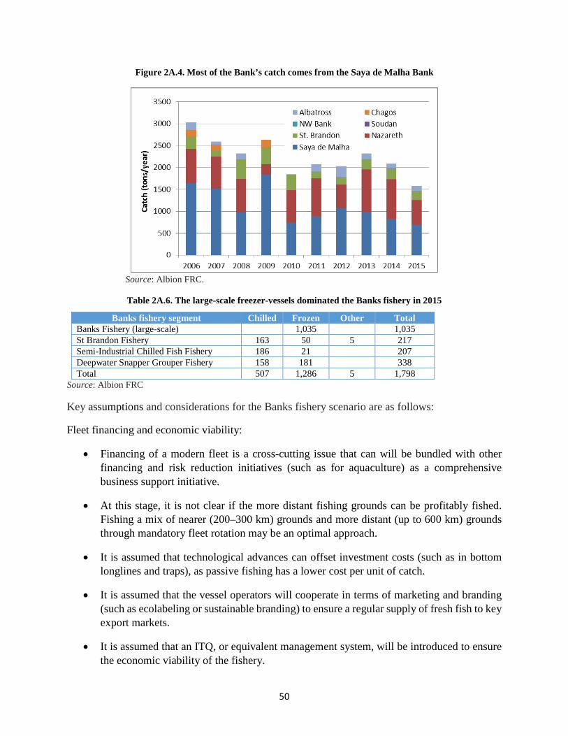
50
Figure 2A.4. Most of the Bank’s catch comes from the Saya de Malha Bank
Source: Albion FRC.
Table 2A.6. The large-scale freezer-vessels dominated the Banks fishery in 2015
Banks fishery segment Chilled Frozen Other Total Banks Fishery (large-scale)
1,035
1,035
St Brandon Fishery 163 50 5 217 Semi-Industrial Chilled Fish Fishery 186 21
207
Deepwater Snapper Grouper Fishery 158 181
338 Total 507 1,286 5 1,798
Source: Albion FRC
Key assumptions and considerations for the Banks fishery scenario are as follows:
Fleet financing and economic viability:
• Financing of a modern fleet is a cross-cutting issue that can will be bundled with other financing and risk reduction initiatives (such as for aquaculture) as a comprehensive business support initiative.
• At this stage, it is not clear if the more distant fishing grounds can be profitably fished. Fishing a mix of nearer (200–300 km) grounds and more distant (up to 600 km) grounds through mandatory fleet rotation may be an optimal approach.
• It is assumed that technological advances can offset investment costs (such as in bottom longlines and traps), as passive fishing has a lower cost per unit of catch.
• It is assumed that the vessel operators will cooperate in terms of marketing and branding (such as ecolabeling or sustainable branding) to ensure a regular supply of fresh fish to key export markets.
• It is assumed that an ITQ, or equivalent management system, will be introduced to ensure the economic viability of the fishery.
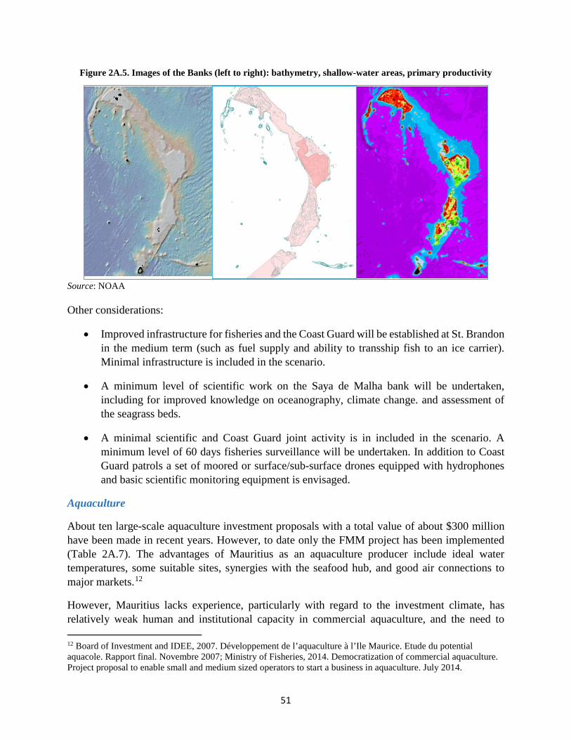
51
Figure 2A.5. Images of the Banks (left to right): bathymetry, shallow-water areas, primary productivity
Source: NOAA
Other considerations:
• Improved infrastructure for fisheries and the Coast Guard will be established at St. Brandon in the medium term (such as fuel supply and ability to transship fish to an ice carrier). Minimal infrastructure is included in the scenario.
• A minimum level of scientific work on the Saya de Malha bank will be undertaken, including for improved knowledge on oceanography, climate change. and assessment of the seagrass beds.
• A minimal scientific and Coast Guard joint activity is in included in the scenario. A minimum level of 60 days fisheries surveillance will be undertaken. In addition to Coast Guard patrols a set of moored or surface/sub-surface drones equipped with hydrophones and basic scientific monitoring equipment is envisaged.
Aquaculture
About ten large-scale aquaculture investment proposals with a total value of about $300 million have been made in recent years. However, to date only the FMM project has been implemented (Table 2A.7). The advantages of Mauritius as an aquaculture producer include ideal water temperatures, some suitable sites, synergies with the seafood hub, and good air connections to major markets.12
However, Mauritius lacks experience, particularly with regard to the investment climate, has relatively weak human and institutional capacity in commercial aquaculture, and the need to 12 Board of Investment and IDEE, 2007. Développement de l’aquaculture à l’Ile Maurice. Etude du potential aquacole. Rapport final. Novembre 2007; Ministry of Fisheries, 2014. Democratization of commercial aquaculture. Project proposal to enable small and medium sized operators to start a business in aquaculture. July 2014.
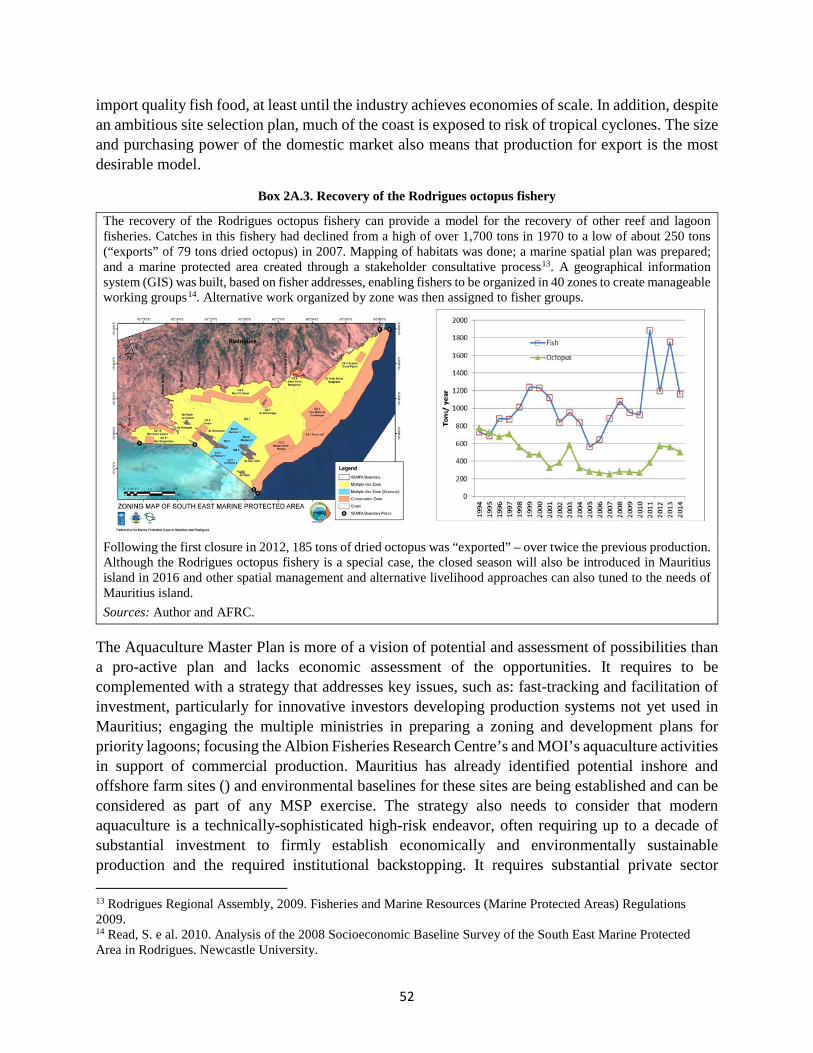
52
import quality fish food, at least until the industry achieves economies of scale. In addition, despite an ambitious site selection plan, much of the coast is exposed to risk of tropical cyclones. The size and purchasing power of the domestic market also means that production for export is the most desirable model.
Box 2A.3. Recovery of the Rodrigues octopus fishery
The recovery of the Rodrigues octopus fishery can provide a model for the recovery of other reef and lagoon fisheries. Catches in this fishery had declined from a high of over 1,700 tons in 1970 to a low of about 250 tons (“exports” of 79 tons dried octopus) in 2007. Mapping of habitats was done; a marine spatial plan was prepared; and a marine protected area created through a stakeholder consultative process13. A geographical information system (GIS) was built, based on fisher addresses, enabling fishers to be organized in 40 zones to create manageable working groups14. Alternative work organized by zone was then assigned to fisher groups.
Following the first closure in 2012, 185 tons of dried octopus was “exported” – over twice the previous production. Although the Rodrigues octopus fishery is a special case, the closed season will also be introduced in Mauritius island in 2016 and other spatial management and alternative livelihood approaches can also tuned to the needs of Mauritius island. Sources: Author and AFRC.
The Aquaculture Master Plan is more of a vision of potential and assessment of possibilities than a pro-active plan and lacks economic assessment of the opportunities. It requires to be complemented with a strategy that addresses key issues, such as: fast-tracking and facilitation of investment, particularly for innovative investors developing production systems not yet used in Mauritius; engaging the multiple ministries in preparing a zoning and development plans for priority lagoons; focusing the Albion Fisheries Research Centre’s and MOI’s aquaculture activities in support of commercial production. Mauritius has already identified potential inshore and offshore farm sites () and environmental baselines for these sites are being established and can be considered as part of any MSP exercise. The strategy also needs to consider that modern aquaculture is a technically-sophisticated high-risk endeavor, often requiring up to a decade of substantial investment to firmly establish economically and environmentally sustainable production and the required institutional backstopping. It requires substantial private sector 13 Rodrigues Regional Assembly, 2009. Fisheries and Marine Resources (Marine Protected Areas) Regulations 2009. 14 Read, S. e al. 2010. Analysis of the 2008 Socioeconomic Baseline Survey of the South East Marine Protected Area in Rodrigues. Newcastle University.
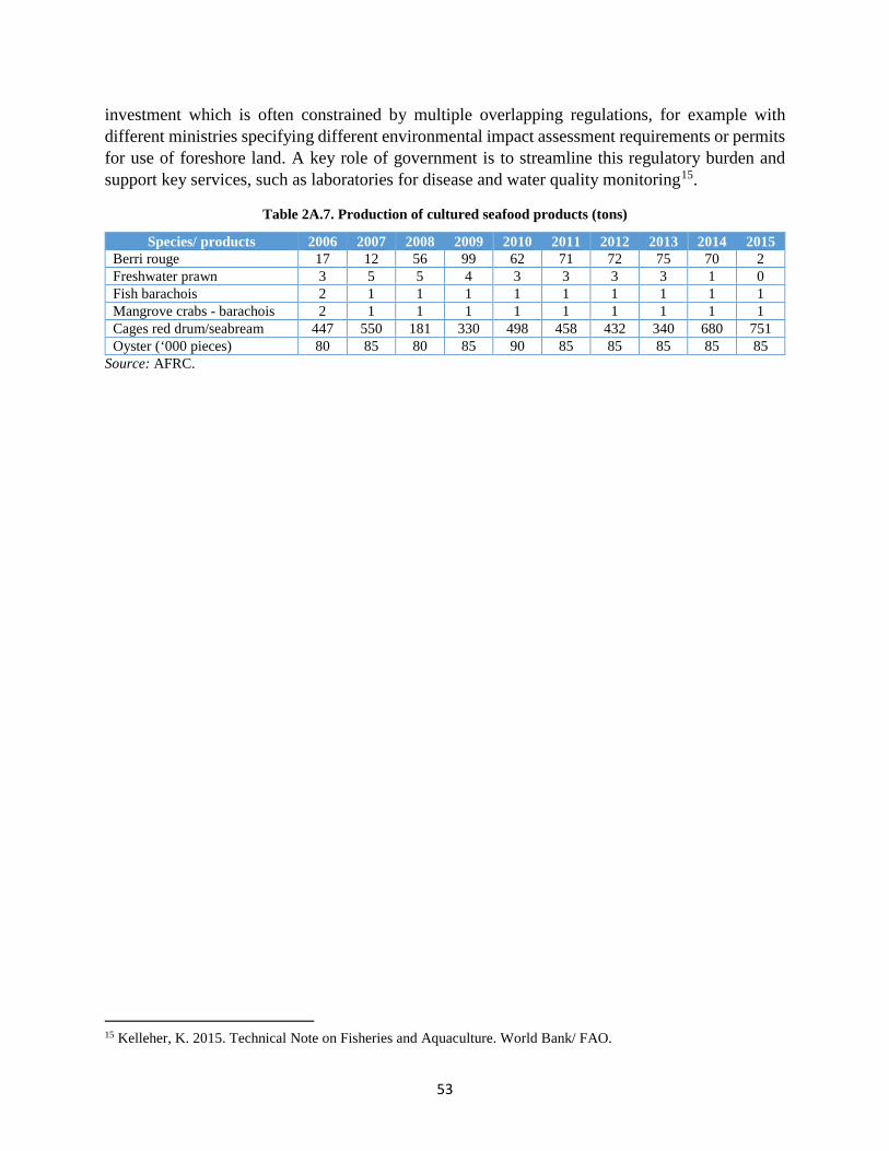
53
investment which is often constrained by multiple overlapping regulations, for example with different ministries specifying different environmental impact assessment requirements or permits for use of foreshore land. A key role of government is to streamline this regulatory burden and support key services, such as laboratories for disease and water quality monitoring15.
Table 2A.7. Production of cultured seafood products (tons)
Species/ products 2006 2007 2008 2009 2010 2011 2012 2013 2014 2015 Berri rouge 17 12 56 99 62 71 72 75 70 2 Freshwater prawn 3 5 5 4 3 3 3 3 1 0 Fish barachois 2 1 1 1 1 1 1 1 1 1 Mangrove crabs - barachois 2 1 1 1 1 1 1 1 1 1 Cages red drum/seabream 447 550 181 330 498 458 432 340 680 751 Oyster (‘000 pieces) 80 85 80 85 90 85 85 85 85 85
Source: AFRC.
15 Kelleher, K. 2015. Technical Note on Fisheries and Aquaculture. World Bank/ FAO.
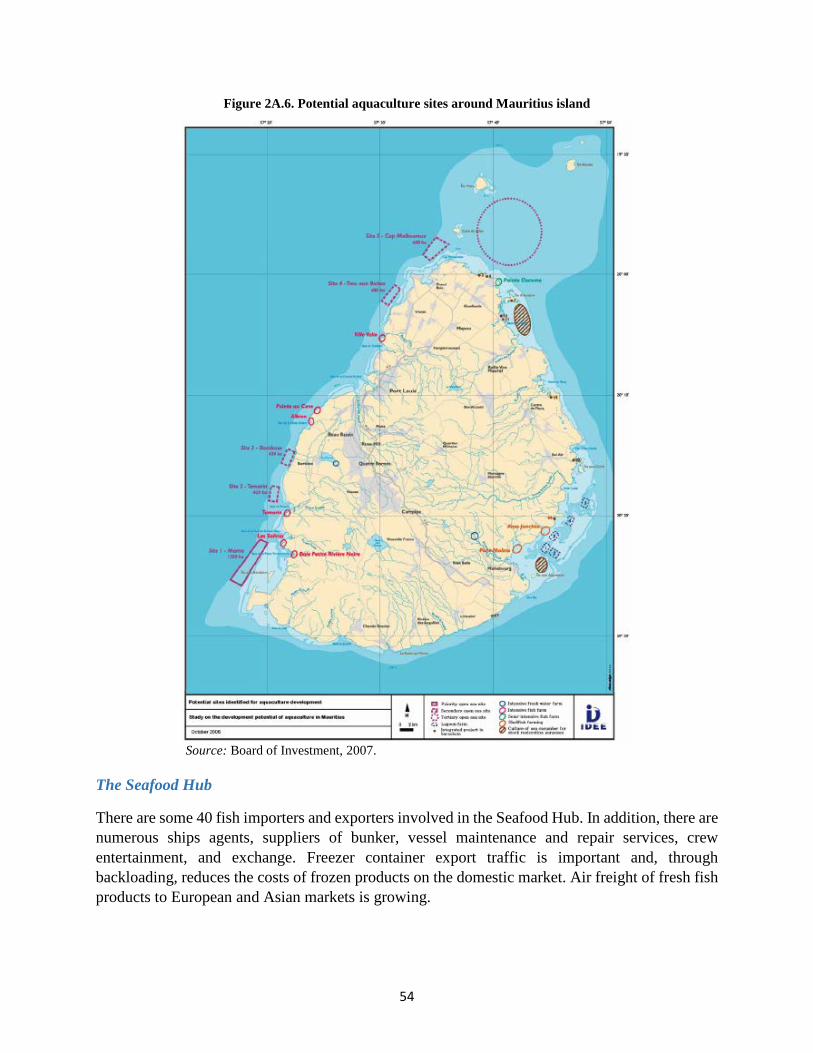
54
Figure 2A.6. Potential aquaculture sites around Mauritius island
Source: Board of Investment, 2007.
The Seafood Hub
There are some 40 fish importers and exporters involved in the Seafood Hub. In addition, there are numerous ships agents, suppliers of bunker, vessel maintenance and repair services, crew entertainment, and exchange. Freezer container export traffic is important and, through backloading, reduces the costs of frozen products on the domestic market. Air freight of fresh fish products to European and Asian markets is growing.

55
The Seafood Hub scenario is based on two drivers: (i) an increase in the vessel calls, and (ii) and increase in the landings of fish (mainly tuna and tuna bycatch) both for processing and to supply the domestic market. Both drivers relay on improved efficiency of the port operations, including improved coordination between MPA, the operators of private quays, the various fleet managers, the agents servicing the fleets, and the processing and fish handling companies.
Box 2A.4. Government’s strategic objectives for the Seafood Hub
Doing Business • Increasing economic yield through income generation from the fisheries sector. • Consolidating Mauritius stakeholding in the industry. • Increasing Mauritius attractiveness as a transshipment hub. • Upgrading of fish landing infrastructures.
Products • Maximizing domestic processing. • Value addition from landings of tuna and tuna-like species in the Southwest Indian Ocean region. • Enhancing competitiveness of the seafood industry. • Strengthened the health certification capacity for Mauritius to meet the norms and standards for
the export of fish and fish products. • Promote a Mauritius seafood brand to indicate top quality seafood products. • Improving Mauritius’ image in the tuna world.
International • Global sourcing for onshore processing. • Pursuing bilateral negotiations for concluding fisheries agreements and MOUs. • Maximizing benefits from business opportunities available under various bilateral and multilateral
arrangements. Resource Management
• Maintaining sustainable level of exploitation and resources conservation and management. • Implementing and abiding with national, regional and international conventions.
Source: Fisheries Department, March 2017.
The development scenario is partly based on the following statement in the draft MPA plan16. “The cargo forecast for fish concludes that, compared to 2014 throughputs, there is an additional 25,000 tonnes/annum to be handled in Port Louis for the Base Case scenario and 55,000 tonnes/annum for the High Case scenario. This would imply that an additional berth is required to facilitate further growth of the fisheries sector. Handling of tuna reefer vessels to serve Froid des Mascareignes and Mauritius Freeport Development would require a minimum of extra berth length of 150m.” The additional infrastructure is addressed in the chapter on the port development. The scenario is based on the conservative Base Case.
16 Preliminary Draft Report. Port Louis Masterplan. Mauritius Ports Authority. Reference: M&WBD1734R002D01. Revision: 01/Draft. Date: 15 December 2015
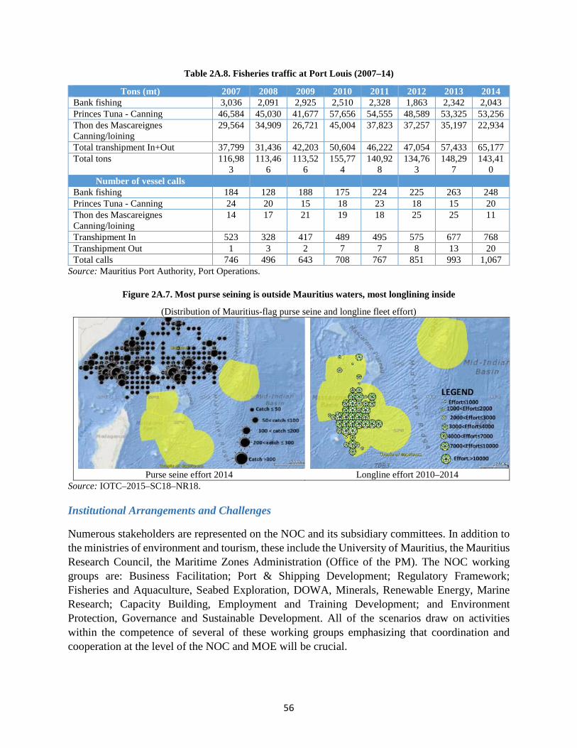
56
Table 2A.8. Fisheries traffic at Port Louis (2007–14)
Tons (mt) 2007 2008 2009 2010 2011 2012 2013 2014 Bank fishing 3,036 2,091 2,925 2,510 2,328 1,863 2,342 2,043 Princes Tuna - Canning 46,584 45,030 41,677 57,656 54,555 48,589 53,325 53,256 Thon des Mascareignes Canning/loining
29,564 34,909 26,721 45,004 37,823 37,257 35,197 22,934
Total transhipment In+Out 37,799 31,436 42,203 50,604 46,222 47,054 57,433 65,177 Total tons 116,98
3 113,46
6 113,52
6 155,77
4 140,92
8 134,76
3 148,29
7 143,41
0 Number of vessel calls
Bank fishing 184 128 188 175 224 225 263 248 Princes Tuna - Canning 24 20 15 18 23 18 15 20 Thon des Mascareignes Canning/loining
14 17 21 19 18 25 25 11
Transhipment In 523 328 417 489 495 575 677 768 Transhipment Out 1 3 2 7 7 8 13 20 Total calls 746 496 643 708 767 851 993 1,067
Source: Mauritius Port Authority, Port Operations.
Figure 2A.7. Most purse seining is outside Mauritius waters, most longlining inside
(Distribution of Mauritius-flag purse seine and longline fleet effort)
Purse seine effort 2014 Longline effort 2010–2014
Source: IOTC–2015–SC18–NR18.
Institutional Arrangements and Challenges
Numerous stakeholders are represented on the NOC and its subsidiary committees. In addition to the ministries of environment and tourism, these include the University of Mauritius, the Mauritius Research Council, the Maritime Zones Administration (Office of the PM). The NOC working groups are: Business Facilitation; Port & Shipping Development; Regulatory Framework; Fisheries and Aquaculture, Seabed Exploration, DOWA, Minerals, Renewable Energy, Marine Research; Capacity Building, Employment and Training Development; and Environment Protection, Governance and Sustainable Development. All of the scenarios draw on activities within the competence of several of these working groups emphasizing that coordination and cooperation at the level of the NOC and MOE will be crucial.
57
Within the MOE, in addition to the Directorate of Fisheries, several institutions have a prominent role in fisheries, including: the Mauritius Oceanographic Institute (MOI), the Albion Fisheries Research Center (AFRC), the Fisheries Training and Extension Centre (FITEC), the Mauritius Maritime Training Academy, and the Fishermen Investment Trust. The MOE has 750 staff. The annual public expenditure on fisheries17 is approximately $6.5 million of which 90 percent is recurrent expenditure with over 65 percent attributable to staff costs. The capital budget for the 2016–2020 period is in the order of $3 million.18 In general,19 the various fisheries plans are descriptive or prescriptive but tend to lack an implementation process, milestones, sequencing, specification of responsibilities for activities, cost estimates linked to outcomes and specific requirements for allocation of staff and resources. Some reallocation of human and financial resources will be required to progress the OE. Clear policies and strategic decisions on allocation will be a considerable institutional challenge as some of the systems and institutional arrangements have a historical inertia.
Box 2A.5 outlines some of the linkages between the fisheries sector and other OE clusters.
Box 2A.5. Linkages between the fisheries sector and the broader ocean Economy
Marine tourism. The environmental health of the coastal lagoons is vital both to tourism and artisanal fisheries, both of which contribute to the decline of the coastal marine ecosystem. The coral reefs and mangroves provide essential ecosystem services, maintaining beaches and mitigating coastal erosion. The proposed Marine Spatial Planning approach could prioritize tourism and fisheries as primary users of coastal marine areas. Seaport-related activities. Increased fish raw material delivery to port (for processing, re-export, import replacement) through stakeholder agreements (port, ships agents, processors), efficiency gains in quay use, and reform of the bycatch sales arrangements Marine energy. The proposed Deep Ocean Water Applications (DOWA) includes an aquaculture component. Ocean knowledge. The current marine research capacity is concentrated in fisheries (Albion) and with Marine Oceanographic Institute (MOI) and the University could establish a comprehensive program to monitor the environmental health of the coastal ecosystems and form a nucleus for a center of excellence on a climate-resilient ocean economy. Marine biotechnology. Incubation is closely linked to excellence in research on living marine resources. Seabed hydrocarbon and minerals. The EIAs required for seabed use will need to draw on the fisheries-driven knowledge of the marine environment and integrate with marine spatial planning processes. Marine ICT. This can envisage the development of a Fisheries Information Management System (catch statistics, licensing, control of foreign fishing, and port controls) and possible development of an electronic market for long-line tuna – essentially a remote trading system with integrated banking and trade insurance activities. Marine finance. This can include enhancement of the fisheries grant and loan schemes currently being developed by the government. Ship registration. These activities can link to the existing regional register of tuna vessels associated with responsible tuna fishing in the region. Cross-cutting opportunities. These include the preparation of a fisheries policy and strategic action plan within the broader OE context to address challenges such as cost-effective reduction of foreign illegal fishing, safety at
17 Actual expenditure 2014. 18 PSIP, 2015/16 – 2019/20. This excludes externally-financed projects. 19 In contrast, the plan for Rodrigues has considerable detail on implementation. Rodrigues Regional Assembly. 2009. Sustainable Integrated Development Plan for Rodrigues. KPMG and UNDP.
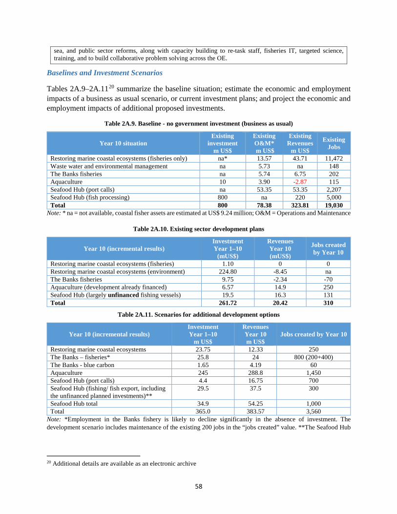
58
sea, and public sector reforms, along with capacity building to re-task staff, fisheries IT, targeted science, training, and to build collaborative problem solving across the OE.
Baselines and Investment Scenarios
Tables 2A.9–2A.1120 summarize the baseline situation; estimate the economic and employment impacts of a business as usual scenario, or current investment plans; and project the economic and employment impacts of additional proposed investments.
Table 2A.9. Baseline - no government investment (business as usual)
Year 10 situation Existing
investment m US$
Existing O&M* m US$
Existing Revenues
m US$
Existing Jobs
Restoring marine coastal ecosystems (fisheries only) na* 13.57 43.71 11,472 Waste water and environmental management na 5.73 na 148 The Banks fisheries na 5.74 6.75 202 Aquaculture 10 3.90 -2.87 115 Seafood Hub (port calls) na 53.35 53.35 2,207 Seafood Hub (fish processing) 800 na 220 5,000 Total 800 78.38 323.81 19,030
Note: * na = not available, coastal fisher assets are estimated at US$ 9.24 million; O&M = Operations and Maintenance
Table 2A.10. Existing sector development plans
Year 10 (incremental results) Investment Year 1–10
(mUS$)
Revenues Year 10 (mUS$)
Jobs created by Year 10
Restoring marine coastal ecosystems (fisheries) 1.10 0 0 Restoring marine coastal ecosystems (environment) 224.80 -8.45 na The Banks fisheries 9.75 -2.34 -70 Aquaculture (development already financed) 6.57 14.9 250 Seafood Hub (largely unfinanced fishing vessels) 19.5 16.3 131 Total 261.72 20.42 310
Table 2A.11. Scenarios for additional development options
Year 10 (incremental results) Investment Year 1–10
m US$
Revenues Year 10 m US$
Jobs created by Year 10
Restoring marine coastal ecosystems 23.75 12.33 250 The Banks – fisheries* 25.8 24 800 (200+400) The Banks - blue carbon 1.65 4.19 60 Aquaculture 245 288.8 1,450 Seafood Hub (port calls) 4.4 16.75 700 Seafood Hub (fishing/ fish export, including the unfinanced planned investments)**
29.5 37.5 300
Seafood Hub total 34.9 54.25 1,000 Total 365.0 383.57 3,560
Note: *Employment in the Banks fishery is likely to decline significantly in the absence of investment. The development scenario includes maintenance of the existing 200 jobs in the “jobs created” value. **The Seafood Hub
20 Additional details are available as an electronic archive

59
scenario assumes that the planned investments (under “existing development plans”) will be financed and these are included in the “additional development scenario”.
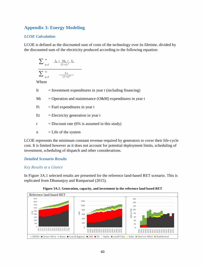
60
Appendix 3: Energy Modeling
LCOE Calculation
LCOE is defined as the discounted sum of costs of the technology over its lifetime, divided by the discounted sum of the electricity produced according to the following equation:
Where
It = Investment expenditures in year t (including financing)
Mt = Operation and maintenance (O&M) expenditures in year t
Ft = Fuel expenditures in year t
Et = Electricity generation in year t
r = Discount rate (6% is assumed in this study)
n = Life of the system
LCOE represents the minimum constant revenue required by generators to cover their life-cycle cost. It is limited however as it does not account for potential deployment limits, scheduling of investment, scheduling of dispatch and other considerations.
Detailed Scenario Results
Key Results at a Glance
In Figure 3A.1 selected results are presented for the reference land-based RET scenario. This is replicated from Dhununjoy and Ramparsad (2015).
Figure 3A.1. Generation, capacity, and investment in the reference land based RET
Reference land-based RET
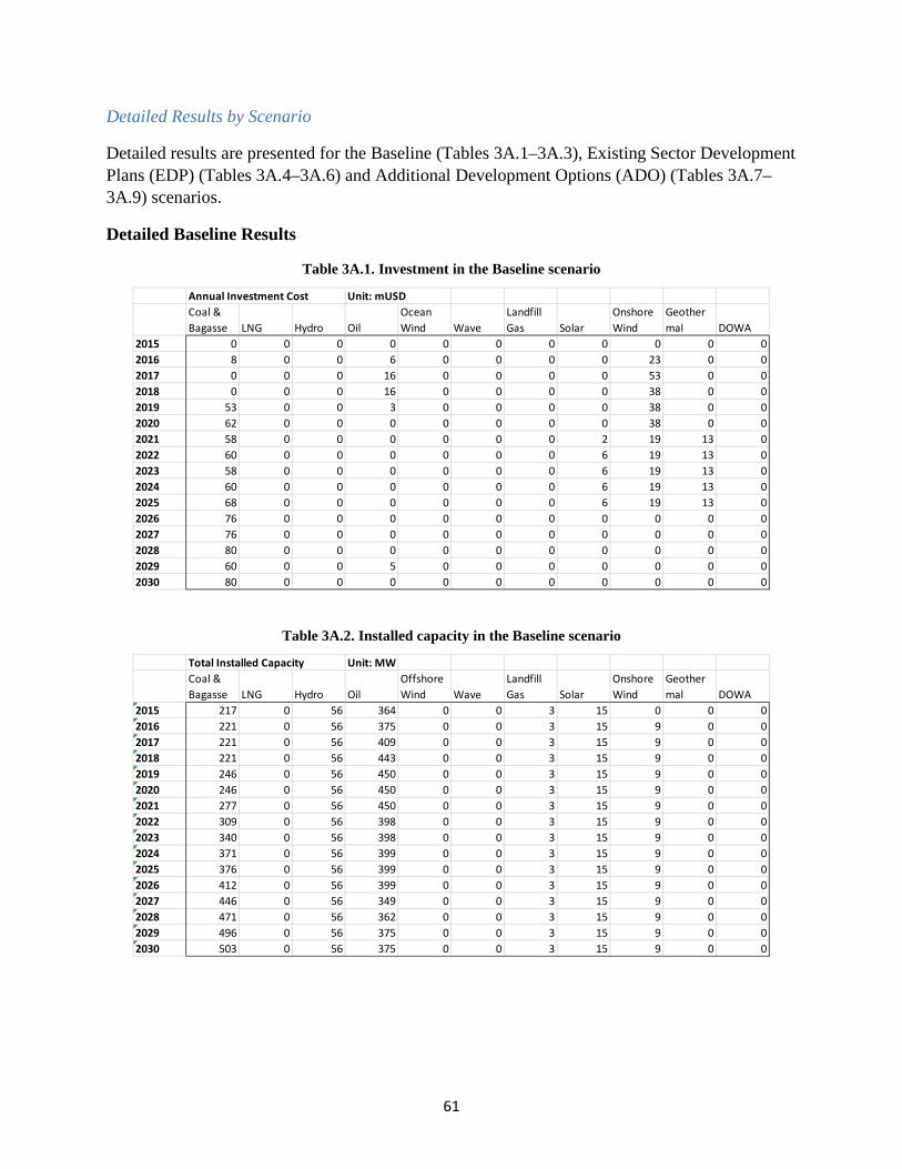
61
Detailed Results by Scenario
Detailed results are presented for the Baseline (Tables 3A.1–3A.3), Existing Sector Development Plans (EDP) (Tables 3A.4–3A.6) and Additional Development Options (ADO) (Tables 3A.7–3A.9) scenarios.
Detailed Baseline Results
Table 3A.1. Investment in the Baseline scenario
Table 3A.2. Installed capacity in the Baseline scenario
Annual Investment Cost Unit: mUSDCoal & Bagasse LNG Hydro Oil
Ocean Wind Wave
Landfill Gas Solar
Onshore Wind
Geothermal DOWA
2015 0 0 0 0 0 0 0 0 0 0 02016 8 0 0 6 0 0 0 0 23 0 02017 0 0 0 16 0 0 0 0 53 0 02018 0 0 0 16 0 0 0 0 38 0 02019 53 0 0 3 0 0 0 0 38 0 02020 62 0 0 0 0 0 0 0 38 0 02021 58 0 0 0 0 0 0 2 19 13 02022 60 0 0 0 0 0 0 6 19 13 02023 58 0 0 0 0 0 0 6 19 13 02024 60 0 0 0 0 0 0 6 19 13 02025 68 0 0 0 0 0 0 6 19 13 02026 76 0 0 0 0 0 0 0 0 0 02027 76 0 0 0 0 0 0 0 0 0 02028 80 0 0 0 0 0 0 0 0 0 02029 60 0 0 5 0 0 0 0 0 0 02030 80 0 0 0 0 0 0 0 0 0 0
Total Installed Capacity Unit: MWCoal & Bagasse LNG Hydro Oil
Offshore Wind Wave
Landfill Gas Solar
Onshore Wind
Geothermal DOWA
2015 217 0 56 364 0 0 3 15 0 0 02016 221 0 56 375 0 0 3 15 9 0 02017 221 0 56 409 0 0 3 15 9 0 02018 221 0 56 443 0 0 3 15 9 0 02019 246 0 56 450 0 0 3 15 9 0 02020 246 0 56 450 0 0 3 15 9 0 02021 277 0 56 450 0 0 3 15 9 0 02022 309 0 56 398 0 0 3 15 9 0 02023 340 0 56 398 0 0 3 15 9 0 02024 371 0 56 399 0 0 3 15 9 0 02025 376 0 56 399 0 0 3 15 9 0 02026 412 0 56 399 0 0 3 15 9 0 02027 446 0 56 349 0 0 3 15 9 0 02028 471 0 56 362 0 0 3 15 9 0 02029 496 0 56 375 0 0 3 15 9 0 02030 503 0 56 375 0 0 3 15 9 0 0
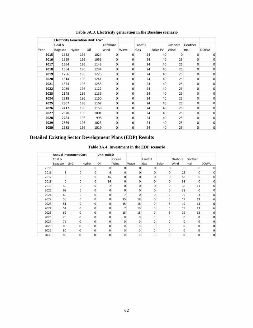
62
Table 3A.3. Electricity generation in the Baseline scenario
Detailed Existing Sector Development Plans (EDP) Results
Table 3A.4. Investment in the EDP scenario
Electricity Generation Unit: GWh
YearCoal & Bagasse Hydro Oil
Offshore wind Wave
Landfill Gas Solar PV
Onshore Wind
Geothermal DOWA
2015 1632 196 1024 0 0 24 40 0 0 02016 1659 196 1055 0 0 24 40 25 0 02017 1664 196 1143 0 0 24 40 25 0 02018 1664 196 1234 0 0 24 40 25 0 02019 1756 196 1225 0 0 24 40 25 0 02020 1814 196 1241 0 0 24 40 25 0 02021 1874 196 1255 0 0 24 40 25 0 02022 2089 196 1122 0 0 24 40 25 0 02023 2148 196 1136 0 0 24 40 25 0 02024 2218 196 1150 0 0 24 40 25 0 02025 2307 196 1162 0 0 24 40 25 0 02026 2412 196 1158 0 0 24 40 25 0 02027 2670 196 1001 0 0 24 40 25 0 02028 2784 196 998 0 0 24 40 25 0 02029 2869 196 1023 0 0 24 40 25 0 02030 2983 196 1019 0 0 24 40 25 0 0
Annual Investment Cost Unit: mUSDCoal & Bagasse LNG Hydro Oil
Ocean Wind Wave
Landfill Gas Solar
Onshore Wind
Geothermal DOWA
2015 0 0 0 0 0 0 0 0 0 0 02016 8 0 0 6 0 0 0 0 23 0 02017 0 0 0 16 0 0 0 0 53 0 02018 0 0 0 16 0 0 0 0 38 0 02019 53 0 0 2 0 0 0 0 38 11 02020 62 0 0 0 0 0 0 0 38 0 02021 62 0 0 0 7 0 0 2 19 3 02022 53 0 0 0 15 18 0 6 19 13 62023 51 0 0 0 15 18 0 6 19 13 62024 54 0 0 0 7 18 0 6 19 13 62025 62 0 0 0 15 18 0 6 19 13 62026 76 0 0 0 0 0 0 0 0 0 02027 76 0 0 0 0 0 0 0 0 0 02028 80 0 0 0 0 0 0 0 0 0 02029 80 0 0 0 0 0 0 0 0 0 02030 80 0 0 0 0 0 0 0 0 0 0
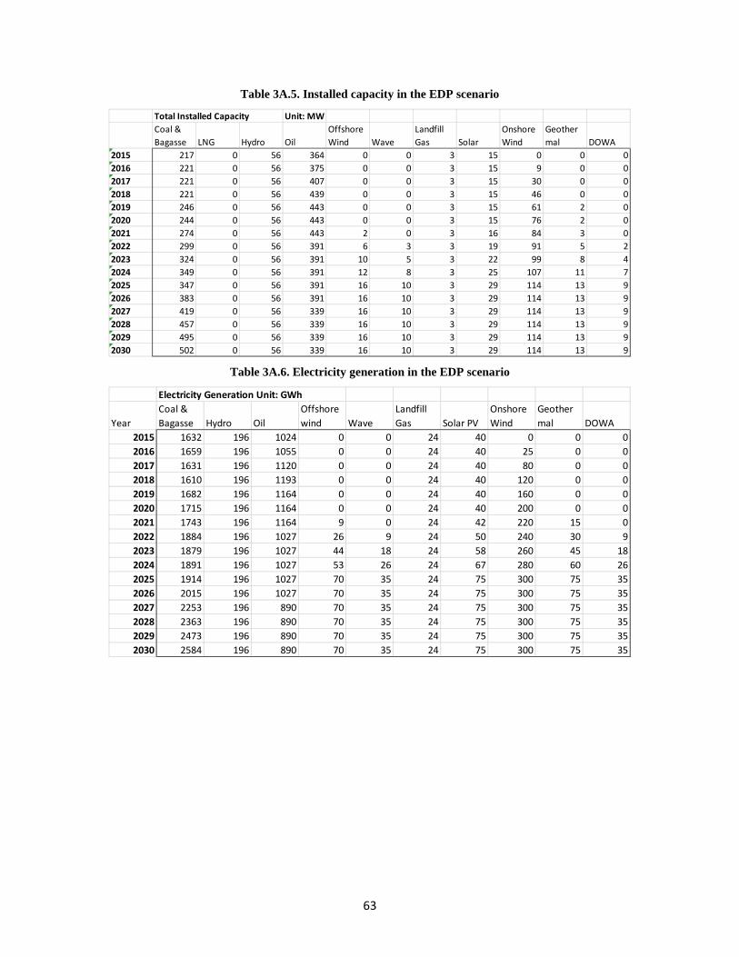
63
Table 3A.5. Installed capacity in the EDP scenario
Table 3A.6. Electricity generation in the EDP scenario
Total Installed Capacity Unit: MWCoal & Bagasse LNG Hydro Oil
Offshore Wind Wave
Landfill Gas Solar
Onshore Wind
Geothermal DOWA
2015 217 0 56 364 0 0 3 15 0 0 02016 221 0 56 375 0 0 3 15 9 0 02017 221 0 56 407 0 0 3 15 30 0 02018 221 0 56 439 0 0 3 15 46 0 02019 246 0 56 443 0 0 3 15 61 2 02020 244 0 56 443 0 0 3 15 76 2 02021 274 0 56 443 2 0 3 16 84 3 02022 299 0 56 391 6 3 3 19 91 5 22023 324 0 56 391 10 5 3 22 99 8 42024 349 0 56 391 12 8 3 25 107 11 72025 347 0 56 391 16 10 3 29 114 13 92026 383 0 56 391 16 10 3 29 114 13 92027 419 0 56 339 16 10 3 29 114 13 92028 457 0 56 339 16 10 3 29 114 13 92029 495 0 56 339 16 10 3 29 114 13 92030 502 0 56 339 16 10 3 29 114 13 9
Electricity Generation Unit: GWh
YearCoal & Bagasse Hydro Oil
Offshore wind Wave
Landfill Gas Solar PV
Onshore Wind
Geothermal DOWA
2015 1632 196 1024 0 0 24 40 0 0 02016 1659 196 1055 0 0 24 40 25 0 02017 1631 196 1120 0 0 24 40 80 0 02018 1610 196 1193 0 0 24 40 120 0 02019 1682 196 1164 0 0 24 40 160 0 02020 1715 196 1164 0 0 24 40 200 0 02021 1743 196 1164 9 0 24 42 220 15 02022 1884 196 1027 26 9 24 50 240 30 92023 1879 196 1027 44 18 24 58 260 45 182024 1891 196 1027 53 26 24 67 280 60 262025 1914 196 1027 70 35 24 75 300 75 352026 2015 196 1027 70 35 24 75 300 75 352027 2253 196 890 70 35 24 75 300 75 352028 2363 196 890 70 35 24 75 300 75 352029 2473 196 890 70 35 24 75 300 75 352030 2584 196 890 70 35 24 75 300 75 35
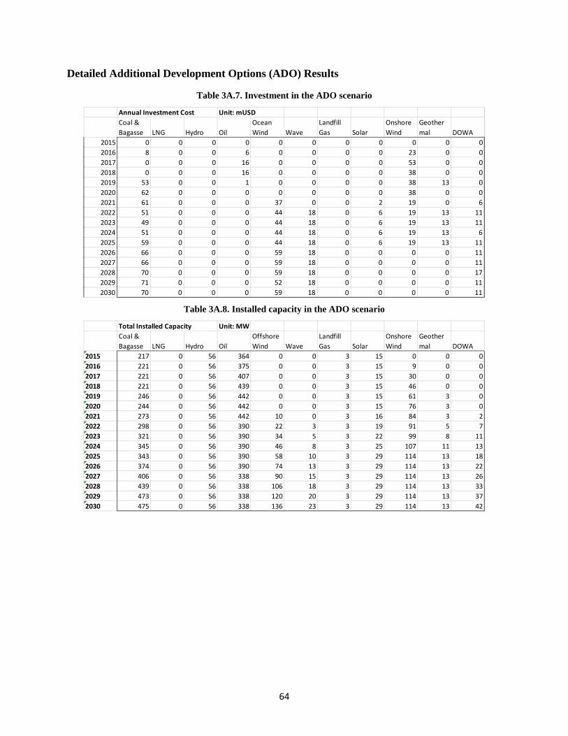
64
Detailed Additional Development Options (ADO) Results
Table 3A.7. Investment in the ADO scenario
Table 3A.8. Installed capacity in the ADO scenario
Annual Investment Cost Unit: mUSDCoal & Bagasse LNG Hydro Oil
Ocean Wind Wave
Landfill Gas Solar
Onshore Wind
Geothermal DOWA
2015 0 0 0 0 0 0 0 0 0 0 02016 8 0 0 6 0 0 0 0 23 0 02017 0 0 0 16 0 0 0 0 53 0 02018 0 0 0 16 0 0 0 0 38 0 02019 53 0 0 1 0 0 0 0 38 13 02020 62 0 0 0 0 0 0 0 38 0 02021 61 0 0 0 37 0 0 2 19 0 62022 51 0 0 0 44 18 0 6 19 13 112023 49 0 0 0 44 18 0 6 19 13 112024 51 0 0 0 44 18 0 6 19 13 62025 59 0 0 0 44 18 0 6 19 13 112026 66 0 0 0 59 18 0 0 0 0 112027 66 0 0 0 59 18 0 0 0 0 112028 70 0 0 0 59 18 0 0 0 0 172029 71 0 0 0 52 18 0 0 0 0 112030 70 0 0 0 59 18 0 0 0 0 11
Total Installed Capacity Unit: MWCoal & Bagasse LNG Hydro Oil
Offshore Wind Wave
Landfill Gas Solar
Onshore Wind
Geothermal DOWA
2015 217 0 56 364 0 0 3 15 0 0 02016 221 0 56 375 0 0 3 15 9 0 02017 221 0 56 407 0 0 3 15 30 0 02018 221 0 56 439 0 0 3 15 46 0 02019 246 0 56 442 0 0 3 15 61 3 02020 244 0 56 442 0 0 3 15 76 3 02021 273 0 56 442 10 0 3 16 84 3 22022 298 0 56 390 22 3 3 19 91 5 72023 321 0 56 390 34 5 3 22 99 8 112024 345 0 56 390 46 8 3 25 107 11 132025 343 0 56 390 58 10 3 29 114 13 182026 374 0 56 390 74 13 3 29 114 13 222027 406 0 56 338 90 15 3 29 114 13 262028 439 0 56 338 106 18 3 29 114 13 332029 473 0 56 338 120 20 3 29 114 13 372030 475 0 56 338 136 23 3 29 114 13 42
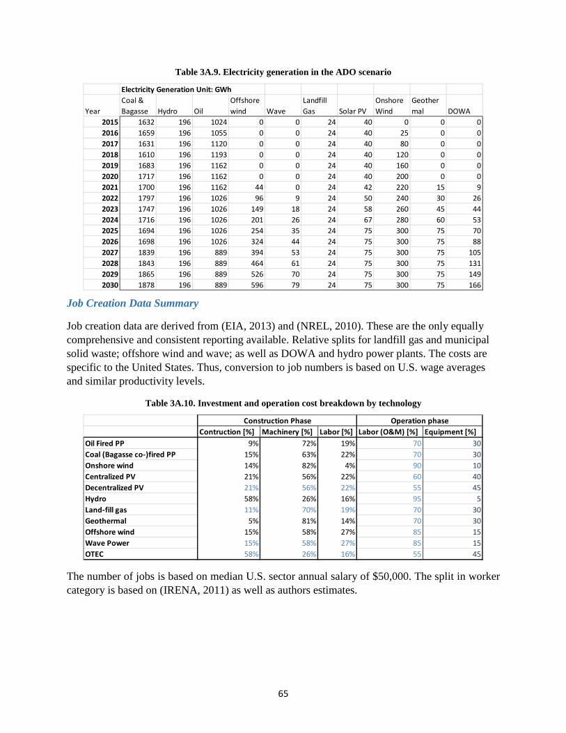
65
Table 3A.9. Electricity generation in the ADO scenario
Job Creation Data Summary
Job creation data are derived from (EIA, 2013) and (NREL, 2010). These are the only equally comprehensive and consistent reporting available. Relative splits for landfill gas and municipal solid waste; offshore wind and wave; as well as DOWA and hydro power plants. The costs are specific to the United States. Thus, conversion to job numbers is based on U.S. wage averages and similar productivity levels.
Table 3A.10. Investment and operation cost breakdown by technology
The number of jobs is based on median U.S. sector annual salary of $50,000. The split in worker category is based on (IRENA, 2011) as well as authors estimates.
Electricity Generation Unit: GWh
YearCoal & Bagasse Hydro Oil
Offshore wind Wave
Landfill Gas Solar PV
Onshore Wind
Geothermal DOWA
2015 1632 196 1024 0 0 24 40 0 0 02016 1659 196 1055 0 0 24 40 25 0 02017 1631 196 1120 0 0 24 40 80 0 02018 1610 196 1193 0 0 24 40 120 0 02019 1683 196 1162 0 0 24 40 160 0 02020 1717 196 1162 0 0 24 40 200 0 02021 1700 196 1162 44 0 24 42 220 15 92022 1797 196 1026 96 9 24 50 240 30 262023 1747 196 1026 149 18 24 58 260 45 442024 1716 196 1026 201 26 24 67 280 60 532025 1694 196 1026 254 35 24 75 300 75 702026 1698 196 1026 324 44 24 75 300 75 882027 1839 196 889 394 53 24 75 300 75 1052028 1843 196 889 464 61 24 75 300 75 1312029 1865 196 889 526 70 24 75 300 75 1492030 1878 196 889 596 79 24 75 300 75 166
Contruction [%] Machinery [%] Labor [%] Labor (O&M) [%] Equipment [%]Oil Fired PP 9% 72% 19% 70 30Coal (Bagasse co-)fired PP 15% 63% 22% 70 30Onshore wind 14% 82% 4% 90 10Centralized PV 21% 56% 22% 60 40Decentralized PV 21% 56% 22% 55 45Hydro 58% 26% 16% 95 5Land-fill gas 11% 70% 19% 70 30Geothermal 5% 81% 14% 70 30Offshore wind 15% 58% 27% 85 15Wave Power 15% 58% 27% 85 15OTEC 58% 26% 16% 55 45
Construction Phase Operation phase
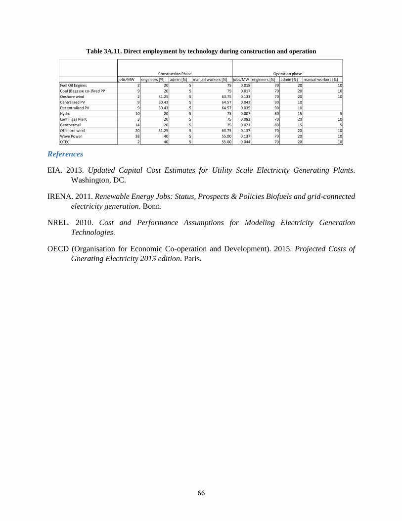
66
Table 3A.11. Direct employment by technology during construction and operation
References
EIA. 2013. Updated Capital Cost Estimates for Utility Scale Electricity Generating Plants. Washington, DC.
IRENA. 2011. Renewable Energy Jobs: Status, Prospects & Policies Biofuels and grid-connected electricity generation. Bonn.
NREL. 2010. Cost and Performance Assumptions for Modeling Electricity Generation Technologies.
OECD (Organisation for Economic Co-operation and Development). 2015. Projected Costs of Gnerating Electricity 2015 edition. Paris.
jobs/MW engineers [%] admin [%] manual workers [%] jobs/MW engineers [%] admin [%] manual workers [%]Fuel Oil Engines 2 20 5 75 0.018 70 20 10Coal (Bagasse co-)fired PP 9 20 5 75 0.017 70 20 10Onshore wind 2 31.25 5 63.75 0.133 70 20 10Centralized PV 9 30.43 5 64.57 0.042 90 10Decentralized PV 9 30.43 5 64.57 0.035 90 10Hydro 10 20 5 75 0.007 80 15 5Lanfill gas Plant 3 20 5 75 0.082 70 20 10Geothermal 14 20 5 75 0.071 80 15 5Offshore wind 20 31.25 5 63.75 0.137 70 20 10Wave Power 38 40 5 55.00 0.137 70 20 10OTEC 2 40 5 55.00 0.044 70 20 10
Construction Phase Operation phase
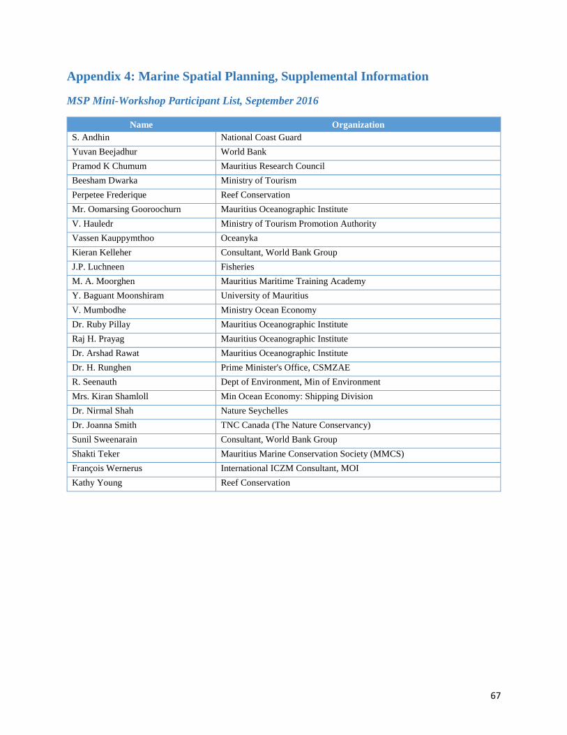
67
Appendix 4: Marine Spatial Planning, Supplemental Information
MSP Mini-Workshop Participant List, September 2016
Name Organization S. Andhin National Coast Guard Yuvan Beejadhur World Bank Pramod K Chumum Mauritius Research Council Beesham Dwarka Ministry of Tourism Perpetee Frederique Reef Conservation Mr. Oomarsing Gooroochurn Mauritius Oceanographic Institute V. Hauledr Ministry of Tourism Promotion Authority Vassen Kauppymthoo Oceanyka Kieran Kelleher Consultant, World Bank Group J.P. Luchneen Fisheries M. A. Moorghen Mauritius Maritime Training Academy Y. Baguant Moonshiram University of Mauritius V. Mumbodhe Ministry Ocean Economy Dr. Ruby Pillay Mauritius Oceanographic Institute Raj H. Prayag Mauritius Oceanographic Institute Dr. Arshad Rawat Mauritius Oceanographic Institute Dr. H. Runghen Prime Minister's Office, CSMZAE R. Seenauth Dept of Environment, Min of Environment Mrs. Kiran Shamloll Min Ocean Economy: Shipping Division Dr. Nirmal Shah Nature Seychelles Dr. Joanna Smith TNC Canada (The Nature Conservancy) Sunil Sweenarain Consultant, World Bank Group Shakti Teker Mauritius Marine Conservation Society (MMCS) François Wernerus International ICZM Consultant, MOI Kathy Young Reef Conservation
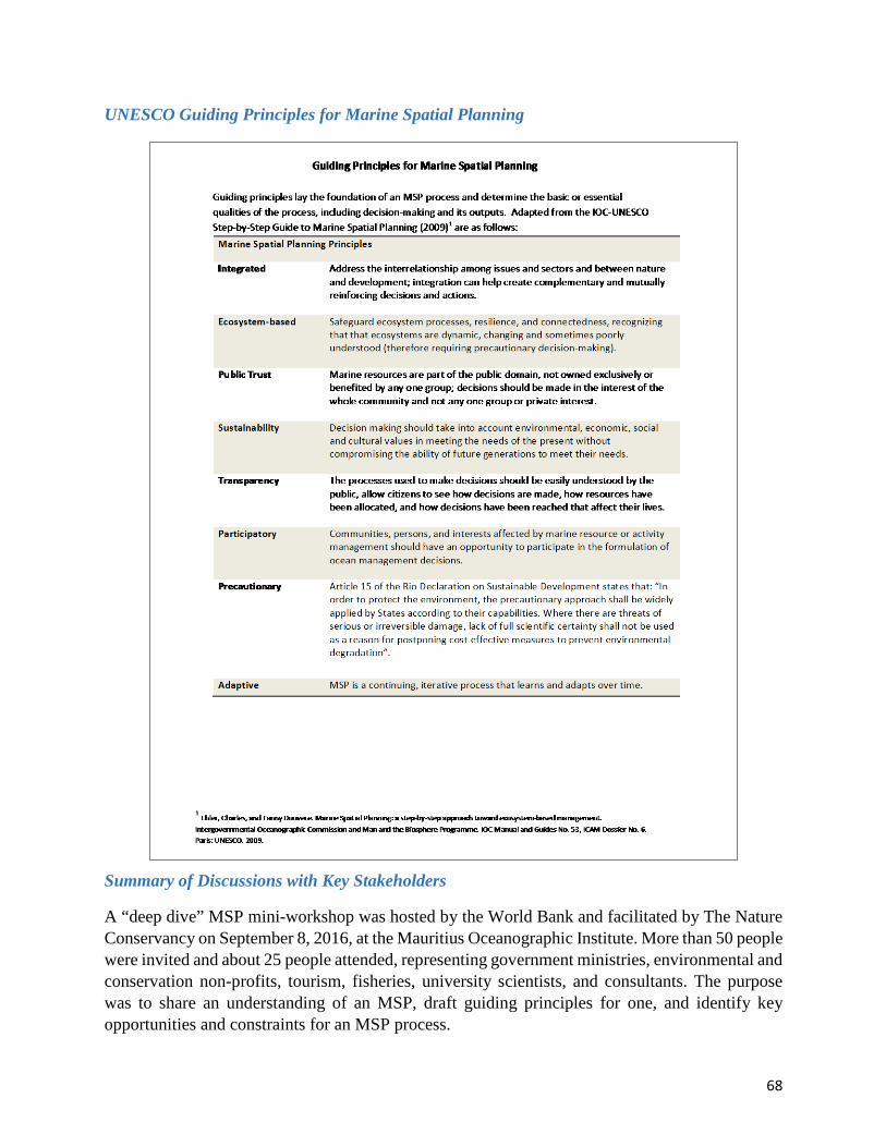
68
UNESCO Guiding Principles for Marine Spatial Planning
Summary of Discussions with Key Stakeholders
A “deep dive” MSP mini-workshop was hosted by the World Bank and facilitated by The Nature Conservancy on September 8, 2016, at the Mauritius Oceanographic Institute. More than 50 people were invited and about 25 people attended, representing government ministries, environmental and conservation non-profits, tourism, fisheries, university scientists, and consultants. The purpose was to share an understanding of an MSP, draft guiding principles for one, and identify key opportunities and constraints for an MSP process.
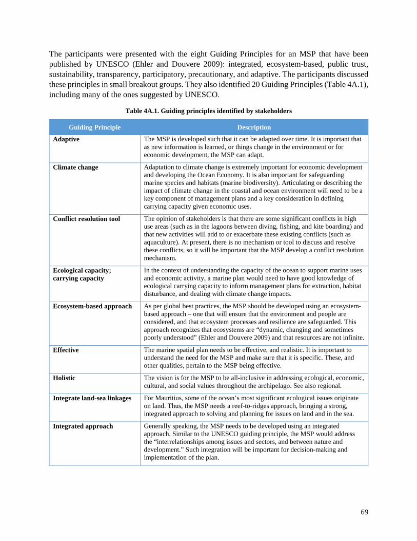
69
The participants were presented with the eight Guiding Principles for an MSP that have been published by UNESCO (Ehler and Douvere 2009): integrated, ecosystem-based, public trust, sustainability, transparency, participatory, precautionary, and adaptive. The participants discussed these principles in small breakout groups. They also identified 20 Guiding Principles (Table 4A.1), including many of the ones suggested by UNESCO.
Table 4A.1. Guiding principles identified by stakeholders
Guiding Principle Description
Adaptive The MSP is developed such that it can be adapted over time. It is important that as new information is learned, or things change in the environment or for economic development, the MSP can adapt.
Climate change Adaptation to climate change is extremely important for economic development and developing the Ocean Economy. It is also important for safeguarding marine species and habitats (marine biodiversity). Articulating or describing the impact of climate change in the coastal and ocean environment will need to be a key component of management plans and a key consideration in defining carrying capacity given economic uses.
Conflict resolution tool The opinion of stakeholders is that there are some significant conflicts in high use areas (such as in the lagoons between diving, fishing, and kite boarding) and that new activities will add to or exacerbate these existing conflicts (such as aquaculture). At present, there is no mechanism or tool to discuss and resolve these conflicts, so it will be important that the MSP develop a conflict resolution mechanism.
Ecological capacity; carrying capacity
In the context of understanding the capacity of the ocean to support marine uses and economic activity, a marine plan would need to have good knowledge of ecological carrying capacity to inform management plans for extraction, habitat disturbance, and dealing with climate change impacts.
Ecosystem-based approach As per global best practices, the MSP should be developed using an ecosystem-based approach – one that will ensure that the environment and people are considered, and that ecosystem processes and resilience are safeguarded. This approach recognizes that ecosystems are “dynamic, changing and sometimes poorly understood” (Ehler and Douvere 2009) and that resources are not infinite.
Effective The marine spatial plan needs to be effective, and realistic. It is important to understand the need for the MSP and make sure that it is specific. These, and other qualities, pertain to the MSP being effective.
Holistic The vision is for the MSP to be all-inclusive in addressing ecological, economic, cultural, and social values throughout the archipelago. See also regional.
Integrate land-sea linkages For Mauritius, some of the ocean’s most significant ecological issues originate on land. Thus, the MSP needs a reef-to-ridges approach, bringing a strong, integrated approach to solving and planning for issues on land and in the sea.
Integrated approach Generally speaking, the MSP needs to be developed using an integrated approach. Similar to the UNESCO guiding principle, the MSP would address the “interrelationships among issues and sectors, and between nature and development.” Such integration will be important for decision-making and implementation of the plan.
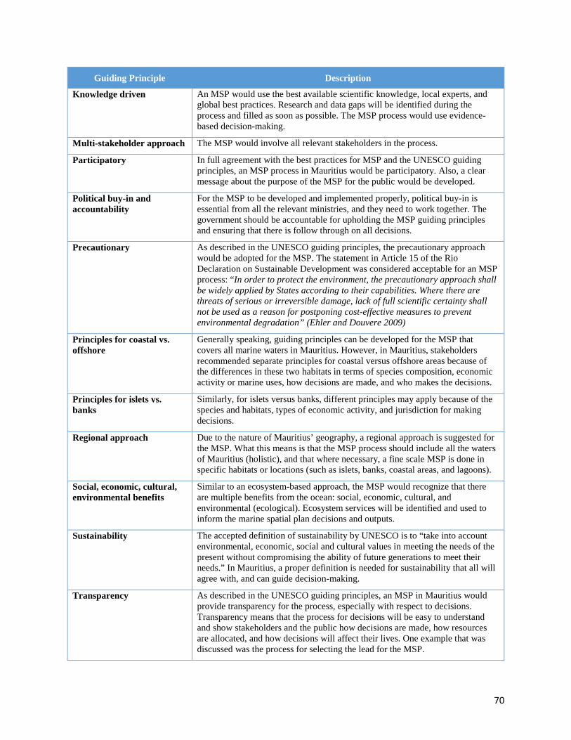
70
Guiding Principle Description
Knowledge driven An MSP would use the best available scientific knowledge, local experts, and global best practices. Research and data gaps will be identified during the process and filled as soon as possible. The MSP process would use evidence-based decision-making.
Multi-stakeholder approach The MSP would involve all relevant stakeholders in the process.
Participatory In full agreement with the best practices for MSP and the UNESCO guiding principles, an MSP process in Mauritius would be participatory. Also, a clear message about the purpose of the MSP for the public would be developed.
Political buy-in and accountability
For the MSP to be developed and implemented properly, political buy-in is essential from all the relevant ministries, and they need to work together. The government should be accountable for upholding the MSP guiding principles and ensuring that there is follow through on all decisions.
Precautionary As described in the UNESCO guiding principles, the precautionary approach would be adopted for the MSP. The statement in Article 15 of the Rio Declaration on Sustainable Development was considered acceptable for an MSP process: “In order to protect the environment, the precautionary approach shall be widely applied by States according to their capabilities. Where there are threats of serious or irreversible damage, lack of full scientific certainty shall not be used as a reason for postponing cost-effective measures to prevent environmental degradation” (Ehler and Douvere 2009)
Principles for coastal vs. offshore
Generally speaking, guiding principles can be developed for the MSP that covers all marine waters in Mauritius. However, in Mauritius, stakeholders recommended separate principles for coastal versus offshore areas because of the differences in these two habitats in terms of species composition, economic activity or marine uses, how decisions are made, and who makes the decisions.
Principles for islets vs. banks
Similarly, for islets versus banks, different principles may apply because of the species and habitats, types of economic activity, and jurisdiction for making decisions.
Regional approach Due to the nature of Mauritius’ geography, a regional approach is suggested for the MSP. What this means is that the MSP process should include all the waters of Mauritius (holistic), and that where necessary, a fine scale MSP is done in specific habitats or locations (such as islets, banks, coastal areas, and lagoons).
Social, economic, cultural, environmental benefits
Similar to an ecosystem-based approach, the MSP would recognize that there are multiple benefits from the ocean: social, economic, cultural, and environmental (ecological). Ecosystem services will be identified and used to inform the marine spatial plan decisions and outputs.
Sustainability The accepted definition of sustainability by UNESCO is to “take into account environmental, economic, social and cultural values in meeting the needs of the present without compromising the ability of future generations to meet their needs.” In Mauritius, a proper definition is needed for sustainability that all will agree with, and can guide decision-making.
Transparency As described in the UNESCO guiding principles, an MSP in Mauritius would provide transparency for the process, especially with respect to decisions. Transparency means that the process for decisions will be easy to understand and show stakeholders and the public how decisions are made, how resources are allocated, and how decisions will affect their lives. One example that was discussed was the process for selecting the lead for the MSP.

71
Additional comments included: (i) the need to consider the human aspect of planning in relation to the speed of the process, given that planning processes can put a strain on people’s schedules and time; (ii) the need to build local capacity to ensure that Mauritius has the needed planning tools for the MSP; and (iii) the need for a clear, public message about the purpose of, and need for, an MSP.
List of opportunities that MSP could bring to Mauritius:
• Adaptive capacity building • Climate change • Collaboration (win-win) • Communications • Community (public) participation • Ecosystem-based management • Encourage investment - enhance the Ocean Economy • Involve the private sector • Participatory • Reduce conflicts • Social justice • Strong leadership • Transparency
List of constraints for MSP in Mauritius:
• Conflict among stakeholders, spatial and administrative • Data sharing and intellectual property rights (IPR) • Lack of appropriate data • Lack of capacity building • Lack of capital investment • Lack of community participation • Lack of cooperation amongst stakeholders to take action • Lack of dialogue • Lack of evidence-based management and decision-making • Lack of funding for MSP and implementation • Lack of policy and planning • Lack of political will • Lack of proper regulatory framework/authority (regulations, policy, legislation) • Lack of social integration • Pleasure versus commercial uses • Pollution from land-based activities • Traditional rights of uses

72
MSP Sample Work Plan for Option 2.
Years Pre Planning
i ii 1 2 3 4 5 6 … … PROCESS MANAGEMENT AND TOOLS Identify need and establish authority Obtain financial support Organize the planning process*
Governance framework Guiding principles
Issue, Opportunities, Tasks List of outputs
Roles and Responsibilities Schedule of meetings
Science Advisors or Committee Workplan
Organize and develop communications Website
Overview document(s) Public information packet
Media packet Publications and reports
Conferences and presentations STAKEHOLDER ENGAGEMENT Organize stakeholder participation
Establish committees Terms of Reference
Organize sector representatives Stakeholder support funding
Stakeholder workshops Public Open Houses
PREPARE AND APPROVE A MARINE PLAN Define and analyze existing conditions
Current conditions and trends Define and analyze future conditions
Vision statement Future scenarios
Develop planning tools Spatial Data Catalogue
Ecosystem-based approach framework Master list of Definitions
Compatibility matrix Zoning framework
MPA network design criteria MSP Atlas
On-line data viewer and planning tool Complete scientific and technical work
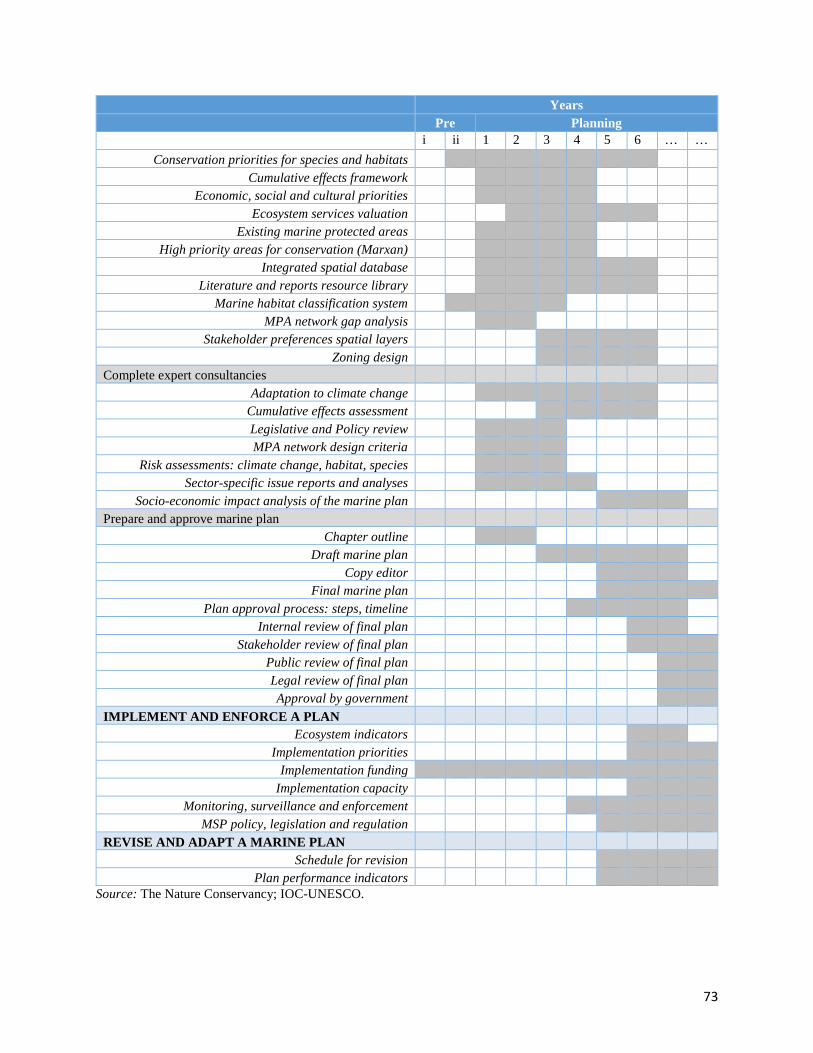
73
Years Pre Planning
i ii 1 2 3 4 5 6 … … Conservation priorities for species and habitats
Cumulative effects framework Economic, social and cultural priorities
Ecosystem services valuation Existing marine protected areas
High priority areas for conservation (Marxan) Integrated spatial database
Literature and reports resource library Marine habitat classification system
MPA network gap analysis Stakeholder preferences spatial layers
Zoning design Complete expert consultancies
Adaptation to climate change Cumulative effects assessment Legislative and Policy review MPA network design criteria
Risk assessments: climate change, habitat, species Sector-specific issue reports and analyses
Socio-economic impact analysis of the marine plan Prepare and approve marine plan
Chapter outline Draft marine plan
Copy editor Final marine plan
Plan approval process: steps, timeline Internal review of final plan
Stakeholder review of final plan Public review of final plan Legal review of final plan Approval by government
IMPLEMENT AND ENFORCE A PLAN Ecosystem indicators
Implementation priorities Implementation funding
Implementation capacity Monitoring, surveillance and enforcement
MSP policy, legislation and regulation REVISE AND ADAPT A MARINE PLAN
Schedule for revision Plan performance indicators
Source: The Nature Conservancy; IOC-UNESCO.
74
Marine Protected Area Designations in Mauritius
Marine parks. The two marine parks in Mauritius are Balaclava Marine Park and Blue Bay Marine Park, designated in 1997 and 2008, respectively. These are no-take areas and recreational activities are allowed and promoted within the parks. The Ministry of Fisheries manages marine parks and Blue Bay Marine Park has status as a Ramsar Wetland of International Importance. Marine Parks are considered IUCN Category II, meaning that they are designated for the purpose of large-scale ecosystem protection and allow use by visitors for recreational and other purposes (like scientific research).
Fishing reserves. Currently, there are six designated fishing reserves in Mauritius: Black River Fishing Reserve, Grand Port Fishing Reserve, Port Louis Fishing Reserve, Poste Lafayette Fishing Reserve, Poudre d’Or Fishing Reserve, and Trou d’Eau Douce Fishing Reserve. Post Lafayette was designated in 1983, while the rest were designated in 2000. The Ministry of Fisheries manages fishing reserves and net fishing is prohibited, but licenses or permits may be granted to fish using bait gear or basket traps. Fishing reserves are considered IUCN Category IV, meaning that they are specifically designed to protect particular species or habitats.
Marine reserves. There are four marine reserves in Mauritius, all designated in 2007: Riviere Banane, English Bay, Grande Bassin, Passe Demie were demarcated as marine reserves (Hardman et al. 2008). These reserves were created by the Rodrigues Regional Assembly, following consultation with local fishing communities about declines in fish stocks. Fishing is only permitted with authorised permits from the government authority.
Marine protected area. In 2009, the Rodrigues Regional Assembly delimited the South East Marine Protected Area (SEMPA), an area covering 43 square kilometers. Similar to marine parks, recreational activities are popular in a marine protected area but regulations prohibiting coastal development, removal of sediment and cultural artifacts, and damage to wildlife are aimed at protecting the marine ecosystem as a whole.
Turtle reserves. There are two proposed turtle reserves in Mauritius: Fregate Island Turtle Reserve and Pearl Island Turtle Reserves. They have been proposed by the Ministry of Fisheries and the Rodrigues Regional Assembly and not yet officially designated.
Nature reserves. Nature reserves in Mauritius are not strictly dedicated to protecting marine areas and may encompass both terrestrial and marine areas. UNEP-WCMC identifie 18 nature reserves that meet this criterion. They include Ile Aux Cocos, Ile Aux Sables, Grande Montagne, Anse Quitor, Ile aux Serpents, Bois Sec, Ilot Gabriel, Coin de Mire, Ile aux Aigrettes, Ile Ronde, Ile Plate, Perrier, Les Mares, Ile Aux Mariannes, Cropas de garde, Gouly Pere, Le Pouce, and Cabinet Nature Reserve. Most are managed by the Forestry Service, but Ile aux Aigrettes is managed by the Mauritian Wildlife Foundation and Ile Aux Cocos, Ile Aux Sables, Grande Montagne, and Anse Quitor are managed by the Rodrigues Regional Assembly.
75
Legal Instruments of Relevance for an MSP Process in Mauritius
Environment Protection Act 1991 (2002). This act provides a policy framework for environmental stewardship and sustainable development. This act covers the coastal zone, meaning any area that is situated within 1 km or any other distance as may be prescribed from the high watermark, extending either side into the sea or inland. Specifically, this act grants authority for preserving and conserving the coastal zone through the enforcement of environmental standards, particularly those pertaining to the control and prevention of pollution. MSP can provide a framework and tools for effectively promoting sustainable growth while managing natural resources, which is a primary objective of this act.
Fisheries and Marine Resources Act (2007). This act describes regulations related to permitted fishing and fish farming methods and zones; registration and licensing of fishing vessels and gear; import, export, and manufacturing; and other provisions related to fishing and fisheries. Fisheries are considered a major driver for the need of MSP in Mauritius, according to the PMO, and successful implementation of MSP can lead to improved fisheries management. This policy is relevant to MSP in that it describes the locations and types of fishing activities that can take place within Mauritius maritime zones. Any MSP effort in Mauritius will have to take into account existing regulations pertaining to fisheries management.
Integrated Coastal Zone Management Framework (2010). This framework was developed by the Integrated Coastal Zone Management (ICZM) Division using ICZM Action and Area Plans, ICZM Strategy, ICZM legislative and policy framework, and others. This framework aims to promote sustainable development in the coastal zone through the optimization of long-term socio-economic and environmental benefits. It was adopted in 2010 and is presently under implementation. Current implementation activities include coastal protection works, beach re-profiling and other erosion control measures, as well as coral reef ecosystem monitoring and lagoon water quality monitoring. As described in previous sections, ICZM and MSP share many of the same principles and goals, including optimization of socio-economic and environmental benefits; reducing conflicts among ocean users, and improving efficiency among governmental authorities. The successful implementation of an ICZM framework can lay the groundwork for MSP by fostering stakeholder engagement, and furthering institutional integration and cooperation. An MSP effort will need to be informed by the outcomes and lessons learned of ICZM implementation.
Maritime Zones Act 1977 (2005). This act asserts the sovereign right of Mauritius to manage natural resources, as well as development activities, out to the EEZ, and defines the extent, legal status and jurisdiction of Mauritius in various maritime zones, including the territorial sea and internal historic and archipelagic waters, contiguous zone, exclusive economic zone (EEZ), and continental shelf. This act also provides a legal instrument for protecting cultural heritage and regulating other activities such as navigation and research within these zones. This act is relevant to MSP in that it provides geographic references to inform the planning process and its boundaries. As referenced earlier in this chapter, MSP’s offshore geographic boundary can vary depending on planning authority decisions, and can extend out to the 200 nm EEZ, but it should be clearly

76
defined. Understanding where the government has jurisdiction over certain activities can also help inform MSP by providing spatial information about where certain activities (for example, offshore development) are more or less likely to take place. Additionally, this act also provides the geographic coordinates for the Mauritius-Seychelles Joint Management Area. Given that an MSP process is already underway in Seychelles, understanding the geographic overlap of management zones between these two nations will be important in coordinating future MSP implementation efforts.
Merchant Shipping Act. This act defines provisions related to merchant shipping in Mauritius waters, including “registration of ships, proprietary and other rights in ships, safety of navigation, carriage of grain and dangerous goods, liability for maritime claims, enforcement and legal proceedings.” Shipping is typically one of the economic sub-sectors included in an MSP process due to its importance to the local economy. Successful implementation of MSP can lead to reductions in conflicts between the shipping industry and other sectors and the environment. Any MSP effort in Mauritius will have to take into account existing regulations pertaining to shipping. Understanding regulations related to shipping and navigation can inform MSP by providing spatial information as to where shipping activities are most likely to take place.
Petroleum Act. Although Mauritius has no known indigenous sources of petroleum, the Petroleum Act includes provisions for granting prospecting and mining leases for petroleum. An MSP process may consider potential future uses of marine areas, such as petroleum extraction, and will have to take into account existing regulations related to that activity. Many MSP processes plan for the possibility of future offshore energy development, whether it is extraction of fossil fuels or siting renewable energy infrastructure. Successful MSP implementation can reduce the risk of conflicts between the energy sector and other ocean stakeholders, so understanding regulations related to petroleum extraction, and other energy-related uses is an important component of MSP.
Planning and Development Act. This act provides a policy framework for coordination and management of economic use and development of land in Mauritius. Objectives of this act include promoting ecologically sustainable development, facilitating inter-agency cooperation in planning and development, and establishing institutions and processes to achieve effective planning and development, all of which align with MSP objectives. While this act is more specific to land-based activities, it does have provisions for coastal frontage land, and therefore is likely to have some geographic relevance to ICZM and MSP. This framework can also serve as a model for how planning and development may be carried out using MSP.
Prohibition of Driftnet Act. This act prohibits the use of a drift net within the fishing limits of Mauritius. Drift nets are defined as gill nets which exceed 250 m in length, are made of up mesh of any size, and are designed with floats or weights to suspend vertically either at the water’s surface or in mid-water. As described previously, fisheries are considered a major driver for MSP, and understanding the fisheries regulations, and specifically the interactions among fisheries using varying types of gear, is an important component of the MSP process.
77
United Nations Convention of the Law of the Sea. This international agreement defines the rights and responsibilities of nations pertaining to their use of ocean space. It establishes guidelines for both economic activities and environmental management in ocean waters. It grants sovereignty of a coastal state to establish the breadth of its surrounding waters, including its internal waters, territorial waters, archipelagic waters, contiguous zone, exclusive economic zone, and continental shelf, and defines the extent of a state’s jurisdiction within each area. This agreement is relevant to MSP in Mauritius in that it grants Mauritius the right to define its surrounding waters through the Maritime Zones Act, described above. By extension, this gives Mauritius jurisdiction to carry out MSP activities within its waters.
Wildlife and National Parks Act. This act provides a policy framework for designating and managing national parks and land reserves, and for protecting flora and fauna. Although this act deals with national parks and wildlife on land, it may be relevant to MSP as it relates to identifying areas that have particular biological or ecological importance, which is sometimes part of an MSP process. Conservation of protected species is often an objective of MSP. As such, this act may be relevant in the event that the MSP process includes consideration of species that use both marine and terrestrial habitats (for example, turtles or birds).
Waste Water Management Authority Act. This act establishes the Waste Water Management Authority to oversee activities related to waste water treatment and reuse, ensuring that wastewater treatment systems and facilities are functioning, and controlling and monitoring pollution that results from waste water. According to the Minister of the Environment, pollution control from wastewater is one of the primary drivers of MSP in Mauritius. Successful implementation of MSP can lead to improved pollution control and reduced impacts on the environment through better understanding of the spatial extent of the impact as well as vulnerable habitats. Therefore, coordination with this authority will likely be necessary to achieve this goal within the MSP process.
Beach Authority Act. This act establishes an authority to manage public beaches, particularly with respect to conservation, protection, management, maintenance, infrastructure and facilities development, and water quality enhancement of public beaches and to regulate activities on public beaches. Tourism is a significant economic sub-sector is likely to be a part of the MSP process. As public beaches can be a major draw for a variety of tourism activities, regulations with regard to beaches and beach use will likely inform MSP. Since coastal erosion is a key environmental issue in Mauritius, understanding how the management of beaches relates to erosion control can inform how coastal erosion is addressed within the planning process. Finally, this act is also relevant to MSP as it relates to the management and restoration of coastal habitats, including managing water quality.
Tourism Act. This act establishes an authority to manage tourism activities, specifically, the licensing of tourist enterprises, and regulations surrounding the registration and operation of pleasure craft. As noted above, tourism activities are likely to be a component of an MSP process. This act has particular relevance as it relates to water-based recreation and specifically, the use of recreational vessels. Coordinating with an authority that regulates recreational vessels will inform
78
the MSP process, especially if the authority is able to identify areas that are heavily used by various vessel-based activities.
Local Government Act. This act allows for the creation of local authorities at the city, town, district, and village level. This is relevant to MSP as it is generally beneficial for an MSP process to incorporate input from government stakeholders from various levels of government in order to gain a diverse perspective. An MSP process will have to consider the authority of governments at a variety of levels.
Removal of Sand Act. This act provides a legal framework for overseeing and regulation the designation and leasing of sand quarries and sand landing places, and the management of sand removal and transport. As described earlier in the chapter, coastal erosion is a major environmental issue in Mauritius. Beach re-nourishment using mined sand is sometimes used to mitigate coastal erosion, but these activities can often conflict with other ocean uses. A goal of MSP is to reduce conflicts among ocean users and to help address environmental issues such as coastal erosion. As such, it may be helpful to consider sand removal and transport regulations in the MSP process.
79
Appendix 5: Climate Change Modeling
Description of Methods for Cyclone Event Set Modeling
Methods Summary21
We here describe the methods we use to generate hurricane (tropical cyclone) event sets. We apply a method to assess the probability distribution of hurricane tracks and then run a deterministic numerical model along each track to estimate storm wind magnitudes. The track generation begins by generating a large class of synthetic, time-varying wind fields at 850 and 250 hPa whose variance, co-variance and monthly means match NCEP re-analysis data and whose kinetic energy follows an 3ω− geostrophic turbulence spectral frequency distribution. Hurricanes are assumed to move with a weighted mean of the 850 and 250 hPa flow plus a "beta drift" correction, after originating at points determined from historical genesis data. The statistical characteristics of tracks generated by these two means are compared with historical track data.
For a given point in space, a large number (~104) of synthetic tracks are generated that can be filtered to a particular ocean basin, to pass within a specified distance of a point of interest, or to pass through any of a number of user-specified line segments, which may or may not comprise a closed polygon. For each of the tracks, a deterministic, coupled, numerical simulation of the storm's intensity is carried out, using monthly mean upper ocean and potential intensity climatologies together with time-varying vertical wind shear generated from the synthetic time series of 850 and 250 hPa winds as described above. The tracks and the shear are generated using the same wind fields and are therefore mutually consistent.
The track and intensity data are finally used together with a vortex structure model to construct probability distributions of wind speed at fixed points in space.
Details of the method are described in two key references: Emanuel et al. (2006) and Emanuel, Sundararajan, and Williams (2008). Comparison with historical hurricane data and the application of extant methods are described in these two references and in Emanuel (2006). Some applications of the method are given in a set of published papers (for example, Emanuel 2010; Emanuel and Jagger 2010; Emanuel et al. 2010; Federov, Brierley, and Emanuel 2010; Gnanadesikan et al. 2010; Lin et al. 2010; Emanuel 2011; Mendelsohn et al. 2012).
In-Depth Description of Synthetic Methods
Overview of Extant and New Methods
Existing event set generation techniques begin with historical compilations of hurricane tracks and intensities, such as the so-called "best track" data compilations maintained by forecasting operations such as the National Oceanic and Atmospheric Administration's Tropical Prediction Center (TPC) and the U.S. Navy's Joint Typhoon Warning Center (JTWC). The records typically contain storm center position every six hours together with a single intensity estimate (maximum 21 This technical appendix was prepared by Kerry Emanuel and Sai Ravela of WindRiskTech Consulting.
80
wind speed and/or central pressure) every time period. Early risk assessments ( for example, Georgiou, Davenport, and Vickery 1983; Neumann 1987) fit standard distribution functions, such as log-normal or Weibull distributions, to the distribution of maximum intensities of all historical storms coming within a specified radius of the point of interest, and then, drawing randomly from such distributions, use standard models of the radial structure of storms, together with translation speed and landfall information, to estimate the maximum wind achieved at the point of interest. A clear drawback of this approach is that estimates of the frequency of high intensity events are sensitive to the shape of the tail of the assumed distribution, for which there is very little supporting data. This limitation was, to some extent, circumvented in the work of Darling (1991) and Chu and Wang (1998), who used empirical global distributions of relative intensity (the ratio of actual to potential intensity) together with climatology of potential intensity to infer local intensity distributions. A similar approach was taken by Murnane et al. (2000), who used global estimates of hurricane actual (rather than relative) wind intensity cumulative probability distributions. A somewhat different tack was taken by Vickery, Skerjl, and Twisdale (2000), who used statistical properties of historical tracks and intensities to generate a large number of synthetic storms in the North Atlantic basin. Six hour changes in direction, translation speed and intensity along each track were modeled as linear functions of previous values of those quantities as well as of position and sea surface temperature. The method used here follows Vickery, Skerjl, and Twisdale (2000) in generating large numbers of tracks, but uses different techniques to accomplish this.
Most of the aforementioned wind risk assessment methods rely directly on historical hurricane track data to estimate the frequency of storms passing close to points of interest, and must assume that the intensity evolution is independent of the particular track taken by the storm (though Darling 1991, accounts for the time elapsed after storm formation). Moreover, the relative intensity method must fail when storms move into regions of small or vanishing potential intensity, as they often do in the western North Atlantic. Return period estimation is particularly problematic in places like New England, which have experienced infrequent but enormously destructive storms but for which the historical record is sparse.
As a step toward circumventing some of these difficulties, we developed a technique for generating large numbers of synthetic hurricane tracks, along each of which we run a deterministic, coupled numerical model to simulate storm intensity.
Event set generation begins by randomly seeding a given ocean basin with weak tropical cyclone-like disturbances, and using our intensity mode to determine which one of these develop to tropical storm strength or greater. The storms move according to a weighted average of the ambient flow at 850 and 250 hPa plus a constant "beta drift" correction; this constitutes the so-called “beta-and-advection” model that is still used by professional hurricane forecasters as part of their suite of track guidance. The ambient flow used to determine the storm tracks is one that is randomly varying in time, but whose mean, variance and co-variances conform to monthly mean climatologies derived from re-analysis or global climate model data sets, and whose kinetic energy follows the 3ω− power law of geostrophic turbulence. We compare the 6-hour displacement statistics of such tracks to the corresponding statistics of historical tracks.
81
Tracks can be generated globally, or for a specified ocean basin, and filters can be applied to the track generator to select tracks coming within a specified distance of a point or region of interest (for example, a city or county) or passing through any of a set of user-specified line segments. In filtering the tracks, a record is kept of the number of discarded tracks and this is used to calculate the overall frequency of storms that pass the filter.
Once the tracks have been generated, a coupled hurricane intensity model is then run along each of the selected tracks to produce a history of storm maximum wind speed. This model uses monthly climatological atmospheric and upper ocean thermodynamic information, but is also affected by ambient environmental wind shear that varies randomly in time according to the procedure described in the previous paragraph. This wind shear is generated from exactly the same randomly varying wind fields as were used to generate the storm tracks; thus the storm motion and the vertical wind shear are mutually consistent.
The coupled deterministic model produces a maximum wind speed and a radius of maximum winds, but the detailed aspects of the radial storm structure are not used, owing to the coarse spatial resolution of the model. Instead, as a post-processing step, we use idealized radial wind profiles, fitted to the numerical output, to estimate maximum winds at fixed points in space away from the storm center.
For each point of interest, the intensity model is run many O(104) times to produce desired statistics such as wind speed exceedence probabilities for that point. Both the synthetic track generation method and the deterministic model are fast enough that it is practical to estimate exceedence probabilities to a comfortable level of statistical significance. We have compare such probabilities to those estimated using previously published techniques.
The following sections describe in greater detail the synthetic track generation technique and the simulation of storm intensity.
Genesis Technique
Our genesis technique consists in randomly seeding a given ocean basin with candidate disturbances, and then calculating the track using either of the track methods described in sections 3 and 4. Our coupled numerical hurricane intensity model is then run along each track, but beginning with a weak disturbance, whose maximum wind speed is 24 knots. The vast majority of such disturbances fail to achieve minimal tropical storm strength and are discarded, and the number of discards relative to the number of successful candidates is recorded. This ratio, when normalized by a suitable constant scaling factor, gives the overall frequency of genesis. Figure 5A.1 shows an example of a genesis probability distribution generated using this technique.
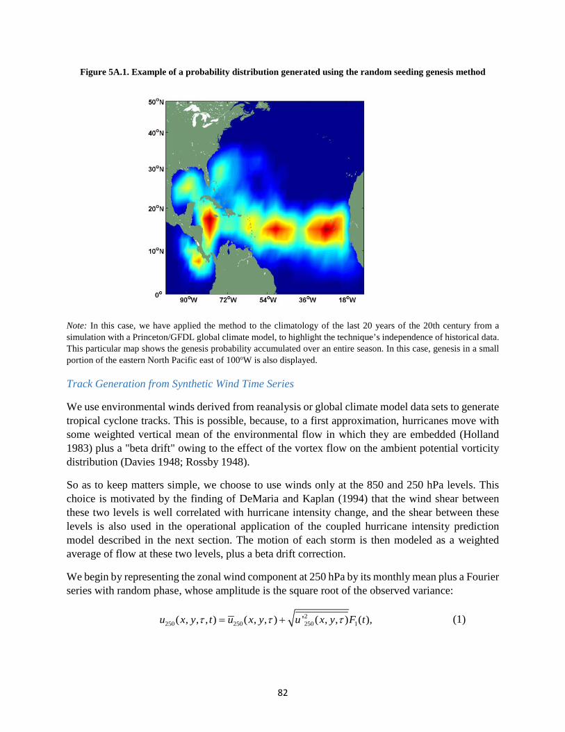
82
Figure 5A.1. Example of a probability distribution generated using the random seeding genesis method
Note: In this case, we have applied the method to the climatology of the last 20 years of the 20th century from a simulation with a Princeton/GFDL global climate model, to highlight the technique’s independence of historical data. This particular map shows the genesis probability accumulated over an entire season. In this case, genesis in a small portion of the eastern North Pacific east of 100oW is also displayed.
Track Generation from Synthetic Wind Time Series
We use environmental winds derived from reanalysis or global climate model data sets to generate tropical cyclone tracks. This is possible, because, to a first approximation, hurricanes move with some weighted vertical mean of the environmental flow in which they are embedded (Holland 1983) plus a "beta drift" owing to the effect of the vortex flow on the ambient potential vorticity distribution (Davies 1948; Rossby 1948).
So as to keep matters simple, we choose to use winds only at the 850 and 250 hPa levels. This choice is motivated by the finding of DeMaria and Kaplan (1994) that the wind shear between these two levels is well correlated with hurricane intensity change, and the shear between these levels is also used in the operational application of the coupled hurricane intensity prediction model described in the next section. The motion of each storm is then modeled as a weighted average of flow at these two levels, plus a beta drift correction.
We begin by representing the zonal wind component at 250 hPa by its monthly mean plus a Fourier series with random phase, whose amplitude is the square root of the observed variance:
2250 250 250 1( , , , ) ( , , ) ' ( , , ) ( ),u x y t u x y u x y F tτ τ τ= + (1)
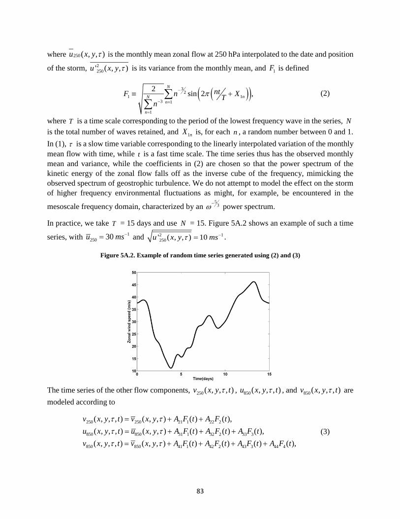
83
where 250( , , )u x y τ is the monthly mean zonal flow at 250 hPa interpolated to the date and position
of the storm, 2250' ( , , )u x y τ is its variance from the monthly mean, and 1F is defined
( )( )32
1 13 1
1
2 sin 2 ,N
nNn
n
ntF n XTn
π−
− =
=
≡ +∑∑
(2)
where T is a time scale corresponding to the period of the lowest frequency wave in the series, N is the total number of waves retained, and 1nX is, for each n , a random number between 0 and 1. In (1), τ is a slow time variable corresponding to the linearly interpolated variation of the monthly mean flow with time, while t is a fast time scale. The time series thus has the observed monthly mean and variance, while the coefficients in (2) are chosen so that the power spectrum of the kinetic energy of the zonal flow falls off as the inverse cube of the frequency, mimicking the observed spectrum of geostrophic turbulence. We do not attempt to model the effect on the storm of higher frequency environmental fluctuations as might, for example, be encountered in the
mesoscale frequency domain, characterized by an 5
3ω− power spectrum.
In practice, we take T = 15 days and use N = 15. Figure 5A.2 shows an example of such a time
series, with 1250 30u ms−= and 2 1
250' ( , , ) 10u x y msτ −= .
Figure 5A.2. Example of random time series generated using (2) and (3)
The time series of the other flow components, 250( , , , )v x y tτ , 850( , , , )u x y tτ , and 850( , , , )v x y tτ are modeled according to
250 250 21 1 22 2
850 850 31 1 32 2 33 3
850 850 41 1 42 2 43 3 44 4
( , , , ) ( , , ) ( ) ( ),( , , , ) ( , , ) ( ) ( ) ( ),( , , , ) ( , , ) ( ) ( ) ( ) ( ),
v x y t v x y A F t A F tu x y t u x y A F t A F t A F tv x y t v x y A F t A F t A F t A F t
τ ττ ττ τ
= + += + + += + + + +
(3)
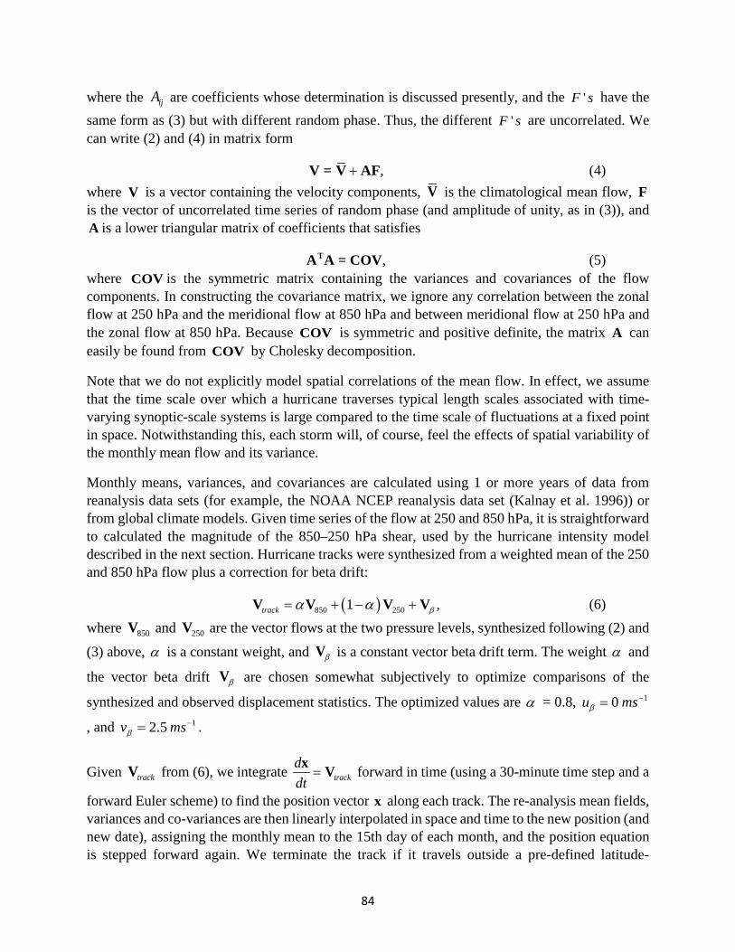
84
where the ijA are coefficients whose determination is discussed presently, and the 'F s have the same form as (3) but with different random phase. Thus, the different 'F s are uncorrelated. We can write (2) and (4) in matrix form
,+V = V AF (4) where V is a vector containing the velocity components, V is the climatological mean flow, F is the vector of uncorrelated time series of random phase (and amplitude of unity, as in (3)), and A is a lower triangular matrix of coefficients that satisfies
,TA A = COV (5) where COV is the symmetric matrix containing the variances and covariances of the flow components. In constructing the covariance matrix, we ignore any correlation between the zonal flow at 250 hPa and the meridional flow at 850 hPa and between meridional flow at 250 hPa and the zonal flow at 850 hPa. Because COV is symmetric and positive definite, the matrix A can easily be found from COV by Cholesky decomposition.
Note that we do not explicitly model spatial correlations of the mean flow. In effect, we assume that the time scale over which a hurricane traverses typical length scales associated with time-varying synoptic-scale systems is large compared to the time scale of fluctuations at a fixed point in space. Notwithstanding this, each storm will, of course, feel the effects of spatial variability of the monthly mean flow and its variance.
Monthly means, variances, and covariances are calculated using 1 or more years of data from reanalysis data sets (for example, the NOAA NCEP reanalysis data set (Kalnay et al. 1996)) or from global climate models. Given time series of the flow at 250 and 850 hPa, it is straightforward to calculated the magnitude of the 850–250 hPa shear, used by the hurricane intensity model described in the next section. Hurricane tracks were synthesized from a weighted mean of the 250 and 850 hPa flow plus a correction for beta drift:
( )850 2501 ,track βα α= + − +V V V V (6) where 850V and 250V are the vector flows at the two pressure levels, synthesized following (2) and
(3) above, α is a constant weight, and βV is a constant vector beta drift term. The weight α and
the vector beta drift βV are chosen somewhat subjectively to optimize comparisons of the
synthesized and observed displacement statistics. The optimized values are α = 0.8, 10u msβ−=
, and 12.5v msβ−= .
Given trackV from (6), we integrate trackddt
=x V forward in time (using a 30-minute time step and a
forward Euler scheme) to find the position vector x along each track. The re-analysis mean fields, variances and co-variances are then linearly interpolated in space and time to the new position (and new date), assigning the monthly mean to the 15th day of each month, and the position equation is stepped forward again. We terminate the track if it travels outside a pre-defined latitude-
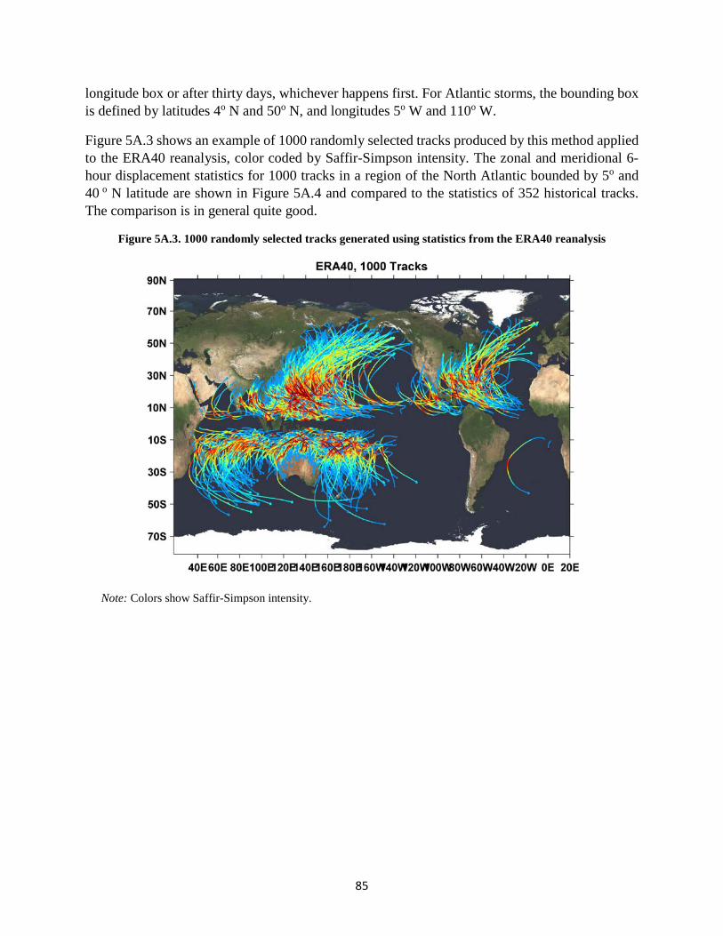
85
longitude box or after thirty days, whichever happens first. For Atlantic storms, the bounding box is defined by latitudes 4o N and 50o N, and longitudes 5o W and 110o W.
Figure 5A.3 shows an example of 1000 randomly selected tracks produced by this method applied to the ERA40 reanalysis, color coded by Saffir-Simpson intensity. The zonal and meridional 6-hour displacement statistics for 1000 tracks in a region of the North Atlantic bounded by 5o and 40 o N latitude are shown in Figure 5A.4 and compared to the statistics of 352 historical tracks. The comparison is in general quite good.
Figure 5A.3. 1000 randomly selected tracks generated using statistics from the ERA40 reanalysis
Note: Colors show Saffir-Simpson intensity.
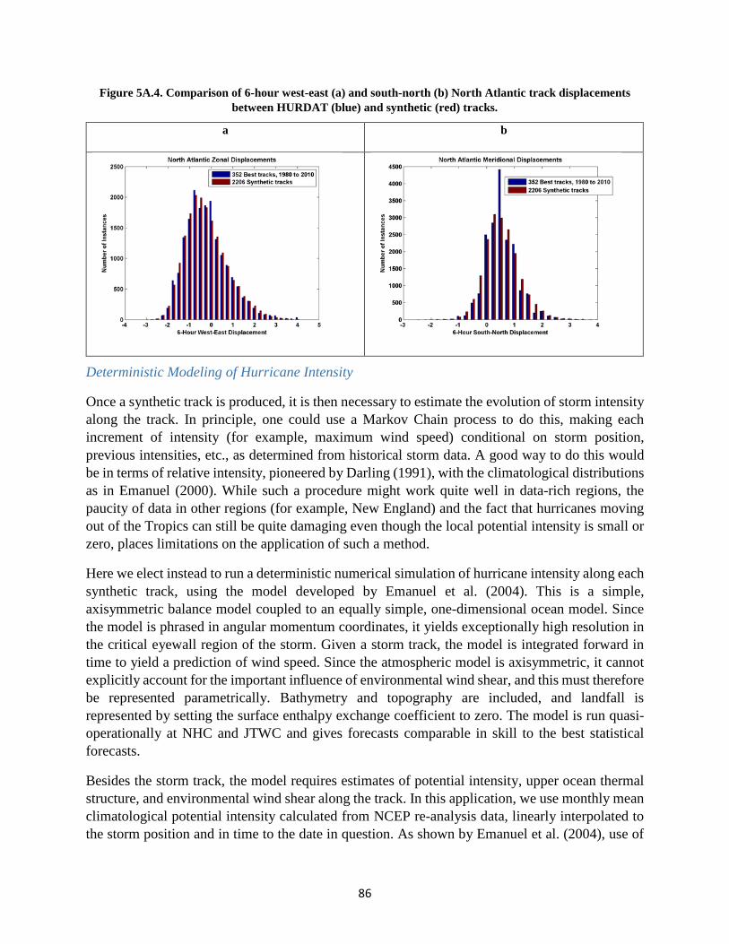
86
Figure 5A.4. Comparison of 6-hour west-east (a) and south-north (b) North Atlantic track displacements between HURDAT (blue) and synthetic (red) tracks.
a b
Deterministic Modeling of Hurricane Intensity
Once a synthetic track is produced, it is then necessary to estimate the evolution of storm intensity along the track. In principle, one could use a Markov Chain process to do this, making each increment of intensity (for example, maximum wind speed) conditional on storm position, previous intensities, etc., as determined from historical storm data. A good way to do this would be in terms of relative intensity, pioneered by Darling (1991), with the climatological distributions as in Emanuel (2000). While such a procedure might work quite well in data-rich regions, the paucity of data in other regions (for example, New England) and the fact that hurricanes moving out of the Tropics can still be quite damaging even though the local potential intensity is small or zero, places limitations on the application of such a method.
Here we elect instead to run a deterministic numerical simulation of hurricane intensity along each synthetic track, using the model developed by Emanuel et al. (2004). This is a simple, axisymmetric balance model coupled to an equally simple, one-dimensional ocean model. Since the model is phrased in angular momentum coordinates, it yields exceptionally high resolution in the critical eyewall region of the storm. Given a storm track, the model is integrated forward in time to yield a prediction of wind speed. Since the atmospheric model is axisymmetric, it cannot explicitly account for the important influence of environmental wind shear, and this must therefore be represented parametrically. Bathymetry and topography are included, and landfall is represented by setting the surface enthalpy exchange coefficient to zero. The model is run quasi-operationally at NHC and JTWC and gives forecasts comparable in skill to the best statistical forecasts.
Besides the storm track, the model requires estimates of potential intensity, upper ocean thermal structure, and environmental wind shear along the track. In this application, we use monthly mean climatological potential intensity calculated from NCEP re-analysis data, linearly interpolated to the storm position and in time to the date in question. As shown by Emanuel et al. (2004), use of
87
real-time potential intensity offers only a marginal improvement over the climatological means. As in the quasi-operational model, we use monthly mean climatological upper ocean thermal structure obtained from Levitus (1982). On the other hand, Emanuel et al. (2004) showed that upper ocean thermal variability can have a significant influence on hurricane intensity in this model. Although we do not account for such variability here, we intend to include this in future versions of our model, using sea surface altimetry data to help quantify the climatological variability of the upper ocean.
Vertical wind shear is an important influence on hurricane intensity, in this model as in nature. Here we apply the wind shear calculated from synthetic time series of winds at 850 and 250 hPa, as described in section 3.
In the quasi-operational application of the intensity model, the integration is initialized by matching the time evolution of the intensity to that of the observed storm prior to the initialization time. Here we simply prescribe an initial intensity of 112 ms− and an initial intensification rate of about 1 16 ms day− − . If and when the predicted maximum drops below 117 ms− , the storm is assumed to have dissipated and the integration is discontinued. In rare cases, the storm may reach the end of a track before this happens.
The rate of genesis of tropical cyclones is taken from the random seeding technique, as previously described, and is independent of the wind field taken at the beginning of the synthetic time series whose generation was described in section 4. While it is unrealistic to assume that storms will be generated under conditions of large shear, the intensity model will quickly kill storms under these conditions.
The intensity model takes, on the average, about 15 seconds of wall-clock time to run a single track on a typical workstation computer. Thus it is feasible to run a large number of tracks.
To estimate wind speeds at fixed points in space, it is necessary to estimate the radial structure of the storm's wind field. While the intensity model does predict such structure, it is not particularly realistic and we elect instead to use a parametric form for the radial structure, fitted to the predicted maximum wind speed and radius of maximum winds. We offer several different parametric wind models, including those of Holland (1983), Emanuel (2004), and Emanuel and Rotunno (2011).
To the axisymmetric wind field we add a fraction of the storm's translation velocity in the direction of the storm's motion. We find, empirically, that relatively good agreement with historical data is obtained using a fraction of the translation speed that is a weak function of latitude.
A weakness of the present approach is that dynamical interactions with extratropical systems are specifically excluded. Were such interactions linear, and were both the tropical cyclone and the extratropical systems with which it interacts quasi-geostrophic, then the wind fields of all the systems could be linearly superposed and the extratropical interaction would be accounted for to some degree by having added the translation speed to the wind speed. But extratropical transition is no doubt strongly nonlinear, and the circulation around the tropical cyclone may be expected, under some circumstances, to enhance the amplitude of extratropical potential vorticity anomalies,
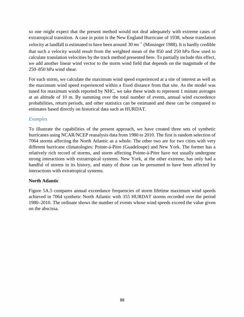
88
so one might expect that the present method would not deal adequately with extreme cases of extratropical transition. A case in point is the New England Hurricane of 1938, whose translation velocity at landfall is estimated to have been around 130 ms− (Minsinger 1988). It is hardly credible that such a velocity would result from the weighted mean of the 850 and 250 hPa flow used to calculate translation velocities by the track method presented here. To partially include this effect, we add another linear wind vector to the storm wind field that depends on the magnitude of the 250–850 hPa wind shear.
For each storm, we calculate the maximum wind speed experienced at a site of interest as well as the maximum wind speed experienced within a fixed distance from that site. As the model was tuned for maximum winds reported by NHC, we take these winds to represent 1 minute averages at an altitude of 10 m. By summing over the total number of events, annual wind exceedence probabilities, return periods, and other statistics can be estimated and these can be compared to estimates based directly on historical data such as HURDAT.
Examples
To illustrate the capabilities of the present approach, we have created three sets of synthetic hurricanes using NCAR/NCEP reanalysis data from 1980 to 2010. The first is random selection of 7064 storms affecting the North Atlantic as a whole. The other two are for two cities with very different hurricane climatologies: Pointe-á-Pitre (Guadeloupe) and New York. The former has a relatively rich record of storms, and storm affecting Pointe-á-Pitre have not usually undergone strong interactions with extratropical systems. New York, at the other extreme, has only had a handful of storms in its history, and many of those can be presumed to have been affected by interactions with extratropical systems.
North Atlantic
Figure 5A.5 compares annual exceedance frequencies of storm lifetime maximum wind speeds achieved in 7064 synthetic North Atlantic with 355 HURDAT storms recorded over the period 1980–2010. The ordinate shows the number of events whose wind speeds exceed the value given on the abscissa.
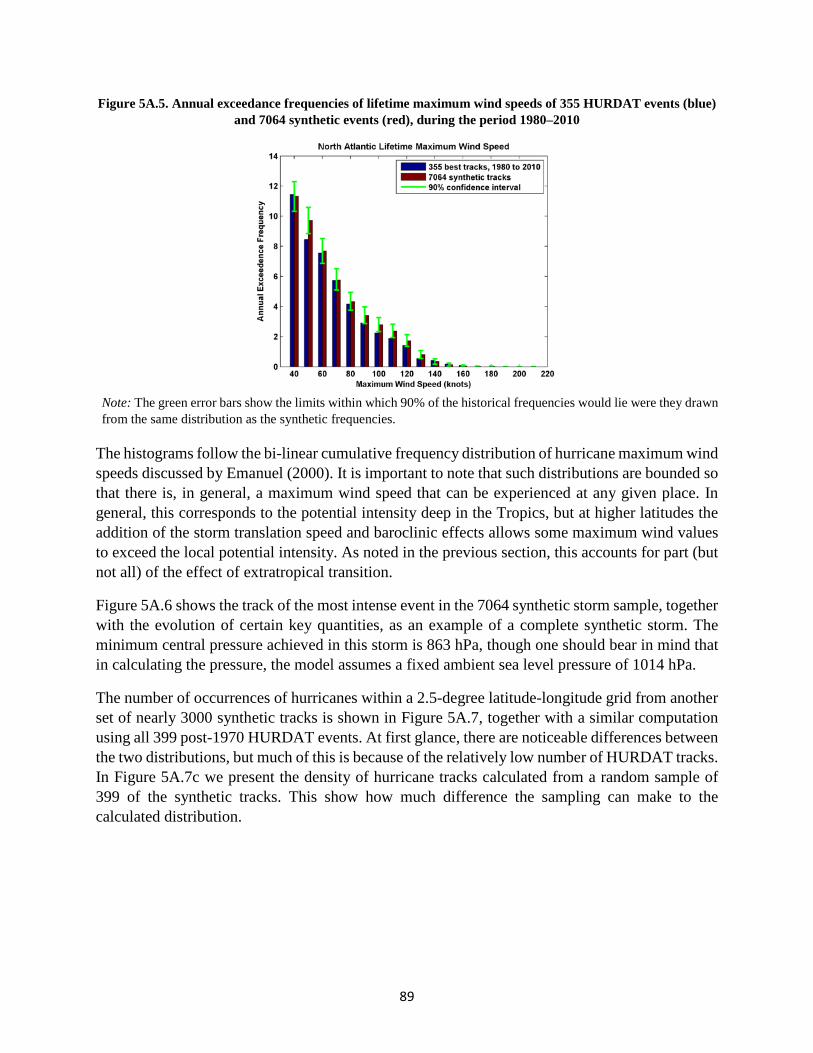
89
Figure 5A.5. Annual exceedance frequencies of lifetime maximum wind speeds of 355 HURDAT events (blue) and 7064 synthetic events (red), during the period 1980–2010
Note: The green error bars show the limits within which 90% of the historical frequencies would lie were they drawn from the same distribution as the synthetic frequencies.
The histograms follow the bi-linear cumulative frequency distribution of hurricane maximum wind speeds discussed by Emanuel (2000). It is important to note that such distributions are bounded so that there is, in general, a maximum wind speed that can be experienced at any given place. In general, this corresponds to the potential intensity deep in the Tropics, but at higher latitudes the addition of the storm translation speed and baroclinic effects allows some maximum wind values to exceed the local potential intensity. As noted in the previous section, this accounts for part (but not all) of the effect of extratropical transition.
Figure 5A.6 shows the track of the most intense event in the 7064 synthetic storm sample, together with the evolution of certain key quantities, as an example of a complete synthetic storm. The minimum central pressure achieved in this storm is 863 hPa, though one should bear in mind that in calculating the pressure, the model assumes a fixed ambient sea level pressure of 1014 hPa.
The number of occurrences of hurricanes within a 2.5-degree latitude-longitude grid from another set of nearly 3000 synthetic tracks is shown in Figure 5A.7, together with a similar computation using all 399 post-1970 HURDAT events. At first glance, there are noticeable differences between the two distributions, but much of this is because of the relatively low number of HURDAT tracks. In Figure 5A.7c we present the density of hurricane tracks calculated from a random sample of 399 of the synthetic tracks. This show how much difference the sampling can make to the calculated distribution.
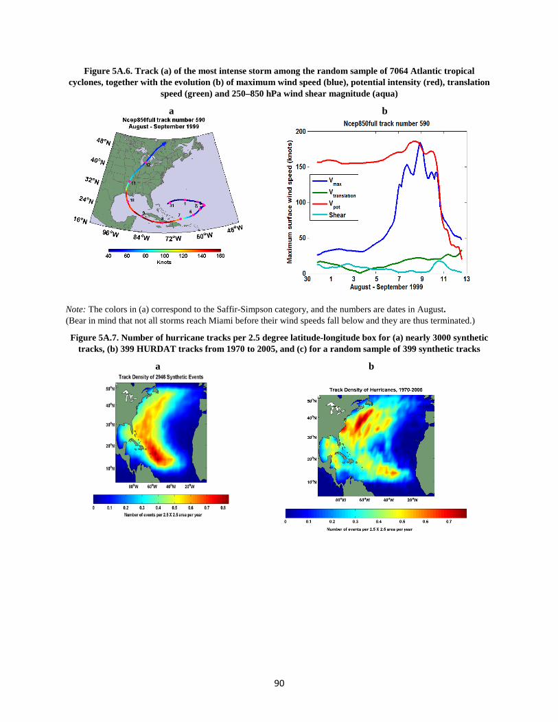
90
Figure 5A.6. Track (a) of the most intense storm among the random sample of 7064 Atlantic tropical cyclones, together with the evolution (b) of maximum wind speed (blue), potential intensity (red), translation
speed (green) and 250–850 hPa wind shear magnitude (aqua)
a b
Note: The colors in (a) correspond to the Saffir-Simpson category, and the numbers are dates in August. (Bear in mind that not all storms reach Miami before their wind speeds fall below and they are thus terminated.)
Figure 5A.7. Number of hurricane tracks per 2.5 degree latitude-longitude box for (a) nearly 3000 synthetic tracks, (b) 399 HURDAT tracks from 1970 to 2005, and (c) for a random sample of 399 synthetic tracks
a b
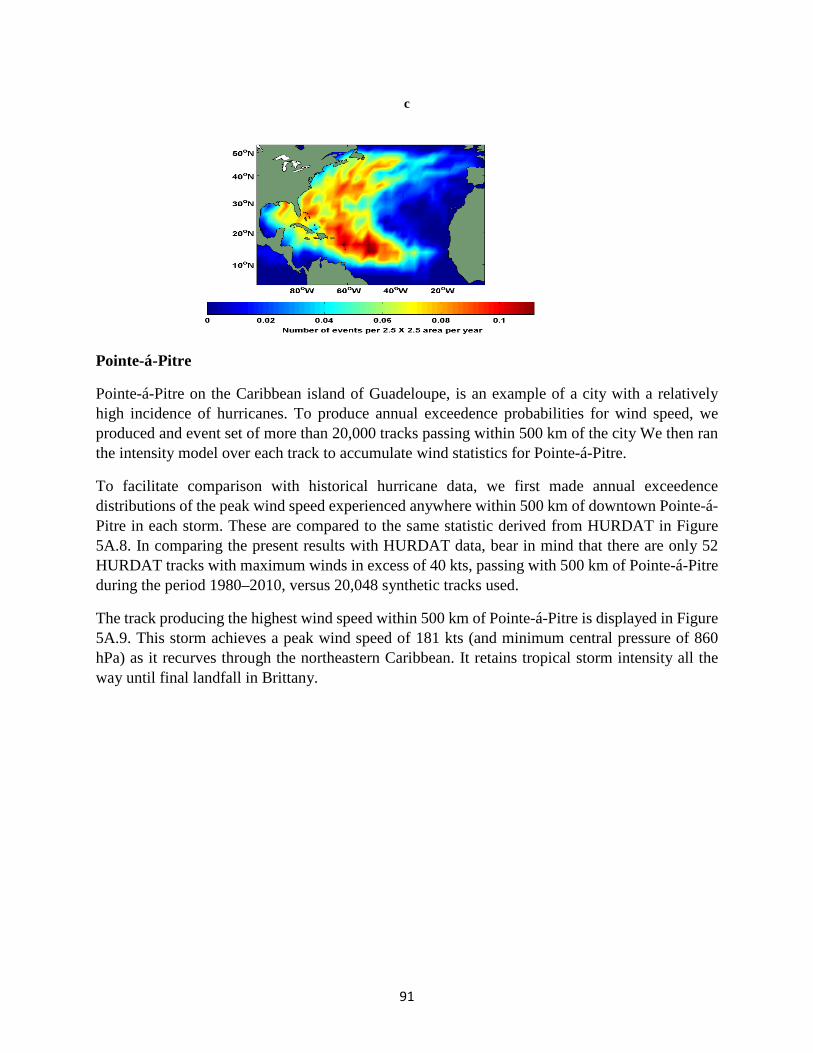
91
c
Pointe-á-Pitre
Pointe-á-Pitre on the Caribbean island of Guadeloupe, is an example of a city with a relatively high incidence of hurricanes. To produce annual exceedence probabilities for wind speed, we produced and event set of more than 20,000 tracks passing within 500 km of the city We then ran the intensity model over each track to accumulate wind statistics for Pointe-á-Pitre.
To facilitate comparison with historical hurricane data, we first made annual exceedence distributions of the peak wind speed experienced anywhere within 500 km of downtown Pointe-á-Pitre in each storm. These are compared to the same statistic derived from HURDAT in Figure 5A.8. In comparing the present results with HURDAT data, bear in mind that there are only 52 HURDAT tracks with maximum winds in excess of 40 kts, passing with 500 km of Pointe-á-Pitre during the period 1980–2010, versus 20,048 synthetic tracks used.
The track producing the highest wind speed within 500 km of Pointe-á-Pitre is displayed in Figure 5A.9. This storm achieves a peak wind speed of 181 kts (and minimum central pressure of 860 hPa) as it recurves through the northeastern Caribbean. It retains tropical storm intensity all the way until final landfall in Brittany.
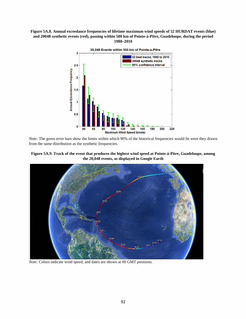
92
Figure 5A.8. Annual exceedance frequencies of lifetime maximum wind speeds of 52 HURDAT events (blue) and 20048 synthetic events (red), passing within 500 km of Pointe-á-Pitre, Guadeloupe, during the period
1980–2010
Note: The green error bars show the limits within which 90% of the historical frequencies would lie were they drawn from the same distribution as the synthetic frequencies.
Figure 5A.9. Track of the event that produces the highest wind speed at Pointe-á-Pitre, Guadeloupe, among the 20,048 events, as displayed in Google Earth
Note: Colors indicate wind speed, and dates are shown at 00 GMT positions.
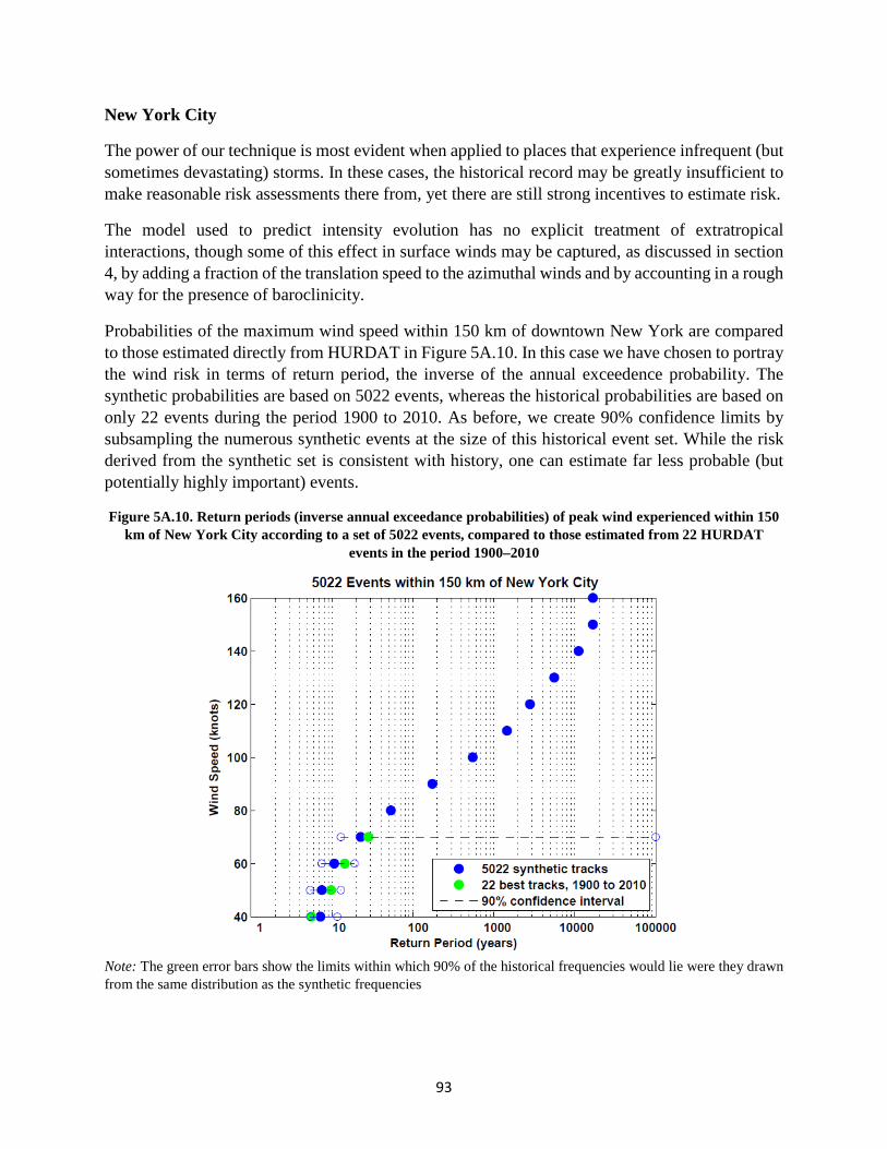
93
New York City
The power of our technique is most evident when applied to places that experience infrequent (but sometimes devastating) storms. In these cases, the historical record may be greatly insufficient to make reasonable risk assessments there from, yet there are still strong incentives to estimate risk.
The model used to predict intensity evolution has no explicit treatment of extratropical interactions, though some of this effect in surface winds may be captured, as discussed in section 4, by adding a fraction of the translation speed to the azimuthal winds and by accounting in a rough way for the presence of baroclinicity.
Probabilities of the maximum wind speed within 150 km of downtown New York are compared to those estimated directly from HURDAT in Figure 5A.10. In this case we have chosen to portray the wind risk in terms of return period, the inverse of the annual exceedence probability. The synthetic probabilities are based on 5022 events, whereas the historical probabilities are based on only 22 events during the period 1900 to 2010. As before, we create 90% confidence limits by subsampling the numerous synthetic events at the size of this historical event set. While the risk derived from the synthetic set is consistent with history, one can estimate far less probable (but potentially highly important) events.
Figure 5A.10. Return periods (inverse annual exceedance probabilities) of peak wind experienced within 150 km of New York City according to a set of 5022 events, compared to those estimated from 22 HURDAT
events in the period 1900–2010
Note: The green error bars show the limits within which 90% of the historical frequencies would lie were they drawn from the same distribution as the synthetic frequencies
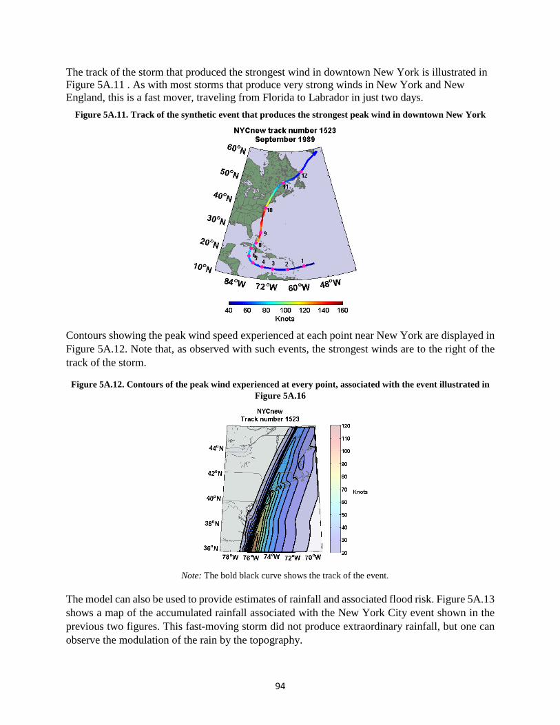
94
The track of the storm that produced the strongest wind in downtown New York is illustrated in Figure 5A.11 . As with most storms that produce very strong winds in New York and New England, this is a fast mover, traveling from Florida to Labrador in just two days.
Figure 5A.11. Track of the synthetic event that produces the strongest peak wind in downtown New York
Contours showing the peak wind speed experienced at each point near New York are displayed in Figure 5A.12. Note that, as observed with such events, the strongest winds are to the right of the track of the storm.
Figure 5A.12. Contours of the peak wind experienced at every point, associated with the event illustrated in Figure 5A.16
Note: The bold black curve shows the track of the event.
The model can also be used to provide estimates of rainfall and associated flood risk. Figure 5A.13 shows a map of the accumulated rainfall associated with the New York City event shown in the previous two figures. This fast-moving storm did not produce extraordinary rainfall, but one can observe the modulation of the rain by the topography.
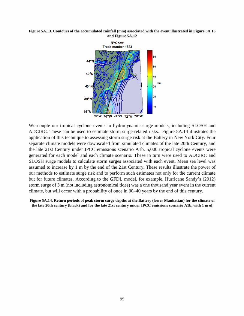
95
Figure 5A.13. Contours of the accumulated rainfall (mm) associated with the event illustrated in Figure 5A.16 and Figure 5A.12
We couple our tropical cyclone events to hydrodynamic surge models, including SLOSH and ADCIRC. These can be used to estimate storm surge-related risks. Figure 5A.14 illustrates the application of this technique to assessing storm surge risk at the Battery in New York City. Four separate climate models were downscaled from simulated climates of the late 20th Century, and the late 21st Century under IPCC emissions scenario A1b. 5,000 tropical cyclone events were generated for each model and each climate scenario. These in turn were used to ADCIRC and SLOSH surge models to calculate storm surges associated with each event. Mean sea level was assumed to increase by 1 m by the end of the 21st Century. These results illustrate the power of our methods to estimate surge risk and to perform such estimates not only for the current climate but for future climates. According to the GFDL model, for example, Hurricane Sandy’s (2012) storm surge of 3 m (not including astronomical tides) was a one thousand year event in the current climate, but will occur with a probability of once in 30–40 years by the end of this century.
Figure 5A.14. Return periods of peak storm surge depths at the Battery (lower Manhattan) for the climate of the late 20th century (black) and for the late 21st century under IPCC emissions scenario A1b, with 1 m of
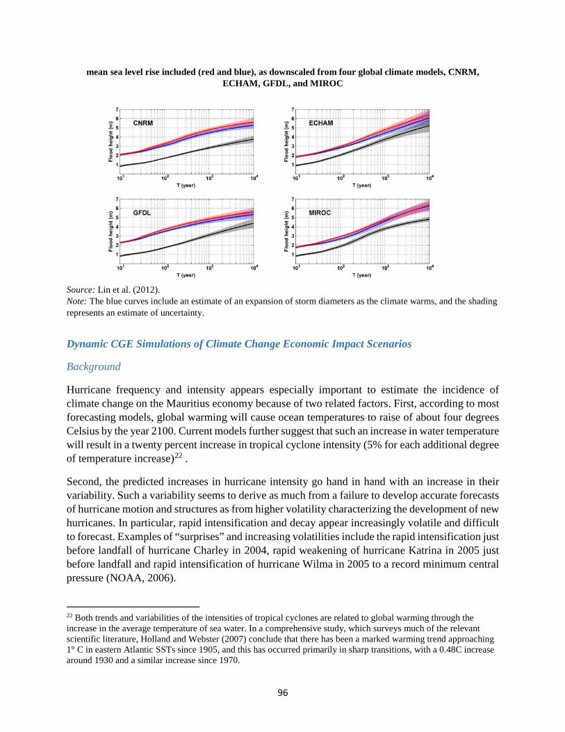
96
mean sea level rise included (red and blue), as downscaled from four global climate models, CNRM, ECHAM, GFDL, and MIROC
Source: Lin et al. (2012). Note: The blue curves include an estimate of an expansion of storm diameters as the climate warms, and the shading represents an estimate of uncertainty.
Dynamic CGE Simulations of Climate Change Economic Impact Scenarios
Background
Hurricane frequency and intensity appears especially important to estimate the incidence of climate change on the Mauritius economy because of two related factors. First, according to most forecasting models, global warming will cause ocean temperatures to raise of about four degrees Celsius by the year 2100. Current models further suggest that such an increase in water temperature will result in a twenty percent increase in tropical cyclone intensity (5% for each additional degree of temperature increase)22 .
Second, the predicted increases in hurricane intensity go hand in hand with an increase in their variability. Such a variability seems to derive as much from a failure to develop accurate forecasts of hurricane motion and structures as from higher volatility characterizing the development of new hurricanes. In particular, rapid intensification and decay appear increasingly volatile and difficult to forecast. Examples of “surprises” and increasing volatilities include the rapid intensification just before landfall of hurricane Charley in 2004, rapid weakening of hurricane Katrina in 2005 just before landfall and rapid intensification of hurricane Wilma in 2005 to a record minimum central pressure (NOAA, 2006).
22 Both trends and variabilities of the intensities of tropical cyclones are related to global warming through the increase in the average temperature of sea water. In a comprehensive study, which surveys much of the relevant scientific literature, Holland and Webster (2007) conclude that there has been a marked warming trend approaching 1° C in eastern Atlantic SSTs since 1905, and this has occurred primarily in sharp transitions, with a 0.48C increase around 1930 and a similar increase since 1970.
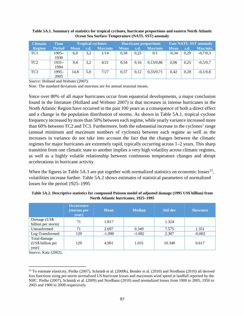
97
Table 5A.1. Summary of statistics for tropical cyclones, hurricane proportions and eastern North Atlantic Ocean Sea Surface Temperature (NATL SST) anomaly
Climatic Regime
Time Period
Tropical cyclones Hurricane proportions East NATL SST anomaly Mean s.d. Max/min Mean s.d. Max/min Mean s.d. Max/min
TC1 1905–1930
6,0 3,2 1/14 0,58 0,25 0/1 -0,34 0,29 -0,7/0,3
TC2 1931–1994
9,4 3,2 4/21 0,54 0,16 0,13/0,86 0,06 0,25 -0,5/0,7
TC3 1995–2005
14,8 5,0 7/27 0,57 0,12 0,33/0,71 0,42 0,28 -0,1/0,8
Source: Holland and Webster (2007). Note: The standard deviations and min/max are for annual seasonal means.
Since over 80% of all major hurricanes occur from equatorial developments, a major conclusion found in the literature (Holland and Webster 2007) is that increases in intense hurricanes in the North Atlantic Region have occurred in the past 100 years as a consequence of both a direct effect and a change in the population distribution of storms. As shown in Table 5A.1, tropical cyclone frequency increased by more than 50% between each regime, while yearly variance increased more than 60% between TC2 and TC3. Furthermore, both the substantial increase in the cyclones’ range (annual minimum and maximum numbers of cyclones) between each regime as well as the increases in variance do not take into account the fact that the changes between the climatic regimes for major hurricanes are extremely rapid, typically occurring across 1–2 years. This sharp transition from one climatic state to another implies a very high volatility across climatic regimes, as well as a highly volatile relationship between continuous temperature changes and abrupt accelerations in hurricane activity.
When the figures in Table 5A.1 are put together with normalized statistics on economic losses23, volatilities increase further. Table 5A.2 shows estimates of statistical parameters of normalized losses for the period 1925–1995
Table 5A.2. Descriptive statistics for compound Poisson model of adjusted damage (1995 US$ billion) from North Atlantic hurricanes, 1925–1995
Occurrence (storms per
year) Mean Median Std dev Skewness
Damage (US$ billion per storm) 71 1.817 1.324
Untrasformed 71 2.697 0.349 7.575 1.351 Log-Transformed 129 -1.090 -1.082 2.307 -0.002 Total damage (US$ billion per year)
129 4.901 1.031 10.349 0.617
Source: Katz (2002).
23 To estimate elasticity, Pielke (2007), Schmidt et al. (2009b), Bender et al. (2010) and Nordhaus (2010) all derived loss functions using per-storm normalized US hurricane losses and maximum wind speed at landfall reported by the NHC. Pielke (2007), Schmidt et al. (2009) and Nordhaus (2010) used normalized losses from 1900 to 2005, 1950 to 2005 and 1900 to 2008 respectively.
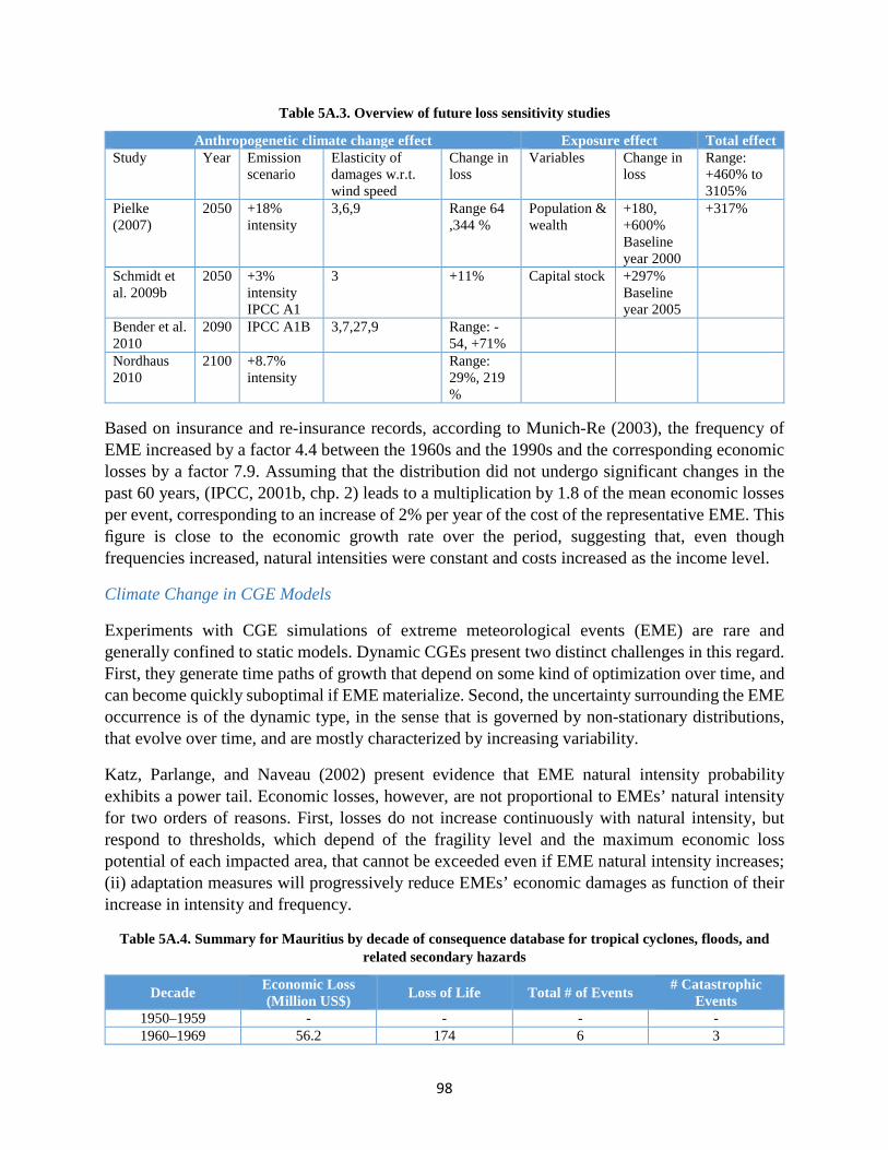
98
Table 5A.3. Overview of future loss sensitivity studies
Anthropogenetic climate change effect Exposure effect Total effect Study Year Emission
scenario Elasticity of damages w.r.t. wind speed
Change in loss
Variables Change in loss
Range: +460% to 3105%
Pielke (2007)
2050 +18% intensity
3,6,9 Range 64 ,344 %
Population & wealth
+180, +600% Baseline year 2000
+317%
Schmidt et al. 2009b
2050 +3% intensity IPCC A1
3 +11% Capital stock +297% Baseline year 2005
Bender et al. 2010
2090 IPCC A1B 3,7,27,9 Range: -54, +71%
Nordhaus 2010
2100 +8.7% intensity
Range: 29%, 219 %
Based on insurance and re-insurance records, according to Munich-Re (2003), the frequency of EME increased by a factor 4.4 between the 1960s and the 1990s and the corresponding economic losses by a factor 7.9. Assuming that the distribution did not undergo significant changes in the past 60 years, (IPCC, 2001b, chp. 2) leads to a multiplication by 1.8 of the mean economic losses per event, corresponding to an increase of 2% per year of the cost of the representative EME. This figure is close to the economic growth rate over the period, suggesting that, even though frequencies increased, natural intensities were constant and costs increased as the income level.
Climate Change in CGE Models
Experiments with CGE simulations of extreme meteorological events (EME) are rare and generally confined to static models. Dynamic CGEs present two distinct challenges in this regard. First, they generate time paths of growth that depend on some kind of optimization over time, and can become quickly suboptimal if EME materialize. Second, the uncertainty surrounding the EME occurrence is of the dynamic type, in the sense that is governed by non-stationary distributions, that evolve over time, and are mostly characterized by increasing variability.
Katz, Parlange, and Naveau (2002) present evidence that EME natural intensity probability exhibits a power tail. Economic losses, however, are not proportional to EMEs’ natural intensity for two orders of reasons. First, losses do not increase continuously with natural intensity, but respond to thresholds, which depend of the fragility level and the maximum economic loss potential of each impacted area, that cannot be exceeded even if EME natural intensity increases; (ii) adaptation measures will progressively reduce EMEs’ economic damages as function of their increase in intensity and frequency.
Table 5A.4. Summary for Mauritius by decade of consequence database for tropical cyclones, floods, and related secondary hazards
Decade Economic Loss (Million US$) Loss of Life Total # of Events # Catastrophic
Events 1950–1959 - - - - 1960–1969 56.2 174 6 3
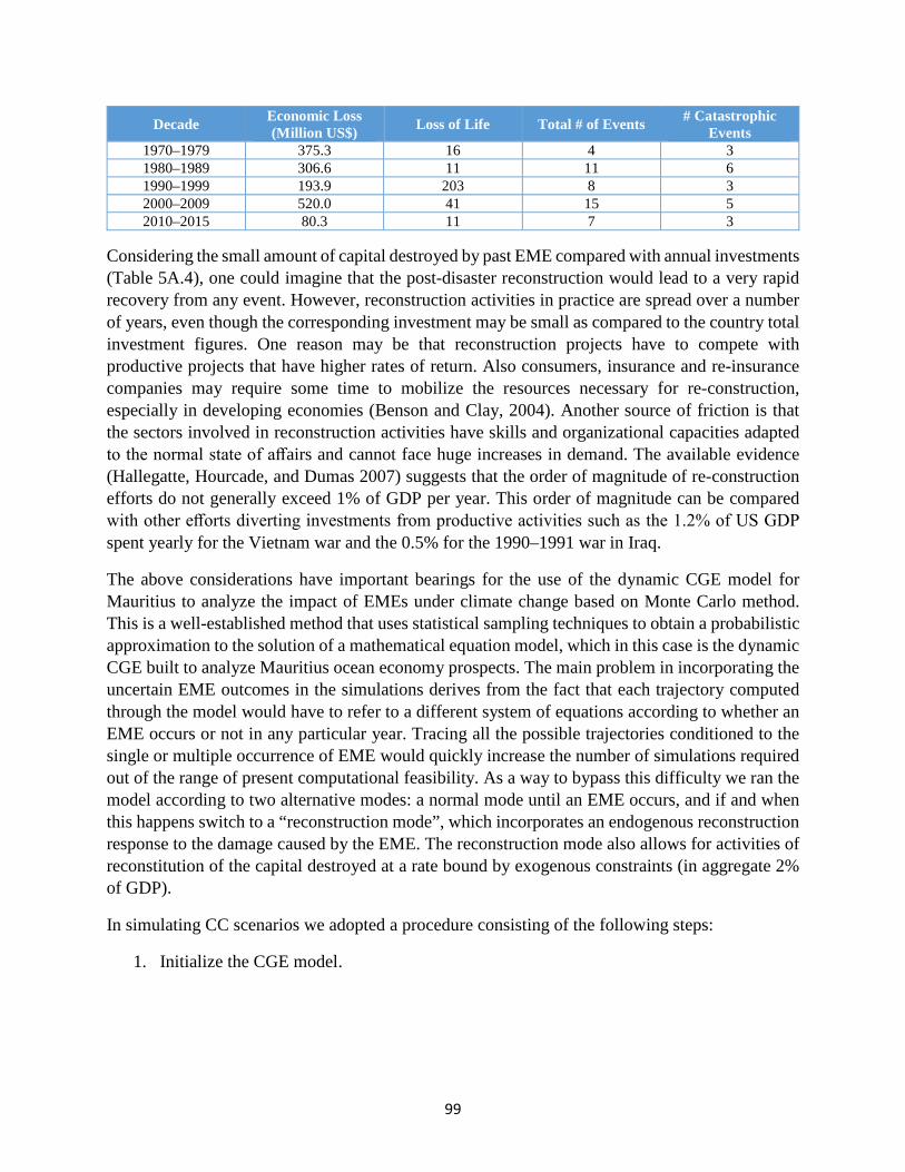
99
Decade Economic Loss (Million US$) Loss of Life Total # of Events # Catastrophic
Events 1970–1979 375.3 16 4 3 1980–1989 306.6 11 11 6 1990–1999 193.9 203 8 3 2000–2009 520.0 41 15 5 2010–2015 80.3 11 7 3
Considering the small amount of capital destroyed by past EME compared with annual investments (Table 5A.4), one could imagine that the post-disaster reconstruction would lead to a very rapid recovery from any event. However, reconstruction activities in practice are spread over a number of years, even though the corresponding investment may be small as compared to the country total investment figures. One reason may be that reconstruction projects have to compete with productive projects that have higher rates of return. Also consumers, insurance and re-insurance companies may require some time to mobilize the resources necessary for re-construction, especially in developing economies (Benson and Clay, 2004). Another source of friction is that the sectors involved in reconstruction activities have skills and organizational capacities adapted to the normal state of affairs and cannot face huge increases in demand. The available evidence (Hallegatte, Hourcade, and Dumas 2007) suggests that the order of magnitude of re-construction efforts do not generally exceed 1% of GDP per year. This order of magnitude can be compared with other efforts diverting investments from productive activities such as the 1.2% of US GDP spent yearly for the Vietnam war and the 0.5% for the 1990–1991 war in Iraq.
The above considerations have important bearings for the use of the dynamic CGE model for Mauritius to analyze the impact of EMEs under climate change based on Monte Carlo method. This is a well-established method that uses statistical sampling techniques to obtain a probabilistic approximation to the solution of a mathematical equation model, which in this case is the dynamic CGE built to analyze Mauritius ocean economy prospects. The main problem in incorporating the uncertain EME outcomes in the simulations derives from the fact that each trajectory computed through the model would have to refer to a different system of equations according to whether an EME occurs or not in any particular year. Tracing all the possible trajectories conditioned to the single or multiple occurrence of EME would quickly increase the number of simulations required out of the range of present computational feasibility. As a way to bypass this difficulty we ran the model according to two alternative modes: a normal mode until an EME occurs, and if and when this happens switch to a “reconstruction mode”, which incorporates an endogenous reconstruction response to the damage caused by the EME. The reconstruction mode also allows for activities of reconstitution of the capital destroyed at a rate bound by exogenous constraints (in aggregate 2% of GDP).
In simulating CC scenarios we adopted a procedure consisting of the following steps:
1. Initialize the CGE model.
100
2. Assign a probability distribution function to each of the input stochastic variables. For example, define the number of Extreme Meteorological Events (EME) by a Poisson24 process and a damage scale of each EME by drawing from a gamma distribution. If an EME happens, the parameter models (for example, input output coefficients) will be affected according to the damage scale.
3. Generate a sample of N solutions by running N times the model on the basis of a random selection from the probability distributions for each of the input variables (number and damage level).
4. Use the N solutions to generate a probability distribution for the model output values.
5. Because the CGE model is dynamic, the random extraction of the input (shock) variables is carried out for every year over the time horizon considered. This means that the model is: (i) run N times under a random assignment of input values, (ii) for all the runs, once an EME occurs, the model switches to reconstruction mode. This mode is identical to the normal mode, except for the fact that a pre-determined part of fixed capital formation is devoted to reconstitute the capital stock destroyed by the EME, (iii) outcomes from the N runs are stored and generate an outcome distribution.
6. Besides reconstruction, other types of preventive and adaptive measures can be incorporated in the model. These include: (i) protection costs (protection capital, alarm systems, spatial planning); (ii) insurance, (iii) financing strategies, (iv) learning mechanisms (from perfect foresight to early warning systems).
The CGE incorporates storm damages as a fraction of the capital assets destroyed in a particular sector as a result of storm strike. Among the EMEs tropical cyclone damages were singled out as the most likely events to be affected by climate change in major way. In order to simulate their economic impact, we thus focused on four future scenarios:
• No tropical cyclones,
• Tropical cyclone frequency and severity consistent with historical patterns,
• Tropical cyclones expected under a high-impact climate scenario, and
• Tropical cyclones expected under a low-impact climate scenario.
The no-tropical cyclone baseline is described in Chapter 2. Storm damages input to the CGE are identified based on 1) a Poisson distribution of storm frequency as defined by the parameters
24 In terms of tropical cyclone formation, the southwest Indian basin is one of the most active areas in the world. On average, 13 tropical cyclones with wind speeds exceeding 63 km/h form here each year. Statistical goodness-of-fit tests reveal that the annual frequency of tropical cyclone formation in the model domain is best represented by a Poisson distribution.
101
projected in the CHIPS model, and 2) a gamma function of storm damage defined by CHIPS model outputs and a maximum wind speed based damage function.
Each year from 2020 to 2060, the CGE model randomly selects the number of events from the Poisson distribution, and then assigns damages of each selected event from the log-normal damage distribution. The damages associated with tropical cyclones under both historical and future climate conditions are identified in five categories of loss: residential, commercial, infrastructure, industrial, and public. Each type of loss will be attributed to the 112 sectors by category. The model enters the “reconstruction mode” once hit with an extreme event, where the expected damages enter the CGE as a shock to capital in the designated sector(s). For a set number of years following the event or events, a defined proportion of GDP is directed to restore the damaged capital in a manner that maximizes a welfare function, which weighs exponentially the incomes of the different households in inverse proportion to their levels. This process is repeated for the high impact climate scenario, a low impact climate scenario, and a historical climate scenario.
The CGE Re-formulation with Climate Change Shocks
The CGE model can be synthetically represented by the following mathematical expression:
(1) ξ𝑡𝑡 = Φ𝑡𝑡(𝜉𝜉𝑡𝑡|𝑌𝑌𝑡𝑡,𝑉𝑉𝑡𝑡 ) + 𝑈𝑈𝑡𝑡
In (1), 𝜉𝜉𝑡𝑡 is a vector of market equilibrium quantities, incomes and prices, 𝑌𝑌𝑡𝑡 a vector of exogenous drivers (investment, exports, etc.) and 𝑉𝑉𝑡𝑡 ,𝑈𝑈𝑡𝑡 two vectors of stochastic shocks. Totally differentiating this expression, we obtain:
(2) 𝑑𝑑𝜉𝜉𝑡𝑡 = Φ𝑥𝑥𝑡𝑡(𝜉𝜉𝑡𝑡|𝑌𝑌𝑡𝑡,𝑉𝑉𝑡𝑡 )𝑑𝑑𝜉𝜉𝑡𝑡 + Φ𝑦𝑦𝑡𝑡(𝜉𝜉𝑡𝑡|𝑌𝑌𝑡𝑡,𝑉𝑉𝑡𝑡 )𝑑𝑑𝑌𝑌𝑡𝑡 + Φ𝑣𝑣𝑡𝑡(𝜉𝜉𝑡𝑡|𝑌𝑌𝑡𝑡,𝑉𝑉𝑡𝑡 )𝑑𝑑𝑉𝑉𝑡𝑡 + 𝑑𝑑𝑈𝑈𝑡𝑡
where Φ𝑥𝑥𝑡𝑡 is the (square) matrix of first derivatives (the “Jacobian”) of the CGE mapping with respect to the vector of market variables, Φ𝑦𝑦𝑡𝑡 and Φ𝑣𝑣𝑡𝑡 the matrix of first derivatives of the same mapping with respect to the exogenous drivers and the stochastic shocks. Note that these two matrices incorporate the effects of exogenous changes in the production and consumption parameters. This implies, for example, that investment increases will change the productive structure of the production parameters. It also implies that stochastic shocks, such as those caused by extreme weather events, may alter both production and consumption parameters.
CGE simulations for extreme weather events can be carried out by solving equation (2) to obtain:
(3) 𝑑𝑑𝜉𝜉𝑡𝑡 = [I −Φ𝑥𝑥𝑡𝑡(𝜉𝜉𝑡𝑡|𝑌𝑌𝑡𝑡,𝑉𝑉𝑡𝑡 )]−1[Φ𝑦𝑦𝑡𝑡(𝜉𝜉𝑡𝑡|𝑌𝑌𝑡𝑡,𝑉𝑉𝑡𝑡 )𝑑𝑑𝑌𝑌𝑡𝑡 + Φ𝑣𝑣𝑡𝑡(𝜉𝜉𝑡𝑡|𝑌𝑌𝑡𝑡 ,𝑉𝑉𝑡𝑡 )𝑑𝑑𝑉𝑉𝑡𝑡 + 𝑑𝑑𝑈𝑈𝑡𝑡]
where I is the identity matrix. Notice that this solution is able to incorporate two different effects of weather shocks: (i) the additive changes 𝑑𝑑𝑈𝑈𝑡𝑡 of the aggregate demand components (for example, destruction of crops, reduction of exports, etc.), and (2) the structural changes due to the destruction of capital Φ𝑣𝑣𝑡𝑡𝑑𝑑𝑉𝑉𝑡𝑡, as well as those due to the reconstruction activities Φ𝑦𝑦𝑡𝑡 𝑑𝑑𝑌𝑌𝑡𝑡. In order to carry out Monte Carlo simulations under given assumption on the probability distribution functions of 𝑑𝑑𝑉𝑉𝑡𝑡 and 𝑑𝑑𝑈𝑈𝑡𝑡, however, the investment activities necessary to proceed to reconstruct

102
have to be partitioned into two groups: 𝑑𝑑𝑌𝑌𝑎𝑎𝑡𝑡𝑑𝑑𝑌𝑌𝑣𝑣𝑡𝑡 where 𝑑𝑑𝑌𝑌𝑎𝑎𝑡𝑡 is the vector of autonomous investment
level, while 𝑑𝑑𝑌𝑌𝑣𝑣𝑡𝑡 𝑖𝑖𝑖𝑖 defined as the investment in reconstruction contingent to the occurrence of the weather events:
(4) 𝑑𝑑𝑌𝑌𝑣𝑣𝑡𝑡 = 𝐿𝐿𝐿𝐿 Φ𝑣𝑣𝑡𝑡(𝜉𝜉𝑡𝑡|𝑌𝑌𝑡𝑡,𝑉𝑉𝑡𝑡 )𝑑𝑑𝑉𝑉𝑡𝑡
where 𝐿𝐿 is a lag operator and 𝐿𝐿 is a function that links the investment in reconstruction, and limits its size every year, to the changes that have occurred in the productive capacity and value added structure of the different sectors of the economy.
Substituting (4) into (3) and simplifying, we obtain the basic equation to be used in the Monte Carlo simulations:
(5) 𝑑𝑑𝜉𝜉𝑡𝑡 = [I −Φ𝑥𝑥𝑡𝑡(𝜉𝜉𝑡𝑡|𝑌𝑌𝑡𝑡,𝑉𝑉𝑡𝑡 )]−1[Φ𝑦𝑦𝑡𝑡(𝜉𝜉𝑡𝑡|𝑌𝑌𝑡𝑡,𝑉𝑉𝑡𝑡 )𝑑𝑑𝑌𝑌𝑎𝑎𝑡𝑡 + (Φ𝑦𝑦𝑡𝑡(𝜉𝜉𝑡𝑡|𝑌𝑌𝑡𝑡,𝑉𝑉𝑡𝑡 )𝐿𝐿𝐿𝐿 +𝐼𝐼)Φ𝑣𝑣𝑡𝑡(𝜉𝜉𝑡𝑡|𝑌𝑌𝑡𝑡,𝑉𝑉𝑡𝑡 )𝑑𝑑𝑉𝑉𝑡𝑡 + 𝑑𝑑𝑈𝑈𝑡𝑡]
The Main Results
Impact on expected damages and risk
Total expected annual damage is a function of both the frequency of events and the intensity of the events that occur. The CHIPS model is used to project historic and future storm frequency and intensity, as defined by maximum wind speeds, for both a low- and high-impact climate scenarios. Storm damages are defined by a damage function relating storm return periods to a percentage of asset damage. Although the function used reflects the context of U.S. hurricane damages (Emanuel 2011), historical damage estimates were verified against existing estimates for Mauritius (AIR Worldwide 2016). As seen in Figure 5A.15, in the high impact scenario both frequency and intensity are projected to increase in both future eras (2021 to 2040 and 2041 to 2060). Under the low-impact scenario, the frequency of damaging Tropical Cyclones is expected to decrease slightly, while the damage per storm increases by a very similar magnitude.
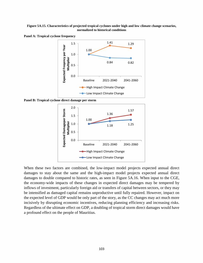
103
Figure 5A.15. Characteristics of projected tropical cyclones under high and low climate change scenarios, normalized to historical conditions
Panel A: Tropical cyclone frequency
Panel B: Tropical cyclone direct damage per storm
When these two factors are combined, the low-impact model projects expected annual direct damages to stay about the same and the high-impact model projects expected annual direct damages to double compared to historic rates, as seen in Figure 5A.16. When input to the CGE, the economy-wide impacts of these changes in expected direct damages may be tempered by inflows of investment, particularly foreign aid or transfers of capital between sectors, or they may be intensified as damaged capital remains unproductive until fully repaired. However, impact on the expected level of GDP would be only part of the story, as the CC changes may act much more incisively by disrupting economic incentives, reducing planning efficiency and increasing risks. Regardless of the ultimate effect on GDP, a doubling of tropical storm direct damages would have a profound effect on the people of Mauritius.
1.00
1.41 1.29
0.84 0.82
0.0
0.5
1.0
1.5
Baseline 2021-2040 2041-2060Expe
cted
Fre
qenc
y pe
r Yea
r M
ultip
lier
High Impact Climate Change
Low Impact Climate Change
1.00
1.361.57
1.18 1.25
0.0
0.5
1.0
1.5
2.0
Baseline 2021-2040 2041-2060Expe
cted
Dam
agep
er S
torm
M
ultip
lier
High Impact Climate Change
Low Impact Climate Change
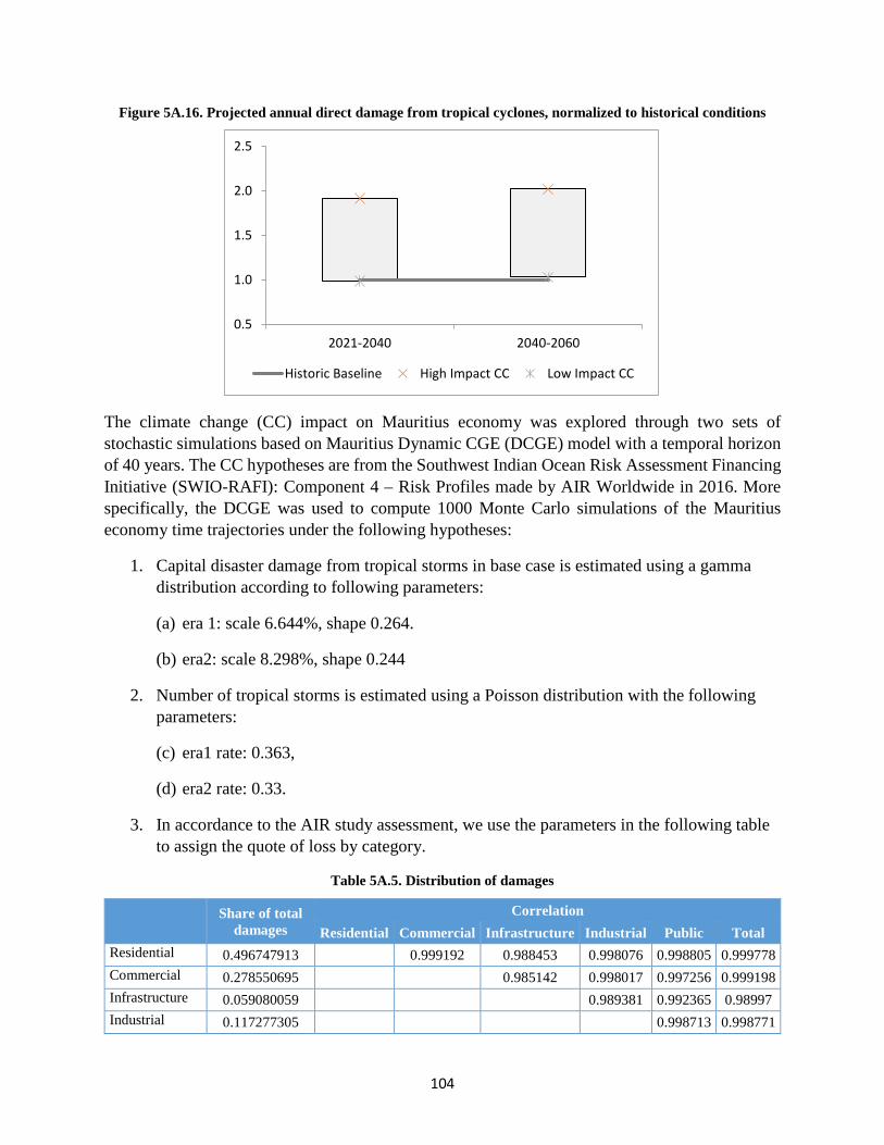
104
Figure 5A.16. Projected annual direct damage from tropical cyclones, normalized to historical conditions
The climate change (CC) impact on Mauritius economy was explored through two sets of stochastic simulations based on Mauritius Dynamic CGE (DCGE) model with a temporal horizon of 40 years. The CC hypotheses are from the Southwest Indian Ocean Risk Assessment Financing Initiative (SWIO-RAFI): Component 4 – Risk Profiles made by AIR Worldwide in 2016. More specifically, the DCGE was used to compute 1000 Monte Carlo simulations of the Mauritius economy time trajectories under the following hypotheses:
1. Capital disaster damage from tropical storms in base case is estimated using a gamma distribution according to following parameters:
(a) era 1: scale 6.644%, shape 0.264.
(b) era2: scale 8.298%, shape 0.244
2. Number of tropical storms is estimated using a Poisson distribution with the following parameters:
(c) era1 rate: 0.363,
(d) era2 rate: 0.33.
3. In accordance to the AIR study assessment, we use the parameters in the following table to assign the quote of loss by category.
Table 5A.5. Distribution of damages
Share of total damages
Correlation Residential Commercial Infrastructure Industrial Public Total
Residential 0.496747913 0.999192 0.988453 0.998076 0.998805 0.999778 Commercial 0.278550695 0.985142 0.998017 0.997256 0.999198 Infrastructure 0.059080059 0.989381 0.992365 0.98997 Industrial 0.117277305 0.998713 0.998771
0.5
1.0
1.5
2.0
2.5
2021-2040 2040-2060
Historic Baseline High Impact CC Low Impact CC
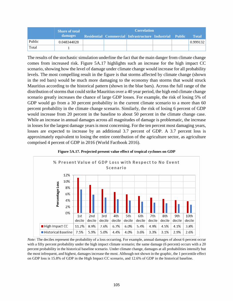
105
Share of total damages
Correlation Residential Commercial Infrastructure Industrial Public Total
Public 0.048344028 0.999132 Total 1
The results of the stochastic simulation underline the fact that the main danger from climate change comes from increased risk. Figure 5A.17 highlights such an increase for the high impact CC scenario, showing how the level of damage under climate change would increase for all probability levels. The most compelling result in the figure is that storms affected by climate change (shown in the red bars) would be much more damaging to the economy than storms that would struck Mauritius according to the historical pattern (shown in the blue bars). Across the full range of the distribution of storms that could strike Mauritius over a 40 year period, the high end climate change scenario greatly increases the chance of large GDP losses. For example, the risk of losing 5% of GDP would go from a 30 percent probability in the current climate scenario to a more than 60 percent probability in the climate change scenario. Similarly, the risk of losing 6 percent of GDP would increase from 20 percent in the baseline to about 50 percent in the climate change case. While an increase in annual damages across all magnitudes of damage is problematic, the increase in losses for the largest damage years is most concerning. For the ten percent most damaging years, losses are expected to increase by an additional 3.7 percent of GDP. A 3.7 percent loss is approximately equivalent to losing the entire contribution of the agriculture sector, as agriculture comprised 4 percent of GDP in 2016 (World Factbook 2016).
Figure 5A.17. Projected present value effect of tropical cyclones on GDP
Note: The deciles represent the probability of a loss occurring. For example, annual damages of about 6 percent occur with a fifty percent probability under the high impact climate scenario; the same damage (6 percent) occurs with a 20 percent probability in the historical baseline scenario. Under climate change, damages at all probabilities intensify but the most infrequent, and highest, damages increase the most. Although not shown in the graphic, the 1 percentile effect on GDP loss is 15.8% of GDP in the High Impact CC scenario, and 12.6% of GDP in the historical baseline.
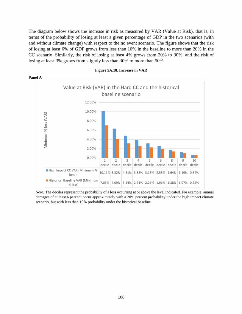
106
The diagram below shows the increase in risk as measured by VAR (Value at Risk), that is, in terms of the probability of losing at least a given percentage of GDP in the two scenarios (with and without climate change) with respect to the no event scenario. The figure shows that the risk of losing at least 6% of GDP grows from less than 10% in the baseline to more than 20% in the CC scenario. Similarly, the risk of losing at least 4% grows from 20% to 30%, and the risk of losing at least 3% grows from slightly less than 30% to more than 50%.
Figure 5A.18. Increase in VAR
Panel A
Note: The deciles represent the probability of a loss occurring at or above the level indicated. For example, annual damages of at least 6 percent occur approximately with a 20% percent probability under the high impact climate scenario, but with less than 10% probability under the historical baseline
1decile
2decile
3decile
4decile
5decile
6decile
8decile
9decile
10decile
High Impact CC VAR (Minimum %loss ) 10.11% 6.32% 4.81% 3.83% 3.13% 2.55% 1.64% 1.19% 0.64%
Historical Baseline VAR (Minimum% loss) 7.03% 4.09% 3.14% 2.61% 2.25% 1.96% 1.38% 1.07% 0.62%
0.00%
2.00%
4.00%
6.00%
8.00%
10.00%
12.00%
Min
imum
% lo
ss (V
AR)
Value at Risk (VAR) in the Hard CC and the historical baseline scenario
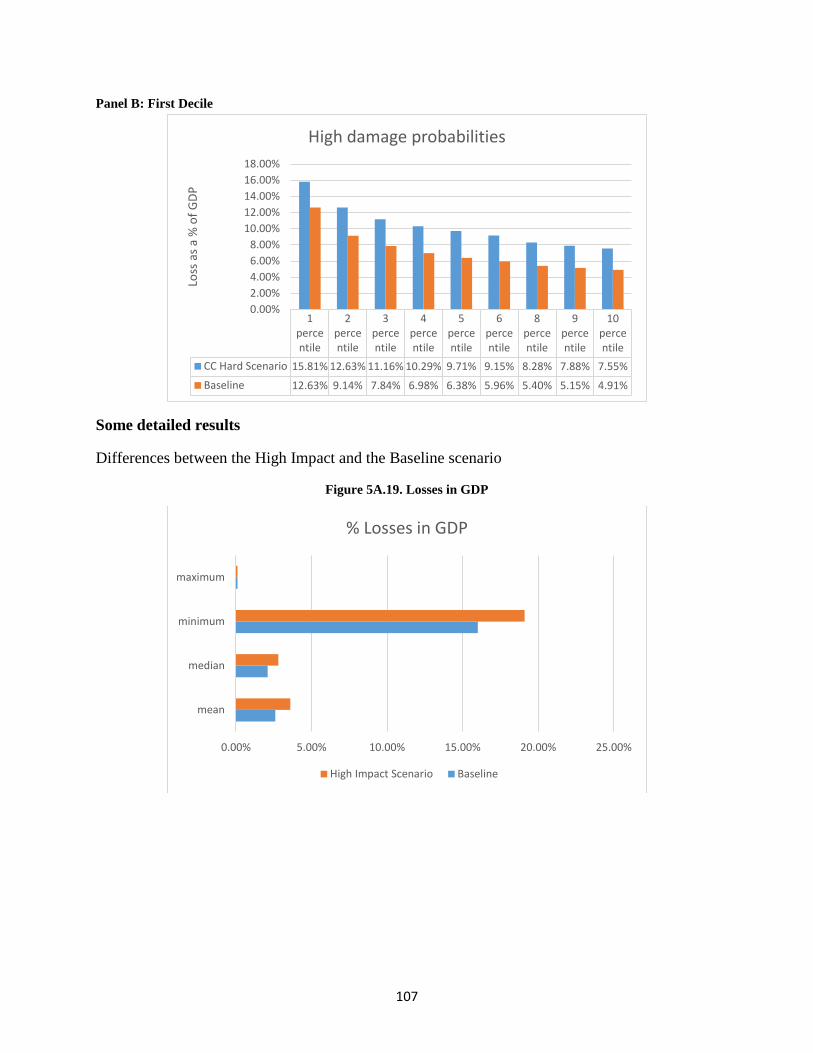
107
Panel B: First Decile
Some detailed results
Differences between the High Impact and the Baseline scenario
Figure 5A.19. Losses in GDP
1percentile
2percentile
3percentile
4percentile
5percentile
6percentile
8percentile
9percentile
10percentile
CC Hard Scenario 15.81% 12.63% 11.16% 10.29% 9.71% 9.15% 8.28% 7.88% 7.55%Baseline 12.63% 9.14% 7.84% 6.98% 6.38% 5.96% 5.40% 5.15% 4.91%
0.00%2.00%4.00%6.00%8.00%
10.00%12.00%14.00%16.00%18.00%
Loss
as a
% o
f GDP
High damage probabilities
0.00% 5.00% 10.00% 15.00% 20.00% 25.00%
mean
median
minimum
maximum
% Losses in GDP
High Impact Scenario Baseline

108
Figure 5A.20. GDP time paths
Figure 5A.21. Expected losses in GDP growth in the high impact scenario
0
200,000,000
400,000,000
600,000,000
800,000,000
1,000,000,000
1,200,000,000
1,400,000,000
1 3 5 7 9 11 13 15 17 19 21 23 25 27 29 31 33 35 37 39
GDP
mean base line
Mean pessimistic scenario
NO EVENT
0.00%0.50%1.00%1.50%2.00%2.50%3.00%3.50%4.00%4.50%5.00%
1 2 3 4 5 6 7 8 9 10 11 12 13 14 15 16 17 18 19 20 21 22 23 24 25 26 27 28 29 30 31 32 33 34 35 36 37 38 39 40
GDP rate of growth
mean base line
Mean pessimistic scenario
NO EVENT
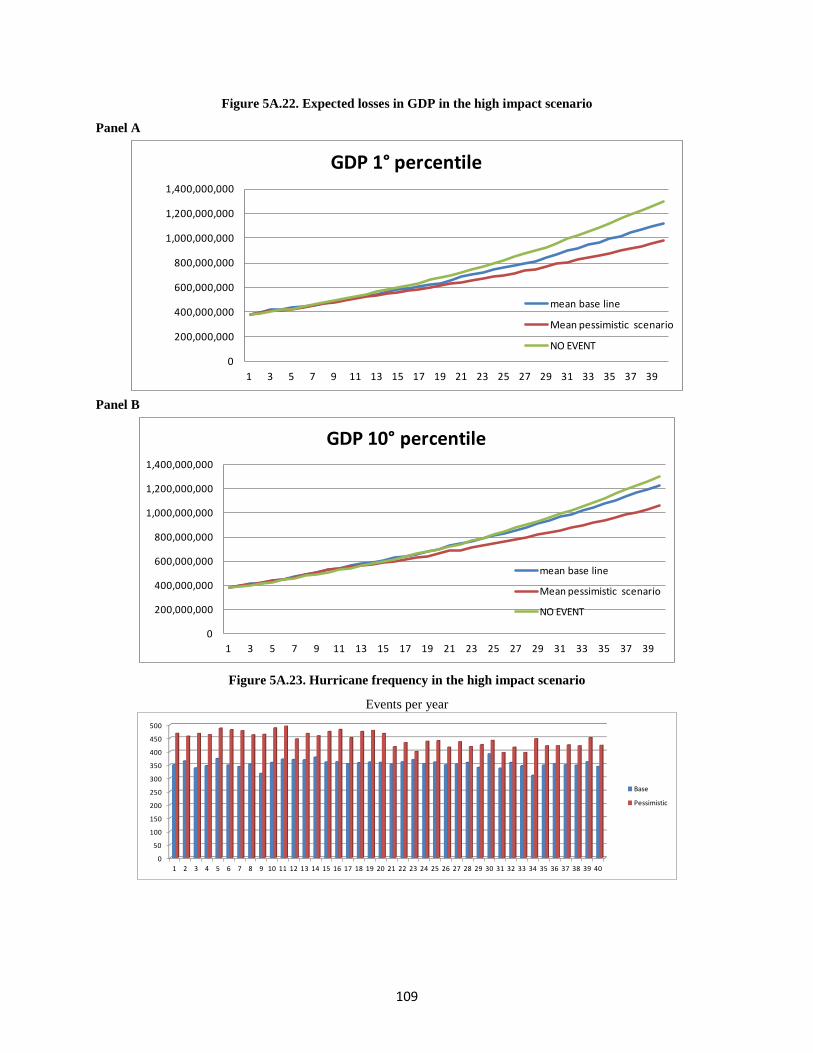
109
Figure 5A.22. Expected losses in GDP in the high impact scenario
Panel A
Panel B
Figure 5A.23. Hurricane frequency in the high impact scenario
Events per year
0
200,000,000
400,000,000
600,000,000
800,000,000
1,000,000,000
1,200,000,000
1,400,000,000
1 3 5 7 9 11 13 15 17 19 21 23 25 27 29 31 33 35 37 39
GDP 1° percentile
mean base line
Mean pessimistic scenario
NO EVENT
0
200,000,000
400,000,000
600,000,000
800,000,000
1,000,000,000
1,200,000,000
1,400,000,000
1 3 5 7 9 11 13 15 17 19 21 23 25 27 29 31 33 35 37 39
GDP 10° percentile
mean base line
Mean pessimistic scenario
NO EVENT
0
50
100
150
200
250
300
350
400
450
500
1 2 3 4 5 6 7 8 9 10 11 12 13 14 15 16 17 18 19 20 21 22 23 24 25 26 27 28 29 30 31 32 33 34 35 36 37 38 39 40
Base
Pessimistic
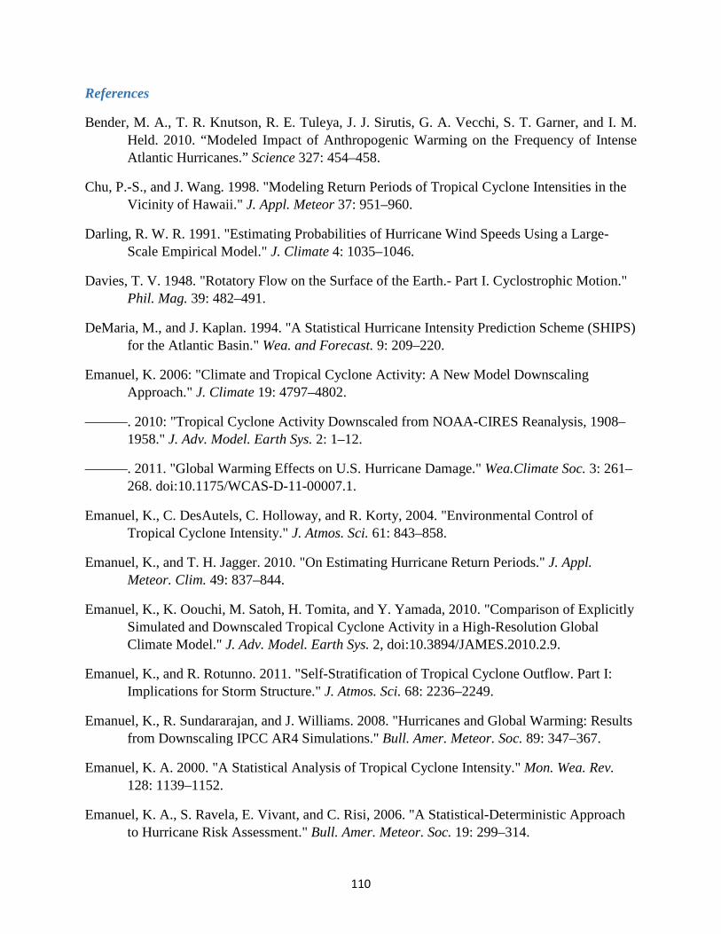
110
References
Bender, M. A., T. R. Knutson, R. E. Tuleya, J. J. Sirutis, G. A. Vecchi, S. T. Garner, and I. M. Held. 2010. “Modeled Impact of Anthropogenic Warming on the Frequency of Intense Atlantic Hurricanes.” Science 327: 454–458.
Chu, P.-S., and J. Wang. 1998. "Modeling Return Periods of Tropical Cyclone Intensities in the Vicinity of Hawaii." J. Appl. Meteor 37: 951–960.
Darling, R. W. R. 1991. "Estimating Probabilities of Hurricane Wind Speeds Using a Large-Scale Empirical Model." J. Climate 4: 1035–1046.
Davies, T. V. 1948. "Rotatory Flow on the Surface of the Earth.- Part I. Cyclostrophic Motion." Phil. Mag. 39: 482–491.
DeMaria, M., and J. Kaplan. 1994. "A Statistical Hurricane Intensity Prediction Scheme (SHIPS) for the Atlantic Basin." Wea. and Forecast. 9: 209–220.
Emanuel, K. 2006: "Climate and Tropical Cyclone Activity: A New Model Downscaling Approach." J. Climate 19: 4797–4802.
———. 2010: "Tropical Cyclone Activity Downscaled from NOAA-CIRES Reanalysis, 1908–1958." J. Adv. Model. Earth Sys. 2: 1–12.
———. 2011. "Global Warming Effects on U.S. Hurricane Damage." Wea.Climate Soc. 3: 261–268. doi:10.1175/WCAS-D-11-00007.1.
Emanuel, K., C. DesAutels, C. Holloway, and R. Korty, 2004. "Environmental Control of Tropical Cyclone Intensity." J. Atmos. Sci. 61: 843–858.
Emanuel, K., and T. H. Jagger. 2010. "On Estimating Hurricane Return Periods." J. Appl. Meteor. Clim. 49: 837–844.
Emanuel, K., K. Oouchi, M. Satoh, H. Tomita, and Y. Yamada, 2010. "Comparison of Explicitly Simulated and Downscaled Tropical Cyclone Activity in a High-Resolution Global Climate Model." J. Adv. Model. Earth Sys. 2, doi:10.3894/JAMES.2010.2.9.
Emanuel, K., and R. Rotunno. 2011. "Self-Stratification of Tropical Cyclone Outflow. Part I: Implications for Storm Structure." J. Atmos. Sci. 68: 2236–2249.
Emanuel, K., R. Sundararajan, and J. Williams. 2008. "Hurricanes and Global Warming: Results from Downscaling IPCC AR4 Simulations." Bull. Amer. Meteor. Soc. 89: 347–367.
Emanuel, K. A. 2000. "A Statistical Analysis of Tropical Cyclone Intensity." Mon. Wea. Rev. 128: 1139–1152.
Emanuel, K. A., S. Ravela, E. Vivant, and C. Risi, 2006. "A Statistical-Deterministic Approach to Hurricane Risk Assessment." Bull. Amer. Meteor. Soc. 19: 299–314.
111
Federov, A. V., C. M. Brierley, and K. Emanuel. 2010. "Tropical Cyclones and Permanent El Niño in the Early Pliocene Epoch." Nature 463: 1066–1070.
Georgiou, P. N., A. G. Davenport, and P. J. Vickery. 1983. "Design Wind Speeds in Regions Dominated by Tropical Cyclones." J. Wind Eng. Ind. Aerodyn. 13: 139–152.
Gnanadesikan, A., K. Emanuel, G. A. Vecchi, G. Anderson, and R. Hallberg. 2010. "How Ocean Color Can Steer Pacific Tropical Cyclones." Geophy. Res. Lett. 37, doi:10.1029/2010GL044514.
Hallegatte, S., J. Hourcade, and P. Dumas. 2007. “Why Economic Dynamics Matter in Assessing Climate Change Damages: Illustration on Extreme Events.” Ecological Economics 62 (2): 330–340
Holland, G. J. 1983. "Tropical Cyclone Motion: Environmental Interaction Plus a Beta Effect." J. Atmos. Sci. 40: 328–342.
Holland, G. J., and P. J. Webster. 2007. “Heightened Tropical Cyclone Activity in the North Atlantic: Natural Variability or Climate Trend?” Philosophical Transactions of the Royal Society.
Kalnay, E., et al. 1996. "The NCEP/NCAR 40-Year Reanalysis Project." Bull. Amer. Meteor. Soc. 77: 437–471.
Katz, R.W., M. Parlange, and P. Naveau. 2002 “Statistics of Extremes in Hydrology.” Advances in Water Resources 25: 8–12, 1287–1304.
Levitus, S. 1982. "Climatological Atlas of the World Ocean." Prof. Pap. No. 13.
Lin, N., K. Emanuel, M. Oppenheimer, and E. Vanmarcke. 2012. "Physically Based Assessment of Hurricane Surge Threat under Climate Change." Nature Clim. Change 2: 462–467 doi:10.1038/nclimate1389.
Lin, N., K. A. Emanuel, J. A. Smith, and E. Vanmarcke. 2010. "Risk Assessment of Hurricane Storm Surge for New York City." J. Geophys. Res. 115, doi:10.1029/2009JD013630.
Mendelsohn, R., K. Emanuel, S. Chonabayashi, and L. Bakkensen, 2012. "The Impact of Climate Change on Global Tropical Cyclone Damage." Nature Clim. Change 2: 205–209. doi:10.1038/nclimate1357.
Minsinger, W. E. 1988. The 1938 Hurricane: An Historical and Pictoral Summary. Greenhill Books, 128 pp.
Murnane, R. J., et al. 2000. "Model Estimates of Hurricane Wind Speed Probabilities." EOS 81: 433–438.
Neumann, C. J. 1987. "The National Hurricane Center Risk Analysis Program (HURISK)." NOAA Tech. Memo NWS NHC 38, 56 pp.
112
Nordhaus, W. D. 2010. “The Economics of Hurricanes and Implications of Global Warming.” Climate Change Economics 1: 1–20.
Pielke Jr., R. A. 2007. “Future Economic Damage from Tropical Cyclones: Sensitivities to Societal and Climate Changes.” Philos. T. Roy. Soc. A 365 (1860): 2717–2729.
Rossby, C.-G. 1948. "On Displacement and Intensity Changes of Atmospheric Vortices." J. Mar. Res. 7: 175–187.
Schmidt, S., C. Kemfert, and E. Faust. 2009. “Simulation of Economic Losses from Tropical Cyclones in 2050. The Effects of Anthropogenic Climate Change and Growing Capital Stock at Risk.” DIW Discussion Paper, 914.
Vickery, P. J., P. F. Skerjl, and L. A. Twisdale. 2000. "Simulation of Hurricane Risk in the U.S. using Empirical Track Model." J. Struct. Eng. 126: 1222–1237.
113
Appendix 6: Ocean Governance: The International Experience
Institutional and governance models can play a critical role in facilitating the development of the blue ocean economy. Some countries have targeted the ocean economy funding strategies and supportive regulatory and business frameworks, others do not specifically assess the potential of the ocean economy. In the following, some approaches chosen by “ocean economy leaders” are identified and analysed with a focus on how countries in particular approach and evaluate investment opportunities and what supportive and sustainable policies, regulatory bodies or other institutional arrangements are in place or are being considered. These challenges are discussed along a number of markers for success:
• Comprehensive assessment approach
• A clear strategy, communicated with strong national blue economy goals
• Engagement of all stakeholders, with dedicated government structures
• Regulatory framework
• Seed funding and investment support
• Business follow-through
• Long-term sustainability
Comprehensive Assessment Approach
Countries attempt to balance competing interests through multi-stakeholder processes. One assessment framework that looked at the institutional capacities towards ocean prosperity was the Economist Coastal Governance Index 201525. It ranked countries such as Norway and New Zealand highly, suggesting that participatory inclusion in decision-making and accountability may contribute to better policies in this area. Well-developed regulatory frameworks around coastal management and marine spatial planning.
Such assessment needs to take account not only business opportunities and job creation but also assess the opportunity cost of continuing unsustainable practices. The ocean economy encompasses ocean-based industries (such as shipping, fishing, offshore wind, marine biotechnology), but also the natural assets and ecosystem services that the ocean provides (fish, shipping lanes, CO2 absorption and the like). Balancing investment opportunities effectively requires identification of future revenue opportunities in a rapidly changing marine environment.
Recent OECD research26 suggests that there will be comparatively high rates of growth in sectors such as marine aquaculture, offshore wind and port activities. On the other hand ocean risks and
25https://www.oceanprosperityroadmap.org/wp-content/uploads/2015/05/EIU_CGIndex_WEB-revised-June-4.pdf 26OECD (2016), The Ocean Economy in 2030, OECD Publishing, Paris. http://dx.doi.org/10.1787/9789264251724-en.

114
threats, such as the impact of ocean warming on storm surges have implications for coastal resilience planning and required infrastructure investments. As a consequence, forward-thinking ocean economies use broadly-based risk-assessment processes that draw on science and scenario planning approaches and are coordinated by governments and established high-level advisory bodies and necessary supporting components for public investment decisions into the ocean economy27. This is particularly important for early-stage technology investments with longer time horizons, such as for ocean energy.
A Clearly Strategy, Communicated with Strong National Blue Economy Goals
Ireland set itself ambitious targets and a clearly communicated strategy through its integrated marine plan28. It identified Ireland’s marine assets as a key element of economic recovery and sustainable growth for the country, based on a specific target to double Ocean Wealth to 2.4% of GDP by 2030. This public leadership is critical to set out the government commitment and give civil servants as well as the broader economy a visible sign of engagement.
A number of countries have raised the profile for the blue economy by creating relevant Ministries and integrating the maritime sector at cabinet level. Grenada has set up a National Ocean Governance Committee that includes senior officials from key ministries and authorities. Portugal’s Minister for the Sea, Ana Paula Vitorino, has stated that "the economy of the sea will always be the future of Portugal”. This form of signalling is useful to engage the public and assure investors.
Ireland, Portugal29 and recently Norway have well-elaborated and published long-term ocean economy strategies, based on transitioning their existing marine sectors through science and technology innovation into long-term sustainable growth along the pillars of a marine bio-economy, ocean logistics and coastal development, including for tourism and renewable energy. These strategies aim for the ocean economy to grow in excess of the terrestrial economy, doubling its value by 2030. These strategies recognise that ocean economy growth and job creation will not come from extractive marine activities but rather from services and innovation, and will require investment in protecting the natural capital of the ocean. We need healthy and productive seas and innovative technology so that we can obtain more food, medicines and energy from the oceans’, said recently Norway’s Prime Minister Erna Solberg. All three European countries have Ministries with specific responsibilities for the sector, supported by a range of subsidiary bodies.
Other ocean countries such as Canada or New Zealand have a less integrated approach. In the latter there is already a debate ongoing, suggesting that better integration is needed in managing different activities and pressures and across sectors. Marine spatial planning is seen as an under-utilised tool and institutional arrangements may be reformed. Currently oceans management is split between agencies but a dedicated oceans agency may be considered.
27 Relevant examples are the German Advisory Council on Global Change and the UK Natural Capital Committee. 28 http://oar.marine.ie/bitstream/10793/810/1/Harnessing%20Our%20Ocean%20Wealth%20Report.pdf. 29 http://search.proquest.com/docview/1816604094?pq-origsite=gscholar.
115
Engagement of All Stakeholders, with Dedicated Government Structures
Bringing all parties into the process of fostering marine solutions is key, starting with science, business and wider civil society. In Ireland for instance, task forces were established to strengthen the work of the Marine Coordination Group (MCG) and to progress a number of the actions agreed. It benchmarked itself against countries with strong marine sectors such as Norway, the UK, Singapore & Canada’s maritime province of Nova Scotia, identified key components of its national value composition and used a “whole-of-enterprise” approach to market its propositions. A Development Task Force was set up to facilitate transformative actions required across government departments, public agencies, as well as business, regional and local organisations.
Drawing on business associations and other relevant bodies is an important way to achieve wide participation in particular of small and medium enterprise, thereby increasing the likelihood for more job creation and other broader economy benefits. In many critical ways the positive impact of an ocean economy push will only be felt if related support industries likewise improve performance. Their progress and positive impact on the tax base is an necessary feedback mechanism.
However countries still have need for additional marine research to unlock knowledge and understanding required to support sustainable growth. Generally the data provided for instance does not include the added value of ecosystems services. The main subjects of non-market valuation research for oceans and marine ecosystems include: ocean physical resources (real estate value, shoreline protection, aesthetics, ambient and facilities temperature moderation, geological features); aspects of marine tourism and recreation; ecosystem services (biodiversity, waste assimilation, life support, climate regulation); research and education, culture and heritage, health (air and water quality); and investment (bequest and option values). By fully assessing the opportunities along all of those vectors public funding can be targeted to areas that will have the most impact.
Regulatory Framework
Developing a comprehensive regulatory framework for ocean activities that provide investors with planning clarity, rapid permitting and other facilitation is another aspect of successful governance. In 2014, Portugal approved Law n. 17/2014, 10 April, which established the legal basis for its policy on marine spatial planning and management applicable to its whole maritime space adjacent to its mainland and archipelagos, including the continental shelf beyond 200 nautical miles.30
The Irish Department of Communications, Energy and Natural Resources has prepared an Offshore Renewable Energy Development Plan (OREDP) which describes the policy context for development of offshore wind, wave and tidal stream energy in Irish waters for the period to 2030. A Strategic Environmental Assessment has been undertaken to evaluate the likely significant 30 Ferreira, M.A.; Johnson, D.; and Pereira da Silva, C., 2016. Measuring success of Ocean governance: a set of indicators from Portugal. In: Vila-Concejo, A.; Bruce, E.; Kennedy, D.M., and McCarroll, R.J. (eds.), Proceedings of the 14th International Coastal Symposium (Sydney, Australia). Journal of Coastal Research, Special Issue, No. 75, pp. 982 - 986. Coconut Creek (Florida), ISSN 0749-0208
116
environmental effects of implementing the plans to develop offshore renewable (offshore wind, wave and tidal) energy in Irish waters.
Creating an infrastructure to support the blue economy is seen as critical to the success of Ireland’s integrated marine plan. SmartBay Subsea Observatory has now started streaming high speed data from the seabed at Galway Bay to businesses, researchers, scientists and policy makers. It will drive innovation in SMEs and multinational companies in the ocean energy sector. A dedicated Marine Development Team involving major development agencies of the state in an integrated inter agency based approach tis tasked to deliver further development of the blue economy. It makes recommendations to the cross Departmental Marine Coordination Group.
Canada’s Oceans Act was the world’s first comprehensive legislation for oceans management in 1997. Since Canada has developed its Oceans Strategy, Canada’s Oceans Action Plan and a number of Health of the Oceans Initiatives. All this information about the various roles the federal government as well as the provinces plays within Canada’s oceans sector is accessible from a single website.31 Canada’s federal and provincial government departments, universities and ENGOs comprising this sector occupy a relatively large presence in the marine economy as managers, stewards and researchers.
The EU Commission further identified the fundamental aspects for an efficient planning of the maritime space: a predictable legal regime, internal coordinating structures for maritime affairs, avoidance of duplication of regulatory powers of different national or regional authorities, and replacing overlapping and double-track decision-making by a one-stop-shop approach.
Seed Funding and Investment Support
Whilst there is limited international capacity in fully publicly financing the roll-out of the new ocean economy, creating incentives and mechanisms at a country or regional level through innovative finance and investment support to develop and advance new technologies and to demonstrate the viability of a sustainable blue economy. The European Union has an extensive support framework for such efforts through its Horizon 2020 program. In Canada support activities focus for instance on community economic diversification, small and medium enterprises, and collaborative research and development.
The Irish development plan suggests that scale of investment required by the State will require a detailed analysis of each of the thematic areas, including consideration of existing sectoral plans. Based on the target of increasing turnover from the marine economy of €3bn and assuming a threefold return on investment, leveraged investment funds of the order of €1bn would be required. Further assuming a three to one private to public contribution to investment funds, indicative seed funding of €250m over 5 years is estimated. Since 2009, the Irish agency has supported over 80 early stage ocean energy projects through its Prototype Development Fund to the value of €13
31 http://www.dfo-mpo.gc.ca/oceans/publications/cg-gc/index-eng.html
117
million, many of which are now at full-scale testing or are nearing commercialisation.32 A recent example is the €2.8m package to assist 13 Coastal Local Authorities to undertake and complete 51 development and repair projects on harbours and slipways owned by them.
Portugal decided to set up a central mechanism that could be used as a “first push” in all activities related to the ocean in particular the ones that are priorities: ocean economy, marine environment and natural capital, scientific research, innovation and knowledge transference. The Fundo Azul (Blue Fund) reconciles public investment, risk capital, and contributions of usage of maritime spaces. The financing of the Blue Economy in Portugal is not an exclusive obligation of the government, who concentrates on simplifying the administrative burdens for business companies. Portugal also has a program dedicated to fisheries and integrated maritime policy, “Mar 2020” which is complementary to the “Blue Fund”. In the private sector the Blue Bio Alliance is a cluster of actors (companies, research groups, associations) working in the marine bio-resources and blue biotech value chain.
Finance can not only be sourced from national sources but will require support from multinational institutions and commercial funders. To develop a pipeline of bankable projects requires a full analysis of the key cost and revenue components, and the overall project risk will be critically depend on the long-term stability and predictability of the governance framework for these transactions. The European Investment Bank is one of the large multilateral infrastructure funding providers that is involved in such ocean finance33.
In Norway, Innovation Norway is owned by the Ministry of Trade, Industry and Fisheries (51%) and the county authorities (49%). The Norwegian Industrial Biotechnology Network and the Norwegian Innovation Clusters strengthen collaboration in regional business clusters to make enterprises more innovative and competitive.
• Business Networks support small and medium-sized businesses that enter into commercially strategic collaborations with other enterprises.
• Competence Development in regional business communities make relevant expertise more accessible to enterprises in the regions through collaboration with universities and university colleges.
• Regional development provide guidance and quality assurance to local authorities in municipalities/regions with development/restructuring status.
InnovFin is a joint initiative launched by the European Investment Bank (EIB) and the European Investment Fund (EIF) in cooperation with the European Commission under the EU framework programme for research and innovation – Horizon 2020. Norway is an associated country to
32 https://www.ouroceanwealth.ie/sites/default/files/sites/default/files/news/Final%20Our%20Ocean%20Wealth%20Development%20Task%20Force%20Report.pdf 33 http://www.eib.org/projects/sectors/index.htm
118
Horizon 2020 and participates fully in the framework programme. Norwegian stakeholders have full access to the InnovFin financial instruments and advisory services.
A recent Norwegian foreign policy white paper summarises its development policy efforts to promote sustainable use of the oceans. The Government will
• launch dialogues on ocean affairs with relevant countries with a view to sharing experience and expertise and cooperating on measures to promote clean and healthy oceans, sustainable use of marine resources and growth in the blue economy
• strengthen the dialogue with influential countries on the part the shipping industry can play in further improving the environmental performance of the transport sector at global level
• call for higher priority to be given to fisheries and aquaculture in efforts to improve global food security
• consider establishing a centre of expertise on ocean and Arctic issues in Tromsø
• establish a development programme with a budget of NOK 100 million to combat marine litter and microplastics; this will include steps to reduce waste quantities and improve waste management
• allocate over NOK 5 billion to climate-related measures through the development assistance budget in 2017, in order to reduce the negative impacts of climate
• change on the oceans increase support for sustainable blue growth as part of its development policy by providing more funding for the Fish for Development programme. The new research vessel RV Dr Fridtjof Nansen will make it possible to significantly step up Norway's assistance for ecosystem-based marine management in developing countries
• intensify efforts to combat IUU fishing and fisheries crime, and urge more states to ratify the Port State Measures Agreement on IUU fishing.
Business Follow-Through
Business engagement and private sector investment will be primarily driven by the long-term revenue opportunity, which does not only depend on market access but also on how linked the companies will be to international value chains. Investment blueprints and pathways will need to take account of market conditions and dynamics, including the terms of capital at risk and types of grant support. Identifying interconnected clusters of economic activities that can garner more attention and benefit from more coherent strategic approaches to their development. Examples are the biotechnology sector – health and medicine, agriculture and food, industry – have come to be
119
perceived as “bioeconomy” in their strategic goals34. Norway has both a specific research counsel and leading companies and support efforts for the marine biotech sector35.
Looking to 2030, scientific and technological advances are expected to play a crucial role both in addressing many of the ocean-related environmental challenges and in the further development of ocean-based economic activities. Funding and better use of innovations for gathering better data quality are all part of delivering meaningful progress for the ocean economy. Innovations in advanced materials, subsea engineering and technology, sensors and imaging, satellite technology and nanotechnology will affect every sector of the ocean economy. Therefore corporate engagement and global business connectivity will ultimately decide the success of the ocean economy sector and thus the specific support to the ocean sector will be less important than the overall climate in the country for business innovation and success.
Long-term Sustainability
Investments in maritime infrastructure such as ports need to be predicated upon the development of long-term sustainability, for instance through sound fisheries management36. Likewise coastal tourism, one of the most readily available sectors for blue economy growth, depends on clean waters and healthy marine life. Food security and the economic well-being of millions of people depend on sustainable fisheries, which require innovative approaches to management that can balance ecological, economic, and social objectives. There is empirical evidence that dynamic ocean management, or real-time ocean management, can increase the efficacy and efficiency of fisheries management over static approaches by better aligning human and ecological scales of use.37
All ocean economies mentioned have identified long-term challenges for their marine environment.
As an example, the New Zealand Ministry of the Environment suggested recently, that the three key issues are:
• Global greenhouse gas emissions are causing ocean acidification and warming
• Native marine birds and mammals are threatened with extinction
• Coastal marine habitats and ecosystems are degraded
The most important coastal pressures, alongside ocean acidification and climate change impacts, are excess sedimentation, seabed trawling and dredging for fish and shellfish, marine pests and excess nutrients carried down waterways. Other coastal pressures include harmful fishing methods,
34 German Bioeconomy, 2015 35 http://www.marinebiotech.eu/wiki/Marine_Biotechnology_in_Norway 36 Long RD, Charles A, Stephenson RL (2015) Key principles of marine ecosystem-based management. Mar Policy 57:53–60 37Dunn, D.C., Maxwell, S.M. Boustany, A.M. and Halpin, P.N. (2016) Dynamic ocean management increases the efficiency and efficacy of fisheries management. vol. 113 no. 3 pp668–673, doi: 10.1073/pnas.1513626113

120
dumping of dredge spoils, reclamation (infilling of harbours and estuaries for coastal development) and pollution from waste water and plastic debris.38
As a consequence, an important part of blue economy growth will need to focus to strengthening coastal resilience and marine ecosystems. Offshore wind is for instance expected to grow rapidly as economies transition to renewable energy, where it has shown early success is in countries with clear regulatory frameworks and funding regimes.
Conclusions
Successful ocean economies have developed clearly articulated strategies and governance approaches that assure that the relevant sectors have visibility, are fully engaged in the governance process and have access to support and seed funding in particular during early development stages. Science, innovation and conservation are critical components of these strategies.
However whilst the public sector acts as facilitator, investment decisions are ultimately taken by private business, and funding beyond the early technology stage is provided through existing commercial and other avenues in the normal way. Successful ocean economies tend to also have a range of other supporting institutional features, including experienced bureaucracies, established public-private partnership mechanisms, deep capital markets and longer-term planning horizons.
Sector choices and priorities reflect broader societal choices, reflecting for instance the shift from extraction to a renewable and circular economy. Whilst coastal tourism will remain in many places a large component of ocean sector revenues it will critically depend both on protection of the marine biodiversity and development of sustainable coastal infrastructure, traditional activities such as fishing and shipping will require help with the transition to long-term sustainability.
Ocean energy will take time and significant investment before it becomes a larger part of the energy mix39, whilst ocean data and ocean biotech are still small but offer exciting growth opportunities provided they can be embedded into a supportive science and innovation technology policy. Government and the public sector will need to continue to offer a supportive infrastructure, whilst it will in the end depend on the private sector to build a resilient economy.
Successful open economies with clear regulatory structures, government strategies and support mechanisms for innovation are also likely to have successful marine sectors, but these may be small in the context of the overall economy.
A strategic emphasis in the form of a national ocean plan (for example, Ireland), supported by a dedicated Minister for the Sea (for example, Portugal), targeted support and investment into marine innovation (for example, Norway), funding support for research and infrastructure (for example, European Union), including at regional and local level (for example, Canada) and a comprehensive
38 http://www.eds.org.nz/assets/MediaReleases/2016%20Releases/Our%20marine%20environment%202016%20report.pdf 39 http://www.seai.ie/Publications/SEAI_Corporate_Publications_/Strategy_Documents/SEAI_5yr_strategy.pdf

121
analysis of the specific future challenges (for example, New Zealand) are identified here is key components for sustainable blue growth.