Microsoft® Excel

® 2010 Training

Excel 2010 Basics

Overview

• Excel is a spreadsheet, a grid made from columns and rows. It is a software program that can make number manipulation easy and somewhat painless.

• Excel called as “Workbook” and it contains one or more worksheets.

• Spreadsheets are made up of

• Columns

• Rows

• and their intersections are called cells

What is a COLUMN ?

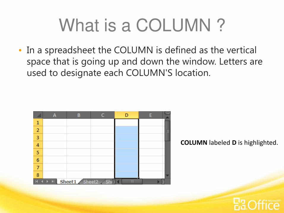
• In a spreadsheet the COLUMN is defined as the vertical space that is going up and down the window. Letters are used to designate each COLUMN'S location.

COLUMN labeled D is highlighted.

What is a row?

• In a spreadsheet the ROW is defined as the horizontal space that is going across the window. Numbers are used to designate each ROW'S location.

ROW labeled 4 is highlighted.

What is a CELL ?

• A CELL is the space where a row and column intersect. Each CELL is assigned a name according to its COLUMN letter and ROW number.

In the above diagram the CELL labeled

C2 is highlighted.

Microsoft® Excel

® 2010 Training

Part 1 – Formula’s & Functions

Basic Math Functions

• Math functions built into them. Of the most basic operations are the standard multiply, divide, add and subtract.

Sum function

Average Function

• The average function finds the average of the specified data. (Simplifies adding all of the indicated cells together and dividing by the total number of cells.)

Max & Min Functions

• The Max function will return the largest (max) value in the selected range of cells. The Min function will display the smallest value in a selected set of cells.

Count Function

• The Count function will return the number of entries (actually counts each cell that contains NUMBER DATA) in the selected range of cells.

• Remember: cell that are blank or contain text will not be counted.

IF Function

• IF Functions are like programing - they provide multiple answers based on certain conditions.

IF Function

• The IF function will check the logical condition of a statement and return one value if true and a different value if false.

• The syntax is: =IF (condition, value-if-true, value-if-false)

Other Useful Functions

Date & Time Functions

• Date()

• Now()

• Today()

• Year()

• Month()

• Day()

Other Useful Functions

• Text Functions

• Concatenate

• Left

• Right

• Proper

• Upper

• Lower

• Trim

Example

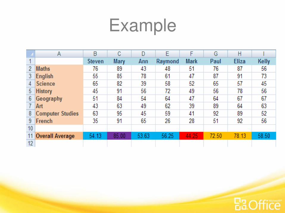
• Create the following spreadsheet.

• Mark sheet for 8 students.

• Subjects are : Maths , English, Science, History, geography, Art, Computer Science & French

• Find the average for 8 students and the subjects

Example

Microsoft® Excel

® 2010 Training

Part 2 -Conditional Formatting

Conditional Formatting

• Conditional Formatting allows you to change the appearance of a cell, depending on certain conditions.

Example

• Highlight the cells with Overall Grades, which should be cells B11 to I11.

• The Overall Averages range from 44 to 85. We'll colour each grade, depending on a scale. A different colour will apply to the following grades.

• 50 and below

• 51 to 60

• 61 to 70

• 71 to 80

Example

• So five different bands, and a colour for each. To set the Conditional Formatting in Excel, do the following:

• With your Overall Averages highlighted, click on the Home menu at the top of Excel

• Locate the Styles panel, and the Conditional Formatting item:

Example

• The Conditional Formatting menu gives you various options. click on More Rules, from the Colour Scales submenu-> Format only cells that contain

Example

• Under the heading Edit the Rule Description. It says Cell Value and Between, in the drop down boxes. These are the ones we want. We only need to type a value for the two boxes that are currently blank in the image above. We can then click the Format button to choose a colour.

• So type 0 in the first box and 50 in the second one:

Make the switch to Excel 2010

Example

• Then click the Format button. You'll get another dialogue box popping up. This is just the Format Cells one though.

• Click on the Fill tab and choose a colour. Click OK and you should see something like this under Edit the Rule Description:

Example

• "If the Cell Value is between 0 and 50 then colour the cell Red".

• Click OK on this dialogue box to get back to Excel. From the menu, click on Manage Rules:

Click the New Rule button, Set a new

colour for the next scores - 51 to 60.

Choose a colour, and keep clicking OK until

you get back to the Rules Manager dialogue

box. It should now look something like this

one:

Example

• Set a new colour for the next scores - 51 to 60. Choose a colour, and keep clicking OK until you get back to the Rules Manager dialogue box. It should now look something like this one:

Example 1. We now have to colours in our range. Do the rest of the scores,

choosing a colour for each. The scores are these, remember:

2. 50 and below

3. 51 to 60

4. 61 to 70

5. 71 to 80

6. 81 and above

7. When you've done them all, your dialogue box should have five colours:

Make the switch to Excel 2010

Example

The colours above are entirely arbitrary, and you don't have to select the same

ones we did. The point is to have a different colour for each range of scores.

But click OK when you're done. Your Overall Averages will then look something

like this:

Example

Microsoft® Excel

® 2010 Training

Part 3 - Charts

Charts

• A chart is a tool you can use in Excel to communicate your data graphically.

• Charts allow your audience to see the meaning behind the numbers, and they make showing comparisons and trends a lot easier.

• In this lesson, you will learn how to insert charts and modify them so that they communicate information effectively.

Types of charts

• Column Chart

• Bar Chart

• Line Chart

• Pie chart

• Area Chart

• Surface Chart

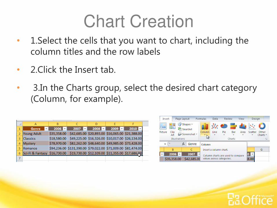
Chart Creation • 1.Select the cells that you want to chart, including the

column titles and the row labels

• 2.Click the Insert tab.

• 3.In the Charts group, select the desired chart category (Column, for example).

Chart Creation

• 4.Select the desired chart type from the drop-down menu (Clustered Column, for example

Chart Creation

Chart Tools

• Once you insert a chart, a set of Chart Tools, arranged into three tabs, will appear on the Ribbon. These are only visible when the chart is selected. You can use these three tabs to modify your chart.

Make the switch to Excel 2010

Microsoft® Excel

® 2010 Training

Part 4 – Spark Lines

Spark Lines • A Sparkline is a small chart that is aligned with rows

of some tabular data and usually shows trend information.

• Select the data from which you want to make a sparkline.

• Go to Insert > Sparkline and select the type of sparkline (you have 3 options – line, column and win-loss chart)

• Specify a target cell where you want the sparkline to be placed

• Optional: Format the Sparkline if you want.

• Here is a short screen-cast showing you how a Sparkline is created.

How to create sparklines

Types of Sparklines • There are 3 basic types of sparklines in Excel

2010. They are,

• Line chart

• Column chart

• Win-loss chart (useful for showing a bunch of wins & losses denoted by 1s and -1s)

Microsoft® Excel

® 2010 Training

Part 5 - VLookup / HLookup

VLOOKUP / HLOOKUP

• The “V” in vlookup stands for “vertical” and “lookup”.

• The “H” in Hlookup stands for “Horizontal” and “lookup”.

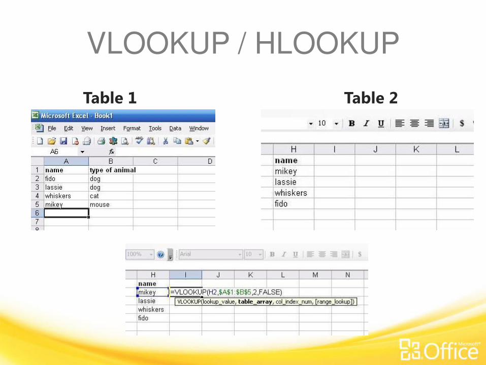
• This function allows you to look up values in a table that are listed in column format (how most tables are laid out), given another value (let’s call this the “key”). Vlookup’s format looks like the following:

• =vlookup(lookup value, table where values reside, column # where values are located, false)

Vlookup’s format looks like the following:

• =lhookup(lookup value, table where values reside, row# where values are located, false)

VLOOKUP / HLOOKUP

Table 1 Table 2

Microsoft® Excel

® 2010 Training

Part 6 , 7 & 8- Pivot Table , Pivot Charts & Slicers

Pivot Table

• As name implies it pivots down the existing data table and tries to make user understand the crux of it.

• It has been extensively used to summarize and clean up the data

• Make sure that all rows and columns are selected

Pivot Table

• You will reach Create Pivot Table dialog box. Excel fills in data range from first to last selected columns and rows. You can also specify any external data source to be used. Finally choose worksheet to save the pivot table report. Click OK to proceed further

Pivot Table

• . Now we will populate this table with data fields which is being present at the right side of the Excel window.

Pivot Table

• . Now we will populate this table with data fields which is being present at the right side of the Excel window.

Pivot Charts

• A pivot chart is the visual representation of a pivot table in Excel. Pivot charts and pivot tables are connected with each other.

• Below you can find a two-dimensional pivot table.

Slicers

• Slicers are easy-to-use filtering components that contain a set of buttons that enable you to quickly filter the data in a PivotTable report, without the need to open drop-down lists to find the items that you want to filter.

• A slicer header indicates the category of the items in the slicer.

• A filtering button that is not selected indicates that the item is not included in the filter.

• A filtering button that is selected indicates that the item is included in the filter.

Create a slicer in an existing

PivotTable • Click anywhere in the PivotTable report for which you

want to create a slicer.

• This displays the PivotTable Tools, adding an Options and a Design tab.

• On the Options tab, in the Sort & Filter group, click Insert Slicer.

Create a slicer in an existing

PivotTable

• In the Insert Slicers dialog box, select the check box of the PivotTable fields for which you want to create a slicer.

• Click OK.

• Slicer is displayed for every field that you selected.

• In each slicer, click the items on which you want to filter.

• To select more than one item, hold down CTRL, and then click the items on which you want to filter.

Microsoft® Excel

® 2010 Training

Part 9 – Record Macro

Record Macro

• This helps us to save time by automating tasks that you perform frequently.

• A macro is a series of commands grouped together that you can run whenever you need to perform the task.

Record Macro • Display the Developer tab

• The Developer tab provides access to the macro commands, but this tab doesn't appear by default. To display the Developer tab, follow these steps:

• Click the File tab and then click Options.

• The Excel Options dialog box appears.

• Click Customize Ribbon in the left pane, and then select the Developer check box under Main Tabs on the right side of the dialog box.

• Click OK.

• The Developer tab appears in the Ribbon.

Record Macro • Record a macro

• Follow these steps to record a macro:

• Choose Record Macro in the Code group of the Developer tab.

• The Record Macro dialog box appears.

• Type a name for the macro in the Macro Name text box.

• The first character of the macro name must be a letter, and the name cannot contain spaces or cell references. Macro names are not case-sensitive.

• (Optional) Assign a Shortcut Key.

Record Macro • If you select a shortcut key already used in Excel, the macro

shortcut key overrides the Excel shortcut key while the workbook that contains the macro is open.

• From the Store Macro In drop-down list, select where you want to store the macro:

• This Workbook: Save the macro in the current workbook file.

• New Workbook: Create macros that you can run in any new workbooks created during the current Excel session.

• Personal Macro Workbook: Choose this option if you want the macro to be available whenever you use Excel, regardless of which worksheet you're using.

• (Optional) Type a description of the macro in the Description text box.

Record Macro

• Click OK.

• The Record Macro option on the Developer tab changes to Stop Recording.

• Perform the actions you want to record.

• Excel records your steps exactly — such as (Select cell C3) — but you can also record the steps relative to any current cell — such as (Go up one row and insert a blank line). To do so, click the Use Relative References button on the Developer tab. You can turn the Use Relative References feature on and off as needed when recording the macro.

• Choose Stop Recording in the Code group of the Developer tab.

Record Macro