Journal of Computational Physics 257 (2014) 937–953

Contents lists available at ScienceDirect

Journal of Computational Physics

www.elsevier.com/locate/jcp

Well-Balanced Adaptive Mesh Refinement for shallow waterflows ✩

Rosa Donat a, M. Carmen Martí a, Anna Martínez-Gavara b, Pep Mulet a,∗a Departament de Matemàtica Aplicada, Universitat de València, Spainb Departament de Estadística i Investigació Operativa, Universitat de València, Spain

a r t i c l e i n f o a b s t r a c t

Article history:Received 18 January 2013Received in revised form 19 September2013Accepted 20 September 2013Available online 27 September 2013

Keywords:Structured Adaptive Mesh RefinementWell-balanced schemesShallow water equationsWell-balanced interpolation

Well-balanced shock capturing (WBSC) schemes constitute nowadays the state of the artin the numerical simulation of shallow water flows. They allow to accurately representdiscontinuous behavior, known to occur due to the non-linear hyperbolic nature of theshallow water system, and, at the same time, numerically maintain stationary solutions.In situations of practical interest, these schemes often need to be combined with somekind of adaptivity, in order to speed up computing times. In this paper we discuss whatingredients need to be modified in a block-structured AMR technique in order to ensurethat, when combined with a WBSC scheme, the so-called ‘water at rest’ stationary solutionsare exactly preserved.

© 2013 Elsevier Inc. All rights reserved.

1. Introduction

The shallow water equations are a non-linear, hyperbolic, system of balance laws, which are obtained from the Navier–Stokes equations by depth averaging, after neglecting effects such as turbulence or shear stress. If only the effect of thebottom elevation, or bathymetry is considered, they take the following form

ht + div(hv) = 0

(hv)t + div

(hv ⊗ v + gh2

2I2

)= −gh∇z, (1)

where h denotes water depth, v = (vx, v y) is the depth-averaged velocity, g is the gravity acceleration, z is the bottomelevation and I2 is the 2 × 2 identity matrix. We will also denote the discharge by q := hv . This system is widely used inmany applications to model flows in river and coastal areas, and has received a lot of attention in the scientific communityduring the last ten to fifteen years. There has been a tremendous research effort towards the development of numericaltechniques for the shallow water equations. This effort is due in part to the many modeling applications of shallow waterflows, but it is also due to the fact that there are specific difficulties in the numerical simulation of this system that makethe problem attractive and challenging.

On a flat bathymetry, the shallow water equations (1) become a homogeneous system of conservation laws. Their solu-tions may develop discontinuities, even when the initial flow is smooth, which requires the use of shock-capturing schemesin order to ensure a proper handling of discontinuities in numerical simulations concerning this system of equations.

✩ This research was partially supported by Spanish MINECO MTM 2011-22741.

* Corresponding author.E-mail addresses: donat@uv.es (R. Donat), maria.c.marti@uv.es (M.C. Martí), Ana.Martinez-Gavara@uv.es (A. Martínez-Gavara), mulet@uv.es (P. Mulet).

0021-9991/$ – see front matter © 2013 Elsevier Inc. All rights reserved.http://dx.doi.org/10.1016/j.jcp.2013.09.032

938 R. Donat et al. / Journal of Computational Physics 257 (2014) 937–953

The presence of a non-flat bathymetry leads to the inclusion of source terms in the system related to the bottomgeometry. It is well known that naive discretizations of these source terms may lead to spurious, numerical, waves thatcan obscure, or even ruin, the real solution that needs to be computed. This spurious numerical behavior occurs whencomputing stationary, or nearly stationary, solutions, for which the balance between the convective fluxes and the sourceterms associated to the bathymetry is not respected by the numerical scheme. Well-balanced schemes [8,20] are specificallydesigned in order to maintain this balance, to machine accuracy if possible, and Well-balanced Shock Capturing (WBSC)schemes constitute nowadays the state of the art in the numerical simulation of shallow water flows.

Robust and accurate WBSC schemes often have a high computational cost, which is related to the fact that they incorpo-rate upwinding through characteristic information that needs to be computed at each cell boundary in the computationaldomain, high order reconstruction procedures, and a sophisticated numerical treatment of the bathymetry source term. Insituations of practical interest, it is highly desirable to combine a WBSC scheme with an adaptive technique that can lowerits high computational cost in 2D simulations [18,6,23,27,24].

The efficiency of an AMR algorithm is related to the reliability of the mesh adaption procedure, which is usually con-trolled by user-dependent thresholding parameters. Good efficiency factors are obtained when the thresholding parameter isrelatively large, however, the use of an ‘efficient’ thresholding parameter might lead to spurious numerical behavior, akin tothat observed when a non-Well-Balanced (NWB) numerical scheme is used on a uniform mesh, when computing stationaryor nearly stationary solutions to the water shallow model, even if the underlying solver is a WBSC scheme.

In this work we analyze a block structured AMR technique developed in [4] and point out that, in addition to usinga WBSC scheme as the underlying scheme in the AMR process, it is necessary to implement Well-Balanced interpolatorytechniques in the transfer operators involved in the multi-level grid structure in order for the combined AMR-WBSC schemeto maintain its well-balanced character.

The paper is organized as follows: In Section 2 we briefly recall the underlying WBSC scheme used by the blockstructured AMR technique and in Section 3 we recall the main ingredients of this technique, identifying those which arepotentially responsible for the Well-Balance (WB) loss. In Section 4 we describe the necessary corrections to obtain a WB-AMR code and in Section 5 we show several numerical experiments that support our discussion. We close in 6 with someconclusions and perspectives for future work.

2. Well-balanced schemes for shallow water flows

The shallow water system (1) admits stationary solutions, in which non-zero flux-gradients are exactly balanced by thesource terms. Such solutions, along with their perturbations, are difficult to capture numerically because straightforwarddiscretizations of the source term fail to preserve this balance. Computing these solutions is indeed a challenge and thereis a large body of recent research concerning numerical techniques that incorporate the necessary balance in their discretedesign (e.g. [28,9,18,16,33,31,12]). Such schemes are termed well-balanced (WB) schemes after the work of Leroux andcollaborators [20,21]. Bermúdez and Vázquez-Cendón, in an independent work [8], introduced the concept of the C-property.A scheme is said to satisfy the exact C-property if it preserves exactly the ‘water at rest’ stationary solution. Schemes thatsatisfy the exact C-property are WB for quiescent steady states.

All WBSC schemes preserve exactly the ‘water at rest’ stationary solution, for which vx = v y = 0 and h+ z = C (constant).However, as we shall see later on, the ‘water at rest’ might not be exactly preserved if the same scheme is used in amulti-scale framework. Our goal in this paper is to address the issue of well-balancing when a WBSC scheme is used as theunderlying solver within a block-structured AMR technique.

The numerical experiments in this paper are carried out using a WBSC scheme developed in [28,14], which preservesexactly the water at rest steady state. For the sake of completeness, we give next a brief description of the scheme for thesimpler 1D shallow water model, which takes the form (v = vx)

ht + (hv)x = 0

(hv)t +(

hv2 + gh2

2

)x= −ghzx. (2)

Using the notation:

u = [ h hv ]T , f (u) = [hv hv2 + gh2

2

]T, s(x, u) = [ 0 −ghzx ]T ,

system (2) can be written as:

ut + f (u)x = s(x, u)

which, in turn, can be rewritten in the homogeneous form: ut + g[u]x = 0, where the functional g (dependent on f and s)acts on u = u(x, t) as:

R. Donat et al. / Journal of Computational Physics 257 (2014) 937–953 939

g[u](x, t) = f(u(x, t)

) −x∫

x0

s(r, u(r, t)

)dr.

Here x0 is a reference point in the computational domain, e.g. x0 = 0 when the latter is [0,1]. This reformulation, firstproposed in [17], allows a ‘unified treatment’ of the flux and the source terms, so that upwind numerical methods fornon-homogeneous conservation laws can be derived from well established techniques for homogeneous conservation laws[17,11,28,14].

The first two authors of the present paper proposed in [14,28] a Lax–Wendroff-type finite differences discretizationfor ut + g[u]x = 0, which is hybridized with a first order monotone scheme through flux-limiting techniques. The schemeapplied to the exact solution u(x, t) can be expressed as follows:

un+1i = un

i − �t

�x

(Gn

i+ 12

− Gni− 1

2

)(3)

where Gi+ 12

are hybrid numerical fluxes for g[u]. The scheme follows the finite difference framework, so that its design

makes use of the quantities

gni := g[u](xi, tn) = f

(u(xi, tn)

) −xi∫

x0

s(r, u(r, tn)

)dr. (4)

It is shown in [14,28] that the flux difference Gni+ 1

2− Gn

i− 12

in (3) can be written as a sum of terms which contain the

quantities �gni± 1

2

�gni+ 1

2:= gn

i+1 − gni = f

(u(xi+1, tn)

) − f(u(xi, tn)

) + bni,i+1,

where

bni,i+1 = −

xi+1∫xi

s(r, u(r, tn)

)dr. (5)

Hence, to get a fully discrete numerical method one needs to approximate the integral in (5) by some appropriatequadrature rule, which provides an approximation bn

i,i+1 ≈ bni,i+1. Then,

�gni+ 1

2:= f

(un

i+1

) − f(un

i

) + bni,i+1

approximates �gni+ 1

2.

As observed in [14,28], exact preservation of a stationary solution is obtained if the approximation bni,i+1 ≈ bn

i,i+1 is exactfor that solution. In fact, if one takes a stationary solution u that verifies f (u(x))x = s(x, u(x)) or, equivalently g[u]x = 0, then

gni = g[u](xi, tn) is constant ∀i. If bn

i,i+1 = bni,i+1, this immediately gives that �gn

i+ 12

= �gni+ 1

2= gn

i+1 − gni = 0,∀i,n, which

implies that un+1i = un

i ,∀i,n. Hence, the scheme preserves exactly the stationary solution u(x) iff bni,i+1(u(x)) = bn

i,i+1(u(x)).

For the shallow water equations, suitable bni,i+1 can be defined to get exact preservation of the water at rest stationary

solution, via an appropriate definition of the integral in (5), see [28,2]. The exactness of bni,i+1 relies heavily on the scheme

being based on point-values. The resulting scheme follows the finite-difference framework and is formally second orderaccurate on smooth regions. The WB character of the scheme is a consequence of the hybridization procedure on g[u]above, which leads to hybrid fluxes for the convective terms and a specific upwinding of the source terms compatible withit. We refer the interested reader to [14,28,2] for further details on the scheme and its performance when applied to theshallow water equations.

3. Adaptivity: Block-structured AMR

The expected computational cost of explicit schemes for balance laws in d-dimensional simulations on uniform meshesis O(Nd+1), with N = 1/�x, and the storage requirements are O(Nd). The running time of a multidimensional simulationcan, hence, be quite large for simulations on uniform meshes with �x relatively small, which might be necessary in orderto guarantee a certain, prescribed, accuracy in the simulation.

Because of the hyperbolic nature of the system of balance laws, numerical errors on uniform meshes are not uniformlydistributed. Larger errors occur at discontinuities, whereas much smaller errors occur at smooth regions, hence adaptiveschemes, that incorporate refinement only where higher errors occur, are appropriate, and often absolutely necessary, for

940 R. Donat et al. / Journal of Computational Physics 257 (2014) 937–953

Fig. 1. Nested mesh refinement. N0 = 3, L = 3.

Fig. 2. Non-nested mesh refinement. N0 = 3, L = 2. For l = 2 the first patch of cells is not contained in any patch at the previous level.

multidimensional simulations and high precision needs. There are various approaches to achieve this goal [13,29,4,3], and inthis paper we use the (block-structured) Adaptive Mesh Refinement framework, proposed in [7] for finite volume schemesand extended by many authors (e.g. [5,30,4]), which we briefly review next.

Block-structured AMR algorithms compute the time evolution of a multi-scale representation of the solution, based ona hierarchical system of grids G0, . . . , G L . For simplicity of the exposition, we assume that the computational domain isΩ = [0,1]d . The coarsest grid, G0, is a uniform mesh, while at higher resolution levels, the computational cells are obtainedfrom a uniform subdivision of some of the cells in the immediately coarser level. Specifically, assume that the coarsest gridis obtained by subdividing the unit interval in each dimension into N0 subintervals, so that a coarse cell is given by

c0j =

d∏k=1

[jkh0, ( jk + 1)h0

], j ∈ G0 := {1, . . . , N0}d, h0 = 1

N0.

If each refinement level is obtained by bisecting each cell of the immediately coarser level, a cell at refinement level l isgiven by:

clj =

d∏k=1

[jkhl, ( jk + 1)hl

], j ∈ Gl ⊆ {1, . . . , Nl}d, hl = 1

Nl, Nl = 2l N0.

The extent of Gl , i.e. the union of the cells indexed by elements of Gl , is denoted by Ωl(Gl):

Ωl(Gl) = ∪ j∈Gl clj.

At the coarsest level, it is required that Ω0(G0) = Ω . At higher resolution levels, Ωl(Gl) is formed by a set of disjointuniform patches composed of cells at resolution l. Only nested grid hierarchies are considered, i.e., Ωl(Gl) ⊆ Ωl−1(Gl−1) for1 � l � L is assumed to hold.

For the sake of illustration, we consider the 1D framework, with Ω = [0,1] as the computational domain. The coarsestmesh G0 is given by a uniform partition of [0,1], composed by N0 subintervals of length h0 = 1/N0. A mesh Gl at res-olution level l can be identified as a subset of the index set {0, . . . , Nl}, where Nl = 2l N0. The cells at resolution level lare sub-intervals of length h0/2l . Figs. 1 and 2 show samples of grid hierarchies that do and do not satisfy the nestednessrequirement.

At a given time, t , and resolution level, l, we have a multi-scale numerical solution utl = (ut

l, j) j∈Gtl, where Gt

l is the mesh

at resolution level l and time t and utl, j is the data attached to some point xl

j ∈ clj (may be the center or an edge of the

cell) at time t . The AMR algorithm specifies the time evolution of the multi-scale numerical solution and the associatedhierarchical grid system. Each mesh on this system is dynamically updated so that the entire hierarchical structure adaptsto the features of the associated multi-scale numerical solution at each step of a time-evolution procedure, from time t = 0to time t = T > 0.

R. Donat et al. / Journal of Computational Physics 257 (2014) 937–953 941

Step 1 ut0 → ut+�t0

0

Step 2 ut1 → ut+�t1

1

Step 3 ut2 → ut+�t2

2 → ut+2�t22

Step 4 ut+�t11 → ut+2�t1

1

Step 5 ut+2�t22 → ut+3�t2

2 → ut+4�t22

Fig. 3. Integration process for L = 2 from time t to time t + �t0.

We briefly describe next the main building blocks of the AMR algorithm. We emphasize those aspects that are relevantfor the analysis in this paper, and refer the reader to [4] for a complete description of the algorithm.

3.1. Flow integration

In order to advance the multi-scale solution from time t to time t + �t0, �t0 must be a suitable time step for thecoarsest grid, so that the following CFL condition relevant for the grid Gt

0 is satisfied:

�t0 = Ch0

maxu∈U t | f ′(u)| , 0 < C � 1,

where U t = (utl, j) j∈Gt

l, l = 0, . . . , L. As described in [30,4] an adaptive time-stepping strategy must be used, in order to

avoid unnecessary restrictions on the time step used on the coarsest grids (i.e. C = O (1)). Here, the corresponding timestep for the evolution of patches in Gl is given by �tl = �tl−1/2 = �t0/2l , which implies that the equivalent CFL conditionholds automatically for Gl , but also that a time step for G0 corresponds to 2l time steps for Gl . The grids are integratedfrom coarse to fine in a sequential fashion, according to the order dictated by the following condition: tl′ � tl � tl′ + �tl , ifl � l′ . For L = 2, the evolution sequence from ut = (ut

0, ut1, ut

2) to ut+�t0 = (ut+�t00 , ut+2�t1

1 , ut+4�tl2 ) would be computed in

5 steps, ordered as shown in Fig. 3.At resolution level l, Gl is composed by a set of uniform, disjoint patches, where a patch is

d∏k=1

{mk,mk+1, . . . ,nk}.

Each patch at a given resolution level must have been surrounded by a sufficiently wide layer of ghost cells (2 cells in ourcode), which are given appropriate flow information prior to the application of the numerical scheme to the patch. Then,one step of the time evolution of a given patch at resolution level l can be done by a single call to the main solver, in thiscase a WBSC scheme.

For the integration from time t to t +�tl , the data at the ghost cells is obtained by spatial interpolation from (utl−1, Gl−1).

On the other hand, for the integration from time t +�tl to t + 2�tl , the boundary data is obtained by applying first a linearinterpolation in time from (ut

l−1, Gl−1), (ut+�tl−1l−1 , Gl−1), and then the usual spatial interpolation operator.

It should be noticed that this procedure leads to several numerical representations of the solution on areas covered byoverlapping grids at consecutive resolution levels. In particular, since 2�tl = tl−1, once (ut+2�tl

l , Gl) is computed we have

also some data coming from (ut+�tl−1l−1 , Gl−1) filling the same region in space. At this point, a projection operator, to be

discussed later on, needs to be applied in order to provide data that is consistent throughout the multiresolution ladder.

3.2. Adaption

The grids corresponding to the various levels Gl , 1 � l � L have to be constructed according to the characteristics of theflow at the current time. The main goal of the process is to ensure that discontinuities that are initially covered by a grid ata given resolution level, continue being covered at the same resolution at later time, as long as the discontinuity persists.On the other hand, the refinement procedure should be aware of newly generated discontinuities as they are forming.The adaptation at each refinement level is performed by discarding the current grid and creating a new one according tospecified refinement criteria. In this way, coarsening is not directly performed on refined areas, but implicitly obtained bynot refining.

The refinement criteria are based on thresholding of interpolation errors and discrete gradients (see [3] for more details).A cell at level l < L, cl

i , is selected for refinement if∣∣utl+1, j − I

(ut

l , xl+1j

)∣∣ > τ · maxq<L,s

∣∣utq+1,s − I

(ut

q, xq+1s

)∣∣,for some j ∈ Gl+1 such that jk ∈ {2ik,2ik + 1}, k = 1, . . . ,d (i.e., xl+1

j ∈ cli ), where the thresholding parameter on relative

interpolation errors, denoted by τ in this paper, is user/problem dependent.

942 R. Donat et al. / Journal of Computational Physics 257 (2014) 937–953

Furthermore, we also include cli , l � L, in the refinement list if the max-norm of the discrete gradient exceeds some large

threshold (10 in our experiments), so that shock formation can be detected from steepened data. For the discrete gradientwe use the approximation

∂u

∂xm

(xl

i, t) ≈ 1

hlmax

{∣∣utl,i+em

− utl,i

∣∣, ∣∣utl,i − ut

l,i−em

∣∣},where em,k = δm,k .

Once a new grid-patch is constructed the solution on this patch is updated by copying from existing data, or by spatialinterpolation from coarser grid data [4,32].

3.3. Interpolation and projection

The transfer of information between grids is carried out by two operators: Interpolation, which is used in order togenerate data at a given resolution level (ghost cell data prior to integration and new data, after refinement takes place)and Projection, which is used in order to enforce consistency between data at different resolution levels. The definition ofthe projection operator is related to the multi-scale framework used, which we briefly recall next in the 1D case.

3.3.1. The cell-average settingWe may consider the data to be attached to the points xl

j = ( j + 1/2)hl . Since (xl2 j + xl

2 j−1)/2 = xl−1j , this corresponds

to the so-called cell-average multiresolution setting (see [13,22] and references therein). This setting is used when theunderlying shock capturing scheme is a finite volume scheme, since the numerical solution is, then, naturally associatedto the cell-averages of the true solution. For any L1 function, u(x), the relation between its cell-averages at consecutiveresolution levels also satisfies (ul,2 j + ul,2 j−1)/2 = ul−1, j .

The canonical definition of the projection operator in the (1D) cell-average setting is as follows (see e.g. [22]): for each jsuch that 2 j ∈ Gl we recompute

ut+�tl−1l−1, j ← [

P(ut+2�tl

l

)]j = ut+2�tl

l,2 j + ut+2�tll,2 j−1

2. (6)

3.3.2. The point-value settingOn the other hand, we may consider instead the data attached to the points xl

j = jhl , which corresponds to the point-value setting [22], since now xl

2 j = xl−1j . This setting is linked to finite-difference schemes, like the so-called Shu–Osher

numerical schemes for hyperbolic conservation laws, whose numerical solutions are naturally interpreted as approximationsto the point-values of the true solution.

In the (1D) point-value framework projection is just given by copying [22],

ut+�tl−1l−1, j ← [

P(ut+2�tl

l

)]j = ut+2�tl

l,2 j ,

since xl−1j = xl

2 j .

4. Well-balanced AMR

Our goal is to obtain an adaptive mesh refinement algorithm that preserves at least a class of stationary solutions.Based on the above description, it seems necessary to require that its components (single grid solver, but also interpolationand projection), should also preserve the selected steady states. We recall that in the adaptation step, new values of thenumerical solution are created by interpolation from a lower resolution level. Obviously, if a steady state, such as the ‘waterat rest’, is to be maintained, these new values should comply with the ‘water at rest’ conditions. Also, numerical values areproduced by space and space-time interpolation at ghost-cells, and the new values produced should also comply with thesteady state conditions which we seek to preserve.

In fact, as we shall see in Section 5, if the interpolation and/or projection operator do not comply with this requirement,the AMR algorithm will not preserve stationary solutions in the same sense as the basic WBSC scheme, which is a fact thatis never explicitly mentioned in [23,24], where adaptive techniques, in combination with WBSC schemes, are also appliedto shallow water models. A similar approach as the one proposed in this paper may be found in [26] in the cell-averageframework. Since the numerical oscillations induced by a non-WB interpolation /projection operator are only observed nearstationary solutions, the need for this requirement may have been unnoticed, in particular if only moving water experimentswere performed.

We examine next the necessary conditions to be imposed on the prediction and interpolation operators in order toenforce preservation of the ‘water at rest’ stationary solution. As usual, and for the sake of clarity, the description will becarried out in the 1D framework.

Let us assume that we use a WBSC scheme that preserves exactly at least the ‘water at rest’ steady state as the basicsolver. Then, at each step of the time evolution for a given patch, we have that whenever i, j ∈ Gl

R. Donat et al. / Journal of Computational Physics 257 (2014) 937–953 943

htl, j + zl, j = ht

l,i + zl,i = C → ht+�tll, j + zl, j = ht+�tl

l,i + zl,i, (7)

where zl = (zl, j) j∈Gl is an appropriate discretization of the bathymetry at the l-th level of resolution.The projection operator respects well-balancing iff whenever i, j ∈ Gl−1[

P(ht+2�tl

l

)]j + zl−1, j = [

P(ht+2�tl

l

)]i + zl−1,i. (8)

4.1. Well-balanced projection in the cell-average setting

As mentioned previously, the canonical definition of the projection operator in the cell-average setting is as follows: foreach j such that 2 j ∈ Gl we recompute

ut+�tl−1l−1, j ← [

P(ut+2�tl

l

)]j = ut+2�tl

l,2 j + ut+2�tll,2 j−1

2. (9)

Hence, dropping the time for the sake of simplicity, relation (8) becomes

1

2(hl,2 j−1 + hl,2 j) + zl−1, j = 1

2(hl,2 j+1 + hl,2 j+2) + zl−1, j+1

which, taking into account (7) is equivalent to

1

2

(zl,2 j+2 + zl,2 j+1 − (zl,2 j + zl,2 j−1)

) = zl−1, j+1 − zl−1, j

hence, the prediction operator in the cell-average setting can only be well-balanced if the discretization of the bathymetryalong the different resolution levels follows the cell-average framework, i.e.

zl−1, j = 1

2(zl,2 j + zl,2 j−1).

Remark 1. The cell-average projection (6) is not well-balanced if the discretization of the bathymetry at each resolutionlevel is obtained in a point-value manner, i.e. considering zl, j = z(xl

j) when xlj = ( j + 1/2)hl , unless very special (e.g. linear)

z are considered.

Remark 2. We note that the projection operator (9) maintains conservation in the homogeneous case (no source terms). Forhomogeneous conservation laws, the use of a conservative scheme at each resolution level ensures that the values obtainedimmediately after the application of a single integration step satisfy∑

j∈Gl

utl+�tlj =

∑j∈Gl

utlj .

If utll−1, j = u

tll,2 j+u

tll,2 j+1

2 , then this consistency is maintained after application of the projection step, i.e.∑j∈Gl−1

utl−1+�tl−1j =

∑j∈Gl−1

utl−1j

see [3].

4.2. Well-balanced projection in the point-value setting

In the point-value framework, the projection operator is just given by copying

ut+2�tll−1, j ← [

P(ut+2�tl

l

)]j = ut+2�tl

l,2 j .

In this framework, (8) becomes

hl,2 j + zl−1, j = hl,2 j+2 + zl−1, j+1

which, taking into account (7) is equivalent to

zl,2 j+2 − zl,2 j = zl−1, j+1 − zl−1, j.

Hence, the prediction operator in the point-value setting is well-balanced if the discretization of the bathymetry along thedifferent resolution levels follows the point-value framework, i.e.

944 R. Donat et al. / Journal of Computational Physics 257 (2014) 937–953

zl−1, j = zl,2 j,

which is ensured when using the following assignment:

zl, j = z(xl, j).

Remark 3. We note that, in the homogeneous case, discrete conservation on coarser grids cannot be ensured for this projec-tion operator. On the other hand, in the AMR context no adverse effects have been observed when this projection operatorhas been implemented [32]. Our own experience for balance laws supports this evidence.

4.3. Well-balanced interpolation

The interpolation operator in the AMR algorithm is constructed using piecewise polynomial interpolatory techniques.Linear interpolation is used for the generation of ghost-cells by space-time interpolation, but higher order polynomial piecesmight be used for space interpolation. In any case, the interpolation operator within the AMR algorithm is always used inthe following general context: Data at level l − 1 is known, say ul−1, and a piecewise polynomial function is constructed inorder to generate new data by evaluation of a polynomial, specifically constructed to comply with the requirements of themulti-scale framework considered, i.e.

I(ul−1, xl

k

) = p j(xl

k

)where p j(x) is the polynomial piece corresponding to the jth computational cell, which is the cell at level l−1 that containsxl

k .Let us consider, for example, the space interpolation used when filling data at a newly created patch, in the adaption step

of the AMR algorithm, and assume that a WBSC scheme, which maintains exactly the water at rest steady state, has beenused to determine the solution at time t so that (dropping the t superscript for simplicity) the data available at resolutionlevel l − 1 satisfies

hl−1,i + zl−1,i = hl−1, j + zl−1, j = C, ql−1, j = 0, i, j ∈ Gl−1,

and

hl,i + zl,i = hl, j + zl, j = C, ql, j = 0, i, j ∈ Gl.

To ensure that the water at rest conditions hold for the data generated through the interpolation process, we propose toapply the interpolatory technique on the data obtained from the equilibrium variables for the water at rest steady-state,

V(x, [h,q]) = [

h + z(x),q].

For ‘water at rest’ solutions, Vl−1 = [hl−1 + zl−1,ql−1] = [C,0], hence any piecewise polynomial interpolatory technique thatpreserves constants will lead to

I(

Vl−1, xlj

) = [C,0].Then, the space interpolation is implemented as follows

utl, j = [

htl, j,qt

l, j

] ={I(V t

l−1, xlj) − [zl, j,0] if j ∈ Gt

l \ Gtl ,

utl, j if j ∈ Gt

l ,

where Gtl is the adapted grid resulting from Gt

l . This well-balanced interpolation is related to hydrostatic reconstruction [1](see also [10,15] for other recent approaches).

In order to preserve the ‘water at rest’ stationary solution, the interpolation operator involved in the transfer of informa-tion between levels should act on the so-called equilibrium variables for the ‘water at rest’ steady state, V = [h + z,q]. Forthe one-dimensional shallow water equations, a general stationary solution u(x) for which f (u)x = s(x, u) is characterizedby the equilibrium variables:

V(x, [h,q]) = [ (q/h)2

2 + g(h + z(x)), q].

In order to preserve general stationary solutions a similar technique could be employed, i.e. the interpolation procedureshould be applied on the equilibrium variables for the steady state to be preserved. If V (x, ·) is bijective onto some relevantrange then we could define an interpolator that preserves equilibrium variables by:

I((ui); x

) = V (x, ·)−1(I((V i); x

)), V i = V (xi, ui).

R. Donat et al. / Journal of Computational Physics 257 (2014) 937–953 945

Fig. 4. Stationary flow over rough topography. T = 200, τ = 10−2, N0 = 50, L = 7, (N7 = 6400) with WB interpolation in the transfer operators.

For the shallow water system, V (x, ·) is not injective in general. But one could select, as in [9], an appropriate branch ofthe inverse (helped here by the fact that interpolation takes place at smooth regions). This issue will be pursued in a futurepaper.

The Well-Balanced interpolatory technique can be made positivity preserving by considering instead

I((ui); x

) = P(

V (x, ·)−1(I((V i); x

))), V i = V (xi, ui), ui ∈R2

P([ h,q ]

) = [max(h,0), q

].

Thus, the proposed space interpolation should be implemented as follows

utl, j =

{I(ut

l−1, xlj) if j ∈ Gt

l \ Gtl ,

utl, j if j ∈ Gt

l .

5. Numerical results

In this section we perform a series of numerical tests that intend to show the effects of incorporating a WB interpolatorytechnique in the transfer operators. The results in this section are obtained with an AMR code based on the code used in[4,3]. Here we use a point-value-based grid hierarchy, instead of the cell-based grid hierarchy used in [4,3]. The interpolationoperator used for the transfer of information between levels is cubic in our experiments. A non-WB scheme results if theinterpolatory technique is applied directly on the variables (h,q). Neumann boundary conditions are used at the domainboundary.

In this section the gravity acceleration is set to 9.812 and the CFL number is set to 0.6 for the one-dimensional simula-tions and to 0.4 in the two-dimensional setting.

5.1. Stationary flow

We consider first the case of steady-state and quasi-steady-state flow. The following tests demonstrate that the useof Well-Balanced interpolation operators is essential in order to maintain the exact C-property in the numerical solutioncomputed with the AMR code.

5.1.1. Test 1: Water at rest over an irregular topographyThe following test case was proposed in a workshop on dam-break wave simulation [19]. The initial data are taken as in

[11], Section 4.1.1.In Fig. 4, we show the water height at T = 200 obtained with the WB-AMR code with N0 = 50, L = 7 (i.e. eight levels

with N7 = 6400), for a threshold parameter τ = 10−2. The bottom topography and the grid patches active at each resolution

946 R. Donat et al. / Journal of Computational Physics 257 (2014) 937–953

Fig. 5. Same set-up and conditions as in Fig. 4 with regular (non-WB) interpolation in transfer operators of AMR code.

Table 1Steady state over rough topography test (N0 = 50). Errors ‖h + z − 12‖∞ . For τ = 10−4, the adaptive patches cover the entire computational domain forL = 5, but not for L = 7.

Interp type WB NWB WB NWB WB NWB

L = 5 7.1e−15 6.8e−3 7.1e−15 3.9e−4 8.8e−15 8.8e−15L = 7 2.8e−13 9.4e−3 1.6e−14 5.3e−4 1.2e−14 4.9e−5Thresholding τ = 1e−2 τ = 1e−3 τ = 1e−4

Table 22D-water at rest over smooth topography. Computational results at T = 1.0. N0,x = N0,y = 25, L = 3.

Interp type WB NWB WB NWB

‖h + z − 1‖∞ 6.38e−14 3.3e−2 6.04e−14 7.1e−3‖vx‖∞ 2.0e−13 5.8e−2 1.4e−13 2.86e−2‖v y‖∞ 3.0e−13 6.09e−2 2.3e−13 2.45e−2Thresholding τ = 1e−1 τ = 1e−2

level at the time of the simulation are also shown. Table 1 confirms that the steady state solution is maintained up tomachine precision.

On the other hand, if the WB interpolation is not implemented in the transfer operators of the AMR code, numericalerrors do occur. The effects of a rough thresholding parameter, τ , can readily be appreciated in Fig. 5. The results in Table 1and Fig. 5 show that the loss of the exact C-property when using a non-WB interpolation in the transfer operators isanalogous to that observed when using a high order non-WB scheme on a similar mesh.

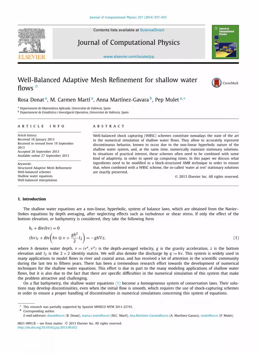
5.1.2. Test 2: Two-dimensional steady flowTo test the C-property in a 2D setting we consider a test proposed in [25]. The initial conditions correspond to water at

rest with a total height of 1 and a smooth bottom topography displayed in Fig. 6. The computational domain is the unitsquare and we have used τ = 10−1, N0 = 25, 4 levels (L = 3, N3 = 200).

Table 2 shows the errors with respect to the steady state solution at T = 1.0. As in the previous example, the use ofa non-WB interpolation in the transfer operators of the AMR code leads to the loss of the exact C-property. In Fig. 6 wedisplay the approximation to the ‘water at rest’ surface obtained using the AMR scheme without well-balanced interpolation,in order to show the numerical oscillations present in the simulation.

5.1.3. Quasi-Stationary Flow over smooth topographyThe following test, proposed by R. LeVeque in [25], has become a standard test for evaluating the capability of a nu-

merical scheme to accurately compute small perturbations of ‘water at rest’ flows over non-flat topographies. The (smooth)bottom topography is given by the following function,

R. Donat et al. / Journal of Computational Physics 257 (2014) 937–953 947

Fig. 6. Left: Bottom topography in 2D ‘water at rest’ test. Right: Computed water–surface using the AMR scheme without WB interpolation.

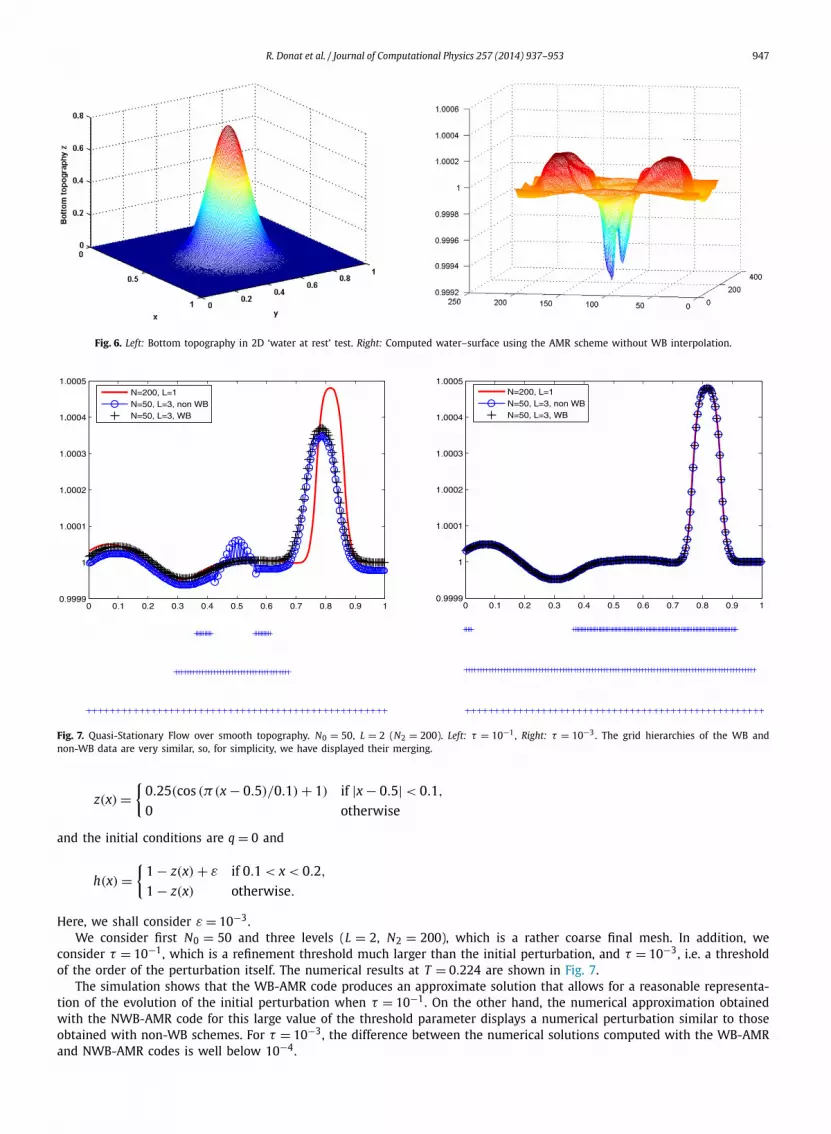
Fig. 7. Quasi-Stationary Flow over smooth topography. N0 = 50, L = 2 (N2 = 200). Left: τ = 10−1, Right: τ = 10−3. The grid hierarchies of the WB andnon-WB data are very similar, so, for simplicity, we have displayed their merging.

z(x) ={

0.25(cos (π(x − 0.5)/0.1) + 1) if |x − 0.5| < 0.1,

0 otherwise

and the initial conditions are q = 0 and

h(x) ={

1 − z(x) + ε if 0.1 < x < 0.2,

1 − z(x) otherwise.

Here, we shall consider ε = 10−3.We consider first N0 = 50 and three levels (L = 2, N2 = 200), which is a rather coarse final mesh. In addition, we

consider τ = 10−1, which is a refinement threshold much larger than the initial perturbation, and τ = 10−3, i.e. a thresholdof the order of the perturbation itself. The numerical results at T = 0.224 are shown in Fig. 7.

The simulation shows that the WB-AMR code produces an approximate solution that allows for a reasonable representa-tion of the evolution of the initial perturbation when τ = 10−1. On the other hand, the numerical approximation obtainedwith the NWB-AMR code for this large value of the threshold parameter displays a numerical perturbation similar to thoseobtained with non-WB schemes. For τ = 10−3, the difference between the numerical solutions computed with the WB-AMRand NWB-AMR codes is well below 10−4.

948 R. Donat et al. / Journal of Computational Physics 257 (2014) 937–953

Fig. 8. Temporal evolution of the perturbation of the steady state in Fig. 4. N0 = 50, L = 4, (N4 = 800), τ = 10−2. T = 1 (a), T = 2 (c), T = 5 (e). (b), (d) and(f) are enlarged views of (a), (c) and (e) respectively. The grid hierarchies of the WB and non-WB data are very similar, so, for simplicity, we have displayed

their merging.

R. Donat et al. / Journal of Computational Physics 257 (2014) 937–953 949

Fig. 9. Dam Break over a discontinuous topography (N0 = 50, L = 7, τ = 10−2). We display the water surface and multilevel grids structure. Left: T = 15.Right: T = 60 s.

Table 3Dam break errors. In this case (hfixed, vfixed) is a reference solution with N = 12 800 points.

interp type WB NWB

‖h − hfixed‖1 2.77e−3 2.77e−3‖v − vfixed‖1 2.74e−3 2.74e−3

Fig. 10. Zoom of the approximations in Fig. 9. Left: T = 15. Right: T = 60 s.

5.1.4. Quasi-Stationary Flow over rough topographyWith the same bottom topography as in Test 1, we consider now a slight perturbation of the steady state h + z = 12, as

follows

η(x) = h(x) + z(x) ={

12.01 x ∈ [680,720]

12 otherwise

950 R. Donat et al. / Journal of Computational Physics 257 (2014) 937–953

Fig. 11. Circular Dam-break problem (N0 = 25, L = 2, (N2 = 100) and τ = 10−1). (a) T = 0.15. (c) T = 0.25. (b) and (d) are slices of the channel at y = 1.

and v(x) ≡ 0. For this simulation, we use N0 = 50, L = 5, so that N5 = 800, and τ = 10−2. In Fig. 8 we compare theapproximated solutions obtained with N0 = 800, L = 1 (single-grid solution) with those obtained with the AMR code withand without WB interpolations in the transfer operators.

Again, the lack of WB interpolation in the transfer operators leads to oscillations, that are of the same order as themoving perturbations, hence displaying the typical behavior of a non-WB approximation.

5.2. Rapidly varying flow in 1D and 2D

The well-balancing of the transfer operators is not a crucial issue when computing numerical solutions of rapidly movingshallow water flow. This might explain the fact that the issue of WB interpolation in the inter-level transfer operators hasnot been discussed in previous works. The following tests illustrate the performance of the AMR technique for rapidlymoving flows. In these cases, there are no significant differences between the WB-AMR and non-WB-AMR results.

5.2.1. Test 4: Dam break over a square bump bottom topographyThis test involves a rapidly varying flow over a discontinuous bottom topography, see e.g. [11] for details. The initial

conditions are q = 0 and

h(x) ={

20 − z(x), x � 750

15 − z(x), otherwise.

The bottom topography is given as z(x) = 8 if |x−750| � 1500/8 and z(x) = 0 elsewhere. In Figs. 9 and 10 we display thecomputed water level at T = 15 and T = 60, together with the bottom topography. Fig. 9 shows also the grid patches active(at that time) at each resolution level. For this test, we have used τ = 10−2, N0 = 50, and eight levels (L = 7, N7 = 6400).

R. Donat et al. / Journal of Computational Physics 257 (2014) 937–953 951

Fig. 12. Multi-level grid structure for the Circular Dam-break problem at times T = 0.15 (a) and T = 0.25 (b). Here L = 4, and τ = 10−1.

We readily observe that the AMR technique is able to identify correctly the discontinuities in the flow variables. InTable 3, we display the difference between the AMR solution and a reference solution computed by the single-grid algorithmon a very fine mesh. As expected, the error is lower than the chosen tolerance. The CPU speedup of the AMR computationis ≈ 17.36.

5.2.2. Test 5: Circular Dam-Break ProblemThis test, proposed in [12], simulates a circular dam break problem over a non-flat topography. The domain is the square

[0,2] × [0,2] with outflow boundary conditions.In Fig. 11 we display the numerical results for the WB-adaptive scheme at T = 0.15 and T = 0.25. In Fig. 12 we show the

multilevel grid structure for a simulation with L = 4 and in Fig. 13 a longitudinal section at y = 1 of h and a longitudinalsection at y = 1 of q1 = uxh at time T = 0.15, which allow for a direct comparison with [12,28]. The CPU speedup whenusing L = 2 (Fig. 11) is 3.26 while using L = 4 (Fig. 12) it is 9.57. As mentioned before, there is no noticeable differencebetween the solutions computed with the WB-AMR code and those obtained with the non-WB-AMR code for this test.

6. Conclusions

Adaptive Mesh Refinement algorithms are a necessary tool in order to obtain realistic simulations involving shallowwater flows. We have shown that, even when the underlying scheme is well-balanced (WB), the numerical solution obtainedwhen implementing block-structured AMR techniques for shallow water flows will fail to satisfy the exact C-property if theoperators that are in charge of transferring information between levels are not well-balanced themselves.

We have pointed out some of the difficulties for getting finite-volume well-balanced adaptive mesh refinement schemesfor the shallow water equation, and we have presented a technique for obtaining point-value-based adaptive mesh refine-ment schemes for shallow water flow which are well-balanced for water at rest solutions, provided the underlying schemeis so. Our technique is based on interpolating the equilibrium variables, instead of the state variables, as in the originalblock-structured AMR technique [5,4,32].

We have performed a series of numerical tests, taking as the underlying well-balanced scheme the hybrid second orderscheme described in [14,28], that confirm that the proposed AMR technique is able to preserve, up to machine accuracy,water-at-rest steady state solutions of the shallow water equations in 1D and 2D.

As future research, we plan to work on the parallelization of the code and its extension to deal with dry zones. Weare also exploring the possibility of getting an adaptive scheme that preserves more stationary solutions if the underlyingscheme does so.

References

[1] E. Audusse, F. Bouchut, M.-O. Bristeau, R. Klein, B. Perthame, A fast and stable well-balanced scheme with hydrostatic reconstruction for shallow waterflows, SIAM J. Sci. Comput. 25 (2004) 2050–2065.

952 R. Donat et al. / Journal of Computational Physics 257 (2014) 937–953

Fig. 13. Circular Dam-break problem: Top: a longitudinal section at y = 1 of h. Bottom: longitudinal section at y = 1 of q1 = uxh at time T = 0.15.

[2] A. Baeza, R. Donat, A. Martinez-Gavara, A numerical treatment of wet/dry zones in well-balanced hybrid schemes for shallow water flow, Appl. Numer.Math. 62 (2012) 264–277.

[3] A. Baeza, A. Martínez-Gavara, P. Mulet, Adaptation based on interpolation errors for high order mesh refinement methods applied to conservation laws,Appl. Numer. Math. 62 (2012) 278–296.

[4] A. Baeza, P. Mulet, Adaptive mesh refinement techniques for high-order shock capturing schemes for multi-dimensional hydrodynamic simulations, Int.J. Numer. Methods Fluids 52 (2006) 455–471.

[5] M.J. Berger, P. Colella, Local adaptative mesh refinement for shock hydrodynamics, J. Comput. Phys. 82 (1989) 64–84.[6] M.J. Berger, D.L. George, R.J. LeVeque, K. Mandli, The geoclaw software for depth-averaged flows with adaptative refinement, Adv. Water Resour. 34

(2011) 1195–1206.[7] M.J. Berger, J. Oliger, Adaptive mesh refinement for hyperbolic partial differential equations, J. Comput. Phys. 53 (1984) 484–512.[8] A. Bermúdez, M.E. Vázquez, Upwind methods for hyperbolic conservation laws with source terms, Comput. Fluids 23 (1994) 1049–1071.[9] F. Bouchut, T. Morales de Luna, A subsonic-well-balanced reconstruction scheme for shallow water flows, SIAM J. Numer. Anal. 48 (2010) 1733–1758.

[10] S. Bryson, Y. Epshteyn, A. Kurganov, G. Petrova, Well-balanced positivity preserving central-upwind scheme on triangular grids for the Saint-Venantsystem, ESAIM Math. Model. Numer. Anal. 45 (2011) 423–446.

[11] V. Caselles, R. Donat, G. Haro, Flux-gradient and source-term balancing for certain high resolution shock-capturing schemes, Comput. Fluids 38 (2009)16–36.

[12] M.J. Castro, E.D. Fernández-Nieto, A.M. Ferreiro, J.A. García-Rodríguez, C. Parés, High order extensions of roe schemes for two-dimensional nonconser-vative hyperbolic systems, J. Sci. Comput. 39 (2009) 67–114.

[13] A. Cohen, S.M. Kaber, S. Müller, M. Postel, Fully adaptive multiresolution finite volume schemes for conservation laws, Math. Comput. 72 (2003)183–225, (electronic).

[14] R. Donat, A. Martinez-Gavara, A hybrid second order scheme for scalar balance laws, J. Sci. Comput. 48 (2011) 52–69.[15] A. Duran, Q. Liang, F. Marche, On the well-balanced numerical discretization of shallow water equations on unstructured meshes, J. Comput. Phys. 235

(2013) 565–586.[16] T. Gallouët, J.M. Hérard, N. Seguin, Some approximate Godunov schemes to compute shallow water equations with topography, Comput. Fluids 32

(2003) 479–513.[17] L. Gascón, J.M. Corberán, Construction of second-order TVD schemes for nonhomogeneous hyperbolic conservation laws, J. Comput. Phys. 172 (2001)

261–297.[18] D.L. George, Adaptive finite volume methods with well-balanced Riemann solvers for modeling floods in rugged terrain: Application to the Malpasset

dam-break flood (France, 1959), Int. J. Numer. Methods Fluids 66 (2011) 1000–1018.[19] N. Goutal, F. Maurel, in: Proceedings of the 2nd Workshop on Dam-Break Wave Simulation, EDF-DER Report, HE-43/97/016/B, 1997.

R. Donat et al. / Journal of Computational Physics 257 (2014) 937–953 953

[20] J.M. Greenberg, A.Y. Leroux, A well-balanced scheme for the numerical processing of source terms in hyperbolic equations, SIAM J. Numer. Anal. 33(1996) 1–16.

[21] J.M. Greenberg, A.Y. Leroux, R. Baraille, A. Noussair, Analysis and approximation of conservation laws with source terms, SIAM J. Numer. Anal. 34 (1997)1980–2007.

[22] A. Harten, Multiresolution algorithms for the numerical solution of hyperbolic conservation laws, Commun. Pure Appl. Math. 48 (1995) 1305–1342.[23] M. Hubbard, N. Dodd, A 2D numerical model of wave run-up and overtopping, Coast. Eng. 47 (2002) 1–26.[24] P. Lamby, R. Müller, Y. Stiriba, Solution of shallow water equations using fully-adaptative multiscale schemes, Int. J. Numer. Methods Fluids 49 (2005)

417–437.[25] R.J. LeVeque, Balancing source terms and flux gradients in high-resolution Godunov methods: the quasi-steady wave-propagation algorithm, J. Comput.

Phys. 146 (1998) 346–365.[26] R.J. LeVeque, D.L. George, M.J. Berger, Tsunami modelling with adaptively refined finite volume methods, Acta Numer. 20 (2011) 211–289.[27] Q. Liang, A structured but non-uniform cartesian grid-based model for the shallow water equations, Int. J. Numer. Methods Fluids 66 (2011) 537–554.[28] A. Martinez-Gavara, R. Donat, A hybrid second order scheme for shallow water flows, J. Sci. Comput. 48 (2011) 241–257.[29] S. Müller, Y. Stiriba, Fully adaptive multiscale schemes for conservation laws employing locally varying time stepping, J. Sci. Comput. 30 (2007) 493–531.[30] J. Quirk, A parallel adaptive grid algorithm for computational shock hydrodynamics, Appl. Numer. Math. 20 (1996) 427–453.[31] M. Ricchiuto, R. Abgrall, H. Deconinck, Application of conservative residual distribution schemes to the solution of the shallow water equations on

unstructured meshes, J. Comput. Phys. 222 (2007) 287–331.[32] C. Shen, J. Qiu, A. Christlieb, Adaptative mesh refinement based on high order finite difference WENO scheme for multi-scale simulations, J. Comput.

Phys. 230 (2011) 3780–3802.[33] Y. Xing, C.W. Shu, High order finite difference WENO schemes with the exact conservation property for the shallow water equations, J. Comput. Phys.

208 (2005) 206–227.