Journal of Computational and Applied Mathematics 233 (2010) 3178–3188

Contents lists available at ScienceDirect

Journal of Computational and AppliedMathematics

journal homepage: www.elsevier.com/locate/cam

A two-mesh adaptive mesh refinement technique for SN neutral-particletransport using a higher-order DGFEMJean C. Ragusa ∗, Yaqi WangDepartment of Nuclear Engineering, Texas A&M University, College Station, TX, 77843-3133, USA

a r t i c l e i n f o

Article history:Received 3 April 2009Received in revised form 7 December 2009

Keywords:Adaptive mesh refinementSN transportDiscontinuous Galerkin finite elementmethodDiffusion synthetic acceleration

a b s t r a c t

We present a two-mesh Adaptive Mesh Refinement technique for the SN neutral-particletransport equation in 2D. A high-order (up to order 4) Discontinuous Galerkin (DG)finite element discretization is employed with standard upwinding. A suitable DiffusionSynthetic Acceleration (DSA) scheme is derived to precondition the transport solves. TheDSA scheme, also based on aDGdiscretization, is derived directly from the discretized high-order DG SN transport equation. Results are presented to demonstrate the superiority ofAMR for DSA-accelerated SN transport solves.

© 2009 Elsevier B.V. All rights reserved.

1. Introduction

The steady-state transport of mono-energetic neutral particle (e.g., neutrons, photons) through matter is described bythe following integro-differential equation(

EΩ · E∇ + σ(Er))Ψ =

∫4πσs(Er, EΩ ′ · EΩ)Ψ (Er, EΩ ′)dΩ ′ + Q (Er, EΩ), inD × S2, (1)

with the general boundary condition

Ψ (Erb, EΩ) = Ψ inc(Erb, EΩ)+∫EΩ ′·Enb>0

β(Erb, EΩ ′ → EΩ)Ψ (Erb, EΩ ′)dΩ ′ on Erb ∈ ∂D−, (2)

where D is the spatial domain, S2 the unit sphere, EΩ the direction of flight, Er the position, σ(Er) the total cross section,σs(Er) =

∫4π dΩ σs(Er, EΩ

′· EΩ) the scattering cross section, σs(Er, EΩ ′ · EΩ) the differential scattering cross section, Q (Er, EΩ) the

source term, Ψ inc(Erb, EΩ) the incoming flux, and β(Erb, EΩ ′ → EΩ) the boundary redistribution kernel (albedo). The incomingdomain boundary ∂D− is defined by

∂D− =Erb ∈ ∂D, EΩ · En(Erb) < 0

, (3)

with En(Erb) the outward unit normal vector at position Erb. For brevity, we only consider Dirichlet conditions hereafter (i.e.,β = 0). Despite Eq. (1) being linear, its numerical solution is challenging, even on current computers, due to1. the high dimensionality of the phase-space. In complete generality, the angular flux Ψ depends upon seven variables:three for the standard physical space, two for the angular variable, one variable for the particles’ energy, and one for time.After the application of an implicit time integrator and the multigroup approximation in energy, an equation of the formgiven in Eq. (1) is obtained;

∗ Corresponding author. Tel.: +1 979 862 2033.E-mail addresses: ragusa@ne.tamu.edu (J.C. Ragusa), yaqiwang@tamu.edu (Y. Wang).

0377-0427/$ – see front matter© 2009 Elsevier B.V. All rights reserved.doi:10.1016/j.cam.2009.12.020

J.C. Ragusa, Y. Wang / Journal of Computational and Applied Mathematics 233 (2010) 3178–3188 3179

2. the presence of singularities in the transport solution [1] and the greatly disparate values of σ(Er) and σs(Er) in practicalapplications;

3. the change in the nature of the PDE, from a hyperbolic behavior in materials with small scattering ratio, i.e., c = σsσ 1,

to an elliptic behavior for highly diffusive materials, i.e., c ' 1, [2].

In radiation transport production codes, low-order spatial differencing techniques are often employed, either onstructured [3] or unstructured [4] grids. In addition, while Adaptive Mesh Refinement (AMR) techniques are now widelyused in many science and engineering disciplines [5–7], only a limited number of references are available regarding theapplications of mesh adaptivity to radiation transport. The higher-order spatial adaptivity technique described here isapplied to the SN angular approximation of Eq. (1). Patch-AMR techniques [8–10] for the SN transport equation have beendevised and are based on a hierarchy of nested grids. Some of the drawbacks of patch-AMR include the fact that the physicsare not followed as closely as possible (the extent of refined patch being often too large), leading to more unknowns thanneeded, and the need to converge inflow/outflow values in between nested grids (a feature that is not present in cell-based AMR). Oftentimes, a gradient-based error estimator is employed to drive the adaptive mesh refinement in Cartesianstructured geometries but it is overly conservative for high-order spatial discretization schemes. In [11], a local refinement(cell-based AMR) technique is described for SN transport spatially discretized using low-order finite differences, wherethe value of the particle mean free path (MFP) in a given cell is used as a mesh refinement criterion. While this approachtakes into account the size of potential internal layers at a given location in the domain, it does not account for the actualsmoothness of the solution at these locations and is, therefore, far from optimal; for example, within optically thick areas,the solution may well be approximated by a smooth spatial representation on coarse meshes despite the smallness of themean free path. In [12], a lower-order angular flux solution serves to compute a converged scattering source which is thenused as a fixed source term for a higher-order transport solve. The differences between the two solutions is then used toprescribe local mesh refinements; their technique was demonstrated for one-group, 2D rectangular structured meshes. Theerror estimate employed in our present work is based on the difference between the numerical solutions computed oncoarser and finer AMR meshes at any adaptivity cycle; the local error hereby obtained is used to prescribe the new coarserAMR mesh at the next adaptivity cycle, the finer AMR mesh being obtained by refinement of the coarser mesh.Additionally, preconditioning techniques are necessary to accelerate the transport solution in highly diffusive

configurations; it is well established that the spatial discretization of the Diffusion Synthetic Acceleration (DSA) equationsmust be ‘‘consistent’’ in some sense with the one used in the SN transport solves in order to yield unconditionally stableand efficient DSA schemes [13,14,4,15,16]. With the exception of [17] for block structured AMR with linear finite elements,little work has been reported to devise DSA schemes (i) for higher-order spatial discretizations and, more importantly, (ii)for unstructured AMRmeshes. Using a variational argument, we obtain here a DGFEM DSA procedure (since it is based on aDG method, it is suitable for AMR meshes) and we show its relation with the standard Interior Penalty (IP) DGFEMmethodfor elliptic PDEs [18,19].Thework presented here describes (i) an AMR technique to accurately solve the SN transport equation using a high-order

Discontinuous Galerkin Finite Element Method (DGFEM) in space and (ii) an efficient DSA preconditioner for AMR meshes.Section 2 briefly reviews the SN approximation and describes the DGFEM variational form of the SN transport equation. InSection 3, we present our modified IP DSA preconditioner. The AMR technique and error estimator employed are explainedin Section 4. Numerical results are given in Section 5 and we provide conclusions in Section 6.

2. Numerical solution techniques

2.1. Space/angle discretization

In this section, we briefly review the SN angular discretization for Eq. (1) and present a DGFEM high-order spatialdiscretization. Given an angular quadrature set EΩm, wm, m = 1, . . . ,M , consisting of M directions EΩm and weights wm,the SN discrete ordinates [2] version of Eq. (1) is

(EΩm · E∇ + σ

)Ψm(Er) =

Na∑n=0

n∑k=−n

(σs,n(Er)Φn,k(Er)+ Qn,k(Er)

)An,k( EΩm), (4)

for m = 1, . . . ,M , supplemented with appropriate boundary conditions. The scattering source term in Eq. (4) has beenmanipulated by decomposing the differential scattering cross section on Legendre polynomials (up to anisotropy order Na)and introducing the flux moments

Φn,k(Er) =∫4πdΩ An,k( EΩ)Ψ (Er, EΩ) ≈

M∑m=1

wmAn,k( EΩm)Ψm(Er), (5)

where An,k represents the real spherical harmonic function of degree n and order kwith the Schmidt semi-normalization.

3180 J.C. Ragusa, Y. Wang / Journal of Computational and Applied Mathematics 233 (2010) 3178–3188

The spatial domain D is triangulated into an unstructured mesh Th = K , ∪K∈Th K = D and we employ a DGdiscretization technique in space, with Pp(K) denoting the space of polynomial of degree ≤ p on element K . Hierarchicalbasis functions (up to order 4) are chosen for the spatial discretization [20,21]. For a given streaming direction EΩm, the DGscheme with standard upwinding reads:

Find Ψm ∈ Vp(K), such that ∀Ψ ∗m ∈ Vp(K),(Ψm, (− EΩm · E∇ + σ)Ψ

∗

m

)K +

⟨Ψ−m ,Ψ

∗

m

⟩∂K+ −

⟨Ψ−m ,Ψ

∗

m

⟩∂K− =

Na∑n=0

n∑k=−n

An,k( EΩm)(σs,nΦn,k + Qn,k,Ψ ∗m

)K , (6)

where ∂K− is the inflow boundary, ∂K+ is the outflow boundary of element K . The traces Ψ+ and Ψ− are defined withrespect to the particle direction EΩm, i.e., on an inflow boundary, Ψ+ (resp. Ψ−) is the value of Ψ taken fromwithin elementK (resp. from the upwind neighbor) and on an outflow boundary,Ψ+ (resp.Ψ−) is the value ofΨ taken from the downwindneighbor (resp. from within element K ). These definitions are expressed as follows:

Ψ±m ≡ lims→0±

Ψm(Er + s EΩm) (7)

(f , g)K ≡∫Kf g (8)

〈f , g〉e ≡∫e| EΩm · En(Er)|f g (9)

∂K± ≡Er ∈ ∂K , En(Er) · EΩm R 0

(10)

where En is the outward unit normal vector of element K and e represents any edge (or face in 3D) of K . Since the finiteelement approximation used is discontinuous, the quantity EΩΨ is not defined at the element interfaces. Here, the upwindscheme is obtaining by explicitly employing a numerical flux H(f +, f −, En) defined as

H(f +, f −, En) = EΩ · Enf − (11)

such that∫∂KH(Ψ+m ,Ψ

−

m , En)Ψ∗

m =⟨Ψ−m ,Ψ

∗

m

⟩∂K+ −

⟨Ψ−m ,Ψ

∗

m

⟩∂K− . (12)

Eq. (12) was used in deriving Eq. (6). Transport solves are based on Eq. (6). By integrating Eq. (6) by parts, an equivalentformulation is obtained:

(( EΩm · E∇ + σ)Ψm,Ψ

∗

m

)K +

⟨[[Ψm]],Ψ

∗

m

⟩∂K− =

Na∑n=0

n∑k=−n

An,k( EΩm)(σs,nΦn,k + Qn,k,Ψ ∗m

)K , (13)

where the inter-element jump is given by [[Ψm]] = Ψ+m − Ψ−m . Eq. (13) will be useful in deriving the diffusion synthetic

accelerator in Section 3.

2.2. Iterative procedure

The system of equations formed by Eq. (6) needs not to be assembled for all elements but can be solved element byelement. This strategy is often referred to as a ‘‘transport sweep’’ in direction EΩm. The order in which the elements aresolved constitutes the graph of the sweep (for brevity, we do not expand on situations where the graph can present somedependencies, in which case these dependencies are simply lagged within the iterative procedure; for additional details,refer to [4]). With appropriate numbering, the angular fluxes and flux moment unknowns are described by 9 and 8,respectively, and the transport sweeps over all directions can be represented in the following matrix form:

L9 = MΣ8+ Q8 = DΨ , (14)

where L is the block-diagonal matrix due to particle streaming and total interaction (one block = one direction), 6 is thescattering matrix which operates on the flux moments,M is the moment-to-direction matrix, D is the direction-to-momentmatrix (hereafter, we assumeMD = I for conciseness in the derivations of Section 3, although not all quadrature formulaenecessarily satisfy this). We can recast Eq. (14) in terms of flux moments as follows:[

I− DL−1MΣ]8 = DL−1Q. (15)

J.C. Ragusa, Y. Wang / Journal of Computational and Applied Mathematics 233 (2010) 3178–3188 3181

None of these global matrices are explicitly formed and L is inverted in a ‘‘matrix-free’’ fashion using transport sweeps.Eq. (15) is solved using GMRes. Alternatively, a Richardson iteration is employed, leading to the scattering Source Iteration(SI) technique

9(i+1) = L−1[M68(i) + Q

]8(i+1) = D9(i+1),

(16)

where the previous fluxmoment iterate8(i) is utilized to build the scattering source term. Both the SI scheme and theGMRessolution are known to be slow converging for highly diffusive problems and a Diffusion Synthetic Acceleration (DSA) [16]must be implemented to address this issue. This DSA technique can be utilized as a preconditioner for both the SI schemeor the GMRes solves and is discussed next.

3. Diffusion preconditioner for AMRmeshes

For highly diffusive configurations (i.e., materials with scattering ratios c close to 1 and optically thick domains), thestandard iterative techniques to solve the transport equation can become quite ineffective due to their slow convergenceproperties and a DSA preconditioner is needed to accelerate the convergence of the process. The diffusion operator mustbe spatially discretized in a manner that is ‘‘consistent’’ with the discretization of the transport equation [13–16] to ensureunconditional stability (however, a diffusion-based synthetic accelerator is not necessarily effective for multidimensionalproblems containing highly diffusive regions with discontinuities in material properties, [22]). To obtain consistentlydiscretized DSA equations, the zeroth and first angular moments of the discretized transport equation are taken, leadingto a mixed DGFEM discretization of a diffusion equation. The mixed formulation results in a nonsymmetric PD saddlepoint problem [4] that is CPU expensive and partially consistent DSA schemes, motivated by the difficulties associatedwith the algebraic elimination of the vector unknowns to yield an elliptic diffusion equations, are more popular. Withpartial consistency, it is hoped that the reduction in complexity outweighs the degradation in effectiveness but few partiallyconsistent schemes have been applied to AMRmeshes [17]. Additionally, finite-element-based partially consistent schemesemploy a Continuous Finite Element (CFE) discretization of the diffusion operator [23]. However, the algorithmic andimplementation simplicity of employing an AMR-DG solution for the transport solves would be severely reduced if theDSA preconditioner solves were based on a CFE method requiring hanging nodes treatment.In our new approach, we have chosen to derive partially consistent DSA schemes employing a DGFEM discretization by

directly deriving them from the DGFEM discretization of the SN transport equations. Our scheme belongs to the family ofpartially consistent DSA methods because in our derivation, only the zeroth angular moment of the discretized transportequation is used and we assume that the continuous first angular moment of the transport equation (Fick’s law) to beverified in order to eliminate the current unknowns EJ = [Φ1,−1; Φ1,0; Φ1,1]T . The resulting DGFEM discretization for thediffusion equation is remarkably similar to the Interior Penalty (IP) stabilizationmethod for diffusion equations solved usinga DGFEM. Due to the discontinuous nature of the DGFEM approximation, it is particularly well suited for meshes arising inAMR calculations, i.e., hanging nodes are seamlessly incorporated into the DG method. This property also leads to an easyimplementation of high-order test functions. For brevity, we only outline the DSA derivation here.

Step 1: Using Eq. (13), we have the following variational form the DGFEM SN transport formulation:Find Ψm ∈ W hD , ∀Ψ

∗m ∈ W

hD , m = 1, . . . ,M such that:

b(Ψ ,Ψ ∗) = l(Ψ ∗)+N∑n=0

n∑k=−n

(σs,nΦn,k,Φ

∗

n,k

)D, (17)

where the bilinear and linear forms are

b(Ψ ,Ψ ∗) =M∑m=1

wm(( EΩm · E∇ + σ)Ψm,Ψ

∗

m

)D+

M∑m=1

wm⟨[[Ψm]],Ψ

∗+

m

⟩Eih

(18)

l(Ψ ∗) =N∑n=0

n∑k=−n

(Qn,k,Φ∗n,k

)D+

∑e∈∂D

∑EΩm·Enb<0

wm⟨Ψ incm ,Ψ ∗m

⟩e . (19)

W hD =Ψ ∈ L2(D); Ψ |K ∈ V (K),∀K ∈ Th

and E ih = ∪K∈Th ∂K \ ∂D is the set of all interior edges. Note that Eq. (17)

is the zeroth angular moment of the discretized transport equation, hence the weighted summation over all directions inEqs. (18) and (19).

Step 2: Assume a linear dependence in angle (i.e., P1 approximation) for the angular flux Ψm and the test function Ψ ∗m

Ψm =14π(φ + 3EJ · EΩm) and Ψ ∗m =

14π(φ∗ + 3EJ∗ · EΩm) (20)

3182 J.C. Ragusa, Y. Wang / Journal of Computational and Applied Mathematics 233 (2010) 3178–3188

with φ ≡ Φ0,0 the scalar flux and EJ the net current. Further assume that the continuous Fick’s law (EJ = −D E∇φ andEJ∗ = D E∇φ∗) to be valid, yielding:

Ψm =14π(φ − 3D E∇φ · EΩm) and Ψ ∗m =

14π(φ∗ + 3D E∇φ∗ · EΩm). (21)

Step 3: Insert Eq. (21) in Eq. (17) and carry out the angular summation. After some considerable algebra, the applicationof angular quadrature properties, and further simplifications [24], the following Modified Interior Penalty (MIP) DGFEMformulation is obtained:

bMIP(φ, φ∗) =(σaφ, φ

∗)D+

(D E∇φ, E∇φ∗

)D+(κMIPe [[φ]], [[φ

∗]])Eih+([[φ]], D∂nφ∗

)Eih

+(D∂nφ, [[φ∗]]

)Eih+(κMIPe φ, φ∗

)∂D−12

(φ,D∂nφ∗

)∂D−12

(D∂nφ, φ∗

)∂D

(22)

lMIP(φ∗) =(Q0, φ∗

)D+

(EQ1, 3D E∇φ∗

)D+(J inc, φ∗

)∂D, (23)

with the incoming current given by:

J inc =∑

EΩm·En(Erb)<0

wm| EΩm · En(Erb)|Ψ incm . (24)

[[]] and represent the inter-element jumps and averages on interior edges, respectively. The absorption cross sectionσa = σ − σs and the diffusion coefficient D = 1

3(σ−σs,1)are not imposed or coerced but are naturally obtained from this

derivation. The penalty coefficient κMIPe in Eq. (22) is given by:

κMIPe = max(κ IPe ,

14

)(25)

where the value of 1/4 is the value obtained by strictly applying the procedure, κ IPe =c(p+)2

D+

h+⊥

+c(p−)2

D−

h−⊥

is the standard IP

penalty value (see, e.g., [25]); the± symbols in κ IPe represent the values in the adjacent cells K− and K+ sharing a given edge

e, D is the diffusion coefficient, h±⊥is the length of cell K± orthogonal to the edge, c(p) = p(p+ 1), and p is the polynomial

order.Wenote that Eq. (22) is SPD and can, therefore, be solved using a standard preconditioned ConjugateGradient (CG) solver;

we used SSOR as the preconditioner for CG. A Fourier analysis of the iteration operator (DSA+transport solves) shows that ourmodified scheme (MIP) yields unconditional stability when employed as a diffusion synthetic accelerator, in both the thinand thick diffusion limits, whereas the standard IP scheme (κ = κ IP ) or the original scheme (κ = 1/4) are only conditionallystable accelerators. This Fourier analysis is discussed after the derivation of the MIP-DG scheme. Steps 1–3 describe how adiscretized diffusion operator, that is partially consistent with the discretized transport equation, is obtained. Next, webriefly present how this MIP-DGFEM diffusion is employed as a preconditioner to accelerate transport sweeps. For a givenSI iteration, one transport solve yields 8(i+1/2) = DL−1

[MΣΦ(i) + Q

](this is simply Eq. (16) in which the new iterate has

now been labeled i + 1/2); next we define the error e(i+1/2) = 8 − 8(i+1/2) where 8 represents the converged solution.This error satisfies the following transport equation(

I− DL−1M6)e(i+1/2) = DL−1M6

[8(i+1/2) −8(i)

], (26)

or, equivalently, (DLM− 6) e(i+1/2) = 6[8(i+1/2) −8(i)

]. In the error equation, Eq. (26), the external volumetric source is

no longer present, the Dirichlet boundary conditions are now homogeneous (vacuum) and the new volumetric source is thescattering source due to the difference in successive iterates. Nonetheless, this error equation is just as difficult to solve asEq. (16) and a simpler estimate for the error term e(i+1/2) is sought by replacing the (DLM− 6) operator with the diffusionoperator obtained through steps 1–3, resulting in the following equation:

Ae(i+1/2) = 6[8(i+1/2) −8(i)

], (27)

where A is the matrix notation for the MIP-DGFEM bilinear form of Eq. (22). Finally, the DSA-accelerated SI scheme (orpreconditioned Richardson iteration) reads as follows:

8(i+1) = 8(i+1/2) + e(i+1/2) = DL−1[MΣΦ(i) + Q

]+ A−16

[8(i+1/2) −8(i)

], (28)

and the preconditioned GMRes solve is(I+ A−16

) (I− DL−1M6

)8 =

(I+ A−16

)DL−1Q. (29)

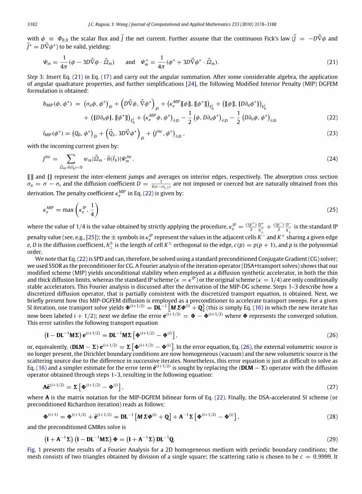
Fig. 1 presents the results of a Fourier Analysis for a 2D homogeneous medium with periodic boundary conditions; themesh consists of two triangles obtained by division of a single square; the scattering ratio is chosen to be c = 0.9999. It

J.C. Ragusa, Y. Wang / Journal of Computational and Applied Mathematics 233 (2010) 3178–3188 3183

Fig. 1. Fourier analysis for the various DSA forms as a function of the mesh optical thickness, homogeneous infinite medium case (the right pane is azoomed portion of the left pane).

is well known that spectral radius of SI process is also equal to c , hence SI can be arbitrarily slow to converge. In Fig. 1, wehave graphed the spectral radius obtained with the DSA-accelerated SI schemes when using the following three penaltycoefficients: κ = 1/4, κ = κ IP (the standard IP formulation), and κ = κMIP (the Modified IP formulation). The results arepresented as a function of the mesh optical thickness (expressed in MFP). We can note that the schemes employing eitherκ = 1/4 or κ = κ IP can have spectral radii greater than 1, and hence are only conditionally stable for some range of opticalthickness, whereas the MIP scheme has maximum spectral radius of about 0.48 and thus always converges. An S4 angularquadrature was used for this Fourier analysis.

4. A two-mesh AMR approach for high-order SN transport

In radiation transport and radiative transfer, lower-order spatial schemes aremost commonly used. The AMR techniquesemployedwith such schemes typically rely on gradient-based error estimates [8], with a few exceptions, e.g., [26], where anadjoint-based estimator is derived, but at the cost of computing an adjoint solution. Here, we wish to obtain error estimatesfor high-order spatial approximations and, therefore, cannot rely on simpler estimates such as the gradient of the numericalsolution. We have chosen to follow the approach proposed in [7,27], where two adapted AMR meshes are utilized at eachadaptivity cycle: a coarse AMR mesh Tkh and a fine AMR mesh Tkh/2 obtained by uniform refinement of T

kh; in the preceding,

k denotes the mesh adaptivity cycle index.

4.1. Error estimation procedure

The error estimate at cycle k is simply the difference in the solutions obtained on Tkh/2 and Tkh. This is computed in the L2norm, element by element. However, in steady-state transport algorithms, the angular fluxes Ψm are never kept (except onalbedo boundaries and for elements causing dependencies in the graph of the sweep), hence our error estimate is based onangle-integrated quantities such as the scalar flux φ or the current EJ = [Jx; Jy; Jz]T , as shown in Eq. (30) for 2D:

µkK =

∫K

[(Jxh − J

xh/2)

2+ (Jyh − J

yh/2)

2]

∫D

[(Jxh)2 + (J

yh)2] ∀K ∈ Tkh. (30)

We tested error estimates based on either the scalar flux or the current and did not find significant changes in the AMRresults and grids. Themotivation to employ an estimate based on the current comes frompriorwork onAMR for the diffusionequation [28] where the diffusion approximation for the current is a mathematically appropriate choice.For efficiency, we first solve for the transport solution on the coarser mesh and use the converged scattering source as

an initial guess for the solution on the finer mesh, hence reducing the number of transport iterations needed on the finermesh. The projection operation in Eq. (30) is defined as:FindΠhΦ ∈ W hD , such that,(

ΠhΦ,Φ∗)D=(Φ,Φ∗

)D, ∀Φ∗ ∈ W hD (31)

This projection is easily carried out element by element, due to the discontinuous nature of the spatial discretization. Thecriterion for refinement is defined as follows: an element K of Tkh is selected for refinement if

µkK ≥ α maxK ′∈Tkh

(µkK ′

), (32)

where α is a user-defined fraction (we used α = 0.3). This criterion allows us to focus the computational effort on elementswith the largest errors and tends to equi-distribute the spatial error. The global error, obtained by summing the errorestimates over all elements, i.e.,

ηk =

√∑K∈Tkh

µkK , (33)

3184 J.C. Ragusa, Y. Wang / Journal of Computational and Applied Mathematics 233 (2010) 3178–3188

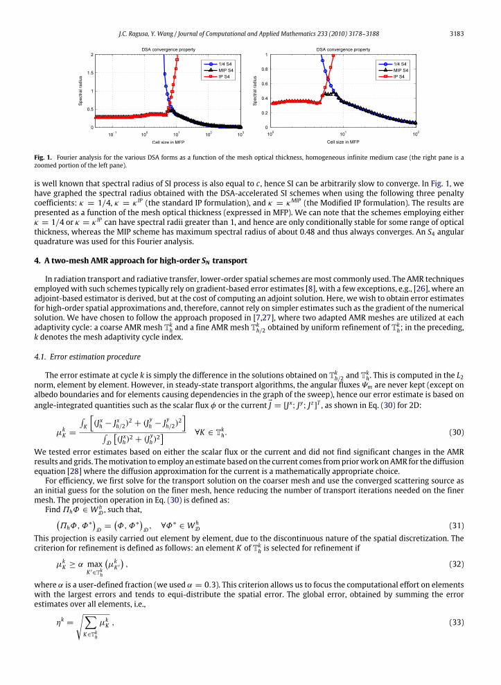
(a) Same refinement level. (b) Coarser upwind element. (c) Finer upwind element.

Fig. 2. Edge-coupling cases for refinement level differences≤ 1.

is used to terminate the adaptivity procedure (ηk < tolAMR). The final result of the calculation is the last solution obtainedon the finer AMR mesh.

4.2. Mesh coupling

Once an element has been flagged for refinement, it becomes inactive and the child-elements are the new active cells.Appropriate refinement rules allow for an efficient visit of the tree structure. Any level of refinement difference is allowedbetween neighboring elements. The element-coupling algorithm is based on recursive calls to the function dealing with the1-level refinement difference. The cases of 0- and 1-level refinement difference are shown in Fig. 2 and are dealt with asfollows. Fig. 2(a) is the standard situation without refinement between neighbors, where the edge-coupling from elementK ′ to K is simply achieved by

LAB6Ci,jΨK ′ , (34)

where Ci,j is a coupling matrix. In 2D problems, Ci,j is akin to a 1D mass matrix (see Eq. (6)) but contains several emptyrows and columns because it applies to the whole solution vector of element K ′ (only the components of ΨK ′ belonging toedge K ∩ K ′ play a role in edge-coupling). It was our deliberate choice to achieve edge-coupling through whole-elementoperations, as this is necessary for the diffusion solves (where the edge integrals present gradient terms and hence requirethe entire element solution). A few templates for the Ci,j matrices need to be stored, depending on the local numbering ofvertices i and j; thanks to the hierarchical nature of the basis functions used, the templates for any polynomial order areembedded in the single template for the highest order employed. Fig. 2(b) shows the situation when the contribution toelement K results from the contribution of two smaller elements (1-level refinement difference). The contribution is simplycomputed for each element separately, yielding

LAB6PTi1Ci,jΨK ′2 +

LBC6PTi2Ci,jΨK ′1 , (35)

where Pk are cell prolongationmatrices operating on the local solution vector and providing the solution vectors on the fourchild-elements. These matrices are independent of the element shape. Finally, the case shown in Fig. 2(c) requires a simpletransposition of the case in Fig. 2(b), yielding the contribution from K ′ to K as follows:

LAB6Ci,jPj1ΨK ′ . (36)

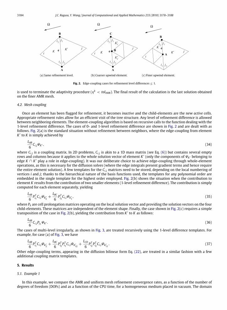
The cases of multi-level irregularly, as shown in Fig. 3, are treated recursively using the 1-level difference templates. Forexample, for case (a) of Fig. 3, we have

LAB6PTi1Ci,jΨK ′2 +

LBC6PTi2P

Ti1Ci,jΨK ′12 +

LCD6PTi2P

Ti2Ci,jΨK ′11 . (37)

Other edge-coupling terms, appearing in the diffusion bilinear form Eq. (22), are treated in a similar fashion with a fewadditional coupling matrix templates.

5. Results

5.1. Example 1

In this example, we compare the AMR and uniform mesh refinement convergence rates, as a function of the number ofdegrees of freedom (DOFs) and as a function of the CPU time, for a homogeneous medium placed in vacuum. The domain

J.C. Ragusa, Y. Wang / Journal of Computational and Applied Mathematics 233 (2010) 3178–3188 3185

Fig. 3. Multi-irregularity, i.e., differences> 1 in refinement levels.

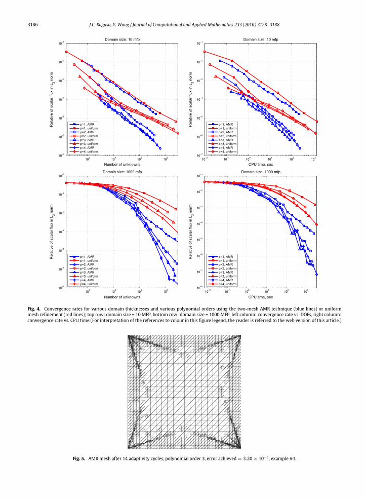
size is [10 × 10] cm2; the total cross section σt is varied from 1 to 100 cm−1 to model a wide range of domain opticalthicknesses (from 10 MFP to 1000 MFP). The scattering ratio c = σs/σ is equal to 0.9. A uniform and isotropic volumetricsource is present in the domain. All computations are performed using an S4 level-symmetric angular quadrature [29].Fig. 4 displays the convergence rates obtained using the two-mesh AMR technique for polynomial orders 1 through 4and compares it with a uniform mesh refinement approach. The comparison is performed in terms of both DOFs and CPUtime. For the AMR runs, the DOFs are the ones from the finer AMR mesh, i.e., Th/2. A reference solution, obtained usingthe AMR technique with tighter tolerance, more adaptivity cycles and polynomial order 4, serves an exact solution tocompute the error displayed in Fig. 4. First, we see a clear benefit in employing at least quadratic polynomials, regardlessof the refinement strategy. For optically thin domains, AMR provides savings in memory and CPU time of about oneorder of magnitude when compared to the uniform mesh approach. For thicker domains, the savings with AMR are evenlarger. Fig. 5 shows the adapted mesh after 14 refinement cycles. Clearly, the S4 singularity lines have been refined(with S4, there are 3 singularities originating from each corner of the domain; the 45 singularity from the bottom-left corner and the 135 singularity from the top-right corner are exactly aligned with the mesh and thus not visiblehere).

5.2. Example 2

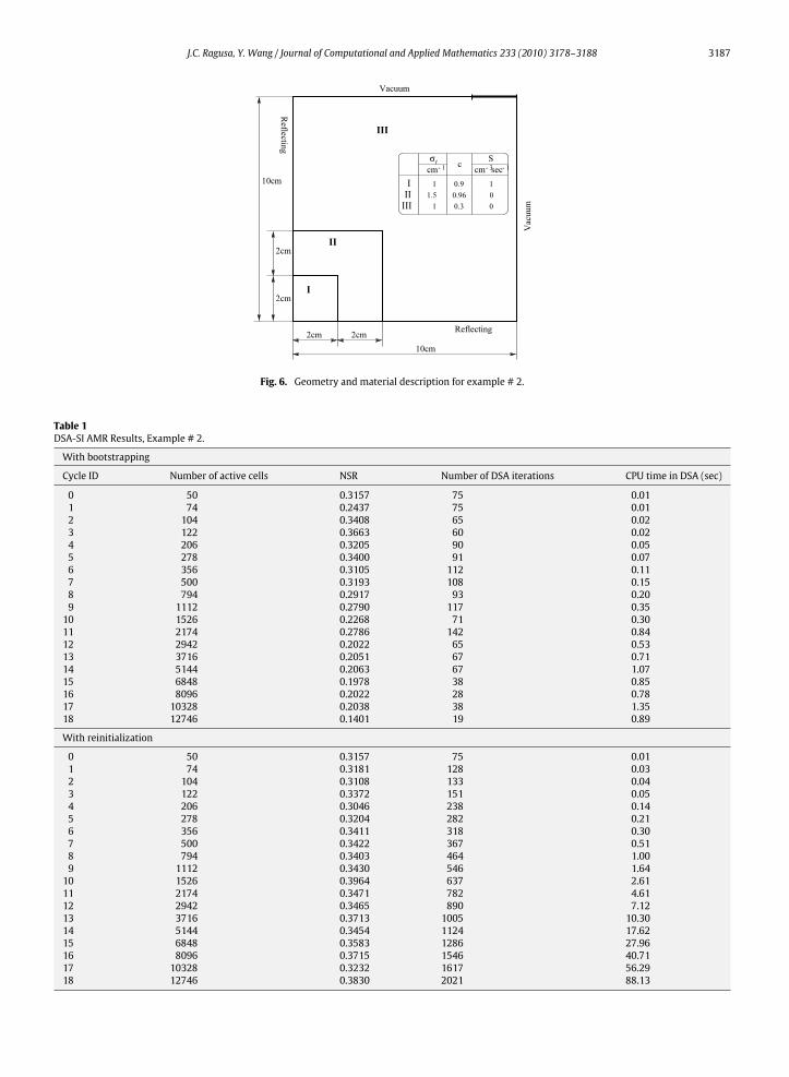
The geometry and material descriptions are shown in Fig. 6. The polynomial order used is 2 and the angular quadratureis S4; scattering is isotropic. Table 1 presents the numerical spectral radius (NSR) obtained with employing DSA as apreconditioner for SI. The NSR is defined as the ratio of successive differences, ‖u

i+1−ui‖2

‖ui−ui−1‖2. For this problem, we can note

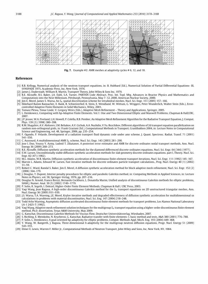
that the NSR is about 0.34 and decreases as the AMR proceeds. Even though the mesh size is increased at each AMRcycle, the total number of CG iterations in DSA per AMR cycle does not vary significantly. Most of the acceleration workoccurs at the inception of the AMR process, when the meshes are coarse. Consequently the CPU time spent in DSA is small,even for highly refined meshes. For comparison purposes, we also present results in which the solution from the previousadaptivity cycle is discarded, hence no bootstrapping for the next adaptivity cycle is performed. In this case, the NSR remainsabout constant and the number of DSA iterations grows significantly: the total number of CG iterations doubles each timethe number of unknowns is quadrupled. Should a large initial mesh be provided, a significant amount of work would bespent in DSA iterations. We note that the AMR process (with bootstrapping as one would always prefer to utilize availableinformation) can be quite effective at focusing most of the DSA work when the AMR meshes are still relatively coarse aswas noted by the decrease in the NSR when the adaptivity index increased. The AMR meshes obtained at adaptivity cycles# 6, 12 and 18 are given in Fig. 7 where we note that the interfaces and their associated S4 singularities are predominantlyrefined.

6. Conclusions

A two-mesh Adaptive Mesh Refinement technique for the SN neutral-particle transport equation in 2D has been devisedusing a high-order (up to order 4) Discontinuous Galerkin (DG) finite element discretization with standard upwinding. Ata given mesh adaptivity iteration, the difference in the solutions obtained on two AMR meshes, a coarser one and a finerone, is used to drive the AMR process. A Diffusion Synthetic Acceleration (DSA) scheme has been derived to preconditionthe transport solves. The DSA scheme, also based on a DG discretization, is obtained directly from the discretized high-order DG SN transport equation. The diffusion form upon which this DSA scheme is based is closely related to the standardInterior Penalty method for elliptic equations. The penalty stabilization coefficient was adjusted to yield unconditionallystable acceleration.

3186 J.C. Ragusa, Y. Wang / Journal of Computational and Applied Mathematics 233 (2010) 3178–3188

Fig. 4. Convergence rates for various domain thicknesses and various polynomial orders using the two-mesh AMR technique (blue lines) or uniformmesh refinement (red lines); top row: domain size = 10 MFP, bottom row: domain size = 1000 MFP, left column: convergence rate vs. DOFs, right column:convergence rate vs. CPU time.(For interpretation of the references to colour in this figure legend, the reader is referred to the web version of this article.)

Fig. 5. AMR mesh after 14 adaptivity cycles, polynomial order 3, error achieved= 3.20× 10−6 , example #1.

J.C. Ragusa, Y. Wang / Journal of Computational and Applied Mathematics 233 (2010) 3178–3188 3187

Fig. 6. Geometry and material description for example # 2.

Table 1DSA-SI AMR Results, Example # 2.

With bootstrapping

Cycle ID Number of active cells NSR Number of DSA iterations CPU time in DSA (sec)

0 50 0.3157 75 0.011 74 0.2437 75 0.012 104 0.3408 65 0.023 122 0.3663 60 0.024 206 0.3205 90 0.055 278 0.3400 91 0.076 356 0.3105 112 0.117 500 0.3193 108 0.158 794 0.2917 93 0.209 1112 0.2790 117 0.3510 1526 0.2268 71 0.3011 2174 0.2786 142 0.8412 2942 0.2022 65 0.5313 3716 0.2051 67 0.7114 5144 0.2063 67 1.0715 6848 0.1978 38 0.8516 8096 0.2022 28 0.7817 10328 0.2038 38 1.3518 12746 0.1401 19 0.89

With reinitialization

0 50 0.3157 75 0.011 74 0.3181 128 0.032 104 0.3108 133 0.043 122 0.3372 151 0.054 206 0.3046 238 0.145 278 0.3204 282 0.216 356 0.3411 318 0.307 500 0.3422 367 0.518 794 0.3403 464 1.009 1112 0.3430 546 1.6410 1526 0.3964 637 2.6111 2174 0.3471 782 4.6112 2942 0.3465 890 7.1213 3716 0.3713 1005 10.3014 5144 0.3454 1124 17.6215 6848 0.3583 1286 27.9616 8096 0.3715 1546 40.7117 10328 0.3232 1617 56.2918 12746 0.3830 2021 88.13

3188 J.C. Ragusa, Y. Wang / Journal of Computational and Applied Mathematics 233 (2010) 3178–3188

Fig. 7. Example #2: AMR meshes at adaptivity cycles # 6, 12, and 18.

References

[1] R.B. Kellogg, Numerical analysis of the neutron transport equations, in: B. Hubbard (Ed.), Numerical Solution of Partial Differential Equations- III,SYNSPADE 1975, Academic Press, Inc, New York, 1976.

[2] James J. Duderstadt, William R. Martin, Transport Theory, John Wiley & Sons Inc, 1979.[3] R.E. Alcouffe, R.S. Baker, J.A. Dahl, S.A. Turner, PARTISN Code Abstract, Proc. Int. Topl. Mtg. Advances in Reactor Physics and Mathematics andComputations into the Next Millenium, Pittsburgh, Pennsylvania, May 7–12, 2000, American Nuclear Society, 2000.

[4] Jim E. Morel, James S. Warsa, An SN spatial discretization scheme for tetrahedral meshes, Nucl. Sci. Engr. 151 (2005) 157–166.[5] Ekkehard Ramm Rannacher, E. Rank, R. Schweizerhof, K. Stein, E. Wendland, W. Wittum, G. Wriggers, Peter Wunderlich, Walter Stein (Eds.), Error-controlled Adaptive Finite Elements in Solid Mechanics, Wiley, 2001.

[6] Tomasz Plewa, Timur Linde, V. Gregory Weirs (Eds.), Adaptive Mesh Refinement – Theory and Applications, Springer, 2005.[7] L. Demkowicz, Computing with hp-Adaptive Finite Elements. Vol.1: One and Two Dimensional Elliptic and Maxwell Problems, Chapman & Hall/CRC,2007.

[8] J.P. Jessee,W.A. Fiveland, L.H. Howell, P. Colella, R.B. Pember, An AdaptiveMesh Refinement Algorithm for the Radiative Transport Equation, J. Comput.Phys. 139 (2) (1998) 380–398.

[9] R.M. Shagaliev, A.V. Alekseev, I.M. Beliakov, A.V. Gichuk, A.A. Nuzhdin, V.Yu. Rezchikov, Different algorithms of 2d transport equation parallelization onrandom non-orthogonal grids, in: Frank Graziani (Ed.), Computational Methods in Transport, Granlibakken 2004, in: Lecture Notes in ComputationalScience and Engineering, vol. 48, Springer, 2006, pp. 235–254.

[10] F. Ogando, P. Velarde, Development of a radiation transport fluid dynamic code under amr scheme, J. Quant. Spectrosc. Radiat. Transf. 71 (2001)541–550.

[11] C. Aussourd, A multidimensional AMR SN scheme, Nucl. Sci. Engr. 143 (2003) 281–290.[12] Jose I. Duo, Yousry Y. Azmy, Ludmil T. Zikatanov, A posteriori error estimator and AMR for discrete ordinates nodal transport methods, Ann. Nucl.

Energy 36 (2009) 268–273.[13] R.E. Alcouffe, Diffusion synthetic acceleration methods for the diamond differenced discrete-ordinates equations, Nucl. Sci. Engr. 64 (344) (1977).[14] E.W. Larsen, Unconditionally stable diffusion-synthetic acceleration methods for slab geometry discrete ordinates equations. part I, Theory. Nucl. Sci.

Engr. 82 (47) (1982).[15] M.L. Adams, W.R. Martin, Diffusion-synthetic acceleration of discontinuous finite-element transport iterations, Nucl. Sci. Engr. 111 (1992) 145–167.[16] Marvin L. Adams, Edward W. Larsen, Fast iterative methods for discrete ordinates particle transport calculations., Prog. Nucl. Energy 40 (1) (2002)

31–59.[17] Robert C. Ward, Randal S. Baker, Jim E. Morel, A diffusion synthetic acceleration method for block adaptive mesh refinement, Nucl. Sci. Engr. 152 (2)

(2006) 164–179.[18] J. Douglas, T. Dupont, Interior penalty procedures for elliptic and parabolic Galerkin method, in: Computing Methods in Applied Sciences, in: Lecture

Notes in Physics, vol. 58, Springer-Verlag, 1976, pp. 207–216.[19] Douglas N. Arnold, Franco Brezzi, Bernardo Cockburn, L. Donatella Marini, Unified analysis of discontinuous Galerkin methods for elliptic problems,

SIAM J. Numer. Anal. 39 (5) (2002) 1749–1779.[20] P. Solin, K. Segeth, I. Dolezel, Higher-Order Finite Element Methods, Chapman & Hall / CRC Press, 2003.[21] Yaqi Wang, Jean Ragusa, A high-order discontinuous Galerkin method for the SN transport equations on 2D unstructured triangular meshes, Ann.

Nucl. Energy 36 (2009) 931–939.[22] J.S. Warsa, T.A. Wareing, J.E. Morel, Krylov iterative methods and degraded effectiveness of diffusion synthetic acceleration for multidimensional sn

calculations in problems with material discontinuities, Nucl. Sci. Eng. 147 (2004) 218–248.[23] Todd Arlin Wareing, Asymptotic diffusion accelerated discontinuous finite element methods for transport problems, Los Alamos National Laboratory

LA-1 2425-T (1992).[24] YaqiWang, Adaptivemesh refinement solution techniques for themultigroup SN transport equation using a higher-order discontinuous finite element

method, Ph.D. dissertation, Texas A&M University, May 2009.[25] G. Kanschat, Discontinuous Galerkin Methods for Viscous Flow, Deutscher Universitätsverlag, Wiesbaden, 2007.[26] S. Richling, E. Meinkohn, N. Kryzhevoi, G. Kanschat, Radiative transfer with finite elements: I. basic method and tests, A&A 380 (2001) 776–788.[27] P. Solin, L. Demkowicz, A goal-oriented hp-adaptivity for elliptic problems, Comput. Methods Appl. Mech. Eng. 193 (2004) 449–468.[28] Y. Wang, W. Bangerth, J. Ragusa, Three-dimensional h-adaptivity for the multigroup neutron diffusion equations, Progr. Nucl. Energy 51 (2009)

543–555.[29] Elmer E. Lewis, Warren F. Miller Jr., Computational Methods of Neutron Transport, John Wiley and Sons, Inc, New York, NY, 1984.