visual workflows for oil and gas exploration - thomas höllt
TRANSCRIPT

Visual Workflows for Oil and Gas Exploration
Thesis by
Thomas Hollt
In Partial Fulfillment of the Requirements
For the Degree of
Doctor of Philosophy
King Abdullah University of Science and Technology, Thuwal,
Kingdom of Saudi Arabia
April 2013

2
The thesis of Thomas Hollt is approved by the examination committee
Committee Chairperson: Dr. Markus Hadwiger
Committee Member: Dr. Charles D. Hansen
Committee Member: Dr. Ibrahim Hoteit
Committee Member: Dr. Helmut Pottmann

3
Copyright ©2013
Thomas Hollt
All Rights Reserved

4
ABSTRACT
Visual Workflows for Oil and Gas Exploration
Thomas Hollt
The most important resources to fulfill today’s energy demands are fossil fuels,
such as oil and natural gas. When exploiting hydrocarbon reservoirs, a detailed
and credible model of the subsurface structures to plan the path of the borehole, is
crucial in order to minimize economic and ecological risks. Before that, the place-
ment, as well as the operations of oil rigs need to be planned carefully, as off-shore
oil exploration is vulnerable to hazards caused by strong currents. The oil and gas
industry therefore relies on accurate ocean forecasting systems for planning their
operations.
This thesis presents visual workflows for creating subsurface models as well as
planning the placement and operations of off-shore structures.
Creating a credible subsurface model poses two major challenges: First, the
structures in highly ambiguous seismic data are interpreted in the time domain.
Second, a velocity model has to be built from this interpretation to match the model
to depth measurements from wells. If it is not possible to obtain a match at all po-
sitions, the interpretation has to be updated, going back to the first step. This
results in a lengthy back and forth between the different steps, or in an unphys-
ical velocity model in many cases. We present a novel, integrated approach to

5
interactively creating subsurface models from reflection seismics, by integrating
the interpretation of the seismic data using an interactive horizon extraction tech-
nique based on piecewise global optimization with velocity modeling. Computing
and visualizing the effects of changes to the interpretation and velocity model on
the depth-converted model, on the fly enables an integrated feedback loop that
enables a completely new connection of the seismic data in time domain, and well
data in depth domain.
For planning the operations of off-shore structures we present a novel inte-
grated visualization system that enables interactive visual analysis of ensemble
simulations used in ocean forecasting, i.e, simulations of sea surface elevation.
Changes in sea surface elevation are a good indicator for the movement of loop
current eddies. Our visualization approach enables their interactive exploration
and analysis. We enable analysis of the spatial domain, for planning the place-
ment of structures, as well as detailed exploration of the temporal evolution at any
chosen position, for the prediction of critical ocean states that require the shut-
down of rig operations. We illustrate this using a real-world simulation of the Gulf
of Mexico.

6
ACKNOWLEDGEMENTS
This thesis would not have been possible without the efforts of many people and
institutions. The majority of the work resulting in this thesis and the related pub-
lications has been carried out at the center for Geometric Modeling and Scientific
Visualization at the King Abdullah University of Science and Technology. In ad-
dition, before moving to KAUST, the first year of this work was conducted ad the
VRVis Research Center.
Foremost, I want to thank my advisor Markus Hadwiger for giving me the
opportunity to pursue a PhD, first at the VRVis and then at KAUST and for his
continuous support over the last four years. Helmut Pottmanns’ and the whole
GMSV staffs’ efforts to build the center from ground up and making it a great
place to conduct research cannot be valued highly enough. I am extremely grateful
to Helmut Doleisch and Chuck Hansen for giving me the opportunity to escape
the desert heat and providing me with summer internships at SimVis and the SCI
Institute, respectively.
None of my publications would have been possible without the help of my
co-authors and project partners; Johanna Beyer, Guoning Chen, Helmut Doleisch,
Wolfgang Freiler, Laura Fritz, Ganesh Gopalakrishnan, Fritz M. Gschwantner,
Markus Hadwiger, Chuck Hansen, Gabor Heinemann, Ibrahim Hoteit, Ahmed
Magdy, Philipp Muigg and Daniel Patel.

7
Working at VRVis, SimVis, SCI and KAUST over the last four years, I always
found a great atmosphere, therefore I’d like to thank all my previous and cur-
rent colleagues, especially Harald, I remembered your name, Matthias, Michael,
Thomas, Waltraud, Wolfgang and the rest of the render chat for a continuous flow
of entertainment, Fritz, Laura, Philipp, Wolfgang, thanks for the billiard lessons,
Johanna, for being humble enough to not talk about her degrading tennis victories,
Peter, I think we can go even smaller, Tom, Markus and Mathias.
Finally, I’d like to express my sincere gratitude to my family and friends back
home for their continuous support.
Thuwal, KSA
April 2013

8
TABLE OF CONTENTS
Examination Committee Approval 2
Copyright 3
Abstract 4
Acknowledgements 6
List of Figures 10
List of Tables 12
1 Introduction 141.1 Contributions of this Thesis . . . . . . . . . . . . . . . . . . . . . . . . 15
1.1.1 Subsurface Modeling and Seismic Visualization . . . . . . . . 161.1.2 Visual Analysis of Uncertainties in Ocean Forecasts . . . . . . 17
1.2 Subsurface Modeling . . . . . . . . . . . . . . . . . . . . . . . . . . . . 171.3 Analysis of Ocean Forecasts . . . . . . . . . . . . . . . . . . . . . . . . 22
2 Related Work 242.1 Subsurface Modeling and Seismic Interpretation . . . . . . . . . . . . 242.2 Volume Visualization for Seismic Data . . . . . . . . . . . . . . . . . . 272.3 Image and Volume Segmentation . . . . . . . . . . . . . . . . . . . . . 292.4 Volume Deformation . . . . . . . . . . . . . . . . . . . . . . . . . . . . 312.5 Ensemble Visualization . . . . . . . . . . . . . . . . . . . . . . . . . . . 322.6 Uncertainty Visualization . . . . . . . . . . . . . . . . . . . . . . . . . 33
3 Visual Subsurface Modeling 353.1 Current Practice . . . . . . . . . . . . . . . . . . . . . . . . . . . . . . . 36
3.1.1 Weaknesses and Proposed Enhancements . . . . . . . . . . . . 383.2 Joint Time/Depth Domain Visualization . . . . . . . . . . . . . . . . . 39
3.2.1 Rendering Pipeline . . . . . . . . . . . . . . . . . . . . . . . . . 41
9
3.2.2 On the Fly Deformation . . . . . . . . . . . . . . . . . . . . . . 443.2.3 Performance . . . . . . . . . . . . . . . . . . . . . . . . . . . . . 47
3.3 Prism-Based Workflow . . . . . . . . . . . . . . . . . . . . . . . . . . . 503.4 Horizon Extraction using Global Optimization . . . . . . . . . . . . . 52
3.4.1 Requirements for Horizon Extraction . . . . . . . . . . . . . . 533.4.2 Local Horizon Extraction: Tracing Diffusion Tensors . . . . . 553.4.3 Minimum Cost Circulation Network Flow . . . . . . . . . . . 603.4.4 Extracting the Surface from the Saturated Graph . . . . . . . . 663.4.5 Cost Function . . . . . . . . . . . . . . . . . . . . . . . . . . . . 67
3.5 Results . . . . . . . . . . . . . . . . . . . . . . . . . . . . . . . . . . . . 743.5.1 Evaluation . . . . . . . . . . . . . . . . . . . . . . . . . . . . . . 74
3.6 Conclusion . . . . . . . . . . . . . . . . . . . . . . . . . . . . . . . . . . 84
4 Visual Parameter Space Exploration for Horizon Extraction 864.1 Ensemble Computation . . . . . . . . . . . . . . . . . . . . . . . . . . 874.2 Statistical Analysis . . . . . . . . . . . . . . . . . . . . . . . . . . . . . 874.3 Ensemble Visualization . . . . . . . . . . . . . . . . . . . . . . . . . . . 894.4 Computation and Visualization Pipeline . . . . . . . . . . . . . . . . . 944.5 Results . . . . . . . . . . . . . . . . . . . . . . . . . . . . . . . . . . . . 984.6 Conclusion . . . . . . . . . . . . . . . . . . . . . . . . . . . . . . . . . . 103
5 Enhancing Seismic Visualization 1045.1 Horizon Enhancing Shading . . . . . . . . . . . . . . . . . . . . . . . . 1045.2 Exploded Views . . . . . . . . . . . . . . . . . . . . . . . . . . . . . . . 109
6 Visual Analysis of Uncertainties in Ocean Forecasts 1146.1 Ocean Forecast Simulation . . . . . . . . . . . . . . . . . . . . . . . . . 1156.2 Application Framework . . . . . . . . . . . . . . . . . . . . . . . . . . 1186.3 Statistical Analysis . . . . . . . . . . . . . . . . . . . . . . . . . . . . . 1196.4 Ensemble Visualization . . . . . . . . . . . . . . . . . . . . . . . . . . . 1206.5 Computation and Visualization Pipeline . . . . . . . . . . . . . . . . . 124
6.5.1 Performance . . . . . . . . . . . . . . . . . . . . . . . . . . . . . 1266.6 Results . . . . . . . . . . . . . . . . . . . . . . . . . . . . . . . . . . . . 129
6.6.1 Placement Planning . . . . . . . . . . . . . . . . . . . . . . . . 1306.6.2 Final Placement / Operational Phase . . . . . . . . . . . . . . 132
6.7 Conclusion . . . . . . . . . . . . . . . . . . . . . . . . . . . . . . . . . . 134

10
7 Summary and Discussion 135
References 138
Appendices 150
11
LIST OF FIGURES
1.1 Illustration of subsurface structures in the time domain and afterdepth conversion. . . . . . . . . . . . . . . . . . . . . . . . . . . . . . . 21
2.1 Illustration of the differences between shortest paths and minimalsurfaces. . . . . . . . . . . . . . . . . . . . . . . . . . . . . . . . . . . . 31
3.1 Conventional and proposed workflows for subsurface modeling. . . 373.2 Joint time/depth domain views. . . . . . . . . . . . . . . . . . . . . . 403.3 The rendering pipeline for joint time/depth interaction. . . . . . . . . 413.4 Illustration of the surface deformation with computation of deformed
boundaries. . . . . . . . . . . . . . . . . . . . . . . . . . . . . . . . . . 453.5 Pseudo code for live volume deformation. . . . . . . . . . . . . . . . . 473.6 Volume renderings of the two datasets used for the performance
measurements. . . . . . . . . . . . . . . . . . . . . . . . . . . . . . . . . 483.7 The original prism unfolded into a single slice. . . . . . . . . . . . . . 513.8 Different steps through the diffusion based tracing pipeline. . . . . . 563.9 Results of the different seismic horizon tracing methods we have
implemented. . . . . . . . . . . . . . . . . . . . . . . . . . . . . . . . . 583.10 Correspondence between picture elements and items in the primal
and dual graphs. . . . . . . . . . . . . . . . . . . . . . . . . . . . . . . 623.11 The horizon extraction computation pipeline. . . . . . . . . . . . . . . 643.12 Dual edges in 2D and 3D. . . . . . . . . . . . . . . . . . . . . . . . . . 683.13 Comparison of the cost obtained via the components of the snappi-
ness term. . . . . . . . . . . . . . . . . . . . . . . . . . . . . . . . . . . 703.14 Comparison of three horizon patches computed using our algorithm. 753.15 Screenshot of our subsurface modeling application. . . . . . . . . . . 763.16 Comparison of the horizons extracted during the expert evaluation. . 803.17 Results of the evaluation, compared to ground truth data. . . . . . . . 813.18 Screenshot of the 1422⇥ 667⇥ 1024 voxel dataset. . . . . . . . . . . . 83
12
4.1 Cut sections of all surfaces of one ensemble rendered into a singleslice view with reduced opacity. . . . . . . . . . . . . . . . . . . . . . . 89
4.2 Comparison of the maximum likelihood surface with synthetic meansurface of a seismic horizon ensemble. . . . . . . . . . . . . . . . . . . 91
4.3 Visualization of a horizon ensemble. . . . . . . . . . . . . . . . . . . . 934.4 Pipeline for extracting and visualizing seismic horizon ensembles. . . 944.5 Comparison of the visualization of uncertain areas in an extracted
horizon, using the cost and the variance of an ensemble. . . . . . . . 994.6 Exploration of the parameter space of a seismic horizon ensemble. . 1004.7 Different statistical properties extracted from a seismic horizon en-
semble. . . . . . . . . . . . . . . . . . . . . . . . . . . . . . . . . . . . . 102
5.1 Comparison of different kernel sizes for the cost modulated shading. 1055.2 An example of a visualization of a seismic cube highlighting reflec-
tions of positive amplitude. . . . . . . . . . . . . . . . . . . . . . . . . 1065.3 Horizon extracted using the horizon enhancing shading. . . . . . . . 1075.4 Renderings with different parameters for cost function prototyping. . 1085.5 Exploded view and clipping of an interpreted seismic cube. . . . . . 1105.6 Exploded view of an interpreted seismic cube. . . . . . . . . . . . . . 111
6.1 The Gulf of Mexico simulation area covered by the presented dataset. 1156.2 Overview of the ocean forecast visualization system. . . . . . . . . . . 1186.3 Iso contouring and pdf volume rendering. . . . . . . . . . . . . . . . . 1216.4 The Time-Series View in detail. . . . . . . . . . . . . . . . . . . . . . . 1226.5 The glyph developed for visualizing the ensemble properties at a
defined spatial position. . . . . . . . . . . . . . . . . . . . . . . . . . . 1236.6 The extensions to the computation and rendering pipeline presented
in Section 4.4. . . . . . . . . . . . . . . . . . . . . . . . . . . . . . . . . 1246.7 Walkthrough for the placement planning for off-shore structures. . . 1316.8 Comparison of the time series for two very close positions. . . . . . . 133
7.1 Different fault types. . . . . . . . . . . . . . . . . . . . . . . . . . . . . 136

13
LIST OF TABLES
3.1 Textures and buffers needed in our pipeline. . . . . . . . . . . . . . . 423.2 Surface deformation performance for the on the fly depth conversion. 493.3 Performance comparison of the live depth conversion. . . . . . . . . . 503.4 Timings for the interpretation process. . . . . . . . . . . . . . . . . . . 82
5.1 Performance for horizon enhancing rendering vs. Phong shading. . . 1095.2 Performance comparison of the exploded views. . . . . . . . . . . . . 113
6.1 Comparison of computation times between GPU (CUDA) and CPU. 1276.2 Statistic computation times for 50 and 500 surfaces. . . . . . . . . . . 128
14
Chapter 1
Introduction
Most of today’s energy demand is fulfilled by fossil fuels, and even though
alternative and renewable energy sources are getting more important, the U.S. En-
ergy Information Administration predicts that oil and gas will still account for
more than 50% of the worldwide marketed energy in 2035 [104]. For efficient and
safe operations the oil and gas industry relies strongly on the correct analysis of
large amounts of data collected in various fields. Seismic surveys, resulting in
large amounts data of diverse kinds, are conducted to understand the properties
of the subsurface and locate oil and gas reservoirs. Based on these data, simula-
tions are computed, for example, to study the flow of liquids in the subsurface,
to predict the effects of exploiting an oil reservoir. But also in less obvious areas
scientific computing is used to aid operations. Ocean forecasts are simulated to
predict dangerous situations, requiring off shore rigs to be shut down. All these
problems can profit from visual, interactive workflows. In this thesis we present
research conducted to improve two of these workflows.
We present an interactive workflow for subsurface modeling in Chapter 3. The
workflow is based on a novel joint time/depth visualization technique, to integrate
data recorded in different domains, time and spatial depth, to guide extraction of
subsurface layers from seismic reflection tomography data. We extend this work
by a visual parameter space exploration technique for ensembles of extracted seis-

15
mic horizons (Chapter 4) and techniques to enhance the visualization of the dense
and noisy seismic reflection data (Chapter 5).
In Chapter 6 we present a novel, visualization driven workflow for planning
the placement and operations of off-shore structures. Based on ensemble simula-
tions of the ocean surface, the risk for an existing structure or an area for potential
placement, can be predicted.
We implemented both workflows in a flexible visual analysis framework. We
use multiple linked views, specific to the different applications, to present the data
to the user and allow easy interaction and verification of results. The framework
is integrated as a plugin into the SimVis framework [20].
Structure
In the remainder of this chapter we present the contributions of this thesis (Sec-
tion 1.1) and give detailed introductions to the two application areas, subsurface
modeling and the analysis of ocean forecasts (Section 1.2 and 1.3, respectively).
We present the related work to both fields combined in Chapter 2. In Chapter 3 we
present our workflow for subsurface modeling. Our technique for visual parame-
ter space exploration of horizon ensembles is presented in Chapter 4. In Chapter 5
we present techniques to enhance the visualization seismic reflection data. Our
visual workflow for the analysis of ocean forecasts is presented in Chapter 6. Fi-
nally we conclude with a discussion of the contributions and open questions in
Chapter 7.
1.1 Contributions of this Thesis
This thesis introduces novel workflows for subsurface modeling and the analysis
of ocean forecasts. Section 1.1.1 presents the contributions in the field of subsurface

16
modeling and seismic visualization in detail. The details for the visual analysis of
uncertainties in ocean forecasts are given in Section 1.1.2.
1.1.1 Subsurface Modeling and Seismic Visualization
We propose a novel workflow for subsurface modeling based on well positions and
joint time-depth domain views (Chapter 3). We triangulate the spatial positions of
all available wells, which divides the volume into a set of triangular prisms. In-
stead of interpreting the volume slice-by-slice in 2D, we propose performing full
3D seismic interpretation, going from prism to prism. The part of a horizon inter-
secting a given prism can be extracted by specifying as little as a single seed point,
using global energy minimization techniques to compute a horizon surface of min-
imal “cost”. We combine very fast 2D minimal cost path tracing for determining
horizon intersections along the faces of the prisms resulting from well log triangu-
lation with subsequent 3D minimal cost surface computation, which is constrained
by the 2D contours on the prism faces. By combining the optimal surfaces from the
individual prisms, we receive a piecewise globally optimized horizon. Extracting
the horizon in a piecewise manner allows for an interactive algorithm which gives
the user full control over adjusting the surface by setting an arbitrary number of
constraints, forcing the surface to pass through specified locations. Our novel joint
time/depth domain workflow, which integrates horizon extraction, velocity mod-
eling and on the fly depth conversion, for the first time enables depth-domain
ground-truth data to be integrated directly into a time domain-based workflow.
Therefore well data can be used during the interpretation process to constrain the
surface extraction.

17
Furthermore we present a framework for interactively analyzing the parameter
space of the presented surface extraction technique (Chapter 4). We automatically
sample the parameter space of the cost function used for horizon extraction, to
compute ensembles of horizon surfaces. We provide an interactive system that
enables analysis and visualization of the extracted ensemble data and facilitates
real time exploration of the parameter space of these data.
Finally we present a novel shading technique, aimed at highlighting horizon
structures in seismic volume data, as well as a technique for single pass exploded
views based on extracted horizons (Chapter 5).
1.1.2 Visual Analysis of Uncertainties in Ocean Forecasts
We present a GPU-based interactive visualization system for the exploration and
analysis of ensemble heightfield data, with a focus on the specific requirements of
ocean forecasts. Based on an efficient GPU pipeline we perform on-the-fly statisti-
cal analysis of the ensemble data, allowing interactive parameter exploration. We
present a novel workflow for planning the placement and operation of off-shore
structures needed by the oil and gas industry. While we focus on the visualization
and analysis of ocean forecast data, the presented approach could also be used for
the exploration of heightfield ensembles from other areas, such as weather fore-
casting or climate simulation.
1.2 Subsurface Modeling
For the planning of production wells to drill into oil and gas reservoirs, one has to
have an exact model of the subsurface structures. These include the different geo-
logical layers, the boundaries between these layers (seismic horizons), but also faults,

18
as well as other structures. The basis for creating such a subsurface model is usu-
ally a seismic survey. A typical survey contains 3D seismic reflection data(seismic
cubes), as well as additional data such as well logs and well tops.
Seismic Cube
The Seismic Cube is a regular grid of scalar values. It is acquired by sending seis-
mic waves into the ground. At a seismic horizon, part of the waves will be re-
flected, while others will proceed. The reflected waves are then measured on the
ground using a 2D grid of geophones. The result is a set of 1D traces along the
z-axis, one for each geophone, with z corresponding to the two-way travel time
of the seismic wave, and f(z) being the measured amplitude. The seismic traces
are then usually time- or depth-migrated. In this process, the actual lateral positions
of the reflection events in the (x, y)-plane have to be computed, as in the original
data one does not know from which direction the event actually arrived at the
geophone. For a 3D survey, the migrated 1D traces are combined to form a 3D
seismic cube. The dimensions of the resulting volume are lateral distances for the
geophone grid, and time or depth on the z-axis, depending on the migration tech-
nique. Even though the depth migration delivers depth on the z-axis, this value
does not directly correspond to actual spatial depth in the real world, because the
so-called provelocities used in the depth-migration do not account for the horizontal
energy in the seismic waves [22].
Well Data
Two kinds of data are aquired from exploration wells: Well logs are 1D datasets,
containing detailed records of certain properties of the subsurface structures at the
drill hole. Logs can be either geological or geophysical. The former are acquired
19
by visually or chemically inspecting samples brought to the surface, but also con-
tain live drilling parameters such as the speed at which the drill bit deepens the
borehole (i.e., the rate of penetration), the latter by lowering a measurement device
into the borehole. A comprehensive survey of a drilling usually contains several
well logs, geological as well as geophysical. Typical properties besides the rate of
penetration are for example weight, porosity or resistivity. Well tops contain exact
information on the position of subsurface layer boundaries. While well log data
is usually a continuous 1D data stream along the borehole, well top data consists
only of a few discrete samples per well. A single well top is simply a point in
3D marking the depth for a defined horizon at the included (x, y)-position. Both,
well logs as well as well tops, can function as ground truth data when interpret-
ing the seismic cube. Well log and well top data come in three different types: (1)
measured in spatial depth at the drill holes, (2) measured in spatial depth, and con-
verted to the time- or depth-migration domain, or (3) measured directly in the time
domain. Unlike well data available in the time domain, the much more common
and also more accurate data only available in the spatial depth domain cannot be
used directly for interpreting a time-migrated seismic measurement. In the con-
ventional workflow for seismic interpretation, after finishing the interpretation,
the extracted features are converted into the spatial depth domain. Only then can
the interpretation be matched to the ground truth data available only in the spatial
depth domain.
Seismic Horizons
Seismic horizons define the boundaries of subsurface layers. In the seismic cube
they are represented by bands of locally extremal values, whereas most other struc-
tures like faults are primarily defined by their interaction with horizons.

20
Seismic Interpretation
The extraction of seismic horizons is one of the main tasks when interpreting the
seismic cube to build a model of the subsurface structures. In most cases, the seis-
mic interpretation is not based solely on the seismic cube. Usually, well log and
top data from physical drillings provide additional information. However, since
the seismic cube and the well data are usually in different domains the well data
can not be used directly during the interpretation process, but only after a com-
plete interpretation path with subsequent depth conversion. Interpreting the seismic
cube is a cumbersome, time-consuming process. The data is dense, hard to visual-
ize in 3D, noisy, and ambiguous. It may happen that after hours of interpretation
work it becomes apparent during time-depth conversion that large parts of the
volume were misinterpreted due to a single wrong decision in what seems to be a
branching horizon. In current practice, which is mainly based on manual inline-
and crossline-slice inspection, this is very tedious, as it requires manual correction
of multiple slices. Additionally, these slices need to be adjusted according to well
log information which usually is only available for very few slices, and might be
located between interpreted slices where no interpretation has been performed.
Depth Conversion
Depth Conversion is the process of computing actual spatial depths for seismic
structures. Etris et al. [22] explain the need for depth conversion of the seismic
interpretation and why depth migration, even though resulting in a seismic cube
in the depth domain is not sufficient to get a good subsurface model. Figure 1.1
illustrates why depth conversion is necessary to get a correct impression of the
subsurface structures and why structural interpretation is hard in the time domain.

21
V = 3,000 m/s
V = 5,000 m/s
Target Unit
Sands & Shales
Limestone
Target Unit
Apparent Structure True Structure
De
pth
Tim
e
Figure 1.1: Illustration of subsurface structures in the time domain (right) and after depthconversion (left). Image adapted from Etris et al. [22].
While in the time domain it appears that the bottom layer is bulged, in the depth
converted model it becomes apparent that it is actually flat and the bulging in
the time domain is caused by the different velocities of the layers on top. The
depth conversion is carried out using the extracted horizons and a velocity model.
Each subsurface layer is assumed to consist of a single material only, or an equal
distribution of a mixture of materials. This makes it possible to assign an average
velocity value to each layer. In the same way subsurface layers do not intersect,
neither do their boundaries. Here, we assume that boundaries do not fold over,
and thus can be defined as a function over the lateral domain, i.e., a heightfield.
According to our domain expert collaborators, this is a reasonable assumption that
subsumes the largest part of seismic interpretation work. These two constraints
make it possible to interpret the depth conversion process as a piecewise linear
scaling of layers along the z-axis.
22
1.3 Analysis of Ocean Forecasts
Oil exploration in the deep Gulf of Mexico is vulnerable to hazards due to strong
currents at the fronts of highly non-linear warm-core eddies [108]. The dynamics
in the Gulf of Mexico are indeed dominated by the powerful northward Yucatan
Current flowing into a semi-enclosed basin. This current forms a loop, called the
Loop Current, that exits through the Florida Straits, and in turn merges with the
Gulf Stream. At irregular intervals, the loop current sheds large eddies that prop-
agate westward across the Gulf of Mexico. This eddy shedding involves a rapid
growth of non-linear instabilities [17], and the occasional eddies detachment and
reattachment make it very difficult to clearly define, identify, monitor, and forecast
an eddy shedding event [16, 18, 40].
The predictability of loop current shedding events in the Gulf of Mexico poses
a major challenge for the oil and gas industry operating in the Gulf. The presence
of these strong loop currents with speeds exceeding 1 ms�1 potentially causes se-
rious problems and safety concerns for the rig operators. Millions of dollars are
lost every year due to drilling downtime caused by these powerful currents. As
oil production moves further into deeper waters, the costs related to strong cur-
rent hazards are increasing accordingly, and accurate three-dimensional forecasts
of currents are needed. These can help rig operators to avoid some of these losses
through better planning, and avoid potentially dangerous scenarios. A three-
dimensional ocean forecasting system for the Gulf of Mexico therefore becomes
crucial and highly desired by the oil and gas industry, where accurate loop current
forecasts over a time frame of one to two weeks provide a reasonable time window
for planning the drilling operations.

23
Developing efficient tools to visualize and clearly disseminate forecast outputs
and results is becoming a very important part of the forecasting process. Such tools
have to be conceived in a way that allows users to easily extract and clearly identify
the necessary information from large ensembles and the associated statistics repre-
senting the forecast and its uncertainties. In this paper, we present the first system
for the visual exploration and analysis of these kinds of forecasts. Our system han-
dles multivalued ensembles of heightfields comprising multiple time steps. A set
of statistical properties is derived from the ensemble and can be explored in mul-
tiple linked views, while the complete ensemble is always available for detailed
inspection on demand. Our system enables domain experts to efficiently plan the
placement and operation of off-shore structures, such as oil platforms.
24
Chapter 2
Related Work
This thesis combines the work from several publications, covering diverse areas of
research. In this chapter we present the most important previous work.
The major theme is visualization and feature extraction from seismic data. Sec-
tion 2.1 gives an overview over applications, workflows and techniques, specific to
subsurface modeling and seismic interpretation. The following Section 2.2 focuses
on visualization in this area. A more general look at segmentation techniques, not
specific to seismic data, is given in Section 2.3. We introduce volume deforma-
tion and exploded views to seismic visualization. Section 2.4 presents common
techniques.
The simulations used for creating the ocean forecast data, just like the param-
eter sampling approach to horizon extraction, map uncertainty to variation in the
resulting ensemble data. The final two sections give an overview over other ap-
plications and techniques for ensemble visualization (Section 2.5) as well as uncer-
tainty visualization in general (Section 2.6).
2.1 Subsurface Modeling and Seismic Interpretation
The importance of oil and gas for today’s societies has resulted in a considerable
amount of previous work in the area of seismic interpretation and visualization, as
25
well as commercial software packages, such as HydroVR [55], Petrel [100] or Avizo
Earth [106].
One important area is seismic interpretation and seismic horizon extraction.
Pepper and Bejarano [78] give a good overview over seismic interpretation tech-
niques.
Gao [28] presents a complete workflow in four phases for visualization and in-
terpretation of seismic volumes. The phases are data collection and conditioning,
exploration, analysis, and finally design of well-bore paths. The exploration phase,
which includes interpretation, carried by slicing the volume along the axes, results
in a conceptual model. Gao guides through the workflow using several case stud-
ies.
A lot of work has focused on fully automatic approaches for horizon extrac-
tion. These techniques usually require the definition of some parameters, but after-
wards work without user interaction. Keskes et al. [49] and Lavest and Chipot [52]
show an abstract outline of such algorithms for fully automated 3D seismic hori-
zon extraction and surface mesh generation. Tu et al. [103] present an automatic
approach for extracting 3D horizons, based on grouping 2D traces. Faraklioti and
Petrou [27] and later Blinov and Petrou [7] present real 3D surface reconstruction
using connected component analysis parameterized by the local waveform and
layer direction. However, processing the complete volume at once is a lengthy
process, thus parameter tuning is inconvenient. Additionally, optimal parameters
are not necessarily equal for all features in the volume.
Castanie et al. [15] propose a semi-automatic approach. Horizons are traced
one by one from a user-defined seed point. Interactivity in these kind of methods is
limited as the horizon extraction is costly, resulting in long waiting times between
seeding.
26
Patel et al. [74] present a technique for quick illustrative rendering of seismic
slices for interpretation. They use transfer functions based on precomputed hori-
zon properties. Their method, however, only works on 2D slices. In a subsequent
publication [76] they extended their illustration technique for rendering of 3D vol-
umes to be used in a framework for knowledge-assisted visualization of seismic
data. This method still relies on slice-based precomputation.
Borgos et al. [8], as well as Patel et al. [73], propose interactive workflows for
the surface generation based on an automatic preprocessing step. Both extract
surface patches from the volume in a preprocessing step by extrema classification
and growing, respectively. This step lasts for several hours. In a second, interac-
tive step the user then builds the horizon surface using the pre-computed patches.
Where in the work of Borgos et al. the surface patches function as simple build-
ing blocks, Patel et al.’s approach is more sophisticated. The extracted patches are
subdivided and stored hierarchically. The user starts the surface generation with a
single seed patch and by climbing up the hierarchy adds connected patches. The
authors themselves target their approach to quick extraction of horizon sketches
which then need to be refined in a second step.
Kadlec et al. present a method for real-time calculation of channels [44] and
faults [45] using level sets on the GPU, an approach which grows the seismic struc-
tures from a seed point according to local properties of the volume. In a subsequent
publication [46] they present a user study to validate their techniques. Jeong et
al. [42] implemented a method based on coherence-enhancing anisotropic diffu-
sion filtering using the GPU to identify faults in real-time.

27
2.2 Volume Visualization for Seismic Data
Engel et al. [21] give a comprehensive overview of the basics of volume graphics,
including slicing and ray casting-based approaches.
Kidd [50] presents basic ideas for seismic volume visualization. He argues that
volume rendering can be used to gain an overview of a seismic cube without time
consuming interpretation. Kidd proposes a fairly simple zone system that par-
titions the data range in six parts, to which then predefined colors are assigned
automatically.
Castanie et al. [14, 15] were the first to use pre-integrated ray casting for seismic
visualization. They give an overview of the special demands for visualization of
seismic data and demonstrate the advantages of ray casting compared to slicing
approaches for direct volume rendering of seismic data.
Meaningful visualization of 3D seismic data is a hard problem, since seismic
volume data are very dense and noisy. Gradients cannot be used well in large parts
of the volume, and generally have different semantics than for example in typical
medical datasets. Where a strong gradient in a computed tomography (CT) scan
usually corresponds to a material boundary, in seismic reflection data the subsur-
face boundaries are represented as local extrema, where the gradients are usually
very small. This means that volume illumination with gradient-based approaches
like the Blinn-Phong model [6] in combination with classical volume rendering
approaches does not work well for these data.
Silva [102] shows that the gradient of the so called instantaneous phase at-
tribute yields a better normal candidate, which is normal to the peak amplitudes.
He then compares the renderings of volumes shaded with standard gradients with
volumes shaded with the new gradients which give better results.
28
Patel et al. [73] present a volume rendering technique that employs gradient-
free shading. They argue that local ambient occlusion as presented by Ropinski
et al. [93], a common gradient-free shading approach, is not a good fit for seis-
mic data. The reasons are not only time- and memory-intensive pre-computation,
but also the high frequency and noisy nature of seismic data. Instead, they pro-
pose a technique called forward scattering. However, since their particular ap-
proach is based on slicing, their technique cannot easily be adapted to ray casting.
Solteszova et al. [107] investigate how shadows and shading relate to curvature
and depth perception. In addition they introduce a shading technique that repre-
sents shadows with modified luminance rather than by darkening, to avoid con-
veying information by over darkening.
Besides shading, visibility is a big problem for visualizing dense data such as
seismic volumes. There exist a lot of techniques to conquer this problem, most of
them borrowed from illustration.
Ropinski et al. [94] introduce focus+context methods to seismic visualization.
They employ different transfer function to different regions of the seismic cube.
Furthermore their system is integrated into a virtual workbench, providing stereo-
scopic visualization for a more immersive experience.
A typical example for illustrative techniques are exploded views. Exploded
views allow looking inside the data by cutting parts away, but instead of remov-
ing these parts, context is maintained by displacing the cut away objects. Bruckner
et al. [13] present exploded views for volume data. In their approach, the dataset
is first split into multiple convex parts which are then transformed using a force-
directed layout. They render these parts one by one. Therefore, the parts have to
be sorted according to their visibility and, after rendering, blended into a single
buffer. Design Principles for cutaway illustrations for visualization of 3D geolog-

29
ical models are presented by Lidal et al. [54]. Birkeland et al. [5] have created a
cut plane that adapts to the volumetric data by acting like a deformable mem-
brane. This works particularly well when cutting through seismic data along the
depth axis. The membrane will then adapt itself and snap to strong reflectors as
the membrane is pushed downwards.
2.3 Image and Volume Segmentation
We propose an interactive seismic interpretation workflow exploiting global en-
ergy minimization inspired by segmentation techniques employed in computer
vision. Our method does not require any pre-computation and allows modifica-
tion of computed surface patches by adding constraints. By applying the surface
extraction on smaller chunks (i.e, prisms) instead of the complete volume at once,
we maintain an interactive workflow for extracting piecewise global optimal hori-
zon surfaces.
Typical image segmentation systems based on energy minimization can be di-
vided into two classes, based on the types of constraints they provide. Approaches
based on graph cuts [9, 10, 11] work by dividing the image in fore- and back-
ground elements. The boundary is then defined implicitly between neighboring
fore- and background image elements. Consequentially, constraints can be set by
defining specific elements as fore- or background. The second type of energy min-
imization algorithms for segmentation are algorithms like Live Wire/Intelligent
Scissors [66, 68], which trace a line through a set of given points (the constraints)
which is supposed to bound the feature which is to be extracted. Here constraints
are explicit, giving the user full control over the boundary.

30
Depending on the application, both types of constraints have their advantages.
For seismic interpretation it is crucial to be able to directly interact with the bound-
ary (representing the seismic horizon), making explicit constraints a much better
choice than implicit ones.
While graph cuts adapt naturally to 3D [3, 10], or higher dimensions in general
(the cut in an n-dimensional graph is always of dimension n-1), the application of
Live Wire/Intelligent Scissors will always produce a line. These lines can be used
as a boundary for 2D objects, but not 3D objects, which are bounded by a surface.
Poon et al. [84] exploit this property to track vessels in 3D. There are a number
of publications dealing with the extension of Live Wire to 3D to create minimal
cost surfaces. Falcao and Udupa [24, 26] propose automatic tracing in 2D using a
user-defined trace on orthogonal slices as constraints. Their approach, however,
requires considerable user supervision, especially when trying to segment objects
with a topology different from a sphere. Schenk et al. [99] introduce a combi-
nation of Live-Wire and shape-based interpolation. Poon et al. [85, 86] present a
technique similar to Falcao et al. [24, 26] which can handle features with arbitrary
topology, by defining inner and outer contours. However, all these methods are
based on creating some kind of network of lines computed using the classical 2D
Live Wire algorithm, which has several drawbacks; A set of minimal cost paths in
a 3D image does not necessarily assemble a minimum cost surface. Consider two
circles. A minimal surface connecting the circles will be a catenoid. The shortest
path connecting any two points from the two circles will however be a straight line
and will thus not lie on the surface of the catenoid (compare Figure 2.1). Another
major problem is that the placement of the key paths is crucial for the quality of
the resulting surface, especially if the topology changes between slices as might be
the case for concave objects. Additionally, from a user perspective it can be much
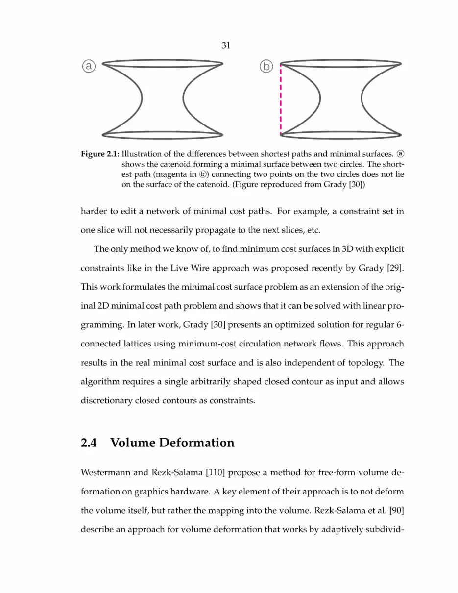
31
a b
Figure 2.1: Illustration of the differences between shortest paths and minimal surfaces. a
shows the catenoid forming a minimal surface between two circles. The short-est path (magenta in b ) connecting two points on the two circles does not lieon the surface of the catenoid. (Figure reproduced from Grady [30])
harder to edit a network of minimal cost paths. For example, a constraint set in
one slice will not necessarily propagate to the next slices, etc.
The only method we know of, to find minimum cost surfaces in 3D with explicit
constraints like in the Live Wire approach was proposed recently by Grady [29].
This work formulates the minimal cost surface problem as an extension of the orig-
inal 2D minimal cost path problem and shows that it can be solved with linear pro-
gramming. In later work, Grady [30] presents an optimized solution for regular 6-
connected lattices using minimum-cost circulation network flows. This approach
results in the real minimal cost surface and is also independent of topology. The
algorithm requires a single arbitrarily shaped closed contour as input and allows
discretionary closed contours as constraints.
2.4 Volume Deformation
Westermann and Rezk-Salama [110] propose a method for free-form volume de-
formation on graphics hardware. A key element of their approach is to not deform
the volume itself, but rather the mapping into the volume. Rezk-Salama et al. [90]
describe an approach for volume deformation that works by adaptively subdivid-
32
ing the volume into blocks which can be linearly deformed. They reached interac-
tive rendering speeds for small datasets on then-available programmable graphics
hardware. Their approach, however, does not work when using advanced mem-
ory layouts like bricking. Schulze et al. [101] have presented an approach for non-
physically-based direct volume deformation. They resample the volume during
deformation and render the deformed volume with standard volume rendering.
Their technique allows deformation of moderately-sized volumes, at voxel reso-
lution, at interactive frame rates, but the affected area must be limited. Lampe et
al. [51] present a technique to deform and render volumes along curves. They il-
lustrate two applications, one of which is the visualization of seismic data along
well logs.
2.5 Ensemble Visualization
Early work on visualization of ensemble data was conducted by Pang, Kao and
colleagues [47, 48, 56, 58]. While the authors did not use the term ensemble, these
works deal with the visualization of what they call spatial distribution data, which
they define as a collection of n values for a single variable in m dimensions. These
are essentially ensemble data. The authors adapt standard visualization tech-
niques to visualize these data gathered from various sensors, e.g. satellite imag-
ing or mutli-return Lidar. Frameworks for visualization of ensemble data gained
from weather simulations include Ensemble-Vis by Potter et al. [89] and Noodles by
Sanyal et al. [97]. These papers describe fully featured applications focused on
the specific needs for analyzing weather simulation data. They implement multi-
ple linked views to visualize a complete set of multidimensional, multivariate and
multivalued ensemble members. While these frameworks provide tools for visual-

33
izing complete simulation ensembles including multiple dimensions, to solve the
problem presented in this work we focus on 2.5D surfaces, i.e. heightfield ensem-
ble data.
Matkovic et al. [61] present a framework for visual analysis of families of sur-
faces by projecting the surface data into lower dimensional spaces. Piringer et
al. [83] describe a system for comparative analysis of 2D function ensembles used
in the development process of powertrain systems. Their design focuses on com-
parison of 2D functions at multiple levels of detail. Healey and Snoeyink [33]
present a similar approach for visualizing error in terrain representation. Here, the
error, which can be introduced by sensors, data processing or data representation,
is modeled as the difference between the active model and a given ground truth.
2.6 Uncertainty Visualization
A good introduction to uncertainty visualization is provided by Pang et al. [72],
who present a detailed classification of uncertainty, as well as numerous visual-
ization techniques including several concepts applicable to (iso-)surface data, like
fat surfaces. Johnson and Sanderson [43] give a good overview of uncertainty
visualization techniques for 2D and 3D scientific visualization, including uncer-
tainty in surfaces. For a definition of the basic concepts of uncertainty and another
overview of visualization techniques for uncertain data, we refer to Griethe and
Schumann [31]. Riveiro [92] provides an evaluation of different uncertainty visu-
alization techniques for information fusion. Rhodes et al. [91] present the use of
color and texture to visualize uncertainty of iso-surfaces. Brown [12] employs an-
imation for the same task. Grigoryan and Rheingans [32] present a combination
of surface and point based rendering to visualize uncertainty in tumor growth.

34
There, uncertainty information is provided by rendering point clouds in areas of
large uncertainty, as opposed to crisp surfaces in certain areas.
Recently, Pothkow et al. [87, 88] as well as Pfaffelmoser et al. [80] presented
techniques to extract and visualize uncertainty in probabilistic iso-surfaces. In
these approaches for visualizing uncertainty in iso-surfaces, a mean surface is ren-
dered as the main representative surface, while the positional uncertainty is rep-
resented by a ’cloud’ based on the variance around this surface. Pfaffelmoser and
Westermann [81] describe a technique for the visualization of correlation struc-
tures in uncertain 2D scalar fields. They use spatial clustering based on the degree
of dependency of a random variable and its neighborhood. They color-code the
clusters, but also allow the visualization of primary information like the standard
deviation, for example by extruding clusters into the third dimension.
Lundstrom et al. [57] propose the use of animation to show the effects of prob-
abilistic transfer functions for volume rendering. A system which models and vi-
sualizes uncertainty in segmentation data based on a priori shape and appearance
knowledge has been presented by Saad et al. [96].

35
Chapter 3
Visual Subsurface Modeling
This chapter is based on the papers Interactive Seismic Interpretation with Piecewise
Global Energy Minimization [35] and SeiVis: An Interactive Visual Subsurface Mod-
eling Application [37] as well as the poster Seismic Horizon Tracing with Diffusion
Tensors [38].
Creating a subsurface model from a seismic survey consists of several steps.
The major tasks are extracting the relevant features from the seismic cube, fol-
lowed by the creation of a velocity model, based on the extracted features and
corresponding to the speed of the seismic waves in the subsurface. Finally using
the velocity model the extracted features can be converted from time into spatial
depth. In this chapter we describe how these steps are carried out in current prac-
tice (Section 3.1). Even though we use the same three modules, using our joint
time/depth visualization (Section 3.2) results in a completely different workflow.
The joint time/depth visualization in combination with our prism based work-
flow (Section 3.3) allows direct use of depth domain based well data during the
time domain based horizon extraction. In Section 3.4 we discuss the weaknesses
of common horizon extraction techniques based on local solvers and present our
approach to a horizon extraction using global optimization. The results and eval-
uation of this work can be found in Section 3.5.

36
3.1 Current Practice
The following description of the current practice is based on the industry stan-
dard software Schlumberger Petrel [100]. While implementation details might
vary for different software tools, to our knowledge the workflow description re-
flects the common practice in the industry.
Horizon Extraction
The horizon extraction is usually carried out as a combination of 2D segmentations
on the axis-aligned slices of the seismic reflection data. The user manually, or us-
ing semi-automatic growing techniques, tags the important horizons as lines on
the slice. The auto tracer of Petrel, which is used for the semi-automatic growing,
uses a local approach, which cannot be forced through constraint points and stops
at ambiguous areas. Depending on the variation in the data, up to ten slices are
skipped between 2D segmentations, and filled by interpolation or automatic grow-
ing. The horizon extraction process is very lengthy and accounts for the major part
of the time in the typical workflow. Tagging several horizons on tens to hundreds
of slices takes at least several hours but can easily keep an interpreter busy for
multiple days, if the structures are not clearly visible or ambiguous. The output of
the horizon extraction module is a set of surfaces describing the boundaries of the
subsurface layers.
Velocity Modeling
After the horizon extraction is finished, the resulting horizon surfaces are used as
a basis for creating a velocity model. The velocity model is defined in a table view,
where for every subsurface layer the corresponding top and bottom boundaries
(horizons or other surfaces), as well as velocities are set. Once all desired layers
37
are defined, a volume containing per-voxel velocities (the so-called velocity cube)
can be computed off-line.
Depth Conversion
Finally, based on the velocity cube, the depth conversion can be computed. Using
the per-voxel velocities, the original volume and the extracted horizons can be
resampled, again off-line, from top to bottom into a new, depth-converted dataset.
Integration
Creating the velocity cube, as well as the final depth conversion, requires the user
to manually create a new derived dataset, as well as lengthy computations. In
addition, the derived datasets are not coupled. An update in one of the modules
does not automatically trigger the re-evaluation of subsequent modules. Instead, a
new derived data set has to be set up manually. This results in the linear workflow
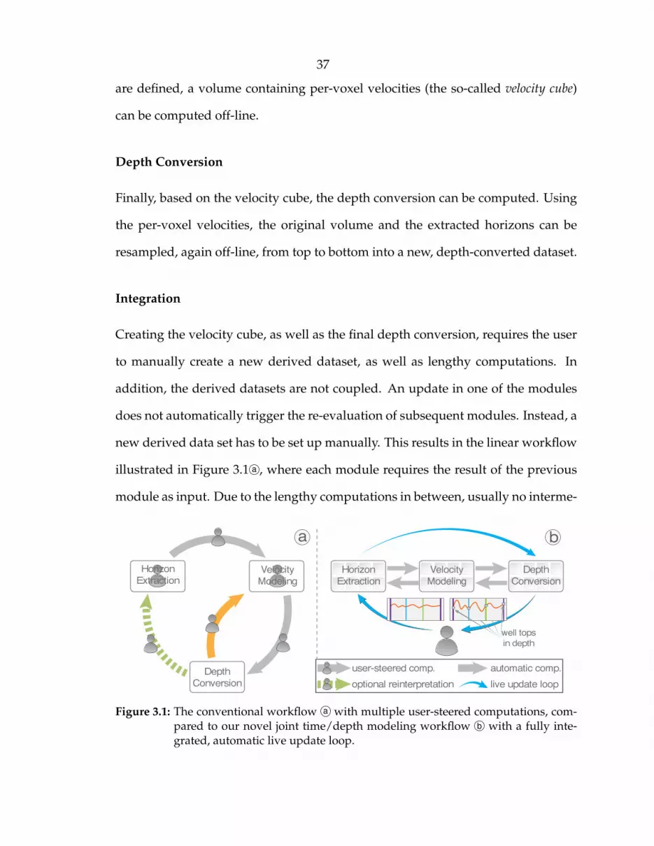
illustrated in Figure 3.1 a , where each module requires the result of the previous
module as input. Due to the lengthy computations in between, usually no interme-
Depth
Conversion
Depth
Conversion
Horizon
Extraction
Velocity
Modeling
user-steered comp.
optional reinterpretation live update loop
automatic comp.
well tops
in depth
a b
Horizon
Extraction
Velocity
Modeling
Figure 3.1: The conventional workflow a with multiple user-steered computations, com-pared to our novel joint time/depth modeling workflow b with a fully inte-grated, automatic live update loop.
38
diate results are pushed to the next module in the pipeline. A major drawback of
this approach is that mistakes that occur during the horizon extraction often only
become visible after finishing the complete pipeline, when matching the depth
converted data to the ground truth data, which is available only in depth. In an
ideal workflow, the interpreter would go back to the interpretation and fix mis-
takes (indicated by the green arrow in Figure 3.1 a ). More commonly, however, a
shortcut is taken to save time, by locally “hot fixing” the velocity cube to match the
features, accepting a possibly unphysical velocity model.
3.1.1 Weaknesses and Proposed Enhancements
The traditional workflow has two major shortcomings.
1. The precise ground truth data gathered from drillings and only available in
the depth domain is not available while interpreting the seismic cube in the
time domain, but only after a complete interpretation cycle.
2. Since re-interpreting the seismic data after a complete interpretation cycle is
very tedious and time consuming often a shortcut is taken after a few cy-
cles, by ’hot fixing’ the velocity model locally to match the ground truth data
(indicated by the orange arrow Figure 3.1 a ).
Proposed Enhancements
In this work, we propose a novel integrated workflow as shown in Figure 3.1 b .
This workflow consists of the same three modules as the traditional workflow;
horizon extraction, velocity modeling and depth conversion, however, we propose
several modifications, which drastically alter the overall workflow, to eliminate the
weaknesses, described above.
39
Our most important goal is to integrate the spatial ground truth data, gathered
from wells, into the time domain-based horizon extraction. This allows the cre-
ation of a correct model in a single pass, eliminating the need to go through mul-
tiple iterations. Therefore we propose two modifications to the traditional work-
flow:
1. Provide the user with a joint time/depth domain workflow, which integrates
the ground truth data gathered from wells into the interpretation workflow.
Therefore we propose side by side views of the time and depth domains,
where the depth domain view provides on the fly updates based on the in-
termediary results from the horizon extraction and velocity modeling.
2. To make as much use as possible of the well data, we subdivide the seismic
cube into prisms based on well positions for the horizon extraction, rather
than axis aligned slices. Each of the prisms will allow access to data from
three wells, while the availability of well data on axis aligned slices is mostly
random.
In addition, to ease the surface extraction itself, we propose the use of an inter-
active, user-steered global optimization technique instead of local solvers.
3.2 Joint Time/Depth Domain Visualization
To allow matching features extracted in the time domain to the ground truth
well data in the depth domain, we propose the use of side by side views of the data
in both domains as illustrated in Figure 3.2. The goal of these side by side views is
to allow the user to modify the interpretation in one view and immediately provide
the results of the modifications on the depth converted model in the other view.
40
taggedhorizon
horizon 1
horizon 2 horizon 2 horizon 2 horizon 2
horizon 1
faulty segmentationin unclear area
time domain view depth domain view
horizon markerin depth view
horizon 1
horizon 1
originalseismic
deformedseismic
Figure 3.2: An example for our joint time/depth domain views. The left view shows theoriginal data in the time domain. A horizon was tagged wrongly in an uncleararea. The right view shows the depth converted data. Well tops are availablein this view to guide the segmentation. The user can now fix the horizon in thetime domain view and get live updates on the fit to the well top in the depthdomain view.
Interactive updates in both views are essential for this joint time/depth domain
workflow to work properly.
Converting the complete data from one domain into the other at interactive
rates is not a trivial task. State of the art commercial software, like Schlumberger
Petrel [100] convert the data from one domain into the other by resampling the
complete dataset in an off-line process. Converting the whole seismic cube can take
from several seconds to minutes, even for small datasets. Such a process makes
interactive updates impossible.
To enable interactive updates in our joint time/depth domain views, we imple-
mented a visualization pipeline specifically optimized to handle frequent updates
of the extracted horizon surfaces, as well as a volume deformation approach where
41
surfaceextraction
timedomainhorizon
extraction
surfaceextractionvelocitymodeling
time todepth
surfacedeformation
velocitieshorizons
Interpretation Shared GPU data Rendering
horizonsin time
horizonsin depth
layervelocities
surfacerendering
volumerendering
volumesetup
displacementvertex shadercoloringfragment shader
volume renderingfragment shaderwith deformation& explosion
write read
3D boundary texture
a1
3
6
5
4
2
1D velocity textureb
mYFE�WFSUFY�CVGGFS
c
deformation factor
d
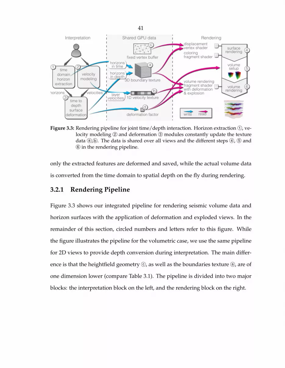
Figure 3.3: Rendering pipeline for joint time/depth interaction. Horizon extraction 1 , ve-locity modeling 2 and deformation 3 modules constantly update the texturedata a , b . The data is shared over all views and the different steps 4 , 5 and6 in the rendering pipeline.
only the extracted features are deformed and saved, while the actual volume data
is converted from the time domain to spatial depth on the fly during rendering.
3.2.1 Rendering Pipeline
Figure 3.3 shows our integrated pipeline for rendering seismic volume data and
horizon surfaces with the application of deformation and exploded views. In the
remainder of this section, circled numbers and letters refer to this figure. While
the figure illustrates the pipeline for the volumetric case, we use the same pipeline
for 2D views to provide depth conversion during interpretation. The main differ-
ence is that the heightfield geometry c , as well as the boundaries texture a , are of
one dimension lower (compare Table 3.1). The pipeline is divided into two major
blocks: the interpretation block on the left, and the rendering block on the right.

42
Texture /Buffer
Dim.3D/2D
Type Function Size 3D Size 2D
a bounds 3D/2D luminance↵ texture
layer boundaries inoriginal (.r) anddeformed (.a) space
x·y·#B·2 x ·#B · 2
b velocities 1D luminancetexture
layer velocities #L #L
c heightfieldgeometry
2D/1D vertexbuffer
generic vertexbuffer for horizons
x · y · 3 x · 2
Table 3.1: Textures and buffers needed in our pipeline in addition to basic volume render-ing. a , b , and c correspond to Figure 3.3. #B and #L represent the number ofboundaries and the number of layers, respectively. Sizes are given in number of32-bit floating point entries.
Interpretation
Interpretation comprises three modules. The horizon extraction module 1 , and
the velocity modeling module 2 , which comprise the actual surface extraction
and the definition of the velocity values for the corresponding layers. The out-
put of the horizon extraction is a 2D heightfield that covers the complete volume
domain, plus a 1D heightfield for the boundary of the current prism. Both are con-
stantly updated during the interpretation process. Each heightfield corresponds to
a single horizon, and is stored as a layer in the first channel of the 3D or 2D bound-
aries texture a on the rendering side, and is also available to the depth conversion
module on the interpretation side.
The velocity modeling module 2 outputs a velocity value for each layer, which
is stored into the 1D velocities texture b .
The surface deformation module 3 takes the updated heightfields from the
horizon extraction module 1 , and converts the values from the time to the depth
domain using the velocity model from the velocity modeling module 2 . Com-

43
pared to recomputing the deformation for the complete volume, very little data
needs to be processed, allowing real time updates (compare Table 3.2 in the per-
formance discussion in Section 3.2.3).
The resulting depth-converted heightfields are stored in the second channel of
the 2D or 3D boundaries texture a . In addition, the depth conversion module
outputs the maximum scaling factor d needed to cover the depth conversion at
any (x, y)-position.
Rendering
The data is shared between all views and steps in the visualization pipeline. Ta-
ble 3.1 gives an overview of the shared textures and buffers. Basically all of our
views make use of vertex and fragment shaders to exploit the possibilities of the
programmable OpenGL pipeline. We used this, for example, to streamline the
horizon surface rendering part 4 of the pipeline. Instead of creating geometry
for each horizon, we use a single generic vertex buffer c , covering the complete
(x, y)-domain, but without the depth (z) information at the vertices. We render the
surfaces one by one and use the boundaries texture a in the vertex stage to assign
the appropriate z-values to each vertex.
Invalid fragments, i.e., the fragments belonging to triangles in the mesh that
are not yet covered by the interpretation, are discarded. Additionally, we use the
fragment shader to compute several properties of the surfaces on the fly. Using
the data which is already available for the other rendering stages on the GPU,
several properties can be plotted directly onto the surface without precomputing a
separate texture. The amplitude can be looked up directly from the volume texture.
Cost or deviation from the target amplitude can be computed on the fly based on

44
data from the same texture. The distance to other surfaces can be evaluated using
the boundaries texture.
3.2.2 On the Fly Deformation
The volume deformation required for the depth conversion is highly constrained.
Deformation only needs to be applied to the depth axis of the volume, in order to
convert its unit from time to spatial depth in the subsurface. We represent hori-
zons as heightfields, and we can safely assume that no horizons intersect. Thus,
every two adjacent horizons enclose one subsurface layer. Furthermore, the veloc-
ity for each layer in the volume can be assumed to be constant, using an average
value. Thus, the deformation can be simplified to a piecewise linear stretching or
compression of the volume between each two adjacent horizons. Taking these con-
straints into account, it is possible to implement the deformation in a simple and
efficient manner. This enables depth conversion at real-time frame rates during
volume and slice rendering, without precomputing a deformed volume.
Concept
Our approach is inspired by the work of Westermann and Rezk-Salama [110]. Con-
ceptually, we never deform the original volume, but render a virtually deformed
volume, converting the look-ups in this volume into the original volume space on
the fly in the fragment shader. We do that by converting only the layer boundaries
(which are the result of the interpretation in progress) from time to depth. The n-th
deformed boundary b0n
can be computed as
b0n
(x, y) =
nX
k=1
(bk
(x, y)� bk�1(x, y)) · vk (3.1)

45
from the time domain boundaries bn
and velocities vn
. Figure 3.4 illustrates the
deformation with this simple iterative computation of the deformed boundaries.
The boundaries have to be recomputed only when a velocity value is changed or
a horizon is modified. Computational complexity is O(n), with n the number of
vertices that need to be updated. Since the computation is independent for each
(x, y)-position, we have parallelized it using OpenMP. We measured computation
times for several surfaces and even for larger surfaces consisting of roughly a mil-
lion quads, the update time for a couple of horizons is interactive (see Table 3.3 in
the performance discussion in Section 3.2.3).
For volume rendering, we use a single-pass ray caster. The ray caster is set up
to cast into a virtual volume, resized with the scaling factor d , which is set to the
maximum value of the bottom boundary to fit the deformed volume. During ray
casting, the depth-converted boundaries are used to compute the actual look-up in
time to depth surface deformation
layer0 / v0b0: top boundaryb1: horizon0
b2: horizon1
b3: horizon2
b4: bottom boundary
layer1 / v1
layer2 / v2
layer3 / v3
bb
b
b
b
b0 = b0
def.fac. = max(b4)deformed volbounding box
b1 = b0 +(b1 - b0)・v0
b2 = b1 +(b2 - b1)・v1
b3 = b2 +(b3 - b2)・v2
b4 = b3 +(b4 - b3)・v3
bbb
b
b
bdd
Figure 3.4: Illustration of the surface deformation (Fig. 3.3 3 ) with computation of de-formed boundaries.
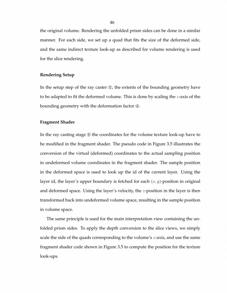
46
the original volume. Rendering the unfolded prism sides can be done in a similar
manner. For each side, we set up a quad that fits the size of the deformed side,
and the same indirect texture look-up as described for volume rendering is used
for the slice rendering.
Rendering Setup
In the setup step of the ray caster 5 , the extents of the bounding geometry have
to be adapted to fit the deformed volume. This is done by scaling the z-axis of the
bounding geometry with the deformation factor d .
Fragment Shader
In the ray casting stage 6 the coordinates for the volume texture look-up have to
be modified in the fragment shader. The pseudo code in Figure 3.5 illustrates the
conversion of the virtual (deformed) coordinates to the actual sampling position
in undeformed volume coordinates in the fragment shader. The sample position
in the deformed space is used to look up the id of the current layer. Using the
layer id, the layer’s upper boundary is fetched for each (x, y)-position in original
and deformed space. Using the layer’s velocity, the z-position in the layer is then
transformed back into undeformed volume space, resulting in the sample position
in volume space.
The same principle is used for the main interpretation view containing the un-
folded prism sides. To apply the depth conversion to the slice views, we simply
scale the side of the quads corresponding to the volume’s z-axis, and use the same
fragment shader code shown in Figure 3.5 to compute the position for the texture
look-ups.

47
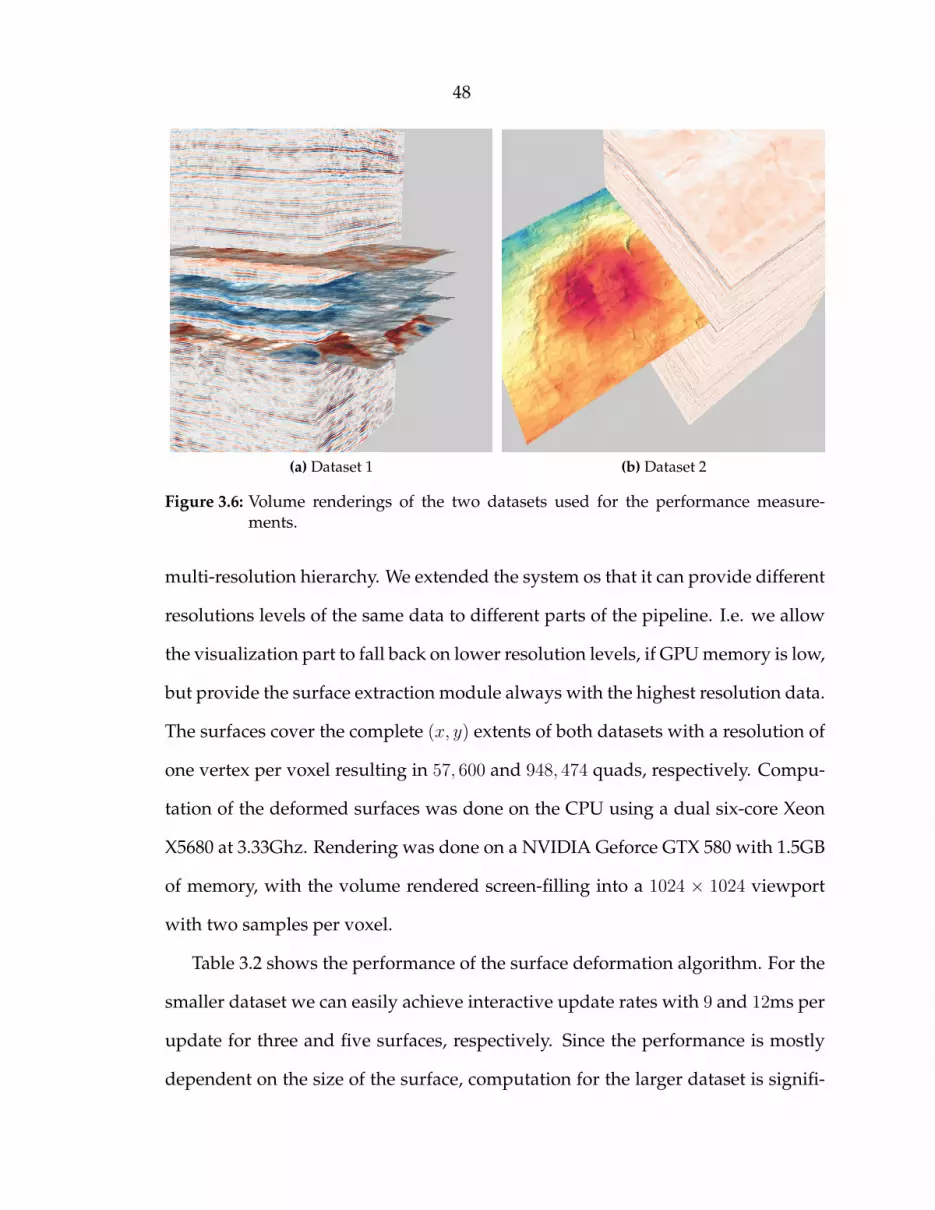
3.2.3 Performance
We have measured the rendering performance for the live deformation with two
different datasets: The first dataset, shown in Figure 3.6a is moderately sized with
240⇥240⇥1509 voxels, and at 330MB fits completely into GPU memory. The second
dataset (Figure 3.6b) comprises 1422⇥ 667⇥ 1024 voxels, resulting in roughly 4GB,
meaning the dataset does not fit the GPU memory of our test system described
below. Therefore, for rendering the second dataset, we use a multi-resolution ap-
proach as presented by Beyer et al. [4]. This approach allows rendering differ-
ent parts of the data at different resolution levels with smooth transitions using a
1 uniform sampler1D velocities;2 uniform sampler3D boundaries;3 uniform float scaleFactor;45 convertSamplePosToVolumeSpace( x, y, z )6 {7 // scale from [0..1] to deformed volume coordinates
8 z *= scaleFactor;9
10 // get the id of the current layer
11 float layerId = getLayerId( x, y, z );1213 // lookup layer offset in undeformed and deformed volume coordinates
14 vec2 layerOffset = texture3D( boundaries, vec3( x, y, layerId ) ).xw;1516 // distance to layer boundary in deformed volume coordinates
17 float posInLayer = z - layerOffset.y;1819 // distance to layer boundary in deformed volume coordinates
20 float velocity = texture1D( velocities, layerId );21 posInLayer /= velocity;2223 // update z coordinate to sample in volume coordinates
24 z = layerOffset.x + posInLayer;2526 return vec3( x, y, z );27 }
Figure 3.5: Pseudo code for live volume deformation. Virtual (deformed) coordinates areconverted to undeformed coordinates on the fly during rendering in the frag-ment shader. The syntax is similar to GLSL.
48
(a) Dataset 1 (b) Dataset 2
Figure 3.6: Volume renderings of the two datasets used for the performance measure-ments.
multi-resolution hierarchy. We extended the system os that it can provide different
resolutions levels of the same data to different parts of the pipeline. I.e. we allow
the visualization part to fall back on lower resolution levels, if GPU memory is low,
but provide the surface extraction module always with the highest resolution data.
The surfaces cover the complete (x, y) extents of both datasets with a resolution of
one vertex per voxel resulting in 57, 600 and 948, 474 quads, respectively. Compu-
tation of the deformed surfaces was done on the CPU using a dual six-core Xeon
X5680 at 3.33Ghz. Rendering was done on a NVIDIA Geforce GTX 580 with 1.5GB
of memory, with the volume rendered screen-filling into a 1024 ⇥ 1024 viewport
with two samples per voxel.
Table 3.2 shows the performance of the surface deformation algorithm. For the
smaller dataset we can easily achieve interactive update rates with 9 and 12ms per
update for three and five surfaces, respectively. Since the performance is mostly
dependent on the size of the surface, computation for the larger dataset is signifi-

49
Dataset Samples perSurface
Number ofSurfaces
ComputationTime
240⇥ 240⇥ 1509 57, 6003 9ms
5 12ms
3 144ms1422⇥ 667⇥ 1024 948, 474
5 174ms
Table 3.2: Surface deformation performance for the on the fly depth conversion.
cantly slower. Computation time of 144ms for three surfaces, however still allows
for seven updates per second. While this does not quite allow updates in real
time during the surface deformation, it should be noted that the computation only
needs to be carried out when the surface geometry or the velocity model is modi-
fied and thus does not have an impact on rendering speed during regular interac-
tion. In addition in a typical workflow, where surfaces are extracted top to bottom
only the last layer needs to be updated, meaning that the case for three surfaces is
basically the worst case.
Performance for the ray casting algorithm with live depth conversion, as pre-
sented in Section 3.2.2, is shown in Table 3.3. In comparison to the standard ray
casting algorithm used for rendering the undeformed volume, this technique re-
quires three additional texture look-ups and four floating point operations per
sample to compute the sample position in the original volume (compare the source-
code in Figure 3.5). In addition, to get the layer id of the current sample, a number
of additional texture look-ups have to be performed. The actual number depends
on the search algorithm used. Right now we step through all layers from top to
bottom until reaching the current sample point. This results in the performance
loss shown in Table 3.3, when adding more layers.

50
Dataset Number ofSurfaces
Base DepthConversion
% ofBase
240⇥ 240⇥ 1509
3117fps
99fps 85%
5 87fps 66%
3 81fps 80%
1422⇥ 667⇥ 1024
5101fps
77fps 76%
Table 3.3: Performance comparison of the live depth conversion. We used standard raycasting without illumination for the comparison.
Overall, performance stays well within the limits needed for interactivity for
both datasets. For the larger dataset it can be seen that rendering speeds scale very
well, using the multiresolution representation. Since the surfaces are deformed at
full resolution there is a bigger performance penalty, however, update rates are still
interactive and updates are only needed when surfaces or the velocity model is up-
dated. In addition our visualization pipeline, described in Section 3.2.1 basically
decouples the resolution of the extracted surfaces from the geometry. Thus one
could imagine a similar multi-resolution approach for the deformation as for ren-
dering, in case surface resolution becomes too big to handle at interactive rates.
3.3 Prism-Based Workflow
With the on the fly depth conversion in place we can now show the original
and depth converted data side by side to allow adjusting the time domain based
interpretation to the depth domain based well data. However the well data is
very sparse and thus, in a slice based workflow only available on a few slices.
To maximize the availability of the additional data during the interpretation we
propose a workflow that is based on well positions rather than axis-aligned slices.
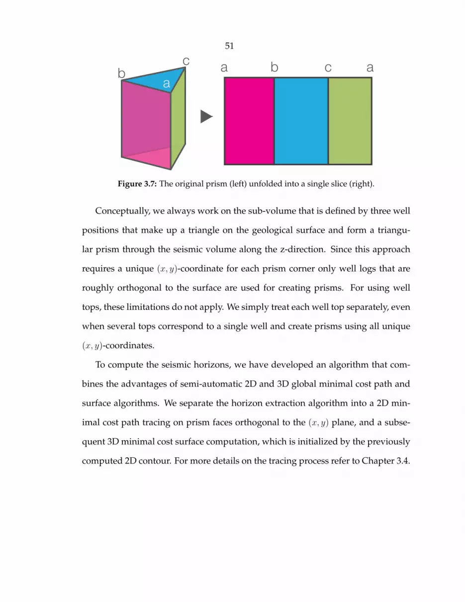
51
aaa cbc
b
Figure 3.7: The original prism (left) unfolded into a single slice (right).
Conceptually, we always work on the sub-volume that is defined by three well
positions that make up a triangle on the geological surface and form a triangu-
lar prism through the seismic volume along the z-direction. Since this approach
requires a unique (x, y)-coordinate for each prism corner only well logs that are
roughly orthogonal to the surface are used for creating prisms. For using well
tops, these limitations do not apply. We simply treat each well top separately, even
when several tops correspond to a single well and create prisms using all unique
(x, y)-coordinates.
To compute the seismic horizons, we have developed an algorithm that com-
bines the advantages of semi-automatic 2D and 3D global minimal cost path and
surface algorithms. We separate the horizon extraction algorithm into a 2D min-
imal cost path tracing on prism faces orthogonal to the (x, y) plane, and a subse-
quent 3D minimal cost surface computation, which is initialized by the previously
computed 2D contour. For more details on the tracing process refer to Chapter 3.4.

52
User interaction in this approach is mostly limited to the 2D optimization on
the sides of the prism. Therefore the prism sides are unfolded into a single 2D slice
as shown in Figure 3.7.
This approach was proposed by our collaborating domain experts. The main
advantage of this approach is that the horizon can easily be adjusted directly at
the well position, which is the point where errors in the interpretation become
visible when adjusting the horizon to the ground truth data from the well log dur-
ing time/depth-conversion of the seismic volume. In combination with our joint
time/depth domain workflow this allows direct interaction with well data from
three positions on each slice during the interpretation. After extracting a horizon
surface patch for one well prism, the horizon can then be extended by processing
the neighboring prisms, creating a set of horizon surface patches that constitute
the horizon surface. The result from one prism will therefore be transferred to the
neighbors. As a result, the interpretation itself is done triangle (prism) by trian-
gle (prism), instead of slice by slice, making ground truth data from three wells
available in every working set. To extend the horizon trace to areas not covered by
wells, additional points of interest (e.g. the corners of the volume) can be added to
the triangulation.
3.4 Horizon Extraction using Global Optimization
As discussed in Section 3.1 we identified several shortcomings in the current
practice of horizon extraction. We presented the joint time/depth domain visual-
ization in combination with the well based workflow above, to solve the issue of
integrating the depth domain-based well data into the time domain-based horizon
extraction workflow. In the following sections we will present a global optimiza-
tion technique to enhance the feature extraction itself.
53
In Section 3.4.1 we discuss the requirements for the horizon extraction. We
exemplarily present a horizon extraction technique based on a local solver in Sec-
tion 3.4.2 and discuss the problems of the local solver in general as well as the
weaknesses with regard to our defined requirements. In the following Sections 3.4.3 –
3.4.5 we present our proposed approach to horizon surface computation which is
implemented in the presented workflow.
3.4.1 Requirements for Horizon Extraction
Horizon surface extraction using the conventional workflows of available state
of the art software is a very tedious process. It is done either manually or semi-
automatically using local solvers on axis-aligned slices. Fixing a mistake with
these approaches is very tedious, as it requires manual correction of multiple slices.
On the one hand, this is caused by the noisy and ambiguous seismic data, which
causes big problems for automatic solvers, on the other hand the local solvers
which are usually used, limit the possibility for semi-automatic adjustments. To
enhance the process we define a set of specifications, which are desired for a semi-
automatic horizon extraction workflow, based on the presented joint time/depth
domain views as well as the prism-based workflow:
1. The solver should always extract a complete path/surface.
2. It must be possible to force the path/surface through desired positions.
3. The user should be able to directly interact with the surface.
The first point can be achieved with local, as well as global solvers. However,
some local solvers, like ant tracking [77], which is commonly used in seismic ap-
plications, do not guarantee a complete surface. Other techniques, like level set
methods [71] do not have the same problems.

54
Forcing the path or surface through a desired positions, as required by the sec-
ond point is necessary to make sure that the tracing on the prism sides results in a
closed curve, but also to allow the user to easily adjust a faulty segmentation. This
is, however, not achievable with local solvers. Since only the local neighborhood is
evaluated, it is not possible to guarantee that any point will be part of the final path
or surface, except for the seed point. Global approaches, such as shortest path al-
gorithms, allow this. These shortest path algorithms always find the optimal path
between two points. If a third point is desired to be part of the path, the algorithm
can simply search for two optimal segments, one from the start to the added point
and a second from the added point to the target.
Recently, graph based image segmentation approaches, like the described short-
est path algorithms, became very popular in computer vision. These approaches
can be divided into explicit and implicit boundary approaches. The difference be-
tween these approaches lies in the objects which are segmented. Implicit boundary
approaches, for example graph cuts [9], segment fore- and background, the result
is a set of pixels/voxels that belong to the segmented object, the boundary is im-
plicit. The result of explicit boundary approaches is a curve or surface, which
encloses the segmented object. Explicit boundary approaches map naturally to
the third requirement described above. While implicit boundary approaches can
be constrained by fore- or background pixels/voxels, the explicit boundary ap-
proaches can be constrained by curve or surface segments, meaning that user-
defined positions, which need to be part of the contour or surface map directly
to constraints for the optimization.
55
3.4.2 Local Horizon Extraction: Tracing Diffusion Tensors
In this section we present a horizon extraction approach based on tracing a
diffusion tensor based vector field derived from the seismic cube. Based on this
technique we show the weaknesses, common to most local approaches.
Implementation
Edge-enhancing anisotropic diffusion [109] is a non-linear smoothing technique
which preserves edges by computing an edge direction vector for every sample
and using this vector as a parameter for the smoothing operation
@ut
= div(D ·ru), (3.2)
where D is the diffusion tensor, and ru is the gradient of the intensity volume
u(x, y, z). Together, D ·ru determines the direction which the divergence operator
uses to smooth the image. In the general 3D case, the diffusion tensor is computed
as
D = [v1v2v3]
2
6666666666664
�1 0 0
0 �2 0
0 0 �3
3
7777777777775
2
6666666666664
vT1
vT2
vT3
3
7777777777775
. (3.3)
Based on the edge-enhancing diffusion tensor, in our system the first basis vector
v1 is computed by applying a 7⇥ 7⇥ 7 Gaussian derivative kernel to the volume at
each sample point. This results in the smoothed gradient ru�
at position (x, y, z)
(Figure 3.8 b ). A vector orthogonal to v1 is then chosen as v2, and v3 is a vector or-
thogonal to both, v1 and v2. �1, �2, and �3 are scaling factors, which are responsible
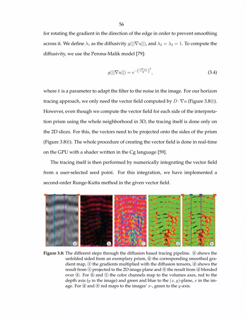
56
for rotating the gradient in the direction of the edge in order to prevent smoothing
across it. We define �1 as the diffusivity g(||ru||), and �2 = �3 = 1. To compute the
diffusivity, we use the Perona-Malik model [79]:
g(||ru||) = e�(||ru||
k
)
2
, (3.4)
where k is a parameter to adapt the filter to the noise in the image. For our horizon
tracing approach, we only need the vector field computed by D ·ru (Figure 3.8 c ).
However, even though we compute the vector field for each side of the interpreta-
tion prism using the whole neighborhood in 3D, the tracing itself is done only on
the 2D slices. For this, the vectors need to be projected onto the sides of the prism
(Figure 3.8 e ). The whole procedure of creating the vector field is done in real-time
on the GPU with a shader written in the Cg language [59].
The tracing itself is then performed by numerically integrating the vector field
from a user-selected seed point. For this integration, we have implemented a
second-order Runge-Kutta method in the given vector field.
a c eb d
Figure 3.8: The different steps through the diffusion based tracing pipeline. a shows theunfolded sided from an exemplary prism, b the corresponding smoothed gra-dient map, c the gradients multiplied with the diffusion tensors, d shows theresult from c projected to the 2D image plane and e the result from d blendedover a . For b and c the color channels map to the volumes axes, red to thedepth axis (y in the image) and green and blue to the (x, y)-plane, x in the im-age. For d and e red maps to the images’ x-, green to the y-axis.
57
Jeong et al. [42] use coherence-enhancing anisotropic diffusion filtering as basis
for fault detection in seismic data. In that work, the tensor is computed as shown
in Equation 3.3. However, instead of directly using the smoothed gradient to create
the diffusion tensor, here the Eigenvectors of the structure tensor J(ru�
) = rI�
⌦
rI�
of the smoothed image I�
= K�
⇤ I , with I the input image, ⇤ the convolution
operator and K�
a Gaussian
K�
(x) =1p2⇡�
e�kxk2
�
2 , (3.5)
are used as v1, v2, and v3, in order of their contribution. The smoothed matrix J⇢
is
computed by smoothing the structure tensor with another Gaussian
K⇢
(x) =1p2⇡⇢
e� kxk2
⇢
2 , (3.6)
resulting in
J⇢
(rI�
) = K⇢
⇤ (rI�
⌦rI�
). (3.7)
Additionally �1 ⇡ 0 and �i
= e�(v
i
·rI)2
k
2 , for i = 2, 3, where vi
is the i-th eigenvec-
tor of the structure tensor J and k is a user adjustable parameter to adjust to the
contrast of the image.
For comparison, we have also implemented a variant of our approach using the
coherence-enhancing diffusion tensor. Results showing the tracing, both with the
coherence-enhancing, as well as the edge-enhancing diffusion tensor are shown in
Figure 3.9 a .
Finally, as horizons are marked by local extrema in the scalar data, we have
implemented an additional version of both approaches that incorporates searching
the scalar field for a local maximum or minimum in the tracing algorithm. Rather

58
than using the result of an integration step directly as input for the next step, the
neighborhood of a user-defined size in the �z and +z directions is scanned for the
highest or lowest scalar value, respectively. The location of this value is then used
instead of the integration result as support for the traced horizon, as well as input
for the next integration step. Results for this method are shown in Figure 3.9 b .
Results and Discussion
Figure 3.9 shows some exemplary results of the different tracing algorithms for
three reflections in a seismic dataset. It can be seen that overall the traces match
the reflections (or ridge-lines in this case) quite well. Comparing tracing using
the edge-enhancing diffusion tensor with the coherence-enhancing tensor (Fig-
ure 3.9 a ) shows that the former is a little closer to the actual areas of maximum
amplitude and more responsive to changes in the horizon direction. The differ-
ence between both incorporating the snapping to maximum intensity values is
very small (Figure 3.9 b ) and for both the correctly traced parts are closest to the
actual horizon of all compared methods. However, the deviation from the vector
a b
Figure 3.9: Results of the different seismic horizon tracing methods we have implemented.a edge-enhancing vs. coherence-enhancing diffusion tensor and b , just as a ,but with snapping to the largest scalar value.

59
field there introduces a much higher chance of false classification, as can be seen
on the right side of the uppermost image.
Even though promising, the results exhibit some of the typical weaknesses of
local approaches. The area highlighted by the green circle in Figure 3.9 b shows
an area where integrating the vector field, which is based on a single sample at
each step, results in a segment, where a path which is locally better, is followed
(upper part of the image), resulting in the miss of the clear reflection in the lower
part of the image, which would be the correct solution. With a global approach, a
reflection this strong would usually not be missed. A similar behavior can be seen
in the area highlighted by the blue circle in Figure 3.9 a .
The magenta circles in Figure 3.9 b show another problem, caused by the local
nature of the approach. Since the next segment of the path is only influenced by
the current sample, it is not possible to force the segmentation through any desired
points. This means that we can not guarantee a closed cycle around the prism sides
when using a local solver in our prism based workflow. In Figure 3.9 b this can be
seen at the left and right sides of the slice, which correspond to the same well
position. Ideally, the segmented path should join here, however, as indicated by
the magenta circles, the positions at both sides varies strongly. The fact that it is
not possible to force the segmentation through desired positions also makes it very
hard to edit the computed paths. When a segmentation is faulty, the only way to
fix it is to remove the faulty part from the segmentation and then retrace this area,
or even do the segmentation completely manually in this area.
We have shown that at least the second and third requirements set in Sec-
tion 3.4.1 can not be fulfilled using this approach. The biggest problem is the fact
that it can not be guaranteed that the trace results in a closed contour. In addition it
is not clear how to extend the approach to three-dimensional surfaces from the ex-
60
tracted contours. In slice based approaches typically the gap between interpreted
lines on neighboring slices is interpolated. With our well prism-based approach
the area inside a prism is usually larger than the area between interpreted slices.
Simply interpolating would most likely lead to very imprecise results.
3.4.3 Minimum Cost Circulation Network Flow
Instead of interpolating the horizon surfaces in between two dimensional curves,
we propose performing full three dimensional optimization. The part of a horizon
intersecting a given prism can be extracted by specifying as little as a single seed
point, using global energy minimization techniques to compute a horizon surface
of minimal cost. We combine very fast two dimensional minimal cost path trac-
ing with subsequent three dimensional minimal cost surface computation. The
path tracing computes horizon intersections along the faces of the prisms, which
are then used to constrain the surface computation. By combining the optimal
surfaces from the individual prisms, we receive a piecewise globally optimized
horizon. Extracting the horizon in a piecewise manner allows for an interactive
algorithm which gives the user full control over adjusting the surface by setting
an arbitrary number of constraints, forcing the surface to pass through specified
locations, while the global optimization can help fixing mistakes with very little
interaction by placing a few constraints.
Algorithm
Our approach for computing horizon surfaces using global energy minimization is
based on previous work of Grady [29, 30]. In his work, Grady formulates the min-
imization problem for boundary constrained 3D minimum cost surface computation
and shows that minimal-cost circulation network flow (MCNF) is an optimized
solution for the dual of this particular problem. By circulating the maximum pos-

61
sible amount of flow in the dual graph through any initial surface z0 fulfilling the
boundary constraints, eventually a set of edges will be saturated. This forms a
cut, which corresponds to the minimal cost surface in the primal. The process is
similar to the maximum flow, minimum cut method used for graph cuts, with the
type of constraints being the main difference. Graph cuts define fore- and back-
ground elements in the image as constraints, which then form the source and sink
nodes in the graph, whereas for MCNF, with no source or sink nodes present, the
constraints are added as the boundary of the initial surface z0. Hence the MCNF
approach naturally matches the third requirement from Section 3.4.1.
Our algorithm for computing minimal horizon surfaces consists of the follow-
ing main steps:
1. A closed contour bounding the desired surface within a prism has to be com-
puted. This is done in a flattened representation of the prism’s sides (see
Figure 3.7).
2. Next, the volume contained in the prism has to be represented as a weighted,
directed graph.
3. The initial surface z0 fitting the boundary acquired in the first step needs to
be inscribed in the graph.
4. The MCNF through z0 is computed.
5. The minimal-cost surface is constructed from the set of saturated edges of the
circulation, bounded by the initial contour.
6. If the surface is not satisfactory, it can be forced through desired points by
placing additional constraints. These constraints are then added as addi-
tional (inner) boundary patches in step 3. Steps 4 and 5 need to be reapplied.

62
Below, the steps of our algorithm are explained in more detail.
2D Contour Creation
The initial closed contour for each prism is computed as a minimal-cost path on the
prism sides. For any prism, the three sides are re-sampled from the volume using
texture mapping with tri-linear interpolation, and stitched together into a single
image. This image, superimposed with selected well log data from the prism cor-
ners, is shown in the main interpretation view and also used to construct the graph
used for the minimum cost path computation. Figure 3.10 shows the mapping of
an image to primal and dual graph elements. In contrast to standard approaches
in image segmentation [25, 67], where the minimal-cost path/surface computation
is done on the dual graph, resulting in a boundary in between image elements,
the seismic horizons we want to extract are represented in the data by bands of
extremal values. Thus, for seismic interpretation we do not compute the minimal-
cost path in between the voxel grid but directly on the grid. The underlying graph
Pixel Primal
node
node
edgeedge
facet
facet
Dual 2D
node
edge
facet
Dual 3D 2D Lattice
cube
cube
3D only:
Figure 3.10: Correspondence between image/volume elements and items in the primaland dual graph. In the primal an n-dimensional pixel always maps to a node,whereas in the dual the mapping changes depending on the dimension.

63
then has to be the primal graph, instead of the dual graph. The resulting minimal
cost path will be a set of edges connecting pixels in the image instead of dividing
pixels.
Despite working on the primal instead of the dual graph, our approach is very
similar to the well known live-wire workflow [66, 68]. We have implemented the
minimal cost path computation in CUDA [69] on the GPU using a parallel variant
of Dijkstra’s algorithm [19] called delta stepping [63, 64]. The algorithm is applied
on the primal graph constructed, as a 4-connected lattice according to Figure 3.10,
from the stitched image of the prism sides. Edge weights are defined using the
cost function defined in Section 3.4.5. The minimal path has to be bounded by at
least two nodes, otherwise it will not contain any edges. To be able to compute
the minimal cost path using just a single seed point, the cyclic nature of the prism
sides has to be taken into account when creating the graph. Therefore all nodes in
the rightmost column are connected to their counterparts in the leftmost column
of the lattice. The path is forced around the prism by removing all arcs pointing
to nodes in the same columns as the seed point. That way, the single seed point
simultaneously functions as start- and endpoint of the path and it is ensured that
the path completely encircles the prism.
Dijkstra’s algorithm cannot handle constraints directly. However, constraints
can be added simply by dividing the problem. Instead of trying to compute the
complete path at once, the path can be coerced through any node (the constraint)
in the graph by computing the minimal cost path in segments. Every constraint
will then bound two connected segments, one as a start- and one as a target-node.

64
3D Graph Initialization and MCNF
MCNF describes the problem of putting as much flow as possible through the
edges of a network at minimal cost, without adding or draining flow with dedi-
cated source or sink nodes. Therefore, a capacity and a cost is assigned to every
edge. As the graph does not contain a source or a sink, the incoming and outgoing
flow at every node must be equal, thus flow can only circulate in the graph. The
cost is always prioritized over the capacity of edges. If a cycle adds cost to the total
flow network, it will not be used, regardless of its capacity. The capacity of a cycle
is defined by the lowest capacity of the edges it consists of and the total flow in the
graph is defined by the accumulated flow of all cycles.
To compute the maximum flow in a prism, the dual graph is created by using
all voxels contained in the prism, according to the volume-graph scheme shown
in Figure 3.10. The graph is constructed in two steps: first, the basic graph struc-
ture of the dual is created (Figure 3.11 a ), and costs and capacities are assigned to
cost & capacityinitialization
z0 surfaceinitialization
cost 1 for all edges
capacity denoted byedge thickness! on sides
initial surfacein primal graph
MCNFextract min cost surface
2D horizon functionsas surface boundary
Dual Graph
Dual Node
Primal GraphVoxels - grey value
indicates amplitude
Dual Edgeon projectedDual Facet
Primal Nodesbelonging to
boundary
2D sliceused for
illustration
Prism
saturateddual
edges
minimal path/surface candidatesin primal corresponding to satu-rated dual edges
2 alternatevalid paths
dead end pathseparate patch
cut backpointing arc for dual edgescorresponding to initial surface
-n -n-n-n
-nn
-n n-n
cost -n for dual edgescorresponding to initialsurface to induce flow
MC
----nnnnnnnnnnnnnnn
minimalpath/surface
a
f hg
b c d e
Figure 3.11: The computation pipeline for our global optimization based horizon extrac-tion approach. The pipeline consosts of five major steps. The graph structureis defined as shown in a , costs and capacities for the edges are defined in b .The initial surface is created as shown in c , d shows the result of the MCNFcomputation and finally e the resulting optimal surface.

65
each edge (Figure 3.11 b ). In this step, a cost of 1 is used for all edges (not indi-
cated in the figure). The capacities of the dual edges correspond to the costs of the
primal facets and are computed using Equation 3.19 in Section 3.4.5. The edges
contained in the outer facets in the graph, have to be treated separately. These
edges do not have all four adjacent voxels and thus the cost cannot be computed
using the cost function. We initialize these edges with infinite capacity. Edge ca-
pacities are indicated in Figure 3.11 b by the thickness of the edge. At this point,
there will be no flow in the graph, because all edges have positive cost. In the
second step, the initial surface z0 is added to the graph. The initial surface is a set
of facets in the primal, bounded by the closed contour obtained from the prism
sides. In Figure 3.11 c , the boundary is indicated by the two purple primal nodes,
the initial surface by the path between these nodes. To induce flow through the
initial surface, negative costs are assigned to the dual edges corresponding to the
primal facets of z0. To allow all possible paths, the cost is the negative of the sum
of all positive costs in the graph, such that every path through z0 is negative and
thus reducing total cost for the circulation. Additionally, we allow flow through
the surface only in one direction by cutting all edges in the opposite direction. This
guarantees that no cycles going back and forth through the surface are generated.
Here it becomes obvious why we assign infinite capacity to the outer edges in the
first step. All allowed cycles will go through the initial surface and the inner edges
in one direction, and come back on the (much fewer) edges on the faces of the
prism. If the capacity of these edges were limited, the algorithm would most likely
terminate, delivering a set of saturated edges on the outside of the prism, which
would not be helpful for finding the minimal-cost surface.
For most image segmentation approaches, the initial 2D trace will be performed
on one slice in the volume, resulting in a planar boundary. In that case, the part

66
of the slice bounded by the obtained 2D trace is the simplest match for the initial
surface z0. The 2D trace in our approach, does not result in a single planar bound-
ary, however, a very simple initial surface can be constructed dividing the surface
into four planar parts. First we cut the prism above the highest point in the trace
with an orthogonal slice, resulting in a triangle shaped boundary in that slice. This
triangle functions as the cover of our surface. The other three parts are on each side
of the prism, bounded by the initial trace on the bottom, the cover slice on the top
and the prism edges on the sides. Figure 3.11 g shows a sketch of an initial surface
fitting a 2D horizon path on the sides of a prism, the cover is depicted in light, the
sides in dark cyan, the 2D trace on the prisms sides by the purple curve.
For the actual MCNF computation, we use the LEMON C++ graph library [1],
which can compute the flow for all edges in the graph. This is used to identify the
saturated edges in the graph.
3.4.4 Extracting the Surface from the Saturated Graph
The set of saturated edges does not translate directly to the desired minimal cost
surface. In real world datasets, usually a certain amount of edges not contribut-
ing to the minimum cost surface are saturated. Figure 3.11 d shows the cases of
saturated dual edges which have to be removed. Dual edges/primal facets not
connected to the initial boundary could simply be avoided by growing the surface
from the initial boundary. However, dead end paths/surface patches, connected
to the surface would not be removed by growing.
Instead, we prune facets by checking that all four of the facet’s edges are either
shared with another facet candidate, or are part of the initial boundary. By iterating
over all facets and discarding facets which do not fit these criteria, the set of surface

67
candidates is gradually reduced. Once a pass over all facet candidates finishes
without finding any more facets that need to be discarded, the remaining facets
form the minimal-cost surface and the algorithm returns (Figure 3.11 e / h ). If two
alternate surfaces bounded by the initial contour exist (top left part of the path in
Figure 3.11 d ), both must be of the same cost and thus are equivalent solutions. As
the user can always force one of these we just use the first complete closed surface
found by the algorithm.
3.4.5 Cost Function
For the global optimization to produce meaningful results, a proper cost func-
tion must be designed to assign low costs to pixels/voxels with a high probability
of belonging to a seismic horizon and high costs otherwise. Horizons are marked
by strong reflections in the seismic data. These can be identified by the scalar value
only, or more precisely by looking at the local neighborhood. The seismic cube is
constructed by a set of one dimensional traces or waves. Horizons are indicated in
this data by local extrema of the waveform. In the following, we construct a cost
function which is based on the scalar values as well as the local waveform. We
use the same cost function for the contour extraction in 2D by assigning the cost
to each edge, derived from the pixels at the two ends of the edge, as well as for
the surface extraction in 3D by assigning the cost to the capacity of the dual edges.
The dual edges correspond to facets in the primal graph, connecting four voxels.
The cost is thus derived from the gray values as well as the local waveform of all
four corners of the facets.
We define edge and facet weights using a cost function containing two major
components. The first component gsnap defines the snappiness of the surface to ridge
and valley lines/surfaces in the image/volume. The snappiness term defines the

68
likeliness of each of the corresponding pixels/voxels belonging to a horizon sur-
face based on the scalar value, as well as the local waveform at that pixel/voxel.
The second component gsmooth of the cost function is important for the smoothness
of the traced line/surface. The smoothness term is supposed to avoid large jumps
of the scalar value within a single edge or facet. Therefore it is defined by the sim-
ilarity of the voxels belonging to the edge/facet in question. The higher the dif-
ference of voxel grey values, the higher the cost. Both components are combined
using a linear combination. If needed, the relative weight of the two cost function
components can be adjusted to reach a smoother result or one that is closer to the
strongest reflection.
For n-dimensional images the dimensionality of the boundary items in the pri-
mal graph are always of dimension n � 1. In 2D the boundary is defined by a
start and end node, in 3D by a set of edges forming a closed contour. In the dual,
however, the bounding item is always an edge. Thus, we define the cost using
the scalar values f(x, y, z) of the set of pixels/voxels (x, y, z) in the neighborhood
N (e) of an edge e in the dual graph. The neighborhood is defined by the pixels or
voxels, which share the edge e as an outer edge (compare Figure 3.12). For the two
dimensional case N (e) contains two pixels, in 3D four voxels.
Pixel
2D 3D
DualEdge
Figure 3.12: The dual edges in 2D and 3D. In 2D the two adjacent pixels are used to com-pute the cost for the edge, in 3D the four neighboring voxels.
69
As described above, we define the snappiness component by a combination
of the scalar value as well as the local waveform. We define a scalar value-based
term ggray as well as a waveform-based term gwave. The cost ggray(e) for an edge e is
simply defined by the difference of the scalar values of the neighboring voxels and
a predefined target value t:
ggray(e) =X
(x,y,z)2N (e)
|t� f(x, y, z)| , (3.8)
where t = 1 for tracing maxima and t = �1 for tracing minima, assuming a scalar
value range of [�1..1]. Figure 3.13 a shows a plot of the scalar value and the corre-
sponding normalized cost for an exemplary seismic trace.
The cost gwave(e) is supposed to map local extrema of the seismic trace to low
costs. The obvious approach to such a term would be to compute the derivative,
e.g., via central differences, to find extrema, and then use the result of the central
difference computation as the cost. In addition, one could modulate the result to
enhance the extrema; for example, using a smooth bump function such as:
�(v) =
8>><
>>:
exp
� 11�v
2 for |v| < 1
0 else,(3.9)
where v is set to the derivative fz
(x, y, z) = @f(x, y, z)/@z scaled with a user-
defined scale factor ↵ to define the threshold for mapping the result to zero. Fig-
ure 3.13 b shows the plot of the cost defined as:
g�
(e) =X
(x,y,z)2N (e)
⇣1� �
�↵ · f
z
(x, y, z)�⌘
. (3.10)

70
!0.8
0.0
1.0 a
b
!0.8
0.0
1.0
c
ï0.8
0.0
1.0
ï0.8
0.0
1.0
d
ï0.8
0.0
1.0
e
ï0.8
0.0
1.0
f
amplitudecost
0 40 80 120
Figure 3.13: Comparison of the cost obtained via the components of the snappiness term.a shows the gray value based component ggray (Equation 3.8). The derivative-based term is shown in b (Equation 3.10), and the final non-linear term forgwave in c (Equation 3.11). d - f show the final snappiness term (linear com-bination of a and c , Equation 3.15) with p0 = 0.25, p0 = 0.5 and p0 = 0.75,respectively.

71
For the plot, minima are canceled out using the second derivative. This is already
a good result. The sharp features are desired and some local maxima, that are
not assigned a low cost using ggray are tagged correctly (compare for example the
small local maximum marked by the green box). However, some problems become
obvious in the plot. While minima can be canceled out effectively using the second
derivative, this is not true for saddles, resulting in undesired low costs at the two
areas highlighted by the blue boxes. In addition, the strong maximum marked
with the magenta box was assigned a relatively high cost due to the fact that it has
two samples on its peak which results in an asymmetry of the samples around the
peak.
These shortcomings can be removed by the use of the following non-linear
waveform-based term to replace g�
:
gwave(e) =X
(x,y,z)2N (e)
1�
mX
k=1
's
(x, y, z, k)
!, (3.11)
where m is a predefined 1D neighborhood size, and
's
(x, y, z, k) =
8>>>>>><
>>>>>>:
'(x, y, z, k) if (k � s) or
(k < s and '(x, y, z, k + 1) 6= 0)
0 else,
(3.12)
with
'(x, y, z, k) =
8>>>>>><
>>>>>>:
1n
if f(x, y, z � k) < f(x, y, z) and
f(x, y, z + k) < f(x, y, z)
0 else,
(3.13)
72
for maxima, or
'(x, y, z, k) =
8>>>>>><
>>>>>>:
1n
if f(x, y, z � k) > f(x, y, z) and
f(x, y, z + k) > f(x, y, z)
0 else,
(3.14)
for minima, respectively. This cost function is a simple step function which ba-
sically returns a smaller value the closer the current sample point is to a local
extremum in the predefined neighborhood, and 1 if there is no extremum in the
neighborhood. The additional constraint in 's
provides an implicit smoothing,
using s to define the minimal feature size.
The resulting cost-plot is shown in Figure 3.13 c . As can be seen, the problems
for the derivative-based term are canceled out in this plot, while the sharp features
for the maxima are retained as desired.
With ggray and gwave in place, gsnap is now simply computed by a linear blending
of both normalized terms, with a user adjustable parameter p0 between 0 and 1:
gsnap = p0 · ggray + (1� p0) · gwave (3.15)
Figures 3.13 d - f show results for p0 equaling 0.25, 0.5 and 0.75 respectively. While
the sharp features of gwave are very desirable when the data is clear, the fact that
the cost is always 1.0 in between the detected features can lead to unpredictable
results in unclear regions. Adding ggray to the cost function provides additional
guidance in these areas.

73
The smoothness component is much simpler. It simply describes the similarity
of all pixels/voxels adjacent to the current edge, similar to the standard deviation,
by computing the average
avg(e) =1
|N (e)|X
(x,y,z)2N (e)
f(x, y, z) (3.16)
with |N (e)| the number of pixels/voxels adjacent to the edge (two in 2D, four in
3D) and building the sum of the differences.
gsmooth(e) =X
(x,y,z)2N (e)
|f(x, y, z)� avg(e)| . (3.17)
Just like the snappiness term before, gsmooth and gsnap are normalized and combined
according to a user adjustable parameter p1 between 0 and 1:
gcombined = p1 · gsnap + (1� p1) · gsmooth. (3.18)
Finally we introduce a third parameter p2, to influence the effect of the length of
the path or the area of the surface on the total cost. The path length (or surface area)
is encoded implicitly in the global optimization. Since the cost for the complete
path is the sum of all its segments, a longer path with the same average cost for
each segment is always more costly than the shorter path. p2 is designed to let the
user modify the implicit cost of the path length. Since we compute heightfields the
number of horizontal segments is constant, while vertical segments are variable
and thus define the length of the path. By adjusting the weight of vertical segments

74
we can effectively adjust the cost of longer paths and thus influence the flexibility.
The final cost function is thus
cost(e) =
8>><
>>:
gcombined(e) when e is horizontal
p2 · gcombined(e) when e is vertical,(3.19)
or in its complete form
cost(e) = p1 ·�p0 · ggray + (1� p0) · gwave
�+ (1� p1) · gsmooth (3.20)
for the horizontal case and
cost(e) = p2 ·⇣p1 ·
�p0 · ggray + (1� p0) · gwave
�+ (1� p1) · gsmooth
⌘(3.21)
for the vertical case.
3.5 Results
Figure 3.14 shows some exemplary surfaces extracted with the presented sys-
tem, as well as comparisons to reference surfaces extracted manually by our do-
main expert partners. While the extracted surfaces seem to be very promising re-
sults we conducted an expert evaluation as described below to find out how well
our system performs under real world conditions.
3.5.1 Evaluation
We have evaluated our system in a real-world scenario with our domain expert
partners, in order to compare our workflow with the industry standard as de-
scribed below.

75
Figure 3.14: Three horizon patches computed using our algorithm. a , b and c show thedistance in pixels from a manual trace of the same horizon. d , e and f showdetailed slice view cutouts of the surface indicated by the green boxes in a ,b and c . Manual traces are in cyan, traces computed with our method inmagenta. d shows a region of the first horizon, with > 2 pixel difference,where the manual trace is clearly better than the automatic trace, manual andautomatic traces in e are very similar. f shows a part of the horizon with > 4pixel difference. Here, the automatic trace is closer to the actual ridgeline.

76
Figure 3.15: A screenshot of our application illustrating our novel joint time/depth do-main visualization for a seismic reflection dataset with two interactively in-terpreted seismic horizons. The two 3D views on the left show volume ren-derings of the seismic in time and depth domain, respectively, cut open at thehorizons. The two 2D views on the top right show our interpretation viewsin time and depth as well. The 2D slice view on the bottom right shows thereflection data from the top in combination with well positions.
Setup
For comparison, we asked our partners to provide us with a typical application
scenario. To avoid an interpretation session over several days with our expert
partner we asked for a rather small dataset. We were provided with a moderately-
sized dataset consisting of 325 inlines and 275 crosslines at 151 samples per trace.
The dataset covers an area of roughly 7.5 ⇥ 6.5km in western Hungary. Time be-
tween samples was 4ms. In addition to the seismic cube, we were provided with a
total of 39 well positions, with well tops for two horizons each, of which five were
available in depth and time, and the remaining 34 in depth only. A large part of the
dataset was covered by the resulting triangulation. We added 10 more positions so
that it is possible to create the interpretation up to the volume’s boundaries with-
out falling back to a slice-based approach. A screenshot of our application with the
data described above loaded is shown in Figure 3.15.
77
The task for the interpreter was then to interpret the horizon defining the top
boundary of a clay layer throughout the volume. Well tops indicating the top and
bottom boundaries of this layer were provided. Velocity modeling is usually done
using well logs. Using our joint time/depth workflow, the interpreter could simply
adjust the velocity values such that the well tops available in time and depth were
matching. For comparison, we gave the expert one hour with our workflow, and
one hour with the standard workflow using the Petrel [100] software framework,
and asked to create an interpretation, as complete as possible, without sacrificing
exactness. A comparison of the resulting interpretations is shown in Figures 3.16
and 3.16. Table 3.4 shows timing comparisons of the different steps. For quality
comparison, we were provided with the actual interpretation of the same horizon
used for production, which was created manually over several working days.
Before starting the evaluation, we gave our partners an in-depth introduction to
our framework and provided guidance during a test drive with a different dataset
for several hours. Even though we also supervised the actual evaluation run, the
expert was able to work on his own and did not ask for any further assistance.
We conducted a second evaluation session to get an indication of how well our
approach scales to larger datasets. For this test, we had two students with basic
knowledge in seismic interpretation interpret a horizon in the large dataset intro-
duced above. The dataset measures 1422 ⇥ 667 ⇥ 1024 voxels and covers an area
of roughly 17.8 ⇥ 8.3km. The sampling distance in depth was 2ms. We were pro-
vided with 15 well tops in spatial depth and six in time, covering the center of a
salt dome. The outer region was covered by triangulating arbitrary positions de-
fined by the students. The task was to interpret a horizon above the salt dome. The
resulting area of interest was a rectangle above the salt dome, measuring roughly
800 ⇥ 600 pixels. For comparison, we were provided with a production surface

78
of the same area which was created in roughly two working days by our domain
experts.
Joint Time/Depth Domain Workflow
After the test drive, the domain expert decided to approach the interpretation task
in the following way: First, he adjusted the velocity model to match the well tops
available in the time as well as depth domain. Then he started with seeding a
horizon at one prism and adjusted the 2D curve on the prism side. Using the
live depth conversion, he was able to directly match the interpretation to the well
tops regardless of the domain they were available in. In the background, our sys-
tem would use the intermediate interpretation to recursively create interpretations
on the neighboring prisms as well as compute the optimal surface on the inside.
After being satisfied with the current prism, the expert would then proceed to a
neighboring prism and check the precomputed curve and adjust it if necessary.
The expert was able to go over all prisms in well under one hour. After finish-
ing the complete horizon, he quickly checked the result by skimming inlines and
crosslines and looking at the extracted horizon overlaid with the amplitude. He
then proceeded to adjust a few imprecisions resulting from the 3D optimization.
After the last change, the expert had to wait only for a few seconds for the final
result, as the optimization runs continuously in the background.
Conventional Workflow
For the comparison run, the expert interpreted the same horizon using Petrel,
which is the industry standard software for geological modeling. The software of-
fers automated tracing on 2D slices, as well as in 3D. From what we could gather,
from testing these automated approaches are both local. Starting from a seed in

79
2D, or an interpreted slice in 3D, the horizon is propagated into as many neighbor-
ing pixels/slices as possible. When the data is ambiguous, the auto-tracer stops. It
is also not possible to set constraints besides the initial seed. If the interpretation is
wrong, it needs to be fixed manually and 3D traces between two interpreted slices
do not necessarily connect these slices. When doing the interpretation, the expert
started out with a single slice and fully tagged the horizon on this slice using a
combination of piecewise auto-tracing and manual intervention for corrections, as
well as to connect the automatically traced parts at areas where the automatic ap-
proach stopped. After that he used the 3D auto-tracer for a first result. Besides
the described disadvantages of using a local approach, a big advantage compared
to our global approach is that the auto-tracer computes a result nearly instantly.
However, according to our expert the resulting surfaces are far from complete and
need thorough inspection. As a result they are used mostly for guidance during
a manual interpretation rather than for directly producing final results. After this
first slice, the expert gradually refined the interpretation by manually adjusting ev-
ery tenth slice followed by another 3D trace. After 60 minutes, the expert finished
18 slices in steps of ten slices, covering roughly 60% of the dataset.
Comparison
Figures 3.16 and 3.17 show comparisons of the created surfaces. For the manually
interpreted part, it can be seen that the results of both approaches are quite sim-
ilar. The lower third shows the part that was not reached within the time frame.
There, large holes and also a phase jump can be seen, which clearly shows that
the automatic tracing alone is not sufficient to reach acceptable results with the
conventional workflow. After the 60 minutes, we also measured the time for com-
puting the velocity model and the deformed seismic cube (see Table 3.4).

80
a
b
Figure 3.16: Comparison of the horizons extracted during the expert evaluation. a showsa screen capture of Petrel with the extracted surface using the conventionalworkflow. b shows the result using our workflow. The relative height isencoded in the surface coloring, but with slightly different colormaps for a
and b . We imported the result from Petrel into our application to compare itto our result (see Figure 3.17).

81
4.5
0
-4.5not set
a
b
Figure 3.17: The results shown in Figure 3.16 compared to a ground truth interpretation.a shows the result from Petrel, with gaps in the surface marked in yellow, b
shows our result.

82
Task Petrel SeiVis
Initial Interpretation > 60min⇤ ⇡ 45min
Velocity Computation 21s on the fly
Depth Conversion 29s on the fly
Refine n/a+ < 10min
#Slices/Prisms 18
⇤63
Avg. Time per Slice/Prism 3:20min 43s
⇤With the Petrel software the expert was able to finish 18 slices (about 60%of the dataset) before the time limit of 60 minutes.+Not reached before the time limit of 60 minutes.
Table 3.4: Timings for the interpretation process. Initial Interpretation corresponds to afirst complete extraction of the horizon. Velocity- and DC Computation corre-spond to the time needed to compute the velocity cube and the depth conver-sion, respectively. Refine describes the time used by the expert to refine the auto-matic interpretation between the manually interpreted slices and inside prismsafter the first complete run.
After the interpretation, we conducted a brief interview with the expert. The
expert was impressed by the live depth conversion in combination with the prism-
based workflow. Having three well tops on each 2D slice and being able to match
the interpretation directly to the tops in the depth domain was really helpful in
finding the correct surfaces. A big advantage of the global optimization used for
the automatic tracing is the possibility to set constraints and force the auto-tracer
through defined points. Also, it will always result in a closed surface even when
the data is unclear. A point that we did not expect was made by the expert that
the prism-based approach was also very motivating in contrast to the standard
approach of going from slice to slice. The data on nearby slices is often very sim-
ilar, making slice-based interpretation a very tedious process so that subtle, but
important, changes are sometimes missed by the interpreter.

83
Student Evaluation
Since the second evaluation session was carried out by students rather than experts
we do not want to make any claims regarding the quality of the extracted surfaces
besides the fact that all important structures were found by the students and are
visible in the resulting surface (compare Figure 3.18).
After a brief introduction, both students were able to work on their own. The
two students approached the dataset slightly differently. Student 1 added 25 addi-
tional pseudo well positions to cover the area of interest outside the provided well
tops. The result were rather large prisms used for the surface extraction. Student 2
added roughly 100 additional points resulting in much smaller prisms. As a result,
Student 1 spent only about two and a half hours on the extraction of the horizon
on the prism sides, but had to wait about an hour for the computation of the 3D
Saltdome
Channels
Figure 3.18: Screenshot of the 1422⇥ 667⇥ 1024 voxel dataset. The horizon surface, whichwas interpreted during our evaluation, clearly shows the important features,a large saltdome in the center and adjacent two channels, of the dataset.

84
surface. Student 2 on the other hand spent about four hours tuning the horizon on
the large amount of prisms, but since the computation on the smaller prisms ran
much faster, Student 2 barely had to wait for the computation.
Conclusion
We can say that the expert was able to work with our system on his own after
a short introduction. He was able to extract surfaces close to manual interpreta-
tions in a very short time. While we used a small dataset with the domain ex-
pert, we show that the presented approach scales well for larger datasets with the
additional student evaluation. Being able to match an interpretation in the time
domain to ground truth data in the depth domain has two advantages. First it
speeds up the interpretation process significantly and secondly it allows for very
exact results without tedious back and forth between the different domains. By
using asynchronous computations in the background, it is also possible to min-
imize waiting times for the interpretation, even though the global optimization
technique is much more computationally demanding than local approaches. Fol-
lowing the evaluation, our partners installed our application on a testing system
where it is now used for experimental projects.
3.6 Conclusion
In this chapter we have presented an interactive workflow for rapid interpretation
of seismic volumes using a combination of 2D and 3D cost minimization tech-
niques. The main contributions are a novel joint time/depth domain workflow for
creating subsurface models, merging time and spatial depth domains using on-the-
fly volume deformation, and the integration of these techniques into an integrated
workflow for seismic interpretation and depth conversion. The workflow guides

85
the user through the interpretation process using a combination of multiple linked
2D and 3D views. The prism-based workflow, instead of working along inline and
crossline directions only, was received very well by our collaborators. It bounds
the size of the working volume, and allows incrementing the piecewise optimal
horizon surface bit by bit, by subsequently appending additional optimal surface
patches that were created by processing neighboring prisms. For the actual hori-
zon extraction, we presented a global optimization technique that integrates very
well into our workflow. Decoupling the interaction in 2D and the eventual compu-
tation in 3D was also perceived very well by the experts, as it simplifies user inter-
action and time expenditure considerably. Additionally, our approach is scalable
to large seismic volumes, because the time needed for computing minimal-cost
paths and surfaces depends on the size of the selected prism instead of the volume
size. We conducted an expert evaluation that clearly shows the advantages of this
new workflow.

86
Chapter 4
Visual Parameter Space Explorationfor Horizon Extraction
This chapter is based on the short paper Extraction and Visual Analysis of Seismic
Horizon Ensembles [36], and in parts on the paper Visual Analysis of Uncertainties in
Ocean Forecasts for Planning and Operation of Off-Shore Structures [39].
In the previous chapter, we introduced a novel workflow for extracting seismic
horizons. Since seismic data is very noisy and often exhibits ambiguous features,
the workflow is specifically designed to allow the user to interact with the results
of the automatic computations at any time, for example by placing constraints or
changing the parameters for the cost function, triggering immediate updates of the
computed surface patches. One weakness of this approach is arguably the compli-
cated cost function. While it is very powerful, and allows the creation of very
good segmentations with the right parameter settings, tweaking three parameters
to find a good fit can overburden the user. For this reason, we propose to sample
the parameter space of the cost function automatically, and create an ensemble of
surfaces for each horizon.
Section 4.1 gives an overview of the ensemble computation. In Section 4.2 we
present the statistical analysis which builds the foundation for the visualization
of the ensemble data (Section 4.3). The computation and rendering pipeline is
explained in Section 4.4 in detail. Results can be found in Section 4.5.
87
4.1 Ensemble Computation
To start the ensemble computation, only a single seed point is required. How-
ever, an arbitrary number of points can be defined as additional constraints to
force the resulting surfaces through user-specified positions. The same seed point
and set of constraints are used to compute all surfaces in the ensemble. Once the
seed point and constraints are defined, the user can define a range and sampling
rate for each parameter to compute the ensemble. For each parameter setting, the
seed point and constraints, as well as the parameterized cost function, are given
to the surface extraction algorithm. The surface extraction is then carried out for
each parameter set as described in the previous chapter, however without any user
interaction. Since the surfaces for each parameter setting are computed indepen-
dently from all others, the ensemble computation can easily be parallelized for
faster computation of the ensemble data.
The result of each surface extraction step is a single horizon surface represented
as a height field or function f : N ⇥ N 7! R, mapping each (x, y)-position on
a regular grid to a single depth value. Even though we focus on height fields
in this work, our approach would also be applicable to generic surfaces, as long
as correspondences between the ensemble members can be established. Here we
assume that the (x, y)-position defines this correspondence.
4.2 Statistical Analysis
To analyze the results of the ensemble computation, we compute a range of
basic statistical properties. The basis for these computations is provided by a 3D
histogram, h : N⇥N⇥N 7! N, mapping each volume position (x, y, z) to the number
of surfaces passing through that position. With the (x, y)-position as the correspon-
88
dence between ensemble members, as described above, this 3D histogram resem-
bles a set of 1D histograms mapping each depth value at any given (x, y)-position
to the number of surfaces passing through that depth. As such, after normaliza-
tion this histogram can also be interpreted as a probability distribution. Due to the
fact that all surfaces in an ensemble share the same domain, we know that the sum
of all surfaces passing through all depth values at any (x, y)-position equals the
number of ensemble runs. We can therefore directly derive a probability for each
voxel being part of a horizon surface, by dividing the number of surfaces passing
through that voxel by the number of ensemble runs.
In addition, we estimate the probability density distribution for each (x, y)-
position by computing the kernel density estimate. Based on this data, we compute
a maximum likelihood surface. This surface is an actual surface from the ensemble,
which is chosen according to an overall likelihood value assigned to each of the
surfaces. This likelihood value is computed by taking the height- or function-value
f(x, y) at each (x, y)-position of the surface f , and summing over all the individual
probabilities on the surface, which result from a look-up in the probability density
function (pdf) at each position:
likelihood(f) =X
x
X
y
pdf(x, y, f(x, y)). (4.1)
The ensemble member with the highest likelihood value is then defined as the
maximum likelihood surface. This surface corresponds to a global measure, in
contrast to a surface such as the mean surface, where each point is only locally the
point of highest probability.
By interpreting the 3D histogram as a set of 1D histograms, we can also com-
pute a complete set of statistical properties per (x, y)-position, such as mean, stan-

89
dard deviation, or kurtosis. These properties can be divided into two sets. Mean
and median depth value, as well as the maximum mode of the pdf result in a
height value for each (x, y)-coordinate. By combining these additional surfaces
can be synthesized. Other properties, such as variance or skewness result in scalar
values which are not part of the original domain. These can be used to augment
the surfaces, for example by texturing the surface with the color-mapped scalar
field or by extracting iso contours.
4.3 Ensemble Visualization
The surface distributions resulting from the ensemble computation have signif-
icantly different properties than distributions common for ensemble data resulting
from simulations or, for example, the probabilistic iso-surfaces presented by Pfaf-
felmoser et al. [80, 81] or Pothkow et al. [87, 88]. Whereas the distributions of the
Figure 4.1: Cut sections of all surfaces of one ensemble rendered into a single slice viewwith reduced opacity. It is clearly visible that on the left side there is closeto no variation. On the right side, the surfaces spread and form several clus-ters of very similar surfaces. This behavior is very different from a Gaussiandistribution, which is often assumed by probabilistic approaches. Here, how-ever, a mean surface, which would be the perfect representative for a Gaussiandistribution, would lie between the clusters and would not correspond to anydesired horizon surface.

90
latter can usually be modeled as a Gaussian distribution, each parameter setting in
our approach can produce a completely different surface. In fact, typically there is
very little variation as long as the surfaces tag the same horizon. In uncertain areas,
however, it often happens that different parameter settings lead to surfaces tagging
different horizons, which results in disconnected clusters of very similar surfaces
in each cluster. This behavior is clearly visible in the example shown in Figure 4.1.
Here cut sections of all surfaces from one ensemble are blended on top of a seismic
slice. The clustering is clearly visible. Thus, the visualization techniques presented
by Pfaffelmoser et al. and Pothkow et al. [80, 87] are not applicable for our ensem-
bles. That is, the mean surface used in these approaches as a representative surface
would not correspond to a horizon surface, since it would likely result in a surface
in between two possible segmentations, but tag neither one correctly.
Instead of synthesizing a surface, we have decided to extract the maximum
likelihood surface for use as the representative of the ensemble, as described in
Section 4.2. A comparison of the maximum likelihood surface and a mean surface
can be seen in Figure 4.2. Figure 4.2a shows an example of a maximum likelihood
surface. Even though there is a somewhat large variance in the ensemble, the max-
imum likelihood surface fits the underlying data quite well. In contrast, the mean
surface shown in Figure 4.2b is basically a mixture of two large clusters of surfaces
and does not fit either one of the tagged horizons for large parts of the surface.
Even though the median surface is typically very similar to the maximum likeli-
hood surface, we prefer the maximum likelihood surface for another reason. As
this surface is an actual result of the optimization, we can use it as a basis to further
edit the surface, e.g. by adding constraints, without recomputing large parts of the
surface.
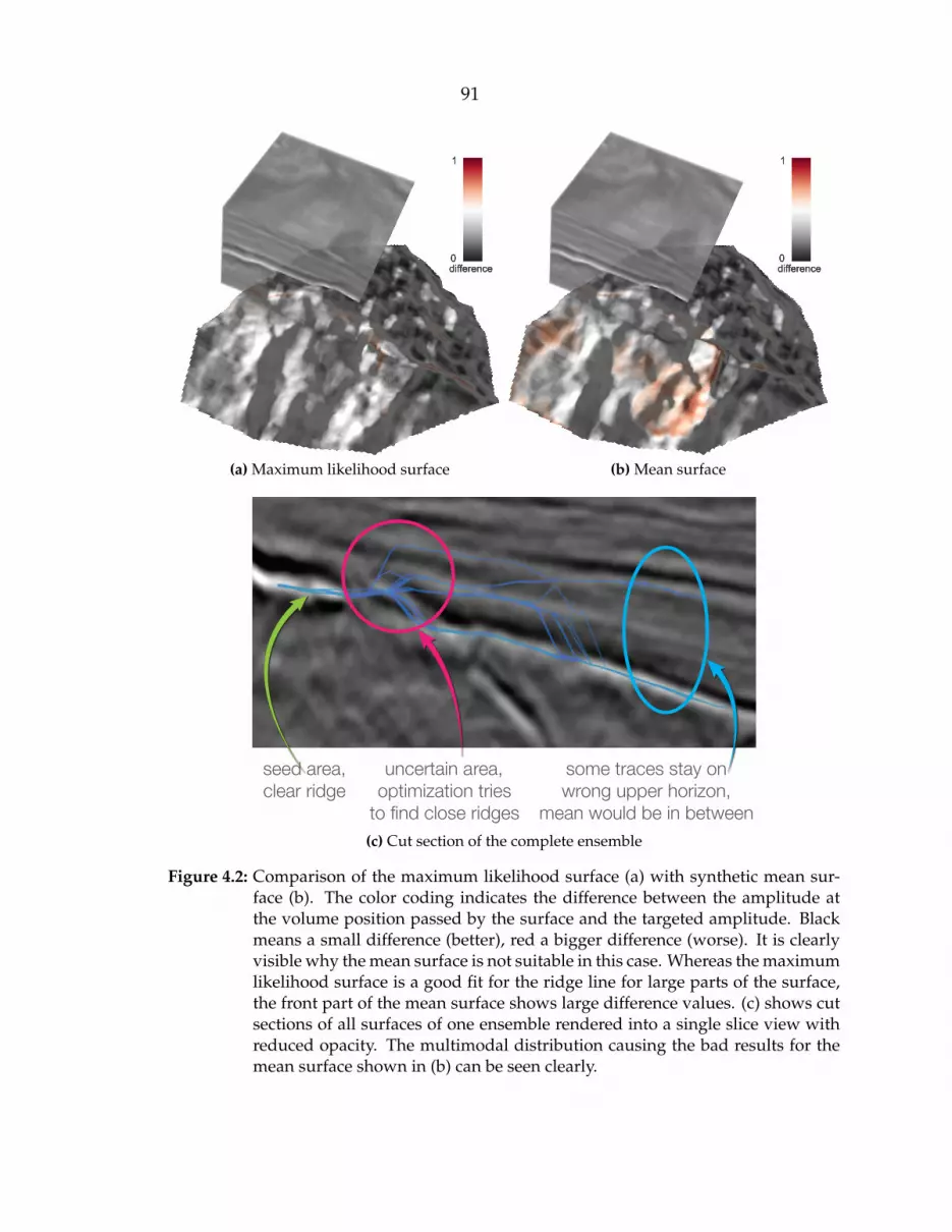
91
(a) Maximum likelihood surface (b) Mean surface
seed area,clear ridge
uncertain area,optimization tries[V�ÄUK�JSVZL�YPKNLZ
some traces stay onwrong upper horizon,
mean would be in between(c) Cut section of the complete ensemble
Figure 4.2: Comparison of the maximum likelihood surface (a) with synthetic mean sur-face (b). The color coding indicates the difference between the amplitude atthe volume position passed by the surface and the targeted amplitude. Blackmeans a small difference (better), red a bigger difference (worse). It is clearlyvisible why the mean surface is not suitable in this case. Whereas the maximumlikelihood surface is a good fit for the ridge line for large parts of the surface,the front part of the mean surface shows large difference values. (c) shows cutsections of all surfaces of one ensemble rendered into a single slice view withreduced opacity. The multimodal distribution causing the bad results for themean surface shown in (b) can be seen clearly.
92
However, simply displaying the maximum likelihood surface itself without
any additional information does not provide much information about the ensem-
ble. Therefore, we also depict the results of the statistical analysis described in Sec-
tion 4.2. In the standard setting, we compute what we call virtual surfaces from the
mean, median, and maximum mode from each (x, y)-position. Virtual here means
that we do not render these as surfaces, but only use them in order to compute
the distance to the maximum likelihood surface for each (x, y)-position. These dis-
tances are then color-coded and used to texture the maximum likelihood surface.
If desired by the user, however, these virtual surfaces can also be rendered directly.
We allow pseudo-coloring the surface with these results, using one of several
pre-defined, or user-defined color maps. These properties immediately provide a
good idea about how the surface extraction behaves in different areas, i.e. very
stable areas are clearly visible throughout all properties, indicated by small values
in range, standard deviation, variance, close to zero values in the skewness, or very
large values in the kurtosis. In addition, it is possible to automatically animate all
surfaces in a pre-defined range. Animating the ensemble gives a nice impression
of the parameters that result in similar surfaces, as well as of which areas in the
dataset react more or less to changes in the parametrization of the cost function.
Similar surfaces or surface parts in the ensemble will result in little variation in
the animation, whereas areas of large variance will show more movement and
thus automatically draw the user’s attention. An example for this can be seen in
Figure 4.3.
All the described techniques have in common that they can be used to visualize
the complete ensemble or any user-defined subset. Using a set of sliders, the user
can define a subrange for each parameter, and the statistical analysis is carried out
on the fly for this range. This allows an interactive exploration of the parameter

93
Figure 4.3: Visualization of a horizon ensemble using the representative surface aug-mented with the variance color-coded on the left and the histogram of a se-lected position on the right.
space, which is helpful to define interesting ranges for each parameter. To allow
this live exploration of the parameter space, we implemented an efficient, com-
pletely GPU-based pipeline for computing the statistics as well as rendering the
results, as presented in Section 4.4.
The same pipeline also allows efficient implementation of a number of other
features. If desired, the user can choose to render any surface from the ensemble.
This requires no data transfer to or from the GPU, except for the ID of the surface
in the ensemble to render. In addition, it is possible to automatically animate all
surfaces in a predefined range. In the presented application this can be useful in
two ways; As shown by Brown [12], as well as Lundstrom et al. [57], animation is a
powerful tool for visualizing uncertainty. The user can choose to animate through
all members of a single time step to get an impression of the surface distribution.
The described visualization techniques can give a very good impression of the
quantitative variation in the data. Detailed information on the surface distribu-
tion can be gained by animating through or manually selecting individual surfaces
from the ensemble. However, it is hard to compare more than two surfaces this
way. We therefore provide an additional view showing the histogram and proba-
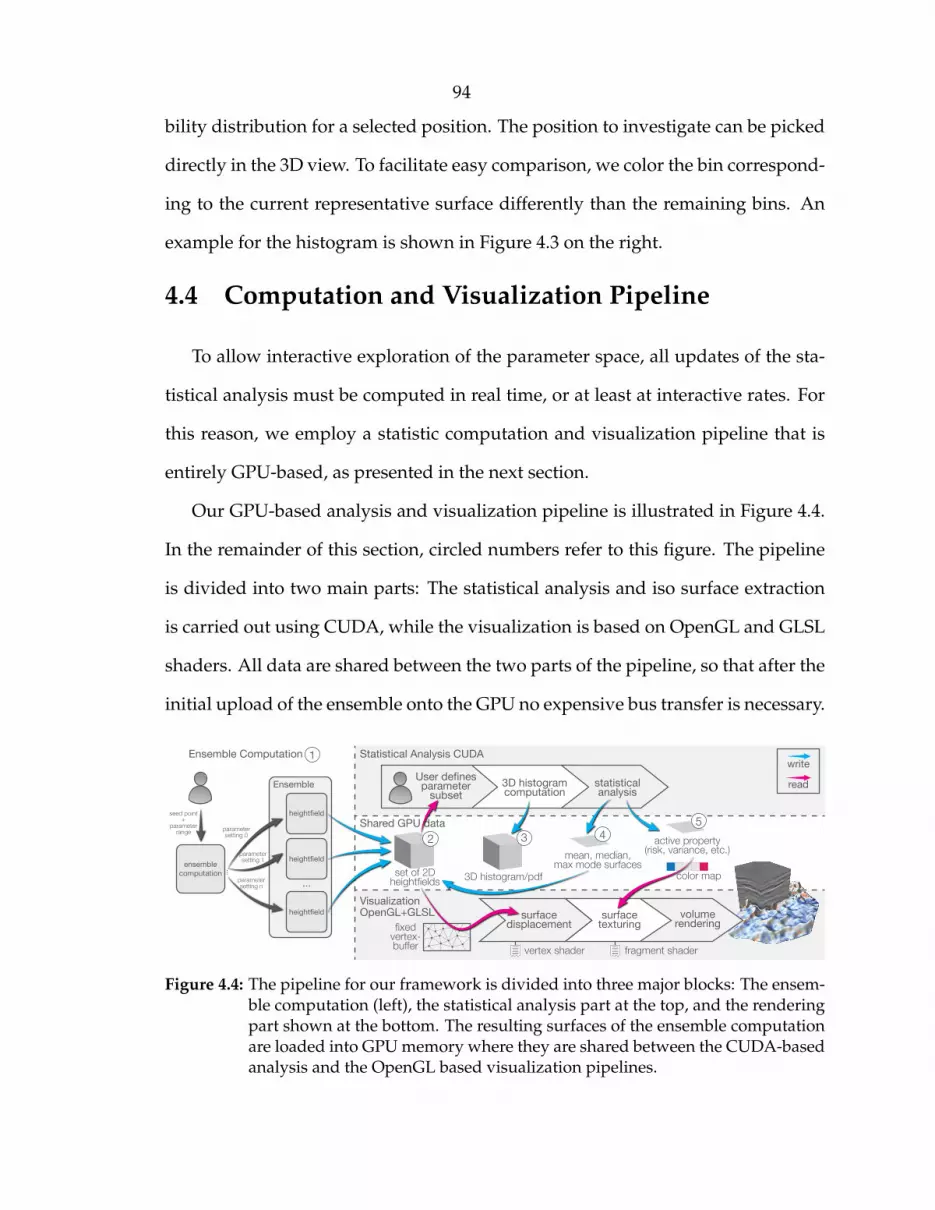
94
bility distribution for a selected position. The position to investigate can be picked
directly in the 3D view. To facilitate easy comparison, we color the bin correspond-
ing to the current representative surface differently than the remaining bins. An
example for the histogram is shown in Figure 4.3 on the right.
4.4 Computation and Visualization Pipeline
To allow interactive exploration of the parameter space, all updates of the sta-
tistical analysis must be computed in real time, or at least at interactive rates. For
this reason, we employ a statistic computation and visualization pipeline that is
entirely GPU-based, as presented in the next section.
Our GPU-based analysis and visualization pipeline is illustrated in Figure 4.4.
In the remainder of this section, circled numbers refer to this figure. The pipeline
is divided into two main parts: The statistical analysis and iso surface extraction
is carried out using CUDA, while the visualization is based on OpenGL and GLSL
shaders. All data are shared between the two parts of the pipeline, so that after the
initial upload of the ensemble onto the GPU no expensive bus transfer is necessary.
1Ensemble Computation
Shared GPU data
Statistical Analysis CUDA
Visualization
OpenGL+GLSL
mean, median,max mode surfaces
active property(risk, variance, etc.)
parametersetting 0
seed point+
parameterrange
...
parametersetting 1
parametersetting n
OLPNO[ÄLSK
OLPNO[ÄLSKensemble
computation
OLPNO[ÄLSK
...
Ensemble
surfacedisplacement
surfacetexturing
volumerendering
set of 2DOLPNO[ÄLSKZ 3D histogram/pdf
3D histogramcomputation
<ZLY�KLÄULZparameter
subset
statisticalanalysis
vertex shader fragment shader
JVSVY�THW
Ä_LKvertex-buffer
write
read
2 3 45
Figure 4.4: The pipeline for our framework is divided into three major blocks: The ensem-ble computation (left), the statistical analysis part at the top, and the renderingpart shown at the bottom. The resulting surfaces of the ensemble computationare loaded into GPU memory where they are shared between the CUDA-basedanalysis and the OpenGL based visualization pipelines.

95
Since usually only a small part of the ensemble is required by the visualization, a
streaming approach would be possible for datasets that are larger than GPU mem-
ory, but we currently assume that the dataset fits into GPU memory.
Ensemble Computation
The input to our system is a set of heightfields resulting from the ensemble compu-
tation 1 . Even though we focus on heightfields in this work, our approach could
also be applied to surfaces in n dimensions as long as the correspondences between
all surfaces in the dataset are known for every nD-datapoint. In our framework,
we assume the 2D spatial (x, y)-coordinate to be the correspondence between the
surfaces.
Data Representation
Before computation of statistics or visualization, the ensemble is converted into a
3D texture 2 and loaded onto the GPU. Every heightfield of the ensemble will be
represented by one slice in this texture. Additionally, space for the mean, median
and maximum mode heightfield will also be reserved in this texture. The surfaces
are indexed using the original parametrization. If there is only a single parameter,
for example the time steps in a time series, the surface ID corresponds to the texture
index. For higher-dimensional parameter spaces, as in our case the three param-
eters from the cost function (Section 3.4.5), the linear texture index is computed
from the original parameters. This allows the user to define subranges for each
parameter separately in order to examine the influence of each of the parameters
on the segmentation individually.
96
Statistical Analysis
The first step in the statistical analysis is the creation of the 3D histogram 3 . Changes
in the parameter range trigger an update of the 3D histogram and subsequently of
the representative surface and property texture. Since each ensemble member pro-
vides exactly one entry to the histogram per (x, y)-position, rather than using a
thread for each member, we use one thread per (x, y)-position. Each thread then
loops over all selected surfaces and computes the complete 1D histogram for this
position. This way, write conflicts can be avoided and no critical sections or atomic
operations are needed. The kernels for the derived properties are set up in a sim-
ilar fashion. The desired statistical property is computed by one thread per (x, y)-
position. The main difference to the histogram computation is that this results in a
single scalar per thread, all of which are then assembled into a 2D texture. While
mean, median and maximum mode 4 are attached to the 3D heightfield texture
to be used as representative surfaces, the other properties 5 are copied into a 2D
texture available to the visualization pipeline for texturing the surface. Exploiting
the parallelism of the GPU and eliminating costly bus transfers between CPU and
GPU allows interactive modification of the parameter range even for ensembles
containing several hundred surfaces.
Rendering
The rendering pipeline takes advantage of the fact that all ensemble data are al-
ready stored in GPU memory, which facilitates efficient surface rendering. Instead
of creating new surface geometry every time a different surface of the ensemble
is rendered, a single generic vertex buffer of fixed size is created. This buffer cov-
ers the entire (x, y)-domain, but does not contain any height information. The

97
z-value of each vertex is set later in the vertex shader. Before transforming the ver-
tex coordinates into view space, the object space (x, y)-coordinates of the vertex in
combination with the ID of the active surface are used to look up the z-value of the
current vertex in the ensemble texture. At this point, the desired surface geometry
is available. In order to be able to visualize the results of the statistical analysis, the
object space coordinates are attached to each vertex as texture coordinates (x and
y are sufficient). In the fragment shader, this information can then be used to look
up the active statistical property in the 2D texture. This texture contains the raw
information from the statistical analysis, which is then converted to the fragment
color by a look up in a 1D color map. We provide a selection of several continuous,
diverging cool-to-warm color maps, as presented by Moreland [65], but also al-
low the creation of custom color maps. These color maps minimally interfere with
shading, which is very important in this case, as shading is an important feature to
judge the shape of a surface. During testing we realized that using the continuous
version made it very hard to relate an actual value to a color in the rendering so we
decided to optionally provide a discrete version with ten steps. After the surface
geometry has been rendered, the seismic cube can be rendered on top, providing
spatial context. This is done in a second rendering pass in order to guarantee cor-
rect visibility [98].
Detailed Inspection
We enable the detailed inspection of the ensemble with the linked histogram view
as described in Section 4.3. The histogram view shows the 1D histogram of any po-
sition picked by the user directly in the main view. In fact, the histogram refreshes
automatically when the user moves the mouse cursor over the representative sur-
face. All information that is required for picking is already available in our ren-

98
dering pipeline: We use the same vertex shader as described before for rendering
the surface into an off-screen buffer of the same size as the frame buffer. Instead
of using the object space coordinates to look up the scalar values in the fragment
shader, we use the coordinates directly as the vertex color. This way, we can look
up the current mouse position directly in the downloaded off-screen buffer. With
the (x, y)-part of the resulting volume position, we can then directly look up the
histogram and probability density distribution for this position.
4.5 Results
Figure 4.5 shows an example where the standard parameter setting for the cost
function produces a wrong result due to large uncertainty in the data. While the
incorrect result could be fixed by placing a constraint and recomputing the surface,
the color coding of the cost (Figure 4.5a), which could indicate an uncertain area by
large costs, gives no indication of this area. Instead of the cost, we use the standard
deviation to texture the maximum likelihood surface resulting from the ensemble
computation (Figure 4.5b). Using the standard deviation of the computed ensem-
ble immediately leads to the very prominent area in the center.
A cut section through this area is given in Figure 4.5c. The blue line corre-
sponds to the original surface and the green line to the maximum likelihood sur-
face. Once we identified this region we could find a third surface, corresponding
to the magenta line, by narrowing the parameter range and skimming through
the remaining surfaces. Even though the differences between the maximum likeli-
hood surface and this third surface are subtle (compare the overlay in Figure 4.5c),
this third surface represents the underlying data slightly better than the maximum
likelihood surface.

99
(a) Original surface. (b) Maximum likelihood surface.
(c) Cut sections through the surfaces.
Figure 4.5: Surfaces extracted and visualized using our technique, described in Chapter 3(a) and using the ensemble technique (b). While the cost (color coding in (a))shows little variation over the surface and thus does not reveal problems inthe segmentation, the standard deviation (b) clearly highlights an area in thecenter of the surface (compare the areas marked by the arrows). (c) showsa cut section of the surfaces, the blue line corresponds to (a) the green lineto the maximum likelihood surface in (b). The magenta line corresponds toa third surface extracted from the ensemble using the proposed explorationframework.
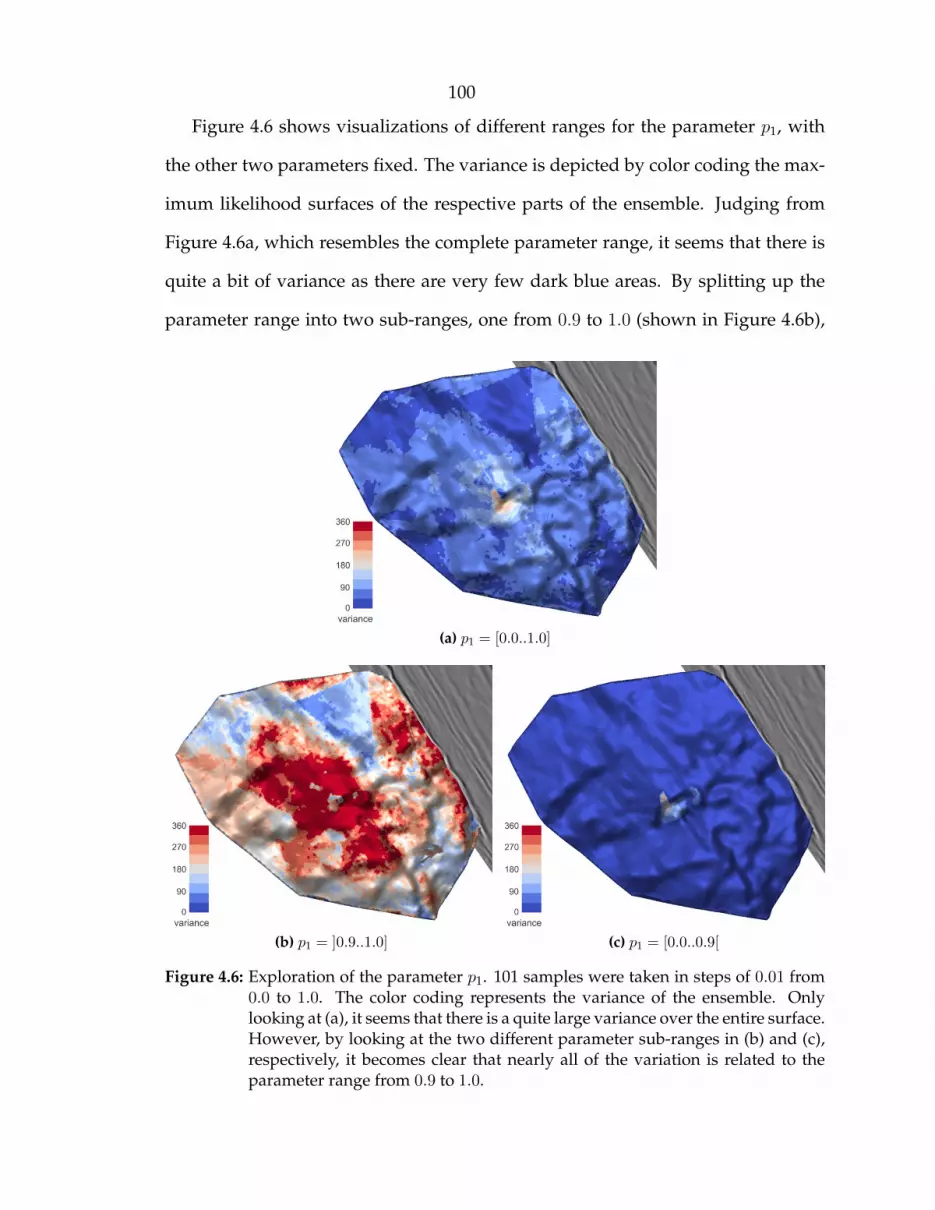
100
Figure 4.6 shows visualizations of different ranges for the parameter p1, with
the other two parameters fixed. The variance is depicted by color coding the max-
imum likelihood surfaces of the respective parts of the ensemble. Judging from
Figure 4.6a, which resembles the complete parameter range, it seems that there is
quite a bit of variance as there are very few dark blue areas. By splitting up the
parameter range into two sub-ranges, one from 0.9 to 1.0 (shown in Figure 4.6b),
(a) p1 = [0.0..1.0]
(b) p1 = ]0.9..1.0] (c) p1 = [0.0..0.9[
Figure 4.6: Exploration of the parameter p1. 101 samples were taken in steps of 0.01 from0.0 to 1.0. The color coding represents the variance of the ensemble. Onlylooking at (a), it seems that there is a quite large variance over the entire surface.However, by looking at the two different parameter sub-ranges in (b) and (c),respectively, it becomes clear that nearly all of the variation is related to theparameter range from 0.9 to 1.0.
101
and one from 0.0 to 0.9 (Figure 4.6c), it becomes clear that nearly all of the variation
is in the upper ten percent of the parameter range.
By sweeping through the different subranges of p1, we could quickly find out
that the usable parameter range for p0, for this specific dataset, is between 0.0 and
0.9, but also that a parameter in this range will have very little effect on the re-
sulting surfaces, meaning that the user does not have to be very careful with this
parameter, as long as it is between 0.0 and 0.9.
Finally, Figure 4.7 shows a selection of the computed statistical properties. Here
the visualization shows all combinations of all three parameters sampled in steps
of 0.1 from 0.0 to 1.0 for p0 and p2, while the range for p1 was limited to [0.0..0.9]
for the reasons described above. This results in a total of 1210 surfaces examined.
Figure 4.7a shows the range, Figure 4.7b shows the standard deviation, Figure 4.7c
the variance, and Figure 4.7d the skewness. For the range, standard deviation and
variance, the color map used indicates zero with blue, and large values with red.
For the skewness, zero is set to white, blue tones indicate negative skew, and red
tones positive skew. There are some notable differences between the range and the
variance. Overall, there are a lot less very small values in the range texture Also,
the large red region in the front left is not present in the variance. The variance
helps filtering out small groups of outliers most likely leading to this region in the
range texture. The highlighted area described in Figure 4.5 is also prominent in
this ensemble for all four textures, even though not as strong for the range texture.
Interesting is the distribution of the skewness. The mentioned highlight is clearly
visible as a large area of negative skew. Another interesting feature in the skewness
is also the strict clustering of negative and positive skewness.
To allow the interactive exploration of the parameter space, it is very impor-
tant that the computation of the statistical analysis is possible at interactive rates.

102
With our GPU-based implementation we achieve these update rates on standard
graphics hardware for hundreds of millions of data points.
Since the features of the computation pipeline presented in this chapter basi-
cally form a subset of the features used for our ocean forecasting application pre-
sented in Chapter 6, we refer to Section 6.5.1 for a detailed performance analysis.
range0
19
39
58
77
(a) Rangestandard deviation
0
4
8
12
16
(b) Standard Deviation
variance0
62
125
188
250
(c) Variance
skewness-1.5
-0.75
0
0.75
1.5
(d) Skewness
Figure 4.7: Comparing statistical properties of the ensemble, varying and sampling allthree parameters.
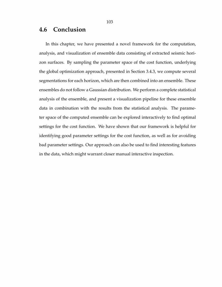
103
4.6 Conclusion
In this chapter, we have presented a novel framework for the computation,
analysis, and visualization of ensemble data consisting of extracted seismic hori-
zon surfaces. By sampling the parameter space of the cost function, underlying
the global optimization approach, presented in Section 3.4.3, we compute several
segmentations for each horizon, which are then combined into an ensemble. These
ensembles do not follow a Gaussian distribution. We perform a complete statistical
analysis of the ensemble, and present a visualization pipeline for these ensemble
data in combination with the results from the statistical analysis. The parame-
ter space of the computed ensemble can be explored interactively to find optimal
settings for the cost function. We have shown that our framework is helpful for
identifying good parameter settings for the cost function, as well as for avoiding
bad parameter settings. Our approach can also be used to find interesting features
in the data, which might warrant closer manual interactive inspection.
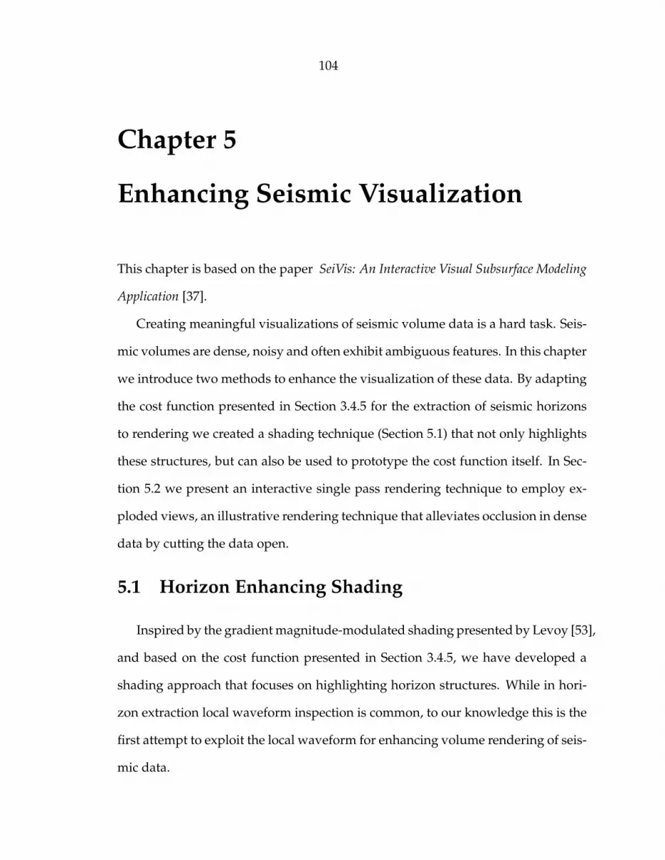
104
Chapter 5
Enhancing Seismic Visualization
This chapter is based on the paper SeiVis: An Interactive Visual Subsurface Modeling
Application [37].
Creating meaningful visualizations of seismic volume data is a hard task. Seis-
mic volumes are dense, noisy and often exhibit ambiguous features. In this chapter
we introduce two methods to enhance the visualization of these data. By adapting
the cost function presented in Section 3.4.5 for the extraction of seismic horizons
to rendering we created a shading technique (Section 5.1) that not only highlights
these structures, but can also be used to prototype the cost function itself. In Sec-
tion 5.2 we present an interactive single pass rendering technique to employ ex-
ploded views, an illustrative rendering technique that alleviates occlusion in dense
data by cutting the data open.
5.1 Horizon Enhancing Shading
Inspired by the gradient magnitude-modulated shading presented by Levoy [53],
and based on the cost function presented in Section 3.4.5, we have developed a
shading approach that focuses on highlighting horizon structures. While in hori-
zon extraction local waveform inspection is common, to our knowledge this is the
first attempt to exploit the local waveform for enhancing volume rendering of seis-
mic data.
105
a b c d
Figure 5.1: Different kernel sizes for the cost-modulated shading ( a : k = 1, b : k = 2, c :k = 3), and comparison with Phong shading d .
Common illumination models use the gradient for shading. For visualizing
horizons, this is not suitable as the gradient vanishes at the local extrema indicating
the horizons. Instead, we compute the inverse of the wave form based component
of the local cost on-the-fly during rendering, and use it to modulate the opacity
from the transfer function, in the same way as the gradient magnitude is used for
gradient magnitude-modulated shading [53].
Using the non-linear filter gwave described by Equation 3.11 in Section 3.4.5, we
can roughly estimate the distance of the current sample to a local minimum or max-
imum in the seismic trace. While the cost function term shown in Equation 3.11
maps extrema to low cost for the rendering, we would like to assign large opacity
to the extrema and low opacity to the remaining data. Where Levoy uses the mag-
nitude of the gradient in 3D directly to modulate opacity and shading intensity, we
can use the term from Equation 3.12, describing the peakness in the trace direction,
to modulate the opacity during volume rendering. Equation 3.12 contains the pa-
rameter k, defining the neighborhood size that is considered. For rendering, this
106
Figure 5.2: An example of a visualization of a seismic cube highlighting reflections of pos-itive amplitude. With a very simple transfer function the most important fea-tures can be highlighted (Note the strong reflection in the bottom right area, aswell as the distinct features on the left side.)
value influences the visual quality of the results, but since here the term needs to be
evaluated on the fly during raycasting, it also has a notable effect on the rendering
performance.
Figure 5.1 shows a comparison of the quality with different neighborhood sizes,
as well as a comparison to standard Phong shading without any opacity modu-
lation. The transfer function is a simple gray map with constant opacity for all
renderings. A big advantage of this approach is that horizons can efficiently be
highlighted without adjusting the transfer function. While similar results could be
achieved with a carefully designed transfer function with amplitude-based shad-
ing, using the proposed render mode requires no user interaction at all.
Figure 5.2 shows another rendering of the same dataset. We used a diverging
blue to red color map, typical for seismic applications, as transfer function with re-
duced opacity in the center. The shader was setup to only highlight local maxima.
The visualization clearly shows the classified horizons as very distinct features,

107
Figure 5.3: An example of a horizon extracted using the horizon enhancing shading only,without any preprocessing. The volume was clipped slightly above the hori-zon. The structure is clearly visible over the complete area of the dataset.
especially on the left side. A strong reflection on the right side is also very promi-
nent in dark red. On major advantage of our waveform based classification over
amplitude only based classification can be seen in this rendering. The highlighted
features cover a wide range of amplitudes, visible in the coloring. Using a simple
amplitude based transfer function, it would not be possible to highlight a lot of the
lower amplitude features, indicated by gray coloring.
A performance comparison for k = 1, k = 2, and k = 3 is shown in Table 5.1,
compared to a shader using standard Phong shading without modulation. It can
be seen that, while there is a performance loss for neighborhoods larger than three
voxels, rates are still interactive. For the performance comparison, we adjusted
the transfer functions such that transparency was similar for the standard and

108
(a) p0 = 0.25 (b) p0 = 0.5
(c) p0 = 0.75 (d) p0 = 1.0
Figure 5.4: Comparison of renderings with different settings for the parameter p0 (Com-pare Equation 3.15). The shader was set up to highlight maxima, the sametransfer function (without any transparency) was used for all renderings. Alltransparency is introduced by the cost based modulation.

109
NeighborhoodSize
Base(Phong)
HorizonEnhancing
% of Base
3 (k = 1) 28fps 28fps 100%
5 (k = 2) 28fps 25fps 89%
7 (k = 3) 28fps 21fps 75%
Table 5.1: Performance for cost function-based, horizon enhancing rendering compared toPhong shading (Base). See Section 3.2.3 for measurement setup.
cost-modulated shading methods, as the modulation usually results in much more
transparent images.
Prototyping the Cost Function
In addition to simply highlighting horizon structures in seismic reflection data the
approach can also be used to locally show the results of changing the cost function
parameter p0. Therefore we allow the evaluation of the complete snappiness term
(Equation 3.15) per voxel during raycasting instead of only the waveform term
from Equation 3.12. Areas of low cost, corresponding to the horizon structures, are
rendered opaque, while areas of high cost will be rendered transparently, allow-
ing an approximation of the surfaces the optimization would extract. Even though
this technique ultimately cannot replace the additional global optimization for ex-
tracting the horizons, it can give a good idea of how the global optimization will
behave.
5.2 Exploded Views
Occlusion is a common problem when visualizing three-dimensional objects. Opac-
ity adjustments are commonly used to reveal hidden structures in volume visu-
alization. However, for very dense data, such as seismic data, this is often not

110
Figure 5.5: Rendering of a seismic cube with two interpreted horizons. The volume isclipped along the upper horizon, the second horizon is used to cut open thevolume for the exploded view. The colormap for the surface geometry indicatesthe position in 3D.
sufficient. Cutaways or clipping can solve this problem, but at the cost of losing
contextual information. Illustrators often employ exploded views to reveal hid-
den structures while retaining context information. An exploded view is basically
created by cutting the data into several parts, which are then shown at displaced
locations in order to reveal the structures of interest. Figur 5.5 shows an example
for a combination of clipping and exploded views.
The general approach to exploded views [13, 62, 95] for volume rendering is
setting up the bounding geometry around each part of the volume, rendering each
of the parts separately, and then compositing the results. These techniques make
very flexible exploded views possible, allowing translation and rotation of arbi-
trary cut planes along/around arbitrary axes. However, the same constraints of
our application scenario, already described in Section 3.2.2, make much of this
flexibility unnecessary. We use the seismic horizons as the cut geometry, and then
for the explosion itself compute layers of piecewise translations along the z-axis.
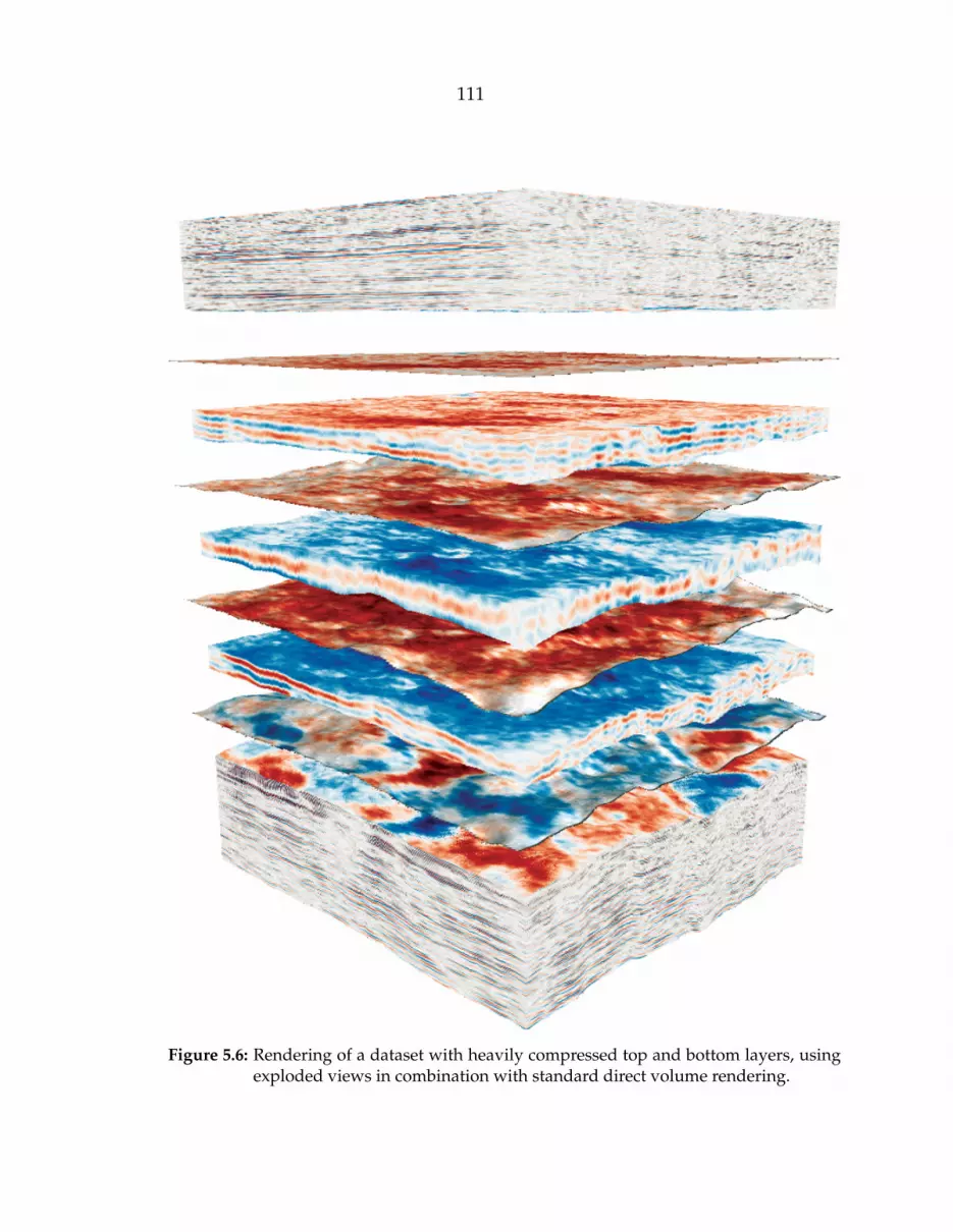
111
Figure 5.6: Rendering of a dataset with heavily compressed top and bottom layers, usingexploded views in combination with standard direct volume rendering.

112
This is sufficient to enable unobstructed views onto the surfaces. Figure 5.6 shows
a rendering of a partially interpreted seismic dataset with a combination of the
volume deformation presented in Section 3.2.2 and exploded views. The exploded
views allow inspection of the extracted horizon surfaces in context of the seismic
data.
Integration into the Rendering Pipeline
Our exploded views approach integrates seamlessly into our framework for the
on the fly volume deformation for live depth conversion (Section 3.2.2). The data
already available for the deformed rendering makes it possible to deploy exploded
views, using the z-axis for translation, and the horizons as cut surfaces. We use a
single-pass ray casting approach without any additional setup besides a modified
scale factor. Again, we set up a virtual volume with a modified size for the z-
axis. To comply with the spacing between the different layers, here the combined
spacing for all horizons is added to the scale factor for the volume’s z-axis. Adding
the spacing to the scale factor for the depth conversion allows us to combine the
exploded views with the depth conversion.
Fragment Shader
The fragment shader for rendering the exploded view is only a slight modification
of the shader described in Section 3.2.2. We interpret the spacing as empty space
preceding each horizon. Thus, the offset to get to the deformed layer is not a direct
look-up in the deformed boundaries texture, but the spacing corresponding to all
preceding horizons has to be added. Assuming a uniform spacing, this is simply
the number of preceding layers, multiplied with the spacing. To check whether
the sample position is inside the spacing or in the volume, the deformed boundary

113
Dataset Number ofSurfaces
Base Expl.Views
% ofDC
% ofBase
240⇥ 240⇥ 1509
3117fps
68fps 69% 58%
5 46fps 53% 39%
3 50fps 62% 50%
1422⇥ 667⇥ 1024
5101fps
27fps 35% 27%
Table 5.2: Performance comparison of the exploded views. We used standard ray castingwithout illumination for the comparison. % of DC compares to rendering withon the fly depth conversion as shown in Table 3.3.
value of the bottom boundary of the current layer has to be fetched. If the current
sample position is larger than the size of the spacing subtracted from the deformed
boundary value, the sample is inside the spacing. If that is the case, we can set the
current sample’s alpha value to zero and proceed with the next sample.
Performance
Performance for the single-pass ray casting with exploded views can be seen in
Table 3.3. Compared to the depth-conversion shader, there is virtually no differ-
ence in computational complexity (the texture fetch, described above, to decide
whether the sample is inside the spacing area can be cached when computing the
current layer). However, we currently do not employ empty space skipping in the
explosion spacing, which results in a performance loss.

114
Chapter 6
Visual Analysis of Uncertainties inOcean Forecasts
This chapter is based on the paper Visual Analysis of Uncertainties in Ocean Forecasts
for Planning and Operation of Off-Shore Structures [39].
In this chapter, we introduce a GPU-based interactive visualization system for
the exploration and analysis of ensemble heightfield data, with a focus on the spe-
cific requirements of ocean forecasts. We propose a novel workflow for planning
the placement and operation of off-shore structures needed by the oil and gas in-
dustry, based on an efficient GPU pipeline for on-the-fly statistical analysis of the
ensemble data. While we focus on the visualization and analysis of ocean forecast
data, the presented approach could also be used for the exploration of heightfield
ensembles from other areas, such as weather forecasting or climate simulation.
The work presented in this chapter shares a foundation with the parameter
space exploration framework presented in Chapter 4. Besides the first two sections,
introducing the simulation- and application frameworks (Sections 6.1 and 6.2, re-
spectively) the structure of this chapter is identical to the structure of Chapter 4.
Statistical analysis (Section 6.3), ensemble visualization (Section 6.4) and Computa-
tion and Visualization Pipeline (Section 6.5) all extend their respective counterparts
presented in Chapter 4 with additional functionality specific to the ocean forecast
analysis application. Section 6.6 presents the results by means of use case scenarios
for planning the placement as well as the operations of off shore rigs.

115
6.1 Ocean Forecast Simulation
The development of a reliable ocean forecasting system requires models capa-
ble of simulating ocean circulation and an efficient assimilation scheme that, given
enough observations, provides accurate initial conditions for forecasting. High-
resolution three-dimensional general circulation ocean models are necessary to
reproduce complex mesoscale dynamics like in the Gulf of Mexico [16] (see Fig-
ure 6.1). However, such models cannot provide accurate forecasts of mesoscale
variability, such as eddy shedding events, without data assimilation. A general
circulation ocean model is subject to several sources of uncertainties, not only
Figure 6.1: The Gulf of Mexico simulation area covered by the presented dataset. The col-ors denote water depth in meters. The spatial domain enclosed by the thickblue line in the Gulf of Mexico represents the area over which loop currentindices were computed [40].
116
from the poorly known inputs such as the initial state, and atmospheric and lat-
eral boundary conditions, but also from the use of approximate parameterization
schemes of sub-grid physics and ocean mixing dynamics. The rapid growth of
nonlinear instabilities in the loop current shedding events amplifies these uncer-
tainties in time, which strongly limits the predictability of the system. Data assim-
ilation methods address this issue by constraining model outputs with incoming
data. This helps keeping the model evolution on a realistic trajectory and provides
optimal initial states for initializing forecast runs, taking into account the model
outputs, the available observations, and their respective uncertainties.
Data assimilation was historically cast as a weighted least-squares problem, in
which an estimate of the ocean state at a given time is computed by optimizing a
cost function measuring a weighted misfit between the model state and available
observations, and constrained by some prior information [111]. The prior term,
generally taken as a model forecast, is used as a regularization term as the ocean
state estimation problem is underdetermined by design, due to the limited amount
of available observations. A forecast is then obtained by integrating the estimated
state forward in time with a general circulation ocean model. The “optimality” of
an ocean state estimate determined by such an approach strongly depends on the
prescribed weights, and also on the accuracy of the prior which is subject to the
model uncertainties. This means that the estimate, and therefore the forecast, is
subject to uncertainties, and these need to be also computed and analyzed as part
of the forecasting step. The important role of uncertainties is now increasingly
recognized in the ocean prediction community, and also in other communities as
the weather prediction community, for proper decision making and efficient risk
management.

117
New assimilation methods based on Bayesian filtering theory have been re-
cently developed by the ocean and atmospheric communities for efficient propa-
gation and quantification of uncertainties [2, 23, 40, 41, 82]. These methods, known
as ensemble Kalman filter methods, follow a Monte Carlo approach to represent
the uncertainties on a state estimate by an ensemble of model states. These are
then integrated forward in time with the general circulation ocean model to quan-
tify uncertainties in the forecast. The estimated forecast uncertainties are then com-
bined with the observation uncertainties to assimilate the new incoming data using
a Kalman filter correction step [23], before a new forecast cycle begins. Develop-
ing and implementing efficient ensemble Kalman filters with state-of-the-art ocean
and atmospheric models is a very active area of research.
With the fast-growing high performance computing resources, the implemen-
tation of ensemble Kalman filters with large ensemble members is now practically
feasible using highly sophisticated general circulation ocean models. When a fil-
ter’s ensemble is available, it is customary to calculate various statistical measures
of the ensemble spread as indicators of the uncertainties and of their evolution in
space and time, which are then used in decision making.
Recently, Hoteit et al. [40] developed an ensemble forecasting system for the
Gulf of Mexico circulation based on the Massachusetts Institute of Technology
General Circulation Model (MITgcm) [60], and the Data Assimilation Research
Testbed (DART) [2]. This system is capable of assimilating various sets of satel-
lite and in-situ ocean observations. We use this system as a real-world scenario
that illustrates the new capabilities for analysis and exploration provided by our
visualization approach. Figure 6.1 gives an overview of the area covered by the
forecasting system.

118
6.2 Application Framework
Our system targets the interpretation of forecasts from the planning phase of
an off-shore structure to its operation. Since the different phases have different
requirements, we provide a set of four main views, which are used in different
combinations depending on the application scenario. Figure 6.2 shows our appli-
cation with the main views plus a unified settings panel. The views are two spatial
views showing the surface data themselves, one in 3D a , the other one in 2D b , a
linked histogram view c as well as a time-series view d .
While the accessibility of an existing reservoir is the key factor when planning
an oil platform, ocean forecasts can provide valuable additional information. Mod-
ern drilling techniques to some extent allow flexible paths and thus considerable
flexibility for the actual placement of a platform. However, the complexity of the
path has implications on the cost of drilling. On the other hand, slight changes of
the position might move a platform from an area that is strongly affected by eddy
Figure 6.2: Our application for exploration of ocean forecast ensembles consists of fourmain views. The simulated ocean surface, or a derived version, like the meansurface for a time step, can be shown in 3D or 2D ( a and b ). The histogramview ( c ) shows the complete distribution of the ensemble at a selected posi-tion, while the time-series view ( d ) shows the distribution and the resultingoperational risk at a selected position for multiple time steps.
119
shedding, which leads to long downtimes, to a less affected area, overall resulting
in more efficient operations.
6.3 Statistical Analysis
The input to our framework is an ensemble of heightfields representing the sea
surface height. The data is very similar to the horizon ensembles we extract and an-
alyze in Chapter 4. Therefore we use the same statistics computations presented in
Section 4.2 as the basis for our ocean forecast analysis framework and extend it by
some details, specific to the planning of off-shore structures. The main difference
to the framework presented above is the parameter-space exploration. Instead of
mapping parameters for a cost function, in this case we have different starting con-
ditions and different models for the simulation. In addition, we map time to one
of the parameters. While in the standard setting the statistics are only computed
for one time-step at a time, it would also be possible to compute the statistics over
any desired timespan. Furthermore, since the distributions of the simulation re-
sults are mostly Gaussian, here it makes sense to use the mean surface as the main
representative surface instead of the previously introduced maximum likelihood
surface. The two main additions to the statistics are a discrete probability density
function (pdf) volume for the ensemble distribution, derived from the histogram
volume, as well as a risk estimate, defining a risk value for each position with
respect to a predefined critical sea surface level.
Probability Density Function
We compute a discrete pdf for each (x, y)-position by applying a kernel density
estimate to the 1D histograms at each position. Just like for the histograms, we
combine the set of one dimensional pdfs to a 3D volume, which can be rendered
120
alongside the representative surface to give an overview of the complete distribu-
tion of the ensemble.
Risk Estimate
We define and visualize a simple risk estimate as the percentage of ensemble mem-
bers above the defined critical height. This value is computed for every (x, y)-
position for every time step. The surface in Figure 6.2 a , as well as the glyphs in
Figure 6.2 d are color-mapped with such a risk estimate. The risk value is not only
dependent on the ensemble itself, but also the critical sea level. Therefore the user
can interactively modify this value, just like it is possible to constrict the parameter
range, and get live updates on the results for the defined value.
6.4 Ensemble Visualization
Similar to the statistical analysis, we base our visualization framework on the tech-
niques developed for the visualization of horizon ensembles, presented in Sec-
tion 4.3. We added a 2D view for overview, as well as a time-series view to inspect
the complete time series for a single position to the existing linked 3D and his-
togram views. Furthermore, we extended the 3D surface rendering technique by
the possibility to blend extracted iso contours onto the surface, as well as a volu-
metric cursor to locally show the distribution of the ensemble directly in the 3D
view.
3D View
The 3D view provides a spatial overview of the data. Using the same techniques
for surface rendering as described in Section 4.3, we allow rendering the represen-
tative for the sea surface, usually the mean of the ensemble, in 3D. In addition to

121
Figure 6.3: 3D View Detail. a shows iso contours of the mean surfaces for all time stepsblended over the current surface. The area of interest is rendered with fullopacity, while the context is preserved by rendering the remaining parts semi-transparently. b shows a volume rendering of the pdf around a user-selectedposition. The surface is color-mapped with the variance. The large spread inareas of high variance is clearly visible in the volume rendering.
the statistical properties described above, we can also use the risk estimate (Sec-
tion 6.3) to color code the surface. To allow visualization of a second property
resulting from the statistical analysis, or information from several time steps at
once, we also added the extraction of iso contours from any of the scalar fields
derived from the ensemble. Figure 6.3 a shows an example, where iso contours
corresponding to the critical sea level were extracted from the mean surfaces for
all time steps and overlaid on the texture.
An additional benefit of the 3D view is that it is possible to use volume render-
ing for showing details of the distribution of the ensemble. Similar to approaches
presented by Pothkow et al. [87, 88], as well as Pfaffelmoser et al. [80], we depict
the actual distribution of the ensemble as a volume around the surface. Instead
of using a parametric representation of the data based on mean and variance, we
allow rendering the full probability density function (pdf) of the distribution, to al-
low detailed inspection of the actual data. However, since rendering the complete

122
volume would most likely result in the complete occlusion of the representative
surface, we propose to render only a a small subset of the volume, which is of
adjustable size. Similar to the linked histogram view, this allows showing details
on demand, without occluding the context. The technique essentially works like a
volumetric cursor (see Figure 6.3 b ). The user can simply probe the data by hover-
ing with the mouse over a position of interest, and the probability density volume
is then rendered around the picked position.
Time-Series View
Specifically for planning the operations of a platform at a defined position, we
developed the time-series view, shown in Figures 6.2 d and 6.4. This view al-
ways shows the complete time-series for a single lateral position. Once defined,
or loaded, our application caches several positions of off-shore structures, from
which one can be selected using a drop-down menu. The selected position is high-
lighted by markers in the spatial views. The view shows the ensemble distribution
-50cm
-100cm
timesteps, color-codedto match iso contours
red line indicates critical sea levelsea lvl
Glyphs represent ensembledistribution: (downscaledpdf at selected position)
mean sealvl over timeindicated byconnection
Risk100%
80%60%40%20%
0%
50cm
0cm17cm
100cm
t0 t1 t2 t3 t4 t5 t6 t7 t8 t9
Figure 6.4: The Time-Series View in detail. The y axis corresponds to the sea level, the xaxis to time. Each glyph shows the distribution of the selected position for onetime step. Glyphs are colored using the associated risk, i.e., the fraction of thedistribution above the selected critical sea level.
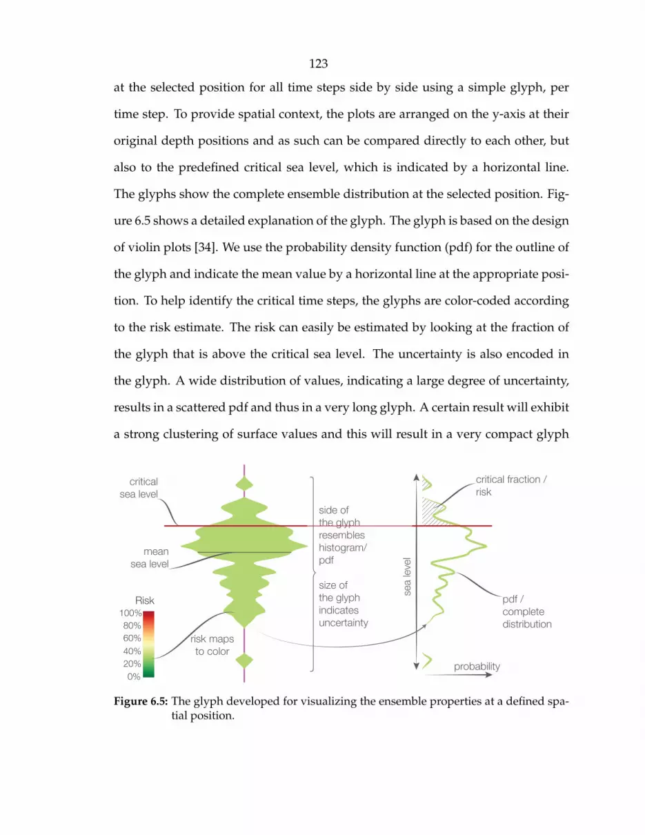
123
at the selected position for all time steps side by side using a simple glyph, per
time step. To provide spatial context, the plots are arranged on the y-axis at their
original depth positions and as such can be compared directly to each other, but
also to the predefined critical sea level, which is indicated by a horizontal line.
The glyphs show the complete ensemble distribution at the selected position. Fig-
ure 6.5 shows a detailed explanation of the glyph. The glyph is based on the design
of violin plots [34]. We use the probability density function (pdf) for the outline of
the glyph and indicate the mean value by a horizontal line at the appropriate posi-
tion. To help identify the critical time steps, the glyphs are color-coded according
to the risk estimate. The risk can easily be estimated by looking at the fraction of
the glyph that is above the critical sea level. The uncertainty is also encoded in
the glyph. A wide distribution of values, indicating a large degree of uncertainty,
results in a scattered pdf and thus in a very long glyph. A certain result will exhibit
a strong clustering of surface values and this will result in a very compact glyph
probability
sea
level
critical fraction /risk
criticalsea level
risk mapsto color
side ofthe glyphresembleshistogram/pdf
size ofthe glyphindicatesuncertainty
pdf /completedistribution
meansea level
Risk100%80%60%40%20%0%
Figure 6.5: The glyph developed for visualizing the ensemble properties at a defined spa-tial position.

124
(compare for example time step t0 and time step t3 in Figure 6.4). In addition, we
can show any of the derived statistical properties by coloring the glyph.
Using the time-series view, domain experts can then easily identify the points
in time where operations should be halted. Without ensemble forecasts, rigs were
operated based on a single simulation. However, even when ensemble forecasts
are available, a visual exploration approach is necessary. Without our visualization
system, our domain experts would define the safeness by simply looking at the
mean and variance values of the ensemble. In each time step, we indicate the mean
value of the distribution by a bold black bar, providing the same information as
before, for all time steps in a single view. The user can immediately identify critical
time steps, looking at the color and position of each glyph, and possibly order an
unavoidable shutdown of operations. If the situation is unclear, the glyph provides
the complete distribution to enable the expert to make a decision.
6.5 Computation and Visualization Pipeline
As described before, the ocean forecast visualization framework presented in
this chapter and the horizon ensemble framework presented in Chapter 4 share
Input
Shared GPU data
Statistical Analysis CUDA
Visualization
OpenGL+GLSL
mean, median,max mode surfaces
active property(risk, variance, etc.)area of interest
maskiso contours
(rendered to tex)
OLPNO[ÄLSK
OLPNO[ÄLSK
OLPNO[ÄLSK
...
Ensemble
surfacedisplacement
surfacetexturing
volumerendering
set of 2DOLPNO[ÄLSKZ 3D histogram/pdf
3D histogram/pdf computation
<ZLY�KLÄULZsubset &
focus area
statisticalanalysis
iso contourextraction
vertex shader fragment shader
JVSVY�THW
Ä_LKvertex-buffer
write
read
b ca
Figure 6.6: The extensions to the computation and rendering pipeline presented in Sec-tion 4.4.

125
large parts of the analysis and visualization pipeline. The additions specific to the
pipeline used for the ocean forecasting are highlighted in Figure 6.6. Besides the
addition of a risk estimate, described in Section 6.3, which integrates into the statis-
tical analysis part of the pipeline, we added three major features to ease the plan-
ning of off-shore structures. We allow defining a focus area, which is highlighted
in the spatial views (Figure 6.6 a ), we added the pdf (Figure 6.6 b ) which can be
rendered as a volume on top of the representative surface to show the complete
distribution of the ensemble, and finally we added the extraction of iso contours
(Figure 6.6 c ) from all 2D scalar fields (statistical properties as well as surfaces) to
allow the inspection of multiple properties as well as multiple times teps at once.
Area of Interest Definition
The focus area, or area of interest, can be defined by painting directly on the sur-
faces in the 2D view (Figure 6.2 b ). In the pipeline, the painted area is rendered
into a texture, which is used as a mask during rendering. The focus area is then
rendered with full opacity, while the context is rendered translucently (Compare
Figure 6.3 a ).
Probability Density Volume
The pdf volume is derived from the 3D histogram when needed by applying a
kernel density estimate for each of the 1D histograms. It is stored as an additional
3D texture in GPU memory, allowing it to be rendered directly using standard ray
casting on top of the surface geometry similar to the seismic cube in the horizon
extraction application. However, here we render the volume only on demand and
only a small part of the complete volume. We use the same technique as described
under Detailed Inspection in Section 4.4 to pick the position of the mouse cursor on

126
the surface. The geometry for ray casting into the pdf is then set up as a small cube,
centered around the picked position and with user adjustable size.
Iso Contouring
We have implemented marching squares using CUDA, based on the marching
cubes example from the CUDA SDK, as well as a CPU version. The result of the
iso contour extraction is a set of edges forming the contours. We keep the initial
geometric representation of the contours, for example for use in the 2D view, but
for overlaying the contours onto the 3D surfaces we render the contours into an
offscreen buffer, which is then used for texturing. Just like the rest of the analysis
pipeline, the iso contour extraction happens interactively, allowing adjustments of
the parameter range, as well as the iso value with instant feedback.
6.5.1 Performance
The performance of the statistical analysis is crucial for interactive exploration of
the parameter space. We used the dataset of the Gulf of Mexico, computed by the
simulation system described above, for measuring the performance of the statistics
computation. The dataset consists of a total of 500 surfaces spread over ten time
steps. The spatial resolution is 275⇥325, resulting in 89, 375 data points per surface.
Since usually one time step is investigated at a time, we show performance for a
single time step, consisting of 50 surfaces, as well as the complete dataset. Table 6.1
shows the resulting computation times for a single time step.
The computations were performed using an NVIDIA GeForce GTX 580 with
1.5GB of graphics memory. The timings were averaged over 1000 kernel execu-
tions. As all data stays on the GPU, no bus transfer has to be considered. For
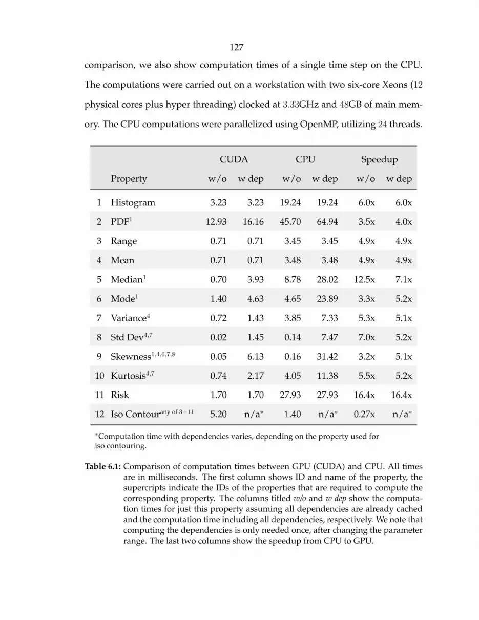
127
comparison, we also show computation times of a single time step on the CPU.
The computations were carried out on a workstation with two six-core Xeons (12
physical cores plus hyper threading) clocked at 3.33GHz and 48GB of main mem-
ory. The CPU computations were parallelized using OpenMP, utilizing 24 threads.
CUDA CPU Speedup
Property w/o w dep w/o w dep w/o w dep
1 Histogram 3.23 3.23 19.24 19.24 6.0x 6.0x
2 PDF1 12.93 16.16 45.70 64.94 3.5x 4.0x
3 Range 0.71 0.71 3.45 3.45 4.9x 4.9x
4 Mean 0.71 0.71 3.48 3.48 4.9x 4.9x
5 Median1 0.70 3.93 8.78 28.02 12.5x 7.1x
6 Mode1 1.40 4.63 4.65 23.89 3.3x 5.2x
7 Variance4 0.72 1.43 3.85 7.33 5.3x 5.1x
8 Std Dev4,7 0.02 1.45 0.14 7.47 7.0x 5.2x
9 Skewness1,4,6,7,8 0.05 6.13 0.16 31.42 3.2x 5.1x
10 Kurtosis4,7 0.74 2.17 4.05 11.38 5.5x 5.2x
11 Risk 1.70 1.70 27.93 27.93 16.4x 16.4x
12 Iso Contourany of 3�11 5.20 n/a⇤ 1.40 n/a⇤ 0.27x n/a⇤
⇤Computation time with dependencies varies, depending on the property used foriso contouring.
Table 6.1: Comparison of computation times between GPU (CUDA) and CPU. All timesare in milliseconds. The first column shows ID and name of the property, thesupercripts indicate the IDs of the properties that are required to compute thecorresponding property. The columns titled w/o and w dep show the computa-tion times for just this property assuming all dependencies are already cachedand the computation time including all dependencies, respectively. We note thatcomputing the dependencies is only needed once, after changing the parameterrange. The last two columns show the speedup from CPU to GPU.
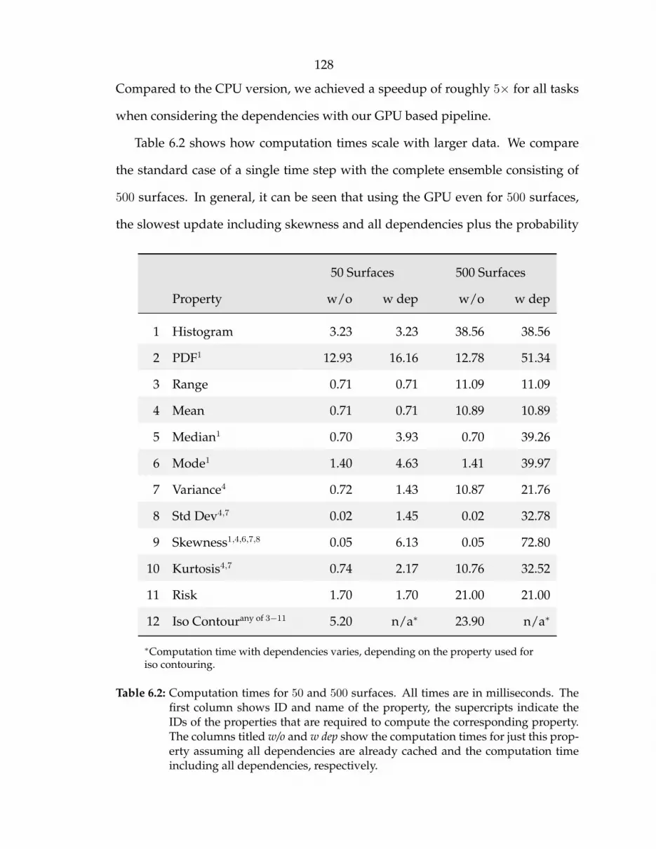
128
Compared to the CPU version, we achieved a speedup of roughly 5⇥ for all tasks
when considering the dependencies with our GPU based pipeline.
Table 6.2 shows how computation times scale with larger data. We compare
the standard case of a single time step with the complete ensemble consisting of
500 surfaces. In general, it can be seen that using the GPU even for 500 surfaces,
the slowest update including skewness and all dependencies plus the probability
50 Surfaces 500 Surfaces
Property w/o w dep w/o w dep
1 Histogram 3.23 3.23 38.56 38.56
2 PDF1 12.93 16.16 12.78 51.34
3 Range 0.71 0.71 11.09 11.09
4 Mean 0.71 0.71 10.89 10.89
5 Median1 0.70 3.93 0.70 39.26
6 Mode1 1.40 4.63 1.41 39.97
7 Variance4 0.72 1.43 10.87 21.76
8 Std Dev4,7 0.02 1.45 0.02 32.78
9 Skewness1,4,6,7,8 0.05 6.13 0.05 72.80
10 Kurtosis4,7 0.74 2.17 10.76 32.52
11 Risk 1.70 1.70 21.00 21.00
12 Iso Contourany of 3�11 5.20 n/a⇤ 23.90 n/a⇤
⇤Computation time with dependencies varies, depending on the property used foriso contouring.
Table 6.2: Computation times for 50 and 500 surfaces. All times are in milliseconds. Thefirst column shows ID and name of the property, the supercripts indicate theIDs of the properties that are required to compute the corresponding property.The columns titled w/o and w dep show the computation times for just this prop-erty assuming all dependencies are already cached and the computation timeincluding all dependencies, respectively.
129
density function (which needs to be computed for the histogram and time series
views) still allows for interactive update rates.
The histogram, range, mean, variance, kurtosis and the risk estimate are cal-
culated directly from the ensemble and as such the complexity relies solely on
the number of surfaces and valid data points per surface. We would expect the
computation time for these values to scale linearly with the number of surfaces/-
valid data points, which seems to be in line with the measured numbers. For even
larger datasets, however, it would make sense to compute range, mean, variance,
kurtosis and the risk estimate using the histogram. This would result in constant
time, only depending on the size of the histogram. For the datasets here, however,
the histogram computation is the limiting factor. The probability density func-
tion, median and mode are looked up using the histogram, and therefore there is
no difference between the small and the large data set. Standard deviation and
skewness are implemented as linear combinations of other surface properties, and
thus computation times are also independent of the number of surfaces. With the
dependencies precomputed, the computation of both properties is trivial, which
results in very short computation times.
6.6 Results
The following Sections 6.6.1 and 6.6.2 illustrate workflows for planning place-
ment as well as operations of off-shore structures using a real-world Gulf of Mexico
ocean forecast dataset. The dataset covers the Gulf of Mexico basin between 8.5� N
and 31
� N, and 262
� E and 287.5� E on a 1/10� ⇥ 1/10� grid with 40 vertical layers.
Forecasting experiments were performed over a six-month period in 1999 between
May and October during which a strong loop current event occurred (Eddy “Jug-
gernaut”) [70]. The resulting dataset consists of ten time steps, each consisting of
130
50 ensemble members. The lateral dimensions are represented by a grid consisting
of 275⇥ 325 samples.
6.6.1 Placement Planning
Planning the placement of an off-shore structure demands a complete overview of
the ensemble in the spatial domain, but also over all available time steps. Figure 6.7
outlines all necessary steps. First, the user defines the area of interest (defined by
factors not available in the ocean forecast, like reservoir reachability) in the 2D
view (Figure 6.7a) either by a simple bounding rectangle, or completely free by
painting directly on the map. In Figure 6.7b, the sea level of the mean surface for
a single time step is mapped to the third dimension. The standard deviation is
used for pseudo-coloring in the 3D view. By animating all time steps, the user
can now get an overview of the mean sea level at the selected area of interest, as
well as the corresponding uncertainties. Besides the 3D view, animation can also
be used in the 2D view, showing the sea level using iso contours and pseudo-
coloring (inset). While the animation is very effective to give a first impression
of the changing sea level, it is challenging to derive qualitative results. Therefore,
in the next step, the user can look at iso contours from the mean surfaces, or risk
estimates of multiple time steps in a single view. The contour for a single selected
sea level and maximum allowed risk is extracted for all time steps and rendered
on the mean surface. The selected sea level, as well as the maximum risk, can be
changed on the fly (compare the animation in Figure 6.7c). Starting with a low
sea level and zero risk, the user can gradually approach a suitable compromise of
available positions, critical sea surface height and resulting risk, to narrow down
the area of interest to a few points. Once a compromise is found, the ensemble
distribution can be probed interactively at the interesting positions, to verify the

131
(a) Area of Interest Definition. (b) Sea Level and Std. Deviation.
(c) Time Series Sea Level Contours. (d) Distribution Detail.
Figure 6.7: Spatial Exploration for placement planning consists of four main steps: Def-inition of the area of interest based for example on reservoir reachability (a),general overview (b), time series analysis (c) and detailed analysis for verifica-tion (d).
132
results (Figure 6.7d). At this point, the potential placement is narrowed down to
a few positions. A detailed analysis of all time steps, identical to the analysis for
operations (Section 6.6.2) can be performed.
6.6.2 Final Placement / Operational Phase
Most of the ensemble analysis for planning operations and unavoidable down-
times is carried out in the time-series view shown in Figure 6.8. After definition of
a set of positions corresponding to the managed rigs, one position can be selected
at a time from a drop-down box. This location is then depicted in the 2D and 3D
views for spatial context. The critical sea level, as well as the acceptable risk, can
be defined from the user interface. We provide a set of standard color maps for col-
oring the glyphs. The color map is also freely customizable, most importantly to
adapt to the acceptable risk. A good color map should highlight three cases based
on the risk estimate: Time steps which are safe for operation with a high certainty,
time steps where the rig needs to be shut down with large certainty, and finally
uncertain time steps.
In the final phase of planning the placement, when positioning is narrowed
down to a few potential positions, the time-series view can be used to compare
these positions. Figure 6.8 shows a comparison for two close positions. While
Figure 6.8 a indicates a position which would allow minimal downtimes (actually
none of the time steps exhibits any risk) the position in Figure 6.8 b , which is very
close in space, exhibits a very different result. The sea level will certainly be above
the critical level for six of the ten time steps. In addition even the first two time
steps, which overall are less risky, expose a large amount of uncertainty. Using this
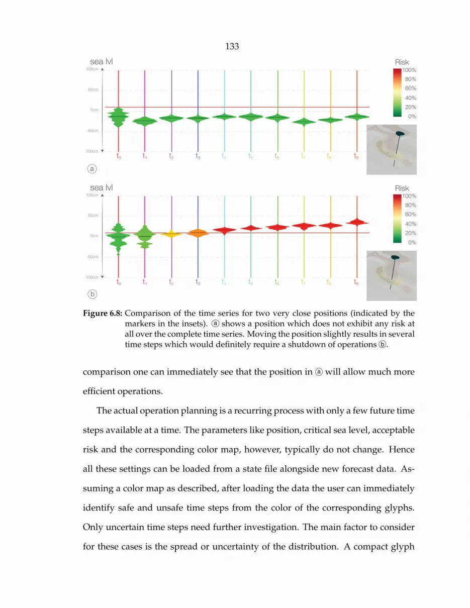
133
-50cm
-100cm
sea lvl Risk100%80%60%40%20%0%
50cm
0cm
100cm
t0 t1 t2 t3 t4 t5 t6 t7 t8 t9
a
-50cm
-100cm
sea lvl Risk100%80%60%40%20%0%
50cm
0cm
100cm
t0 t1 t2 t3 t4 t5 t6 t7 t8 t9
b
Figure 6.8: Comparison of the time series for two very close positions (indicated by themarkers in the insets). a shows a position which does not exhibit any risk atall over the complete time series. Moving the position slightly results in severaltime steps which would definitely require a shutdown of operations b .
comparison one can immediately see that the position in a will allow much more
efficient operations.
The actual operation planning is a recurring process with only a few future time
steps available at a time. The parameters like position, critical sea level, acceptable
risk and the corresponding color map, however, typically do not change. Hence
all these settings can be loaded from a state file alongside new forecast data. As-
suming a color map as described, after loading the data the user can immediately
identify safe and unsafe time steps from the color of the corresponding glyphs.
Only uncertain time steps need further investigation. The main factor to consider
for these cases is the spread or uncertainty of the distribution. A compact glyph

134
corresponds to a distribution with little uncertainty. Here, the risk estimate can
immediately be used for making a decision to shut down the rig. A large glyph
in general indicates large uncertainty. Here, the user must carefully weigh several
properties: Are ensemble members in the critical range close to the critical sea level
or far above, is the distribution skewed to either side, etc. While in general this in-
formation can be derived from the glyph, the user can also access the raw results
from the statistical analysis at this point, before making a final decision.
6.7 Conclusion
In this chapter, we have presented an interactive system for the visualization,
exploration and analysis of ocean forecasts in the form of heightfield ensemble
data. The core of our framework, which consists of statistical analysis and render-
ing, is implemented in an efficient GPU-based pipeline. We show the utility of our
framework for ocean forecasting in a case study based on real world forecast data
of the Gulf of Mexico.
135
Chapter 7
Summary and Discussion
This thesis presents several visual, interactive techniques, to enhance workflows
for oil and gas exploration. We introduce novel applications for the creation of
subsurface models and the visual analysis of ocean forecasts. Both applications
help to plan safe and efficient operations for oil and gas exploration.
Our application for subsurface modeling, for the first time, allows the integra-
tion of well data, recorded in spatial depth, into the seismic interpretation work-
flows, based on seismic reflection tomography data, recorded in time. Our novel
joint/time depth domain workflow is made possible by an on the fly depth con-
version technique. Additionally, rather than axis aligned, we set up slice views
based on well positions, to maximize the availability of the information gathered
from wells. We introduce an interactive global optimization technique for hori-
zon extraction. Based on the horizon extraction technique we introduce ensemble
computation to seismic interpretation, by automatically sampling the parameter
space of the cost function, underlying the global optimization. Based on these en-
sembles, we present a framework for efficient exploration of the parameter space
of the cost function. Finally we introduce a novel shading technique, based on
the local waveform of seismic traces, to highlight horizon structures without pre-
processing and present the application of exploded views for the visualization of
seismic data.

136
The second application, presented in this thesis allows planning the placement
and operations of off-shore structures, like oil rigs. We present a framework for the
interactive visual analysis of ensemble simulations of the sea surface. The frame-
work is based on an efficient, completely GPU-based framework, for statistical
analysis and visualization of ensembles of surfaces. We present a case study, based
on simulation data of the Gulf of Mexico, that shows the application of our frame-
work in a real world scenario.
Limitations and Open Questions
The presented subsurface modeling application focuses on the extraction of seis-
mic horizons only. A complete subsurface model includes additional structures,
most importantly faults. Faults are areas where the rock slipped (Compare Fig-
ure 7.1), creating discontinuities in the subsurface layers. The integration of faults
into our subsurface modeling workflow is left to future work. A possible approach
could be integrating a term, describing the likeliness of an edge belonging to a
fault, into our cost function, to guide the global optimization along faults. A good
fit for such a term could be based on the work of Jeong et al. [42].
Reverse faultNo Faulting Normal fault Strike-slip fault
Figure 7.1: Different fault types. Horizons intersected by normal and strike slip faults canstill be handled as height fields. Reverse faults would require splitting up thevolume. Figure reproduced from the USGS Earthquake Glossary [105].

137
At first glance, representing the horizons as heightfields seems a major limita-
tion for the inclusion of faults. However, our complete extraction pipeline can han-
dle arbitrary geometry. Only after extracting the optimal surface from the graph,
as described in Section 3.4.4, we convert it to a heightfield for efficient render-
ing. Additionally, as can be seen in Figure 7.1, only reverse faulting creates layers
whose boundaries can not be represented as heightfields, the more common nor-
mal faults, as well as strike-slip faults result in horizons where no (x, y)-position
maps to more than one depth value. The on the fly depth conversion, as presented
in Section 3.2.2, does only work for subsurface layers bound by heightfields. How-
ever, once faults are extracted, the reverse faults could be used to divide the dataset
into subsets, for which the depth conversion would work again.
We also use a property of heightfields for our statistical analysis of ensemble
data, presented in Chapters 4 and 6. For both we compute the statistics for each
(x, y)-position, knowing that each surface passes through each (x, y)-position ex-
actly once. Such an approach would not work for comparing arbitrary geometry.
However, if correspondences between ensemble members are known, these can be
used as the basis for the statistics computation. As long as the connectivity of the
vertices does not change even our rendering framework, which creates the final
geometry on the fly, would still work, by simply using vertex indices to lookup the
final position in the ensemble texture, instead of (x, y)-coordinates.
Finally our prism based workflow, presented in Section 3.3 approximates each
well position with a single straight line, orthogonal to the surface. Modern drilling
techniques allow complicated bore hole paths. When using well logs, we can not
handle such paths in our framework, as is. As long as wells do not intersect, and
the topology of the object, enclosed by three wells, corresponds to a prism, an
approach, where the sides of the ’prism’ are deformed for visualization and inter-

138
action, would be thinkable. For the use of well tops the trajectory of the bore hole
is irrelevant. Since well tops are sparse, discrete samples along the well, we simply
treat each top separately. When two or more tops from a single well correspond to
separate (x, y)-positions we consider them separately during triangulation. While
this results in prisms, where not all corners provide information for all hroizons,
none of the well data is lost.

139
REFERENCES
[1] LEMON library for efficient modeling and optimization in networks. Avail-able online at http://lemon.cs.elte.hu (Mar. 08 2013).
[2] J. Anderson, T. Hoar, K. Raeder, H. Liu, N. Collins, R. Torn, and A. Avellano.The data assimilation research testbed: A community facility. Bulletin of theAmerican Meteorological Society, 90:1283–1296, 2009.
[3] C. Armstrong, B. Price, and W. A. Barrett. Interactive segmentation of imagevolumes with live surface. Computers & Graphics, 31(2):212–22, 2007.
[4] J. Beyer, M. Hadwiger, T. Moller, and L. Fritz. Smooth mixed-resolution GPUvolume rendering. In Proceedings of IEEE/EG International Symposium on Vol-ume and Point-Based Graphics, pages 163–170, 2008.
[5] A. Birkeland, S. Bruckner, A. Brambilla, and I. Viola. Illustrative membraneclipping. Computer Graphics Forum, 31(3):905–914, 2012.
[6] J. F. Blinn. Models of light reflection for computer synthesized pictures. InProceedings of the 4th Annual Conference on Computer Graphics and InteractiveTechniques, SIGGRAPH ’77, pages 192–198, 1977.
[7] A. Blinov and M. Petrou. Reconstruction of 3-d horizons from 3-d seismicdatasets. IEEE Transactions on Geoscience and Remote Sensing, 43(6):1421–1431,2005.
[8] H. G. Borgos, O. Gramstad, G. V. Dahl, P. L. Guern, L. Sonneland, and J. F.Rosalba. Extracting horizon patches and geo-bodies from 3d seismic wave-form sequences. SEG Technical Program Expanded Abstracts, 25(1):1595–1599,2006.
[9] Y. Boykov and M.-P. Jolly. Interactive organ segmentation using graph cuts.In MICCAI ’00: Proceedings of the Third International Conference on Medical Im-age Computing and Computer-Assisted Intervention, pages 147–175, 2000.
140
[10] Y. Boykov and M.-P. Jolly. Interactive graph cuts for optimal boundary ®ion segmentation of objects in n-d images. In Proceedings of IEEE Interna-tional Conference on Computer Vision, 2001, pages 105–112 vol.1, 2001.
[11] Y. Boykov, O. Veksler, and R. Zabih. Fast approximate energy minimizationvia graph cuts. IEEE Transactions on Pattern Analysis and Machine Intelligence,23(11):1222–1239, 2001.
[12] R. A. Brown. Animated visual vibrations as an uncertainty visualisationtechnique. In International Conference on Computer Graphics and InteractiveTechniques in Australasia and South East Asia, pages 84–89, 2004.
[13] S. Bruckner and M. E. Groller. Exploded views for volume data. IEEE Trans-actions on Visualization and Computer Graphics, 12(5):1077–1084, 2006.
[14] L. Castanie, B. Levy, and F. Bosquet. Advances in seismic interpretation us-ing new volume visualization techniques. First Break Journal, pages 69–72,2005.
[15] L. Castanie, B. Levy, and F. Bosquet. VolumeExplorer: Roaming large vol-umes to couple visualization and data processing for oil and gas exploration.In Proceedings of IEEE Visualization Conference ’05, pages 247–254, 2005.
[16] E. P. Chassignet, H. E. Hurlburt, O. M. Smedstad, C. N. Barron, D. S. Ko,R. C. Rhodes, J. F. Shriver, A. J. Wallcraft, and R. A. Arnone. Assessmentof data assimilative ocean models in the gulf of mexico using ocean color.Circulation in the Gulf of Mexico: Observations and Models, 161:87–100, 2005.
[17] L. M. Cherubin, W. Sturges, and E. Chassignet. Deep flow variability in thevicinity of the yucatan straits from a high resolution MICOM simulation.Journal of Geophysical Research, 110:20–72, 2005.
[18] F. Counillon and L. Bertino. High-resolution ensemble forecasting for thegulf of mexico eddies and fronts. Ocean Dynamics, 59:83–95, 2009.
[19] E. Dijkstra. A note on two problems in connexion with graphs. NumerischeMathematik, 1(1):269–271, 1959.
[20] H. Doleisch, M. Gasser, and H. Hauser. Interactive feature specification forfocus+context visualization of complex simulation data. In Proceedings of the
141
5th Joint IEEE TCVG - EUROGRAPHICS Symposium on Visualization (VisSym2003), pages 239–248, 2003.
[21] K. Engel, M. Hadwiger, J. M. Kniss, C. Rezk-Salama, and D. Weiskopf. Real-Time Volume Graphics. A K Peters, 2006.
[22] E. L. Etris, N. J. Crabtree, J. Dewar, and S. Pickford. True depth conversion:More than a pretty picture. CSEG Recorder, 26:11–22, 2001.
[23] G. Evensen. Data Assimilation: The Ensemble Kalman Filter. Springer, 2006.
[24] A. X. Falcao and J. K. Udupa. Segmentation of 3d objects using live wire. InMedical Imaging 1997: Image Processing, pages 228–235, 1997.
[25] A. X. Falcao, J. K. Udupa, S. Samarasekera, S. Sharma, B. E. Hirsch, andR. de Lotufo. User-steered image segmentation paradigms: Live wire andlive lane. Graphical Models and Image Processing, 60(4):233–260, 1998.
[26] A. X. Falcao and K. J. Udupa. A 3d generalization of user-steered live-wiresegmentation. Medical Image Analysis, 4(4):389–402, 2000.
[27] M. Faraklioti and M. Petrou. Horizon picking in 3d seismic data volumes.Machine Vision and Applications, 15:216–219, 2004.
[28] D. Gao. 3d seismic volume visualization and interpretation: An integratedworkflow with case studies. Geophysics, 74(1):W1–W12, 2009.
[29] L. Grady. Computing exact discrete minimal surfaces: Extending and solv-ing the shortest path problem in 3d with application to segmentation. InIEEE Conference on Computer Vision and Pattern Recognition, 2006, volume 1,pages 69–78, 2006.
[30] L. Grady. Minimal surfaces extend shortest path segmentation methods to3d. IEEE Transactions on Pattern Analysis and Machine Intelligence, 32(2):321–334, 2010.
[31] H. Griethe and H. Schumann. The visualization of uncertain data: Methodsand problems. In Proceedings of SimVis ’06, 2006.
[32] G. Grigoryan and P. Rheingans. Point-based probabilistic surfaces to showsurface uncertainty. IEEE Transactions on Visualization and Computer Graphics,10(5):564–573, 2004.
142
[33] C. G. Healey and J. Snoeyink. VisTRE: A visualization tool to evaluate errorsin terrain representation. In 3D Data Processing, Visualization, and Transmis-sion, Third International Symposium on, pages 1056–1063, 2006.
[34] J. L. Hintze and R. D. Nelson. Violin plots: A box plot-density trace syner-gism. The American Statistician, 52(2):181–184, 1998.
[35] T. Hollt, J. Beyer, F. Gschwantner, P. Muigg, H. Doleisch, G. Heinemann, andM. Hadwiger. Interactive seismic interpretation with piecewise global en-ergy minimization. In Proceedings of the IEEE Pacific Visualization Symposium2011, pages 59–66, 2011.
[36] T. Hollt, G. Chen, C. D. Hansen, and M. Hadwiger. Extraction and visualanalysis of seismic horizon ensembles. To appear in Proceedings of Eurographics2013 Short Papers, 2013.
[37] T. Hollt, W. Freiler, F. M. Gschwantner, H. Doleisch, G. Heinemann, andM. Hadwiger. SeiVis: An interactive visual subsurface modeling applica-tion. IEEE Transactions on Visualization and Computer Graphics, 18(12):2226–2235, 2012.
[38] T. Hollt, M. Hadwiger, L. Fritz, P. Muigg, and H. Doleisch. Seismic horizontracing with diffusion tensors. Poster Presentation IEEE Visualization 2009,Atlantic City, NJ, 2009.
[39] T. Hollt, A. Magdy, G. Chen, G. Gopalakrishnan, I. Hoteit, C. D. Hansen,and M. Hadwiger. Visual analysis of uncertainties in ocean forecasts forplanning and operation of off-shore structures. In Proceedings of the IEEEPacific Visualization Symposium 2013, pages 59–66, 2013.
[40] I. Hoteit, T. Hoar, G. Gopalakrishnan, J. Anderson, N. Collins, B. Cornuelle,A. Kohl, and P. Heimbach. A MITgcm/DART ensemble analysis and predic-tion system with application to the gulf of mexico. Dynamics of Atmospheresand Oceans, 63:1–23, 2013.
[41] I. Hoteit, D. T. Pham, and J. Blum. A simplified reduced order kalman filter-ing and application to altimetric data assimilation in tropical pacific. Journalof Marine Systems, 36:101–127, 2002.
143
[42] W.-K. Jeong, R. Whitaker, and M. Dobin. Interactive 3d seismic fault detec-tion on the graphics hardware. In Eurographics / IEEE VGTC Workshop onVolume Graphics, pages 111–118, 2006.
[43] C. R. Johnson and A. R. Sanderson. A next step: Visualizing errors anduncertainty. IEEE Computer Graphics and Applications, 23(5):6–10, 2003.
[44] B. J. Kadlec, G. A. Dorn, and H. M. Tufo. Confidence and curvature-guidedlevel sets for channel segmentation. In SEG Annual Meeting 2008, pages 879–883, 2008.
[45] B. J. Kadlec, G. A. Dorn, and H. M. Tufo. Interactive visualization and in-terpretation of geologic surfaces in 3-d seismic data. In SEG Annual Meeting2009, pages 1147–1151, 2009.
[46] B. J. Kadlec, H. M. Tufo, and G. A. Dorn. Knowledge-assisted visualizationand segmentation of geologic features. Computer Graphics and Applications,30(1):30–39, 2010.
[47] D. Kao, J. Dungan, and A. Pang. Visualizing 2d probability distributionsfrom EOS satellite image-derived data sets: a case study. In Proceedings of theconference on Visualization ’01. VIS ’01., pages 457–560, 2001.
[48] D. Kao, M. Kramer, A. Love, J. Dungan, and A. Pang. Visualizing distri-butions from multi-return lidar data to understand forest structure. In InGeoinformatics, Gavle Sweden, 2004.
[49] N. Keskes, P. Zaccagnino, D. Rether, and P. Mermey. Automatic extraction of3-d seismic horizons. SEG Technical Program Expanded Abstracts, 2(1):557–559,1983.
[50] G. Kidd. Fundamentals of 3d seismic volume visualization. In Offshore Tech-nology Conference, 1999.
[51] O. D. Lampe, C. Correa, K.-L. Ma, and H. Hauser. Curve-centric volumereformation for comparative visualization. IEEE Transactions on Visualizationand Computer Graphics, 15(6):1235–1242, 2009.
[52] P. Lavest and Y. Chipot. Building complex horizons for 3-d seismic. SEGTechnical Program Expanded Abstracts, 12(1):159–161, 1993.

144
[53] M. Levoy. Display of surfaces from volume data. IEEE Computer Graphicsand Applications, 8(3):29–37, may 1988.
[54] E. M. Lidal, H. Hauser, and I. Viola. Design principles for cutaway visual-ization of geological models. In Proceedings of Spring Conference on ComputerGraphics 2012, pages 53–60, 2012.
[55] E. M. Lidal, T. Langeland, C. Giertsen, J. Grimsgaard, and R. Helland. Adecade of increased oil recovery in virtual reality. IEEE Computer Graphicsand Applications, 27:94–97, 2007.
[56] A. Love, A. Pang, and D. Kao. Visualizing spatial multivalue data. IEEEComputer Graphics and Applications, 25(3):69–79, 2005.
[57] C. Lundstrom, P. Ljung, A. Persson, and A. Ynnerman. Uncertainty visu-alization in medical volume rendering using probabilistic animation. IEEETransactions on Visualization and Computer Graphics, 13(6):1648–1655, 2007.
[58] A. Luo, D. Kao, and A. Pang. Visualizing spatial distribution data sets. InVISSYM ’03: Proceedings of the Symposium on Data Visualisation 2003, pages29–38, 2003.
[59] W. R. Mark, R. S. Glanville, K. Akeley, and M. J. Kilgard. Cg: a system forprogramming graphics hardware in a C-like language. In SIGGRAPH ’03:ACM SIGGRAPH 2003 Papers, pages 896–907, New York, NY, USA, 2003.ACM.
[60] J. Marshall, A. Adcroft, C. Hill, L. Perelman, and C. Heisey. A finite-volume,incompressible Navier Stokes model for studies of the ocean on parallel com-puters. Journal of Geophysical Research, 102:5735–5766, 1997.
[61] K. Matkovic, D. Gracanin, B. Klarin, and H. Hauser. Interactive visual anal-ysis of complex scientific data as families of data surfaces. IEEE Transactionson Visualization and Computer Graphics, 15(6):1351–1358, 2009.
[62] M. J. McGuffin, L. Tancau, and R. Balakrishnan. Using deformations forbrowsing volumetric data. In Proceedings of IEEE Visualization 2003, pages401–408, 2003.
[63] U. Meyer and P. Sanders. �-stepping: A parallel single source shortest pathalgorithm. In Proceedings of the 6th Annual European Symposium on Algorithms,1998, pages 393–404, 1998.

145
[64] U. Meyer and P. Sanders. �-stepping: a parallelizable shortest path algo-rithm. Journal of Algorithms, 49(1):114–152, 2003.
[65] K. Moreland. Diverging color maps for scientific visualization. In Proceedingsof the 5th International Symposium on Visual Computing, pages 92–103, 2009.
[66] E. N. Mortensen and W. A. Barrett. Intelligent scissors for image composi-tion. In SIGGRAPH ’95: Proceedings of the 22nd Annual Conference on ComputerGraphics and Interactive Techniques, pages 191–198, 1995.
[67] E. N. Mortensen and W. A. Barrett. Interactive segmentation with intelligentscissors. Graphical Models and Image Processing, 60(5):349–384, 1998.
[68] E. N. Mortensen, B. Morse, W. A. Barrett, and J. K. Udupa. Adaptive bound-ary detection using ‘live-wire’ two-dimensional dynamic programming. InProceedings of Computers in Cardiology, 1992, pages 635–638, 1992.
[69] NVIDIA Corporation. CUDA C programming guide version 5.0, 2012.Available online at http://docs.nvidia.com/cuda/pdf/CUDA_C_
Programming_Guide.pdf (Mar. 08 2013).
[70] L. Oey, T. Ezer, and H. Lee. Loop current, rings and related circulation inthe gulf of mexico: A review of numerical models and future challenges.Geophysical Monograph-American Geophysical Union, 161:31, 2005.
[71] S. Osher and N. Paragios. Geometric Level Set Methods in Imaging,Vision,andGraphics. Springer-Verlag New York, Inc., 2003.
[72] A. T. Pang, C. M. Wittenbrink, and S. K. Lodha. Approaches to uncertaintyvisualization. The Visual Computer, 13:370–390, 1997.
[73] D. Patel, S. Bruckner, I. Viola, and M. E. Groller. Seismic volume visual-ization for horizon extraction. In Proceedings of the IEEE Pacific VisualizationSymposium 2010, pages 73–80, 2010.
[74] D. Patel, C. Giertsen, J. Thurmond, J. Gjelberg, and M. E. Groller. The seismicanalyzer: Interpreting and illustrating 2d seismic data. IEEE Transactions onVisualization and Computer Graphics, 14(6):1571–1578, 2008.
[75] D. Patel, T. Hollt, and M. Hadwiger. To appear in Novel Visualization Tools inGeoscience and Petroleum Engineering. Springer-Verlag GmbH, 2013.

146
[76] D. Patel, Ø. Sture, H. Hauser, C. Giertsen, and M. E. Groller. Knowledge-assisted visualization of seismic data. Computers & Graphics, 33(5):585–596,2009.
[77] S. I. Pedersen, T. Skov, T. Randen, and L. Sønneland. Automatic fault ex-traction using artificial ants. In A. Iske and T. Randen, editors, MathematicalMethods and Modelling in Hydrocarbon Exploration and Production, volume 7 ofMathematics in Industry, pages 107–116. 2005.
[78] R. Pepper and G. Bejarano. Advances in seismic fault interpretation automa-tion. Search and Discovery Article 40170, Poster presentation at AAPG AnnualConvention, pages 19–22, 2005.
[79] P. Perona and J. Malik. Scale-space and edge detection using anisotropicdiffusion. IEEE Transactions on Pattern Analysis and Machine Intelligence,12(7):629–639, 1990.
[80] T. Pfaffelmoser, M. Reitinger, and R. Westermann. Visualizing the positionaland geometrical variability of isosurfaces in uncertain scalar fields. ComputerGraphics Forum, 30(3):951–960, 2011.
[81] T. Pfaffelmoser and R. Westermann. Visualization of global correlation struc-tures in uncertain 2d scalar fields. Computer Graphics Forum, 31(3):1025–1034,2012.
[82] D. T. Pham. Stochastic methods for sequential data assimilation in stronglynonlinear systems. Monthly Weather Review, 129:1194–1207, 2001.
[83] H. Piringer, S. Pajer, W. Berger, and H. Teichmann. Comparative visual anal-ysis of 2d function ensembles. Computer Graphics Forum, 31(3):1195–1204,2012.
[84] M. Poon, G. Hamarneh, and R. Abugharbieh. Live-vessel: Extendinglivewire for simultaneous extraction of optimal medial and boundary pathsin vascular images. In Lecture Notes in Computer Science, Medical Image Com-puting and Computer-Assisted Intervention (MICCAI), pages 444–451, 2007.
[85] M. Poon, G. Hamarneh, and R. Abugharbieh. Segmentation of complex ob-jects with non-spherical topologies from volumetric medical images using3d livewire. In SPIE Medical Imaging, volume 6512-31, pages 1–10, 2007.

147
[86] M. Poon, G. Hamarneh, and R. Abugharbieh. Efficient interactive 3dlivewire segmentation of objects with arbitrary topology. Computerized Med-ical Imaging and Graphics, 32(8):639–650, 2008.
[87] K. Pothkow and H.-C. Hege. Positional uncertainty of isocontours: Condi-tion analysis and probabilistic measures. IEEE Transactions on Visualizationand Computer Graphics, 17(10):1393–1406, 2011.
[88] K. Pothkow, B. Weber, and H.-C. Hege. Probabilistic marching cubes. Com-puter Graphics Forum, 30(3):931–940, 2011.
[89] K. Potter, A. Wilson, P.-T. Bremer, D. Williams, C. Doutriaux, V. Pascucci, andC. R. Johhson. Ensemble-Vis: A framework for the statistical visualization ofensemble data. In IEEE Workshop on Knowledge Discovery from Climate Data:Prediction, Extremes and Impacts, pages 233–240, 2009.
[90] C. Rezk-Salama, M. Scheuering, G. Soza, and G. Greiner. Fast volumetricdeformation on general purpose hardware. In Proceedings of the ACM Sig-graph/Eurographics Workshop On Graphics Hardware, HWWS ’01, pages 17–24,2001.
[91] P. J. Rhodes, R. S. Laramee, R. D. Bergeron, and T. M. Sparr. Uncertaintyvisualization methods in isosurface rendering. In EUROGRAPHICS 2003Short Papers, pages 83–88, 2003.
[92] M. Riveiro. Evaluation of uncertainty visualization techniques for informa-tion fusion. In Information Fusion, 2007 10th International Conference on, pages1–8, 2007.
[93] T. Ropinski, J. Meyer-Spradow, S. Diepenbrock, J. Mensmann, and K. H. Hin-richs. Interactive volume rendering with dynamic ambient occlusion andcolor bleeding. Computer Graphics Forum (Eurographics 2008), 27(2):567–576,2008.
[94] T. Ropinski, F. Steinicke, and K. H. Hinrichs. Visual exploration of seismicvolume datasets. Journal Proceedings of the 14th International Conference in Cen-tral Europe on Computer Graphics, Visualization and Computer Vision (WSCG06),14:73–80, 2006.
148
[95] M. Ruiz, I. Viola, I. Boada, S. Bruckner, M. Feixas, and M. Sbert. Similarity-based exploded views. In Proceedings of 8th International Symposium on SmartGraphics, pages 154–165, 2008.
[96] A. Saad, G. Hamarneh, and T. Moller. Exploration and visualization of seg-mentation uncertainty using shape and appearance prior information. IEEETransactions on Visualization and Computer Graphics, 16(6):1366–1375, 2010.
[97] J. Sanyal, S. Zhang, J. Dyer, A. Mercer, P. Amburn, and R. J. Moorhead. Noo-dles: A tool for visualization of numerical weather model ensemble uncer-tainty. IEEE Transactions on Visualization and Computer Graphics, 16(6):1421 –1430, 2010.
[98] H. Scharsach, M. Hadwiger, A. Neubauer, and K. Buhler. Perspective iso-surface and direct volume rendering for virtual endoscopy applications. InEurovis 2006, pages 315–322, 2006.
[99] A. Schenk, G. Prause, and H. O. Peitgen. Efficient semiautomatic segmenta-tion of 3d objects in medical images. In MICCAI ’00: Proceedings of the ThirdInternational Conference on Medical Image Computing and Computer-Assisted In-tervention, pages 186–195, 2000.
[100] Schlumberger Information Solutions. Petrel seismic to simulation software.Available online at http://www.slb.com/services/software/geo/petrel.aspx (Mar. 08 2013).
[101] F. Schulze, K. Buhler, and M. Hadwiger. Direct volume deformation. InComputer Vision and Computer Graphics. Theory and Applications, volume 21 ofCommunications in Computer and Information Science, pages 59–72. 2009.
[102] P. M. Silva, M. Machado, and M. Gattass. 3d seismic volume rendering. InEighth International Congress of The Brazilian Geophysical Society, pages 181–193, 2003.
[103] P. Tu, A. Zisserman, I. Mason, and I. Cox. Identification of events from 3dvolumes of seismic data. In IEEE International Conference on Image Processing,ICIP ’94, volume 3, pages 309–313, 1994.
[104] U.S. Energy Information Administration. International energy outlook 2010,2010.

149
[105] U.S. Geological Survey. Earthquake glossary, 2013. Available online athttp://earthquake.usgs.gov/learn/glossary/ (Mar. 08 2013).
[106] vsg Visualizaton Sciences Group. Avizo earth. Available online at http://www.vsg3d.com/avizo/earth (Mar. 08 2013).
[107] V. Solteszova, D. Patel, and I. Viola. Chromatic shadows for improved per-ception. In Proceedings of Non-photorealistic Animation and Rendering 2011,pages 105–115, 2011.
[108] F. M. Vukovich. An updated evaluation of the loop current’s eddy-sheddingfrequency. Journal of Geophysical Research, 100:8655–8659, 1995.
[109] J. Weickert. Anisotropic Diffusion in Image Processing. PhD thesis, Universityof Kaiserslautern, 1996.
[110] R. Westermann and C. Rezk-Salama. Real-time volume deformations. Com-puter Graphics Forum, 20(3):443–451, 2001.
[111] C. Wunsch. The Ocean Circulation Inverse Problem. Cambridge UniversityPress, 1996.

150
APPENDICES

151
A Publications Relevant to thisDissertation.
• Daniel Patel, Thomas Hollt, and Markus Hadwiger, Real-Time Algorithms for
Visualizing and Segmenting Seismic Data, in Novel Visualization Tools in Geo-
science and Petroleum Engineering, Springer-Verlag GmbH, to appear, 2013.
• Thomas Hollt, Guoning Chen, Charles D. Hansen, and Markus Hadwiger, Ex-
traction and Visual Analysis of Seismic Horizon Ensembles, Proceedings of Euro-
graphics 2013 Short Papers, to appear, 2013.
• Thomas Hollt, Ahmed Magdy, Guoning Chen, Ganesh Gopalakrishnan, Ibrahim
Hoteit, Charles D. Hansen, and Markus Hadwiger, Visual Analysis of Uncertain-
ties in Ocean Forecasts for Planning and Operation of Off-Shore Structures, Pro-
ceedings of IEEE Pacific Visualization 2013, pp. 185–192, 2013. Honorable mention
for best paper award.
• Thomas Hollt, Wolfgang Freiler, Fritz Gschwantner, Helmut Doleisch, Gabor
Heinemann, and Markus Hadwiger, SeiVis: An Interactive Visual Subsurface
Modeling Application, IEEE Transactions on Visualization and Computer Graphics,
18(12) (Proceedings IEEE Scientific Visualization 2012); pp. 2226–2235, 2012.
• Thomas Hollt, Johanna Beyer, Fritz Gschwantner, Philipp Muigg, Helmut Doleisch,
Gabor Heinemann, and Markus Hadwiger, Interactive Seismic Interpretation with
Piecewise Global Energy Minimization, Proceedings of IEEE Pacific Visualization
2011, pp. 59–66, 2011.

152
• Thomas Hollt, Markus Hadwiger, Laura Fritz, Philipp Muigg, and Helmut Doleisch,
Seismic Horizon Tracing with Diffusion Tensors, Poster Presentation IEEE Visual-
ization 2009, Atlantic City, NJ, 2009.

153
B Other Publications.
• Mathias Schott, Tobias Martin, A.V. Pascal Grosset, Carson Brownlee, Thomas
Hollt, Benjamin P. Brown, Sean T. Smith, and Charles D. Hansen, Combined Sur-
face and Volumetric Occlusion Shading, Proceedings of IEEE Pacific Visualization
2012, pp. 169–176 2012.
• Georg Geier, Thomas Pabel, Daniel Habe, Jordis Rosc, Markus Hadwiger, Thomas
Hollt, and Laura Fritz, Computertomographie als zerstorungsfreies Prufverfahren
fur Gussteile, Druckguss, 7(8), pp. 171–174, 2010.
• Markus Hadwiger, Laura Fritz, Christof Rezk-Salama, Thomas Hollt, Georg Geier,
and Thomas Pabel, Interactive Volume Exploration for Feature Detection and
Quantification in Industrial CT Data, IEEE Transactions on Visualization and Com-
puter Graphics, 14(6) (Proceedings IEEE Visualization 2008); pp. 1507–1514, 2008.
• Georg Geier, Markus Hadwiger, Thomas Hollt, Laura Fritz, and Thomas Pa-
bel, Interaktive Exploration und Quantifizierung von Unganzen in komplexen
Bauteilen, Proceedings of Industrielle Computertomografie (CT Tagung Wels), pp. 103–
108, 2008.