the ogs-eclipse code for simulation of coupled multiphase
TRANSCRIPT
https://doi.org/10.1007/s10596-020-09951-8
ORIGINAL PAPER
The OGS-Eclipse code for simulation of coupled multiphase flowand geomechanical processes in the subsurface
Katharina Benisch1 ·WenqingWang2 · Jens-Olaf Delfs1 · Sebastian Bauer1
Received: 27 July 2018 / Accepted: 27 February 2020© The Author(s) 2020
AbstractThis paper presents a numerical simulation tool for the analysis of coupled processes related to subsurface operations. Thetool combines the open-source scientific code OpenGeoSys with the reservoir simulator Eclipse enabling the coupling ofthermal, hydraulic, mechanical and geochemical processes. While the coupling of multiphase flow with heat and reactivegeochemical component transport has been already implemented, OpenGeoSys-Eclipse is now extended for the couplingof multiphase flow and deformation. By this, OpenGeoSys-Eclipse is capable of addressing the impact of pore pressurechanges on rock stability and deformation as well as the feedback effects of geomechanical processes on multiphase flowvia pore volume coupling and porosity and permeability update. The coupling is verified by several test cases of gas storagescenarios and compared with reference simulations of OpenGeoSys. The results are in good agreement regarding the generaleffects of geomechanical feedback on pore pressure as well as porosity and permeability changes. Differences in the resultsare only observed for the pore volume coupling arising from the different implementation of rock compressibility models inthe two simulators. The simulations are furthermore used to investigate the relevance of addressing geomechanical feedbackin numerical scenario simulations for the assessment of subsurface operations. The results show clearly, that, depending onthe given storage site conditions and rock types, the feedback of deformation on pore pressure can be significant and shouldtherefore be accounted for in the assessment.
Keywords Numerical simulation · Coupled hydromechanical processes · Code development and verification ·OpenGeoSys-Eclipse
Symbol Description Unita Empiric constant (-)b Biots constant (-)c Empiric constant (-)D Elastic material tensor (MPa)E Young’s modulus (MPa)G Shear modulus (MPa)g Gravitational force (m/s2)I Identity tensor (-)j Jacobian matrix (-)
� Katharina [email protected]
Sebastian [email protected]
1 Christian-Albrechts-University of Kiel, Kiel, Germany
2 Helmholtz Centre for Environmental Research,Leipzig, Germany
Ks Bulk modulus of solid (MPa)Kb Drained bulk modulus of (MPa)
porous medium
Kα Bulk modulus of fluid (MPa)
phase α
k Permeability tensor (m2)
k0 Initial permeability (m2)kr,α Relative permeability of (-)
fluid phase α
N Linear shape function (-)
Ni High order shape function (-)pα Pressure of fluid phase α (MPa)p Mean pressure (MPa)pc Capillary pressure (MPa)pc,0 Initial capillary pressure (MPa)qα Flux of fluid phase α (m3/s)qα Source/sink of fluid (m/s)
phase α
Computational Geosciences (2020) 24:1315–1331
/ Published online: 12 May 2020

Sα saturation of fluid phase alpha (-)u Displacement vector (m)vs Solid velocity (m/s)w Weighting function (-)ST Storage term (Pa−1)α Fluid phase (-)δ Kronecker delta (-)ε Strain tensor (-)λ Lame constant (MPa)μα Dynamic viscosity of (Pa s)
fluid phase α
ν Poisson ratio (-)ρs Solid density (kg/m3)ρα Density of fluid (kg/m3)
phase α
ρ Mean density (kg/m3)σ Total stress tensor (MPa)σ ′ Effective stress tensor (MPa)σ Mean effective stress (MPa)
tensorφ Porosity (-)φ0 Initial porosity (-)φr Residual porosity (-)
� Delta (-)∇·A Divergence of (-)
a vector∇A Gradient of a scalar (-)MT Transpose of (-)
matrix M
1 Introduction
Long-time monitoring of the earth’s climate has shown anincreasing impact of the anthropogenic CO2 emissions onglobal warming [13]. CO2 is one of the main greenhousegases enhancing atmospheric radiation and warming of theground surface. Due to the large industrialization and pop-ulation growth, CO2 emission has increased significantlyin the last decades enhancing global temperature rise andtherefore climate change [25]. This has emerged publicand politic concern to climate change worldwide. There-fore, international climate protection agreements has beenadopted to limit global temperature increases by reducingindustrial carbon emissions and passing to a sustainableenergy supply from renewables [24].
One method to reduce CO2 release from industries tothe atmosphere is the permanent storage or sequestrationof CO2 in the subsurface. CO2 is hereby captured from
fossil-fuel power plants as one of the main emission sourcesfor CO2 and stored in deep geological porous formations.Impermeable sealing cap rock formation above the storageformation inhibit the CO2 from migrating upward into theshallow subsurface. Potential global storage capacity isestimated to be of about 8000 to 15,000 Gt CO2 [23]. Withactual 31 Gt CO2 global emissions per year, the amountof CO2 released to the atmosphere could be significantlydecreased by this method [25]. Further efforts in reducingCO2 emissions are done in the field of energy productionfrom renewable sources, which has been significantlyenhanced in the last decades [14]. One disadvantage of theseenergy sources is their natural fluctuation, e.g., wind andsolar power, resulting in a fluctuating electricity delivery tothe grid [53]. To overcome this gap in renewable energyproduction, new storage technologies have been consideredfor the temporary underground storage of surplus energy[22]. These include compressed air energy storage andpower-to-X technologies, where electricity from renewablesis used to produce hydrogen by hydrolysis, which can bestored underground or in a second step, can be converted tomethane and then stored [34].
Besides new technologies for subsurface gas and energystorage, also existing subsurface application like oil andgas production, groundwater withdrawal and retention,nuclear waste disposal or the reinjection of waste andthermal water has increased due to the rising demandof energy and water consumption worldwide [71]. Thisincrease in new and old subsurface engineering andgeotechnical applications have evoked growing awarenessof the environmental and drinking water protection, asany subsurface activity is accompanied by environmentalimpacts on the subsurface including pressurization andstresses, heating of the ground, migration of fluids orchanges in the geochemical and biological system [2]. Toassess these potential thermal, hydraulic, geochemical andgeomechanical processes and impacts related to subsurfaceapplications, a profound understanding of the complexsubsurface system is essential.
Especially the storage of mass or energy in the subsur-face can induce large-scale hydraulic and geomechanicalimpacts on the subsurface environment [72]. The injectionhereby causes an overpressure at the injection well, whichpropagates far into the surrounding formations, both later-ally and vertically as shown, e.g., for the case of long-termCO2 storage [7, 47, 54]. Similar effects were also inves-tigated for the topics of natural gas and hydrogen storage[53, 64] or compressed air energy storage [67]. The pres-sure increase also affects the earth’s stress field. Depend-ing on the site-specific geomechanical conditions and theinjection-induced overpressure, changes in the subsurface
Comput Geosci (2020) 24:1315–13311316

stress field may lead to large-scale deformation processes.This can result in ground uplift, hydraulic fracturing orfault reactivation within the cap rock risking the long-termintegrity of the storage site [36, 38, 50]. Therefore, theinjection rate needs to be limit to a maximum overpres-sure allowed to be applied in the target storage formation toavoid any rock damage [50]. The injection-induced defor-mation processes in turn affect injection performance asthey cause an increase or decrease of the pore volume ofthe porous rock leading to changes in the fluid pressurewithin the pores as well as in the relevant fluid flow param-eters permeability and porosity [21]. This strong interactionbetween fluid flow and deformation reinforces the impor-tance of a thorough process assessment and determination ofgeomechanical effects during subsurface storage operations.
Coupled numerical process simulations help to considerthe link between fluid flow and deformation. They allowto predict the individual processes and their feedbackto the system and with that to adequately assess thesubsurface operation. Two main coupling components haveto be considered in the process coupling: volume coupling,accounting for pore volume changes due to stress changes,and flow properties coupling, considering strain and stress-related changes in permeability and porosity [56]. Severalnumerical methods exist capable of solving the complexdifferential equation system that describes the processcoupling. The fully coupled method solves for all processessimultaneously through one system of equations. It offers ahigh internal consistency and accurate solution, but requireslong computation times and large development efforts [57].The iterative coupling method is used when each process issolved separately. Information between the flow simulatorand the geomechanics module is transferred back and forthuntil convergence of fluid flow and stress unknowns isreached. The iterative coupling is less accurate and needsome more iterations, but results in a faster run time[63]. It is therefore a good compromise between accuracyand feasibility and more flexible than fully coupled as itenables the coupling of various reservoir simulators andgeomechanics codes [45, 62]. The explicit coupling methodis the loosest coupling method. Results of the fluid flow aresent to the geomechanical process to calculate deformation,but there is no feedback to the fluid flow.
Various simulation codes have been developed for thenumerical modelling of coupled processes. These includeSTARS [8], FEMH [10], CODE-BRIGHT [40, 65], DuMuX[16], DYNAFLOW [46], or OpenGeoSys [28, 30], to namea few. These codes can be used for all types of coupling,especially fully coupled simulations, as all processes aresolved within one code. Though these codes provide highnumerical accuracy, the development effort is high. Another
more efficient option is the coupling of two existing codes,where each code solves for one process and the codesare then coupled using the iterative or explicit coupling.This has been done, e.g., for TOUGH-FLAC [49, 52],TOUGH2-Code-Aster [48], Eclipse-Visage [41, 42], NUFT-GEODYN-L [38], or Sierra [35]. Most of these codes wereoriginally flow simulators, which has been coupled to e.g.a mechanical module. This is of huge benefit instead ofdeveloping a complete new code as the coupling is moreflexible and can be adjusted more easily to the individualrequirements.
However, many codes, whether single or coupled codes,are subject to individual limits regarding process spectrum,available coupling methods or simulation efficiency. There-fore, a new coupling approach is presented here, whichcombines two well-developed and well-proven simulationcodes in order to cover the entire complexity of sub-surface processes by one simulation code and to benefitfurthermore from the individual strengths of both codes,e.g. robustness, flexibility, run time speed and numericalstability. For this, the scientific open-source code Open-GeoSys is coupled to the commercial Eclipse softwaresuite [55]. OpenGeoSys provides the simulation of cou-pled thermal-hydraulic-mechanical-chemical processes inthe subsurface with flexible process coupling and has beenapplied to a variety of scientific problems, e.g. energystorage [9, 33], reactive transport [58, 59], geochemicalmodelling [12] or heat storage [39]. Eclipse is well knownfor its stable and robust simulation capability for mul-tiphase and multicomponent flow [11, 26]. By couplingOpenGeoSys with Eclipse, the process capabilities and flex-ibility of OpenGeoSys can be combined with the efficiency,the high numerical stability and the computation speedof Eclipse [19, 44]. Up to now, the OpenGeoSys-Eclipsesimulator can handle single and multiphase flow, compo-nent transport, heat transport and geochemical reactions[44] and has been successfully applied to coupled THC-problems, e.g. CO2 storage or cyclic hydrogen injection andextraction [19, 33, 37, 43]. Coupled hydromechanical pro-cesses, especially the geomechanical feedback on flow arenot yet considered.
Therefore, OpenGeoSys-Eclipse is now extended forcoupled flow and geomechanical processes includinggeomechanical feedback. Fluid flow is hereby solved inEclipse and deformation is solved in OpenGeoSys. Thenew implementation includes the whole complexity of theprocess feedback between the two processes including porevolume update and changes in the fluid flow parametersporosity and permeability and can be run in an iterative orexplicit manner to enable the individually optimal methodfor the given problem.
Comput Geosci (2020) 24:1315–1331 1317
2 Simulation codes
2.1 OpenGeoSys
The open-source scientific software OpenGeoSys is afinite element code [27, 28, 68]. It uses an object-oriented and process-oriented approach that allows thesolution of partial differential equations for differentphysical problems in the subsurface using a generic objectstructure [27]. OpenGeoSys has been already used formultiple underground storage applications, e.g. gas storageor nuclear waste disposal [4, 9, 18, 29] and could besuccessfully compared and verified to other simulationcodes [3, 11, 17, 21, 69]. Coupled processes can besolved sequentially (iterative and explicit coupling) ormonolithic (fully coupled). Fluid flow can be solved in apressure-pressure or in a pressure-saturation formulation,using pressure of the non-wetting phase pnw and thecapillary pressure pc or pressure of the wetting phase pw
and saturation of the non-wetting phase Snw as primaryvariables, respectively. For the simulation of geomechanicalprocess, several constitutive models are implemented,e.g. a poroelastic model using Biot formulation solvingfor solid displacement, stresses and strains. OpenGeoSystherefore provides a wide range of geomechanical processapplications.
2.2 Eclipse
Eclipse is a conventional reservoir simulator suite mainlyused by the oil and gas industry. It offers high robustnessas well as computational speed. The simulator suiteinvolves two flow simulators E100 and E300 [55] forthe simulation of black oil and compositional system,respectively. Both Eclipse simulators use the finite volumemethod. The implemented numerical methods provide afully implicit formulation or an implicit pressure, explicitsaturation (IMPES) formulation. Besides traditional oil andgas reservoir simulations, Eclipse has been also appliedto further energy-related problems as unconventionalresources and underground storage of CO2, H2, andcompressed air energy [26, 43, 54, 67]. The advantages ofEclipse regarding simulation speed and numerical stabilityhave been demonstrated by several authors [1, 11]. Topredict geomechanical processes related to subsurfaceoperations, Eclipse can be coupled to the finite elementcode Visage. Visage has been a stand-alone simulation code[41], which has been incorporated into the SchlumbergerSoftware Package as Reservoir Geomechanics Tool in 2010.More details and application examples of this Eclipse-Visage code will be presented in Section 5. In this study,only Eclipse is used for the simulation of multiphase flowwithin the coupled OpenGeoSys-Eclipse code.
3Mathematical model
The coupling of fluid flow and deformation is described by aset of basic equations solved for the variables fluid pressurep and solid displacement u. The equation formulationsare based on the continuum approach representing theporous medium on an averaged, macroscopic scale withcontinuously distributed constituents [20].
3.1 Geomechanical process
The solid phase mechanics can be described by thefollowing linear momentum equation based on the conceptof effective stress [5, 61].
∇ (σ ′ − b (pI )
) + ρg = 0 (1)
This concept states that the effective stress σ ′, which actson the subsurface rock is composed of the total stress σ
and the mean fluid pressure p. Using the conventional stressdefinition with positive stress for tensile stress, the effectivestress is defined by
σ ′ = σ + b (pI ) (2)
Biot’s constant b defines the amount of change in bulkvolume related to changes in fluid pressure [6].
b = 1 − Kb
Ks
with b = 1, ifKs = ∞, (3)
where Kb is the drained bulk modulus and Ks is thebulk modulus of solid. For Ks = ∞, the solid matrix isincompressible. To account for multiple phases (n phases),mean fluid pressure p and mean density ρ are calculated by
p =α=n∑α=1
(Sαpα) (4)
ρ = φ
(α=n∑α=1
(Sαρα)
)+ (1 − φ) ρs, (5)
where pα is pressure and Sα is saturation of fluid phase α.For the stress-strain relationship in terms of the effectivestress, the following constitutive law is applied [70].
dσ ′ = D(dε), (6)
where the material tensor D describes the linear elasticmaterial constitutive. For an isotropic material, it is definedas [70]:
D = λδij δkl + 2Gδij δkl (7)
With the solid dependent material constants defined asλ = E·ν
(1+ν)·(1−2·ν)and G = E
2(1+ν). The strain-displacement
relationship for linear elasticity can be written as [31]:
ε = 1
2
(∇u + (∇u)T
)(8)
Comput Geosci (2020) 24:1315–13311318
Here, displacement vector u is the primary variable to besolved. Strain ε is then derived from u.
3.2 Fluid flow process
Following [32], the balance equation for one phase in amultiphase deformable porous medium based on Biot’sconsolidation concept [5] is governed by
Sα
(φ
Kα
+ b − φ
Ks
)∂pα
∂t+ ∇qα + bSα
∂ε
∂t= qα (9)
The compressibility of the system is expressed by modulusKα for the fluid phase and Ks for the solid. Geomechanicalfeedback on fluid flow is considered by the volumetricstrain rate ∂ε
∂t. It causes a change in the pore volume, which
accordingly influences the pressure of the pore filling fluids.The ratio of mechanical feedback to fluid flow is expressedby Biot’s coefficient. Effects of non-isothermal processesare neglected. All phases are related to each other bycapillary pressure-saturation-relationships. The individualflux of one phase can be written as an extended Darcy’s law[32]
qα =(
kr,αk
μα
(−∇pα + gρα)
), (10)
where kr,α expresses the relative permeability of one phasederived from permeability-saturation relationships.
3.3 Hydromechanical parameters
Deformation-induced changes of permeability k and poros-ity φ can be approximated using empirical relationshipsbetween stress and porosity [51].
φ = (φ0 − φr)e(a·σ ′) + φr (11)
where σ ′ is calculated from the three effective principlestresses
σ ′ = 1
3(σ ′
1 + σ ′2 + σ ′
3)
= 1
3((σ1 + b · p) + (σ2 + b · p) + (σ3 + b · p)) (12)
Bases on the porosity change, permeability k can be updatedas follows:
k = k0 · e
[c(
φφ0
−1)]
(13)
The presented formulations of deformation and fluid flowform a complex and strongly coupled differential equationsystem, which can be solved by numerical approximationmethods. Depending on the problem, different couplingmethods can be used as presented above.
4 The coupled OpenGeoSys-Eclipsesimulator
4.1 General coupling scheme
The general process coupling structure between Open-GeoSys and Eclipse is based on the process-orientedapproach of OpenGeoSys. A detailed description can befound in [44]. All processes including flow, transport, defor-mation and geochemical reactions (THMC processes) aresolved consecutively in a coupled or uncoupled manner. Forthe coupled OpenGeoSys-Eclipse simulator, Eclipse is inte-grated into the OpenGeoSys process structure within theflow and mass transport processes and can be used as analternative simulator for these processes [44]. Flow pro-cesses in Eclipse can be either single-phase or multiphase(E100) or multiphase multicomponent (E300).
Eclipse is coupled to OpenGeoSys using an operatorsplitting approach. Hereby, OpenGeoSys controls thesimulation configuration and schedule and defines the timestep lengths. For each time step, the Eclipse executableis called within the OpenGeoSys simulation to performthe flow process. The results of Eclipse are then passedthrough the interface to OpenGeoSys, where the remainingprocesses are calculated for the current time step. For eachindividual process, a feedback to the flow process in Eclipsecan be incorporated through the THMC feedback unit.Before running the next time step in Eclipse, the data entriesof Eclipse are updated accounting for the chosen processfeedbacks.
As mentioned above, OpenGeoSys and Eclipse usedifferent numerical schemes. OpenGeoSys uses the finiteelement method, where the numerical grid consists ofeither 1D (lines), 2D (triangles, quadrilaterals), or 3D(tetrahedron, hexahedron) elements to represent a certaingeometry. Eclipse on the other hand uses the finite volumemethod. It provides high flexible grids consisting of regularor irregular (collapsed or distorting) hexahedrons [55] andalso allows for non-neighbor connections. For the coupledOpenGeoSys-Eclipse simulation, an identical mesh for bothsimulators is required. Therefore, a mesh converter has beendeveloped which converts even complex Eclipse grids tothe OpenGeoSys grid structure [19, 66]. Although bothsimulators use the same grid for a coupled OpenGeoSys-Eclipse simulation, they store the numerical solutions atdifferent element positions. In OpenGeoSys, values arestored at the element nodes, whereas in Eclipse, valuesare stored at the element center. Therefore, the transferreddata at the element centers of Eclipse is interpolatedto the element nodes of OpenGeoSys using the inversevolume weighting approach [44]. Also phase velocitiesfrom the element faces of the Eclipse grid are transferredto the Gauss points of the respective OpenGeoSys grid
Comput Geosci (2020) 24:1315–1331 1319
elements. Correspondingly, the results of OpenGeoSys areinterpolated back to the Eclipse grid before the next Eclipserun.
4.2 Hydromechanical coupling approach
4.2.1 Geomechanical feedback to the flow equation inOpenGeoSys
First, the method of geomechanical feedback on fluid flowin OpenGeoSys is presented. The feedback is done throughthe volumetric strain rate dε
dt, which is added as source term
to the fluid flow equation (see Eq. 9). Following [32], thestrain rate is defined as
dε
dt= ∇(vs), (14)
where ε is the volumetric strain and vs the solid velocity.The strain rate is therefore the change in solid velocity,meaning the change of the rate of displacement u of theporous medium with time.
∂ε
∂t= ∇ ∂u
∂t= ∂2u
∂x · t+ ∂2u
∂y · t+ ∂2u
∂z · t(15)
The equation system in OpenGeoSys is solved for theprimary variable displacement u using the Galerkin finiteelement method [31]. This method of weighted residualsconverts the differential equations (Eqs. 1 and 9) to weakformulations, which are then approximated by trial solutionusing the values at the element nodes and interpolationfunctions (shape functions). For a precise solution of thedeformation process, displacement u is approximated usingquadratic shape functions.
u ≈NN∑i=1
Nui · ui , (16)
where ui is the approximated value of displacement u atnode i, Nu
i is the quadratic shape function of node i, andNN is the number of quadratic nodes [31]. The discretizedweak form of strain change is then calculated by
∫∂ε
∂tNjd� =
∫(∇u)Njd�, (17)
where Nj is the linear shape function of element j . Byinserting Eq. 16 into Eq. 17, the calculation of the change ofthe strain rate ∂ε for one element j can be written as
∫∂ε
∂tNjd� =
NN∑i=1
∫(∇(Nu
i · ˙ui )Njd� (18)
Applying the method of weighted residuals, the numericalapproximation of Eq. 18 is then∫
∂ε
∂tNjd� =
NG∑k=1
wk · jk
NN∑i=1
∇(Nui · ˙ui )Nj (19)
with wk as the weighting function, jk the Jacobian matrix(mapping global to local coordinates), and NG the numberof Gauss points of the finite element. The interpolationfunctions are merged into a large coupling matrix. Itis therefore appropriable for monolithic and sequentialcoupling.∫
∂ε
∂tNjd� =
(NG∑k=1
wk · jk
NN∑i=1
∇ (Nu
i
)Nj
)· ˙ui (20)
The strain rate at each node for the current time step oriteration is calculated by Eq. 20 and added as source termto the fluid flow equation system of the next time step oriteration.
4.2.2 Geomechanical feedback to the flow equation inOpenGeoSys-Eclipse
The effect of strain changes on fluid flow, which isexpressed by bSα
∂ε∂t
in Eq. 9, is not considered in the fluidflow equation of a pure Eclipse simulation. Therefore, toaccount for geomechanical feedback on fluid flow in theOpenGeoSys-Eclipse interface, the volumetric strain ratecalculated by OpenGeoSys is translated into a fluid pressurechange in Eclipse. This is done by a strain equivalentpressure correction, which is derived for the mass balanceequation for one phase α in a deformable porous medium(see Eq. 9).
Sα
(φ
Kα
+ b − φ
Ks
)∂pα
∂t+ ∇qα + bSα
∂ε
∂t= qα (21)
By summarizing compressibilities to a storage term ST andneglecting mass flux and source terms, Eq. 21 reduces to
ST Sα
∂pα
∂t+ Sαb
∂ε
∂t= 0 (22)
For one time step �t , Eq. 22 can be rewritten as
ST Sα
pk+1α − pk
α
�t+ Sαb
εk+1 − εk
�t= 0 (23)
Solving Eq. 23 for the new time k + 1, it becomes
pk+1α = pk
α + bεk+1 − εk
ST
, (24)
where the right term represents the strain equivalent pres-sure correction. As the compressibility is the denominatorof the pressure correction term, a compressible systemis essential for the numerical stability of this couplingapproach.
Comput Geosci (2020) 24:1315–13311320
As Eclipse uses the finite volume method, the strainrate �ε (Eq. 24) calculated in the geomechanical processof OpenGeoSys is sum up for each element instead ofinterpolating the values to the finite element nodes. Thus,Eq. 19 reduces to
∫∂ε
∂td� =
NG∑k=1
wk · jk
NN∑i=1
∇(Nui · ˙ui ) (25)
The strain changes are calculated using Eq. 25 andinserted into Eq. 24 to calculate the pressure correction.The corrected pressures are then added to the currentpressure values in Eclipse. For multiple phases, the pressurecorrection is applied to all phase pressures factorized bytheir phase saturation. The updated pressure values are thentransferred back to Eclipse to perform the next time step oriteration.
The pressure correction procedure is implemented withinthe interface of OpenGeoSys-Eclipse. It can be switched onor off depending on the coupling method applied.
4.2.3 Porosity and permeability update inOpenGeoSys-Eclipse
Besides the strain-related pressure correction, mechan-ical feedback on flow also includes the update ofhydromechanical parameters, because mechanical loadleads to deformation of the porous medium and thereforecauses changes in porosity and permeability. To incor-porate this effect in the hydromechanical coupling ofOpenGeoSys-Eclipse, new porosity and permeability mod-els have been implemented in OpenGeoSys accordingly
to the presented porosity-mean effective stress relation-ship of Eq. 11 and permeability-porosity relationship ofEq. 13. These empiric formulations can be used either fora coupled OpenGeoSys-Eclipse simulation or for a singleOpenGeoSys simulation.
4.3 Numerical procedure
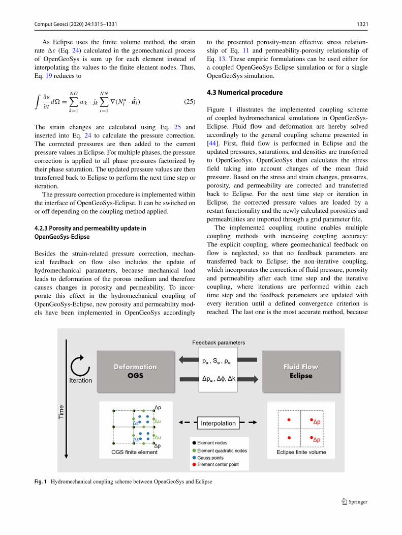
Figure 1 illustrates the implemented coupling schemeof coupled hydromechanical simulations in OpenGeoSys-Eclipse. Fluid flow and deformation are hereby solvedaccordingly to the general coupling scheme presented in[44]. First, fluid flow is performed in Eclipse and theupdated pressures, saturations, and densities are transferredto OpenGeoSys. OpenGeoSys then calculates the stressfield taking into account changes of the mean fluidpressure. Based on the stress and strain changes, pressures,porosity, and permeability are corrected and transferredback to Eclipse. For the next time step or iteration inEclipse, the corrected pressure values are loaded by arestart functionality and the newly calculated porosities andpermeabilities are imported through a grid parameter file.
The implemented coupling routine enables multiplecoupling methods with increasing coupling accuracy:The explicit coupling, where geomechanical feedback onflow is neglected, so that no feedback parameters aretransferred back to Eclipse; the non-iterative coupling,which incorporates the correction of fluid pressure, porosityand permeability after each time step and the iterativecoupling, where iterations are performed within eachtime step and the feedback parameters are updated withevery iteration until a defined convergence criterion isreached. The last one is the most accurate method, because
Fig. 1 Hydromechanical coupling scheme between OpenGeoSys and Eclipse
Comput Geosci (2020) 24:1315–1331 1321
compatibility of pore volume from flow and stress is assuredwithin each time step.
5Model verification
The hydromechanical coupling method implemented inOpenGeoSys-Eclipse is verified by several test cases in2D and 3D using the explicit and iterative couplingmethods (Table 1). All OpenGeoSys-Eclipse results arecompared with those of a pure OpenGeoSys simulation.As OpenGeoSys has been extensively tested before, thiscomparison satisfies the validation process [21, 29, 30].Both, single-phase and multiphase flow are tested to verifythe correct data transfer and averaging of the pressure andsaturation data. In addition to the method verification, thedifferent coupling methods are discussed with regard totheir impact on the simulation results. For an adequatecomparison, the same mesh dimensions and elements areused in both simulators for all test cases. As Eclipse canonly handle hexahedron element types, the 2D test casegrids consist of three-dimensional hexahedrons, but can betreated as quasi-2D models as they comprise only one cellin the third direction (Y-direction). The 3D model containsmultiple cells in all directions.
5.1 Pressure correction
5.1.1 Test case 1: Brine injection into a saline aquifer (2D)
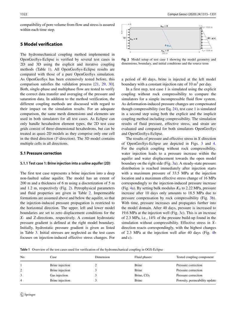
The first test case represents a brine injection into a deepnon-faulted saline aquifer. The model has an extent of200 m and a thickness of 6 m using a discretization of 5 mand 1.2 m, respectively (Fig. 2). Petrophysical parametersand fluid properties are given in Table 2. Impermeableformations are assumed above and below the aquifer, so thatthe injection-induced pressure propagation is restricted tothe horizontal direction. The upper, left and lower modelboundaries are set to zero displacement conditions for theX- and Z-directions, respectively. A constant hydrostaticpressure gradient is defined at the right model boundary.Initially, hydrostatic pressure gradient is given as listedin Table 3. Initial stresses are neglected as the test casesfocuses on injection-induced effective stress changes. For
Fig. 2 Model setup of test case 1 showing the model geometry anddimensions, boundary, and initial conditions and the source term
a period of 40 days, brine is injected at the left modelboundary with a constant injection rate of 10 m3 per day.
In a first step, test case 1 is simulated using the explicitcoupling without rock compressibility to compare thesimulators for a simple incompressible fluid flow system.As deformation-induced pressure changes are compensatedthough compressibility (see Eq. 24), test case 1 is simulatedin a second step using both the explicit and the implicitcoupling method including compressibility. The simulationresults of fluid pressure, effective stress, and strain areevaluated and compared for both simulators OpenGeoSysand OpenGeoSys-Eclipse.
The results of pressure and effective stress in X-directionof OpenGeoSys-Eclipse are depicted in Figs. 3 and 4.For the explicit coupling without rock compressibility,water injection leads to a pressure increase within theaquifer and water displacement towards the open modelboundary on the right side (Fig. 3a). A steady-state pressuredistribution is reached immediately after injection startswith a maximum pressure of 33.5 MPa at the injectionlocation and a maximum effective stress change of 16 MPacorrespondingly to the injection-induced pressure increase(Fig. 4a). By setting bulk modulus Kb to 2.22 MPa, pressureincrease after 10 days only amounts to 18.5 MPa due topressure compensation by rock compressibility (Fig. 3b).With time, pressure increases and propagates further intothe model domain. After 40 days, pressure is increased to19.6 MPa at the injection well (Fig. 3c). This is an increaseof 2.3 MPa, i.e., 14% of the pressure build-up found in thesimulation without compressibility. Effective stress in X-direction reacts correspondingly, with the highest changesof 2.3 MPa at the injection well after 40 days (Fig. 4band c).
Table 1 Overview of the test cases used for verification of the hydromechanical coupling in OGS-Eclipse
No. Case Dimension Fluid phases Tested coupling component
1 Brine injection 2 Brine Pressure correction
2 Brine injection 3 Brine Pressure correction
3 Gas injection 3 Brine, CO2 Pressure correction
4 Brine injection 3 Brine Porosity, permeability update
Comput Geosci (2020) 24:1315–13311322
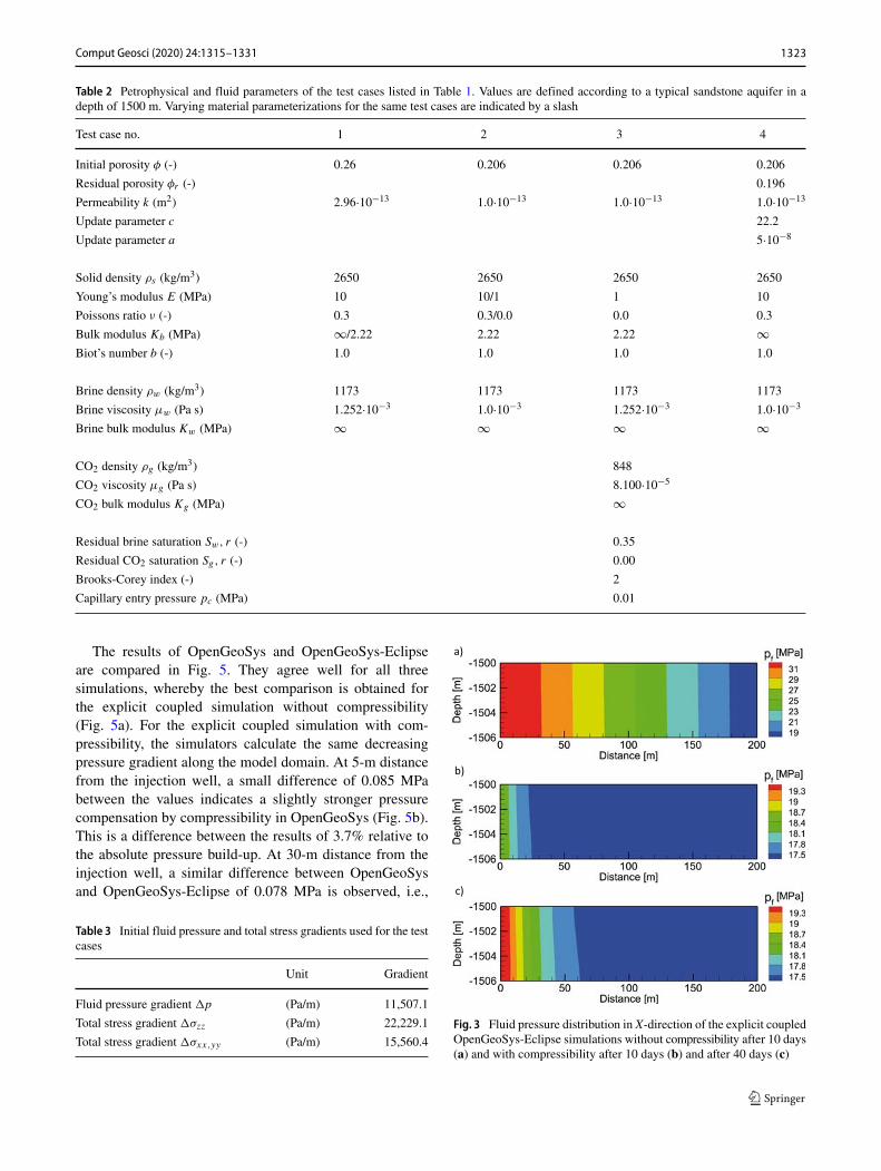
Table 2 Petrophysical and fluid parameters of the test cases listed in Table 1. Values are defined according to a typical sandstone aquifer in adepth of 1500 m. Varying material parameterizations for the same test cases are indicated by a slash
Test case no. 1 2 3 4
Initial porosity φ (-) 0.26 0.206 0.206 0.206
Residual porosity φr (-) 0.196
Permeability k (m2) 2.96·10−13 1.0·10−13 1.0·10−13 1.0·10−13
Update parameter c 22.2
Update parameter a 5·10−8
Solid density ρs (kg/m3) 2650 2650 2650 2650
Young’s modulus E (MPa) 10 10/1 1 10
Poissons ratio ν (-) 0.3 0.3/0.0 0.0 0.3
Bulk modulus Kb (MPa) ∞/2.22 2.22 2.22 ∞Biot’s number b (-) 1.0 1.0 1.0 1.0
Brine density ρw (kg/m3) 1173 1173 1173 1173
Brine viscosity μw (Pa s) 1.252·10−3 1.0·10−3 1.252·10−3 1.0·10−3
Brine bulk modulus Kw (MPa) ∞ ∞ ∞ ∞
CO2 density ρg (kg/m3) 848
CO2 viscosity μg (Pa s) 8.100·10−5
CO2 bulk modulus Kg (MPa) ∞
Residual brine saturation Sw, r (-) 0.35
Residual CO2 saturation Sg, r (-) 0.00
Brooks-Corey index (-) 2
Capillary entry pressure pc (MPa) 0.01
The results of OpenGeoSys and OpenGeoSys-Eclipseare compared in Fig. 5. They agree well for all threesimulations, whereby the best comparison is obtained forthe explicit coupled simulation without compressibility(Fig. 5a). For the explicit coupled simulation with com-pressibility, the simulators calculate the same decreasingpressure gradient along the model domain. At 5-m distancefrom the injection well, a small difference of 0.085 MPabetween the values indicates a slightly stronger pressurecompensation by compressibility in OpenGeoSys (Fig. 5b).This is a difference between the results of 3.7% relative tothe absolute pressure build-up. At 30-m distance from theinjection well, a similar difference between OpenGeoSysand OpenGeoSys-Eclipse of 0.078 MPa is observed, i.e.,
Table 3 Initial fluid pressure and total stress gradients used for the testcases
Unit Gradient
Fluid pressure gradient �p (Pa/m) 11,507.1
Total stress gradient �σzz (Pa/m) 22,229.1
Total stress gradient �σxx,yy (Pa/m) 15,560.4Fig. 3 Fluid pressure distribution in X-direction of the explicit coupledOpenGeoSys-Eclipse simulations without compressibility after 10 days(a) and with compressibility after 10 days (b) and after 40 days (c)
Comput Geosci (2020) 24:1315–1331 1323
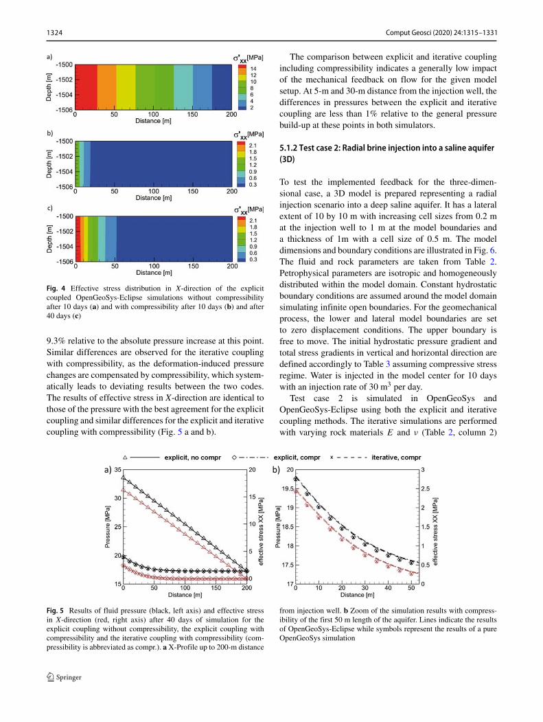
Fig. 4 Effective stress distribution in X-direction of the explicitcoupled OpenGeoSys-Eclipse simulations without compressibilityafter 10 days (a) and with compressibility after 10 days (b) and after40 days (c)
9.3% relative to the absolute pressure increase at this point.Similar differences are observed for the iterative couplingwith compressibility, as the deformation-induced pressurechanges are compensated by compressibility, which system-atically leads to deviating results between the two codes.The results of effective stress in X-direction are identical tothose of the pressure with the best agreement for the explicitcoupling and similar differences for the explicit and iterativecoupling with compressibility (Fig. 5 a and b).
Fig. 5 Results of fluid pressure (black, left axis) and effective stressin X-direction (red, right axis) after 40 days of simulation for theexplicit coupling without compressibility, the explicit coupling withcompressibility and the iterative coupling with compressibility (com-pressibility is abbreviated as compr.). aX-Profile up to 200-m distance
from injection well. b Zoom of the simulation results with compress-ibility of the first 50 m length of the aquifer. Lines indicate the resultsof OpenGeoSys-Eclipse while symbols represent the results of a pureOpenGeoSys simulation
The comparison between explicit and iterative couplingincluding compressibility indicates a generally low impactof the mechanical feedback on flow for the given modelsetup. At 5-m and 30-m distance from the injection well, thedifferences in pressures between the explicit and iterativecoupling are less than 1% relative to the general pressurebuild-up at these points in both simulators.
5.1.2 Test case 2: Radial brine injection into a saline aquifer(3D)
To test the implemented feedback for the three-dimen-sional case, a 3D model is prepared representing a radialinjection scenario into a deep saline aquifer. It has a lateralextent of 10 by 10 m with increasing cell sizes from 0.2 mat the injection well to 1 m at the model boundaries anda thickness of 1m with a cell size of 0.5 m. The modeldimensions and boundary conditions are illustrated in Fig. 6.The fluid and rock parameters are taken from Table 2.Petrophysical parameters are isotropic and homogeneouslydistributed within the model domain. Constant hydrostaticboundary conditions are assumed around the model domainsimulating infinite open boundaries. For the geomechanicalprocess, the lower and lateral model boundaries are setto zero displacement conditions. The upper boundary isfree to move. The initial hydrostatic pressure gradient andtotal stress gradients in vertical and horizontal direction aredefined accordingly to Table 3 assuming compressive stressregime. Water is injected in the model center for 10 dayswith an injection rate of 30 m3 per day.
Test case 2 is simulated in OpenGeoSys andOpenGeoSys-Eclipse using both the explicit and iterativecoupling methods. The iterative simulations are performedwith varying rock materials E and ν (Table 2, column 2)
Comput Geosci (2020) 24:1315–13311324
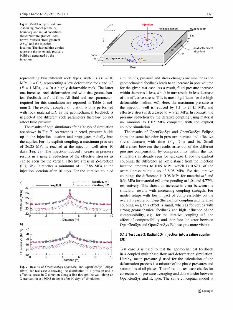
Fig. 6 Model setup of test case2 showing model geometry,boundary and initial conditions(blue: pressure gradient �p;brown: vertical stress gradient�σzz) and the injectionlocation. The dashed blue circlesrepresent the schematic pressurebuild-up generated by theinjection
representing two different rock types, with m1 (E = 10MPa, ν = 0.3) representing a low deformable rock and m2(E = 1 MPa, ν = 0) a highly deformable rock. The latterone increases rock deformation and with that geomechan-ical feedback to fluid flow. All fluid and rock parametersrequired for this simulation are reported in Table 2, col-umn 2. The explicit coupled simulation is only performedwith rock material m1, as the geomechanical feedback isneglected and different rock parameters therefore do notaffect fluid pressure.
The results of both simulators after 10 days of simulationare shown in Fig. 7. As water is injected, pressure buildsup at the injection location and propagates radially intothe aquifer. For the explicit coupling, a maximum pressureof 26.25 MPa is reached at the injection well after 10days (Fig. 7a). The injection-induced increase in pressureresults in a general reduction of the effective stresses ascan be seen for the vertical effective stress in Z-direction(Fig. 7b). It reaches a minimum of − 7.86 MPa at theinjection location after 10 days. For the iterative coupled
Fig. 7 Results of OpenGeoSys (symbols) and OpenGeoSys-Eclipse(lines) for test case 2 showing the distribution of a pressure and beffective stress in Z-direction along a line through the well along anX-transection at 1500.5-m depth after 10 days of simulation
simulations, pressure and stress changes are smaller as thegeomechanical feedback leads to an increase in pore volumefor the given test case. As a result, fluid pressure increasewithin the pores is less, which in turn results in less decreaseof the effective stress. This is most significant for the highdeformable medium m2. Here, the maximum pressure atthe injection well is reduced by 1.1 to 25.15 MPa andeffective stress is decreased to − 9.25 MPa. In contrast, thepressure reduction by the iterative coupling using materialm1 amounts to 0.07 MPa compared with the explicitcoupled simulation.
The results of OpenGeoSys and OpenGeoSys-Eclipseshow the same behavior in pressure increase and effectivestress decrease with time (Fig. 7 a and b). Smalldifferences between the results arise out of the differentpressure compensation by compressibility within the twosimulators as already seen for test case 1. For the explicitcoupling, the difference at 1-m distance from the injectionlocation amounts to 0.05 MPa, which is 0.62% of theoverall pressure build-up of 8.05 MPa. For the iterativecoupling, the difference is 0.08 MPa for material m1 and0.34 MPa for material m2 corresponding to 1.04 and 4.77%,respectively. This shows an increase in error between thesimulator results with increasing coupling strength. Formodel setups with low impact of compressibility on theoverall pressure build-up (the explicit coupling and iterativecoupling m1), this effect is small, whereas for setups withstrong geomechanical feedback and high influence of thecompressibility, e.g., for the iterative coupling m2, theeffect of compressibility and therefore the error betweenOpenGeoSys and OpenGeoSys-Eclipse gets more visible.
5.1.3 Test case 3: Radial CO2 injection into a saline aquifer(3D)
Test case 3 is used to test the geomechanical feedbackin a coupled multiphase flow and deformation simulation.Hereby, mean pressure p used for the calculation of thedeformation process is a mixture of the phase pressures andsaturations of all phases. Therefore, this test case checks forcorrectness of pressure averaging and data transfer betweenOpenGeoSys and Eclipse. The same conceptual model is
Comput Geosci (2020) 24:1315–1331 1325

used as in test case 2 (Fig. 6). The injected phase is a gasphase simulating CO2 injection into a saline aquifer. Phaseand material parameters are given in Table 2, column 3.All phase properties, i.e., densities and viscosities of brineand CO2, are assumed to be constant and dissolution isnot considered. These assumptions are not realistic for sitespecific applications but are made to be able to clearlydiscern the coupling effects between fluid pressure androck deformation, as these are within the focus of thismanuscript. Boundary and initial conditions for the fluidflow and deformation processes are adopted from Fig. 6 andTable 3. Initially, the aquifer is filled with water. CO2 isinjected with a rate of 1.3 m3 per day for 10 days. The modelis simulated with OpenGeoSys and OpenGeoSys-Eclipseusing again the explicit and iterative coupling methods. Toincrease deformation and therefore geomechanical feedbackon fluid flow, a high deformable rock is assumed.
As CO2 is injected, it spreads radially into the aquifer andleads to a concentric pressure increase around the injectionlocation (Fig. 8 a and b). Due to the increase in pressure,effective stress in Z-direction is concurrently reduced with
Fig. 8 Comparison of the simulation results of OpenGeoSys (symbols)and OpenGeoSys-Eclipse (lines) for test case 3. a Pressure, b gassaturation, and c effective stress in Z-direction along a line throughthe well along the X-direction at 1500.5-m depth after 10 days ofinjection. The result of the gas saturation of the iterative coupling casein OpenGeoSys-Eclipse is additionally marked by red crosses as thereis only a small, invisible difference to the explicit coupling case
a maximum decrease at the injection location (Fig. 8c).Towards the outer model boundaries, pressure build-uptends towards zero due to the open boundary conditions andso effective stress changes are zero. After 10 days, the CO2
saturation at the injection well reaches a maximum of 0.42in OpenGeoSys-Eclipse and 0.51 in OpenGeoSys.
Comparing the iterative and explicit coupling methods,pressure build-up and stress reduction is slightly reduceddue to the pore volume coupling. This effect is strongestat the injection well and decreases towards the far fieldcorrespondingly to the magnitude of pressure and stresschanges. In OpenGeoSys, the difference between iterativeand explicit coupling is 0.8 MPa at the injection well andless than 0.1 MPa in the far field of the aquifer. Becausechanges in pressures are small between iterative and explicitcoupling, no visible differences in the CO2 saturationdistribution can be observed. A stronger change in pressurewould consequently impact on the saturation distribution ascapillary pressure is affected by these changes.
Comparing OpenGeoSys and OpenGeoSys-Eclipse, asimilar pressure build-up and stress reduction is observedfor the explicit coupling (Fig. 8a, c). Small differencesbetween the results occur due to a steeper pressureand saturation gradient in OpenGeoSys indicating lessnumerical dispersion compared with OpenGeoSys-Eclipse.This results in a higher maximum CO2 saturation at theinjection well in OpenGeoSys. Regarding the iterativecoupling, the effect of geomechanical feedback on flow isstronger in OpenGeoSys as pressure increase is less than inOpenGeoSys-Eclipse (Fig. 8a) demonstrating the strongerimpact of compressibility in OpenGeoSys. At 1-m distancefrom the injection well, the difference in pressure betweenboth simulators is 0.01 MPa for the explicit couplingcorresponding to 3.18% of the absolute pressure build-up,and for the iterative coupling, the difference amounts to0.048 MPa, which is 11.72%. Also, the decrease in effectivestress changes causes by the iterative coupling is less forthe OpenGeoSys simulation (Fig. 8c) according to higherpressure compensation.
However, although the impact of the geomechanicalfeedback is generally lower in OpenGeoSys-Eclipse dueto the different compressibility models, both simulatorscalculate the same dampening effects by the iterative porevolume coupling.
5.2 Porosity and permeability update
The implementation of stress-dependent porosity and per-meability changes within OpenGeoSys-Eclipse is verifiedin test case 4 using the model setup depicted in Fig. 6.Porosity and permeability values are given in Table 2 (col-umn 4), parameters for permeability and porosity update inEqs. 11 and 13 are taken from the study of [51] representing
Comput Geosci (2020) 24:1315–13311326
properties of a typical sandstone. The test case is performedin both simulators with and without porosity and permeabil-ity update, respectively. The implemented update equationswill be verified as well as the data transfer of porosity andpermeability between OpenGeoSys and Eclipse. Compress-ibility is neglected for all simulations to avoid overlappingof the hydromechanical coupling effects.
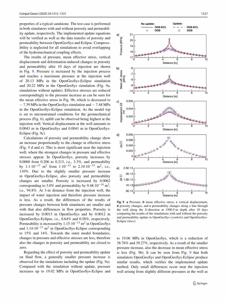
The results of pressure, mean effective stress, verticaldisplacement and deformation-induced changes in porosityand permeability after 10 days of injection are shownin Fig. 9. Pressure is increased by the injection processand reaches a maximum pressure at the injection wellof 20.13 MPa in the OpenGeoSys-Eclipse simulationand 20.22 MPa in the OpenGeoSys simulation (Fig. 9a,simulations without update). Effective stresses are reducedcorrespondingly to the pressure increase as can be seen forthe mean effective stress in Fig. 9b, which is decreased to− 7.39 MPa in the OpenGeoSys simulation and− 7.48 MPain the OpenGeoSys-Eclipse simulation. As the model topis set to unconstrained conditions for the geomechanicalprocess (Fig. 6), uplift can be observed being highest at theinjection well. Vertical displacement at the well amounts to0.0043 m in OpenGeoSys and 0.0041 m in OpenGeoSys-Eclipse (Fig. 9c).
Calculations of porosity and permeability change showan increase proportionally to the change in effective stress(Fig. 9 d and e). This is most significant near the injectionwell, where the strongest changes in pressure and effectivestresses appear. In OpenGeoSys, porosity increases by0.0068 from 0.206 to 0.213, i.e., 3.3%, and permeabilityby 1.1·10−13 m2 from 1·10−13 to 2.10·10−13 m2, i.e.,110%. Due to the slightly smaller pressure increasein OpenGeoSys-Eclipse, also porosity and permeabilitychanges are smaller. Porosity is increased by 0.0062corresponding to 3.0% and permeability by 9.48·10−14 m2,i.e., 94.8%. At 3-m distance from the injection well, theimpact of water injection and therefore pressure increaseis less. As a result, the differences of the results ofpressure changes between both simulators are smaller andwith that also differences in flow properties. Porosity isincreased by 0.0013 in OpenGeoSys and by 0.0012 inOpenGeoSys-Eclipse, i.e., 0.64% and 0.58%, respectively.Permeability is increased by 1.15·10−13 m2 in OpenGeoSysand 1.14·10−13 m2 in OpenGeoSys-Eclipse correspondingto 15% and 14%. Towards the outer model boundaries,changes in pressure and effective stresses are less, thereforealso the changes in porosity and permeability are closed tozero.
Regarding the effect of porosity and permeability updateon fluid flow, a generally smaller pressure increase isobserved for the simulations including the update (Fig. 9a).Compared with the simulation without update, pressureincreases up to 19.02 MPa in OpenGeoSys-Eclipse and
Fig. 9 a Pressure, b mean effective stress, c vertical displacement,d porosity changes, and e permeability changes along a line throughthe well along the X-direction at 1500.5-m depth after 10 dayscomparing the results of the simulations with and without the porosityand permeability update in OpenGeoSys (symbols) and OpenGeoSys-Eclipse (lines)
to 19.06 MPa in OpenGeoSys, which is a reduction of38.76% and 39.27%, respectively. As a result of the smallerpressure increase, also the decrease in mean effective stressis less (Fig. 9b). It can be seen from Fig. 9 that bothsimulators OpenGeoSys and OpenGeoSys-Eclipse producesimilar results, which verifies the implemented updatemethod. Only small differences occur near the injectionwell arising from slightly different pressures at the well as
Comput Geosci (2020) 24:1315–1331 1327
well as the interpolation method and data transfer betweenOpenGeoSys and Eclipse, as already detected for differenttest cases by [44].
5.3 Computation speed
As mentioned above, OpenGeoSys is coupled to Eclipseto benefit from its fast and efficient computation timeof flow processes. To evaluate the time savings by thiscoupling, simulation times of the presented test casesare compared in Table 4. For small simple single-phasemodels (case 1), no simulation speed-up is archivedby the OpenGeoSys-Eclipse simulator. The data transferthrough the Eclipse interface is time consuming comparedwith a single OpenGeoSys simulation without any datatransfer. Increasing the dimensions and phases in the model,OpenGeoSys-Eclipse shows significant faster run times.Test case 2 is speed up by a factor of about 1.5 andtest case 3 by a factor of 5.6 for the iterative coupling.Regarding potential large-scale and long-term scenariosimulations of gas storage, this time speed-up archived bythe OpenGeoSys-Eclipse coupling will significantly reducesimulation times.
6 Discussion and conclusion
Numerical simulation codes are a useful tool to assessthe complex process system related to subsurface opera-tions such as gas storage. The simulation and prediction ofgeomechanical processes is of particular importance for theoperation safety as pressure disturbances associated withthe injection or extraction of mass can significantly changethe subsurface stress regime and causes rock deformation.Adequate simulation tools are required capable of takinginto account each individual process as well as the processcoupling to investigate the impact of process feedback tothe system. Therefore, the coupled simulator OpenGeoSys-Eclipse, developed to simulate coupled thermal, hydraulic,geomechanical and geochemical processes in the subsur-face, has been extended for the hydromechanical processcoupling, whereby Eclipse solves for fluid flow and Open-GeoSys for deformation. The newly developed processfeedback incorporates two feedback components: The porevolume coupling, which is translated into a pressure correc-tion term in Eclipse and the stress-dependent porosity andpermeability update based on changes of the mean effec-tive stress. Two different coupling methods, the explicit andthe iterative coupling method, are implemented to simu-late the feedback. The feedback component as well as thetype of process coupling can be chosen for the individ-ual OpenGeoSys-Eclipse simulation demonstrating the veryflexible and effective handling of this simulator.
The hydromechanical coupling in OpenGeoSys-Eclipseis verified using several test cases in 2D and 3D withincreasing complexity. This is important as the transferparameters between OpenGeoSys and Eclipse vary with thenumber of fluid phases in the model, the feedback com-ponents and the model dimensions. Differences betweenthe simulation results arise for the volume coupling, whichare mainly caused by different handling of compressibil-ity in the individual simulators. Thus, pressure build-upby injection is compensated differently leading to varyingpressure signals in the simulation results, whereby Eclipseshows a generally lower pressure compensation by com-pressibility than OpenGeoSys for all test cases. As theimpact of compressibility depends on the model setup, dif-ferences between OpenGeoSys and OpenGeoSys-Eclipsevary between 1 and 10% relative to the overall pressurebuild-up for the given test cases. The difference betweenthe simulation results caused by compressibility systemat-ically increases with increasing impact of geomechanicalfeedback on flow as seen, e.g., for test case 2. However, thegeomechanical coupling causes the same dampening effecton the pressure build-up in both simulators.
Besides the verification of coupled hydromechanicalsimulations in OpenGeoSys-Eclipse, the test cases are usedto evaluate the differences between explicit and iterativecoupling and their impact on the simulation results. By this,the advantages and disadvantages of each method can beevaluated, especially with regard to simulation accuracy andefficiency.
The simulations including pore volume coupling (testcases 1 to 3) show generally less differences betweenthe explicit and the iterative coupling for the givenmodel setups. This is due to the fact, that the modelparameterizations are related to a deep underground gasstorage featuring low compressibility and a less deformablerock. The induced changes in effective stresses and strainsare small and with that also the geomechanical feedback onflow. By increasing the deformability of the rock (e.g., testcase 2, material m2), a stronger geomechanical feedbackto the flow is observed leading to a significantly smallerpressure build-up. Similar results are found when increasingthe compressibility of the porous medium (not shown here).The parameter sets used in the test cases were chosen toenable a clear model verification and comparison betweenthe different coupling approaches. Both the use of anincompressible CO2 phase and the use of independentvalues for bulk modulus, Youngs modulus, and Poissonratio, which are related to each other through E = 3K(1 −2ν) [15], would not be valid for a site-specific study.In test case 2 and for material 2, this would lead to ahigher compressibility and thus a somewhat lower pressureincrease, while for the other results shown here changeswould be small.
Comput Geosci (2020) 24:1315–13311328

Table 4 Comparison of the computation time for the test cases 1, 2, and 3. Times are given in hours. Ex., explicit coupling; It., iterative coupling.The simulation times are compared for a single core performance
Computation times [hours] Case 1 Case 2 Case 3
Ex. It. Ex. m1 It. m1 Ex. m2 It. m2 Ex. It.
OGS 0.032 0.098 0.053 0.316 0.041 0.656 1.413 31.406
OGS-Eclipse 0.036 0.142 0.037 0.217 0.037 0.432 1.128 5.577
It can be seen, that the impact of deformation on flowis strongly controlled by the individual reservoir rock andreservoir conditions. Therefore, iterative coupling should bepreferred for high compressible and high deformable mediato archive adequate accuracy in the simulation results. Forlow compressible and low deformable systems, the explicitcoupling produces sufficient results within a faster run time.For test case 2 with material m1, the simulation time is0.05 h for the explicit coupling and 0.32 h for the iterativecoupling, although the difference between the simulationresults is less than 0.1 MPa. However, it is probable that theaccuracy of the explicit coupling may decrease for biggertime step sizes as the change in pore volume per time stepincreases as shown by [60].
In contrast to the simulation with pore volume coupling,the porosity and permeability update has a stronger effecton the pressure build-up using the same model setup andparameterization (test case 4). An increase of permeabilityby maximum factor of about 2 is observed within the modelarea as the injection-induced changes in effective stressescause an elastic expansion of the rock. This leads to aless pressure increase compared with the simulation withoutupdate. Similar changes in permeability of a factor of 1.3to 1.7 were already obtained by [51] using the TOUGH-FLAC3D simulator.
In general, geomechanical feedback should be consid-ered when assessing subsurface operations. Depending onthe given storage site conditions and rock types, the feed-back of deformation on the pressure can be significant. Thisis an important fact regarding the risk analysis of under-ground storage processes, e.g., the potential of ground upliftand hydraulic fracturing. The presented test cases show, thatthe feedback has an overall positive effect to the storageoperation. For both coupling components, the pore volumeand the stress-dependent porosity and permeability, pressurebuild-up in the reservoir tends to be smaller. This wouldallow for a higher injection flow rate without risking anincrease of the injection pressure and with that hydraulicfracturing. Rutqvist et al. [51], for example, presented areduction of 3 MPa in pressure in the long term of a realisticstorage scenario, when considering geomechanical feed-back. The reduction of the pressure build-up will positivelyact on geomechanical processes as changes of the stress
field are reduced and therefore also deformation and verti-cal uplift (e.g., Fig. 9 b and c). To investigate these effectson a larger scale, more realistic storage scenario simulationsare needed. For this purpose, the OpenGeoSys-Eclipse sim-ulator offers an appropriate tool, as it provides flexibilityregarding the process coupling and a fast run time speed,especially for multiphase flow simulations.
Acknowledgments Open Access funding provided by Projekt DEAL.
Funding information The presented work is part of the ANGUS+and CO2-MoPa research projects. This projects received fundingfrom the Federal Ministry of Education and Research (BMBF) underGrant number 03EK3022 through the energy storage funding initiative”Energiespeicher” of the German Federal Government as well asEnBW Energie Baden-Wuerttemberg AG, E.ON Energie AG, E.ONGas Storage AG, RWE Dea AG, Vattenfall Europe TechnologyResearch GmbH, Wintershall Holding AG, and Stadtwerke Kiel AGfor being part of the Special Program GEOTECHNOLOGIEN.
Open Access This article is licensed under a Creative CommonsAttribution 4.0 International License, which permits use, sharing,adaptation, distribution and reproduction in any medium or format, aslong as you give appropriate credit to the original author(s) and thesource, provide a link to the Creative Commons licence, and indicateif changes were made. The images or other third party material inthis article are included in the article’s Creative Commons licence,unless indicated otherwise in a credit line to the material. If materialis not included in the article’s Creative Commons licence and yourintended use is not permitted by statutory regulation or exceedsthe permitted use, you will need to obtain permission directly fromthe copyright holder. To view a copy of this licence, visit http://creativecommonshorg/licenses/by/4.0/.
References
1. Afanasyev, A., Kempka, T., Kuehn, M., Melnik, O.: Validation ofthe mufits reservoir simulator against co2 storage benchmarks andhistory-matched models of the ketzin pilot site. Energy Procedia97, 395–402 (2016)
2. Bauer, S., Beyer, C., Dethlefsen, F., Dietrich, P., Duttmann, R.,Ebert, M., Feeser, V., Goerke, U., Koeber, R., Kolditz, O., Rabbel,W., Schanz, T., Schaefer, D., Wuerdemann, H., Dahmke, A.:Impacts of the use of the geological subsurface for energy storage:an investigation concept. Environ Earth Sci 70(8), 3935–3943(2013)
3. Benisch, K., Graupner, B., Bauer, S.: The coupled opengeosys-eclipse simulator for simulation of co2 storage - code comparisonfor fluid flow and geomechanical processes. Energy Procedia 37,3663–3671 (2013)
Comput Geosci (2020) 24:1315–1331 1329
4. Beyer, C., Li, D., Lucia, M.D., Kuehn, M., Bauer, S.: Modellingco2-induced fluid-rock interactions in the altensalzwedel gasreservoir. part ii: coupled reactive transport simulation. EnvironEarth Sci 67(2), 573–588 (2012)
5. Biot, M.A.: General theory of three-dimensional consolidation. J.Appl. Phys. 12, 155–164 (1941)
6. Biot, M.A., Willis, P.G.: The elastic coefficients of the theory ofconsolidation. J. Appl. Mech. 24, 594–601 (1957)
7. Birkholzer, J., Zhou, Q., Tsang, C.-F.: Large-scale impact of co2storage in deep saline aquifers: a sensitivity study on pressureresponse in stratified systems. Int. J. Greenh. Gas Control 3(2),181–194 (2009)
8. Bissel, R.C., Vasco, D.W., Atbi, M., Hamdani, M., Okwelegbe,M., Goldwater, M.H.: A full field simulation of the in salahgas production and co2 storage project using a coupled geo-mechanical and thermal fluid flow simulator. Energy Procedia 4,3290–3297 (2011)
9. Boettcher, N., Taron, J., Kolditz, O., Park, C.-H., Liedl, R.:Evaluation of thermal equations of state for co2 in numericalsimulations. Environ. Earth Sci. 67, 481–495 (2012)
10. Bower, K.M., Zyvoloski, G.: A numerical model for thermo-hydro-mechanical coupling in fractured rock. Int. J. Rock Mech.Min. Sci. 34(8), 1201–1211 (1997)
11. Class, H., Ebigbo, A., Helmig, R., Dahle, H.K., Nordbotten, J.M.,Celia, M., Audigane, P., Darcis, M., Ennis-King, J., Fan, Y.,Flemisch, B., Gasda, S.E., Jin, M., Krug, S., Labregere, D., Beni,A.N., Pawar, R.J., Sbai, A., Thomas, S.G., Trenty, L., Wei, L.: Abenchmark study on problems related to co2 storage in geologicformations. Comput. Geosci. 13(4), 409–434 (2009)
12. De Lucia, M., Bauer, S., Beyer, C., Kuehn, M., Nowak, T., Pudlo,D., Reitenbach, V., Stadler, S.: Modelling co2-induced fluid-rock interactions in the altensalzwedel gas reservoir. part i: fromexperimental data to a reference geochemical model. Environ.Earth Sci. 67(2), 563–572 (2012)
13. Edenhofer, O., Pichs-Madruga, R., Sokona, Y., Farahani, E.,Kadner, S., Seyboth, K., Adler, A., Baum, I., Brunner, S.,Eickemeier, P., Kriemann, B., Savolainen, J., Schloemer, S., vonStechow, C., Zwickel, T., Minx, J.C. (eds.): Climate change 2014Mitigation of climate change. contribution of working group iiito the fifth assessment report of the intergovernmental panel onclimate change. Technical report, International Panel on ClimateChange. Cambridge, United Kingdom (2014)
14. European Commission. Eu energy in figures, statistical pock-etbook 2015. Technical report, Public Office European Union(2015)
15. Fjar, E., Holt, R.M., Raaen, A., Horsrud, P.: Petroleum related rockmechanics, 2 edn. Elsevier Science (2008)
16. Flemisch, B., Darcis, M., Erbertseder, K., Faigle, B., Lauser, A.,Mosthaf, K., Muething, S., Nuske, A., Tatomir, A., Wolff, M.,Helmig, R.: Dumux Dune for multi-(phase, component, scale,physics, ...) flow and transport in porous media. Adv. WaterResour. 34(9), 1102–1112 (2011)
17. Garitte, B., Nguyen, S., Barnichon, J.-D., Graupner, B., Lee, C.,Maekawa, K., Manepally, C., Ofoegbu, G., Dasgupta, B., Fedors,R.Z., Pan, P.T., Feng, X., Rutqvist, J., Chen, F., Birkholzer, J.,Wang, Q., Kolditz, O., Shao, H.: Modelling the mont terri he-d experiment for the thermal-hydraulic-mechanical response ofa bedded argillaceous formation to heating. Environ. Earth Sci.76:345– (2017)
18. Goerke, U.-J., Park, C.-H., Wang, W., Singh, A.K., Kolditz, O.:Numerical simulation of multiphase hydromechanical processesinduced by injection into deep saline aquifers. Oil Gas Sci.Technol. Rev. IFP 66, 105–118 (2011)
19. Graupner, B., Li, D., Bauer, S.: The coupled simulator ECLIPSE-OpenGeoSys for the simulation of co2 storage in salineformations. Energy Procedia 4, 3794–3800 (2011)
20. Gray, W., Hassanizadeh, S.M.: Macroscale continuum mechanicsfor multiphase porous-media flow including phases, interfaces,common lines and common points. Adv. Water Resour. 21, 261–281 (1998)
21. Hou, Z., Goerke, U.-J., Gou, Y., Kolditz, O.: Thermo-hydro-mechanical modeling of carbon dioxide injection for enhancedgas-recovery (co2-egr): a benchmarking study for code compari-son. Environ. Earth Sci. 67, 549–561 (2012)
22. Huggins, R.: Energy storage. Springer, U.S. (2010)23. International Energy Agency IEA. Technology Roadmap: Carbon
Capture and Storage. Technical report, OECD/IEA (2009)24. International Energy Agency IEA. Technology Roadmap: Energy
Storage. Technical report, OECD/IEA (2009)25. International Energy Agency IEA. World energy outlook 2015.
Technical report, OECD/IEA (2015)26. Kempka, T., Kuehn, M., Class, H., Frykmann, P., Kopp, A.,
Nielsen, C.M., Probst, P.: Modelling of co2 arrival time at ketzin-part i. Int. J. Greenh. Gas Control 4, 1007–1015 (2010)
27. Kolditz, O., Bauer, S.: A process-oriented approach to computingmulti-field problems in porous media. J. Hydroinform. 6, 225–244(2004)
28. Kolditz, O., Bauer, S., Bilke, L., Boettcher, N., Delfs, J.O.,Fischer, T., Zehner, B.: Opengeosys: an open-source initiativefor numerical simulation of thermo-hydro-mechanical/chemical(thm/c) processes in porous media. Environ. Earth Sci. 67(2),589–599 (2012a)
29. Kolditz, O., Bauer, S., Boettcher, N., Elsworth, D., Goerke, U.-J., McDermott, C.-I., Park, C.-H., Singh, A.K., Taron, J., Wang,W.: Numerical simulation of two-phase flow in deformable porousmedia: application to carbon dioxide storage in the subsurface.Math. Comput. Simul. 82, 1919–1935 (2012b)
30. Kolditz, O., Goerke, U.-J., Shao, H., Wang, W., Bauer,S.: Thermo-hydro-mechanical-chemical Processes in FracturesPorous Media: Modelling and Benchmarking, Benchmarking Ini-tiatives. Springer International Publishing, Heidelberg (2016)
31. Korsawe, J., Starke, G., Wang, W., Kolditz, O.: Finite elementanalysis of poro-elastic consolidation in porous media Standardand mixed approaches. Comput. Methods Appl. Mech. Eng. 195,1096–1115 (2006)
32. Lewis, R.W., Schrefler, B.A.: The finite element method in thestatic and dynamic deformation and consolidation of porousmedia. Wiley. Chichester (2000)
33. Li, D., Bauer, S., Benisch, K., Graupner, B., Beyer, C.:Opengeosys-chemapp a coupled simulator for reactive transportin multiphase systems - code development and application at arepresentative co2 storage formation in northern germany. ActaGeotech. 9(1), 67–79 (2014)
34. Lund, P.D., Lindgren, J., Mikkola, J., Salpakari, J.: Reviewof energy system flexibility measures to enable high levels ofvariable renewable electricity. Renew Sustain Energy Rev. 45,785–807 (2015)
35. Martinez, M.J., Newell, P., Bishop, J.E., Turner, D.Z.: Coupledmultiphase flow and geomechanics model for analysis of jointreactivation during co2 sequestration operation. Int. J. Greenh. GasControl 17, 148–160 (2013)
36. Mathieson, A., Midgley, J., Dodds, K., Wright, I., Ringrose,P., Saoul, N.: Co2 sequestration monitoring and verificationtechnologies applied in krechba, algeria. Lead Edge 29, 216–222(2010)
37. Mitiku, A.B., Li, D., Bauer, S., Beyer, C.: Geochemical modellingof co2 interaction with water and rock formation and assessment ofits impact referring to northern Germany sedimentary basin. Appl.Geochem. 36, 168–186 (2013)
38. Morris, J., Hao, Y., Foxall, W., McNab, W.: In salah co2 storagejip: Hydromechanical simulations of surface uplift due to co2injection at in salah. Energy Procedia 4, 3269–3275 (2011)
Comput Geosci (2020) 24:1315–13311330
39. Nagel, T., Shao, H., Rosskopf, C., Linder, M., Woerner, A.,Kolditz, O.: The influence of gas-solid reaction kinetics in modelsof thermochemical heat storage under monotonic and cyclicloading. Appl. Energy 136, 289–302 (2014)
40. Olivella, S., Gens, A., Carrera, J., Alonso, E.E.: Numericalformulation for a simulator (code-bright) for the coupled analysisof saline media. Eng. Comput. 13(7), 87–112 (1996)
41. Onaisi, A., Samier, P., Koutsabeloulis, N.C., Longuemare, P.:Management of Stress Sensitive Reservoirs Using Two CoupledStress-Reservoir Simulation Tools: Ecl2vis and Ath2vis. 2002.SPE-78512-MS, Presented at the Abu Dhabi Intl. PetroleumExhibition and Conference In October 2002, Abu Dhabi
42. Ouellet, A., Berard, T., Desroches, J., Frykman, P., Welsh, P.,Minton, J., Pamukcu, Y., Hurter, S., Schmidt-Hattenberger, C.:Reservoir geomechanics for assessing containment in co2 storage:a case study at ketzin, germany. Energy Procedia 4, 3298–3305(2011)
43. Pfeiffer, W.T., Beyer, C., Bauer, S.: Hydrogen storage in aheterogeneous sandstone formation: dimensioning and inducedhydraulic effects. Petro Geosci. 23(3), 315–236 (2017)
44. Pfeiffer, W.T., Graupner, B., Bauer, S.: The coupled non-isothermal, multiphase-multicomponent flow and reactive trans-port simulator opengeosys-eclipse for porous media gas storage.Environ. Earth Sci. 75(20), 1347– (2016)
45. Preisig, M., Prevost, J.H.: Coupled multi-phase thermo-poromechanical effects case study: Co2 injection at in salah,algeria. Int. J. Greenh. Gas Control 5, 1055–1064 (2011)
46. Prevost, J.H.: DYNAFLOW: A Non-linear transient finite elementanalysis program. Department of Civil and EnvironmentalEngineering. Princeton University, Princeton (1981)
47. Reveillere, A., Rohmer, J., Manceau, J.C.: Hydraulic barrierdesign and applicability for managing the risk of co2 leakage fromdeep saline aquifers. Int. J. Greenh. Gas Control 9, 62–71 (2012)
48. Rohmer, J., Seyedi, D.M.: Coupled large scale hydromechanicalmodelling for caprock failure risk assessment of co2 storage indeep saline aquifers. Oil Gas Sci. Techn. - Rev. IFP 65(3), 503–517(2010)
49. Rutqvist, J.: Status of the tough-flac simulator and recent appli-cations related to coupled fluid flow and crustal deformations.Comput. Geosci. 37(6), 739–750 (2011)
50. Rutqvist, J.: The geomechanics of co2 storage in deep sedimentaryformations. Geotech. Geol. Eng. 30(3), 525–551 (2012)
51. Rutqvist, J., Tsang, C.-F.: A study of caprock hydromechanicalchanges associated with co2-injection into a brine formation.Environ. Geol. 42, 296–305 (2002)
52. Rutqvist, J., Wu, Y.S., Tsang, C.-F., Bodvarsson, G.: A modelingapproach for analysis of coupled multiphase fluid flow, heattransfer, and deformation in fractured porous rock. Int. J. RockMech. Min. Sci. 39(4), 429–442 (2002)
53. Sainz-Garcia, A., Abarca, E., Rubi, V., Grandia, F.: Assessment offeasible strategies for seasonal underground hydrogen storage insaline aquifers. Int. J. Hydro. Ener. 42, 16657–16666 (2017)
54. Schaefer, F., Walter, L., Class, H., Mueller, C.: The regionalpressure impact of co2 storage: a showcase study from the northgerman basin. Environ. Earth Sci. 65(7), 2037–2049 (2012)
55. Schlumberger, L.: Eclipse 100 technical description and usermanual. Technical Report (2015)
56. Settari, A., Maurits, F.: Coupled reservoir and geomechanicalsimulation system. SPE J. 3, 219–226 (1998)
57. Settari, A., Walters, S.A.: Advances in Coupled Geomechan-ical and Reservoir Modeling with Applications to Reservoir
Compaction. SPE-51927-MS, Presented at The 1999 SPE Reser-voir Simulation Symposium in February 1999, Houston (1999)
58. Shao, H., Kosakowski, G., Berner, U., Kulik, D., Maeder, U.,Kolditz, O.: Reactive transport modeling of clogging processat maqarin natural analogue site. Phys. Chem. Earth 64, 21–31(2013)
59. Steefel, C.I., Appelo, C.A.J., Arora, B., Jacques, D., Kolditz,O., Kalbacher, T., Lagneau, V., Lichtner, P.C., Mayer, K.U.,Meeussen, J.C.L., Molins, S., Moulton, D., Shao, H., Simunek, J.,Spycher, N., Yabusaki, S.B., Yeh, G.T.: Reactive transport codesfor subsurface environmental simulation. Comput. Geosc. 19(3),445–478 (2015)
60. Taron, J., Elsworth, D., Min, K.-B.: Numerical simula-tion of thermal-hydrologic-mechanical-chemical processes indeformable, fractured porous media. Int. J. Rock Mech. Min. Sci.46, 842–854 (2009)
61. Terzaghi, K.: Die berechnung der durchlaessigkeitsziffer des tonesaus dem verlauf der hydrodynamischen spannungserscheinungen.Technical report, Sitz. Akad. Wissen. Wien, Math. Naturwiss. Kl.,Abt. IIa 132 (1923)
62. Tran, D., Nghiem, L., Buchanan, L.: Improved Iterative Couplingof Geomechanics with Reservoir Simulation. SPE-93244-MS,Presented at the 1SPE Reservoir Simulation Symposium Feburary2005. The Woodlands (2005)
63. Tran, D., Settari, A., Nghiem, L.: New iterative coupling betweena reservoir simulator and a geomechanics module. Soc Petro Eng.SPE 88989 (2004)
64. U.S. Energy Department. Ensuring safe and reliable undergroundnatural gas storage, Final Report of the Interagency Task Forceon Natural Gas Storage Safety. Technical report, Washington(2016)
65. Vilarrasa, V., Bolster, D., Olivella, S., Carrera, J.: Coupledhydromechanical modeling of co2 sequestration in deep salineaquifers. Int. J. Greenh. Gas Control 4, 910–919 (2010)
66. Wang, B., Bauer, S.: Converting heterogeneous complex geolog-ical models to consistent finite element models: methods, devel-opment, and application to deep geothermal reservoir operation.Environ. Earth Sci. 75(20), 1349 (2016)
67. Wang, B., Bauer, S.: Compressed air energy storage in porousformations: a feasibility and deliverability study. Petro Geosc.23(3), 306–314 (2017)
68. Wang, W., Kolditz, O.: Object-oriented finite element analysis ofthermo-hydro-mechanical (thm) problems in porous media. Int. J.Numer. Methods Eng. 69(1), 162–201 (2007)
69. Wang, W., Rutqvist, J., Goerke, U.-J., Birkholzer, J., Kolditz,O.: Non-isothermal flow in low permeable porous media: acomparison of richards’s and two-phase flow approaches. Environ.Earth Sci. 62, 1197–1207 (2011)
70. Watanabe, N.: Finite element method for coupled thermos-hydro-mechanical processes in discretely fractured and non-fracturedporous media. Phd Thesis, Technische Universitaet Dresden(2011)
71. Zillman, D.N., McHarg, A., Bradbrook, A., Barrera-Hernandez,L.: The law of energy underground. Understanding new develop-ments in subsurface production, transmission, and storage. OxfordUniversity Press, Oxford (2014)
72. Zoback, M.D.: Reservoir Geomechanics. Cambridge UniversityPress, Cambridge (2010)
Publisher’s note Springer Nature remains neutral with regard tojurisdictional claims in published maps and institutional affiliations.
Comput Geosci (2020) 24:1315–1331 1331