arX

iv:0

907.

1653

v1 [

astr

o-ph

.EP

] 9

Jul 2

009

Astronomy & Astrophysicsmanuscript no. 12102 c© ESO 2009July 9, 2009

The secondary eclipse of CoRoT-1b ⋆

Alonso, R.1,2, Alapini, A.3, Aigrain, S.3, Auvergne, M.4, Baglin, A.4, Barbieri, M.1, Barge, P.1, Bonomo, A.S.1, Borde,P.5, Bouchy, F.6, Chaintreuil, S.4, De la Reza, R.7, Deeg, H.J.8, Deleuil, M.1, Dvorak, R.9, Erikson, A.10, Fridlund,M.11, Fialho, F.4, Gondoin, P.11, Guillot, T.12, Hatzes, A.13, Jorda, L.1, Lammer, H.14, Leger, A.5, Llebaria, A.1,

Magain, P.15, Mazeh, T.16, Moutou, C.1, Ollivier, M.5, Patzold, M.17, Pont, F.3, Queloz, D.2, Rauer, H.9,18, Rouan, D.3,Schneider, J.19, and Wuchterl, G.12

(Affiliations can be found after the references)

Received 18 March 2009/ Accepted 7 July 2009

ABSTRACT

The transiting planet CoRoT-1b is thought to belong to thepM-class of planets, in which the thermal emission dominates in the optical wavelengths.We present a detection of its secondary eclipse in the CoRoT white channel data, whose response function goes from∼400 to∼1000 nm. We usedtwo different filtering approaches, and several methods to evaluatethe significance of a detection of the secondary eclipse. We detect a secondaryeclipse centered within 20 min at the expected times for a circular orbit, with a depth of 0.016±0.006%. The center of the eclipse is translated ina 1-σ upper limit to the planet’s eccentricity ofe cosω <0.014. Under the assumption of a zero Bond Albedo and blackbody emission from theplanet, it corresponds to a TCoRoT=2330+120

−140 K. We provide the equilibrium temperatures of the planet as afunction of the amount of reflected light.If the planet is in thermal equilibrium with the incident fluxfrom the star, our results imply an inefficient transport mechanism of the flux from theday to the night sides.

Key words. planetary systems – techniques: photometric

1. Introduction

When a Hot Jupiter transits its host star, unless the eccentric-ity is anomalously large, it will also produce secondary eclipses,sometimes also called occultations, from which precious infor-mation about the atmospheres of these intriguing objects canbe inferred. During the last four years, we have witnessed thefirst detections of thermal emission from several Hot Jupitersat different band passes in the infrared, most of them fromspace (Charbonneau et al. 2005; Deming et al. 2005). These pi-oneering studies have revealed some features of their atmo-spheres, such as thermal inversions at hight atmospheric alti-tudes (Knutson et al. 2008, 2009).

The different opacity of the planetary atmosphere, especiallydue to the abundances of TiO and VO, can make the spec-trum emitted by the planet very different, what led Fortney et al.(2008) to propose two classes of exoplanets,pM andpL. Thosereceiving more incident flux from their star, thepM class, wouldexhibit thermal inversions of their stratospheres, and as acon-sequence the depths of the secondary eclipses in the opticalandnear infrared bands will be bigger than expected for apL planet.These authors, as well as Lopez-Morales & Seager (2007), arguethat in the red parts of the optical spectrum, the thermal emissionfrom these objects is much more important than the contribu-tion of the reflected light, as theoretical models are in agreementwith a very low albedoA for pM planets (Sudarsky et al. 2000;Burrows et al. 2008; Hood et al. 2008).

Send offprint requests to: e-mail:roi.alonso@oamp.fr⋆ Based on observations obtained with CoRoT, a space project op-

erated by the French Space Agency, CNES, with participationof theScience Programme of ESA, ESTEC/RSSD, Austria, Belgium, Brazil,Germany and Spain.

The first transiting planet detected from space, CoRoT-1b (Barge et al., 2008), completes an orbit around its G0V starevery 1.5 d. Its incident flux puts this planet in thepM cate-gory. In this paper, we focus on the detection of its secondaryeclipse. We describe the data set and the preparation of the lightcurve for the search for the secondary in Section 2, and the dif-ferent techniques used to evaluate the significance and depths ofthe secondary in Section 3. Finally, in Section 4, we discussthephysical implications of our results.

2. Observations

CoRoT-1b was observed during the first observing run ofCoRoT, attaining a total duration of 52.7 d. In the presentstudy, the photometry was performed using the latest version ofthe pipeline, which uses the information about the instrument’sPoint Spread Function and the centroids of the stars measured inthe asteroseismic channel to correct for the effects of the satellitejitter in the white light curve. The effect of the Earth eclipses, inwhich a thermal shock is translated in a bigger jitter and thus lessflux inside the photometric apertures, is greatly improved in thisnew version of the pipeline.

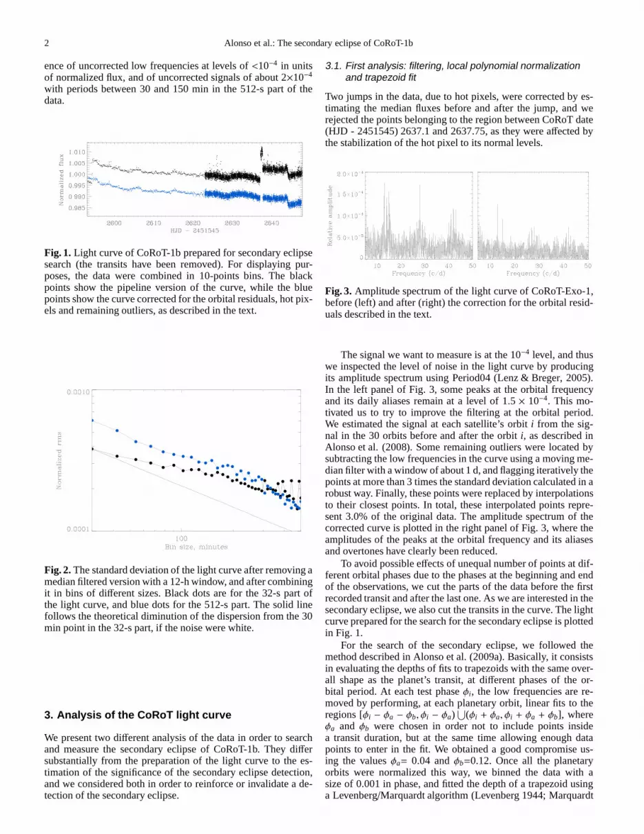
The light curve was sampled every 512 s for the first 28 days,and then changed to 32 s until the end of the run. During the512 s part, the dispersion of the normalized data is 0.00079,and0.0019 in the 32 s section. The pipeline version of the light curveis plotted in Fig. 1. To evaluate the red noise content in our data(e.g. Pont et al. 2006), we computed the standard deviation of thelight curve (filtered with a median filter with a window of 12 h)with different bin sizes, ranging from 30 to 500 min. The result isplotted in Fig. 2; the 32-s part of the curve shows less noise thanthe 512-s part below bins of∼150 min, while it achieves similarlevels as the 512-s part above that size. This reveals the pres-

2 Alonso et al.: The secondary eclipse of CoRoT-1b

ence of uncorrected low frequencies at levels of<10−4 in unitsof normalized flux, and of uncorrected signals of about 2×10−4

with periods between 30 and 150 min in the 512-s part of thedata.

Fig. 1. Light curve of CoRoT-1b prepared for secondary eclipsesearch (the transits have been removed). For displaying pur-poses, the data were combined in 10-points bins. The blackpoints show the pipeline version of the curve, while the bluepoints show the curve corrected for the orbital residuals, hot pix-els and remaining outliers, as described in the text.

Fig. 2. The standard deviation of the light curve after removing amedian filtered version with a 12-h window, and after combiningit in bins of different sizes. Black dots are for the 32-s part ofthe light curve, and blue dots for the 512-s part. The solid linefollows the theoretical diminution of the dispersion from the 30min point in the 32-s part, if the noise were white.

3. Analysis of the CoRoT light curve

We present two different analysis of the data in order to searchand measure the secondary eclipse of CoRoT-1b. They differsubstantially from the preparation of the light curve to thees-timation of the significance of the secondary eclipse detection,and we considered both in order to reinforce or invalidate a de-tection of the secondary eclipse.

3.1. First analysis: filtering, local polynomial normalizationand trapezoid fit

Two jumps in the data, due to hot pixels, were corrected by es-timating the median fluxes before and after the jump, and werejected the points belonging to the region between CoRoT date(HJD - 2451545) 2637.1 and 2637.75, as they were affected bythe stabilization of the hot pixel to its normal levels.

Fig. 3. Amplitude spectrum of the light curve of CoRoT-Exo-1,before (left) and after (right) the correction for the orbital resid-uals described in the text.

The signal we want to measure is at the 10−4 level, and thuswe inspected the level of noise in the light curve by producingits amplitude spectrum using Period04 (Lenz & Breger, 2005).In the left panel of Fig. 3, some peaks at the orbital frequencyand its daily aliases remain at a level of 1.5 × 10−4. This mo-tivated us to try to improve the filtering at the orbital period.We estimated the signal at each satellite’s orbiti from the sig-nal in the 30 orbits before and after the orbiti, as described inAlonso et al. (2008). Some remaining outliers were located bysubtracting the low frequencies in the curve using a moving me-dian filter with a window of about 1 d, and flagging iterativelythepoints at more than 3 times the standard deviation calculated in arobust way. Finally, these points were replaced by interpolationsto their closest points. In total, these interpolated points repre-sent 3.0% of the original data. The amplitude spectrum of thecorrected curve is plotted in the right panel of Fig. 3, wheretheamplitudes of the peaks at the orbital frequency and its aliasesand overtones have clearly been reduced.

To avoid possible effects of unequal number of points at dif-ferent orbital phases due to the phases at the beginning and endof the observations, we cut the parts of the data before the firstrecorded transit and after the last one. As we are interestedin thesecondary eclipse, we also cut the transits in the curve. Thelightcurve prepared for the search for the secondary eclipse is plottedin Fig. 1.

For the search of the secondary eclipse, we followed themethod described in Alonso et al. (2009a). Basically, it consistsin evaluating the depths of fits to trapezoids with the same over-all shape as the planet’s transit, at different phases of the or-bital period. At each test phaseφi, the low frequencies are re-moved by performing, at each planetary orbit, linear fits to theregions [φi − φa − φb, φi − φa)

⋃(φi + φa, φi + φa + φb], where

φa and φb were chosen in order not to include points insidea transit duration, but at the same time allowing enough datapoints to enter in the fit. We obtained a good compromise us-ing the valuesφa= 0.04 andφb=0.12. Once all the planetaryorbits were normalized this way, we binned the data with asize of 0.001 in phase, and fitted the depth of a trapezoid usinga Levenberg/Marquardt algorithm (Levenberg 1944; Marquardt

Alonso et al.: The secondary eclipse of CoRoT-1b 3

Fig. 4. Depth of a trapezoid with the shape and duration of atransit, as a function of the planet’s orbital phase. The maximumis centered in phase 0.5, corresponding to the secondary eclipse.In grey, the result in a light curve where the secondary eclipsesignal has been diluted (see text for details).

Fig. 5. Phase folded curve of CoRoT-1b during the phases ofsecondary eclipse. The data have been binned in 0.01 in phase(∼22 min).

Fig. 6. Theχ2 space for different centers and depths of the sec-ondary eclipse, and the differentσ confidence limits.

1963), fixing the rest of the trapezoid’s parameters to the val-ues of the transit. The final depth of the fits as a function of theorbital phase is plotted in Fig. 4, where the maximum is wellcentered at the expected orbital phase 0.5. We can evaluate thesignificance of this detection by computing the dispersion of thefitted depths in the parts of the phase diagram not affected bythe inclusion of the secondary eclipse at phase 0.5 in the regions

Fig. 7. Theχ2 for the duration of the secondary eclipse, and the1,2 and 3σ confidence limits. The vertical line shows the totalduration of a transit. The detected signal has the same durationas the transit at 1-sigma level.

where the fits used to normalize the transits were computed, i.e.,φ ∈ [0, 0.5− φa− φb)

⋃(0.5+ φa+ φb, 1]. The significance of the

detection calculated this way results in 2.1-σ. The phase foldedlight curve around the secondary phase and the best fit trapezoid(with duration and shape fixed to that of the transits) are shownin Fig. 5.

We performed the same technique in a light curve where wediluted the signal of the secondary eclipse. To do so, we sub-tracted from the light curve a version of it, filtered with a mov-ing median using a window of∼1 d in duration. We shuffledrandomly the residuals, and we added back the subtracted fil-tered curve. The resulting depth vs. phase diagram using themethod described above in this curve is plotted as a grey linein the Fig. 4. If we take the dispersion of this measured depth(3.29×10−5) as the precision in the measurement of the sec-ondary eclipse, then the significance of the signal at phase 0.5is 4.5-σ.

Additionally, three different methods to evaluate the depthand significance of the secondary eclipse signal were tested. Inthe first method, we removed the best fit trapezoid to the data(where the only fitted parameter was the depth, the rest wasfixed to the values of the transit), shifted circularly the residu-als, reinserted the signal, and re-evaluated the fitted depth. Thefinal depth thus takes into account the effect of red noise in thedata, and it is of 0.014±0.002%. The second method consisted infitting two gaussians to 1) the distribution of points insidetotaleclipse and 2) a subset of the points outside the eclipse withthesame number of points as in 1), and compare their fitted centers.This fit was performed to 500 subsets of 2), with a randomly cho-sen starting point and varying the size of the bins in the distribu-tion between 0.005% and 0.02%. The result is of 0.021±0.003%.In the third method, we explored theχ2 distribution in a gridof centers (from -60 to+60 minutes from the expected center)and depths (from 0.01% to 0.04%) of the secondary eclipse. Theother parameters of the trapezoid were fixed to the values of thetransit. The minimumχ2 and the 1,2 and 3-σ confidence lev-els are presented in Fig. 6, and the best fitted depth using thismethod is 0.016±0.006%. We show theχ2 map of the durationof the trapezoid and the 1,2,3-σ confidence levels in Fig. 7. Theduration of the secondary eclipse is, as expected, compatible ata<2-σ level with the duration of the transits.

3.2. Second analysis: using the IRF filter

The analysis presented so far shows encouraging evidence forthe detection of a secondary eclipse at the expected phase andduration for a circular or almost circular orbit. However, the de-

4 Alonso et al.: The secondary eclipse of CoRoT-1b

tection is unavoidably tentative given the extremely shallow na-ture of the signal. Each step of the analysis involved a numberof free parameters, from the hot pixel and satellite orbit resid-ual corrections to the individual corrections applied for stellarvariability local to each putative secondary location.

In an effort to reinforce or invalidate the detection, we car-ried out a separate secondary eclipse search using different pre-processing and eclipse detection methods which were designedto minimize the number of free parameters. The regions aroundthe hot pixel events were simply clipped out, no correction fororbital residuals was applied, and we used the iterative recon-struction filter (IRF) of Alapini & Aigrain (2009), which hasonly two free parameters, to isolate signal at the planet’s orbitalperiod from other signals including stellar variability.

The starting point of this analysis was the same light curve,as described in Section 2. To circumvent the issue of varyingdataweights associated with different time sampling, the oversam-pled section of the light curve was rebinned to 512s sampling.Outliers were then identified and clipped out using a moving me-dian filter (see Aigrain et al. 2009 for details). Finally, wealsodiscarded two segments of the light curve, in the CoRoT dateranges 2594.25–2594.45 and 2637.10–2637.70), correspondingto the two hot pixel events visible in Fig. 1. This last step wasnecessary as the IRF cannot remove the sharp flux variations as-sociated with hot pixels without affecting the transit signal.

The resulting time-series was then fed into the IRF. A full de-scription of this filter is given in Alapini & Aigrain (2009),butwe repeat the basic principles of the method here for complete-ness. The IRF treats the light curve{Y(i)} asY(i) = F(i) A(i) +R(i), where{A(i)} represents the signal at the period of the planet,which is a multiplicative term applied to the intrinsic stellar flux{F(i)}, and{R(i)} represents observational noise. A first estimateof {A(i)} is obtained by folding the light curve at the period ofthe transit and smoothing it using a smoothing length of 0.0006in phase, and is divided into the original light curve. This is thenrun through an iterative non-linear filter (Aigrain & Irwin,2004)which preserves signal at frequencies longer than 0.5 days togive an estimate of the stellar signal{F(i)}, which is assumedto be primarily concentrated on relatively long time-scales. Thissignal in turn is removed from the original light curve and theprocess is iterated until the the dispersion of the residuals re-mains below 10−4 for 3 consecutive iterations, which occurs af-ter 3 iterations in this case.

The free parameters of the IRF are the smoothing lengthsused when estimating{A(i)} and {F(i)}. The former representsa compromise between reducing the noise and blurring out po-tential sharp features associated with the planet, and the latterbetween removing the stellar signal without affecting the plan-etary signal. The values chosen here were adopted by trial anderror and gave the best results when evaluating the performace ofthe IRF for transit reconstruction purposes (Alapini & Aigrain,2009).

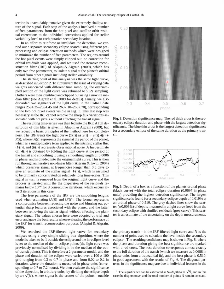
We searched the IRF-filtered light curve for secondaryeclipses using a very simple sliding box algorithm, where themodel is taken to be 1 outside the eclipse and the in-eclipse levelis set to the median of the in-eclipse points (the light curvewaspreviously normalised by dividing it be the median of the out-of-transit points). This is therefore a 2-parameter model,and thephase and duration of the eclipse were varied over a 100× 100grid ranging from 0.3 to 0.7 in phase and from 0.02 to 0.2 induration, where the duration is measured in phase units (corre-sponding to 0.7 to 7.2 hours). We then evaluate the significanceof the detection, in arbitrary units, by dividing the eclipse depthby σ/

√(N), where sigma is the scatter of the points - outside

Fig. 8. Detection significance map. The red thick cross is the sec-ondary eclipse duration and phase with the largest detection sig-nificance. The blue thin cross is the largest detection significancefor a secondary eclipse of the same duration as the primary tran-sit.

Fig. 9. Depth of a box as a function of the planets orbital phase(black curve) with the total eclipse duration (0.0697 in phaseunits) providing the highest detection significance. The largestsignificance is found for a secondary eclipse depth of 0.019%atan orbital phase of 0.510. The grey dashed lines show the scat-ter (±0.006%) of depths measured in a light curve freed from thesecondary eclipse with shuffled residuals (grey curve). This scat-ter is an estimate of the uncertainty on the depth measurements.

the primary transit - in the IRF-filtered light curve andN is thenumber of point used to calculate the level inside the secondaryeclipse1. The resulting confidence map is shown in Fig. 8, wherethe phase and duration giving the best significance are markedwith a red cross. The best duration corresponds almost exactlyto the full duration of the transit (which we measure as 0.0688 inphase units from a trapezoidal fit), and the best phase is 0.510,in good agreement with the results of Fig. 6. The diagonal pat-terns in the significance map are due to individual features in the

1 The significance can be estimated as S=depth/σ ×√

N, and in thiscase the dispersionσ, and the total number of points N remain constant.

Alonso et al.: The secondary eclipse of CoRoT-1b 5

folded, filtered light curve, which influence a wider range oftrialphases at longer durations.

Fig. 9 shows the eclipse depth as a function of orbital phaseat the best duration. The best-fit depth is 0.019%, consistent withthe results presented above. One should bear in mind when com-paring the different results that the eclipse depth was measuredhere relative to the overall median flux rather than to a locales-timate of the out-of-eclipse flux.

To calculate the significance of the detection, we measuredthe depth and associated uncertainty and divided the formerbythe latter. In this case, we calculated the uncertainty as the dis-persion (estimated as 1.48×MAD) around the median level ofthe light curve outside the primary transit, and divided this valueby the square root of the number of points inside the secondaryeclipse. This results in an uncertainty of 0.005%, i.e. a 3.5σdetection. We also applied the three other methods already pre-sented in Section 3.1. All of these give an uncertainty estimate of0.006%, which we adopt as the final uncertainty on the eclipsedepth derived from the IRF.

The fact that we arrived at consistent estimates of the sec-ondary eclipse depth and significance using different approachesto filter the light curve and evaluate the uncertainty on the depthlends confidence to the detection. Our final adopted values forthe depth is 0.016±0.006%, consistent with all our estimateswithin one sigma. The eclipse center occurs at the expectedphase for a circular orbit, with an uncertainty of about 20 min.

4. Discussion

We have shown that a decrease in the flux of the light curveof CoRoT-1b at the phases of secondary eclipse is detected atmore than 3-σ level. Its duration is, within 1-σ, the same asthe duration of the transits, and its shallow depth is of only0.016±0.006%. We thus interpret this signal as the secondaryeclipse, detected at the optical part of the spectrum.

If we were to explain the secondary eclipse detectionas reflected light, it would imply a geometric albedo ofAg=0.20±0.08, which is a bigger value than several up-per limits provided by other works in different exoplanets(Collier Cameron et al. 2002; Rowe et al. 2008). Furthermore,theoretical models predict a strong optical absorption in the HotJupiters’ atmospheres (e.g. Sudarsky et al. 2000; Burrows et al.2008; Hood et al. 2008), and for thepM-class of planets, ther-mal emission dominates by more than an order of magnitudethe reflected light. Consequently, we suspect that the secondaryeclipse signature is not produced entirely by reflected light, butmost probably by a combination of thermal emission and somereflected light, as in the case of CoRoT-2b (Alonso et al., 2009b).

The CoRoT bi-prism allows to recover chromatic informa-tion from the signal. In this case, the difference between the sig-nificance of the secondary signal in the blue and the red chan-nels might clarify if our detected signal is dominated by reflectedlight or by thermal emission in the optical, as we assumed giventhe arguments above. In the first case, the secondary should bedetected mostly in the blue channel, while in the case of ther-mal emission the red channel would carry most of the signal. Wechecked the colors in the CoRoT-1 aperture, but unfortunatelythe residuals of the jitter correction and the noisier individualchannels did not allow us to conclude on this subject.2

2 After submission of the original manuscript of this paper, we be-came aware of an independent analysis of the red CoRoT channel per-formed by Snellen et al. (2009), that allowed these authors to detect a0.0126±0.0033% secondary eclipse. This result points towards a small

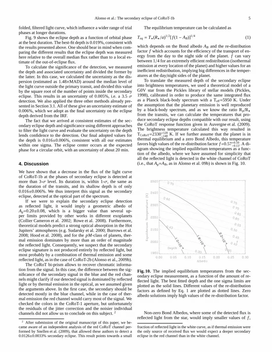
The equilibrium temperature can be calculated as

Teq = T⋆(R⋆/a)1/2[ f (1− AB)]1/4 (1)

which depends on the Bond albedoAB and the re-distributionfactor f which accounts for the efficiency of the transport of en-ergy from the day to the night side of the planet.f can varybetween 1/4 for an extremely efficient redistribution (isothermalemission at every location of the planet) and higher values for aninefficient redistribution, implying big differences in the temper-atures at the day/night sides of the planet.

To translate the measured depth of the secondary eclipseinto brightness temperatures, we used a theoretical model of aG0V star from the Pickles library of stellar models (Pickles,1998), calibrated in order to produce the same integrated fluxas a Planck black-body spectrum with a Teff=5950 K. Underthe assumption that the planetary emission is well reproducedby a black-body spectrum, and as we know the ratio Rp/R⋆from the transits, we can calculate the temperatures that pro-duce secondary eclipse depths compatible with our result, usingthe CoRoT response function given in Auvergne et al. (2009).The brightness temperature calculated this way resulted inTCoRoT=2330+120

−140 K. If we further assume that the planet is inthermal equilibrium and a zero Bond Albedo, this temperaturefavors high values of the re-distribution factorf=0.57+0.10

−0.13. A di-agram showing the implied equilibrium temperatures as a func-tion of the albedo, where we have assumed for simplicity thatall the reflected light is detected in the white channel of CoRoT(i.e., thatAg=AB, as in Alonso et al. 09b) is shown in Fig. 10.

Fig. 10. The implied equilibrium temperatures from the sec-ondary eclipse measurement, as a function of the amount of re-flected light. The best fitted depth and the one sigma limits areplotted as the solid lines. Different values of the re-distributionfactors as defined by Eq. 1 are plotted as dotted lines. Zeroalbedo solutions imply high values of the re-distribution factor.

Non-zero Bond Albedos, where some of the detected flux isreflected light from the star, would imply smaller values off ,

fraction of reflected light in the white curve, as if thermal emission werethe only source of received flux we would expect a deeper secondaryeclipse in the red channel than in the white channel.

6 Alonso et al.: The secondary eclipse of CoRoT-1b

whilst solutions with A>0.30 are not compatible with the mea-sured secondary eclipse. All the solutions with equilibrium tem-peratures higher than 1900 K are forf values bigger than 1/4.Thus, the secondary eclipse detection favors inefficient redistri-butions of the incident flux from the day to the night side.

One may wonder if thek = Rpl/R⋆ obtained from the transitfit should be different because of the lack of inclusion of theemitted light from the planet in the model. Even for an extremecase off = 1/4, the correction to be applied on thek is a factorof 3 below the uncertainty given in Barge et al. (2008), and thuswe do not consider it necessary.

The measured center of the secondary eclipse, with an un-certainty of 20 min, can be used to constrain thee cosω <0.014at a 1-σ level.

Our measured brightness temperature can be used to predicteclipse depths in theKs andz bands of 0.25% and 0.014% re-spectively. In these bands, ground-based observations have re-cently been successful in the detections of secondary eclipses ofexoplanets (Sing & Lopez-Morales 2009; de Mooij & Snellen2009), and for the case of CoRoT-1b, the observations might re-veal departures from the black-body assumption such as the ther-mal inversions observed in several planets (e.g. Knutson etal.2008, 2009).3

Acknowledgements. R.A acknowledges support by the grant CNES-COROT-070879. A.H. acknowledges the support of DLR grants 50OW0204, 50OW0603,and 50QP0701. H.J.D. acknowledges support by grants ESP2004-03855-C03-03and ESP2007-65480-C02-02 of the Spanish Education and Science ministry.

ReferencesAigrain, S. & Irwin, M. 2004, MNRAS, 350, 331Aigrain, S., Pont, F., Fressin, F., et al. 2009, A&A, in press, arXiv:0903.1829Alapini, A. & Aigrain, S. 2009, MNRAS, accepted, arXiv:0905.3062Alonso, R., et al. 2008, A&A, 482, L21Alonso, R., Aigrain, S., Pont, F., Mazeh, T., & The CoRoT Exoplanet Science

Team 2009a, IAU Symposium, 253, 91Alonso, R., Guillot, T., Mazeh, T., Aigrain, S., Alapini, A., Barge, P., Hatzes, A.,

& Pont, F. 2009b, arXiv:0906.2814Auvergne, M., et al. 2009, A&A, accepted, arXiv:0901.2206Barge, P., et al. 2008, A&A, 482, L17Burrows, A., Budaj, J., & Hubeny, I. 2008, ApJ, 678, 1436Charbonneau, D., et al. 2005, ApJ, 626, 523Collier Cameron, A., Horne, K., Penny, A., & Leigh, C. 2002, MNRAS, 330,

187Deming, D., Seager, S., Richardson, L. J., & Harrington, J. 2005, Nature, 434,

740Fortney, J. J., Lodders, K., Marley, M. S., & Freedman, R. S. 2008, ApJ, 678,

1419Gillon, M., et al. 2009, arXiv:0905.4571Hood, B., Wood, K., Seager, S., & Collier Cameron, A. 2008, MNRAS, 389, 257Knutson, H. A., Charbonneau, D., Allen, L. E., Burrows, A., &Megeath, S. T.

2008, ApJ, 673, 526Knutson, H. A., Charbonneau, D., Burrows, A., O’Donovan, F.T., & Mandushev,

G. 2009, ApJ, 691, 866Levenberg, K. 1944,The Quarterly of Applied Mathematics, 2, 164Lenz, P., & Breger, M. 2005, Communications in Asteroseismology, 146, 53Lopez-Morales, M., & Seager, S. 2007, ApJ, 667, L191Marquardt, D. 1963, SIAM Journal on Applied Mathematics, 11, 431de Mooij, E. J. W., & Snellen, I. A. G. 2009, A&A, 493, L35Pickles, A. J. 1998, PASP, 110, 863Pont, F., Zucker, S., & Queloz, D. 2006, MNRAS, 373, 231Rowe, J. F., et al. 2008, ApJ, 689, 1345Sing, D. K., & Lopez-Morales, M. 2009, A&A, 493, L31Snellen, I. A. G., de Mooij, E. J. W., & Albrecht, S. 2009, Nature, 459, 543Sudarsky, D., Burrows, A., & Pinto, P. 2000, ApJ, 538, 885

3 After submission of this work, Gillon et al. (2009) reporteda detec-tion in theKs-band of a 0.28+0.04

−0.07% eclipse, in good agreement with theextrapolation of our results.

1 Laboratoire d’Astrophysique de Marseille, UMR 6110,Technopole de Marseille-Etoile,F-13388 Marseille cedex 13,France2 Observatoire de Geneve, Universite de Geneve, 51 Ch. des

Maillettes, 1290 Sauverny, Switzerland3 School of Physics, University of Exeter, Stocker Road, Exeter

EX4 4QL, United Kingdom4 LESIA, CNRS UMR 8109, Observatoire de Paris, 5 place J.

Janssen, 92195 Meudon, France5 IAS, UMR 8617 CNRS, bat 121, Universite Paris-Sud, F-91405

Orsay, France6 Observatoire de Haute-Provence, 04870 St Michel l’Observatoire,

France7 Observatorio Nacional, Rio de Janeiro, RJ, Brazil8 Instituto de Astrofısica de Canarias, E-38205 La Laguna, Spain9 Institute for Astronomy, University of Vienna,

Turkenschanzstrasse 17, 1180 Vienna, Austria10 Institute of Planetary Research, DLR, Rutherfordstr. 2, 12489Berlin, Germany11 Research and Scientific Support Department, European SpaceAgency, ESTEC, 2200 Noordwijk, The Netherlands12 Observatoire de la Cote d’Azur, Laboratoire Cassiopee, CNRSUMR 6202, BP 4229, 06304 Nice Cedex 4, France13 Thuringer Landessternwarte Tautenburg, Sternwarte 5, 07778Tautenburg, Germany14 Space Research Institute, Austrian Academy of Sciences,Schmiedlstrasse 6, 8042 Graz, Austria15 Institut d’Astrophysique et de Geophysique, Universitede Liege,Allee du 6 aout 17, Sart Tilman, Liege 1, Belgium16 School of Physics and Astronomy, R. and B. Sackler Faculty ofExact Sciences, Tel Aviv University, Tel Aviv 69978, Israel17 Rheinisches Institut fur Umweltforschung, Universitatzu Koln,Abt. Planetenforschung, Aachener Str. 209, 50931 Koln, Germany18 Center for Astronomy and Astrophysics, TU Berlin,Hardenbergstr. 36, D-10623 Berlin, Germany19 LUTH, Observatoire de Paris-Meudon, 5 place J. Janssen, 92195Meudon, France