goce level 1b data processing

1 23

�� !�"��#$��%��!!�&��'(�!!)�#$* $�� $+,��!�-!�� .��!��!!��

��

��

1 23

Your article is protected by copyright andall rights are held exclusively by Springer-Verlag. This e-offprint is for personal use onlyand shall not be self-archived in electronicrepositories. If you wish to self-archive yourwork, please use the accepted author’sversion for posting to your own website oryour institution’s repository. You may furtherdeposit the accepted author’s version on afunder’s repository at a funder’s request,provided it is not made publicly available until12 months after publication.

J Geod (2011) 85:759–775DOI 10.1007/s00190-011-0497-4

ORIGINAL ARTICLE

GOCE level 1b data processing

Björn Frommknecht · Daniel Lamarre ·Marco Meloni · Alberto Bigazzi ·Rune Floberghagen

Received: 11 January 2011 / Accepted: 17 June 2011© Springer-Verlag 2011

Abstract In this article, the processing steps applied tothe raw GOCE science payload instrument data (level 0) inorder to obtain input data for the gravity field determina-tion (level 1b) are described. The raw gradiometer measure-ments, which are given at the level of control voltages, haveto be transformed into accelerations and gradients. For thelatter step, knowledge about the GOCE attitude is required,which is provided by the star trackers. In addition, the data ofthe satellite to satellite tracking instrument are used to datethe measurements, after its clock error has been corrected.All intermediate steps of the processing flow are described.Together with the explanation of the processing flow, an over-view of the main level 1b products is given. The final partof the article discusses the means of quality control of theL1b data currently used and gives an outlook on potentialprocessor evolutions.

Keywords GOCE · Electrostatic gravity gradiometer ·Gravity gradient determination · Star tracker · Satellite tosatellite tracking instrument · Fusion of gradiometer andstar tracker data

1 GOCE payload data ground segment overview

The GOCE data are acquired at the ESA Satellite Station atKiruna, Sweden, and then transferred to the European SpaceOperations Centre (ESOC), Germany, and flow from there tothe processing facility at the European Space Research Insti-tute (ESRIN), for level 1b (L1b) data generation, archiving,and data distribution. The L1b data are distributed to the high

B. Frommknecht (B) · D. Lamarre · M. Meloni · A. Bigazzi ·R. FloberghagenESA/ESRIN, Via G. Galilei, 00044 Frascati, Italye-mail: [email protected]

level processing facility (HPF) for processing to level 2, i.e.,gravity field models. Both level 1b and level 2 products aredistributed from ESRIN to the user community. The over-all data flow is depicted in Fig. 1. The L1b data are gener-ated from the level 0 (L0) data, which contain the individualinstrument’s data packets, which have been extracted beforefrom the acquired telemetry.

The processing logic in terms of processing functions isdepicted in Fig. 2. In order to process the electrostatic grav-ity gradiometer (EGG) data, first the data of the satellite tosatellite tracking instrument (SSTI) have to be processed toobtain a consistent datation in GPS time, then the star tracker(STR) data have to be processed to yield the satellite attitude.Both the processing of the SSTI and the EGG data require cal-ibration information. The SSTI data have to be corrected forthe effects of the inter-frequency bias and the inter-channelbias. The inter-frequency bias depends on the temperature ofthe GPS receiver and thus can be measured on-ground. Thederived information is stored in a look-up table for whichthe current SSTI temperature measurement contained in thehousekeeping data is used as an index. The inter-channelbias has to be determined in-orbit, this was done once at thebeginning of the mission, and the results have been saved ina table that is used in the nominal processing chain for thepseudo range correction. The gradiometer calibration func-tion foresees also an interaction with the satellite, where val-ues derived on-ground are uplinked to eliminate the effects ofthe quadratic factor on the gradiometer measurements. First,the data of the SSTI is processed, in order to derive accu-rate timing information for both the STR and the EGG data,which have to be synchronized for further processing. Thenext step consists in processing the STR data to obtain infor-mation about the absolute orientation of GOCE, which isfollowed by the processing of the EGG data to finally yieldthe gravity gradients. The individual processing functions

123

Author's personal copy

760 B. Frommknecht et al.

Fig. 1 GOCE processing centers and data flow

Fig. 2 Overview of processing functions and product flow for the grav-ity gradient generation

will be explained in the sequence of the processing logic.Table 1 gives an overview of the execution frequency of theindividual processing functions, Tables 5 and 6 of Appendixcontain an overview of the individual L1b products and theircontents. The first step that is common to all processing func-tions, the depacketing and sorting of the measured quantities,is only described here; in this processing step, the individualdata packets are extracted from the telemetry data stream,converted into engineering units and time ordered. The indi-vidual measurements are then dated with GPS time using theinformation derived in the SSTI data processing.

2 Satellite to satellite tracking instrument dataprocessing

2.1 Instrument description

The SSTI is a state-of-the-art GNSS receiver that has beendesigned to operate in a low Earth orbit environment and is

Table 1 GOCE L1b processing function execution frequencies

Processor Exectution frequency

EGG nominal Regularly

EGG calibration

ICM calibration Every 2 months

(satellite shaking)

K2F determination Several times at

(proof mass shaking) beginning of mission

STR nominal Regulary

SSTI nominal Regularly

SSTI calibration

Inter-channel bias Once

shown in Fig. 3. The objective is to provide the satellite-to-satellite tracking-high/low (SST-hl) contribution to thegravity field recovery, by the simultaneous tracking of up to12 GPS satellite signals. In addition, the SSTI provides datafor precise orbit determination and is also used for real-timeon-board navigation.

2.2 SSTI calibration processor description

The purpose of the SSTI calibration processor is to determinethe inter-channel bias of the pseudo range measurements,which is a standard correction applied to GNSS receiversmeasurements. This is achieved by defining one of the 12channels as master and deriving the range differences whentracking the same GPS satellite on all channels. It is to benoted that there is no dedicated processing function for theinter-frequency bias, as this quantity can be determined on-ground and is assumed to be stable during the mission life-time.

2.2.1 Filtering and outlier identification

During this processing step, outliers in the code measure-ments are identified using a polynomial fit to the pseudo rangemeasurements and by comparing the fit residuals againsta configurable threshold (currently, a standard 3σ test isexecuted). Observations flagged as outliers are not used forfurther processing. The outlier identification function is iden-tical to the one used in the nominal processor.

2.2.2 Inter channel bias determination

The inter channel bias is derived for each channel and foreach of the pseudo range measurement types P1, P2, andC/A code. Let Nobs be the number of available observations

123


GOCE level 1b data processing 761

Fig. 3 SSTI lagrange receiver

and k be the channel number (k = 1, . . . , 12):

ICBP1[k] = 1Nobs

·Nobs∑

i=1

PRMP1[master][i]

− PRMP1[k][i] (1)

ICBP2[k] = 1Nobs

·Nobs∑

i=1

PRMP2[master][i]

− PRMP2[k][i] (2)

ICBC/A[k] = 1Nobs

·Nobs∑

i=1

PRMC/A[master][i]

− PRMC/A[k][i] (3)

The resulting bias values are then stored in a dedicated prod-uct for use in the nominal processing chain.

2.3 SSTI nominal processor description

The purpose of the SSTI nominal processor is to derive anorbit solution with an accuracy of about 10 m in order toenable high-level monitoring of the SSTI health and func-tionality. As observations, the code measurements correctedfor the inter-frequency and the inter-channel bias are used.For the derivation of the position solution, no phase measure-ments are utilized.

2.3.1 Interchannel and interfrequency bias correction

The objective of this processing step is the correction ofinstrument dependent errors of the code and phase measure-ments. The code measurements are corrected for the inter-channel bias, the phase measurements are corrected for theinter-frequency bias. The inter-frequency bias is derived froma look-up table, where the measured SSTI temperature servesas an index. Typical correction values are shown in Fig. 4. The

Fig. 4 Inter-frequency bias correction values

correction values are represented by a linear function and risetowards high-temperatures, the correction values are belowone cycle. The inter-channel bias values to be applied to thecode measurements are derived in the SSTI calibration pro-cessor during a dedicated calibration measurement phase, asdiscussed in Sect. 2.2.

2.3.2 Filtering and outlier identification

The code and phase measurements are then filtered for out-liers by applying a 3σ test. The standard deviation is esti-mated as residuals to a degree n = 3 polynomial that is fittedthrough m = 5 observations:

x =[ATPA

]−1· ATPy, with (4)

A=

⎛

⎜⎜⎜⎜⎜⎜⎜⎜⎜⎜⎝

1 (t1 − tc) (t1 − tc)2 · · · (t1 − tc)n

1 (t2 − tc) (t2 − tc)2 · · · (t2 − tc)n

......

......

...

1 0 0 0 0...

......

......

1 (tm−1 − tc) (tm−1 − tc)2 · · · (tm−1 − tc)n

1 (tm − tc) (tm − tc)2 · · · (tm − tc)n

⎞

⎟⎟⎟⎟⎟⎟⎟⎟⎟⎟⎠

.

(5)

where A is the matrix of the partial derivatives and y is thevector of observations, the sampling interval of the observa-tions is 1 s.

2.3.3 Position, velocity, and time solution

This processing step can be divided into two major steps:

1. Derivation of the GOCE satellite position and GNSSreceiver clock error and

2. derivation of the GOCE satellite velocity.

123



The first step is an iterative process and is carried out foreach epoch to be processed separately: for each epoch, thefollowing steps are conducted:

– the GOCE position is initialized to the onboard-naviga-tion solution

– the positions and clocks of the tracked GPS satellites areinterpolated to the measurement epoch

– the GPS satellite clocks are corrected for relativisticeffects

– the GPS satellite positions are corrected for the shiftcaused by earth rotation during signal travel time

– the observations are then corrected for the effect of theionosphere, either by forming a ionosphere-free linearcombination or by use of a ionosphere model derivedcorrection

A standard least squares adjustment is conducted to fit theGOCE satellite position and clock error to the observations.The iteration is stopped if the clock error change is below athreshold of 10 µs or if 100 iterations have been executed.

The second step consists in the derivation of the GOCEsatellite velocity, by fitting a fourth-order polynomial to thepositions derived previously. The first derivative of the poly-nomial then yields the satellite velocity plus associated accu-racy information.

3 Star tracker data processing


The star tracker or advanced stellar compass is used to deter-mine the 3-axis inertial attitude of the GOCE satellite. Theattitude is derived by comparing sky images with known stel-lar constellations from a star catalogue. It has been manu-factured by the measurement and instrumentation systems(MIS) section of the Ørsted department at the Technical Uni-versity of Denmark (DTU). In the case of GOCE, the mea-surement system consists of one data processing unit (DPU)and three camera head units (CHU) hosting each a CCD chipthat is used for the optical image reception, see Fig. 5. Thebasic L0 product generated by the star tracker contains theGOCE attitude in quaternion representation. More details canbe found e.g., in Jørgenson (2004).

3.2 STR nominal processor description

The purpose of the STR nominal processor is to date theSTR measurements with GPS time, which is achieved byusing the correlation between on-board time (OBT) and GPStime derived in the SSTI nominal processor. In a second step,the STR observations are corrected for the orbital relativis-

Fig. 5 The star tracker. The image shows two star tracker CHU withthe baffles

tic aberration, the annual relativistic aberration error causedby the movement of the orbit with the Earth around the Sunis already corrected on board. The details can be found inCesare et al. (2008).

4 The electrostatic gravity gradiometer


The electrostatic gravity gradiometer (EGG) measures thegravity gradient tensor along the GOCE orbit through threepairs of three-axial accelerometers A1–A4, A2–A5 andA3–A6, see Fig. 6. A set of two accelerometers forms a one-axis gradiometer (OAG), i.e., a device capable to measure thespatial gradient of the acceleration along the segment join-ing the centres of the two sensors. The three OAGs are thefundamental gradiometric measurement units of the GOCEgradiometer.

In each accelerometer, a metal alloy proof mass is electro-statically suspended and actively controlled in its six degreesof freedom at the centre of a cage by means of voltagesapplied to eight pairs of electrodes. A polarization voltageis applied to the proof mass through a gold wire glued onit. The proof mass displacement relative to the electrodesis measured by capacitive sensors. The control voltages areproportional to the accelerations of the proof mass relativeto the cage and constitute the basic measurement of the EGGinstrument. The principal layout of a single GOCE acceler-ometer is shown in Fig. 7.

123



Fig. 6 The gradiometer structure, showing the three-one axis gradi-ometers constituting the gradiometer reference frame

Fig. 7 An individual accelerometer electrode pairs and layout

Each accelerometer has two ultra-sensitive axes and oneless-sensitive axis, (perpendicular to the broad side of thecage. One of the two ultra-sensitive axes of each of the twoaccelerometers forming an OAG is parallel to the OAG base-line. The less-sensitive axis can be tested under Earth gravityconditions, i.e., on-ground, as the four electrode pairs cancompensate for the residual accelerations during e.g., a droptower experiment.

4.2 The gravity gradients tensor

A detailed description of the measurement process and rel-evant theory, whose synthesis is reported hereafter, can befound in Cesare (2008), Rummel (1985) and B. Hofmann-Wellenhof and H. Moritz (2005).

The principal quantity derived from GOCE measurements isthe gravity gradient tensor (GGT). The tensor is defined as:

U =

⎛

⎝Vxx Vxy VxzVyx Vyy VyzVzx Vzy Vzz

⎞

⎠ (6)

where Vi j = ∂2V/∂xi∂x j and V is the gravitational potential.The gravity gradient tensor components Vi j are not

observable directly, but only in combination with the centrif-ugal acceleration and angular acceleration, due to the mea-surement performed in a moving frame fixed to the satellite.Each single accelerometer i senses, an acceleration

ai ∼= −(

U − !2 − !)

· Ai + D. (7)

where Ai is the vector from the origin of the OAG to the cen-ter of mass (CoM) of the accelerometer’s proof mass, D isthe vector of the non conservative accelerations acting on thesatellite CoM (caused by surface forces like air drag, solarradiation pressure and others). ! is the angular rates tensor,!2 its square and the angular accelerations matrix !:

! =

⎛

⎝0 −ωz ωyωz 0 −ωx

−ωy ωx 0

⎞

⎠ , (8)

!2 =

⎛

⎝−ω2

z − ω2y ωxωy ωxωz

ωxωy −ω2z − ω2

x ωyωzωxωz ωyωz −ω2

x − ω2y

⎞

⎠ , (9)

! =

⎛

⎝0 −ωz ωyωz 0 −ωx

−ωy ωx 0

⎞

⎠ . (10)

Equation (7) assumes that all OAG centers are aligned andcoincides with the CoM of the satellite. It neglects effectsdependent on time variability of the satellite CoM, imperfec-tions of the accelerometers, coupling with the Earth’s mag-netic field and self gravitation. This neglecting is justified inpart by the gradiometer calibration described in the followingsection. Concerning the effects of coupling with the Earth’smagnetic field and the self gravitation, the assumption is thatthey are small enough to be neglected.

In order to isolate different quantities of interest from thesingle accelerometer measurements, linear combinations ofthem have to be formed. A comprehensive description of theunderlying logic is given e.g., in Marque at al. (2010): let usnow define two quantities, the so-called in line common andin line differential mode accelerations:

ac,i j ≡ 12

(ai + a j

)= 1

22D = D, (11)

ad,i j ≡ 12

(ai − a j

)= −

(U − !2 − !

)· Ai . (12)

123



These combinations are only formed between accelerometersbelonging to one OAG (i.e., in line); therefore, the commonmode accelerations become the drag acceleration, the dif-ferential mode accelerations contain the gravity gradients,which can be derived when the angular rates are known. Inorder to derive the angular rates, the angular accelerationshave to be extracted, this is achieved via forming the trans-verse differential accelerations, see Sect. 4.4.2.

The in line differential accelerations have to be calibrated,in order to remove the impact of gradiometer imperfectionsfrom the measurements. This process is described in the fol-lowing section.

4.3 EGG calibration processor description

In-flight calibration of the GOCE gradiometer happens in twosteps. The first step is concerned with the correction of thenon-linearities. The second step consists in retrieving relativemisalignments and scale factors between the six accelerom-eters, and then the absolute scale factor of the gradiometer.

4.3.1 Adjustment of accelerometer non-linearity

The accelerometers of the gradiometer aim at providing out-put voltages that are simply proportional to the experiencedaccelerations. Modelling shows that this is easily achievedby construction for what concerns the less-sensitive (LS)axes, but that quadratic (2nd-order) terms cannot be neglectedalong ultra-sensitive (US) axes without performance degra-dation.

The quadratic terms need not only to be identifiedbut should be reduced by appropriate adjustment. High-frequency acceleration content, through 2nd-order non-line-arity, creates spurious signals in the measurement bandwidththat cannot be corrected even if the non-linear terms wouldbe perfectly known. This is because the necessary high-fre-quency content which would be necessary for correctionby post-processing is not measured and not transmitted toground by the gradiometer.

Correction of the non-linear terms takes place in an itera-tive manner where the quadratic terms are first measured, andthen corrected by offsetting the proof mass position in eachaccelerometer, then measured again, etc. The procedure isstopped when the residual 2nd-order term is measured to bebelow a threshold value, which is achieved in a few iterations,see Cesare et al. (2008).

In the accelerometric chain, the sources of non-linearitycan be classified in two groups. The first group consistsin non-linearity contributors that are outside of the proofmass control loop. They consist e.g., in the output amplifierand analog to digital converter (ADC) non-linearities. Thesecontributors were measured on-ground and are assumed toremain the same in orbit. The other group consists of con-

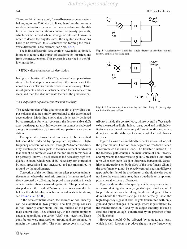
Fig. 8 Accelerometer simplified single degree of freedom controlloop: G is the electrostatic gain

Fig. 9 K2 measurement technique by injection of high frequency sig-nal inside the control loop

tributors inside the control loop, whose overall effect needsto be measured in-flight. Indeed, on-ground and in-flight lev-itations are achieved under very different conditions, whichdo not warrant the stability of a number of electrical charac-teristics.

Figure 8 shows the simplified feedback and control loop ofthe proof masses. Each of the 6 degrees of freedom of eachaccelerometer has such a loop. The transfer function G inthe feedback path contains the main source of non-linearityand represents the electrostatic gain. G presents a 2nd-orderterm whenever there is a gain difference between the capac-itive configurations on both sides of the proof mass. Shouldthe proof mass e.g., not be exactly centred, causing differentgaps on both sides of the proof mass, or should the electrodesnot have the exact same area, then a quadratic term appears,proportional to these differences.

Figure 9 shows the technique by which the quadratic termis measured. A high-frequency signal is injected in the controlloop of the accelerometer along the desired degree of free-dom. Should the electrostatic gain G be perfectly linear, thehigh-frequency signal at 100 Hz gets transmitted with onlygain and phase changes in the loop, where it gets filtered bythe transfer function H and by the output circuitry. In such acase, the output voltage is unaffected by the presence of the100 Hz signal.

However, should G be affected by a quadratic term,which is well- known to produce signals at the frequencies

123



Fig. 10 Timeline of output modulation, as a function of the high fre-quency signal injected in the accelerometer control loop, in presence ofa quadratic term in the electrostatic gain

corresponding to the sum and differences of the frequenciespresent in the input, a signal at DC (zero frequency) and at200 Hz will appear. The DC signal will find its way to theaccelerometer output and is thus detectable. The 200 Hz sig-nal, as well as the 100 Hz, is filtered and are not seen atthe output. By creating a series of high-frequency pulses, asshown in Fig. 10, a modulation appears at the output of theaccelerometer, which—signed—amplitude is proportional tothe quadratic term. The period of the pulses is 20 s, to givea signal in the middle of the measurement bandwidth, i.e.,50 mHz.

To nullify a given quadratic term, the proof mass posi-tion (i.e., the position which the feedback and control looptries to achieve) is slightly changed. As explained earlier,by doing this, the relative distance to the electrodes on bothsides of the proof mass is changed, which causes a gain dif-ference, and thus a change of the quadratic factor. In thismanner, the overall quadratic term can be compensated andreduced to a sufficiently small value. The first measurementsof the quadratic term, also called K2 factor, were performedabout 2 months after launch, while the spacecraft altitudewas being decreased. These measurements were thus notperformed under drag-free conditions, but under accelera-tion due to atmospheric drag. The first values are given in thethird column of Table 2.

The quadratic terms were compensated and measuredagain three times. However, the last measurement took placeunder drag-free conditions and did not give the expectedresults. The conclusion was drawn that there is a non-linearitywhich is a function of the average acceleration experiencedby the accelerometer. For this reason, the procedure wasrepeated under drag-free conditions. The final K2s obtainedafter the last iterations are shown in the last column of Table 2.The quadratic terms along the less-sensitive axes were alsomeasured to confirm the hypothesis that they are negligiblealready from construction. The results are in agreement withthe hypothesis. They are shown in Table 3.

Some tests were performed to further consolidate the con-clusion that the quadratic terms had been adequately nulli-

Table 2 Results of the first measurements of the K2 factors, and thefinal values after adjustment

ASH Axis (S/C frame) Initial FinalK2 (s2/m) K2 (s2/m)

1 x −287.6 −1.1

1 z −323.0 3.3

2 x −196.3 −3.4

2 y 81.5 0.0

3 x 570.5 −0.4

3 z 263.5 −0.4

4 x −685.2 0.9

4 z −445.8 1.9

5 x −165.3 2.3

5 y −571.0 0.1

6 x −93.7 1.0

6 z 588.9 1.4

ASH denotes the accelerometer sensor head

Table 3 K2 factors measured along the less sensitive axes

ASH Axis (S/C frame) K2 (s2/m)

1 y −0.3

2 z −0.7

3 y −0.4

4 y 0.4

5 z 0.5

6 y −0.2

ASH denotes the acceleromter sensor head

fied. The K2 values were changed several times to verifythat no noise attenuation could be obtained with differentadjustments. Best fit computations were also performed toattempt to identify, in the accelerometer noise, signatureswhich would correspond to the square of the accelerations.The conclusion of these investigations is that the K2 factorshave been adequately compensated.

4.3.2 Characterisation of relative parameters betweenaccelerometers

After adjustment of the quadratic terms, each accelerometeris assumed to have a linear response. This is however notsufficient to retrieve accurately the gravity gradients. WhileFig. 6 gives the nominal position and orientation of the sixaccelerometers, the real accelerometers differ from the idealones according to the following model:

– The position of the accelerometer: three coordinates– The direction of each sensitive axis: 3 × 2 angles– The responsivity of each sensitive axis: three scale

factors.

123



Fig. 11 The 12 parameters describing an accelerometer, illustrated foraccelerometer one

The 12 parameters describing an accelerometer are shownin Fig. 11.

The gradiometer counts six accelerometers and is thusmodelled as 6 × 12 = 72 parameters. The second step of thein-flight calibration consists in retrieving these parameters,from which the calibration matrices to be used in the nominalprocessing chain are deduced. The principle of this retrieval isto shake the spacecraft with high levels of linear and angularaccelerations, making them much more significant than thegravity gradient signals, and to find the gradiometer parame-ter values which remove from the gravity gradient measure-ments any trace of these applied accelerations. Furthermore,star tracker and gradiometer angular rate measurements dur-ing this shaking are also compared, to deduce the absolutescale factor of the gradiometer. Shaking of the spacecraft isachieved along the flight direction (x-axis) with a modulationof the ion thrust, while the five other degrees of freedom areexcited with the gradiometer calibration device (GCD). TheGCD consists in two sets of four cold gas thrusters, firing inthe yz plane, the sets being at both extremities of the space-craft. The pseudo-random time series used in the activationof the thrusters are meant to generate signals in all degreesof freedom ranging from 50 to 100 mHz , where gravity gra-dients have very low-amplitude. They also aim at achievingangular accelerations near 1.3 mHz for the angular rate com-parison. On one hand, modulation of the ion thrust with finesteps manages to achieve a spectral density well localizedbetween 50 and 100 mHz. On the other hand, with the coldgas thrusters being limited to on–off operation, amplitudemodulation is not possible. The desired spectral densitiescan only be approximated by a combination of frequency andduty cycle modulations. The results are illustrated in Fig. 12.

The shaking is also performed to ensure that the threeangular and three linear accelerations are weakly correlated.It should not be possible to approximate one of the acceler-ations as a linear combination of the five others. In this way,each of the six accelerations has a unique signature which willallow its identification in the gradiometer output products.

Fig. 12 Linear (positive side) and angular (negative side) accelerationspectral densities during shaking of the spacecraft. x-, y- and z-axescorrespond respectively to red, green and blue curves

Assuming that during shaking the accelerometer outputs aredominated by linear and angular accelerations, i.e., neglect-ing centrifugal accelerations and gravity gradients, the out-puts provide a lot of redundancy. Since only six accelerationshave to be identified, and since the gradiometer provides 18measurements, there are 12 redundant equations which canbe used to provide information about gradiometer parame-ters. With an ideal gradiometer, i.e., with all accelerometershaving the same scale factor in all directions, and being per-fectly aligned, the following quantities, which are obtainedthrough a linear combination of measurements, should benull:

– 6 diagonal and off-diagonal gravity gradient terms– 6 differences of linear acceleration estimates between

accelerometer pairs.

With the notation used in Sect. 4, they would be writtenas:

ad,14,x = 0,

ad,14,y + ad,25,x = 0,

ac,14,x − ac,25,x = 0,

ac,25,y − ac,36,y = 0,

ad,25,y = 0,

ad,14,z + ad,36,x = 0,

ad,14,x − ac,36,x = 0,

ac,36,z − ac,14,z = 0, (13)

ad,36,z = 0,

ad,25,z + ad,36,y = 0,

123



ac,25,y − ac,14,y = 0,

ac,36,z − ac,25,z = 0.

Should any of the 72 parameters of the gradiometer not havethe nominal value, i.e., should any scale factor be differentfrom the others, or a sensitive axis not be perfectly aligned,at least one of the 12 quantities above would not be equal tozero. This means that a residual would appear, equal to a lin-ear combination of the six accelerations acting on the space-craft. The coefficients of this linear combination are foundby a best fit algorithm, i.e., multiple linear regression. Thus,there are 6×12 = 72 equations linking the residuals obtainedfrom the 12 redundant equations to the six accelerations act-ing on the gradiometer, as a function of the 72 gradiometerparameters. They have been obtained first by numerical mod-elling of the gradiometer, see Lamarre (2008), but have nowbeen derived analytically. In fact, in linear approximation,there are only 69 equations, since an angular accelerationabout a given axis cannot create a residual on the in-linegravity gradient term along the same axis.

To give a simple example, assume that the scale factorsk1X and k4X of accelerometers 1 and 4, in the x direction, arenot equal. Then, it is clear that the in-line gravity gradientVxx along x will not give zero if computed as the differ-ence between the readings of the two linear accelerations ofthese accelerometers in the x direction. A residual of the xlinear acceleration ax acting on the gradiometer will appear,proportional to the difference in scale factors. This can beexpressed mathematically as:

a1x = k1x ax , a4x = k4x ax , (14)

and

Vxx ∼= (a1x − a4x )

Lx= (k1x ax − k4x ax )

Lx= ax (k1x − k4x )

Lx.

(15)

where Lx is the baseline of the pair of accelerometers oneand four. It should be noted that in contrast with usual char-acterisation methods, where a known source of input signalis used to calibrate a given instrument, here the input signalsare not known and are estimated by the gradiometer itself.The measurements of the six accelerometers are used both toestimate the six accelerations acting on the gradiometer, aswell as the 12 residual terms. This is possible since the gradi-ometer is already well-aligned, with scale factors sufficientlysimilar.

In addition to the 69 residual equations given above, a fewadditional ones have to be added:

– The average scale factor of the gradiometer is unity (1equation). This is because it is not possible for the gradi-ometer to retrieve its own scale factor. The absolute scalefactor of the gradiometer will be retrieved in a second step

by comparing the angular rates between gradiometer andstar tracker.

– The average position and orientation of the gradiometeris nominal (6 equations). Again, it is not possible for thegradiometer to retrieve its own position and orientation.Position and orientation are well-controlled by manu-facturing and are not required to be known anyhow to abetter accuracy in-flight.

– The distances between accelerometers of the same pairare equal to the values measured on-ground (3 equa-tions). These quantities, also called the baselines, can-not be evaluated in-flight, because the equation systembecomes underdetermined. Either the baselines or thescale factors can be retrieved, but not both. The base-lines have been measured on-ground to 100 ppm (50 µm)accuracy, which is sufficient.

– The angles between the sensitive axes of the same accel-erometer are perpendicular to within 20 µ rad (18 equa-tions). This constraint, given by manufacturing accuracy,is implemented as an orthogonality condition, with a low-weight.

The above equations are used in the following iterativemanner:

1. Initial guess of gradiometer parameters2. Estimation of accelerations acting on the gradiometer3. Computation of residuals4. Multiple regression of acceleration coefficients inside

residuals5. Retrieval of gradiometer parameters by inversion of

equations6. Check of convergence criteria. Stop or repeat from 2.

The above retrieval method, to be complete, is also com-prised an estimation of the centrifugal accelerations, whichare subtracted from the relevant residuals prior to the multipleregression. The computation of the centrifugal accelerationsrequires a combination of angular rates estimations from thestar tracker and the gradiometer, in the spectral domain, priorto squaring. The star tracker provides an excellent angularrate estimates at low-frequency, while the gradiometer pro-vides them with better accuracy in the measurement band-width, see the following Sect. 4.3.3.

4.3.3 Determination of the absolute scale factor

Since the gradiometer itself cannot determine its own scalefactor, some information needs to be provided externally. Anabsolute point of comparison is provided by the star tracker.Since the latter knows the star position with excellent abso-lute accuracy, and since elapsed time is also very preciselymeasured, a star tracker can provide very accurate angular

123



rates. The gradiometer being also able to provide angular rateestimates by integration of angular accelerations, the com-parison of angular rates allows to retrieve the absolute scalefactor of the gradiometer.

As explained earlier, when discussing the retrieval of cen-trifugal accelerations, the star tracker provides good angularrates at low-frequency, while the gradiometer has best sensi-tivity in the measurement bandwidth. Comparison of angularrates at low- or high-frequencies is not possible as it wouldyield very poor signal to noise ratio.

An intermediate bandwidth has to be found where bothinstruments provide sufficiently accurate estimates. For thisreason, and because of constraints due to spacecraft controland the presence of stray signals, it was decided to angu-larly shake the spacecraft near 1.3 mHz. This is illustrated inFig. 12.

The best fit between the angular rates of both instrumentsis performed in a 1 mHz bandwidth centred at 1.3 mHz. Themodelling assumes the following:

– The star tracker provides the rates in an orthogonalreference frame

– The star tracker has unity scale factor– The gradiometer provides the rates in an orthogonal

reference frame– The gradiometer does not have unity scale factor– The gradiometer scale factors along the three axes are

the same– The gradiometer frame is rotated with respect to the star

tracker frame.

This can be described as:

ωg = k · R · ωs (16)

where ωg is the vector of gradiometer estimated angular rates,k is the absolute scale factor of the gradiometer, R is the rota-tion matrix between gradiometer and star tracker, ωs is thevector of star tracker estimated angular rates.

The best fit retrieves the absolute scale factor k and therotation matrix R. The latter is in fact not further used inthe processing of gravity gradients, since the orientation ofthe gradiometer is already sufficiently well known by man-ufacturing and verification on-ground.

Retrieving the absolute scale factor from the compar-ison can be performed on a single star tracker or betteron a combination of star trackers. In case only one startracker would be available, the accuracy of the method canbe improved by removing the orbital harmonics from theangular rate estimations. This has to be performed in bothstar tracker and gradiometer derived angular rates, to ensureconsistency of the comparison. Figure 13 shows the filternormally used to keep the desired comparison bandwidth,

Fig. 13 Superimposition of the filter used for angular rate comparisonand of multiples of the orbital frequency

Fig. 14 Absolute scale factor retrieved values for all shakings per-formed since launch. The red, green, and blue curves correspond to val-ues obtained respectively with STR 1 only, STR 2 only or STRV data.The crosses and the circles identify the retrievals performed respectivelywith and without filtering of orbital harmonics

superimposed on it the orbital harmonics. Twelve harmonicsare included in the useful signal and should be removed.

Figure 14 shows the results of absolute scale factor retri-evals performed on the data obtained from the six shakingperiods conducted since the beginning of the mission. Sha-kings number 1 and number 2 were conducted during thecommissioning phase. The more relevant shakings number3 to number 6 were conducted in the measurement phasein a stable gradiometer configuration. The plots show theretrievals from STR 1 data or STR 2 data only, and also fromthe combination of two STRs, which is coined the virtualstar tracker STRV. Plots also include the retrievals with andwithout removal of orbital harmonics. The average value ofall retrieved scale factors has been subtracted to ease thecomparison.

123



It can be deduced that (1) a combination of star trackersseems to provide more accurate estimates and (2) filtering oforbital harmonics should be used whenever only one STR isavailable.

4.3.4 Mapping of the in-flight calibration parametersto the inverse calibration matrix

The inverse calibration matrix or ICM is defined as the matrixthat transforms the sensed quantities to the true ones, see Eqs.(17–19). The underlying logic is to imagine a matrix, thecalibration matrix or CM, which would describe the relationbetween the true quantities and the sensed ones. In order toobtain the true quantities from the measured ones, one needsto derive the inverse of this matrix, the inverse calibrationmatrix.

The method for the derivation of the relative parametersdescribed in Sect. 4.3.2 is not identical to the algorithm thatis implemented in the ground segment at ESRIN, as it waselaborated close to the GOCE launch and thus could not beincorporated in time. The main difference lies in the factthat the method implemented in the ESRIN ground segmentdetermines only 54 parameters out of the 72 parameters thein-flight shaking provides, thus that have to be reduced.

This is possible because, from manufacturing andon-ground verification, the average centre positions and ori-entations of the accelerometer pairs, and the errors on thebaselines, are sufficiently small to be ignored in the post-processing. Here is an example with the pair of accelerome-ters one and four, which parameters are shown in Table 4 asaverage and difference of accelerometers, i.e., common anddifferential parameters.

Pursuing with the example, the common positions$pc14x ,

$pc14y , and $pc14z are ignored for the computation of cal-ibration matrices. The differential position $pd14x , in factequal to half the baseline Lx , is taken into account and com-bined with the scale factors $k. The other differential posi-tions $pd14y and $pd14z are also taken into account andcombined with the misalignments %.

Table 4 Format of the 24 parameters describing the pair of accelerom-eters one and four

Common Differential

⎡

⎢⎢⎢⎣

$kc14x θc14xy θc14xz

θc14yx $kc14y θc14yz

θc14zx θc14zy $kc14z

$pc14x $pc14y $pc14z

⎤

⎥⎥⎥⎦

⎡

⎢⎢⎢⎣

$kd14x θd14xy θd14xz

θd14yx $kd14y θd14yz

θd14zx θd14zy $kd14z$pd14x $pd14y $pd14z

⎤

⎥⎥⎥⎦

Only differences with respect to the nominal (ideal) parameters arekept. The parameters appear as average (common) parameters of thetwo accelerometers and as the difference (differential) of the parame-ters, divided by two

Fig. 15 Trace (black) and individual diagonal gravity gradient (red,green and blue) performance for uncalibrated gradiometer (with non-linearity correction applied). Note that <30 mHz the noise is not visibleon individual gravity gradient curves, since signal dominates

The calibration matrices to be applied to the uncalibratedcommon and differential mode accelerations in the EGGnominal processor can thus be defined as:

ICMi j =(

Ci j Di jDi j Ci j

), (17)

Ci j =

⎛

⎝$kci j x θci j xy θci j xzθci j yx $kci j y θci j yzθci j zx θci j zy $kci j z

⎞

⎠ , (18)

Di j =

⎛

⎝$kdi j x θdi j xy θdi j xzθdi j yx $kdi j y θdi j yzθdi j zx θdi j zy $kdi j z

⎞

⎠ . (19)

The parameter i j takes on values of 14, 25 or 36 as it denotesthe accelerometer pair the matrix has to be applied to.

The impact of calibration on the quality of the data can beseen in Figs. 15 and 16. The trace and the individual diago-nal gravity gradients Vxx and Vyy see an enormous improve-ment, while Vzz turns out to be quite good from the start.Only a small reduction of the noise level on Vzz is visiblenear 40 mHz. Improvement at lower frequency is hidden bythe gravity gradient signal itself.

Inspection of the gradiometer parameters retrieved overthe six shakings performed to date reveal that the gradiom-eter mechanical stability is excellent. Internal alignment isstable to a few µ rad. On the other hand, some of the scalefactors experience some change. This is illustrated in Figs. 17and 18, where the in-line differential scale factors of the pairof accelerometers one and four and the pair of accelerom-eters two and five seem to drift in a constant manner. Thisbehaviour could eventually be taken into account to improve

123



Fig. 16 Trace (black) and individual diagonal gravity gradient (red,green and blue) performance for calibrated gradiometer (with non-linearity correction applied). Note that <30 mHz the noise is not visibleon individual gravity gradient curves, since signal dominates

Fig. 17 Plot of retrieved values for the in-line differential scale fac-tors of the pair of accelerometers one and four. The x-axes of the plotsindicate the shaking number, while on the curves, the circles indicatingthe data points have been moved horizontally to correctly represent theelapsed times between calibrations

the accuracy of the calibration matrices by some form ofinterpolation between shakings.

4.4 EGG nominal processor description

The basic measurements of the gradiometer are the con-trol voltages applied to the eight electrodes surroundingeach proof-mass. The purpose of the EGG nominal pro-cessor is to transform these measurements into gravity gra-

Fig. 18 Plot of retrieved values for the in-line differential scale fac-tors of the pair of accelerometers two and five. The x-axes of the plotsindicate the shaking number, while on the curves, the circles indicatingthe data points have been moved horizontally to correctly represent theelapsed times between calibrations

dients. The gravity gradients are contained in the productEGG_NOM_1b that contains all datasets relevant for sci-entific processing.The main algorithm steps are describedhereafter:

4.4.1 Voltage to acceleration conversion

Before the voltages can be converted to acceleration mea-surements, they have to be corrected for several effects whosecharacteristics can be determined on-ground and are assumedto be stable during flight. Each correction corresponds toa processing step applied in-flight in the instrument, seeFig. 19, which better explains the output chain of Fig. 8:

– correction of the effect of the accelerometer transferfunction and the read-out function (RO). Both gain andphase are corrected.

– correction of the effect of the analog to digital converter(ADC) non-linearities. The non-linearities are correctedby application of a third-order polynomial.

– correction of the effect of the science filter. This filter isa low-pass Butterworth filter and is applied before thedata are down-sampled from the native 10 Hz samplingto 1 Hz. It introduces errors both in phase and in gainwhich are corrected.

All corrections for transfer functions/filters are implementedas convolutions in the time domain.

123



Fig. 19 Detailed view of the accelerometer readout chain. RO read outfunction, ADC analog to digital converter, SF science filter

After these corrections, the eight electrode voltages figuresare converted into six accelerations, one for each degree offreedom through multiplication with a recombination matrix,which also applies appropriate electrostatic gains that trans-form from control voltages Vci to accelerations:

⎛

⎝ai,1ai,5ai,6

⎞

⎠ = Ax

⎛

⎜⎜⎝

Vci,1Vci,2Vci,3Vci,4

⎞

⎟⎟⎠ (20)

⎛

⎝ai,2ai,3ai,4

⎞

⎠ = Ayz

⎛

⎜⎜⎝

Vci,5Vci,6Vci,7Vci,8

⎞

⎟⎟⎠ (21)

where

Ax = 14Gx

⎛

⎝+Ges,i,1 +Ges,i,2 +Ges,i,3 +Ges,i,4+Ges,i,13 +Ges,i,14 −Ges,i,15 −Ges,i,16−Ges,i,17 +Ges,i,18 +Ges,i,19 −Ges,i,20

⎞

⎠

(22)

and

Ayz = 12G yz

⎛

⎝+Ges,i,5 +Ges,i,6 0 00 0 +Ges,i,7 +Ges,i,8−Ges,i,11 +Ges,i,12 +Ges,i,9 −Ges,i,10

⎞

⎠

(23)

In the above equations, the principle how the linear accel-erations (ai,1−3) and the angular accelerations (ai,4−6) arederived is visible: the sum of the measurements of theelectrode pairs divided by the number of pairs give the lin-ear accelerations, the parameters Gx,yz, Ges,i, j scale volt-ages to accelerations. The angular accelerations, however,are derived by forming the differences of the electrode pairmeasurements, e.g., the four pairs of the x axis are used toderive the angular acceleration about the y and z axis, c.f.Fig. 7. The final processing step consists in the derivationof the common and differential mode accelerations for theaccelerometer pairs 14, 25, 36, according to Eqs. (11) and(12) using the linear accelerations ai,1−3.

4.4.2 Proof mass acceleration retrieval

In this processing step, the uncalibrated common and dif-ferential mode accelerations are calibrated by applying theinverse calibration matrices defined in Sect. 4.3.4:

(a′

c,i ja′

d,i j

)

= ICMi j ·(

ac,i jad,i j

), (24)

where a′c,i j are the calibrated common mode accelerations,

a′d,i j are the calibrated differential mode accelerations

From the calibrated differential-mode accelerations, thethree angular accelerations of the gradiometer about the x, y,z axes of the GRF are obtained:

ωx = −a′

d,36,y

Lz+

a′d,25,z

L y(25)

ωy = −a′

d,14,z

Lx+

a′d,36,x

Lz(26)

ωz = −a′

d,25,x

L y+

a′d,14,y

Lx. (27)

4.4.3 Angular rate reconstruction

The purpose of the angular rate reconstruction is twofold: asa first objective, the angular rates (ωx ,ωy,ωz) are computedin the GRF, as a second objective the attitude quaternionsdefining the orientation of the gradiometer with reference toan inertial frame are derived. This is achieved by merging themeasurements of the gradiometer and the star tracker, follow-ing the so called principle of hybridization: the quality of thegradiometer measurements is better than the quality of thestar tracker measurements in a certain frequency band andvice versa, i.e., up to a the so-called hybridization frequencyinformation from the star tracker is used mainly, whereasfor higher frequencies, the information of the gradiometer isused. This frequency has different values for each axis. Asan example Fig. 20 shows the hybridization frequency fory-axis of the gradiometer reference frame.

The combination is achieved by using a Kalman filterapproach including a prediction and correction step: thegradiometer derived angular accelerations are integrated toderive angular rate variations to propagate the attitude qua-ternion. The propagated attitude quaternion is then comparedwith the measured one from the star tracker. From the differ-ence a correction both for angular rate and attitude is derivedby applying a static gain matrix that has been derived frompre-launch performance measurements. The parametrizationof the state vector also contains parameters describing theangular acceleration error in terms of error drift caused bythe bias in the angular accelerations and its drift rate besides

123



Fig. 20 Angular rate reconstruction hybridization frequency, y-axisGRF, shown for angular accelerations

the angular rates and the attitude quaternion. The integrationof the gradiometer angular acceleration is conducted usinga Lagrange interpolator. The overall scheme is shown inFig. 21.

A drawback of the implementation is that in case of datagaps the filter has to be reinitialized, which causes data qual-ity degradation for about half a day of data due to the long

warm up time of the filter. Currently, the data gap thresh-old for a reinitialization of the filter is set to 5 s, both forgaps in the gradiometer and star sensor data, which in linewith the algorithm specifications. Gaps that are shorter thanthe threshold are filled via spherical interpolation for the starsensor quaternions and via a spline interpolation on the levelof control voltages for the gradiometer measurements.Another drawback of the algorithms is that individual prod-ucts have to processed sequentially, as the last Kalman filterstate has to be passed on to the following product, whichprevents the parallelization of the data processing.

4.4.4 Gravity gradient tensor computation

As now both angular rates and calibrated differential modeaccelerations are available, the six independent componentsof the GGT in the GRF are obtained as:

Vxx = −2a′

d,14,x

Lx− ω2

y − ω2z ,

Vyy = −2a′

d,25,y

L y− ω2

x − ω2z , (28)

Vzz = −2a′

d,36,z

Lz− ω2

x − ω2y .

Fig. 21 Angular ratereconstruction processingschema

123



and:

Vxy = −a′

d,14,y

Lx−

a′d,25,x

L y+ ωxωy,

Vxz = −a′

d,14,z

Lx−

a′d,36,x

Lz+ ωxωz, (29)

Vyz = −a′

d,25,z

L y−

a′d,36,y

Lz+ ωyωz .

where a′d,i j,k are the calibrated differential mode accelera-

tions and ωk are the the angular rates.

5 L1b processing status and performance assessment

GOCE has been collecting data since its launch on18/03/2009 uninterruptedly but for two events:

1. February 12, 2010: the switchover to CDMU B causinga gap of 19 days.

2. July 8, 2010: telemetry module anomaly causing a gapof 55 days.

During operations the instrument performance is dailymonitored and the trace PSD is taken as an overall L1bdata quality indicator. The PSDs of the diagonal componentsof the gravity gradients tensor (see Eq. 28) for 2 days ofoperations with the derived trace PSD are reported inFig. 22.

The flat part of trace PSD is at about 20 mE/√

Hz above thespecification in the upper part of the measurement bandwidthdue to the noisier component Vzz of the gravity gradientstensor, whose underlying cause is currently not understood.But it is assumed that the L1b processing is not causing theincrease in the noise level, which has been confirmed by theinstrument manufacturer.

The product performance is not uniform in time, it ismainly influenced by the events reported below:

– Change of the used STR for the attitude control.– Beam out events.

5.1 Change of the used STR for the attitude control

A clear effect of performance worsening in the lower part ofthe measured bandwidth occurs when the STR1 is used in theloop for the attitude control. The effect is shown in Fig. 23(based on 2 days of operations). Since November 2009, 75days of operation are affected by the use of STR 1 for theattitude control.

Fig. 22 Diagonal components (Vxx, Vyy and Vzz expressed inmE/

√Hz) and the derived trace PSD of the gravity gradients tensor

PSD in GRF reference frame from EGG_GGT_i dataset contained inEGG_NOM_1b product

Fig. 23 Trace PSD expressed in (mE/√

Hz) using different STR cam-era head units

5.2 Beam out events

A beam out is caused by a short-circuit of the ion enginebackplate and the accelerator grid, see Tato et al. (2004),which causes a sudden loss of thrust. The effect of a beamout event in the common mode acceleration is reported inFig. 24.

This oscillation enters the gradients time series notablyin the Vxx component. Since November 2009, 21 beam outevents occurred.

123



Fig. 24 Beam out event on 04/04 affected the Common mode acceleration (see Eq. 13) component 14X expressed in (m/s2)

6 Conclusions and outlook

The L1b processing steps for the STR, SSTI and EGG havebeen described. Concerning the STR and the SSTI, no majorweaknesses of the applied algorithms have been identified,they seem to be stable both in terms of nominal processing,as well as calibration (only applicable to the SSTI). For thegradiometer, however, areas of potential improvement havebeen found, that seem worthwhile to be implemented. Theincreased noise level of the trace for the upper part of the mea-surement bandwidth seems not to be related to the processingapplied to the raw data. Concerning the application of the cal-ibration results of the EGG, a linear drift has been observedin the differential mode scale factors, that is currently nottaken into account in the processing algorithms. The drifte.g., in the in line differential scale factor of pair 2,5 affectsthe Vyy gradient significantly, see e.g., Siemes (2011). Thecurrent implementation uses an updated ICM always fromthe time of the calibration onwards until the next calibration.An updated processor version could consider this drift bylinearly interpolating between two ICM. Clearly this wouldhave an impact on the availability of the final EGG product,as it could only be generated after the time frame betweentwo satellite shakings. In addition, three other weaknesseshave been identified: (1) the gradient quality depends on theSTR that is used in the processing, (2) already gaps of more

than 5 s cause data loss of half a day due to the warm-upeffect of the Kalman filter and (3) the processing of indi-vidual products is sequential as the Kalman filter parametershave to be passed on. In order to overcome the first weakness,a feasible solution could be to create a ‘virtual’ star trackerby combining the measurements of the two star trackers thatare available, in future it may also be possible to downlinkadditionally the data from the third star tracker. Concerningthe second point, an update of the angular rate reconstruc-tion algorithm seems feasible: the Kalman filter currentlyimplemented uses only past measurements coming from real-time applications, which makes no sense as the GOCE dataare anyway post-processed and there is no need for (near)real-time products. By using a symmetric filter one couldreduce the filter length to about 1 orbit. The possibility toresolve the third point depends on the chosen filter toimplement the angular rate reconstruction, but using e.g.,a FIR filter realized as a convolution in the time domain, theindividual gradiometer products could be processed indepen-dently from each other.

Appendix: GOCE L1b products overview

A detailed product description can be found in ESA (2008).

123



Table 5 GOCE L1b EGG data product overview

Product name Description

EGG_NOM_1b Measurement data sets:

EGG_TCT_1i:

time correlation table

EGG_CTR_1i:

gradiometer control voltages

EGG_NLA_1i:

uncalibrated linear/angular acc

EGG_NCD_1i:

uncalibrated commin/differential mode

EGG_NGA_1i:

uncalibrated gradiometer ang. acc

EGG_CCV_1i:

corrected control voltages

EGG_CCD_1i:

calibrated common/differential mode

EGG_CGA_1i:

calibrated gradiometer ang. acc

EGG_GAR_1i:

gradiometer angular rates

EGG_IAQ_1i:

inertial attitude quaternions

EGG_GGT_1i:

gravity gradient tensor in GRF

EGG_GIM_1i:rotation matrix GRF to IRF

Table 6 GOCE L1b SSTI data products overview


SST_NOM_1b Measurement data sets:

SST_TCT_1i:time correlation table

SST_RNG_1i:raw code and phase measurements

SST_NAV_1i:on board navigation solution

SST_PRM_1i:code measurements, corrected for ICB

SST_CPM_1i:phase measurements, corrected for IFB

SST_IFB_1i:IFB correction values

SST_CPN_1i:estimated noise for code measurements

SST_CPF_1i:phase measurements flagged for outliers

SST_PRF_1i:code measurements flagged for outliers

Table 6 Continued


SST_SRF_1i:smoothed code measurements

SST_PVT_1i:position, velocity and time solution

SST_GPS_1i:GPS satellites positions used for solution

SST_COV_1i:covariance information for solution

SST_RIN_1b This product contains the code andphase measurements of the SSTIcorrected for the inter-channel biasand the inter-frequency bias in theRINEX format

References

Cesare S, Sechi E, Catastini G (2008) Gradiometer ground processingalgorithm specification. GO-TN-AI-0067

Cesare S (2008) Performance requirements and budgets for the gradio-metric mission. GO-TN-AI-0027

Detoma E, Cesare S (2004) GPS receiver ground processing algorithmspecification. GO-SP-AI-0004

ESA (2008) L1b product user handbook. GOCE-GSEG-EOPG-TN-06-0137

Frommknecht B (2009) Detailed processing model for the EGG. GO-TN-IAPG-GS-0001

Frommknecht B (2009) Detailed processing model for the SSTI. GO-TN-IAPG-GS-0002

Hofmann B, Moritz H (2005) Physical Geodesy. Springer, Wien, NewYork

Jørgenson J (2004) Advanced stellar compass user’s manual. GO-DTU-MA-2001

Lamarre D (2008) Algorithm description: retrieval of gradiometerparameters. Version 2.0 draft

Marque J-P, Christophe B, Foulon B (2010) Accelerometers of theGOCE mission: return of experience from one year in orbit. ESASP-686, 2010

Rummel R (1985) Satellitengradiometrie. ZfV 6 242-257Scaciga L (2007) Data & Communication interface control document.

GO-IC-LAB-5000Siemes C (2011) Upgrade of the GOCE level 1b gradiometer process-

ing. In: 4th International GOCE User Workshop, MunichTato C, Palencia J, de la Cruz F (2004) The power control unit for the

propulsion engine of GOCE program. ESA SP-555

123


goce level 1b data processing

Documents