quality evaluation of goce gradients

Quality Evaluation of GOCE Gradients

Jürgen Müller, Focke Jarecki, Insa Wolf, and Phillip Brieden

1 Cross-Over Analysis

The first ESA Earth Explorer Core Mission GOCE (Gravity Field and Steady-State Ocean Circulation Explorer) entered the operational measurement phase inSeptember 2009. Before gravity field processing, the quality of the GOCE gradi-ents has to be assessed. Here, two procedures have been developed in Hanover,the mutual comparison and analysis of observed gradients in satellite track cross-overs and the application of terrestrial gravity data which are upward continuedand transformed into reference gradients for the GOCE observations. As shown inJarecki et al. (2006), comparison of the gravity tensor elements in satellite groundtrack cross-overs (“XO analysis”) offers a good opportunity to validate the gra-dients measured by a satellite gravity gradiometer. There, closed loop results arepresented, with accuracies fitting well into the margins of the overall GOCE gra-diometer performance. The radial tensor component can be reproduced with anaccuracy of better than 3 mE, just using the un-filtered measurements in correspond-ing track parts and a recent high-resolution geopotential model like the combinedGRACE/terrestrial model (e.g. EIGEN-GL04C, Förste et al., 2006). The XOs areidentified by a measurement oriented search algorithm (independent of the predictedorbit characteristics) resulting in the actual position of the ground track crossing.Gradiometer measurements and auxiliary data are interpolated into the position ofthe XO along each of the crossing orbit tracks. Gradient differences from differingorbit altitudes and orientations of the measurement reference frame are reduced byapplying the geopotential model (and auxiliary data). These closed loop tests show,that residual gradient differences in the XO can be assigned to measurement errors,as they should vanish in the absence of noise and systematic errors. Such noiseand systematic errors have been modelled for the integrated gradiometer (singlecomponents of the system, like specific accelerometers, are not treated separately)

J. Müller (B)Institut für Erdmessung, Leibniz Universität Hannover, 30167 Hannover, Germanye-mail: [email protected]

265F. Flechtner et al. (eds.), System Earth via Geodetic-Geophysical Space Techniques,Advanced Technologies in Earth Sciences, DOI 10.1007/978-3-642-10228-8_21,C© Springer-Verlag Berlin Heidelberg 2010

266 J. Müller et al.

by Koop et al. (2002), with model refinements by Denker et al. (2003), as

Vmeasij (t) = V real

ij (t)+V∗ij+o(t) V∗ij+Vij′t+

n∑k=1

ak cos (kωt)+bk sin (kωt)+ε(t). (1)

In the XOs, differences of the measured gradients are further investigated. Butnot all modelled systematic errors project into those XO differences according toEq. (2). Temporally constant or, due to the relation to a discrete point on the earthsphere, locally constant features Vij

∗ vanish. The first vanishes because of the rela-tive nature of this internal validation approach, the latter could also be characterisedas some kind of geographical signal (and therefore not as measurement error).Constant biases Vij

∗, which are not present in the whole time series investigatedo(t) �= const, can project into the XO differences. A linear trend Vij

′ projects lin-early (with the measurement time difference �tXO = t2 – t1 in the XO) into theinvestigated value �Vij

meas. Fourier harmonics ak cos(kωt) + bk sin(kωt) sum upto combined terms and are still present in the gradient differences. Contrary to thetrend (and polynomial parameters of higher degree) where only time differences�tXO show up, they carry absolute time information into the differences, modelledas t1 and t2. The noise parameter ε(t) represents the stochastic noise. Thus, thefollowing systematic parts of the gradients’ differences remain in the XOs:

�Vmeasij =

(o(t2)− o(t1)

)V∗ij + Vij

′ �tXO

+n∑

k=1ak(cos (kωt1)− cos (kωt2)

)+ bk(sin (kωt1)− sin (kωt2)

).

(2)

Consequently, the XO approach is (only) capable to detect three kinds of sys-tematic errors, namely linear trends (and polynomial drifts), Fourier-type periodicdisturbing effects and biases which are only present in short parts of the data (calledShort Term Biases). The latter may reach from single outliers (affecting just onespecial measurement) to larger portions of the data set under investigation.

In the following sections, it will be discussed if and under which conditions thosesystematic errors can be detected, and which approaches might be used to get robust,accurate and reliable results. The studies are shown for the tensor component Vzz,for the ease of formulation and readability, but similar results are achieved for theother diagonal and off-diagonal tensor components.

1.1 Short Term Biases

Biases which are not present in the whole data set (called sequential outliers) projectinto XO gradient differences in contrast to biases affecting the whole data set. In thefirst case there is some data left which can be considered as “reference data”. Theamount and the coverage (and, of course, the quality) of reference data is the maincriterion to decide, whether the detection of outliers and short term biases works: Onthe one hand, there has to be enough reference data to intersect with the erroneouspart of the track at all. On the other hand, shorter erroneous parts of the track (leavingmore correct reference data) might be hidden between the single XOs, especially

Quality Evaluation of GOCE Gradients 267

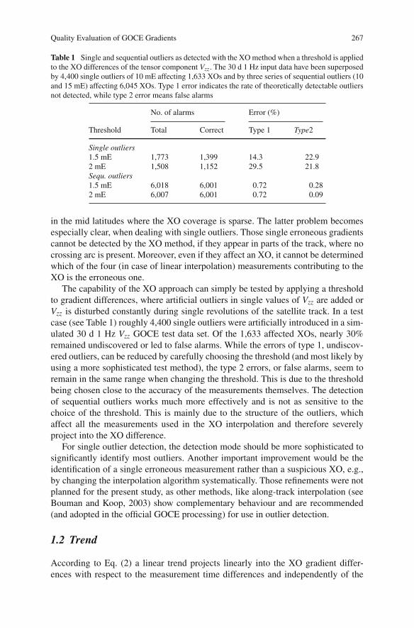
Table 1 Single and sequential outliers as detected with the XO method when a threshold is appliedto the XO differences of the tensor component Vzz. The 30 d 1 Hz input data have been superposedby 4,400 single outliers of 10 mE affecting 1,633 XOs and by three series of sequential outliers (10and 15 mE) affecting 6,045 XOs. Type 1 error indicates the rate of theoretically detectable outliersnot detected, while type 2 error means false alarms

No. of alarms Error (%)

Threshold Total Correct Type 1 Type2

Single outliers1.5 mE 1,773 1,399 14.3 22.92 mE 1,508 1,152 29.5 21.8Sequ. outliers1.5 mE 6,018 6,001 0.72 0.282 mE 6,007 6,001 0.72 0.09

in the mid latitudes where the XO coverage is sparse. The latter problem becomesespecially clear, when dealing with single outliers. Those single erroneous gradientscannot be detected by the XO method, if they appear in parts of the track, where nocrossing arc is present. Moreover, even if they affect an XO, it cannot be determinedwhich of the four (in case of linear interpolation) measurements contributing to theXO is the erroneous one.

The capability of the XO approach can simply be tested by applying a thresholdto gradient differences, where artificial outliers in single values of Vzz are added orVzz is disturbed constantly during single revolutions of the satellite track. In a testcase (see Table 1) roughly 4,400 single outliers were artificially introduced in a sim-ulated 30 d 1 Hz Vzz GOCE test data set. Of the 1,633 affected XOs, nearly 30%remained undiscovered or led to false alarms. While the errors of type 1, undiscov-ered outliers, can be reduced by carefully choosing the threshold (and most likely byusing a more sophisticated test method), the type 2 errors, or false alarms, seem toremain in the same range when changing the threshold. This is due to the thresholdbeing chosen close to the accuracy of the measurements themselves. The detectionof sequential outliers works much more effectively and is not as sensitive to thechoice of the threshold. This is mainly due to the structure of the outliers, whichaffect all the measurements used in the XO interpolation and therefore severelyproject into the XO difference.

For single outlier detection, the detection mode should be more sophisticated tosignificantly identify most outliers. Another important improvement would be theidentification of a single erroneous measurement rather than a suspicious XO, e.g.,by changing the interpolation algorithm systematically. Those refinements were notplanned for the present study, as other methods, like along-track interpolation (seeBouman and Koop, 2003) show complementary behaviour and are recommended(and adopted in the official GOCE processing) for use in outlier detection.

1.2 Trend

According to Eq. (2) a linear trend projects linearly into the XO gradient differ-ences with respect to the measurement time differences and independently of the


Table 2 Statistics of estimated trend factors for all 475 ascending arcs from least-squares andfrom robust estimation on the basis of XO differences from different time spans

XOs withtracks from

Mean trend(mE/d)

Abs. error(mE) Std (mE/d)

Min trend(mE/d)

Max trend(mE/d)

30 days Least squares 6.7979 0.0005 0.0014 6.7033 6.9407Robust 6.7974 0.0000 0.0001 6.7967 6.7980

10 days Least squares 6.7994 0.0020 0.0330 6.6339 7.1368Robust 6.7974 0.0000 0.0001 6.7971 6.7978

1 day Least squares 6.7992 0.0018 0.0168 6.7742 6.9150Robust 6.7975 0.0001 0.0001 6.7972 6.7977

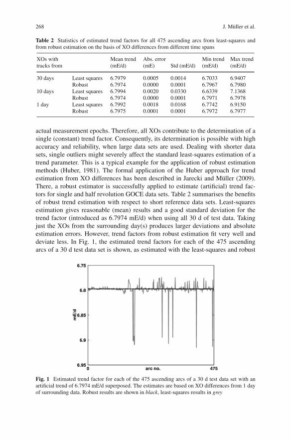
actual measurement epochs. Therefore, all XOs contribute to the determination of asingle (constant) trend factor. Consequently, its determination is possible with highaccuracy and reliability, when large data sets are used. Dealing with shorter datasets, single outliers might severely affect the standard least-squares estimation of atrend parameter. This is a typical example for the application of robust estimationmethods (Huber, 1981). The formal application of the Huber approach for trendestimation from XO differences has been described in Jarecki and Müller (2009).There, a robust estimator is successfully applied to estimate (artificial) trend fac-tors for single and half revolution GOCE data sets. Table 2 summarises the benefitsof robust trend estimation with respect to short reference data sets. Least-squaresestimation gives reasonable (mean) results and a good standard deviation for thetrend factor (introduced as 6.7974 mE/d) when using all 30 d of test data. Takingjust the XOs from the surrounding day(s) produces larger deviations and absoluteestimation errors. However, trend factors from robust estimation fit very well anddeviate less. In Fig. 1, the estimated trend factors for each of the 475 ascendingarcs of a 30 d test data set is shown, as estimated with the least-squares and robust

Fig. 1 Estimated trend factor for each of the 475 ascending arcs of a 30 d test data set with anartificial trend of 6.7974 mE/d superposed. The estimates are based on XO differences from 1 dayof surrounding data. Robust results are shown in black, least-squares results in grey


approach, using 16 XOs. While several least-squares estimates obviously sufferfrom outliers in the reference data, the robust estimates look smooth and correct.A change in trend factors would easily be observable in the timeline of arc-wiseestimates.

The long-term trend estimation assesses the overall coherence of the data set, butneglects time-variable physical effects on the measurements. Repeated determina-tion of trend factors for short parts of the data and their comparison is a fast and easymethod to monitor the behaviour of the measurement system. Robust trend estima-tion provides those features and will be applied in the GOCE project as part of thevalidation activities of the CalVal-Team (ESA, 2006).

1.3 Fourier Coefficients

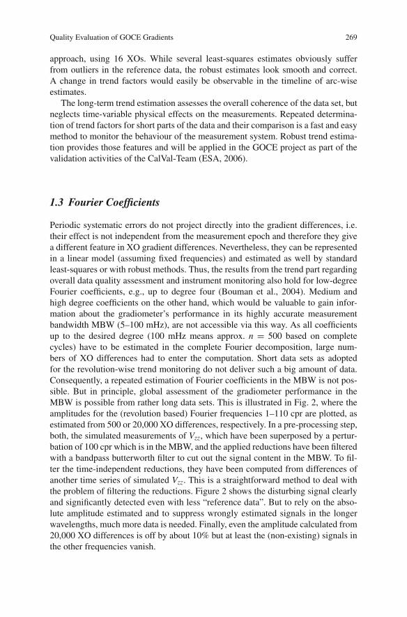
Periodic systematic errors do not project directly into the gradient differences, i.e.their effect is not independent from the measurement epoch and therefore they givea different feature in XO gradient differences. Nevertheless, they can be representedin a linear model (assuming fixed frequencies) and estimated as well by standardleast-squares or with robust methods. Thus, the results from the trend part regardingoverall data quality assessment and instrument monitoring also hold for low-degreeFourier coefficients, e.g., up to degree four (Bouman et al., 2004). Medium andhigh degree coefficients on the other hand, which would be valuable to gain infor-mation about the gradiometer’s performance in its highly accurate measurementbandwidth MBW (5–100 mHz), are not accessible via this way. As all coefficientsup to the desired degree (100 mHz means approx. n = 500 based on completecycles) have to be estimated in the complete Fourier decomposition, large num-bers of XO differences had to enter the computation. Short data sets as adoptedfor the revolution-wise trend monitoring do not deliver such a big amount of data.Consequently, a repeated estimation of Fourier coefficients in the MBW is not pos-sible. But in principle, global assessment of the gradiometer performance in theMBW is possible from rather long data sets. This is illustrated in Fig. 2, where theamplitudes for the (revolution based) Fourier frequencies 1–110 cpr are plotted, asestimated from 500 or 20,000 XO differences, respectively. In a pre-processing step,both, the simulated measurements of Vzz, which have been superposed by a pertur-bation of 100 cpr which is in the MBW, and the applied reductions have been filteredwith a bandpass butterworth filter to cut out the signal content in the MBW. To fil-ter the time-independent reductions, they have been computed from differences ofanother time series of simulated Vzz. This is a straightforward method to deal withthe problem of filtering the reductions. Figure 2 shows the disturbing signal clearlyand significantly detected even with less “reference data”. But to rely on the abso-lute amplitude estimated and to suppress wrongly estimated signals in the longerwavelengths, much more data is needed. Finally, even the amplitude calculated from20,000 XO differences is off by about 10% but at least the (non-existing) signals inthe other frequencies vanish.


Fig. 2 Fourier amplitudes (1–110 cpr) estimated from 500 (grey) and 20,000 (black) Vzz XO dif-ferences with standard least squares (dotted) and robust methods (solid lines). Measurement andreduction data have been filtered to cover the MBW. A superposed disturbing signal of 100 cpr isdetected significantly, even in case of sparse XO data while the lower frequencies are misfits (notethe logarithmic scale)

2 Accuracy Analysis of External Reference Gradientsin the Frequency Domain

To prove the planned accuracy level, the gradiometer measurements will be cali-brated and validated internally and externally. Internal calibration will be performedby industry and ESA. External evaluation is done by comparing measured gradientswith reference data, where we worked in the frequency domain, as it easily allows acomparison with the given baseline accuracy. Here, the highest accuracy level of thegradiometer within the MBW is 11 mE/

√Hz, valid for the sum of the main diagonal

components of the gravitational tensor (1 mE = 10–12 1/s2). We took this value asworst case assumption for single tensor components, too.

One strategy of an external evaluation includes the use of gravity data on groundupward continued to satellite altitude (e.g., Bouman et al., 2004; Denker, 2003;Pail, 2003; Wolf, 2007). The evaluation can only be applied regionally, becausesufficiently accurate ground data are only available for selected areas. Therefore,a global potential model, representing the long wavelength part, is introduced ina remove-restore procedure. The error estimation for the external reference data iscarried out empirically in a synthetic environment permitting closed-loop validationin all points.

2.1 Spectral Combination Method

In the present study, the radial tensor component Vzz is computed using integralformulas, see Wolf (2007) for the other five components. In the following the


tensor component Vzz is considered with respect to the disturbing potential T as Tzz.Applying the remove-restore technique residual gravity anomalies �gR = �gT –�gM as differences between the terrestrial gravity anomalies �gT and those from ageopotential model �gM are used in the computations. The resulting residual tensorcomponent T̂R

zz has to be restored using again the GPM (T̂Mzz ): T̂zz = T̂M

zz + T̂Rzz.

Integral formulas with spectral weighting are applied to combine regional ter-restrial gravity data with a geopotential model for the computation of the tensorcomponent based on the remove-restore procedure. For more theoretical detailssee Wolf (2007). The spectral weights are based on the error degree varianceinformation of the GPM and of the terrestrial gravity data.

2.2 Synthetic Data

The input data (�gT, �gM) and the output data (T[ij]) are based on a syn-thetic Earth model composed of a Digital Topography Model (DTM) and aGPM. Simulated noise is added to the input data. The ground-truth GPM(SYNGPM1300S) consists of the EIGEN-GRACE02S (n = 2. . .104, Reigberet al., 2005), the EGM96 (n = 105. . .360, Lemoine et al., 1998) and the GPM(n = 361. . .1,300, Wenzel, 1999). The characteristics of the synthetic scenariosare chosen based on a statistical accuracy estimation using least-squares esti-mation (Wolf, 2007). From the SYNGPM1300S, the test data sets are derived.The gravity anomalies �gM are based on the SYNGPM1300S up to a spheri-cal harmonic degree nmax = 360, the appropriate noise is generated accordingto the coefficients’ standard deviations of the SYNGPM1300S. For the terrestrialdata �gT, the complete synthetic model is used and different noise scenarios areinvestigated: 1 mGal uncorrelated (1UC), 1 mGal correlated (1C) and 5 mGalcorrelated (5C).

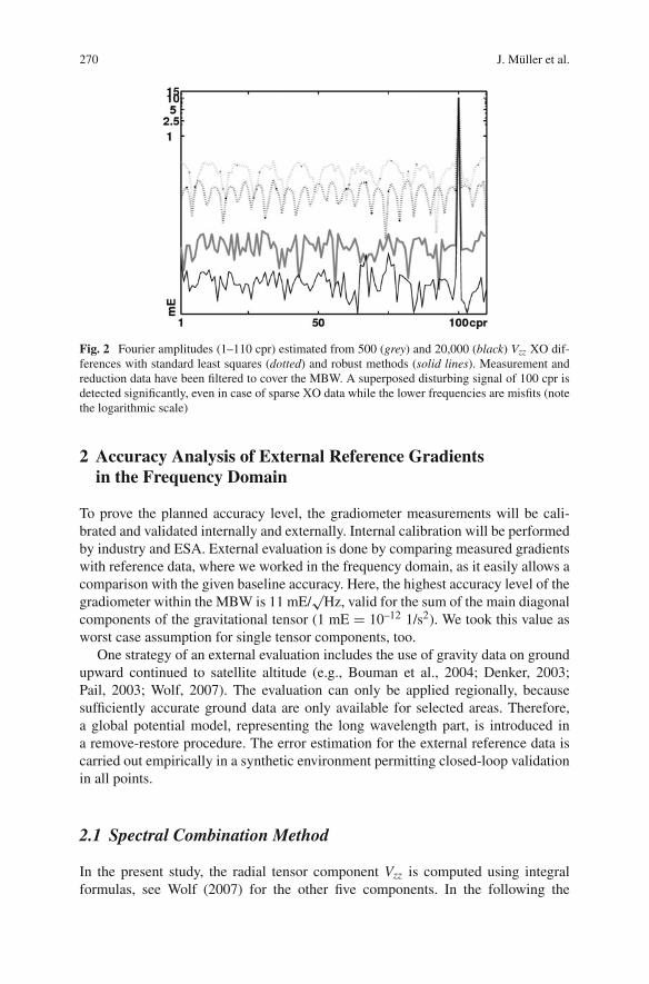
Fig. 3 A number of 26 tracksfrom a 29-days global data setcover the test area


The test area is located in Central Europe (Fig. 3), the data sets are computed ina 0.1◦ geographical grid. The spectral signal content of the synthetic data is limitedto a resolution of about 8′ (nmax = 1,300). The synthetic gravity data representgravity anomalies reduced from the gravitational effect of a residual terrain model(RTM reduction). The gravity anomalies �gT have a mean signal content of 10.07± 33.36 mGal, the tensor values 2,747.107 ± 0.187 E.

2.3 Closed-Loop Differences in the Frequency Domain

The differences between the tensor component values directly computed from theSYNGPM1300S and the values derived from the noisy synthetic gravity anomalies(�gM, �gT) are analysed in an inner area (marked in Fig. 3) to avoid edge effects.For the frequency domain analysis, the following steps are performed:

(a) computation of all tensor components in points of a three dimensional grid(spherical surfaces with a 6′ data grid; 5 km height difference between eachinterpolation level),

(b) interpolation into points of a simulated GOCE orbit (SCVII, 2000) using a cubicspline approach,

(c) rotation of the tensor into the gradiometer reference frame (according to ESA,2006),

(d) derivation of closed-loop differences with error-free tensor values (directlycomputed from SYNGPM1300S),

(e) computation of the spectral densities from the times series based on the closed-loop differences.

Due to the limited regional data area, only parts of the GOCE tracks can beevaluated. Within the test area, a number of 26 tracks from a global 29-days timeseries cover each at least a time span of 225 s (Fig. 3).

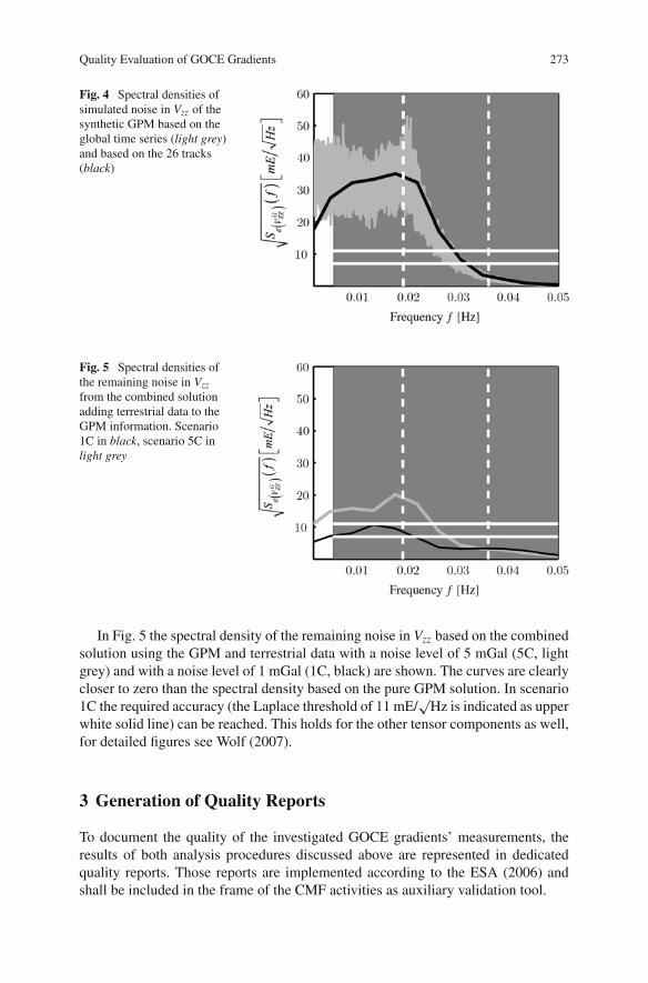
In Fig. 4 the spectral density (for Vzz) of the simulated noise of the syntheticGPM based on the global time series (grey) is compared with the spectral densitycomputed as mean curve from the 26 tracks (black). Within the MBW (dark greybox) the track-wise computed spectral density can be used as approximation of theglobal one. The solid lines in white mark the accuracy level of 7 and 11 mE/

√Hz,

respectively. The white dashed lines mark the interesting frequency band for GOCE.The line at 0.019 Hz corresponds to a spherical harmonic degree 105. The peakformed by the spectral density based on the global times series is caused by themuch higher noise of the SYNGPM1300S in this frequency band resulting fromthe EGM96. A similar peak can also be found in the spectral density curve whenthe noise simulation is based on the accuracy of the EIGEN-GL04C, the currentcombination model from GRACE, altimetry, terrestrial and other data (Förste et al.,2006). The line at 0.036 Hz corresponds to a spherical harmonic degree of 200.Here, the signal of the tensor components approaches zero at GOCE altitude andthe noise decreases, too.


Fig. 4 Spectral densities ofsimulated noise in Vzz of thesynthetic GPM based on theglobal time series (light grey)and based on the 26 tracks(black)

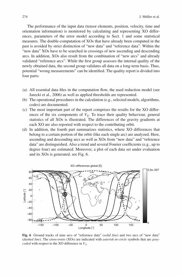
Fig. 5 Spectral densities ofthe remaining noise in Vzzfrom the combined solutionadding terrestrial data to theGPM information. Scenario1C in black, scenario 5C inlight grey

In Fig. 5 the spectral density of the remaining noise in Vzz based on the combinedsolution using the GPM and terrestrial data with a noise level of 5 mGal (5C, lightgrey) and with a noise level of 1 mGal (1C, black) are shown. The curves are clearlycloser to zero than the spectral density based on the pure GPM solution. In scenario1C the required accuracy (the Laplace threshold of 11 mE/

√Hz is indicated as upper

white solid line) can be reached. This holds for the other tensor components as well,for detailed figures see Wolf (2007).

3 Generation of Quality Reports

To document the quality of the investigated GOCE gradients’ measurements, theresults of both analysis procedures discussed above are represented in dedicatedquality reports. Those reports are implemented according to the ESA (2006) andshall be included in the frame of the CMF activities as auxiliary validation tool.


The performance of the input data (tensor elements, position, velocity, time andorientation information) is monitored by calculating and representing XO differ-ences, parameters of the error model according to Sect. 1 and some statisticalmeasures. The double-computation of XOs that have already been computed in thepast is avoided by strict distinction of “new data” and “reference data”. Within the“new data” XOs have to be searched in crossings of new ascending and descendingarcs. In addition, XOs also result from the combination of “new arcs” and alreadyvalidated “reference arcs”. While the first group assesses the internal quality of thenewly obtained data, the second group validates all data on a long-term basis. Thus,potential “wrong measurements” can be identified. The quality report is divided intofour parts:

(a) All essential data files in the computation flow, the used reduction model (seeJarecki et al., 2006) as well as applied thresholds are represented.

(b) The operational procedures in the calculation (e.g., selected models, algorithms,codes) are documented.

(c) The most important part of the report comprises the results for the XO differ-ences of the six components of Vij. To trace their quality behaviour, generalstatistics of all XOs is illustrated. The differences of the gravity gradients ateach XO are also reported with respect to the contributing orbit.

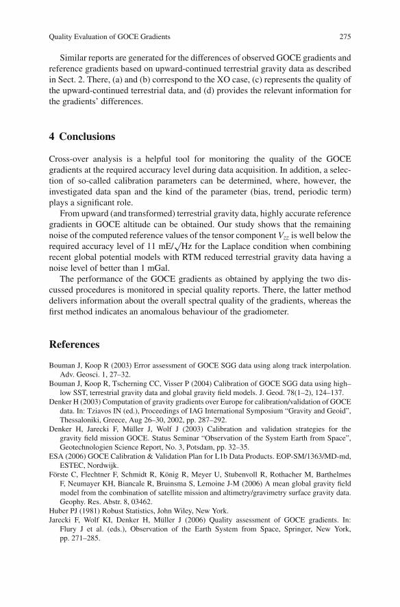
(d) In addition, the fourth part summarizes statistics, where XO differences thatbelong to a certain portion of the orbit (like each single arc) are analyzed. Here,ascending and descending arcs as well as XOs from “new data” and “referencedata” are distinguished. Also a trend and several Fourier coefficients (e.g., up todegree four) are estimated. Moreover, a plot of each data set under evaluationand its XOs is generated, see Fig. 6.

−150 −100 −50 0 50 100 150

−80

−60

−40

−20

0

20

40

60

80

XO−differences global [E]

Longitude [°]

Latit

ude

[°]

0

3.2e−007

Fig. 6 Ground tracks of nine arcs of “reference data” (solid line) and two arcs of “new data”(dashed line). The cross-overs (XOs) are indicated with asterisk-in-circle symbols that are gray-coded with respect to the XO difference in Vzz


Similar reports are generated for the differences of observed GOCE gradients andreference gradients based on upward-continued terrestrial gravity data as describedin Sect. 2. There, (a) and (b) correspond to the XO case, (c) represents the quality ofthe upward-continued terrestrial data, and (d) provides the relevant information forthe gradients’ differences.

4 Conclusions

Cross-over analysis is a helpful tool for monitoring the quality of the GOCEgradients at the required accuracy level during data acquisition. In addition, a selec-tion of so-called calibration parameters can be determined, where, however, theinvestigated data span and the kind of the parameter (bias, trend, periodic term)plays a significant role.

From upward (and transformed) terrestrial gravity data, highly accurate referencegradients in GOCE altitude can be obtained. Our study shows that the remainingnoise of the computed reference values of the tensor component Vzz is well below therequired accuracy level of 11 mE/

√Hz for the Laplace condition when combining

recent global potential models with RTM reduced terrestrial gravity data having anoise level of better than 1 mGal.

The performance of the GOCE gradients as obtained by applying the two dis-cussed procedures is monitored in special quality reports. There, the latter methoddelivers information about the overall spectral quality of the gradients, whereas thefirst method indicates an anomalous behaviour of the gradiometer.

References

Bouman J, Koop R (2003) Error assessment of GOCE SGG data using along track interpolation.Adv. Geosci. 1, 27–32.

Bouman J, Koop R, Tscherning CC, Visser P (2004) Calibration of GOCE SGG data using high–low SST, terrestrial gravity data and global gravity field models. J. Geod. 78(1–2), 124–137.

Denker H (2003) Computation of gravity gradients over Europe for calibration/validation of GOCEdata. In: Tziavos IN (ed.), Proceedings of IAG International Symposium “Gravity and Geoid”,Thessaloniki, Greece, Aug 26–30, 2002, pp. 287–292.

Denker H, Jarecki F, Müller J, Wolf J (2003) Calibration and validation strategies for thegravity field mission GOCE. Status Seminar “Observation of the System Earth from Space”,Geotechnologien Science Report, No. 3, Potsdam, pp. 32–35.

ESA (2006) GOCE Calibration & Validation Plan for L1b Data Products. EOP-SM/1363/MD-md,ESTEC, Nordwijk.

Förste C, Flechtner F, Schmidt R, König R, Meyer U, Stubenvoll R, Rothacher M, BarthelmesF, Neumayer KH, Biancale R, Bruinsma S, Lemoine J-M (2006) A mean global gravity fieldmodel from the combination of satellite mission and altimetry/gravimetry surface gravity data.Geophy. Res. Abstr. 8, 03462.

Huber PJ (1981) Robust Statistics, John Wiley, New York.Jarecki F, Wolf KI, Denker H, Müller J (2006) Quality assessment of GOCE gradients. In:

Flury J et al. (eds.), Observation of the Earth System from Space, Springer, New York,pp. 271–285.


Jarecki F, Müller J (2009) Robust trend estimates from GOCE SGG satellite track cross-over dif-ferences. In: Sideris M (ed.), Observing Our Changing Earth. IAG Symposia 133, Springer,New York, pp. 363–370.

Koop R, Bouman J, Schrama EJO, Visser P (2002) Calibration and error assessment of GOCEdata. In: Adam J et al. (eds.), Vistas for Geodesy in the New Millenium. IAG Symposia 125,Springer, New York, pp. 167–174.

Lemoine FG, Kenyon SC, Factor JK, Trimmer RG, Pavlis NK, Chinn DS, Cox CM, KloskoSM, Luthcke SB, Torrence MH, Wang YM, Williamson RG, Pavlis EC, Rapp RH, Olson TR(1998) The Development of the Joint NASA GSFC and NIMA Geopotential Model EGM96,NASA/TP-1998-206861. Technical Report, NASA, Greenbelt, MD.

Pail R (2003) Local gravity field continuation for the purpose of in-orbit calibration of GOCE SGGobservations. Adv. Geosci. 1, 11–18.

Reigber C, Schmidt R, Flechtner F, König R, Meyer U, Neumayer K-H, Schwintzer P, Zhu SY(2005) An earth gravity field model complete to degree and order 150 from GRACE: EIGEN-GRACE02S. J. Geodynamics 39(1), 1–10.

SCVII (2000) Simulation Scenarios for Current Satellite Missions. IAG SpecialCommission VII, http://www.geod.uni-bonn.de/apmg/lehrstuhl/simulationsszenarien/sc7/satellitenmissionen.php (July 13, 2006).

Wenzel H-G (1999) Schwerefeldmodellierung durch ultra-hochauflösende Kugelfunktion-smodelle. ZFV 124(5), 144–154.

Wolf KI (2007) Kombination globaler Potentialmodelle mit terrestrischen Schweredaten fürdie Berechnung der zweiten Ableitungen des Gravitationspotentials in Satellitenbahnhöhe.Deutsche Geodätische Kommission, Reihe C, Nr. 603.

quality evaluation of goce gradients

Documents