MNRAS 506, 1295–1308 (2021) https://doi.org/10.1093/mnras/stab1836Advance Access publication 2021 July 1

The role of gas kinematics in setting metallicity gradients at high redshift

Piyush Sharda ,1,2‹ Emily Wisnioski ,1,2‹ Mark R. Krumholz 1,2‹ and Christoph Federrath 1,2

1Research School of Astronomy and Astrophysics, Australian National University, Canberra, ACT 2611, Australia2Australian Research Council Centre of Excellence for All Sky Astrophysics in 3 Dimensions (ASTRO 3D), Australia

Accepted 2021 June 25. Received 2021 June 2; in original form 2021 January 26

ABSTRACTIn this work, we explore the diversity of ionized gas kinematics (rotational velocity vφ and velocity dispersion σ g) and gas-phase metallicity gradients at 0.1 ≤ z ≤ 2.5 using a compiled data set of 74 galaxies resolved with ground-based integral fieldspectroscopy. We find that galaxies with the highest and the lowest σ g have preferentially flat metallicity gradients, whereas thosewith intermediate values of σ g show a large scatter in the metallicity gradients. Additionally, steep negative gradients appearalmost only in rotation-dominated galaxies (vφ /σ g > 1), whereas most dispersion-dominated galaxies show flat gradients. Weuse our recently developed analytical model of metallicity gradients to provide a physical explanation for the shape and scatterof these observed trends. In the case of high σ g, the inward radial advection of gas dominates over metal production and causesefficient metal mixing, thus giving rise to flat gradients. For low σ g, it is the cosmic accretion of metal-poor gas diluting themetallicity that gives rise to flat gradients. Finally, the reason for intermediate σ g showing the steepest negative gradients is thatboth inward radial advection and cosmic accretion are weak as compared to metal production, which leads to the creation ofsteeper gradients. The larger scatter at intermediate σ g may be due in part to preferential ejection of metals in galactic winds,which can decrease the strength of the production term. Our analysis shows how gas kinematics play a critical role in settingmetallicity gradients in high-redshift galaxies.

Key words: ISM: abundances – galaxies: abundances – galaxies: evolution – galaxies: high-redshift – galaxies: ISM – galaxies:kinematics and dynamics.

1 IN T RO D U C T I O N

Understanding the distribution of metals in galaxies is crucial tolearn about galaxy formation and evolution. It is now well known thatmetals in both the gas and stars show a negative, radial gradient acrossthe discs of most galaxies. Since the discovery of metallicity gradientsin galactic discs (Aller 1942; Searle 1971; Shaver et al. 1983), severalattempts have been made to put the measurements in context ofgalaxy evolution theory, as well as understand the physics driving themagnitude of the gradient by exploring trends with galaxy properties,such as mass, star formation rate (SFR), star formation efficiency,specific SFR, radial inflows, cosmic infall, etc. (see recent reviewsby Kewley, Nicholls & Sutherland 2019; Maiolino & Mannucci2019; Forster Schreiber & Wuyts 2020; Sanchez 2020; Sanchez et al.2021). With the advent of large resolved spectroscopic surveys usingintegral field unit (IFU) spectroscopy, we are now able to explorethe relationship between metallicity gradients and galaxy kinematics(i.e. the rotational velocity vφ and the velocity dispersion σ g). Thereare several reasons why we would expect such a correlation to exist.For example, turbulent mixing and transport, processes whose ratesare expected to scale with σ g, should be important processes thatinfluence metallicity gradients (e.g. Yang & Krumholz 2012; Forbeset al. 2014; Petit et al. 2015; Armillotta, Krumholz & Fujimoto 2018;

� E-mail: piyush.sharda@anu.edu.au (PS); emily.wisnioski@anu.edu.au(EW); mark.krumholz@anu.edu.au (MRK)

Krumholz & Ting 2018; Kreckel et al. 2020; Li et al. 2021). Similarly,rates of cosmic infall that can dilute both the overall metallicityand its gradients should correlate strongly with halo mass, whichis closely linked to vφ (e.g. Tully & Fisher 1977; McGaugh et al.2000; Bell & de Jong 2001; Faucher-Giguere, Keres & Ma 2011). Theproduction of metals is dictated by star formation in galaxies, and starformation feedback also impacts galaxy kinematics (e.g. Ostriker &Shetty 2011; Faucher-Giguere, Quataert & Hopkins 2013; Forbeset al. 2014; Kim & Ostriker 2015; Goldbaum, Krumholz & Forbes2016; Krumholz et al. 2018; Furlanetto 2021). The amount of metalslost in outflows is also expected to scale inversely with vφ (Garnett2002). Thus, there are several links between metallicity gradientsand galaxy kinematics, and it is clear that these links likely generatea rather complex relationship between each other as well as otherrelevant mechanisms.

This connection is perhaps most readily explored at high redshift(z ≤ 2.5), when galaxies show a more diverse range of metallicitygradients and kinematics than are found in the local Universe(Maiolino & Mannucci 2019; Forster Schreiber & Wuyts 2020; Tac-coni, Genzel & Sternberg 2020). The last decade has seen immenseprogress in these areas, thanks to IFU spectroscopy instruments likeMulti Unit Spectroscopic Explorer (MUSE; Bacon et al. 2010), K-band Multi Object Spectrograph (KMOS; Sharples et al. 2004),Spectrograph for INtegral Field Observations in the Near Infrared(SINFONI; Eisenhauer et al. 2003; Bonnet et al. 2004), Fibre LargeArray Multi Element Spectrograph (FLAMES; Pasquini et al. 2002),Gemini Multi Object Spectrograph (GMOS; Davies et al. 1997),Gemini Near-infrared Integral Field Spectrograph (NIFS; McGregor

C© 2021 The Author(s)Published by Oxford University Press on behalf of Royal Astronomical Society

Dow

nloaded from https://academ

ic.oup.com/m

nras/article/506/1/1295/6312513 by guest on 25 July 2022

1296 P. Sharda et al.

et al. 2003), and OH-Suppressing InfraRed Imaging Spectrograph(OSIRIS; Larkin et al. 2006).

Studies using these instruments have revealed that, while high-zgalaxies show a diverse range of metallicity gradients, the averageevolution of these gradients is rather shallow, almost non-existent(see fig. 8 of Curti et al. 2020). On the other hand, there is ampleevidence for redshift evolution of galaxy kinematics. In particular,σ g evolves with z implying that high-z discs are thicker andmore turbulent (Kassin et al. 2012; Wisnioski et al. 2015, 2019;Simons et al. 2017; Ubler et al. 2019). The mass-averaged rotationalvelocities are also expected to evolve with time (e.g. Dutton et al.2011; Tiley et al. 2016; Ma et al. 2017; Straatman et al. 2017; Ubleret al. 2017; Glowacki, Elson & Dave 2020; see, however, Tiley et al.2019a). However, links between kinematics and metallicity gradientsat high redshift have been investigated by observations only in ahandful of studies (Queyrel et al. 2012; Gillman et al. 2021), mostof which were limited to gravitationally lensed samples (Yuan et al.2011; Jones et al. 2013; Leethochawalit et al. 2016), yielding no clearconnections between the two. Some simulations have also startedto explore joint evolution of metallicity gradients and kinematics(Ma et al. 2017; Hemler et al. 2020), but at present theoreticalwork is limited to empirical examination of simulation results. Nomodels proposed to date have quantitatively discussed the observedcorrelations between metallicity gradients and gas kinematics.

In a companion paper (Sharda et al. 2021a), we presented anew model for the physics of gas-phase metallicity gradients fromfirst principles. We showed that our model successfully reproducesseveral trends of metallicity gradients with galaxy properties, forexample the observed cosmic evolution of metallicity gradients(Sharda et al. 2021a) and the mass–metallicity gradient relation(MZGR; Sharda et al. 2021b). The goal of this paper is to apply themodel to existing observations of high-redshift galaxies to investigatethe relationship between metallicity gradients and gas kinematics.

This paper is organized as follows: Section 2 describes the dataon metallicity gradients and galaxy kinematics that we compilefrom observations, Section 3 presents the resulting trends we findin the data, Section 4 presents a discussion on the comparison ofthe observational data with our theoretical model, and Section 5lists our conclusions. For this work, we use the Lambda colddark matter cosmology with H0 = 71 km s−1 Mpc−1, �m = 0.27,and �� = 0.73 (Springel & Hernquist 2003). Further, we expressZ = Z/Z�, where Z� = 0.0134 (Asplund et al. 2009), and we usethe Chabrier (2003) initial mass function (IMF).

2 C OMPILED DATA AND ANALYSIS

We compile a sample of 74 non-lensed high-z (0.1 ≤ z ≤ 2.5)galaxies from the literature, studied with ground-based IFU instru-ments suitable for the measurement of metallicity gradients andgas kinematics. We only work with non-lensed galaxies becauseit is not yet clear whether lens reconstructions accurately reproducemetallicity maps (see section 6.7 of Maiolino & Mannucci 2019).However, we note that there is a similar diversity of gradients inlensed galaxies (Leethochawalit et al. 2016; Wuyts et al. 2016),and including them does not change our results. We describe eachof the samples we use in Section 2.1, and provide a summary inTable 1. Our data base is inhomogeneous, because the sources wedraw from have different sample selections and varying resolution,and use different techniques to obtain the metallicity gradients andkinematics. To alleviate some of the inhomogeneity, we reanalyse thekinematics using the same method for the full data base, a process thatwe describe in Section 2.2. Additionally, where possible, we use a

common metallicity diagnostic and calibration to estimate metallicitygradients. We list the data base along with the reanalysed kinematicsfor all 74 galaxies in Appendix A.

We acknowledge that there are many challenges associated withmeasuring metallicity gradients and kinematics in IFU observations,particularly at high z. Metallicity measurements in H II regions relyon accurately modelling the H II-region physics, and systematicvariations in the physical parameters with redshift, if any (e.g. Kewleyet al. 2013b; Shirazi, Brinchmann & Rahmati 2014; Strom et al. 2018;Davies et al. 2021), emission line diagnostics and calibrations (e.g.Kewley & Ellison 2008; Poetrodjojo et al. 2021), spatial and spectralresolution (e.g. Yuan, Kewley & Rich 2013; Mast et al. 2014), andcontamination from shocks and active galactic nuclei (AGNs; Kewleyet al. 2013a; Newman et al. 2014). Similarly, kinematic measure-ments rely on model assumptions, source blending, beam smearing,and spectral resolution limits (e.g. Davies et al. 2011; Di Teodoro &Fraternali 2015; Burkert et al. 2016; Wisnioski et al. 2018). Thus,systematic errors originating from these physical and observationaleffects should be kept in mind in the context of our work. We note thatsome of the kinematic uncertainties are not captured in the quotederrors, which only account for uncertainties in the beam smearing,inclination, and instrumental resolution corrections.

2.1 Samples

(i) MASSIV. We use data from the Mass Assembly Survey withSINFONI in VIMOS VLT Deep Survey (MASSIV; Contini et al.2012) of star-forming galaxies between 1 < z < 2. The kinematicsand the metallicity gradients from this survey are described in Epinatet al. (2012) and Queyrel et al. (2012), respectively. The authorsreport on metallicity gradients using the [N II]/H α ratio followingthe Perez-Montero & Contini (2009) calibration. In order to beconsistent with the other samples described below, we reverse thePerez-Montero & Contini (2009) calibration to obtain the [N II]/H α

flux at different locations in the galactic disc, and use the flux to findthe metallicities using the Pettini & Pagel (2004) calibration. We thenuse metallicities based on the Pettini & Pagel (2004) calibration tomeasure the metallicity gradients. We reanalyse the kinematics forthis sample following the procedure described below in Section 2.2.

(ii) HiZELS. This sample consists of galaxies at z ∼ 0.8 thatwere observed through KMOS as part of the High-z Emission LineSurvey (HiZELS; Sobral et al. 2009, 2013a). The kinematics forthese galaxies are reported in Sobral et al. (2013b) and the metallicitygradients in Stott et al. (2014). The metallicity gradients are measuredwith the [N II]/H α ratio using the Pettini & Pagel (2004) calibration.

(iii) SHiZELS. In addition to the HiZELS survey above, we alsouse observations from the SINFONI-HiZELS survey (SHiZELS;Swinbank et al. 2012) that report on metallicity gradients andkinematics of eight galaxies in the redshift range 0.8−2.2. Thegradients are measured with the [N II]/H α ratio using the Pettini &Pagel (2004) calibration.

(iv) MUSE-WIDE. We take measurements of metallicity gradientscarried out by Carton et al. (2018) for galaxies at low redshift (0.08< z < 0.84) using MUSE. The authors use a forward-modellingBayesian approach to estimate the metallicity gradients (Carton et al.2017) from nebular emission lines (for z ≤ 0.4, H β, O III, H α, andS II, and for z > 0.4, O II, H γ , H β, and O III). The kinematics forthese galaxies are not available in the literature, so we obtain themby fitting publicly available data (Herenz et al. 2017; Urrutia et al.2019) using the emission-line fitting code LZIFU (Ho et al. 2016).We describe this in detail in Section 2.2. We obtain the half-lightradii for these galaxies from The Cosmic Assembly Near-infrared

MNRAS 506, 1295–1308 (2021)

Dow

nloaded from https://academ

ic.oup.com/m

nras/article/506/1/1295/6312513 by guest on 25 July 2022

Kinematics and metallicity gradients at high z 1297

Table 1. Summary of the data adopted from different sources in the literature. Columns 1−3 list the different samples, instruments used to measure emissionlines, and the number of galaxies N that we use from each sample, respectively. Columns 4 and 5 list the ranges of redshift and stellar mass of the observedgalaxies. Column 6 lists the spectral resolution for each instrument, and columns 7 and 8 list the point spread function (PSF) full width at half-maximum(FWHM) in arcsec and kpc, respectively. Finally, column 9 lists the references for each sample: (a) Epinat et al. (2012), (b) Queyrel et al. (2012), (c) Sobralet al. (2013b), (d) Stott et al. (2014), (e) Swinbank et al. (2012), (f) Carton et al. (2018), and (g) Forster Schreiber et al. (2018).

Sample Instrument N z log10M�/M� RPSF FWHM

(arcsec) PSF FWHM (kpc) Ref.(1) (2) (3) (4) (5) (6) (7) (8) (9)

MASSIV SINFONI 19 0.9−1.6 9.4−11.0 2000−2640 0.3−1.0 2−7 a, bHiZELS KMOS 9 ≈0.81 9.8−10.7 ≈3400 ∼0.8 ∼6 c, dSHiZELS SINFONI 6 0.8−2.2 9.4−11.0 ≈4500 ∼0.1 0.7−0.8 eMUSE-WIDE MUSE 23 0.1−0.8 8.3−10.6 1650−3800 0.6−0.7 1−5 fSINS / zC-SINF SINFONI 17 1.4−2.4 10.1−11.5 2730−5090 0.1−0.3 ∼0.8 g

Deep Extragalactic Legacy Survey (CANDELS; van der Wel et al.2012) and from 3D-HST photometry (Skelton et al. 2014).

(v) SINS / zC-SINF. Forster Schreiber et al. (2018) report SIN-FONI observations of metallicity gradients and kinematics in galax-ies at z ∼ 1.5−2.2 from the SINS / zC-SINF survey, where theauthors use the [N II]/H α ratio to quantify the metallicity gradient.In order to homogenize their sample with other samples above, weuse their recommended conversion factor to scale the gradients to thecalibration given by Pettini & Pagel (2004). The reported kinematicsfor this sample are already corrected for instrumental and beamsmearing effects using the approach from Burkert et al. (2016), whichwe utilize for the other samples in Section 2.2.

All the above surveys also include information on the stellarmass M� (scaled to the Chabrier IMF where required) and the dust-corrected SFR from H α, except for the SINS / zC-SINF survey. Toobtain dust-corrected SFR estimates for SINS / zC-SINF, we use theintegrated H α fluxes reported by the authors, and scale them tofind the dust-corrected H α luminosity following Calzetti (2001),and convert it to SFR based on the Chabrier (2003) IMF followingKennicutt & Evans (2012).

Fig. 1 shows the distributions of redshift, stellar mass, and SFRof galaxies in our compiled sample from the above surveys. Thedistribution in redshift is quite uniform, except around z ≈ 1.7, wherethere is no available data due to atmospheric absorption. This impliesthat the data we use are not biased towards a particular redshift. Itis also clear from Fig. 1 that the observations consist primarily ofmore massive (M� > 1010 M�) galaxies; the few low-mass galaxies(M� ≤ 109.5 M�) that we are able to study belong to the MUSE-WIDE sample. The overall sample is somewhat biased to high SFRs:20 per cent of the galaxies in the compiled sample have SFRs morethan 3× the main-sequence SFR for their mass and redshift (Whitakeret al. 2012). This bias is not surprising, given that large H α fluxes(corresponding to large SFRs) are typically necessary for spatiallyresolved measurements at high redshift. However, we emphasize thatthe sample is not dominated by merging or interacting galaxies: basedon the classifications provided by the source papers from which wedraw the sample, less than 9 per cent of the galaxies are mergers orinteractions. This means that our sample is not significantly affectedby the flattening of gradients that typically occurs when galaxiesmerge (e.g. Rupke, Kewley & Chien 2010; Rich et al. 2012; Torres-Flores et al. 2014; Sillero et al. 2017).

2.2 Kinematics

To obtain the global kinematics for each galaxy, rotational velocityvφ , and characteristic velocity dispersion σ g, we use 1D velocity and

dispersion curves extracted along the kinematic major axis followingWisnioski et al. (2019). Briefly, we measure the observed velocityby calculating the average of the absolute value of the minimum andmaximum velocity measured along the kinematic axis and correctingfor inclination. The measured velocity dispersion is calculated bytaking the weighted mean of the outer data points of the 1D velocitydispersion profile. We adopt this non-parametric analysis to enablethe use of galaxies with a variety of kinematic classifications. By notlimiting the sample to the highest signal-to-noise disc galaxies, wecan investigate the metallicity gradients of galaxies with kinematicperturbations.

One-dimensional kinematic extractions are directly provided forboth the HiZELS and SHiZELS samples. For the MUSE-WIDE andMASSIVE samples, the 1D kinematic profiles need to be measured.We use the datacubes for MASSIV (B. Epinat, private communica-tion) and MUSE-WIDE (Herenz et al. 2017; Urrutia et al. 2019)samples to derive these. We fit the data with the emission linediagnostic package LZIFU (Ho et al. 2016). LZIFU runs spectraldecomposition on IFU datacubes to produce 2D emission line andkinematic maps based on the Levenberg–Marquardt least-squaresmethod.

We first produce emission line and kinematic maps for the entiregalaxy by passing the complete datacube to LZIFU. We supply anexternal continuum map to LZIFU that we create by finding themedian flux for every spatial pixel (spaxel; e.g. MUSE-WIDE) orwhere the signal-to-noise of the continuum is negligible we simplysupply a null external continuum map for the galaxies (e.g. MASSIV).We use the resulting flux and moment-1 maps from the fit to locatethe galaxy centre and the kinematic major axis, respectively. Oncethe kinematic major axis and the galaxy centre are determined, wecreate apertures with the size of the FWHM of the PSF across themajor axis. We sum the flux in each spaxel within these aperturesalong the major axis. This gives a spatially summed spectrum forevery aperture, thus increasing the signal-to-noise ratio. We then fitthe aperture spectra with LZIFU, which returns a single value ofvφ(r) and σ g(r) for every aperture that we use to create 1D radialcurves.

After we derive the global velocities and dispersions from the 1Dradial curves for all galaxies in the MASSIV, HiZELS, SHiZELS, andMUSE-WIDE samples, we apply inclination, instrumental resolution,and beam smearing corrections on them. To correct for inclination,we simply divide the observed velocities by sin(i), where i is theinclination angle. We use the inclinations reported in the sourcepapers for this purpose. Following Wisnioski et al. (2015), we adda 30 per cent uncertainty in quadrature to σ g if it is comparableto the instrumental resolution; if σ g is less than the instrumentalresolution, we add a 60 per cent uncertainty in quadrature. To correct

MNRAS 506, 1295–1308 (2021)

Dow

nloaded from https://academ

ic.oup.com/m

nras/article/506/1/1295/6312513 by guest on 25 July 2022

1298 P. Sharda et al.

Figure 1. Distribution of galaxies at different redshifts (left), stellar mass (middle), and star formation rate (right) in the compiled sample used in this work.

for beam smearing, we follow Burkert et al. (2016, Appendix A2), asdone by Forster Schreiber et al. (2018; N. Forster-Schreiber, privatecommunication). We note that this model makes the assumption thatthe galaxy kinematics are well described by a simple disc model.This may not apply to all galaxies in our sample, thus providing anovercorrection for the beam in certain cases. The model assumesa Gaussian PSF and returns the beam-smearing correction factorbased on the ratio of the stellar effective half-light radius to the beameffective half-light radius (re/re,b),1 and the ratio of the radius wherethe rotational velocity is calculated to the galactic effective half-light radius (rvel/re). While it is straightforward to use these ratios tocalculate the beam-smearing correction factor for vφ , those for σ g

also depend on the mass, inclination, and redshift of the source. Weincorporate a 40 per cent error in σ g to account for uncertainties inthe beam smearing correction model (see section 3.3 of Wisnioskiet al. 2018); however, it is possible that we may overestimate orunderestimate the correction factor in certain cases. We present theresulting kinematics for all galaxies in Appendix A, and illustrate thereanalysis procedure through a representative galaxy G103012059(from the MUSE-WIDE sample) in Fig. 2.

2.3 Final sample

We do not include all the galaxies that are available in the compiledsurveys. We only select galaxies where the ratio of the radius at whichvφ is measured (rvel) to the half-light radius, re, is greater than unity,as the beam-smearing correction model for vφ requires rvel > re.We also remove galaxies that only contain three or fewer resolutionelements in our kinematic reanalysis, because we cannot derive areasonable value for vφ and σ g in such cases. Further, we note thatall the samples above exclude galaxies that contain contaminationfrom AGNs, as diagnosed using the criteria described in Kewleyet al. (2001, 2006) based on the Baldwin, Phillips & Terlevich (1981,BPT) diagram. The exception to this statement is the SINS / zC-SINF sample, where the corresponding authors explicitly remove thecontamination in gradients due to AGNs for some of their galaxies.Our final sample consists of 74 galaxies with measured metallicitygradients and gas kinematics.

1The measurements of the half-light radius for the different samples are basedon broad-band photometry using different bands; however, it has a negligibleeffect on the beam smearing correction factor (Nelson et al. 2016).

3 R ESULTS

Fig. 3 shows the distributions of the metallicity gradients, and theresulting homogenized kinematics for all galaxies in the compileddata set. Our compilation recovers the diversity of gradients seen inthe literature (by design) as well as the diversity of kinematics. Thisdiversity is crucial for us to explore the correlations between galaxykinematics and metallicity gradients, and is the primary driver of ourwork. We do not preferentially select disc galaxies however samplesare likely to consist of primarily disc-dominated galaxies due tothe high fraction of discs at these epochs (Wisnioski et al. 2015,2019; Stott et al. 2016; Simons et al. 2017). Another indicator of thegalaxy kinematics is the ratio of the rotational velocity to the velocitydispersion, vφ /σ g (e.g. Forster Schreiber et al. 2009, 2018; Burkertet al. 2010; Kassin et al. 2014; Jones et al. 2015; Wisnioski et al.2015, 2018, 2019; Simons et al. 2019), which is used to determinethe rotational support of galaxies. We find from Fig. 3 that whilemost galaxies in the sample are rotation-dominated (i.e. vφ /σ g � 1),around 18 per cent of the galaxies are dispersion dominated (vφ /σ g

� 1).Fig. 4 shows the measured metallicity gradients as a function

of the reanalysed velocity dispersion σ g, colour-coded by redshift.We consider metallicity gradients as shallow or flat if the absolutestrength of the gradient is less than 0.05 dex kpc−1. We observe thatall galaxies in the sample with both high σg (�60 km s−1) and lowσg (�20 km s−1) show shallow or flat metallicity gradients, thoughwe caution that the small velocity dispersions suffer significantuncertainties, as discussed in Section 2. By contrast, galaxies withintermediate σ g (20−50 km s−1) show both the steepest gradients(∼ − 0.25 dex kpc−1) and the largest scatter (∼0.1) in gradients. Wefind only one galaxy with a steep gradient (∼ − 0.09 dex kpc−1) andhigh σ g (∼109 km s−1). Fig. 5 shows the same data as in Fig. 4,but as a function of vφ /σ g, thereby separating galaxies that arerotation-dominated from those that are dispersion-dominated. Themain conclusion that we can draw from Fig. 5 is that all dispersion-dominated galaxies (vφ /σ g � 1) possess shallow or flat gradients,whereas rotation-dominated galaxies (vφ /σ g � 1) show a largescatter, and can have flat as well as steep gradients.2 The exception

2Note, however, that this conclusion depends on the value vφ /σ g ∼ 1 thatwe choose to separate rotation- and dispersion-dominated galaxies. If wewere to use vφ /σ g = 3 as the break point, for example, we would find thatdispersion-dominated galaxies show a large scatter in metallicity gradientswhereas rotation-dominated galaxies show shallow or flat gradients. A more

MNRAS 506, 1295–1308 (2021)

Dow

nloaded from https://academ

ic.oup.com/m

nras/article/506/1/1295/6312513 by guest on 25 July 2022

Kinematics and metallicity gradients at high z 1299

Figure 2. Left to right − observed-frame IJH colour composite image from CANDELS HST imaging (Grogin et al. 2011; Koekemoer et al. 2011), nebular lineflux with the strongest emission (O II in this case), rotational velocity v, velocity dispersion σ , as well as the 1D radial curves of v and σ derived from kinematicextractions for the galaxy G103012059 from the MUSE-WIDE sample.

Figure 3. Same as Fig. 1, but for the measured metallicity gradients (left), and reanalysed kinematics – velocity dispersion σ g (middle) and the ratio of rotationalvelocity to velocity dispersion vφ /σ g (right).

Figure 4. Metallicity gradients in the compiled sample of high-redshiftgalaxies plotted as a function of velocity dispersion σ g, colour-coded byredshift. We use the same method to derive the kinematics of all galaxiesin our sample (see Section 2.2 for details). The quoted error bars includeuncertainties due to inclination, instrumental resolution, and beam smearing(Wisnioski et al. 2015, 2018; Burkert et al. 2016).

to this is a couple of dispersion-dominated galaxies at z < 1 in theMUSE-WIDE sample that exhibit steep gradients. We also find fromFig. 5 that the scatter in gradients narrows down as vφ /σ g increases.While our data compilation spans a wide redshift range, the above

precise statement, which we will see below is naturally predicted by ourtheoretical model, is that metallicity gradients show a very large scatter forvφ /σ g ∼ few, and shallow gradients on either side of this region.

Figure 5. Same data as Fig. 4, but plotted against the ratio of rotationalvelocity to velocity dispersion, vφ /σ g. Galaxies with vφ /σ g ≥ 1 are classifiedas rotation-dominated (and typically have a well-defined disc) whereasothers are classified as dispersion-dominated (and typically have irregularstructures).

conclusions are not substantially different when considering just z

> 1 versus z < 1. A more complete analysis exploring possibleevolutionary effects requires a larger data set.

Recent cosmological simulations like FIRE (Hopkins et al. 2014,2018) and IllustrisTNG50 (Pillepich et al. 2018) have also exploredthe connection between metallicity gradients and kinematics, par-ticularly focusing on the relation between gradients and vφ /σ g.One of the key results of both these simulations is that negativemetallicity gradients only form in galaxies with vφ /σ g > 1 (i.e.

MNRAS 506, 1295–1308 (2021)

Dow

nloaded from https://academ

ic.oup.com/m

nras/article/506/1/1295/6312513 by guest on 25 July 2022

1300 P. Sharda et al.

rotation-dominated systems), however, many such galaxies also showshallow gradients (Ma et al. 2017; Hemler et al. 2020). Thesesimulations also find that dispersion-dominated galaxies alwaysshow shallow/flat gradients, consistent with mixing due to efficientfeedback. However, some simulations may require more powerfulradial mixing or feedback to match both kinematics and gradients(Gibson et al. 2013). We see from Figs 4 and 5 that these findingsare consistent with the data analysed here, with only a couple ofdispersion-dominated outliers that show steep metallicity gradients.

4 C O M PA R I S O N W I T H A NA LY T I C A L M O D E LFOR METALLICITY GRADIENTS

In order to better understand the underlying physics that drives thediversity of metallicity gradients found in high-redshift galaxies, wecompare the observations with the analytical metallicity gradientmodel we presented in Sharda et al. (2021a). Our model predicts theradial distribution of gas-phase metallicities based on the equilibriumbetween production, consumption, loss, and transport of metals ingalaxies. It is a stand-alone metallicity model, but requires inputsfrom a galaxy evolution model to describe the properties of the gas– velocity dispersion, surface densities of gas and star formation,etc. – to solve for the metallicity. We use the galactic disc model ofKrumholz et al. (2018) for this purpose, since we showed in previousworks that using this model allows us to successfully reproducethe observed trend of metallicity gradient with redshift (Shardaet al. 2021a), as well as the mass–metallicity and mass–metallicitygradient relations (MZR and MZGR) found in local galaxies (Shardaet al. 2021b). Note that, in what follows, we do not fit the model tothe data while comparing the two.

4.1 Model description

In our model, the metallicity distribution profile in the galactic discdepends on four dimensionless ratios (equations 13 and 37–40 inSharda et al. 2021a),

T ∝(

vφ

σg

)2

(metal equilibrium), (1)

P ∝(

1 − σsf

σg

)(metal advection), (2)

S ∝ φy

(vφ

σg

)2

(metal production), (3)

A ∝ 1

σ 3g

(cosmic accretion) , (4)

where we have only retained the dependencies on vφ and σ g for thepurposes of the present study. Here, T is the ratio of the orbitalto diffusion time-scales, which describes the time it takes for agiven metallicity distribution to reach equilibrium, P is the Pecletnumber of the galaxy (e.g. Patankar 1980), which describes the ratioof advection (radial inflow) to diffusion of metals in the disc, Sis the source term, which describes the ratio of metal production(including loss of metals in outflows) and diffusion, and A is theratio of cosmic accretion (infall) to diffusion. Finally, σ sf denotes thevelocity dispersion that can be maintained by star formation feedbackalone, with no additional energy input from transport of gas throughthe disc (Krumholz et al. 2018). Note that the model can only beapplied in cases where the metal equilibration time (dictated by T )is shorter than the Hubble time and shorter than or comparable tothe molecular gas depletion time. If these conditions are not met, themetallicity distribution does not reach equilibrium within the galaxy.

We showed in Sharda et al. (2021a, section 5) that inverted gradientsmay or may not be in equilibrium, so for this work we do not applyour model to study such gradients.

The parameter φy that appears in S describes the reduced yield ofmetals in the disc due to preferential metal ejection through galacticoutflows: φy = 1 corresponds to metals being thoroughly-mixed intothe interstellar medium (ISM) before ejection, whereas φy = 0 meansthat all the newly produced metals are directly ejected before theycan mix into the ISM. In line with previous works, we leave φy

as a free parameter in the model. However, we showed in Shardaet al. (2021b) that our model reproduces both the local MZR andthe MZGR only if φy increases with M�: low-mass galaxies prefer alower φy, and vice versa.

4.2 Model application

To produce metallicity gradients from the model, we select a valueof vφ and σ g, and fix all other parameters in the model to thoseappropriate for high-z galaxies (tables 1 and 2 of Sharda et al. 2021a)at z = 2; we discuss how the results depend on the choice of redshiftbelow. We find the spatial distribution of metallicity, Z(r), within0.5–2.0 re using equation (41) of Sharda et al. (2021a), which wethen linearly fit in logarithmic space to obtain a metallicity gradientin dex kpc−1 from the model (e.g. Carton et al. 2018). We use thisrange in r because it is well matched to the observations (rvel/re ≈ 2)and the input galaxy model does not apply to the innermost regionsof the galaxy.

While the choice of most of the parameters used as inputs intothe metallicity model have no appreciable effect on the results,some (e.g. the Toomre Q parameter and the circumgalactic medium(CGM) metallicity ZCGM) matter at the level of tens of per cent.For example, changing the Toomre Q parameter by a factor of 2induces a 20 per cent change in the metallicity gradient. The effectsof changing the Toomre Q are similar to that of changing the rotationcurve index β in the model, a topic we explore below in Section 4.2.3.Changing ZCGM by ±0.1 changes the metallicity gradient by at most±50 per cent. This implies that increasing the CGM metallicity leadsto shallower metallicity gradients. Finally, varying the redshift atwhich we compute the gradient by ±1 yields changes in the gradientfrom ∓36 per cent for massive galaxies to ∓19 per cent for low-mass galaxies. However, the overall impact of these parameterson the resulting metallicity gradients is limited compared to thedependence on φy, so in the following we focus on studying theeffects of changing φy. In the main text that follows, we will continueto measure metallicity gradients in dex kpc−1; we provide results onmetallicity gradients measured in dex r−1

e , which would potentiallyaccount for evolution in galaxy size, in Appendix B.

4.2.1 Metallicity gradient versus velocity dispersion

The left-hand panel of Fig. 6 shows the same observational data as inFig. 4, now with our model as computed for a fixed vφ = 105 km s−1

(the median vφ in the data). Since φy is a free parameter, we obtaina range of model predictions at every σ g; the range shown in theplot corresponds to varying φy between 0.1 and 1, as represented bythe arrows in Fig. 6. We colour code bars within this range by theratio P/A, which describes the relative importance of advection andaccretion of metal-poor gas. A key conclusion that can be drawnfrom this model–data comparison is that the model predicts flatmetallicity gradients in galaxies with high σ g, irrespective of φy,in good agreement with the observational data. The model generates

MNRAS 506, 1295–1308 (2021)

Dow

nloaded from https://academ

ic.oup.com/m

nras/article/506/1/1295/6312513 by guest on 25 July 2022

Kinematics and metallicity gradients at high z 1301

Figure 6. Left-hand panel: Same data as Fig. 4, but overplotted with one of the Sharda et al. (2021a) models. The model is for a high-redshift galaxy atfixed vφ = 105 km s−1 (median vφ in the data) and z = 2. The spread in the model (represented by the length of the coloured bands) is a result of the yieldreduction factor φy, which describes the preferential ejection of metals through galactic winds. Here we show models with φy = 0.1–1, where the top and bottomdashed lines corresponds to φy = 0.1 and 1.0, respectively. The colourbar denotes the ratio of advection of gas (P) to cosmic accretion of metal-poor gas (A).The steepest gradients produced by the model correspond to a transition from the accretion-dominated to the advection-dominated regime, as σ g increases.Right-hand panel: Same as the left-hand panel, but overlaid with different models (corresponding to different vφ ) at z = 2. Only the φy = 1 model is shownhere; thus, the model curves represent the most negative gradients produced by the model for a given set of parameters. The data are also binned around themodel vφ as shown through the colourbar. Note that the model is not being fit to the data.

a uniform metallicity distribution across the disc (i.e. a flat/shallowgradient) as a result of efficient radial transport of the gas. The modeldoes not produce any steep negative (< − 0.1 dex kpc−1) metallicitygradients at high σ g (>60 km s−1), consistent with both data andsimulations.

The largest diversity in metallicity gradients in the model occurs atσg ≈ 20–40 km s−1, where galaxies transition from being accretion-dominated (blue, P < A) to being advection-dominated (red, P >

A). This transition in the ratio P/A and the corresponding scatter inthe steepness of the metallicity gradients are key results of the model.Moreover, the transition in P/A from high to low values mirrors thetransition seen in σ g from gravity-driven to star formation feedback-driven turbulence (Krumholz et al. 2018). The region around thetransition is where both advection (P) and accretion (A) are weakeras compared to metal production (S), resulting in steep metallicitygradients, since star formation and thus metal production are centrallypeaked (Krumholz et al. 2018).3 The scatter near the transition arisesdue to the yield reduction factor φy, which can decrease the strengthof S as compared to P or A because S ∝ φy . Lastly, we note thatwhile metal diffusion is an important process that can also flatten thegradient, it never simultaneously dominates advection and cosmic ac-cretion, since bothP andA are never less than unity at the same time.

The model is consistent with the very few data points at lowσ g, which show shallow/flat metallicity gradients. In the model, theflattening at the low-σ g end is caused by accretion of metal-poorgas, following a 1/r2 profile, that dilutes the metallicity primarily inthe central regions. Given the scarcity of data at low σ g, as well assignificant observational uncertainties, it is unclear whether the trendseen in the model is also present in the data. Future instruments withhigher sensitivity and spectral and spatial resolution (e.g. GMTIFS,HARMONI, MAVIS, ERIS) will be able to measure low σ g in high-

3Note that the input cosmic accretion profile in the model is also centrallypeaked, similar to the SFR profile. However, as we show in appendix Aof Sharda et al. (2021a), changing the form of the input accretion profilehas only modest effects on the resulting metallicity gradients: less centrallypeaked accretion profiles give rise to slightly steeper gradients.

redshift galaxies with higher precision (Thatte et al. 2014; Fernandez-Ontiveros et al. 2017; Davies et al. 2018; Ellis et al. 2020; McDermidet al. 2020; Richardson et al. 2020), expanding the currently availablesample by a considerable margin.

In the right-hand panel of Fig. 6, we now fix φy = 1 (implyingno preferential metal ejection in winds), and look at the modeldifferences for different values of vφ . Note that vφ is a proxy forstellar mass, as higher vφ typically corresponds to massive galaxiesin the compiled sample. The data are the same as in the left-handpanel of Fig. 6, but now binned and colour-coded by the measured vφ .Thus, the model curves represent the steepest metallicity gradientsthat we can obtain for the given set of galaxy parameters. Weemphasize that we do not fit the model to the data while plottingthe model curves. It is clear that low vφ (low-mass) galaxies showmore scatter in the model gradients as compared to high vφ (massive)galaxies, consistent with observations (Carton et al. 2018; Simonset al. 2020). As vφ increases, the point of inflection (or, the point ofsteepest gradients) shifts towards higher σ g and towards shallowermetallicity gradients. Additionally, for sufficiently high σ g, modelswith different vφ converge towards a lower bound for metallicitygradients, implying that the flatness of metallicity gradients at highσ g is independent of the galaxy mass (see, however, Section 4.2.3).When the data are binned in vφ , they are broadly consistent with themodel. Thus, the model suggests a lower limit in metallicity gradientsat high-velocity dispersions consistent with the compiled data.

Taken at face value, it seems from the left-hand panel of Fig. 6 thatmost galaxies in the sample favour a value of φy close to 0.1, implyinga high metal enrichment in their winds. A close examination of theright-hand panel of Fig. 6 reveals that this is only the case for galaxieswith vφ < 150 km s−1 (i.e. low-mass galaxies); galaxies with highervφ prefer both low and high values of φy. When combined with resultsfrom the local Universe showing that low-mass galaxies prefer lowerφy (Sharda et al. 2021b), the finding that low-mass galaxies at highredshift also prefer lower φy is not surprising. Not only were outflowsmore common in the past in actively star-forming galaxies (Muratovet al. 2015), galaxies also had shallower potential wells (Mosteret al. 2010) that made it easier for metals to preferentially escapevia galactic winds without mixing into the ISM. This effect is more

MNRAS 506, 1295–1308 (2021)

Dow

nloaded from https://academ

ic.oup.com/m

nras/article/506/1/1295/6312513 by guest on 25 July 2022

1302 P. Sharda et al.

Figure 7. Scatter in the model metallicity gradient shown in the left-handpanel of Fig. 6, compared to the scatter for observed data, as a function ofthe gas velocity dispersion σ g for a fixed rotational velocity vφ = 105 km s−1

(median vφ in the data). The scatter in the model is calculated as 68 per centof the difference between the model metallicity gradients with φy = 1 and0.1 at every σ g. Errors on the scatter in the data represent the width of thebins used.

pronounced at the low-mass end, thus low-mass galaxies tend toprefer φy ∼ 0.1.

Fig. 7 quantifies the scatter present in the model and the dataas a function of σ g. To construct a 1σ scatter in the model in theabsence of a priori knowledge of the distribution of φy, we simplycompute model gradients for φy = 1 and 0.1 for every σ g, and takethe scatter to be 68 per cent of this range, i.e. our model-predicted‘scatter’ is simply 68 per cent of the distance between the two blackdashed lines in the left-hand panel of Fig. 6. To estimate the scatterin the data, we bin by σ g such that we have one bin each for σg <

10 km s−1 and σg > 90 km s−1, and we divide the parameter space10 ≤ σg/km s−1 ≤ 90 in five logarithmically spaced bins.

We find from Fig. 7 that the model is able to reproduce thequalitative shape of the variation in scatter with σ g observed in thedata, but not the exact level of scatter. This is not surprising, sincethe true scatter expected for the model depends on the distributionof φy values in real galaxies, which is at present unknown. Futureobservations of galactic wind metallicity at low and high redshifts, orsimulations with enough resolution to capture the hot-cold interfacewhere mixing between SN ejecta and the ambient ISM occurs (some-thing no current cosmological simulation possesses – Gentry et al.2019), will enable us to constrain φy and provide a more quantitativeanalysis of how φy scales with galaxy mass at different redshifts.

4.2.2 Metallicity gradient versus rotational support

The ratio of rotation to velocity dispersion provides a quantificationof the overall rotational support of a galaxy. The left-hand panelof Fig. 8 shows the metallicity gradients as a function of vφ /σ g

in the data, overplotted with the analytical model for fixed vφ =105 km s−1. The parameter space of the model denotes variationsin P/A, the same as that shown in Fig. 6. The grey-shaded regioncorresponds to an extrapolation of the model where it is not directlyapplicable because the assumption of a disc likely breaks down atvφ /σ g < 1. We first find a steepening of the gradient in the model asvφ /σ g increases from <1 to ∼10, after which the gradients begin toflatten again for vφ /σ g � 10. We can again understand this trend interms of P/A: values of vφ /σ g � 10 typically correspond to massivegalaxies, within which strong centrally peaked accretion (large A)

flattens the gradients. Galaxies with vφ /σ g � 1 have flat gradientsdue to strong advection of gas through the disc (large P) mixing andtherefore homogenizing the metal distribution throughout the disc.In the intermediate range of vφ /σ g, the gradients are the steepestbecause the production term S dominates over both P and A.

The location of the turnover is sensitive to the value of vφ , as weshow in the right-hand panel of Fig. 8. This figure is similar to theright-hand panel of Fig. 6, but we now show metallicity gradientsas a function of vφ /σ g for different values of vφ . We see that as vφ

increases, the parameter space of the model shifts to flatter gradientsand higher vφ /σ g. These shifts in the inflection point where galaxiestransition from the advection-dominated to the accretion-dominatedregime imply that massive galaxies have higher vφ /σ g and shallowergradients as compared to low-mass galaxies.

Similar to Fig. 6, we notice that most low-mass (low-vφ) galaxiesprefer a lower value of φy. The bounds provided by the model interms of the most negative gradient it can produce (represented byφy = 1) are consistent with the majority of the data. The four rotation-dominated (vφ /σ g > 1) outliers that we observe have vφ less than100 km s−1, so it is not surprising that the model does not producea bound that is consistent with these galaxies. However, as we sawearlier in the right-hand panel of Fig. 6, the same outliers are withinthe constraints of the model when we study the trends with σ g. Thus,while the agreement of the model with the lower bound in metallicitygradient as a function of σ g is good, it is less so in metallicity gradientas a function of vφ /σ g. This is a shortcoming of the model, whichmay be a result of our fundamental approach of treating galaxies asdiscs breaking down as we approach vφ /σ g ∼ 1, or restricting vφ toa handful of values in the model.

Fig. 9 plots the scatter in the model and the data as a function ofvφ /σ g, in the same manner as that in Fig. 7. We bin the data suchthat we have one bin each for vφ /σ g < 1 and vφ /σ g > 10, with fivelogarithmically spaced bins in between. Consistent with our findingsabove, we see that the model fails to reproduce the shape of thescatter as a function of rotational support. The discrepancy is largelydue to restricting the model to a single value of vφ whereas the dataspans a wide range in vφ . However, the current sample is too limitedfor us to bin the data in different vφ bins and study the trends in thescatter by using several different values of vφ in the model.

Overall, we find that the model is able to reproduce the observednon-monotonic trends (but not the scatter) between metallicitygradients and vφ /σ g, and provide a physical explanation for them.However, reproducing the full distribution of the data is beyond thescope of the model without better constraints on model parameterslike φy. Additional data, particularly at high mass (M� ∼ 1010.5 M�)and low redshift (0 < z < 1) would provide further constraints onthe performance of the model as a function of rotational support (e.g.Foster et al. 2020).

4.2.3 Metallicity gradient versus rotation curve index

So far, we have only considered applications of the model that assumea flat rotation curve, β = 0, for all galaxies, where β ≡ dln vφ /dln ris the index of the rotation curve. However, at high redshift whengalaxies are more compact, the visible baryons are more likely tobe in a baryon-dominated regime, which can give rise to non-flatrotation curves such that β �= 0. Recent observations suggest thatthe inner regions of several high-z galaxies are baryon dominated(Genzel et al. 2017, 2020; Lang et al. 2017; Teklu et al. 2018; see,however, Tiley et al. 2019b), such that β < 0. Keeping these findingsin mind, we now explore the effects of varying β on the metallicitygradients produced by our model.

MNRAS 506, 1295–1308 (2021)

Dow

nloaded from https://academ

ic.oup.com/m

nras/article/506/1/1295/6312513 by guest on 25 July 2022

Kinematics and metallicity gradients at high z 1303

Figure 8. Left-hand panel: Same data as in Fig. 5, and model as in Fig. 6 (left-hand panel), but now plotted as a function of vφ /σ g for a fixed vφ = 105 km s−1

(median vφ in the data). The grey-shaded area corresponds to the predictions of the model for vφ /σ g < 1, where the assumption of a disc-like structure likelybreaks down; hence, the galaxy disc model (Krumholz et al. 2018) used as an input to the metallicity model (Sharda et al. 2021a) may not be fully applicable.Right-hand panel: Same as Fig. 6 (right-hand panel), but with metallicity gradients plotted as a function of vφ /σ g, overlaid with a set of models for different vφ .The models are not fit to the data.

Figure 9. Scatter in the model metallicity gradient shown in the left-handpanel of Fig. 8, compared to the scatter for observed data, as a function ofrotational support, vφ /σ g. The scatter in the model is calculated as 68 per centof the difference between the model metallicity gradients with φy = 1 and 0.1at every σ g for a fixed vφ = 105 km s−1 (median vφ in the data). The grey-shaded extension of the model scatter corresponds to the grey-shaded regionin the left-hand panel of Fig. 8. Errors on the scatter in the data represent thewidth of the bins used.

In the context of our model, the rotation curve has several effects.First, the model is based on the premise that Toomre Q ≈ 1, andQ depends on the epicyclic frequency and thus on β – changing β

therefore changes the relationship between the gas surface densityand the velocity dispersion; this manifests as a change in the sourceterm S, which depends on the SFR and thus on the gas content.Secondly, the rotation curve index changes the amount of energyreleased by inward radial flows, which alters the inflow rate requiredto maintain energy balance; this manifests as a change in P .4

From Sharda et al. (2021a, equations 38 and 39), we find thatP ∝ (1 + β)/(1 − β) and S ∝ (1 + β). Thus, β < 0 reduces both Sand P , weakening metal production and advection in comparison tocosmological accretion and diffusion.

4Both of these effects also alter the equilibration time-scale, and thus T , butby little enough that our finding that all the galaxies under consideration arein equilibrium is unaffected. We therefore do not discuss T further.

Figure 10. Metallicity gradients from the model for different values of vφ

and the rotation curve index β at fixed z = 2. The curves are only plotted forthe highest possible yield reduction factor φy = 1, thus providing a limit onthe most negative metallicity gradient the model can produce given a set ofinput parameters. The main takeaway from this plot is that high-z galaxiesthat are very turbulent (high σ g) but show falling rotation curves (β < 0) canstill maintain a steep metallicity gradient in equilibrium.

Fig. 10 shows the same model curves as in Fig. 6, but with threedifferent rotation curve indices, β = −0.25, 0, and 0.25. For thesake of clarity, we do not overplot the observational data in thisfigure. While changing β does not significantly change the range ofmetallicity gradients produced by the model for large vφ (i.e. moremassive galaxies), it has some effect for galaxies with smaller vφ .If β < 0, the model allows for steeper gradients (by a factor of 3)for low-mass galaxies with high σ g. This is because as compared tothe default β = 0, the Peclet number P decreases by a larger factorthan the source term S when β < 0 (equations 38 and 39 of Shardaet al. 2021a). Thus, S dominates, giving rise to steeper gradients.On the other hand, P increases by a larger factor than S for β > 0as compared to the default β = 0. Thus, P dominates, giving riseto flatter gradients. This analysis tells us that high-z galaxies withhigh levels of turbulence and falling rotation curves (β < 0) can stillmaintain a steep metallicity gradient due to the decreased strength ofadvection as compared to metal production.

With respect to β, a detailed comparison of the model withobservational data is beyond the scope of the present study. Future

MNRAS 506, 1295–1308 (2021)

Dow

nloaded from https://academ

ic.oup.com/m

nras/article/506/1/1295/6312513 by guest on 25 July 2022

1304 P. Sharda et al.

observations will provide further constraints to the model parameterssuch as varying β and Q.

5 C O N C L U S I O N S

In this work, we explore the relationship between gas kinematics(rotational velocity vφ and velocity dispersion σ g) and gas-phasemetallicity gradients in star-forming galaxies at 0.1 ≤ z ≤ 2.5using a compilation of 74 galaxies across five ground-based IFUspectroscopy samples, and our new analytical model (Sharda et al.2021a). To partially alleviate the inhomogeneities in the compileddata that used diverse instruments and techniques, we reanalyse thekinematics for all galaxies following Forster Schreiber et al. (2018).All the samples (except for one) use the [N II]/H α ratio and thePettini & Pagel (2004) calibration to obtain the metallicity gradients.

We find that high-redshift galaxies that are highly turbulent(σg > 60 km s−1) show shallow or flat metallicity gradients (> −0.05 dex kpc−1), whereas galaxies with intermediate levels of turbu-lence (σg ≈ 20–50 km s−1) show comparatively the largest scatter intheir measured metallicity gradients. Finally, galaxies with the lowestσ g (<20 km s−1) show flat gradients, although the small number oflow-σ g galaxies in our sample renders this conclusion tentative. Ourfindings are consistent with the predictions made by simulations ofgalaxy formation (FIRE and IllustrisTNG50), which find that steepnegative metallicity gradients only occur in galaxies that are rotation-dominated (vφ /σ g > 1), whereas all dispersion-dominated galaxiesshow relatively flat gradients (Ma et al. 2017; Hemler et al. 2020).

We compare the data against predictions from our recently devel-oped model of gas-phase metallicity gradients in galaxies (Shardaet al. 2021a) to provide a physical explanation for the observedtrends. We find that the model is able to reproduce the observed,non-monotonic relationship between metallicity gradients and gaskinematics. Strong inward advection of gas leads to efficient metalmixing when the gas velocity dispersion is high. This mixing resultsin flatter gradients. However, the relationship between velocitydispersion and inward advection rate also depends on the index ofthe galaxy rotation curve – galaxies with falling rotation curves canmaintain high velocity dispersion with relatively lower inflow rates,and thus can retain steeper metal gradients than their counterpartswith flat or rising rotation curves. In contrast, the flat gradientsseen with low gas velocity dispersion are due to stronger cosmicaccretion of metal-poor gas that dilutes the central regions of galaxies.In these cases of high and low gas velocity dispersion, advectionand accretion, respectively, dominate over metal production that isotherwise responsible for creating negative gradients that follow thestar formation profile.

The steepest gradients as well as the largest scatter in the gradientsin the model are found for intermediate velocity dispersions whereboth the inward advection of gas and cosmic accretion of metal-poor gas are weak compared to metal production. The scatter atintermediate velocity dispersions may arise from galaxy-to-galaxyvariations in the preferential ejection of metals through galacticwinds before they mix with the ISM: the most negative metallicitygradients arise in galaxies where metals mix efficiently with theISM before ejection, while flatter gradients occur in galaxies wherea substantial fraction of supernova-produced metals are ejecteddirectly into galactic winds before mixing with the ISM. However,we note the large number of observational uncertainties that mayalso dominate this scatter. We also find that while metal diffusion isalso an important process that contributes to flattening the metallicitygradients, it never simultaneously dominates inward advection andcosmic accretion.

While our metallicity evolution model successfully reproduces theobserved shape and scatter of the non-linear relationship betweenmetallicity gradients and gas kinematics in high-redshift galaxies, itis in better agreement with the data in the gradient−σ g space thanthat in the gradient−vφ /σ g space. The model also cannot predict thefull distribution of galaxies in either set of parameters without betterconstraints on the metal enrichment of outflows. The current sampleonly consists of 74 galaxies, and there is clearly scope for moreobservations of galaxies at high redshift against which we can testour inferences about the physics behind the impacts of gas kinematicson metallicity gradients.

AC K N OW L E D G E M E N T S

We thank the anonymous reviewer for a constructive feedback onthe manuscript. We also thank John Forbes for going through apreprint of this paper and providing comments. We are grateful toXiangcheng Ma, Benoit Epinat, Natascha Forster-Schreiber, Chao-Ling Hung, and Henry Poetrodjojo for kindly sharing their simu-lation and/or observational data, and to Nicha Leethochawalit, LisaKewley, Ayan Acharyya, Brent Groves, and Philipp Lang for usefuldiscussions. PS is supported by the Australian Government ResearchTraining Program (RTP) Scholarship. PS and EW acknowledgesupport by the Australian Research Council Centre of Excellencefor All Sky Astrophysics in 3 Dimensions (ASTRO 3D), throughproject number CE170100013. MRK and CF acknowledge fundingprovided by the Australian Research Council (ARC) through Dis-covery Projects DP190101258 (MRK) and DP170100603 (CF) andFuture Fellowships FT180100375 (MRK) and FT180100495 (CF).MRK is also the recipient of an Alexander von Humboldt award.CF further acknowledges an Australia–Germany Joint ResearchCooperation Scheme grant (UA-DAAD). Parts of this paper werewritten during the ASTRO 3D writing retreat 2019. This work isbased on observations taken by the MUSE-Wide Survey as part ofthe MUSE Consortium (Herenz et al. 2017; Urrutia et al. 2019).This work is also based on observations collected at the EuropeanSouthern Observatory under ESO programmes 60.A-9460, 092.A-0091, 093.A-0079, 094.A-0205, 179.A-0823, 75.A-0318, 78.A-0177, and 084.B-0300. This research has made extensive use ofPYTHON packages ASTROPY (Astropy Collaboration 2013, 2018),NUMPY (Oliphant 2006; Harris et al. 2020), SCIPY (Virtanen et al.2020), and MATPLOTLIB (Hunter 2007). This research has also madeextensive use of NASA’s Astrophysics Data System BibliographicServices, the Wright (2006) cosmology calculator, and the image-to-data tool WebPlotDigitizer.

DATA AVAI LABI LI TY

No new data were generated for this work. The compiled data withreanalysed kinematics are available in Appendix A.

REFERENCES

Aller L. H., 1942, ApJ, 95, 52Armillotta L., Krumholz M. R., Fujimoto Y., 2018, MNRAS, 481, 5000Asplund M., Grevesse N., Sauval A. J., Scott P., 2009, ARA&A, 47, 481Astropy Collaboration, 2013, A&A, 558, A33Astropy Collaboration, 2018, AJ, 156, 123Bacon R. et al., 2010, in McLean I. S., Ramsay S. K., Takami H., eds, Proc.

SPIE Conf. Ser. Vol. 7735, Ground-Based and Airborne Instrumentationfor Astronomy III. SPIE, Bellingham, p. 773508

Baldwin J. A., Phillips M. M., Terlevich R., 1981, PASP, 93, 5

MNRAS 506, 1295–1308 (2021)

Dow

nloaded from https://academ

ic.oup.com/m

nras/article/506/1/1295/6312513 by guest on 25 July 2022

Kinematics and metallicity gradients at high z 1305

Belfiore F. et al., 2017, MNRAS, 469, 151Bell E. F., de Jong R. S., 2001, ApJ, 550, 212Bonnet H. et al., 2004, in Bonaccini Calia D., Ellerbroek B. L., Ragazzoni R.,

eds, Proc. SPIE Conf. Ser. Vol. 5490, Advancements in Adaptive Optics.SPIE, Bellingham, p. 130

Burkert A. et al., 2010, ApJ, 725, 2324Burkert A. et al., 2016, ApJ, 826, 214Calzetti D., 2001, PASP, 113, 1449Carton D. et al., 2017, MNRAS, 468, 2140Carton D. et al., 2018, MNRAS, 478, 4293Chabrier G., 2003, PASP, 115, 763Contini T. et al., 2012, A&A, 539, A91Curti M. et al., 2020, MNRAS, 492, 821Davies R. L. et al., 1997, in Ardeberg A. L., ed., Proc. SPIE Conf. Ser. Vol.

2871, Optical Telescopes of Today and Tomorrow. SPIE, Bellingham, p.1099

Davies R. et al., 2011, ApJ, 741, 69Davies R. et al., 2018, in Evans C. J., Simard L., Takami H., eds, Proc. SPIE

Conf. Ser. Vol. 10702, Ground-Based and Airborne Instrumentation forAstronomy VII. SPIE, Bellingham, p. 1070209

Davies R. L. et al., 2021, ApJ, 909, 78Di Teodoro E. M., Fraternali F., 2015, MNRAS, 451, 3021Dutton A. A. et al., 2011, MNRAS, 410, 1660Eisenhauer F. et al., 2003, in Iye M., Moorwood A. F. M., eds, Proc.

SPIE Conf. Ser. Vol. 4841, Instrument Design and Performance forOptical/Infrared Ground-Based Telescopes. SPIE, Bellingham, p. 1548

Ellis S. et al., 2020, in Evans C. J., Bryant J. J., Motohara K., eds, Proc. SPIEConf. Ser., Ground-based and Airborne Instrumentation for AstronomyVIII. SPIE, Bellingham, p. 11447A0

Epinat B. et al., 2012, A&A, 539, A92Faucher-Giguere C.-A., Keres D., Ma C.-P., 2011, MNRAS, 417, 2982Faucher-Giguere C.-A., Quataert E., Hopkins P. F., 2013, MNRAS, 433, 1970Fernandez-Ontiveros J. A. et al., 2017, Publ. Astron. Soc. Aust., 34, e053Forbes J. C., Krumholz M. R., Burkert A., Dekel A., 2014, MNRAS, 438,

1552Forster Schreiber N. M. et al., 2009, ApJ, 706, 1364Forster Schreiber N. M. et al., 2018, ApJS, 238, 21Forster Schreiber N. M., Wuyts S., 2020, ARA&A, 58, 661Foster C. et al., 2020, preprint (arXiv:2011.13567)Furlanetto S. R., 2021, MNRAS, 500, 3394Garnett D. R., 2002, ApJ, 581, 1019Gentry E. S., Krumholz M. R., Madau P., Lupi A., 2019, MNRAS, 483, 3647Genzel R. et al., 2017, Nature, 543, 397Genzel R. et al., 2020, ApJ, 902, 98Gibson B. K., Pilkington K., Brook C. B., Stinson G. S., Bailin J., 2013,

A&A, 554, A47Gillman S. et al., 2021, MNRAS, 500, 4229Glowacki M., Elson E., Dave R., 2020, preprint (arXiv:2011.08866)Goldbaum N. J., Krumholz M. R., Forbes J. C., 2016, ApJ, 827, 28Grogin N. A. et al., 2011, ApJS, 197, 35Harris C. R. et al., 2020, Nature, 585, 357Hemler Z. S. et al., 2020, preprint (arXiv:2007.10993)Herenz E. C. et al., 2017, A&A, 606, A12Ho I. T. et al., 2016, Ap&SS, 361, 280Hopkins P. F. et al., 2018, MNRAS, 480, 800Hopkins P. F., Keres D., Onorbe J., Faucher-Giguere C.-A., Quataert E.,

Murray N., Bullock J. S., 2014, MNRAS, 445, 581Hunter J. D., 2007, Comput. Sci. Eng., 9, 90Jones T. et al., 2015, AJ, 149, 107Jones T., Ellis R. S., Richard J., Jullo E., 2013, ApJ, 765, 48Kassin S. A. et al., 2012, ApJ, 758, 106Kassin S. A., Brooks A., Governato F., Weiner B. J., Gardner J. P., 2014, ApJ,

790, 89Kennicutt R. C., Evans N. J., 2012, ARA&A, 50, 531Kewley L. J., Ellison S. L., 2008, ApJ, 681, 1183Kewley L. J., Heisler C. A., Dopita M. A., Lumsden S., 2001, ApJS, 132, 37Kewley L. J., Groves B., Kauffmann G., Heckman T., 2006, MNRAS, 372,

961

Kewley L. J., Maier C., Yabe K., Ohta K., Akiyama M., Dopita M. A., YuanT., 2013a, ApJ, 774, L10

Kewley L. J., Dopita M. A., Leitherer C., Dave R., Yuan T., Allen M., GrovesB., Sutherland R., 2013b, ApJ, 774, 100

Kewley L. J., Nicholls D. C., Sutherland R. S., 2019, ARA&A, 57, 511Kim C.-G., Ostriker E. C., 2015, ApJ, 815, 67Koekemoer A. M. et al., 2011, ApJS, 197, 36Kreckel K. et al., 2020, MNRAS, 499, 193Krumholz M. R., Ting Y.-S., 2018, MNRAS, 475, 2236Krumholz M. R., Burkhart B., Forbes J. C., Crocker R. M., 2018, MNRAS,

477, 2716Lang P. et al., 2017, ApJ, 840, 92Larkin J. et al., 2006, in McLean I. S., Iye M., eds, Proc. SPIE Conf.

Ser., Ground-based and Airborne Instrumentation for Astronomy. SPIE,Bellingham, p. 62691A

Leethochawalit N., Jones T. A., Ellis R. S., Stark D. P., Richard J., Zitrin A.,Auger M., 2016, ApJ, 820, 84

Li Z., Krumholz M. R., Wisnioski E., Mendel J. T., Kewley L. J., Sanchez S.F., Galbany L., 2021, MNRAS, 504, 5496

Ma X., Hopkins P. F., Feldmann R., Torrey P., Faucher-Giguere C.-A., KeresD., 2017, MNRAS, 466, 4780

Maiolino R., Mannucci F., 2019, A&AR, 27, 3Mast D. et al., 2014, A&A, 561, A129McDermid R. M. et al., 2020, preprint (arXiv:2009.09242)McGaugh S. S., Schombert J. M., Bothun G. D., de Blok W. J. G., 2000, ApJ,

533, L99McGregor P. J. et al., 2003, in Iye M., Moorwood A. F. M., eds,

Proc. SPIE Conf. Ser. Vol. 4841, Instrument Design and Perfor-mance for Optical/Infrared Ground-Based Telescopes. SPIE, Bellingham,p. 1581

Moster B. P., Somerville R. S., Maulbetsch C., van den Bosch F. C., MaccioA. V., Naab T., Oser L., 2010, ApJ, 710, 903

Mowla L., van der Wel A., van Dokkum P., Miller T. B., 2019, ApJ, 872, L13Muratov A. L., Keres D., Faucher-Giguere C.-A., Hopkins P. F., Quataert E.,

Murray N., 2015, MNRAS, 454, 2691Nelson E. J. et al., 2016, ApJ, 828, 27Newman S. F. et al., 2014, ApJ, 781, 21Oliphant T. E., 2006, A Guide to NumPy, Vol. 1. Trelgol Publishing, USAOstriker E. C., Shetty R., 2011, ApJ, 731, 41Pasquini L. et al., 2002, The Messenger, 110, 1Patankar S. V., 1980, Numerical Heat Transfer and Fluid Flow. Series on

Computational Methods in Mechanics and Thermal Science. HemispherePublishing Corporation (CRC Press, Taylor & Francis Group), Availableat: http://www.crcpress.com/product/isbn/9780891165224

Perez-Montero E., Contini T., 2009, MNRAS, 398, 949Petit A. C., Krumholz M. R., Goldbaum N. J., Forbes J. C., 2015, MNRAS,

449, 2588Pettini M., Pagel B. E. J., 2004, MNRAS, 348, L59Pillepich A. et al., 2018, MNRAS, 473, 4077Poetrodjojo H. et al., 2021, MNRAS, 502, 3357Queyrel J. et al., 2012, A&A, 539, A93Rich J. A., Torrey P., Kewley L. J., Dopita M. A., Rupke D. S. N., 2012, ApJ,

753, 5Richardson M. L. A., Routledge L., Thatte N., Tecza M., Houghton R. C. W.,

Pereira-Santaella M., Rigopoulou D., 2020, MNRAS, 498, 1891Rupke D. S. N., Kewley L. J., Chien L. H., 2010, ApJ, 723, 1255Sanchez S. F., 2020, ARA&A, 58, 99Sanchez S. F., Walcher C. J., Lopez-Coba C., Barrera-Ballesteros J. K., Mejıa-

Narvaez A., Espinosa-Ponce C., Camps-Farina A., 2021, RMxAA, 57,3

Searle L., 1971, ApJ, 168, 327Sharda P., Krumholz M. R., Wisnioski E., Forbes J. C., Federrath C., Acharyya

A., 2021a, MNRAS, 502, 5935Sharda P., Krumholz M. R., Wisnioski E., Acharyya A., Federrath C., Forbes

J. C., 2021b, MNRAS, 504, 53Sharples R. M. et al., 2004, in Moorwood A. F. M., Iye M., eds, Proc.

SPIE Conf. Ser. Vol. 5492, Ground-Based Instrumentation for Astronomy.SPIE, Bellingham, p. 1179

MNRAS 506, 1295–1308 (2021)

Dow

nloaded from https://academ

ic.oup.com/m

nras/article/506/1/1295/6312513 by guest on 25 July 2022

1306 P. Sharda et al.

Shaver P. A., McGee R. X., Newton L. M., Danks A. C., Pottasch S. R., 1983,MNRAS, 204, 53

Shirazi M., Brinchmann J., Rahmati A., 2014, ApJ, 787, 120Sillero E., Tissera P. B., Lambas D. G., Michel-Dansac L., 2017, MNRAS,

472, 4404Simons R. C. et al., 2017, ApJ, 843, 46Simons R. C. et al., 2019, ApJ, 874, 59Simons R. C. et al., 2020, preprint (arXiv:2011.03553)Skelton R. E. et al., 2014, ApJS, 214, 24Sobral D. et al., 2009, MNRAS, 398, 75Sobral D. et al., 2013b, ApJ, 779, 139Sobral D., Smail I., Best P. N., Geach J. E., Matsuda Y., Stott J. P., Cirasuolo

M., Kurk J., 2013a, MNRAS, 428, 1128Springel V., Hernquist L., 2003, MNRAS, 339, 289Stott J. P. et al., 2014, MNRAS, 443, 2695Stott J. P. et al., 2016, MNRAS, 457, 1888Straatman C. M. S. et al., 2017, ApJ, 839, 57Strom A. L., Steidel C. C., Rudie G. C., Trainor R. F., Pettini M., 2018, ApJ,

868, 117Swinbank A. M., Sobral D., Smail I., Geach J. E., Best P. N., McCarthy I. G.,

Crain R. A., Theuns T., 2012, MNRAS, 426, 935Tacconi L. J., Genzel R., Sternberg A., 2020, ARA&A, 58, 157Teklu A. F., Remus R.-S., Dolag K., Arth A., Burkert A., Obreja A., Schulze

F., 2018, ApJ, 854, L28Thatte N. A. et al., 2014, in Ramsay S. K., McLean I. S., Takami H., eds, Proc.

SPIE Conf. Ser. Vol. 9147, Ground-Based and Airborne Instrumentationfor Astronomy V. SPIE, Bellingham, p. 914725

Tiley A. L. et al., 2016, MNRAS, 460, 103Tiley A. L. et al., 2019a, MNRAS, 482, 2166Tiley A. L. et al., 2019b, MNRAS, 485, 934Torres-Flores S., Scarano S., Mendes de Oliveira C., de Mello D. F., Amram

P., Plana H., 2014, MNRAS, 438, 1894Tully R. B., Fisher J. R., 1977, A&A, 500, 105Urrutia T. et al., 2019, A&A, 624, A141van der Wel A. et al., 2012, ApJS, 203, 24Virtanen P. et al., 2020, Nat. Methods, 17, 261Whitaker K. E., van Dokkum P. G., Brammer G., Franx M., 2012, ApJ, 754,

L29Wisnioski E. et al., 2015, ApJ, 799, 209Wisnioski E. et al., 2018, ApJ, 855, 97Wisnioski E. et al., 2019, ApJ, 886, 124Wright E. L., 2006, PASP, 118, 1711Wuyts E. et al., 2016, ApJ, 827, 74Yang C.-C., Krumholz M., 2012, ApJ, 758, 48Yuan T. T., Kewley L. J., Swinbank A. M., Richard J., Livermore R. C., 2011,

ApJ, 732, L14Yuan T. T., Kewley L. J., Rich J., 2013, ApJ, 767, 106Ubler H. et al., 2017, ApJ, 842, 121Ubler H. et al., 2019, ApJ, 880, 48

APPENDI X A : C OMPI LED DATA W I THR E A NA LY S E D K I N E M AT I C S

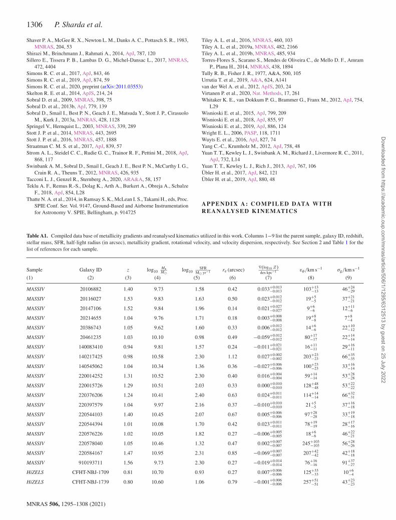
Table A1. Compiled data base of metallicity gradients and reanalysed kinematics utilized in this work. Columns 1−9 list the parent sample, galaxy ID, redshift,stellar mass, SFR, half-light radius (in arcsec), metallicity gradient, rotational velocity, and velocity dispersion, respectively. See Section 2 and Table 1 for thelist of references for each sample.

Sample Galaxy ID z log10M�M� log10

SFRM� yr−1 re (arcsec) ∇(log10 Z)

dex kpc−1 vφ/km s−1 σg/km s−1

(1) (2) (3) (4) (5) (6) (7) (8) (9)

MASSIV 20106882 1.40 9.73 1.58 0.42 0.033+0.013−0.013 103+13

−13 46+24−29

MASSIV 20116027 1.53 9.83 1.63 0.50 0.023+0.012−0.012 19+5

−5 37+21−21

MASSIV 20147106 1.52 9.84 1.96 0.14 0.021+0.027−0.027 9+6

−6 12+11−6

MASSIV 20214655 1.04 9.76 1.71 0.18 0.003+0.008−0.008 19+8

−8 7+8−4

MASSIV 20386743 1.05 9.62 1.60 0.33 0.006+0.012−0.012 14+6

−6 22+10−12

MASSIV 20461235 1.03 10.10 0.98 0.49 −0.059+0.012−0.012 80+17

−17 22+14−14

MASSIV 140083410 0.94 9.81 1.57 0.24 −0.011+0.021−0.021 16+11

−11 29+16−11

MASSIV 140217425 0.98 10.58 2.30 1.12 0.027+0.002−0.002 203+23

−23 66+35−35

MASSIV 140545062 1.04 10.34 1.36 0.36 −0.027+0.006−0.006 100+23

−23 33+16−14

MASSIV 220014252 1.31 10.52 2.30 0.40 0.016+0.004−0.004 59+14

−14 53+28−28

MASSIV 220015726 1.29 10.51 2.03 0.33 0.000+0.010−0.010 128+48

−48 53+22−22

MASSIV 220376206 1.24 10.41 2.40 0.63 0.024+0.011−0.011 114+14

−14 66+32−31

MASSIV 220397579 1.04 9.97 2.16 0.37 −0.010+0.010−0.010 21+5

−5 37+16−18

MASSIV 220544103 1.40 10.45 2.07 0.67 0.005+0.006−0.006 97+28

−28 33+19−18

MASSIV 220544394 1.01 10.08 1.70 0.42 0.023+0.011−0.011 78+19

−19 28+17−16

MASSIV 220576226 1.02 10.05 1.82 0.27 −0.006+0.005−0.005 18+6

−6 46+22−21

MASSIV 220578040 1.05 10.46 1.32 0.47 0.002+0.007−0.007 245+103

−103 56+28−26

MASSIV 220584167 1.47 10.95 2.31 0.85 −0.069+0.007−0.007 207+42

−42 42+18−18

MASSIV 910193711 1.56 9.73 2.30 0.27 −0.019+0.014−0.014 76+16

−16 91+37−27

HiZELS CFHT-NBJ-1709 0.81 10.70 0.93 0.27 0.007+0.006−0.006 125+33

−33 10+6−4

HiZELS CFHT-NBJ-1739 0.80 10.60 1.06 0.79 −0.001+0.006−0.006 257+51

−51 43+23−23

MNRAS 506, 1295–1308 (2021)

Dow

nloaded from https://academ

ic.oup.com/m

nras/article/506/1/1295/6312513 by guest on 25 July 2022

Kinematics and metallicity gradients at high z 1307

Table A1 – continued

Sample Galaxy ID z log10M�M� log10

SFRM� yr−1 re (arcsec) ∇(log10 Z)

dex kpc−1 vφ/km s−1 σg/km s−1

(1) (2) (3) (4) (5) (6) (7) (8) (9)

HiZELS CFHT-NBJ-1740 0.81 10.40 0.95 0.65 0.016+0.005−0.005 285+60

−60 49+23−23

HiZELS CFHT-NBJ-1745 0.82 9.80 0.75 0.54 0.025+0.009−0.009 264+47

−48 58+26−26

HiZELS CFHT-NBJ-1759 0.80 10.30 1.11 0.54 −0.018+0.003−0.003 302+44

−44 15+9−7

HiZELS CFHT-NBJ-1774 0.81 9.80 0.62 0.50 0.013+0.006−0.006 82+24

−24 86+37−32

HiZELS CFHT-NBJ-1787 0.81 10.60 1.08 0.85 0.007+0.004−0.004 303+27

−27 22+10−10

HiZELS CFHT-NBJ-1790 0.81 9.90 0.67 0.22 0.032+0.006−0.006 111+31

−31 10+7−4

HiZELS CFHT-NBJ-1795 0.81 9.80 0.81 0.39 −0.063+0.010−0.010 96+26

−26 10+6−4

SHiZELS HiZELS1 0.84 10.03 0.30 0.23 −0.037+0.030−0.058 100+26

−26 57+23−23

SHiZELS HiZELS7 1.46 9.81 0.90 0.43 −0.019+0.019−0.040 106+18

−18 4+2−1

SHiZELS HiZELS8 1.46 10.32 0.85 0.36 0.006+0.017−0.004 190+26

−26 34+18−18

SHiZELS HiZELS9 1.46 10.08 0.78 0.48 −0.027+0.010−0.018 151+46

−46 59+29−29

SHiZELS HiZELS10 1.45 9.42 1.00 0.27 −0.031+0.016−0.014 37+19

−19 53+25−25

SHiZELS HiZELS11 1.49 11.01 0.90 0.15 −0.087+0.032−0.006 311+42

−42 109+39−33

MUSE-WIDE G103012059 0.56 10.25 1.37 0.72 −0.075+0.014−0.017 223+40

−40 43+18−18

MUSE-WIDE G118011046 0.58 10.54 1.28 1.36 −0.038+0.003−0.003 275+29

−29 37+15−15

MUSE-WIDE G105002016 0.34 10.31 0.25 0.45 −0.025+0.019−0.014 141+11

−11 64+14−16

MUSE-WIDE G122003050 0.21 9.97 0.02 1.44 −0.065+0.001−0.001 169+37

−37 43+6−6

MUSE-WIDE G102021103 0.25 9.22 − 0.68 0.78 −0.024+0.024−0.021 62+15

−15 41+6−6

MUSE-WIDE G105012048 0.68 10.39 1.07 0.92 −0.044+0.006−0.008 149+27

−27 46+19−19

MUSE-WIDE G104005033 0.40 8.64 − 0.72 0.90 0.047+0.021−0.021 43+10

−10 33+10−10

MUSE-WIDE G107029135 0.74 9.75 0.84 0.50 −0.144+0.024−0.024 39+22

−22 35+14−14

MUSE-WIDE G101001006 0.31 8.64 − 0.65 0.64 −0.049+0.010−0.011 61+28

−28 31+5−5

MUSE-WIDE G114007070 0.13 8.66 − 1.50 1.46 −0.131+0.080−0.069 91+22

−22 38+6−6

MUSE-WIDE G108016127 0.21 8.50 − 1.05 0.62 −0.188+0.046−0.061 62+19

−19 46+13−10

MUSE-WIDE HDFS3 0.56 9.75 1.39 1.34 −0.032+0.002−0.002 68+17

−17 24+13−13

MUSE-WIDE HDFS6 0.42 9.40 − 0.02 0.60 0.002+0.005−0.006 37+12

−12 33+10−10

MUSE-WIDE HDFS7 0.46 9.49 0.19 0.73 −0.133+0.007−0.007 50+17

−17 40+12−12

MUSE-WIDE HDFS8 0.58 10.00 1.12 0.30 −0.058+0.013−0.014 69+21

−21 53+27−27

MUSE-WIDE HDFS9 0.56 9.49 0.96 0.42 −0.124+0.009−0.010 72+33

−33 45+22−22

MUSE-WIDE HDFS11 0.58 9.31 0.52 0.17 −0.262+0.052−0.028 8+15

−4 21+9−9

MUSE-WIDE UDF1 0.62 10.60 1.19 1.34 −0.026+0.003−0.003 131+13

−13 34+15−15

MUSE-WIDE UDF2 0.42 9.89 − 0.07 0.58 0.002+0.003−0.003 119+12

−12 50+4−4

MUSE-WIDE UDF3 0.62 10.13 0.82 0.86 −0.081+0.012−0.013 75+25

−25 45+22−22

MUSE-WIDE UDF4 0.77 10.06 1.26 0.98 −0.037+0.003−0.003 47+19

−19 37+16−16

MUSE-WIDE UDF7 0.62 9.39 0.70 0.68 −0.188+0.011−0.010 10+5

−3 27+13−13

MUSE-WIDE UDF10 0.28 8.34 − 0.81 0.64 0.034+0.018−0.017 50+16

−16 39+22−22

SINS / zC-SINF Q2343-BX389 2.17 10.61 1.76 0.74 −0.048+0.032−0.030 299+40

−21 56+13−15

SINS / zC-SINF Q2346-BX482 2.26 10.26 1.53 0.72 0.007+0.039−0.034 287+63

−30 58+14−15

SINS / zC-SINF Q2343-BX513 2.11 10.43 1.23 0.31 −0.021+0.075−0.075 102+64

−26 55+24−28

SINS / zC-SINF Q1623-BX599 2.33 10.75 1.73 0.29 −0.036+0.037−0.042 139+62

−36 71+18−27

SINS / zC-SINF Q2343-BX610 2.21 11.00 1.56 0.53 −0.066+0.023−0.020 241+62

−38 64+17−24

MNRAS 506, 1295–1308 (2021)

Dow

nloaded from https://academ

ic.oup.com/m

nras/article/506/1/1295/6312513 by guest on 25 July 2022

1308 P. Sharda et al.

Table A1 – continued

Sample Galaxy ID z log10M�M� log10

SFRM� yr−1 re (arcsec) ∇(log10 Z)

dex kpc−1 vφ/km s−1 σg/km s−1

(1) (2) (3) (4) (5) (6) (7) (8) (9)

SINS / zC-SINF Deep3a-15504 2.38 11.04 1.73 0.72 −0.026+0.013−0.013 305+138

−80 63+13−15

SINS / zC-SINF Deep3a-6004 2.39 11.50 1.92 0.61 −0.032+0.023−0.028 362+109

−126 55+11−17

SINS / zC-SINF Deep3a-6397 1.51 11.08 1.63 0.69 −0.041+0.011−0.015 351+138

−107 59+13−17

SINS / zC-SINF ZC400528 2.39 11.04 1.69 0.29 −0.009+0.045−0.049 341+184

−89 28+23−15

SINS / zC-SINF ZC400569N 2.24 11.11 1.59 0.85 −0.064+0.016−0.014 364+138

−64 43+16−21

SINS / zC-SINF ZC400569 2.24 11.21 1.63 0.88 −0.050+0.013−0.014 312+19

−13 41+23−21

SINS / zC-SINF ZC403741 1.45 10.65 1.33 0.26 −0.123+0.065−0.081 189+73

−36 36+13−12

SINS / zC-SINF ZC406690 2.20 10.62 1.80 0.83 −0.046+0.028−0.027 313+88

−107 60+16−15

SINS / zC-SINF ZC407302 2.18 10.39 1.78 0.43 −0.023+0.020−0.020 217+71

−40 56+11−25

SINS / zC-SINF ZC407376S 2.17 10.14 1.51 0.19 −0.021+0.071−0.073 89+65

−45 77+37−41

SINS / zC-SINF ZC407376 2.17 10.40 1.65 0.65 −0.048+0.044−0.048 86+24

−20 56+28−27

SINS / zC-SINF ZC412369 2.03 10.34 1.62 0.36 −0.047+0.050−0.051 120+40

−27 75+13−27

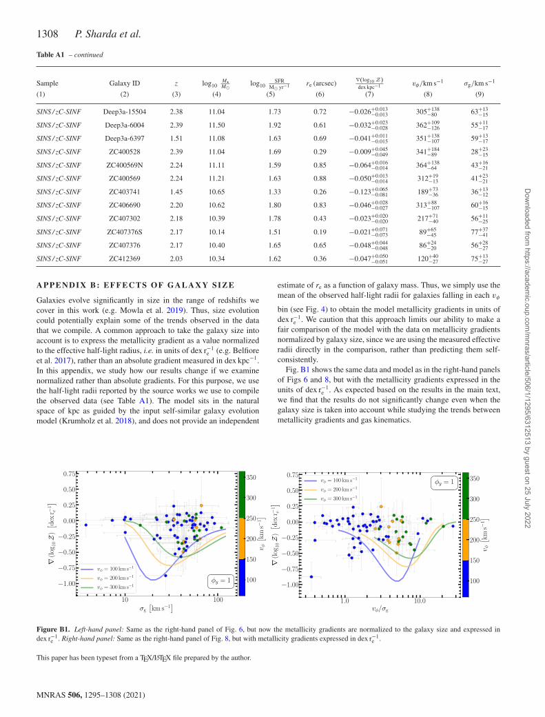
APPENDIX B: EFFECTS O F G ALAXY SIZE

Galaxies evolve significantly in size in the range of redshifts wecover in this work (e.g. Mowla et al. 2019). Thus, size evolutioncould potentially explain some of the trends observed in the datathat we compile. A common approach to take the galaxy size intoaccount is to express the metallicity gradient as a value normalizedto the effective half-light radius, i.e. in units of dex r−1

e (e.g. Belfioreet al. 2017), rather than an absolute gradient measured in dex kpc−1.In this appendix, we study how our results change if we examinenormalized rather than absolute gradients. For this purpose, we usethe half-light radii reported by the source works we use to compilethe observed data (see Table A1). The model sits in the naturalspace of kpc as guided by the input self-similar galaxy evolutionmodel (Krumholz et al. 2018), and does not provide an independent

estimate of re as a function of galaxy mass. Thus, we simply use themean of the observed half-light radii for galaxies falling in each vφ

bin (see Fig. 4) to obtain the model metallicity gradients in units ofdex r−1

e . We caution that this approach limits our ability to make afair comparison of the model with the data on metallicity gradientsnormalized by galaxy size, since we are using the measured effectiveradii directly in the comparison, rather than predicting them self-consistently.

Fig. B1 shows the same data and model as in the right-hand panelsof Figs 6 and 8, but with the metallicity gradients expressed in theunits of dex r−1

e . As expected based on the results in the main text,we find that the results do not significantly change even when thegalaxy size is taken into account while studying the trends betweenmetallicity gradients and gas kinematics.

Figure B1. Left-hand panel: Same as the right-hand panel of Fig. 6, but now the metallicity gradients are normalized to the galaxy size and expressed index r−1

e . Right-hand panel: Same as the right-hand panel of Fig. 8, but with metallicity gradients expressed in dex r−1e .

This paper has been typeset from a TEX/LATEX file prepared by the author.

MNRAS 506, 1295–1308 (2021)

Dow

nloaded from https://academ

ic.oup.com/m

nras/article/506/1/1295/6312513 by guest on 25 July 2022