molecular hydrogen kinematics in cepheus a
TRANSCRIPT
arX
iv:a
stro
-ph/
0408
395v
1 2
2 A
ug 2
004
Molecular Hydrogen Kinematics in Cepheus A1
David Hiriart2 and Luis Salas2
Instituto de Astronomıa (Unidad Ensenada), Universidad Nacional Autonoma de Mexico
Apdo. Postal 877, 22830 Ensenada, B.C. Mexico
[email protected], [email protected]
and
Irene Cruz-Gonzalez2
Instituto de Astronomıa, UNAM
Circuito Exterior C.U., 04510 Mexico, D. F., Mexico
ABSTRACT
We present the radial velocity structure of the molecular hydrogen outflows associated tothe star forming region Cepheus A. This structure is derived from the doppler shift of the H2
v=1–0 S(1) emission line obtained by Fabry–Perot spectroscopy. The East and West regions ofemission, called Cep A (E) and Cep A (W), show radial velocities in the range of -20 to 0 km s−1
with respect to the molecular cloud. Cep A (W) shows an increasing velocity with position offsetfrom the core indicating the existence of a possible accelerating mechanism. Cep A (E) hasan almost constant mean radial velocity of -18 km s−1 along the region although with a largedispersion in velocity, indicating the possibility of a turbulent outflow. A detailed analysis ofthe Cep A (E) region shows evidence for the presence of a Mach disk on that outflow. Also, weargue that the presence of a velocity gradient in Cep A (W) is indicative of a C-shock in thisregion. Following Riera et al. (2003), we analyzed the data using wavelet analysis to study theline width and central radial velocity distributions. We found that both outflows have complexspatial and velocity structure characteristic of a turbulent flow.
Subject headings: ISM: individual (Cepheus A) – ISM: jets and outflows – ISM: kinematics and dynamics– ISM: molecules – ISM: Turbulence – infrared: ISM
1. Introduction
Cepheus A is the densest core within theCepheus OB3 molecular cloud complex (Sargent1977) and a massive star forming region. It con-tains a deeply embedded infrared source whichgenerates a total luminosity of ∼ 2.4 × 10⁴L⊙
(Koppenaal et al. 1979).
1Based on observations made at the 2.1 m telescope ofthe Observatorio Astronomico Nacional at San PedroMartir, B.C., Mexico.
2Observatorio Astronomico Nacional, San Pedro Martir,B.C., Mexico.
Two main regions of ionized and molecular gasabout 2 arc minutes apart and oriented roughlyin the east-west direction, have been detected,Cepheus A East (Bally & Lane 1982) and CepheusA West (Simon & Joyce 1983; Garay et al. 1996).The first molecular hydrogen map of both regionsusing Fabry-Perot spectroscopy was presented byDoyon & Nadeau (1988). Later, Hartigan etal. (1986) obtained high resolution images in thev=1–0 S(1) line emission of H2 from Cepheus AWest. The two Cepheus A regions with molecularhydrogen emission show quite different composi-tions.
1
The eastern region (hereon Cep A (E)) hostsone of the first detected CO bipolar molecular out-flows (Rodrıguez, Ho, & Moran 1980). High reso-lution observations show a more complex outflowof a quadrupole nature (Torrelles et al. 1993).Torrelles et al. (1993) suggested that the sourceCep A East:HW2 (Hughes & Wouterloot 1984)is powering the PA=45◦ outflow but it is notclear if the powering source of the PA=115◦ out-flow is Cep A East:HW3 or another source (L.F. Rodrıguez, personal communication). Obser-vations of 12CO, CS, and CSO give evidence ofmultiple episodes of outflow activity (Narayanan& Walker 1996). Observations by Codella etal. (2003) of H2S and SO2 confirm the pres-ence of multiple outflows. Highly variable H2Oand OH masers, commonly associated to youngstellar objects, are surrounded by very dense NH3
condensations that probably redirect the outflowinto a quadrupole structure (Torrelles et al. 1993;Narayanan & Walker 1996).
The western region (hereon Cep A (W)) con-tains several radio continuum sources at 3 cm(Garay et al. 1996) and Hartigan et al. (1986)identified a region of several Herbig-Haro objectsknown as HH 168 (GGD 37) with large radialvelocities and line widths. A bipolar outflow ofCO with overlapping red- and blue-shifted lobesis associated to this region (Bally & Lane 1982;Narayanan & Walker 1996). It should be pointedout that the energy source of Cep A (W) remainselusive (Raines et al. 2000; Garay et al. 1996;Torrelles et al. 1993; Hartigan & Lada 1985).
Although the two regions Cep A (E) andCep A (W) could constitute a single large struc-ture outflow, several authors have presented ev-idence which suggests that Cep A (W) may bean independent region of activity, distinct fromCep A (E) (Raines et al. 2000; Garay et al.1996; Hartigan & Lada 1985).
In this paper we present the radial velocitystructure of the Cepheus A molecular hydro-gen outflows obtained from the H2 v=1–0 S(1)doppler shifted emission line at 2.122 µm mea-sured by scanning Fabry-Perot spectroscopy. Dueto the complexity found in the velocity structures,we decided to study the kinematics by using anasymmetric wavelet analysis following Riera etal. (2003), who used this method to study HαFabry-Perot observations of the HH 100 jet.
Our results show that the two regions representturbulent H2 outflows with significant differencesfrom a kinematic point of view. A detailed analy-sis of the Cep A (E) region provides evidence forthe presence of a Mach disk near the tip of theoutflow.
In § 2 we described the observations. From thisdata, in § 3 we generate a doppler shift H2 image,radial velocity, velocity gradient and line widthmaps, and study the flux-velocity diagrams (Salas& Cruz-Gonzalez 2002). By using the asymmetricwavelet transform, the clumpy structures of bothregions of Cepheus A are kinetically analyzed anddiscussed in § 4. The conclusions are then sum-marized and presented in § 5.
2. Observations
In October 5, 1998, we observed the Cepheus Aregion with the 2.1 m telescope of the ObservatorioAstronomico Nacional at San Pedro Martir, B.C.in Mexico.
The measurements were obtained with theCAMILA near-infrared camera/spectrograph (Cruz-Gonzalez et al. 1994) with the addition of a cooledtunable Fabry-Perot interferometer (located in thecollimated beam of the cooled optical bench), anda 2.12 µm interference filter. A detailed descrip-tion for the infrared scanning Fabry-Perot instru-mental setup is presented by Salas et al. (1999).
The Fabry-Perot has a spectral resolution of 24km s−1 and to restrict the spectral range for thev=1–0 S(1) H2 line emission, an interference fil-ter (2.122 µm with ∆λ= 0.02 µm ) was used.The bandwidth of this filter allows 11 orders ofinterference. Only one of these orders contain the2.122 µm line and the remaining orders contributeto the observed continuum. The spatial resolutionof the instrumental array is ∼ 0.86′′ pixel−1. Thefield of view allows to cover a 3.67′ × 3.67′ re-gion, which corresponds to 0.7 × 0.7 pc2 at theadopted distance of 725 pc (Johnson 1957). Withthis field of view, one set of images was requiredfor the eastern portion and another for the westernregion of Cepheus A.
Images of each region of interest were obtainedat 26 etalon positions, corresponding to incre-ments of 9.82 km s−1. The observing sequenceconsists of tunning the etalon to a new positionand imaging the source followed by a sky expo-
2
sure at an offset of 5′ south from the source.The integration time of 60 s per frame was shortenough to cancel the atmospheric lines variationsat each etalon position, but long enough to obtaina good signal-to-noise ratio. Images were takenunder photometric conditions with a FWHM of1.6′′.
Spectral calibration was obtained by observingthe line at 2.1332885 µm of the Argon lamp ateach position of the etalon, giving a velocity un-certainty of 1 km s−1 in the wavelength fit. A setof high- and low-illumination sky flats were ob-tained for flat-fielding purposes.
We reduced the data to obtain the velocitychannel images using the software and the data re-duction technique described in Salas et al. (1999).
3. Results
3.1. H2 Velocity Maps
Velocity channel images were individually ob-tained for Cep A (E) and Cep A (W) from theposition-velocity cube data. For each pixel on theimage we subtracted a continuum intensity levelcalculated from the median of the channels withno H2 emission. H2 v=1–0 S(1) line emission wasdetected in velocity channels -40 to 0 km s−1 inCep A (E) and in channels -40 to 10 km s−1 inCep A (W). The two sets of maps were pasted to-gether to create velocity channel maps of the com-plete region. Figure 1 shows five of these maps (8to 12) covering Local Standard of Rest (LSR) ve-locities from -42 km s−1 to -3 km s−1. Cep A (E)shows H2 emission in six separated clumps of emis-sion (labeled B–G in Fig. 1), while Cep A (W) theemission may be distinguished in six regions (la-beled H–M).
We created a color coded velocity image fromthe three channel velocity maps with more copiousemission (-32.3, -22.5, and -12.7 km s−1) as blue,green, and red respectively. Figure 2 presentsthis color composite map. It should be notedthat these velocities are somewhat bluer than the-11.2 km s−1 systemic velocity found from mil-limeter wavelength line observations of CO (e.g.Narayanan & Walker (1996)), as had already beennoted by Doyon & Nadeau (1988).
The velocity structure in both regions shows avery complex pattern. However, a slightly system-
atic change from blue to red starting at the centerof the image can be appreciated on the westernoutflow, that is not present in the eastern region.On the other hand, the Ceph A (E) region showsa large amount of small clumps with different ve-locities lying side by side.
We have calculated the centroid radial velocityfor each pixel by taking only 10 velocity channelsaround the peak intensity. Figure 3 presents his-tograms of centroid radial velocity for the two H2
emission regions of the image in Fig. 2. Regardlessof the difference in morphology for the two regions,they have similar fractional distribution of pixelsfor a given radial velocity. However, Cep A (W)has a wing that extends into positive radial veloc-ities and a small peak in the negative velocities.
Figure 4 presents the centroid radial veloc-ity as a function of displacement along the rightascension axis for both regions Cep A (E) andCep A (W). All the channels with detected emis-sion of H2 from Fig. 2 are shown. The radial ve-locity of Cep A (E) has an almost constant meanvalue of ∼-18 km s−1 along the region with a highdispersion around this value. Meanwhile, radialvelocity of Cep A (W) increases its value with off-set position to the West. We have fitted a lineto each position-velocity data for each region andfound rms residual values of 8.3 and 10.2 km s−1
for Cep A(W) and Cep A(E), respectively. Thesmaller velocity dispersion and the large numberof small clumps with different velocities (see Fig 2)in the East region indicate a more turbulent out-flow in Cep A(E) compared to Cep A(W).
3.2. A Mach disk in CephA(E)
The Cep A (E) outflow culminates in an arcshaped structure (labeled G in Fig. 1) that re-sembles a bow shock. This region is amplified inFig. 5a. A bright spot can be seen in the center ofthe bow. The centroid velocities corresponding tothis region are shown in Fig. 5c. The highest blue-shifted velocity of the region (-40 km s−1) corre-sponds to a slightly elongated region (in the direc-tion perpendicular to the outflow) that includesthe bright spot and decreases toward the bow, ascan also be seen in a position-velocity diagram inFig. 5d. This kinematic behavior is expected ifthe bright spot corresponds to the Mach disk ofthe jet, where the jet material interacts with pre-viously swept material accumulating in front of the
3
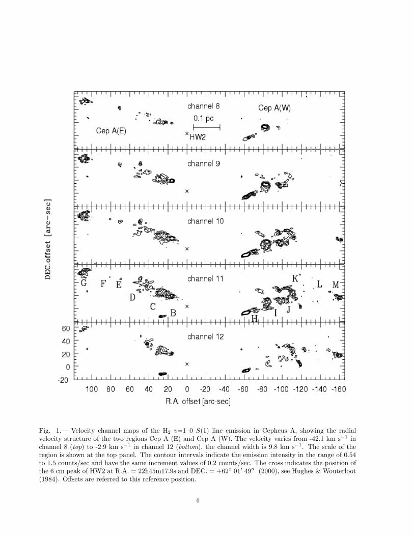
Fig. 1.— Velocity channel maps of the H2 v=1–0 S(1) line emission in Cepheus A, showing the radialvelocity structure of the two regions Cep A (E) and Cep A (W). The velocity varies from -42.1 km s−1 inchannel 8 (top) to -2.9 km s−1 in channel 12 (bottom), the channel width is 9.8 km s−1. The scale of theregion is shown at the top panel. The contour intervals indicate the emission intensity in the range of 0.54to 1.5 counts/sec and have the same increment values of 0.2 counts/sec. The cross indicates the position ofthe 6 cm peak of HW2 at R.A. = 22h45m17.9s and DEC. = +62◦ 01′ 49′′ (2000), see Hughes & Wouterloot(1984). Offsets are referred to this reference position.
4
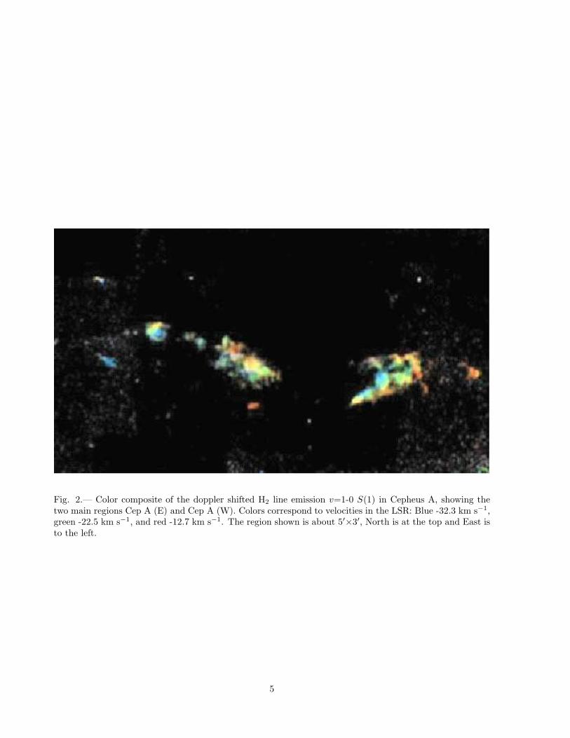
Fig. 2.— Color composite of the doppler shifted H2 line emission v=1-0 S(1) in Cepheus A, showing thetwo main regions Cep A (E) and Cep A (W). Colors correspond to velocities in the LSR: Blue -32.3 km s−1,green -22.5 km s−1, and red -12.7 km s−1. The region shown is about 5′×3′, North is at the top and East isto the left.
5
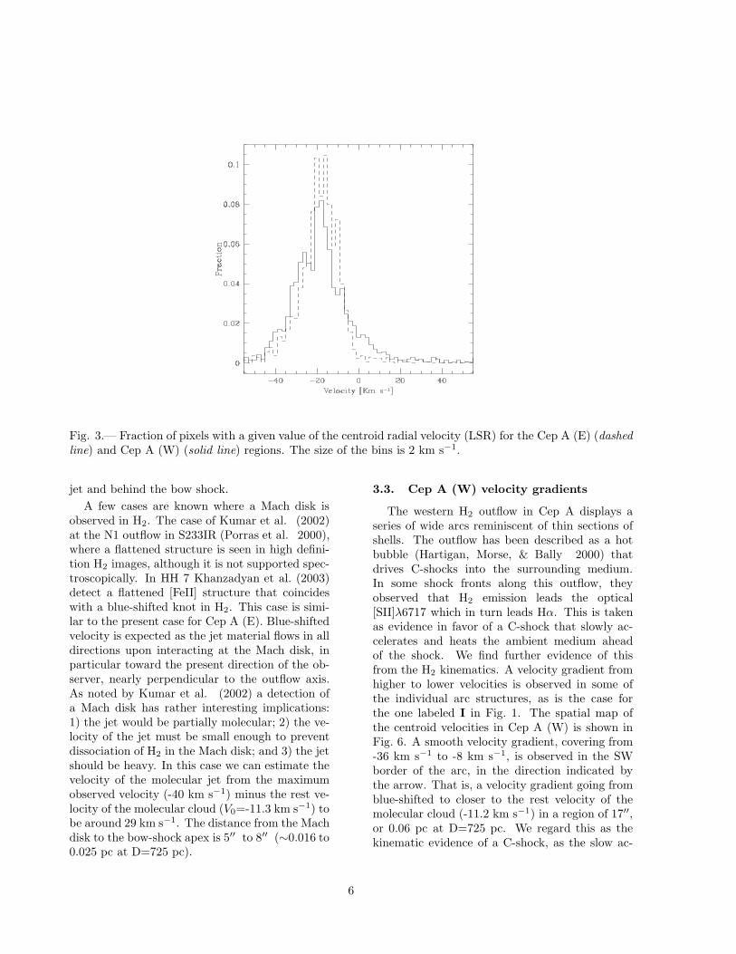
Fig. 3.— Fraction of pixels with a given value of the centroid radial velocity (LSR) for the Cep A (E) (dashedline) and Cep A (W) (solid line) regions. The size of the bins is 2 km s−1.
jet and behind the bow shock.
A few cases are known where a Mach disk isobserved in H2. The case of Kumar et al. (2002)at the N1 outflow in S233IR (Porras et al. 2000),where a flattened structure is seen in high defini-tion H2 images, although it is not supported spec-troscopically. In HH 7 Khanzadyan et al. (2003)detect a flattened [FeII] structure that coincideswith a blue-shifted knot in H2. This case is simi-lar to the present case for Cep A (E). Blue-shiftedvelocity is expected as the jet material flows in alldirections upon interacting at the Mach disk, inparticular toward the present direction of the ob-server, nearly perpendicular to the outflow axis.As noted by Kumar et al. (2002) a detection ofa Mach disk has rather interesting implications:1) the jet would be partially molecular; 2) the ve-locity of the jet must be small enough to preventdissociation of H2 in the Mach disk; and 3) the jetshould be heavy. In this case we can estimate thevelocity of the molecular jet from the maximumobserved velocity (-40 km s−1) minus the rest ve-locity of the molecular cloud (V0=-11.3 km s−1) tobe around 29 km s−1. The distance from the Machdisk to the bow-shock apex is 5′′ to 8′′ (∼0.016 to0.025 pc at D=725 pc).
3.3. Cep A (W) velocity gradients
The western H2 outflow in Cep A displays aseries of wide arcs reminiscent of thin sections ofshells. The outflow has been described as a hotbubble (Hartigan, Morse, & Bally 2000) thatdrives C-shocks into the surrounding medium.In some shock fronts along this outflow, theyobserved that H2 emission leads the optical[SII]λ6717 which in turn leads Hα. This is takenas evidence in favor of a C-shock that slowly ac-celerates and heats the ambient medium aheadof the shock. We find further evidence of thisfrom the H2 kinematics. A velocity gradient fromhigher to lower velocities is observed in some ofthe individual arc structures, as is the case forthe one labeled I in Fig. 1. The spatial map ofthe centroid velocities in Cep A (W) is shown inFig. 6. A smooth velocity gradient, covering from-36 km s−1 to -8 km s−1, is observed in the SWborder of the arc, in the direction indicated bythe arrow. That is, a velocity gradient going fromblue-shifted to closer to the rest velocity of themolecular cloud (-11.2 km s−1) in a region of 17′′,or 0.06 pc at D=725 pc. We regard this as thekinematic evidence of a C-shock, as the slow ac-
6
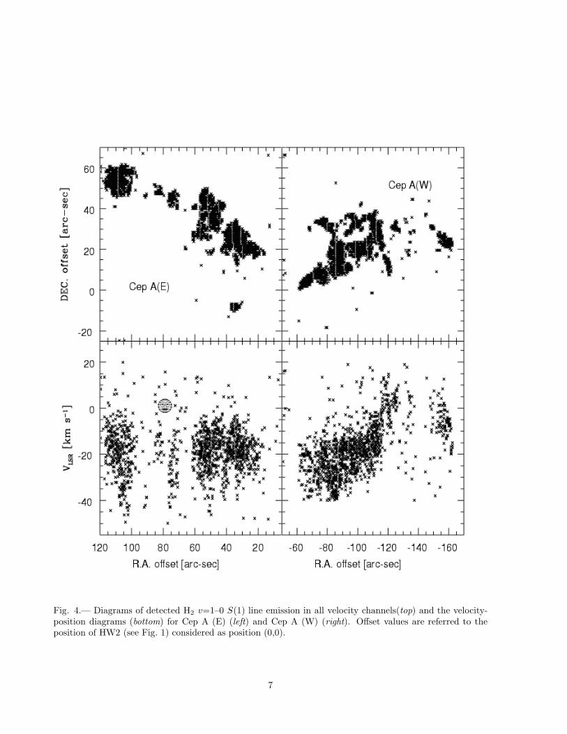
Fig. 4.— Diagrams of detected H2 v=1–0 S(1) line emission in all velocity channels(top) and the velocity-position diagrams (bottom) for Cep A (E) (left) and Cep A (W) (right). Offset values are referred to theposition of HW2 (see Fig. 1) considered as position (0,0).
7
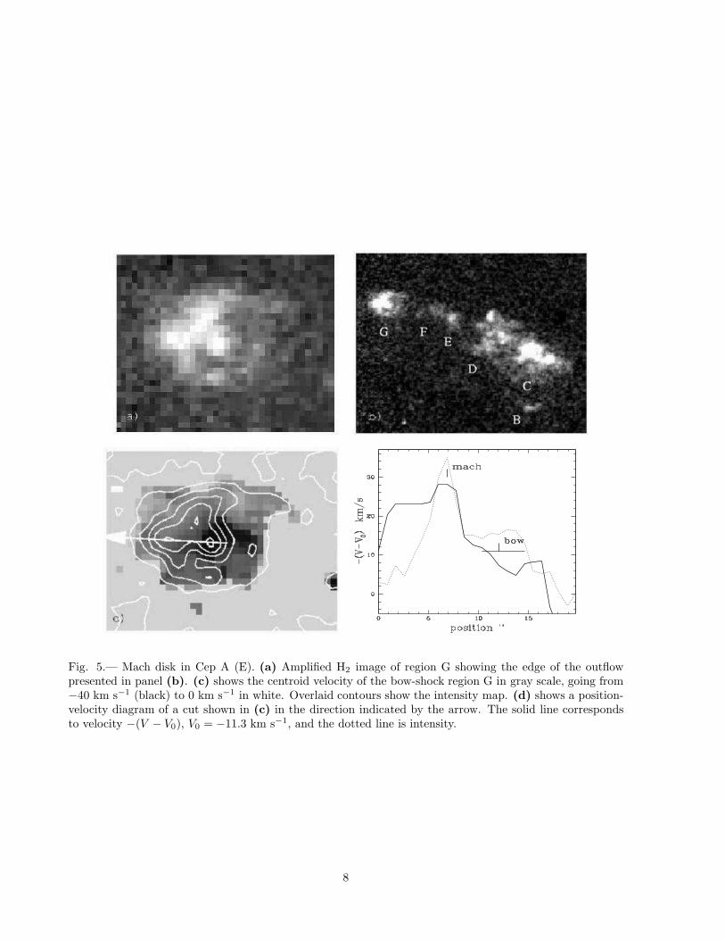
Fig. 5.— Mach disk in Cep A (E). (a) Amplified H2 image of region G showing the edge of the outflowpresented in panel (b). (c) shows the centroid velocity of the bow-shock region G in gray scale, going from−40 km s−1 (black) to 0 km s−1 in white. Overlaid contours show the intensity map. (d) shows a position-velocity diagram of a cut shown in (c) in the direction indicated by the arrow. The solid line correspondsto velocity −(V − V0), V0 = −11.3 km s−1, and the dotted line is intensity.
8
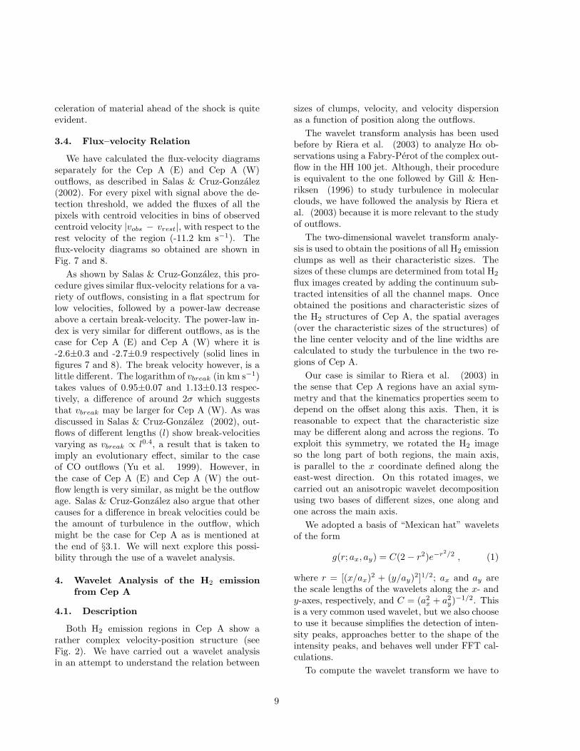
celeration of material ahead of the shock is quiteevident.
3.4. Flux–velocity Relation
We have calculated the flux-velocity diagramsseparately for the Cep A (E) and Cep A (W)outflows, as described in Salas & Cruz-Gonzalez(2002). For every pixel with signal above the de-tection threshold, we added the fluxes of all thepixels with centroid velocities in bins of observedcentroid velocity |vobs − vrest|, with respect to therest velocity of the region (-11.2 km s−1). Theflux-velocity diagrams so obtained are shown inFig. 7 and 8.
As shown by Salas & Cruz-Gonzalez, this pro-cedure gives similar flux-velocity relations for a va-riety of outflows, consisting in a flat spectrum forlow velocities, followed by a power-law decreaseabove a certain break-velocity. The power-law in-dex is very similar for different outflows, as is thecase for Cep A (E) and Cep A (W) where it is-2.6±0.3 and -2.7±0.9 respectively (solid lines infigures 7 and 8). The break velocity however, is alittle different. The logarithm of vbreak (in km s−1)takes values of 0.95±0.07 and 1.13±0.13 respec-tively, a difference of around 2σ which suggeststhat vbreak may be larger for Cep A (W). As wasdiscussed in Salas & Cruz-Gonzalez (2002), out-flows of different lengths (l) show break-velocitiesvarying as vbreak ∝ l0.4, a result that is taken toimply an evolutionary effect, similar to the caseof CO outflows (Yu et al. 1999). However, inthe case of Cep A (E) and Cep A (W) the out-flow length is very similar, as might be the outflowage. Salas & Cruz-Gonzalez also argue that othercauses for a difference in break velocities could bethe amount of turbulence in the outflow, whichmight be the case for Cep A as is mentioned atthe end of §3.1. We will next explore this possi-bility through the use of a wavelet analysis.
4. Wavelet Analysis of the H2 emissionfrom Cep A
4.1. Description
Both H2 emission regions in Cep A show arather complex velocity-position structure (seeFig. 2). We have carried out a wavelet analysisin an attempt to understand the relation between
sizes of clumps, velocity, and velocity dispersionas a function of position along the outflows.
The wavelet transform analysis has been usedbefore by Riera et al. (2003) to analyze Hα ob-servations using a Fabry-Perot of the complex out-flow in the HH 100 jet. Although, their procedureis equivalent to the one followed by Gill & Hen-riksen (1996) to study turbulence in molecularclouds, we have followed the analysis by Riera etal. (2003) because it is more relevant to the studyof outflows.
The two-dimensional wavelet transform analy-sis is used to obtain the positions of all H2 emissionclumps as well as their characteristic sizes. Thesizes of these clumps are determined from total H2
flux images created by adding the continuum sub-tracted intensities of all the channel maps. Onceobtained the positions and characteristic sizes ofthe H2 structures of Cep A, the spatial averages(over the characteristic sizes of the structures) ofthe line center velocity and of the line widths arecalculated to study the turbulence in the two re-gions of Cep A.
Our case is similar to Riera et al. (2003) inthe sense that Cep A regions have an axial sym-metry and that the kinematics properties seem todepend on the offset along this axis. Then, it isreasonable to expect that the characteristic sizemay be different along and across the regions. Toexploit this symmetry, we rotated the H2 imageso the long part of both regions, the main axis,is parallel to the x coordinate defined along theeast-west direction. On this rotated images, wecarried out an anisotropic wavelet decompositionusing two bases of different sizes, one along andone across the main axis.
We adopted a basis of “Mexican hat” waveletsof the form
g(r; ax, ay) = C(2 − r2)e−r2/2 , (1)
where r = [(x/ax)2 + (y/ay)2]1/2; ax and ay arethe scale lengths of the wavelets along the x- andy-axes, respectively, and C = (a2
x + a2y)−1/2. This
is a very common used wavelet, but we also chooseto use it because simplifies the detection of inten-sity peaks, approaches better to the shape of theintensity peaks, and behaves well under FFT cal-culations.
To compute the wavelet transform we have to
9
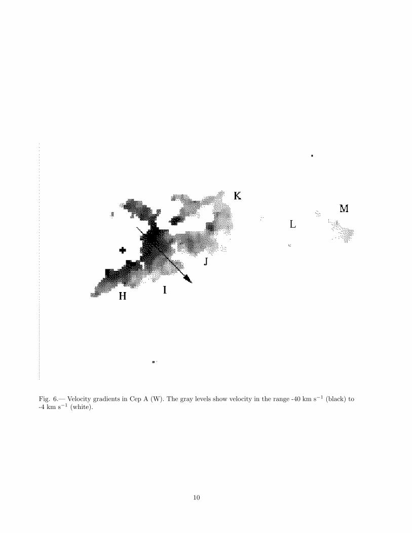
Fig. 6.— Velocity gradients in Cep A (W). The gray levels show velocity in the range -40 km s−1 (black) to-4 km s−1 (white).
10
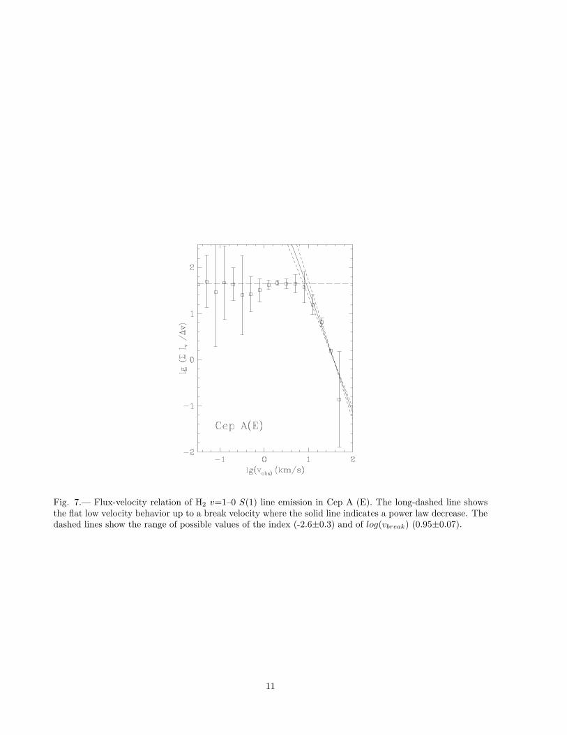
Fig. 7.— Flux-velocity relation of H2 v=1–0 S(1) line emission in Cep A (E). The long-dashed line showsthe flat low velocity behavior up to a break velocity where the solid line indicates a power law decrease. Thedashed lines show the range of possible values of the index (-2.6±0.3) and of log(vbreak) (0.95±0.07).
11
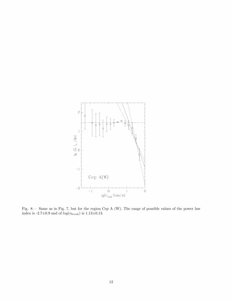
Fig. 8.— Same as in Fig. 7, but for the region Cep A (W). The range of possible values of the power lawindex is -2.7±0.9 and of log(vbreak) is 1.13±0.13.
12
calculate the convolutions
Tax,ay(x, y) =
∫ ∫I(x′, y′)g(r′; ax, ay)dx′dy′ ,
(2)for each pair (ax, ay), where r′ = {[(x′−x)/ax]2 +[(y′ − y)/ay]2}1/2, I(x, y) is the intensity at pixelposition (x, y), and g(r′; ax, ay) is give by eq. (1).These convolutions are calculated by using a FastFourier Transform (FFT) algorithm (Press et al.1992).
The wavelet transformed images Tax,ay(x, y)
correspond to smoothed versions of the intensityof the H2 image. We use this images to find thesizes of the structures in the H2 regions of Ceph A.First, on the transformed image with ax = ay = 1,we fixed the position of x and find all the valuesof y where Tax,ay
(x, y) has a local maximum. Sev-eral maxima may be found for each position x thatcorrespond to different structures observed acrossthe regions. The maxima found with ax = ay = 1will correspond also to the local maxima of I(x, y).
For each pair (x,y) where I(x, y) has a max-imum we determine (ax, ay), in the ax and ay
space, where the wavelet transform has a localmaximum. ax and ay will be the characteristic sizeof the clump with a maximum intensity at (x,y).The (ax,ay) space is search in such way that wefirst identify the size of the smaller clumps andthen the bigger ones. This progressive selectionallow us avoid to choose clumps that overlap withits neighbors. Naturally, the biggest clumps willhave an structure similar to the whole region.
4.2. Size of the H2 Clumps
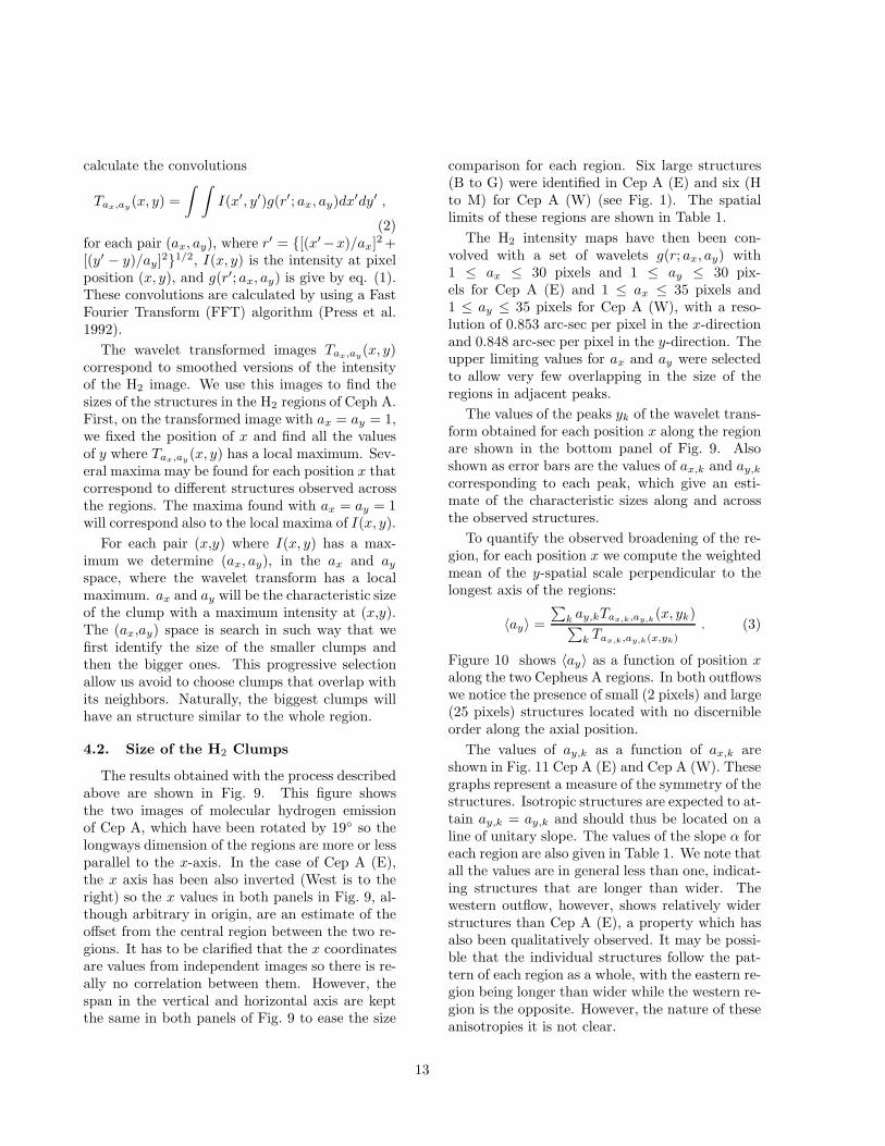
The results obtained with the process describedabove are shown in Fig. 9. This figure showsthe two images of molecular hydrogen emissionof Cep A, which have been rotated by 19◦ so thelongways dimension of the regions are more or lessparallel to the x-axis. In the case of Cep A (E),the x axis has been also inverted (West is to theright) so the x values in both panels in Fig. 9, al-though arbitrary in origin, are an estimate of theoffset from the central region between the two re-gions. It has to be clarified that the x coordinatesare values from independent images so there is re-ally no correlation between them. However, thespan in the vertical and horizontal axis are keptthe same in both panels of Fig. 9 to ease the size
comparison for each region. Six large structures(B to G) were identified in Cep A (E) and six (Hto M) for Cep A (W) (see Fig. 1). The spatiallimits of these regions are shown in Table 1.
The H2 intensity maps have then been con-volved with a set of wavelets g(r; ax, ay) with1 ≤ ax ≤ 30 pixels and 1 ≤ ay ≤ 30 pix-els for Cep A (E) and 1 ≤ ax ≤ 35 pixels and1 ≤ ay ≤ 35 pixels for Cep A (W), with a reso-lution of 0.853 arc-sec per pixel in the x-directionand 0.848 arc-sec per pixel in the y-direction. Theupper limiting values for ax and ay were selectedto allow very few overlapping in the size of theregions in adjacent peaks.
The values of the peaks yk of the wavelet trans-form obtained for each position x along the regionare shown in the bottom panel of Fig. 9. Alsoshown as error bars are the values of ax,k and ay,k
corresponding to each peak, which give an esti-mate of the characteristic sizes along and acrossthe observed structures.
To quantify the observed broadening of the re-gion, for each position x we compute the weightedmean of the y-spatial scale perpendicular to thelongest axis of the regions:
〈ay〉 =
∑k ay,kTax,k,ay,k
(x, yk)∑k Tax,k,ay,k(x,yk)
. (3)
Figure 10 shows 〈ay〉 as a function of position xalong the two Cepheus A regions. In both outflowswe notice the presence of small (2 pixels) and large(25 pixels) structures located with no discernibleorder along the axial position.
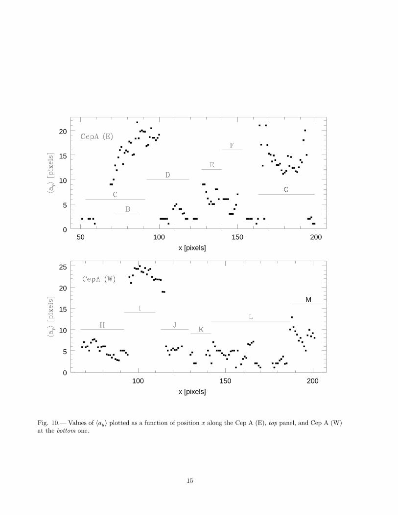
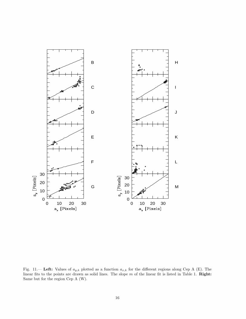
The values of ay,k as a function of ax,k areshown in Fig. 11 Cep A (E) and Cep A (W). Thesegraphs represent a measure of the symmetry of thestructures. Isotropic structures are expected to at-tain ay,k = ay,k and should thus be located on aline of unitary slope. The values of the slope α foreach region are also given in Table 1. We note thatall the values are in general less than one, indicat-ing structures that are longer than wider. Thewestern outflow, however, shows relatively widerstructures than Cep A (E), a property which hasalso been qualitatively observed. It may be possi-ble that the individual structures follow the pat-tern of each region as a whole, with the eastern re-gion being longer than wider while the western re-gion is the opposite. However, the nature of theseanisotropies it is not clear.
13
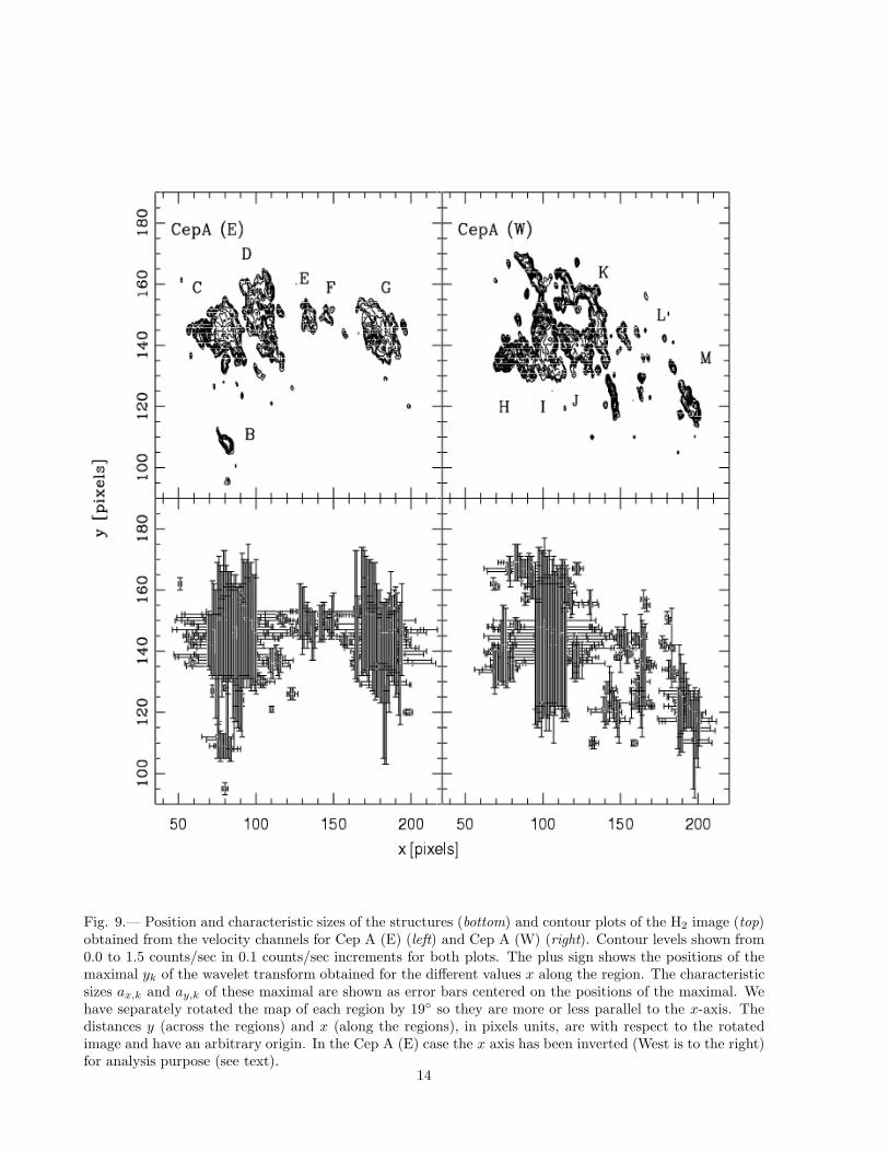
Fig. 9.— Position and characteristic sizes of the structures (bottom) and contour plots of the H2 image (top)obtained from the velocity channels for Cep A (E) (left) and Cep A (W) (right). Contour levels shown from0.0 to 1.5 counts/sec in 0.1 counts/sec increments for both plots. The plus sign shows the positions of themaximal yk of the wavelet transform obtained for the different values x along the region. The characteristicsizes ax,k and ay,k of these maximal are shown as error bars centered on the positions of the maximal. Wehave separately rotated the map of each region by 19◦ so they are more or less parallel to the x-axis. Thedistances y (across the regions) and x (along the regions), in pixels units, are with respect to the rotatedimage and have an arbitrary origin. In the Cep A (E) case the x axis has been inverted (West is to the right)for analysis purpose (see text).
14
50 100 150 2000
5
10
15
20
x [pixels]
100 150 2000
5
10
15
20
25
x [pixels]
M
Fig. 10.— Values of 〈ay〉 plotted as a function of position x along the Cep A (E), top panel, and Cep A (W)at the bottom one.
15
B
C
D
E
F
0 10 20 300
10
20
30
G
H
I
J
K
L
M
0 10 20 300
10
20
30
Fig. 11.— Left: Values of ay,k plotted as a function ax,k for the different regions along Cep A (E). Thelinear fits to the points are drawn as solid lines. The slope m of the linear fit is listed in Table 1. Right:Same but for the region Cep A (W).
16
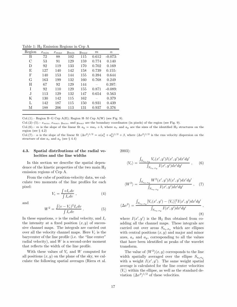
Table 1: H2 Emission Regions in Cep A
Region xmin xmax ymin ymax m αB 72 88 102 115 0.612 -0.073:C 53 91 129 159 0.774 0.140D 92 119 133 170 0.702 0.169E 127 140 142 158 0.739 0.155:F 140 153 144 155 0.394 0.644G 163 199 132 160 0.768 0.249H 67 92 129 144 – 0.397:I 92 110 129 155 0.871 -0.089:J 113 129 132 147 0.654 0.563K 130 142 115 162 – 0.379L 142 187 115 150 0.931 0.439M 188 206 113 131 0.937 0.376
Col.(1).– Region B–G Cep A(E); Region H–M Cep A(W) (see Fig. 9).
Col.(2)–(5).– xmin, xmax, ymin, and ymax are the boundary coordinates (in pixels) of the region (see Fig. 9).
Col.(6).– m is the slope of the linear fit ay = max + b, where ax and ay are the sizes of the identified H2 structures on theregion (see § 4.2)
Col.(7).– α is the slope of the linear fit 〈∆v2〉1/2 = α(a2x + a2
y)1/2 + β, where 〈∆v2〉1/2 is the rms velocity dispersion on thestructure of size ax and ay (see § 4.4)
4.3. Spatial distributions of the radial ve-locities and the line widths
In this section we describe the spatial depen-dence of the kinetic properties of the two main H2
emission regions of Cep A.
From the cube of position-velocity data, we cal-culate two moments of the line profiles for eachpixel:
Vc =
∫vIvdv∫Ivdv
, (4)
and
W 2 =
∫(v − Vc)
2Ivdv∫Ivdv
. (5)
In these equations, v is the radial velocity, and Iv
the intensity at a fixed position (x, y) of succes-sive channel maps. The integrals are carried outover all the velocity channel maps. Here Vc is thebarycenter of the line profile (i.e. the “line center”radial velocity), and W is a second-order momentthat reflects the width of the line profile.
With these values of Vc and W computed forall positions (x, y) on the plane of the sky, we cal-culate the following spatial averages (Riera et al.
2003):
〈Vc〉 =
∫Sax,ay
Vc(x′, y′)I(x′, y′)dx′dy′
∫Sax,ay
I(x′, y′)dx′dy′, (6)
〈W 2〉 =
∫Sax,ay
W 2(x′, y′)I(x′, y′)dx′dy′
∫Sax,ay
I(x′, y′)dx′dy′, (7)
〈∆v2〉 =
∫Sax,ay
[Vc(x′, y′) − 〈Vc〉]
2I(x′, y′)dx′dy′
∫Sax,ay
I(x′, y′)dx′dy′,
(8)where I(x′, y′) is the H2 flux obtained from co-adding all the channel maps. These integrals arecarried out over areas Sax,ay
which are ellipseswith central positions (x, y) and major and minoraxes, ax and ay, corresponding to all the valuesthat have been identified as peaks of the wavelettransform.
The value of 〈W 2〉(x, y) corresponds to the linewidth spatially averaged over the ellipse Saxay
with a weight I(x′, y′). The same weight spatialaverage is calculated for the line center velocities〈Vc〉 within the ellipse, as well as the standard de-viation 〈∆v2〉1/2 of these velocities.
17
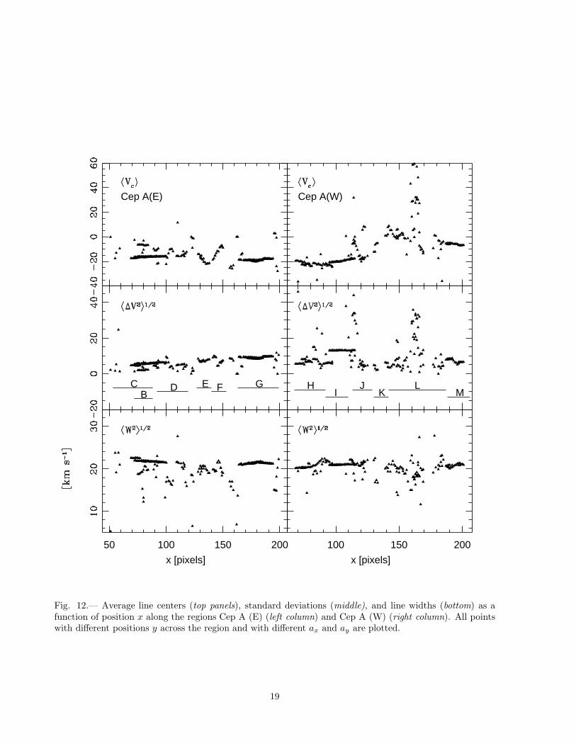
Figure 12 shows the line centers, widths, andstandard deviations as a function of position xalong the region (all of the points at different posi-tions y across the region and with different ax anday are plotted). The line center or centroid ve-locity displayed in the top panels, shows differentbehaviors for Cep A (E) and Cep A (W). As hadbeen previously noted, Cep A (E) has a constantvelocity along the outflow (∼-19 km s−1) whileCep A (W) shows a velocity gradient from about -21 to -2 km s−1. A large dispersion in the line cen-ters for Cep A (W) around positions 115 and 162is probably due to insufficient S/N, since a similarincrease in the dispersion velocity (medium panel)is concurrent, but lacks a corresponding incrementof the line width (bottom panel). Other featurespresent in these figures seem real. Most remark-ably, the velocity dispersion (medium panel) forCep A (E) increases monotonically with distancefrom the source, going from around 4 to 10 km s−1
in 150 pixels or 0.5 pc. No such increase is ob-served in the western outflow, where we obtaina constant 3±2 km s−1 velocity dispersion. Theline widths (bottom panel) seem dominated by thewidth of the instrumental profile of 22 km s−1.
Hence, we conclude from this analysis that theeastern and western outflows seem intrinsically dif-ferent. While the eastern outflow shows a constantline center velocity and an increasing velocity dis-persion, the western outflow behaves otherwise,showing a velocity gradient and a constant veloc-ity dispersion with a lower value. This had beennoticed in our qualitative analysis of the obser-vations. Now, if we take the velocity dispersionwithin each cell as a measure of turbulence, whichseems reasonable, then the region Cep A (E) ismore turbulent than Cep A (W), and it is notice-able that the turbulence increases with distancefrom the “central” source compared to a constantbehavior in the western source.
4.4. Deviations of the line center velocityand the size of the region
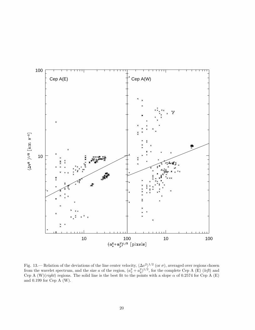
Figure 13 shows the deviations of the line centervelocity (velocity dispersion), averaged over sizeschosen from the wavelet spectrum, as a function ofthe size of each region. Such deviations of the linecenter velocity, averaged over sizes chosen from awavelet spectrum, have been previously used byGill & Henriksen (1996) to study turbulence in
molecular clouds. In this figure we can appreciatea large dispersion of values. However, points tendto clump together around certain regions of thediagrams.
A closer examination of Fig. 13 for Cep A (E)shows a cluster of points at position (20,9) corre-sponding to structure labeled G (see Fig. 9), whilethe points corresponding to structure C lie just be-low of them. Taken separately, each one of thesegroups seem to define a line in the diagram, off-set vertically from one another, but of compara-ble slopes. The slope of the lines, in fact, is alsosimilar to the slope of the line that would be ob-tained by fitting a line to all the data, m=0.26(indicated with a solid line in Fig. 13). The dis-persion is large, but there is at least another fac-tor contributing to the amount of velocity disper-sion that has already been mentioned: the dis-tance from the components of the structure to theoutflow source. We take out this effect by sub-tracting this systematic linear contribution withthe distance. Thus, in Fig. 13, points belongingto the C group, which are closer to the source,would merge together with those points of the far-ther G group. The dispersion would be lower andthe slope would have a similar value. This definesa relation similar to Larson’s law for molecularclouds (Larson 1981). Larson found that molec-ular clouds show a suprathermal velocity disper-sion that correlates with the size a of the cloud asσv ∝ a0.38. Although different values of the powerindex, α, have been mentioned in the literature,ranging from 0.33, for pure Kolmogorov turbu-lence, to 0.5, a more appropriate value in termsof the Virial Theorem (Goodman et al. 1998). Inthe Cep A (E) case we obtain a slope α of 0.25which is closer to the Kolmogorov value.
In the western outflow it is more difficult toidentify clumps of points, and we were not ableto find a relation of velocity dispersion with posi-tion either. A least square fit of a line to the datagives a slope of 0.20. However, there appears tobe two disperse clumps of points, a lower one andan upper one, each defining a line with a largerslope α ∼0.5 and parallel to each other. This lat-ter value would be closer to a case where VirialTheorem applies.
The analysis of the individual H2 condensations(c.f. Fig. 1) in the Cep A (E) and Cep A (W) isillustrated in Fig. 14 and 15. We show the devi-
18
Cep A(E)
C D E F GB
x [pixels]
50 100 150 200
Cep A(W)
HI
JK
LM
x [pixels]
100 150 200
Fig. 12.— Average line centers (top panels), standard deviations (middle), and line widths (bottom) as afunction of position x along the regions Cep A (E) (left column) and Cep A (W) (right column). All pointswith different positions y across the region and with different ax and ay are plotted.
19
Cep A(E)
10 100
10
100
Cep A(W)
10 100
Fig. 13.— Relation of the deviations of the line center velocity, 〈∆v2〉1/2 (or σ), averaged over regions chosenfrom the wavelet spectrum, and the size a of the region, (a2
x + a2y)1/2, for the complete Cep A (E) (left) and
Cep A (W)(right) regions. The solid line is the best fit to the points with a slope α of 0.2574 for Cep A (E)and 0.199 for Cep A (W).
20
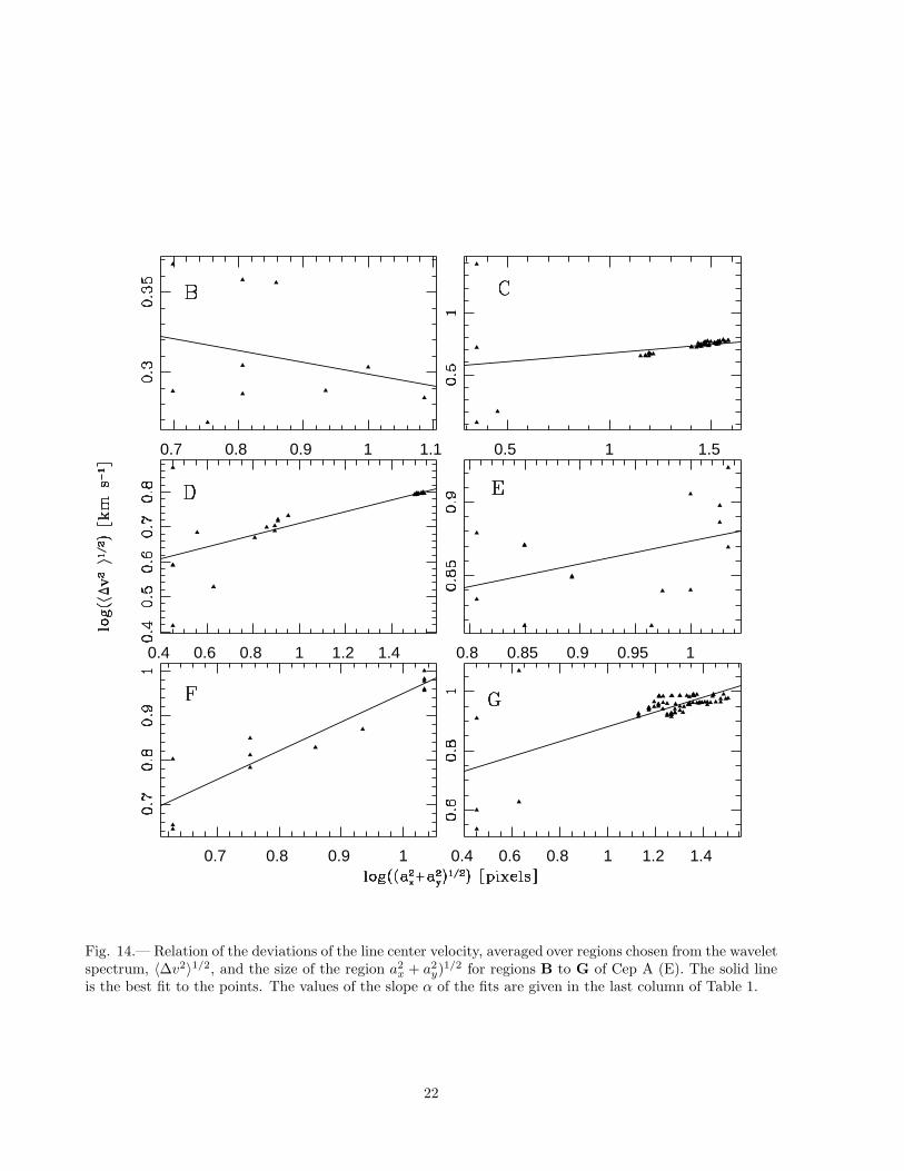
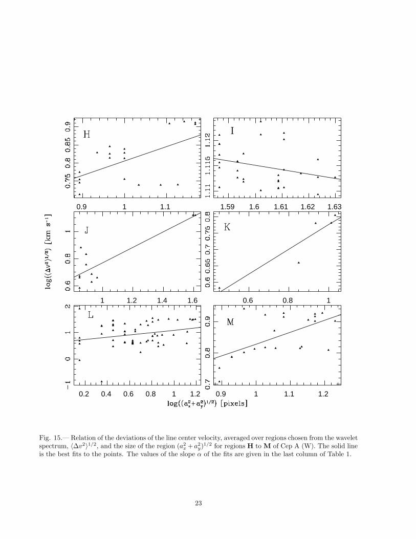
ations for the line center velocity, averaged oversizes chosen from the wavelet spectrum for eachcondensation. For each H2 condensation the val-ues of the best fit slope α are presented in the lastcolumn of Table 1. The Cep A (E) clumps yield amean α of 0.21±0.21 while the Cep A (W) yield aslightly higher value of 0.34±0.20. However, someknots show poor correlations than others (see plotsfor knots B, E, H and I). Using only knots C, D,F and G for Cep A (E) and knots J, K, L andM for Cep A (W) yields an α of 0.30±0.20 and0.44±0.08, which support a Kolmogorov case inthe first and a more virialized region for the west-ern case.
5. Conclusions
We have presented the velocity structure ofthe molecular hydrogen outflows from the regionsCep A (E) and Cep A (W) obtained from theH2 v=1–0 S(1) doppler shifted line emission at2.12 µm. Both the velocity channel maps and theintegrated H2 image show a complex structure of12 individual clumps along two separated struc-tures oriented roughly in the east-west direction.
Given the complexity of these structures, wehave carried out an anisotropic wavelet analysisof the H2 image, which automatically detects theposition and characteristic sizes (along and acrossthe region axis) of the clumps.
1. There is evidence for a Mach disk in Cep A (E).The efflux point is located at the center of abow shock structure and we measure blue-shifted velocities of 22 to 28 km s−1. Thisobservation implies that a molecular jet isdriving the outflow.
2. Cep A (W) on the other hand, is consistentwith a hot bubble in expansion driving C-shocks. We presented the kinematic gradientof one of such shocks as an example.
3. The H2 flux-velocity relation is present inboth outflows. The break velocity of theeastern outflow is lower than that of thewestern outflow, and we have argued thatthis is indicative of greater turbulence inCep A (E).
4. The wavelet analysis has confirmed andquantified trends observed in the centroid
velocity measurements: that the easternoutflow shows a constant line center velocityand an increasing velocity dispersion, whilethe western outflow shows a velocity gradi-ent and a constant velocity dispersion. Thelarger velocity dispersion and gradient in theeastern outflow is taken as indicative of tur-bulence, and allows us to conclude also thatturbulence increases with distance.
5. Suggestive propositions about the kind ofturbulence present in both outflows, are ex-tracted from an analysis of the relation of thevelocity dispersion as a function of the size ofthe structures (cells) identified as unities bythe wavelet spectrum. Using only knots witha good correlation yields an α of 0.30±0.20for Cep A (E) and 0.44±0.08 for Cep A (W),which support a Kolmogorov case in the firstand a more virialized region for the westerncase.
We thank to L. F. Rodrıguez for his valuablecomments. Our appreciation to the Observato-rio Astronomico Nacional (OAN/SPM) staff fortheir assistance and technical support during theobservations, most specially the night assistantsG. Garcıa and F. Montalvo. I. Cruz-Gonzalez andL. Salas acknowledge support from CONACyT re-search grant 36574-E. We thank the referee, An-tonio Chrysostomou, for his useful comments toimprove this paper.
REFERENCES
Bally, J., & Lane, A. P. 1982, ApJ, 257, 612
Codella, C., Bachiller, R., Benedettini, M., &Caselli, P. 2003, MNRAS, 341, 707
Cruz-Gonzalez, I., Carrasco, L., Ruiz, E., Salas,L., Skrutskie, M., Meyer, M., Sotelo, P., Bar-bosa, F., Gutierrez, L. , Iriarte, A., Cobos, F.,Bernal, A., Sanchez, B., Valdez, J., Arguelles,S., Conconi, P.: 1994, Proc. SPIE 2198, p. 774.
Doyon, R., & Nadeau, D. 1988, ApJ, 334, 883
Garay, G., Ramırez, S., Rodrıguez, L. F., Curiel,S., & Torrelles, J. M. 1996, ApJ, 459,193
Gill, A. G., & Henriksen, R. N. 1990, ApJ, 365,L27
21
0.7 0.8 0.9 1 1.1 0.5 1 1.5
0.4 0.6 0.8 1 1.2 1.4 0.8 0.85 0.9 0.95 1
0.7 0.8 0.9 1 0.4 0.6 0.8 1 1.2 1.4
Fig. 14.— Relation of the deviations of the line center velocity, averaged over regions chosen from the waveletspectrum, 〈∆v2〉1/2, and the size of the region a2
x + a2y)1/2 for regions B to G of Cep A (E). The solid line
is the best fit to the points. The values of the slope α of the fits are given in the last column of Table 1.
22
0.9 1 1.1 1.59 1.6 1.61 1.62 1.63
1 1.2 1.4 1.6 0.6 0.8 1
0.2 0.4 0.6 0.8 1 1.2 0.9 1 1.1 1.2
Fig. 15.— Relation of the deviations of the line center velocity, averaged over regions chosen from the waveletspectrum, 〈∆v2〉1/2, and the size of the region (a2
x + a2y)1/2 for regions H to M of Cep A (W). The solid line
is the best fits to the points. The values of the slope α of the fits are given in the last column of Table 1.
23
Goodman, A. A., Barranco, J. A., Wilner, D. J.& Heyer, M. H. 1998, ApJ, 504, 223
Hartigan, P., Morse, J., & Bally, J. 2000, ApJ,120, 1436
Hartigan, P., Carpenter, J., Dougados, C., &Skrutskie M. 1996, AJ, 111, 1278
Hartigan, P., Raymond, J., & Hartmann, L. 1987,ApJ, 316, 323
Hartigan, P., Lada, C., Stocke, J., & Tapia, S.1986, AJ, 92, 1155
Hartigan, P., & Lada, C. J. 1985, ApJS, 59, 383
Hughes, V. A. & Wouterlloot, J. G. A. 1984, ApJ,276, 204
Johnson, H. L. 1957, ApJ, 126, 121
Khanzadyan, T., Smith, M. D., Davis, C. J., Gre-del, R., Stanke, T., & Chrysostomou, A. 2003,MNRAS, 338, 57
Koppenaal, K., Sargent, A. I., Nordh, L., vanDuinen, R. J., & Aslders, J. W. G. 1979, A&A,75, L1
Kumar, M.S.N., Bachiller, R., & Davis, C.J. 2002,ApJ, 576, 313
Larson, R. B. 1981, MNRAS, 194, 809
Narayanan, G., & Walker, C. K. 1996, ApJ, 466,844
Porras, A., Cruz-Gonzalez, I., & Salas, L. 2000,A&A, 361, 660
Press, W. H., Teukolsky, S. A., Vetterling, W. T.,& Flannery, B. P. 1992, “Numerical Recipes inC”. Second Ed. Cambidge University Press
Raines, S. N., Watson, D. M., Pipher, J. L.,; For-rest, W. J., Greenhouse, M. A., Satyapal, S.,Woodward, C. E., Smith, H. A., Fischer, J.,Goetz, J. A., Frank, A. 2000, ApJ, 528, L115
Riera, A., Raga, C. A., Reipurth, B., Amram, P.,Boulesteix, J., Canto, J., & Toledano, O. 2003,AJ, 126, 327
Rodrıguez, L. F., Ho, P. T. P, & Moran, J. M.1980, ApJ, 240, L149
Salas, L. et al. 1999, ApJ, 511, 822
Salas, L., & Cruz-Gonzalez, I. 2002, ApJ, 572, 227
Simon, T., & Joyce, R. R. 1983, ApJ, 265, 864
Sargent, A. I. 1977, ApJ, 218, 736
Torrelles, J. M., Verdes-Montenegro, L., Ho, P. T.P., Rodrıguez, L. F., & Canto, J. 1993, ApJ,106, 613
Yu, K. C., Billawala, Y., & Bally, J. 1999, AJ, 118,2940
This 2-column preprint was prepared with the AAS LATEXmacros v5.2.
24