arX

iv:a

stro

-ph/

0603

859v

2 2

5 Se

p 20

06Draft version February 5, 2008Preprint typeset using LATEX style emulateapj v. 6/22/04

THE NON-GAUSSIAN COLD SPOT IN THE 3-YEAR WMAP DATA

M. Cruz1

IFCA, CSIC-Univ. de Cantabria, Avda. los Castros, s/n,E-39005-Santander,

Spain

L. CayonDepartment of Physics, Purdue University, 525 Northwestern Avenue, West Lafayette,

IN 47907-2036, USA

E. Martınez-GonzalezIFCA, CSIC-Univ. de Cantabria, Avda. los Castros s/n,

39005-Santander,Spain

P. Vielva2

IFCA, CSIC-Univ. de Cantabria, Avda. los Castros, s/n,39005-Santander,Spain

and

J. JinDepartment of Statistics. Purdue University. 150 N. University Street, West Lafayette,

IN 47907-2067Draft version February 5, 2008

ABSTRACT

The non-Gaussian cold spot detected in wavelet space in the WMAP 1–year data, is detected againin the coadded WMAP 3–year data at the same position (b = −57◦, l = 209◦) and size in the sky(≈ 10◦). The present analysis is based on several statistical methods: kurtosis, maximum absolutetemperature, number of pixels below a given threshold, volume and Higher Criticism. All thesemethods detect deviations from Gaussianity in the 3–year data set at a slightly higher confidencelevel than in the WMAP 1–year data. These small differences are mainly due to the new foregroundreduction technique and not to the reduction of the noise level, which is negligible at the scale ofthe spot. In order to avoid a posteriori analyses, we recalculate for the WMAP 3–year data thesignificance of the deviation in the kurtosis. The skewness and kurtosis tests were the first testsperformed with wavelets for the WMAP data. We obtain that the probability of finding an at leastas high deviation in Gaussian simulations is 1.85%. The frequency dependence of the spot is shownto be extremely flat. Galactic foreground emissions are not likely to be responsible for the detecteddeviation from Gaussianity.

Subject headings: methods: data analysis – cosmic microwave background

1. INTRODUCTION

The Cosmic Microwave Background (CMB) is at themoment the most useful tool in the study of the ori-gin of the universe. A precise knowledge of its powerspectrum constrains significantly the values of the cos-mological parameters which determine the cosmologicalmodel. The 1–year Wilkinson Microwave AnisotropyProbe data (WMAP, Bennett et al. 2003a), measuredthe anisotropies of the CMB with unprecedented accu-racy, finding that the standard model fits these data.A flat Λ–dominated Cold Dark Matter (ΛCDM) uni-

1 Also at Dpto. de Fısica Moderna, Univ. de Cantabria, Avda.los Castros, s/n, 39005-Santander, SpainElectronic address: cruz@ifca.unican.esElectronic address: cayon@physics.purdue.eduElectronic address: martinez@ifca.unican.es

2 Also at Astrophysics Group, Cavendish Laboratory, MadingleyRoad, Cambridge CB3 0HE, UKElectronic address: vielva@ifca.unican.esElectronic address: jinj@stat.purdue.edu

verse with standard inflation explains most of the ob-servations confirming the widely accepted concordancemodel. According to standard inflation, the tempera-ture anisotropies of the CMB are predicted to representa homogeneous and isotropic Gaussian random field onthe sky. A first Gaussianity analysis found the data tobe compatible with Gaussianity (Komatsu et al. 2003).

Several non–Gaussian signatures or asymmetries weredetected in the 1–year WMAP data in subsequent works.A variety of methods were used and applied in real, har-monic and wavelet space: low multipole alignment statis-tics (de Oliveira–Costa et al. 2004, Copi et al. 2004,2005, Schwarz et al. 2004, Land & Magueijo 2005a,b,c,Bielewicz et al. 2005, Slosar & Seljak 2004); phase cor-relations (Chiang et al. 2003, Coles et al. 2004); hotand cold spot analysis (Larson & Wandelt 2004, 2005);local curvature methods (Hansen et al. 2004, Cabella etal. 2005); correlation functions (Eriksen et al. 2004a,2005, Tojeiro et al. 2005); structure alignment statistics

2

(Wiaux et al. 2006); multivariate analysis (Dineen &Coles 2005); Minkowski functionals (Park 2004, Eriksenet al. 2004b); gradient and dispersion analyses (Chyzy etal. 2005); and several statistics applied in wavelet space(Vielva et al. 2004, Mukherjee & Wang 2004, Cruz etal. 2005, 2006, McEwen et al. 2005a and Cayon, Jin &Treaster 2005).

The recently released 3–year WMAP data with highersignal to noise ratio is key to confirm or disprove all theseresults.

In the 3–year papers, the WMAP team (Hinshaw et al.2006) re-evaluates potential sources of systematic errorsand concludes that the 3–year maps are consistent withthe 1–year maps. The exhaustive polarization analysisenhances the confidence on the accuracy of the temper-ature maps. The ΛCDM model continues to provide thebest fit to the data.

Spergel et al. (2006) perform a Gaussianity analysisof the 3–year data. No departure from Gaussianity isdetected based on the one point distribution function,Minkowski functionals, the bispectrum and the trispec-trum of the maps. The authors do not re-evaluate theother statistics showing asymmetries or non–Gaussiansignatures in the 1–year data.

The aim of this paper is to check the results of Vielvaet al. (2004), Cruz et al. (2005), Cayon, Jin & Treaster(2005) and Cruz et al. (2006), (hereafter V04, C05, CJTand C06 respectively) with the recently released WMAPdata. All these analyses were based on wavelet space.In particular the data were convolved with the SphericalMexican Hat Wavelet (SMHW). Convolution of a CMBmap with the SMHW at a particular wavelet scale in-creases the signal to noise ratio at that scale. Moreover,the spatial location of the different features of a map ispreserved.

V04 detected an excess of kurtosis in the 1–yearWMAP data compared to 10000 Gaussian simulations.This excess occurred at wavelet scales around 5◦ (an-gular size in the sky of ≈ 10◦). The excess was foundto be localized in the southern Galactic hemisphere. Avery cold spot, called the Spot, at galactic coordinates(b = −57◦, l = 209◦), was pointed out as the possiblesource of this deviation.

C05 showed that indeed the Spot was responsible forthe detection. The number of cold pixels below sev-eral thresholds (cold Area) of the Spot was unusuallyhigh compared to the spots appearing in the simulations.Compatibility with Gaussianity was found when mask-ing this spot in the data. The minimum temperature ofthe Spot was as well highly significant.

C06 confirmed the robustness of the detection andanalysed the morphology and the foreground contribu-tion to the Spot. The Spot appeared statistically robustin all the performed tests, being the probability of find-ing a similar or bigger spot in the Gaussian simulationsless than 1%. The shape of the Spot was shown to beroughly circular, using Elliptical Mexican Hat Waveletson the sphere. Moreover the foreground contribution inthe region of the Spot was found to be very low. TheSpot remained highly significant independently of theused foreground reduction technique. In addition thefrequency dependence of the Spot was shown to be ex-tremely flat. Even considering large errors in the fore-ground estimation it was not possible to explain the non-

Gaussian properties of the Spot.CJT applied Higher Criticism statistics (hereafter HC)

to the 1–year maps after convolving them with theSMHW. This method provided a direct detection of theSpot. The HC values appeared to be higher than 99% ofthe Gaussian simulations.

Note that although the Spot has not been detectedin real space, this structure exists but is hidden bystructures at different scales. The convolution with theSMHW at the appropriate scale, amplifies the Spot, mak-ing it more prominent.

Several attempts have been made in order to explainthe non-Gaussian nature of this cold spot. Tomita (2005)suggested that local second–order gravitational effectscould produce the Spot. Inoue & Silk (2006) consid-ered the possibility of explaining the Spot and other largescale anomalies by local compensated voids. Jaffe et al.(2005a) and Cayon et al. (2006) assumed an anisotropicBianchi VIIh model showing that it could explain the ex-cess of kurtosis and the HC detection as well as severallarge scale anomalies. On the other hand, McEwen et al.(2005b) still detect non-Gaussianity in the Bianchi cor-rected maps. Jaffe et al. (2005b) proved the incompati-bility of the extended Bianchi models including the darkenergy term with the 1–year data. Adler et al. (2006),developed a finite cosmology model which would explainthe Spot and the low multipoles in the angular powerspectrum. Up to date there are no further evidences ofthe validity of any of the above suggested explanations.

Our paper is organized as follows. We discuss thechanges in the new WMAP data release and the simula-tions in section §2. The analysis using all the mentionedestimators is described in section §3. In section §4, thesignificance of our findings is discussed. We analyse thefrequency dependence of the Spot in section §5, and ourdiscussion and conclusions are presented in sections §6and §7.

2. WMAP 3–YEAR DATA AND SIMULATIONS

The WMAP data are provided at five frequency-bands,namely K–band (22.8 GHz, one receiver), Ka–band (33.0GHz, one receiver), Q–band (40.7 GHz, two receivers),V–band (60.8 GHz, two receivers) and W–band (93.5GHz, four receivers). Foreground cleaned maps forthe Q, V, and W channels are also available at theLegacy Archive for Microwave BAckground Data Anal-ysis (LAMBDA) web site 3.

Most of the 1–year Gaussianity analyses were per-formed using the WMAP combined, foreground cleanedQ–V–W map (hereafter WCM; see Bennett et al. 2003a).CMB is the dominant signal at these bands and noiseproperties are well defined for this map. The de-biasedInternal Linear Combination map, (DILC) proposed bythe WMAP team, estimates the CMB on the whole sky.However its noise properties are complicated and regionsclose to the Galactic plane will be highly contaminatedby foregrounds. Chiang, Naselsky & Coles (2006) findevidences for the foreground contamination of the DILC.Therefore we will still use the more reliable WCM in the3–year data analysis.

Hinshaw et al. (2006) describe some changes in the3–year temperature analysis with respect to the 1–year

3 http://lambda.gsfc.nasa.gov

3

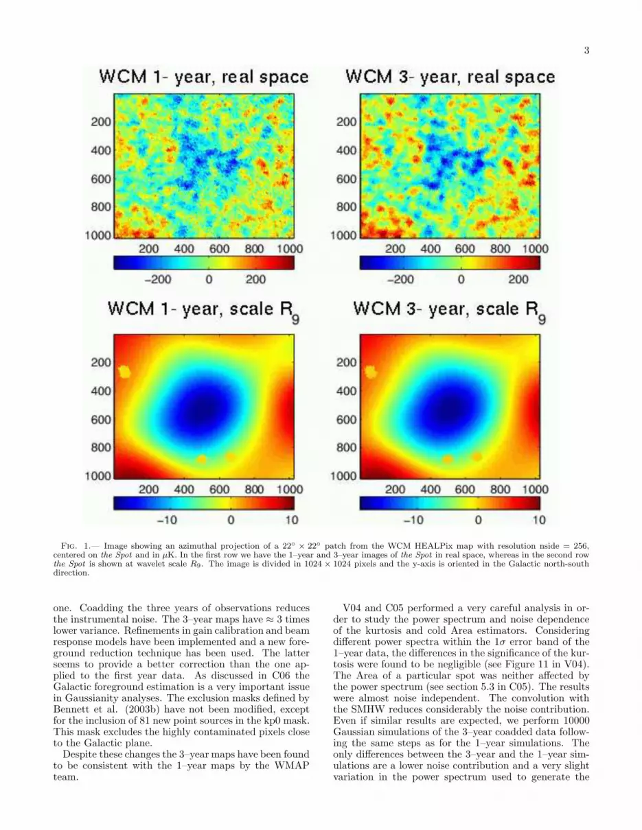
Fig. 1.— Image showing an azimuthal projection of a 22◦ × 22◦ patch from the WCM HEALPix map with resolution nside = 256,centered on the Spot and in µK. In the first row we have the 1–year and 3–year images of the Spot in real space, whereas in the second rowthe Spot is shown at wavelet scale R9. The image is divided in 1024 × 1024 pixels and the y-axis is oriented in the Galactic north-southdirection.

one. Coadding the three years of observations reducesthe instrumental noise. The 3–year maps have ≈ 3 timeslower variance. Refinements in gain calibration and beamresponse models have been implemented and a new fore-ground reduction technique has been used. The latterseems to provide a better correction than the one ap-plied to the first year data. As discussed in C06 theGalactic foreground estimation is a very important issuein Gaussianity analyses. The exclusion masks defined byBennett et al. (2003b) have not been modified, exceptfor the inclusion of 81 new point sources in the kp0 mask.This mask excludes the highly contaminated pixels closeto the Galactic plane.

Despite these changes the 3–year maps have been foundto be consistent with the 1–year maps by the WMAPteam.

V04 and C05 performed a very careful analysis in or-der to study the power spectrum and noise dependenceof the kurtosis and cold Area estimators. Consideringdifferent power spectra within the 1σ error band of the1–year data, the differences in the significance of the kur-tosis were found to be negligible (see Figure 11 in V04).The Area of a particular spot was neither affected bythe power spectrum (see section 5.3 in C05). The resultswere almost noise independent. The convolution withthe SMHW reduces considerably the noise contribution.Even if similar results are expected, we perform 10000Gaussian simulations of the 3–year coadded data follow-ing the same steps as for the 1–year simulations. Theonly differences between the 3–year and the 1–year sim-ulations are a lower noise contribution and a very slightvariation in the power spectrum used to generate the

4

0 5 10 15−2

−1.5

−1

−0.5

0

0.5

1

1.5

2

2.5

# R

Kur

tosi

s

1−year data3−year data

Fig. 2.— WCM kurtosis values for the 1–year (asterisks) and the3–year data (circles). The acceptance intervals for the 32% (inner),5% (middle) and 1% (outer) significance levels, given by the 10000simulations are also plotted.

simulations. For a detailed description of the simulationpipeline, see section 2 of V04.

We will use all these maps in the HEALPix pixelisationscheme (Gorski et al. 2005) 4 with resolution parameterNside = 256.

3. ANALYSIS

Our aim in this section is to repeat the same tests per-formed in V04, C05, CJT and C06 but with the 3–yeardata. Then we will compare the new results to the oldones. One can see the region of the Spot in real andwavelet space at scale 5◦ for both releases of the WMAPdata in Figure 1. In real space the 3–year data image ap-pears clearly less noisy, whereas the wavelet space imagespresent only very small differences.

In V04, data and simulations were convolved with theSMHW at 15 scales, namely (R1 = 13.7, R2 = 25,R3 = 50, R4 = 75, R5 = 100, R6 = 150, R7 = 200,R8 = 250, R9 = 300, R10 = 400, R11 = 500, R12 = 600,R13 = 750, R14 = 900 and R15 = 1050 arcmin). TheSMHW optimally enhances some non-Gaussian signa-tures on the sphere (Martınez–Gonzalez et al. 2002) andhas the following expression:

ΨS(y, R) =1√

2πN(R)

[

1 +(y

2

)2]2[

2 −( y

R

)2]

e−y2/2R2

,

where N(R) is a normalisation constant: N(R) ≡R

√

1 + R2/2 + R4/4. The distance y on the tangentplane is related to the polar angle (θ) as: y ≡ 2 tan θ/2.

We will use the same 15 scales in our present analy-sis, considering those estimators where non-Gaussianitywas found in the 1–year data, namely kurtosis, Area,

4 http://www.eso.org/science/healpix/

Max, HC and a new one, the volume. The definitions ofeach estimator will be given in the following subsections.Analyses were also performed in real space, which willbe referred as wavelet scale zero. In real space, the dataare found to be compatible with Gaussian predictions

In the following subsections we will give the upper tailprobabilities of the data at one particular scale. The up-per tail probability is the probability that the relevantstatistic takes a value at least as large as the one ob-served, when the null hypothesis is true.

In section §4 we will give a more rigorous measure ofthe significance, considering the total number of per-formed tests to calculate the p-value of the Spot. Thep-value is the probability that the relevant statistic takesa value at least as extreme as the one observed, when thenull hypothesis is true. In our case, the null hypothesisis the Gaussianity of the temperature fluctuations.

3.1. Kurtosis

Given a random variable X , the kurtosis κ is defined

as κ(X) = E[X4](E[X2])2 − 3. In V04 the kurtosis of the

wavelet coefficients was compared to the acceptance in-tervals given by the simulations. In Figure 2 the kurtosisof the 1–year data are represented by asterisks and the 3–year data by circles. Hereafter we will use these symbolsto represent 1–year and 3–year data. Both are plottedversus the 15 wavelet scales. Scale 0 corresponds to realspace. The acceptance intervals given by the simulationswill be plotted in the same way in all figures: the 32%interval corresponds to the inner band, the 5% interval tothe middle band and the 1% acceptance interval, to theouter one. As expected, the acceptance intervals remainalmost unchanged with respect to those obtained from1–year simulations. This will happen as well for all theother estimators. The 3–year kurtosis values follow thesame pattern as the 1–year ones, confirming the initialresults. However there are slight differences at the scaleswhere the deviation is detected, being the kurtosis evenhigher in the 3–year data. The most significant deviationfrom the Gaussian values, occurs at scale R9 = 5◦. In Ta-ble 1 we list the kurtosis values at scale R9, consideringthe 1–year data as published in 2003, the 1–year data re-lease applying the changes in the data analysis describedin Hinshaw et al.(2006), and the coadded 3–year data.The biggest difference is found between both releases ofthe 1–year data. The kurtosis value of the 1–year dataincreases ≈ 7%. This may be due to the new foregroundreduction technique. As expected the noise reductiondue to coadding the three years of observations, impliesa much lower increase in the kurtosis, since the noise con-tribution in wavelet space is very small. The upper tailprobabilities (i.e. the probabilities of obtaining higheror equal values assuming the Gaussian hypothesis) aregiven in the right column of Table 1. Hereafter we willcompare the first release of the 1–year data with the 3–year data.

Analysing both Galactic hemispheres separately, weobtain the results presented in Figure 3. Again the kur-tosis follows the same pattern as in the 1–year results.As expected, the deviation appears only in the southernhemisphere and it is slightly higher in the 3–year data.The upper tail probability obtained in V04 was 0.11%at scale R7 in the southern hemisphere, whereas now we

5

0 5 10 15−1.5

−1

−0.5

0

0.5

1

1.5

2

2.5

# R

Kurto

sis N

orth

0 5 10 15−1.5

−1

−0.5

0

0.5

1

1.5

2

2.5

3

# R

Kurto

sis S

outh

1−year data3−year data

Fig. 3.— As in Figure 2 but for the northern (left plot) and southern (right plot) Galactic hemispheres.

TABLE 1Kurtosis values at scale R9

Data kurtosis probabilitya

1–year data (2003) 0.836 0.38%1–year data (2006) 0.895 0.28%

3–year data 0.915 0.23%

Note. — Kurtosis values of different WCM versions at scaleR9. The right column gives the probability of obtaining a higheror equal value in Gaussian simulations.

have 0.08% again at scale R7. The deviation from Gaus-sianity is localised in the southern hemisphere becausethe Spot is responsible for it (see C05).

3.2. Maximum statistic

Given n individual observations Xi, Max is defined asthe largest (absolute) observation :

Maxn = max{|X1|, |X2|, . . . , |Xn|}.The very cold minimum temperature of the Spot, wasshown to deviate from the Gaussian behaviour in V04.In this work and in C05, C06 the minimum tempera-ture estimator was used to characterise the Spot whereasin CJT the chosen estimator was Max. As Max is aclassical and more conservative estimator, we will use itin the present paper instead of the minimum tempera-ture. Our n observations correspond to values in real orwavelet space (normalized to zero mean and dispersionone). The Spot appears to be the maximum absoluteobservation of the data at scales between 200 and 400arcmin. In Figure 4, the 1–year and 3–year WMAP datavalues of Max are compared to those obtained from thesimulations. As for the kurtosis, both data releases show

0 5 10 151.5

2

2.5

3

3.5

4

4.5

5

5.5

6

6.5

# R

Ma

xim

um

ab

sou

te o

bse

rva

tion

1−year data3−year data

Fig. 4.— Maximum absolute observation versus the 15 waveletscales. Again the circles represent the 3–year data and the asterisksthe 1–year data. The bands represent the acceptance intervals asin previous figures.

very similar results. The data lie outside the 1% accep-tance interval at scales R9 and R10. The 3–year datashow slightly higher values than the 1–year data at thesescales. In particular, the upper tail probability for the1–year data was 0.56%, whereas for the 3–year data weobtain 0.38% at scale R9.

6

2 2.5 3 3.5 4 4.50

1000

2000

3000

4000

5000

6000

7000

8000

9000

10000

11000

Threshold

Area

, pixe

ls

Scale R9

0 5 10 150

100

200

300

400

500

600

# R

Area

, pixe

lsThreshold = 4.0

1−year data3−year data

Fig. 5.— The left panel shows the cold Area in pixels, at threshold 4.0 versus the number of the scale. In the right panel the cold Areais represented versus the thresholds, while the scale is fixed at R9. As in previous figures the asterisks represent the 1–year and the circlesthe 3–year data. The bands represent the acceptance intervals as in Figure 2

0 200 400 600 800 1000 12001

10

100

1000

10000

Spot area, number of pixels

Scale R9, threshold 4.0

1−year data3−year data

Fig. 6.— Histogram of all biggest spots of the simulations atthreshold 4.0 and scale R9. The dashed vertical line represents theSpot in the 1–year data and the solid one represents the Spot inthe 3–year data.

3.3. Area

We define the hot Area as the number of pixels abovea given threshold ν and the cold Area as the numberof pixels below a given threshold −ν. The threshold isgiven in units of the dispersion of the considered map.

In C05 the total cold Area of the 1–year data was found

TABLE 2Upper tail probabilities for the Area of the Spot at scale

R9

threshold probability 1–year data probability 3–year data

3.0 0.68% 0.63%3.5 0.36% 0.37%4.0 0.34% 0.27%4.5 0.44% 0.35%

TABLE 3Upper tail probabilities for the volume of the Spot, scale

R9

threshold probability 1–year data probability 3–year data

3.0 0.51% 0.45%3.5 0.33% 0.38%4.0 0.32% 0.27%4.5 0.44% 0.35%

to deviate from the Gaussian behaviour at scales R8 andR9 and thresholds above 3.0 (see Figures 1 and 2 in C05).

C05 found that the large cold Area of the Spot wasresponsible for this deviation. Such a big spot was veryunlikely to be found under the Gaussian model at severalthresholds (see Table 2 of C05).

In the present paper we will define the Area as themaximum between hot and cold Area at a given thresholdand scale. As for the Max estimator, we obtain in thisway a more conservative estimator since the Spot willbe compared to the biggest spot in each simulation no

7

0 5 10 150

50

100

150

200

250

# R

Hig

he

r C

ritic

ism

1−year data3−year data

Fig. 7.— Higher Criticism values of the 1–year WCM (aster-isks) and the 3–year WCM (circles). The acceptance intervals areplotted as in previous figures.

matter if it is a cold or a hot spot.However the Area still deviates from the Gaussian be-

haviour as can be seen in Figure 5. The most significantdeviation is again found at scale R9 and thresholds above3.0.

Figure 6 shows the histogram of the biggest spot ofeach simulation compared to the 1–year and 3–year Areaof the Spot at scale R9 and threshold 4.0. The Spot ismore prominent in the 3–year data and only very fewsimulations show bigger spots. The upper tail proba-bilities obtained at scale R9 for 1–year and 3–year dataare presented in table 2. As in the previous estimators,the 3–year data are in general slightly more significant.The new and more conservative definition of the Areaestimator reduces the upper tail probability of the Spotalthough it is still widely below 1%.

3.4. Volume

From the previous subsections we know that the Spotis extremely cold and it has a large Area at thresholdsabove 3.0. The best estimator to characterise the Spotwould be therefore the volume. Hence we define thevolume referred to a particular threshold as the sum ofthe temperatures of the pixels conforming a spot at thisthreshold. In Table 3 we compare the probability of find-ing a spot with higher or equal Volume as the data, as-suming the Gaussian hypothesis. The values are verysimilar to those obtained for the Area estimator. Val-ues for the Volume are slightly more significant and theyshow less variations with the threshold.

3.5. Higher Criticism

The HC statistic proposed by Donoho & Jin (2004) wasdesigned to detect deviations from Gaussianity that arecaused by either a few extreme observations or a small

Fig. 8.— Higher Criticism of the 3–year WCM at scale R9.

Fig. 9.— Image projected as in Figure 1, showing the 3–yearWCM map (upper panel) and the Higher Criticism map (lowerpanel), both at scale R9.

proportion of moderately extreme observations. More-over, the statistic provides a direct method to locatethese extreme observations by means of HC values cal-culated at every individual data point.

For a set of n individual observations Xi from a cer-tain distribution (Xi normalized to zero mean and dis-persion one), HC is defined as follows. The Xi ob-served values are first converted into p-values: p(i) =P{|N(0, 1)| > |Xi|}. After sorting the p-values in as-cending order p(1) < p(2) < . . . < p(n), we define the HC

8

at each pixel with p-value pi, by:

HCn,i =√

n

∣

∣

∣

∣

i/n− p(i)√

p(i)(1 − p(i))

∣

∣

∣

∣

,

We compute the values of the HC statistic of the 3–yearWCM in real and in wavelet space. The obtained valuesof the HC statistic are presented in Figure 7. These val-ues correspond to the maximum of the HC values foundat the individual pixels. As in previous figures, circlesdenote the results obtained from the 3–year WCM, as-terisks those from the 1–year WCM and the bands repre-sent the acceptance intervals. As one can see in the Fig-ure, the data in wavelet space are not compatible withGaussian predictions at scales R8 and R9 at the 99% c.l.This is in agreement with the result obtained by CJT forthe 1–year WMAP data although there the HC valuesat scale R8 were just below the 99% c.l. The upper tailprobabilities for the 1–year and 3–year maximum HC val-ues at scale R9, are 0.56% and 0.36% respectively. Themap of HC values at scale R9 is presented in Figure 8. Itis clear that the pixels responsible for the detected devi-ation from Gaussianity are located at the position of theSpot. Convolution with the wavelet causes the observedring structure in the HC map. Figure 9 shows a blowoutimage of the Spot as it appears at scale R9 in the waveletmap and in the HC map.

4. SIGNIFICANCE

In the previous section, the upper tail probabilities ofeach estimator at scale R9 were given. All the consid-ered estimators showed the lowest upper tail probabilityat scale R9. However these are not rigorous measuresof the significance of the Spot, since the number of per-formed tests is not taken into account. In this section wewill recalculate the p-value of the deviation in the kur-tosis found by V04 and discuss the issue of a posteriorisignificances.

When an anomaly is detected in a data set following ablind approach, usually several additional tests are per-formed afterwards to further characterize the anomaly.In most of these cases, the only reason these tests havebeen performed is the previous finding of the initialanomaly. If another anomaly would have been detected,other followup tests would have been performed. Hencethese followup tests have not been performed blindly andshould not be taken into account to calculate the signif-icance of the initial detection.

This issue was already discussed in C06 and McEwen etal. (2005). Both papers recalculated the significance ofthe excess of kurtosis in the 1–year WCM found by V04.The excess of kurtosis was found performing a blind test,since no model was used and no previous findings con-ditioned the choice of the scales. Since 15 wavelet scalesand two estimators (skewness and kurtosis) were consid-ered, a total sum of 30 tests were performed. Three ofthese tests detected a strong deviation from Gaussianity.Scales R7, R8 and R9 presented upper tail probabilities0.67%, 0.40% and 0.38% in the 1–year data. This factwas taken into account in C06, but it was not by McEwenet al. (2005). The latter searched through the simula-tions in order to find how many of them showed a higheror equal deviation than the maximum deviation of thedata, ignoring that the data showed a high deviation attwo adjacent scales. The p-value found in this way was

TABLE 4p-values for different estimators.

Estimators p-value

kurtosis 0.86%skewness + kurtosis 1.85%

Max 11.64%Area 3.0 3.27%Area 4.0 1.09%

Higher Criticism 3.48%

4.97% whereas C06 obtained 1.91% taking into accountthat the data deviate at three consecutive scales. It isalso interesting to note that, when both Galactic hemi-spheres were considered independently, C06 found a p-value of 0.69%, although this could be considered as afollowup test.

Some readers could find that the three-consecutive-scales criterion is an a posteriori choice since we look firstat the data and given that they deviate at three consec-utive scales, we then calculate from the simulations howprobable this is. Therefore we should consider a new testwhich eliminates this a posteriori choice. We fix a prioria significance level which is the 1% acceptance intervalgiven in all figures, and count for each estimator (skew-ness and kurtosis) how many scales lie outside, no matterif they are consecutive or not. Then we search throughthe simulations how many show at least that many scalesoutside the 1% acceptance interval as the data.

Applying this test to the 3–year WCM, we find thatscales R8 and R9 lie outside the 1% acceptance intervaland scale R7 lies on the border for the kurtosis estimatoras can be seen in Figure 2. Searching through the sim-ulations how many deviate in three scales either in theskewness or in the kurtosis estimator, we find a p-valueof 1.85%, which is still below the p-value obtained for the1–year data with the three-consecutive-scales criterion.

As already discussed we should not include the fol-lowup tests in a rigorous significance analysis. Howeverit is difficult to assess if some of these tests would havebeen performed or not without the first finding of V04.In fact, the area and maxima analyses are very intuitiveand simple. If V04 had performed their blind analysis onthose estimators instead of using skewness and kurtosis,then the significance would be different. We should dis-tinguish between those tests which are clearly followuptests, because the only reason they have been performedis the initial detection, and other tests which just havebeen performed after the initial detection, but could havebeen performed before.

Hence we apply our new robustness test to kurtosis,Max, Area at thresholds 3.0 and 4.0 and Higher Crit-icism separately. Note that whereas the first two esti-mators are two-sided, the Area and Higher Criticism areone sided estimators. The p-values obtained in this wayare listed in Table 4. The kurtosis and Area at thresh-old 4.0 show p-values around 1%, Higher Criticism andArea at threshold 3.0 around 3%. On the contrary theMax estimator does not show a significant deviation fromGaussianity according to this robustness test.

The most conservative and reliable value is the 1.85%

9

30 40 50 60 70 80 90 100 110−0.021

−0.0205

−0.02

−0.0195

−0.019

−0.0185

−0.018

−0.0175

frequency, GHz

T, m

K

Fig. 10.— Frequency dependence of the temperature at thecenter of the Spot at scale R9. Again the asterisks represent the 1–year data and the circles the 3–year data. The horizontal line showsthe value of the 3–year WCM. The data at the same frequency havebeen slightly offset in abscissa for readability.

0 5 10 151.5

2

2.5

3

3.5

4

4.5

5

5.5

6

6.5

# R

Max

imum

abs

oute

obs

erva

tion

Q−BandV−BandW−BandWCM

Fig. 11.— Maximum absolute observation for the Q, V and Wbands, compared to the 3–year WCM values.

figure since it is not suspicious of being obtained througha posteriori analyses. Nevertheless it is still noticeablethat the followup tests performed in C05, C06, CJT andin the present paper, confirm the initial finding with avery similar significance. Even if strictly speaking theseshould not be taken into account for establishing the sig-nificance of the Spot, they confirm the robustness of thedetection.

30 40 50 60 70 80 90 100400

500

600

700

800

900

1000

1100

1200

1300

1400

frequency, GHz

Are

a of

the

Spo

t, pi

xels

Scale= R9

Threshold = 3.0

Threshold = 3.5

Threshold = 4.0

Fig. 12.— Frequency dependence of the Area of the Spot atscale R9 and several thresholds. Asterisks represent the 1–yeardata and the circles the 3–year data. The 3–year WCM values arerepresented by horizontal lines.

0 5 10 150

50

100

150

200

250

# R

HC

Q−BandV−BandW−BandWCM

Fig. 13.— Higher Criticism values for the Q, V and W bands,compared to the 3–year WCM values.

5. FREQUENCY DEPENDENCE

In this section we will analyse the frequency depen-dence of the previously analysed estimators. A flat fre-quency dependence is characteristic of CMB, whereasother emissions such as Galactic foregrounds show astrong frequency dependence. Figure 14 shows that thekurtosis has almost identical values at the three fore-ground cleaned channels, namely Q,V and W. Same be-haviour was observed in the 1–year data (see Figure 7 in

10

0 5 10 15−2

−1.5

−1

−0.5

0

0.5

1

1.5

2

2.5

# R

Ku

rto

sis

Q−BandV−BandW−BandWCM

Fig. 14.— Kurtosis values for the Q, V and W bands, comparedto the 3–year WCM values.

C06). Strong frequency dependent foreground emissionsare unlikely to produce the detected excess of kurtosis.

The frequency dependence of the temperature at thecenter of the Spot, i.e. at the pixel where the temperatureof the Spot is minimum in the WCM map, is presented inFigure 10. The error bars of the 1–year data have beenestimated performing 1000 noise simulations as explainedin section 5.1 of C06. As the noise variance is ≈ 3 timeslower in the 3–year data, we estimate the new error barssimply by dividing the old ones by

√3. No frequency de-

pendence is found for the new data set in agreement withthe results for the 1–year data. Max, Area and HC val-ues at different frequencies (see Figure 11, Figure 12 andFigure 13) show a very low relative variation comparedto the 3–year WCM.

All these results confirm the analysis performed in sec-tion 5 of C06 where the data were found to fit a flatCMB spectrum. The present analysis confirms the dis-agreement between the conclusions of C06 and those ofthe work of Liu & Zhang (2005) where Galactic fore-grounds were considered to be the most likely source fornon-Gaussian features found with spherical wavelets.

6. DISCUSSION

Spergel et al. (2006) enumerate several reasons tobe cautious about the different anomalies found in theWMAP data: Galactic foregrounds or noise could begenerating the non-Gaussianity, and in addition most ofthe claimed detections are based on a posteriori statis-tics. Also spatial variations of the noise variance and 1/fnoise could affect some of the perfomed analyses. Theysuggest several tests to be done using difference maps(year 1 - year 2, year 2 - year 3, etc.) and multi-frequencydata.

We have tried to address all those points for the Spot.The a posteriori analysis is one of the most important

issues raised by Spergel et al. (2006), since it is very dif-ficult to get completely rid of it. Most analyses performmany tests and it is not easy to assess how many of themare followup tests and which is the probability of findingan anomaly by chance. As discussed in section 4 a verycareful analysis shows that the Spot remains statisticallysignificant at least at the 98% confidence level, withoutusing any a posteriori statistics.

In addition C06 proved that the Spot remained highlysignificant no matter which foreground reduction tech-nique was used. These results are confirmed in thepresent paper. The new foreground reduction used inthe 3–year data enhances slightly the significance of ourdetection. Moreover the multi-frequency analysis of theprevious section shows an even flatter frequency depen-dence of the Spot.

As already discussed in previous sections the noise doesnot affect significantly our wavelet analysis. In fact thecoadded 3–year results are very similar to those obtainedwith the 1–year data of the new data release. No signif-icant cold spot is observed based on the analysis of thethree difference maps (year 1 - year 2, year 2 - year 3, andyear 1 - year 3). Moreover Figure 10 shows that even theparticularly 1/f contaminated W4 Difference Assemblyshows almost the same result as all the other DifferenceAssemblies.

7. CONCLUSIONS

In this paper we repeat the analyses that detected thenon-Gaussian cold spot called the Spot at (b = −57◦, l =209◦) in wavelet space in the 1–year of WMAP data, us-ing the recently released 3–year WMAP data. The pre-vious works V04, C05, CJT and C06 found the Spot todeviate significantly from the Gaussian behaviour. TheSpot was detected using several estimators, namely kur-tosis, Area, Max and HC. This work confirms the de-tection applying all these estimators to the recently pub-lished 3–year WMAP data. At scale R9, the upper tailprobabilities of all these estimators when applied to the3 year WMAP data are smaller than the correspondingones for the first year WMAP data. This is mostly dueto the improved foreground reduction of the data. Wecalculate the probability of finding such a deviation fromGaussianity considering only skewness and kurtosis sincethese were initially used by V04 following a blind ap-proach. Therefore excluding followup tests which couldbe considered as a posteriori analyses we obtain a p-valueof 1.85%. Moreover, the Spot appears to be almost fre-quency independent. This result reinforces the previousforeground analyses performed by C06. It is very unlikelythat foregrounds are responsible for the non-Gaussian be-haviour of the Spot. Comparing the WMAP single yearsky maps, we conclude that the noise has a very low con-tribution to our wavelet analysis as already claimed inV04, C05. Future works will be aimed at finding the ori-gin of the Spot. As discussed in the introduction severalpossibilities have been considered, based on Rees-Sciamaeffects (Rees & Sciama 1968, Martınez–Gonzalez & Sanz1990, Martınez–Gonzalez et al. 1990) and inhomogenousor anisotropic universes. We are presently working onstudying another: topological defects (Turok & Spergel1990, Durrer et al. 1999) as textures could produce coldspots. New and more detailed analyses are required inorder to answer that question.

11

The authors kindly thank R.B. Barreiro, L.M. Cruz-Orive and J.L. Sanz for very useful comments and R.Marco for computational support. MC thanks SpanishMinisterio de Educacion Cultura y Deporte (MECD) fora predoctoral FPU fellowship. PV thanks a I3P contractfrom the Spanish National Research Council (CSIC).MC, EMG and PV acknowledge financial support fromthe Spanish MCYT project ESP2004-07067-C03-01 andthe use of the Legacy Archive for Microwave BackgroundData Analysis (LAMBDA). Support for LAMBDA is

provided by the NASA Office of Space Science. Thiswork has used the software package HEALPix (Hierar-chical, Equal Area and iso-latitude pixelization of thesphere, http://www.eso.org/science/healpix), developedby K.M. Gorski, E. F. Hivon, B. D. Wandelt, J. Banday,F. K. Hansen and M. Barthelmann; the visualisation pro-gram Univiewer, developed by S.M. Mingaliev, M. Ash-down and V. Stolyarov; and the CAMB and CMBFASTsoftware, developed by A. Lewis and A. Challinor and byU. Seljak and M. Zaldarriaga respectively.

REFERENCES

Adler R. J., Bjorken J. D., Overduin J. M., 2006, gr-qc/0602102.Bennett C.L., et al., 2003, ApJS, 148, 1.Bennett C.L., et al., 2003, ApJS, 148, 97.Bielewicz P., Eriksen H. K., Banday A. J., Gorski K. M., Lilje P.

B., 2005, ApJ, 635, 750BCabella P., Liguori M., Hansen F.K., Marinucci D.,Matarrese S.,

Moscardini L., Vittorio N., 2005, MNRAS, 358, 684.Cayon L., Jin J., Treaster A., 2005, MNRAS, 362, 826.(CJT)Cayon L., Banday A. J., Jaffe T., Eriksen H. K., Hansen

F.K., Gorski K. M., Jin J., 2005, submitted to MNRAS,(astro-ph/0602023).

Chiang L. -Y., Naselsky P. D., Verkhodanov O. V., 2003, ApJ, 590,65.

Chiang L-Y, Naselsky P.D., Coles P., 2006, (astro-ph/0603662).Chyzy K.T., Novosyadlyj B., Ostrowski M., 2005,

(astro-ph/0512020).Coles P., Dineen P., Earl J., Wright D., 2004, MNRAS, 350, 989.Copi C. J., Huterer D., Starkman G. D., 2004, Phys. Rev. D., 70,

043515.Copi C. J., Huterer D., Schwarz D. J., Starkman G. D., 2005,

submitted to MNRAS (astro-ph/0508047).Cruz M., Martınez–Gonzalez E., Vielva P., Cayon L., 2005,

MNRAS, 356, 29. (C05).Cruz M., Tucci M., Martınez–Gonzalez E., Vielva P., 2006,

accepted in MNRAS, (astro-ph/0601427). (C06).Dineen P., Coles P., 2005, submitted to MNRAS

(astro-ph/0511802).Donoho D., Jin J., 2004, Ann. Statist., 32, 962Durrer R., 1999, New Astron. Rev., 43, 111.Eriksen H. K., Banday A. J., Gorski K. M., Lilje P. B., 2005, ApJ,

622, 58.Eriksen H. K., Hansen F. K., Banday A. J., Gorski K. M., Lilje P.

B., 2004, ApJ, 605, 14.Eriksen, H. K., Novikov, D. I., Lilje, P. B, Banday, A. J., Gorski

K. M., 2004, ApJ, 612, 64.Gorski K.M., Hivon E. F., Wandelt B. D., Banday J., Hansen F.

K., Barthelmann M., 2005, ApJ 622, 759.Hansen F.K., Cabella P., Marinucci D., Vittorio N., 2004, ApJL,

607, L67.Hinshaw et al., 2006, submitted to ApJ, (astro-ph/0603451)

Inoue K. T., Silk J., 2006, (astro-ph/0602478)Jaffe T. R., Banday A. J., Eriksen H. K., Gorski K. M., Hansen F.

K., 2005, ApJ, 629, 1.Jaffe T. R., Hervik S., Banday A. J., Gorski K. M., 2005, submitted

to ApJ (astro-ph/0512433).Komatsu E. et al. , 2003, ApJs, 148, 119.Land K., Magueijo J., 2005a, MNRAS, 357, 994.Land K., Magueijo J., 2005b, MNRAS, 362, 16.Land K., Magueijo J., 2005d, MNRAS, 362, 838.Larson D. L., Wandelt B. D., 2004, ApJ, 613, 85.Larson D. L., Wandelt B. D., 2005, submitted to Phys. Rev. D.

(astro-ph/0505046).Liu X., Zhang S.N., 2005, ApJ, 633, 542.Martınez–Gonzalez E. & Sanz J. L., Silk, J., 1990, ApJL, 335, 5.Martınez–Gonzalez E. & Sanz J. L., 1990, MNRAS, 247, 473.Martınez–Gonzalez E., Gallegos J. E., Argueso F., Cayon L. &

Sanz J. L., 2002, MNRAS, 336, 22.McEwen J. D., Hobson M. P., Lasenby A. N., Mortlock D. J., 2005,

MNRAS, 359, 1583.McEwen J. D., Hobson M. P., Lasenby A. N., Mortlock D. J., 2005,

submitted to MNRAS (astro-ph/0510349).Mukherjee P., Wang Y., 2004, ApJ, 613, 51.

de Oliveira-Costa A., Tegmark M., Zaldarriaga M., Hamilton A.,2004, Phys. Rev. D., 69, 63516.

Park C. G. 2004, MNRAS 349, 313-320.Rees M. J. & Sciama D. W., 1968, Nature, 517, 611.Schwarz D. J., Starkman G. D., Huterer D., and Copi C. J., 2004,

Phys. Rev. Lett., 93, 221301.Slosar A., Seljak U., 2004, Phys. Rev. D., 70, 8.Spergel et al. 2006, submitted to ApJ, (astro-ph/0603449)Tojeiro R., Castro P.G., Heavens A.F., Gupta S., 2005, submitted

to MNRAS (astro-ph/0507096).Tomita K., 2005, Phys. Rev. D, 72, 10.Turok N. & Spergel D. N., 1990, Phys. Rev. Letters, 64, 2736Vielva P., Martınez–Gonzalez E., Barreiro R. B., Sanz J.L., Cayon

L., 2004, ApJ, 609, 22. (V04).Wiaux Y., Vielva P., Martınez–Gonzalez E., Vandergheynst P.,

2006, submitted to Phys. Rev. Letters.