the dynamics of the space shuttle orbiter with a flexible payload

Acta Astronautica Vol. lO, No. 4, pp. 163-178,1983 0094-5765183 $3.00+.00 Printed in Great Bdtain. Pergamon Press Ltd.

THE DYNAMICS OF THE SPACE SHUTTLE ORBITER WITH A FLEXIBLE PAYLOADf

MICHAEL PALUSZEK The Charles Stark Draper Laboratory, Inc., Cambridge, MA 02139, U.S.A.

(Received 11 January 1983)

Abstract--The Space Shuttle Orbiter will be used as an orbital base for near-term space operations. Its payloads will range from compact satellites to large, flexible antennas. This paper addresses the problem of the dynamics and control of the Orbiter with a flexible payload. Two different cases are presented as examples. The first is a long, slender beam which might be used as an element in a large orbiting structure. The second is a compact satellite mounted on a spin table in the Orbiter payload bay. The dosed loop limit cycles are determined for the first payload and the open loop eigenvalues are calculated for the second. Models of both payloads are mechanized in a simulation with the Shuttle on-orbit autopilot. The vehicle is put through a series of representative maneuvers and its behavior analyzed. The degree of interaction for each payload is determined and strategies are discussed for its reduction.

l. INTRODUCTION The Space Shuttle Orbiter will be used as an orbital base for near term space operations. Its payloads will range from compact satellites to large, flexible antennas. As the system matures the on-orbit operations will increase in complexity. Typical near term operations may involve self-deploying structures, moving payloads with the Remote Manipulator System (RMS) or spinning up satellites prior to release from the payload bay. Further in the future, complex construction operations may be performed.

This paper addresses the problem of the dynamics and control of the Orbiter with a flexible payload. Two different cases are presented as examples. The first is a long, slender beam which might be used as an element in a larger orbiting structure. This structure has very large inertias and low fundamental frequencies. A model of the beam/Orbiter system is mechanized in a simulation with the Shuttle on-orbit digital autopilot. The vehicle is put through a series of representative maneuvers and its behavior analyzed. The results demonstrate that there can be significant interaction between a payload of this type and the autopilot. Depending on the mission, the interaction might require the implementation of strategies to avoid such interaction.

The second payload is a hypothetical satellite on a spinup turntable with a flexible mountiffg to the Orbiter. The spin table spins up the payload prior to deployment from the payload bay. This payload is representative of the communication satellites the Space Shuttle will carry to orbit. It represents a fairly rigid payload that may interact with the autopilot because of its motion about its connection to the Orbiter. The simulation and analysis for this class of payloads demonstrates some interaction problems and identifies strategies to reduce their effect.

fPaper presented at the 33rd Congress of the International Astronautical Federation, Paris, France, 27 September-2 October 1982.

2. THE ON-ORBIT FLIGHT CONTROL SYSTEM

2.1 Introduction This section describes selected components of the

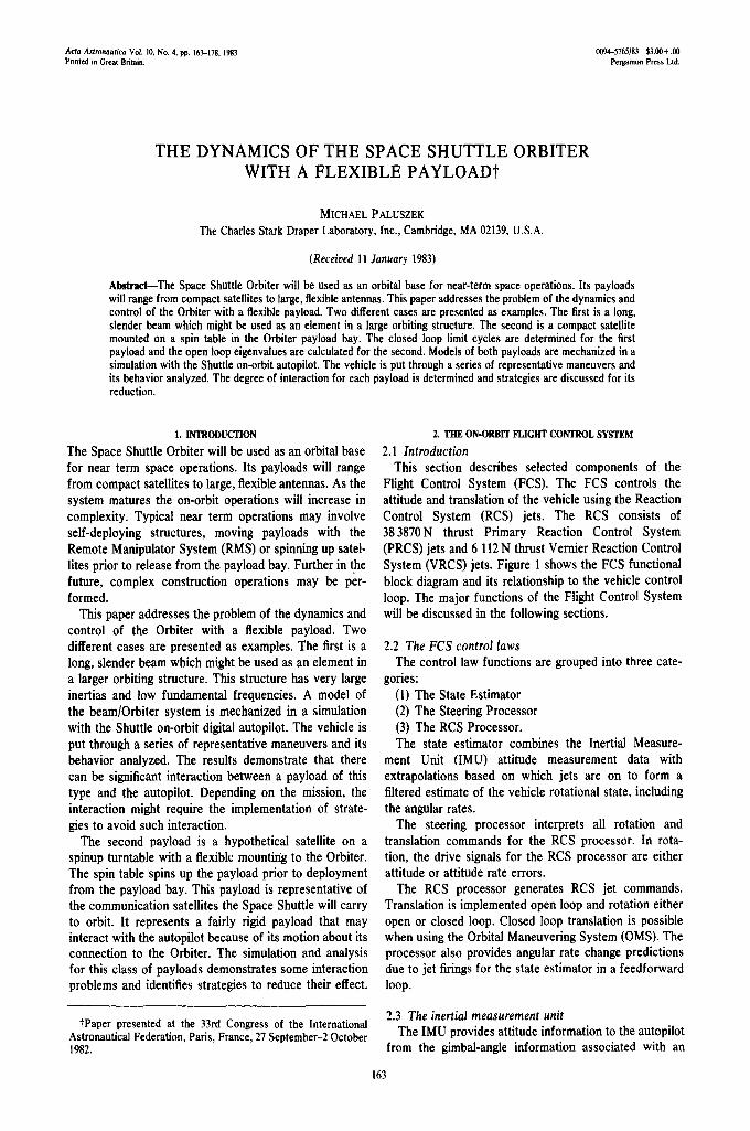
Flight Control System (FCS). The FCS controls the attitude and translation of the vehicle using the Reaction Control System (RCS) jets. The RCS consists of 383870N thrust Primary Reaction Control System (PRCS) jets and 6 112 N thrust Vernier Reaction Control System (VRCS) jets. Figure 1 shows the FCS functional block diagram and its relationship to the vehicle control loop. The major functions of the Flight Control System will be discussed in the following sections.

2.2 The FCS control laws The control law functions are grouped into three cate-

gories: (1) The State Estimator (2) The Steering Processor (3) The RCS Processor. The state estimator combines the Inertial Measure-

ment Unit (IMU) attitude measurement data with extrapolations based on which jets are on to form a filtered estimate of the vehicle rotational state, including the angular rates.

The steering processor interprets all rotation and translation commands for the RCS processor. In rotation, the drive signals for the RCS processor are either attitude or attitude rate errors.

The RCS processor generates RCS jet commands. Translation is implemented open loop and rotation either open or closed loop. Closed loop translation is possible when using the Orbital Maneuvering System (OMS). The processor also provides angular rate change predictions due to jet firings for the state estimator in a feedforward loop.

2.3 The inertial measurement unit The IMU provides attitude information to the autopilot

from the gimbal-angle information associated with an

163

64 M. P~I.USZEK

VEHICLE DYNAMICS

r I I I I I I I I I

i -~- I- z < °"

I I I I

i'< ,J

I= o

18

<in. w ®.~,,-, ; |

~°-

~ i l a Iv"

~ w

~ 8

~ I : : ~ l : i .-,~I:~ ~ S I ~ : E

.--z~_l~. |.~I~ ~I~ ~I~--

i

E

f,

<

J

The dynamics of the Space Shuttle Orbiter 165

inertially stabilized platform. Direct measurement of rate is not provided as the rate gyros are powered down on orbit. The IMUs are located at the navigation base which is forward of the crew compartment.

2.4 The state estimator The state estimator consists of two parallel filters, one

for estimating the angular accelerations due to dis- turbances and one for estimating angular rate. Each filter has a measurement incorporation section and an extrapolation section. Measurement updates occur at 6.25 Hz while extrapolation is done at 12.5 Hz. The attitude extrapolation is done only on alternate cycles and reset to a pure measurement at 6.25 Hz.

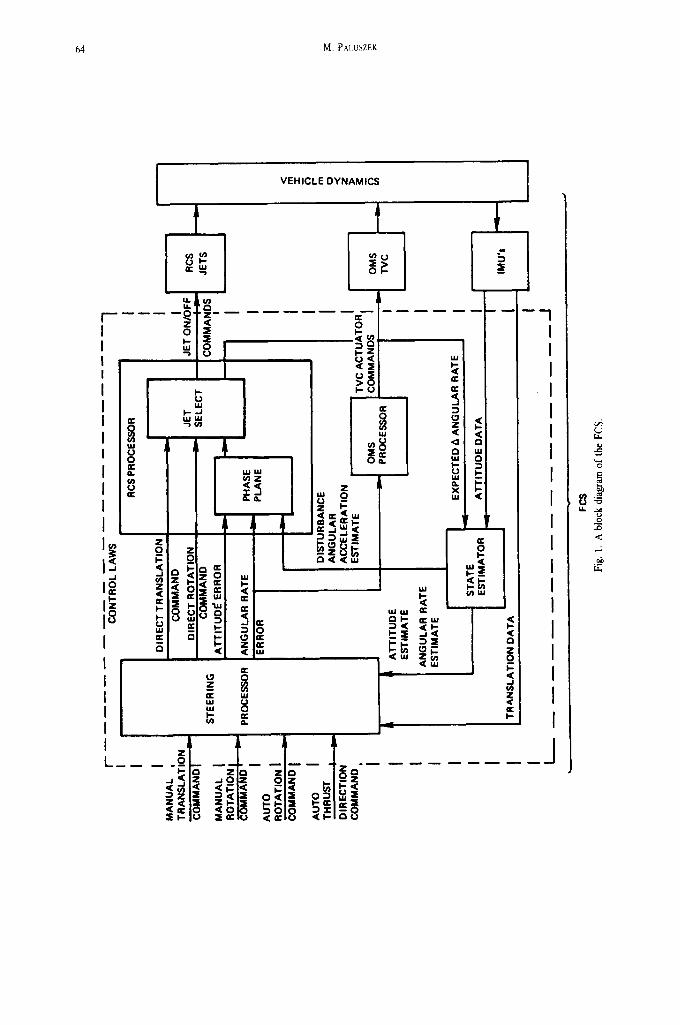
The state estimator has a frequency response that is similar to a second-order low-pass filter. This serves to filter out quantization noise from the IMUs. It also filters out the high frequency vibration component of the Orbiter rate. The frequency response of the state estimator is given in Fig. 2 for both the vernier and primary gains.

2.5 The RCS phase-plane controller This module determines whether to effect an angular

rate change for each body axis during closed loop operation. The phase plane operates at 12.5 Hz.

The phase plane switching logic computes desired changes in angular rates to force the vehicle into a limit cycle about a desired attitude and angular rate. A

separate phase plane is applied to each of the three vehicle axes. The phase plane logic was designed assuming that the Orbiter is a rigid body with low cross- coupling between axes.

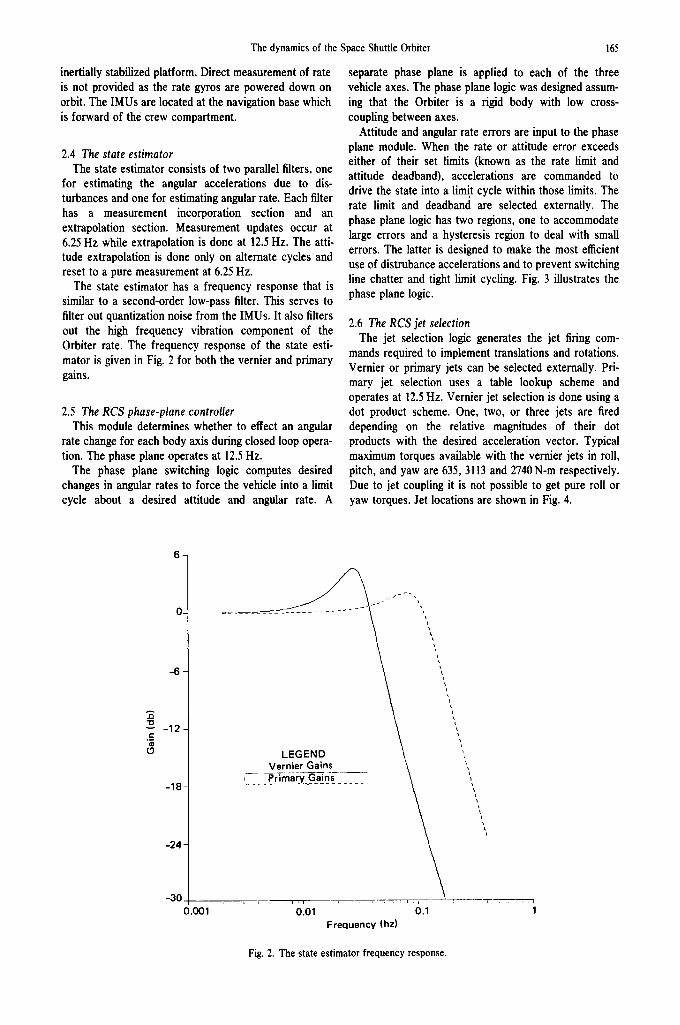
Attitude and angular rate errors are input to the phase plane module. When the rate or attitude error exceeds either of their set limits (known as the rate limit and attitude deadband), accelerations are commanded to drive the state into a limit cycle within those limits. The rate limit and deadband are selected externally. The phase plane logic has two regions, one to accommodate large errors and a hysteresis region to deal with small errors. The latter is designed to make the most efficient use of distrubance accelerations and to prevent switching line chatter and tight limit cycling. Fig. 3 illustrates the phase plane logic.

2.6 The RCS jet selection The jet selection logic generates the jet firing com-

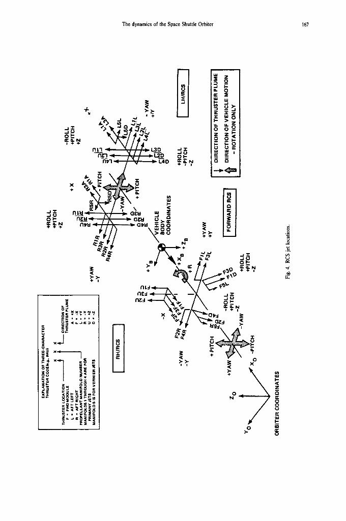
mands required to implement translations and rotations. Vernier or primary jets can be selected externally. Pri- mary jet selection uses a table lookup scheme and operates at 12.5 Hz. Vernier jet selection is done using a dot product scheme. One, two, or three jets are fired depending on the relative magnitudes of their dot products with the desired acceleration vector. Typical maximum torques available with the vernier jets in roll, pitch, and yaw are 635, 3113 and 2740 N-m respectively. Due to jet coupling it is not possible to get pure roll or yaw torques. Jet locations are shown in Fig. 4.

6 -

" 0

e-

O-

- 6 -

- 1 2 -

- 1 8 -

- 2 4 -

- 3 0 0 .001

L E G E N D V e r n i e r Ga ins

~. . . . . P r_i_m a_ r_y pG_a_i n s_ . . . . .

o .01 ! 0.1 Frequency (hz)

i

t L i

Fig. 2. The state estimator frequency response.

166 M. PALtlSZEK

REGION 2 N 9

REGION 3 -'.4f S~ IF ad<0

REGION 5

%

REGION 1

. . . . . - 4 ~ , O_

REGION 8 S 1 2 ~ REGION 7

Fig. 3. The phase plane. Region I: Fire (-), 2: If firing (-) continue else* 3: If firing (+) continue else*, 4: If entered from 1 fire to S else coast, 5: Fire (+), 6: If firing (+) continue else* 7: If firing (-) continue else* 8: If entered from

5 fire to S else coast, 9:. *Off axis preference (vernier's only).

3. THE MATHEMATICAL MODEL FOR THE BEAM AND ORBITER

3.1 The truss beam

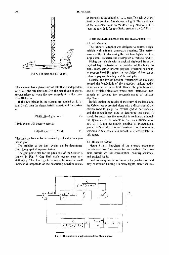
The beam is 50 m long and has a 250 kg tip mass. The average density of the beam is 1.4 kg/m which is typical of structural elements designed for space applications. The beam and the Orbiter are shown in Fig. 5.

The beam is rigidly fixed to the Orbiter. This joint was modeled as a cantilever boundary condition. The beam model was a finite element model composed of a string of one dimensional beam elements. This approximation is justified because of the low torsional moment of inertia of the beam.

The Orbiter was modeled as a rigid body at the base of the beam, thus the beam and Orbiter could be treated together as a free-free beam. This model was mechanized using NASTRAN with six degrees of freedom at each node. The beam model was composed of 20 finite elements.

The mass and .stiffness matrices are assembled by forcing the displacement and rotations to be compatible at all the joints. The equations of motion are then trans- formed to modal coordinates. The structure has six rigid body modes and 120 flexible body modes. Only the first 10 flexible body modes were included in the simulation since the higher modes were well beyond the controller bandwidth. Coupling between the modes due to rotation was ignored. Indeed, the modal model assumes that there is no steady or unsteady rotation of the system. Since the Orbiter normally does not operate at high angular rates or accelerations, this assumption is valid.

4. AN APPROXIMATE STABILITY ANALYSIS FOR THE BEAM

If the Orbiter is maneuvered only in pitch, coupling due to the jets is very small. Since the torques in roll and yaw are less than a tenth of a percent of those in pitch, the pitch equations can be decoupled from roll and yaw.

In its simplest form the autopilot can be approximated

as a relay with a deadband and a second-order filter in the feedback loop. The relay is triggered by body rates exceeding the rate limit. This assumes that the other phase plane parameter, the deadband or limit on attitude excursions, is never reached. This model does not include the hysteresis logic of the autopilot or the feedforward loop but adequately demonstrates the closed- loop behavior of the system when the amplitude of oscillations exceeds the rate limits.

The simplified closed-loop system is illustrated in Fig. 6. The system plant consists of the second-order transfer function for the beam and a double integrator for the rigid body. Input to the system is a commanded rate.

The autopilot receives position information at a rate of 6.25Hz. This is accounted for in the s plane approximation by a zero order hold. The transfer function for a zero order hold is:

l - e Ts (l)

A zero order hold maintains the value it is given from the beginning to end of the cycle. This can be seen from the transfer function which is the sum of the Laplace trans- form of a step, and a step delayed by time T.

The autopilot is still nonlinear. To analyze the system, a describing function was used to model the relay with a deadband. The describing function is a single sinusoidal input type as it is assumed that the system filters out any higher frequencies. This assumption is based on the strong filter characteristics of the state estimator and the spread of resonant frequencies in the beam. The first resonance frequency of the beam is 0.049 Hz and the second is 2.11 Hz.

The describing function for the relay is:

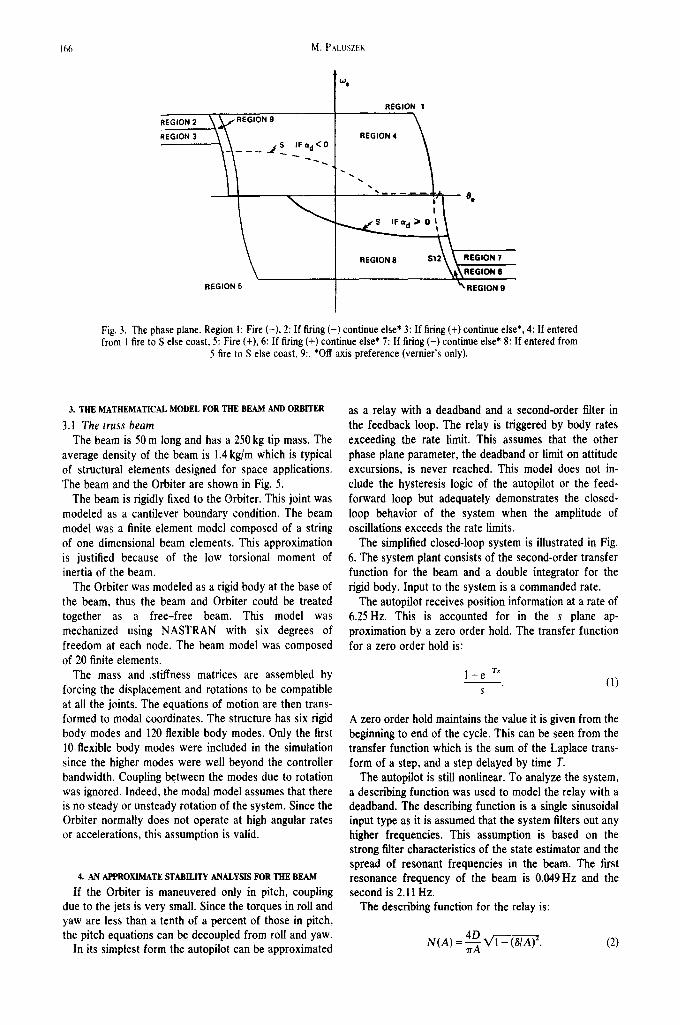
4D N(A) - ~-~ ~ . (2)


z ¢.)_

x~ ku i,,,

: IX . I o P - _ _ N, ' I - .~ . v - L - 4 D + ¢ ~ N ~ , , ~

x ~ " ~.~_. : - :L_~ .u

,A l-

n- >1 ~ <

n ~ u ~ o ~ u " ~ o o > > -

÷ 4-

O ~ X > > N N . . . . .

-- l l l l l

.A x 4

W L

I- I -ZCC

nc-, "*~'A-~- n~J -*---~ ~'-~

~ L

<

~'\A'

÷ 0 \ ' 0 • x <

0 ~

0 >.

° ~

,4

r~ W p. < Z g

0 0 U

I'- N n,. o

168 M. PAI,L SZEK

Fig. 5. The beam and the Orbiter.

This element has a phase shift of 1800 that is independent of A. 8 is the rate limit and D is the magnitude of the jet torque triggered when the rate exceeds & In this case, D = 3100 N-re.

If the two blocks in the system are labeled as L~(to) and L:(~o), then the characteristic equation of the system is:

N ( A ) L , ( j t o ) L2(j~o) = - 1. (3)

Limit cycles will occur wherever:

L, ( jo ) )L2( jo ) ) = - 1 I N ( A ) . (4)

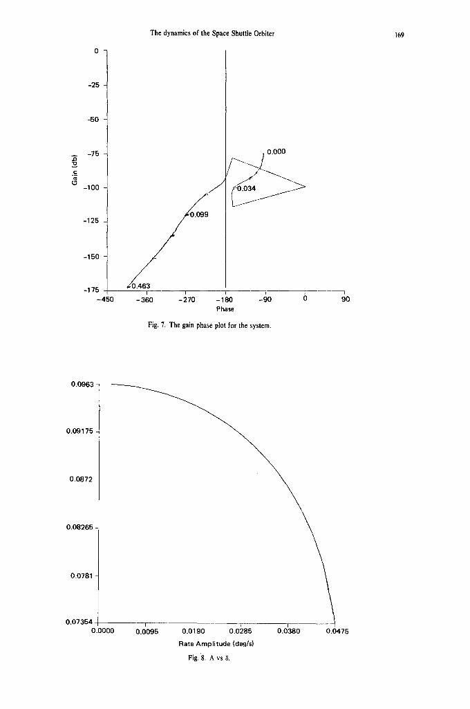
The limit cycles can be determined graphically on a gain phase plot.

The stability of the limit cycles can be determined from the graphical representation.

The gain phase plot for the pitch axis of the Orbiter is shown in Fig. 7. One limit cycle occurs near oJ = 0.0416Hz. This limit cycle is unstable since a small increase in amplitude of the describing function causes

an increase in the gain of L,(j~o)L2(j~o). The gain A at the limit cycle point vs 8 is shown in Fig. 8. The amplitude of the sinusoidal input to the describing function is less than the rate limit for rate limits greater than 0.475°/s.

5. THE SIMULATION RESULTS FOR THE BEAM AND ORBITER

5.1 Introduction The orbiter's autopilot was designed to control a rigid

vehicle with minimal cross-axis coupling. The performance of the Orbiter during the first four flights has, to a large extent, validated the assumption of vehicle rigidity.

Flying the vehicle with a payload deployed from the payload bay reintroduces the problem of flexibility. In many cases, either inherent payload structural flexibility or support flexibility raises the possibility of interaction between payload bending and the autopilot.

Usually, the lowest bending frequencies of payloads exceed the bandwidth of the autopilot, making active vibration control impractical. Hence, the goal becomes one of avoiding situations where such interaction may impede or prevent the accomplishment of mission objectives.

In this section the results of the study of the beam and the Orbiter are presented along with a discussion of the criteria used to judge the overall system performance and the methodology used to determine test cases. It should be noted that the autopilot is nonlinear, although the dynamics of the vehicle in the cases studied were not, so it is not necessarily possible to extrapolate a given case's results to other situations. For this reason, selection of test cases is important, as discussed later in this paper.

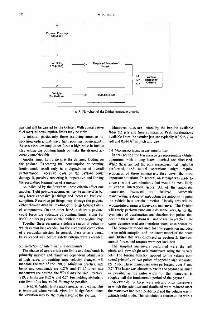
5.2 Maneuver criteria Figure 9 is a flowchart of the primary maneuver

criteria and how they relate to one another. The three main criteria ate fuel consumption, pointing accuracy, and payload loads.

Fuel consumption is an important consideration and may be mission limiting. On many flights, more than one

~ s Kb z + 2~cos + z

K. L~ 1 - e -'T + 2~.c~.s + J , [ ' 7 ] s

Fig. 6. The nonlinear single axis model of the autopilot.


"10

c

-25

-50

-75

-100

-125

-150

-175 -450

~0.463

,,_j,_ 0.000

~,.J / ~ ' - ~ , , _

I I I

- 360 - 270 - 180 - 9 0 () Phase

Fig. 7. The gain phase plot for the system.

q

9O

0.0963

0.09175

0.0872

0.08265

0.0781

0.07354 0.0000

I

0.0095 0.0190 0.0285 0.0380

Rate Amplitude (deg/s)

0.0475

Fig. 8. A vs 8.

170 M. PALUSZEK

Payload Pointing Accuracy

Jet Firing Frequency

I

Vehicle Oscillations

I

Required Propellant Budget

Pa~oad Loads

Fig. 9. Flowchart of the Orbiter maneuver criteria.

Vehlcle Maneuver Criteria

payload will he carried by the Orbiter. With conservative fuel margins consumption limits may be strict.

A mission, particularly those involving antennas or precision optics, may have tight pointing requirements. Excess vibration may either force a high price in fuel to stay within the pointing limits or make the desired accuracy unachievable.

Another important criteria is the dynamic loading on the payload. Exceeding fuel consumption or pointing limits would result only in a degradation of overall performance. Excessive loads on the payload could damage it, possibly rendering it inoperative and forcing the premature termination of a mission.

As indicated by the flowchart, these criteria affect one another. Tight pointing accuracies may be achievable but may force excessive jet firings and increased fuel consumption. Excessive jet firings may damage the payload either through dynamic loading or through fatigue failure of components. On the other hand, a delicate payload could force the widening of pointing limits, either for itself or other payloads carried with it in the payload bay.

Together these parameters define a region of behavior which cannot be exceeded for the successful completion of a particular mission. In general, these criteria would be exceeded well before safety criteria were exceeded.

5.3 Selection o.f rate limits and deadbands The choice of appropriate rate limits and deadbands is

primarily mission and maneuver dependent. Maneuvers at high rates, or requiting large velocity changes, will mandate the use of the PRCS. Minimum practical rate limits and deadbands are 0.2°/s and 1 °. If lower rate maneuvers are desired, the VRCS may be used. Practical VRCS limits are 0.02°/s and 0.2 °. For holding attitude, a rate limit of as low as 0.01°/s may be possible.

In general, tighter limits imply greater jet cycling. This is important when vehicle vibration is significant, since the vibration may be the main driver of the system.

Maneuver rates are limited by the impulse available from the jets and time constraints. Peak accelerations available from the vernier jets are typically 0.0228°/s 2 in roll and 0.014°/s 2 in pitch and yaw.

5.4 Maneuvers tested in the simulations In this section the ten maneuvers representing Orbiter

operations with a long beam attached are discussed. While these are not the only maneuvers that might be performed, and actual operations might require sequences of these maneuvers, they cover the most important situations. In general, an attempt was made to uncover worst cast situations that would be most likely to expose interaction issues. All of the automatic maneuvers discussed are idealized. Automatic maneuvering is done by instructing the autopilot to point the vehicle in a certain direction. Usually this will be accomplished using a three-axis maneuver. The Orbiter will rarely perform pure one-axis maneuvers, hence the symmetry of acceleration and deceleration pulses that occur in these simulations will not be seen in practice. The cases demonstrated are therefore worst case scenarios.

The computer model used for this simulation included the on-orbit autopilot and the linear model of the beam and Orbiter that was discussed in Section 2. Environ- mental forces and torques were not included.

The simplest maneuvers performed were the roll, pitch, and yaw single axis maneuvers using the vernier jets. The forcing function applied to the vehicle con- sisted primarily of two pulses of opposite sign separated by 15 sec. These maneuvers were performed over 5 ° and 3.2 ° . The latter was chosen to excite the payload as much as possible as the pulse width for that maneuver is roughly half the fundamental period of the payload.

An extension of these were roll and pitch maneuvers in which the rate limit and deadband were reduced after the maneuver had been performed and the vehicle was in attitude hold mode. This simulated a reorientation with a

The dynamics of the Space Shuttle Orbiter

tightening of pointing limits that might be required with an antenna or telescope. The autopilot responded by firing jets as it attempted to maneuver to the lower limit.

A manual maneuver with the astronaut forcing the payload by firing jets periodically was simulated to test the ability of the autopilot to damp out pilot-induced oscillations. This is significant because manual mode may be the preferred method of operation in many cases.

One of the worst case scenarios is the failure of one of the primary jets. In this case a jet sticks "on", imparting a continuous velocity change to the vehicle. If the autopilot is on, it will attempt to compensate for the rate and attitude error so produced by firing other jets. The jet cycling caused by autopilot commands may have large components at payload or Orbiter resonance frequencies forcing the structures to diverge. It is estimated that 30 sec could pass before the crew could shut the jet off by turning off its manifold. The two cases simulated here were that of a pure pitch jet, F3U, and one with roll coupling, R4U. It should be noted that it is possible to turn off the primary jets completely since the primary and vernier jets have separate power supplies. This might be done if the payload could not withstand loads due to the primary jets, as might be the case with a beam such as this one.

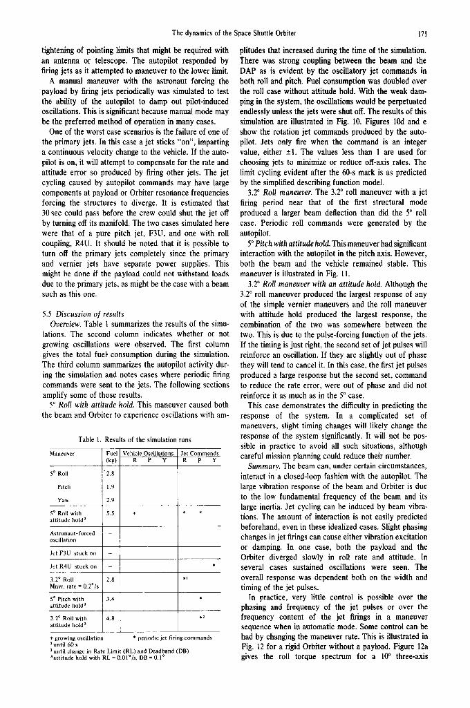
5.5 Discussion of results Overview. Table 1 summarizes the results of the simu-

lations. The second column indicates whether or not growing oscillations were observed. The first column gives the total fue~ consumption during the simulation. The third column summarizes the autopilot activity during the simulation and notes cases where periodic firing commands were sent to the jets. The following sections amplify some of those results.

5 ° Roll with attitude hold. This maneuver caused both the beam and Orbiter to experience oscillations with am-

Table 1. Results of the simulation runs

Maneuver Fuel Vehicle Oscil lat ions (kg) R P Y

i. 5 ° Roll 2.8

Pitch 1.9

Yaw 2.9

5 ° Roll with 5.5 + * * a t t i tude hold 3

As t ronau t - fo rced oscillation

Je t F 3 U s tuck on -

Je t R 4 U stuck on -

3.2 ° Roll 2 .8 , t Mnvr. rate = 0 ,2° / s

5 ° Pitch with 3.4 * a t t i tude hold 3

3.2 ° Roll wi th 4.8 ,2 a t t i tude hold 3

+ growing oscil lat ion * periodic je t firing commands I unti l 60 s 2 unti l change in Rate L imi t (RL) and Deadband (DB) 3a t t i tude hold with RL = O.Ol°/s, DB = 0.1 °

Je t Commands R P Y

171

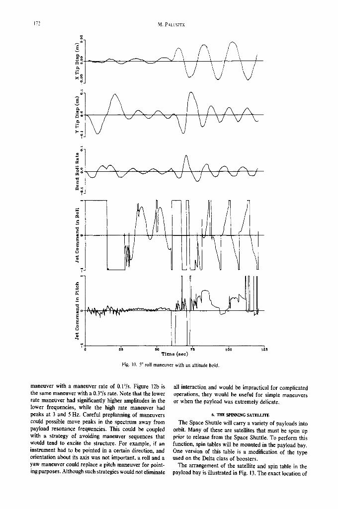
plitudes that increased during the time of the simulation. There was strong coupling between the beam and the DAP as is evident by the oscillatory jet commands in both roll and pitch. Fuel consumption was doubled over the roll case without attitude hold. With the weak damping in the system, the oscillations would be perpetuated endlessly unless the jets were shut off. The results of this simulation are illustrated in Fig. 10. Figures 10d and e show the rotation jet commands produced by the autopilot. Jets only fire when the command is an integer value, either -+l. The values less than 1 are used for choosing jets to minimize or reduce off-axis rates. The limit cycling evident after the 60-s mark is as predicted by the simplified describing function model.

3.20 Roll maneuver. The 3.2 ° roll maneuver with a jet firing period near that of the first structural mode produced a larger beam deflection than did the 5 ° roll case. Periodic roll commands were generated by the autopilot.

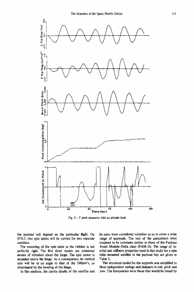
50 Pitch with attitude hold. This maneuver had significant interaction with the autopilot in the pitch axis. However, both the beam and the vehicle remained stable. This maneuver is illustrated in Fig. l l.

3.2 ° Roll maneuver with an attitude hold. Although the 3.2 o roll maneuver produced the largest response of any of the simple vernier maneuvers and the roll maneuver with attitude hold produced the largest response, the combination of the two was somewhere between the two. This is due to the pulse-forcing function of the jets. If the timing is just right, the second set of jet pulses will reinforce an oscillation. If they are slightly out of phase they will tend to cancel it. In this case, the first jet pulses produced a large response but the second set, command to reduce the rate error, were out of phase and did not reinforce it as much as in the 5 o case.

This case demonstrates the difficulty in predicting the response of the system. In a complicated set of maneuvers, slight timing changes will likely change the response of the system significantly. It will not be possible in practice to avoid all such situations, although careful mission planning could reduce their number.

Summary. The beam can, under certain circumstances, interact in a closed-loop fashion with the autopiiot. The large vibration response of the beam and Orbiter is due to the low fundamental frequency of the beam and its large inertia. Jet cycling can be induced by beam vibrations. The amount of interaction is not easily predicted beforehand, even in these idealized cases. Slight phasing changes in jet firings can cause either vibration excitation or damping. In one case, both the payload and the Orbiter diverged slowly in roll rate and attitude. In several cases sustained oscillations were seen. The overall response was dependent both on the width and timing of the jet pulses.

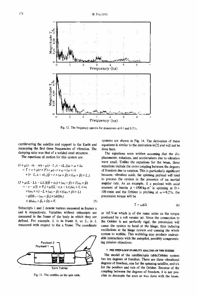
In practice, very little control is possible over the phasing and frequency of the jet pulses or over the frequency content of the jet firings in a maneuver sequence when in automatic mode. Some control can be had by changing the maneuver rate. This is illustrated in Fig. 12 for a rigid Orbiter without a payload. Figure 12a gives the roll torque spectrum for a l0 ° three-axis

172 M. P a, Lt.!SZEK

E v

~o ~ o " ~ d et

o I

AvAvA / ,_ /

:1 d

7

!1 " ~ c | h IK. t~

2's s'o ,'s l~o d5 T i m e ( s e e )

Fig. 10. 5 ° roll maneuver with an attitude hold.

maneuver with a maneuver rate of 0.1%. Figure 12b is the same maneuver with a 0.3°/s rate. Note that the lower rate maneuver had significantly higher amplitudes in the lower frequencies, while the high rate maneuver had peaks at 3 and 5 Hz. Careful preplanning of maneuvers could possible move peaks in the spectrum away from payload resonance frequencies. This could be coupled with a strategy of avoiding maneuver sequences that would tend to excite the structure. For example, if an instrument had to be pointed in a certain direction, and orientation about its axis was not important, a roll and a yaw maneuver could replace a pitch maneuver for pointing purposes. Although such strategies would not eliminate

all interaction and would be impractical for complicated operations, they would be useful for simple maneuvers or when the payload was extremely delicate.

6. THE SPINNING SATELLITE

The Space Shuttle will carry a variety of payloads into orbit. Many of these are satellites that must be spun up prior to release from the Space Shuttle. To perform this function, spin tables will be mounted in the payload bay. One version of this table is a modification of the type used on the Delta class of boosters.

The arrangement of the satellite and spin table in the payload bay is illustrated in Fig. 13. The exact location of


X ' 2

~o

.~_ o.b

°1

vvV v

0

0

b . f

J

$

'13

~°

E o

.q

P Z5 5O

Time (see) ?5 ]00

Fig. 11. 5 ° pitch maneuver with an attitude hold.

173

the payload will depend on the particular flight. On STS-5, two spin tables will be carded for two separate satellites.

The mounting of the spin table to the Orbiter is not perfectly rigid. The first three modes are rotational modes of vibration about the hinge. The spin motor is mounted above the hinge. As a consequence, its vertical axis will be at an angle to that of the Orbiter's, as determined by the bending of the hinge.

In this analysis, the inertia dyadic of the satellite and

its mass were considered variables so as to cover a wide range of payloads. The rest of the parameters were assumed to be constants similar to those of the Payload Assist Module-Delta class (PAM-D). The range of inertial and stiffness properties used in this study for a spin table mounted satellite in the payload bay are given in Table 2,

The structural model for the supports was simplified to three independent springs and dampers in roll, pitch and yaw. The frequencies were those that would be found by

174 M. PALUSZEK

~ 6 -

t ~

D

tD

~ea

t ~

o

i i E i i f

1 2 3 4 % 6

F r e q u e n c y (hz )

1 2 3 4 ,5 6

F r e q u e n c y (hz )

Fig. 12. The frequency spectra for maneuvers at 0.1 and 0.3°/s.

cantilevering the satellite and support to the Earth and measuring the first three frequencies of vibration. The damping ratio was that of a welded steel structure.

The equations of motion for this system are:

( I + Ix(r " rA - rr) - t x ( r . L~A - rL1)) tb + to x h o

= T + v + p ( r × F ) + / ~ ( - r x t o x(to x r)

+ ( r . LtA - rLl)/~ + r × (co +/3) × ((to +/3) × L,)

(J + /z (L . L,X - L L ) ) ( ~ + ~b2) + (to2 +/3) × J(co~ +/3) = - v - p ( L × F2) +p.((L • r2A - Lr2)(02 + L ×'co2

x (,.,,~ x r~) - L x (co~ + 8) x ((o,~ + ~) x L)

x ¢ ( ~ I + ~ + n) = E. (5)

Subscripts 1 and 2 denote vectors measured in frames a and b respectively. Variables without subscripts are measured in the frame of the body in which they are defined. For example, L is in frame b, so L, is L measured with respect to the a frame. The coordinate

Pay load 2 Payload1 q "~

Spin Tables

Fig. 13. The satellite on the spin table.

systems are shown in Fig. 14. The derivation of these equations is similar to the derivation in[2] and will not be done here.

The equations were written assuming that the dis- placements, rotations, and accelerations due to vibration were small. Unlike the equations for the beam, these equations include the cross coupling between the degrees of freedom due to rotation. This is particularly significant because, vibration aside, the spinning payload will tend to precess the system in the presence of an inertial angular rate. As an example, if a payload with axial moment of inertia $ = 4500kg-m 2 is spinning at I] = 100 r/min and the Orbiter is pitching at to = 0.2°/s, the precession torque will be

T = to$~ (6)

or 165 N-m which is of the same order as the torque produced by a roll vernier jet. Since the connection to the Orbiter is not perfectly rigid, the precession will cause the system to bend at the hinge, thus inducing oscillations at the hinge system and causing the whole system to wobble. This wobbling may produce undesirable interactions with the autopilot, possibly compromis- ing mission objectives.

7. THE OPEN-LOOP STABILITY ANALYSIS OF THE SYSTEM

The model of the satellite/spin table/Orbiter system has ten degrees of freedom. There are three vibrational degrees of freedom, one for the spinning satellite, and six for the position and rate of the Orbiter. Because of the coupling between the degrees of freedom, it is not possible to decouple the axes as was done with the beam.


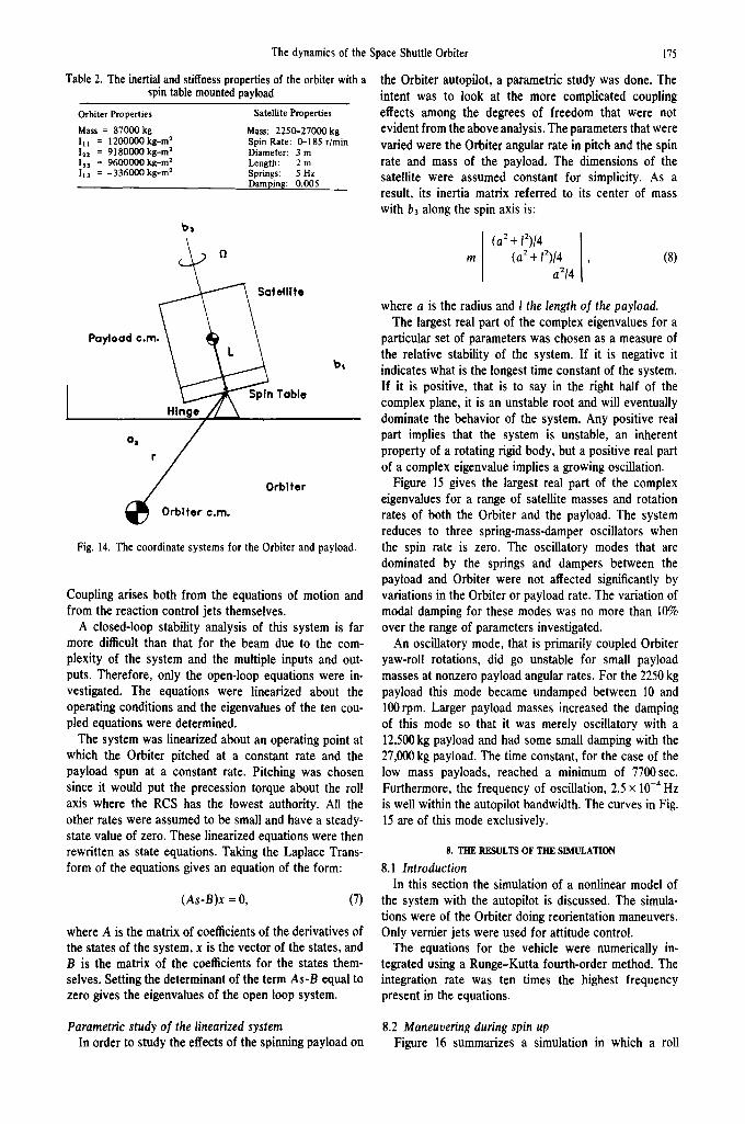
Table 2. The inertial and stiffness properties of the orbiter with a spin table mounted payload

Orbiter Properties Satellite Properties

Mass = 87000 kg Mass: 2250-27000 kg It1 = 1200000 kg-m 2 Spin Rate: 0-185 r/min 122 = 9180000 kg-m 2 Diameter: 3 m Iss = 9600000 kg-m 2 Length: 2 m lls = -336000 kg-m 2 Springs: 5 Hz

Damping: 0.005

~ Satelllte

Payload c.m. ~ Hinge~ ~ Spin Table

Orbiter C.l"rl.

Fig. 14. The coordinate systems for the Orbiter and payload.

Coupling arises both from the equations of motion and from the reaction control jets themselves.

A closed-loop stability analysis of this system is far more difficult than that for the beam due to the complexity of the system and the multiple inputs and out- puts. Therefore, only the open-loop equations were investigated. The equations were linearized about the operating conditions and the eigenvalues of the ten coupled equations were determined.

The system was lineafized about an operating point at which the Orbiter pitched at a constant rate and the payload spun at a constant rate. Pitching was chosen since it would put the precession torque about the roll axis where the RCS has the lowest authority. All the other rates were assumed to be small and have a steady- state value of zero. These linearized equations were then rewritten as state equations. Taking the Laplace Trans- form of the equations gives an equation of the form:

(As-B)x = 0, (7)

where A is the matrix of coefficients of the derivatives of the states of the system, x is the vector of the states, and B is the matrix of the coefficients for the states themselves. Setting the determinant of the term As-B equal to zero gives the eigenvalues of the open loop system.

175

the Orbiter autopilot, a parametric study was done. The intent was to look at the more complicated coupling effects among the degrees of freedom that were not evident from the above analysis. The parameters that were varied were the Orbiter angular rate in pitch and the spin rate and mass of the payload. The dimensions of the satellite were assumed constant for simplicity. As a result, its inertia matrix referred to its center of mass with b3 along the spin axis is:

(a 2 + 12)/4 (a 2 + 12)/4

a2/4 (8)

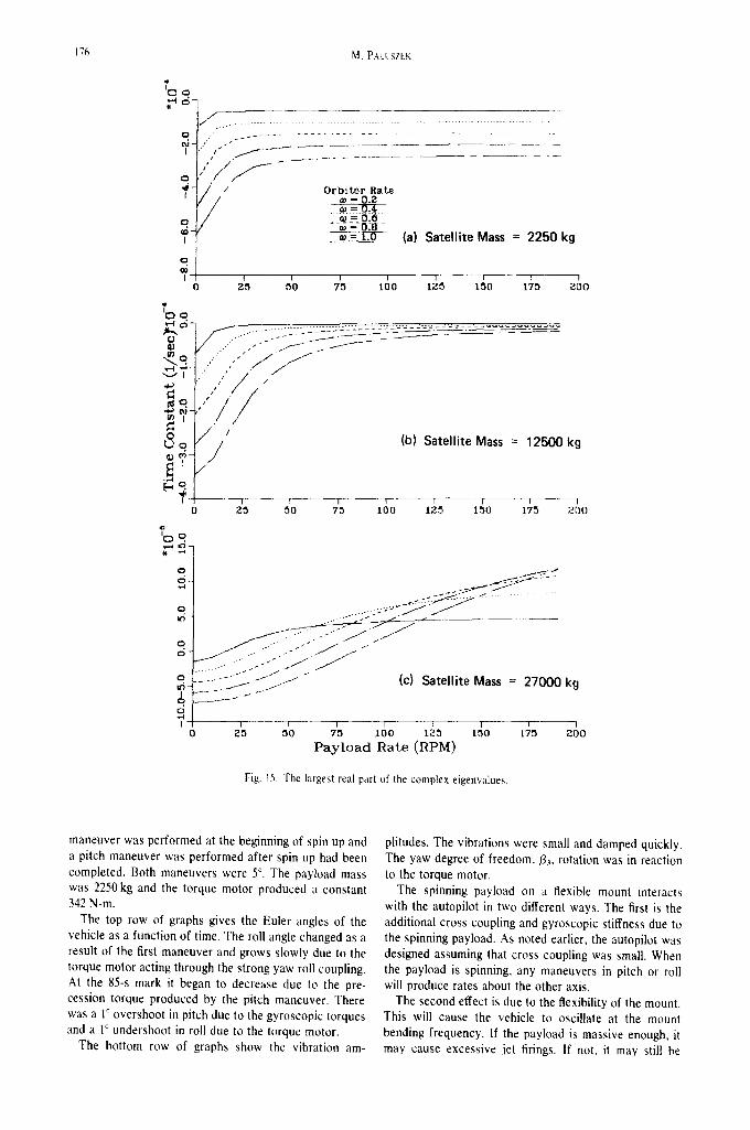
where a is the radius and 1 the length of the payload. The largest real part of the complex eigenvalues for a

particular set of parameters was chosen as a measure of the relative stability of the system. If it is negative it indicates what is the longest time constant of the system. If it is positive, that is to say in the fight half of the complex plane, it is an unstable root and will eventually dominate the behavior of the system. Any positive real part implies that the system is unstable, an inherent property of a rotating rigid body, but a positive real part of a complex eigenvalue implies a growing oscillation.

Figure 15 gives the largest real part of the complex eigenvalues for a range of satellite masses and rotation rates of both the Orbiter and the payload. The system reduces to three spring-mass-damper oscillators when the spin rate is zero. The oscillatory modes that are dominated by the springs and dampers between the payload and Orbiter were not affected significantly by variations in the Orbiter or payload rate. The variation of modal damping for these modes was no more than 10% over the range of parameters investigated.

An oscillatory mode, that is primarily coupled Orbiter yaw-roll rotations, did go unstable for small payload masses at nonzero payload angular rates. For the 2250 kg payload this mode became undamped between 10 and 100 rpm. Larger payload masses increased the damping of this mode so that it was merely oscillatory with a 12,500 kg payload and had some small damping with the 27,000 kg payload. The time constant, for the case of the low mass payloads, reached a minimum of 7700sec. Furthermore, the frequency of oscillation, 2.5 × l0 -4 Hz is well within the autopilot bandwidth. The curves in Fig. 15 are of this mode exclusively.

8. THE RESULTS OF THE SIMULATION

8.1 Introduction In this section the simulation of a nonlinear model of

the system with the autopilot is discussed. The simulations were of the Orbiter doing reorientation maneuvers. Only vernier jets were used for attitude control.

The equations for the vehicle were numerically in- tegrated using a Runge-Kutta fourth-order method. The integration rate was ten times the highest frequency present in the equations.

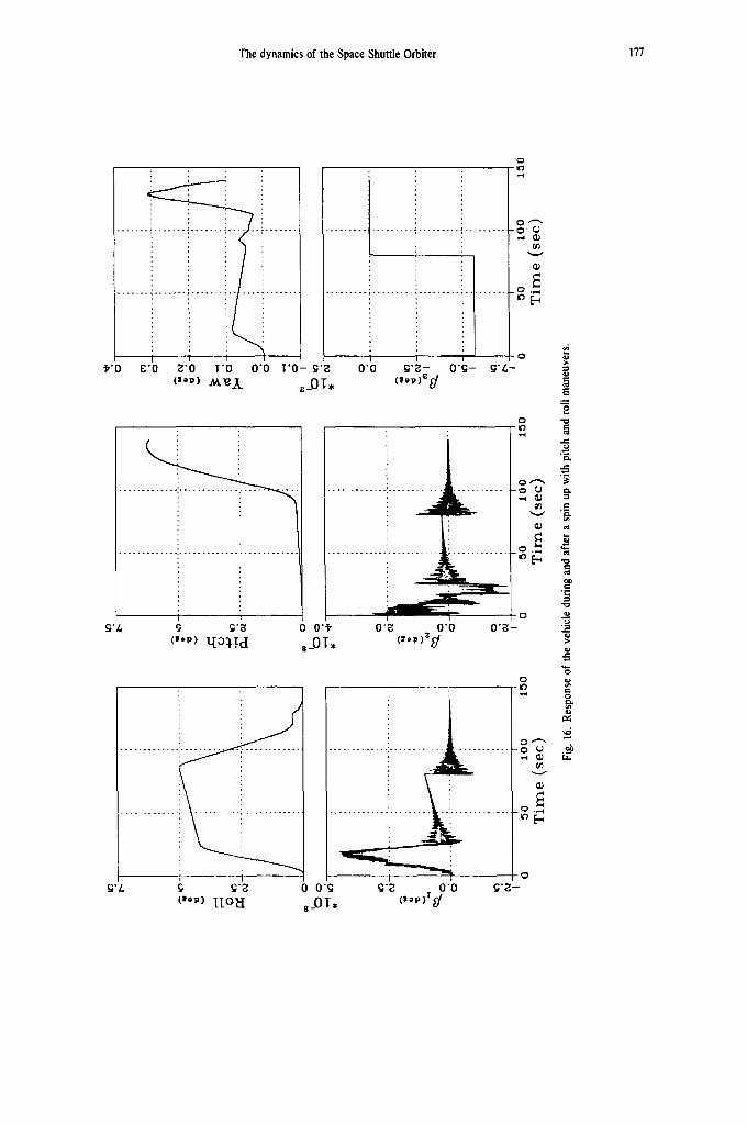
Parametric study of the linearized system 8.2 Maneuvering during spin up In order to study the effects of the spinning payload on Figure 16 summarizes a simulation in which a roll

176 M. PALI'SZEK

0 E3 ~

q

?.

¢3 O0

I o

/ ' . - - . . . . . . . . ~- - - - - iL- . . . . . . . . . . . . . . . . . . . . . . . . . . . . L _ - - L

~/ Orbiter Rate =0= 0.2

....=...-.~ ~ = O . O

- -~ ~--0:8- ¢o = t.o (a) Satel l i te Mass = 2 2 5 0 kg

7'5 1;5

........... :--5 L'- . . . . . . . . ~.~Lz--. - ~ - - - --%==-2~ - --==-- - = ~ - --===="-

~ j - I . . / / . , / I" / / _ "

r~ o y / / (b) Satel l i te Mass = 12500 kg

O 25 50 7~ IOO 125 150 175 2 4 0

o

o

q

0 =6-

I 0 g ~

f ~ j . j / (c) Satellite Mass = 27000 kg

. . . . . ~ . . . . . I - - - - T ~ I - - I - - 1 ~o 7~ loo 1 5 tso 175 ~oo

P a y l o a d R a t e ( R P M )

Fig. 15. The largest real part of the complex eigenvalues.

maneuver was performed at the beginning of spin up and a pitch maneuver was performed after spin up had been completed. Both maneuvers were 5 ° . The payload mass was 2250 kg and the torque motor produced a constant 342 N-m.

The top row of graphs gives the Euler angles of the vehicle as a function of time. The roll angle changed as a result of the first maneuver and grows slowly due to the torque motor acting through the strong yaw roll coupling. At the 85-s mark it began to decrease due to the precession torque produced by the pitch maneuver. There was a 1 ° overshoot in pitch due to the gyroscopic torques and a 1 ° undershoot in roll due to the torque motor.

The bottom row of graphs show the vibration am-

plitudes. The vibrations were small and damped quickly. The yaw degree of freedom, 13,, rotation was in reaction to the torque motor.

The spinning payload on a flexible mount interacts with the autopilot in two different ways. The first is the additional cross coupling and gyroscopic stiffness due to the spinning payload. As noted earlier, the autopilot was designed assuming that cross coupling was small. When the payload is spinning, any maneuvers in pitch or roll will produce rates about the other axis.

The second effect is due to the flexibility of the mount. This will cause the vehicle to oscillate at the mount bending frequency. If the payload is massive enough, it may cause excessive jet firings. If not, it may still be


iiiiii iiiiii "~'0

,"4

OQ

v

E'O 8"0 T'O 0"0 T'O- (~'~ 0"0 g '~ - O'g- g'~,- (~'P) --"~- ~/L ~_OT, (~'~')~/

g •/,,, g'~ 0 0"@

<"p> yc)1 !c[ 8_OT, 0'~ 0"0

0

. . . . . 0

.... ~

e--

,

0"~ -

iiiiiiiiiiiii g'/. g ~'8

("~) I[O~I 00"g

,_OT,

. . . . . . . . . 0 ~

f~ v

........ I-,~

~'8 0 "0 (~':~-

B:

" I "

o

,,6

b:

17~ M. PALUSZEK

undesirable due to the possible deleterious effects of excessive vibration on the satellite.

The obvious strategy is not to maneuver when the payload is spinning, if one has that option. Other con- siderations, such as maintaining uniform payload tem- peratures when in the sun, may preclude this strategy. If one must maneuver while the payload is spinning, it is desirable to maneuver at the lowest rate possible. A further alternative is to take advantage of the precession to do multiaxis maneuvers. For example, a two-axis maneuver requiring angle changes in roll and pitch would be done by switching into manual mode with the pitch and yaw phase planes on, and firing jets to pitch the vehicle. The precession torque would roll the vehicle in a predictable fashion. Some fuel savings might be obtained in this fashion.

fuel consumption. When this is not feasible it is desirable, whenever possible, to avoid maneuvering while the payload is spinning.

Acknowledgements--In the course of this project, a great many persons made contributions to it. The author would like to thank Kim Kirchwey for his consultations on the autopilot and Orbiter flight simulations, Marilyn Ham for contributions in the area of numerical analysis, Margaret Conley for administrative support, and Lisa Kern for secretarial support.

This paper was prepared by The Charles Stark Draper Labora- tory, Inc., under contract NAS9-16023 with the National Aeronau- tics and Space Administration. The work was supported by NASA Johnson Space Center (JSC).

Publication of this report does not constitute approval by NASA of findings or conclusions contained herein. It is published for the exchange and stimulation of ideas.

9. SUMMARY AND CONCLUSIONS

The dynamics of the Orbiter and autopilot with two different payloads were analyzed in this paper. The first payload, a long flexible beam, was shown to have ap- preciable coupling with the autopilot due to its large inertia and low first resonant frequency. Potential unstable limit cycles were identified using a relay approximation to the autopilot and were confirmed through simulations using a functional representation of the on- orbit DAP. Short of modifying the autopilot to damp vibrations the interaction can best be minimized by carefully selecting the maneuvers to be performed while the payload is deployed. This process can also serve to reduce the risk of overstressing the payload.

The second payload, a spinning satellite, has far more complex dynamics which involve coupling between the angular degrees of freedom. Linear analysis showed that the vibration modes were not appreciably affected by rotational coupling, but a roll-yaw mode did become unstable, albeit with a very long time constant, for low payload masses and moderate-to-high payload rates. The simulations of the nonlinear system with the autopilot showed negligible vibration effects. For large payloads the effect of vehicle precession was to increase the number of jet firings needed for a maneuver as a result of compensating for the precession torque. Under certain circumstances, it may be possible to take advantage of the precession to do multiaxis maneuvers with reduced

REFERENCES

1. Space Shuttle Orbiter Operational Level C Functional Sub- system Software Requirements--Guidance, Navigation, and Control, Part C, Flight Control Orbit DAP, STS 81-0009, WBS 1.3.4.5.2. IRD SE-694T2, Rockwell International, 1 May, 1981.

2. H. J. Fletcher, L. Rongved, and E. Y. Yu, Dynamics analysis of a two-body gravitationally oriented satellite. Bell System Tech. J. 42 (5) 2239-2265 (Sept. 1%3).

3. M. Ham and M. Paluszek, The Large Space Structures Experiment Program Final Report, R-1496. The Charles Stark Draper Laboratory, Inc., Cambridge, MA, to be published.

4. D. Bruno Stability Prediction and Compensation of a Booster Control System with a Rate-Limited Actuator, T-755, The Charles Stark Draper Laboratory, Inc., Aug. 1982.

5. A. Gelb and W. E. Vander Velde, Multiple Input Describing Functions and Nonlinear System. McGraw-Hill, New York (1%8).

Acronyms DAP FCS IMU NASA NASTRAN OMS PAM-D PRCS RCS STS VRCS

APPENDIX l

Digital AutoPilot Flight Control System Inertial Measurement Unit National Aeronautics and Space Administration NAsa STRuctural ANalysis program Orbital Maneuvering System Payload Assist Module Delta class Primary Reaction Control System Reaction Control System Space Transportation System Vernier Reaction Control System

the dynamics of the space shuttle orbiter with a flexible payload

Documents