Proceedings of the 2002 Winter Simulation Conference E. Yücesan, C.-H. Chen, J. L. Snowdon, and J. M. Charnes, eds.

MODELING THE SPACE SHUTTLE

Grant R. Cates Martin J. Steele

PH-M3 (Cates) YA-D (Steele)

Kennedy Space Center KSC, FL 32899, U.S.A.

Mansooreh Mollaghasemi Ghaith Rabadi

Industrial Engineering & Management Systems

4000 Central Florida Blvd University of Central Florida Orlando, FL 32816, U.S.A.

ABSTRACT

We summarize our methodology for modeling space shut-tle processing using discrete event simulation. Why the project was initiated, what the overall goals were, how it was funded, and who were the members of the project team are identified. We describe the flow of the space shut-tle flight hardware through the supporting infrastructure and how the model was created to accurately portray the space shuttle. The input analysis methodology that was used to populate the model elements with probability dis-tributions for process durations is described in the paper. Verification, validation, and experimentation activities are briefly summarized.

1 INTRODUCTION

A discrete event simulation model of the space shuttle was created using commercial off-the-shelf software. In creat-ing this model through a joint-project with the University of Central Florida, NASA has established within the Ken-nedy Space Center, the space shuttle program, and the Space Launch Initiative (the program intended to ulti-mately build a shuttle replacement vehicle), an ability to make use of simulation as a tool to aid decision making. This paper focuses primarily on describing the process that was undertaken to produce the shuttle simulation model. Output analysis from the model is also looked at, although briefly, and future directions are described. In 1999, at a time when NASA was considering plans to increase the flight rate from 7 flights per year to as many as 15 flights per year, the Kennedy Space Center began discussions with the University of Central Florida to de-velop a simulation model of space shuttle processing. The doubling of the flight rate was expected to strain the exist-ing workforce, facilities, ground support equipment, and flight hardware elements. The question was which parts would be strained and how much? Would we need addi-tional resources or might expected process improvements

suffice? As the lead time to add critical resources, either people, facilities, or flight hardware, is measured in years, not to mention the cost of potentially billions of dollars, it was important to identify the system bottleneck as early as possible. Discrete event simulation appeared to be an excellent tool to meet this challenge. An additional goal of the project was to educate per-sonnel at the Kennedy Space Center in the use of discrete event simulation. In this way NASA would be able to con-duct future projects either in-house, or be able to manage contracted out projects with more expertise with respect to cost and schedule. In order to minimize costs, a require-ment was levied and accepted to use commercial off-the-shelf software. 2 PROJECT APPROVAL One of the keys to gaining project approval was the crea-tion of a prototype model that placed an emphasis on ani-mation. This “core model” was developed so as to demon-strate to management the type of simulation that was being proposed, the intended benefits, as well as to help estimate costs and time to complete. The core model was limited to the Orbiter flow and its focus was on visual animation. This allowed management to see what was being proposed. The visual aspect of the core model was very beneficial to securing funding to proceed to the more all-encompassing models. The core model also gave management a visual understanding of what discrete event simulation is, and how it would be used to model the shuttle. The core model was built in-house by NASA over a period of three months and we used it each time we briefed the various decision reviewers and makers leading up to the projects ultimate approval for full funding. The project was initially estimated to take one year to accomplish at a cost of $300,000. These estimates were reduced to $200,000 and 9 months by the time the project was actu-ally approved. After securing the needed funding and en-tering into a NASA Space Act Agreement with the Univer-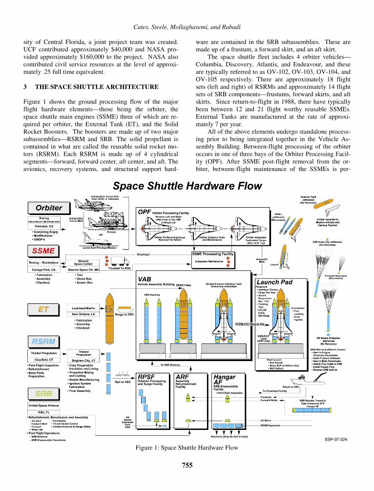

Cates, Steele, Mollaghasemi, and Rabadi

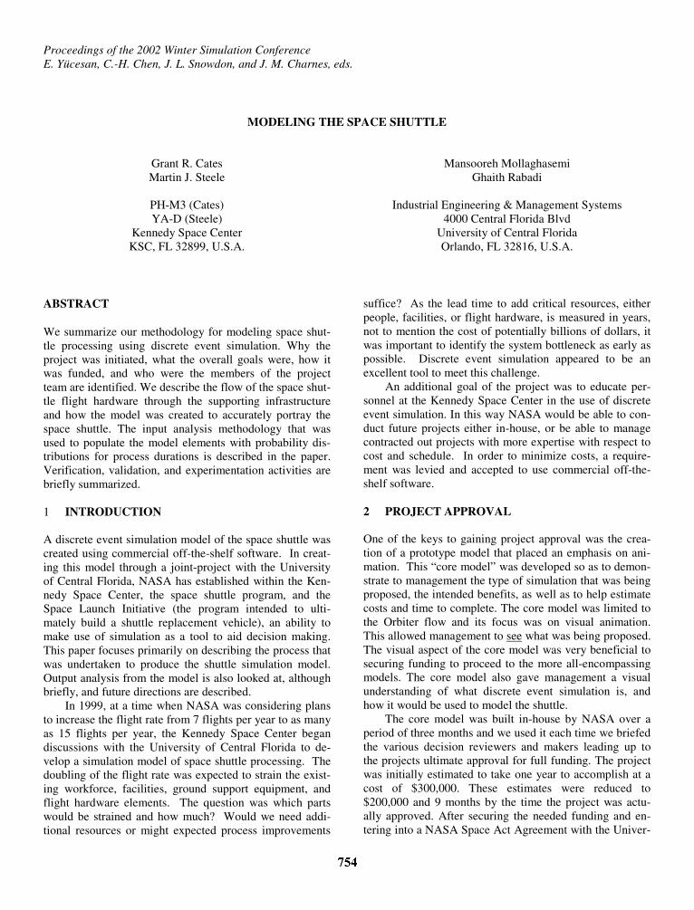
sity of Central Florida, a joint project team was created. UCF contributed approximately $40,000 and NASA pro-vided approximately $160,000 to the project. NASA also contributed civil service resources at the level of approxi-mately .25 full time equivalent. 3 THE SPACE SHUTTLE ARCHITECTURE Figure 1 shows the ground processing flow of the major flight hardware elements—those being the orbiter, the space shuttle main engines (SSME) three of which are re-quired per orbiter, the External Tank (ET), and the Solid Rocket Boosters. The boosters are made up of two major subassemblies—RSRM and SRB. The solid propellant is contained in what are called the reusable solid rocket mo-tors (RSRM). Each RSRM is made up of 4 cylindrical segments—forward, forward center, aft center, and aft. The avionics, recovery systems, and structural support hard-

ware are contained in the SRB subassemblies. These are made up of a frustum, a forward skirt, and an aft skirt. The space shuttle fleet includes 4 orbiter vehicles—Columbia, Discovery, Atlantis, and Endeavour, and these are typically referred to as OV-102, OV-103, OV-104, and OV-105 respectively. There are approximately 18 flight sets (left and right) of RSRMs and approximately 14 flight sets of SRB components—frustums, forward skirts, and aft skirts. Since return-to-flight in 1988, there have typically been between 12 and 21 flight worthy reusable SSMEs. External Tanks are manufactured at the rate of approxi-mately 7 per year. All of the above elements undergo standalone process-ing prior to being integrated together in the Vehicle As-sembly Building. Between-flight processing of the orbiter occurs in one of three bays of the Orbiter Processing Facil-ity (OPF). After SSME post-flight removal from the or-biter, between-flight maintenance of the SSMEs is per-

Figure 1: Space Shuttle Hardware Flow

Cates, Steele, Mollaghasemi, and Rabadi

formed in a dedicated facility. After launch, each of the two boosters are recovered at sea by the SRB Retrieval Vessels—Freedom and Liberty Star. The boosters are towed to Hangar AF and disassembled into their separate SRB and RSRM components. The RSRM segments are shipped by rail to Utah for refurbishment and propellant loading and then returned by rail to the Rotation Process-ing and Surge Facility at KSC. The SRB Frustum, Forward and Aft Skirts are towed over roads to the Assembly Re-furbishment Facility. Assembly and integration of the Space Shuttle Vehicle—RSRM/SRB, ET, and Orbiter—occurs in one of two integration cells (High Bays 1 or 3) in the Vehicle Assembly Building (VAB). In the VAB, the space shuttle is assembled atop one of three mobile launcher platforms (MLP). A crawler/transporter is used to move the MLP, with the space shuttle vehicle, out to one of the two launch pads Figure 2 shows a “quicklook” or snapshot in time of where the flight hardware elements are located at the Ken-nedy Space Center. This product is produced on a weekly basis. Not shown are off-site flight hardware such as OV-

102, which was in California undergoing major overhaul, and RSRM segments that are located in Utah. Note also that Figures 1 and 2 were available prior to beginning the project.

4 PREVIOUS MODELS VS THIS MODEL The use of discrete event simulation to model the space shut-tle began as early as 1970 before the shuttle was approved for development (Schlagheck and Byers 1971). That initial work suffered from a lack of an established baseline for what the shuttle architecture would actually be. As the shut-tle entered flight testing in 1981 another simulation model was developed and showed that the shuttle flight rate was going to be less than originally estimated (Wilson, Vaughan, Naylor, and Voss 1982). Both earlier models had to rely on estimates for ground processing durations. The most significant change between the previous mod-els and the current model was the availability of historical data for ground processing durations and event probabilities. This allowed us to input process durations and event prob-abilities that were representative of true capabilities.

Figure 2: Flight Hardware Quicklook

asemi, and Rabadi

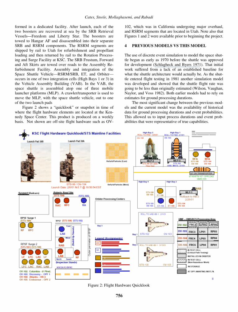
Cates, Steele, Mollagh The current model accurately simulates the activities shown in Figure 2, i.e. the major flight hardware elements move from standalone processing facilities to the VAB for integration, then out to the launch pad, and ultimately to on-orbit operations. The orbiter returns to earth and the process repeats. 5 THE SCHEDULE AND

PROJECT STRATEGY During the project approval process, a project schedule was created using Microsoft Project. Figure 3 shows the as-planned versus as-run schedule. Our strategy was to start small and build upon success. To this end, we decided to first build a model that only in-cluded the orbiters and their supporting facilities and ground support equipment. This was referred to as the Phase A model. The Phase B model would build upon the A model and incorporate the SSMEs, RSRMs, SRB, and ET and their attendant infrastructure. In order to accomplish our goals we needed to proceed down parallel paths. One path was to build the model in Arena. We needed to create a space shuttle architecture in-frastructure consisting of the major processing facilities, ground support equipment, and flight hardware elements. The flight hardware elements were coded so that they moved in the appropriate manner through the various fa-cilities. This path was performed, at least initially, in the absence of the exact probability distributions for how long processes would take. After NASA provided UCF with the

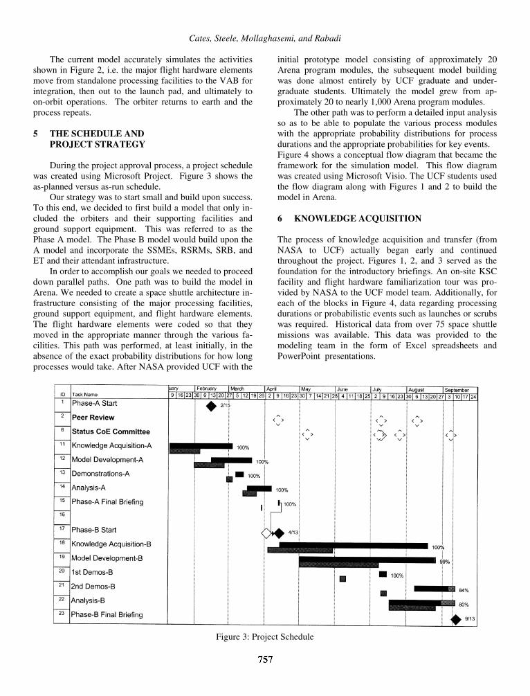
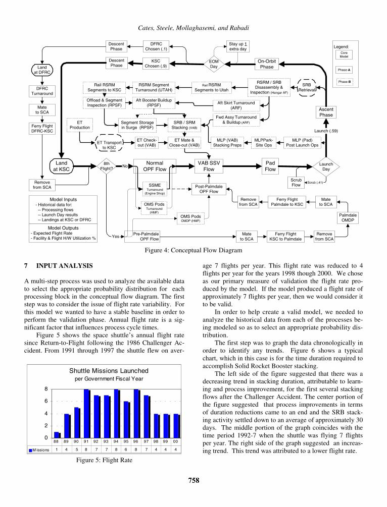
initial prototype model consisting of approximately 20 Arena program modules, the subsequent model building was done almost entirely by UCF graduate and under-graduate students. Ultimately the model grew from ap-proximately 20 to nearly 1,000 Arena program modules. The other path was to perform a detailed input analysis so as to be able to populate the various process modules with the appropriate probability distributions for process durations and the appropriate probabilities for key events. Figure 4 shows a conceptual flow diagram that became the framework for the simulation model. This flow diagram was created using Microsoft Visio. The UCF students used the flow diagram along with Figures 1 and 2 to build the model in Arena. 6 KNOWLEDGE ACQUISITION The process of knowledge acquisition and transfer (from NASA to UCF) actually began early and continued throughout the project. Figures 1, 2, and 3 served as the foundation for the introductory briefings. An on-site KSC facility and flight hardware familiarization tour was pro-vided by NASA to the UCF model team. Additionally, for each of the blocks in Figure 4, data regarding processing durations or probabilistic events such as launches or scrubs was required. Historical data from over 75 space shuttle missions was available. This data was provided to the modeling team in the form of Excel spreadsheets and PowerPoint presentations.

Figure 3: Project Schedule

Cates, Steele, Mollaghasemi, and Rabadi

NormalOPF Flow

VAB SSVFlow

PadFlow

AscentPhase

LaunchDay

On-OrbitPhase

Launch (.59)

EOMDay

Stay up 1extra day

DescentPhase

DescentPhase

Landat KSC

Landat DFRC

8thFlight?

Pre-PalmdaleOPF Flow

Post-PalmdaleOPF Flow

Ferry FlightKSC to Palmdale

Mateto SCA

Ferry FlightPalmdale to KSC

Removefrom SCA

Removefrom SCA

Mateto SCA

PalmdaleOMDP

Ferry FlightDFRC-KSC

Removefrom SCA

Mateto SCA

DFRCTurnaround

ScrubFlow

Scrub (.41)

No

Model Outputs- Expected Flight Rate- Facility & Flight H/W Utilization %

Model Inputs- Historical data for: -- Processing flows -- Launch Day results -- Landings at KSC or DFRC

Yes

RSRM / SRBDisassembly &

Inspection (Hangar AF)

SSMETurnaround

(Engine Shop)

OMS PodsTurnaround

(HMF)

Rail RSRMSegments to Utah

ET Check-out (VAB)

SRB / SRMStacking (VAB)

ET Mate &Close-out (VAB)

ETProduction

DFRCChosen (.1)

KSCChosen (.9)

Legend:Core

Model

Phase-B

Phase-A

SRBRetrieval

ET Transportto KSC

OMS PodsOMDP (HMF)

MLP (Pad)Post Launch Ops

MLPPark-Site Ops

MLP (VAB)Stacking Preps

RSRM SegmentTurnaround (UTAH)

Aft Booster Buildup(RPSF) Aft Skirt Turnaround

(ARF)

Rail RSRMSegments to KSC

Fwd Assy Turnaround& Buildup (ARF)

Offload & SegmentInspection (RPSF)

Segment Storagein Surge (RPSF)

Figure 4: Conceptual Flow Diagram

7 INPUT ANALYSIS A multi-step process was used to analyze the available data to select the appropriate probability distribution for each processing block in the conceptual flow diagram. The first step was to consider the issue of flight rate variability. For this model we wanted to have a stable baseline in order to perform the validation phase. Annual flight rate is a sig-nificant factor that influences process cycle times. Figure 5 shows the space shuttle’s annual flight rate since Return-to-Flight following the 1986 Challenger Ac-cident. From 1991 through 1997 the shuttle flew on aver-

0

2

4

6

8

M issions 1 4 5 8 7 7 8 6 8 7 4 4 4

88 89 90 91 92 93 94 95 96 97 98 99 00

Shuttle Missions Launched per Government Fiscal Year

Figure 5: Flight Rate

age 7 flights per year. This flight rate was reduced to 4 flights per year for the years 1998 though 2000. We chose as our primary measure of validation the flight rate pro-duced by the model. If the model produced a flight rate of approximately 7 flights per year, then we would consider it to be valid. In order to help create a valid model, we needed to analyze the historical data from each of the processes be-ing modeled so as to select an appropriate probability dis-tribution. The first step was to graph the data chronologically in order to identify any trends. Figure 6 shows a typical chart, which in this case is for the time duration required to accomplish Solid Rocket Booster stacking. The left side of the figure suggested that there was a decreasing trend in stacking duration, attributable to learn-ing and process improvement, for the first several stacking flows after the Challenger Accident. The center portion of the figure suggested that process improvements in terms of duration reductions came to an end and the SRB stack-ing activity settled down to an average of approximately 30 days. The middle portion of the graph coincides with the time period 1992-7 when the shuttle was flying 7 flights per year. The right side of the graph suggested an increas-ing trend. This trend was attributed to a lower flight rate.

asemi, and Rabadi

Cates, Steele, Mollagh

0

10

20

30

40

50

60

70

80

939186837975696365615552494837313427

SRB Stacking Flow Duration Calendar Days

STS-Flow (Chronological Order)

Figure 6: SRB Stacking Data points from time periods where a decreasing trend were evident were excluded. Likewise, data from periods where an increasing trend were noted that was attributable to a low flight rate were also excluded. For the SRB stacking flows, the data ultimately chose is shown in Figure 7.

0

10

20

30

40

50

60

878584828078767273706766645960585756

SRB Stacking Flow Duration Calendar Days

STS-Flow (Chronological Order)

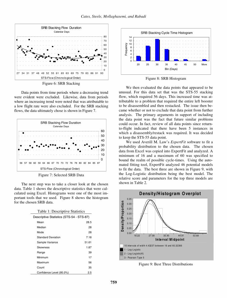
Figure 7: Selected SRB Data The next step was to take a closer look at the chosen data. Table 1 shows the descriptive statistics that were cal-culated using Excel. Histograms were one of the most im-portant tools that we used. Figure 8 shows the histogram for the chosen SRB data.

Table 1: Descriptive Statistics

Descriptive Statistics (STS-54 - STS-87)

Mean 28.5

Median 28

Mode 28

Standard Deviation 7.18

Sample Variance 51.61

Skewness 1.87

Range 39

Minimum 17

Maximum 56

Count 35

Confidence Level (95.0%) 2.5

02468

101214

20 25 30 35 40 45 50 More

Bin (Days)

Fre

quen

cy

SRB Stacking Cycle Time Histogram

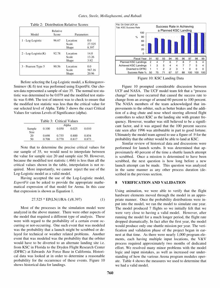
Figure 8: SRB Histogram We then evaluated the data points that appeared to be unusual. For this data set that was the STS-55 stacking flow, which required 56 days. This increased time was at-tributable to a problem that required the entire left booster to be disassembled and then restacked. The issue then be-came whether or not to exclude that data point from further analysis. The primary arguments in support of including the data point was the fact that future similar problems could occur. In fact, review of all data points since return-to-flight indicated that there have been 5 instances in which a disassembly/restack was required. It was decided to keep the STS-55 data point. We used Averill M. Law’s ExpertFit software to fit a probability distribution to the chosen data. The chosen data from Excel was copied into ExpertFit and analyzed. A minimum of 16 and a maximum of 60 was specified to bound the realm of possible cycle-times. Using the auto-mated fitting tool, ExpertFit analyzed 46 potential models to fit the data. The best three are shown in Figure 9, with the Log-Logistic distribution being the best model. The relative score and parameters for the top three models are shown in Table 2.

10 interv a ls o f w id th 4.43237 b e tw een 16 and 60.32366

1 - Log-Logistic

2 - Log-Logistic(K)

3 - Pearson T ype 5

0.00

0.05

0.10

0.15

0.20

0.25

0.30

0.35

D ensity/H istogram O verplot

Inte rva l M idpoint

Den

sity

/Pro

po

rtio

n

18 .22 27 .08 35 .95 44 .81 53 .68

Figure 9: Best Three Distributions

Cates, Steele, Mollaghasemi, and Rabadi

Table 2: Distribution Relative Scores

Relative

Model Score Parameters

1 - Log-Logistic 96.67 Location 0.0 Scale 27.525 Shape 8.397

2 - Log-Logistic(K) 92.78 Location 14.0 Scale 13.26 Shape 3.92

3 - Pearson Type 5 90.56 Location 0.0 Scale 567.16 Shape 20.96

Before selecting the Log-Logistic model, a Kolmogorov-Smirnov (K-S) test was performed using ExpertFit. Our cho-sen data represented a sample of size 35. The normal test sta-tistic was determined to be 0.079 and the modified test statis-tic was 0.466. The test of interest was to check to ensure that the modified test statistic was less than the critical value for our selected level of Alpha. Table 3 shows the exact Critical Values for various Levels of Significance (alpha).

Table 3: Critical Values Alpha Sample

Size 0.100 0.050 0.025 0.010

20 0.698 0.755 0.800 0.854 50 0.708 0.770 0.817 0.873

Note that to determine the precise critical values for our sample of 35, we would need to interpolate between the value for sample size 20 and sample size 50. However, because the modified test statistic (.466) is less than all the critical values shown in the table, interpolation is not re-quired. More importantly, we cannot reject the use of the Log-Logistic model as a valid model. Having accepted the use of the Log-Logistic model, ExpertFit can be asked to provide the appropriate mathe-matical expression of that model for Arena. In this case that expression is shown as Equation 1.

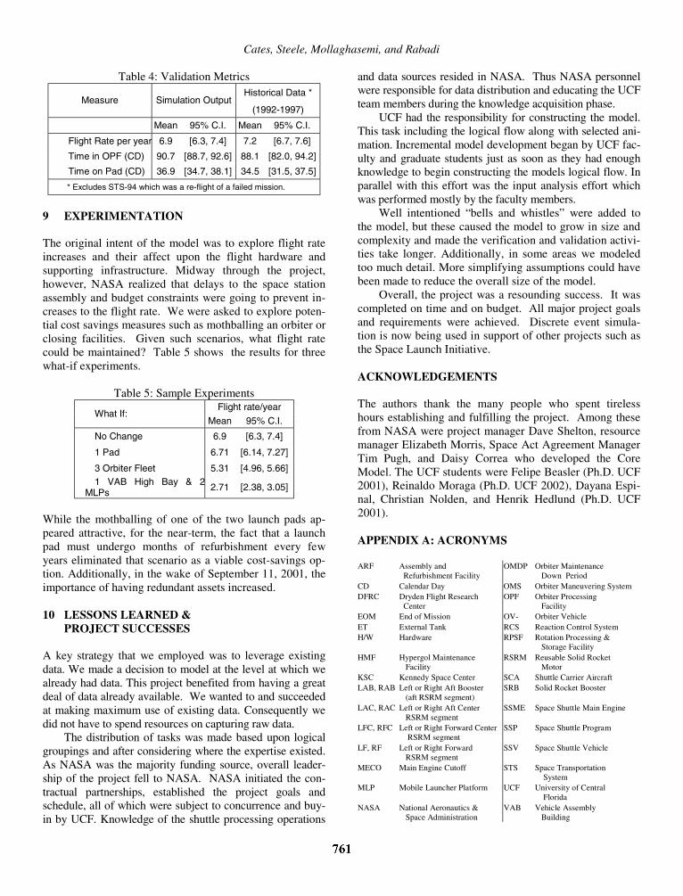
27.525 * EP(LN(1/RA-1)/8.397) (1) Most of the processes in the simulation model were analyzed in the above manner. There were other aspects of the model that required a different type of analysis. These were with regard to the probability of a certain event oc-curring or not-occurring. One such event that was modeled was the probability that a launch might be scrubbed or de-layed for technical or weather related problems. Another event that was modeled was the probability that the orbiter would have to be diverted to an alternate landing site i.e. from KSC in Florida to the Dryden Flight Research Center (DFRC) at Edwards Air Force Base in California. Histori-cal data was looked at in order to determine a reasonable probability for the occurrence of these events. Figure 10 shows historical data for landings.

Fiscal Year 91 92 93 94 95 96 97 98 99Planned KSC Landings 2 4 7 6 7 8 7 5 4

Achieved KSC Landings 1 3 5 4 4 7 7 5 4Diverted to DFRC 1 1 2 2 3 1 0 0 0Success Rate % 50 75 71 67 57 88 100 100 100

0

20

40

60

80

100

Success Rate in Achieving a Planned KSC Landing

File: On Orbit UCF.xls Tab: KSC Success Rate

%

Figure 10: KSC Landing Data

Figure 10 prompted considerable discussion between UCF and NASA. The UCF model team felt that a “process change” must have occurred that caused the success rate to change from an average of around 60 percent to 100 percent. The NASA members of the team acknowledged that im-provements to the orbiter, such as better brakes and the addi-tion of a drag chute and nose wheel steering allowed flight controllers to select KSC as the landing site with greater fre-quency. However, weather was still believed to be a signifi-cant factor, and it was argued that the 100 percent success rate seen after 1996 was attributable in part to good fortune. Ultimately the model team agreed to use a figure of .9 for the probability that the orbiter would be able to land at KSC. Similar review of historical data and discussions were performed for launch scrubs. It was determined that ap-proximately 40 percent of the time a shuttle launch attempt is scrubbed. Once a mission is determined to have been scrubbed, the next question is how long before a new launch attempt can be made. This question was analyzed in the same manner as any other process duration (de-scribed in the previous section. 8 VERIFICATION AND VALIDATION Using animation, we were able to verify that the flight hardware elements moved through the model in an appro-priate manner. Once the probability distributions were in-put into the model, we ran the model to simulate one year. The model produced 7 flights so we initially felt that we were very close to having a valid model. However, after running the model for a much longer period, the flight rate dropped dramatically. In fact after the first year, the model would produce only one shuttle mission per year. The veri-fication and validation phase of the project began in ear-nest at that time. As there were nearly 1,000 program ele-ments, each having multiple input locations, the V&V process required approximately two months of dedicated effort. We resolved many minor problems with the model logic and input mistakes, as well as increased our under-standing of how the various Arena program modules oper-ate. Table 4 shows the measures we used to determine that we had a valid model.

Cates, Steele, Mollaghasemi, and Rabadi

Table 4: Validation Metrics Historical Data *

Measure Simulation Output (1992-1997)

Mean 95% C.I. Mean 95% C.I.

Flight Rate per year 6.9 [6.3, 7.4] 7.2 [6.7, 7.6]

Time in OPF (CD) 90.7 [88.7, 92.6] 88.1 [82.0, 94.2]

Time on Pad (CD) 36.9 [34.7, 38.1] 34.5 [31.5, 37.5]

* Excludes STS-94 which was a re-flight of a failed mission.

9 EXPERIMENTATION The original intent of the model was to explore flight rate increases and their affect upon the flight hardware and supporting infrastructure. Midway through the project, however, NASA realized that delays to the space station assembly and budget constraints were going to prevent in-creases to the flight rate. We were asked to explore poten-tial cost savings measures such as mothballing an orbiter or closing facilities. Given such scenarios, what flight rate could be maintained? Table 5 shows the results for three what-if experiments.

Table 5: Sample Experiments Flight rate/year

What If: Mean 95% C.I.

No Change 6.9 [6.3, 7.4]

1 Pad 6.71 [6.14, 7.27]

3 Orbiter Fleet 5.31 [4.96, 5.66] 1 VAB High Bay & 2

MLPs 2.71 [2.38, 3.05]

While the mothballing of one of the two launch pads ap-peared attractive, for the near-term, the fact that a launch pad must undergo months of refurbishment every few years eliminated that scenario as a viable cost-savings op-tion. Additionally, in the wake of September 11, 2001, the importance of having redundant assets increased. 10 LESSONS LEARNED &

PROJECT SUCCESSES A key strategy that we employed was to leverage existing data. We made a decision to model at the level at which we already had data. This project benefited from having a great deal of data already available. We wanted to and succeeded at making maximum use of existing data. Consequently we did not have to spend resources on capturing raw data. The distribution of tasks was made based upon logical groupings and after considering where the expertise existed. As NASA was the majority funding source, overall leader-ship of the project fell to NASA. NASA initiated the con-tractual partnerships, established the project goals and schedule, all of which were subject to concurrence and buy-in by UCF. Knowledge of the shuttle processing operations

and data sources resided in NASA. Thus NASA personnel were responsible for data distribution and educating the UCF team members during the knowledge acquisition phase. UCF had the responsibility for constructing the model. This task including the logical flow along with selected ani-mation. Incremental model development began by UCF fac-ulty and graduate students just as soon as they had enough knowledge to begin constructing the models logical flow. In parallel with this effort was the input analysis effort which was performed mostly by the faculty members. Well intentioned “bells and whistles” were added to the model, but these caused the model to grow in size and complexity and made the verification and validation activi-ties take longer. Additionally, in some areas we modeled too much detail. More simplifying assumptions could have been made to reduce the overall size of the model. Overall, the project was a resounding success. It was completed on time and on budget. All major project goals and requirements were achieved. Discrete event simula-tion is now being used in support of other projects such as the Space Launch Initiative. ACKNOWLEDGEMENTS The authors thank the many people who spent tireless hours establishing and fulfilling the project. Among these from NASA were project manager Dave Shelton, resource manager Elizabeth Morris, Space Act Agreement Manager Tim Pugh, and Daisy Correa who developed the Core Model. The UCF students were Felipe Beasler (Ph.D. UCF 2001), Reinaldo Moraga (Ph.D. UCF 2002), Dayana Espi-nal, Christian Nolden, and Henrik Hedlund (Ph.D. UCF 2001). APPENDIX A: ACRONYMS ARF Assembly and

Refurbishment Facility OMDP Orbiter Maintenance

Down Period CD Calendar Day OMS Orbiter Maneuvering System DFRC Dryden Flight Research

Center OPF Orbiter Processing

Facility EOM End of Mission OV- Orbiter Vehicle ET External Tank RCS Reaction Control System H/W Hardware RPSF Rotation Processing &

Storage Facility HMF Hypergol Maintenance

Facility RSRM Reusable Solid Rocket

Motor KSC Kennedy Space Center SCA Shuttle Carrier Aircraft LAB, RAB Left or Right Aft Booster

(aft RSRM segment) SRB Solid Rocket Booster

LAC, RAC Left or Right Aft Center RSRM segment

SSME Space Shuttle Main Engine

LFC, RFC Left or Right Forward Center RSRM segment

SSP Space Shuttle Program

LF, RF Left or Right Forward RSRM segment

SSV Space Shuttle Vehicle

MECO Main Engine Cutoff STS Space Transportation System

MLP Mobile Launcher Platform UCF University of Central Florida

NASA National Aeronautics & Space Administration

VAB Vehicle Assembly Building

Cates, Steele, Mollaghasemi, and Rabadi

REFERENCES

Cates, G., Mollaghasemi, M., Rabadi, G., Sepulveda, J.A., and Steele, M., “Simulation, Modeling, and Analysis of Space Shuttle Flight Hardware Processing,” World Automation Congress, Orlando, FL, June 9-13, 2002.

Cates, G., Mollaghasemi, M., Rabadi, G., and Steele, M., “Macro-Level Simulation Model of Space Shuttle Processing,” Symposium on Military, Government & Aerospace Simulation, Sponsored by the Society for Computer Simulation International, Seattle Wash., April 22-26, 2001.

Morris, W. D., NASA Langley Research Center, Hampton, Virginia, interview, 2001.

Mollaghasemi, M. and G. Rabadi, G. Cates, M. Steele, D. Correa, D. Shelton, “Simulation Modeling and Analy-sis of Space Shuttle Flight Hardware Processing,” Proceedings of the International Workshop on Har-bour, Maritime & Multimodal Logistics Modelling and Simulation, A.G. Bruzzone, L.M. Gambardella, P. Giribone, Y.A. Merkuryev, eds., Oct. 5-7, 2000, Por-tofino, Italy, 2000. A Publication of The Society for Computer Simulation International.

Schlagheck, R. A. and J.K. Byers, “Simulating the Opera-tions of the Reusable Shuttle Space Vehicle,” Proceedings of the 1971 Summer Computer Simulation Conference, pp. 192-152, July 1971.

Wilson, J.R., Vaughan, D.K., Naylor, E., Voss R.G., “Analysis of Space Shuttle Ground Operations,” Simulation, June 1982, pp. 187-203.

AUTHOR BIOGRAPHIES

GRANT R. CATES has 20 years of experience working on the space shuttle in various capacities including con-struction and activation of the launch complex, payload in-tegration and processing, and space shuttle vehicle ground operations. His email address is grant.cates-1@ksc .nasa.gov

MARTIN J. STEELE is an engineer with NASA at the Kennedy Space Center (KSC) with a wide range of experi-ence, from shuttle and payload operations to ground sys-tems and facilities development. He is currently leading several efforts at KSC to employ simulation modeling in the operations analysis of existing and future launch vehi-cles. His research interests include simulation modeling and analysis of complex systems, simulation input model-ing, generic system simulations, and neural networks. His email address is martin.steele-1@ksc.nasa.gov

MANSOOREH MOLLAGHASEMI is an associate pro-fessor in the Industrial Engineering and Management Sys-tems Department at UCF. Her research and teaching inter-ests include simulation modeling and analysis of complex systems, statistical aspects of simulation and simulation optimization, operations research, probability and statistics,

neural networks, and multiple criteria decision making. Her email address is mollagha@mail.ucf.edu

GHAITH RABADI is an assistant professor at Engineer-ing Management Department at Old Dominion University. He has managed simulation and risk analysis research pro-jects funded by NASA. His main research interests are Operations Research, Scheduling, Simulation, and Ma-chine Learning. His email address is grabadi@odu.edu