arX

iv:c

ond-

mat

/050

9748

v1 [

cond

-mat

.mes

-hal

l] 2

8 S

ep 2

005

Quantum Noise in the Electromechanical Shuttle

D. Wahyu Utami,1,∗ Hsi-Sheng Goan,2, † C. A. Holmes,3 and G. J. Milburn4

1School of Physical Sciences, The University of Queensland,QLD 4072, Australia2Department of Physics, National Taiwan University, Taipei106, Taiwan, ROC

3Department of Mathematics, School of Physical Sciences,The University of Queensland, QLD 4072, Australia

4Center for Quantum Computer Technology and Department of Physics,School of Physical Sciences, The University of Queensland,QLD 4072, Australia

AbstractWe consider a type of Quantum Electro-Mechanical System, known as the shuttle system, first

proposed by Goreliket al. , [Phys. Rev. Lett.,80, 4526, (1998)]. We use a quantum master equationtreatment and compare the semi-classical solution to a fullquantum simulation to reveal the dynamics,followed by a discussion of the current noise of the system. The transition between tunnelling andshuttling regime can be measured directly in the spectrum ofthe noise.

PACS numbers: 72.70.+m,73.23.-b,73.63.Kv,62.25.+g,61.46.+w,42.50.Lc

1

I. INTRODUCTION

Nanofabrication techniques, combined with single electronics, have recently enabled po-sition measurements on an electromechanical oscillator toapproach the Heisenberg limit1,2,3.In this paper we present a master equation treatment of a version of a quantum electromechan-ical system (QEMS), the charge shuttle, first proposed by Gorelik4. In the original proposal ametallic grain is surrounded by elastic soft organic molecules and placed between two elec-trodes. This forms a Single Electron Transistor (SET) with amovable island. The couplingbetween the vibration of the island and the tunnelling onto the SET island dramatically altersthe transport properties of the SET. The tunnelling amplitudes between the reservoirs andthe island are an exponential function of the separation between island and the reservoirs. Ifthe island is oscillating with a non negligible amplitude, this separation is a function of thedisplacement of the island from equilibrium and thus the tunneling current is modulated bythe motion of the island. When there is a non-zero charge on the island the applied electricfield accelerates the island. As the electron number on the island is a stochastic quantity,the resulting applied force is itself stochastic, but constant for a given electron occupancyof the island. Assuming the restoring force on the island canbe approximated as harmonic,we have a picture of a system moving on multiple quadratic potential surfaces, with differ-ing equilibrium displacements, connected by conditional Poisson processes corresponding totunneling of electrons on and off the island. The shuttle thus provides a fascinating exam-ple of a quantum stochastic system in which electron transport and vibrational motion arestrongly coupled.

In this paper we idealise the island to a single quantum dot with only one quasi-boundelectronic state. This corresponds to an extreme Coulomb blockade regime in which the en-ergy required for double occupancy is not bound. This minimal model captures the essentialquantum stochastic dynamics of the shuttle system. The quantum dot jumps between twoquadratic potential surfaces, displaced from each other, corresponding to no electron on theisland and one electron on the island. As noted by previous authors, the system exhibitsrich dynamics including a fixed point to limit cycle bifurcation in which the average electronoccupation number on the island exhibits a periodic square wave dependence. In this paperwe give a quantum master equation treatment of this quantum stochastic dynamical system,with particular attention to the shuttling and the current noise spectrum. We use the QuantumOptics Toolbox5 to compare and contrast the well known semiclassical predictions to the fullquantum dynamics. In particular, we compare the picture of ensemble averaged dynamics ofvarious moments with a ‘quantum trajectory’6 simulation of moments. A quantum trajectoryis a concept taken from quantum optics to describe the conditional dynamics of the systemconditioned on a particular history of stochastic events. Such conditional dynamics provideinsight into the effect of quantum noise on the the semiclassical prediction of regular electronshuttling on the limit cycle.

Various versions of a charge shuttle system have been experimentally investigated. A re-view of the theoretical and experimental achievements in shuttle transport can also be foundin the work of Shekhteret al.7. When a voltage bias is applied between the electrodes, acurrent quantisation resulting from electron interactions with the vibrational levels for dif-ferent voltage bias was found. By using C60 embedded between two gold electrodes, Parket al.8 have demonstrated that indeed there is current quantisation for various bias voltagewhich results in a stair-like feature within the current-voltage curve. Although because ofits high frequency (around Terra Hertz) and low amplitude oscillation, the molecule hardlyshuttles between the electrodes in this setup, this experiment has provided key evidence ofthe involvement of vibrational levels in changing the properties of the current. This quan-

2

tized conductance also was observed in several other experiments9,10. Zhitenevet al.9 utilizemetal single electron transistor attached on the tip of quartz rods as scanning probe while theexperiment by Erbeet al.10, combines a nanomechanical resonator with an electron island toproduce a QEMS system. The experimental setup used by Erbe issimilar to the one proposedby Gorelik4. Huanget al. also reported the operation of a GHz mechanical oscillator11.

Several attempts to explain the behaviour of the system havebeen offered both from clas-sical and quantum point of view. The current quantisation and its low frequency noise wasinvestigated via a classical approach by Isacsson12. The current-voltage relation in the shuttlesystem exists within two regimes. The first regime is when theelectron tunnels straight intothe dot from the source and off to the drain, without much involvement of the island move-ment. This is called the tunnel regime. The C60 system lies within this tunnel regime. Theother regime is when the island oscillates to accommodate the current flow, which we callthe shuttle regime. However, measurement of average current alone cannot provide enoughinformation to distinguish whether the system is in the shuttle regime or tunnel regime. Itwas shown that a calculation of the noise is needed in addition. Therefore the noise signaturewas first obtained by finding the Fano factor at zero frequency13. Recently Flindt et al.14 havecalculated the current noise spectrum using a method different form that used in this paper.We compare the two methods in section VI.

Another interesting property of the system is the existenceof a dynamical instability withlimit-cycle behavior which was found in a similar setup using a single metallic grain placedon a cantilever between two electrodes15. This forms a three-terminal contact shuttle system.Classical analysis of the system points to the fact that thisinstability in the system leads todeterministic chaos. The semiclassical dynamics of the simpler case of the isolated island,the subject of this paper, was thoroughly investigated by Donarini et al.16.

One of the early attempt to investigate the system within thequantum limit is given byAji et al.17 where electronic-vibrational coupling is investigated both in elastic and inelas-tic electron transport by looking at the current-voltage relationship and conductance. Otherproperties of the transport within the shuttle system such as negative differential conductancehave also been found18 although the derivation only considers terms linear in the position ofthe island. Various conditions, such as when the electron tunnelling length is much greaterthan the amplitude of the zero point oscillations of the central island, have been investigatedby Fedorets19. Using phase space methods in terms of Wigner function Novotny et al.20,21

identify crossover from tunnelling to shuttling regime.Another variation of the shuttle is offered by Armour and MacKinnon22. In this model

the steady state current across a chain of three quantum dotssystem (one dot connected toeach leads and one dot as vibrating island) was analysed by looking at the eigenspectrum.Numerical simulation here considers 25 phonon levels, within the large bias limit.

In a recent thesis of Donarini16, the single dot quantum shuttle and the three dot shuttlesystem was investigated using Generalized Master Equationapproach using Wigner distribu-tion functions. The current and Fano factor at zero frequency is also investigated.

II. THE MODEL

The system consists of a quantum dot ’island’ moving betweentwo electrodes, the sourceand the drain. This is analogous to a quantum dot SET in which the island of the SET isallowed to oscillate and thus modulate the tunnel conductance between itself and the reser-voirs. However unlike a SET we do not include a separate charging gate for the island. Whena voltage bias is applied between the two electrodes, the electron from the source can tunnelonto the island and as the island moves closer to the drain theelectron can tunnel off, thus

3

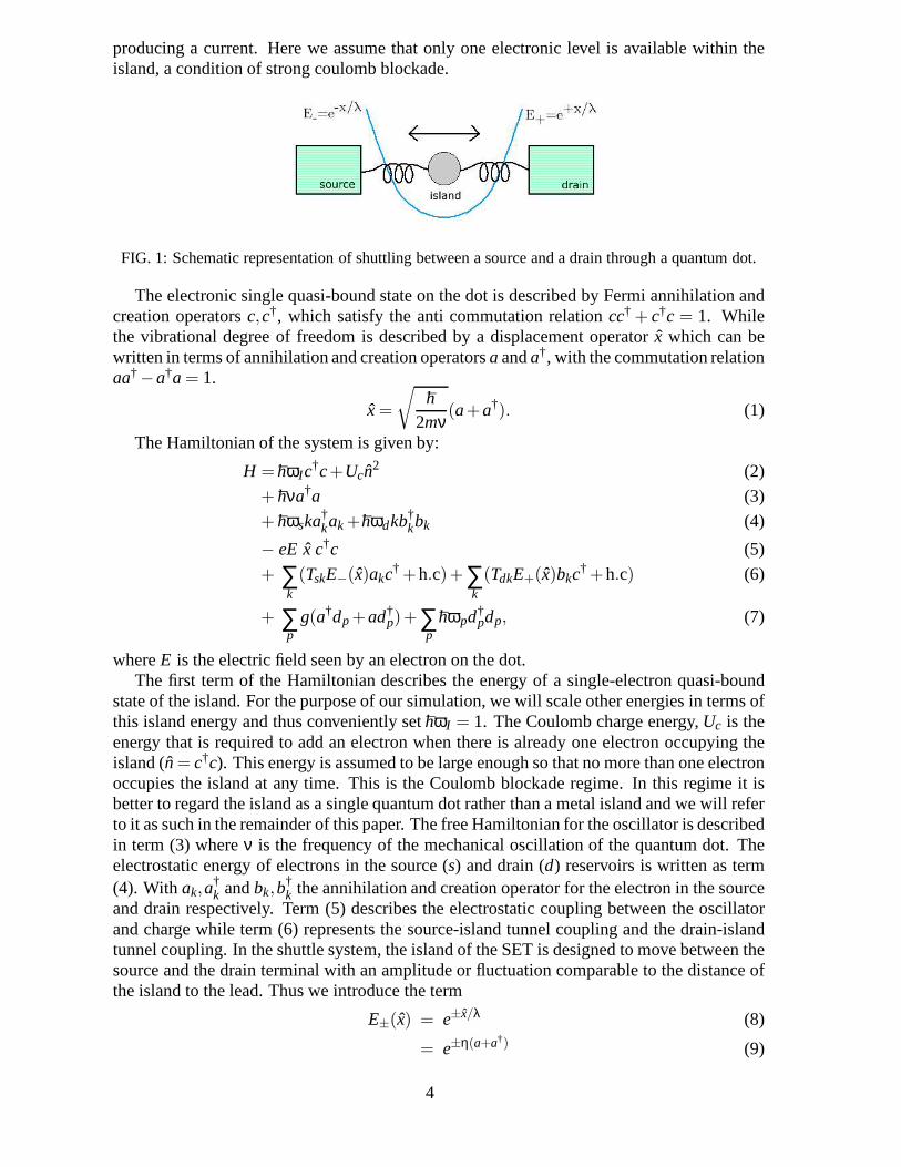
producing a current. Here we assume that only one electroniclevel is available within theisland, a condition of strong coulomb blockade.

FIG. 1: Schematic representation of shuttling between a source and a drain through a quantum dot.

The electronic single quasi-bound state on the dot is described by Fermi annihilation andcreation operatorsc,c†, which satisfy the anti commutation relationcc† + c†c = 1. Whilethe vibrational degree of freedom is described by a displacement operator ˆx which can bewritten in terms of annihilation and creation operatorsaanda†, with the commutation relationaa†−a†a = 1.

x =

√

h2mν

(a+a†). (1)

The Hamiltonian of the system is given by:

H = hωI c†c+Ucn

2 (2)

+ hνa†a (3)

+ hωska†kak +hωdkb†

kbk (4)

− eE x c†c (5)

+ ∑k

(TskE−(x)akc† +h.c)+∑

k

(TdkE+(x)bkc†+h.c) (6)

+ ∑p

g(a†dp+ad†p)+∑

phωpd†

pdp, (7)

whereE is the electric field seen by an electron on the dot.The first term of the Hamiltonian describes the energy of a single-electron quasi-bound

state of the island. For the purpose of our simulation, we will scale other energies in terms ofthis island energy and thus conveniently sethωI = 1. The Coulomb charge energy,Uc is theenergy that is required to add an electron when there is already one electron occupying theisland (n= c†c). This energy is assumed to be large enough so that no more than one electronoccupies the island at any time. This is the Coulomb blockaderegime. In this regime it isbetter to regard the island as a single quantum dot rather than a metal island and we will referto it as such in the remainder of this paper. The free Hamiltonian for the oscillator is describedin term (3) whereν is the frequency of the mechanical oscillation of the quantum dot. Theelectrostatic energy of electrons in the source (s) and drain (d) reservoirs is written as term(4). With ak,a

†k andbk,b

†k the annihilation and creation operator for the electron in the source

and drain respectively. Term (5) describes the electrostatic coupling between the oscillatorand charge while term (6) represents the source-island tunnel coupling and the drain-islandtunnel coupling. In the shuttle system, the island of the SETis designed to move between thesource and the drain terminal with an amplitude or fluctuation comparable to the distance ofthe island to the lead. Thus we introduce the term

E±(x) = e±x/λ (8)

= e±η(a+a†) (9)

4

with

η =

(

h2mν

)1/2 1λ

(10)

to account for the change in the tunnelling rate to the left and the right lead as the position ofthe shuttle varies.

The last term, (7), describes the coupling between the oscillator and the thermo-mechanical bath responsible for damping and thermal noise in the mechanical system in therotating wave approximation23. We include it in order to bound the motion under certain biasconditions.

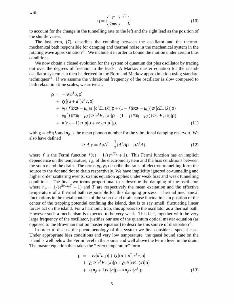
We now obtain a closed evolution for the system of quantum dotplus oscillator by tracingout over the degrees of freedom in the leads. A Markov master equation for the island-oscillator system can then be derived in the Born and Markov approximation using standardtechniques24. If we assume the vibrational frequency of the oscillator isslow compared tobath relaxation time scales, we arrive at:

ρ = −iν[a†a,ρ]

+ iχ[(a+a†)c†c,ρ]

+ γL(

f (hωI −µL)D [c†E−(x)]ρ+(1− f (hωI −µL))D [cE−(x)]ρ)

+ γR(

f (hωI −µR)D [c†E+(x)]ρ+(1− f (hωI −µR))D [cE+(x)]ρ)

+ κ(np+1)D [a]ρ+κnpD [a†]ρ, (11)

with χ = eEηλ andnp is the mean phonon number for the vibrational damping reservoir. Wealso have defined

D [A]ρ = AρA†−12(A†Aρ+ρA†A), (12)

where f is the Fermi functionf (ε) = 1/(eε/Tel + 1). This Fermi function has an implicitdependence on the temperature,Tel, of the electronic system and the bias conditions betweenthe source and the drain. The termsγL,γR describe the rates of electron tunnelling form thesource to the dot and dot to drain respectively. We have implicitly ignored co-tunnelling andhigher order scattering events, so this equation applies under weak bias and weak tunnellingconditions. The final two terms proportional toκ describe the damping of the oscillator,where np = 1/(ehν/kBT − 1) and T are respectively the mean excitation and the effectivetemperature of a thermal bath responsible for this damping process. Thermal mechanicalfluctuations in the metal contacts of the source and drain cause fluctuations in position of thecenter of the trapping potential confining the island, that is to say small, fluctuating linearforces act on the island. For a harmonic trap, this appears tothe oscillator as a thermal bath.However such a mechanism is expected to be very weak. This fact, together with the verylarge frequency of the oscillator, justifies our use of the quantum optical master equation (asopposed to the Brownian motion master equation) to describethis source of dissipation23.

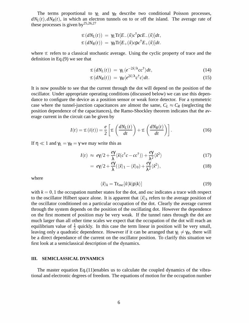
In order to discuss the phenomenology of this system we first consider a special case.Under appropriate bias conditions and very low temperature, the quasi bound state on theisland is well below the Fermi level in the source and well above the Fermi level in the drain.The master equation then takes the “ zero temperature” form

ρ = −iν[a†a,ρ]+ iχ[(a+a†)c†c,ρ]

+ γLD [c†E−(x)]ρ+ γRD [cE+(x)]ρ)

+ κ(np+1)D [a]ρ+κnpD [a†]ρ. (13)

5

The terms proportional toγL and γR describe two conditional Poisson processes,dNL(t),dNR(t), in which an electron tunnels on to or off the island. The average rate ofthese processes is given by25,26,27

E (dNL(t)) = γLTr[E−(x)c†ρcE−(x)]dt,

E (dNR(t)) = γRTr[E+(x)cρc†E+(x)]dt.

whereE refers to a classical stochastic average. Using the cyclic property of trace and thedefinition in Eq.(9) we see that

E (dNL(t)) = γL〈e−2x/λcc†〉dt, (14)

E (dNR(t)) = γR〈e2x/λc†c〉dt. (15)

It is now possible to see that the current through the dot willdepend on the position of theoscillator. Under appropriate operating conditions (discussed below) we can use this depen-dance to configure the device as a position sensor or weak force detector. For a symmetriccase where the tunnel-junction capacitances are almost thesame,CL ≈ CR (neglecting theposition dependence of the capacitances), the Ramo-Shockley theorem indicates that the av-erage current in the circuit can be given by

I(t) = E (i(t)) =e2

[

E

(

dNL(t)dt

)

+E

(

dNR(t)dt

)]

. (16)

If η ≪ 1 andγL = γR = γ we may write this as

I(t) ≈ eγ/2+eγλ〈x(c†c−cc†)〉+

eγλ2〈x

2〉 (17)

= eγ/2+eγλ

(〈x〉1−〈x〉0)+eγλ2〈x

2〉, (18)

where〈x〉k = Trosc[x〈k|ρ|k〉] (19)

with k = 0,1 the occupation number states for the dot, andoscindicates a trace with respectto the oscillator Hilbert space alone. It is apparent that〈x〉k refers to the average position ofthe oscillator conditioned on a particular occupation of the dot. Clearly the average currentthrough the system depends on the position of the oscillating dot. However the dependenceon the first moment of position may be very weak. If the tunnel rates through the dot aremuch larger than all other time scales we expect that the occupation of the dot will reach anequilibrium value of12 quickly. In this case the term linear in position will be verysmall,leaving only a quadratic dependence. However if it can be arranged thatγL 6= γR, there willbe a direct dependance of the current on the oscillator position. To clarify this situation wefirst look at a semiclassical description of the dynamics.

III. SEMICLASSICAL DYNAMICS

The master equation Eq.(11)enables us to calculate the coupled dynamics of the vibra-tional and electronic degrees of freedom. The equations of motion for the occupation number

6

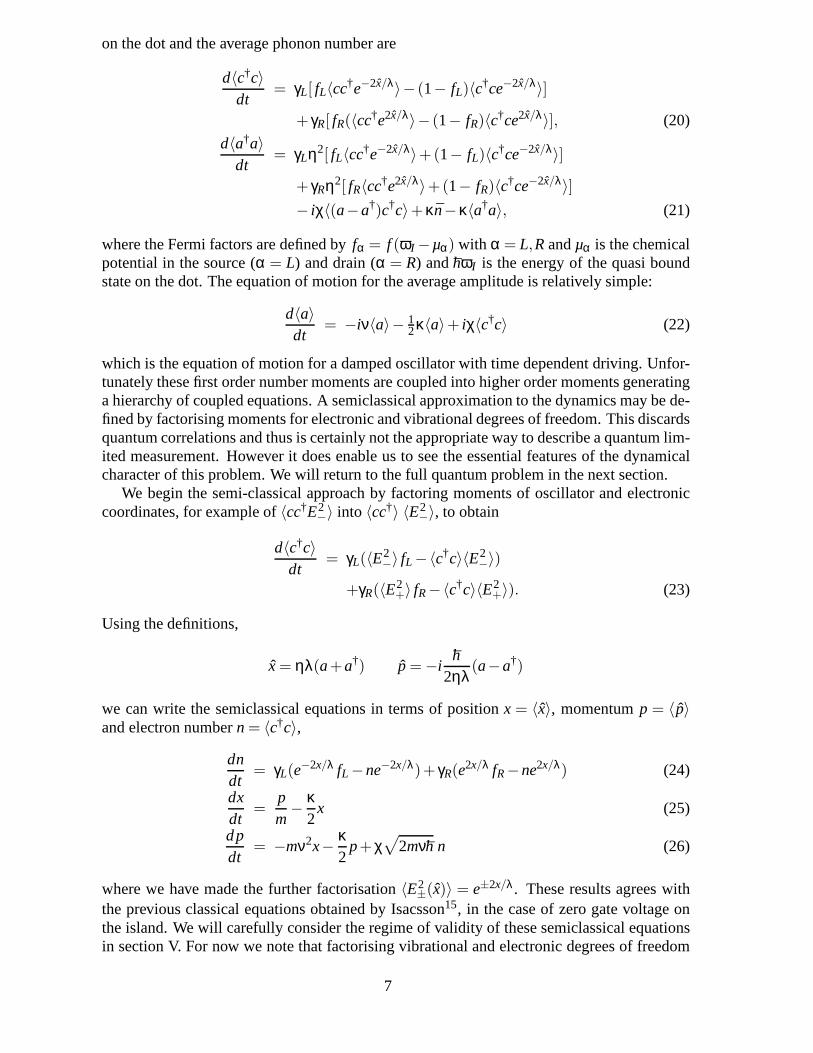
on the dot and the average phonon number are

d〈c†c〉dt

= γL[ fL〈cc†e−2x/λ〉− (1− fL)〈c†ce−2x/λ〉]

+ γR[ fR(〈cc†e2x/λ〉− (1− fR)〈c†ce2x/λ〉], (20)

d〈a†a〉dt

= γLη2[ fL〈cc†e−2x/λ〉+(1− fL)〈c†ce−2x/λ〉]

+ γRη2[ fR〈cc†e2x/λ〉+(1− fR)〈c†ce−2x/λ〉]

− iχ〈(a−a†)c†c〉+κn−κ〈a†a〉, (21)

where the Fermi factors are defined byfα = f (ωI −µα) with α = L,Randµα is the chemicalpotential in the source (α = L) and drain (α = R) andhωI is the energy of the quasi boundstate on the dot. The equation of motion for the average amplitude is relatively simple:

d〈a〉dt

= −iν〈a〉− 12κ〈a〉+ iχ〈c†c〉 (22)

which is the equation of motion for a damped oscillator with time dependent driving. Unfor-tunately these first order number moments are coupled into higher order moments generatinga hierarchy of coupled equations. A semiclassical approximation to the dynamics may be de-fined by factorising moments for electronic and vibrationaldegrees of freedom. This discardsquantum correlations and thus is certainly not the appropriate way to describe a quantum lim-ited measurement. However it does enable us to see the essential features of the dynamicalcharacter of this problem. We will return to the full quantumproblem in the next section.

We begin the semi-classical approach by factoring moments of oscillator and electroniccoordinates, for example of〈cc†E2

−〉 into 〈cc†〉 〈E2−〉, to obtain

d〈c†c〉dt

= γL(〈E2−〉 fL−〈c†c〉〈E2

−〉)

+γR(〈E2+〉 fR−〈c†c〉〈E2

+〉). (23)

Using the definitions,

x = ηλ(a+a†) p = −ih

2ηλ(a−a†)

we can write the semiclassical equations in terms of position x = 〈x〉, momentump = 〈p〉and electron numbern = 〈c†c〉,

dndt

= γL(e−2x/λ fL −ne−2x/λ)+ γR(e2x/λ fR−ne2x/λ) (24)

dxdt

=pm−

κ2

x (25)

dpdt

= −mν2x−κ2

p+χ√

2mνh n (26)

where we have made the further factorisation〈E2±(x)〉 = e±2x/λ. These results agrees with

the previous classical equations obtained by Isacsson15, in the case of zero gate voltage onthe island. We will carefully consider the regime of validity of these semiclassical equationsin section V. For now we note that factorising vibrational and electronic degrees of freedom

7

ignores any entanglement between these systems, while factorising the exponential assumesthe oscillator is very well localised in position.

In the zero temperature limit and appropriate bias we have that fL = 1, fR = 0. Thesemiclassical equations of motion then take the form

dndt

= γL(1−n)e−4ηX − γRne4ηX (27)

dαdt

= −iνα−κ2

α+ iχn (28)

withα = 〈a〉 = 〈x〉/(2λη)+ i〈p〉λη/h≡ X + iY .

The system of equations, Eq.(27, 28) has a fixed point, which undergoes a hopf bifurcation.To see this we begin by scaling the parameters byν andη; γ

ν → γ, κν → κ and ηχ

ν → χ andν → 1 by scaling timeτ = νt and redefiningX andY by lettingα = η(X + iY). Then

dndτ

= γL(1−n)e−4X − γRne4X (29)

dαdτ

= −iα−κ2

α+ iχn. (30)

The fixed point is given implicitly by

n∗ =γLe−4X∗

γLe−4X∗ + γRe4X∗=

1

1+ γRγL

e8X∗, (31)

X∗ =χ

1+(κ2)2n∗ (32)

Y∗ =χκ

2

1+(κ2)2n∗ (33)

from which we can see that it must satisfy,

χ = X∗(1+(κ2)2)(1+

γR

γLe8X∗). (34)

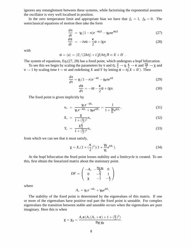
At the hopf bifurcation the fixed point looses stability and alimitcycle is created. To seethis, first obtain the linearized matrix about the stationary point.

DF =

−A∗ −8γLγRA∗

00 −κ

2 1χ −1 −κ

2

whereA∗ = γLe−4X∗ + γRe4X∗ .

The stability of the fixed point is determined by the eigenvalues of this matrix. If oneor more of the eigenvalues have positive real part the fixed point is unstable. For complexeigenvalues the transition between stable and unstable occurs when the eigenvalues are pureimaginary. Here this is when

χ = χh =A∗κ(A∗(A∗ +κ)+1+(κ

2)2)

8γLγR.

8

At χ = χh the eigenvalues are−(A∗+κ),±iµ whereµ=√

A∗κ+1+(κ2)2 and the fixed point

has a one dimensional stable manifold and a two dimensional center manifold. Forχ < χh thefixed point is stable and forχ > χh it is unstable. This suggests a hopf bifurcation, howeverit is necessary to work out the stability coefficient to determine if it is subcritical, creating anunstable limitcycle or supercritical, creating a stable limitcycle. This involves some algebra.First transform the system in the vicinity of the fixed point to normal form via the matrix ofeigenvectorsP.

P =

8γLγR 0 8γLγR

A∗κ −A∗µ −A2∗

−A∗κ(A∗ + κ2) −A∗(A∗ + κ

2) −A∗(A∗κ2 +1+(κ

2)2)

Then in normal form coordinatesu = P−1(n−n∗, X−X∗, Y−Y∗)T the system becomes

dudτ

=

−(A∗ +κ) 0 00 0 −iµ0 iµ 0

u+gNl(u)+8γLγRf(χ−χh)(u1+u3), (35)

whereg andf are column vectors, whose entries aregi = P−1i1 , fi = P−1

i3 . Nl(u) is a scalarnonlinear function ofui obtained by perturbation. To cubic order inui

Nl(u) = −4n′X′√

A2∗−4γLγR−8n′X′2A∗−

64γLγRX′3

3A∗

where(n′,X′,Y′)T = PuT.

Now the limitcycle bifurcates into the center manifold which is tangent to theu1 = 0 plane.So if u1 = h(u2, u3) is the equation of the center manifold through(0, 0, 0) at χ = χh, thenh(0, 0) = 0 and ∂h

∂ui(0, 0) = 0. This means that a Taylor series approximation to the center

manifold will have no constant or linear term and so the first nonzero terms are of quadraticorder inui and

h(u2, u3) = a20u22+a11u2u3+a02u

23+higher order terms,

for somea20, a11 anda02. Now differentiatingu1 = h(u2, u3) gives;

du1

dτ=

∂h∂u2

du2

dτ+

∂h∂u3

du3

dτ.

On the center manifoldduidτ (h(u2, u3), u2, u3) are functions ofu2 and u3 only, so this

equation can be used to calculate the coefficientsai, j in the Taylor series approx-imation to h(u2, u3) recursively, by equating coefficients of like powers ofu2 andu3. Once h(u2, u3) is found this can be fed back into the equations of motion foru2 and u3 to obtain the approximate equations of motion on the center manifold.Finally the stability coefficient for a two dimensional system in normal form28 is

a =116

( fxxx+gxxy+ fxyy+gyyy)+1

16ω( fxy( fxx+ fyy)−gxy(gxx+gyy)− fxxgxx+ fyygyy)

evaluated at(0, 0), where hereω = µ =√

A∗κ+1+(κ2)2. The subscripts indicate partial

derivatives of functionf or g with respect to the variablesx andy. For instancefxx, fxxx is

9

χh

Radius of Limit cycle

Stable Limit Cycle

Unstable Limt Cycle

χχsn

a) b)

χh

Radius of Limit cycle

Stable Limit Cycle

χ Stable critical point Unstable critical point

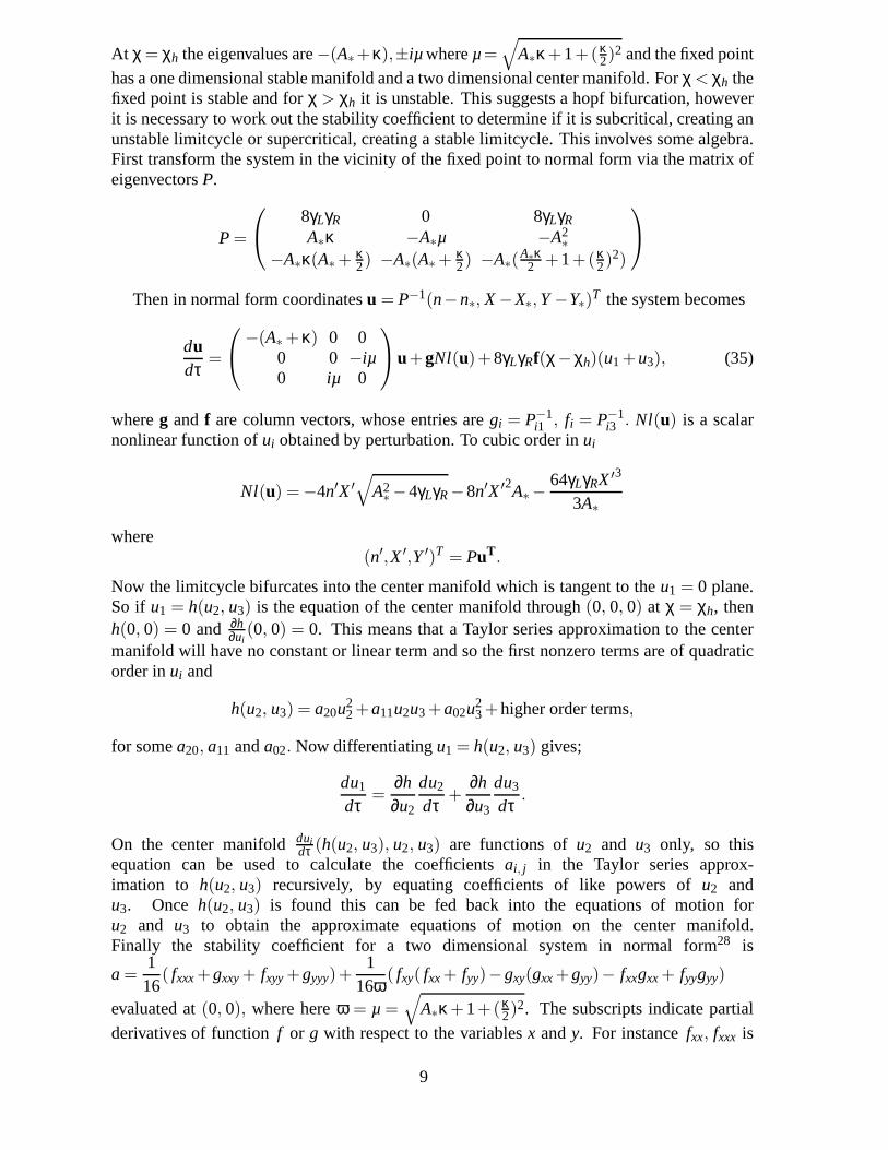
FIG. 2: Illustration of two possible type of Hopf bifurcation in the shuttle system with varying couplingχ, a) supercritical and b) subcritical and saddle node bifurcation of the limit cycles.

0 0.5 1 1.5 2 2.5 3 3.5 4 4.5 50

0.05

0.1

0.15

0.2

0.25

0.3

0.35

0.4

0.45

0.5

χ

Critical value of χh

h

γ L

γ = 5R

γ = 1R

γ = 4R

γ = 3R

γ = 2R

γ = 0.5R

γ = 0.25R

γ = 0.1R

χ sn

FIG. 3: Plot ofχh for various fixed values ofγR as a function ofγL. The line is solid where the hopfbifurcation is supercritical and dashed where it is a subcritical hopf bifurcation.

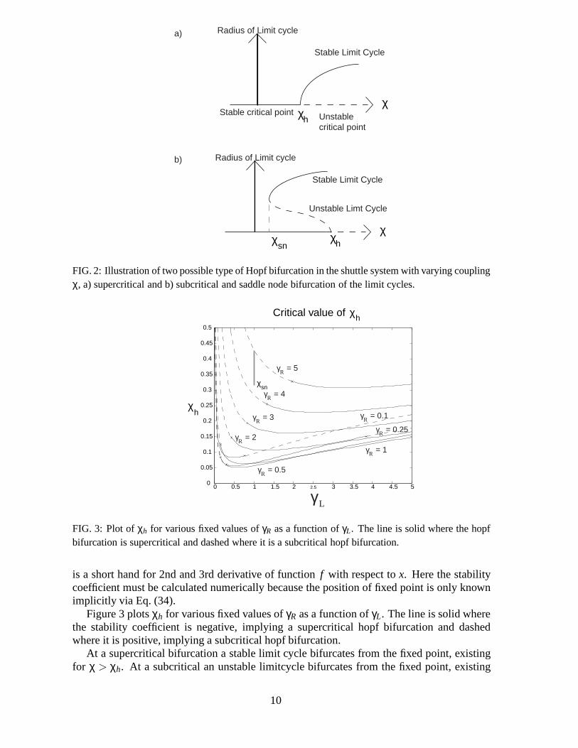
is a short hand for 2nd and 3rd derivative of functionf with respect tox. Here the stabilitycoefficient must be calculated numerically because the position of fixed point is only knownimplicitly via Eq. (34).

Figure 3 plotsχh for various fixed values ofγR as a function ofγL. The line is solid wherethe stability coefficient is negative, implying a supercritical hopf bifurcation and dashedwhere it is positive, implying a subcritical hopf bifurcation.

At a supercritical bifurcation a stable limit cycle bifurcates from the fixed point, existingfor χ > χh. At a subcritical an unstable limitcycle bifurcates from the fixed point, existing

10

for χ < χh. Continuity of solutions as the parameterγL is changed suggests that the stablelimitcycle existing forχ > χh above the solid critical line also exists above the dashed line.Numerical evidence shows this to be the case and that it continues to exist well below thedashed line, eventually being annihilated in a saddle-nodebifurcation with the unstable limitcycle created in the subcritical hopf bifurcation at the dashed line. A schematic diagram ofthe two bifurcations are shown in figure 2. ForγR = 5 andγL = 1.01 the hopf bifurcationoccurs atχh = 0.42650636 and the saddle node bifurcation atχsn= 0.315. A glance at Fig.reffig:chih, where a vertical grey line indicates the range of χ for γR = 5 andγL = 1.01 forwhich there are two limit cycles shows that there is a significant parameter region, where twolimit cycles coexist.

In general for fixedγR the stability coefficient is positive for small and very large γL andnegative in between. This means that ifγL and γR are about 1, say, a stable limit cyclebifurcates and is present forχ > χh. But if (γL/γR) is much less than 1, a more complicatedsituation may arise forχ < χh, where an unstable limit cycle exists close to the critical pointsurrounded by a stable limit cycle.

We then solved numerically the full system of equations, Eqs.(27) and (28), for variousvalues of the parameters. In the shuttling regime the electron number on the dotn(t) exhibits asquare wave dependence as a single electron is carried from source to drain, where it tunnelsonto the drain and the dot returns empty to the source to repeat the cycle. This is shownas the thin line in Fig.8(a). The effect of shuttling generally occurs when the maximumdisplacement of the island is quite large, and where the strength of the tunneling dependsstrongly on the position of the island (λ small). During shuttling, the electron number on thedot is constant. This gives, from Eq. (27), an implicit relation between the shuttle positionand the dot occupation,

n(X) =γLe−4ηX

γLe−4ηX + γRe4ηX . (36)

Near the equilibrium point,X = 0, this implies that forγL = γR, n = 0.5. Away from theequilibrium point we have that

n(X) =

{

0 X > 0,1 X < 0.

(37)

This behaviour is evident in the semiclassical dependance of n(t) (thin solid line) in Fig.8(a).A condition for shuttling is given also by Gorelik4 by specifying the requirement for the

amplitude of the shuttle oscillation to be much bigger than the tunnelling lengthλ. Donarini16

set the shuttling condition as to when the mechanical relaxation rate is much smaller than themechanical frequency and also that the average injection and ejection rate is approximatelyequal to the mechanical frequency of the oscillator.

The quantum dynamics may be determined by solving the masterequation in the phononnumber basis of the oscillator and the charge basis for the dot. It is necessary to truncate thephonon number basis high enough to include the amplitude of the limit cycle.

To overcome the numerical difficulties with simulating large number of phonon levels forthe quantum case described in Sec.V later, we choose a set of values ofχ andη which willgive a rather small limit cycle in the semiclassical approximation in Fig.8. The accuracy ofthe semiclassical simulation is dependent onλ as can be seen in Sec.V by comparing thefactorized and unfactorized result from the numerical method.

We now return to consider the dependance of the total currenton the oscillator position.The total current through the device is given by Eq.(16). In the semiclassical approximationthis is given by

IT(t) =γL

2(1−n)e−4ηX +

γR

2e4ηXn. (38)

11

At the fixed point region, thisn can be substituted byn∗ given in Eq.(31) to give:

IT =γLγR

γLe−4ηX∗ + γRe4ηX∗. (39)

Whenη is small, we can simplify the current further to:

IT =γLγR

γL + γR−4ηX∗(γL − γR). (40)

Here we need to remember that the tunelling ratesγL andγR determine the steady state posi-tion of X∗. We can express, from Eqs. (31) and (32) the tunneling ratesγR as:

γR =γL(B−X∗)(1−4ηX∗)

X∗(1+4ηX∗), (41)

where for simplicity we have set:

B =χv

v2+(κ/2). (42)

We can thus rewrite the current:

IT =γL(B−X∗)

B+4ηX∗. (43)

We can see that whenη is small the currentIT is linearly dependent on the fixed point positionX∗, with a slope of−γL

B .We check this result using the full quantum simulation (Eqs.(20), (21)) and compare it with

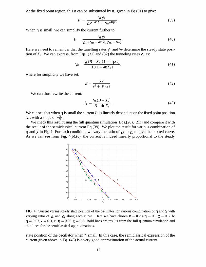
the result of the semiclassical current Eq.(39). We plot theresult for various combination ofη andχ in Fig.4. For each condition, we vary the ratio ofγR to γL to give the plotted curve.As we can see from Fig. 4(b),(c), the current is indeed linearly proportional to the steady

0 0.05 0.1 0.15 0.2 0.25 0.3 0.35 0.4 0.45 0.50

0.1

0.2

0.3

0.4

0.5

0.6

0.7

0.8

0.9

1

X*

I

a b c

FIG. 4: Current versus steady state position of the oscillator for various combination ofη andχ withvarying ratio ofγL and γR along each curve. Here we have chosenκ = 0.2 a:η = 0.3,χ = 0.3, b:η = 0.03,χ = 0.3, c: η = 0.03,χ = 0.5. Bold lines are results from the full quantum simulation andthin lines for the semiclassical approximations.

state position of the oscillator whenη small. In this case, the semiclassical expression of thecurrent given above in Eq. (43) is a very good approximation of the actual current.

12

IV. A POSITION TRANSDUCER SCENARIO

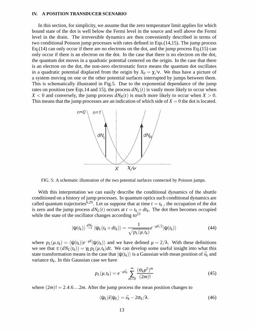
In this section, for simplicity, we assume that the zero temperature limit applies for whichbound state of the dot is well below the Fermi level in the source and well above the Fermilevel in the drain. The irreversible dynamics are then conveniently described in terms oftwo conditional Poisson jump processes with rates defined inEqs.(14,15). The jump processEq.(14) can only occur if there are no electrons on the dot, and the jump process Eq.(15) canonly occur if there is an electron on the dot. In the case that there is no electron on the dot,the quantum dot moves in a quadratic potential centered on the origin. In the case that thereis an electron on the dot, the non-zero electrostatic force means the quantum dot oscillatesin a quadratic potential displaced from the origin byX0 = χ/ν. We thus have a picture ofa system moving on one or the other potential surfaces interrupted by jumps between them.This is schematically illustrated in Fig.5. Due to the exponential dependance of the jumprates on position (see Eqs.14 and 15), the processdNL(t) is vastly more likely to occur whenX < 0 and conversely, the jump processdNR(t) is much more likely to occur whenX > 0.This means that the jump processes are an indication of whichside ofX = 0 the dot is located.

FIG. 5: A schematic illustration of the two potential surfaces connected by Poisson jumps.

With this interpretation we can easily describe the conditional dynamics of the shuttleconditioned on a history of jump processes. In quantum optics such conditional dynamics arecalled quantum trajectories6,29. Let us suppose that at timet = tk , the occupation of the dotis zero and the jump processdNL(t) occurs att = tk + dtk. The dot then becomes occupiedwhile the state of the oscillator changes according to23

|ψ(tk)〉dNL→ |ψL(tk +dtk)〉 =

1√

pL(µ, tk)e−µx/2|ψ(tk)〉 (44)

wherepL(µ, tk) = 〈ψ(tk)|e−µx|ψ(tk)〉 and we have definedµ = 2/λ. With these definitionswe see thatE (dNL(tk)) = γLpL(µ, tk)dt. We can develop some useful insight into what thisstate transformation means in the case that|ψ(tk)〉 is a Gaussian with mean position of ¯xk andvarianceσk. In this Gaussian case we have

pL(µ, tk) = e−µxk∞

∑m=0

(σkµ2)m

(2m)!(45)

where(2m)! = 2.4.6....2m. After the jump process the mean position changes to

〈ψL|x|ψL〉 = xk−2σk/λ. (46)

13

This equation applies equally well to jumps to the right,dNR, with a change in the sign ofλ.Thus we see that if there is jump due todNL, on average the conditional state moves to statewith a meancloser to the source, while if a jump occurs to the right,dNR, the conditionalstate changes to a state with a mean positioncloserto the drain. This conditional behaviour isconsistent with the interpretation of the jumps as effective measurements of the position of thequantum dot. More discussions on the quantum trajectory picture and numerical simulationson the conditional dynamics will be presented in the next section.

V. SOLVING MASTER EQUATION NUMERICALLY

With the help of the Quantum Optics toolbox5, we can solve the master equation directlyby finding the time evolution of the density matrix. This was done by preparing the Liouvil-lian matrix in Matlab and solving the differential equationgiven the initial conditions.

The expectation values for any desired quantities such as the electron number〈c†c〉, thephonon number〈a†a〉, position〈x〉 and the momentum〈p〉 of the oscillator can be calculatedby tracing the product of this quantities with density matrix ρ. The result can then be plottedagainst time. The same method can be applied to calculate thesteady state solution of theexpectation values usingρss.

The initial state of the system has been set up to incorporatethe two electron levels, namelythe occupied and empty state, combined with anN levels of phonon. The number of phononlevels included determines the accuracy of the calculation. Of course the more phonon levelsincluded the more accurate the simulation will be. However only a limited number of phononlevels can be considered. This is due to the limited computermemory that is available andalso considering the calculation time which will be significantly higher for largerN. Thus wetry to find the minimum number of phonon levels which gives convergent results. This willensure that the simulation still has a reasonably accurate solution. Donarini16 use the Arnoldiiteration30 to find the stationary solution of the matrix to overcome thismemory problem.However here we have proceeded without, in the hope of looking at not only the stationarysolution but also the dynamical evolution of the shuttle.

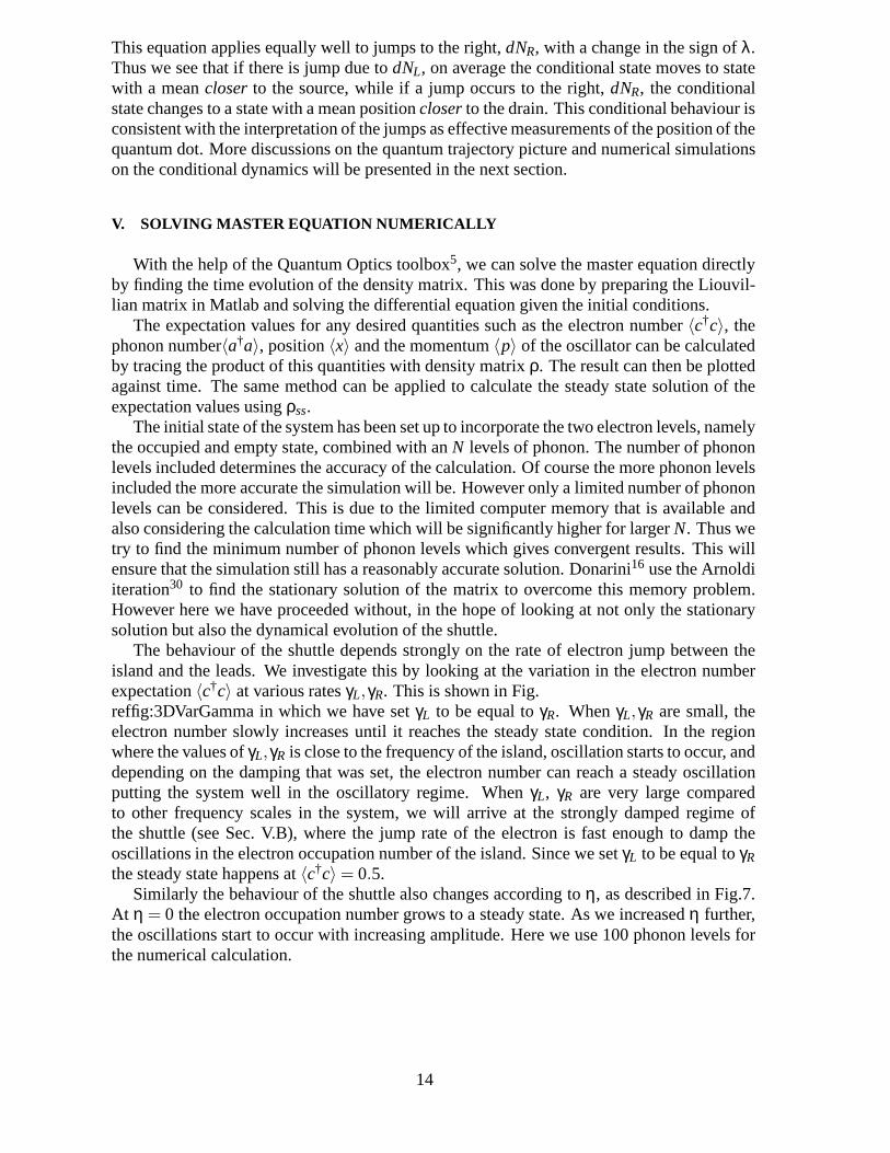
The behaviour of the shuttle depends strongly on the rate of electron jump between theisland and the leads. We investigate this by looking at the variation in the electron numberexpectation〈c†c〉 at various ratesγL,γR. This is shown in Fig.reffig:3DVarGamma in which we have setγL to be equal toγR. WhenγL,γR are small, theelectron number slowly increases until it reaches the steady state condition. In the regionwhere the values ofγL,γR is close to the frequency of the island, oscillation starts to occur, anddepending on the damping that was set, the electron number can reach a steady oscillationputting the system well in the oscillatory regime. WhenγL, γR are very large comparedto other frequency scales in the system, we will arrive at thestrongly damped regime ofthe shuttle (see Sec. V.B), where the jump rate of the electron is fast enough to damp theoscillations in the electron occupation number of the island. Since we setγL to be equal toγRthe steady state happens at〈c†c〉 = 0.5.

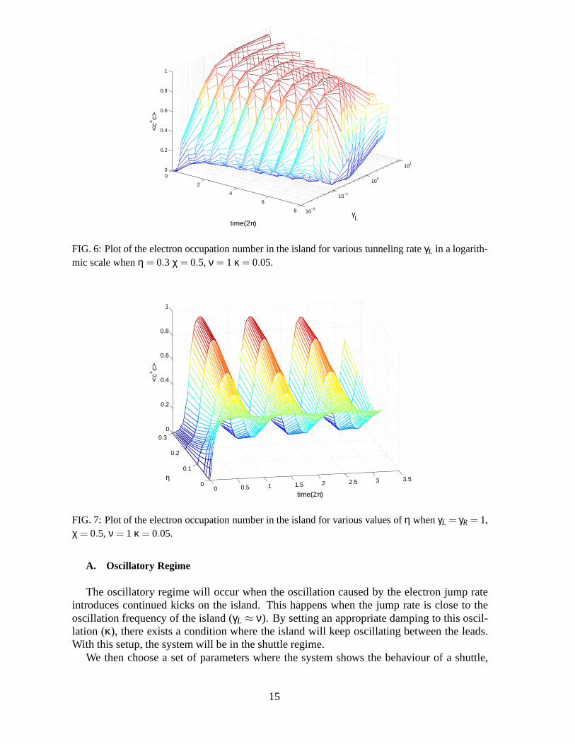
Similarly the behaviour of the shuttle also changes according toη, as described in Fig.7.At η = 0 the electron occupation number grows to a steady state. As we increasedη further,the oscillations start to occur with increasing amplitude.Here we use 100 phonon levels forthe numerical calculation.

14

0

2

4

6

8 10−2

10−1

100

101

0

0.2

0.4

0.6

0.8

1

γL

time(2π)

<c+

c>

FIG. 6: Plot of the electron occupation number in the island for various tunneling rateγL in a logarith-mic scale whenη = 0.3 χ = 0.5, ν = 1 κ = 0.05.

0 0.5 1 1.5 2 2.5 3 3.50

0.1

0.2

0.30

0.2

0.4

0.6

0.8

1

time(2π)

η

<c+

c>

FIG. 7: Plot of the electron occupation number in the island for various values ofη whenγL = γR = 1,χ = 0.5, ν = 1 κ = 0.05.

A. Oscillatory Regime

The oscillatory regime will occur when the oscillation caused by the electron jump rateintroduces continued kicks on the island. This happens whenthe jump rate is close to theoscillation frequency of the island (γL ≈ ν). By setting an appropriate damping to this oscil-lation (κ), there exists a condition where the island will keep oscillating between the leads.With this setup, the system will be in the shuttle regime.

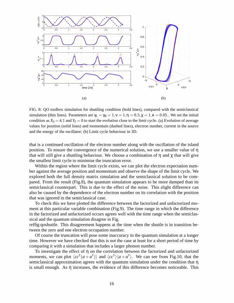
We then choose a set of parameters where the system shows the behaviour of a shuttle,

15

0 0.5 1 1.5 2 2.5 3 3.5−5

0

5

<X

>,<

Y>

0 0.5 1 1.5 2 2.5 3 3.5

0

0.5

1<

c+c>

0 0.5 1 1.5 2 2.5 3 3.50

1

2

<i s>

0 0.5 1 1.5 2 2.5 3 3.55

10

15

20

time (2π)

<a+

a>

(a)

−5

0

5

−5

0

5

0

0.2

0.4

0.6

0.8

1

<X><Y>

<c+

c>

(b)

FIG. 8: QO toolbox simulation for shuttling condition (boldlines), compared with the semiclassicalsimulation (thin lines). Parameters areγL = γR = 1,ν = 1,η = 0.3,χ = 1,κ = 0.05.. We set the initialcondition asX0 = 4.1 andY0 = 0 to start the evolution close to the limit cycle. (a) Evolution of averagevalues for position (solid lines) and momentum (dashed lines), electron number, current in the sourceand the energy of the oscillator; (b) Limit cycle behaviour in 3D.

that is a continued oscillation of the electron number alongwith the oscillation of the islandposition. To ensure the convergence of the numerical solution, we use a smaller value ofηthat will still give a shuttling behaviour. We choose a combination ofη andχ that will givethe smallest limit cycle to minimise the truncation error.

Within the region where the limit cycle exists, we can plot the electron expectation num-ber against the average position and momentum and observe the shape of the limit cycle. Weexplored both the full density matrix simulation and the semiclassical solution to be com-pared. From the result (Fig.8), the quantum simulation appears to be more damped than itssemiclassical counterpart. This is due to the effect of the noise. This slight difference canalso be caused by the dependence of the electron number on itscorrelation with the positionthat was ignored in the semiclassical case.

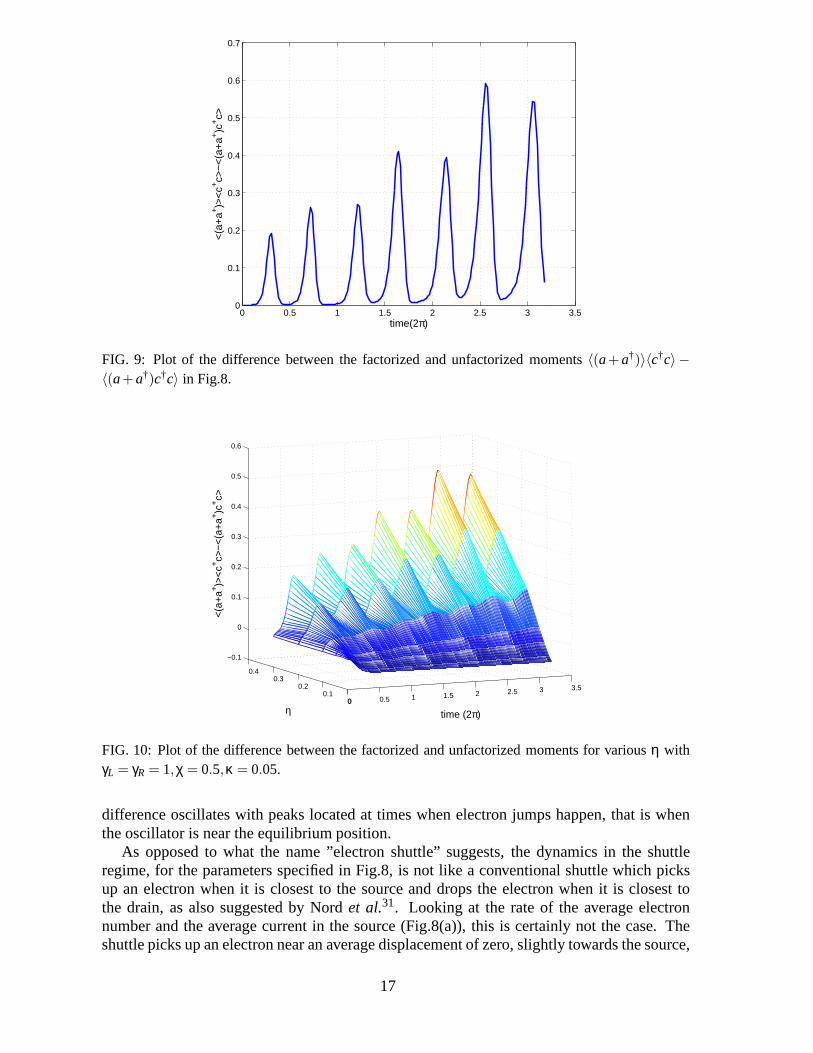
To check this we have plotted the difference between the factorized and unfactorized mo-ment at this particular variable combination (Fig.9). The time range in which the differencein the factorized and unfactorized occurs agrees well with the time range when the semiclas-sical and the quantum simulation disagree in Fig.reffig:qoshuttle. This disagreement happens at the time when the shuttle is in transition be-tween the zero and one electron occupation number.

Of course the truncation will pose some inaccuracy in the quantum simulation at a longertime. However we have checked that this is not the case at least for a short period of time bycomparing it with a simulation that includes a larger phononnumber.

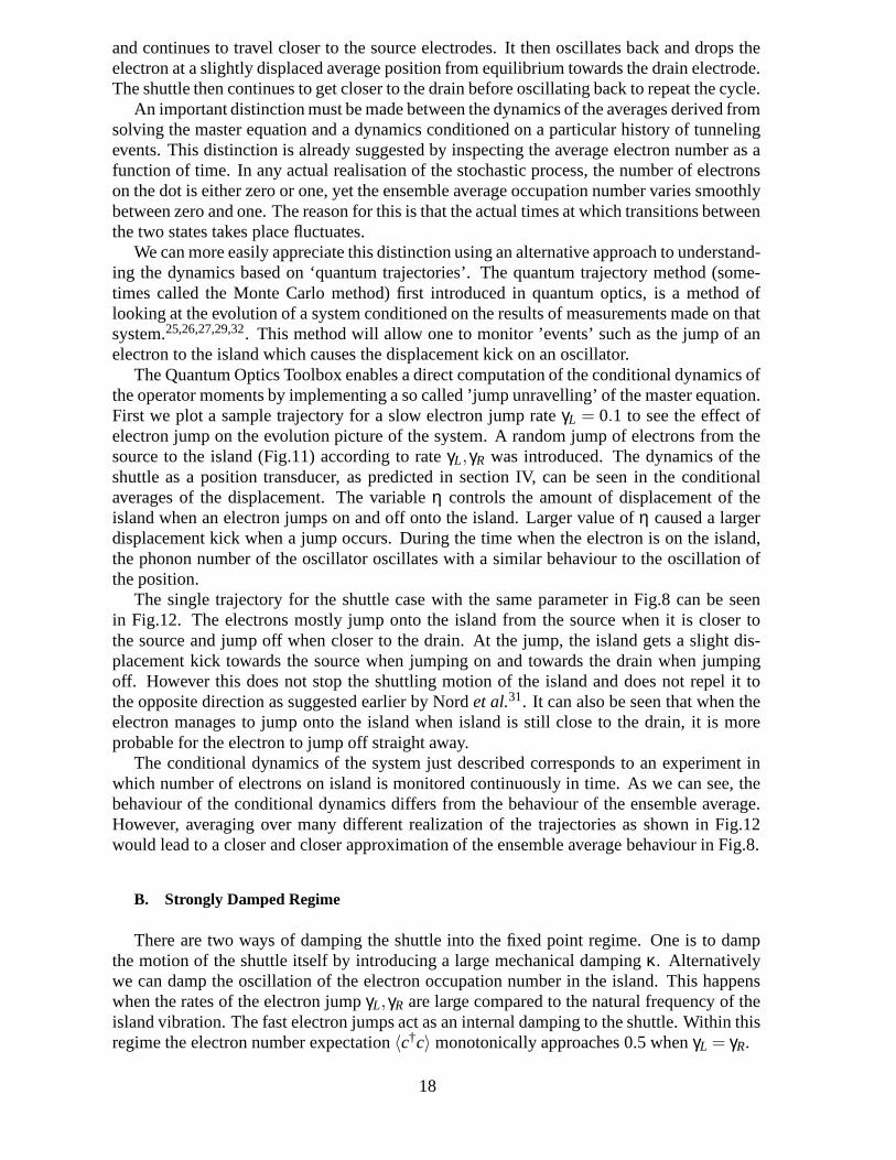
To investigate the effect ofη on the correlation between the factorized and unfactorizedmoments, we can plot〈cc†(a+a†)〉 and 〈cc†〉〈a+a†〉. We can see from Fig.10, that thesemiclassical approximation agrees with the quantum simulation under the condition thatηis small enough. Asη increases, the evidence of this difference becomes noticeable. This

16

0 0.5 1 1.5 2 2.5 3 3.50

0.1

0.2

0.3

0.4

0.5

0.6

0.7

time(2π)

<(a

+a+

)><

c+c>

−<

(a+

a+)c

+c>

FIG. 9: Plot of the difference between the factorized and unfactorized moments〈(a+a†)〉〈c†c〉 −〈(a+a†)c†c〉 in Fig.8.

0 0.5 1 1.5 2 2.5 3 3.5

00.1

0.20.3

0.4

−0.1

0

0.1

0.2

0.3

0.4

0.5

0.6

time (2π)η

<(a

+a+

)><

c+c>

−<

(a+

a+)c

+c>

FIG. 10: Plot of the difference between the factorized and unfactorized moments for variousη withγL = γR = 1,χ = 0.5,κ = 0.05.

difference oscillates with peaks located at times when electron jumps happen, that is whenthe oscillator is near the equilibrium position.

As opposed to what the name ”electron shuttle” suggests, thedynamics in the shuttleregime, for the parameters specified in Fig.8, is not like a conventional shuttle which picksup an electron when it is closest to the source and drops the electron when it is closest tothe drain, as also suggested by Nordet al.31. Looking at the rate of the average electronnumber and the average current in the source (Fig.8(a)), this is certainly not the case. Theshuttle picks up an electron near an average displacement ofzero, slightly towards the source,

17

and continues to travel closer to the source electrodes. It then oscillates back and drops theelectron at a slightly displaced average position from equilibrium towards the drain electrode.The shuttle then continues to get closer to the drain before oscillating back to repeat the cycle.

An important distinction must be made between the dynamics of the averages derived fromsolving the master equation and a dynamics conditioned on a particular history of tunnelingevents. This distinction is already suggested by inspecting the average electron number as afunction of time. In any actual realisation of the stochastic process, the number of electronson the dot is either zero or one, yet the ensemble average occupation number varies smoothlybetween zero and one. The reason for this is that the actual times at which transitions betweenthe two states takes place fluctuates.

We can more easily appreciate this distinction using an alternative approach to understand-ing the dynamics based on ‘quantum trajectories’. The quantum trajectory method (some-times called the Monte Carlo method) first introduced in quantum optics, is a method oflooking at the evolution of a system conditioned on the results of measurements made on thatsystem.25,26,27,29,32. This method will allow one to monitor ’events’ such as the jump of anelectron to the island which causes the displacement kick onan oscillator.

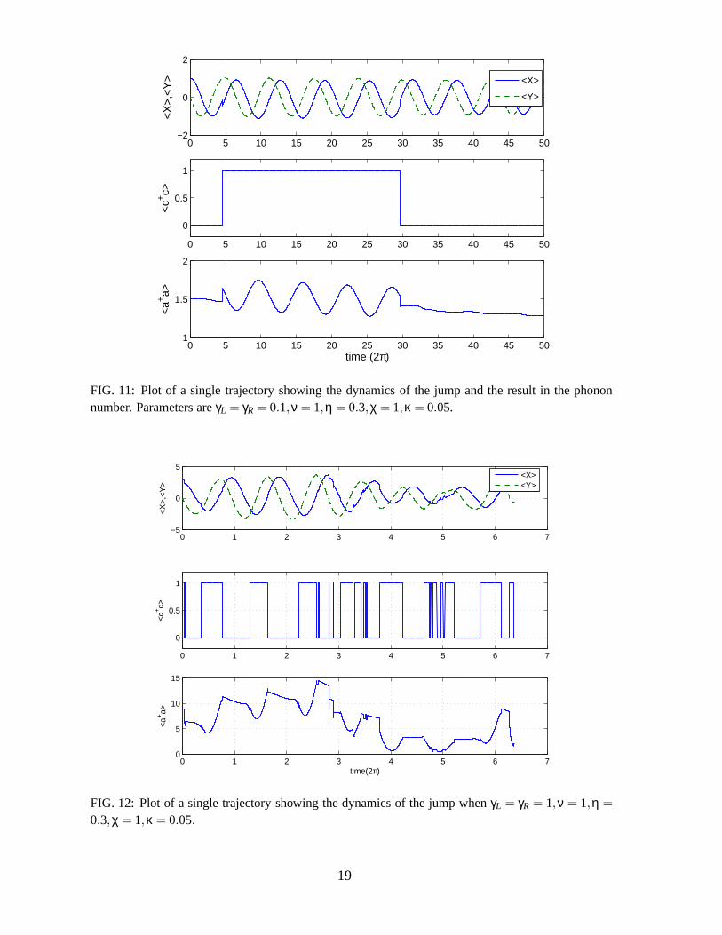
The Quantum Optics Toolbox enables a direct computation of the conditional dynamics ofthe operator moments by implementing a so called ’jump unravelling’ of the master equation.First we plot a sample trajectory for a slow electron jump rate γL = 0.1 to see the effect ofelectron jump on the evolution picture of the system. A random jump of electrons from thesource to the island (Fig.11) according to rateγL,γR was introduced. The dynamics of theshuttle as a position transducer, as predicted in section IV, can be seen in the conditionalaverages of the displacement. The variableη controls the amount of displacement of theisland when an electron jumps on and off onto the island. Larger value ofη caused a largerdisplacement kick when a jump occurs. During the time when the electron is on the island,the phonon number of the oscillator oscillates with a similar behaviour to the oscillation ofthe position.

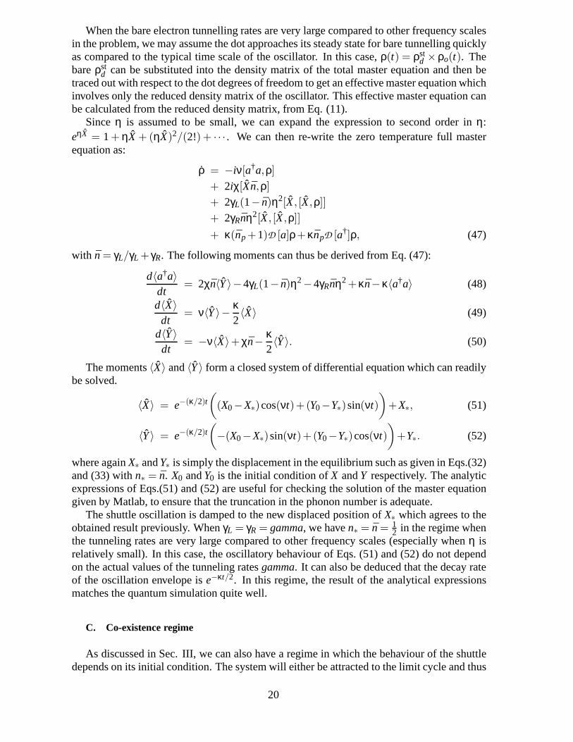
The single trajectory for the shuttle case with the same parameter in Fig.8 can be seenin Fig.12. The electrons mostly jump onto the island from thesource when it is closer tothe source and jump off when closer to the drain. At the jump, the island gets a slight dis-placement kick towards the source when jumping on and towards the drain when jumpingoff. However this does not stop the shuttling motion of the island and does not repel it tothe opposite direction as suggested earlier by Nordet al.31. It can also be seen that when theelectron manages to jump onto the island when island is stillclose to the drain, it is moreprobable for the electron to jump off straight away.

The conditional dynamics of the system just described corresponds to an experiment inwhich number of electrons on island is monitored continuously in time. As we can see, thebehaviour of the conditional dynamics differs from the behaviour of the ensemble average.However, averaging over many different realization of the trajectories as shown in Fig.12would lead to a closer and closer approximation of the ensemble average behaviour in Fig.8.

B. Strongly Damped Regime

There are two ways of damping the shuttle into the fixed point regime. One is to dampthe motion of the shuttle itself by introducing a large mechanical dampingκ. Alternativelywe can damp the oscillation of the electron occupation number in the island. This happenswhen the rates of the electron jumpγL,γR are large compared to the natural frequency of theisland vibration. The fast electron jumps act as an internaldamping to the shuttle. Within thisregime the electron number expectation〈c†c〉 monotonically approaches 0.5 whenγL = γR.

18

0 5 10 15 20 25 30 35 40 45 50−2

0

2

<X

>,<

Y>

0 5 10 15 20 25 30 35 40 45 50

0

0.5

1<

c+c>

0 5 10 15 20 25 30 35 40 45 501

1.5

2

time (2π)

<a+

a>

<X>

<Y>

FIG. 11: Plot of a single trajectory showing the dynamics of the jump and the result in the phononnumber. Parameters areγL = γR = 0.1,ν = 1,η = 0.3,χ = 1,κ = 0.05.

0 1 2 3 4 5 6 7−5

0

5

<X

>,<

Y>

0 1 2 3 4 5 6 7

0

0.5

1

<c+

c>

0 1 2 3 4 5 6 70

5

10

15

time(2π)

<a+

a>

<X><Y>

FIG. 12: Plot of a single trajectory showing the dynamics of the jump whenγL = γR = 1,ν = 1,η =

0.3,χ = 1,κ = 0.05.

19

When the bare electron tunnelling rates are very large compared to other frequency scalesin the problem, we may assume the dot approaches its steady state for bare tunnelling quicklyas compared to the typical time scale of the oscillator. In this case,ρ(t) = ρst

d ×ρo(t). Thebareρst

d can be substituted into the density matrix of the total master equation and then betraced out with respect to the dot degrees of freedom to get aneffective master equation whichinvolves only the reduced density matrix of the oscillator.This effective master equation canbe calculated from the reduced density matrix, from Eq. (11).

Sinceη is assumed to be small, we can expand the expression to secondorder in η:eηX = 1+ ηX + (ηX)2/(2!) + · · · . We can then re-write the zero temperature full masterequation as:

ρ = −iν[a†a,ρ]

+ 2iχ[Xn,ρ]

+ 2γL(1− n)η2[X, [X,ρ]]

+ 2γRnη2[X, [X,ρ]]

+ κ(np+1)D [a]ρ+κnpD [a†]ρ, (47)

with n = γL/γL + γR. The following moments can thus be derived from Eq. (47):

d〈a†a〉dt

= 2χn〈Y〉−4γL(1− n)η2−4γRnη2+κn−κ〈a†a〉 (48)

d〈X〉dt

= ν〈Y〉−κ2〈X〉 (49)

d〈Y〉dt

= −ν〈X〉+χn−κ2〈Y〉. (50)

The moments〈X〉 and〈Y〉 form a closed system of differential equation which can readilybe solved.

〈X〉 = e−(κ/2)t(

(X0−X∗)cos(νt)+(Y0−Y∗)sin(νt)

)

+X∗, (51)

〈Y〉 = e−(κ/2)t(

−(X0−X∗)sin(νt)+(Y0−Y∗)cos(νt)

)

+Y∗. (52)

where againX∗ andY∗ is simply the displacement in the equilibrium such as given in Eqs.(32)and (33) withn∗ = n. X0 andY0 is the initial condition ofX andY respectively. The analyticexpressions of Eqs.(51) and (52) are useful for checking thesolution of the master equationgiven by Matlab, to ensure that the truncation in the phonon number is adequate.

The shuttle oscillation is damped to the new displaced position of X∗ which agrees to theobtained result previously. WhenγL = γR = gamma, we haven∗ = n = 1

2 in the regime whenthe tunneling rates are very large compared to other frequency scales (especially whenη isrelatively small). In this case, the oscillatory behaviourof Eqs. (51) and (52) do not dependon the actual values of the tunneling ratesgamma. It can also be deduced that the decay rateof the oscillation envelope ise−κt/2. In this regime, the result of the analytical expressionsmatches the quantum simulation quite well.

C. Co-existence regime

As discussed in Sec. III, we can also have a regime in which thebehaviour of the shuttledepends on its initial condition. The system will either be attracted to the limit cycle and thus

20

0 0.5 1 1.5 2 2.5 3 3.5−0.5

0

0.5

<X

>,<

Y>

0 0.5 1 1.5 2 2.5 3 3.50

0.5

1

<c+

c>

0 0.5 1 1.5 2 2.5 3 3.5

4

5

<i s>

,<i d>

0 0.5 1 1.5 2 2.5 3 3.50

1

2

time(2π)<

a+a>

FIG. 13: Average evolution of the shuttle with a largeγL andγR. Here we have chosenγL = γR =

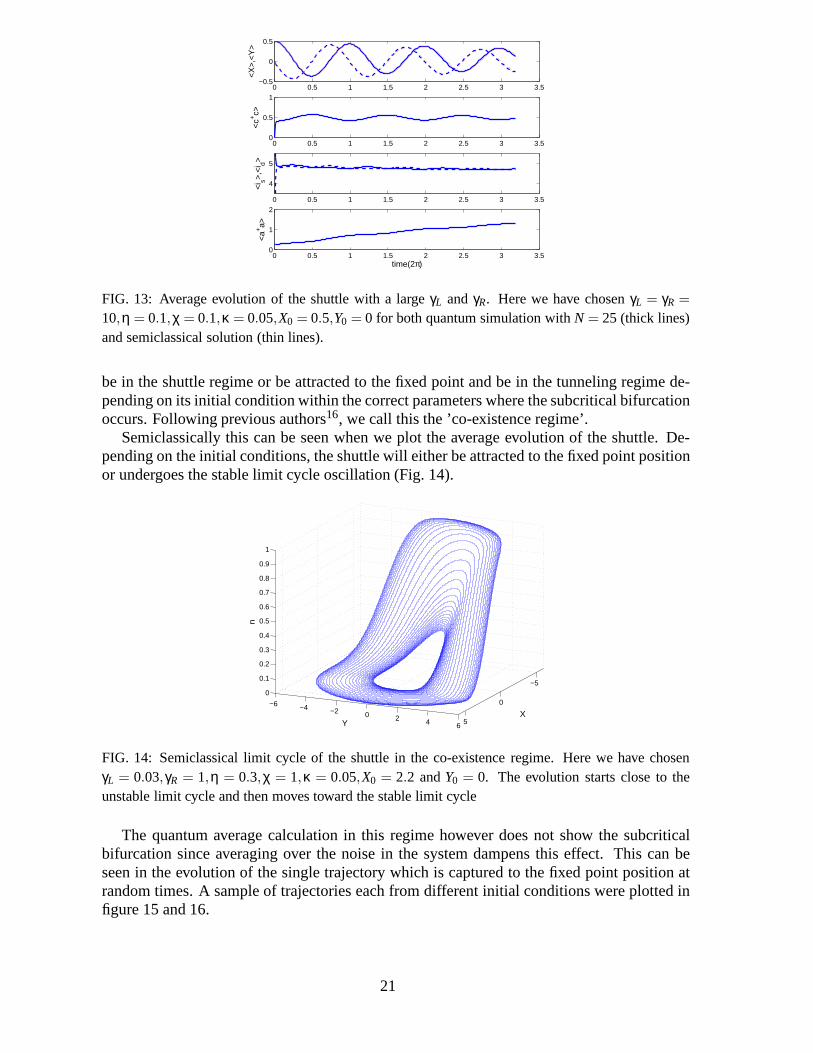
10,η = 0.1,χ = 0.1,κ = 0.05,X0 = 0.5,Y0 = 0 for both quantum simulation withN = 25 (thick lines)and semiclassical solution (thin lines).

be in the shuttle regime or be attracted to the fixed point and be in the tunneling regime de-pending on its initial condition within the correct parameters where the subcritical bifurcationoccurs. Following previous authors16, we call this the ’co-existence regime’.

Semiclassically this can be seen when we plot the average evolution of the shuttle. De-pending on the initial conditions, the shuttle will either be attracted to the fixed point positionor undergoes the stable limit cycle oscillation (Fig. 14).

−5

0

5

−6 −4 −2 0 2 4 6

0

0.1

0.2

0.3

0.4

0.5

0.6

0.7

0.8

0.9

1

XY

n

FIG. 14: Semiclassical limit cycle of the shuttle in the co-existence regime. Here we have chosenγL = 0.03,γR = 1,η = 0.3,χ = 1,κ = 0.05,X0 = 2.2 andY0 = 0. The evolution starts close to theunstable limit cycle and then moves toward the stable limit cycle

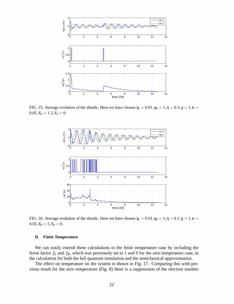
The quantum average calculation in this regime however doesnot show the subcriticalbifurcation since averaging over the noise in the system dampens this effect. This can beseen in the evolution of the single trajectory which is captured to the fixed point position atrandom times. A sample of trajectories each from different initial conditions were plotted infigure 15 and 16.

21

0 2 4 6 8 10 12 14−2

0

2

<X

>,<

Y>

0 2 4 6 8 10 12 14

0

0.5

1

<c+

c>

0 2 4 6 8 10 12 140

0.5

1

1.5

time (2π)

<a+

a>

<X><Y>

FIG. 15: Average evolution of the shuttle. Here we have chosen γL = 0.01,γR = 1,η = 0.3,χ = 1,κ =

0.05,X0 = 1.2,Y0 = 0.

0 2 4 6 8 10 12 14−5

0

5

<X

>,<

Y>

0 2 4 6 8 10 12 14

0

0.5

1

<c+

c>

0 2 4 6 8 10 12 140

20

40

60

<a+

a>

time (2π)

<x><p>

FIG. 16: Average evolution of the shuttle. Here we have chosen γL = 0.01,γR = 1,η = 0.3,χ = 1,κ =

0.05,X0 = 5,Y0 = 0.

D. Finite Temperature

We can easily extend these calculations to the finite temperature case by including thefermi factor fL and fR, which was previously set to 1 and 0 for the zero temperature case, inthe calculation for both the full quantum simulation and thesemiclassical approximation.

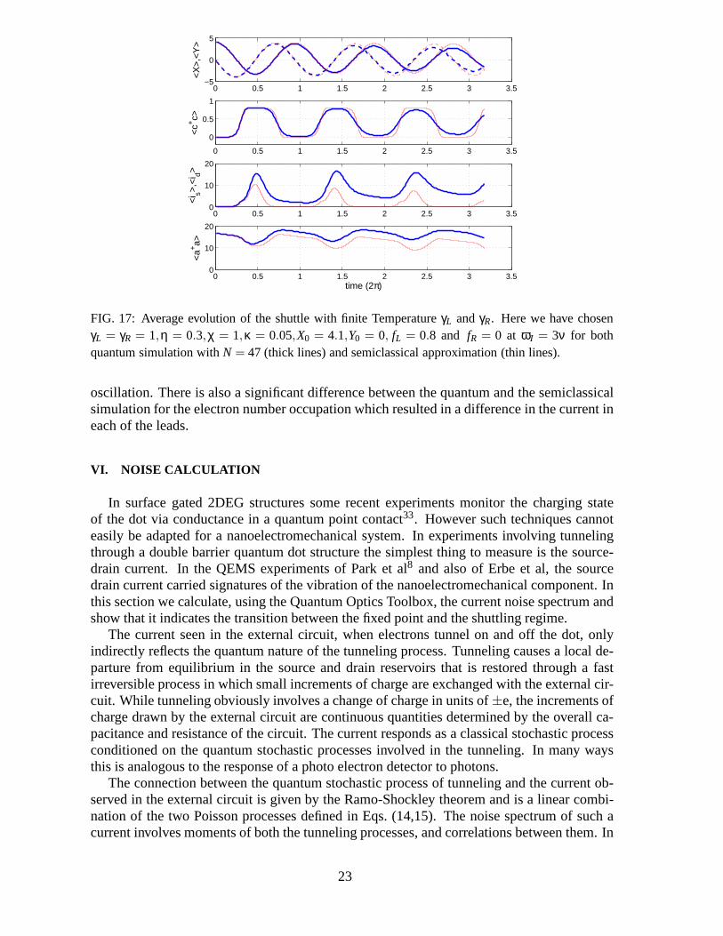
The effect on temperature on the system is shown in Fig. 17. Comparing this with pre-vious result for the zero temperature (Fig. 8) there is a suppression of the electron number

22

0 0.5 1 1.5 2 2.5 3 3.5−5

0

5

<X

>,<

Y>

0 0.5 1 1.5 2 2.5 3 3.5

0

0.5

1

<c+

c>

0 0.5 1 1.5 2 2.5 3 3.50

10

20

<i s>

,<i d>

0 0.5 1 1.5 2 2.5 3 3.50

10

20

time (2π)

<a+

a>

FIG. 17: Average evolution of the shuttle with finite Temperature γL andγR. Here we have chosenγL = γR = 1,η = 0.3,χ = 1,κ = 0.05,X0 = 4.1,Y0 = 0, fL = 0.8 and fR = 0 at ωI = 3ν for bothquantum simulation withN = 47 (thick lines) and semiclassical approximation (thin lines).

oscillation. There is also a significant difference betweenthe quantum and the semiclassicalsimulation for the electron number occupation which resulted in a difference in the current ineach of the leads.

VI. NOISE CALCULATION

In surface gated 2DEG structures some recent experiments monitor the charging stateof the dot via conductance in a quantum point contact33. However such techniques cannoteasily be adapted for a nanoelectromechanical system. In experiments involving tunnelingthrough a double barrier quantum dot structure the simplestthing to measure is the source-drain current. In the QEMS experiments of Park et al8 and also of Erbe et al, the sourcedrain current carried signatures of the vibration of the nanoelectromechanical component. Inthis section we calculate, using the Quantum Optics Toolbox, the current noise spectrum andshow that it indicates the transition between the fixed pointand the shuttling regime.

The current seen in the external circuit, when electrons tunnel on and off the dot, onlyindirectly reflects the quantum nature of the tunneling process. Tunneling causes a local de-parture from equilibrium in the source and drain reservoirsthat is restored through a fastirreversible process in which small increments of charge are exchanged with the external cir-cuit. While tunneling obviously involves a change of chargein units of±e, the increments ofcharge drawn by the external circuit are continuous quantities determined by the overall ca-pacitance and resistance of the circuit. The current responds as a classical stochastic processconditioned on the quantum stochastic processes involved in the tunneling. In many waysthis is analogous to the response of a photo electron detector to photons.

The connection between the quantum stochastic process of tunneling and the current ob-served in the external circuit is given by the Ramo-Shockleytheorem and is a linear combi-nation of the two Poisson processes defined in Eqs. (14,15). The noise spectrum of such acurrent involves moments of both the tunneling processes, and correlations between them. In

23

Sun et al.34, one can find a detailed example of how such correlations are determined by thecorresponding master equation for the quantum dot system.

Recently Flindt et al.14, have calculated a noise spectrum for the shuttle system defined interms of the fluctuating electron number accumulating in thedrain reservoir. Here we adopta different (but equivalent) approach based on the framework of quantum trajectories. In thissection we calculate, using quantum trajectory methods, the stationary current noise spectrumin thesourcecurrent alone as this suffices to illustrate how the current noise spectrum reflectsthe transition from fixed point to shuttling. The total current shows the same features but hasa different noise background.

The two time correlation function quantifies the fluctuations in the observed current andis defined by:

G(τ) =e2

i∞δ(τ)+E(I(t)I(t + τ))τ 6=0t→∞,

The first term is responsible for shot noise in the current, while the second term quantifiesnoise correlations. We now show how the second term can be defined in terms of the station-ary state of the quantum dot itself.

Let ρ(t) be the density operator representing the dot at timet. What is the conditionalprobability that, given an electron tunnels onto the dot from the drain betweent andt + dt,another similar tunneling event takes place a timeτ later (with no regard for what tunnelingevents have occurred in the mean time)? If an electron tunnels onto the dot from the drain attime t, the conditional state of the dot (unnormalised), conditioned on this event is given by

ρ(1)(t) = γLe−x/λc†ρ(t)ce−x/λ. (53)

Given this state, the probability that another tunneling event takes place a timeτ later is

G(t,τ) = γLtr(

e−2x/λcc†eL τ[ρ(1)(t)])

= γ2Ltr

(

e−2x/λcc†eL τ[e−x/λc†ρ(t)ce−x/λ])

.

where formally we have represented the irreversible dynamics from timet to t + τ as thepropagatoreL τ. Let us now assume that the first conditioning event takes place at a timetlong after any information about the initial state of the quantum dot has decayed away. Thatis to say the first conditioning event occurs when the dot has settled into the stationary state,ρ∞ = limt→∞ ρ(t). The stationary two-time correlation function for the source current is thendefined by

G(τ) = γ2Ltr

(

e−2x/λcc†eL τ[e−x/λc†ρ∞ce−x/λ])

(54)

In terms of the dimensionless position operator,X, the noise in the two time correlationfunctions becomes

G(τ) = E(IL(t)IL(t + τ))τ>0t→∞ = γ2

LTr[e−4ηXcc†eL τ(e−2ηXc†ρ∞ce−2ηX)]

whereeL τ is the master equation evolution.The noise power spectrum of the current is given by:

S(ω) = 2∫ ∞

0G(τ)(eiωτ +e−iωτ)dτ (55)

This noise spectrum can be directly calculated using the Quantum Optics Toolbox by firstcalculating the steady state solutionρ∞ and settinge−2ηXc†ρ∞ce−2ηX as an initial condition

24

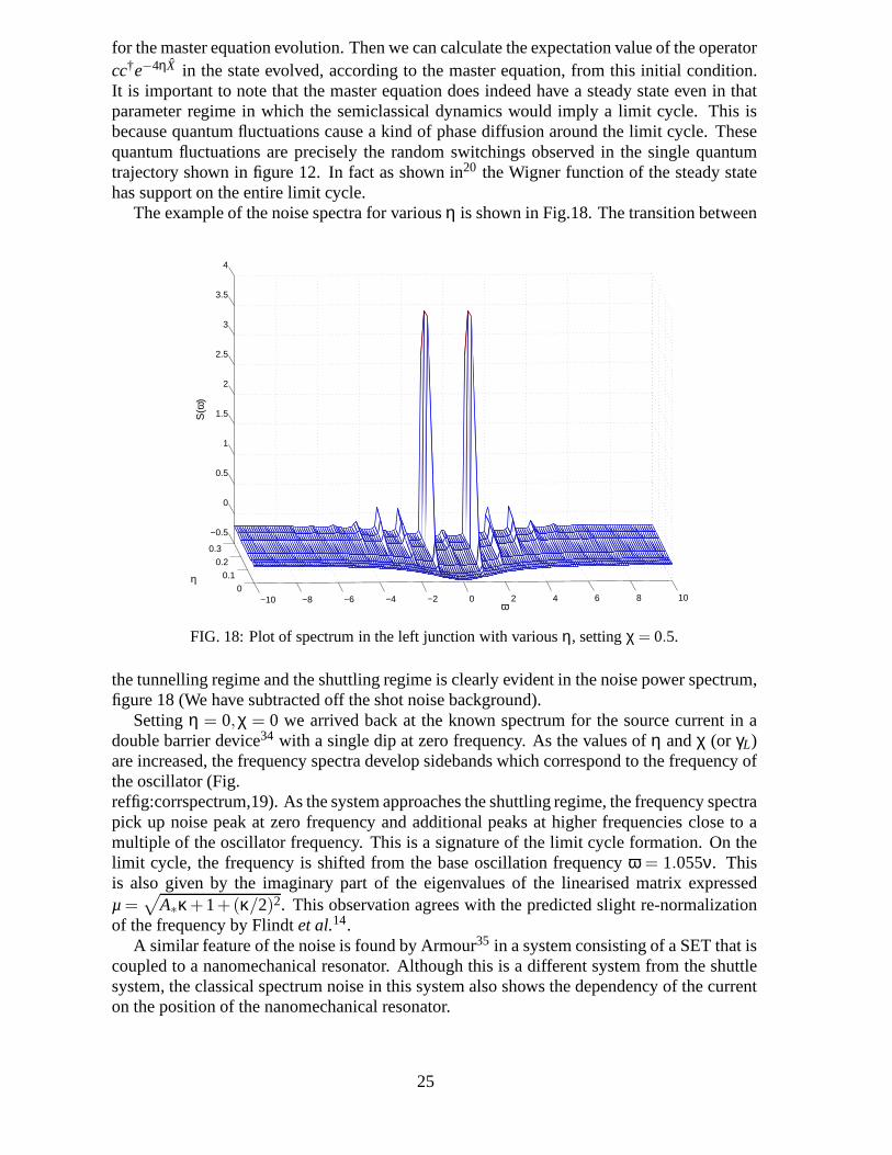
for the master equation evolution. Then we can calculate theexpectation value of the operatorcc†e−4ηX in the state evolved, according to the master equation, fromthis initial condition.It is important to note that the master equation does indeed have a steady state even in thatparameter regime in which the semiclassical dynamics wouldimply a limit cycle. This isbecause quantum fluctuations cause a kind of phase diffusionaround the limit cycle. Thesequantum fluctuations are precisely the random switchings observed in the single quantumtrajectory shown in figure 12. In fact as shown in20 the Wigner function of the steady statehas support on the entire limit cycle.

The example of the noise spectra for variousη is shown in Fig.18. The transition between

−10 −8 −6 −4 −2 0 2 4 6 8 100

0.1

0.2

0.3

−0.5

0

0.5

1

1.5

2

2.5

3

3.5

4

ω

S(ω

)

η

FIG. 18: Plot of spectrum in the left junction with variousη, settingχ = 0.5.

the tunnelling regime and the shuttling regime is clearly evident in the noise power spectrum,figure 18 (We have subtracted off the shot noise background).

Settingη = 0,χ = 0 we arrived back at the known spectrum for the source currentin adouble barrier device34 with a single dip at zero frequency. As the values ofη andχ (or γL)are increased, the frequency spectra develop sidebands which correspond to the frequency ofthe oscillator (Fig.reffig:corrspectrum,19). As the system approaches the shuttling regime, the frequency spectrapick up noise peak at zero frequency and additional peaks at higher frequencies close to amultiple of the oscillator frequency. This is a signature ofthe limit cycle formation. On thelimit cycle, the frequency is shifted from the base oscillation frequencyω = 1.055ν. Thisis also given by the imaginary part of the eigenvalues of the linearised matrix expressedµ =

√

A∗κ+1+(κ/2)2. This observation agrees with the predicted slight re-normalizationof the frequency by Flindtet al.14.

A similar feature of the noise is found by Armour35 in a system consisting of a SET that iscoupled to a nanomechanical resonator. Although this is a different system from the shuttlesystem, the classical spectrum noise in this system also shows the dependency of the currenton the position of the nanomechanical resonator.

25

−10 −8 −6 −4 −2 0 2 4 6 8 1010−1

100

101

−2

0

2

4

6

8

10

12

14

ω

S(ω

)

γL

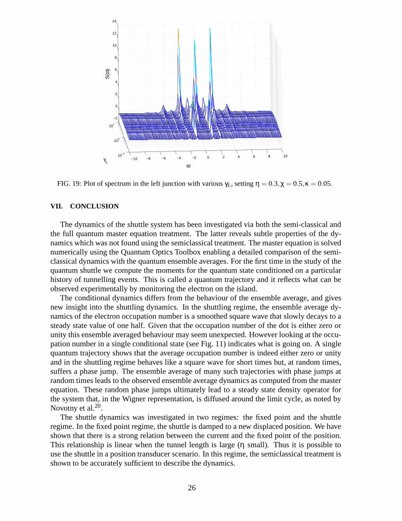
FIG. 19: Plot of spectrum in the left junction with variousγL, settingη = 0.3,χ = 0.5,κ = 0.05.

VII. CONCLUSION

The dynamics of the shuttle system has been investigated viaboth the semi-classical andthe full quantum master equation treatment. The latter reveals subtle properties of the dy-namics which was not found using the semiclassical treatment. The master equation is solvednumerically using the Quantum Optics Toolbox enabling a detailed comparison of the semi-classical dynamics with the quantum ensemble averages. Forthe first time in the study of thequantum shuttle we compute the moments for the quantum stateconditioned on a particularhistory of tunnelling events. This is called a quantum trajectory and it reflects what can beobserved experimentally by monitoring the electron on the island.

The conditional dynamics differs from the behaviour of the ensemble average, and givesnew insight into the shuttling dynamics. In the shuttling regime, the ensemble average dy-namics of the electron occupation number is a smoothed square wave that slowly decays to asteady state value of one half. Given that the occupation number of the dot is either zero orunity this ensemble averaged behaviour may seem unexpected. However looking at the occu-pation number in a single conditional state (see Fig. 11) indicates what is going on. A singlequantum trajectory shows that the average occupation number is indeed either zero or unityand in the shuttling regime behaves like a square wave for short times but, at random times,suffers a phase jump. The ensemble average of many such trajectories with phase jumps atrandom times leads to the observed ensemble average dynamics as computed from the masterequation. These random phase jumps ultimately lead to a steady state density operator forthe system that, in the Wigner representation, is diffused around the limit cycle, as noted byNovotny et al.20.

The shuttle dynamics was investigated in two regimes: the fixed point and the shuttleregime. In the fixed point regime, the shuttle is damped to a new displaced position. We haveshown that there is a strong relation between the current andthe fixed point of the position.This relationship is linear when the tunnel length is large (η small). Thus it is possible touse the shuttle in a position transducer scenario. In this regime, the semiclassical treatment isshown to be accurately sufficient to describe the dynamics.

26

We provide the condition in which the shuttle regime will appear from the system by iden-tifying the appearance of limit cycle in the phase space of the shuttle. A careful analysis ofthe nonlinear dynamics using centre manifold method indicates that whenγL = γR, the limitcycle forms through a supercritical pitchfork bifurcation. However whenγL 6= γR there is a re-gion of parameter space in which the bifurcation can be subcritical, and for which hysteresisis possible. Adjusting the dampingκ with respect to these parameters will cause the shuttle tobe sufficiently damped and thus allow the shuttling to take place. The shuttle regime also ap-pears when the rate of the electron tunnelling is close to theoscillator frequency. The shuttleregime corresponds to the continuous oscillation of the electron number and results in addi-tional peaks at multiples of the limit cycle frequency in thenoise spectra. This is destroyedwhenκ is too large or when a large electron jumpγL,γR are introduced to the system. Both ofthese conditions will damp the shuttle into the displaced equilibrium position. The quantumshuttle thus provides a fascinating example of a quantum stochastic system in which electrontransport is coupled to mechanical motion. In future studies we will investigate how such asystem can be configured for sensitive force detection.

Acknowledgment

HSG is grateful to the Centre for Quantum Computer Technology at the University ofQueensland for their hospitality during his visit. HSG would also like to acknowledge thesupport from the National Science Council, Taiwan under Contract No. NSC 94-2112-M-002-028, and support from the focus group program of the National Center for TheoreticalSciences, Taiwan under Contract No. NSC 94-2119-M-002-001. GJM acknowledges thesupport of the Australian Research Council through the Federation Fellowship Program.

∗ Electronic address: wahyu@physics.uq.edu.au† Electronic address: goan@phys.ntu.edu.tw1 R. G. Knobel and A. N. Cleland, Nature424, 291 (2003).2 M. D. LaHaye, O. Buu, B. Camarota, and K. Schwab, Science304, 74 (2004).3 K. L. Ekinci, X. M. H. Huang, and M. L. Roukes, Appl. Phys. Lett. 84, 4469 (2004).4 L. Gorelik et al., Phys. Rev. Lett.80, 4526 (1998).5 S. Tan, Quantum Optics Toolbox, http://www.phy.auckland.ac.nz/Staff/smt/qotoolbox/download.html.6 K. Molmer, Y. Castin, and J. Dalibard, Journal of the OpticalSociety of America B (Optical

Physics)10, 524 (1993).7 R. I. Shekhteret al., J. Phys.: Condens. Matter15, R441 (2003).8 H. Parket al., Nature407, 57 (2000).9 N. Zhitenev, H. Meng, and Z. Bao, Phys. Rev. Lett.88, 226801 (2002).

10 A. Erbe, C. Weiss, W. Zwerger, and R. Blick, Phys. Rev. Lett.87, 096106 (2001).11 X. M. H. Huang, C. A. Zorman, M. Mehregany, and M. L. Roukes, Nature421, 496 (2003).12 A. Isacsson and T. Nord, Europhys. Lett.66, 708 (2004).13 T. Novotny, A. Donarini, C. Flindt, and A.-P. Jauho, Phys. Rev. Lett 92, 248302 (2004).14 C. Flindt, T. Novotny, and A.-P. Jauho, Physica E28, in press (2005).15 A. Isacsson, Phys. Rev. B64, 035326 (2001).16 A. Donarini, cond-mat/0501242 v1, 2005.17 V. Aji, J. E. Moore, and C. M. Varma, APS Meeting Abstracts 17004 (2003).18 K. D. McCarthy, N. Prokof’ev, and M. T. Tuominen, Phys. Rev. B67, 245415 (2003).

27

19 D. Fedorets, L. Gorelik, R. Shekhter, and M. Jonson, Phys. Rev. Lett 92, 166801 (2004).20 T. Novotny, A. Donarini, and A.-P. Jauho, Phys. Rev. Lett.90, 256801 (2003).21 A.-P. Jauho, T. Novotny, A. Donarini, and C. Flindt, cond-mat/0411107 v1 .22 A. Armour and A. MacKinnon, Phys. Rev. B66, 035333 (2002).23 C. W. Gardiner and P. Zoller,Quantum Noise, 2nd ed. (Springer-Verlag, Berlin, 2000).24 D. W. Utami, H.-S. Goan, and G. J. Milburn, Phys. Rev. B70, 075303 (2004).25 H.-S. Goan, G. J. Milburn, H. M. Wiseman, and H. B. Sun, Phys. Rev. B63, 125326 (2001).26 H.-S. Goan and G. J. Milburn, Phys. Rev. B64, 235307 (2001).27 H.-S. Goan, Phys. Rev. B72, 075305 (2005).28 P. Glendinning,Stability, instability and chaos: an introduction to the theory of nonlinear differen-

tial equations(Cambridge University Press, New York, 1994).29 H. J. Carmichael,An open systems approach to quantum optics(Springer-Verlag, Berlin, Heidel-

berg, 1993).30 G. H. Golub and C. F. Loan,Matrix Computations, 3rd ed. (The John Hopkins University Press,

Baltimore, Maryland 21218, USA, 1996).31 T. Nord, L. Gorelik, R. Shekhter, and M.Jonson, Phys. Rev. B65, 165312 (2002).32 R. Dum, P. Zoller, and H. Ritsch, Phys. Rev. A45, 4879 (1992).33 J. M. Elzermanet al., Nature403, 431 (2004).34 H. B. Sun and G. Milburn, Phys. Rev. B59, 10748 (1999).35 A. Armour, Phys. Rev. B70, 165315 (2004).

28