This article was downloaded by: [University of Delaware]On: 10 July 2013, At: 12:31Publisher: Taylor & FrancisInforma Ltd Registered in England and Wales Registered Number: 1072954 Registeredoffice: Mortimer House, 37-41 Mortimer Street, London W1T 3JH, UK

International Journal of RemoteSensingPublication details, including instructions for authors andsubscription information:http://www.tandfonline.com/loi/tres20

Remote sensing of emergent andsubmerged wetlands: an overviewV. Klemas aa School of Marine Science and Policy , University of Delaware ,Newark , DE , 19716 , USAPublished online: 06 Jun 2013.

To cite this article: V. Klemas (2013) Remote sensing of emergent and submergedwetlands: an overview, International Journal of Remote Sensing, 34:18, 6286-6320, DOI:10.1080/01431161.2013.800656

To link to this article: http://dx.doi.org/10.1080/01431161.2013.800656

PLEASE SCROLL DOWN FOR ARTICLE

Taylor & Francis makes every effort to ensure the accuracy of all the information (the“Content”) contained in the publications on our platform. However, Taylor & Francis,our agents, and our licensors make no representations or warranties whatsoever as tothe accuracy, completeness, or suitability for any purpose of the Content. Any opinionsand views expressed in this publication are the opinions and views of the authors,and are not the views of or endorsed by Taylor & Francis. The accuracy of the Contentshould not be relied upon and should be independently verified with primary sourcesof information. Taylor and Francis shall not be liable for any losses, actions, claims,proceedings, demands, costs, expenses, damages, and other liabilities whatsoever orhowsoever caused arising directly or indirectly in connection with, in relation to or arisingout of the use of the Content.

This article may be used for research, teaching, and private study purposes. Anysubstantial or systematic reproduction, redistribution, reselling, loan, sub-licensing,systematic supply, or distribution in any form to anyone is expressly forbidden. Terms &Conditions of access and use can be found at http://www.tandfonline.com/page/terms-and-conditions

International Journal of Remote Sensing, 2013Vol. 34, No. 18, 6286–6320, http://dx.doi.org/10.1080/01431161.2013.800656

Remote sensing of emergent and submerged wetlands: an overview

V. Klemas*

School of Marine Science and Policy, University of Delaware, Newark, DE 19716, USA

(Received 27 June 2012; accepted 26 February 2013)

To plan for wetland protection and responsible coastal development, scientists and man-agers need to monitor changes in the coastal zone, as the sea level continues to riseand the coastal population keeps expanding. Advances in sensor design and data analy-sis techniques are now making remote-sensing systems practical and cost-effective formonitoring natural and human-induced coastal changes. Multispectral and hyperspectralimagers, light detection and ranging (lidar), and radar systems are available for mappingcoastal marshes, submerged aquatic vegetation, coral reefs, beach profiles, algal blooms,and concentrations of suspended particles and dissolved substances in coastal waters.Since coastal ecosystems have high spatial complexity and temporal variability, theyshould be observed with high spatial, spectral, and temporal resolutions. New satellites,carrying sensors with fine spatial (0.4–4 m) or spectral (200 narrow bands) resolution,are now more accurately detecting changes in coastal wetland extent, ecosystem health,biological productivity, and habitat quality. Using airborne lidars, one can producetopographic and bathymetric maps, even in moderately turbid coastal waters. Imagingradars are sensitive to soil moisture and inundation and can detect hydrologic fea-tures beneath the vegetation canopy. Combining these techniques and using time-seriesof images enables scientists to study the health of coastal ecosystems and accuratelydetermine long-term trends and short-term changes.

1. Introduction and background

Wetlands and estuaries are highly productive and act as critical habitats for a wide vari-ety of plants, fish, shellfish, and other wildlife. Wetlands also provide flood protection,protection from storm and wave damage, water quality improvement through filtering ofagricultural and industrial waste, and recharge of aquifers (Odum 1993; Morris et al. 2002).However, wetlands have been exposed to a wide range of stress-inducing alterations, includ-ing dredge and fill operations, hydrologic modifications, pollutant run-off, eutrophication,impoundments, and fragmentation by roads and ditches (Waycott et al. 2009).

Recently, there has also been considerable concern regarding the impact of climatechange on coastal wetlands, especially due to relative sea-level rise, increasing tempera-tures, and changes in precipitation. The rate of sea-level rise around the world has increasedover the past century to an average of about 3 mm a year, due to melting glaciers and theexpansion of ocean water as it warms. The Intergovernmental Panel on Climate Changeestimates that the rate of sea-level rise will accelerate in the future, with a total sea-levelrise of 0.59 m by 2100 (Church and White 2006; IPCC 2007). This substantial sea-level riseand more severe storms predicted for the next 100 years will impact coastal wetlands, beach

*Email: klemas@udel.edu

© 2013 Taylor & Francis

Dow

nloa

ded

by [

Uni

vers

ity o

f D

elaw

are]

at 1

2:31

10

July

201

3

International Journal of Remote Sensing 6287

erosion control strategies, salinity of estuaries and aquifers, coastal drainage systems, andcoastal economic development (McInnes et al. 2003).

Coastal areas such as barrier islands, beaches, and wetlands are especially sensitiveto sea-level changes. Rising seas will intensify coastal flooding and increase the erosionof beaches, bluffs, and wetlands, as well as threaten jetties, piers, seawalls, harbours, andwaterfront property. Along barrier islands, the erosion of beachfront property by floodingwater will be severe, leading to greater probability of overwash during storm surges (NOAA1999). A major hurricane can devastate a wetland (Klemas 2009). For instance, duringhurricanes Katrina and Rita, several hundred square kilometres of Louisiana wetlandspractically vanished.

In addition to immediate impacts due to anthropogenic activities and storms,global warming and sea-level rise will have serious long-term consequences for coastalecosystems such as marshes and submerged aquatic vegetation (SAV) beds, including habi-tat destruction, a shift in species composition, and habitat degradation in existing wetlands(Baldwin and Mendelssohn 1998; Titus et al. 2009). Coastal wetlands have already provento be susceptible to climate change, with a net loss of 13,450 ha from 1998 to 2004 in theUSA alone (Dahl 2006). This loss was primarily due to conversion of coastal salt marsh toopen salt water. Rising sea levels can cause not only the drowning of salt marsh habitatsbut also the reduction in germination periods (Noe and Zedler 2001).

Coastal scientists and managers are concerned about the impact of climate change,sea-level rise, and increasing storm activity on fisheries, wetlands, estuaries, and shore-lines; municipal infrastructure such as water, wastewater, and street systems; storm waterdrainage and flooding; and salinity intrusion into ground water supplies. To plan for wetlandprotection and sensible coastal development, there is a need to monitor changes in coastalecosystems, as the sea level continues to rise and the coastal population keeps expanding.

Recent advances in sensor design and data analysis techniques are making remote-sensing systems more practical and attractive for monitoring natural and man-madechanges impacting coastal ecosystems. High-resolution multispectral and hyperspectralimagers, light detection and ranging (lidar), and radar systems are available for monitor-ing changes in coastal marshes, submerged aquatic vegetation, coral reefs, beach profiles,algal blooms, and concentrations of suspended particles and dissolved substances in coastalwaters. Using airborne lidar, one can produce beach profiles and bathymetric maps.Imaging radars are sensitive to soil moisture and inundation and can detect hydrologic fea-tures beneath the vegetation canopy. Radars can also be used to detect water levels throughinterferometry and other methods. Thermal infrared scanners can map coastal water tem-peratures, while microwave radiometers can measure water salinity, soil moisture, and otherhydrologic parameters. Radar imagers, scatterometers, and altimeters provide informationon ocean waves, winds, sea surface height, and coastal currents (Ikeda and Dobson 1995;Martin 2004; Robinson 2004).

To obtain the required high spatial, spectral, and temporal resolutions, coastalecosystems have to be observed using high-resolution sensors aboard the satellites or air-craft. Some of the ecosystem health indicators that can be mapped with high-resolutionremote sensors include natural vegetation cover, wetland loss and fragmentation, wetlandbiomass change, percentage of impervious watershed area, buffer degradation, changesin hydrology, water turbidity, chlorophyll concentration, eutrophication level, salinity, etc.(Lathrop, Cole, and Showalter 2000; Martin 2004; Wang 2010).

With the rapid development of new remote sensors, data bases, and image analysistechniques, potential users need help in choosing remote sensors and data analysis methodsthat are most appropriate for wetland studies (Yang 2009). The objective of this paper is

Dow

nloa

ded

by [

Uni

vers

ity o

f D

elaw

are]

at 1

2:31

10

July

201

3

6288 V. Klemas

to review and compare remote-sensing techniques that are cost-effective and practical forshoreline delineation and wetland mapping.

2. Remote sensing of coastal wetlands

2.1. Wetland mapping

For more than three decades, remote-sensing techniques have been used by researchers andgovernment agencies to map and monitor wetlands (Tiner 1996; Dahl 2006). For instance,the US Fish and Wildlife Service (FWS) has been using remote sensors to determine thebiological extent of wetlands for the past 30 years. Through its National Wetlands Inventory,FWS has provided federal and state agencies, the private sector, and citizens with scientificdata on wetland location, extent, status, and trends. To accomplish this important task, FWShas used multiple sources of aircraft and satellite imagery and on-the-ground observations(Tiner 1996). Many states have also conducted a wide range of wetland inventories, usingboth aircraft and satellite imagery. The aircraft imagery typically included natural colourand colour-infrared pictures. The satellite data consisted of both high-resolution (1–4 m)and medium-resolution (10–30 m) multispectral imagery.

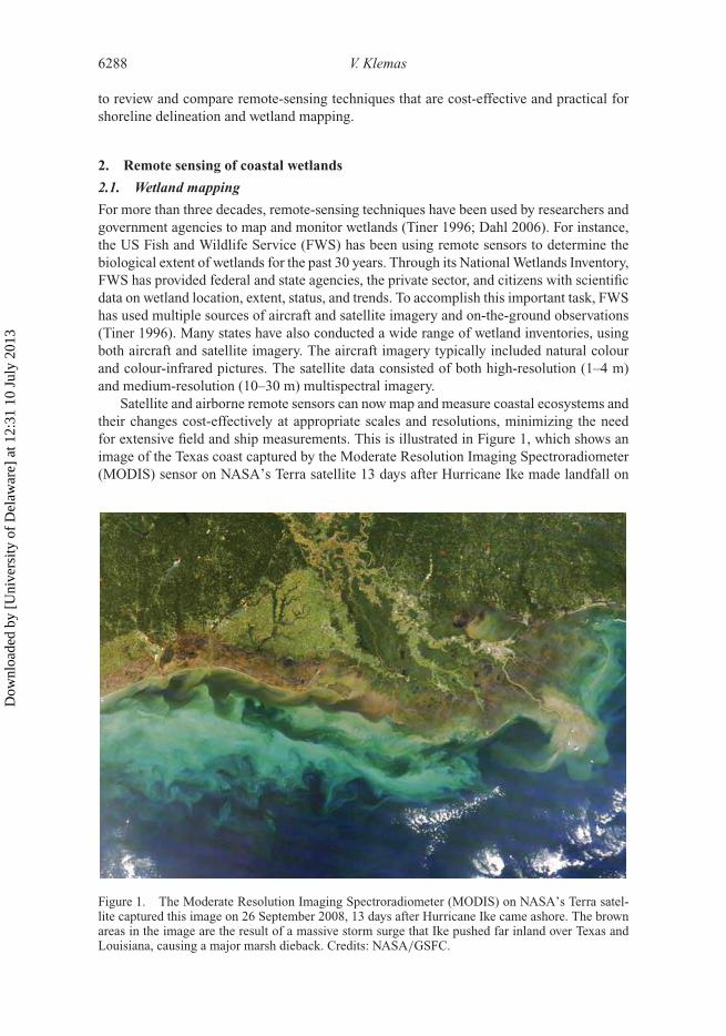
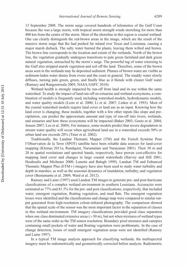
Satellite and airborne remote sensors can now map and measure coastal ecosystems andtheir changes cost-effectively at appropriate scales and resolutions, minimizing the needfor extensive field and ship measurements. This is illustrated in Figure 1, which shows animage of the Texas coast captured by the Moderate Resolution Imaging Spectroradiometer(MODIS) sensor on NASA’s Terra satellite 13 days after Hurricane Ike made landfall on

Figure 1. The Moderate Resolution Imaging Spectroradiometer (MODIS) on NASA’s Terra satel-lite captured this image on 26 September 2008, 13 days after Hurricane Ike came ashore. The brownareas in the image are the result of a massive storm surge that Ike pushed far inland over Texas andLouisiana, causing a major marsh dieback. Credits: NASA/GSFC.

Dow

nloa

ded

by [

Uni

vers

ity o

f D

elaw

are]

at 1

2:31

10

July

201

3

International Journal of Remote Sensing 6289

13 September 2008. The storm surge covered hundreds of kilometres of the Gulf Coastbecause Ike was a large storm, with tropical storm strength winds stretching for more than400 km from the centre of the storm. Most of the shoreline in this region is coastal wetland.One can clearly distinguish the red-brown areas in the image, which are the result of themassive storm surge that Ike had pushed far inland over Texas and Louisiana, causing amajor marsh dieback. The salty water burned the plants, leaving them wilted and brown.The brown line corresponds to the location and extent of the wetlands. North of the brownline, the vegetation gradually undergoes transitions to pale green farmland and dark greennatural vegetation, untouched by the storm’s surge. The powerful tug of water returning tothe Gulf also stripped marsh vegetation and soil off the land. Therefore, some of the brownareas seen in the wetlands may be deposited sediment. Plumes of brown water are visible assediment-laden water drains from rivers and the coast in general. The muddy water slowlydiffuses, turning pale green, green, and finally blue as it blends with clearer Gulf water(Ramsey and Rangoonwala 2005; NASA/GSFC 2010).

Wetland health is strongly impacted by run-off from land and its use within the samewatershed. To study the impact of land run-off on estuarine and wetland ecosystems, a com-bination of models is frequently used, including watershed models, hydrodynamic models,and water quality models (Leon et al. 2000; Li et al. 2007; Linker et al. 1993). Most ofthe coastal watershed models require land cover or land use as an input. Knowing how theland cover is changing, these models, together with a few other inputs like slope and pre-cipitation, can predict the approximate amount and type of run-off into rivers, wetlands,and estuaries and how these ecosystems will be impacted (Baker 2003; Goetz et al. 2004;Jensen 2007; Lee et al. 2009). For instance, some models predict that severe degradation instream water quality will occur when agricultural land use in a watershed exceeds 50% orurban land use exceeds 20% (Tiner et al. 2002).

Traditionally, the Landsat Thematic Mapper (TM) and the French Système Pourl’Observation de la Terre (SPOT) satellite have been reliable data sources for land-covermapping (Klemas 2011a; Rundquist, Narumalani and Narayanan 2001). Their 30 m and20 m spatial resolutions and spectral bands, respectively, have proven cost-effective formapping land cover and changes in large coastal watersheds (Harvey and Hill 2001;Houhoulis and Michener 2000; Lunetta and Balogh 1999). Landsat TM and EnhancedThematic Mapper Plus (ETM+) imagery have also been used to study water turbidity anddepth in marshes, as well as the seasonal dynamics of inundation, turbidity, and vegetationcover (Bustamante et al. 2009; Ward et al. 2012).

Ramsey and Laine (1997) used Landsat TM images to generate pre- and post-hurricaneclassifications of a complex wetland environment in southern Louisiana. Accuracies wereestimated as 77% and 81.5% for the pre- and post classifications, respectively, that includedwater, emergent vegetation, floating vegetation, and mud flats. The emergent vegetationlosses were identified and the classifications and change map were compared to similar out-put generated from high-resolution colour-infrared photography. The comparison showedthat the spatial scale of the sensor was the most important factor in the separation of classesin this wetland environment. TM imagery classifications provided good class separationwhen one class dominated extensive areas (>30 m), but not when mixtures of wetland typeswere of the same order as the TM sensor resolution. Boundary pixel mixtures and canopiescontaining small pockets of water and floating vegetation were problematic. In the case ofchange detection, losses of small emergent vegetation areas were not identified (Ramseyand Laine 1997).

In a typical TM image analysis approach for classifying wetlands, the multispectralimagery must be radiometrically and geometrically corrected before analysis. Radiometric

Dow

nloa

ded

by [

Uni

vers

ity o

f D

elaw

are]

at 1

2:31

10

July

201

3

6290 V. Klemas

correction reduces the influence of haze and other atmospheric scattering particles and anysensor anomalies. The geometric correction compensates for the Earth’s rotation and forvariations in the position and altitude of the satellite.

Image segmentation simplifies the analysis by first dividing the image into homoge-neous patches or ecologically distinct areas. The actual classification of the land-cover datainto themes can be performed by using supervised and unsupervised classification meth-ods (Campbell 2007; Jensen 1996; Lillesand, Kiefer, and Chipman 2008). Throughout theclassification process, ancillary data are used whenever available (e.g. aerial photographs,soil maps, field samples, etc.). Multitemporal imagery and data from other sensors can alsohelp in the classification of wetlands (McCarthy, Gumbricht, and McCarthy 2005; Ozesmiand Bauer 2002). For instance, to distinguish forested wetlands from upland forests, onecan use radar imagery (Ramsey 1995). If possible, wetlands should be separated from otherland-cover types prior to their classification.

2.2. High-spatial resolution applications

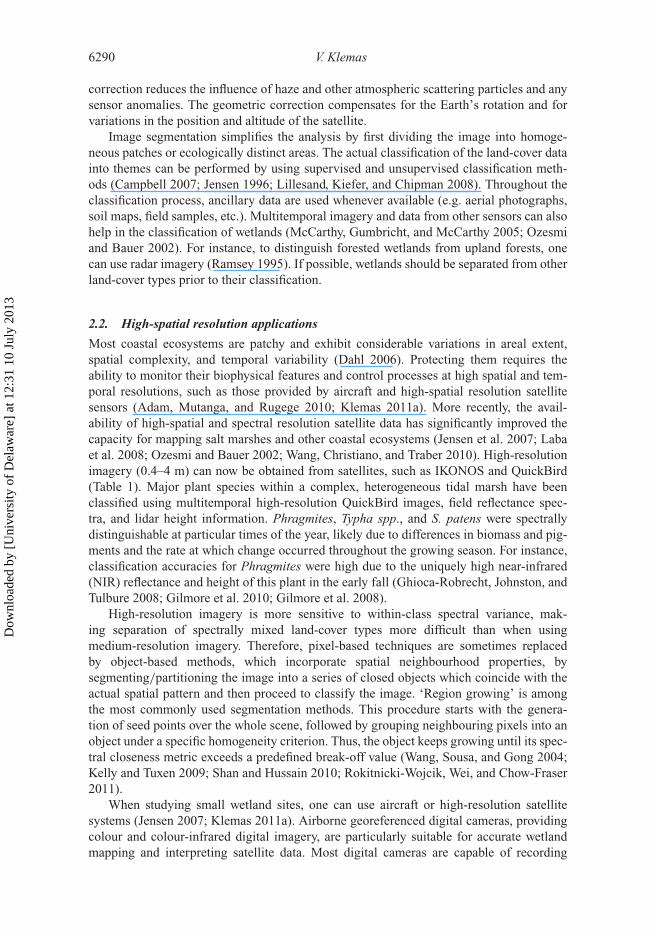
Most coastal ecosystems are patchy and exhibit considerable variations in areal extent,spatial complexity, and temporal variability (Dahl 2006). Protecting them requires theability to monitor their biophysical features and control processes at high spatial and tem-poral resolutions, such as those provided by aircraft and high-spatial resolution satellitesensors (Adam, Mutanga, and Rugege 2010; Klemas 2011a). More recently, the avail-ability of high-spatial and spectral resolution satellite data has significantly improved thecapacity for mapping salt marshes and other coastal ecosystems (Jensen et al. 2007; Labaet al. 2008; Ozesmi and Bauer 2002; Wang, Christiano, and Traber 2010). High-resolutionimagery (0.4–4 m) can now be obtained from satellites, such as IKONOS and QuickBird(Table 1). Major plant species within a complex, heterogeneous tidal marsh have beenclassified using multitemporal high-resolution QuickBird images, field reflectance spec-tra, and lidar height information. Phragmites, Typha spp., and S. patens were spectrallydistinguishable at particular times of the year, likely due to differences in biomass and pig-ments and the rate at which change occurred throughout the growing season. For instance,classification accuracies for Phragmites were high due to the uniquely high near-infrared(NIR) reflectance and height of this plant in the early fall (Ghioca-Robrecht, Johnston, andTulbure 2008; Gilmore et al. 2010; Gilmore et al. 2008).

High-resolution imagery is more sensitive to within-class spectral variance, mak-ing separation of spectrally mixed land-cover types more difficult than when usingmedium-resolution imagery. Therefore, pixel-based techniques are sometimes replacedby object-based methods, which incorporate spatial neighbourhood properties, bysegmenting/partitioning the image into a series of closed objects which coincide with theactual spatial pattern and then proceed to classify the image. ‘Region growing’ is amongthe most commonly used segmentation methods. This procedure starts with the genera-tion of seed points over the whole scene, followed by grouping neighbouring pixels into anobject under a specific homogeneity criterion. Thus, the object keeps growing until its spec-tral closeness metric exceeds a predefined break-off value (Wang, Sousa, and Gong 2004;Kelly and Tuxen 2009; Shan and Hussain 2010; Rokitnicki-Wojcik, Wei, and Chow-Fraser2011).

When studying small wetland sites, one can use aircraft or high-resolution satellitesystems (Jensen 2007; Klemas 2011a). Airborne georeferenced digital cameras, providingcolour and colour-infrared digital imagery, are particularly suitable for accurate wetlandmapping and interpreting satellite data. Most digital cameras are capable of recording

Dow

nloa

ded

by [

Uni

vers

ity o

f D

elaw

are]

at 1

2:31

10

July

201

3

International Journal of Remote Sensing 6291

Tabl

e1.

Hig

h-re

solu

tion

sate

llit

epa

ram

eter

san

dsp

ectr

alba

nds

(Dig

ital

Glo

be20

03;O

rbim

age

2003

;Par

kins

on20

03;S

pace

Imag

ing

2003

).

IKO

NO

SQ

uick

Bir

dO

rbV

iew

-3W

orld

Vie

w-1

Geo

Eye

-1W

orld

Vie

w-2

Spo

nsor

Spa

ceIm

agin

gD

igit

alG

lobe

Orb

imag

eD

igit

alG

lobe

Geo

Eye

Dig

ital

Glo

beL

aunc

hed

Sep

tem

ber

1999

Oct

ober

2001

June

2003

Sep

tem

ber

2007

Sep

tem

ber

2008

Oct

ober

2009

Spa

tial

reso

luti

on(m

)Pa

nchr

omat

ic1.

00.

611.

00.

50.

410.

5M

ulti

spec

tral

4.0

2.44

4.0

n/a

1.65

2S

pect

ralr

ange

(nm

)Pa

nchr

omat

ic52

5–92

845

0–90

045

0–90

040

0–90

045

0–80

045

0–80

0C

oast

albl

uen/

an/

an/

an/

an/

a40

0–45

0B

lue

450–

520

450–

520

450–

520

n/a

450–

510

450–

510

Gre

en51

0–60

052

0–60

052

0–60

0n/

a51

0–58

051

0–58

0Y

ello

wn/

an/

an/

an/

an/

a58

5–62

5R

ed63

0–69

063

0–69

062

5–69

5n/

a65

5–69

063

0–69

0R

eded

gen/

an/

an/

an/

an/

a70

5–74

5N

ear-

infr

ared

760–

850

760–

890

760–

900

n/a

780–

920

770–

1040

Sw

ath

wid

th(k

m)

11.3

16.5

817

.615

.216

.4O

ffna

dir

poin

ting

±26◦

±30◦

±45◦

±45◦

±30◦

±45◦

Rev

isit

tim

e(d

ays)

2.3–

3.4

1–3.

51.

5–3

1.7–

3.8

2.1–

8.3

1.1–

2.7

Orb

ital

alti

tude

(km

)68

145

047

049

668

177

0

Dow

nloa

ded

by [

Uni

vers

ity o

f D

elaw

are]

at 1

2:31

10

July

201

3

6292 V. Klemas

reflected visible to NIR light. A filter is placed over the lens that transmits only selectedportions of the wavelength spectrum. For a single camera operation, a filter is chosen thatgenerates natural colour (blue–green–red wavelengths) or colour-infrared (green–red–NIRwavelengths) imagery. For multiple camera operation, filters that transmit narrower bandsare chosen. For example, a four-camera system may be configured so that each camera fil-ter passes a spectral band matching a specific satellite imaging band, e.g. blue, green, red,and NIR bands matching the bands of the IKONOS satellite (Table 1) multispectral sensor(Ellis and Dodd 2000).

Digital camera imagery can be integrated with global positioning system (GPS) posi-tion information and used as layers in a geographical information system (GIS) for a widerange of modelling applications (Lyon and McCarthy 1995). Small aircraft flown at lowaltitudes (e.g. 200–500 m) can also be used to guide field data collection (McCoy 2005).However, cost becomes excessive if the study site is larger than a few hundred square kilo-metres, and in that case, medium-resolution multispectral sensors, such as Landsat TM(30 m) and SPOT (20 m), become more cost-effective than the high-resolution systems(Klemas 2011a).

2.3. Hyperspectral remote sensing

Airborne hyperspectral imagers, such as the advanced visible infrared imaging spectrom-eter (AVIRIS) and the Compact Airborne Spectrographic Imager (CASI) have been usedfor mapping coastal wetlands (Li, Ustin, and Lay 2005; Rosso, Ustin, and Hastings 2005;Thomson et al. 1998; Ozesmi and Bauer 2002; Schmidt and Skidmore 2003). Hyperspectralimagers may contain hundreds of narrow spectral bands located in the visible, NIR, mid-infrared, and sometimes thermal portions of the electromagnetic (EM) spectrum (Jensenet al. 2007).

The advantages and problems associated with hyperspectral mapping have been clearlydemonstrated by Hirano, Madden, and Welch (2003), who used AVIRIS hyperspectraldata to map vegetation for a portion of Everglades National Park in Florida. AVIRISprovides 224 spectral bands from 0.4 to 2.45 µm, each with 0.01 µm bandwidth, 20 mspatial resolution, and a swath width of 10.5 km. After removing atmospheric effects,the authors improved the signal-to-noise (S/N) ratio by reducing inherent noise in theimage data by employing the minimum noise fraction (MNF) transform implemented inthe Environment for Visualizing Images (ENVI; Research Systems, Inc., Norwalk, CT,USA) image-processing software package. Applying principal component analysis (PCA)to the Everglades AVIRIS imagery yielded the first 12 bands from the MNF image contain-ing the most useful signal information. There was also a need to rectify the image in orderto remove geometric distortions caused by variations in aircraft tilt.

Hirano, Madden and Welch (2003) compared the geographic locations of spectrallypure pixels in the AVIRIS image with dominant vegetation polygons of the EvergladesVegetation Database and classified spectrally pure pixels into 10 different vegetationclasses, plus water and mud. An adequate number of pure pixels were identified to per-mit the selection of training samples used in the automated classification procedure. Thespectral signatures from the training samples were then matched to the spectral signaturesof each of the individual pixels. Image classification was undertaken using the ENVI spec-tral angle mapper (SAM) classifier in conjunction with the spectral library created for theEverglades study area. The SAM classifier examines the digital numbers (DNs) of all bandsfrom each pixel in the AVIRIS data set to determine similarity between the angular direc-tion of the spectral signature (i.e. colour) of the image pixel and that of a specific classin the spectral library. A coincident or small spectral angle between the vector for the

Dow

nloa

ded

by [

Uni

vers

ity o

f D

elaw

are]

at 1

2:31

10

July

201

3

International Journal of Remote Sensing 6293

unknown pixel and that for a vegetation class training sample indicates that the image pixellikely belongs to that vegetation class. In the case of spectrally mixed pixels, the relativeprobability of membership (based on the spectral angle) to all vegetation classes is calcu-lated. Mixed pixels are then assigned to the class of the greatest probability of membership(Hirano, Madden, and Welch 2003).

The hyperspectral data proved effective in discriminating spectral differences amongmajor Everglades plants such as red, black, and white mangrove communities and enabledthe detection of exotic invasive species (Hirano, Madden, and Welch 2003). The overallclassification accuracy for all vegetation pixels was 65.7%, with the accuracy for dif-ferent mangrove tree species ranging from 73.5% to 95.7%. Limited spatial resolutionwas a problem, resulting in too many mixed pixels. Another problem was the complex-ity of image-processing procedures that are required before the hyperspectral data can beused for automated classification of wetland vegetation. To obtain improved results, allof the 224 hyperspectral bands had to be used in the analysis. The tremendous volumeof hyperspectral image data necessitated the use of specific software packages, large datastorage, and extended processing times (Hirano, Madden, and Welch 2003). A detailedaccuracy assessment of airborne hyperspectral data for mapping plant species in freshwatercoastal wetlands has been performed by Lopez et al. (2004).

A number of advanced new techniques have been developed for mapping wetlandsand even identifying wetland types and plant species (Schmidt et al. 2004; Jensen et al.2007; Klemas 2011a; Yang et al. 2009). For instance, using lidar, hyperspectral and radarimagery, and narrow-band vegetation indices, researchers have been able to not only dis-criminate some wetland species but also make progress on estimating biochemical andbiophysical parameters of wetland vegetation, such as water content, biomass, and leafarea index (Adam, Mutanga, and Rugege 2010; Artigas and Yang 2006; Filippi and Jensen2006; Gilmore et al. 2010; Ozesmi and Bauer 2002; Pengra, Johnston and Loveland 2007;Schmidt et al. 2004; Simard, Fatoyinbo and Pinto 2010; Wang 2010). The integration ofhyperspectral imagery and lidar-derived elevation has also significantly improved the accu-racy of mapping salt marsh vegetation. The hyperspectral images help to distinguish highmarsh from other salt marsh communities due to their high reflectance in the NIR regionof the spectrum, and the lidar data help to separate invasive Phragmites from low marshplants (Yang and Artigas 2010).

Hyperspectral imaging systems are now available not only for airborne applications,but also in space, such as the satellite-borne Hyperion system, which can detect fine differ-ences in spectral reflectance, assisting in species discrimination on a global scale (Brandoand Decker 2003; Christian and Krishnayya 2009; Papes et al. 2010; Pengra, Johnston,and Loveland 2007). The Hyperion sensor provides imagery with 220 spectral bands ata spatial resolution of 30 m. Although there have been few studies using satellite-basedhyperspectral remote sensing to detect and map coastal vegetation species, results so farhave shown that discrimination between multiple species is possible (Blasco, Aizpuru, andDin Ndongo 2005; Vaiphasa et al. 2005; Heumann 2011).

2.4. Synthetic aperture radar (SAR)

Imaging radars provide information that is fundamentally different from sensors that oper-ate in the visible and infrared portions of the EM spectrum. This is primarily due to themuch longer wavelengths used by SAR sensors and the fact that they give out and receivetheir own energy (i.e. active sensors). One of the most common types of imaging radaris SAR. SAR technology provides the increased spatial resolution that is necessary for

Dow

nloa

ded

by [

Uni

vers

ity o

f D

elaw

are]

at 1

2:31

10

July

201

3

6294 V. Klemas

regional wetland mapping, and SAR data have been used extensively for this purpose.(Novo et al. 2002; Lang and McCarty 2008).

When mapping and monitoring wetland ecosystems, imaging radars have many advan-tages over sensors that operate in the visible and infrared portions of the EM spectrum.Microwave energy is sensitive to variations in soil moisture and inundation and is only par-tially attenuated by vegetation canopies, especially in areas of lower biomass (Baghdadiet al. 2001; Kasischke, Melack, and Dobson 1997; Lang and Kasischke 2008; Rosenqvistet al. 2007; Townsend 2000, 2002; Townsend and Walsh 1998) or when using data collectedat longer wavelengths (Hess, Melack, and Simonett 1990; Martinez and Le Toan 2007).

The sensitivity of microwave energy to water, and its ability to penetrate vegetativecanopies, make SAR ideal for the detection of hydrologic features below the vegetation(Hall 1996; Kasischke, Melack, and Dobson 1997; Kasischke and Bourgeau-Chavez 1997;Phinn, Hess, and Finlayson 1999; Rao et al. 1999; Wilson and Rashid 2005). The presenceof standing water interacts with the radar signal differently depending on the dominantvegetation type/structure (Hess et al. 1995) as well as the biomass and condition of veg-etation (Töyrä et al. 2002; Costa and Telmer 2007). When exposed to open water withoutvegetation, specular reflection occurs and a dark signal (weak or no return) is observed(Dwivedi, Rao, and Bhattacharya 1999). The radar signal is often reduced in wetlands dom-inated by lower-biomass herbaceous vegetation when a layer of water is present largely dueto specular reflectance (Kasischke, Bourgeau-Chavez, Smith et al. 1997). Conversely, theradar signal is often increased in forested wetlands when standing water is present due tothe double-bounce effect (Harris and Digby-Argus 1986; Dwivedi, Rao, and Bhattacharya1999). This occurs in flooded forests when the radar pulse is reflected strongly by the watersurface away from the sensor (specular reflectance) but is then redirected back towards thesensor by a second reflection from a nearby tree trunk. The use of small incidence angles(closer to nadir) enhances the ability to map hydrology beneath the forest canopy due toincreased penetration of the canopy (Hess, Melack, and Simonett 1990; Bourgeau-Chavezet al. 2001; Töyrä, Pietroniro, and Martz 2001; Lang and McCarty 2008).

2.5. Wetland change detection

Vegetated wetlands are stable only when the marsh platform is able to accrete sediment ata rate equal to or greater than the prevailing rate of sea level rise. Rapid sea level rise cancause segmentation of barrier islands or disintegration of wetlands, especially if the sedi-ment supply cannot keep up with the sea level rise. This ability to accrete is proportionalto the biomass density of the plants, concentration of suspended sediment, time of submer-gence, depth of the marsh surface, and tidal range (Field and Philipp 2000). Many coastalwetlands, such as the tidal salt marshes along the Louisiana coast, are generally withinfractions of a metre of sea level and will be lost, especially if the impact of sea-level rise isamplified by coastal storms. Man-made modifications of wetland hydrology and extensiveurban development will further limit the ability of wetlands to survive sea-level rise. Forinstance, man-made channelization of the Mississippi River flow causes much of the riversediment to be carried into the Gulf, rather than be deposited in the wetlands along theLouisiana coast (Farris 2005; Pinet 2009).

To identify long-term trends and short-term variations, such as the impact of risingsea levels and hurricanes on wetlands, one needs to analyse time-series of remotely-sensedimagery. High temporal resolution, precise spectral bandwidths, and accurate georeferenc-ing procedures are factors that contribute to the frequent use of satellite image data forchange-detection analysis (Jensen 1996; Coppin et al. 2004; Baker et al. 2007; Shalaby and

Dow

nloa

ded

by [

Uni

vers

ity o

f D

elaw

are]

at 1

2:31

10

July

201

3

International Journal of Remote Sensing 6295

Tateishi 2007). A good example is the study of the onset and progression of marsh diebackperformed by Ramsey and Rangoonwala (2010).

The acquisition and analysis of time-series of multispectral imagery is a challengingtask. The imagery must be acquired under similar environmental conditions (e.g. same timeof year, sun angle, etc.) and in the same or similar spectral bands. There will be changes inboth time and spectral content. One way to approach this problem is to reduce the spectralinformation to a single index, reducing the multispectral imagery into one single field ofthe index for each time step. In this way, the problem is simplified to the analysis of atime-series of a single variable, one for each pixel of the images.

The most commonly used index is the normalized difference vegetation index (NDVI),which is expressed as the difference between red and NIR reflectance divided by theirsum (Jensen 2007). These two spectral bands represent the most detectable spectral char-acteristic of green plants. This is because the red (and blue) radiation is absorbed by thechlorophyll in the surface layers of the plant (palisade parenchyma), and NIR radiationis reflected from the inner leaf cell structure (spongy mesophyll) as it penetrates severalleaf layers in a canopy. Thus, NDVI can be related to plant biomass or stress, since NIRreflectance depends on the abundance of plant tissue, whereas red reflectance indicates thesurface condition of the plant. It has been shown by researchers that time-series remote-sensing data can be used effectively to identify long-term trends and subtle changes inNDVI by means of PCA (Yuan, Elvidge, and Lunetta 1998; Young and Wang 2001; Jensen2007).

When absolute comparisons between different dates are to be carried out, the pre-processing of multi-date sensor imagery is much more demanding than the single-datecase. It requires a sequence of operations, including calibration to radiance or at-satellitereflectance, atmospheric correction, image registration, geometric correction, mosaicking,sub-setting, and masking out clouds and irrelevant features (Lunetta and Elvidge 1998;Coppin et al. 2004).

Detecting the actual changes between two registered and radiometrically correctedimages from different dates can be accomplished by employing one of the several tech-niques, including post-classification comparison (PCC), spectral image differencing (SID),and change vector analysis (CVA). In PCC change detection, two images from differentdates are independently classified. The two classified maps are then compared on a pixel-by-pixel basis. One disadvantage is that every error in the individual date classificationmaps will also be present in the final change-detection map (Dobson et al. 1995; Jensen1996; Lunetta and Elvidge 1998).

SID is the most widely applied change-detection algorithm. SID techniques rely on theprinciple that land-cover changes result in changes in the spectral signature of the affectedland surface. SID techniques involve the transformation of two original images to a newsingle-band or multi-band image in which the areas of spectral change are highlighted. Thisis accomplished by subtracting one date of raw or transformed (e.g. vegetation indices,albedo, etc.) imagery from a second date, which has been precisely registered to the imageof the first date. Pixel difference values exceeding a selected threshold are considered aschanged. This approach eliminates the need to identify land-cover changes in areas whereno significant spectral change has occurred between the two dates of imagery (Coppin et al.2004; Jensen 1996; Yuan, Elvidge, and Lunetta 1998). A comparison of the SID and thePCC change-detection algorithms is provided by Macleod and Congalton (1998).

The SID- and the PCC-based change-detection methods are often combined in a hybridapproach. For instance, SID can be used to identify areas of significant spectral change,and then PCC can be applied within areas where spectral change was detected in order to

Dow

nloa

ded

by [

Uni

vers

ity o

f D

elaw

are]

at 1

2:31

10

July

201

3

6296 V. Klemas

obtain class-to-class change information. A detailed, step-by-step procedure for performingchange detection was developed by the National Oceanic and Atmospheric Administration(NOAA) Coastal Change Analysis Program (C-CAP) and is described in Dobson et al.(1995) and Klemas et al. (1993).

The changeable nature of wetland ecosystems sometimes requires a more dynamicchange-detection procedure. These ecosystems can exhibit a variety of vegetative orhydrologic changes that might not be detected when using only one or two spectral bands.CVA is a change-detection technique that can measure change in more than two spectralbands, giving it an advantage when mapping rapidly changing and highly diverse wetlands(Whigham 1999; Mitsch and Gosselink 2000; Coppin et al. 2004; Baker et al. 2007). CVAdetermines the direction and magnitude of changes in multi-dimensional spectral space(Allen and Kupfer 2000; Houhoulis and Michener 2000; Civco et al. 2002). CVA con-currently analyses changes in all the data layers, rather than a few selected spectral bands(Coppin et al. 2004). The CVA method identifies a change magnitude threshold that is usedto separate actual land-cover changes from subtle changes due to the variability withinland-cover classes, as well as radiometric changes associated with instrument and atmo-spheric variations (Hame, Heiler, and Miguel-Ayanz 1998; Johnson and Kasischke 1998).Defining spectral threshold values to separate true landscape changes from inherent spec-tral variation is particularly beneficial for studies of broadly diverse ecosystems, such aswetlands (Houhoulis and Michener 2000). Human interpretation and sometimes an empiri-cal threshold method need to be applied for interpretation of CVA results to obtain accurateinformation on wetland changes.

3. Submerged aquatic vegetation

Submerged aquatic vegetation (SAV) is an important part of wetland and coastalecosystems, playing a major role in the ecological functions of these habitats (Silva et al.2008). Seagrass beds provide essential habitat for many aquatic species, stabilize and enrichsediments, dissipate turbulence, reduce current flow, cycle nutrients, and improve waterquality (Hughes et al. 2009). However, in many parts of the world, the health and quantityof seagrass beds have been declining (Hemminga and Duarte 2000; Green and Short 2003;Orth et al. 2006; Waycott et al. 2009). The decline of coral reefs and SAV is closely linkedto human activity, since the coastlines and estuaries that host them are often heavily pop-ulated. Specifically, the decline has been attributed to reduction in water clarity, alterationof sediment migration via dredging, and destruction from coastal engineering, boating, andcommercial fishing. High concentrations of nutrients exported from agriculture or urbansprawl in coastal watersheds are causing algal blooms in many estuaries and coastal waters(Klemas 2012). Algal blooms are harmful. They cause eutrophic conditions, depleting oxy-gen levels needed for organic life and limiting aquatic plant growth by reducing watertransparency.

Submerged aquatic plants and their properties are not as easily detectable as terres-trial vegetation. The spectral response of aquatic vegetation resembles that of terrestrialvegetation, yet the submerged or flooded conditions introduce factors that alter its overallspectral characteristics. (Midwood and Chow-Fraser 2010; Underwood et al. 2006). Thegreen region of the spectrum is considered as the best for sensing submerged macrophytes,followed by the red and red edge regions (Fyfe 2003; Han and Rundquist 2003; Pinnel,Heege, and Zimmermann 2004; Thomson et al. 1998; Williams et al. 2003). This indi-cates that common underlying conditions, such as pigment concentration and cellularstructure, are responsible for the main differences among macrophyte species (Silva et al.

Dow

nloa

ded

by [

Uni

vers

ity o

f D

elaw

are]

at 1

2:31

10

July

201

3

International Journal of Remote Sensing 6297

2008). The green wavelengths also provide greater light penetration in waters with higherconcentrations of suspended and dissolved materials (Kirk 1994).

In addition to bottom reflectance, optically active materials, such as plankton, sus-pended sediment, and dissolved organics, affect the scattering and absorption of radiation.Thus, the main challenge for remote sensing of submerged aquatic plants is to isolate theweakened plant signal from the interference by the water column, the bottom, and theatmosphere. A careful correction of atmospheric effects is important prior to the analysisof submerged vegetation radiometry derived from satellite or high-altitude airborne data(Silva et al. 2008).

Ackleson and Klemas (1987) used a single-scattering reflectance model to represent theinteraction between the three main components of the signal from submerged vegetation(water, bottom, and plants). Using this physical representation and a set of predetermined,representative parameter values, the authors showed that, in shallow waters, the overallreflectance signal is determined mainly by the vegetation density, assuming that bottomreflectance is constant and differs significantly from that of the vegetation. As depthincreases, dominance of reflectance shifts to the water column components. Hence, theauthors suggest that incorporating depth information into the classification method canreduce the influence of water column variation (Ackleson and Klemas 1987; Silva et al.2008).

More recently, water column optical models have been used to correct water and bot-tom effects by including bathymetric information as one of the variables (Dierssen et al.2003; Heege, Bogner, and Pinnel 2003). Paringit et al. (2003) developed a seagrass canopymodel to predict the spectral response of submerged macrophytes in shallow waters. Themodel considers not only the effects of the water column through radiative transfer mod-elling but also viewing and illumination conditions, leaf and bottom reflectance, leaf areaindex, and the vertical distribution of biomass. By inverting the model, the authors wereable to estimate plant coverage and abundance with IKONOS satellite imagery and com-pare the remotely-sensed results with field measurements (Silva et al. 2008). In severalother studies, digital elevation models and bathymetric data have also been successfullyincorporated in the SAV classification approach in order to relate the change in the SAV towater depth (Valta-Hulkonen et al. 2003; Valta-Hulkkonen, Kanninen, and Pellikka 2004;Wolter, Johnston, and Niemi 2005).

Since SAV communities have high spatial complexity and temporal variability, stan-dard methods for determining seagrass status and trends have been based on high-resolutionaerial colour photography taken from low- to medium-altitude flights (Ferguson, Wood, andGraham 1993; Finkbeiner, Stevenson, and Seaman 2001; Pulich, Blair, and White 1997).The colour photos are traditionally analysed by photo-interpreting the 9 × 9 inch posi-tive photo-transparencies to map SAV distribution. This is often followed by digitizationof the seagrass polygons from map overlays and compilation of digital data into a spatialGIS database. Details of these photo-interpretation and computer-mapping methods aredescribed in detail in Dobson et al. (1995), Pulich, Blair, and White (1997), and Finkbeiner,Stevenson, and Seaman (2001). The Chesapeake Bay Estuary Program has monitored SAVbeds for many years using aerial photography at a scale of 1:24,000 to determine sta-tus and trends (Orth and Moore 1983). In other applications, using airborne colour andcolour-infrared video imagery, researchers have been able to distinguish between waterhyacinth and hydrilla with an accuracy of 87.7 % (Everitt et al. 1999). Good mappingresults have also been obtained with recently available airborne digital cameras (Kolasaand Craw 2009).

Evaluation of sampling scale and resolution by several investigators indicates thatseagrass sites photographed with 9 × 9 inch film at 1:9600 or larger scale are capable

Dow

nloa

ded

by [

Uni

vers

ity o

f D

elaw

are]

at 1

2:31

10

July

201

3

6298 V. Klemas

of detecting 33 cm minimum ground feature changes in seagrass landscapes including bedfragmentation, species discrimination, and seagrass bed changes along the shallow-to-deepwater gradient (Pulich et al. 2000; Robbins 1997; McEachron et al. 2001; Ferguson andWood 1990). Priority monitoring objectives generally focus on detecting seagrass stress orimpacts to seagrass health from factors such as water quality degradation, physical destruc-tion by dredging or prop scarring, storms and climatic events, and diseases. Examplesof macroscale (i.e. landscape) change indicators observed include seagrass species suc-cession, abundance of macroalgae (seaweeds), spatial distribution of vegetation in deepor light-limited water, patchiness or fragmentation indicating disturbance, and temporalvariations in plant cover (Robbins and Bell 1994; Pulich et al. 2003).

Large SAV beds and other benthic habitats have been mapped using Landsat TM,with limited accuracies ranging from 60% to 74%. Eight bottom types could be spectrallyseparated using supervised classification: sand, dispersed communities over sand, denseseagrass, dispersed seagrass over sand, reef communities, mixed vegetation over muddybottom, and deep water (Ferguson and Korfmacher 1997; Gullstrom et al. 2006; Nobi andThangaradjou 2012; Schweitzer, Armstrong, and Posada 2005; Wabnitz et al. 2008). SAVbiomass has been mapped with Landsat TM using regression analysis between the principalcomponents and biomass, after eigenvector rotation of four TM bands (Armstrong 1993;Zhang 2010). Changes in eelgrass and other seagrass beds have also been mapped withTM data with accuracy of about 66%, including a study which showed that image differ-encing was more effective than post-classification or principal component change-detectionanalysis (Macleod and Congalton 1998; Gullstrom et al. 2006).

The mapping of SAV, coral reefs, and general bottom characteristics from satelliteshas become more accurate since high-resolution (0.4–4 m) multispectral imagery becameavailable (Mumby and Edwards 2002; Purkis et al. 2002; Philpot et al. 2004; Purkis 2005;Mishra et al. 2006). Coral reef ecosystems usually exist in clear water and can be classifiedto show different forms of coral reef, dead coral, coral rubble, algal cover, sand, lagoons,different densities of seagrasses, etc. SAV often grows in somewhat turbid waters and thusis more difficult to map. Aerial hyperspectral scanners and high-resolution multispectralsatellite imagers, such as IKONOS and QuickBird, have been used to map SAV withaccuracies of about 75% for classes including high-density seagrass, low-density seagrass,and unvegetated bottom (Dierssen et al. 2003; Wolter, Johnston, and Niemi 2005; Mishraet al. 2006; Akins, Wang, and Zhou 2010).

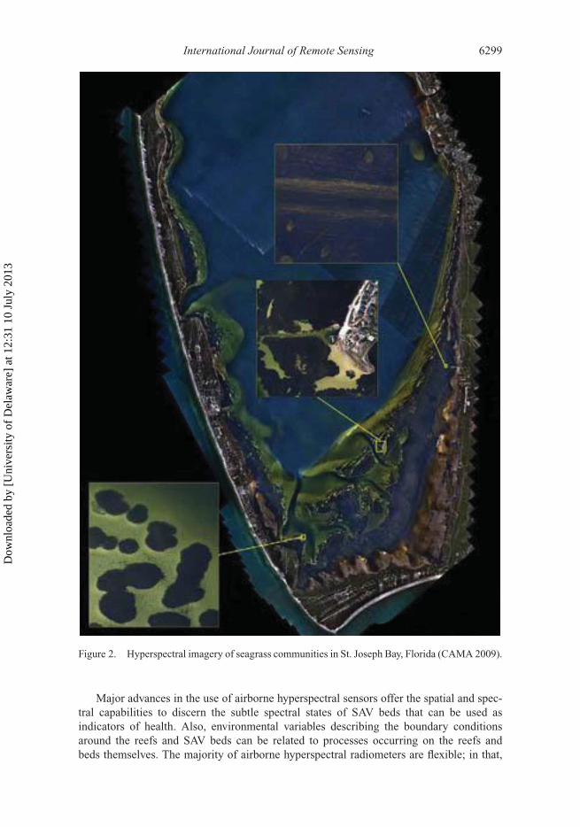
Hyperspectral imagers have improved SAV and coral reef mapping results by beingable to identify a larger number of estuarine and intertidal habitat classes (Maeder et al.2002; Louchard et al. 2003; Garono et al. 2004; Philpot et al. 2004; Mishra et al. 2006;Porter et al. 2006; Phinn et al. 2008; Pu et al. 2012; Purkis, Graham, and Riegl 2008;Nayegandhi and Brock 2008; Wang and Philpot 2007). Figure 2 shows a 2006 hyperspectralimage of seagrass communities in the St. Joseph Bay Aquatic Preserve in Florida. Themaps produced from such images show coverage and extent of seagrass communities inthe bay and provide an indicator of the bay’s health. The maps were used to identify‘good’ areas to be targeted for protection and ‘poor’ areas to be targeted for restoration(CAMA 2009).

SAV has been mapped with high accuracy by using airborne hyperspectral imagers andregression models, binary decision trees incorporating spectral mixture analysis, spectralangle mapping, and band indexes (Hestir et al. 2008; Peneva, Griffith, and Carter 2008;Underwood et al. 2006). Combining airborne hyperspectral imaging with field spectrom-etry, researchers have determined that the best time for mapping is at the end of the SAVgrowing season (Williams et al. 2003).

Dow

nloa

ded

by [

Uni

vers

ity o

f D

elaw

are]

at 1

2:31

10

July

201

3

International Journal of Remote Sensing 6299

Figure 2. Hyperspectral imagery of seagrass communities in St. Joseph Bay, Florida (CAMA 2009).

Major advances in the use of airborne hyperspectral sensors offer the spatial and spec-tral capabilities to discern the subtle spectral states of SAV beds that can be used asindicators of health. Also, environmental variables describing the boundary conditionsaround the reefs and SAV beds can be related to processes occurring on the reefs andbeds themselves. The majority of airborne hyperspectral radiometers are flexible; in that,

Dow

nloa

ded

by [

Uni

vers

ity o

f D

elaw

are]

at 1

2:31

10

July

201

3

6300 V. Klemas

they can be ‘tuned’ to the demands of a specific project, such as mapping SAV or coralreefs (Andréfouët and Riegl 2004; Wang 2010). Airborne lidars have also been used withmultispectral or hyperspectral imagers to map coral reefs and SAV (Brock et al. 2004;Brock et al. 2006; Wang and Philpot 2007; Brock and Purkis 2009; Walker 2009; Yang2009). Protocols have been developed for hyperspectral remote sensing of SAV in shallowwaters (Bostater and Santoleri 2004).

Acoustic techniques have been used for rapid detection of SAV in turbid waters. Theacoustic impedance (density difference between the plant and surrounding water), whichproduces the reflections, is thought to result primarily from the gas within the plant,since the more buoyant species (with more gas) reflect acoustic signals more strongly.Hydroacoustic techniques include horizontally aimed side-scanning sonar systems and ver-tically aimed echo-sounders. Side-scan sonar systems provide complete bottom coverageand generate an image. They have been effective in delineating seagrass beds (Moreno,Siljestrom, and Rey 1998; Sabol et al. 2002). The horizontal orientation of the acousticbeam results in a stronger reflected signal from the vertically oriented grass blades.

Echo-sounders are pointed vertically downward and traverse a path generating a lineon an analogue strip chart, where the horizontal axis is equal to distance, vertical axis isequal to depth, and echo intensity is shown as grey scale. Numerous researchers, usingecho-sounders, have reported success in detecting and qualitatively characterizing seagrassbeds (Spratt 1989; Miner 1993; Hundley 1994). For instance, Sabol et al. (2002) usedhigh-resolution digital echo-sounders linked with GPS equipment. The acoustic reflec-tivity of SAV allowed for the detection and measurement of canopy geometry, usingdigital signal processing algorithms. Comparison with field data showed good detectionand measurement performance over a wide range of conditions.

4. Beach profiling and shoreline change detection

Information on beach profiles and coastal bathymetry is needed for studies of near-shoregeomorphology, hydrology, and sedimentary processes. In order to plan sustainable coastaldevelopment and implement effective beach erosion control, flood zone delineation, andecosystem protection, coastal managers and researchers need information on both long-and short-term changes taking place along the coast, including changes in beach profilesdue to erosion by storms and littoral drift, wetlands changes due to inundation, etc. (West,Lillycrop, and Pope 2001; Gesch 2009).

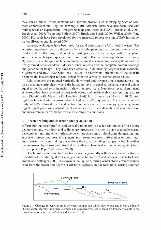
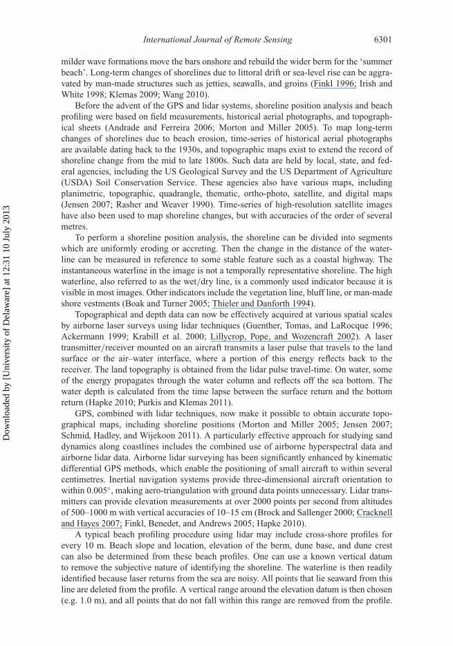
Beach profiles and shoreline positions can change rapidly with seasons and after storms,in addition to exhibiting slower changes due to littoral drift and sea-level rise (Stockdon,Doran, and Sallenger 2009). As shown in the Figure 3, during winter storms, waves removesand from the beach and deposit it offshore, typically in bar formation. During summer,

Figure 3. Changes in beach profiles between summer and winter due to changes in wave climate.During winter storms, the beach is eroded and seaward cross-shore sediment transport results in theformation of offshore bars (Purkis and Klemas 2011).

Dow

nloa

ded

by [

Uni

vers

ity o

f D

elaw

are]

at 1

2:31

10

July

201

3

International Journal of Remote Sensing 6301

milder wave formations move the bars onshore and rebuild the wider berm for the ‘summerbeach’. Long-term changes of shorelines due to littoral drift or sea-level rise can be aggra-vated by man-made structures such as jetties, seawalls, and groins (Finkl 1996; Irish andWhite 1998; Klemas 2009; Wang 2010).

Before the advent of the GPS and lidar systems, shoreline position analysis and beachprofiling were based on field measurements, historical aerial photographs, and topograph-ical sheets (Andrade and Ferreira 2006; Morton and Miller 2005). To map long-termchanges of shorelines due to beach erosion, time-series of historical aerial photographsare available dating back to the 1930s, and topographic maps exist to extend the record ofshoreline change from the mid to late 1800s. Such data are held by local, state, and fed-eral agencies, including the US Geological Survey and the US Department of Agriculture(USDA) Soil Conservation Service. These agencies also have various maps, includingplanimetric, topographic, quadrangle, thematic, ortho-photo, satellite, and digital maps(Jensen 2007; Rasher and Weaver 1990). Time-series of high-resolution satellite imageshave also been used to map shoreline changes, but with accuracies of the order of severalmetres.

To perform a shoreline position analysis, the shoreline can be divided into segmentswhich are uniformly eroding or accreting. Then the change in the distance of the water-line can be measured in reference to some stable feature such as a coastal highway. Theinstantaneous waterline in the image is not a temporally representative shoreline. The highwaterline, also referred to as the wet/dry line, is a commonly used indicator because it isvisible in most images. Other indicators include the vegetation line, bluff line, or man-madeshore vestments (Boak and Turner 2005; Thieler and Danforth 1994).

Topographical and depth data can now be effectively acquired at various spatial scalesby airborne laser surveys using lidar techniques (Guenther, Tomas, and LaRocque 1996;Ackermann 1999; Krabill et al. 2000; Lillycrop, Pope, and Wozencraft 2002). A lasertransmitter/receiver mounted on an aircraft transmits a laser pulse that travels to the landsurface or the air–water interface, where a portion of this energy reflects back to thereceiver. The land topography is obtained from the lidar pulse travel-time. On water, someof the energy propagates through the water column and reflects off the sea bottom. Thewater depth is calculated from the time lapse between the surface return and the bottomreturn (Hapke 2010; Purkis and Klemas 2011).

GPS, combined with lidar techniques, now make it possible to obtain accurate topo-graphical maps, including shoreline positions (Morton and Miller 2005; Jensen 2007;Schmid, Hadley, and Wijekoon 2011). A particularly effective approach for studying sanddynamics along coastlines includes the combined use of airborne hyperspectral data andairborne lidar data. Airborne lidar surveying has been significantly enhanced by kinematicdifferential GPS methods, which enable the positioning of small aircraft to within severalcentimetres. Inertial navigation systems provide three-dimensional aircraft orientation towithin 0.005◦, making aero-triangulation with ground data points unnecessary. Lidar trans-mitters can provide elevation measurements at over 2000 points per second from altitudesof 500–1000 m with vertical accuracies of 10–15 cm (Brock and Sallenger 2000; Cracknelland Hayes 2007; Finkl, Benedet, and Andrews 2005; Hapke 2010).

A typical beach profiling procedure using lidar may include cross-shore profiles forevery 10 m. Beach slope and location, elevation of the berm, dune base, and dune crestcan also be determined from these beach profiles. One can use a known vertical datumto remove the subjective nature of identifying the shoreline. The waterline is then readilyidentified because laser returns from the sea are noisy. All points that lie seaward from thisline are deleted from the profile. A vertical range around the elevation datum is then chosen(e.g. 1.0 m), and all points that do not fall within this range are removed from the profile.

Dow

nloa

ded

by [

Uni

vers

ity o

f D

elaw

are]

at 1

2:31

10

July

201

3

6302 V. Klemas

Finally, a linear regression is fitted through the cluster of points to produce the horizontalposition of the shoreline and the slope, using the elevation datum and regression analysis(Stockdon et al. 2002).

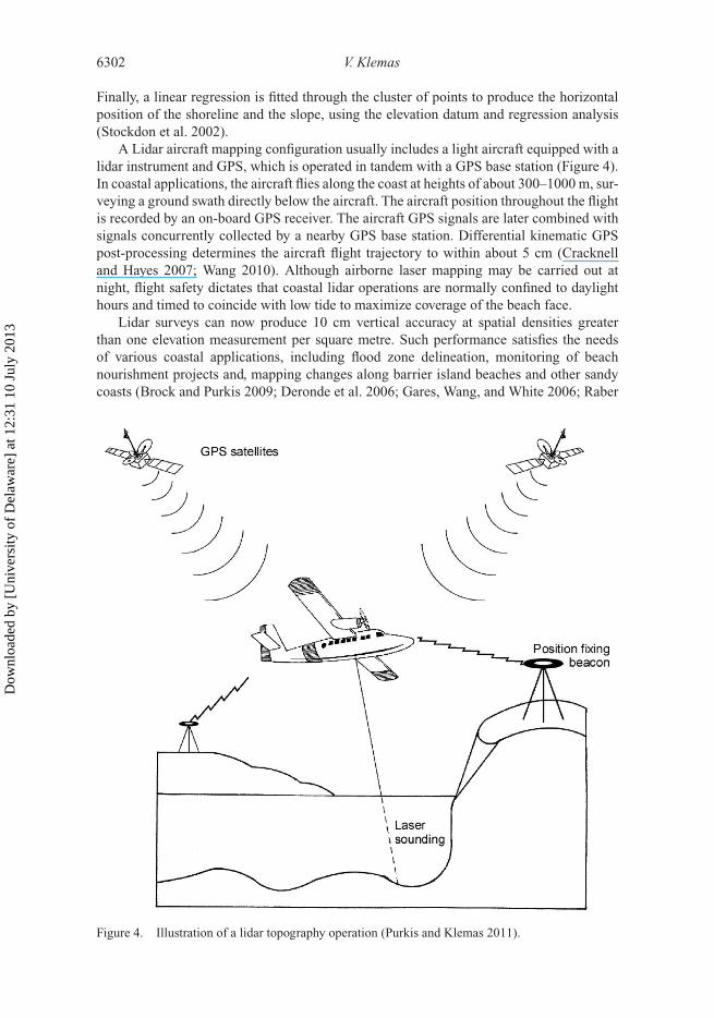
A Lidar aircraft mapping configuration usually includes a light aircraft equipped with alidar instrument and GPS, which is operated in tandem with a GPS base station (Figure 4).In coastal applications, the aircraft flies along the coast at heights of about 300–1000 m, sur-veying a ground swath directly below the aircraft. The aircraft position throughout the flightis recorded by an on-board GPS receiver. The aircraft GPS signals are later combined withsignals concurrently collected by a nearby GPS base station. Differential kinematic GPSpost-processing determines the aircraft flight trajectory to within about 5 cm (Cracknelland Hayes 2007; Wang 2010). Although airborne laser mapping may be carried out atnight, flight safety dictates that coastal lidar operations are normally confined to daylighthours and timed to coincide with low tide to maximize coverage of the beach face.

Lidar surveys can now produce 10 cm vertical accuracy at spatial densities greaterthan one elevation measurement per square metre. Such performance satisfies the needsof various coastal applications, including flood zone delineation, monitoring of beachnourishment projects and, mapping changes along barrier island beaches and other sandycoasts (Brock and Purkis 2009; Deronde et al. 2006; Gares, Wang, and White 2006; Raber

Figure 4. Illustration of a lidar topography operation (Purkis and Klemas 2011).

Dow

nloa

ded

by [

Uni

vers

ity o

f D

elaw

are]

at 1

2:31

10

July

201

3

International Journal of Remote Sensing 6303

et al. 2007; Webster et al. 2004; Wozencraft and Millar 2005). The ability of lidar torapidly survey long, narrow strips of terrain is important because beaches are elongate,highly dynamic, sedimentary environments that undergo seasonal and long-term erosion oraccretion and are also impacted by severe storms (Kempeneers et al. 2009; Krabill et al.2000; Stockdon et al. 2002; Zhou 2010).

In order to develop digital flood insurance maps and data for habitat studies and veg-etation identification, in 2005, the State of Delaware contracted with the US GeologicalSurvey (USGS) and NASA to produce high-detail elevation data using NASA’s exper-imental advanced airborne research lidar (EAARL), which was specifically designed tomeasure submerged topography and adjacent coastal land elevations. Emergency managershave been able to use these data to develop statewide inundation maps and to incorporatethe data into flood and storm surge models to create an early flood warning system (Carterand Scarborough 2010).

Interferometric SAR (InSAR) is also a good candidate as a data source for changedetection on land and in coastal areas. InSAR can be used jointly with GPS and altimeterdata, which helps resolve the integer ambiguity in InSAR phases. Some recent innovativeapplications of InSAR, together with altimeter observations, are described in the literature(Kim et al. 2009; Lu et al. 2009).

5. Bathymetry

The lack of accurate near-shore bathymetric data has been identified as a key limita-tion in the application of geospatial data to coastal environments (Malthus and Mumby2003). Remote-sensing techniques that have been used to map coastal water depth includemultispectral imaging, photogrammetric (stereoscopic) imaging, and lidar depth sounding.The photogrammetric imaging technique is not very effective in coastal waters, since thewater column and its turbidity may distort the bottom image and make the stereo analy-sis difficult. The multispectral imaging approach depends on the fact that different visiblewavelengths penetrate to different depths. It has not been very accurate until the recentphysics-based approach developed by Lee et al. (2010). Acoustic systems, such as echo-sounding profilers, multi-beam echo-sounders, and side-scan sonars, are operated fromships and submerged vehicles to measure depths and map bottom features, especially indeep or turbid waters (Costa, Battista, and Pittman 2009; Mayer et al. 2007; Pittenger1989; Wilson et al. 2007). Since lidar and acoustic depth sounding are the two most reliabletechniques, they will be emphasized in this article.

In lidar bathymetry, a laser transmitter/receiver mounted on an aircraft transmits a pulsethat reflects off the air–water interface and the sea bottom. Since the velocity of the lightpulse is known, the water depth can be calculated from the time lapse between the surfacereturn and the bottom return. Because laser energy is lost due to refraction, scattering, andabsorption at the water surface, the sea bottom, and inside the water column, these effectslimit the strength of the bottom return and limit the maximum detectable depth (Klemas2011b; USACE 2010; Muirhead and Cracknell 1986).

Examples of lidar applications include regional mapping of changes along sandy coastsdue to storms or long-term sedimentary processes and in the analysis of shallow benthicenvironments (Guenther, Tomas, and LaRocque 1996; Irish and Lillycrop 1997; Gutierrezet al. 1998; Sallenger et al. 1999; Bonisteel, Nayegandhi, Brock et al. 2009; Kempeneerset al. 2009). Bertels et al. (2012) used integrated optical and acoustic remote-sensing dataover the backshore–foreshore–nearshore continuum to study sediment dynamics along the

Dow

nloa

ded

by [

Uni

vers

ity o

f D

elaw

are]

at 1

2:31

10

July

201

3

6304 V. Klemas

Belgian coastline. To accomplish this, the authors combined airborne hyperspectral imag-ing spectroscopy, airbore laser scanning, and seaborne sonar. The lidar and hyperspectraldata were combined with side-scan sonar and single- and multi-beam depth and backscatterdata to construct integrated sedimentological and morphological maps (Bertels et al. 2012).In the coastal zone, there is considerable utility in being able to capture seamlessly andsimultaneously topographical lidar above the water with bathymetric postings in the adja-cent ocean. This objective is achievable but, as will be seen below, it demands the use ofmultiple lasers and/or advanced profiling technologies.

To maximize water penetration, bathymetric lidars employ a blue–green laser with atypical wavelength of 530 nm to range the distance to the seabed. With the near-exponentialattenuation of EM energy by water with increasing wavelength, a pure blue laser with awavelength shorter than 500 nm would offer greater penetration. However, this wavelengthis not used because, first, blue light interacts much more strongly with the atmosphere thanlonger wavelengths and second, creating a high-intensity blue laser is energetically lessefficient than blue-green and consumes a disproportionately large amount of instrumentpower.

Conversely, terrestrial topographical lidars typically utilize NIR lasers with wavelengthsof 1064 nm. As is the case for the blue-green laser used for hydrography, this NIR wave-length is focused and easily absorbed by the eye. Therefore, the maximum power of thelidar system is limited by the need to make it eye-safe. While bathymetric lasers are limitedin their accuracy by water column absorption, terrestrial infrared lasers suffer from null orpoor returns from certain materials and surfaces such as water, asphalt, tar, clouds, and fog,all of which absorb NIR wavelengths.

Because NIR topographical lasers do not penetrate water predictably, they cannot beused to assess bathymetry. However, blue-green hydrographical lasers do reflect off terres-trial targets and can be used to measure terrain. Traditionally, their accuracy and spatialresolution have been lower than those provided by a dedicated NIR topographical instru-ment. Dual-wavelength lidar provides both bathymetric and topographical lidar mappingcapability by carrying both an NIR and a blue-green laser. The NIR laser is not redundantover water, because it reflects off the air–water interface and can be used to refine the alti-tude above the sea surface, as well as to distinguish dry land from water using the signalpolarization (Guenther 2007).

In addition, specific lidar systems, such as the Scanning Hydrographic OperationalAirborne Lidar System (SHOALS), record the red wavelength Raman signal (647 nm). TheRaman signal comes from interactions between the blue-green laser and water molecules,causing part of the energy to be backscattered while changing wavelength (Guenther,LaRocque, and Lillycrop 1994; Irish and Lillycrop 1999). A detailed description of theSHOALS system is provided by Lillycrop, Irish, and Parson (1997).

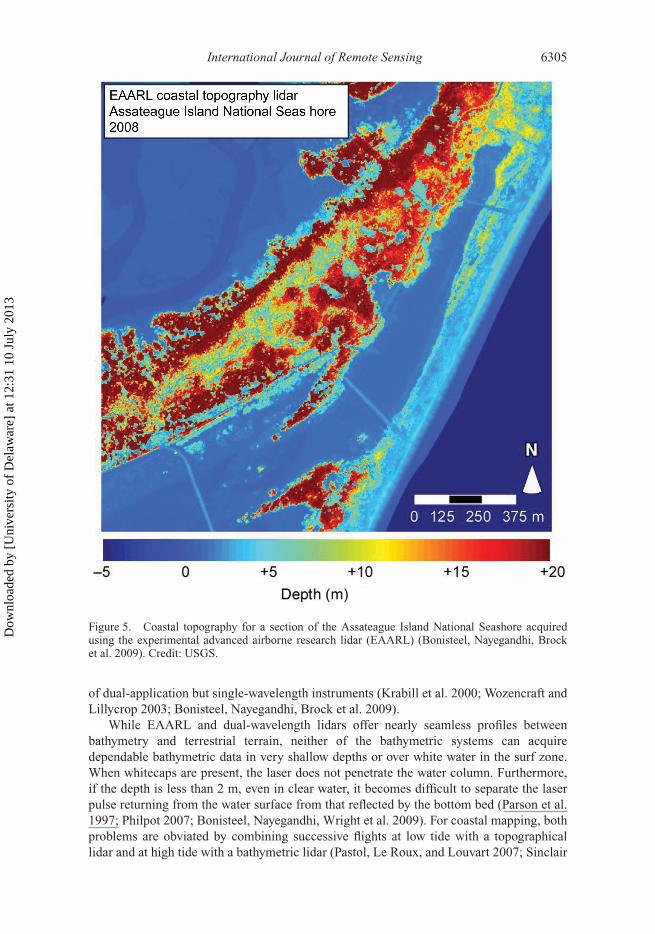
By employing a very high scan-rate, state-of-the-art systems, such as EAARL, havebeen used to measure both topography and bathymetry from the return time of a single blue-green laser (Bonisteel, Nayegandhi, Brock et al. 2009; McKean et al. 2009; Nayegandhi,Brock, and Wright 2009). Operating in the blue-green portion of the EM spectrum, theEAARL is specifically designed to measure submerged topography and adjacent coastalland elevations seamlessly in a single scan of transmitted laser pulses. Figure 5 shows sucha bathymetric-topographical digital elevation model (DEM) of a section of the AssateagueIsland National Seashore, captured by the EAARL. Assateague Island National Seashoreconsists of a 37 mile-long barrier island along the Atlantic coasts of Maryland and Virginia.This experimental advance signalled the future move towards commercial implementation

Dow

nloa

ded

by [

Uni

vers

ity o

f D

elaw

are]

at 1

2:31

10

July

201

3

International Journal of Remote Sensing 6305

Figure 5. Coastal topography for a section of the Assateague Island National Seashore acquiredusing the experimental advanced airborne research lidar (EAARL) (Bonisteel, Nayegandhi, Brocket al. 2009). Credit: USGS.

of dual-application but single-wavelength instruments (Krabill et al. 2000; Wozencraft andLillycrop 2003; Bonisteel, Nayegandhi, Brock et al. 2009).

While EAARL and dual-wavelength lidars offer nearly seamless profiles betweenbathymetry and terrestrial terrain, neither of the bathymetric systems can acquiredependable bathymetric data in very shallow depths or over white water in the surf zone.When whitecaps are present, the laser does not penetrate the water column. Furthermore,if the depth is less than 2 m, even in clear water, it becomes difficult to separate the laserpulse returning from the water surface from that reflected by the bottom bed (Parson et al.1997; Philpot 2007; Bonisteel, Nayegandhi, Wright et al. 2009). For coastal mapping, bothproblems are obviated by combining successive flights at low tide with a topographicallidar and at high tide with a bathymetric lidar (Pastol, Le Roux, and Louvart 2007; Sinclair

Dow

nloa

ded

by [

Uni

vers

ity o

f D

elaw

are]

at 1

2:31

10

July

201

3

6306 V. Klemas

Table 2. Lidar flight parameters.

Flying height 200–500 m (400 m typical)

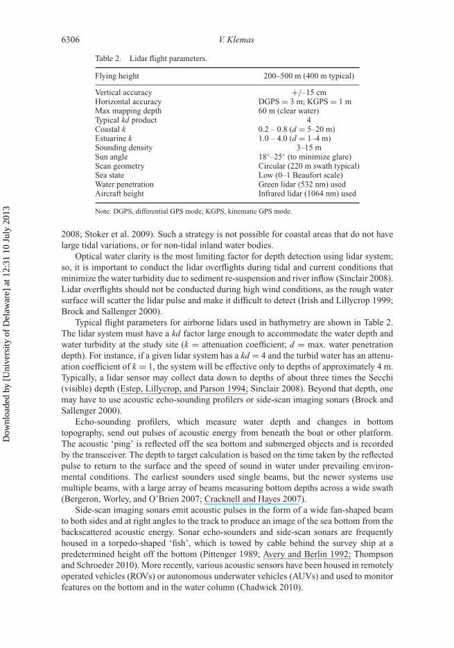
Vertical accuracy +/–15 cmHorizontal accuracy DGPS = 3 m; KGPS = 1 mMax mapping depth 60 m (clear water)Typical kd product 4Coastal k 0.2 – 0.8 (d = 5–20 m)Estuarine k 1.0 – 4.0 (d = 1–4 m)Sounding density 3–15 mSun angle 18◦–25◦ (to minimize glare)Scan geometry Circular (220 m swath typical)Sea state Low (0–1 Beaufort scale)Water penetration Green lidar (532 nm) usedAircraft height Infrared lidar (1064 nm) used

Note: DGPS, differential GPS mode; KGPS, kinematic GPS mode.

2008; Stoker et al. 2009). Such a strategy is not possible for coastal areas that do not havelarge tidal variations, or for non-tidal inland water bodies.

Optical water clarity is the most limiting factor for depth detection using lidar system;so, it is important to conduct the lidar overflights during tidal and current conditions thatminimize the water turbidity due to sediment re-suspension and river inflow (Sinclair 2008).Lidar overflights should not be conducted during high wind conditions, as the rough watersurface will scatter the lidar pulse and make it difficult to detect (Irish and Lillycrop 1999;Brock and Sallenger 2000).

Typical flight parameters for airborne lidars used in bathymetry are shown in Table 2.The lidar system must have a kd factor large enough to accommodate the water depth andwater turbidity at the study site (k = attenuation coefficient; d = max. water penetrationdepth). For instance, if a given lidar system has a kd = 4 and the turbid water has an attenu-ation coefficient of k = 1, the system will be effective only to depths of approximately 4 m.Typically, a lidar sensor may collect data down to depths of about three times the Secchi(visible) depth (Estep, Lillycrop, and Parson 1994; Sinclair 2008). Beyond that depth, onemay have to use acoustic echo-sounding profilers or side-scan imaging sonars (Brock andSallenger 2000).

Echo-sounding profilers, which measure water depth and changes in bottomtopography, send out pulses of acoustic energy from beneath the boat or other platform.The acoustic ‘ping’ is reflected off the sea bottom and submerged objects and is recordedby the transceiver. The depth to target calculation is based on the time taken by the reflectedpulse to return to the surface and the speed of sound in water under prevailing environ-mental conditions. The earliest sounders used single beams, but the newer systems usemultiple beams, with a large array of beams measuring bottom depths across a wide swath(Bergeron, Worley, and O’Brien 2007; Cracknell and Hayes 2007).

Side-scan imaging sonars emit acoustic pulses in the form of a wide fan-shaped beamto both sides and at right angles to the track to produce an image of the sea bottom from thebackscattered acoustic energy. Sonar echo-sounders and side-scan sonars are frequentlyhoused in a torpedo-shaped ‘fish’, which is towed by cable behind the survey ship at apredetermined height off the bottom (Pittenger 1989; Avery and Berlin 1992; Thompsonand Schroeder 2010). More recently, various acoustic sensors have been housed in remotelyoperated vehicles (ROVs) or autonomous underwater vehicles (AUVs) and used to monitorfeatures on the bottom and in the water column (Chadwick 2010).

Dow

nloa

ded

by [

Uni

vers

ity o

f D

elaw

are]

at 1

2:31

10

July

201

3

International Journal of Remote Sensing 6307

6. Summary and conclusions

Advances in technology and decreases in cost are making remote-sensing systems practicalfor use in coastal ecosystem research and management. They are also allowing researchersto take a broader view of ecological patterns and processes. Environmental indicatorsthat can be detected by remote sensors are available to provide quantitative estimates ofcoastal and estuarine habitat conditions and trends. Such indicators include the percentageof impervious watershed area, natural vegetation cover, buffer degradation, wetland lossand fragmentation, wetland biomass change, invasive species, water turbidity, chlorophyllconcentration, and eutrophication. Advances in the application of GIS help to combineremotely-sensed images with other georeferenced data layers, such as DEMs, providing aconvenient means for modelling ecosystem behaviour. A good example is the predictivemodelling of the impact of sea-level rise on coastal wetlands.

Because wetlands are spatially complex and temporally quite variable, mapping emer-gent and submerged aquatic vegetation requires high-spatial resolution satellite or aircraftimagery and, in some cases, hyperspectral data. Traditionally, aerial colour photography hasbeen used to map emergent and submerged wetlands. The recent availability of airbornedigital cameras and satellites carrying sensors with fine spatial (0.4–4 m) or spectral (200+narrow bands) resolution are providing another option for detecting changes in coastalwetlands extent, ecosystem health, biological productivity, and habitat quality.

New image analysis techniques using hyperspectral imagery and narrow-band vegeta-tion indices have been able to discriminate some wetland species and estimate biochemicaland biophysical parameters of wetland vegetation, such as water content, biomass, and leafarea index. The integration of hyperspectral imagery and lidar-derived elevation data hassignificantly improved the accuracy of mapping salt marsh vegetation. Major plant specieswithin a complex, heterogeneous tidal marsh have been classified using multitemporal,high-resolution QuickBird satellite images, field reflectance spectra, and lidar height infor-mation. High-resolution SARs allow one to distinguish between forested wetlands andupland forests.

To identify long-term trends and short-term variations, such as the impact of risingsea levels and hurricanes on wetlands, one needs to analyse time-series of remotely-sensedimagery acquired ideally under similar environmental conditions (e.g. same time of year,sun angle, etc.) and in similar spectral bands. In the pre-processing of multi-date images,the most critical steps are the registration of these images and their radiometric rectifi-cation. Registration accuracies of a fraction of a pixel must be attained. Detecting theactual changes between two corrected images from different dates can be accomplishedby employing one of the several techniques, including post-classification comparison andspectral image differencing. More research is needed to improve the various change-detection techniques, especially for complex coastal landscapes containing wetlands andsubmerged aquatic vegetation.

The main challenge for remote sensing of submerged aquatic plants is to isolate theplant signal from the interference by the water column, the bottom, and the atmosphere.In addition to atmospheric effects and bottom reflectance, optically active materials, such asplankton, suspended sediment, and dissolved organics, affect the scattering and absorptionof radiation. The green region of the spectrum is considered optimal for sensing submergedmacrophytes, followed by the red and red edge regions. The mapping of submerged aquaticvegetation, coral reefs, and general bottom characteristics has benefited from newly avail-able high-resolution (0.6–4.0 m) satellite and aerial hyperspectral imagery. High-resolutionmultispectral data provided by satellites, such as IKONOS and QuickBird, have been used

Dow

nloa

ded

by [

Uni

vers

ity o

f D

elaw

are]

at 1

2:31

10

July

201

3

6308 V. Klemas

to map SAV with accuracies of about 75% for classes including high-density seagrass, low-density seagrass, and unvegetated bottom. Airborne hyperspectral imagers have improvedSAV and coral reef mapping results by being able to identify more estuarine and intertidalhabitat classes.

Lidar techniques, combined with GPS, can provide accurate topographical andbathymetric maps, including shoreline positions. Lidar surveys can produce a 10–15 cmvertical accuracy at a high spatial resolution. Lidar data are used in many research and man-agement applications, including flood zone delineation, monitoring of beach nourishmentprojects, and mapping of changes along sandy coasts and shallow benthic environmentsdue to storms or long-term sedimentary processes. Typically, a lidar sensor may collect datadown to depths of about three times the Secchi depth. If the depth or the water turbidity istoo great, acoustic echo-sounding is used.

Limited spatial resolution has been a problem in wetland studies, resulting in toomany mixed pixels. Another problem has been the complexity of image-processing pro-cedures that are required before hyperspectral data can be used for automated classificationof wetland vegetation. Furthermore, the tremendous volume of hyperspectral image datanecessitates the use of specific software packages, large data storage capacity, and extendedprocessing time (Hirano, Madden, and Welch 2003).

Some practical recommendations are as follows.

(1) The cost per square kilometre of imagery and its analysis rises very rapidly asone goes from medium- to high-resolution imagery. Large wetland areas should bemapped using medium-resolution sensors (e.g. Landsat TM at 30 m), if the lossof accuracy is acceptable, and only small, critical areas should be examined withhigh-resolution sensors (e.g. IKONOS at 1–4 m).

(2) When considering optical passive data, multispectral imagery should be usedfor most applications, with hyperspectral imagery reserved for difficult speciesidentification cases, larger budgets, and highly experienced image analysts.

(3) Airborne digital camera imagery is not only useful for mapping coastal land coverbut is also very helpful in interpreting satellite images.

(4) The combined use of lidar, radar, and multispectral or hyperspectral imagery canimprove the accuracy of emergent and submerged aquatic species discriminationand provide a better understanding of the topography/bathymetry and hydrologicconditions.

(5) High-resolution imagery is more sensitive to within-class spectral variance, mak-ing separation of spectrally mixed land-cover types more difficult. Therefore,pixel-based techniques are sometimes replaced by object-based methods, whichincorporate spatial neighbourhood properties. In the object-based approach, theimage is segmented/partitioned into a series of closed objects which coincide withthe actual spatial pattern and are only then classified.

In summary, one can conclude that when remote-sensing systems are used wisely, includingcomplementary combinations of different satellite and airborne sensors, they can providedata that enhance the research and management of coastal ecosystems. Remote sensors canmonitor and assess long-term trends and short-term changes of vegetation and hydrologyfaster, more completely, and at lower cost per unit area than field or ship surveys alone.

Future research priorities should include better understanding and description ofbiotope classes, the functional interpretation of biotope maps, and the radiative properties

Dow

nloa

ded

by [

Uni

vers

ity o

f D

elaw

are]

at 1

2:31

10

July

201

3

International Journal of Remote Sensing 6309

of coastal environments. Additional knowledge is required about the spatial and tempo-ral variations of water column optical properties and its constituents. Best approachesfor processing hyperspectral data need to be further investigated and hyperspectral sen-sors need to be tested for bottom type discrimination using data obtained from satellites.Finally, there is a need to investigate the improvements gained from the synergistic use ofmulti-wavelength remote-sensing approaches, change-detection techniques, multitemporalcomparisons, and knowledge-based approaches, used for improving classification accuracy(Malthus and Mumby 2003).

References

Ackermann, F. 1999. “Airborne Laser Scanning – Present Status and Future Expectations.” ISPRSJournal of Photogrammetry and Remote Sensing 54: 64–67.

Ackleson, S. G., and V. Klemas. 1987. “Remote Sensing of Submerged Aquatic Vegetation inLower Chesapeake Bay: A Comparison of Landsat MSS to TM Imagery.” Remote Sensing ofEnvironment 22: 235–248.

Adam, E., O. Mutanga, and D. Rugege. 2010. “Multispectral and Hyperspectral Remote Sensingfor Identification and Mapping of Wetland Vegetation: A Review.” Wetlands Ecology andManagement 18: 281–296.

Akins, E. R., Y. Wang, and Y. Zhou. 2010. “EO-1 Advanced Land Imager Data in Submerged AquaticVegetation Mapping.” In Remote Sensing of Coastal Environment, edited by J. Wang, 297–312,Boca Raton, FL: CRC Press.

Allen, T. R., and J. A. Kupfer. 2000. “Application of Spherical Statistics to Change Vector Analysisof Landsat Data: Southern Appalachian Spruce-Fir Forest.” Remote Sensing of Environment 74:482–493.

Andrade, F., and M. A. Ferreira. 2006. “A Simple Method of Measuring Beach Profiles.” Journal ofCoastal Research 22: 995–999.

Andréfouët, S., and B. M. Riegl. 2004. “Remote Sensing: A Key Tool for InterdisciplinaryAssessment of Coral Reef Processes.” Coral Reefs 23: 1–4.

Armstrong, R. A. 1993. “Remote Sensing of Submerged Vegetation Canopies for BiomassEstimation.” International Journal of Remote Sensing 14: 621–627.

Artigas, F. J., and J. Yang. 2006. “Spectral Discrimination of Marsh Vegetation Types in the NewJersey Meadowlands, USA.” Wetlands 26: 271–277.

Avery, T. E., and G. L. Berlin. 1992. Fundamentals of Remote Sensing and Airphoto Interpretation.New York: Macmillan Publishing Company.

Baghdadi, N., M. Bernier, R. Gauthier, and I. Neeson. 2001. “Evaluation of C-band SAR Data forWetlands Mapping.” International Journal of Remote Sensing 22: 71–88.

Baker, A. 2003. “Land Use and Water Quality.” Hydrological Processes 17: 2499–2501.Baker, C., R. L. Lawrence, C. Montagne, and D. Patten. 2007. “Change Detection of Wetland

Ecosystems Using Landsat Imagery and Change Vector Analysis.” Wetlands 27: 610–619.Baldwin, A. H., and I. A. Mendelssohn. 1998. “Effects of Salinity and Water Level on Coastal

Marshes: An Experimental Test of Disturbance as a Catalyst for Vegetation Change.” AquaticBotany 61: 255–268.

Bergeron, E., C. R. Worley, and T. O’Brien. 2007. “Progress in the Development of Shallow WaterMapping Systems.” Sea Technology 48: 10–15.

Bertels, L., R. Houthuys, B. Deronde, R. Janssens, E. Verfaillie, and V. Van Lancker. 2012.“Integration of Optical and Acoustic Remote Sensing Data over the Backshore-Foreshore-Nearshore Continuum: A Case Study in Ostend (Belgium).” Journal of Coastal Research 28:1426–1436.

Blasco, F., M. Aizpuru, and D. Din Ndongo. 2005. “Mangroves Remote Sensing.” In Encyclopediaof Coastal Science, edited by M. L. Schwartz, 614–617. Dordrecht: Springer.

Boak, E. H., and I. L. Turner. 2005. “Shoreline Definition and Detection: A Review.” Journal ofCoastal Research 21: 688–703.

Bonisteel, J. M., A. Nayegandhi, J. C. Brock, C. W. Wright, S. Stevens, X. Yates, and E. S. Klipp.2009. EAARL Coastal Topography – Assateague Island National Seashore 2008: First Surface.Reston, VA: US Geological Survey Data Series 446.

Dow

nloa

ded

by [

Uni

vers

ity o

f D

elaw

are]

at 1

2:31

10

July

201

3

6310 V. Klemas

Bonisteel, J. M., A. Nayegandhi, C. W. Wright, J. C. Brock, and D. B. Nagle. 2009. ExperimentalAdvanced Airborne Research LiDAR (EAARL) Data Processing Manual. Reston, VA: USGeological Survey Open-File Report 2009–1078.

Bostater, C. R. Jr., and R. Santoleri. 2004. “Hyperspectral Remote Sensing Protocol Development forSubmerged Aquatic Vegetation in Shallow Waters.” In Proceedings of the SPIE 5233, Barcelona,September 9, 199–215. Bellingham, WA: Society of Photo-Optical Instrumentation Engineers.

Bourgeau-Chavez, L. L., E. S. Kasischke, S. M. Brunzell, J. P. Mudd, K. B. Smith, and A. L.Frick. 2001. “Analysis of Space-Borne SAR Data for Wetland Mapping in Virginia RiparianEcosystems.” International Journal of Remote Sensing 22: 3665–3687.

Brando, V. E., and A. G. Decker. 2003. “Satellite Hyperspectral Remote Sensing for EstimatingEstuarine and Coastal Water Quality.” IEEE Transactions on Geoscience and Remote Sensing41: 1378–1387.

Brock, J., and A. Sallenger. 2000. Airborne Topographic Mapping for Coastal Science and ResourceManagement. Reston, VA: USGS Open-File Report 01–46.

Brock, J. C., and S. J. Purkis. 2009. “The Emerging Role of LiDAR Remote Sensing in CoastalResearch and Resource Management. Special Issue 53 – Coastal Applications of AirborneLiDAR.” Journal of Coastal Research 53: 1–5.

Brock, J. C., C. W. Wright, T. D. Clayton, and A. Nayegandhi. 2004. “LIDAR Optical Rugosity ofCoral Reefs in Biscayne National Park, Florida.” Coral Reefs 23: 48–59.

Brock, J. C., C. W. Wright, I. B. Kuffner, R. Hernandez, and P. Thompson. 2006. “Airborne LiDARSensing of Massive Stony Coral Colonies on Patch Reefs in the Northern Florida Reef Tract.”Remote Sensing of Environment 104: 31–42.

Bustamante, J., F. Pacios, R. Diaz-Delgado, and D. Aragones. 2009. “Predictive Models of Turbidityand Water Depth in the Donana Marshes Using Landsat TM and ETM+ Images.” Journal ofEnvironmental Management 90: 2219–2225.

CAMA. 2009. “Mapping and Monitoring Seagrass Communities.” Office of Coastal and AquaticManagement Areas, Florida Department of Environmental Protection. Accessed June 21, 2012.http://www.dep.state.fl.us/coastal/habitats/seagrass/management/mapping.htm

Campbell, J. B. 2007. Introduction to Remote Sensing. New York: The Guilford Press.Carter, D., and R. Scarborough. 2010. “Sharing Delaware’s Lidar Lessons. NOAA Coastal Services

Center Report.” Local Strategies for Addressing Climate Change 2: 16–17.Chadwick, W. 2010. “Remotely Operated Vehicles (ROVs) and Autonomous Underwater Vehicles

(AUVs).” NOAA Ocean Explorer: Submarine Ring of Fire 2002: Background. AccessedOctober 1, 2011. http://oceanexplorer.noaa.gov/explorations/02fire/background/rovsauvs/rov_auv.html

Christian, B., and N. S. R. Krishnayya. 2009. “Classification of Tropical Trees Growing in a SanctuaryUsing Hyperion (EO-1) and SAM Algorithm.” Current Science 96: 1601–1607.

Church, J. A., and N. J. White. 2006. “A 20th Century Acceleration of Global Sea-Level Rise.”Geophysical Research Letters 33: L01602.

Civco, D. L., J. D. Hurd, E. H. Wilson, M. Song, and Z. Zhang. 2002. “A Comparison of LandUse and Land Cover Change Detection Methods.” In American Congress on Surveying andMapping – American Society for Photogrammetry and Remote Sensing 2002 Annual ConferenceProceedings. Bethesda, MD: American Society for Photogrammetry and Remote Sensing.

Coppin, P., I. Jonckhere, K. Nackaerts, B. Mays, and E. Lambin. 2004. “Digital Change DetectionMethods in Ecosystem Monitoring: A Review.” International Journal of Remote Sensing 25:1565–1596.

Costa, B. M., T. A. Battista, and S. J. Pittman. 2009. “Comparative Evaluation of Airborne LiDAR andShip-Based Multibeam SoNAR Bathymetry and Intensity for Mapping Coral Reef Ecosystems.”Remote Sensing of Environment 113: 1082–1100.

Costa, M. P. F., and K. H. Telmer. 2007. “Mapping and Monitoring Lakes in the BrazilianPantanal Wetland Using Synthetic Aperture Radar Imagery.” Aquatic Conservation: Marine andFreshwater Ecosystems 17: 277–288.

Cracknell, A. P., and L. Hayes. 2007. Introduction to Remote Sensing. New York: CRC Press.Dahl, T. E. 2006. Status and Trends of Wetlands in the Conterminous United States 1998 to 2004,

112 p. Washington, DC: US Department of the Interior, Fish and Wildlife Service Publication.Deronde, B., R. Houthuys, W. Debruyn, D. Fransaer, V. V. Lancker, and J.-P. Hernriet. 2006. “Use

of Airborne Hyperspectral Data and Laserscan Data to Study Beach Morphodynamics along theBelgian Coast.” Journal of Coastal Research 22: 1108–1117.

Dow

nloa

ded

by [

Uni

vers

ity o

f D

elaw

are]

at 1

2:31

10

July

201

3

International Journal of Remote Sensing 6311

Dierssen, H. M., R. C. Zimmermann, R. A. Leathers, V. Downes, and C. O. Davis. 2003. “OceanColor Remote Sensing of Seagrass and Bathymetry in the Bahamas Banks by High ResolutionAirborne Imagery.” Limnology and Oceanography 48: 444–455.

DigitalGlobe. 2003. Quickbird Imagery Products and Product Guide (revision 4). Longmont, CO:Digital Globe.

Dobson, J. E., E. A. Bright, R. L. Ferguson, D. W. Field, L. L. Wood, K. D. Haddad, H. Iredale, III, J. R.Jensen, V. V. Klemas, R. J. Orth, and J. P. Thomas. 1995. NOAA Coastal Change Analysis Program(C-CAP): Guidance for Regional Implementation, 92 p. NOAA Technical Report NMFS-123.Washington, DC: US Department of Commerce.

Dwivedi, R., B. Rao, and S. Bhattacharya. 1999. “Mapping Wetlands of the Sundaban Delta and it’sEnvirons Using ERS-1 SAR Data.” International Journal of Remote Sensing 20: 2235–2247.

Ellis, J. M., and H. S. Dodd. 2000. “Applications and Lessons Learned with Airborne MultispectralImaging.” In Fourteenth International Conference on Applied Geologic Remote Sensing, LasVegas, Nevada. Dordrecht: Springer.

Estep, L. L., W. J. Lillycrop, and L. E. Parson. 1994. “Estimation of Maximum Depth of Penetrationof a Bathymetric Lidar System Using a Secchi Depth Data Base.” Marine Technology SocietyJournal 28: 31–36.

Everitt, J. H., C. Yang, D. E. Escobar, C. F. Webster, R. I. Lonard, and M. R. Davis. 1999.“Using Remote Sensing and Spatial Information Technologies to Detect and Map Two AquaticMacrophytes.” Journal of Aquatic Plant Management 37: 71–80.

Farris, G. S. 2005. “USGS Reports New Wetland Loss from Hurricane Katrina in SoutheasternLouisiana.” Accessed October 1, 2011. http://www.usgs.gov/newsroom/article

Ferguson, R. L., and K. F. Korfmacher, 1997. “Remote Sensing and GIS Analysis of SeagrassMeadows in North Carolina, USA.” Aquatic Botany 58: 241–258.

Ferguson, R. L., and L. L. Wood. 1990. “Mapping Submerged Aquatic Vegetation in NorthCarolina with Conventional Aerial Photography.” Fish and Wildlife Service Biological Report90: 125–133.

Ferguson, R. L., L. L. Wood, and D. B. Graham. 1993. “Monitoring Spatial Change in SeagrassHabitat with Aerial Photography.” Photogrammetric Engineering and Remote Sensing 59:1033–1038.

Field, R. T., and K. R. Philipp. 2000. “Vegetation Changes in the Freshwater Tidal Marsh of theDelaware Estuary.” Wetlands Ecology and Management 8: 79–88.

Filippi, A. M., and J. R. Jensen. 2006. “Fuzzy Learning Vector Quantization for Hyperspectral CoastalVegetation Classification.” Remote Sensing of Environment 100: 512–530.

Finkbeiner, M., W. Stevenson, and R. Seaman. 2001. Guidance for Benthic Habitat Mapping: AnAerial Photographic Approach, 73 p. NOAA/CSC/20117-PUB. Charleston, SC: NOAA-CSC.

Finkl, C. W. 1996. “What Might Happen to America’s Shorelines if Artificial Beach Replenishmentis Curtailed: A Prognosis for Southeastern Florida and Other Sandy Regions along RegressiveCoasts.” Journal of Coastal Research 12: ii–ix.

Finkl, C. W., L. Benedet, and J. L. Andrews. 2005. “Interpretation of Seabed Geomorphology Basedon Spatial Analysis of High-Density Airborne Laser Bathymetry (ALB).” Journal of CoastalResearch 21: 501–514.

Fyfe, S. K. 2003. “Are Seagrasses Spectrally Distinct?” Limnology and Oceanography 48: 464–479.Gares, P. A., Y. Wang, and S. A. White. 2006. “Using Lidar to Monitor a Beach Nourishment Project

at Wrightsville Beach, North Carolina, USA.” Journal of Coastal Research 22: 1206–1219.Garono, R. J., C. A. Simenstad, R. Robinson, and H. Ripley. 2004. “Using High Spatial Resolution

Hyperspectral Imagery to Map Intertidal Habitat Structure in Hood Canal Washington, USA.”Canadian Journal of Remote Sensing 30: 54–63.

Gesch, D. B. 2009. “Analysis of Lidar Elevation Data for Improved Identification and Delineation ofLands Vulnerable to Sea-Level Rise.” Journal of Coastal Research 53: 49–58.

Ghioca-Robrecht, D. M., C. A. Johnston, and M. G. Tulbure. 2008. “Assessing the Use of MultiseasonQuickBird Imagery for Mapping Invasive Species in Great Lakes Coastal Marsh.” Wetlands 28:1028–1039.

Gilmore, M. S., D. L. Civco, E. H. Wilson, N. Barrett, S. Prisloe, J. D. Hurd, and C. Chadwick. 2010.“Remote Sensing and In Situ Measurements for Delineation and Assessment of Coastal Marshesand their Constituent Species.” In Remote Sensing of Coastal Environment, edited by J. Wang,261–280. Boca Raton, FL: Springer.

Dow

nloa

ded

by [

Uni

vers

ity o

f D

elaw

are]

at 1

2:31

10

July

201

3

6312 V. Klemas

Gilmore, M. S., E. H. Wilson, N. Barrett, D. L. Civco, S. Prisloe, J. D. Hurd, and C. Chadwick. 2008.“Integrating Multitemporal Spectral and Structural Information to Map Wetland Vegetation in aLower Connecticut River Tidal Marsh.” Remote Sensing of Environment 112: 4048–4060.

Goetz, S. J., C. A. Jantz, S. D. Prince, A. J. Smith, D. Varlyguin, and R. K. Wright. 2004. “IntegratedAnalysis of Ecosystem Interactions with Land Use Change: The Chesapeake Bay Watershed.”Ecosystems and Land Use Change Geophysical Monograph Series 153: 263–275.

Green, E. P., and F. T. Short. 2003. World Atlas of Seagrasses. Berkeley, CA: California UniversityPress.

Guenther, G. 2007. “Airborne LiDAR Bathymetry Digital Elevation. Model Technologies andApplications.” In The DEM Users Manual, edited by D. Maune, 253–320. Bethesda, MD:American Society for Photogrammetry and Remote Sensing.

Guenther, G., P. LaRocque, and W. Lillycrop. 1994. “Multiple Surface Channels in SHOALSAirborne LiDAR.” SPIE: Ocean Optics XII 2258: 422–430.

Guenther, G. C., R. W. L. Tomas, and P. E. LaRocque. 1996. “Design Considerations for AchievingHigh Accuracy with the SHOALS Bathymetric LiDAR System.” SPIE: Laser Remote Sensing ofNatural Waters: From Theory to Practice 15: 54–71.

Gullstrom, M., B. Lunden, M. Bodin, J. Kangwe, M. C. Ohman, S. P. Mtolera, and M. Bjork.2006. “Assessment of Changes in the Seagrass-Dominated Submerged Vegetation of TropicalChwaka Bay (Zanzibar) Using Satellite Remote Sensing.” Estuarine, Coastal and Shelf Science67: 399–408.

Gutierrez, R., J. C. Gibeaut, M. M. Crawford, M. P. Mahoney, S. Smith, W. Gutelius, D. Carswell,and E. MacPherson. 1998. “Airborne Laser Swath Mapping of Galveston Island and BolivarPeninsula, Texas.” In Proceedings of the Fifth International Conference on Remote Sensing forMarine and Coastal Environments, Vol. 1, San Diego, CA, October 5–7, 236–243. Ann Arbor,MI: Environmental Research Institute of Michigan.

Hall, D. K. 1996. “Remote Sensing Applications to Hydrology: Imaging Radar.” HydrologicalSciences Journal 41: 609–624.

Hame, T. I., I. Heiler, and J. S. Miguel-Ayanz. 1998. “An Unsupervised Change Detection andRecognition System for Forestry.” International Journal of Remote Sensing 19: 1079–1099.

Han, L., and D. Rundquist. 2003. “The Spectral Responses of Cerathophyllum demersum at VaryingDepths in an Experimental Tank.” International Journal of Remote Sensing 24: 859–864.

Hapke, C. J. 2010. “Integration of LiDAR and Historical Maps to Measure Coastal Change on aVariety of Time and Spatial Scales.” In Remote Sensing of Coastal Environments, edited by Y.Wang, 79–102. Boca Raton, FL: Springer CRC Press.

Harris, J., and S. Digby-Argus. 1986. “The Detection of Wetlands on Radar Imagery.” In Proceedingsof the Tenth Canadian Symposium on Remote Sensing, Edmonton, May 5–8. Ottawa: CanadianAeronautics and Space Institute.

Harvey, K. R., and J. E. Hill. 2001. “Vegetation Mapping of a Tropical Freshwater Swamp in theNorthern Territory, Australia: A Comparison of Aerial Photography, Landsat TM and SPOTSatellite Imagery.” Remote Sensing of Environment 22: 2911–2925.

Heege, T., A. Bogner, and N. Pinnel. 2003. “Mapping of Submerged Aquatic Vegetation with aPhysically Based Process Chain.” SPIE Proceedings on Remote Sensing 5233: 43–50.

Hemminga, M. A., and C. M. Duarte. 2000. Seagrass Ecology. Cambridge: Cambridge UniversityPress.

Hess, L., J. Melack, S. Filoso, and Y. Wang. 1995. “Delineation of Inundated Area and Vegetationalong the Amazon Floodplain with the SIR-C Synthetic Aperture Radar.” IEEE Transactions onGeoscience and Remote Sensing 33: 896–904.

Hess, L., J. Melack, and D. Simonett. 1990. “Radar Detection of Flooding Beneath the Forest Canopy:A Review.” International Journal of Remote Sensing 11: 1313–1325.

Hestir, E. L., S. Khanna, M. E. Andrew, M. J. Santos, J. H. Viers, J. A. Greenberg, S. S. Rajapakse,and S. Ustin. 2008. “Identification of Invasive Vegetation Using Hyperspectral Remote Sensingin the California Delta Ecosystem.” Remote Sensing of Environment 112: 4034–4047.

Heumann, B. W. 2011. “Satellite Remote Sensing of Mangrove Forests: Recent Advances and FutureOpportunities.” Progress in Physical Geography 35: 87–108.

Hirano, A., M. Madden, and R. Welch. 2003. “Hyperspectral Image Data for Mapping WetlandVegetation.” Wetlands 23: 436–448.

Houhoulis, P., and W. Michener. 2000. “Detecting Wetland Change: A Rule-Based Approach UsingNWI and SPOT-XS Data.” Photogrammetric Engineering and Remote Sensing 66: 205–211.

Dow

nloa

ded

by [

Uni

vers

ity o

f D

elaw

are]

at 1

2:31

10

July

201

3

International Journal of Remote Sensing 6313

Hughes, A. R., S. L. Williams, C. M. Duarte, K. L. Heck, Jr., and M. Waycott. 2009. “Associationsof Concern: Declining Seagrasses and Threatened Dependent Species.” Frontiers in Ecology andthe Environment 7: 242–246.

Hundley, A. 1994. Report on the Use of an Acoustic Method for Mapping Seagrass Density andLocation. Report No. 940401. Sydney, NSW: Offshore Scientific Services.

Ikeda, M., and F. W. Obson. 1995. Oceanographic Applications of Remote Sensing. New York: CRCPress.

Intergovernmental Panel on Climate Change. 2007. Climate Change 2007: The Physical ScienceBasis, Paris. Accessed January 6, 2009. WMO/UNEP.www.ipcc.ch

Irish, J. L., and W. J. Lillycrop. 1997. “Monitoring New Pass, Florida, with High-Density LiDARBathymetry.” Journal of Coastal Research 13: 1130–1140.

Irish, J. L., and W. J. Lillycrop. 1999. “Scanning Laser Mapping of the Coastal Zone: The SHOALSSystem.” ISPRS Journal of Photogram and Remote Sensing 54: 123–129.

Irish, J. L., and T. E. White. 1998. “Coastal Engineering Applications of High ResolutionBathymetry.” Coastal Engineering 35: 47–71.

Jensen, J. R. 1996. Introductory Digital Image Processing: A Remote Sensing Perspective. 2nd ed.Upper Saddle River, NJ: Pearson Prentice-Hall.

Jensen, J. R. 2007. Remote Sensing of the Environment: An Earth Resource Perspective. Upper SaddleRiver, NJ: Pearson Prentice-Hall.

Jensen, R. R., P. Mausel, N. Dias, R. Gonser, C. Yang, J. Everitt, and R. Fletcher. 2007. “SpectralAnalysis of Coastal Vegetation and Land Cover Using AISA+ Hyperspectral Data.” GeocartoInternational 22: 17–28.

Johnson, R. D., and E. S. Kasischke. 1998. “Change Vector Analysis: A Technique for theMultispectral Monitoring of Land Cover and Condition.” International Journal of RemoteSensing 19: 411–426.

Kasischke, E., and L. Bourgeau-Chavez. 1997. “Monitoring South Florida Wetlands Using ERS-1 SAR Imagery.” Photogrammetric Engineering and Remote Sensing 63: 281–291.

Kasischke, E., L. Bourgeau-Chavez, K. Smith, E. Romanowicz, and C. Richardson. 1997.“Monitoring Hydropatterns in South Florida Ecosystems Using ERS SAR Data.” In 3rd ERSSymposium on Space at the Service of our Environment, Florence, March 5. Paris: EuropeanSpace Agency.

Kasischke, E., J. Melack, and M. Dobson. 1997. “The Use of Imaging Radars for EcologicalApplications-A Review.” Remote Sensing of Environment 59: 141–156.

Kelly, M., and K. Tuxen. 2009. “Remote Sensing Support for Tidal Wetland Vegetation Researchand management.” In Remote Sensing and Geospatial Technologies for Coastal EcosystemAssessment and Management, edited by X. Yang, 341–363. Berlin: Springer-Verlag.

Kempeneers, P., B. Deronde, S. Provoost, and R. Houthuys. 2009. “Synergy of Airborne DigitalCamera and LiDAR Data to Map Coastal Dune Vegetation.” Journal of Coastal Research 53:73–82.

Kim, J. W., Z. Lu, H. Lee, C. K. Shum, C. H. Swarzenski, T. W. Doyle, and S.-H. Baek. 2009.“Integrated Analysis of PALSAR/Radarsat-1 InSAR and ENVISAT Altimeter Data for Mappingof Absolute Water Level Changes in Louisiana Wetlands.” Remote Sensing of Environment 113:2356–2365.

Kirk, J. T. O. 1994. Light and Photosynthesis in Aquatic Ecosystems. Cambridge: CambridgeUniversity Press.

Klemas, V. 2009. “The Role of Remote Sensing in Predicting and Determining Coastal StormImpacts.” Journal of Coastal Research 25: 1264–1275.

Klemas, V. 2011a. “Remote Sensing of Wetlands: Case Studies Comparing Practical Techniques.”Journal of Coastal Research 27: 418–427.

Klemas, V. 2011b. “Beach Profiling and LIDAR Bathymetry: An Overview with Case Studies.”Journal of Coastal Research 27: 1019–1028.

Klemas, V. 2012. “Remote Sensing of Algal Blooms: An Overview with Case Studies.” Journal ofCoastal Research 28: 34–43.

Klemas, V., J. E. Dobson, R. L. Ferguson, and K. D. Haddad. 1993. “A Coastal Land CoverClassification System for the NOAA Coastwatch Change Analysis Project.” Journal of CoastalResearch 9: 862–872.

Kolasa, K. V., and V. Craw. 2009. “Improving Seagrass Maps of Florida’s Springs Coast throughDigital Imagery.” In Proceedings of the ASPRS 2009 Annual Conference, Baltimore, MD, March9–13. Bethesda, MD: American Society for Photogrammetry and Remote Sensing.

Dow

nloa

ded

by [

Uni

vers

ity o

f D

elaw

are]

at 1

2:31

10

July

201

3

6314 V. Klemas

Krabill, W. B., C. W. Wright, R. N. Swift, E. B. Frederick, S. S. Manizade, J. K. Yungel, C. F. Martin,J. G. Sonntag, M. Duffy, W. Hulslander, and J. C. Brock. 2000. “Airborne Laser Mapping ofAssateague National Seashore Beach.” Photogrammetric Engineering and Remote Sensing 66:65–71.

Laba, M., R. Downs, S. Smith, S. Welsh, C. Neider, S. White, M. Richmond, W. Philpot, andP. Baveye. 2008. “Mapping Invasive Wetland Plants in the Hudson River National EstuarineResearch Reserve Using Quickbird Satellite Imagery.” Remote Sensing of Environment 112:286–300.

Lang, M., G. McCarty, and M. Anderson. 2008. “Monitoring Wetland Hydrology at a WatershedScale: Dynamic Information for Adaptive Management.” Journal of Soil and Water Conservation63: 49A.

Lang, M. W., and E. S. Kasischke. 2008. “Using C-band Synthetic Aperture Radar Data toMonitor Forested Wetland Hydrology in Maryland’s Coastal Plain, USA.” IEEE Transactionson Geoscience and Remote Sensing 46: 535–546.

Lang, M. W., and G. W. McCarty. 2008. “Remote Sensing Data for Regional Wetland Mappingin the United States: Trends and Future Prospects.” In Wetlands: Ecology, Conservation andRestoration, edited by R. E. Russo, 1–40. Hauppauge, NY: Nova Science Publishers.

Lathrop, R. G., M. B. Cole, and R. D. Showalter. 2000. “Quantifying the Habitat Structure and SpatialPattern of New Jersey (USA) Salt Marshes under Different Management Regimes.” WetlandsEcology and Management 8: 163–172.

Lee, S. W., S. J. Hwang, S. B. Lee, H. S. Hwang, and H. C. Sung. 2009. “LandscapeEcological Approach to the Relationships of Land Use Patterns in Watersheds to Water QualityCharacteristics.” Landscape and Urban Planning 92: 80–89.

Lee, Z. P., C. Hu, B. Casey, S. Shang, H. Dierssen, and R. Arnone. 2010. “Global Shallow-WaterBathymetry from Satellite Ocean Color Data. American Geophysical Union.” EOS Transactions91: 1–2.

Leon, L. F., D. C. Lam, D. A. Swayne, D. J. Farquhar, and E. D. Soulis. 2000. “Integration of aNonpoint Source Pollution Model with a Decision Support System.” Journal of EnvironmentalModeling and Software 15: 249–255.

Li, L., S. L. Ustin, and M. Lay. 2005. “Application of Multiple Endmember Spectral Mixture Analysis(MESMA) to AVIRIS Imagery for Coastal Salt Marsh Mapping: A Case Study in China Camp,CA, USA.” International Journal of Remote Sensing 26: 5193–5207.

Li, M., L. Zhong, W. C. Boicourt, S. Zhang, and D. Zhang. 2007. “Hurricane-Induced Stratificationand Destratification in a Partially-Mixed Estuary.” Journal of Marine Research 65: 169–192.

Lillesand, T. M., R. W. Kiefer, and J. W. Chipman. 2008. Remote Sensing and Image Interpretation,750p. 6th ed. New York: John Wiley and Sons.

Lillycrop, W. J., J. L. Irish, and L. E. Parson. 1997. “SHOALS System.” Sea Technology 38: 17–25.Lillycrop, W. J., R. W. Pope, and J. M. Wozencraft. 2002. “Airborne Lidar Hydrography: A Vision for

Tomorrow.” Sea Technology 43: 27–34.Linker, L. C., G. E. Stigall, C. H. Chang, and A. S. Donigian. 1993. “The Chesapeake Bay

Watershed Model.” In USEPA and Computer Sciences Corporation, Report CSC.MD1J.7/93,1–9. Rockville, MD: Computer Sciences Corporation.

Lopez, R. D., C. M. Edmonds, T. S. Slonecker, K. B. Jones, D. T. Heggem, J. G. Lyon, E. Jaworski,D. Garofalo, and D. Williams. 2004. “Accuracy Assessment of Airborne Hyperspectral Data forMapping Opportunistic Plant Species in Freshwater Coastal Wetlands.” In Remote Sensing andGIS Accuracy Assessment, edtied by R. S. Lunetta and J. G. Lyon, 253–267. New York: CRCPress.

Louchard, E. M., R. P. Reid, F. C. Spehens, C. O. Davis, R. A. Leathers, and T. V. Downes. 2003.“Optical Remote Sensing of Benthic Habitats and Bathymetry in Coastal Environments at LeeStocking Island, Bahamas: A Comparative Spectral Classification Approach.” Limnology andOceanography 48: 511–521.

Lu, Z., J. W. Kim, H. Lee, C. K. Shum, J. Duan, M. Ibaraki, O. Akyilmaz, and C. H. Read. 2009.“Helmand River Hydrologic Studies Using ALOS PALSAR InSAR and ENVISAT Altimetry.”Marine Geodesy 32: 320–333.

Lunetta, R. S., and M. E. Balogh. 1999. “Application of Multi-Temporal Landsat 5 TM Imagery forWetland Identification.” Photogrammetric Engineering and Remote Sensing 65: 1303–1310.

Lunetta, R. S., and C. D. Elvidge. 1998. Remote Sensing Change Detection: EnvironmentalMonitoring Methods and Applications. Ann Arbor, MI: Ann Arbor Press.

Dow

nloa

ded

by [

Uni

vers

ity o

f D

elaw

are]

at 1

2:31

10

July

201

3

International Journal of Remote Sensing 6315

Lyon, J. G., and J. McCarthy. 1995. Wetland and Environmental Applications of GIS. New York:Lewis Publishers.

Macleod, R. D., and R. G. Congalton. 1998. “A Quantitative Comparison of ChangeDetection Algorithms for Monitoring Eelgrass from Remotely Sensed Data.” PhotogrammetricEngineering and Remote Sensing 64: 207–216.

Maeder, J., S. Narumalani, D. Rundquist, R. Perk, J. Schalles, K. Hutchins, and J. Keck. 2002.“Classifying and Mapping General Coral-Reef Structure Using Ikonos Data.” PhotogrammetricEngineering and Remote Sensing 68: 1297–1305.

Malthus, T. J., and P. J. Mumby. 2003. “Remote Sensing of the Coastal Zone: An Overview andPriorities for Future Research.” International Journal of Remote Sensing 24: 2805–2815.

Martin, S. 2004. An Introduction to Remote Sensing. Cambridge: Cambridge University Press.Martinez, J. M., and T. Le Toan. 2007. “Mapping of Flood Dynamics and Spatial Distribution

of Vegetation in the Amazon Floodplain Using Multitemporal SAR Data.” Remote SensingEnvironment 108: 209–223.

Mayer, L. A., R. Raymond, G. Glang, M. D. Richardson, P. A. Traykovski, and A. C. Trembanis. 2007.“High Resolution Mapping of Mines and Ripples at the Martha’s Vineyard Coastal Observatory.”IEEE Journal of Oceanic Engineering 32: 133–149.

McCarthy, J., T. Gumbricht, and T. S. McCarthy. 2005. “Ecoregion Classification in the OkavangoDelta, Botswana from Multitemporal Remote Sensing.” International Journal of Remote Sensing26: 4339–4357.

McCoy, R. 2005. Field Methods in Remote Sensing. New York: Guilford Press.McEachron, L. W., W. Pulich, B. Hardegree, and K. Dunton. 2001. “Seagrass Restoration and

Protection (Redfish Bay).” Final Grant Report to National Marine Fisheries Service for NMFSGrant NA96FK0204, 56 p. Austin, TX: TPWD, Resource Protection Division

McInnes, K. L., K. J. E. Walsh, G. D. Hubbert, and T. Beer. 2003. “Impact of Sea-Level Rise andStorm Surge on a Coastal Community.” Natural Hazards 30: 187–207

McKean, J., D. Nagel, D. Tonina, P. Bailey, C. W. Wright, C. Bohn, and A. Nayegandhi. 2009.“Remote Sensing of Channels and Riparian Zones with a Narrow-Beam Aquatic-TerrestrialLiDAR.” Remote Sensing 1: 1065–096.

Midwood, J. D., and P. Chow-Fraser. 2010. “Mapping Floating and Emergent Aquatic Vegetation inCoastal Wetlands of Eastern Georgian Bay, Lake Huron, Canada.” Wetlands 30: 1141–1152.

Miner, S. P. 1993. “Application of Acoustic Hydrosurvey Technology to the Mapping of Eelgrass(Zostera Marina) Distribution in Humboldt Bay, California.” In Coastal Zone ’93. Proceedingsof the 8th Symposium on Coastal and Ocean Management, New Orleans, LA, July 19–23. NewYork: American Society of Civil Engineers.

Mishra, D., S. Narumalani, D. Rundquist, and M. Lawson. 2006. “Benthic Habitat Mappingin Tropical Marine Environments Using QuickBird Multispectral Data.” PhotogrammetricEngineering and Remote Sensing 72: 1037–1048.

Mitsch, W. J., and J. G. Gosselink. 2000. “The Value of Wetlands: Importance of Scale and LandscapeSetting.” Ecological Economics 35: 25–33.

Moreno, A., P. Siljestrom, and J. Rey. 1998. “Benthic Phanerogam Species Recognition in Side ScanSonar Images: Importance of the Sensor Direction.” In Proceedings 4th European Conferenceon Underwater Acoustics, edited by A. Alippi and G. B. Cannelli, 173–178, September 21–25.Rome: Italian National Research Council.

Morris, J. T., P. V. Sundareshwar, C. T. Nietch, B. Kjerfve, and D. R. Cahoon. 2002. “Responses ofCoastal Wetlands to Rising Sea Level.” Ecology 83: 2869–2877.

Morton, R. A., and T. L. Miller. 2005. National Assessment of Shoreline Change: Part 2. HistoricalShoreline Change and Associated Coastal Land Loss along the US Southeast Atlantic Coast.Reston, VA: US Geological Survey Open-File Report 2005–1401.

Muirhead, K., and A. P. Cracknell. 1986. “Review Article: Airborne Lidar Bathymetry.” InternationalJournal of Remote Sensing 7: 597–606.

Mumby, P. J., and A. J. Edwards. 2002. “Mapping Marine Environments with IKONOS Imagery:Enhanced Spatial Resolution can Deliver Greater Thematic Accuracy.” Remote Sensing ofEnvironment 82: 248–257.

NASA/GSFC. 2010. Hurricane Ike: Storm Surge Flooding Image of the Gulf Coast. Greenbelt, MD:NASA Image Courtesy Jeff Schmaltz, MODIS Rapid Response Team at NASA GSFC.

Nayegandhi, A., and J. C. Brock. 2008. “Assessment of Coastal Vegetation Habitats using LiDAR.”In Lecture Notes in Geoinformation and Cartography – Remote Sensing and Geospatial

Dow

nloa

ded

by [

Uni

vers

ity o

f D

elaw

are]

at 1

2:31

10

July

201

3

6316 V. Klemas

Technologies for Coastal Ecosystem Assessment and Management, edited by X. Yang, 365–389.New York: Springer.

Nayegandhi, A., J. C. Brock, and C. W. Wright. 2009. “Small-Footprint, Waveform-Resolving LiDAREstimation of Submerged and Sub-Canopy Topography in Coastal Environments.” InternationalJournal of Remote Sensing 30: 861–878.

NOAA. 1999. “Trends in US Coastal Regions 1970–1998.” In Addendum to the Proceedings: Trends,and Future Challenges for US National Ocean and Coastal Policy, August 1999. Rockville, MD:NOAA.

Nobi, E. P., and T. Thangaradjou. 2012. “Evaluation of the Spatial Changes in Seagrass Cover inthe Lagoons of Lakshadweep Islands, India, Using IRS LISS III Satellite Images.” GeocartoInternational 27: 647–660.

Noe G. B., and J. B. Zedler. 2001. “Variable Rainfall Limits the Germination of Upper IntertidalMarsh Plants in Southern California.” Estuaries 24: 30–40.

Novo, E. M. L. M., M. P. F. Costa, J. E. Mantovani, and I. B. T. Lima. 2002. “Relationship betweenMacrophyte Stand Variables and Radar Backscatter at L and C Band, Tucurui Reservoir, Brasil.”International Journal of Remote Sensing 23: 1241–1260.

Odum, E. P. 1993. Ecology and Our Endangered Life-Support Systems. 2nd ed. Sunderland, MA:Sinauer Associates.

Orbimage. 2003. OrbView-3 Satellite and Ground Systems Specifications. Herndon, VA: Orbimage.Orth, R. J., T. J. B. Carruthers, W. C. Dennison, C. M. Duarte, J. W. Fourqurean, K. L. Heck, Jr., A.

R. Hughes, G. A. Kendrick, W. J. Kenworthy, S. Olyarnik, F. T. Short, M. Waycott, and S. L.Williams. 2006. “A Global Crisis for Seagrass Ecosystems.” Bioscience 56: 987–996.

Orth, R. J., and K. A. Moore. 1983. “Chesapeake Bay: An Unprecedented Decline in SubmergedAquatic Vegetation.” Science 222: 51–53.

Ozesmi, S. L., and M. E. Bauer. 2002. “Satellite Remote Sensing of Wetlands.” Wetland Ecology andManagement 10: 381–402.

Papes, M., R. Tupayachi, P. Martinez, A. T. Peterson, and G. V. N. Powell. 2010. “Using HyperspectralSatellite Imagery for Regional Inventories: A Test with Tropical Emergent Trees in the AmazonBasin.” Journal of Vegetation Science 21: 342–354.

Paringit, E. C., K. Nadaoka, M. D. Fortes, S. Harii, H. Tamura, and J. Mistui. 2003. “Multiangularand Hyperspectral Reflectance Modeling of Seagrass Beds for Remote Sensing Studies.” InProceedings of the International Geoscience and Remote Sensing Symposium’03, Vol. 3, 21–25.New York: IEEE.

Parkinson, C. L. 2003. “Aqua: An Earth-Observing Satellite Mission to Examine Water and OtherClimate Variables.” IEEE Transactions on Geoscience and Remote Sensing 41: 173–183.

Parson, L. E., W. J. Lillycrop, C. J. Klein, R. C. Ives, and S. P. Orlando. 1997. “Use of LiDARTechnology for Collecting Shallow Bathymetry of Florida Bay.” Journal of Coastal Research13: 1173–1180.

Pastol, Y., C. Le Roux, and L. Louvart. 2007. “LITTO3D: A Seamless Digital Terrain Model.” TheInternational Hydrographic Review 8: 38–44.

Peneva, E. I., J. A. Griffith, and G. A. Carter. 2008. “Seagrass Mapping in the Northern Gulfof Mexico Using Airborne Hyperspectral Imagery: A Comparison of Classification Methods.”Journal of Coastal Research 24: 850–856.

Pengra, B. W., C. A. Johnston, and T. R. Loveland. 2007. “Mapping an Invasive Plant, PhragmitesAustralis, in Coastal Wetlands Using the EO-1 Hyperion Hyperspectral Sensor.” Remote Sensingof Environment 108: 74–81.

Philpot, W. 2007. “Estimating Atmospheric Transmission and Surface Reflectance from a Glint-Contaminated Spectral Image.” IEEE Transactions on Geoscience and Remote Sensing 45:448–457.

Philpot, W. D., C. O. Davis, P. Bissett, C. D. Mobley, D. D. Kohler, Z. Lee, W. A. Snyder, R. G.Steward, Y. Agrawal, J. Trowbridge, R. Gould, and R. Arnone. 2004. “Bottom Characterizationfrom Hyperspectral Image Data.” Oceanography 17: 76–85.

Phinn, S., L. L. Hess, and C. M. Finlayson. 1999. “An Assessment of the Usefulness ofRemote Sensing for Wetland Inventory and Monitoring in Australia.” In Techniques forEnhanced Wetland Inventory and Monitoring, edited by C. M. Finlayson and A. G. Spiers,44–81. Supervising Scientist Report 147, Supervising Scientist Group. Canberra: EnvironmentAustralia.

Phinn, S., C. Roelfsema, A. Decker, V. Brando, and J. Anstee. 2008. “Mapping Seagrass Species,Cover and Biomass in Shallow Waters: An Assessment of Satellite Multi-Spectral and Airborne

Dow

nloa

ded

by [

Uni

vers

ity o

f D

elaw

are]

at 1

2:31

10

July

201

3

International Journal of Remote Sensing 6317

Hyper-Spectral Imaging Systems in Moreton Bay (Australia).” Remote Sensing of Environment112: 3413–3425.

Pinet, P. R. 2009. Invitation to Oceanography. 5th ed. Sudbury, MA: Jones & Bartlett.Pinnel, N., T. Heege, and S. Zimmermann. 2004. “Spectral Discrimination of Submerged

Macrophytes in Lakes Using Hyperspectral Remote Sensing Data.” SPIE Proceedings on OceanOptics XVII 1: 1–16.

Pittenger, R. F. 1989. “Exploring and Mapping the Seafloor.” National Geographic 177: 61A.Porter, D. E., D. W. Field, V. V. Klemas, J. R. Jensen, A. Malhotra, R. T. Field, and S. P. Walker.

2006. RESAAP Final Report: NOAA/NERRS Remote Sensing Applications Assessment Project.Columbia, SC: University of South Carolina.

Pu, R., S. Bell, L. Baggett, C. Meyer, and Y. Zhao. 2012. “Discrimination of Seagrass Species andCover Classes with In Situ Hyperspectral Data.” Journal of Coastal Research 28: 1330–1344.

Pulich, W. Jr., C. Blair, and W. A. White. 1997. Current Status and Historical Trends of Seagrass inthe Corpus Christi Bay National Estuary Program Study Area. Publication CCBNEP-20, 131 p.Austin, TX: Texas Natural Resource Conservation Commission.

Pulich, W. Jr., B. Hardegree, A. Kopecky, S. Schwelling, C. Onuf, and K. Dunton. 2000. “TexasSeagrass Monitoring Program- 2000: Strategic Plan.” Accessed June 26, 2012. http://www.tpwd.state.tx.us/landwater/water/habitats/seagrass/monitoring. phtml

Pulich, W. M. J. R., R. W. Virnstein, S. Willie-Echeverria, R. Fletcher, and H. D. Berry. 2003.“Deriving Landscape Indicators of Stress for the Seagrass Biome.” In 17th InternationalConference of the Estuarine Research Federation, Seattle, WA, September 2003. Port Republic,MD: Coastal and Estuarine Research Federation.

Purkis, S., and V. Klemas. 2011. Remote Sensing and Global Environmental Change. Oxford: Wiley-Blackwell.

Purkis, S. J. 2005. “A ‘Reef-Up’ Approach to Classifying Coral Habitats from IKONOS Imagery.”IEEE Transactions on Geoscience and Remote Sensing 43: 1375–1390.

Purkis, S. J., N. A. J. Graham, and B. M. Riegl. 2008. “Predictability of Reef Fish Diversity andAbundance Using Remote Sensing Data in Diego Garcia (Chagos Archipelago).” Coral Reefs27: 167–178.

Purkis, S. J., J. A. M. Kenter, E. K. Oikonomou, and I. S. Robinson. 2002. “High-Resolution GroundVerification, Cluster Analysis and Optical Model of Reef Substrate Coverage on Landsat TMimagery (Red Sea, Egypt).” International Journal of Remote Sensing 23: 1677–1698.

Raber, G. T., J. R. Jensen, M. E. Hodgson, J. A. Tullis, B. A. Davis, and J. Berglund. 2007. “Impact ofLidar Nominal Post-Spacing on DEM Accuracy and Flood Zone Delineation.” PhotogrammetricEngineering and Remote Sensing 73: 793–804.

Ramsey, E. 1995. “Monitoring Flooding in Coastal Wetlands by Using Radar Imagery and Ground-Based Measurements.” International Journal of Remote Sensing 16: 2495–2502.

Ramsey, E., III., and S. Laine, 1997. “Comparison of Landsat Thematic Mapper and High ResolutionPhotography to Identify Change in Complex Coastal Marshes.” Journal of Coastal Research 13:281–292.

Ramsey, E., and A. Rangoonwala. 2005. “Leaf Optical Property Changes Associated with theOccurrence of Spartina Alterniflora Dieback in Coastal Louisiana Related to Remote SensingMapping.” Photogrammetric Engineering and Remote Sensing 71: 299–311.

Ramsey, E., and A. Rangoonwala. 2010. “Mapping the Onset and Progression of Marsh Dieback.”In Remote Sensing of Coastal Environment, edited by J. Wang, 123–150. Boca Raton, FL: CRCPress.

Rao, B. R. M., R. S. Dwivedi, S. P. S. Kushwaha, S. N. Bhattacharya, J. B. Anand, and S.Dasgupta. 1999. “Monitoring the Spatial Extent of Coastal Wetlands Using ERS-1 SAR Data.”International Journal of Remote Sensing 20: 2509–2517.

Rasher, M. E., and W. Weaver. 1990. Basic Photo Interpretation: A Comprehensive Approach toInterpretation of Vertical Aerial Photography for Natural Resource Applications. Washington,DC: US Department of Agriculture.

Robbins, B. D. 1997. “Quantifying Temporal Change in Seagrass Areal Coverage: The Use of GISand Low Resolution Aerial Photography.” Aquatic Botany 58: 259–267.

Robbins, B. D., and S. S. Bell. 1994. “Seagrass Landscapes: A Terrestrial Approach to the SubtidalMarine Environment.” Trends in Evolutionary Ecology 9: 301–303.

Robinson, I. S. 2004. Measuring the Oceans from Space: The Principles and Methods of SatelliteOceanography. Berlin: Springer-Praxis.

Dow

nloa

ded

by [

Uni

vers

ity o

f D

elaw

are]

at 1

2:31

10

July

201

3

6318 V. Klemas

Rokitnicki-Wojcik, D., A. Wei, and P. Chow-Fraser. 2011. “Transferability of Object-Based Rule Setsfor Mapping Coastal High Marsh Habitat among Different Regions in Georgian Bay, Canada.”Wetlands Ecology and Management 19: 223–236.

Rosenqvist, A., C. M. Finlayson, J. Lowry, and D. Taylor. 2007. “The Potential of Long-WavelengthSatellite-Borne Radar to Support Implementation of the Ramsar Wetland Convention.” AquaticConservation: Marine and Freshwater Ecosystems 17: 229–244.

Rosso, P. H., S. L. Ustin, and A. Hastings. 2005. “Mapping Marshland Vegetation of San FranciscoBay, California, Using Hyperspectral Data.” International Journal of Remote Sensing 26:5169–5191.

Rundquist, D. C., S. Narumalani, and R. M. Narayan, 2001. “A Review of Wetland Remote Sensingand Defining New Considerations.” Remote Sensing Reviews 20: 207–226.

Sabol, B. M., R. E. Melton, Jr., R. Chamberlain, P. Doering, and K. Haunert. 2002. “Evaluation ofa Digital Echo-Sounder System for Detection of Submersed Aquatic Vegetation.” Estuaries 25:133–141.

Sallenger, A. H., W. B. Krabill, J. C. Brock, R. N. Swift, M. Jansen, S. Manizade, B. Richmond,M. Hampto, and D. Eslinger. 1999. “Airborne Laser Study Quantifies El Niño-Induced CoastalChange.” American Geophysical Union, EOS Transactions 80: 89–93.

Schmid, K. A., B. C. Hadley, and N. Wijekoon. 2011. “Vertical Accuracy and Use of TopographicLIDAR Data in Coastal Marshes.” Journal of Coastal Research 27: 116–132.

Schmidt, K. S., and K. A. Skidmore. 2003. “Spectral Discrimination of Vegetation Types in a CoastalWetland.” Remote Sensing of Environment 85: 92–108.

Schmidt, K. S., A. K. Skidmore, E. H. Kloosterman, H. Van Oosten, L. Kumar, and J. A. M. Janssen.2004. “Mapping Coastal Vegetation Using an Expert System and Hyperspectral Imagery.”Photogrammetric Engineering and Remote Sensing 70: 703–716.

Schweitzer, D., R. A. Armstrong, and J. Posada. 2005. “Remote Sensing Characterization ofBenthic Habitats and Submerged Vegetation Biomass in Los Roques Archipelago National Park,Venezuela.” International Journal of Remote Sensing 26: 2657–2667.

Shalaby, A., and R. Tateishi. 2007. “Remote Sensing and GIS for Mapping and Monitoring LandCover and Land-Use Changes in the Northwestern Coastal Zone of Egypt.” Applied Geography27: 28–41.

Shan, J., and E. Hussain. 2010. “Object-Based Data Integration and Classification for High-Resolution Coastal Mapping.” In Remote Sensing of Coastal Environment, edited by J. Wang,209–234. Boca Raton, FL: CRC Press.

Silva, T. S., M. P. Costa, J. M. Melack, and E. M. Novo. 2008. “Remote Sensing of AquaticVegetation: Theory and Applications.” Environmental Monitoring and Assessment 140: 131–145.

Simard, M., L. E. Fatoyinbo, and N. Pinto. 2010. “Mangrove Canopy 3D Structure and EcosystemProductivity Using Active Remote Sensing.” In Remote Sensing of Coastal Environment, editedby J. Wang, 61–78. Boca Raton, FL: CRC Press.

Sinclair, M. 2008. “Airborne LiDAR Hydrographic Survey for Homeland Security.” In SeaTechnology 49: 15–20.

Space Imaging. 2003. IKONOS Imagery Products and Product Guide (version 1.3). Longmont, CO:Space Imaging LLC.

Spratt, J. D. 1989. “The Density and Distribution of Eelgrass in Tomales Bay, California.” CaliforniaFish and Game 75: 204–212.

Stockdon, H. F., K. S. Doran, and A. H. Sallenger. 2009. “Extraction of LiDAR-Based Dune-CrestElevations for Use in Examining the Vulnerability of Beaches to Inundation during Hurricanes.”Journal of Coastal Research 35: 59–65.

Stockdon, H. F., A. H. Sallenger, J. H. List, and R. A. Holman. 2002. “Estimation of ShorelinePosition and Change Using Airborne Lidar Topographic Data.” Journal of Coastal Research 18:502–513.

Stoker, J. M., D. J. Tyler, D. P. Turnipseed, K. Van Wilson, and M. J. Oimoen. 2009. “IntegratingDisparate Lidar Datasets for a Regional Storm Tide Inundation Analysis of Hurricane Katrina.”In Journal of Coastal Research: Special Issue 53- Coastal Applications of Airborne Lidar,edited by J. Brock and S. Purkis, 66–72. West Palm Beach, FL: Coastal Education and ResearchFoundation.

Thieler, E. R., and W. W. Danforth. 1994. “Historical Shoreline Mapping: Improving Techniques andReducing Positioning Errors.” Journal of Coastal Research 10: 539–548.

Dow

nloa

ded

by [

Uni

vers

ity o

f D

elaw

are]

at 1

2:31

10

July

201

3

International Journal of Remote Sensing 6319

Thomson, A. G., R. M. Fuller, T. H. Sparks, M. G. Yates, and J. A. Eastwood. 1998. “Ground andAirborne Radiometry over Intertidal Surfaces: Waveband Selection for Cover Classification.”International Journal of Remote Sensing 19: 1189–1205.

Thompson, R. L., and A. J. Schroeder, Jr. 2010. “High-definition 3-D Tools for Underwater Surveyingand Inspection.” Sea Technology 51: 43.

Tiner, R. W. 1996. “Wetlands.” In: Manual of Photographic Interpretation. 2nd ed., 2440 p. FallsChurch, VA: American Society for Photogrammetry and Remote Sensing.

Tiner, R. W., H. C. Bergquist, G. P. Dealessio, and M. J. Starr. 2002. Geographically IsolatedWetlands: A Preliminary Assessments of their Characteristics and Status in Selected Areas of theUnited States. Northeast Region, Hadley, MA: US Department of the Interior, Fish and WildlifeService.

Titus, J. G., D. E. Hudgens, D. L. Trescott, M. Craghan, W. H. Nuckols, C. H. Hreshner, J. M.Kassakian, C. J. Linn, P. G. Merritt, T. M. Mccue, J. F. O’Connell, J. Tanski, and J. Wang. 2009.“State and Local Government Plan for Development of Most Land Vulnerable to Rising SeaLevel along the US Atlantic Coast.” Environmental Research Letters 4: 7.

Townsend, P., and S. Walsh. 1998. “Modeling Floodplain Inundation Using an Integrated GIS withRadar and Optical Remote Sensing.” Geomorphology 21: 295–312.

Townsend, P. A. 2000. “A Quantitative Fuzzy Approach to Assess Mapped Vegetation Classificationsfor Ecological Applications.” Remote Sensing of Environment 72: 253–267.

Townsend, P. A. 2002. “Relationships between Forest Structure and the Detection of Flood Inundationin Forested Wetlands Using C-band SAR.” International Journal of Remote Sensing 23: 443–460.

Töyrä, J., A. Pietroniro, and L. W. Martz. 2001. “Multisensor Hydrologic Assessment of a FreshwaterWetland.” Remote Sensing Environment 75: 162–173.

Töyrä, J., A. Pietroniro, L. W. Martz, and T. D. Prowse. 2002. “A Multi-sensor Approach to WetlandFlood Monitoring.” Hydrological Processes 16: 1569–1581.

Underwood, E. C., M. J. Mulitsch, J. A. Greenberg, M. L. Whiting, S. L. Ustin, and S. C.Kefauver. 2006. “Mapping Invasive Aquatic Vegetation in the Sacramento-San Joaquin DeltaUsing Hyperspectral Imagery.” Environmental Monitoring and Assessment 121: 47–64.

USACE. 2010. National Coastal Mapping Program. Vicksburg, MS: US Army Corps of Engineers.Vaiphasa, C., S. Ongsomwang, T. Vaiphasa, and A. K. Skidmore. 2005. “Tropical Mangrove Species

Discrimination Using Hyperspectral Data: A Laboratory Study.” Estuarine, Coastal and ShelfScience 65: 371–379.

Valta-Hulkkonen, K., A. Kanninen, and P. Pellikka. 2004. “Remote Sensing and GIS for DetectingChanges in the Aquatic Vegetation of a Rehabilitated Lake.” International Journal of RemoteSensing 25: 5745–5758.

Valta-Hulkonen, K., P. Pellika, H. Tanskanen, A. Ustinov, and O. Sandman. 2003. “Digital FalseColor Aerial Photographs for Discrimination of Aquatic Macrophyte Species.” Aquatic Botany75: 71–88.

Wabnitz, C. C., S. Andrefouet, D. Torres-Puliza, F. E. Muller-Karger, and P. A. Kramer. 2008.“Regional-scale Seagrass Habitat Mapping in the Wider Caribbean Region Using LandsatSensors: Applications to Conservation and Ecology.” Remote Sensing of Environment 112:3455–3467.

Walker, B. K. 2009. “Benthic Habitat Mapping of Miami-Dade County: Visual Interpretation ofLADS Bathymetry and Aerial Photography.” Florida DEP Report #RM069, 47 p. Miami Beach,FL: Florida Department of Environmental Protection.

Wang, C.-K., and W. D. Philpot. 2007. “Using Airborne Bathymetric LiDAR to Detect Bottom TypeVariation in Shallow Waters.” Remote Sensing of Environment 106: 123–135.

Wang, L., W. P. Sousa, and P. Gong. 2004. “Integration of Object-Based and Pixel-BasedClassification for Mapping Mangroves with IKONOS Imagery.” International Journal of RemoteSensing 25: 5655–5668.

Wang, Y. 2010. “Remote Sensing of Coastal Environments: An Overview.” In Remote Sensing ofCoastal Environments, edited by J. Wang, 1–24. Boca Raton, FL: CRC Press.

Wang, Y., M. Christiano, and M. Traber. 2010. “Mapping Salt Marshes in Jamaica Bay and TerrestrialVegetation in Fire Island National Seashore Using QuickBird satellite Data.” In Remote Sensingof Coastal Environments, edited by J. Wang, 191–208. Boca Raton, FL: CRC Press.

Ward, D. P., S. K. Hamilton, T. D. Jardine, N. E. Pettit, E. K. Tews, J. M. Olley, and S.E. Bunn. 2012. “Assessing the Seasonal Dynamics of Inundation, Turbidity and Aquatic

Dow

nloa

ded

by [

Uni

vers

ity o

f D

elaw

are]

at 1

2:31

10

July

201

3

6320 V. Klemas

Vegetation in the Australian Wet-Dry Tropics Using Optical Remote Sensing.” Ecohydrologydoi:10.1002/eco.1270.

Waycott, M., C. M. Duarte, T. J. B. Carruthers, R. J. Orth, W. C. Dennison, S. Olyarnik, A. Calladine,J. W. Fourqurean, K. L. Heck, A. R. Hughes, G. A. Kendrick, W. J. Kenworthy F. T. Short, andS. L. Williams. 2009. “Accelerating Loss of Seagrasses Across the Globe Threatens CoastalEcosystems.” Proceedings of the National Academy of Sciences 106: 12377–12381.

Webster, T. L., D. L. Forbes, S. Dickie, and R. Shreenan. 2004. “Using Topographic Lidar toMap Flood Risk from Storm-Surge Events for Charlottetown, Prince Edward Island, Canada.”Canadian Journal of Remote Sensing 30: 64–76.

West, G. R., W. J. Lillycrop, and R. W. Pope. 2001. “Utilization of Airborne LiDAR Bathymetry forRapid Environmental Assessment.” Sea Technology 42: 10–15.

Whigham, D. F. 1999. “Ecological Issues Related to Wetland Preservation, Restoration, Creationsand Assessment.” The Science of the Total Environment 240: 31–40.

Williams, D. J., N. B. Rybicki, A. V. Lombana, T. M. O’Brien, and R. B. Gomez. 2003. “PreliminaryInvestigation of Submerged Aquatic Vegetation Mapping Using Hyperspectral Remote Sensing.”Environmental Monitoring and Assessment 81: 383–392.

Wilson, B. A., and H. Rashid. 2005. “Monitoring the 1997 Flood in the Red River Valley UsingHydrologic Regimes and RADARSAT Imagery.” Canadian Geographer 49: 100–109.

Wilson, M. F. J., B. O’Connell, C. Brown, J. C. Guinan, and A. J. Grehan. 2007. “Multiscale TerrainAnalysis of Multibeam Bathymetry Data for Habitat Mapping on the Continental Slope.” MarineGeodesy 30: 3–35.

Wolter, P. T., C. A. Johnston, and G. J. Niemi. 2005. “Mapping Submerged Aquatic Vegetation in theUS Great Lakes Using Quickbird Satellite Data.” International Journal of Remote Sensing 26:5255–5274.

Wozencraft, J. M., and W. J. Lillycrop. 2003. “Airborne Coastal Mapping, Past, Present, and Future.”Journal of Coastal Research 38: 207–215.

Wozencraft, J. M., and D. Millar. 2005. “Airborne Lidar and Integrated Technologies for CoastalMapping and Charting.” Marine Technology Society Journal 39: 27–35.

Yang, C., J. H. Everitt, R. S. Fletcher, J. R. Jensen, and P. W. Mausel. 2009. “Mapping Black Mangrovealong the South Texas Gulf Coast Using AISA+ Hyperspectral Imagery.” PhotogrammetricEngineering and Remote Sensing 75: 425–436.

Yang, J., and F. J. Artigas. 2010. “Mapping Salt Marsh Vegetation by Integrating Hyperspectral andLiDAR Remote Sensing. In Remote Sensing of Coastal Environment, edited by J. Wang, 173–190.Boca Raton, FL: CRC Press.

Yang, X. 2009. Remote Sensing and Geospatial Technologies for Coastal Ecosystem Assessment andManagement. Berlin: Springer-Verlag.

Young, S. S., and C. Y. Wang. 2001. “Land-Cover Change Analysis of China Using Global-ScalePathfinder AVHRR Landcover (PAL) Data 1982–92.” International Journal of Remote Sensing22: 1457–1477.

Yuan, D., C. D. Elvidge, and R. S. Lunetta. 1998. “Survey of Multispectral Methods for Land CoverChange Analysis.” In Remote Sensing Change Detection: Environmental Monitoring Methodsand Applications, edited by R. S. Lunetta and C. D. Elvidge, 21–39. Ann Arbor, MI: Ann ArborPress.

Zhang, X. 2010. “On the Estimation of Biomass of Submerged Vegetation Using Landsat ThematicMapper (TM) Imagery: A Case Study of the Honghu Lake, PR China.” International Journal ofRemote Sensing 19: 11–20.

Zhou, G. 2010. “Coastal 3D Change Pattern Analysis Using LiDAR Series Data.” In Remote Sensingof Coastal Environments, edited by Y. Wang, 103–122. Boca Raton, FL: CRC Press.

Dow

nloa

ded

by [

Uni

vers

ity o

f D

elaw

are]

at 1

2:31

10

July

201

3